Updated Core Libraries of the ALPS Project

Markus Wallerbergera,∗, Sergei Iskakova, Alexander Gaenkoa, Joseph Kleinhenza, Igor Krivenkoa,Ryan Levyb, Jia Lia, Hiroshi Shinaokac, Synge Todod,e, Tianran Chenf, Xi Cheng,

James P. F. LeBlanch, Joseph E. Pakia, Hanna Terletskai, Matthias Troyerj, Emanuel Gulla

aUniversity of Michigan, Ann Arbor, Michigan 48109, USAbUniversity of Illinois, Urbana-Champaign, Illinois 61820, USA

cDepartment of Physics, Saitama University, Saitama 338-8570, JapandDepartment of Physics, University of Tokyo, Tokyo 113-0033, Japan

eInstitute for Solid State Physics, University of Tokyo, Kashiwa 277-8581, JapanfWest Chester University of Pennsylvania, West Chester, Pennsylvania 19383, USA

gCenter for Computational Quantum Physics, Flatiron Institute, New York, NY 10010, USAhDepartment of Physics and Physical Oceanography, Memorial University of Newfoundland, St. Johns,

Newfoundland & Labrador A1B 3X7, CanadaiMiddle Tennessee State University, Murfreesboro, Tennessee 37132, USAjInstitut fur Theoretische Physik, ETH Zurich, 8093 Zurich, Switzerland

Abstract

The open source ALPS (Algorithms and Libraries for Physics Simulations) project provides acollection of physics libraries and applications, with a focus on simulations of lattice models andstrongly correlated electron systems. The libraries provide a convenient set of well-documented andreusable components for developing condensed matter physics simulation codes, and the applica-tions strive to make commonly used and proven computational algorithms available to a non-expertcommunity. In this paper we present an update of the core ALPS libraries. We present in particularnew Monte Carlo libraries and new Green’s function libraries.

PROGRAM SUMMARYProgram Title: ALPS Core libraries 2.3

Project homepage: http://alpscore.org

Catalogue identifier: –

Journal Reference: –

Operating system: Unix, Linux, macOS

Programming language: C++11 or later

Computers: any architecture with suitable compilers including PCs, clusters and supercomputers

Licensing provisions: GNU General Public License (GPLv2+)

Classification: 6.5, 7.3, 20

Dependencies: CMake (≥ 3.1), Boost (≥ 1.56), HDF5 (≥ 1.8), Eigen (≥ 3.3.4)

Optional dependencies: MPI (≥ 2.1), Doxygen

Nature of problem: Modern, lightweight, tested and documented libraries covering the basic requirements of

rapid development of efficient physics simulation codes, especially for modeling strongly correlated electron

systems.

∗Corresponding author.Email address: mwallerb@umich.edu (Markus Wallerberger)

Preprint submitted to Computer Physics Communications November 21, 2018

arX

iv:1

811.

0833

1v1

[ph

ysic

s.co

mp-

ph]

19

Nov

201

8

Solution method: We present C++ open source computational libraries that provide a convenient set of

components for developing parallelized physics simulation codes. The library features a short development

cycle and up-to-date user documentation.

1. Introduction

The open source ALPS (Algorithms and Libraries for Physics Simulations) project [1, 2, 3, 4]provides a collection of computational physics libraries and applications, especially suited for thesimulation of lattice models and strongly correlated systems. The libraries are lightweight, thor-oughly tested and documented. The libraries are targeted at code developers who implementgeneric algorithms and utilities for rapid development of efficient computational physics applica-tions.

Computer codes based on the ALPS (core) libraries have provided physical insights into manysubfields of condensed matter. Highlights include nonequilibrium dynamics [5, 6], continuous-timequantum Monte Carlo [7, 8, 9, 10], LDA+DMFT materials simulations [11], simulations of quantum[12] and classical [13] spin systems, correlated boson [14] and fermion [15] models, as well as cupratesuperconductivity [16].

In this paper we present an updated and refactored version of the ALPS core libraries. Thisversion introduces a new module to the library: ALPS ALEA, which is designed as a replacementof the previous accumulator framework. It provides significant runtime speed-ups for all of itsaccumulator types, improved compile times, as well as support for complex random variables, non-linear propogation of uncertainty and statistical hypothesis testing as a way to compare stochasticresults (Section 2).

Improvements and bug fixes were made to the existing modules. The Green’s function librarywas rewritten to be faster and more versatile (Section 3). Section 4 briefly discusses the othercomponents of the library with the corresponding improvements.

An effort was made to make the installation procedure more robust and straight-forward. InSection 5, we list the software packages prerequisite for compiling and installing the library, as wellas outline the installation procedure. In Section 6 we specify the ALPS citation policy and license,and in Sections 7 and 8 we summarize the paper and acknowledge our contributors. Additionally,Appendix A provides installation examples.

2. ALEA library

The ALEA library (namespace alps::alea) is the next-generation statistics library for Markovchain Monte Carlo calculations in the ALPS core libraries. It is intended to supersede the oldaccumulators library (namespace alps::accumulators), which is still supported for backwardscompatibility. Compared to the old library, ALEA features:

• improved runtime scaling for full binning and logarithmic binning accumulators, which wereboth reduced from O(N logN) to O(N) in terms of the number of samples N .[17]

• improved runtime performance for vector-valued accumulators due to the use of the Eigenlibrary and the avoidance of the creation of temporary objects.

• improved memory footprint: (a) the use of finalize() semantics avoids duplicating theaccumulator’s data when evaluating the mean and variance; (b) computed objects allowcreating and adding a new measurement in one step without the need to create a temporary.

2

106 107 108 109

N

0.0

0.2

0.4

0.6

0.8

1.0

1.2

1.4

CP

Use

cond

spe

rmea

sure

men

t

×10−6

O(N) impl. (ALEA)O(N log N) impl. (legacy)

Figure 1: CPU time spent per data point when accumulating N data points of a random vector with k = 100components for the legacy accumulators framework (red crosses) and the ALEA library (black plusses).

• improved full binning procedure allows the retention of more fine-grained data while keepinglinear runtime scaling.[17]

• improved compilation times and error messages: (a) the interface was greatly simplified,the metaprogramming logic was removed, and the numerics are now in the compiled libraryinstead of the headers; (b) the compile-time dependence on MPI and HDF5 was removedand superseded by clearly specified interfaces.

• native support for complex random variables, with user choice of computing either circularerror bars or an error ellipse.

• support for computing the full covariance matrix.

• support for statistical hypothesis testing [18] as a robust way to compare Monte Carlo results.

To illustrate the improvements, we compare the CPU time needed per data point for accumu-lating the autocorrelation time for a random vector with k = 100 components between the oldaccumulators framework and ALEA (Figure 1). One can see that there is both an offset to thescaling, which comes from avoiding temporaries, as well as a better overall O(N) vs. O(N logN)scaling.

Accumulators. In Monte Carlo simulations, we are interested in obtaining statistical propertiesof some random vector X with k components by estimating it from a sequence of N samples or“measurements” x = (x1, x2 . . . , xN ). Typically, N is so large that retaining the individual samplepoints is impossible or at least impractical. ALEA accumulators provide a workaround by retainingonly certain aggregates of the measurements by performing reductions over the measurements onthe fly, one measurement at a time.

ALEA defines five accumulators, which differ in the stored statistical estimates and associatedruntime and memory cost (cf. Table 1). They represent commonly used cases ranging from fast

3

ALEA name old name time memory mean var cov tau batch

〈x〉 σ2x Σx τint,x xi

mean acc MeanAccumulator Nk k Xvar acc NoBinningAccumulator Nk k X Xcov acc — Nk2 k2 X X Xautocorr acc LogBinningAccumulator Nk k logN X X Xbatch acc FullBinningAccumulator Nk Bk X X X X

Table 1: Accumulators in ALEA. Asymptotic complexity O(· · · ) for memory and runtime in terms of sample sizeN , number of components of random vector k, and number of bins B. Available statistical estimates are markedwith “X”, where 〈x〉 is the sample mean, σ2

x is the sample variance, Σx is the sample covariance matrix, τint,x is thelogarithmic binning estimate for the integrated autocorrelation time, and xi are bin means.

Figure 2: Accumulator and result types: finite state machine for accumulator lifecycle. The boxes “empty”, “ac-cumulating” and “finalized” represent the possible states of the accumulator. Calling the method indicated on theedges takes the accumulator from one state to another.

and memory efficient to slow but precise. In all accumulators, size() returns k, while count()

returns N .

Complex variances. In the case of complex random variables, the concept of error bars becomessomewhat ambiguous. ALEA supports two common strategies by admitting an additional Strtemplate argument to var acc and cov acc:

• Error with circularity constraint (circular var): error based on the distance from the mean(circle) in the complex plane. Provides an upper bound to the total error and ignores anyerror structure in the real and imaginary part of the variable.

• Error ellipse (elliptic var): Treats the real and imaginary part of a complex variable astwo separate random variables, thus creating an error ellipse around the mean in the complexplane. Retains the full error structure in the complex plane and allows one to plot separateerror bars for real and imaginary part.

Accumulators and results. Each accumulator type has a matching result type (e.g., mean acc has amatching mean result). Accumulators and results are facade types over a common base type (e.g.,mean data), but differ conceptually and thus have complementary functionality: accumulators

4

support adding data to them, while results allow one to perform transformations, reductions, aswell as extracting statistical estimates such as the sample mean.

To obtain a result from an accumulator, the accumulators provide both a result() and afinalize() method. The result() method creates an intermediate result, which leaves theaccumulator untouched and thus must involve a copy of the data, while the finalize() methodinvalidates the accumulator and repurposes its internal data as simulation result (it replaces thesum with the mean and the sum of squares with the variance). A finite state machine for thesesemantics is shown in Figure 2.

One can not only add a vector of data points to an accumulator, but also a computed object,which creates and adds the data to the accumulator. The result and computed semantics takentogether allow one to use ALEA with very large random vectors which may fit in memory onlyonce.

Reductions and serializations. For parallel codes, all results support reduction (averaging overelements) through the reduce() method, which takes an instance of the abstract reducer interface.Depending on the implementation of the reducer, the reduction is performed over different instances(threads, processes, etc.) using MPI, OpenMP, ssh etc. without introducing a hard dependencyon any of these libraries.

Similarly, all results support serialization (converting to permanent format) though theserialize() method and deserialization through the deserialize() method, which take an in-stance of the abstract serializer and deserializer interface, respectively. Depending on theimplementation, serialization to HDF5 as well as support for the HPX parallelization framework[19] is provided.

Nonlinear propagation of uncertainty. Transformations of results can be performed using thetransform method. The definition of transform, somewhat simplified, is:

1template <typename Strategy , typename Function , typename Result >2Result transform(Strategy strategy , Function f, const Result &x);

where strategy is a tag denoting the strategy for error propagation, f is the function f , and x isthe stochastic result.

Care has to be taken to correctly propagate the uncertainties if these functions are non-linear,since neglecting the proper error propagation leads to biasing both the mean and the variance ofthe transformed result. Several strategies exist for performing these transforms, and we summarizethe ones supported by ALEA in Table 2. Similar to the case of the accumulators, there is atradeoff between computer time required (in particular where f has to be evaluated repeatedly)and requirements on the Result type, such as the presence of binned data.[17]

If f is a linear function, propagation through linear prop is exact. For non-linear func-tions on moderate number of components k, we suggest the use of Jackknife (jackknife prop),which strikes a good tradeoff between bias correction and cost. The strategies sampling prop andbootstrap prop will be implemented in a later version.

Hypothesis testing. A common task arising in statistical post-processing is to compare a stochasticresult with a deterministic one, e.g., when testing the algorithm against known benchmark results,as well as comparing two stochastic results with each other, e.g., when trying to determine whetheran iterative procedure has converged. This is usually done by visual inspection or some ad hoccriterion.

5

propagationstrategy

preimagedistribution

meanbias

variancebias

Nfrequires

〈x〉 Σx τx xi

no prop any N−1 — 1 Xlinear prop Gauss N−1 1 k X X X

sampling prop known S− 12 S− 1

2 S X X Xjackknife prop any B−2 B−2 B X

bootstrap prop any S− 12 S− 1

2 S X

Table 2: Common strategies for uncertainty propagation through a function Y = f(X). The preimage distributionis the distribution of X. Bias describes the asymptotic O(· · · ) worst-case behavior of the bias on the mean in termsof the bin size B, the number of measurements N taken, or the number of samples S used for resampling. Nf

summarizes the number of function invocations required. The statistical estimates required by each strategy aremarked with “X”. 〈x〉 is the sample mean, Σx is the sample covariance matrix, τ intx is the integrated autocorrelationtime, and xi are the bin means.

Statistical hypothesis testing[18] provides a controlled alternative to these methods. ALEA pro-vides the method test mean(x, y), which allows for hypothesis testing. If x is a statistical resultwith proper (co-)variances and y is a benchmark (or vice-versa), test mean performs Hotelling’sT 2 test for the following null hypothesis H0:[20]

H0 : 〈x〉 = y, (1)

whereas if both are statistical results, the null hypothesis

H0 : 〈x〉 = 〈y〉 (2)

is checked. In both cases, an object providing the test score and the corresponding p-value isreturned, which, roughly speaking, indicates the probability of the two results being in agreement.The p-value can then be compared with a suitable threshold α ∈ [0, 1), and one considers theresults equal (accepts the null hypothesis) if p > α.

3. Green’s function library

The Green’s functions component provides a type-safe interface to manipulate objects represent-ing bosonic or fermionic many-body Green’s functions, self-energies, susceptibilities, polarizationfunctions, and similar objects. From a programmer’s perspective, these objects are multidimen-sional arrays of floating-point or complex numbers, defined over a set of meshes and addressableby a tuple of indices, each belonging to a grid. Currently, real frequency, Matsubara (imaginaryfrequency), imaginary time (uniform, power, [21] Legendre [22] and Chebyshev [23]), momentumspace, real space, and arbitrary index meshes are supported.

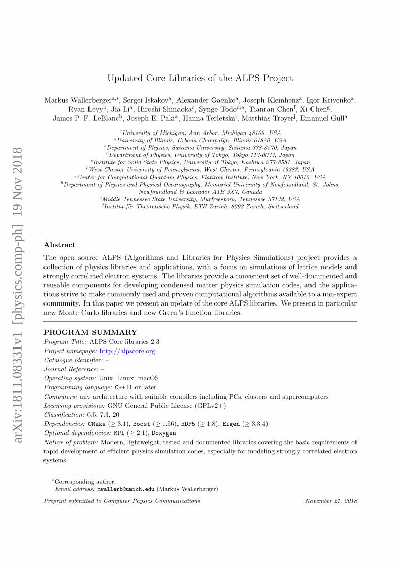
These many-body objects often need to be supplemented with analytic tail information encap-sulating the high frequency / short time moments of the Green’s functions, so that high precisionFourier transforms, density evaluations, or energy evaluations can be performed. In addition to thisfunctionality, the Green’s function component supports saving data to and loading it from binaryHDF5 files. The UML diagram illustrating the Green’s function classes and their interdependenciesis given in Fig. 3.

6

extends base_mesh1

1..*

gf_base

- data_:Storage- meshes_:MESHES

+ operator()(MESHES::index_type...):gf_base<VTYPE, View>+ operator()(MESHES::index_type...): VTYPE+ operator+(gf_base): gf_base+ operator-(gf_base): gf_base+ operator+=(gf_base): gf_base+ operator-=(gf_base): gf_base+ operator*(gf_base): gf_base+ operator*=(scalar): gf_base+ operator/(scalar): gf_base+ operator/=(scalar): gf_base+ operator-(): gf_base

VTYPE, Storage, MESHES

BaseStorage

ViewStorage

MemoryStorage

Figure 3: UML class diagram of Green’s function library, indicating the main classes in the Green’s function library.Each box corresponds to a class, and arrows correspond to relationships between classes.

The central class of the Green’s function library is gf base. This class should be parametrizedby the scalar type, the type of storage and the list of meshes (grids). It provides the followingbasic arithmetic operations:

• Addition/subtraction;

• In-place addition/subtraction;

• Multiplication by a constant.

The addition/subtraction operations can be performed on the Green’s function objects that aredefined on the same grid and have the same shape of the data array. There are two possiblestorage types for this class. The memory storage version of the class is called greenf, whereasthe view-based class is called greenf view. Instead of having only pre-defined Green’s functionclasses of fixed dimension, we provide a flexible interface that makes it possible to declare Green’sfunction types of any dimension. The following example defines 4-dimensional Green’s function onMatsubara, arbitrary index, imaginary time and Legendre meshes:

1// define meshes2alps::gf:: matsubara_positive_mesh x(100, 10);3alps::gf:: index_mesh y(10);4alps::gf:: itime_mesh z(100, 10);5alps::gf:: legendre_mesh w(100, 10);67greenf <double , alps::gf:: matsubara_positive_mesh , alps::gf::index_mesh , alps::gf::

itime_mesh , alps::gf:: legendre_mesh > g(x, y, z, w);

Using view-storage Green’s function one can easily get access to a part of another Green’sfunction object using index slicing. This idea is illustrated by the following code,

1// define meshes and Green ’s function object2alps::gf:: matsubara_positive_mesh x(100, 10);3alps::gf:: index_mesh y(20);4greenf <double , alps::gf:: matsubara_positive_mesh , alps::gf::index_mesh > g(x,y);56// loop over leading index7for(alps::gf:: matsubara_positive_mesh :: index_type w(0); w<x.extent (); ++w) {8greenf_view <double , alps::gf::index_mesh > g2 = g(w);9// do some operation on the Green’s function view object10// defined on the ’y’ mesh alone11}

7

In the current implementation we support only a slicing over a set of the leading indices. Moredetails on the Green’s function library can be found in the respective tutorial.

4. Some of the other key library components

In this section, we provide a brief overview of the purpose and functionality of some of the keycomponents comprising the ALPS core libraries. For a more detailed exposition with a workingexample, see the previous publication[1]. Additional information is available online and as partof the Doxygen code documentation. It should be noted that the components maintain minimalinterdependence, and using a component in a program does not bring in other components, unlessthey are required dependencies, in which case they will be used automatically.

Building a parallel Monte Carlo simulation. A generic Monte Carlo simulation can be easily as-sembled from the classes provided by the Monte Carlo Scheduler component. The programmerneeds to define only the problem-specific methods that are called at each Monte Carlo step, suchas methods to update the configuration of the Markov chain and to collect the measured data. Thesimulation is parallelized implicitly, using one MPI process per chain.

Storing, restoring, and checkpointing simulation results. To store the results of a simulation in across-platform format for subsequent analysis, one can use the Archive component. The componentprovides convenient interface to saving and loading of common C++ data structures (primitive types,complex numbers, STL vectors and maps), as well as of objects of user-defined classes to/fromHDF5 [24], which is a universally supported and machine independent data format.

Reading command-line arguments and parameter files. Input parameters to a simulation can bepassed via a combination of a parameter file and command line arguments. The Parameters librarycomponent is responsible for parsing the files and the command line, and providing access to thedata in the form of an associative array (akin to C++ map or Python dictionary). The parameterfiles use the standard “*.ini” format, a plain text format with a line-based syntax containingkey = value pairs, optionally divided into sections.

5. Prerequisites and Installation

To build the ALPS core libraries, any recent C++ compiler can be used; the libraries are testedwith GCC [25] 4.8.1 and above, Intel [26] C++ 15.0 and above, and Clang [27] 3.2 and above. Thelibrary follows the C++11 standard [28] to facilitate the portability to a wide range of programmingenvironments, including HPC clusters with older compilers. The library depends on the followingexternal packages:

• The CMake build system [29] of version 3.1 and above.

• The Boost C++ libraries [30] of version 1.56.0 and above. Only the headers of the Boostlibrary are required.

• The HDF5 library [24] version 1.8 and above.

• The Eigen library [31] version 3.3.4 and above (can be requested to be downloaded automat-ically).

8

To make use of (optional) parallel capabilities, an MPI implementation supporting standard 2.1 [32]and above is required. Generating the developer’s documentation requires Doxygen [33] along withits dependencies.

The installation of the ALPS core libraries follows the standard procedure for any CMake-basedpackage. The first step is to download the ALPS core libraries source code; the recommendedway is to download the latest ALPS core libraries release from https://github.com/ALPSCore/

ALPSCore/releases. Assuming that all above-mentioned prerequisite software is installed, theinstallation consists of unpacking the release archive and running CMake from a temporary builddirectory, as outlined in the shell session example below (the $ sign designates a shell prompt):

1$ tar -xzf ALPSCore -2.3.0. tar.gz2$ mkdir build3$ cd build4$ export ALPSCore_DIR=$HOME/software/ALPSCore5$ cmake -DCMAKE_INSTALL_PREFIX=$ALPSCore_DIR \6-DALPS_INSTALL_EIGEN=yes \7../ ALPSCore -2.3.08$ make9$ make test10$ make install

The command at line 1 unpacks the release archive (version 2.3.0 in this example); at line 4 thedestination install directory of the ALPS core libraries is set ($HOME/software/ALPSCore in thisexample). At line 6 the downloading and co-installation of Eigen library is requested (see AppendixA for more details).

The ALPS core libraries come with an extensive set of tests; it is strongly recommended torun the tests (via make test) to verify the correctness of the build, as it is done at line 9 in theexample above.

The installation procedure is outlined in more details in Appendix A; Also, the filecommon/build/build.jenkins.sh in the library release source tree contains a build and installa-tion script that can be further consulted for various build options.

Binary packages are available for some operating systems. On macOS operating system, theALPS core libraries package can be downloaded and installed from the MacPorts [34] repository,using a command port install alpscore. On GNU/Debian Linux operating system, the ALPScore Debian package is provided by the MateriApps LIVE! project [35] (see [36] for more details).

6. License and citation policy

The GitHub version of ALPS core libraries is licensed under the GNU General Public Licenseversion 2 (GPL v. 2) [37] or later. The older ALPS license under which previous versions of the codewere licensed [4] has been retired. We kindly request that the present paper be cited, along withany relevant original physics or algorithmic paper, in any published work utilizing an applicationcode that uses this library.

7. Summary

We have presented an updated and repackaged version of the core ALPS libraries, a lightweightC++ library, designed to facilitate rapid development of computational physics applications, andhave described its main features.

The new version contains the next-generation statistics library ALEA, a major overhaul of theGreen’s function library as well as updates to other components.

9

8. Acknowledgments

Work on the ALPS library project is supported by the Simons collaboration on the many-electron problem. Aspects of the library are supported by NSF DMR-1606348 and DOE ER46932.

References

[1] A. Gaenko, A. Antipov, G. Carcassi, T. Chen, X. Chen, Q. Dong, L. Gamper, J. Gukelberger, R. Igarashi,S. Iskakov, M. Konz, J. LeBlanc, R. Levy, P. Ma, J. Paki, H. Shinaoka, S. Todo, M. Troyer, E. Gull, Updated corelibraries of the alps project, Comput. Phys. Commun. 213 (2017) 235 – 251. doi:10.1016/j.cpc.2016.12.009.URL http://www.sciencedirect.com/science/article/pii/S0010465516303885

[2] F. Alet, P. Dayal, A. Grzesik, A. Honecker, M. Korner, A. Lauchli, S. R. Manmana, I. P. McCulloch, F. Michel,R. M. Noack, G. Schmid, U. Schollwock, F. Stockli, S. Todo, S. Trebst, M. Troyer, P. Werner, S. Wessel, TheALPS project: Open source software for strongly correlated systems, Journal of the Physical Society of Japan74 (Suppl) (2005) 30–35. arXiv:cond-mat/0410407, doi:10.1143/JPSJS.74S.30.URL http://dx.doi.org/10.1143/JPSJS.74S.30

[3] A. Albuquerque, F. Alet, P. Corboz, P. Dayal, A. Feiguin, S. Fuchs, L. Gamper, E. Gull, S. Gurtler, A. Honecker,R. Igarashi, M. Korner, A. Kozhevnikov, A. Lauchli, S. Manmana, M. Matsumoto, I. McCulloch, F. Michel,R. Noack, G. Paw lowski, L. Pollet, T. Pruschke, U. Schollwock, S. Todo, S. Trebst, M. Troyer, P. Werner,S. Wessel, The ALPS project release 1.3: Open-source software for strongly correlated systems, Journal ofMagnetism and Magnetic Materials 310 (2, Part 2) (2007) 1187 – 1193, proceedings of the 17th InternationalConference on Magnetism. doi:10.1016/j.jmmm.2006.10.304.URL http://www.sciencedirect.com/science/article/pii/S0304885306014983

[4] B. Bauer, L. D. Carr, H. G. Evertz, A. Feiguin, J. Freire, S. Fuchs, L. Gamper, J. Gukelberger, E. Gull,S. Guertler, A. Hehn, R. Igarashi, S. V. Isakov, D. Koop, P. N. Ma, P. Mates, H. Matsuo, O. Parcollet,G. Paw lowski, J. D. Picon, L. Pollet, E. Santos, V. W. Scarola, U. Schollwock, C. Silva, B. Surer, S. Todo,S. Trebst, M. Troyer, M. L. Wall, P. Werner, S. Wessel, The ALPS project release 2.0: open source software forstrongly correlated systems, Journal of Statistical Mechanics: Theory and Experiment 2011 (05) (2011) P05001.URL http://stacks.iop.org/1742-5468/2011/i=05/a=P05001

[5] M. Eckstein, M. Kollar, P. Werner, Thermalization after an interaction quench in the Hubbard model, Phys.Rev. Lett. 103 (2009) 056403. doi:10.1103/PhysRevLett.103.056403.URL http://link.aps.org/doi/10.1103/PhysRevLett.103.056403

[6] P. Werner, T. Oka, A. J. Millis, Diagrammatic Monte Carlo simulation of nonequilibrium systems, Phys. Rev.B 79 (2009) 035320. doi:10.1103/PhysRevB.79.035320.URL http://link.aps.org/doi/10.1103/PhysRevB.79.035320

[7] P. Werner, A. Comanac, L. de’ Medici, M. Troyer, A. J. Millis, Continuous-time solver for quantum impuritymodels, Phys. Rev. Lett. 97 (2006) 076405. doi:10.1103/PhysRevLett.97.076405.URL http://link.aps.org/doi/10.1103/PhysRevLett.97.076405

[8] E. Gull, P. Werner, O. Parcollet, M. Troyer, Continuous-time auxiliary-field Monte Carlo for quantum impuritymodels, EPL (Europhysics Letters) 82 (5) (2008) 57003.URL http://stacks.iop.org/0295-5075/82/i=5/a=57003

[9] H. Shinaoka, E. Gull, P. Werner, Continuous-time hybridization expansion quantum impurity solver for multi-orbital systems with complex hybridizations, Computer Physics Communications 215 (2017) 128–136. doi:

10.1016/j.cpc.2017.01.003.URL http://linkinghub.elsevier.com/retrieve/pii/S0010465517300036

[10] H. Shinaoka, Y. Nomura, E. Gull, Efficient implementation of the continuous-time interaction-expansion quan-tum monte carlo method. arXiv:1807.05238.

[11] J. Ferber, K. Foyevtsova, R. Valentı, H. O. Jeschke, LDA + DMFT study of the effects of correlation in LiFeAs,Phys. Rev. B 85 (2012) 094505. doi:10.1103/PhysRevB.85.094505.URL http://link.aps.org/doi/10.1103/PhysRevB.85.094505

[12] E. Cremades, S. Gmez-Coca, D. Aravena, S. Alvarez, E. Ruiz, Theoretical study of exchange coupling in 3d-Gdcomplexes: Large magnetocaloric effect systems, Journal of the American Chemical Society 134 (25) (2012)10532–10542, pMID: 22640027. doi:10.1021/ja302851n.URL http://dx.doi.org/10.1021/ja302851n

10

[13] D. Bergman, J. Alicea, E. Gull, S. Trebst, L. Balents, Order-by-disorder and spiral spin-liquid in frustrateddiamond-lattice antiferromagnets, Nat Phys 3 (7) (2007) 487–491.URL http://dx.doi.org/10.1038/nphys622

[14] L. Pollet, J. D. Picon, H. P. Buchler, M. Troyer, Supersolid phase with cold polar molecules on a triangularlattice, Phys. Rev. Lett. 104 (2010) 125302. doi:10.1103/PhysRevLett.104.125302.URL http://link.aps.org/doi/10.1103/PhysRevLett.104.125302

[15] J. P. F. LeBlanc, A. E. Antipov, F. Becca, I. W. Bulik, G. K.-L. Chan, C.-M. Chung, Y. Deng, M. Ferrero, T. M.Henderson, C. A. Jimenez-Hoyos, E. Kozik, X.-W. Liu, A. J. Millis, N. V. Prokof’ev, M. Qin, G. E. Scuseria,H. Shi, B. V. Svistunov, L. F. Tocchio, I. S. Tupitsyn, S. R. White, S. Zhang, B.-X. Zheng, Z. Zhu, E. Gull,Solutions of the two-dimensional Hubbard model: Benchmarks and results from a wide range of numericalalgorithms, Phys. Rev. X 5 (2015) 041041. doi:10.1103/PhysRevX.5.041041.URL http://link.aps.org/doi/10.1103/PhysRevX.5.041041

[16] E. Gull, O. Parcollet, A. J. Millis, Superconductivity and the pseudogap in the two-dimensional Hubbard model,Phys. Rev. Lett. 110 (2013) 216405. doi:10.1103/PhysRevLett.110.216405.URL http://link.aps.org/doi/10.1103/PhysRevLett.110.216405

[17] M. Wallerberger, E. Gull, Estimating uncertainties in Markov Chain Monte Carlo simulations, submitted toAm. J. Phys.

[18] M. Wallerberger, E. Gull, Hypothesis testing of scientific monte carlo calculations, Phys. Rev. E 96 (2017)053303. doi:10.1103/PhysRevE.96.053303.URL https://link.aps.org/doi/10.1103/PhysRevE.96.053303

[19] H. Kaiser, T. Heller, B. Adelstein-Lelbach, A. Serio, D. Fey, HPX: A Task Based Programming Model ina Global Address Space, in: Proceedings of the 8th International Conference on Partitioned Global AddressSpace Programming Models, PGAS ’14, ACM, New York, NY, USA, 2014, pp. 6:1–6:11. doi:10.1145/2676870.2676883.URL http://doi.acm.org/10.1145/2676870.2676883

[20] H. Hotelling, The generalization of Student’s ratio 2 (3) (1931) 360–378. doi:10.1214/aoms/1177732979.URL http://dx.doi.org/10.1214/aoms/1177732979

[21] W. Ku, Electronic excitations in metals and semiconductors: Ab initio studies of realistic many-particle systems.,Ph.D. thesis, University of Tennessee (2000).URL http://trace.tennessee.edu/utk_graddiss/2030

[22] L. Boehnke, H. Hafermann, M. Ferrero, F. Lechermann, O. Parcollet, Orthogonal polynomial representation ofimaginary-time green’s functions, Phys. Rev. B 84 (2011) 075145. doi:10.1103/PhysRevB.84.075145.URL https://link.aps.org/doi/10.1103/PhysRevB.84.075145

[23] E. Gull, S. Iskakov, I. Krivenko, A. A. Rusakov, D. Zgid, Chebyshev polynomial representation of imaginary-time response functions, Phys. Rev. B 98 (2018) 075127. doi:10.1103/PhysRevB.98.075127.URL https://link.aps.org/doi/10.1103/PhysRevB.98.075127

[24] The HDF Group. Hierarchical Data Format, version 5 [online] (1997–2016). http://www.hdfgroup.org/HDF5/.[25] R. M. Stallman, the GCC Developer Community, Using the GNU Compiler Collection (1988–2016).

URL https://gcc.gnu.org/onlinedocs/gcc-6.1.0/gcc.pdf

[26] Intel Corporation, User and Reference Guide for the Intel C++ Compiler 15.0 (2015).URL https://software.intel.com/en-us/compiler_15.0_ug_c

[27] clang: a C language family frontend for LLVM [online] (2016). http://clang.llvm.org/.[28] ISO, ISO/IEC 14882:2011 Information technology — Programming languages — C++, International Organi-

zation for Standardization, Geneva, Switzerland, 2012.URL http://www.iso.org/iso/iso_catalogue/catalogue_tc/catalogue_detail.htm?csnumber=50372

[29] K. Martin, B. Hoffman, Mastering CMake, Kitware, Inc, 2015.[30] Boost software libraries [online] (2016). http://www.boost.org/.[31] G. Guennebaud, B. Jacob, et al. Eigen v3 [online] (2010). http://eigen.tuxfamily.org.[32] Message Passing Interface Forum, MPI: A Message-Passing Interface Standard, Version 2.1, High Performance

Computing Center Stuttgart (HLRS), 2008, https://www.mpi-forum.org/docs/mpi-2.1/mpi21-report.pdf.[33] D. van Heesch. Doxygen [online] (1997–2015). http://www.doxygen.org/.[34] The MacPorts Project. Macports [online] (2007–2014). http://www.macports.org/.[35] MateriApps LIVE! [online] (2013–2018). https://cmsi.github.io/MateriAppsLive/.[36] ALPS Core Debian Package [online] (2018). https://github.com/cmsi/ma-alpscore.[37] GNU general public license.

URL http://www.gnu.org/licenses/gpl.html

11

Appendix A. Detailed installation procedure

In the following discussion we assume that all prerequisite software (section 5) is installed,and the ALPS core libraries release (here, release 2.3.0) is downloaded into the current directoryas ALPSCore-2.3.0.tar.gz. Also, we assume that the libraries are to be installed in ALPSCore

subdirectory of the current user’s home directory. The commands are given assuming bash as auser shell.

The first step is to unpack the release archive and set the desired install directory:

1$ tar -xzf ALPSCore -2.3.0.tar.gz2$ export ALPSCore_DIR=$HOME/software/ALPSCore

The next step is to perform the build of the library (note that the build should not be performedin the source directory):

3$ mkdir build4$ cd build5$ cmake ../ ALPSCore -2.3.0 -DCMAKE_INSTALL_PREFIX=$ALPSCore_DIR \6-DALPS_INSTALL_EIGEN=yes

The cmake command at lines 5 and 6 accepts additional arguments in the format-Dvariable =value . A number of relevant CMake variables is listed in Table A.3. The instal-lation process is also affected by environment variables, some of which are listed in Table A.4;the CMake variables take precedence over the environment variables. The build and installationscript common/build/build.jenkins.sh in the ALPS core libraries release source tree providesan example of using some of the build options.

It should be noted that line 6 of the example above will cause the ALPSCore installation processto download a copy of Eigen library[31] and co-install it with ALPSCore. If the Eigen library isalready installed on your system, it may be preferable to use the installed version. In this case,instead of requesting the installation of Eigen, the location of the Eigen library should be specified:

5$ cmake ../ ALPSCore -2.3.0 -DCMAKE_INSTALL_PREFIX=$ALPSCore_DIR \6-DEIGEN3_INCLUDE_DIR =/usr/local/Eigen3

In this example, the location of the Eigen library is assumed to be /usr/local/Eigen3;the actual location depends on your local Eigen installation. The directory specified by the-DEIGEN3 INCLUDE DIR option must contain the Eigen subdirectory.

12

Variable Default value Comment

CMAKE CXX COMPILER (system default) Path to C++ compiler executable.*

ALPS CXX STD c++11 The C++ standard to compile ALPSCore with.

CMAKE INSTALL PREFIX /usr/local library target install directory.

CMAKE BUILD TYPE RelWithDebInfo Specifies build type.

BOOST ROOT Boost install directory. Set if CMake fails to findBoost.

Boost NO SYSTEM PATHS false Set to true to disable search in default systemdirectories, if the wrong version of Boost isfound.

Boost NO BOOST CMAKE false Set to true to disable search for Boost CMake

file, if the wrong version of Boost is found.

Documentation ON Build developer’s documentation.

ENABLE MPI ON Enable MPI build (set to OFF to disable).

Testing ON Build unit tests (recommended).

ALPS BUILD TYPE dynamic Can be dynamic or static: build libraries asdynamic (“shared”) or static libraries,respectively.*

EIGEN3 INCLUDE DIR Location of Eigen headers* (containing Eigen

subdirectory)

Eigen3 DIR Location of CMake-based Eigen installation*(containing Eigen3Config.cmake)

ALPS INSTALL EIGEN NO set to yes to request downloading andco-installation of Eigen*

ALPS EIGEN UNPACK DIR (autodetected) directory where to unpack Eigen forco-installation

ALPS EIGEN TGZ FILE (autodetected) location of Eigen archive to unpack

*Note: For the change of this variable to take effect, remove your build directory and redo the build.

Table A.3: CMake arguments relevant to building of ALPS core libraries.

13

Variable Comment

CXX Path to C++ compiler executable.*

BOOST ROOT Boost install directory. Set if CMake fails to find Boost.

HDF5 ROOT HDF5 install directory. Set if CMake fails to find HDF5.

Eigen3 DIR Eigen install directory. Set if you use CMake-based installation of Eigen.

*Note: For the change of this variable to take effect, remove your build directory and redo the build.

Table A.4: Environment variables arguments relevant to building of ALPS core libraries.

14