ii

“2010*Update” — 2012/2/19 — 21:06 — page 1 — #1 ii

ii

ii

1

Updates for Excel 2010

This book was written for use with Microsoft Excel 2003. The newest version of Excelis 2010, which is not terribly different from 2003. Below are some points to note whenconsidering the use of this book with Excel 2010:

1. The formulas entered into cells are identical.

2. Charts, scrollbars, tables, and Solver all operate in the same basic way. The maindifference is the location of the commands.

3. Every spreadsheet built in this book can be built in Excel 2010 with very little modifi-cation.

This document replaces Appendix A and describes the most commonly used Excel tools inthis book.

Basic Terminology

When you first open Excel 2010, you should get a window that looks similar to Figure1. (Your window may not look exactly like that in the figure due to customization of theribbons.)

Each rectangle, called a cell, is a place where data, text, or formulas can be entered. Acollection of cells is called a worksheet. The name of the worksheet is given in the worksheettab near the bottom of the worksheet. The worksheet name can be changed by right–clicking on the worksheet tab and selecting Rename. A collection of worksheets is calleda workbook. Worksheets can be added or deleted from a workbook by right–clicking on theworksheet tab and selecting either Insert... or delete. A worksheet tab can be moved tothe left or right by left–clicking, holding, and dragging.

The name of each column is listed along the top of the worksheet while the number of eachrow is listed along the left–hand side of the worksheet. The width or height of a column orrow can be changed by left–clicking and holding on the right or bottom and then draggingto the desired width or height. A cell is named according to its column and row position.The selected cell has a thicker border around it and its name is shown in the name box.The selected cell can be changed using the arrow keys or by clicking on another cell.

A two–dimensional range of cells can be selected by left–clicking on the cell in the upperleft–hand corner of the range, holding, and dragging to the cell lower right–hand corner ofthe range. This highlights these cells indicating they are all selected. Ranges are referred

ii

“2010*Update” — 2012/2/19 — 21:06 — page 2 — #2 ii

ii

ii

2

Name Box Formula Bar

Worksheet Tabs

Tabs Ribbon

Figure 1

to by the cells in the upper left–hand and lower right–hand corners in the form (UpperLeft):(Lower Right).

Along the top of the screen are the tabs that label the ribbons which contain variouscommands. These ribbons can be customized by selecting File → Options → CustomizeRibbon.

Entering Text, Data, and Formulas

Text, data, and formulas are easily entered by selecting the desired cell, typing the desiredcontents, and pressing Enter. To practice doing this, format a blank worksheet as in Figure2. This worksheet contains two columns of data named “x” and “y” and a third columnnamed “z” that we will define later.

123

A B Cx y z

1 52 8

Figure 2

ii

“2010*Update” — 2012/2/19 — 21:06 — page 3 — #3 ii

ii

ii

3

Notice that when you press enter, the selected cell moves to the cell directly under theprevious one. By default text is left–justified. The text in row 1 can be changed to boldand centered by selecting the range A1:A3, and then clicking on the bold font icon inthe Font section of the Home ribbon and then the center icon located in the Alignmentsection.

Now suppose we want to define the quantity z to be x + y. We can easily do this byentering the formula in Figure 3. Every formula begins with an equal sign. This formulacan be entered by typing it as in the figure and then pressing Enter, or you can type =,click on cell A2, type +, click on cell B2, and then press Enter.

2C

=A2+B2

Figure 3

Once the formula is entered, select cellC2 and click in the formula bar. Notice how differentcolored boxes are put around cells A2 and B2 and that the A2 and B2 in the formulaare changed to the corresponding colors. This feature simplifies the process of debuggingformulas.

To calculate the second value of z, we could type the formula =A3+B3 in cell C3, butthere is an easier way. Select cell C2, left–click and hold on the dark square in the lowerright–hand corner of the cell. Then drag the box down one row and release. The resultsare shown in Figure 4. This is exactly what we want.

123

Cz

=A2+B2=A3+B3

Figure 4

Understanding Cell References

To understand why the formula in cell C2 copied down to cell C3 in this way, we needto understand what we mean when we reference cells in formulas. The formula in cell C2should not be interpreted as “add cell A2 to cell B2.” Rather, it should be interpreted as“add the cell two columns to the left and in the same row to the cell one column to the leftand in the same row.” In other words, these cell references are relative. When this formulais copied down one row, the cell “two columns to the left and in the same row” is now A3and the cell “one column to the left and in the same row” is now B3.

ii

“2010*Update” — 2012/2/19 — 21:06 — page 4 — #4 ii

ii

ii

4

Now, change the formula in cell C2 to that shown in Figure 5. The $’s can be enteredmanually or you can delete the contents of C2, then type =, click on cell A2, press theF4 key, type +, click on cell B2, press the F4 key, and then press Enter.

2C

=$A$2+$B$2

Figure 5

Copy the formula in cell C2 down to C3. The results are shown in Figure 6. Notice thatthe formula did not change. This is because the $’s “fix” the row and column reference.So the formula in C2 really does mean “add cell A2 to cell B2.” When we copy it down,the meaning does not change.

123

Cz

=$A$2+$B$2=$A$2+$B$2

Figure 6

Now, change the formula in cell C2 to that shown in Figure 7. The $’s can be manuallyentered or they can entered by selecting the cells and pressing F4 two or three times, similarto above.

12

Cz

=A$2+$B2

Figure 7

Copy the formula in cell C2 down one row and to the right one column. The results areshown in Figure 8.

123

C Dz

=A$2+$B2 =B$2+$B2=A$2+$B3

Figure 8

We get these results because the $ in A$2 “fixes” the row at 2, but the column is stillrelative. When we copy down, this row does not change, but when we copy to the right,the column changes to B. Likewise, the $ in $B2 “fixes” the column at B, but the row isstill relative. When we copy down, this row changes, but when we copy to the right, thecolumn does not change.

ii

“2010*Update” — 2012/2/19 — 21:06 — page 5 — #5 ii

ii

ii

5

Formatting Cells

The formats of a cell or range can be easily changed by first selecting the cell or range andthen right–clicking within the cell or range. Selecting Format Cells... yields the windowshown in Figure 9.

Figure 9

Several of these tabs are useful for building the models in this book:

Number – The number tab allows you to change the way numbers are displayed. Forinstance, selecting Number under Category: allows you to, among other things, setthe number of displayed decimal places.

Font – The font tab allows you to change the font, font style, and size of text. It alsoallows you to add effects such as superscript or subscript.

Border – The border tab allows you to change the border around and between cells.

Patterns – The patterns tab allows you to change the background color and patternof cells.

Creating Charts and Graphs

To illustrate the process of creating charts and graphs, rename a blank worksheet Graphand format it as in Figure 10.

To create a simple plot of y vs. x, follow these steps:

ii

“2010*Update” — 2012/2/19 — 21:06 — page 6 — #6 ii

ii

ii

6

123456

A Bx y

1 22 53 94 125 13

Figure 10

1. Select the range A1:B6 and click on the Insert tab. In the Charts section of theribbon, select Scatter and choose the type in the upper-left hand corner of the drop-down box. This creates the chart shown in Figure 11.

0

2

4

6

8

10

12

14

0 1 2 3 4 5 6

y

y

Figure 11

2. The color and style of the points can be changed by right–clicking on a point andselecting Format Data Series... The plot area (the region on which the pointslie) can be change by right–clicking on it and selecting Format Plot Area... Thegridlines and legend can be deleted (if desired) by left–clicking on them and pressingDelete.

3. The chart title may be changed by left–clicking on it. To add axis titles, left–clickanywhere on the chart. This causes three Chart Tools tabs to appear. The Layouttab contains commands for adding the desired titles. Once created, the fonts of thetitles may be changed by right–clicking on them.

4. The format of the x– and y–axes can be changed by right–clicking on a numbernext to an axis and selecting Format Axis... Under Axis Options we may setthe minimum and maximum values on the axis and change the Major units (thedistance between tick-marks).

5. After adding some titles and changing axis options, we get the chart in Figure 12.

ii

“2010*Update” — 2012/2/19 — 21:06 — page 7 — #7 ii

ii

ii

7

0

2

4

6

8

10

12

14

0 1 2 3 4 5

y

x

y vs. x

Figure 12

Adding Data Series

Oftentimes we want to add another series of data points to a chart after the chart has beencreated. To illustrate how to do this, add the data shown in Figure 13 to the worksheetGraph.

1

2

3

4

5

6

C

z

3

4

8

10

11

Figure 13

To add this z data to the chart, right-click anywhere on the chart and select Select Data...In the resulting Select Data Source Window, press the Add button. Format theresulting Edit Series window as in Figure 14 by clicking the icon next to a formula boxand then selecting the appropriate range on the worksheet. (Note that Series X Valuesand Series Y Values are generic names corresponding to the horizontal and vertical axes,respectively.)

Press OK twice. After changing the chart title and adding the legend by selecting Layout→ Legend → Show Legend at Right, we get the chart in Figure 15.

Graphing Functions

Excel does not have a built–in tool for graphing functions, but we can easily create an x–ytable and then plot the points. For example, to graph the function f (x) = x2 over the

ii

“2010*Update” — 2012/2/19 — 21:06 — page 8 — #8 ii

ii

ii

8

Figure 14

0

2

4

6

8

10

12

14

0 1 2 3 4 5

x

Two Data Series

y

z

Figure 15

interval [−2, 2], format a blank worksheet as in Figure 16. Copy row 3 down to row 42.

123

A Bx y

-2 =A2^2=A2+0.1 =A3^2

Figure 16

Select columns A and B by left–clicking and holding on the column A header and thendragging to column B. Choose Insert → Scatter and choose the type in the middle of theleft called “Scatter with Smooth Lines.” Once the chart is created, delete the gridlines andlegend; set the x–axis min and max to -2 and +2, respectively with a major unit of 1; andthe y–axis min and max to 0 and 4, respectively, also with a major unit of 1. Change thechart title to y = x2, and the result should look like Figure 17.

Scroll Bars

Scroll bars allow us to change the value of a cell with a graphical interface. This allows usto dynamically change the values of parameters within a model and analysis the results. To

ii

“2010*Update” — 2012/2/19 — 21:06 — page 9 — #9 ii

ii

ii

9

0

1

2

3

4

-2 -1 0 1 2

y = x2

Figure 17

access the scroll bar commands, we must add the Developer tab. To do this, select File →Options → Customize Ribbon. Under Main Tabs, check the box next to Developerand press OK.

In a blank worksheet, select Developer → Insert. A drop-down box similar to that inFigure 18 should appear.

Scroll Bar

Design Mode

Figure 18

When you press the scroll bar button, the cursor changes to a small cross. Use this to drawa long, skinny rectangle. Right–click on the resulting scroll bar and select Properties. Awindow similar to that in Figure 19 should appear.

There are three important properties we need to change. The LinkedCell is the cell whosevalue we want to change. Set this to A1 by typing A1 in the box next to it. The Minand Max are the minimum and maximum values of the cell. Set these to 0 and 1,000,respectively. Close the properties window and click on the Design Mode button so it isnot highlighted. The scroll bar is now ready to use. Move the slider on the scroll bar backand forth and note that the number in cell A1 changes between 0 and 1,000 in incrementsof 1. The scroll bar properties can be changed by clicking on the Design Mode buttonand right–clicking on the scroll bar.

In most instances, we may want the value of a cell to change in increments other than 1.

ii

“2010*Update” — 2012/2/19 — 21:06 — page 10 — #10 ii

ii

ii

10

Figure 19

This can be accomplished using a formula that references the linked cell. For instance,enter the formula shown in Figure 20. Move the slider back and forth and note that thenumber in cell A2 changes between 0 and 100 in increments of 0.1.

2A

=A1/10

Figure 20

(Note: There is a somewhat easier way to create scroll bars using the Form Controlversion of the scroll bar. However, these scroll bars do not work as well with graphs. Withthe method described above, if the scroll bar changes a value on a graph, the graph changesin a continuous manner as the slider is moved back and forth. If the Forms toolbar is used,the graph will not change until you release the mouse button.)

Array Formulas

Excel can perform simple matrix operations such as addition, multiplication, and finding

inverses. For example, if A =

[1 2

3 4

]and B =

[3 4

5 6

], to compute C = A+B, format

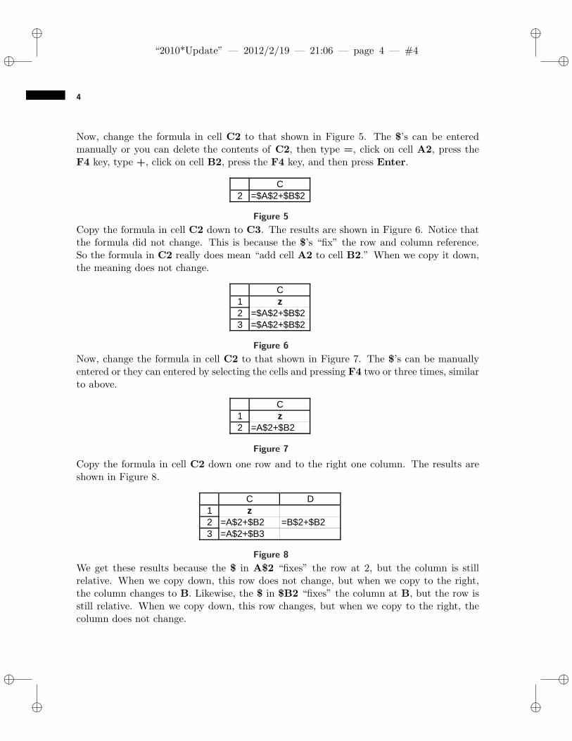
a blank worksheet as in Figure 21. To center the text “A” between cells A1 and B1, selectthe range A1:B1 and then press the Merge and Center icon in the Alignment sectionof the Home tab.

Next, select the range G2:H3, type =A2:B3+D2:E3, and press the combination of keysCtrl-Shift-Enter (this combination tells Excel to compute an array formula). The results

ii

“2010*Update” — 2012/2/19 — 21:06 — page 11 — #11 ii

ii

ii

11

123

A B C D E F G H

1 2 5 63 4 7 8

A B C

Figure 21

are shown in Figure 22. Notice that when you select any cell in the range G2:H3, theformula is in curly brackets, {...}. This indicates that an array formula has been entered.

123

G H

6 810 12

C

Figure 22

Other Tools

Other tools used in this book work the same way in Excel 2010 as they do in 2003, but areaccessed differently. Below we describe how to access them in 2010. For details on how touse them, see the corresponding sections of the text.

1. Data Analysis: The Regression command of the Data Analysis tool is usedin Section 3.5 for doing multiple regression. To install the Data Analysis add-in,select File→Options→Add-Ins. Near the bottom of the window, selectManage:Excel Add-ins and press Go... Check the box beside Analysis ToolPak and pressOK. In theData tab there should now be anAnalysis section with aData Analysiscommand. Selecting this command opens a window identical to that in Excel 2003.

2. Tables: Tables are used extensively in Chapter 6 for doing simulations. To define atable, select the desired range and then press Data → What-If Analysis → DataTable... This opens a box identical to that in Excel 2003.

3. Solver: Solver is used extensively in Chapter 7 for doing linear programming. Toinstall the Solver add-in, select File → Options → Add-Ins. Near the bottomof the window, select Manage: Excel Add-ins and press Go... Check the boxbeside Solver and press OK. In the Data tab there should now be an Analysissection with a Solver command. Selecting this command opens a window that looksdifferent than that in Excel 2003, but operates the same way. One difference is thatExcel 2010 allows you to Select a Solving Method. When solving linear programs

ii

“2010*Update” — 2012/2/19 — 21:06 — page 12 — #12 ii

ii

ii

12

in Sections 7.2–7.7, select Simplex LP. When solving nonlinear program in Section7.8, select GRG Nonlinear.