Updates to the MODFLOW Groundwater Model of the San Antonio Segment of the

Edwards Aquifer

Presented by

Jim Winterle

November 14, 2017

1

EAA Modeling Team:Angang “Al” LiuNed TroshanovAndi ZhangJim Winterle

Background• The goal of the MODFLOW model in the Phase II

EAHCP process is to examine spring flow protection measures and inform any refinements that need to be made to those measures

• The EAA model represents a multi-year update of a 2004 model produced by Lindgren et al. (2004)

• The EAA completed updates and solicited feedback from a Groundwater Model Advisory Panel (GMAP) in March 2017

• A report documenting parameterization, calibration, and validation was also reviewed by GMAP members and ready for publication

2

In-Depth Review of Original MODFLOW Model: “Functionality and Verification Analyses”

• Original model calibrated to data from period 1947—2000

• Functionality Analysis conducted to compare original model simulation results to observation data not used in the original calibration

• Verification Analysis ran original model forward for years 2001—2009 to evaluate how well model predicts water levels and spring flows for a period it was not calibrated to

• Results of these analyses informed model updates

3

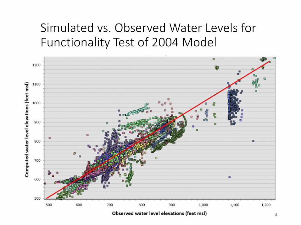
Simulated vs. Observed Water Levels for Functionality Test of 2004 Model

4

Locations of Wells with Largest Errors in Functionality Test

5

Model Update and RecalibrationMajor changes from original model include:• Removed Barton Spring segment• New tops and bottom layer elevation model• Hydraulic conductivity zones modified to remove explicit

conduits• Added HFB flow barriers to represent Knippa Gap and

Haby’s Crossing fault zone• Known locations of wells and annual pumping totals• Added two new spring locations to represent Hueco

Springs and subsurface discharge in Leona River basin• Increase rate of interformational flow in norther Bexar

County

6

7

8

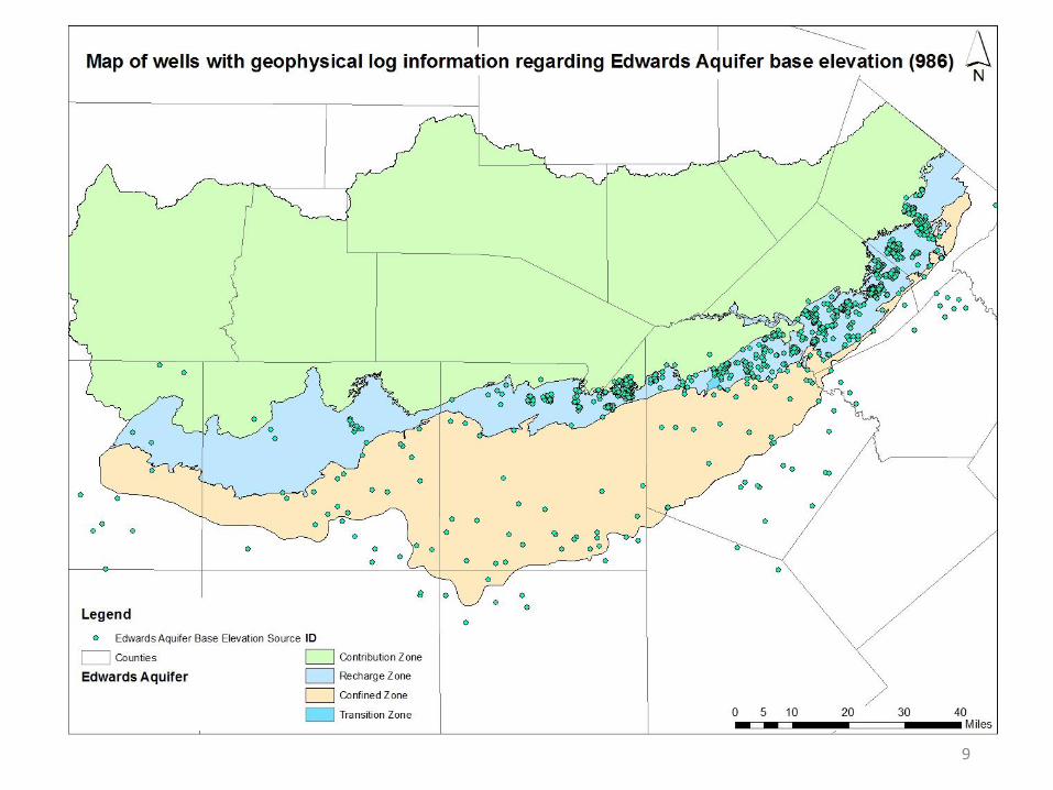
9

Contour of Simulated Model Top Elevation (Range from -4064 (blue) to 2018 ft (red) above msl)

Updated Model Top Elevation

10

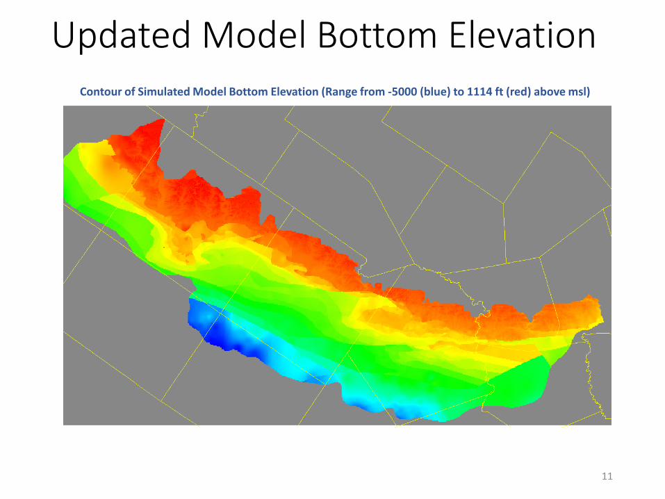
Contour of Simulated Model Bottom Elevation (Range from -5000 (blue) to 1114 ft (red) above msl)

Updated Model Bottom Elevation

11

Simulated Distribution of Hydraulic Conductivity, Ranging from 1 ft/day (dark blue) to 48,500 ft/day (orange)

Hydraulic Conductivity Zones

12

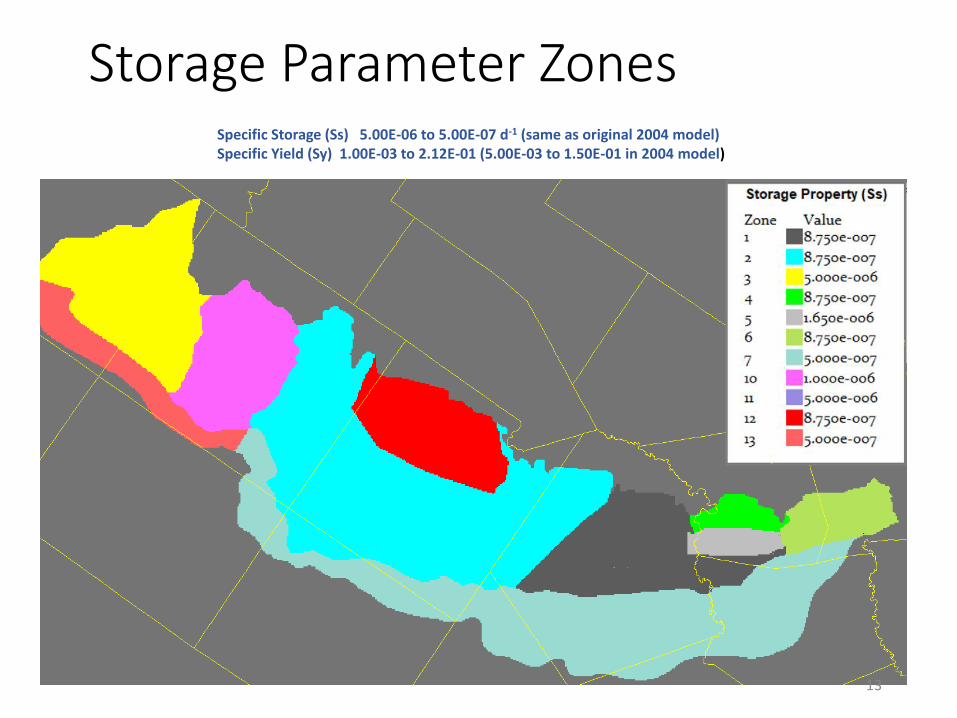
Storage Parameter ZonesSpecific Storage (Ss) 5.00E-06 to 5.00E-07 d-1 (same as original 2004 model)Specific Yield (Sy) 1.00E-03 to 2.12E-01 (5.00E-03 to 1.50E-01 in 2004 model)

13

Horizontal Flow Barriers

Knippa Gap K=0.01/day, Haby Crossing Fault K=0.03/day

Knippa Gap HFB cells

Haby’s Crossing Fault HFB cells

14

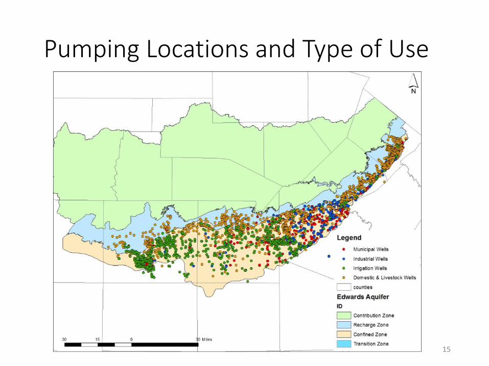
Pumping Locations and Type of Use

15

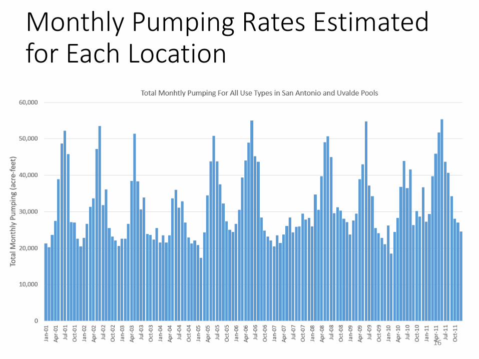
Monthly Pumping Rates Estimated for Each Location

16

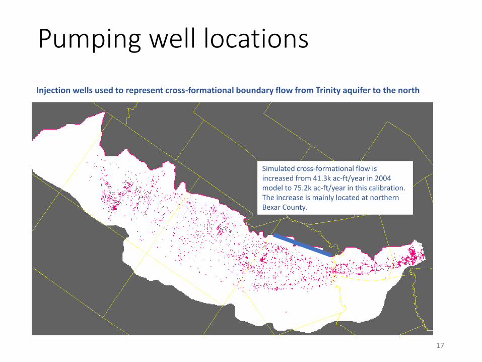
Injection wells used to represent cross-formational boundary flow from Trinity aquifer to the north

Simulated cross-formational flow is increased from 41.3k ac-ft/year in 2004 model to 75.2k ac-ft/year in this calibration. The increase is mainly located at northern Bexar County.

Pumping well locations

17

Modeled Springflow Locations

18

Modifications to USGS recharge estimates based on same method developed by Lindgren et al. for the original model

• Recharge to the Cibolo and Dry Comal Creek watershed area is reduced by a factor of 0.5 for all monthly stress periods

• In years when the USGS aquifer-wide total annual recharge estimate exceeds 1.4 million acre-feet, recharge to all basins is multiplied by a factor of 0.8 for all stress periods during that year, after applying the above corrections. In the updated model, this reduction was applied to years 2002, 2004, and 2007

• Recharge to Nueces-West Nueces River watershed was increased by a factor of 1.048 for all monthly stress periods

• Recharge to Frio – Dry Frio watershed area was increased by a factor of 1.011 for all monthly stress periods.

19

Recharge estimates start with USGS estimates for 8 watershed areasGuadalupe watershed (9) not estimated by USGS

20

2

1

3

10

98

7

6

5

4

Distribution of Recharge15% assigned as distributed recharge in nine watershed zones85% assigned to 23 stream segmentsOnly distributed recharge in Guadalupe River basin, based on average rates for adjacent basins

21

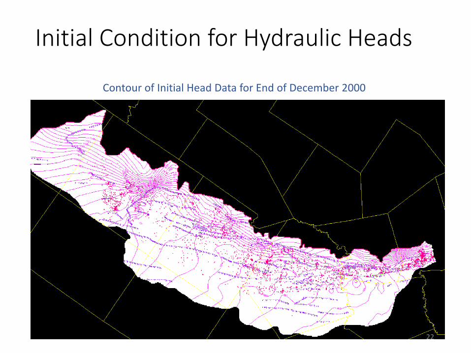
Contour of Initial Head Data for End of December 2000

Initial Condition for Hydraulic Heads

22

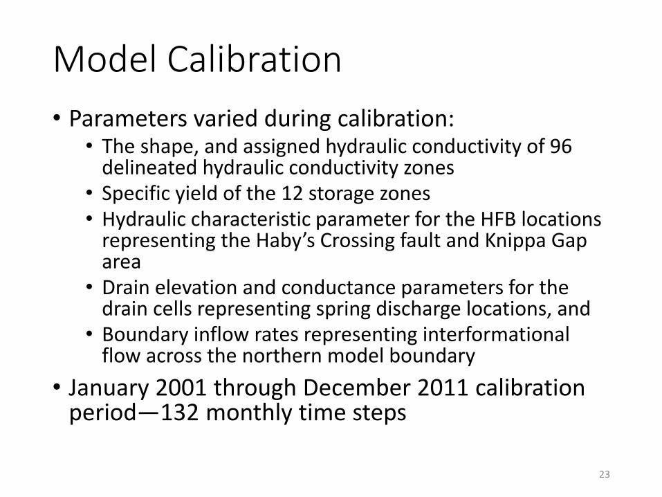
Model Calibration

• Parameters varied during calibration:• The shape, and assigned hydraulic conductivity of 96

delineated hydraulic conductivity zones• Specific yield of the 12 storage zones• Hydraulic characteristic parameter for the HFB locations

representing the Haby’s Crossing fault and Knippa Gap area

• Drain elevation and conductance parameters for the drain cells representing spring discharge locations, and

• Boundary inflow rates representing interformational flow across the northern model boundary

• January 2001 through December 2011 calibration period—132 monthly time steps

23

Water-Level Observation Locations

24

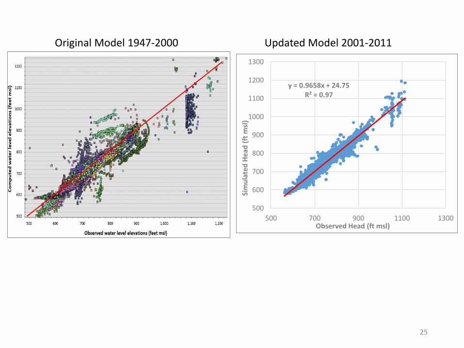
y = 0.9658x + 24.75R² = 0.97

500

600

700

800

900

1000

1100

1200

1300

500 700 900 1100 1300

Sim

ula

ted

Hea

d (

ftm

sl)

Observed Head (ft msl)

25

Original Model 1947-2000 Updated Model 2001-2011

610

620

630

640

650

660

670

680

690

700

7101

/1/0

1

6/1

/01

11

/1/0

1

4/1

/02

9/1

/02

2/1

/03

7/1

/03

12

/1/0

3

5/1

/04

10

/1/0

4

3/1

/05

8/1

/05

1/1

/06

6/1

/06

11

/1/0

6

4/1

/07

9/1

/07

2/1

/08

7/1

/08

12

/1/0

8

5/1

/09

10

/1/0

9

3/1

/10

8/1

/10

1/1

/11

6/1

/11

11

/1/1

1

Wat

er L

evel

(ft

msl

)Model Calibration: J-17 Water Level

Observed

Simulated

26

830

840

850

860

870

880

890

900

1/1

/01

6/1

/01

11

/1/0

1

4/1

/02

9/1

/02

2/1

/03

7/1

/03

12

/1/0

3

5/1

/04

10

/1/0

4

3/1

/05

8/1

/05

1/1

/06

6/1

/06

11

/1/0

6

4/1

/07

9/1

/07

2/1

/08

7/1

/08

12

/1/0

8

5/1

/09

10

/1/0

9

3/1

/10

8/1

/10

1/1

/11

6/1

/11

11

/1/1

1

Wat

er L

evel

(ft

msl

)

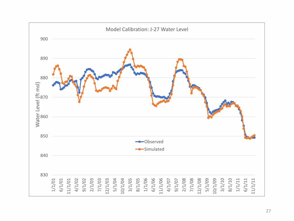
Model Calibration: J-27 Water Level

Observed

Simulated

27

100

150

200

250

300

350

400

450

500

550

1/1

/01

6/1

/01

11

/1/0

1

4/1

/02

9/1

/02

2/1

/03

7/1

/03

12

/1/0

3

5/1

/04

10

/1/0

4

3/1

/05

8/1

/05

1/1

/06

6/1

/06

11

/1/0

6

4/1

/07

9/1

/07

2/1

/08

7/1

/08

12

/1/0

8

5/1

/09

10

/1/0

9

3/1

/10

8/1

/10

1/1

/11

6/1

/11

11

/1/1

1

Spri

ng

Flo

w (

cfs)

Model Calibration: Comal Springs Discharge

Observed

Simulated

28

0

50

100

150

200

250

300

350

400

450

1/1

/01

6/1

/01

11

/1/0

1

4/1

/02

9/1

/02

2/1

/03

7/1

/03

12

/1/0

3

5/1

/04

10

/1/0

4

3/1

/05

8/1

/05

1/1

/06

6/1

/06

11

/1/0

6

4/1

/07

9/1

/07

2/1

/08

7/1

/08

12

/1/0

8

5/1

/09

10

/1/0

9

3/1

/10

8/1

/10

1/1

/11

6/1

/11

11

/1/1

1

Spri

ng

Flo

w (

cfs)

Model Calibration: San Marcos Springs Discharge

Observed

Simulated

29

0

20

40

60

80

100

1201

/24

/01

5/2

4/0

1

9/2

4/0

1

1/2

4/0

2

5/2

4/0

2

9/2

4/0

2

1/2

4/0

3

5/2

4/0

3

9/2

4/0

3

1/2

4/0

4

5/2

4/0

4

9/2

4/0

4

1/2

4/0

5

5/2

4/0

5

9/2

4/0

5

1/2

4/0

6

5/2

4/0

6

Spri

ng

Dis

char

ge (

cfs)

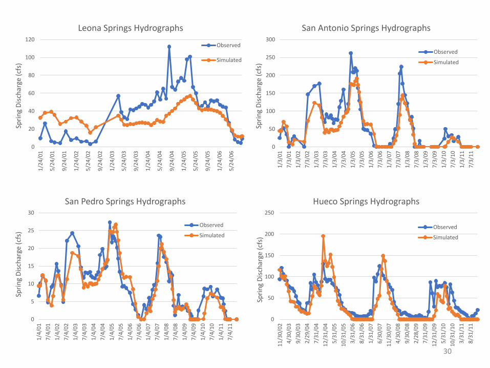
Leona Springs Hydrographs

Observed

Simulated

0

50

100

150

200

250

300

1/3

/01

7/3

/01

1/3

/02

7/3

/02

1/3

/03

7/3

/03

1/3

/04

7/3

/04

1/3

/05

7/3

/05

1/3

/06

7/3

/06

1/3

/07

7/3

/07

1/3

/08

7/3

/08

1/3

/09

7/3

/09

1/3

/10

7/3

/10

1/3

/11

7/3

/11

Spri

ng

Dis

char

ge (

cfs)

San Antonio Springs Hydrographs

Observed

Simulated

0

5

10

15

20

25

30

1/4

/01

7/4

/01

1/4

/02

7/4

/02

1/4

/03

7/4

/03

1/4

/04

7/4

/04

1/4

/05

7/4

/05

1/4

/06

7/4

/06

1/4

/07

7/4

/07

1/4

/08

7/4

/08

1/4

/09

7/4

/09

1/4

/10

7/4

/10

1/4

/11

7/4

/11

Spri

ng

Dis

char

ge (

cfs)

San Pedro Springs Hydrographs

Observed

Simulated

0

50

100

150

200

250

11

/30

/02

4/3

0/0

3

9/3

0/0

3

2/2

9/0

4

7/3

1/0

4

12

/31

/04

5/3

1/0

5

10

/31

/05

3/3

1/0

6

8/3

1/0

6

1/3

1/0

7

6/3

0/0

7

11

/30

/07

4/3

0/0

8

9/3

0/0

8

2/2

8/0

9

7/3

1/0

9

12

/31

/09

5/3

1/1

0

10

/31

/10

3/3

1/1

1

8/3

1/1

1

Spri

ng

Dis

char

ge (

cfs)

Hueco Springs Hydrographs

Observed

Simulated

30

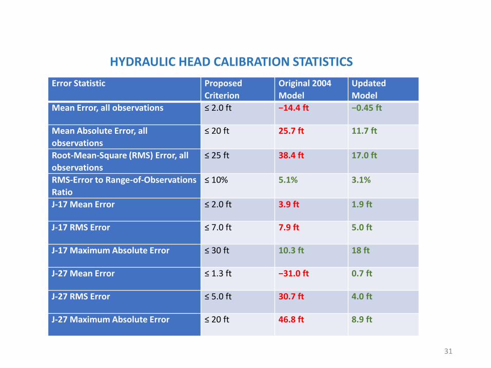
HYDRAULIC HEAD CALIBRATION STATISTICS

31

Error Statistic Proposed

Criterion

Original 2004

Model

Updated

Model

Mean Error, all observations ≤ 2.0 ft −14.4 ft −0.45 ft

Mean Absolute Error, all

observations

≤ 20 ft 25.7 ft 11.7 ft

Root-Mean-Square (RMS) Error, all

observations

≤ 25 ft 38.4 ft 17.0 ft

RMS-Error to Range-of-Observations

Ratio

≤ 10% 5.1% 3.1%

J-17 Mean Error ≤ 2.0 ft 3.9 ft 1.9 ft

J-17 RMS Error ≤ 7.0 ft 7.9 ft 5.0 ft

J-17 Maximum Absolute Error ≤ 30 ft 10.3 ft 18 ft

J-27 Mean Error ≤ 1.3 ft −31.0 ft 0.7 ft

J-27 RMS Error ≤ 5.0 ft 30.7 ft 4.0 ft

J-27 Maximum Absolute Error ≤ 20 ft 46.8 ft 8.9 ft

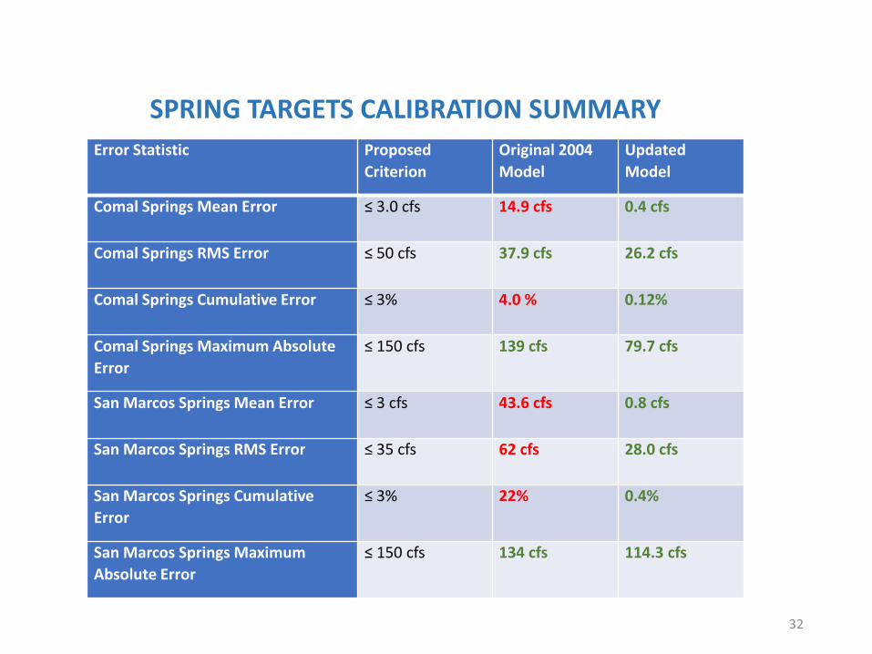
SPRING TARGETS CALIBRATION SUMMARY

32

Error Statistic Proposed

Criterion

Original 2004

Model

Updated

Model

Comal Springs Mean Error ≤ 3.0 cfs 14.9 cfs 0.4 cfs

Comal Springs RMS Error ≤ 50 cfs 37.9 cfs 26.2 cfs

Comal Springs Cumulative Error ≤ 3% 4.0 % 0.12%

Comal Springs Maximum Absolute

Error

≤ 150 cfs 139 cfs 79.7 cfs

San Marcos Springs Mean Error ≤ 3 cfs 43.6 cfs 0.8 cfs

San Marcos Springs RMS Error ≤ 35 cfs 62 cfs 28.0 cfs

San Marcos Springs Cumulative

Error

≤ 3% 22% 0.4%

San Marcos Springs Maximum

Absolute Error

≤ 150 cfs 134 cfs 114.3 cfs

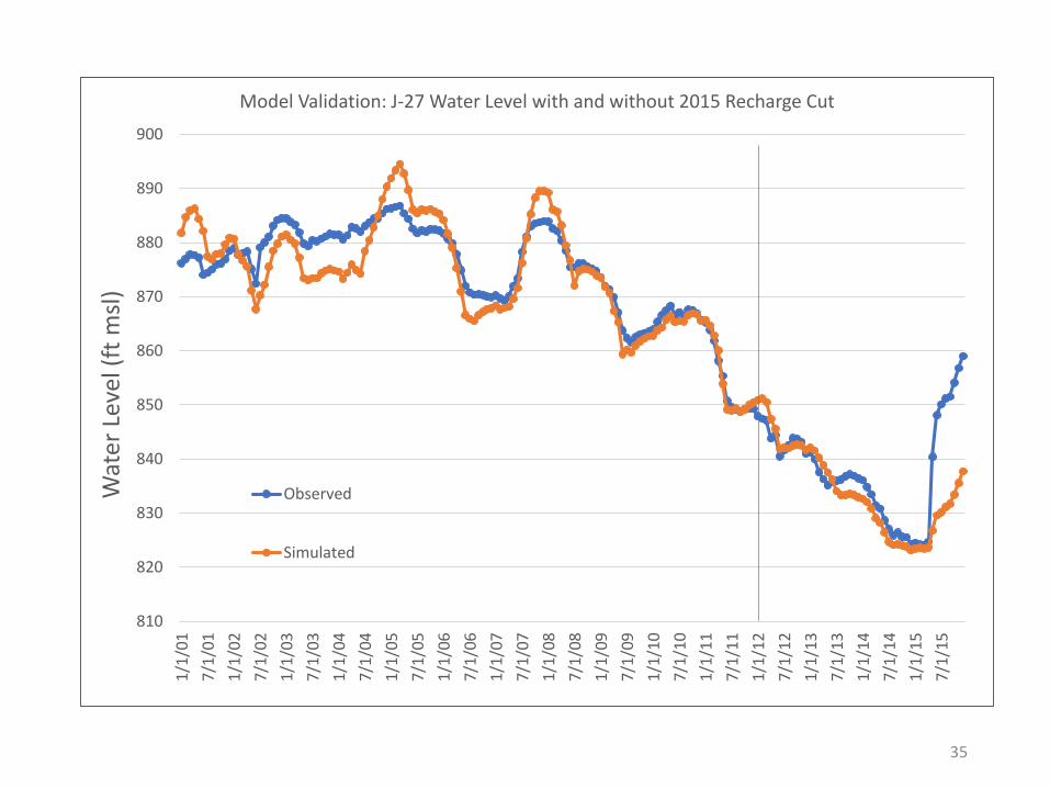
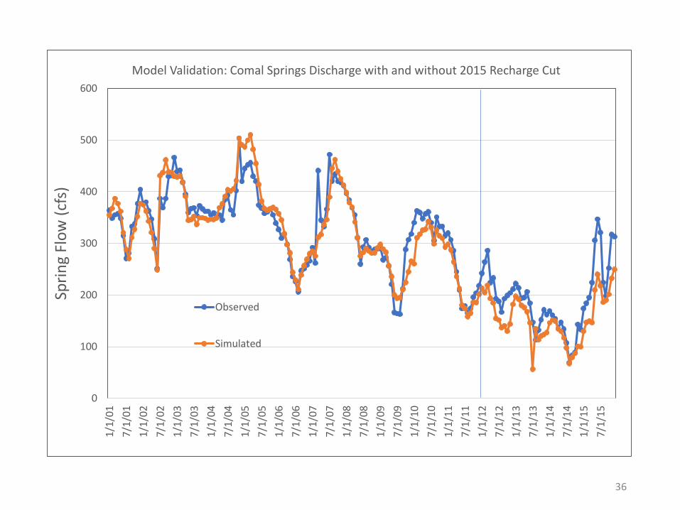
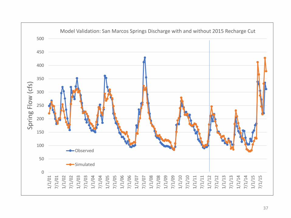
Model Validation Test

• Model run forward for a period that was not used in the calibration: January 2012—December 2015

• 48 additional monthly time steps

• Specifically suggested in NAS 2

• Includes lowest water levels observed during the 2008—2014 drought and recovery from drought in 2015

33

600

620

640

660

680

700

720

1/1

/01

8/1

/01

3/1

/02

10

/1/0

2

5/1

/03

12

/1/0

3

7/1

/04

2/1

/05

9/1

/05

4/1

/06

11

/1/0

6

6/1

/07

1/1

/08

8/1

/08

3/1

/09

10

/1/0

9

5/1

/10

12

/1/1

0

7/1

/11

2/1

/12

9/1

/12

4/1

/13

11

/1/1

3

6/1

/14

1/1

/15

8/1

/15

Wat

er L

evel

(ft

msl

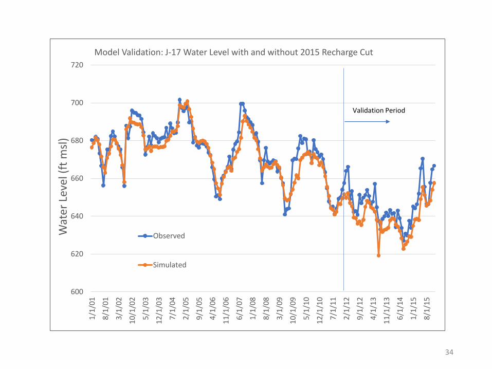
)Model Validation: J-17 Water Level with and without 2015 Recharge Cut

Observed

Simulated

Validation Period

34

810

820

830

840

850

860

870

880

890

900

1/1

/01

7/1

/01

1/1

/02

7/1

/02

1/1

/03

7/1

/03

1/1

/04

7/1

/04

1/1

/05

7/1

/05

1/1

/06

7/1

/06

1/1

/07

7/1

/07

1/1

/08

7/1

/08

1/1

/09

7/1

/09

1/1

/10

7/1

/10

1/1

/11

7/1

/11

1/1

/12

7/1

/12

1/1

/13

7/1

/13

1/1

/14

7/1

/14

1/1

/15

7/1

/15

Wat

er L

evel

(ft

msl

)Model Validation: J-27 Water Level with and without 2015 Recharge Cut

Observed

Simulated

35

0

100

200

300

400

500

600

1/1

/01

7/1

/01

1/1

/02

7/1

/02

1/1

/03

7/1

/03

1/1

/04

7/1

/04

1/1

/05

7/1

/05

1/1

/06

7/1

/06

1/1

/07

7/1

/07

1/1

/08

7/1

/08

1/1

/09

7/1

/09

1/1

/10

7/1

/10

1/1

/11

7/1

/11

1/1

/12

7/1

/12

1/1

/13

7/1

/13

1/1

/14

7/1

/14

1/1

/15

7/1

/15

Spri

ng

Flo

w (

cfs)

Model Validation: Comal Springs Discharge with and without 2015 Recharge Cut

Observed

Simulated

36

0

50

100

150

200

250

300

350

400

450

500

1/1

/01

7/1

/01

1/1

/02

7/1

/02

1/1

/03

7/1

/03

1/1

/04

7/1

/04

1/1

/05

7/1

/05

1/1

/06

7/1

/06

1/1

/07

7/1

/07

1/1

/08

7/1

/08

1/1

/09

7/1

/09

1/1

/10

7/1

/10

1/1

/11

7/1

/11

1/1

/12

7/1

/12

1/1

/13

7/1

/13

1/1

/14

7/1

/14

1/1

/15

7/1

/15

Spri

ng

Flo

w (

cfs)

Model Validation: San Marcos Springs Discharge with and without 2015 Recharge Cut

Observed

Simulated

37

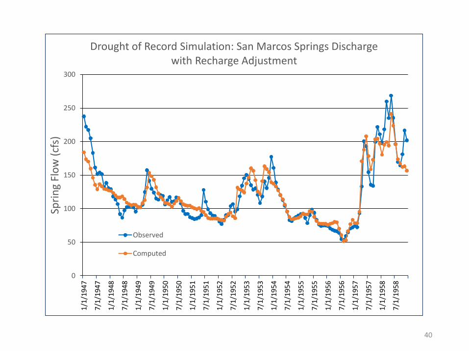
Drought-of-Record Simulations

• Set up drought-of-record scenario using pumping and recharge estimates for the period of January 1947 through December 1958 to use for HCP Adaptive Management evaluations

• Model goal for DOR scenario is to closely match observed spring flows—especially minimum flows observed during 1956

• No changes made to calibrated model parameters

• Small adjustment made to recharge near San Marcossprings to better match observed spring flows

38

0

50

100

150

200

250

300

350

400

450

1/1

/19

47

7/1

/19

47

1/1

/19

48

7/1

/19

48

1/1

/19

49

7/1

/19

49

1/1

/19

50

7/1

/19

50

1/1

/19

51

7/1

/19

51

1/1

/19

52

7/1

/19

52

1/1

/19

53

7/1

/19

53

1/1

/19

54

7/1

/19

54

1/1

/19

55

7/1

/19

55

1/1

/19

56

7/1

/19

56

1/1

/19

57

7/1

/19

57

1/1

/19

58

7/1

/19

58

Spri

ng

Flo

w (

cfs)

Drought of Record Simulation: Comal Springs Dischargewith Recharge Adjustment

Observed

Computed

39

0

50

100

150

200

250

3001

/1/1

94

7

7/1

/19

47

1/1

/19

48

7/1

/19

48

1/1

/19

49

7/1

/19

49

1/1

/19

50

7/1

/19

50

1/1

/19

51

7/1

/19

51

1/1

/19

52

7/1

/19

52

1/1

/19

53

7/1

/19

53

1/1

/19

54

7/1

/19

54

1/1

/19

55

7/1

/19

55

1/1

/19

56

7/1

/19

56

1/1

/19

57

7/1

/19

57

1/1

/19

58

7/1

/19

58

Spri

ng

Flo

w (

cfs)

Drought of Record Simulation: San Marcos Springs Dischargewith Recharge Adjustment

Observed

Computed

40

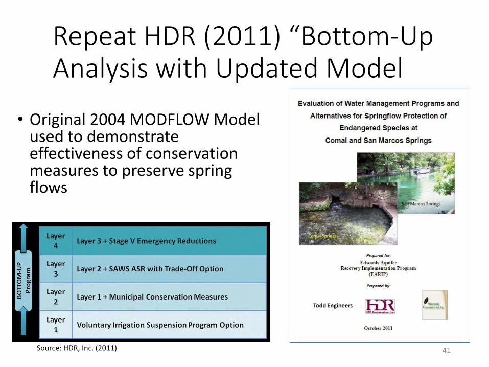
Repeat HDR (2011) “Bottom-Up Analysis with Updated Model

• Original 2004 MODFLOW Model used to demonstrate effectiveness of conservation measures to preserve spring flows

41Source: HDR, Inc. (2011)

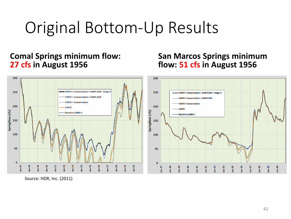
Original Bottom-Up Results

Comal Springs minimum flow: 27 cfs in August 1956

San Marcos Springs minimum flow: 51 cfs in August 1956

42

Source: HDR, Inc. (2011)

Updated model Bottom-Up Results

Comal Springs minimum flow:29.7 cfs in August 1956

San Marcos Springs minimum flow: 48 cfs in August 1956

43

Next Steps

• Publish Model Update Report by December 2017

• Use model to support HCP Adaptive Management• Repeat HDR (2011) bottom-up analysis with new

assumptions regarding ASR leases and triggers

44

Next Steps

• Uncertainty analysis using PEST++ inverse parameter estimation software• Collaboration with USGS’ Austin Office using their high-

performance computer cluster and parallel processing methods

• Evaluate uncertainty in hydraulic parameters and recharge quantity distribution

• Simultaneous inversion to both the 2001—2015 period and the 1947—1958 drought-of-record period

• Expected completion by March 2019

45

Questions?

46