Upper bounds on the star chromatic index forbipartite graphs

Department of Mathematics, Linköping University

Victor Melinder

LiTH-MAT-EX–2020/02–SE

Credits: 16 hp

Level: G2

Supervisor: Carl Johan Casselgren,Institute of mathematics, Linköping University

Examiner: Axel Hultman,Department of Mathematics, Linköping University

Linköping: March 2020

Abstract

An area in graph theory is graph colouring, which essentially is a labeling of thevertices or edges according to certain constraints. In this thesis we consider staredge colouring, which is a variant of proper edge colouring where we additionallyrequire the graph to have no two-coloured paths or cycles with length 4. Thesmallest number of colours needed to colour a graph G with a star edge colouringis called the star chromatic index of G and is denoted χ′st(G).

This paper proves an upper bound of the star chromatic index of bipartitegraphs in terms of the maximum degree; the maximum degree of G is the largestnumber of edges incident to a single vertex in G.For bipartite graphs Bk with maximum degree k ≥ 1, the star chromatic indexis proven to satisfy

χ′st(Bk) ≤ k2 − k + 1. (1)

For bipartite graphs Bk,n, where all vertices in one part have degree n, andall vertices in the other part have degree k, it is proven that the star chromaticindex satisfies

χ′st(Bk,n) ≤ k2 − 2k + n+ 1, k ≥ n > 1. (2)

We also prove an upper bound for a special case of multipartite graphs,namely Kn,1,1,...,1 with m parts of size one. The star chromatic index of such agraph satisfies

χ′st(Kn,1,1,...,1) ≤ 15dn8e · dm

8e+

1

2m(m− 1),m ≥ 5.

For complete multipartite graphs wherem < 5, we prove lower upper boundsthan the one above.

Keywords:Graph Theory, Star edge colouring, Star chromatic index, Graph colour-ing, Biregular, Graph.

Melinder, 2020. iii

Sammanfattning

Inom grafteorin finns graffärgning, ett område som innebär att märka hörn ellerkanter efter några givna regler. En variant av regler kallas stjärnkantsfärgningsom innebär en färgning av kanterna, där tvåfärgade vägar eller cykler av läng-den 4 är otillåtna. Det minsta antal färger som behövs för att stjärnkantsfärgaen graf G kallas det stjärnkromatiska indexet av G och skrivs χ′st(G).

I detta arbete bevisar vi en övre gräns för det stjärnkromatiska indexet hosbipartita grafer Bk med avseende på det högsta gradtalet k i Bk, det vill sägadet högsta antalet kanter som angränsar till ett hörn i Bk. Det stjärnkromatiskaindexet bevisas uppfylla

χ′st(Bk) ≤ k2 − k + 1, k ≥ 1 (3)

.För en bireguljär graf Bk,n, det vill säga en bipartit graf där alla hörn i

ena delen har gradtal n och i den andra har de gradtal k, bevisas det att detstjärnkromatiska indexet uppfyller

χ′st(Bk,n) ≤ k2 − 2k + n+ 1, k ≥ n > 1 (4)

.För kompletta, multipartita grafer Kn,1,1...,1 med m stycken delar som har

storleken 1, visas det att det stjärnkromatiska indexet hos dessa uppfyller föl-jande:

χ′st(Kn,1,1,...,1) ≤ 15dn8e · dm

8e+

1

2m(m− 1),m ≥ 5.

För kompletta, multipartita grafer där m < 5 bevisar vi bättre övre gränser änolikheten ovan.

Nyckelord:Grafteori, stjärnkantsfärgning, stjärnkromatiskt index, graffärgning, Bire-guljär, Graf.

Melinder, 2020. v

Acknowledgements

The author wants to thank Carl Johan Casselgren for the patience, early accessto his research and for showing me star edge colouring. This paper would nothave been possible without his work and late-night emails. Thanks also go toAxel Hultman for being available in such short notice.

Melinder, 2020. vii

Contents

1 Introduction 1

2 Central Definitions and Common Theorems 5

3 Bipartite graphs with ∆ = k 9

4 Multipartite graphs Kn,[m,1] 15

5 (n, k)−biregular graphs 19

Melinder, 2020. ix

Chapter 1

Introduction

Graph Theory is as many other areas in math; it all started with Euler. Hiswork on the bridges of Königsberg marked the beginning of graphs as it is knowntoday.

A graph G = (V,E) consists of a vertex set V and an edge set E, where E isa set of two-subsets from V . The theory of graphs has been studied thoroughlywith landmark theorems like the Marriage theorem by Hall, Tutte’s theoremand Menger’s theorem, but the area has also created a plethora of unsolvedproblems.

There are plenty of applications of graph theory; for example, modelling ofnetworks for computer science, and calculating the impact of a rumour in apopulation. One area within Graph Theory is colouring: i.e. to label verticesor edges by positive integers according to a set of rules. There is a magnitudeof research about colouring since it has plenty of applications, from decidingfrequencies in a network of antennas so the antennas do not interfere with eachother [10] to proving the weak Riemann Hypothesis for Graphs [13].

The area seems easy at first and straightforward enough that a 5-year-oldcould get a crack at it, but the problems within have gone unsolved for centuries.Some proofs are even considered controversial like that of the four-colour theo-rem. It states that any planar map’s faces can be coloured using only 4 colours.The four-colour theorem was proven with (albeit intelligently designed) bruteforce using a computer, making it the first major computer-aided proof [3].

Melinder, 2020. 1

2 Chapter 1. Introduction

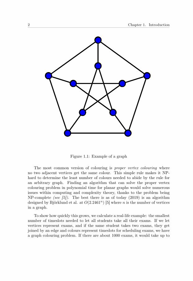
Figure 1.1: Example of a graph

The most common version of colouring is proper vertex colouring whereno two adjacent vertices get the same colour. This simple rule makes it NP-hard to determine the least number of colours needed to abide by the rule foran arbitrary graph. Finding an algorithm that can solve the proper vertexcolouring problem in polynomial time for planar graphs would solve numerousissues within computing and complexity theory, thanks to the problem beingNP-complete (see [5]). The best there is as of today (2019) is an algorithmdesigned by Björklund et al. at O(2.2461n) [5] where n is the number of verticesin a graph.

To show how quickly this grows, we calculate a real-life example: the smallestnumber of timeslots needed to let all students take all their exams. If we letvertices represent exams, and if the same student takes two exams, they getjoined by an edge and colours represent timeslots for scheduling exams, we havea graph colouring problem. If there are about 1000 exams, it would take up to

3

2.24611000 ≈ 10351 operations and about 10316 years to compute the minimumnumber of timeslots required for every student to take all of their exams. Theuniverse would probably have died before the algorithm terminates. Calculatinghow to colour a graph is notoriously complex but due to Brooks’ theorem, weknow that there is an upper bound for the number of colours needed for a propercolouring that can be constructed in polynomial time [6]. That upper bound isthe largest number of participants +1 for a single exam among our 1000 exams.So if the exam with the most participants has 240 participants, 241 colours willsuffice.

The colouring variant we consider in this paper is Star edge colouring whichis a colouring of the edges where a bi-chromatic path or cycle of length four ormore, in other words Blue, Green, Blue, Green, is illegal. Finding the smallestnumber of colours in a star edge colouring intuitively seems NP-hard. It isalso a relatively new area of mathematics - 11 years of age, first formalised byLiu and Deng [11] in 2008. This article looks into three problems on star edgecolouring, all in regards of the least number of colours χ′st(B) needed for a staredge colouring of B:

1. For bipartite graphs Bk with highest vertex degree k, what can be saidabout the least number of colours for a star edge colouring?

2. For complete (m+ 1)-partite graphs G ∼= Kn,1,1...1 with m parts of size 1,is there a better upper bound than |E(G)|?

3. For (k, n)-biregular graphs Bk,n = (X,Y ;E) defined as a bipartite graphwhere all vertices in X have degree k, and all vertices in the other partY have degree n, what can be said about the upper bound for χ′st(Bk,n)?More specifically, can the upper bound be lowered on (3, 4)-biregulargraphs from the currently known 13 [2]?

Chapter 2

Central Definitions andCommon Theorems

The following definitions will be used throughout the article and are thereforedefined here. Notations, definitions and theorems bound to a single chapter willbe found there. Any other common definition can be found in Graph Theory byDiestel [8].

Definition 2.1. A subgraph H of a graph G is a graph such that E(H) ⊆ E(G)and V (H) ⊆ V (G). If V (H) = V (G), then H is a spanning subgraph.

Definition 2.2. A matching M is a set of edges such that no two edges in Mshare a vertex. If edges from M cover every vertex in G, then M is a perfectmatching.

Definition 2.3. A vertex colouring of G is a colouring of the vertices such thatif two vertices are adjacent, they do not share a colour. The minimum numberof required colours for a vertex colouring of G is called the chromatic numberand is denoted χ(G).

Definition 2.4. An edge colouring of G is a colouring of the edges such thattwo edges incident to a common vertex do not share a colour. The minimumnumber of required colours for an edge colouring of G is called the chromaticindex and is denoted χ′(G).

Definition 2.5. A bi-chromatic path from v to u is a path Pi,j(v, u) that alter-nates between two colours i and j on the edges between v and u.

Definition 2.6. A star edge colouring is an edge colouring with no bi-chromaticpaths or cycles of length four. The smallest number of colours needed for a star

Melinder, 2020. 5

6 Chapter 2. Central Definitions and Common Theorems

edge colouring of G is denoted by χ′st(G) and is called the star chromatic indexof G.

Definition 2.7. A contraction is an operation on an edge e = uv ∈ E(G) wherethe vertices u and v are merged to create a new vertex w, and where every edgeincident to v or u is replaced by a corresponding edge incident to w in thenew graph; any multiple edges between two vertices are replaced by an singleedge. The operation is also defined on an independent edge-set E′ ⊆ E(G) bycontracting all edges of E′. The resulting graph after a contraction is a minorof G.

Definition 2.8. The degree of a vertex v in G is the number of edges incidentto v and is denoted by dG(v). The largest degree of all vertices in G is themaximum degree of G and is denoted ∆(G).

Definition 2.9. Two edges are at distance 1 if they are non-adjacent and bothadjacent to a common edge.

Definition 2.10. A strong edge colouring is a colouring of the edges such thatany two edges with distance at most 1 have distinct colours. The minimum num-ber of colours needed for a strong edge colouring is called the strong chromaticindex and is denoted by χ′s(G).

Definition 2.11. Let H be a subgraph of G. A restricted-strong edge-colouringofH onG is a colouring of the edges inH such that if two edges are at distance atmost 1 in G, they get distinct colours. The minimum number of colours neededfor a restricted-strong edge colouring is called the restricted-strong chromaticindex and is denoted by χ′s(H|G).

Definition 2.12. An edge-partition of G is an ordered pair (F,H) where F andH are two edge-disjoint graphs such that E(F ) ∪ E(H) = E(G) and V (G) =V (F ) = V (H).

Except for these definitions, Brooks’ Theorem and König’s Theorem will beused in chapter 3 and 5 and are therefore presented here.

Theorem 2.13. [8] (Brooks’ Theorem) For any graph G, χ(G) ≤ ∆(G) + 1with equality if and only if the graph G is a complete graph or a cycle on anodd number of vertices.

Theorem 2.14. [8] (König’s Theorem) If B is a bipartite graph with ∆(B) = k,then χ′(B) = k.

Wang, Wang and Wang’s paper [1] from 2018, contains a method for obtain-ing an upper bound for the star chromatic index by edge-partitioning a graph.This result will be used to prove Theorem 3.5 in Chapter 3 and for deducingresults on the star chromatic index of Kn,[m,1] in Chapter 4.

7

Theorem 2.15. [1] Let (F,H) be an edge-partition of G. Then

χ′st(G) ≤ χ′st(F ) + χ′s(H|G).

Chapter 3

Bipartite graphs with ∆ = k

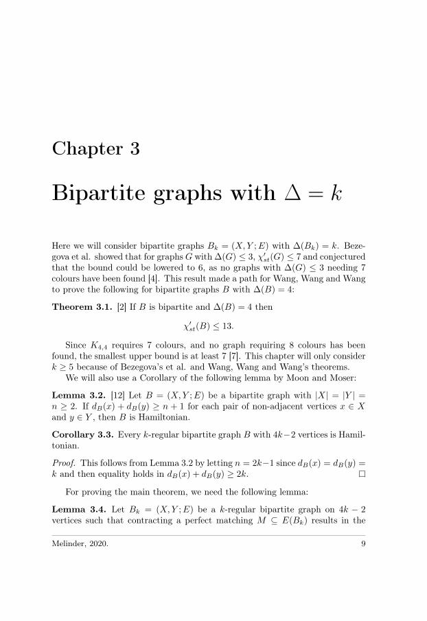
Here we will consider bipartite graphs Bk = (X,Y ;E) with ∆(Bk) = k. Beze-gova et al. showed that for graphsG with ∆(G) ≤ 3, χ′st(G) ≤ 7 and conjecturedthat the bound could be lowered to 6, as no graphs with ∆(G) ≤ 3 needing 7colours have been found [4]. This result made a path for Wang, Wang and Wangto prove the following for bipartite graphs B with ∆(B) = 4:

Theorem 3.1. [2] If B is bipartite and ∆(B) = 4 then

χ′st(B) ≤ 13.

Since K4,4 requires 7 colours, and no graph requiring 8 colours has beenfound, the smallest upper bound is at least 7 [7]. This chapter will only considerk ≥ 5 because of Bezegova’s et al. and Wang, Wang and Wang’s theorems.

We will also use a Corollary of the following lemma by Moon and Moser:

Lemma 3.2. [12] Let B = (X,Y ;E) be a bipartite graph with |X| = |Y | =n ≥ 2. If dB(x) + dB(y) ≥ n + 1 for each pair of non-adjacent vertices x ∈ Xand y ∈ Y , then B is Hamiltonian.

Corollary 3.3. Every k-regular bipartite graph B with 4k−2 vertices is Hamil-tonian.

Proof. This follows from Lemma 3.2 by letting n = 2k−1 since dB(x) = dB(y) =k and then equality holds in dB(x) + dB(y) ≥ 2k.

For proving the main theorem, we need the following lemma:

Lemma 3.4. Let Bk = (X,Y ;E) be a k-regular bipartite graph on 4k − 2vertices such that contracting a perfect matching M ⊆ E(Bk) results in the

Melinder, 2020. 9

10 Chapter 3. Bipartite graphs with ∆ = k

minor graph B∗ ∼= K2k−1. Then any two edges e, f ∈ M, e 6= f are at distance1 and e and f have exactly one common adjacent edge.

Proof. An edge e is adjacent to 2k − 2 other edges since Bk is k-regular. IfB∗ ∼= K2k−1, the vertex w resulting from contracting e has to be adjacentto every other vertex. Thus any two edges e, f ∈ M are at distance 1. Letus assume that e and f are both adjacent to at least two common edges andderive a contradiction. Let w and u be vertices resulting from contracting eand f , respectively. Contracting e and f would result in multiple edges betweencorresponding vertices w and u. Then dBk

(w) = dBk(u) ≤ 2k−3 after removing

any multiple edges, thus w, u can’t be adjacent to all other vertices in B∗, henceB∗ 6∼= K2k−1, a contradiction.

Theorem 3.5. If Bk is a bipartite graph with ∆(Bk) = k ≥ 5 then

χ′st(Bk) ≤ χ′st(Bk−1) + 2k − 2, (3.1)

where χ′st(Bk−1) is the maximum star chromatic index of a bipartite graph withmaximum degree k − 1 and with the same number of vertices as Bk.

Proof. This proof will be similar to the proof by Wang, Wang and Wang forbipartite graphs with ∆(B4) = 4.

By König’s theorem, Bk is k-edge-colourable; let Φ be such a colouring of Bkusing the colours 1, 2, . . . , k. By setting M = {e ∈ E(B)|Φ(e) = 1} we obtain amatching M covering all vertices with degree k. By removing the matching Mfrom Bk, we create a new graph Bk−1 with ∆(Bk−1) = k − 1. Let B∗ be theresulting minor obtained by contracting all edges in M . Now since ∆(Bk) = k,it follows that ∆(B∗) ≤ 2k − 2. Since k ≥ 5, it follows from Brooks’ Theoremthat χ(B∗) ≤ 2k − 1 with equality iff B∗ ∼= K2k−1.

Case 1. When B∗ 6∼= K2k−1, since every edge in M has a correspondingvertex in B∗ and χ(B∗) ≤ 2k − 2, this implies that χ′s(GM |Bk

) ≤ 2k − 2 whereGM = (V (Bk);M). Since GM and Bk−1 form an edge-partition of Bk, we canapply Theorem 2.15 to obtain

χ′st(Bk) ≤ χ′st(Bk−1) + χ′s(GM |Bk) ≤ χ′st(Bk−1) + 2k − 2 (3.2)

Case 2. B∗ ∼= K2k−1:The conditions imply that Bk is a k-regular graph on 4k − 2 vertices. ByCorollary 3.3, B has a Hamiltonian cycle H = x0y0 . . . x2k−2y2k−2, and we canchoose two perfect matchings M0 and M1 on H whereM0 = {y0x0, y1x1 . . . y2k−2x2k−2} and M1 = {y0x1, y1x2 . . . y2k−2x0}. Let B∗0

11

and B∗1 be minors of Bk obtained by contractingM0 andM1 respectively. Thenwe may assume that both B∗0 and B∗1 are isomorphic to K2k−1. We shall showthat there exists a perfect matching M ′ in Bk such that contracting all edgesin M ′ results in a minor not isomorphic to K2k−1.

Claim 3.6. If Bk has a perfect matchingM ′ and a 4−cycle that uses two edgesof the matching M ′, then contracting all edges of M ′ yields a minor B∗M ′ notisomorphic to K2k−1.

Proof. This follows trivially from Lemma 3.4.

Figure 3.1: Section of Bk with M−2 in red and M3 in blue.

It follows from Lemma 3.4 that if a minor graph B∗ obtained from Bk bycontracting a perfect matching M is isomorphic to K2k−1, then every pair ofedges in M are at distance 1. To begin with, we observe that if y0x2 ∈ E(Bk),then there exists a 4−cycle y0x1y1x2y0 where y0x1 and y1x2 ∈M1 so by Claim3.6, we may assume that y2x0 ∈ E(Bk) and more generally, yixi−2 ∈ E(Bk) fori = 0, 1 . . . 2k − 2 where the subscript is modulo 2k − 1. Another observation isthat if y0x2k−2 ∈ E(Bk), joining y0x1 and y2k−3x2k−2 from M1, then a 4−cycley0x2k−2y2k−2x0y0 exists where y2k−2x2k−2 and y0x0 ∈ M0, so we may assumethat y2k−3x1 ∈ E(Bk) and more generally, yixi+3 ∈ E(Bk) for i = 0, 1 . . . 2k−2where the subscript is modulo 2k − 1. We define the perfect matchings

M−2 =

2k−2⋃i=0

{yixi−2} and M3 =

2k−2⋃i=0

{yixi+3}

12 Chapter 3. Bipartite graphs with ∆ = k

respectively as seen in figure 3.1.Now there is the problem of joining y2k−3x2k−3 and y3x3 by an edge. Re-

member that every pair of edges of M0 and M1 has to be joined by an edge,otherwise contracting that matching results in a minor not isomorphic toK2k−1.If the edge y2k−3x3 ∈ E(Bk), then there exists a 4−cycle y0x3y2k−3x1y0 wherey0x3 and y2k−3x1 ∈ M3. Therefore we may assume that y3x2k−3 has to bein E(Bk). But this also results in a 4−cycle y0x1y3x2k−3y0 where x1y3 andx2k−3y0 ∈ M−2. In other words, we can not join y2k−3x2k−3 and y3x3 withoutcreating a 4−cycle countering the claim and therefore there is always a perfectmatchingM3 orM−2 that when contracted, results in a minor B∗ 6∼= K2k−1. Bycontracting all edges in this matching and proceeding as in case 1, we concludethat

χ′st(Bk) ≤ χ′st(Bk−1) + 2k − 2. (3.3)

Corollary 3.7. If Bk is a bipartite graph with ∆(Bk) = k > 2, then

χ′st(Bk) ≤ χ′st(Bk−1) + 2k − 2 (3.4)

where χ′st(Bk−1) is the maximum star chromatic index of a bipartite graph withmaximum degree k − 1 and with the same number of vertices as Bk.

Proof. To prove this corollary, we prove each ∆(Bk) separately, and we assumethat each graph is connected.

Case 1. ∆(B3) = 3If B2 is a 4−cycle, then it is trivial that χ′st(B2) = 3 which implies thatχ′st(Bk−1) ≥ 3. Bezegova et al. proved that for ∆(B3) = 3, χ′st(B3) ≤ 7[4]. Since 7 ≤ χ′st(B2) + 2 · 3 − 2, Bezegova’s et al. upper bound satisfy theinequality.

Case 2. ∆(B4) = 4This follows from the proof of Wang, Wang and Wang’s theorem for ∆(B4) = 4[2]

Case 3. ∆(Bk) = k ≥ 5By Theorem 3.5, χ′st(Bk) ≤ χ′st(Bk−1) + 2k − 2.

Theorem 3.8. If Bk is a bipartite graph with ∆(Bk) = k ≥ 1 then χ′st(Bk) ≤k2 − k + 1

13

Proof. This is proven by induction on k.Our base steps are for k = 1 and 2. The case of k = 1 is trivial. For k = 2, itfollows from Corollary 3.7 that

χ′st(B2) ≤ 1 + 2 · 2− 2 = 3 = 22 − 2 + 1. (3.5)

Now assume that it holds true that ∆(Bk) = k. Let us show that ∆(Bk+1) =k + 1, then by Corollary 3.7 we have

χ′st(Bk+1) ≤ χ′st(Bk) + 2(k + 1)− 2 (3.6)

and by the assumption, we deduce

χ′st(Bk+1) ≤ k2 − k + 1 + 2(k + 1)− 2, (3.7)

and after a bit of cleanup, completing squares and rearranging of terms, weobtain

χ′st(Bk+1) ≤ (k + 1)2 − (k + 1) + 1 (3.8)

Chapter 4

Multipartite graphs Kn,[m,1]

In this chapter we consider complete multipartite graphs as a natural continu-ation of the work by Casselgren et al. [7].

Definition 4.1. A k−partite graph is a graph G = (X1, X2, . . . , Xk;E) wherek⋃i=1

Xi = V (G), Xi ∩ Xj = ∅ if i 6= j, and x1x2 /∈ E(G) for any x1, x2 ∈ Xi

for every i = 1 . . . k. A bipartite graph is equivalent to a 2-partite graph. Ak−partite graph is also called a multipartite graph.

There are infinite families of multipartite graphs, all from the trivial graphswith an empty edge-set to the complete graphs, where every part has size one.In this paper we will prove an upper bound for the following family.

Definition 4.2. Kn,[m,k] denotes a complete (m+ 1)-partite graph with parts(N,M1,M2 . . .Mm) where |N | = n and |Mi| = k.

We will only consider Kn,[m,1] in this paper.Let us observe that Kn,[m,1] is a edge-disjoint union of two other graphs, the

complete graph Km and the complete bipartite graph Kn,m. Thus by Theorem2.15, we have

χ′st(Kn,[m,1]) ≤ χ′st(Kn,m) + χ′s(Km|Kn,[m,1])

χ′st(Kn,[m,1]) ≤ χ′st(Km) + χ′s(Kn,m|Kn,[m,1])

which can be simplified since χ′s(Km|Kn,[m,1]) = χ′s(Km) = 1

2m(m − 1) andχ′s(Kn,m|Kn,[m,1]

) = χ′s(Kn,m) = nm, because in a complete graph or a complete

Melinder, 2020. 15

16 Chapter 4. Multipartite graphs Kn,[m,1]

Figure 4.1: Examples of K3,[m,1] with m = 2 . . . 7.

bipartite graph every pair of edges is adjacent.

χ′st(Kn,[m,1]) ≤ χ′st(Kn,m) + χ′s(Km) (4.1)χ′st(Kn,[m,1]) ≤ χ′st(Km) + χ′s(Kn,m) (4.2)

From Casselgren et al. [7] we have the following theorems:

Theorem 4.3. For n ≥ 3, χ′st(Kn,2) = 2n− bn2 c.

Theorem 4.4. For n ≥ 5, χ′st(Kn,3) = 3dn2 e.

Theorem 4.5. For any n, χ′st(Kn,4) ≤ 20d n12e.

As stated above, we have χ′s(Km) = m(m−1)2 and using this, we deduce the

following:

Theorem 4.6. Let Kn,[m,1] be a complete (m + 1)-partite graph with m ≤ 4.Then

χ′st(Kn,[m,1]) ≤

n, if m = 1,

2n− bn2 c+ 1, if m = 2,

3dn2 e+ 3, if m = 3,

20d n12e+ 6, if m = 4.

(4.3)

Proof. By calculating χ′s(Km) = m(m−1)2 for m ≤ 4 and edge-partitioning

Kn,[m,1] into Km and Km,n, the theorem then follows by applying Theorem4.3, 4.4 and 4.5 to (4.3).

17

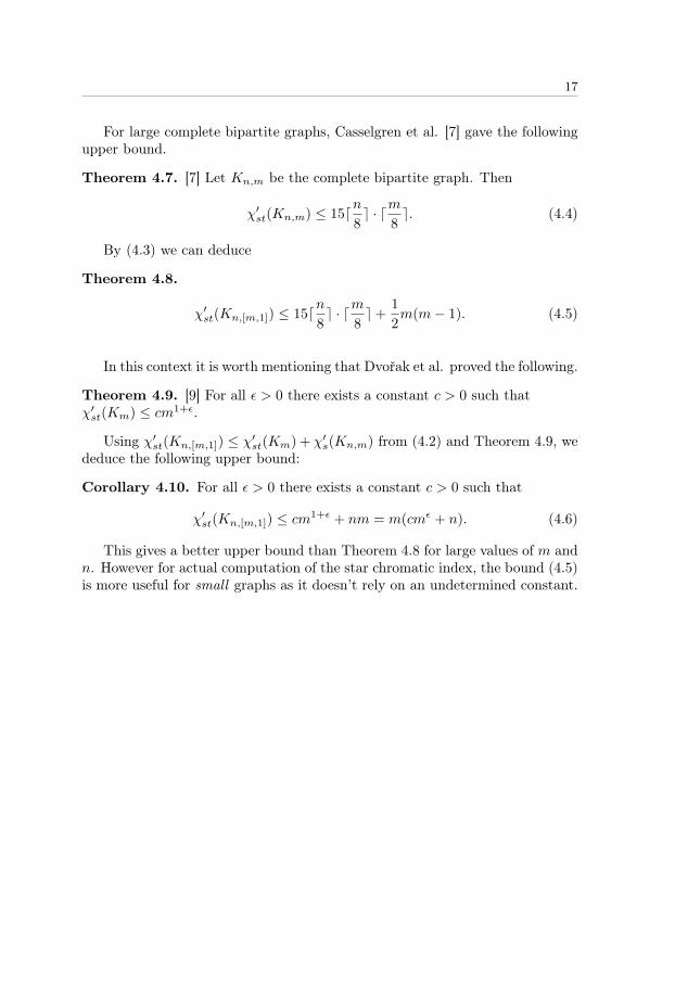
For large complete bipartite graphs, Casselgren et al. [7] gave the followingupper bound.

Theorem 4.7. [7] Let Kn,m be the complete bipartite graph. Then

χ′st(Kn,m) ≤ 15dn8e · dm

8e. (4.4)

By (4.3) we can deduce

Theorem 4.8.

χ′st(Kn,[m,1]) ≤ 15dn8e · dm

8e+

1

2m(m− 1). (4.5)

In this context it is worth mentioning that Dvořak et al. proved the following.

Theorem 4.9. [9] For all ε > 0 there exists a constant c > 0 such thatχ′st(Km) ≤ cm1+ε.

Using χ′st(Kn,[m,1]) ≤ χ′st(Km) + χ′s(Kn,m) from (4.2) and Theorem 4.9, wededuce the following upper bound:

Corollary 4.10. For all ε > 0 there exists a constant c > 0 such that

χ′st(Kn,[m,1]) ≤ cm1+ε + nm = m(cmε + n). (4.6)

This gives a better upper bound than Theorem 4.8 for large values of m andn. However for actual computation of the star chromatic index, the bound (4.5)is more useful for small graphs as it doesn’t rely on an undetermined constant.

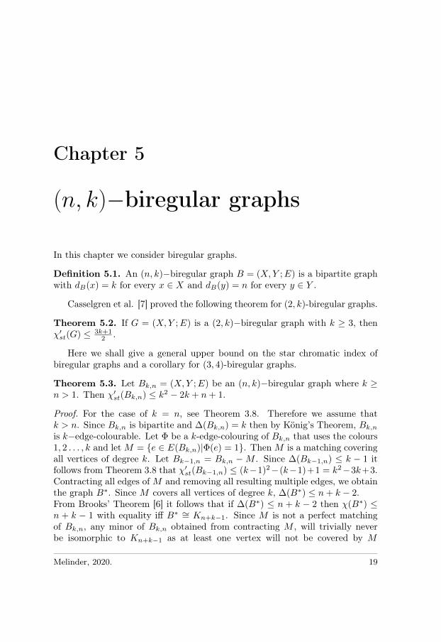
Chapter 5

(n, k)−biregular graphs

In this chapter we consider biregular graphs.

Definition 5.1. An (n, k)−biregular graph B = (X,Y ;E) is a bipartite graphwith dB(x) = k for every x ∈ X and dB(y) = n for every y ∈ Y .

Casselgren et al. [7] proved the following theorem for (2, k)-biregular graphs.

Theorem 5.2. If G = (X,Y ;E) is a (2, k)−biregular graph with k ≥ 3, thenχ′st(G) ≤ 3k+1

2 .

Here we shall give a general upper bound on the star chromatic index ofbiregular graphs and a corollary for (3, 4)-biregular graphs.

Theorem 5.3. Let Bk,n = (X,Y ;E) be an (n, k)−biregular graph where k ≥n > 1. Then χ′st(Bk,n) ≤ k2 − 2k + n+ 1.

Proof. For the case of k = n, see Theorem 3.8. Therefore we assume thatk > n. Since Bk,n is bipartite and ∆(Bk,n) = k then by König’s Theorem, Bk,nis k−edge-colourable. Let Φ be a k-edge-colouring of Bk,n that uses the colours1, 2 . . . , k and letM = {e ∈ E(Bk,n)|Φ(e) = 1}. ThenM is a matching coveringall vertices of degree k. Let Bk−1,n = Bk,n −M . Since ∆(Bk−1,n) ≤ k − 1 itfollows from Theorem 3.8 that χ′st(Bk−1,n) ≤ (k−1)2−(k−1)+1 = k2−3k+3.Contracting all edges ofM and removing all resulting multiple edges, we obtainthe graph B∗. Since M covers all vertices of degree k, ∆(B∗) ≤ n+ k − 2.From Brooks’ Theorem [6] it follows that if ∆(B∗) ≤ n + k − 2 then χ(B∗) ≤n + k − 1 with equality iff B∗ ∼= Kn+k−1. Since M is not a perfect matchingof Bk,n, any minor of Bk,n obtained from contracting M , will trivially neverbe isomorphic to Kn+k−1 as at least one vertex will not be covered by M

Melinder, 2020. 19

20 Chapter 5. (n, k)−biregular graphs

and will therefore not be connected to every other vertex in the minor. Sinceχ(B∗) ≤ n+ k − 2 we have χ′s(GM |B) ≤ n+ k − 2 where GM = (V (Bk,n);M).Since GM and Bk−1,n is an edge-partition of Bk,n, Theorem 2.15 yields that

χ′st(Bk,n) ≤ χ′st(Bk−1,n) + χ′s(GM |B) ≤ k2 − 2k + n+ 1. (5.1)

To answer a question posed by Wang, Wang and Wang on what can be saidof (3, 4)-biregular graphs [2], we prove the following:

Corollary 5.4. For a (3, 4)-biregular graph B4,3, χ′st(B4,3) ≤ 12.

Proof. This corollary follows trivially from Theorem 5.3.

Bibliography

[1] W. Wang, Y. Wang, and Y. Wang. ”Edge-partition and star chromaticindex”. In: Appl. Math. Comput. 333.1 (2018), pp. 480–489. doi: 10.1016/j.amc.2018.03.079.

[2] W. Wang, Y. Wang, and Y. Wang. ”Star edge-coloring of graphs withmaximum degree four”. In: Appl. Math. Comput. 340.1 (2019), pp. 268–275. doi: 10.1016/j.amc.2018.08.035.

[3] K. Appel and W. Haken. ”Every Planar Map is Four Colorable”. In: Bull.Am. Math. Soc. 82.5 (1976), pp. 711–713. doi: 10.1090/conm/098.

[4] L. Bezegová et al. ”Star Edge Coloring of Some Classes of Graphs”. In:Journal of Graph Theory 81.1 (2015), pp. 73–82.

[5] A. Björklund, T. Husfeldt, and M. Koivisto. ”Set Partitioning by inclusion-exclusion”. In: SIAM J. Sci. Comput. 39.2 (2009), pp. 546–563. doi: 10.1137/070683933.

[6] L. Brooks R. ”On colouring the nodes of a network”. In: Math. Proc. Camb.Philos. Soc 37.2 (1941), pp. 194–197.

[7] C. J. Casselgren, J. B. Granholm, and A. Raspaud. On star edge coloringsof bipartite and subcubic graphs. 2019. arXiv: 1912.02467 [math.CO].

[8] R. Diestel. Graph Theory. Springer-Verlag Berlin Heidelberg, 2017.

[9] Z. Dvořák, B. Mohar, and R. Šámal. ”Star Chromatic Index”. In: J GraphTheory. 72.1 (2011), pp. 313–326. doi: 10.1002/jgt.21644.

[10] J. M. Hernández and J. Mieghem. ”Classification of graph metrics”. In:TU Delft (2011).

[11] X. Liu and K. Deng. ”An upper bound on the star chromatic index ofgraphs with δ = 7”. In: Journal of Lanzhou University. Natural Sciences44 (Jan. 2008).

Melinder, 2020. 21

22 Bibliography

[12] J. Moon and L. Moser. ”On Hamiltonian bipartite graphs”. In: Israel J.Math. 1.3 (1963), pp. 163–165.

[13] A. Terras. Zeta functions of graphs - A stroll through the garden. Cam-bridge University Press, 2011. isbn: 978-0-521-11367-0.

Linköping University Electronic Press

CopyrightThe publishers will keep this document online on the Internet – or its possiblereplacement – from the date of publication barring exceptional circumstances.

The online availability of the document implies permanent permission foranyone to read, to download, or to print out single copies for his/her own useand to use it unchanged for non-commercial research and educational purpose.Subsequent transfers of copyright cannot revoke this permission. All other usesof the document are conditional upon the consent of the copyright owner. Thepublisher has taken technical and administrative measures to assure authentic-ity, security and accessibility.

According to intellectual property law the author has the right to be men-tioned when his/her work is accessed as described above and to be protectedagainst infringement.

For additional information about the Linköping University Electronic Pressand its procedures for publication and for assurance of document integrity,please refer to its www home page: http://www.ep.liu.se/.

UpphovsrättDetta dokument hålls tillgängligt på Internet – eller dess framtida ersättare –från publiceringsdatum under förutsättning att inga extraordinära omständig-heter uppstår.

Tillgång till dokumentet innebär tillstånd för var och en att läsa, laddaner, skriva ut enstaka kopior för enskilt bruk och att använda det oförändrat förickekommersiell forskning och för undervisning. Överföring av upphovsrätten viden senare tidpunkt kan inte upphäva detta tillstånd. All annan användning avdokumentet kräver upphovsmannens medgivande. För att garantera äktheten,säkerheten och tillgängligheten finns lösningar av teknisk och administrativ art.

Upphovsmannens ideella rätt innefattar rätt att bli nämnd som upphovsmani den omfattning som god sed kräver vid användning av dokumentet på ovanbeskrivna sätt samt skydd mot att dokumentet ändras eller presenteras i sådanform eller i sådant sammanhang som är kränkande för upphovsmannens litteräraeller konstnärliga anseende eller egenart.

För ytterligare information om Linköping University Electronic Press se för-lagets hemsida http://www.ep.liu.se/.

c© 2020, Victor Melinder