Upper Limit for Hydropower in an Open-Channel Flowwl.fst.tu-darmstadt.de/wl/publications/paper... · Upper Limit for Hydropower in an Open-Channel Flow Peter F. Pelz1 Abstract: It

Technical Note

Upper Limit for Hydropower in anOpen-Channel Flow

Peter F. Pelz1

Abstract: It is proved on the basis of the axiomatic energy equation that the theoretical upper limit for the hydropower gained by a water

wheel or turbine per unit width in a rectangular open channel cannot exceed ð2=5Þ5=2ρg3=2H5=2eff by any means in which Heff = effective water

head, which is the sum of specific energy E1 ¼ h1 þ u21=2g and the drop of ground level Δz; ρ = density; and g = gravity body force. As adimensionless measure, a coefficient of performance or harvesting factor is introduced that is an analogue to the one introduced by AlbertBetz for wind turbines. DOI: 10.1061/(ASCE)HY.1943-7900.0000393. © 2011 American Society of Civil Engineers.

CE Database subject headings: Hydro power; Open channel flow.

Author keywords: Hydropower; Open channel; Performance; Efficiency; Water wheel; Water turbine.

Introduction

In the context of both limited fossil fuel reservoirs on the planet andglobal warming caused by the combustion of those fuels, there is anincreasing demand to exploit renewable energy sources. The U.S.Energy Information Administration (2009) expects that electricpower gained from renewable energy sources will increase inthe next two decades by 70%, reaching a share of 11% of the2030 energy mix. It is further assumed that water and wind energywill be the predominant renewable energy sources to that point,whereas the exploration of larger unexploited hydropower sourceswill take place in Asia, South America, and Africa. In NorthAmerica and Europe, most of the larger (> 0:1–1 MW) water-power sources have already been explored. It is believed, at leastin Europe, that small waterpower sources (< 0:1–1 MW) will beworthwhile to explore in the future. But one has to be aware that thespecific power installation costs are, on average, six times higherthan the specific power installation costs for a wind turbine by com-parable electricity production costs (Giesecke and Mosonyi 2009).To overcome this problem today, several machine types fromhydrostatic machines (water wheels) to hydrodynamic machines(water turbines) are again in the focus of research and development(Bassett 1989; Müller et al. 2007). This is historically interesting, asthere has been no research on water wheels after the Second WorldWar for over half a century. Going further back to the year 1846, thestatement made by Ferdinand Redtenbacher, who is considered tobe the founder of scientific engineering in Germany, in the first twosentences in the preamble of his monograph on “Theorie und Bauder Wasserräder” (Rettenbacher 1846) reads:

A work about water wheels with horizontal axis is today notup to date, since these wheels are, due to the rapidly increas-ing number of turbines, nearly considered to be antique.

Nevertheless they are still useful machines which presumablywill never be completely replaced by turbines even thoughthey are not anymore so such important as they were a fewyears ago.

From today’s point of view, the argument for the success ofturbines is their superior specific power volume and hence lowerinvestment costs compared with hydrostatic water wheels: for thesame known head drop HT over the machine and known volumeflow Q through the machine, the typical length, i.e., outer diameterd of the turbine is smaller than that of the hydrostatic acting waterwheel. In contrast, the rotational speed n of the turbine is higherthan that of a hydrostatic machine, which is again favorable forelectrodynamic power generation. This relation was made clearin 1953 by Otto Cordier (1955). He introduced the dimensionlessspecific diameter δ ∼ dðgHTÞ1=4Q�1=2 and the dimensionless spe-cific speed of the machine σ ∼ nðgHTÞ�3=4Q1=2 by a dimensionalanalysis. Cordier showed by comparing machines that their oper-ating points at best hydraulic efficiency are lined up at one singlemonotonic decreasing curve δ ¼ δðσÞ, known as the Cordier curve.

The task of this work is not to give a contribution on a specificdesign of a water wheel or turbine and to compare it with othersolutions. This should be done by a physical, theoretical modelingof a specific machine design and would be followed by model testsand full scale validation tests or alternative applying upscalingmethods. This is the approach taken by Redtenbacher in 1846(Redtenbacher 1846), 60 years later by the first head of the author’schair Adolph Pfarr in 1906 (Pfarr 1912), who influenced the devel-opment of water turbines significantly and more recently by severalresearch studies (Müller et al. 2007). The newer research work hasalways an empirical part and thus is only valid for a specific design,operating point, and test setup. Instead the approach of the presentpaper takes a wider angle. The open question raised in this paper is:“What is the maximum hydraulic power that can be transformedinto mechanical energy by any possible machine in an open chan-nel?” (sketched in Fig. 1).

The answer to this question is important in three aspects: First,different design solutions or operating conditions, especially forsmall hydro power sources (< 1 MW), can be compared on anobjective basis. This is important for a scientific discussion in com-paring designs and operating conditions. When the machine type is

1Professor and Head of the Chair of Fluid Systems Technology,Technische Universität Darmstadt, Magdalenenstraße 4, 64289 Darmstadt,Germany. E-mail: [email protected]

Note. This manuscript was submitted on July 8, 2009; approved onJanuary 7, 2011; published online on January 10, 2011. Discussion periodopen until April 1, 2012; separate discussions must be submitted forindividual papers. This technical note is part of the Journal of HydraulicEngineering, Vol. 137, No. 11, November 1, 2011. ©ASCE, ISSN 0733-9429/2011/11-1536–1542/$25.00.

1536 / JOURNAL OF HYDRAULIC ENGINEERING © ASCE / NOVEMBER 2011

Downloaded 19 Dec 2011 to 130.83.195.141. Redistribution subject to ASCE license or copyright. Visit http://www.ascelibrary.org

http://dx.doi.org/10.1061/(ASCE)HY.1943-7900.0000393




not fixed, the hydraulic efficiency at an early planning stage is onlyof minor importance, which changes as soon as the principle typeof the machine is known. Second, society, i.e., politicians and in-vestors, can decide on the basis of realistic upper bounds. It is theduty of scientists to give such a background. Third and finally, theupper bound serves as a target to develop machines with reducedspecific power installation costs.

The classic work of Albert Betz, published in 1920 (Betz 1920,1959), which gives such an upper bound for wind turbines, reducedthe specific power installation costs by increasing the amount ofpower gained out of a wind turbine of given size. Typically forBetz, he took a characteristically abstract look at the subject, whichwas a great talent of this researcher. From basic principles he wasable to derive his famous 16=27 ¼ 59:3% limit for the coefficientof performance, or energy harvesting factor, of a wind turbine.Since he got this result from basic principles, i.e., physical axioms,in a truly analytic manner, it is justified to call it a proof. Betzclearly distinguished between hydraulic efficiency and harvestingfactor as one has to do. Hydraulic efficiency is the ratio of themechanical power PT gained at the shaft of the water wheel or tur-bine and the hydraulic power supplied to the machine PH , i.e.,η :¼ PT=PH . The harvesting factor is the ratio of mechanical powerto the available power Pavail : CP :¼ PT=Pavail ¼ ηPH=Pavail. Bothquantities η and CP are dimensionless ratios of power. Only the firstone is a measure of the dissipation attributable to viscous fluid fric-tion. The second one is a measure of the amount of energy thatcannot be converted into mechanical energy. Since there has tobe a flow downstream of the machine (wind or water), this flowwill transport energy that is greater than zero and is lost for energyconversion. This is the case even for a hydraulic efficiency of onefor a hypothetically frictionless flow. Indeed, there are other matterswhere it is suitable to define ratios of power than the efficiency η.For the example of marine propulsion systems, the Froudeefficiency is defined as ηF :¼ UW=ðUWþ loss rate of kineticenergyþ dissipation rateÞ, where UW = product of speed and re-sistance force. Again, even for the frictionless case, ηF is smallerthan one because of the flux of kinetic energy downstream of thevehicle (Newmann 1977) or slender fish, whose propulsion effi-ciency was considered by Lighthill (1960). At the beginning ofthe 19th century, the French engineer Sadi Carnot proved that onlya fraction of the heat put into a system can be transferred intomechanical work done by the system. Hence the Carnot factoris always smaller than one. Carnot was one of the first who discov-ered the second law of thermodynamics by his work on steamengines.

In the literature on water wheels or turbines for small power(< :1–1 MW), only the efficiency is in focus but not the harvestingfactor introduced in this paper. In current research, the water heightand speed downstream of the machine is always assumed to be

known (Müller et al. 2007). As stated previously, if one looks atthe machine as one module of the system this makes sense, whenit is the task to determine the efficiency analytically, numerically, orexperimentally. For the specific power installation costs, the coef-ficient of performance is most important. For the design of a waterwheel or turbine, especially for small power plant, the ratio CP=η ¼PH=Pavail is most important.

The outline of this paper is as follows. Consecutive to this in-troduction, in the section “Energy Equation for an Open ChannelContaining a Hydraulic Machine,” the energy equation for an openchannel including a hydraulic machine will be considered by start-ing from its most general form. The attempt is made to make eachtransformation and assumption as clear as possible. There is a needfor this careful derivation, as the results from this section carry overto the conditions for maximum power transformation in the section“Condition for Maximum Power Conversion and the TheoreticalUpper Limit for the Mechanical Power.” In the section “Hypotheti-cal Ideal Machine Defined as Reference,” an ideal but hypotheticalmachine is discussed that serves to define a suitable reference.The section “Comparison of a Hydropower Machine in an OpenChannel and a Wind Turbine” compares the findings of this workwith the basic work of Betz on wind turbines. The paper will closewith a critical discussion of the results in the section “CriticalDiscussion and Conclusion” and a list of references.

Energy Equation for an Open Channel Containinga Hydraulic Machine

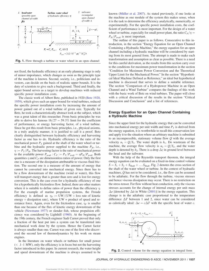
Since the upper limit for the hydraulic energy that can be convertedinto mechanical energy per unit width and time PT is derived fromthe energy equation, it is worthwhile to recall this conservation lawand apply it to the situation where an arbitrary machine is submittedto an incompressible, stationary volume flow Q with the averagevelocity u1 ¼ Q=S1. The water depth is h1. Do wnstream of themachine, the average flow velocity is u2 ¼ Q=S2, and the waterdepth is denoted by h2. There is a drop Δz in ground level betweenthe head and the tailwater.

With the help of the Reynolds transport theorem, the integralenergy equation can be evaluated on a fixed-in-time control volumeS ¼ S1 þ S2 þ SShaft þ…:SShaft. Fig. 2 denotes the cross section ofthe shaft of the water wheel or turbine. In the context of hydraulicmachines, _Q has not to be considered, i.e., the flow can be assumedto be adiabatic. For the flow through the turbine, viscous stressesand hence viscous dissipation may occur. There is no restriction onthe stress tensor. For flow without heat conduction, only the viscousstresses accounts for the change of internal energy per unit massΔe [denoted by Δu in White (2001)] in the energy equation. Thischange is in the adiabatic case proportional to the temperaturedifference ΔT between 1 and 2, since water can be consideredas calorically ideal: Δe ¼ cΔT with the specific heat of water c.

Fig. 1. Flow through a turbine or water wheel in an open channel

Fig. 2. Control volume for the energy equation in integral form

JOURNAL OF HYDRAULIC ENGINEERING © ASCE / NOVEMBER 2011 / 1537


It is assumed that the machine is operating at a stationary point.Therefore, every partial time derivative vanishes at least in the aver-age over one cycle time 1=n. Finally, at the positions 1 and 2—andonly there—the flow is assumed to be in the time average unidi-rectional. Hence the normal component of the viscous stress tensorvanishes at these positions. If there is a velocity profile ~u andtemperature profile ~T ¼ ~e=c (internal energy per unit mass ~e) atpositions 1 and 2, it is necessary to introduce a velocity profile fac-tor and an averaged internal energy or temperature in the sense

α1;2 :¼1

Qu21;2

ZS1;2

~u3dS; e1;2 :¼1Q

ZS1;2

~u~edS; T :¼ e=c

ð1Þto be used in the energy equation. Applying Reynolds’ transporttheorem (White 2001) using the control volume V shown in Fig. 2,the energy equation _K þ _E ¼ P in which _K = change of the kineticenergy of the fluid body; _E = change of internal energy of the fluidbody; and P = work done by surface and body forces on the fluid,becomes

ρQ�α2u222

� α1u212

�þ ρQðe2 � e1Þ

¼ZSShaft

~τ ·~udSþZVρ~g ·~udV þ

ZS1þS2

~τ ·~udS ð2Þ

The work done by the surface and volume forces on the fluid hasthree additive contributions (right side of Eq. (2)). First, the workdone by the stress vector ~τ on the turbine or water wheel is themechanical power gained at the shaft by the water wheel or turbine.This is the quantity for which a theoretical upper bound is given inthis work:

PT ¼ �ZSShaft

~τ ·~udS ð3Þ

The minus sign was introduced for convenience; as a result, PTis positive in the context of this paper. Second, the work per unittime by the gravitational force~g is the volume integral on the righthand side of Eq. (2). With the help of the potential ψ ¼ gðzþ yÞ,where z ¼ const is constant and y denotes the channel coordinate(see Fig. 2), the volume integral is transformed into a surfaceintegral using Gauss’ theorem:

ZVρ~g ·~udV ¼

IS�ρψ~u ·~ndSþ

ZVψ∇ · ðρ~uÞdV

¼ ρQgðz1 � z2Þ þZS1þS2

�ρgy~u ·~ndy ð4Þ

Eq. (4) is valid either for a constant density flow or for a sta-tionary flow in a time-averaged sense, since only for those twocases∇ · ðρ~uÞ, which is attributable to the continuity equation equalto �∂ρ=∂t, vanishes.

Third, the work done per unit time of the stress vector at the inletsurface 1 and the outlet surface 2 plus the work per unit time by thegravitational force~g on the fluid body within the volume (Eq. (4))yields, for a unidirectional flow and hence a hydrostatic pressuredistribution p ¼ ðh� yÞρg at the positions 1 and 2:

ZVρ~g ·~udV þ

ZS1þS2

~τ ·~udS ¼ ρQgΔz�ZS1þS2

ðρgyþ pÞ~n ·~udS

¼ ρQgΔzþ ρQgðh1 � h2Þ ð5Þ

Multiplying the energy Eq. (2) by minus one, and usingEqs. (3)–(5) yields

ρQ�α1u212

� α2u222

�þ ρQgðh1 � h2Þ þ ρQgðz1 � z2Þ

¼ PT þ ρQðe2 � e1Þ ð6Þ

Dividing by ρQg, the energy equation is given in its final form as�h1 þ α1

u212g

þ z1

��h2 þ α2

u222g

þ z2

�¼ PT

ρQgþ e2 � e1

gð7Þ

With the abbreviations specific energy E ¼ hþ αu2=2g, totalhead H ¼ E þ z, head drop attributable to the turbine HT :¼PT=ρQg, and the dissipative head loss attributable to viscous fric-tion within the fluid as hL :¼ ðe2 � e1Þ=g, Eq. (7) can be written inthe easy to remember form:

H1 � H2 ¼ HT þ hL; or equivalent ð8Þ

H1 � H2 ¼1ηHT ; with η ¼ 1

1þ hL=HTð9Þ

Eqs. (8) and (9) are still the same energy equation _K þ _E ¼ P inits integral form. The hydraulic efficiency is a measure for the dis-sipation hL as stated previously. Rearrangement of Eqs. (8) and (9)gives

η ¼ PT

ρQgðH1 � H2Þ¼ HT

H1 � H2¼ 1� c

gT2 � T1

H1 � H2ð10Þ

The last equality is worthwhile to note, since it is the basis for avery simple method to determine the hydraulic efficiency by meas-uring the temperature difference. But one has to be aware that T1;2are averaged temperatures by the definition [Eq. (1)]. Not takingthe temperature distribution into account may lead to a wronghydraulic efficiency. In addition, the measurable temperature differ-ences are rather small because of the high specific heat c of water.

The energy equation in the forms of Eqs. (8)–(10) is still in theintegral form and should not be mismatched with Bernoulli’s equa-tion. Again, the only assumptions made are unidirectional flow atpositions 1 and 2, incompressibility and stationary flow in the timeaverage over one period time 1=n. At no point in the derivation hasit been necessary to assume that the fluid is frictionless.

Condition for Maximum Power Conversion and theTheoretical Upper Limit for the Mechanical Power

Employing Eq. (10), a theoretical upper limit for the mechanicalpower is derived in this section, by looking at the flow rate per unitwidth in the tailwater q2 ¼ Q=ðbh2Þ and the water depth h2 in therectangular channel of the tailwater. Hence, the mechanical energygained per unit time is

PTðh2; q2Þ ¼ ηρgq2bðH1 � H2Þ ¼ ηρgq2b�Heff � h2 � α2

q222gh22

�

ð11Þin which the identity H1 � H2 ¼ E1 þΔz� E2 and the definitionof the introduced effective head

Heff :¼ E1 þΔz; with E1 > 0; Δz ≥ 0 ð12Þ



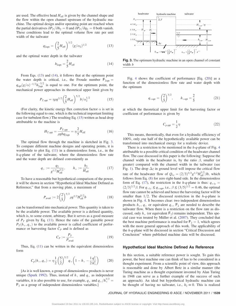
are used. The effective head Heff is given by the channel shape andthe flow within the open channel upstream of the hydraulic ma-chine. The optimal design and/or operating point are reached whenthe partial derivatives ∂PT=∂h2 ¼ 0 and ∂PT=∂q2 ¼ 0 both vanish.These conditions lead to the optimal volume flow rate per unitwidth of the tailwater

q2opt ¼�25Heff

�3=2

ðg=α2Þ1=2 ð13Þ

and the optimal water depth in the tailwater

h2opt ¼25Heff ð14Þ

From Eqs. (13) and (14), it follows that at the optimum pointthe water depth is critical, i.e., the Froude number F2opt ¼qoptðg=αÞ�1=2h�3=2

2opt is equal to one. For the optimum point, themechanical power approaches its theoretical upper limit given by

PT;opt ¼ ηρg3=2�25Heff

�5=2

b=α1=22 ð15Þ

(For clarity, the kinetic energy flux correction factor α is set inthe following equal to one, which is the technical important limitingcase for turbulent flow.) The resulting Eq. (15) written as head dropattributable to the machine is

HT ;opt ¼PT;opt

ρgbq2opt¼ η

25Heff ð16Þ

The optimal flow through the machine is sketched in Fig. 3.To compare different machine designs and operating points, it isworthwhile to plot Eq. (11) in a dimensionless form, i.e., in theh-q-plane of the tailwater, where the dimensionless flow rateand the water depth are defined conveniently as

qþ :¼ q2g1=2H3=2

eff

; hþ :¼ h2Heff

ð17Þ

To have a reasonable but hypothetical comparison of the power,it will be shown in section “Hypothetical Ideal Machine Defined asReference,” that from a moving plate, a maximum of

Pavail :¼ 2

�25

�5=2

ρg3=2H5=2eff b ð18Þ

can be transformed into mechanical power. This quantity is taken tobe the available power. The available power is a defined quantity,which is, to some extent, arbitrary. But it serves as a good measureof PT given by Eq. (11). Hence the ratio of the gainable powerPTðhþ; qþÞ to the available power is called coefficient of perfor-mance or harvesting factor CP and is defined as

CP :¼ PT

Pavailð19Þ

Thus, Eq. (11) can be written in the equivalent dimensionlessform

Cpðhþ; qþÞ ¼ η12

�52

�5=2

qþ

�1� hþ � 1

2q2þh2þ

�ð20Þ

[As it is well known, a group of dimensionless products is neverunique (Spurk 1992). Thus, instead of hþ and qþ as independent

variables, it is also possible to use, for example, qþ and qþ=h3=2þ ¼

F2 as a group of independent dimensionless variables.]

Fig. 4 shows the coefficient of performance [Eq. (20)] as afunction of the dimensionless flow rate and water depth withthe optimum

qþopt ¼�25

�3=2

; hþopt ¼25

ð21Þ

at which the theoretical upper limit for the harvesting factor orcoefficient of performance is given by

Cp;opt ¼12η ð22Þ

This means, theoretically, that even for a hydraulic efficiency of100%, only one half of the hypothetically available power can betransformed into mechanical energy for a realistic device.

There is a restriction to be mentioned in the h-q-plane of Fig. 4attributable to a possible critical condition of the headwater channelflow. The case discussed in this paper is the following: Suppose thechannel width in the headwater is, by the ratio β, smaller (orgreater) compared with the channel width in the tailwater (seeFig. 1). The drop Δz in ground level will impose the critical flow

rate of the headwater flow of Q1c ¼ ð2=3Þ3=2g1=2H3=2eff βb, which

follows from Eq. (8) for zero right-hand side. In the dimensionlessform of Eq. (17), the restriction in the h-q-plane is thus: qþ1c ¼ð2=3Þ3=2β. For qþ1c ≤ qþopt, i.e., β ≤ ð3=5Þ3=2 ¼ 0:46, the optimalflow rate cannot be achieved and hence the harvesting factor will besmaller than 1=2. The discussed restriction in the h-q-plane isshown in Fig. 4. It becomes clear: two independent dimensionlessproducts hþ, qþ or equivalent qþ, F2 are needed to describe thetailwater flow. When there is a restriction on the flow rate as dis-cussed, only hþ (or equivalent F2) remains independent. This spe-cial case was treated by Müller et al. (2007). They concluded thatthe best machine performance is reached for F2 ¼ 1, which agreeswith the more general approach of this work. The applicability ofthe h-q-plane will be discussed in section “Critical Discussion andConclusion” where published machine data will be discussed.

Hypothetical Ideal Machine Defined As Reference

In this section, a suitable reference power is sought. To gain thispower, the best machine one can think of has to be considered in athought experiment. From a scientific point of view, this approachis reasonable and done by Albert Betz in a similar manner (theTuring machine as a thought experiment invented by Alan Turingin 1948 can serve as a further example of the success of suchan approach). An ideal but hypothetical hydraulic machine canbe thought of having no tailwater, i.e., h2 ≡ 0. This is realized

Fig. 3. The optimum hydraulic machine in an open channel of constantwidth b



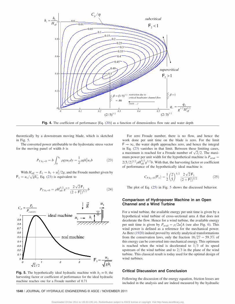
theoretically by a downstream moving blade, which is sketchedin Fig. 5.

The converted power attributable to the hydrostatic stress vectorfor the moving panel of width b is

PT;h2¼0 ¼ bZ

h1

0ρgyu1dy ¼

12ρgh21u1b ð23Þ

With Heff ¼ E1 ¼ h1 þ u21=2g, and the Froude number given byF1 ¼ u1=

ffiffiffiffiffiffiffigh1

p, Eq. (23) is equivalent to

PT ;h2¼0 ¼ ρH5=2eff g

3=2 2ffiffiffi2

pF1

ð2þ F21Þ5=2

b ð24Þ

For zero Froude number, there is no flow, and hence thework done per unit time on the blade is zero. For the limitF → ∞, the water depth approaches zero, and hence the integralin Eq. (23) vanishes in that limit. Between these limiting cases,a maximum is reached for a Froude number of

ffiffiffi2

p=2. The maxi-

mum power per unit width for the hypothetical machine is Pavial ¼2ð5=2Þ5=2ρH5=2

eff g3=2b. With that, the harvesting factor or coefficient

of performance of the hypothetically ideal machine is

CP;h2¼0ðF1Þ ¼12

�25

�5=2 2

ffiffiffi2

pF1

ð2þ F21Þ5=2

ð25Þ

The plot of Eq. (25) in Fig. 5 shows the discussed behavior.

Comparison of Hydropower Machine in an OpenChannel and a Wind Turbine

For a wind turbine, the available energy per unit time is given by ahypothetical wind turbine of cross-sectional area A that does notdecelerate the flow. Hence for a wind turbine, the available energyper unit time is given by Pavail ¼ ρ=2u31A (see also Fig. 6). Thiswind power is defined as a reference for the mechanical power.As Betz (1920) indeed proved by strictly analytical transformationsfrom the conservation laws, only the fraction 16=27 ¼ 59:3% ofthis energy can be converted into mechanical energy. This optimumis reached when the wind is decelerated to 1=3 of its speedupstream of the wind turbine and to 2=3 in the plane of the windturbine. This classical result is today used for the optimal design ofwind turbines.

Critical Discussion and Conclusion

Following the discussion of the energy equation, friction losses areincluded in the analysis and are indeed measured by the hydraulic

F

F

Fig. 4. The coefficient of performance [Eq. (20)] as a function of dimensionless flow rate and water depth

Fig. 5. The hypothetically ideal hydraulic machine with h2 ≡ 0; theharvesting factor or coefficient of performance for the ideal hydraulicmachine reaches one for a Froude number of 0.71



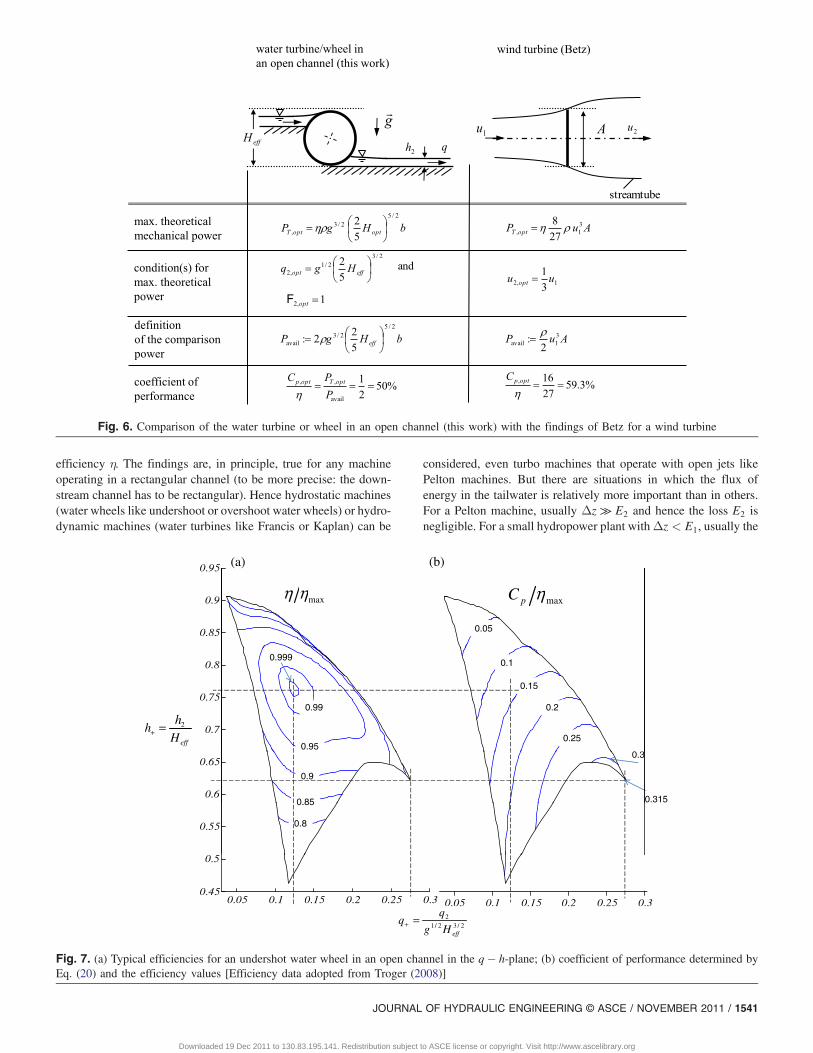
efficiency η. The findings are, in principle, true for any machineoperating in a rectangular channel (to be more precise: the down-stream channel has to be rectangular). Hence hydrostatic machines(water wheels like undershoot or overshoot water wheels) or hydro-dynamic machines (water turbines like Francis or Kaplan) can be

considered, even turbo machines that operate with open jets likePelton machines. But there are situations in which the flux ofenergy in the tailwater is relatively more important than in others.For a Pelton machine, usually Δz ≫ E2 and hence the loss E2 isnegligible. For a small hydropower plant withΔz < E1, usually the

F

Fig. 6. Comparison of the water turbine or wheel in an open channel (this work) with the findings of Betz for a wind turbine

0 9

0.95

0

0

ηη ηC

(a) (b)

0.85

0.9

0

0maxηη maxηpC

0.05

0.75

0.8

0

00.999

0.1

0.15

0.7

0.75

0

0

0.95

0.99 0.2

0.25

0 3

0.6

0.65

0

0

0 85

0.9

0.3

0.315

0

0.55

0

00.8

0.85

0.05 0.1 0.15 0.2 0.25 0.30.45

0.5

0.05 0.1 0.15 0.2 0.25 0.30

0

2/32/12

effHg

qq =+

effHh 2=+

h

Fig. 7. (a) Typical efficiencies for an undershot water wheel in an open channel in the q� h-plane; (b) coefficient of performance determined byEq. (20) and the efficiency values [Efficiency data adopted from Troger (2008)]



situation is different, and E2 is significant. Indeed, this is shown bythe typical behavior of an undershoot water wheel in a rectangularchannel with Δz ¼ 0 in h� q-plane (Fig. 7). The data are adoptedfrom the diploma theses by Troger (2008). Fig. 7(a) shows the con-tour plot of the efficiency η scaled by the maximal efficiency ηmax

in the h-q-plane for the undershoot water wheel in a channel ofconstant width β ¼ 1 and no elevation Δz ¼ 0. In the example,η=ηmax ¼ 1 is reached at the conditions in the tailwater hþ ¼0:76 and qþ ¼ 0:12. At this best operating point of the machine,roughly 14% of the available energy is transformed into mechanicalenergy, as shown in Fig. 7(b). At the alternative operating pointhþ ¼ 0:62 and qþ ¼ 0:28, the efficiency is only 0:83ηmax, i.e.,reduced by 17% from the best operating point of the machine,but more important is that at this point, 31% of the available poweris used. Even though the efficiency is lower, the power output isincreased by nearly the same factor, and the most important specificpower installation costs will be reduced to one-third. Therefore, it isworthwhile to look first at the h-q-plane and the coefficient ofperformance. The efficiency is only of minor importance in theconsidered context.

One objective could be that hydropower plants are controlled insuch a way that the flow rate Q is the control variable in the controlloop to ensure required water level. When the water level is not themain issue, the power PT that is supplied to the power grid is usu-ally the dominant control variable. For small hydropower plants,the last one is usually not the control variable, since the power planthas to work at its best point Cpmax. To ensure a flow rate Q > Qopt

might indeed be a restriction from an ecological point of view. Anywater plant, in principle, reduces the volume flow, and hence thisdiscussion is similar for any hydro plant. Even though this issue isnot discussed in this paper, one has to be aware that it is indeedimportant for the ecosystem of small streams.

In conclusion:• In the context of water power, a new dimensionless quantity

called harvesting factor or coefficient of performance is intro-duced. It is defined as the ratio of gained mechanical power tothe available hydraulic power.

• It is proved on the basis of the energy equation that the harvest-ing factor for a rectangular channel has the upper limit of ½, i.e.,even for an ideal machine, one-half of the available hydraulicenergy remains unused and is washed down the tailwater.

• In general, there are two independent dimensionless productsthat describe the tailwater flow: the dimensionless water depthor Froude number and dimensionless flow rate.

• The optimal tailwater flow is critical, and the optimal flow rateis a function of the effective water depth.

• The h-q-plane and the associated harvesting factor might serveto compare different machines and/or operating points on an ob-jective basis. In an example, it is shown that the hydraulic effi-ciency is only of secondary importance in comparing machines.

References

Bassett, D. E. (1989). “A historical survey of low head hydropowergenerators and recent laboratory based work at the University ofSalford.” Ph.D. thesis, Univ. of Salford, Salford, UK.

Betz, A. (1920). “Das Maximum der theoretisch möglichen Ausnut-zung des Windes durch Windmotoren.” Zeitschrift für das gesamteTurbinenwesen, Sep. (in German).

Betz, A. (1959). Einführung in die Theorie der Strömungsmaschinen,Braun, Karlsruhe, Germany (in German).

Cordier, O. (1955). Ähnlichkeitsbedingungen für Strömungsmaschinen,VDI, Berlin (in German).

Giesecke, J., and Mosonyi, E. (2009). Wasserkraftanlagen—Grundsätzeder Planung und Projektierung, Springer, Berlin (in German).

Lighthill, M. J. (1960). “Note on the swimming of a slender fish.” J. FluidMech., 9(02), 305–317.

Müller, G., Denchfield, S., Marth, R., and Shelmerdine, B. (2007). “Streamwheels for applications in shallow and deep water.” Proc. 32ndIAHR Congress, Theme C2c, International Association for Hydro-Environment Engineering and Research , Paper 291.

Newmann, J. N. (1977). Marine hydrodynamics, The MIT Press,Cambridge, MA.

Pfarr, A. (1912). Die Turbinen für Wasserkaftbetrieb, 2nd Ed., Springer,Berlin (in German).

Redtenbacher, F. (1846). Theorie und Bau der Wasserräder, FriedrichBassermann, Mannheim, Germany (in German).

Spurk, J. H. (1992). Dimensionsanalyse in der Strömungslehre, Springer,Berlin (in German).

Troger, M. (2008). “Wie effizient sind Wasserräder zur Gewinnung vonEnergie in Fließgewässern mit geringen Fallhöhen?” Diplomarbeit,Technische Universität Darmstadt, Darmstadt, Germany (in German).

U.S. Energy Information Administration. (2009). “World energy demandand economic outlook.” International Energy Outlook 2009, ⟨http://www.eia.doe.gov/oiaf/ieo/world.html⟩ (Apr. 6, 2009).

White, F. M. (2001). Fluid mechanics, McGraw-Hill, Boston.



http://dx.doi.org/10.1017/S0022112060001110

http://dx.doi.org/10.1017/S0022112060001110

http://www.eia.doe.gov/oiaf/ieo/world.html






Documents

Upper Limit for Hydropower in an Open-Channel Flowwl.fst.tu-darmstadt.de/wl/publications/paper... · Upper Limit for Hydropower in an Open-Channel Flow Peter F. Pelz1 Abstract: It