Upper Mississippi River System Flow Frequency Study .... F...Upper Mississippi River System Flow Frequency Study Hydrology and Hydraulics Appendix F Missouri River U.S. Army Corps

Upper Mississippi River System Flow Frequency Study

Hydrology and Hydraulics Appendix F

Missouri River

U.S. Army Corps of Engineers Omaha District

November 2003

F-ii

UPPER MISSISSIPPI RIVER SYSTEM FLOW FREQUENCY STUDY Omaha District

Missouri River

Hydrology & Hydraulics Appendix F

Table of Contents

INTRODUCTION......................................................................................................................F-1

PURPOSE...................................................................................................................................... F-1

SCOPE .......................................................................................................................................... F-1

OBJECTIVES ................................................................................................................................ F-1

PREVIOUS STUDIES..................................................................................................................... F-2

REPORT FORMAT........................................................................................................................ F-5

ACKNOWLEDGEMENTS .............................................................................................................. F-5

BASIN DESCRIPTION.............................................................................................................F-5

WATERSHED CHARACTERISTICS .............................................................................................. F-6

CLIMATOLOGY ........................................................................................................................... F-7

FLOOD HISTORY......................................................................................................................... F-8

WATER RESOURCES DEVELOPMENT ...................................................................................... F-12 Flood Control Reservoirs ........................................................................................... F-13 Irrigation Development .............................................................................................. F-15 Navigation Channel .................................................................................................... F-16

HYDROLOGIC ANALYSIS ..................................................................................................F-17

METHODOLOGY .................................................................................................................. F-17

DATABASE.............................................................................................................................. F-18 Stream flow Records................................................................................................... F-18 Meteorological Records .............................................................................................. F-18

UNREGULATED FLOW ....................................................................................................... F-23 Hydrologic Model Description (UFDM) ................................................................... F-23 Input Data Development ............................................................................................ F-25 Model Calibration/Verification ................................................................................. F-30 Period of Record Simulation...................................................................................... F-32 Sensitivity Analysis ..................................................................................................... F-32 Sensitivity to Routing Method ................................................................................... F-32

F-iii

REGULATED FLOW............................................................................................................. F-39 Hydrologic Model Description (DRM)...................................................................... F-39 Input Data Development ............................................................................................ F-41 Routing Parameters .................................................................................................... F-41 Model Calibration/Verification ................................................................................. F-42 Period of Record Simulation...................................................................................... F-44 Sensitivity Analysis ..................................................................................................... F-44

FREQUENCY ANALYSIS ..................................................................................................... F-45 Unregulated Flow Frequency..................................................................................... F-45 Regulated-Unregulated Relationships ...................................................................... F-52 Regulated Flow Frequency......................................................................................... F-56 Volume-Duration-Probability Relationships............................................................ F-56

HYDROLOGIC SUMMARY ................................................................................................. F-63

HYDRAULIC ANALYSIS......................................................................................................F-65

GEOGRAPHIC COVERAGE. ....................................................................................................... F-65

BASIN DESCRIPTION. ................................................................................................................ F-65 Missouri River Mainstem Dams. ............................................................................... F-65 Recreational River Reach........................................................................................... F-65 Navigation and Bank Stabilization............................................................................ F-67 Levee System. .............................................................................................................. F-67

TRIBUTARY SYSTEM................................................................................................................. F-67 James River - RM 797.7 ............................................................................................. F-67 Vermillion River - RM 771.9...................................................................................... F-68 Big Sioux River - RM 734.0........................................................................................ F-68 Little Sioux River - RM 669.2 .................................................................................... F-68 Soldier River - RM 664.0............................................................................................ F-68 Boyer River - RM 635.2.............................................................................................. F-68 Platte River - RM 594.8 .............................................................................................. F-68 Weeping Water Creek - RM 568.7 ............................................................................ F-68 Nishnabotna River - RM 542.1 .................................................................................. F-68 Little Nemaha - RM 527.8. ......................................................................................... F-69

ICE IMPACTS ON PEAK STAGE . ................................................................................................ F-69

AGGRADATION AND DEGRADATION TRENDS. ........................................................................ F-69 Gavins Point Dam to Omaha, NE.............................................................................. F-69 Omaha, NE to Rulo, NE. ............................................................................................ F-69 Gage Stage Trends. ..................................................................................................... F-70

CONNECTIONS WITH OTHER DISTRICTS. ............................................................................... F-70

UNET APPLICATION. ............................................................................................................... F-71 Model Geometry Development and Description ...................................................... F-71 River Geometry........................................................................................................... F-71 Boundary Conditions.................................................................................................. F-73

F-iv

Levees........................................................................................................................... F-75

UNET CALIBRATION. .............................................................................................................. F-78 Calibration Data ......................................................................................................... F-78 UNET Calibration Procedure Overview. ................................................................. F-78 Base Manning Roughness Values. ............................................................................. F-79 Application of Null Internal Boundary Condition for Ungaged Inflow................. F-80 Application of Automatic Calibration Conveyance Adjustment............................ F-81 Fine Tuning for Flow/Stage Effects........................................................................... F-83

CALIBRATION EVENTS AND RESULTS ..................................................................................... F-85 Gage Station Calibrated KR Curves......................................................................... F-85 Seasonal Variation Calibration ................................................................................. F-86 Measured Profiles ....................................................................................................... F-87 Selection of Calibration Events.................................................................................. F-87 Flow and Stage Reproduction at Gages .................................................................... F-88 High Water Marks...................................................................................................... F-88 Hourly Data Comparison........................................................................................... F-88 Calibration Results and Discussion........................................................................... F-88

PERIOD OF RECORD SIMULATION........................................................................................... F-90 Ungaged Inflow Determination ................................................................................. F-90 Operational Policy ...................................................................................................... F-91 UNET POR Simulation .............................................................................................. F-91

STAGE-FREQUENCY FROM UNET RESULTS .......................................................................... F-92 Cross Section Flow Frequency................................................................................... F-92 Flow Changes .............................................................................................................. F-94 Association of Stages with flows ................................................................................ F-94

SENSITIVITY ANALYSIS. ........................................................................................................... F-96 River Conveyance Reduction..................................................................................... F-96 River Conveyance Increase........................................................................................ F-96 Confined Levee............................................................................................................ F-96 Fast Levee Connection................................................................................................ F-96 No Ungaged Inflow ..................................................................................................... F-97 Period of Record Length – Flow Factoring .............................................................. F-97

RISK AND UNCERTAINTY ANALYSIS DATA. ............................................................................ F-97

FINAL PROFILE DEVELOPMENT .............................................................................................. F-99 Profile Smoothing. ...................................................................................................... F-99 Interface at Rulo, NE.................................................................................................. F-99 Final Profiles. ............................................................................................................ F-100 Study Applicability to the National Flood Insurance Program............................ F-100

HYDRAULIC SUMMARY .......................................................................................................... F-101

REFERENCES.......................................................................................................................F-103

F-v

LIST OF TABLES

Table Title Page F-1 Missouri River Discharges (1932 Study) F-2 F-2 Missouri River Design Flows (1947 Study) F-3 F-3 Missouri River Discharge-Frequency Based on 1962 Study F-4 F-4 Corps of Engineers Reservoirs in Missouri Basin. F-15 F-5 Bureau of Reclamation Projects Operated for Flood Control. F-16 F-6 Missouri River Main Stem Streamgage Records F-19 F-7 Precipitation Data Sources Used in UFDM F-19 F-8 Precipitation Data Used To Fill In Missing Records F-20 F-9 Evaporation Data Sources Used in UFDM F-21 F-10 Pan Evaporation Coefficients F-22 F-11 Dates of Available Area-Capacity Surveys F-25 F-12 Reservoir Hydrologic Data Availability F-26 F-13 Lag-Average Parameters Used F-29 F-14 Comparison of Average Annual Flows F-31 F-15 Comparison of annual statistics for regression and lag-average routing methods F-33 F-16 Difference in 1%- and 0.2%-flood for regression and lag-average routings. F-33 F-17 Comparison of annual statistics with and without reservoir precipitation and

evaporation data F-33 F-18 Difference in 1%- and 0.2%-flood for with and without precipitation and

evaporation data. F-34 F-19 Comparison of annual statistics with and without depletion data F-34 F-20 Difference in 1%- and 0.2%-flood for with and without depletion data F-35 F-21 Increases in Peak Flows at Sioux City Due to Reduced Ice Jam Breakup F-35 F-22 Increase in Flow Frequency Caused by Adjustments to Peak Flows for Ice Jam

Effects at Sioux City F-36 F-23 Mean Monthly Flows and Standard Deviations (1000 cfs), Yankton F-37 F-24 Mean Monthly Flows and Standard Deviations (1000 cfs), Sioux City F-37 F-25 Mean Monthly Flows and Standard Deviations (1000 cfs), Decatur F-37 F-26 Mean Monthly Flows and Standard Deviations (1000 cfs), Omaha F-37 F-27 Mean Monthly Flows and Standard Deviations (1000 cfs), Nebraska City F-38 F-28 Mean Monthly Flows and Standard Deviations (1000 cfs), Rulo F-38 F-29 Stations with Differences Between Monthly Means at 0.01 Significance Level F-39 F-30 Routing Coefficients Used in DRM Model F-41 F-31 Comparison of Simulated and Observed Peak Regulated Flows. F-42 F-32 Average Annual Difference Between Simulated and Observed Peak Regulated

Flows. F-43 F-33 Comparison of Simulated Annual Peaks with Different Depletion Data. F-44 F-34 Statistics of log-flows of Gages Above the Kansas River F-46 F-35 Unregulated Flow Frequency Relations for Annual Series of Gages in Omaha

District. F-46 F-36 Top 10 Annual Flood Events at Each Gage and Season of Occurrence. F-47 F-37 Seasonal Statistics of log-flows of Gages Above the Kansas River F-48 F-38 At-Station Frequency Relations for Spring and Summer Populations and Mixed

Distribution, Yankton to Omaha F-49

F-vi

LIST OF TABLES (CONTINUED)

Table Title Page F-39 At-Station Frequency Relations for Spring and Summer Populations and Mixed

Distribution, Nebraska City to St. Joseph F-49 F-40 Statistics for Regional Flow Frequency Analysis F-50 F-41 Regional Frequency Relations for Spring and Summer Populations and Mixed

Distribution, Yankton to Omaha F-50 F-42 Regional Frequency Relations for Spring and Summer Populations and Mixed

Distribution, Nebraska City to St. Joseph F-50 F-43 Difference Between At-Station and Regionally Computed Frequency Curves F-51 F-44 Conversion of Daily Means to Instantaneous Flows F-51 F-45 Unregulated Flow Frequency Profiles F-52 F-46 Synthetic Unregulated Flood Annual Peaks (Mean Daily Peaks) F-53 F-47 Synthetic Regulated Flood Annual Peaks (Mean Daily Peaks) F-54 F-48 Synthetic Floods Used for Extending the Regulated-Unregulated Relationship F-55 F-49 Regulated Frequency Curves, Yankton to Rulo F-56 F-50 Initial Regional Skew Values for Duration F-57 F-51 Statistics of Annual and Mixed Populations, Volume-Duration-Probability Analysis F-57 F-52 Individual Skews and Regional Skews, Spring Flows F-58 F-53 Individual Skews and Regional Skews, Summer Flows F-59 F-54 Individual Skews and Regional Skews, Annual Flows F-59 F-55 Adopted Mean, Standard Deviation, and Skew for Determination of Volume-

Duration Frequency Curves F-60 F-56 Volume-Probability Relationship, 1-day F-61 F-57 Volume-Probability Relationship, 3-day F-61 F-58 Volume-Probability Relationship, 7-day F-61 F-59 Volume-Probability Relationship, 15-day F-62 F-60 Volume-Probability Relationship, 31-day F-62 F-61 Volume-Probability Relationship, 91-day F-62 F-62 Volume-Probability Relationship, 181-day F-63 F-63 Tributary Stream Gaging Stations F-74 F-64 Missouri River Gaging Station Locations F-74 F-65 Missouri River Levee Summary F-76 F-66 Base Model Roughness Values F-80 F-67 Selection of Missouri River Calibration Events F-87 F-68 Missouri River Calibration Accuracy Summary F-89

LIST OF FIGURES

Figure Title Page F-1 Observed and Computed End of Month Mainstem Storage, 1967-1997 F-44 F-2 Omaha District Model Schematic F-66 F-3 Omaha District General Plan F-72 F-4 Sioux City Measured Gage Data Variation F-85 F-5 Platte River Backwater Evaluation F-95 F-6 Sensitivity Analysis Comparison to Base Condition F-98

F-vii

LIST OF APPENDICES

Appendix Title F-A Tables of Study Results and Data F-B Descriptions of Gages and Derivation of Flow from Stage Records F-C A Study to Determine the Historic and Present-Level Streamflow Depletions in the

Missouri River Basin Above Hermann, Missouri F-D Auxiliary Programs Developed for Use in Data Processes F-E Null Internal Boundary Condition F-F Ungaged Inflow Computation F-G UNET Model Parallel Flow Algorithm F-H Stage-Frequency Analysis F-I Profile Smoothing

LIST OF PLATES

Plate Title F-1 Mean Annual Unregulated Flow at Sioux City vs. Upper Missouri Palmer Drought Index F-2 Mean Annual Unregulated Flow at Nebraska City vs. Upper Missouri Palmer Drought Index F-3 Mean Annual Unregulated Flow at Kansas City vs. Upper Missouri Palmer Drought Index F-4 Mean Annual Unregulated Flow at Hermann vs. Upper Missouri Palmer Drought Index F-5 Comparison of Annual Mean Unregulated Flow and Area-Weighted Drought Index at Sioux City F-6 Comparison of Annual Mean Unregulated Flow and Area-Weighted Drought Index at Nebraska

City F-7 Comparison of Annual Mean Unregulated Flow and Area-Weighted Drought Index at Kansas

City F-8 Comparison of Annual Mean Unregulated Flow and Area-Weighted Drought Index at Hermann F-9 Mean Annual Incremental Unregulated Flow from Sioux City to Nebraska City vs. Area-

Weighted Palmer Drought Index F-10 Mean Annual Incremental Unregulated Flow from Nebraska City to Kansas City vs. Area-

Weighted Palmer Drought Index F-11 Mean Annual Incremental Unregulated Flow from Kansas City to Hermann vs. Area-Weighted

Palmer Drought Index F-12 Comparison of Distributions for Unregulated Flow, Yankton F-13 Comparison of Distributions for Unregulated Flow, Sioux City F-14 Comparison of Distributions for Unregulated Flow, Decatur F-15 Comparison of Distributions for Unregulated Flow, Omaha F-16 Comparison of Distributions for Unregulated Flow, Nebraska City F-17 Comparison of Distributions for Unregulated Flow, Rulo F-18 Adopted Unregulated Flow Frequency Curve, Yankton F-19 Adopted Unregulated Flow Frequency Curve, Sioux City F-20 Adopted Unregulated Flow Frequency Curve, Decatur F-21 Adopted Unregulated Flow Frequency Curve, Omaha F-22 Adopted Unregulated Flow Frequency Curve, Nebraska City F-23 Adopted Unregulated Flow Frequency Curve, Rulo F-24 Unregulated Flow Profiles, Gavins Point Dam to Rulo, NE

F-viii

LIST OF PLATES (CONTINUED)

Plate Title F-25 Regulated-Unregulated Relationship Year-Ordered Pairs, Yankton F-26 Regulated-Unregulated Relationship Year-Ordered Pairs, Sioux City F-27 Regulated-Unregulated Relationship Year-Ordered Pairs, Omaha F-28 Regulated-Unregulated Relationship Year-Ordered Pairs, Nebraska City F-29 Regulated-Unregulated Relationship Year-Ordered Pairs, Rulo F-30 Regulated-Unregulated Relationship Rank-Ordered Pairs, Yankton F-31 Regulated-Unregulated Relationship Rank-Ordered Pairs, Sioux City F-32 Regulated-Unregulated Relationship Rank-Ordered Pairs, Omaha F-33 Regulated-Unregulated Relationship Rank-Ordered Pairs, Nebraska City F-34 Regulated-Unregulated Relationship Rank-Ordered Pairs, Rulo F-35 Regulated-Unregulated Relationship, Adopted, Yankton F-36 Regulated-Unregulated Relationship, Adopted, Sioux City F-37 Regulated-Unregulated Relationship, Adopted, Omaha F-38 Regulated-Unregulated Relationship, Adopted, Nebraska City F-39 Regulated-Unregulated Relationship, Adopted, Rulo F-40 Adopted Regulated Flow Frequency Curve, Yankton F-41 Adopted Regulated Flow Frequency Curve, Sioux City F-42 Adopted Regulated Flow Frequency Curve, Omaha F-43 Adopted Regulated Flow Frequency Curve, Nebraska City F-44 Adopted Regulated Flow Frequency Curve, Rulo F-45 Regulated Flow Profiles, Gavins Point Dam to Rulo, NE F-46 Volume-Duration Unregulated Frequency Curves, Yankton F-47 Volume-Duration Unregulated Frequency Curves, Sioux City F-48 Volume-Duration Unregulated Frequency Curves, Decatur F-49 Volume-Duration Unregulated Frequency Curves, Omaha F-50 Volume-Duration Unregulated Frequency Curves, Nebraska City F-51 Volume-Duration Unregulated Frequency Curves, Rulo F-52 Missouri River from Gavins Point to St. Joseph Drainage Area Accounting F-53 Missouri River Specific Gage Analysis – Sioux City, IA River Mile 732.3 F-54 Missouri River Specific Gage Analysis – Omaha, NE River Mile 615.9 F-55 Missouri River Specific Gage Analysis – Nebraska City, NE River Mile 562.6 F-56 Missouri River Survey Data Accuracy F-57 Omaha District UNET Model Levee Cell Location F-58 Levee R520 Cell Storage Volume – Omaha District F-59 Levee L536 Cell Storage Volume – Omaha District F-60 Levee R548 Cell Storage Volume – Omaha District F-61 Levee L550 South Cell Storage Volume – Omaha District F-62 Levee L550 North Cell Storage Volume – Omaha District F-63 Levee R562 Cell Storage Volume – Omaha District F-64 Levee L561 Cell Storage Volume – Omaha District F-65 Levee R573 Cell Storage Volume – Omaha District F-66 Levee L575 South Cell Storage Volume – Omaha District F-67 Levee L575 Middle Cell Storage Volume – Omaha District F-68 Levee L575 North Cell Storage Volume – Omaha District F-69 Levee L594 Cell Storage Volume – Omaha District F-70 Levee L601 North Cell Storage Volume – Omaha District

F-ix


Plate Title F-71 Levee L601 NE Cell Storage Volume – Omaha District F-72 Levee L611 South 1 Cell Storage Volume – Omaha District F-73 Levee L611 South 2 Cell Storage Volume – Omaha District F-74 Levee L611 North 1 Cell Storage Volume – Omaha District F-75 Levee L611 North 2 Cell Storage Volume – Omaha District F-76 Levee R613 Cell Storage Volume – Omaha District F-77 Levee L614 Cell Storage Volume – Omaha District F-78 Levee R616 Cell Storage Volume – Omaha District F-79 Levee L624 Cell Storage Volume – Omaha District F-80 Levee L627 Cell Storage Volume – Omaha District F-81 Council Bluffs Levee Cell Storage Volume – Omaha District F-82 Omaha Levee South Cell Storage Volume – Omaha District F-83 Omaha Floodwall Levee Cell Storage Volume – Omaha District F-84 Omaha Levee North Cell Storage Volume – Omaha District F-85 Missouri River Flow Frequency Study - Omaha District Hydraulic Modeling Levee Data F-86 Sioux City Measured Gage Data Variation F-87 Decatur Measured Gage Data Variation F-88 Omaha Measured Gage Data Variation F-89 Nebraska City Measured Gage Data Variation F-90 Rulo Measured Gage Data Variation F-91 Yankton Measured Gage Data \ Rating Curves F-92 Gayville Computed Rating Curves F-93 Maskell Computed Rating Curves F-94 Ponca Computed Rating Curves F-95 Sioux City Measured Gage Data \ Rating Curves F-96 Decatur Measured Gage Data \ Rating Curves F-97 Blair Computed Rating Curves F-98 Omaha Measured Gage Data \ Rating Curves F-99 Plattsmouth Computed Rating Curves F-100 Nebraska City Measured Gage Data \ Rating Curves F-101 Brownville Computed Rating Curves F-102 Rulo Measured Gage Data \ Rating Curves F-103 Missouri River at Omaha, Measured Data Plotted By Season F-104 Missouri River – UNET Computed vs. Measured Profiles RM 498-550 F-105 Missouri River – UNET Computed vs. Measured Profiles RM 550-600 F-106 Missouri River – UNET Computed vs. Measured Profiles RM 600-650 F-107 Missouri River – UNET Computed vs. Measured Profiles RM 650-700 F-108 Missouri River – UNET Computed vs. Measured Profiles RM 700-750 F-109 Missouri River – UNET Computed vs. Measured Profiles RM 750-810 F-110 Missouri River at Yankton, SD 1997 Computed vs. Observed Data F-111 Missouri River at Gayville, SD 1997 Computed vs. Observed Data F-112 Missouri River at Maskell, SD 1997 Computed vs. Observed Data F-113 Missouri River at Ponca, NE 1997 Computed vs. Observed Data F-114 Missouri River at Sioux City, IA 1997 Computed vs. Observed Data F-115 Missouri River at Decatur, NE 1984 Computed vs. Observed Data F-116 Missouri River at Decatur, NE 1993 Computed vs. Observed Data

F-x


Plate Title F-117 Missouri River at Decatur, NE 1997 Computed vs. Observed Data F-118 Missouri River at Blair, NE 1984 Computed vs. Observed Data F-119 Missouri River at Blair, NE 1993 Computed vs. Observed Data F-120 Missouri River at Blair, NE 1997 Computed vs. Observed Data F-121 Missouri River at Omaha, NE 1984 Computed vs. Observed Data F-122 Missouri River at Omaha, NE 1993 Computed vs. Observed Data F-123 Missouri River at Omaha, NE 1997 Computed vs. Observed Data F-124 Missouri River at Plattsmouth, NE 1984 Computed vs. Observed Data F-125 Missouri River at Plattsmouth, NE 1993 Computed vs. Observed Data F-126 Missouri River at Plattsmouth, NE 1997 Computed vs. Observed Data F-127 Missouri River at Nebraska City, NE 1984 Computed vs. Observed Data F-128 Missouri River at Nebraska City, NE 1993 Computed vs. Observed Data F-129 Missouri River at Nebraska City, NE 1997 Computed vs. Observed Data F-130 Missouri River at Brownville, NE 1984 Computed vs. Observed Data F-131 Missouri River at Brownville, NE 1993 Computed vs. Observed Data F-132 Missouri River at Brownville, NE 1997 Computed vs. Observed Data F-133 Missouri River at Rulo, NE 1984 Computed vs. Observed Data F-134 Missouri River at Rulo, NE 1993 Computed vs. Observed Data F-135 Missouri River at Rulo, NE 1997 Computed vs. Observed Data F-136 Missouri River Computed vs High Water Mark Data RM 498-530 F-137 Missouri River Computed vs High Water Mark Data RM 530-560 F-138 Missouri River Computed vs High Water Mark Data RM 560-590 F-139 Missouri River Computed vs High Water Mark Data RM 590-620 F-140 Missouri River at Nebraska City, NE, 1993 Obs. Hourly Data Compared to Daily Data F-141 Missouri River Flow Profile, RM 750-810 F-142 Missouri River Flow Profile, RM 700-750 F-143 Missouri River Flow Profile, RM 650-700 F-144 Missouri River Flow Profile, RM 600-650 F-145 Missouri River Flow Profile, RM 550-600 F-146 Missouri River Flow Profile, RM 498-550 F-147 Sensitivity Analysis – Section 721.23 F-148 Sensitivity Analysis – Spline Curve at Section 721.23 F-149 Sensitivity Analysis – Section 655.71 F-150 Sensitivity Analysis – Spline Curve at Section 655.71 F-151 Sensitivity Analysis – Section 612.37 F-152 Sensitivity Analysis – Section 557.96 F-153 Sensitivity Analysis – Spline Curve at Section 557.96 F-154 Sensitivity Analysis – Section 522.67 F-155 Sensitivity Analysis – RM 498-550 F-156 Sensitivity Analysis – RM 550-600 F-157 Sensitivity Analysis – RM 600-650 F-158 Sensitivity Analysis – RM 650-700 F-159 Sensitivity Analysis – RM 700-750 F-160 Sensitivity Analysis – RM 750-810 F-161 Minimum Change from Base by Alternative, 100-Year Event F-162 Maximum Change from Base by Alternative, 100-Year Event

F-xi


Plate Title F-163 Missouri River Stage Frequency Profiles – RM 498-530 F-164 Missouri River Stage Frequency Profiles – RM 530-560 F-165 Missouri River Stage Frequency Profiles – RM 560-590 F-166 Missouri River Stage Frequency Profiles – RM 590-620 F-167 Missouri River Stage Frequency Profiles – RM 620-650 F-168 Missouri River Stage Frequency Profiles – RM 650-680 F-169 Missouri River Stage Frequency Profiles – RM 680-710 F-170 Missouri River Stage Frequency Profiles – RM 710-740 F-171 Missouri River Stage Frequency Profiles – RM 740-770 F-172 Missouri River Stage Frequency Profiles – RM 770-810 F-173 Missouri River FFS, Gavins Point Dam to Rulo NE, Tabulated Values F-174 Missouri River FFS Gavins Point Dam to Rulo NE, Tabulated Values (Continued) F-175 Missouri River FFS Gavins Point Dam to Rulo NE, Tabulated Values (Continued) F-176 Missouri River FFS Gavins Point Dam to Rulo NE, Tabulated Values (Continued) F-177 Missouri River FFS Gavins Point Dam to Rulo NE, Tabulated Values (Continued) F-178 Missouri River FFS Gavins Point Dam to Rulo NE, Tabulated Values (Continued) F-179 Missouri River FFS Gavins Point Dam to Rulo NE, Tabulated Values (Continued) F-180 Missouri River FFS Gavins Point Dam to Rulo NE, Tabulated Values (Continued) F-181 Missouri River FFS Gavins Point Dam to Rulo NE, Tabulated Values (Continued) F-182 Missouri River FFS Gavins Point Dam to Rulo NE, Tabulated Values (Continued) F-183 Missouri River FFS Gavins Point Dam to Rulo NE, Tabulated Values (Continued) F-184 Missouri River FFS Gavins Point Dam to Rulo NE, Tabulated Values (Continued) F-185 Missouri River FFS Gavins Point Dam to Rulo NE, Tabulated Values (Continued) F-186 Missouri River FFS – Tabulated Values (Continued) F-187 2003 vs. 1978 Missouri River Stage Frequency Profiles – RM 498-530 F-188 2003 vs. 1978 Missouri River Stage Frequency Profiles – RM 530-560 F-189 2003 vs. 1978 Missouri River Stage Frequency Profiles – RM 560-590 F-190 2003 vs. 1978 Missouri River Stage Frequency Profiles – RM 590-620 F-191 2003 vs. 1978 Missouri River Stage Frequency Profiles – RM 620-650 F-192 2003 vs. 1978 Missouri River Stage Frequency Profiles – RM 650-680 F-193 2003 vs. 1978 Missouri River Stage Frequency Profiles – RM 680-710 F-194 2003 vs. 1978 Missouri River Stage Frequency Profiles – RM 710-740 F-195 2003 vs. 1978 Missouri River Stage Frequency Profiles – RM 740-770 F-196 2003 vs. 1978 Missouri River Stage Frequency Profiles – RM 770-810

F-1

INTRODUCTION

PURPOSE The purpose of this appendix is to document the Hydrologic and Hydraulic analysis conducted by the Omaha District as part of the Upper Mississippi, Lower Missouri and Illinois Rivers Flow Frequency Study. Prior to this study, the discharge frequency relationships established for the Missouri River are those that were developed in 1962 and published in the Missouri River Agricultural Levee Restudy Program Hydrology Report. This hydrology information was used for the water surface profiles and flood inundation areas that were developed for the Missouri River Flood Plain Study during the mid to late 1970's. Almost 40 years of additional streamflow data were available since the Missouri River Hydrology was last updated. Also, significant channel changes have occurred since the previous Hydraulic studies were completed. SCOPE This study was initiated by the Rock Island District with five Corps Districts participating in this study effort including Omaha, Kansas City, St. Paul, Rock Island, and St. Louis. Development of unregulated flows and regulated flows for a long-term period of record was a monumental task for the Missouri River because of the extensive water development that has occurred in the basin. Daily flow hydrographs were developed through model studies for both unregulated and regulated flow conditions. Adjustments or refinements were required to the simulated flow hydrographs based on judgment and past operating experience. Estimates of historical and current level depletions were developed by the US Bureau of Reclamation and incorporated into the analysis. Regulated flow conditions include the current level of water resources development and flood control regulation on the tributaries in addition to the regulation provided by the Missouri River Main Stem Reservoir system. Water surface profiles were developed using the UNET unsteady flow routing model. Historical flood information was utilized to calibrate and verify the UNET model. The calibrated UNET model was used with period of record flows for both the observed and regulated flow data sets to develop a stage-flow relationship at each cross section location within the model. By combining the previously developed regulated flow-frequency with the period of record stage-flow relationship, updated stage-frequency profiles were determined.

OBJECTIVES The main objective of the Upper Mississippi River and Lower Missouri River Flood Frequency Study is to update the discharge frequency relationships and water surface profiles on the Mississippi River above Cairo, Illinois, and the Missouri River downstream from Gavins Point Dam. The primary objective of the hydrologic analysis is to establish the discharge frequency relationships for the Missouri River from Gavins Point Dam to the confluence with the Mississippi River near St. Louis. Establishing the discharge frequency relationships first involved extensive effort in developing unregulated flows and regulated flows for a long-term period of record at each of the main stem gaging stations. Once the unregulated and regulated hydrographs were developed, the annual peak discharges were selected for use in the discharge frequency analysis. The Corps Districts, HEC, Technical and Interagency Advisory Groups selected regional shape estimation methodology from among available statistical methods for estimating the unregulated annual peak flood distributions from the unregulated flow values (see Hydrologic Engineering Center, 1999 and 2000, and Appendix F-A of this report). The

F-2

regulated frequency curve was obtained by transforming the unregulated frequency curve using a regulated versus unregulated relationship determined from a comparison of the derived unregulated and regulated curves.

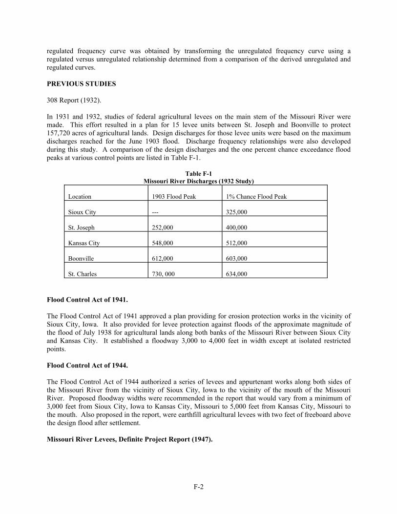
PREVIOUS STUDIES 308 Report (1932). In 1931 and 1932, studies of federal agricultural levees on the main stem of the Missouri River were made. This effort resulted in a plan for 15 levee units between St. Joseph and Boonville to protect 157,720 acres of agricultural lands. Design discharges for those levee units were based on the maximum discharges reached for the June 1903 flood. Discharge frequency relationships were also developed during this study. A comparison of the design discharges and the one percent chance exceedance flood peaks at various control points are listed in Table F-1.

Table F-1 Missouri River Discharges (1932 Study)

Location

1903 Flood Peak

1% Chance Flood Peak

Sioux City

---

325,000

St. Joseph

252,000

400,000

Kansas City

548,000

512,000

Boonville

612,000

603,000

St. Charles

730, 000

634,000

Flood Control Act of 1941. The Flood Control Act of 1941 approved a plan providing for erosion protection works in the vicinity of Sioux City, Iowa. It also provided for levee protection against floods of the approximate magnitude of the flood of July 1938 for agricultural lands along both banks of the Missouri River between Sioux City and Kansas City. It established a floodway 3,000 to 4,000 feet in width except at isolated restricted points. Flood Control Act of 1944. The Flood Control Act of 1944 authorized a series of levees and appurtenant works along both sides of the Missouri River from the vicinity of Sioux City, Iowa to the vicinity of the mouth of the Missouri River. Proposed floodway widths were recommended in the report that would vary from a minimum of 3,000 feet from Sioux City, Iowa to Kansas City, Missouri to 5,000 feet from Kansas City, Missouri to the mouth. Also proposed in the report, were earthfill agricultural levees with two feet of freeboard above the design flood after settlement. Missouri River Levees, Definite Project Report (1947).

F-3

During 1946-1947 a comprehensive hydrologic study of the Missouri River agricultural levees were made as part of the Definite Project Report (DPR). This DPR presented a plan for protection of about 1.5 million acres of agricultural land between Sioux City and the mouth of the Missouri River by a system of levees, supplemented by reservoirs, to protect the area against floods at least equal to or in excess of the highest floods of past record. Design flows for the levees above St. Joseph were based on studies of critical combinations of flows from past floods, runoff from transposed storms, and moderate releases from the main stem reservoir system. At and below St. Joseph the levee design flows were based on the expected one percent chance flood, assuming tributary reservoirs were in place, but without the reservoirs on the main stem of the Missouri. The initially recommended design flows are listed in Table F-2.

Table F-2 Missouri River Design Flows (1947 Study)

Station

Drainage Area (sq

mi)*

Design Discharge (cfs)

Sioux City

314,617

150,000

Decatur

316,140

167,000

Omaha

322,820

250,000

Nebraska City

414,420

295,000

Rulo

418,905

310,000

St. Joseph

424,340

325,000

Kansas City

489,162

431,000

Waverly

491,230

437,000

Boonville

505,710

475,000

Hermann

528,200

529,000

* Note that drainage area revision since the 1947 study has revised tabulated values. Floodway widths between levees varied from 3,000 feet at Sioux City to 5,000 feet at Hermann. Levee freeboard of two feet was used for the design of agricultural levees. Mississippi Basin Model Studies. A number of model studies have been conducted for the Missouri River below Sioux City, Iowa by the Waterways Experiment Station (WES) using the Missouri River portion of the Mississippi Basin Model (MBM). In general, model studies were conducted to assist in evaluating the effect of levee confinement on flood peaks and water surface profiles, freeboard requirements for dynamic effects, travel time of flood peaks, water surface profiles for various flood and floodway conditions, the effects of railroad and highway fills on flood heights, the effects of channel cutoffs on water surface profiles, and the timing and magnitude of flood peaks and probable areas of flooding for assisting flood fighting operations. Results of these studies are contained in numerous MBM reports prepared by WES. Main Stem Flood Control Benefits Re-evaluation (1956).

F-4

In 1950, investigations and studies were initiated which led to the preparation of the Re-evaluation of Main Stem Flood Control Benefits Report, Missouri River dated February 1956. This report presented the results of the studies used to determine the flood damages on the bottom lands of the main stem of the Missouri River from Fort Peck Dam in Montana to the confluence with the Mississippi River at St. Louis, Missouri. In general, this report re-evaluated the flood damages that would result under several conditions of reservoir and levee construction and allocated the resulting benefits to the various features of the flood control program. A comprehensive reanalysis of streamflow probabilities was made using available stream discharge or stage data which extended back into the 1870's for the key gaging stations in the reach of the Missouri River between Sioux City and the mouth. Missouri River Agricultural Levee Restudy Program (1962). This study developed hydrologic data, flood damages and benefits for the Missouri River Agricultural Levee Restudy Program which was directed in September 1959 by the Chief of Engineers to determine which levee units, or group of physically interrelated levee units would provide benefits equal to or in excess of their costs. The hydrologic studies covered the entire reach from Sioux City, Iowa to the mouth of the Missouri River. Hydrologic data developed as part of this study included flow hydrographs, annual peak discharge probability curves, stage-discharge rating curves, evaluation of levee confinement effects, and effects of reservoir control. These data were developed for nine key stream gaging stations on the main stem of the Missouri River from Sioux City, Iowa to Hermann, Missouri. The discharge frequency relationships derived for this study are shown in Table F-3. Although eight different conditions were analyzed as part of this study, the values shown in the table are for condition VI. Condition VI represents existing and near future reservoirs (except Grand River reservoirs) in operation, Federal Agricultural levees constructed above Kansas City, and a 3,000 foot minimum floodway between levees below Kansas City.

Table F-3

Missouri River Discharge-Frequency Based on 1962 Study

LOCATION

50 %

10 %

2%

1%

Sioux City

44,000

65,000

82,000

90,000

Omaha

74,000

125,000

170,000

190,000

Nebraska City

108,000

160,000

200,000

220,000

Rulo

117,000

170,000

220,000

241,000

St. Joseph

120,000

187,000

246,000

270,000

Kansas City

150,000

270,000

375,000

425,000

Waverly

158,000

285,000

395,000

445,000

Boonville

195,000

365,000

495,000

550,000

Hermann

220,000

405,000

555,000

620,000

F-5

REPORT FORMAT The report is organized into a main report that gives a general overview of the Mississippi River Basin and study approach including flood distribution selection, quality assurance/quality control, public involvement and coordination. Each of the five COE Districts within the Upper Mississippi River Basin (MVP, MVR, MVS, NWO and NWK) will have an appendix summarizing their hydrologic and hydraulic analysis. Appendix A is developed by the Hydrologic Engineering Center (HEC) and provides a detailed summary of the technical procedures adopted for the study and the efforts made to assure regional consistency of the frequency relationships and flood profiles between the districts. ACKNOWLEDGEMENTS The Corps of Engineers and the Omaha District would like to thank the numerous Federal, State, and Local government agencies for their involvement and the public for their support and comments throughout the course of this very complex and comprehensive investigation. Without your support this study would not have been successful.

BASIN DESCRIPTION

The Missouri River rises along the Continental Divide in the northern Rocky Mountains and flows generally easterly and southeasterly to join the Mississippi River near St. Louis Missouri. The river drains approximately 9,700 square miles of Canada and 513,300 square miles or one-sixth of the contiguous United States. Its headwaters begin near Three Forks, Montana where the Madison River, the Jefferson River and the Gallatin River join to form the Missouri River. From there it travels 2,315 miles to its confluence making it the longest river in the United States. Basin topography varies from the 56,000 square miles in the Rocky Mountain area in the west, where many peaks exceed 14,000 feet in elevation, to the approximately 370,000 square mile Great Plains area in the heartland of the basin, to the 90,000 square mile Central Lowlands in the lower basin where the elevation is 450 NGVD near the mouth at St. Louis, Missouri. The Black Hills in South Dakota and the Ozarks in Missouri, consisting of 13,000 square miles, are isolated dome like uplifts that have been eroded into a hilly and mountainous topography. Stream slopes vary from about 200 feet per mile in the mountains to about 0.9 foot per mile in the Great Plains and Central Lowlands. Major Missouri River tributaries are the Yellowstone River, which drains an area of 70,000 square miles, joining the Missouri River near the Montana-North Dakota border; the Platte River with a 90,000 square mile drainage area entering the Missouri River in eastern Nebraska; and the Kansas River which empties into the Missouri River in eastern Kansas and drains an area of approximately 60,000 square miles. A prominent feature in the drainage pattern of the upper portion of the basin is that every major tributary, with the exception of the Milk River, is a right bank tributary flowing to the east or to the northeast. Only in the extreme lower basin, below the mouth of the Kansas River, is there a fair balance reached between left and right bank major tributaries. The direction of flow of the major tributaries is of particular importance from the standpoint of the potential concentration of flows from storms that typically move across the basin in an easterly direction. It is also important in another respect on the Yellowstone River, since early spring temperatures in the headwaters of the Yellowstone and its tributaries are normally from 8 to 12 degrees Fahrenheit higher than along the northern most reach of the Missouri near the Yellowstone confluence. This ordinarily results in ice breakup on the Yellowstone prior to the time the ice goes out of the Missouri River, thereby contributing to ice jam floods along the Missouri River downstream from the confluence to near Williston, North Dakota.

F-6

The broad range in latitude, longitude, and elevation of the Missouri River basin and its location near the geographical center of the North American Continent results in a wide variation in climatic conditions. The climate of the basin is produced largely by interactions of three great air masses that have their origins over the Gulf of Mexico, the northern Pacific Ocean, and the northern polar regions. They regularly invade and pass over the basin throughout the year, with the Gulf air tending to dominate the weather in summer and the polar air dominating in winter. This seasonal domination by the air masses and the frontal activity caused by their collisions produce the general weather regimens found within the basin. As is typical of continental-interior plains area, the variations from normal climatic conditions from season to season and from year to year are extreme. The outstanding climatic rarity in the basin was the severe drought of the 1930's when excessive summer temperatures and subnormal precipitation continued for more than a decade. Streams having their source in the Rocky Mountains are fed by snowmelt. They are clear flowing and have steep gradients with cobble-lined channels. Stream valleys often are narrow in the mountains onto the outwash plains. Flood flows in this area are generally associated with the snowmelt runoff period occurring in May and June. Occasionally, summer rainfall floods having high, sharp peaks occur in the lower mountainous areas, such as the Rapid City flood in June 1972 and the Big Thompson River flood in July 1976. Streams flowing across the plains area of Montana, Wyoming, and Colorado have variable characteristics. The larger streams with tributaries originating in the mountain areas carry sustained spring and summer flows from mountain snowmelt, and they have moderately broad alluvial valleys. Streams originating locally often are wide, sandy-bottomed, and intermittent, and they are subject to high peak rainfall floods. In the plains region of North and South Dakota, Nebraska, and Kansas with the exception of the Nebraska sand hills area, streams generally have flat gradients and broad valleys. Except for the Platte River, most of the streams originate in the plains area and are fed by snowmelt in the early spring and rainfall runoff throughout the warm season. Stream flow is erratic. Stream channels are small for the size of the drainage areas, and flood potentials are high. When major rainstorms occur in the tributary area, streams are forced out of their banks onto the broad flood plains. In the regions east of the Missouri River, streams have variable characteristics. Those in the Dakotas, such as the Big Sioux and James Rivers, are meandering streams with extremely flat gradients and very small channel capacities in relation to their drainage areas. These areas are generally covered with glacial drift and contain many pothole lakes and marshes. Rainfall in the spring often combines with the annual plains snowmelt to produce floods that exceed channel capacities and spread onto the broad flood plains. Streams in the Ozark Highlands of Missouri resemble mountain streams with their clear, dependable base flows. Much of the area is underlain by limestone, and there are cavernous underground springs. The hilly terrain produces high peak runoff, which contributes to frequent floods with large volumes due to this area’s higher annual rainfall. WATERSHED CHARACTERISTICS Because the basin is so vast and was influenced by a variable geologic historical development, it is best to describe the basin in sections. There are three major physiographic divisions within the Missouri Basin -the Interior Highlands, the Interior Plains, and the Rocky Mountain System. The Rocky Mountain System division includes parts of the Northern Rocky Mountains, Middle Rocky Mountains, Wyoming Basin, and Southern Rocky Mountains provinces. The Interior Plains division includes parts of the Great Plains and Central Lowlands provinces. Sections and subsections within the Great Plains

F-7

province include such distinct topographic features as the Black Hills in South Dakota and Wyoming, and the Sand Hills in Nebraska. The Interior Highlands division is characterized by the Ozark Plateaus province, but will not be discussed further here as it lies within Kansas City District. The Rocky Mountain System forms the western boundary of the basin and reflects an exceptionally rugged topography, with numerous peaks surpassing 14,000 feet in elevation. The approximately 55,000-square-mile mountainous area is punctuated with many high valleys, but the peaks and mountain spurs dominate the physical features. Extending eastward from the Rocky Mountain System division is the Interior Plains division that characterizes the major portion of the Missouri Basin. The Interior Plains division can be divided into two areas - the Great Plains and Central Lowlands provinces. The Great Plains province is a 360,000-square-mile area that forms the heartland of the basin. The eastern boundary of this province lies approximately along the 1500-foot contour, and the western boundary lies at the foot of the Rocky Mountain System, averaging about 5,500 feet in elevation. Average slopes from west-to-east are about 10 feet to the mile. South and west of the Missouri River the surface mantle and topography have been developed largely by erosion of a fluvial plain extending from the mountains. The alluvial outwash laid down a heterogeneous mixture of mantle material. Simultaneous and subsequent water and wind erosion of the mantle produced a variable topographic relief, dependent on variations in climate and erodibility of the mantle. That portion of the Great Plains province north and east of the Missouri River, and at places extending south of the river, has been influenced by continental glaciation. Here the topography was shaped mainly by erosion of the glacial drift and till. Morainic drift belts are in evidence and large boulders abound. Some relatively uneroded glacial debris remains as the ice left it, piled in hummocks without order and enclosing many shallow basins, ponds, and swamps. Within the Great Plains province are isolated mountainous areas developed by erosion of dome-type uplifts. Principal among these are the Black Hills in western South Dakota and northeastern Wyoming, an elliptical-shaped area 60 miles wide and 125 miles long. Another distinctive area within the province is the Sand Hills in north-central Nebraska, covering about 24,000-square-miles. The Central Lowlands province, within the Interior Plains division, borders the Great Plains province to the east, but generally there is no perceptible line of demarcation between them. This roughly 88,000-square-mile area extends between a line from Jamestown, North Dakota, to Salina, Kans., and the Mississippi River drainage divide. This entire area has been developed by erosion of a mantle of drift and till deposited by the continental glaciers. An abundance of rainfall and stream development has created a hilly topography in many places, but especially in the southern portion of the province. CLIMATOLOGY The climate within the basin is determined largely by the interaction of three great air masses that have their origins over the Gulf of Mexico, the northern Pacific Ocean, and the northern polar regions. They regularly invade and pass over the basin throughout the year, with the gulf air tending to dominate the weather in summer and the polar air dominating in winter. It is the seasonal domination of the air masses and the frontal activity caused by their colliding with each other that produces the general weather regimens found within the basin. A major factor affecting the climate is the remoteness of the basin from the source areas of the air masses. This means that the air masses have to cross vast areas before they reach the basin. In crossing these areas they leave much of their available precipitation, and their air temperatures are changed considerably by radiation from the land surface.

F-8

Primarily because of its midcontinental location, the basin experiences weather that is known for fluctuations, extremes, and variability within the basin. Winters are relatively long and cold over much of the basin, while summers are fair and hot. Spring is cool, moist and windy; autumn is cool, dry and sunny. Weather tends to fluctuate widely around annual averages, with the occurrence and degree of the fluctuations being unpredictable. Thus the climatic averages have to be thought of as generalizations of the more common occurrences over a period of time. Average annual precipitation varies from over 40 inches in parts of the Rocky Mountains and southeastern parts of the basin, to as low as 6 to 12 inches immediately east of the Rocky Mountains. Complicating the annual variations, there is a wide variation in the basinwide pattern of monthly precipitation. Precipitation received from November through March generally is in the form of snowfall. Thunderstorms are prevalent in May through August and often are localized, with high-intensity rainfall. Prolonged droughts and lesser periods of deficient moisture may be interspersed with periods of abundant precipitation. There are periods of extremely cold winter and hot summer temperatures in the basin. Extremes range from winter lows of - 60 F. in Montana to summer highs of up to 120 F. in Nebraska, Kansas, and Missouri. The basin regularly experiences over 100-degree temperatures in summer and below-zero temperatures in winter over most of its area. Winds in the basin are the rule rather than the exception, particularly in the plains area. Average wind velocities of 10 miles per hour are prevalent over much of the basin. In the plains area strong winds accompanied by snow sometimes create "blizzard" conditions. High winds occasionally prevail during periods of high temperatures and deficient moisture that can destroy crops and desiccate rangeland within a few days. FLOOD HISTORY Prior to development of flood control reservoirs on the upper Missouri River basin, the Missouri River was a source of frequent flooding. In the plains areas of the upper basin, almost all large floods are caused by snowmelt. Rainfall becomes progressively a greater factor in flooding as the focus shifts from northern and western to southern and eastern drainage areas. Following is a narrative of some of the significant floods in the Missouri River basin. Flood of 1844. The flood of 1844 was of great magnitude throughout practically the entire Missouri River basin. Very little is known of the exact behavior of the flood except that it was caused by abnormally high rainfall over that portion of the basin lying in the humid zone, coincident with an extraordinary June rise from the upper part of the basin. The crest exceeded flood stage at various points from 12 to 17 feet. Estimated peak discharges were St. Joseph 350,000 cfs, Kansas City 625,000 cfs, Boonville 710,000 cfs, and Hermann 892,000 cfs. These discharges were the greatest ever estimated at Kansas City and Hermann. Flood of 1881. Following a wet year in 1880, the winter of 1880-1881 was marked by below normal temperatures and heavy snows, resulting in an exceedingly heavy snow blanket over the plains area of the upper Missouri River Basin by spring and resulting in river ice thickness of 24 to 32 inches in the vicinity of Yankton and Omaha. Spring thaws and ice breakup began in the upper basin while the lower river was still frozen, resulting in huge ice gorges in the Dakotas. The jam near Yankton were especially devastating, as the jam was estimated to be over 30 miles in length and produced a peak stage 15 feet higher than any other

F-9

flood at Yankton. The April 1881 peak discharge from Sioux City to St. Joseph was the highest of record until 1952 when it was exceeded by another plains snowmelt flood. Estimated peak discharge at St Joseph was 370,000 cfs; the volume of the flood was estimated at over 40 million acre-feet at Sioux City, Iowa. Flood of 1903. The flood of 1903 was caused by prolonged and heavy rainfall over the lower Kansas River basin coinciding with the June rise from the upper Missouri basin. Tributary inflow below Kansas City materially increased the discharges, but the principal tributaries, such as the Grand, Osage, and Gasconade, were considerably below the maximum stages of record. Very little overflow occurred between St. Joseph, Missouri, and Atchison, Kansas. Below Atchison the flooding was more general, and below Kansas City, Missouri, the flood waters extended from bluff to bluff. Approximately 615,000 acres of agricultural land were inundated. Estimated peak discharges were St Joseph 252,000 cfs, Kansas City 548,000 cfs, Boonville 612,000 cfs, and Hermann 676,000 cfs. Flood of 1951 The spring and summer of 1951 was a period of excessive rainfall over the Kansas River basin which culminated in an exceptionally heavy downpour during the 4-day period 9-13 July. The Kansas River crest fortunately coincided with a low flow out of the upper Missouri River, and there was no flooding, except from backwater, on the Missouri River above Kansas City. Several of the Federal levee units at Kansas City were overtopped. Below Kansas City, the entire Missouri River valley was flooded to depths up to 20 feet. The peak discharge at Kansas City of 573,000 cfs was the highest since the 1844 flood. Flood of 1952. The following spring, in March-April 1952, a flood of exceptional magnitude and severity on both the Missouri River itself and most of its plains area tributaries at and above Sioux City, Iowa, was generated from rapid snowmelt over the plains areas of the upper basin. On the Missouri River, flooding was continuous from the Yellowstone River in Montana to the mouth. Between Williston, North Dakota, and St. Joseph, Missouri, with the exception of isolated localities where past ice jams have occurred, this flood reached unprecedented heights. The 1952 flood was caused exclusively by melting snow because rainfall over the basin prior to and during the flood was light. The winter of 1951 and 1952 produced one of the heaviest plains snow covers in history. Significant snow cover extended over almost all of the Dakotas and the Yellowstone river basin in Montana. Snow surveys taken in March indicated a 2.4 inch water content over 10,000 square miles of the Yellowstone River basin. Water equivalents as high as 3.6 inches were reported in the Grand River basin of North and South Dakota. Up to 6.0 inches of water content was present in the lower Grand, lower Moreau, and eastern Big Sioux River basins. The great magnitude of the flood can be attributed to the unusual areal cover of the accumulated snow cover, the high water content of the snowpack, the rapidity at which the snow melted, and the presence of an ice layer under the snow which allowed for rapid runoff. At and below Kansas City, because little water was being added from tributary areas, the flood, although still severe, became less than the maximum of record. Peak discharges at Sioux City 441,00 cfs, Omaha 396,000 cfs, Nebraska City 414,000 cfs, Rulo 358,000 cfs and St Joseph 397,000 cfs were the highest discharges ever recorded. The 1952 flood caused an estimated $200 million in damages.

F-10

Flood of 1967. The flood of 1967 is of particular interest within the Missouri River basin because it was the first major flood occurring after the initial filling of the main stem reservoir system. The reservoirs did help reduce flooding during the flood of 1960, but the reservoir system was not full, and system operations as we see them today did not begin until 1967. Above normal runoff originated from three primary sources during 1967, plains snowmelt, mountain snowmelt, and intense summer rainfall. In the Missouri River headwaters of Montana and Wyoming, mountain snows accumulated at a greater than normal rate. While the mountain snows were accumulating, flood discharges occurred in March and April resulted from rapid plains snowmelt caused by a sustained period of warm temperatures over a large portion of the basin. Water content over much of the upper basin was high and combined with frozen saturated soils; therefore, little infiltration occurred as the snowpack melted. Snowpack water content in the lower basin was somewhat less, but soil conditions were similar and melting snows produced discharges higher than those normally expected. By May of 1967 many mountain snow courses were reporting record high-water contents. During late May and early June, heavy upper basin rainfall coinciding with mountain snowmelt resulted in the third highest May through June runoff volume above Sioux City, Iowa. During June of 1967, intense rains over Nebraska, Kansas, and Missouri caused severe flooding along many tributaries and the Missouri River from the Platte River confluence downstream to the mouth. However, operation of the main stem system reduced the flood peak at Sioux City, Iowa, by almost 200,000 cfs and eliminated Missouri River flood damages from Fort Peck Dam in Montana to the mouth of the Platte River in Nebraska. Flooding primarily occurred on the Missouri River within the Omaha District from Omaha downstream to Rulo, Nebraska. The volume of Missouri River inflow into the main stem system was the highest of record for the month of March since 1898. It was estimated that the main stem system reduced flood peaks by as much as 10 feet in the lower Missouri River. Flood of 1984. The flood of 1984 had its beginnings in late spring when heavy, wet snow and rain fell over a large area of southern South Dakota through Nebraska, Kansas, and Missouri. Persistent rains continued through April producing the highest April runoff volumes upstream from Sioux City since record keeping began in 1889. The weather pattern that caused the record and near record flooding in the lower Missouri River basin in 1984 consisted of warm moist air from the Gulf of Mexico funneled into the central United States by a strong ridge of high pressure located over the east coast. A series of upper air disturbances coupled with polar cold fronts and warm Gulf air produced a series of intense rainfall events covering much of the lower Missouri River basin. This intense rainfall fell over a wide area already saturated from heavy April and May rainfall. During early June, the heaviest rainfall occurred in the lower basin over northwest Missouri and southeast Nebraska. Average rainfall amounts of 3 to 4 inches on the night of June 12 were reported over a large area of eastern and central Nebraska, with localized areas reporting as high as 7 to 8 inches. This storm caused record floods on many of the smaller tributaries and produced the highest stages since 1952 on the Missouri River from the confluence of the Platte River to St. Joseph, Missouri. During mid and late June, the intense rainfall pattern shifted north over the Dakotas. Rainfall amounts exceeded 7 inches over South Dakota on June 18 and 19 with an additional 4 inches on June 20. This rainfall produced record and near record stages on many southeast South Dakota tributaries and produced the highest Missouri River stages since 1952 from Sioux City, Iowa to Omaha, Nebraska. Flood of 1993

F-11

Much of the eastern and southern Missouri River basin in Iowa, Nebraska, South Dakota, Kansas and Missouri had soil moisture conditions wetter than normal going into the summer of 1993. This was primarily due to the above average precipitation received in the last half of 1992 and the spring of 1993. Much of the late winter, including the 2-week period prior to the warmup that started the spring flooding in Nebraska was dominated by an upper level atmospheric pattern that favored storms followed by cold weather. The subpolar jet generally ran from northwest to southeast across the Rockies and the southern Plains. During January and February, occasional polar outbreaks of bitterly cold air invaded the central Plains as the polar jet stream was forced south into the Plains by strong low pressure in the upper atmosphere over Hudson Bay. A strong overrunning pattern from the eastern Pacific brought ample upper level moisture to the Midwest to feed the surface storms moving off the central Rockies, often producing freezing rain in the cold air below. At the end of February the subpolar jet stream ran from west to east across the southern states. By March 1, a vigorous cutoff low formed over New Mexico and moved northeastward, setting the stage for the additional precipitation that fell over the Platte River basin in Nebraska just prior to the melt. By March 5, the subpolar jet began to shift east and lift north as a weak high pressure ridge began to build in the upper atmosphere off the coast of California. This pattern edged the storm track north of Nebraska and began the thaw. High temperatures warmed from the 30's to the 40's and clouds gave way to sunshine between March 2 and 7. On March 8, the jet stream ran directly over eastern Nebraska on its eastward journey, allowing warmer air to pour across the frozen watersheds. High pressure built over the Rockies, strengthening the warmup. On March 9, daytime high temperatures pushed into the upper 40's and low 50's across the region, with nighttime lows near freezing. The snow continued to melt rapidly, until much of east and central Nebraska had lost its snow cover with only an inch or two remaining in extreme northeast Nebraska by March 10. By early June a stationary high pressure system was located over the southeast United States and a stationary low pressure system was located over the northwest. The location of these two systems created a boundary or convergence zone where the jet stream, which dipped to the south over the western United States, was forced in a northeasterly direction through the Midwest. The thunderstorms that persisted in the Midwest through July were caused by the mixing of warm moist tropical air with unseasonably cool, dry air from Canada in this convergence zone. Chain reacting tropical storms off the western coast of Mexico during this period funneled moisture into the jet stream aimed at the Midwest. This convergence zone moved back and forth from the Dakotas, Minnesota, and Wisconsin to Kansas, Missouri, and Illinois producing more than twice the normal rainfall in much of the Missouri River basin east of the 100th meridian. The precipitation was not only very heavy but also very persistent. Rain fell somewhere in the Missouri River basin every day from March 14 through July 29. During the period of June 1 to July 27, rainfall occurred on 34 out of 57 days at Omaha, Nebraska. The most severe flooding since 1952 occurred on the Missouri River from the confluence of the Platte River to the mouth. Within this reach, record or near record peak discharges were experienced during the period of July 23-31. On July 23-24, a record crest of the Missouri River overtopped federal levee L-550 near Brownville, Nebraska. On July 24, the St. Joseph Airport Levee Unit R-471-460 overtopped. On July 26, levee units L-400 and L-246 overtopped. Flood of 1997 Runoff in the Missouri River basin upstream from Sioux City totaled 49.6 million acre-feet during calendar year 1997, the highest annual runoff in 100 years of record. This is nearly double the average of 24.8 million acre-feet and nearly 20 percent higher than the previous record runoff that occurred in 1978.

F-12

Record flooding occurred on the main stem of the Missouri River upstream from Canyon Ferry Reservoir and downstream of Canyon Ferry Reservoir to the confluence with the Sun River. In addition, the highest flows since the main stem reservoir system went into operation were experienced below Oahe Reservoir, Fort Randall Reservoir and Gavins Point Reservoir. Below Garrison the second highest releases on record occurred, while at Fort Peck, the releases reached the fourth highest on record. Above Canyon Ferry Reservoir at Toston, Mt, the peak stage of 12.22 feet on June 12, exceeded the previous record stage that occurred in 1948 by about 0.5 feet. The estimated peak discharge of 33,300 cfs was also the highest on record. Downstream from Canyon Ferry Reservoir at Ulm, the peak stage of 15.20 feet exceeded the previous record stage that occurred in 1981 by about 0.2 feet. The estimated peak discharge at Ulm of 27,900 cfs was the second highest on record. Upstream from Fort Peck Reservoir at Virgelle, the peak stage of 12.29 feet on June 16 was more than 11 feet below the record stage set in 1953. Downstream from Fort Peck at Culbertson, the peak stage of 17.52 feet on March 31 was about 2 feet below the record set in 1979. Upstream from Garrison Reservoir at Williston, the peak stage of 26.1 feet on June 26 was within 0.5 feet of the record stage set in 1994. With the second highest releases of 59,000 cfs from Garrison Reservoir, the peak stage climbed to 14 feet at Bismarck on July 25, within 0.8 foot of the highest stage experienced since construction of Garrison Dam, but well below the pre-dam record stage of 27.9 feet set in 1952. Record releases of 59,500 cfs from Oahe Dam pushed the peak stage at Pierre to almost above 12.5 feet during parts of April, July and August but below the peak ice-affected stage of 12.9 feet that occurred on January 10. At Yankton, the highest discharge since the construction of the main stem dams of 70,000 cfs was experienced through much of the fall during October, November and early December while evacuating the flood storage resulting from the Missouri River Main Stem Reservoir System. At Sioux City and Omaha, the Missouri River remained well below flood stage. However, low lying agricultural areas adjacent to the river experienced flooding and drainage problems throughout the spring, summer and fall. Without the Missouri River Main Stem Reservoirs, the peak stage at Omaha of 26.4 feet on April 15 would have been about 13.1 feet higher which would have been only 0.7 feet below the record stage set in 1952. Below the confluence of the Platte River, the Missouri River exceeded flood stage for much of the April through July period. At Nebraska City, the peak stage of 21.06 feet occurred on April 18. This stage was about 3 feet above flood stage. Without the main stem reservoirs, the peak stage would have been about 10 feet higher, which would have exceeded the record stage set in 1952 by more than 3 feet. Record floods also occurred on the James River in North and South Dakota, the upper Big Sioux River, the upper Yellowstone River, and the Moreau River as a result of melting of the unusually heavy snowpacks in those basins. Most tributaries in Montana, North Dakota, and South Dakota experienced stages exceeding flood stage. Record pool elevations occurred at the Fort Randall, Pipestem and Jamestown projects. Flood fight efforts and Advance Measures projects constructed by the corps prevented $100 million in flood damages. The Missouri River Main Stem Reservoirs prevented $ 5.2 billion in flood damages. Other Corps Projects prevented over $ 300 million in flood damages. There are many other notable floods in the upper Missouri River basin that are confined to smaller areas of the basin, but did not have a large impact on the mainstem. Their omission from this report in no way minimizes the impact or severity of these floods. WATER RESOURCES DEVELOPMENT

F-13

Water resources development in the Missouri River basin has been dramatic over the past 150 years. Significant periods of development were prior to 1910 and since 1949. Early water resource developments were oriented largely towards single-purpose improvements to meet specific needs without substantial regard for other potential functions. However, as the region's demand for water resources grew, and technology improved, multi-purpose programs became more prevalent. Flood Control Reservoirs Numerous reservoirs and impoundments constructed by different interests for flood control, irrigation, power production, recreation, water supply, and fish and wildlife are located throughout the basin. The Bureau of Reclamation and the Corps of Engineers have constructed the most significant of these structures. Although primarily constructed for irrigation and power production, the projects constructed by the Bureau of Reclamation do provide some limited flood control in the upper basin. Six main stem dams constructed by the Corps are the most significant authorized flood control projects within the basin, providing a combined capacity in excess of 73.5 million acre-feet of which more than 16 million acre-feet is for flood control. These six projects were completed in 1964 and provide flood protection by controlling runoff from the upper 279,000 square miles of the Missouri River basin. The flood control storage zones in the Missouri River main stem reservoirs were designed in a series of Detailed Project Reports in the mid-1940's to provide control of the severe 1881 flood, with maximum releases of about 100,000 cfs from all projects other than Fort Peck and with maximum pools at or near the top of the exclusive flood control storage space. The 1881 flood inflows were based on estimates of what actually occurred, without reduction to allow for operational effects of upstream tributary reservoirs or for consumptive use by upstream irrigation and other purposes. If the flood runoff were to recur today, its severity as far as the main stem reservoir designs are concerned would be significantly reduced by these factors. On the other hand, regulation criteria used in the 1881 reservoir design studies were based largely on hindsight, with little regard for downstream runoff conditions. Releases of approximately 100,000 cfs were assumed to be made from mid-April to mid-July from the five lowermost reservoirs, without any requirement for reducing releases to desynchronize with downstream flood peaks.

Regulation of the main stem reservoir system follows a repetitive annual cycle. Winter snows and spring and summer rains produce most of the year’s water supply, which results in rising pools and increasing storage accumulation. After reaching a peak, usually during July, storage declines until late winter when the cycle begins anew. A similar pattern may be found in rates of releases from the system, with the higher levels of flows from mid-March to late November, followed by low rates of winter discharge from late November until mid-March, after which the cycle repeats. Two primary high-risk flood seasons are the plains snowmelt season extending from late February through April and the mountain snowmelt period extending from May through July. Overlapping the two snowmelt flood seasons is the primary rainfall flood season, which includes both upper and lower basin regulation considerations. The highest average power generation period extends from mid-April to mid-October with high peaking loads during the winter heating season (mid-December to mid-February) and the summer air conditioning season (mid-June to mid-August). The power needs during winter are supplied primarily with Fort Peck and Garrison releases and the peaking capacity of Oahe and Big Bend. During the spring and summer period, releases are geared to navigation and flood control requirements and primary power loads are supplied using the four lower dams. During the fall when power needs diminish, Fort Randall pool is drawn down to permit generation during the winter period when the pool is refilled by Oahe and Big Bend peaking power releases. The major maintenance period for the main stem power facilities extends from mid-February through May and from September to mid-November which normally are the lower demand and off-peak energy periods. The exception is Gavins Point where

F-14

maintenance is performed after the end of the navigation season since all three power facilities are normally required to provide navigation flow needs. Normally, the navigation season extends from April 1 through December 1 during which time reservoir releases are increased to meet downstream target flows in combination with downstream tributary inflows. Much of the increased flow for navigation comes from the large carryover storage in Oahe Reservoir. Winter releases after the close of navigation season are much lower and vary depending on the need to conserve or evacuate main stem storage volumes, downstream ice conditions permitting. Minimum release restrictions and pool fluctuations for fish spawning management generally occur from April 1 through July. Endangered and threatened species including the interior least tern and piping plover nesting occurs from early May through August. During this period, special release patterns are made from Garrison, Fort Randall, and Gavins Point to avoid flooding nesting sites on low-lying sandbars and islands downstream from these projects. Overall, the general regulation principles presented above provide the backbone philosophy for main stem system regulation. Detailed operation plans are developed, followed and adjusted as conditions warrant periodically as the system is monitored day-to-day. Beginning in 1953, projected operation of the Missouri River main stem reservoir system for the year ahead was developed annually as a basis for advance coordination with the various interested Federal, State, and local agencies and private citizens. These regulation schedules are prepared by the Reservoir Control Center, Missouri River Region, Northwest Division, Corps of Engineers. In addition to the six main stem projects operated by the Corps, 65 tributary reservoirs operated by the Bureau of Reclamation and the Corps provide over 15 million acre-feet of flood control storage. Tables F-4 and F-5 list the mainstem and tributary flood control projects operated by the Corps of Engineers and the Bureau of Reclamation. The Bureau of Reclamation operates many additional reservoirs for irrigation and power production, which provide incidental flood control benefits. Additional storage can be found in many other reservoirs throughout the Omaha District. However, only a few have significant enough storage as to impact flow peaks downstream of Gavins Point Dam. Hebgen Lake, Gibson Reservoir, Fresno Reservoir, Angostura Reservoir, and North Platte reservoirs in aggregate are the only reservoirs with significant non-flood control storage to be considered for this study.

F-15

Table F-4. Corps of Engineers Reservoirs in Missouri Basin. Project Name River or Stream Located On Date of Closure Total Storage

Volume, acre-feet

Flood Control Storage, acre-feet

Fort Peck Missouri River June 24, 1937 18,688,000 3,692,000 Garrison Missouri River April 15, 1953 23,821,000 5,711,000 Oahe Missouri River August 3, 1958 23,137,000 4,303,000 Big Bend Missouri River July 24, 1963 1,859,000 177,000 Fort Randall Missouri River July 20, 1952 5,494,000 2,301,000 Gavins Point Missouri River July 31, 1955 492,000 152,000 Bowman-Haley North Fork Grand River August 1966 91,482 72,717 Cold Brook Cold Brook September 1952 7,200 6,680 Cottonwood Springs Cottonwood Springs Creek May 1969 8,385 7,730 Cedar Canyon Deadmans Gulch 1959 136 123 Bull Hook Scott Coulee Bull Hook Creek 1955 6,500 6,500 Pipestem Pipestem Creek July 1973 146,880 137,010 Papio Creek (10 dams) Papillion Creek 1972-1984 42,237 31,323 Cherry Creek Cherry Creek October 1948 135,647 122,842 Chatfield South Platte River August 1973 235,098 206,945 Bear Creek Bear Creek July 1977 30,684 28,757 Kelly Road Westerly Creek 1953 360 360 Westerly Creek Westerly Creek 1991 4,150 4,150 Salt Creek (10 dams) Salt Creek 1963-1973 189,933 139,462 Harlan County Republican 1951 825,782 496,718 Milford Republican 1964 1,145,485 756,669 Tuttle Creek Big Blue 1959 2,257,185 1,922,085 Wilson Saline 1963 772,732 530,204 Kanopolis Smoky Hill 1946 418,752 369,278 Perry Delaware 1966 725,509 515,961 Clinton Wakarusa 1965 397,538 268,367 Smithville Little Platte 1976 243,443 101,777 Longview Little Blue 1983 46,944 24,810 Blue Springs Little Blue 1986 26,557 15,715 Long Branch Little Chariton 1976 64,516 30,327 Rathbun Chariton 1967 545,621 345,791 Melvern Osage 1970 360,258 208,207 Pomona Osage 1962 243,102 176,460 Hillsdale Osage 1980 159,840 83,570 Stockton Osage 1968 1,650,943 776,066 Pomme De Terre Osage 1960 644,177 406,821 Harry S Truman Osage 1977 5,209,353 4,005,949 Total COE Project Storage 90,127,429 28,135,374

Irrigation Development Irrigation first appeared in the Missouri Basin about 1650 by the Taos Indians along Ladder Creek in northern Scott County, Kansas. 'Modern' irrigation appeared in the basin in the 1860s, and water use for irrigation and other uses grew rapidly through the remainder of the 19th century and into the early 20th century as agricultural uses of water grew, especially in the more arid western plains. Estimates of irrigation and other use depletions by the U.S. Bureau of Reclamation range as high as 9,000,000 acre-feet by 1920 upstream of Rulo, Nebraska. Irrigation development leveled off for the next 30 years but since has been steadily increasing. According to USBR estimates, irrigation and other depletions have reached 13.5 million acre-feet by the mid-1990s above Rulo, Nebraska. Approximately 60% of the depletions in the Omaha District occur upstream of Sioux City, Iowa.

F-16

Table F-5. Bureau of Reclamation Projects Operated for Flood Control. Project Name River or Stream

Located On Date of Closure Total Storage

Volume, acre-feet Flood Control Storage, acre-feet

Clark Canyon Beaverhead River June 1964 257,150 79,090 Canyon Ferry Missouri River December 1951 2,051,520 99,460 Tiber Marias River 1952 1,555,960 400,900 Boysen Wind River October 1951 952,400 150,400 Yellowtail Bighorn River November 3, 1965 1,328,360 258,330 Heart Butte Heart River October 4, 1949 223,600 147,900 Shadehill Grand River July 1, 1950 357,400 218,300 Keyhole Belle Fourche River February 12, 1952 334,200 140,500 Pactola Rapid Creek August 1956 99,029 43,057 Jamestown James River February 1954 221,000 185,400 Glendo North Platte River October 17, 1957 789,400 271,900 Enders Frenchman Creek 1950 74,520 30,040 Hugh Butler Red Willow Creek 1961 86,630 48,854 Bonny S. Fk. Republican 1950 170,160 128,820 Swanson Republican 1953 246,291 134,077 Harry Strunk Republican 1949 88,420 52,715 Keith Sebelius Prairie Dog Creek 1964 134,740 98,805 Lovewell White Rock Creek 1957 92,150 50,450 Kirwin N. Fk. Soloman 1955 314,550 215,115 Webster S. Fk. Soloman 1956 260,740 183,370 Waconda Soloman 1967 963,775 722,315 Cedar Bluff Smoky Hill 1950 418,752 191,860 Total USBR Project Storage 11,020,747 3,851,658 Navigation Channel The Missouri River has served as a form of transportation for centuries. Early fur traders used the river and its tributaries as a means of bringing in goods and exporting their furs. As the westward expansion of the country progressed, the Missouri River was used to transport goods and people to the river towns which served as gateways for wagon routes to the west. As railroads became more prevalent, use of the river for transportation dwindled. The first river navigation development work consisted of snagging and clearing to remove obstructions which hindered early steamboat traffic. In 1912, Congress authorized a 6-foot channel between Kansas City and the mouth, as well as improvements and maintenance from Kansas City to Fort Benton, Montana. In 1927, Congress authorized the extension of the navigation channel to Sioux City, as well as a study to determine the feasibility of a nine-foot channel. In 1945, Congress finally authorized the nine-foot channel to be constructed to Sioux City. In 1981, the navigation channel project was officially declared finished, with the terminus of the project at River Mile 734.8 at Sioux City. Levees The Federal Government had no official role in the construction of flood control projects on the Missouri River during the 19th century. However, landowners, municipalities and the railroads built dikes and levees to protect their properties. After floods of the early 1900s, States in the Missouri River basin authorized local drainage districts to construct flood protection works. Some of the drainage districts came to the Corps of Engineers for assistance in their flood control efforts. The Missouri River levee system was authorized by the Flood Control Acts of 1941 and 1944 to provide protection to agricultural lands and communities from Sioux City, Iowa to the mouth at St. Louis, Missouri. No Federal levees have been constructed from Gavins Point Dam to the Omaha, Nebraska-Council Bluffs, Iowa, area due to the significant protection afforded this reach by the Missouri River

F-17

mainstem reservoirs and due to gradual channel degradation through much of this reach. This reach does have non-Federal levees providing varying degrees of protection. The Federal levee system begins in the Omaha-Council Bluffs metropolitan area, protecting a large urban area. Downstream of Omaha to Rulo, Nebraska, the Federal levee system protects agricultural lands and several small towns. All of these levee units were designed to operate in conjunction in with the six mainstem reservoirs to reduce flood damages. Most Federal levees were constructed in the 1950s and are generally set back from the riverbank 500 to 1500 feet. Federal levees provide left bank protection from river mile 515.2 to 619.7. Right bank levees are intermittent, as the river is often near the bluff. There are a total of 191 levee miles from Omaha, Nebraska to Rulo, Nebraska, of which 133.5 miles are along the Missouri River and 57.5 miles are levee tiebacks. Following construction of the Federal levee system, farming of the lands riverward of the Federal levees became more extensive. Farmers constructed secondary levees at or near the riverbank to prevent crop damages caused by normal high flows on the Missouri River. Private levees have also been built in those areas where Federal levees were not built. For example, the left bank reach from river mile 515.5 to 498.1 is protected solely by private levees.

HYDROLOGIC ANALYSIS

The hydrologic analysis performed for this study was composed of many steps. In order to provide a homogenous data set from which frequency analysis can be performed, effects of reservoir regulation and stream depletions had to be removed. This produced the data set referred to as the "unregulated flow" data set. A homogeneous "regulated flow" data set was then developed by extrapolating reservoir and stream depletions to current use level over the period of record. A relationship between the annual unregulated and regulated flow peaks was established in order to determine the regulated flow frequency at various points. A more detailed description of the analysis methodology is contained herein. METHODOLOGY The following is a brief description of the work performed to estimate the flow frequency for points along the Missouri River. The existing stream flow data for mainstem gaging stations were extended by converting stage records to discharge through use of old rating curve information at each gage prior to the establishment of USGS gaging records. Discharges had to be estimated or interpolated based on other stations during periods of no stage records at some stations. This extended the period of record for the study back to 1898. Estimates of historic and current level irrigation water use and other consumptive uses (otherwise referred to as depletions, in sum) were developed by the USBR. The historic level depletions were utilized in estimating the unregulated flow data set, while the current level depletions were used in developing the regulated flow data set. Historic evaporation and precipitation records were researched and compiled for inclusion in the input data set to the unregulated flow model. Reservoir regulation data were compiled for inclusion in the input data set to the unregulated flow model. The unregulated flow computer model was run, using data developed by both Omaha and Kansas City Districts, to determine a daily record of unregulated flows from Yankton, South Dakota to Hermann, Missouri covering the period from January 1, 1898 to December 31, 1997. Flow frequency analyses were performed on the annual peaks using procedures found in Bulletin #17b. The results indicated the use of a mixed distribution of spring and summer peaks above the Kansas River and the use of annual peaks downstream of the Kansas River.

F-18

The regulated flow computer model was run, using data developed by both Omaha and Kansas City Districts, to determine a daily record of regulated flows from Gavins Point Dam to Hermann, Missouri covering the period from January 1, 1898 to December 31, 1997. The regulated flow frequency curve is determined by transforming the unregulated curve using an unregulated versus regulated relationship. To determine this relationship, annual peaks for regulated and unregulated flows were compared, the regulated flow data being determined at each station by routing studies. The annual peaks from the regulated and unregulated data sets were then paired against each other in descending order. A relationship between regulated and unregulated flow frequencies could then be established at each station. Volume-duration-probability relationships were determined at each gage using procedures found in this report. The results indicated the use of a mixed distribution for durations up to 30 days above the Kansas River, while an annual distribution was used for longer durations. DATABASE Stream flow Records The first river stage station on the Missouri River was established on January 1, 1872 at Fort Leavenworth, Kansas, which is currently located in the Kansas City District. Within the current boundaries of the Omaha District, the first stage gage on the Missouri River was established on April 10, 1872 at Omaha, Nebraska. Other river stage gages were established at Plattsmouth, Nebraska on April 19, 1873; at Nebraska City on August 1, 1878; and at Sioux City, Iowa on September 2, 1878. These river stage stations were operated by the Corps of Engineers from the date of their establishment to December 31, 1899. On January 1, 1900, the work of securing a record of river stages was taken over by the United States Weather Bureau, who maintained daily river stage records until 1930. At that time, the USGS had taken over the responsibility of collecting and recording river gage records. Available records at key stations are shown in Table F-6. Gage Description Descriptions of each gage in the Omaha District used for this study are listed in Appendix F-B, along with descriptions of how flow data were derived from stage data. Meteorological Records Meteorological records such as precipitation and evaporation were need for determining unregulated flows, as precipitation and evaporation affect the amount of water in reservoir storage. Evaporation from large flood control reservoirs is a major loss of water from the basin and must be accounted for in determining unregulated flows. Precipitation on reservoir surfaces must also be accounted for. Since the reservoir surfaces are so much larger than the original channel, precipitation that used to fall on soil and infiltrate into the soil now runs directly into the reservoir, thereby increasing the amount of water in the basin system.

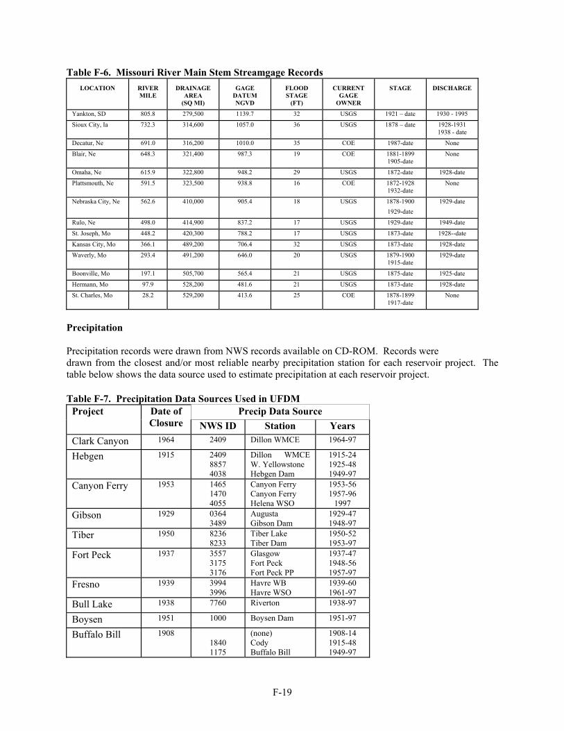
F-19

Table F-6. Missouri River Main Stem Streamgage Records

LOCATION

RIVER MILE

DRAINAGE

AREA (SQ MI)

GAGE

DATUM NGVD

FLOOD STAGE

(FT)

CURRENT

GAGE OWNER

STAGE

DISCHARGE

Yankton, SD 805.8 279,500 1139.7 32 USGS 1921 – date 1930 - 1995

Sioux City, Ia 732.3 314,600 1057.0 36 USGS 1878 – date 1928-1931 1938 - date

Decatur, Ne 691.0 316,200 1010.0 35 COE 1987-date None

Blair, Ne 648.3 321,400 987.3 19 COE 1881-1899 1905-date

None

Omaha, Ne 615.9 322,800 948.2 29 USGS 1872-date 1928-date

Plattsmouth, Ne 591.5 323,500 938.8 16 COE 1872-1928 1932-date

None

Nebraska City, Ne 562.6 410,000 905.4 18 USGS 1878-1900 1929-date

1929-date

Rulo, Ne 498.0 414,900 837.2 17 USGS 1929-date 1949-date

St. Joseph, Mo 448.2 420,300 788.2 17 USGS 1873-date 1928--date

Kansas City, Mo 366.1 489,200 706.4 32 USGS 1873-date 1928-date

Waverly, Mo 293.4 491,200 646.0 20 USGS 1879-1900 1915-date

1929-date

Boonville, Mo 197.1 505,700 565.4 21 USGS 1875-date 1925-date

Hermann, Mo 97.9 528,200 481.6 21 USGS 1873-date 1928-date

St. Charles, Mo 28.2 529,200 413.6 25 COE 1878-1899 1917-date

None

Precipitation Precipitation records were drawn from NWS records available on CD-ROM. Records were drawn from the closest and/or most reliable nearby precipitation station for each reservoir project. The table below shows the data source used to estimate precipitation at each reservoir project. Table F-7. Precipitation Data Sources Used in UFDM

Precip Data Source Project Date of Closure NWS ID Station Years

Clark Canyon 1964 2409 Dillon WMCE 1964-97

Hebgen 1915 2409 8857 4038

Dillon WMCE W. Yellowstone Hebgen Dam

1915-24 1925-48 1949-97

Canyon Ferry 1953 1465 1470 4055

Canyon Ferry Canyon Ferry Helena WSO

1953-56 1957-96

1997 Gibson 1929 0364

3489 Augusta Gibson Dam

1929-47 1948-97

Tiber 1950 8236 8233

Tiber Lake Tiber Dam

1950-52 1953-97

Fort Peck 1937 3557 3175 3176

Glasgow Fort Peck Fort Peck PP

1937-47 1948-56 1957-97

Fresno 1939 3994 3996

Havre WB Havre WSO

1939-60 1961-97

Bull Lake 1938 7760 Riverton 1938-97

Boysen 1951 1000 Boysen Dam 1951-97

Buffalo Bill 1908 1840 1175

(none) Cody Buffalo Bill

1908-14 1915-48 1949-97

F-20

Precip Data Source Project Date of Closure NWS ID Station Years

Yellowtail 1966 9240 Yellowtail Dam 1966-97

Garrison 1953 7585 3376

Riverdale Garrison 1NW

1953-81 1982-97

Heart Butte 1949 0136 4091

Altmont 7W Heart Butte

1949-83 1984-87

Bowman-Haley

1966 0995 Bowman Ct Hs 1966-97

Shadehill 1950 7567 4864

Shadehill Dam Lemmon

1950-77 1978-97

Keyhole 1952 Keyhole Dam Devil’s Tower

1952-58 1959-97

Pactola 1956 6427 Pactola Dam 1956-97

Angostura 1949 0217 6304

Angostura Oral

1949-71 1972-97

Oahe 1958 6597 6170

Pierre FAA AP Oahe Dam

1958-59 1960-97

Big Bend 1963 1690 0649 4766

Chamberlain Big Bend Dam Lake Sharpe

1963-64 1965-71 1972-97

Fort Randall 1952 6574 Pickstown 1952-97

Gavins Point 1955 9502 3165 9502

Yankton 2E Gavins Point Yankton 2E

1955-60 1961-95 1996-97

Pipestem 1973 4413 Jamestown AP 1973-97

Jamestown 1953 4413 Jamestown AP 1953-97

Missing precipitation records were filled in with the average monthly precipitation computed from available records. For each day with a missing precipitation record, the average monthly values were divided by the number of days in the month and used to replace the missing record. Average monthly precipitation values used for each project are shown in the following table. Table F-8. Precipitation Data Used To Fill In Missing Records

Project Precip Station Jan Feb Mar Apr May Jun Jul Aug Sep Oct Nov Dec Oahe Oahe .19 .36 .68 1.53 2.26 2.81 2.01 1.38 1.17 .72 .34 .30 Big Bend Oahe .19 .36 .68 1.53 2.26 2.81 2.01 1.38 1.17 .72 .34 .30 Fort Randall Pickstown .41 .58 1.42 2.40 3.26 3.62 2.75 2.52 2.27 1.45 .82 .57 Pactola Pactola .27 .45 .86 2.21 3.76 3.91 3.11 1.99 1.34 1.17 .55 .38 Gavins Pt Gavins Pt .44 .55 1.61 2.34 3.42 3.71 3.18 2.96 2.37 1.73 .87 .66 Angostura Angostura .34 .50 .88 1.51 2.77 3.11 2.24 1.17 1.30 .74 .39 .37 Shadehill Lemmon .53 .50 .93 1.79 2.65 3.33 2.50 1.86 1.36 .99 .63 .53 Garrison Garrison .47 .37 .60 1.22 1.86 3.06 2.36 1.72 1.37 .85 .50 .43 Jamestown Jamestown .66 .50 .86 1.41 2.34 3.37 3.28 1.98 1.66 1.10 .62 .54 Pipestem Jamestown .66 .50 .86 1.41 2.34 3.37 3.28 1.98 1.66 1.10 .62 .54 Bowman-Haley Bowman .45 .35 .61 1.34 2.34 3.45 2.13 1.48 1.28 .99 .45 .33 Heart Butte Altmont .44 .39 .69 1.65 2.27 3.52 2.10 2.12 1.38 .93 .46 .39 Fort Peck Fort Peck PP .33 .28 .38 .96 1.77 2.22 1.97 1.28 1.10 .72 .30 .25 Gibson Dam Gibson Dam 1.01 .76 .99 1.56 3.02 3.18 1.57 1.59 1.46 1.01 1.01 .90 Clark Canyon Dillon .57 .49 .88 1.36 2.35 2.23 1.29 1.14 1.21 .79 .61 .52 Canyon Ferry Canyon Ferry .48 .33 .54 .94 1.84 1.95 1.30 1.24 1.12 .67 .48 .48 Tiber Tiber Dam .32 .23 .43 .84 1.71 2.25 1.28 1.17 .84 .51 .34 .29 Yellowtail Yellowtail .95 .69 1.33 2.28 2.99 2.57 1.48 1.06 1.87 1.63 .96 .83 Fresno Fort Peck .33 .28 .38 .96 1.77 2.22 1.97 1.28 1.10 .72 .30 .25

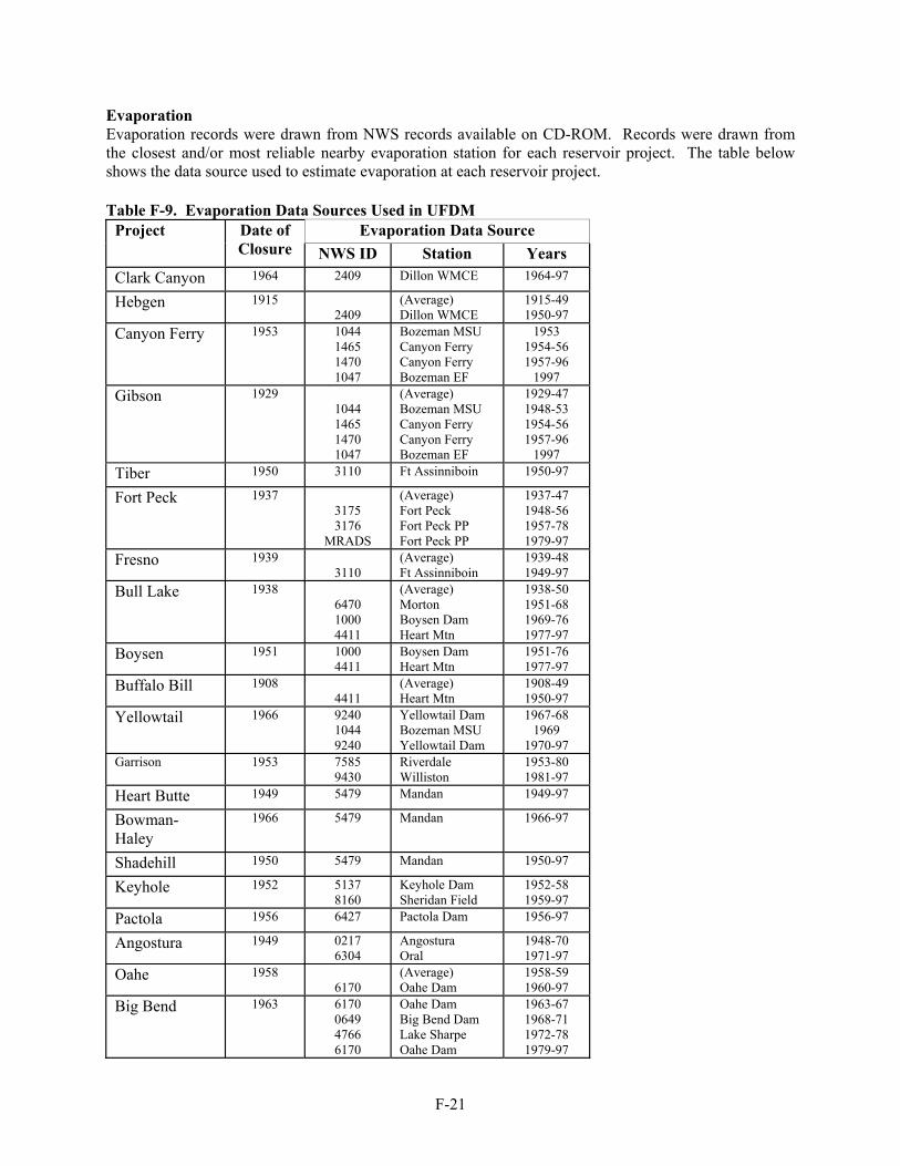
F-21

Evaporation Evaporation records were drawn from NWS records available on CD-ROM. Records were drawn from the closest and/or most reliable nearby evaporation station for each reservoir project. The table below shows the data source used to estimate evaporation at each reservoir project. Table F-9. Evaporation Data Sources Used in UFDM

Evaporation Data Source Project Date of Closure NWS ID Station Years

Clark Canyon 1964 2409 Dillon WMCE 1964-97

Hebgen 1915 2409

(Average) Dillon WMCE

1915-49 1950-97

Canyon Ferry 1953 1044 1465 1470 1047

Bozeman MSU Canyon Ferry Canyon Ferry Bozeman EF

1953 1954-56 1957-96

1997 Gibson 1929

1044 1465 1470 1047

(Average) Bozeman MSU Canyon Ferry Canyon Ferry Bozeman EF

1929-47 1948-53 1954-56 1957-96

1997 Tiber 1950 3110 Ft Assinniboin 1950-97

Fort Peck 1937 3175 3176

MRADS

(Average) Fort Peck Fort Peck PP Fort Peck PP

1937-47 1948-56 1957-78 1979-97

Fresno 1939 3110

(Average) Ft Assinniboin

1939-48 1949-97

Bull Lake 1938 6470 1000 4411

(Average) Morton Boysen Dam Heart Mtn

1938-50 1951-68 1969-76 1977-97

Boysen 1951 1000 4411

Boysen Dam Heart Mtn

1951-76 1977-97

Buffalo Bill 1908 4411

(Average) Heart Mtn

1908-49 1950-97

Yellowtail 1966 9240 1044 9240

Yellowtail Dam Bozeman MSU Yellowtail Dam

1967-68 1969

1970-97 Garrison 1953 7585

9430 Riverdale Williston

1953-80 1981-97

Heart Butte 1949 5479 Mandan 1949-97

Bowman-Haley

1966 5479 Mandan 1966-97

Shadehill 1950 5479 Mandan 1950-97

Keyhole 1952 5137 8160

Keyhole Dam Sheridan Field

1952-58 1959-97

Pactola 1956 6427 Pactola Dam 1956-97

Angostura 1949 0217 6304

Angostura Oral

1948-70 1971-97

Oahe 1958 6170

(Average) Oahe Dam

1958-59 1960-97

Big Bend 1963 6170 0649 4766 6170

Oahe Dam Big Bend Dam Lake Sharpe Oahe Dam

1963-67 1968-71 1972-78 1979-97

F-22

Evaporation Data Source Project Date of Closure NWS ID Station Years

Fort Randall 1952 6574 Pickstown 1952-97

Gavins Point 1955 6474 Pickstown 1955-97

Pipestem 1973 4413 Jamestown 1973-97

Jamestown 1953 4413 Jamestown 1953-97

Evaporation records generally are not as extensive as those for precipitation, nor do they cover as long a timeframe. Several reservoirs, such as Hebgen, Fresno, Bull Lake, and Buffalo Bill, antecede evaporation records, so the daily average from the period of record at each station was used to estimate evaporation records at these reservoirs prior to the period of record. Additionally, some stations do not report evaporation records during winter months, so monthly average values, taken from NWS 34 (NWS, 1982b), were used at these stations. As evaporation is minimal during winter, it was felt that the average values would suffice. Evaporation estimates for the Huron station were used to fill in missing records at Oahe, Big Bend, Fort Randall, and Gavins Point. Values from Rapid City were used to fill in missing records at Angostura and Pactola. Estimates at Bismarck were used for Pipestem, Jamestown, Garrison, Heart Butte and Bowman-Haley. Missoula evaporation estimates were used to fill in missing data at Dillon, while Helena estimates were used for Canyon Ferry. At Fort Peck, missing records were based on average values observed at Fort Peck. For missing evaporation records at Yellowtail Dam, estimates at Billings were used. The evaporation records needed to be adjusted, as the published values are pan evaporation records. Annual pan evaporation coefficients were taken from NWS 33 (NWS, 1982a) and applied to the pan evaporation data to obtain the final evaporation values for the USBR and smaller COE reservoirs. Pan evaporation coefficient values for the six mainstem reservoirs were taken from (NWS, 1982b) and applied to the mainstem evaporation records. The table below shows the pan evaporation coefficients used to obtain lake evaporation at each reservoir project. Table F-10. Pan Evaporation Coefficients Jan Feb Mar Apr May Jun Jul Aug Sep Oct Nov Dec Fort Peck

1.28 0.70 0.60 0.11 0.22 0.32 0.39 0.64 1.21 1.32 2.57 4.22

Garrison

0.70 0.70 0.70 0.14 0.20 0.21 0.26 0.64 1.13 1.44 3.74 5.04

Oahe 0.73 0.56 0.49 0.13 0.16 0.18 0.22 0.50 0.89 1.19 2.22 3.42 Big Bend

0.63 0.63 0.54 0.47 0.35 0.39 0.53 0.70 0.82 1.05 1.52 1.36

Fort Randall

0.70 0.70 0.63 0.19 0.32 0.37 0.42 0.78 1.31 1.42 1.62 1.39

Gavins Point

0.70 0.70 0.62 0.53 0.53 0.53 0.56 0.70 0.93 0.97 1.59 1.57

Boysen 0.72 (annual) Fresno, Bowman-Haley, Heart Butte, Keyhole, Shadehill 0.73 (annual) Canyon Ferry, Tiber, Pactola 0.74 (annual) Hebgen, Clark Canyon, Yellowtail 0.75 (annual) Gibson, Buffalo Bill, Bull Lake 0.76 (annual) Pipestem, Jamestown 0.77 (annual)

F-23

UNREGULATED FLOW The unregulated flow data set was developed through use of the Unregulated Flow Development Model (UFDM), utilizing data sets for discharge, reservoir inflow and outflow or storage change, evaporation, precipitation, area-storage relationships, depletion data, and routing parameters. The following sections describe the UFDM model and its inputs. Hydrologic Model Description (UFDM) The UFDM is a computer model developed by the U.S. Army Corps of Engineers Reservoir Control Center at the Missouri River Region Office (MRR-RCC) to determine unregulated flows for a base level of water resource development in the basin. The model is used to assist in determining flood control benefits for the mainstem reservoir system as well as to determine the amount of runoff from the upper Missouri River basin. Model Philosophy Reliable runoff or flow data are a continuing need for purposes of efficient utilization of the available water supply in the Missouri Basin. With these data the nature and distribution of the supply becomes apparent, long term normals are defined more precisely, effects of basin water resources development can be estimated, and reservoir regulation effects on downstream flood flows or low water conditions may be developed. In basic terms, the model determines reservoir holdouts and adds these holdouts to irrigation and other water-use depletions to obtain total holdouts in each mainstem reservoir reach. The total holdouts are routed through the system of reservoirs and then downstream to each gage, with the holdouts added to observed flow at each gage to determine unregulated flow. A more detailed description of the UFDM modeling philosophy may be found in USACE (1973). Modifications to UFDM The UFDM model, as developed by MRR-RCC, is written in FORTRAN source code and is set up to determine one year of flow record downstream to St. Joseph, with output directed to a text file, as well as a MRADS database. The model also only considers holdouts and depletions above Sioux City in developing unregulated flows. Several modifications to the program source code were necessary for the purposes of this study. Period of record simulation. The UFDM, as originally programmed, was set to run one year of data at a time. In order to simplify data processing, an additional program loop was added that gives the user the option of running as many years of data as desired at one time. The program does not, however, carry over data from year to year. In other words, the initial reservoir storage values and other initial values are reset at the beginning of every year so that any errors that may accrue in computed reservoir storage do not compound from year-to-year. Routing one stretch (OAHE-BEND). The outflows from Oahe to Big Bend and Big Bend to Fort Randall were routed by regression coefficients, rather than by lag-average method, as the travel time is so short. However, upon investigation of the code algorithm for computing the Big Bend and Fort Randall holdouts, it was discovered that the computed holdout at Big Bend and Fort Randall was dependent upon today's and yesterday's values. However, yesterday's value was already modified, so the computed value for today's holdout was incorrect. The code algorithm was changed so that today's computed holdout used yesterday's actual inflow, rather than the modified inflow.

F-24

Choice of routing method. The UFDM was programmed to route flows from station to station using the lag-average method. This method is somewhat simplistic, but has the advantage over most other routing methods in that flow volumes are preserved. However, the computer model used for the regulated flow data set uses regression routing from station to station (which also preserves flow volumes) below Gavins Point Dam. In order to have the ability to maintain consistent routing methodology, the UFDM code was altered to give the user the option of choosing lag-average routing or regression routing at gage stations downstream of Gavins Point Dam; a subroutine that routes flows with regression routing was also added to the UFDM code. Routing downstream of Gavins Point was also altered, as the UFDM originally routed holdouts above Gavins Point to each station from Gavins Point; the code was altered so that holdouts are routed from station to station below Gavins to be consistent with the routing methodology in the regulated flow model. The model input allows different lag-average values to be input for different years, while the regression routing uses constant values for the entire period of simulation. However, the program code could be altered to allow different regression values for different years, if desired. The tributary holdouts downstream of Gavins Point are routed from station to station using the regression routing only. Output to DSS. The UFDM output capability was limited to the MRADS database and a text file for each year. Since HEC-DSS is more widely used within COE as a database, the program was changed so that all output that was sent to text files was also written to a DSS file. A new subroutine to the program was developed to handle the output to DSS. Auxiliary programs for input and output. Due to the size and complexity of the data input and output required for this program, several auxiliary programs were developed or modified to streamline some of the input and output processes. These auxiliary programs, along with descriptions, are presented in Appendix F-D. Depletions and depletion level. The UFDM used USBR estimates of depletions adjusted to 1949 levels of development in data input files. However, use of a 1949 level of depletion development would not have met the definition of unregulated flow for this study. Therefore, the code and input file format were modified to use historic levels of depletions, as determined by the USBR. The UFDM also did not include estimates of Platte or Kansas River depletions, so additional code was written to allow the inclusion of Platte and Kansas River basin depletions so as to determine their effect on observed flows. The Platte River estimates of depletions included reservoir holdouts, as well as irrigation and other uses. The Kansas River depletion data did not include reservoir holdouts. The Kansas River depletion data was added to the Kansas River basin reservoir holdouts for model input purposes. Additional Flood Control Reservoirs The UFDM originally did not include several flood control reservoirs used in this study (Jamestown, Pipestem, Bowman-Haley, Kansas City District reservoirs). In order to more accurately reflect unregulated flow conditions, the model was altered to allow the impacts of these reservoirs on observed flows to be modeled. The addition of Bowman-Haley to the model did not require much change in programming, other than increasing some array sizes and increasing some variable counters. However, adding the other reservoirs to the model required changes in the way routing was done, as the model routed all mainstem and tributary holdouts from Gavins Point to each station individually. In order to route Jamestown, Pipestem and the Kansas City District reservoirs, their individual holdouts had to be routed with regression routing from station to station by means of a new subroutine and using regression coefficients that corresponded to those used in the DRM.

F-25

Input Data Development Copious amounts of data were required for input to the UFDM model. The development of the various parameters is discussed below. Area-Capacity Relationships Area-capacity relationships at each reservoir are important for determining how much water is lost to evaporation and how much water is gained from precipitation at each reservoir. Survey data was gathered for each reservoir modeled in the UFDM, either from the USBR, COE, or dam operator. Even though each reservoir has suffered from sedimentation, the area-capacity relationship has remained amazingly stable over time. Because of this, it was decided to use one area-capacity relationship over the period of record of reservoir operation, rather than trying to interpolate the relationship between survey dates and having a slightly different relationship each year. The table below lists each reservoir and the dates from which survey data was available. Table F-11. Dates of Available Area-Capacity Surveys Reservoir Date(s) of Survey Availability Clark Canyon 1963 Hebgen 1962 Canyon Ferry 1946, 1964, 1983 Gibson 1929, 1965, 1975, 1996 Tiber 1950, 1963 Fort Peck 1937, 1946, 1961, 1972, 1986 Fresno 1953 Bull Lake 1965 Boysen 1946, 1966, 1996 Buffalo Bill 1970, 1986, 1992 Yellowtail 1946, 1963, 1982 Garrison 1954, 1964, 1969, 1979, 1988 Heart Butte 1944, 1992 Bowman-Haley 1966, 1984 Shadehill 1950, 1993 Keyhole 1946, 1966, 1978 Pactola 1956, 1965, 1988 Angostura 1945, 1966, 1979 Oahe 1950, 1968, 1976, 1989 Big Bend 1971, 1975, 1979, 1991 Fort Randall 1950, 1962, 1967, 1973, 1981, 1986,

1996 Gavins Point 1953, 1965, 1970, 1975, 1979, 1985,

1995 Pipestem 1971, 1973, 1990 Jamestown 1948 Reservoir Hydrologic Data In order to accurately estimate how much each reservoir is affecting flows through holdouts, it is necessary to have accurate records of reservoir inflow and outflow and/or reservoir storage, precipitation at or near the reservoir, and evaporation at or near the reservoir. Data for inflow, outflow and storage is

F-26

available from the USBR, COE and USGS for federal reservoirs, and from private companies for the privately owned reservoirs. Data for inflow must be in daily values. Storage data can be either daily or monthly; the UFDM automatically translates monthly data to daily data in a linear manner for modeling purposes. Precipitation and evaporation data was gathered from National Weather Service sources and can be either daily or monthly, as the UFDM will translate monthly values to daily values in a linear manner for modeling purposes. The following table shows the period of record for which various data were available for modeling purposes, and whether the data was daily or monthly. Table F-12. Reservoir Hydrologic Data Availability

Project

Date of Initial

Storage Inflow Outflow Storage Evaporation PrecipitationClark Canyon

8/28/1964 Daily: 9/1/64-12/31/97

Daily: 9/1/64-12/31/97

Daily: 9/1/64-9/30/98

Daily: 1/1/63-12/31/97

Daily: 1/1/60-12/31/97

Hebgen 1914 Daily: 1/1/31-9/30/98

Daily: 1/1/31-9/30/98

Monthly: 6/14-12/29 Daily: 1/1/31-9/30/98

Daily: 1/1/50-12/31/97

Daily: 1/1/15-12/31/97

Canyon Ferry

3/1953 Daily: 3/28/53-12/31/97

Daily: 3/28/53-12/31/97

Daily: 3/27/53-9/30/98

Daily: 1/1/54-12/31/97

Daily: 1/1/48-12/31/97

Gibson 1929 Daily: 1/1/73-9/30/98

Daily: 1/1/30-9/30/98

Monthly: 12/29-9/95 Daily: 10/1/38-9/30/49 & 1/1/73-9/30/98

Daily: 1/1/54-12/31/97

Daily: 1/1/28-12/31/97

Tiber 10/28/1955 Daily: 1/1/56-4/3/98

Daily: 1/1/56-4/3/98

Daily: 1/1/56-9/30/98

Daily: 1/1/54-12/31/97

Daily: 1/1/48-12/31/97

Fort Peck 1937 Daily: 1/1/38-12/31/97

Daily: 1/1/38-12/31/97

Monthly: 9/37-8/98

Daily: 1/1/48-12/31/97

Daily: 1/1/37-12/31/97

Fresno 1939 Daily: 1/1/48-7/22/98

Daily: 1/1/48-7/22/98

Monthly: 12/39-9/50 Daily: 1/1/48-7/22/98

Daily: 1/1/49-12/31/97

Daily: 1/1/38-12/31/97

Bull Lake 10/1937 Daily: 12/1/68-9/17/98

Daily: 12/1/68-9/17/98

Monthly: 10/37-8/98 Daily: 12/1/68-9/17/98

Daily: 1/1/51-12/31/97

Daily: 1/1/37-12/31/97

Boysen 10/1951 Monthly: 3/52-6/66 Daily: 3/1/52-12/31/97

Daily: 3/1/52-12/31/97

Monthly: 10/51-8/98 Daily: 3/1/52-9/30/98

Daily: 1/1/49-12/31/97

Daily: 8/1/48-12/31/97

Buffalo Bill 5/1909 Daily: 4/1/52-12/31/97

Daily: 3/24/52-12/31/97

Monthly: 04/09-8/98 Daily: 3/23/52-9/30/98

Daily: 1/1/50-12/31/97

Daily: 1/1/15-12/31/97

Yellowtail 11/3/1965 Daily: 11/1/65-4/3/98

Daily: 10/1/65-4/3/98

Daily: 11/1/65-9/30/98

Daily: 1/1/65-12/31/97

Daily: 1/1/62-12/31/97

Garrison 11/1953 Daily: 12/1/53-12/31/97

Daily: 12/1/53-12/31/97

Monthly: 10/53-8/98

Daily: 1/1/49-12/31/97

Daily: 1/1/48-12/31/97

Heart Butte 9/29/1949 Daily: 10/1/49-4/3/98

Daily: 10/1/49-4/3/98

Daily: 10/1/49-9/30/98

Daily: 1/1/49-12/31/97

Daily: 1/1/48-12/31/97

Bowman-Haley

Daily: 3/2/67-12/31/97

Daily: 1/1/67-12/31/97

Daily: 3/31/67-12/31/97

Daily: 1/1/67-12/31/97

Daily: 1/1/60-12/31/97

Shadehill 7/1/1950 Daily: 4/1/52-4/3/98

Daily: 4/1/52-4/3/98

Monthly: 7/50-3/52 Daily:

Daily: 1/1/50-12/31/97

Daily: 1/1/50-12/31/97

F-27

Project

Date of Initial

Storage Inflow Outflow Storage Evaporation Precipitation4/1/52-9/30/98

Keyhole 2/12/1952 Daily: 4/1/52-4/3/98

Daily: 4/1/52-4/3/98

Daily: 4/1/52-9/30/98

Daily: 1/1/52-12/31/97

Daily: 11/1/49-12/31/97

Pactola 8/22/1956 Daily: 8/22/56-4/3/98

Daily: 8/22/56-4/3/98

Daily: 8/22/56-9/30/98

Daily: 1/1/55-12/31/97

Daily: 1/1/55-12/31/97

Angostura 10/3/1949 Daily: 4/1/52-9/17/98

Daily: 4/1/52-9/17/98

Monthly: 10/49-3/52 Daily: 4/1/52-9/17/98

Daily: 1/1/48-12/31/97

Daily: 1/1/48-12/31/97

Oahe 8/1958 Daily: 8/3/58-12/31/97

Daily: 8/3/58-12/31/97

Monthly: 7/58-8/98

Daily: 1/1/60-12/31/97

Daily: 1/1/57-12/31/97

Big Bend 7/1963 Daily: 8/1/63-12/31/97

Daily: 8/1/63-12/31/97

Monthly: 6/63-8/98

Daily: 1/1/68-12/31/97

Daily: 1/1/62-12/31/97

Fort Randall 12/1952 Daily: 1/1/53-12/31/97

Daily: 1/1/53-12/31/97

Monthly: 11/52-9/98

Daily: 1/1/51-12/31/97

Daily: 1/1/48-12/31/97

Gavins Point 7/1955 Daily: 8/1/55-12/31/97

Daily: 8/1/55-12/31/97

Monthly: 6/55-9/98

Daily: 1/1/55-12/31/97

Daily: 1/1/54-12/31/97

Pipestem 7/1973 Daily: 3/1/74-3/31/98

Daily: 3/1/74-3/31/98

Daily: 2/14/78-3/31/98 Lots of daily values missing

Daily: 1/1/73-12/31/97

Daily: 1/1/48-12/31/97

Jamestown 10/1/1953 Daily: 2/2/54-4/3/98

Daily: 2/2/54-4/3/98

Monthly: 10/53-2/54 Daily: 2/1/54-4/3/98

Daily: 1/1/48-12/31/97

Daily: 1/1/48-12/31/97

Storage values were used only in the absence of daily inflow and outflow records, which was often the case in the first month or two of reservoir operation. As can be seen above, not all reservoirs have evaporation or precipitation records extending back to the beginning of regulation at that dam site. In this instance, the monthly averages from the period of record for evaporation and precipitation were computed, then used for the missing months. The monthly data was then distributed evenly over each day of the month. All the reservoirs for which this was done, with the exception of Fort Peck, are fairly small and it was felt that precipitation and evaporation from these reservoirs had very little impact on annual peaks, especially considering the smaller number of reservoirs in operation prior to evaporation records being kept. Hebgen Reservoir had one year of storage/flow records missing, as there was no storage or flow data available for 1930 from the Montana Power Company. The total change in storage from 12/31/29 to 1/1/31 was computed, and then monthly volume changes were patterned after long-term monthly storage changes to achieve the proper annual storage change at Hebgen. Historic Depletion Estimates In order to properly develop unregulated flows, an accurate accounting of streamflow depletions by irrigation, reservoir holdouts, and other consumptive uses was needed. The USBR was contracted with to provide estimates of streamflow depletions for the period 1898-1996 for the Missouri River upstream of Hermann, Missouri. The methodologies and results of the USBR are presented as Appendix F-C.

F-28

The values provided by the USBR were by month, and included historic (actual) level of depletions and current-use level depletions. The UFDM as originally coded used 1949 levels of depletion. This program code was modified to use the actual depletions. The monthly values are read into the UFDM program, and the program automatically prorates the monthly values to daily values at each appropriate node in the model. The historic depletion data provided by the USBR included reservoir holdouts at USBR projects that were already modeled in the UFDM, so those reservoir projects were subtracted out of the depletion data before input to the UFDM model. The Platte (NE) River depletions were converted from monthly values to daily values by patterning the depletions after the observed daily hydrograph on the Platte River at either the Ashland gage (1928-1953) or the Louisville gage (1953-1997). This was done by computing the mean monthly flow on the Platte River and computing the ratio of monthly depletions to monthly Platte River flows. The daily Platte River flows were then multiplied by the monthly ratio to determine daily depletions. The computed daily depletions were then smoothed by use of a 3-day moving average. The monthly depletion values were prorated on a daily basis for data prior to 1928. Routing Parameters Parameters for the lag-average routing were taken from existing model input files used by MRR-RCC and from USACE (1973). However, there was concern that with channel changes, there would be differences in the routing parameters with time. Work was done to determine if these parameters changed with time. Two methods were used to determine the lag and the average values for each of the reaches. The first method was to optimize the lag and the average for each yearly high flow period using HEC-1 and the optimization function. The second method attempted to determine the lag and the average by minimizing the total yearly negative incremental inflows. Observed flows at Sioux City and Omaha were configured in an HEC-1 model with the optimization function. Because mean daily flows on the Missouri River were used in the analysis, the average value and the lag values were derived using a time step of 1-day. Optimized values were based on the high flow event for each year. The average flow optimized at two flow values for the majority of the years. However, the lag optimized almost equally between 1 day and 2 days for any given year. To derive the incremental inflow, two DSSMATH models were configured using an average flow based on 2-days of flow values for both models and lag of 1-day for the first model and 2-days for the second. When the calculated incremental inflows for the period of record were analyzed, it was observed that there were numerous negative inflows. The negative incremental inflows are likely caused by errors in the flows used in the analysis. Mean daily flows are being used with a 1-day time step for the averaging and lag. In addition, some of the flow data at the gages were derived from stage records for part of the period of record or reconstituted using nearby streamflow data when there was no flow of stage data available for that gage. With the construction of the navigation channel and bank stabilization works on the Missouri River, the length of the river channel has been reduced. This may have the effect of altering the lag and average. Based on the first method used, a second calibration method used was an iterative process where the lag and average values were varied and the negative incremental inflows for the year accumulated and compared to each other with the objective of minimizing negative inflows. DSSMATH was used for the analysis. This process was performed for each reach between the main stem gages. The yearly negative totals were observed to determine if the chosen lag and average changed, and if they were the least over time. No significant change was found over the period of record, so the lag and average were not altered

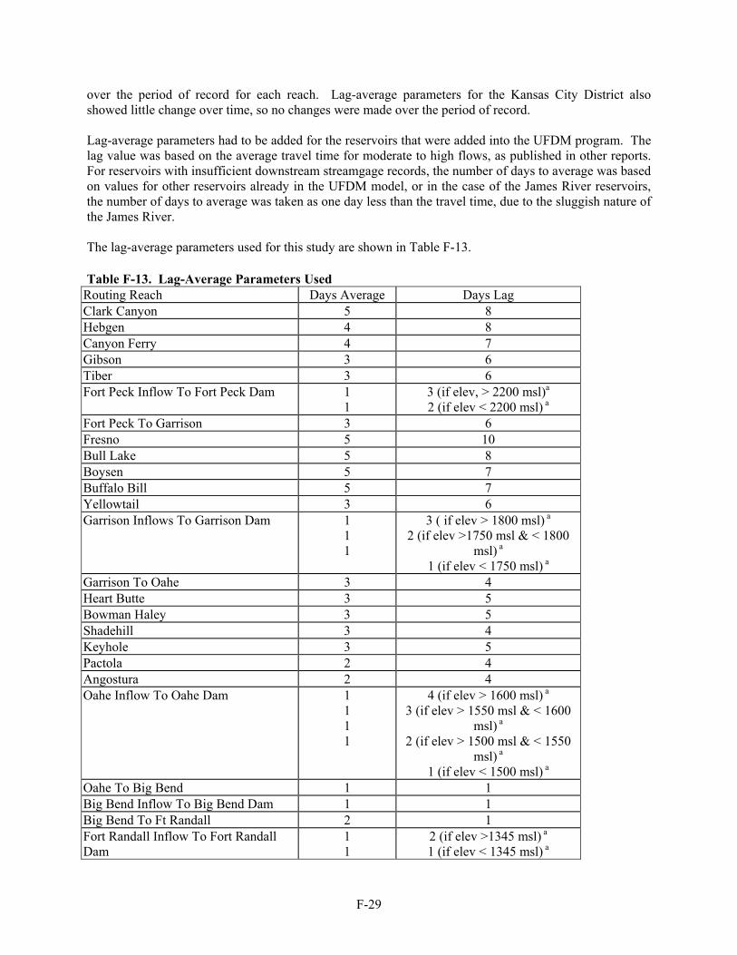
F-29

over the period of record for each reach. Lag-average parameters for the Kansas City District also showed little change over time, so no changes were made over the period of record. Lag-average parameters had to be added for the reservoirs that were added into the UFDM program. The lag value was based on the average travel time for moderate to high flows, as published in other reports. For reservoirs with insufficient downstream streamgage records, the number of days to average was based on values for other reservoirs already in the UFDM model, or in the case of the James River reservoirs, the number of days to average was taken as one day less than the travel time, due to the sluggish nature of the James River. The lag-average parameters used for this study are shown in Table F-13. Table F-13. Lag-Average Parameters Used

Routing Reach Days Average Days Lag Clark Canyon 5 8 Hebgen 4 8 Canyon Ferry 4 7 Gibson 3 6 Tiber 3 6 Fort Peck Inflow To Fort Peck Dam 1

1 3 (if elev, > 2200 msl)a 2 (if elev < 2200 msl) a

Fort Peck To Garrison 3 6 Fresno 5 10 Bull Lake 5 8 Boysen 5 7 Buffalo Bill 5 7 Yellowtail 3 6 Garrison Inflows To Garrison Dam 1

1 1

3 ( if elev > 1800 msl) a 2 (if elev >1750 msl & < 1800

msl) a 1 (if elev < 1750 msl) a

Garrison To Oahe 3 4 Heart Butte 3 5 Bowman Haley 3 5 Shadehill 3 4 Keyhole 3 5 Pactola 2 4 Angostura 2 4 Oahe Inflow To Oahe Dam 1

1 1 1

4 (if elev > 1600 msl) a 3 (if elev > 1550 msl & < 1600

msl) a 2 (if elev > 1500 msl & < 1550

msl) a 1 (if elev < 1500 msl) a

Oahe To Big Bend 1 1 Big Bend Inflow To Big Bend Dam 1 1 Big Bend To Ft Randall 2 1 Fort Randall Inflow To Fort Randall Dam

1 1

2 (if elev >1345 msl) a 1 (if elev < 1345 msl) a

F-30

Routing Reach Days Average Days Lag Fort Randall To Gavins Point 1

1

Gavins Point Inflow To Gavins Point Dam

1 1

Gavins Point To Yankton 2 1 Gavins Point To Sioux City 2 1 Fort Peck Q To Garrison Headwaters 3 5 Garrison Q To Oahe Headwaters 2 3 Oahe Release To Big Bend Headwaters 0.1 b 0.9b Big Bend Q To Ftr Headwaters 0.1 b 0.9b Ft Randall Q To Gavins Headwater 1 1 Sioux City To Decatur 2 2 Sioux City To Omaha 2 2 Sioux City To Nebraska City 2 3 Sioux City To Rulo 2 3 Sioux City To St. Joseph 2 4 Fort Peck To Wolf Point 2 1 Fort Peck To Culbertson 2 3 Garrison To Bismarck 2 2 Pipestem To Sioux City 67 66 Jamestown To Sioux City 67 66 Gavins Point To Kansas City 3 4 Gavins Point To Waverly 3 4 Gavins Point To Boonville 3 5 Gavins Point To Hermann 4 5 Gavins Point To Mouth 4 6 Platte River Louisville To Nebraska City

2 1

Platte River (Missouri) To Kansas City 2 1 Kansas River To Kansas City 1 1 Chariton River To Boonville 2 1 Osage River To Hermann 2 1 a Elevation refers to the computed elevation of the reservoir. b Because of the very short travel distances from Oahe to Big Bend and from Big Bend to Fort Randall, flows were routed using regression coefficients, rather than lag-average. Model Calibration/Verification Traditionally, hydrologic computer models are calibrated to observed events to obtain some degree of confidence in the model parameters. However, as this model's purpose is to obtain hypothetical flows, the model cannot be calibrated to observed flows. However, the model was tested using zero reservoir holdouts and zero depletions to ensure the model output at each of the mainstem gages matched the observed flow. One means to verify the accuracy of the model output is to compare it to various hydrologic and climatological data. Since the 1898-1928 period appears to have some differences (whether in mean or variance) with the rest of the period of record, the climatological record was investigated for differences. One readily available measure of climatological conditions is the Palmer Drought Severity Index. The

F-31

Palmer Drought Severity Index uses temperature and rainfall data to measure long-term dryness. The data is available on a monthly basis for regions within each state for the period 1895-present from the National Climate Data Center. Data for regions within the Missouri River basin were collected. Monthly regional values within each state were averaged to obtain a statewide monthly average, as regions within each state are roughly equal in area. However, only those regions within the Missouri River basin were used. The monthly statewide drought values were weighted by each month’s percent of mean annual flow (i.e., 2.3%-Jan, 3.2%-Feb., 7.6%-Mar., 10.9%-Apr, 11.2%-May, 19.6%-Jun, 19.2%-Jul, 10.3%-Aug, 6.0%-Sep, 4.3%-Oct, 3.3%-Nov, 2.2%-Dec for Sioux City) to obtain an annual drought index for each state. The annual drought index for each state was then weighted by drainage area upstream of the gage in question to obtain an overall basin drought index. The annual drought index and annual unregulated flow at Sioux City, Nebraska City, Kansas City, and Hermann were analyzed using linear regression. The period 1929-1997 showed a fairly strong correlation, while the data for 1898-1928 showed a fair correlation but within the scatter of the 1929-1997 data. The results of the regression are shown on Plates F-1 to F-4. Plates F-5 to F-8 show the annual time-series for both the annual flow and annual drought index. The trend in both parameters can be seen to follow quite closely. On the basis of this analysis, it appears that the period 1898-1928 may have been wetter above Sioux City than the period 1929-1997. The annual flow volumes appear reasonable for Sioux City as computed with a single rating curve. A similar analysis was performed to determine the correlation between mean annual reach inflow and the drought index from Sioux City to Nebraska City, Nebraska City to Kansas City, and Kansas City to Hermann to determine if the annual mean incremental flow is reasonable. Again, the period 1929-1997 showed a strong correlation, while the data for 1898-1928 showed a fair to poor correlation. The Sioux City to Nebraska City reach shows the poorest correlation and greatest scatter for the pre-1928 period, while the Kansas City to Hermann reach appears consistently low (see Plates F-9 to F-11). On the basis of the above information, it is likely that the annual flow volumes at Sioux City, Nebraska City, and Kansas City are reasonable for the 1898-1928 period, while the values at Hermann may be slightly low. In all, the comparison between annual flow and annual drought index supports the mean annual flows as reasonable for the pre-USGS gaging period. An analysis of annual stream flows tends to further support this position. In order to further verify the reasonableness of the historic flows derived for the period of 1898-1928, the following procedures were used. First the average annual historic flows for the period 1898-1928 were compared to the average flows for various other periods measured by the USGS. Results of this comparison are shown in Table F-14.

Table F-14. Comparison of Average Annual Flows

Average Annual Flow (million acre-feet per year) Period Sioux City Omaha Nebraska City

1898-1928 32.9 35.8 43.7 1929-1942 16.4 17.0 20.7 1943-1952 26.4 27.8 33.0 1953-1968 16.9 18.0 22.4 1969-1992 22.8 25.6 30.2 1993-1997 29.1 34.4 39.2

F-32

Although the 1898-1928 estimated flows are higher than any other period during the historical record, they are reasonable when considering the effects of droughts, depletions, and reservoirs. Since 1898, basin depletions for irrigation and other uses (not including reservoirs) upstream from Sioux City have increased from about 2 million acre-feet to over 8 million acre-feet per year and Platte River basin depletions have increased by about 4 million acre-feet per year. In addition, construction of the main stem and tributary reservoirs has added 2 to 3 million acre-feet per year in evaporation losses. The period of 1929-1942 was affected by the 1930’s drought, the most severe recorded drought in the Missouri River basin, and the filling of Fort Peck Reservoir. Runoff during the 1943-1952 period was also affected by the 1930’s drought during the recovery of basin groundwater and pothole storage. Many large tributary irrigation and flood control reservoirs also came online during this period including Tiber, Boysen, Keyhole, and Heart Butte reservoirs. The 1953-1968 period was affected by a drought during the mid-50’s and the filling of the main stem reservoir system. During the 1969-1992 period, the late 1980s drought resulted in reduced runoff conditions. Recorded flows during the 1993-1997 period, a relatively wet period, compare favorably to the estimated flows during the 1898-1928 period when considering the increased basin depletions due to irrigation, reservoir evaporation and other water uses. The USGS prepared estimates of monthly flows at Sioux City for the period 1897 through 1928 based on the recorded discharge at Williston, North Dakota and weather records. Results of that study, published in USGS Circular 108 (USGS), indicate that the average annual flow at Sioux City from 1898-1928 was 27.8 million acre-feet per year. That estimate appears low when compared to recorded flows at Sioux City during the post main-stem reservoir filling period (1968-1997) which averaged 23.9 million acre-feet per year. Considering basin depletions and reservoir evaporation upstream from Sioux City (approximately 6 to 8 maf/yr), the USGS estimate of flows during the 1898-1928 period equate to about 20 million acre-feet per year adjusted for present level of development conditions. Results of this verification indicate that the estimates of annual discharges for the period of 1898-1928 prepared for this study may be overestimated by about 1 to 2 million acre-feet per year. This would be equivalent to an average of about 1,400 to 2,800 cfs throughout the year. Because the discharges were estimated by use of a single rating curve derived from measurements made primarily during the summer months, it is believed that the majority of the overestimation would occur during late fall and winter periods, when flows were at their lowest. Therefore, it is concluded that high flows and peak flows estimated for the period 1898-1928 are reasonable and adequate for peak flow frequency and high flow volume investigations. If the flows for the low flow periods developed for this study are to be used in future study, additional adjustment to those flows may be required. Period of Record Simulation Once all input data were compiled, the model was run, covering the period of January 1, 1898 to December 31, 1997. Annual daily peaks were extracted from the output data and are compiled in Table FA-1. Various other data extracted from the output data are compiled in Tables FA-2 and FA-3. Sensitivity Analysis The model accuracy was assessed by testing the sensitivity of simulated values to a reasonable range of input parameter values. Sensitivity to Routing Method The UFDM allows for two routing methods to be employed below Gavins Point for routing reservoir holdouts. Output from the UFDM using the lag-average method was compared to the output used for the regression routing method. The following table compares the statistics of the two methods.

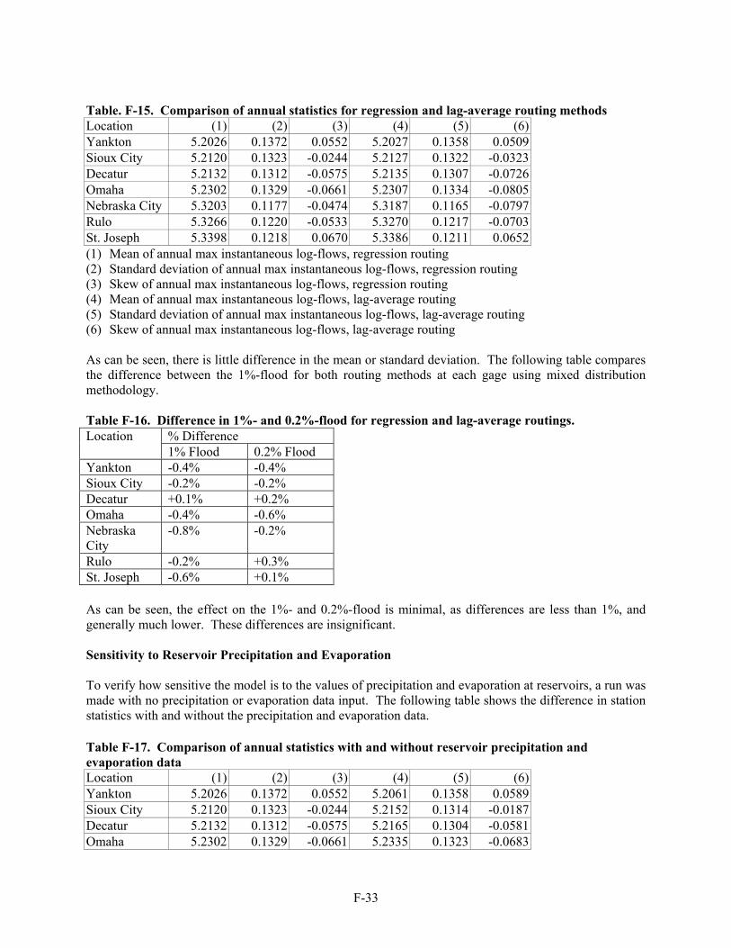
F-33

Table. F-15. Comparison of annual statistics for regression and lag-average routing methods Location (1) (2) (3) (4) (5) (6) Yankton 5.2026 0.1372 0.0552 5.2027 0.1358 0.0509 Sioux City 5.2120 0.1323 -0.0244 5.2127 0.1322 -0.0323 Decatur 5.2132 0.1312 -0.0575 5.2135 0.1307 -0.0726 Omaha 5.2302 0.1329 -0.0661 5.2307 0.1334 -0.0805 Nebraska City 5.3203 0.1177 -0.0474 5.3187 0.1165 -0.0797 Rulo 5.3266 0.1220 -0.0533 5.3270 0.1217 -0.0703 St. Joseph 5.3398 0.1218 0.0670 5.3386 0.1211 0.0652 (1) Mean of annual max instantaneous log-flows, regression routing (2) Standard deviation of annual max instantaneous log-flows, regression routing (3) Skew of annual max instantaneous log-flows, regression routing (4) Mean of annual max instantaneous log-flows, lag-average routing (5) Standard deviation of annual max instantaneous log-flows, lag-average routing (6) Skew of annual max instantaneous log-flows, lag-average routing As can be seen, there is little difference in the mean or standard deviation. The following table compares the difference between the 1%-flood for both routing methods at each gage using mixed distribution methodology. Table F-16. Difference in 1%- and 0.2%-flood for regression and lag-average routings.

% Difference Location 1% Flood 0.2% Flood

Yankton -0.4% -0.4% Sioux City -0.2% -0.2% Decatur +0.1% +0.2% Omaha -0.4% -0.6% Nebraska City

-0.8% -0.2%

Rulo -0.2% +0.3% St. Joseph -0.6% +0.1% As can be seen, the effect on the 1%- and 0.2%-flood is minimal, as differences are less than 1%, and generally much lower. These differences are insignificant. Sensitivity to Reservoir Precipitation and Evaporation To verify how sensitive the model is to the values of precipitation and evaporation at reservoirs, a run was made with no precipitation or evaporation data input. The following table shows the difference in station statistics with and without the precipitation and evaporation data. Table F-17. Comparison of annual statistics with and without reservoir precipitation and evaporation data Location (1) (2) (3) (4) (5) (6) Yankton 5.2026 0.1372 0.0552 5.2061 0.1358 0.0589 Sioux City 5.2120 0.1323 -0.0244 5.2152 0.1314 -0.0187 Decatur 5.2132 0.1312 -0.0575 5.2165 0.1304 -0.0581 Omaha 5.2302 0.1329 -0.0661 5.2335 0.1323 -0.0683

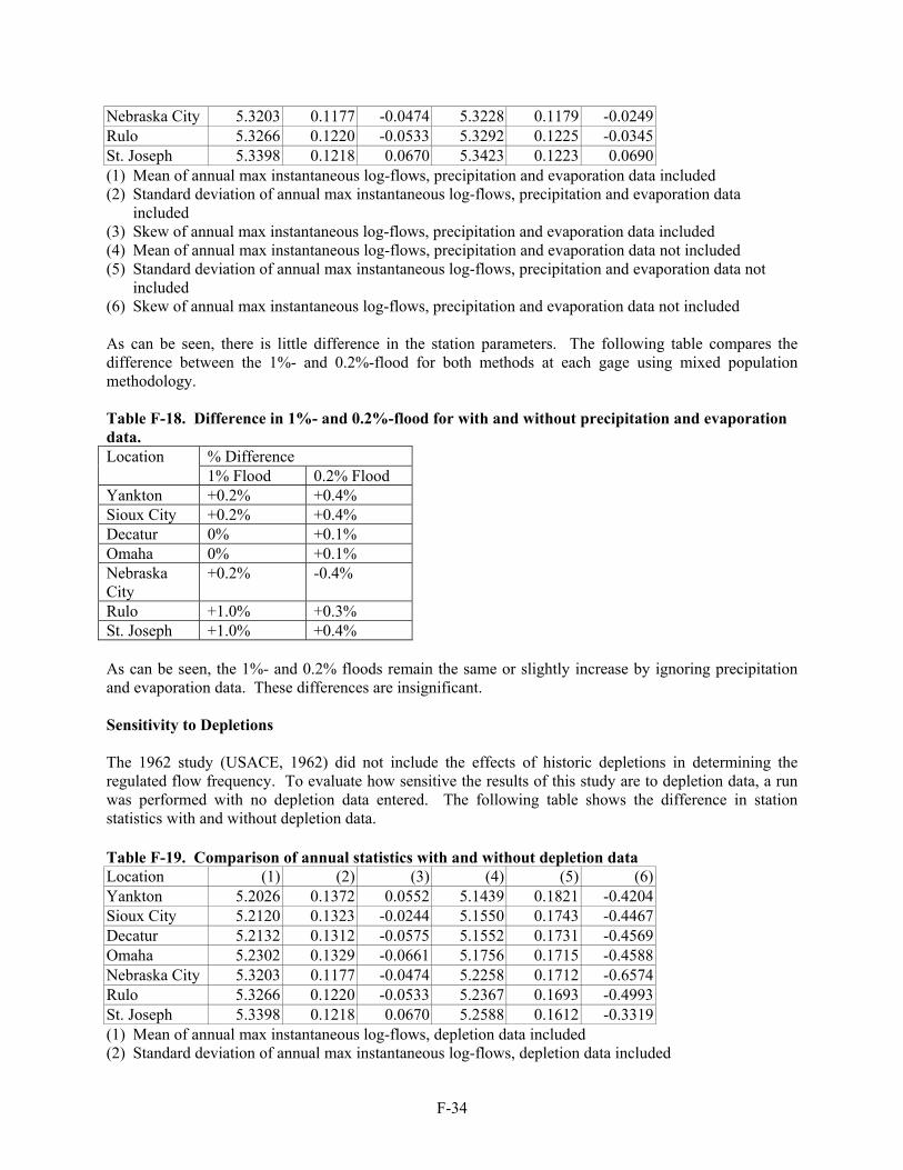
F-34

Nebraska City 5.3203 0.1177 -0.0474 5.3228 0.1179 -0.0249 Rulo 5.3266 0.1220 -0.0533 5.3292 0.1225 -0.0345 St. Joseph 5.3398 0.1218 0.0670 5.3423 0.1223 0.0690 (1) Mean of annual max instantaneous log-flows, precipitation and evaporation data included (2) Standard deviation of annual max instantaneous log-flows, precipitation and evaporation data

included (3) Skew of annual max instantaneous log-flows, precipitation and evaporation data included (4) Mean of annual max instantaneous log-flows, precipitation and evaporation data not included (5) Standard deviation of annual max instantaneous log-flows, precipitation and evaporation data not

included (6) Skew of annual max instantaneous log-flows, precipitation and evaporation data not included As can be seen, there is little difference in the station parameters. The following table compares the difference between the 1%- and 0.2%-flood for both methods at each gage using mixed population methodology. Table F-18. Difference in 1%- and 0.2%-flood for with and without precipitation and evaporation data.

% Difference Location 1% Flood 0.2% Flood

Yankton +0.2% +0.4% Sioux City +0.2% +0.4% Decatur 0% +0.1% Omaha 0% +0.1% Nebraska City

+0.2% -0.4%

Rulo +1.0% +0.3% St. Joseph +1.0% +0.4% As can be seen, the 1%- and 0.2% floods remain the same or slightly increase by ignoring precipitation and evaporation data. These differences are insignificant. Sensitivity to Depletions The 1962 study (USACE, 1962) did not include the effects of historic depletions in determining the regulated flow frequency. To evaluate how sensitive the results of this study are to depletion data, a run was performed with no depletion data entered. The following table shows the difference in station statistics with and without depletion data.

Table F-19. Comparison of annual statistics with and without depletion data Location (1) (2) (3) (4) (5) (6) Yankton 5.2026 0.1372 0.0552 5.1439 0.1821 -0.4204 Sioux City 5.2120 0.1323 -0.0244 5.1550 0.1743 -0.4467 Decatur 5.2132 0.1312 -0.0575 5.1552 0.1731 -0.4569 Omaha 5.2302 0.1329 -0.0661 5.1756 0.1715 -0.4588 Nebraska City 5.3203 0.1177 -0.0474 5.2258 0.1712 -0.6574 Rulo 5.3266 0.1220 -0.0533 5.2367 0.1693 -0.4993 St. Joseph 5.3398 0.1218 0.0670 5.2588 0.1612 -0.3319 (1) Mean of annual max instantaneous log-flows, depletion data included (2) Standard deviation of annual max instantaneous log-flows, depletion data included

F-35

(3) Skew of annual max instantaneous log-flows, depletion data included (4) Mean of annual max instantaneous log-flows, depletion data not included (5) Standard deviation of annual max instantaneous log-flows, depletion data not included (6) Skew of annual max instantaneous log-flows, depletion data not included As can be seen, the mean decreases significantly, the standard deviation increases significantly, and skew becomes significantly more negative. The following table compares the difference in the 1%- and 0.2%-floods for with and without depletions using mixed distribution methods at each gage. Table F-20. Difference in 1%- and 0.2%-flood for with and without depletion data Location % Difference,

1% % Difference, 0.2%

Yankton +0.6% +0.8% Sioux City +0.1% +0.1% Decatur +0.1% +0.1% Omaha -0.2% -0.1% Nebraska City -2.8% -0.1% Rulo -6.4% -3.5% St. Joseph -9.5% -7.2% As can be seen, the elimination of depletion data only slightly impacts the 1- and 0.2%-floods, except at St. Joseph. Even though depletions can account for as much as 25% of the annual unregulated flow, depletions generally have a small impact on larger floods. Limitation of Routing Method’s Effect on Ice Jams In the 1962 study (USACE, 1962), it was recognized that the lag-average routing method used was inadequate to accurately route the dynamic peaking of ice jam breakups in the development of the unregulated flow record; additionally, the construction of the mainstem reservoir system prevents this dynamic ice breakup from occurring. It was felt that this led to an underestimation of the instantaneous peak value at downstream stations. Accordingly, peak values were adjusted upwards in years following the closure of Fort Peck that were judged to have a reduced ice breakup due to the reservoirs. The following Table F-21 lists those years in which peaks were adjusted and by how much at Sioux City. However, there was little documentation as to how these values were derived. Table F-21. Increases in Peak Flows at Sioux City Due to Reduced Ice Jam Breakup Year Increase in Peak

Flow Value 1939 +31,000 1943 +25,000 1947 +45,000 1950 +11,000 1952 +38,000 1959 +54,000 1960 +58,000 In order to determine what impact this may have on the flow frequency results, flood years after 1960 were identified that may have had significant ice jam breakups on the Missouri River if the mainstem reservoirs were not in place – these were 1962, 1966, 1969, 1972, 1978, 1979, 1982, 1986, 1987, 1994, 1995, and 1997. These years were selected on the basis of climatic data and occurrence of ice jams on

F-36

tributary streams. The unregulated spring flood peaks in these years were all increased by 40,000 cfs at Sioux City (roughly the average amount of the values in Table F-21), and a flow frequency analysis was performed (see the section on Mixed Population Analysis for further details on methodology) using these modified values. The revised values with the ice jam adjustment show a sharp increase over the values determined without an ice jam adjustment. The following table shows the increase in discharges for various flow events at Sioux City. As can be seen, an adjustment to peak flows has a significant impact on the less frequent events. Table F-22. Increase in Flow Frequency Caused by Adjustments to Peak Flows for Ice Jam Effects at Sioux City Exceedance Probability

% Increase in Flow Estimate

0.5 1.48% 0.2 2.83% 0.1 5.24%

0.05 10.71% 0.02 15.23% 0.01 17.44%

0.005 19.81% 0.002 22.38%

However, a more careful examination of the record shows that an adjustment to flow may not be necessary. The 1881 flood resulted in a tremendous ice jam at Yankton, raising stages some 35 feet above flood stage and resulting in a tremendous volume of water being retained, if only for a short time. The effect of this ice jam may have been to reduce peak flows, and thus stages, downstream. The 1952 flood also had a tremendous ice jam upstream of Bismarck, North Dakota that released. The flood wave caused a significant increase in flow at Bismarck, but by the time the flood wave reached Pierre, South Dakota, the sharp peak in the Bismarck flood crest was attenuated. It is recognized that the routing methods, and underlying assumptions, used in the unregulated analysis do not adequately account for ice jams that no longer occur on the Missouri mainstem. However, as demonstrated by the 1881 and 1952 floods, this may be a moot point, as the peaking effects of ice jams do not always propagate themselves downstream to the stations in question and they can actually reduce flows if the ice jam is large enough and stable enough to retain significant volumes of water. Therefore, it was deemed unnecessary to make any adjustments to the flow record to account for ice jam breakups on peak discharges through the study reach. Sensitivity of Period Modeled to Monthly Volumes There is some degree of uncertainty in the use of rating curves to develop flows for the period prior to USGS flow records. The Drought Series analysis appears to support that these flows are reasonable on an annual basis, and various statistical tests show that peak flows and volumes are stationary in nature throughout the period of record. In order to evaluate shorter time frames, monthly mean volumes can be compared for various periods to see if there is any significant difference. The following Tables F-23 to F-28 list the computed monthly mean and standard deviation of flows at Yankton, Sioux City, Decatur, Omaha, Nebraska City and Rulo.

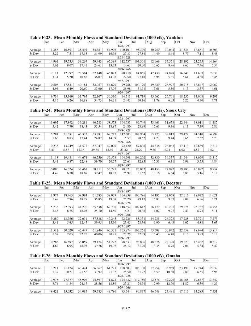
F-37

Table F-23. Mean Monthly Flows and Standard Deviations (1000 cfs), Yankton

Jan Feb Mar Apr May Jun Jul Aug Sep Oct Nov Dec 1898-1997

Average 11.358 16.591 35.492 54.381 54.998 100.101 95.309 50.750 30.064 21.336 16.881 10.803St Dev 5.22 7.51 17.15 31.99 16.93 23.33 27.84 14.49 8.64 8.73 7.11 5.45

1898-1928 Average 14.961 19.755 39.267 59.443 65.389 112.537 103.301 62.069 37.551 28.192 23.275 14.164St Dev 5.62 9.07 17.41 24.61 13.73 14.61 20.00 13.65 8.96 9.63 7.46 5.54

1929-1966 Average 9.111 12.997 28.584 52.148 46.823 90.210 84.865 42.430 24.828 16.249 11.693 7.030St Dev 3.31 5.20 10.85 36.07 14.78 22.50 27.18 8.98 5.85 5.61 4.38 3.45

1967-1997 Average 10.508 17.831 40.184 52.057 54.629 99.788 100.120 49.629 28.997 20.715 16.847 12.067St Dev 4.94 6.49 20.60 33.60 17.07 25.98 31.91 13.65 5.50 6.19 3.37 4.61

1929-1997 Average 9.739 15.169 33.795 52.107 50.330 94.513 91.719 45.665 26.701 18.255 14.008 9.293St Dev 4.15 6.26 16.88 34.73 16.21 24.42 30.16 11.79 6.03 6.25 4.70 4.71 Table F-24. Mean Monthly Flows and Standard Deviations (1000 cfs), Sioux City


Average 11.692 17.892 39.281 60.283 58.573 104.033 99.749 53.461 31.658 22.444 18.011 11.487St Dev 5.42 7.79 18.43 35.54 18.87 24.80 28.99 15.61 9.36 9.11 7.39 5.80

1898-1928 Average 15.281 21.381 43.332 63.781 69.217 117.303 107.934 65.277 39.817 29.479 24.510 14.899St Dev 5.66 8.83 17.44 24.87 14.39 15.57 20.52 14.23 9.44 9.65 7.52 5.73

1929-1966 Average 9.233 13.749 31.577 57.047 49.070 92.420 87.808 44.336 26.063 17.113 12.639 7.210St Dev 3.40 5.57 12.38 39.74 15.92 23.32 28.20 9.75 6.34 6.02 4.87 3.62

1967-1997 Average 11.118 19.481 44.674 60.750 59.578 104.998 106.202 52.830 30.357 21.944 18.099 13.317St Dev 5.41 6.87 22.48 39.70 20.57 27.61 32.85 15.31 6.31 6.99 3.75 4.84

1929-1997 Average 10.080 16.324 37.461 58.711 53.791 98.071 96.072 48.152 27.992 19.283 15.092 9.954St Dev 4.48 6.78 18.69 39.47 18.77 25.92 31.52 13.16 6.64 6.87 5.16 5.18 Table F-25. Mean Monthly Flows and Standard Deviations (1000 cfs), Decatur


Average 11.973 18.463 39.984 61.385 59.029 104.839 100.796 54.195 32.068 22.616 18.022 11.621St Dev 5.48 7.96 18.79 35.85 19.08 25.20 29.17 15.83 9.37 9.02 6.96 5.71

1898-1928 Average 15.733 22.393 44.270 65.638 69.730 118.652 109.612 66.479 40.237 29.278 23.787 14.756St Dev 5.45 8.75 18.03 25.10 14.50 16.21 20.38 14.02 9.27 9.49 6.73 5.11

1929-1966 Average 9.280 13.986 32.031 57.538 49.245 92.725 88.331 44.735 26.323 17.228 12.771 7.273St Dev 3.41 5.65 12.47 39.95 15.99 23.45 28.36 9.90 6.43 6.02 4.88 3.63

1967-1997 Average 11.512 20.020 45.449 61.846 60.321 105.874 107.261 53.508 30.942 22.559 18.694 13.814St Dev 5.57 7.03 22.75 40.06 20.85 27.75 32.89 15.47 6.40 7.17 3.93 5.10

1929-1997 Average 10.283 16.697 38.059 59.474 54.222 98.633 96.836 48.676 28.398 19.623 15.432 10.212St Dev 4.62 6.95 18.93 39.76 19.02 26.12 31.70 13.35 6.78 7.04 5.34 5.42 Table F-26. Mean Monthly Flows and Standard Deviations (1000 cfs), Omaha


Average 13.211 21.124 43.424 66.867 61.221 108.603 106.100 57.954 33.969 23.199 17.744 12.032St Dev 7.37 10.21 21.56 37.92 21.32 28.50 31.72 18.59 10.80 9.89 6.55 5.96

1898-1928 Average 17.978 27.377 48.907 74.897 71.823 124.632 117.750 72.576 42.226 28.068 19.637 13.647St Dev 8.74 11.84 24.17 28.56 18.89 23.21 24.94 17.99 12.00 11.82 6.39 4.29

1929-1966 Average 9.421 15.032 34.085 59.785 49.796 93.744 90.837 46.648 27.491 17.616 13.283 7.531

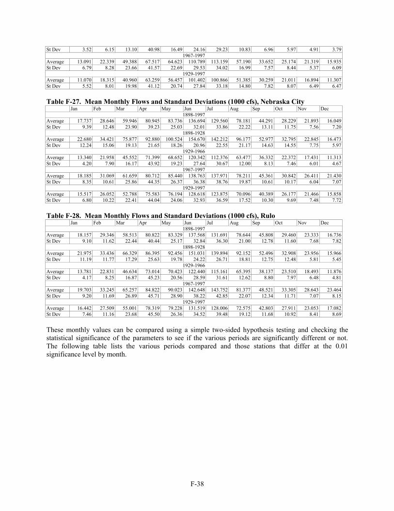
F-38

St Dev 3.52 6.15 13.10 40.98 16.49 24.16 29.23 10.83 6.96 5.97 4.91 3.791967-1997

Average 13.091 22.339 49.388 67.517 64.623 110.789 113.159 57.190 33.652 25.174 21.319 15.935St Dev 6.79 8.28 23.66 41.57 22.69 29.53 34.02 16.99 7.57 8.44 5.37 6.09

1929-1997 Average 11.070 18.315 40.960 63.259 56.457 101.402 100.866 51.385 30.259 21.011 16.894 11.307St Dev 5.52 8.01 19.98 41.12 20.74 27.84 33.18 14.80 7.82 8.07 6.49 6.47 Table F-27. Mean Monthly Flows and Standard Deviations (1000 cfs), Nebraska City


Average 17.737 28.646 59.946 80.945 83.736 136.694 129.560 78.181 44.291 28.229 21.893 16.049St Dev 9.39 12.48 23.90 39.23 25.03 32.01 33.86 22.22 13.11 11.75 7.56 7.20

1898-1928 Average 22.680 34.421 75.877 92.880 100.524 154.670 142.212 96.177 52.977 32.795 22.845 16.473St Dev 12.24 15.06 19.13 21.65 18.26 20.96 22.55 21.17 14.63 14.55 7.75 5.97

1929-1966 Average 13.340 21.958 45.552 71.399 68.652 120.342 112.376 63.477 36.332 22.372 17.431 11.313St Dev 4.20 7.90 16.17 43.92 19.23 27.64 30.67 12.00 8.13 7.46 6.01 4.67

1967-1997 Average 18.185 31.069 61.659 80.712 85.440 138.763 137.971 78.211 45.361 30.842 26.411 21.430St Dev 8.35 10.61 25.86 44.35 26.37 36.38 38.76 19.87 10.61 10.17 6.04 7.07

1929-1997 Average 15.517 26.052 52.788 75.583 76.194 128.618 123.875 70.096 40.389 26.177 21.466 15.858St Dev 6.80 10.22 22.41 44.04 24.06 32.93 36.59 17.52 10.30 9.69 7.48 7.72 Table F-28. Mean Monthly Flows and Standard Deviations (1000 cfs), Rulo


Average 18.157 29.346 58.513 80.822 83.329 137.568 131.691 78.644 45.808 29.460 23.333 16.736St Dev 9.10 11.62 22.44 40.44 25.17 32.84 36.30 21.00 12.78 11.60 7.68 7.82

1898-1928 Average 21.975 33.436 66.329 86.395 92.456 151.031 139.894 92.152 52.496 32.908 23.956 15.966St Dev 11.19 11.77 17.29 25.63 19.78 24.22 26.71 18.81 12.75 12.48 5.81 5.45

1929-1966 Average 13.781 22.831 46.634 73.014 70.423 122.440 115.161 65.395 38.137 23.510 18.493 11.876St Dev 4.17 8.25 16.87 45.23 20.56 28.59 31.61 12.62 8.80 7.97 6.48 4.81

1967-1997 Average 19.703 33.245 65.257 84.822 90.023 142.648 143.752 81.377 48.521 33.305 28.643 23.464St Dev 9.20 11.69 26.89 45.71 28.90 38.22 42.85 22.07 12.34 11.71 7.07 8.15

1929-1997 Average 16.442 27.509 55.001 78.319 79.228 131.519 128.006 72.575 42.803 27.911 23.053 17.082St Dev 7.46 11.16 23.68 45.50 26.36 34.52 39.48 19.12 11.68 10.92 8.41 8.69 These monthly values can be compared using a simple two-sided hypothesis testing and checking the statistical significance of the parameters to see if the various periods are significantly different or not. The following table lists the various periods compared and those stations that differ at the 0.01 significance level by month.

F-39

Table F-29. Stations with Differences Between Monthly Means at 0.01 Significance Level Jan Feb Mar Apr May Jun Jul Aug Sep Oct Nov Dec

1898-1928 vs. 1929-1997 Yankton a a a a a a a a Sioux City a a a a a a a a a Decatur a a a a a a a a a Omaha a a a a a a a a Nebraska City a a a a a a a a a Rulo a a a a a St. Joseph

1898-1928 vs. 1929-1966 Yankton a a a a a a a a a a a Sioux City a a a a a a a a a a a Decatur a a a a a a a a a a a Omaha a a a a a a a a a a a Nebraska City a a a a a a a a a a a a Rulo a a a a a a a a a a a St. Joseph a a a a a a

1898-1928 vs. 1967-1997 Yankton a a a a a a Sioux City a a a a a Decatur a a a a a Omaha a a Nebraska City a a Rulo a a St. Joseph a a a

1929-1966 vs. 1967-1997 Yankton a a a a a a Sioux City a a a a a a a Decatur a a a a a a a Omaha a a a a a a a a a a Nebraska City a a a a a a a a a a Rulo a a a a a a a a a a St. Joseph a a a a a a a a a a A check mark indicates a statistically significant difference between periods compared As can be seen, the mean monthly flows at most stations for most months differ significantly for the periods 1898-1928 and 1929-1997. However, it appears that this difference may be due to the period 1929-1966 being lower. The periods 1898-1928 and 1967-1997 both differ significantly from the period 1929-1966 in most months. It is also interesting to note that most months for the periods 1898-1928 and 1967-1997 do not differ significantly. This further verifies that the flow values for the period 1898-1928 are likely reasonable. One thing to note is that the monthly values for the period 1898-1928 shown above differ from monthly flow values published by the USGS. However, the USGS values were based on rainfall-runoff characteristics of the basin in the late 1930s and early 1940s, and observed differences in the rainfall-runoff characteristics over various periods may account for the differences in the monthly flow volumes derived for this report and those published by the USGS for 1898-1928. REGULATED FLOW The regulated flow data set was developed through use of the Daily Routing Model (DRM), utilizing data sets for discharge, reservoir inflow and outflow, and depletions. The following sections describe the DRM and its inputs. Hydrologic Model Description (DRM) Model Philosophy

F-40

The DRM was not developed for this study; rather, it was developed for use in the Missouri River Master Water Control Manual Update Study to evaluate flood control, interior drainage, and groundwater levels along the Missouri River and navigation contributions to the Mississippi River. The DRM contains 20 nodes including the six mainstem reservoirs and 14 gaging stations – Wolf Point and Culbertson, Montana; Williston and Bismarck, North Dakota; Sioux City, Iowa; Omaha, Nebraska City, and Rulo, Nebraska; and St. Joseph, Kansas City, Waverly, Boonville, and Hermann, Missouri on the Missouri River and St. Louis, Missouri on the Mississippi River. The model utilizes two sets of input data. The first set of input files contains historic reach inflow and streamflow depletion data, and the second contains the various constants and variable parameters that define regulation decisions. The historic data is organized in yearly files that contain daily data for each of the reservoir and gage locations and includes annual evaporation values for the six mainstem reservoirs. Monthly incremental inflow for each node and depletions that adjust historic monthly inflow to current water year uses are also included. Each yearly file contains 14 months of data – December of the previous year through January of the following year. The second set of data contains five files that establish the variables and constants to define the capacity and operational limits of the river and reservoirs and to establish the guide curves and operating limits of a particular run. Program considerations include (1) reductions in historic inflows to reflect current levels of water uses; (2) reductions in reservoir volumes to reflect continued sediment accumulation from the date of the last sediment survey to the date of the study; (3) reductions in tailwater levels due to degradation; (4) reductions in inflow due to reservoir evaporation; (5) factors for determining the amount of tributary inflow that is available for meeting navigation targets; and (6) seasonal flow limits for flood control, navigation, hydropower, water supply, irrigation, endangered species, and evacuation of excess water during high runoff years. Navigation guidelines are based on system storage on March 15 and July 1. Four navigation flow target gages are used: Sioux City, Omaha, Nebraska City, and Kansas City. System storage on March 15 determines whether navigation flows from April 1 to July 1 will be full service or minimum service or some intermediate level (where minimum service is 6000 cfs less than full service). The length of the navigation season is based on the system storage on July 1. Winter release rates are based on system storage on September 1. If system storage drops below 19.6 MAF, navigation will not be supported, so as to prevent system storage from dropping below permanent pool storage of 18 MAF. The model uses a set of flow factors that are applied to incremental inflow between gaging stations to assign the amount of the inflow that is applicable on a monthly basis for navigation purposes, as not all local inflow can be considered usable for navigation. Releases from Oahe, Garrison, and Fort Peck are checked and adjustments made for flood control, environmental, fish reproduction, irrigation, recreation, power, safety, and other considerations. The last check before saving each period’s data is a routine to adjust releases for terns and plovers. After any final release adjustments are made, individual reservoir storages are recomputed, downstream flows are rerouted, and hydropower is adjusted as necessary. The program goes through the same process for each period, and the data is stored in arrays. The data is output to a file after completing the last period of each year. The program halts after processing all of the data or when the system storage limits are exceeded which necessitates adjusting parameters and restarting.

F-41

The DRM also has a supplemental program named ROUTE.EXE. This program is designed for analysis of daily data, but can also be used for graphing monthly data. More detailed information on the background and use of the DRM can be found in USACE (1998). Modifications to DRM The source code for the DRM was not modified for this study. The model does however continue to go through various periods of refinement for the Missouri River Master Water Control Manual Study. Input Data Development Virtually all input data required for the DRM was previously developed for the unregulated flow analysis or developed for previous studies utilizing the DRM. Input data at gaging stations includes incremental reach inflow, observed gage flow data, and incremental reach depletion data. Input for the six mainstem reservoirs includes reservoir inflow, reservoir outflow, incremental reach inflow, evaporation, and storage. The remaining data sets are the rule curves which dictate the operation of the reservoirs given various parameters. Data that was not modified included the rule curves and reservoir data. The gage data and reach inflow developed for the unregulated analysis were put into the DRM input files. Additionally, depletion data developed by the USBR was used for all depletion data in the model.

Current Depletion Estimates The USBR developed estimates of current level depletions for the period 1898-1996. The DRM uses depletion data by adjusting historic flows to present day consumptive water uses. The depletion data input to the DRM is actually the difference between historic and current level depletions. This necessitated a slight adjustment to the depletion data used in the UFDM, as the UFDM modeled the USBR reservoirs that operate for flood control upstream of Sioux City, and hence the depletion data for these reservoirs was taken out of the depletion data used in the UFDM to eliminate duplicity. For the DRM, both the current and historic depletion data sets included all reservoir depletions (exclusive of the six mainstem reservoirs). Tables A-20 to A-35 list the historic and current level depletions used for the DRM. Routing Parameters The DRM uses routing coefficients for routing flows from one gage to the next (i.e. does not include incremental inflows, as they are routed separately). The routing coefficients used in the model had previously been calibrated for the period 1967-1997. Since one of the study assumptions was to use existing conditions, these values were used in this study, and are the same as used for the UFDM regression routing option. The table below lists the coefficients used. Table F-30. Routing Coefficients Used in DRM Model Reach A1 A2 A3 Gavins Point to Sioux City 0.17532 0.53734 0.28734 Sioux City to Omaha 0.16794 0.72176 0.11030 Omaha to Nebraska City 0.58790 0.41210 0.0 Nebraska City to Rulo 0.58837 0.41163 0.0 Rulo to St. Joseph 0.77547 0.22453 0.0 St. Joseph to Kansas City 0.42647 0.44863 0.12490

F-42

Reach A1 A2 A3 Kansas City to Waverly 0.47605 0.52395 0.0 Waverly to Boonville 0.35420 0.61748 0.02832 Boonville to Hermann 0.38146 0.43382 0.18472 Regression routing equation: Qds = Qus(d)*A1 + Qus(d-1)*A2 + Qus(d-2)*A3 Where: Qds = Flow at downstream station Qus = Flow at upstream station d-1 = yesterday, d= today, d+1 = tomorrow, etc. A1, A2, A3 = regression routing coefficients Model Calibration/Verification The output for the DRM can be compared to observed data for a relatively good check on the validity of model results. The mainstem reservoir system reached operational volume in 1967, so results from 1968 to 1997 can be compared to see how well the model reproduces the observed hydrograph. The Table F-31 below compares the observed and modeled annual peaks at each of the stations within Omaha District. As can be seen, some modeled peaks are higher, while some modeled peaks are lower. Table F-31. Comparison of Simulated and Observed Peak Regulated Flows.

Observed Daily Mean Max-Calendar Simulated Daily Mean Max-calendar Year

Yankton Sioux City Omaha Nebraska City

Rulo Yankton Sioux City Omaha Nebraska City

Rulo

1968 38400 38300 47000 62600 71500 41200 40200 48200 64800 73300

1969 55700 76400 99500 103000 106000 58700 77100 99400 103300 103400

1970 46100 45600 47200 57300 62000 56300 53900 53900 56800 55900

1971 54500 69800 79700 112000 125000 55000 72000 80600 125000 131800

1972 51200 54100 66800 80800 91300 52400 57100 69400 81000 89000

1973 33800 40900 52400 82200 122000 42100 41300 45500 82500 121200

1974 37400 40000 47900 75000 87800 39400 39300 46500 72600 86100

1975 63400 66200 73900 76700 81800 61500 62000 66300 71100 82300

1976 41700 41100 47000 61600 69100 50300 53000 52700 60800 65800

1977 36700 37800 43900 58600 77700 34500 36100 42400 54300 71000

1978 53500 61200 81200 154000 160000 60500 67100 86100 154100 164300

1979 43900 50100 82800 114000 135000 44400 55900 80300 109400 135100

1980 38500 42000 47000 64300 73600 35500 40300 47400 64400 72700

1981 36300 37000 47200 57400 56100 38100 36200 46300 56800 55200

1982 44600 49900 58000 97500 121000 56800 62800 72100 99200 124700

1983 39100 44000 80500 119000 121000 48100 57100 93800 136100 139200

1984 47800 103000 114000 180000 216000 48300 116300 125800 198200 231000

1985 41200 49500 68800 79100 85600 34500 46200 65000 75900 81500

1986 50300 56600 76300 99700 128000 64000 69400 88900 124100 150100

1987 34400 46600 58800 119000 140000 40100 39500 52800 109800 129700

1988 38900 38400 42200 48100 50700 36000 36500 41700 48200 51200

1989 32700 33500 44500 81600 114000 32200 32600 40600 78400 110400

1990 33400 36700 71700 114000 118000 31500 33600 72300 111800 116300

1991 32100 32600 74100 89200 94600 33000 35200 76800 91500 99100

1992 29100 37100 52500 54700 79800 31500 41800 51300 59300 120300

1993 24300 71300 113000 188000 289000 31500 89300 120500 201200 299500

1994 32400 49200 62100 86600 90400 34500 45700 53900 79900 85200

F-43

Observed Daily Mean Max-Calendar Simulated Daily Mean Max-calendar Year

Yankton Sioux City Omaha Nebraska City

Rulo Yankton Sioux City Omaha Nebraska City

Rulo

1995 56100 65300 80300 108000 118000 65000 95500 109400 136700 148500

1996 55000 79900 116000 139000 146000 57300 96800 137100 136000 137600

1997 70100 97400 108000 113000 121000 70000 106000 109500 114600 121000

Table F-32 shows the average difference between simulated and observed annual peaks, as well as the standard deviation of those annual differences. As can be seen, the modeled peaks are a few thousand cfs higher on average. However, for the highest flow year (1997), the simulated and observed peaks are nearly identical. Table F-32. Average Annual Difference Between Simulated and Observed Peak Regulated Flows.

Yankton Sioux City

Omaha Nebraska City

Rulo

Average 3053 4810 3073 2727 3347St. Dev. 4963 8342 8530 9176 11505 Some difference can be expected between observed and simulated, as the actual and current level of depletion differ somewhat; therefore it should be expected that the simulated values are slightly higher than the observed. Another way to compare the accuracy of the computer simulation is to compare observed and computed system storage in the mainstem reservoirs. A table of computed and observed end-of-month storage is shown in Table FA-37. The mainstem reservoir system reached operating capacity in 1967, so a graph showing end of month storage as observed and as computed by the DRM was plotted and is shown in Figure F-1. As can be seen, there is sometimes a significant difference between observed and computed until the mid-1980s. However, most of this difference is due to depletions. If the difference between computed and observed end-of-month storage is plotted, it can be shown that the difference between computed and observed decreases by about 117,000 acre-feet per year. If the differences between observed and current level depletions are compared, it can be seen that depletions increased on average by about 82,000 acre-feet per year from 1967 through the 1990s. This indicates that about 70% of the difference between observed and computed end-of-month storage is due to increasing depletions throughout the upper basin. There have also been some minor differences in reservoir operation over the years. The monthly computed storage trends do track the trends in observed, so that indicates that the model is doing a good job of modeling reservoir operation over the period of record. The final check of model validity is to compare the computed daily discharge versus observed daily discharge at Gavins Point. As pointed out above, some difference in discharge can be expected due to differences between actual and current level depletions. Daily observed and computed releases are available electronically. In several years, however, there are significant differences at various times of the year. Most often this is due to the model being unable to more accurately forecast future inflows in order to step up or step down releases.

F-44

Figure F-1. Observed and Computed End of Month Mainstem Storage, 1967-1997 Period of Record Simulation Once all input data was compiled, the model was run, covering the period of January 1, 1898 to December 31, 1997. Annual peaks were extracted from the output data and are compiled in Table FA-19. Sensitivity Analysis To see the model’s sensitivity to depletion data, a comparison can be made between the results of this study and of that done by the RCC. All input data should be the same, except for some slight differences in depletion data. Table F-33 compares the results for the simulated Gavins Point peak outflow. As can be seen, there is little difference in most years, but in other years there can be a difference in excess of 10000 cfs. This shows that the model can be sensitive to depletion input. Presumably, the model would be equally sensitive to differences in input for observed flows at each gage or inflows to the mainstem reservoirs. As the simulations were continuous over the period of record, it is also possible that differences in storage carrying over from one year to the next may cause the model to hit a threshold for larger releases, thereby causing one data set to be higher than the other. This does point out that great care must be taken in using this model and interpreting its results. Table F-33. Comparison of Simulated Annual Peaks with Different Depletion Data. Year RCC NWO Year RCC NWO Year RCC NWO Year RCC NWO

1898 61000 60500 1923 61850 62000 1948 45550 40800 1973 35770 42100

1899 61500 60000 1924 48720 61000 1949 40790 41200 1974 37120 39400

1900 34500 48300 1925 46820 56700 1950 60260 52800 1975 61390 61500

1901 40080 59500 1926 40780 36800 1951 59690 59700 1976 40540 50300

1902 34500 47200 1927 66500 65500 1952 65000 70800 1977 34500 34500

1903 36130 53800 1928 58430 66500 1953 41220 49300 1978 65000 60500

Observed and Computed End of Month Mainstem Storage, 1967-1997

40000

45000

50000

55000

60000

65000

70000

75000

Jan-67 Jul-72 Jan-78 Jul-83 Dec-88 Jun-94 Dec-99Date

Stor

age,

K-A

cre-

feet

Observed End of MonthMainstem StorageComputed End of MonthM i t St

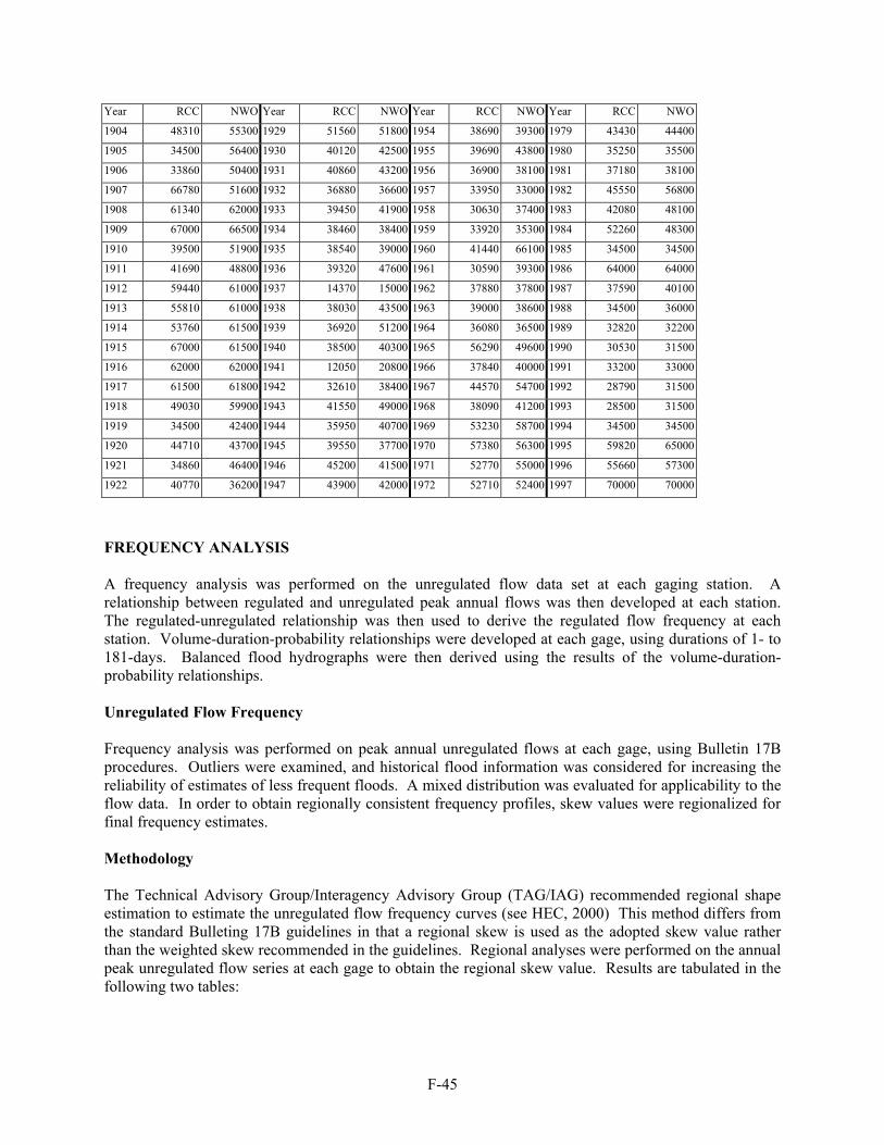
F-45

Year RCC NWO Year RCC NWO Year RCC NWO Year RCC NWO

1904 48310 55300 1929 51560 51800 1954 38690 39300 1979 43430 44400

1905 34500 56400 1930 40120 42500 1955 39690 43800 1980 35250 35500

1906 33860 50400 1931 40860 43200 1956 36900 38100 1981 37180 38100

1907 66780 51600 1932 36880 36600 1957 33950 33000 1982 45550 56800

1908 61340 62000 1933 39450 41900 1958 30630 37400 1983 42080 48100

1909 67000 66500 1934 38460 38400 1959 33920 35300 1984 52260 48300

1910 39500 51900 1935 38540 39000 1960 41440 66100 1985 34500 34500

1911 41690 48800 1936 39320 47600 1961 30590 39300 1986 64000 64000

1912 59440 61000 1937 14370 15000 1962 37880 37800 1987 37590 40100

1913 55810 61000 1938 38030 43500 1963 39000 38600 1988 34500 36000

1914 53760 61500 1939 36920 51200 1964 36080 36500 1989 32820 32200

1915 67000 61500 1940 38500 40300 1965 56290 49600 1990 30530 31500

1916 62000 62000 1941 12050 20800 1966 37840 40000 1991 33200 33000

1917 61500 61800 1942 32610 38400 1967 44570 54700 1992 28790 31500

1918 49030 59900 1943 41550 49000 1968 38090 41200 1993 28500 31500

1919 34500 42400 1944 35950 40700 1969 53230 58700 1994 34500 34500

1920 44710 43700 1945 39550 37700 1970 57380 56300 1995 59820 65000

1921 34860 46400 1946 45200 41500 1971 52770 55000 1996 55660 57300

1922 40770 36200 1947 43900 42000 1972 52710 52400 1997 70000 70000

FREQUENCY ANALYSIS A frequency analysis was performed on the unregulated flow data set at each gaging station. A relationship between regulated and unregulated peak annual flows was then developed at each station. The regulated-unregulated relationship was then used to derive the regulated flow frequency at each station. Volume-duration-probability relationships were developed at each gage, using durations of 1- to 181-days. Balanced flood hydrographs were then derived using the results of the volume-duration-probability relationships. Unregulated Flow Frequency Frequency analysis was performed on peak annual unregulated flows at each gage, using Bulletin 17B procedures. Outliers were examined, and historical flood information was considered for increasing the reliability of estimates of less frequent floods. A mixed distribution was evaluated for applicability to the flow data. In order to obtain regionally consistent frequency profiles, skew values were regionalized for final frequency estimates. Methodology The Technical Advisory Group/Interagency Advisory Group (TAG/IAG) recommended regional shape estimation to estimate the unregulated flow frequency curves (see HEC, 2000) This method differs from the standard Bulleting 17B guidelines in that a regional skew is used as the adopted skew value rather than the weighted skew recommended in the guidelines. Regional analyses were performed on the annual peak unregulated flow series at each gage to obtain the regional skew value. Results are tabulated in the following two tables:

F-46

Table F-34. Statistics of log-flows of Gages Above the Kansas River Location Drainage Area, sq.

mi. Mean Standard

Deviation Computed Skew

Yankton 279500 5.2026 0.1372 0.0552 Sioux City 314580 5.2120 0.1323 -0.0244 Decatur 316200 5.2132 0.1312 -0.0575 Omaha 322800 5.2302 0.1329 -0.0661 Nebraska City 410000 5.3203 0.1177 -0.0474 Rulo 414900 5.3266 0.1220 -0.0532 St. Joseph 420300 5.3398 0.1218 0.0670 Table F-35. Unregulated Flow Frequency Relations for Annual Series of Gages in Omaha District. Exceedanc

e Probability

Yankton Sioux City Decatur Omaha Nebraska City

Rulo

0.002 400000 386000 381000 399000 448000 467000 0.005 363000 354000 349000 366000 414000 431000 0.01 335000 328000 325000 341000 388000 403000 0.02 307000 303000 301000 315000 362000 374000 0.05 269000 268000 267000 279000 325000 335000

0.1 239000 240000 240000 251000 295000 304000 0.2 208000 211000 211000 220000 263000 269000 0.5 159000 163000 164000 171000 210000 213000 0.8 122000 126000 127000 131000 167000 168000 0.9 106000 110000 111000 115000 147000 148000

0.95 95100 98400 98900 102000 133000 133000 0.99 77000 79500 79800 82000 110000 109000

Historical Flood Information

For all the gages upstream of the Kansas River, the 1952 flood was the highest of record since the 1881 flood. According to estimates of the peak flow at Omaha, the 1881 flood would be the 2nd largest flood of the unregulated flow series, if the period of record were extended. There were notations in some of the early stage record books that indicated that the 1844 flood at Omaha was 10 feet higher than the 1881 flood. However, further study found no credible evidence to support this, and a considerable amount of evidence to refute it. A consensus was reached among all Districts to not use historic floods to extend the period of record, as study area land use conditions become much more different as one goes back further than 1898. Outliers

The 1952 flood is identified as a high outlier by the Bulletin 17B outlier test at all gages upstream of the Kansas River for an annual series analysis. Flow records are considered quite reliable for the 1952 flood, so it is unlikely that the observed flow data is greatly in error. As the flood occurred in the early spring, there are not many depletions or holdouts to drastically affect the computed peak discharge either. The 1881 flood could be added to the period of record, but it would not keep the 1952 flood from being

F-47

considered a high outlier. Further analyses would show that the snowmelt season and rainfall season events have different distributions, and should therefore be treated as a mixed population. Mixed Population Analysis Downstream of Yankton, South Dakota, the Missouri River has historically been subject to two main annual flood events: a spring plains snowmelt period, and a summer mountain snowmelt and plains rainfall period. Each series of floods was examined to see if they were significantly different and if the two flood periods could be combined to better describe the flow frequency at each gage. For purposes of analysis, the calendar year was divided into two seasons: spring (January 1 - April 30) and summer (May 1 - December 31). Virtually all plains snowmelt-related floods occur from mid-March through late-April, while all other floods occur from mid-May through late-July. First, the top 10 floods in the annual series at each gage were examined to see if they were spring or summer floods. The following table lists the top 10 floods at each gage and notes whether a spring or summer event. Table F-36. Top 10 Annual Flood Events at Each Gage and Season of Occurrence.

Rank Yankton Sioux City Decatur Omaha Nebraska

City Rulo St Joseph 1 1952 – S1 1952 - S 1952 – S 1952 – S 1952 – S 1952 – S 1952 – S 2 1943 – S 1997 – S 1997 – S 1997 – S 1960 – S 1993 – R 1993 – R 3 1953 – R2 1978 – S 1978 – S 1978 – S 1993 – R 1960 – S 1960 – S 4 1978 – S 1953 – R 1953 – R 1960 – S 1967 – R 1984 – R 1903 – R 5 1950 - S 1960 – S 1960 – S 1953 – R 1978 – S 1978 – S 1978 – S 6 1899 - S 1899 – S 1899 – S 1967 - R 1984 – R 1967 – R 1984 – R 7 1905 - R 1950 – S 1967 – R 1972 – S 1996 – R 1996 – R 1967 – R 8 1997 – S 1972 – S 1972 – S 1899 - S 1997 – S 1997 – S 1996 – R 9 1972 – S 1967 – R 1950 - S 1984 – R 1921 - R 1965 – R 1917 - R 10 1967 - R 1905 - R 1964 - R 1964 – R 1944 - R 1983 - R 1965 - R 1 S=Plains snowmelt flood 2 R=Summer rainfall/mountain snowmelt flood As can be seen, the majority of large floods above the Platte River result from plains snowmelt floods, while between the Platte and Kansas Rivers, plains snowmelt floods are in the minority of top 10 floods, but constitute the majority of top 5 floods. Overall, plains snowmelt floods account for 16 of the top 25 annual and only 24 of the 100 annual peak floods at Yankton and 7 of the top 25 annual and only 16 of the 100 annual peak floods at St. Joseph. This suggests that plains snowmelt floods have an impact on the larger floods, and the impact decreases as one moves downstream, until the impact is negligible downstream of the Kansas River. USACE (1993) suggests the use of mixed population analysis when there are two or more different, but independent, causative conditions, as exists on the upper Missouri basin. The plains snowmelt and mountain snowmelt can be considered independent of each other, or very nearly so, as plains snowpack typically peaks from February to late-March, and is non-existent by the end of April, while the mountain snowpack typically continues to accumulate until mid-May or later. Rainfall sometimes augments a plains snowmelt and sometimes a very late snowfall may occur in May over much of the upper basin. However, runoff characteristics differ greatly from early spring to late spring, with mostly frozen soil

F-48

early in the spring resulting in much greater runoff than occurs later in the spring from the same volume of precipitation. USACE (1993) prescribes that the frequency relation of each population be derived by analytical techniques and then combined to yield the mixed population frequency curve. The individual populations are combined by “probability of union,” with the equation: Pc = P1 + P2 – P1*P2 where: Pc = Annual exceedance probability of combined populations for a selected magnitude P1 = Annual exceedance probability of same selected magnitude for population series 1 P2 = Annual exceedance probability of same sleected magnitude for population series 2 The largest flood event from the January-April and May-December time frame for each year was determined from the unregulated flow data set at each gage and examined to make sure each was either a plains snowmelt or mountain snowmelt/plains rainfall event per the time frame. In only a couple years did it appear that the plains snowmelt lasted into May, but the difference between late April and early May peaks was nominal, so the January-April data was not changed. In those years that snowmelt may have persisted into May, either a later peak surpassed it in magnitude, or the difference between later peaks was nominal (less than 10% difference), so the May-December data was not changed either. In no case did the floods in question rank in the top half of either population, so the impacts on computed frequency may be considered insignificant. The following statistics were derived from the analysis of each population at each gage: Table F-37. Seasonal Statistics of log-flows of Gages Above the Kansas River Location (1) (2) (3) (4) (5) (6) Yankton 5.000 0.256 -0.003 5.162 0.123 -0.416 Sioux City 5.014 0.249 -0.085 5.171 0.119 -0.475 Decatur 5.012 0.246 -0.067 5.173 0.119 -0.472 Omaha 5.031 0.243 -0.046 5.190 0.121 -0.344 Nebraska City

5.083 0.221 0.008 5.298 0.111 -0.183

Rulo 5.084 0.218 0.120 5.306 0.116 -0.092 St. Joseph 5.101 0.214 0.172 5.320 0.118 0.032 (1) Mean of annual max 1-day log-flows (January-April) (2) Standard deviation of annual max 1-day log-flows (January-April) (3) Skew of annual max 1-day log-flows (January-April) (4) Mean of annual max 1-day log-flows (May-December) (5) Standard deviation of annual max 1-day log-flows (May-December) (6) Skew of annual max 1-day log-flows (May-December) The above results in the following frequency relation at each gage for spring and summer populations, as well as the mixed distribution frequency relation.

F-49

Table F-38. At-Station Frequency Relations for Spring and Summer Populations and Mixed Distribution, Yankton to Omaha

Yankton Sioux City Decatur Omaha (1) (2) (3 (4) (2) (3 (4) (2) (3 (4) (2) (3 (4)

99 25000 69000 81000 26000 71000 83000 26000 71000 84000 29000 76000 87000 95 38000 89000 100000 40000 91000 103000 40000 92000 104000 43000 96000 108000 90 47000 100000 112000 49000 103000 115000 49000 104000 116000 52000 108000 120000 80 61000 115000 127000 64000 119000 131000 64000 119000 131000 67000 123000 136000 50 100000 148000 162000 104000 152000 165000 104000 153000 166000 107000 157000 172000 20 164000 185000 206000 168000 188000 207000 166000 189000 207000 172000 197000 217000 10 213000 206000 235000 214000 207000 235000 211000 208000 234000 219000 219000 247000

5 264000 224000 274000 261000 223000 270000 257000 224000 269000 269000 239000 283000 2 336000 244000 335000 325000 242000 327000 319000 243000 322000 338000 262000 335000 1 395000 258000 394000 375000 254000 378000 369000 255000 373000 393000 279000 387000

0.5 457000 271000 462000 428000 265000 438000 420000 266000 432000 452000 294000 449000 0.2 547000 287000 544000 501000 278000 507000 491000 279000 501000 535000 313000 521000

(1) Percent Chance Exceedance (2) Spring Frequency Relation (3) Summer Frequency Relation (4) Mixed Distribution Relation Table F-39. At-Station Frequency Relations for Spring and Summer Populations and Mixed Distribution, Nebraska City to St. Joseph

Nebraska City Rulo St. Joseph (1) (2) (3 (4) (2) (3 (4) (2) (3 (4)

99 37000 106000 116000 39000 107000 116000 43000 111000 121000 95 53000 129000 138000 54000 129000 139000 58000 134000 143000 90 63000 143000 152000 64000 143000 153000 68000 148000 157000 80 79000 161000 170000 79000 162000 171000 83000 166000 176000 50 121000 200000 211000 120000 203000 214000 124000 209000 220000 20 186000 247000 260000 185000 253000 267000 190000 263000 277000 10 232000 274000 292000 232000 284000 301000 239000 296000 315000

5 279000 298000 325000 281000 311000 338000 291000 327000 355000 2 344000 326000 366000 349000 345000 383000 365000 365000 405000 1 395000 346000 406000 405000 369000 425000 426000 393000 449000

0.5 448000 365000 458000 463000 392000 481000 492000 420000 505000 0.2 523000 389000 527000 547000 422000 553000 587000 456000 578000

(1) Percent Chance Exceedance (2) Spring Frequency Relation (3) Summer Frequency Relation (4) Mixed Distribution Relation Regionalization of Statistics In order to obtain regionally consistent frequency curves at each gage, it is necessary to regionalize the results of the flow frequency analysis. However, there is no guidance for regionalizing computed flow statistics in a mixed distribution, other than USACE (1993) stating, “If annual flood peaks have been separated by causative factors, a generalized skew must be derived for each separate series to apply the log-Pearson Type III distribution as recommended by Bulletin 17B.” An examination of the station statistics, as shown in Table F-37, shows that there appears to be a flood regime change in computed values between Omaha and Nebraska City (see HEC, 2000). Therefore, it was decided to regionalize skew for the gages above the Platte River and for those between the Platte and Kansas Rivers. The following table shows the computed skew at each station, and the average skew for each region, by season.

F-50

Table F-40. Statistics for Regional Flow Frequency Analysis (1) (2) (3) (4) (5) (6)

Yankton 4.9999 0.256 -0.003 5.1624 0.123 -0.416 Sioux City 5.0142 0.249 -0.085 5.1712 0.119 -0.476 Decatur 5.0118 0.246 -0.067 5.1735 0.119 -0.472 Omaha 5.0306 0.243 -0.046 5.1905 0.121 -0.345

Region Average -0.050 -0.427 Nebraska City 5.0830 0.221 0.008 5.2982 0.111 -0.183 Rulo 5.0840 0.223 0.096 5.3057 0.117 -0.100 St. Joseph 5.1013 0.225 0.126 5.3200 0.121 0.013 Region Average 0.077 -0.090 (1) Log-mean of spring instantaneous peaks (2) Standard deviation of spring 1-day means (3) Computed skew of spring 1-day means (4) Log-mean of summer instantaneous peaks (5) Standard deviation of summer 1-day means (6) Computed skew of summer 1-day means Use of the above regional skew values results in the following frequency relationships at each gage (Tables F-41 to F-42). Table F-41. Regional Frequency Relations for Spring and Summer Populations and Mixed Distribution, Yankton to Omaha

Yankton Sioux City Decatur Omaha (4) (1) (2) (3) (1) (2) (3) (1) (2) (3) (1) (2) (3)

99 24800 68900 80500 26600 72000 83700 27000 72400 84000 28600 74300 86800 95 37600 88300 100100 39900 91600 103400 40200 92000 103700 42500 94900 107400 90 46800 100000 111800 49400 103000 115200 49600 104000 115600 52300 107000 119700 80 61000 115000 127600 63800 119000 130800 63900 119000 131100 67200 123000 136200 50 100000 148000 162200 104000 151000 165100 103000 152000 165300 108000 158000 172100 20 164000 185000 205300 168000 187000 207500 166000 188000 207400 172000 197000 216200 10 212000 206000 234600 215000 208000 236300 212000 208000 235300 219000 218000 245200

5 261000 223000 272100 263000 225000 273200 259000 226000 270100 267000 236000 280200 2 330000 243000 330300 330000 244000 330200 324000 245000 324400 334000 257000 334400 1 386000 257000 385600 384000 257000 383800 376000 258000 376000 387000 271000 387000

0.5 444000 269000 450000 440000 269000 446000 431000 270000 436100 442000 284000 447700 0.2 526000 284000 526400 519000 284000 519500 507000 285000 507100 520000 300000 519600

(1) Spring Frequency Relation (2) Summer Frequency Relation (3) Mixed Distribution Relation (4) Percent Chance Exceedance Table F-42. Regional Frequency Relations for Spring and Summer Populations and Mixed Distribution, Nebraska City to St. Joseph

Nebraska City Rulo St. Joseph (4) (1) (2) (3) (1) (2) (3) (1) (2) (3)

99 38100 108000 116700 38200 106000 115700 38900 107000 117800 95 53000 130000 138700 53100 129000 138600 54400 131000 141800 90 63300 143000 152000 63500 143000 152600 65300 146000 156500 80 78700 160000 169800 78900 161000 171400 81400 165000 176400 50 120000 199000 210100 121000 203000 214200 125000 210000 222000 20 185000 247000 260900 186000 254000 268400 195000 264000 280100 10 233000 275000 293900 234000 285000 303000 246000 298000 317500

5 283000 300000 329100 283000 313000 340400 299000 328000 357700 2 352000 332000 374100 352000 347000 386200 374000 365000 406900 1 407000 354000 417600 408000 372000 429300 434000 392000 452800

0.5 466000 375000 473600 467000 396000 485200 498000 418000 511700 0.2 549000 403000 548700 551000 427000 557900 588000 452000 588400

(1) Spring Frequency Relation

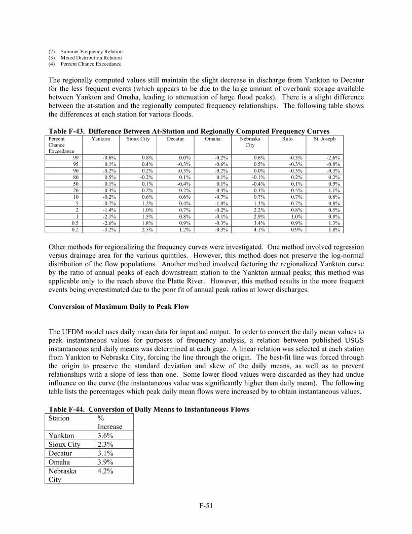
F-51

(2) Summer Frequency Relation (3) Mixed Distribution Relation (4) Percent Chance Exceedance The regionally computed values still maintain the slight decrease in discharge from Yankton to Decatur for the less frequent events (which appears to be due to the large amount of overbank storage available between Yankton and Omaha, leading to attenuation of large flood peaks). There is a slight difference between the at-station and the regionally computed frequency relationships. The following table shows the differences at each station for various floods. Table F-43. Difference Between At-Station and Regionally Computed Frequency Curves Percent Chance Exceedance

Yankton Sioux City Decatur Omaha Nebraska City

Rulo St. Joseph

99 -0.6% 0.8% 0.0% -0.2% 0.6% -0.3% -2.6% 95 0.1% 0.4% -0.3% -0.6% 0.5% -0.3% -0.8% 90 -0.2% 0.2% -0.3% -0.2% 0.0% -0.3% -0.3% 80 0.5% -0.2% 0.1% 0.1% -0.1% 0.2% 0.2% 50 0.1% 0.1% -0.4% 0.1% -0.4% 0.1% 0.9% 20 -0.3% 0.2% 0.2% -0.4% 0.3% 0.5% 1.1% 10 -0.2% 0.6% 0.6% -0.7% 0.7% 0.7% 0.8%

5 -0.7% 1.2% 0.4% -1.0% 1.3% 0.7% 0.8% 2 -1.4% 1.0% 0.7% -0.2% 2.2% 0.8% 0.5% 1 -2.1% 1.5% 0.8% -0.1% 2.9% 1.0% 0.8%

0.5 -2.6% 1.8% 0.9% -0.3% 3.4% 0.9% 1.3% 0.2 -3.2% 2.5% 1.2% -0.3% 4.1% 0.9% 1.8%

Other methods for regionalizing the frequency curves were investigated. One method involved regression versus drainage area for the various quintiles. However, this method does not preserve the log-normal distribution of the flow populations. Another method involved factoring the regionalized Yankton curve by the ratio of annual peaks of each downstream station to the Yankton annual peaks; this method was applicable only to the reach above the Platte River. However, this method results in the more frequent events being overestimated due to the poor fit of annual peak ratios at lower discharges. Conversion of Maximum Daily to Peak Flow

The UFDM model uses daily mean data for input and output. In order to convert the daily mean values to peak instantaneous values for purposes of frequency analysis, a relation between published USGS instantaneous and daily means was determined at each gage. A linear relation was selected at each station from Yankton to Nebraska City, forcing the line through the origin. The best-fit line was forced through the origin to preserve the standard deviation and skew of the daily means, as well as to prevent relationships with a slope of less than one. Some lower flood values were discarded as they had undue influence on the curve (the instantaneous value was significantly higher than daily mean). The following table lists the percentages which peak daily mean flows were increased by to obtain instantaneous values. Table F-44. Conversion of Daily Means to Instantaneous Flows Station %

Increase Yankton 3.6% Sioux City 2.3% Decatur 3.1% Omaha 3.9% Nebraska City

4.2%

F-52

Unregulated Flow Frequency Profiles Flow frequency profiles were developed to determine the various flood frequency relationships at points intermediate to the gaging stations. Values were determined by linearly interpolating between gages based on drainage area. Subsequent analysis determined that drainage area may not be suitable for flow distribution upstream of Sioux City. Refer to the cross section flow frequency section for further information. The following table lists the flow frequency relationships at various points along the Missouri River mainstem from Yankton to St. Joseph. Table F-45. Unregulated Flow Frequency Profiles *

Exceedance Probability

Location

1960 River Mile

Drainage Area, sq mi 99 95 90 80 50 20 10 5 2 1 0.5 0.2

Gavins Point Dam 811.1 279400 80500 100100 111800 127600 162200 205300 234600 272100 330300 385600 450000 526400

Yankton, SD 805.8 279500 80500 100100 111800 127600 162200 205300 234600 272100 330300 385600 450000 526400

279600 80500 100100 111800 127600 162200 205300 234600 272100 330300 385600 450000 526400James River 797.7 301700 82500 102200 114000 129600 164000 206700 235700 272800 330200 384500 447500 522000

302295 82600 102200 114000 129700 164100 206700 235700 272800 330200 384400 447400 521900Vermillion River 771.9 304480 82800 102400 114200 129900 164300 206900 235800 272900 330200 384300 447200 521500

305110 82800 102500 114300 129900 164300 206900 235800 272900 330200 384300 447100 521400Big Sioux River 734.0 314680 83700 103400 115200 130800 165100 207500 236300 273200 330200 383800 446000 519500

Sioux City, IA 732.3 314600 83700 103400 115200 130800 165100 207500 236300 273200 330200 383800 446000 519500

314620 83700 103400 115200 130800 165100 207500 236300 273200 330100 383700 445900 519300Floyd River 731.3 315541 83900 103600 115400 131000 165200 207400 235700 271400 326800 379200 440200 512200

Decatur, NE 691.0 316200 84000 103700 115600 131100 165300 207400 235300 270100 324400 376000 436100 507100

316370 84100 103800 115700 131200 165500 207600 235600 270400 324700 376300 436400 507400Little Sioux River 669.2 320877 86000 106300 118500 134700 170100 213600 242300 277300 331500 383600 444300 516000

320900 86000 106300 118500 134700 170100 213700 242400 277300 331500 383600 444400 516000Soldier River 664.0 321345 86200 106600 118800 135100 170600 214300 243000 278000 332200 384300 445100 516800

321500 86200 106700 118900 135200 170800 214500 243300 278200 332400 384600 445400 517100Boyer River 635.2 322688 86800 107300 119600 136100 172000 216100 245000 280000 334200 386500 447500 519400

Omaha, NE 615.9 322800 86800 107400 119700 136200 172100 216200 245200 280200 334400 386700 447700 519600

323530 87000 107700 120000 136500 172400 216600 245600 280600 334700 387000 447900 519800Platte River 594.8 410020 116600 138600 151900 169700 209900 260700 293700 328900 373900 417500 473500 548600

Nebraska City, NE 562.6 410400 116700 138700 152000 169800 210100 260900 293900 329100 374100 417600 473600 548700

410530 116700 138700 152000 169800 210200 261100 294200 329400 374400 417900 473900 549000Nishnabotna River 542.1 413525 116000 138600 152400 170900 212900 266100 300200 336900 382500 425700 481700 555100

413525 116000 138600 152400 170900 212900 266100 300200 336900 382500 425700 481700 555100Little Nemaha 527.8 414366 115800 138600 152500 171200 213700 267500 301900 339100 384800 427900 483800 556800

414366 115800 138600 152500 171200 213700 267500 301900 339100 384800 427900 483800 556800Tarkio River 507.6 414900 115700 138600 152600 171400 214200 268400 303000 340400 386200 429300 485200 557900

Rulo, NE 498.0 414900 115700 138600 152600 171400 214200 268400 303000 340400 386200 429300 485200 557900

* Drainage area distribution method was revised upstream of Sioux City as described in the cross section flow frequency section of the hydraulic analysis. Regulated-Unregulated Relationships Frequency analysis of a regulated data set is not done by normal analytical methods. In order to determine an accurate regulated frequency relationship, it is necessary to determine the unregulated

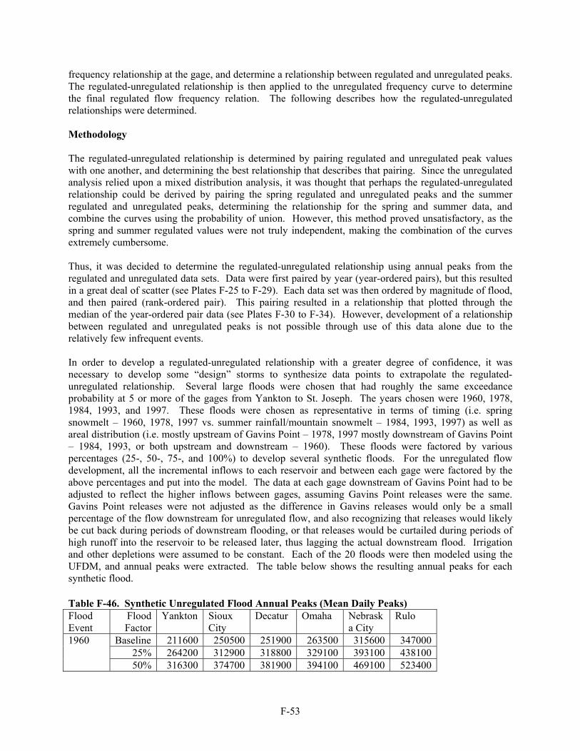
F-53

frequency relationship at the gage, and determine a relationship between regulated and unregulated peaks. The regulated-unregulated relationship is then applied to the unregulated frequency curve to determine the final regulated flow frequency relation. The following describes how the regulated-unregulated relationships were determined. Methodology The regulated-unregulated relationship is determined by pairing regulated and unregulated peak values with one another, and determining the best relationship that describes that pairing. Since the unregulated analysis relied upon a mixed distribution analysis, it was thought that perhaps the regulated-unregulated relationship could be derived by pairing the spring regulated and unregulated peaks and the summer regulated and unregulated peaks, determining the relationship for the spring and summer data, and combine the curves using the probability of union. However, this method proved unsatisfactory, as the spring and summer regulated values were not truly independent, making the combination of the curves extremely cumbersome. Thus, it was decided to determine the regulated-unregulated relationship using annual peaks from the regulated and unregulated data sets. Data were first paired by year (year-ordered pairs), but this resulted in a great deal of scatter (see Plates F-25 to F-29). Each data set was then ordered by magnitude of flood, and then paired (rank-ordered pair). This pairing resulted in a relationship that plotted through the median of the year-ordered pair data (see Plates F-30 to F-34). However, development of a relationship between regulated and unregulated peaks is not possible through use of this data alone due to the relatively few infrequent events. In order to develop a regulated-unregulated relationship with a greater degree of confidence, it was necessary to develop some “design” storms to synthesize data points to extrapolate the regulated-unregulated relationship. Several large floods were chosen that had roughly the same exceedance probability at 5 or more of the gages from Yankton to St. Joseph. The years chosen were 1960, 1978, 1984, 1993, and 1997. These floods were chosen as representative in terms of timing (i.e. spring snowmelt – 1960, 1978, 1997 vs. summer rainfall/mountain snowmelt – 1984, 1993, 1997) as well as areal distribution (i.e. mostly upstream of Gavins Point – 1978, 1997 mostly downstream of Gavins Point – 1984, 1993, or both upstream and downstream – 1960). These floods were factored by various percentages (25-, 50-, 75-, and 100%) to develop several synthetic floods. For the unregulated flow development, all the incremental inflows to each reservoir and between each gage were factored by the above percentages and put into the model. The data at each gage downstream of Gavins Point had to be adjusted to reflect the higher inflows between gages, assuming Gavins Point releases were the same. Gavins Point releases were not adjusted as the difference in Gavins releases would only be a small percentage of the flow downstream for unregulated flow, and also recognizing that releases would likely be cut back during periods of downstream flooding, or that releases would be curtailed during periods of high runoff into the reservoir to be released later, thus lagging the actual downstream flood. Irrigation and other depletions were assumed to be constant. Each of the 20 floods were then modeled using the UFDM, and annual peaks were extracted. The table below shows the resulting annual peaks for each synthetic flood. Table F-46. Synthetic Unregulated Flood Annual Peaks (Mean Daily Peaks) Flood Event

Flood Factor

Yankton Sioux City

Decatur Omaha Nebraska City

Rulo

Baseline 211600 250500 251900 263500 315600 347000 25% 264200 312900 318800 329100 393100 438100

1960

50% 316300 374700 381900 394100 469100 523400

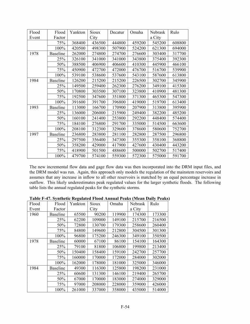
F-54

Flood Event

Flood Factor

Yankton Sioux City

Decatur Omaha Nebraska City

Rulo

75% 368400 436500 444800 459200 545200 608800 100% 420500 498300 507900 524200 621300 694000

Baseline 262000 274800 274700 276600 303400 317700 25% 326100 341000 341000 343800 375400 392300 50% 388500 406900 406600 410300 445900 466100 75% 450900 472700 472000 476700 516700 539900

1978

100% 539100 538600 537600 543100 587600 613800 Baseline 126200 215200 215200 226500 302700 345900

25% 149500 259400 262300 276200 349100 415300 50% 170800 303500 307100 323800 410900 481300 75% 192500 347600 351800 371300 465300 547300

1984

100% 391600 391700 396800 419000 519700 613400 Baseline 113000 166700 170900 207900 313800 395900

25% 136000 206000 215900 249400 382200 485200 50% 160100 241400 253800 292200 448400 574400 75% 184100 276800 291700 335000 514500 663600

1993

100% 208100 312300 329600 378600 580600 752700 Baseline 236800 283800 281100 282800 287500 296800

25% 297500 356400 347300 355300 358100 368800 50% 358200 429000 417900 427600 430400 443200 75% 418900 501500 488600 500000 502700 517400

1997

100% 479700 574100 559300 572300 575000 591700 The new incremental flow data and gage flow data was then incorporated into the DRM input files, and the DRM model was run. Again, this approach only models the regulation of the mainstem reservoirs and assumes that any increase in inflow to all other reservoirs is matched by an equal percentage increase in outflow. This likely underestimates peak regulated values for the larger synthetic floods. The following table lists the annual regulated peaks for the synthetic storms. Table F-47. Synthetic Regulated Flood Annual Peaks (Mean Daily Peaks) Flood Event

Flood Factor

Yankton Sioux City

Omaha Nebraska City

Rulo

Baseline 65500 90200 119900 174300 17330025% 62200 109000 149100 215700 21650050% 72800 130700 179300 258600 26040075% 84800 149600 212800 304500 301300

1960

100% 96800 175200 246300 349100 350500Baseline 60000 67100 86100 154100 164300

25% 79100 81800 106800 199800 21340050% 150400 158400 159100 242700 25770075% 160000 170000 172000 284000 302000

1978

100% 162000 178000 181000 325000 346000Baseline 49300 116300 125800 198200 231000

25% 60600 131300 146100 219400 26570050% 67000 170000 183000 274000 32900075% 97000 208000 228000 359000 426000

1984

100% 261000 337000 358000 435000 514000

F-55

Flood Event

Flood Factor

Yankton Sioux City

Omaha Nebraska City

Rulo

Baseline 31500 89300 120500 201200 29950025% 31500 112400 152500 238900 37130050% 47900 127700 179600 291500 44420075% 98000 145800 198000 337300 515100

1993

100% 187900 199400 233400 380800 585300Baseline 70000 106000 109500 114600 121000

25% 147500 191400 201000 212800 21840050% 205200 277800 285200 293300 30250075% 365000 383600 393000 354600 363100

1997

100% 423700 450900 464600 472800 469900 Volume-duration curves were also determined for each of the synthetic unregulated floods and compared to the volume-duration relation of the baseline unregulated flood (see section on volume-duration-probability relationships for more detail on development of volume-duration curves). Those floods that did not reasonably preserve the consistency of the volume-duration curve of the baseline flood were not used for extending the regulated-unregulated relationships. The remaining floods were then plotted with the year-ordered pairs and rank-ordered pairs to ensure they fell within the scatter of points (or as best could be extrapolated). The following floods were judged to be reasonable estimates for extending the regulated-unregulated relationship at each gage. Table F-48. Synthetic Floods Used for Extending the Regulated-Unregulated Relationship Location Synthetic Floods Used Yankton 1960: 25-, 50-, 75-,

100% Sioux City 1960: 25-, 50-, 75-,

100% 1978: 25-, 50% 1984: 25-, 50% 1997: 25%

Omaha 1960: 25-, 50-, 75-, 100% 1978: 25-, 50% 1984: 25-, 50% 1997: 25-, 50%

Nebraska City 1960: 25-, 50-, 75-, 100% 1978: 25-, 50% 1984: 25% 1993: 25-, 50% 1997: 25-, 50-, 75-, 100%

Rulo 1960: 25-, 50% 1978: 25-, 50% 1984: 25% 1993: 25% 1997: 25-, 50-, 75%

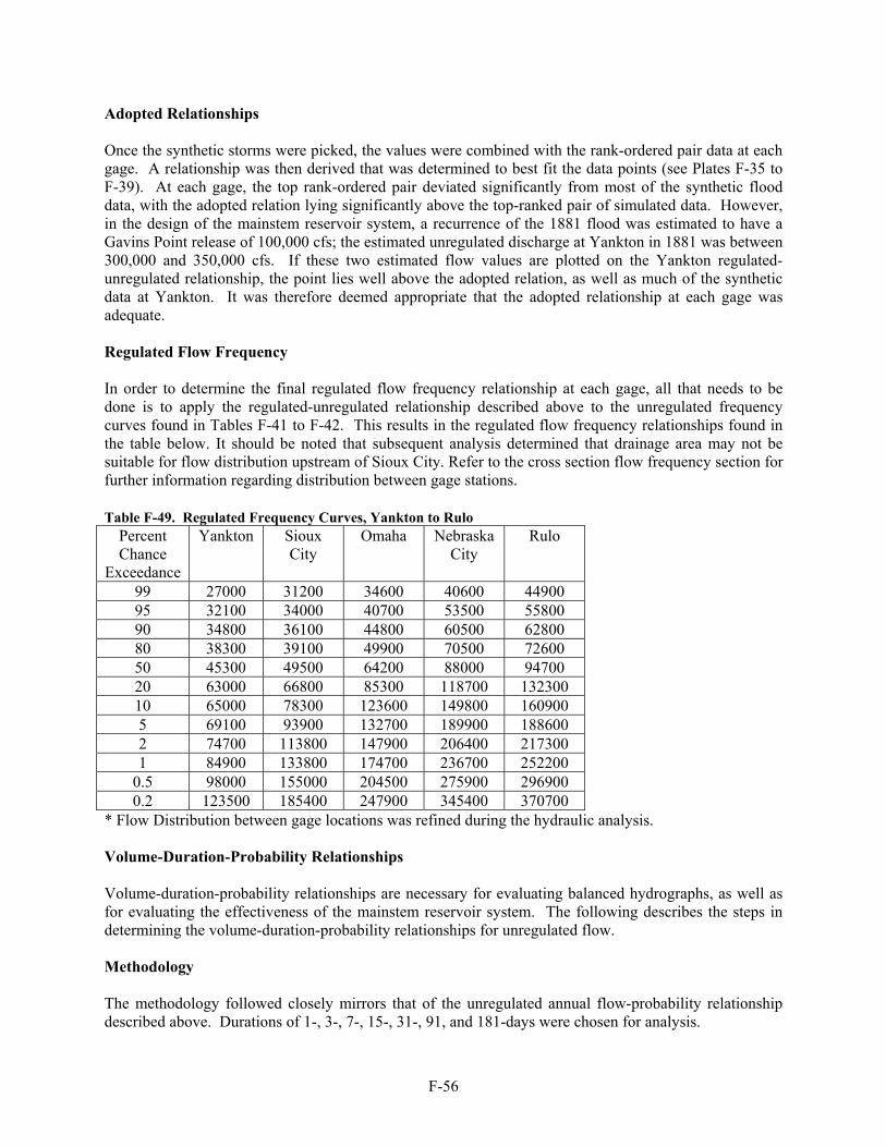
F-56

Adopted Relationships Once the synthetic storms were picked, the values were combined with the rank-ordered pair data at each gage. A relationship was then derived that was determined to best fit the data points (see Plates F-35 to F-39). At each gage, the top rank-ordered pair deviated significantly from most of the synthetic flood data, with the adopted relation lying significantly above the top-ranked pair of simulated data. However, in the design of the mainstem reservoir system, a recurrence of the 1881 flood was estimated to have a Gavins Point release of 100,000 cfs; the estimated unregulated discharge at Yankton in 1881 was between 300,000 and 350,000 cfs. If these two estimated flow values are plotted on the Yankton regulated-unregulated relationship, the point lies well above the adopted relation, as well as much of the synthetic data at Yankton. It was therefore deemed appropriate that the adopted relationship at each gage was adequate. Regulated Flow Frequency In order to determine the final regulated flow frequency relationship at each gage, all that needs to be done is to apply the regulated-unregulated relationship described above to the unregulated frequency curves found in Tables F-41 to F-42. This results in the regulated flow frequency relationships found in the table below. It should be noted that subsequent analysis determined that drainage area may not be suitable for flow distribution upstream of Sioux City. Refer to the cross section flow frequency section for further information regarding distribution between gage stations. Table F-49. Regulated Frequency Curves, Yankton to Rulo

Percent Chance

Exceedance

Yankton Sioux City

Omaha Nebraska City

Rulo

99 27000 31200 34600 40600 44900 95 32100 34000 40700 53500 55800 90 34800 36100 44800 60500 62800 80 38300 39100 49900 70500 72600 50 45300 49500 64200 88000 94700 20 63000 66800 85300 118700 132300 10 65000 78300 123600 149800 160900 5 69100 93900 132700 189900 188600 2 74700 113800 147900 206400 217300 1 84900 133800 174700 236700 252200

0.5 98000 155000 204500 275900 296900 0.2 123500 185400 247900 345400 370700

* Flow Distribution between gage locations was refined during the hydraulic analysis. Volume-Duration-Probability Relationships Volume-duration-probability relationships are necessary for evaluating balanced hydrographs, as well as for evaluating the effectiveness of the mainstem reservoir system. The following describes the steps in determining the volume-duration-probability relationships for unregulated flow. Methodology The methodology followed closely mirrors that of the unregulated annual flow-probability relationship described above. Durations of 1-, 3-, 7-, 15-, 31-, 91, and 181-days were chosen for analysis.

F-57

Since the instantaneous data was best described using a mixed distribution-type analysis, it was decided to analyze the volume-duration-probability relationships using both an annual series and a mixed distribution. DSS macros were used to calculate the mean flow volume for these various durations, using a centered-moving average, over the entire period of record. Additional macros were used to extract the maximum value for each duration by year and by season, and an executable program was used to tabulate all the results. In an effort to make a comparison between annual and mixed distributions, regional skew coefficients need to be incorporated into the analysis. Values recommended by Beard (Beard, 1962) for annual flood volume frequency computations were plotted, and the appropriate values were determined for each duration above. The following table lists the values used for regional skew values in the analysis. Table F-50. Initial Regional Skew Values for Duration Duration Skew Coefficient 1 day -0.04 3 days -0.12 7 days -0.195 15 days -0.267 31 days -0.322 91 days -0.37 181 days -0.388 Annual and mixed distribution results were computed using log-Pearson type III analysis, and the results were graphically compared. It was noted that, just like in the annual flow-probability relationships, the mixed distribution provided a better fit of the data than the annual series for durations of 31-days or less. There was virtually no difference between the annual or mixed results for the 91- or 181-day durations. It was decided to use the mixed distribution analysis for durations of 31-days and less, and to use annual series analysis for the 91- and 181-day durations. The following table lists the computed statistics for each distribution checked. Table F-51. Statistics of Annual and Mixed Populations, Volume-Duration-Probability Analysis Location Duration (1) (2) (3) (4) (5) (6) (7) (8) (9) Yankton 1 day 4.985 0.256 -0.008 5.147 0.123 -0.342 5.187 0.137 0.040 3 days 4.947 0.256 0.099 5.132 0.123 -0.370 5.171 0.136 0.024 7 days 4.890 0.254 0.159 5.109 0.121 -0.411 5.141 0.129 -0.070 15 days 4.820 0.238 0.112 5.081 0.118 -0.402 5.099 0.120 -0.200 31 days 4.744 0.211 0.043 5.044 0.114 -0.444 5.052 0.114 -0.413 91 days 4.742 0.140 -0.264 4.934 0.105 -0.513 4.934 0.105 -0.513 181 days 4.760 0.110 -0.340 4.813 0.107 -0.389 4.813 0.107 -0.389 Sioux City 1 day 5.004 0.249 -0.077 5.161 0.119 -0.386 5.202 0.132 -0.027 3 days 4.973 0.252 0.003 5.149 0.120 -0.414 5.188 0.133 -0.040 7 days 4.921 0.252 0.053 5.125 0.120 -0.466 5.158 0.130 -0.103 15 days 4.856 0.240 0.019 5.097 0.118 -0.479 5.119 0.122 -0.251 31 days 4.783 0.215 -0.020 5.061 0.114 -0.505 5.071 0.115 -0.479 91 days 4.771 0.148 -0.306 4.954 0.109 -0.511 4.954 0.109 -0.511 181 days 4.786 0.114 -0.395 4.837 0.112 -0.408 4.837 0.112 -0.408 Decatur 1 day 4.999 0.246 -0.062 5.160 0.119 -0.384 5.200 0.131 -0.055 3 days 4.973 0.249 -0.009 5.150 0.120 -0.420 5.188 0.131 -0.075 7 days 4.925 0.251 0.031 5.128 0.120 -0.464 5.161 0.129 -0.128 15 days 4.861 0.241 -0.004 5.100 0.118 -0.481 5.122 0.122 -0.268 31 days 4.789 0.216 -0.045 5.064 0.115 -0.510 5.074 0.115 -0.490 91 days 4.776 0.149 -0.324 4.958 0.110 -0.513 4.958 0.110 -0.513

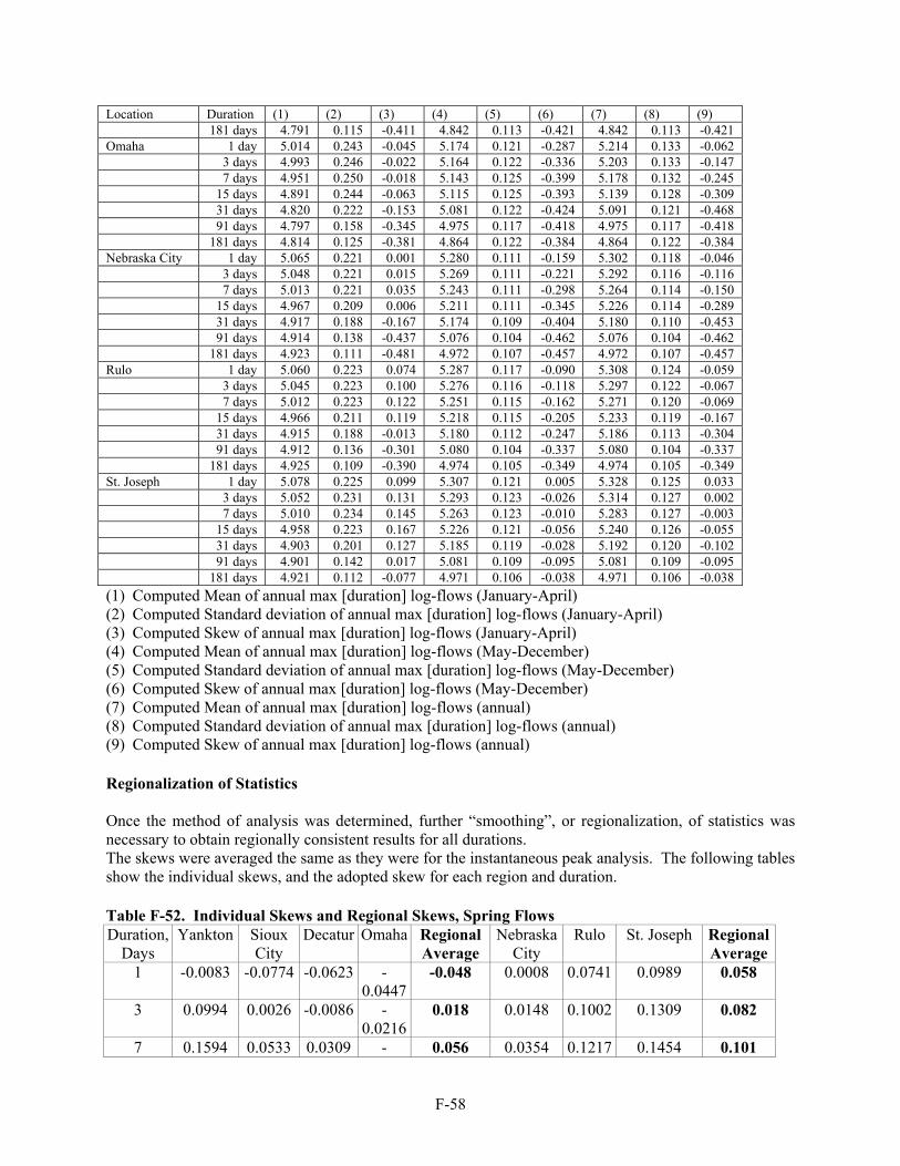
F-58

Location Duration (1) (2) (3) (4) (5) (6) (7) (8) (9) 181 days 4.791 0.115 -0.411 4.842 0.113 -0.421 4.842 0.113 -0.421 Omaha 1 day 5.014 0.243 -0.045 5.174 0.121 -0.287 5.214 0.133 -0.062 3 days 4.993 0.246 -0.022 5.164 0.122 -0.336 5.203 0.133 -0.147 7 days 4.951 0.250 -0.018 5.143 0.125 -0.399 5.178 0.132 -0.245 15 days 4.891 0.244 -0.063 5.115 0.125 -0.393 5.139 0.128 -0.309 31 days 4.820 0.222 -0.153 5.081 0.122 -0.424 5.091 0.121 -0.468 91 days 4.797 0.158 -0.345 4.975 0.117 -0.418 4.975 0.117 -0.418 181 days 4.814 0.125 -0.381 4.864 0.122 -0.384 4.864 0.122 -0.384 Nebraska City 1 day 5.065 0.221 0.001 5.280 0.111 -0.159 5.302 0.118 -0.046 3 days 5.048 0.221 0.015 5.269 0.111 -0.221 5.292 0.116 -0.116 7 days 5.013 0.221 0.035 5.243 0.111 -0.298 5.264 0.114 -0.150 15 days 4.967 0.209 0.006 5.211 0.111 -0.345 5.226 0.114 -0.289 31 days 4.917 0.188 -0.167 5.174 0.109 -0.404 5.180 0.110 -0.453 91 days 4.914 0.138 -0.437 5.076 0.104 -0.462 5.076 0.104 -0.462 181 days 4.923 0.111 -0.481 4.972 0.107 -0.457 4.972 0.107 -0.457 Rulo 1 day 5.060 0.223 0.074 5.287 0.117 -0.090 5.308 0.124 -0.059 3 days 5.045 0.223 0.100 5.276 0.116 -0.118 5.297 0.122 -0.067 7 days 5.012 0.223 0.122 5.251 0.115 -0.162 5.271 0.120 -0.069 15 days 4.966 0.211 0.119 5.218 0.115 -0.205 5.233 0.119 -0.167 31 days 4.915 0.188 -0.013 5.180 0.112 -0.247 5.186 0.113 -0.304 91 days 4.912 0.136 -0.301 5.080 0.104 -0.337 5.080 0.104 -0.337 181 days 4.925 0.109 -0.390 4.974 0.105 -0.349 4.974 0.105 -0.349 St. Joseph 1 day 5.078 0.225 0.099 5.307 0.121 0.005 5.328 0.125 0.033 3 days 5.052 0.231 0.131 5.293 0.123 -0.026 5.314 0.127 0.002 7 days 5.010 0.234 0.145 5.263 0.123 -0.010 5.283 0.127 -0.003 15 days 4.958 0.223 0.167 5.226 0.121 -0.056 5.240 0.126 -0.055 31 days 4.903 0.201 0.127 5.185 0.119 -0.028 5.192 0.120 -0.102 91 days 4.901 0.142 0.017 5.081 0.109 -0.095 5.081 0.109 -0.095 181 days 4.921 0.112 -0.077 4.971 0.106 -0.038 4.971 0.106 -0.038 (1) Computed Mean of annual max [duration] log-flows (January-April) (2) Computed Standard deviation of annual max [duration] log-flows (January-April) (3) Computed Skew of annual max [duration] log-flows (January-April) (4) Computed Mean of annual max [duration] log-flows (May-December) (5) Computed Standard deviation of annual max [duration] log-flows (May-December) (6) Computed Skew of annual max [duration] log-flows (May-December) (7) Computed Mean of annual max [duration] log-flows (annual) (8) Computed Standard deviation of annual max [duration] log-flows (annual) (9) Computed Skew of annual max [duration] log-flows (annual) Regionalization of Statistics Once the method of analysis was determined, further “smoothing”, or regionalization, of statistics was necessary to obtain regionally consistent results for all durations. The skews were averaged the same as they were for the instantaneous peak analysis. The following tables show the individual skews, and the adopted skew for each region and duration. Table F-52. Individual Skews and Regional Skews, Spring Flows Duration,

Days Yankton Sioux

City Decatur Omaha Regional

Average Nebraska

City Rulo St. Joseph Regional

Average1 -0.0083 -0.0774 -0.0623 -

0.0447-0.048 0.0008 0.0741 0.0989 0.058

3 0.0994 0.0026 -0.0086 -0.0216

0.018 0.0148 0.1002 0.1309 0.082

7 0.1594 0.0533 0.0309 - 0.056 0.0354 0.1217 0.1454 0.101

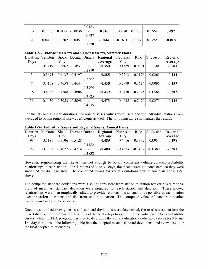
F-59

0.018315 0.1117 0.0192 -0.0036 -

0.06270.016 0.0058 0.1185 0.1669 0.097

31 0.0430 -0.0202 -0.0451 -0.1528

-0.044 -0.1671 -0.013 0.1265 -0.018

Table F-53. Individual Skews and Regional Skews, Summer Flows Duration,

Days Yankton Sioux


Average Nebraska


Average 1 -0.3419 -0.3862 -0.3837 -

0.2870-0.350 -0.1589 -0.0901 0.0048 -0.081

3 -0.3695 -0.4137 -0.4197 -0.3362

-0.385 -0.2213 -0.1176 -0.0261 -0.122

7 -0.4108 -0.4658 -0.4644 -0.3994

-0.435 -0.2979 -0.1624 -0.0095 -0.157

15 -0.4022 -0.4788 -0.4806 -0.3925

-0.439 -0.3450 -0.2045 -0.0564 -0.202

31 -0.4439 -0.5053 -0.5098 -0.4235

-0.473 -0.4035 -0.2470 -0.0275 -0.226

For the 91- and 181-day durations, the annual series values were used, and the individual stations were averaged to obtain regional skew coefficients as well. The following table summarizes the results. Table F-54. Individual Skews and Regional Skews, Annual Flows Duration,

Days Yankton Sioux


Average Nebraska


Average 91 -0.5131 -0.5106 -0.5128 -

0.4182-0.489 -0.4616 -0.3372 -0.0954 -0.298

181 -0.3887 -0.4077 -0.4214 -0.3838

-0.400 -0.4573 -0.3487 -0.0380 -0.281

However, regionalizing the skews was not enough to obtain consistent volume-duration-probability relationships at each station. For durations of 3- to 31-days, the means were not consistent, so they were smoothed by drainage area. The computed means for various durations can be found in Table F-51 above. The computed standard deviations were also not consistent from station to station for various durations. Plots of mean vs. standard deviation were prepared for each station and duration. These plotted relationships were then graphically edited to provide relationships as smooth as possible at each station over the various durations and also from station to station. The computed values of standard deviation can be found in Table F-56 above. Once the smoothed skews, means and standard deviations were determined, the results were put into the mixed distribution program for durations of 1- to 31- days to determine the volume-duration-probability curves, while the FFA program was used to determine the volume-duration-probability curves for 91- and 181-day durations. The following table lists the adopted means, standard deviations, and skews used for the final adopted relationships.

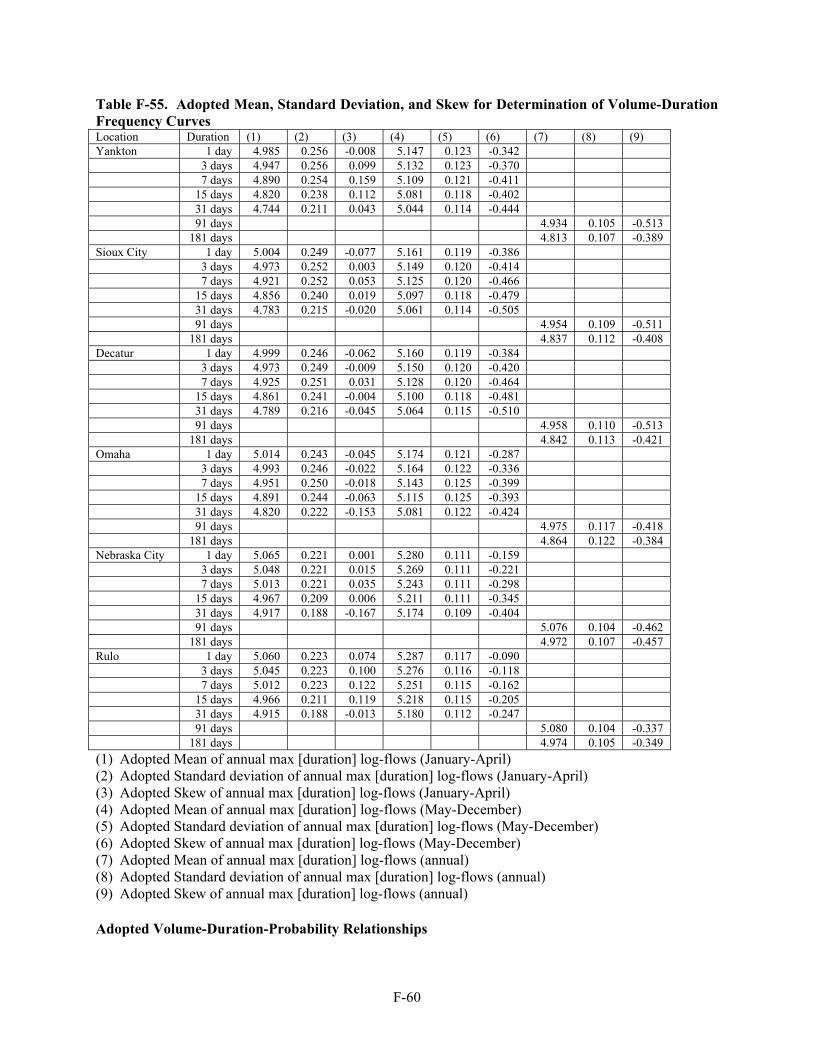
F-60

Table F-55. Adopted Mean, Standard Deviation, and Skew for Determination of Volume-Duration Frequency Curves Location Duration (1) (2) (3) (4) (5) (6) (7) (8) (9) Yankton 1 day 4.985 0.256 -0.008 5.147 0.123 -0.342 3 days 4.947 0.256 0.099 5.132 0.123 -0.370 7 days 4.890 0.254 0.159 5.109 0.121 -0.411 15 days 4.820 0.238 0.112 5.081 0.118 -0.402 31 days 4.744 0.211 0.043 5.044 0.114 -0.444 91 days 4.934 0.105 -0.513 181 days 4.813 0.107 -0.389 Sioux City 1 day 5.004 0.249 -0.077 5.161 0.119 -0.386 3 days 4.973 0.252 0.003 5.149 0.120 -0.414 7 days 4.921 0.252 0.053 5.125 0.120 -0.466 15 days 4.856 0.240 0.019 5.097 0.118 -0.479 31 days 4.783 0.215 -0.020 5.061 0.114 -0.505 91 days 4.954 0.109 -0.511 181 days 4.837 0.112 -0.408 Decatur 1 day 4.999 0.246 -0.062 5.160 0.119 -0.384 3 days 4.973 0.249 -0.009 5.150 0.120 -0.420 7 days 4.925 0.251 0.031 5.128 0.120 -0.464 15 days 4.861 0.241 -0.004 5.100 0.118 -0.481 31 days 4.789 0.216 -0.045 5.064 0.115 -0.510 91 days 4.958 0.110 -0.513 181 days 4.842 0.113 -0.421 Omaha 1 day 5.014 0.243 -0.045 5.174 0.121 -0.287 3 days 4.993 0.246 -0.022 5.164 0.122 -0.336 7 days 4.951 0.250 -0.018 5.143 0.125 -0.399 15 days 4.891 0.244 -0.063 5.115 0.125 -0.393 31 days 4.820 0.222 -0.153 5.081 0.122 -0.424 91 days 4.975 0.117 -0.418 181 days 4.864 0.122 -0.384 Nebraska City 1 day 5.065 0.221 0.001 5.280 0.111 -0.159 3 days 5.048 0.221 0.015 5.269 0.111 -0.221 7 days 5.013 0.221 0.035 5.243 0.111 -0.298 15 days 4.967 0.209 0.006 5.211 0.111 -0.345 31 days 4.917 0.188 -0.167 5.174 0.109 -0.404 91 days 5.076 0.104 -0.462 181 days 4.972 0.107 -0.457 Rulo 1 day 5.060 0.223 0.074 5.287 0.117 -0.090 3 days 5.045 0.223 0.100 5.276 0.116 -0.118 7 days 5.012 0.223 0.122 5.251 0.115 -0.162 15 days 4.966 0.211 0.119 5.218 0.115 -0.205 31 days 4.915 0.188 -0.013 5.180 0.112 -0.247 91 days 5.080 0.104 -0.337 181 days 4.974 0.105 -0.349 (1) Adopted Mean of annual max [duration] log-flows (January-April) (2) Adopted Standard deviation of annual max [duration] log-flows (January-April) (3) Adopted Skew of annual max [duration] log-flows (January-April) (4) Adopted Mean of annual max [duration] log-flows (May-December) (5) Adopted Standard deviation of annual max [duration] log-flows (May-December) (6) Adopted Skew of annual max [duration] log-flows (May-December) (7) Adopted Mean of annual max [duration] log-flows (annual) (8) Adopted Standard deviation of annual max [duration] log-flows (annual) (9) Adopted Skew of annual max [duration] log-flows (annual) Adopted Volume-Duration-Probability Relationships

F-61

The final adopted volume-duration-probability relationships for unregulated flows are shown in the following Tables F-56 to F-62. Table F-56. Volume-Probability Relationship, 1-day Flow (cfs) Exceedance Probability

Yankton Sioux City Decatur Omaha Nebraska City Rulo

99 78300 82100 82400 83600 111700 111600

95 96800 100900 101000 103100 132700 133300

90 108000 112200 112300 114900 145500 146400

80 122900 127400 127100 130600 162700 164200

50 156400 161000 160000 165700 201600 204400

20 198800 203400 201200 209400 250700 255200

10 227900 232200 229100 238300 282700 287700

5 264200 267800 263100 272700 316400 322500

2 319800 321900 315300 322500 359000 364900

1 372800 373400 365300 372200 399600 404500

0.5 435200 433700 423800 431000 452200 455400

0.2 509200 505100 492900 500300 520600 522000

Table F-57. Volume-Probability Relationship, 3-day Flow (cfs) Exceedance Probability


99 74400 79200 79400 81500 108500 108800

95 92400 97500 97700 100500 129300 130100

90 103100 108500 108700 112000 141800 143000

80 117600 123200 123400 127300 158600 160400

50 149500 155300 155700 160900 196200 199400

20 189200 195000 195500 202500 243200 248400

10 215400 221400 221900 229700 273400 279300

5 248300 253700 254300 262900 305100 312600

2 299300 305100 305800 313100 345400 353700

1 351500 356100 356900 364400 384500 393100

0.5 414000 416700 417600 425500 435300 444900

0.2 489100 489100 490200 498600 504300 513700



99 69900 74200 74700 76200 101800 102300

95 86800 91400 91900 94200 121400 122500

90 97000 101700 102300 105100 133200 134700

80 110600 115500 116300 119600 149000 151100

50 140100 145400 146400 151100 184000 187500

20 175700 181300 182400 188300 227200 232500

10 198300 204300 205500 211900 254000 260500

5 224600 231000 232300 238300 282600 290000

2 267100 274000 275300 277400 317600 325600

1 314300 320700 322100 323100 351900 359500

0.5 371600 376800 378600 379200 398100 404800

0.2 440900 444500 446500 446600 459800 465300

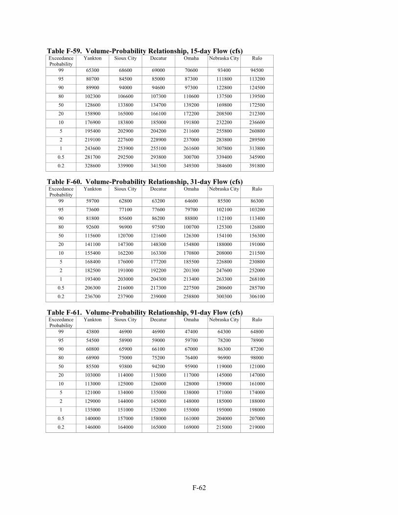
F-62



99 65300 68600 69000 70600 93400 94500

95 80700 84500 85000 87300 111800 113200

90 89900 94000 94600 97300 122800 124500

80 102300 106600 107300 110600 137500 139500

50 128600 133800 134700 139200 169800 172500

20 158900 165000 166100 172200 208500 212300

10 176900 183800 185000 191800 232200 236600

5 195400 202900 204200 211600 255800 260800

2 219100 227600 228900 237000 283800 289500

1 243600 253900 255100 261600 307800 313800

0.5 281700 292500 293800 300700 339400 345900

0.2 328600 339900 341500 349300 384600 391800



99 59700 62800 63200 64600 85500 86300

95 73600 77100 77600 79700 102100 103200

90 81800 85600 86200 88800 112100 113400

80 92600 96900 97500 100700 125300 126800

50 115600 120700 121600 126300 154100 156300

20 141100 147300 148300 154800 188000 191000

10 155400 162200 163300 170800 208000 211500

5 168400 176000 177200 185500 226800 230800

2 182500 191000 192200 201300 247600 252000

1 193400 203000 204300 213400 263300 268100

0.5 206300 216000 217300 227500 280600 285700

0.2 236700 237900 239000 258800 300300 306100



99 43800 46900 46900 47400 64300 64800

95 54500 58900 59000 59700 78200 78900

90 60800 65900 66100 67000 86300 87200

80 68900 75000 75200 76400 96900 98000

50 85500 93800 94200 95900 119000 121000

20 103000 114000 115000 117000 145000 147000

10 113000 125000 126000 128000 159000 161000

5 121000 134000 135000 138000 171000 174000

2 129000 144000 145000 148000 185000 188000

1 135000 151000 152000 155000 195000 198000

0.5 140000 157000 158000 161000 204000 207000

0.2 146000 164000 165000 169000 215000 219000

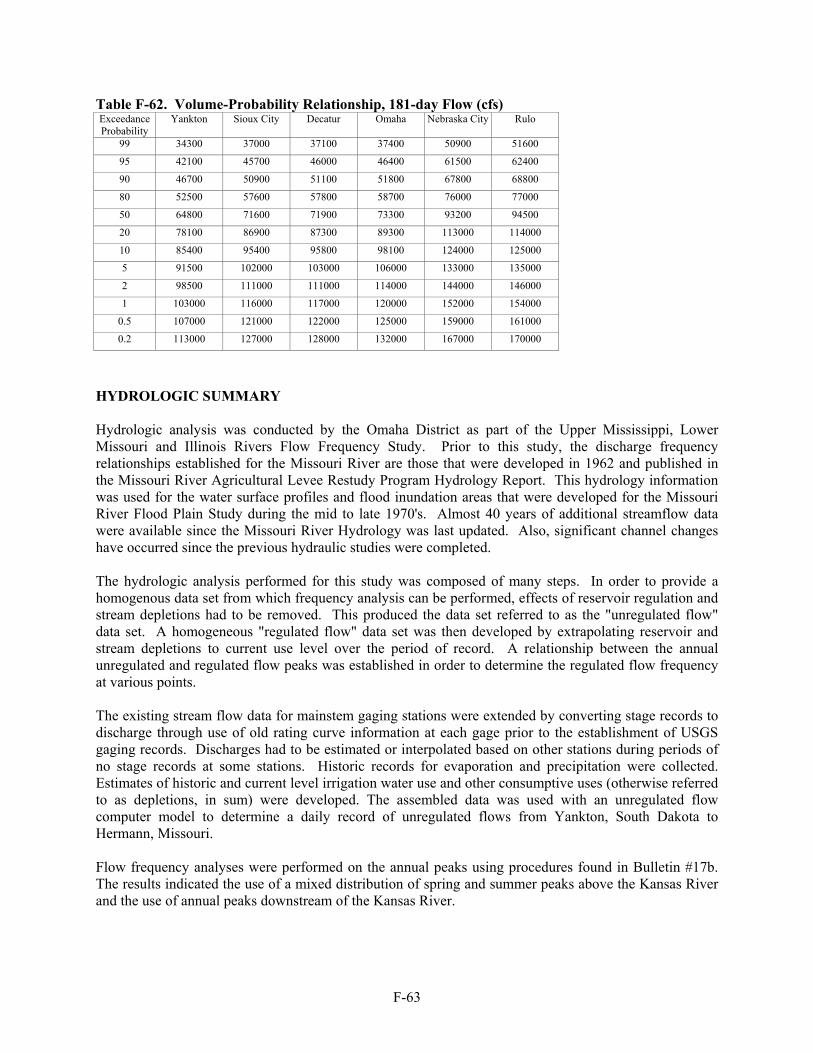
F-63



99 34300 37000 37100 37400 50900 51600

95 42100 45700 46000 46400 61500 62400

90 46700 50900 51100 51800 67800 68800

80 52500 57600 57800 58700 76000 77000

50 64800 71600 71900 73300 93200 94500

20 78100 86900 87300 89300 113000 114000

10 85400 95400 95800 98100 124000 125000

5 91500 102000 103000 106000 133000 135000

2 98500 111000 111000 114000 144000 146000

1 103000 116000 117000 120000 152000 154000

0.5 107000 121000 122000 125000 159000 161000

0.2 113000 127000 128000 132000 167000 170000

HYDROLOGIC SUMMARY Hydrologic analysis was conducted by the Omaha District as part of the Upper Mississippi, Lower Missouri and Illinois Rivers Flow Frequency Study. Prior to this study, the discharge frequency relationships established for the Missouri River are those that were developed in 1962 and published in the Missouri River Agricultural Levee Restudy Program Hydrology Report. This hydrology information was used for the water surface profiles and flood inundation areas that were developed for the Missouri River Flood Plain Study during the mid to late 1970's. Almost 40 years of additional streamflow data were available since the Missouri River Hydrology was last updated. Also, significant channel changes have occurred since the previous hydraulic studies were completed. The hydrologic analysis performed for this study was composed of many steps. In order to provide a homogenous data set from which frequency analysis can be performed, effects of reservoir regulation and stream depletions had to be removed. This produced the data set referred to as the "unregulated flow" data set. A homogeneous "regulated flow" data set was then developed by extrapolating reservoir and stream depletions to current use level over the period of record. A relationship between the annual unregulated and regulated flow peaks was established in order to determine the regulated flow frequency at various points. The existing stream flow data for mainstem gaging stations were extended by converting stage records to discharge through use of old rating curve information at each gage prior to the establishment of USGS gaging records. Discharges had to be estimated or interpolated based on other stations during periods of no stage records at some stations. Historic records for evaporation and precipitation were collected. Estimates of historic and current level irrigation water use and other consumptive uses (otherwise referred to as depletions, in sum) were developed. The assembled data was used with an unregulated flow computer model to determine a daily record of unregulated flows from Yankton, South Dakota to Hermann, Missouri. Flow frequency analyses were performed on the annual peaks using procedures found in Bulletin #17b. The results indicated the use of a mixed distribution of spring and summer peaks above the Kansas River and the use of annual peaks downstream of the Kansas River.

F-64

A regulated flow computer model was run, using data developed by both Omaha and Kansas City Districts, to determine a daily record of regulated flows from Gavins Point Dam to Hermann, Missouri. The regulated flow frequency curve is determined by transforming the unregulated curve using an unregulated versus regulated relationship. To determine this relationship, annual peaks for regulated and unregulated flows were compared, the regulated flow data being determined at each station by routing studies. The annual peaks from the regulated and unregulated data sets were then paired against each other in descending order. A relationship between regulated and unregulated flow frequencies was then established at each station. The hydraulic analysis employed the regulated flow frequency values determined at each gage location.

F-65

HYDRAULIC ANALYSIS

GEOGRAPHIC COVERAGE. The Omaha District performed hydraulic modeling along the Missouri River. The hydraulic model extends from Gavins Point Dam, at river mile (RM) 811.1, downstream to Rulo, NE, at RM 498.0. Rulo, NE, corresponds with the Omaha District boundary with the Kansas City District. The Omaha District hydraulic model includes 313 miles of the Missouri River and 211 miles of tributaries. Within the model limits, the Missouri River drainage area increases from 279,500 square miles at Gavins Point Dam to 414,900 square miles at Rulo. Shown in Figure F-2 is a schematic of the modeled area. The schematic illustrates the Missouri River gaging stations on the main stem, tributaries that are included as routing reaches, lateral inflows to the model, and the river mile location of hydrologic features. In order to provide an accurate downstream boundary, the hydraulic model also includes geometry between Rulo, NE and St. Joseph, MO. This adds an additional Missouri River length of 49.9 miles to the hydraulic model. All features pertaining to the Missouri River downstream of Rulo, NE, are described within the Kansas City District section of the report, appendix E. All river miles referenced in the Omaha District appendix use the 1960 mileage for the Missouri River. BASIN DESCRIPTION. The Missouri River originates in the northern Rocky Mountains along the continental divide and flows south and east to join the Mississippi River near St. Louis, Missouri. At 2,315 miles (1960 mileage), it is the longest river in the United States. The Omaha District encompasses approximately 414,900 square miles of the drainage basin upstream of Rulo, NE to the river headwaters in the Rocky Mountains. The Missouri River basin contains numerous reservoirs and impoundments constructed by different interests for flood control, irrigation, power production, recreation, and water supply. Missouri River Mainstem Dams. The most significant flood control projects constructed within the basin are the six main stem Missouri River Dams. The six dams, which were completed by 1964, provide flood protection by controlling runoff from the upper most 279,000 square miles of the drainage basin. The reservoir system has a total combined capacity in excess of 73 million acre-feet of which more than 16 million acre-feet is for flood control. Gavins Point Dam, located near Yankton, SD at river mile 811.1, forms Lewis and Clark Lake and is the most downstream of the projects. Recreational River Reach. The Gavins-to-Ponca reach (RM 811 to 752) of the Missouri river was designated a Recreational River pursuant to Section 707 of the National Parks and Recreation Act (PL 95-625) which amended the Wild and Scenic Rivers Act (PL 90-542). The river is channelized starting at the downstream end of the Recreational River, a segment known as "Kenslers Bend". Demonstration bank stabilization projects on the Missouri River were authorized under Section 32 of the Streambank Erosion Control Evaluation and Demonstration Act of 1974 (P.L. 93-251). Nine of these projects are located in the reach from Gavins Point Dam down to Ponca State Park. The recreational river reach has been impacted by Gavins Point Dam including flow regulation and the capture of sediment. Within this reach, the riverbed has experienced significant degradation and the loss of high bank. Bank stabilization such as the Section 32 projects has greatly reduced the migration of the high banks. However, in many areas, the river is characterized by a dynamic channel with shifting islands and sand bars.

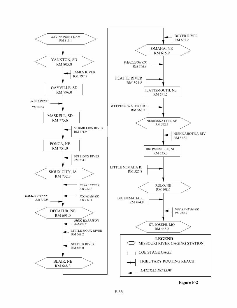
F-66

BOW CREEK

RM 787.6

PERRY CREEK RM 732.1

FLOYD RIVER RM 731.3

OMAHA CREEKRM 719.9

MON. HARRISON RM 670.0

PAPILLION CRRM 596.6

LEGEND MISSOURI RIVER GAGING STATION COE STAGE GAGE TRIBUTARY ROUTING REACH LATERAL INFLOW

GAVINS POINT DAM RM 811.1

YANKTON, SD RM 805.8

JAMES RIVER RM 797.7

GAYVILLE, SD RM 796.0

MASKELL, SD RM 775.6

VERMILLION RIVERRM 771.9

PONCA, NE RM 751.0

BIG SIOUX RIVERRM 734.0

SIOUX CITY, IA RM 732.3

DECATUR, NE RM 691.0

LITTLE SIOUX RIVER RM 669.2

SOLDIER RIVER RM 664.0

BLAIR, NE RM 648.3

BOYER RIVER RM 635.2

OMAHA, NE RM 615.9

PLATTE RIVERRM 594.8

PLATTSMOUTH, NE RM 591.5

WEEPING WATER CRRM 568.7

NEBRASKA CITY, NE RM 562.6

NISHNABOTNA RIV RM 542.1

BROWNVILLE, NE RM 535.3

LITTLE NEMAHA R.RM 527.8

RULO, NE RM 498.0

BIG NEMAHA R.RM 494.8

NODAWAY RIVER RM 463.0

ST. JOSEPH, MO RM 448.2

Figure F-2

F-67

Navigation and Bank Stabilization. There were seven acts of Congress that provided for the construction, operation and maintenance of a navigation channel and bank stabilization works on the Missouri River. The most recent was authorized in 1945 and provided for bank stabilization combined with a 9-foot deep and not less than 300 feet wide navigation channel. The authorized project for the Missouri River extends from its confluence with the Mississippi River at St Louis, MO to Sioux City, IA for a total distance of 734.2 river miles. This was accomplished through revetment of banks, construction of permeable dikes, cutoff of oxbows, closing minor channels, removal of snags and dredging. In order to achieve the project objectives of bank stabilization and navigation, the river was shaped into a series of smoothly curved bends of the proper radii and channel width. Stabilization of the bank along the concave alignment of the design curve was accomplished with pile and stone fill revetments. Dikes were constructed along the convex bank, approximately perpendicular to the flow. These dikes were designed to prevent bank erosion and to promote accretion, forcing the channel to develop and maintain itself along the design alignment. In areas where the natural river channel did not conform to the design alignment, canals were excavated and natural channels blocked in order to force the river to flow along the design alignment. Levee System. The Missouri River levee system was authorized by the Flood Control Acts of 1941 and 1944 to provide protection to agricultural lands and communities along the Missouri River from Sioux City, IA to the mouth at St. Louis, MO. The levees were designed to operate in accord with the six main stem dams. The extent of the levee system within the Omaha District consists of levee units on both banks from near Omaha, NE to near Rulo, NE. Although many federal levees were proposed north of Omaha, NE along the Missouri River, few have been built due to the significant contribution of the main stem dams in this reach and channel degradation that has occurred following dam closure. The majority of the area planned for protection by federal levees north of Omaha, NE is protected by private or non-federal levees with varying degrees of protection. TRIBUTARY SYSTEM. Numerous tributaries enter the Missouri River within the model reach. Refer to the model schematic shown in Figure F-2 for the location of significant tributaries. Major tributaries were included as separate routing reaches within the forecast model. Minor tributaries were included as lateral inflow to the model. Routing of the tributary flows from the gaging station location to the confluence with the Missouri River was found to increase the simulation accuracy. Tributary modeling efforts were of limited detail and intended for flow routing only. As a result of the coarse cross section data, computed stage information on the tributaries may not be accurate. Flow data from the USGS gaging station provides flow required for the tributary upstream model boundary. A drainage area accounting is provided in Plate F-52 that lists significant tributaries included in the model. A brief description of the tributaries included as separate routing reaches within the model is provided in the following sections. James River - RM 797.7 The James River is a major left bank tributary that enters the Missouri River downstream of Yankton, SD at river mile 797.7. The basin has a drainage area of approximately 20,942 square miles and includes portions of South Dakota and North Dakota. Federal projects on the James River include Pipestem and Jamestown Dams located near Jamestown, ND. The James River has a large drainage basin but an extremely flat channel gradient. The USGS gaging station #06478500 at Scotland, SD, is the upstream model inflow boundary and is located over 50 river miles from the Missouri River.

F-68

Vermillion River - RM 771.9 The Vermillion River is a major left bank tributary that enters the Missouri River near Vermillion, SD. The basin has a drainage area of approximately 2302 square miles within east central South Dakota. The USGS gaging station #06479010 at Vermillion, SD, is the upstream model inflow boundary and is located 10.8 river miles from the Missouri River. Big Sioux River - RM 734.0 The Big Sioux River is a left bank tributary that enters the Missouri River near Sioux City, IA at river mile 734.2. The basin has a drainage area of approximately 8424 square miles and includes portions of South Dakota, Minnesota and Iowa. The USGS gaging station #06485500 at Akron, IA, is the upstream model boundary and is located about 45 river miles measured along the channel from the Missouri River. The Big Sioux River floodplain length is slightly more than 30 miles measured from the Missouri River. Little Sioux River - RM 669.2 The Little Sioux River is a left bank tributary to the Missouri River that drains approximately 3,526 square miles within northwest Iowa above its confluence with the Missouri River at river mile 669.2. Extensive systems of federal levees have been constructed in the lower basin on both the Little Sioux and its tributaries to protect primarily agricultural lands. The levee construction began in 1956 and was completed in 1966. The USGS gaging station #06607500 near Turin, IA, is the upstream model inflow boundary and is located 13.3 river miles from the Missouri River. During extreme events flow may be diverted between the Little Sioux River and the Monona-Harrison Ditch at the Missouri River confluence. Soldier River - RM 664.0 The Soldier River is a small left bank tributary to the Missouri River located immediately to the north of the Boyer River Basin. It drains approximately 407 square miles of western Iowa and enters the Missouri River at river mile 664.0. The USGS gaging station #06608500 at Pisgah, IA, is the upstream model inflow boundary and is located 13.1 river miles from the Missouri River. Boyer River - RM 635.2 The Boyer River is a small left bank tributary to the Missouri River at river mile 635.2. It drains approximately 871 square miles of western IA. Much of the lower portion of the Boyer River is protected by private levees with varying levels of protection. The USGS gaging station #06609500 at Logan, IA, is the upstream model inflow boundary and is located 15.8 river miles from the Missouri River. Platte River - RM 594.8 The Platte River is a major right bank tributary to the Missouri River draining an area of approximately 85,370 square miles of northeast Colorado, southeast Wyoming and most of central Nebraska. The Platte River joins the Missouri River approximately 21 miles downstream of Omaha, NE at river mile 594.80. In eastern Nebraska, major tributaries to the Platte River are Salt Creek, the Elkhorn and Loup Rivers. The USGS gaging station #06805500 at Louisville, NE, is the upstream model inflow boundary and is located 16.5 river miles from the Missouri River. Weeping Water Creek - RM 568.7 Weeping Water Creek is a right bank tributary to the Missouri River located in southeast Nebraska at river mile 568.70. It has a drainage area of approximately 241 square miles. The USGS gaging station #06806500 at Union, NE, is the upstream model inflow boundary and is located 6.2 river miles from the Missouri River. Nishnabotna River - RM 542.1 The Nishnabotna River is a major left bank tributary to the Missouri River located approximately 20 miles downstream of Nebraska City, NE at river mile 542.1. It has a total drainage area of 2,806 square

F-69

miles. Major changes within the basin include the construction of federal levees, private agricultural levees, channel changes and drainage improvements. The Nishnabotna River has federal levees along the right bank from the Missouri River confluence to Highway 275 located upstream of Hamburg, IA. The left bank also has federal levees from the Missouri River confluence upstream to Highway 275. The USGS gaging station #06810000 near Hamburg, IA, is the upstream model inflow boundary and is located 13.8 river miles from the Missouri River. Little Nemaha - RM 527.8. The Little Nemaha River located in southeast Nebraska is a right bank tributary to the Missouri River. The basin has a drainage area of approximately 793 square miles and enters the Missouri River at river mile 527.80 near Nemaha, NE. The USGS gaging station #06811500 at Auburn, NE, is the upstream model inflow boundary and is located 10.4 river miles from the Missouri River. ICE IMPACTS ON PEAK STAGE . The flood history within the Missouri River basin provides documentation of numerous impacts of ice causing much higher stages than would normally occur for an open water condition. Refer to the flood history section of this report for a detailed discussion of ice impacts. The hydrologic analysis evaluated the requirement for an ice affected flow adjustment as described within the text and illustrated in Table F-21 and F-22. The hydraulic analysis does not include any adjustment for ice. Typically, flood events in the early spring will include floating ice with the potential for ice jams to occur. Installation of the mainstem dams has altered the frequency of spring floods and the accompanying ice jams. However, extreme flood events in the upper reaches of the Missouri River may include ice conditions. AGGRADATION AND DEGRADATION TRENDS. Over the last 100 years, significant change has occurred in channel conveyance as a result of aggradation and degradation. Missouri River natural variability and construction including flood control projects, channel cutoffs, channel and bank stability projects have all contributed to conveyance change. Numerous studies have been conducted by the Omaha District to quantify the impact of Missouri River geometry changes on the stage-flow relationship (USACE, 2001). Gavins Point Dam to Omaha, NE. Downstream of the Missouri River main stem reservoir system, significant channel degradation has occurred. Degradation analysis and impacts have been outlined in several reports prepared by the Omaha District (USACE, 1981, 2001). Missouri River degradation is a complex issue with several contributing causes. Since construction of Gavins Point Dam (RM 811.05) in 1952, water surface elevations for a discharge of 30,000 cfs have decreased between 4 and 6 feet at Yankton, SD (RM 805.8), Sioux City, IA (RM 732.3), and Decatur, NE (RM 691.0). Many of the tributaries are also experiencing significant degradation. Data analysis indicates that future degradation rates are declining as the river elevation becomes more stable. Current data has generally been observed to indicate that Missouri River channel degradation dissipates prior to reaching Omaha, NE (RM 615.9). Omaha, NE to Rulo, NE. An assessment of the impact of aggradation and degradation trends on channel capacity was performed in the study Missouri River Channel Capacity Study (USACE, 1992). The reach between Omaha, NE (RM 615.) and Rulo, NE (RM 498.0) has illustrated general aggradational trends. Since 1955, thalweg elevations have increased by as much as 4 to 6 feet. Based on measured data for a low-flow continuous water surface profile, the increase in water surface elevations varies from 1 to 3 feet. Average bed slope

F-70

has remained relatively constant at 0.8 to 1.1 foot per mile. An additional increase of 1 - 2 feet in water surface elevation is projected by the year 2020. Within the reach, aggradation at and downstream of the Platte River confluence indicates that the Platte River continues to deliver significant sediment quantities. Sediment Deposition Factors. Sediment deposition within the floodplain near the channel is a common occurrence. In many river systems, natural levees are formed when deposition occurs outside of a channel during high flows (mainly during flood recessions) because vegetation traps sediment and increases hydraulic roughness, reducing velocities and sediment transport capacities. Another general characteristic of this phenomenon is the deposition of the larger size sediment particles immediately adjacent to the channel with a lateral reduction in grainsize down to clay away from the channel. A levee project can exacerbate the sediment deposition because overbank flows that once spread across a major portion of the floodplain are now confined to a relatively narrow zone adjacent to the river banks. Therefore, a given volume of sediment is deposited over a smaller surface area, resulting in increased deposit depths. Although the federal levees are generally set back from the river bank, many areas include private levee cells between the federal levee and the river bank. These cells act as sediment settling basins when the levee elevation is exceeded. Field Reconnaissance. Field reconnaissance was conducted by the Omaha District to evaluate sediment deposition patterns in the area between the Missouri River bank and the federal levee. The reconnaissance was conducted in September 1993 following the extensive summer 1993 flooding. Standing water and mud limited the reconnaissance to accessible areas. Material deposited near the levee base consisted entirely of silts and clays. Depths of deposition were determined by digging to the vegetation layer at several locations. Deposition depth averaged about one foot. Large sand deposits were observed immediately adjacent to the channel. These observations with sand deposits near the channel and silts and clays at a distance away are consistent with expected floodplain deposition patterns, as discussed in the preceding paragraph. Another reconnaissance was conducted in April 1994. This reconnaissance confirmed the presence of sand deposits immediately adjacent to the channel. It was also noted at this time that lands experiencing the greatest volume of sand deposits were those riverward of failed agricultural levees. These agricultural levees run parallel to the river and are located inside of the federal tie-back levee. In all likelihood, these levees confined flows, resulting in increased channel velocities, allowing the sand sized particles to be transported through the reach. When they failed, the large concentrations of sand were deposited when the flow spread across the overbank and velocities were reduced. Gage Stage Trends. Data collected at Missouri River gaging stations demonstrates shifts in the stage-discharge relationship. The shift of the rating curve varies according to location with degradation in the upper reach and aggradation in the lower reach. Gage stage trends are illustrated on Plates F-53 thru F-55 for Sioux City, Omaha, and Nebraska City. CONNECTIONS WITH OTHER DISTRICTS. The Omaha District UNET model is the most upstream model for the Missouri River. Therefore, there is no connection with other Districts upstream. However, on the downstream end of the model the UNET model includes a portion of the Kansas City District from Rulo, NE, to St. Joseph, MO. The reach within the Kansas City District allows for a convergence reach at the downstream end of the model to smooth any computational instabilities that could result within the model near the downstream boundary condition. Computed results for the reach downstream of Rulo, NE, should be obtained from the Kansas City District hydraulic appendix and are not reported here.

F-71

UNET APPLICATION. The Omaha District constructed an unsteady flow model of the Missouri River. UNET was employed as the unsteady flow model for the basin wide modeling tool. UNET is a one-dimensional unsteady flow program that includes the capability of simulating a complex network of open channels. Unsteady flow routing accounts for the variation in flow with both time and space. The UNET model has the ability to account for critical backwater effects in the routing and can directly simulate flows that spill over or breach a levee. Customized versions of UNET were developed as necessary via contracts with Dr. Barkau by several District offices involved in the Flow Frequency Study. The UNET model utilized for computational purposes was version 4.0, LAN version 1.0 executable date 9/12/2002. The UNET version contains additional capabilities developed by Dr. Robert L. Barkau that are not included in the normal UNET program distributed by the Hydrologic Engineering Center. The UNET model background and capability is only briefly described in this appendix. Refer to appendix A for a detailed description of UNET model features. Model Geometry Development and Description The geometry input file consists of the HEC-2 style cross sectional geometry developed by the user. Cross section data for the Missouri River was extracted from digital models developed from floodplain and hydrographic survey data. Federal levee areas are included within the model as storage cells. The UNET model also requires flow and stage hydrograph data to provide boundary conditions and inflow data. Figure F-3 illustrates a general plan view of the model features. River Geometry. River geometry within the UNET model is required to describe the Missouri River and all tributary routing reaches. River geometry is described in a cross section format using station-elevation data. Data is coded in a format similar to HEC-2 using X1 and GR cards (HEC, 1990). Floodplain Topography. Aerial photography, airborne global positioning system (GPS) control, ground survey control, and aero triangulation were used in development of a digital terrain model (DTM) and digital elevation model (DEM) of the project area for the Omaha District. The aerial photography for the DTM was taken in the fall of 1999. The DTM data is composed of mass points and break lines that adequately define elevated roads, railroads, levees (features that would impede flow) and other major topographic changes required for accurate DEM development. The aerial mapping is based on surveyed ground control points. These surveyed ground control points are very accurate, but the aerial mapping of well-defined features between the ground control points can vary by as much as 0.67 foot 67 percent of the time in accordance with the ASPRS Class I mapping standards. Ground surface elevations developed by the aerial mapping will be accurate to within 1.33 feet. A description of survey accuracy is included in Plate F-56. Hydrographic Data. Hydrographic survey data was collected in 1994 between Rulo, NE, and Ponca, NE (river mile 498 to 752). Hydrographic survey data from Ponca to Gavins Point Dam was collected in 1995 (river mile 752 to 811). Hydrographic data is collected in a cross section format at a spacing of approximately 500 feet. Accuracy of the hydrographic survey data equipment is approximately 0.5 for the elevations. However, it should be noted that the Missouri River has a high sediment concentration with notable bed

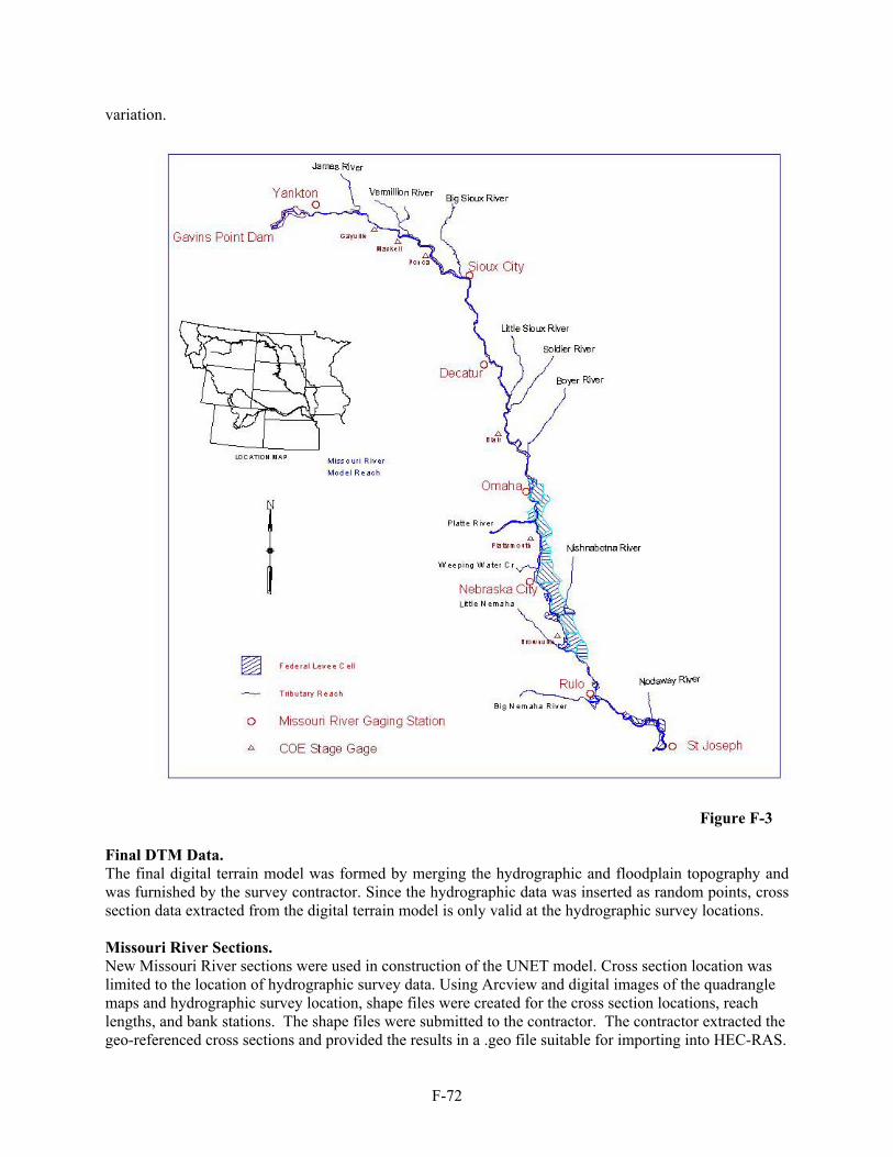
F-72

variation.

Figure F-3 Final DTM Data. The final digital terrain model was formed by merging the hydrographic and floodplain topography and was furnished by the survey contractor. Since the hydrographic data was inserted as random points, cross section data extracted from the digital terrain model is only valid at the hydrographic survey locations. Missouri River Sections. New Missouri River sections were used in construction of the UNET model. Cross section location was limited to the location of hydrographic survey data. Using Arcview and digital images of the quadrangle maps and hydrographic survey location, shape files were created for the cross section locations, reach lengths, and bank stations. The shape files were submitted to the contractor. The contractor extracted the geo-referenced cross sections and provided the results in a .geo file suitable for importing into HEC-RAS.

F-73

Cross sections were extracted from the dtm model at an interval of roughly 2000 feet. Extracted cross sections extended from bluff to bluff within the river valley. The total number of cross sections is in excess of 800 through the model reach. A number of editing steps were performed within HEC-RAS prior to incorporating the new sections within the UNET model. These steps included checking reach lengths, correcting the river mile cross section identifier to 1960 river miles, removing storage from the effective section width, adding additional sections at bridge locations, adding effective flow area encroachments, inserting the horizontal roughness, etc. The program RAS2UNET, furnished by the Hydrologic Engineering Center, was used to translate the cross section data from RAS to UNET format. Section Bank Stations and Effective Flow Areas. Many steady flow analysis models require construction of separate models for different frequency events making it possible to vary the effective flow area within a cross section for different flow rates. The UNET model employs a single geometry for the entire period of record. Within the UNET model, bank stations and effective flow areas are specified at each cross section. The model included an encroachment at the bank station to confine all flow to the channel until the bank station is exceeded. An additional station was specified within the section to define ineffective flow within the model after the channel capacity is exceeded. Since the model was constructed to model a full range of flows, placement of a single encroachment station within the floodplain was usually based on higher flows. Starting with the original section width that extended from bluff to bluff, section width was reduced to eliminate ineffective flow areas. Section reduction was required to avoid double counting storage areas behind levees and to correctly model effective flow. An analysis of active top width at a specific flow determined that some inconsistencies occur. The single geometry for the cross section is a limitation of the UNET model. Model Roughness. Most cross sections within the model employed horizontal roughness variation to specify Manning n values. Roughness values were coded for the main channel, sand bars and light vegetation, farming areas, and trees or heavy vegetation. Model roughness is further discussed in section UNET Calibration. Tributary River Sections. Cross section geometry was included within the UNET model for all major tributaries for the reach from the confluence with the Missouri River upstream to the USGS gaging station location. Most tributary gaging stations are located approximately 10-15 river miles upstream of the confluence with the Missouri River. Tributary cross section data were taken from USGS 7.5 minute quadrangle topographic maps or the best available topographic information. Tributary cross section spacing varied from 5,000 to 20,000 feet. The assembled cross section data for each tributary is suitable for flow routing only. Accurate stage computation on the tributaries is not possible with the coarse data employed in the model. UNET Model Geometry Assembly. Further editing was required within UNET to complete UNET model assembly. The UNET editing steps included insertion of the tributary routing reaches within the Missouri River section data, specification of model connectivity, and setting UNET model parameters. Levee information was coded within an include file to describe stage-storage information and overtopping elevations for each levee cell and provide levee connection UNET data. Hydrograph information and calibration record cards were inserted at gage station locations. Boundary Conditions Flow and stage hydrographs for the Missouri River and tributaries are required for all boundary conditions and lateral inflow points. Daily hydrographs were employed for all UNET analysis. Historic hydrologic data was obtained from the USGS' Automated Data Processing System (ADAPS) that is part of the National Water Information System (NWIS). USGS and COE streamflow gages with their

F-74

locations, gage identification numbers and other pertinent data are shown in Table F-63 for the tributaries and Table F-64 for the main stem Missouri River.

Table F-63 Tributary Stream Gaging Stations

Tributary Gage and Location USGS Gage ID Confluence River Mile (1960 River Miles)

Gavins Point Dam Flow Release ---- 811.1 James River at Scotland, SD 06478500 797.7 Vermillion River nr Vermillion, SD 06479010 771.9 Big Sioux River at Akron, IA 06485500 734.0 Perry Creek at Sioux City, IA 06600000 732.1 Floyd River at James, IA 06600500 731.3 Monona Harrison Ditch at Turin, IA 06602400 670.0 Little Sioux River nr Turin, IA 06607500 669.2 Soldier River at Pisgah, IA 06608500 664.0 Boyer River at Logan, IA 06609500 635.2 Papillion Creek at Fort Crook, NE Corps Gage 596.6 Platte River at Louisville, NE 06805500 594.8 Weeping Water Creek at Union, NE 06806500 568.7 Nishnabotna River above Hamburg, IA 06810000 542.1 Little Nemaha River at Auburn, NE 06811500 527.8 Big Nemaha River at Fall City, NE 06815000 494.8 Nodaway River at Graham, MO 06817700 463.0

Table F-64 Missouri River Gaging Station Locations

Missouri River Gage Location

USGS Gage ID

Gage Datum

(feet 1929 NGVD)

River Mile Location

(1960 RM) Yankton, SD–5.2 Miles D/S of Gavins Point Dam 06467500 1139.7 805.8

Gayville, SD – 3.8 Miles S.W. of Gayville Corps Stage Gage 1100 796.0

Maskell, SD – 3.0 Miles N.E. of Maskell Corps Stage Gage 1100 775.6

Ponca, NE - Right Bank of Missouri River Corps Stage Gage 1080 751.0

Sioux City, IA - 1.9 Miles D/S of Big Sioux River 06486000 1056.98 732.3

Decatur, NE – 0.1 Miles U/S of Hwy 175 06601200 1010 691.0

Blair, NE Corps Stage Gage 977.28 648.3

Omaha, NE – 0.1 Miles D/S of I-480 06610000 948.24 615.9

Plattsmouth, NE - 3.2 Miles D/S of Platte River Corps Stage Gage 928.31 591.5

F-75

Nebraska City, NE – 2.0 Miles U/S of Hwy 2 06807000 905.36 562.6 Brownville, NE - 6.8 Miles D/S of Nishnabotna River Corps Stage Gage 860 535.3

Rulo, NE - D/S Hwy 159 and 3.2 Miles U/S of Big Nemaha River 06813500 837.23 498.0

St. Joseph, MO 06818000 788.2 448.2 Levees Within the Omaha District, areas to the landward side of the federal levees were included within the UNET model by describing each area with a stage-storage relationship. Large overbank areas behind the federal levees will affect model timing and computed results if a significant amount of flow is conveyed into the levee cells. A levee interior acts as a storage cell, which interacts with the river through a breach or breaches in the embankment, until the interior area is filled to overflowing. At this point flow may be transmitted to adjacent levee cells or the river. For extreme floods, the flow transfer between adjacent levee cells continues until all levee areas have been filled and the transfer of flow between cells begins to approximate floodplain conveyance. Therefore, the UNET program must simulate the following situations. First, the active flow area is confined between the levees and the area behind a levee acts as a storage cell. Secondly, the Missouri River water surface elevation exceeds the levee top elevation and water is flowing into the storage area behind the levee. Next, the levee storage area is filled and water begins to spill to the adjacent levee cell or back to the Missouri River as dictated by computed water elevations. In this manner, flow is transferred down the levee system parallel to the main channel for extreme events. The routing between levee cells is similar to level pool routing common to hydrologic models. Both a high peak flow and sufficient volume are required to maintain cascading flow between the levee cells. As the flood hydrograph starts to recede, the river flow and water level falls to the point that the area behind the levee reverses flow direction and the levee cell is drained. Finally, when the flood hydrograph recedes below the specified levee cell elevation, the levee cell is no longer connected to the river and the levee is repaired. These situations can occur simultaneously up and down the river. During an extreme event a combination of all events may occur simultaneously with some levees intact, some levees filling, and other levee filled and transferring flow to adjacent levee cells or back to the Missouri River. Levee overflow from the main channel into the adjacent overbank requires additional coding of data within the UNET model as described in section UNET Levee Modeling Parameters. Federal Levees. A system of federal levees exists from Omaha, NE, to near Rulo, NE. Levees were constructed as part of local flood protection projects in the larger metropolitan areas of Omaha, NE and Council Bluffs, IA. The remainder of the federal levees were constructed as part of the Missouri River basin Comprehensive Plan to protect smaller communities and agricultural lands. All of the levee units on the Missouri River were designed to operate in conjunction with the six main stem dams to reduce flood damages as part of the Pick-Sloan plan. Previous studies, including a levee adequacy study, have identified a declining level of protection for the federal levee system (USACE, 1986). Federal levees were constructed in the 1950's and are usually set-back from the river bank a distance of 500-1500 feet. Levee top elevation was extracted from the 1999 aerial topography. Federal levees cover the left bank from river mile 515.2 to river mile 619.7. Levees on the right bank are intermittent since the river is often near the bluff. Total federal levee length is estimated as 191 miles in the reach from Omaha,

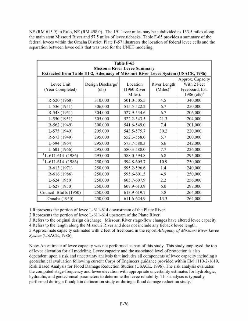
F-76

NE (RM 615.9) to Rulo, NE (RM 498.0). The 191 levee miles may be subdivided as 133.5 miles along the main stem Missouri River and 57.5 miles of levee tiebacks. Table F-65 provides a summary of the federal levees within the Omaha District. Plate F-57 illustrates the location of federal levee cells and the separation between levee cells that was used for the UNET modeling.

Table F-65 Missouri River Levee Summary

Extracted from Table III-2, Adequacy of Missouri River Levee System (USACE, 1986)

Levee Unit (Year Completed)

Design Discharge3

(cfs)

Location

(1960 River Miles).

River Length

(Miles)4

Approx. CapacityWith 2 Feet

Freeboard, Est. 1986 (cfs)5

R-520 (1960) 310,000 501.0-505.5 4.5 340,000 L-536 (1951) 306,000 515.5-522.2 6.7 250,000 R-548 (1951) 304,000 527.9-534.6 6.7 206,000 L-550 (1951) 305,000 522.2-543.5 21.3 204,000 R-562 (1949) 300,000 541.6-549.0 7.4 201,000 L-575 (1949) 295,000 543.5-575.7 30.2 220,000 R-573 (1949) 295,000 552.3-558.0 5.7 200,000 L-594 (1964) 295,000 573.7-580.3 6.6 242,000 L-601 (1966) 295,000 580.3-588.0 7.7 226,000

1 L-611-614 (1986) 295,000 588.0-594.8 6.8 295,000 2 L-611-614 (1986) 250,000 594.8-605.7 10.9 250,000

R-613 (1971) 250,000 595.2-596.6 1.4 240,000 R-616 (1986) 250,000 595.6-601.5 4.9 250,000 L-624 (1950) 250,000 605.7-607.9 2.2 256,000 L-627 (1950) 250,000 607.9-613.9 6.0 297,000

Council Bluffs (1950) 250,000 613.9-619.7 5.8 264,000 Omaha (1950) 250,000 611.6-624.9 13.3 264,000

1 Represents the portion of levee L-611-614 downstream of the Platte River. 2 Represents the portion of levee L-611-614 upstream of the Platte River. 3 Refers to the original design discharge. Missouri River stage-flow changes have altered levee capacity. 4 Refers to the length along the Missouri River and does not include any tieback levee length. 5 Approximate capacity estimated with 2 feet of freeboard in the report Adequacy of Missouri River Levee System (USACE, 1986). Note: An estimate of levee capacity was not performed as part of this study. This study employed the top of levee elevation for all modeling. Levee capacity and the associated level of protection is also dependent upon a risk and uncertainty analysis that includes all components of levee capacity including a geotechnical evaluation following current Corps of Engineers guidance provided within EM 1110-2-1619, Risk Based Analysis for Flood Damage Reduction Studies (USACE, 1996). The risk analysis evaluates the computed stage-frequency and levee elevation with appropriate uncertainty estimates for hydrologic, hydraulic, and geotechnical parameters to determine the levee reliability. This analysis is typically performed during a floodplain delineation study or during a flood damage reduction study.

F-77

Private Levees. Following construction of river training structures, federal levees, and chute closures, deposited sediment filled many areas riverward of the federal levees. Farming of these areas became extensive. To prevent crop damages caused by normal high flows on the Missouri River, farmers constructed secondary levees at or near the river bank. Many of the secondary private levees tie directly into the federal levees. Private levees have also been constructed along the river bank in areas where federal levees were not constructed. The left bank reach from river mile 515.5 to river mile 498.0 near Rulo, NE is protected solely by private levees. Total length of private levees along the Missouri River, interior levees, spoil banks, and tiebacks is unknown but is substantial. UNET Levee Modeling Parameters. All federal levees were included within the UNET model as separate cells. Description within the UNET model of the levee area consists of the specification of stage vs. storage curves. Many of the large levee cells were subdivided using interior topographic features such as roads or railroads. Stage-storage relationships were determined using the 1999 digital terrain model. The stage-storage curves were smoothed to reduce model instability. Stage-storage curves developed for each of the UNET model storage cells are displayed in Plates F-58 to F-84. The levee cell is connected to the mainstem Missouri River within the UNET model. Connections were established within the UNET model at the upstream and downstream limits of each levee cell. During the POR analysis, the model will activate either or both levee connection if the computed water surface elevation exceeds the coded levee top elevation. When both the upstream and downstream connections are active, the levee cell conveys flow parallel to the main river. Levee connections are specified within the UNET model using the levee SF card. Plate F-85 summarizes levee design details and parameters specified within the UNET model. Incorporation of UNET modeling of levee failures is as follows: UNET Model Levee Modeling Assumptions:

a. Private levees within the Omaha District were not included as levee cells. b. Levee cells contain at least 2 river connections, generally located at the downstream and upstream

end of the levee cell. c. Levee top elevations were coded at the top of levee using the best available survey data. d. Levees were coded within the UNET model to fail when the top of levee elevation is exceeded. e. Flood fighting efforts were not considered in the analysis. f. For the POR analysis, levee cells repair after the river stage drops below the stage specified

within the UNET model. Thus, the model restores the levee to the original elevation for following years during the POR.

Connection with the SF card allows the simulation of flow within the levee cell during extreme events. Simulation with the SF card requires the specification of several factors as follows: RE 19 534.90 SF -25 903.7 892 .010 0.01 48. 0.0 0.0 The RE card specifies the reach number (19 for this example) and the river mile for the connection (534.90) to the Missouri River. The SF card specifies the storage cell number to connect with (-25), the water surface elevation at which the levee breach initiates (903.7), the elevation for the levee breach repair (892), the linear routing constant for flow from the river to the levee cell (.01), the linear routing constant for return flow from the levee to the river (.01), and the time in hours to fill the levee cell assuming a constant inflow (48). The specified linear routing coefficients impact the rate of flow transfer from the river to the levee cell. Model evaluation determined that setting the coefficient too high caused model instability. Linear routing coefficients were patterned after the L550 levee failure during the 1993

F-78

event. POR analysis employed routing coefficients of 0.01 and 0.02. Sensitivity analysis was performed to evaluate the impact of the levee failure routing coefficients. Application to Regulatory Flood Profiles The UNET model developed for this study employed the top of levee elevation for all levee connections. The model also assumes a levee breach occurs when the computed river elevation exceeds the levee top elevation. Levee modeling assumptions were coordinated during task force meetings with Corps of Engineers, FEMA, and state representatives. A description of the discussion and conclusions is presented within Appendix A. Previous Missouri River studies within the Omaha District conducted to develop regulatory products such as the stage-frequency elevation and floodway (USACE, 1978) used different assumptions including levee overtopping without any levee breach. Therefore, modeling for regulatory purposes to establish floodway locations may require additional evaluation of levee performance. An estimate of the minimum level of protection provided by the individual federal levee units was not performed as part of this study. Levee level of protection and the associated levee capacity are dependent upon a risk and uncertainty analysis that includes estimating the uncertainty for many parameters. Risk and uncertainty analysis should follow the guidance provided within Appendix A and the current Corps of Engineers guidance provided within EM 1110-2-1619, Risk Based Analysis for Flood Damage Reduction Studies (USACE, 1996). The risk analysis evaluates the computed stage-frequency relationship and levee elevation at each location with appropriate uncertainty estimates for hydrologic, hydraulic, and geotechnical parameters to determine the levee reliability. This analysis is typically performed during a floodplain delineation study or during a flood damage reduction study. Refer to the Risk and Uncertainty Analysis Data section for further details. UNET CALIBRATION. UNET model calibration was performed in a series of steps. Initial model assembly and debugging was performed with HEC-RAS to set base roughness values, bank stations, reach lengths, and similar cross section parameters. UNET calibration was performed for historical events, measured water surface profiles, and high water mark data. Model calibration was performed for different flow periods to include a full range of flows. All UNET model calibration was performed with daily flow data. Previous studies have used hourly data to achieve better model reproduction of observed values. However, since the intended model use is for the POR analysis that uses daily flow records for all inflow, daily values were also used for model calibration to provide modeling consistency. Calibration Data Calibration data consisted of the gage station flow and stage records listed in Table F-64, measured water surface profiles, and high water mark data. Selected calibration events varied according to location. Calibration was performed with both flow and stage data. Gage station data consists of observed stage and flow hydrographs and actual USGS discharge measurements taken at the gaging station. Discharge measurements are taken at least once a week on the mainstem Missouri River. Discharge measurements illustrate seasonal variation in the stage-discharge relationship that occurs on the Missouri River. UNET Calibration Procedure Overview. Calibration of the UNET model was an iterative process performed in several stages. Calibration efforts focused on reproducing observed stage hydrographs at gaging stations along the Missouri River and verifying with discharge measurements. Calibration of an unsteady flow model is an iterative process. Significant changes to model geometry will also affect routed flow. The calibration process strives to maintain both flow and stage accuracy. Initial calibration was performed by setting Manning roughness values at each cross section. The calibration was refined by adjusting the developed rating curves (KR records) in order to correct for

F-79

deficiencies. The conveyance change and discharge conveyance relationship can also be used in conjunction with the rating curves to finalize the model calibration. Therefore, final calibration is a combination of the effects of all the parameters employed in both the geometry and boundary condition files. A brief overview of the main procedures used in model calibration is as follows: Base Roughness. The base Mannings’ roughness values were calibrated to recent measured steady water surface profiles. All measured profiles were for within channel flows in the normal operating flow range during the navigation season. Ungaged Inflow. The model evaluates ungaged inflow using the Null Internal Boundary Condition. This parameter is an important feature to maintain model flow consistent with observed gage data. Automated Calibration. Once the model is nearly calibrated, the automated calibration is performed by pairing observed stages at the stream gages on the Missouri River with routed flow. Initial values are determined by fitting a fifth order polynomial to the paired data to create a rating curve. Data is stored in a DSS file for use with UNET. Since for each flow, a water surface elevation is produced at each cross-section, this procedure develops a relationship between elevation and factor at each cross-section. Using a KR record in the UNET geometry file at each stream gage location, this relationship is then applied to the ordinates in the cross section tables. The KR DSS file record is modified during the calibration process to increase accuracy. Calibrated KR records were employed at all river gaging stations. Final Calibration. Final calibration was performed using conveyance change and discharge-conveyance relationships for separate reaches within the model. The conveyance change relationship applies a constant factor to the cross section conveyance and storage determined from section geometry. The discharge-conveyance relationship applies a factor to cross section conveyance that may be varied according to flow rate. Base Manning Roughness Values. Initial horizontal roughness values were assigned based on material type using available aerial photographs. Various roughness values were assigned to represent the channel, sand bars, farmland, woody vegetation, and urban areas. Material types were defined using aerial photographs and then translated to the HEC-RAS model. Since the aerial photographs were not ortho-rectified with the digital terrain model, some difficulties were encountered when setting the horizontal roughness for each cross section. Adjustments were made to the horizontal roughness station within the cross section based on elevation data when required. Within the reach from Gavins Point Dam to Ponca, the Missouri River is a braided stream with numerous islands. Significant channel degradation and bank failure has occurred following the collection of hydrographic data used within the model. The channel in this area is active with migrating sand bars and other indications of instability. Unreasonable roughness values were required in this location to compensate for the poor model geometry data. The roughness values allowed computational results to match observed water surface elevations from recent flow events. Base roughness values were determined within the model using calibration data at the gaging stations and the measured profiles. Calibration of tributary routing reaches was not performed. Stage calibration was performed on a system wide basis for the entire hydrograph. Base channel roughness values varied throughout the model. Note: The base roughness values do not represent final calibration values for the UNET model. In addition, roughness values for an unsteady flow model differ from a steady flow model such as HEC-RAS due to computational differences. Calibration with HEC-RAS or a similar model will require the use

F-80

of different roughness values than those employed in the UNET model. In addition, roughness values at bridge sections were increased to provide additional head loss. UNET does not employ standard expansion and contraction losses such as steady flow model. Refer to the HEC-RAS manual users guide for an explanation of computation differences between unsteady and steady flow models at structures (HEC, 2002). Table F-66 summarizes the range of roughness values employed within the model.

Table F-66 Base Model Roughness Values

River Mile Range Channel N Floodplain N Method2 810 – 804 .0211 .037 – 0.085 Horizontal Roughness 803 – 802 .0241 .037 – 0.085 Horizontal Roughness 801 – 789 .033 - .0381 .037 – 0.085 Horizontal Roughness 788 – 776 .025 - .0271 .037 – 0.085 Horizontal Roughness 775 – 768 .028 - .0301 .037 – 0.085 Horizontal Roughness 768 – 745 .026 - .0231 .037 – 0.085 Horizontal Roughness 745 – 710 .0231 .055 Channel Roughness 710 – 691 .0221 .055 Channel Roughness 690 – 669 .026 .055 Channel Roughness 668 – 618 .024 .055 Channel Roughness 618 – 615 .024 .042 Channel Roughness 614 – 590 .024 .038 - .057 Horizontal Roughness 590 – 584 .027 .038 - .057 Horizontal Roughness 584 – 567 .026 .038 - .057 Horizontal Roughness 566 – 498 .027 .038 - .057 Horizontal Roughness

1 Unreasonable Manning N values were required to match measured profile data at some locations. Hydrographic survey data, collected in 1994 and 1995, does not reflect the impact of the 1997 sustained high Gavins Point release that caused significant channel modification as previously described. 2 At some locations, the horizontal roughness variation was changed to standard channel roughness due to calibration errors. Application of Null Internal Boundary Condition for Ungaged Inflow. The Null Internal Boundary Condition (NIBC) is a tool for estimating ungaged lateral inflow in a river system. The NIBC feature is used by the Omaha District to reproduce flow at the USGS gage locations at Sioux City, Decatur, Omaha, Nebraska City, and Rulo. Use of the NIBC is an important component of calibrating the model to both flow and stage. The technique optimizes ungaged inflow to reproduce either a stage hydrograph or a flow hydrograph at the NIBC station. When optimizing the stage hydrograph, the reproduction of flow is secondary, being dependent on the calibration of the model. Likewise, when optimizing the flow hydrograph, the reproduction of stage is secondary, being dependent on the calibration of the model. Optimizing stage is generally used for a flood forecast model, where stage accuracy is the primary goal. Optimizing flow is used whenever the observed flow record must be maintained, such as a period-of-record frequency analysis. In either case, the ungaged inflow compensates for all the errors in the measurement of stage and flow and for systematic changes in roughness and geometry that may not be included in the model. As a result, the ungaged inflow determined using the NIBC procedure includes both flow and an error correction term.

F-81

All ungaged inflow was determined by optimizing flow. Using the observed flow hydrographs, the river routing reach is divided into two routing reaches that are bounded by two streamflow gages. For example, Omaha to Nebraska City forms a routing reach bounded by gage stations. Flow is routed from the upstream station to the downstream station using the upstream flow. This flow does not include the ungaged flow. Next, to determine the flow at the downstream location with the ungaged included, the flow upstream based on a stage boundary condition is computed from the hydrodynamics and the geometry reach downstream. The ungaged inflow hydrograph is determined using DSSMATH procedures. The hydrograph is estimated by subtracting the routed hydrograph from the computed hydrograph. The computed difference is lagged backward in time and inserted into the model as a uniform lateral inflow. The lag time varies according to travel time between the gage stations. Ungaged inflow between the gaging stations is distributed according to drainage area. The ungaged drainage area is summarized within Plate F-52. A further description of the NIBC employed within the Omaha District is available in appendix F-E. A comparison between UNET determined ungaged inflow using the Null Internal Boundary Condition and ungaged inflow determined for the Omaha District hydrologic analysis (the UFDM model) was not performed. The two models are not computationally similar and will not produce similar results. An evaluation of the impact of ungaged inflow on POR results was evaluated in the sensitivity analysis. Application of Automatic Calibration Conveyance Adjustment After setting base roughness values, the model was calibrated to reproduce rating curves at the principal gaging stations along the Missouri. The base roughness values were determined to match the highest observed event at each gage station. The automatic calibration conveyance adjustment record continues the base roughness replication at the highest stage and also allows modification of the stage-discharge relationship for other events. In essence, this allows the model to incorporate a change in roughness for different flows compared to the base calibration model that relies on fixed roughness values within each element of the horizontal section. The rating curve calibration technique is described in the report “Rating Curve Calibration” (Barkau 1994). A rating curve reflects the stage-conveyance structure of the cross-section. At elevation z the conveyance is computed from Manning’s Equation,

ARn49.1K 3/2= (1)

where: K = conveyance. n = Manning’s roughness factor.

,WAR

p

= the hydraulic radius (ft).

=pW the wetted perimeter (ft). A = cross-sectional area (sq ft). In equation 1 the area and the wetted perimeter are cross-section properties, but the roughness is unknown. If the friction slope, Sf, is known, the conveyance can be computed from

2

f KQS

= (2)

where:

F-82

Q = flow (cfs) When the stream gradient is steep (greater than ten feet per mile), the water surface slope approximately equals the friction slope and conveyance can be computed from the rating curve. But, when the gradient is shallow, the friction slope is controlled by backwater and conveyance cannot be calculated from a single rating curve. If a second rating curve is known at a downstream cross-section, the stage at the upstream cross-section can be computed using steady state backwater. A constant flow is assumed between the first and second rating curve and many cross-sections can be defined between the rating curves. Most likely the upstream stage will not match the stage at the upstream rating curve for the constant flow. Adjusting Manning’s “n” to match the stage at the upstream rating curve calibrates the reach to reproduce the upstream rating curve. Note that the entire reach is being calibrated. The stages at the intermediate cross-sections may not be correct, but no information is available to further refine the calibration. The Manning’s “n” can be different from cross-section to cross-section. Generally, one assumes a constant “n” value for the wetted channel area along a reach, but “n” values for exposed areas such as islands in the channel and overbank areas can vary from cross-section to cross-section. The density and type of the vegetation is variable. Base roughness values address the observed variation at each cross section using available topographic and aerial data. Base channel calibration was performed using the measured profile data. Base cross section calibration was also performed using high water mark data. When calibrating a model, the special variation of Manning’s “n” from cross-section to cross-section poses a problem. How does one distribute changes in roughness throughout the reach? The calibration reach has stage information at the upstream and downstream ends and nothing in between. Therefore, changing roughness uniformly through the reach is a reasonable solution to this problem. River stage is inversely related to conveyance: Increasing conveyance causes water levels to fall and decreasing conveyance causes water levels to rise. When calibrating river conveyance, multiplying a single conveyance factor times the conveyance properties at all the cross-section can adjust the reach to reproduce an upstream stage. Hence, optimizing a single reach calibration factor calibrates a reach for a single flow. While the base calibration remains the basis of the stage-flow relationship at each individual cross section, the calibration is refined on a reach basis using the automatic calibration adjustment. The automatic calibration technique was employed to modify the base roughness values for each reach. Base roughness values for the model were determined to match the maximum observed stage. Therefore, the automatic calibration record is employed to increase accuracy for a full range of flows. Within the federal levee reach, the KR card selection must be consistent with the levee modeling method. For levee overtopping flows, total conveyance should reflect flow conveyed on the floodplain side of the levee. Within the Omaha District, all federal levees were modeled as cells. The predominant impact of levee cells is to provide storage. Limited conveyance through the upstream and downstream connections of the levee cell is possible. For extreme events, the linear storage routing coefficients limit the amount of flow conveyed behind the levee. UNET has an additional option, referred to as the Kansas City levee algorithm, for modeling floodplain conveyance. This method produces excellent results within the Kansas City District on the Missouri River for the 1993 flood event. Refer to Appendix E of this report for additional information regarding the Kansas City modeling methods. The 1993 flood provided sufficient data to calibrate the floodplain routing within the Kansas City District. However, within the Omaha District the 1993 flood peaks were much lower and calibration data for floodplain routing was not available. Model results for the POR analysis show that for extreme events flow is transferred between adjacent levee cells parallel to the main channel as previously described in the levee section of this appendix. The interaction between levee cells and computed river elevation is variable and dependent on

F-83

model calibration and levee connection parameters. Therefore, sensitivity analysis was performed to evaluate the impact of levee parameters and the KR record on computed results. Fine Tuning for Flow/Stage Effects The UNET program has three tools for fine-tuning the calibration of the model. These tools are applied within the boundary condition file and consist of different methods to affect the discharge-stage-conveyance relationship at a cross section within the model. Conveyance Change Factors. These factors, one for the channel and one for the overbank, adjust the conveyance at multiple cross-sections for all stages. The factors simulate a systematic change in roughness – one that is apparent for all stages over the entire length of the simulation. Discharge-Conveyance Change Factors. This relationship adjusts conveyance with discharge over multiple cross-sections along the same river, a calibration reach. This relationship is the primary tool for adjusting systematic errors in stage at the same discharge. Seasonal Conveyance Change Factors. This relationship changes an overall conveyance multiplier with time, simulating seasonal shifts in roughness. The seasonal factor is applied to all the cross-sections in a calibration reach at all stages. Conveyance Change Factors Increasing a conveyance change factor causes the computed stage to fall and decreasing the conveyance change factor causes the computed stage to rise. For each separate calibration reach, a table of discharge and conveyance change factors may be specified. A conveyance change factor for discharge Qi is

where: Fi = conveyance change factor for discharge i. Knew = new conveyance value. Kold = old conveyance value. For each river discharge Qi, the conveyance property is multiplied by Fi, thereby adjusting the calibration of the model. An example of a conveyance change specified within the bc file is: REACH=15 CONVEYANCE CHANGE FACTORS 591.5 568.63 1 21 0.95 0.95 -0.85 -0.85 0 0

The format of the conveyance change factors are explained within the UNET Manual. The channel and overbank factors are multiplied times the 21 channel and overbank conveyance entries in the cross section table for sections within the specified range. Within the final calibration model, conveyance change factors were employed on a limited basis. Discharge – Conveyance Change Factors. These factors are also applied to section conveyance. The factors are specified for a range of cross sections for various discharges. A table of flow and conveyance change factors are defined manually. The table values are always at an equal interval of flow, in this case 20,000 cfs. The flow range, 0 to 380,000 cfs, is the expected range of flow. At each time step, conveyance change factors are interpolated from the flow at each cross-section in the calibration reach. Therefore, each cross-section has a different

old

newi K

KF =

F-84

factor, since the routed flow is different at each cross-section. Within the final calibration model, limited use of the discharge-conveyance factor was employed. Factors were employed in some reaches to enhance reproduction of high water mark data. An example of a discharge-conveyance specification is as follows: REACH=15 DISCHARGE-CONVEYANCE RELATION 594.82 583.0 20000 20000 16 20000 1.00 40000 1.00 60000 0.92 … and continued at a 20000 cfs increment for 20 values. Modify Seasonal Conveyance. The seasonal conveyance change factors adjust the conveyance for all stages according to a time series of factors. Larger rivers such as the Mississippi and the Missouri have a cold season roughness regime and a warm season roughness regime. During the cold season, the more viscous water reduces the period and height of the dunes, reducing the roughness. The initiation of roughness changes can be predicted by water temperature. Studies conducted by the Omaha District have verified the roughness change (USGS, 1976). However, the time at which the roughness change occurs varies yearly. The fall season roughness transition usually occurs around October. The spring season transition occurs in late April or early May with a transition period from one to two weeks. Minor modifications in vegetation height and density may also be addressed by the seasonal factor. However, the factor is applied uniformly to the entire section. An example of a seasonal conveyance change specified is: REACH=7 SEASONAL CONVEYANCE CORRECTION 714.99 669.23 11 01JAN 1.05 25APR 1.05 15MAY 1.05 25MAY 1.03 05JUN 1.0 20JUL 0.99 15SEP 1.00 01OCT 1.02 15OCT 1.04 01NOV 1.05 31DEC 1.05 Seasonal calibration parameters were evaluated during the calibration process. Refer to section Calibration Events and Results for a discussion of seasonal factors employed for the POR analysis. Model Implementation of Calibration Factors. One or all of the section conveyance change factors may be specified within the model. Within the model, at cross-section i, the adjusted conveyance is

ixsSiQFcci K)T(F)Q(FFK ⋅⋅⋅= (3) where: Ki = adjusted conveyance at cross-section i. FCC = conveyance change factor, a constant value. FQF(Qi) = discharge conveyance change factor, interpolated from the flow, Qi, at cross-section i. FS(T) = seasonal conveyance change factor at day T.

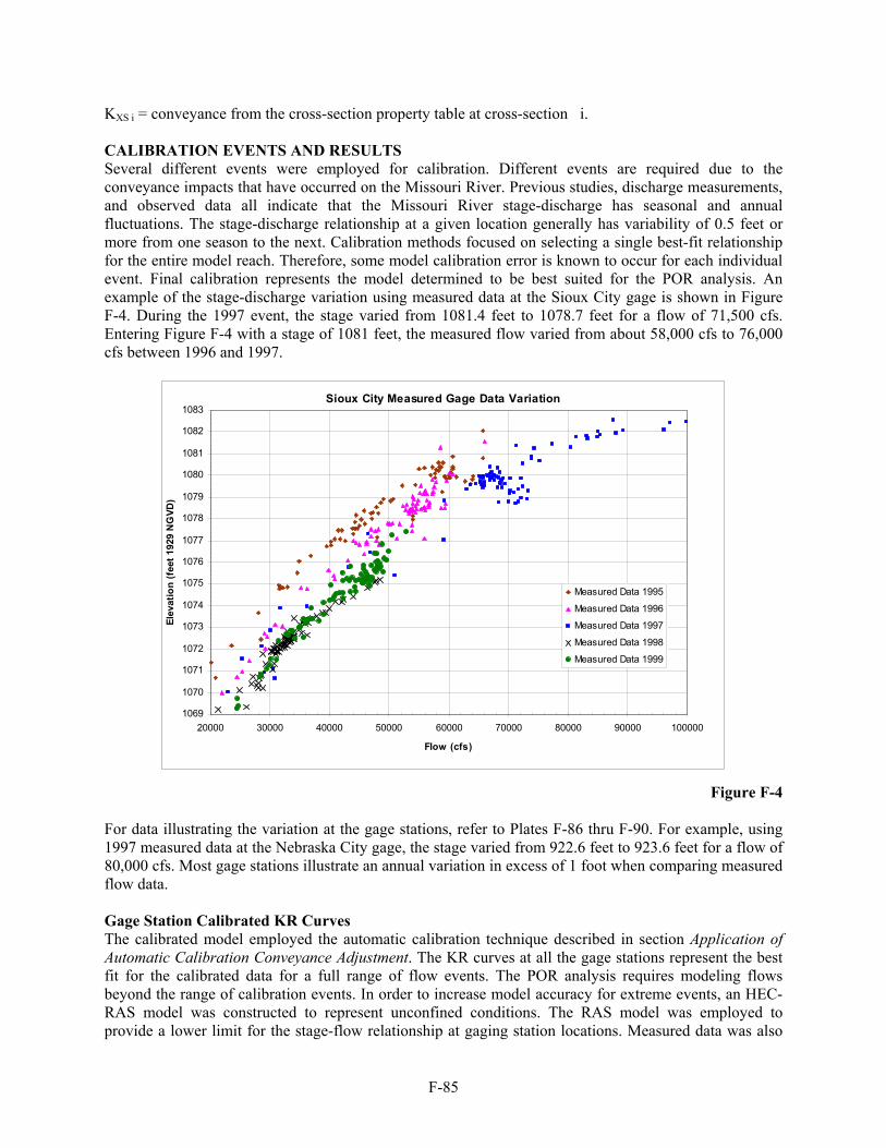
F-85

KXS i = conveyance from the cross-section property table at cross-section i. CALIBRATION EVENTS AND RESULTS Several different events were employed for calibration. Different events are required due to the conveyance impacts that have occurred on the Missouri River. Previous studies, discharge measurements, and observed data all indicate that the Missouri River stage-discharge has seasonal and annual fluctuations. The stage-discharge relationship at a given location generally has variability of 0.5 feet or more from one season to the next. Calibration methods focused on selecting a single best-fit relationship for the entire model reach. Therefore, some model calibration error is known to occur for each individual event. Final calibration represents the model determined to be best suited for the POR analysis. An example of the stage-discharge variation using measured data at the Sioux City gage is shown in Figure F-4. During the 1997 event, the stage varied from 1081.4 feet to 1078.7 feet for a flow of 71,500 cfs. Entering Figure F-4 with a stage of 1081 feet, the measured flow varied from about 58,000 cfs to 76,000 cfs between 1996 and 1997.

Figure F-4 For data illustrating the variation at the gage stations, refer to Plates F-86 thru F-90. For example, using 1997 measured data at the Nebraska City gage, the stage varied from 922.6 feet to 923.6 feet for a flow of 80,000 cfs. Most gage stations illustrate an annual variation in excess of 1 foot when comparing measured flow data. Gage Station Calibrated KR Curves The calibrated model employed the automatic calibration technique described in section Application of Automatic Calibration Conveyance Adjustment. The KR curves at all the gage stations represent the best fit for the calibrated data for a full range of flow events. The POR analysis requires modeling flows beyond the range of calibration events. In order to increase model accuracy for extreme events, an HEC-RAS model was constructed to represent unconfined conditions. The RAS model was employed to provide a lower limit for the stage-flow relationship at gaging station locations. Measured data was also

Sioux City Measured Gage Data Variation

1069

1070

1071

1072

1073

1074

1075

1076

1077

1078

1079

1080

1081

1082

1083

20000 30000 40000 50000 60000 70000 80000 90000 100000

Flow (cfs)

Elev

atio

n (f

eet 1

929

NG

VD)

Measured Data 1995

Measured Data 1996

Measured Data 1997

Measured Data 1998

Measured Data 1999

F-86

consulted when available. The final model employed an automatic calibration record that reflects the best fit to the calibration events plus a method of extending model to simulate extreme events. Gage station UNET model curves, measured data, and HEC-RAS computed data are illustrated in Plates F-91 thru F-102. Sensitivity analysis to evaluate the impact of the automatic calibration was performed and is discussed in section Sensitivity Analysis. Seasonal Variation Calibration The UNET model was calibrated to reproduce summer stages with normal roughness values. Therefore, the spring and fall seasonal adjustments are to increase conveyance and generate a lower stage at the same flow that occurred during the summer. The gage station data shows that the seasonal roughness change magnitude varies with location. Observed data from the 1997 event, which had a fairly constant flow from May through October, demonstrates the seasonal change at the gaging stations. For the POR analysis, the seasonal conveyance change was applied in a standard manner to account for possible variations in the date that the seasonal variation occurs. In addition, the seasonal conveyance change factors were reduced to a minimum in order to avoid underestimating stages for some events and reduce profile conflicts. In the historic record prior to dam construction, many annual peaks were caused by snowmelt and occur in the April time period. However, the system of reservoirs for the current condition significantly reduces spring snowmelt runoff below Gavins Point Dam. Therefore, the POR analysis capped seasonal adjustments at a reasonable value in order to accurately predict annual peak stages. The stage reduction caused by the seasonal factors is particularly noticeable at the Decatur, Blair, Omaha, and Plattsmouth gages. As a result, the April to May 1997 calibration at these gage stations shows more error than other locations. However, employing a larger seasonal adjustment to further reduce computed stage was determined to be non-conservative and not desirable for the POR analysis. A large seasonal adjustment factor will increase the variability of the computed stage-flow results. The time and degree of seasonal adjustment varies annually. Historical events illustrate that calibration to spring\fall and summer events is not possible with the same calibration parameters. The historical period of record includes a significant flow record that does not reflect the current flood control reservoir storage. Since most flood events in the post-reservoir construction era downstream of Omaha occur in the summer, the seasonal adjustment was limited to provide a summer weighted flow-stage relationship. For the purpose of determining valid annual maximum stage-flow relationships, the POR analysis focused on the reproduction of summer stages to develop an accurate annual maximum stage-flow relationship that is not dependent on the seasonal time that the event occurs. The spring roughness change, expressed within the model as a conveyance factor, was limited to a maximum value that varied depending on location. The selected maximum value was used to reflect possible flood sources at each location. Within the Gavins Point Dam (RM 811.1) to Sioux City (RM 732.3) reach, the maximum adjustment factor applied to base summer conveyance was 1.05. This factor was transitioned downward to a value of 1.03 at Omaha (RM 615.9) and a value of 1.02 below the Platte River. The transition reach was selected based on Gavins Point releases for the regulated period and tributary inflow. Since the time and degree of the seasonal shift varies, using higher conveyance change factors was determined to be non-conservative for the POR analysis. In order to evaluate the transition used for the seasonal adjustment, measured gage data was evaluated. The evaluation was performed in an attempt to determine a definite correction that could be applied within the model. Measured data at the Omaha gage was evaluated to determine an average seasonal adjustment. However, the measured data did not reveal a definite trend that could be used to set the maximum seasonal adjustment or refine the transition of the adjustment factor. Therefore, the empirically determined factors and the adopted transition reach from Sioux City to Plattsmouth were used in the POR analysis. Refer to Plate F-103 for an illustration of the varying seasonal shift at Omaha.

F-87

Measured Profiles The Omaha District routinely collects Missouri River water surface profiles between Gavins Point Dam and Rulo, NE. The profiles are typically collected at a fairly constant inflow period to avoid changing tributary inflow to the extent possible. As a result, the profiles are usually collected during a normal flow period and are not available for high flow events. Calibration efforts used the measured profile data to verify the channel roughness value. Four different events were utilized for the calibration. Plots illustrating the calibration accuracy are illustrated in Plates F-104 thru F-109. The highest recent measured profile occurred in May 1997 with a flow rate that varied from 70,000 cfs at Yankton to 120,000 cfs at Rulo. Selection of Calibration Events As previously discussed in the section Aggradation and Degradation Trends, the Missouri River stage-discharge relationship has changed considerably with time. Calibration events are limited to include only events that are applicable to current conditions. The calibration event selected varied by gage station. A summary of the selected events are illustrated in Table F-67.

Table F-67 Selection of Missouri River Calibration Events

Missouri River Gage

River Mile

Observed Peak Elev.1 (ft)

Peak Flow1 (cfs)

Date

Appr. Flow Freq.2 (Yrs)

Remark

Yankton, SD 805.8 1159.2 68,000 Oct 97 25 Degradation impact, only valid events

are post 1997 Gayville, SD 796.0 1152.1 78,200 Apr 97 >10 Degradation impact, only valid events

are post 1997

Maskell, SD 775.6 1128.1 76,000 Apr 97 >10 Degradation impact, only valid events are post 1997

Ponca, NE 751.0 1101.1 77,000 Apr 97 >10 Degradation impact, only valid events are post 1997

Sioux City, IA 732.3

1082.8 1080.0 1087.0

97,000 69,000 103,000

Apr 97 Jul 97 Jun 84

25 >5 >25

Degradation impact, only valid events are post 1997. 1984 event not used due to degradation.

Decatur, NE 691.0 1041.0 1042.0 1044.6

100,000 75,000 98,000


25 >5 <25

1997 is primary event, degradation in 1997 that may not be permanent. Note stage change since 1984

Blair, NE 648.3 1002.2 1004.2 1004.6

106,000 102,000 117,000


< 10 <10 10

1993 and 1997 are equal weighted events for calibration, 1984 is secondary

Omaha, NE 615.9 974.6 978.2 977.3

109,000 118,000 114,000


<10 <10 <10

1993 is primary event, 1997 and 1984 are secondary, some stage-flow changes have occurred

Plattsmouth, NE 591.5

957.2 964.2 963.1

116,000 193,000 184,000


5 >25 <25

1993 primary event, notable stage-flow change since 1984

Nebraska City, NE 562.6

926.5 932.1 930

115,000 188,000 180,000


<5 25 <25


Brownville, NE 535.3

896.8 904.2 900.5

117,000 230,000 210,000


<5 >50 50


F-88

Table F-67 Selection of Missouri River Calibration Events

Missouri River Gage

River Mile

Observed Peak Elev.1 (ft)

Peak Flow1 (cfs)

Date

Appr. Flow Freq.2 (Yrs)

Remark

Rulo, NE 498.0 857.6 862.3 961.5

120,000 290,000 215,000


<5 >100 50

1993 primary event, limited stage-flow change since 1984

1 The tabulated peak flow and stage values are the average daily flow determined from gaging station records. Computed peak flow is tabulated at COE non-rated gages where USGS flow is not available. 2 The tabulated approximate frequency is that flow frequency that corresponds to the peak flow determined at the gage site. The stage value does not necessarily correspond to the results from the stage-frequency study at the gage location. Flow and Stage Reproduction at Gages Calibration was performed at all gage stations shown in Table F-64. The NIBC was employed to enhance model reproduction of observed gage station flow. For the 1997 event, flows were more constant through the summer months. For the 1993 event, significant inflow between the gage stations occurred. Good reproduction of observed flow was achieved for all calibration events. Model results determined large negative values for ungaged inflow for some reaches and events. In particular, the Omaha to Nebraska City reach shows a persistent negative inflow even during periods with constant tributary inflow from the Platte River and Weeping Water Creek. Negative ungaged inflow for calibration was allowed to achieve the proper flow distribution. For the POR analysis, negative ungaged inflow was limited to –5000 cfs to eliminate concerns regarding unforeseen impacts to the energy gradient. An illustration of the model computed results and observed data at the gage locations are illustrated in Plates F-110 thru F-135. High Water Marks High water mark data is available for the 1984 and 1993 events between RM 515 and RM 616. The 1984 event is of secondary importance since significant changes to the floodplain topography have occurred since the 1984 event. Therefore, the current condition model is expected to produce some variation from the 1984 event. High water mark data should be evaluated with caution. The collected data exhibits some discrepancies with several points conflicting. Setting high water mark points following an extreme event is subjective and also may be impacted by unsteady flow phenomenon, levee failures (both federal and private), localized heavy rainfall, and the distribution of ungaged inflow. High water mark calibration accuracy for the 1984 event is reduced due to the general upward stage trend. Plots illustrating the high water mark calibration are shown in Plates F-136 thru F-139. Hourly Data Comparison All model analysis was performed with daily values for all inflow hydrographs. Previous modeling efforts used hourly flow data when available. In order to be consistent with the POR analysis, daily data was used. As a result, calibration accuracy is reduced. The reduction of calibration accuracy does not impact the final stage-frequency results since the analysis method relies on the developed stage-flow relationship. The use of hourly data allows further refinement of the ungaged inflow estimate. An illustration of the difference between hourly and daily data during the 1993 flood peak at Nebraska City is provided in Plate F-140. Calibration Results and Discussion Calibration results varied with gage location. Missouri River stage trends, seasonal variation, and natural variation limit calibration accuracy. The stage trend impact is very noticeable when comparing the 1984 event to the 1993 event at Brownville, Nebraska City, and Plattsmouth gages. Data from 1997 indicates

F-89

that stages-flow relationship decreased at most locations. The data illustrate the impact of sustained high flows on the stage-flow relationship. Table F-68 summarizes calibration peak stage accuracy. The 1952 flood is the record flow event through the Omaha District on the Missouri River. Because of the significant changes within the stage-flow relationship, this event is not suitable for use with calibration. The 1952 event was used to provide general information concerning the shape of the rating curve for extreme events using the measured flow data. Also, off channel storage areas were provided between Sioux City and Omaha to approximate the discharge reduction that was observed in the 1952 flood. Calibration of the 1993 flood required a deviation from the POR model in order to simulate failure of the L550 levee upstream of Brownville. During the 1993 flood, the L550 levee failed as the result of a geotechnical failure, not overtopping. All levee failure within the POR analysis was coded to fail by levee overtopping.

Table F-68 Missouri River Calibration Accuracy Summary

Missouri River Gage

River Mile

Observed Peak Elev.1

(ft)

Computed Peak Elev.1

(ft)

Difference (Computed -Observed)

(ft)

Date of

Peak

Peak Flow1 (cfs)

Yankton, SD 805.8 1159.1 1159.2 0.1 1 Oct 97 67,700

Gayville, SD 796.0 1151.8 1152.0 0.2 1 May 97 78,200

Maskell, SD 775.6 1128.0 1127.9 -0.1 1 May 97 73,500

Ponca, NE 751.0 1101.1 1100.9 -0.2 29 Apr 97 77,000

Sioux City, IA 732.3

1082.8 1080.3 1087.0

1082.8 1080.3 1084.2

0.0 0.0

-2.8 (degradation)

10 Apr 97 2 Jul 97

25 Jun 84

97,400 67,200

103,000

Decatur, NE 691.0 1041.6 1042.0 1044.6

1042.3 1041.1 1042.9

0.7 (minimal degradation)

-0.9 -1.7

12 Apr 97 16 Jul 93 26 Jun 84

99,000 75,000 98,000

Blair, NE 648.3 1002.2 1004.2 1004.6

1003.6 1004.3 1005.9

1.4 (seasonal adjust.) 0.1 1.3

16 Apr 97 17 Jul 93 27 Jun 84

106,000 100,000 117,000

Omaha, NE 615.9 974.6 978.2 977.3

976.3 977.9 978.1

1.7 (seasonal adjust.) -0.3 0.4

17 Apr 97 11 Jul 93 27 Jun 84

108,000 113,000 114,000

Plattsmouth, NE 591.5

957.2 964.2 963.1

957.4 964.4 964

0.2 0.2 0.9

17 Apr 97 25 Jul 93 14 Jun 84

117,000 196,000 187,000

Nebraska City, NE 562.6

926.5 932.1 930.0

926.6 932.0 931.5

0.1 -0.1 1.5

18 Apr 97 23 Jul 93 15 Jun 84

113,000 190,000 180,000

Brownville, NE 535.3

896.8 904.2 900.5

896.6 904.1 903.9

-0.2 -0.1 3.4

14 Apr 97 23 Jul 93 15 Jun 84

117,000 230,000 220,000

Rulo, NE 498 857.6 862.3 861.5

858.9 862.6 861.4

1.3 0.3 -0.1

15 Apr 97 24 Jul 93 16 Jun 84

121,000 290,000 215,000

1 The tabulated peak flow and stage values are determined from model and gaging station daily values. 2 The difference value may require a timing shift to compare peak values. Refer to the plotted hydrographs for detailed comparison.

F-90

Notes regarding calibration accuracy at specific locations are: Sioux City to Gavins: The accuracy for the reach is good. Calibration is limited to a single event due to degradation impacts. Model results at Sioux City show nearly 3 feet of degradation from 1984 to 1997. Decatur: Model results shows degradation in 1997 compared to 1993 and 1984. Final calibration is a combination of all 3 events. Blair: Model results show over 1 foot of stage rise from 1984 to 1993 for a similar flow. The 1997 event shows significant seasonal adjustment. Omaha: Model results show a seasonal impact for the 1997 event. The 1993 and 1984 events are consistent. Plattsmouth: Model results show nearly 1 foot of change between 1993 and 1984 for a similar flow. Gage inundation may have impacted high water level accuracy for both the 1993 and 1984 event. Nebraska City: Model results show about 1.5 feet of stage rise between 1993 and 1984 for a similar flow. Brownville: Model results show over 3 feet of change between 1993 and 1984 for a similar flow. 1993 results are impacted by the L550 levee failure. Also, the Brownville gage was flooded and gage readings were performed manually. Rulo: Model results are consistent for 1993 and 1984. This location has an extremely flat stage-flow rating curve due to the very wide floodplain. The accuracy of computed flow may be reduced as a result. PERIOD OF RECORD SIMULATION The calibrated UNET model was used to perform a period of record analysis. For the hydraulic model, the period of record refers to the time frame from 1900 to 2000. The POR is slightly different from the previously performed hydrologic analysis. The POR analysis period corresponds to the gaging station data length of record that was available for analysis and was extended to the year 2000 to allow for model calibration to the most recent data. Refer to the Omaha District Hydrologic technical summary for details regarding the hydrologic analysis that was performed to determine 100-years of flow data at the Missouri River gaging stations. While significant geometry and conveyance changes have occurred in the past 100 years, the POR analysis uses the historical flow record, not the stage record. Since the model is calibrated to the current condition, the period of record analysis computes stages that would occur if the historical record were repeated. Ungaged Inflow Determination Additional analysis was performed to determine ungaged inflow for the period of record. Ungaged inflow determination was performed for the period of record using the procedure outlined in the section Application of Null Internal Boundary Condition for Ungaged Inflow. Inflow for the period of record analysis used the tributary gaging station record for the available length. The computation of ungaged inflow results in negative flow for many periods. Negative flow occurs due to natural phenomenon such as floodplain storage and groundwater recharge. Negative flow also may be due to model error. For the POR analysis, negative flow was eliminated to prevent model timing issues from impacting results by changing the local slope of the energy gradient. As a result, the POR analysis volume is larger than the observed flow data indicates. For the early portion of the record prior to the establishment of the tributary gage, the tributary drainage area was included in the ungaged drainage area. Most tributary gages were established in the period between 1928 and 1950. Therefore, prior to 1928 all inflow between the gaging stations was distributed within the UNET model based on drainage area. In addition, Missouri River mainstem flow data has reduced accuracy prior to 1928. Sensitivity analysis was performed to evaluate the impact of ungaged inflows.

F-91

Ungaged inflow determination for the POR analysis was performed by a contractor to the Omaha District. Refer to appendix F-F for details regarding the computation of ungaged inflow. It should be noted that the ungaged inflow determination was made with a series of models calibrated to produce reasonable flow and stages for the entire period of record. Computation of ungaged inflow also includes hydrograph timing. Channel changes and river shortening affect the timing of flow events. For these reasons, translating the ungaged inflow from the historic model to the current condition may have unforeseen impacts on the final results. The elimination of high negative ungaged inflow values mitigates potential impacts of these changes on POR results. The ungaged inflow computation focused on the preservation of peaks. While preservation of volume is recognized as important, volume is of secondary importance compared to peak flow and stage. The unsteady flow model requires a minimum base flow for the Missouri River and tributary reaches to achieve model stability during the period of record. For these reasons, the period of record model is not intended to provide computed volumes that are suitable for further volumetric based computations. Volume computations using computed results will determine a difference between model routed flows and observed gage flows. Sensitivity analysis was performed to evaluate the change in computed stage-frequency results caused by volume changes. Operational Policy The period of record analysis uses observed historical flow data. Therefore, any future operational changes that occur are not incorporated in the analysis. Any changes that occur in the Missouri River basin reservoir system operational policy would primarily affect flow-frequency below Gavins Point. Operational changes could also impact flow volume that may have stage impacts. Future changes in depletions or other consumptive use that would impact flow volume are also not addressed. Downstream of Gavins Point Dam, there are no operable structures on the main stem Missouri River. The federal levee system does not require operation. Flood fighting efforts were not considered in this analysis. UNET POR Simulation The POR analysis is performed with the calibrated UNET model. The analysis uses daily flow data for all inflow hydrographs with a 3 hour computational time step. The purpose of the POR analysis is to generate 100 years of stage-flow data at all UNET model cross section locations by simulating the observed flows. Annual maximum flows and stages are collected using the Annual Maximum flag within the UNET boundary condition file. In order to correctly account for total flow at a cross section, the flow within the levee cell must be included in the total flow. The total flow is determined by using the Parallel Flow flag within the UNET boundary condition file. An explanation of the levee parallel flow method is included in appendix F-G. Boundary condition file flags specific to the POR analysis are as follows: PARALLEL=ON ANNUAL MAXIMUM=ON annual.dss 5 5 5 The POR analysis stores output data in the dss file annual.dss. The three “5” parameters specified with the annual maximum command sets the curve fit algorithm to use a 5th order polynomial. Files created with this method are available for use with a separate spreadsheet method of determining stage-frequency. The POR analysis determines the annual maximum flow and stage that would occur for the current condition model using 100 years of observed historical flow data. The output from the POR analysis is a set of data files that can be used by further analysis to determine stage-frequency relationships at all cross sections. For the portion of the model downstream of the Platte River, the upper end of the rating curve did not include sufficient points to define the 500-year event. Additional runs were employed using ratios of the 1952 flood, from 1.1 to 0.9, to provide additional data points at the upper end of the rating curve.

F-92

STAGE-FREQUENCY FROM UNET RESULTS Using the output from the UNET POR analysis, stage-frequency relationships may be determined at all UNET model cross section locations. The POR analysis does not generate a traditional 100-year profile. Several additional steps are required using software analysis programs developed by the Hydrologic Engineering Center (HEC). A detailed description of the stage-frequency analysis is provided in appendix F-H. The steps involved are summarized as follows: a. Run the UNET POR model from 1900-2000.

b. Run the UNET model with a ratio of the 1952 flood to define the upper end of the rating curve and combine with results from the POR model.

c. Extract the annual maximum flow and stage values at each cross section. d. Fit a spline curve through the stage-flow relationship at each cross section.

e. Interpolate the flow-frequency between the gage stations to each cross section using period of record flow statistics from Gavins Point Dam to Sioux City and drainage area from Sioux City to Rulo, NE.

f. For the flow-frequency value at each cross section, determine the corresponding stage from the stage-flow relationship.

g. Develop the final profile after corrections for backwater areas and profile smoothing. A spline curve was selected as the technique to fit a curve through the computed stage-flow points to form a rating curve at each cross section. The rating curve can be very non-linear, reflecting changes in channel cross section geometry. A polynomial curve fit uses all points for the curve to minimize the sum of squared residuals for all points. In this respect, the polynomial is weighting information for the low flow data points to fit the rating curve at the largest flow points. In general, this is not desirable since the upper end of the curve is more critical. Another issue is how the curve is fit between points at the upper end of the curve. The spline fit allows you to adjust this fit depending on 1) the bandwidth (how many points you average in the smoothing) and 2) the algorithm also allows you to fit the largest flood exactly. An analysis using a fifth order polynomial curve determined similar results with differences at the 100-year event at most locations of 0.1 feet or less. Cross Section Flow Frequency The previously described Omaha District hydrologic analysis determined the unregulated flow-frequency statistics at the Missouri River mainstem gaging stations. The hydrologic analysis also determined the unregulated vs. regulated relationship at all gaging station locations. Plates F-35 thru F-39 illustrate the regulatd-unregulated relationship at each gage station. Using software provided by HEC, a regulated flow-frequency relationship was determined at each cross section. The HEC program preserves the unregulated gage statistics and the regulated-unregulated relationship at the gage locations. The flow-frequency at each cross section is determined by distributing the flow change between the gages by using two methods. Analysis used either the quantile method, that is based on the period of record flow statistics determined with the UNET model, or the drainage area at each cross section to determine flow-frequency at all cross section locations. Both methods preserve the regulated flow frequency determined by the hydrologic analysis at the Missouri River gage station locations. In the Yankton to Sioux City reach, the cross section flow-frequency values using the drainage area distribution method did not agree with the values determined using the period of record routings. Downstream of Sioux City, the two methods generated similar results. The difference between the two methods upstream of Sioux City is due to the contribution from the James River. Between Yankton and Sioux City, the James and Big Sioux Rivers account for 85% of the drainage area. Of the 35,000 square mile drainage area increase, the James River drainage area is over 20,000

F-93

square miles and the Big Sioux River drainage area is about 8,500 square miles. Statistical analysis of the downstream gage for each stream was performed and historical flood hydrographs were compared. Although the James River drainage area is over twice the size of the Big Sioux, the James River 100-year peak flow is less than 30,000 cfs while the Big Sioux 100-year peak flow is nearly 80,000 cfs. In general, the Big Sioux River has a higher peak flow of shorter duration while the James River has lower peak flow and a prolonged receding limb on the hydrograph. The two streams are physically quite different. The James River basin flow length is quite long with a very small slope. In central South Dakota, the James River is noted for very small channel capacity. The James River also has considerable floodplain storage and attenuation. After comparison of the two methods, the quantile method was selected to distribute cross-section flow frequency in the reach from Yankton to Sioux City. Downstream of Sioux City, the drainage area distribution method was employed. Although the two methods were similar downstream of Sioux City, the drainage area method was selected since the period of record flow distribution method introduced small undesirable flow variations that appeared to be correlated to the UNET POR simulation results. A condensed methodology summary follows. Refer to Appendix F-H for additional information. Drainage Area Method Distribution.

1. Read in the regulated flow determined by the hydrologic analysis at each gage station location. Read in the drainage area at each cross section location. Compute the regulated flow at each cross section for the probability of interest using linear interpolation by drainage area and river mile.

2. Read in the previously determined spline fit relationship from the UNET POR simulation relating peak flow to peak stage. The POR simulation was performed using the observed flow record at Yankton for the entire POR from 1900 - 2000. 3. Compute the stage frequency curve at each cross section by combining the regulated frequency curve and the spline relationship at each cross-section.

Quantile Method Distribution.

1. Compute the difference between regulated flows at each gage for each exceedance probability of interest. Call this difference DQ.

2. Obtain estimates of the regulated frequency curve at each cross section from the 100- year UNET POR simulation using the regulated inflow from Gavins Point Dam combined with the observed tributary and ungaged inflow. The cross section frequency curve is obtained from UNET the output file based on the annual peaks. Compute the difference between regulated flows at each gage cross section location for each exceedance probability of interest. Call this difference DX.

3. Compute the difference between regulated flow at each cross-section for the probability of interest. The differences may be called dx2, .dxi.. dxN, where N is the number of cross-sections between two gages. Note that sum of the all the dx = DX. The value of dx2 is the difference in flow between the second and first cross-sections in the reach defined by a pair of gages.

4. Compute the adjusted flow at each cross section as Q(i)=Q(i-1)+(DQ/DX)dxi. For the cross section at the upstream gage Q(1)=gage estimate. Then at the next downstream cross-section Q(2)=Q(1)+(DQ/DX)dx2.

F-94

5. Read in the previously determined spline fit relationship from the UNET POR simulation that was performed using the observed Yankton flow relating peak flow to peak stage. Note the variation from step 2 which uses the regulated Gavins Point Dam flow. 6. Compute the stage frequency curve at each cross section by combining the regulated frequency curve and the spline relationship at each cross-section.

Flow Changes Notable flow changes have occurred since the 1978 Flood Hazard Study. Downstream of the Platte River, the 500-year flow has increased substantially. Other locations of large flow changes include the reach from Gavins Point Dam to Sioux City. Flow-frequency at all sections and comparison to the 1978 Flood Hazard Study is shown in Plates F-141 thru F-146. The flow changes must be considered when evaluating stage-frequency results. Association of Stages with flows The UNET period-of-record simulation produced a DSS file containing the annual maximum discharge and annual maximum stage information for 1900 through 2000. Additional runs were performed with the UNET model using multiple inflow ratios of the 1952 flood to provide better definition to the 500-year event downstream of the Platte River. Results from the POR model and the 1952 flow ratio events were combined to form a single set of annual maximum data. The suite of HEC developed software programs were then used to process this annual maximum data to produce the 2-year, 5-year, 10-year, 25-year, 50-year, 100-year, 200-yr, and 500-year discharge and stage profiles. From the POR output file, the HEC software determines a best-fit spline curve of the paired, ranked data. While the spline curve is typically referred to as a rating curve, it is, in essence, a curve relating the discharge and stage frequencies. Using the developed discharge-frequency relationship, the HEC software then computes a stage-frequency relationship at each cross section. By combining the results at all cross sections, the profile for a single event, such as the 100-year, may be developed. Open River Locations For the majority of the study reach, the stage-frequency profiles were determined following the procedure previously outlined using HEC software. Omaha District does not include any locks or dams on the Missouri River within the study reach. The majority of the Missouri River is not impacted by tributary backwater affects. Backwater Influenced locations In reaches influenced by tributary backwater effects (backwater reaches), a plot of the paired data shows more scatter about the spline rating curve. The most severe backwater reach is upstream of the Platte River. A large amount of scatter was observed in the stage-flow data at Missouri River cross sections upstream of the Platte River. The scatter reflects the fact that the Missouri River stage in the reach upstream of a tributary that is backwater impacted is not simply a function of the Missouri River flow. The stage downstream of the junction is a function of the total flow between the Missouri River and the tributary. The stage upstream of the junction is a function of the downstream stage and the Missouri River flow. Since the stage in the backwater reach is a function of two variables, a family of rating curves is necessary to truly define the stage-discharge relationship. Within the stage-frequency analysis procedure, rating curves generated by the rating_curve.exe program are only a function of the mainstem river discharge upstream of the tributary. Therefore, the stage obtained from the rating curve may not have the same frequency as the discharge used to get the stage from the rating curve. At backwater locations, the tributary flow that contributes to the total river flow also impacts the stage-flow relationship. If one does assume that the frequency of the stage obtained from

F-95

the rating curve is equivalent to the frequency of the discharge, an unrealistic jump in the flood profile will occur across the tributary since the backwater affects are obscured. Figure F-5 illustrates the computed results upstream and downstream of the Platte River confluence.

Platte River Backwater Evaluation

950

955

960

965

970

975

50000 100000 150000 200000 250000 300000 350000 400000Flow (cfs)

Elev

atio

n (fe

et 1

929

NGVD

)

Spline Curve U/S Platte River Section 594.83Spline Curve D/S Platte River RM 594.82Annual Max Points from POR U/S Platte RiverAnnual Max Points from POR D/S Platte River100-Year Flow U/S Platte100-Year Flow D/S Platte River

Upstream of the Platte River, the 100-year f low of 175,400 cfs corresponds to an elevation of 968.6 ft determined w ith the spline curve. Dow nstream of the Platte River, the 100-year f low of 236,100 cfs corresponds to a spline curve elevation of 969.0 ft. Therefore, the stage-frequenyc analysis determines an elevation decrease thru the junction of 0.4 feet. The shape of the spline curve upstream of the Platte River also show s the backw ater influence. Smoothing w as required to remove the junction discontinuity.

Figure F-5 Results shown in Figure F-5 illustrate the problem with stage-flow relationships upstream of the tributary junction. Because this is a backwater location, the Missouri River annual maximum computed stage is not well correlated with the annual maximum Missouri River flow upstream of the junction. If the Platte River is contributing a significant portion of the flow, then the stage upstream of the junction is higher. If the Platte River flow is low, then the stage is more closely correlated with the Missouri River flow. An alternative method that also may be used to develop a final profile uses the spreadsheet input files written by the POR analysis. The spreadsheet allows examination of the stage-frequency plot at each cross section. This method was examined at the tributary junctions but did not appear to perform better than the adopted procedure. A smoothing procedure was required to eliminate the tributary backwater impact on final profiles. The procedure used an HEC-RAS model developed from UNET model cross sections to evaluate profile slope upstream of the confluence using the downstream starting stage. The final stage-frequency relationship at each cross section within the backwater area was a result of combining the POR analysis results with the backwater profile to develop a smooth profile. The backwater correction was performed in a spreadsheet. Plots of the stage-flow relationship upstream of the tributary junction were examined to determine the backwater influenced cross sections. For the Platte River junction, the backwater influenced reach extends upstream to RM 605 with a decreasing influence to about RM 610. The applied spreadsheet correction was generally 0.6 feet or less between RM 595 and 605. For all other tributaries, the backwater influenced area was less than 5 river miles.

F-96

SENSITIVITY ANALYSIS. Sensitivity analysis was performed with the UNET model to evaluate the impact on computed profiles. Sensitivity analysis looked at several parameters including river conveyance increase, river conveyance reduction, levee confinement with no federal levee failure, a fast levee connection model that increased conveyance through the levee cell, simulating without any ungaged inflow, and factor flows for a portion of the period of record length. The parameters were designed to evaluate model sensitivity to parameters such as model calibration, model conveyance, period of record length, and flow volume. Sensitivity analysis was performed by river mile for the entire model. Analysis compared results to the base calibrated model. Comparison between results was performed at each cross section and summarized for 50-mile incremental reaches. The results of the sensitivity analysis were used to verify model performance and develop stage error estimates for the risk analysis. Comparison analysis evaluated the stage-flow data computed at a specific cross section, the spline curve developed from the data, and the final estimated stage. Results are illustrated in Plates F-147 thru F-162. River Conveyance Reduction Model response to a conveyance change was assessed by applying a uniform conveyance reduction to all Missouri River cross sections. Within the UNET model, conveyance is inversely proportional to roughness. Therefore, the conveyance reduction is similar to a roughness value increase. The conveyance reduction evaluation was performed with a conveyance change factor within the UNET model boundary condition file. Results of the seasonal correction calibration were used to assist with selecting the appropriate conveyance change factor. Calibration indicated a maximum conveyance change of 1.1 to 1.12 was sufficient to bracket the seasonal stage variation. Model results show that the conveyance reduction causes a significant change from the base condition. River Conveyance Increase Similar to the river conveyance reduction, a conveyance increase was applied within the UNET model boundary condition file to all Missouri River cross sections. The same conveyance change factor of 10% was applied. Model results show that the conveyance increase causes a significant change from the base condition. Confined Levee The impact of levee overtopping and breaching was assessed by performing a POR analysis with all levee connections removed from the UNET model. Federal levee cells impact the stage-frequency relationship by removing flow from the main channel during a flood event. The impact of levee cells varies with the magnitude of the event and the timing of the levee overtopping compared to the peak. In order to model the confined condition, the levee connections were removed from the UNET model. This modification only impacts the portion of the model that has federal levees. Results provide an indication of the stage-frequency impact if flow is confined to the federal levee corridor. The greatest impact is for the 500-year event. Fast Levee Connection Within the UNET model, the levee connection parameters include the specification of a linear routing coefficient to describe the rate of flow transfer from the main river to the levee cell. The value selected for the base condition model was based on calibration to the 1993 event. The sensitivity analysis evaluated the impact of the routing coefficient by increasing the base condition coefficient of 0.02 to 0.12. The 0.12 value was selected based on model results and appears to be an upper threshold for model stability. Therefore, the fast levee connection alternative represents a condition with the maximum flow within the levee cell after the cell is breached. This alternative only impacts the federal levee reach and flood events

F-97

that cause levee breaching. Since the flow through the levee cell is increased, the expected result is that the corresponding main river flow and stage are reduced. Results from this alternative should be interpreted with caution. The fast levee connection alternative represents the maximum floodplain conveyance if all federal levees have been breached and flow is “bluff to bluff”. This alternative has a dramatic impact on extreme events including the 500-year. The levee routing coefficients used in the base condition model were based on the calibration for the 1993 event. The fast levee routing coefficients are significantly greater and do not have a calibration basis. The coefficients represent the maximum rate of flow transfer possible while maintaining model stability. The purpose of the fast levee connection is to demonstrate a lower bound and should not be construed as reasonable. Flow through the floodplain would be reduced by infrastructure (roads and railroads) as well as flow roughness. The fast levee connection model ignores these constraints since the floodplain is modeled as interconnected storage cells with the UNET routing procedure. No Ungaged Inflow The sensitivity analysis for this change from the base condition evaluates the impact of ungaged inflow and flow volume on computed results. All ungaged inflow was removed from the model boundary condition file. Since the ungaged inflows were determined from model simulations, the model results for this alternative are used to assess if the simulated ungaged inflow has a major impact on model results. Based on the sensitivity analysis, it does not appear that the ungaged inflow data set skews results. Period of Record Length – Flow Factoring Performing a POR analysis from 1950 to 2000 instead of 1900 to 2000 assessed the impact of the record length on computed results. Most tributary gages were installed by 1950 and Missouri River gaging station data has a higher level of accuracy. After performing the analysis, results showed that the 1950-2000 period does not contain sufficient high flow values to define the upper end of the stage-flow relationship at each cross section. Therefore, a second run was performed for the 1950-2000 period with all inflow values factored by a value of 2.1 in order to generate sufficient high flow values to define the upper end of the stage-flow relationship and provide additional values for the stage-frequency analysis and curve fit procedures. Factoring was applied to tributary inflows only and not the ungaged inflow data. Sufficient high flow values were produced for the entire model reach using this approach. In addition to increasing peak flows, flow factoring also increases flow volume and may skew results that are volume dependent. Therefore, the sensitivity analysis assesses both the period of record length and flow factoring impact on results. The dss files generated by the 2 sets of analysis were combined using the store_rating module within the HEC program software as described in appendix F-H. Minor changes were observed compared to the base condition. RISK AND UNCERTAINTY ANALYSIS DATA. Analysis was performed to determine an estimate of stage uncertainty. The estimated stage uncertainty is used to develop reliability estimates. Development of the stage uncertainty estimate follows the Corps of Engineers guidance provided within EM 1110-2-1619, Risk Based Analysis for Flood Damage Reduction Studies (USACE, 1996). Stage uncertainty can be estimated using calibration error at gage stations. However, the feasibility of using model calibration error is limited within the Omaha District. Many reaches of the model have experienced significant change in the stage-discharge relationship during the period of record. Due to the ongoing rating curve shift, the peak stage model calibration is based on a single event with a corresponding low model calibration error. Model calibration is based on the 1993 event from Omaha and downstream. Above Decatur, model calibration is based on the 1997 event. In addition, the seasonal correction was limited to prevent low estimates of stage-frequency that are dependent upon the season at which the flood event occurs. Therefore, the April 1997 calibration model results are high since the peak occurred before the seasonal shift. Based on an assessment of all

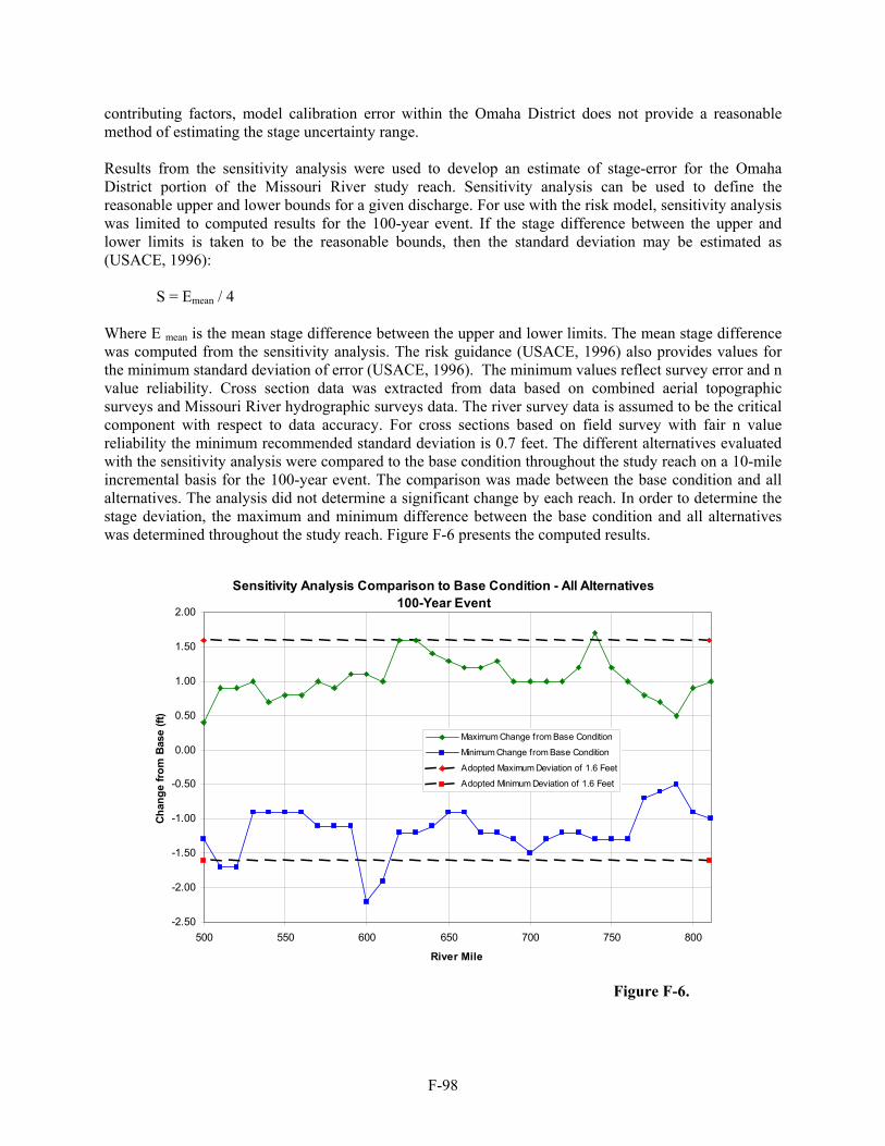
F-98

contributing factors, model calibration error within the Omaha District does not provide a reasonable method of estimating the stage uncertainty range. Results from the sensitivity analysis were used to develop an estimate of stage-error for the Omaha District portion of the Missouri River study reach. Sensitivity analysis can be used to define the reasonable upper and lower bounds for a given discharge. For use with the risk model, sensitivity analysis was limited to computed results for the 100-year event. If the stage difference between the upper and lower limits is taken to be the reasonable bounds, then the standard deviation may be estimated as (USACE, 1996): S = Emean / 4 Where E mean is the mean stage difference between the upper and lower limits. The mean stage difference was computed from the sensitivity analysis. The risk guidance (USACE, 1996) also provides values for the minimum standard deviation of error (USACE, 1996). The minimum values reflect survey error and n value reliability. Cross section data was extracted from data based on combined aerial topographic surveys and Missouri River hydrographic surveys data. The river survey data is assumed to be the critical component with respect to data accuracy. For cross sections based on field survey with fair n value reliability the minimum recommended standard deviation is 0.7 feet. The different alternatives evaluated with the sensitivity analysis were compared to the base condition throughout the study reach on a 10-mile incremental basis for the 100-year event. The comparison was made between the base condition and all alternatives. The analysis did not determine a significant change by each reach. In order to determine the stage deviation, the maximum and minimum difference between the base condition and all alternatives was determined throughout the study reach. Figure F-6 presents the computed results.

Sensitivity Analysis Comparison to Base Condition - All Alternatives100-Year Event

-2.50

-2.00

-1.50

-1.00

-0.50

0.00

0.50

1.00

1.50

2.00

500 550 600 650 700 750 800

River Mile

Chan

ge fr

om B

ase

(ft)

Maximum Change from Base Condition

Minimum Change from Base Condition

Adopted Maximum Deviation of 1.6 Feet

Adopted Minimum Deviation of 1.6 Feet

Figure F-6.

F-99

Using the sensitivity analysis results and professional judgment, the reasonable upper and lower bounds of stage were estimated as 1.6 feet as shown on figure F-6. Using the adopted deviation of 1.6 feet, the standard stage error may be computed as: S = (1.6 + 1.6) /4 or S = 0.8 feet. The standard stage error of 0.8 feet exceeds the minimum recommend value of 0.7 feet. The selected standard stage error is applied to the risk analysis (HEC, 1996). Plots that illustrate the change from the base condition for each alternative for the 100-year event are shown in Plates F-163 and F-164. FINAL PROFILE DEVELOPMENT The final step in determination of the stage-frequency relationship is to import the data from the HEC suite of programs into the profile plotting spreadsheet. The final output file from the HEC program contains tabulated flow-frequency and stage-frequency for each cross section. Refer to appendix F-H for an example of the final output file. Spreadsheet modifications performed to develop the final profiles consist of profile smoothing and adjustment within backwater areas. Profile Smoothing. Initial results exhibited some areas where the profile had dips or inconsistencies. These variations were most pronounced for the 500-year event and the 100-year event to a lesser extent. Given that the methodology employed a single geometry file for the entire analysis, some inconsistencies are not unexpected. For large events, top width and flow velocity variation contributes to excessive stage variation between adjacent sections. A simple profile smoothing algorithm was applied to the final results within a spreadsheet prior to plotting. Refer to Appendix F-I for a description of the profile smoothing. Interface at Rulo, NE. The boundary between the Kansas City and Omaha Districts occurs at Rulo, NE. The Rulo area geometry includes a system of privately constructed levees that provides a limited level of protection. The floodplain is extremely wide at Rulo with a flat sloping stage-flow rating curve for extreme events. Stage at Rulo can also be impacted by flows from the Big Nemaha River that enters the Missouri River approximately 3.2 miles downstream of the gage. Both Districts developed UNET models for the period of record analysis that included an overlap section with the adjacent District. The downstream boundary of the Omaha model was at St. Joseph, Missouri, while the upstream boundary of the Kansas City model was at Nebraska City, Nebraska. Considerable differences occurred between the methodology employed in model construction within the two Districts. For example, the Kansas City District employed a different UNET levee routing algorithm. In addition, the Kansas City District employed a different approach to generate stage-frequency from the POR results. Kansas City District also used UNET model results to modify the flow-frequency relationships derived from the hydrologic analysis. Because of the analysis variations between the two Corps Districts, differences in the flow-frequency and stage-frequency results occurred at Rulo, NE. Refer to Appendix E for a complete description of the Kansas City District analysis methods. In order to develop consistent profiles at the Rulo, NE, interface, the results from the two Districts were merged as practical. Flow-frequency differences for the 2-year through the 100-year were minor and may be attributed to numerical round off and slight computational differences. For the 200-year and 500-year profiles, Kansas City District adjusted the flow values based on the UNET analysis. The flow adjustment was not performed in the Omaha District, therefore the flow values are different. Stage-frequency differences were minor and generally less than 0.5 feet. Comparison illustrated that Kansas City District results were slightly higher than Omaha District results for all profiles. This is true even for the 200-year and 500-year events for which Kansas City District has a lower flow. In order to develop a smooth

F-100

profile, Omaha District adopted Kansas City District stage-frequency results at Rulo,NE. Slight adjustments at the next two cross sections upstream of Rulo, NE, were necessary to merge the profile. The final tabulated stage-frequency results reflect the merged profile condition. Final Profiles. Profile smoothing was applied to adjust the final profiles and remove all inconsistencies. The output results were also modified in the vicinity of the major tributaries as previously discussed in the section Backwater Influenced Locations. The combined results from the stage-frequency software, the smoothing algorithm, and the backwater analysis were used to determine the final profiles. Additional profile modification was required at the Omaha District boundary with the Kansas City District located at Rulo, NE. A few profiles required some minor adjustments in elevations, but these adjustments were generally less than 0.5 ft. The final smoothed profiles were then interpolated from cross section locations to locations at even river miles to provide the standard tabulated format. Water surface profiles developed for various flood events are shown in Plates F-165 thru F-173. Tabulated values for the same events are illustrated in Plate F-174 thru F-186. Study Applicability to the National Flood Insurance Program Development of revised Flood Insurance Rate Maps (FIRM) was not a task of this study. The Federal Insurance and Mitigation Administration (FIMA) within FEMA are responsible for administering the National Flood Insurance Program (NFIP). FEMA defines technical requirements and policy for Flood Hazard Maps and related NFIP products in Guidelines and Specifications for Flood Hazard Mapping Partners, (FEMA, 2002). Comparison to the existing Flood Hazard Study (USACE, 1978) determined significant change in the flow-frequency and stage-frequency results determined by this study. A comparison between study profiles and the 100-year profile from the Flood Hazard Study (USACE, 1978) is shown in Plates F-187 thru F-195. Prior to revising the existing Flood Hazard Study (USACE, 1978) with the new results computed with this study, an additional study that develops FEMA regulatory parameters is required. Regulatory parameters that may be revised include the 10-, 50-, 100-, and 500-year flood profile, the 100- and 500-year flood boundary, and the 100-year floodway boundary. Products of this study that may be used to assist in development of revised NFIP parameters include the computed flow-frequency and stage-frequency values along the Missouri River from Gavins Point Dam to Rulo, NE. However, substantial effort is required to translate these products into the necessary parameters required by FEMA to administer the NFIP along the Missouri River. While the FEMA study methodology has not been determined, items that would require additional effort may include the development of a traditional hydraulic regulatory model such as HEC-RAS, performance of floodway computations, and flood outline mapping according to FEMA guidelines to develop Flood Insurance Rate Maps (FIRM). Ice impacts should be evaluated according to FEMA guidelines and adjustments may be required where ice is determined to be a problem. The flow-frequency and stage-frequency relationships determined at each location by this study would serve as a base for development of a HEC-RAS model. The HEC-RAS model can be calibrated to the stage-frequency results obtained from this study. Minor variation of computed elevations should be expected. Determination of regulatory elevations within levee reaches must also consider the possibility that two NFIP regulatory elevations may be required to provide different elevations riverward and landward of the levee. The profile riverward of the levee would reflect the computed river water surface elevation. The NFIP regulatory elevation landward of the levee would reflect the maximum water surface computed within the levee unit that reflects several possible conditions including an upstream breach that fills levee storage. The regulatory elevation will also consider tributary inflow along tie-back levees in applicable locations.

F-101

HYDRAULIC SUMMARY Hydrologic and hydraulic analysis was conducted by the Omaha District as part of the Upper Mississippi, Lower Missouri and Illinois Rivers Flow Frequency Study. Prior to this study, the discharge frequency relationships established for the Missouri River are those that were developed in 1962 and published in the Missouri River Agricultural Levee Restudy Program Hydrology Report. This hydrology information was used for the water surface profiles and flood inundation areas that were developed for the Missouri River Flood Plain Study during the mid to late 1970's. Almost 40 years of additional streamflow data were available since the Missouri River Hydrology was last updated. Also, significant channel changes have occurred since the previous hydraulic studies were completed. The hydraulic model extends from Gavins Point Dam, at RM 811.1, downstream to Rulo, NE, at RM 498.0. Rulo, NE, corresponds with the Omaha District boundary with Kansas City District. A UNET period of record analysis was employed to develop stage-flow relationships at all cross sections. The UNET model developed for this study employed the top of levee elevation for all levee connections. The model also assumes a levee breach occurs when the computed river elevation exceeds the levee top elevation. Levee modeling assumptions were coordinated during task force meetings with Corps of Engineers, FEMA, and state representatives. A description of the discussion and conclusions is presented within appendix A. Previous Missouri River studies within the Omaha District conducted to develop regulatory products such as the stage-frequency elevation and 100-year floodway (USACE, 1978) used different assumptions including levee overtopping without any levee breach. Therefore, modeling for regulatory purposes to establish floodway locations may require additional evaluation of levee performance. An estimate of the minimum level of protection provided by each individual federal levee unit was not performed as part of this study. Levee level of protection and the associated levee capacity are dependent upon a risk and uncertainty analysis that includes estimating the uncertainty for many parameters. A complete risk and uncertainty analysis should follow the guidance provided within Appendix A and the current Corps of Engineers guidance provided within EM 1110-2-1619, Risk Based Analysis for Flood Damage Reduction Studies (USACE, 1996). The risk analysis evaluates the computed stage-frequency relationship and levee elevation at each location with appropriate uncertainty estimates for hydrologic, hydraulic, and geotechnical parameters to determine the levee reliability. This analysis is typically performed during a floodplain delineation study or during a flood damage reduction study. Products of this study that may be used to assist in development of revised NFIP parameters include the computed flow-frequency and stage-frequency values along the Missouri River from Gavins Point Dam to Rulo, NE. However, substantial effort is required to translate these products into the necessary parameters required by FEMA to administer the NFIP along the Missouri River. Software was employed to determine stage-frequency relationship at all cross sections using hydrologic data, regulated-unregulated relationships, and UNET results. Profile smoothing and adjustment to the profile through backwater areas was also required. A sensitivity analysis was performed to evaluate the impact of model parameters on computed results. Final profiles for the study reach were developed that include a comparison to the previous study results. Significant results include the following:

• Final profiles for the 10-, 50-, 100- and 500-year events were determined from Gavins Point Dam (RM 811.1) to Rulo, NE (RM 498).

F-102

• Significant changes to the flow-frequency relationship have occurred since the previous flood hazard study (USACE, 1978). The most notable changes are the 500-year event downstream of the Platte River and all events upstream of Sioux City.

• Significant changes to stage-frequency have occurred since the previous flood hazard study (USACE, 1978). The 100-year profile has increased significantly downstream of the Platte River. The federal levees in this area do not provide 100-year protection.

• Profiles in the vicinity of the Omaha and Council Bluffs urban levees have not changed significantly from previous studies. Increases in the stage-discharge relationship within this reach have been offset by decreases in the flow-frequency relationship.

• Calibration accuracy was limited by the dynamic stage-flow relationship on the Missouri River. Degradation within the upper end of the model and aggradation in the lower end has significantly impacted the stage-flow relationship.

• The UNET period of record (POR) analysis employed a single calibrated model to best-fit current conditions. Missouri River stage-discharge relationship has seasonal and annual fluctuations. Model calibration error is known to occur for each individual event. Final calibration represents the model determined to be best suited for the POR analysis.

• The POR analysis employed a model calibrated to summer stages. The impact of seasonal stage-flow was minimized in order to reduce model variability and prevent computation of lower stages for spring or fall events in the POR analysis.

• Stage-frequency results are based on the calibrated model for current conditions. Model calibration does not reflect any future stage trends.

• Ice impacts on peak stages were not included in the analysis and are not reflected in the stage-frequency results.

• All model calibration and the POR analysis was performed with daily flow data. While calibration accuracy may be reduced, the computed results, which rely on the developed stage-flow relationships, are still valid.

• The POR analysis used the Null Internal Boundary Condition to determine ungaged inflow. The impact of ungaged inflows on final model results was evaluated and determined to be minimal. The POR analysis was focused on the peak stage and flow relationship. Using model results for performing volumetric computations or evaluations that are volume sensitive is not recommended.

• A sensitivity analysis was performed to evaluate the impact of model parameters such as model calibration method, ungaged inflow, levee overtopping and conveyance, the period of record length, and flow factoring. Results indicated that the model performed adequately.

• A risk and uncertainty analysis to estimate of the minimum level of protection provided by each individual federal levee unit was not performed as part of this study. This analysis is typically performed during a floodplain delineation study or during a flood damage reduction study.

• Prior to revising the current National Flood Insurance Program regulatory parameters with presented results, an additional study to develop regulatory parameters essential for the NFIP is required.

F-103

REFERENCES

Barkau, 1994, Rating Curve Calibration, Personal Workshop Notes. Beard, Leo R., 1962. “Statistical Methods in Hydrology, Revised Edition Published Under Civil

Works Investigations Project CW-151”, U.S. Army Engineer District, Corps of Engineers, Sacramento, California.

FEMA, 2002. Guidelines and Specifications for Flood Hazard Mapping Partners, Federal Emergency

Management Agency, February 2002. Ferrell, John, 1996. Soundings, 100 Years of the Missouri River Navigation Project. Hydrologic Engineering Center, 2002. HEC-RAS River Analysis System, Version 3.1, Hydrologic

Engineering Center, U.S. Army Corps of Engineers, Davis California. November 2002. Hydrologic Engineering Center, 2000. “Investigation of Methods for Obtaining Regionally

Consistent Flood Distributions, Upper Mississippi Flood Frequency Study,” U.S Army Corps of Engineers, Davis, CA.

Hydrologic Engineering Center, 1999. “An Investigation of Flood Frequency Estimation

Methods for the upper Mississippi Basin,” U.S. Army Corps of Engineers, Davis, CA. Hydrologic Engineering Center, 1992. DSSMATH - Mathematical Manipulation of DSS Data

Program, U.S. Army Corps of Engineers, Hydrologic Engineering Center, Davis California, April 1992.

Hydrologic Engineering Center, 1990. HECDSS - Data Storage System Program, Hydrologic

Engineering Center, U.S. Army Corps of Engineers, Davis California. Interagency Advisory Committee on Water Data (IACWD), 1982. “Guidelines for Determining

Flood Flow Frequency, Bulletin 17B,” U.S. Department of the Interior, Geological Survey, Office of Water Data Collection, Reston, VA.

Missouri Basin Inter-Agency Committee, 1969. Comprehensive Framework Study, Missouri

River Basin. Missouri Basin States Association, 1983. Final Report, Missouri River Flood Plain Study. U.S. Army Corps of Engineers, 2001. Investigation of Channel Degradation, 2001 Update. U.S. Army

Corps of Engineers, Omaha District. U.S. Army Corps of Engineers, 1998. Volume 2A: Reservoir Regulation Studies, Daily Routing

Model Studies. Missouri River Master Water Control Manual Review and Update Study, Missouri River Region, Northwestern Division, U.S. Army Corps of Engineers, Omaha, NE.

F-104

U.S. Army Corps of Engineers, 1996. EM 1110-2-1619. Risk-Based Analysis for Flood Damage Reduction Studies. U.S. Army Corps of Engineers, Washington, DC, June 1996.

U.S. Army Corps of Engineers, 1995, Floodplain Management Assessment of the Upper Mississippi and

Lower Missouri Rivers and Their Tributaries - Main Report and Appendices, U.S. Army Corps of Engineers, Washington, DC, June 1995.

U.S. Army Corps of Engineers, 1994. Post-Flood Report, The Great Flood of 1993, Lower Missouri River

Basin, Appendix D, U.S. Army Corps of Engineers, Omaha District, September 1994. U.S. Army Corps of Engineers, 1993. Hydrologic Frequency Analysis, EM 1110-2-1415, U.S. Army

Corps of Engineers, Washington, D.C., March 1993. U.S. Army Corps of Engineers, 1992. Missouri River Channel Capacity Study, Omaha to Rulo, Nebraska,

Prepared by Resource Consultants & Engineers, Inc., for the Omaha District, U.S. Army Corps of Engineers, August 1992.

U.S. Army Corps of Engineers, 1992. Emergency System Operating Plan, Missouri River Main Stem

Res. System, Gavins Point Dam to Rulo, Nebraska, Omaha District, August, 1992. U.S. Army Corps of Engineers, 1986. Adequacy of Missouri River Levee System, Rulo, Nebraska, to

Omaha, Nebraska, Omaha District, April, 1986. U.S. Army Corps of Engineers, 1981. Missouri River Degradation, Volume IV, Supporting Technical

Report, Review Report for Water and Related Land Res. Man. Study, Omaha District, U.S. Army Corps of Engineers, August, 1981.

U.S. Army Corps of Engineers, 1978. Flood Hazard Information, Missouri River, Gavins Point Dam to

Rulo, Nebraska, Volumes I and II, 1978-1979, Omaha District. U.S. Army Corps of Engineers, 1976. Missouri River Temperature Effects in the Transition From Dunes

to Plane Bed, Prepared by USGS in Cooperation with the US Army Corps of Engineers, Omaha District, M.R.D. Sediment Series No. 14.

U.S. Army Corps of Engineers, 1973. MRD-RCC Technical Study S-73. Upper Missouri River,

Unregulated Flow Development. U.S. Army Corps of Engineers, 1962. “ Missouri River Agricultural Levee Restudy Program”,

Hydrology Report, Missouri River Division, March 1962. U.S. Army Corps of Engineers, 1954. “Missouri River Study of Effects of Navigation and

Channel Stabilization Works”, Omaha District, April 1954. U.S. Army Corps of Engineers 1946. “Missouri River Levees – Definite Project Report”,

Appendix I – Hydrology, Missouri River Division, Omaha, NE, August 1946. U.S. Department of Agriculture, 1895-1928. “Daily River Stages at River Gage Stations of the

Principal Rivers of the United States”, Weather Bureau Parts VI through XXVI. Washington, D.C. 1895-1928.

F-105

U.S. Department of Commerce, 1982(a). Evaporation Atlas for the Contiguous 48 United States.

NOAA Technical Report NWS 33, NWS, Washington, D.C. U.S. Department of Commerce, 1982(b). Mean Monthly, Seasonal, and Annual Pan Evaporation

for the United States. NOAA technical Report NWS 34, NWS, Washington, D.C. U.S. Geological Survey, 1928-1997. Water Resources Data for Montana, Wyoming, North

Dakota, South Dakota, Colorado, Nebraska and Iowa. U.S. Geological Survey, USGS Circular 108. U.S. Secretary of War, 1935. “ Missouri River”, House Document No. 308, Washington, D.C.

1935.

FA-1


Appendix F-A

Tables of Study Results and Data

FA-2

Table A-1. Peak Annual Unregulated Flows at Omaha District Gages Year Yankton Sioux City Decatur Omaha Nebraska City 1898 173600 175000 175300 168400 206400 1899 252600 254000 252700 241700 273000 1900 132100 131400 127900 122000 177600 1901 143000 150600 149400 144200 182100 1902 131800 132700 131900 124800 166800 1903 151000 152700 151000 152900 223300 1904 189900 180400 178700 184700 184000 1905 251500 239000 227200 175300 244500 1906 181300 184300 188400 200800 195700 1907 184300 184300 184800 194900 231300 1908 173000 188000 195400 232000 260200 1909 166900 174500 181500 217200 236000 1910 202100 204600 202200 231900 207000 1911 144600 141500 143500 158400 175300 1912 194000 194500 196300 204100 225900 1913 209600 200700 199200 208000 205600 1914 155400 158900 155100 140900 239000 1915 189700 181100 176900 178200 210200 1916 188000 186900 186200 176600 212300 1917 199700 201400 196700 206800 223600 1918 180600 183300 184200 188500 211400 1919 151600 141800 138500 151900 150500 1920 206800 201100 204100 233500 270300 1921 188700 180200 185100 215500 296600 1922 166600 163500 165400 180500 216200 1923 166400 157200 161500 190000 230700 1924 127600 134800 135000 151400 213200 1925 180100 173900 179900 205800 218000 1926 118900 114700 114600 122300 156700 1927 211300 209200 207400 233900 250300 1928 154700 153900 157200 170400 192200 1929 194000 191100 196600 219000 252100 1930 87700 88800 88000 87300 127000 1931 81200 83000 83500 85900 130800 1932 151400 151400 153000 157900 182800 1933 134200 132700 132500 129900 144900 1934 74100 79200 79700 91000 134100 1935 162500 160800 148500 133400 164300 1936 102900 102100 100900 101000 122200 1937 130700 130000 131300 133100 144900 1938 174400 171900 170300 164800 216600 1939 171500 170000 165500 146400 159800 1940 85700 91100 89300 93700 153100 1941 167700 151400 148700 138200 146500 1942 151300 153200 149700 154400 223500 1943 291400 221600 214800 218400 237200 1944 196700 208100 202400 188700 296400 1945 120100 133200 130900 128500 172100 1946 126300 126700 126700 122400 160600 1947 187600 195000 189700 186800 247700 1948 169700 173400 174700 173500 224700 1949 183200 192000 192000 201600 207600

FA-3

Year Yankton Sioux City Decatur Omaha Nebraska City 1950 260300 247700 244700 226500 220600 1951 130200 161000 158300 163500 225200 1952 497300 479400 464300 469200 487800 1953 272700 262500 263200 271600 283800 1954 95900 105100 108800 138600 185300 1955 105400 106900 107800 115500 137100 1956 161800 159700 160800 161500 180700 1957 150500 160800 163100 169500 273900 1958 152400 148800 150300 153000 179000 1959 138100 135900 136500 140100 200300 1960 219200 256300 259700 273800 328900 1961 111900 112000 113100 114800 140500 1962 176800 185400 186100 188900 224100 1963 175100 173900 174400 176200 274300 1964 237700 231900 233900 234500 272300 1965 173400 178600 178600 181300 273400 1966 132600 134600 135000 135900 147200 1967 238700 242300 245700 255700 323000 1968 160600 158100 159300 161600 244500 1969 157400 196400 201900 225700 236500 1970 169900 169200 170200 172300 205900 1971 166400 166500 168100 172200 216800 1972 245200 244500 245600 247300 253700 1973 115200 114300 115500 118200 169800 1974 190000 188000 189500 191400 211600 1975 216200 213900 216100 219500 231600 1976 144700 145400 146700 149200 183400 1977 91000 91300 92200 95100 118200 1978 271400 281100 283200 287400 316100 1979 179000 180400 182700 188000 225200 1980 114100 114800 115900 119000 177100 1981 170300 172000 174000 182800 210800 1982 175300 175100 178400 193000 242000 1983 125500 151500 157100 188200 280500 1984 130700 220100 221900 235300 315400 1985 92700 98700 99500 105400 134200 1986 169800 187200 193500 227000 250100 1987 207500 219600 219300 232300 276800 1988 89600 89200 90500 92600 119700 1989 104300 104400 106800 109600 150600 1990 101600 103900 106600 123300 253600 1991 164800 164000 165300 205800 248700 1992 89100 95900 99800 111700 132100 1993 117100 170500 176200 216000 327000 1994 144200 152900 154800 156800 171800 1995 193900 198500 200300 209700 274600 1996 177700 185800 188900 230900 307000 1997 245300 290300 289800 293800 299600

FA-4

Table A-2. Peak Jan-April Unregulated Flows at Omaha District Gages Year Yankton Sioux City Decatur Omaha Nebraska City 1898 134900 129900 125500 123500 114200 1899 252600 254000 252700 241700 273000 1900 118300 123600 110500 106500 120800 1901 97700 95500 90300 80700 107800 1902 104900 107200 100500 97300 106500 1903 109000 112200 109600 110500 135700 1904 189900 180400 178700 184700 168600 1905 75300 73200 72000 68900 87300 1906 128000 126900 116500 124700 122000 1907 147500 145100 137400 135100 109800 1908 80600 84400 83500 97000 94600 1909 112200 105600 105900 151200 147800 1910 202100 204600 202200 231900 207000 1911 90400 86900 91000 111600 106000 1912 194000 194500 196300 204100 225900 1913 209600 200700 199200 208000 205600 1914 116700 113600 97400 65700 111500 1915 182200 168300 169200 167300 204900 1916 159200 147900 144800 139500 141100 1917 199700 201400 196700 206800 211100 1918 165400 165100 163400 180000 162300 1919 151600 141800 138500 151900 142400 1920 192800 179800 178400 207600 192500 1921 68400 72000 73400 77600 107200 1922 120700 120200 118400 133600 150300 1923 99900 101600 105500 122000 122100 1924 124200 126600 130700 151100 180500 1925 151500 135300 137200 153600 160900 1926 97300 86500 85700 101800 113400 1927 97800 97300 91200 99000 171000 1928 141300 127700 122400 137800 144900 1929 194000 181400 175700 169700 183000 1930 76600 85300 85100 87300 92100 1931 44100 39600 38500 39100 53600 1932 83200 84100 79700 69000 85800 1933 90100 90000 89000 78500 91300 1934 72500 71700 71000 89300 82000 1935 46000 45900 45200 44900 50100 1936 90900 93300 89600 87800 114300 1937 58600 63300 62900 73000 86500 1938 142500 145200 140300 118900 119200 1939 171500 170000 165500 146400 159800 1940 39800 40500 40000 41400 48600 1941 55700 58300 58500 60200 70100 1942 71200 83500 83100 86100 86900 1943 291400 221600 214800 218400 214000 1944 196700 196400 190800 163600 186500 1945 103700 118200 118200 113800 121900 1946 62000 67100 65100 65100 81400 1947 183100 182500 176000 165300 178100 1948 105500 114800 113700 111100 129500 1949 183200 192000 192000 201600 207600

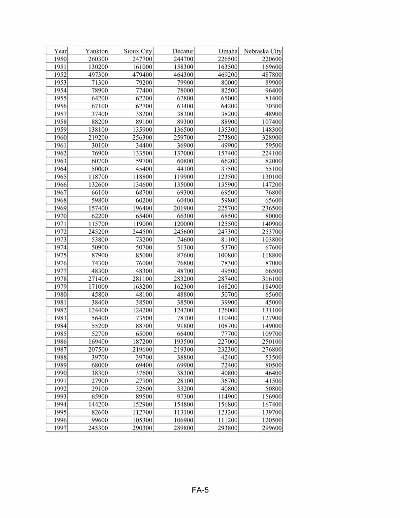
FA-5


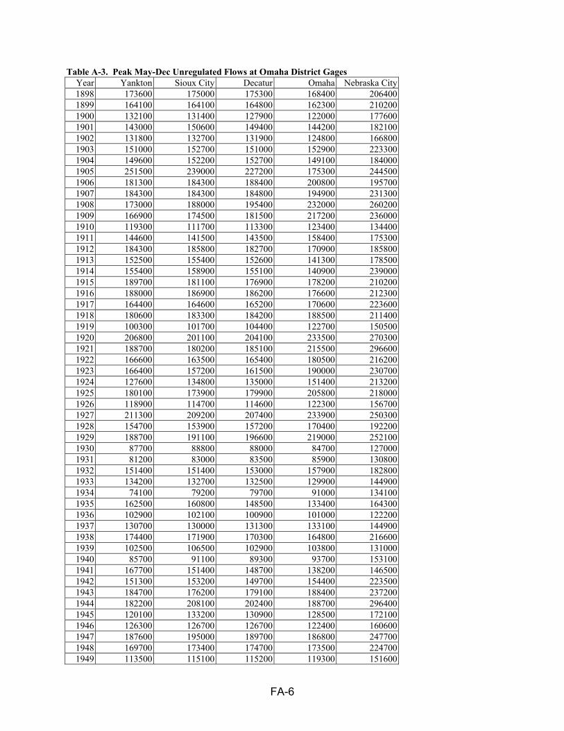
FA-6

Table A-3. Peak May-Dec Unregulated Flows at Omaha District Gages Year Yankton Sioux City Decatur Omaha Nebraska City 1898 173600 175000 175300 168400 206400 1899 164100 164100 164800 162300 210200 1900 132100 131400 127900 122000 177600 1901 143000 150600 149400 144200 182100 1902 131800 132700 131900 124800 166800 1903 151000 152700 151000 152900 223300 1904 149600 152200 152700 149100 184000 1905 251500 239000 227200 175300 244500 1906 181300 184300 188400 200800 195700 1907 184300 184300 184800 194900 231300 1908 173000 188000 195400 232000 260200 1909 166900 174500 181500 217200 236000 1910 119300 111700 113300 123400 134400 1911 144600 141500 143500 158400 175300 1912 184300 185800 182700 170900 185800 1913 152500 155400 152600 141300 178500 1914 155400 158900 155100 140900 239000 1915 189700 181100 176900 178200 210200 1916 188000 186900 186200 176600 212300 1917 164400 164600 165200 170600 223600 1918 180600 183300 184200 188500 211400 1919 100300 101700 104400 122700 150500 1920 206800 201100 204100 233500 270300 1921 188700 180200 185100 215500 296600 1922 166600 163500 165400 180500 216200 1923 166400 157200 161500 190000 230700 1924 127600 134800 135000 151400 213200 1925 180100 173900 179900 205800 218000 1926 118900 114700 114600 122300 156700 1927 211300 209200 207400 233900 250300 1928 154700 153900 157200 170400 192200 1929 188700 191100 196600 219000 252100 1930 87700 88800 88000 84700 127000 1931 81200 83000 83500 85900 130800 1932 151400 151400 153000 157900 182800 1933 134200 132700 132500 129900 144900 1934 74100 79200 79700 91000 134100 1935 162500 160800 148500 133400 164300 1936 102900 102100 100900 101000 122200 1937 130700 130000 131300 133100 144900 1938 174400 171900 170300 164800 216600 1939 102500 106500 102900 103800 131000 1940 85700 91100 89300 93700 153100 1941 167700 151400 148700 138200 146500 1942 151300 153200 149700 154400 223500 1943 184700 176200 179100 188400 237200 1944 182200 208100 202400 188700 296400 1945 120100 133200 130900 128500 172100 1946 126300 126700 126700 122400 160600 1947 187600 195000 189700 186800 247700 1948 169700 173400 174700 173500 224700 1949 113500 115100 115200 119300 151600

FA-7


FA-8

Table A-4. Peak Annual Unregulated Mean Flow Volumes at Yankton Year 1-day 3-day 7-day 15-day 31-day 91-day 181-day 1898 167600 167100 163500 158900 143700 113300 78000 1899 243800 242100 227000 175200 139400 121000 96100 1900 127500 120600 116400 113200 106900 87900 62900 1901 138000 130700 128800 124700 116200 94000 65200 1902 127200 126200 124300 119200 110700 94100 75200 1903 145800 140900 132900 130000 125200 103600 78400 1904 183300 162700 138600 125400 115700 96400 78300 1905 242800 218300 168000 137200 119400 87100 60600 1906 175000 171100 151000 135500 122900 96800 73400 1907 177900 161300 147900 140900 134300 112900 91800 1908 167000 166000 158400 150700 139500 109200 75000 1909 161100 155600 145300 140400 135200 102300 69800 1910 195100 172300 123400 93700 88100 71800 61400 1911 139600 135000 131900 128300 120300 89000 64600 1912 187300 182600 165100 133400 127000 98400 86100 1913 202300 195800 150800 136800 135700 109900 88200 1914 150000 146100 142600 132600 125400 105900 79400 1915 183100 162500 150600 129200 115700 102500 84700 1916 181500 173900 165700 159800 153800 116800 101000 1917 192800 186400 162300 151400 139700 116600 96300 1918 174300 172900 170300 163100 138800 101700 83300 1919 146300 116900 95600 89000 86500 70400 59600 1920 199600 178000 161200 145300 133600 111400 85600 1921 182100 175400 168600 151500 130100 95000 63700 1922 160800 156400 144400 139800 128200 98000 77100 1923 160600 142700 137500 127600 118800 104000 78500 1924 123200 117200 111500 96600 95200 83300 68000 1925 173800 161900 146900 131700 114200 93800 72400 1926 114800 106700 98500 94000 91700 80600 59300 1927 204000 173300 150500 147400 133500 104900 78200 1928 149300 145800 141700 130900 117200 97100 70400 1929 187300 179800 168700 143400 121300 84100 62500 1930 84700 81900 78900 72500 68300 57100 48700 1931 78400 76300 74300 71500 66400 47400 35200 1932 146100 141000 131000 116800 107800 78500 57200 1933 129500 127300 126400 120500 106200 77700 54400 1934 71500 66700 62600 60200 58900 49000 37800 1935 156900 128200 114200 102800 96200 66600 46200 1936 99300 92700 80000 73700 70700 57500 45400 1937 126200 124500 108600 96300 83700 65800 46500 1938 168300 160300 154300 143300 122500 80900 57400 1939 165500 164200 142800 101500 67700 61000 50800 1940 82700 79400 76100 73200 68500 53300 40000 1941 161900 153700 129800 104100 86500 61000 44800 1942 146000 140300 132700 123700 116800 95800 67300 1943 281300 261200 220000 164500 140300 98800 83600 1944 189900 187400 174800 156300 141300 94600 72300 1945 115900 113400 104500 91300 85600 68100 53500 1946 121900 117100 105700 97600 85800 63700 47200 1947 181100 179100 167900 144500 116800 91400 72400 1948 163800 160600 157000 148100 136400 95900 72000 1949 176800 174100 161500 124600 95300 72200 60100

FA-9

Year 1-day 3-day 7-day 15-day 31-day 91-day 181-day 1950 251300 241000 216200 156400 126600 87000 74600 1951 125700 124700 118100 102000 94200 80300 66700 1952 480000 455100 378300 283800 194700 123800 87100 1953 263200 253900 234700 210600 166800 107100 76900 1954 92600 88700 85100 84600 76600 66500 48800 1955 101700 100000 95700 91400 84800 67700 51800 1956 156200 154100 148200 137800 122500 81600 59000 1957 145300 143500 138800 134700 122700 90900 60400 1958 147100 144800 140400 129900 119300 88500 66000 1959 133300 131500 127800 125000 110500 72700 57400 1960 211600 207100 187400 154800 104000 68400 55700 1961 108000 106200 103800 101100 89300 56000 38200 1962 170700 168000 161600 155700 148000 106800 73800 1963 169000 165900 157800 150200 142900 105900 74400 1964 229400 223300 205000 178800 159500 105400 66500 1965 167400 165200 163000 159500 150900 114600 79700 1966 128000 127100 115800 92100 74800 63400 54200 1967 230400 227300 213500 203600 191400 124200 83200 1968 155000 151900 147000 142100 127600 84900 60300 1969 151900 146500 138600 134600 109400 89700 78000 1970 164000 163800 160100 150700 147100 110400 74500 1971 160600 159700 158300 157300 149500 105600 83700 1972 236700 230300 210500 172100 138900 94700 81700 1973 111200 109600 106200 100700 97900 76600 55700 1974 183400 181800 176300 162200 141800 93100 62700 1975 208700 205600 197400 191800 171000 131000 90900 1976 139700 138600 133400 128000 121700 97100 68800 1977 87800 87300 85800 81000 69700 52100 41400 1978 262000 257600 243000 215300 163900 116500 101700 1979 172800 165500 144400 116700 108400 91000 74700 1980 110100 109400 107500 107000 99500 73800 51700 1981 164400 163300 158000 148500 125900 83300 53900 1982 169200 167000 163700 152400 138000 108800 81400 1983 121100 119200 115200 109400 102800 80800 59600 1984 126200 125000 120700 117800 115700 90800 65000 1985 89500 88500 84000 77100 70500 57500 47200 1986 163900 162000 156700 149600 127800 93600 78500 1987 200300 187500 150900 110100 87500 63900 53800 1988 86500 85400 84300 80000 72600 55500 40100 1989 100700 99700 96400 92100 82700 67800 53100 1990 98100 95100 94300 91500 89200 65700 47600 1991 159100 154600 150200 139900 137200 96600 61800 1992 86000 83900 80000 76900 69000 56900 40800 1993 113000 111800 110600 107100 102800 95000 69600 1994 139200 133300 119600 103400 82100 62900 55100 1995 187200 183300 174600 157900 139300 114600 82000 1996 171500 170800 168000 162800 145800 103900 82600 1997 236800 232300 221500 192800 173800 124000 107900

FA-10

Table A-5. Peak Annual Unregulated Mean Flow Volumes at Sioux City Year 1-day 3-day 7-day 15-day 31-day 91-day 181-day 1898 171100 171100 167600 162800 147700 117400 81500 1899 248300 245600 231700 179300 142700 126400 99600 1900 128400 122500 118200 114600 109200 90800 66700 1901 147200 142400 139400 133300 124000 99800 70000 1902 129700 128700 126000 120600 112200 96300 77700 1903 149300 145600 135600 134500 129000 108000 82800 1904 176300 163600 140700 129700 121700 100300 81600 1905 233600 214400 170300 140300 124100 90800 64100 1906 180200 177700 158000 145000 131700 103800 80000 1907 180200 167500 154900 147100 142400 120500 99600 1908 183800 182500 174500 164200 150900 115800 80700 1909 170600 166000 157300 150300 147900 110900 78100 1910 200000 182000 132200 103400 89400 74200 65300 1911 138300 134600 132400 128900 121400 90000 65500 1912 190100 187400 169400 137900 129300 101200 89400 1913 196200 190900 153500 139600 139400 113900 92700 1914 155300 152500 149400 138800 134000 110500 82900 1915 177000 164600 156500 134800 120800 108600 91200 1916 182700 179200 170700 165100 159200 122100 107200 1917 196900 186200 165100 154500 142900 119500 98900 1918 179200 177500 174700 166900 141700 104700 86500 1919 138600 116800 97600 93100 90100 72900 62100 1920 196600 186600 168500 151700 139300 118100 91900 1921 176100 173500 168200 152000 131500 97900 67100 1922 159800 154800 144800 140500 129000 99300 78400 1923 153700 146800 143100 136400 125500 109500 82900 1924 131800 121600 117200 113700 105400 89000 72800 1925 170000 162300 148600 133700 116800 95200 73300 1926 112100 107300 100200 95400 93400 81800 60300 1927 204500 179500 151000 148300 135200 108500 81900 1928 150400 148300 144400 133800 119700 99900 72700 1929 186800 184800 172800 149100 128300 88900 70200 1930 86800 83400 80100 73700 70300 59500 52800 1931 81100 79300 75700 73200 67400 47800 35400 1932 148000 142700 132900 118600 109000 79200 58300 1933 129700 127500 126500 120700 106600 78000 55100 1934 77400 72200 65700 61600 60200 49700 38200 1935 157200 128500 114900 103500 96700 67000 46500 1936 99800 93400 80500 74100 71900 58000 46800 1937 127100 125500 109600 97400 84700 66700 47900 1938 168000 162300 157000 147400 124800 82200 58900 1939 166200 157200 135000 101200 68800 62000 51900 1940 89100 83100 77600 74200 69200 54000 40900 1941 148000 142800 120800 100900 85700 61200 45400 1942 149800 143100 129300 126500 120000 98400 69800 1943 216600 202800 185300 155800 139800 101100 85100 1944 203400 186200 170900 160600 146100 103000 79000 1945 130200 123700 111300 97900 93300 72800 58200 1946 123900 121000 108100 98600 86400 64400 49000 1947 190600 187100 169900 142900 118300 93200 75500 1948 169500 168100 164300 152900 139300 99100 76500 1949 187700 184400 170800 134300 104000 76900 64200

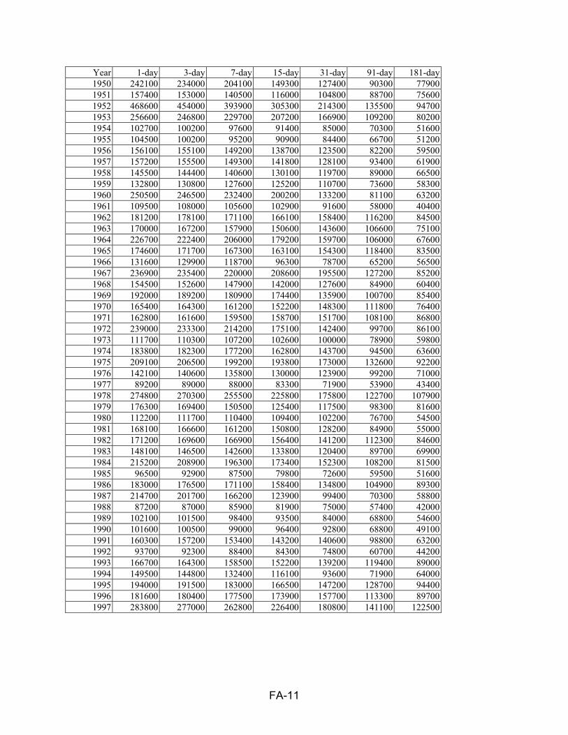
FA-11


FA-12

Table A-6. Peak Annual Unregulated Mean Flow Volumes at Decatur Year 1-day 3-day 7-day 15-day 31-day 91-day 181-day 1898 170000 169400 165900 160400 145800 117000 82100 1899 245100 241800 227000 178500 142700 127000 100400 1900 124100 120300 117200 113400 107800 89900 66400 1901 144900 141200 138400 132900 123800 99500 69500 1902 127900 127200 124500 119700 111800 96400 77700 1903 146500 142700 133000 132300 127200 107800 83200 1904 173300 160700 141000 130100 122600 101600 81800 1905 220400 202700 164900 136600 121200 87200 61600 1906 182700 177400 159600 146700 133600 104300 81400 1907 179200 169600 157600 151100 146400 124800 102500 1908 189500 188200 181200 171200 157300 120500 84400 1909 176000 172200 163300 158200 155200 116300 82700 1910 196100 180900 139000 109500 91400 76500 68300 1911 139200 137200 134900 131600 123700 92500 67800 1912 190400 187400 170000 136600 128700 100500 89200 1913 193200 188400 152600 137700 137300 110800 90700 1914 150400 149400 146400 136000 132100 108200 80400 1915 171600 164900 157200 137200 122600 109400 91100 1916 180600 176400 169700 164100 157800 121100 106700 1917 190800 184000 167100 155000 144000 120800 100300 1918 178700 177800 175200 167600 143200 106100 87500 1919 134300 118400 102600 95600 92600 75700 64500 1920 198000 187700 171800 155600 143000 121700 95200 1921 179500 178000 171100 154800 134300 99800 68000 1922 160400 157600 147600 142800 131400 100700 80300 1923 156600 152000 148200 140200 129100 112000 85200 1924 130900 124800 120500 116800 107800 91200 74900 1925 174500 166800 152000 137000 120200 98000 75800 1926 111200 108200 101200 96200 94300 83300 61700 1927 201200 183100 157700 155100 141900 114900 86300 1928 152500 150800 147100 136900 123200 103100 75600 1929 190700 186500 174100 149900 129000 89200 70800 1930 85400 81400 79200 73500 70400 59600 53100 1931 81000 79300 76100 73400 67500 47800 35400 1932 148400 144400 134200 119300 109100 79400 58500 1933 128500 126900 125900 119900 106000 77700 55000 1934 77300 73000 66800 62000 60200 49800 38300 1935 144000 127000 114700 103300 96500 67100 46700 1936 97900 92800 80100 73900 71800 58000 47000 1937 127400 124000 110400 97700 84800 67100 48300 1938 165200 160800 156600 147100 124800 82300 59200 1939 160500 153700 133400 100700 69200 62100 52000 1940 86600 82500 77300 74200 69400 54300 41200 1941 144200 139400 120600 101100 86000 61300 45600 1942 145200 139800 130600 127300 121000 99300 70400 1943 208300 198600 180600 155400 140800 101800 85500 1944 196300 183600 169900 161100 147700 103800 79500 1945 127000 123100 111200 98200 93700 73800 59100 1946 122900 119800 107300 98200 86200 64400 49000 1947 184000 181700 169500 144000 119800 94100 76100 1948 169400 167600 164200 153000 139400 99200 76700 1949 186200 181800 167800 136100 105600 77600 64700

FA-13


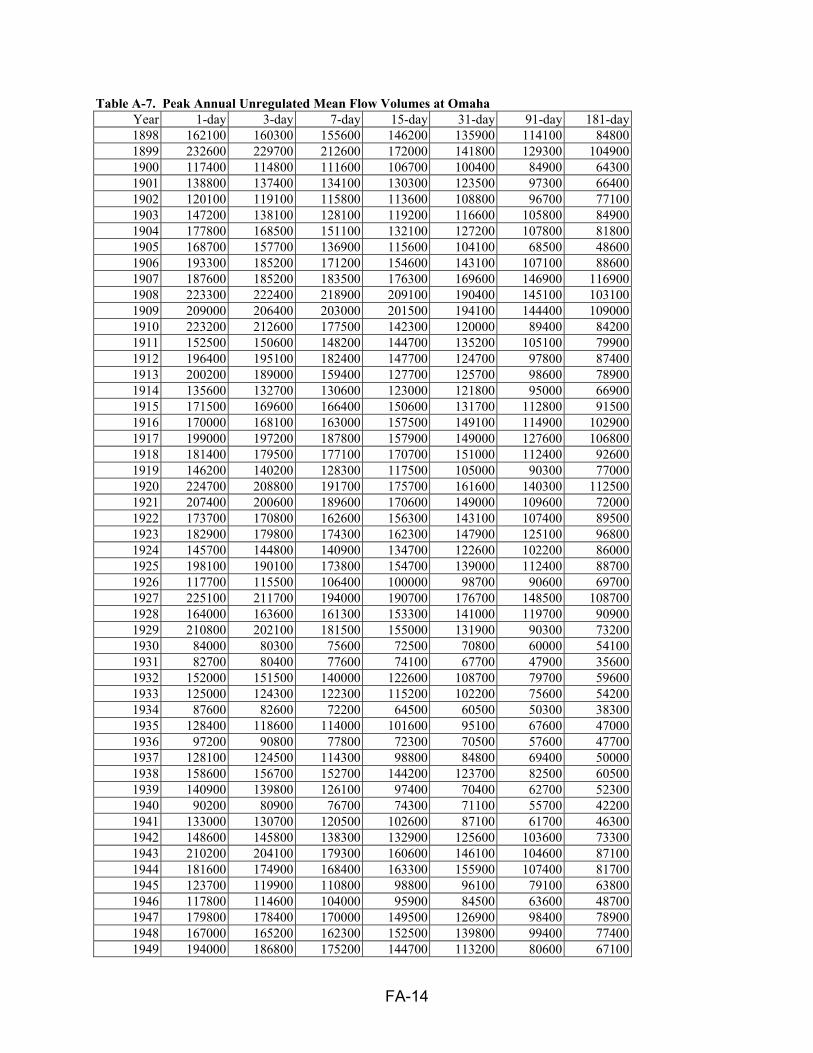
FA-14

Table A-7. Peak Annual Unregulated Mean Flow Volumes at Omaha Year 1-day 3-day 7-day 15-day 31-day 91-day 181-day 1898 162100 160300 155600 146200 135900 114100 84800 1899 232600 229700 212600 172000 141800 129300 104900 1900 117400 114800 111600 106700 100400 84900 64300 1901 138800 137400 134100 130300 123500 97300 66400 1902 120100 119100 115800 113600 108800 96700 77100 1903 147200 138100 128100 119200 116600 105800 84900 1904 177800 168500 151100 132100 127200 107800 81800 1905 168700 157700 136900 115600 104100 68500 48600 1906 193300 185200 171200 154600 143100 107100 88600 1907 187600 185200 183500 176300 169600 146900 116900 1908 223300 222400 218900 209100 190400 145100 103100 1909 209000 206400 203000 201500 194100 144400 109000 1910 223200 212600 177500 142300 120000 89400 84200 1911 152500 150600 148200 144700 135200 105100 79900 1912 196400 195100 182400 147700 124700 97800 87400 1913 200200 189000 159400 127700 125700 98600 78900 1914 135600 132700 130600 123000 121800 95000 66900 1915 171500 169600 166400 150600 131700 112800 91500 1916 170000 168100 163000 157500 149100 114900 102900 1917 199000 197200 187800 157900 149000 127600 106800 1918 181400 179500 177100 170700 151000 112400 92600 1919 146200 140200 128300 117500 105000 90300 77000 1920 224700 208800 191700 175700 161600 140300 112500 1921 207400 200600 189600 170600 149000 109600 72000 1922 173700 170800 162600 156300 143100 107400 89500 1923 182900 179800 174300 162300 147900 125100 96800 1924 145700 144800 140900 134700 122600 102200 86000 1925 198100 190100 173800 154700 139000 112400 88700 1926 117700 115500 106400 100000 98700 90600 69700 1927 225100 211700 194000 190700 176700 148500 108700 1928 164000 163600 161300 153300 141000 119700 90900 1929 210800 202100 181500 155000 131900 90300 73200 1930 84000 80300 75600 72500 70800 60000 54100 1931 82700 80400 77600 74100 67700 47900 35600 1932 152000 151500 140000 122600 108700 79700 59600 1933 125000 124300 122300 115200 102200 75600 54200 1934 87600 82600 72200 64500 60500 50300 38300 1935 128400 118600 114000 101600 95100 67600 47000 1936 97200 90800 77800 72300 70500 57600 47700 1937 128100 124500 114300 98800 84800 69400 50000 1938 158600 156700 152700 144200 123700 82500 60500 1939 140900 139800 126100 97400 70400 62700 52300 1940 90200 80900 76700 74300 71100 55700 42200 1941 133000 130700 120500 102600 87100 61700 46300 1942 148600 145800 138300 132900 125600 103600 73300 1943 210200 204100 179300 160600 146100 104600 87100 1944 181600 174900 168400 163300 155900 107400 81700 1945 123700 119900 110800 98800 96100 79100 63800 1946 117800 114600 104000 95900 84500 63600 48700 1947 179800 178400 170000 149500 126900 98400 78900 1948 167000 165200 162300 152500 139800 99400 77400 1949 194000 186800 175200 144700 113200 80600 67100

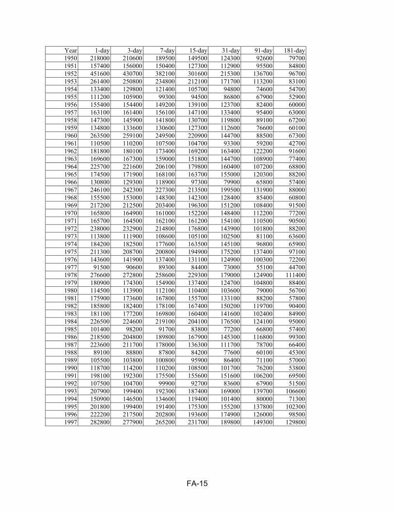
FA-15


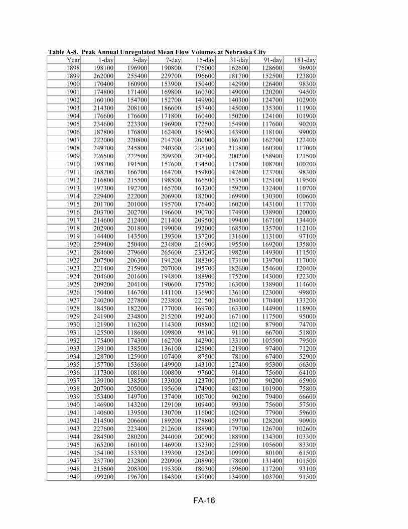
FA-16

Table A-8. Peak Annual Unregulated Mean Flow Volumes at Nebraska City Year 1-day 3-day 7-day 15-day 31-day 91-day 181-day 1898 198100 196900 190800 176000 162600 128600 96900 1899 262000 255400 229700 196600 181700 152500 123800 1900 170400 160900 153900 150400 142900 126400 98300 1901 174800 171400 169800 160300 149000 120200 94500 1902 160100 154700 152700 149900 140300 124700 102900 1903 214300 208100 186600 157400 145000 135300 111900 1904 176600 176600 171800 160400 150200 124100 101900 1905 234600 223300 196900 172500 154900 117600 90200 1906 187800 176800 162400 156900 143900 118100 99000 1907 222000 220800 214700 200000 186300 162700 122400 1908 249700 245800 240300 235100 213800 160300 117000 1909 226500 222500 209300 207400 200200 158900 121500 1910 198700 191500 157600 134500 117800 108700 100200 1911 168200 166700 164700 159800 147600 123700 98300 1912 216800 215500 198500 166500 153500 125100 119500 1913 197300 192700 165700 163200 159200 132400 110700 1914 229400 222000 206900 182000 169900 130300 100600 1915 201700 201000 195700 176400 160200 143100 117700 1916 203700 202700 196600 190700 174900 138900 120000 1917 214600 212400 211400 209500 199400 167100 134400 1918 202900 201800 199000 192000 168500 135700 112100 1919 144400 143500 139300 137200 131600 113100 97100 1920 259400 250400 234800 216900 195500 169200 135800 1921 284600 279600 265600 233200 198200 149300 111500 1922 207500 206300 194200 188300 173100 139700 117000 1923 221400 215900 207000 195700 182600 154600 120400 1924 204600 201600 194800 188900 175200 143000 122300 1925 209200 204100 190600 175700 163000 138900 114600 1926 150400 146700 141100 136900 136100 123000 99800 1927 240200 227800 223800 221500 204000 170400 133200 1928 184500 182200 177000 169700 163300 144900 118900 1929 241900 234800 215200 192400 167100 117500 95000 1930 121900 116200 114300 108800 102100 87900 74700 1931 125500 118600 109800 98100 91100 66700 51800 1932 175400 174300 162700 142900 133100 105500 79500 1933 139100 138500 136100 128000 121900 97400 71200 1934 128700 125900 107400 87500 78100 67400 52900 1935 157700 153600 149900 143100 127400 95300 66300 1936 117300 108100 100800 97600 91400 75600 64100 1937 139100 138500 133000 123700 107300 90200 65900 1938 207900 205000 195600 174900 148100 101900 75800 1939 153400 149700 137400 106700 90200 79400 66600 1940 146900 143200 129100 109400 99300 75600 57500 1941 140600 139500 130700 116000 102900 77900 59600 1942 214500 206600 189200 178800 159700 128200 90900 1943 227600 223400 212600 188900 179700 126700 102600 1944 284500 280200 244000 200900 188900 134300 103300 1945 165200 160100 146900 132300 125900 105600 83300 1946 154100 153300 139300 128200 109900 80100 61500 1947 237700 232800 220900 208900 178000 131400 101500 1948 215600 208300 195300 180300 159600 117200 93100 1949 199200 196700 184300 159000 134900 103700 91500

FA-17


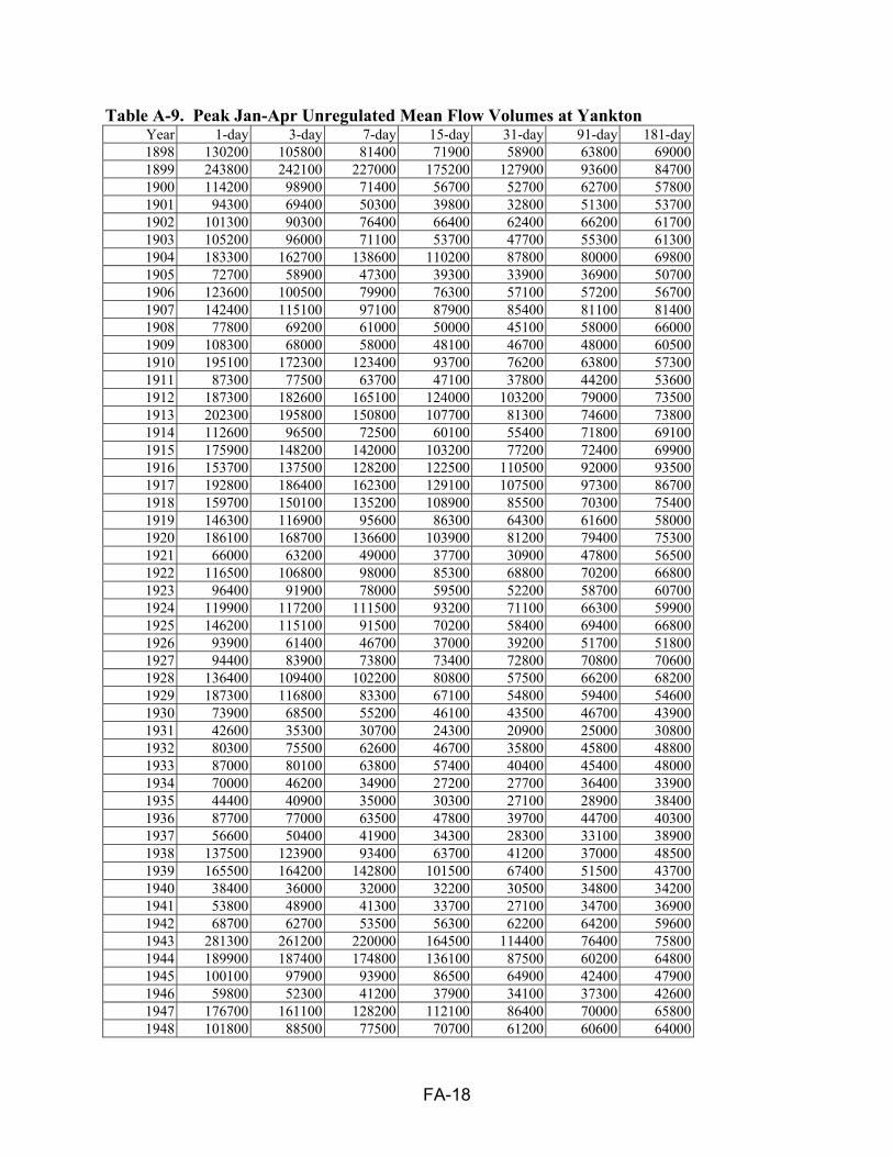
FA-18

Table A-9. Peak Jan-Apr Unregulated Mean Flow Volumes at Yankton Year 1-day 3-day 7-day 15-day 31-day 91-day 181-day 1898 130200 105800 81400 71900 58900 63800 69000 1899 243800 242100 227000 175200 127900 93600 84700 1900 114200 98900 71400 56700 52700 62700 57800 1901 94300 69400 50300 39800 32800 51300 53700 1902 101300 90300 76400 66400 62400 66200 61700 1903 105200 96000 71100 53700 47700 55300 61300 1904 183300 162700 138600 110200 87800 80000 69800 1905 72700 58900 47300 39300 33900 36900 50700 1906 123600 100500 79900 76300 57100 57200 56700 1907 142400 115100 97100 87900 85400 81100 81400 1908 77800 69200 61000 50000 45100 58000 66000 1909 108300 68000 58000 48100 46700 48000 60500 1910 195100 172300 123400 93700 76200 63800 57300 1911 87300 77500 63700 47100 37800 44200 53600 1912 187300 182600 165100 124000 103200 79000 73500 1913 202300 195800 150800 107700 81300 74600 73800 1914 112600 96500 72500 60100 55400 71800 69100 1915 175900 148200 142000 103200 77200 72400 69900 1916 153700 137500 128200 122500 110500 92000 93500 1917 192800 186400 162300 129100 107500 97300 86700 1918 159700 150100 135200 108900 85500 70300 75400 1919 146300 116900 95600 86300 64300 61600 58000 1920 186100 168700 136600 103900 81200 79400 75300 1921 66000 63200 49000 37700 30900 47800 56500 1922 116500 106800 98000 85300 68800 70200 66800 1923 96400 91900 78000 59500 52200 58700 60700 1924 119900 117200 111500 93200 71100 66300 59900 1925 146200 115100 91500 70200 58400 69400 66800 1926 93900 61400 46700 37000 39200 51700 51800 1927 94400 83900 73800 73400 72800 70800 70600 1928 136400 109400 102200 80800 57500 66200 68200 1929 187300 116800 83300 67100 54800 59400 54600 1930 73900 68500 55200 46100 43500 46700 43900 1931 42600 35300 30700 24300 20900 25000 30800 1932 80300 75500 62600 46700 35800 45800 48800 1933 87000 80100 63800 57400 40400 45400 48000 1934 70000 46200 34900 27200 27700 36400 33900 1935 44400 40900 35000 30300 27100 28900 38400 1936 87700 77000 63500 47800 39700 44700 40300 1937 56600 50400 41900 34300 28300 33100 38900 1938 137500 123900 93400 63700 41200 37000 48500 1939 165500 164200 142800 101500 67400 51500 43700 1940 38400 36000 32000 32200 30500 34800 34200 1941 53800 48900 41300 33700 27100 34700 36900 1942 68700 62700 53500 56300 62200 64200 59600 1943 281300 261200 220000 164500 114400 76400 75800 1944 189900 187400 174800 136100 87500 60200 64800 1945 100100 97900 93900 86500 64900 42400 47900 1946 59800 52300 41200 37900 34100 37300 42600 1947 176700 161100 128200 112100 86400 70000 65800 1948 101800 88500 77500 70700 61200 60600 64000

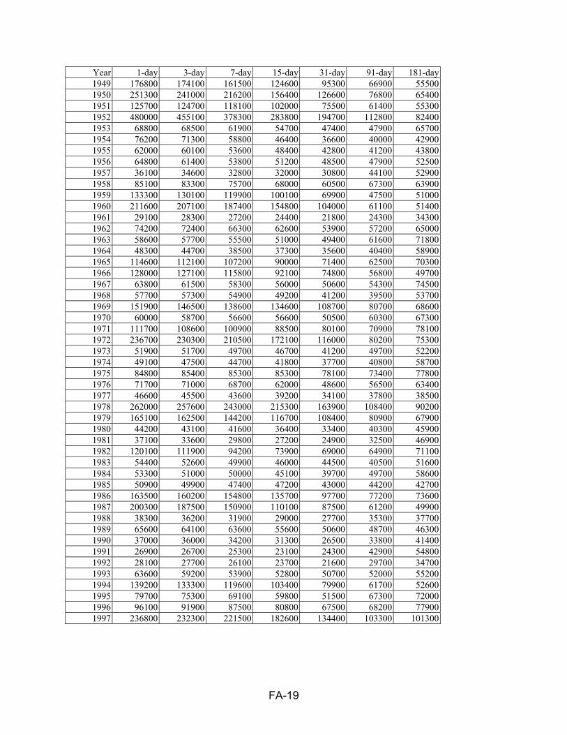
FA-19

Year 1-day 3-day 7-day 15-day 31-day 91-day 181-day 1949 176800 174100 161500 124600 95300 66900 55500 1950 251300 241000 216200 156400 126600 76800 65400 1951 125700 124700 118100 102000 75500 61400 55300 1952 480000 455100 378300 283800 194700 112800 82400 1953 68800 68500 61900 54700 47400 47900 65700 1954 76200 71300 58800 46400 36600 40000 42900 1955 62000 60100 53600 48400 42800 41200 43800 1956 64800 61400 53800 51200 48500 47900 52500 1957 36100 34600 32800 32000 30800 44100 52900 1958 85100 83300 75700 68000 60500 67300 63900 1959 133300 130100 119900 100100 69900 47500 51000 1960 211600 207100 187400 154800 104000 61100 51400 1961 29100 28300 27200 24400 21800 24300 34300 1962 74200 72400 66300 62600 53900 57200 65000 1963 58600 57700 55500 51000 49400 61600 71800 1964 48300 44700 38500 37300 35600 40400 58900 1965 114600 112100 107200 90000 71400 62500 70300 1966 128000 127100 115800 92100 74800 56800 49700 1967 63800 61500 58300 56000 50600 54300 74500 1968 57700 57300 54900 49200 41200 39500 53700 1969 151900 146500 138600 134600 108700 80700 68600 1970 60000 58700 56600 56600 50500 60300 67300 1971 111700 108600 100900 88500 80100 70900 78100 1972 236700 230300 210500 172100 116000 80200 75300 1973 51900 51700 49700 46700 41200 49700 52200 1974 49100 47500 44700 41800 37700 40800 58700 1975 84800 85400 85300 85300 78100 73400 77800 1976 71700 71000 68700 62000 48600 56500 63400 1977 46600 45500 43600 39200 34100 37800 38500 1978 262000 257600 243000 215300 163900 108400 90200 1979 165100 162500 144200 116700 108400 80900 67900 1980 44200 43100 41600 36400 33400 40300 45900 1981 37100 33600 29800 27200 24900 32500 46900 1982 120100 111900 94200 73900 69000 64900 71100 1983 54400 52600 49900 46000 44500 40500 51600 1984 53300 51000 50000 45100 39700 49700 58600 1985 50900 49900 47400 47200 43000 44200 42700 1986 163500 160200 154800 135700 97700 77200 73600 1987 200300 187500 150900 110100 87500 61200 49900 1988 38300 36200 31900 29000 27700 35300 37700 1989 65600 64100 63600 55600 50600 48700 46300 1990 37000 36000 34200 31300 26500 33800 41400 1991 26900 26700 25300 23100 24300 42900 54800 1992 28100 27700 26100 23700 21600 29700 34700 1993 63600 59200 53900 52800 50700 52000 55200 1994 139200 133300 119600 103400 79900 61700 52600 1995 79700 75300 69100 59800 51500 67300 72000 1996 96100 91900 87500 80800 67500 68200 77900 1997 236800 232300 221500 182600 134400 103300 101300

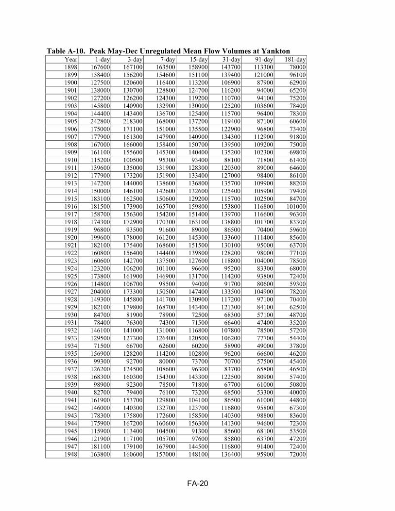
FA-20

Table A-10. Peak May-Dec Unregulated Mean Flow Volumes at Yankton Year 1-day 3-day 7-day 15-day 31-day 91-day 181-day 1898 167600 167100 163500 158900 143700 113300 78000 1899 158400 156200 154600 151100 139400 121000 96100 1900 127500 120600 116400 113200 106900 87900 62900 1901 138000 130700 128800 124700 116200 94000 65200 1902 127200 126200 124300 119200 110700 94100 75200 1903 145800 140900 132900 130000 125200 103600 78400 1904 144400 143400 136700 125400 115700 96400 78300 1905 242800 218300 168000 137200 119400 87100 60600 1906 175000 171100 151000 135500 122900 96800 73400 1907 177900 161300 147900 140900 134300 112900 91800 1908 167000 166000 158400 150700 139500 109200 75000 1909 161100 155600 145300 140400 135200 102300 69800 1910 115200 100500 95300 93400 88100 71800 61400 1911 139600 135000 131900 128300 120300 89000 64600 1912 177900 173200 151900 133400 127000 98400 86100 1913 147200 144000 138600 136800 135700 109900 88200 1914 150000 146100 142600 132600 125400 105900 79400 1915 183100 162500 150600 129200 115700 102500 84700 1916 181500 173900 165700 159800 153800 116800 101000 1917 158700 156300 154200 151400 139700 116600 96300 1918 174300 172900 170300 163100 138800 101700 83300 1919 96800 93500 91600 89000 86500 70400 59600 1920 199600 178000 161200 145300 133600 111400 85600 1921 182100 175400 168600 151500 130100 95000 63700 1922 160800 156400 144400 139800 128200 98000 77100 1923 160600 142700 137500 127600 118800 104000 78500 1924 123200 106200 101100 96600 95200 83300 68000 1925 173800 161900 146900 131700 114200 93800 72400 1926 114800 106700 98500 94000 91700 80600 59300 1927 204000 173300 150500 147400 133500 104900 78200 1928 149300 145800 141700 130900 117200 97100 70400 1929 182100 179800 168700 143400 121300 84100 62500 1930 84700 81900 78900 72500 68300 57100 48700 1931 78400 76300 74300 71500 66400 47400 35200 1932 146100 141000 131000 116800 107800 78500 57200 1933 129500 127300 126400 120500 106200 77700 54400 1934 71500 66700 62600 60200 58900 49000 37800 1935 156900 128200 114200 102800 96200 66600 46200 1936 99300 92700 80000 73700 70700 57500 45400 1937 126200 124500 108600 96300 83700 65800 46500 1938 168300 160300 154300 143300 122500 80900 57400 1939 98900 92300 78500 71800 67700 61000 50800 1940 82700 79400 76100 73200 68500 53300 40000 1941 161900 153700 129800 104100 86500 61000 44800 1942 146000 140300 132700 123700 116800 95800 67300 1943 178300 175800 172600 158500 140300 98800 83600 1944 175900 167200 160600 156300 141300 94600 72300 1945 115900 113400 104500 91300 85600 68100 53500 1946 121900 117100 105700 97600 85800 63700 47200 1947 181100 179100 167900 144500 116800 91400 72400 1948 163800 160600 157000 148100 136400 95900 72000

FA-21


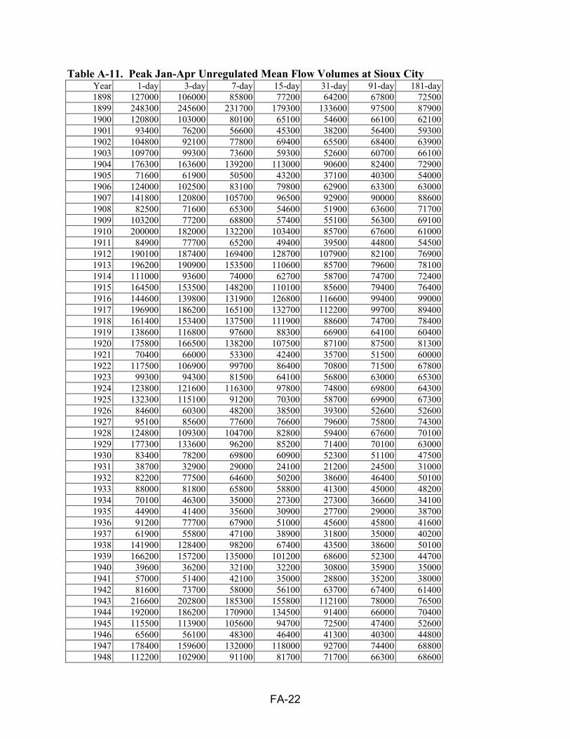
FA-22

Table A-11. Peak Jan-Apr Unregulated Mean Flow Volumes at Sioux City Year 1-day 3-day 7-day 15-day 31-day 91-day 181-day 1898 127000 106000 85800 77200 64200 67800 72500 1899 248300 245600 231700 179300 133600 97500 87900 1900 120800 103000 80100 65100 54600 66100 62100 1901 93400 76200 56600 45300 38200 56400 59300 1902 104800 92100 77800 69400 65500 68400 63900 1903 109700 99300 73600 59300 52600 60700 66100 1904 176300 163600 139200 113000 90600 82400 72900 1905 71600 61900 50500 43200 37100 40300 54000 1906 124000 102500 83100 79800 62900 63300 63000 1907 141800 120800 105700 96500 92900 90000 88600 1908 82500 71600 65300 54600 51900 63600 71700 1909 103200 77200 68800 57400 55100 56300 69100 1910 200000 182000 132200 103400 85700 67600 61000 1911 84900 77700 65200 49400 39500 44800 54500 1912 190100 187400 169400 128700 107900 82100 76900 1913 196200 190900 153500 110600 85700 79600 78100 1914 111000 93600 74000 62700 58700 74700 72400 1915 164500 153500 148200 110100 85600 79400 76400 1916 144600 139800 131900 126800 116600 99400 99000 1917 196900 186200 165100 132700 112200 99700 89400 1918 161400 153400 137500 111900 88600 74700 78400 1919 138600 116800 97600 88300 66900 64100 60400 1920 175800 166500 138200 107500 87100 87500 81300 1921 70400 66000 53300 42400 35700 51500 60000 1922 117500 106900 99700 86400 70800 71500 67800 1923 99300 94300 81500 64100 56800 63000 65300 1924 123800 121600 116300 97800 74800 69800 64300 1925 132300 115100 91200 70300 58700 69900 67300 1926 84600 60300 48200 38500 39300 52600 52600 1927 95100 85600 77600 76600 79600 75800 74300 1928 124800 109300 104700 82800 59400 67600 70100 1929 177300 133600 96200 85200 71400 70100 63000 1930 83400 78200 69800 60900 52300 51100 47500 1931 38700 32900 29000 24100 21200 24500 31000 1932 82200 77500 64600 50200 38600 46400 50100 1933 88000 81800 65800 58800 41300 45000 48200 1934 70100 46300 35000 27300 27300 36600 34100 1935 44900 41400 35600 30900 27700 29000 38700 1936 91200 77700 67900 51000 45600 45800 41600 1937 61900 55800 47100 38900 31800 35000 40200 1938 141900 128400 98200 67400 43500 38600 50100 1939 166200 157200 135000 101200 68600 52300 44700 1940 39600 36200 32100 32200 30800 35900 35000 1941 57000 51400 42100 35000 28800 35200 38000 1942 81600 73700 58000 56100 63700 67400 61400 1943 216600 202800 185300 155800 112100 78000 76500 1944 192000 186200 170900 134500 91400 66000 70400 1945 115500 113900 105600 94700 72500 47400 52600 1946 65600 56100 48300 46400 41300 40300 44800 1947 178400 159600 132000 118000 92700 74400 68800 1948 112200 102900 91100 81700 71700 66300 68600

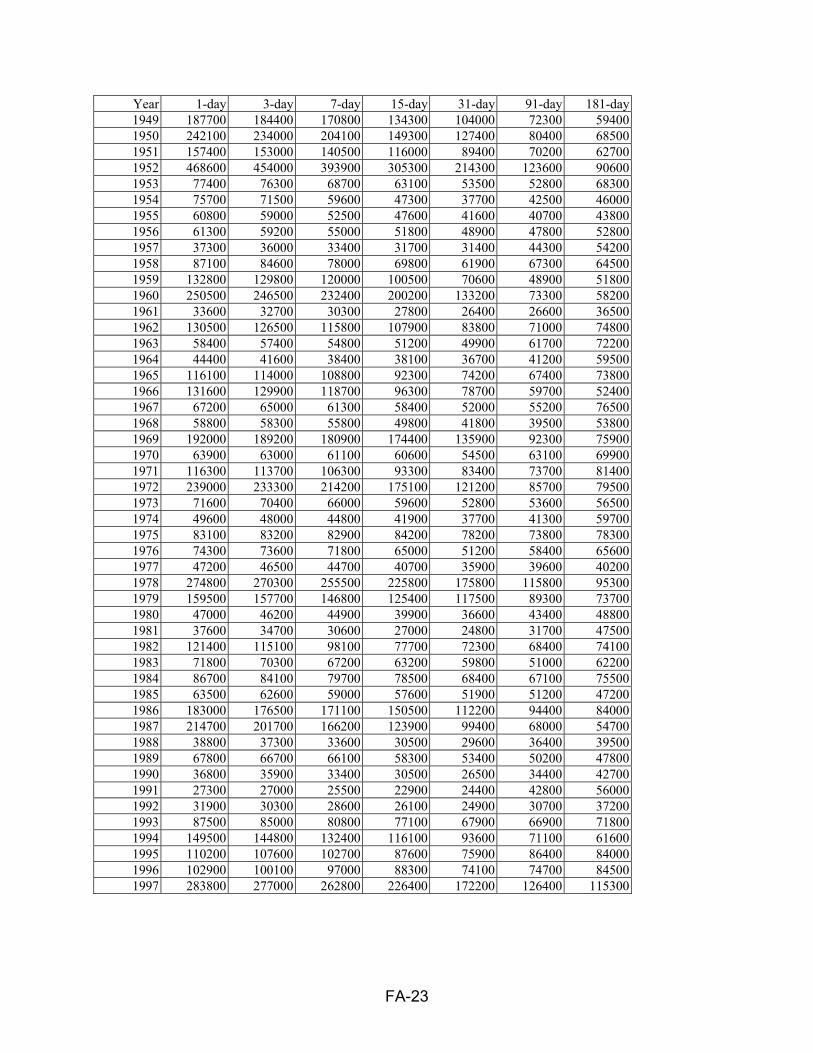
FA-23


FA-24

Table A-12. Peak May-Dec Unregulated Mean Flow Volumes at Sioux City Year 1-day 3-day 7-day 15-day 31-day 91-day 181-day 1898 171100 171100 167600 162800 147700 117400 81500 1899 160400 158400 156600 154200 142700 126400 99600 1900 128400 122500 118200 114600 109200 90800 66700 1901 147200 142400 139400 133300 124000 99800 70000 1902 129700 128700 126000 120600 112200 96300 77700 1903 149300 145600 135600 134500 129000 108000 82800 1904 148800 147700 140700 129700 121700 100300 81600 1905 233600 214400 170300 140300 124100 90800 64100 1906 180200 177700 158000 145000 131700 103800 80000 1907 180200 167500 154900 147100 142400 120500 99600 1908 183800 182500 174500 164200 150900 115800 80700 1909 170600 166000 157300 150300 147900 110900 78100 1910 109200 101300 96400 94100 89400 74200 65300 1911 138300 134600 132400 128900 121400 90000 65500 1912 181600 176100 156600 137900 129300 101200 89400 1913 151900 148800 144000 139600 139400 113900 92700 1914 155300 152500 149400 138800 134000 110500 82900 1915 177000 164600 156500 134800 120800 108600 91200 1916 182700 179200 170700 165100 159200 122100 107200 1917 160900 158800 157300 154500 142900 119500 98900 1918 179200 177500 174700 166900 141700 104700 86500 1919 99400 97000 95900 93100 90100 72900 62100 1920 196600 186600 168500 151700 139300 118100 91900 1921 176100 173500 168200 152000 131500 97900 67100 1922 159800 154800 144800 140500 129000 99300 78400 1923 153700 146800 143100 136400 125500 109500 82900 1924 131800 120000 117200 113700 105400 89000 72800 1925 170000 162300 148600 133700 116800 95200 73300 1926 112100 107300 100200 95400 93400 81800 60300 1927 204500 179500 151000 148300 135200 108500 81900 1928 150400 148300 144400 133800 119700 99900 72700 1929 186800 184800 172800 149100 128300 88900 70200 1930 86800 83400 80100 73700 70300 59500 52800 1931 81100 79300 75700 73200 67400 47800 35400 1932 148000 142700 132900 118600 109000 79200 58300 1933 129700 127500 126500 120700 106600 78000 55100 1934 77400 72200 65700 61600 60200 49700 38200 1935 157200 128500 114900 103500 96700 67000 46500 1936 99800 93400 80500 74100 71900 58000 46800 1937 127100 125500 109600 97400 84700 66700 47900 1938 168000 162300 157000 147400 124800 82200 58900 1939 104100 96500 79300 71800 68800 62000 51900 1940 89100 83100 77600 74200 69200 54000 40900 1941 148000 142800 120800 100900 85700 61200 45400 1942 149800 143100 129300 126500 120000 98400 69800 1943 172200 170500 166300 154300 139800 101100 85100 1944 203400 186100 170200 160600 146100 103000 79000 1945 130200 123700 111300 97900 93300 72800 58200 1946 123900 121000 108100 98600 86400 64400 49000 1947 190600 187100 169900 142900 118300 93200 75500 1948 169500 168100 164300 152900 139300 99100 76500 1949 112500 110100 103700 94500 87700 76900 64200

FA-25


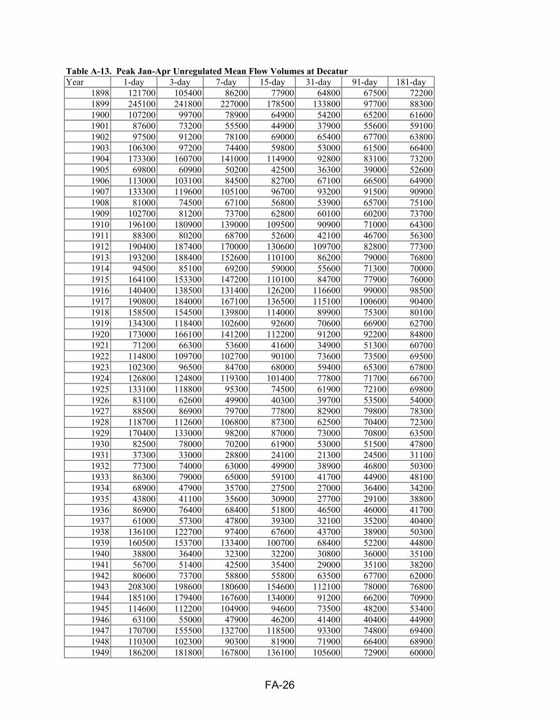
FA-26

Table A-13. Peak Jan-Apr Unregulated Mean Flow Volumes at Decatur Year 1-day 3-day 7-day 15-day 31-day 91-day 181-day

1898 121700 105400 86200 77900 64800 67500 72200 1899 245100 241800 227000 178500 133800 97700 88300 1900 107200 99700 78900 64900 54200 65200 61600 1901 87600 73200 55500 44900 37900 55600 59100 1902 97500 91200 78100 69000 65400 67700 63800 1903 106300 97200 74400 59800 53000 61500 66400 1904 173300 160700 141000 114900 92800 83100 73200 1905 69800 60900 50200 42500 36300 39000 52600 1906 113000 103100 84500 82700 67100 66500 64900 1907 133300 119600 105100 96700 93200 91500 90900 1908 81000 74500 67100 56800 53900 65700 75100 1909 102700 81200 73700 62800 60100 60200 73700 1910 196100 180900 139000 109500 90900 71000 64300 1911 88300 80200 68700 52600 42100 46700 56300 1912 190400 187400 170000 130600 109700 82800 77300 1913 193200 188400 152600 110100 86200 79000 76800 1914 94500 85100 69200 59000 55600 71300 70000 1915 164100 153300 147200 110100 84700 77900 76000 1916 140400 138500 131400 126200 116600 99000 98500 1917 190800 184000 167100 136500 115100 100600 90400 1918 158500 154500 139800 114000 89900 75300 80100 1919 134300 118400 102600 92600 70600 66900 62700 1920 173000 166100 141200 112200 91200 92200 84800 1921 71200 66300 53600 41600 34900 51300 60700 1922 114800 109700 102700 90100 73600 73500 69500 1923 102300 96500 84700 68000 59400 65300 67800 1924 126800 124800 119300 101400 77800 71700 66700 1925 133100 118800 95300 74500 61900 72100 69800 1926 83100 62600 49900 40300 39700 53500 54000 1927 88500 86900 79700 77800 82900 79800 78300 1928 118700 112600 106800 87300 62500 70400 72300 1929 170400 133000 98200 87000 73000 70800 63500 1930 82500 78000 70200 61900 53000 51500 47800 1931 37300 33000 28800 24100 21300 24500 31100 1932 77300 74000 63000 49900 38900 46800 50300 1933 86300 79000 65000 59100 41700 44900 48100 1934 68900 47900 35700 27500 27000 36400 34200 1935 43800 41100 35600 30900 27700 29100 38800 1936 86900 76400 68400 51800 46500 46000 41700 1937 61000 57300 47800 39300 32100 35200 40400 1938 136100 122700 97400 67600 43700 38900 50300 1939 160500 153700 133400 100700 68400 52200 44800 1940 38800 36400 32300 32200 30800 36000 35100 1941 56700 51400 42500 35400 29000 35100 38200 1942 80600 73700 58800 55800 63500 67700 62000 1943 208300 198600 180600 154600 112100 78000 76800 1944 185100 179400 167600 134000 91200 66200 70900 1945 114600 112200 104900 94600 73500 48200 53400 1946 63100 55000 47900 46200 41400 40400 44900 1947 170700 155500 132700 118500 93300 74800 69400 1948 110300 102300 90300 81900 71900 66400 68900 1949 186200 181800 167800 136100 105600 72900 60000

FA-27


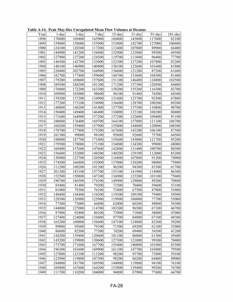
FA-28

Table A-14. Peak May-Dec Unregulated Mean Flow Volumes at Decatur Year 1-day 3-day 7-day 15-day 31-day 91-day 181-day 1898 170000 169400 165900 160400 145800 117000 82100 1899 159800 158000 155900 153800 142700 127000 100400 1900 124100 120300 117200 113400 107800 89900 66400 1901 144900 141200 138400 132900 123800 99500 69500 1902 127900 127200 124500 119700 111800 96400 77700 1903 146500 142700 133000 132300 127200 107800 83200 1904 148100 146900 140400 130100 122600 101600 81800 1905 220400 202700 164900 136600 121200 87200 61600 1906 182700 177400 159600 146700 133600 104300 81400 1907 179200 169600 157600 151100 146400 124800 102500 1908 189500 188200 181200 171200 157300 120500 84400 1909 176000 172200 163300 158200 155200 116300 82700 1910 109900 103000 98600 96100 91400 76500 68300 1911 139200 137200 134900 131600 123700 92500 67800 1912 177200 173100 154900 136600 128700 100500 89200 1913 148000 146200 141400 137700 137300 110800 90700 1914 150400 149400 146400 136000 132100 108200 80400 1915 171600 164900 157200 137200 122600 109400 91100 1916 180600 176400 169700 164100 157800 121100 106700 1917 160200 159400 157900 155000 144000 120800 100300 1918 178700 177800 175200 167600 143200 106100 87500 1919 101300 99000 98100 95600 92600 75700 64500 1920 198000 187700 171800 155600 143000 121700 95200 1921 179500 178000 171100 154800 134300 99800 68000 1922 160400 157600 147600 142800 131400 100700 80300 1923 156600 152000 148200 140200 129100 112000 85200 1924 130900 123700 120500 116800 107800 91200 74900 1925 174500 166800 152000 137000 120200 98000 75800 1926 111200 108200 101200 96200 94300 83300 61700 1927 201200 183100 157700 155100 141900 114900 86300 1928 152500 150800 147100 136900 123200 103100 75600 1929 190700 186500 174100 149900 129000 89200 70800 1930 85400 81400 79200 73500 70400 59600 53100 1931 81000 79300 76100 73400 67500 47800 35400 1932 148400 144400 134200 119300 109100 79400 58500 1933 128500 126900 125900 119900 106000 77700 55000 1934 77300 73000 66800 62000 60200 49800 38300 1935 144000 127000 114700 103300 96500 67100 46700 1936 97900 92800 80100 73900 71800 58000 47000 1937 127400 124000 110400 97700 84800 67100 48300 1938 165200 160800 156600 147100 124800 82300 59200 1939 99800 95600 79100 71500 69200 62100 52000 1940 86600 82500 77300 74200 69400 54300 41200 1941 144200 139400 120600 101100 86000 61300 45600 1942 145200 139800 130600 127300 121000 99300 70400 1943 173700 171600 167700 155400 140800 101800 85500 1944 196300 183600 169900 161100 147700 103800 79500 1945 127000 123100 111200 98200 93700 73800 59100 1946 122900 119800 107300 98200 86200 64400 49000 1947 184000 181700 169500 144000 119800 94100 76100 1948 169400 167600 164200 153000 139400 99200 76700 1949 111700 110200 104000 94800 87900 77600 64700

FA-29


FA-30

Table A-15. Peak Jan-Apr Unregulated Mean Flow Volumes at Omaha Year 1-day 3-day 7-day 15-day 31-day 91-day 181-day 1898 118900 106200 91300 82400 66700 65100 70200 1899 232600 229700 212600 172000 133600 98100 89800 1900 102500 96600 78100 64400 54600 59900 58400 1901 77700 70200 52800 43800 36000 50700 57600 1902 93600 89800 78900 69700 64200 63400 62600 1903 106400 94700 77300 62900 54500 65500 67300 1904 177800 168500 151100 126600 103400 85700 74400 1905 66300 59900 49100 39300 32200 32500 44700 1906 120000 113000 102800 101200 89600 83000 73900 1907 130000 118300 107800 102700 96800 99100 101800 1908 93400 88500 78400 68400 64200 76000 92600 1909 145500 134000 120100 101700 95300 80500 97500 1910 223200 212600 177500 142300 120000 89400 81500 1911 107400 95500 86600 70400 56000 56500 65200 1912 196400 195100 182400 147700 119600 85700 78900 1913 200200 189000 159400 120900 92100 75000 69600 1914 63200 55300 47100 39000 39300 52100 56600 1915 161000 154100 146700 115000 86800 68500 72800 1916 134300 132400 128100 122800 116000 95800 94600 1917 199000 197200 187800 157900 129800 104000 94600 1918 173200 168800 151800 127800 96600 79400 88900 1919 146200 140200 128300 117500 90500 81300 74200 1920 199800 187300 164000 137800 114800 116000 103000 1921 74700 68300 54600 37300 30400 49500 63800 1922 128600 126200 120800 109800 88800 83400 77700 1923 117400 112300 102600 88800 76400 77000 81000 1924 145400 142000 136300 119800 93200 81500 78700 1925 147800 138800 117700 96100 78700 83100 82900 1926 98000 77700 60500 50000 43700 57600 60900 1927 95300 94500 92600 89100 97800 99600 99000 1928 132600 129800 124400 110700 82300 85100 83000 1929 163300 136900 107500 96300 80600 73900 65600 1930 84000 80000 74500 66500 56700 53200 48800 1931 37600 34100 28900 24000 21300 24200 31000 1932 66400 60200 55100 48000 41200 48300 51200 1933 75600 72800 63300 59900 43500 43700 47400 1934 85900 53100 38100 28400 25500 35300 34200 1935 43200 40900 35800 31400 27800 28900 38700 1936 84500 77400 72400 56600 50600 46700 42100 1937 70300 64800 51400 41200 33300 36100 41400 1938 114400 110700 94800 68000 44500 39700 51100 1939 140900 139800 126100 97400 67000 51400 45200 1940 39800 36900 32800 32500 30700 36600 35700 1941 57900 53100 44800 37100 30000 34600 39000 1942 82900 78200 64000 52800 62400 69200 64500 1943 210200 204100 179300 151500 111300 77500 78200 1944 157500 156800 152200 130600 89400 67000 73300 1945 109500 107600 100900 93400 78100 52600 57600 1946 62700 56000 47000 45500 41400 40400 45000 1947 159100 150200 140100 121400 95700 76500 72100 1948 106900 100900 87100 82400 75000 65900 69700 1949 194000 186800 175200 144700 113200 75600 62600

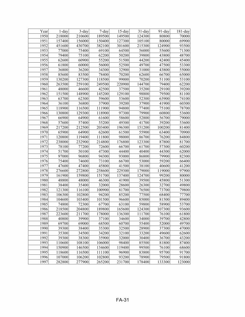
FA-31


FA-32

Table A-16. Peak May-Dec Unregulated Mean Flow Volumes at Omaha Year 1-day 3-day 7-day 15-day 31-day 91-day 181-day 1898 162100 160300 155600 146200 135900 114100 84800 1899 156200 154300 150800 150300 141800 129300 104900 1900 117400 114800 111600 106700 100400 84900 64300 1901 138800 137400 134100 130300 123500 97300 66400 1902 120100 119100 115800 113600 108800 96700 77100 1903 147200 138100 128100 119200 116600 105800 84900 1904 143500 143500 139300 132100 127200 107800 81800 1905 168700 157700 136900 115600 104100 68500 48600 1906 193300 185200 171200 154600 143100 107100 88600 1907 187600 185200 183500 176300 169600 146900 116900 1908 223300 222400 218900 209100 190400 145100 103100 1909 209000 206400 203000 201500 194100 144400 109000 1910 118800 116400 111100 105900 101400 88800 84200 1911 152500 150600 148200 144700 135200 105100 79900 1912 164500 161300 145400 128600 124700 97800 87400 1913 136000 134400 130800 127700 125700 98600 78900 1914 135600 132700 130600 123000 121800 95000 66900 1915 171500 169600 166400 150600 131700 112800 91500 1916 170000 168100 163000 157500 149100 114900 102900 1917 164200 161800 159700 157000 149000 127600 106800 1918 181400 179500 177100 170700 151000 112400 92600 1919 118100 117200 112500 110500 105000 90300 77000 1920 224700 208800 191700 175700 161600 140300 112500 1921 207400 200600 189600 170600 149000 109600 72000 1922 173700 170800 162600 156300 143100 107400 89500 1923 182900 179800 174300 162300 147900 125100 96800 1924 145700 144800 140900 134700 122600 102200 86000 1925 198100 190100 173800 154700 139000 112400 88700 1926 117700 115500 106400 100000 98700 90600 69700 1927 225100 211700 194000 190700 176700 148500 108700 1928 164000 163600 161300 153300 141000 119700 90900 1929 210800 202100 181500 155000 131900 90300 73200 1930 81500 80300 75600 72500 70800 60000 54100 1931 82700 80400 77600 74100 67700 47900 35600 1932 152000 151500 140000 122600 108700 79700 59600 1933 125000 124300 122300 115200 102200 75600 54200 1934 87600 82600 72200 64500 60500 50300 38300 1935 128400 118600 114000 101600 95100 67600 47000 1936 97200 90800 77800 72300 70500 57600 47700 1937 128100 124500 114300 98800 84800 69400 50000 1938 158600 156700 152700 144200 123700 82500 60500 1939 99900 94400 78600 72600 70400 62700 52300 1940 90200 80900 76700 74300 71100 55700 42200 1941 133000 130700 120500 102600 87100 61700 46300 1942 148600 145800 138300 132900 125600 103600 73300 1943 181300 178500 174100 160600 146100 104600 87100 1944 181600 174900 168400 163300 155900 107400 81700 1945 123700 119900 110800 98800 96100 79100 63800 1946 117800 114600 104000 95900 84500 63600 48700 1947 179800 178400 170000 149500 126900 98400 78900 1948 167000 165200 162300 152500 139800 99400 77400 1949 114800 110700 105300 96200 88500 80600 67100

FA-33


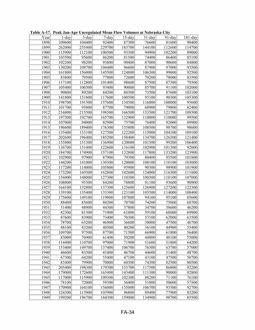
FA-34

Table A-17. Peak Jan-Apr Unregulated Mean Flow Volumes at Nebraska City Year 1-day 3-day 7-day 15-day 31-day 91-day 181-day 1898 109600 104400 92400 87300 76600 81600 90400 1899 262000 255400 229700 183700 144100 112600 114700 1900 115900 112100 100500 93300 94900 102200 89000 1901 103500 95600 86200 81500 74400 86400 85100 1902 102200 98200 93800 90400 87000 90600 84800 1903 130200 108700 104400 96600 87900 97000 93500 1904 161800 156000 145500 124800 106300 99800 92500 1905 83800 79500 77800 72600 70200 78000 83500 1906 117100 112800 101400 98600 87500 87300 79300 1907 105400 100300 93400 90000 85700 91100 102000 1908 90800 89200 84200 80300 73500 87600 103100 1909 141800 131800 117600 100500 95100 90300 105300 1910 198700 191500 157600 134500 116000 100000 95600 1911 101700 95800 87700 79000 68900 79800 82400 1912 216800 215500 198500 166500 153500 121700 109300 1913 197300 192700 165700 132900 118000 110000 99500 1914 107000 94000 82900 75700 76400 92000 89900 1915 196600 189400 176300 135800 108500 98700 98600 1916 135400 133100 127500 122200 115000 104100 109100 1917 202600 196400 185200 158400 134700 126500 121400 1918 155800 151300 136900 120000 101500 99200 106400 1919 136700 131400 122600 116100 102900 101300 92000 1920 184700 174900 157100 132800 117800 133200 123900 1921 102900 97900 87900 79300 80400 95500 101800 1922 144200 141000 130300 120000 108100 110100 103000 1923 117200 114000 105800 95900 90300 98900 101900 1924 173200 169300 162800 142600 124000 116300 111800 1925 154400 148000 127300 110300 100300 110100 107000 1926 108800 95300 84200 78800 81100 93600 90900 1927 164100 152800 137300 125600 126900 127200 122300 1928 139100 135400 133300 123100 105500 114000 108400 1929 175600 149100 119800 107800 94100 95100 85600 1930 88400 85600 80200 70700 74200 75000 68700 1931 51400 48900 44300 37800 34700 38600 46200 1932 82300 81300 71000 61000 59100 68000 69900 1933 87600 83900 73400 70300 53100 62000 63500 1934 78700 63200 46900 36600 38000 47500 46700 1935 48100 43200 40500 40200 36100 44900 55400 1936 109700 97500 87700 71500 66900 61800 56400 1937 83000 76900 61400 50200 44800 48100 55000 1938 114400 110700 97000 71900 51600 51800 64200 1939 153400 149700 137400 106700 76300 63700 57000 1940 46600 43500 41000 46700 44600 51400 48700 1941 67300 64200 55400 47100 43100 47500 50700 1942 83400 79900 70000 60300 74300 82500 80500 1943 205400 198300 179300 153700 117500 86800 92200 1944 179000 172600 165400 143400 111300 90000 92800 1945 117000 115900 109300 102300 88200 71100 76100 1946 78100 72000 59300 56400 51800 50600 57500 1947 170900 164100 156000 135000 106700 93500 92700 1948 124300 113900 103900 96800 89400 77900 83200 1949 199200 196700 184300 159000 134900 98700 85500

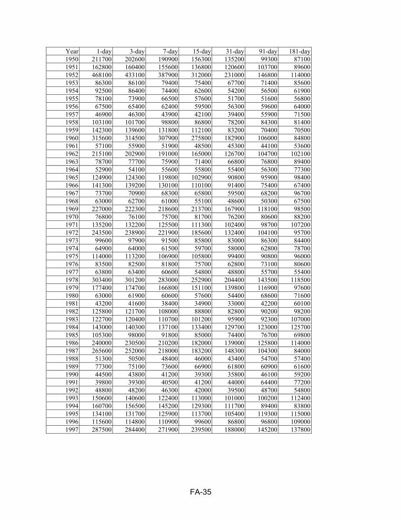
FA-35


FA-36

Table A-18. Peak May-Dec Unregulated Mean Flow Volumes at Nebraska City Year 1-day 3-day 7-day 15-day 31-day 91-day 181-day 1898 198100 196900 190800 176000 162600 128600 96900 1899 201700 201500 198700 196600 181700 152500 123800 1900 170400 160900 153900 150400 142900 126400 98300 1901 174800 171400 169800 160300 149000 120200 94500 1902 160100 154700 152700 149900 140300 124700 102900 1903 214300 208100 186600 157400 145000 135300 111900 1904 176600 176600 171800 160400 150200 124100 101900 1905 234600 223300 196900 172500 154900 117600 90200 1906 187800 176800 162400 156900 143900 118100 99000 1907 222000 220800 214700 200000 186300 162700 122400 1908 249700 245800 240300 235100 213800 160300 117000 1909 226500 222500 209300 207400 200200 158900 121500 1910 129000 125200 121400 118700 117800 108700 100200 1911 168200 166700 164700 159800 147600 123700 98300 1912 178300 175900 164000 151200 150600 125100 119500 1913 171300 168900 164800 163200 159200 132400 110700 1914 229400 222000 206900 182000 169900 130300 100600 1915 201700 201000 195700 176400 160200 143100 117700 1916 203700 202700 196600 190700 174900 138900 120000 1917 214600 212400 211400 209500 199400 167100 134400 1918 202900 201800 199000 192000 168500 135700 112100 1919 144400 143500 139300 137200 131600 113100 97100 1920 259400 250400 234800 216900 195500 169200 135800 1921 284600 279600 265600 233200 198200 149300 111500 1922 207500 206300 194200 188300 173100 139700 117000 1923 221400 215900 207000 195700 182600 154600 120400 1924 204600 201600 194800 188900 175200 143000 122300 1925 209200 204100 190600 175700 163000 138900 114600 1926 150400 146700 141100 136900 136100 123000 99800 1927 240200 227800 223800 221500 204000 170400 133200 1928 184500 182200 177000 169700 163300 144900 118900 1929 241900 234800 215200 192400 167100 117500 95000 1930 121900 116200 114300 108800 102100 87900 74700 1931 125500 118600 109800 98100 91100 66700 51800 1932 175400 174300 162700 142900 133100 105500 79500 1933 139100 138500 136100 128000 121900 97400 71200 1934 128700 125900 107400 87500 78100 67400 52900 1935 157700 153600 149900 143100 127400 95300 66300 1936 117300 108100 100800 97600 91400 75600 64100 1937 139100 138500 133000 123700 107300 90200 65900 1938 207900 205000 195600 174900 148100 101900 75800 1939 125700 118600 103900 96500 90200 79400 66600 1940 146900 143200 129100 109400 99300 75600 57500 1941 140600 139500 130700 116000 102900 77900 59600 1942 214500 206600 189200 178800 159700 128200 90900 1943 227600 223400 212600 188900 179700 126700 102600 1944 284500 280200 244000 200900 188900 134300 103300 1945 165200 160100 146900 132300 125900 105600 83300 1946 154100 153300 139300 128200 109900 80100 61500 1947 237700 232800 220900 208900 178000 131400 101500 1948 215600 208300 195300 180300 159600 117200 93100 1949 145500 143300 138500 134400 125000 103700 91500

FA-37


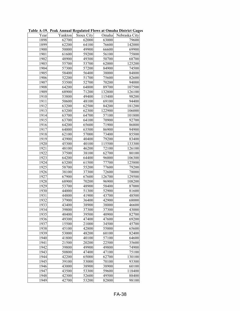
FA-38

Table A-19. Peak Annual Regulated Flows at Omaha District Gages Year Yankton Sioux City Omaha Nebraska City1898 62700 62000 63000 796001899 62200 64100 76600 1420001900 50000 49900 66600 699001901 61600 59200 56100 758001902 48900 49300 50700 687001903 55700 53700 62000 1252001904 57300 57200 84900 745001905 58400 56400 38000 848001906 52200 51700 75600 826001907 53500 52700 70200 940001908 64200 64800 89700 1075001909 68900 71200 132800 1261001910 53800 49400 115400 982001911 50600 48100 69100 944001912 63200 62500 84200 1812001913 63200 62300 122900 1060001914 63700 64700 57100 1018001915 63700 64100 70900 927001916 64200 65600 71900 868001917 64000 63500 86900 949001918 62100 57000 73400 855001919 43900 40400 79200 834001920 45300 40100 115500 1333001921 48100 46200 72100 1261001922 37500 38100 62700 801001923 64200 64400 96000 1063001924 63200 61500 77700 1258001925 58700 55200 77600 792001926 38100 37300 72600 780001927 67900 67600 126700 1295001928 68900 70200 96900 1082001929 53700 48900 58400 870001930 44000 51300 52900 816001931 44800 41900 43700 485001932 37900 36400 42900 680001933 43400 38900 38000 466001934 39800 37300 37300 430001935 40400 39500 40900 827001936 49300 47400 47600 692001937 15500 21000 34500 457001938 45100 42800 55000 656001939 53000 48200 60100 824001940 41800 40100 57100 646001941 21500 20200 22500 356001942 39800 49900 49800 749001943 50800 47400 47100 751001944 42200 65000 62700 1301001945 39100 53000 70100 933001946 43000 38900 38900 601001947 43500 53300 59600 1184001948 42300 52600 49500 884001949 42700 53200 82800 98100

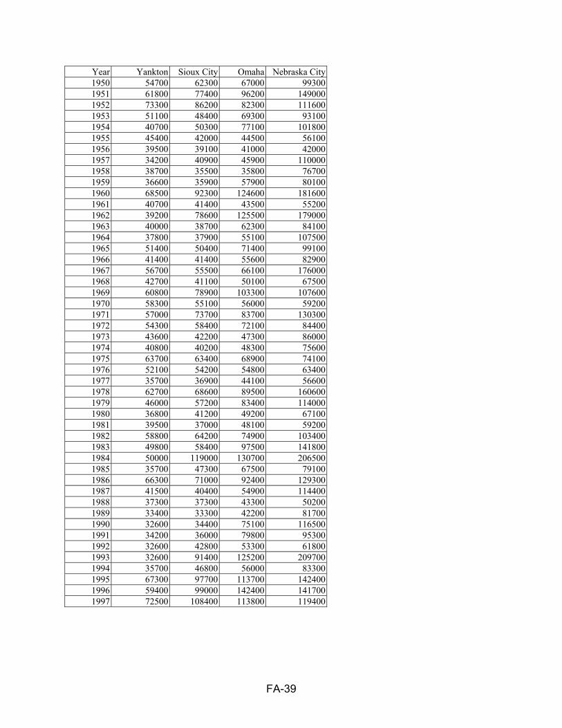
FA-39

Year Yankton Sioux City Omaha Nebraska City1950 54700 62300 67000 993001951 61800 77400 96200 1490001952 73300 86200 82300 1116001953 51100 48400 69300 931001954 40700 50300 77100 1018001955 45400 42000 44500 561001956 39500 39100 41000 420001957 34200 40900 45900 1100001958 38700 35500 35800 767001959 36600 35900 57900 801001960 68500 92300 124600 1816001961 40700 41400 43500 552001962 39200 78600 125500 1790001963 40000 38700 62300 841001964 37800 37900 55100 1075001965 51400 50400 71400 991001966 41400 41400 55600 829001967 56700 55500 66100 1760001968 42700 41100 50100 675001969 60800 78900 103300 1076001970 58300 55100 56000 592001971 57000 73700 83700 1303001972 54300 58400 72100 844001973 43600 42200 47300 860001974 40800 40200 48300 756001975 63700 63400 68900 741001976 52100 54200 54800 634001977 35700 36900 44100 566001978 62700 68600 89500 1606001979 46000 57200 83400 1140001980 36800 41200 49200 671001981 39500 37000 48100 592001982 58800 64200 74900 1034001983 49800 58400 97500 1418001984 50000 119000 130700 2065001985 35700 47300 67500 791001986 66300 71000 92400 1293001987 41500 40400 54900 1144001988 37300 37300 43300 502001989 33400 33300 42200 817001990 32600 34400 75100 1165001991 34200 36000 79800 953001992 32600 42800 53300 618001993 32600 91400 125200 2097001994 35700 46800 56000 833001995 67300 97700 113700 1424001996 59400 99000 142400 1417001997 72500 108400 113800 119400

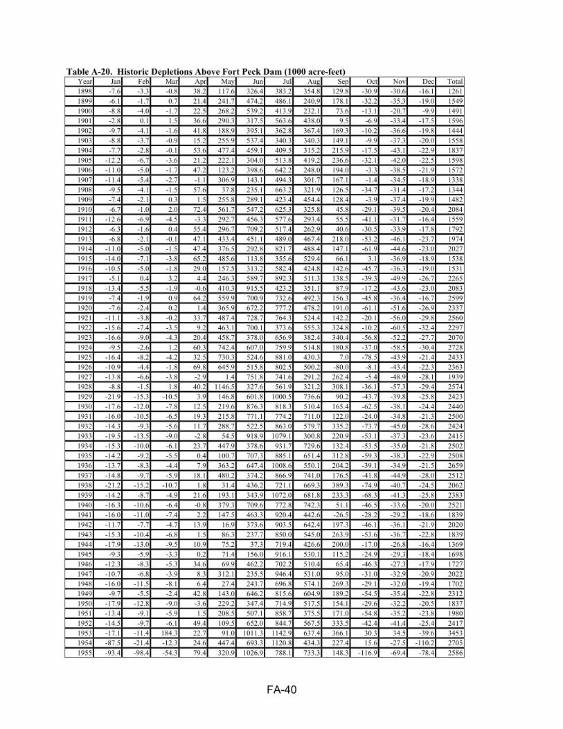
FA-40

Table A-20. Historic Depletions Above Fort Peck Dam (1000 acre-feet) Year Jan Feb Mar Apr May Jun Jul Aug Sep Oct Nov Dec Total1898 -7.6 -3.3 -0.8 38.2 117.6 326.4 383.2 354.8 129.8 -30.9 -30.6 -16.1 1261 1899 -6.1 -1.7 0.7 21.4 241.7 474.2 486.1 240.9 178.1 -32.2 -35.3 -19.0 15491900 -8.8 -4.0 -1.7 22.5 268.2 539.2 413.9 232.1 73.6 -13.1 -20.7 -9.9 1491 1901 -2.8 0.1 1.5 36.6 290.3 317.5 563.6 438.0 9.5 -6.9 -33.4 -17.5 1596 1902 -9.7 -4.1 -1.6 41.8 188.9 395.1 362.8 367.4 169.3 -10.2 -36.6 -19.8 1444 1903 -8.8 -3.7 -0.9 15.2 255.9 537.4 340.3 340.3 149.1 -9.9 -37.3 -20.0 1558 1904 -7.7 -2.8 -0.1 53.6 477.4 459.1 409.5 315.2 215.9 -17.5 -43.1 -22.9 1837 1905 -12.2 -6.7 -3.6 21.2 222.1 304.0 513.8 419.2 236.6 -32.1 -42.0 -22.5 1598 1906 -11.0 -5.0 -1.7 47.2 123.2 398.6 642.2 248.0 194.0 -3.3 -38.5 -21.9 1572 1907 -11.4 -5.4 -2.7 -1.1 306.9 143.1 494.3 301.7 167.1 -1.4 -34.5 -18.9 1338 1908 -9.5 -4.1 -1.5 57.6 37.8 235.1 663.2 321.9 126.5 -34.7 -31.4 -17.2 1344 1909 -7.4 -2.1 0.3 1.5 255.8 289.1 423.4 454.4 128.4 -3.9 -37.4 -19.9 1482 1910 -6.7 -1.0 2.0 72.4 561.7 547.2 625.3 325.8 45.8 -29.1 -39.5 -20.4 2084 1911 -12.6 -6.9 -4.5 -3.3 292.7 456.3 577.6 293.4 55.5 -41.1 -31.7 -16.4 1559 1912 -6.3 -1.6 0.4 55.4 296.7 709.2 517.4 262.9 40.6 -30.5 -33.9 -17.8 1792 1913 -6.8 -2.1 -0.1 47.1 433.4 451.1 489.0 467.4 218.0 -53.2 -46.1 -23.7 1974 1914 -11.0 -5.0 -1.5 47.4 376.5 292.8 821.7 488.4 147.1 -61.9 -44.6 -23.0 2027 1915 -14.0 -7.1 -3.8 65.2 485.6 113.8 355.6 529.4 66.1 3.1 -36.9 -18.9 1538 1916 -10.5 -5.0 -1.8 29.0 157.5 313.2 582.4 424.8 142.6 -45.7 -36.3 -19.0 1531 1917 -5.1 0.4 3.2 4.4 246.3 589.7 892.3 511.3 138.5 -39.3 -49.9 -26.7 2265 1918 -13.4 -5.5 -1.9 -0.6 410.3 915.5 423.2 351.1 87.9 -17.2 -43.6 -23.0 2083 1919 -7.4 -1.9 0.9 64.2 559.9 700.9 732.6 492.3 156.3 -45.8 -36.4 -16.7 2599 1920 -7.6 -2.4 0.2 1.4 365.9 672.2 777.2 478.2 191.0 -61.1 -51.6 -26.9 2337 1921 -11.1 -3.8 -0.2 33.7 487.4 728.7 764.3 524.4 142.2 -20.1 -56.0 -29.8 2560 1922 -15.6 -7.4 -3.5 9.2 463.1 700.1 373.6 555.3 324.8 -10.2 -60.5 -32.4 2297 1923 -16.6 -9.0 -4.3 20.4 458.7 378.0 656.9 382.4 340.4 -56.8 -52.2 -27.7 2070 1924 -9.5 -2.6 1.2 60.3 742.4 607.0 759.9 514.8 180.8 -37.0 -58.5 -30.4 2728 1925 -16.4 -8.2 -4.2 32.5 730.3 524.6 881.0 430.3 7.0 -78.5 -43.9 -21.4 2433 1926 -10.9 -4.4 -1.8 69.8 645.9 515.8 802.5 500.2 -80.0 -8.1 -43.4 -22.3 2363 1927 -13.8 -6.6 -3.8 -2.9 1.4 751.8 741.6 291.2 262.4 -5.4 -48.9 -28.1 1939 1928 -8.8 -1.5 1.8 40.2 1146.5 327.6 561.9 321.2 308.1 -36.1 -57.3 -29.4 2574 1929 -21.9 -15.3 -10.5 3.9 146.8 601.8 1000.5 736.6 90.2 -43.7 -39.8 -25.8 2423 1930 -17.6 -12.0 -7.8 12.5 219.6 876.3 818.3 510.4 165.4 -62.5 -38.1 -24.4 2440 1931 -16.0 -10.5 -6.5 19.3 215.8 771.1 774.2 711.0 122.0 -24.0 -34.8 -21.3 2500 1932 -14.3 -9.3 -5.6 11.7 288.7 522.5 863.0 579.7 335.2 -73.7 -45.0 -28.6 2424 1933 -19.5 -13.5 -9.0 -2.8 54.5 918.9 1079.1 300.8 220.9 -53.1 -37.3 -23.6 2415 1934 -15.3 -10.0 -6.1 23.7 447.9 378.6 931.7 729.6 132.4 -53.5 -35.0 -21.8 2502 1935 -14.2 -9.2 -5.5 0.4 100.7 707.3 885.1 651.4 312.8 -59.3 -38.3 -22.9 2508 1936 -13.7 -8.3 -4.4 7.9 363.2 647.4 1008.6 550.1 204.2 -39.1 -34.9 -21.5 2659 1937 -14.8 -9.7 -5.9 18.1 480.2 374.2 866.9 741.0 176.5 -41.8 -44.9 -28.0 2512 1938 -21.2 -15.2 -10.7 1.8 31.4 436.2 721.1 669.3 389.3 -74.9 -40.7 -24.5 2062 1939 -14.2 -8.7 -4.9 21.6 193.1 343.9 1072.0 681.8 233.3 -68.3 -41.3 -25.8 2383 1940 -16.3 -10.6 -6.4 -0.8 379.3 709.6 772.8 742.3 51.1 -46.5 -33.6 -20.0 2521 1941 -16.0 -11.0 -7.4 2.2 147.5 463.3 920.4 442.6 -26.5 -28.2 -29.2 -18.6 1839 1942 -11.7 -7.7 -4.7 13.9 16.9 373.6 903.5 642.4 197.3 -46.1 -36.1 -21.9 2020 1943 -15.3 -10.4 -6.8 1.5 86.3 237.7 850.0 545.0 263.9 -53.6 -36.7 -22.8 1839 1944 -17.9 -13.0 -9.5 10.9 75.2 37.3 719.4 426.6 200.0 -17.0 -26.8 -16.4 1369 1945 -9.3 -5.9 -3.3 0.2 71.4 156.0 916.1 530.1 115.2 -24.9 -29.3 -18.4 1698 1946 -12.3 -8.3 -5.3 34.6 69.9 462.2 702.2 510.4 65.4 -46.3 -27.3 -17.9 1727 1947 -10.7 -6.8 -3.9 8.3 312.1 235.5 946.4 531.0 95.0 -31.0 -32.9 -20.9 2022 1948 -16.0 -11.5 -8.1 6.4 27.4 243.7 696.8 574.1 269.3 -29.1 -32.0 -19.4 1702 1949 -9.7 -5.5 -2.4 42.8 143.0 646.2 815.6 604.9 189.2 -54.5 -35.4 -22.8 2312 1950 -17.9 -12.8 -9.0 -3.6 229.2 347.4 714.9 517.5 154.1 -29.6 -32.2 -20.5 1837 1951 -13.4 -9.1 -5.9 1.5 208.5 507.1 858.7 375.5 171.0 -54.8 -35.2 -23.8 1980 1952 -14.5 -9.7 -6.1 49.4 109.5 652.0 844.7 567.5 333.5 -42.4 -41.4 -25.4 2417 1953 -17.1 -11.4 184.3 22.7 91.0 1011.3 1142.9 637.4 366.1 30.3 34.5 -39.6 3453 1954 -87.5 -21.4 -12.3 24.6 447.4 693.3 1120.8 434.3 227.4 15.6 -27.5 -110.2 2705 1955 -93.4 -98.4 -54.3 79.4 320.9 1026.9 788.1 733.3 148.3 -116.9 -69.4 -78.4 2586

FA-41

Year Jan Feb Mar Apr May Jun Jul Aug Sep Oct Nov Dec Total1956 -71.2 -122.3 75.8 129.0 625.4 1108.5 840.8 367.9 219.2 -89.8 17.7 -83.6 3017 1957 -170.3 -111.6 -77.5 4.8 632.7 561.8 879.8 436.5 146.9 -77.9 -13.0 -80.3 2132 1958 -143.3 -84.6 28.0 -17.9 793.9 509.3 432.3 586.8 123.5 -86.8 -50.1 -25.8 2065 1959 -47.2 -24.4 138.0 168.6 70.5 819.2 929.8 434.7 80.3 2.1 -99.6 -237.6 2234 1960 25.7 70.2 114.4 -2.9 212.1 930.5 900.2 289.8 130.5 -167.5 -98.0 -33.5 23711961 -90.9 9.4 26.2 -54.9 225.2 1252.0 685.6 438.5 -33.3 33.1 -21.3 -110.5 2359 1962 -106.6 -21.1 -73.4 249.6 403.1 938.4 712.6 358.7 188.1 -34.6 6.8 -9.0 2612 1963 -78.7 34.0 -7.4 12.5 195.8 311.7 878.6 536.1 198.7 -70.8 -23.5 -105.3 1882 1964 -44.5 -5.5 -16.5 -18.9 285.4 670.5 965.1 194.3 199.5 -26.4 -55.0 -106.3 2042 1965 -64.1 -57.3 -97.3 89.8 294.9 1090.9 850.9 310.3 -180.1 -347.2 -158.7 -114.1 1618 1966 -89.8 -28.2 -8.1 -18.4 366.3 559.3 822.4 349.1 167.7 1.4 58.0 -124.1 2056 1967 -172.9 -164.1 -144.7 -29.5 605.0 1131.2 834.3 550.5 191.1 -32.1 42.9 -159.5 2652 1968 -123.7 -88.7 -243.1 -79.2 174.3 963.8 890.5 257.9 158.0 -56.0 -25.8 -110.2 1718 1969 -113.1 -75.2 -65.7 219.4 591.0 459.3 843.2 586.5 173.7 19.5 -32.2 -118.8 2488 1970 -140.8 -69.1 -83.3 -152.3 370.6 1237.1 709.6 444.7 44.7 -76.7 -46.0 -121.3 2117 1971 -122.4 -28.9 -163.0 -79.0 320.2 1283.1 866.9 439.7 117.2 -36.7 -24.8 -142.5 2430 1972 -116.2 -83.3 138.6 -121.4 218.8 1246.8 520.3 240.5 22.6 -80.6 -28.9 -136.9 1820 1973 -100.9 -54.0 46.8 119.4 609.5 735.7 835.6 395.0 178.1 15.6 13.4 -81.7 2712 1974 -100.5 -85.7 -80.9 55.7 165.1 1386.6 699.1 125.0 143.8 -6.0 24.9 -78.4 2249 1975 -162.9 -125.2 -111.3 22.1 403.7 1223.3 585.4 326.2 208.4 -56.0 -111.1 -71.1 2132 1976 -84.1 -100.9 -159.7 -72.4 748.9 685.3 812.3 347.8 167.6 8.2 -17.7 -92.5 2243 1977 -142.8 -57.2 -31.6 108.1 138.6 947.5 766.4 322.9 106.8 57.0 -33.5 -117.0 2065 1978 -136.8 -136.6 64.0 32.9 253.6 1149.0 837.9 526.1 121.3 -9.3 -102.1 -158.5 2442 1979 -216.1 -106.6 92.2 56.1 662.3 1072.7 805.5 498.4 292.0 -65.4 8.2 -81.5 3018 1980 -176.3 -45.3 17.0 175.5 638.8 725.2 866.5 340.9 268.1 -40.5 -44.7 -78.1 2647 1981 -116.2 -120.2 -62.7 38.8 631.7 510.2 840.9 676.1 281.9 36.0 14.9 -81.8 2650 1982 -185.5 -68.8 -73.7 42.1 361.7 994.8 959.7 582.5 164.0 -11.8 -8.0 -75.2 2682 1983 -70.7 -92.3 -50.6 -21.0 373.9 1057.8 801.9 604.3 183.8 37.9 -76.8 -167.6 2581 1984 -84.2 -91.3 -73.5 37.5 614.3 863.1 934.1 517.2 -101.8 -87.9 -2.0 -139.1 2386 1985 -101.2 -114.0 24.4 221.1 505.7 1087.9 930.6 284.2 59.8 56.0 -149.6 -98.6 2706 1986 -86.2 27.2 19.6 85.3 394.6 1197.8 709.2 471.4 23.3 -7.1 -71.7 -131.1 2632 1987 -172.4 -35.0 23.7 114.3 180.1 971.0 621.0 379.1 293.7 -48.5 -59.1 -98.3 2170 1988 -117.9 -34.6 -14.7 117.5 389.1 1003.1 789.7 434.8 56.4 -43.6 -13.5 -15.4 2551 1989 -70.2 -123.3 65.2 96.6 319.6 1029.2 812.9 289.0 317.5 -39.9 98.6 -80.4 2715 1990 -87.0 -105.7 -60.4 147.9 228.3 1109.6 809.6 331.3 357.4 -58.0 34.7 -145.4 2562 1991 -168.0 -54.9 -39.7 13.3 443.8 818.1 953.7 429.5 54.8 -80.9 11.6 -70.7 2311 1992 -112.5 -64.8 -11.0 74.3 434.6 626.9 724.8 528.9 201.7 5.3 35.2 -74.3 2369 1993 -119.9 -82.0 108.5 107.3 543.8 549.6 325.4 294.9 207.4 -88.1 -68.7 -116.4 1662 1994 -135.0 -127.0 24.7 167.8 419.8 766.6 710.6 538.1 256.2 -64.4 1.8 -43.4 2516 1995 -66.0 -9.4 -3.8 12.1 175.7 1082.4 612.2 505.8 124.5 -41.8 45.8 -69.0 2368 1996 -180.8 -51.8 -181.8 32.1 397.9 1033.8 709.4 526.4 77.4 -43.0 5.6 -109.4 2216

Note: Positive numbers indicate streamflow depletions from the system, negative numbers indicate returns of water withdrawals back into the system.

FA-42

Table A-21. Historic Depletions Between Fort Peck and Garrison Dams (1000 acre-feet) Year Jan Feb Mar Apr May Jun Jul Aug Sep Oct Nov Dec Total1898 -4.4 -1.8 -0.4 47.1 43.0 134.3 272.5 198.7 73.6 -20.3 -17.0 -9.1 716 1899 -4.0 -1.4 0.0 31.8 153.4 205.6 200.5 162.4 88.6 -17.7 -18.3 -9.6 791 1900 -2.9 -0.6 0.8 26.4 352.4 358.9 230.1 119.7 26.1 -14.0 -13.3 -5.9 1078 1901 -1.3 0.4 1.1 72.8 402.3 185.0 337.5 228.8 38.2 -11.1 -23.9 -12.2 1218 1902 -6.5 -3.0 -1.4 75.5 313.0 253.6 304.7 207.8 94.4 -16.9 -25.5 -13.3 1182 1903 -7.7 -4.3 -2.6 13.7 210.7 318.7 226.7 195.2 48.9 -8.0 -21.0 -11.0 959 1904 -3.5 -0.7 0.8 107.8 301.5 244.7 333.5 232.6 121.9 -17.8 -28.0 -14.8 1278 1905 -8.4 -4.5 -2.5 77.5 72.2 231.9 326.5 341.1 110.1 -30.5 -26.3 -13.8 1073 1906 -4.7 -1.0 1.3 102.8 217.8 382.8 467.6 175.7 162.4 -20.2 -31.6 -17.4 1436 1907 -8.2 -3.8 -1.8 30.9 178.0 369.8 421.3 305.3 145.8 -7.9 -33.7 -18.4 1377 1908 -7.9 -3.0 -0.5 136.7 170.7 414.7 493.1 266.7 141.7 -43.8 -32.4 -17.3 1519 1909 -8.4 -3.9 -1.7 6.9 237.3 388.6 430.1 360.4 90.5 -23.4 -32.5 -17.0 1427 1910 -6.1 -1.4 1.0 146.3 406.2 517.0 458.6 236.9 76.4 -9.4 -23.4 -11.2 1791 1911 -5.0 -1.7 -0.2 81.9 363.1 621.6 400.3 207.3 58.4 -49.7 -29.5 -14.9 1631 1912 -7.5 -4.0 -2.3 75.0 299.1 589.8 330.9 227.4 0.3 -42.9 -24.9 -12.3 1429 1913 -2.3 0.7 2.2 129.6 507.6 566.6 475.3 345.1 87.7 -57.8 -33.7 -22.2 1999 1914 -10.3 -6.2 -10.4 89.8 634.4 420.2 651.5 373.3 170.3 -29.5 -51.6 -46.4 2185 1915 -37.8 -26.2 -26.0 264.2 337.1 168.6 333.4 410.8 16.8 -7.7 -45.1 -30.4 1358 1916 -27.9 -17.2 0.7 128.8 430.2 440.8 471.3 259.4 71.5 -53.2 -47.9 -37.6 1619 1917 -31.1 -16.3 -17.4 3.0 250.8 631.8 797.3 351.1 152.3 -58.3 -60.2 -37.9 1965 1918 -26.5 -17.4 -3.3 32.0 577.2 976.1 572.3 283.6 84.0 -11.4 -60.8 -44.6 2361 1919 -28.1 -18.0 -18.7 152.7 810.9 799.7 576.1 408.7 166.7 -81.0 -52.2 -31.6 2685 1920 -27.4 -21.0 -17.8 -12.7 559.9 798.9 794.0 476.2 179.9 -65.5 -98.9 -99.0 2467 1921 -35.3 -21.7 -60.4 106.8 609.1 816.7 721.8 517.1 143.7 -26.6 -60.1 -36.6 2674 1922 -15.4 -7.7 -2.4 7.9 555.0 940.0 280.5 582.1 230.4 -68.0 -62.3 -39.8 2400 1923 -18.2 -9.1 -8.6 106.4 690.3 604.1 666.5 379.9 -22.8 -50.8 -46.8 -32.3 2259 1924 -14.9 -4.4 -2.5 89.6 458.2 255.2 698.9 515.1 246.4 -35.9 -55.7 -39.2 2111 1925 -16.0 -4.4 1.0 311.8 1004.6 493.8 649.9 526.1 167.7 -95.6 -63.7 -37.6 2938 1926 -24.7 -12.5 -7.4 205.7 799.0 763.3 657.0 438.1 52.2 -19.4 -36.5 -29.8 2785 1927 -38.0 -9.5 -2.5 98.1 299.5 822.8 695.4 384.3 161.1 -26.6 -54.1 -38.9 2292 1928 -13.0 -9.5 1.7 166.5 1388.9 423.3 605.2 440.4 254.8 -96.8 -66.6 -35.8 3059 1929 -19.3 -9.9 2.6 59.6 571.8 828.4 866.9 610.1 91.3 -64.4 -63.2 -34.0 2840 1930 -19.2 -4.7 -0.6 288.7 739.9 815.6 793.9 478.1 176.7 -74.9 -99.6 -62.8 3031 1931 -18.7 -8.5 5.8 139.3 868.4 1097.4 726.7 498.0 157.4 -43.5 -52.2 -37.8 3332 1932 -19.1 -8.8 -7.1 101.1 844.3 598.7 866.5 474.7 119.9 -81.0 -61.8 -37.2 2790 1933 -15.8 -8.4 0.6 68.4 552.1 1290.0 940.0 227.5 246.7 -44.3 -54.3 -29.4 3173 1934 -9.8 0.2 2.8 284.8 1476.4 695.8 767.4 502.3 93.8 -32.0 -56.9 -29.2 3696 1935 -19.8 -8.1 -5.8 30.8 443.9 1017.3 907.7 547.2 288.7 -93.9 -70.7 -39.1 2998 1936 -16.4 -6.0 1.7 196.8 1307.0 886.6 921.1 497.8 183.1 -66.1 -63.2 -30.9 3811 1937 -18.1 -9.4 -1.8 152.5 1180.0 620.2 808.6 630.6 203.3 -85.5 -68.3 -36.2 3376 1938 -22.3 -12.4 -4.2 168.3 556.8 871.8 752.3 545.4 346.8 -66.4 -67.9 -36.9 3031 1939 -15.9 -9.1 11.0 310.0 913.0 444.3 1017.3 481.1 238.1 -106.9 -157.4 -70.9 3055 1940 -23.9 -6.3 18.6 101.0 1180.6 916.8 841.2 593.0 245.8 -79.3 -126.9 -110.3 3550 1941 -22.6 -11.0 2.7 132.9 1133.1 908.1 855.5 575.5 46.7 -52.3 -68.7 -41.1 3459 1942 -27.8 -17.1 3.6 213.0 366.2 772.2 994.2 561.4 163.0 -81.3 -70.0 -51.6 2826 1943 -34.8 -13.9 26.9 367.4 640.8 551.8 947.3 573.3 268.5 -77.5 -80.3 -51.6 3118 1944 -46.6 -31.3 -24.1 167.2 847.6 610.7 755.4 474.8 135.7 -41.4 -79.1 -42.8 2726 1945 -38.4 -26.5 -10.1 11.3 477.0 591.3 1044.8 531.0 132.9 -26.8 -63.1 -43.7 2580 1946 -30.5 -18.5 -1.6 365.4 470.6 717.5 906.5 520.5 105.8 -89.6 -70.4 -49.5 2826 1947 -33.8 -19.7 63.2 100.4 973.4 428.3 954.5 579.8 166.9 -39.7 -78.8 -52.4 3042 1948 -35.1 -27.4 -15.7 256.5 1033.6 725.9 643.4 581.3 266.4 -75.1 -92.0 -70.6 3191 1949 -58.8 -38.9 -28.6 335.3 974.4 960.6 819.3 624.4 164.9 -115.3 -85.1 -68.1 3484 1950 -61.2 -46.2 -21.1 79.9 585.4 842.0 839.7 499.7 96.1 6.6 -67.5 -57.2 2696 1951 -44.2 -18.8 6.0 74.9 991.0 653.3 1009.6 462.5 108.9 -104.9 -85.7 -64.3 2988 1952 -56.6 -28.6 87.0 420.9 1048.8 1336.4 788.6 562.9 294.6 -112.8 -126.6 -80.9 4134 1953 -58.6 -62.0 -42.3 -12.5 396.0 1354.3 1205.1 596.7 273.3 -107.6 -115.6 -95.8 3331 1954 -36.4 15.1 18.8 145.6 1071.7 911.0 1197.7 464.7 165.3 -120.5 -126.4 -106.8 3600 1955 -86.7 -42.3 -55.3 89.7 656.5 1090.2 1037.0 715.4 168.2 -75.8 -113.5 -82.5 3301

FA-43

Year Jan Feb Mar Apr May Jun Jul Aug Sep Oct Nov Dec Total1956 -95.4 -100.0 7.0 113.1 1197.9 1739.2 881.5 427.3 194.4 -151.6 -170.5 -122.5 3920 1957 -84.2 -51.6 -11.0 55.2 947.2 1120.5 1072.8 600.2 198.6 -129.3 -145.7 -116.6 3456 1958 -134.7 -109.9 -62.7 204.7 1956.1 747.5 543.9 565.5 163.2 -197.9 -166.4 -125.2 3384 1959 -93.9 -2.6 86.2 127.1 726.4 1556.8 1105.2 607.3 119.5 -98.3 -96.6 -74.9 3962 1960 -56.7 -47.5 52.1 151.4 1019.5 1075.8 976.5 417.7 231.0 -29.1 -33.9 -23.7 3733 1961 -13.4 2.1 17.4 82.4 952.0 1644.3 864.6 693.9 -15.7 -43.2 -81.9 -85.7 4017 1962 -65.1 10.6 -78.8 402.9 567.3 1388.4 764.7 484.7 188.6 -112.5 -116.1 -108.4 3326 1963 -68.5 -2.8 -18.6 101.5 1197.5 1090.2 954.6 663.5 384.9 -101.9 -148.2 -148.1 3904 1964 -118.2 -39.7 -44.9 55.8 1073.7 959.2 1260.9 413.5 242.2 -97.1 -114.8 -90.2 3500 1965 -68.9 -77.6 -76.5 173.0 655.8 1317.8 940.2 470.8 8.6 -54.0 14.6 -83.3 3221 1966 -72.8 11.0 141.4 130.2 1324.5 1097.6 995.4 463.7 345.8 -32.0 -55.7 -83.3 4266 1967 -37.4 -39.8 20.4 -14.7 880.8 1522.8 733.6 618.0 224.2 -67.1 -140.4 -228.2 3472 1968 -224.1 -98.0 -75.0 -36.9 610.6 1186.8 1113.7 538.6 212.8 -84.5 -125.3 -150.7 2868 1969 -119.8 -104.4 -53.5 322.4 1451.5 824.6 844.6 643.4 251.8 -154.5 -123.7 -161.7 3621 1970 -169.8 -113.9 -11.2 75.2 1037.6 1519.4 877.6 681.8 127.8 -97.7 -111.3 -183.2 3632 1971 -134.9 -67.4 -136.8 -37.1 724.7 1839.6 1002.0 672.1 139.8 -131.0 -174.8 -156.4 3540 1972 -138.5 -23.5 24.8 -120.7 856.8 1673.5 669.9 522.3 167.5 -115.9 -199.9 -150.4 3166 1973 -127.1 -103.3 -26.1 93.6 1155.2 1136.4 954.9 516.2 112.2 -102.7 -178.9 -73.3 3357 1974 -76.4 -117.4 -126.6 100.3 648.3 1794.4 896.1 281.9 132.2 -137.3 -129.0 -169.1 3097 1975 -155.2 -115.8 -50.2 -4.7 430.4 1076.0 1425.7 378.0 209.4 -99.9 -166.1 -149.2 2779 1976 -136.9 -107.6 -92.2 38.8 1275.4 1100.5 1224.7 562.7 270.3 -68.1 -196.6 -163.2 3708 1977 -166.6 -62.6 -6.0 438.0 961.7 1254.3 781.2 416.4 173.8 4.2 -21.3 -50.9 3722 1978 -74.7 -96.4 50.9 117.2 646.1 1584.3 844.5 460.8 36.5 -91.7 -172.0 -176.8 3128 1979 -118.8 -93.3 102.8 61.7 1044.2 1336.7 809.2 583.4 329.2 -49.1 -67.7 -113.6 3825 1980 -109.9 -83.3 -44.9 322.9 1342.0 1390.7 930.5 343.1 188.5 -142.3 -86.3 -101.8 3949 1981 -99.1 -73.0 -12.0 303.8 871.7 1199.3 789.1 637.0 293.0 -124.0 -157.9 -153.4 3474 1982 -136.4 -87.6 -84.4 -18.6 627.5 1242.1 1135.7 591.1 95.9 -3.1 -190.8 -197.4 2974 1983 -129.3 -86.8 -68.1 44.5 755.0 1548.3 798.2 761.4 86.2 -81.7 -178.3 -163.3 3286 1984 -84.9 -81.3 0.0 123.6 1298.7 1154.1 1073.9 622.5 54.0 -133.0 -170.2 -162.9 3695 1985 -115.8 -110.2 -13.2 323.5 1246.0 1096.3 934.3 395.2 97.2 -46.2 -106.0 -104.3 3597 1986 -75.1 25.3 -34.3 90.9 777.8 1835.3 664.9 545.6 -7.4 -80.0 -140.3 -149.9 3453 1987 -103.1 -41.5 1.9 424.5 1176.1 1269.5 606.9 388.1 264.3 -41.7 -135.6 -125.7 3684 1988 -97.2 -51.7 -4.0 252.1 1068.1 1414.2 802.1 523.2 63.3 -24.2 -50.2 -55.3 3840 1989 -47.5 -41.1 53.1 186.4 919.3 1382.6 1179.9 507.2 267.0 13.1 -73.3 -147.4 4199 1990 -116.7 -89.0 -39.3 182.9 888.5 1387.8 888.5 594.2 374.3 -50.0 -83.4 -146.6 3791 1991 -133.9 -44.6 -13.5 169.5 1243.0 1223.7 765.3 690.2 110.4 -152.8 -129.6 -149.5 3578 1992 -130.9 -42.7 11.2 156.1 1143.9 1064.6 716.6 451.6 254.6 -38.6 -109.6 -123.4 3353 1993 -97.2 -49.7 61.0 164.1 1450.1 955.7 293.1 455.1 204.1 -153.5 -177.1 -115.5 2990 1994 -104.3 -67.7 26.0 222.3 1318.2 854.2 658.8 572.7 214.7 -19.0 -36.3 -51.4 3588 1995 -46.0 23.3 39.5 25.6 725.7 1549.3 935.8 606.3 147.3 -118.9 -81.7 -107.3 3699 1996 -87.2 -44.9 -86.4 -37.5 505.1 1714.5 1118.4 686.8 119.3 -81.4 -105.0 -128.6 3573

FA-44

Table A-22. Historic Depletions Between Garrison and Oahe Dams (1000 acre-feet) Year Jan Feb Mar Apr May Jun Jul Aug Sep Oct Nov Dec Total1898 -1.4 -0.6 -0.2 0.0 33.6 69.2 71.1 69.2 28.3 -8.9 -6.1 -3.1 251 1899 -1.7 -0.9 -0.4 -0.2 17.2 54.8 68.9 43.0 36.4 -1.9 -5.7 -3.2 207 1900 -0.9 -0.1 0.3 13.3 105.5 81.2 69.8 38.8 -0.2 1.6 -3.8 -1.7 304 1901 -0.8 -0.3 -0.1 13.8 106.3 22.6 67.5 61.0 11.8 1.2 -4.1 -1.9 277 1902 -0.8 -0.2 0.1 7.2 93.2 36.9 85.4 40.8 38.1 1.7 -7.0 -3.9 292 1903 -2.2 -1.2 -0.7 7.7 60.3 66.4 78.0 28.3 8.4 7.4 -5.3 -3.1 244 1904 -1.3 -0.5 -0.1 16.1 56.3 44.7 81.0 53.3 34.6 5.8 -7.1 -4.0 279 1905 -2.2 -1.1 -0.6 0.9 18.4 46.8 70.4 78.5 47.5 -1.1 -7.4 -4.1 246 1906 -2.0 -1.0 -0.3 11.4 -0.9 51.4 91.2 44.9 49.8 4.6 -7.1 -4.2 238 1907 -2.1 -1.0 -0.5 -0.1 13.7 67.9 49.3 65.2 22.3 2.1 -5.7 -3.2 208 1908 -1.3 -0.5 0.0 5.9 22.6 50.7 76.1 61.9 44.8 -5.2 -6.7 -3.6 245 1909 -1.9 -0.9 -0.4 -0.1 21.7 67.9 51.6 43.7 38.9 1.9 -6.1 -3.4 213 1910 -1.2 -0.4 0.1 13.0 53.9 57.0 76.6 50.4 30.6 6.4 -4.7 -2.5 279 1911 -0.9 -0.2 0.2 6.1 76.6 93.8 79.0 36.1 26.1 -5.1 -6.3 -3.3 302 1912 -1.8 -1.0 -0.6 6.4 51.8 75.3 55.5 44.7 18.0 2.8 -5.7 -3.1 242 1913 -1.4 -0.6 -0.2 9.7 25.8 83.4 62.7 61.4 33.7 -2.7 -4.4 -2.2 265 1914 -1.0 -0.4 0.0 0.2 49.2 19.2 77.3 48.8 40.5 5.1 -6.5 -3.7 229 1915 -2.3 -1.2 -0.7 15.5 16.6 23.2 33.5 59.1 21.9 -0.3 -4.5 -2.4 158 1916 -0.9 -0.3 0.1 1.5 22.0 42.4 88.7 44.3 32.4 0.1 -5.8 -3.3 221 1917 -1.2 -0.3 0.1 0.3 48.1 65.4 90.5 60.9 25.6 0.1 -6.7 -3.7 279 1918 -1.8 -0.8 -0.3 -0.1 51.2 80.2 70.0 45.5 30.7 3.8 -6.7 -3.8 268 1919 -1.8 -0.9 -0.4 0.8 20.4 61.5 85.2 71.1 38.2 -5.0 -4.6 -2.3 262 1920 -1.1 -0.4 0.0 0.1 30.9 32.5 69.4 59.0 27.3 4.5 -5.9 -3.3 213 1921 -1.4 -0.4 0.1 0.3 51.2 88.9 77.1 46.9 11.9 2.2 -5.9 -3.2 268 1922 -1.8 -0.9 -0.5 2.3 36.3 30.4 60.2 69.1 33.1 2.7 -4.4 -2.2 224 1923 -1.2 -0.5 -0.1 2.0 47.1 31.7 54.8 44.9 14.4 1.4 -4.5 -2.4 188 1924 -1.4 -0.7 -0.3 -0.2 20.8 20.1 55.6 53.8 25.6 -3.0 -4.6 -2.4 163 1925 -1.0 -0.3 0.1 12.9 60.6 1.1 62.3 53.1 33.6 -3.9 -5.4 -2.8 210 1926 -1.4 -0.6 -0.2 9.6 56.6 54.2 61.2 43.6 9.6 -3.8 -4.6 -2.3 222 1927 -1.5 -0.9 -0.6 -0.4 8.2 44.8 39.3 43.9 23.9 3.5 -4.6 -2.6 153 1928 -1.1 -0.5 -0.1 0.9 69.5 23.8 41.6 25.3 22.3 -1.2 -4.1 -2.2 174 1929 -0.8 -0.3 -0.1 0.0 9.7 37.9 49.3 34.8 11.4 -1.8 -3.1 -1.7 135 1930 -0.7 -0.2 0.1 0.2 28.5 28.3 43.5 41.2 22.6 -2.8 -3.9 -2.0 155 1931 -0.8 -0.3 0.0 1.6 31.9 54.2 47.6 33.7 21.0 -1.5 -2.8 -1.4 183 1932 -0.6 -0.2 0.0 0.1 18.4 43.3 52.6 35.4 22.8 -4.5 -3.8 -2.0 162 1933 -0.9 -0.4 -0.1 0.0 3.7 56.4 53.7 29.0 20.9 -0.2 -2.9 -1.6 158 1934 -0.5 -0.1 0.2 1.5 60.8 26.8 45.4 31.8 8.5 -0.3 -2.4 -1.1 170 1935 -0.6 -0.2 -0.1 0.4 0.9 32.6 60.4 37.0 22.9 -1.1 -3.9 -2.2 146 1936 -0.7 -0.1 0.2 0.4 49.3 48.6 55.3 40.5 16.8 -2.6 -3.0 -1.4 204 1937 -0.9 -0.5 -0.2 2.6 24.6 24.7 36.3 42.9 13.3 -0.9 -3.4 -1.8 137 1938 -0.9 -0.4 -0.1 0.8 5.8 37.6 43.2 36.9 18.0 -0.1 -3.6 -2.0 135 1939 -0.8 -0.3 0.0 3.7 43.4 23.5 46.0 26.2 17.6 -1.9 -3.2 -1.6 153 1940 -0.8 -0.4 -0.1 0.0 39.1 30.6 38.9 29.0 14.9 -0.4 -2.3 -1.1 147 1941 -0.6 -0.3 -0.1 0.0 34.9 16.7 43.5 23.1 5.0 -1.8 -2.4 -1.2 117 1942 -0.7 -0.3 -0.2 -0.1 2.0 18.6 46.5 30.4 9.0 -1.3 -2.5 -1.3 100 1943 -0.5 0.0 0.2 4.0 24.1 14.1 38.3 38.2 20.6 -1.9 -3.4 -1.8 132 1944 -1.0 -0.5 -0.2 0.3 20.9 12.4 33.8 28.9 19.6 -1.0 -2.9 -1.6 109 1945 -0.8 -0.4 -0.1 2.0 12.7 8.4 47.1 32.1 5.7 0.4 -2.4 -1.3 103 1946 -0.7 -0.2 0.0 0.5 0.6 19.4 50.0 35.2 6.0 -3.9 -2.3 -1.2 103 1947 -0.2 0.1 0.3 0.4 34.8 8.8 58.9 47.7 16.2 -2.0 -3.7 -1.9 159 1948 -1.0 -0.4 -0.1 0.3 35.9 20.8 46.8 35.3 26.0 -1.8 -3.9 -2.1 156 1949 -0.8 -0.3 0.1 1.3 36.8 46.0 60.2 44.4 17.1 -5.0 -4.1 -2.1 194 1950 -1.1 -0.5 -0.2 -0.1 29.3 53.3 47.2 35.6 9.8 -0.2 -3.6 -1.9 168 1951 -1.1 -0.6 -0.3 1.5 34.4 17.0 46.2 26.8 8.6 4.8 4.4 4.7 146 1952 6.7 16.6 29.6 27.6 42.9 48.1 26.4 -9.1 -0.9 -5.8 -7.3 -0.5 174 1953 1.4 3.6 30.0 4.8 47.8 89.8 1.1 22.3 -8.7 -1.8 1.6 4.9 197 1954 4.9 12.7 13.1 21.5 36.9 37.8 13.7 -5.6 -10.8 -2.8 0.5 6.0 128 1955 7.0 7.7 35.0 92.5 43.7 32.2 4.4 21.4 -1.1 3.0 -3.5 11.7 254

FA-45

Year Jan Feb Mar Apr May Jun Jul Aug Sep Oct Nov Dec Total1956 5.5 7.4 25.2 10.2 29.5 30.9 -9.7 -16.1 -1.7 -1.5 5.5 8.0 93 1957 5.5 11.8 16.4 20.3 71.4 44.5 20.3 -5.9 5.9 1.0 2.9 3.8 198 1958 -2.8 8.8 22.2 32.2 68.6 26.6 28.2 -4.4 -5.9 -4.3 -3.8 3.1 168 1959 4.0 4.3 30.8 13.2 20.5 44.2 43.4 6.6 2.2 3.4 2.0 6.9 182 1960 7.5 8.2 51.0 15.1 21.3 39.8 29.4 15.2 20.6 0.6 1.0 5.6 215 1961 6.4 8.1 8.9 5.4 40.7 64.7 26.0 48.4 5.6 2.8 0.9 4.2 222 1962 6.3 32.2 27.8 10.3 148.2 97.7 57.0 14.2 -6.0 4.6 3.7 6.1 402 1963 6.8 35.0 21.9 11.4 54.5 54.1 17.8 -5.1 12.5 -6.2 1.3 4.9 209 1964 8.9 10.0 14.1 24.1 43.9 105.7 46.1 -21.3 3.0 8.2 0.9 8.2 252 1965 11.9 18.8 22.2 41.5 33.6 26.5 48.3 3.8 -9.9 -0.3 6.2 9.3 212 1966 10.9 4.3 17.9 3.4 60.9 -0.6 25.9 17.4 -3.8 5.0 8.7 6.2 156 1967 13.5 20.2 39.9 16.1 58.1 32.0 36.9 -9.2 -1.0 4.2 6.8 7.2 225 1968 11.5 15.5 31.6 17.5 25.0 41.7 17.4 5.8 9.6 0.9 5.9 7.2 190 1969 10.1 10.3 43.7 37.8 53.5 18.4 43.0 3.8 0.9 -2.2 7.8 7.7 235 1970 14.5 18.7 20.2 44.4 50.9 70.6 14.0 8.2 -5.5 6.5 8.0 11.6 262 1971 12.9 42.8 47.4 54.9 31.9 58.1 9.5 -8.1 -1.5 31.1 14.4 13.2 307 1972 13.7 46.0 33.4 0.6 14.6 32.0 11.9 18.0 4.7 9.2 12.3 11.2 207 1973 16.7 4.2 9.5 11.3 46.7 65.7 17.5 2.7 24.1 14.0 13.3 12.9 238 1974 27.5 21.9 17.8 3.0 23.1 50.9 15.3 -7.1 20.2 6.8 7.4 9.6 196 1975 12.7 13.5 49.6 47.8 68.7 54.2 52.8 -1.6 8.2 3.5 5.1 11.0 325 1976 16.7 18.1 24.1 20.6 61.7 93.8 60.5 37.6 25.1 4.9 5.9 8.6 377 1977 11.5 13.0 26.1 60.7 82.0 65.2 63.1 27.1 29.9 17.5 4.0 8.8 409 1978 11.7 12.2 145.9 29.5 73.2 53.1 53.8 17.9 22.9 6.1 5.1 9.8 441 1979 10.2 11.9 44.8 27.6 32.5 39.9 27.8 31.3 14.3 -1.3 2.0 7.3 248 1980 10.1 21.5 15.2 17.8 42.8 73.8 21.4 2.3 36.7 1.3 3.8 10.8 258 1981 10.5 10.3 12.9 10.8 17.7 45.6 35.4 19.2 8.3 5.6 4.3 7.4 188 1982 7.0 17.2 22.3 15.4 125.5 103.3 73.4 38.0 6.3 28.2 11.6 10.2 458 1983 18.6 21.2 4.0 2.5 39.5 65.3 35.8 43.7 5.9 8.5 7.2 8.5 261 1984 13.3 21.7 43.7 17.9 107.6 45.3 63.9 34.4 3.3 11.7 8.1 8.7 380 1985 10.6 10.4 38.2 19.9 42.7 6.7 8.0 -1.1 8.3 8.8 6.9 9.1 168 1986 10.8 23.9 59.0 51.5 73.3 58.4 9.3 19.7 5.3 23.5 9.0 7.6 351 1987 11.5 17.8 41.5 33.6 33.8 72.9 24.9 20.8 27.1 5.8 0.9 6.5 297 1988 7.8 12.8 23.6 22.7 33.5 27.0 56.8 17.6 18.4 10.1 5.5 8.4 244 1989 9.3 9.1 30.3 20.5 87.2 50.9 39.6 124.7 27.1 2.2 5.5 9.9 416 1990 11.1 16.1 24.1 17.5 57.6 57.4 27.8 31.8 30.7 3.2 2.0 5.6 285 1991 7.1 10.0 12.8 15.7 114.0 61.2 66.2 45.1 27.9 0.9 6.8 8.0 376 1992 8.2 10.6 12.6 15.2 55.5 48.9 29.5 16.1 31.9 4.8 3.9 5.2 242 1993 7.2 8.0 54.5 36.7 76.1 91.9 55.4 48.8 13.1 2.7 -6.4 8.1 396 1994 12.8 32.9 46.9 14.9 83.4 51.6 23.8 24.9 37.7 20.5 6.9 9.2 365 1995 11.4 14.5 26.0 20.0 50.5 58.3 65.3 42.8 16.3 12.8 15.1 1.9 335 1996 14.1 31.4 46.7 12.2 26.6 82.9 62.9 57.0 0.8 9.9 -2.9 7.5 349

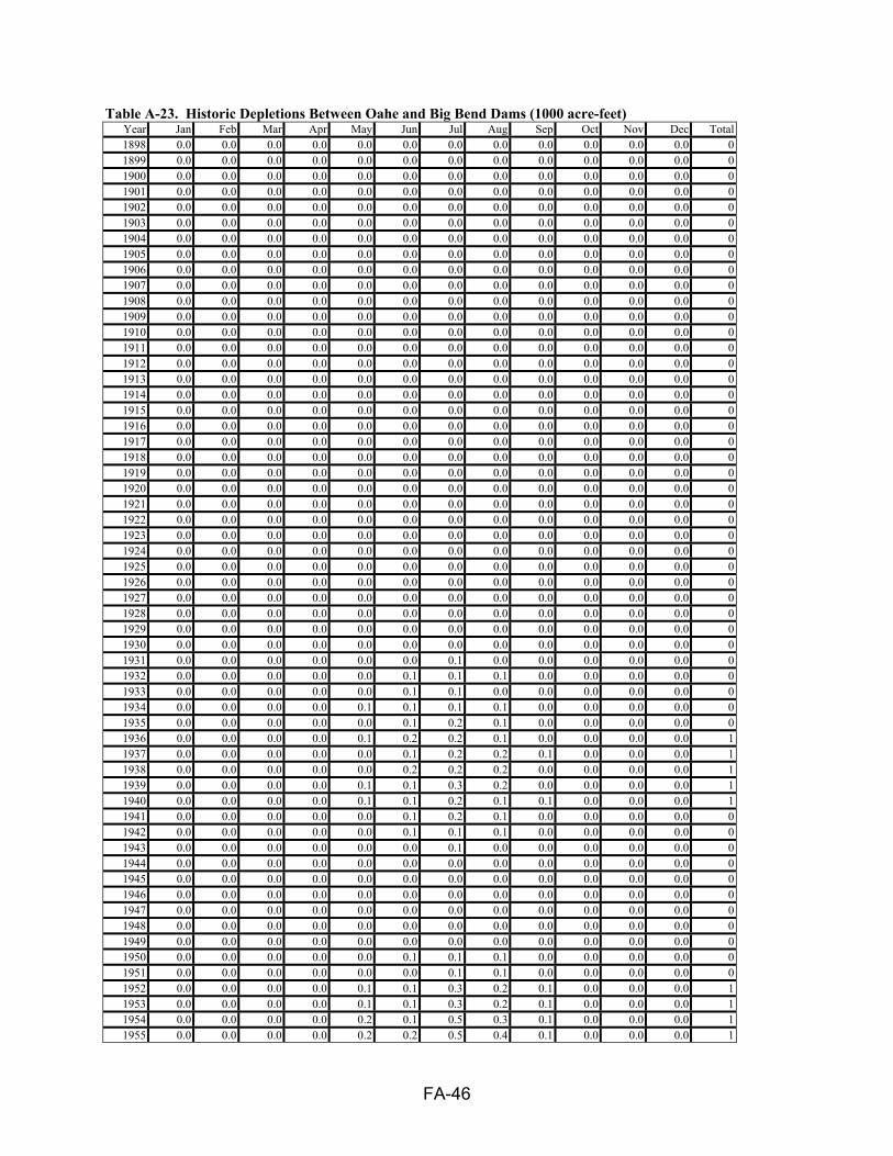
FA-46

Table A-23. Historic Depletions Between Oahe and Big Bend Dams (1000 acre-feet) Year Jan Feb Mar Apr May Jun Jul Aug Sep Oct Nov Dec Total1898 0.0 0.0 0.0 0.0 0.0 0.0 0.0 0.0 0.0 0.0 0.0 0.0 0 1899 0.0 0.0 0.0 0.0 0.0 0.0 0.0 0.0 0.0 0.0 0.0 0.0 0 1900 0.0 0.0 0.0 0.0 0.0 0.0 0.0 0.0 0.0 0.0 0.0 0.0 0 1901 0.0 0.0 0.0 0.0 0.0 0.0 0.0 0.0 0.0 0.0 0.0 0.0 0 1902 0.0 0.0 0.0 0.0 0.0 0.0 0.0 0.0 0.0 0.0 0.0 0.0 0 1903 0.0 0.0 0.0 0.0 0.0 0.0 0.0 0.0 0.0 0.0 0.0 0.0 0 1904 0.0 0.0 0.0 0.0 0.0 0.0 0.0 0.0 0.0 0.0 0.0 0.0 0 1905 0.0 0.0 0.0 0.0 0.0 0.0 0.0 0.0 0.0 0.0 0.0 0.0 0 1906 0.0 0.0 0.0 0.0 0.0 0.0 0.0 0.0 0.0 0.0 0.0 0.0 0 1907 0.0 0.0 0.0 0.0 0.0 0.0 0.0 0.0 0.0 0.0 0.0 0.0 0 1908 0.0 0.0 0.0 0.0 0.0 0.0 0.0 0.0 0.0 0.0 0.0 0.0 0 1909 0.0 0.0 0.0 0.0 0.0 0.0 0.0 0.0 0.0 0.0 0.0 0.0 0 1910 0.0 0.0 0.0 0.0 0.0 0.0 0.0 0.0 0.0 0.0 0.0 0.0 0 1911 0.0 0.0 0.0 0.0 0.0 0.0 0.0 0.0 0.0 0.0 0.0 0.0 0 1912 0.0 0.0 0.0 0.0 0.0 0.0 0.0 0.0 0.0 0.0 0.0 0.0 0 1913 0.0 0.0 0.0 0.0 0.0 0.0 0.0 0.0 0.0 0.0 0.0 0.0 0 1914 0.0 0.0 0.0 0.0 0.0 0.0 0.0 0.0 0.0 0.0 0.0 0.0 0 1915 0.0 0.0 0.0 0.0 0.0 0.0 0.0 0.0 0.0 0.0 0.0 0.0 0 1916 0.0 0.0 0.0 0.0 0.0 0.0 0.0 0.0 0.0 0.0 0.0 0.0 0 1917 0.0 0.0 0.0 0.0 0.0 0.0 0.0 0.0 0.0 0.0 0.0 0.0 0 1918 0.0 0.0 0.0 0.0 0.0 0.0 0.0 0.0 0.0 0.0 0.0 0.0 0 1919 0.0 0.0 0.0 0.0 0.0 0.0 0.0 0.0 0.0 0.0 0.0 0.0 0 1920 0.0 0.0 0.0 0.0 0.0 0.0 0.0 0.0 0.0 0.0 0.0 0.0 0 1921 0.0 0.0 0.0 0.0 0.0 0.0 0.0 0.0 0.0 0.0 0.0 0.0 0 1922 0.0 0.0 0.0 0.0 0.0 0.0 0.0 0.0 0.0 0.0 0.0 0.0 0 1923 0.0 0.0 0.0 0.0 0.0 0.0 0.0 0.0 0.0 0.0 0.0 0.0 0 1924 0.0 0.0 0.0 0.0 0.0 0.0 0.0 0.0 0.0 0.0 0.0 0.0 0 1925 0.0 0.0 0.0 0.0 0.0 0.0 0.0 0.0 0.0 0.0 0.0 0.0 0 1926 0.0 0.0 0.0 0.0 0.0 0.0 0.0 0.0 0.0 0.0 0.0 0.0 0 1927 0.0 0.0 0.0 0.0 0.0 0.0 0.0 0.0 0.0 0.0 0.0 0.0 0 1928 0.0 0.0 0.0 0.0 0.0 0.0 0.0 0.0 0.0 0.0 0.0 0.0 0 1929 0.0 0.0 0.0 0.0 0.0 0.0 0.0 0.0 0.0 0.0 0.0 0.0 0 1930 0.0 0.0 0.0 0.0 0.0 0.0 0.0 0.0 0.0 0.0 0.0 0.0 0 1931 0.0 0.0 0.0 0.0 0.0 0.0 0.1 0.0 0.0 0.0 0.0 0.0 0 1932 0.0 0.0 0.0 0.0 0.0 0.1 0.1 0.1 0.0 0.0 0.0 0.0 0 1933 0.0 0.0 0.0 0.0 0.0 0.1 0.1 0.0 0.0 0.0 0.0 0.0 0 1934 0.0 0.0 0.0 0.0 0.1 0.1 0.1 0.1 0.0 0.0 0.0 0.0 0 1935 0.0 0.0 0.0 0.0 0.0 0.1 0.2 0.1 0.0 0.0 0.0 0.0 0 1936 0.0 0.0 0.0 0.0 0.1 0.2 0.2 0.1 0.0 0.0 0.0 0.0 1 1937 0.0 0.0 0.0 0.0 0.0 0.1 0.2 0.2 0.1 0.0 0.0 0.0 1 1938 0.0 0.0 0.0 0.0 0.0 0.2 0.2 0.2 0.0 0.0 0.0 0.0 11939 0.0 0.0 0.0 0.0 0.1 0.1 0.3 0.2 0.0 0.0 0.0 0.0 1 1940 0.0 0.0 0.0 0.0 0.1 0.1 0.2 0.1 0.1 0.0 0.0 0.0 1 1941 0.0 0.0 0.0 0.0 0.0 0.1 0.2 0.1 0.0 0.0 0.0 0.0 0 1942 0.0 0.0 0.0 0.0 0.0 0.1 0.1 0.1 0.0 0.0 0.0 0.0 0 1943 0.0 0.0 0.0 0.0 0.0 0.0 0.1 0.0 0.0 0.0 0.0 0.0 0 1944 0.0 0.0 0.0 0.0 0.0 0.0 0.0 0.0 0.0 0.0 0.0 0.0 0 1945 0.0 0.0 0.0 0.0 0.0 0.0 0.0 0.0 0.0 0.0 0.0 0.0 0 1946 0.0 0.0 0.0 0.0 0.0 0.0 0.0 0.0 0.0 0.0 0.0 0.0 0 1947 0.0 0.0 0.0 0.0 0.0 0.0 0.0 0.0 0.0 0.0 0.0 0.0 0 1948 0.0 0.0 0.0 0.0 0.0 0.0 0.0 0.0 0.0 0.0 0.0 0.0 0 1949 0.0 0.0 0.0 0.0 0.0 0.0 0.0 0.0 0.0 0.0 0.0 0.0 0 1950 0.0 0.0 0.0 0.0 0.0 0.1 0.1 0.1 0.0 0.0 0.0 0.0 0 1951 0.0 0.0 0.0 0.0 0.0 0.0 0.1 0.1 0.0 0.0 0.0 0.0 0 1952 0.0 0.0 0.0 0.0 0.1 0.1 0.3 0.2 0.1 0.0 0.0 0.0 1 1953 0.0 0.0 0.0 0.0 0.1 0.1 0.3 0.2 0.1 0.0 0.0 0.0 1 1954 0.0 0.0 0.0 0.0 0.2 0.1 0.5 0.3 0.1 0.0 0.0 0.0 1 1955 0.0 0.0 0.0 0.0 0.2 0.2 0.5 0.4 0.1 0.0 0.0 0.0 1

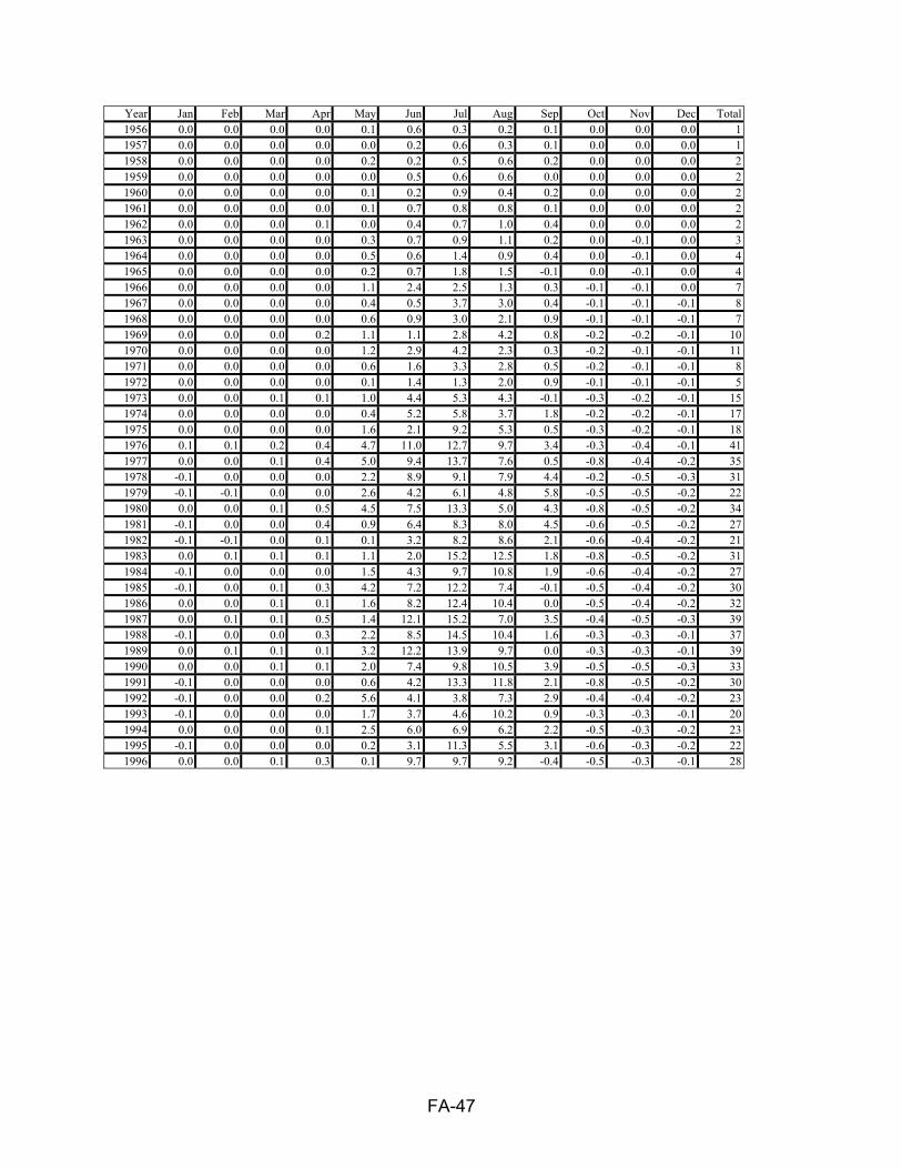
FA-47

Year Jan Feb Mar Apr May Jun Jul Aug Sep Oct Nov Dec Total1956 0.0 0.0 0.0 0.0 0.1 0.6 0.3 0.2 0.1 0.0 0.0 0.0 1 1957 0.0 0.0 0.0 0.0 0.0 0.2 0.6 0.3 0.1 0.0 0.0 0.0 1 1958 0.0 0.0 0.0 0.0 0.2 0.2 0.5 0.6 0.2 0.0 0.0 0.0 2 1959 0.0 0.0 0.0 0.0 0.0 0.5 0.6 0.6 0.0 0.0 0.0 0.0 2 1960 0.0 0.0 0.0 0.0 0.1 0.2 0.9 0.4 0.2 0.0 0.0 0.0 2 1961 0.0 0.0 0.0 0.0 0.1 0.7 0.8 0.8 0.1 0.0 0.0 0.0 2 1962 0.0 0.0 0.0 0.1 0.0 0.4 0.7 1.0 0.4 0.0 0.0 0.0 2 1963 0.0 0.0 0.0 0.0 0.3 0.7 0.9 1.1 0.2 0.0 -0.1 0.0 3 1964 0.0 0.0 0.0 0.0 0.5 0.6 1.4 0.9 0.4 0.0 -0.1 0.0 4 1965 0.0 0.0 0.0 0.0 0.2 0.7 1.8 1.5 -0.1 0.0 -0.1 0.0 4 1966 0.0 0.0 0.0 0.0 1.1 2.4 2.5 1.3 0.3 -0.1 -0.1 0.0 7 1967 0.0 0.0 0.0 0.0 0.4 0.5 3.7 3.0 0.4 -0.1 -0.1 -0.1 8 1968 0.0 0.0 0.0 0.0 0.6 0.9 3.0 2.1 0.9 -0.1 -0.1 -0.1 7 1969 0.0 0.0 0.0 0.2 1.1 1.1 2.8 4.2 0.8 -0.2 -0.2 -0.1 10 1970 0.0 0.0 0.0 0.0 1.2 2.9 4.2 2.3 0.3 -0.2 -0.1 -0.1 11 1971 0.0 0.0 0.0 0.0 0.6 1.6 3.3 2.8 0.5 -0.2 -0.1 -0.1 8 1972 0.0 0.0 0.0 0.0 0.1 1.4 1.3 2.0 0.9 -0.1 -0.1 -0.1 5 1973 0.0 0.0 0.1 0.1 1.0 4.4 5.3 4.3 -0.1 -0.3 -0.2 -0.1 15 1974 0.0 0.0 0.0 0.0 0.4 5.2 5.8 3.7 1.8 -0.2 -0.2 -0.1 17 1975 0.0 0.0 0.0 0.0 1.6 2.1 9.2 5.3 0.5 -0.3 -0.2 -0.1 18 1976 0.1 0.1 0.2 0.4 4.7 11.0 12.7 9.7 3.4 -0.3 -0.4 -0.1 41 1977 0.0 0.0 0.1 0.4 5.0 9.4 13.7 7.6 0.5 -0.8 -0.4 -0.2 35 1978 -0.1 0.0 0.0 0.0 2.2 8.9 9.1 7.9 4.4 -0.2 -0.5 -0.3 31 1979 -0.1 -0.1 0.0 0.0 2.6 4.2 6.1 4.8 5.8 -0.5 -0.5 -0.2 22 1980 0.0 0.0 0.1 0.5 4.5 7.5 13.3 5.0 4.3 -0.8 -0.5 -0.2 34 1981 -0.1 0.0 0.0 0.4 0.9 6.4 8.3 8.0 4.5 -0.6 -0.5 -0.2 27 1982 -0.1 -0.1 0.0 0.1 0.1 3.2 8.2 8.6 2.1 -0.6 -0.4 -0.2 21 1983 0.0 0.1 0.1 0.1 1.1 2.0 15.2 12.5 1.8 -0.8 -0.5 -0.2 31 1984 -0.1 0.0 0.0 0.0 1.5 4.3 9.7 10.8 1.9 -0.6 -0.4 -0.2 27 1985 -0.1 0.0 0.1 0.3 4.2 7.2 12.2 7.4 -0.1 -0.5 -0.4 -0.2 30 1986 0.0 0.0 0.1 0.1 1.6 8.2 12.4 10.4 0.0 -0.5 -0.4 -0.2 32 1987 0.0 0.1 0.1 0.5 1.4 12.1 15.2 7.0 3.5 -0.4 -0.5 -0.3 39 1988 -0.1 0.0 0.0 0.3 2.2 8.5 14.5 10.4 1.6 -0.3 -0.3 -0.1 37 1989 0.0 0.1 0.1 0.1 3.2 12.2 13.9 9.7 0.0 -0.3 -0.3 -0.1 39 1990 0.0 0.0 0.1 0.1 2.0 7.4 9.8 10.5 3.9 -0.5 -0.5 -0.3 33 1991 -0.1 0.0 0.0 0.0 0.6 4.2 13.3 11.8 2.1 -0.8 -0.5 -0.2 30 1992 -0.1 0.0 0.0 0.2 5.6 4.1 3.8 7.3 2.9 -0.4 -0.4 -0.2 23 1993 -0.1 0.0 0.0 0.0 1.7 3.7 4.6 10.2 0.9 -0.3 -0.3 -0.1 20 1994 0.0 0.0 0.0 0.1 2.5 6.0 6.9 6.2 2.2 -0.5 -0.3 -0.2 23 1995 -0.1 0.0 0.0 0.0 0.2 3.1 11.3 5.5 3.1 -0.6 -0.3 -0.2 22 1996 0.0 0.0 0.1 0.3 0.1 9.7 9.7 9.2 -0.4 -0.5 -0.3 -0.1 28

FA-48

Table A-24. Historic Depletions Between Big Bend and Fort Randall Dams (1000 acre-feet) Year Jan Feb Mar Apr May Jun Jul Aug Sep Oct Nov Dec Total1898 -0.1 -0.1 0.0 0.0 0.7 3.8 3.6 6.2 2.8 -0.4 -0.5 -0.2 16 1899 -0.1 -0.1 0.0 0.0 0.7 1.3 4.7 4.2 3.7 -0.4 -0.4 -0.2 13 1900 -0.1 0.0 0.0 0.4 5.1 5.0 4.3 4.1 1.5 -0.7 -0.4 -0.2 19 1901 -0.1 -0.1 0.0 0.5 5.3 0.1 7.0 5.4 -0.8 -0.3 -0.3 -0.2 17 1902 -0.1 0.0 0.0 0.3 5.7 3.2 7.0 2.7 2.3 -0.3 -0.5 -0.2 20 1903 -0.1 -0.1 0.0 0.7 1.8 4.7 3.2 5.8 0.1 -0.2 -0.3 -0.2 15 1904 -0.1 0.0 0.0 0.5 2.7 1.2 4.8 5.3 3.8 -0.4 -0.5 -0.3 17 1905 -0.1 -0.1 0.0 0.3 0.6 0.4 5.4 7.2 2.3 -0.4 -0.4 -0.2 15 1906 -0.1 0.0 0.0 0.7 3.1 1.7 7.2 2.5 1.0 -0.2 -0.3 -0.2 15 1907 -0.1 0.0 0.0 0.0 1.5 2.3 1.4 7.7 1.6 0.1 -0.4 -0.2 14 1908 -0.1 -0.1 0.0 0.4 0.0 0.7 6.5 4.7 3.6 -0.3 -0.5 -0.3 15 1909 -0.1 0.0 0.0 0.1 0.5 3.9 6.4 4.1 2.4 -0.3 -0.4 -0.2 16 1910 -0.1 0.0 0.0 0.7 2.8 4.2 5.6 3.6 1.9 0.1 -0.3 -0.2 18 1911 -0.1 0.0 0.0 0.6 4.9 3.9 5.4 3.1 1.5 -0.6 -0.4 -0.2 18 1912 -0.1 0.0 0.0 0.4 4.9 5.4 3.4 1.8 2.0 0.2 -0.4 -0.2 17 1913 -0.1 0.0 0.0 0.3 1.2 4.9 4.7 5.4 2.9 0.0 -0.3 -0.2 19 1914 -0.1 0.0 0.0 0.5 1.8 1.2 6.5 4.2 1.1 -0.4 -0.3 -0.2 14 1915 -0.1 -0.1 0.0 0.6 1.1 0.7 0.1 5.3 2.2 0.0 -0.3 -0.2 9 1916 0.0 0.0 0.0 0.2 0.7 3.0 10.0 4.6 2.2 -0.1 -0.5 -0.3 20 1917 -0.1 -0.1 0.0 0.0 0.8 4.5 7.3 5.4 1.0 -0.2 -0.4 -0.2 18 1918 -0.1 -0.1 0.0 0.1 1.4 2.6 2.9 5.2 2.6 -0.1 -0.4 -0.2 14 1919 -0.1 0.0 0.0 0.1 4.1 1.8 7.2 5.9 2.6 -0.5 -0.5 -0.3 20 1920 -0.2 -0.1 -0.1 0.1 0.5 0.8 5.5 4.7 2.9 0.3 -0.5 -0.3 14 1921 -0.1 0.0 0.0 0.6 2.2 7.9 6.5 3.2 2.2 0.1 -0.3 -0.2 22 1922 -0.1 0.0 0.0 0.8 3.6 4.5 2.3 6.3 4.4 0.0 -0.4 -0.2 21 1923 -0.1 -0.1 0.0 0.3 4.7 0.9 7.1 1.9 3.1 0.1 -0.5 -0.3 17 1924 -0.1 -0.1 0.0 0.7 3.0 1.9 6.3 5.4 1.7 0.1 -0.5 -0.3 18 1925 -0.1 0.0 0.0 0.9 4.8 3.7 6.2 6.2 4.1 -0.2 -0.4 -0.2 25 1926 -0.1 -0.1 0.0 1.1 4.1 3.3 7.1 4.7 0.5 0.0 -0.3 -0.1 20 1927 -0.1 0.0 0.0 0.0 0.6 5.2 5.1 4.6 2.7 0.2 -0.3 -0.2 18 1928 0.0 0.0 0.0 0.4 6.8 0.7 6.4 5.1 2.8 -0.3 -0.5 -0.3 21 1929 -0.1 0.0 0.0 0.0 2.5 3.6 7.8 5.9 2.0 -0.7 -0.5 -0.2 20 1930 -0.1 0.0 0.0 0.0 2.0 4.1 9.4 6.3 3.2 -0.9 -0.6 -0.3 23 1931 -0.1 0.0 0.0 0.8 3.0 6.9 8.2 5.4 3.2 -0.4 -0.6 -0.3 26 1932 -0.2 -0.1 0.0 0.0 2.5 3.3 7.5 6.4 3.8 -0.7 -0.6 -0.3 22 1933 -0.1 -0.1 0.0 0.2 1.1 8.1 7.0 4.9 4.3 0.0 -0.5 -0.2 25 1934 -0.1 0.0 0.0 0.4 7.5 6.0 7.6 5.6 1.3 -0.3 -0.4 -0.2 27 1935 -0.1 0.0 0.0 0.0 0.0 4.0 8.1 6.9 4.6 -0.2 -0.7 -0.4 22 1936 -0.1 0.0 0.0 0.0 4.0 6.1 9.9 6.7 2.2 -0.3 -0.4 -0.2 28 1937 -0.1 0.0 0.0 0.2 3.4 4.3 7.8 6.5 3.6 -0.2 -0.4 -0.2 25 1938 -0.1 0.0 0.0 0.0 1.4 5.0 7.0 7.5 3.6 0.0 -0.7 -0.4 23 1939 -0.2 -0.1 0.0 0.4 3.4 2.9 9.9 6.4 1.6 -0.6 -0.5 -0.3 23 1940 -0.1 -0.1 0.0 0.0 5.0 3.5 7.5 5.1 3.7 -0.3 -0.6 -0.3 23 1941 -0.2 -0.1 -0.1 0.0 3.4 2.4 6.3 4.8 0.5 -0.6 -0.3 -0.2 16 1942 -0.1 0.0 0.0 0.0 0.0 1.8 5.6 5.7 1.7 -0.2 -0.4 -0.2 14 1943 -0.1 0.0 0.0 0.3 0.9 1.7 6.9 5.2 2.8 -0.5 -0.5 -0.2 16 1944 -0.1 -0.1 0.0 0.1 1.7 1.5 3.2 3.8 2.6 0.0 -0.3 -0.2 12 1945 -0.1 0.0 0.0 0.2 1.8 1.0 3.9 4.0 1.9 0.0 -0.3 -0.2 12 1946 -0.1 0.0 0.0 0.4 0.4 2.2 6.2 4.5 0.0 -0.4 -0.2 -0.1 13 1947 0.0 0.0 0.0 0.1 2.6 1.1 6.8 6.9 2.2 0.1 -0.3 -0.1 19 1948 -0.1 0.0 0.0 0.2 2.0 1.6 6.4 5.5 3.0 -0.2 -0.4 -0.2 18 1949 -0.1 0.0 0.0 0.0 1.4 5.2 6.9 5.8 2.6 -0.7 -0.5 -0.2 20 1950 -0.1 0.0 0.0 0.0 2.0 7.0 5.0 4.4 0.8 0.2 -0.4 -0.2 19 1951 -0.1 -0.1 0.0 0.4 1.1 2.0 6.3 4.8 1.1 -0.4 -0.3 -0.2 15 1952 0.0 0.1 0.1 1.3 1.7 5.6 10.3 5.8 4.5 0.1 -0.4 -0.2 29 1953 -0.1 0.0 0.0 0.1 2.7 4.0 9.8 9.1 6.6 -0.6 -0.8 -0.4 31 1954 -0.2 -0.1 0.0 0.3 6.2 3.4 12.9 9.2 4.9 -0.9 -0.7 -0.4 35 1955 -0.2 -0.1 0.0 1.0 3.5 6.6 14.7 7.6 3.8 0.0 -0.7 -0.4 36

FA-49

Year Jan Feb Mar Apr May Jun Jul Aug Sep Oct Nov Dec Total1956 -0.2 -0.1 0.0 0.0 4.7 10.9 7.6 6.4 5.7 -0.2 -0.8 -0.4 34 1957 -0.2 -0.1 -0.1 0.0 1.0 3.6 12.8 6.3 5.2 -0.7 -0.6 -0.4 27 1958 -0.1 0.0 0.0 0.1 8.8 4.6 5.6 11.1 6.4 -0.1 -0.9 -0.5 35 1959 -0.2 -0.1 -0.1 0.0 1.8 8.8 10.0 10.9 0.8 -0.5 -0.6 -0.3 30 1960 -0.2 -0.1 0.0 0.0 2.0 5.4 9.6 8.5 3.7 -0.1 -0.7 -0.4 28 1961 -0.2 0.0 0.0 0.5 1.0 7.1 11.7 8.5 2.6 -0.3 -0.6 -0.3 30 1962 -0.2 -0.1 0.0 0.7 0.2 2.8 6.1 9.4 4.9 -0.3 -0.6 -0.3 23 1963 -0.1 0.0 0.0 0.1 3.5 4.5 9.2 10.6 1.7 0.1 -0.6 -0.3 28 1964 -0.1 0.0 0.0 0.0 4.6 5.8 10.5 9.1 5.4 -0.1 -0.8 -0.4 34 1965 -0.3 -0.1 -0.1 0.0 2.0 4.3 8.0 9.3 -0.9 0.1 -0.4 -0.2 22 1966 -0.1 0.0 0.1 0.1 9.9 6.9 9.9 4.9 1.7 -0.5 -0.5 -0.3 32 1967 -0.1 0.0 0.0 1.0 3.0 2.5 13.3 10.8 5.3 -0.5 -0.8 -0.4 34 1968 -0.2 -0.1 0.0 0.0 2.9 3.7 12.3 6.3 4.1 0.0 -0.6 -0.3 28 1969 -0.1 0.0 0.1 0.9 8.0 4.9 9.2 11.2 6.6 -1.3 -0.8 -0.4 38 1970 -0.2 -0.1 0.0 0.0 4.5 8.2 12.5 10.2 4.7 -0.5 -0.5 -0.2 39 1971 -0.1 0.0 0.0 0.0 3.0 8.2 9.3 10.4 3.2 -0.6 -0.4 -0.2 33 1972 -0.1 0.0 0.0 0.0 1.0 6.9 5.8 8.0 5.2 -0.5 -0.6 -0.3 25 1973 -0.1 0.0 0.0 0.1 2.8 9.9 11.5 9.6 -0.5 -0.3 -0.5 -0.2 32 1974 0.0 0.1 0.1 0.1 3.2 10.6 13.3 11.5 6.9 -0.1 -0.9 -0.5 44 1975 -0.2 0.0 0.1 0.1 7.4 7.2 20.4 13.1 5.2 -0.5 -0.9 -0.4 51 1976 -0.1 0.1 0.1 0.3 9.5 17.1 18.8 15.3 8.2 -0.2 -0.7 -0.3 68 1977 -0.1 0.0 0.1 1.2 8.3 19.0 20.0 13.4 5.6 -1.0 -1.0 -0.5 65 1978 -0.1 0.1 0.1 0.2 5.8 16.8 21.7 23.3 14.5 -0.2 -1.4 -0.7 80 1979 -0.3 -0.1 0.0 0.3 9.2 15.9 15.9 14.9 14.7 -1.4 -1.3 -0.6 67 1980 -0.2 0.0 0.1 1.9 14.8 16.5 26.7 11.3 11.1 -0.8 -0.9 -0.4 80 1981 -0.1 0.1 0.1 2.6 8.0 16.3 19.2 21.3 14.8 -1.8 -1.4 -0.7 78 1982 -0.4 -0.2 -0.1 0.4 0.0 13.9 19.7 18.0 3.1 -1.4 -0.8 -0.4 52 1983 0.0 0.1 0.2 0.2 3.6 9.4 24.6 27.3 8.7 -1.3 -1.3 -0.6 71 1984 -0.3 -0.1 0.1 0.1 7.0 12.0 21.0 18.7 9.6 -1.4 -1.2 -0.6 65 1985 -0.2 -0.1 0.0 0.3 16.5 14.3 21.6 11.4 0.7 -0.1 -0.8 -0.4 63 1986 -0.1 0.0 0.1 0.1 7.9 13.4 24.9 19.4 0.2 -0.4 -0.9 -0.4 64 1987 -0.1 0.0 0.1 1.3 8.7 17.0 20.6 15.7 8.4 -0.4 -1.2 -0.6 69 1988 -0.2 0.0 0.1 1.0 0.9 21.3 26.9 23.5 5.4 0.3 -0.8 -0.3 78 1989 0.0 0.2 0.2 1.0 15.6 20.8 23.2 22.7 6.4 0.5 -1.3 -0.6 89 1990 -0.3 -0.1 0.0 0.3 2.0 14.7 19.7 21.8 16.4 -0.5 -1.5 -0.8 72 1991 -0.3 -0.1 0.0 0.1 1.2 11.4 30.7 22.8 8.1 -1.8 -1.2 -0.6 70 1992 -0.3 -0.1 0.1 1.5 20.0 10.4 9.3 16.5 7.9 0.4 -1.1 -0.5 64 1993 -0.3 -0.2 -0.1 0.0 6.7 5.4 10.6 22.3 3.6 0.1 -0.9 -0.4 47 1994 -0.1 0.0 0.1 0.2 17.1 7.6 16.5 16.5 8.1 -0.9 -1.1 -0.5 63 1995 -0.2 -0.1 0.0 0.0 0.1 12.4 25.4 17.2 7.0 -1.7 -1.0 -0.5 59 1996 -0.2 0.0 0.1 0.6 0.1 16.7 20.4 21.9 1.0 -1.0 -0.9 -0.4 58

FA-50

Table A-25. Historic Depletions Between Fort Randall and Gavins Point Dams (1000 acre-feet) Year Jan Feb Mar Apr May Jun Jul Aug Sep Oct Nov Dec Total1898 -0.1 -0.1 0.0 0.3 0.4 5.0 3.6 5.9 4.3 -0.7 -0.5 -0.3 18 1899 -0.1 0.0 0.0 0.2 2.5 3.3 6.8 4.1 5.1 0.4 -0.7 -0.4 21 1900 -0.2 -0.1 0.0 0.2 3.0 6.1 1.9 8.0 2.6 -0.1 -0.6 -0.3 20 1901 -0.2 -0.1 0.0 0.3 2.7 0.0 12.0 6.1 -1.0 0.2 -0.4 -0.2 19 1902 -0.2 -0.1 0.0 0.2 4.6 -0.1 3.9 2.8 -0.3 0.7 -0.3 -0.2 11 1903 -0.1 0.0 0.0 0.3 0.0 3.8 4.1 3.7 3.4 0.2 -0.5 -0.3 15 1904 -0.1 -0.1 0.0 0.1 1.0 2.7 4.8 3.2 4.4 -0.4 -0.5 -0.3 15 1905 -0.1 -0.1 0.0 0.2 0.3 1.7 3.3 4.5 1.2 0.3 -0.3 -0.2 11 1906 -0.1 0.0 0.0 0.2 1.3 3.1 6.1 4.2 2.5 -0.6 -0.4 -0.2 16 1907 -0.1 -0.1 0.0 0.1 1.2 0.3 2.1 8.1 1.8 0.8 -0.5 -0.3 13 1908 -0.1 -0.1 0.0 0.3 0.7 0.1 6.4 4.7 5.7 -0.1 -0.6 -0.3 17 1909 -0.2 -0.1 0.0 0.2 0.0 0.3 6.5 8.2 4.5 -0.2 -0.6 -0.3 18 1910 -0.2 -0.1 0.0 0.3 2.1 5.6 5.0 4.8 3.3 0.3 -0.6 -0.3 20 1911 -0.1 -0.1 0.0 0.2 4.2 6.9 4.8 4.6 2.6 -0.8 -0.5 -0.3 22 1912 -0.1 -0.1 0.0 0.2 0.6 6.1 4.2 4.5 3.0 0.3 -0.5 -0.3 18 1913 -0.1 -0.1 0.0 0.2 0.4 2.1 7.4 5.0 4.2 0.1 -0.4 -0.2 19 1914 -0.1 0.0 0.0 0.3 1.5 5.1 7.8 7.1 -0.3 0.4 -0.5 -0.3 21 1915 -0.2 -0.1 0.0 0.2 0.3 1.1 1.3 7.3 4.9 0.7 -0.6 -0.3 15 1916 -0.1 0.0 0.0 0.3 4.3 4.6 8.4 6.1 1.5 0.3 -0.4 -0.2 25 1917 -0.1 0.0 0.0 0.1 0.1 2.8 8.1 5.5 3.4 0.4 -0.6 -0.3 19 1918 -0.2 -0.1 0.0 0.2 0.6 1.5 7.3 4.0 3.6 0.1 -0.5 -0.3 16 1919 -0.1 -0.1 0.0 0.2 0.9 0.2 6.9 6.7 2.9 -0.1 -0.5 -0.3 17 1920 -0.1 0.0 0.0 0.0 0.7 2.3 6.3 5.5 4.5 0.6 -0.6 -0.4 19 1921 -0.2 -0.1 0.0 0.3 0.2 7.0 3.7 5.1 4.7 0.5 -0.6 -0.4 20 1922 -0.2 -0.1 0.0 0.3 3.9 4.3 3.3 6.4 4.7 0.2 -0.5 -0.2 22 1923 -0.1 -0.1 0.0 0.3 0.3 2.1 8.9 1.9 2.5 0.4 -0.4 -0.3 16 1924 -0.1 0.0 0.0 0.2 2.0 1.3 6.1 6.2 2.8 0.5 -0.5 -0.3 18 1925 -0.1 -0.1 0.0 0.4 4.2 1.2 5.0 7.7 2.8 0.0 -0.6 -0.3 20 1926 -0.2 -0.1 0.0 0.4 4.1 3.4 8.0 4.8 1.2 0.3 -0.5 -0.3 21 1927 -0.2 -0.1 -0.1 0.0 0.5 0.9 6.8 3.4 4.3 0.7 -0.5 -0.3 15 1928 -0.1 -0.1 0.0 0.2 1.6 2.8 7.1 5.9 2.0 -0.2 -0.3 -0.2 19 1929 -0.1 0.0 0.0 0.1 0.8 1.1 3.2 5.3 0.0 -0.4 -0.2 -0.1 10 1930 0.0 0.0 0.0 0.0 0.3 2.0 5.8 3.5 2.5 -0.5 -0.3 -0.2 13 1931 -0.1 0.0 0.0 0.3 1.5 2.3 5.1 4.4 2.5 -0.2 -0.4 -0.2 15 1932 -0.1 0.0 0.0 0.1 1.1 2.1 4.8 4.5 3.1 -0.6 -0.4 -0.2 14 1933 -0.1 0.0 0.0 0.1 0.3 5.1 5.7 3.3 3.4 0.1 -0.4 -0.2 17 1934 -0.1 0.0 0.0 0.3 3.4 3.1 5.8 5.6 1.2 0.0 -0.4 -0.2 19 1935 -0.1 0.0 0.0 0.0 0.1 1.8 7.2 6.3 3.7 0.0 -0.5 -0.3 18 1936 -0.1 0.0 0.0 0.1 1.9 3.3 8.5 6.2 3.2 0.0 -0.3 -0.2 23 1937 -0.1 0.0 0.0 0.1 1.6 1.5 6.7 6.7 3.2 -0.4 -0.3 -0.1 19 1938 0.0 0.0 0.0 0.0 0.3 3.9 4.4 8.3 2.6 0.4 -0.5 -0.3 19 1939 -0.1 0.0 0.0 0.2 1.5 3.2 7.3 6.5 4.3 -0.7 -0.5 -0.2 21 1940 -0.1 0.0 0.0 0.0 3.2 3.7 7.5 6.5 2.6 -0.2 -0.3 -0.1 23 1941 -0.1 0.0 0.0 0.0 2.3 1.5 5.6 6.5 1.8 -0.6 -0.3 -0.2 17 1942 -0.1 0.0 0.0 0.0 0.1 1.5 5.7 6.9 1.9 -0.4 -0.3 -0.2 15 1943 -0.1 0.0 0.0 0.2 1.0 1.6 6.6 6.8 3.1 -0.5 -0.4 -0.2 18 1944 -0.1 -0.1 0.0 0.1 1.0 1.0 3.4 5.6 3.7 0.1 -0.3 -0.2 14 1945 0.0 0.0 0.0 0.2 1.4 1.2 7.9 6.8 3.2 0.4 -0.4 -0.2 21 1946 0.0 0.0 0.1 0.8 0.5 5.1 11.2 11.4 1.0 -0.8 -0.4 -0.2 29 1947 0.0 0.1 0.1 0.3 2.0 1.9 15.5 18.8 7.2 0.5 -0.5 -0.2 46 1948 0.0 0.1 0.1 0.7 3.6 3.7 15.7 19.3 10.3 0.2 -1.0 -0.5 52 1949 -0.2 0.0 0.1 0.2 0.9 8.2 23.4 24.2 8.0 -1.2 -0.6 -0.2 63 1950 -0.1 0.0 0.1 0.1 1.9 9.9 12.3 17.6 5.0 1.8 -0.9 -0.4 47 1951 -0.3 -0.1 0.0 0.3 1.9 2.8 11.4 12.6 7.0 -0.8 -0.6 -0.3 34 1952 0.2 0.3 0.3 0.4 1.3 15.9 31.8 21.6 17.7 1.5 -0.9 -0.4 90 1953 -0.1 0.1 0.2 0.2 4.8 7.9 16.7 29.3 22.5 -1.8 -1.6 -0.8 77 1954 -0.3 -0.1 0.1 0.5 5.6 5.9 34.8 20.9 10.6 -0.9 -1.2 -0.6 75 1955 -0.1 0.1 0.2 1.3 3.9 6.6 40.8 32.5 9.8 1.9 -0.9 -0.3 96

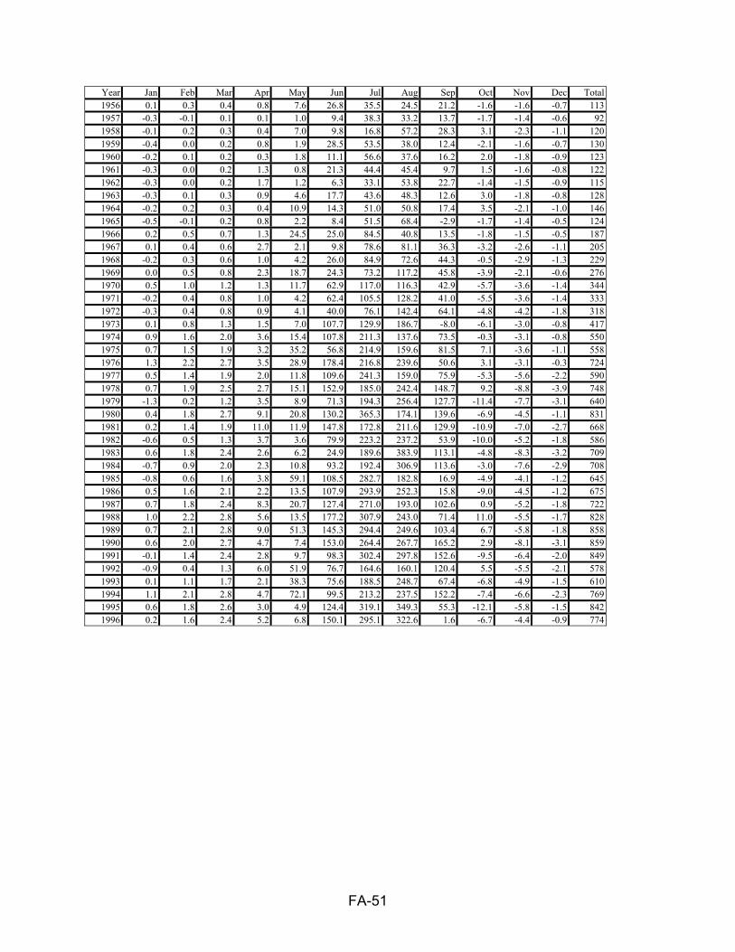
FA-51

Year Jan Feb Mar Apr May Jun Jul Aug Sep Oct Nov Dec Total1956 0.1 0.3 0.4 0.8 7.6 26.8 35.5 24.5 21.2 -1.6 -1.6 -0.7 113 1957 -0.3 -0.1 0.1 0.1 1.0 9.4 38.3 33.2 13.7 -1.7 -1.4 -0.6 92 1958 -0.1 0.2 0.3 0.4 7.0 9.8 16.8 57.2 28.3 3.1 -2.3 -1.1 120 1959 -0.4 0.0 0.2 0.8 1.9 28.5 53.5 38.0 12.4 -2.1 -1.6 -0.7 130 1960 -0.2 0.1 0.2 0.3 1.8 11.1 56.6 37.6 16.2 2.0 -1.8 -0.9 123 1961 -0.3 0.0 0.2 1.3 0.8 21.3 44.4 45.4 9.7 1.5 -1.6 -0.8 122 1962 -0.3 0.0 0.2 1.7 1.2 6.3 33.1 53.8 22.7 -1.4 -1.5 -0.9 115 1963 -0.3 0.1 0.3 0.9 4.6 17.7 43.6 48.3 12.6 3.0 -1.8 -0.8 128 1964 -0.2 0.2 0.3 0.4 10.9 14.3 51.0 50.8 17.4 3.5 -2.1 -1.0 146 1965 -0.5 -0.1 0.2 0.8 2.2 8.4 51.5 68.4 -2.9 -1.7 -1.4 -0.5 124 1966 0.2 0.5 0.7 1.3 24.5 25.0 84.5 40.8 13.5 -1.8 -1.5 -0.5 187 1967 0.1 0.4 0.6 2.7 2.1 9.8 78.6 81.1 36.3 -3.2 -2.6 -1.1 205 1968 -0.2 0.3 0.6 1.0 4.2 26.0 84.9 72.6 44.3 -0.5 -2.9 -1.3 229 1969 0.0 0.5 0.8 2.3 18.7 24.3 73.2 117.2 45.8 -3.9 -2.1 -0.6 276 1970 0.5 1.0 1.2 1.3 11.7 62.9 117.0 116.3 42.9 -5.7 -3.6 -1.4 344 1971 -0.2 0.4 0.8 1.0 4.2 62.4 105.5 128.2 41.0 -5.5 -3.6 -1.4 333 1972 -0.3 0.4 0.8 0.9 4.1 40.0 76.1 142.4 64.1 -4.8 -4.2 -1.8 318 1973 0.1 0.8 1.3 1.5 7.0 107.7 129.9 186.7 -8.0 -6.1 -3.0 -0.8 417 1974 0.9 1.6 2.0 3.6 15.4 107.8 211.3 137.6 73.5 -0.3 -3.1 -0.8 550 1975 0.7 1.5 1.9 3.2 35.2 56.8 214.9 159.6 81.5 7.1 -3.6 -1.1 558 1976 1.3 2.2 2.7 3.5 28.9 178.4 216.8 239.6 50.6 3.1 -3.1 -0.3 724 1977 0.5 1.4 1.9 2.0 11.8 109.6 241.3 159.0 75.9 -5.3 -5.6 -2.2 590 1978 0.7 1.9 2.5 2.7 15.1 152.9 185.0 242.4 148.7 9.2 -8.8 -3.9 748 1979 -1.3 0.2 1.2 3.5 8.9 71.3 194.3 256.4 127.7 -11.4 -7.7 -3.1 640 1980 0.4 1.8 2.7 9.1 20.8 130.2 365.3 174.1 139.6 -6.9 -4.5 -1.1 831 1981 0.2 1.4 1.9 11.0 11.9 147.8 172.8 211.6 129.9 -10.9 -7.0 -2.7 668 1982 -0.6 0.5 1.3 3.7 3.6 79.9 223.2 237.2 53.9 -10.0 -5.2 -1.8 586 1983 0.6 1.8 2.4 2.6 6.2 24.9 189.6 383.9 113.1 -4.8 -8.3 -3.2 709 1984 -0.7 0.9 2.0 2.3 10.8 93.2 192.4 306.9 113.6 -3.0 -7.6 -2.9 708 1985 -0.8 0.6 1.6 3.8 59.1 108.5 282.7 182.8 16.9 -4.9 -4.1 -1.2 645 1986 0.5 1.6 2.1 2.2 13.5 107.9 293.9 252.3 15.8 -9.0 -4.5 -1.2 675 1987 0.7 1.8 2.4 8.3 20.7 127.4 271.0 193.0 102.6 0.9 -5.2 -1.8 722 1988 1.0 2.2 2.8 5.6 13.5 177.2 307.9 243.0 71.4 11.0 -5.5 -1.7 828 1989 0.7 2.1 2.8 9.0 51.3 145.3 294.4 249.6 103.4 6.7 -5.8 -1.8 858 1990 0.6 2.0 2.7 4.7 7.4 153.0 264.4 267.7 165.2 2.9 -8.1 -3.1 859 1991 -0.1 1.4 2.4 2.8 9.7 98.3 302.4 297.8 152.6 -9.5 -6.4 -2.0 849 1992 -0.9 0.4 1.3 6.0 51.9 76.7 164.6 160.1 120.4 5.5 -5.5 -2.1 578 1993 0.1 1.1 1.7 2.1 38.3 75.6 188.5 248.7 67.4 -6.8 -4.9 -1.5 610 1994 1.1 2.1 2.8 4.7 72.1 99.5 213.2 237.5 152.2 -7.4 -6.6 -2.3 769 1995 0.6 1.8 2.6 3.0 4.9 124.4 319.1 349.3 55.3 -12.1 -5.8 -1.5 842 1996 0.2 1.6 2.4 5.2 6.8 150.1 295.1 322.6 1.6 -6.7 -4.4 -0.9 774

FA-52

Table A-26. Historic Depletions Between Gavins Point Dam and Sioux City (1000 acre-feet) Year Jan Feb Mar Apr May Jun Jul Aug Sep Oct Nov Dec Total1898 0.0 0.0 0.0 0.0 0.0 0.0 0.0 0.0 0.0 0.0 0.0 0.0 0 1899 0.0 0.0 0.0 0.0 0.0 0.0 0.0 0.0 0.0 0.0 0.0 0.0 0 1900 0.0 0.0 0.0 0.0 0.0 0.0 0.0 0.0 0.0 0.0 0.0 0.0 0 1901 0.0 0.0 0.0 0.0 0.0 0.0 0.0 0.0 0.0 0.0 0.0 0.0 0 1902 0.0 0.0 0.0 0.0 0.0 0.0 0.0 0.0 0.0 0.0 0.0 0.0 0 1903 0.0 0.0 0.0 0.0 0.0 0.0 0.0 0.0 0.0 0.0 0.0 0.0 0 1904 0.0 0.0 0.0 0.0 0.0 0.0 0.0 0.0 0.0 0.0 0.0 0.0 0 1905 0.0 0.0 0.0 0.0 0.0 0.0 0.0 0.0 0.0 0.0 0.0 0.0 0 1906 0.0 0.0 0.0 0.0 0.0 0.0 0.0 0.0 0.0 0.0 0.0 0.0 0 1907 0.0 0.0 0.0 0.0 0.0 0.0 0.0 0.0 0.0 0.0 0.0 0.0 0 1908 0.0 0.0 0.0 0.0 0.0 0.0 0.0 0.0 0.0 0.0 0.0 0.0 0 1909 0.0 0.0 0.0 0.0 0.0 0.0 0.0 0.0 0.0 0.0 0.0 0.0 0 1910 0.0 0.0 0.0 0.0 0.0 0.0 0.0 0.0 0.0 0.0 0.0 0.0 0 1911 0.0 0.0 0.0 0.0 0.0 0.0 0.0 0.0 0.0 0.0 0.0 0.0 0 1912 0.0 0.0 0.0 0.0 0.0 0.0 0.0 0.0 0.0 0.0 0.0 0.0 0 1913 0.0 0.0 0.0 0.0 0.0 0.0 0.0 0.0 0.0 0.0 0.0 0.0 0 1914 0.0 0.0 0.0 0.0 0.0 0.0 0.0 0.0 0.0 0.0 0.0 0.0 0 1915 0.0 0.0 0.0 0.0 0.0 0.0 0.0 0.0 0.0 0.0 0.0 0.0 0 1916 0.0 0.0 0.0 0.0 0.0 0.0 0.0 0.0 0.0 0.0 0.0 0.0 0 1917 0.0 0.0 0.0 0.0 0.0 0.0 0.0 0.0 0.0 0.0 0.0 0.0 0 1918 0.0 0.0 0.0 0.0 0.0 0.0 0.0 0.0 0.0 0.0 0.0 0.0 0 1919 0.0 0.0 0.0 0.0 0.0 0.0 0.0 0.0 0.0 0.0 0.0 0.0 0 1920 0.0 0.0 0.0 0.0 0.0 0.0 0.0 0.0 0.0 0.0 0.0 0.0 0 1921 0.0 0.0 0.0 0.0 0.0 0.0 0.0 0.0 0.0 0.0 0.0 0.0 0 1922 0.0 0.0 0.0 0.0 0.0 0.0 0.0 0.0 0.0 0.0 0.0 0.0 0 1923 0.0 0.0 0.0 0.0 0.0 0.0 0.0 0.0 0.0 0.0 0.0 0.0 0 1924 0.0 0.0 0.0 0.0 0.0 0.0 0.0 0.0 0.0 0.0 0.0 0.0 0 1925 0.0 0.0 0.0 0.0 0.0 0.0 0.0 0.0 0.0 0.0 0.0 0.0 0 1926 0.0 0.0 0.0 0.0 0.0 0.0 0.0 0.0 0.0 0.0 0.0 0.0 0 1927 0.0 0.0 0.0 0.0 0.0 0.0 0.0 0.0 0.0 0.0 0.0 0.0 0 1928 0.0 0.0 0.0 0.0 0.0 0.0 0.0 0.0 0.0 0.0 0.0 0.0 0 1929 0.0 0.0 0.0 0.0 0.0 0.0 0.0 0.0 0.0 0.0 0.0 0.0 0 1930 0.0 0.0 0.0 0.0 0.0 0.0 0.0 0.0 0.0 0.0 0.0 0.0 0 1931 0.0 0.0 0.0 0.0 0.0 0.0 0.0 0.0 0.0 0.0 0.0 0.0 0 1932 0.0 0.0 0.0 0.0 0.0 0.0 0.1 0.0 0.0 0.0 0.0 0.0 0 1933 0.0 0.0 0.0 0.0 0.0 0.1 0.1 0.0 0.0 0.0 0.0 0.0 0 1934 0.0 0.0 0.0 0.0 0.0 0.0 0.1 0.1 0.0 0.0 0.0 0.0 0 1935 0.0 0.0 0.0 0.0 0.0 0.0 0.1 0.0 0.0 0.0 0.0 0.0 0 1936 0.0 0.0 0.0 0.0 0.0 0.1 0.2 0.1 0.0 0.0 0.0 0.0 0 1937 0.0 0.0 0.0 0.0 0.0 0.0 0.1 0.1 0.0 0.0 0.0 0.0 0 1938 0.0 0.0 0.0 0.0 0.0 0.1 0.1 0.2 0.0 0.0 0.0 0.0 0 1939 0.0 0.0 0.0 0.0 0.0 0.0 0.2 0.1 0.1 0.0 0.0 0.0 0 1940 0.0 0.0 0.0 0.0 0.1 0.1 0.2 0.1 0.1 0.0 0.0 0.0 0 1941 0.0 0.0 0.0 0.0 0.1 0.1 0.2 0.1 0.0 0.0 0.0 0.0 0 1942 0.0 0.0 0.0 0.0 0.0 0.1 0.1 0.1 0.0 0.0 0.0 0.0 0 1943 0.0 0.0 0.0 0.0 0.0 0.0 0.1 0.1 0.0 0.0 0.0 0.0 0 1944 0.0 0.0 0.0 0.0 0.0 0.0 0.1 0.1 0.0 0.0 0.0 0.0 0 1945 0.0 0.0 0.0 0.0 0.0 0.0 0.2 0.2 0.0 0.0 0.0 0.0 1 1946 0.0 0.0 0.0 0.0 0.0 0.1 0.4 0.3 0.0 0.0 0.0 0.0 1 1947 0.0 0.0 0.0 0.0 0.1 0.1 0.7 0.6 0.0 0.0 0.0 0.0 2 1948 0.0 0.0 0.0 0.0 0.1 0.1 0.6 0.6 0.1 0.0 0.0 0.0 2 1949 0.0 0.0 0.0 0.0 0.1 0.4 0.9 0.6 0.0 0.0 0.0 0.0 2 1950 0.0 0.0 0.0 0.0 0.1 1.0 1.0 1.2 0.0 0.0 0.0 0.0 3 1951 0.0 0.0 0.0 0.0 0.1 0.2 1.4 0.8 0.3 0.0 0.0 0.0 3 1952 0.1 0.1 0.1 0.1 0.5 1.2 2.4 1.5 0.9 0.0 0.0 0.0 7 1953 0.0 0.1 0.1 0.1 0.2 0.7 2.6 2.0 0.8 0.0 0.0 0.0 7 1954 0.0 0.1 0.1 0.1 0.3 1.1 3.5 2.3 0.5 -0.1 0.0 0.0 8 1955 0.1 0.1 0.1 0.2 0.6 1.6 4.7 4.8 1.4 0.0 0.0 0.1 14

FA-53

Year Jan Feb Mar Apr May Jun Jul Aug Sep Oct Nov Dec Total1956 0.1 0.2 0.2 0.2 1.0 5.4 4.7 3.2 1.9 0.0 0.0 0.1 17 1957 0.1 0.1 0.2 0.2 0.3 2.1 9.4 5.6 0.6 -0.2 0.0 0.1 19 1958 0.2 0.3 0.3 0.3 2.2 5.1 6.4 11.0 2.6 0.3 0.0 0.1 29 1959 0.2 0.3 0.3 0.4 0.6 6.5 14.3 7.6 0.8 -0.1 0.0 0.2 31 1960 0.2 0.2 0.3 0.3 1.0 3.3 15.8 6.4 0.9 0.0 0.0 0.1 28 1961 0.2 0.3 0.3 0.3 0.5 4.8 11.9 12.8 1.0 -0.3 0.0 0.1 32 1962 0.1 0.1 0.1 0.1 0.3 2.1 5.9 9.5 0.6 0.0 0.0 0.1 19 1963 0.2 0.3 0.3 0.3 1.1 6.4 9.3 11.5 1.6 0.0 0.0 0.1 31 1964 0.2 0.3 0.3 0.3 2.4 8.2 14.4 7.8 1.7 0.4 0.1 0.2 36 1965 0.2 0.2 0.2 0.2 0.6 2.2 13.3 10.1 -0.4 -0.2 0.0 0.1 26 1966 0.3 0.3 0.3 0.3 2.5 7.8 14.8 8.0 1.2 -0.2 0.1 0.2 36 1967 0.3 0.4 0.4 0.5 2.6 2.8 18.9 12.8 3.4 -0.1 -0.1 0.1 42 1968 0.2 0.2 0.3 0.3 1.7 4.1 14.8 12.2 0.6 -0.2 0.0 0.1 34 1969 0.2 0.3 0.3 0.4 1.1 4.0 12.1 13.8 4.7 -0.4 -0.1 0.1 37 1970 0.6 0.7 0.8 0.8 2.5 13.3 27.1 29.1 2.5 -0.4 0.0 0.3 77 1971 0.3 0.4 0.5 0.5 2.8 9.7 19.6 23.8 3.2 -0.4 0.0 0.3 61 1972 0.2 0.3 0.3 0.3 0.6 10.4 10.3 15.6 3.5 -0.3 0.0 0.2 41 1973 0.8 0.9 0.9 0.9 4.5 23.0 28.8 31.7 -0.6 -0.5 0.1 0.5 91 1974 0.8 0.9 1.0 1.0 1.8 19.5 46.1 21.7 13.4 0.1 0.2 0.5 107 1975 1.3 1.4 1.5 1.5 7.9 12.5 79.9 33.0 11.0 0.9 0.4 0.9 152 1976 2.7 2.9 3.0 3.4 18.0 61.7 95.0 84.7 21.5 0.5 1.2 2.0 296 1977 2.2 2.5 2.6 2.8 19.5 75.3 115.5 55.4 3.5 -1.0 0.5 1.5 280 1978 1.9 2.3 2.4 2.4 7.4 58.6 79.8 83.5 29.9 1.3 0.1 1.2 271 1979 1.1 1.5 1.7 1.7 7.1 42.5 71.0 51.7 25.9 -1.3 -0.1 0.8 204 1980 2.0 2.2 2.4 3.4 15.7 46.7 109.1 45.4 34.1 -0.6 0.3 1.3 262 1981 2.2 2.5 2.6 4.2 23.1 59.3 91.6 68.5 34.2 -0.5 0.4 1.4 290 1982 1.4 1.8 1.9 2.1 3.0 61.1 86.5 63.0 10.7 -1.1 0.3 1.2 232 1983 2.4 2.7 2.9 2.9 11.5 16.7 119.2 135.5 12.4 -1.8 0.2 1.5 306 1984 2.2 2.6 2.9 2.9 10.2 45.4 120.3 107.8 22.1 -1.8 0.2 1.5 316 1985 1.1 1.6 1.8 2.0 14.7 46.9 101.2 51.9 0.0 -0.1 0.5 1.2 223 1986 2.1 2.3 2.4 2.4 12.5 56.1 107.9 77.3 -1.3 -0.6 0.5 1.4 263 1987 2.4 2.7 2.9 4.1 14.9 72.4 105.5 83.1 16.1 0.9 0.7 1.7 308 1988 3.1 3.5 3.6 3.9 17.4 113.4 144.1 81.0 5.7 4.0 1.9 2.7 384 1989 2.8 3.1 3.3 3.4 19.9 55.0 136.3 95.1 19.0 4.1 1.4 2.3 346 1990 2.5 2.9 3.0 3.0 6.4 39.8 103.8 111.7 46.0 -0.7 0.4 1.6 320 1991 1.9 2.3 2.5 2.6 5.1 28.9 114.7 110.4 10.1 -1.0 0.2 1.3 279 1992 0.6 1.0 1.3 1.4 23.7 39.0 36.1 51.5 6.0 -0.2 0.2 0.9 161 1993 0.9 1.1 1.2 1.3 6.4 11.0 35.3 73.5 10.4 -0.3 -0.1 0.6 141 1994 1.8 2.1 2.2 2.2 21.5 26.8 83.2 75.7 11.5 -0.9 0.3 1.2 228 1995 1.8 2.1 2.3 2.3 2.8 54.7 100.4 68.9 10.5 -1.0 0.4 1.3 246 1996 1.8 2.1 2.2 3.0 2.2 57.7 87.5 84.7 1.9 -0.8 0.4 1.3 244

FA-54

Table A-27. Historic Depletions Between Omaha and Nebraska City (1000 acre-feet) Year Jan Feb Mar Apr May Jun Jul Aug Sep Oct Nov Dec Total1898 -28.5 -18.8 -13.2 58.2 91.2 641.6 735.6 834.7 262.7 -42.5 -76.9 -46.5 23981899 -27.7 -18.0 -12.5 68.5 327.5 727.6 722.8 754.2 337.6 -63.0 -82.2 -49.3 26851900 -29.3 -19.8 -14.2 -10.1 571.6 717.9 755.1 752.2 251.3 -50.0 -74.7 -44.2 28061901 -26.9 -18.2 -13.4 13.8 439.9 494.4 1072.9 752.0 181.2 -39.2 -66.5 -41.2 27491902 -25.8 -16.4 -11.9 75.5 410.0 557.9 773.6 711.8 91.2 -47.2 -63.7 -39.1 24161903 -24.0 -15.5 -11.1 60.7 421.4 518.6 786.1 758.7 257.7 -13.0 -78.9 -47.4 26131904 -28.7 -18.4 -12.9 72.4 290.0 631.0 728.0 805.2 268.8 -43.3 -75.7 -46.2 25701905 -27.4 -17.7 -12.1 4.5 227.6 663.6 715.3 852.2 351.3 -75.5 -80.0 -46.6 25551906 -26.3 -16.7 -10.8 62.3 412.7 678.9 882.5 813.6 275.2 -103.7 -79.6 -45.9 28421907 -27.6 -18.0 -5.7 40.1 247.6 606.9 712.6 775.8 306.1 45.3 -81.9 -49.9 25511908 -29.0 -17.7 -11.7 88.2 187.5 560.2 773.6 702.1 495.3 -78.7 -81.0 -47.6 25411909 -25.5 -15.8 -9.8 32.3 386.2 492.3 1023.7 980.9 300.5 -32.2 -88.9 -52.1 29911910 -29.1 -16.9 12.3 157.5 664.6 911.6 1050.1 741.0 229.4 -14.0 -91.8 -56.1 35591911 -31.7 -19.3 4.6 40.0 731.8 1228.8 824.8 704.3 311.2 -105.6 -95.3 -53.6 35401912 -33.4 -2.0 18.3 213.2 767.5 965.2 695.3 493.5 -207.0 -304.7 -110.3 -34.1 24611913 -17.9 11.0 42.2 382.6 767.1 1000.9 615.5 1068.2 124.3 -67.9 -50.8 -31.5 38441914 -8.5 3.0 48.7 225.8 901.3 1142.2 848.9 764.6 215.6 -149.9 -70.4 -35.7 38861915 -17.5 -4.6 16.1 133.3 430.2 606.9 729.1 495.6 237.0 2.2 -39.9 -13.5 25751916 4.4 20.4 128.2 186.2 568.3 1059.5 1036.0 703.1 326.3 -58.9 -65.6 -26.7 38811917 -7.5 2.4 24.0 305.0 436.0 1028.4 1342.5 688.3 176.1 -24.1 -58.8 -23.6 38891918 -1.8 7.4 61.3 98.3 773.6 1394.9 796.6 684.9 86.0 -47.5 -57.7 -21.3 37751919 -9.7 6.6 34.8 178.2 886.5 723.4 771.8 879.3 232.2 -122.9 -64.9 -26.3 34891920 -6.1 16.7 60.7 158.9 962.3 944.5 1000.7 736.9 345.3 -43.4 -61.5 -36.5 40791921 -3.3 13.1 91.7 57.5 850.4 989.0 1142.3 911.7 372.4 -70.7 -87.5 -41.5 42251922 -14.9 -3.7 51.0 128.5 488.1 1116.0 1039.2 954.1 381.7 -90.6 -78.2 -41.0 39301923 -11.2 1.0 18.3 118.9 653.3 1025.9 927.5 710.7 159.6 -39.3 -31.9 -24.2 35091924 -1.7 20.4 29.8 202.1 257.6 1137.0 978.1 843.4 -96.0 -0.4 -47.9 -22.5 33001925 0.5 17.1 88.7 254.6 844.0 818.2 1086.0 684.5 348.3 -34.0 -52.3 -21.0 40351926 -9.6 19.0 75.6 439.6 872.2 997.2 860.9 978.5 109.7 -44.4 -76.5 -44.3 41781927 -32.9 1.0 34.7 203.6 1299.1 512.7 965.7 660.4 238.3 17.2 -36.3 -31.9 38321928 15.5 18.8 107.6 214.3 889.3 323.8 696.7 943.3 318.9 -120.7 -61.2 -32.3 33141929 -11.4 7.6 33.0 319.9 877.8 1167.4 1252.9 784.8 -83.8 -27.7 -57.3 -14.7 42481930 -11.2 17.3 52.7 320.3 565.9 1194.7 956.5 659.0 376.3 -24.6 -80.4 -35.8 39911931 -7.2 15.1 31.7 236.2 662.4 1125.5 1110.0 676.9 535.7 -41.8 -89.3 -38.3 42171932 -9.1 12.7 47.8 329.6 1139.8 963.4 1017.6 919.9 322.2 -79.0 -72.9 -42.8 45491933 -7.9 1.0 51.2 141.8 569.8 1605.8 967.6 466.1 268.0 54.7 -56.9 -30.5 40311934 4.6 21.9 44.6 205.4 859.0 899.3 1156.4 984.0 282.6 -8.2 -56.2 -18.1 43751935 0.1 16.0 26.2 49.2 219.6 1124.7 1227.9 945.1 286.5 24.2 -64.2 -35.6 38201936 -4.4 12.2 53.6 243.3 865.1 1000.9 1065.8 871.0 275.3 -43.8 -56.0 -25.5 42571937 -22.4 5.2 62.2 309.3 649.1 851.0 1134.2 978.1 231.2 -31.9 -56.1 -16.0 40941938 -0.6 -2.1 50.0 192.0 548.2 1040.4 866.2 840.3 190.7 76.7 -60.1 -20.8 37211939 4.7 8.0 69.9 197.2 701.6 731.9 1037.8 831.4 460.6 -30.4 -62.3 -33.8 39171940 -15.4 3.4 26.0 160.0 890.4 1022.0 1071.0 923.3 227.0 -30.0 -58.4 -30.6 41891941 -16.9 23.5 46.5 223.0 983.9 700.0 793.2 833.9 173.3 81.5 60.8 21.4 39241942 62.7 65.2 96.0 270.9 890.4 894.9 894.2 719.0 147.0 15.4 12.9 8.0 40771943 25.4 80.0 141.4 155.4 246.2 1014.2 874.3 885.6 325.0 -54.2 -77.7 -2.6 36131944 17.0 75.4 113.7 157.7 754.9 779.1 649.1 786.1 305.2 58.9 -18.6 -42.3 36361945 31.0 55.5 99.4 94.5 752.5 839.3 964.8 503.6 224.4 166.3 31.4 -11.0 37521946 93.5 92.7 143.6 268.0 346.3 888.0 932.9 360.4 209.6 117.2 45.5 52.7 35511947 54.9 58.9 112.7 269.5 608.3 960.0 1186.6 985.4 265.0 -5.5 8.6 64.1 45681948 56.8 80.4 167.6 294.5 610.7 687.8 896.5 695.4 432.1 -9.5 16.6 19.1 39481949 20.1 80.0 150.9 313.0 767.6 986.3 1102.5 752.9 324.8 2.9 -43.6 -12.9 44441950 41.7 81.2 90.0 226.4 436.5 1184.9 654.1 763.8 246.7 143.0 -7.4 26.6 38871951 18.8 61.1 41.7 57.4 725.9 749.3 712.7 668.0 244.1 -4.8 15.2 4.6 32941952 34.1 -5.1 21.0 293.4 655.3 1387.2 758.5 476.9 256.1 35.3 -4.7 71.5 39791953 110.1 86.9 99.2 87.8 551.9 832.0 503.1 585.6 417.2 2.3 17.5 71.2 33651954 72.7 65.0 108.4 243.9 467.5 725.7 776.6 510.0 338.2 32.2 -27.1 12.9 33261955 56.8 72.1 105.7 267.3 450.2 644.1 1048.5 781.4 139.3 32.0 -24.1 29.4 3603

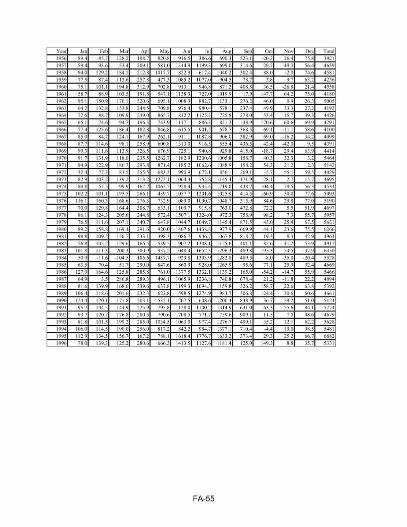
FA-55

Year Jan Feb Mar Apr May Jun Jul Aug Sep Oct Nov Dec Total1956 89.4 85.7 128.2 198.7 820.8 916.5 386.6 690.3 523.1 -20.2 26.4 75.8 39211957 59.4 93.6 53.4 209.1 581.0 1314.9 1199.3 699.0 314.6 29.2 49.3 56.4 46591958 94.0 129.2 184.1 212.8 1017.7 822.9 617.4 1040.2 302.4 88.0 -2.0 74.6 45811959 77.5 87.4 113.6 257.8 477.3 1085.2 1077.0 904.5 78.7 3.8 9.7 63.2 42361960 75.1 101.1 194.8 312.9 702.8 913.1 946.8 871.2 408.8 36.5 -26.8 21.4 45581961 58.7 88.9 103.5 191.8 547.1 1138.3 727.0 1019.9 17.9 147.7 64.2 75.0 41801962 95.1 150.9 170.1 520.6 695.1 1008.3 882.7 1133.1 276.2 46.0 0.9 26.3 50051963 64.2 132.8 153.8 248.5 709.8 976.4 980.4 578.1 237.4 49.9 33.3 27.2 41921964 72.6 88.7 109.9 239.0 865.7 812.2 1125.3 725.8 278.0 53.4 15.7 39.3 44261965 65.1 74.6 94.7 196.3 743.9 1117.1 886.3 851.2 -38.9 170.6 60.6 69.9 42911966 77.4 125.6 186.4 182.8 846.8 615.5 901.5 678.7 368.5 69.1 -11.1 58.6 41001967 85.0 84.7 124.1 167.9 262.1 911.1 1087.8 906.0 382.9 69.0 -16.2 34.2 40991968 87.7 114.6 98.1 258.9 600.8 1313.0 916.5 555.4 436.5 42.4 -42.0 9.5 43911969 99.3 111.6 113.9 326.5 676.9 725.1 940.8 929.8 415.0 -18.7 29.4 63.9 44141970 91.7 131.9 118.0 235.5 1262.7 1182.9 1200.6 1005.8 158.7 40.3 32.3 3.2 54641971 94.9 122.9 186.7 293.8 871.4 1185.2 1062.6 1088.9 158.2 54.3 21.2 2.3 51421972 32.4 77.3 83.5 255.5 683.3 990.9 672.1 856.1 269.1 -5.7 55.1 59.5 40291973 82.9 103.2 139.2 313.2 1272.1 1064.3 755.8 1145.4 -171.9 -28.1 2.7 15.7 46951974 80.8 57.5 -99.9 167.7 1065.5 928.4 935.4 719.0 438.7 104.4 79.5 56.3 45331975 102.2 101.1 195.5 266.1 439.7 1057.7 1201.6 1025.9 414.5 160.9 50.0 77.6 50931976 116.1 160.3 168.6 276.3 732.9 1089.0 1090.7 1048.7 315.9 84.6 29.8 77.0 51901977 70.0 129.8 164.4 308.7 633.1 1109.7 915.8 763.0 472.8 72.2 5.5 51.9 46971978 86.1 124.3 205.6 244.8 572.4 1507.1 1324.0 972.3 758.9 98.2 7.3 55.7 59571979 76.5 111.6 207.1 340.7 647.8 1044.7 1049.7 1145.4 871.5 43.0 25.4 67.5 56311980 89.2 158.8 169.4 291.6 920.0 1407.6 1438.8 977.9 669.9 44.1 23.6 75.5 62661981 98.8 109.2 150.7 233.1 398.3 1086.7 946.7 1067.8 818.7 19.3 -8.3 42.9 49641982 56.8 105.2 129.6 166.5 539.5 907.2 1308.1 1125.6 401.1 82.6 41.2 53.9 49171983 101.8 111.3 200.3 300.9 937.2 1048.4 1652.3 1296.3 489.8 195.3 54.5 -37.9 63501984 50.9 -11.6 -104.5 106.6 1437.7 929.8 1393.9 1282.8 489.5 8.0 -35.0 -20.4 55281985 63.5 70.4 51.7 290.0 847.6 860.9 928.0 1265.9 95.6 77.1 25.9 92.4 46691986 127.9 164.6 125.8 285.8 761.0 1377.5 1332.1 1139.2 165.0 -54.2 -14.7 55.9 54661987 64.9 3.5 286.8 289.3 496.1 1065.9 1236.8 740.8 678.4 21.2 -11.8 22.2 48941988 81.6 139.9 168.6 339.6 637.8 1199.3 1094.3 1159.8 326.2 158.7 22.6 63.8 53921989 106.4 118.6 201.6 232.3 622.8 598.5 1274.9 983.7 306.8 124.4 30.6 60.6 46611990 124.4 120.1 171.8 203.1 532.1 1207.5 608.6 1200.4 838.9 36.7 29.2 51.0 51241991 95.7 134.5 144.9 225.9 795.8 1128.0 1100.2 1314.9 631.0 63.3 55.6 84.1 57741992 93.7 120.7 176.8 280.5 790.6 708.5 771.7 759.6 909.1 11.5 7.5 48.6 46791993 81.8 101.5 199.2 285.0 1034.5 1063.0 977.4 1276.7 499.1 35.2 12.1 62.2 56281994 106.0 114.5 190.0 256.0 817.2 842.2 954.7 1377.1 710.4 -4.4 19.0 98.5 54811995 112.9 134.5 156.7 167.2 788.1 1618.4 1776.7 1633.2 373.4 29.3 25.2 66.7 68821996 78.0 139.3 125.2 280.6 666.3 1413.5 1127.6 1181.4 125.0 149.3 8.8 35.7 5331

FA-56

Table A-28. Current Level Depletions Above Fort Peck Dam (1000 acre-feet) Year Jan Feb Mar Apr May Jun Jul Aug Sep Oct Nov Dec Total1898 -101.1 -64.5 23.8 78.4 291.6 750.5 566.0 612.0 288.1 -88.2 -66.1 -87.9 22031899 -99.4 -62.8 25.5 80.1 343.9 1105.9 688.2 446.8 359.9 -95.9 -71.9 -91.7 26281900 -102.8 -65.9 22.3 77.2 332.9 1189.8 623.1 391.1 158.3 -59.6 -44.8 -75.5 24461901 -93.0 -59.2 26.8 80.4 333.7 795.9 777.3 700.6 62.2 -37.1 -64.7 -87.7 24351902 -102.0 -64.2 23.8 91.1 316.9 910.6 487.7 582.3 330.1 -48.1 -71.9 -92.1 23641903 -102.7 -65.4 23.2 78.2 371.6 1116.4 443.3 528.0 287.1 -47.5 -71.4 -91.7 24691904 -102.7 -65.8 22.5 88.8 538.9 962.4 468.9 413.3 313.2 -46.9 -49.9 -78.2 24651905 -94.9 -60.8 25.8 79.9 347.7 731.0 643.8 613.4 398.2 -75.9 -74.3 -93.1 24411906 -104.0 -66.3 22.6 77.8 304.7 858.0 778.2 363.5 324.1 -45.0 -68.8 -91.4 23531907 -103.5 -65.9 21.9 76.8 489.8 550.2 582.7 439.7 297.9 -38.4 -64.7 -88.2 20981908 -102.4 -65.6 22.3 90.4 290.5 549.1 741.3 447.6 194.3 -97.9 -55.1 -82.0 19321909 -98.1 -62.3 24.9 79.0 345.3 600.1 448.9 607.4 209.8 -34.6 -61.6 -85.9 19731910 -98.8 -62.3 25.8 93.1 498.1 960.3 690.4 468.9 99.2 -68.1 -60.6 -85.0 24611911 -101.7 -65.5 21.8 75.8 330.1 755.6 659.8 403.3 108.7 -93.7 -52.0 -80.1 19621912 -96.1 -61.0 25.7 79.5 319.4 1148.7 569.9 350.5 100.5 -82.0 -55.4 -82.3 22171913 -97.2 -62.2 24.5 78.3 371.4 826.9 530.1 571.4 330.9 -112.6 -67.3 -88.1 23061914 -101.1 -64.9 23.4 78.0 331.5 584.0 847.6 605.4 230.3 -111.8 -63.7 -86.4 22721915 -102.7 -65.8 22.2 76.5 436.2 489.8 349.5 601.8 101.8 -25.0 -54.4 -81.5 17481916 -98.6 -63.0 24.6 78.5 306.1 577.0 557.0 496.1 205.6 -102.9 -54.3 -80.9 18451917 -95.1 -59.9 27.4 81.5 307.9 887.7 817.5 584.9 189.9 -77.7 -67.2 -89.0 25081918 -102.0 -64.5 23.5 77.8 496.5 1273.8 363.4 415.3 142.8 -50.8 -62.2 -86.0 24281919 -98.4 -63.1 24.2 101.3 482.3 1081.2 680.2 511.3 207.7 -79.3 -49.3 -77.3 27211920 -94.9 -60.5 26.0 79.8 360.5 1029.3 706.6 516.2 260.8 -115.5 -67.7 -88.7 25521921 -100.7 -64.2 23.7 78.1 380.9 1023.6 658.9 565.8 230.6 -41.9 -71.0 -91.6 25921922 -103.7 -66.1 22.2 76.8 383.9 987.6 353.8 563.3 383.0 -42.2 -74.5 -93.5 23911923 -105.2 -68.1 20.7 75.9 356.4 644.2 527.7 403.6 410.0 -98.1 -64.3 -87.3 20151924 -97.4 -61.6 26.4 94.2 705.1 943.0 631.3 536.7 239.2 -81.7 -71.1 -90.3 27741925 -104.8 -67.9 20.2 74.8 529.9 765.1 739.8 450.1 32.6 -105.9 -53.3 -80.1 22011926 -98.0 -62.7 24.0 90.7 410.4 775.5 652.1 513.1 -45.3 -27.4 -53.0 -81.1 20981927 -98.5 -62.4 24.5 78.0 265.5 944.2 555.7 281.5 310.9 -48.9 -62.3 -87.5 21011928 -99.1 -63.1 24.3 79.0 917.4 613.8 420.4 329.3 352.6 -71.3 -66.8 -88.1 23481929 -56.2 -89.1 -2.4 52.1 462.2 963.9 875.3 414.0 -34.2 -72.1 -85.8 -69.3 23581930 -69.0 -73.8 80.2 288.2 481.3 911.5 604.1 309.4 44.3 -99.9 -69.4 -94.1 23131931 -78.4 -40.3 72.5 117.3 390.1 846.9 569.0 479.0 27.7 -77.3 -80.4 -30.7 21951932 -25.1 -3.2 81.6 137.6 565.9 862.6 701.4 316.6 175.8 -147.8 -64.2 -63.8 25371933 -71.7 -64.1 30.2 44.6 395.3 1172.8 810.6 112.5 100.0 -148.8 -53.7 -62.3 22651934 -51.8 -59.7 56.1 92.2 482.2 390.4 687.3 439.8 -1.2 -85.9 -59.5 -52.6 18371935 -46.6 -5.8 49.0 77.6 279.4 931.0 736.4 402.6 202.7 -91.4 -47.5 2.9 24901936 21.9 -49.0 64.9 141.8 741.0 811.5 738.2 379.6 127.4 -61.1 -19.6 -8.4 28881937 -58.0 -37.9 76.0 90.2 613.5 468.6 651.8 470.7 84.2 -70.4 -60.2 -17.1 22111938 -19.4 -36.6 31.0 41.1 354.4 827.0 589.5 379.6 196.2 -119.4 -42.9 -66.0 21341939 -87.1 -80.0 118.9 199.9 523.4 418.5 805.0 417.9 124.6 -113.1 -99.6 -75.8 21531940 -72.4 -41.8 79.6 130.8 667.4 870.8 523.8 506.9 -17.3 -88.5 -99.2 -54.7 24051941 -65.9 -63.9 55.9 71.9 311.9 683.2 711.9 266.5 38.3 1.6 -32.2 -55.8 19231942 -124.3 197.0 -86.6 187.5 309.8 746.5 764.9 410.1 100.8 -92.4 -43.5 -69.1 23011943 -159.3 -119.2 -77.3 152.2 406.2 807.4 809.9 339.2 106.3 -121.8 -50.6 -75.7 20171944 -90.7 -61.2 12.7 41.2 216.3 614.8 895.0 330.6 136.7 -74.3 -58.9 -103.8 18581945 -59.4 -48.9 69.7 62.3 318.5 568.7 1018.2 497.1 54.4 -72.4 -54.9 -91.4 22621946 -79.8 -67.7 42.3 206.7 452.0 724.8 707.2 405.5 68.4 -162.5 -54.8 -75.4 21671947 -113.1 -106.2 -97.4 25.0 822.1 679.7 1061.4 399.4 25.4 -81.6 -44.4 -84.2 24861948 -103.7 -81.2 -24.9 133.0 457.3 493.1 742.5 459.2 200.5 -66.8 -44.3 -80.8 20841949 -100.6 -70.6 29.3 210.3 583.6 860.6 773.3 502.3 172.6 -86.4 -65.1 -98.8 27101950 -120.4 -47.5 34.1 73.4 410.8 865.5 755.4 373.4 36.3 -50.4 -59.8 -61.7 22091951 -125.1 -72.1 -2.3 89.0 696.3 738.5 793.4 270.2 97.8 -85.8 -58.1 -100.7 22411952 -119.4 -100.9 -139.8 149.2 748.4 915.4 864.6 436.4 218.4 -138.7 -78.2 -80.0 26751953 -52.2 -55.0 6.7 35.7 104.4 1073.2 1102.7 475.0 217.1 -75.0 -34.2 -107.7 26911954 -103.8 -39.6 97.3 124.5 540.8 728.0 1011.2 262.8 121.5 -71.9 -28.5 -95.0 25471955 -101.0 -95.3 46.1 111.6 338.4 975.9 643.8 675.0 115.0 -122.6 -64.6 -59.8 2463

FA-57

Year Jan Feb Mar Apr May Jun Jul Aug Sep Oct Nov Dec Total1956 -66.8 -95.8 1.7 87.3 585.3 1076.2 793.6 305.6 217.7 -104.7 -0.8 -91.8 27081957 -135.6 -65.2 -43.8 -48.4 482.5 836.7 1005.0 429.2 159.1 -107.5 -55.9 -89.8 23661958 -112.8 -68.5 43.2 123.7 910.9 456.2 501.8 614.3 172.8 -77.8 -76.6 -69.6 24181959 -97.7 -90.2 98.2 74.9 189.3 1147.4 1029.8 359.1 -19.2 -47.6 52.5 37.3 27341960 -202.8 -143.4 171.9 190.5 401.8 1035.9 964.8 329.1 219.1 -143.3 -90.7 -66.0 26671961 -73.3 -29.8 57.3 37.2 242.5 1319.5 778.2 557.5 32.3 14.8 10.7 -70.7 28761962 -77.1 -24.4 9.5 176.2 206.9 1071.9 691.8 351.6 159.3 -87.0 -13.5 -80.3 23851963 -152.6 19.6 -15.5 -43.7 364.8 827.7 979.8 514.3 209.8 -99.3 -42.0 -113.9 24491964 -112.2 9.3 -103.8 -110.2 311.0 1178.3 1065.2 147.7 131.1 -93.7 -68.1 -108.4 22461965 -61.6 -68.2 -116.9 165.2 494.4 1256.3 915.0 262.2 -158.5 -96.8 -64.5 -153.7 23731966 -174.3 -141.2 142.4 148.4 461.9 646.1 913.9 452.7 224.4 -110.6 -136.6 -85.8 23411967 -86.9 -112.5 -157.3 -178.2 419.6 1316.4 1007.8 620.8 288.9 -151.9 -81.6 -191.7 26931968 -139.3 -81.3 4.7 -15.5 187.5 1010.1 1048.4 241.2 88.7 -38.1 -38.1 -144.0 21241969 -138.4 -86.6 -14.2 271.7 740.5 457.4 1016.8 611.2 149.7 -81.9 -50.9 -119.3 27561970 -132.4 -89.0 -127.5 -104.0 479.2 1476.7 803.6 515.9 -4.0 -124.9 -69.7 -138.0 24861971 -116.4 -14.7 -172.7 24.3 584.9 1218.1 1001.9 444.2 91.8 -53.8 -47.3 -160.7 28001972 -129.9 -75.8 127.6 6.5 361.3 1329.9 608.3 290.6 106.4 -50.1 -20.5 -142.1 24121973 -130.9 -100.7 114.7 141.4 647.9 817.1 901.8 421.2 159.4 -50.9 0.4 -82.1 28391974 -90.0 -66.9 -26.1 94.8 197.0 1582.8 846.2 194.3 171.7 -32.8 -54.3 -64.7 27521975 -112.0 -106.0 -109.3 -17.6 320.7 1386.8 684.9 410.2 233.0 -146.6 -91.9 -98.7 23531976 -177.1 -171.6 -174.3 52.6 1054.0 701.8 851.8 374.3 174.2 -56.8 -63.7 -148.3 24171977 -199.2 -139.9 60.8 209.5 197.4 934.3 727.7 339.5 81.9 -19.9 -52.0 -76.7 20641978 -86.8 -50.6 135.7 53.9 263.5 1121.8 789.1 482.0 60.8 -42.4 -79.5 -117.7 25301979 -155.3 -94.1 150.1 89.2 671.1 961.3 751.7 442.2 237.7 -119.3 -47.9 -70.5 28161980 -118.0 -48.5 -67.4 71.5 536.1 1057.1 901.9 222.9 93.5 -80.4 -48.9 -71.5 24481981 -94.7 -114.1 -174.7 -91.7 537.4 1087.2 872.8 610.9 189.0 -88.0 -46.1 -83.6 26041982 -138.5 -63.7 -97.1 2.6 377.2 1172.9 926.9 559.9 78.7 -76.6 -64.7 -133.4 25441983 -22.2 -117.3 46.1 59.9 402.5 1102.7 766.9 584.9 106.5 -45.9 -34.2 -197.4 26521984 -126.2 -117.8 -135.3 -56.5 633.9 1183.6 947.9 627.7 135.5 -107.2 -57.4 -191.8 27371985 -191.8 -291.4 126.2 324.6 568.1 1014.6 846.3 207.5 -2.4 13.0 -140.6 -108.0 23661986 -102.3 18.1 3.6 71.2 414.5 1322.1 749.2 472.6 -3.3 -82.6 -68.4 -138.7 26561987 -169.6 -111.9 87.1 213.2 219.3 1003.4 638.4 404.7 309.9 -53.8 -62.4 -102.3 23761988 -122.6 -38.8 -20.2 113.4 383.1 998.2 773.6 417.2 50.5 -48.1 -17.9 -19.5 24691989 -73.9 -127.4 61.9 92.1 319.0 1021.4 798.3 276.4 307.7 -42.8 95.5 -84.2 26441990 -91.0 -110.3 -63.9 143.9 224.7 1105.6 799.0 319.6 349.8 -62.0 30.1 -149.7 24961991 -171.7 -58.5 -43.5 9.2 441.3 812.7 944.9 421.0 50.3 -83.8 8.1 -74.5 22551992 -116.1 -69.2 -14.5 70.8 431.5 624.0 721.2 525.4 199.1 -1.8 30.8 -78.1 23231993 -121.8 -83.9 106.1 104.7 542.0 546.8 323.5 293.4 204.9 -89.8 -71.3 -118.9 16361994 -139.4 -130.6 20.3 164.6 415.2 758.8 703.3 533.6 251.4 -68.2 -2.3 -47.4 24591995 -69.4 -12.2 -6.7 9.0 172.8 1079.2 609.8 502.7 122.3 -44.6 44.4 28.8 24361996 -84.1 44.8 -186.1 28.9 394.2 1030.0 705.6 522.7 74.5 -47.1 1.9 -113.2 2372

FA-58

Table A-29. Current Level Depletions Between Fort Peck and Garrison Dams (1000 acre-feet) Year Jan Feb Mar Apr May Jun Jul Aug Sep Oct Nov Dec Total1898 -142.9 -100.6 -36.8 208.9 326.7 1024.8 1042.2 634.6 213.1 -119.3 -143.6 -154.2 27531899 -142.5 -100.2 -36.4 127.8 774.4 1250.9 691.7 444.6 243.6 -105.6 -144.1 -153.9 28501900 -139.0 -98.2 -34.9 96.3 1511.2 1739.7 739.2 259.4 12.0 -92.0 -125.4 -140.7 37281901 -133.9 -96.1 -35.2 253.8 1578.2 1075.9 1029.4 570.4 43.3 -79.8 -155.2 -159.2 38911902 -149.2 -106.0 -42.5 248.3 1188.8 1255.1 867.6 468.2 200.9 -93.5 -154.3 -159.6 35241903 -149.9 -107.6 -44.0 39.2 812.7 1404.1 596.8 402.2 62.5 -64.7 -136.4 -149.8 26651904 -137.7 -97.6 -35.1 318.4 1039.6 1145.6 846.5 468.2 243.2 -90.1 -152.5 -158.9 33901905 -149.1 -106.8 -43.2 219.8 340.7 1082.1 788.5 710.0 201.3 -116.1 -142.6 -153.1 26311906 -139.3 -97.7 -33.8 277.0 731.0 1425.1 1085.1 276.0 306.9 -91.1 -153.7 -161.3 34241907 -147.2 -104.4 -41.2 75.2 598.6 1352.3 927.8 549.0 253.8 -60.1 -154.1 -160.9 30891908 -145.3 -102.0 -38.0 337.7 559.5 1413.6 1041.7 434.8 229.6 -136.7 -148.6 -157.2 32891909 -145.3 -103.4 -40.2 10.9 702.0 1318.1 863.0 603.4 113.3 -90.3 -145.2 -154.4 29321910 -140.3 -98.3 -34.9 332.3 1071.1 1551.7 882.7 329.5 76.5 -63.0 -126.4 -142.8 36381911 -137.7 -98.8 -37.4 175.4 935.7 1716.4 730.0 253.3 35.9 -137.7 -135.7 -148.5 31511912 -141.2 -102.2 -40.4 155.3 769.8 1610.0 572.7 277.3 -71.9 -120.8 -124.3 -142.0 26431913 -132.3 -94.5 -33.3 255.8 1158.9 1522.2 807.6 464.9 78.7 -145.4 -146.5 -153.8 35821914 -135.5 -96.7 -44.4 159.9 1291.2 1107.7 1111.6 550.8 247.3 -82.5 -158.8 -173.7 37771915 -166.2 -118.9 -62.0 479.9 663.0 641.6 535.4 591.2 -5.0 -33.6 -135.6 -148.2 22421916 -149.7 -105.0 -31.0 213.3 836.3 1079.0 749.5 337.0 91.1 -104.6 -140.1 -156.2 26201917 -153.1 -104.5 -49.7 3.2 462.6 1329.4 1241.4 487.8 223.7 -110.4 -157.5 -160.2 30131918 -149.7 -105.9 -35.4 38.5 996.4 1833.8 848.5 363.6 104.6 -49.7 -157.6 -166.5 35201919 -151.4 -107.2 -51.8 247.3 1350.9 1574.2 845.5 516.2 210.7 -138.3 -143.9 -149.8 40021920 -149.8 -110.3 -51.4 -21.0 920.5 1482.6 1118.3 588.1 219.7 -114.0 -194.4 -220.1 34681921 -158.9 -111.1 -93.7 171.2 961.2 1469.9 985.0 627.9 164.4 -61.3 -154.5 -157.4 36431922 -139.2 -97.5 -36.2 -0.6 900.1 1671.3 358.0 693.1 286.7 -107.8 -155.4 -159.4 32131923 -140.6 -98.3 -41.7 147.6 1083.4 1150.9 854.1 417.3 -63.5 -93.8 -131.8 -147.1 29361924 -135.6 -92.3 -35.0 118.2 721.8 692.4 878.7 577.7 277.2 -76.4 -140.9 -154.4 26321925 -136.5 -91.9 -30.8 412.4 1471.9 988.8 787.9 560.7 170.2 -143.7 -151.2 -154.1 36841926 -146.6 -101.8 -41.1 293.0 1156.6 1314.3 781.7 445.2 29.8 -50.4 -118.1 -143.1 34201927 -157.7 -97.1 -35.0 116.6 488.7 1341.6 810.1 371.8 155.6 -54.9 -134.9 -152.0 26531928 -132.3 -96.6 -30.1 208.8 1862.4 860.5 672.7 417.5 253.8 -137.1 -149.9 -150.1 35791929 -174.6 -154.2 258.3 73.2 818.1 1248.1 884.1 612.7 98.3 -107.3 -150.5 -156.5 32501930 -183.3 -114.0 -13.0 333.9 974.2 1268.7 930.7 560.7 143.7 -144.0 -196.9 -184.2 33761931 -163.9 -127.2 -47.1 174.5 1238.2 1575.8 650.1 481.2 121.7 -64.5 -120.0 -156.8 35621932 -130.3 -93.6 -55.1 15.7 1228.9 1084.9 940.6 437.2 125.9 -175.0 -131.0 -158.1 30901933 -139.8 -129.9 -36.0 21.1 716.8 2061.2 863.3 217.0 222.8 -105.8 -139.8 -110.9 34401934 -92.5 -68.9 -57.3 330.9 1711.3 694.2 716.0 461.3 61.7 -28.0 -66.7 -59.0 36031935 -59.5 -52.5 20.5 -57.9 437.3 1802.4 949.7 488.4 247.9 -146.0 -141.2 -138.0 33511936 -131.7 -113.3 -35.8 212.8 1572.2 1399.1 892.7 460.9 122.7 -108.3 -136.9 -142.2 39921937 -167.7 -138.8 -57.6 72.7 1355.2 1111.2 958.7 551.4 138.8 -122.8 -143.4 -115.9 34421938 -115.8 -95.1 -89.5 91.1 668.4 1344.6 854.3 482.8 325.1 -103.5 -154.8 -143.5 30641939 -135.4 -132.8 -17.1 324.4 1093.6 682.0 963.2 404.7 199.9 -145.6 -176.1 -96.7 29641940 -73.5 -49.6 -10.5 95.9 1270.2 1010.7 808.4 562.6 254.3 -26.2 -165.7 -100.0 35771941 -91.2 -87.0 -78.7 165.2 1439.8 1205.9 859.0 544.9 25.6 -54.8 -178.2 -145.1 36051942 -185.6 -151.3 -76.2 263.8 692.3 1091.9 966.8 502.0 121.7 -114.3 -156.6 -205.7 27491943 -171.0 -106.7 -9.5 260.8 636.3 1099.8 1233.1 552.1 249.9 -140.8 -156.9 -185.3 32621944 -193.9 -148.3 -119.1 61.7 1214.4 1251.2 857.5 472.2 114.5 -88.9 -156.5 -192.3 30721945 -144.8 -105.7 -62.6 -75.6 630.6 1059.8 1408.2 589.2 150.3 -72.7 -173.2 -184.2 30191946 -167.3 -114.1 -44.5 415.7 663.0 1218.4 1025.3 524.4 70.4 -67.9 -192.2 -188.2 31431947 -198.0 -150.0 -19.6 -58.6 1261.0 924.4 1295.1 598.9 153.1 -74.0 -169.4 -193.7 33691948 -175.8 -96.1 -33.8 284.3 1259.8 1286.6 610.3 582.0 273.1 -127.7 -174.1 -193.3 34951949 -185.9 -137.0 -65.1 359.7 1258.7 1451.6 882.1 625.5 148.5 -137.5 -165.1 -201.2 38341950 -191.1 -148.3 -116.7 123.9 636.4 1195.4 1149.1 502.2 81.1 -14.0 -159.8 -178.7 28801951 -182.7 -136.9 -105.8 18.2 1177.4 1058.6 1270.5 447.1 104.5 -140.5 -172.5 -187.5 31501952 -180.6 -145.2 -64.7 428.6 1160.9 1319.5 834.8 610.7 275.0 -141.8 -205.6 -167.9 37241953 -145.8 -96.7 -75.5 81.3 473.0 1328.9 1217.2 632.9 302.0 -69.8 -116.8 -105.0 34261954 -75.9 -101.4 -100.7 145.1 1226.4 991.5 1287.7 420.2 144.4 -175.5 -148.2 -151.4 34621955 -126.4 -138.6 -43.0 223.0 775.0 1230.8 989.5 688.5 155.0 -102.7 -110.5 -103.4 3437

FA-59

Year Jan Feb Mar Apr May Jun Jul Aug Sep Oct Nov Dec Total1956 -95.5 -70.2 -92.4 58.7 1250.6 1864.0 763.6 394.3 200.2 -134.6 -170.3 -137.1 38311957 -153.8 -115.6 -146.6 -236.3 855.7 1475.2 1340.8 588.6 172.2 -129.4 -185.5 -208.0 32571958 -154.5 -124.5 -111.9 224.8 2140.7 865.8 515.7 517.9 178.7 -168.7 -162.1 -88.6 36331959 -74.4 -120.3 20.7 146.6 753.2 1702.8 1137.1 571.1 75.9 -113.0 -156.9 -155.3 37881960 -139.2 -122.4 62.7 127.5 1028.0 1130.5 947.2 387.3 199.4 -24.0 -57.8 -54.5 34851961 -40.0 -7.8 -7.0 25.8 1000.0 1696.0 844.4 668.7 17.9 29.5 -10.2 -201.0 40161962 -196.5 21.7 -52.2 403.8 535.0 1554.6 679.0 470.1 181.1 -111.1 -180.8 -148.4 31561963 -174.9 -73.3 -112.3 -65.6 1062.6 1673.4 980.1 607.2 358.1 -139.9 -181.1 -164.3 37701964 -138.5 -155.1 -138.1 23.0 1117.9 1115.8 1348.1 369.8 216.4 -119.1 -164.0 -156.1 33201965 -122.3 -98.4 -152.2 40.4 445.3 1605.0 1340.7 325.1 -12.5 -40.2 -173.8 -125.8 30311966 -159.0 -149.7 -26.0 52.8 1267.6 1053.1 972.0 416.5 271.1 -35.4 -29.7 -93.5 35401967 -70.7 -36.2 -60.8 -237.2 586.9 1643.0 1128.0 573.8 188.6 -130.2 -160.2 -197.2 32281968 -193.5 -94.1 -34.7 43.7 671.5 1432.9 1044.8 390.8 229.7 -140.9 -149.5 -195.6 30051969 -205.4 -128.0 1.7 318.6 1374.2 810.2 952.5 719.9 274.0 -161.3 -162.6 -177.2 36161970 -176.1 -93.1 -64.1 -19.5 986.3 1630.2 1026.5 695.4 43.2 -160.8 -152.5 -192.9 35231971 -149.0 -63.5 -143.6 -62.3 779.4 1985.6 920.4 742.2 68.0 -112.9 -180.9 -256.9 35271972 -200.8 -63.8 16.9 52.5 909.9 1888.3 608.0 500.4 158.8 -120.7 -165.2 -183.4 34011973 -174.2 -167.0 -88.9 76.0 1332.5 1303.5 922.4 579.6 48.5 -112.1 -162.0 -194.4 33641974 -198.3 -137.4 -74.7 184.7 636.2 1936.5 1163.4 311.0 131.9 -135.0 -154.1 -155.6 35091975 -157.3 -134.5 -102.8 -171.2 368.7 1106.6 1601.6 542.4 251.4 -143.4 -168.7 -180.5 28121976 -151.5 -97.8 -54.1 141.5 1383.1 1159.8 1136.1 458.1 223.8 -126.3 -191.0 -148.7 37331977 -152.0 -128.3 -86.7 404.0 935.8 1277.5 806.5 502.8 136.2 -21.9 -64.9 -83.6 35251978 -79.6 -82.9 62.8 4.1 402.3 1553.5 1116.1 588.9 -11.3 -90.8 -174.0 -179.7 31091979 -183.1 -156.5 91.0 159.1 1083.8 1380.1 841.8 560.5 305.5 -134.0 -154.5 -161.6 36321980 -145.4 -93.4 -67.2 325.2 1229.2 1441.0 1085.7 335.6 205.5 -143.7 -138.6 -125.7 39081981 -125.4 -102.7 -46.5 219.8 784.9 1394.2 821.2 628.3 280.7 -137.3 -141.9 -134.8 34411982 -148.6 -95.1 -48.8 22.9 554.3 1169.9 1239.2 636.7 60.8 8.8 -197.2 -212.0 29911983 -172.7 -131.4 -135.6 -88.4 641.6 1636.7 1147.1 812.6 131.1 -76.6 -163.9 -217.3 33831984 -160.8 -131.9 -25.4 97.3 1351.8 1244.8 1066.8 661.7 60.4 -132.4 -162.8 -177.7 36921985 -172.5 -174.7 0.7 406.2 1301.5 1109.1 956.9 403.6 96.9 -22.8 -90.9 -113.7 37001986 -91.8 4.4 -39.8 -13.5 626.9 1957.0 711.4 540.2 3.7 -83.2 -143.2 -185.4 32871987 -170.4 -95.7 25.0 553.2 1224.0 1300.1 601.6 350.1 216.2 -52.6 -140.5 -130.6 36811988 -103.6 -58.1 -9.4 245.0 1052.9 1414.1 804.1 518.9 55.7 -30.1 -56.8 -61.9 37711989 -53.3 -47.2 46.4 181.4 909.3 1375.3 1176.1 502.9 259.2 7.4 -78.6 -153.9 41251990 -122.1 -94.9 -43.3 178.6 880.3 1382.3 886.3 592.4 369.9 -56.0 -89.8 -151.7 37321991 -139.3 -49.4 -19.7 164.2 1246.7 1219.6 761.5 685.6 103.3 -159.0 -134.5 -153.0 35261992 -136.3 -47.6 6.8 151.1 1139.1 958.7 712.9 447.6 250.2 -43.2 -115.6 -129.2 31951993 -100.6 -54.0 57.2 159.1 1445.9 951.4 289.4 452.8 200.4 -156.7 -181.4 -119.5 29441994 -109.2 -73.7 18.9 216.9 1311.0 847.8 653.2 568.5 207.8 -25.3 -42.9 -58.2 35151995 -52.0 18.1 32.6 20.7 721.7 1547.9 939.6 572.3 123.8 -122.5 -116.1 -115.4 35711996 -92.1 -51.2 -91.2 -42.6 499.6 1707.6 1112.9 681.5 112.2 -87.0 -110.4 -134.3 3505

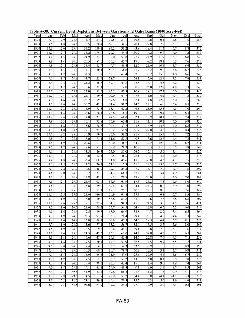
FA-60

Table A-30. Current Level Depletions Between Garrison and Oahe Dams (1000 acre-feet) Year Jan Feb Mar Apr May Jun Jul Aug Sep Oct Nov Dec Total1898 9.7 12.0 24.8 15.7 51.9 79.5 37.1 30.5 13.8 0.1 4.8 7.6 2881899 9.5 11.8 24.6 15.5 28.4 62.1 34.5 -0.1 22.8 7.9 5.3 7.6 2301900 10.3 12.6 25.4 35.2 159.1 97.2 38.2 -3.8 -19.4 11.4 6.7 8.8 3821901 10.3 12.4 25.0 38.2 176.9 27.3 44.8 30.9 -4.2 9.7 4.0 7.2 3831902 9.0 11.5 24.3 24.9 132.8 39.0 53.8 -2.7 24.9 11.9 3.7 6.8 3401903 8.9 11.4 24.3 26.5 87.6 75.3 45.7 -17.0 -9.2 18.1 5.5 7.6 2851904 9.8 12.1 24.8 38.4 82.9 49.7 49.4 12.0 21.0 16.6 3.7 6.6 3271905 8.9 11.5 24.4 17.1 30.1 52.4 36.6 41.7 36.2 9.2 3.6 6.7 2781906 9.2 11.7 24.7 32.3 2.2 58.3 62.4 2.5 38.7 15.5 4.0 6.6 2681907 9.1 11.7 24.6 15.7 23.4 78.7 11.1 26.3 7.0 12.4 5.2 7.6 2331908 9.9 12.2 25.0 24.2 36.3 57.3 43.8 22.5 33.1 4.3 4.2 7.1 2801909 9.3 11.7 24.6 15.6 35.1 78.7 14.0 0.9 26.0 12.2 4.8 7.3 2401910 10.0 12.3 25.1 34.9 83.6 67.5 47.5 10.8 18.1 17.5 6.0 8.2 3421911 10.2 12.4 25.1 24.1 110.8 109.0 47.7 -7.3 11.6 4.2 4.4 7.3 3591912 9.3 11.6 24.3 25.2 79.2 87.8 18.8 2.1 1.8 12.9 5.0 7.5 2861913 9.7 12.0 24.8 30.7 43.0 101.4 30.2 24.6 22.1 6.8 6.4 8.5 3201914 10.1 12.2 25.0 15.9 75.3 18.4 45.2 6.8 28.0 15.8 4.3 7.0 2641915 8.9 11.4 24.3 38.6 28.1 23.8 -8.5 19.0 6.2 9.4 6.4 8.3 1761916 10.2 12.4 25.1 17.8 35.5 47.5 60.0 2.1 18.9 10.1 5.1 7.4 2521917 9.9 12.3 25.1 16.1 73.8 75.9 62.4 21.9 11.1 10.2 4.0 6.9 3301918 9.3 11.8 24.7 15.6 78.5 94.4 37.2 3.5 16.9 14.3 4.0 6.8 3171919 9.3 11.8 24.6 17.1 35.3 75.2 59.9 36.7 27.8 4.2 6.2 8.4 3161920 10.0 12.2 25.0 15.9 50.3 36.6 39.2 21.9 14.1 15.3 4.7 7.2 2531921 9.8 12.3 25.1 16.0 83.1 111.6 52.8 9.8 -3.6 12.6 4.4 7.2 3411922 9.5 11.9 24.7 20.6 73.2 46.0 46.7 54.9 32.7 12.2 2.6 6.2 3411923 8.5 11.2 24.3 18.6 83.0 39.9 28.3 10.7 0.3 11.5 5.5 7.8 2491924 9.5 11.8 24.6 15.5 40.3 25.0 33.0 26.2 17.1 5.9 5.4 7.8 2221925 10.1 12.4 25.2 38.8 112.1 -3.5 46.5 28.1 30.3 4.5 4.0 7.1 3151926 9.4 11.8 24.7 33.4 108.3 81.8 49.6 17.9 -3.8 4.3 4.7 7.5 3501927 9.1 11.5 24.2 15.2 20.1 71.5 17.3 21.0 19.3 15.6 4.7 7.2 2371928 9.7 12.2 25.0 17.6 145.9 37.3 24.2 -7.9 18.1 7.7 4.7 7.5 3021929 9.6 12.0 24.9 16.2 33.0 71.2 66.3 32.2 0.2 3.4 4.9 7.5 2811930 9.7 12.1 24.9 15.8 48.0 49.5 70.8 27.9 20.9 1.9 4.0 7.0 2931931 9.6 12.1 25.0 21.4 65.6 89.6 61.9 17.3 23.2 7.3 5.6 8.0 3461932 9.8 12.1 24.9 15.8 39.0 69.4 63.5 24.1 24.3 0.2 3.9 7.0 2941933 9.6 12.1 25.0 16.1 15.1 117.2 75.1 30.5 28.1 8.0 5.1 7.6 3491934 10.1 12.5 25.3 24.0 140.4 56.9 61.8 37.9 4.4 6.8 5.7 8.3 3941935 9.7 11.9 24.7 16.0 10.2 58.8 81.8 43.2 32.6 7.8 3.8 6.8 3071936 10.0 12.6 25.6 18.1 122.7 101.7 98.3 41.5 24.5 3.5 4.5 7.6 4711937 9.3 11.6 24.5 21.0 58.2 53.7 36.5 64.4 18.8 6.5 3.2 6.6 3141938 9.0 11.6 24.6 19.5 19.8 68.0 64.9 52.8 14.7 8.9 3.4 6.5 3041939 9.3 11.9 24.9 22.3 93.7 35.3 70.4 29.4 28.1 4.6 4.4 7.3 3421940 9.6 12.0 24.9 15.8 98.1 69.8 43.9 34.6 24.5 6.4 5.5 8.1 3531941 9.7 11.9 24.7 15.6 77.1 33.2 56.7 32.0 -13.5 3.7 5.6 8.0 2651942 9.5 11.9 24.6 15.5 9.3 30.4 49.5 39.1 3.8 7.6 5.3 7.6 2141943 10.0 12.4 25.3 24.5 47.3 26.1 63.0 44.7 34.8 4.6 3.1 6.5 3021944 8.8 11.4 24.4 16.6 48.7 26.3 45.4 14.7 22.8 7.6 4.5 7.1 2381945 9.3 11.8 24.6 19.5 30.4 14.7 53.9 38.5 -4.5 9.9 5.5 7.7 2211946 9.5 12.0 24.8 17.4 6.6 33.9 54.3 33.6 -8.9 1.0 6.3 8.3 1991947 10.4 12.7 25.5 16.3 69.5 10.7 79.7 60.3 12.5 3.3 3.7 6.9 3111948 9.1 11.7 24.7 16.0 66.6 31.9 47.9 25.6 39.0 4.6 3.5 6.7 2871949 9.4 11.9 24.8 19.5 62.0 83.7 54.2 44.0 16.0 -0.4 3.8 7.0 3361950 9.1 11.5 24.5 15.4 38.3 83.3 43.4 15.5 1.4 9.0 4.9 7.4 2641951 9.3 11.7 24.5 19.1 62.1 24.0 49.4 -9.3 -6.9 3.4 6.7 8.5 2031952 7.9 19.3 39.5 44.9 32.4 47.8 68.5 21.3 31.2 1.3 -2.9 5.1 3161953 0.1 2.8 29.5 4.5 53.7 99.9 57.2 54.4 15.8 -4.1 -1.1 3.3 3161954 4.0 12.2 12.7 23.1 49.1 49.4 70.5 32.2 0.3 -5.0 -1.9 4.6 2511955 6.2 7.3 34.8 92.6 61.9 47.2 54.2 77.4 12.9 3.0 -6.3 10.2 401

FA-61

Year Jan Feb Mar Apr May Jun Jul Aug Sep Oct Nov Dec Total1956 4.5 6.7 24.8 11.4 37.4 75.7 16.9 11.7 20.3 -1.0 2.8 6.3 2181957 4.6 11.1 15.9 19.9 73.7 51.3 64.6 27.6 10.0 -1.5 1.3 2.9 2811958 -3.3 8.6 22.0 32.6 94.6 37.0 52.4 40.4 18.1 -5.4 -6.5 1.6 2921959 3.1 3.7 30.4 14.8 20.6 67.6 97.0 46.7 8.5 2.5 0.6 6.0 3021960 7.0 7.9 50.9 15.8 29.5 61.7 81.7 49.5 41.1 0.5 -0.7 4.6 3501961 5.8 7.7 8.6 5.7 48.2 100.6 62.7 91.5 4.7 3.4 -0.5 3.4 3421962 5.7 31.9 27.6 10.9 147.8 106.4 85.8 51.4 -3.7 4.1 2.3 5.3 4761963 6.3 34.7 21.7 11.2 61.8 75.1 54.4 26.4 20.9 -6.3 -0.6 3.8 3091964 8.2 9.5 13.7 23.9 55.5 112.2 86.1 4.3 16.3 8.4 -0.9 7.1 3441965 11.3 18.4 21.9 41.0 34.6 37.4 83.3 36.9 -11.7 0.3 4.9 8.5 2871966 10.3 3.9 17.6 3.1 70.1 15.7 54.1 29.4 10.5 4.8 7.2 5.2 2321967 13.0 19.9 39.6 15.9 63.1 37.3 81.7 24.4 7.2 2.8 5.1 6.2 3161968 10.9 15.2 31.3 17.2 31.1 47.6 56.9 32.5 25.0 0.3 4.1 6.1 2781969 9.4 9.8 43.3 39.4 59.9 26.2 67.2 43.0 19.5 -4.3 5.8 6.5 3261970 13.7 18.1 19.7 44.0 53.3 90.2 45.2 38.9 -1.6 6.0 7.0 11.0 3451971 12.5 42.5 47.3 54.7 35.5 69.4 45.3 26.3 5.3 28.6 12.7 12.2 3921972 13.1 45.6 33.2 0.4 15.2 48.1 42.2 49.4 21.0 6.7 10.4 10.1 2961973 15.9 3.5 9.0 10.9 49.3 80.9 45.6 24.9 26.0 13.1 12.5 12.4 3041974 27.0 21.5 17.5 2.6 21.4 69.5 38.6 4.7 26.9 6.5 6.7 9.1 2521975 12.1 13.0 49.0 47.3 66.5 53.8 64.9 8.1 10.1 2.9 4.4 10.4 3421976 15.9 17.3 23.3 19.8 51.6 88.5 51.8 31.9 19.0 5.4 6.8 8.9 3401977 11.1 12.4 25.4 58.7 56.8 37.2 38.8 10.8 21.3 19.2 5.6 9.4 3071978 12.2 12.5 146.1 29.5 70.3 51.2 54.8 18.3 22.3 6.3 4.9 9.5 4381979 9.9 11.6 44.4 27.1 28.8 44.5 34.3 39.6 17.9 -1.5 1.3 6.8 2651980 9.5 21.0 14.6 17.7 40.1 74.3 24.0 4.4 38.5 0.8 3.3 10.3 2581981 10.2 9.9 12.6 10.7 14.3 44.8 38.4 22.5 9.9 5.4 3.8 7.0 1901982 6.5 16.7 21.8 15.0 121.7 101.5 74.7 38.1 5.9 28.0 11.3 9.8 4511983 18.1 20.7 3.5 2.0 36.9 62.4 33.0 41.2 5.8 8.3 6.8 8.0 2471984 12.8 21.2 43.3 17.4 105.2 45.5 64.0 33.8 3.6 11.4 7.6 8.2 3741985 10.2 10.1 37.8 19.9 42.5 10.0 12.6 2.8 9.6 8.2 6.1 8.5 1781986 10.5 23.5 58.7 51.2 75.2 65.1 17.2 29.8 4.1 22.7 8.2 7.0 3731987 10.9 17.3 41.0 34.2 35.5 82.2 33.3 26.0 30.4 5.3 -0.1 5.7 3221988 7.1 12.2 23.0 22.8 35.7 34.2 65.9 23.3 20.8 9.5 4.5 7.6 2671989 8.4 8.2 29.5 19.7 89.4 54.9 45.3 98.2 29.7 2.4 5.2 9.3 4001990 10.8 15.8 23.8 17.2 58.5 60.7 32.2 36.1 32.5 2.6 1.2 5.0 2961991 6.4 9.4 12.3 15.1 114.1 61.9 68.1 46.4 28.2 0.3 6.2 7.5 3761992 7.7 10.1 12.2 14.7 55.6 48.7 29.4 16.2 31.8 4.5 3.4 4.8 2391993 7.0 7.8 54.3 36.5 79.3 92.7 57.1 58.1 17.2 2.7 -7.2 7.5 4131994 12.0 32.2 46.2 14.3 83.1 51.5 24.1 25.4 37.7 19.9 6.4 8.7 3611995 11.0 14.1 25.6 19.6 50.1 58.8 67.4 44.8 16.8 12.2 14.6 1.4 3371996 13.6 30.9 46.2 11.7 26.1 82.5 62.5 56.5 0.3 9.5 -3.4 7.0 343

FA-62

Table A-31. Current Level Depletions Between Oahe and Big Bend Dams (1000 acre-feet) Year Jan Feb Mar Apr May Jun Jul Aug Sep Oct Nov Dec Total1898 -0.1 0.0 0.0 0.1 3.4 5.8 8.1 7.3 2.4 -0.3 -0.4 -0.2 261899 -0.1 -0.1 0.0 0.0 1.9 5.1 8.5 5.8 2.6 -0.1 -0.4 -0.2 231900 0.0 0.0 0.1 0.9 13.5 10.8 9.9 4.8 -0.6 -0.2 -0.5 -0.2 381901 -0.1 -0.1 0.0 1.4 12.1 2.7 11.1 7.0 0.3 -0.3 -0.5 -0.2 331902 -0.1 -0.1 0.0 0.7 11.5 2.7 10.8 5.0 3.3 0.1 -0.5 -0.3 331903 -0.2 -0.1 0.0 0.8 9.6 5.6 7.7 5.2 1.5 0.3 -0.5 -0.2 301904 -0.1 -0.1 0.0 1.4 3.4 8.4 9.1 7.2 2.6 0.3 -0.5 -0.3 311905 -0.2 -0.1 0.0 0.3 1.0 4.3 8.4 8.4 5.3 -0.2 -0.6 -0.3 261906 -0.1 -0.1 0.0 1.2 0.1 9.0 10.3 4.3 3.5 0.0 -0.5 -0.3 271907 -0.1 0.0 0.0 0.0 1.2 8.6 8.0 9.2 2.0 -0.3 -0.5 -0.2 281908 -0.1 0.0 0.0 1.3 2.8 5.8 6.7 6.9 5.2 -0.2 -0.5 -0.3 271909 -0.1 -0.1 0.0 0.1 4.4 9.1 3.9 7.3 3.2 0.2 -0.5 -0.3 271910 -0.1 0.0 0.0 2.1 4.2 10.0 11.7 8.7 2.9 0.3 -0.4 -0.2 391911 -0.1 0.0 0.0 2.2 10.2 14.0 11.3 5.7 1.2 0.0 -0.4 -0.2 441912 -0.1 0.0 0.0 1.0 10.2 12.0 9.8 5.1 2.0 0.1 -0.6 -0.3 391913 -0.1 0.0 0.0 1.9 4.8 13.0 12.8 10.3 3.7 -0.1 -0.5 -0.2 461914 -0.1 0.0 0.0 0.9 6.3 8.7 11.9 7.4 3.1 -0.2 -0.4 -0.2 371915 -0.1 -0.1 -0.1 1.2 -0.1 3.0 4.7 8.6 2.0 0.3 -0.4 -0.2 191916 0.0 0.0 0.1 0.5 2.9 7.4 13.1 7.7 4.5 -0.1 -0.6 -0.3 351917 -0.2 -0.1 0.0 0.2 2.6 10.6 13.9 7.5 3.5 -0.1 -0.6 -0.3 371918 -0.2 -0.1 0.0 0.1 6.4 12.5 9.5 6.7 2.1 0.2 -0.6 -0.3 361919 -0.1 -0.1 0.0 0.2 7.8 4.8 11.2 10.0 4.3 -0.5 -0.4 -0.2 371920 -0.1 0.0 0.0 0.0 1.6 5.6 13.1 8.5 3.2 0.1 -0.6 -0.3 311921 -0.1 0.0 0.0 1.1 5.1 12.9 8.6 8.8 3.4 0.1 -0.4 -0.2 391922 -0.1 0.0 0.0 0.3 4.6 4.9 3.7 11.8 5.7 0.1 -0.7 -0.3 301923 -0.2 -0.1 -0.1 0.4 6.0 4.3 7.0 5.8 1.8 -0.1 -0.4 -0.2 241924 -0.1 0.0 0.0 0.5 7.2 6.2 10.0 9.0 3.6 0.1 -0.6 -0.3 361925 -0.1 -0.1 0.0 2.1 9.7 3.7 12.0 10.4 4.3 -0.3 -0.4 -0.2 411926 -0.1 0.0 0.0 1.6 7.6 8.9 8.2 9.1 4.0 -0.1 -0.6 -0.3 381927 -0.2 -0.1 -0.1 0.0 1.4 6.6 8.7 6.8 4.4 0.4 -0.5 -0.3 271928 -0.1 0.0 0.0 1.0 11.0 3.8 8.4 10.1 2.7 -0.1 -0.6 -0.3 361929 -0.1 0.0 0.0 0.0 1.7 6.7 13.0 10.1 1.2 -0.6 -0.3 -0.1 311930 0.0 0.0 0.0 0.0 1.9 8.6 14.7 6.4 3.1 -0.6 -0.3 -0.2 341931 0.0 0.0 0.0 0.2 1.6 10.2 13.9 9.4 2.0 -0.3 -0.3 -0.2 371932 -0.1 0.0 0.0 0.0 1.0 7.7 14.4 7.8 2.9 -0.7 -0.5 -0.3 321933 -0.1 0.0 0.0 0.0 1.3 11.0 12.5 4.6 3.3 -0.1 -0.3 -0.2 321934 0.0 0.0 0.0 0.2 7.6 9.0 12.2 9.3 0.1 -0.4 -0.3 -0.1 381935 0.0 0.0 0.0 0.0 1.0 7.8 16.2 10.4 4.0 -0.3 -0.4 -0.2 391936 0.0 0.0 0.1 0.2 3.0 12.6 17.6 7.9 3.1 -0.4 -0.4 -0.2 431937 -0.1 0.0 0.0 0.2 1.6 6.1 11.6 11.9 4.3 -0.2 -0.4 -0.2 351938 -0.1 0.0 0.0 0.0 1.0 7.4 10.9 12.6 1.0 -0.2 -0.5 -0.3 321939 -0.1 0.0 0.0 0.2 2.1 4.5 13.1 10.3 2.4 -0.5 -0.3 -0.2 321940 0.0 0.0 0.1 0.1 5.4 7.3 12.7 8.3 3.5 -0.4 -0.4 -0.2 361941 -0.1 0.0 0.0 0.0 1.5 4.1 12.4 8.9 0.3 -0.7 -0.4 -0.2 261942 -0.1 0.0 0.0 0.0 0.1 7.9 9.5 7.5 -0.1 -0.4 -0.3 -0.2 241943 -0.1 0.0 0.0 0.4 1.4 3.2 12.0 10.5 3.7 -0.6 -0.5 -0.3 301944 -0.2 -0.1 0.0 0.0 1.4 5.5 8.2 5.1 3.2 -0.2 -0.4 -0.2 221945 -0.1 0.0 0.0 0.1 1.2 2.5 11.7 5.3 0.5 -0.2 -0.3 -0.2 211946 -0.1 0.0 0.0 0.2 0.3 3.9 10.9 4.7 0.0 -0.5 -0.2 -0.1 191947 0.0 0.1 0.1 0.1 3.1 2.3 14.3 12.7 2.9 -0.4 -0.4 -0.2 341948 -0.1 0.0 0.0 0.0 1.5 2.4 10.0 7.4 3.5 -0.5 -0.4 -0.2 231949 -0.1 0.0 0.0 0.1 1.2 9.8 11.8 8.2 1.2 -0.8 -0.4 -0.2 311950 -0.1 0.0 0.0 0.2 1.0 12.3 8.4 8.0 0.3 -0.5 -0.4 -0.2 291951 -0.1 -0.1 0.0 0.0 1.1 2.7 9.2 4.3 2.5 -0.5 -0.3 -0.2 191952 0.0 0.0 0.1 0.4 2.0 6.2 12.8 8.4 3.9 -0.2 -0.4 -0.2 331953 -0.1 0.0 0.0 0.0 1.6 3.8 11.9 5.3 4.7 -0.5 -0.5 -0.3 261954 -0.1 0.0 0.0 0.1 2.1 2.8 15.4 8.7 2.8 -0.8 -0.5 -0.3 301955 -0.1 0.0 0.0 0.1 2.2 4.0 14.4 9.6 2.3 -0.4 -0.5 -0.3 31

FA-63

Year Jan Feb Mar Apr May Jun Jul Aug Sep Oct Nov Dec Total1956 -0.1 -0.1 0.0 0.0 1.4 13.0 8.5 4.4 3.0 -0.5 -0.5 -0.2 291957 -0.1 0.0 0.0 0.0 0.4 4.1 14.7 8.0 2.7 -0.7 -0.5 -0.2 281958 -0.1 0.0 0.0 0.0 2.6 4.5 10.4 12.2 4.6 -0.5 -0.6 -0.3 331959 -0.2 -0.1 0.0 0.2 0.5 9.8 12.8 10.4 -0.4 -0.6 -0.4 -0.2 321960 -0.1 0.0 0.0 0.2 1.1 3.3 16.3 6.5 2.8 -0.4 -0.5 -0.3 291961 -0.1 0.0 0.0 0.1 0.7 9.9 11.0 11.6 0.3 -0.3 -0.3 -0.1 331962 -0.1 0.0 0.0 0.2 0.3 2.4 8.0 11.5 3.4 -0.5 -0.5 -0.2 241963 -0.1 0.0 0.0 0.0 1.3 5.7 9.2 11.0 0.3 -0.6 -0.4 -0.2 261964 -0.1 0.0 0.0 0.0 1.8 6.0 11.3 9.3 3.6 -0.3 -0.6 -0.3 311965 -0.2 -0.1 0.0 0.0 0.7 4.6 11.9 9.8 -0.9 -0.4 -0.4 -0.2 251966 -0.1 0.0 0.0 0.0 4.0 11.4 11.1 6.4 1.0 -0.5 -0.5 -0.2 331967 -0.1 -0.1 0.0 0.0 0.8 1.4 14.6 11.4 0.6 -0.5 -0.4 -0.2 271968 -0.1 -0.1 0.0 0.0 1.1 2.5 9.1 6.9 2.7 -0.2 -0.4 -0.2 211969 -0.1 0.0 0.0 0.2 2.2 2.8 7.8 11.8 1.4 -0.6 -0.4 -0.2 251970 -0.1 0.0 0.0 0.0 2.3 7.0 11.3 5.1 0.4 -0.5 -0.3 -0.2 251971 0.0 0.0 0.0 0.0 2.0 5.5 13.2 10.6 1.7 -0.8 -0.5 -0.2 311972 -0.1 -0.1 0.0 0.0 0.4 6.6 6.0 9.8 4.2 -0.7 -0.5 -0.3 251973 -0.1 0.0 0.0 0.0 1.8 10.1 12.8 10.5 -0.5 -0.8 -0.4 -0.2 331974 -0.1 0.0 0.0 0.0 0.3 10.5 11.8 7.9 3.4 -0.4 -0.4 -0.2 331975 -0.1 0.0 0.0 0.0 1.5 2.8 14.9 8.1 -0.1 -0.5 -0.3 -0.2 261976 0.0 0.0 0.1 0.2 4.1 11.7 13.5 9.8 3.2 -0.4 -0.4 -0.2 421977 -0.1 -0.1 0.0 0.1 2.9 6.6 10.4 5.8 0.1 -0.6 -0.3 -0.2 251978 -0.1 0.0 0.0 0.0 1.7 8.6 9.1 7.9 4.3 -0.3 -0.5 -0.3 301979 -0.2 -0.1 0.0 0.0 2.1 4.1 6.0 4.5 5.7 -0.5 -0.4 -0.2 211980 -0.1 0.0 0.0 0.4 3.8 7.6 13.8 5.0 4.3 -0.9 -0.5 -0.3 331981 -0.1 -0.1 0.0 0.3 0.8 6.6 8.6 8.4 4.6 -0.7 -0.5 -0.3 271982 -0.1 -0.1 0.0 0.0 0.1 3.3 8.6 9.1 2.2 -0.7 -0.4 -0.2 221983 -0.1 0.0 0.0 0.1 1.0 1.8 15.4 12.5 1.7 -0.8 -0.5 -0.3 311984 -0.2 -0.1 0.0 0.0 1.4 4.0 9.3 10.4 1.8 -0.6 -0.4 -0.2 251985 -0.1 0.0 0.0 0.2 3.7 6.6 11.2 6.8 -0.2 -0.5 -0.4 -0.2 271986 -0.1 0.0 0.0 0.0 1.4 7.1 11.0 9.1 0.0 -0.5 -0.4 -0.2 271987 -0.1 0.0 0.0 0.4 1.1 10.2 12.9 6.0 2.9 -0.4 -0.5 -0.3 321988 -0.1 0.0 0.0 0.2 1.9 7.3 12.7 9.1 1.4 -0.3 -0.3 -0.1 321989 0.0 0.0 0.0 0.1 2.9 11.0 12.6 8.7 0.0 -0.4 -0.3 -0.1 341990 -0.1 0.0 0.0 0.0 1.8 6.9 9.1 9.7 3.6 -0.5 -0.5 -0.3 301991 -0.1 -0.1 0.0 0.0 0.5 4.0 12.8 11.3 2.0 -0.8 -0.5 -0.2 291992 -0.1 -0.1 0.0 0.2 5.5 4.1 3.7 7.3 2.8 -0.4 -0.4 -0.2 221993 -0.1 -0.1 0.0 0.0 1.7 3.6 4.6 10.2 0.9 -0.4 -0.4 -0.2 201994 -0.1 0.0 0.0 0.0 2.4 5.9 6.8 6.1 2.2 -0.6 -0.4 -0.2 221995 -0.1 0.0 0.0 0.0 0.1 3.1 11.3 5.4 3.1 -0.6 -0.4 -0.2 221996 -0.1 0.0 0.0 0.3 0.0 9.6 9.7 9.2 -0.5 -0.6 -0.4 -0.2 27

FA-64

Table A-32. Current Level Depletions Between Big Bend and Fort Randall Dams (1000 acre-feet) Year Jan Feb Mar Apr May Jun Jul Aug Sep Oct Nov Dec Total1898 -0.4 -0.2 0.0 0.0 3.1 16.4 17.1 29.1 13.5 -1.2 -1.6 -0.8 751899 -0.4 -0.2 -0.1 0.0 3.5 5.8 21.5 19.9 17.0 -1.0 -1.5 -0.8 641900 -0.3 -0.1 0.1 1.9 23.9 22.2 20.6 19.5 7.5 -2.3 -1.4 -0.7 911901 -0.4 -0.2 -0.1 2.5 24.6 0.8 32.6 25.4 -2.8 -0.9 -1.1 -0.5 801902 -0.2 0.0 0.0 1.4 26.5 14.3 32.7 13.1 11.3 -0.8 -1.6 -0.8 961903 -0.5 -0.3 -0.2 3.4 8.6 20.4 15.1 27.2 1.0 -0.2 -1.2 -0.6 731904 -0.3 -0.1 0.0 2.3 12.8 5.1 22.3 25.1 17.6 -0.9 -1.7 -0.9 811905 -0.5 -0.3 -0.1 1.3 3.0 1.9 24.8 33.6 11.2 -1.3 -1.5 -0.8 711906 -0.4 -0.2 0.0 3.1 14.6 7.5 33.5 12.2 5.2 -0.2 -1.1 -0.6 741907 -0.3 -0.2 -0.1 0.0 7.1 10.0 6.7 35.7 7.9 1.0 -1.5 -0.8 661908 -0.4 -0.2 0.0 1.8 -0.1 3.0 30.0 21.9 16.8 -0.6 -1.5 -0.9 701909 -0.4 -0.1 0.0 0.5 2.3 17.0 29.6 19.5 11.7 -0.8 -1.4 -0.8 771910 -0.3 -0.1 0.0 3.6 13.9 19.3 27.3 17.9 9.8 1.2 -1.0 -0.5 911911 -0.2 -0.1 0.0 2.7 22.9 17.3 25.5 15.2 7.4 -2.2 -1.3 -0.7 871912 -0.3 -0.2 -0.1 1.7 22.9 23.6 16.1 9.3 9.6 1.4 -1.4 -0.8 821913 -0.3 -0.2 -0.1 1.6 6.0 22.4 23.1 26.6 14.6 0.5 -1.2 -0.6 931914 -0.3 -0.1 0.0 2.2 8.7 5.3 29.9 20.0 5.5 -1.1 -1.1 -0.6 681915 -0.4 -0.2 -0.1 3.0 5.5 2.9 0.5 24.6 10.0 0.4 -1.1 -0.6 451916 -0.1 0.0 0.1 0.6 3.3 12.9 46.1 22.1 10.6 0.2 -1.7 -0.9 931917 -0.5 -0.2 -0.1 0.0 4.0 19.6 33.8 25.7 5.4 -0.1 -1.5 -0.8 851918 -0.5 -0.2 -0.1 0.4 6.6 11.3 13.6 24.4 12.4 0.2 -1.4 -0.8 661919 -0.3 -0.1 0.1 0.6 18.8 8.1 33.4 27.7 12.3 -1.4 -1.8 -0.9 971920 -0.6 -0.3 -0.2 0.3 2.6 3.4 25.2 22.2 13.6 1.8 -1.5 -0.9 661921 -0.3 0.0 0.1 3.0 11.2 36.5 31.9 16.5 11.5 1.2 -1.2 -0.6 1101922 -0.2 0.0 0.0 4.0 17.8 20.8 11.4 30.8 21.8 0.7 -1.5 -0.7 1051923 -0.4 -0.2 -0.1 1.3 21.7 4.2 32.9 9.4 14.6 1.1 -1.6 -0.9 821924 -0.4 -0.2 -0.1 3.1 14.0 8.2 29.4 25.4 8.6 1.0 -1.6 -0.9 871925 -0.3 -0.1 0.1 4.4 23.4 17.0 30.1 30.6 20.2 -0.3 -1.5 -0.7 1231926 -0.4 -0.2 -0.1 5.5 20.1 15.2 34.6 23.3 3.2 0.4 -1.0 -0.4 1001927 -0.2 -0.1 0.0 0.0 2.9 23.9 24.7 22.9 13.5 1.6 -1.1 -0.6 881928 -0.2 0.0 0.1 1.9 31.7 3.4 30.0 24.0 13.4 -0.8 -1.8 -0.9 1011929 -0.3 -0.1 0.0 0.0 7.4 12.3 25.3 21.8 6.1 -1.9 -1.2 -0.6 691930 -0.3 -0.1 0.0 0.0 7.1 12.8 32.2 19.1 9.9 -2.1 -1.4 -0.7 761931 -0.3 -0.1 0.0 2.3 8.9 19.9 28.5 19.3 10.0 -0.9 -1.4 -0.7 851932 -0.4 -0.2 -0.1 0.2 7.8 11.2 27.4 20.4 11.2 -1.6 -1.4 -0.8 741933 -0.3 -0.1 0.0 0.5 3.6 27.9 23.9 16.0 14.2 0.6 -1.1 -0.6 851934 -0.2 0.0 0.1 1.3 25.5 18.9 27.2 19.6 4.6 -0.5 -1.0 -0.4 951935 -0.3 -0.1 0.0 0.0 0.1 12.9 30.0 23.5 13.9 -0.2 -1.5 -0.8 781936 -0.3 -0.1 0.1 0.1 13.2 20.6 36.4 24.1 7.8 -0.4 -1.1 -0.5 1001937 -0.3 -0.1 0.0 0.5 10.4 13.8 29.2 22.8 12.0 -0.3 -1.1 -0.5 861938 -0.2 -0.1 0.0 0.1 3.7 17.1 24.6 26.2 11.2 0.3 -1.7 -0.9 801939 -0.4 -0.2 -0.1 1.1 10.2 10.4 32.0 23.3 7.0 -1.2 -1.4 -0.7 801940 -0.4 -0.1 0.0 0.0 17.6 12.6 29.1 17.3 12.8 -0.3 -1.5 -0.8 861941 -0.5 -0.3 -0.1 -0.1 12.7 9.4 26.9 19.2 2.8 -1.9 -1.1 -0.5 671942 -0.3 -0.1 -0.1 0.0 0.0 7.5 25.4 23.2 6.3 -0.3 -1.2 -0.7 601943 -0.2 0.0 0.1 1.0 4.4 9.1 33.4 24.5 12.4 -1.6 -1.6 -0.9 811944 -0.5 -0.2 -0.1 0.4 8.3 8.9 19.8 18.7 12.7 -0.1 -1.4 -0.8 661945 -0.4 -0.2 -0.1 0.7 7.2 4.8 22.3 19.0 8.5 0.1 -1.2 -0.7 601946 -0.4 -0.2 -0.1 1.4 1.3 10.7 28.2 19.2 0.1 -1.6 -0.9 -0.4 571947 -0.1 0.0 0.1 0.3 9.8 5.1 29.7 30.5 9.0 0.1 -1.2 -0.6 831948 -0.3 -0.1 0.0 0.5 7.3 6.2 25.1 21.7 11.0 -0.4 -1.4 -0.8 691949 -0.4 -0.2 0.0 0.0 4.6 18.9 23.9 20.0 7.4 -2.1 -1.3 -0.7 701950 -0.3 -0.2 -0.1 0.0 5.3 22.9 16.6 14.3 3.1 0.5 -1.0 -0.6 601951 -0.3 -0.2 -0.1 0.9 2.6 6.4 18.7 14.4 3.1 -0.9 -0.8 -0.4 431952 -0.1 0.1 0.1 2.7 4.9 15.9 28.8 15.4 12.6 0.5 -1.0 -0.5 791953 -0.2 -0.1 0.0 0.1 6.1 10.0 26.3 20.5 15.8 -0.8 -1.6 -0.9 751954 -0.4 -0.2 -0.1 0.5 11.2 7.9 30.1 19.6 9.8 -1.6 -1.4 -0.7 751955 -0.3 -0.1 0.0 1.9 8.6 14.3 34.5 19.7 8.8 0.1 -1.4 -0.8 85

FA-65

Year Jan Feb Mar Apr May Jun Jul Aug Sep Oct Nov Dec Total1956 -0.4 -0.1 0.0 0.0 10.9 27.5 19.1 15.3 12.7 -0.4 -1.6 -0.9 821957 -0.5 -0.3 -0.1 -0.1 1.6 9.1 31.0 17.5 10.9 -1.4 -1.3 -0.7 661958 -0.3 -0.1 0.1 0.1 18.0 12.3 15.6 28.4 15.4 0.0 -1.9 -1.0 871959 -0.5 -0.3 -0.1 0.2 3.3 22.3 27.9 27.1 2.5 -1.3 -1.3 -0.7 791960 -0.4 -0.2 0.0 0.0 3.9 13.8 27.6 20.3 9.0 0.0 -1.4 -0.8 721961 -0.4 -0.1 0.0 0.9 2.2 18.3 28.5 22.2 6.0 -0.5 -1.3 -0.7 751962 -0.4 -0.2 -0.1 1.1 0.3 6.6 16.0 22.4 11.0 -0.3 -1.3 -0.7 541963 -0.3 -0.1 0.0 0.1 7.8 11.1 21.9 26.1 3.5 0.4 -1.3 -0.7 691964 -0.3 -0.1 0.0 0.0 9.7 13.4 25.4 21.9 11.5 0.2 -1.6 -0.9 791965 -0.5 -0.3 -0.2 -0.1 4.5 9.1 19.5 22.4 -1.8 0.3 -0.9 -0.4 511966 -0.2 0.0 0.1 0.1 18.6 17.0 24.9 11.5 4.6 -0.9 -1.1 -0.6 741967 -0.3 -0.1 0.0 1.6 6.1 5.6 31.1 23.6 11.1 -0.9 -1.5 -0.8 751968 -0.5 -0.2 -0.1 0.0 4.9 8.6 28.5 15.8 8.2 -0.2 -1.2 -0.7 631969 -0.3 -0.1 0.0 1.4 12.4 11.8 20.5 23.8 12.4 -2.4 -1.5 -0.8 771970 -0.4 -0.2 0.0 0.0 8.4 17.5 28.5 22.7 9.6 -1.0 -1.0 -0.5 841971 -0.2 0.0 0.0 0.1 6.5 20.4 23.9 26.4 7.9 -1.5 -1.1 -0.5 821972 -0.3 -0.1 0.0 0.0 1.9 16.2 16.0 21.1 13.1 -1.2 -1.4 -0.8 651973 -0.3 -0.2 0.0 0.0 4.9 20.7 24.0 20.7 -1.0 -0.7 -1.0 -0.5 671974 -0.2 0.0 0.1 0.1 5.0 19.5 26.9 22.3 13.0 -0.2 -1.7 -0.9 841975 -0.4 -0.2 -0.1 0.0 11.1 10.9 33.2 21.5 8.1 -0.8 -1.3 -0.7 811976 -0.3 -0.1 0.0 0.2 10.8 23.1 25.7 20.8 10.4 -0.4 -1.0 -0.5 891977 -0.3 -0.1 0.0 0.9 7.8 21.1 22.0 14.5 5.8 -1.2 -1.2 -0.6 691978 -0.2 -0.1 0.0 0.0 5.6 17.6 22.5 24.2 14.8 -0.3 -1.6 -0.9 821979 -0.4 -0.2 -0.1 0.2 9.2 16.9 16.5 15.5 15.3 -1.6 -1.5 -0.8 691980 -0.3 -0.1 0.0 1.9 15.1 17.5 28.6 11.8 11.5 -1.1 -1.1 -0.5 831981 -0.2 -0.1 0.0 2.5 8.2 17.3 20.4 22.5 15.5 -1.9 -1.7 -0.9 821982 -0.5 -0.3 -0.2 0.4 -0.1 14.6 21.1 19.3 3.2 -1.6 -0.9 -0.5 541983 -0.2 0.0 0.1 0.1 3.7 9.6 26.1 29.1 9.1 -1.5 -1.5 -0.8 741984 -0.4 -0.2 -0.1 0.0 7.2 12.5 22.1 19.3 9.9 -1.5 -1.3 -0.7 671985 -0.3 -0.2 -0.1 0.2 16.8 14.7 22.5 11.5 0.5 -0.2 -0.9 -0.5 641986 -0.2 -0.1 0.0 0.0 8.1 13.7 25.7 19.6 0.1 -0.5 -1.0 -0.5 651987 -0.2 -0.1 0.0 1.2 9.2 17.0 20.8 15.7 8.2 -0.5 -1.3 -0.7 691988 -0.3 -0.1 0.0 0.9 0.9 21.8 27.1 23.5 5.1 0.2 -0.9 -0.4 781989 -0.1 0.0 0.1 0.8 15.5 20.6 23.2 22.6 6.3 0.4 -1.4 -0.7 871990 -0.4 -0.2 -0.1 0.2 1.9 14.7 19.6 21.4 16.2 -0.6 -1.6 -0.9 701991 -0.4 -0.2 -0.1 0.0 1.1 11.3 30.3 22.5 7.9 -1.9 -1.3 -0.7 691992 -0.4 -0.1 0.0 1.4 19.6 10.2 9.1 16.1 7.7 0.3 -1.2 -0.6 621993 -0.4 -0.2 -0.2 -0.1 6.5 5.3 10.5 22.0 3.5 0.0 -0.9 -0.5 451994 -0.2 -0.1 0.0 0.1 16.8 7.4 16.3 16.2 7.9 -1.0 -1.2 -0.6 621995 -0.3 -0.2 -0.1 0.0 0.1 12.3 25.3 17.1 6.9 -1.8 -1.1 -0.6 581996 -0.3 -0.1 0.0 0.5 0.0 16.6 20.3 21.8 0.9 -1.1 -0.9 -0.5 57

FA-66

Table A-33. Current Level Depletions Between Fort Randall and Gavins Point Dams (1000 acre-feet) Year Jan Feb Mar Apr May Jun Jul Aug Sep Oct Nov Dec Total1898 -2.5 -0.8 0.3 0.6 4.2 210.5 263.1 240.9 83.2 -19.5 -11.7 -5.9 7621899 -2.4 -0.7 0.3 0.7 18.9 135.9 351.2 176.3 134.6 -11.6 -12.9 -6.9 7831900 -2.9 -0.8 0.2 0.7 19.1 277.4 248.5 323.2 -8.0 -19.2 -10.6 -4.9 8231901 -2.3 -0.6 0.4 0.5 16.9 81.0 501.8 228.4 -11.7 -9.8 -5.7 -2.4 7961902 -1.9 -0.4 0.2 0.2 47.6 77.0 253.2 140.9 -10.8 -5.1 -5.9 -2.9 4921903 -1.0 0.2 0.7 0.7 4.6 157.3 247.0 155.7 51.9 -11.4 -8.5 -4.4 5931904 -1.8 -0.4 0.2 0.5 11.4 118.3 264.2 142.9 89.0 -15.4 -9.3 -4.9 5951905 -2.5 -1.0 -0.3 0.0 3.7 88.7 231.0 185.3 -5.6 -8.9 -6.4 -3.1 4811906 -1.0 0.3 0.8 0.9 11.9 124.4 325.3 175.0 -3.7 -14.0 -7.3 -3.6 6091907 -1.4 0.0 0.6 0.6 11.6 71.2 258.9 334.7 -8.8 -11.1 -9.4 -4.4 6431908 -2.2 -0.5 0.5 4.2 7.7 82.8 319.2 185.4 89.3 -17.4 -10.3 -5.4 6531909 -1.7 0.0 0.9 1.2 4.9 89.8 325.4 331.9 106.1 -20.1 -13.9 -7.0 8171910 -3.5 -1.2 0.1 4.1 14.9 247.5 281.4 211.3 40.5 -14.8 -10.4 -5.2 7651911 -2.1 -0.5 0.3 0.5 26.1 300.7 278.8 203.5 -8.1 -16.3 -8.9 -4.3 7701912 -1.7 -0.3 0.4 4.1 7.6 292.9 259.0 181.5 38.6 -13.8 -9.8 -5.0 7531913 -1.7 -0.2 0.5 0.8 4.1 113.1 394.2 207.0 120.1 -11.6 -8.1 -3.8 8141914 -1.0 0.6 1.3 5.2 12.3 201.6 386.2 303.0 -20.8 -16.8 -10.5 -5.0 8561915 -2.7 -0.7 0.2 0.2 3.9 59.7 230.6 347.7 126.2 -4.3 -14.5 -7.5 7391916 -1.8 0.4 1.9 103.7 114.3 284.1 441.3 283.6 -10.7 -11.0 -7.9 -3.2 11951917 -2.3 -0.7 0.0 0.4 0.8 122.6 430.6 238.7 27.1 -4.5 -11.1 -5.8 7961918 -3.0 -0.8 0.1 0.3 7.6 100.6 374.7 169.1 93.2 -15.5 -10.9 -5.8 7101919 -2.6 -0.7 0.1 0.5 7.8 100.7 340.1 279.5 -7.4 -17.3 -9.1 -4.3 6871920 -1.9 -0.1 0.7 0.8 8.1 112.8 323.7 237.5 83.8 -10.5 -11.8 -6.1 7371921 -2.4 -0.4 0.6 4.6 4.4 287.1 278.1 202.4 87.6 -13.8 -12.2 -6.3 8301922 -2.4 -0.6 0.3 3.9 33.2 215.0 228.7 290.9 112.0 -12.3 -8.8 -3.9 8561923 -2.0 -0.6 0.2 0.5 4.3 101.3 433.3 134.6 -5.1 -11.5 -7.3 -3.9 6441924 -1.2 0.5 0.9 4.6 29.9 111.3 360.1 256.6 22.8 -12.6 -10.4 -5.2 7571925 -2.5 -0.6 0.3 0.5 48.0 118.9 275.6 328.0 -8.3 -15.3 -10.0 -4.6 7301926 -2.3 -0.5 0.5 4.2 26.0 146.8 408.6 197.1 -13.8 -13.6 -8.6 -4.3 7401927 -2.4 -0.6 0.1 0.1 7.5 79.9 349.1 147.0 67.6 -7.0 -9.4 -5.1 6271928 -1.5 0.3 1.0 8.6 15.5 162.5 419.6 273.8 -8.8 -19.6 -10.2 -5.0 8361929 -0.5 0.6 1.3 3.1 20.3 68.5 263.9 345.8 6.9 -10.9 -5.5 -2.0 6921930 0.0 1.2 1.9 1.9 7.1 123.5 405.6 186.6 124.3 -12.7 -7.0 -3.1 8291931 -0.2 1.2 1.9 7.3 38.6 181.5 342.5 292.4 101.4 -0.2 -6.8 -2.7 9571932 -0.9 0.5 1.2 4.1 26.5 128.6 299.8 226.6 143.4 -12.0 -7.5 -3.3 8071933 -0.5 0.8 1.6 4.5 12.3 266.9 297.0 159.1 142.8 11.7 -7.8 -3.7 8841934 -0.6 0.8 1.5 8.6 80.0 144.2 334.2 306.5 52.9 8.4 -6.2 -2.4 9281935 -0.6 0.8 1.5 1.7 4.5 74.3 365.8 261.9 151.8 7.9 -8.8 -4.2 8561936 -0.4 1.3 2.2 5.0 41.2 164.4 466.1 299.6 116.4 7.9 -4.7 -1.3 10981937 0.1 1.3 1.9 3.7 32.1 111.2 357.3 294.0 130.2 -6.3 -4.3 -1.1 9201938 0.3 1.3 1.9 2.1 5.6 136.1 259.3 355.1 74.6 16.7 -7.0 -3.0 8431939 -0.5 0.9 1.8 5.4 33.3 134.7 336.3 249.6 153.3 -9.9 -7.0 -2.9 8951940 0.0 1.3 2.1 2.4 91.1 155.7 364.2 282.2 115.9 0.8 -4.2 -1.0 10111941 -0.3 0.8 1.3 1.5 48.2 63.5 287.8 296.8 53.3 -10.6 -6.1 -2.4 7341942 -0.7 0.5 1.2 2.2 3.2 88.6 288.4 292.4 54.7 -5.9 -6.3 -2.6 7161943 -0.4 0.9 1.6 5.2 24.1 66.8 348.2 274.0 96.3 -9.9 -7.3 -3.1 7961944 -1.5 -0.1 0.7 2.6 21.6 57.1 208.0 229.6 120.1 5.3 -7.1 -3.4 6331945 -1.1 0.1 0.9 2.9 20.2 34.9 298.4 204.3 69.8 13.0 -6.0 -2.9 6341946 -0.8 0.5 1.1 9.1 7.1 111.2 266.5 262.0 18.9 -9.9 -5.0 -1.9 6591947 0.4 1.5 2.0 3.7 21.3 28.0 332.8 367.2 107.5 7.2 -5.8 -2.1 8641948 -0.5 0.8 1.5 6.0 45.9 59.1 257.3 275.7 136.5 3.5 -8.0 -3.7 7741949 -1.0 0.4 1.3 1.6 9.1 141.3 310.9 289.4 73.1 -7.9 -4.3 -1.3 8131950 -0.8 0.2 0.8 0.9 12.1 114.9 176.5 189.9 44.0 14.6 -5.1 -2.3 5461951 -1.3 -0.3 0.2 2.1 12.5 24.6 178.1 132.2 53.1 -5.0 -3.7 -1.6 3911952 1.8 2.5 2.9 3.8 11.0 204.1 352.0 208.4 163.0 16.8 -4.7 -1.6 9601953 -0.1 1.0 1.5 1.8 28.6 99.8 212.4 293.4 176.8 -6.5 -8.8 -3.9 7961954 -1.6 -0.2 0.8 2.9 31.3 61.5 356.4 192.4 71.7 -4.6 -5.9 -2.6 7021955 -0.1 1.2 1.8 7.5 24.1 54.8 375.2 306.1 81.5 15.7 -4.1 -1.2 863

FA-67

Year Jan Feb Mar Apr May Jun Jul Aug Sep Oct Nov Dec Total1956 0.6 1.8 2.3 4.2 39.2 211.5 315.0 225.9 144.0 -5.3 -6.7 -2.7 9301957 -1.3 0.0 0.7 1.0 4.5 64.8 288.1 253.7 74.4 -8.0 -6.2 -2.7 6691958 -0.2 1.0 1.7 1.8 56.9 85.4 123.0 364.4 165.0 20.0 -9.7 -4.5 8051959 -1.7 -0.1 1.0 3.2 8.5 179.5 332.3 226.0 60.8 -8.4 -6.2 -2.6 7921960 -0.8 0.4 1.0 2.1 7.2 64.1 344.6 213.0 77.3 10.8 -6.7 -3.2 7101961 -1.1 0.3 1.0 4.7 3.7 110.5 263.5 259.3 44.0 7.5 -6.1 -2.7 6851962 -1.1 0.1 0.8 6.1 5.1 35.6 187.2 277.6 97.9 -3.2 -5.2 -3.1 5981963 -0.7 0.5 1.3 3.3 23.2 115.7 243.7 258.2 53.8 13.0 -6.3 -2.8 7031964 -0.8 0.5 1.2 1.4 47.4 74.9 288.6 237.4 71.7 15.4 -6.9 -3.2 7281965 -1.8 -0.4 0.3 2.3 7.6 34.0 235.2 285.1 -9.5 -5.0 -4.5 -1.7 5421966 0.3 1.3 1.9 3.6 81.4 110.3 353.4 166.4 50.9 -4.5 -4.2 -1.5 7591967 0.0 1.0 1.4 6.7 5.8 37.9 304.7 284.1 113.3 -8.6 -7.3 -3.2 7361968 -1.0 0.4 1.2 2.3 11.9 90.4 269.2 236.1 128.8 -1.1 -7.3 -3.4 7281969 -0.8 0.5 1.3 4.7 42.7 69.8 216.0 336.0 120.6 -9.4 -5.1 -1.7 7751970 0.3 1.3 2.0 2.2 23.9 161.1 302.6 282.6 97.6 -11.7 -7.5 -3.1 8511971 -1.2 0.2 1.0 1.2 7.3 132.0 236.5 292.7 85.6 -10.5 -6.9 -2.9 7351972 -1.2 0.0 0.8 1.0 6.2 78.5 155.9 285.0 123.8 -7.8 -7.2 -3.2 6321973 -0.6 0.6 1.4 1.7 10.4 189.6 239.7 342.7 -12.7 -9.9 -5.3 -1.8 7561974 0.3 1.4 2.1 4.6 22.4 177.5 358.4 231.1 123.4 -0.1 -5.0 -1.7 9141975 0.2 1.3 1.9 3.7 47.5 87.8 355.3 255.6 129.1 11.2 -5.4 -2.0 8861976 0.2 1.4 2.0 3.1 30.7 228.3 287.8 314.1 64.9 4.3 -3.8 -0.8 9321977 -0.3 0.6 1.2 1.3 10.9 118.2 276.0 178.8 81.0 -5.1 -5.6 -2.4 6541978 0.1 1.1 1.7 1.9 14.1 162.4 202.7 266.0 160.5 10.4 -8.7 -4.1 8081979 -1.8 -0.3 0.6 2.7 7.9 73.5 206.0 271.5 133.0 -10.8 -7.5 -3.3 6711980 -0.3 0.9 1.7 7.6 19.0 133.4 380.2 180.3 143.3 -6.7 -4.7 -1.7 8531981 -0.5 0.6 1.1 9.1 10.6 141.6 174.7 213.6 126.1 -9.8 -6.5 -2.9 6571982 -1.1 -0.1 0.6 2.6 2.6 76.8 216.7 232.8 51.0 -9.2 -5.0 -2.0 5661983 0.0 1.0 1.5 1.7 5.2 23.2 192.5 383.2 109.4 -4.5 -7.9 -3.4 7021984 -1.2 0.2 1.2 1.5 9.2 92.6 201.5 312.4 112.8 -3.1 -7.6 -3.3 7161985 -1.2 0.0 0.9 2.9 55.4 113.0 299.9 190.5 17.1 -5.1 -4.5 -1.8 6671986 -0.1 0.9 1.4 1.5 12.9 113.5 319.9 272.9 16.0 -9.7 -5.2 -2.0 7221987 -0.1 1.1 1.7 7.7 21.7 143.3 302.6 215.2 108.4 0.6 -6.1 -2.6 7941988 0.0 1.2 1.8 4.7 13.1 192.7 335.5 262.8 74.1 10.9 -6.4 -2.7 8881989 -0.4 1.0 1.7 7.9 51.6 151.6 313.6 262.6 108.2 6.4 -6.8 -2.8 8951990 -0.6 0.8 1.5 3.5 6.2 156.5 275.0 276.2 169.0 2.1 -9.1 -4.2 8771991 -1.3 0.2 1.2 1.6 8.4 98.8 307.1 301.5 153.0 -10.3 -7.4 -3.1 8501992 -1.8 -0.4 0.4 5.1 49.6 75.6 163.2 158.6 118.6 4.8 -6.0 -2.9 5651993 -0.8 0.2 0.8 1.1 36.6 74.3 187.1 247.0 66.1 -7.4 -5.6 -2.3 5971994 -0.1 0.9 1.6 3.5 70.2 98.1 211.6 235.8 150.4 -8.4 -7.6 -3.4 7531995 -0.6 0.6 1.4 1.7 3.6 122.9 317.5 347.6 54.0 -13.3 -7.1 -2.8 8251996 -1.0 0.4 1.2 4.0 5.6 148.9 293.9 321.4 0.4 -7.9 -5.6 -2.1 759

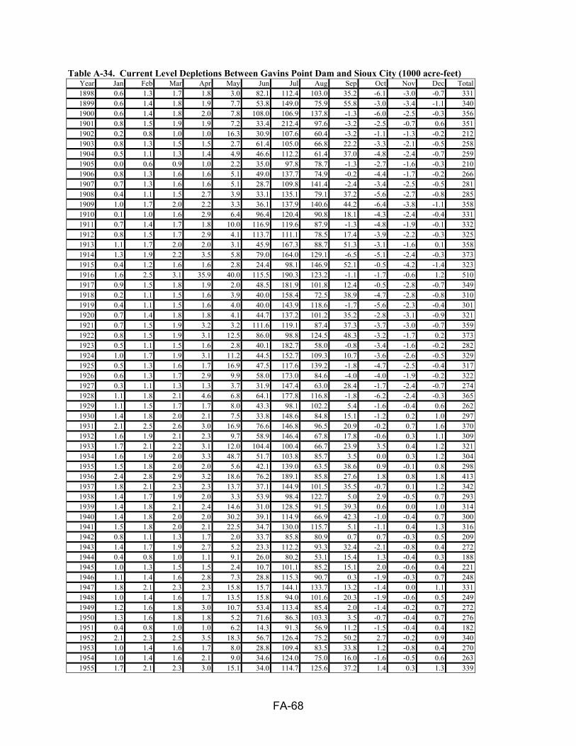
FA-68

Table A-34. Current Level Depletions Between Gavins Point Dam and Sioux City (1000 acre-feet) Year Jan Feb Mar Apr May Jun Jul Aug Sep Oct Nov Dec Total1898 0.6 1.3 1.7 1.8 3.0 82.1 112.4 103.0 35.2 -6.1 -3.0 -0.7 3311899 0.6 1.4 1.8 1.9 7.7 53.8 149.0 75.9 55.8 -3.0 -3.4 -1.1 3401900 0.6 1.4 1.8 2.0 7.8 108.0 106.9 137.8 -1.3 -6.0 -2.5 -0.3 3561901 0.8 1.5 1.9 1.9 7.2 33.4 212.4 97.6 -3.2 -2.5 -0.7 0.6 3511902 0.2 0.8 1.0 1.0 16.3 30.9 107.6 60.4 -3.2 -1.1 -1.3 -0.2 2121903 0.8 1.3 1.5 1.5 2.7 61.4 105.0 66.8 22.2 -3.3 -2.1 -0.5 2581904 0.5 1.1 1.3 1.4 4.9 46.6 112.2 61.4 37.0 -4.8 -2.4 -0.7 2591905 0.0 0.6 0.9 1.0 2.2 35.0 97.8 78.7 -1.3 -2.7 -1.6 -0.3 2101906 0.8 1.3 1.6 1.6 5.1 49.0 137.7 74.9 -0.2 -4.4 -1.7 -0.2 2661907 0.7 1.3 1.6 1.6 5.1 28.7 109.8 141.4 -2.4 -3.4 -2.5 -0.5 2811908 0.4 1.1 1.5 2.7 3.9 33.1 135.1 79.1 37.2 -5.6 -2.7 -0.8 2851909 1.0 1.7 2.0 2.2 3.3 36.1 137.9 140.6 44.2 -6.4 -3.8 -1.1 3581910 0.1 1.0 1.6 2.9 6.4 96.4 120.4 90.8 18.1 -4.3 -2.4 -0.4 3311911 0.7 1.4 1.7 1.8 10.0 116.9 119.6 87.9 -1.3 -4.8 -1.9 -0.1 3321912 0.8 1.5 1.7 2.9 4.1 113.7 111.1 78.5 17.4 -3.9 -2.2 -0.3 3251913 1.1 1.7 2.0 2.0 3.1 45.9 167.3 88.7 51.3 -3.1 -1.6 0.1 3581914 1.3 1.9 2.2 3.5 5.8 79.0 164.0 129.1 -6.5 -5.1 -2.4 -0.3 3731915 0.4 1.2 1.6 1.6 2.8 24.4 98.1 146.9 52.1 -0.5 -4.2 -1.4 3231916 1.6 2.5 3.1 35.9 40.0 115.5 190.3 123.2 -1.1 -1.7 -0.6 1.2 5101917 0.9 1.5 1.8 1.9 2.0 48.5 181.9 101.8 12.4 -0.5 -2.8 -0.7 3491918 0.2 1.1 1.5 1.6 3.9 40.0 158.4 72.5 38.9 -4.7 -2.8 -0.8 3101919 0.4 1.1 1.5 1.6 4.0 40.0 143.9 118.6 -1.7 -5.6 -2.3 -0.4 3011920 0.7 1.4 1.8 1.8 4.1 44.7 137.2 101.2 35.2 -2.8 -3.1 -0.9 3211921 0.7 1.5 1.9 3.2 3.2 111.6 119.1 87.4 37.3 -3.7 -3.0 -0.7 3591922 0.8 1.5 1.9 3.1 12.5 86.0 98.8 124.5 48.3 -3.2 -1.7 0.2 3731923 0.5 1.1 1.5 1.6 2.8 40.1 182.7 58.0 -0.8 -3.4 -1.6 -0.2 2821924 1.0 1.7 1.9 3.1 11.2 44.5 152.7 109.3 10.7 -3.6 -2.6 -0.5 3291925 0.5 1.3 1.6 1.7 16.9 47.5 117.6 139.2 -1.8 -4.7 -2.5 -0.4 3171926 0.6 1.3 1.7 2.9 9.9 58.0 173.0 84.6 -4.0 -4.0 -1.9 -0.2 3221927 0.3 1.1 1.3 1.3 3.7 31.9 147.4 63.0 28.4 -1.7 -2.4 -0.7 2741928 1.1 1.8 2.1 4.6 6.8 64.1 177.8 116.8 -1.8 -6.2 -2.4 -0.3 3651929 1.1 1.5 1.7 1.7 8.0 43.3 98.1 102.2 5.4 -1.6 -0.4 0.6 2621930 1.4 1.8 2.0 2.1 7.5 33.8 148.6 84.8 15.1 -1.2 0.2 1.0 2971931 2.1 2.5 2.6 3.0 16.9 76.6 146.8 96.5 20.9 -0.2 0.7 1.6 3701932 1.6 1.9 2.1 2.3 9.7 58.9 146.4 67.8 17.8 -0.6 0.3 1.1 3091933 1.7 2.1 2.2 3.1 12.0 104.4 100.4 66.7 23.9 3.5 0.4 1.2 3211934 1.6 1.9 2.0 3.3 48.7 51.7 103.8 85.7 3.5 0.0 0.3 1.2 3041935 1.5 1.8 2.0 2.0 5.6 42.1 139.0 63.5 38.6 0.9 -0.1 0.8 2981936 2.4 2.8 2.9 3.2 18.6 76.2 189.1 85.8 27.6 1.8 0.8 1.8 4131937 1.8 2.1 2.3 2.3 13.7 37.1 144.9 101.5 35.5 -0.7 0.1 1.2 3421938 1.4 1.7 1.9 2.0 3.3 53.9 98.4 122.7 5.0 2.9 -0.5 0.7 2931939 1.4 1.8 2.1 2.4 14.6 31.0 128.5 91.5 39.3 0.6 0.0 1.0 3141940 1.4 1.8 2.0 2.0 30.2 39.1 114.9 66.9 42.3 -1.0 -0.4 0.7 3001941 1.5 1.8 2.0 2.1 22.5 34.7 130.0 115.7 5.1 -1.1 0.4 1.3 3161942 0.8 1.1 1.3 1.7 2.0 33.7 85.8 80.9 0.7 0.7 -0.3 0.5 2091943 1.4 1.7 1.9 2.7 5.2 23.3 112.2 93.3 32.4 -2.1 -0.8 0.4 2721944 0.4 0.8 1.0 1.1 9.1 26.0 80.2 53.1 15.4 1.3 -0.4 0.3 1881945 1.0 1.3 1.5 1.5 2.4 10.7 101.1 85.2 15.1 2.0 -0.6 0.4 2211946 1.1 1.4 1.6 2.8 7.3 28.8 115.3 90.7 0.3 -1.9 -0.3 0.7 2481947 1.8 2.1 2.3 2.3 15.8 15.7 144.1 133.7 13.2 -1.4 0.0 1.1 3311948 1.0 1.4 1.6 1.7 13.5 15.8 94.0 101.6 20.3 -1.9 -0.6 0.5 2491949 1.2 1.6 1.8 3.0 10.7 53.4 113.4 85.4 2.0 -1.4 -0.2 0.7 2721950 1.3 1.6 1.8 1.8 5.2 71.6 86.3 103.3 3.5 -0.7 -0.4 0.7 2761951 0.4 0.8 1.0 1.0 6.2 14.3 91.3 56.9 11.2 -1.5 -0.4 0.4 1821952 2.1 2.3 2.5 3.5 18.3 56.7 126.4 75.2 50.2 2.7 -0.2 0.9 3401953 1.0 1.4 1.6 1.7 8.0 28.8 109.4 83.5 33.8 1.2 -0.8 0.4 2701954 1.0 1.4 1.6 2.1 9.0 34.6 124.0 75.0 16.0 -1.6 -0.5 0.6 2631955 1.7 2.1 2.3 3.0 15.1 34.0 114.7 125.6 37.2 1.4 0.3 1.3 339

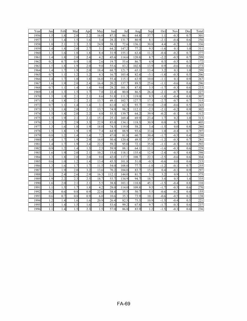
FA-69

Year Jan Feb Mar Apr May Jun Jul Aug Sep Oct Nov Dec Total1956 1.5 1.8 2.0 2.2 16.0 87.3 86.1 64.8 37.7 1.1 -0.3 0.7 3011957 1.1 1.4 1.5 1.6 3.4 28.2 131.7 80.9 8.1 -2.1 -0.4 0.6 2561958 1.8 2.1 2.3 2.3 24.9 58.1 72.6 136.1 30.8 4.4 -0.2 1.0 3361959 1.4 1.8 2.0 2.7 5.1 64.2 147.2 77.2 9.5 -1.6 0.1 1.0 3111960 1.3 1.6 1.8 1.8 8.4 31.9 155.1 63.4 11.2 -0.4 -0.2 0.7 2771961 1.4 1.8 2.0 2.4 4.2 45.6 114.6 120.8 8.7 -2.2 -0.5 0.7 2991962 0.2 0.7 0.9 1.0 2.6 19.7 55.6 86.7 4.9 0.3 -0.5 0.3 1721963 1.5 1.8 1.9 2.0 9.8 55.6 83.2 102.8 13.9 0.9 -0.6 0.6 2731964 1.4 1.7 1.9 2.0 18.4 68.7 121.7 65.1 13.4 3.2 0.1 1.0 2991965 0.7 1.1 1.2 1.2 4.3 16.7 103.4 82.4 -3.1 -1.8 -0.3 0.5 2061966 1.4 1.7 1.8 1.8 16.0 55.4 115.1 63.9 10.0 -1.1 0.1 0.9 2671967 1.6 1.9 2.0 2.4 16.4 20.2 137.7 89.5 25.6 -1.1 -0.6 0.6 2961968 0.7 1.1 1.4 1.4 9.0 28.2 101.3 87.8 3.5 -1.7 -0.3 0.6 2331969 1.0 1.3 1.5 1.7 7.8 22.4 80.8 86.5 26.4 -2.1 -0.7 0.4 2271970 1.5 1.9 2.1 2.1 8.6 51.8 111.5 119.0 9.5 -1.8 -0.4 0.8 3071971 1.4 1.8 2.1 2.1 13.7 49.1 102.7 127.7 17.3 -2.7 -0.7 0.7 3151972 0.7 1.1 1.4 1.4 3.1 61.0 62.3 93.7 19.8 -2.0 -0.6 0.5 2431973 1.5 1.8 2.0 2.1 13.7 74.9 98.2 112.1 -2.5 -2.1 -0.2 0.9 3021974 1.5 1.8 2.0 2.2 4.8 55.3 139.7 64.2 39.9 -0.2 -0.1 0.9 3121975 1.5 1.9 2.1 2.1 15.1 25.1 169.4 69.9 23.4 1.7 0.2 1.0 3131976 2.3 2.7 2.9 3.3 22.9 85.0 134.1 118.5 30.9 0.0 0.7 1.7 4051977 1.3 1.6 1.8 1.9 18.0 74.5 119.8 58.2 3.4 -1.5 0.0 0.8 2801978 1.5 1.8 1.9 1.9 7.4 64.9 88.9 93.6 33.6 1.0 -0.4 0.7 2971979 0.8 1.2 1.4 1.4 7.2 47.0 81.8 60.7 30.4 -1.7 -0.5 0.4 2301980 1.4 1.7 1.9 2.9 16.0 50.4 120.4 49.5 37.3 -1.2 -0.3 0.7 2811981 1.4 1.7 1.9 3.4 22.2 59.2 95.0 72.1 35.8 -1.1 -0.3 0.8 2921982 0.9 1.2 1.4 1.5 2.5 59.9 88.1 64.1 11.1 -1.6 -0.3 0.6 2291983 1.6 1.9 2.0 2.1 10.2 15.6 118.1 135.4 12.9 -2.4 -0.5 0.8 2981984 1.3 1.8 2.0 2.0 9.0 42.0 117.5 108.7 22.3 -2.5 -0.6 0.6 3041985 0.6 1.0 1.2 1.4 13.4 45.5 101.8 51.0 -0.5 -0.6 0.0 0.6 2151986 1.3 1.6 1.7 1.7 11.5 54.0 108.0 77.7 -1.8 -1.2 -0.1 0.7 2551987 1.5 1.9 2.0 3.2 13.6 70.2 104.0 83.7 15.6 0.4 -0.1 0.9 2971988 2.1 2.4 2.6 2.9 16.3 112.1 144.0 81.7 5.1 3.2 0.9 1.7 3751989 1.9 2.2 2.3 2.5 18.7 53.7 134.9 94.7 18.7 3.4 0.5 1.4 3351990 1.6 2.0 2.1 2.1 5.5 38.8 103.1 110.8 45.1 -1.5 -0.4 0.8 3101991 1.1 1.5 1.7 1.8 4.2 28.0 114.0 109.8 9.5 -1.7 -0.5 0.6 2701992 0.2 0.6 0.8 0.9 22.6 38.4 35.5 50.7 5.5 -0.6 -0.2 0.4 1551993 0.6 0.7 0.8 0.9 6.0 10.6 35.3 73.9 10.1 -0.6 -0.5 0.2 1381994 1.2 1.4 1.6 1.6 20.9 26.4 82.5 75.5 10.9 -1.5 -0.4 0.5 2211995 1.1 1.4 1.5 1.6 2.1 53.6 99.2 67.8 9.7 -1.7 -0.3 0.6 2371996 1.1 1.4 1.5 2.3 1.5 57.0 86.8 83.9 1.2 -1.5 -0.3 0.6 236

FA-70

Table A-35. Current Level Depletions Between Omaha and Nebraska City (1000 acre-feet) Year Jan Feb Mar Apr May Jun Jul Aug Sep Oct Nov Dec Total1898 41.9 81.5 128.0 256.8 360.5 1114.6 1154.5 1206.3 400.7 23.4 -8.4 22.5 47821899 43.8 83.2 129.6 266.4 616.4 1174.2 925.9 1103.9 695.5 40.0 -19.8 16.0 50751900 40.1 79.9 126.9 191.5 972.9 1298.0 944.3 1116.0 374.8 12.5 0.2 29.6 51871901 46.4 83.5 128.8 210.7 758.6 888.5 1680.0 1196.2 99.2 16.8 9.7 32.6 51511902 42.4 81.3 126.0 261.7 716.7 898.6 825.6 1014.3 106.0 13.0 16.6 36.0 41381903 49.0 85.1 129.4 249.1 684.7 904.3 844.3 853.8 498.2 68.0 -3.0 24.5 43881904 41.8 79.9 125.4 258.7 553.6 949.5 738.6 991.0 358.0 17.9 5.7 28.9 41491905 44.8 81.8 127.2 200.5 465.3 972.5 671.0 1174.8 378.6 -15.2 1.8 29.4 41321906 46.1 82.9 128.7 249.8 645.8 1028.7 895.6 915.3 287.0 -43.8 8.3 33.2 42781907 46.8 82.8 132.7 227.7 466.8 884.8 743.5 990.4 374.5 158.2 -2.4 23.5 41291908 40.5 79.6 125.4 262.4 402.1 795.7 643.2 694.3 803.8 -28.3 0.3 26.7 38461909 48.2 84.3 129.8 223.5 584.2 722.4 934.9 1323.6 386.9 40.8 -6.8 23.9 44961910 44.8 84.1 138.0 274.6 694.3 1101.3 1408.7 854.9 363.7 146.8 -4.6 20.9 51271911 15.5 52.0 99.6 185.0 953.5 1751.9 898.9 788.8 348.5 -65.0 -28.1 1.8 50021912 16.4 69.1 112.3 355.2 1013.9 1341.8 814.4 757.9 -209.7 -277.9 -52.6 15.1 39561913 32.4 83.6 138.5 522.2 922.6 1246.7 912.8 1503.8 257.2 37.4 12.6 21.2 56911914 41.0 75.3 144.6 369.6 1030.0 1337.6 1249.5 932.7 377.6 -92.4 -4.3 18.2 54801915 27.3 62.5 106.3 273.6 555.8 784.0 492.3 593.0 259.9 113.3 24.2 37.3 33301916 55.7 93.1 224.1 325.3 677.3 1184.5 1411.1 776.4 505.7 2.3 5.0 29.4 52901917 43.5 74.8 119.1 437.2 619.1 1193.7 1664.6 848.4 135.3 68.3 11.8 32.3 52481918 48.7 79.4 156.0 233.0 794.4 1698.8 930.0 948.0 199.1 -4.2 13.8 35.7 51331919 41.5 78.7 129.7 318.8 903.6 852.5 898.7 1247.8 343.3 -104.9 -0.5 26.7 47361920 42.0 86.5 154.0 306.6 1040.9 1230.5 1158.3 759.0 532.4 -34.4 1.9 14.9 52931921 43.7 81.2 182.9 194.7 876.1 1208.0 1155.0 1004.0 428.9 -15.4 -11.7 17.0 51641922 37.8 68.8 145.7 275.8 588.8 1424.8 856.4 1135.4 556.0 15.6 -3.0 17.2 51191923 38.2 70.1 109.8 256.8 795.8 1142.9 1111.2 707.9 101.1 7.7 36.6 28.7 44071924 44.6 87.8 118.5 335.9 427.1 1177.3 829.0 1001.5 -73.3 49.4 19.6 30.5 40481925 47.6 84.6 179.1 359.5 874.3 941.1 1153.2 760.0 427.2 4.8 18.7 33.6 48841926 37.4 86.2 165.3 543.4 949.7 1090.6 927.7 982.8 -30.1 30.3 -1.1 11.8 47941927 15.5 69.7 125.2 325.8 1249.7 713.8 1013.0 651.3 232.4 152.3 29.6 17.4 45961928 28.0 82.8 191.0 339.1 941.0 468.0 594.2 1185.3 433.9 -109.0 2.7 20.7 41781929 29.7 69.4 116.5 437.8 922.0 1172.2 1211.5 1032.2 -176.1 4.0 11.9 38.3 48691930 33.6 82.0 138.4 423.3 626.3 1158.0 1127.6 593.2 482.4 9.8 -11.4 15.9 46791931 37.3 79.6 116.9 335.4 711.7 1190.3 1171.1 812.6 538.3 10.9 -13.0 18.3 50101932 37.7 78.4 133.8 437.5 1202.6 1052.7 918.6 1026.3 425.8 -31.8 -10.0 5.2 52771933 35.5 64.5 135.9 270.2 701.0 1924.2 1053.0 357.0 296.2 199.3 4.7 15.2 50571934 45.8 84.1 127.7 316.1 988.1 1135.2 1472.2 1123.8 182.0 74.2 7.4 29.8 55861935 42.5 79.2 110.2 183.0 403.6 1238.7 1560.3 941.5 409.9 81.7 -4.6 10.1 50561936 38.2 75.7 138.0 356.5 966.3 1249.6 1546.4 1138.1 430.9 41.0 0.3 18.5 60001937 15.4 64.9 143.3 420.9 768.1 998.4 1262.9 1258.4 289.7 1.0 1.4 28.7 52531938 40.3 59.6 133.2 317.9 707.2 1237.1 995.3 1130.4 236.7 217.0 -4.9 21.9 50921939 42.5 67.4 150.9 230.7 695.9 896.4 1342.1 1062.5 769.4 48.0 -21.3 3.7 52881940 78.6 104.2 129.5 250.5 954.3 1081.7 1248.2 1168.1 403.3 33.9 32.2 54.3 55391941 78.9 98.5 120.5 274.1 992.3 653.3 913.8 1212.5 100.8 70.1 68.2 75.3 46591942 123.8 123.0 151.9 336.2 869.5 906.5 1305.2 961.2 59.0 65.6 69.1 63.5 50341943 86.9 138.5 197.6 217.8 287.0 1016.4 1142.4 1384.1 537.3 -20.4 -27.7 50.1 50101944 75.8 131.2 167.9 227.8 777.5 801.8 778.7 1135.9 559.8 131.6 19.6 2.3 48101945 86.3 109.2 150.5 157.4 769.8 828.6 1171.0 819.2 286.1 285.7 74.7 36.2 47751946 148.4 145.9 193.8 307.0 332.2 971.4 1286.9 658.2 197.3 153.6 93.2 103.3 45911947 111.9 113.0 164.6 301.4 618.0 925.2 1335.0 1498.6 398.1 68.5 50.7 111.3 56961948 109.6 131.0 216.6 327.2 620.4 636.1 984.0 941.2 670.1 76.2 58.4 64.6 48361949 73.3 130.4 199.5 340.7 758.9 942.6 1235.5 1014.2 377.4 45.2 5.0 37.1 51601950 96.5 132.4 138.8 263.4 429.5 1237.9 551.8 825.2 375.7 240.4 41.4 75.5 44091951 74.8 109.3 91.2 86.2 711.7 711.0 662.0 763.2 257.2 56.7 64.1 55.3 36431952 86.9 42.5 71.6 340.2 684.8 1619.1 1005.5 666.4 513.0 147.0 29.5 96.6 53031953 151.8 126.9 136.0 118.9 620.0 949.0 762.7 894.4 722.7 85.2 49.9 104.9 47221954 112.9 103.7 144.3 283.6 539.3 884.1 1281.3 721.8 587.5 74.6 3.2 44.9 47811955 95.5 109.6 140.2 302.4 513.7 675.0 1481.3 1240.8 253.8 138.1 8.5 62.6 5021

FA-71

Year Jan Feb Mar Apr May Jun Jul Aug Sep Oct Nov Dec Total1956 126.0 121.3 160.8 231.4 869.5 1018.6 598.3 946.2 766.3 42.8 57.1 106.9 50451957 96.9 129.3 86.1 244.1 613.2 1319.7 1342.0 841.0 310.3 70.1 83.3 85.0 52211958 76.5 113.5 169.6 197.7 987.3 840.3 669.0 1413.7 470.4 129.0 -29.5 52.5 50901959 57.3 69.4 97.3 231.0 439.7 1079.5 1351.8 1207.4 149.8 -20.7 -14.9 42.5 46901960 54.7 82.6 177.4 291.1 650.0 899.3 1195.2 1171.2 545.3 51.8 -54.6 -2.3 50621961 39.9 72.3 88.2 172.9 511.6 1164.4 919.6 1355.5 57.6 148.6 40.1 54.8 46251962 76.1 133.7 154.1 506.2 652.1 992.5 1003.3 1522.7 365.6 42.5 -26.2 4.1 54271963 41.2 111.8 128.7 218.1 649.1 1056.9 1272.3 830.1 228.2 81.8 -22.1 13.4 46091964 50.2 68.4 90.5 212.2 840.6 841.3 1460.1 1026.0 381.4 75.2 -18.5 11.1 50391965 45.7 57.8 79.1 177.5 700.6 1109.2 1068.1 1163.1 -72.4 146.2 40.5 53.0 45681966 54.7 104.2 165.7 156.1 848.1 634.7 1151.4 962.7 489.9 69.6 -47.0 28.9 46191967 63.4 65.4 106.1 148.5 236.9 908.6 1319.7 1312.8 531.5 49.3 -49.5 8.2 47011968 62.0 91.3 76.3 232.1 560.0 1387.4 1172.1 783.0 563.5 6.4 -75.3 -18.2 48411969 73.1 87.2 90.6 300.1 667.9 734.3 1175.1 1286.4 571.1 -67.6 -10.3 31.9 49401970 61.5 104.1 91.8 206.2 1246.9 1234.6 1515.6 1367.3 198.7 0.8 -3.2 -27.2 59971971 66.7 96.5 159.5 266.2 839.3 1240.1 1288.5 1442.4 233.8 11.7 -17.7 -30.3 55971972 3.6 50.5 58.1 229.5 667.7 1048.0 842.4 1159.6 331.4 -45.1 17.1 27.7 43901973 54.3 76.6 113.8 287.6 1273.4 1204.2 920.9 1510.4 -217.2 -67.1 -34.3 -15.3 51071974 47.7 26.2 -130.0 141.7 1081.0 1006.9 1232.8 934.3 550.9 68.6 36.4 19.1 50161975 66.2 67.1 162.5 231.6 407.4 1080.7 1362.9 1236.1 478.2 147.9 9.3 41.0 52911976 77.2 122.9 132.0 237.4 691.1 1126.1 1210.1 1175.4 327.9 48.1 -12.8 37.4 51731977 31.4 92.2 127.5 269.6 590.1 1119.1 957.7 784.2 465.7 37.6 -34.4 13.6 44541978 45.1 83.9 165.5 200.9 518.7 1477.1 1330.8 981.6 754.3 62.8 -34.8 14.6 56001979 39.6 75.1 170.8 304.0 598.0 1002.0 1029.8 1171.5 862.6 4.0 -13.3 30.0 52741980 44.7 114.6 125.5 245.7 863.3 1357.0 1432.1 967.0 644.0 0.4 -20.9 31.3 58051981 59.7 70.3 111.9 188.9 348.5 1041.6 912.3 1042.6 794.3 -19.6 -47.2 4.0 45071982 25.5 73.9 98.3 133.0 496.6 861.2 1276.0 1087.3 373.2 51.3 10.8 23.1 45101983 62.6 72.0 160.9 261.2 891.0 1004.8 1644.1 1301.7 466.9 154.2 13.3 -78.5 59541984 11.0 -51.3 -144.0 66.9 1396.2 897.4 1420.5 1317.0 480.1 -36.5 -78.0 -61.8 52171985 27.7 35.2 17.0 256.8 822.3 855.5 970.6 1330.2 64.5 37.9 -13.7 54.9 44591986 90.9 128.3 90.4 252.6 739.5 1389.5 1423.0 1234.6 151.7 -99.4 -57.8 16.1 53591987 26.6 -33.8 250.1 260.0 461.4 1111.4 1370.7 821.8 706.6 -18.5 -58.5 -20.3 48771988 39.3 99.1 128.7 304.4 603.3 1228.2 1172.6 1246.2 319.8 126.3 -23.9 20.6 52641989 66.4 79.8 163.4 199.9 611.2 585.0 1334.8 1028.1 284.3 90.6 -11.7 20.3 44521990 84.1 80.7 132.8 166.6 499.7 1201.1 609.4 1221.4 834.9 -4.3 -12.8 10.6 48241991 53.9 93.2 103.9 186.4 761.2 1098.1 1087.1 1308.1 603.2 21.6 13.6 42.9 53731992 58.1 85.3 141.6 245.3 755.0 672.8 736.3 724.3 873.9 -23.4 -27.4 13.7 42561993 48.1 67.8 165.5 251.2 1000.5 1028.9 943.3 1242.6 465.1 1.5 -21.6 28.5 52211994 63.6 72.1 147.7 213.6 774.5 799.5 912.0 1334.5 667.9 -46.8 -23.3 56.1 49711995 71.3 92.9 115.1 125.6 746.5 1576.6 1734.9 1591.3 331.7 -12.3 -16.4 25.1 63821996 40.9 102.2 88.0 243.4 629.2 1376.3 1090.3 1144.2 87.9 112.2 -28.4 -1.4 4885

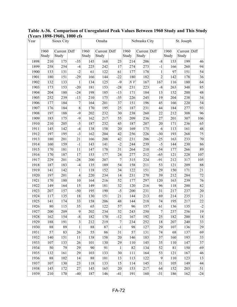
FA-72

Table A-36. Comparison of Unregulated Peak Values Between 1960 Study and This Study (Years 1898-1960), 1000 cfs

Sioux City Omaha Nebraska City St. Joseph Year

1960 Study

Current Study

Diff 1960 Study

Current Study

Diff 1960 Study

Current Study

Diff 1960 Study

Current Study

Diff

1898 210 175 -35 145 168 23 214 206 -8 153 199 461899 258 254 -4 225 242 17 274 273 -1 166 260 941900 133 131 -2 61 122 61 177 178 1 97 151 541901 180 151 -29 166 144 -22 180 182 2 142 178 361902 132 133 1 134 125 -9 N V 167 167 116 180 641903 173 153 -20 181 153 -28 231 223 -8 263 348 851904 204 180 -24 198 185 -13 171 184 13 152 200 481905 252 239 -13 210 175 -35 226 245 19 204 238 341906 177 184 7 164 201 37 151 196 45 166 220 541907 176 184 8 170 195 25 187 231 44 184 277 931908 197 188 -9 202 232 30 238 260 22 212 308 961909 183 175 -9 162 217 55 209 236 27 201 307 1061910 210 205 -5 187 232 45 187 207 20 171 236 651911 145 142 -4 138 158 20 169 175 6 113 161 481912 197 195 -3 162 204 42 256 226 -30 193 268 751913 180 201 21 166 208 42 231 206 -25 163 233 701914 160 159 -1 143 141 -2 244 239 -5 144 230 861915 170 181 11 147 178 31 264 210 -54 177 266 891916 170 187 17 153 177 24 277 212 -65 121 228 1071917 229 201 -28 200 207 7 315 224 -91 212 317 1051918 187 183 -4 135 189 54 158 211 53 121 209 881919 141 142 1 118 152 34 122 151 29 150 171 211920 197 201 4 220 234 14 231 270 39 212 284 721921 170 180 10 164 216 52 177 297 120 163 239 761922 149 164 15 149 181 32 120 216 96 118 200 821923 207 157 -50 195 190 -5 200 231 31 217 237 201924 117 135 18 130 151 21 144 213 69 214 235 211925 141 174 33 158 206 48 144 218 74 195 217 221926 80 115 35 65 122 57 96 157 61 136 135 -21927 200 209 9 202 234 32 243 250 7 237 256 191928 162 154 -8 182 170 -12 167 192 25 182 200 181929 188 191 3 212 219 7 234 252 18 207 240 331930 88 89 1 88 87 -1 98 127 29 107 136 291931 57 83 26 55 86 31 57 131 74 68 137 691932 140 151 11 138 158 20 146 183 37 160 193 331933 107 133 26 101 130 29 110 145 35 110 147 371934 50 79 29 90 91 1 82 134 52 81 150 691935 132 161 29 103 133 30 111 164 53 121 167 461936 88 102 14 88 101 13 113 122 9 110 123 131937 107 130 23 118 133 15 114 145 31 105 149 441938 145 172 27 145 165 20 153 217 64 152 203 511939 210 170 -40 187 146 -41 191 160 -31 186 162 -24

FA-73

Sioux City Omaha Nebraska City St. Joseph Year

1960 Study

Current Study

Diff 1960 Study

Current Study

Diff 1960 Study

Current Study

Diff 1960 Study

Current Study

Diff

1940 65 91 26 65 94 29 70 153 83 76 158 821941 130 151 21 118 138 20 116 147 31 123 158 351942 149 153 4 149 154 5 178 224 46 184 234 501943 248 222 -26 244 218 -26 231 237 6 212 237 251944 197 208 11 183 189 6 231 296 65 187 237 501945 121 133 12 116 129 13 142 172 30 170 195 251946 109 127 18 101 122 21 118 161 43 121 165 441947 259 195 -64 231 187 -44 230 248 18 233 244 111948 164 173 9 166 174 8 178 225 47 183 223 401949 200 192 -8 208 202 -6 203 208 5 191 209 181950 255 248 -7 223 227 4 212 221 9 205 210 51951 170 161 -9 176 164 -13 175 225 50 206 254 481952 521 479 -42 490 469 -21 498 488 -10 490 467 -231953 208 263 55 214 272 58 217 284 67 223 278 551954 84 105 21 109 139 30 136 185 49 129 176 471955 76 107 31 82 116 34 86 137 51 102 145 431956 94 160 66 97 162 65 98 181 83 99 178 791957 118 161 43 130 170 40 174 274 100 176 286 1101958 76 149 73 76 153 77 89 179 90 158 204 461959 184 136 -48 182 140 -42 194 200 6 192 210 181960 308 256 -52 334 274 -60 387 329 -58 384 353 -31

N V = No value contained in 1960 Study report.

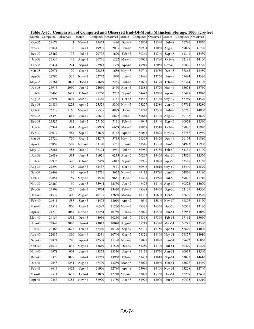
FA-74

Table A-37. Comparison of Computed and Observed End-Of-Month Mainstem Storage, 1000 acre-feet Month Computed Observed Month Computed Observed Month Computed Observed Month Computed Observed

Oct-37 24174 3 May-41 19455 1480 Dec-44 51804 11340 Jul-48 56796 17820

Nov-37 23841 30 Jun-41 19981 2005 Jan-45 50904 11060 Aug-48 57029 16720

Dec-37 23462 77 Jul-41 20778 1690 Feb-45 50369 11340 Sep-48 61341 15430

Jan-38 23535 141 Aug-41 20771 1222 Mar-45 50051 11780 Oct-48 62181 14100

Feb-38 23434 274 Sep-41 22943 1339 Apr-45 49949 12050 Nov-48 60806 13720

Mar-38 22971 70 Oct-41 22855 1686 May-45 50741 12550 Dec-48 58863 13480

Apr-38 22795 335 Nov-41 22742 1970 Jun-45 53496 13760 Jan-49 57484 13320

May-38 22761 1025 Dec-41 23619 2255 Jul-45 53638 14170 Feb-49 56344 13190

Jun-38 23913 2090 Jan-42 24610 2470 Aug-45 52884 13770 Mar-49 55674 13750

Jul-38 23466 2427 Feb-42 25260 2707 Sep-45 54442 12970 Apr-49 55427 13940

Aug-38 22991 1801 Mar-42 25346 3161 Oct-45 54563 12380 May-49 55269 14570

Sep-38 24886 1223 Apr-42 25528 3800 Nov-45 53227 12380 Jun-49 57792 15280

Oct-38 26717 1165 May-42 25535 4829 Dec-45 51740 12530 Jul-49 60265 14800

Nov-38 25490 813 Jun-42 26631 6827 Jan-46 50615 12790 Aug-49 60138 13620

Dec-38 25527 512 Jul-42 27120 7151 Feb-46 49945 13140 Sep-49 60924 12590

Jan-39 25944 484 Aug-42 29989 6659 Mar-46 49858 13510 Oct-49 59875 11940

Feb-39 26019 481 Sep-42 33699 6142 Apr-46 50043 13890 Nov-49 57786 11950

Mar-39 25720 750 Oct-42 34247 5735 May-46 50375 14420 Dec-49 56174 11880

Apr-39 25857 508 Nov-42 33170 5731 Jun-46 51516 15100 Jan-50 54923 11900

May-39 25861 485 Dec-42 32324 5961 Jul-46 50957 15380 Feb-50 54331 12100

Jun-39 28088 513 Jan-43 31921 6235 Aug-46 50267 14460 Mar-50 53826 12550

Jul-39 27976 320 Feb-43 32469 6817 Sep-46 50996 13890 Apr-50 53507 13160

Aug-39 27599 128 Mar-43 32437 7561 Oct-46 50943 13610 May-50 53440 13520

Sep-39 28468 116 Apr-43 32721 8622 Nov-46 49112 13780 Jun-50 54826 15180

Oct-39 27854 159 May-43 33500 9651 Dec-46 48421 13970 Jul-50 59825 15710

Nov-39 26260 159 Jun-43 35944 12530 Jan-47 48423 14140 Aug-50 60523 15070

Dec-39 24509 255 Jul-43 39824 13410 Feb-47 48388 14470 Sep-50 62139 14350

Jan-40 24532 400 Aug-43 40135 12880 Mar-47 48333 15600 Oct-50 62690 13520

Feb-40 24611 588 Sep-43 44472 12010 Apr-47 48640 15840 Nov-50 61808 13190

Mar-40 24512 866 Oct-43 46397 11220 May-47 49325 16570 Dec-50 60331 13120

Apr-40 24230 1061 Nov-43 45254 10750 Jun-47 52026 17530 Jan-51 58953 13050

May-40 24154 1532 Dec-43 44036 10250 Jul-47 54368 17360 Feb-51 57192 13050

Jun-40 23847 2080 Jan-44 43017 10040 Aug-47 55219 16320 Mar-51 56745 13580

Jul-40 23466 1622 Feb-44 42440 10120 Sep-47 58103 15150 Apr-51 56870 14020

Aug-40 22637 810 Mar-44 42331 10740 Oct-47 58321 14100 May-51 56877 14910

Sep-40 22874 780 Apr-44 42508 11120 Nov-47 57027 13820 Jun-51 57672 16060

Oct-40 21633 837 May-44 42840 11590 Dec-47 55250 13700 Jul-51 60420 16420

Nov-40 19971 905 Jun-44 43873 13330 Jan-48 54131 13750 Aug-51 60957 15540

Dec-40 19378 1098 Jul-44 47258 13950 Feb-48 53403 13810 Sep-51 63021 14610

Jan-41 19658 1254 Aug-44 47400 13280 Mar-48 53078 14060 Oct-51 63677 13460

Feb-41 19613 1422 Sep-44 51966 12790 Apr-48 53080 14400 Nov-51 63258 12740

Mar-41 19511 1631 Oct-44 53889 12210 May-48 53090 15350 Dec-51 62209 12430

Apr-41 19453 1383 Nov-44 52920 11750 Jun-48 54972 18000 Jan-52 60405 12210

FA-75

Table A-37 (continued). Comparison of Computed and Observed End-Of-Month Mainstem Storage, 1000 acre-feet Month Computed Observed Month Computed Observed Month Computed Observed Month Computed Observed

Feb-52 58304 12310 Sep-55 51692 14343 Apr-59 44014 23955 Nov-62 49219 35309

Mar-52 57421 13010 Oct-55 51244 13209 May-59 44218 24409 Dec-62 48470 35225

Apr-52 57315 14250 Nov-55 49270 13311 Jun-59 47034 26216 Jan-63 48069 35532

May-52 57905 15540 Dec-55 47625 13563 Jul-59 47074 26383 Feb-63 47537 36538

Jun-52 59414 16280 Jan-56 46340 14020 Aug-59 47113 25098 Mar-63 47242 38072

Jul-52 67520 16410 Feb-56 46371 14327 Sep-59 48291 23914 Apr-63 47239 37732

Aug-52 67345 15480 Mar-56 46464 15011 Oct-59 47880 23284 May-63 48285 38245

Sep-52 67678 14480 Apr-56 46688 14060 Nov-59 46294 23400 Jun-63 49581 42021

Oct-52 65677 13490 May-56 46875 15343 Dec-59 45141 24355 Jul-63 49691 42153

Nov-52 63085 13240 Jun-56 48241 17053 Jan-60 44533 27425 Aug-63 50049 41059

Dec-52 60376 13094 Jul-56 48444 16689 Feb-60 44016 24771 Sep-63 52542 40131

Jan-53 58297 13092 Aug-56 48564 15704 Mar-60 44469 28632 Oct-63 52271 38921

Feb-53 56567 13266 Sep-56 50090 14436 Apr-60 44693 30553 Nov-63 50806 37946

Mar-53 55844 13453 Oct-56 49517 13610 May-60 45157 31276 Dec-63 49849 37706

Apr-53 55615 13387 Nov-56 48167 13978 Jun-60 48520 32214 Jan-64 48915 38258

May-53 55672 14201 Dec-56 46541 14010 Jul-60 50414 31104 Feb-64 47933 38695

Jun-53 57177 17254 Jan-57 45315 14014 Aug-60 50658 29986 Mar-64 47390 38873

Jul-53 57148 17374 Feb-57 44586 14362 Sep-60 51321 28680 Apr-64 47602 39169

Aug-53 58102 16633 Mar-57 44460 15728 Oct-60 49760 27685 May-64 47831 40983

Sep-53 62995 15086 Apr-57 44325 16284 Nov-60 48294 27177 Jun-64 47995 45891

Oct-53 62710 13881 May-57 44510 17221 Dec-60 46869 26807 Jul-64 48457 47468

Nov-53 61198 14233 Jun-57 45392 20788 Jan-61 45861 26945 Aug-64 49652 46397

Dec-53 58855 14196 Jul-57 45787 21832 Feb-61 45116 27393 Sep-64 53871 45375

Jan-54 56875 14200 Aug-57 46846 20650 Mar-61 44564 27973 Oct-64 54948 44169

Feb-54 55481 14690 Sep-57 49612 19963 Apr-61 44515 27194 Nov-64 53599 43139

Mar-54 54964 14861 Oct-57 49756 19233 May-61 44813 26772 Dec-64 52634 42859

Apr-54 54639 15245 Nov-57 48349 19718 Jun-61 45300 27283 Jan-65 51441 43456

May-54 55195 15629 Dec-57 47573 19964 Jul-61 44710 25096 Feb-65 50367 44182

Jun-54 55449 17139 Jan-58 46920 20105 Aug-61 44109 24878 Mar-65 50077 45001

Jul-54 55612 16422 Feb-58 46803 20515 Sep-61 44432 23838 Apr-65 50443 47837

Aug-54 55238 15680 Mar-58 46806 21560 Oct-61 42679 23767 May-65 50867 50645

Sep-54 55923 14617 Apr-58 46763 22127 Nov-61 40634 24339 Jun-65 51500 54683

Oct-54 55081 14084 May-58 47044 22339 Dec-61 39571 23917 Jul-65 54519 57131

Nov-54 53625 14623 Jun-58 47624 23363 Jan-62 38543 24115 Aug-65 57279 56582

Dec-54 52155 14593 Jul-58 47962 23931 Feb-62 38068 24747 Sep-65 60955 56089

Jan-55 51373 14520 Aug-58 47775 22608 Mar-62 37470 26539 Oct-65 63048 55823

Feb-55 50576 14688 Sep-58 48757 21435 Apr-62 37586 27929 Nov-65 62139 55135

Mar-55 50334 15509 Oct-58 48744 20503 May-62 38056 30525 Dec-65 60935 55054

Apr-55 49984 16318 Nov-58 46961 20803 Jun-62 39446 35309 Jan-66 59783 54721

May-55 50003 16340 Dec-58 45474 20893 Jul-62 41046 37492 Feb-66 58083 54772

Jun-55 50448 17377 Jan-59 44511 21003 Aug-62 43668 37296 Mar-66 57577 57942

Jul-55 50978 17477 Feb-59 44001 21066 Sep-62 47986 36578 Apr-66 57377 58231

Aug-55 50890 15949 Mar-59 43994 24095 Oct-62 49902 35976 May-66 57641 58136

FA-76


Jun-66 60656 58415 Jan-70 58976 59645 Aug-73 60630 63047 Mar-77 55471 58721

Jul-66 60967 57456 Feb-70 58053 59373 Sep-73 61317 61490 Apr-77 55273 59484

Aug-66 60775 56123 Mar-70 57432 59676 Oct-73 60299 60751 May-77 55610 59150

Sep-66 61161 54744 Apr-70 57145 59862 Nov-73 58201 60138 Jun-77 56407 58790

Oct-66 60298 53181 May-70 57441 61075 Dec-73 57660 59286 Jul-77 56037 58638

Nov-66 58570 51949 Jun-70 57733 64043 Jan-74 57151 59011 Aug-77 55699 57058

Dec-66 56850 51755 Jul-70 59151 66871 Feb-74 56528 59113 Sep-77 55660 55322

Jan-67 55301 51890 Aug-70 61930 67051 Mar-74 56284 59504 Oct-77 54257 54387

Feb-67 54017 52519 Sep-70 63909 65022 Apr-74 56541 60033 Nov-77 52546 53303

Mar-67 53530 54324 Oct-70 62883 63339 May-74 56941 60616 Dec-77 51844 51931

Apr-67 53177 54973 Nov-70 60580 61639 Jun-74 57199 61436 Jan-78 51213 51758

May-67 53293 55841 Dec-70 59280 60151 Jul-74 57685 64246 Feb-78 50263 51463

Jun-67 55173 62325 Jan-71 58385 59611 Aug-74 58430 64774 Mar-78 50200 51620

Jul-67 56043 64414 Feb-71 57559 59660 Sep-74 60828 63713 Apr-78 50055 58870

Aug-67 57358 63105 Mar-71 57131 61139 Oct-74 60841 62303 May-78 50219 62261

Sep-67 63343 61760 Apr-71 56607 64156 Nov-74 59535 60827 Jun-78 57451 65733

Oct-67 64543 61734 May-71 57365 65520 Dec-74 57798 59917 Jul-78 61265 68017

Nov-67 62483 60374 Jun-71 60426 66183 Jan-75 56513 59752 Aug-78 65024 69067

Dec-67 60266 59502 Jul-71 61381 68597 Feb-75 55682 59171 Sep-78 66662 67139

Jan-68 59008 58882 Aug-71 62022 68015 Mar-75 55533 59102 Oct-78 67255 65550

Feb-68 57911 59106 Sep-71 65159 65809 Apr-75 55082 59941 Nov-78 64961 63031

Mar-68 57084 59414 Oct-71 64431 63928 May-75 54999 62816 Dec-78 63083 60383

Apr-68 57274 60614 Nov-71 61860 62542 Jun-75 55972 66647 Jan-79 60250 59666

May-68 57574 60575 Dec-71 60086 60516 Jul-75 59031 70136 Feb-79 57921 59324

Jun-68 58297 60273 Jan-72 59406 59564 Aug-75 62595 71832 Mar-79 57467 59027

Jul-68 58187 63314 Feb-72 58541 59176 Sep-75 65723 69765 Apr-79 57344 62494

Aug-68 57702 63332 Mar-72 57755 59460 Oct-75 67076 66789 May-79 56918 66144

Sep-68 60304 62568 Apr-72 57337 64588 Nov-75 64765 64029 Jun-79 60343 66777

Oct-68 60076 61653 May-72 57407 64426 Dec-75 62001 61335 Jul-79 64234 67350

Nov-68 59189 60793 Jun-72 62327 66174 Jan-76 59957 60951 Aug-79 64536 66905

Dec-68 58079 59931 Jul-72 61647 68526 Feb-76 58099 60784 Sep-79 65181 65590

Jan-69 57143 59350 Aug-72 63384 68031 Mar-76 58052 61366 Oct-79 64648 63967

Feb-69 56655 59444 Sep-72 65361 66531 Apr-76 57789 62225 Nov-79 62989 62145

Mar-69 56186 59604 Oct-72 64487 64447 May-76 58166 62343 Dec-79 60984 60513

Apr-69 56389 62205 Nov-72 62817 62450 Jun-76 59098 63706 Jan-80 59361 59686

May-69 56602 65643 Dec-72 60903 61021 Jul-76 59476 65842 Feb-80 58228 58904

Jun-69 59036 66294 Jan-73 59499 60395 Aug-76 60834 65774 Mar-80 57544 58927

Jul-69 63153 67282 Feb-73 58254 60482 Sep-76 63069 64266 Apr-80 56899 59303

Aug-69 63528 68956 Mar-73 57646 60613 Oct-76 63152 62550 May-80 56906 59187

Sep-69 64575 66391 Apr-73 57831 61994 Nov-76 61452 61008 Jun-80 57225 58923

Oct-69 65551 63731 May-73 58088 62176 Dec-76 59560 59401 Jul-80 57357 60236

Nov-69 62632 61625 Jun-73 60013 62936 Jan-77 57705 58799 Aug-80 57145 59545

Dec-69 60210 60142 Jul-73 60216 64011 Feb-77 55920 58407 Sep-80 58169 57882

FA-77


Oct-80 57097 56366 May-84 58693 62329 Dec-87 60339 56928 Jul-91 41902 47563

Nov-80 55865 55371 Jun-84 60079 63952 Jan-88 58548 56285 Aug-91 43239 48127

Dec-80 54552 54128 Jul-84 61871 67735 Feb-88 57241 55776 Sep-91 47031 46847

Jan-81 53748 53715 Aug-84 63327 67444 Mar-88 56492 55414 Oct-91 47581 45711

Feb-81 52872 53841 Sep-84 66249 65516 Apr-88 56047 55692 Nov-91 46107 44635

Mar-81 52500 54127 Oct-84 66135 63549 May-88 55997 54833 Dec-91 44885 44899

Apr-81 52685 54075 Nov-84 63850 61808 Jun-88 56507 54803 Jan-92 43867 44815

May-81 52953 52835 Dec-84 61398 59926 Jul-88 55756 54279 Feb-92 43483 44880

Jun-81 53306 54087 Jan-85 59933 59003 Aug-88 55483 52788 Mar-92 43487 45399

Jul-81 52418 56122 Feb-85 58313 58793 Sep-88 54960 50603 Apr-92 43673 45833

Aug-81 53114 55937 Mar-85 57531 58745 Oct-88 53504 48770 May-92 44113 45275

Sep-81 55119 54775 Apr-85 57474 60329 Nov-88 51210 46958 Jun-92 44653 44869

Oct-81 54949 52946 May-85 57659 60219 Dec-88 49483 46164 Jul-92 44110 45038

Nov-81 53920 51543 Jun-85 58787 59859 Jan-89 47967 45693 Aug-92 43630 45474

Dec-81 52440 51286 Jul-85 58890 59398 Feb-89 46970 45504 Sep-92 43914 44805

Jan-82 51461 50942 Aug-85 58382 57870 Mar-89 46503 45323 Oct-92 44274 43855

Feb-82 50983 50593 Sep-85 58120 56852 Apr-89 46349 46974 Nov-92 43341 43385

Mar-82 50637 51589 Oct-85 56707 55726 May-89 46328 47316 Dec-92 42562 43730

Apr-82 50338 53752 Nov-85 55731 54941 Jun-89 47750 47696 Jan-93 42016 42726

May-82 51320 55643 Dec-85 54870 53462 Jul-89 48299 47845 Feb-93 41737 42774

Jun-82 53579 58312 Jan-86 54460 53244 Aug-89 48712 47004 Mar-93 40942 42996

Jul-82 55739 61862 Feb-86 53548 53481 Sep-89 49026 45373 Apr-93 41049 45426

Aug-82 58300 63818 Mar-86 53522 54026 Oct-89 48303 44188 May-93 41287 46084

Sep-82 61655 63235 Apr-86 53816 58376 Nov-89 46732 42981 Jun-93 43963 47562

Oct-82 63623 62158 May-86 54440 60538 Dec-89 45751 43092 Jul-93 44796 50293

Nov-82 62846 61908 Jun-86 59355 63002 Jan-90 44576 42621 Aug-93 46116 55617

Dec-82 61062 60324 Jul-86 61953 64947 Feb-90 44122 43140 Sep-93 48823 57163

Jan-83 60282 59692 Aug-86 64920 64832 Mar-90 43799 43390 Oct-93 53474 57138

Feb-83 58539 59427 Sep-86 66533 63083 Apr-90 44300 44453 Nov-93 54763 56932

Mar-83 58136 59859 Oct-86 66136 63131 May-90 44596 44082 Dec-93 54797 56634

Apr-83 58123 61217 Nov-86 63852 62184 Jun-90 45377 44209 Jan-94 54566 56728

May-83 58745 61858 Dec-86 63681 60654 Jul-90 45066 45234 Feb-94 54429 56632

Jun-83 60646 62927 Jan-87 62035 59545 Aug-90 45034 45017 Mar-94 54626 56786

Jul-83 61653 64800 Feb-87 59979 58910 Sep-90 45920 43958 Apr-94 54727 60713

Aug-83 62733 65978 Mar-87 59692 59048 Oct-90 45698 42533 May-94 55022 61015

Sep-83 64065 64571 Apr-87 59314 62100 Nov-90 44522 41382 Jun-94 59342 61575

Oct-83 65064 62839 May-87 59715 63107 Dec-90 43224 41547 Jul-94 59823 62130

Nov-83 63580 61674 Jun-87 62763 63338 Jan-91 42106 40904 Aug-94 60635 61140

Dec-83 61179 60606 Jul-87 63646 62943 Feb-91 41475 41025 Sep-94 61316 59456

Jan-84 59679 59439 Aug-87 63903 62143 Mar-91 40961 41488 Oct-94 60300 58025

Feb-84 58287 59684 Sep-87 63512 60920 Apr-91 41229 42097 Nov-94 58570 57261

Mar-84 57360 60392 Oct-87 62744 59694 May-91 41694 41849 Dec-94 57113 55936

Apr-84 57779 61266 Nov-87 61500 58100 Jun-91 41982 43441 Jan-95 56438 55630

FA-78


Feb-95 55066 55215 Nov-95 64714 61183 Aug-96 65122 67706 May-97 61714 67129

Mar-95 54882 55902 Dec-95 62211 59045 Sep-96 68053 65217 Jun-97 65847 67616

Apr-95 54509 57207 Jan-96 60344 58402 Oct-96 67217 63048 Jul-97 67357 71155

May-95 55223 58698 Feb-96 58605 58131 Nov-96 64834 60767 Aug-97 67931 71158

Jun-95 56927 63143 Mar-96 58000 60162 Dec-96 62513 58442 Sep-97 71153 69080

Jul-95 58531 66664 Apr-96 57555 62289 Jan-97 60181 57785 Oct-97 71122 66230

Aug-95 62734 68019 May-96 59339 63315 Feb-97 58258 57744 Nov-97 68963 62947

Sep-95 65389 65942 Jun-96 61478 65352 Mar-97 59006 59377 Dec-97 65910 59824

Oct-95 66491 63329 Jul-96 62634 68453 Apr-97 59909 64609

FB-1


Appendix F-B

Descriptions of Gages and Derivation of Flow from Stage Records Stream flow Records The first river stage station on the Missouri River was established on January 1, 1872 at Fort Leavenworth, Kansas, which is currently located in the Kansas City District. Within the current boundaries of the Omaha District, the first stage gage on the Missouri River was established on April 10, 1872 at Omaha, Nebraska. Other river stage gages were established at Plattsmouth, Nebraska on April 19, 1873; at Nebraska City on August 1, 1878; and at Sioux City, Iowa on September 2, 1878. These river stage stations were operated by the Corps of Engineers from the date of their establishment to December 31, 1899. On January 1, 1900, the work of securing a record of river stages was taken over by the United States Weather Bureau, who maintained daily river stage records until 1930. At that time, the USGS had taken over the responsibility of collecting and recording river gage records. Available records at key stations are shown in Table B-1. Table B-1 Missouri River Main Stem Streamgage Records

Yankton, SD 805.8 279,500 1139.7 32 USGS 1921 – date 1930 - 1995

Sioux City, Ia 732.3 314,600 1057.0 36 USGS 1878 – date 1928-1931 1938 - date

Decatur, Ne 691.0 316,200 1010.0 35 COE 1987-date None

Blair, Ne 648.3 321,400 987.3 19 COE 1881-1899 1905-date

None

Omaha, Ne 615.9 322,800 948.2 29 USGS 1872-date 1928-date

Plattsmouth, Ne 591.5 323,500 938.8 16 COE 1872-1928 1932-date

None

Nebraska City, Ne 562.6 414,400 905.4 18 USGS 1878-1900 1929-date

1929-date

Rulo, Ne 498.1 418,900 837.2 17 USGS 1929-date 1949-date

St. Joseph, Mo 448.2 420,300 788.2 17 USGS 1873-date 1928--date

Kansas City, Mo 366.1 485,200 706.4 32 USGS 1873-date 1928-date

Waverly, Mo 293.4 487,200 646.0 20 USGS 1879-1900 1915-date

1929-date

Boonville, Mo 197.1 501,700 565.4 21 USGS 1875-date 1925-date

Hermann, Mo 97.9 524,200 481.6 21 USGS 1873-date 1928-date

St. Charles, Mo 28.2 529,200 413.6 25 COE 1878-1899 1917-date

None

Gage Description Descriptions of each gage in the Omaha District used for this study are listed below: Missouri River At Sioux City, Iowa Presently, the U.S. Geological Survey (USGS) operates gaging station number 06486000, Missouri River at Sioux City, Iowa. The gage is located on the right bank on the upstream side

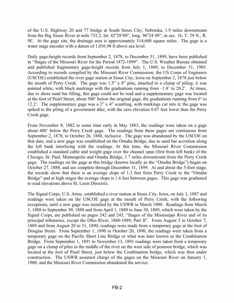
FB-2

of the U.S. Highway 20 and 77 bridge at South Sioux City, Nebraska, 1.9 miles downstream from the Big Sioux River at mile 732.2, lat. 42o29’09”, long. 96o24’49”, in sec. 16, T. 29 N., R. 9E. At the gage site, the drainage area is approximately 314,600 square miles. The gage is a water stage encoder with a datum of 1,056.98 ft above sea level. Daily gage-height records from September 2, 1878, to December 31, 1899, have been published in “Stages of the Missouri River for the Period 1872-1899”. The U.S. Weather Bureau obtained and published fragmentary gage-height records from July 1, 1889, to December 31, 1905. According to records compiled by the Missouri River Commission, the US Corps of Engineers (USCOE) established the river gage station at Sioux City, Iowa on September 2, 1878 just below the mouth of Perry Creek. The gage was 1.5” x 8” pine, attached to a clump of piling; it was painted white, with black markings with the graduations running from –1.8’ to 20.2’. At times, due to shore sand bar filling, this gage could not be read and a supplementary gage was located at the foot of Pearl Street, about 500’ below the original gage, the graduations running from 0’ to 12.2’. The supplementary gage was a 2” x 4” scantling, with markings cut into it; the gage was spiked to the piling of a government dike, with the zero elevation 0.07 feet lower than the Perry Creek gage. From November 8, 1882 to some time early in May 1883, the readings were taken on a gage about 400’ below the Perry Creek gage. The readings from these gages are continuous from September 2, 1878, to October 26, 1888, inclusive. The gage was abandoned by the USCOE on that date, and a new gage was established on the Omaha Bridge, due to sand bar accretion along the left bank interfering with the readings. At this time, the Missouri River Commission established a standard cable and weight gage over the channel span (first from left bank) of the Chicago, St. Paul, Minneapolis and Omaha Bridge, 1.7 miles downstream from the Perry Creek gage. The readings on the gage at this bridge (known locally as the “Omaha Bridge”) began on October 27, 1888, and are complete through December 31, 1899. At and about the 5-foot stage, the records show that there is an average slope of 1.3 feet from Perry Creek to the “Omaha Bridge” and at high stages the average slope is 1.6 feet between gages. This gage was graduated to read elevations above St. Louis Directrix.

The Signal Corps, U.S. Army, established a river station at Sioux City, Iowa, on July 1, 1887 and readings were taken on the USCOE gage at the mouth of Perry Creek, with the following exceptions, until a new gage was installed by the USWB in March 1900. Readings from March 1, 1888 to September 30, 1888 and from April 1, 1889 to June 30, 1889, which were taken by the Signal Corps, are published on pages 242 and 243, “Stages of the Mississippi River and of its principal tributaries, except the Ohio River, 1860-1889, Part II”. From August 5 to October 7, 1889 and from August 20 to 31, 1890, readings were made from a temporary gage at the foot of Douglas Street. From September 1, 1890 to October 20, 1890, the readings were taken from a temporary gage on the Pacific Short Line Bridge or what was later known as the Combination Bridge. From September 1, 1891 to November 13, 1891 readings were taken from a temporary gage on a clump of piles in the middle of the river on the west side of pontoon bridge, which was located at the foot of Pearl Street, just below the Combination bridge, which was then under construction. The USWB assumed charge of the gages on the Missouri River on January 1, 1900, and the Missouri River Commission abandoned the service.

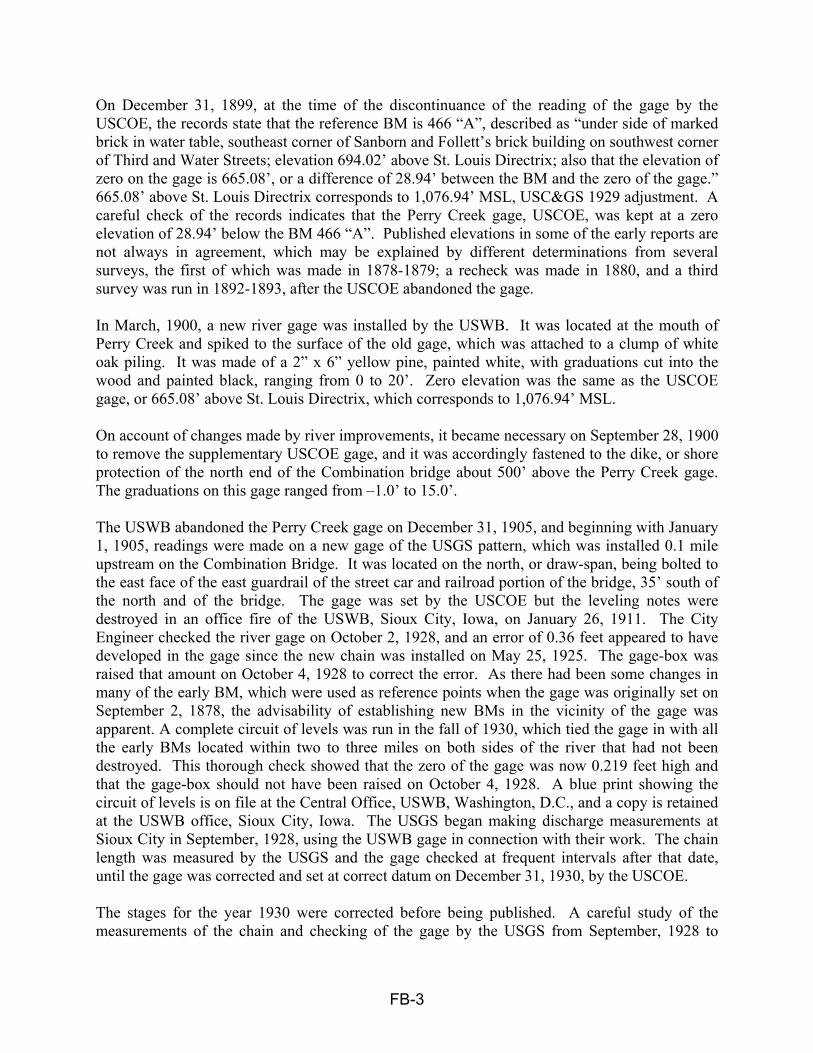
FB-3

On December 31, 1899, at the time of the discontinuance of the reading of the gage by the USCOE, the records state that the reference BM is 466 “A”, described as “under side of marked brick in water table, southeast corner of Sanborn and Follett’s brick building on southwest corner of Third and Water Streets; elevation 694.02’ above St. Louis Directrix; also that the elevation of zero on the gage is 665.08’, or a difference of 28.94’ between the BM and the zero of the gage.” 665.08’ above St. Louis Directrix corresponds to 1,076.94’ MSL, USC&GS 1929 adjustment. A careful check of the records indicates that the Perry Creek gage, USCOE, was kept at a zero elevation of 28.94’ below the BM 466 “A”. Published elevations in some of the early reports are not always in agreement, which may be explained by different determinations from several surveys, the first of which was made in 1878-1879; a recheck was made in 1880, and a third survey was run in 1892-1893, after the USCOE abandoned the gage. In March, 1900, a new river gage was installed by the USWB. It was located at the mouth of Perry Creek and spiked to the surface of the old gage, which was attached to a clump of white oak piling. It was made of a 2” x 6” yellow pine, painted white, with graduations cut into the wood and painted black, ranging from 0 to 20’. Zero elevation was the same as the USCOE gage, or 665.08’ above St. Louis Directrix, which corresponds to 1,076.94’ MSL. On account of changes made by river improvements, it became necessary on September 28, 1900 to remove the supplementary USCOE gage, and it was accordingly fastened to the dike, or shore protection of the north end of the Combination bridge about 500’ above the Perry Creek gage. The graduations on this gage ranged from –1.0’ to 15.0’.

The USWB abandoned the Perry Creek gage on December 31, 1905, and beginning with January 1, 1905, readings were made on a new gage of the USGS pattern, which was installed 0.1 mile upstream on the Combination Bridge. It was located on the north, or draw-span, being bolted to the east face of the east guardrail of the street car and railroad portion of the bridge, 35’ south of the north and of the bridge. The gage was set by the USCOE but the leveling notes were destroyed in an office fire of the USWB, Sioux City, Iowa, on January 26, 1911. The City Engineer checked the river gage on October 2, 1928, and an error of 0.36 feet appeared to have developed in the gage since the new chain was installed on May 25, 1925. The gage-box was raised that amount on October 4, 1928 to correct the error. As there had been some changes in many of the early BM, which were used as reference points when the gage was originally set on September 2, 1878, the advisability of establishing new BMs in the vicinity of the gage was apparent. A complete circuit of levels was run in the fall of 1930, which tied the gage in with all the early BMs located within two to three miles on both sides of the river that had not been destroyed. This thorough check showed that the zero of the gage was now 0.219 feet high and that the gage-box should not have been raised on October 4, 1928. A blue print showing the circuit of levels is on file at the Central Office, USWB, Washington, D.C., and a copy is retained at the USWB office, Sioux City, Iowa. The USGS began making discharge measurements at Sioux City in September, 1928, using the USWB gage in connection with their work. The chain length was measured by the USGS and the gage checked at frequent intervals after that date, until the gage was corrected and set at correct datum on December 31, 1930, by the USCOE. The stages for the year 1930 were corrected before being published. A careful study of the measurements of the chain and checking of the gage by the USGS from September, 1928 to

FB-4

March 29, 1930 and the checking of the BM’s and the gage by the USCOE disclosed that the following corrections should be applied to the published stages in the USWB Daily River Stages, years 1925 to 1929, inclusive, for the Sioux City River gage from September 1, 1925 to December 31, 1929: Subtract 0.2 feet from September 1, 1925 to May 31, 1928; subtract 0.3 feet from June 1, 1928 to October 4, 1928, and add 0.1 feet from October 5, 1928 to December 31, 1929. On September 2, 1931, the 53rd anniversary of the establishment of the river station, a new short-box pattern chain and weight gage was installed 73 feet from the right bank abutment by the USGS, at a zero elevation of 665.1’ above St. Louis Directrix, which corresponds to 1076.96’, USC&GS 1929 adjustment. On December 2, 1936, the USGS installed a Type A wire-weight gage on the Combination Bridge for the USWB. This gage was set to the same datum as the former chain gage and has been in use since that date. USGS used a chain gage located 160 feet from left end of bridge on which present gage is located from September 1, 1928, to September 30, 1931. This chain gage was the property of the Weather Bureau and was used by them also. From October 1, 1931, to July 31, 1938, the collection of discharge records was discontinued by the USGS. During this period, the Weather Bureau installed a recording gage on February 14, 1935. This gage was maintained for the Weather Bureau by the USGS until the gage was reestablished as a USGS gaging station on September 1, 1938. It remained at this location, 227 feet downstream from the present site, at a datum 20 feet higher than present until September 30, 1970 and until Jan 30, 1981 at the present datum. Maximum stage recorded by the Weather Bureau was 22.5 feet on April 23, 1881. However, according to the station description for Missouri River at Sioux City, Iowa, dated March 24, 1934, which was prepared by the War Department, a stage of 25.0 feet occurred on May 18, 1892 as a result of backwater from the Floyd River. A maximum discharge of 441,000 cfs occurred on April 14, 1952 at a gage height of 24.28 feet. Missouri River At Omaha, Nebraska The U.S. Geological Survey (USGS) presently operates gaging station number 06610000, Missouri River at Omaha, Nebraska. The gage is located on the right bank on the left side of the concrete floodwall, at the foot of Douglas Street, 275 ft. downstream from the Interstate 480 Highway Bridge in Omaha, and at river mile 615.9, lat. 41o15’32”, long 95o55’20”, in SE ¼ NW ¼ sec.23, T. 15 N., R. 13 E., Douglas County. Drainage area above the gage is approximately 322,800 square miles. Present gage datum is 948.24 feet above sea level. From Oct. 1, 1936 to Sept. 30, 1982 the gage datum was 10 feet higher. Daily gage-height records have been collected from April 10, 1872, to date by U.S. Army Engineers and U.S. Weather Bureau. The records from April 10, 1872, to December 11, 1899, were published by the Missouri River Commission in “Stages of the Missouri River.” The records since January 1, 1900, have been published by the U.S. Weather bureau in “Daily River Stages of Principal Rivers of the United States”. The gages used at or near this site were as follows:

FB-5

From April 10, 1872, to August 31, 1878, the Union Pacific Railroad (UPRR) used a cable gage on their bridge about 0.6 miles below present gage on Douglas Street Bridge, which was demolished Dec. 1968. From September 1, 1878, to February 28, 1907, the U.S. Corps of Engineers collected records from the several gages. From Sept. 1, 1878, to Apr. 26, 1879, readings were at the UPRR gage site. From April 27, 1879, to May 20, 1886, a staff gage 700 ft. upstream at the foot of Farnam Street was used. The gage heights were corrected for slope to correspond with readings on the UPRR gage. From May 21, 1886, to Feb. 28, 1907, gage heights were obtained from the UPRR gage, except for the period Nov. 19, 1886, to Mar. 9, 1887, during which time the gage was moved to a temporary bridge while repairs were being made to old bridge. From March 1, 1907, to date, the U.S. Weather Bureau has obtained gage heights from the several gages. A chain and weight gage bolted to the downstream guardrail on the Douglas Street Bridge was used from March 1, 1907, to September 21, 1934. According to letter, dated April 7, 1930, from the U.S. Weather Bureau, the zero of this chain gage was 0.43 feet higher than the zero of the UPRR gage in order to compensate for slope of river. From September 22, 1934 to May 2, 1968, the U.S. Weather Bureau Type A wire-weight gage was located on the upstream truss of the main span of the Ak-Sar-Ben (Douglas Street) Bridge at Sta. 135. Standard check bar elevation was 76.83 ft. above zero of gage. From September 1, 1928, to date, the U.S. Geological Survey has obtained gage heights from several gages. From September 1, 1928, to November 30, 1929, readings were made from the chain gage attached to the Illinois Central R.R. Bridge, about two miles upstream from former Douglas Street Bridge. The zero of this gage was 2.97 feet higher than the zero of the present gage. From December 1, 1929, to May 26, 1930, readings were made from the Douglas Street gage. From May 27, 1930, to October 18, 1931, a Canfield wire-weight gage was used near the chain gage on the Douglas Street Bridge and set to the same datum as that gage. From October 19, 1931, to September 30, 1936, a Stevens recording gage in a 36-inch corrugated iron pipe bolted to Nebraska Power and Light Company’s concrete intake wall was used. This gage was set to the same datum as the Douglas Street gage and was located 1900 feet downstream from that gage. From October 1, 1936, to February 4, 1952, Eriez and Stevens recording gages in 36” corrugated house and 18” galvanized spiral-welded pipe well attached to the downstream end of the pier at the left end of the main truss span of the Douglas Street Bridge at station 396 were used. The recorders were set to read the same as the outside gage. On February 7, 1952, the recorder was moved to the current gage location and was used until September 30, 1965. A digital punched-tape water stage recorder with 15 minute punch interval was installed to be used beginning Oct. 1, 1965. It is driven by means of sprocket and chain from the Stevens A-35 water stage recorder. Reference gage is the inside float tape, which is an integral part of the Stevens A-35 recorder. A Stevens A-35 continuous water-stage recorder with gage-height ratio 1:6 and 2.4” per day is operated as an auxiliary recorder. The gage is housed in a reinforced concrete house and well, 6 ft. 4 inches square with two 3-inch intakes, both connected to a flushing system equipped with an electric pump. The outside gage is a staff gage attached to the downstream landward side of the right pier of the Interstate 480 Highway bridge and was

FB-6

installed May 2, 1968, at which time the wire-weight gage was removed prior to demolition of Ak-Sar-Ben Bridge on Dec. 14, 1968. The gage height for April 25, 1881, is given as 569.4 feet St. Louis Directrix. On page 6 of the Missouri River Commission book “Stages of the Missouri River from its Mouth to Sioux City, Iowa, 1890-1894”, the table of corrections shows that 1.003 feet must be added to the 1881 datum in order to transfer it to St. Louis Directrix correctly. Therefore, the true elevation of the 1881 high water at the Union Pacific Bridge, referred to the St. Louis Directrix is 570.403 feet. The 1929 Adjustment of the Primary Level Net of the U.S. Coast and Geodetic Survey gives a difference between the St. Louis Directrix and the U.S. Coast and Geodetic Survey datum at Omaha of 412.057 ft. Therefore, the true elevation of the 1881 flood referred to the 1929 Adjustment of the Primary Level Net by the U.S. Coast and Geodetic Survey at Omaha would be (570.403 plus 412.057) 982.460 feet, m.s.l. The zero of the gage on the Union Pacific Railroad bridge used from 1872 to 1907 was 957.807 feet above mean sea level, U.S.C. & G.S. General Adjustment of 1929, as determined by the following method: On page 7 of the Missouri River Commission Report of “Stages of the Missouri River for 1895 to 1899”, the adjusted elevation of the zero of the gage is given as 545.75 feet above St. Louis Directrix. In order to convert this to mean sea level elevation, 1929 adjustment, it is necessary to add 412.057 feet, which gives 957.807 feet. Therefore, the flood of April 25, 1881, corresponded to a stage of 24.65 feet (982.460 – 957.807) on the gage on the Union Pacific Railroad bridge, which was used from 1872 to 1907. With the USWB chain gage installed on the Douglas Street bridge in 1907 set to read the same as the gage on the Union Pacific Railroad bridge and the U.S.W.B. wire gage on the Douglas Street bridge set to the same datum as the chain gage located there, it is assumed that the flood of April 25, 1881, corresponded to a stage of 24.65 feet on both the USWB chain and wire gages on the Douglas Street bridge, which were used by the USWB from 1907 to date. As the present USGS recording gage is set to read the same as the USWB wire weight gage, the flood of April 25, 1881 also reached a stage of 24.65 feet on the present U.S.G.S. recording gage. Maximum stage at this gage of 30.20 feet occurred on April 16, 1952 with a peak discharge of 396,000 cfs. Missouri River At Nebraska City, Nebraska The USGS currently operates gaging station number 0680700, Missouri River at Nebraska City, Nebraska. The gage is located on the right bank 2 miles upstream from the Highway 2 Bridge at mile 562.6, lat. 40o40’55”, long. 95 o50’48”. Drainage area upstream from the gage is approximately 414,400 square miles. The current datum of the gage is 905.36 feet above sea level. The U.S. Corps of Engineers obtained daily gage heights from an inclined masonry gage 2700 feet downstream from the C.B. & Q.R.R. bridge from August 1, 1878, to October 30, 1888, and from the cable gage on the bridge from October 31, 1888, to December 31, 1899. The Missouri River Commission published these records in “Stages of the Missouri River.” The C.B. & Q.R.R. obtained daily gage heights from the cable gage on the railroad bridge from November 1917 to August 12, 1929.

FB-7

The USGS obtained daily gage heights from a chain gage on the C.B. & Q.R.R. bridge from August 12, 1929, to June 27, 1930 and from a Canfield wire-weight gage on that bridge from June 27, 1930, to October 22, 1931. From October 22, 1931, to Apr 1, 1963, a recording gage on the Waubonsie Highway Bridge was used. The Canfield wire-weight gage was moved from the railroad to highway bridge on August 1, 1932. All these USGS gages were set and maintained to the same datum. During the flood of 1881, the maximum stage occurred April 27, 1881. In “Stages of the Missouri River” the stage recorded for that date was 509.1 ft. According to pages V and VI of this report for 1895 to 1899, 0.36 ft. must be added to this figure in order to make it refer to correct St. Louis directrix. According to page XII of report for 1886 to 1889, the gage maintained during 1881 was an inclined masonry gage located 2700 feet downstream from C.B. & Q.R.R. bridge and the fall in water surface between the bridge and inclined gage at a stage of 499 feet was 0.37 feet. Therefore, the correct elevation for the maximum stage of April 27, 1881, at the railroad bridge was (509.1+0.36+0.37) 509.83 feet. The zero of USGS gages on railroad and highway bridges is 491.80 feet above St. Louis directrix. Therefore, the maximum stage of April 27, 1881 was (509.83-491.80) 18.03 feet, referred to the present USGS gage. The maximum flood of record occurred on April 19, 1952 with a discharge of 414,000 cfs and a peak stage of 27.66 feet. Additional gages along the Missouri River in the Omaha District used in this study are briefly described below: Yankton- LOCATION.--Lat 42 51'58", long 97 23'37", in SW¼ SW¼ sec.18, T.93 N., R.55 W., Yankton County, Hydrologic Unit 10170101, near left bank in downstream end of left pier of Meridian Highway Bridge on U.S. Highway 81, 5.2 mi downstream from Gavins Point Dam, 6.0 mi upstream from James River, and at mile 805.8. DRAINAGE AREA.--279,500 mi2, approximately. PERIOD OF RECORD.--October 1995 to current year, daily gage-height records. October 1930 to September 1995, daily discharge determined. Monthly discharge only for some periods, published in WSP 1309. Gage-height records collected at same site March 1873 to November 1886, March 1905 to May 1908 (fragmentary), August 1921 to September 1950 (except winter months prior to 1932), are contained in reports of the National Weather Service. GAGE.--Water-stage recorder. Datum of gage is 1,139.68 ft above National Geodetic Vertical Datum of 1929. Prior to Sept. 20, 1932, nonrecording gage, and Sept. 20, 1932, to Mar. 9, 1967, water-stage recorder at present site and at datum 20.0 ft higher. Decatur- LOCATION.--Lat 42 00'26", long 96 14'29", in NE¼ SW¼ sec. 36, T.24 N., R.10 E., Burt County, Hydrologic Unit 10230001, on right bank 0.1 mi upstream from Iowa Highway 175 bridge at Decatur, and at mile 691.0. DRAINAGE AREA.--316,200 mi2, approximately. The 3,959 mi2 Great Divide basin are not included. PERIOD OF RECORD.--October 1987 to current year.

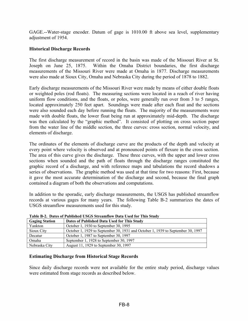
FB-8

GAGE.--Water-stage encoder. Datum of gage is 1010.00 ft above sea level, supplementary adjustment of 1954. Historical Discharge Records The first discharge measurement of record in the basin was made of the Missouri River at St. Joseph on June 25, 1875. Within the Omaha District boundaries, the first discharge measurements of the Missouri River were made at Omaha in 1877. Discharge measurements were also made at Sioux City, Omaha and Nebraska City during the period of 1878 to 1882. Early discharge measurements of the Missouri River were made by means of either double floats or weighted poles (rod floats). The measuring sections were located in a reach of river having uniform flow conditions, and the floats, or poles, were generally run over from 3 to 5 ranges, located approximately 250 feet apart. Soundings were made after each float and the sections were also sounded each day before running the floats. The majority of the measurements were made with double floats, the lower float being run at approximately mid-depth. The discharge was then calculated by the “graphic method”. It consisted of plotting on cross section paper from the water line of the middle section, the three curves: cross section, normal velocity, and elements of discharge. The ordinates of the elements of discharge curve are the products of the depth and velocity at every point where velocity is observed and at pronounced points of flexure in the cross section. The area of this curve gives the discharge. These three curves, with the upper and lower cross sections when sounded and the path of floats through the discharge ranges constituted the graphic record of a discharge, and with reference maps and tabulations the record shadows a series of observations. The graphic method was used at that time for two reasons: First, because it gave the most accurate determination of the discharge and second, because the final graph contained a diagram of both the observations and computations. In addition to the sporadic, early discharge measurements, the USGS has published streamflow records at various gages for many years. The following Table B-2 summarizes the dates of USGS streamflow measurements used for this study. Table B-2. Dates of Published USGS Streamflow Data Used for This Study Gaging Station Dates of Published Data Used for This Study Yankton October 1, 1930 to September 30, 1995 Sioux City October 1, 1929 to September 30, 1931 and October 1, 1939 to September 30, 1997 Decatur October 1, 1987 to September 30, 1997 Omaha September 1, 1928 to September 30, 1997 Nebraska City August 11, 1929 to September 30, 1997 Estimating Discharge from Historical Stage Records Since daily discharge records were not available for the entire study period, discharge values were estimated from stage records as described below.

FB-9

Missouri River At Sioux City At Sioux City, daily stage records were generally available from early March through November during 1898-1904 and 1909. All other years had daily stage records available for the entire year. These records were obtained from “U.S. Department of Agriculture, Weather Bureau. Daily River Stages at River Gage Stations of the Principal Rivers of the United States. Parts VI through XXVI.” For the years 1898 through 1905, the records were obtained at the gage below Perry Creek, while the years 1906 through 1928 were obtained at the Combination Bridge. Datums for the gages published in the reports were 1077.8 ft msl in 1898, 1078.9 ft msl in 1900, 1078.2 in 1911, and 1078.6 in 1920. The first attempt to develop a historical flow record at Sioux City utilized the family of rating curves developed for previous studies in the mid-forties and the 1962 Hydrology Study. Search of our files found the original rating curves as well as a listing of which curves were used for each year. However, no rational was found on how the different rating curves were selected for each year as well as how the family of rating curves was developed. In general, rating curve numbers 5, 6, and 7 were used for most years. Rating curve number 5 was used for 1898, 1901, 1903, 1911, and 1928. Rating curve number 6 was used for 1900, 1902, 1904-05, 1908-09, 1912-14, 1917-18, and 1921-22. Rating curve number 4 was used for 1927. Rating curve number 7 was used for all remaining years. After computing the daily flows from this approach, they were compared to the USGS estimates of monthly flows obtained from USGS Circular 108. In most years, the monthly flow volumes derived from the daily flow estimates were significantly higher than the USGS estimates of the monthly flow volumes. Therefore, an alternative approach was used to compute the historical flows. This consisted of developing a stage discharge rating curve based on historical measurements. As shown in Table 8, measurements were made in 1878 and 1879 at a location about 700 feet downstream from Perry Creek. These measurements were obtained from the report “Missouri River Study of Effects of Navigation and Channel Stabilization Works”, dated April 1954. In that report, the discharge measurements were plotted along with a reference curve. The Reference curve was derived from USGS discharge measurements made during the period of 1928 through 1952. In order to derive the reference curve, upper and lower limit curves were drawn to bound the discharge measurements and the reference curve was drawn midway between the upper and lower limits. Table B-3. Missouri River at Sioux City, Iowa - Historic Discharge Measurements

No. Date Width (feet)

Area (sq ft)

Velocity (fps)

Gage Height (feet)

Discharge (kcfs)

Method

1 9/17/1878 1130 8,643 3.51 5.50 30.3 DOUBLE FLOAT 2 9/18/1878 1130 8,453 3.56 5.50 30.1 DOUBLE FLOAT 3 9/19/1878 1125 8,613 3.46 5.50 29.8 ROD FLOAT 4 9/21/1878 1127 8,398 3.52 5.90 29.5 ROD FLOAT 5 9/26/1878 1125 7,958 3.46 5.80 27.5 ROD FLOAT 6 9/30/1878 1150 8,107 3.22 5.80 26.1 ROD FLOAT 7 10/02/1878 1115 7,779 3.31 5.60 25.7 ROD FLOAT 8 10/03/1878 1120 7,565 3.41 5.50 25.8 DOUBLE FLOAT 9 10/04/1878 1120 7,743 3.28 5.50 25.4 ROD FLOAT

10 10/05/1878 1125 7,600 3.12 5.50 23.6 ROD FLOAT 11 10/07/1878 1125 7,054 3.13 5.20 22.1 ROD FLOAT 12 10/09/1878 1120 7,194 3.15 5.10 22.6 ROD FLOAT 13 10/11/1878 1123 7.551 3.04 5.10 22.9 ROD FLOAT 14 11/01/1878 1125 5,951 3.53 4.90 21.0 ROD FLOAT 15 7/01/1879 1390 26,284 7.48 14.30 196.7 DOUBLE FLOAT 16 7/02/1879 - 26,263 7.43 14.20 195.1 DOUBLE FLOAT 17 7/05/1879 - 24,850 6.34 13.50 157.6 DOUBLE FLOAT

FB-10


Area (sq ft)

Velocity (fps)

Gage Height (feet)

Discharge (kcfs)

Method

18 7/07/1879 - 24,830 6.50 12.80 161.5 DOUBLE FLOAT 19 7/09/1879 - 23,068 5.96 12.70 137.4 DOUBLE FLOAT 20 7/10/1879 - 20,497 6.05 12.80 124.0 DOUBLE FLOAT 21 7/14/1879 - 20,394 5.32 11.70 108.5 DOUBLE FLOAT 22 7/15/1879 - 20,120 5.24 11.60 105.5 DOUBLE FLOAT 23 7/16/1879 - 19,967 5.27 11.60 105.3 DOUBLE FLOAT 24 7/22/1879 - 16,943 5.20 10.50 88.1 DOUBLE FLOAT 25 7/23/1879 - 15,840 5.37 10.40 85.0 DOUBLE FLOAT 26 7/24/1879 - 16,387 4.97 10.00 81.4 DOUBLE FLOAT 27 7/25/1879 1335 15,733 5.13 9.70 80.7 DOUBLE FLOAT 28 7/28/1879 - 18,654 5.32 10.20 99.2 DOUBLE FLOAT 29 7/30/1879 - 17,706 5.68 10.70 100.5 DOUBLE FLOAT 30 8/01/1879 1390 14,871 6.27 10.40 93.2 DOUBLE FLOAT 31 8/08/1879 - 10,927 5.34 7.70 58.3 DOUBLE FLOAT 32 8/13/1879 - 10,993 4.22 7.20 46.4 DOUBLE FLOAT 33 8/14/1879 - 10,912 4.18 7.00 45.6 DOUBLE FLOAT 34 8/15/1879 - 10,705 3.76 7.00 40.2 DOUBLE FLOAT 35 8/20/1879 - 9,007 4.14 6.40 37.3 DOUBLE FLOAT 36 8/21/1879 - 7.930 4.29 6.40 34.0 DOUBLE FLOAT 37 8/26/1879 - 8,138 3.86 6.20 31.4 DOUBLE FLOAT 38 9/06/1879 - 6,425 3.84 5.30 24.7 DOUBLE FLOAT 39 9/13/1879 - 6,354 3.59 4.80 22.8 DOUBLE FLOAT 40 9/19/1879 1080 5,548 3.37 4.30 18.7 DOUBLE FLOAT 41 11/02/1895 - 4,655 3.24 7.40 15.1 DOUBLE FLOAT 42 2/18/1905 - 3,515 1.97 6.70 6.9 CURRENT METER

Figure B-1. Historic Stage-Discharge Rating Curve at Sioux City To develop the rating curve for use in this study, an eye fit curve was drawn through the 1878-1879 measurements and transitioned to the reference curve at a discharge of about 100,000 cfs. A first attempt used the eye fit curve for all points but that resulted in an unreasonably high

Missouri River at Sioux City Historic Stage Discharge Rating Curve

0

5

10

15

20

0 50 100 150 200 250Discharge (1000 cfs)

Stag

e (ft

)

MeasurementsAdoptedReference 1929-1952

FB-11

estimate of the 1881 peak. This is consistent with a study completed by the St. Louis District that concluded that historic discharge measurements based on surface floats tended to overestimate discharges that exceeded bank full capacity by about 4 to 20 percent. Therefore, for the high flows the reference curve was used. Figure XX shows the adopted curve compared to the reference curve and actual discharge measurements. Since these curves were based on a site about 1,200 feet downstream from the USWB gage, an adjustment of 0.3 to 0.4 feet was made to transfer the curve the USWB site at the Combination Bridge. For flows less than 100,000 cfs, 0.3 feet was added to the stage, while 0.4 feet was added for flows above 100,000 cfs when computing the final stage discharge curve. This would have the same effect of subtracting like amounts from the stage records. These values were based on USGS studies comparing stages at the USWB gage and the USGS gage made in 1939, which indicated that the water surface slope was 1.3 feet from Perry Creek to the Omaha Bridge (a distance of 1.7 miles) at average flows and 1.6 feet at high flows. The USWB records were also researched for periods of ice cover. During those periods, an ice affected rating curve was applied, as stages are higher for the same discharge during periods of partial or complete ice cover. The ice curve was derived by first adjusting computed discharges to match monthly USGS volumes. Dates of ice cover were determined based on notes in the USWB stage records, as well as checking meteorological records from Nebraska, Iowa, South Dakota and North Dakota. Volumes for those months with ice cover were noted from the USGS and compared to those computed using the historic rating curve. The average monthly computed discharge was plotted against the ratio of USGS monthly flow volume and computed monthly flow volume. The bulk of the ratio values fell between 0.2 and 0.6, so a value of 0.4 was used to factor the historic rating curve to determine an average ice-affected rating curve during those periods of noted ice cover. The same factor was used to determine the ice-affected rating curve at downstream stations for periods, or duration, of noted ice cover (the period of ice cover decreased with distance downstream). Missing records were estimated based on comparison of the USGS monthly estimates of flows and eye fitting the missing discharge hydrograph to preserve the monthly volumes. A comparison was made with the USGS monthly volumes and the flows appeared reasonable. A comparison was also made with the previous estimates of discharges and the use of the single rating curve seemed to match the USGS monthly estimates much better than using a family of rating curves. Missouri River At Omaha At Omaha, daily stage records were generally available from early March through mid to late December during 1900-1908 and 1912-1915. All other years had daily stage records available for the entire year. These records were obtained from “U.S. Department of Agriculture, Weather Bureau. Daily River Stages at River Gage Stations of the Principal Rivers of the United States. Parts VI through XXVI.” For the years 1898 through 1906, the records were obtained at the gage on the UPRR Bridge, while the years 1907 through 1928 were obtained at the Douglas Street Bridge. Datums for the gages published in the reports were 958.5 ft msl in 1898, 959.6 ft msl in 1900, 958.9 in 1911, 958.2 in 1916, and 959.3 in 1920. The first attempt to develop a historical flow record at Omaha utilized the family of rating curves developed for previous studies in the mid-forties and the 1962 Hydrology Study. These curves

FB-12

included the family of rating curves at Sioux City and a relationship between stage at Omaha and Stage at Sioux City, which varied by time period. These curves were combined to form individual rating curves for each year at Omaha. Search of our files found the original rating curves as well as a listing of which curves were used for each year. However, no rational was found on how the different rating curves were selected for each year as well as how the family of rating curves was developed. In general, rating curve numbers 5, 6, and 7 were used for most years. Rating curve number 5 was used for 1898, 1901, 1903, 1911, and 1928. Rating curve number 6 was used for 1900, 1902, 1904-05, 1908-09, 1912-14, 1917-18, and 1921-22. Rating curve number 4 was used for 1927. Rating curve number 7 was used for all remaining years. After computed the daily flows from this approach, they were compared to the USGS estimates of monthly flows obtained from. In most years, the daily flow estimates were significantly higher than the USGS estimates of the monthly flow volumes. Therefore, an alternative approach was used to compute the historical flows. This consisted of developing a stage discharge rating curve based on historical measurements. As shown in Table B-4, measurements were made in 1877, 1878, 1879, 1880, 1882 and 1895 at a location believed to the UPRR bridge, about 0.6 miles downstream from the Douglas Street Bridge. These measurements were obtained from the report “Missouri River Study of Effects of Navigation and Channel Stabilization Works”, dated April 1954. In that report, the discharge measurements were plotted along with a reference curve. The Reference curve was derived from USGS discharge measurements made during the period of 1928 through 1952. An additional reference curve was developed using data for the 1929 through 1933 period. Table B-4. Missouri River at Omaha, Nebraska - Historic Discharge Measurements


Area (sq ft)

Velocity (fps)

Gage Height (feet)

Discharge (kcfs)

Method

1 -/-/1877 - 5,008 3.29 7.06 20.2 DOUBLE FLOAT 2 10/01/1878 1000 8,644 3.68 8.66 31.9 DOUBLE FLOAT 3 10/02/1878 955 8,717 3.40 8.66 29.7 DOUBLE FLOAT 4 10/03/1878 845 7,285 3.62 8.46 26.4 DOUBLE FLOAT 5 10/10/1878 810 6,532 2.66 7.96 17.4 DOUBLE FLOAT 6 10/111878 820 7,332 2.92 7.96 21.6 DOUBLE FLOAT 7 10/12/1878 670 5,426 4.25 7.86 23.1 DOUBLE FLOAT 8 10/14/1878 620 5,312 3.50 7.96 19.6 DOUBLE FLOAT 9 10/18/1878 680 5,858 4.15 7.86 24.3 DOUBLE FLOAT

10 10/22/1878 740 6,850 2.78 7.76 19.1 DOUBLE FLOAT 11 10/28/1878 434 4,397 5.60 7.86 24.6 DOUBLE FLOAT 12 11/06/1878 485 5,426 3.86 7.86 21.0 DOUBLE FLOAT 13 11/09/1878 470 4,892 4.62 7.86 22.6 DOUBLE FLOAT 14 11/12/1878 675 5,316 4.15 7.86 22.1 DOUBLE FLOAT 15 11/14/1878 675 5,838 4.17 7.86 24.3 DOUBLE FLOAT 16 11/15/1878 675 6,344 3.83 7.86 24.3 DOUBLE FLOAT 17 11/16/1878 680 7.179 3.44 7.86 24.7 DOUBLE FLOAT 18 11/19/1878 1260 6,745 3.40 7.86 22.9 DOUBLE FLOAT 19 11/21/1878 595 4,658 5.11 7.86 24.0 DOUBLE FLOAT 20 11/22/1878 595 4,585 5.52 7.76 25.3 DOUBLE FLOAT 21 8/26/1879 932 7,681 4.91 8.86 37.7 DOUBLE FLOAT 22 8/30/1879 920 6,789 4.53 8.56 30.6 DOUBLE FLOAT 23 9/02/1879 910 7,368 3.72 8.16 27.4 DOUBLE FLOAT 24 9/04/1879 890 7,351 3.65 8.06 26.8 DOUBLE FLOAT 25 9/22/1879 1055 5,479 3.23 6.76 17.7 DOUBLE FLOAT 26 9/27/1879 980 5,171 3.16 6.56 17.3 DOUBLE FLOAT 27 10/03/1879 1238 5,502 3.13 6.76 17.2 DOUBLE FLOAT 28 10/10/1879 973 4,849 3.01 6.76 14.6 DOUBLE FLOAT 29 4/16/1880 633 9,880 4.70 9.46 46.5 ROD FLOAT 30 4/22/1880 633 9,421 6.12 10.36 57.5 ROD FLOAT 31 5/03/1880 1270 7,477 5.23 8.66 39.1 DOUBLE FLOAT 32 5/05/1880 770 5,919 5.67 8.36 33.6 DOUBLE FLOAT 33 11/01/1880 797 4,582 4.17 6.86 19.1 DOUBLE FLOAT

FB-13


Area (sq ft)

Velocity (fps)

Gage Height (feet)

Discharge (kcfs)

Method

34 6/13/1882 1119 13,927 7.85 11.56 109.4 DOUBLE FLOAT 35 6/15/1882 1093 14,502 7.82 11.56 113.5 DOUBLE FLOAT 36 7/10/1882 1160 16,168 7.01 12.96 113.4 DOUBLE FLOAT 37 7/11/1882 1160 16,659 8.12 13.16 135.3 DOUBLE FLOAT 38 7/19/1882 1160 13,898 7.70 12.56 107.0 DOUBLE FLOAT 39 7/22/1882 1160 12,541 6.43 11.46 80.7 DOUBLE FLOAT 40 7/25/1882 1097 12,385 5.56 10.56 88.8 DOUBLE FLOAT 41 7/26/1882 1096 11,455 5.66 10.26 64.8 DOUBLE FLOAT 42 7/27/1882 1093 11,102 6.10 10.36 67.7 DOUBLE FLOAT 43 8/28/1882 1045 7,623 4.03 7.96 31.6 DOUBLE FLOAT 44 8/29/1882 1034 7,922 4.22 7.86 33.5 DOUBLE FLOAT 45 8/30/1882 1035 7,584 4.11 7.86 31.2 DOUBLE FLOAT 46 8/31/1882 1048 7,953 4.35 7.76 34.7 DOUBLE FLOAT 47 9/01/1882 1046 7,636 4.01 7.66 30.6 DOUBLE FLOAT 48 9/02/1882 1049 7,429 4.39 7.56 32.7 DOUBLE FLOAT 49 9/04/1882 1041 6,853 4.27 7.36 29.5 DOUBLE FLOAT 50 9/05/1882 1049 7,246 3.99 7.26 28.9 DOUBLE FLOAT 51 9/11/1882 1045 7,145 3.30 6.76 23.6 DOUBLE FLOAT 52 9/12/1882 1051 7,270 3.38 6.66 24.6 DOUBLE FLOAT 53 9/13/1882 1044 7,261 3.39 6.56 24.6 DOUBLE FLOAT 54 9/16/1882 1044 6,731 3.62 6.56 24.4 DOUBLE FLOAT 55 9/26/1882 1060 6,251 3.55 6.26 21.9 DOUBLE FLOAT 56 9/27/1882 1055 4,920 3.42 6.26 16.8 DOUBLE FLOAT 57 9/28/1882 1053 5,802 3.39 6.28 19.7 DOUBLE FLOAT 58 9/29/1882 974 6,762 3.43 6.26 19.4 DOUBLE FLOAT 59 9/30/1882 914 6,673 3.12 6.26 20.8 DOUBLE FLOAT 60 10/02/1882 900 6,030 3.35 6.16 21.1 DOUBLE FLOAT 61 11/08/1895 5,590 2.77 7.18 16.5 DOUBLE FLOAT

To develop the rating curve for use in this study, an eye fit curve was drawn through the 1877-1895 measurements and compared with the reference curve developed from measurements in 1929 through 1933. Adjustments were made to this rating curve to provide consistent flows with those computed at Sioux City and Omaha. These adjustments were made by trial and error based on inspection of the computed hydrographs at Sioux City, Omaha, and Nebraska City for each year of the period 1898 through 1928. As shown on Figure 2, the final adopted stage discharge curve resulted in an increase of the stage of about 4 feet for discharges less than 20,000 cfs, slightly lowering the curve for discharges in the 50,000 to 120,000 cfs range, and a gradual increase in the curve by up to 2.5 feet at discharges of 350,000 cfs. Datum shifts were added to the gage records as follows: For the period of 1898-1899, 1.7 feet was added which includes a datum change of 1.1 feet and 0.6 feet for a change of location of 0.6 river miles, assuming 1 foot per mile slope; For the period 1900 to 1906, 1.0 feet was added to the stage records which includes a datum change of 0.4 feet and 0.6 feet for change in gage location; for the period of 1920 to 1929, 0.2 feet was subtracted from the gage records to account for shift due to channel changes. Missing records were estimated by routing the Sioux City flows using lag average routing coefficients of 1 day lag and averaging two days flows. Missing records only occurred during the ice season or low flow conditions. A comparison was made with the USGS monthly volumes at Sioux City and the computed flows at Sioux City and the flows appeared reasonable. A comparison was also made with the previous estimates of discharges and the use of the single rating curve seemed to match the computed flows at Sioux City much better than using a family of rating curves.

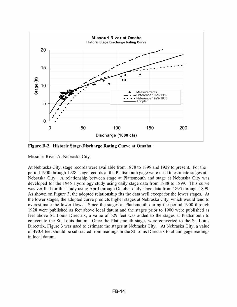
FB-14

Figure B-2. Historic Stage-Discharge Rating Curve at Omaha. Missouri River At Nebraska City At Nebraska City, stage records were available from 1878 to 1899 and 1929 to present. For the period 1900 through 1928, stage records at the Plattsmouth gage were used to estimate stages at Nebraska City. A relationship between stage at Plattsmouth and stage at Nebraska City was developed for the 1945 Hydrology study using daily stage data from 1888 to 1899. This curve was verified for this study using April through October daily stage data from 1895 through 1899. As shown on Figure 3, the adopted relationship fits the data well except for the lower stages. At the lower stages, the adopted curve predicts higher stages at Nebraska City, which would tend to overestimate the lower flows. Since the stages at Plattsmouth during the period 1900 through 1928 were published as feet above local datum and the stages prior to 1900 were published as feet above St. Louis Directrix, a value of 529 feet was added to the stages at Plattsmouth to convert to the St. Louis datum. Once the Plattsmouth stages were converted to the St. Louis Directrix, Figure 3 was used to estimate the stages at Nebraska City. At Nebraska City, a value of 490.4 feet should be subtracted from readings in the St Louis Directrix to obtain gage readings in local datum.

Missouri River at Omaha Historic Stage Discharge Rating Curve

0

5

10

15

20

0 50 100 150 200Discharge (1000 cfs)

Stag

e (ft

)

MeasurementsReference 1929-1952Reference 1929-1933Adopted

FB-15

Figure B-3. Relationship Between Plattsmouth and Nebraska City Stages

To compute the historical flows at Nebraska City from the estimated stages, a stage discharge rating curve was developed based on historical measurements. As shown in Table B-5, measurements were made in 1878. These measurements were obtained from the report “Missouri River Study of Effects of Navigation and Channel Stabilization Works”, dated April 1954. In that report, the discharge measurements were plotted along with a reference curve. The Reference curve was derived from USGS discharge measurements made during the period of 1928 through 1952. To develop the rating curve for use in this study, an eye fit curve was drawn through the 1877 discharge measurements. Two stage-discharge rating curves were found in the files that were developed in 1945. The first rating curve was identified as the 1903 curve and closely fit the upper bound of the discharge measurements. The second rating curve was identified as the 1908 rating curve and had about 25 percent less discharge for flows exceeding about 100,000 cfs when compared to the 1903 rating curve. The 1903 stage discharge rating curve was used for the period of 1898-1905, while the 1908 rating curve was used for the period of 1906-1928. These rating curves are shown on Figure 4 along with the 1882 measurements and the reference curve for the period of 1929-1952. The reference curve was based on the mid-point of the USGS discharge measurements obtained during the period of 1929 through 1952. For stage readings in the St Louis Directrix a value of 490.4 feet is added to the stage at Nebraska City.

Missouri River Stage Relationship Plattsmouth vs Nebraska City (April - October)

496

498

500

502

504

506

508

510

530 532 534 536 538 540 542Stage at Plattsmouth (ft)

Stag

e at

Neb

rask

a C

ity (f

t)

Observed 1895-1899Adopted

FB-16

Since the Plattsmouth stages were generally only available during the March through July period, the flows at Nebraska City during the missing periods were based on those estimated at Omaha and routed to Nebraska City. USGS discharge records from 1929 through 1995 were used to compute the average flow during the period of October through February at Omaha and Nebraska City. Next, the ratio of the flow at Nebraska City to the flow at Omaha during this period was computed as 1.2. Therefore, the missing flows at Nebraska City were based on increasing the Omaha flows by 20 percent and routing to Nebraska City using the lag average method by averaging 2 days of flows with no lag.

Table B-5. Missouri River at Nebraska City, Nebraska - Historic Discharge Measurements


Area (sq ft)

Velocity (fps)

Gage Height (feet)

Discharge (kcfs)

Method

1 5/10/1878 1890 13,173 3.69 8.86 48.6 DOUBLE FLOAT 2 5/24/1878 2195 18,530 4.96 10.56 92.0 DOUBLE FLOAT 3 5/29/1878 2340 23,040 4.96 10.96 114.3 DOUBLE FLOAT 4 5/31/1878 2060 21,130 4.95 10.76 104.7 DOUBLE FLOAT 5 6/02/1878 2020 20,040 4.44 10.06 88.9 DOUBLE FLOAT 6 6/05/1878 2045 20,200 3.70 9.56 74.8 DOUBLE FLOAT 7 6/07/1878 1490 14,900 4.18 9.26 62.2 DOUBLE FLOAT 8 6/10/1878 1470 14,260 4.23 9.26 60.3 DOUBLE FLOAT 9 6/13/1878 2135 18,220 6.41 10.86 116.8 DOUBLE FLOAT

10 6/15/1878 2160 18,580 6.36 11.16 118.2 DOUBLE FLOAT 11 6/20/1878 2800 31,340 6.37 13.56 199.6 DOUBLE FLOAT 12 6/22/1878 2810 30,580 6.84 13.86 209.3 DOUBLE FLOAT 13 6/24/1878 2820 30,340 6.64 14.16 201.6 DOUBLE FLOAT 14 6/26/1878 2810 29,140 7.37 14.36 214.7 DOUBLE FLOAT 15 6/28/1878 2830 29,800 7.10 14.36 239.6 DOUBLE FLOAT 16 6/30/1878 2825 28,660 7.32 14.46 209.8 DOUBLE FLOAT 17 7/03/1878 2840 27,460 6.04 14.26 175.9 DOUBLE FLOAT 18 7/07/1878 2850 28,440 5.05 13.06 143.1 DOUBLE FLOAT 19 7/10/1878 2850 28,840 4.35 12.76 125.4 DOUBLE FLOAT 20 7/12/1878 2840 30,560 4.91 12.76 150.0 DOUBLE FLOAT 21 7/14/1878 2845 30,860 4.63 12.76 143.0 DOUBLE FLOAT 22 7/17/1878 2850 28,440 5.14 12.76 146.2 DOUBLE FLOAT 23 7/19/1878 2850 26,580 4.65 12.06 123.5 DOUBLE FLOAT 24 7/21/1878 2840 23,900 4.55 11.66 108.6 DOUBLE FLOAT 25 7/24/1878 2840 20,920 4.25 10.96 88.8 DOUBLE FLOAT 26 7/31/1878 2825 19,860 3.65 10.16 72.6 DOUBLE FLOAT 27 8/12/1878 2660 14,760 3.41 8.96 50.4 DOUBLE FLOAT 28 8/24/1878 2240 11,565 3.97 7.86 40.9 DOUBLE FLOAT 29 8/28/1878 2260 11,025 3.13 7.76 34.5 DOUBLE FLOAT 30 8/31/1878 2320 10,860 3.28 7.56 35.7 DOUBLE FLOAT 31 9/04/1878 2800 10,710 2.92 7.36 31.3 DOUBLE FLOAT 32 9/07/1878 2480 9,750 3.10 7.16 30.3 DOUBLE FLOAT 33 9/26/1878 1560 8,920 2.42 6.16 21.6 DOUBLE FLOAT

FB-17

Figure B-4. Historic Stage-Discharge Rating Curve at Nebraska City

The following table summarizes the dates of available stage records used for reconstructing the flow record. Table B-6. Dates of Published Stage Records Used for This Study Station Dates of Published Data Used for This Study Sioux City 3/8/1898-11/21/1898, 4/5/1899-12/4/1899, 3/25/1900-11/20/1900, 3/13/1901-12/8/1901, 3/10/1902-12/4/1902,

3/12/1903-11/17/1903, 3/18/1904-12/31/1908, 3/21/1909-12/6/1909, 1/1/1910-9/30/1929 Omaha 2/25/1898-11/22/1898, 3/26/1899-12/31/1899, 1/21/1900-1/22/1900, 3/13/1900-2/23/1901, 3/1/1901, 12/13/1901,

3/1/1902-12/4/1902, 3/2/1903-12/25/1903, 3/19/1904-9/30/1904, 3/1/1905-12/3/1905, 12/24/1905-2/15/1906, 2/21/1906-3/22/1906, 3/26/1906-6/18/1906, 6/20/1906-12/19/1906, 3/1/1907-11/30/1907, 2/1/1908, 2/12/1908-12/1/1908, 12/25/1908-1/7/1909, 2/28/1909-12/9/1909, 12/14/1909-12/17/1909, 12/31/1909-1/2/1911, 3/1/1911-12/27/1911, 2/19/1912-3/15/1912, 3/19/1912-12/11/1912, 2/17/1913-12/25/1913, 1/6/1914-2/5/1914, 2/9/1914-12/11/1914, 1/11/1915-12/29/1915, 12/3/1916-8/31/1928

Plattsmouth Mar. 1 – July 31, 1900-1928 Nebraska City 1/1/1898-12/31/1899, 1/1/1929-8/10/1929

Missouri River at Nebraska CityHistoric Stage Discharge Rating Curve

0

5

10

15

20

0 50 100 150 200 250Discharge (1000 cfs)

Stag

e (ft

)

Measurements

Adopted 1898-1905

Adopted 1906-1929

Reference 1929-1952

FC-1


Appendix F-C

A Study to Determine the

Historic and Present-Level Streamflow Depletions

in the

Missouri River Basin

Above Hermann, Missouri

Prepared by:

Water Resources Service Group

Great Plains Regional Office

Bureau of Reclamation

Billings, Montana

August, 1999

FC-2

Table of Contents

Page

I. Introduction .................................................................................................…........... 1 II. Use of Existing Data - 1982 Missouri Basin State Association ....................…........ 2 III. Irrigated Acres Used in the MBSA Study .....................................................…....... 2 IV. Determination of Irrigated Acres for Years not included in MBSA Study ....…...... 2 V. Determination of 1898 to 1928 Irrigated Acres by Major Node Basin ........…......... 3 VI. Accumulation of County Irrigated Acres to Node Basin Irrigated Acres .................. 7 VII. Calculation of Irrigation Depletions ........................................................................ 10

Climatological/Meteorological Data .................................................................... 10 Crop Distribution Patterns ................................................................................... 11 Conveyance and On-Farm Efficiencies ............................................................... 12 Return Flow Distribution Patterns ........................................................................ 12 Non-Beneficial Consumptive Use ........................................................................ 13

VIII. Calculation of Historic Depletion ............................................................................ 14 IX. Calculation of the Present-Level Depletion ................................................................. 14 X. Historic Depletions Due to Irrigation by Ground Water .............................................. 15 XI. Present-Level Depletions Due to Irrigation by Ground Water ................................... 17 XII. Historic Major Reservoir Depletions ......................................................................... 18 XIII. Present-Level Major Reservoir Depletions ................................................................ 18 XIV. Historic ‘Other’ Depletions ....................................................................................... 21 XV. Present-Level ‘Other’ Depletions ............................................................................... 24 XVI. Other Impacts to Streamflow .................................................................................... 25 Appendix A - Sample Worksheets Appendix B - Graphs of Total Historic Streamflow Depletions Appendix C - Graphs of Total Present-Level Streamflow Depletions

FC-3

A Study to Determine the Historic and Present-Level Streamflow Depletions

in the Missouri River Basin

Above Hermann, Missouri

August, 1999

I. Introduction In April 1998, the Corps of Engineers (COE) requested that the Bureau of Reclamation determine monthly streamflow depletion estimates for selected node basins throughout the Missouri River Basin. These node basins included: Missouri River above Ft Peck Dam, Montana Missouri River - Ft Peck Dam to Garrison Dam, North Dakota Missouri River - Garrison Dam to Oahe Dam, South Dakota Missouri River - Oahe Dam to Big Bend Dam, South Dakota Missouri River - Big Bend Dam to Ft Randall Dam, South Dakota Missouri River - Ft Randall Dam to Gavins Point Dam, South Dakota Missouri River - Gavins Point Dam to Sioux City, Iowa Missouri River - Sioux City to Omaha, Nebraska Missouri River - Omaha to Nebraska City, Nebraska Missouri River - Nebraska City to St Joseph, Missouri Missouri River - St Joseph to Kansas City, Missouri Kansas River Basin Missouri River – Kansas City to Boonville, Missouri Osage River Basin Missouri River – Boonville to Hermann, Missouri The COE planned to use these depletions to determine natural flow and present level streamflows in the Upper Mississippi, Lower Missouri River, and Illinois River Flow Frequency Study. A requirement of this analysis was to provide depletion estimates, both historic and present-level, for the period 1898 to 1996 for all node basins in the Missouri River above Boonville, Missouri, the mouth of the Missouri River. The following is a summary of the process used to calculate irrigation acres, consumptive use, historic and present-level depletions in this study. The intent of this document is to explain data sources, methodologies, and assumptions used to develop the depletion estimates. Backup data and input files are all being archived at the Regional Office of the Bureau of Reclamation in Billings, Montana.

FC-4

II. Use of Existing Data - 1982 Missouri Basin States Association In 1977, the Bureau of Reclamation, along with state agencies within the Missouri River Basin states, and 10 Federal agencies, formed work teams to evaluate and determine the depletion effects of development on streamflows in the Missouri River Basin. This 4-year study effort was initiated originally by the Missouri River Basin Commission, later to be known as the Missouri Basin States Association (MBSA). The MBSA study identified 16 depletion categories to be evaluated in the determination of total depletions in the basin. Categories besides irrigation included municipal, industrial, rural domestic, livestock, forest accretions, stock ponds, large and small reservoir evaporation, and conservation land practices (contour farming, tillage, and border grading). It was not feasible in the time frame of the present study to collect and compile information for all these categories. Therefore, it was decided to concentrate on the irrigated acres depletions, since the majority of the depletions can be attributed to this use. The other depletions would be generally accounted for by using the data developed during the MBSA study and adding an appropriate adjustment to the irrigation depletions. III. Irrigated Acres Used in the MBSA Study Irrigated acres were taken from the U.S. Agricultural Census (Ag Census) and the Soil Conservation Service, now the Natural Resources Conservation Service (NRCS). The study period for this study was 1944 to 1978. County data was published in the Ag Census for years 1944, 1949, 1954, 1959, 1964, 1969, 1974, and 1978 census years. IV. Determination of Irrigated Acres for Years not included in the MBSA Study It needs to be noted that like in many studies, the data is only as good as its source. It is recognized that the procedure to collect agricultural irrigated acres varied throughout time as did the definitions of the data requested. Since the Ag Census is the largest complete data source available for irrigated acres, it was decided to use this data source exclusively for all county data throughout the period of record. The MBSA study only looked at the 1944 to 1978 period of record. In order to evaluate depletions for the 1898 to 1996 period, it was necessary to locate county information from all available U.S. Ag Census reports. From 1900 to 1940, the Ag Census was coordinated with the population census and collected on 10 year intervals. Beginning in 1944 through 1997, the Ag Census deviated from the population census and began data collection on five year intervals. Irrigated acres for each county in the study period were recorded. Annual values were determined by straight line interpolation between known Ag Census values. Several problems with the early Ag Census data were discovered. In the 1900 and 1910 Ag Census periods, some states were only recognized as territories; and counties, as we know them today, had different boundaries or did not exist. Note: the 1900 Ag Census data reported irrigated acres for the 1889 and 1899 periods. In Montana, only 24 counties were identified in the 1900 Ag Census whereas, in the 1930 Ag Census, Montana had 56 reporting counties. In

FC-5

Wyoming, only 13 counties were identified in the 1900 Ag Census, while in the 1930 Ag Census, 24 counties were reporting irrigated acres. In Colorado, 56 counties were identified in the 1900 Ag Census as opposed to 63 counties in the 1930 Ag Census. Along with Nebraska and Kansas, these were the only states that reported irrigated acres in Ag Census Year 1900 within the study area. For all the other states, irrigated acres by county were assumed to be zero for all Ag Census periods until actual data was displayed. Since the number of counties in Montana and Wyoming changed between the 1900 and 1930 Ag Census periods, it was necessary to establish a methodology of assigning irrigated acres to node basins rather than trying to work with individual counties. The following methodology describes the procedure used to compute irrigated acres between major river reaches for the period 1898 to 1929. V. Determination of 1898 to 1928 Irrigated Acres by Major Node Basin. Irrigated acreage estimates by county were made based upon the relative size of the county and its location. Only Montana, Nebraska, Colorado, Kansas and Wyoming had any data presented in the 1900 Ag Census. In these states, only county data was displayed where actual irrigation took place. All other county figures were not listed, thus it was assumed that the acreage was zero. For the rest of the states within the Missouri River drainage, it was assumed the irrigated acres were zero. In addition, the 1900 Ag Census data also contained simple maps showing relative size of irrigated acreages located in each county. These maps were used to visually estimate the percentage of irrigated acres in each county to be distributed to the different basins.

Missouri River Above Ft Peck, Montana Using the 1898 county data, and subtracting the counties within the Yellowstone River Basin, the total irrigated acres for the contributing counties in this reach was 581,931 acres.

County 1898 Irrigated Acres Beaverhead 138,022 Broadwater 30,144

Cascade 27,593 Chouteau 49,086

Teton 30,784 Valley 9,878 Fergus 71,152 Gallatin 60,267 Jefferson 16,149

Lewis and Clark 30,663 Madison 74,980 Meagher 43,213

Total 581,931

1929 Total Irrigated Acres - from accumulated node basins - 1,141,763 Acres

FC-6

Irrigated acres for the years between 1898 and 1929 was determined by straight line interpolation between the two known values. (1,141,763 -581,931)/31 equals annual increment.

Missouri River - Ft Peck to Garrison, North Dakota In the reach Missouri River - Ft Peck and Garrison Dams, a similar process was used. The irrigated acres for Ag Census year 1898 for selected counties in Montana and Wyoming were summed.

Montana Counties

County 1898 Irrigated Acres

Custer 18,659

Dawson 999

Carbon 51,287

Park 29,917

Sweetgrass 37,494

Yellowstone 35,364

Total Montana Acres 173,270

Wyoming Counties

Bighorn 50,465

Fremont 26,620

Sheridan 49,263

Johnson 25,217

Total Wyoming Counties 151,565

Total of Montana and Wyoming - 325,285 Acres

The 1900 Ag Census did not provide any estimates for North Dakota in year 1889 or 1899. However, North Dakota served 19,540 acres of irrigation in 1929. It was assumed that there was irrigation in this node basin from the state of North Dakota for the 1898 to 1929 period. It was also assumed that the irrigation came on line in the same manner as it did in Montana and Wyoming. The following equation was used to determine North Dakota s portion of irrigated land for the period for each year 1898 to 1928.

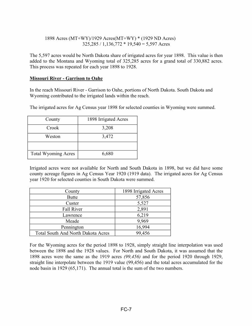
FC-7

1898 Acres (MT+WY)/1929 Acres(MT+WY) * (1929 ND Acres)

325,285 / 1,136,772 * 19,540 = 5,597 Acres

The 5,597 acres would be North Dakota share of irrigated acres for year 1898. This value is then added to the Montana and Wyoming total of 325,285 acres for a grand total of 330,882 acres. This process was repeated for each year 1898 to 1928. Missouri River - Garrison to Oahe In the reach Missouri River - Garrison to Oahe, portions of North Dakota. South Dakota and Wyoming contributed to the irrigated lands within the reach. The irrigated acres for Ag Census year 1898 for selected counties in Wyoming were summed.

County 1898 Irrigated Acres

Crook 3,208

Weston 3,472

Total Wyoming Acres 6,680

Irrigated acres were not available for North and South Dakota in 1898, but we did have some county acreage figures in Ag Census Year 1920 (1919 data). The irrigated acres for Ag Census year 1920 for selected counties in South Dakota were summed.

County 1898 Irrigated Acres Butte 57,856 Custer 5,527

Fall River 2,891 Lawrence 6,219

Meade 9,969 Pennington 16,994

Total South And North Dakota Acres 99,456 For the Wyoming acres for the period 1898 to 1928, simply straight line interpolation was used between the 1898 and the 1928 values. For North and South Dakota, it was assumed that the 1898 acres were the same as the 1919 acres (99,456) and for the period 1920 through 1929, straight line interpolate between the 1919 value (99,456) and the total acres accumulated for the node basin in 1929 (65,171). The annual total is the sum of the two numbers.

FC-8

Missouri River - Oahe to Big Bend The cumulative total of irrigated acres for year 1929 was 0 acres. Since there were no county irrigated acreage data for Ag Census years 1900 to 1930, it was assumed that there were no irrigation in this reach for the period 1898 to 1928. Missouri River - Big Bend to Ft Randall Irrigated acres for the period 1898 to 1928 in this node basin was assumed to be the same as was irrigated in year 1929. An annual figure of 8,609 acres was used for all years 1898 to 1928.

Missouri River - Ft Randall to Gavins Point Irrigated acres for the period 1898 to 1928 in this node basin was assumed to be the same as was irrigated in year 1929. An annual figure of 8,248 acres was used for all years 1898 to 1928.

Missouri River - Gavins Point to Sioux City The cumulative total of irrigated acres for year 1929 was 0 acres. Since there were no county irrigated acreage data for Ag Census years 1900 to 1930, it was assumed that there were no irrigation in this reach for the period 1898 to 1928.

Missouri River Sioux City to Omaha The cumulative total of irrigated acres for year 1929 was 0 acres. Since there were no county irrigated acreage data for Ag Census years 1900 to 1930, it was assumed that there were no irrigation in this reach for the period 1898 to 1928.

Missouri River - Omaha to Nebraska City Irrigated acres in the 1900 Ag Census were available for the State of Wyoming. Counties in the Platte River drainage included:

County 1898 Irrigated Acres Carbon 108,806 Natrona 17,601 Albany 104,260

Converse 18,015 Laramie 64,901

Total Wyoming Acres 313,583 Since Wyoming was the only state to provide 1900 Ag Census data, all other county data was assumed to be zero.

Missouri River - Nebraska City to St Joseph

FC-9

Irrigated acres for the period 1898 to 1928 was assumed to be zero for this reach. Missouri River - St. Joseph to Kansas City Irrigated acres for the period 1898 to 1928 was assumed to be zero for this reach. Kansas River Basin Irrigated acres for the period 1898 to 1928 was assumed to be zero for this reach. Missouri River - Kansas City to Boonville Irrigated acres for the period 1898 to 1928 was assumed to be zero for this reach. Osage River Basin Irrigated acres for the period 1898 to 1928 was assumed to be zero for this reach. Missouri River - Boonville to Hermann Irrigated acres for the period 1898 to 1928 was assumed to be zero for this reach. VI. Accumulation of County Irrigated Acres to Node Basin Irrigated Acres. U.S. Ag Census county data for the 1944, 1949, 1954, 1959, 1964, 1969, 1974 and 1978 Ag Census was used in the MBSA Hydrology Study. Yearly data for the period 1979 to 1982 was provided to the MBSA by the NRCS for all counties in the study area. In several cases, individually states had performed agriculture surveys in the 1970 s, thus resulting in better estimates and were used accordingly. The Missouri River basin was originally delineated into 93 node basins of interest where depletions would be calculated. A portion of the Upper Missouri was further broken down to evaluate depletions at smaller node basin boundaries, bringing the total number of node basins in the study to 118. Since all of the U.S. Ag Census is reported on a county wide basis, it was necessary to aggregate the county data into node basin data. In many cases, the irrigated acres within a county would need to be distributed into one or several different node basins, depending upon the geographical layout of the lands within the county. In addition, as acres became irrigated throughout the years, the distribution of acres to each node basin would change. In order to use the best and most current data available at the time, i.e., 1978 data, the MBSA Agricultural Work Group requested that each Soil Conservation Service District Conservationist provide their best estimate of irrigation use within their county. This information would include locations of irrigated lands, types of irrigation, confirmation of actual irrigated lands, efficiencies of conveyance and on-farm systems and crop distributions. Information packets were sent to each District and the following information was requested. Based upon the number of node basins represented within the county: 1. Verify the 1978 irrigated acre value for their county

FC-10

2. Determine the acreage value for each node basin in 1978. (See sample worksheet Number 1)

3. Determine a crop distribution for the acres within each node basin. (See sample worksheet Number 1)

4. Estimate the irrigation water source in percent for the periods 1944, 1964 and 1978. (See sample worksheet Number 2)

5. Determine type of irrigation and estimate the efficiency of that type of irrigation. (See sample worksheet Number 2)

This information was accumulated for all 493 counties within the Missouri River Basin. Worksheets were prepared for the 118 node basins that displayed the number of counties represented in each node, the percentage of irrigated lands found within that basin and the distribution of crops. In some cases, only one county or a portion of that county, was represented in the node basis, or in some cases in excess of 20 counties were inclusive within the node basin. Using the data, averages of crop distributions, efficiencies, and types of irrigation were calculated. Using the information provided by the District Conservationists in the MBSA study and the annual irrigation values established for each county, it was possible to accumulate node basin acreages for the node basins from the county data. A computer program, TOTAL4, was written to perform the task. Because of time constraints, it was not possible to collect new information for 1996 conditions, therefore it was assumed the percent distribution provided in the MBSA for year 1978 would be the same for all years in the study. The TOTAL4 program provides the following functions based upon the information provided by the NRCS: 1. Separates the county data into the node basin. During the MBSA study, the lower basin states provided information about distribution of county to the node basin throughout the study period. In other words, the percentage distribution in 1944 was different than it was in 1964 and 1978. The TOTAL4 program was modified to be able to redistribute this data throughout the study period in accordance with the data provided by the states. The upper basins states did not provide data of this sort. 2. Separates irrigation according to source of irrigation, surface water supply or groundwater supply. 3. Separates both the surface water acres and groundwater acres into types of irrigation. These types include furrow/border, full and partial; water-spreaders, full and partial; center pivot sprinklers, full and partial; and other sprinklers, full and partial. All of these categories were established in an attempt to analysis depletion estimates based upon different efficiencies for different types of irrigation.

FC-11

4. Sums all the individual county data together into the node basin. Since all of the information about irrigation types and uses were taken from data provided at only one point in time, 1978, it was necessary to logically evaluate the data and make adjustments that were reasonable for the times. For example, it is not realistic to assume that extensive groundwater pumping took place in the 1890 s and early 1900 s. Although some areas were probably irrigated from windmills, etc., the majority of the irrigation would be from surface gravity flow systems. Therefore, it was necessary to make adjustments to account for changes in irrigations practices. The program was modified to shift all acres from any type of sprinkler irrigation to gravity systems at a predesignated year. This year varies depending upon the node basin and the available data. The original purpose behind defining the types of irrigation was to improve the accuracy of the depletion estimates. It was assumed that each different type of system would have a unique efficiency, conveyance and on-farm, associated with it. However, the information provided by the District Conservationists indicated that there was not a significant difference in many of the irrigation systems. In order to avoid multiple consumptive use runs, irrigated acres, within the node basin, with the same or similar efficiencies were added together. In Montana, the state had performed actual field verification of irrigated acres at two time intervals, 1975 and 1987. In order to use their information, it was necessary to compare the data estimated by the U.S. Ag Census and the actual data provided by the state, determine the relative difference as a ratio and adjust the previous records accordingly. In this case, the Montan county data was first adjusted for the period 1929 to 1975 using the ratio of 1975 Actual data to 1975 Ag Census data and then again for the period 1976 to 1987 period using the ratio of 1987 actual data to 1987 Ag Census data. This ratio was used for the period 1987 to 1992 also. During the MBSA study, several states, North Dakota, South Dakota, Colorado, Missouri, and Nebraska, elected to use the Ag Census for the 1944 to 1974 period while providing their own county figures for the ensuing years. The following describes the data and years where actual data was used. These values were used in our analysis. Whenever possible, field verified data was used.

North Dakota 1974 to 1996 Data from State South Dakota 1970 to 1977 Data from the State

1978 to 1996 US Ag Census Colorado 1974 to 1978 Data form the State 1978 to 1996 US Ag Census Missouri 1974 to 1978 Data from the State 1978 to 1996 US Ag Census Nebraska 1974 to 1978 Data from the State 1978 to 1996 US Ag Census 1997 U. S Ag Census data was not available at the time of this study. Data for the period 1993 to 1996 was assumed to be the same as the 1992 data for each county.

FC-12

The biggest drawback of this process is the fact that, in most cases, a single value provided by the District Conservationist in 1978 was used throughout the entire period of record. This process would assume that if 50 percent of Gallatin County was contributing to the Madison River Basin in 1978, that 50 percent was also contributing in 1929 as well as in 1996. Historical records of land use within each county by drainage basin is unavailable and unknown, so for a lack of better information, an assumption was made to use the 1978 data for all years. As mentioned earlier, time constraints of this analysis did not allow for the investigations of more updated data as each node basin, so again the same figures were used for the 1978 to 1996 period. VII. Calculation of Irrigation Depletions In order to determine the effects of irrigation on a watershed, it is necessary to compute the crop irrigation requirement, the diversion requirement, and a return flow component of the irrigation. The difference between the diversion need and the return flow is the water loss, or depletion. This value is the sum of the crop use, the transmission losses, the non beneficial consumptive uses, and the return flow losses. A computer program to calculate the crop evapotranspiration was written for the MBSA study. Although several modifications have been made to the program, it is essential the same uses in this analysis. This program combines several programs and allows the user to select either the Blaney-Criddle methodology or the Jensen-Haise methodology to calculate crop consumptive use. Input requirement for these programs include monthly mean temperature, total monthly precipitation, monthly solar radiation, crop data, which includes plant dates, cover dates, and harvest dates. The results of this program is the crop irrigation requirement. The crop irrigation requirement is the amount of water needed in addition to natural precipitation in order to aid the crops to grow to maturity.

A. Climatological/Meteorological Data For each of the 118 node basins, a representative climatological station, or in some cases more than one, were selected based upon the relative location of the station within the node basin and the years of recorded data available at that station. All data was taken from National Weather Service recorded data. In the upper portion of the region, above Sioux City, missing data was filled in by using a station with data in the same general area. This was done for both temperature and precipitation data. In the lower portion of the region, below Sioux City, the Corps of Engineers provided complete records for the period 1898 to 1996 for all representative station in the node basins. In the Jensen-Haise consumptive use methodology, solar radiation is a required input item. The data is read in as percent of possible sunshine data. A subroutine program within the main program converts the percent of possible sunshine data into usable solar radiation data. Across the Missouri River Basin, there are only a few National Weather Service stations that record percent of possible sunshine data. Especially in the early years, 1898 to 1929, data was not

FC-13

available at some of the stations. In these cases, the average monthly percent of possible sunshine data for the 1929 to 1996 period was used for the 1898 to 1928 period. The percent of possible sunshine stations that were used included:

Helena WSO AP, Montana Cheyenne WSO AP, Wyoming Williston WSO AP, North Dakota Bismarck WSO AP, North Dakota Rapid City WSO AP, South Dakota Huron WSO AP, South Dakota Sioux City WSO AP (with Valentine), Nebraska Valentine WSO AP, Nebraska North Platte WSO AP, Nebraska Lincoln WSO AP, Nebraska Concordia WSO AP, Kansas

A complete listing of the climatological used for each node basin is included in Appendix A.

B. Crop Distribution Percentages Based upon the information received from the District Conservationists in the MBSA study, an average crop distribution percentage was calculated for each node basin. It was assumed that the cropping pattern would not change throughout the period of record since no other data was available. Although it is recognized that this assumption may lead to inaccuracies in the crop irrigation requirement over time, it is also known that major changes in the cropping patterns are necessary to significantly alter the monthly consumptive use requirements. Planting dates and harvest dates were taken from the NRCS s Crop Irrigation Guides and information accumulated in the MBSA study. Cover dates were determined based upon the planting date and information from the NRCS. Using the temperature, precipitation, and cropping data described above, the CONUSE5 program then calculates the crop irrigation requirement (CIR). The CIR is used as an input item in the DEPOPS subroutine of the program to calculate the following:

Diversion requirement in Acre-feet per acre Return flow requirement in Acre-feet per acre Depletion requirement in Acre-feet per acre

Additional input data is required, including conveyance and on-farm efficiencies, return flow distribution patterns, and non-beneficial consumptive use.~

FC-14

C. Conveyance and On-Farm Efficiencies (or losses) The conveyance system is that portion of the delivery system that provide water from the source of supply to the farm lateral. As the water moves through this system, inherent losses will take place, those being canal seepage, deep percolation, and evaporation. Data for each of the node basin was taken from estimates provided by the District Conservationists in the MBSA study. Conveyance losses were estimates for a variety of systems, i.e., open channel, pipe, or a combination of both. In addition, monthly losses were estimated to account for the early season build up of seepage in the canal prism, to minimal losses during the height of the irrigation season, to additional losses as they would occur at the end of the season to account for canal draw down and late season irrigations. The on-farm system is that portion of the delivery of the system that provides water from the farm delivery lateral to the farms and crops itself. Losses include deep percolation, operational waste, and in the case of sprinklers, wind drift and spray losses. Data for each of the node basin was taken from estimates provided by the District Conservationists in the MBSA study. Conveyance losses were estimates for a variety of systems, i.e., open channel, pipe, or a combination of both. Monthly losses were estimated to account for more efficient operation during the irrigation season.

D. Return Flow Distribution Patterns Irrigation water that is not consumptively used or lost in other ways is available to be returned to the river system and used again downstream. The return of this water is not instantaneous in many cases, and may require several months to work it way back to the river. In this study, it was assumed that all return flows would occur within the node basin of the diversion. Hydrogeologists from the Montana Department of Natural Resources and Conservation provided estimates of return flow patterns for all node basins in the reach above Ft Peck Reservoir. This was done for a joint study between Reclamation and the State in 1989. For the rest of the node basins, a representative pattern was used based upon information used in the MBSA study. The return flows are broken into two portions. It is assumed that a portion of the diversion will return immediately in the same month of the diversion. The remaining portion is then lagged throughout a 12-month period at a rate established as an input item. Return flow values at accumulated throughout the year for the entire period of record. For example, assume that of the diverted amount in July of this irrigation season, 1.0 acre-foot is available for return in the month of the diversion. Assume the following return flow pattern.

FC-15

Available return flow in diversion month 60% Month one following diversion 50% Month two following diversion 15% Month three following diversion 13% Month four following diversion 8% Month five following diversion 4% Month six following diversion 3%

Month seven following diversion 2% Month eight following diversion 1% Month nine following diversion 1% Month ten following diversion 1%

Month eleven following diversion 1% Month twelve following diversion 1%

Based upon an example of an available return flow of 1.0 acre-foot for July, the return flow would be lagged in the following pattern.

Month Available Return Flow (in acre-feet) July .60

August .20(50% of the remaining 40%) September .06(15% of the remaining 40%)

October .05 (13% of the remaining 40%) November .03 (8% of the remaining 40%) December .02(4% of the remaining 40%) January .01 (3% of the remaining 40%) February .01 (2% of the remaining 40%) March .01 (1% of the remaining 40%) April .01 (1% of the remaining 40%) May .00 (1% of the remaining 40%) June .00 (1% of the remaining 40%) July .00 (1% of the remaining 40%)

E. Non-Beneficial Consumptive Use Non-beneficial consumptive use is a loss that occur within the irrigation system. It is primarily weeds, trees and other vegetation that grows along canals, ditches, return flow ditches and waste ditches and uses water that would normally be returned to the stream as return flow. The available return is adjusted to account for these losses. Although accurate figures are very difficult to measure and studies on these water losses in this area have not been done, a common values that is used is 15 to 20%. In this study, the non-beneficial consumptive use value of 20 % for both conveyance and on-farm losses was used for all the node basins.

FC-16

VIII. Calculation of the Historic Depletions Using the monthly diversion, return flow and depletion figures calculated from the process mentioned above, the monthly and annual historic depletion are calculated by applying the annual irrigated acres to the monthly depletion number. Of primary concern is the historical depletions. The irrigated acres, taken from the TOTAL 4 program, are multiplied by the monthly depletions value to determine the monthly depletion. The program also computes historic diversion and historic return flows. As mentioned earlier, in each node basin, several consumptive runs may have been made to account for the different type of irrigation that was taking place within that basin. The CONUSE5 program will make multiple runs and combine all of the total historical depletions into one monthly value for the period of record. Adding the historical irrigation depletions and other depletions identified below to the historic streamflow will represent an estimate of potential natural or virgin flow within the node basin. Graphs of estimated historic total depletions (irrigation + major reservoir + other depletions) are shown in Appendix B. IX. Calculation of the Present-Level Depletions The concept of present level depletions is defined as the impact that today’s development would have on the development of any past year. For example, how would the irrigation development of today effect the development in 1935 assuming 1935 climatological conditions? How much additional depletion would take place? Present-level irrigation depletions are calculated the same way as historical depletions, with the exception that the irrigated acres for all years from 1898 thru 1996 were the same as the number of acres irrigated in 1996. The resultant depletions can then be applied to the historic natural flow record to get present-level depleted streamflows. A typical example of the determination of the present-level depletion would be:

Assume: 1929 Irrigated acres for node basin X is 10,000 Acres 1996 Irrigated acres for node basin X is 25,000 Acres

July, 1929 Irrigation Depletion for July is .87 acre-feet per acre (Depletion is diversion minus return flow)

1996 Effect on July 1929 would be 25,000 times .87 equals 21,750 Acre-feet

This means that had 25,000 acres of irrigation been in place in a climatological year such as July, of 1929 that the depletion for that month would have bee 21,750 acre-feet. Historically, only 8,700 acre-feet of depletion took place. (10,000 acres times .87 acre-feet pe acre)

FC-17

As mentioned previously, there are many other depletions that affect the streamflow in the basin. The following sections describe the methodology used to project these other depletions to the historic and present level. X. Historic Depletions Due to Irrigation by Ground Water Large capacity wells located near streams can reduce streamflow significantly by reducing aquifer discharge to streams or by inducing flow out of the stream. Factors controlling the degree of depletions include, but are not limited to, the hydraulic connection between the aquifer and stream, distance of well from stream, quantity and duration of water pumped. Time and financial constraints did not allow for the collection of data to calculate those depletions. The U.S. Agricultural Census data does not differentiate between ground water and surface water irrigated acreage, it is all lumped to one annual value. Because of these constraints, assumptions were drawn from the MBSA study which looked into and utilized simplified methods for estimating ground water depletions. In general, the Kansas and Platte river basins have much more extensive well development than other basins because of the occurrence aquifer systems of large areal extent. For the present study, it was assumed that for all drainage basins other than the Kansas and Platte River basins, any irrigation wells in those basins are located in narrow river valley alluvial channels. Most of the water pumped by the wells is essentially assumed to be coming from the streams. With those assumptions, ground water irrigated acreage was assumed to be the same as surface-water acreage using sprinkler system efficiencies. Therefore, ground water depletions for basins other than the Kansas and Platte are inclusive of the surface-water depletion calculations described in previous sections. The Kansas and Platte river basins have a large number of irrigated acres supplied by wells completed in aquifers that have minimal hydraulic connections with streams, or are located quite distant from perennial streams. Generally, the further a well is from a stream, the less impact it will have on stream flows. For the present study, net ground water usage was approximated using ground water irrigated acreage estimated from U.S. Agriculture Census data. Again, since the Ag Census data does not differentiate between surface and ground water irrigated acreage, it was assumed for the Platte and Kansas basins that all acreage using sprinklers was the same as ground water acreage. Sprinkler acreage was defined using percentages of total irrigated acreage. Those percentages were taken from the MBSA study for each node basin. The ground water acreage (sprinkler acres) was input to the CONUSE5 program to estimate net aquifer withdrawals. These are ‘net’ withdrawals since the CONUSE5 program takes into account return flows. Although the return flows are originally intended to be returning to a stream, we are assuming that the return flows are returning in a similar fashion to the aquifer. Although we now have estimated net withdrawals, we do not have any information on where the ground-water irrigated acreage is located, and how far that acreage is from a stream. A procedure needed to be developed to adjust the ground water usage output by CONUSE5 to

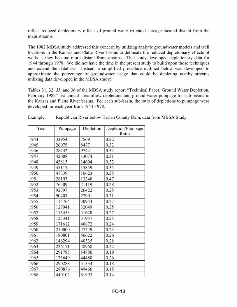
FC-18

reflect reduced depletionary effects of ground water irrigated acreage located distant from the main streams. The 1982 MBSA study addressed this concern by utilizing analytic groundwater models and well locations in the Kansas and Platte River basins to delineate the reduced depletionary effects of wells as they became more distant from streams. That study developed depletionary data for 1944 through 1978. We did not have the time in the present study to build upon those techniques and extend the database. Instead, a simplified procedure outlined below was developed to approximate the percentage of groundwater usage that could be depleting nearby streams utilizing data developed in the MBSA study: Tables 31, 32, 35, and 36 of the MBSA study report “Technical Paper, Ground Water Depletion, February 1982” list annual streamflow depletions and ground water pumpage for sub-basins in the Kansas and Platte River basins. For each sub-basin, the ratio of depletions to pumpage were developed for each year from 1944-1978. Example: Republican River below Harlan County Dam, data from MBSA Study

Year Pumpage Depletion Depletion/PumpageRatio

1944 33954 7569 0.22 1945 26075 8477 0.33 1946 28742 9744 0.34 1947 42688 13074 0.31 1948 43815 14604 0.33 1949 45117 15859 0.35 1950 47339 16623 0.35 1951 28197 13240 0.47 1952 76509 21119 0.28 1953 92797 26422 0.28 1954 90407 27901 0.31 1955 114764 30944 0.27 1956 127941 32049 0.25 1957 115453 31620 0.27 1958 125341 31957 0.25 1959 171612 40872 0.24 1960 210000 47449 0.23 1961 180801 46622 0.26 1962 146294 40335 0.28 1963 226171 48968 0.22 1964 291785 54886 0.19 1965 173649 44480 0.26 1966 290288 51334 0.18 1967 280876 49466 0.18 1968 440102 61993 0.14

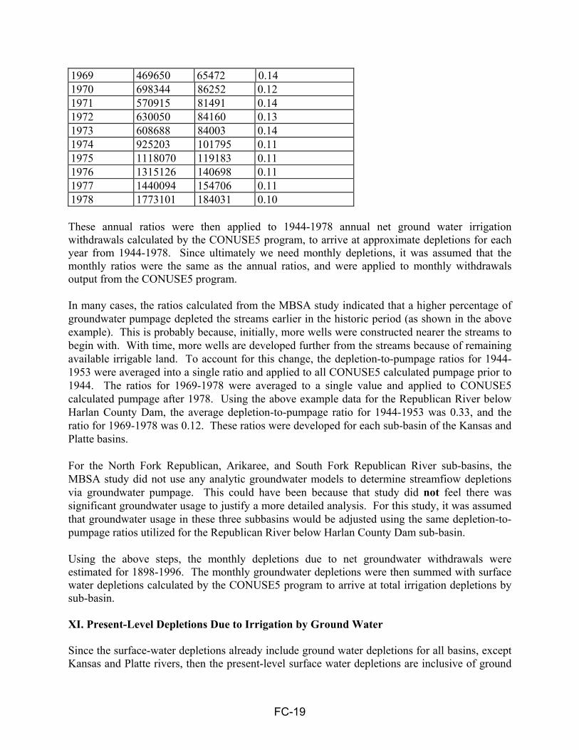
FC-19

1969 469650 65472 0.14 1970 698344 86252 0.12 1971 570915 81491 0.14 1972 630050 84160 0.13 1973 608688 84003 0.14 1974 925203 101795 0.11 1975 1118070 119183 0.11 1976 1315126 140698 0.11 1977 1440094 154706 0.11 1978 1773101 184031 0.10 These annual ratios were then applied to 1944-1978 annual net ground water irrigation withdrawals calculated by the CONUSE5 program, to arrive at approximate depletions for each year from 1944-1978. Since ultimately we need monthly depletions, it was assumed that the monthly ratios were the same as the annual ratios, and were applied to monthly withdrawals output from the CONUSE5 program. In many cases, the ratios calculated from the MBSA study indicated that a higher percentage of groundwater pumpage depleted the streams earlier in the historic period (as shown in the above example). This is probably because, initially, more wells were constructed nearer the streams to begin with. With time, more wells are developed further from the streams because of remaining available irrigable land. To account for this change, the depletion-to-pumpage ratios for 1944-1953 were averaged into a single ratio and applied to all CONUSE5 calculated pumpage prior to 1944. The ratios for 1969-1978 were averaged to a single value and applied to CONUSE5 calculated pumpage after 1978. Using the above example data for the Republican River below Harlan County Dam, the average depletion-to-pumpage ratio for 1944-1953 was 0.33, and the ratio for 1969-1978 was 0.12. These ratios were developed for each sub-basin of the Kansas and Platte basins. For the North Fork Republican, Arikaree, and South Fork Republican River sub-basins, the MBSA study did not use any analytic groundwater models to determine streamfiow depletions via groundwater pumpage. This could have been because that study did not feel there was significant groundwater usage to justify a more detailed analysis. For this study, it was assumed that groundwater usage in these three subbasins would be adjusted using the same depletion-to-pumpage ratios utilized for the Republican River below Harlan County Dam sub-basin. Using the above steps, the monthly depletions due to net groundwater withdrawals were estimated for 1898-1996. The monthly groundwater depletions were then summed with surface water depletions calculated by the CONUSE5 program to arrive at total irrigation depletions by sub-basin. XI. Present-Level Depletions Due to Irrigation by Ground Water Since the surface-water depletions already include ground water depletions for all basins, except Kansas and Platte rivers, then the present-level surface water depletions are inclusive of ground

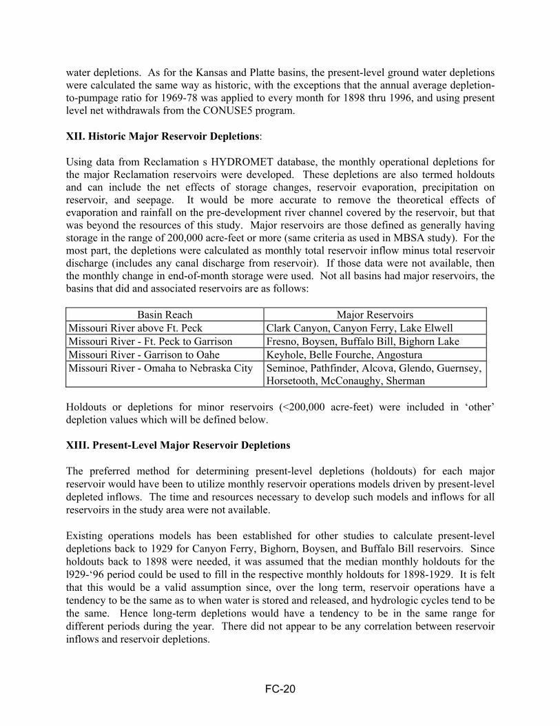
FC-20

water depletions. As for the Kansas and Platte basins, the present-level ground water depletions were calculated the same way as historic, with the exceptions that the annual average depletion-to-pumpage ratio for 1969-78 was applied to every month for 1898 thru 1996, and using present level net withdrawals from the CONUSE5 program. XII. Historic Major Reservoir Depletions: Using data from Reclamation s HYDROMET database, the monthly operational depletions for the major Reclamation reservoirs were developed. These depletions are also termed holdouts and can include the net effects of storage changes, reservoir evaporation, precipitation on reservoir, and seepage. It would be more accurate to remove the theoretical effects of evaporation and rainfall on the pre-development river channel covered by the reservoir, but that was beyond the resources of this study. Major reservoirs are those defined as generally having storage in the range of 200,000 acre-feet or more (same criteria as used in MBSA study). For the most part, the depletions were calculated as monthly total reservoir inflow minus total reservoir discharge (includes any canal discharge from reservoir). If those data were not available, then the monthly change in end-of-month storage were used. Not all basins had major reservoirs, the basins that did and associated reservoirs are as follows:

Basin Reach Major Reservoirs Missouri River above Ft. Peck Clark Canyon, Canyon Ferry, Lake Elwell Missouri River - Ft. Peck to Garrison Fresno, Boysen, Buffalo Bill, Bighorn Lake Missouri River - Garrison to Oahe Keyhole, Belle Fourche, Angostura Missouri River - Omaha to Nebraska City Seminoe, Pathfinder, Alcova, Glendo, Guernsey,

Horsetooth, McConaughy, Sherman Holdouts or depletions for minor reservoirs (<200,000 acre-feet) were included in ‘other’ depletion values which will be defined below. XIII. Present-Level Major Reservoir Depletions The preferred method for determining present-level depletions (holdouts) for each major reservoir would have been to utilize monthly reservoir operations models driven by present-level depleted inflows. The time and resources necessary to develop such models and inflows for all reservoirs in the study area were not available. Existing operations models has been established for other studies to calculate present-level depletions back to 1929 for Canyon Ferry, Bighorn, Boysen, and Buffalo Bill reservoirs. Since holdouts back to 1898 were needed, it was assumed that the median monthly holdouts for the l929-‘96 period could be used to fill in the respective monthly holdouts for 1898-1929. It is felt that this would be a valid assumption since, over the long term, reservoir operations have a tendency to be the same as to when water is stored and released, and hydrologic cycles tend to be the same. Hence long-term depletions would have a tendency to be in the same range for different periods during the year. There did not appear to be any correlation between reservoir inflows and reservoir depletions.

FC-21

For the remainder of the major reservoirs where we did not have models, historic holdouts were used to represent present-level, and used the median monthly historic holdouts for years prior to historic data. Validity in using those procedures was based on comparisons of historic and present-level holdouts for Canyon Ferry. Those comparisons did not suggest a large difference between the two conditions. In addition, the difference is a small percentage of overall depletions (inclusive of irrigation depletions) in the basins and therefore would have minimal impact on total depletions. For example, in the basin reach above Ft. Peck reservoir, the ratio of annual historic reservoir depletions to total depletions for 1953 to 1996 averaged about 2 percent. For the Platte River basin, ratio of annual historic reservoir depletions to total depletions for 1910 to 1996 averaged about 3 percent. Because historic holdouts are usually large when a reservoir initially fills, the historic holdouts during the first year the reservoir filled were not used to represent present-level conditions. Following is an explanation of how present-level holdouts were estimated for each major reservoir:

Missouri Basin above Ft. Peck: Clark Canyon Reservoir: 1965-1996 are historic holdouts, 1898-1964 are monthly median historic holdouts. Canyon Ferry Reservoir: 1929-1996 are present-level holdouts, 1898-1928 are monthly median of the present-level holdouts. Lake Elwell: 1957-1996 are historic holdouts, 1898-1956 are monthly median historic holdouts.

Ft. Peck to Garrison: Fresno Reservoir: 1940-1996 are historic holdouts, 1898-1939 are monthly median historic holdouts. Boysen Reservoir: Used 1990-level depletion study and 1988-1996 historic holdouts for the period 1929-1996, 1898-1928 are monthly median historic holdouts. Buffalo Bill Reservoir: 1914-1996 are historic holdouts, 1898-1913 are monthly median historic holdouts. Bighorn Reservoir: Used 1990-level depletion study and 1988-1996 historic holdouts for the period 1929-1996, 1898-1928 are monthly median historic holdouts.

Garrison to Oahe: Keyhole Reservoir: 1953-1996 are historic holdouts, 1898-1952 are monthly median historic holdouts.

FC-22

Belle Fourche Reservoir: 1952-1996 are historic holdouts, 1898-1951 are monthly median historic holdouts. Angostura Reservoir: 1953-1996 are historic holdouts, 1898-1952 are monthly median historic holdouts.

Oahe to Big Bend: No major reservoirs.

Big Bend to Fort Randall: No major reservoirs.

Fort Randall to Gavins Point: No major reservoirs.

Gavins Point to Sioux City: No major reservoirs.

Sioux City to Omaha: No major reservoirs.

Omaha to Nebraska City: Seminoe Reservoir: 1940-1996 are historic holdouts, 1898-1939 are monthly median historic holdouts. Pathfinder Reservoir: 1911-19.96 are historic holdouts, 1898-19 10 are monthly median historic holdouts. Alcova Reservoir: 1946-1996 are historic holdouts, 1898-1945 are monthly median historic holdouts. Glendo Reservoir: 1958-1996 are historic holdouts, 1898-1957 are monthly median historic holdouts. Guernsey Reservoir: 1929-1996 are historic holdouts, 1898-1928 are monthly median historic holdouts. Horsetooth Reservoir: 1953-1996 are historic holdouts, 1898-1952 are monthly median historic holdouts.

FC-23

McConaughy Reservoir: 1942-1996 are historic holdouts, 1898-1941 are monthly median historic holdouts. Sherman Reservoir: 1964-1996 are historic holdouts, 1898-1963 are monthly median historic holdouts.

Remainder of basins:

COE did not want major reservoir holdouts included in present-level depletions. XIV. Historic ‘Other Depletions Other depletions include the effects of conservation tillage practices, farm ponds, small reservoirs 1 (those less than 200,000 acre-feet normal storage), livestock, municipal, energy, industrial, and rural domestic uses. The MBSA study had compiled annual depletion data for 1944 -1978 for each usage category by sub-basin. This data had been collected by field personal from each state and is summarized for each major basin in the MBSA study report “Missouri River Basin Hydrology Study Final Report, May 1983”. Data is also listed in computer printouts for each sub-basin by year. Apparently for the MBSA study, small reservoir depletions were developed using an average reservoir surface area and a net evaporation value. For the eastern Missouri basins, that net evaporation value is sometimes negative because of higher precipitation than evaporation. This results in negative reservoir depletions that are accruals to streamflow. It would have been desirable for the present study to add to the existing database. However, to collect and compile similar data for the present study for 1898-1943 and 1979-1996 would be difficult and time consuming to do. It is doubtful any detailed early years data can be found. One potential source of data is USGS estimated use of water in the United States. The USGS has been compiling that data on approximate five year intervals from 1950 to present. However, their data is presented as water withdrawals and consumptive use, as they don t directly calculate depletions to streamflow. The USGS data also did not evaluate depletion effects from farm ponds and soil conservation practices, which can be significant. Also their, database doesn’t help with the need for data prior to 1944. Simplified procedures were needed to estimate the other depletions for the present study. Methods selected to estimate other depletions include using a percentage of irrigation depletions and using MBSA data for the time period it covered, and to define the trend of other depletions for extended years. In some instances, the USGS estimated water use data were used to quantify relationships between consumed water for other uses and consumed irrigation water. Following is a breakdown of how historic other depletions were developed by basin reach. Also note that the estimated annual depletion was distributed evenly to all 12 months of the year.

FC-24

All Reaches above Gavins Point:

Based on MBSA other depletions, the river basins above Gavins Point generally had other depletions that were about 7 percent of the irrigation depletions. Therefore, for all basins above Gavins Point, the other depletions were calculated as 7 percent of annual irrigation depletions.

Missouri River - Gavins Point to Sioux City:

Since the population density was felt to increase significantly in this reach, it was felt that using 7 percent of irrigation depletions to represent other depletions may not be valid, and a new method was developed to estimate what the percentage of other depletions to irrigation depletions would be. Depletions from other uses was calculated as 15 percent of annual irrigation depletion. This percentage was determined from USGS estimated water use data for 1985 and 1990. For the two sub-basins in this reach, the USGS water-use categories for total-irrigation consumptive use and total-all-water consumptive use were subtracted, with remainder assumed to be consumed other-water. Ratio of consumed other-water to irrigation consumed was established, and the average for two time periods was calculated to be 15 percent.

Missouri River - Sioux City to Omaha:

In this reach, depletions from other uses is much greater than irrigation depletions. A review of 1985 and 1990 USGS water use data for Blackbird and Soldier drainage basins showed an average ratio of 205% for ‘other consumed water versus irrigation consumed water (total consumed water minus irrigation consumed divided by irrigation consumed). A review of 1978 annual ‘other depletions compared to irrigation depletions from the MBSA study showed a ratio of 67% for the two node basins in this reach. From the MBSA study, depletions in 1944 showed ‘other’ depletions, but no irrigation depletions. Because there are no irrigation depletions in the earlier years, it became apparent that using a percentage relationship between ‘other’ and irrigation depletions would not work for earlier years. Therefore, the annual ‘other’ depletion data for 1944 to 1978 from the MBSA was used as the ‘other depletions for this reach. It was assumed that depletions from 1978 to present would be the same as year 1978 from the MBSA study. Due to the lack of usage data for earlier year, it was assumed that ‘other’ depletions in 1898 were the same as the 1944 MBSA livestock depletions and would ramp up linearly from 1898 to the 1944 MBSA ‘other’ depletion. Use of 1944 livestock depletions to represent 1898 total other depletions is a very arbitrary decision. It was felt that there had to be some water being consumed in 1898, but depletions from municipalities, reservoirs, industry, conservation practices, etc. were probably very small. It was assumed that livestock would have been one of the more significant other depletions during the earlier years.

Missouri River - Omaha to Nebraska City

Selected other depletion data for 1944, 1960, and 1978 from the MBSA study (final summary report) were used to establish a ratio of other depletion to irrigation depletions for those same years. Ratios were linearly ramped between those years to get additional ratios.

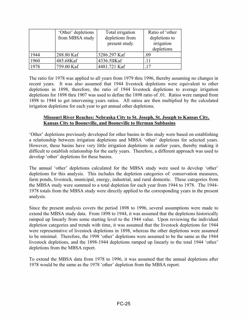
FC-25

‘Other’ depletions from MBSA study

Total irrigation depletions from present study

Ratio of ‘other depletions to

irrigation depletions

1944 288.80 Kaf 3286.297 Kaf .09 1960 485.68Kaf 4336.5lIKaf .11 1978 759.00 Kaf 4481.721 Kaf .17 The ratio for 1978 was applied to all years from 1979 thru 1996, thereby assuming no changes in recent years. It was also assumed that 1944 livestock depletions were equivalent to other depletions in 1898, therefore, the ratio of 1944 livestock depletions to average irrigation depletions for 1898 thru 1907 was used to define the 1898 ratio of .01. Ratios were ramped from 1898 to 1944 to get intervening years ratios. All ratios are then multiplied by the calculated irrigation depletions for each year to get annual other depletions.

Missouri River Reaches: Nebraska City to St. Joseph, St. Joseph to Kansas City, Kansas City to Booneville, and Booneville to Herman Subbasins

‘Other’ depletions previously developed for other basins in this study were based on establishing a relationship between irrigation depletions and MBSA ‘other’ depletions for selected years. However, these basins have very little irrigation depletions in earlier years, thereby making it difficult to establish relationship for the early years. Therefore, a different approach was used to develop ‘other’ depletions for these basins. The annual ‘other’ depletions calculated for the MBSA study were used to develop ‘other’ depletions for this analysis. This includes the depletion categories of: conservation measures, farm ponds, livestock, municipal, energy, industrial, and rural domestic. These categories from the MBSA study were summed to a total depletion for each year from 1944 to 1978. The 1944-1978 totals from the MBSA study were directly applied to the corresponding years in the present analysis. Since the present analysis covers the period 1898 to 1996, several assumptions were made to extend the MBSA study data. From 1898 to 1944, it was assumed that the depletions historically ramped up linearly from some starting level to the 1944 value. Upon reviewing the individual depletion categories and trends with time, it was assumed that the livestock depletions for 1944 were representative of livestock depletions in 1898, whereas the other depletions were assumed to be minimal. Therefore, the 1998 ‘other’ depletions were assumed to be the same as the 1944 livestock depletions, and the 1898-1944 depletions ramped up linearly to the total 1944 ‘other’ depletions from the MBSA report. To extend the MBSA data from 1978 to 1996, it was assumed that the annual depletions after 1978 would be the same as the 1978 ‘other’ depletion from the MBSA report.

FC-26

Kansas and Osage River Basins Annual other depletions were estimated by sub-basin using MBSA data (data from computer printouts for each sub-basin). All other usage categories were summed to a total value for each year for 1944 to 1978. Other depletion for 1898 was assumed to be same as 1944 livestock depletion from MBSA study. Values were then linearly ramped from 1898 to 1944. 1979 and later were assumed to be same as 1978. XV. Present-Level ‘Other Depletions Based on a conversation with COE, the ‘other depletion ratio of 7% of irrigation depletions used for historic depletion estimates in the upper Missouri River basin was lowered to 5%. The COE felt that it would be better to err on the low side of depletions for present-level conditions. Therefore, an ‘other’ depletion ratio of 5 percent was used for all Missouri basin reaches above Gavins Point. Below Gavins Point, the influence of larger population centers, which have higher municipal and industrial depletions, required that different ‘other’ depletion ratios were needed versus what was used above Gavins Point. Following are those ratios selected by reach: Gavins Point to Sioux City: A 15% ratio of ‘other’ to irrigation depletions was used for historic depletions. That ratio was based on 1985 and 1990 USGS water-use compilations of sub-basins in this reach. Following the COE’s request to use 5% vs. 7% in basins above Gavins Point for present-level depletions, it was decided to use a present-level ‘other’ depletion ratio of 11% (5/7ths of 15%) for this reach. Sioux City to Omaha: A review of 1985 and 1990 USGS water use data for Blackbird and Soldier drainages showed an average ratio of 205% for ‘other’ consumed water versus irrigation consumed water (total consumed water minus irrigation consumed divided by irrigation consumed). A review of 1978 annual ‘other’ depletions compared to irrigation depletions from the MBSA study showed a ratio of 67% for the two node basins in this reach. It was decided to use the MBSA derived ration of 67% of irrigation depletions to represent annual ‘other’ depletions for present-level conditions. Omaha to Nebraska City: A review of 1978 total ‘other’ and irrigation depletions fro the Platte-Niobrara basin from the MBSA study indicated that the ratio of ‘other’ to irrigation depletions is 176%. A review of 1985 and 1990 USGS water use data fro sub-major hydrologic units of 1018, 1019, 1020, 1021, and 1022 suggested that the average ration of other-consumed water to irrigation consumed water is about 6%. It was arbitrarily decided to use 6% as a present-level ration of ‘other’ depletions to irrigation depletions.

FC-27

Remainder of Missouri Reaches: COE did not want ‘other’ depletions to be included in basins below Nebraska City for present-level depletions. Therefore, no present-level other depletions estimates were made. XVI. Other Impacts to Streamflow There were other factors which alter streamflow from natural conditions or impact natural flow calculations but were not addressed in this study because of time and funding constraints;

Inter-basin transfers of water.

If historic natural flows are to be calculated by adding historic depletions to recorded streamflow, then there may be an additional seepage and evaporation losses from having more water in the stream. Those additional seepage losses were not determined.

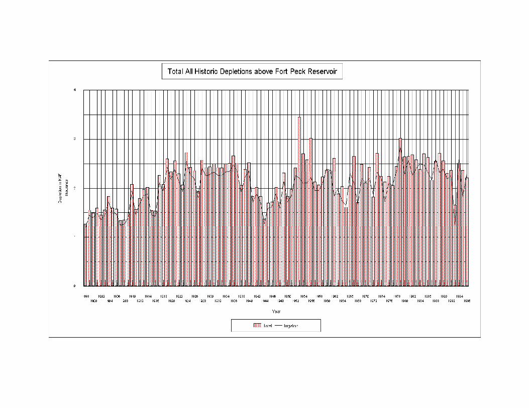
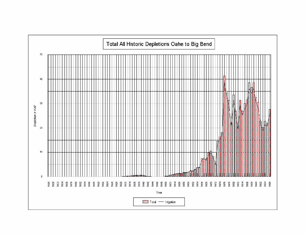
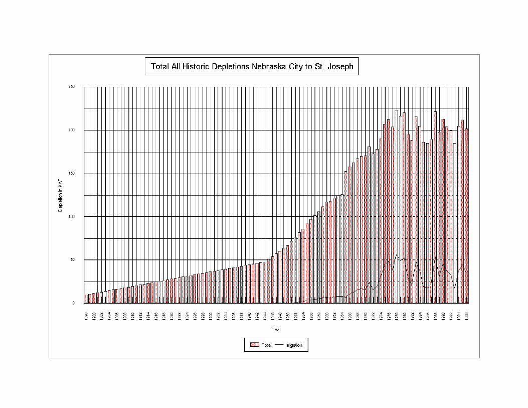
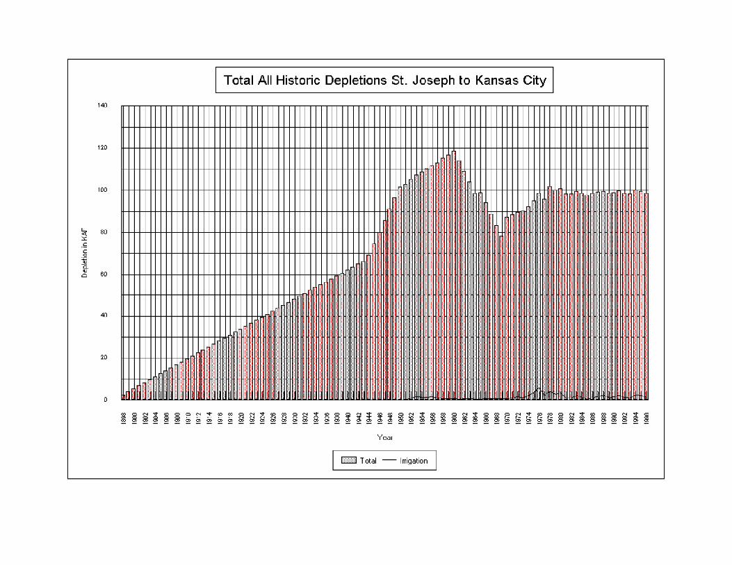
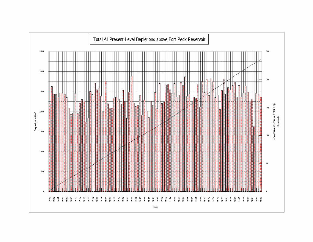
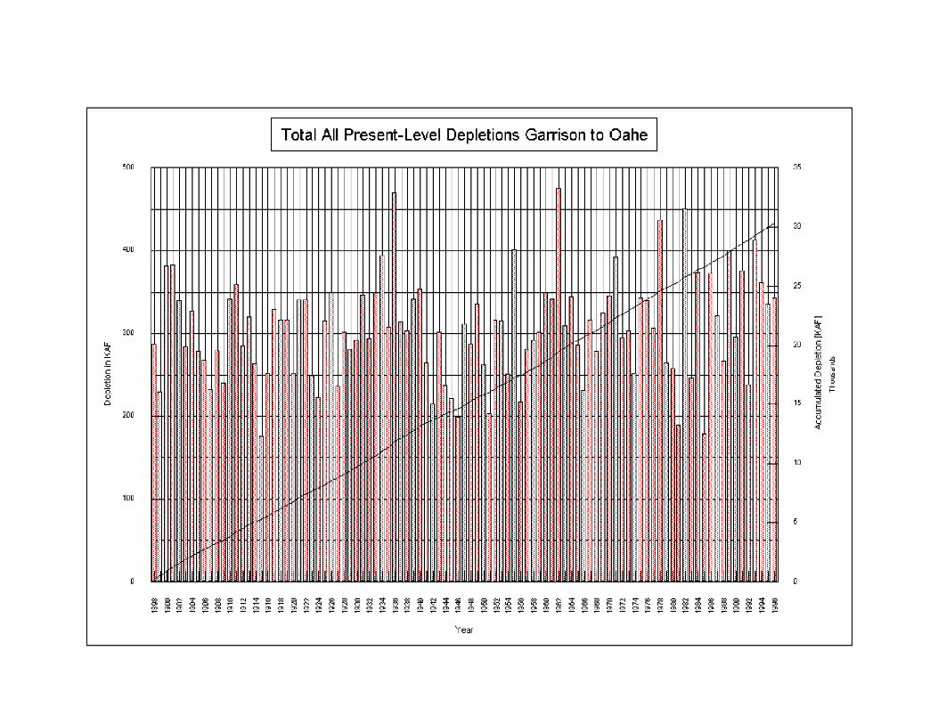
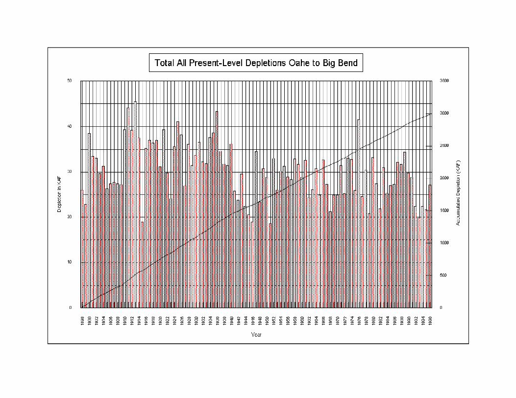
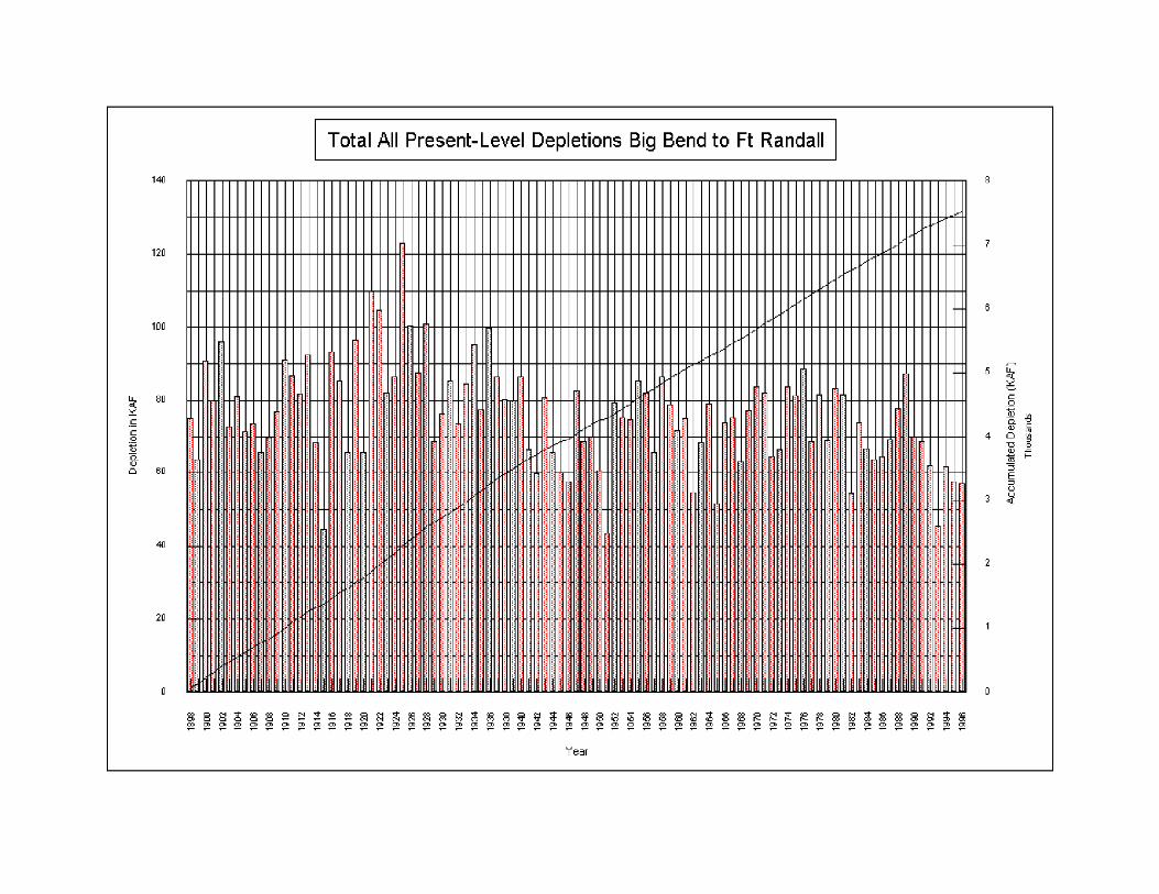
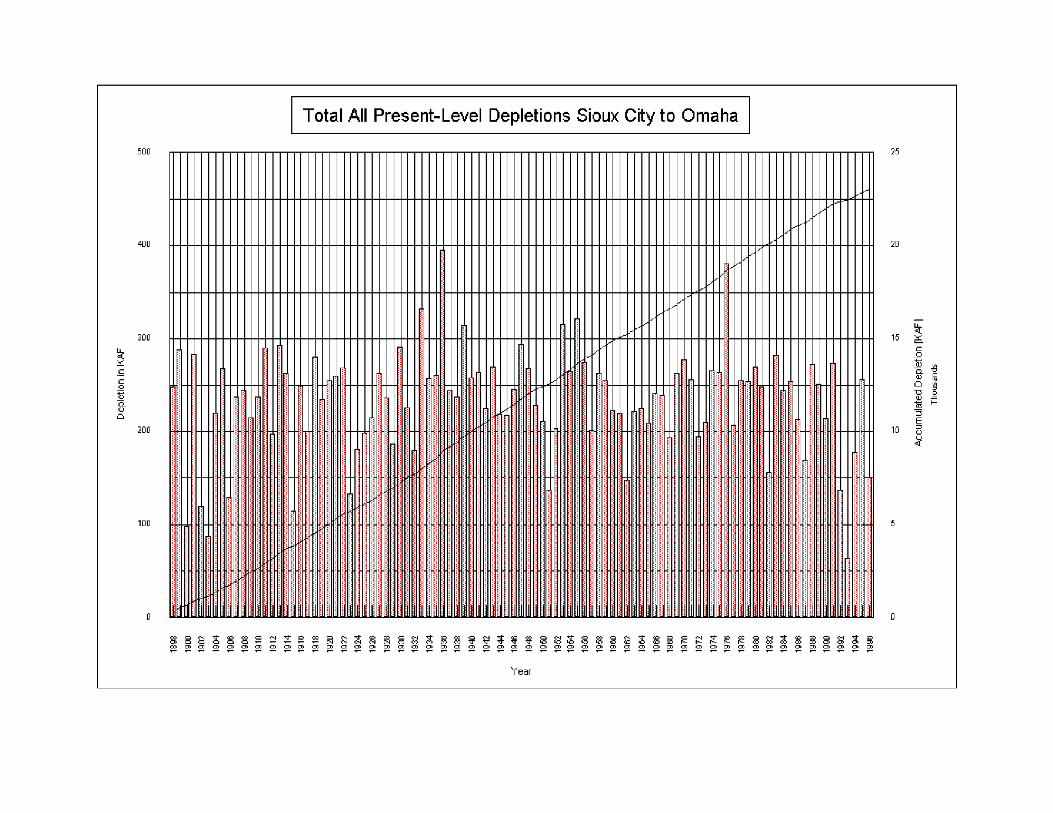
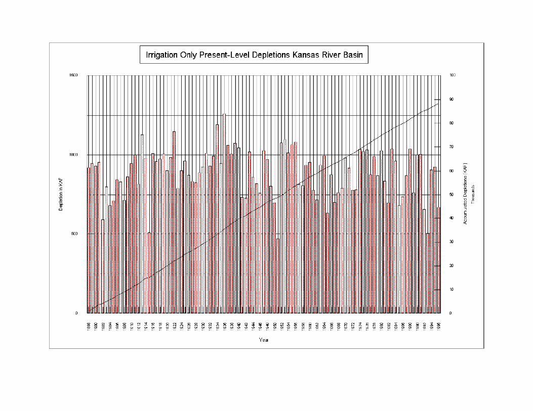
FD-1


Appendix F-D

Auxiliary Programs Developed for Use in Data Processes Executable Programs – Unless otherwise noted, all executable programs were compiled with Microsoft Fortran

PowerStation Version 4.0.

converter.exe – Program takes data from USBR (in format as submitted) at each reservoir location and converts it into format that will be readable by creator.exe. Program prompts user for input file name, output file name, type of data (inflow, outflow, storage, or elevation), and the 4-letter code for the reservoir. Input data is by water year and must be converted to calendar year.

creator.exe – Program that creates one or more years of input data for the UFDM model (starting with

reservoir and station data) using files created by DSSconvert.exe or converter.exe. Program prompts user whether one or multiple years of data files are desired to be created, what year(s), and whether or not reach inflow data is to be built into the input files. The program then goes station by station prompting the user for: the name of the input file for flows (gage stations only); whether reservoir records are based on records of inflow and outflow, storage, or both; whether reach inflow records at each mainstem reservoir are to be included (if user previously answered yes); and whether the reservoir should have precipitation and evaporation records built into the input file. The program automatically creates a file named HOLDxxxx.in1, where xxxx stands for the year of each file.

DSSconvert.exe – Program takes data from DSS format and converts it to format readable by creator.exe.

As written, the data must first be written to a text file from DSSUTL using the WR.T command, but the program could be modified to read directly from a DSS file. Program prompts user for the desired station, the type of data being input, the beginning date of data, as well as the ending year for data. The program automatically names the output file based on station name and type of data.

evap.exe – Program reads climate data (evaporation) and computes monthly evaporation. Missing daily

data is filled in from monthly average values supplied by user. freq.exe - This program will read in a file, freqhold.in, containing years and the names of files created with

DSSMATH macros (see maxYYYY.txt below) that have the maximum unregulated flow values for each gaging station below Gavins Point for each year as determined using UFDM. The program then outputs the maximum flow values in a text-format file (can be imported into EXCEL).

freqreg.exe - This program will read in a file, freqreg.in, containing the names of files created with

DSSMATH macros (see regYYYY.txt) that have the maximum regulated flow values for each gaging station below Gavins Point for each year. The program then outputs the maximum flow values in a text-format file (can be imported into EXCEL). The program is very similar to freq.exe, except for the number of stations that are processed.

janstore.exe - This program will read in a file, janstore.in, containing the names of files created with

DSSMATH macros (see storjan.bat) that have storage values for each reservoir project on January 1 of each year. The program will then output the storage values in a format for the UFDM program.

mixtest.exe – Program developed by HEC to take results from two populations of flow data and combine

into one final frequency curve. Unknown compiler.

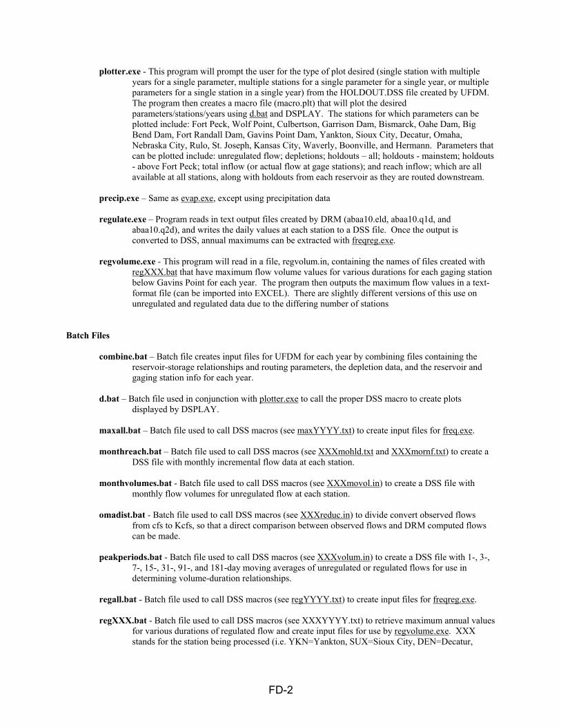
FD-2

plotter.exe - This program will prompt the user for the type of plot desired (single station with multiple years for a single parameter, multiple stations for a single parameter for a single year, or multiple parameters for a single station in a single year) from the HOLDOUT.DSS file created by UFDM. The program then creates a macro file (macro.plt) that will plot the desired parameters/stations/years using d.bat and DSPLAY. The stations for which parameters can be plotted include: Fort Peck, Wolf Point, Culbertson, Garrison Dam, Bismarck, Oahe Dam, Big Bend Dam, Fort Randall Dam, Gavins Point Dam, Yankton, Sioux City, Decatur, Omaha, Nebraska City, Rulo, St. Joseph, Kansas City, Waverly, Boonville, and Hermann. Parameters that can be plotted include: unregulated flow; depletions; holdouts – all; holdouts - mainstem; holdouts - above Fort Peck; total inflow (or actual flow at gage stations); and reach inflow; which are all available at all stations, along with holdouts from each reservoir as they are routed downstream.

precip.exe – Same as evap.exe, except using precipitation data regulate.exe – Program reads in text output files created by DRM (abaa10.eld, abaa10.q1d, and

abaa10.q2d), and writes the daily values at each station to a DSS file. Once the output is converted to DSS, annual maximums can be extracted with freqreg.exe.

regvolume.exe - This program will read in a file, regvolum.in, containing the names of files created with

regXXX.bat that have maximum flow volume values for various durations for each gaging station below Gavins Point for each year. The program then outputs the maximum flow values in a text-format file (can be imported into EXCEL). There are slightly different versions of this use on unregulated and regulated data due to the differing number of stations

Batch Files

combine.bat – Batch file creates input files for UFDM for each year by combining files containing the reservoir-storage relationships and routing parameters, the depletion data, and the reservoir and gaging station info for each year.

d.bat – Batch file used in conjunction with plotter.exe to call the proper DSS macro to create plots

displayed by DSPLAY. maxall.bat – Batch file used to call DSS macros (see maxYYYY.txt) to create input files for freq.exe. monthreach.bat – Batch file used to call DSS macros (see XXXmohld.txt and XXXmornf.txt) to create a

DSS file with monthly incremental flow data at each station. monthvolumes.bat - Batch file used to call DSS macros (see XXXmovol.in) to create a DSS file with

monthly flow volumes for unregulated flow at each station. omadist.bat - Batch file used to call DSS macros (see XXXreduc.in) to divide convert observed flows

from cfs to Kcfs, so that a direct comparison between observed flows and DRM computed flows can be made.

peakperiods.bat - Batch file used to call DSS macros (see XXXvolum.in) to create a DSS file with 1-, 3-,

7-, 15-, 31-, 91-, and 181-day moving averages of unregulated or regulated flows for use in determining volume-duration relationships.

regall.bat - Batch file used to call DSS macros (see regYYYY.txt) to create input files for freqreg.exe. regXXX.bat - Batch file used to call DSS macros (see XXXYYYY.txt) to retrieve maximum annual values

for various durations of regulated flow and create input files for use by regvolume.exe. XXX stands for the station being processed (i.e. YKN=Yankton, SUX=Sioux City, DEN=Decatur,

FD-3

OMA=Omaha, NCN=Nebraska City, RUN=Rulo, STJ=St. Joseph, MKC=Kansas City, WVM=Waverly, BNM=Boonville, HEM=Hermann).

storjan.bat - Batch file used to call DSS macros (see storYYYY.txt) to create that will be read by

janstore.exe for use in UFDM input files.

values.bat - Batch file used to call DSS macros (see XXXvolum.in) to create volume-duration relationships for design floods.

DSS Macros

4kc.in – Macro that retrieves the daily unregulated flow record for NWK gages created by UFDM from HOLDOUT.DSS and writes to a new DSS file.

4kcobs.in - Macro that retrieves the daily observed flow record for NWK gages from HOLDOUT.DSS and

writes to a new DSS file. adjbend.in – Macro used with monthly.in to smooth out oscillating reach inflow values for Big Bend

inflow. adjftra. in – Macro used with monthly.in to smooth out oscillating reach inflow values for Fort Randall

inflow. adjplne.in – Macro that retrieves USGS daily and monthly observed flow record on Platte (NE) River and

patterns the monthly depletion data after the observed hydrograph ashmonth.in – Macro to convert observed USGS daily observed Platte (NE) River flows to mean monthly

flow values; used with adjplne.in. conhist.txt - Macro used to convert USBR historic monthly depletion data to daily flows for DRM model

input.

convert.txt – Macro used to convert USBR current level monthly depletion data to daily flows for DRM model input.

denecom2.in – Macro used with denecomp.in to compute Decatur flows prior to USGS records by routing

Sioux City flows to Decatur, then to Omaha, and then computing the incremental inflow from Sioux City to Omaha. It then ratios the inflow by incremental drainage areas, and back-route the Sioux City to Decatur incremental inflow to determine the Decatur flows.

denecomp.in - Macro used with denecom2.in to compute Decatur flows prior to USGS records by routing

Sioux City flows to Decatur, then to Omaha, and then computing the incremental inflow from Sioux City to Omaha. It then ratios the inflow by incremental drainage areas, and back-route the Sioux City to Decatur incremental inflow to determine the Decatur flows.

differ.txt – Macro used to compute difference between historic and current level depletions for input into

DRM model; used after conhist.txt and convert.txt.

dplmonth.in – Macro to convert daily Platte (NE) River depletions to mean monthly values; used to help determine ratio of monthly depletions and monthly observed flow.

dplsmoth.in – Macro used to smooth Platte (NE) River depletions using 3- and 7-day moving averages. gavinmax.txt – Macro used to retrieve maximum annual Gavins Point flow over period of record from

DRM output.

FD-4

maxYYYY.txt - Macro used to retrieve the maximum unregulated flow at each station for each year. Used

in conjunction with freq.exe. YYYY stands for the year (1898-1997).

monthly.in - Macro used with adjbend.in and adjftra.in to smooth out oscillating reach inflow values for Big Bend and Fort Randall inflow. This is necessary as the computed reach inflow in high flow periods can oscillate due to the short travel times into Big Bend and Fort Randall. Otherwise, the oscillating reach inflows into these reservoirs will be routed downstream in the UFDM as part of the computed holdouts, and cause the computed unregulated flow values to oscillate downstream.

platcomb.in – Macro that combines the Platte (NE) River observed flows and depletions to produce an

unregulated flow data set for the Platte River at either Ashland or Louisville. plnem2da.in – Macro that prorates Platte River depletions from monthly values to daily values prior to

1928. reachall.txt – Macro that retrieves all daily computed reach inflow values from HOLDOUT.DSS and

places in another DSS file. reachXXX.txt – Macros used to retrieve computed reach inflows and multiply by a given percent for use

in computing design floods. XXX stands for the percent the values are increased by (i.e. 25=25%, 50=50%, 75=75%, 100=100%)

rechinf2.txt – Macro similar to reachall.txt, except Yankton and Sioux City reach inflows are combined

and Decatur and Omaha reach inflows are combined for use with DRM data.

regYYYY.txt – Macros used to retrieve the annual maximum regulated flow at each gaging station. Used with regall.bat and freqreg.exe. YYYY stands for the year being processed (1898-1997).

runecom2.in - Macro used with runecomp.in to compute Rulo flows prior to USGS records by routing

Nebraska City flows to Rulo, then to St. Joseph, and then computing the incremental inflow from Nebraska City to St. Joseph. It then ratios the inflow by incremental drainage areas, and back-route the Nebraska City to Rulo incremental inflow to determine the Rulo flows.

runecomp.in – Macro used with runecom2.in to compute Rulo flows prior to USGS records by routing

Nebraska City flows to Rulo, then to St. Joseph, and then computing the incremental inflow from Nebraska City to St. Joseph. It then ratios the inflow by incremental drainage areas, and back-route the Nebraska City to Rulo incremental inflow to determine the Rulo flows.

storYYYY.txt- Macros used to retrieve storage values at each reservoir on 1Jan of each year for input into

UFDM. Used with storjan.bat. YYYY stands for the year being processed (1910-1997).

sumYYYY.txt - Macros used to retrieve the maximum unregulated daily flow at each station for the period 1May to 31Dec for each year for use in mixed population analysis. Similar to winYYYY.txt. YYYY stands for the year (1898-1997).

unreg.in – Macro to retrieve daily unregulated flow values at all gages from HOLDOUT.DSS file. usbrmnth.in – Macro to convert Platte (NE) River depletions from acre-feet (as supplied by USBR) to d-sf

before manipulation by other macros.

winYYYY.txt - Macros used to retrieve the maximum unregulated daily flow at each station for the period 1Jan to 30Apr for each year for use in mixed population analysis. Similar to sumYYYY.txt. YYYY stands for the year (1898-1997).

FD-5

XXfloinY.txt – Macros used to increase flow at gaging stations to correspond with increased reach inflows for use in modeling design floods with UFDM and DRM to extend the regulated-unregulated relationships. XX stands for the % increase in reach inflow (i.e. 25=25%, 50=50%, 75=75%, 00=100%). Y designates various design flood years (i.e. 1960, 1978, 1984, 1993, 1997).

XXX19YY.txt - Macros used to retrieve maximum flow value for various durations of flow from regulated

flow data set; used with regXXX.bat. XXX represents the station being processed (i.e. YKN-Yankton, SUX-Sioux City, DEN-Decatur, OMA-Omaha, NCN-Nebraska City, RUN-Rulo, STJ-St. Joseph, MKC-Kansas City, WVM-Waverly, BNM-Boonville, HEM-Hermann). YY stands for the last two digits in the year being processed.

XXXmornf.txt - Macros that extract computed reach inflow at each station form HOLDOUT.DSS and

converts daily values to monthly values.

XXXmovol.in – Macro that converts daily unregulated flow to mean monthly flows for analysis of monthly flows over various periods.

XXXreduc.in – Macro to convert observed flows from cfs to Kcfs, to compare against DRM output. XXX

stands for station (i.e. SUX-Sioux City, OMA-Omaha, NCN-Nebraska City, and RUN-Rulo). XXXvolum.in – Macros used to retrieve daily flow from UFDM and DRM output and compute mean flow

for various periods (1-, 3-, 7-, 15-, 31-, 91-, & 181-days) at each station. Values used to assist in volume-duration analysis; used with peakperiods.bat. XXX stands for station being processed.

XXXXevap.txt – Macros to convert pan evaporation to lake evaporation at tributary reservoirs. XXXX is

4-letter symbol for tributary reservoir (ANGA-Angostura, BOHA-Bowman-Haley, BOYN-Boysen, BUBI- Buffalo Bill, BULA-Bull Lake, CAFE-Canyon Ferry, CLCA-Clark Canyon, FDMT-Fresno, GDMT-Gibson, HEBN-Hebgen, HEBU-Heart Butte, JATO-Jamestown, KEYO-Keyhole, PACA-Pactola, PIPE-Pipestem, SHHI-Shade Hill, TIBR-Tiber, YETL-Yellowtail).

XXXXmoev.in – Macros used to convert pan evaporation to lake evaporation at each mainstem dam.

XXXX stands for the dam (i.e. FTPK-Fort Peck, GARR-Garrison, OAHE-Oahe, BEND-Big Bend, FTRA-Fort Randall, GAPT-Gavins Point).

XXXYYYY.txt – Macro used to retrieve annual maximum unregulated or regulated flow volumes for

various durations at each station. XXX stands for the station being processed (i.e. YKN=Yankton, SUX=Sioux City, DEN=Decatur, OMA=Omaha, NCN=Nebraska City, RUN=Rulo, STJ=St. Joseph, MKC=Kansas City, WVM=Waverly, BNM=Boonville, HEM=Hermann). YYYY stands for the year being processed (1898-1997).

yknsux.in - Macro to subtract incremental inflow data from DRM input data at Sioux City from the

observed Sioux City flows and back-route to Yankton to obtain pre-USGS period Yankton flows.

FE-1


Appendix F-E

Null Internal Boundary Condition Ungaged Inflow Optimization Null Internal Boundary Condition

The Null Internal Boundary Condition (NIBC) is a tool for estimating ungaged lateral inflow in a river system. The NIBC feature is used by the Omaha District to reproduce flow at the USGS gage locations at Sioux City, Decatur, Omaha, Nebraska City, and Rulo. Use of the NIBC is an important component of calibrating the model to both flow and stage. The technique optimizes ungaged inflow to reproduce either a stage hydrograph or a flow hydrograph at the NIBC station. When optimizing the stage hydrograph, the reproduction of flow is secondary, being dependent on the calibration of the model. Likewise, when optimizing the flow hydrograph, the reproduction of stage is secondary, being dependent on the calibration of the model. Optimizing stage is generally used for a flood forecast model, where stage accuracy is the primary goal. Optimizing flow is used whenever the observed flow record must be maintained, such as a period-of-record frequency analysis. In either case, the ungaged inflow compensates for all the errors in the measurement of stage and flow and for systematic changes in roughness and geometry, that may not be included in the model. As a result, the ungaged inflow determined using the NIBC procedure includes both flow and an error correction term. Using the observed flow hydrographs, the river routing reach is divided into two routing reaches that are bounded by two streamflow gages. For example, Omaha to Nebraska City forms a routing reach bounded by gage stations. Flow is routed from the upstream station to the downstream station using the upstream flow . This flow does not include the ungaged flow. Next, to determine the flow at the downstream location with the ungaged included, the flow upstream based on a stage boundary condition is computed from the hydrodynamics and the geometry reach downstream. The ungaged inflow hydrograph is determined using DSSMATH procedures. The hydrograph is estimated by subtracting the routed hydrograph from the computed hydrograph. The computed difference is lagged backward in time and inserted into the model as a uniform lateral inflow. The lag time varies according to travel time between the gage stations. Ungaged inflow between the gaging stations is distributed according to drainage area. The ungaged drainage area is summarized within plate 1. UNET Application of NIBC.

Within the UNET model, the NIBC is inserted between two identical cross-sections that are separated by a small distance. NIBC flags were inserted at Sioux City, Decatur,

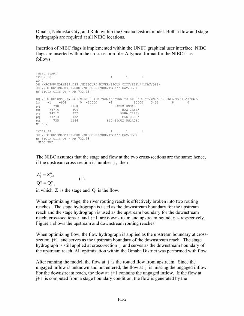
FE-2

Omaha, Nebraska City, and Rulo within the Omaha District model. Both a flow and stage hydrograph are required at all NIBC locations. Insertion of NIBC flags is implemented within the UNET graphical user interface. NIBC flags are inserted within the cross section file. A typical format for the NIBC is as follows: !NIBC START IX732.38 1 1 1 Z0 0 OH \MROPOR\MORHIST.DSS:/MISSOURI RIVER/SIOUX CITY/ELEV//1DAY/OBS/ OH \MROPOR\OMADAILY.DSS:/MISSOURI/SUX/FLOW//1DAY/OBS/ HY SIOUX CITY US - RM 732.38 uq \MROPOR\oma_uq.DSS:/MISSOURI RIVER/YANKTON TO SIOUX CITY/UNGAGED INFLOW//1DAY/EST/ lg -1 -901 0 -15000 -1 10000 3432 0 0 pq 798 1158 JAMES UNGAGED pq 787.6 304 BOW CREEK pq 745.2 222 AOWA CREEK pq 737.3 132 ELK CREEK pq 735 1146 BIG SIOUX UNGAGED NI SUX IX732.38 1 1 1 OH \MROPOR\OMADAILY.DSS:/MISSOURI/SUX/FLOW//1DAY/OBS/ HY SIOUX CITY DS - RM 732.38 !NIBC END The NIBC assumes that the stage and flow at the two cross-sections are the same; hence, if the upstream cross-section is number j , then

n1j

nj

n1j

nj

QQ

ZZ

+

+

=

= (1)

in which Z is the stage and Q is the flow. When optimizing stage, the river routing reach is effectively broken into two routing reaches. The stage hydrograph is used as the downstream boundary for the upstream reach and the stage hydrograph is used as the upstream boundary for the downstream reach; cross-sections j and j+1 are downstream and upstream boundaries respectively. Figure 1 shows the upstream and downstream routing reaches. When optimizing flow, the flow hydrograph is applied as the upstream boundary at cross-section j+1 and serves as the upstream boundary of the downstream reach. The stage hydrograph is still applied at cross-section j and serves as the downstream boundary of the upstream reach. All optimization within the Omaha District was performed with flow. After running the model, the flow at j is the routed flow from upstream. Since the ungaged inflow is unknown and not entered, the flow at j is missing the ungaged inflow. For the downstream reach, the flow at j+1 contains the ungaged inflow. If the flow at j+1 is computed from a stage boundary condition, the flow is generated by the

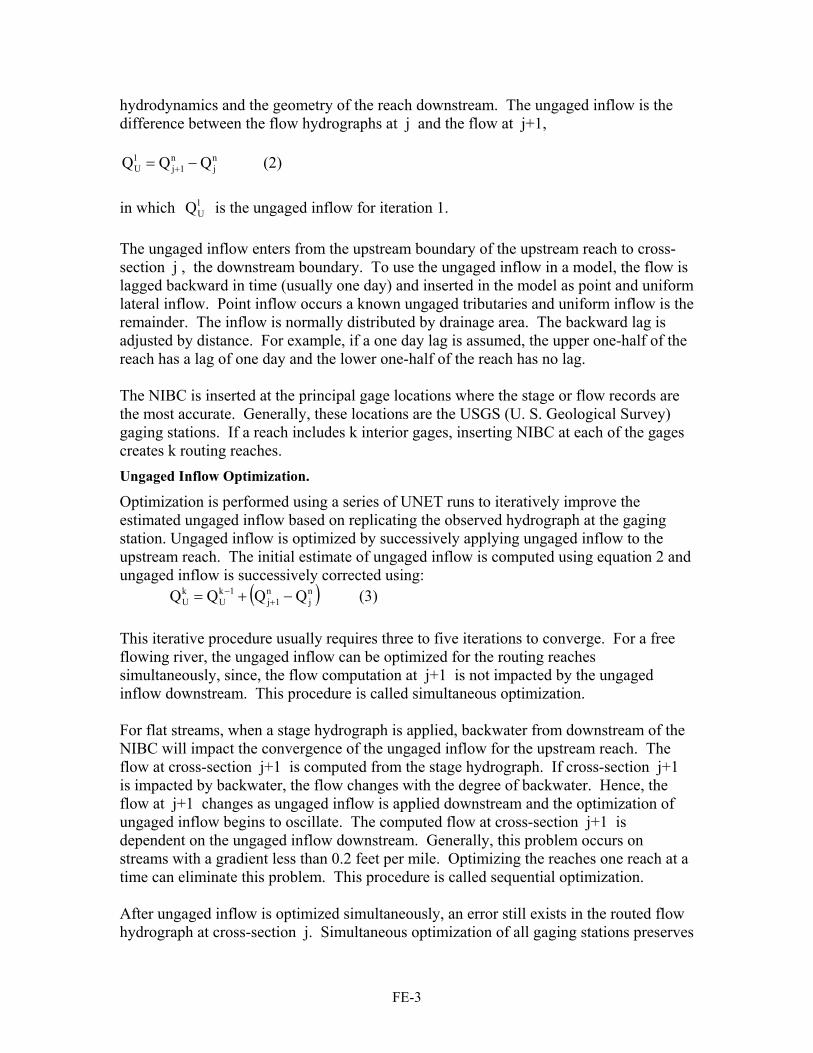
FE-3

hydrodynamics and the geometry of the reach downstream. The ungaged inflow is the difference between the flow hydrographs at j and the flow at j+1,

nj

n1j

1U QQQ −= + (2)

in which 1

UQ is the ungaged inflow for iteration 1. The ungaged inflow enters from the upstream boundary of the upstream reach to cross-section j , the downstream boundary. To use the ungaged inflow in a model, the flow is lagged backward in time (usually one day) and inserted in the model as point and uniform lateral inflow. Point inflow occurs a known ungaged tributaries and uniform inflow is the remainder. The inflow is normally distributed by drainage area. The backward lag is adjusted by distance. For example, if a one day lag is assumed, the upper one-half of the reach has a lag of one day and the lower one-half of the reach has no lag. The NIBC is inserted at the principal gage locations where the stage or flow records are the most accurate. Generally, these locations are the USGS (U. S. Geological Survey) gaging stations. If a reach includes k interior gages, inserting NIBC at each of the gages creates k routing reaches. Ungaged Inflow Optimization.

Optimization is performed using a series of UNET runs to iteratively improve the estimated ungaged inflow based on replicating the observed hydrograph at the gaging station. Ungaged inflow is optimized by successively applying ungaged inflow to the upstream reach. The initial estimate of ungaged inflow is computed using equation 2 and ungaged inflow is successively corrected using: ( )n

jn

1j1k

UkU QQQQ −+= +

− (3) This iterative procedure usually requires three to five iterations to converge. For a free flowing river, the ungaged inflow can be optimized for the routing reaches simultaneously, since, the flow computation at j+1 is not impacted by the ungaged inflow downstream. This procedure is called simultaneous optimization. For flat streams, when a stage hydrograph is applied, backwater from downstream of the NIBC will impact the convergence of the ungaged inflow for the upstream reach. The flow at cross-section j+1 is computed from the stage hydrograph. If cross-section j+1 is impacted by backwater, the flow changes with the degree of backwater. Hence, the flow at j+1 changes as ungaged inflow is applied downstream and the optimization of ungaged inflow begins to oscillate. The computed flow at cross-section j+1 is dependent on the ungaged inflow downstream. Generally, this problem occurs on streams with a gradient less than 0.2 feet per mile. Optimizing the reaches one reach at a time can eliminate this problem. This procedure is called sequential optimization. After ungaged inflow is optimized simultaneously, an error still exists in the routed flow hydrograph at cross-section j. Simultaneous optimization of all gaging stations preserves

FE-4

this error, which can be significant after the stage hydrographs at the NIBC’s are released. However, sequential optimization corrects these errors as the optimization moves downstream. Therefore, after simultaneous optimization, the model should be optimized sequentially to correct the residual errors.

The NIBC is inserted into the UNET cross-section file using the NI card between cross-section j and j+1. Cross-section j is a repeat of cross-section j+1 and the reach length between the cross-sections is very small, usually one foot. The only parameter on the NI card is a eight character name which uniquely defines the name of the NIBC when attaching an observed stage or flow hydrograph in the boundary condition file. HY cards must be inserted at cross-sections j and j+1 to define output hydrographs. The OH cards upstream and downstream attach the USGS hydrograph to the plot macro. Within the Omaha District, all null interior boundary simulations were optimized with flow.

FF-1


Appendix F-F

Ungaged Inflow Computation Historic UNET Model. The Missouri River has undergone major changes in its planform and length in the 20th century. In order to conduct a period-of-record UNET analysis of the desired 100-year period, it is necessary to be able to estimate the ungaged local inflow to the river for the entire period. Since the hydraulic characteristics of the river changed during the century, it was necessary to develop several UNET geometry models of the Missouri River to simulate historic hydraulic routings for the entire study period. A Missouri River historic UNET model was developed expressly for the purpose of computing the ungaged inflow for the early 1900’s. The geometry of this model reflects the natural conditions of the Missouri River before canalization, and the construction of dikes and levees. The natural channel was wide, braided, and shallow, and meandered freely back and forth across the floodplain. Geometry data from the early 1900’s is inexact and incomplete. No data could be located for bluff to bluff overbank geometry. Maps were found for several hydrographic surveys in the early 1900’s. In order to compile channel geometry for the entire reach of the Missouri River from RM 498 to the mouth, data from different surveys had to be used. The data used were from surveys conducted in the early 1920’s. The maps of the 1920’s hydrographic surveys show the channel and the near overbanks, and depict depth below water surface elevation. Thus, the location of the channel in the floodplain cannot be ascertained from these maps. Also, the locations of the depth measurements along the river are known only approximately, since river miles along the Missouri River have been revised several times over the years. Additionally, the vertical datum, which was used in the early 1900’s, is obscure. Its elevation could never be precisely verified. The channel geometry from the 1920’s mapping was merged with the overbank geometry from the 1998 UNET model at each cross section in the 1998 model. The 1920’s channel was centered on the channel location in the 1998 model’s cross sections. The 1920’s channel geometry, which was inserted into each 1998 cross section, was selected according to what was determined to be the closest 1920’s depth measurements to that particular 1998 cross section. Following preparation of the historic model’s cross sections, the model was calibrated to reproduce flow volumes using flow data from the early 1900’s. Computation of Ungaged Lateral Inflow In order to perform a period-of-record analysis using UNET, it is first necessary to determine the sources and amounts of historic inflows to the Missouri River that have occurred in the past. This was done by using the historic records at each gage, and an automated routine that has been built

FF-2

into UNET. The automated UNET flow calibration technique was also used for these computations.

Null Internal Boundary. Ungaged tributary inflow and other sources of inflow between the mainstem USGS gages must be accounted for in the UNET model. Estimates of ungaged inflow are computed using the Null Internal Boundary Condition (NIBC) procedure of the UNET program. To use NIBC, the UNET model was automatically calibrated using rating curves at the mainstem USGS gaging stations listed in Table E-19. The exception is the St. Charles gage, which is a stage gage in the backwater of the Mississippi River. Rating curves are derived for the gages from the observed data. The automatic calibration routine of the UNET program derives the rating curves and calibrates the model by adjusting the rating curves to reproduce stage at the USGS gages, based on observed flows. Then the NIBC procedure in UNET is used to estimate ungaged lateral inflow throughout the model by optimizing to USGS observed flow. In the cross section file, the NIBC feature is inserted at each of the mainstem gage locations between two identical cross sections. The two cross sections are exact duplicates separated for computational purposes by an extremely small distance, such as one foot. The first cross section is the downstream boundary of a mainstem routing reach, and the second cross section is the upstream boundary of the subsequent mainstem routing reach. Flow data at the upstream cross section is flow computed from routing through the upstream reach. Flow data at the downstream cross section is the target USGS observed flow data. The NIBC procedure requires iterative executions of UNET until the flow is the same at both the upstream and downstream cross sections. The first execution results in computed flow at the cross section just upstream of each NIBC. The differences in the computed and observed flows at these locations are calculated to get the residual or ungaged inflows for each reach. To achieve flow continuity at the NIBC locations, the ungaged inflows are then distributed throughout the upstream reach and lagged in time as appropriate. The second execution uses these ungaged inflows as lateral and/or point inflow hydrographs. The differences in computed and observed flows are again calculated, and the procedure is repeated until the differences in flow approach zero. The last execution removes the NIBC and runs with the final computed ungaged lateral inflows. Computation of Ungaged Lateral Inflow. Ungaged inflow for the period of record analysis was developed by Dr. Robert Barkau using the three different Missouri River UNET models – the historic UNET model for 1900 through 1940, the 1998 UNET model without levees for 1940 through 1961, and the 1998 UNET model with levees for 1961 through 2000. The three models used to calculate the ungaged inflows, were each calibrated using the UNET processes. These steps in the calibration process are the Null Internal Boundary Condition (NIBC), Manning’s n, fine tuning, and levee performance for the 1961 – 2000 model, which is the only model with levees. To compute the ungaged inflow with UNET, several boundary conditions files were needed. Each boundary conditions file was for a different time period, ranging from five to ten years. This was needed to accommodate the establishment of tributary gaging stations as they were brought into service at different times.

FF-3

Using the historic and current condition UNET models, the ungaged inflows were calculated for the period of record. These calculations occasionally produced negative inflows. To avoid instability in the current conditions UNET model, some of these negative inflows were eliminated from the data files. The ungaged inflows were then added to the boundary conditions file of the current conditions UNET model for use in the period of record analysis. In the boundary conditions file of the current conditions model, the ungaged inflows were distributed by average flow at the tributary gages. UNET has the capacity to distribute this ungaged lateral inflow at various tributaries, or to uniformly distribute lateral inflow through the reach, or a combination of the two methods. Initially the allocation of flow was based on the drainage areas of the major tributaries. Later on, it was found that the ratio of the mean annual discharges at the tributaries gave more satisfactory results. This capacity was used to extend the inflow records at the tributary gages, none of which was long enough to conduct the period of record analysis. The net result of this procedure is a .dss file for historic inflows to the Missouri River at points between the principal gaging stations. This file served as an input flow file in the period-of-record analysis.

FG-1


UNET Model Parallel Flow Algorithm

Prepared by Dr. Robert L. Barkau Appendix F-G

Robert L. Barkau, Ph.D., P. E. Hydraulic Engineer

4965 Eagle Lake Drive, Fort Collins, Colorado 80524 Office: (970) 482-9294; Fax: (970) 482-9281

March 14, 2001 Mr. John Burant Hydraulics Branch Rock Island District, Corps of Engineers Clock Tower Building P.O. Box 2004 Rock Island, Illinois 61204-2004 Re: UNET Parallel Flow Algorithm. Dear John, This letter describes the parallel flow algorithm that I wrote for the UNET program.

The parallel flow algorithm writes the flow behind a levee system to DSS, including the parallel levee flow in the total river flow. The algorithm functions with simple (SF) and complex (EF) levee breaches. The levee storage must be modeled as a storage cell. Figure 1 demonstrates a typical problem. After the upstream and downstream breaches have failed, water flows parallel to the river from the upstream breach to the downstream breach. The river flow between the breaches is reduced by the flow into the upstream breach. In the original UNET formulation, the flow output to DSS is the computed river flow without the parallel river flow. The new program combines the parallel river flow behind the levee with the parallel flow behind the levee and outputs the total flow to DSS.

FG-2

At a hydrograph location between levee breaches, with the parallel flow option on, the following information is output:

Parameter DSS C Part Flow in the river RIVER FLOW Parallel flow behind the levee LEVEE FLOW Total river and levee flow TOTAL FLOW

Figure 2 shows a sample hydrograph plot between the upstream and downstream breaches of the Elsberry Levee system. In addition to the river stage hydrograph, the program output river flow, levee flow, and total flow hydrographs.

Figure 1. A typical levee system with parallel flow. Flow enters the levee through the

upstream breach and exits through the downstream breach. The parallel flow is the minimum of the inflow and the outflow.

FG-3

Figure 2. Hydrograph at RM 258.7, which is between the upstream and downstream

breaches of the Elsberry Levee. The river flow, the levee flow, and the total flow, the sum of river and levee flow are plotted.

With the parallel flow option on, the maximum flow profile includes both river and levee flow. Figure 3 shows the maximum flow profile for the Mississippi River. The flow profile is relatively smooth. In contrast, Figure 4 shows the maximum river flow profile, with and without parallel levee flow. The profile shows the diversions into the Riverland, Elsberry, Columbia, and Harrisonville Levees. Figure 6 shows a more complex levee system. Flow enters Levee 1 through the upstream and downstream breaches and exits through a breach in the flank levee, entering Levee 2. Water from Levee 2 exits through the downstream breach. This system is similar to the Columbia-Harrisonville complex south of St. Louis.

To solve this system and other more complex systems, the following parallel flow algorithm is defined:

1. Parallel flow only occurs when inflow and outflow occur. 2. The maximum parallel flow for any river system is the minimum of the total

inflow and the total outflow – the flux of water from storage does not count; hence,

( )OutInPMin Q,QMinQ =

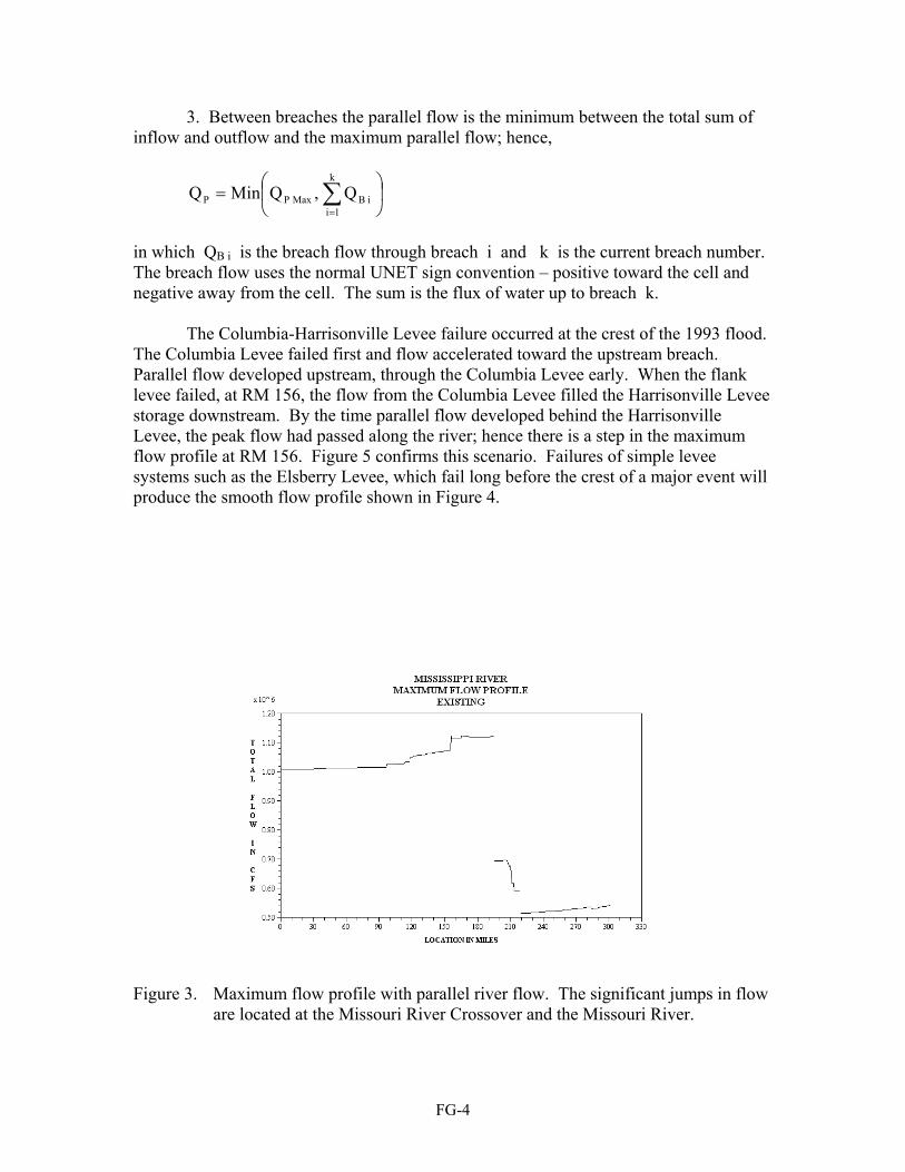
FG-4

3. Between breaches the parallel flow is the minimum between the total sum of inflow and outflow and the maximum parallel flow; hence,

= ∑

=

k

1iiBMaxPP Q,QMinQ

in which QB i is the breach flow through breach i and k is the current breach number. The breach flow uses the normal UNET sign convention – positive toward the cell and negative away from the cell. The sum is the flux of water up to breach k. The Columbia-Harrisonville Levee failure occurred at the crest of the 1993 flood. The Columbia Levee failed first and flow accelerated toward the upstream breach. Parallel flow developed upstream, through the Columbia Levee early. When the flank levee failed, at RM 156, the flow from the Columbia Levee filled the Harrisonville Levee storage downstream. By the time parallel flow developed behind the Harrisonville Levee, the peak flow had passed along the river; hence there is a step in the maximum flow profile at RM 156. Figure 5 confirms this scenario. Failures of simple levee systems such as the Elsberry Levee, which fail long before the crest of a major event will produce the smooth flow profile shown in Figure 4.

Figure 3. Maximum flow profile with parallel river flow. The significant jumps in flow

are located at the Missouri River Crossover and the Missouri River.

FG-5

Figure 4. Comparison of maximum flow profiles of total flow and of river flow. The

most dramatic impacts are the diversion of water through the Elsberry Levee system, from RM 250 to 260. Because of the timing of the levee failures, the parallel flow behind the Harrisonville Levee has no impact on peak flow.

FG-6

Figure 5. Stage and flow at Brickeys Landing, which is between the upstream and

downstream breaches of the Harrisonville Levee. Because of the timing of the failure, the parallel flow behind the levee started after the peak flow. This explains the reduction in flow at RM 156 in Figure 4.

The parallel flow computation is called by including the following line in the boundary condition file: PARALLEL=ON The line can appear anywhere in the BC file before the EJ card. Figure 6. Complex levee systems, similar to the Columbia-Harrisonville Levees

downstream of St. Louis.

FG-7

Final comments: The parallel flow algorithm smoothes the flow profile in the vicinity of levee systems where the levee fails before the flood crest. This scenario is illustrated by the Elsberry and Riverland systems in Figure 4. But also consider this: The stage between the levee crests results from the river flow not the total flow. Therefore, the water surface elevation is different at the river than inside the levee; hence using the total flow and the river stage will not produce a representative rating curve.

Secondly, if the levee fails near the flood crest, water accelerates toward the levee breach as demonstrated for the Columbia Levee as a step in the maximum flow profile in Figure 3. The acceleration is real and upstream of the breach. The acceleration cannot be removed by computing parallel flow.

If you have questions or comments, please call. If you send a E-mail, please

follow-up with a telephone call. I am still uncertain that I am receiving all my E-mail. Kindest regards, Bob Barkau

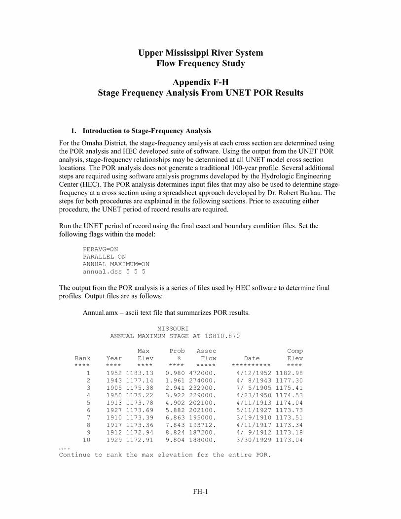
FH-1


Appendix F-H

Stage Frequency Analysis From UNET POR Results

1. Introduction to Stage-Frequency Analysis

For the Omaha District, the stage-frequency analysis at each cross section are determined using the POR analysis and HEC developed suite of software. Using the output from the UNET POR analysis, stage-frequency relationships may be determined at all UNET model cross section locations. The POR analysis does not generate a traditional 100-year profile. Several additional steps are required using software analysis programs developed by the Hydrologic Engineering Center (HEC). The POR analysis determines input files that may also be used to determine stage-frequency at a cross section using a spreadsheet approach developed by Dr. Robert Barkau. The steps for both procedures are explained in the following sections. Prior to executing either procedure, the UNET period of record results are required. Run the UNET period of record using the final csect and boundary condition files. Set the following flags within the model:

PERAVG=ON PARALLEL=ON ANNUAL MAXIMUM=ON annual.dss 5 5 5

The output from the POR analysis is a series of files used by HEC software to determine final profiles. Output files are as follows: Annual.amx – ascii text file that summarizes POR results. MISSOURI ANNUAL MAXIMUM STAGE AT 1S810.870 Max Prob Assoc Comp Rank Year Elev % Flow Date Elev **** **** **** **** ***** ********** **** 1 1952 1183.13 0.980 472000. 4/12/1952 1182.98 2 1943 1177.14 1.961 274000. 4/ 8/1943 1177.30 3 1905 1175.38 2.941 232900. 7/ 5/1905 1175.41 4 1950 1175.22 3.922 229000. 4/23/1950 1174.53 5 1913 1173.78 4.902 202100. 4/11/1913 1174.04 6 1927 1173.69 5.882 202100. 5/11/1927 1173.73 7 1910 1173.39 6.863 195000. 3/19/1910 1173.51 8 1917 1173.36 7.843 193712. 4/11/1917 1173.34 9 1912 1172.94 8.824 187200. 4/ 9/1912 1173.18 10 1929 1172.91 9.804 188000. 3/30/1929 1173.04 ….. Continue to rank the max elevation for the entire POR.

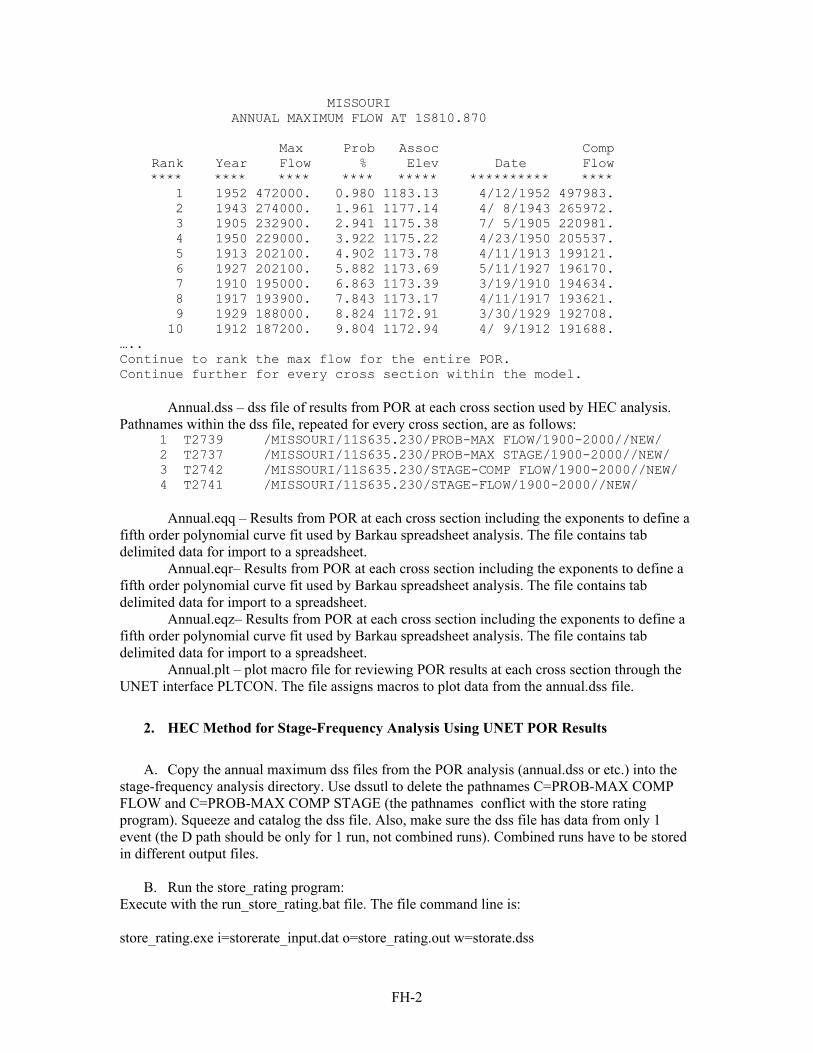
FH-2

MISSOURI ANNUAL MAXIMUM FLOW AT 1S810.870 Max Prob Assoc Comp Rank Year Flow % Elev Date Flow **** **** **** **** ***** ********** **** 1 1952 472000. 0.980 1183.13 4/12/1952 497983. 2 1943 274000. 1.961 1177.14 4/ 8/1943 265972. 3 1905 232900. 2.941 1175.38 7/ 5/1905 220981. 4 1950 229000. 3.922 1175.22 4/23/1950 205537. 5 1913 202100. 4.902 1173.78 4/11/1913 199121. 6 1927 202100. 5.882 1173.69 5/11/1927 196170. 7 1910 195000. 6.863 1173.39 3/19/1910 194634. 8 1917 193900. 7.843 1173.17 4/11/1917 193621. 9 1929 188000. 8.824 1172.91 3/30/1929 192708. 10 1912 187200. 9.804 1172.94 4/ 9/1912 191688. ….. Continue to rank the max flow for the entire POR. Continue further for every cross section within the model. Annual.dss – dss file of results from POR at each cross section used by HEC analysis. Pathnames within the dss file, repeated for every cross section, are as follows: 1 T2739 /MISSOURI/11S635.230/PROB-MAX FLOW/1900-2000//NEW/ 2 T2737 /MISSOURI/11S635.230/PROB-MAX STAGE/1900-2000//NEW/ 3 T2742 /MISSOURI/11S635.230/STAGE-COMP FLOW/1900-2000//NEW/ 4 T2741 /MISSOURI/11S635.230/STAGE-FLOW/1900-2000//NEW/ Annual.eqq – Results from POR at each cross section including the exponents to define a fifth order polynomial curve fit used by Barkau spreadsheet analysis. The file contains tab delimited data for import to a spreadsheet.

Annual.eqr– Results from POR at each cross section including the exponents to define a fifth order polynomial curve fit used by Barkau spreadsheet analysis. The file contains tab delimited data for import to a spreadsheet. Annual.eqz– Results from POR at each cross section including the exponents to define a fifth order polynomial curve fit used by Barkau spreadsheet analysis. The file contains tab delimited data for import to a spreadsheet. Annual.plt – plot macro file for reviewing POR results at each cross section through the UNET interface PLTCON. The file assigns macros to plot data from the annual.dss file.

2. HEC Method for Stage-Frequency Analysis Using UNET POR Results

A. Copy the annual maximum dss files from the POR analysis (annual.dss or etc.) into the

stage-frequency analysis directory. Use dssutl to delete the pathnames C=PROB-MAX COMP FLOW and C=PROB-MAX COMP STAGE (the pathnames conflict with the store rating program). Squeeze and catalog the dss file. Also, make sure the dss file has data from only 1 event (the D path should be only for 1 run, not combined runs). Combined runs have to be stored in different output files.

B. Run the store_rating program: Execute with the run_store_rating.bat file. The file command line is: store_rating.exe i=storerate_input.dat o=store_rating.out w=storate.dss

FH-3

The storerate_input.dat file has the .dss filename specified. Edit the .dss file name in the storerate_input.dat file. The file format is: 0 1 annual???.dss For multiple POR dss files, change the 1 to the number of files and add the name of the dss file after the annual.dss name. The batch file specifies the text output file store_rating.out and the output file for the paired data (omarate.dss). The output is paired data of with path stage-flow at each cross section in the omarate.dss file. The rating curve data for the input dss files are combined into a single output dss file called Rating_data.dss (this file name is written automatically and cannot be changed –watch out for data overwriting). This file can then be used for subsequent curve fitting by the module RATING_CURVE.

C. Run the rating_curve program: Execute with the run_rating_curve_all.bat. Files are: rating_curve.exe i=oma_rate_all.dat o=omrating.out d=rating_data.dss w=crv???.dss Rename the W=??curve file name for each alternative. The input file contains data as: flag spline fit, ifix (fix last point -1,0-no),nwidth no pts avg width 1,1,6 top of levee followed by pathnames (o for no levee) 0.0 /MISSOURI/13S616.030/FLOW-STAGE/1991-2000//NEW/

and etc. repeated for all sections. Pathnames are provided for all the section locations. All output data is stored in the rcurve.dss file. The paths in the input data files (oma_rate_…) can be built by cataloging the file created from the store_rating program. For combined runs, the pathname contains the F part from a single file, but output data is from the combined files. The store_rating program uses the path from the last dss file. All analysis was performed using a 0.0 specified to indicate no levee. The software option to set a levee elevation allows curve fitting to consider the specified elevation. Output data did not indicate a improved curve fit by specifying a levee. Therefore, this option was not included. When initially formatting the input file, the 0.0 elevation must be inserted between all paths.

D. Run the area_vs_stats program: This step was originally separated into spring and summer statistics but has been combined in the final version of the software used by the Omaha District. Execute with the omaha_area_vs_stats.bat. This program interpolates the hydrologic stats by drainage area. The sole purpose of this program is to provide a file format that is easily used to construct the input file for the Omaha_stage-Freq_area program. Results from this program are not used for any other purpose. After building the input file, this program is no longer required. The station values MUST correspond with the stations from the rating_curve program. If new cross sections are added, the data must be revised.

E. Run the reg-vs-unreg program: NOTE: This step was not performed by the Omaha District. The regulated-unregulated relationship was previously developed during the hydrologic analysis. The reg-unreg dss file

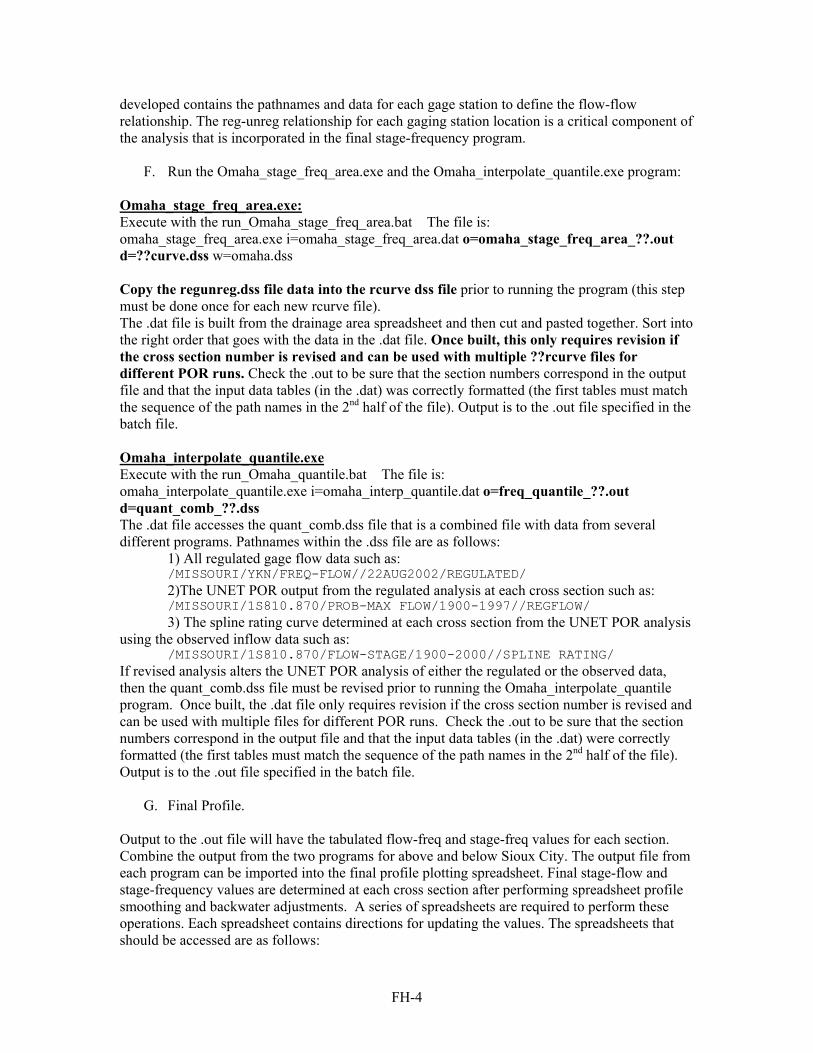
FH-4

developed contains the pathnames and data for each gage station to define the flow-flow relationship. The reg-unreg relationship for each gaging station location is a critical component of the analysis that is incorporated in the final stage-frequency program.

F. Run the Omaha_stage_freq_area.exe and the Omaha_interpolate_quantile.exe program: Omaha_stage_freq_area.exe: Execute with the run_Omaha_stage_freq_area.bat The file is: omaha_stage_freq_area.exe i=omaha_stage_freq_area.dat o=omaha_stage_freq_area_??.out d=??curve.dss w=omaha.dss Copy the regunreg.dss file data into the rcurve dss file prior to running the program (this step must be done once for each new rcurve file). The .dat file is built from the drainage area spreadsheet and then cut and pasted together. Sort into the right order that goes with the data in the .dat file. Once built, this only requires revision if the cross section number is revised and can be used with multiple ??rcurve files for different POR runs. Check the .out to be sure that the section numbers correspond in the output file and that the input data tables (in the .dat) was correctly formatted (the first tables must match the sequence of the path names in the 2nd half of the file). Output is to the .out file specified in the batch file. Omaha_interpolate_quantile.exe Execute with the run_Omaha_quantile.bat The file is: omaha_interpolate_quantile.exe i=omaha_interp_quantile.dat o=freq_quantile_??.out d=quant_comb_??.dss The .dat file accesses the quant_comb.dss file that is a combined file with data from several different programs. Pathnames within the .dss file are as follows: 1) All regulated gage flow data such as: /MISSOURI/YKN/FREQ-FLOW//22AUG2002/REGULATED/ 2)The UNET POR output from the regulated analysis at each cross section such as:

/MISSOURI/1S810.870/PROB-MAX FLOW/1900-1997//REGFLOW/ 3) The spline rating curve determined at each cross section from the UNET POR analysis

using the observed inflow data such as: /MISSOURI/1S810.870/FLOW-STAGE/1900-2000//SPLINE RATING/

If revised analysis alters the UNET POR analysis of either the regulated or the observed data, then the quant_comb.dss file must be revised prior to running the Omaha_interpolate_quantile program. Once built, the .dat file only requires revision if the cross section number is revised and can be used with multiple files for different POR runs. Check the .out to be sure that the section numbers correspond in the output file and that the input data tables (in the .dat) were correctly formatted (the first tables must match the sequence of the path names in the 2nd half of the file). Output is to the .out file specified in the batch file.

G. Final Profile. Output to the .out file will have the tabulated flow-freq and stage-freq values for each section. Combine the output from the two programs for above and below Sioux City. The output file from each program can be imported into the final profile plotting spreadsheet. Final stage-flow and stage-frequency values are determined at each cross section after performing spreadsheet profile smoothing and backwater adjustments. A series of spreadsheets are required to perform these operations. Each spreadsheet contains directions for updating the values. The spreadsheets that should be accessed are as follows:

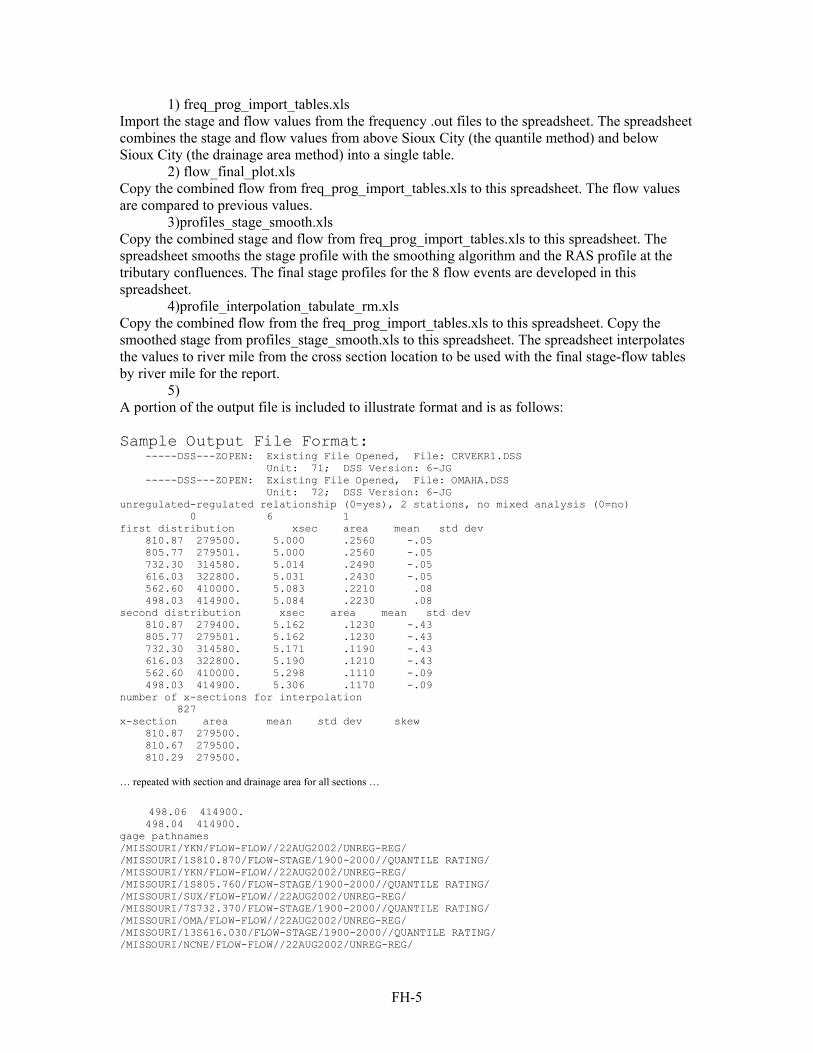
FH-5

1) freq_prog_import_tables.xls Import the stage and flow values from the frequency .out files to the spreadsheet. The spreadsheet combines the stage and flow values from above Sioux City (the quantile method) and below Sioux City (the drainage area method) into a single table. 2) flow_final_plot.xls Copy the combined flow from freq_prog_import_tables.xls to this spreadsheet. The flow values are compared to previous values. 3)profiles_stage_smooth.xls Copy the combined stage and flow from freq_prog_import_tables.xls to this spreadsheet. The spreadsheet smooths the stage profile with the smoothing algorithm and the RAS profile at the tributary confluences. The final stage profiles for the 8 flow events are developed in this spreadsheet. 4)profile_interpolation_tabulate_rm.xls Copy the combined flow from the freq_prog_import_tables.xls to this spreadsheet. Copy the smoothed stage from profiles_stage_smooth.xls to this spreadsheet. The spreadsheet interpolates the values to river mile from the cross section location to be used with the final stage-flow tables by river mile for the report. 5) A portion of the output file is included to illustrate format and is as follows: Sample Output File Format: -----DSS---ZOPEN: Existing File Opened, File: CRVEKR1.DSS Unit: 71; DSS Version: 6-JG -----DSS---ZOPEN: Existing File Opened, File: OMAHA.DSS Unit: 72; DSS Version: 6-JG unregulated-regulated relationship (0=yes), 2 stations, no mixed analysis (0=no) 0 6 1 first distribution xsec area mean std dev 810.87 279500. 5.000 .2560 -.05 805.77 279501. 5.000 .2560 -.05 732.30 314580. 5.014 .2490 -.05 616.03 322800. 5.031 .2430 -.05 562.60 410000. 5.083 .2210 .08 498.03 414900. 5.084 .2230 .08 second distribution xsec area mean std dev 810.87 279400. 5.162 .1230 -.43 805.77 279501. 5.162 .1230 -.43 732.30 314580. 5.171 .1190 -.43 616.03 322800. 5.190 .1210 -.43 562.60 410000. 5.298 .1110 -.09 498.03 414900. 5.306 .1170 -.09 number of x-sections for interpolation 827 x-section area mean std dev skew 810.87 279500. 810.67 279500. 810.29 279500. … repeated with section and drainage area for all sections … 498.06 414900. 498.04 414900. gage pathnames /MISSOURI/YKN/FLOW-FLOW//22AUG2002/UNREG-REG/ /MISSOURI/1S810.870/FLOW-STAGE/1900-2000//QUANTILE RATING/ /MISSOURI/YKN/FLOW-FLOW//22AUG2002/UNREG-REG/ /MISSOURI/1S805.760/FLOW-STAGE/1900-2000//QUANTILE RATING/ /MISSOURI/SUX/FLOW-FLOW//22AUG2002/UNREG-REG/ /MISSOURI/7S732.370/FLOW-STAGE/1900-2000//QUANTILE RATING/ /MISSOURI/OMA/FLOW-FLOW//22AUG2002/UNREG-REG/ /MISSOURI/13S616.030/FLOW-STAGE/1900-2000//QUANTILE RATING/ /MISSOURI/NCNE/FLOW-FLOW//22AUG2002/UNREG-REG/

FH-6

/MISSOURI/17S562.740/FLOW-STAGE/1900-2000//QUANTILE RATING/ /MISSOURI/RUNE/FLOW-FLOW//22AUG2002/UNREG-REG/ /MISSOURI/21S498.030/FLOW-STAGE/1900-2000//QUANTILE RATING/ interpolated section pathnames /MISSOURI/1S810.870/FLOW-STAGE/1900-2000//SPLINE RATING/ /MISSOURI/1S810.670/FLOW-STAGE/1900-2000//SPLINE RATING/ … repeated section pathnames … -----DSS---ZWRITE Unit 72; Vers. 3: /MISSOURI/21S498.040/FREQ-FLOW/1900-2000//UNREGULATED/ -----DSS---ZWRITE Unit 72; Vers. 3: /MISSOURI/21S498.040/FREQ-STAGE/1900-2000//STAGE/ exceedance probability vs flow gages sta 0.500 0.200 0.100 0.040 0.020 0.010 0.005 0.002 810.87 45266. 63009. 65017. 69129. 74723. 84879. 98027. 123460. 805.77 45266. 63009. 65017. 69129. 74723. 84879. 98027. 123460. 732.30 49539. 66820. 78335. 93925. 113799. 133759. 155008. 185400. 616.03 64182. 85318. 123554. 132687. 147927. 174713. 204465. 247940. 562.60 88034. 118656. 149766. 189924. 206378. 236694. 275891. 345400. 498.03 94705. 132349. 160874. 188576. 217315. 252221. 296913. 370700. exeedance probability vs flow sections sta 0.500 0.200 0.100 0.040 0.020 0.010 0.005 0.002 810.87 45266. 63009. 65017. 69129. 74723. 84879. 98027. 123460. 810.67 45266. 63009. 65017. 69129. 74723. 84879. 98027. 123460. … repeated with tabulated flow at all sections … 498.04 94705. 132349. 160874. 188576. 217315. 252221. 296913. 370700. exceedance probability vs stage gages sta 0.500 0.200 0.100 0.040 0.020 0.010 0.005 0.002 810.87 1160.9 1163.0 1163.2 1163.7 1164.3 1165.3 1166.4 1168.5 805.77 1156.5 1158.7 1158.9 1159.4 1159.9 1160.9 1162.0 1163.7 732.30 1076.8 1080.2 1081.6 1082.9 1084.2 1085.8 1086.8 1088.5 616.03 971.2 974.2 978.1 978.8 979.5 980.4 981.6 983.6 562.60 924.1 927.5 929.8 932.0 932.5 933.2 934.3 935.4 498.03 856.1 859.7 860.4 860.8 861.1 861.8 862.4 862.6 exceedance probability vs stage sections sta 0.500 0.200 0.100 0.040 0.020 0.010 0.005 0.002 810.87 1160.9 1163.0 1163.2 1163.7 1164.2 1165.2 1166.4 1168.5 810.67 1160.8 1162.8 1163.0 1163.4 1164.0 1165.0 1166.1 1168.1 … repeated with tabulated stage at all sections … 498.06 856.1 859.6 860.4 860.9 861.2 861.9 862.6 863.0 498.04 856.1 859.6 860.4 860.8 861.2 861.8 862.5 862.9

3. Barkau Spreadsheet Method

The Barkau spreadsheet method was used to evaluate the results from the HEC software program. The method uses a similar theory and allows an independent verification of results obtained with the HEC software. The steps required are as follows:

A. Copy the files from the POR analysis to the stage-freq\ directory for the spreadsheet analysis. This includes the files as follows: Annual.dss Annual.eqq Annual.eqr

FH-7

Annual.eqz

B. Open the profile spreadsheet – oma_profiles_dec02_barkau.xls, enable macros. Open each of the .e?? files from excel, the files are tabulated delimited. Copy and paste the data into the appropriate page of the master profiles spreadsheet.

C. Check the flow data in the TAG flow column for the 10, 50, 100, 500 profile worksheets. Update if needed from the HEC output file above. This step is not needed unless drainage area is changed.

D. Run the visual basic macro to update the computations for the 10, 50, 100, and 500 yr profile sheets. The macro is run from the tools – macro button. In visual basic, click run and pick the run sub/user form. NOTE: If the path is changed, the macro will not work. Check the path in the freq_profiles module, in the sub frequency profiles routine.

E. Copy the computed profile, under the TAG stage heading, into the final spreadsheet for comparison to the HEC method final profiles. Note that the computed elevations are prior to performing any smoothing operations.

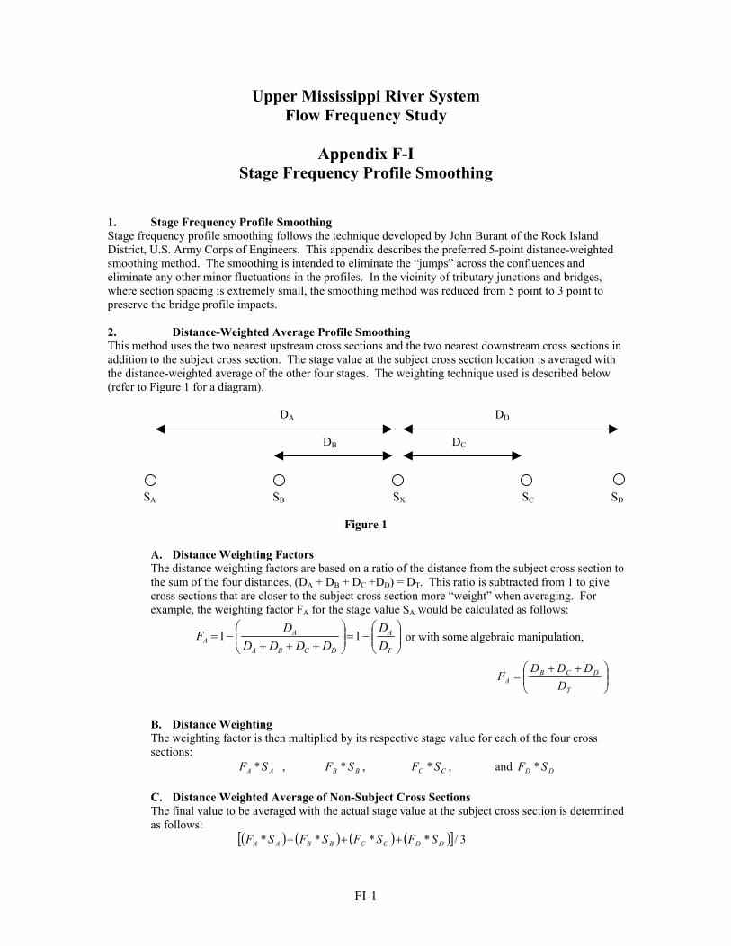
FI-1


Appendix F-I

Stage Frequency Profile Smoothing 1. Stage Frequency Profile Smoothing Stage frequency profile smoothing follows the technique developed by John Burant of the Rock Island District, U.S. Army Corps of Engineers. This appendix describes the preferred 5-point distance-weighted smoothing method. The smoothing is intended to eliminate the “jumps” across the confluences and eliminate any other minor fluctuations in the profiles. In the vicinity of tributary junctions and bridges, where section spacing is extremely small, the smoothing method was reduced from 5 point to 3 point to preserve the bridge profile impacts. 2. Distance-Weighted Average Profile Smoothing This method uses the two nearest upstream cross sections and the two nearest downstream cross sections in addition to the subject cross section. The stage value at the subject cross section location is averaged with the distance-weighted average of the other four stages. The weighting technique used is described below (refer to Figure 1 for a diagram). DA DD DB DC SA SB SX SC SD

Figure 1

A. Distance Weighting Factors The distance weighting factors are based on a ratio of the distance from the subject cross section to the sum of the four distances, (DA + DB + DC +DD) = DT. This ratio is subtracted from 1 to give cross sections that are closer to the subject cross section more “weight” when averaging. For example, the weighting factor FA for the stage value SA would be calculated as follows:

−=

+++

−=T

A

DCBA

AA D

DDDDD

DF 11 or with some algebraic manipulation,

++=

T

DCBA D

DDDF

B. Distance Weighting The weighting factor is then multiplied by its respective stage value for each of the four cross sections: AA SF * , BB SF * , CC SF * , and DD SF * C. Distance Weighted Average of Non-Subject Cross Sections The final value to be averaged with the actual stage value at the subject cross section is determined as follows: ( ) ( ) ( ) ( )[ ] 3/**** DDCCBBAA SFSFSFSF +++

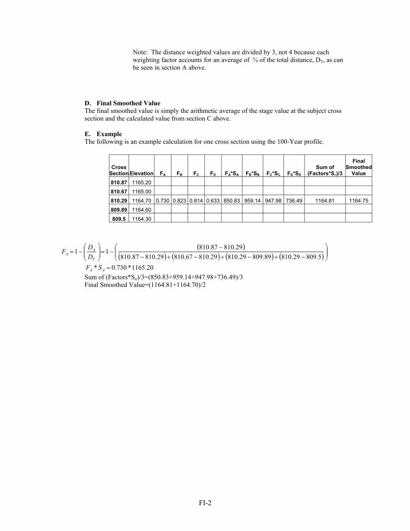
FI-2

Note: The distance weighted values are divided by 3, not 4 because each weighting factor accounts for an average of ¾ of the total distance, DT, as can be seen in section A above.

D. Final Smoothed Value The final smoothed value is simply the arithmetic average of the stage value at the subject cross section and the calculated value from section C above.

E. Example

The following is an example calculation for one cross section using the 100-Year profile.

Cross Section Elevation FA FB FC FD FA*SA FB*SB FC*SC FD*SD

Sum of (Factors*Sn)/3

Final Smoothed

Value 810.87 1165.20

810.67 1165.00

810.29 1164.70 0.730 0.823 0.814 0.633 850.83 959.14 947.98 736.49 1164.81 1164.75

809.89 1164.60

809.5 1164.30

( )( ) ( ) ( ) ( )

−+−+−+−

−−=

−=

5.80929.81089.80929.81029.81067.81029.81087.81029.81087.81011

T

AA D

DF

20.1165*730.0* =AA SF Sum of (Factors*Sn)/3=(850.83+959.14+947.98+736.49)/3

Final Smoothed Value=(1164.81+1164.70)/2


Appendix F

Plates

Plate F- 1

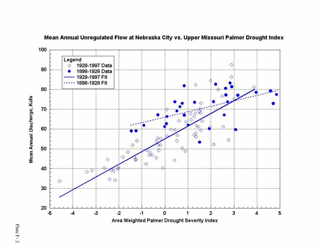
Plate F- 2

Plate F- 3

Plate F- 4

Plate F- 5

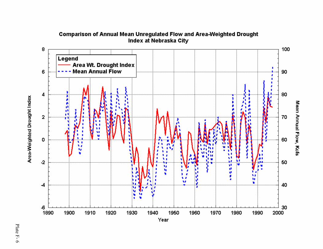
Plate F- 6

Plate F- 7

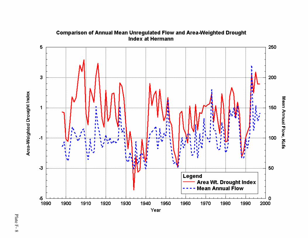
Plate F- 8

Plate F- 9

Plate F- 10

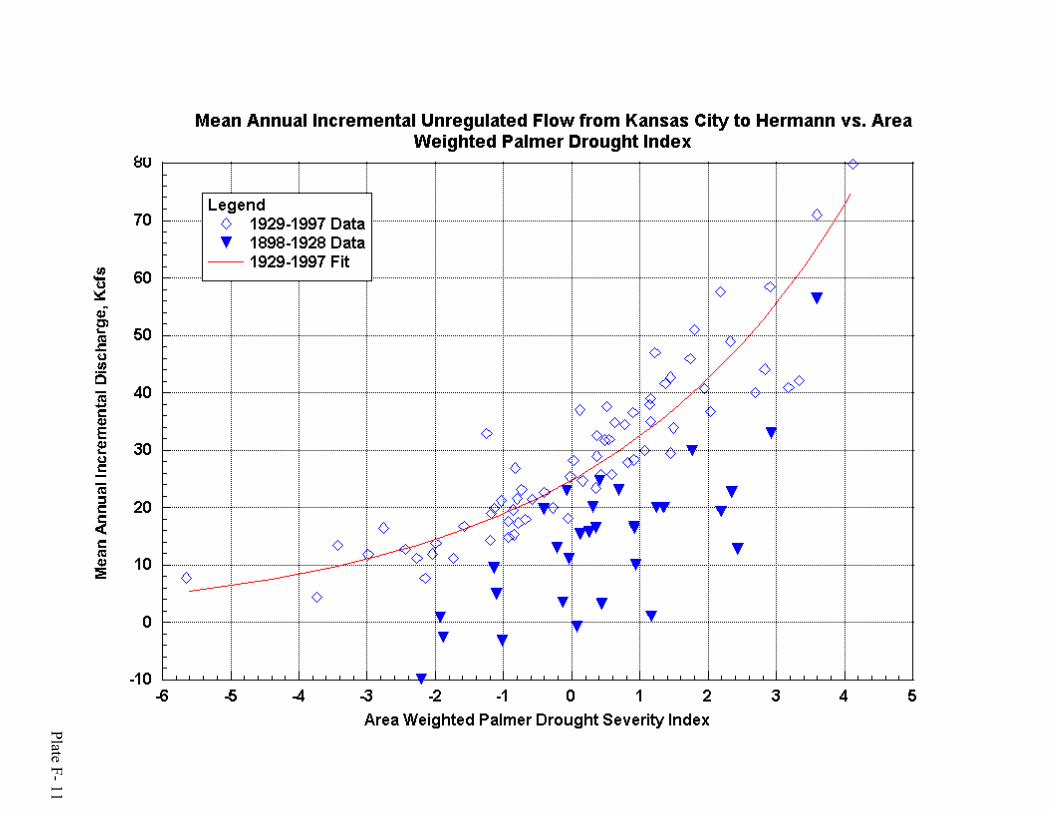
Plate F- 11

Plate F- 12

Plate F- 13

Plate F- 14

Plate F- 15

Plate F- 16

Plate F- 17

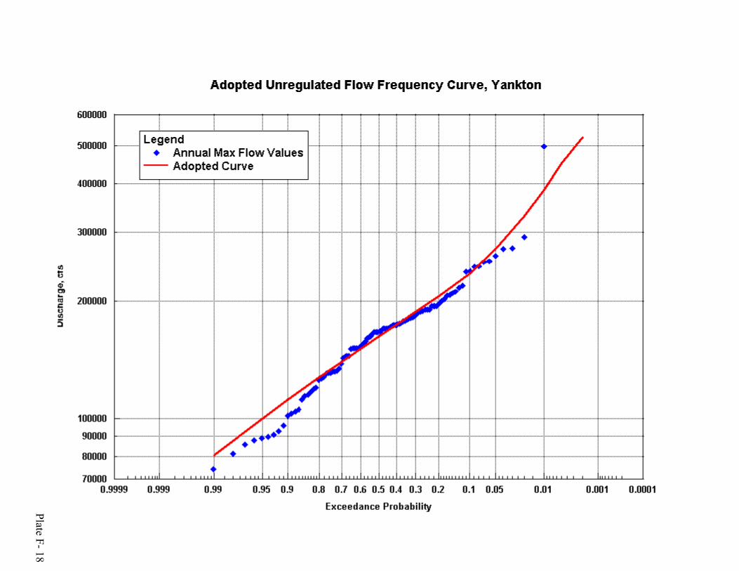
Plate F- 18

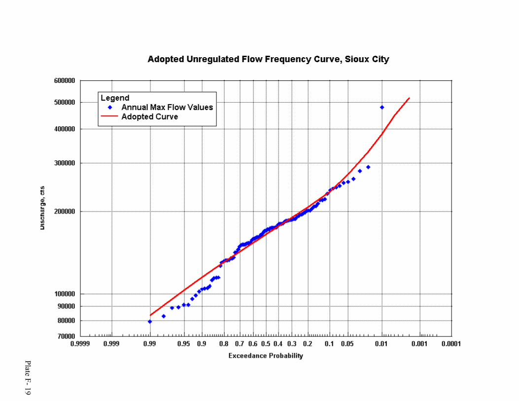
Plate F- 19

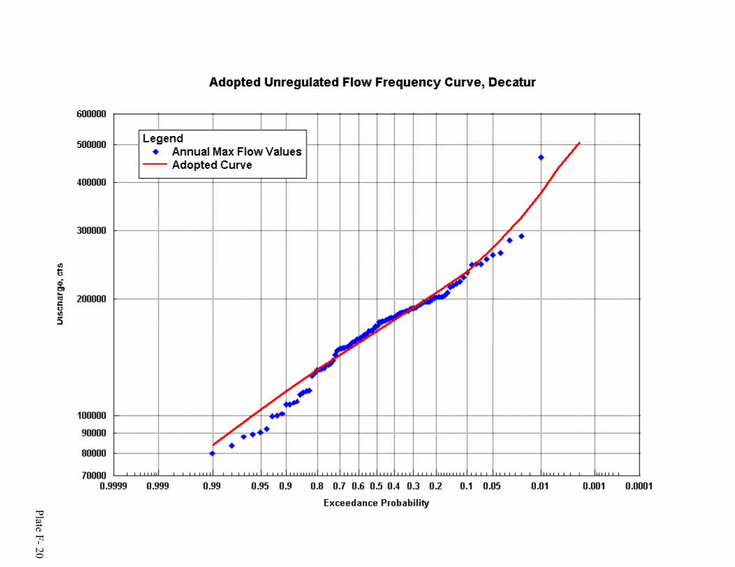
Plate F- 20

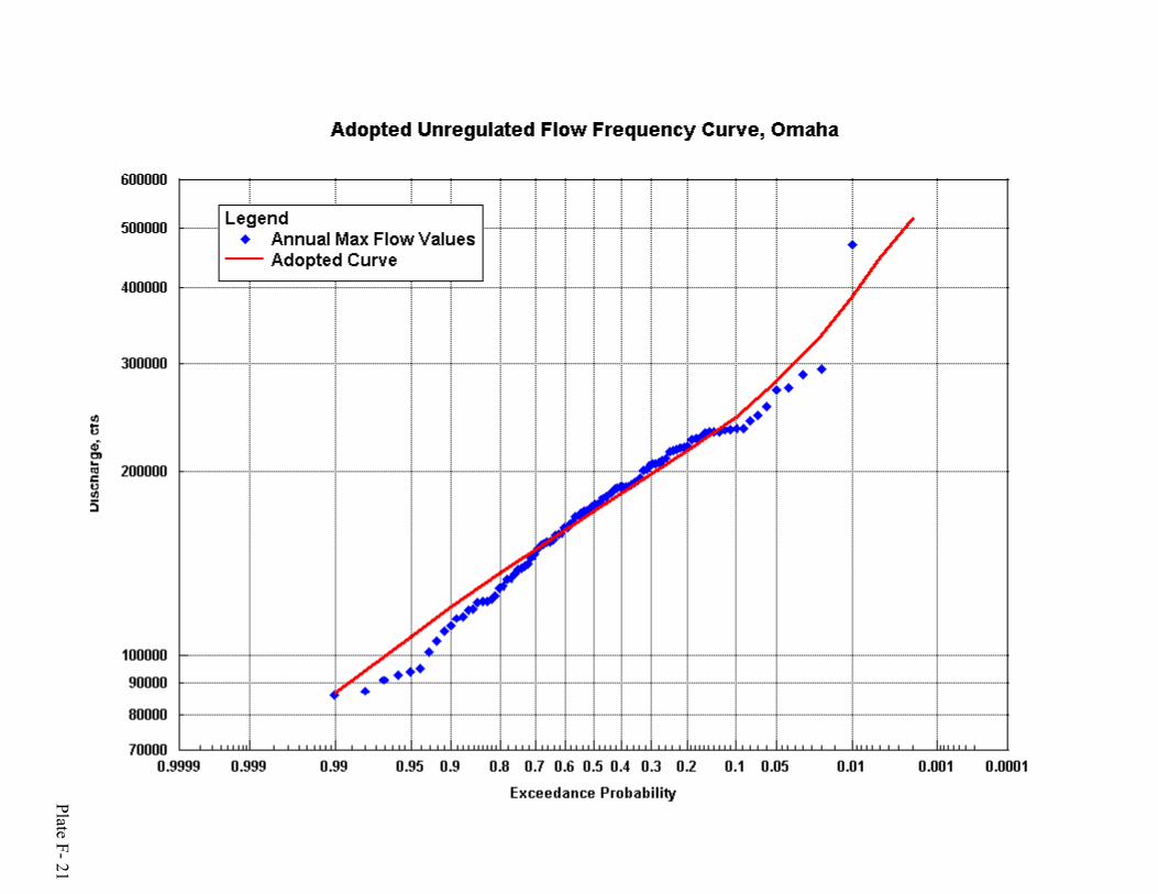
Plate F- 21

Plate F- 22

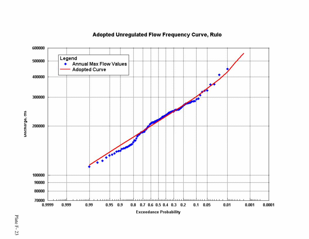
Plate F- 23

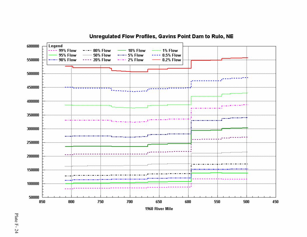
Plate F- 24

Plate F- 25

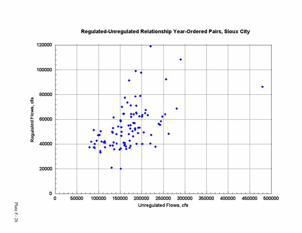
Plate F- 26

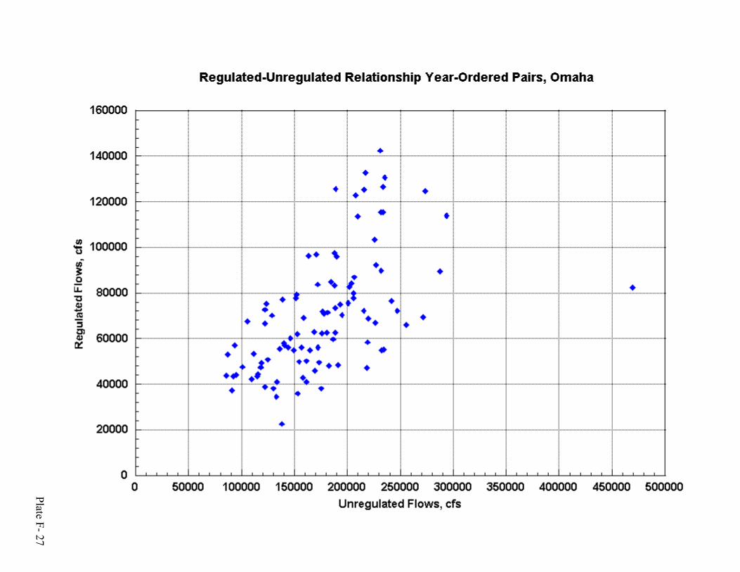
Plate F- 27

Plate F- 28

Plate F- 29

Plate F- 30

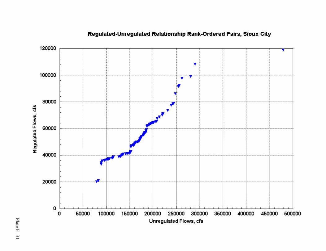
Plate F- 31

Plate F- 32

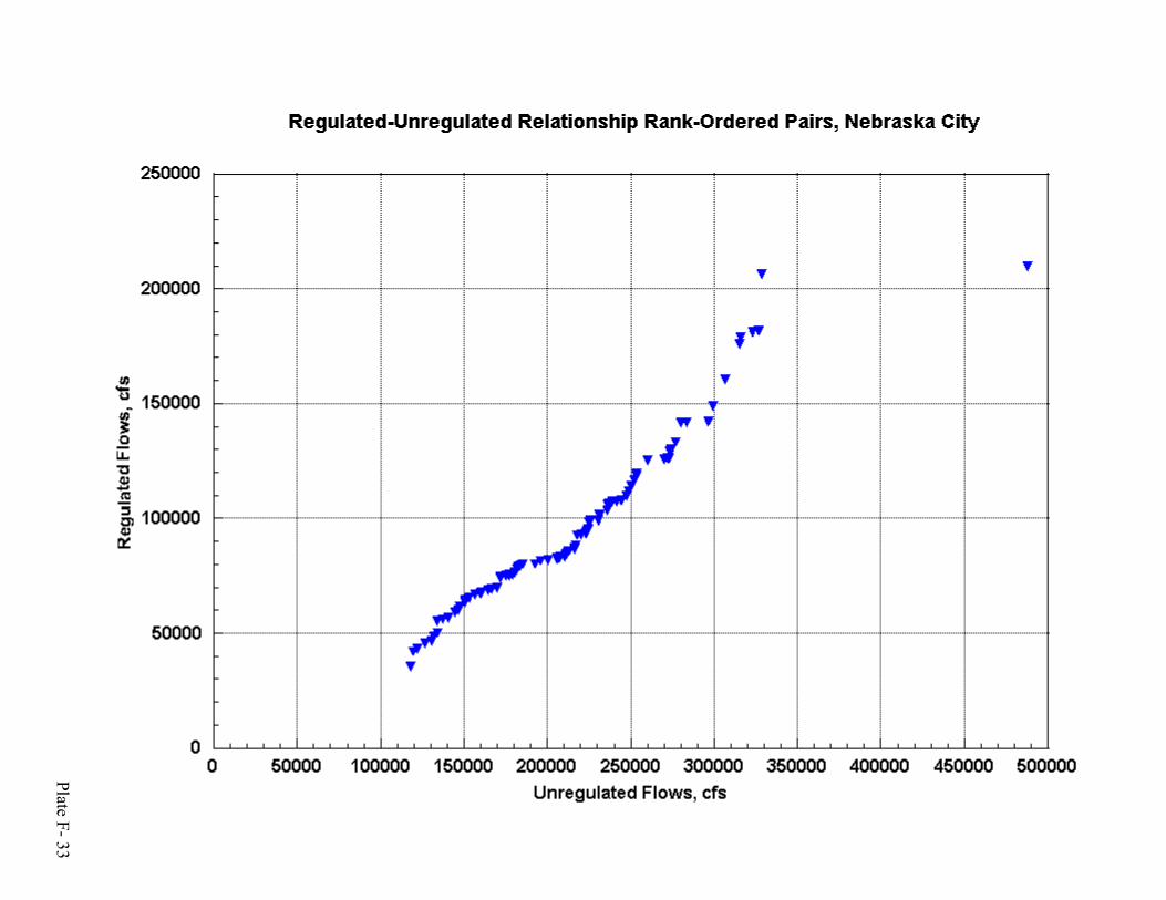
Plate F- 33

Plate F- 34

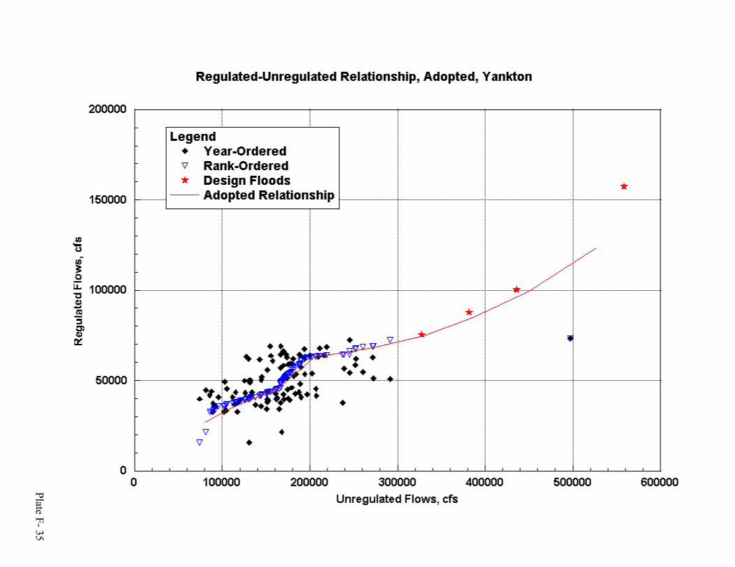
Plate F- 35

Plate F- 36

Plate F- 37

Plate F- 38

Plate F- 39

Plate F- 40

Plate F- 41

Plate F- 42

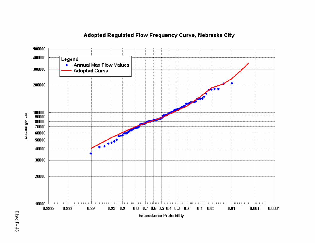
Plate F- 43

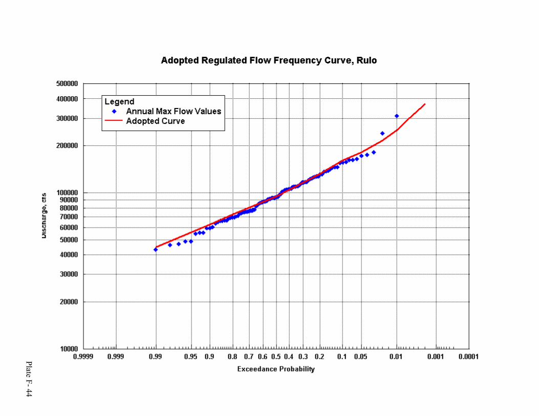
Plate F- 44

Plate F- 45

NOTE: Data revised during the Hydraulic Analysis.

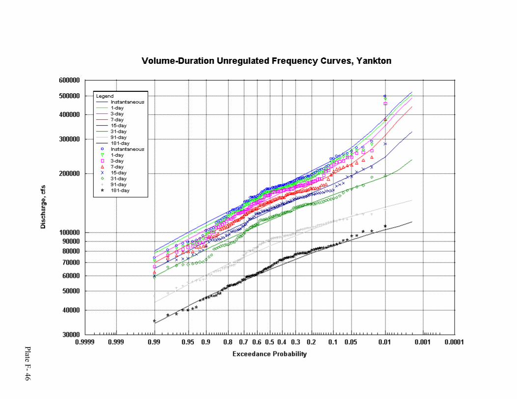
Plate F- 46

Plate F- 47

Plate F- 48

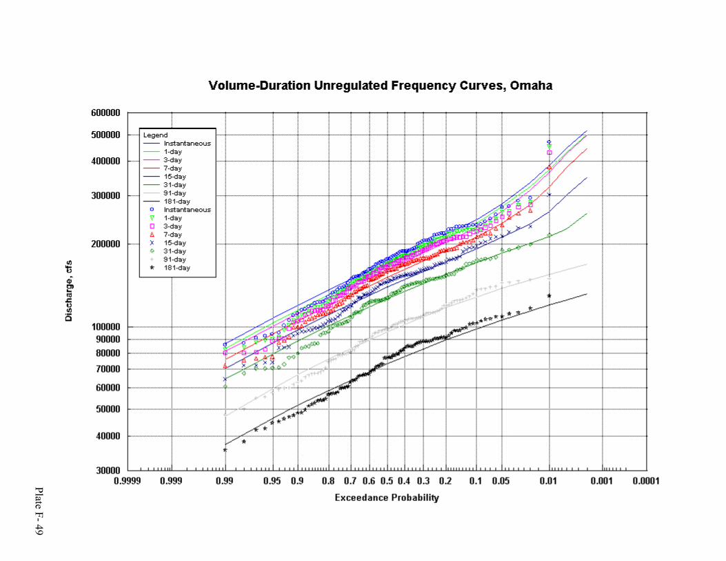
Plate F- 49

Plate F- 50

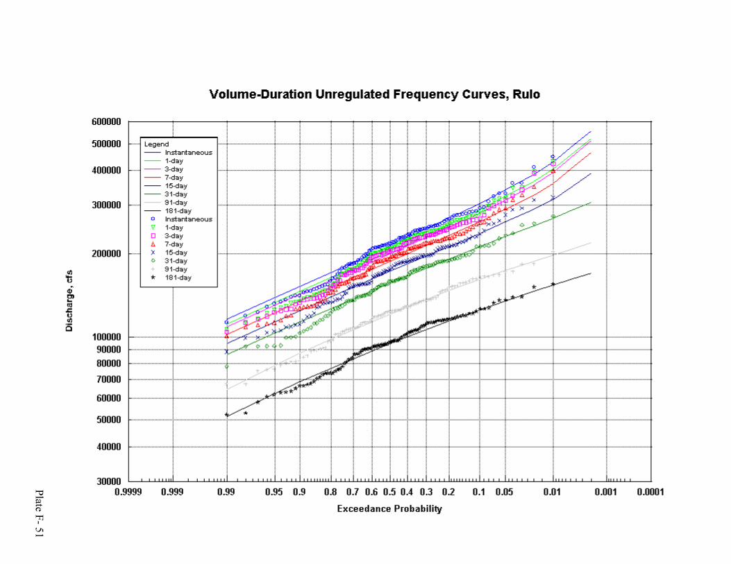
Plate F- 51

Plate F-52

Stream StationMo.

River Mile

Mo. River Drainage

Area

USGS Flow

Record

Tributary Drainage

Area

Drainage Area

Cumulative

RM Weighted Ungaged

Area

Cumul. With

Ungaged

Missouri River Yankton, SD 805.8 279,500 10/1/30 --> 279,500 279,500James River Yankton-Scot. 797.7 9/1/28 --> 20,942 300,442 305.7 300,748 Bow Creek St James, NE 787.6 10/1/78 --> 304 300,746 381.2 301,433 Vermillion River Vermill-Wak. 771.9 10/1/45 --> 2,302 303,048 592.5 304,327 Aowa Creek Ponca, NE 745.2 None 222 303,270 1007.7 305,557 Elk Creek 737.3 None 132 303,402 298.2 305,987 Big Sioux River Akron, IA 734.0 10/1/28 --> 8,424 311,826 124.5 314,536 Unknown Ungaged 2,774 314,600 64.2

Missouri River Sioux City, IA 732.3 314,600

10/1/28 - 7/30/31

10/1/38 --> 314,600 314,600 Perry Creek Sioux City, IA 732.1 10/1/45 --> 65 314,665 1.8 314,667 Floyd River James, IA 731.3 10/1/35 --> 886 315,551 7.1 315,560 Omaha Creek Homer, NE 719.9 10/1/45 --> 174 315,725 101.8 315,836 Blackbird Creek 697.6 None 106 315,831 199.2 316,141 Unknown Ungaged 369 316,200 59.0

Missouri River Decatur, NE 691.0 316,200 10/1/87 --> 316,200 316,200 Monona Har. Ditch Turin, IA 670.0 10/1/39 --> 900 317,100 106.8 317,207 Little Sioux River Turin, IA 669.2 5/7/42 --> 3,526 320,626 4.1 320,737 Tekamah Dv. Ditch 665.0 None 124 320,750 21.4 320,882 Soldier River Pisgah, IA 664.0 3/5/40 --> 407 321,157 5.1 321,294 Old Soldier R.Ditch 649.3 None 100 321,257 74.8 321,469 Fish Creek 647.9 None 124 321,381 7.1 321,600 Boyer River Logan, IA 635.2 5/24/18 --> 871 322,252 64.6 322,536 Pigeon Creek 622.0 None 166 322,418 67.1 322,769 Unknown Ungaged 382 322,800 31.0

Missouri River Omaha, NE 615.9 322,800 9/1/28 --> 322,800 322,800 Mosquito Cr 605.8 None 238 323,038 148.2 323,186 Big Papillion Cr Fort Crook 596.6 08/1/86 --> 384 323,422 135.0 323,705 Platte River Ashland-Louis. 594.8 10/1/28 --> 85,370 408,792 26.4 409,102 Watkins Ditch 587.5 None 185 408,977 107.1 409,394 Weeping Water Cr Union 568.7 3/1/50 --> 241 409,218 275.8 409,911 Unknown 782 410,000 89.5

Missouri River Nebraska City 562.6 410,000 8/11/29 --> 410,000 410,000 Nishnabotna River Hamburg 542.1 3/1/22 --> 2,806 412,806 214.8 413,021 Little Nemaha River Auburn 527.8 9/1/49 --> 793 413,599 149.9 413,964 Rock Creek 522.2 None 104 413,703 58.7 414,126 Tarkio River Fairfax, MO 507.6 4/1/22 --> 520 414,223 153.0 414,799 Unknown 677 414,900 100.6

Missouri River Rulo 498.0 414,900 9/1/49 --> 414,900 414,900 Muddy Creek Big Nem. Trib 495.0 None 258 415,158 109.8 415,268 Big Nemaha River Falls City, NE 494.8 4/1/44 --> 1,340 416,498 7.3 416,615 Little Tarkio River 492.4 None 170 416,668 87.9 416,873 Squaw Creek 486.3 None 178 416,846 223.3 417,274 Wolf Creek 478.8 None 251 417,097 274.5 417,800 Nodaway River Graham/Burling 463.0 4/1/22 --> 1,380 418,477 578.4 419,758 Unknown 1,823 420,300 541.8 420,300

Missouri River St. Joseph 448.2 420,300 9/1/28 --> 420,300

Missouri River from Gavins Point to St. Joseph Drainage Area Accounting

Plate F-53

Missouri River Specific Gage AnalysisSioux City, IA River Mile 732.3

8

13

18

23

28

33

1930 1940 1950 1960 1970 1980 1990 200Year

Gag

e H

eigh

t (ft)

100,000 CFS

50,000 CFS

40,000 CFS

30,000 CFS

20,000 CFS

10,000 CFS

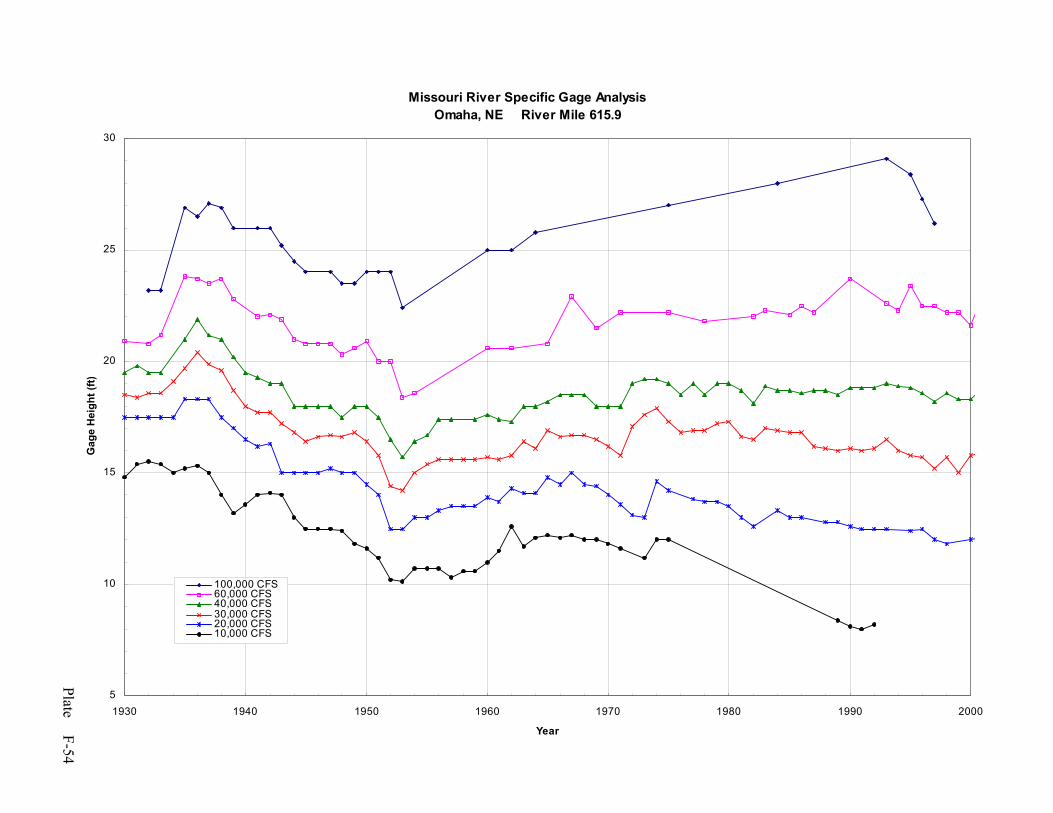
Plate F-54

Missouri River Specific Gage AnalysisOmaha, NE River Mile 615.9

5

10

15

20

25

30

1930 1940 1950 1960 1970 1980 1990 2000

Year

Gag

e H

eigh

t (ft)

100,000 CFS60,000 CFS40,000 CFS30,000 CFS20,000 CFS10,000 CFS

Plate F-55

Missouri River Specific Gage AnalysisNebraska City, NE River Mile 562.6

0

5

10

15

20

25

1930 1940 1950 1960 1970 1980 1990 2000

Year

Gag

e H

eigh

t (ft)

100,000 CFS

70,000 CFS

40,000 CFS

30,000 CFS

20,000 CFS

Plate F-56

Missouri River Survey Data Accuracy The photogrammetric mapping products were designed and collected according to American Society of Photogrammetry and Remote Sensing (ASPRS) Standards. The accuracy and quality of the digital elevation data is suitable for 4’ contour interval mapping. The mapping contractor included breaklines to define levee, road and railroad locations and elevations. No ground surveys to increase elevation data accuracy were included. As a result, well defined grided elevation points shown on the levee profile should be within 1.33 feet RMSE (95% of the time) of the actual elevation in areas that are clearly identified in the aerial photography. Areas that are hard surfaces (i.e. roads, parking areas, cleared fields) will provide elevations that are within 0.67 feet RMSE (67% of the time).

The survey coordinate system is: Horizontal: UTM Zone 15 NAD 1983 Vertical: NGVD 1929

U.S. Feet The following were requirements were furnished to the survey contractor for collection of survey data from 1999 aerial photography along the Missouri River corridor within the Omaha District. 1. The Contractor shall collect DTM data (mass points and breaklines) to sufficiently depict the horizontal and vertical location of elevated roads, railroads, and levees. Additional (minimal) DTM points shall be collected to optimize the vertical accuracy of DEM data points. All DTM data shall be in ASCII X,Y,Z (Easting, Northing and Elevation respectively) format fully compatible with Intergraph InRoads software. All data shall be referenced to NAD 27 and NGVD 29 datum and use UTM projection. The DTM data (mass points and breaklines) shall have an RMSE of 0.67' with a one sigma (0.67%) confidence factor. 2. The Contractor shall also generate DEM data at the posting of 15 feet. The DEM data shall be referenced to NAD 27 and NGVD 29 datums and use UTM projection. All DEM data shall be in ASCII X,Y,Z (Easting, Northing and Elevation respectively) format fully compatible with Intergraph InRoads software. The X and Y coordinates for the DEM data will be evenly devisable by 15 and a 1/10 foot vertical resolution. The RMSE of well defined DEM elevations shall not exceed 1.33' and the DEM must be of sufficient accuracy to support generation of 4' contours that meet U.S. Army Corps of Engineers Standards for Class I mapping as per EM1110-1-1000, dated 31 March 1993. NOTE: The map accuracy standards refer to the photogrammetric mapping products only. Below water survey information was previously collected in 1994 and 1995 and merged with the photogrammetric data to form the final dtm. The dtm files contain Missouri River hydrographic surveys in the form of random points along a cross section line at roughly 500 foot intervals. Since the hydrographic data are entered as random points and contain no breaklines, the cross section is only valid at the hydrographic data location. No hydrographic data is included for any tributaries or lakes other than the Missouri River.

Plate F-57

Omaha District UNET Model Levee Cell Location

Note: Figure illustrates levee cell subdivisions used within the UNET Model.

##

####

#

#

#

#

#

#

#

#

#

#

#

#

#

#

#

##

#

#

##

#

#

#

#

###

#

#

#

##

##

##

#

#

#

#

#

#

#

#

#

#

#

#

#

#

#

##

##

#

#

#

#

#

#

#

#

#

#

#

#

#

#

#

#

#

#

#

#

#

#

#

#

#

#

#

#

#

#

#

#

#

#

#

#

#

#

#

#

#

#

#

#

#

#

#

#

#

##

#

###

#

#

#

#

#

#

##

#

#

##

#

#

#

L536

L550 LOW

L550 UP

L575 LOW

L575 UP

L594

R548

R562

R573

R613

R616

L627 L624L614

L561

L601 N

OmahaFloodwall

L611 S2

L611 N2

C.B.Levee

L611 N1

L601 NEL611

S1

L601 S

L575 MID

RM620

RM610

RM600

RM590

RM580

RM570

RM560

RM550

RM540

RM530

RM520

RM510

RM500

OmahaNorth

Omaha South

R520

MATCH LINE

MATCH LINE

FLOW

FLOW

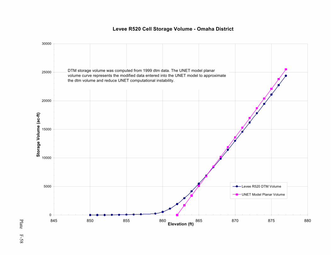
Plate F-58

Levee R520 Cell Storage Volume - Omaha District

0

5000

10000

15000

20000

25000

30000

845 850 855 860 865 870 875 880Elevation (ft)

Stor

age

Volu

me

(ac-

ft)

Levee R520 DTM Volume

UNET Model Planar Volume

DTM storage volume was computed from 1999 dtm data. The UNET model planar volume curve represents the modified data entered into the UNET model to approximate the dtm volume and reduce UNET computational instability.

Plate F-59

Levee L536 Cell Storage Volume - Omaha District

0

20000

40000

60000

80000

100000

120000

140000

160000

180000

865 870 875 880 885 890 895Elevation (ft)

Stor

age

Volu

me

(ac-

ft)

Levee L 536 DTM Volume


DTM storage volume was computed from 1999 dtm data. The UNET model planar volume is the modified data entered into the UNET model to approximate the dtm volume and reduce UNET computational instability.

Plate F-60


0

10000

20000

30000

40000

50000

60000

70000

80000

875 880 885 890 895 900 905 910Elevation (ft)

Stor

age

Volu

me

(ac-

ft)

Levee R 548 DTM Volume



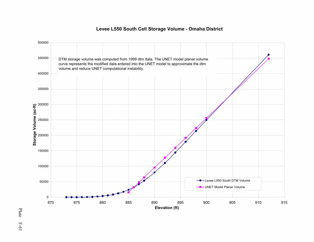
Plate F-61

Levee L550 South Cell Storage Volume - Omaha District

0

50000

100000

150000

200000

250000

300000

350000

400000

450000

500000

870 875 880 885 890 895 900 905 910 915Elevation (ft)

Stor

age

Volu

me

(ac-

ft)

Levee L550 South DTM Volume



Plate F-62

Levee L550 North Cell Storage Volume - Omaha District

0

100000

200000

300000

400000

500000

600000

880 885 890 895 900 905 910 915 920 925Elevation (ft)

Stor

age

Volu

me

(ac-

ft)

Levee L550 North DTM Volume



Plate F-63


0

10000

20000

30000

40000

50000

60000

70000

80000

90000

895 900 905 910 915 920Elevation (ft)

Stor

age

Volu

me

(ac-

ft)




Plate F-64


0

10000

20000

30000

40000

50000

60000

70000

80000

90000

890 895 900 905 910 915 920 925Elevation (ft)

Stor

age

Volu

me

(ac-

ft)

Levee L561 DTM Volume



Plate F-65


0

5000

10000

15000

20000

25000

908 910 912 914 916 918 920 922 924 926 928Elevation (ft)

Stor

age

Volu

me

(ac-

ft)




Plate F-66

Levee L575 South Cell Storage Volume - Omaha District

0

50000

100000

150000

200000

250000

300000

350000

400000

890 895 900 905 910 915 920 925 930Elevation (ft)

Stor

age

Volu

me

(ac-

ft)

Levee L575 South DTM Volume



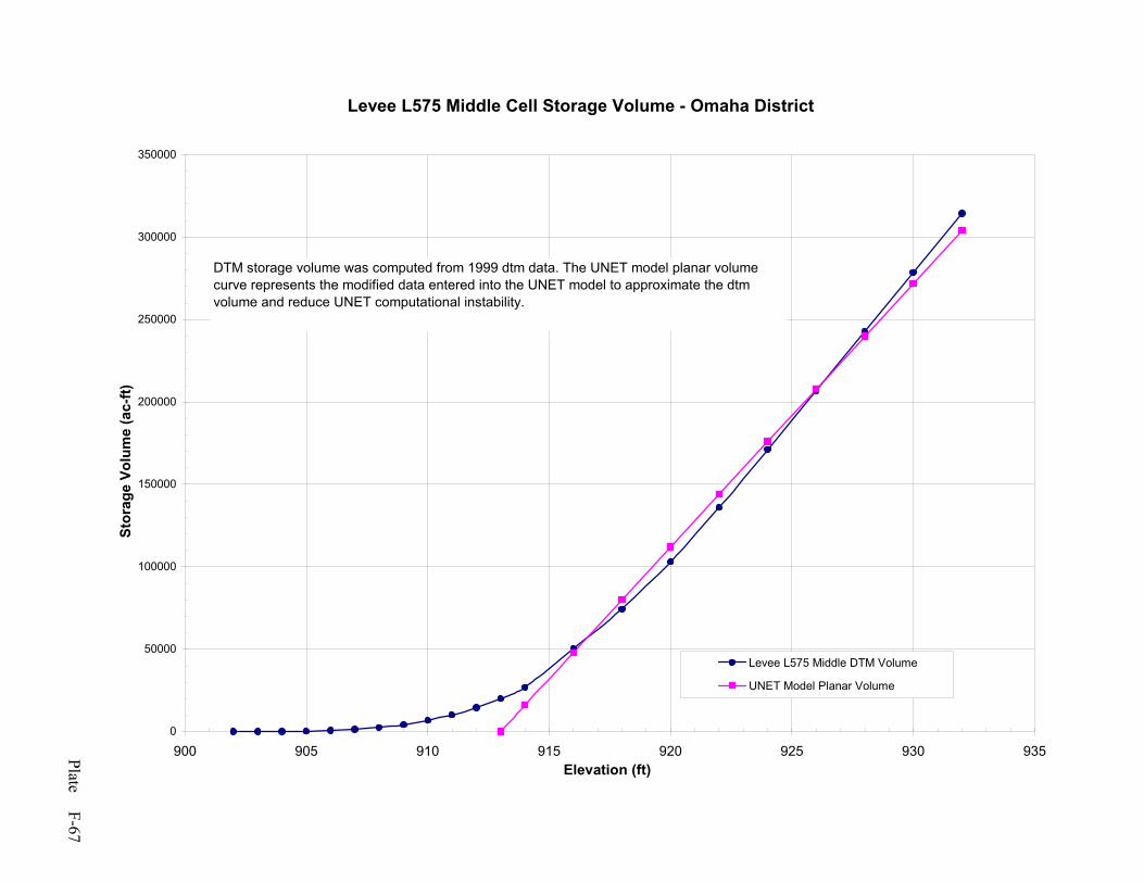
Plate F-67

Levee L575 Middle Cell Storage Volume - Omaha District

0

50000

100000

150000

200000

250000

300000

350000

900 905 910 915 920 925 930 935Elevation (ft)

Stor

age

Volu

me

(ac-

ft)

Levee L575 Middle DTM Volume



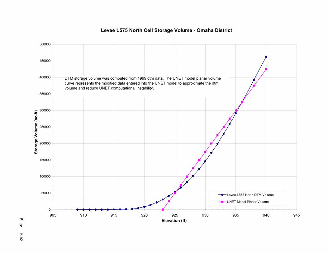
Plate F-68


0

50000

100000

150000

200000

250000

300000

350000

400000

450000

500000

905 910 915 920 925 930 935 940 945Elevation (ft)

Stor

age

Volu

me

(ac-

ft)




Plate F-69


0

20000

40000

60000

80000

100000

120000

140000

160000

180000

925 930 935 940 945 950 955 960Elevation (ft)

Stor

age

Volu

me

(ac-

ft)




Plate F-70


0

20000

40000

60000

80000

100000

120000

930 935 940 945 950 955 960 965 970Elevation (ft)

Stor

age

Volu

me

(ac-

ft)




Plate F-71

Levee L601 NE Cell Storage Volume - Omaha District

0

10000

20000

30000

40000

50000

60000

70000

945 950 955 960 965 970 975 980 985Elevation (ft)

Stor

age

Volu

me

(ac-

ft)

Levee L601 NE DTM Volume



Plate F-72

Levee L611 South 1 Cell Storage Volume - Omaha District

0

10000

20000

30000

40000

50000

60000

70000

940 945 950 955 960 965 970 975 980Elevation (ft)

Stor

age

Volu

me

(ac-

ft)

Levee L611 South 1 DTM Volume



Plate F-73

Levee L611 South 2 Cell Storage Volume - Omaha District

0

50000

100000

150000

200000

250000

300000

350000

940 945 950 955 960 965 970 975 980 985Elevation (ft)

Stor

age

Volu

me

(ac-

ft)

Levee L611 South 2 DTM Volume



Plate F-74

Levee L611 North 1 Cell Storage Volume - Omaha District

0.00

10000.00

20000.00

30000.00

40000.00

50000.00

60000.00

70000.00

80000.00

940 945 950 955 960 965 970 975 980 985 990

Elevation (ft)

Stor

age

(acr

e-ft)

L611 North 1

UNET Model PlanarVolume


Plate F-75

Levee L611 North 2 Cell Storage Volume - Omaha District

0

10000

20000

30000

40000

50000

60000

70000

80000

940 945 950 955 960 965 970 975 980 985 990Elevation (ft)

Stor

age

Volu

me

(ac-

ft)

Levee L611 North 2 DTM Volume



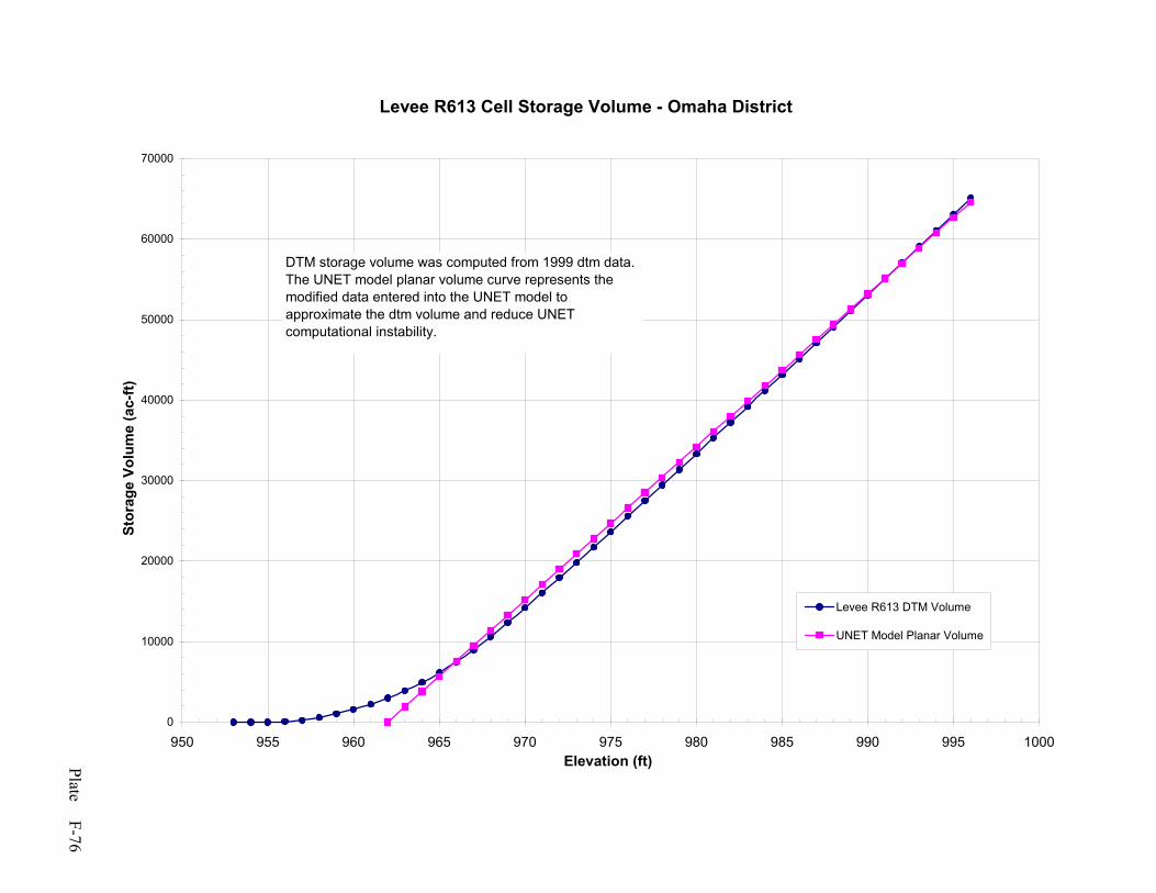
Plate F-76


0

10000

20000

30000

40000

50000

60000

70000

950 955 960 965 970 975 980 985 990 995 1000Elevation (ft)

Stor

age

Volu

me

(ac-

ft)




Plate F-77


0

5000

10000

15000

20000

25000

30000

35000

955 960 965 970 975 980 985 990Elevation (ft)

Stor

age

Volu

me

(ac-

ft)




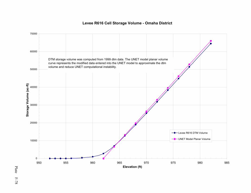
Plate F-78


0

10000

20000

30000

40000

50000

60000

70000

950 955 960 965 970 975 980 985Elevation (ft)

Stor

age

Volu

me

(ac-

ft)




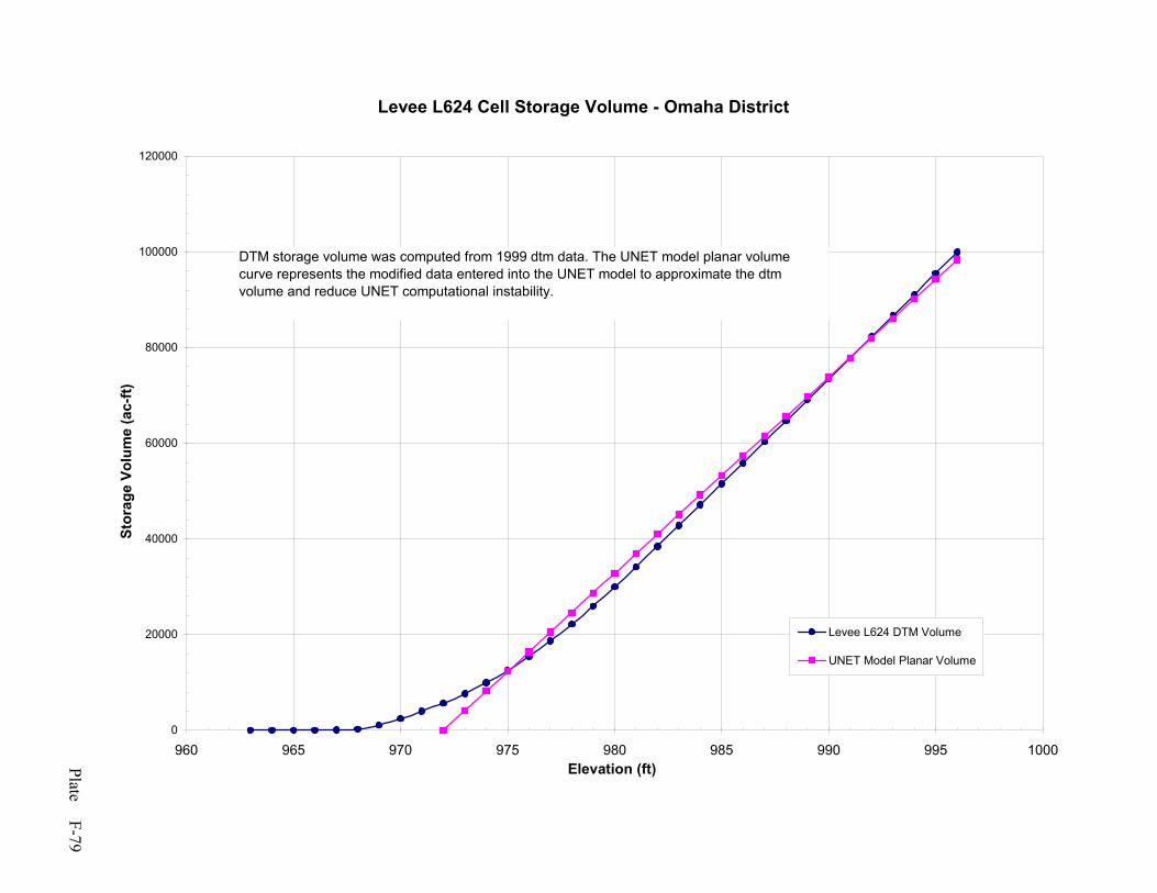
Plate F-79


0

20000

40000

60000

80000

100000

120000

960 965 970 975 980 985 990 995 1000Elevation (ft)

Stor

age

Volu

me

(ac-

ft)




Plate F-80


0

10000

20000

30000

40000

50000

60000

70000

80000

960 965 970 975 980 985 990 995Elevation (ft)

Stor

age

Volu

me

(ac-

ft)




Plate F-81

Council Bluffs Levee Cell Storage Volume - Omaha District

0

20000

40000

60000

80000

100000

120000

140000

960 965 970 975 980 985 990 995 1000 1005Elevation (ft)

Stor

age

Volu

me

(ac-

ft)

Council Bluffs Levee DTM Volume



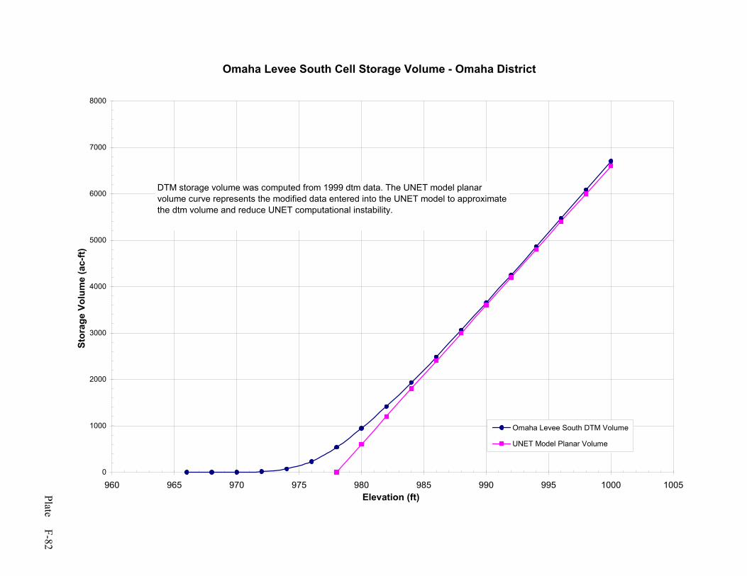
Plate F-82

Omaha Levee South Cell Storage Volume - Omaha District

0

1000

2000

3000

4000

5000

6000

7000

8000

960 965 970 975 980 985 990 995 1000 1005Elevation (ft)

Stor

age

Volu

me

(ac-

ft)

Omaha Levee South DTM Volume



Plate F-83

Omaha Floodwall Levee Cell Storage Volume - Omaha District

0

20000

40000

60000

80000

100000

120000

140000

960 965 970 975 980 985 990 995 1000 1005Elevation (ft)

Stor

age

Volu

me

(ac-

ft)

Omaha Floodwall DTM Volume


DTM storage volume was computed from 1999 dtm data. The UNET model planar volumecurve represents the modified data entered into the UNET model to approximate the dtm volume and reduce UNET computational instability.

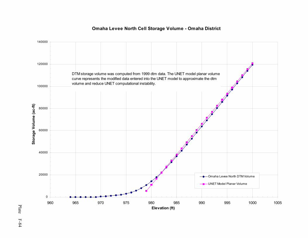
Plate F-84

Omaha Levee North Cell Storage Volume - Omaha District

0

20000

40000

60000

80000

100000

120000

140000

960 965 970 975 980 985 990 995 1000 1005Elevation (ft)

Stor

age

Volu

me

(ac-

ft)

Omaha Levee North DTM Volume


DTM storage volume was computed from 1999 dtm data. The UNET model planar volumecurve represents the modified data entered into the UNET model to approximate the dtm volume and reduce UNET computational instability.

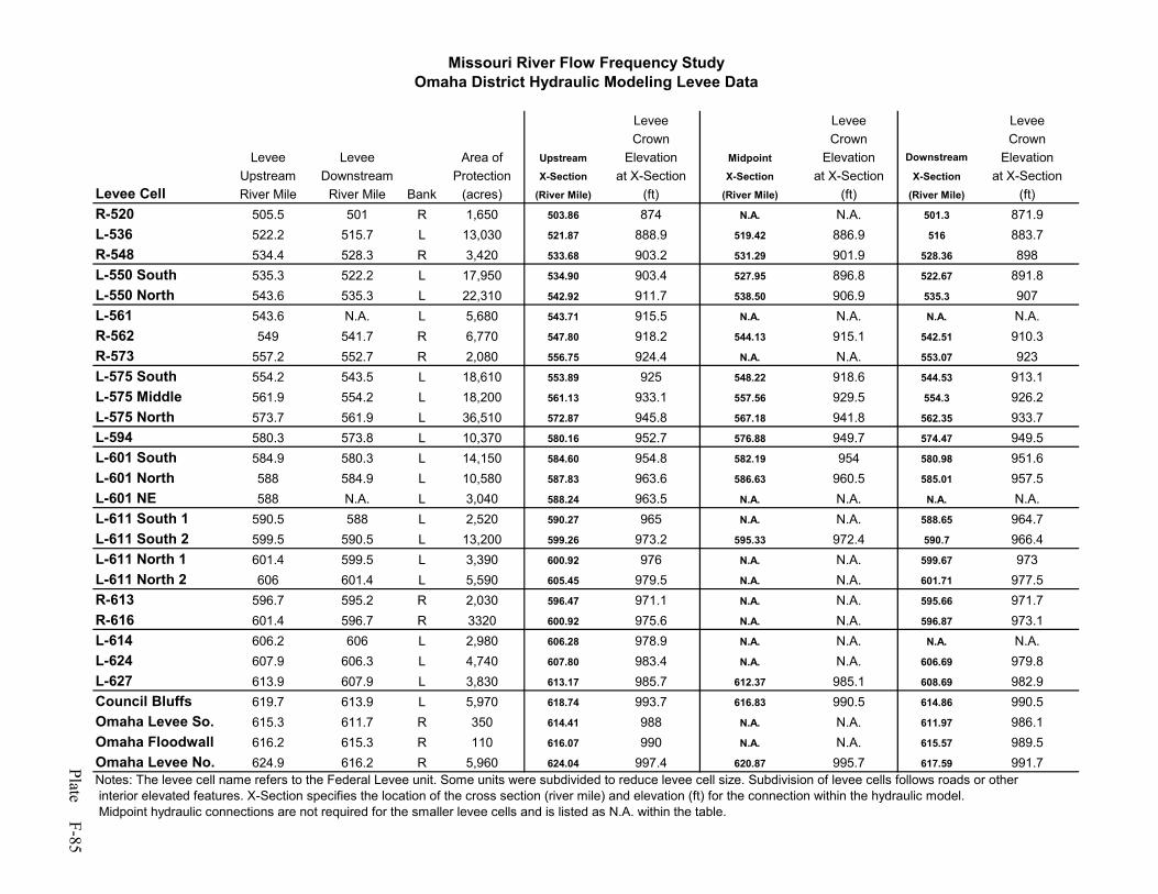
Plate F-85

Levee Levee LeveeCrown Crown Crown

Levee Levee Area of Upstream Elevation Midpoint Elevation Downstream ElevationUpstream Downstream Protection X-Section at X-Section X-Section at X-Section X-Section at X-Section

Levee Cell River Mile River Mile Bank (acres) (River Mile) (ft) (River Mile) (ft) (River Mile) (ft)R-520 505.5 501 R 1,650 503.86 874 N.A. N.A. 501.3 871.9L-536 522.2 515.7 L 13,030 521.87 888.9 519.42 886.9 516 883.7R-548 534.4 528.3 R 3,420 533.68 903.2 531.29 901.9 528.36 898L-550 South 535.3 522.2 L 17,950 534.90 903.4 527.95 896.8 522.67 891.8L-550 North 543.6 535.3 L 22,310 542.92 911.7 538.50 906.9 535.3 907L-561 543.6 N.A. L 5,680 543.71 915.5 N.A. N.A. N.A. N.A.R-562 549 541.7 R 6,770 547.80 918.2 544.13 915.1 542.51 910.3R-573 557.2 552.7 R 2,080 556.75 924.4 N.A. N.A. 553.07 923L-575 South 554.2 543.5 L 18,610 553.89 925 548.22 918.6 544.53 913.1L-575 Middle 561.9 554.2 L 18,200 561.13 933.1 557.56 929.5 554.3 926.2L-575 North 573.7 561.9 L 36,510 572.87 945.8 567.18 941.8 562.35 933.7L-594 580.3 573.8 L 10,370 580.16 952.7 576.88 949.7 574.47 949.5L-601 South 584.9 580.3 L 14,150 584.60 954.8 582.19 954 580.98 951.6L-601 North 588 584.9 L 10,580 587.83 963.6 586.63 960.5 585.01 957.5L-601 NE 588 N.A. L 3,040 588.24 963.5 N.A. N.A. N.A. N.A.L-611 South 1 590.5 588 L 2,520 590.27 965 N.A. N.A. 588.65 964.7L-611 South 2 599.5 590.5 L 13,200 599.26 973.2 595.33 972.4 590.7 966.4L-611 North 1 601.4 599.5 L 3,390 600.92 976 N.A. N.A. 599.67 973L-611 North 2 606 601.4 L 5,590 605.45 979.5 N.A. N.A. 601.71 977.5R-613 596.7 595.2 R 2,030 596.47 971.1 N.A. N.A. 595.66 971.7R-616 601.4 596.7 R 3320 600.92 975.6 N.A. N.A. 596.87 973.1L-614 606.2 606 L 2,980 606.28 978.9 N.A. N.A. N.A. N.A.L-624 607.9 606.3 L 4,740 607.80 983.4 N.A. N.A. 606.69 979.8L-627 613.9 607.9 L 3,830 613.17 985.7 612.37 985.1 608.69 982.9Council Bluffs 619.7 613.9 L 5,970 618.74 993.7 616.83 990.5 614.86 990.5Omaha Levee So. 615.3 611.7 R 350 614.41 988 N.A. N.A. 611.97 986.1Omaha Floodwall 616.2 615.3 R 110 616.07 990 N.A. N.A. 615.57 989.5Omaha Levee No. 624.9 616.2 R 5,960 624.04 997.4 620.87 995.7 617.59 991.7Notes: The levee cell name refers to the Federal Levee unit. Some units were subdivided to reduce levee cell size. Subdivision of levee cells follows roads or other interior elevated features. X-Section specifies the location of the cross section (river mile) and elevation (ft) for the connection within the hydraulic model. Midpoint hydraulic connections are not required for the smaller levee cells and is listed as N.A. within the table.

Missouri River Flow Frequency StudyOmaha District Hydraulic Modeling Levee Data

Plate F- 86

Sioux City Measured Gage Data Variation

1069

1070

1071

1072

1073

1074

1075

1076

1077

1078

1079

1080

1081

1082

1083

1084

1085

1086

1087

1088

20000 30000 40000 50000 60000 70000 80000 90000 100000 110000

Flow (cfs)

Elev

atio

n (fe

et 1

929

NG

VD)

Measured Data 1984

Measured Data 1993

Measured Data 1996

Measured Data 1997

Measured Data 1999

Plate F- 87

Decatur Measured Gage Data Variation

1029

1030

1031

1032

1033

1034

1035

1036

1037

1038

1039

1040

1041

1042

20000 30000 40000 50000 60000 70000 80000 90000 100000

Flow (cfs)

Elev

atio

n (fe

et 1

929

NG

VD)

Measured Data 1984

Measured Data 1993

Measured Data 1996

Measured Data 1997

Measured Data 1999

Plate F- 88

Omaha Measured Gage Data Variation

961

962

963

964

965

966

967

968

969

970

971

972

973

974

975

976

977

978

979

30000 40000 50000 60000 70000 80000 90000 100000 110000 120000

Flow (cfs)

Elev

atio

n (fe

et 1

929

NG

VD)

Measured Data 1984

Measured Data 1993

Measured Data 1996

Measured Data 1997

Measured Data 1999

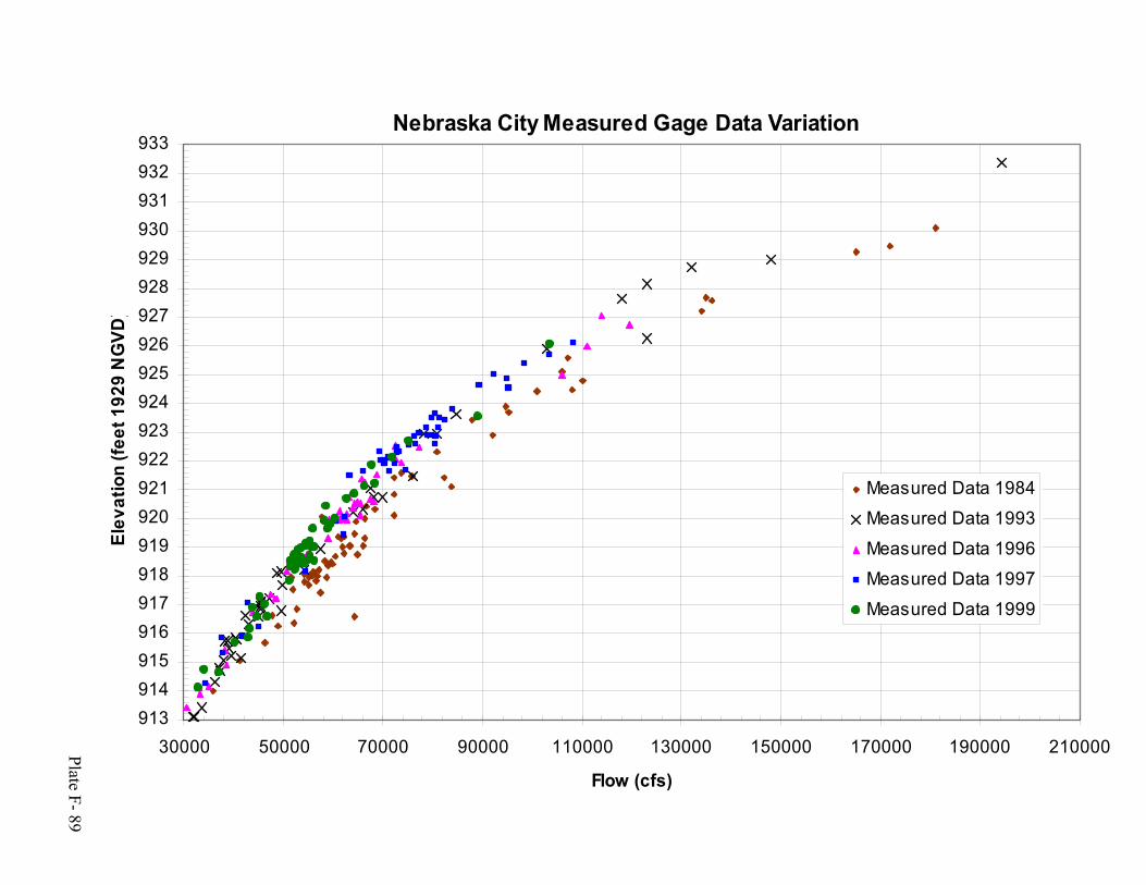
Plate F- 89

Nebraska City Measured Gage Data Variation

913914915916917918919920921922923924925926927928929930931932933

30000 50000 70000 90000 110000 130000 150000 170000 190000 210000

Flow (cfs)

Elev

atio

n (fe

et 1

929

NG

VD)

Measured Data 1984

Measured Data 1993

Measured Data 1996

Measured Data 1997

Measured Data 1999

Plate F- 90

Rulo Measured Gage Data Variation

844

845

846

847

848

849

850

851

852

853

854

855

856

857

858

859

860

861

862

863

30000 50000 70000 90000 110000 130000 150000 170000 190000 210000 230000

Flow (cfs)

Elev

atio

n (fe

et 1

929

NG

VD)

Measured Data 1984

Measured Data 1993

Measured Data 1996

Measured Data 1997

Measured Data 1999

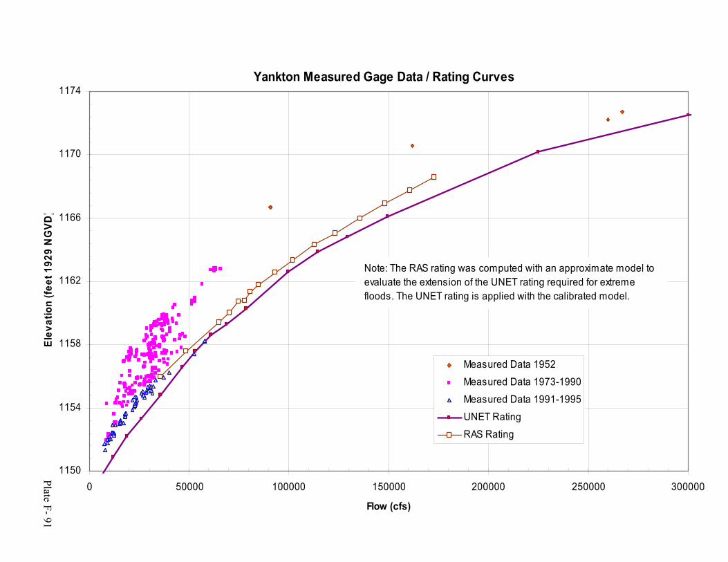
Plate F- 91

Yankton Measured Gage Data / Rating Curves

1150

1154

1158

1162

1166

1170

1174

0 50000 100000 150000 200000 250000 300000

Flow (cfs)

Elev

atio

n (fe

et 1

929

NG

VD)

Measured Data 1952

Measured Data 1973-1990


UNET Rating

RAS Rating

Note: The RAS rating was computed with an approximate model to evaluate the extension of the UNET rating required for extreme floods. The UNET rating is applied with the calibrated model.

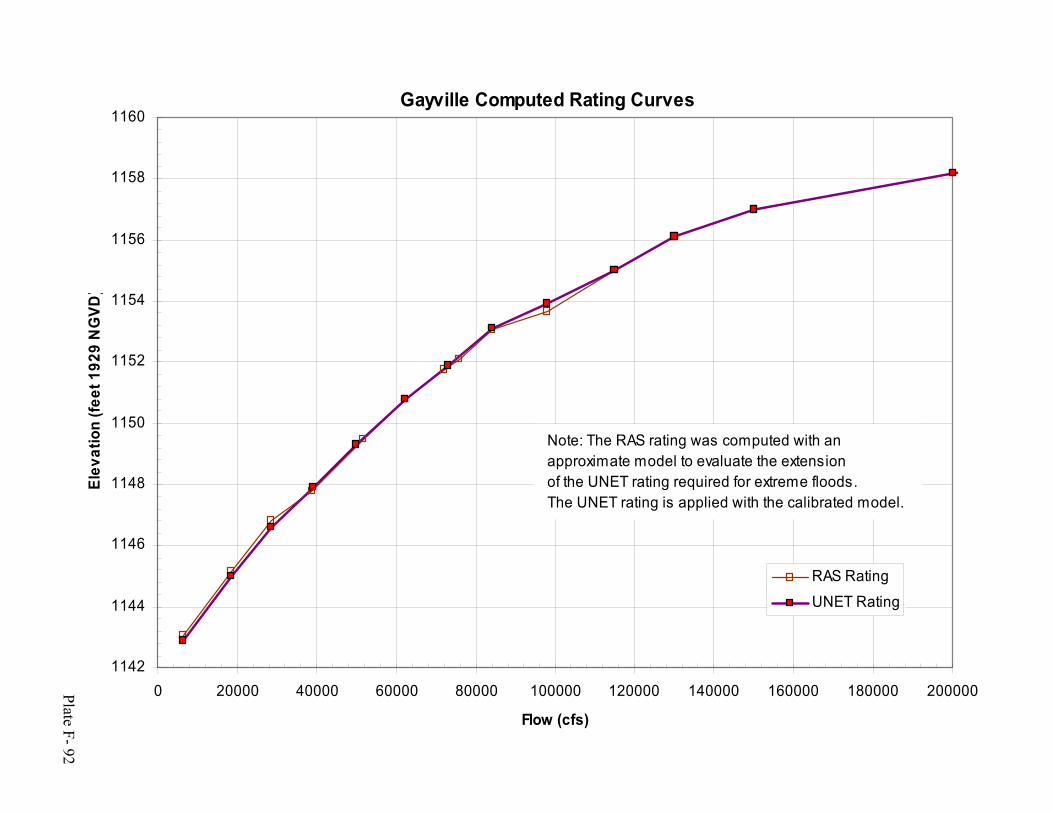
Plate F- 92

Gayville Computed Rating Curves

1142

1144

1146

1148

1150

1152

1154

1156

1158

1160

0 20000 40000 60000 80000 100000 120000 140000 160000 180000 200000

Flow (cfs)

Elev

atio

n (fe

et 1

929

NG

VD)

RAS Rating

UNET Rating

Note: The RAS rating was computed with anapproximate model to evaluate the extensionof the UNET rating required for extreme floods. The UNET rating is applied with the calibrated model.

Plate F- 93

Maskell Computed Rating Curves

1117

1119

1121

1123

1125

1127

1129

1131

1133

1135

0 20000 40000 60000 80000 100000 120000 140000 160000 180000 200000

Flow (cfs)

Elev

atio

n (fe

et 1

929

NG

VD)

RAS Rating

UNET Rating

Note: The RAS rating was computed with anapproximate model to evaluate the extensionof the UNET rating required for extreme floods. The UNET rating is applied with the calibrated model.

Plate F- 94

Ponca Computed Rating Curves

1085

1087

1089

1091

1093

1095

1097

1099

1101

1103

1105

1107

1109

1111

1113

0 20000 40000 60000 80000 100000 120000 140000 160000 180000 200000

Flow (cfs)

Elev

atio

n (f

eet 1

929

NG

VD)

RAS Rating

UNET Rating

Note: The RAS rating w as computed w ith anapproximate model to evaluate the extensionof the UNET rating required for extreme floods. The UNET rating is applied w ith the calibrated model.

Plate F- 95

Sioux City Measured Gage Data / Rating Curves

1066

1070

1074

1078

1082

1086

1090

1094

1098

0 25000 50000 75000 100000 125000 150000 175000 200000 225000 250000 275000 300000

Flow (cfs)

Elev

atio

n (fe

et 1

929

NG

VD)




UNET Rating

Plate F- 96

Decatur Measured Gage Data / Rating Curves

1026

1030

1034

1038

1042

1046

1050

1054

0 25000 50000 75000 100000 125000 150000 175000 200000 225000 250000 275000 300000

Flow (cfs)

Elev

atio

n (f

eet 1

929

NG

VD)


Ras Confined Rating

RAS Unconfined Rating


Measured Data 1997 - 2000

UNET Rating

Note: The RAS rating was computed with an approximate model to evaluate the extension of the UNET rating required for extreme floods. Approximate RAS models were constructed for both confined and unconfined conditions. The UNET rating is applied with the calibrated model.

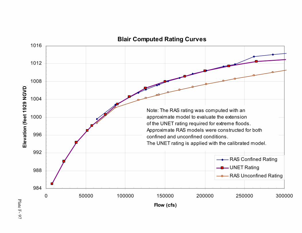
Plate F- 97

Blair Computed Rating Curves

984

988

992

996

1000

1004

1008

1012

1016

0 50000 100000 150000 200000 250000 300000

Flow (cfs)

Elev

atio

n (fe

et 1

929

NG

VD)

RAS Confined Rating

UNET Rating


Note: The RAS rating was computed with anapproximate model to evaluate the extensionof the UNET rating required for extreme floods. Approximate RAS models were constructed for both confined and unconfined conditions.The UNET rating is applied with the calibrated model.

Plate F- 98

Omaha Measured Gage Data / Rating Curves

959

963

967

971

975

979

983

987

991

0 50000 100000 150000 200000 250000 300000 350000

Flow (cfs)

Elev

atio

n (fe

et 1

929

NG

VD)




UNET Rating

Plate F- 99

Plattsmouth Computed Rating Curves

942

946

950

954

958

962

966

970

974

0 50000 100000 150000 200000 250000 300000 350000 400000

Flow (cfs)

Elev

atio

n (fe

et 1

929

NG

VD)


UNET RatingRAS Confined Rating

Note: The RAS rating was computed with anapproximate model to evaluate the extensionof the UNET rating required for extreme floods. Approximate RAS models were constructed for both confined and unconfined conditions.The UNET rating is applied with the calibrated model.

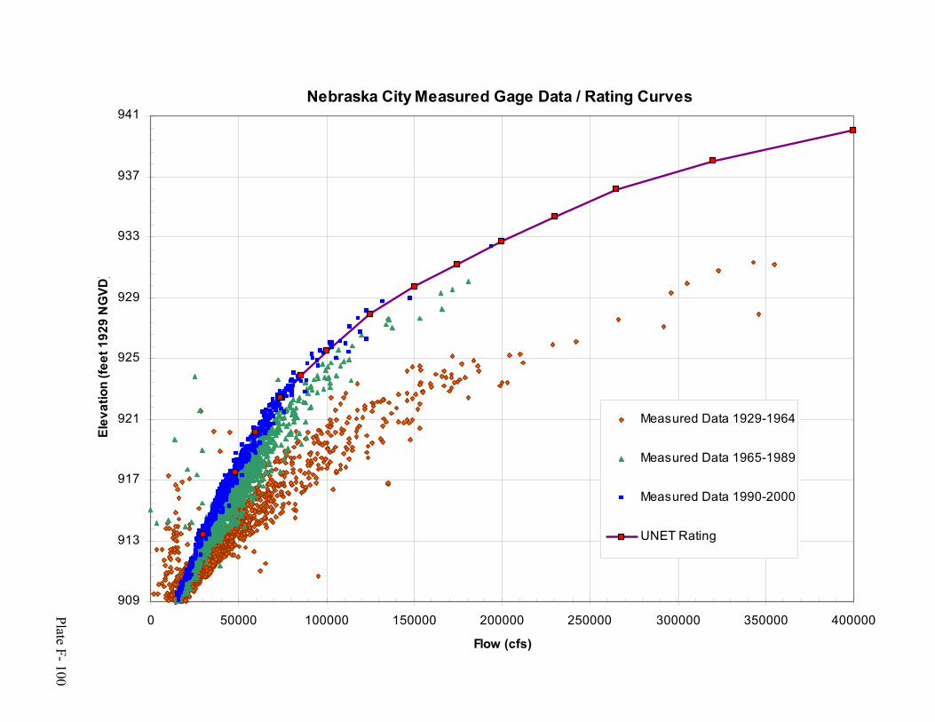
Plate F- 100

Nebraska City Measured Gage Data / Rating Curves

909

913

917

921

925

929

933

937

941

0 50000 100000 150000 200000 250000 300000 350000 400000

Flow (cfs)

Elev

atio

n (fe

et 1

929

NG

VD)




UNET Rating

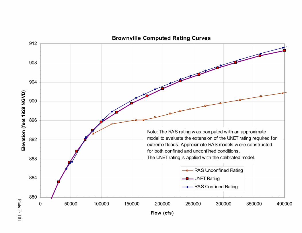
Plate F- 101

Brownville Computed Rating Curves

880

884

888

892

896

900

904

908

912

0 50000 100000 150000 200000 250000 300000 350000 400000

Flow (cfs)

Elev

atio

n (f

eet 1

929

NG

VD)


UNET Rating

RAS Confined Rating

Note: The RAS rating w as computed w ith an approximate model to evaluate the extension of the UNET rating required for extreme floods. Approximate RAS models w ere constructed for both confined and unconfined conditions.The UNET rating is applied w ith the calibrated model.

Plate F- 102

Rulo Measured Gage Data / Rating Curves

840

844

848

852

856

860

864

0 50000 100000 150000 200000 250000 300000 350000 400000

Flow (cfs)

Elev

atio

n (fe

et 1

929

NG

VD)



UNET Rating

Note: The UNET rating was estimated using the observed gage record and measured data. Extension for extreme floods follows the

Plate F- 103

Missouri River at Omaha, NEMeasured Data Plotted By Season

70000 75000 80000 85000 90000 95000 100000 105000 110000 115000

Flow (cfs)

970

971

972

973

974

975

976

977

978

979

Elev

atio

n (ft

192

9 N

GVD

)

12/1/1997

11/24/199711/17/1997

11/10/1997

11/4/199710/27/1997

10/15/1997

4/28/1997

4/22/19974/15/19974/11/1997

4/8/1997

4/4/1997

4/19/1984

7/29/97

7/1/97

6/24/97

6/10/97

6/2/97 5/27/975/19/97

5/12/97

5/6/97

8/5/96

7/18/96

7/17/96

6/25/96

6/22/96

7/21/93

7/16/93

7/11/93

6/27/84

6/26/84

6/21/846/18/84

LegendMeasured Flow Spring/FallMeasured Flow May-SepSummer Exponential TrendSpring/Fall Expon. Trend

Computed trends from the measured data areinconclusive. Although an elevation shift isevident, the time of occurence and the magnitudeof the shift appears to vary.

Note large stage range at 104,000 cfs measuredflow value between 7/11/93 and 7/17/96.

Plate F- 104

Missouri River - UNET vs Measured Profiles RM 495-550

845

850

855

860

865

870

875

880

885

890

895

900

905

910

495 505 515 525 535 545

River Mile

Elev

atio

n (F

eet 1

929

NG

VD)

5-May-97 UNET

5-May-97 Measured

23-Sep-97 UNET

23-Sep-97 Measured

21-Jul-98 UNET

21-Jul-98 Measured

14-Sep-99 UNET

14-Sep-99 Measured

Plate F- 105


905

910

915

920

925

930

935

940

945

950

955

960

965

550 555 560 565 570 575 580 585 590 595 600

River Mile

Elev

atio

n (F

eet 1

929

NG

VD)

5-May-97 UNET

5-May-97 Measured

23-Sep-97 UNET

23-Sep-97 Measured

21-Jul-98 UNET

21-Jul-98 Measured

14-Sep-99 UNET

14-Sep-99 Measured

Plate F- 106


955

960

965

970

975

980

985

990

995

1000

1005

600 605 610 615 620 625 630 635 640 645 650

River Mile

Elev

atio

n (F

eet 1

929

NG

VD)

5-May-97 UNET

5-May-97 Measured

23-Sep-97 UNET

23-Sep-97 Measured

21-Jul-98 UNET

21-Jul-98 Measured

14-Sep-99 UNET

14-Sep-99 Measured

Plate F- 107


995

1000

1005

1010

1015

1020

1025

1030

1035

1040

1045

1050

650 655 660 665 670 675 680 685 690 695 700

River Mile

Elev

atio

n (F

eet 1

929

NG

VD)

5-May-97 UNET

5-May-97 Measured

23-Sep-97 UNET

23-Sep-97 Measured

21-Jul-98 UNET

21-Jul-98 Measured

14-Sep-99 UNET

14-Sep-99 Measured

Plate F- 108


1040

1045

1050

1055

1060

1065

1070

1075

1080

1085

1090

1095

1100

700 705 710 715 720 725 730 735 740 745 750

River Mile

Elev

atio

n (F

eet 1

929

NG

VD)

5-May-97 UNET

5-May-97 Measured

23-Sep-97 UNET

23-Sep-97 Measured

21-Jul-98 UNET

21-Jul-98 Measured

14-Sep-99 UNET

14-Sep-99 Measured

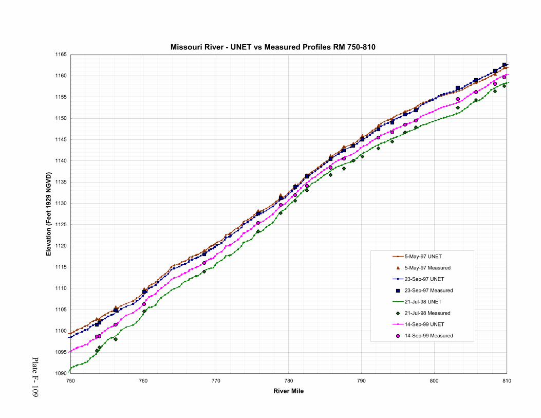
Plate F- 109


1090

1095

1100

1105

1110

1115

1120

1125

1130

1135

1140

1145

1150

1155

1160

1165

750 760 770 780 790 800 810

River Mile

Elev

atio

n (F

eet 1

929

NG

VD)

5-May-97 UNET

5-May-97 Measured

23-Sep-97 UNET

23-Sep-97 Measured

21-Jul-98 UNET

21-Jul-98 Measured

14-Sep-99 UNET

14-Sep-99 Measured

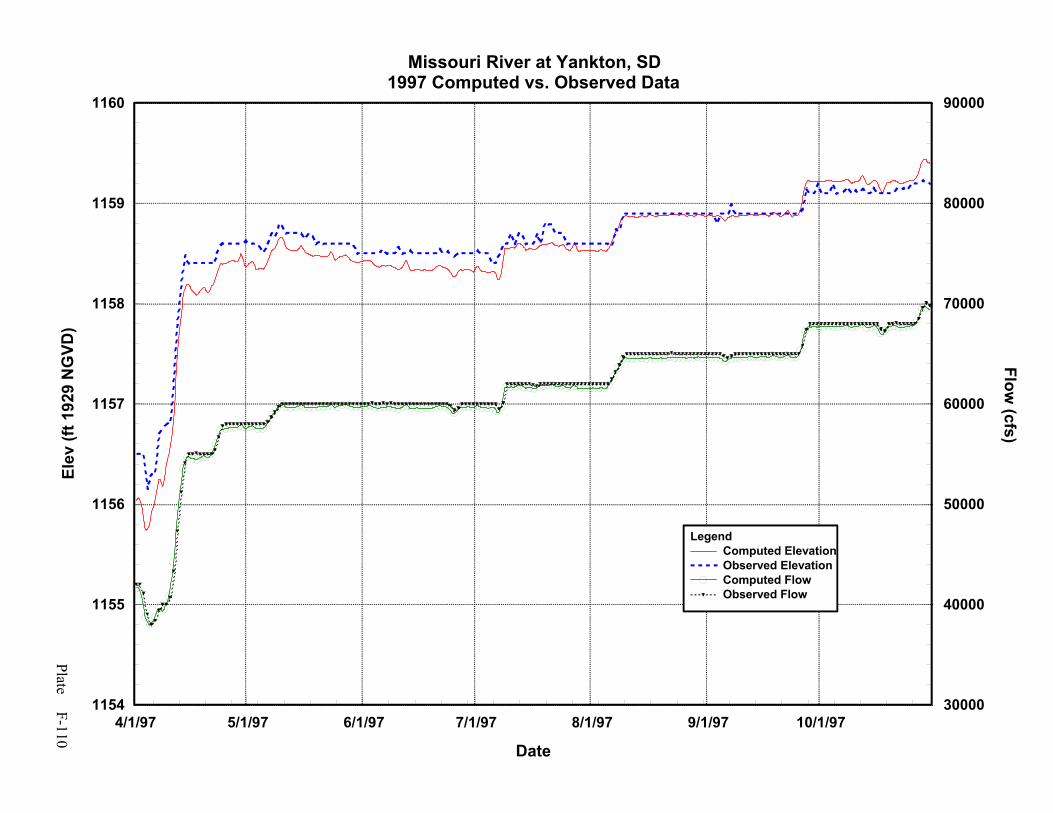
Plate F-110 4/1/97 5/1/97 6/1/97 7/1/97 8/1/97 9/1/97 10/1/97

Date

1154

1155

1156

1157

1158

1159

1160

Elev

(ft 1

929

NG

VD)

30000

40000

50000

60000

70000

80000

90000

Flow (cfs)

LegendComputed ElevationObserved ElevationComputed FlowObserved Flow

Missouri River at Yankton, SD1997 Computed vs. Observed Data

Plate F-111 4/1/97 5/1/97 6/1/97 7/1/97 8/1/97 9/1/97 10/1/97

Date

1148

1149

1150

1151

1152

1153

Elev

(ft 1

929

NG

VD)

50000

60000

70000

80000

90000

100000

Flow (cfs)

LegendComputed ElevationComputed FlowObserved Elevation

Missouri River at Gayville, SD1997 Computed vs. Observed Data

Plate F-112 4/1/97 5/1/97 6/1/97 7/1/97 8/1/97 9/1/97 10/1/97

Date

1124

1125

1126

1127

1128

1129

Elev

(ft 1

929

NG

VD)

45000

55000

65000

75000

85000

95000

Flow (cfs)


Missouri River at Maskell, SD1997 Computed vs. Observed Data

Plate F-113 4/1/97 5/1/97 6/1/97 7/1/97 8/1/97 9/1/97 10/1/97

Date

1096

1097

1098

1099

1100

1101

1102

Elev

(ft 1

929

NG

VD)

50000

60000

70000

80000

90000

100000

110000

Flow (cfs)


Missouri River at Ponca, NE1997 Computed vs. Observed Data

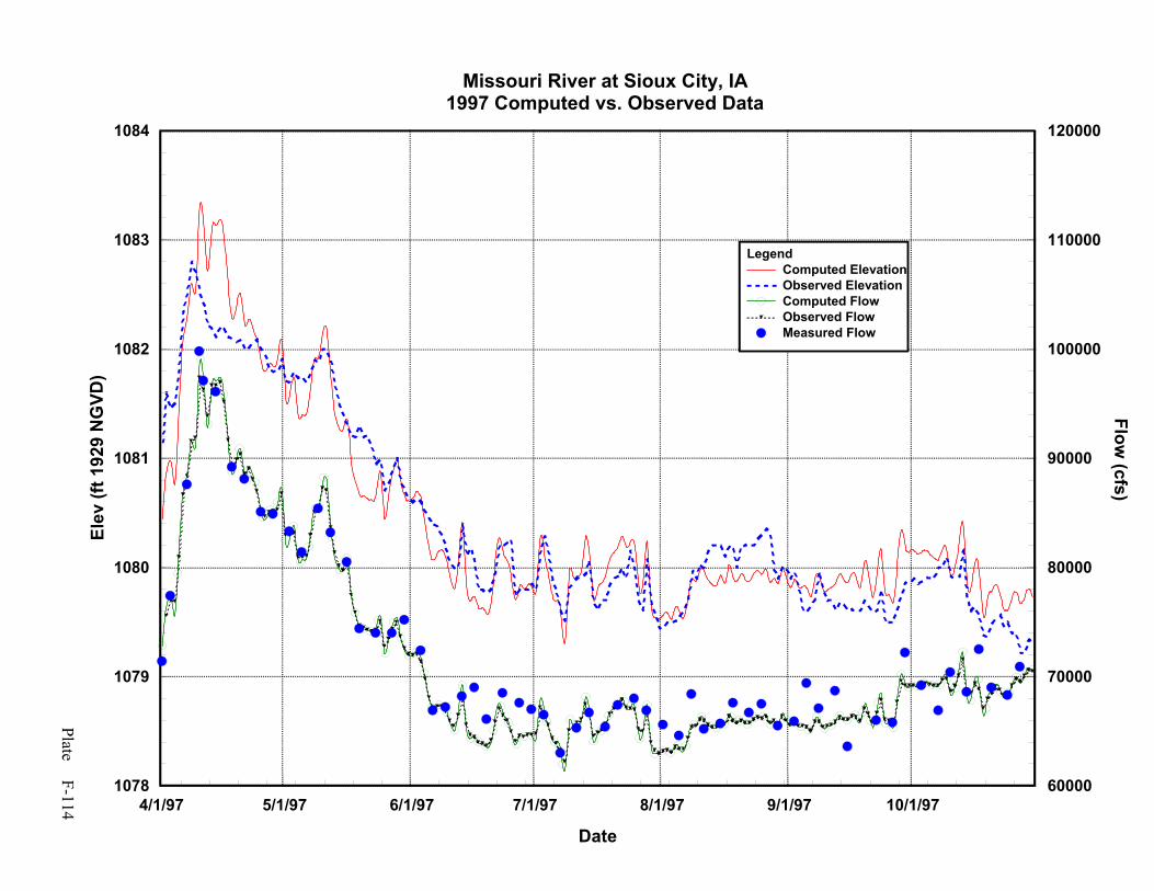
Plate F-114 4/1/97 5/1/97 6/1/97 7/1/97 8/1/97 9/1/97 10/1/97

Date

1078

1079

1080

1081

1082

1083

1084

Elev

(ft 1

929

NG

VD)

60000

70000

80000

90000

100000

110000

120000

Flow (cfs)

LegendComputed ElevationObserved ElevationComputed FlowObserved FlowMeasured Flow

Missouri River at Sioux City, IA1997 Computed vs. Observed Data

Plate F-115 5/1/84 6/1/84 7/1/84 8/1/84 9/1/84 10/1/84

Date

1023

1024

1025

1026

1027

1028

1029

1030

1031

1032

1033

1034

1035

1036

1037

1038

1039

1040

1041

1042

1043

1044

1045

Elev

(ft 1

929

NG

VD)

15000

25000

35000

45000

55000

65000

75000

85000

95000

105000

115000

125000

Flow (cfs)

LegendComputed ElevationObserved ElevationComputed FlowMeasured Flow

Missouri River at Decatur, NE1984 Computed vs. Observed Data

Compare Calibration Error at Peakto 93, 97 Flood With Similar Peak Flow

Plate F-116 5/1/93 6/1/93 7/1/93 8/1/93 9/1/93 10/1/93

Date

1023

1024

1025

1026

1027

1028

1029

1030

1031

1032

1033

1034

1035

1036

1037

1038

1039

1040

1041

1042

1043

Elev

(ft 1

929

NG

VD)

15000

35000

55000

75000

95000

115000

Flow (cfs)



Calibration Error 1 Foot Low at PeakCompare to 97 Flood Calibration

Plate F-117 4/1/97 5/1/97 6/1/97 7/1/97 8/1/97 9/1/97 10/1/97

Date

1037.5

1038.5

1039.5

1040.5

1041.5

1042.5

1043.5

Elev

(ft 1

929

NG

VD)

50000

65000

80000

95000

110000

125000

140000

Flow (cfs)



Limited Seasonal Correction Appliedto Early Spring Computed Stage for

Period of Record Analysis

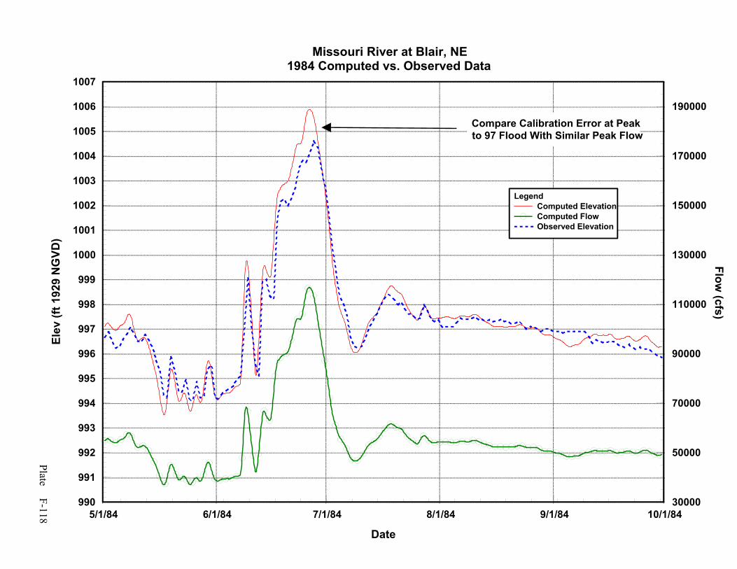
Plate F-118 5/1/84 6/1/84 7/1/84 8/1/84 9/1/84 10/1/84

Date

990

991

992

993

994

995

996

997

998

999

1000

1001

1002

1003

1004

1005

1006

1007

Elev

(ft 1

929

NG

VD)

30000

50000

70000

90000

110000

130000

150000

170000

190000

Flow (cfs)


Missouri River at Blair, NE1984 Computed vs. Observed Data

Compare Calibration Error at Peakto 97 Flood With Similar Peak Flow

Plate F-119 5/1/93 6/1/93 7/1/93 8/1/93 9/1/93 10/1/93

Date

985

986

987

988

989

990

991

992

993

994

995

996

997

998

999

1000

1001

1002

1003

1004

1005

Elev

(ft 1

929

NG

VD)

0

50000

100000

150000

200000

Flow (cfs)




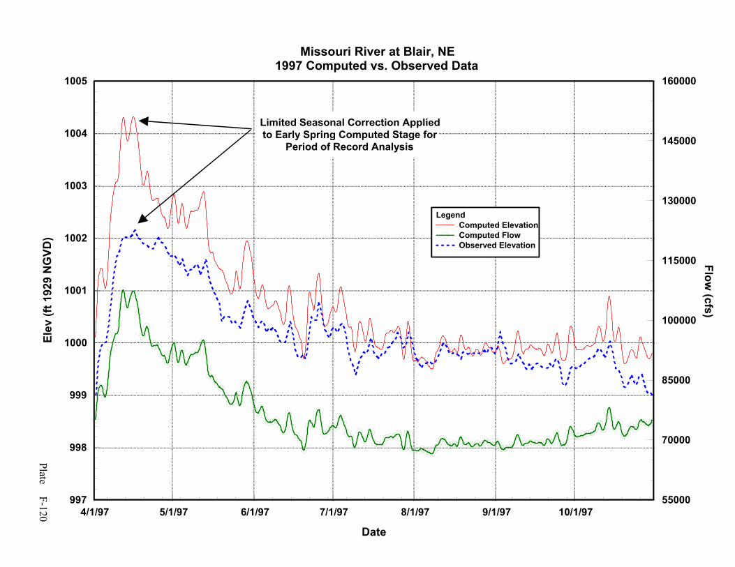
Plate F-120 4/1/97 5/1/97 6/1/97 7/1/97 8/1/97 9/1/97 10/1/97

Date

997

998

999

1000

1001

1002

1003

1004

1005

Elev

(ft 1

929

NG

VD)

55000

70000

85000

100000

115000

130000

145000

160000

Flow (cfs)



Limited Seasonal Correction Appliedto Early Spring Computed Stage for

Period of Record Analysis

Plate F-121 5/1/84 6/1/84 7/1/84 8/1/84 9/1/84 10/1/84

Date

964

965

966

967

968

969

970

971

972

973

974

975

976

977

978

979

Elev

(ft 1

929

NG

VD)

30000

40000

50000

60000

70000

80000

90000

100000

110000

120000

130000

140000

150000

160000

170000

180000

Flow (cfs)


Missouri River at Omaha, NE1984 Computed vs. Observed Data


Plate F-122 5/1/93 6/1/93 7/1/93 8/1/93 9/1/93 10/1/93

Date

958

959

960

961

962

963

964

965

966

967

968

969

970

971

972

973

974

975

976

977

978

979

Elev

(ft 1

929

NG

VD)

20000

40000

60000

80000

100000

120000

140000

160000

Flow (cfs)




Plate F-123 4/1/97 5/1/97 6/1/97 7/1/97 8/1/97 9/1/97 10/1/97

Date

969

970

971

972

973

974

975

976

977

Elev

(ft 1

929

NG

VD)

60000

70000

80000

90000

100000

110000

120000

130000

140000

Flow (cfs)



Limited Seasonal Correction Applied to Early Spring Computed Stage for Periodof Record Analysis. Compare to 93 Event.

Plate F-124 5/1/84 6/1/84 7/1/84 8/1/84 9/1/84 10/1/84

Date

940

942

944

946

948

950

952

954

956

958

960

962

964

966

Elev

(ft 1

929

NG

VD)

30000

50000

70000

90000

110000

130000

150000

170000

190000

210000

230000

250000

270000

290000

Flow (cfs)


Missouri River at Plattsmouth, NE1984 Computed vs. Observed Data


Plate F-125 5/1/93 6/1/93 7/1/93 8/1/93 9/1/93 10/1/93

Date

941

943

945

947

949

951

953

955

957

959

961

963

965

Elev

(ft 1

929

NG

VD)

30000

70000

110000

150000

190000

230000

270000

Flow (cfs)




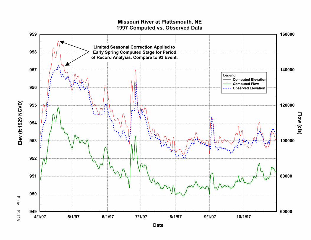
Plate F-126 4/1/97 5/1/97 6/1/97 7/1/97 8/1/97 9/1/97 10/1/97

Date

949

950

951

952

953

954

955

956

957

958

959

Elev

(ft 1

929

NG

VD)

60000

80000

100000

120000

140000

160000

Flow (cfs)



Limited Seasonal Correction Applied to Early Spring Computed Stage for Periodof Record Analysis. Compare to 93 Event.

Plate F-127 5/1/84 6/1/84 7/1/84 8/1/84 9/1/84 10/1/84

Date

914

916

918

920

922

924

926

928

930

932

Elev

(ft 1

929

NG

VD)

40000

60000

80000

100000

120000

140000

160000

180000

200000

220000

Flow (cfs)


Missouri River at Nebraska City, NE1984 Computed vs. Observed Data

Compare Calibration Error at Peakto 93 and 97 Flood at Similar Flow

Plate F-128 5/1/93 6/1/93 7/1/93 8/1/93 9/1/93 10/1/93

Date

910

912

914

916

918

920

922

924

926

928

930

932

934

Elev

(ft 1

929

NG

VD)

0

50000

100000

150000

200000

250000

300000

Flow (cfs)




Plate F-129 4/1/97 5/1/97 6/1/97 7/1/97 8/1/97 9/1/97 10/1/97

Date

919

920

921

922

923

924

925

926

927

Elev

(ft 1

929

NG

VD)

60000

70000

80000

90000

100000

110000

120000

130000

140000

Flow (cfs)



Plate F-130 5/1/84 6/1/84 7/1/84 8/1/84 9/1/84 10/1/84

Date

880

882

884

886

888

890

892

894

896

898

900

902

904

906

Elev

(ft 1

929

NG

VD)

30000

50000

70000

90000

110000

130000

150000

170000

190000

210000

230000

250000

270000

290000

Flow (cfs)


Missouri River at Brownville, NE1984 Computed vs. Observed Data


Possible Gage Error in Observed Data(Constant Stage for Varying Flow)

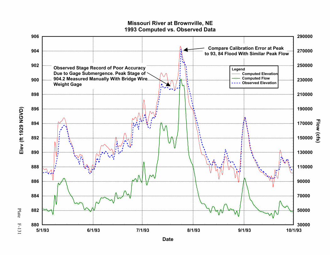
Plate F-131 5/1/93 6/1/93 7/1/93 8/1/93 9/1/93 10/1/93

Date

880

882

884

886

888

890

892

894

896

898

900

902

904

906

Elev

(ft 1

929

NG

VD)

30000

50000

70000

90000

110000

130000

150000

170000

190000

210000

230000

250000

270000

290000

Flow (cfs)




Observed Stage Record of Poor AccuracyDue to Gage Submergence. Peak Stage of904.2 Measured Manually With Bridge WireWeight Gage

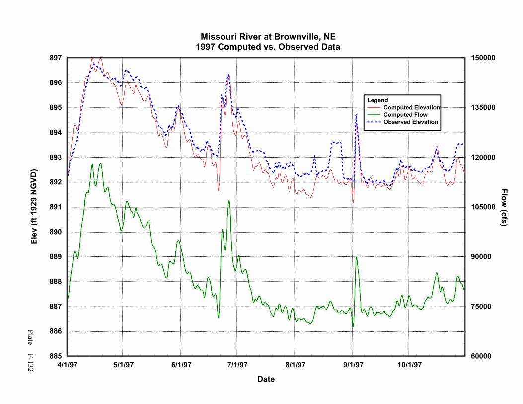
Plate F-132 4/1/97 5/1/97 6/1/97 7/1/97 8/1/97 9/1/97 10/1/97

Date

885

886

887

888

889

890

891

892

893

894

895

896

897

Elev

(ft 1

929

NG

VD)

60000

75000

90000

105000

120000

135000

150000

Flow (cfs)



Plate F-133 5/1/84 6/1/84 7/1/84 8/1/84 9/1/84 10/1/84

Date

848

849

850

851

852

853

854

855

856

857

858

859

860

861

862

Elev

(ft 1

929

NG

VD)

30000

70000

110000

150000

190000

230000

270000

310000

Flow (cfs)


Missouri River at Rulo, NE1984 Computed vs. Observed Data

Compare Calibration Error at Peakto 93, 97 Flood at Similar Flow

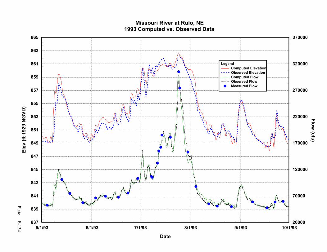
Plate F-134 5/1/93 6/1/93 7/1/93 8/1/93 9/1/93 10/1/93

Date

837

839

841

843

845

847

849

851

853

855

857

859

861

863

865

Elev

(ft 1

929

NG

VD)

20000

70000

120000

170000

220000

270000

320000

370000

Flow (cfs)



Plate F-135 4/1/97 5/1/97 6/1/97 7/1/97 8/1/97 9/1/97 10/1/97

Date

850

851

852

853

854

855

856

857

858

859

860

Elev

(ft 1

929

NG

VD)

60000

80000

100000

120000

140000

160000

Flow (cfs)



Plate F- 136

Missouri River UNET Maximum Water Surface and High Water Mark Comparison RM 498-530

860

865

870

875

880

885

890

895

900

498 503 508 513 518 523 528

River Mile

Elev

atio

n (ft

)

1993 UNET Results1993 High Water Marks1984 UNET Results1984 High Water Marks

Note: Computed elevations and accuracy of high water mark data is limited below Brownville and River Mile 535 due to multiple levee failures.

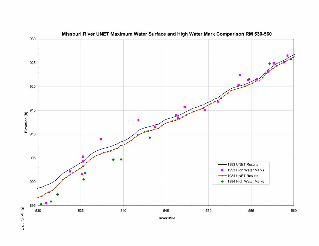
Plate F- 137

Missouri River UNET Maximum Water Surface and High Water Mark Comparison RM 530-560

895

900

905

910

915

920

925

930

530 535 540 545 550 555 560

River Mile

Elev

atio

n (ft

)


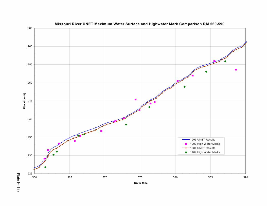
Plate F- 138

Missouri River UNET Maximum Water Surface and Highwater Mark Comparison RM 560-590

925

930

935

940

945

950

955

960

965

560 565 570 575 580 585 590

River Mile

Elev

atio

n (ft

)


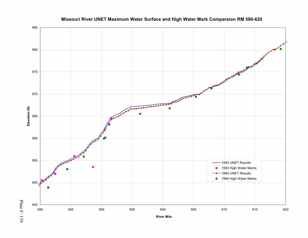
Plate F- 139

Missouri River UNET Maximum Water Surface and High Water Mark Comparsion RM 580-620

945

950

955

960

965

970

975

980

985

580 585 590 595 600 605 610 615 620

River Mile

Elev

atio

n (ft

)


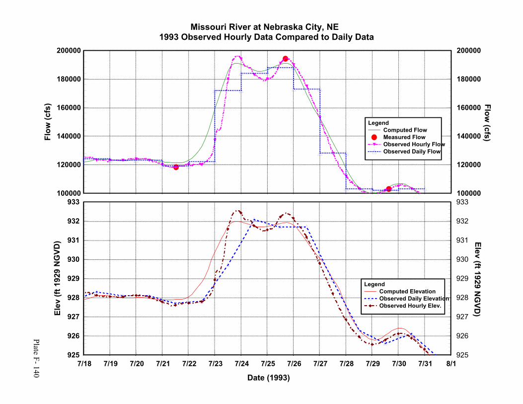
Plate F- 140

100000

120000

140000

160000

180000

200000Fl

ow (c

fs)

100000

120000

140000

160000

180000

200000

Flow (cfs)

LegendComputed FlowMeasured FlowObserved Hourly FlowObserved Daily Flow

Missouri River at Nebraska City, NE1993 Observed Hourly Data Compared to Daily Data

7/18 7/19 7/20 7/21 7/22 7/23 7/24 7/25 7/26 7/27 7/28 7/29 7/30 7/31 8/1

Date (1993)

925

926

927

928

929

930

931

932

933

Elev

(ft 1

929

NG

VD)

925

926

927

928

929

930

931

932

933

Elev (ft 1929 NG

VD)

LegendComputed ElevationObserved Daily ElevationObserved Hourly Elev.

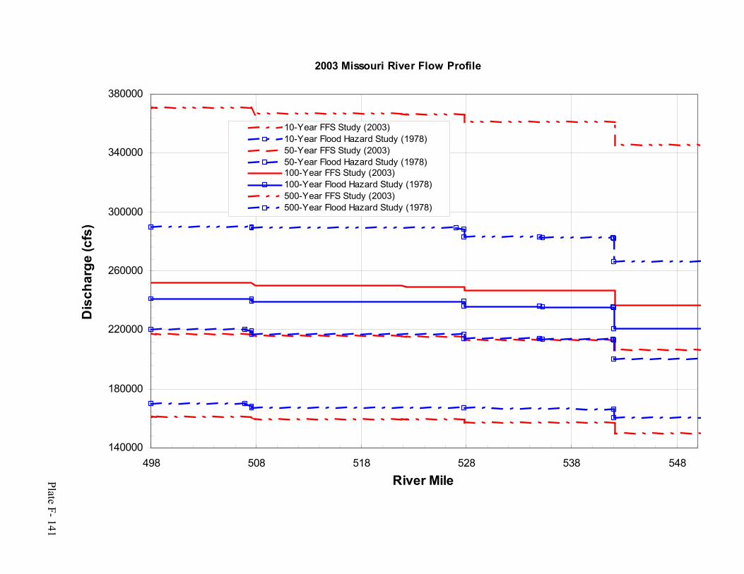
Plate F- 141

2003 Missouri River Flow Profile

140000

180000

220000

260000

300000

340000

380000

498 508 518 528 538 548

River Mile

Dis

char

ge (c

fs)

10-Year FFS Study (2003)10-Year Flood Hazard Study (1978)50-Year FFS Study (2003)50-Year Flood Hazard Study (1978)100-Year FFS Study (2003)100-Year Flood Hazard Study (1978)500-Year FFS Study (2003)500-Year Flood Hazard Study (1978)

Plate F- 142


120000

160000

200000

240000

280000

320000

360000

550 555 560 565 570 575 580 585 590 595 600

River Mile

Dis

char

ge (c

fs)


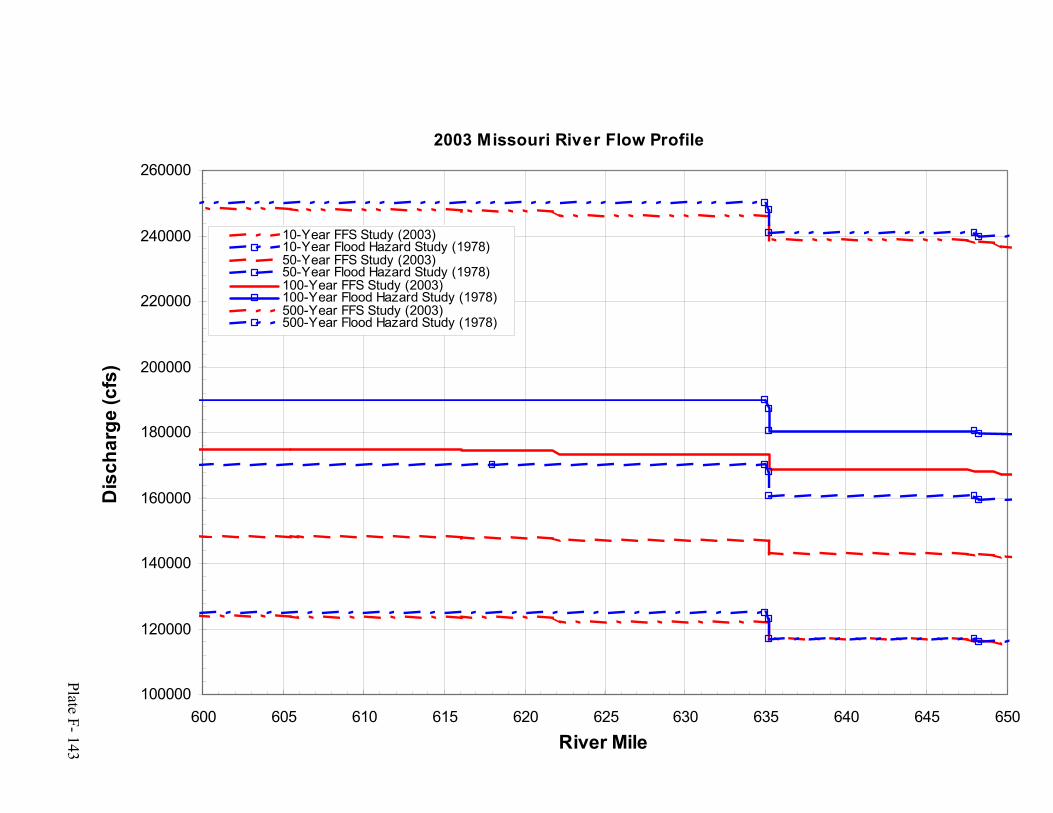
Plate F- 143


100000

120000

140000

160000

180000

200000

220000

240000

260000

600 605 610 615 620 625 630 635 640 645 650

River Mile

Dis

char

ge (c

fs)


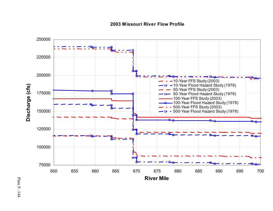
Plate F- 144


75000

100000

125000

150000

175000

200000

225000

250000

650 655 660 665 670 675 680 685 690 695 700

River Mile

Dis

char

ge (c

fs) 10-Year FFS Study (2003)

10-Year Flood Hazard Study (1978)50-Year FFS Study (2003)50-Year Flood Hazard Study (1978)100-Year FFS Study (2003)100-Year Flood Hazard Study (1978)500-Year FFS Study (2003)500-Year Flood Hazard Study (1978)

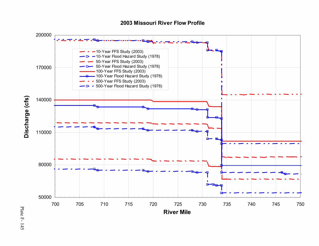
Plate F- 145


50000

80000

110000

140000

170000

200000

700 705 710 715 720 725 730 735 740 745 750

River Mile

Dis

char

ge (c

fs)


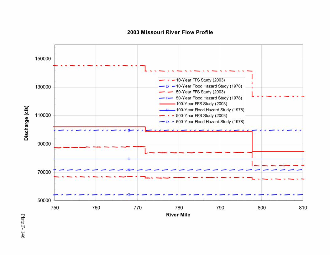
Plate F- 146


50000

70000

90000

110000

130000

150000

750 760 770 780 790 800 810River Mile

Disc

harg

e (c

fs)


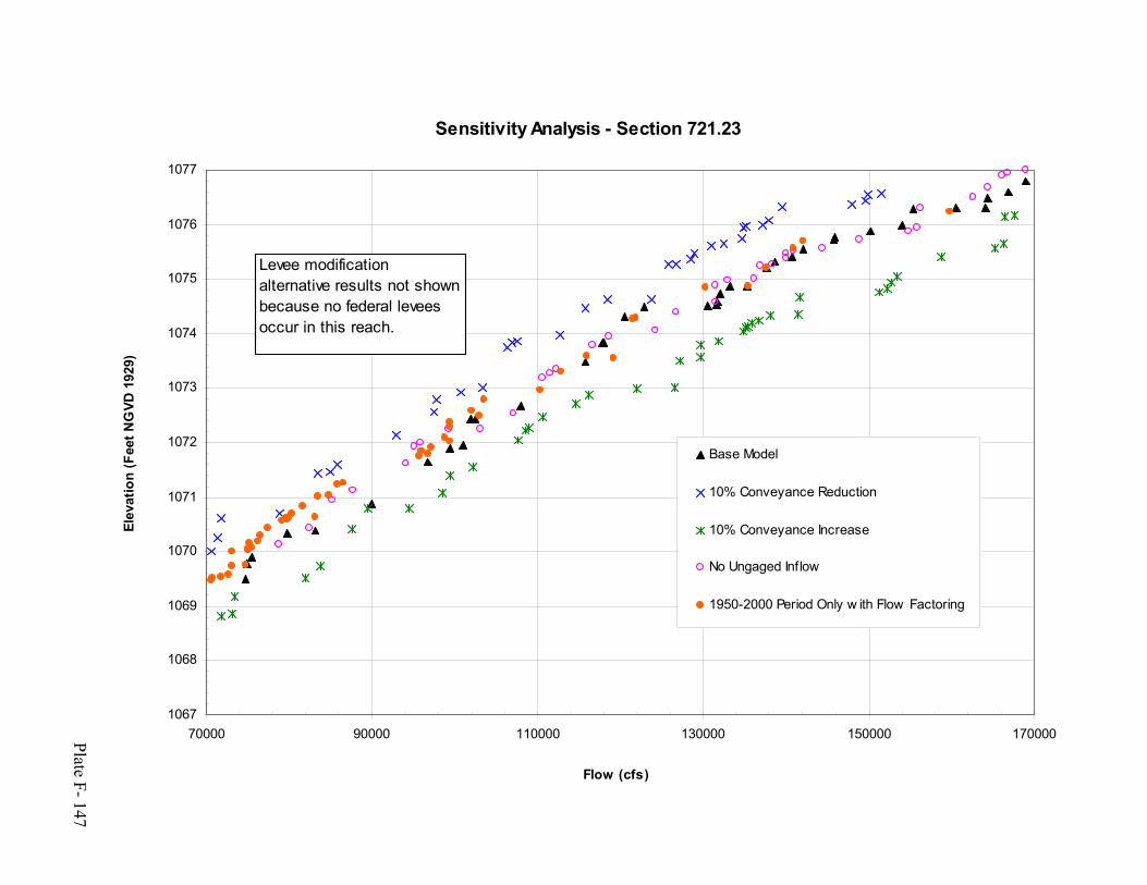
Plate F- 147

Sensitivity Analysis - Section 721.23

1067

1068

1069

1070

1071

1072

1073

1074

1075

1076

1077

70000 90000 110000 130000 150000 170000

Flow (cfs)

Elev

atio

n (F

eet N

GVD

192

9)

Base Model

10% Conveyance Reduction

10% Conveyance Increase

No Ungaged Inflow

1950-2000 Period Only w ith Flow Factoring

Levee modification alternative results not shown because no federal levees occur in this reach.

Plate F- 148

Sensitivity Analysis - Spline Curve at Section 721.23

1,067

1,069

1,071

1,073

1,075

1,077

1,079

60,000 90,000 120,000 150,000 180,000

Flow (cfs)

Elev

atio

n (F

eet N

GVD

192

9)

Base Model



No Ungaged Inflow


Levee modif ication alternative results not show n because no federal levees occur in this reach.

Plate F- 149


1009

1010

1011

1012

1013

1014

1015

1016

1017

1018

110000 130000 150000 170000 190000 210000 230000Flow (cfs)

Elev

atio

n (F

eet N

GVD

192

9

Base Model



No Ungaged Inflow


Levee modif ication alternative results not show n because no federal levees occur in this

Plate F- 150


1008

1009

1010

1011

1012

1013

1014

1015

1016

1017

1018

90,000 120,000 150,000 180,000 210,000 240,000

Flow (cfs)

Elev

atio

n (F

eet N

GVD

192

9)

Base Model



No Ungaged Inflow

1950-2000 Period Only with Flow Factoring

Levee modification alternative results not shown because no federal levees occur in this reach.

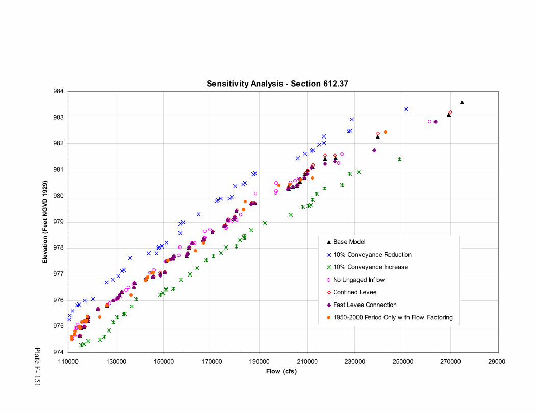
Plate F- 151


974

975

976

977

978

979

980

981

982

983

984

110000 130000 150000 170000 190000 210000 230000 250000 270000 29000Flow (cfs)

Elev

atio

n (F

eet N

GVD

192

9)

Base Model



No Ungaged Inflow

Confined Levee

Fast Levee Connection


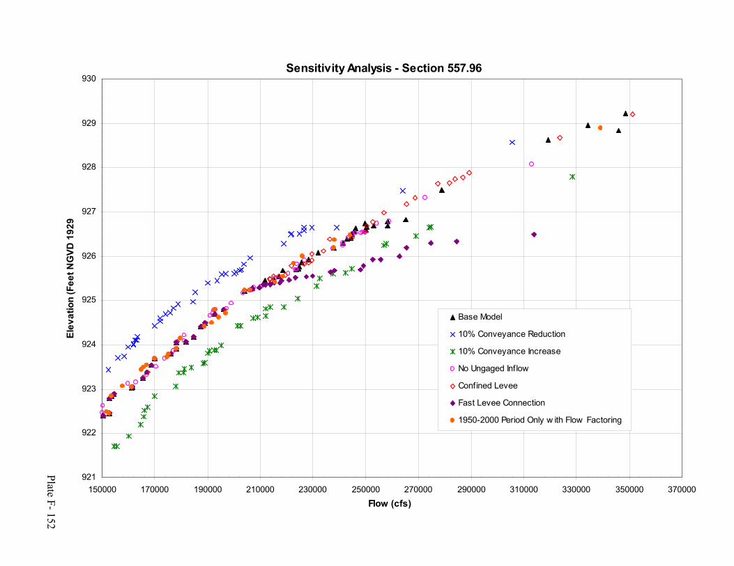
Plate F- 152


921

922

923

924

925

926

927

928

929

930

150000 170000 190000 210000 230000 250000 270000 290000 310000 330000 350000 370000Flow (cfs)

Elev

atio

n (F

eet N

GVD

192

9

Base Model



No Ungaged Inf low

Confined Levee



Plate F- 153


922

923

924

925

926

927

928

929

930

931

932

140,000 170,000 200,000 230,000 260,000 290,000 320,000 350,000

Flow (cfs)

Elev

atio

n (F

eet N

GVD

192

9)

Base Model



Confined Levee


No Ungaged Inflow


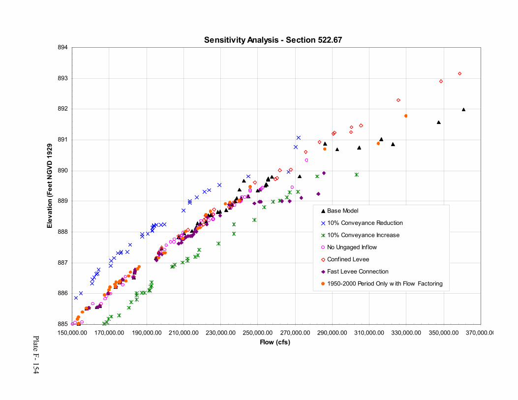
Plate F- 154


885

886

887

888

889

890

891

892

893

894

150,000.00 170,000.00 190,000.00 210,000.00 230,000.00 250,000.00 270,000.00 290,000.00 310,000.00 330,000.00 350,000.00 370,000.00Flow (cfs)

Elev

atio

n (F

eet N

GVD

192

9

Base Model



No Ungaged Inflow

Confined Levee



Plate F- 155

Sensitivity Analysis - RM 498 to 55010-Year Event

-3.00

-2.00

-1.00

0.00

1.00

2.00

3.00

4.00

10% Convey.Reduce

10% Convey.Increase

ConfinedLevee

Fast LeveeConn.

No UngagedInflow

1950-2000Only

Alternative

Cha

nge

From

Bas

e (fe

et) Average

95thPercentile


-3.00

-2.00

-1.00

0.00

1.00

2.00

3.00

4.00

10% Convey.Reduce

10% Convey.Increase

ConfinedLevee

Fast LeveeConn.

No UngagedInflow

1950-2000Only

Alternative

Cha

nge

From

Bas

e (fe

et) Average

95thPercentile


-3.00

-2.00

-1.00

0.00

1.00

2.00

3.00

4.00

10% Convey.Reduce

10% Convey.Increase

ConfinedLevee

Fast LeveeConn.

No UngagedInflow

1950-2000Only

Alternative

Cha

nge

From

Bas

e (fe

et) Average

95thPercentile


-3.00

-2.00

-1.00

0.00

1.00

2.00

3.00

4.00

10% Convey.Reduce

10% Convey.Increase

ConfinedLevee

Fast LeveeConn.

No UngagedInflow

1950-2000Only

Alternative

Cha

nge

From

Bas

e (fe

et) Average

95thPercentile

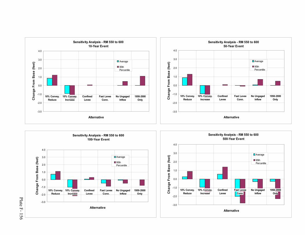
Plate F- 156


-3.0

-2.0

-1.0

0.0

1.0

2.0

3.0

4.0

10% Convey.Reduce

10% Convey.Increase

ConfinedLevee

Fast LeveeConn.

No UngagedInflow

1950-2000Only

Alternative

Cha

nge

From

Bas

e (fe

et) Average

95thPercentile


-3.0

-2.0

-1.0

0.0

1.0

2.0

3.0

4.0

10% Convey.Reduce

10% Convey.Increase

ConfinedLevee

Fast LeveeConn.

No UngagedInflow

1950-2000Only

Alternative

Cha

nge

From

Bas

e (fe

et) Average

95thPercentile


-3.0

-2.0

-1.0

0.0

1.0

2.0

3.0

4.0

10% Convey.Reduce

10% Convey.Increase

ConfinedLevee

Fast LeveeConn.

No UngagedInflow

1950-2000Only

Alternative

Cha

nge

From

Bas

e (fe

et) Average

95thPercentile


-3.0

-2.0

-1.0

0.0

1.0

2.0

3.0

4.0

10% Convey.Reduce

10% Convey.Increase

ConfinedLevee

Fast LeveeConn.

No UngagedInflow

1950-2000Only

Alternative

Cha

nge

From

Bas

e (fe

et) Average

95thPercentile

Plate F- 157


-3.0

-2.0

-1.0

0.0

1.0

2.0

3.0

4.0

10% Convey.Reduce

10% Convey.Increase

ConfinedLevee

Fast LeveeConn.

No UngagedInflow

1950-2000Only

Alternative

Cha

nge

From

Bas

e (fe

et)

Average

95thPercentile


-3.0

-2.0

-1.0

0.0

1.0

2.0

3.0

4.0

10% Convey.Reduce

10% Convey.Increase

ConfinedLevee

Fast LeveeConn.

No UngagedInflow

1950-2000Only

Alternative

Cha

nge

From

Bas

e (fe

et)

Average

95thPercentile


-3.0

-2.0

-1.0

0.0

1.0

2.0

3.0

4.0

10% Convey.Reduce

10% Convey.Increase

ConfinedLevee

Fast LeveeConn.

No UngagedInflow

1950-2000Only

Alternative

Cha

nge

From

Bas

e (fe

et)

Average

95thPercentile


-3.0

-2.0

-1.0

0.0

1.0

2.0

3.0

4.0

10% Convey.Reduce

10% Convey.Increase

ConfinedLevee

Fast LeveeConn.

No UngagedInflow

1950-2000Only

Alternative

Cha

nge

From

Bas

e (fe

et)

Average

95thPercentile

Plate F- 158


-3.0

-2.0

-1.0

0.0

1.0

2.0

3.0

4.0

10% Convey.Reduce

10% Convey.Increase

ConfinedLevee

Fast LeveeConn.

No UngagedInflow

1950-2000Only

Alternative

Cha

nge

From

Bas

e (fe

et)

Average

95thPercentile


-3.0

-2.0

-1.0

0.0

1.0

2.0

3.0

4.0

10% Convey.Reduce

10% Convey.Increase

ConfinedLevee

Fast LeveeConn.

No UngagedInflow

1950-2000 Only

Alternative

Cha

nge

From

Bas

e (fe

et)

Average

95thPercentile


-3.0

-2.0

-1.0

0.0

1.0

2.0

3.0

4.0

10% Convey.Reduce

10% Convey.Increase

ConfinedLevee

Fast LeveeConn.

No UngagedInflow

1950-2000Only

Alternative

Cha

nge

From

Bas

e (fe

et)

Average

95thPercentile


-3.0

-2.0

-1.0

0.0

1.0

2.0

3.0

4.0

10% Convey.Reduce

10% Convey.Increase

ConfinedLevee

Fast LeveeConn.

No UngagedInflow

1950-2000 Only

Alternative

Cha

nge

From

Bas

e (fe

et)

Average

95thPercentile

Plate F- 159


-3.0

-2.0

-1.0

0.0

1.0

2.0

3.0

4.0

10% Convey.Reduce

10% Convey.Increase

ConfinedLevee

Fast LeveeConn.

No UngagedInflow

1950-2000Only

Alternative

Cha

nge

From

Bas

e (fe

et)

Average

95thPercentile


-3.0

-2.0

-1.0

0.0

1.0

2.0

3.0

4.0

10% Convey.Reduce

10% Convey.Increase

ConfinedLevee

Fast LeveeConn.

No UngagedInflow

1950-2000Only

Alternative

Cha

nge

From

Bas

e (fe

et)

Average

95thPercentile


-3.0

-2.0

-1.0

0.0

1.0

2.0

3.0

4.0

10% Convey.Reduce

10% Convey.Increase

ConfinedLevee

Fast LeveeConn.

No UngagedInflow

1950-2000Only

Alternative

Cha

nge

From

Bas

e (fe

et)

Average

95thPercentile


-3.0

-2.0

-1.0

0.0

1.0

2.0

3.0

4.0

10% Convey.Reduce

10% Convey.Increase

ConfinedLevee

Fast LeveeConn.

No UngagedInflow

1950-2000Only

Alternative

Cha

nge

From

Bas

e (fe

et)

Average

95thPercentile

Plate F- 160


-3.0

-2.0

-1.0

0.0

1.0

2.0

3.0

4.0

10% Convey.Reduce

10% Convey.Increase

ConfinedLevee

Fast LeveeConn.

No UngagedInflow

1950-2000Only

Alternative

Cha

nge

From

Bas

e (fe

et)

Average

95thPercentile


-3.0

-2.0

-1.0

0.0

1.0

2.0

3.0

4.0

10% Convey.Reduce

10% Convey.Increase

Confined Levee Fast LeveeConn.

No UngagedInflow

1950-2000 Only

Alternative

Cha

nge

From

Bas

e (fe

et)

Average

95thPercentile


-3.0

-2.0

-1.0

0.0

1.0

2.0

3.0

4.0

10% Convey.Reduce

10% Convey.Increase

ConfinedLevee

Fast LeveeConn.

No UngagedInflow

1950-2000Only

Alternative

Cha

nge

From

Bas

e (fe

et)

Average

95thPercentile


-3.0

-2.0

-1.0

0.0

1.0

2.0

3.0

4.0

10% Convey.Reduce

10% Convey.Increase

Confined Levee Fast LeveeConn.

No UngagedInflow

1950-2000 Only

Alternative

Cha

nge

From

Bas

e (fe

et)

Average

95thPercentile

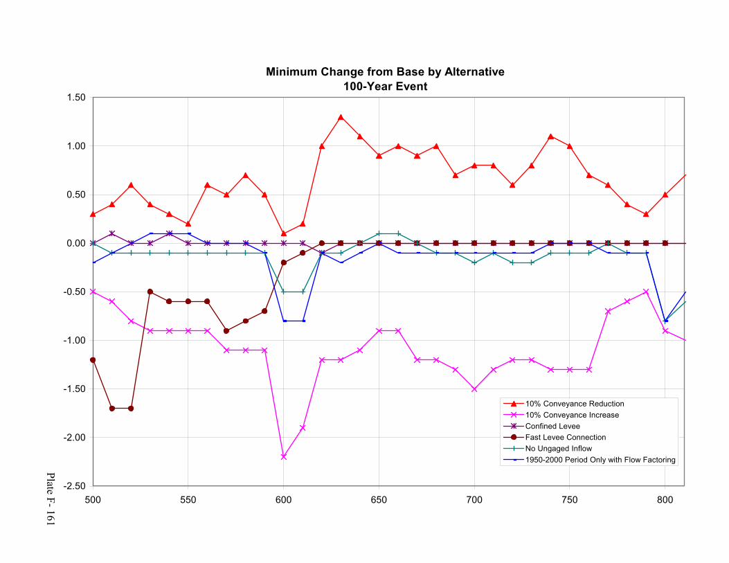
Plate F- 161

Minimum Change from Base by Alternative100-Year Event

-2.50

-2.00

-1.50

-1.00

-0.50

0.00

0.50

1.00

1.50

500 550 600 650 700 750 800

10% Conveyance Reduction10% Conveyance IncreaseConfined LeveeFast Levee ConnectionNo Ungaged Inflow1950-2000 Period Only with Flow Factoring

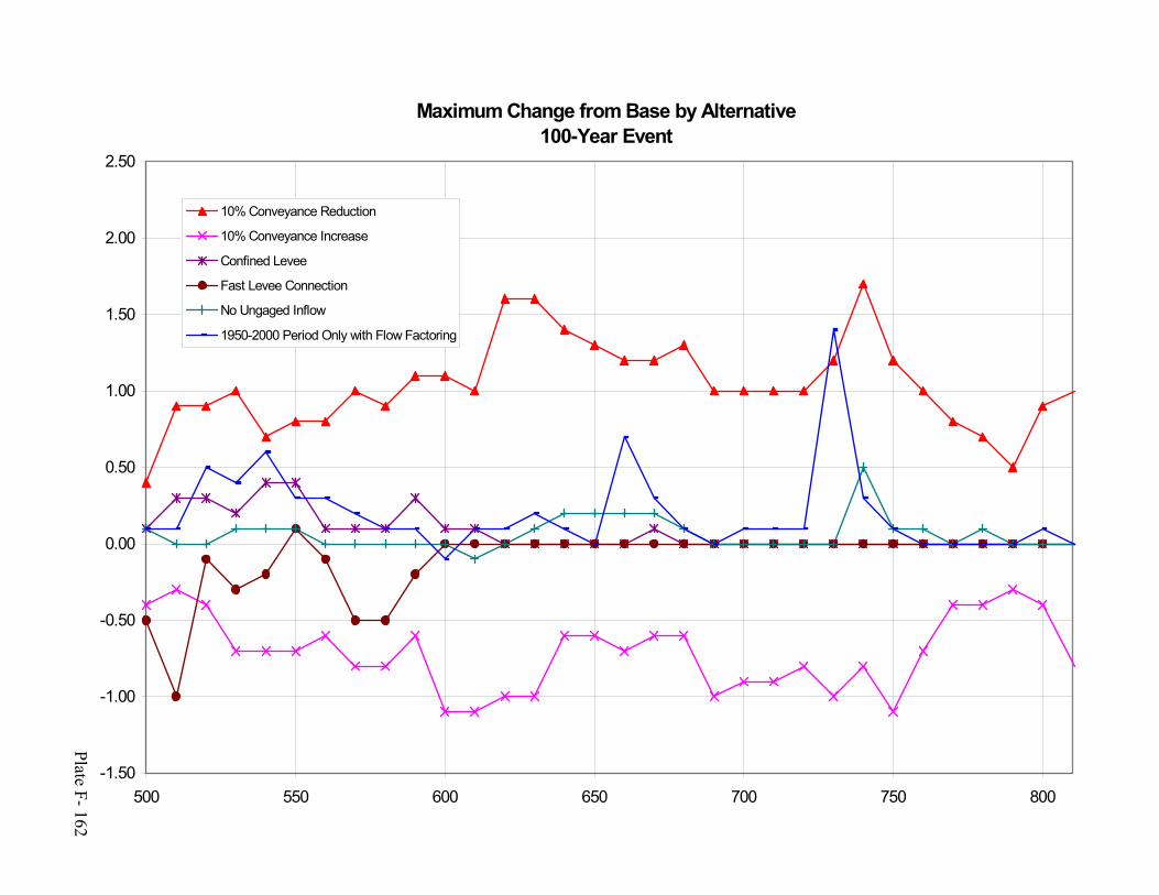
Plate F- 162

Maximum Change from Base by Alternative100-Year Event

-1.50

-1.00

-0.50

0.00

0.50

1.00

1.50

2.00

2.50

500 550 600 650 700 750 800



Confined Levee


No Ungaged Inflow


Plate F- 163

505 508 510 513 515 518 520 523 525 528 530

River Mile

855

865

875

885

895

905

Elev

atio

n (F

eet 1

929

NG

VD)

L-536

L-536

L-550 South

R-548

R-520

R-520

Legend2-Year FFS 20035-Year FFS 200310-Year FFS 200325-Year FFS 200350-Year FFS 2003100-Year FFS 2003200-Year FFS 2003500-Year FFS 2003Left Bank LeveeRight Bank Levee

Missouri River Stage Frequency Profiles - River Mile 498-530

RM

527

.8

500

RM

498

.0

Rul

o, N

E

Littl

e N

emah

a R

iver

at A

ubur

n, N

E

Note: The illustrated levee elevations reflect the UNET modelconnection elevations only. Actual levee elevation between the illustrated points may vary and should not be assumed to be linear.

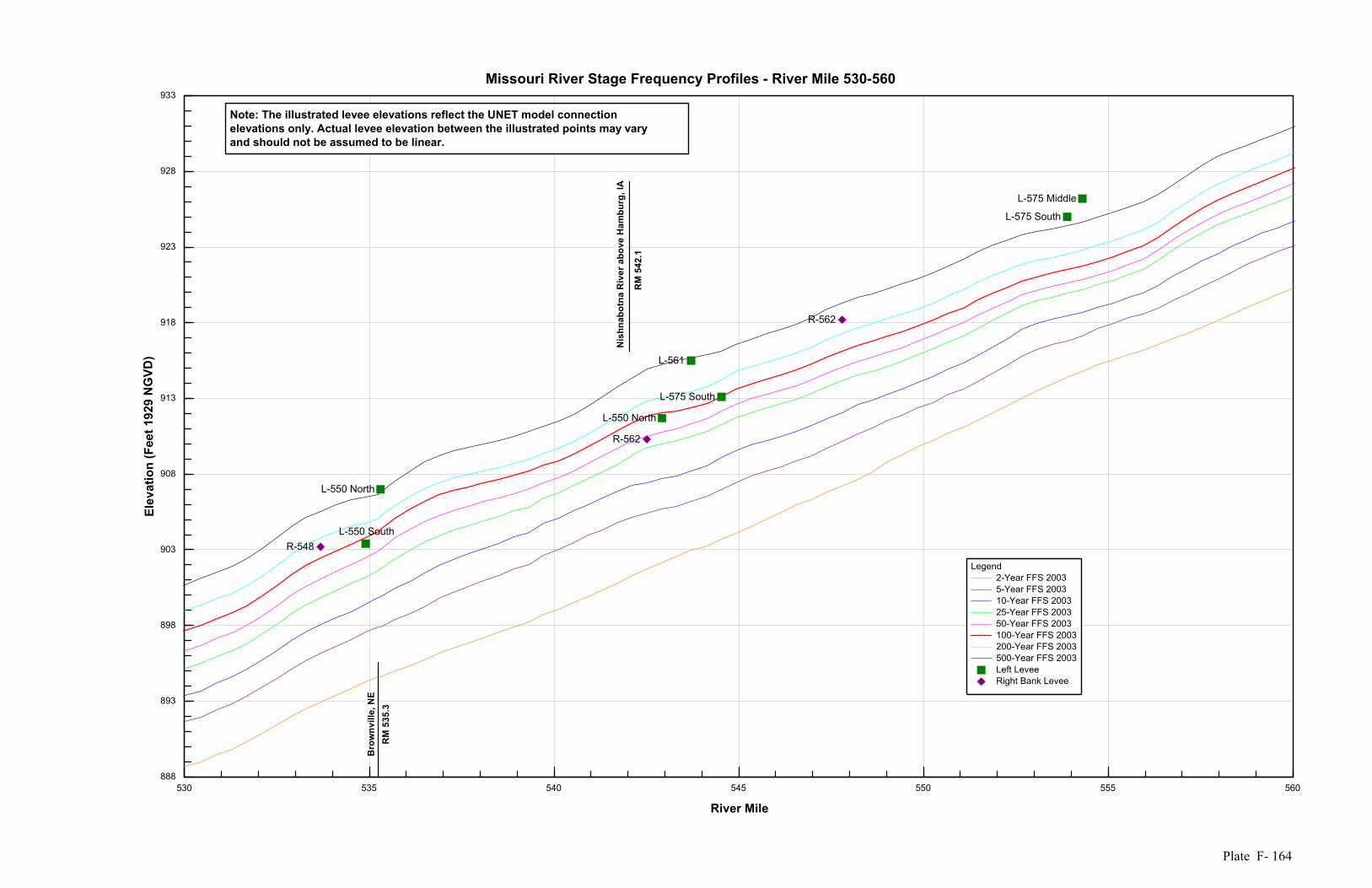
Plate F- 164

530 535 540 545 550 555 560

River Mile

888

893

898

903

908

913

918

923

928

933

Elev

atio

n (F

eet 1

929

NG

VD)

L-550 South

L-550 North

L-550 North

L-561

L-575 South

L-575 South

L-575 Middle

R-548

R-562

R-562

Legend2-Year FFS 20035-Year FFS 200310-Year FFS 200325-Year FFS 200350-Year FFS 2003100-Year FFS 2003200-Year FFS 2003500-Year FFS 2003Left LeveeRight Bank Levee


Bro

wnv

ille,

NE

RM

535

.3

Nis

hnab

otna

Riv

er a

bove

Ham

burg

, IA

RM

542

.1

Note: The illustrated levee elevations reflect the UNET model connection elevations only. Actual levee elevation between the illustrated points may varyand should not be assumed to be linear.

Plate F- 165

560 565 570 575 580 585 590

River Mile

920

925

930

935

940

945

950

955

960

965

970

Elev

atio

n (F

eet 1

929

NG

VD)

L-575 Middle

L-575 North

L-575 North

L-594

L-594L-601 South

L-601 South

L-601 North

L-601 North L-601 NEL-611 South 1

Legend2-Year FFS 20035-Year FFS 200310-Year FFS 200325-Year FFS 200350-Year FFS 2003100-Year FFS 2003200-Year FFS 2003500-Year FFS 2003Left Bank Levee


Wee

ping

Wat

er C

reek

at U

nion

, NE

RM

568

.7

Neb

rask

a C

ity, N

E

RM

562

.6

Note: The illustrated levee elevations reflect the UNET model connection elevations only. Actual levee elevation between the illustrated points may vary and should not be assumed to be linear.

Plate F- 166

590 595 600 605 610 615 620

River Mile

953

958

963

968

973

978

983

988

993

Elev

atio

n (F

eet 1

929

NG

VD)

L-611 South 1

L-611 South 2

L-611 South 2L-611 North 1

L-611 North 1

L-611 North 2

L-611 North 2

L-614

L-624

L-624 L-627

Omaha Levee So. L-627

Omaha Levee So.

Council Bluffs

Omaha FloodwallOmaha Floodwall

Omaha Levee No.

Council Bluffs

R-613R-613

R-616

R-616

Legend2-Year FFS 20035-Year FFS 200310-Year FFS 200325-Year FFS 200350-Year FFS 2003100-Year FFS 2003200-Year FFS 2003500-Year FFS 2003Left Bank LeveeRight Bank Levee


Om

aha,

NE

RM

615

.9

Plat

tsm

outh

, NE

RM

591

.5

Papi

llion

Cre

ek a

t For

t Cro

ok, N

E

RM

596

.6

Plat

te R

iver

at L

ouis

ville

, NE

RM

594

.8


Plate F- 167

620 625 630 635 640 645 650

River Mile

974

979

984

989

994

999

1004

1009

1014

Elev

atio

n (F

eet 1

929

NG

VD)

Legend2-Year FFS 20035-Year FFS 200310-Year FFS 200325-Year FFS 200350-Year FFS 2003100-Year FFS 2003200-Year FFS 2003500-Year FFS 2003


Bla

ir, N

E

RM

648

.3

Boy

er R

iver

at L

ogan

, IA

RM

635

.2Note: The illustrated levee elevations reflect the UNET model connection elevations only. Actual levee elevation between the illustrated points may vary and should not be assumed to be linear.

Plate F- 168

650 655 660 665 670 675 680

River Mile

1000

1005

1010

1015

1020

1025

1030

1035

1040

1045

Elev

atio

n (F

eet 1

929

NG

VD)



Littl

e Si

oux

Riv

er n

ear T

urin

, IA

RM

669

.2

Sold

ier R

iver

at P

isga

h, IA

RM

664

.0


Plate F- 169

680 685 690 695 700 705 710

River Mile

1025

1030

1035

1040

1045

1050

1055

1060

1065

1070

Elev

atio

n (F

eet 1

929

NG

VD)



Dec

atur

, NE

RM

691

.0


Plate F- 170

710 715 720 725 730 735 740

River Mile

1055

1060

1065

1070

1075

1080

1085

1090

1095

1100

Elev

atio

n (F

eet 1

929

NG

VD)



Siou

x C

ity, I

A

RM

732

.3

Big

Sio

ux R

iver

at A

kron

, IA

RM

734

.0

Perr

y C

reek

at S

ioux

City

, IA

RM

732

.1

Floy

d R

iver

at J

ames

, IA

RM

731

.3

Om

aha

Cre

ek

RM

719

.8


Plate F- 171

740 745 750 755 760 765 770

River Mile

1085

1090

1095

1100

1105

1110

1115

1120

1125

1130

Elev

atio

n (F

eet 1

929

NG

VD)



Ponc

a, N

E

RM

751

.0


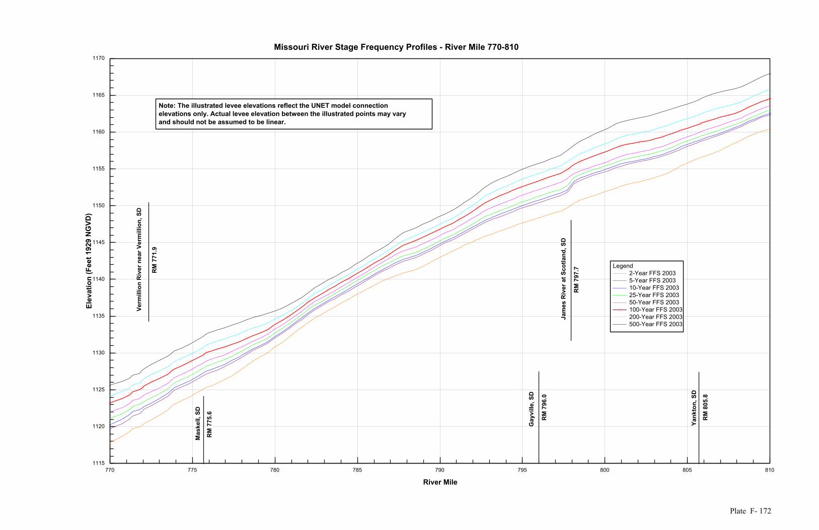
Plate F- 172

770 775 780 785 790 795 800 805 810

River Mile

1115

1120

1125

1130

1135

1140

1145

1150

1155

1160

1165

1170

Elev

atio

n (F

eet 1

929

NG

VD)



Gay

ville

, SD

RM

796

.0

Jam

es R

iver

at S

cotla

nd, S

D

RM

797

.7

Mas

kell,

SD

RM

775

.6

Verm

illio

n R

iver

nea

r Ver

mill

ion,

SD

RM

771

.9

Yank

ton,

SD

RM

805

.8


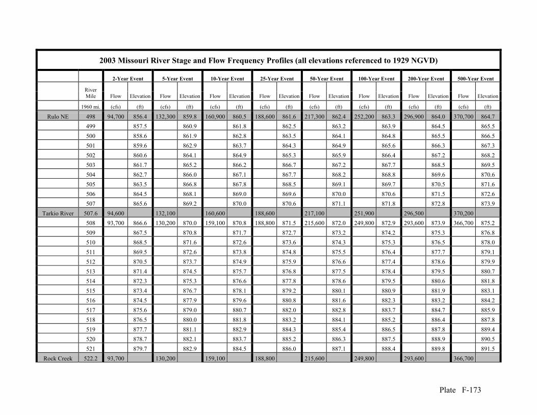
Plate F-173

2003 Missouri River Stage and Flow Frequency Profiles (all elevations referenced to 1929 NGVD)

2-Year Event 5-Year Event 10-Year Event 25-Year Event 50-Year Event 100-Year Event 200-Year Event 500-Year Event

River Mile Flow Elevation Flow Elevation Flow Elevation Flow Elevation Flow Elevation Flow Elevation Flow Elevation Flow Elevation

1960 mi. (cfs) (ft) (cfs) (ft) (cfs) (ft) (cfs) (ft) (cfs) (ft) (cfs) (ft) (cfs) (ft) (cfs) (ft)

Rulo NE 498 94,700 856.4 132,300 859.8 160,900 860.5 188,600 861.6 217,300 862.4 252,200 863.3 296,900 864.0 370,700 864.7 499 857.5 860.9 861.8 862.5 863.2 863.9 864.5 865.5 500 858.6 861.9 862.8 863.5 864.1 864.8 865.5 866.5 501 859.6 862.9 863.7 864.3 864.9 865.6 866.3 867.3 502 860.6 864.1 864.9 865.3 865.9 866.4 867.2 868.2 503 861.7 865.2 866.2 866.7 867.2 867.7 868.5 869.5 504 862.7 866.0 867.1 867.7 868.2 868.8 869.6 870.6 505 863.5 866.8 867.8 868.5 869.1 869.7 870.5 871.6 506 864.5 868.1 869.0 869.6 870.0 870.6 871.5 872.6 507 865.6 869.2 870.0 870.6 871.1 871.8 872.8 873.9

Tarkio River 507.6 94,600 132,100 160,600 188,600 217,100 251,900 296,500 370,200 508 93,700 866.6 130,200 870.0 159,100 870.8 188,800 871.5 215,600 872.0 249,800 872.9 293,600 873.9 366,700 875.2 509 867.5 870.8 871.7 872.7 873.2 874.2 875.3 876.8 510 868.5 871.6 872.6 873.6 874.3 875.3 876.5 878.0 511 869.5 872.6 873.8 874.8 875.5 876.4 877.7 879.1 512 870.5 873.7 874.9 875.9 876.6 877.4 878.6 879.9 513 871.4 874.5 875.7 876.8 877.5 878.4 879.5 880.7 514 872.3 875.3 876.6 877.8 878.6 879.5 880.6 881.8 515 873.4 876.7 878.1 879.2 880.1 880.9 881.9 883.1 516 874.5 877.9 879.6 880.8 881.6 882.3 883.2 884.2 517 875.6 879.0 880.7 882.0 882.8 883.7 884.7 885.9 518 876.5 880.0 881.8 883.2 884.1 885.2 886.4 887.8 519 877.7 881.1 882.9 884.3 885.4 886.5 887.8 889.4 520 878.7 882.1 883.7 885.2 886.3 887.5 888.9 890.5 521 879.7 882.9 884.5 886.0 887.1 888.4 889.8 891.5

Rock Creek 522.2 93,700 130,200 159,100 188,800 215,600 249,800 293,600 366,700

Plate F-174





523 93,400 881.5 129,700 884.3 158,800 886.0 188,800 887.5 215,200 888.7 249,300 890.0 292,900 891.1 365,900 892.7 524 882.5 885.5 887.2 888.7 889.8 891.1 892.2 893.8 525 883.6 886.5 888.0 889.6 890.7 891.9 893.1 894.7 526 884.8 887.7 889.4 890.8 892.0 893.1 894.3 895.8 527 886.1 889.2 891.0 892.5 893.7 894.8 896.1 897.6

Little Nemaha 527.8 93,400 129,700 158,800 188,800 215,200 249,300 292,900 365,900 528 92,100 887.2 127,100 890.1 156,600 891.8 189,100 893.4 213,100 894.7 246,300 895.9 288,900 897.2 361,000 898.9 529 887.9 890.7 892.4 894.1 895.3 896.6 897.9 899.5 530 888.7 891.7 893.4 895.1 896.3 897.6 899.0 900.7 531 889.6 892.6 894.3 896.1 897.3 898.6 899.9 901.6 532 890.8 893.8 895.6 897.3 898.5 899.8 901.1 902.9 533 892.1 895.3 897.2 899.0 900.2 901.5 902.9 904.7 534 893.3 896.5 898.4 900.2 901.5 902.8 904.1 905.9 535 894.4 897.6 899.5 901.3 902.6 903.9 904.9 906.5

Brownville, NE 535.3 92,100 894.6 127,100 897.9 156,600 899.9 189,100 901.7 213,100 903.0 246,300 904.3 288,900 905.2 361,000 906.8 536 895.3 898.7 900.8 902.8 904.2 905.6 906.4 908.1 537 896.3 899.9 902.1 904.0 905.4 906.7 907.5 909.3 538 897.1 900.9 903.0 904.8 906.1 907.3 908.2 910.0 539 898.0 901.8 903.9 905.6 906.8 908.0 908.8 910.6 540 899.0 902.9 905.0 906.6 907.7 908.8 909.6 911.4 541 900.0 904.0 906.1 907.8 908.8 909.9 910.7 912.6 542 901.2 905.1 907.2 909.1 910.1 911.3 912.2 914.2

Nishnabotna River 542.1 92,100 127,100 156,600 189,100 213,100 246,300 288,900 361,000

543 88,000 902.2 118,700 905.7 149,800 907.7 189,900 910.0 206,400 910.8 236,700 912.1 275,900 913.1 345,400 915.3 544 903.2 906.4 908.4 910.7 911.5 912.6 913.7 915.8

Plate F-175





545 904.1 907.5 909.6 911.8 912.7 913.7 914.8 916.6 546 905.3 908.4 910.4 912.5 913.4 914.4 915.6 917.4 547 906.4 909.3 911.3 913.4 914.3 915.3 916.5 918.4 548 907.4 910.4 912.3 914.3 915.3 916.3 917.5 919.5 549 908.8 911.5 913.3 915.1 916.1 917.1 918.3 920.3 550 910.0 912.5 914.2 916.0 916.9 917.9 919.1 921.1 551 911.0 913.6 915.2 917.0 917.9 918.9 920.1 922.1 552 912.2 914.8 916.6 918.3 919.1 920.1 921.3 923.2 553 913.4 916.2 917.9 919.4 920.1 921.0 922.1 924.0 554 914.5 916.9 918.5 920.0 920.7 921.6 922.6 924.5 555 915.4 917.8 919.2 920.7 921.4 922.3 923.3 925.2 556 916.2 918.6 920.0 921.6 922.3 923.1 924.2 926.1 557 917.1 919.7 921.4 923.2 923.8 924.7 925.7 927.5 558 918.2 920.9 922.6 924.5 925.2 926.2 927.2 929.0 559 919.3 922.1 923.8 925.5 926.2 927.2 928.2 930.0 560 920.2 923.0 924.7 926.4 927.2 928.2 929.2 930.9 561 921.4 924.2 925.9 927.7 928.5 929.5 930.5 932.2 562 923.0 926.1 928.3 930.6 931.5 932.8 933.8 935.6

Nebraska City, NE 562.6 88,000 923.7 118,700 926.9 149,800 929.2 189,900 931.7 206,400 932.7 236,700 934.1 275,900 935.0 345,400 936.8

563 924.2 927.4 929.7 932.3 933.3 934.7 935.7 937.5 564 925.3 928.4 930.9 933.5 934.6 936.1 937.1 939.0 565 926.4 929.6 931.9 934.6 935.7 937.2 938.4 940.3 566 927.4 930.5 932.8 935.5 936.5 938.0 939.3 941.2 567 928.5 931.5 933.7 936.3 937.3 938.8 940.0 941.9 568 929.4 932.5 934.6 936.9 937.9 939.4 940.7 942.5

Plate F-176




1960 mi. (cfs) (ft) (cfs) (ft) (cfs) (ft) (cfs) (ft) (cfs) (ft) (cfs) (ft) (cfs) (ft) (cfs) (ft) Weeping Water

Creek 568.7 88,000 118,600 149,700 189,900 206,300 236,600 275,800 345,300 569 87,900 930.5 118,400 933.5 149,600 935.4 189,500 937.8 206,000 938.8 236,300 940.2 275,400 941.5 344,700 943.2 570 931.5 934.6 936.4 938.7 939.7 941.1 942.4 944.1 571 932.5 935.7 937.4 939.3 940.3 941.6 942.9 944.6 572 933.6 936.7 938.3 939.9 940.8 942.1 943.4 945.0 573 934.7 937.7 939.3 940.6 941.5 942.7 944.0 945.4 574 935.7 938.7 940.3 941.8 942.6 943.8 944.9 946.3 575 936.5 939.6 941.4 943.2 944.1 945.3 946.6 948.2 576 937.4 940.7 942.7 944.7 945.6 946.9 948.1 949.7 577 938.5 941.7 943.9 945.8 946.7 948.0 949.2 950.8 578 939.6 943.0 945.1 947.3 948.2 949.4 950.6 952.1 579 940.7 944.1 946.4 948.6 949.4 950.7 951.9 953.4 580 941.6 945.1 947.6 949.8 950.6 951.8 952.9 954.4 581 942.7 946.3 948.8 950.9 951.7 952.6 953.7 955.3 582 943.8 947.4 950.0 952.2 952.9 953.8 954.8 956.4 583 945.1 948.7 951.4 953.8 954.6 955.5 956.6 958.4 584 946.2 949.6 952.2 954.7 955.5 956.4 957.6 959.5 585 947.3 950.6 952.9 955.3 956.0 957.0 958.2 960.1 586 948.5 951.7 953.7 955.9 956.6 957.6 958.8 960.7 587 949.7 952.8 954.8 956.9 957.6 958.6 959.9 961.6

Watkins Ditch 587.5 87,900 118,400 149,600 189,500 206,000 236,300 275,400 344,700 588 87,800 950.9 118,300 954.2 149,500 956.2 189,300 958.3 205,800 959.1 236,100 960.0 275,200 961.3 344,400 963.0 589 951.9 955.3 957.4 959.6 960.3 961.3 962.5 964.2 590 953.0 956.4 958.7 960.9 961.7 962.7 964.0 965.7 591 954.3 957.9 960.4 963.1 964.0 965.3 966.9 968.9

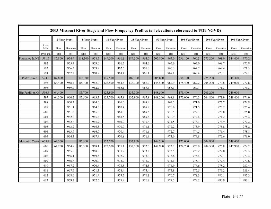
Plate F-177





Plattsmouth, NE 591.5 87,800 954.9 118,300 958.5 149,500 961.1 189,300 964.0 205,800 965.0 236,100 966.3 275,200 968.0 344,400 970.2 592 955.4 959.0 961.7 964.6 965.6 967.0 968.7 970.8 593 956.3 959.9 962.5 965.3 966.3 967.7 969.4 971.5 594 957.2 960.9 963.4 966.1 967.1 968.4 970.1 972.1

Platte River 594.8 87,800 118,300 149,500 189,300 205,800 236,100 275,200 344,400 595 64,400 958.4 85,700 962.0 123,800 964.4 133,300 966.9 148,500 967.9 175,400 969.2 205,200 970.8 249,000 972.8 596 959.7 962.7 965.1 967.3 968.3 969.7 971.3 973.3

Big Papillion Cr 596.6 64,400 85,700 123,800 133,300 148,500 175,400 205,200 249,000 597 64,300 960.2 85,500 963.3 123,700 965.8 132,900 967.8 148,200 968.8 175,000 970.3 204,800 971.9 248,400 974.0 598 960.7 964.0 966.6 968.4 969.5 971.0 972.7 974.8 599 961.1 964.5 967.4 968.9 970.0 971.5 973.2 975.4 600 961.5 965.0 968.0 969.5 970.5 972.1 973.8 976.0 601 962.0 965.3 968.5 969.8 970.9 972.4 974.2 976.4 602 962.6 965.9 969.2 970.4 971.5 973.1 974.9 977.2 603 963.2 966.5 970.0 971.1 972.2 973.9 975.8 978.2 604 963.7 966.9 970.4 971.6 972.7 974.5 976.4 978.8 605 964.3 967.4 970.8 971.9 973.0 974.8 976.6 979.0

Mosquito Creek 605.4 64,300 85,500 123,700 132,900 148,200 175,000 204,800 248,400 606 64,200 964.9 85,300 968.1 123,600 971.1 132,700 972.3 147,900 973.3 174,700 975.0 204,500 976.8 247,900 979.2 607 965.6 968.8 971.7 973.0 973.5 975.2 977.0 979.3 608 966.1 969.5 972.2 973.3 973.8 975.4 977.1 979.4 609 966.6 970.0 972.7 973.7 974.1 975.7 977.4 979.6 610 967.2 970.6 973.5 974.5 974.9 976.6 978.2 980.4 611 967.9 971.3 974.4 975.4 975.8 977.5 979.2 981.4 612 968.6 971.9 975.2 976.1 976.7 978.3 980.1 982.3 613 969.2 972.6 975.9 976.8 977.5 979.2 980.9 983.1

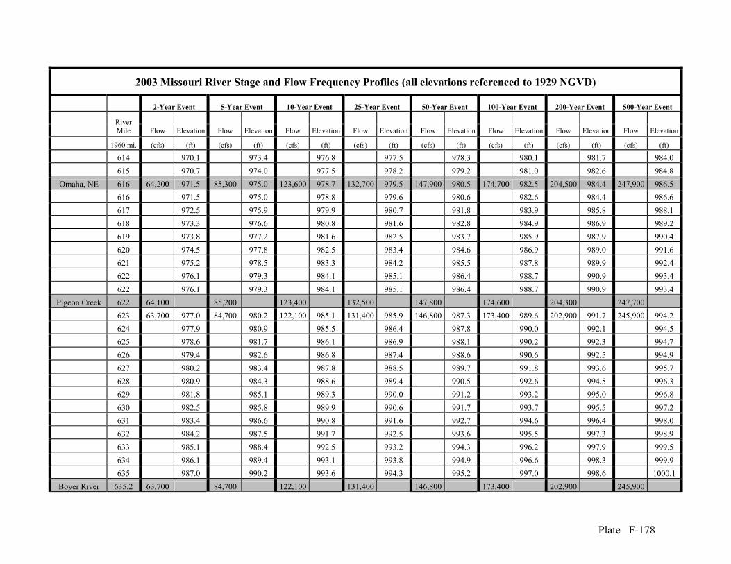
Plate F-178





614 970.1 973.4 976.8 977.5 978.3 980.1 981.7 984.0 615 970.7 974.0 977.5 978.2 979.2 981.0 982.6 984.8

Omaha, NE 616 64,200 971.5 85,300 975.0 123,600 978.7 132,700 979.5 147,900 980.5 174,700 982.5 204,500 984.4 247,900 986.5 616 971.5 975.0 978.8 979.6 980.6 982.6 984.4 986.6 617 972.5 975.9 979.9 980.7 981.8 983.9 985.8 988.1 618 973.3 976.6 980.8 981.6 982.8 984.9 986.9 989.2 619 973.8 977.2 981.6 982.5 983.7 985.9 987.9 990.4 620 974.5 977.8 982.5 983.4 984.6 986.9 989.0 991.6 621 975.2 978.5 983.3 984.2 985.5 987.8 989.9 992.4 622 976.1 979.3 984.1 985.1 986.4 988.7 990.9 993.4 622 976.1 979.3 984.1 985.1 986.4 988.7 990.9 993.4

Pigeon Creek 622 64,100 85,200 123,400 132,500 147,800 174,600 204,300 247,700 623 63,700 977.0 84,700 980.2 122,100 985.1 131,400 985.9 146,800 987.3 173,400 989.6 202,900 991.7 245,900 994.2 624 977.9 980.9 985.5 986.4 987.8 990.0 992.1 994.5 625 978.6 981.7 986.1 986.9 988.1 990.2 992.3 994.7 626 979.4 982.6 986.8 987.4 988.6 990.6 992.5 994.9 627 980.2 983.4 987.8 988.5 989.7 991.8 993.6 995.7 628 980.9 984.3 988.6 989.4 990.5 992.6 994.5 996.3 629 981.8 985.1 989.3 990.0 991.2 993.2 995.0 996.8 630 982.5 985.8 989.9 990.6 991.7 993.7 995.5 997.2 631 983.4 986.6 990.8 991.6 992.7 994.6 996.4 998.0 632 984.2 987.5 991.7 992.5 993.6 995.5 997.3 998.9 633 985.1 988.4 992.5 993.2 994.3 996.2 997.9 999.5 634 986.1 989.4 993.1 993.8 994.9 996.6 998.3 999.9 635 987.0 990.2 993.6 994.3 995.2 997.0 998.6 1000.1

Boyer River 635.2 63,700 84,700 122,100 131,400 146,800 173,400 202,900 245,900

Plate F-179





636 62,000 988.3 82,600 991.1 117,000 994.1 127,000 994.6 142,900 995.5 168,700 997.1 197,200 998.8 238,800 1000.2 637 989.1 991.9 994.6 995.1 996.0 997.4 999.1 1000.5 638 989.9 992.8 995.3 995.9 996.7 998.0 999.5 1000.8 639 990.7 993.5 996.0 996.6 997.4 998.6 1000.1 1001.4 640 991.4 994.2 996.9 997.5 998.4 999.5 1000.9 1002.2 641 992.2 995.1 998.0 998.6 999.5 1000.8 1002.3 1003.7 642 993.0 995.9 998.8 999.5 1000.5 1001.7 1003.2 1004.7 643 993.8 996.6 999.7 1000.5 1001.4 1002.7 1004.2 1005.7 644 994.6 997.6 1001.1 1001.9 1003.1 1004.5 1006.0 1007.5 645 995.5 998.5 1002.1 1003.0 1004.2 1005.7 1007.2 1008.6 646 996.4 999.4 1003.0 1003.9 1005.1 1006.5 1008.0 1009.3 647 997.2 1000.2 1004.0 1004.9 1006.2 1007.3 1008.7 1010.0

Fish Creek 647.8 62,000 82,600 117,000 127,000 142,900 168,700 197,200 238,800 648 61,800 998.2 82,300 1001.3 116,200 1005.3 126,400 1006.1 142,400 1007.1 168,100 1008.3 196,500 1009.5 237,800 1010.9

Near Blair, NE 648.3 998.6 1001.7 1005.6 1006.5 1007.5 1008.6 1009.7 1011.1 649 999.2 1002.3 1006.4 1007.3 1008.4 1009.6 1010.9 1012.1

Old Soldier R. Ditch 649.3 61,800 82,300 116,200 126,400 142,400 168,100 196,500 237,800

650 61,500 1000.0 81,900 1003.2 115,300 1007.0 125,600 1007.9 141,700 1009.0 167,200 1010.3 195,400 1011.6 236,500 1012.8 651 1000.7 1003.9 1007.5 1008.3 1009.5 1010.7 1012.0 1013.1 652 1001.4 1004.6 1008.2 1009.0 1010.2 1011.4 1012.7 1013.9 653 1002.1 1005.3 1009.0 1009.9 1011.2 1012.4 1013.9 1015.0 654 1003.0 1006.2 1009.9 1010.8 1012.1 1013.5 1014.8 1015.7 655 1003.8 1007.0 1010.4 1011.2 1012.5 1013.9 1015.3 1016.2 656 1004.6 1007.7 1011.1 1011.8 1013.0 1014.3 1015.7 1016.6 657 1005.4 1008.6 1011.9 1012.6 1013.8 1015.1 1016.5 1017.6

Plate F-180





658 1006.1 1009.3 1012.8 1013.5 1014.7 1016.0 1017.5 1018.6 659 1006.9 1010.1 1013.5 1014.3 1015.5 1016.9 1018.3 1019.5 660 1007.8 1011.0 1014.6 1015.4 1016.6 1018.0 1019.3 1020.5 661 1008.7 1012.0 1015.6 1016.4 1017.6 1018.8 1020.1 1021.2 662 1009.7 1012.9 1016.5 1017.2 1018.4 1019.5 1020.7 1021.8 663 1010.6 1013.9 1017.5 1018.2 1019.4 1020.5 1021.8 1023.0 664 1011.6 1014.9 1018.3 1019.1 1020.3 1021.5 1022.9 1024.2

Soldier River 664 61,500 81,900 115,300 125,600 141,700 167,200 195,400 236,500 664 60,800 1011.6 81,000 1014.9 113,000 1018.3 123,600 1019.1 140,000 1020.3 165,200 1021.5 192,900 1022.9 233,300 1024.2

665 1012.5 1015.8 1019.2 1020.0 1021.4 1022.6 1024.1 1025.5 Tekamah Div.

Ditch 665 60,800 81,000 113,000 123,600 140,000 165,200 192,900 233,300 666 60,500 1013.4 80,700 1016.8 112,200 1020.1 123,000 1021.0 139,400 1022.3 164,400 1023.5 192,100 1024.9 232,200 1026.2 667 1014.3 1017.6 1020.9 1021.8 1023.0 1024.3 1025.6 1026.8 668 1015.2 1018.5 1021.8 1022.6 1023.9 1025.2 1026.5 1027.7 669 1016.2 1019.4 1022.7 1023.5 1024.9 1026.1 1027.5 1028.7

Little Sioux River 669.2 60,500 80,700 112,200 123,000 139,400 164,400 192,100 232,200

Monona Harr. Ditch 670 54,200 1017.5 72,700 1020.5 92,800 1023.6 106,300 1024.4 124,700 1025.9 146,800 1027.2 170,800 1028.6 205,400 1030.1

671 52,400 1018.4 70,500 1021.7 87,200 1024.4 101,600 1025.3 120,500 1027.1 141,800 1028.2 164,800 1029.7 197,700 1031.3 672 1019.1 1022.5 1024.8 1025.9 1027.6 1028.9 1030.3 1032.0 673 1020.0 1023.3 1025.4 1026.7 1028.4 1029.9 1031.3 1033.2 674 1020.9 1024.2 1026.2 1027.6 1029.3 1030.9 1032.2 1034.2 675 1021.8 1025.2 1027.1 1028.5 1030.4 1032.1 1033.3 1035.3 676 1022.8 1026.3 1028.3 1029.7 1031.6 1033.4 1034.5 1036.4 677 1023.9 1027.3 1029.3 1030.8 1032.7 1034.5 1035.8 1037.6

Plate F-181





678 1024.9 1028.3 1030.3 1031.7 1033.7 1035.6 1036.9 1038.7 679 1025.9 1029.2 1031.2 1032.7 1034.7 1036.6 1037.9 1039.7 680 1026.9 1030.2 1032.1 1033.6 1035.7 1037.5 1038.8 1040.6 681 1027.8 1031.0 1033.0 1034.5 1036.5 1038.4 1039.6 1041.3 682 1028.7 1031.9 1033.8 1035.3 1037.3 1039.1 1040.4 1042.1 683 1029.7 1032.7 1034.6 1036.1 1038.2 1039.9 1041.1 1042.7 684 1030.7 1033.7 1035.5 1036.9 1038.8 1040.5 1041.6 1043.2 685 1031.7 1034.6 1036.3 1037.5 1039.3 1040.9 1042.0 1043.6 686 1032.6 1035.4 1037.0 1038.2 1039.9 1041.5 1042.5 1044.1 687 1033.7 1036.5 1038.0 1039.1 1040.7 1042.3 1043.3 1044.8 688 1034.7 1037.4 1039.0 1040.1 1041.7 1043.2 1044.3 1045.7 689 1035.5 1038.3 1039.9 1041.2 1042.8 1044.4 1045.5 1046.9 690 1036.3 1039.2 1040.9 1042.2 1043.9 1045.4 1046.5 1047.9 691 1037.4 1040.4 1042.0 1043.2 1044.8 1046.3 1047.3 1048.8

Decatur, NE 691 52,400 1037.4 70,500 1040.4 87,200 1042.0 101,600 1043.2 120,500 1044.8 141,800 1046.3 164,800 1047.4 197,700 1048.8 692 1038.0 1041.0 1042.7 1043.9 1045.6 1047.2 1048.4 1050.0 693 1038.7 1041.8 1043.4 1044.7 1046.4 1048.1 1049.3 1051.1 694 1039.5 1042.7 1044.3 1045.6 1047.4 1049.1 1050.4 1052.1 695 1040.4 1043.6 1045.3 1046.6 1048.4 1050.2 1051.6 1053.4 696 1041.4 1044.6 1046.3 1047.6 1049.3 1051.1 1052.5 1054.3 697 1042.3 1045.6 1047.3 1048.5 1050.3 1051.9 1053.1 1055.0

Blackbird Creek 697.4 52,300 70,300 86,900 101,300 120,300 141,500 164,400 197,300 698 51,800 1043.2 69,600 1046.5 85,200 1048.1 99,800 1049.4 119,000 1051.2 140,000 1052.8 162,600 1054.0 195,000 1055.6 699 1044.1 1047.3 1049.0 1050.3 1052.1 1053.8 1055.0 1056.7 700 1045.0 1048.1 1049.8 1051.2 1053.0 1054.8 1056.0 1057.6 701 1045.8 1048.9 1050.6 1051.9 1053.7 1055.5 1056.7 1058.3

Plate F-182





702 1046.7 1049.9 1051.6 1052.9 1054.8 1056.7 1057.8 1059.3 703 1047.7 1050.9 1052.6 1054.0 1055.8 1057.6 1058.7 1060.2 704 1048.6 1051.8 1053.6 1054.9 1056.7 1058.5 1059.7 1061.1 705 1049.7 1052.9 1054.6 1056.0 1057.6 1059.3 1060.4 1061.9 706 1050.7 1053.9 1055.7 1057.1 1058.6 1060.3 1061.5 1063.1 707 1051.6 1054.7 1056.4 1057.7 1059.4 1061.2 1062.4 1064.1 708 1052.6 1055.8 1057.4 1058.7 1060.4 1062.2 1063.6 1065.3 709 1053.7 1056.9 1058.5 1059.9 1061.7 1063.3 1064.5 1066.2 710 1054.6 1057.7 1059.4 1060.7 1062.5 1064.2 1065.5 1067.3 711 1055.6 1058.7 1060.4 1061.8 1063.6 1065.3 1066.5 1068.2 712 1056.4 1059.6 1061.3 1062.6 1064.5 1066.2 1067.5 1069.1 713 1057.3 1060.5 1062.2 1063.6 1065.5 1067.0 1068.1 1069.7 714 1058.4 1061.5 1063.2 1064.7 1066.5 1068.1 1069.2 1070.8 715 1059.5 1062.6 1064.3 1065.7 1067.6 1069.3 1070.3 1071.8 716 1060.7 1063.7 1065.4 1066.9 1068.9 1070.5 1071.5 1072.8 717 1061.6 1064.7 1066.4 1067.8 1069.7 1071.4 1072.3 1073.7 718 1062.6 1065.8 1067.5 1068.8 1070.6 1072.2 1073.2 1074.6 719 1063.4 1066.7 1068.4 1069.7 1071.5 1073.1 1074.2 1075.6

Omaha Creek 719.9 51,800 69,600 85,200 99,800 119,000 140,000 162,600 195,000 720 51,300 1064.5 69,000 1067.8 83,700 1069.4 98,500 1070.7 117,900 1072.6 138,600 1074.0 160,900 1075.1 192,900 1076.6 721 1065.5 1068.7 1070.3 1071.6 1073.5 1074.9 1076.0 1077.6 722 1066.4 1069.6 1071.2 1072.4 1074.3 1075.8 1076.9 1078.4 723 1067.4 1070.6 1072.1 1073.4 1075.3 1076.8 1078.0 1079.6 724 1068.3 1071.5 1073.1 1074.5 1076.3 1077.9 1079.2 1080.9 725 1069.4 1072.5 1074.2 1075.6 1077.4 1079.0 1080.4 1082.0 726 1070.5 1073.6 1075.2 1076.7 1078.5 1080.2 1081.6 1083.4

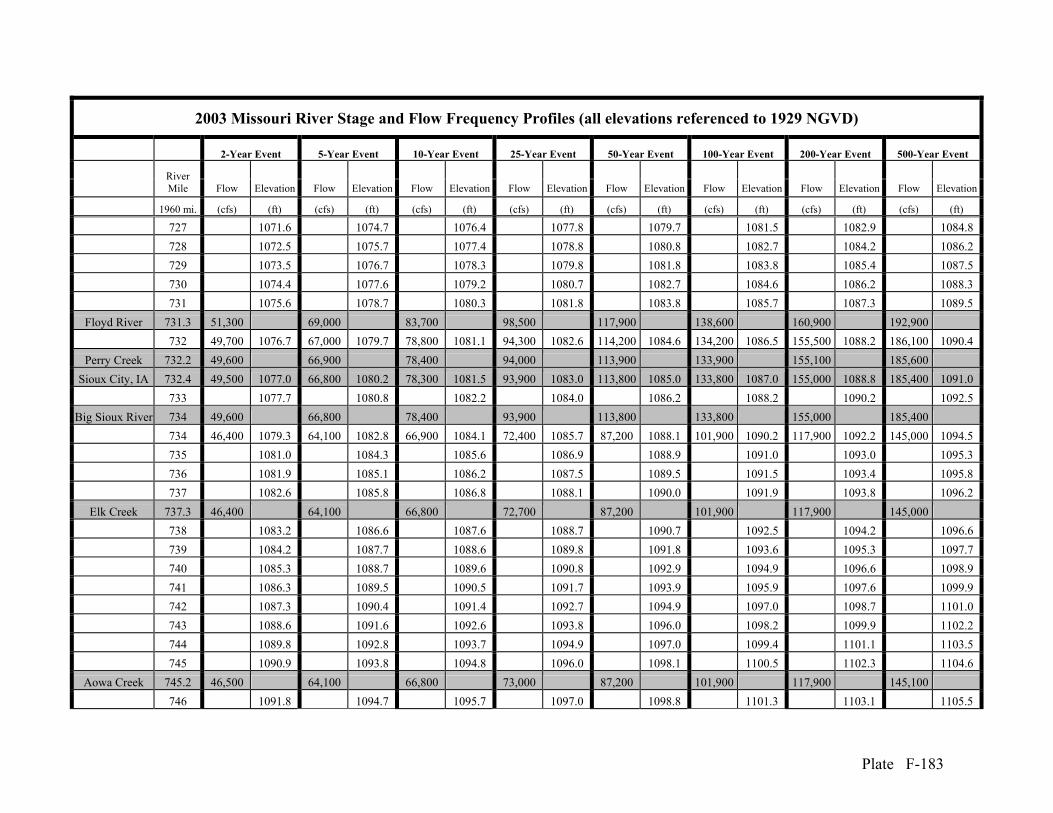
Plate F-183





727 1071.6 1074.7 1076.4 1077.8 1079.7 1081.5 1082.9 1084.8 728 1072.5 1075.7 1077.4 1078.8 1080.8 1082.7 1084.2 1086.2 729 1073.5 1076.7 1078.3 1079.8 1081.8 1083.8 1085.4 1087.5 730 1074.4 1077.6 1079.2 1080.7 1082.7 1084.6 1086.2 1088.3 731 1075.6 1078.7 1080.3 1081.8 1083.8 1085.7 1087.3 1089.5

Floyd River 731.3 51,300 69,000 83,700 98,500 117,900 138,600 160,900 192,900 732 49,700 1076.7 67,000 1079.7 78,800 1081.1 94,300 1082.6 114,200 1084.6 134,200 1086.5 155,500 1088.2 186,100 1090.4

Perry Creek 732.2 49,600 66,900 78,400 94,000 113,900 133,900 155,100 185,600 Sioux City, IA 732.4 49,500 1077.0 66,800 1080.2 78,300 1081.5 93,900 1083.0 113,800 1085.0 133,800 1087.0 155,000 1088.8 185,400 1091.0

733 1077.7 1080.8 1082.2 1084.0 1086.2 1088.2 1090.2 1092.5 Big Sioux River 734 49,600 66,800 78,400 93,900 113,800 133,800 155,000 185,400

734 46,400 1079.3 64,100 1082.8 66,900 1084.1 72,400 1085.7 87,200 1088.1 101,900 1090.2 117,900 1092.2 145,000 1094.5 735 1081.0 1084.3 1085.6 1086.9 1088.9 1091.0 1093.0 1095.3 736 1081.9 1085.1 1086.2 1087.5 1089.5 1091.5 1093.4 1095.8 737 1082.6 1085.8 1086.8 1088.1 1090.0 1091.9 1093.8 1096.2

Elk Creek 737.3 46,400 64,100 66,800 72,700 87,200 101,900 117,900 145,000 738 1083.2 1086.6 1087.6 1088.7 1090.7 1092.5 1094.2 1096.6 739 1084.2 1087.7 1088.6 1089.8 1091.8 1093.6 1095.3 1097.7 740 1085.3 1088.7 1089.6 1090.8 1092.9 1094.9 1096.6 1098.9 741 1086.3 1089.5 1090.5 1091.7 1093.9 1095.9 1097.6 1099.9 742 1087.3 1090.4 1091.4 1092.7 1094.9 1097.0 1098.7 1101.0 743 1088.6 1091.6 1092.6 1093.8 1096.0 1098.2 1099.9 1102.2 744 1089.8 1092.8 1093.7 1094.9 1097.0 1099.4 1101.1 1103.5 745 1090.9 1093.8 1094.8 1096.0 1098.1 1100.5 1102.3 1104.6

Aowa Creek 745.2 46,500 64,100 66,800 73,000 87,200 101,900 117,900 145,100 746 1091.8 1094.7 1095.7 1097.0 1098.8 1101.3 1103.1 1105.5

Plate F-184





747 1092.6 1095.6 1096.6 1097.8 1099.6 1102.0 1103.8 1106.1 748 1093.5 1096.5 1097.5 1098.8 1100.4 1102.8 1104.5 1106.8 749 1094.4 1097.5 1098.5 1099.8 1101.4 1103.6 1105.4 1107.6 750 1095.2 1098.3 1099.3 1100.5 1102.2 1104.5 1106.1 1108.4

Near Ponca, NE 751 46,600 1096.1 64,200 1099.2 66,800 1100.1 73,400 1101.4 87,300 1103.0 101,900 1105.2 117,900 1106.9 145,100 1109.0 752 1096.8 1099.9 1100.9 1102.2 1103.8 1105.9 1107.6 1109.6 753 1097.8 1100.9 1101.8 1103.1 1104.7 1106.8 1108.3 1110.4 754 1098.9 1101.8 1102.7 1103.9 1105.4 1107.4 1109.0 1111.0 755 1100.3 1102.9 1103.7 1104.8 1106.3 1108.2 1109.7 1111.7 756 1101.4 1103.8 1104.6 1105.7 1107.0 1108.8 1110.3 1112.3 757 1102.7 1104.9 1105.6 1106.6 1107.8 1109.5 1110.9 1112.9 758 1103.7 1105.8 1106.4 1107.3 1108.4 1110.0 1111.4 1113.3 759 1104.7 1106.7 1107.3 1108.1 1109.2 1110.7 1112.0 1113.8 760 1106.3 1108.2 1108.8 1109.5 1110.5 1111.8 1113.0 1114.6 761 1108.0 1109.8 1110.4 1111.2 1112.1 1113.4 1114.6 1116.2 762 1109.3 1111.1 1111.7 1112.5 1113.4 1114.7 1115.8 1117.3 763 1110.7 1112.5 1113.1 1113.9 1114.8 1116.1 1117.0 1118.5 764 1112.0 1114.0 1114.6 1115.4 1116.4 1117.6 1118.5 1119.9 765 1112.9 1114.8 1115.5 1116.3 1117.2 1118.5 1119.4 1120.8 766 1113.8 1115.7 1116.4 1117.2 1118.1 1119.3 1120.3 1121.7 767 1114.7 1116.6 1117.2 1118.0 1118.9 1120.1 1121.1 1122.4 768 1115.6 1117.5 1118.1 1118.9 1119.7 1121.0 1121.9 1123.2 769 1116.6 1118.5 1119.1 1119.9 1120.8 1122.1 1123.0 1124.4 770 1117.8 1119.6 1120.3 1121.1 1121.9 1123.2 1124.2 1125.6 771 1119.0 1120.7 1121.4 1122.1 1122.9 1124.1 1125.0 1126.4

Vermillion 771.9 46,900 1120.1 64,300 1122.0 66,900 1122.5 74,000 1123.2 88,000 1124.0 101,900 1125.2 117,900 1126.2 145,100 1127.5

Plate F-185




1960 mi. (cfs) (ft) (cfs) (ft) (cfs) (ft) (cfs) (ft) (cfs) (ft) (cfs) (ft) (cfs) (ft) (cfs) (ft) River

772 45,500 1120.3 64,000 1122.2 65,900 1122.6 70,200 1123.3 83,600 1124.2 99,100 1125.4 114,600 1126.4 141,500 1127.7 773 1121.5 1123.4 1123.8 1124.5 1125.3 1126.5 1127.6 1129.0 774 1123.2 1125.1 1125.4 1126.1 1126.8 1127.9 1128.9 1130.3 775 1124.2 1126.1 1126.4 1127.1 1127.8 1129.0 1130.0 1131.4

Near Maskell, NE 775.6 45,500 1125.0 64,000 1126.8 65,900 1127.2 70,200 1127.9 83,600 1128.6 99,100 1129.7 114,600 1130.7 141,500 1132.2

776 1125.5 1127.3 1127.6 1128.3 1129.0 1130.2 1131.2 1132.7 777 1126.4 1128.2 1128.5 1129.2 1129.8 1130.9 1131.9 1133.5 778 1127.8 1129.4 1129.7 1130.3 1130.9 1131.7 1132.8 1134.3 779 1129.3 1130.7 1130.9 1131.4 1131.9 1132.7 1133.6 1135.0 780 1130.8 1132.1 1132.3 1132.8 1133.2 1133.9 1134.6 1135.7 781 1132.4 1133.5 1133.8 1134.2 1134.7 1135.3 1135.8 1136.7 782 1134.1 1135.2 1135.4 1135.9 1136.3 1136.9 1137.4 1138.2 783 1135.5 1136.6 1136.8 1137.3 1137.7 1138.3 1138.8 1139.6 784 1136.8 1137.9 1138.1 1138.6 1139.0 1139.6 1140.1 1140.9 785 1138.0 1139.1 1139.4 1139.9 1140.3 1140.8 1141.4 1142.2 786 1139.2 1140.5 1140.7 1141.2 1141.7 1142.2 1142.8 1143.6 787 1140.2 1141.6 1141.9 1142.4 1142.9 1143.5 1144.1 1145.0

Bow Creek 787.6 45,500 1140.7 64,000 1142.3 66,200 1142.6 70,300 1143.0 83,900 1143.7 99,100 1144.4 114,600 1145.0 141,500 1146.1 788 1141.0 1142.6 1142.9 1143.3 1144.1 1144.8 1145.5 1146.5 789 1141.8 1143.4 1143.7 1144.1 1144.9 1145.7 1146.4 1147.5 790 1143.0 1144.6 1144.9 1145.3 1146.0 1146.8 1147.5 1148.6 791 1144.1 1145.7 1145.9 1146.3 1147.0 1147.9 1148.6 1149.7 792 1145.1 1146.8 1147.1 1147.6 1148.3 1149.3 1150.1 1151.2 793 1146.1 1148.0 1148.3 1148.8 1149.6 1150.7 1151.6 1152.9

Plate F-186





794 1146.9 1148.9 1149.2 1149.7 1150.6 1151.7 1152.7 1154.0 795 1147.7 1149.7 1150.0 1150.5 1151.4 1152.6 1153.6 1155.0

Near Gayville, SD 796 45,600 1148.4 64,000 1150.4 66,300 1150.8 70,300 1151.3 84,100 1152.2 99,100 1153.4 114,600 1154.4 141,500 1155.8

797 1149.1 1151.2 1151.5 1152.0 1153.0 1154.2 1155.2 1156.6 James River 797.7 45,600 1149.7 64,000 1151.8 66,300 1152.1 70,400 1152.7 84,100 1153.7 99,100 1154.9 114,600 1156.0 141,500 1157.5

798 45,300 1150.2 63,000 1152.6 65,000 1152.9 69,100 1153.5 74,700 1154.2 84,900 1155.4 98,000 1156.4 123,500 1158.0 799 1151.1 1153.9 1154.2 1154.7 1155.1 1156.5 1157.5 1159.3 800 1151.9 1154.6 1154.9 1155.4 1155.9 1157.3 1158.4 1160.4 801 1152.7 1155.4 1155.7 1156.2 1156.7 1158.1 1159.3 1161.4 802 1153.2 1155.9 1156.1 1156.7 1157.2 1158.6 1159.8 1161.9 803 1153.8 1156.4 1156.7 1157.2 1157.8 1159.1 1160.4 1162.4 804 1154.7 1157.1 1157.4 1157.9 1158.5 1159.7 1161.1 1163.1 805 1155.8 1158.1 1158.3 1158.8 1159.4 1160.5 1161.8 1163.8

Yankton, SD 805.8 45,300 1156.5 63,000 1158.7 65,000 1158.9 69,100 1159.4 74,700 1160.0 84,900 1161.1 98,000 1162.4 123,500 1164.4 806 1156.7 1158.9 1159.1 1159.6 1160.2 1161.3 1162.7 1164.7 807 1157.5 1159.6 1159.8 1160.3 1160.9 1162.0 1163.3 1165.5 808 1158.6 1160.5 1160.7 1161.1 1161.7 1162.7 1163.9 1166.0 809 1159.7 1161.5 1161.7 1162.1 1162.7 1163.6 1164.9 1166.9 810 1160.4 1162.3 1162.5 1163.0 1163.5 1164.5 1165.8 1167.9

Gavins Point Dam 810.9 45,300 1160.8 63,000 1162.9 65,000 1163.1 69,100 1163.6 74,700 1164.1 84,900 1165.2 98,000 1166.4 123,500 1168.6

Plate F- 187

505 508 510 513 515 518 520 523 525 528 530

River Mile

855

865

875

885

895

905

Elev

atio

n (F

eet 1

929

NG

VD)

L-536

L-536

L-550 South

R-548

R-520

R-520

Legend10-Year FFS 200350-Year FFS 2003100-Year FFS 2003500-Year FFS 2003100-Year 1978 StudyLeft Bank LeveeRight Bank Levee

2003 vs. 1978 Missouri River Stage Frequency Profiles - River Mile 498-530

RM

527

.8

500

RM

498

.0

Rul

o, N

E

Littl

e N

emah

a R

iver

at A

ubur

n, N

E

Note: The illustrated levee elevations reflect the UNET modelconnection elevations only. Actual levee elevation between the illustrated points may vary and should not be assumed to be linear.

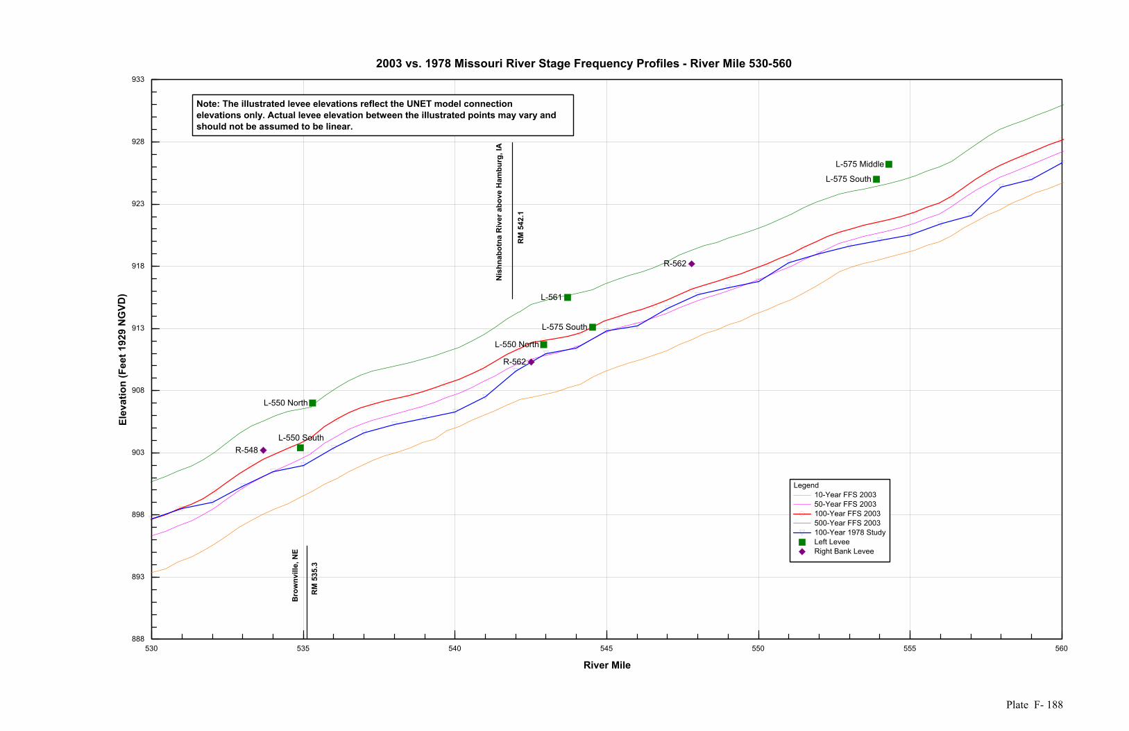
Plate F- 188

530 535 540 545 550 555 560

River Mile

888

893

898

903

908

913

918

923

928

933

Elev

atio

n (F

eet 1

929

NG

VD)

L-550 South

L-550 North

L-550 North

L-561

L-575 South

L-575 South

L-575 Middle

R-548

R-562

R-562

Legend10-Year FFS 200350-Year FFS 2003100-Year FFS 2003500-Year FFS 2003100-Year 1978 StudyLeft LeveeRight Bank Levee


Bro

wnv

ille,

NE

RM

535

.3

RM

542

.1


Nis

hnab

otna

Riv

er a

bove

Ham

burg

, IA

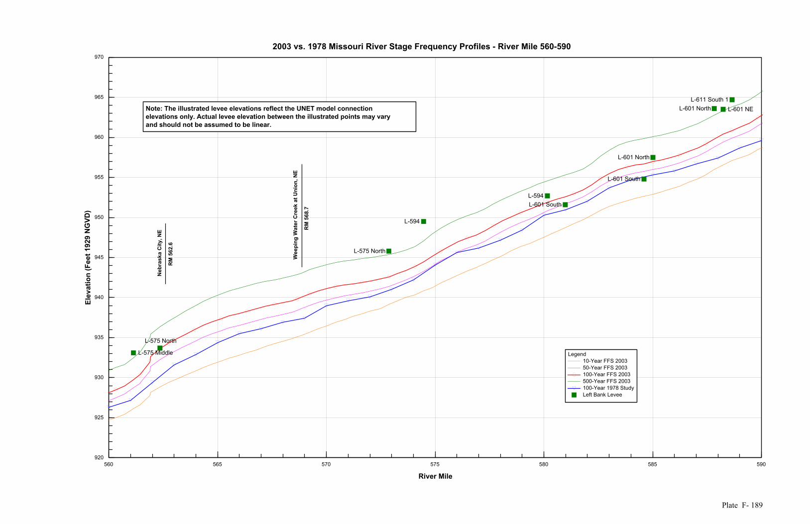
Plate F- 189

560 565 570 575 580 585 590

River Mile

920

925

930

935

940

945

950

955

960

965

970

Elev

atio

n (F

eet 1

929

NG

VD)

L-575 Middle

L-575 North

L-575 North

L-594

L-594L-601 South

L-601 South

L-601 North

L-601 North L-601 NEL-611 South 1

Legend10-Year FFS 200350-Year FFS 2003100-Year FFS 2003500-Year FFS 2003100-Year 1978 StudyLeft Bank Levee


Wee

ping

Wat

er C

reek

at U

nion

, NE

RM

568

.7

Neb

rask

a C

ity, N

E

RM

562

.6


Plate F- 190

590 595 600 605 610 615 620

River Mile

953

958

963

968

973

978

983

988

993

Elev

atio

n (F

eet 1

929

NG

VD)

L-611 South 1

L-611 South 2

L-611 South 2L-611 North 1

L-611 North 1

L-611 North 2

L-611 North 2

L-614

L-624

L-624 L-627

Omaha Levee So. L-627

Omaha Levee So.

Council Bluffs

Omaha FloodwallOmaha Floodwall

Omaha Levee No.

Council Bluffs

R-613R-613

R-616

R-616

Legend10-Year FFS 200350-Year FFS 2003100-Year FFS 2003500-Year FFS 2003100-Year 1978 StudyLeft Bank LeveeRight Bank Levee

2003 vs 1978 Missouri River Stage Frequency Profiles - River Mile 590-620

Om

aha,

NE

RM

615

.9

Plat

tsm

outh

, NE

RM

591

.5

Papi

llion

Cre

ek a

t For

t Cro

ok, N

E

RM

596

.6

Plat

te R

iver

at L

ouis

ville

, NE

RM

594

.8


Plate F- 191

620 625 630 635 640 645 650

River Mile

974

979

984

989

994

999

1004

1009

1014

Elev

atio

n (F

eet 1

929

NG

VD)

Legend10-Year FFS 200350-Year FFS 2003100-Year FFS 2003500-Year FFS 2003100-Year 1978 Study


Bla

ir, N

E

RM

648

.3

Boy

er R

iver

at L

ogan

, IA

RM

635

.2


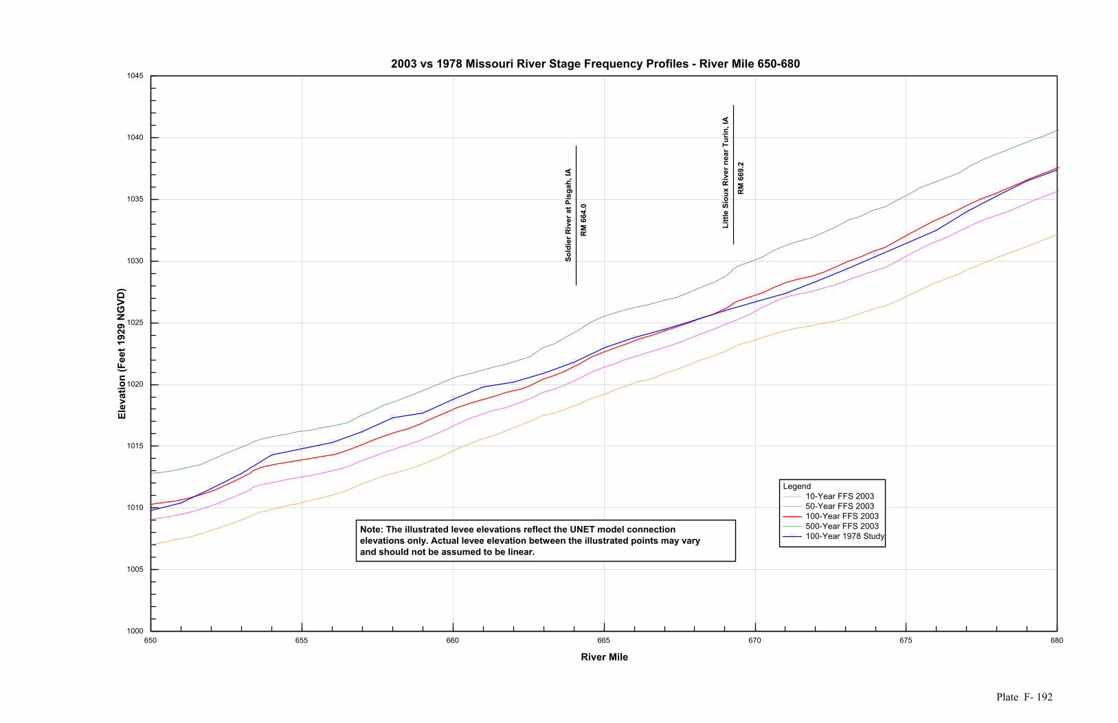
Plate F- 192

650 655 660 665 670 675 680

River Mile

1000

1005

1010

1015

1020

1025

1030

1035

1040

1045

Elev

atio

n (F

eet 1

929

NG

VD)



Littl

e Si

oux

Riv

er n

ear T

urin

, IA

RM

669

.2

Sold

ier R

iver

at P

isga

h, IA

RM

664

.0


Plate F- 193

680 685 690 695 700 705 710

River Mile

1025

1030

1035

1040

1045

1050

1055

1060

1065

1070

Elev

atio

n (F

eet 1

929

NG

VD)



Dec

atur

, NE

RM

691

.0


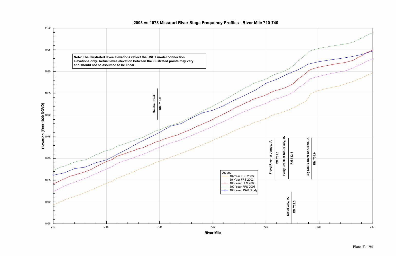
Plate F- 194

710 715 720 725 730 735 740

River Mile

1055

1060

1065

1070

1075

1080

1085

1090

1095

1100

Elev

atio

n (F

eet 1

929

NG

VD)



Siou

x C

ity, I

A

RM

732

.3

Big

Sio

ux R

iver

at A

kron

, IA

RM

734

.0

Perr

y C

reek

at S

ioux

City

, IA

RM

732

.1

Floy

d R

iver

at J

ames

, IA

RM

731

.3

Om

aha

Cre

ek

RM

719

.9


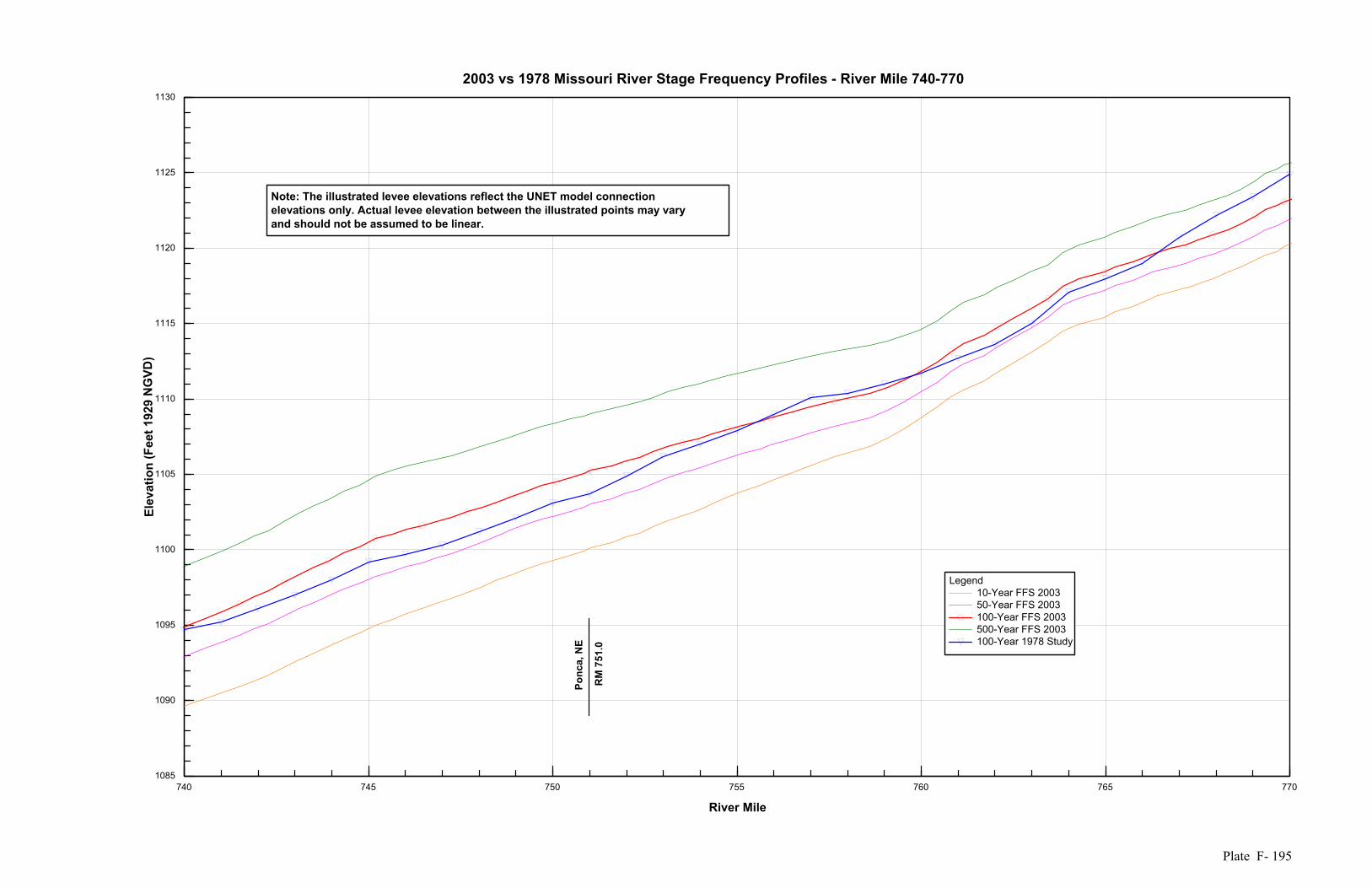
Plate F- 195

740 745 750 755 760 765 770

River Mile

1085

1090

1095

1100

1105

1110

1115

1120

1125

1130

Elev

atio

n (F

eet 1

929

NG

VD)



Ponc

a, N

E

RM

751

.0


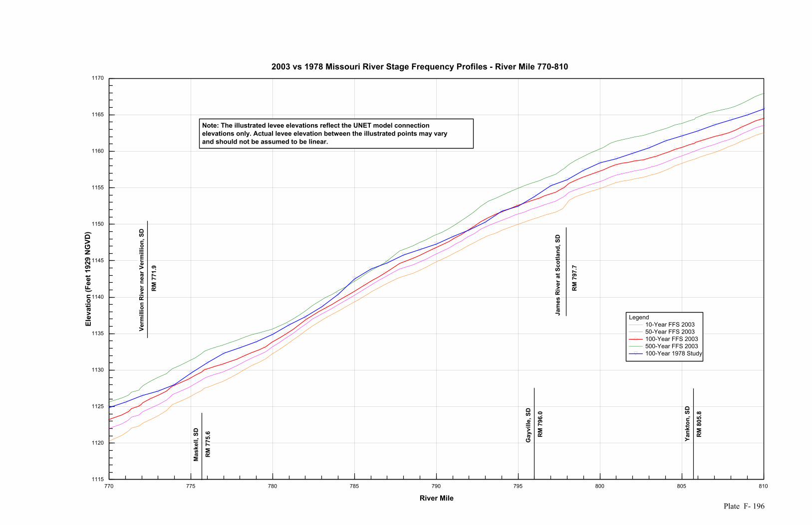
Plate F- 196

770 775 780 785 790 795 800 805 810

River Mile

1115

1120

1125

1130

1135

1140

1145

1150

1155

1160

1165

1170

Elev

atio

n (F

eet 1

929

NG

VD)



Gay

ville

, SD

RM

796

.0

Jam

es R

iver

at S

cotla

nd, S

D

RM

797

.7

Mas

kell,

SD

RM

775

.6

Verm

illio

n R

iver

nea

r Ver

mill

ion,

SD

RM

771

.9

Yank

ton,

SD

RM

805

.8


Documents

Upper Mississippi River System Flow Frequency Study .... F...Upper Mississippi River System Flow Frequency Study Hydrology and Hydraulics Appendix F Missouri River U.S. Army Corps