Upper-Ocean Processes under the Stratus Cloud Deck in the

Upper-Ocean Processes under the Stratus Cloud Deckin the Southeast Pacific Ocean

YANGXING ZHENG,* TOSHIAKI SHINODA,1 GEORGE N. KILADIS,* JIALIN LIN,#

E. JOSEPH METZGER,1 HARLEY E. HURLBURT,1 AND BENJAMIN S. GIESE@

* NOAA/ESRL/CIRES Climate Diagnostics Center, Boulder, Colorado1 Naval Research Laboratory, Stennis Space Center, Mississippi

# Department of Geography, The Ohio State University, Columbus, Ohio@ Department of Oceanography, Texas A&M University, College Station, Texas

(Manuscript received 6 January 2009, in final form 28 July 2009)

ABSTRACT

The annual mean heat budget of the upper ocean beneath the stratocumulus/stratus cloud deck in the

southeast Pacific is estimated using Simple Ocean Data Assimilation (SODA) and an eddy-resolving Hybrid

Coordinate Ocean Model (HYCOM). Both are compared with estimates based on Woods Hole Oceano-

graphic Institution (WHOI) Improved Meteorological (IMET) buoy observations at 208S, 858W. Net surface

heat fluxes are positive (warming) over most of the area under the stratus cloud deck. Upper-ocean processes

responsible for balancing the surface heat flux are examined by estimating each term in the heat equation. In

contrast to surface heat fluxes, geostrophic transport in the upper 50 m causes net cooling in most of the

stratus cloud deck region. Ekman transport provides net warming north of the IMET site and net cooling

south of the IMET site. Although the eddy heat flux divergence term can be comparable to other terms at

a particular location, such as the IMET mooring site, it is negligible for the entire stratus region when area

averaged because it is not spatially coherent in the open ocean. Although cold-core eddies are often generated

near the coast in the eddy-resolving model, they do not significantly impact the heat budget in the open ocean

in the southeast Pacific.

1. Introduction

Sea surface temperature (SST) in the southeast Pacific

near the coasts of Peru and Chile is colder than at any

comparable latitude elsewhere. It is believed that these

cold waters in the southeast Pacific play an important

role in the formation and maintenance of persistent

stratocumulus/stratus cloud decks and that these clouds

have a significant impact on regional and global climate

(e.g., Ma et al. 1996; Miller 1997; Gordon et al. 2000; Xie

2004). Thus, it is important to understand upper-ocean

processes that maintain SST under the stratocumulus

cloud deck for global simulation and climate prediction.

However, until recently, the upper ocean in this region

has been sparsely observed, which limits our ability to

better understand and simulate the behavior of the at-

mosphere and ocean globally. In fact, most atmosphere–

ocean coupled general circulation models (CGCMs)

have systematic errors in the southeast Pacific, including

too warm SSTs and too little cloud cover (e.g., Mechoso

et al. 1995; Ma et al. 1996; Lin 2007), which have im-

portant impacts on the simulated radiation budget and

climate sensitivity.

As part of the Eastern Pacific Investigation of Climate

(EPIC), a well-instrumented surface mooring was de-

ployed under the middle of the stratus cloud deck (208S,

858W) in October 2000, providing 6 yr of upper-ocean

temperature, salinity, velocity, and surface meteorologi-

cal variables (Colbo and Weller 2007). Using these da-

tasets as well as other satellite and historical data, Colbo

and Weller (2007) estimated the upper-ocean heat budget

(upper 250 m) at the location of the mooring to under-

stand upper-ocean processes that maintain the annual

mean heat content of the upper ocean in this region.

They found that the major terms of the heat equation

that balance positive (warming) surface heat fluxes are

geostrophic heat transport and eddy heat flux divergence.

Corresponding author address: Yangxing Zheng, NOAA/ESRL/

CIRES Climate Diagnostics Center, 325 Broadway, R/PSD1,

Boulder, CO 80305.

E-mail: [email protected]

JANUARY 2010 Z H E N G E T A L . 103

DOI: 10.1175/2009JPO4213.1

� 2010 American Meteorological Society

Based on the results of their analysis, they hypothesized

that cooling resulting from the eddy heat flux divergence

is a result of westward propagation of cold coherent

eddies formed near the coast that slowly decay in the

open ocean.

Although the analysis of Colbo and Weller (2007) at

the Improved Meteorological (IMET) site significantly

improved our understanding of the upper ocean in this

region, a variety of assumptions were made in their es-

timates, because it is difficult to calculate all terms in the

heat equation from the data at one location. In partic-

ular, the eddy heat flux divergence was estimated as

a residual from the closure of the heat budget in the heat

equation. Although the estimates for the upper 250-m

layer help understand processes that control the upper-

ocean heat content, SSTs may not be directly affected by

advection and eddy fluxes around 250-m depth because

the deepest mixed layer depth during winter is ;150 m.

Furthermore, the persistent stratus cloud decks occupy a

large portion of southeast Pacific (Klein and Hartmann

1993; Colbo and Weller 2007), and it is difficult to identify

important upper-ocean processes for the entire stratus

region from an analysis of one location.

In this study, three-dimensional upper-ocean processes

for the entire stratus cloud region are examined using

Simple Ocean Data Assimilation (SODA; Carton and

Giese 2008) and an eddy-resolving ocean general cir-

culation model (OGCM): the Hybrid Coordinate Ocean

Model (HYCOM). The datasets obtained from the moor-

ing observations are utilized to evaluate the model per-

formance. The annual mean of the terms contributing

to the heat budget are calculated at the mooring site

and compared with observational estimates. Contribut-

ing terms are also estimated for the entire stratus cloud

deck region to examine the representativeness of the

mooring site for broadscale upper-ocean processes. In

addition, terms contributing to the heat budget in the

upper 50 m are computed from the model output to

improve our understanding of upper-ocean processes

that control sea surface temperature variability in this

region. In particular, the relative importance of horizon-

tal heat advection and eddy heat flux divergence in the

upper-ocean heat budget is emphasized, and the role of

cold-core eddies generated near the coast in the open

ocean heat budget is also discussed.

2. Models and datasets

a. SODA

The SODA methodology, the ingested data, and the

error covariance structure of both the model and the ob-

servations are described by Carton et al. (2000a,b), Carton

and Giese (2008), and Zheng and Giese (2009). The

ocean model is based on the Los Alamos implementation

of the Parallel Ocean Program (POP; Smith et al. 1992).

The model resolution is on average 0.48 3 0.258 (longi-

tude 3 latitude) with 40 levels in the vertical. The model

is forced with the 40-yr European Centre for Medium-

Range Weather Forecasts (ECMWF) Re-Analysis

(ERA-40) daily atmospheric reanalysis winds (Simmons

and Gibson 2002) for the 44-yr period from 1958 to 2001.

We update the analysis in a second run forced by Quick

Scatterometer (QuikSCAT) wind stress from 2002 to

2005.

Surface heat fluxes are computed from bulk formu-

lae (Smith et al. 1992), with atmospheric variables that

come from the National Centers for Environmental

Prediction–National Center for Atmospheric Research

(NCEP–NCAR) reanalysis (Kalnay et al. 1996). The

NCEP–NCAR reanalysis information is used for the

bulk formulas instead of the ERA-40 variables throughout

the experiment to give continuity of surface forcing

during periods for which the ERA-40 winds are not

available. However, the details of surface heat flux

boundary condition are relatively unimportant in influ-

encing the solution, because near-surface temperature

observations are used to update the mixed layer tem-

perature. Vertical diffusion of momentum, heat, and salt

is based on a nonlocal K-profile parameterization (KPP;

Large et al. 1994) scheme and horizontal diffusion for

subgrid-scale processes is based on a biharmonic mixing

scheme.

The model is constrained by observed temperature

and salinity, using a sequential assimilation algorithm,

which is described by Carton et al. (2000a,b) and Carton

and Giese (2008). The basic subsurface temperature and

salinity observation sets consist of approximately 7 3 106

profiles, of which two-thirds have been obtained from the

World Ocean Database 2001 (Boyer et al. 2002; Stephens

et al. 2002) with online updates through December 2004.

This dataset has been extended by the addition of real-

time temperature profile observations from the Tropical

Atmosphere Ocean/Triangle Trans-Ocean Buoy Net-

work (TAO/TRITON) mooring thermistor array and

Argo floats. In addition to the temperature profile data,

a large number of near-surface temperature observations

are available both in the form of in situ observations

[bucket and ship-intake temperatures from the Compre-

hensive Ocean-Atmosphere Dataset (COADS) surface

marine observation set of Diaz et al. (2002)] and from

satellite remote sensing. SODA used the nighttime Na-

tional Oceanic and Atmospheric Administration–National

Aeronautics and Space Administration (NOAA–NASA)

Advanced Very High Resolution Radiometer (AVHRR)

operational SST data, which began November 1981 and

average 25 000 samples per week. Use of only nighttime

104 J O U R N A L O F P H Y S I C A L O C E A N O G R A P H Y VOLUME 40

retrievals reduces the error resulting from skin tem-

perature effects. However, the biggest challenge in re-

trieving SST from an infrared (IR) instrument in the

southeast Pacific Ocean is the cloud detection problem,

because clouds are opaque to infrared radiation and can

effectively mask radiation from the ocean surface. Carton

et al. (2000a,b) used a bias-corrected model error co-

variance in an attempt to reduce such error. The near-

surface salinity observation set averages more than 105

observations per year since 1960 (Bingham et al. 2002).

Nearly continuous sea level information is available from

a succession of altimeter satellites beginning in 1991.

Although the coverage of subsurface data in the south-

east Pacific Ocean is not as good as other regions in the

tropics, a significant amount of satellite observations are

used in SODA, especially after 1980 (not shown). The

yearly number of observations in the southeast Pacific

(358–58S, 1408–708W) exceeds 105 after 1984. Hence, it is

likely that SODA analysis can provide more accurate

estimates of mean heat advection than models with no

data assimilation.

Averages of model output variables (temperature, sa-

linity, and velocity) are saved at 5-day intervals. These

average fields are remapped onto a uniform global 0.58 3

0.58 horizontal grid using the horizontal grid spherical

coordinate remapping and interpolation package with

second-order conservative remapping (Jones 1999).

b. HYCOM

HYCOM was developed from the Miami Isopycnic

Coordinate Ocean Model using the theoretical founda-

tion set forth in Bleck and Boudra (1981), Bleck and

Benjamin (1993), and Bleck (2002). A description of the

recent version of global HYCOM used in this study can

be found in Hurlburt et al. (2008). HYCOM uses a gen-

eralized vertical coordinate that is normally isopycnal in

the open stratified ocean; makes a dynamically smooth

transition to pressure coordinates (nearly z level) in the

mixed layer and other unstratified or weakly stratified

water and to s (terrain following) coordinates in shallow

water, although it is not limited to these coordinate

choices. Another key feature of HYCOM is that it can

have zero thickness layers, allowing isopycnals to in-

tersect sloping topography. Where HYCOM uses pres-

sure coordinates, partial cell topography is an automatic

consequence of the generalized vertical coordinate de-

sign. The system is configured for the global ocean with

HYCOM 2.2 as the dynamical model. Computations are

carried out on a Mercator grid between 788S and 478N

with a horizontal resolution of 1/128 3 1/128 cos(latitude).

North of 478N, the global model grid is a bipolar cap with

the singularities placed over Asia and North America.

There are 32 layers in the vertical. Bottom topography is

derived from a quality-controlled Naval Research Lab-

oratory (NRL) Digital Bathymetry Data Base with 2-min

resolution (DBDB2) dataset. Three-hourly surface forc-

ing is from the Navy Operational Global Atmospheric

Prediction System (NOGAPS; Rosmond et al. 2002) and

includes wind stress, wind speed, heat flux (using bulk

formula; Kara et al. 2005a), and precipitation.

HYCOM uses a penetrating solar radiation scheme

that accounts for the effects of spatial and temporal

variations in water turbidity (Kara et al. 2005b). This

scheme is designed to improve the simulation of upper-

ocean quantities, especially SST. The net longwave flux

is the sum of downward longwave (from the atmosphere)

and upward blackbody radiation. The blackbody radia-

tion from ERA-40 is corrected to allow for the differ-

ence between ERA-40 SST and HYCOM SST (Kara

et al. 2005c). Latent and sensible heat fluxes at the air–

sea interface are computed using efficient and accurate

bulk parameterizations (Kara et al. 2005a).

As in SODA, KPP is used for vertical mixing in the

model. Global HYCOM was integrated for the time

period from January 2003 to April 2007. During this

period, the tropical Pacific Ocean was in a near-normal

condition with no strong El Nino and La Nina events. In

this study, model output from HYCOM is used primarily

for identifying the role of eddies in the heat budget of

the upper ocean under the stratus cloud deck in the

southeast Pacific.

c. Datasets

The dataset used in this study is from a well-

instrumented IMET buoy developed at the Woods Hole

Oceanographic Institution (WHOI) and deployed at 208S,

858W in October 2000. Six years of high-quality data

(8 October 2000–18 October 2006) were used here. The

surface heat fluxes are calculated using SST and surface

meteorological variables from the IMET buoy using the

Tropical Ocean Global Atmosphere Coupled Ocean–

Atmosphere Response Experiment (TOGA COARE)

bulk air–sea flux algorithm version 2.6 (Bradley et al.

2000). More detailed description of IMET datasets can

be found in Colbo and Weller (2007). The World Ocean

Atlas 2005 (WOA05) monthly temperature and salinity

climatology is also used for determining uncertainties in

the model’s annual mean horizontal heat advection. The

gridded (1/38 3 1/38, Mercator grid) product of Ocean

Topography Experiment (TOPEX)/Poseidon, European

Remote Sensing Satellite-1 (ERS-1) and ERS-2, and

Jason-1 and Jason-2 sea surface heights and geostrophic

currents (computed from absolute topography) produced

by Segment Sol Multimissions d’Altimetrie, d’Orbitog-

raphie et de Localisation Precise/Data Unification and

Altimeter Combination System (SSALTO/DUACS) and


distributed by Archiving, Validation, and Interpretation

of Satellite Oceanographic data (AVISO) are used to

validate the model’s ability to simulate eddy activity.

The dataset spans 22 August 2001–28 February 2009.

3. Comparisons with the IMET observations

We first compare the surface heat flux used to force

HYCOM and subsurface temperature in SODA and

HYCOM with those from the IMET buoy observations

at 208S, 858W. Note that surface heat fluxes used for

SODA are not available.

a. Surface heat flux

Figure 1 shows the time series of the 5-day-averaged net

surface heat flux estimates at (208S, 858W) for HYCOM

and the IMET observations spanning 3 January 2004–

8 December 2004. The net surface heat flux is computed

based on the shortwave radiation, longwave radiation,

and surface sensible and latent heat fluxes from NOGAPS

atmospheric variables and HYCOM SST. The seasonal

variation of surface heat flux based on NOGAPS agrees

with the IMET estimate reasonably well (correlation

coefficient 5 0.78). However, there are significant dif-

ferences between estimates based on the IMET and

NOGAPS. For example, during January–early February

and September–November, IMET estimates are larger

by ;80 W m22. The root-mean-square (RMS) differ-

ence is 53 W m22 using the 5-day means over this period.

Because of these discrepancies, the mean surface heat

flux from IMET observations is significantly larger

(Table 1). Nevertheless, as will be discussed in section 4a,

the net surface heat fluxes based on NOGAPS are posi-

tive (warming) in most areas discussed in this study,

which is consistent with the IMET estimate. To further

confirm the spatial distribution of surface heat flux in this

region, we have examined the annual mean heat fluxes

in the Objectively Analyzed Air-Sea Fluxes (OAFlux;

Yu and Weller 2007; Yu et al. 2008) and other atmo-

spheric reanalyses [NCEP–NCAR Global Reanalysis 1

(NCEP-1), NCEP-2, and ERA-40]. All datasets show

the net surface heat fluxes are positive in most of the

stratus region (not shown). Hence, the surface heat flux

estimates based on NOGAPS are suitable for driving

the HYCOM in this study, which primarily examines

upper-ocean processes that balance the positive surface

heat fluxes in the stratus region.

FIG. 1. Time series of 5-day-mean net surface heat flux (W m22; upward positive) from

WHOI IMET measurements (solid line) and estimates based on NOGAPS and HYCOM’s

SST (dashed line) during 3 Jan–8 Dec 2004. The zero lag correlation coefficient between the

data and HYCOM in 2004 is 0.78.

TABLE 1. Comparison between Colbo and Weller’s estimates

based on the IMET buoy datasets (0–250 m) and the models

(0–250 m) in the upper-ocean heat budget. The periods for the av-

eraging are October 2000–December 2004 for Colbo and Weller’s

(2007) estimates, January 1980–November 2005 for SODA, and

January 2003–April 2007 for HYCOM (units are W m22).

(208S, 858W) Qnet 2Vgeo � $T 2Vek � $T �$ � (V9T9)

Colbo and

Weller (2007)

44 220 6 230

SODA — 221 11 219

HYCOM 18 245 244 42


b. Upper-ocean temperature

Model simulations of tropical oceans using HYCOM

were previously evaluated by comparing with in situ and

satellite observations (Shaji et al. 2005; Han 2005; Han

et al. 2006; Shinoda et al. 2008; Shinoda and Lin 2009).

These studies show HYCOM is able to simulate upper-

ocean variability reasonably well, including that within

the stratus cloud deck region.

Figure 2 shows the temperature evolution in the upper

300 m from IMET observations, and from the nearest

grid points in SODA and HYCOM over 1 October

2004–31 October 2005. Both SODA and HYCOM are

able to capture the seasonal evolution of the mixed layer,

in which the mixed layer depth is about 20–30 m in the

austral summer (February–March) and becomes deepest

(;150 m) after the austral winter (September–October).

The thermocline structure is better reproduced in SODA

than HYCOM. This is because observational data were not

assimilated into the HYCOM simulation. Nevertheless,

given that seasonal evolution of the mixed layer (above

;150 m) is well reproduced by models, these experiments

FIG. 2. (a) Daily mean temperature of the upper 300 m at (208S, 858W) during 1 Oct 2004–

31 Oct 2005 from WHOI IMET measurements. Five-day mean temperatures of the upper 300 m

during the same period from (b) SODA and (c) HYCOM. The contour interval is 18C.


are suitable for this study, which primarily discusses es-

timates of the heat budget in the upper 50 m. It should be

noted that the agreement between models and observa-

tions in other years is similar to this period (not shown).

c. Mean heat budget

The heat equation integrated over several years and

down to some depth z0 is

ðyears

0

ð0

z0

›T

›tdz dt 5

ðyears

0

Qnet

Cpr�ð0

z0

V � $hT 1 w

›T

›z1 $ � (V9T9) 1 k

h=2T

� �dz� k

v

dT

dz z0

��( )

dt,

where Qnet is the net surface heat flux, Cp is the specific

heat of seawater at constant pressure, r is the density of

seawater, w is the vertical velocity, V is horizontal ve-

locity vector, T is temperature, and V9 and T9 are de-

viations from the seasonal mean. Here, z0 is assumed to

be deep enough so that the penetrative component of

shortwave radiation is within the layer, and $ � (V9T9)

on the right-hand side is the divergence of eddy heat

flux. The time scale of the mean has to be defined to

calculate this term. Following some previous studies

(Penven et al. 2005; Colbo and Weller 2007), we use the

seasonally averaged velocity and temperature (;90-day

averages) as the mean values in this study. Accordingly,

V, w, and T are the seasonally averaged values from

5-day-averaged data. The first term on the left-hand side is

the rate of temperature change (or temperature tendency),

which is negligible when averaged over several years. The

terms on the right-hand side are net surface heat flux,

horizontal heat advection, vertical heat advection, diver-

gence of eddy heat flux, and horizontal and vertical dif-

fusion, respectively. In this study, horizontal advection and

the divergence of eddy heat flux are the primary focus of

the discussion. Colbo and Weller (2007) suggest that these

terms are important and they can be reliably estimated

from the model output. Note that some of the other terms

are difficult to estimate from the model output because of

variable unavailability and the errors resulting from co-

ordinate transformation and interpolations.

Table 1 shows the mean heat flux resulting from

geostrophic and Ekman currents and eddy heat flux di-

vergence in the upper 250 m at 208S, 858W from the

models and Colbo and Weller’s (2007) estimates based

on IMET datasets. The numbers of Colbo and Weller’s

estimates in this table are obtained directly from their

paper (Colbo and Weller 2007). The periods for the av-

eraging are October 2000–December 2004 for Colbo and

Weller’s (2007) estimates, January 1980–November 2005

for SODA, and January 2003–April 2007 for HYCOM.

We note that the eddy flux divergence was computed

as a residual in Colbo and Weller (2007). Geostrophic

currents are computed from the model temperature and

salinity. Ekman currents are calculated from the dif-

ference between geostrophic and total velocities. This

approximation will be discussed in section 4c. Although it

is unlikely that quantitative agreement of these estimates

would be found at one location because of the variety of

assumptions made for the observational estimates, model

deficiencies, and the errors in the surface forcing fields, it

is noteworthy that some of the terms estimated from the

models are reasonably consistent with the Colbo and

Weller estimates. For instance, the cold advection result-

ing from geostrophic transport in SODA and HYCOM is

comparable to their estimates. Heat advection resulting

from Ekman transport in SODA is also consistent with

their estimates. Eddy flux divergence is large at the IMET

site in the Colbo and Weller estimates as well as in the

models, though HYCOM gives a positive sign. The dif-

ference in geostrophic heat transport is mostly due to the

zonal component of geostrophic currents and the me-

ridional temperature gradient (not shown).

To examine the representativeness of the mooring

observations at a particular location for broadscale upper-

ocean variability in this region, we calculated the mean

heat budget (0–250 m) in SODA and HYCOM aver-

aged over the region (308–108S, 1008–808W) where the

largest annual mean low cloud cover is found (Colbo and

Weller 2007; Table 2). We keep tenths of a unit for those

estimates whose values are between 21 and 11 W m22

to identify the sign. The results are consistent between

the two models. First, cooling from geostrophic trans-

port is large in both SODA and HYCOM. Second, warm

advection resulting from Ekman transport is small, es-

pecially in SODA. Finally, the eddy heat flux divergence

term is significantly small in both models and is negli-

gible over this region. We have also examined the av-

erage over a few different boxes and find that the main

conclusions are similar to those averaged in the box

(308–108S, 1008–808W) presented here.

We also computed these terms at 208S, 858W in the

upper 50 m (Table 3), because horizontal heat advection

and eddy heat flux divergence around 250 m may not

directly affect SST, especially when the mixed layer is

shallow. Heat advection resulting from Ekman transport

at the IMET site is not much smaller than that resulting


from geostrophic transport because the Ekman currents

are confined to the upper shallow layers. Eddy heat flux

divergence provides a small cooling in SODA and a

warming in HYCOM. If averaged over the entire stratus

cloud deck region (308–108S, 1008–808W; Table 4), Ekman

heat advection in SODA is smaller than geostrophic

heat advection. In addition, the area-averaged eddy heat

flux divergence becomes negligible for both SODA and

HYCOM. The role of eddies in the upper-ocean heat

budget will be discussed further in section 4e.

4. Spatial distribution of the upper-oceanheat budget

In this section, the spatial distribution of major con-

tributing terms, discussed in the previous section, is

examined. We explore how geostrophic and Ekman

transports and the divergence of eddy flux contribute to

the upper-ocean heat budget by analyzing the model

output in the entire stratus cloud deck region.

a. Net surface heat flux

The net surface heat flux computed from NOGAPS

and HYCOM SST was averaged over the period 2003–07

(Fig. 3). It is positive (warming the ocean) over most of

the region, including the IMET site (marked by an X on

the map). Strong warming from the net surface heat flux

is found near the coast, south of 158S. This warming must

be balanced by other processes, such as Ekman currents

and strong coastal upwelling there. Over the open ocean,

beneath the stratus cloud deck, the warming resulting

from the net surface heat flux is weaker.

We also examined the net surface heat flux in the

OAFlux (Yu and Weller 2007; Yu et al. 2008) and other

atmospheric reanalyses (NCEP-1, NCEP-2, and ERA-40)

to confirm that the spatial pattern is similar in other

datasets (not shown). Net surface fluxes from all data-

sets show positive (warming of the ocean) in most of the

stratus region, although there are some quantitative

differences. This suggests that the surface heat fluxes

used to force the model are appropriate for this partic-

ular study, which examines upper-ocean processes re-

sponsible for balancing the positive surface heat fluxes.

b. Geostrophic heat advection

Horizontal heat advection resulting from geostrophic

currents was computed from the SODA and HYCOM

output. Geostrophic currents are computed with respect

to the ocean hydrography (i.e., the model temperature

and salinity). Figure 4 shows temporal mean geostrophic

heat advection and geostrophic currents and tempera-

tures in the upper 50 m from SODA and HYCOM. The

periods for the averaging are 1980–2005 for SODA and

2003–07 for HYCOM. It should be noted that we have

also calculated the spatial distribution of this term as

well as other terms in the heat equation using a period

(2003–05) that both SODA and HYCOM cover and

found that the results are similar.

In contrast to warming over most of the stratus cloud

deck region from net surface heat flux, geostrophic

transport causes significant upper-ocean cooling over

TABLE 2. Ocean heat budget (0–250 m) averaged over the region

(308–108S, 1008–808W) from SODA and HYCOM. The periods for

the averaging are January 1980–November 2005 for SODA and

January 2003–April 2007 for HYCOM (units are W m22).

308–108S,

1008–808W Qnet 2Vgeo � $T 2Vek � $T �$ � (V9T9)

SODA — 227 0.1 20.4

HYCOM 11 223 7 21

TABLE 3. Ocean heat budget in the upper 50 m at the IMET site

from SODA and HYCOM. The periods for the averaging are as in

Table 2 (units are W m22).

(208S, 858W) Qnet 2Vgeo � $T 2Vek � $T �$ � (V9T9)

SODA — 26 4 23

HYCOM 18 210 28 6

TABLE 4. Ocean heat budget in the upper 50 m averaged over

the region (308–108S, 1008–808W) from SODA and HYCOM. The

periods for the averaging are as in Table 2 (units are W m22).

308–108S,


SODA — 29 3 0.1

HYCOM 11 25 6 20.1

FIG. 3. Mean net surface heat flux (W m22; downward positive)

based on NOGAPS and HYCOM SST averaged over 2003–07. The

IMET site is marked by a green X on the map.


most of the stratus cloud deck region. The way in which

geostrophic currents produce cooling is demonstrated

by the map of temperature and geostrophic currents in

SODA and HYCOM (Figs. 4c,d). Northwestward geo-

strophic currents in most of the stratus region cross the

isotherms that are nearly perpendicular to the direction

of the currents, and thus geostrophic currents transport

cold water to the stratus cloud region. In some locations

(e.g., in the region south of 308S between 1008 and

908W), geostrophic currents flow along the isotherms

and thus the heat transport resulting from geostrophic

currents is negligible compared to that resulting from

Ekman currents. However, overall in the region shown

in Fig. 4, our analysis indicates that geostrophic trans-

port plays an important role in the upper-ocean heat

budget, which is consistent with Colbo and Weller’s esti-

mates using the IMET datasets (Colbo and Weller 2007).

To examine the uncertainty of annual mean geostrophic

advective heat flux from SODA and HYCOM, we have

also calculated this term using WOA05 temperature and

salinity climatology (not shown). The magnitude and

spatial pattern of this term based on the data agree with

those from the models reasonably well. Geostrophic cur-

rents calculated from WOA05 data provide cooling most

of the stratus cloud region. RMS difference with respect

to the WOA05 data in the entire stratus cloud region

(308–108S, 1008–808W) is 5.7 W m22 for SODA and

11.1 W m22 for HYCOM.

c. Ekman transport of heat

Figure 5 shows the temporal mean Ekman heat trans-

port and the temperature and Ekman currents from

SODA and HYCOM in the upper 50 m. In SODA, the

Ekman transport causes warming north of the IMET site

FIG. 4. (a) Mean geostrophic heat advection (W m22) and (c) mean geostrophic currents

(m s21) and temperature (8C) in the upper 50 m from SODA. (b),(d) As in (a),(c), but from

HYCOM. The periods for the averaging are January 1980–November 2005 for SODA and

January 2003–April 2007 for HYCOM. The color bars (b),(d) are for geostrophic heat ad-

vection and temperature, respectively.


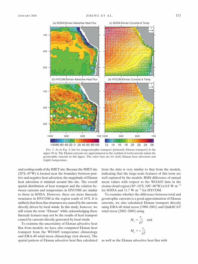
and cooling south of the IMET site. Because the IMET site

(208S, 858W) is located near the boundary between posi-

tive and negative heat advection, the magnitude of Ekman

heat advection is minimal around this site. The overall

spatial distribution of heat transport and the relation be-

tween currents and temperature in HYCOM are similar

to those in SODA. However, there are more finescale

structures in HYCOM in the region south of 168S. It is

unlikely that these fine structures are caused by the currents

directly driven by local winds. In this study, however, we

still retain the term ‘‘Ekman’’ while acknowledging these

finescale features may not be the results of heat transport

caused by currents directly generated by local winds.

To examine the uncertainty of Ekman advective heat

flux from models, we have also computed Ekman heat

transport from the WOA05 temperature climatology

and ERA-40 wind stress climatology (not shown). The

spatial pattern of Ekman advective heat flux calculated

from the data is very similar to that from the models,

indicating that the large-scale features of this term are

well captured by the models. RMS difference of annual

mean values with respect to the WOA05 data in the

stratus cloud region (308–108S, 1008–808W) is 8.8 W m22

for SODA and 11.7 W m22 for HYCOM.

To examine whether the difference between total and

geostrophic currents is a good approximation of Ekman

currents, we also calculated Ekman transport directly

using ERA-40 wind stress (1980–2001) and QuikSCAT

wind stress (2002–2005) using

Mx

5t

y

r fand

My

5�t

x

r f

as well as the Ekman advective heat flux with

FIG. 5. As in Fig. 4, but for nongeostrophic transport (primarily Ekman transport) in the

upper 50 m. The Ekman currents are approximated as the residual of total currents minus the

geostrophic currents in this figure. The color bars are for (left) Ekman heat advection and

(right) temperature.


Hek

5 Hx

1 Hy

5C

pt

y

f

dTmld

dx1 �

Cpt

x

f

dTmld

dy

� �,

where Mx and My are zonal and meridional Ekman

transports, Hx and Hy are zonal and meridional Ekman

advective heat flux, (tx, ty) are zonal and meridional

wind stress from SODA, Tmld is mixed layer tempera-

ture in SODA, r is seawater density, f 5 2V sinu is

the Coriolis parameter, and Cp is the specific heat

capacity at constant pressure. The resulting Ekman

transport and Ekman advective heat flux in the mixed

layer averaged over 1980–2005 are shown in Fig. 6.

Figure 6 also displays mixed layer temperature from

SODA. Ekman advective heat flux in Fig. 6 is quite

similar to that in Fig. 5a. Ekman transport causes net

warming north of the IMET site and net cooling south

of the IMET site. This provides justification for calcu-

lating Ekman heat advection using ageostrophic cur-

rents from the model output. The Ekman transport is

nearly parallel to the mean SST isotherms in the off-

shore region near the IMET site, which is consistent

with the result from Colbo and Weller (2007), although

they used different datasets and a different analysis

period.

d. Vertical heat advection

Figure 7a shows the vertical heat advection in the

upper 50 m calculated from SODA. It is evident that

vertical advection causes weak warming in the open

ocean but not in the coastal region where strong up-

welling occurs. The cooling resulting from the upwelling

near the coast is balanced by the positive net surface

heat flux (Fig. 3). Figure 7b shows the velocity and

temperature section along 208S. A pronounced vertical

circulation centered around 40 m deep is evident at

788W. Cold water upwelled near the coast is transported

offshore by mean flow in the upper 40 m. Because of the

downwelling caused by the convergence of surface cur-

rents in the open ocean, the weak subsurface warming

occurs because of the vertical heat advection in broad

areas of the stratus region.

It should be noted that the vertical heat advection in

z coordinates is nontrivial to calculate reliably from the

available HYCOM output. This is because HYCOM’s

natural coordinate system uses time-dependent hybrid

layers rather than fixed z levels, and interpolated verti-

cal velocities in z coordinates derived from the derivative

of horizontal velocity at each level (layer) contain large

errors.

FIG. 6. The mean advective heat flux in the mixed layer resulting from Ekman transport

(black contours in W m22), mixed layer temperature (green contours in 8C), and Ekman

transport using ERA-40 wind stress (1980–2001) and QuikSCAT wind stress (2002–05; arrows

in m2 s21; from SODA).


e. Eddy heat flux divergence

In this section, heat transport caused by eddies in

models is discussed. We first compare eddy fields in

models with those in satellite observations to examine

whether models are able to generate realistic eddies in

this region. Then eddy heat flux divergence is computed

in the entire stratus cloud region to identify the role of

eddies in overall heat balance in this region.

1) EDDY KINETIC ENERGY

Eddy activity in models is examined by calculating

eddy kinetic energy (EKE). To demonstrate how well

the models can generate realistic eddies, we compare

EKE from models with that derived from satellite al-

timeters (i.e., AVISO surface geostrophic velocity).

HYCOM’s surface geostrophic velocity is first averaged

onto a 1/38 3 1/38 grid to match the spatial resolution of

AVISO geostrophic velocity. Then, EKE is computed

as EKE 5 (u92geo 1 y92

geo)/2, where u92geo and y92

geo are de-

viations of the 5-day-averaged geostrophic velocity from

its seasonally averaged values. Data on a 0.58 3 0.58 grid

are used for SODA. Figure 8 shows the map of annual

mean surface EKE (cm2 s22) from SODA, HYCOM,

and AVISO. The magnitude and spatial pattern of EKE

in HYCOM are similar to those from observations. In

HYCOM and observations, eddies are more active near

the coastal region than in the open ocean (Figs. 8b,c).

Because HYCOM uses sufficiently fine horizontal res-

olution to resolve mesoscale eddies, its overall eddy

activity is much higher than that in SODA, which uses a

relatively coarse resolution. Despite the general agree-

ment between HYCOM and observations, there are some

notable differences. For example, EKE in HYCOM is

larger than observations near the coast. In the open

ocean, particularly in the region of 208–158S, 1008–908W,

the EKE is higher than observations.

Eddy activity in the southeast Pacific Ocean has been

also reported in some previous studies (Hormazabal

et al. 2004; Chaigneau and Pizarro 2005a,b; Penven et al.

2005). The spatial distribution and magnitude of mean

EKE in HYCOM shown in Fig. 8 are similar to those

derived from drifter data (Chaigneau and Pizarro 2005a)

and satellite altimeter data (Hormazabal et al. 2004;

Penven et al. 2005). The good agreement of eddy fields

between HYCOM and observations suggests that the

HYCOM output is suitable for examining the role of

eddies in the upper-ocean heat budget in this region.

The enhanced eddy activity along the coast can be

explained by many processes. For instance, the interac-

tion of the Peru–Chile Current system with the coastline

is able to produce the active eddies (Chaigneau and

Pizarro 2005a). Coastal flows with large interannual and

seasonal variability are relevant to disturbances of equa-

torial origin that may reinforce the unstable coastal jet

(Pizarro et al. 2002; Zamudio et al. 2006, 2007). Also the

strong upwelling fronts observed in spring and summer

could generate baroclinic instabilities that may enhance

mesoscale variability. Furthermore, downwelling coastal

Kelvin waves can strongly intensify the Peru–Chile Un-

dercurrent system (Shaffer et al. 1997), which may de-

stabilize the near-surface-coastal circulation-generating

eddies.

It should be noted that EKE in AVISO data is com-

puted from the deviation of surface geostrophic velocity,

which could be much weaker than the total velocity de-

viation. We also calculated the EKE using total velocities

from SODA and HYCOM [i.e., EKE 5 (u92 1 y92)/2,

FIG. 7. (a) Vertical heat advection (W m22) in the upper 50 m

and (b) its ocean circulation (vectors in m s21) and temperature

(shading contours in 8C) in the zonal–vertical plane at 208S aver-

aged over 1980–2005 from SODA. The strong upwelling near the

coast gives rise to cold vertical heat advection. Downward flow

almost parallel to isotherm causes relatively weak warm vertical

heat advection in the entire cloud deck region.


where u9 and y9 are deviations of the total velocity from

their seasonally averaged values]. Figure 9 illustrates the

annual mean of EKE derived from the total velocity.

The EKE values in SODA and HYCOM are signifi-

cantly higher in both the open ocean and near the coast

than those derived from geostrophic velocity. This sug-

gests that the eddy kinetic energy calculated from AVISO

data can be underestimated, because only a geostrophic

component of velocity field is used.

2) EDDY CHARACTERISTICS

To further illustrate the characteristics of eddies simu-

lated in HYCOM, the vertical component of vorticity and

the Okubo–Weiss parameter (OWP) at 30-m depth were

computed. Figures 10a,d show HYCOM temperatures

FIG. 8. Maps of eddy activity represented by the temporal mean

of surface EKE derived from geostrophic velocity for (a) SODA,

(b) HYCOM, and (c) AVISO. The periods for averages are 1980–

2005 for SODA, 2003–07 for HYCOM, and 22 Aug 2001–28 Feb

2009 for AVISO. The primed terms are deviations from seasonally

averaged values. Units are cm2 s22.

FIG. 9. As in Fig. 8, but the EKE is computed using the total

velocity for (a) SODA and (b) HYCOM. (c) AVISO remains the

same as in Fig. 8c.


(in 8C) and currents (in m s21) at 30-m depth in the

southeast Pacific Ocean associated with the mesoscale

ocean eddy field on 8 January and 21 June 2004. OWPs

on these dates are also shown in Figs. 10c,f. The OWP is

defined as

OWP 5›u

›x� ›y

›y

� �2

1›y

›x1

›u

›y

� �2

� ›y

›x� ›u

›y

� �2

,

where u and y are the horizontal velocity components

and x and y are the horizontal coordinates. The first two

terms on the right-hand side represent the deformation

and the last term is the vertical component of the rela-

tive vorticity. If OWP is positive (negative), the de-

formation (relative vorticity) dominates. Therefore, the

OWP helps identify the boundary of eddies, because

eddies are generally characterized by a strong rotation

in their center and a strong deformation in their pe-

riphery. Thus, eddies can be demonstrated by patches of

negative values of OWP surrounded by positive rings.

The snapshot of subsurface vorticity (Figs. 10b,e) indi-

cates a succession of cyclones and anticyclones, which is

generated at the upwelling front. Eddies are clearly seen

in the image of the OWP (Figs. 10c,f). They appear more

energetic near the coastal area. In the open ocean, includ-

ing near the IMET site, the eddies clearly exist, although

they are relatively weaker. These spatial distributions

are consistent with the spatial pattern of the EKE.

3) EXAMPLE OF COLD-CORE EDDIES

Colbo and Weller (2007) speculated that the cooling at

the IMET site resulting from eddy heat flux divergence is

FIG. 10. Ocean states at 30 m in HYCOM on two dates. (a) Temperature (shading contours

in 8C) and currents (vectors in m s21), (b) relative vorticity (in 1026 s21), and (c) OWP

(10212 s22) on 8 Jan 2004. (d),(e),(f) As in (a),(b),(c), but on 21 Jun 2004. The color bars on

right are for (top) temperature, (middle) vorticity, and (bottom) OWP.


likely to be caused by the cold-core eddies that have

been advected offshore from the upwelling region where

these eddies are generated. To identify such cold eddies

in HYCOM, temperature and velocity anomalies during

the entire period of the experiment are inspected.

Figure 11 shows the maps of temperature and velocity

anomalies averaged in the upper 50 m during March

2005. The anomalies of temperature and velocity are

derived from the 2003–07 pentad climatology. Many

anticyclonic (cyclonic) eddies associated with warm (cold)

waters are found near the coast. During this period, an

eddy associated with cold waters and cyclonic circula-

tion around 208S, 748W on 8 March propagates west-

ward and reaches around 768W on 28 March. Similar

westward-propagating cold-core cyclonic eddies are fre-

quently found in HYCOM. However, these cyclonic

eddies associated with cold waters in the upper layer are

mostly found within several degrees away from the coast-

line and seldom propagate to locations near the IMET site

during the period of model experiment.

4) ROLES OF EDDY HEAT FLUX

The eddy heat flux divergence is computed following

the definition 2(›u9T9/›x 1 ›y9T9/›y), where u9, y9, and

T9 are deviations of the total velocity and temperature

(5-day averaged) from their seasonally averaged values.

Figure 12 shows the spatial distribution of mean eddy

FIG. 11. Maps of temperature anomalies (shaded contours in 8C)

along with velocity anomaly vectors (arrows in m s21) averaged in

the upper 50 m during (top) 8, (middle) 18, and (bottom) 28 March

2005 are illustrated for the evolution of cyclonic eddies (i.e., cold

eddy) in HYCOM. The offshore propagation of a cold eddy is

marked by green ellipses. Anomalies of temperature and velocity

are derived from the 2003–07 pentad climatology.

FIG. 12. Maps of mean eddy heat flux divergence in the upper 50 m

for (a) SODA and (b) HYCOM (units are W m22).


heat flux divergence in the upper 50 m from SODA and

HYCOM. Because of the weak eddy activity in SODA,

the eddy flux divergence is very small in the entire

stratus region. The magnitude of eddy flux divergence in

HYCOM is much larger than that in SODA, particularly

near the coast. Near the IMET site, the temporal mean

of eddy heat flux in HYCOM is positive (16 W m22),

which could be significant at this location. However,

unlike geostrophic and Ekman heat transports, the eddy

flux divergence term is not spatially coherent. As a re-

sult, the temporal mean of eddy heat flux averaged over

308–108S, 1008–808W is much smaller (see Tables 2, 4)

than the estimate by Colbo and Weller (2007) at the

IMET site. Therefore, the overall impact from eddy

flux divergence on the upper-ocean heat budget in

the stratus cloud region is negligible in contrast to geo-

strophic and Ekman transports, which are spatially

more coherent.

The results are consistent with the inspection of in-

dividual eddies in HYCOM, which shows that cold wa-

ters generated near the upwelling region do not often

move with eddies far west into the open ocean, including

toward the IMET site. Although the westward propa-

gation of cyclonic eddies from the coast to the open

ocean is often found in HYCOM, cold surface waters

generated near the coast are not carried very far by these

cyclonic eddies, and thus they do not significantly impact

overall heat balance in the open ocean.

Our result in spatial pattern of the eddy heat flux di-

vergence in the 50-m surface layer is similar to that in a

previous observational study by Chaigneau and Pizarro

(2005a), who used Fickian law to estimate the eddy heat

flux divergence, in which the World Ocean Atlas 2001

(WOA01) temperatures are used and the zonal and

meridional components of eddy diffusivity are estimated

based on the drifter trajectories. Even though using

Fickian law may not be quite appropriate to describe the

eddy heat flux divergence resulting from coherent me-

soscale eddies, we did not detect a significant deviation

in this case, suggesting that their results are useful here.

In their study, the area-averaged eddy heat flux di-

vergence (348–108S, 1008–708W) provides heat to the

surface layer at a rate of 14.4 W m22. Such eddy flux

divergence should be much smaller if averaged over the

stratus region (348–108S, 1008–808W) because the eddy

flux divergence near the coast is much larger than the

open ocean. The small value of eddy heat flux di-

vergence is primarily due to its spatial incoherence.

Cold waters near the surface associated with eddies

can be modified by surface heat fluxes and quickly re-

semble the rest of the upper mixed layer. Thus, cold

waters in lower portions of the eddies may be observable

farther from the coast, because they are insulated from

the atmosphere. In this case, water masses below 50 m

associated with eddies could possibly influence upper-

ocean heat balance in the open ocean. To examine such

a possibility, we also computed the eddy heat flux di-

vergence in the upper 250 m from SODA and HYCOM

(not shown). The results are similar to those in the upper

50 m, in which the eddy heat flux divergence term is not

spatially coherent, although typically the magnitude at

a given location is larger, because it is integrated through

a deeper layer.

5. Discussion

The spatial distribution of horizontal heat advection

resulting from Ekman transport (Fig. 5) indicates that it

causes warming (cooling) to the north (south) of around

208S in the stratus deck region. We have also calculated

the area average of each term north and south of 208S

(Table 5). Heat advection resulting from Ekman trans-

port gives stronger warming in the northern part of the

stratus cloud region. To the south of this region, this

warming becomes much weaker in HYCOM or changes

the sign in SODA. Cooling resulting from geostrophic

transport is evident in both north and south regions, but

it is weaker in the south for SODA. As indicated in the

spatial distribution of the eddy heat flux divergence

term, this term is negligible both north and south of 208S.

Accordingly, the contribution of each term can be very

different in northern and southern parts of the stratus

region; thus, additional observations such as surface

buoys in locations both south and north of 208S will help

improve our understanding of upper-ocean processes

under the stratus cloud decks in the southeast Pacific.

There are other terms in the heat equation that are not

discussed in detail. The major additional term that could

significantly contribute to the heat budget is vertical

diffusion (mixing). Although this term is negligible at

250-m depth (Colbo and Weller 2007), it could be

comparable to other terms in the 0–50-m layer. Un-

fortunately, it is difficult to estimate this term accurately

TABLE 5. Ocean heat budget in the upper 50 m averaged over

the regions (208–108S, 1008–808W) and (308–208S, 1008–808W) from

SODA and HYCOM. The periods for the averaging are as in Table 2

(units are W m22).

208–108S,


SODA — 213 9 0.4

HYCOM 7 26 10 20.2

308–208S,

1008–808W

SODA — 24 23 20.2

HYCOM 14 25 2 0.1


at 50 m from the available model output. We have also

performed the same analyses in this paper for the 0–250-m

layer in which the vertical diffusion term is negligible,

showing that the spatial distribution of horizontal heat

advection and eddy heat flux divergence terms for the

0–250-m layer are similar to those for the 0–50-m layer

(not shown). However, it is possible that the vertical

mixing term could contribute to the closure of the heat

budget for the 0–50-m layer.

Although the analysis of HYCOM output indicates

that the eddy flux divergence term is negligible in the

heat budget of the entire stratus deck region in com-

parison to horizontal advection terms, the result could

be model dependent. Also, HYCOM was integrated for

only 4 yr, and it is possible that the result could be dif-

ferent in other time periods. In fact, large interannual

variations within the upper ocean associated with ENSO

are evident in the stratus cloud region (Shinoda and Lin

2009). Longer integrations using multiple eddy-resolving

models are necessary to further investigate the role of

eddies in this region.

6. Summary

This study examines the upper-ocean processes in the

stratus cloud deck region using SODA data and the

eddy-resolving HYCOM. The model performance is first

evaluated based on comparison with in situ data from the

IMET buoy at 208S, 858W. Then, the annual mean of the

upper-ocean heat budget is calculated from the model

output. The relative importance of physical processes

responsible for the heat budget is also investigated,

particularly the roles of geostrophic and Ekman trans-

ports and the eddy heat flux. The analysis of model

output was conducted for the entire stratus cloud deck

region to examine the representativeness of the IMET

observation site for broadscale upper-ocean processes in

this region.

Both SODA and HYCOM reproduce the seasonal

evolution of the mixed layer reasonably well. The mean

heat budget for the upper 250 m in the models is compared

with the corresponding heat budget based on observations

at 208S, 858W, and it demonstrates some consistencies.

Net surface heat fluxes used in the HYCOM experiment

provide warming in most areas of the stratus deck, in-

cluding the IMET mooring site. One of the major sources

of cooling that balances the positive surface heat fluxes

is geostrophic transport. These results are consistent

with those from observations described in Colbo and

Weller (2007).

Major terms of the heat equation in the upper 50 m

were also calculated over a large portion of the stratus

region. The heat transport produced by mean geostrophic

currents is one of the primary sources of cooling in the

entire stratus region because of its spatial coherence.

Although Ekman currents are generally stronger than

geostrophic currents in the upper 50 m, heat transport

resulting from geostrophic currents is comparable to

that by Ekman currents. This is because the direction of

geostrophic currents in this region is nearly perpendic-

ular to the isotherms of the upper-ocean temperature,

whereas Ekman currents are nearly parallel to the iso-

therms. It is found that Ekman transport generates

warming (cooling) to the north (south) of around 208S.

This result is consistent with the estimates by Colbo and

Weller (2007) in which Ekman heat transport is negli-

gible at the IMET site (208S, 858W).

The role of eddies in the upper-ocean heat budget is

examined using the eddy-resolving HYCOM and obser-

vational data. A comparison of eddy activity in HYCOM

with that derived from satellite observations (i.e., AVISO)

indicates that HYCOM is capable of simulating the re-

alistic eddies in the stratus cloud region. The results

indicate that the eddy heat flux divergence term is neg-

ligible for the entire stratus region because it is not

spatially coherent, although it could be comparable to

other terms at a particular location.

A substantial amount of data in the upper ocean and

atmospheric boundary layer has been collected recently

in the region of stratus cloud deck in the southeast Pa-

cific during the VAMOS Ocean-Cloud-Atmosphere-

Land Study (VOCALS) Regional Experiment (VOCALS

REx; Wood et al. 2007). In the next few years, thorough

analyses of these datasets will be conducted by many

investigators. Hopefully, knowledge of the upper-ocean

heat budget obtained in this study will help interpret the

results of their analyses.

Acknowledgments. Data from the Stratus Ocean Ref-

erence Station were made available by Dr. Robert Weller

of the Woods Hole Oceanographic Institution; these data

were collected with support from Pan American Climate

Study and Climate Observation Programs of the Office of

Global Programs, NOAA Office of Oceanic and Atmo-

spheric Research Grants NA17RJ1223, NA17RJ1224,

and NA17RJ1225. We are thankful for the altimeter

products which were produced by SSALTO/DUACS and

distributed by AVISO, with support from CNES (avail-

able online at http://www.aviso.oceanobs.com/duacs/).

This work was supported in part by a grant from the

Computational and Information Systems Laboratory at

NCAR. Yangxing Zheng is supported by NSF Grant

OCE-0453046. Toshiaki Shinoda is supported by NSF

Grants OCE-0453046 and ATM-0745897; in addition,

Toshiaki Shinoda, E. Joseph Metzger, and Harley

Hurlburt are supported by the 6.1 project Global Remote


Littoral Forcing via Deep Water Pathways sponsored

by the office of Naval Research (ONR) under Program

Element 601153N. Jialin Lin is supported by National

Aeronautics and Space Administration (NASA) under

the Modeling, Analysis, and Prediction (MAP) program

and by NSF Grant ATM-0745872. Benjamin S. Giese is

grateful for support from the NSF Grant OCE-0351802

and the National Oceanic and Atmospheric Adminis-

tration (NOAA) Grant NA06OAR4310146. This work

was supported in part by a grant from the Computa-

tional and Information Systems Laboratory at NCAR.

REFERENCES

Bingham, F. M., S. D. Howden, and C. J. Koblinsky, 2002: Sea surface

salinity measurements in the historical database. J. Geophys.

Res., 107, 8019, doi:10.1029/2000JC000767.

Bleck, R., 2002: An oceanic general circulation model framed in

hybrid isopycnic-Cartesian coordinates. Ocean Modell., 4, 55–88.

——, and D. B. Boudra, 1981: Initial testing of a numerical ocean

circulation model using a hybrid (quasi-isopycnic) vertical

coordinate. J. Phys. Oceanogr., 11, 755–770.

——, and S. G. Benjamin, 1993: Regional weather prediction with

a model combining terrain-following and isentropic coordi-

nates. Part I: Model description. Mon. Wea. Rev., 121, 1770–

1785.

Boyer, T. P., C. Stephens, J. I. Antonov, M. E. Conkright,

L. A. Locarnini, T. D. O’Brien, and H. E. Garcia, 2002: Sa-

linity. Vol. 2, World Ocean Atlas 2001, NOAA Atlas NESDIS

49, 165 pp.

Bradley, E. F., C. W. Fairall, J. E. Hare, and A. A. Grachev, 2000:

An old and improved bulk algorithm for air-sea fluxes. Pre-

prints, 14th Symp. on Boundary Layer and Turbulence, Aspen,

CO, Amer. Meteor. Soc., 294–296.

Carton, J. A., and B. S. Giese, 2008: A reanalysis of ocean climate

using Simple Ocean Data Assimilation (SODA). Mon. Wea.

Rev., 136, 2999–3017.

——, G. A. Chepurin, X. Cao, and B. S. Giese, 2000a: A Simple

Ocean Data Assimilation analysis of the global upper ocean

1950–95. Part I: Methodology. J. Phys. Oceanogr., 30, 294–309.

——, ——, and ——, 2000b: A Simple Ocean Data Assimilation

analysis of the global upper ocean 1950–95. Part II: Results.

J. Phys. Oceanogr., 30, 311–326.

Chaigneau, A., and O. Pizarro, 2005a: Mean surface circulation and

mesoscale turbulent flow characteristics in the eastern South

Pacific from satellite tracked drifters. J. Geophys. Res., 110,

C05014, doi:10.1029/2004JC002628.

——, and ——, 2005b: Eddy characteristics in the eastern South

Pacific. J. Geophys. Res., 110, C06005, doi:10.1029/2004JC002815.

Colbo, K., and R. Weller, 2007: The variability and heat budget of

the upper ocean under the Chile-Peru stratus. J. Mar. Res., 65,607–637.

Diaz, H., C. Folland, T. Manabe, D. Parker, R. Reynolds, and

S. Woodruff, 2002: Workshop on advances in the use of his-

torical marine climate data. WMO Bull., 51, 377–380.

Gordon, C. T., A. Rosati, and R. Gudgel, 2000: Tropical sensitivity

of a coupled model to specified ISCCP low clouds. J. Climate,

13, 2239–2260.

Han, W., 2005: Origins and dynamics of the 90-day and 30–60-day

variations in the equatorial Indian Ocean. J. Phys. Oceanogr.,

35, 708–728.

——, T. Shinoda, L.-L. Fu, and J. P. McCreary, 2006: Impact of

atmospheric intraseasonal oscillations on the Indian Ocean

dipole. J. Phys. Oceanogr., 36, 670–690.

Hormazabal, S., G. Shaffer, and O. Leth, 2004: Coastal transition

zone off Chile. J. Geophys. Res., 109, C01021, doi:10.1029/

2003JC001956.

Hurlburt, H. E., E. J. Metzger, P. J. Hogan, C. E. Tilburg, and

J. F. Shriver, 2008: Steering of upper ocean currents and fronts

by the topographically constrained abyssal circulation. Dyn.

Atmos. Oceans, 45, 102–134.

Jones, P. W., 1999: First- and second-order conservative remapping

schemes for grids in spherical coordinates. Mon. Wea. Rev.,

127, 2204–2210.

Kalnay, E., and Coauthors, 1996: The NCEP/NCAR 40-Year Re-

analysis Project. Bull. Amer. Meteor. Soc., 77, 437–471.

Kara, A. B., H. E. Hurlburt, and A. J. Wallcraft, 2005a: Stability-

dependent exchange coefficients for air–sea fluxes. J. Atmos.

Oceanic Technol., 22, 1080–1094.

——, A. J. Wallcraft, and H. E. Hurlburt, 2005b: A new solar radiation

penetration scheme for use in ocean mixed layer studies: An

application to the Black Sea using a fine-resolution Hybrid Co-

ordinate Ocean Model (HYCOM). J. Phys. Oceanogr., 35, 13–32.

——, ——, and ——, 2005c: Sea surface temperature sensitivity to

water turbidity from simulations of the turbid Black Sea using

HYCOM. J. Phys. Oceanogr., 35, 33–54.

Klein, S. A., and D. L. Hartmann, 1993: The seasonal cycle of low

stratiform clouds. J. Climate, 6, 1587–1606.

Large, W. G., J. C. McWilliams, and S. C. Doney, 1994: Oceanic

vertical mixing: Review and model with a nonlocal boundary

layer parameterization. Rev. Geophys., 32, 363–403.

Lin, J. L., 2007: The double-ITCZ problem in IPCC AR4 coupled

GCMs: Ocean–atmosphere feedback analysis. J. Climate, 20,

4497–4525.

Ma, C.-C., C. R. Mechoso, A. W. Robertson, and A. Arakawa, 1996:

Peruvian stratus clouds and the tropical Pacific circulation: A

coupled ocean–atmosphere GCM study. J. Climate, 9, 1635–1645.

Mechoso, C. R., and Coauthors, 1995: The seasonal cycle over the

tropical Pacific in coupled ocean–atmosphere general circu-

lation models. Mon. Wea. Rev., 123, 2825–2838.

Miller, R. L., 1997: Tropical thermostats and low cloud cover.

J. Climate, 10, 409–440.

Penven, P., V. Echevin, J. Pasapera, F. Colas, and J. Tam, 2005:

Average circulation, seasonal cycle, and mesoscale dynamics

of the Peru Current System: A modeling approach. J. Geo-

phys. Res., 110, C10021, doi:10.1029/2005JC002945.

Pizarro, O., G. Shaffer, B. Dewitte, and M. Ramos, 2002: Dy-

namics of seasonal and interannual variability of the Peru-

Chile Undercurrent. Geophys. Res. Lett., 29, 1581, doi:10.1029/

2002GL014790.

Rosmond, T. E., J. Teixeira, M. Peng, T. F. Hogan, and R. Pauley,

2002: Navy Operational Global Atmospheric Prediction Sys-

tem (NOGAPS): Forcing for ocean models. Oceanography,

15, 99–108.

Shaffer, G., O. Pizarro, L. Djurfeldt, S. Salinas, and J. Rutlant,

1997: Circulation and low-frequency variability near the Chile

coast: Remotely forced fluctuations during the 1991–92

El Nino. J. Phys. Oceanogr., 27, 217–235.

Shaji, C., C. Wang, G. R. Halliwell Jr., and A. Wallcraft, 2005:

Simulation of tropical Pacific and Atlantic Oceans using a

hybrid coordinate ocean model. Ocean Modell., 9, 253–282.

Shinoda, T., and J. L. Lin, 2009: Interannual variability of the upper

ocean in the southeast Pacific stratus cloud region. J. Climate,

22, 5072–5088.


——, P. E. Roundy, and G. E. Kiladis, 2008: Variability of intra-

seasonal Kelvin waves in the equatorial Pacific Ocean. J. Phys.

Oceanogr., 38, 921–944.

Simmons, A. J., and J. K. Gibson, 2002: The ERA-40 project plan.

ECMWF ERA-40 Project Rep. Series 1, 63 pp.

Smith, R. D., J. K. Dukowicz, and R. C. Malone, 1992: Par-

allel ocean general circulation modeling. Physica D, 60,

38–61.

Stephens, C., J. I. Antonov, T. P. Boyer, M. E. Conkright, R. A.

Locarnini, T. D. O’Brien, and H. E. Garcia, 2002: Tempera-

ture. Vol. 1, World Ocean Atlas 2001, NOAA Atlas NESDIS

49, 169 pp.

Wood, R., C. Bretherton, B. Huebert, C. R. Mechoso, and

R. Weller, 2007: The VAMOS Ocean-Cloud-Atmosphere-

Land Study (VOCALS): Improving understanding, model

simulations, and prediction of the southeast Pacific climate

system. Post-VOCALS-Rex Rep. [Available online at http://

www.eol.ucar.edu/projects/vocals/.]

Xie, S.-P., 2004: The shape of continents, air-sea interaction, and

the rising branch of the Hadley circulation. The Hadley Cir-

culation: Present, Past and Future, H. F. Diaz and R. S.

Bradley, Eds., Kluwer Academic, 121–152.

Yu, L., and R. A. Weller, 2007: Objectively analyzed air–sea fluxes

for the global ice-free oceans (1981–2005). Bull. Amer. Me-

teor. Soc., 88, 527–539.

——, X. Jin, and R. A. Weller, 2008: Multidecade global flux datasets

from the Objectively Analyzed Air-Sea Fluxes (OAFlux) Project:

Latent and sensible heat fluxes, ocean evaporation, and related

surface meteorological variables. Woods Hole Oceanographic

Institution OAFlux Project Tech. Rep. OA-2008-01, 64 pp.

Zamudio, L., H. E. Hurlburt, E. J. Metzger, S. L. Morey, J. J.

O’Brien, C. Tilburg, and J. Zavala-Hidalgo, 2006: Interannual

variability of Tehuantepec eddies. J. Geophys. Res., 111, C05001,

doi:10.1029/2005JC003182.

——, ——, ——, and C. E. Tilburg, 2007: Tropical wave-induced

oceanic eddies at Cabo Corrientes and the Marıa Islands, Mex-

ico. J. Geophys. Res., 112, C05048, doi:10.1029/2006JC004018.

Zheng, Y., and B. S. Giese, 2009: Ocean heat transport in Simple

Ocean Data Assimilation: structure and mechanisms. J. Geo-

phys. Res., 114, C11009, doi:10.1029/2008JC005190.


Documents

Upper-Ocean Processes under the Stratus Cloud Deck in the