Embed Size (px)
Citation preview
FINAL PROJECT REPORT
Urban Runoff Impact Study Phase III: Size Distribution, Sources, and Transport of Suspended Particles Along an Inland-to-Ocean Transect Prepared By:
Jong Ho Ahn, Stanley B. Grant, Cristiane Q. Surbeck, and Sunny Jiang, University of California, Irvine
Paul M. DiGiacomo, Jet Propulsion Laboratory/California Institute of Technology
Nikolay P. Nezlin, Southern California Coastal Water Research Project
NWRI Final Project Report
Urban Runoff Impact Study Phase III: Size Distribution, Sources, and Transport of Suspended Particles
along an Inland-to-Ocean Transect
Prepared by:
Jong Ho Ahn, Stanley B. Grant, Cristiane Q. Surbeck, and Sunny Jiang Henry Samueli School of Engineering
University of California, Irvine Irvine, California
Paul M. DiGiacomo
Jet Propulsion Laboratory California Institute of Technology
Pasadena, California
Nikolay P. Nezlin Southern California Coastal Water Research Project
Costa Mesa, California
Published by:
National Water Research Institute 18700 Ward Street
P.O. Box 8096 Fountain Valley, California 92728-8096 USA
November 2008
About NWRI A 501c3 nonprofit organization, the National Water Research Institute (NWRI) was founded in 1991 by a group of California water agencies in partnership with the Joan Irvine Smith and Athalie R. Clarke Foundation to promote the protection, maintenance, and restoration of water supplies and to protect public health and improve the environment. NWRI’s member agencies include Inland Empire Utilities Agency, Irvine Ranch Water District, Los Angeles Department of Water and Power, Orange County Sanitation District, Orange County Water District, and West Basin Municipal Water District. For more information, please contact: National Water Research Institute 18700 Ward Street P.O. Box 8096 Fountain Valley, California 92728-8096 USA Phone: (714) 378-3278 Fax: (714) 378-3375 www.nwri-usa.org NWRI-2008-07 This NWRI Final Project Report is a product of NWRI Project Number 03-WQ-001.
ii
Acknowledgments This report was funded by a joint grant from the National Water Research Institute (03-WQ-001) and the U.S. Geological Survey National Institutes for Water Research (UCOP-33808), together with matching funds from the Counties of Orange, Riverside, and San Bernardino in Southern California and from a Supplemental Environmental Project awarded by the State of California Regional Water Quality Control Board with funding from Conexant Systems, Inc., Bell Industries, and URS Corporation. Partial support for the human virus and fecal indicator virus study was provided by Water Environmental Research Foundation award 01-HHE-2a. We gratefully acknowledge many people involved in the collection of data described in this report, especially the Assistant Manager of the City of Newport Beach, David Kiff, the Chief of the Newport Beach Fire Department, Timothy Riley, John Moore, and Brian O’Rourke, and officials at the Orange County Sanitation District for assisting the collection and analysis of offshore and surf zone water samples. MODIS data were acquired as part of the NASA's Earth Science Enterprise, and processed by the MODIS Adaptive Processing System (MODAPS), the Goddard Distributed Active Archive Center (DAAC), and are archived and distributed by the Goddard DAAC. NEOCO measurements were supported by the University of California Marine Council’s Coastal Environmental Quality Initiative. Some of the data and ship time for this study were donated by the Bight’03 program. We are also thankful for the excellent the input and feedback from numerous colleagues, most notably George L. Robertson, Charles D. McGee, Brett F. Sanders, Patricia Holden, Ronald Linsky, Steve Weisberg, Alexandria Boehm, Karen McLaughlin, Eric Stein, and Linwood Pendleton.
iii
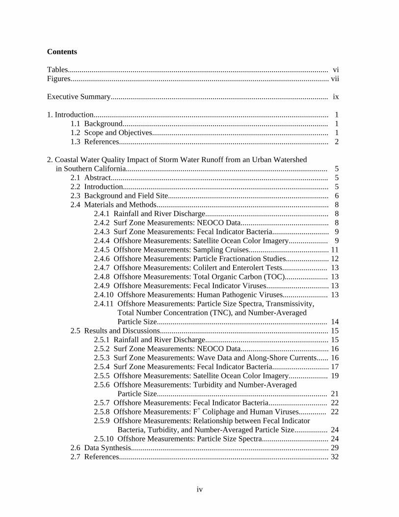
Contents Tables..................................................................................................................................... vi Figures.................................................................................................................................... vii Executive Summary............................................................................................................... ix 1. Introduction........................................................................................................................ 1
1.1 Background......................................................................................................... 1 1.2 Scope and Objectives.......................................................................................... 1 1.3 References........................................................................................................... 2
2. Coastal Water Quality Impact of Storm Water Runoff from an Urban Watershed
in Southern California....................................................................................................... 5 2.1 Abstract............................................................................................................... 5 2.2 Introduction......................................................................................................... 5 2.3 Background and Field Site.................................................................................. 6 2.4 Materials and Methods........................................................................................ 8 2.4.1 Rainfall and River Discharge............................................................... 8 2.4.2 Surf Zone Measurements: NEOCO Data............................................. 8 2.4.3 Surf Zone Measurements: Fecal Indicator Bacteria............................. 9 2.4.4 Offshore Measurements: Satellite Ocean Color Imagery.................... 9 2.4.5 Offshore Measurements: Sampling Cruises......................................... 11 2.4.6 Offshore Measurements: Particle Fractionation Studies...................... 12 2.4.7 Offshore Measurements: Colilert and Enterolert Tests....................... 13 2.4.8 Offshore Measurements: Total Organic Carbon (TOC)...................... 13 2.4.9 Offshore Measurements: Fecal Indicator Viruses................................ 13 2.4.10 Offshore Measurements: Human Pathogenic Viruses....................... 13 2.4.11 Offshore Measurements: Particle Size Spectra, Transmissivity,
Total Number Concentration (TNC), and Number-Averaged Particle Size....................................................................................... 14
2.5 Results and Discussions...................................................................................... 15 2.5.1 Rainfall and River Discharge............................................................... 15 2.5.2 Surf Zone Measurements: NEOCO Data............................................. 16 2.5.3 Surf Zone Measurements: Wave Data and Along-Shore Currents...... 16 2.5.4 Surf Zone Measurements: Fecal Indicator Bacteria............................. 17 2.5.5 Offshore Measurements: Satellite Ocean Color Imagery.................... 19 2.5.6 Offshore Measurements: Turbidity and Number-Averaged
Particle Size....................................................................................... 21 2.5.7 Offshore Measurements: Fecal Indicator Bacteria.............................. 22 2.5.8 Offshore Measurements: F+ Coliphage and Human Viruses.............. 22 2.5.9 Offshore Measurements: Relationship between Fecal Indicator
Bacteria, Turbidity, and Number-Averaged Particle Size................. 24 2.5.10 Offshore Measurements: Particle Size Spectra.................................. 24 2.6 Data Synthesis..................................................................................................... 29 2.7 References........................................................................................................... 32
iv
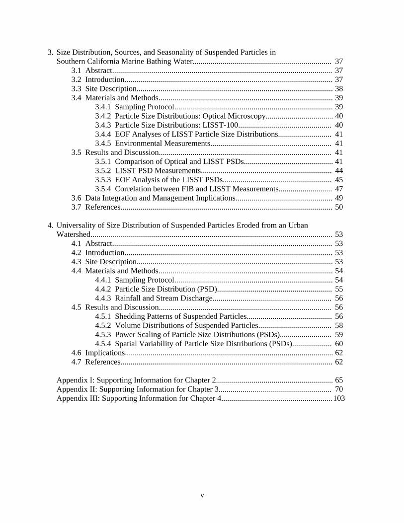
3. Size Distribution, Sources, and Seasonality of Suspended Particles in Southern California Marine Bathing Water...................................................................... 37
3.1 Abstract............................................................................................................... 37 3.2 Introduction......................................................................................................... 37
3.3 Site Description................................................................................................... 38 3.4 Materials and Methods........................................................................................ 39 3.4.1 Sampling Protocol................................................................................ 39 3.4.2 Particle Size Distributions: Optical Microscopy.................................. 40 3.4.3 Particle Size Distributions: LISST-100............................................... 40 3.4.4 EOF Analyses of LISST Particle Size Distributions........................... 41 3.4.5 Environmental Measurements............................................................. 41 3.5 Results and Discussion....................................................................................... 41 3.5.1 Comparison of Optical and LISST PSDs............................................. 41 3.5.2 LISST PSD Measurements.................................................................. 44 3.5.3 EOF Analysis of the LISST PSDs....................................................... 45 3.5.4 Correlation between FIB and LISST Measurements........................... 47 3.6 Data Integration and Management Implications................................................. 49 3.7 References........................................................................................................... 50
4. Universality of Size Distribution of Suspended Particles Eroded from an Urban
Watershed.......................................................................................................................... 53 4.1 Abstract............................................................................................................... 53 4.2 Introduction......................................................................................................... 53 4.3 Site Description................................................................................................... 53 4.4 Materials and Methods........................................................................................ 54 4.4.1 Sampling Protocol................................................................................ 54 4.4.2 Particle Size Distribution (PSD).......................................................... 55 4.4.3 Rainfall and Stream Discharge............................................................ 56 4.5 Results and Discussion....................................................................................... 56 4.5.1 Shedding Patterns of Suspended Particles........................................... 56 4.5.2 Volume Distributions of Suspended Particles..................................... 58 4.5.3 Power Scaling of Particle Size Distributions (PSDs).......................... 59 4.5.4 Spatial Variability of Particle Size Distributions (PSDs).................... 60 4.6 Implications......................................................................................................... 62 4.7 References........................................................................................................... 62 Appendix I: Supporting Information for Chapter 2........................................................... 65 Appendix II: Supporting Information for Chapter 3......................................................... 70 Appendix III: Supporting Information for Chapter 4........................................................ 103
v
Tables 2.1 Summary of Analyses Performed during the Sampling Cruise................................. 11 3.1 Percent of Variance Captured by the Top Three EOF Modes at Each Sampling
Site............................................................................................................................. 49
vi
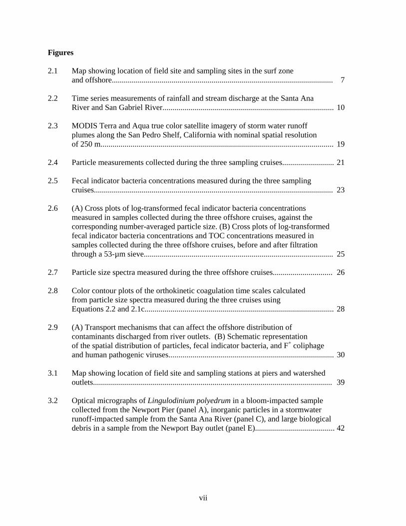
Figures 2.1 Map showing location of field site and sampling sites in the surf zone
and offshore............................................................................................................... 7 2.2 Time series measurements of rainfall and stream discharge at the Santa Ana
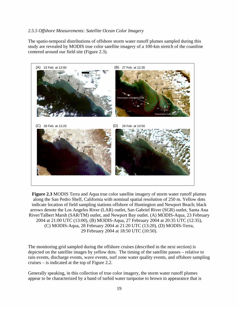
River and San Gabriel River...................................................................................... 10 2.3 MODIS Terra and Aqua true color satellite imagery of storm water runoff
plumes along the San Pedro Shelf, California with nominal spatial resolution of 250 m..................................................................................................................... 19
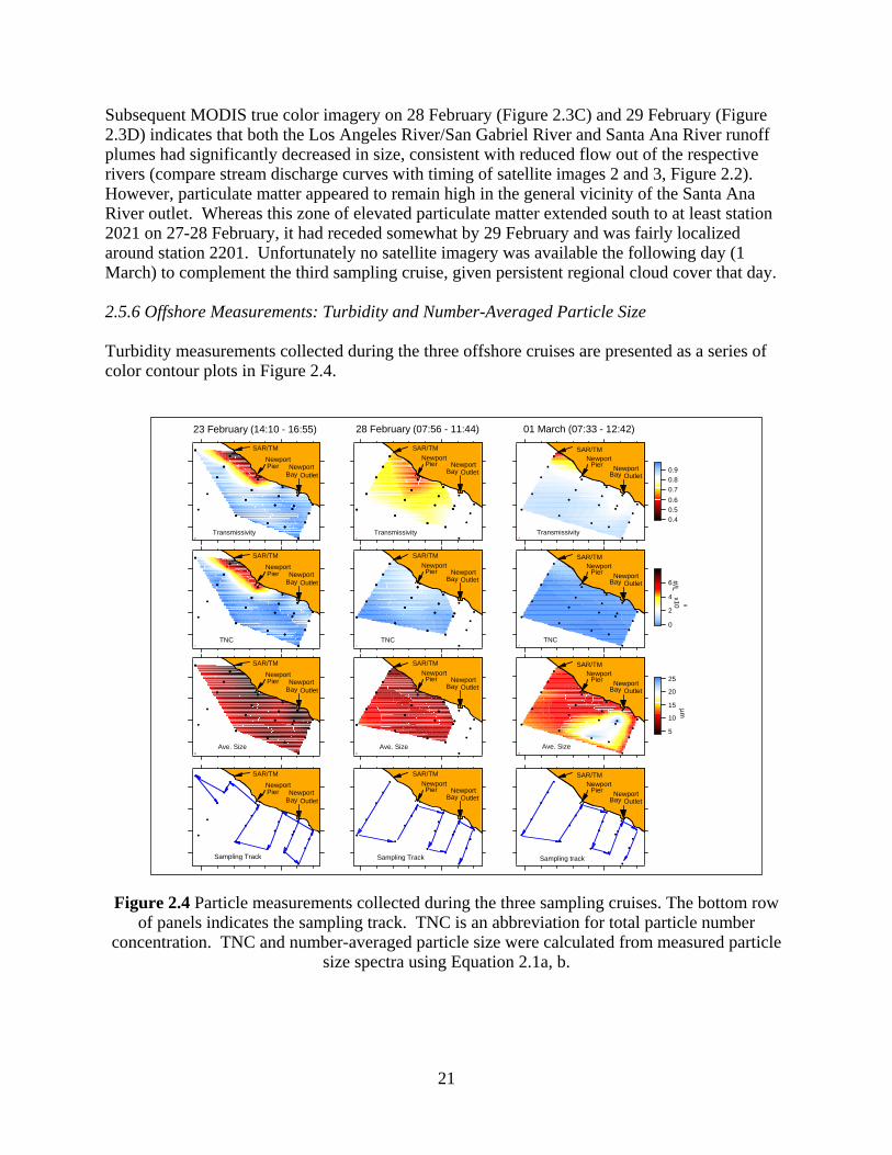
2.4 Particle measurements collected during the three sampling cruises.......................... 21 2.5 Fecal indicator bacteria concentrations measured during the three sampling
cruises........................................................................................................................ 23 2.6 (A) Cross plots of log-transformed fecal indicator bacteria concentrations
measured in samples collected during the three offshore cruises, against the corresponding number-averaged particle size. (B) Cross plots of log-transformed fecal indicator bacteria concentrations and TOC concentrations measured in samples collected during the three offshore cruises, before and after filtration through a 53-µm sieve............................................................................................... 25
2.7 Particle size spectra measured during the three offshore cruises.............................. 26 2.8 Color contour plots of the orthokinetic coagulation time scales calculated
from particle size spectra measured during the three cruises using Equations 2.2 and 2.1c............................................................................................... 28
2.9 (A) Transport mechanisms that can affect the offshore distribution of
contaminants discharged from river outlets. (B) Schematic representation of the spatial distribution of particles, fecal indicator bacteria, and F+ coliphage and human pathogenic viruses................................................................................... 30
3.1 Map showing location of field site and sampling stations at piers and watershed
outlets........................................................................................................................ 39 3.2 Optical micrographs of Lingulodinium polyedrum in a bloom-impacted sample
collected from the Newport Pier (panel A), inorganic particles in a stormwater runoff-impacted sample from the Santa Ana River (panel C), and large biological debris in a sample from the Newport Bay outlet (panel E)........................................ 42
vii
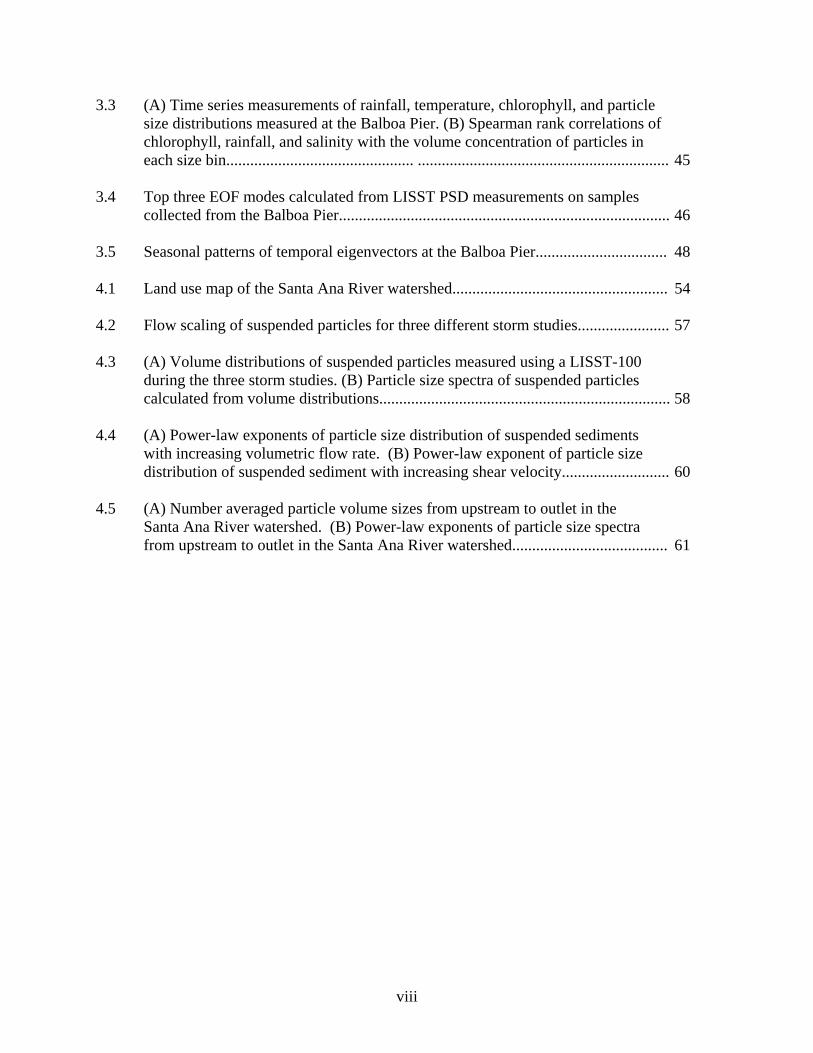
3.3 (A) Time series measurements of rainfall, temperature, chlorophyll, and particle size distributions measured at the Balboa Pier. (B) Spearman rank correlations of chlorophyll, rainfall, and salinity with the volume concentration of particles in each size bin............................................... ............................................................... 45
3.4 Top three EOF modes calculated from LISST PSD measurements on samples
collected from the Balboa Pier................................................................................... 46 3.5 Seasonal patterns of temporal eigenvectors at the Balboa Pier................................. 48 4.1 Land use map of the Santa Ana River watershed...................................................... 54 4.2 Flow scaling of suspended particles for three different storm studies....................... 57 4.3 (A) Volume distributions of suspended particles measured using a LISST-100
during the three storm studies. (B) Particle size spectra of suspended particles calculated from volume distributions......................................................................... 58
4.4 (A) Power-law exponents of particle size distribution of suspended sediments
with increasing volumetric flow rate. (B) Power-law exponent of particle size distribution of suspended sediment with increasing shear velocity........................... 60
4.5 (A) Number averaged particle volume sizes from upstream to outlet in the
Santa Ana River watershed. (B) Power-law exponents of particle size spectra from upstream to outlet in the Santa Ana River watershed....................................... 61
viii
ix
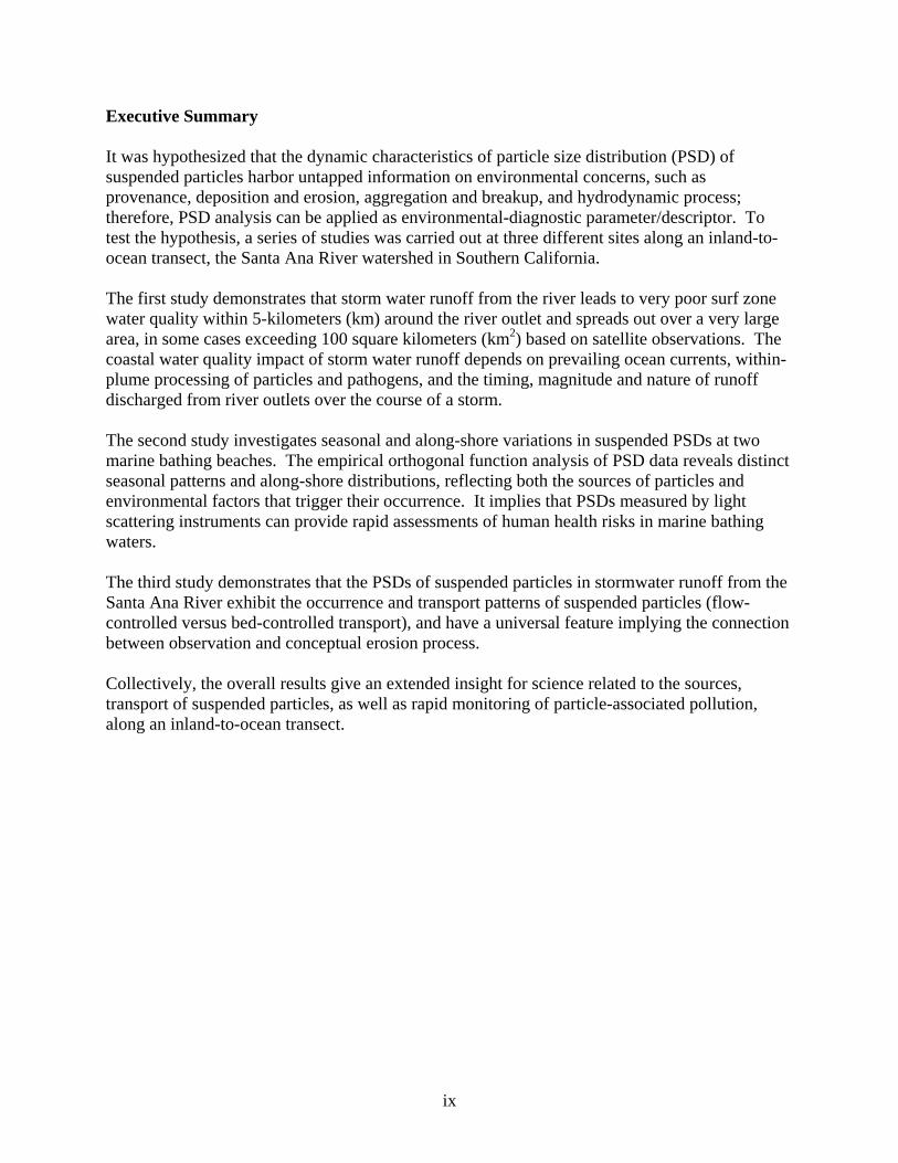
Executive Summary It was hypothesized that the dynamic characteristics of particle size distribution (PSD) of suspended particles harbor untapped information on environmental concerns, such as provenance, deposition and erosion, aggregation and breakup, and hydrodynamic process; therefore, PSD analysis can be applied as environmental-diagnostic parameter/descriptor. To test the hypothesis, a series of studies was carried out at three different sites along an inland-to-ocean transect, the Santa Ana River watershed in Southern California. The first study demonstrates that storm water runoff from the river leads to very poor surf zone water quality within 5-kilometers (km) around the river outlet and spreads out over a very large area, in some cases exceeding 100 square kilometers (km2) based on satellite observations. The coastal water quality impact of storm water runoff depends on prevailing ocean currents, within-plume processing of particles and pathogens, and the timing, magnitude and nature of runoff discharged from river outlets over the course of a storm. The second study investigates seasonal and along-shore variations in suspended PSDs at two marine bathing beaches. The empirical orthogonal function analysis of PSD data reveals distinct seasonal patterns and along-shore distributions, reflecting both the sources of particles and environmental factors that trigger their occurrence. It implies that PSDs measured by light scattering instruments can provide rapid assessments of human health risks in marine bathing waters. The third study demonstrates that the PSDs of suspended particles in stormwater runoff from the Santa Ana River exhibit the occurrence and transport patterns of suspended particles (flow-controlled versus bed-controlled transport), and have a universal feature implying the connection between observation and conceptual erosion process. Collectively, the overall results give an extended insight for science related to the sources, transport of suspended particles, as well as rapid monitoring of particle-associated pollution, along an inland-to-ocean transect.
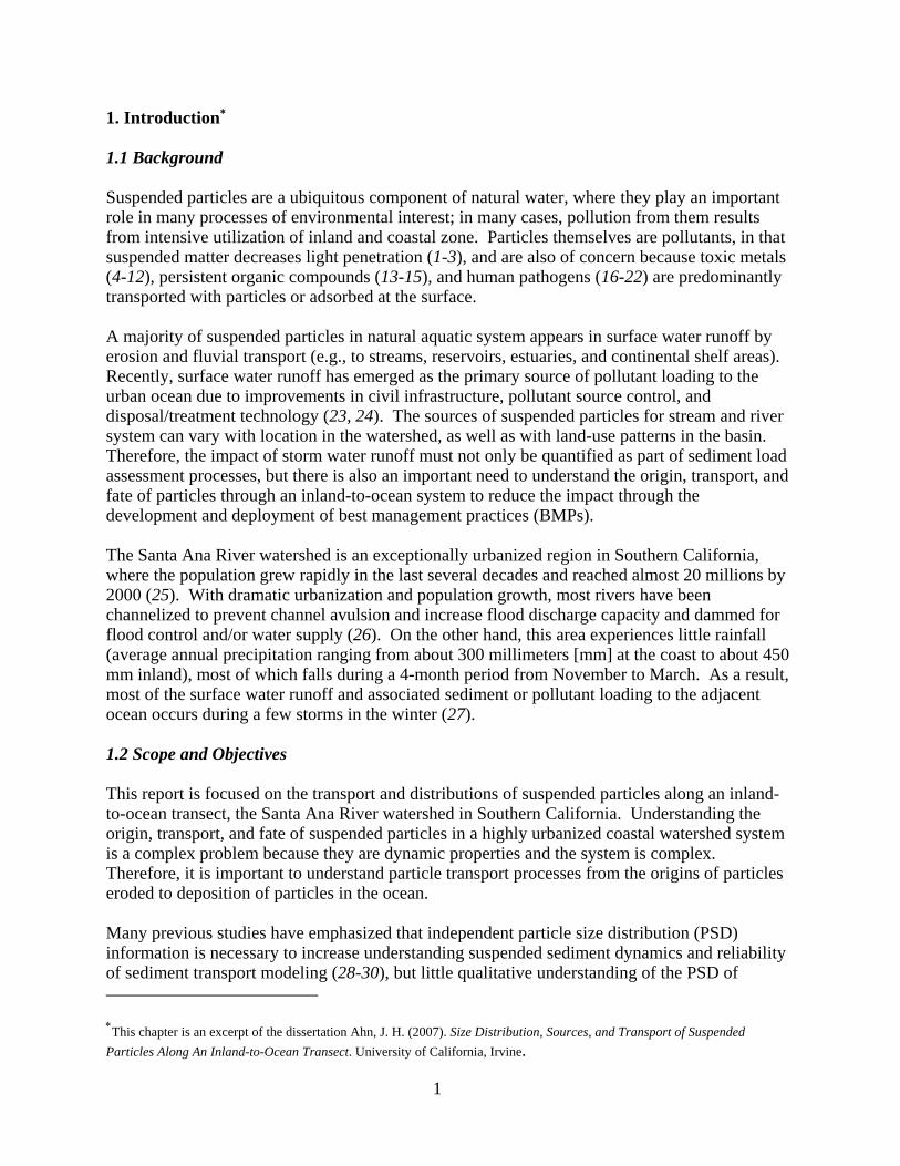
1. Introduction∗ 1.1 Background Suspended particles are a ubiquitous component of natural water, where they play an important role in many processes of environmental interest; in many cases, pollution from them results from intensive utilization of inland and coastal zone. Particles themselves are pollutants, in that suspended matter decreases light penetration (1-3), and are also of concern because toxic metals (4-12), persistent organic compounds (13-15), and human pathogens (16-22) are predominantly transported with particles or adsorbed at the surface. A majority of suspended particles in natural aquatic system appears in surface water runoff by erosion and fluvial transport (e.g., to streams, reservoirs, estuaries, and continental shelf areas). Recently, surface water runoff has emerged as the primary source of pollutant loading to the urban ocean due to improvements in civil infrastructure, pollutant source control, and disposal/treatment technology (23, 24). The sources of suspended particles for stream and river system can vary with location in the watershed, as well as with land-use patterns in the basin. Therefore, the impact of storm water runoff must not only be quantified as part of sediment load assessment processes, but there is also an important need to understand the origin, transport, and fate of particles through an inland-to-ocean system to reduce the impact through the development and deployment of best management practices (BMPs). The Santa Ana River watershed is an exceptionally urbanized region in Southern California, where the population grew rapidly in the last several decades and reached almost 20 millions by 2000 (25). With dramatic urbanization and population growth, most rivers have been channelized to prevent channel avulsion and increase flood discharge capacity and dammed for flood control and/or water supply (26). On the other hand, this area experiences little rainfall (average annual precipitation ranging from about 300 millimeters [mm] at the coast to about 450 mm inland), most of which falls during a 4-month period from November to March. As a result, most of the surface water runoff and associated sediment or pollutant loading to the adjacent ocean occurs during a few storms in the winter (27). 1.2 Scope and Objectives This report is focused on the transport and distributions of suspended particles along an inland-to-ocean transect, the Santa Ana River watershed in Southern California. Understanding the origin, transport, and fate of suspended particles in a highly urbanized coastal watershed system is a complex problem because they are dynamic properties and the system is complex. Therefore, it is important to understand particle transport processes from the origins of particles eroded to deposition of particles in the ocean. Many previous studies have emphasized that independent particle size distribution (PSD) information is necessary to increase understanding suspended sediment dynamics and reliability of sediment transport modeling (28-30), but little qualitative understanding of the PSD of ∗This chapter is an excerpt of the dissertation Ahn, J. H. (2007). Size Distribution, Sources, and Transport of Suspended Particles Along An Inland-to-Ocean Transect. University of California, Irvine.
1
suspended particles develops since insufficient information results from the lack of consistent in situ monitoring. In this study, low-angle light scattering measurements of PSD are applied as a main data resource for assessing the transport and distribution of suspended particles. We hypothesized that the dynamic characteristics of the PSD of suspended particles harbor untapped information on environmental concerns, such as provenance, erosion and deposition, aggregation and breakup, and hydrodynamic process; therefore, PSD analysis can be applied as environmental-diagnostic parameter/descriptor (indicators). To test this hypothesis, a series of studies was carried out at four different sites along an ocean-to-inland transect, including offshore (Chapter 2), surfzone (Chapters 2 and 3), and river (Chapter 4). The specific objectives are to answer the following questions: • What factors and processes affect the coastal water quality of stormwater runoff both in the
surfzone and offshore (Chapter 2)? • Can low-angle light scattering measurements of particle size spectra provide rapid
assessments of human health risks in marine bathing waters (Chapter 3)? • Do particle size spectra have a universal feature, implying the occurrence and transport
patterns of suspended particles eroded from an urban watershed (Chapter 4)? By achieving these objectives, the results will give extended insight for science related to the sources and transport of suspended particle, as well as the monitoring of particle-associated pollution, along an inland-to-ocean transect. 1.3 References (1) Peterson, L. L. The Propagation of Sunlight and the Size Distribution of Suspended Particles in a Municipally Polluted Ocean Water; Ph. D. thesis: California Institute of Technology, Pasadena, California, 1974. (2) Boucier, D. R.; Sharma, R. P. Heavy metals and their relationship to solids in urban runoff, Int. J. Envir. Anal. Chem., 1980, 7, 273-283. (3) Gippel, C. J. Potential of turbidity monitoring for measuring the transport of suspended-solids in streams, Hydrological Processes, 1995, 9, 83-97. (4) Harrison, R. M.; Laxen, D. P. H.; Wilson, S. J. Chemical associations of Lead, Cadmium, Copper and Zinc in street dusts and roadside soils, Environmental Science and Technology, 1978, 15, 1378-1383. (5) Ellis, J. B.; Revitt, D. M. Incidence of heavy metals in street surface sediments: solubility and grain size studies, Water, Air, and Soil Pollution, 1982, 17, 87-100. (6) Lara-Cazenave, M. B.; Levy, V.; Castetbon, A.; Potin-Gautier, M.; Astruc, M.; Albert, E. Pollution of urban runoff waters by heavy metals. Part I: Total metal, Environmental Technology, 1994, 15, 1135-1147.
2
(7) Sansalone, J. J.; Buchberger, S. G.; Koechling, M. T. Correlations between heavy metals and suspended solids in highway runoff: Implications for control strategies, Transportation Research Record, 1995, N1483, 112-119. (8) Sansalone, J. J.; Buchberger, S. G. Characterization of solid and metal element distributions in urban highway stormwater, Water Science Technology, 1997, 36, 155-160. (9) Characklis, G.W.; Wiesner, M. R. Particles, metals, and water quality in runoff from large urban watershed, ASCE J. of Environmental Engineering, 1997, 123, 753-759. (10) Viklander, M. Particle size distribution and metal content in street sediments, ASCE J. of Environmental Engineering, 1998, 124, 761-766. (11) Estèbe, A.; Mouchel, J. M.; Thévenot, D. R. Urban runoff impacts on particulate metal concentrations in river Seine, Water, Air, and Soil Pollution, 1998, 108, 83-105. (12) Karouna-Renier, N. K.; Sparling, D.W. Relationships between ambient geochemistry, watershed land-use and trace metal concentrations in aquatic invertebrates living in stormwater treatment ponds, Environmental Pollution, 2001, 112, 183-192. (13) Bris, F. J.; Garnauda, S.; Apperrya, N.; Gonzaleza, A.; Mouchel, J. M.; Chebbo, G.; Thévenot, D. A street deposit sampling method for metal and hydrocarbon contamination assessment, The Science of the Total Environment, 1999, 235, 211-220. (14) Lopes, T. J.; Dionne, S. G. A review of semivolatile and volatile organic compounds in highway runoff and urban stormwater.; US. Geological Survey Open-File Report, OFR98-409, 1998. (15) Krein, A.; Schorer, M. Road runoff pollution by polycyclic aromatic hydrocarbons and its contribution to river sediments, Water Research, 2000, 34, 4110-4115. (16) Bidle, K. D.; Fletcher, M. Comparison of free-living and particle-associated bacterial communities in the Chesapeake Bay in stable low-molecular-weight RNA analysis, Appl. Environ. Microbiol., 1994, 61, 944-952. (17) Parker, J. A.; Darby, J. L. Particle-associated coliform in secondary effluents: shielding from ultraviolet disinfection, Water Environ. Res., 1995, 67, 1065-1075. (18) Emerick, R. W.; Loge, F. J.; Thompson, D.; Darby, J. L. Factors influencing ultraviolet disinfection performance part II: association of coliform bacteria with wastewater particles, Water Environ. Res., 1999, 71, 1178-1187. (19) Haglund, A.-L.; Tornblom, E.; Bostrom, B.; Tranvik, L. Large differences in the fraction of active bacteria in plankton, sediments, and biofilm, Microb. Ecol., 2002, 43, 232-241. (20) LaMontagne, M. G.; Holden, P. A. Comparison of free-living and particle-associated bacterial communities in a coastal lagoon, Microb. Ecol., 2003, 46, 228-237.
3
4
(21) Ahn, J. H.; Grant, S. B.; Surbeck, C. Q.; DiGiacomo, P.; Nezlin, N.; Jiang, S. Coastal water quality impact of storm water runoff from an urban watershed in southern California, Environ. Sci. Technol., 2005, 39, 5940-5953. (22) Surbeck, C. Q.; Jiang, S.; Ahn, J. H; Grant, S. B. Flow fingerprinting fecal pollution and suspended solids in storm water runoff from an urban coastal watershed, Environ. Sci. Technol., 2005, 40, 4435-4441. (23) Bay, S.; Jones, B. H.; Schiff, K.; Washburn L. Water quality impacts of stormwater discharges to Santa Monica Bay, Mar. Environ. Res., 2003, 56, 205-223. (24) Schiff, K.C. Development of a model publicly owned treatment work (POTW) monitoring program; Southern California Coastal Water Research Project: Westminster, CA, 1999. (25) U.S. Census Bureau. 2003. U.S. Census Bureau population data: [http://www.census.gov] (26) Willis, C. M.; Griggs, G. B. Reductions in fluvial sediment discharge by coastal dams in California and implications for beach sustainability, J. Geology., 2003,111, 167-182. (27) Reeves, R. L.; Grant, S. B.; Mrse, R. D.; Copil Oancea, C. M.; Sanders, B. F.; Boehm, A. B. Scaling and management of fecal indicator bacteria in runoff from a coastal urban watershed in southern California, Environ. Sci. Technol., 2004, 38, 2637-2648. (28) Mehta, A.; Lott, J. W. Sorting of fine sediment during deposition, Proc. Conf. Adv. In understanding of coastal sediment processes, Amer. Soc. Civil Eng., New York; 1987, 348-362. (29) Fennessy, M. J.; Dyer, K. R.; Huntley, D.A. INSSEV an instrument to measure the size and settling velocity of flocs in situ, Marine Geology, 1994, 117, 107-117. (30) Dyer, K. R.; Cornelisse, J.; Dearnaley, M. P.; Fennessy, M. J.; Jones, S. E.; Kappenberg, J.; McCave, I. N.; Pejrup, M.; Puls, W.; van Leussen, W.; Wolfstein, K. A comparison of in situ techniques for estuarine floc settling velocity measurements, Journal of Sea Research, 1996, 36, 15-29.
5
2. Coastal Water Quality Impact of Storm Water Runoff from an Urban Watershed in Southern California∗
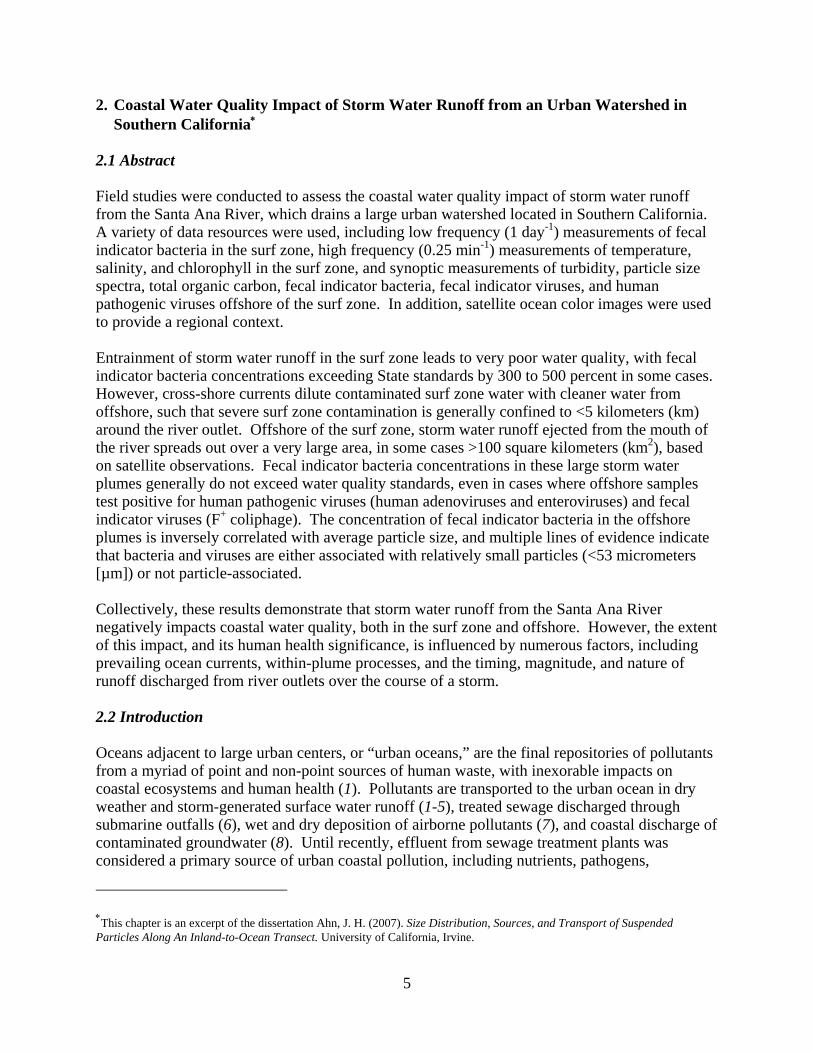
2.1 Abstract Field studies were conducted to assess the coastal water quality impact of storm water runoff from the Santa Ana River, which drains a large urban watershed located in Southern California. A variety of data resources were used, including low frequency (1 day-1) measurements of fecal indicator bacteria in the surf zone, high frequency (0.25 min-1) measurements of temperature, salinity, and chlorophyll in the surf zone, and synoptic measurements of turbidity, particle size spectra, total organic carbon, fecal indicator bacteria, fecal indicator viruses, and human pathogenic viruses offshore of the surf zone. In addition, satellite ocean color images were used to provide a regional context. Entrainment of storm water runoff in the surf zone leads to very poor water quality, with fecal indicator bacteria concentrations exceeding State standards by 300 to 500 percent in some cases. However, cross-shore currents dilute contaminated surf zone water with cleaner water from offshore, such that severe surf zone contamination is generally confined to <5 kilometers (km) around the river outlet. Offshore of the surf zone, storm water runoff ejected from the mouth of the river spreads out over a very large area, in some cases >100 square kilometers (km2), based on satellite observations. Fecal indicator bacteria concentrations in these large storm water plumes generally do not exceed water quality standards, even in cases where offshore samples test positive for human pathogenic viruses (human adenoviruses and enteroviruses) and fecal indicator viruses (F+ coliphage). The concentration of fecal indicator bacteria in the offshore plumes is inversely correlated with average particle size, and multiple lines of evidence indicate that bacteria and viruses are either associated with relatively small particles (<53 micrometers [µm]) or not particle-associated. Collectively, these results demonstrate that storm water runoff from the Santa Ana River negatively impacts coastal water quality, both in the surf zone and offshore. However, the extent of this impact, and its human health significance, is influenced by numerous factors, including prevailing ocean currents, within-plume processes, and the timing, magnitude, and nature of runoff discharged from river outlets over the course of a storm. 2.2 Introduction Oceans adjacent to large urban centers, or “urban oceans,” are the final repositories of pollutants from a myriad of point and non-point sources of human waste, with inexorable impacts on coastal ecosystems and human health (1). Pollutants are transported to the urban ocean in dry weather and storm-generated surface water runoff (1-5), treated sewage discharged through submarine outfalls (6), wet and dry deposition of airborne pollutants (7), and coastal discharge of contaminated groundwater (8). Until recently, effluent from sewage treatment plants was considered a primary source of urban coastal pollution, including nutrients, pathogens,
∗This chapter is an excerpt of the dissertation Ahn, J. H. (2007). Size Distribution, Sources, and Transport of Suspended Particles Along An Inland-to-Ocean Transect. University of California, Irvine.
6
pesticides, and heavy metals (9). However, in the past several decades, pollutant loading from many sewage treatment plants has declined, despite continued population growth, due to improvements in civil infrastructure (e.g., separation of the storm and sanitary sewer systems to prevent combined sewer overflows), pollutant source control, and disposal/treatment technology (10). As a result, surface water runoff has, in many cases, supplanted sewage treatment plants as the primary source of pollutant loading to the urban ocean (3, 9). The focus of this study is on the ocean water quality impact of storm water runoff from a highly urbanized coastal community in Southern California. On a year-round basis, this area experiences little rainfall (average annual precipitation ranging from about 300 mm at the coast to about 450 mm inland), most of which falls during a 4-month period from November to March (11). As a result, on an annual basis, most (in some cases, >99.9 percent, according to Reeves et al. [2]) of the surface water runoff and associated pollutant loading to the adjacent ocean occurs during a few storms in the winter. Described in this report are field studies in coastal Orange County following three moderate (total rainfall of 16, 23, and 51 mm) rainstorms in late February and early March 2004. The studies were designed to compare water quality in two distinct regions of the coastal ocean (surf zone and offshore), with regional distributions of storm water runoff plumes provided by satellite sensors. The study is complementary to, and uses some data from, a larger and ongoing regional study of the effects of storms on coastal water quality in the southern California Bight called “Bight ‘03” (12). This study describes how storm water plumes generated by several watershed outlets – with particular focus on the Santa Ana River – evolve in space and time, and impact coastal water quality, as measured by turbidity, particle size spectra, total organic carbon, fecal indicator bacteria, fecal indicator viruses, and human pathogenic viruses. Previous investigations on this topic focused on the impacts of dry weather flows on offshore and/or surf zone water quality (13, 14), or described the transport and mixing dynamics of sediment plumes as they flow into the coastal ocean from river outlets (5, 15-19). The present study is unique in the combination of data resources used – including data and information from routine surf zone water quality monitoring programs, an automated in situ ocean observing sensor, shipboard sampling cruises, and satellite sensors. Further, this study is the first to examine the linkage between water quality in the surf zone – where routine monitoring samples are collected and most human exposure occurs – and water quality offshore of the surf zone. The surf zone and offshore studies described here were carried out concurrently with studies of the flow scaling of particles and fecal pollution in storm water runoff from several sub-drainages in the Santa Ana River watershed, a major source of storm water runoff in coastal Orange County (20). 2.3 Background and Field Site The study site is a northwest-southeast striking section of the Pacific Ocean coastline, located offshore of Huntington Beach and Newport Beach in Orange County, California (Figure 2.1). This region of coastline has suffered chronic beach water quality postings and closures over the past several years due to elevated fecal indicator bacteria concentrations in the surf zone, which frequently exceed State standards and federal guidelines established for these organisms, during both summer and winter periods (21, 22). Beaches in this region attract approximately 10-million visitors per year and, hence, beach postings and closures can have significant local and statewide economic impacts (23).
7
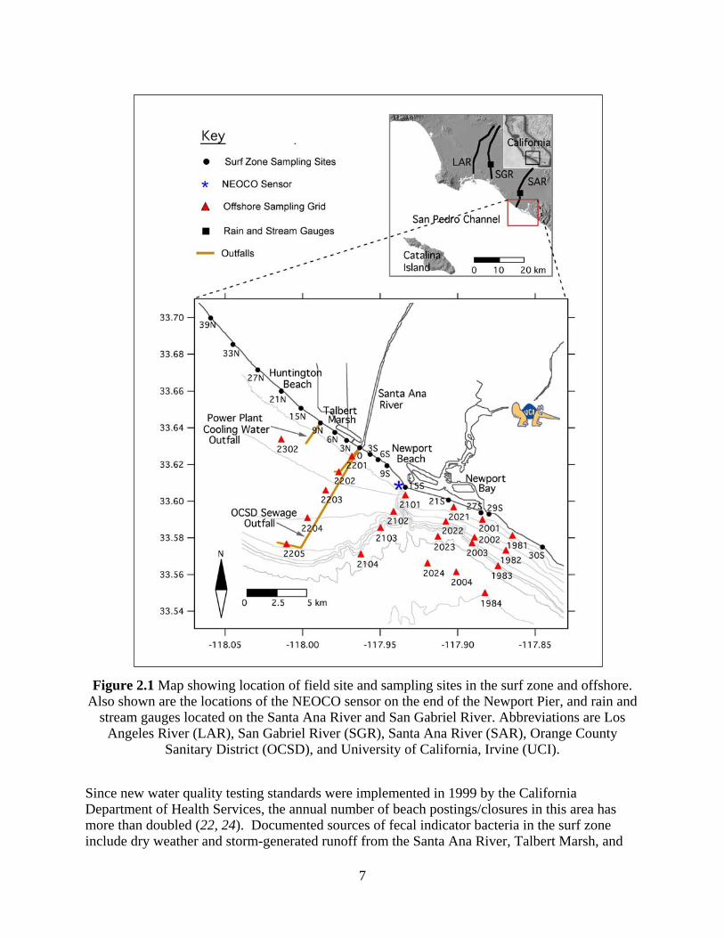
Figure 2.1 Map showing location of field site and sampling sites in the surf zone and offshore. Also shown are the locations of the NEOCO sensor on the end of the Newport Pier, and rain and
stream gauges located on the Santa Ana River and San Gabriel River. Abbreviations are Los Angeles River (LAR), San Gabriel River (SGR), Santa Ana River (SAR), Orange County
Sanitary District (OCSD), and University of California, Irvine (UCI).
Since new water quality testing standards were implemented in 1999 by the California Department of Health Services, the annual number of beach postings/closures in this area has more than doubled (22, 24). Documented sources of fecal indicator bacteria in the surf zone include dry weather and storm-generated runoff from the Santa Ana River, Talbert Marsh, and
8
the Newport Bay outlets (2, 13, 25). Potential sources of fecal indicator bacteria include the coastal discharge of sewage contaminated groundwater (8), the offshore discharge of effluent from the Orange County Sanitation District sewage treatment facility (26), and the offshore discharge of cooling water containing fecal indicator bacteria from a local power plant (25, 27) (see Figure 2.1). In addition, coastal currents may bring fecal indicator bacteria into the study area from other large river outlets located up or down-coast, such as the Los Angeles River and San Gabriel River (see LAR and SGR in inset, Figure 2.1). The origin of fecal indicator bacteria at Huntington Beach continues to be the focus of intense study but, at this time, it appears that both human fecal (28) and non-human (e.g., bird droppings and/or bacterial regrowth in estuarial sediments; 26, 29) sources contribute to surf zone contamination. The combination of poor surf zone water quality and large number of beach visitors together implies that as many as 50,000 people per year may acquire highly credible gastroenteritis from recreational exposure to contaminated surf zone water at Huntington Beach and adjacent beaches (30). For this research investigation, data were collected during the 2003/04 storm season from two regions of coastal ocean: (1) the surf zone where surface waves break against the shore, and (2) offshore of the surf zone to a water depth of approximately 100 m. Data resources include daily monitoring of beach water quality (see onshore edge of surf zone, black circles in Figure 2.1), an automated ocean observing sensor located at the end of Newport Pier (see offshore edge of surf zone, blue star in Figure 2.1), and a set of three ocean cruises in which samples were collected from a grid of 21 stations distributed over a 60 km2 area offshore of Huntington Beach and Newport Beach (see red triangles in Figure 2.1). These sampling efforts, together with the acquisition and processing of satellite imagery, are described below. 2.4 Materials and Methods 2.4.1 Rainfall and River Discharge Weather information and Next Generation Radar (NEXRAD) images for planning the field studies and interpreting rainfall patterns were obtained online from the National Weather Service (http://www.nwsla.noaa.gov/). Precipitation and stream discharge data were obtained at two sites, one located where the Santa Ana River crosses Fifth Street in the City of Santa Ana, and another located where the San Gabriel River crosses Spring Street in the City of Long Beach (black squares in inset, Figure 2.1). These data were obtained, respectively, from the U.S. Army Corps of Engineers and the Los Angeles County Department of Public Works. Both of these gauge sites are located relatively close (within 11 km) to the ocean outlets of the respective rivers; hence, stream flow measured at these sites will likely make its way to the ocean. 2.4.2 Surf Zone Measurements: NEOCO Data Time series of water temperature, conductivity, chlorophyll, and water depth were obtained from an instrument package deployed at the end of the Newport Pier, where the local water depth is between 6.5 and 9 meters (m) (see blue star in Figure 2.1). This instrument package is part of a recently deployed network of coastal sensors in Southern California called the Network for Environmental Observations of the Coastal Ocean (NEOCO). The NEOCO sensor package contains a SBE-16plus CTD (Sea-Bird Electronics, Inc., Bellevue, WA) and a Seapoint
9
Chlorophyll Fluorometer (Seapoint Sensors, Inc.). These instruments are mounted on a pier piling at a depth of approximately 1 m (below mean lower low water) and programmed to acquire data at a sampling frequency of 0.25 min-1. Data from these instruments are available in near real-time at http://www.es.ucsc.edu/~neoco/. 2.4.3 Surf Zone Measurements: Fecal Indicator Bacteria The concentration of fecal indicator bacteria in the surf zone was measured at 17 stations (see black circles along shoreline in Figure 2.1) by the Orange County Sanitation District (OCSD) (Fountain Valley, CA). The stations are designated by OCSD according to their distance (in thousands of feet) north or south of the Santa Ana River outlet (e.g., station 15N is located approximately 15,000 feet [ft], approximately 5 km, north of the Santa Ana River outlet). Water samples were collected once per day (excluding weekends) from 5:30 to 10:00 local time at ankle-depth on an incoming wave, placed on ice in the dark, and returned to OCSD, where they were analyzed within 6 hours of collection for total coliform (TC), fecal coliform (FC), and enterococci bacteria (ENT) using standard methods 9221B and 9221E, and EPA method 1600, respectively. Results from these measurements are reported in units of colony forming units (CFU) per 100 milliliters (mL) of sample (CFU/100 mL). The surf zone monitoring data are available at http://www.ocsd.com/about/reports/lab_results.asp. Wave conditions, including both the direction and height of breaking waves, were recorded by lifeguards at the Newport Beach pier (near surf zone station 15S, Figure 1) twice per day at 7:00 and 14:00 local time. 2.4.4 Offshore Measurements: Satellite Ocean Color Imagery The satellite images used in this study were collected by NASA’s Moderate-Resolution Imaging Spectroradiometer (MODIS) instruments. These instruments operate onboard two near-polar sun-synchronous satellite platforms orbiting at 705-km altitude: Terra (since 24 February 2000) and Aqua (since 24 June 2002). Terra passes across the equator from north to south at ~10:30 local time, while Aqua passes the equator south to north at ~13:30 local time. As such, all images were acquired within 2 hours before or after local noon (or between 18:00 and 22:00 UTC). The MODIS sensors collect data in 36 spectral bands, from 400 to 14,000 nanometers (nm). We utilized bands 1 (250-m spatial resolution, 620-670 nm), 3, and 4 (500-m resolution, 459-479 and 545-565 nm, respectively) to produce “true color” (i.e., RGB) images, with band 1 used for the Red channel, band 4 for the Green channel, and band 3 for the Blue channel. Using a MATLAB program, the 500 m Green (band 4) and Blue (band 3) monochrome channels were “sharpened” to 250-m resolution using fine details from the higher resolution Red channel (band 1). Then, the contrast of each of these monochrome channels was increased to emphasize maximum details in the coastal ocean region of interest. Finally, all three monochrome channels (i.e., Red, Green, and Blue) were combined to form a single true color image. In all, 16 satellite images from February 23 to March 5 were acquired and processed for this study; four of them were selected as most illustrative, based on their quality and observed features. The timing of these satellite acquisitions relative to the storms and sampling periods is indicated at the top of Figure 2.2.
10
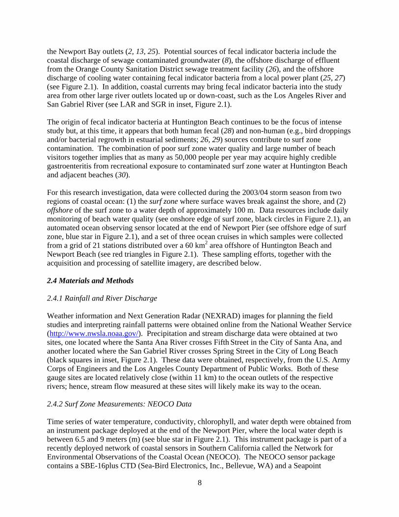
Figure 2.2 Time series measurements of rainfall and stream discharge at the Santa Ana River and San Gabriel River (top panel); water level, salinity, temperature, and chlorophyll measured at the NEOCO sensor (second and third panels); the direction and height of breaking waves at the Newport Beach Pier (fourth panel); and the concentration of fecal indicator bacteria in the
surf zone (color contour plots, fifth through seventh panels). Also shown at the top of the figure is the timing of the satellite images (blue lettering) and the offshore sampling cruises (black
squares).
11
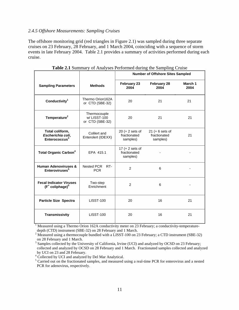
2.4.5 Offshore Measurements: Sampling Cruises The offshore monitoring grid (red triangles in Figure 2.1) was sampled during three separate cruises on 23 February, 28 February, and 1 March 2004, coinciding with a sequence of storm events in late February 2004. Table 2.1 provides a summary of activities performed during each cruise.
Table 2.1 Summary of Analyses Performed during the Sampling Cruise Number of Offshore Sites Sampled
Sampling Parameters Methods February 23 2004
February 28 2004
March 1 2004
Conductivity1 Thermo Orion162A or CTD (SBE-32) 20 21 21
Temperature2 Thermocouple w/ LISST-100
or CTD (SBE-32) 20 21 21
Total coliform, Escherichia coli, Enterococcus3
Colilert and Enterolert (IDEXX)
20 (+ 2 sets of fractionated
samples)
21 (+ 6 sets of fractionated
samples) 21
Total Organic Carbon4 EPA 415.1 17 (+ 2 sets of
fractionated samples)
- -
Human Adenoviruses & Enteroviruses5
Nested PCR RT-PCR 2 6 -
Fecal Indicator Viruses (F+ coliphage)5
Two-step Enrichment 2 6 -
Particle Size Spectra LISST-100 20 16 21
Transmissivity LISST-100 20 16 21
1 Measured using a Thermo Orion 162A conductivity meter on 23 February; a conductivity-temperature-depth (CTD) instrument (SBE-32) on 28 February and 1 March.
2 Measured using a thermocouple bundled with a LISST-100 on 23 February; a CTD instrument (SBE-32) on 28 February and 1 March.
3 Samples collected by the University of California, Irvine (UCI) and analyzed by OCSD on 23 February; collected and analyzed by OCSD on 28 February and 1 March. Fractionated samples collected and analyzed by UCI on 23 and 28 February.
4 Collected by UCI and analyzed by Del Mar Analytical. 5 Carried out on the fractionated samples, and measured using a real-time PCR for enterovirus and a nested PCR for adenovirus, respectively.
12
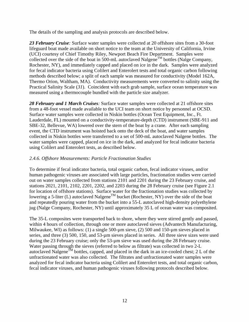
The details of the sampling and analysis protocols are described below. 23 February Cruise: Surface water samples were collected at 20 offshore sites from a 30-foot lifeguard boat made available on short notice to the team at the University of California, Irvine (UCI) courtesy of Chief Timothy Riley, Newport Beach Fire Department. Samples were collected over the side of the boat in 500-mL autoclaved NalgeneTM bottles (Nalge Company, Rochester, NY), and immediately capped and placed on ice in the dark. Samples were analyzed for fecal indicator bacteria using Colilert and Enterolert tests and total organic carbon following methods described below; a split of each sample was measured for conductivity (Model 162A, Thermo Orion, Waltham, MA). Conductivity measurements were converted to salinity using the Practical Salinity Scale (31). Coincident with each grab sample, surface ocean temperature was measured using a thermocouple bundled with the particle size analyzer. 28 February and 1 March Cruises: Surface water samples were collected at 21 offshore sites from a 48-foot vessel made available to the UCI team on short notice by personnel at OCSD. Surface water samples were collected in Niskin bottles (Ocean Test Equipment, Inc., Ft. Lauderdale, FL) mounted on a conductivity-temperature-depth (CTD) instrument (SBE-911 and SBE-32, Bellevue, WA) lowered over the stern of the boat by a crane. After each sampling event, the CTD instrument was hoisted back onto the deck of the boat, and water samples collected in Niskin bottles were transferred to a set of 500-mL autoclaved Nalgene bottles. The water samples were capped, placed on ice in the dark, and analyzed for fecal indicator bacteria using Colilert and Enterolert tests, as described below. 2.4.6. Offshore Measurements: Particle Fractionation Studies To determine if fecal indicator bacteria, total organic carbon, fecal indicator viruses, and/or human pathogenic viruses are associated with large particles, fractionation studies were carried out on water samples collected from stations 2101 and 2201 during the 23 February cruise, and stations 2021, 2101, 2102, 2201, 2202, and 2203 during the 28 February cruise (see Figure 2.1 for location of offshore stations). Surface water for the fractionation studies was collected by lowering a 5-liter (L) autoclaved NalgeneTM bucket (Rochester, NY) over the side of the boat and repeatedly pouring water from the bucket into a 55-L autoclaved high-density polyethylene jug (Nalge Company, Rochester, NY) until approximately 35 L of ocean water was composited. The 35-L composites were transported back to shore, where they were stirred gently and passed, within 4 hours of collection, through one or more autoclaved sieves (Advantech Manufacturing, Milwaukee, WI) as follows: (1) a single 500-µm sieve, (2) 500 and 150-µm sieves placed in series, and three (3) 500, 150, and 53-µm sieves placed in series. All three sieve sizes were used during the 23 February cruise; only the 53-µm sieve was used during the 28 February cruise. Water passing through the sieves (referred to below as filtrate) was collected in two 2-L autoclaved NalgeneTM bottles, capped, and placed in the dark in an ice-cooled chest; 2 L of the unfractionated water was also collected. The filtrates and unfractionated water samples were analyzed for fecal indicator bacteria using Colilert and Enterolert tests, and total organic carbon, fecal indicator viruses, and human pathogenic viruses following protocols described below.
13
2.4.7 Offshore Measurements: Colilert and Enterolert Tests Water samples were transported to the microbiology laboratory at either UCI or OCSD (see Table 2.1) within 6 hours of collection. At the lab, samples were diluted 1:10 with Butterfield’s Phosphate Buffer Solution (Hardy Diagnostics, Santa Maria, CA) and were analyzed for total coliforms (TC) and Escherichia coli (EC) using the Colilert test and enterococci bacteria (ENT) using the Enterolert test (IDEXX, Westbrook, ME), implemented in a 97-well quantitray format. These tests yield the concentration of fecal indicator bacteria in units of most probable number (MPN) of bacteria per 100 mL of sample (MPN/100 mL). 2.4.8 Offshore Measurements: Total Organic Carbon (TOC) All but three of the surface water samples collected during the 23 February cruise were analyzed for TOC (measurements were not carried out on samples collected from stations 2022, 2023, and 2203). Approximately two 40-mL aliquots of each 500-mL sample were transferred to two 40-mL glass vials containing 0.5-mL of 18-percent hydrochloric acid, immediately capped, and stored on ice in the dark for 7 to 9 days. TOC measurements were carried out within the 28-day holding time by a California-certified environmental laboratory (Del Mar Analytical, Irvine, CA), following EPA Method 415.1 implemented using a Shimadzu 5000A high-temperature combustion instrument; TOC results are reported as the arithmetic mean of duplicate analyses. 2.4.9 Offshore Measurements: Fecal Indicator Viruses Analysis for F+ coliphage was performed using two-step enrichment following EPA protocol 1601. In brief, 100-mL water samples from each site were amended with 5-mL sterile 10 x TSB medium (Difco Lab), 0.5-mL log-phase E. coli HS (Famp) host, and a final concentration of 15 mg/L of ampicillin and streptomycin. Negative controls contained 100-mL sterile deionized (DI) water amended with nutrient medium, E. coli host, and antibiotic as with the regular sample assay. The enrichment cultures were incubated at 37°C for 24 hours before spot testing for the presence of F+ coliphage. For spot testing, 1 mL of log phase E. coli host was mixed with TSB top agar and overlaid onto TSB agar plates containing antibiotics to form an even bacterial lawn. One milliliter of overnight enrichment culture was centrifuged at 5,000 rpm to pellet out the bacteria. Two microliters (µL) of each supernatant was spotted onto the freshly prepared E. coli bacterial lawn. After the spots dried, plates were inverted and incubated at 37°C for 8 to16 hours. Clear spots on the E. coli lawn were scored. 2.4.10 Offshore Measurements: Human Pathogenic Viruses For human pathogenic virus analysis, 500 mL of water sample, either filtered through different size sieves or unfiltered (see fractionation protocol above), was concentrated to a final volume of ~500 µL using a Centricon Plus-80 ultrafiltration system with 100 kilo Dalton molecular weight cut off membrane (Millipore Inc.). Viral nucleic acid was purified/extracted from concentrates using QIAmp Viral RNA Mini Kit (Qiagen Inc. CA) following manufacturer’s protocols. Primers for specific amplification of the enteroviruses are 5’-CCTCCGGCCCTGAATG-3’; 5’-ACCGGATGGCCAATCCAA-3’, which target at the 5’ untranslated region (32). The procedure for Reverse Transcription Polymerase Chain Reaction (RT-PCR) of enterovirus followed the protocol developed by Tsai et al. (33). Amplification products were further confirmed by probing with an internal oligonucleotide probe (5’-
14
TACTTTGGGTGTCCGTGTTTC-3’) after southern transfer of DNA to charged nylon membrane (MSI Inc.), as previously described (34). For adenovirus detection, a nested PCR protocol was used as previously described by Pina et al. (35). The outer primers are 5’-GCCGCAGTGGTCTTACATGCACATC-3’ and 5’-CAGCACGCCGCGGATGTCAAAGT-3’, which yield a 301 base pair (bp) amplicon of hexon gene. The nested primers are 5’-GCCACCGAGACGTACTTCAGCCTG-3’ and 5’-TTGTACGAGTACGCGGTATCCTCGCGGTC-3’, which yield a 143 bp amplicon (35). For adenovirus quantification, the real-time PCR protocol developed by He and Jiang (36) was used. The degenerate primer and Taqman probe are AD2: 5’-CCCTGGTAKCCRATRTTGTA-3’; AD3: 5’-GACTCYTCWGTSAGYGGCC-3’ and ADP: FAM-AACCAGTCYTTGGTCATGTTRCATTG-TAMRA. Real-time PCR was carried out in 25-µl reaction mixtures consisting of 1x TaqMan master mix (Applied Biosystems Inc.), primers, TaqMan probe, and template DNA. The final thermocycling profile was 95 °C 15 seconds, 56 °C 15 seconds, and 62 °C 30 seconds with 1 second auto increment every cycle for 45 cycles. All samples were run in triplicates in an ABI Prism 7000 sequence detection system (Applied Biosystems, Inc.). 2.4.11 Offshore Measurements: Particle Size Spectra, Transmissivity, Total Number Concentration (TNC), and Number-Averaged Particle Size Particle size spectra were measured using a LISST-100 (Laser In-Situ Scattering and Transmissometry) analyzer (Sequoia Scientific, Inc., Bellevue, WA) operated in a batch mode during the 23 February cruise, and operated in an in situ mode during the 28 February and 1 March cruises. The LISST-100 is a light diffraction instrument that estimates particle volume resident in 32 logarithmically spaced particle diameter bins, spanning a particle diameter range from 2.5 to 500 µm. The instrument also records water transmissivity, based on the attenuation of light from a 660-nm diode laser, and water temperature. Particle size spectra, transmissivity, and temperature are logged on an internal memory chip, and later downloaded onto a laptop computer. The LISST-100 has been deployed to measure particle size spectra in a variety of marine settings (37-46). Details on the operation of the LISST instrument, and theory underlying its estimation of particle volume, can be found elsewhere (37, 38). During the 23 February cruise, the LISST-100 was operated in batch mode as follows. At each offshore station, approximately 3 L of surface ocean water was collected by lowering a NalgeneTM bucket over the side of the boat, and then pouring the water into a 5-L plexiglass chamber affixed to the end of the LISST-100 instrument. Particle size spectra were immediately measured (within 5 minutes of sample collection) 20 separate times over the course of approximately 20 seconds. During the 28 February and 1 March cruises, the LISST-100 was attached to the CTD instrument package and programmed to acquire particle volume distributions at a frequency of either 1 hertz (Hz) (during the 28 February cruise) or 0.5 Hz (during the 1 March cruise). At each offshore station, the CTD package was lowered through the water column, and particle size spectra, transmissivity, and temperature were automatically logged by the LISST-100 instrument. Only
15
measurements collected at the surface of the water column are reported here. All particle volume distributions acquired at a depth of <1 m were classified as belonging to the surface of the water column. The particle size spectra acquired by the LISST-100 are represented mathematically as ΔV Δ log dp , where ΔV represents particle volume per unit fluid volume present in one of the 32 logarithmically spaced particle diameter bins of median diameter, dp. At least 10 replicates of the particle size spectra were collected at each offshore station. Following the recommendation of Mikkelsen (45), the median particle volume in each size bin is reported in the results presented later. The LISST-100 data are presented in this paper in one of three ways: (1) particle size spectra represented by plots of ΔV Δ log dp against log dp, (2) total number concentration (TNC), which represents the total number of particles per unit fluid volume (in units of particle number per fluid volume), and (3) the number-averaged particle size, d . The last two parameters were computed from the particle size spectra as follows (45, 47):
TNC =6ΔVi
πdp,i3
i=1
32
∑ (2.1a)
d =6π
φTNC
3 (2.1b)
φ = ΔVii=1
32
∑ (2.1c)
where φ is the volume fraction of particles (in units of particle volume per unit water volume). For comparison to d , the median particle size (d50) was also computed from the particle size spectra. 2.5 Results and Discussions 2.5.1. Rainfall and River Discharge Over the period of study (18 February through 3 March 2004), four rain events were recorded by the rain gauge on the Santa Ana River in the City of Santa Ana (see black curve, top panel, Figure 2.2). The first event accumulated 16.0 mm of rain in the afternoon of 21 February (see RE1 in Figure 2.2), the second event accumulated 23.4 mm of rain in the afternoon of 22 February (RE2), the third event accumulated 51.3 mm of rain in the evening of 25 February (RE3), and the fourth event accumulated 6.8 mm of rain in the evening of 1 March (RE4). The rain gauge located on the San Gabriel River in the City of Long Beach did not record RE2, and recorded a fifth rain event on 18 February (see red curve, top panel, Figure 2.2). The difference in rainfall recorded at the Santa Ana River and San Gabriel River sites is a consequence of the spatial variability of rainfall near the coast (see Figures S1 and S2 in Appendix I for NEXRAD maps acquired during RE1 through RE2). Records of stream discharge (in units of cubic meters per second [m3/s]) at the Santa Ana River and San Gabriel River sites
16
are also quite different (see black and red curves, top panel, Figure 2.2). While rainfall and stream discharge are coupled at the San Gabriel River site (i.e., stream discharge increases shortly after locally recorded rain events, compare set of red curves in top panel, Figure 2.2), rainfall and stream discharge are frequently uncoupled at the Santa Ana River site. For example, the Santa Ana River discharge events DE3 and DE4 do not obviously correlate with records of local rainfall. Instead, these two discharge events can be traced to the accumulation and subsequent release of storm water runoff from upstream inflatable dams, operated as part of the Orange County Water District’s water reclamation facility, as described further in a companion paper (20). The uncoupling of rainfall and stream discharge in the Santa Ana River illustrates the degree to which flow in urban rivers can be affected by human manipulation of civil infrastructure in the watershed. 2.5.2 Surf Zone Measurements: NEOCO Data Water level, salinity, temperature, and chlorophyll measurements at the NEOCO sensor – located on the end of the Newport Pier at the offshore edge of the surf zone – are presented in Figure 2.2 (second and third panels). The largest rain event (RE3) and the largest discharge of storm water runoff from the Santa Ana River (DE4) occurred during a neap tide when the daily tide range was small (see quarter moon and tide level measurements in the second panel, Figure 2.2). The other rainfall and stream discharge events occurred during periods of time when the daily tide range was larger, either during the transition from spring to neap tide (RE1, RE2, DE1, DE2, DE3), or during the transition from neap to spring tide (RE4, DE5). Salinity recorded at the NEOCO sensor is characterized by a series of low salinity events, relative to ambient ocean water salinity of 32.5 to 33.0 parts per trillion (ppt) (salinity events SE1 through SE6, Figure 2.2). These low salinity events may be caused, at least in part, by storm water discharged from the Santa Ana River (e.g., SE6 appears to be related to DE4). However, correlating discharge and the low salinity events is complicated by the fact that once river water is discharged to the ocean, its offshore transport is controlled by a complex set of near shore currents (27). These near shore currents, and their impact on the spatial distribution of storm water runoff plumes, are explored in the next several sections. Temperature and chlorophyll records at the NEOCO sensor appear to be relatively unaffected by rainfall and/or discharge from the Santa Ana River. Surf zone temperature exhibits a diurnal pattern consistent with solar heating (i.e., temperatures are higher during the day and lower at night). Chlorophyll measurements indicate a bloom event occurred early in the study period (Bloom Event 1, BE1), but this bloom event had mostly dissipated prior to the rain and discharge events that occurred later. 2.5.3 Surf Zone Measurements: Wave Data and Along-Shore Currents Wave conditions, including the direction and height of breaking waves, were recorded twice per day by lifeguards stationed at the Newport Pier (see surf zone station 15S, Figure 1). These wave data, which are plotted in the fourth panel of Figure 2.2, can be divided into five events, depending on whether waves approach the beach from the west (WE1, WE3, and WE5) or from the south to southwest (WE2 and WE4).
17
Because this particular stretch of shoreline strikes northwest-southeast (see Figure 2.1), waves approaching the beach from the west are likely to yield a down-coast surf zone current (i.e., directed to the southeast). Likewise, waves approaching the beach from the south are likely to yield an up-coast surf zone current (i.e., directed to the northwest) (27). This expectation is consistent with the salinity signal measured at the NEOCO sensor, which is located approximately 5-km down-coast of the Santa Ana River ocean outlet. The onset of low salinity event SE6 at the NEOCO sensor coincides very closely in time with the change in wave conditions from WE2 to WE3 and a likely change in the direction of the surf zone current from up-coast to down-coast (Figure 2.2). Discharge from the Santa Ana River was particularly high during this period (note that discharge event DE4 overlaps wave events WE2 and WE3). Hence, the onset of SE6 was probably triggered by a change in the direction of wave-driven surf zone currents from up-coast during WE2 to down-coast during WE3 and a consequent down-coast transport of storm water runoff entrained in the surf zone from the Santa Ana River during DE4. Employing the same logic, low salinity events SE3 through SE5, which occurred during a period when waves were out of the south to southwest, may have originated from storm water discharged by river outlets and/or embayment located down-coast of the NEOCO sensor (e.g., the Newport Bay outlet). Low salinity events SE1 and SE2, which occurred during a period when waves were out of the west, may have originated from storm water discharged by outlets located up-coast of the NEOCO sensor, although no significant discharge from the Santa Ana River was recorded during this period of time. It should be noted that some of these low salinity events may have originated from the cross-shore transport of lower salinity water from offshore – perhaps from surface runoff plumes or submarine waste water fields associated with local sewage outfalls (26) – and/or from the submarine discharge of low salinity ground water (8). 2.5.4 Surf Zone Measurements: Fecal Indicator Bacteria The concentrations of the three fecal indicator bacteria groups (TC, FC, and ENT) in the surf zone are presented as a set of color contour plots in Figure 2.2 (bottom three panels). Fecal indicator bacteria concentrations were log-transformed to visualize the temporal and spatial variability associated with these measurements. For comparison, the California single-sample standards for the three fecal indicator bacteria (104 for TC, 102.602 for FC, and 102.017 for ENT, all CFU or MPN/100 mL) are indicated by a set of arrows on the scale bar in the figure. The concentration of fecal indicator bacteria was frequently elevated around the ocean outlet of the Santa Ana River (near surf zone station 0), particularly during and after rain events when storm water was discharging from the river. For example, when storm water was being released from upstream dams operated by the Orange County Water District discharge events (DE3 and DE4), water quality around the Santa Ana River outlet was very poor (see water quality events TC2, FC2, and ENT2 in Figure 2.2). During this period of time, fecal indicator bacteria concentrations around the Santa Ana River outlet frequently exceeded one or more State standards, in some cases by as much as 300 to 500 percent. The spatial distribution of fecal indicator bacteria in the surf zone around the Santa Ana River outlet appears to be controlled by local wave conditions, in a manner consistent with the earlier discussion of wave-driven surf zone currents. When waves approach the beach from the west and down-coast currents are likely to prevail, the concentration of fecal indicator bacteria in the
18
surf zone is highest on the down-coast side of the ocean outlet (compare WE1 with TC1, FC1, ENT1 and WE3 with TC3, FC3, ENT3). Likewise, when waves approach the beach from the south and up-coast currents are likely to prevail, the concentration of fecal indicator bacteria in the surf zone is higher on the up-coast side of the ocean outlet (compare WE2 with TC2, FC2, ENT2). The exception is a short period of time when relatively small waves (wave height < 0.5 m) approach the beach from the southwest and the concentration of fecal indicator bacteria is higher on the down-coast side of the river (compare WE4 with TC4, FC4, ENT4). This exception can be rationalized by noting that waves out of the southwest break with their crests parallel to the beach; hence, the direction of long-shore transport in the surf zone is likely to be unpredictable under these conditions. The apparent time delay between change in wave direction (e.g., from WE1 to WE2) and change in the spatial distribution of fecal indicator bacteria around the Santa Ana River outlet (e.g., from TC1 to TC2) is, at least in part, a sampling artifact. Wave height and direction were recorded twice per day, while fecal indicator bacteria concentrations in the surf zone were sampled at most once per day (see gray dots in the color contour plots in Figure 2.2, which indicate the timing of surf samples at each station). Storm water runoff discharged from the Santa Ana River appears to severely impact water quality in the surf zone over a fairly limited stretch of the beach (<5 km either side of the river between surf zone stations 15N and 15S). This spatial confinement of storm water plumes in the surf zone, which is particularly evident for FC and ENT, could be the result of physical transport processes (e.g., dilution by rip cell mediated exchange of water between the surf zone and offshore) and/or non-conservative processes (e.g., the removal of fecal indicator bacteria from the surf zone by die-off and/or sedimentation) (27). An analysis of historical fecal indicator bacteria measurements at the Huntington Beach concluded that the length of surf zone impacted by point sources of fecal indicator bacteria such as the Santa Ana River is influenced more by rip cell dilution, and less by non-conservative processes such as die-off (48). The decay length scale reported here of 5 km is very close to the length scale predicted by rip cell dilution alone (2 to 4 km, assuming a rip cell spacing of 0.5 km; 14, 48). Furthermore, the time it takes fecal indicator bacteria to transport 5 km in the surf zone (4.6 hours, assuming a transport velocity of 0.3 m/s, 27) is small compared to time scales measured for fecal indicator bacteria die-off in the surf zone (T90 of ~1 day). Hence, die-off probably plays a secondary role, compared to dilution, in limiting to the distance over which water quality is impaired in the surf zone by storm water runoff from the Santa Ana River. Fecal indicator bacteria events also occur in the surf zone at the northern (events TC6, TC7, ENT6, ENT7) and southern (events TC5, FC5, and ENT5) edges of our study area. Possible sources of these fecal indicator bacteria events include storm water discharged from the Huntington Harbor and Newport Bay Harbor located at the extreme northern (5 km up-coast of station 39N) and southern (stations 27S and 29S) ends of the study site and, possibly, from river outlets located outside of the study area (e.g., the Los Angeles River and San Gabriel River, see Figure 2.1). Fecal indicator bacteria associated with storm water plumes from distal sources, such as the Los Angeles River and San Gabriel River, might be carried into the study area by coastal currents and, subsequently, transported into the surf zone by cross-shore currents. The relationship between surf zone water quality and storm water plumes offshore of the surf zone is explored in the next several sections.
19
2.5.5 Offshore Measurements: Satellite Ocean Color Imagery The spatio-temporal distributions of offshore storm water runoff plumes sampled during this study are revealed by MODIS true color satellite imagery of a 100-km stretch of the coastline centered around our field site (Figure 2.3).
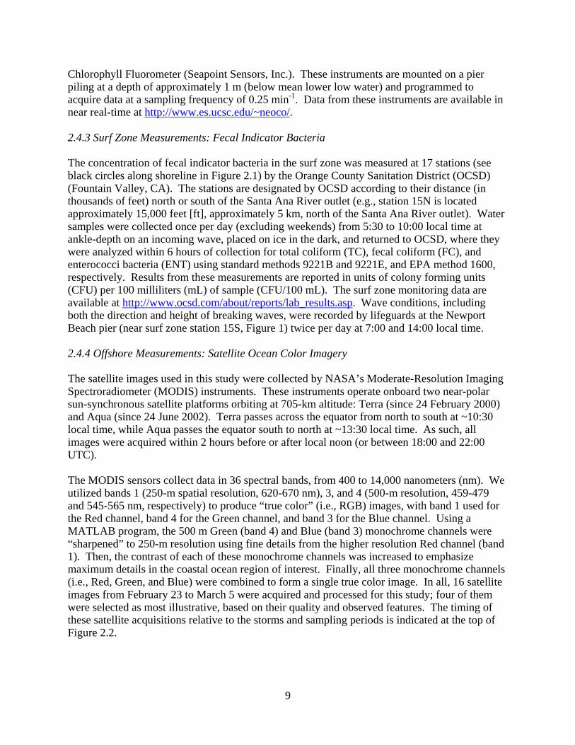
Figure 2.3 MODIS Terra and Aqua true color satellite imagery of storm water runoff plumes along the San Pedro Shelf, California with nominal spatial resolution of 250 m. Yellow dots
indicate location of field sampling stations offshore of Huntington and Newport Beach; black arrows denote the Los Angeles River (LAR) outlet, San Gabriel River (SGR) outlet, Santa Ana
River/Talbert Marsh (SAR/TM) outlet, and Newport Bay outlet. (A) MODIS-Aqua, 23 February 2004 at 21:00 UTC (13:00), (B) MODIS-Aqua, 27 February 2004 at 20:35 UTC (12:35),
(C) MODIS-Aqua, 28 February 2004 at 21:20 UTC (13:20), (D) MODIS-Terra, 29 February 2004 at 18:50 UTC (10:50).
The monitoring grid sampled during the offshore cruises (described in the next section) is depicted on the satellite images by yellow dots. The timing of the satellite passes – relative to rain events, discharge events, wave events, surf zone water quality events, and offshore sampling cruises – is indicated at the top of Figure 2.2. Generally speaking, in this collection of true color imagery, the storm water runoff plumes appear to be characterized by a band of turbid water turquoise to brown in appearance that is
23 Feb. at 13:00 27 Feb. at 12:35
28 Feb. at 13:20 29 Feb. at 10:50
(A)
SAR / TM
Newport Bay
SGR
SAR / TM
Newport Bay
SGR
SAR / TM
Newport Bay
SGR
SAR / TM
Newport Bay
SGR
0 10 20 kmLAR
LAR
LAR
LAR
Presumptive LAR/SGR plume
Presumptive SAR plume
(B)
(C) (D)
20
observed along the entire imaged region, although both cross-shelf and along-shore gradients in the color signature are evident. Following the rain events on 21-22 February (total of 39.4 mm, see RE1 and RE2 in Figure 2.2), a MODIS Aqua imagery from 23 February demonstrates the cross-shelf extent of the runoff plume to be variable, ranging from under 1 km in some places to more than 10-km offshore of the Los Angeles River and San Gabriel River (Figure 2.3A). At our study site, which is centrally located within this broad region, a distinct and apparently heavily particulate-laden runoff plume was observed in the vicinity of the Santa Ana River outlet and nearby station 2201 (see Figure 2.1 for numerical designation of offshore sampling sites). The Santa Ana River plume extended offshore past station 2203, with an apparent turn down-coast (i.e., southeast), continuing past stations 2104 and 2024. During this time, breaking waves were out of the south and the transport direction of fecal indicator bacteria in the surf zone was directed up-coast, opposite the apparent transport direction of storm water plumes offshore of the surf zone (compare timing of satellite image 1 with WE2 and fecal indicator bacteria events TC2, FC2, and ENT2, Figure 2.2). It also appears that a portion of the Los Angeles River and San Gabriel River storm water plumes may have advected south and co-mingled with the Santa Ana River storm water plume. Further south, offshore particulate loadings off the Newport Bay outlet (station 2001) do not appear to be as large as those off the Santa Ana River outlet. A MODIS image on 27 February revealed two distinct plumes of considerable size and offshore extent (Figure 2.3B). This satellite acquisition preceded by one day the sampling cruise on 28 February (described in the next section), followed the large precipitation event on 25-26 February (total of 51.3 mm, see RE3 in Figure 2.2), and followed the large discharge event from the Santa Ana River triggered by release of water from an upstream deflatable dam operated by the Orange County Water District (see previous discussion of DE4). The plume to the northwest in this image appears to be associated with the Los Angeles River and/or San Gabriel River outlets, with an approximate areal extent of 450 km2. The plume to the southeast appears to be distinct from the former plume and likely originated from the Santa Ana River outlet, with an approximate areal extent of 100 km2 (the putative Los Angeles River, San Gabriel River, and Santa Ana River plumes are delineated by red lines in Figure 2.3B). The 27 February Santa Ana River storm water plume is considerably larger in size than the one observed on 23 February (compare Figures 2.3A and 2.3B), consistent with the very large volume of water discharged from the Santa Ana River just prior to this satellite acquisition (approximately 4 x 10⁷ m3, see DE4 in Figure 2.2). Further, the Los Angeles River, San Gabriel River, and Santa Ana River runoff plumes on 27 February differed from those on 23 February in that they penetrated farther offshore (30 km compared to 7 km) and, thus, potentially transported more sediments into the deep waters of the San Pedro Channel. The jet-like appearance of the presumptive Los Angeles River, San Gabriel River, and Santa Ana River storm water runoff plumes in Figure 2.3B has been observed elsewhere in the Southern California Bight (e.g., off the Santa Clara River discharge [5, 49]) and is potentially the result of inertia-driven flow. At the time of this second satellite acquisition, breaking waves were out of the west, and along-shore transport in the surf zone, and offshore of the surf zone, appear to be directed down-coast (compare timing of satellite image 2 with WE3 and fecal indicator events TC3, FC3, and ENT3).
21
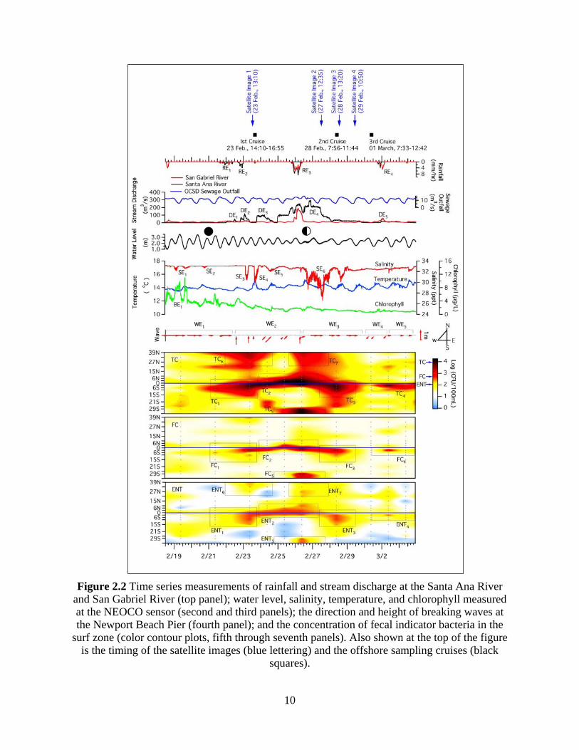
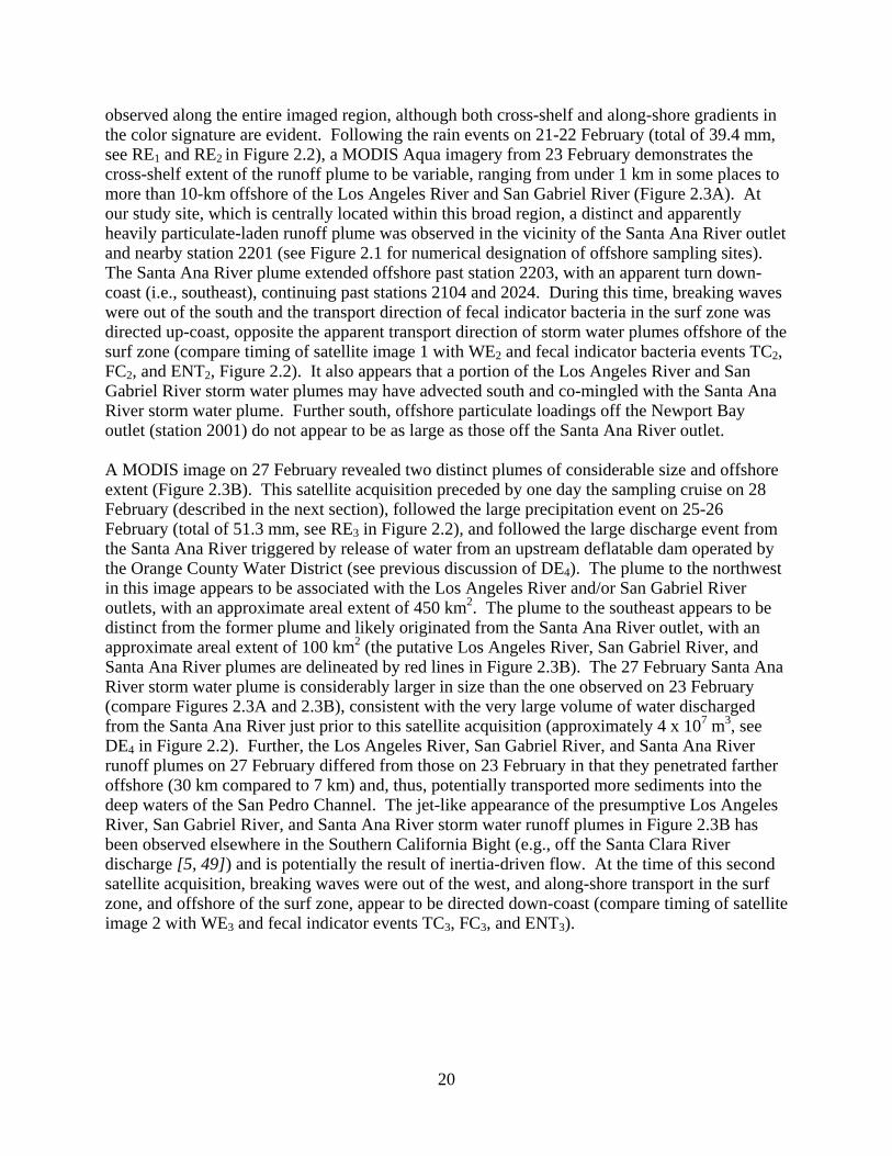
Subsequent MODIS true color imagery on 28 February (Figure 2.3C) and 29 February (Figure 2.3D) indicates that both the Los Angeles River/San Gabriel River and Santa Ana River runoff plumes had significantly decreased in size, consistent with reduced flow out of the respective rivers (compare stream discharge curves with timing of satellite images 2 and 3, Figure 2.2). However, particulate matter appeared to remain high in the general vicinity of the Santa Ana River outlet. Whereas this zone of elevated particulate matter extended south to at least station 2021 on 27-28 February, it had receded somewhat by 29 February and was fairly localized around station 2201. Unfortunately no satellite imagery was available the following day (1 March) to complement the third sampling cruise, given persistent regional cloud cover that day. 2.5.6 Offshore Measurements: Turbidity and Number-Averaged Particle Size Turbidity measurements collected during the three offshore cruises are presented as a series of color contour plots in Figure 2.4.
Figure 2.4 Particle measurements collected during the three sampling cruises. The bottom row of panels indicates the sampling track. TNC is an abbreviation for total particle number
concentration. TNC and number-averaged particle size were calculated from measured particle size spectra using Equation 2.1a, b.
01 March (07:33 - 12:42)28 February (07:56 - 11:44)23 February (14:10 - 16:55)
Ave. Size
TNC
Transmissivity
Sampling Track
SAR/TM
NewportNewportPier
Bay Outlet
SAR/TM
NewportNewportPier
Bay Outlet
SAR/TM
NewportNewportPier
Bay Outlet
SAR/TMNewport
NewportPierBay Outlet
Ave. Size
TNC
Transmissivity
Sampling Track
SAR/TM
Pier NewportBay
Newport
Outlet
SAR/TM
Pier NewportBay
Newport
Outlet
SAR/TM
Pier NewportBay
Newport
Outlet
SAR/TM
Pier NewportBay
Newport
Outlet
Ave. Size
TNC
6
4
2
0
x10 8
25
20
15
10
5
µm
Transmissivity
0.90.80.70.60.50.4
Sampling track
#/L
SAR/TM
Pier NewportBay
Newport
Outlet
SAR/TM
Pier NewportBay
Newport
Outlet
SAR/TM
Pier NewportBay
Newport
Outlet
SAR/TM
Pier NewportBay
Newport
Outlet

22
During the 23 February cruise, a region of high turbidity – as evidenced by low transmissivity and high TNC – is evident offshore of, and to the south of, the Santa Ana River outlet (see left-hand column of panels, Figure 2.4). The number-averaged particle size is depressed in this same region, as well as in the region offshore of the Newport Bay outlet. During subsequent cruises, the ocean became progressively less turbid closer to shore (though not necessarily offshore) – as evidenced by increasing transmissivity and decreasing TNC – and the number-averaged particle size progressively increased (see Figure 2.4). These results suggest that particle concentrations offshore of the surf zone were steadily declining following the rain and stream discharge events that ended on, or before, the evening of 27 February (see rain and stream discharge history, Figure 2.2). The above turbidity patterns are generally consistent with the plume signatures and gradients observed in the true color satellite imagery (see Figure 2.3), though some differences exist which could result from the offset timing (up to several hours) between the acquisition of the satellite images and the field measurements. As a technical aside, the number-averaged particle size ( d , see Equation 2.1b) and median particle size ( d50 ) were found to follow similar trends (i.e., they both rise and fall together), although the magnitude of d50 was generally larger by a factor of 16.1 (Figure S2.4 in Appendix I). However, d was generally less sensitive to outlier values in the particle size spectrum compared to d50 ; hence, d was used in the results reported here. 2.5.7 Offshore Measurements: Fecal Indicator Bacteria Water quality test results from the three offshore cruises are presented as a set of color contour plots in Figure 2.5. During the 23 February cruise, the concentration of fecal indicator bacteria exceeded the California single-sample standards for TC, ENT, and Escherichia coli (EC, a subset of fecal coliform) in several samples collected just offshore, and to the south, of the Santa Ana River and Newport Bay outlets (see left-hand column of panels in Figure 2.5). Nevertheless, the highest concentrations measured offshore of the surf zone are generally lower, in many cases by several orders of magnitude, compared to the highest concentrations measured in the surf zone (compare concentration scales for EC/FC and ENT in Figures 2.2 and 2.5). The difference in offshore and surf zone fecal indicator bacteria concentrations is even more pronounced during the later cruise dates. For example, none of the samples collected during the 28 February and 1 March cruises exceeded State standards for fecal indicator bacteria, yet several of the samples collected from the surf zone during the same time period exceeded single-sample standards for one or more fecal indicator bacteria groups (compare concentrations measured during the second cruise date with TC3, FC3, and ENT3, and concentrations measured during the third cruise date with TC4, FC4, and ENT4, Figures 2.2 and 2.5). 2.5.8 Offshore Measurements: F+ Coliphage and Human Viruses All offshore samples tested positive for F+ coliphage ( n = 8, see Table 2.1), with the exception of a single sample collected on the 28 February cruise from offshore of the Newport Pier (see blue, green, and red plus symbols, bottom panels, Figure 2.5). Human adenoviruses and enteroviruses were also detected by PCR in a sample collected from station 2201 located directly offshore of the Santa Ana River outlet during the 28 February cruise (see red plus, middle bottom panel, Figure 2.5). The concentration of human adenoviruses in this sample is estimated to be 9.5 x 10³ genomes per liter of water, which is approximately equivalent to 10 plaque forming units per
23
liter of water, according to a laboratory study comparing real-time PCR results with plaque assay (50). Human enteroviruses were also found in a sample collected directly offshore of the Santa Ana River outlet (station 2201) on the 23 February cruise (see green plus, bottom left panel, Figure 2.5). While relatively few samples were tested for human viruses (n = 8), these results nevertheless demonstrate that human viruses are present in surface water offshore of the Santa Ana River outlet following storm events, even when the fecal indicator bacteria concentrations are below State standards (e.g., see station 2201 during the 28 February cruise, Figure 2.5). These results are consistent with previously published die-off rates that found human pathogenic viruses and fecal indicator viruses may persist longer than fecal indicator bacteria in ocean water (51). It should also be noted that direct PCR measurement of pathogenic viruses in highly turbid water is challenging due to high concentrations of PCR inhibitors associated with storm water. In general, PCR efficiency decreases with increasing turbidity and concentration of total organic carbon (50).
Figure 2.5 Fecal indicator bacteria concentrations measured during the three sampling cruises.
The bottom row of panels indicates the sampling track (blue arrows) and the detection of F+ coliphage and human viruses. SAR/TM is an abbreviation for the outlet
of the Santa Ana River and Talbert Marsh.
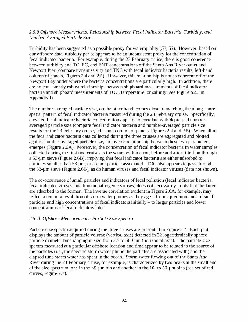
24
2.5.9 Offshore Measurements: Relationship between Fecal Indicator Bacteria, Turbidity, and Number-Averaged Particle Size Turbidity has been suggested as a possible proxy for water quality (52, 53). However, based on our offshore data, turbidity per se appears to be an inconsistent proxy for the concentration of fecal indicator bacteria. For example, during the 23 February cruise, there is good coherence between turbidity and TC, EC, and ENT concentrations off the Santa Ana River outlet and Newport Pier (compare transmissivity and TNC with fecal indicator bacteria results, left-hand column of panels, Figures 2.4 and 2.5). However, this relationship is not as coherent off of the Newport Bay outlet where the bacteria concentrations are particularly high. In addition, there are no consistently robust relationships between shipboard measurements of fecal indicator bacteria and shipboard measurements of TOC, temperature, or salinity (see Figure S2.3 in Appendix I). The number-averaged particle size, on the other hand, comes close to matching the along-shore spatial pattern of fecal indicator bacteria measured during the 23 February cruise. Specifically, elevated fecal indicator bacteria concentration appears to correlate with depressed number-averaged particle size (compare fecal indicator bacteria and number-averaged particle size results for the 23 February cruise, left-hand column of panels, Figures 2.4 and 2.5). When all of the fecal indicator bacteria data collected during the three cruises are aggregated and plotted against number-averaged particle size, an inverse relationship between these two parameters emerges (Figure 2.6A). Moreover, the concentration of fecal indicator bacteria in water samples collected during the first two cruises is the same, within error, before and after filtration through a 53-µm sieve (Figure 2.6B), implying that fecal indicator bacteria are either adsorbed to particles smaller than 53 µm, or are not particle associated. TOC also appears to pass through the 53-µm sieve (Figure 2.6B), as do human viruses and fecal indicator viruses (data not shown). The co-occurrence of small particles and indicators of fecal pollution (fecal indicator bacteria, fecal indicator viruses, and human pathogenic viruses) does not necessarily imply that the latter are adsorbed to the former. The inverse correlation evident in Figure 2.6A, for example, may reflect a temporal evolution of storm water plumes as they age – from a predominance of small particles and high concentrations of fecal indicators initially – to larger particles and lower concentrations of fecal indicators later. 2.5.10 Offshore Measurements: Particle Size Spectra Particle size spectra acquired during the three cruises are presented in Figure 2.7. Each plot displays the amount of particle volume (vertical axis) detected in 32 logarithmically spaced particle diameter bins ranging in size from 2.5 to 500 µm (horizontal axis). The particle size spectra measured at a particular offshore location and time appear to be related to the source of the particles (i.e., the specific storm water plume the particles are associated with) and the elapsed time storm water has spent in the ocean. Storm water flowing out of the Santa Ana River during the 23 February cruise, for example, is characterized by two peaks at the small end of the size spectrum, one in the <5-µm bin and another in the 10- to 50-µm bins (see set of red curves, Figure 2.7).
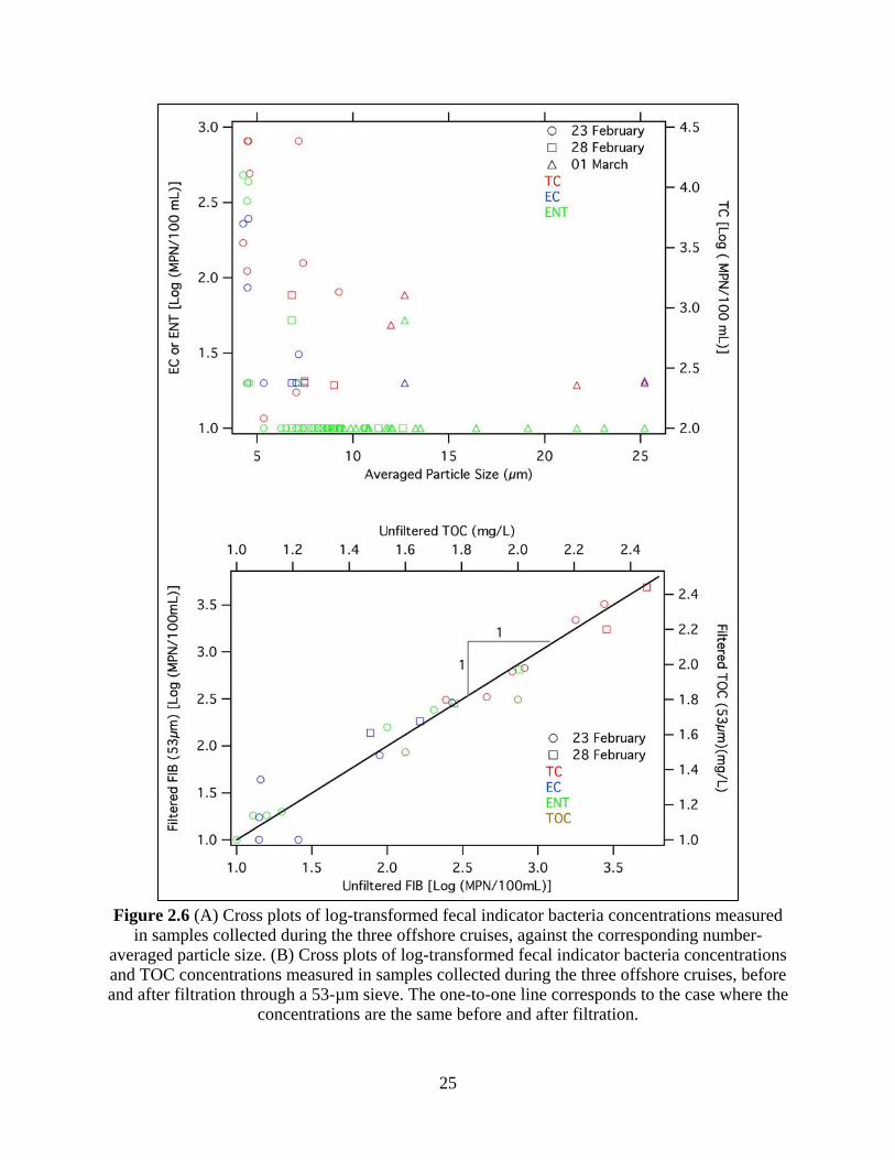
25
Figure 2.6 (A) Cross plots of log-transformed fecal indicator bacteria concentrations measured in samples collected during the three offshore cruises, against the corresponding number-
averaged particle size. (B) Cross plots of log-transformed fecal indicator bacteria concentrations and TOC concentrations measured in samples collected during the three offshore cruises, before and after filtration through a 53-µm sieve. The one-to-one line corresponds to the case where the
concentrations are the same before and after filtration.
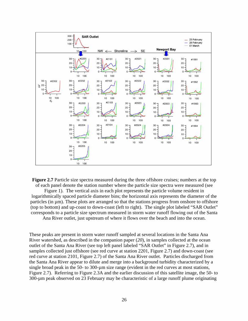
26
Figure 2.7 Particle size spectra measured during the three offshore cruises; numbers at the top
of each panel denote the station number where the particle size spectra were measured (see Figure 1). The vertical axis in each plot represents the particle volume resident in
logarithmically spaced particle diameter bins; the horizontal axis represents the diameter of the particles (in µm). These plots are arranged so that the stations progress from onshore to offshore (top to bottom) and up-coast to down-coast (left to right). The single plot labeled “SAR Outlet” corresponds to a particle size spectrum measured in storm water runoff flowing out of the Santa
Ana River outlet, just upstream of where it flows over the beach and into the ocean.
These peaks are present in storm water runoff sampled at several locations in the Santa Ana River watershed, as described in the companion paper (20), in samples collected at the ocean outlet of the Santa Ana River (see top left panel labeled “SAR Outlet” in Figure 2.7), and in samples collected just offshore (see red curve at station 2201, Figure 2.7) and down-coast (see red curve at station 2101, Figure 2.7) of the Santa Ana River outlet. Particles discharged from the Santa Ana River appear to dilute and merge into a background turbidity characterized by a single broad peak in the 50- to 300-µm size range (evident in the red curves at most stations, Figure 2.7). Referring to Figure 2.3A and the earlier discussion of this satellite image, the 50- to 300-µm peak observed on 23 February may be characteristic of a large runoff plume originating
27
from one or more up-coast sources of storm water runoff, most likely the Los Angeles River and/or the San Gabriel River. During subsequent cruises, the particle size spectra progressively coarsen with the result that, by 1 March, virtually all of the particle volume is associated with the largest size bin (>500 µm, see green curves in Figure 2.7). The observed temporal evolution in particle size spectra – from high turbidity and multiple peaks at the lower end of the particle size spectrum to low turbidity and a single peak at the large end of the particle size spectrum – may reflect the combined influence of decreasing particle supply (i.e., reduced storm water discharge from major river outlets) coupled with within-plume coagulation of particles into larger size classes and, ultimately, removal of the largest particles by gravitational sedimentation. Alternatively, the temporal coarsening of particles in the offshore may reflect changes in the particle size spectra of the storm water runoff before it enters the ocean, from a predominance of smaller particles during the peak of the hydrograph, to a predominance of coarser particles during the falling limb of the hydrograph. Particle size spectra measured over the course of several storms in the Santa Ana River support, at least to some extent, this last hypothesis (20). To explore this issue further, coagulation time scales were calculated from particle size spectra measured during the three cruises. Particle coagulation is, in general, controlled by both the frequency with which particles collide with one another and the efficiency with which particles "stick" upon collision (54, 55). Particle collisions can be driven by several microscale transport mechanisms, including shear-induced collision (orthokinetic coagulation), Brownian motion (perikinetic coagulation), and differential sedimentation (56, 57). Of these, orthokinetic coagulation will likely dominate at the surface of the ocean; hence, a crude estimate for the coagulation time scale can be obtained as follows (58):
τ sh = −0.6934παφG
(2.2)
where φ is the volume fraction of particles in suspension, α is the coagulation efficiency, and G is the local shear rate. The volume fraction can be estimated directly from measurements of the particle size spectra (see Equation 2.1c). The other two parameters (α and G) will, in general, vary spatially and temporally. However, upper-limit estimates for τsh can be obtained by setting α = 1 (which is equivalent to assuming that every particle-particle collision results in a sticking event) and using an upper-limit value for the shear rate of G = 10 sec-1 (59). Using these values of α and G, and calculating values of φ from measured particle size spectra, the resulting coagulation time scales estimated from Equation 2.2 vary from 7 minutes to 4 hours (Figure 2.8). Not surprisingly, the smallest coagulation time scales occur in regions with high turbidity, specifically around the outlet of the Santa Ana River during the 23 February cruise, around the Newport Pier during the 28 February cruise, and around the outlets of the Santa Ana River and Newport Bay during the 1 March cruise.
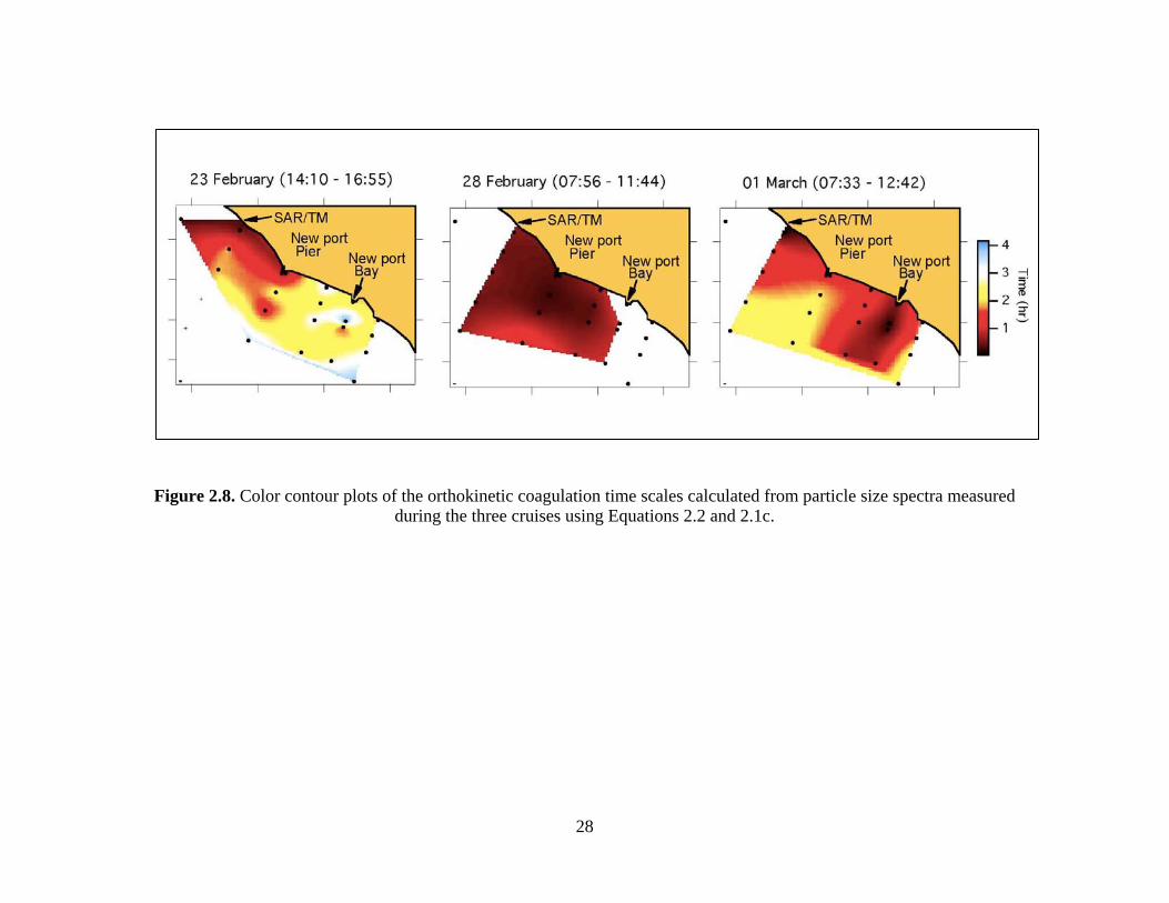
28
Figure 2.8. Color contour plots of the orthokinetic coagulation time scales calculated from particle size spectra measured during the three cruises using Equations 2.2 and 2.1c.
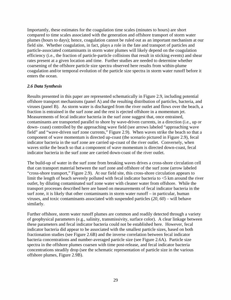
29
Importantly, these estimates for the coagulation time scales (minutes to hours) are short compared to time scales associated with the generation and offshore transport of storm water plumes (hours to days); hence, coagulation cannot be ruled out as an important mechanism at our field site. Whether coagulation, in fact, plays a role in the fate and transport of particles and particle-associated contaminants in storm water plumes will likely depend on the coagulation efficiency (i.e., the fraction of particle-particle collisions that result in sticking events) and shear rates present at a given location and time. Further studies are needed to determine whether coarsening of the offshore particle size spectra observed here results from within-plume coagulation and/or temporal evolution of the particle size spectra in storm water runoff before it enters the ocean. 2.6 Data Synthesis Results presented in this paper are represented schematically in Figure 2.9, including potential offshore transport mechanisms (panel A) and the resulting distribution of particles, bacteria, and viruses (panel B). As storm water is discharged from the river outlet and flows over the beach, a fraction is entrained in the surf zone and the rest is ejected offshore in a momentum jet. Measurements of fecal indicator bacteria in the surf zone suggest that, once entrained, contaminants are transported parallel to shore by wave-driven currents, in a direction (i.e., up or down- coast) controlled by the approaching wave field (see arrows labeled “approaching wave field” and “wave-driven surf zone currents,” Figure 2.9). When waves strike the beach so that a component of wave momentum is directed up-coast (the scenario pictured in Figure 2.9), fecal indicator bacteria in the surf zone are carried up-coast of the river outlet. Conversely, when waves strike the beach so that a component of wave momentum is directed down-coast, fecal indicator bacteria in the surf zone are carried down-coast of the river outlet. The build-up of water in the surf zone from breaking waves drives a cross-shore circulation cell that can transport material between the surf zone and offshore of the surf zone (arrow labeled “cross-shore transport,” Figure 2.9). At our field site, this cross-shore circulation appears to limit the length of beach severely polluted with fecal indicator bacteria to <5 km around the river outlet, by diluting contaminated surf zone water with cleaner water from offshore. While the transport processes described here are based on measurements of fecal indicator bacteria in the surf zone, it is likely that other contaminants in storm water runoff – in particular, human viruses, and toxic contaminants associated with suspended particles (20, 60) – will behave similarly. Further offshore, storm water runoff plumes are common and readily detected through a variety of geophysical parameters (e.g., salinity, transmissivity, surface color). A clear linkage between these parameters and fecal indicator bacteria could not be established here. However, fecal indicator bacteria did appear to be associated with the smallest particle sizes, based on both fractionation studies (see Figure 2.6B) and the inverse correlation between fecal indicator bacteria concentrations and number-averaged particle size (see Figure 2.6A). Particle size spectra in the offshore plumes coarsen with time post-release, and fecal indicator bacteria concentrations steadily drop (see the schematic representation of particle size in the various offshore plumes, Figure 2.9B).
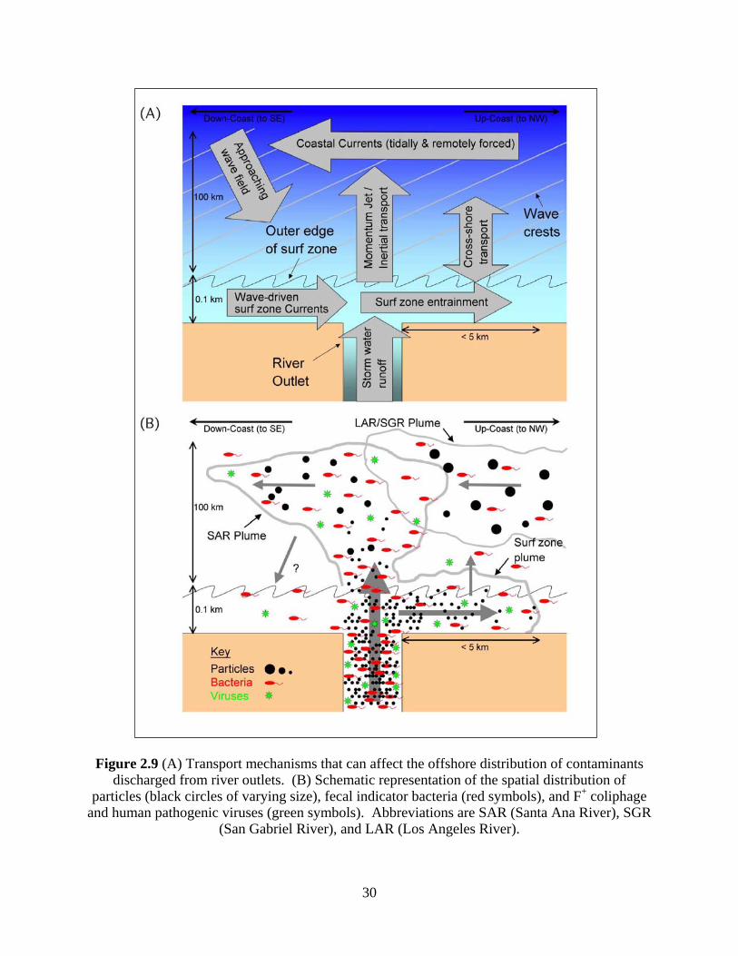
30
Figure 2.9 (A) Transport mechanisms that can affect the offshore distribution of contaminants discharged from river outlets. (B) Schematic representation of the spatial distribution of
particles (black circles of varying size), fecal indicator bacteria (red symbols), and F+ coliphage and human pathogenic viruses (green symbols). Abbreviations are SAR (Santa Ana River), SGR
(San Gabriel River), and LAR (Los Angeles River).
31
These results have several implications. First, they suggest that high concentrations of fecal indicator bacteria in the surf zone at our field site are probably not brought into the study area by coastal currents from distal sources (e.g., the Los Angeles River and/or San Gabriel River). Second, cross-shore transport of water between the surf zone and offshore of the surf zone – for example, by rip cell currents – is likely to improve surf zone water quality by diluting dirty river effluent entrained in the surf zone with relatively clean ocean water from offshore – a result supported by the earlier quantitative analysis of dilution length-scales and die-off time scales. While the concentrations of fecal indicator bacteria in the offshore plumes are generally below surf zone water quality standards, particularly during the latter two cruises, fecal indicator viruses (F+ coliphage) were detected in nearly all offshore samples tested, and human adenoviruses and enteroviruses were detected in several offshore samples, including two collected offshore of the Santa Ana River outlet (station 2201 on 23 and 28 February, see Figure 2.5). It is likely that the human virus results presented here represent a conservative estimate of viral prevalence, because only limited number of samples was tested (n = 8 of 2 were positive). In addition, the presence of PCR inhibitors in storm water reduces the efficiency of PCR detection of human pathogenic viruses, as mentioned earlier. At present, there are no water quality standards for fecal indicator viruses and human pathogenic viruses, largely because epidemiological data are not presently available to link adverse human health outcomes (e.g., gastrointestinal disease) to recreational ocean exposure to these organisms. However, the offshore detection of human pathogenic viruses begs the question of whether these viruses constitute a human health risk, either by contaminating the surf zone directly (see arrow with question mark, indicating the possible transfer of contaminants from offshore into the surf zone, Figure 2.9) or by sequestering in offshore sediments. Taken together, the results presented in this paper demonstrate that storm water runoff from the Santa Ana River is a significant source of near shore pollution, including turbidity, fecal indicator bacteria, fecal indicator viruses, and human pathogenic viruses. However, relationships between variables (e.g., between turbidity and fecal indicator bacteria, and between fecal indicator bacteria and human viruses) vary from site to site (at the same time) and from time to time (at the same site), suggesting that the sources, fate, and transport processes operating at our field site may be highly contaminant specific. The apparent exception is the inverse relationship observed between fecal indicator bacteria and number-averaged particle size, although further studies are needed to determine if this result is generalizable to other storm seasons and coastal sites and, if so, to determine the underlying mechanism at work. The relationship between water quality parameters (e.g., fecal indicator bacteria) and turbidity and other field proxies – such as number-averaged particle size, salinity, colored dissolved organic matter – will be the focus of future studies, as part of the aforementioned Bight ’03 program and other ongoing coastal field investigations in Southern California. Finally, it is worth noting that the highly regulated nature of storm water flow in the Santa Ana River has, from a human health perspective, both positive and negative attributes. On the negative side, the accumulation and subsequent release of storm water at up-stream deflatable dams implies that peak discharge from the Santa Ana River can occur days after the cessation of rainfall, when more people are likely to be at the beach and thus exposed to contaminants flowing out of the river mouth (compare rainfall records with discharge events DE3 and DE4, Figure 2.2). On the positive side, the ability to manipulate flow in the river opens up opportunities to mitigate environmental impacts that might not be available in other, more
32
natural, systems. For example, State and local officials might include beach usage as one of the parameters they consider before releasing water from upstream dams. 2.7 References (1) Culliton, T. J. Population; distribution, density and growth; A state of the coast report; NOAA’s state of the coast report; National Oceanic and Atmospheric Administration: Silver Spring, MD, 1998. (2) Reeves, R. L.; Grant, S. B.; Mrse, R. D.; Copil Oancea, C. M.; Sanders, B. F.; Boehm, A. B. Scaling and management of fecal indicator bacteria in runoff from a coastal urban watershed in southern California. Environ. Sci. Technol. 2004, 38, 2637-2648. (3) Bay, S.; Jones, B. H.; Schiff, K.; Washburn L. Water quality impacts of stormwater discharges to Santa Monica Bay. Mar. Environ. Res. 2003, 56, 205-223. (4) DiGiacomo, P. M.; Hamner, W. M; Hamner, P. P.; Caldeira, R. M. A. Phalaropes feeding at a coastal front in Santa Monica Bay, California. Marine Syst. 2002, 37, 199-212. (5) Warrick, J. A.; Mertes, L. A. K.; Washburn, L.; Siegel, D. A. Dispersal forcing of southern California river plumes, based on field and remote sensing observations. Geo-Mar. Lett. 2004, 24, 46-52. (6) Koh, R. C. Y; Brooks, N. H. Fluid mechanics of wastewater disposal in the ocean. Annual Rev. Fluid Mech. 1975, 7, 187-211. (7) Lu, R.; Turco, R. P.; Stolzenbach, K.; Fiedlander, S. K.; Xiong, C. Dry deposition of airborne trace metals on the Los Angeles Basin and adjacent coastal waters. J. Geophys. Res.-Atmos. 2003, 108, AAC 11, 1-24. (8) Boehm, A. B.; Shellenbarger, G. G.; Paytan, A. Groundwater discharge: potential association with fecal indicator bacteria in the surf zone. Environ. Sci. Technol. 2004, 38, 3558-3566. (9) Schiff, K.C. Development of a model publicly owned treatment work (POTW) monitoring program; Southern California Coastal Water Research Project: Westminster, CA, 1999. (10) Warrick, J. A.; Rubin, D. M. Suspended-sediment rating curve response to urbanization and wildfire, Santa Ana River, California. J. Geo. Res. 2007, 112, F02018, doi:10.1029/2006JF000662. (11) Water control manual, Prado Dam and Reservoir; U.S. Army Corps of Engineers: Santa Ana River, California, 1994. (12) Southern California Bight 2003 Regional Marine Monitoring Survey (Bight ’03); Water quality workplan; Bight ’03 Water Quality Committee, 2003. (13) Grant, S. B.; Sanders, B. F.; Boehm, A. B.; Redman, J. A.; Kim, J. H.; Mrse, R. D.; Chu, A. K.; Gouldin, M.; McGee, C. D.; Gardiner, N. A.; Jones, B. H.; Svejkovsky, J.; Leipzig, G. V.;
33
Brown, A. Generation of Enterococci Bacteria in a coastal saltwater marsh and its impact on surf zone water quality. Environ. Sci. Technol. 2001, 35, 2407-2416. (14) Grant, S. B.; Kim, J. H.; Jones, B. H.; Jenkins, S. A.; Wasyl, J.; Cudaback, C. Surf zone entrainment, along-shore transport, and human health implications of pollution from tidal outlets. J. Geo. Res. 2005, 110, C10025-C10045. (15) Geyer, W. R., Hill, P. S.; Milligan, T. G.; Traykovski, P. The structure of the Eel River plume during floods. Cont. Shelf Res. 2000, 20, 2067-2093. (16) Hill, P. S.; Milligan, T. G.; Geyer, W. R. Controls on effective settling velocity of suspended sediment in the Eel River flood plume. Cont. Shelf Res. 2000, 20, 2095-2111. (17) Jones, B. H.; Noble, M. A.; Dickey, T. D. Hydrographic and particle distributions over the Palos Verdes Continental Shelf: spatial, seasonal and daily variability. Cont. Shelf Res. 2002, 22, 945-965. (18) Curran K. J.; Hill, P. S.; Milligan, T. G. Fine-grained suspended sediment dynamics in the Eel River flood plume. Cont. Shelf Res. 2002, 22, 2537-2550. (19) Washburn, L.; McClure, K. A.; Jones, B. H.; Bay, S. M. Spatial scales and evolution of stormwater plumes in Santa Monica Bay. Mar. Environ. Res. 2003, 56, 103-125. (20) Surbeck, C. Q.; Jiang, S. C.; Ahn, J. H.; Grant, S. B. Flow fingerprinting fecal pollution and suspended solids in stormwater runoff from an urban coastal watershed. Environ. Sci. Technol. 2006, 40, 4435-4441. (21) Boehm, A. B.; Grant, S. B.; Kim, J. H.; Mowbray, S. L.; Mcgee, C. D.; Clark, C. D.; Foley, D. M.; Wellman, D. E. Decadal and shorter period variability of surf zone water quality at Huntington Beach, California. Environ. Sci. Technol. 2002, 36, 3885-3892. (22) Kim, J. H.; Grant, S. B. Public mis-notification of coastal water quality: A probabilistic evaluation of posting errors at Huntington Beach, California. Environ. Sci. Technol. 2004, 38, 2497-2504. (23) King, P.; The potential loss in gross national product and gross state product from a failure to mountain California’s beaches; California department of boating and waterways, 2003. (24) Blomquist; William, A.; Harvey, F. Collins; David, B. F.; Assessing Risk Information Concerning Coastal Runoff; National Water Research Institute Occasional Paper, 2003. (25) Grant, S. B.; Sanders, B. F.; Boehm, A. B.; Arega F.; Ensari, S.; Mrse, R. D.; Kang H. Y.; Reeves R. L.; Kim, J. H.; Redman, J. A. Coastal runoff impact study phase II: Sources and dynamics of fecal indicators in the lower Santa Ana River Watershed; A draft report prepared for the National Water Research Institute: County of Orange, and the Santa Ana Regional Water Quality Control Board, 2002.
34
(26) Boehm, A. B.; Sanders, B. F.; Winant, C. D. Cross-shelf transport at Huntington Beach: Implications for the fate of sewage discharged through an offshore ocean outfall. Environ. Sci. Technol. 2002, 36, 1899-1906. (27) Kim, J. H.; Grant, S. B.; McGee, C. D.; Sanders, B. F.; Largier, J. L. Locating sources of surf zone pollution: A mass budget analysis of fecal indicator bacteria at Huntington Beach. Environ. Sci. Technol. 2004, 38, 2626-2636. (28) Choi, S.; Chu, W.; C; Brown, J.; S.; Becker, S. J.; Harwood, V. J.; Jiang, S. C. Application of enterococci antibiotic resistance patterns for contamination source identification at Huntington Beach, California. Mar. Pollut. Bulletin 2003, 46, 748-755. (29) Noble, R.; Allen, S.; Blackwood, A.; Chu, W.; Jiang, S. C.; Lovelace, G.; Sobsey, M.; Stewart, j.; Wait, D. Use of viral pathogens and indicators to differentiate between human and non-human fecal contamination in a microbial source tracking comparison study. J. Water & Health 2003, 1, 195-207. (30) Turbow, D.; Lin, T. H.; Jiang, S. Impacts of beach closure events on perception of swimming-related health risk in Orange County, California, Mar. Pollut. Bulletin 2004, 48, 312-136. (31) Perkin, R. G.; Lewis, E. L. The practical salinity scale 1979: Fitting the data. IEEE J. Oceanic Eng. 1980, OE-5, 9-16. (32) DeLeon, R.; Shieh, Y. S. C.; Baric, R. S.; Sobey, M. D. Detection of enteroviruses and hepatitis A virus in environmental samples by gene probes and polymerase chain reaction. Water Quality Conference; American Water Works Association: Denver, CO, 1990, 833-853. (33) Tsai, Y. L.; Sobsey, M. D.; Sangermano, L. R.; Palmer, C. J. Simple method of concentrating enteroviruses and hepatitis A virus from sewage and ocean water for rapid detection by reverse transcriptase-polymerase chain reaction. Appl Environ. Microbiol. 1993, 59, 3488-3491. (34) Jiang, S. C.; Chu, W. PCR detection of pathogenic viruses in southern California urban river. J. Appl. Microbiol. 2004, 97, 17-28. (35) Pina, S.; Puig, M.; Lucena, F.; Jofre, J.; Girones, R. Viral pollution in the environment and in shellfish: Human adenovirus detection by PCR as an index of human viruses. Appl Environ. Microbiol. 1998, 64, 3376-3382. (36) He, J.; Jiang, S. Quantification of enterococci and human adenoviruses in environmental samples by real-time PCR. Appl Environ. Microbiol. 2005, 71, 2250-2255. (37) Agrawal, Y. C.; Pottsmith, H. C. Laser Diffraction Particle Sizing in STRESS. Cont. Shelf Res. 1994, 14, 1101-1121. (38) Agrawal, Y. C.; Pottsmith, H. C. Instrument for particle size and settling velocity observation in sediment transport. Mar. Geo. 2000, 168, 89-114.
35
(39) Traykovski, P.; Latter, R. J.; Irish, J. D. A laboratory evaluation of the laser in-situ scattering and transmissometry instrument using natural sediments. Mar. Geo. 1999, 159, 355-367. (40) Gartner, J. W.; Cheng, R. T.; Wang, P.; Richter, K. laboratory and filed evaluations of the LISST-100 instrument for suspended particle size determinations. Mar. Geo. 2001, 175, 199-219. (41) Granata, T.C.; Serra, T.; Colomer, J.; Casamitjana, X.; Duarte, C. M.; Gacia, E. Flow and particle and distributions in a nearshore seagrass meadow before and after a storm. Mar. Ecol. Prog. Ser. 2001, 218, 95-106. (42) Mikkelsen O. A.; Pejrup, M. In-situ particle size spectra and density of particle aggregates in a dredging plume. Mar. Geo. 2000, 170, 443-459. (43) Mikkelsen O. A.; Pejrup, M. The use of a LISST-100 laser particle sizer for in-situ estimates of floc size, density, and settling velocity. Geo-Mar. Lett. 2001, 20, 187-195. (44) Mikkelsen, O. A. Example of spacial and temporal variations of some fine-grained suspended particle characteristics in two Danish coastal water bodies. Oceanologica Acta 2002, 25, 39-49. (45) Mikkelsen, O. A. Variation in the projected surface of suspended particles: Implications for remote sensing assessment of TSM. Rem. Sens. of Environ. 2002, 79, 23-29. (46) Fugate, D. C.; Friedrichs, C. T. Controls on suspended aggregate size in partially mixed estuaries. Est., Coas. & Shelf Sci. 2003, 58, 389-404. (47) Serra, T.; Colomer, J.; Cristina, X. P.; Vila, X.; Arellano, J. B.; Casamitjana, X. Evaluation of laser in situ scattering instrument for measuring concentration of phytoplankton purple sulfur bacteria, and suspended inorganic sediments in lakes. J. Environ. Eng. 2001, 11, 1023-1030. (48) Boehm, A. B. Model of microbial transport and inactivation in the surf zone and application to field measurements of total coliform in northern Orange County, California. Environ. Sci. Technol. 2003, 37, 5511-5517. (49) Mertes, L. A. K.; Warrick, J. A. Measuring flood output from 110 coastal watersheds in California with field measurements and SeaWiFS. Geology 2001, 29, 659-662. (50) Jiang, S. C.; Deszfulian, H.; Chu, W. J. Real-time quantitative PCR for enteric adenovirus serotype 40 in environmental waters. Can. J. Microbiol. 2005, 51, 393-398. (51) Shuval, H. I. Developments in Water Quality Research: Ann Arbor-Humphrey Science, Ann Arbor, 1970. (52) Boucier, D. R.; Sharma, R. P. Heavy metals and their relationship to solids in urban runoff. Int. J. Envir. Anal. Chem. 1980, 7, 273-283.
36
(53) Gippel, C. J. Potential of turbidity monitoring for measuring the transport of suspended-solids in streams. Hydrological Processes. 1995, 9, 83-97. (54) Grant, S. B.; Poor, C.; Relle, S. Scaling theory and solutions for the steady-state coagulation and settling of fractal aggregates in aquatic systems. Colloid and Surfaces. 1996, 107, 155-174. (55) Grant, S. B.; Kim, J. H.; Poor, C. Kinetic theories for the coagulation and sedimentation of particles. J. Colloid Interfaces Sci. 2001, 238, 238-250. (56) O’Melia, C. R. Aquasols: the behavior of small particles in aquatic systems. Environ. Sci. Technol. 1980, 14, 1052. (57) Amirtharajah, A. A.; O’Melia, C. R Water Quality and Treatment: American Water Works Association; McGraw-Hill Book Company: New York, 1990. (58) Birkner, F. B.; Morgan, J. J. Polymer flocculation kinetics of dilute colloidal suspension. J. AWWA. 1968, 60, 175-191. (59) http://mixing.coas.oregonstate.edu/research/oceanmixing.htm (60) Glenn, D. W.; Sansalone, J. J. Accretion and partitioning of heavy metals associated with snow exposed to urban traffic and winter storm maintenance activities. II. J. ASCE. 2002, 2, 167-185.
3. Size Distribution, Sources, and Seasonality of Suspended Particles in Southern California Marine Bathing Water∗
3.1 Abstract In this study, we define seasonal and along-shore variations in suspended PSDs at two marine bathing beaches in Southern California using a low-angle light scattering instrument (LISST). Empirical Orthogonal Function (EOF) analysis of the LISST data set (n=55,651) identified three particle size modes that collectively account for >90 percent of the variance in the de-meaned PSD data at six sites along the shoreline at Huntington Beach and Newport Beach: a dinoflagellate mode, a large particle mode, and a small particle mode. These three modes exhibit distinct seasonal patterns and along-shore distributions, reflecting both the sources and environmental factors that trigger particle occurrence. Comparison of volume-based PSDs generated from the LISST and from image analysis of optical micrographs indicates that the LISST performs well when measuring the size distribution of particles associated with dinoflagellate blooms. However, LISST measurements on storm-water impacted samples consistently yield a rising tail at small particle sizes that may be an artifact arising from the non-spherical nature of inorganic particles in terrestrial runoff. The results presented here demonstrate that PSDs measured by light scattering instruments, such as the LISST, represent a new data resource for assessing water quality and managing human health risk at marine bathing beaches. 3.2 Introduction Coastal marine bathing beaches represent an important economic and recreational resource in California, hosting upwards of 400 million visits per year and providing state and local economic benefits running into the billions of dollars annually (1). At present, water quality at marine bathing beaches in California, and throughout most of the world, is evaluated using fecal indicator bacteria (FIB) – a class of enteric bacteria that are not usually themselves pathogenic, but may indicate the presence of disease-causing organisms from sewage and runoff. The use of FIB as a measure of water quality is supported by epidemiological studies conducted over the last 30 years that demonstrate a dose-response relationship between swimming in marine bathing waters with high concentrations of FIB (in particular, high concentrations of enterococci bacteria) and increased incidence of gastrointestinal illness (2). The dose-response relationships were established in marine settings where the likely source of FIB was partially treated human sewage (3) and were recently extended to marine beaches impacted by urban runoff with no known sewage inputs (4). The use of FIB as an indicator of marine bathing water quality and human health risk has a number of inherent drawbacks, including:
∗This chapter is an excerpt of the dissertation Ahn, J. H. (2007). Size Distribution, Sources, and Transport of Suspended Particles Along An Inland-to-Ocean Transect. University of California, Irvine.
37
• The long turnaround time associated with culture based assays of FIB (>24 hours) frequently exceed the time over which FIB concentrations in marine waters change (<1 hour), raising questions about the timeliness of beach health advisories and beach closures (5-7).
• The validity of the aforementioned dose-response curves in settings where FIB are from natural (i.e., non-human sewage or runoff) sources, such as bird droppings (8) and re-growth in estuaries and freshwater streams (9-11).
• The different survival rates of FIB and pathogens likely to cause human disease in polluted marine waters (12).
Additionally, FIB monitoring programs provide no information on many classes of contaminants that cause nearshore toxicity and human illness after acute or chronic exposure, including harmful algal blooms (HABs), organic pollutants, and heavy metals. Notably, many of the latter contaminants are either particles themselves (HABs) or are frequently associated with organic or inorganic particles of varying sizes (organic pollutants and heavy metals) (13). The development and deployment of coastal ocean observing systems may ultimately address the problems noted above by linking together molecular tools for the rapid detection of FIB and pathogens (14), autonomous marine sensor and telemetry technology, and real-time measurements of ocean currents, temperature, and salinity at appropriate spatial and temporal scales (15). If these observing systems result in an even modest improvement in the accuracy of beach health advisories provided to the general public, they could have significant human health and economic benefits to the local economy through reduced illness rates and fewer unnecessary beach closures (16). In this study, we hypothesized that the size distribution of suspended particles harbors untapped information on the sources and nature of pollutants in marine bathing waters and, therefore, should be one of the variables measured in next-generation ocean observing systems. To test this hypothesis, we carried out low-angle light scattering measurements of suspended PSDs in water samples collected daily for 1 year from six coastal sites at Huntington Beach and Newport Beach, two popular beaches in Orange County, Southern California. To explore potential artifacts associated with the light scattering measurements of PSDs, and to better understand the sources of suspended particles, light scattering measurements were compared with PSDs estimated from optical micrographs prepared from the same water samples. We also investigated the possibility that certain particle size classes were correlated with more traditional measures of coastal water quality, including FIB and chlorophyll fluorescence. To our knowledge, this study represents the first attempt to examine the along-shore and seasonal variability of suspended particles in the very nearshore region of the ocean where ocean monitoring programs are presently focused and where human contact with potential disease causing agents is greatest. 3.3 Site Description The study site is a northwest-southeast striking section of the Pacific Ocean coastline, located along Huntington Beach and Newport Beach in Orange County, California (Figure 3.1). This region of coastline has suffered poor water quality over the past several years due to elevated
38
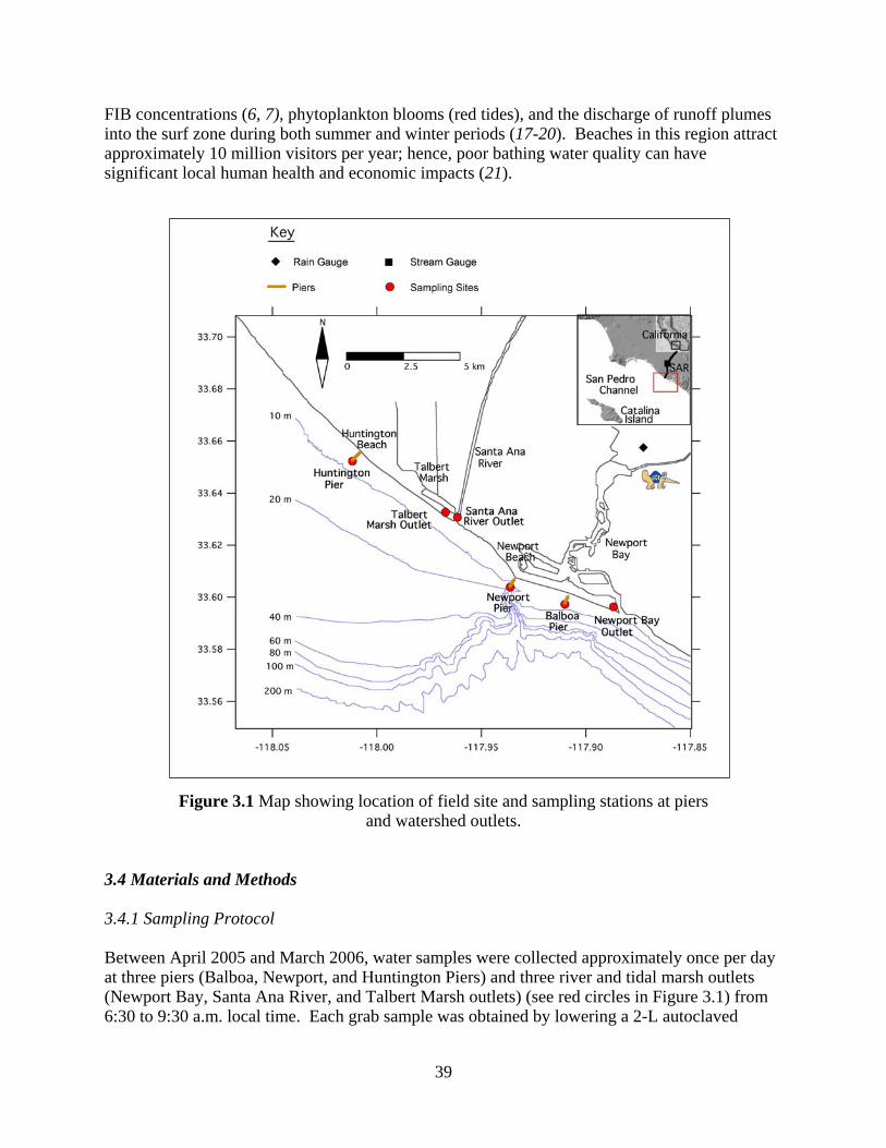
FIB concentrations (6, 7), phytoplankton blooms (red tides), and the discharge of runoff plumes into the surf zone during both summer and winter periods (17-20). Beaches in this region attract approximately 10 million visitors per year; hence, poor bathing water quality can have significant local human health and economic impacts (21).
Figure 3.1 Map showing location of field site and sampling stations at piers and watershed outlets.
3.4 Materials and Methods 3.4.1 Sampling Protocol Between April 2005 and March 2006, water samples were collected approximately once per day at three piers (Balboa, Newport, and Huntington Piers) and three river and tidal marsh outlets (Newport Bay, Santa Ana River, and Talbert Marsh outlets) (see red circles in Figure 3.1) from 6:30 to 9:30 a.m. local time. Each grab sample was obtained by lowering a 2-L autoclaved
39
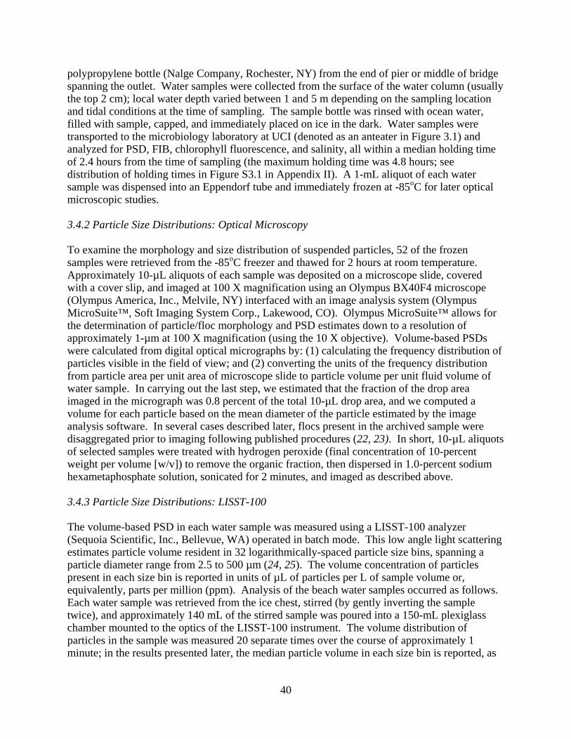
polypropylene bottle (Nalge Company, Rochester, NY) from the end of pier or middle of bridge spanning the outlet. Water samples were collected from the surface of the water column (usually the top 2 cm); local water depth varied between 1 and 5 m depending on the sampling location and tidal conditions at the time of sampling. The sample bottle was rinsed with ocean water, filled with sample, capped, and immediately placed on ice in the dark. Water samples were transported to the microbiology laboratory at UCI (denoted as an anteater in Figure 3.1) and analyzed for PSD, FIB, chlorophyll fluorescence, and salinity, all within a median holding time of 2.4 hours from the time of sampling (the maximum holding time was 4.8 hours; see distribution of holding times in Figure S3.1 in Appendix II). A 1-mL aliquot of each water sample was dispensed into an Eppendorf tube and immediately frozen at -85oC for later optical microscopic studies. 3.4.2 Particle Size Distributions: Optical Microscopy To examine the morphology and size distribution of suspended particles, 52 of the frozen samples were retrieved from the -85oC freezer and thawed for 2 hours at room temperature. Approximately 10-µL aliquots of each sample was deposited on a microscope slide, covered with a cover slip, and imaged at 100 X magnification using an Olympus BX40F4 microscope (Olympus America, Inc., Melvile, NY) interfaced with an image analysis system (Olympus MicroSuite™, Soft Imaging System Corp., Lakewood, CO). Olympus MicroSuite™ allows for the determination of particle/floc morphology and PSD estimates down to a resolution of approximately 1-µm at 100 X magnification (using the 10 X objective). Volume-based PSDs were calculated from digital optical micrographs by: (1) calculating the frequency distribution of particles visible in the field of view; and (2) converting the units of the frequency distribution from particle area per unit area of microscope slide to particle volume per unit fluid volume of water sample. In carrying out the last step, we estimated that the fraction of the drop area imaged in the micrograph was 0.8 percent of the total 10-µL drop area, and we computed a volume for each particle based on the mean diameter of the particle estimated by the image analysis software. In several cases described later, flocs present in the archived sample were disaggregated prior to imaging following published procedures (22, 23). In short, 10-µL aliquots of selected samples were treated with hydrogen peroxide (final concentration of 10-percent weight per volume [w/v]) to remove the organic fraction, then dispersed in 1.0-percent sodium hexametaphosphate solution, sonicated for 2 minutes, and imaged as described above. 3.4.3 Particle Size Distributions: LISST-100 The volume-based PSD in each water sample was measured using a LISST-100 analyzer (Sequoia Scientific, Inc., Bellevue, WA) operated in batch mode. This low angle light scattering estimates particle volume resident in 32 logarithmically-spaced particle size bins, spanning a particle diameter range from 2.5 to 500 µm (24, 25). The volume concentration of particles present in each size bin is reported in units of µL of particles per L of sample volume or, equivalently, parts per million (ppm). Analysis of the beach water samples occurred as follows. Each water sample was retrieved from the ice chest, stirred (by gently inverting the sample twice), and approximately 140 mL of the stirred sample was poured into a 150-mL plexiglass chamber mounted to the optics of the LISST-100 instrument. The volume distribution of particles in the sample was measured 20 separate times over the course of approximately 1 minute; in the results presented later, the median particle volume in each size bin is reported, as
40
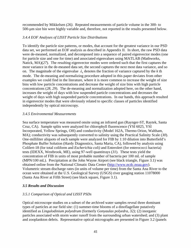
recommended by Mikkelsen (26). Repeated measurements of particle volume in the 300- to 500-µm size bin were highly variable and, therefore, not reported in the results presented below. 3.4.4 EOF Analyses of LISST Particle Size Distributions To identify the particle size patterns, or modes, that account for the greatest variance in our PSD data set, we performed an EOF analysis as described in Appendix II. In short, the raw PSD data were de-meaned, normalized, and decomposed into a sequence of paired eigenvector modes (one for particle size and one for time) and associated eigenvalues using MATLAB (Mathworks, Natick, MA)(27). The resulting eigenvector modes were ordered such that the first captures the most variance in the de-meaned data set, the second captures the next most data variance, and so on. The magnitude of the eigenvalue λk denotes the fraction of variance captured by the k th mode. The de-meaning and normalizing procedure adopted in this paper deviates from other examples we could find in the literature, where it is more common to increase the weight of size bins with low particle concentrations and decrease the weight of size bins with high particle concentrations (28, 29). The de-meaning and normalization adopted here, on the other hand, increases the weight of days with low suspended particle concentrations and decreases the weight of days with high suspended particle concentrations. In our hands, this approach resulted in eigenvector modes that were obviously related to specific classes of particles identified independently by optical microscopy. 3.4.5 Environmental Measurements Sea surface temperature was measured onsite using an infrared gun (Raynger-ST, Raytek, Santa Cruz, CA). Sample splits were analyzed for chlorophyll fluorescence (YSI 6025, YSI Incorporated, Yellow Springs, OH) and conductivity (Model 162A, Thermo Orion, Waltham, MA); conductivity was subsequently converted to salinity using the Practical Salinity Scale (30). One-milliliter aliquots of each sample were analyzed for FIB by 1:10 dilution into Butterfield’s Phosphate Buffer Solution (Hardy Diagnostics, Santa Maria, CA), followed by analysis using Colilert-18 (for total coliform and Escherichia coli) and Enterolert (for enterococci bacteria) tests (IDEXX, Westbrook, ME), using 97-well quantitrays (31). These tests yield the concentration of FIB in units of most probable number of bacteria per 100 mL of sample (MPN/100 mL). Precipitation at the John Wayne Airport (see black triangle, Figure 3.1) was obtained online from the National Climatic Data Center (http://www.ncdc.noaa.gov). Volumetric stream discharge rates (in units of volume per time) from the Santa Ana River to the ocean were obtained at the U.S. Geological Survey (USGS) river gauging station 11078000 (Santa Ana River at Fifth Street) (see black square, Figure 3.1). 3.5 Results and Discussion 3.5.1 Comparison of Optical and LISST PSDs Optical microscope studies on a subset of the archived water samples reveal three dominant types of particles at our field site: (1) summer-time blooms of a dinoflagellate putatively identified as Lingulodinium polyedrum (formerly Gonyaulax polyedra, 32); (2) inorganic particles associated with storm water runoff from the surrounding urban watershed; and (3) plant and zooplankton debris. Representative optical micrographs are presented in Figure 3.2 (panels
41
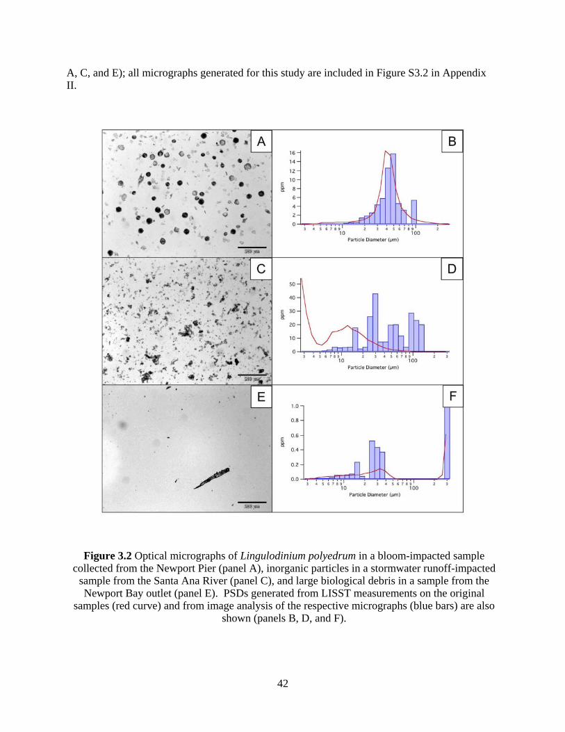
A, C, and E); all micrographs generated for this study are included in Figure S3.2 in Appendix II.
Figure 3.2 Optical micrographs of Lingulodinium polyedrum in a bloom-impacted sample collected from the Newport Pier (panel A), inorganic particles in a stormwater runoff-impacted
sample from the Santa Ana River (panel C), and large biological debris in a sample from the Newport Bay outlet (panel E). PSDs generated from LISST measurements on the original
samples (red curve) and from image analysis of the respective micrographs (blue bars) are also shown (panels B, D, and F).
42
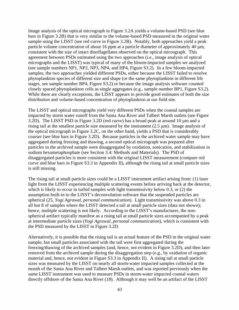
Image analysis of the optical micrograph in Figure 3.2A yields a volume-based PSD (see blue bars in Figure 3.2B) that is very similar to the volume-based PSD measured in the original water sample using the LISST (see red curve in Figure 3.2B). Notably, both approaches yield a peak particle volume concentration of about 16 ppm at a particle diameter of approximately 40 µm, consistent with the size of intact dinoflagellates observed on the optical micrograph. This agreement between PSDs estimated using the two approaches (i.e., image analysis of optical micrographs and the LISST) was typical of many of the bloom-impacted samples we analyzed (see sample numbers NP1, NP2, NP3, NP4, and HP4, Figure S3.2). In a few bloom-impacted samples, the two approaches yielded different PSDs, either because the LISST failed to resolve phytoplankton species of different size and shape (or the same phytoplankton in different life stages, see sample number BP4, Figure S3.2) or because the image analysis software counted closely spaced phytoplankton cells as single aggregates (e.g., sample number BP1, Figure S3.2). While there are clearly exceptions, the LISST appears to provide good estimates of both the size distribution and volume-based concentration of phytoplankton at our field site. The LISST and optical micrographs yield very different PSDs when the coastal samples are impacted by storm water runoff from the Santa Ana River and Talbert Marsh outlets (see Figure 3.2D). The LISST PSD in Figure 3.2D (red curve) has a broad peak at around 10 µm and a rising tail at the smallest particle size measured by the instrument (2.5 µm). Image analysis of the optical micrograph in Figure 3.2C, on the other hand, yields a PSD that is considerably coarser (see blue bars in Figure 3.2D). Because particles in the archived water sample may have aggregated during freezing and thawing, a second optical micrograph was prepared after particles in the archived sample were disaggregated by oxidation, sonication, and stabilization in sodium hexametaphosphate (see Section 3.4: Methods and Materials). The PSD of disaggregated particles is more consistent with the original LISST measurement (compare red curve and blue bars in Figure S3.3 in Appendix II), although the rising tail at small particle sizes is still missing. The rising tail at small particle sizes could be a LISST instrument artifact arising from: (1) laser light from the LISST experiencing multiple scattering events before arriving back at the detector, which is likely to occur in turbid samples with light transmissivity below 0.3, or (2) the assumption built-in to the LISST’s deconvolution software that the suspended particles are spherical (25, Yogi Agrawal, personal communication). Light transmissivity was above 0.3 in all but 8 of samples where the LISST detected a tail at small particle sizes (data not shown); hence, multiple scattering is not likely. According to the LISST’s manufacturer, the non-spherical artifact typically manifest as a rising tail at small particle sizes accompanied by a peak at intermediate particle sizes (Yogi Agrawal, personal communication), which is consistent with the PSD measured by the LISST in Figure 3.2D. Alternatively, it is possible that the rising tail is an actual feature of the PSD in the original water sample, but small particles associated with the tail were first aggregated during the freezing/thawing of the archived samples (and, hence, not evident in Figure 3.2D), and then later removed from the archived sample during the disaggregation step (e.g., by oxidation of organic material and, hence, not evident in Figure S3.3 in Appendix II). A rising tail at small particle sizes was measured by the LISST on nearly all storm-water impacted samples collected at the mouth of the Santa Ana River and Talbert Marsh outlets, and was reported previously when the same LISST instrument was used to measure PSDs in storm-water impacted coastal waters directly offshore of the Santa Ana River (18). Although it may well be an artifact of the LISST
43
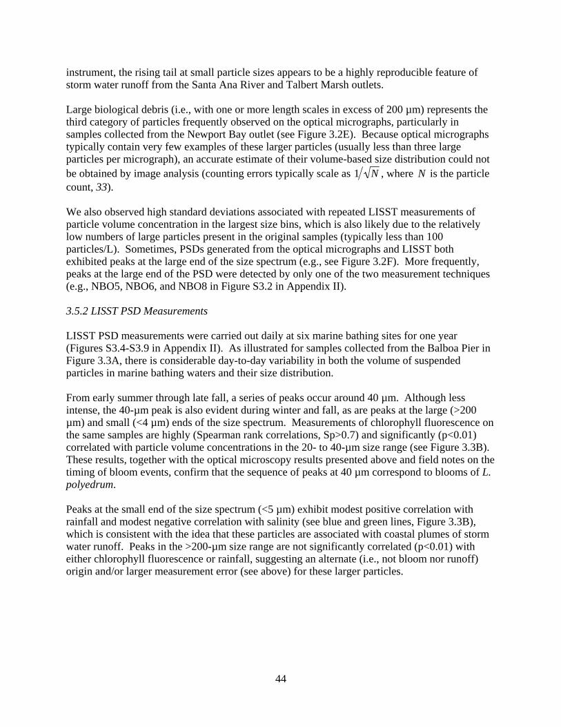
instrument, the rising tail at small particle sizes appears to be a highly reproducible feature of storm water runoff from the Santa Ana River and Talbert Marsh outlets. Large biological debris (i.e., with one or more length scales in excess of 200 µm) represents the third category of particles frequently observed on the optical micrographs, particularly in samples collected from the Newport Bay outlet (see Figure 3.2E). Because optical micrographs typically contain very few examples of these larger particles (usually less than three large particles per micrograph), an accurate estimate of their volume-based size distribution could not be obtained by image analysis (counting errors typically scale as 1 N , where N is the particle count, 33). We also observed high standard deviations associated with repeated LISST measurements of particle volume concentration in the largest size bins, which is also likely due to the relatively low numbers of large particles present in the original samples (typically less than 100 particles/L). Sometimes, PSDs generated from the optical micrographs and LISST both exhibited peaks at the large end of the size spectrum (e.g., see Figure 3.2F). More frequently, peaks at the large end of the PSD were detected by only one of the two measurement techniques (e.g., NBO5, NBO6, and NBO8 in Figure S3.2 in Appendix II). 3.5.2 LISST PSD Measurements LISST PSD measurements were carried out daily at six marine bathing sites for one year (Figures S3.4-S3.9 in Appendix II). As illustrated for samples collected from the Balboa Pier in Figure 3.3A, there is considerable day-to-day variability in both the volume of suspended particles in marine bathing waters and their size distribution. From early summer through late fall, a series of peaks occur around 40 µm. Although less intense, the 40-µm peak is also evident during winter and fall, as are peaks at the large (>200 µm) and small (<4 µm) ends of the size spectrum. Measurements of chlorophyll fluorescence on the same samples are highly (Spearman rank correlations, Sp>0.7) and significantly (p<0.01) correlated with particle volume concentrations in the 20- to 40-µm size range (see Figure 3.3B). These results, together with the optical microscopy results presented above and field notes on the timing of bloom events, confirm that the sequence of peaks at 40 µm correspond to blooms of L. polyedrum. Peaks at the small end of the size spectrum (<5 µm) exhibit modest positive correlation with rainfall and modest negative correlation with salinity (see blue and green lines, Figure 3.3B), which is consistent with the idea that these particles are associated with coastal plumes of storm water runoff. Peaks in the >200-µm size range are not significantly correlated (p<0.01) with either chlorophyll fluorescence or rainfall, suggesting an alternate (i.e., not bloom nor runoff) origin and/or larger measurement error (see above) for these larger particles.
44
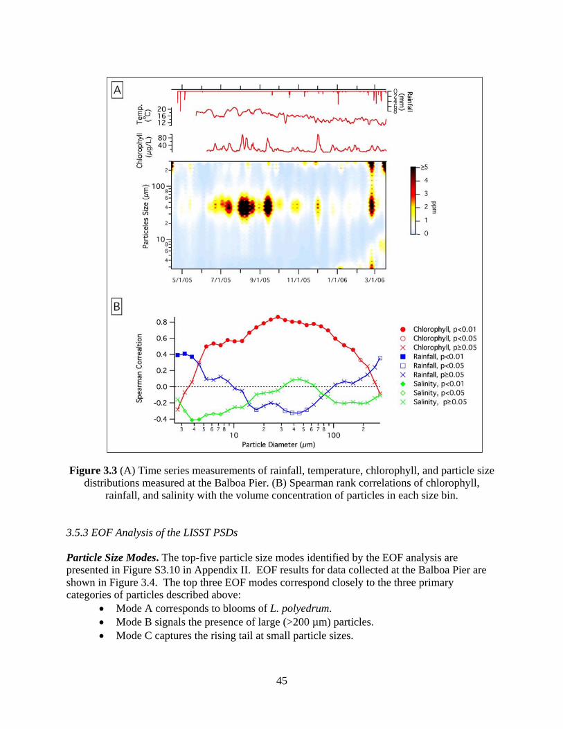
Figure 3.3 (A) Time series measurements of rainfall, temperature, chlorophyll, and particle size
distributions measured at the Balboa Pier. (B) Spearman rank correlations of chlorophyll, rainfall, and salinity with the volume concentration of particles in each size bin.
3.5.3 EOF Analysis of the LISST PSDs Particle Size Modes. The top-five particle size modes identified by the EOF analysis are presented in Figure S3.10 in Appendix II. EOF results for data collected at the Balboa Pier are shown in Figure 3.4. The top three EOF modes correspond closely to the three primary categories of particles described above:
• Mode A corresponds to blooms of L. polyedrum. • Mode B signals the presence of large (>200 µm) particles. • Mode C captures the rising tail at small particle sizes.
45
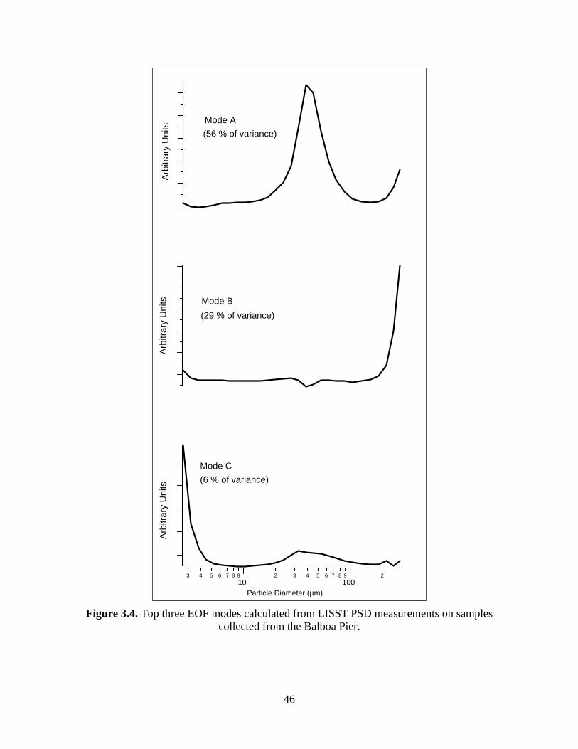
3 4 5 6 7 8 910
2 3 4 5 6 7 8 9100
2
Particle Diameter (µm)
Mode A
Mode B
Mode C
(56 % of variance)
(29 % of variance)
(6 % of variance)
Arb
itrar
y U
nits
A
rbitr
ary
Uni
ts
Arb
itrar
y U
nits
Figure 3.4. Top three EOF modes calculated from LISST PSD measurements on samples collected from the Balboa Pier.
46
These three modes are present, to a greater or lesser extent, at all sampling sites (see Figure S3.10 in Appendix II), where they capture between 91 and 94 percent of the data variance. Higher-order EOF modes exhibit significant site-to-site variability, and appear to capture low-variance and site-specific features of the PSDs (Figure S3.10). Seasonal Patterns. Each EOF mode has an associated temporal eigenvector that indicates how the mode increases and decreases with time. Temporal eigenvectors for the top five modes at each sampling site are presented in Figures S3.11-S3.16 in Appendix II. As illustrated in Figure 3.5, the top three modes at the Balboa Pier exhibit distinct seasonal patterns. The bloom mode (Mode A) is most pronounced during the summer season, from June through October. The large particle mode (Mode B) is relatively weak during the summer and more pronounced from November through May. The rising tail mode (Mode C) peaks during storms in January and February. Mode A follows a nearly identical seasonal pattern at all sampling sites (Figure S3.17). Seasonal patterns for Modes B and C are also fairly consistent across sampling sites, although some site-to-site variability is evident (Figures S3.18 and S3.19). Spatial (Along-Shore) Trends. The amount of variance captured by the top three modes exhibit distinct alongshore trends. These alongshore trends appear to indicate where particles originate along the shore. For example, the variance captured by the bloom mode (Mode A) decreases in a down-coast direction, from 73 percent at the Huntington Pier to 16 percent at the Newport Bay outlet (Table 3.1), consistent with probability distributions of chlorophyll fluorescence that also exhibit a declining down-coast trend (Figure S3.20A). The variance captured by the large particle mode (Mode B), on the other hand, increases in a down-coast direction, from 17 percent at the Huntington Pier to 69 percent at the Newport Bay outlet (see Table 3.1). This last result is consistent with our earlier observation that large biological debris was most frequently observed in samples collected from the outlet of Newport Bay. The amount of variance captured by the small particle mode (Mode C) is highest at the Santa Ana River and Talbert Marsh outlets (approximately 13 percent of the variance at each site, Table 3.1), suggesting that this mode is associated with storm-water runoff from these two outlets. Indeed, probability distributions of salinity at the Santa Ana River and Talbert Marsh have long low-salinity tails (Figure S3.20B), reflecting the impact of storm water runoff on ocean water collected from these two sites. 3.5.4 Correlation between FIB and LISST Measurements At the Santa Ana River and Talbert Marsh outlets, FIB concentrations are significantly (p<0.05) and moderately (Sp=0.2 to 0.45) correlated with LISST measurements of the volume concentration of small particles (<20 µm) (Figure S3.21 in Appendix II). Because the size of single FIB cells (ca., 1 µm) is below the resolution of the LISST instrument (ca., 2.5 µm), it is unlikely that the LISST is detecting single FIB cells.
47
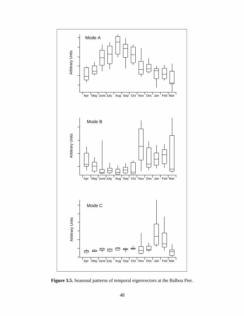
Apr May June July Aug Sep Oct Nov Dec Jan Feb Mar
Apr May June July Aug Sep Oct Nov Dec Jan Feb Mar
Mode A
Mode B
Mode C
Apr May June July Aug Sep Oct Nov Dec Jan Feb Mar
Arb
itrar
y U
nits
A
rbitr
ary
Uni
ts
Arb
itrar
y U
nits
Figure 3.5. Seasonal patterns of temporal eigenvectors at the Balboa Pier.
48
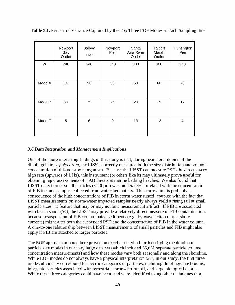
Table 3.1. Percent of Variance Captured by the Top Three EOF Modes at Each Sampling Site
3.6 Data Integration and Management Implications One of the more interesting findings of this study is that, during nearshore blooms of the dinoflagellate L. polyedrum, the LISST correctly measured both the size distribution and volume concentration of this non-toxic organism. Because the LISST can measure PSDs in situ at a very high rate (upwards of 1 Hz), this instrument (or others like it) may ultimately prove useful for obtaining rapid assessments of HAB threats at marine bathing beaches. We also found that LISST detection of small particles (< 20 µm) was moderately correlated with the concentration of FIB in some samples collected from watershed outlets. This correlation is probably a consequence of the high concentrations of FIB in storm water runoff, coupled with the fact that LISST measurements on storm-water impacted samples nearly always yield a rising tail at small particle sizes – a feature that may or may not be a measurement artifact. If FIB are associated with beach sands (34), the LISST may provide a relatively direct measure of FIB contamination, because resuspension of FIB contaminated sediments (e.g., by wave action or nearshore currents) might alter both the suspended PSD and the concentration of FIB in the water column. A one-to-one relationship between LISST measurements of small particles and FIB might also apply if FIB are attached to larger particles. The EOF approach adopted here proved an excellent method for identifying the dominant particle size modes in our very large data set (which included 55,651 separate particle volume concentration measurements) and how these modes vary both seasonally and along the shoreline. While EOF modes do not always have a physical interpretation (27), in our study, the first three modes obviously correspond to specific categories of particles, including dinoflagellate blooms, inorganic particles associated with terrestrial stormwater runoff, and large biological debris. While these three categories could have been, and were, identified using other techniques (e.g.,
4 13 13 9 6 5 Mode C
69
16
296
Newport Bay
Outlet
29
56
340
Balboa
Pier
25
59
340
Newport Pier
20
59
303
Santa Ana River
Outlet
17 19 Mode B
73 60 Mode A
340 300
Talbert Marsh Outlet
Huntington Pier
N
49
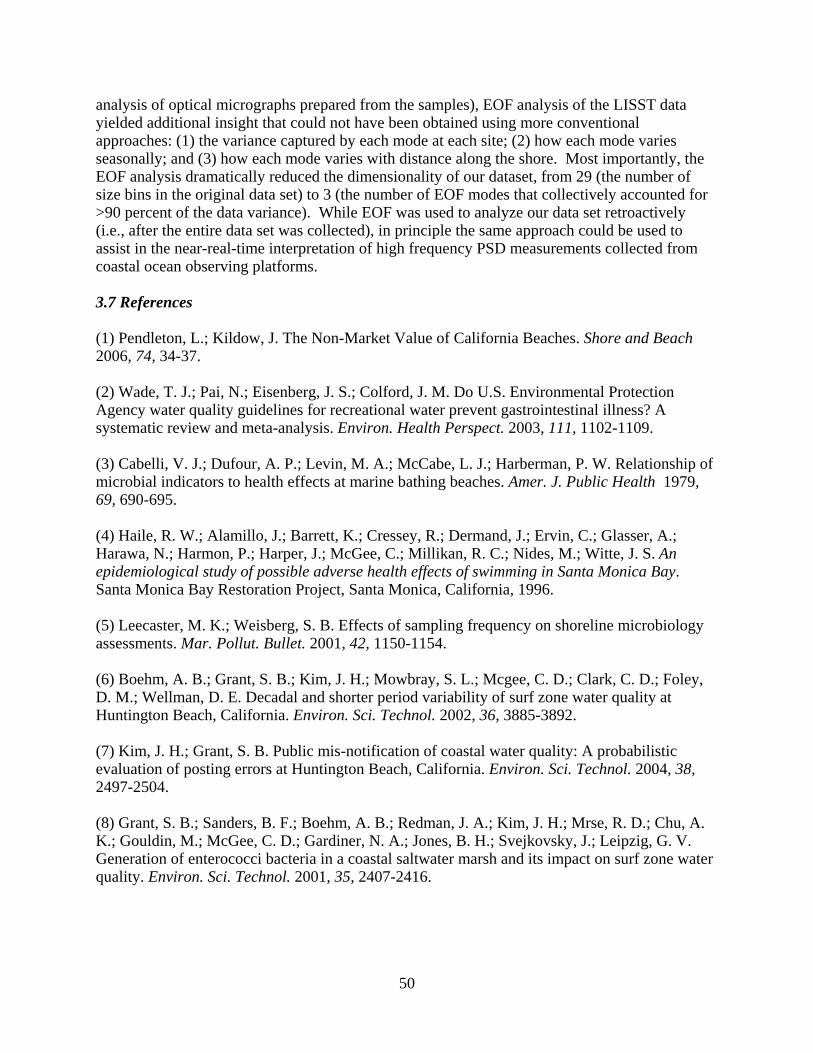
analysis of optical micrographs prepared from the samples), EOF analysis of the LISST data yielded additional insight that could not have been obtained using more conventional approaches: (1) the variance captured by each mode at each site; (2) how each mode varies seasonally; and (3) how each mode varies with distance along the shore. Most importantly, the EOF analysis dramatically reduced the dimensionality of our dataset, from 29 (the number of size bins in the original data set) to 3 (the number of EOF modes that collectively accounted for >90 percent of the data variance). While EOF was used to analyze our data set retroactively (i.e., after the entire data set was collected), in principle the same approach could be used to assist in the near-real-time interpretation of high frequency PSD measurements collected from coastal ocean observing platforms. 3.7 References (1) Pendleton, L.; Kildow, J. The Non-Market Value of California Beaches. Shore and Beach 2006, 74, 34-37. (2) Wade, T. J.; Pai, N.; Eisenberg, J. S.; Colford, J. M. Do U.S. Environmental Protection Agency water quality guidelines for recreational water prevent gastrointestinal illness? A systematic review and meta-analysis. Environ. Health Perspect. 2003, 111, 1102-1109. (3) Cabelli, V. J.; Dufour, A. P.; Levin, M. A.; McCabe, L. J.; Harberman, P. W. Relationship of microbial indicators to health effects at marine bathing beaches. Amer. J. Public Health 1979, 69, 690-695. (4) Haile, R. W.; Alamillo, J.; Barrett, K.; Cressey, R.; Dermand, J.; Ervin, C.; Glasser, A.; Harawa, N.; Harmon, P.; Harper, J.; McGee, C.; Millikan, R. C.; Nides, M.; Witte, J. S. An epidemiological study of possible adverse health effects of swimming in Santa Monica Bay. Santa Monica Bay Restoration Project, Santa Monica, California, 1996. (5) Leecaster, M. K.; Weisberg, S. B. Effects of sampling frequency on shoreline microbiology assessments. Mar. Pollut. Bullet. 2001, 42, 1150-1154. (6) Boehm, A. B.; Grant, S. B.; Kim, J. H.; Mowbray, S. L.; Mcgee, C. D.; Clark, C. D.; Foley, D. M.; Wellman, D. E. Decadal and shorter period variability of surf zone water quality at Huntington Beach, California. Environ. Sci. Technol. 2002, 36, 3885-3892. (7) Kim, J. H.; Grant, S. B. Public mis-notification of coastal water quality: A probabilistic evaluation of posting errors at Huntington Beach, California. Environ. Sci. Technol. 2004, 38, 2497-2504. (8) Grant, S. B.; Sanders, B. F.; Boehm, A. B.; Redman, J. A.; Kim, J. H.; Mrse, R. D.; Chu, A. K.; Gouldin, M.; McGee, C. D.; Gardiner, N. A.; Jones, B. H.; Svejkovsky, J.; Leipzig, G. V. Generation of enterococci bacteria in a coastal saltwater marsh and its impact on surf zone water quality. Environ. Sci. Technol. 2001, 35, 2407-2416.
50
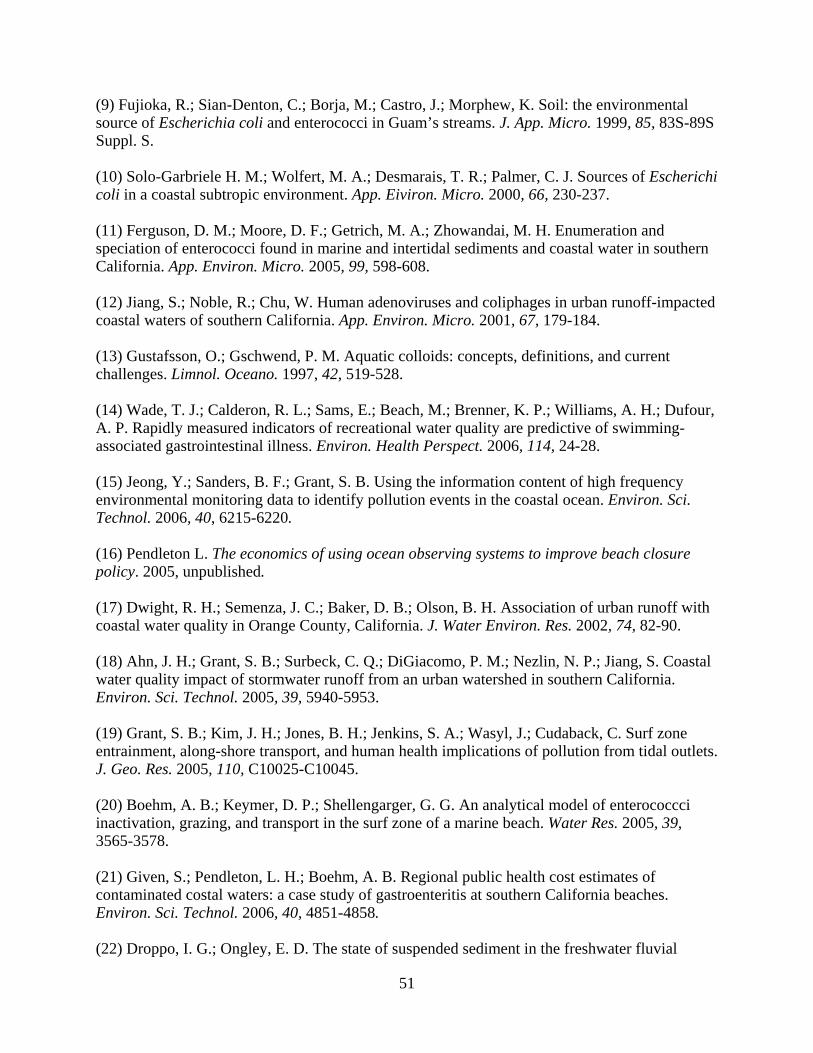
(9) Fujioka, R.; Sian-Denton, C.; Borja, M.; Castro, J.; Morphew, K. Soil: the environmental source of Escherichia coli and enterococci in Guam’s streams. J. App. Micro. 1999, 85, 83S-89S Suppl. S. (10) Solo-Garbriele H. M.; Wolfert, M. A.; Desmarais, T. R.; Palmer, C. J. Sources of Escherichi coli in a coastal subtropic environment. App. Eiviron. Micro. 2000, 66, 230-237. (11) Ferguson, D. M.; Moore, D. F.; Getrich, M. A.; Zhowandai, M. H. Enumeration and speciation of enterococci found in marine and intertidal sediments and coastal water in southern California. App. Environ. Micro. 2005, 99, 598-608. (12) Jiang, S.; Noble, R.; Chu, W. Human adenoviruses and coliphages in urban runoff-impacted coastal waters of southern California. App. Environ. Micro. 2001, 67, 179-184. (13) Gustafsson, O.; Gschwend, P. M. Aquatic colloids: concepts, definitions, and current challenges. Limnol. Oceano. 1997, 42, 519-528. (14) Wade, T. J.; Calderon, R. L.; Sams, E.; Beach, M.; Brenner, K. P.; Williams, A. H.; Dufour, A. P. Rapidly measured indicators of recreational water quality are predictive of swimming-associated gastrointestinal illness. Environ. Health Perspect. 2006, 114, 24-28. (15) Jeong, Y.; Sanders, B. F.; Grant, S. B. Using the information content of high frequency environmental monitoring data to identify pollution events in the coastal ocean. Environ. Sci. Technol. 2006, 40, 6215-6220. (16) Pendleton L. The economics of using ocean observing systems to improve beach closure policy. 2005, unpublished. (17) Dwight, R. H.; Semenza, J. C.; Baker, D. B.; Olson, B. H. Association of urban runoff with coastal water quality in Orange County, California. J. Water Environ. Res. 2002, 74, 82-90. (18) Ahn, J. H.; Grant, S. B.; Surbeck, C. Q.; DiGiacomo, P. M.; Nezlin, N. P.; Jiang, S. Coastal water quality impact of stormwater runoff from an urban watershed in southern California. Environ. Sci. Technol. 2005, 39, 5940-5953. (19) Grant, S. B.; Kim, J. H.; Jones, B. H.; Jenkins, S. A.; Wasyl, J.; Cudaback, C. Surf zone entrainment, along-shore transport, and human health implications of pollution from tidal outlets. J. Geo. Res. 2005, 110, C10025-C10045. (20) Boehm, A. B.; Keymer, D. P.; Shellengarger, G. G. An analytical model of enterococcci inactivation, grazing, and transport in the surf zone of a marine beach. Water Res. 2005, 39, 3565-3578. (21) Given, S.; Pendleton, L. H.; Boehm, A. B. Regional public health cost estimates of contaminated costal waters: a case study of gastroenteritis at southern California beaches. Environ. Sci. Technol. 2006, 40, 4851-4858. (22) Droppo, I. G.; Ongley, E. D. The state of suspended sediment in the freshwater fluvial
51
52
environment: A method of analysis. Water Res. 1992, 26, 65-72. (23) Phillips, J. M.; Walling, D. E. The particle size characteristics of fine-grained channel deposits in the River Exe Basin, Devon, UK. Hydro. Pros. 1999, 13, 1-19. (24) Agrawal, Y. C.; Pottsmith, H. C. Laser diffraction particle sizing in STRESS. Cont. Shelf Res. 1994, 14, 1101-1109. (25) Agrawal, Y. C.; Pottsmith, H. C. Instrument for particle size and settling velocity observation in sediment transport. Mar. Geo. 2000, 168, 89-114. (26) Mikkelsen, O. A. Example of spatial and temporal variations of some fine-grained suspended particle characteristics in two Danish coastal water bodies. Oceanologica Acta. 2002, 25, 39-49. (27) Emery, W. J.; Thomson, R. E. Data Analysis Methods in Physical Oceanography, 2nd Edition. Elsevier, Amsterdam, 2001. (28) Kitchen, J. C.; Menzies, D.; Pak, H.; Zaneveld, R. V. Particle size distributions in a region of coastal upwelling analyzed by characteristic vectors. Limnol. Oceano. 1975, 20, 775-783. (29) Liu, J. T.; Liu, K.; Huang, J. C. The effect of a submarine canyon on the river sediment disposal and inner shelf sediment movements in southern Taiwan. Mar. Geo. 2002, 181, 357-386. (30) Perkin, R. G.; Lewis, E. L. The practical salinity scale 1979: Fitting the data. IEEE J. Oceanic Eng. 1980, OE-5, 9-16. (31) Edberg, S. C.; Allen, M. J.; Smith, D. B.; Study, T. N. C. National field evaluation of a defined substrate method for the simultaneous enumeration of total coliforms and Escherichia coli from drinking water: comparison with the standard multiple tube fermentation method. Appl. Environ. Microbiol. 1988, 54, 1595-1601. (32) Honer, R. A. A Taxonomic Guide to Some Common Marine Phytoplankton. Biopress, United Kingdom, 2002. (33) Glaser, E. M.; Wilson, P. D. The coefficient of error of optical fractionator population size estimates: a computer simulation comparing three estimators. J. Microsc. 1998, 192, 163-171. (34) Lee, C. M.; Lin, T. Y.; Lin, C. C.; Kohbodi, G. A.; Bhatt, A.; Lee, R.; Jay, J. A. Persistence of fecal indicator bacteria in Santa Monica Bay beach sediments, Water Res. 2006, 40, 2593-2602.
53
4. Universality of Size Distribution of Suspended Particles Eroded from an Urban Watershed∗
4.1 Abstract In this study, we investigate the size distributions of suspended particles eroded from the Santa Ana River, a human-impacted “urban” river in Southern California. The occurrence and transport patterns of suspended particles in storm water runoff are highly variable storm-to-storm. Flow-controlled particle transport (channel erosion) was associated with the release of storm water from behind upstream dams, whereas bed-controlled particle transport (slope erosion) was associated with a mixture of storm water runoff from dam releases and local sub-drainages. The PSDs of suspended particles follow scaling laws (with a constant power-law exponent α ~ 2.1) that appear robust relative to transients within individual storms and across different storms. The emergence of “universal” scaling relationships has significant scientific implications, which can explain potentially long standing observation of total suspended solids and particle volume fraction and understand the connection between observation and conceptual erosion process. Practically speaking, the relationship challenges the efficacy of the current practice of treating the first flush of rainstorms and develops a knowledgebase for designing and managing urban coastal watersheds. 4.2 Introduction Global human migration toward the ocean has fueled an urbanization of the earth's coastal regions, replacing natural landscapes (rivers, fields, forests, and estuaries) with urban civil infrastructure (canals, roadways, residential communities, and commercial land-uses). Coastal urbanization has the potential to dramatically alter the flow of material from the land into the ocean, with consequent impacts on coastline stability, biogeochemical cycling, and the health of near-shore ecosystems. The shedding of sediment and fine particles, in particular, increases in response to watershed urbanization (1,2). Given the complexity of the urban watershed from which these particles were eroded, we hypothesized that the PSDs harbor the occurrence and transport patterns of suspended particles in storm water runoff and explain the connection between observation and conceptual erosion process. To test this hypothesis, field studies were conducted in the Santa Ana River – a human-impacted “urban” river – to characterize PSDs of suspended particles in storm water runoff during three episodic storm events in the 2003-2004 winter season. 4.3 Site Description The Santa Ana River watershed includes 6,915 km2 of land bordering the Pacific Ocean between the Cities of Los Angeles and San Diego in Southern California (Figure 4.1). This highly urbanized watershed is home to 10 million people, and includes the Santa Ana River drainage basin and a few small streams located near the coast, most of which drain to the ocean.
∗ This chapter is an excerpt of the dissertation Ahn, J. H. (2007). Size Distribution, Sources, and Transport of Suspended Particles Along An Inland-to-Ocean Transect. University of California, Irvine.
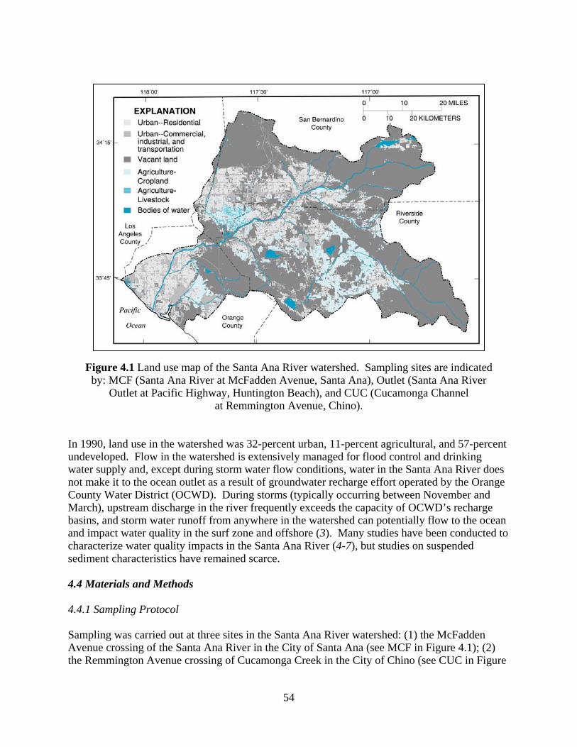
54
Figure 4.1 Land use map of the Santa Ana River watershed. Sampling sites are indicated by: MCF (Santa Ana River at McFadden Avenue, Santa Ana), Outlet (Santa Ana River
Outlet at Pacific Highway, Huntington Beach), and CUC (Cucamonga Channel at Remmington Avenue, Chino).
In 1990, land use in the watershed was 32-percent urban, 11-percent agricultural, and 57-percent undeveloped. Flow in the watershed is extensively managed for flood control and drinking water supply and, except during storm water flow conditions, water in the Santa Ana River does not make it to the ocean outlet as a result of groundwater recharge effort operated by the Orange County Water District (OCWD). During storms (typically occurring between November and March), upstream discharge in the river frequently exceeds the capacity of OCWD’s recharge basins, and storm water runoff from anywhere in the watershed can potentially flow to the ocean and impact water quality in the surf zone and offshore (3). Many studies have been conducted to characterize water quality impacts in the Santa Ana River (4-7), but studies on suspended sediment characteristics have remained scarce. 4.4 Materials and Methods 4.4.1 Sampling Protocol Sampling was carried out at three sites in the Santa Ana River watershed: (1) the McFadden Avenue crossing of the Santa Ana River in the City of Santa Ana (see MCF in Figure 4.1); (2) the Remmington Avenue crossing of Cucamonga Creek in the City of Chino (see CUC in Figure
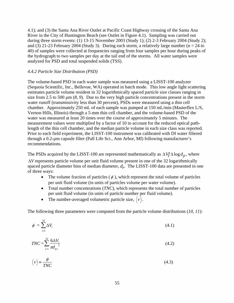
55
4.1); and (3) the Santa Ana River Outlet at Pacific Coast Highway crossing of the Santa Ana River in the City of Huntington Beach (see Outlet in Figure 4.1). Sampling was carried out during three storm events: (1) 13-15 November 2003 (Study 1); (2) 2-3 February 2004 (Study 2); and (3) 21-23 February 2004 (Study 3). During each storm, a relatively large number (n = 24 to 40) of samples were collected at frequencies ranging from four samples per hour during peaks of the hydrograph to two samples per day at the tail end of the storms. All water samples were analyzed for PSD and total suspended solids (TSS). 4.4.2 Particle Size Distribution (PSD) The volume-based PSD in each water sample was measured using a LISST-100 analyzer (Sequoia Scientific, Inc., Bellevue, WA) operated in batch mode. This low angle light scattering estimates particle volume resident in 32 logarithmically spaced particle size classes ranging in size from 2.5 to 500 µm (8, 9). Due to the very high particle concentrations present in the storm water runoff (transmissivity less than 30 percent), PSDs were measured using a thin cell chamber. Approximately 250 mL of each sample was pumped at 150 mL/min (Masterflex L/S, Vernon Hills, Illinois) through a 5-mm thin cell chamber, and the volume-based PSD of the water was measured at least 20 times over the course of approximately 5 minutes. The measurement values were multiplied by a factor of 10 to account for the reduced optical path-length of the thin cell chamber, and the median particle volume in each size class was reported. Prior to each field experiment, the LISST-100 instrument was calibrated with DI water filtered through a 0.2-µm capsule filter (Pall Life Sci., Ann Arbor, MI) following manufacturer’s recommendations. The PSDs acquired by the LISST-100 are represented mathematically as ΔV Δ log dp , where ΔV represents particle volume per unit fluid volume present in one of the 32 logarithmically spaced particle diameter bins of median diameter, dp. The LISST-100 data are presented in one of three ways:
• The volume fraction of particles ( φ ), which represent the total volume of particles per unit fluid volume (in units of particles volume per water volume).
• Total number concentrations (TNC), which represents the total number of particles per unit fluid volume (in units of particle number per fluid volume).
• The number-averaged volumetric particle size, ν . The following three parameters were computed from the particle volume distributions (10, 11):
φ = ΔVii=1
32
∑ (4.1)
TNC = 6ΔVi
πdp,i3
i=1
32
∑ (4.2)
ν =φ
TNC (4.3)
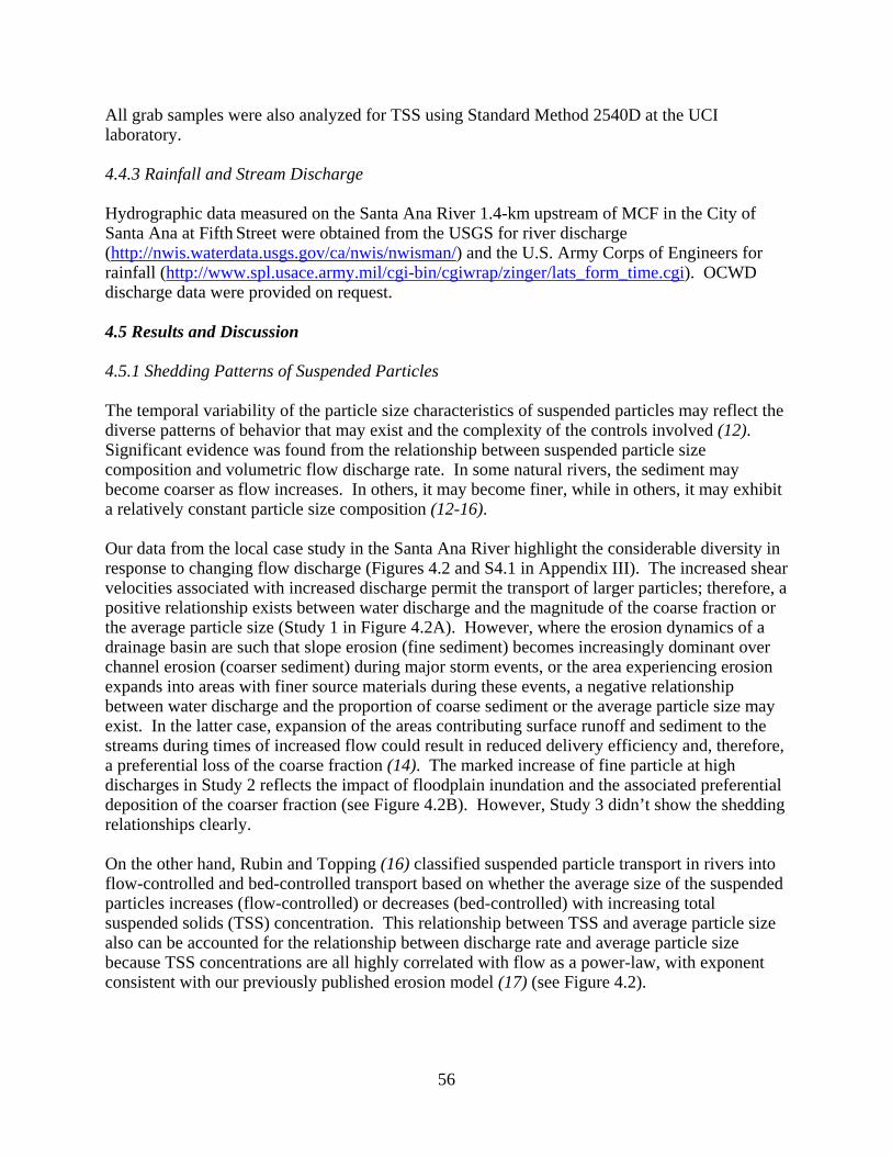
56
All grab samples were also analyzed for TSS using Standard Method 2540D at the UCI laboratory. 4.4.3 Rainfall and Stream Discharge Hydrographic data measured on the Santa Ana River 1.4-km upstream of MCF in the City of Santa Ana at Fifth
Street were obtained from the USGS for river discharge
(http://nwis.waterdata.usgs.gov/ca/nwis/nwisman/) and the U.S. Army Corps of Engineers for rainfall (http://www.spl.usace.army.mil/cgi-bin/cgiwrap/zinger/lats_form_time.cgi). OCWD discharge data were provided on request. 4.5 Results and Discussion 4.5.1 Shedding Patterns of Suspended Particles The temporal variability of the particle size characteristics of suspended particles may reflect the diverse patterns of behavior that may exist and the complexity of the controls involved (12). Significant evidence was found from the relationship between suspended particle size composition and volumetric flow discharge rate. In some natural rivers, the sediment may become coarser as flow increases. In others, it may become finer, while in others, it may exhibit a relatively constant particle size composition (12-16). Our data from the local case study in the Santa Ana River highlight the considerable diversity in response to changing flow discharge (Figures 4.2 and S4.1 in Appendix III). The increased shear velocities associated with increased discharge permit the transport of larger particles; therefore, a positive relationship exists between water discharge and the magnitude of the coarse fraction or the average particle size (Study 1 in Figure 4.2A). However, where the erosion dynamics of a drainage basin are such that slope erosion (fine sediment) becomes increasingly dominant over channel erosion (coarser sediment) during major storm events, or the area experiencing erosion expands into areas with finer source materials during these events, a negative relationship between water discharge and the proportion of coarse sediment or the average particle size may exist. In the latter case, expansion of the areas contributing surface runoff and sediment to the streams during times of increased flow could result in reduced delivery efficiency and, therefore, a preferential loss of the coarse fraction (14). The marked increase of fine particle at high discharges in Study 2 reflects the impact of floodplain inundation and the associated preferential deposition of the coarser fraction (see Figure 4.2B). However, Study 3 didn’t show the shedding relationships clearly. On the other hand, Rubin and Topping (16) classified suspended particle transport in rivers into flow-controlled and bed-controlled transport based on whether the average size of the suspended particles increases (flow-controlled) or decreases (bed-controlled) with increasing total suspended solids (TSS) concentration. This relationship between TSS and average particle size also can be accounted for the relationship between discharge rate and average particle size because TSS concentrations are all highly correlated with flow as a power-law, with exponent consistent with our previously published erosion model (17) (see Figure 4.2).
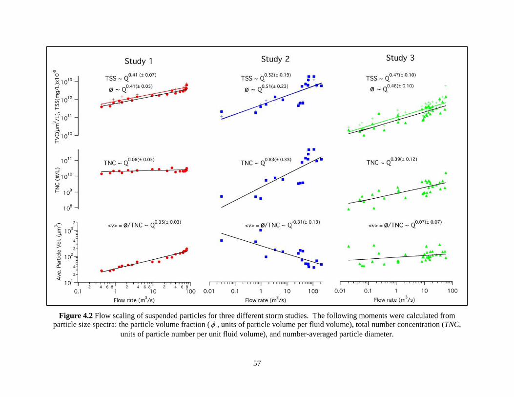
57
Figure 4.2 Flow scaling of suspended particles for three different storm studies. The following moments were calculated from particle size spectra: the particle volume fraction ( φ , units of particle volume per fluid volume), total number concentration (TNC,
units of particle number per unit fluid volume), and number-averaged particle diameter.
58
As presented in Figure 4.2, TSS, φ , and TNC are all highly correlated with flow as a power-law. Interestingly, TNC has a very sensitive power-law exponent (0.06 ~ 0.83), while both TSS and φ have relatively constant power-law exponents (0.41 ~ 0.52) over three different storms. Thus, flow scaling of TNC may apply for flow originating from local runoff compared to flow originating from reclamation releases upstream. In particular, the local runoff flow has a larger power-law exponent (0.83 in Study 2) compared to the reclamation-release dominated flow (0.06 in Study 1). The larger exponent is more consistent with slope erosion originating from expansion of the runoff area. 4.5.2 Volume Distributions of Suspended Particles The volume distributions of suspended particles collected at the surface of water column during the three different studies are shown in Figure 4.3A. Figure 4.3 (A) Volume distributions of suspended particles measured using a LISST-100 during the three storm studies. (B) Particle size spectra of suspended particles calculated from volume
distributions. The total amount of particle in suspension increased with increase of flow rate. Generally, at the low flow rate, the highest volume concentration of particles was in the finer particle size. At this stage, the volume distribution curves were strongly skewed during all studies.
5000
4000
3000
2000
1000
0
dV/d
(log
dp) (
µl/l/
µm)
3 4 5 6 7 8 9
102 3 4 5 6 7 8 9
1002 3 4
dp (µm)
14000
12000
10000
8000
6000
4000
2000
0
dV/d
(log
dp) (
µl/l/
µm)
3 4 5 6 7 8 9
102 3 4 5 6 7 8 9
1002 3 4
dp (µm)
1200
1000
800
600
400
200
0
dV/d
(log
dp) (
µl/l/
µm)
3 4 5 6 7 8 910
2 3 4 5 6 7 8 9100
2 3 4
dp (µm)
10-10
10-7
10-4 10
-1 102
105 108 10
11
n(υ)
(#/
l/µm
3 )
102
103
104
105
106
107
υ (μm3)
10-10
10
-7 10
-4 10
-1 102 105 108 10
11
n(υ)
(#/
l/µm
3 )
102
103
104
105
106
107
υ (μm3)
10-10
10
-7 10
-4 10
-1 102
105 108 10
11
n(υ)
(#/
l/µm
3 )
102
103
104
105
106
107
υ (μm3)
Study 1
Study 2
Study 3
1−α
0 1 10 50 200 cms
59
In Study 1, the volume distributions of suspended particles were markedly bimodal with a deflection point at about 5 µm. With increase of flow rate, as coarser particles were taken into suspension, one strong mode of volume distribution of particles shifted towards a larger particle size (from 10 to 300 µm), but another weaker mode was fixed at about 2.5 µm. In Study 2, the volume distribution of suspended particles showed three modes with one deflection point at about 5 µm and another deflection point at about 200 µm. Increase of flow rate did not change the strong mode of volume distribution of particle at about 150 μm. With an increase of flow rate, the proportion of finer particles increased considerably, leading to a decrease in the mean size of the suspended sediments. In Study 3, the volume distributions of suspended particles were also bimodal with an inflection point at about 5 µm, but increase of flow rate did not change the dominant peak of volume distribution of particle at about 250 µm. 4.5.3 Power Scaling of Particle Size Distributions (PSDs) To investigate the characteristics of PSD and its relationship with the sediment sorting mechanism during suspended sediment transportation over an urban watershed, this study was undertaken with a view to ascertain the physical condition under which the PSDs of suspended particles follow a power-law. As shown in Figure 4.3B, our field observations indicate that the particle population in storm waters has a size distribution that may be fitted by a power-law function (i.e., n[v]~v-α, where n[v] is the particle number distribution of particle volumetric size v, and α is defined as the slope of the size distribution). Physically, the power scaling of PSD means that PSD exhibits self-similar over a finite range of size. All moments of PSD will depend on sample volume and/or range over which PSD is measured (e.g., average particle size, TSS concentration, etc.). The power-law exponent also has some interesting hydro-geographical characteristics. Generally, the power-law exponent indicates the extent of dominant particle size in PSD: lower value indicates that coarser particles are dominant, while high value indicates that the finer particles are dominant. Also, in the point of view of sediment transport processes, the power-law exponent of PSD during storm may reflect a “sorting process” with along-channel transport. The power-law exponents (α) determined experimentally during three storm studies have different responses to increase of volumetric flow discharge rate (Figure 4.4A). In case of Study 1 (channel erosion or flow controlled), increasing flow (or increasing shear velocity) increases the suspension of coarser particles (decreasing α). On the other hand, in the case of Study 2 (slope erosion or bed controlled), increasing flow increases transport potential of fine particle eroded by greater dynamic contribution areas within the basins (increasing α). However, at the flow rate where the shear velocity exceed the settling velocity of the maximum particle size over a measurement size range, all the power-law exponents converge to one single value (~ 2.1) (see Figure 4.4B). It reflects that the environmental conditions do not significantly alter the PSD slope, although they may change the position of the PSD, and power scaling of suspended sediments in watershed environment system has its own self-organized characteristics wherever the sediment source come from. This feature – the signature of scale invariance – may have its dynamic origin in the self-organization of complex system (18-21).
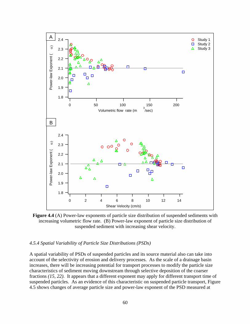
60
Figure 4.4 (A) Power-law exponents of particle size distribution of suspended sediments with increasing volumetric flow rate. (B) Power-law exponent of particle size distribution of
suspended sediment with increasing shear velocity. 4.5.4 Spatial Variability of Particle Size Distributions (PSDs) A spatial variability of PSDs of suspended particles and its source material also can take into account of the selectivity of erosion and delivery processes. As the scale of a drainage basin increases, there will be increasing potential for transport processes to modify the particle size characteristics of sediment moving downstream through selective deposition of the coarser fractions (15, 22). It appears that a different exponent may apply for different transport time of suspended particles. As an evidence of this characteristic on suspended particle transport, Figure 4.5 shows changes of average particle size and power-law exponent of the PSD measured at
2.4
2.3
2.2
2.1
2.0
1.9
1.8
Pow
er-la
w E
xpon
ent (
α)
200150100500Volumetric flow rate (m
3/sec)
2.4
2.3
2.2
2.1
2.0
1.9
1.8
Pow
er-la
w E
xpon
ent (
α)
14121086420Shear Velocity (cm/s)
Study 1 Study 2 Study 3
A
B
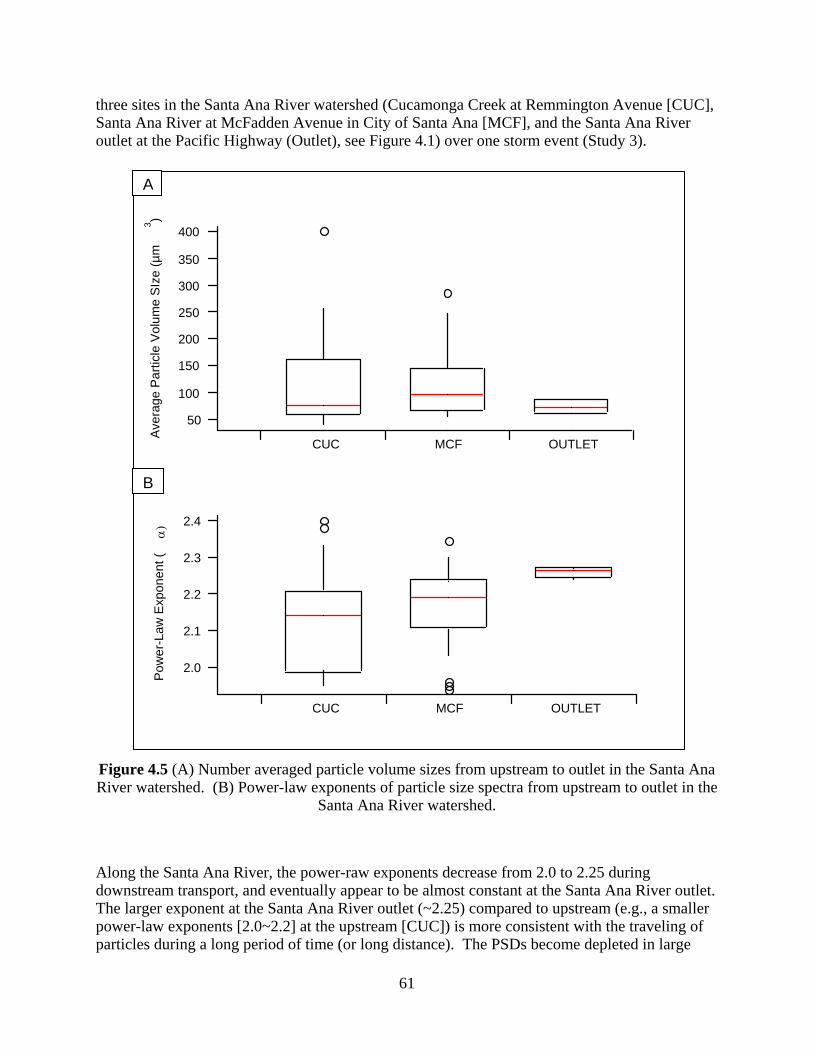
61
three sites in the Santa Ana River watershed (Cucamonga Creek at Remmington Avenue [CUC], Santa Ana River at McFadden Avenue in City of Santa Ana [MCF], and the Santa Ana River outlet at the Pacific Highway (Outlet), see Figure 4.1) over one storm event (Study 3). Figure 4.5 (A) Number averaged particle volume sizes from upstream to outlet in the Santa Ana River watershed. (B) Power-law exponents of particle size spectra from upstream to outlet in the
Santa Ana River watershed.
Along the Santa Ana River, the power-raw exponents decrease from 2.0 to 2.25 during downstream transport, and eventually appear to be almost constant at the Santa Ana River outlet. The larger exponent at the Santa Ana River outlet (~2.25) compared to upstream (e.g., a smaller power-law exponents [2.0~2.2] at the upstream [CUC]) is more consistent with the traveling of particles during a long period of time (or long distance). The PSDs become depleted in large
400
350
300
250
200
150
100
50
Ave
rage
Par
ticle
Vol
ume
SIz
e (µ
m3 )
CUC MCF OUTLET
2.4
2.3
2.2
2.1
2.0
Pow
er-L
aw E
xpon
ent (
α)
CUC MCF OUTLET
B
A
62
particles as suspended particles are transported long distances from their point of erosion to the point of measurement. The loss of large particles during transport could arise in several ways, including turbulence-induced fragmentation of large aggregates into smaller particles and/or the removal of large particles from the flow by gravitational sedimentation. The greater the distance suspended particles are transported during storm events, the more opportunity for alteration of PSDs increases. From this perspective, the power-law exponent of PSD may provide information about the amount of time (or distance) suspended particles are transported from their point of erosion to the point of measurement. 4.6 Implications Despite vast differences in particle properties and environmental conditions in different waters, the exponents of the size distribution are found to vary within a narrow range only, which is mainly from 2.0 to 2.25 over a single storm hydrograph at a single site, over three different storm hydrographs at a single site, and cross an inland-to-ocean transect during a single storm. This “universal” scaling relationship has significant scientific implications that can explain potentially longstanding observations of TSS and particle volume fraction and understand the connection between observation and conceptual erosion process. Also, the relationship challenges the efficacy of the current practice of treating the first flush of rainstorms and develops a knowledgebase for designing and managing urban coastal watersheds. It may possible to construct the entire PSD from knowledge of the volumetric flow rate alone. 4.7 References (1) Warrick, J. A.; Rubin, D. M. Suspended-sediment rating curve response to urbanization and wildfire, Santa Ana River, California. J. Geo. Res. 2007, 112, F02018, doi:10.1029/2006JF000662. (2) Trimble, S. W. Contribution of stream channel erosion to sediment yield from an urbanizing watershed, Science, 1997, 278, 1442-1444. (3) Ahn, J. H.; Grant, S. B.; Surbeck, C. Q.; DiGiacomo, P.; Nezlin, N.; Jiang, S. Coastal water quality impact of storm water runoff from an urban watershed in southern California, Environ. Sci. Technol., 2005, 35, 5940-5953. (4) Burton, C.; Izbicki, J. A.; Paybins, K. Water quality trends in the Santa Ana River at MWD crossing and below Prado Dam, Riverside County, California. U.S. Geological Survey Water Resources Investigation Report, 1998. (5) Reilly, J. F.; Horne, A. J.; Miller, C. D. Nitrate removal from a drinking water supply with large free-surface constructed wetlands prior to groundwater recharge, Ecol. Eng., 2000, 14, 33-47. (6) Leecaster, M. K.; Schiff, K.; Tiefenthaler, L. L. Assessment of efficient sampling designs for urban stormwater monitoring, Water Res., 2002, 36, 1556-1564. (7) Izbicki, J. A.; Pimentel, M. I.; Leddy, M.; Bergamaschi, B. Microbial and dissolved organic carbon characterization of stormflow in the Santa Ana River at Imperial Highway, southern
63
California, 1999-2002. U.S. Geological Survey Scientific Investigations Report, 2004. (8) Agrawal, Y. C.; Pottsmith, H. C. Laser diffraction particle sizing in STRESS, Cont. Shelf Res., 1994, 14, 1101-1109. (9) Agrawal, Y. C.; Pottsmith, H. C. Instrument for particle size and settling velocity observation in sediment transport, Mar. Geo., 2000, 168, 89-114 (10) Mikkelsen, O. A. Variation in the projected surface of suspended particles: Implications for remote sensing assessment of TSM, Rem. Sens. of Environ., 2002, 79, 23-29. (11) Serra, T.; Colmer, J.; Cristina, X. P.; Vila, X.; Arellano, J. B.; Casamitjana, X. J. Evaluation of laser in-situ instrument for measuring concentration of phytoplankton, purple sulfur bacteria, and suspended inorganic sediments in lakes, Environ. Eng., 2001, 11, 1023-1030. (12) Walling, D. E.; Moorehead, P. W. The particle size characteristics of fluvial suspended sediment: an overview, Hydrobiologia, 1989, 176/177, 125-149. (13) Kennedy, V. C. Sediment transported by Georgia streams, US Geological Survey Water Supply Paper, 1964, 1668. (14) Brown, W. M.; Ritter, J. R. Sediment transported and turbidity in the Eel River basin, California, US Geological Survey Water Supply Paper, 1971, 1986. (15) Long, Y.; Qian, N. Erosion and transportation of sediment in the Yellow River basin, Int. J. Sediment Res., 1986, 1, 2-38. (16) Rubin, D. M.; Topping, D. J. Quantifying the relative importance of flow regulation and grain size regulation of suspended sediment transport α and tracking changes in grain size of bed sediment β, Water Resources Res., 2001, 37, 133-146. (17) Reeves, R. L.; Grant, S. B.; Mrse, R. D.; Copil Oancea, C. M.; Sanders, B. F.; Boehm, A. B. Scaling and management of fecal indicator bacteria in runoff from a coastal urban watershed in southern California, Environ. Sci. Technol., 2004, 38, 2637-2648. (18) Bak, P. How nature works, The science of self-organized criticality; Copernicus-Springer: Berlin, 1997. (19) Rodriguez-Iturbe, I.; Rinaldo, A. Fractal river basins: chance and self-organization; Cambridge University Press: New York, 1997. (20) Levin, S. A. Fragile dominion: complexity and the commons; Perseus Books: Reding, MA, 1999. (21) Rinaldo, A.; Maritan, A.; Cavender-Bares, K. K.; Chisholm, S. W. Cross-scale ecological dynamics and microbial size spectra in marine ecosystems, Proc. R. Soc. Lond. B., 2002, 269, 2051-2059.

64
(22) Ball, J. Contribution to the geography of Egypt; Government Press: Cairo, Egypt, 1939.
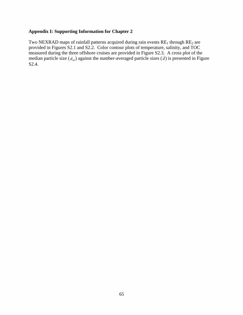
Appendix I: Supporting Information for Chapter 2 Two NEXRAD maps of rainfall patterns acquired during rain events RE1 through RE2 are provided in Figures S2.1 and S2.2. Color contour plots of temperature, salinity, and TOC measured during the three offshore cruises are provided in Figure S2.3. A cross plot of the median particle size ( d ) against the number-averaged particle sizes (50 d) is presented in Figure S2.4.
65
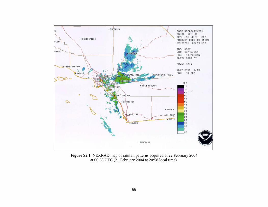
Figure S2.1. NEXRAD map of rainfall patterns acquired at 22 February 2004 at 06:58 UTC (21 February 2004 at 20:58 local time).
66
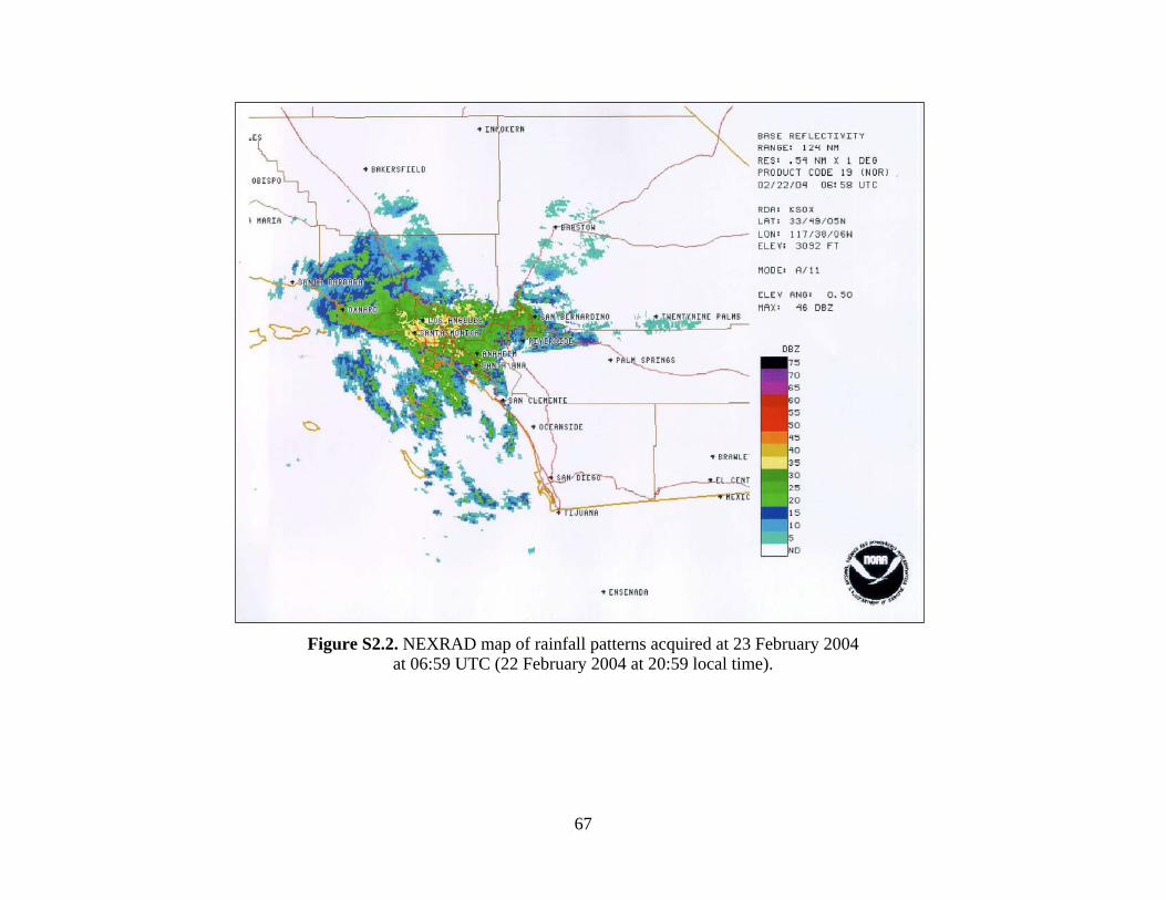
Figure S2.2. NEXRAD map of rainfall patterns acquired at 23 February 2004 at 06:59 UTC (22 February 2004 at 20:59 local time).
67
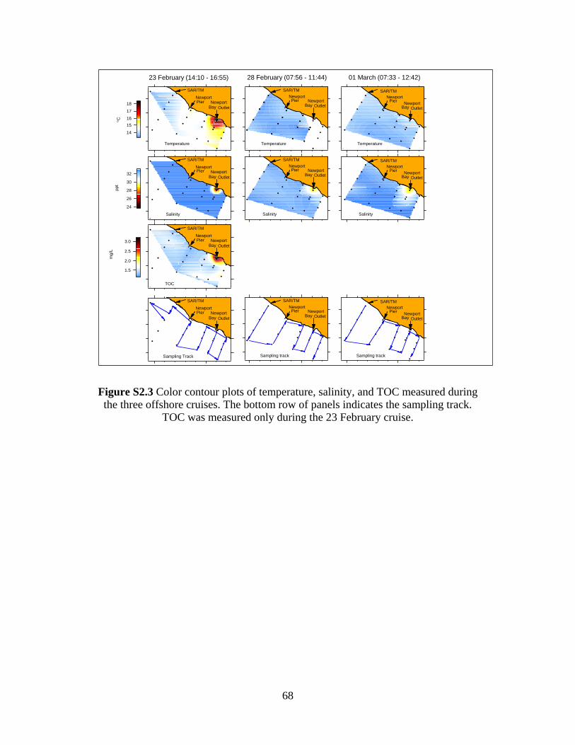
01 March (07:33 - 12:42)28 February (07:56 - 11:44)23 February (14:10 - 16:55)
Temperature
Salinity
Sampling track
SAR/TM
Pier NewportBay
Newport
Outlet
SAR/TM
Pier NewportBay
Newport
Outlet
SAR/TM
Pier NewportBay
Newport
Outlet
Temperature
Sampling track
Salinity
SAR/TM
Pier NewportBay
Newport
Outlet
SAR/TM
Pier NewportBay
Newport
Outlet
SAR/TM
Pier NewportBay
Newport
Outlet
Temperature
18
17
1615
14
oC
TOC
3.0
2.5
2.0
1.5
mg/
L
Salinity
32
30
28
26
24
ppt
Sampling Track
SAR/TM
NewportNewportPier
Bay Outlet
SAR/TM
NewportNewportPier
Bay Outlet
SAR/TM
NewportNewportPier
Bay Outlet
SAR/TM
NewportNewportPier
Bay Outlet
Figure S2.3 Color contour plots of temperature, salinity, and TOC measured during the three offshore cruises. The bottom row of panels indicates the sampling track.
TOC was measured only during the 23 February cruise.
68
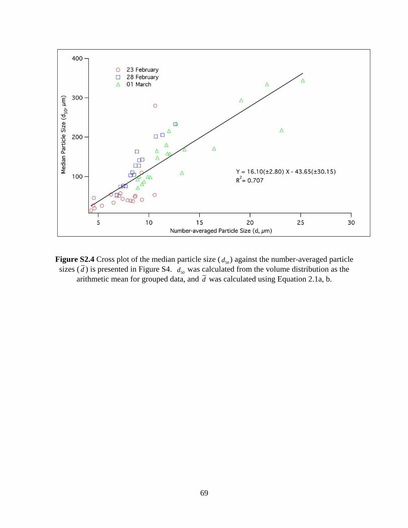
Figure S2.4 Cross plot of the median particle size ( d ) against the number-averaged particle sizes ( d
50
) is presented in Figure S4. was calculated from the volume distribution as the arithmetic mean for grouped data, and d
d50
was calculated using Equation 2.1a, b.
69
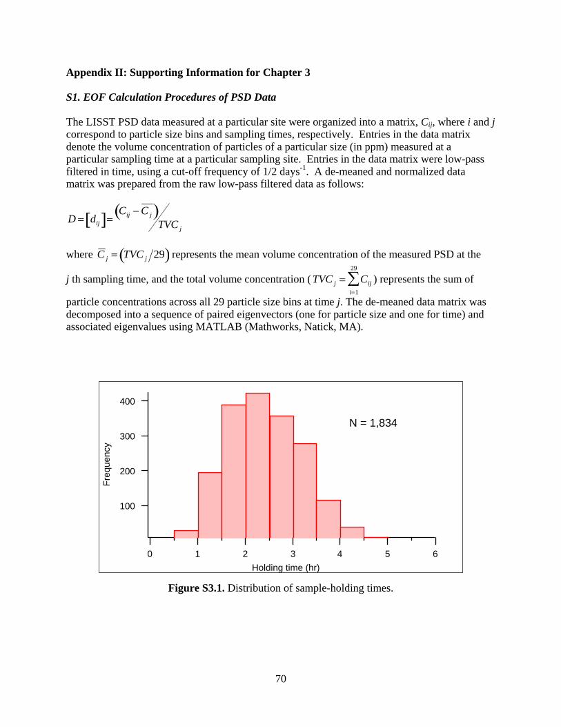
Appendix II: Supporting Information for Chapter 3 S1. EOF Calculation Procedures of PSD Data The LISST PSD data measured at a particular site were organized into a matrix, Cij, where i and j correspond to particle size bins and sampling times, respectively. Entries in the data matrix denote the volume concentration of particles of a particular size (in ppm) measured at a particular sampling time at a particular sampling site. Entries in the data matrix were low-pass filtered in time, using a cut-off frequency of 1/2 days-1. A de-meaned and normalized data matrix was prepared from the raw low-pass filtered data as follows:
D = dij[ ]= Cij −C j( )TVC j
where C j = TVC j 29( ) represents the mean volume concentration of the measured PSD at the
j th sampling time, and the total volume concentration ( TVC j = Ciji=1
29
∑ ) represents the sum of
particle concentrations across all 29 particle size bins at time j. The de-meaned data matrix was decomposed into a sequence of paired eigenvectors (one for particle size and one for time) and associated eigenvalues using MATLAB (Mathworks, Natick, MA).
400
300
200
100
Freq
uenc
y
6543210Holding time (hr)
N = 1,834
Figure S3.1. Distribution of sample-holding times.
70
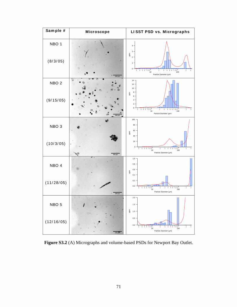
Sample # Microscope LISST PSD vs. Micrographs
NBO 1
(8/3/05)
4
3
2
1
0
ppm
3 4 5 6 7 8 9 2 3 4 5 6 7 8 9 210 100
3
Particle Diameter (µm)
NBO 2
(9/15/05)
14
12
10
8
6
4
2
0
ppm
3 4 5 6 7 8 9 2 3 4 5 6 7 8 9 210 100
3
Particle Diameter (µm)
NBO 3
(10/3/05)
100
80
60
40
20
0
ppm
3 4 5 6 7 8 9 2 3 4 5 6 7 8 9 210 100
3
Particle Diameter (µm)
NBO 4
(11/28/05)
1.0
0.8
0.6
0.4
0.2
0.0
ppm
3 4 5 6 7 8 9 2 3 4 5 6 7 8 9 210 100
3
Particle Diameter (µm)
NBO 5
(12/16/05)
2.0
1.5
1.0
0.5
0.0
ppm
3 4 5 6 7 8 9 2 3 4 5 6 7 8 9 210 100
3
Particle Diameter (µm)
Figure S3.2 (A) Micrographs and volume-based PSDs for Newport Bay Outlet.
71
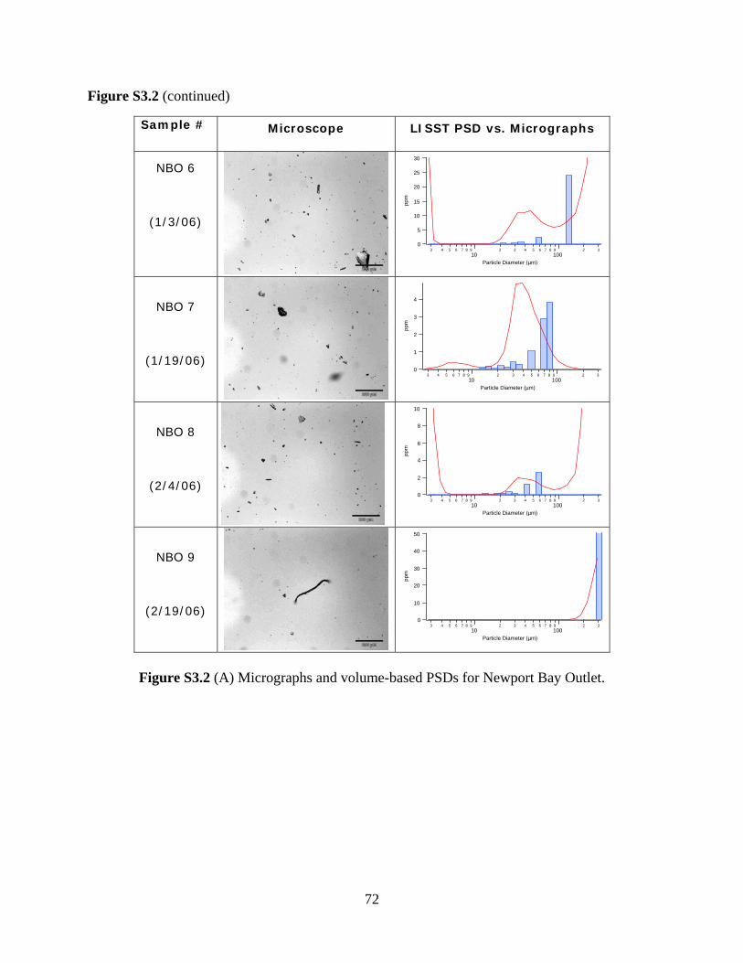
Figure S3.2 (continued)
Sample # Microscope LISST PSD vs. Micrographs
NBO 6
(1/3/06)
30
25
20
15
10
5
0
ppm
3 4 5 6 7 8 9 2 3 4 5 6 7 8 9 210 100
3
Particle Diameter (µm)
NBO 7
(1/19/06)
4
3
2
1
0
ppm
3 4 5 6 7 8 9 2 3 4 5 6 7 8 9 210 100
3
Particle Diameter (µm)
NBO 8
(2/4/06)
10
8
6
4
2
0
ppm
3 4 5 6 7 8 9 2 3 4 5 6 7 8 9 210 100
3
Particle Diameter (µm)
NBO 9
(2/19/06)
50
40
30
20
10
0
ppm
3 4 5 6 7 8 9 2 3 4 5 6 7 8 9 210 100
3
Particle Diameter (µm)
Figure S3.2 (A) Micrographs and volume-based PSDs for Newport Bay Outlet.
72
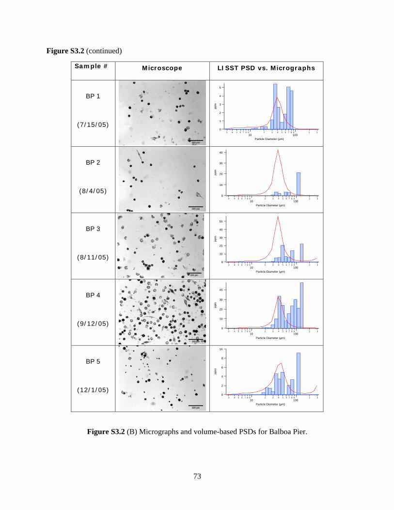
Figure S3.2 (continued)
Sample # Microscope LISST PSD vs. Micrographs
BP 1
(7/15/05)
5
4
3
2
1
0
ppm
3 4 5 6 7 8 9 2 3 4 5 6 7 8 9 210 100
3
Particle Diameter (µm)
BP 2
(8/4/05)
40
30
20
10
0
ppm
3 4 5 6 7 8 9 2 3 4 5 6 7 8 9 210 100
3
Particle Diameter (µm)
BP 3
(8/11/05)
50
40
30
20
10
0
ppm
3 4 5 6 7 8 9 2 3 4 5 6 7 8 9 210 100
3
Particle Diameter (µm)
BP 4
(9/12/05)
40
30
20
10
0
ppm
3 4 5 6 7 8 9 2 3 4 5 6 7 8 9 210 100
3
Particle Diameter (µm)
BP 5
(12/1/05)
10
8
6
4
2
0
ppm
3 4 5 6 7 8 9 2 3 4 5 6 7 8 9 210 100
3
Particle Diameter (µm)
Figure S3.2 (B) Micrographs and volume-based PSDs for Balboa Pier.
73
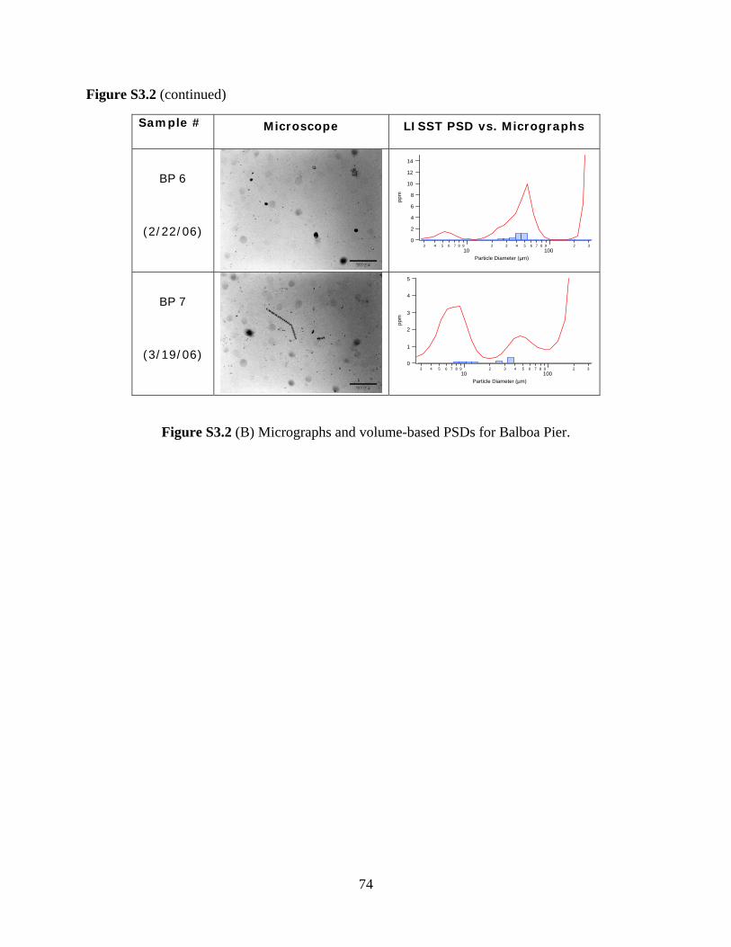
Figure S3.2 (continued)
Sample # Microscope LISST PSD vs. Micrographs
BP 6
(2/22/06)
14
12
10
8
6
4
2
0
ppm
3 4 5 6 7 8 9 2 3 4 5 6 7 8 9 210 100
3
Particle Diameter (µm)
BP 7
(3/19/06)
5
4
3
2
1
0
ppm
3 4 5 6 7 8 9 2 3 4 5 6 7 8 9 210 100
3
Particle Diameter (µm)
Figure S3.2 (B) Micrographs and volume-based PSDs for Balboa Pier.
74
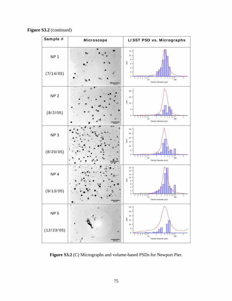
Figure S3.2 (continued)
Sample # Microscope LISST PSD vs. Micrographs
NP 1
(7/14/05)
12
10
8
6
4
2
0
ppm
3 4 5 6 7 8 9 2 3 4 5 6 7 8 910 100
2
Particle Diameter (µm)
NP 2
(8/2/05)
20
15
10
5
0
ppm
3 4 5 6 7 8 9 2 3 4 5 6 7 8 910 100
2
Particle Diameter (µm)
NP 3
(8/20/05)
30
25
20
15
10
5
0
ppm
3 4 5 6 7 8 9 2 3 4 5 6 7 8 910 100
2
Particle Diameter (µm)
NP 4
(9/13/05)
16
14
12
10
8
6
4
2
0
ppm
3 4 5 6 7 8 9 2 3 4 5 6 7 8 910 100
2
Particle Diameter (µm)
NP 5
(12/23/05)
30
25
20
15
10
5
0
ppm
3 4 5 6 7 8 9 2 3 4 5 6 7 8 910 100
2
Particle Diameter (µm)
Figure S3.2 (C) Micrographs and volume-based PSDs for Newport Pier.
75
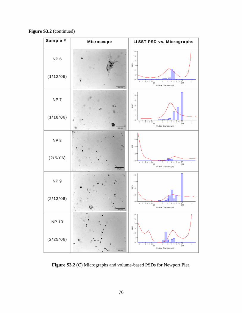
Figure S3.2 (continued)
Sample # Microscope LISST PSD vs. Micrographs
NP 6
(1/12/06)
6
5
4
3
2
1
0
ppm
3 4 5 6 7 8 9 2 3 4 5 6 7 8 910 100
2
Particle Diameter (µm)
NP 7
(1/18/06)
5
4
3
2
1
0
ppm
3 4 5 6 7 8 9 2 3 4 5 6 7 8 910 100
2
Particle Diameter (µm)
NP 8
(2/5/06)
6
4
2
0
ppm
3 4 5 6 7 8 9 2 3 4 5 6 7 8 910 100
2
Particle Diameter (µm)
NP 9
(2/13/06)
8
6
4
2
0
ppm
3 4 5 6 7 8 9 2 3 4 5 6 7 8 910 100
2
Particle Diameter (µm)
NP 10
(2/25/06)
6
5
4
3
2
1
0
ppm
3 4 5 6 7 8 9 2 3 4 5 6 7 8 910 100
2
Particle Diameter (µm)
Figure S3.2 (C) Micrographs and volume-based PSDs for Newport Pier.
76
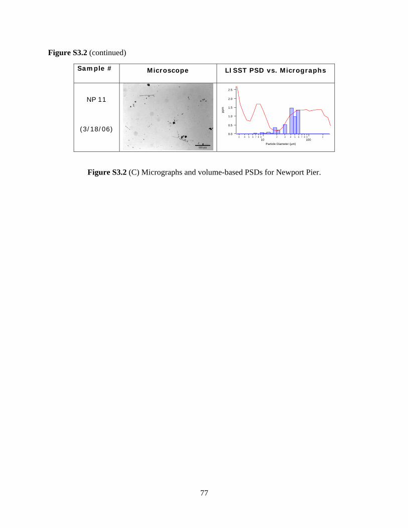
Figure S3.2 (continued)
Sample # Microscope LISST PSD vs. Micrographs
NP 11
(3/18/06)
2.5
2.0
1.5
1.0
0.5
0.0
ppm
3 4 5 6 7 8 9 2 3 4 5 6 7 8 910 100
2
Particle Diameter (µm)
Figure S3.2 (C) Micrographs and volume-based PSDs for Newport Pier.
77
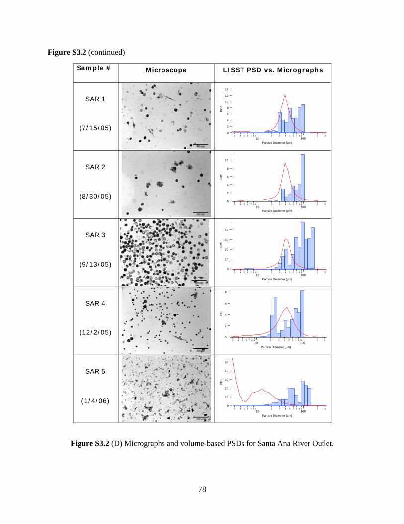
Figure S3.2 (continued)
Sample # Microscope LISST PSD vs. Micrographs
SAR 1
(7/15/05)
14
12
10
8
6
4
2
0
ppm
3 4 5 6 7 8 9 2 3 4 5 6 7 8 9 210 100
3
Particle Diameter (µm)
SAR 2
(8/30/05)
10
8
6
4
2
0
ppm
3 4 5 6 7 8 9 2 3 4 5 6 7 8 9 210 100
3
Particle Diameter (µm)
SAR 3
(9/13/05)
40
30
20
10
0
ppm
3 4 5 6 7 8 9 2 3 4 5 6 7 8 9 210 100
3
Particle Diameter (µm)
SAR 4
(12/2/05)
8
6
4
2
0
ppm
3 4 5 6 7 8 9 2 3 4 5 6 7 8 9 210 100
3
Particle Diameter (µm)
SAR 5
(1/4/06)
50
40
30
20
10
0
ppm
3 4 5 6 7 8 9 2 3 4 5 6 7 8 9 210 100
3
Particle Diameter (µm)
Figure S3.2 (D) Micrographs and volume-based PSDs for Santa Ana River Outlet.
78
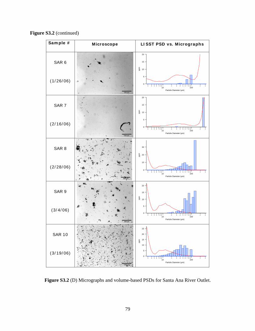
Figure S3.2 (continued)
Sample # Microscope LISST PSD vs. Micrographs
SAR 6
(1/26/06)
20
15
10
5
0
ppm
3 4 5 6 7 8 9 2 3 4 5 6 7 8 9 210 100
3
Particle Diameter (µm)
SAR 7
(2/16/06)
20
15
10
5
0
ppm
3 4 5 6 7 8 9 2 3 4 5 6 7 8 9 210 100
3
Particle Diameter (µm)
SAR 8
(2/28/06)
30
20
10
0
ppm
3 4 5 6 7 8 9 2 3 4 5 6 7 8 9 210 100
3
Particle Diameter (µm)
SAR 9
(3/4/06)
20
15
10
5
0
ppm
3 4 5 6 7 8 9 2 3 4 5 6 7 8 9 210 100
3
Particle Diameter (µm)
SAR 10
(3/19/06)
25
20
15
10
5
0
ppm
3 4 5 6 7 8 9 2 3 4 5 6 7 8 9 210 100
3
Particle Diameter (µm)
Figure S3.2 (D) Micrographs and volume-based PSDs for Santa Ana River Outlet.
79
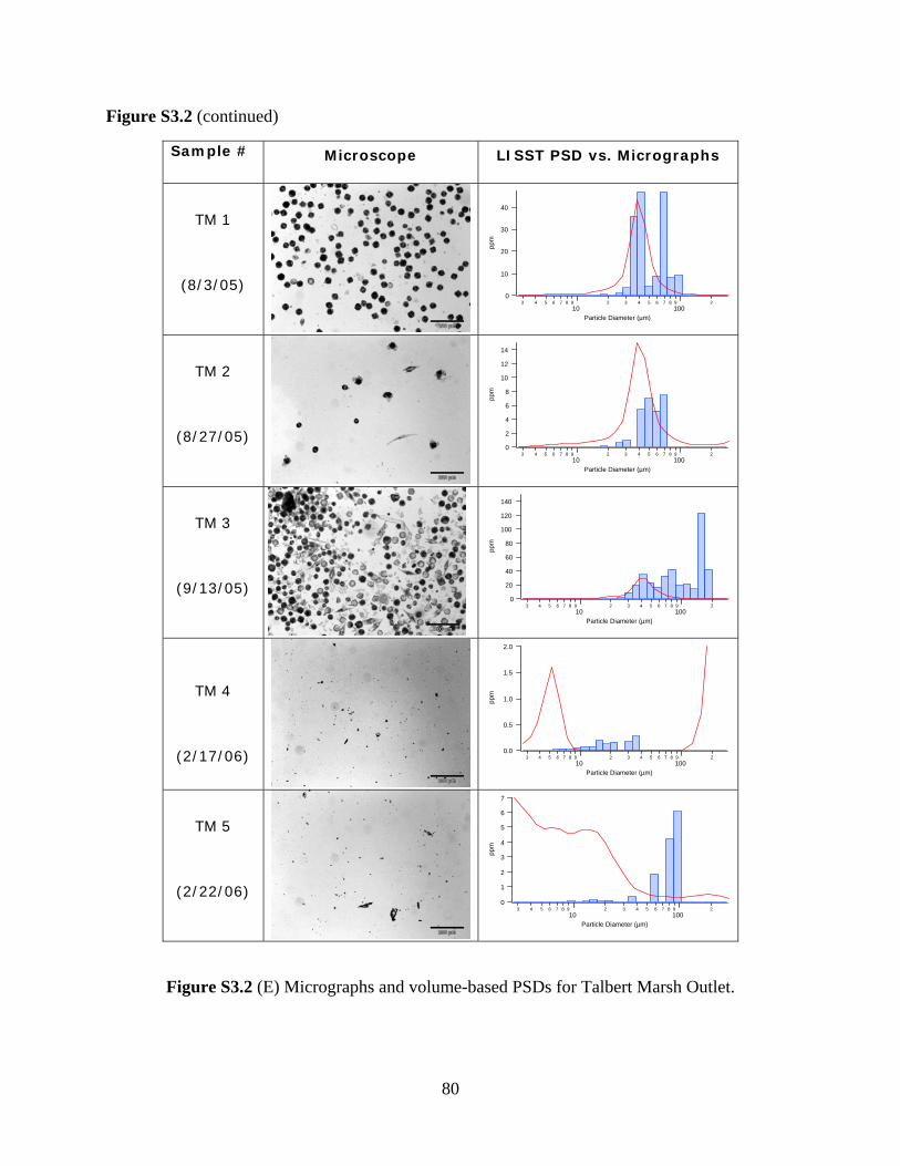
Figure S3.2 (continued)
Sample # Microscope LISST PSD vs. Micrographs
TM 1
(8/3/05)
40
30
20
10
0
ppm
3 4 5 6 7 8 9 2 3 4 5 6 7 8 910 100
2
Particle Diameter (µm)
TM 2
(8/27/05)
14
12
10
8
6
4
2
0
ppm
3 4 5 6 7 8 9 2 3 4 5 6 7 8 910 100
2
Particle Diameter (µm)
TM 3
(9/13/05)
140
120
100
80
60
40
20
0
ppm
3 4 5 6 7 8 9 2 3 4 5 6 7 8 910 100
2
Particle Diameter (µm)
TM 4
(2/17/06)
2.0
1.5
1.0
0.5
0.0
ppm
3 4 5 6 7 8 9 2 3 4 5 6 7 8 910 100
2
Particle Diameter (µm)
TM 5
(2/22/06)
7
6
5
4
3
2
1
0
ppm
3 4 5 6 7 8 9 2 3 4 5 6 7 8 910 100
2
Particle Diameter (µm)
Figure S3.2 (E) Micrographs and volume-based PSDs for Talbert Marsh Outlet.
80
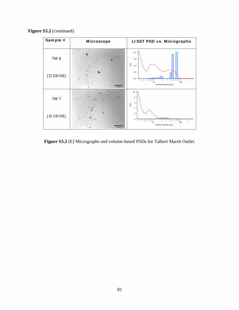
Figure S3.2 (continued)
Sample # Microscope LISST PSD vs. Micrographs
TM 6
(2/28/06)
2.0
1.5
1.0
0.5
0.0
ppm
3 4 5 6 7 8 9 2 3 4 5 6 7 8 910 100
2
Particle Diameter (µm)
TM 7
(3/18/06)
10
8
6
4
2
0
ppm
3 4 5 6 7 8 9 2 3 4 5 6 7 8 910 100
2
Particle Diameter (µm)
Figure S3.2 (E) Micrographs and volume-based PSDs for Talbert Marsh Outlet.
81
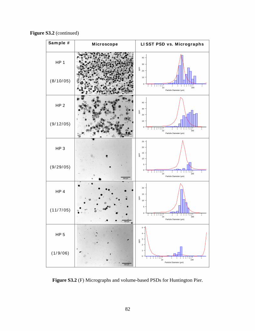
Figure S3.2 (continued)
Sample # Microscope LISST PSD vs. Micrographs
HP 1
(8/10/05)
40
30
20
10
0
ppm
3 4 5 6 7 8 9 2 3 4 5 6 7 8 910 100
2
Particle Diameter (µm)
HP 2
(9/12/05)
40
30
20
10
0
ppm
3 4 5 6 7 8 9 2 3 4 5 6 7 8 910 100
2
Particle Diameter (µm)
HP 3
(9/29/05)
25
20
15
10
5
0
ppm
3 4 5 6 7 8 9 2 3 4 5 6 7 8 910 100
2
Particle Diameter (µm)
HP 4
(11/7/05)
20
15
10
5
0
ppm
3 4 5 6 7 8 9 2 3 4 5 6 7 8 910 100
2
Particle Diameter (µm)
HP 5
(1/9/06)
5
4
3
2
1
0
ppm
3 4 5 6 7 8 9 2 3 4 5 6 7 8 910 100
2
Particle Diameter (µm)
Figure S3.2 (F) Micrographs and volume-based PSDs for Huntington Pier.
82
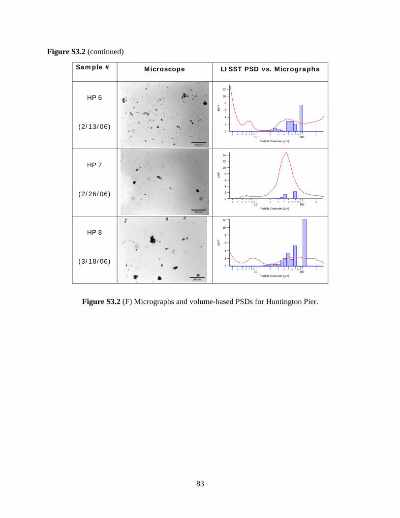
Figure S3.2 (continued)
Sample # Microscope LISST PSD vs. Micrographs
HP 6
(2/13/06)
12
10
8
6
4
2
0
ppm
3 4 5 6 7 8 9 2 3 4 5 6 7 8 910 100
2
Particle Diameter (µm)
HP 7
(2/26/06)
14
12
10
8
6
4
2
0
ppm
3 4 5 6 7 8 9 2 3 4 5 6 7 8 910 100
2
Particle Diameter (µm)
HP 8
(3/18/06)
12
10
8
6
4
2
0
ppm
3 4 5 6 7 8 9 2 3 4 5 6 7 8 910 100
2
Particle Diameter (µm)
Figure S3.2 (F) Micrographs and volume-based PSDs for Huntington Pier.
83
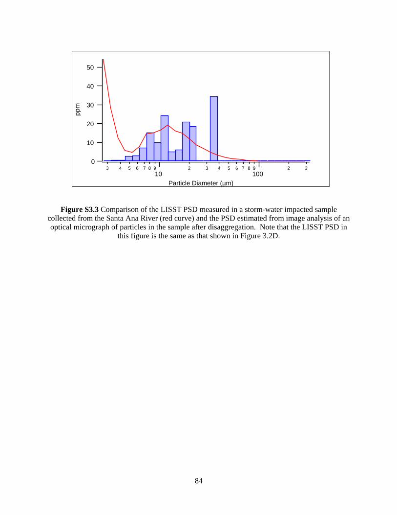
50
40
30
20
10
0
ppm
3 4 5 6 7 8 910
2 3 4 5 6 7 8 9100
2 3
Particle Diameter (µm)
Figure S3.3 Comparison of the LISST PSD measured in a storm-water impacted sample collected from the Santa Ana River (red curve) and the PSD estimated from image analysis of an optical micrograph of particles in the sample after disaggregation. Note that the LISST PSD in
this figure is the same as that shown in Figure 3.2D.
84
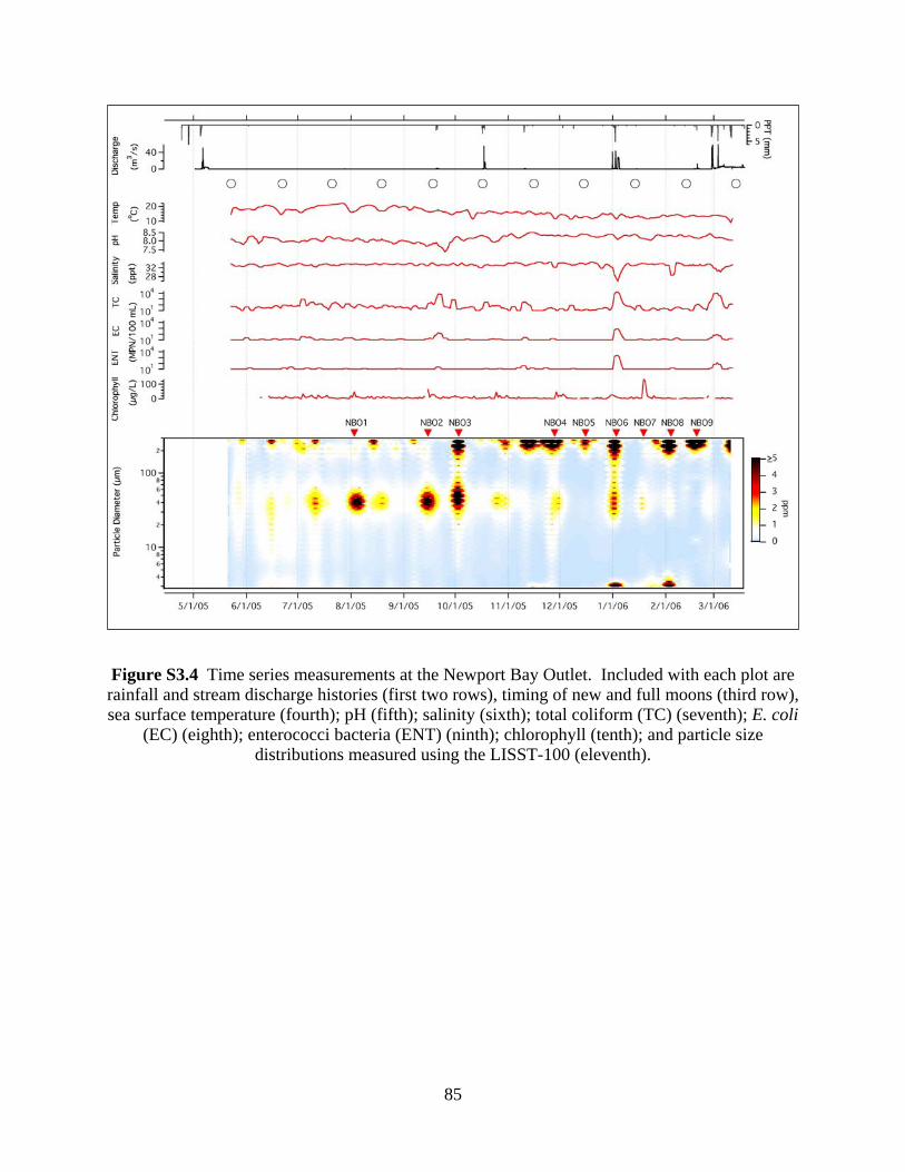
Figure S3.4 Time series measurements at the Newport Bay Outlet. Included with each plot are rainfall and stream discharge histories (first two rows), timing of new and full moons (third row), sea surface temperature (fourth); pH (fifth); salinity (sixth); total coliform (TC) (seventh); E. coli
(EC) (eighth); enterococci bacteria (ENT) (ninth); chlorophyll (tenth); and particle size distributions measured using the LISST-100 (eleventh).
85
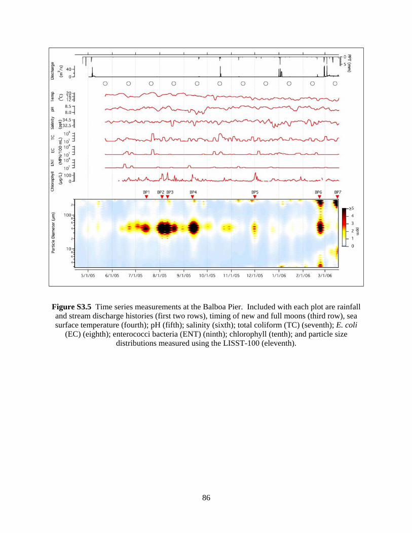
Figure S3.5 Time series measurements at the Balboa Pier. Included with each plot are rainfall and stream discharge histories (first two rows), timing of new and full moons (third row), sea surface temperature (fourth); pH (fifth); salinity (sixth); total coliform (TC) (seventh); E. coli
(EC) (eighth); enterococci bacteria (ENT) (ninth); chlorophyll (tenth); and particle size distributions measured using the LISST-100 (eleventh).
86
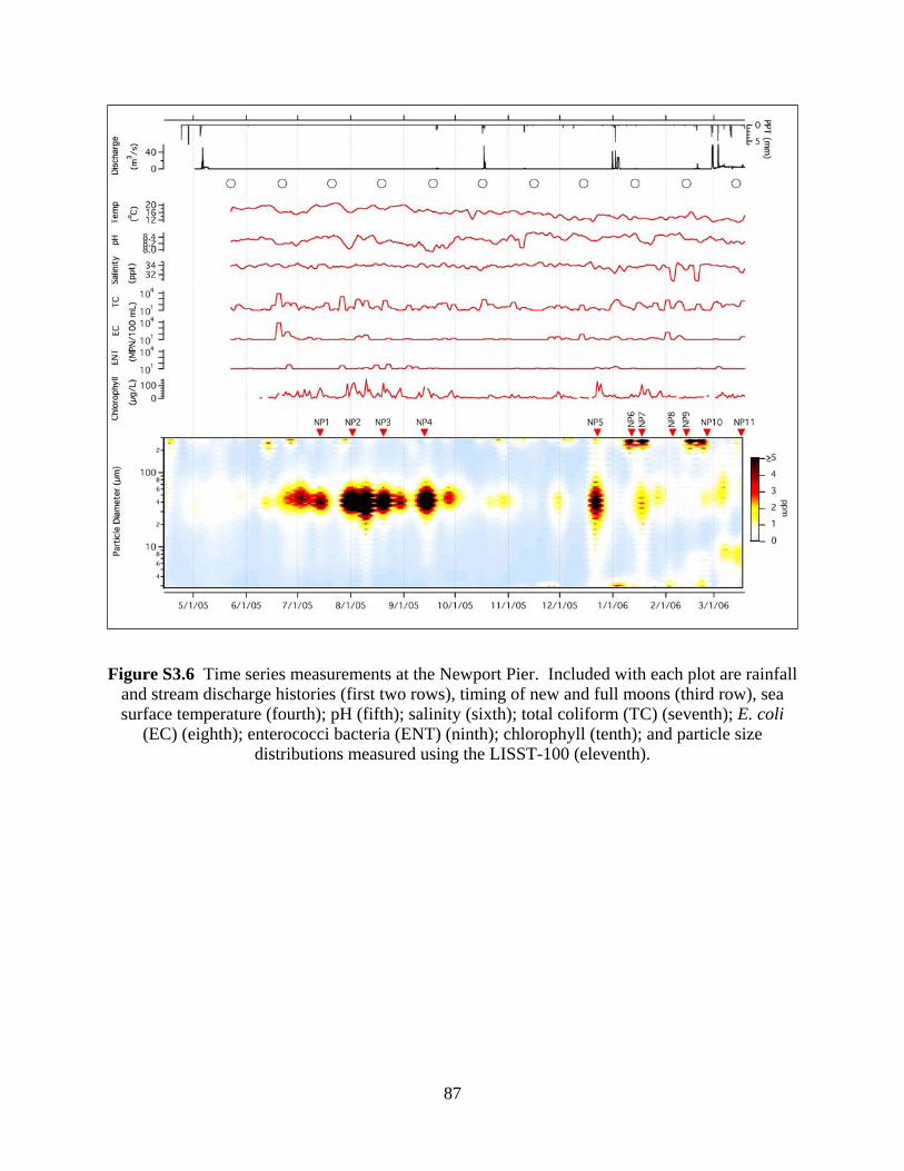
Figure S3.6 Time series measurements at the Newport Pier. Included with each plot are rainfall and stream discharge histories (first two rows), timing of new and full moons (third row), sea surface temperature (fourth); pH (fifth); salinity (sixth); total coliform (TC) (seventh); E. coli
(EC) (eighth); enterococci bacteria (ENT) (ninth); chlorophyll (tenth); and particle size distributions measured using the LISST-100 (eleventh).
87
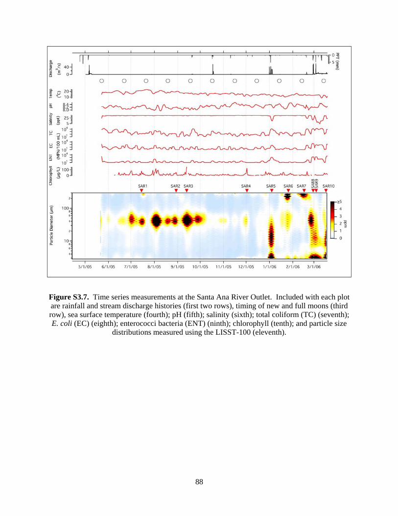
Figure S3.7. Time series measurements at the Santa Ana River Outlet. Included with each plot are rainfall and stream discharge histories (first two rows), timing of new and full moons (third row), sea surface temperature (fourth); pH (fifth); salinity (sixth); total coliform (TC) (seventh); E. coli (EC) (eighth); enterococci bacteria (ENT) (ninth); chlorophyll (tenth); and particle size
distributions measured using the LISST-100 (eleventh).
88
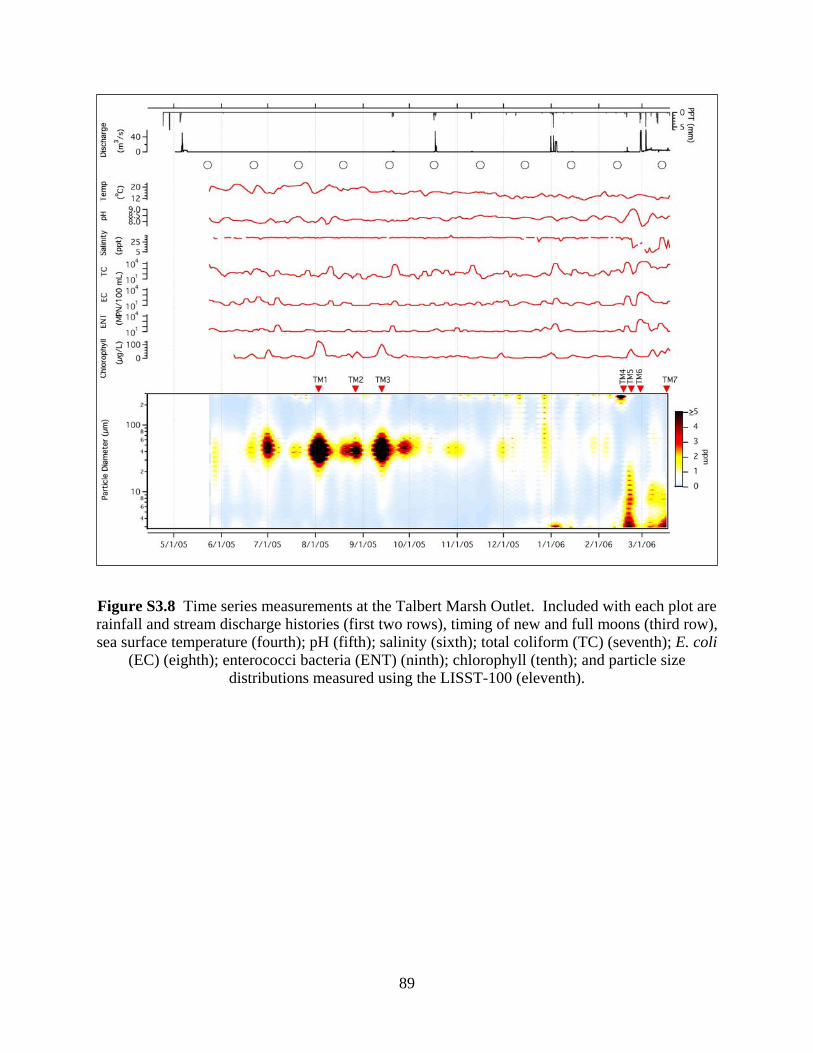
Figure S3.8 Time series measurements at the Talbert Marsh Outlet. Included with each plot are rainfall and stream discharge histories (first two rows), timing of new and full moons (third row), sea surface temperature (fourth); pH (fifth); salinity (sixth); total coliform (TC) (seventh); E. coli
(EC) (eighth); enterococci bacteria (ENT) (ninth); chlorophyll (tenth); and particle size distributions measured using the LISST-100 (eleventh).
89
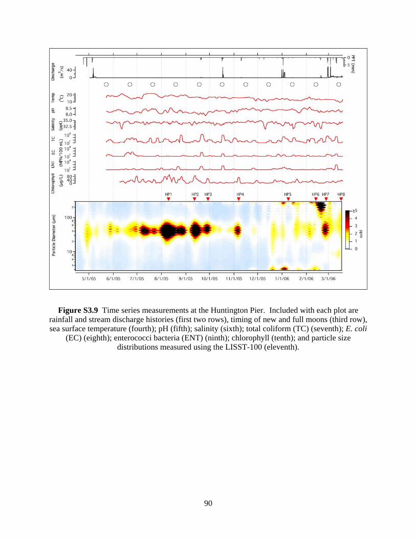
Figure S3.9 Time series measurements at the Huntington Pier. Included with each plot are rainfall and stream discharge histories (first two rows), timing of new and full moons (third row), sea surface temperature (fourth); pH (fifth); salinity (sixth); total coliform (TC) (seventh); E. coli
(EC) (eighth); enterococci bacteria (ENT) (ninth); chlorophyll (tenth); and particle size distributions measured using the LISST-100 (eleventh).
90
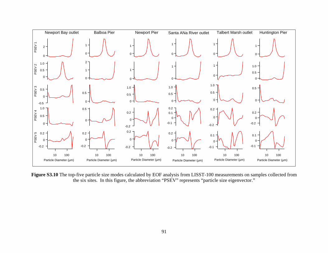
1.0
0.5
0
PS
EV
4
10 100Particle Diameter (µm)
-0.2
0
0.2
PS
EV
5
2
0
PS
EV
1
1.0
0.5
0
PS
EV
2
0.5
0
-0.5
PS
EV
3
1
0
10 100Particle Diameter (µm)
2
1
0
0.5
0
0.5
0
-0.2
0
0.2
-0.2
0
0.2
10 100Particle Diameter (µm)
0.2
0
-0.2
10 100
Particle Diameter (µm)
0.1
0
-0.1
10 100Particle Diameter (µm)
1
0
1
0
1.0
0.5
0
0.2
0
-0.2
1
0
1
0
1.0
0.5
0
0.20.1
0
-0.1
1
0
1
0
1.0
0.5
0
-0.2
0
0.2
1
0
10 100Particle Diameter (µm)
1.0
0.5
0
0.5
0
0.2
0
-0.2
0.1
0
-0.1
Newport Bay outlet Balboa Pier Newport Pier Santa ANa River outlet Talbert Marsh outlet Huntington Pier
Figure S3.10 The top-five particle size modes calculated by EOF analysis from LISST-100 measurements on samples collected from
the six sites. In this figure, the abbreviation “PSEV” represents “particle size eigenvector.”
91
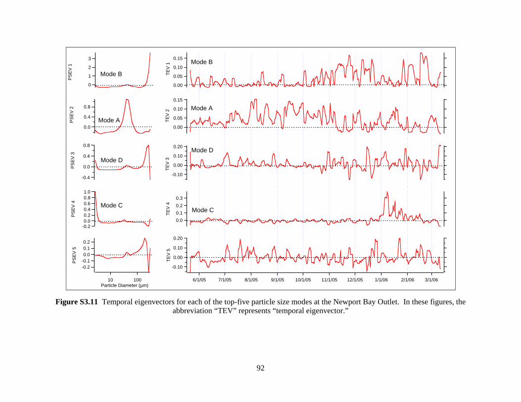
3
2
1
0
PS
EV
1
10 100Particle Diameter (µm)
0.8
0.4
0.0
PS
EV
2
0.8
0.4
0.0
-0.4
PS
EV
3
1.00.80.60.40.20.0
-0.2
PS
EV
4
-0.2-0.10.00.10.2
PS
EV
5
0.15
0.10
0.05
0.00
TEV
1
6/1/05 7/1/05 8/1/05 9/1/05 10/1/05 11/1/05 12/1/05 1/1/06 2/1/06 3/1/06
0.15
0.10
0.05
0.00
TEV
2
0.20
0.10
0.00
-0.10TE
V 3
0.30.20.10.0
TEV
4
0.20
0.10
0.00
-0.10
TEV
5
Mode B
Mode A
Mode D
Mode C
Mode B
Mode A
Mode D
Mode C
Figure S3.11 Temporal eigenvectors for each of the top-five particle size modes at the Newport Bay Outlet. In these figures, the
abbreviation “TEV” represents “temporal eigenvector.”
92
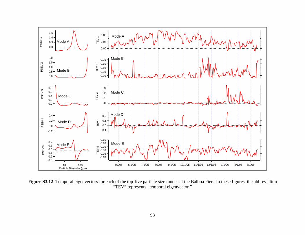
1.5
1.0
0.5
0.0PSEV
1
10 100Particle Diameter (µm)
2.01.51.00.50.0
PSEV
2
0.80.60.40.20.0
PSEV
3
0.4
0.2
0.0
-0.2
PSEV
4
-0.3-0.2-0.10.00.10.2
PSEV
5
0.08
0.04
0.00
TEV
1
5/1/05 6/1/05 7/1/05 8/1/05 9/1/05 10/1/05 11/1/05 12/1/05 1/1/06 2/1/06 3/1/06
0.200.150.100.050.00
TEV
2
0.3
0.2
0.1
0.0
TEV
3
0.2
0.1
0.0
-0.1
TEV
4
0.150.100.050.00
-0.05-0.10
TEV
5
Mode A
Mode B
Mode C
Mode D
Mode E
Mode A
Mode B
Mode C
Mode D
Mode E
Figure S3.12 Temporal eigenvectors for each of the top-five particle size modes at the Balboa Pier. In these figures, the abbreviation
“TEV” represents “temporal eigenvector.”
93
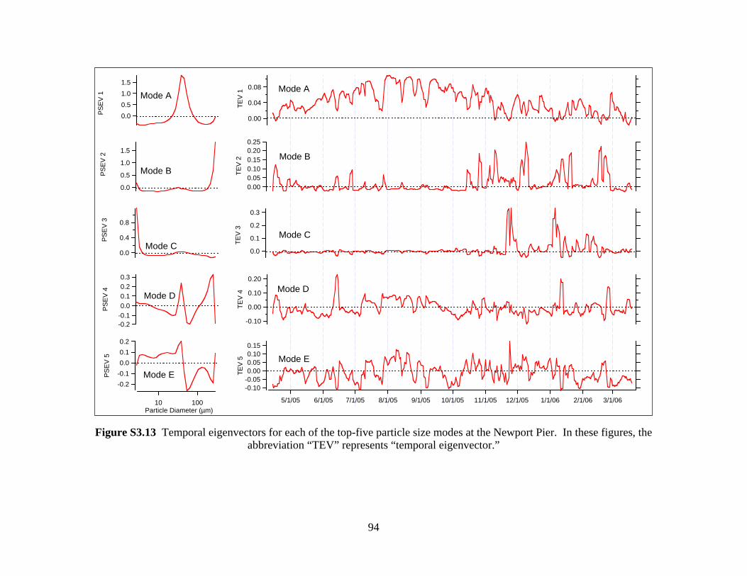
1.51.00.50.0P
SE
V 1
10 100Particle Diameter (µm)
1.5
1.0
0.5
0.0
PS
EV
2
0.8
0.4
0.0
PS
EV
3
0.30.20.10.0
-0.1-0.2
PS
EV
4
-0.2-0.10.00.10.2
PS
EV
5
0.08
0.04
0.00
TEV
1
5/1/05 6/1/05 7/1/05 8/1/05 9/1/05 10/1/05 11/1/05 12/1/05 1/1/06 2/1/06 3/1/06
0.250.200.150.100.050.00
TEV
2
0.3
0.2
0.1
0.0
TEV
3
0.20
0.10
0.00
-0.10
TEV
4
0.150.100.050.00
-0.05-0.10
TEV
5
Mode A
Mode B
Mode C
Mode D
Mode E
Mode A
Mode B
Mode C
Mode D
Mode E
Figure S3.13 Temporal eigenvectors for each of the top-five particle size modes at the Newport Pier. In these figures, the abbreviation “TEV” represents “temporal eigenvector.”
94
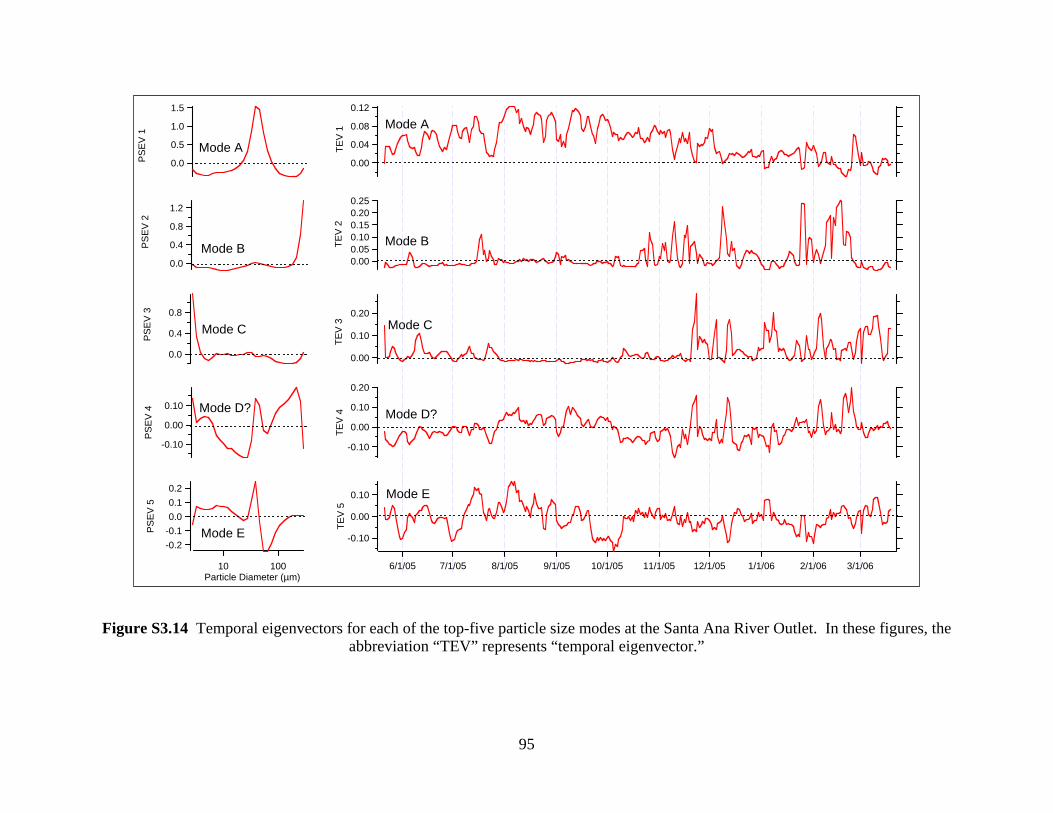
1.5
1.0
0.5
0.0PS
EV
1
10 100Particle Diameter (µm)
1.2
0.8
0.4
0.0
PS
EV
2
0.8
0.4
0.0
PS
EV
3
0.10
0.00
-0.10
PS
EV
4
0.20.10.0
-0.1-0.2
PS
EV
5
0.12
0.08
0.04
0.00
TEV
1
6/1/05 7/1/05 8/1/05 9/1/05 10/1/05 11/1/05 12/1/05 1/1/06 2/1/06 3/1/06
0.250.200.150.100.050.00
TEV
2
0.20
0.10
0.00
TEV
3
0.20
0.10
0.00
-0.10
TEV
4
0.10
0.00
-0.10
TEV
5
Mode A
Mode B
Mode C
Mode D?
Mode E
Mode A
Mode B
Mode C
Mode D?
Mode E
Figure S3.14 Temporal eigenvectors for each of the top-five particle size modes at the Santa Ana River Outlet. In these figures, the
abbreviation “TEV” represents “temporal eigenvector.”
95
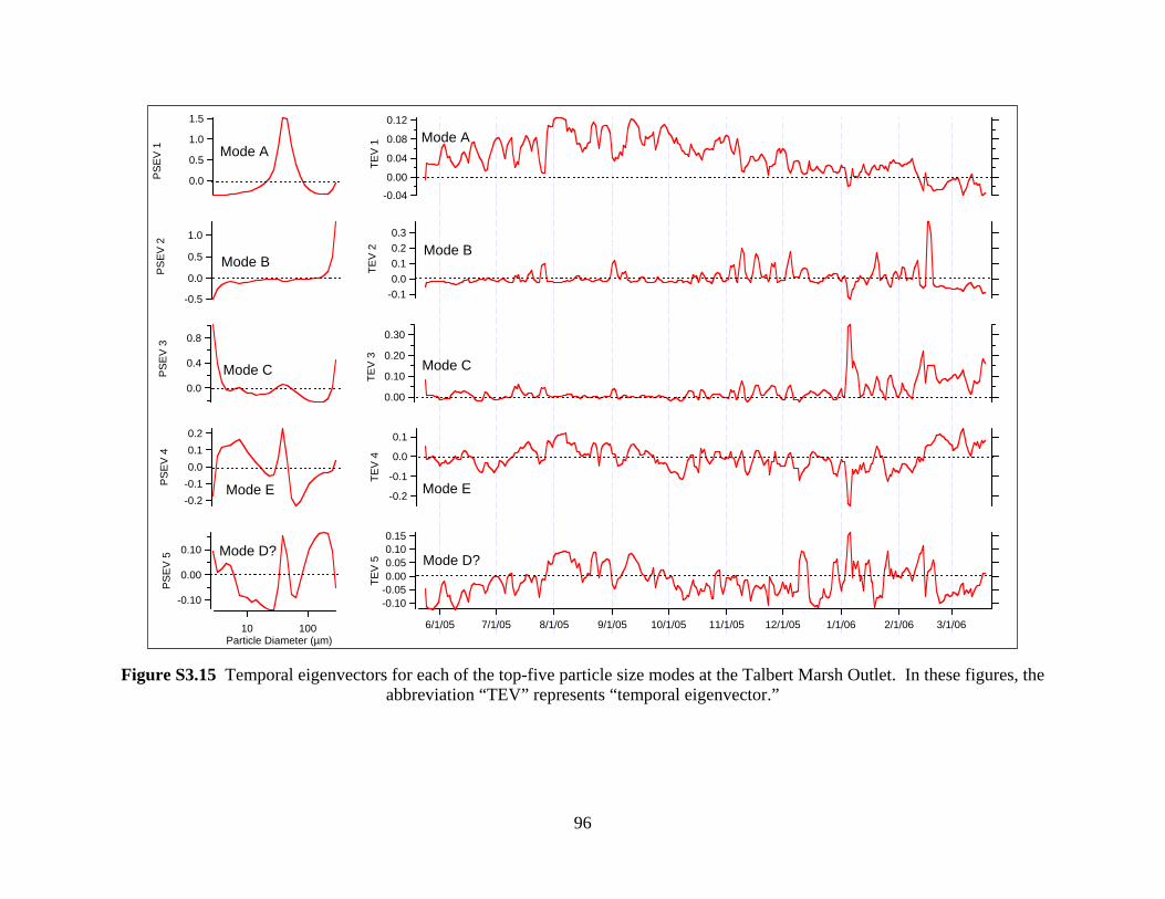
1.5
1.0
0.5
0.0PS
EV
1
10 100Particle Diameter (µm)
1.0
0.5
0.0
-0.5
PS
EV
2
0.8
0.4
0.0
PS
EV
3
-0.2-0.10.00.10.2
PS
EV
4
0.10
0.00
-0.10
PS
EV
5
0.12
0.08
0.04
0.00
-0.04
TEV
1
6/1/05 7/1/05 8/1/05 9/1/05 10/1/05 11/1/05 12/1/05 1/1/06 2/1/06 3/1/06
0.30.20.10.0
-0.1
TEV
2
0.30
0.20
0.10
0.00
TEV
3
-0.2
-0.1
0.0
0.1
TEV
4
0.150.100.050.00
-0.05-0.10
TEV
5
Mode A
Mode B
Mode C
Mode E
Mode D?
Mode A
Mode B
Mode C
Mode E
Mode D?
Figure S3.15 Temporal eigenvectors for each of the top-five particle size modes at the Talbert Marsh Outlet. In these figures, the
abbreviation “TEV” represents “temporal eigenvector.”
96
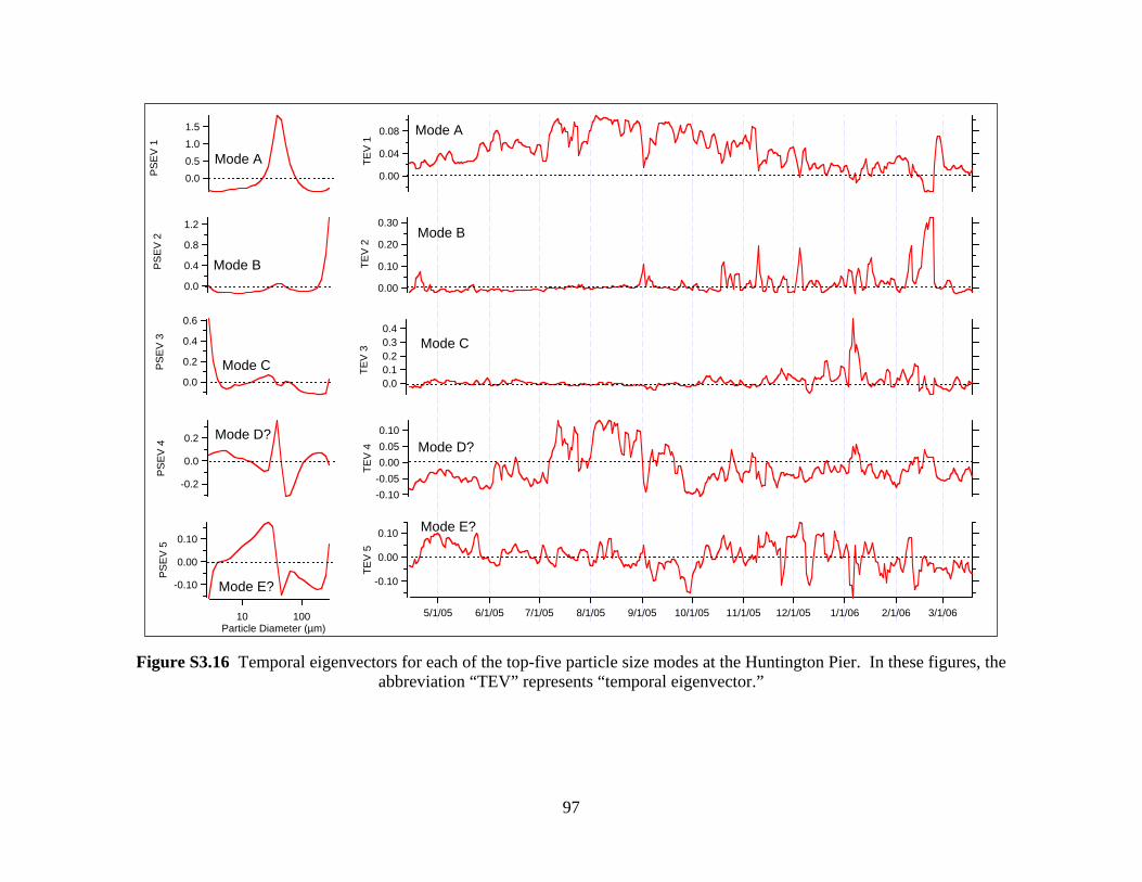
1.51.00.50.0P
SE
V 1
10 100Particle Diameter (µm)
1.2
0.8
0.4
0.0
PS
EV
2
0.6
0.4
0.2
0.0
PS
EV
3
0.2
0.0
-0.2
PS
EV
4
0.10
0.00
-0.10
PS
EV
5
0.08
0.04
0.00
TEV
1
5/1/05 6/1/05 7/1/05 8/1/05 9/1/05 10/1/05 11/1/05 12/1/05 1/1/06 2/1/06 3/1/06
0.30
0.20
0.10
0.00
TEV
2
0.40.30.20.10.0
TEV
3
0.100.050.00
-0.05-0.10
TEV
4
-0.10
0.00
0.10
TEV
5
Mode A
Mode B
Mode C
Mode D?
Mode E?
Mode A
Mode B
Mode C
Mode D?
Mode E?
Figure S3.16 Temporal eigenvectors for each of the top-five particle size modes at the Huntington Pier. In these figures, the abbreviation “TEV” represents “temporal eigenvector.”
97
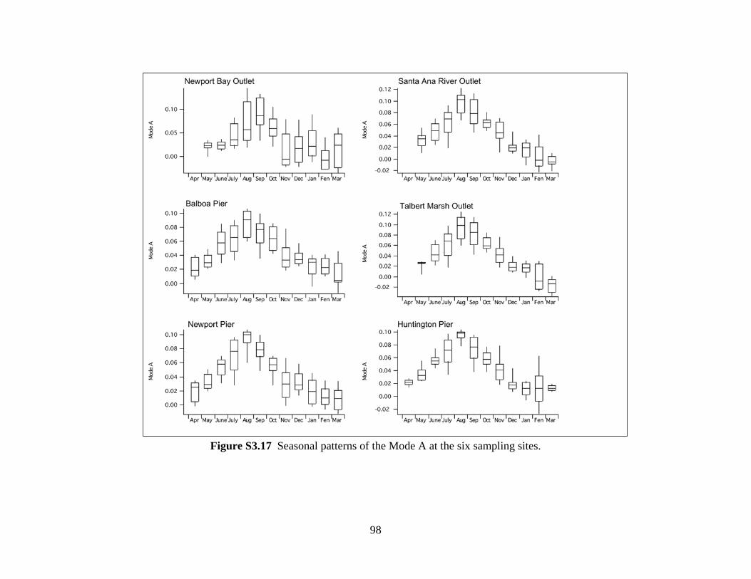
Figure S3.17 Seasonal patterns of the Mode A at the six sampling sites.
98
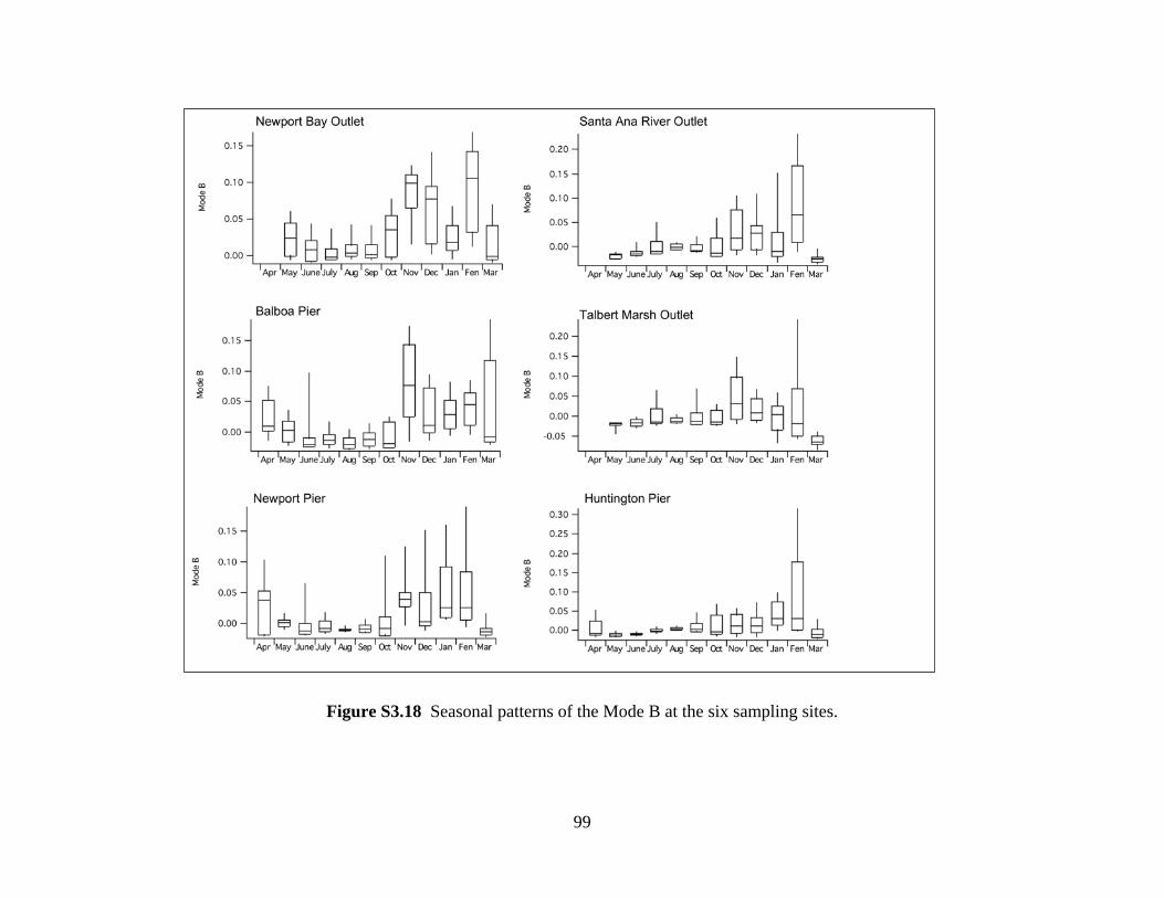
Figure S3.18 Seasonal patterns of the Mode B at the six sampling sites.
99
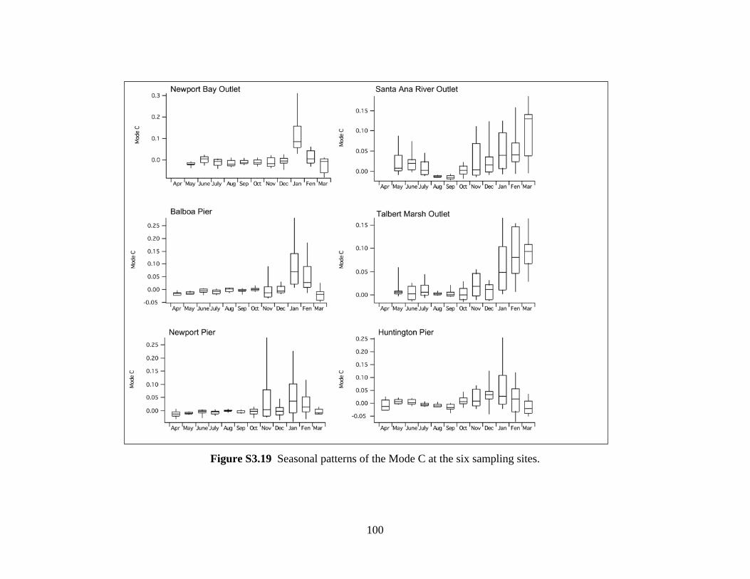
Figure S3.19 Seasonal patterns of the Mode C at the six sampling sites.
100
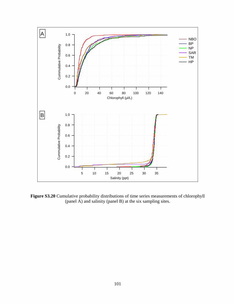
NBO BP NP SAR TM HP
1.0
0.8
0.6
0.4
0.2
0.0
Cum
mul
ativ
e P
roba
bilit
y
140120100806040200Chlorophyll (µl/L)
1.0
0.8
0.6
0.4
0.2
0.0
Cum
mul
ativ
e P
roba
bilit
y
3530252015105Salinity (ppt)
A
B
Figure S3.20 Cumulative probability distributions of time series measurements of chlorophyll (panel A) and salinity (panel B) at the six sampling sites.
101
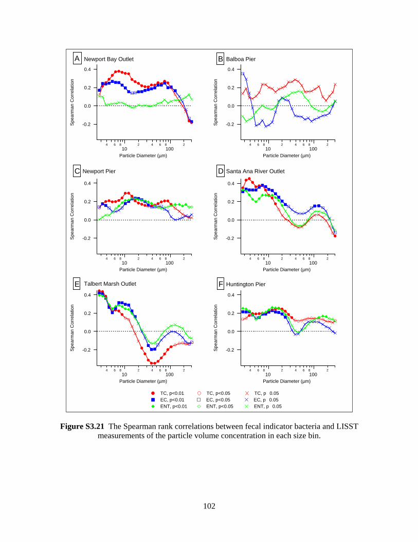
0.4
0.2
0.0
-0.2Spea
rman
Cor
rela
tion
4 6 810
2 4 6 8100
2
Particle Diameter (µm)
0.4
0.2
0.0
-0.2Spea
rman
Cor
rela
tion
4 6 810
2 4 6 8100
2
Particle Diameter (µm)
0.4
0.2
0.0
-0.2Spea
rman
Cor
rela
tion
4 6 810
2 4 6 8100
2
Particle Diameter (µm)
0.4
0.2
0.0
-0.2Spea
rman
Cor
rela
tion
4 6 810
2 4 6 8100
2
Particle Diameter (µm)
0.4
0.2
0.0
-0.2Spea
rman
Cor
rela
tion
4 6 810
2 4 6 8100
2
Particle Diameter (µm)
0.4
0.2
0.0
-0.2Spea
rman
Cor
rela
tion
4 6 810
2 4 6 8100
2
Particle Diameter (µm)
A B
C D
E F
TC, p<0.01 TC, p<0.05 TC, p�0.05 EC, p<0.01 EC, p<0.05 EC, p�0.05 ENT, p<0.01 ENT, p<0.05 ENT, p�0.05
Newport Bay Outlet Balboa Pier
Newport Pier Santa Ana River Outlet
Talbert Marsh Outlet Huntington Pier
Figure S3.21 The Spearman rank correlations between fecal indicator bacteria and LISST measurements of the particle volume concentration in each size bin.
102
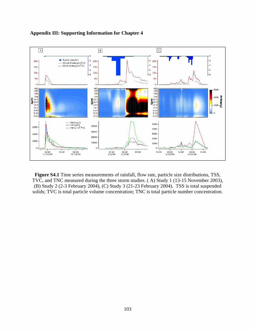
103
Appendix III: Supporting Information for Chapter 4
Figure S4.1 Time series measurements of rainfall, flow rate, particle size distributions, TSS, TVC, and TNC measured during the three storm studies. ( A) Study 1 (13-15 November 2003), (B) Study 2 (2-3 February 2004), (C) Study 3 (21-23 February 2004). TSS is total suspended
solids; TVC is total particle volume concentration; TNC is total particle number concentration.