Model Predictive Control for a Linearised Continuous

Stirred Tank Heater

or

MPC for Dummies

Sebastian Gonzato

September 2, 2016

Abstract

This report gives a brief overview of model predictive control and demonstrates howit can be implemented in MATLAB. It is meant to be used as an accompaniment to theMATLAB files and GUIs that were also produced for this project. A continuous stirredtank heater model is used to illustrate key concepts such as observability, controllability,designing an observer and formulating the optimisation problem. Insight into MPCbehaviour and a comparison with traditional PID control is also provided, The purposeof this report is to introduce the inexperienced reader to MPC and hence the focus isnot on mathematical rigour.

1

Contents

1 Introduction 31.1 Scope of this report . . . . . . . . . . . . . . . . . . . . . . . . . . . . . . . . 31.2 Suggested prior knowledge . . . . . . . . . . . . . . . . . . . . . . . . . . . . . 31.3 MPC and its advantages . . . . . . . . . . . . . . . . . . . . . . . . . . . . . . 41.4 Overview of controlled system . . . . . . . . . . . . . . . . . . . . . . . . . . . 4

2 Observability & Controllability 62.1 Observability . . . . . . . . . . . . . . . . . . . . . . . . . . . . . . . . . . . . 62.2 Controllability . . . . . . . . . . . . . . . . . . . . . . . . . . . . . . . . . . . 7

3 Designing an Observer 83.1 Accurate state estimation . . . . . . . . . . . . . . . . . . . . . . . . . . . . . 83.2 Incorporating disturbance . . . . . . . . . . . . . . . . . . . . . . . . . . . . . 93.3 Incorporating time delay . . . . . . . . . . . . . . . . . . . . . . . . . . . . . . 10

4 Formulating optimisation 114.1 Regulation . . . . . . . . . . . . . . . . . . . . . . . . . . . . . . . . . . . . . . 114.2 Tracking . . . . . . . . . . . . . . . . . . . . . . . . . . . . . . . . . . . . . . . 134.3 Adding slew rate . . . . . . . . . . . . . . . . . . . . . . . . . . . . . . . . . . 154.4 Constraints . . . . . . . . . . . . . . . . . . . . . . . . . . . . . . . . . . . . . 16

5 Additional MATLAB resources 175.1 MATLAB scripts . . . . . . . . . . . . . . . . . . . . . . . . . . . . . . . . . . 175.2 GUIs . . . . . . . . . . . . . . . . . . . . . . . . . . . . . . . . . . . . . . . . . 17

5.2.1 Opening GUI . . . . . . . . . . . . . . . . . . . . . . . . . . . . . . . . 175.2.2 GUI features . . . . . . . . . . . . . . . . . . . . . . . . . . . . . . . . 185.2.3 Observer features . . . . . . . . . . . . . . . . . . . . . . . . . . . . . . 185.2.4 MPC features . . . . . . . . . . . . . . . . . . . . . . . . . . . . . . . . 18

6 Analysis of MPC controller 196.1 MPC behaviour . . . . . . . . . . . . . . . . . . . . . . . . . . . . . . . . . . . 19

6.1.1 Default behaviour . . . . . . . . . . . . . . . . . . . . . . . . . . . . . 196.1.2 Decreasing Q . . . . . . . . . . . . . . . . . . . . . . . . . . . . . . . . 206.1.3 Increase S . . . . . . . . . . . . . . . . . . . . . . . . . . . . . . . . . . 216.1.4 Decrease horizon . . . . . . . . . . . . . . . . . . . . . . . . . . . . . . 22

6.2 Comparison of MPC with PID controller . . . . . . . . . . . . . . . . . . . . . 23

7 Acknowledgements 25

2

1 Introduction

1.1 Scope of this report

The purpose of this report is to provide the reader with a basic grasp of model predic-tive control (MPC). Specifically, this report covers why MPC is superior to traditional PIDcontrollers, some of the theory behind it and how to implement it in MATLAB using thequadratic optimisation function quadprog. It is not supposed to be an in depth introductionto MPC and hence few derivations are provided and mathematical rigour is sidelined.

Given that the author learned all of this reports contents in 6 weeks, there are undoubt-edly mistakes in what follows. If the reader does use this report to implement a basic MPCcontroller in MATLAB (or another capable language such as Python) they are advised toread this report critically and not just take what is written for granted.

All the resources mentioned in this report (such as MATLAB files) can be found on theImperial College Centre for Process Systems Engineering web page [1].

1.2 Suggested prior knowledge

The theory behind MPC may be confusing to the reader with only a basic grasp ofcontrol theory. Due to this, it is suggested that the reader spend some time learning aboutthe following topics:

• State space models and how they are derived [2]

• Behaviour of state space models [3]

• Conversion from continuous time to discrete time models [4]

The first two links come from online resources on modelling and control [2] provided byAnthony Rossiter of the University of Sheffield. The author generally found these to beuseful and hence recommends them. The author also suggests watching the videos on �2speed to save time and discourage lethargy.

The reader may also want to brush up on linear algebra and matrix properties. Theseareas caused the author a lot pain, so a working knowledge of these will make the derivationsand equations that follow easier to understand and to derive independently. Many resourcesare available online and the author recommends Khan Academy [5] and this NYU page [6]for the properties of transpose matrices.

3

1.3 MPC and its advantages

Traditional PID controllers are adequate for many simply systems and have been aroundfor more than a century (the first PID controller was implemented in 1911 [7]). Due to theirsimplicity, they are still the most widely used controllers in industry. However, PID con-trollers are fairly crude in that they are reactionary, and hence cannot be used to controlvery complex systems such as say, cars. They also cannot handle constraints, which can bevery important if the output of a system (such as the temperature of an exothermic reactionmixture) cannot go above a certain value.

To control complex systems while handling constraints requires knowledge of the con-trolled system, hence the creation of model predictive control (MPC). The theory under-pinning MPC first appeared in the 1960s and MPC itself has been in use in the chemicalprocesses industry since the 1980s. The basic idea behind MPC is that a model of the sys-tem is used to make predictions and then the controller optimises the input to the systemto minimise error, control moves, slew rate or any other specification.

It should be noted that MPC is a way of thinking about or approaching control, andhence there are many ways of implementing it. This means there are a range of control al-gorithms that fall under the umbrella of MPC, such as predictive functional control (PFC),generalised predictive control (GPC) which was developed by David Clarke of Cambridgeand David Mayne of Imperial, as well as many others. The key thing to bear in mind isthat in MPC the controller is not just reacting to the output of the system, but using thatoutput to make predictions and determine the best possible way of reaching a set point asdefined by the user.

1.4 Overview of controlled system

In process control it is important to have an understanding of the system being con-trolled as this leads to good control decisions and makes troubleshooting easier.

The system being controlled is a continuous stirred tank heater (CSTH, see Figure 1)studied by Thornhill et al[8] which is composed of a tank, a steam heater, hot and coldwater valves and an outlet. The outlet valve is fully open and hence the flow is gravitycontrolled.

This system exhibits many non linearities due to, for example, the heating coil occupyingvolume and the density of water being a function of temperature. Since non linear MPC isbeyond the scope of this report, a linear model for the CSTH was used. The model, takenfrom the same paper by Thornhill et al [8], was obtained by linearising around the operatingpoint shown in Table 1. The system is described by the state space model shown below,where the variables are deviations from the operating point (i.e. x1 is actually ∆x1)

4

Figure 1: Diagram of controlled sysem, a CSTH

�� 9x1

9x2

9x3

�� � A

��x1

x2

x3

���B

��u1

u2

u3

��

��y1y2y3

�� � C

��x1

x2

x3

��

A �

���3.73� 10�3 1.58� 10�6 0

0 �2.63� 10�1 04.16� 103 1.58� 10�1 �2.73� 10�2

��

B �

��0 0 4.29� 10�5

1 0 00 0.64 8.8712

��

C �

�� 2690 0 0

0 1.5132� 10�1 0�1979.2 0 �1.12� 10�2

��

Continuous state space model of CSTH

It should be noted that while it appears that the cold water valve position has no effecton the tank level, it has an indirect effect since u1 (cold water valve position) affects x2

5

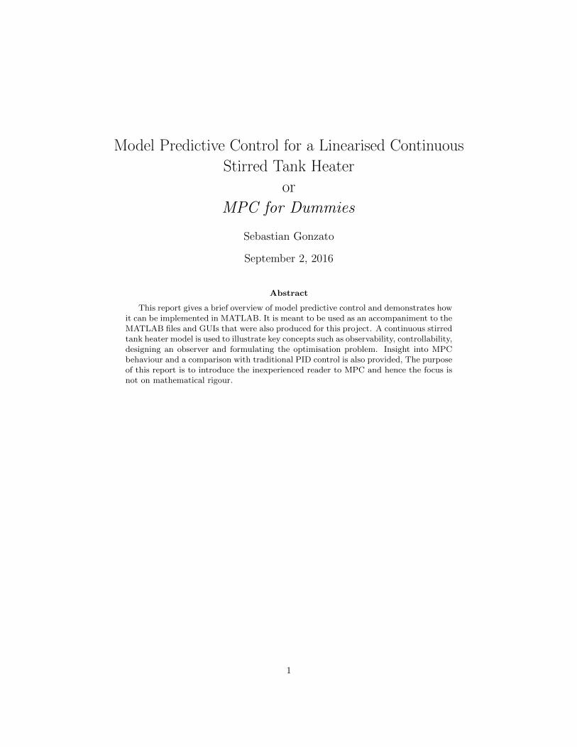
Variable Description Range Operating pointx1 Volume of water, L 0� 8 3.3x2 Cold water valve output, mA 4� 20 12.96x3 Total enthalpy in tank, kJ 0� 3000 589u1 Cold water valve position, mA 4� 20 12.96u2 Steam valve position mA 4� 20 6.053u3 Hot water valve position, mA 4� 20 5.5y1 Level measurement, mA 4� 20 12y2 Cold water flow rate measurement, mA 4� 20 7.33y3 Temperature measurement, mA 4� 20 10.5

Table 1: Operating point

(cold water valve output) which in turn affects x1 (the tank level).

The model above describes the CSTH in continuous time. MPC however requires adiscrete time model since all computation takes a finite amount of time (a continuous MPCcontroller would require the ability to perform computations in an infinitesimally shorttime). The mathematics required to convert a continuous model to a discrete one are notespecially difficult, but fortunately MATLAB makes even this unnecessary and hence thisdiscretisation is covered in the MATLAB files but not in this report.

The system also exhibits a time delay of 1 second on the cold water valve position u1

and 8 seconds on the temperature measurement y3. While the MATLAB scripts and GUIswere produced without taking this time delay into account, section 3.3 illustrates how toincorporate this.

2 Observability & Controllability

A summary of controllability and observability for state space models is presented be-low. For more information the reader is directed to Anthony Rossiter’s videos on state spacemodel behaviour [3].

2.1 Observability

In order to predict the future outputs of a system, the states of that process (e.g. en-thalpy, total mass) have to be known or observable. This is done by estimating them fromthe outputs of the system, which in this case would be the level, temperature or cold waterflow rate. Loosely speaking then a system is said to be observable if it is possible to deter-mine the behaviour of the system from it’s outputs.

With a state space model it is easy to determine whether a system is observable. Simplyconstruct the observability matrix from equation 2.1 and determine whether it is full rank.

6

If it is then the system is observable, and if it isn’t then the rank deficiency corresponds tothe number of unobservable states. No derivation is given since this is beyond the scope ofthis report.

MO �

�������

CCACA2

...CAN�1

������� (2.1)

The observability matrix can be constructed in MATLAB using the obvs command.

2.2 Controllability

Controllability is formally defined as the ability to apply external inputs and move theinternal states of a system from any initial state to any other final state. In other words,any state xN can be arrived at from any initial state x1 given a finite number N of inputsu.

Similarly to before,the system is controllable if the controllability matrix (see equation2.2 below) is full Rank

MC ��B AB A2B . . . AN�1B

�(2.2)

While a full derivation for this is quite complex, some insight into why the controllabilitymatrix in equation 2.2 has to be full rank is given below:

xp1q � Axp0q �Bup0q

xp2q � Axp1q �Bup1q

� A2xp0q �ABup0q �Bup1q

xpNq � Bupn� 1q �ABupN � 2q � � � � �AN�1Bup0q �ANxp0q

The last equation can be rewritten as:

xpNq �Anxp0q ��B AB A2B . . . AN�1B

������upN � 1qupN � 2q

...up0q

�����

It can be shown that any desired xpNq can be solved for the column vector of inputs ifthe controllability matrix has full row rank. It can also be shown that the rank deficiency

7

of MC corresponds to the number of uncontrollable states.

As with observability, there is a MATLAB function to compute the controllability ma-trix, namely ctrb.

3 Designing an Observer

This section looks at how to design an observer that allows the states of a system tobe determined. For more information on the subject the reader is referred to AnthonyRossiter’s videos on state space observers [2].

3.1 Accurate state estimation

In order to control a process, the states of the controlled system must be known. Thisis achieved using an observer which estimates the states using a model of the system. Cru-cially, the observer includes an offset term which is defined as the difference between theprocess output and the model output. Note that an observer can only ever estimate ourstates since there will always be noise, measurement error and disturbances that we cannotaccount for.

In the absence of a disturbance, the observer is defined as:

xk�1 � Axk �Buk � Lpyk � ykq (3.1)

yk � Cxk

We can easily obtain yk by multiplying our state xk by the matric C, while our processoutput yk can be measured directly. A hat on top of a variable indicates that it is a modeland not a process variable, although this distinction is dropped after this section.

The matrix L has to be defined in order to guarantee offset free tracking. Specifically, ithas to be defined such that the eigenvalues of the matrix below are within the unit circle:

A� LC

The derivation for why this is can be found below. Note that qxpkq is simply a variablewe define as being the difference between our process states and our model states. If wewant offset free tracking qxpkq has to tend to 0 as n ÝÑ 8.

8

qxpk � 1q � xpk � 1q � xpk � 1q

� Axpkq ����Bupkq �Axpkq ����Bupkq � Lpy � yq

� A�xpkq � xpkq

�� L

�Cxpkq � Cxpkq

�� A

�xpkq � xpkq

�� LC

�xpkq � xpkq

�� A

�qxpkq�� LC�qxpkq�qxpk � 1q � pA� LCqqxpkqqxpk � 1q � pA� LCqqxpkqqxpk � 2q � pA� LCqpA� LCqqxpkq

...qxpk � nq � pA� LCqnqxpkq

We can apply eigenvector eigenvalue decomposition for the matrix A� LC:

A� LC � TΛT�1

pA� LCq2 � TΛT�1TΛT�1

� TΛ�T�1�T ΛT�1

� TΛ2T�1

pA� LCqn � TΛnT�1

By inspection we not that in order for A � LC to converge to 0 as n ÝÑ 8, its eigen-values (i.e. the elements of Λ) must be   1.

3.2 Incorporating disturbance

If a disturbance acting on the system can be measured and the dynamics of the distur-bance are known then it is possible to incorporate this in the observer and provide betterstate estimation. In the following section it is assumed that the disturbance is roughlyconstant so dk�1 � dk for all k.

The new system’s dynamics are described by:

xk�1 � Axk �Buk �Bddk (3.2)

yk � Cxk � Cddk

9

Given this we define an augmented matrix that incorporates both the disturbance andas follows: �

xk�1

dk�1

��

�A Bd

0 I

� �xk

dk

��

�B0

�uk �

�Lx

Ld

�pyk � Cxk � Cddkq (3.3)

The only restriction on Bd and Cd is that the augmented system has to be observable.

In the MATLAB files and GUI the disturbance was only shown when designing an ob-server; no disturbance dynamics are given for the CSTH so these were not be incorporatedin the controller.

3.3 Incorporating time delay

The CSTH considered in this report exhibited a time delay of 8 seconds in the temper-ature measurement and a 1 second time delay in the cold water valve position. While thesewere not taken into account in this project to keep things simple, this section looks at howa time delay can be included in an observer.

Consider at first a SISO model with no time delay:

xpk � 1q � axpkq � bupkq

Now consider the case where there is an output delay of 2 samples, in other wordsy1pkq � ypk � 2q where y1pkq is the measured output. This is equivalent to the states andinputs being delayed, so x1pkq � xpk�2q and similarly for u. The time delay is incorporatedby augmenting the state space model:�

�xpk � 1qxpkq

xpk � 1q

�� �

��0 0 a

1 0 00 1 0

���� xpkqxpk � 1qxpk � 2q

���

��0 0 b

1 0 00 1 0

���� upkqupk � 1qupk � 2q

��

This is equivalent to:��xpk � 1q

xpkqxpk � 1q

�� � �

0 aI 0

��� xpkqxpk � 1qxpk � 2q

��� �

0 bI 0

��� upkqupk � 1qupk � 2q

�� (3.4)

The reason for the identity matrices in the augmented A and B matrices is that themodel needs some way of remembering past states. If these were not there or the modelwas compacted by removing the middle row then there would be no way of knowing whatthe past states were. Equation 3.4 could also be used for a MIMO model by substituting awith A and adapting the column vectors appropriately.

10

4 Formulating optimisation

4.1 Regulation

In a tracking problem, the objective is to drive the states x of a system to 0. Theobjective function J in this case then is:

J �N

i�1

�xTi Qxi � uT

i Rui

(4.1)

where Q and R are weighting matrices.

The first term in equation 4.1 is fairly obvious; this term ensures that the controllerattempts to drive the error to 0. However, this term on its own leads to unreasonably largeactuator changes and can also lead to divergent input signals. This is because the best wayto punish the errors is simply to invert the plant (so the controller is just the inverse of theplant model) which is not usually a good idea! [9]

Due to this, a second term in the equation 4.1 is need which punishes the number ofmoves the controller makes which are away from it’s final steady state input.

The MATLAB files and GUI produced for this project used the quadprog function tosolve equation 4.1. This function requires inputs of a paricular form as shown in equation4.2 and hence we need to define matrices H, Aeq and beq.

minimizex

1

2xTHx� fTx

subject to Aeqx � beq

Ax ¤ b

(4.2)

For tracking the vector f will just be a vector of zeros.

In order to proceed, the first thing to note is that in the optimisation, the x in quadprog

is not our state but actually the augmented vector:�������

u0

x1

...uN�1

xN

�������

where N is the prediction horizon, xi ��xi,1 xi,2 xi,3

�Tand similarly for u. The first

element u0 is required when defining constraints and is also useful later when an extra termin the objective function is added in order to punish the slew rate pui � ui�1q.

From this, the formulation of H is fairly simple:

11

H �

�������

RQ

RQ

. . .

������� (4.3)

where empty entries are 0 and the number of repetitions of Q,R along the diagonal isequal to the horizon length N . Note that R comes before Q because in the augmentedvector the inputs come before the states.

Formulating Aeq and beq (or determining whether they are needed at all) is less obvi-ous. The equality constraint is needed since our objective function has to satisfy systemdynamics; the state space model determines what routes or sequence of inputs can get thecontrolled system from one set of states to another. Put more simply, the system can’t gofrom A to B in one step.

To define Aeq and beq recall that a state space model is of the form:

xk�1 � Axk �Buk

Rearranging gives:

�A B �I

��� xpkqupkq

xpk � 1q

�� � 0 (4.4)

The r.h.s. is part of Aeq while the l.h.s. is part of beq � 0. This is the form needed forall the entries of Aeq from k � 1 to k � N . For k � 0, the equality is of the form:

��B I

� �up0qxp1q

�� Axp0q (4.5)

At this point a clarification on notation is required. In the optimisation formulation, xi

denotes the value of the states at time step i, while the state space model used xpkq andxpk�1q. These two representations are related; x1 � xpk�1q or more generally xi � xpk�iq.This is why equation 4.4 can be used to solve the optimisation problem.

Therefore we have:

�����������

�B IA B �I

A. . .

A B �I

�����������

�������������

u0

x1

u1

x2

...xN�1

uN�1

xN

��������������

�����������

Ax0

0.........0

�����������

(4.6)

12

where as noted before xi and ui are vectors for a MIMO system. From inspection it canbe seen that the matrix on the r.h.s is Aeq and the vector on the l.h.s. is beq. Care should betaken when defining the equality in MATLAB since while only single zeros or empty entries(which also correspond to zeros) are shown in equation 4.6, these are actually null matriceswhose size needs to be specified in MATLAB.

And that’s it! The MPC problem is now ready to be coded into MATLAB using thequadprog function.

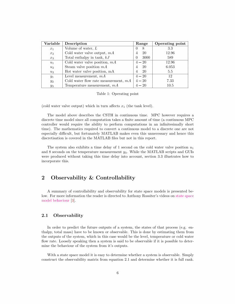
4.2 Tracking

In the last section the objective was to drive the states of a system to 0. This is obviouslynot representative of a real process where the objective is to drive the states of a systemto a value xss which satisfy a required output r, where r stands for reference (this is alsoreferred to as a set point or sp). It is assumed that r is constant in what follows, whichis typical of a chemical process but not of, for example, driving a car. The optimisationproblem gets trickier when this is not the case and hence is beyond the scope of this report.

One way of doing this is to perform a coordinate transformation through a change ofvariables:

∆xpkq � xpkq � xss

∆upkq � upkq � uss

This is also known as delta formulation for tracking, and is essentially the same as thetracking problem except the variables are defined differently. For a linear state space model,the deviation variables satisfy the same model equations:

∆xk�1 � xpk � 1q � xss

� Axpkq �Bupkq � pAxss �Bussq

� A∆xk �B∆uk

Similarly, the objective function J is defined the same as before except in terms ofdeviation variables:

J �N

i�1

�∆xT

i Q∆xi �∆uTi R∆ui

While the problem can be formulated in this form, it adds an extra layer of complexitywhen using the quadprog function since you also have to add extra constraints of the form:

13

Axx ¤ bxñ Ax∆x ¤ bx �Axxss

Auu ¤ buñ Au∆u ¤ bu �Auuss

The output of the controller will also be in terms of deviation variables and hence needsto be converted back using upkq � ∆upkq � uss.

A simpler way of doing this is to define deviation variables only in the objective functionand keep the same constraints in quadprog. The use of deviation variables adds an extralinear term in the objective function which is denoted as a vector f in quadprog. Thederivation for f is as follows:

J � px� xssqTQpx� xssq

� pxTQ� xTssQqpx� xssq

� xTQx� xTssQx� xTQxss ����

��: constantxTssQxss

� xTQx� 2xTQxss

The constant term does not take part in the optimisation and hence is ignored while thetwo linear terms can be factorised since they are scalar quantities. The reader may want towrite these out explicitly if they are not convinced of this.

An almost identical expression can be written for u, and hence an expression for thelinear term f in the optimisation can be obtained:

fTx ���Russ �Qxss � � � �Russ �Qxss

��������

u0

x1

...uN�1

xN

������� (4.7)

Note that the factor of 2 is already taken into account in the formulation of quadprog.

All that’s left is to find the values of xss and uss. These can be obtained by solving thestate space equations for ypkq � r and noting that xpk � 1q � xpkq � xss at steady state:�

I �A �BC 0

� �xss

uss

��

�0r

�(4.8)

Equation 4.8 can be solved in MATLAB using the mldivide function or simply \.

14

4.3 Adding slew rate

Up until now the objective function contained only two terms, one that penalised errors,xTQx, and another that penalised the number of ’moves’ required to get to the desiredstates, uTQu.

While this objective function is sufficient for implementing MPC, it is often useful to adda third term that penalises the slew rate, or even to use as a substitute for the R term. Thisslew rate term is of the form ∆uTS∆u where ∆u � ui�ui�1 and not deviation variables asit did before! A smaller slew rate is desirable since it reduces actuator fatigue and extendsoperational lifetime.

Implementing this extra term is straightforward. For the proof that follows the i sub-script has been dropped to improve legibility.

First the slew rate term is expanded out:

∆uTS∆u ��u� u�1

�TS�u� u�1

���uTS � uT

�1S��u� u�1

�� uTSu� uT

�1Su� uTSu�1 � uT�1Su�1

Note that there are two repeated terms and two mixed terms. Both types of terms can beinserted into the H matrix in quadprog although the mixed terms might not be immediatelyobvious:

xTHx ��u0 x1 � � � uN�1 xN

����������

R� S �SQ

�S R� 2S...

. . .

�S R� SQ

���������

�������

u0

x1

...uN�1

xN

�������(4.9)

Equation 4.9 may seem a little confusing a first, but it is fairly straightforwrd. Theadditional elements are �S one up and to the right and one down and to the left of Q.There is also the addition of a 2S to the R terms except for the first and last two Rentries where this is just S. The reader may want to multiply this out explicitly for thecase where N � 4 to convince themselves of this (note that empty entries are zero matrices).

That’s all there is to it! It should be noted that usually the slew rate is a constraint, andhence is usually added to the constraints in the optimisation function. This may explainwhy the behaviour noted in section 6.

15

4.4 Constraints

It is fairly straightforward to add constraints in quadprog since it is possible to set upupper and lower bounds on each variable by specifying lb and ub. This method makes iteasy to set constraints on u and y.

Another way of implementing constraints is using another option in quadprog whichallows the user to define a matrix A and a vector b satisfying:

Ax ¤ b

The upper and lower bounds for the CSTH are:

4 ¤ u ¤ 20 mA

4 ¤ y ¤ 20 mA

More stringent constraints can also be set, which may be useful if it was known that theheating coil was exposed to the air below 8 mA for example.

Remembering that y � Cx, A and b are defined as shown in below:���������������

I 0 � � �0 C�I 00 �C...

. . .

I 00 C�I 00 �C

���������������

�������

u0

x1

...uN�1

xN

������� ¤

���������������

2020�4�4...

2020�4�4

���������������

(4.10)

This last equation makes use of the fact that �Ax ¤ �b is equivalent to Ax ¥ b, henceif multiplying the first 2 terms of equation 4.10 gives:

u0 ¤ 20

Cx1 ¤ 20

u0 ¥ 4

Cx1 ¥ 4

16

5 Additional MATLAB resources

5.1 MATLAB scripts

As part of this report MATLAB scripts were produced to illustrate the various conceptsthat were presented in this report, such as observability and solving the optimisation prob-lem. These scripts are commented throughout to allow the user to better understand whatMATLAB is doing.

A description of what each script does is given below:

• MPC 1 Initial This script is run at the start of all subsequent scripts. It defines thestate space model of the CSTH and discretises it.

• MPC 2 Observer Defines an observer and plots its behaviour.

• MPC 3 Observerwithdisturbanceandnoise Similar to the previous script with the ex-ception that a disturbance and noise is added to the process.

• MPC 4 Regulation MPC controller that drives states to 0 and plots the result.

• MPC 5 Tracking MPC controller that drives states to a defined reference state andplots the result.

• MPC 6 Trackingwithslewandconstraints Similar to the previous script with the excep-tion of an extra term in the objective function that penalises the slew rate as well asthe addition of constraints.

• PID Comparison Script used to compare PID behaviour in section 6.2

• Tf plant Simulink model of CSTH used in previous script.

5.2 GUIs

As part of this project two MATLAB GUIs were produced to illustrate the behaviour ofan observer and an MPC controller.

5.2.1 Opening GUI

The GUI is opened simply by double clicking the MATLAB .fig file. Make sure the func-tion of the same name is in the same directory as the figure and do not rename anything!

If the GUI produces an error message when you open it, it may be necessary to firstopen the GUI developer and construct the GUI before using it. To do this type guide inthe MATLAB workspace, choose the GUI you want to open then press the green arrow atthe top of the window or use Ctrl+T.

17

5.2.2 GUI features

Some parameters are common to both GUIs, so these are considered below.

• Pole place This determines where the poles of A � LC are placed in the unit circle.The further this slider is to the right, the smaller the poles are and the faster theobserver response is, although the observer will also be more sensitive to noise.

• Noise This adds noise v to the measured output, where v appears in y � Cx� v. Thefurther to the right this slider is the higher the noise gain. The relationship betweenthe slider and the noise gain is non linear.

• Initial states This table determines the initial states of the actual plant and the ob-server. These are set to the operating point by default.

• Timesteps This defines how many time steps the simulation runs for (remember MPChas to be implemented in discrete time). The sample time for this MPC controller is2 seconds.

• Run Runs simulation

5.2.3 Observer features

This GUI is called Observer 2 for historical reasons, and it was not changed since it isannoyingly difficult to rename GUIs. Parameters other than the ones listed in section 5.2.2are listed below.

• Disturbance The entries in this table determine the effect of a disturbance n the states(Bd) and the output of the model (Cd). If you make one entry of Bd or Cd non-zerothey must all be non-zero!

5.2.4 MPC features

Parameters other than the ones listed in section 5.2.2 are listed below.

• Weightings These tables allow you to change the Q, R and S matrices

• Model mismatch This slider introduces a random model mismatch, so the model usedby the MPC controller is not the same as the actual process dynamics. The mismatchis done by multiplying the model parameters by a randomly generated number and sothe mismatch is different each time the simulation is run.

• Set points This table allows you to change the set points at determined times. Theset point time changes are in timesteps (in this case 2 seconds) and not seconds. Thetimesteps also need to be sequential i.e. you can’t have one set point change afterthe next set point occurs. The GUI will still work but an error message should bedisplayed in the workspace.

• Constraints This table allows you to define the constraints on the inputs as well asthe outputs.

• Horizon Use this box to set the prediction horizon and see how it affects the output.

18

6 Analysis of MPC controller

Having designed an MPC controller in MATLAB, it is useful to analyse its behaviour in or-der to obtain insights into how it behaves and why, as well as how it compares to traditionalPID control. In the sections that follow, this analysis was done for the step changes indi-cated in table 2 and the controller horizon was 30 (unless otherwise stated). The observer’sinitial state was kept the same as that of the actual process.

Variable Description Initial Finaly1 Level measurement 12 mA 13 mAy2 Cold water flow rate measurement 11.89 mA 10.5 mAy3 Temperature measurement 10.5 mA 12 mA

Table 2: Set point changes for analysis of MPC behaviour

6.1 MPC behaviour

This section looks at how changing the weightings and event horizon affect controllerbehaviour.

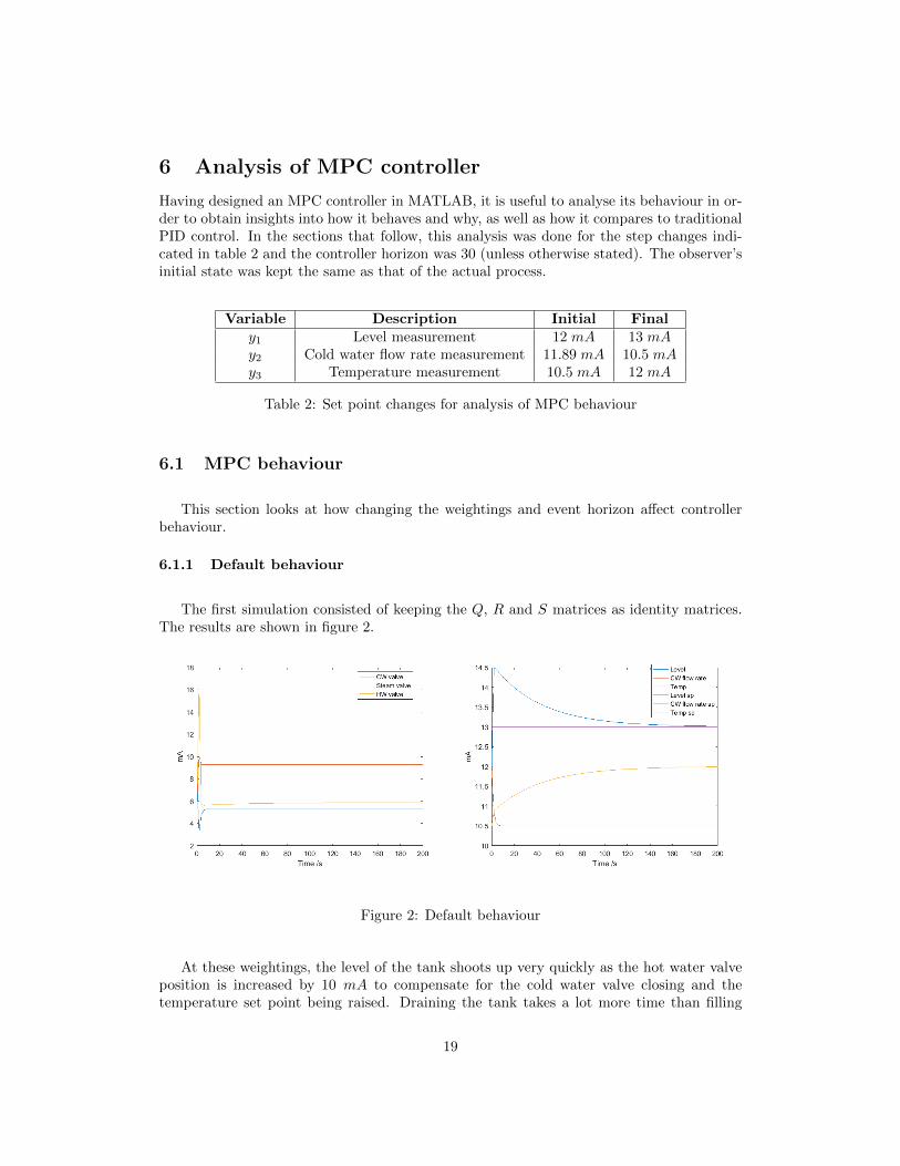
6.1.1 Default behaviour

The first simulation consisted of keeping the Q, R and S matrices as identity matrices.The results are shown in figure 2.

Figure 2: Default behaviour

At these weightings, the level of the tank shoots up very quickly as the hot water valveposition is increased by 10 mA to compensate for the cold water valve closing and thetemperature set point being raised. Draining the tank takes a lot more time than filling

19

it up since the flow is gravity controlled, hence the slow decay to the set points after thefirst move. The temperature takes as much time as the level to reach steady state since thecontroller has made its moves such that once the tank is drained of the water that was thereinitially, all the water will be at the right temperature.

The most noticeable aspect of figure 2 is that the controller only seems to do anythingin it’s first 2 moves, while the rest are pretty much constant save a few moves to ensure0 steady state error. This can be seen quite clearly in figure 3 At these weightings, thesolution to the optimisation problem is to do everything at once in order to reduce thepenalty incurred by the xTQx term.

Figure 3: MPC inputs zoomed in

Evidently this is not desirable; having such rapid changes in controller outputs reducesactuator life as well as the operational life of other components. These changes might alsohave undesirable consequences that are not captured by the model; having the hot watervalve be opened so quickly might mean hot water splashing out of the tank for example.

6.1.2 Decreasing Q

To deal with this, the value of Q can be decreased. Figure 4 shows the results for whenQ is decreased by the amount shown in table 3.

Variable Description Weightingu1 Cold water valve 10�2

u2 Steam valve 10�3

u3 Hot water valve 10�3

Table 3: Q matrix weightings

The controller outputs are now much more reasonable; the hot water valve is makinga jump of only 3 mA in one move and similarly with the other 2 actuators. The system

20

Figure 4: MPC behaviour for reduced Q weighting

outputs are also smoother.

Decreasing Q entries further turns the MPC controller into a very basic predictive func-tional control (PFC) controller in which the first value of u is chosen to be uss. PFCcontroller’s of this form essentially maintain open loop dynamics, which is adequate if openloop dynamics are desirable. This is not optimal however, and solving an optimisation prob-lem only to end up with such a simple (and not particularly good) controller is as displeasingas it is inefficient.

6.1.3 Increase S

There is still a significant slew rate for all 3 actuators which is undesirable. To overcomethis, the S weighting can be increased to the values shown in table 4. The results are shownin 5.

Variable Description Weightingu1 Cold water valve 102

u2 Steam valve 102

u3 Hot water valve 102

Table 4: S matrix weightings

This has not quite had the effect intended. While the slew rate for the hot water valvehas decreased it has only done so after it’s first move. Despite the relatively high weighting,the same is true of all the other actuators which is problematic since the steam valve makesa jump of roughly 3 mA in one move. No increase in the weighting of S can change this.

While the author cannot give an exact reason for why this is the case, it probably hassomething to do with quadprog and how the optimisation problem is formulated. Adding

21

Figure 5: MPC behaviour for increased S weighting

the slew rate constraint in the constraints instead of the objective function could solve this.

Another solution to this would be to use the YALMIP toolbox to solve the optimisationproblem[10]. YALMIP is widely used in academia[11].

6.1.4 Decrease horizon

Figure 6 shows the MPC controller behaviour when the even horizon is decreased to 2while keeping the same weightings as before.

Figure 6: MPC behaviour for a decreased event horizon

Disappointingly, this does not produce any notable changes in the MPC controller’sbehaviour other than a greater overshoot in the level. This can easily be explained by thebehaviour noted before, in that the slew rate of the MPC’s first move cannot be changed.

22

Manipulated variable Controlled variableHot water valve LevelCold water valve Cold water flowrate

Steam valve Temperature

Table 5: PID setup

6.2 Comparison of MPC with PID controller

As the saying goes, ‘less is more’ and there’s no point using an MPC controller whenPID controllers are just as good.

In order to compare PID control with MPC, a SIMULINK file was created which con-tained the linearised CSTH in transfer function form. PID controllers were added and usedto control the control variables as shown in table 5 They were then tuned independently toprovide reasonably good control.

Finally, the same step changes were used as shown in table 2. Normally decouplingwould be applied to minimise interactions, but in practice this did not matter as can beseen in figure 7.

Figure 7: MPC behaviour (left) compared with 3 PID controllers in parallel (right)

If we’re only interested in settling time, the MPC controller appears to perform worsethan the 3 PID controllers! There is less overshoot in the level using PID controllers and asignificantly faster settling time for the level, although the settling time for the temperatureis roughly the same.

However, settling time is not the only important performance index. The inputs to thesystem are also important, since these can change too rapidly (reducing actuator life) orcause the actuator to saturate if the input is greater than 20 mA for example. Figure 8

23

compares the MPC inputs to the PID inputs.

Figure 8: Comparison of MPC and PID controller outputs

The steam valve jumps 12 mA in the first step which is undesirable due to the large slewrate and because the valve is close to saturating.

Where MPC shines is in it’s ability to handle constraints, something PID controllers areincapable of doing. Figure 9 shows a set point change only in the level from 12 mA to 20 mA.

Figure 9: Constraint handling behaviour of MPC illustrated by comparing MPC behaviour(left) with PID behaviour (right)

The PID controller setup again has a slightly faster settling time for the level (roughly60s compared to 100s for MPC), but it has a significant overshoot while the MPC does not.If the PID controllers had been used to control the tank in real life, the tank would haveoverflowed.

24

It should be noted that increasing the gain or decreasing the integral components of thePI controller would lead to less overshoot and so less overflowing, but this would come atthe expense of a slower settling time.

7 Acknowledgements

I would like to thank Nina Thornhill of Imperial College London for agreeing to fundthis project despite it only being useful to me, and also for help throughout.

I would especially like to thank Harsh Shukla of EPFL for all the help he provided de-spite being very busy with his PhD. Without him, this report would have been a very longand boring text on how to implement GPC in Simulink.

References

[1] Gonzato, S. (2016). UROP MPC. [online] Nina Thornhill Imperial Col-lege London Process Systems Personal Pages. Available at: http://personal-pages.ps.ic.ac.uk/ nina/UROP/MPC.html [Accessed 1 Sep. 2016].

[2] Rossiter, A. (2016). Modelling and control. [online] Controleducation.group.shef.ac.uk.Available at: http://controleducation.group.shef.ac.uk/indexwebbook.html [Accessed29 Aug. 2016].

[3] Rossiter, A. (2016). state space behaviours - YouTube. [online] Youtube.com. Availableat: https://www.youtube.com/playlist?list=PLs7mcKy nInFCnBAMQanjRSLdLg6yWiuJ[Accessed 29 Aug. 2016].

[4] Freeman, D. (2016). 2. Discrete-Time (DT) Systems. [online] YouTube. Available at:https://www.youtube.com/watch?v=Ih4s5IFphCw [Accessed 29 Aug. 2016].

[5] Khan, S. (2016). Introduction to matrices. [online] YouTube. Available at:https://www.youtube.com/watch?v=xyAuNHPsq-g&list=PL26BD351D91DFB72E[Accessed 29 Aug. 2016].

[6] Math.nyu.edu. (2016). The Basics: Properties of Matrices. [online] Availableat: http://www.math.nyu.edu/ neylon/linalgfall04/project1/dj/propofmatrix.htm[Accessed 29 Aug. 2016].

[7] Building-automation-consultants.com. (2016). A Brief Building Automation His-tory. [online] Available at: http://www.building-automation-consultants.com/building-automation-history.html [Accessed 29 Aug. 2016].

[8] Thornhill, N., Patwardhan, S. and Shah, S. (2008). A continuous stirred tank heatersimulation model with applications. Journal of Process Control, 18(3-4), pp.347-360.

[9] Skogestad, S. and Postlethwaite, I. (1996). Multivariable feedback control. Chichester:Wiley, pp.49-50.

25

[10] YALMIP : A Toolbox for Modeling and Optimization in MATLAB. J. Lfberg. In Pro-ceedings of the CACSD Conference, Taipei, Taiwan, 2004.

[11] Harsh Shukla, 2nd year PhD, EPFL, 2016.

26

Glossary

actuator fatigue Fatigue he weakening of a material caused by repeatedly applied loadsand is often the cause of actuator failure. 15

offset free tracking Offset free tracking means that the tracking (driving of states to 0)of a controller does not produce an offset, i.e. there is no steady state error. The termcan also be used for observers tracking a systems states. 8

prediction horizon The event horizon of an MPC controller is the number of timestepsinto the future that the MPC controller considers when performing its optimisation.11, 18

rank In linear algebra, the rank of a matrix A is the dimension of the vector space generated(or spanned) by its columns. A matrix is full row rank if the rows are linearly indepen-dent of each other, meaning you cannot produce one row from a linear combination(through addition or multiplication) of the other rows. 6, 7

27