SUBCOURSE EDITION MM5005 8

U.S. ARMY AVIATION CENTER

RADAR TRANSMITTER

THIS SUBCOURSE HAS BEEN REVIEWED FOR OPERATIONS SECURITY.

US ARMY AIR TRAFFIC CONTROL SYSTEMS/SUBSYSTEMS EQUIPMENT REPAIR MOS 93D SKILL LEVELS 1 AND 2

PLEASE NOTE

Proponency for this subcourse has changed from Aviation (AV) to Missile & Munitions (MM).

RADAR TRANSMITTERS

(Development Date: 1 November 1987)

SUBCOURSE NUMBER: AV 5005

US ARMY AVIATION CENTER FORT RUCKER, ALABAMA 36362-5000

10 CREDIT HOURS

GENERAL

The Radar Transmitters subcourse is part of the Ai r Traffic Control System/Subsystems Equipment Repair Course, MOS 93D. This subcourse is designed to teach the knowledge and skills necessar y to troubleshoot and repair radar transmitters. This subcourse is prese nted in four lessons consisting of 14 learning events, each lesson corre sponding to a terminal objective as indicated below. Lesson 1 TRANSMISSION LINES TASK Identify transmission lines used with radar systems , describe the composition and electrical characteristics of real transmission lines on schematic diagrams, and determine time delays in ar tificial transmission lines. CONDITIONS (Performance-Oriented) Given this subcourse, pencil , and paper.

i Whenever pronouns or other references denoting gend er appear in this document, they are written to refer to either male or female unless otherwise indicated.

STANDARD (Performance-Oriented) Demonstrated competency of t ask skills and knowledge by correctly responding to 75 percent of the multip le-choice test covering radar transmitters. (This objective supports SM Task Numbers 011-151-00 03, Repair Radar Set AN/TPN-18; 011-151-0104, Repair Radar Set AN/TPN-18 A; 011-151-0128, Repair Interrogator Set AN/TPX-44; 011-151-4002, Repair Ra dar Set AN/FPN-40; 011-151-4049, Repair Interrogator Set AN/TPX-41.) Lesson 2 HIGH-LEVEL MODULATION TASK Describe the functions performed by the components in a high-level modulator circuit, differentiate between conventional and hyd rogen thyratron circuit operations, determine the width and amplitude of th e pulse applied to the magnetron in a high-level modulator circuit, and di fferentiate between conventional transformers and pulse transformers. CONDITION (Performance-Oriented) Given this subcourse, pencil , and paper. STANDARD (Performance-Oriented) Demonstrate competency of ta sk skills and knowledge by correctly responding to 75 percent of the multip le-choice test covering radar transmitters. (This objective supports SM Task Numbers 011-151-00 03, Repair Radar Set AN/TPN-18; 011-151-0104, Repair Radar Set AN/TPN-18 A; 011-151-0128, Repair Interrogator Set AN/TPX-44; 011-151-4002, Repair Ra dar Set AN/FPN-40; 011-151-4049, Repair Interrogator Set AN/TPX-41.)

ii

Lesson 3 RESONANT CAVITIES AND MAGNETRONS TASK Describe resonant cavities and magnetron operations , recognize coupling and tuning techniques employed with resonant cavities a nd magnetrons, identify different types of magnetrons and describe their mo des of operation. CONDITION (Performance-Oriented) Given this subcourse, pencil , and paper. STANDARD (Performance-Oriented) Demonstrate competency of ta sk skills and knowledge by correctly responding to 75 percent of the multip le-choice test covering radar transmitters. (This objective supports SM Task Numbers 011-151-00 03, Repair Radar Set AN/TPN-18; 011-151-0104, Repair Radar Set AN/TPN-18 A; 011-151-0128, Repair Interrogator Set AN/TPX-44; 011-151-4002, Repair Ra dar Set AN/FPN-40; 011-151-4049, Repair Interrogator Set AN/TPX-41.) Lesson 4 ANTENNAS AND WAVEGUIDES TASK Describe how RF energy is transferred through waveg uides, recognize the various waveguide tuning and coupling devices, iden tify the various antennas and reflectors used in radar systems, and different iate between front and rear antenna feed systems. CONDITION (Performance-Oriented) Given this subcourse, pencil , and paper. STANDARD (Performance-Oriented) Demonstrated competency of t ask skills and knowledge by correctly responding to 75 percent of the multip le-choice test covering radar transmitters. (This objective supports SM Task Numbers 011-151-00 03, Repair Radar Set AN/TPN-18; 011-151-0104, Repair Radar Set AN/TPN-18 A; 011-151-0128, Repair Interrogator Set AN/TPX-44; 011-151-4002, Repair Ra dar Set AN/FPN-40; 011-151-4049, Repair Interrogator Set AN/TPX-41.)

iii

STANDARD (Performance-Oriented) Demonstrated competency of t ask skills and knowledge by correctly responding to 75 percent of the multip le-choice test covering radar transmitters. (This objective supports SM Task Numbers 011-151-00 03, Repair Radar Set AN/TPN-18); 011-151-0104, Repair Radar Set AN/TPN-1 8A; 011-1851-0128, Repair Interrogator Set AN/TPX-44; 011-151-4002, Repair Ra dar Set AN/FPN-40; 011-151-4049, Repair Interrogator Set AN/TPX-41.)

*** IMPORTANT NOTICE ***

THE PASSING SCORE FOR ALL ACCP MATERIAL IS NOW 70%.

PLEASE DISREGARD ALL REFERENCES TO THE 75% REQUIREMENT.

iv

TABLE OF CONTENTS Section Page TITLE PAGE ........................................ ................. i TABLE OF CONTENTS ................................. ................. v ADMINISTRATIVE INSTRUCTIONS ....................... ................. vii GRADING AND CERTIFICATION INSTRUCTIONS ............ ................. vii INTRODUCTION ...................................... ................. ix LESSON 1: TRANSMISSION LINES ...................... ................. 1 LEARNING EVENT 1: RF TRANSMISSION LINES .......... ............ 1 LEARNING EVENT 2: ARTIFICIAL TRANSMISSION LINES .. ............ 28 PRACTICE EXERCISE (PERFORMANCE-ORIENTED) ......... ............. 49 LESSON 2: HIGH-LEVEL MODULATION ................... ................. 62 LEARNING EVENT 1: BASIC RADAR TRANSMITTER ........ ............ 62 LEARNING EVENT 2: BASIC HIGH-LEVEL MODULATION SYSTEM ..................................... 64 LEARNING EVENT 3: PULSE FORMING NETWORK .......... ............ 66 LEARNING EVENT 4: HYDROGEN THYRATRON SWITCH ...... ............ 69 LEARNING EVENT 5: CHARGING IMPEDANCE ............. ............ 73 LEARNING EVENT 6: PULSE TRANSFORMERS ............. ............ 79 LEARNING EVENT 7: MAGNETRON IMPEDANCE ............ ............ 83 LEARNING EVENT 8: REVERSE CURRENT DIODE .......... ............ 84 LEARNING EVENT 9: DISCHARGE ...................... ............ 86 LEARNING EVENT 10: TROUBLESHOOTING HIGH-LEVEL MODULATORS ................................. 87

v

Page PRACTICE EXERCISE (PERFORMANCE-ORIENTED) ......... ............. 92 LESSON 3: RESONANT CAVITIES AND MAGNETRONS ........ ................. 101 LEARNING EVENT 1: RESONANT CAVITIES .............. ............ 101 LEARNING EVENT 2: MAGNETRONS ..................... ............ 121 PRACTICE EXERCISE (PERFORMANCE-ORIENTED) ......... ............. 147 LESSON 4: ANTENNAS AND WAVEGUIDES ................. ................. 158 LEARNING EVENT 1: WAVEGUIDES ..................... ............ 158 LEARNING EVENT 2: RADAR ANTENNAS ................. ............ 184 PRACTICE EXERCISE (PERFORMANCE-ORIENTED) ......... ............. 221 ANSWERS TO PRACTICE EXERCISES ..................... ................. 229

vi

ADMINISTRATIVE INSTRUCTIONS (PERFORMANCE-ORIENTED)

SUBCOURSE CONTENT This subcourse contains four lessons designed to a cquaint you with radar transmitters. You will study and analyze transmitt er waveforms, circuits that generate the transmitter pulse, and the antenn a that sends the RF energy into space. Supplementary Requirements. None Materials Needed. You will need a Number 2 pencil and paper to complete this subcourse. No other materials are required. Supervisory Assistance. There are no supervisory r equirements for completion of this subcourse. References. No supplementary references are needed for this subcourse. Subcourse Prerequisite. MOS Holder

GRADING AND CERTIFICATION INSTRUCTIONS (PERFORMANCE-ORIENTED)

INSTRUCTIONS TO STUDENT 1. This subcourse has a posttest that is a performa nce-oriented multiple-choice test covering four lessons. After you have studied each lesson, solve the practice exercises. Reread the lesson fo r any portion you miss. When you have studied the entire subcourse, and sol ved the practice exercises, you will be ready to take the examinatio n. You may refer to the lesson text and references when solving the examina tion. Follow the specific instructions that precede the examination. You must score a minimum of 75 percent on this test to meet the obje ctives of the subcourse. Answer all questions on the enclosed ACCP examinati on response sheet. After completing the posttest, place the answer sheet in the self-addressed envelope provided and mail it to the Institute for Professional Development (IPD) for scoring. IPD will send you a copy of you r score. A student inquiry sheet is provided. We urge you to use it i f you have a comment or question about the subcourse. This subcourse, at t ime of printing, conforms as closely as possible to US Army Aviation Center a nd Department of the Army doctrine. Therefore, you should base your solution s on the subcourse text and not on unit or individual experience.

vii

2. 10 credit hours will be awarded for the successf ul completion of this subcourse. 3. You are urged to finish this subcourse without d elay; however, there is no specific limitation on the time you may spend on any lesson or the examination.

viii

INTRODUCTION The transmitter is the subsystem of the radar that produces the short duration, high-power RF pulses of energy that are f ocused and radiated into space by the antenna. The history of the practical radar transmitter began in 1940 when Great Britain developed a successful c avity magnetron. This made it possible to generate substantial amounts of power at microwave frequencies. During that year, samples of the cavi ty magnetron were brought to the Radiation Laboratory at Massachusetts Instit ute of Technology, where research and development work was started in the mi crowave field. The term RADAR is an acronym from the expression Radio Detec tion and Ranging. The heart of the radar system is the transmitter. Two main types of transmitters are now in common use. The first is t he keyed-oscillator type. In this transmitter, one stage or tube, usually a m agnetron, produces the RF pulse. The oscillator tube is keyed by a high-powe r DC pulse of energy generated by a separate unit called a modulator. T he second type of transmitter consists of a power-amplifier chain. T his transmitter system begins with an RF pulse of very low power. This lo w-level pulse is then amplified by a series of power amplifiers to the hi gh level of power desired in a transmitter pulse. In most power-amplifier tr ansmitters, each of the power-amplifier stages is pulse modulated in a mann er similar to the oscillator in the keyed-oscillator type. This subc ourse is designed to familiarize you with the radar transmitters and sys tems associated with RF propagation.

ix

LESSON ONE

TRANSMISSION LINES TASK Identify transmission lines used with radar systems , describe the composition and electrical characteristics of real transmission lines on schematic diagrams, and determine time delays in ar tificial transmission lines. CONDITIONS (Performance-Oriented) Given this subcourse, pencil , and paper. STANDARD (Performance-Oriented) Demonstrate competency of ta sk skills and knowledge by correctly responding to 75 percent of the multip le-choice test covering radar transmitters. REFERENCES FM 11-63 Learning Event 1: RF TRANSMISSION LINES 1. GENERAL. a. RF transmission lines are used to transfer or g uide RF energy from one place to another with a minimum loss of power. Transmission lines serve as the connecting link between a source of power an d the load which uses the power. Transmission lines in radio, television, an d radar systems guide the RF signal from the transmitter to the transmitting antenna and from the receiving antenna to the receiver. b. RF transmission lines are like the wires that c arry electric power and telephone messages to your home. In fact, all transmission lines contain the same basic properties of resistance, in ductance, and capacitance. In this respect a transmission line i s similar to ordinary circuits. However, the basic low-frequency transmi ssion line made of wires is not an efficient carrier of RF energy because po wer losses increase as the operating frequency increases. RF transmission lines therefore, must be carefully designed to overcome the limitations of t he basic low-frequency line. Regardless of the operating frequency, all t ransmission lines should have the smallest possible losses in order to trans fer the maximum power to the load.

1

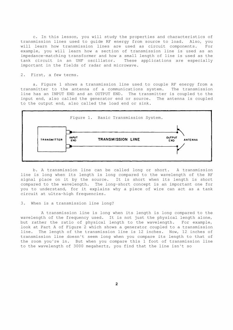
c. In this lesson, you will study the properties a nd characteristics of transmission lines used to guide RF energy from sou rce to load. Also, you will learn how transmission lines are used as circu it components. For example, you will learn how a section of transmissi on line is used as an impedance-matching transformer and how a small leng th of line is used as the tank circuit in an UHF oscillator. These applicati ons are especially important in the fields of radar and microwave. 2. First, a few terms. a. Figure 1 shows a transmission line used to coup le RF energy from a transmitter to the antenna of a communications syst em. The transmission line has an INPUT END and an OUTPUT END. The trans mitter is coupled to the input end, also called the generator end or source. The antenna is coupled to the output end, also called the load end or sink .

Figure 1. Basic Transmission System. b. A transmission line can be called long or short . A transmission line is long when its length is long compared to th e wavelength of the RF signal place on it by the source. It is short when its length is short compared to the wavelength. The long-short concept is an important one for you to understand, for it explains why a piece of w ire can act as a tank circuit at ultra-high frequencies. 3. When is a transmission line long? A transmission line is long when its length is lo ng compared to the wavelength of the frequency used. It is not just t he physical length alone, but rather the ratio of physical length to the wave length. For example, look at Part A of Figure 2 which shows a generator coupled to a transmission line. The length of the transmission line is 12 in ches. Now, 12 inches of transmission line doesn't seem long when you compar e its length to that of the room you're in. But when you compare this 1 fo ot of transmission line to the wavelength of 3000 megahertz, you find that the line isn't so

2

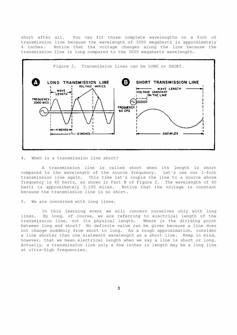
short after all. You can fit three complete wavele ngths on a foot of transmission line because the wavelength of 3000 me gahertz is approximately 4 inches. Notice that the voltage changes along th e line because the transmission line is long compared to the 3000 mega hertz wavelength.

Figure 2. Transmission Lines can be LONG or SHORT. 4. When is a transmission line short? A transmission line is called short when its leng th is short compared to the wavelength of the source frequency. Let's use our 1-foot transmission line again. This time let's couple th e line to a source whose frequency is 60 hertz, as shown in Part B of Figure 2. The wavelength of 60 hertz is approximately 3,100 miles. Notice that th e voltage is constant because the transmission line is so short. 5. We are concerned with long lines. In this learning event we will concern ourselves only with long lines. By long, of course, we are referring to ele ctrical length of the transmission line, not its physical length. Where is the dividing point between long and short? No definite value can be g iven because a line does not change suddenly from short to long. As a rough approximation, consider a line shorter than one sixteenth wavelength as a s hort line. Keep in mind, however, that we mean electrical length when we say a line is short or long. Actually, a transmission line only a few inches in length may be a long line at ultra-high frequencies.

3

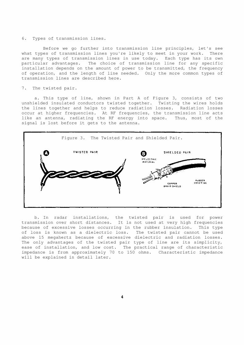
6. Types of transmission lines. Before we go further into transmission line princ iples, let's see what types of transmission lines you're likely to m eet in your work. There are many types of transmission lines in use today. Each type has its own particular advantages. The choice of transmission line for any specific installation depends on the amount of power to be t ransmitted, the frequency of operation, and the length of line needed. Only the more common types of transmission lines are described here. 7. The twisted pair. a. This type of line, shown in Part A of Figure 3, consists of two unshielded insulated conductors twisted together. Twisting the wires holds the lines together and helps to reduce radiation lo sses. Radiation losses occur at higher frequencies. At RF frequencies, th e transmission line acts like an antenna, radiating the RF energy into space . Thus, most of the signal is lost before it gets to the antenna.

Figure 3. The Twisted Pair and Shielded Pair. b. In radar installations, the twisted pair is use d for power transmission over short distances. It is not used at very high frequencies because of excessive losses occurring in the rubber insulation. This type of loss is known as a dielectric loss. The twisted pair cannot be used above 15 megahertz because of excessive dielectric and radiation losses. The only advantages of the twisted pair type of lin e are its simplicity, ease of installation, and low cost. The practical range of characteristic impedance is from approximately 70 to 150 ohms. Ch aracteristic impedance will be explained in detail later.

4

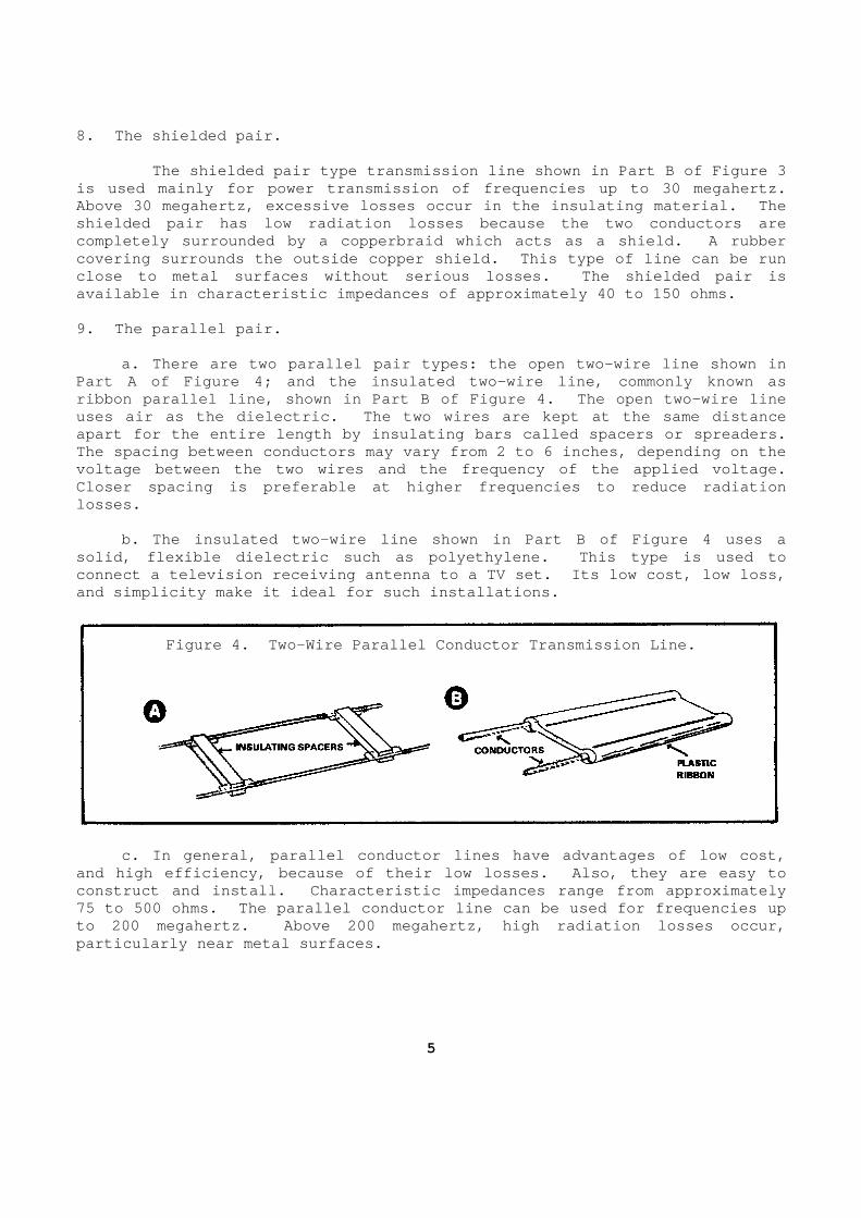
8. The shielded pair. The shielded pair type transmission line shown in Part B of Figure 3 is used mainly for power transmission of frequencie s up to 30 megahertz. Above 30 megahertz, excessive losses occur in the i nsulating material. The shielded pair has low radiation losses because the two conductors are completely surrounded by a copperbraid which acts a s a shield. A rubber covering surrounds the outside copper shield. This type of line can be run close to metal surfaces without serious losses. Th e shielded pair is available in characteristic impedances of approxima tely 40 to 150 ohms. 9. The parallel pair. a. There are two parallel pair types: the open two -wire line shown in Part A of Figure 4; and the insulated two-wire line , commonly known as ribbon parallel line, shown in Part B of Figure 4. The open two-wire line uses air as the dielectric. The two wires are kept at the same distance apart for the entire length by insulating bars call ed spacers or spreaders. The spacing between conductors may vary from 2 to 6 inches, depending on the voltage between the two wires and the frequency of the applied voltage. Closer spacing is preferable at higher frequencies to reduce radiation losses. b. The insulated two-wire line shown in Part B of Figure 4 uses a solid, flexible dielectric such as polyethylene. T his type is used to connect a television receiving antenna to a TV set. Its low cost, low loss, and simplicity make it ideal for such installations .

Figure 4. Two-Wire Parallel Conductor Transmission Line. c. In general, parallel conductor lines have advan tages of low cost, and high efficiency, because of their low losses. Also, they are easy to construct and install. Characteristic impedances r ange from approximately 75 to 500 ohms. The parallel conductor line can be used for frequencies up to 200 megahertz. Above 200 megahertz, high radiat ion losses occur, particularly near metal surfaces.

5

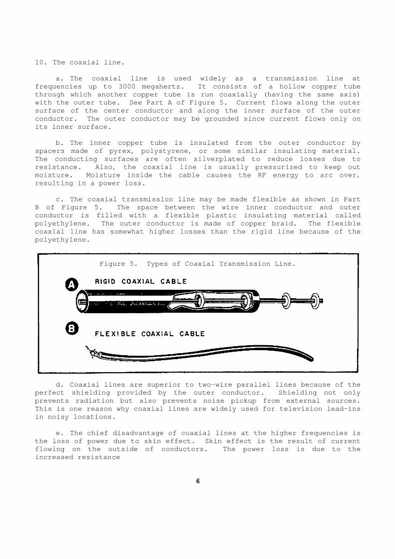
10. The coaxial line. a. The coaxial line is used widely as a transmissi on line at frequencies up to 3000 megahertz. It consists of a hollow copper tube through which another copper tube is run coaxially (having the same axis) with the outer tube. See Part A of Figure 5. Curr ent flows along the outer surface of the center conductor and along the inner surface of the outer conductor. The outer conductor may be grounded sin ce current flows only on its inner surface. b. The inner copper tube is insulated from the out er conductor by spacers made of pyrex, polystyrene, or some similar insulating material. The conducting surfaces are often silverplated to r educe losses due to resistance. Also, the coaxial line is usually pres surized to keep out moisture. Moisture inside the cable causes the RF energy to arc over, resulting in a power loss. c. The coaxial transmission line may be made flexi ble as shown in Part B of Figure 5. The space between the wire inner co nductor and outer conductor is filled with a flexible plastic insulat ing material called polyethylene. The outer conductor is made of coppe r braid. The flexible coaxial line has somewhat higher losses than the ri gid line because of the polyethylene.

Figure 5. Types of Coaxial Transmission Line. d. Coaxial lines are superior to two-wire parallel lines because of the perfect shielding provided by the outer conductor. Shielding not only prevents radiation but also prevents noise pickup f rom external sources. This is one reason why coaxial lines are widely use d for television lead-ins in noisy locations. e. The chief disadvantage of coaxial lines at the higher frequencies is the loss of power due to skin effect. Skin effect is the result of current flowing on the outside of conductors. The power lo ss is due to the increased resistance

6

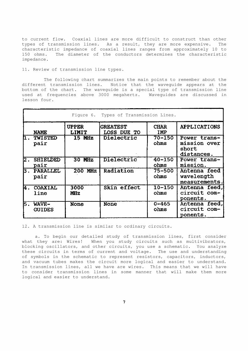
to current flow. Coaxial lines are more difficult to construct than other types of transmission lines. As a result, they are more expensive. The characteristic impedance of coaxial lines ranges fr om approximately 10 to 150 ohms. The diameter of the conductors determine s the characteristic impedance. 11. Review of transmission line types. The following chart summarizes the main points to remember about the different transmission lines. Notice that the wave guide appears at the bottom of the chart. The waveguide is a special ty pe of transmission line used at frequencies above 3000 megahertz. Waveguid es are discussed in lesson four.

Figure 6. Types of Transmission Lines. 12. A transmission line is similar to ordinary circ uits. a. To begin our detailed study of transmission lin es, first consider what they are: Wires! When you study circuits such as multivibrators, blocking oscillators, and other circuits, you use a schematic. You analyze these circuits in terms of current and voltage. Th e use and understanding of symbols in the schematic to represent resistors, capacitors, inductors, and vacuum tubes makes the circuit more logical and easier to understand. In transmission lines, all we have are wires. This means that we will have to consider transmission lines in some manner that will make them more logical and easier to understand.

7

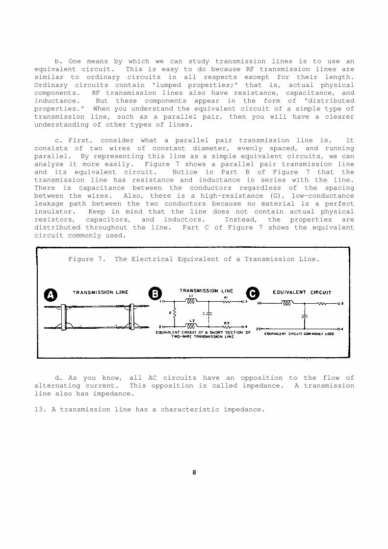
b. One means by which we can study transmission li nes is to use an equivalent circuit. This is easy to do because RF transmission lines are similar to ordinary circuits in all respects except for their length. Ordinary circuits contain "lumped properties;" that is, actual physical components. RF transmission lines also have resist ance, capacitance, and inductance. But these components appear in the for m of "distributed properties." When you understand the equivalent ci rcuit of a simple type of transmission line, such as a parallel pair, then yo u will have a clearer understanding of other types of lines. c. First, consider what a parallel pair transmissi on line is. It consists of two wires of constant diameter, evenly spaced, and running parallel. By representing this line as a simple eq uivalent circuits, we can analyze it more easily. Figure 7 shows a parallel pair transmission line and its equivalent circuit. Notice in Part B of Fi gure 7 that the transmission line has resistance and inductance in series with the line. There is capacitance between the conductors regardl ess of the spacing between the wires. Also, there is a high-resistanc e (G), low-conductance leakage path between the two conductors because no material is a perfect insulator. Keep in mind that the line does not con tain actual physical resistors, capacitors, and inductors. Instead, the properties are distributed throughout the line. Part C of Figure 7 shows the equivalent circuit commonly used.

Figure 7. The Electrical Equivalent of a Transmiss ion Line. d. As you know, all AC circuits have an opposition to the flow of alternating current. This opposition is called imp edance. A transmission line also has impedance. 13. A transmission line has a characteristic impeda nce.

8

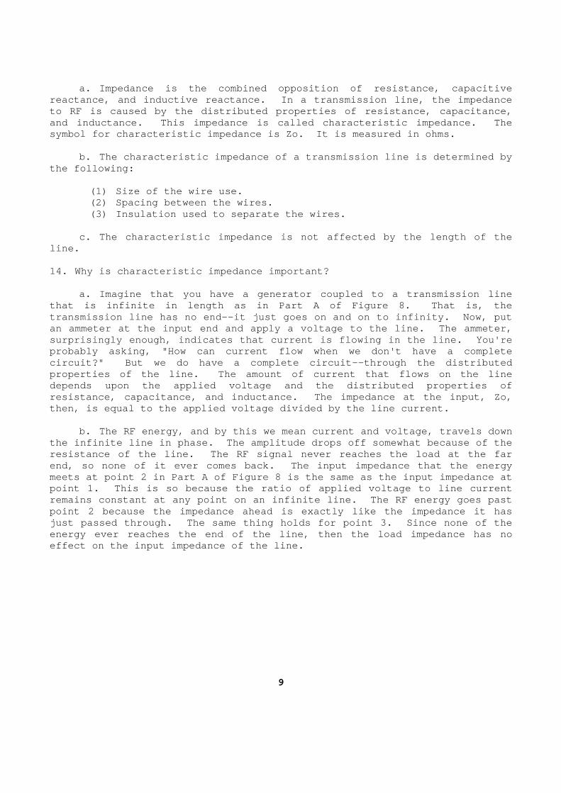
a. Impedance is the combined opposition of resista nce, capacitive reactance, and inductive reactance. In a transmiss ion line, the impedance to RF is caused by the distributed properties of re sistance, capacitance, and inductance. This impedance is called character istic impedance. The symbol for characteristic impedance is Zo. It is m easured in ohms. b. The characteristic impedance of a transmission line is determined by the following: (1) Size of the wire use. (2) Spacing between the wires. (3) Insulation used to separate the wires. c. The characteristic impedance is not affected by the length of the line. 14. Why is characteristic impedance important? a. Imagine that you have a generator coupled to a transmission line that is infinite in length as in Part A of Figure 8 . That is, the transmission line has no end--it just goes on and o n to infinity. Now, put an ammeter at the input end and apply a voltage to the line. The ammeter, surprisingly enough, indicates that current is flow ing in the line. You're probably asking, "How can current flow when we don' t have a complete circuit?" But we do have a complete circuit--throu gh the distributed properties of the line. The amount of current that flows on the line depends upon the applied voltage and the distribute d properties of resistance, capacitance, and inductance. The imped ance at the input, Zo, then, is equal to the applied voltage divided by th e line current. b. The RF energy, and by this we mean current and voltage, travels down the infinite line in phase. The amplitude drops of f somewhat because of the resistance of the line. The RF signal never reache s the load at the far end, so none of it ever comes back. The input impe dance that the energy meets at point 2 in Part A of Figure 8 is the same as the input impedance at point 1. This is so because the ratio of applied v oltage to line current remains constant at any point on an infinite line. The RF energy goes past point 2 because the impedance ahead is exactly like the impedance it has just passed through. The same thing holds for poin t 3. Since none of the energy ever reaches the end of the line, then the l oad impedance has no effect on the input impedance of the line.

9

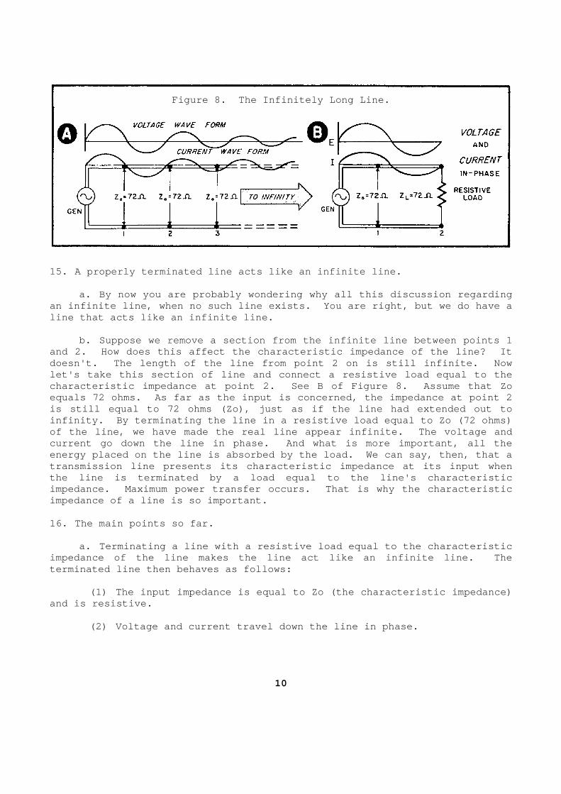
Figure 8. The Infinitely Long Line.

15. A properly terminated line acts like an infinit e line. a. By now you are probably wondering why all this discussion regarding an infinite line, when no such line exists. You ar e right, but we do have a line that acts like an infinite line. b. Suppose we remove a section from the infinite l ine between points 1 and 2. How does this affect the characteristic imp edance of the line? It doesn't. The length of the line from point 2 on is still infinite. Now let's take this section of line and connect a resis tive load equal to the characteristic impedance at point 2. See B of Figu re 8. Assume that Zo equals 72 ohms. As far as the input is concerned, the impedance at point 2 is still equal to 72 ohms (Zo), just as if the line had extended out to infinity. By terminating the line in a resistive l oad equal to Zo (72 ohms) of the line, we have made the real line appear infi nite. The voltage and current go down the line in phase. And what is mor e important, all the energy placed on the line is absorbed by the load. We can say, then, that a transmission line presents its characteristic imped ance at its input when the line is terminated by a load equal to the line' s characteristic impedance. Maximum power transfer occurs. That is why the characteristic impedance of a line is so important. 16. The main points so far. a. Terminating a line with a resistive load equal to the characteristic impedance of the line makes the line act like an in finite line. The terminated line then behaves as follows: (1) The input impedance is equal to Zo (the charac teristic impedance) and is resistive. (2) Voltage and current travel down the line in ph ase.

10

(3) The ratio of voltage to current at any point o n the line is constant and equals Zo. (4) There is maximum transfer of power from source to load. b. Less power is lost when the transmission line i s fitted or matched to the load. What happens when the transmission li ne does not match the impedance of the load? Reflections occur when ther e is an impedance mismatch between the transmission line and the load . Reflections cause a loss in power known as reflection loss. 17. Reflections occur when there is a sudden change in impedance. a. Let's take the statement apart and see what it really means. Suppose you're in a room and you call your buddy ou tside. The sound of your voice reaches him, but some of the power of your vo ice is lost before it gets to him. The loss takes place at the walls of the room. We can call this loss of sound, reflection loss. b. The sound of your voice does all right travelin g through the air until it hits the wall. Some of the sound continue s through the wall to the outside. Another portion of the sound is reflected or bounced back to you. The reflection is called an echo. How much of the sound is reflected depends on how hard the wall is. A hard, solid wal l causes a lot of reflection, because the sound can't penetrate the w all as well as it can penetrate the air. Part of the sound can't get thr ough the wall at all. The reflection takes place right at the point where the conductors change, from air to wood. The reflection loss of sound, th en, is caused by a change or mismatch in the impedance of the conductors. Th e loss occurs right at the point where the mismatch is located, in this ca se, the wall. 18. The same thing happens in RF transmission lines . a. A reflection occurs when the RF energy meets a sudden change in impedance. When the RF energy reaches the point wh ere the mismatch occurs, part of the wave is reflected back to the source. This means less energy is available for the load. This is reflection loss.

11

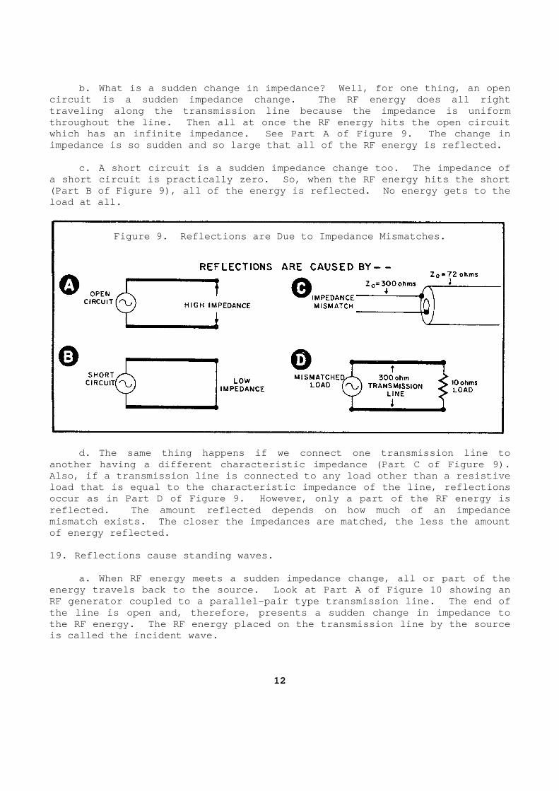
b. What is a sudden change in impedance? Well, fo r one thing, an open circuit is a sudden impedance change. The RF energ y does all right traveling along the transmission line because the i mpedance is uniform throughout the line. Then all at once the RF energ y hits the open circuit which has an infinite impedance. See Part A of Fig ure 9. The change in impedance is so sudden and so large that all of the RF energy is reflected. c. A short circuit is a sudden impedance change to o. The impedance of a short circuit is practically zero. So, when the RF energy hits the short (Part B of Figure 9), all of the energy is reflecte d. No energy gets to the load at all.

Figure 9. Reflections are Due to Impedance Mismatc hes.

d. The same thing happens if we connect one transm ission line to another having a different characteristic impedance (Part C of Figure 9). Also, if a transmission line is connected to any lo ad other than a resistive load that is equal to the characteristic impedance of the line, reflections occur as in Part D of Figure 9. However, only a pa rt of the RF energy is reflected. The amount reflected depends on how muc h of an impedance mismatch exists. The closer the impedances are mat ched, the less the amount of energy reflected. 19. Reflections cause standing waves. a. When RF energy meets a sudden impedance change, all or part of the energy travels back to the source. Look at Part A of Figure 10 showing an RF generator coupled to a parallel-pair type transm ission line. The end of the line is open and, therefore, presents a sudden change in impedance to the RF energy. The RF energy placed on the transmi ssion line by the source is called the incident wave.

12

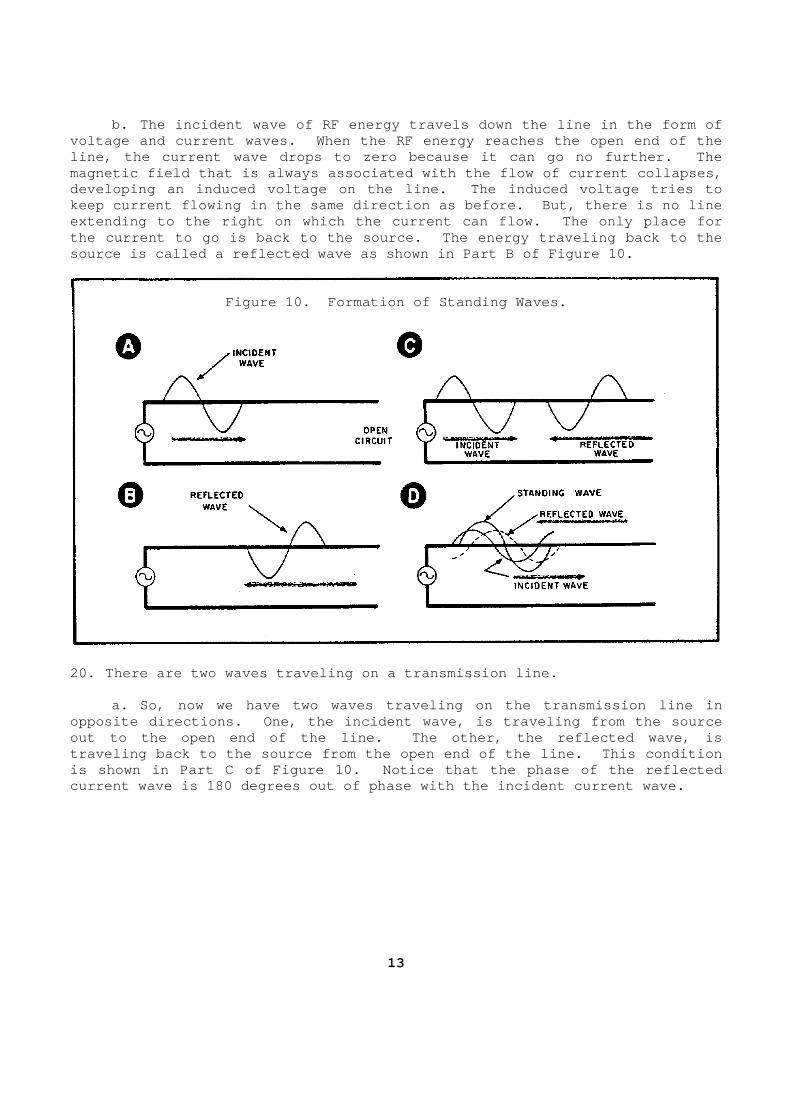
b. The incident wave of RF energy travels down the line in the form of voltage and current waves. When the RF energy reac hes the open end of the line, the current wave drops to zero because it can go no further. The magnetic field that is always associated with the f low of current collapses, developing an induced voltage on the line. The ind uced voltage tries to keep current flowing in the same direction as befor e. But, there is no line extending to the right on which the current can flo w. The only place for the current to go is back to the source. The energ y traveling back to the source is called a reflected wave as shown in Part B of Figure 10.

Figure 10. Formation of Standing Waves.

20. There are two waves traveling on a transmission line. a. So, now we have two waves traveling on the tran smission line in opposite directions. One, the incident wave, is tr aveling from the source out to the open end of the line. The other, the re flected wave, is traveling back to the source from the open end of t he line. This condition is shown in Part C of Figure 10. Notice that the p hase of the reflected current wave is 180 degrees out of phase with the i ncident current wave.

13

b. Now, the reflected wave of the RF current trave ls away from the open end of the line. It meets the incident current wav es coming from the generator. At every point on the line, these two w aves combine to produce a resultant wave, called a standing wave. Part D of Figure 10 shows how the incident and reflected waves combine to produce a s tanding wave. 21. Standing waves are stationary. a. Figure 10 shows that the standing wave is stati onary, it does not move. As the incident wave and reflected wave move past each other, the standing wave changes only its amplitude. Let's se e why this is so with the help of Figure 11. (1) Part A of Figure 11 shows the incident wave an d the reflected wave in phase. Adding the two current waves gives a resultant or standing wave of current equal to twice the amplitude of the traveling waves. (2) Part B of Figure 11 shows a 90 degree phase di fference between the incident and reflected current waves because th ey are moving away from each other. Notice that although the amplitude of the standing wave has decreased, the minimum and maximum points lie in th e same place as they did in Part A of Figure 11. (3) Part C of Figure 11 shows 180 degrees phase di fference between the incident and reflected waves. The two waves ca ncel each other. There is no standing wave of current at this particular t ime. (4) Part D of Figure 11 shows 270 degrees phase di fference between the two traveling waves. Notice now that, although the minimum and maximum points are in the same position, the amplitude has reversed its direction. (5) Part E of Figure 11 shows the two current wave s in phase again. The resultant wave is equal in amplitude but 180 de grees out of phase with the standing wave shown in Part A of Figure 11.

14

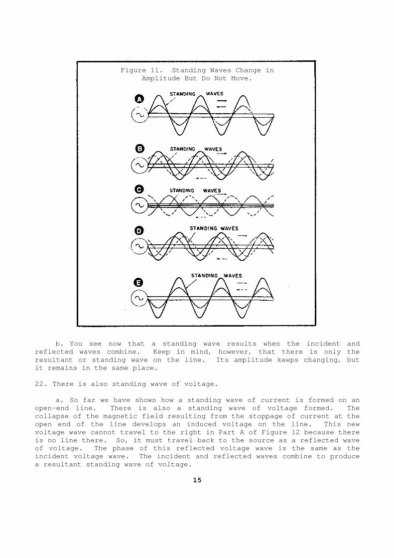
Figure 11. Standing Waves Change in

Amplitude But Do Not Move. b. You see now that a standing wave results when t he incident and reflected waves combine. Keep in mind, however, th at there is only the resultant or standing wave on the line. Its amplit ude keeps changing, but it remains in the same place. 22. There is also standing wave of voltage. a. So far we have shown how a standing wave of cur rent is formed on an open-end line. There is also a standing wave of vo ltage formed. The collapse of the magnetic field resulting from the s toppage of current at the open end of the line develops an induced voltage on the line. This new voltage wave cannot travel to the right in Part A o f Figure 12 because there is no line there. So, it must travel back to the s ource as a reflected wave of voltage. The phase of this reflected voltage wa ve is the same as the incident voltage wave. The incident and reflected waves combine to produce a resultant standing wave of voltage.

15

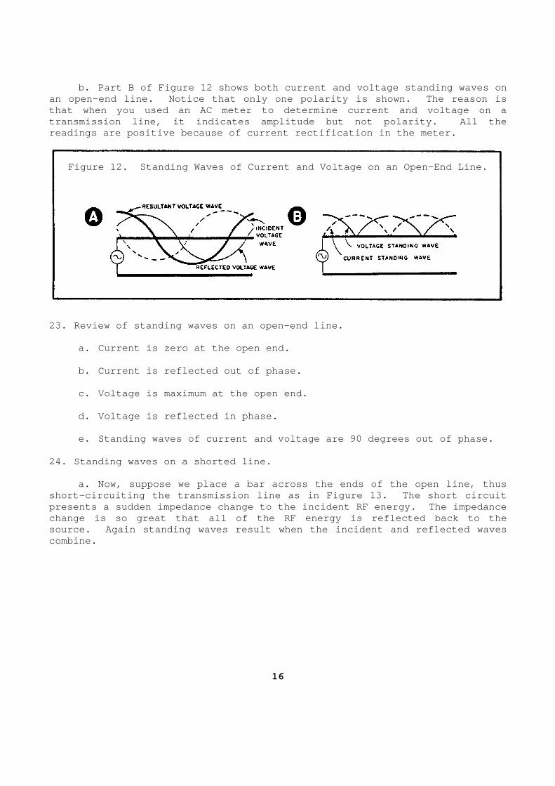
b. Part B of Figure 12 shows both current and volt age standing waves on an open-end line. Notice that only one polarity is shown. The reason is that when you used an AC meter to determine current and voltage on a transmission line, it indicates amplitude but not p olarity. All the readings are positive because of current rectificat ion in the meter.

Figure 12. Standing Waves of Current and Voltage o n an Open-End Line.

23. Review of standing waves on an open-end line. a. Current is zero at the open end. b. Current is reflected out of phase. c. Voltage is maximum at the open end. d. Voltage is reflected in phase. e. Standing waves of current and voltage are 90 de grees out of phase. 24. Standing waves on a shorted line. a. Now, suppose we place a bar across the ends of the open line, thus short-circuiting the transmission line as in Figure 13. The short circuit presents a sudden impedance change to the incident RF energy. The impedance change is so great that all of the RF energy is ref lected back to the source. Again standing waves result when the incid ent and reflected waves combine.

16

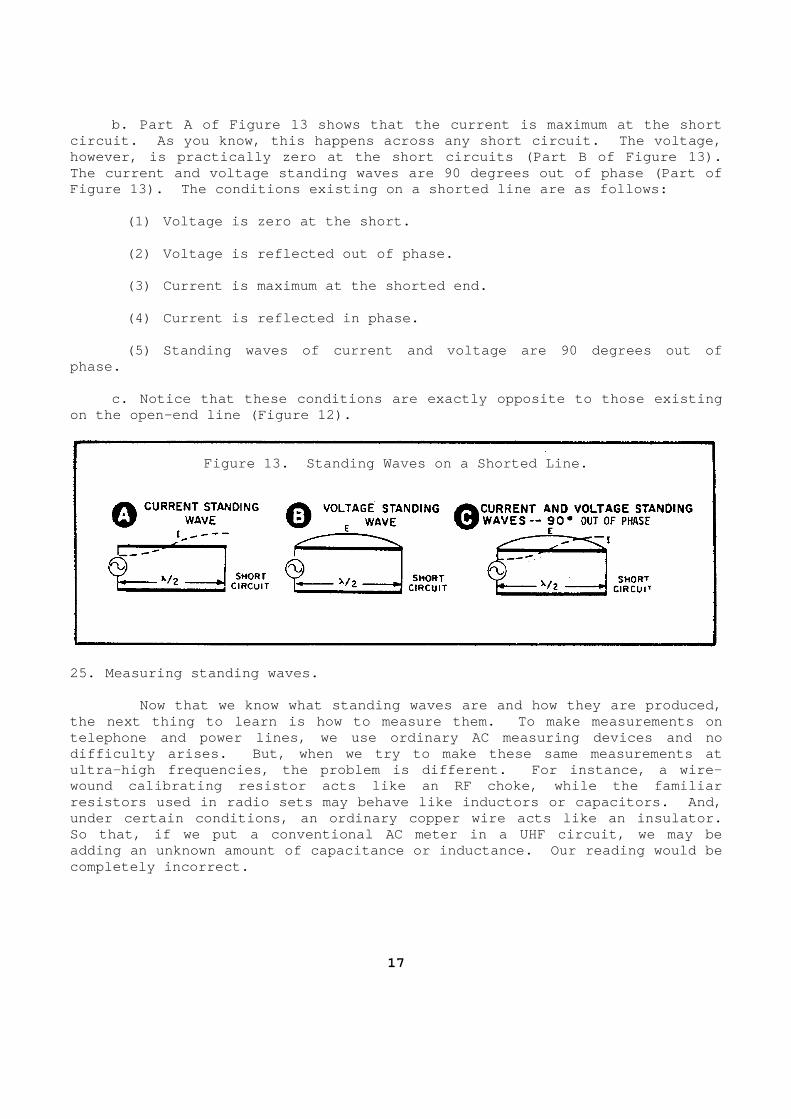
b. Part A of Figure 13 shows that the current is m aximum at the short circuit. As you know, this happens across any shor t circuit. The voltage, however, is practically zero at the short circuits (Part B of Figure 13). The current and voltage standing waves are 90 degre es out of phase (Part of Figure 13). The conditions existing on a shorted l ine are as follows: (1) Voltage is zero at the short. (2) Voltage is reflected out of phase. (3) Current is maximum at the shorted end. (4) Current is reflected in phase. (5) Standing waves of current and voltage are 90 d egrees out of phase. c. Notice that these conditions are exactly opposi te to those existing on the open-end line (Figure 12).

Figure 13. Standing Waves on a Shorted Line.

25. Measuring standing waves. Now that we know what standing waves are and how they are produced, the next thing to learn is how to measure them. To make measurements on telephone and power lines, we use ordinary AC measu ring devices and no difficulty arises. But, when we try to make these same measurements at ultra-high frequencies, the problem is different. For instance, a wire-wound calibrating resistor acts like an RF choke, w hile the familiar resistors used in radio sets may behave like induct ors or capacitors. And, under certain conditions, an ordinary copper wire a cts like an insulator. So that, if we put a conventional AC meter in a UHF circuit, we may be adding an unknown amount of capacitance or inductan ce. Our reading would be completely incorrect.

17

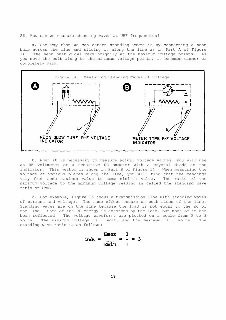
26. How can we measure standing waves at UHF freque ncies? a. One way that we can detect standing waves is by connecting a neon bulb across the line and sliding it along the line as in Part A of Figure 14. The neon bulb glows very brightly at the maxim um voltage points. As you move the bulb along to the minimum voltage poin ts, it becomes dimmer or completely dark.

Figure 14. Measuring Standing Waves of Voltage.

b. When it is necessary to measure actual voltage values, you will use an RF voltmeter or a sensitive DC ammeter with a cr ystal diode as the indicator. This method is shown in Part B of Figur e 14. When measuring the voltage at various places along the line, you will find that the readings vary from some maximum value to some minimum value. The ratio of the maximum voltage to the minimum voltage reading is c alled the standing wave ratio or SWR. c. For example, Figure 15 shows a transmission lin e with standing waves of current and voltage. The same effect occurs on both sides of the line. Standing waves are on the line because the load is not equal to the Zo of the line. Some of the RF energy is absorbed by the load, but most of it has been reflected. The voltage waveforms are plotted on a scale from 0 to 3 volts. The minimum voltage is 1 volt, and the maxi mum is 3 volts. The standing wave ratio is as follows:

18

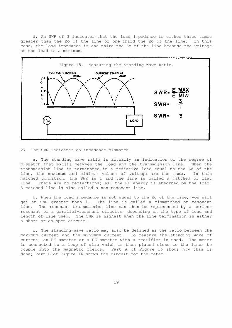
d. An SWR of 3 indicates that the load impedance i s either three times greater than the Zo of the line or one-third the Zo of the line. In this case, the load impedance is one-third the Zo of the line because the voltage at the load is a minimum.

Figure 15. Measuring the Standing-Wave Ratio.

27. The SWR indicates an impedance mismatch. a. The standing wave ratio is actually an indicati on of the degree of mismatch that exists between the load and the trans mission line. When the transmission line is terminated in a resistive load equal to the Zo of the line, the maximum and minimum values of voltage are the same. In this matched condition, the SWR is 1 and the line is cal led a matched or flat line. There are no reflections; all the RF energy is absorbed by the load. A matched line is also called a non-resonant line. b. When the load impedance is not equal to the Zo of the line, you will get an SWR greater than 1. The line is called a mi smatched or resonant line. The resonant transmission line can then be r epresented by a series-resonant or a parallel-resonant circuits, depending on the type of load and length of line used. The SWR is highest when the l ine termination is either a short or an open circuit. c. The standing-wave ratio may also be defined as the ratio between the maximum current and the minimum current. To measur e the standing wave of current, an RF ammeter or a DC ammeter with a recti fier is used. The meter is connected to a loop of wire which is then placed close to the lines to couple into the magnetic fields. Part A of Figure 16 shows how this is done; Part B of Figure 16 shows the circuit for the meter.

19

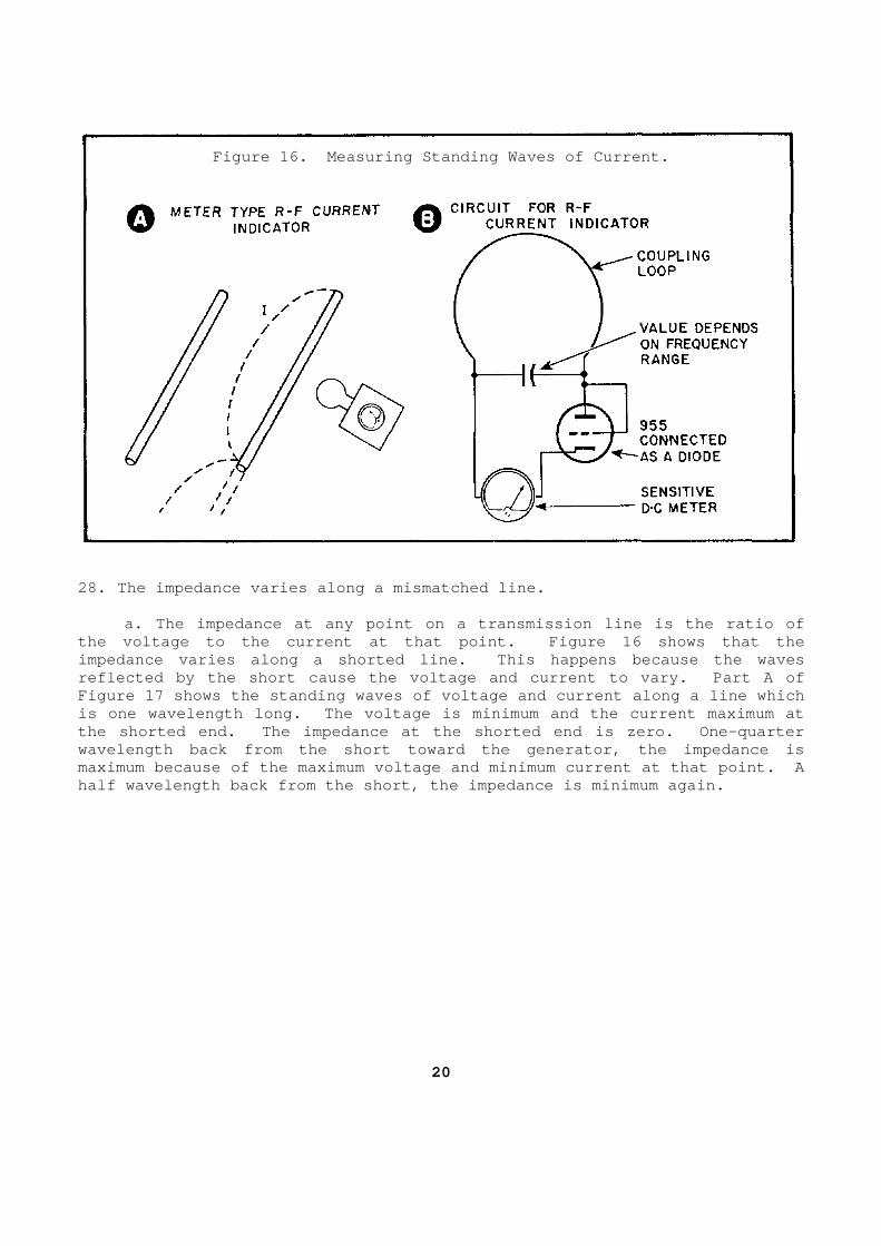
Figure 16. Measuring Standing Waves of Current.

28. The impedance varies along a mismatched line. a. The impedance at any point on a transmission li ne is the ratio of the voltage to the current at that point. Figure 1 6 shows that the impedance varies along a shorted line. This happen s because the waves reflected by the short cause the voltage and curren t to vary. Part A of Figure 17 shows the standing waves of voltage and c urrent along a line which is one wavelength long. The voltage is minimum and the current maximum at the shorted end. The impedance at the shorted end is zero. One-quarter wavelength back from the short toward the generator , the impedance is maximum because of the maximum voltage and minimum current at that point. A half wavelength back from the short, the impedance is minimum again.

20

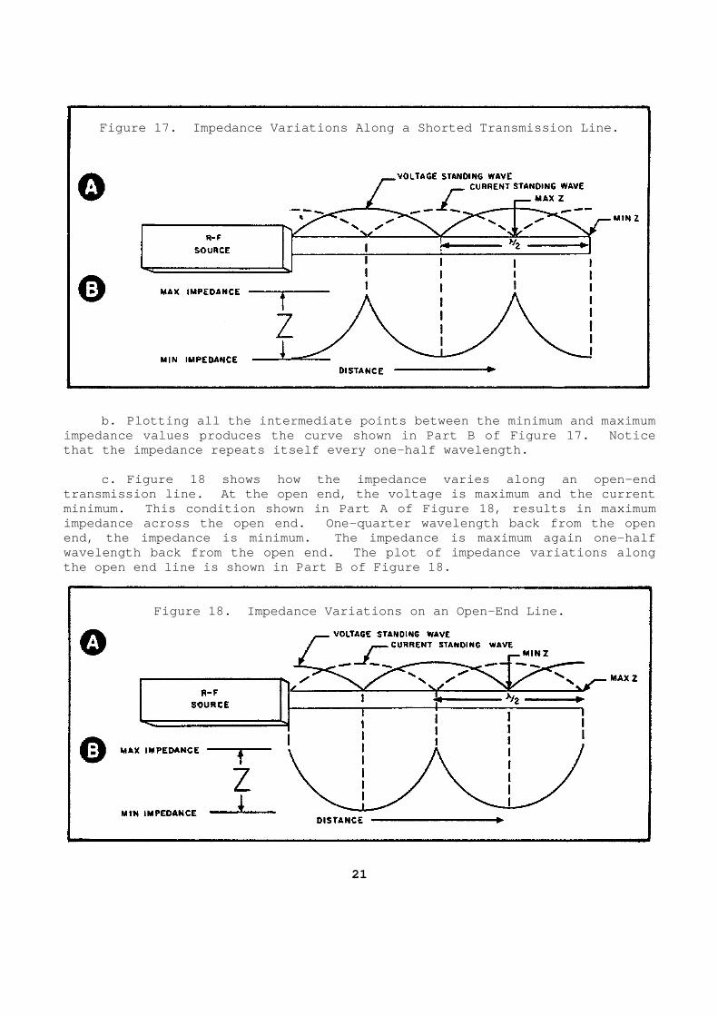
Figure 17. Impedance Variations Along a Shorted Tr ansmission Line.

b. Plotting all the intermediate points between th e minimum and maximum impedance values produces the curve shown in Part B of Figure 17. Notice that the impedance repeats itself every one-half wa velength. c. Figure 18 shows how the impedance varies along an open-end transmission line. At the open end, the voltage is maximum and the current minimum. This condition shown in Part A of Figure 18, results in maximum impedance across the open end. One-quarter wavelen gth back from the open end, the impedance is minimum. The impedance is ma ximum again one-half wavelength back from the open end. The plot of imp edance variations along the open end line is shown in Part B of Figure 18.

Figure 18. Impedance Variations on an Open-End Lin e.

21

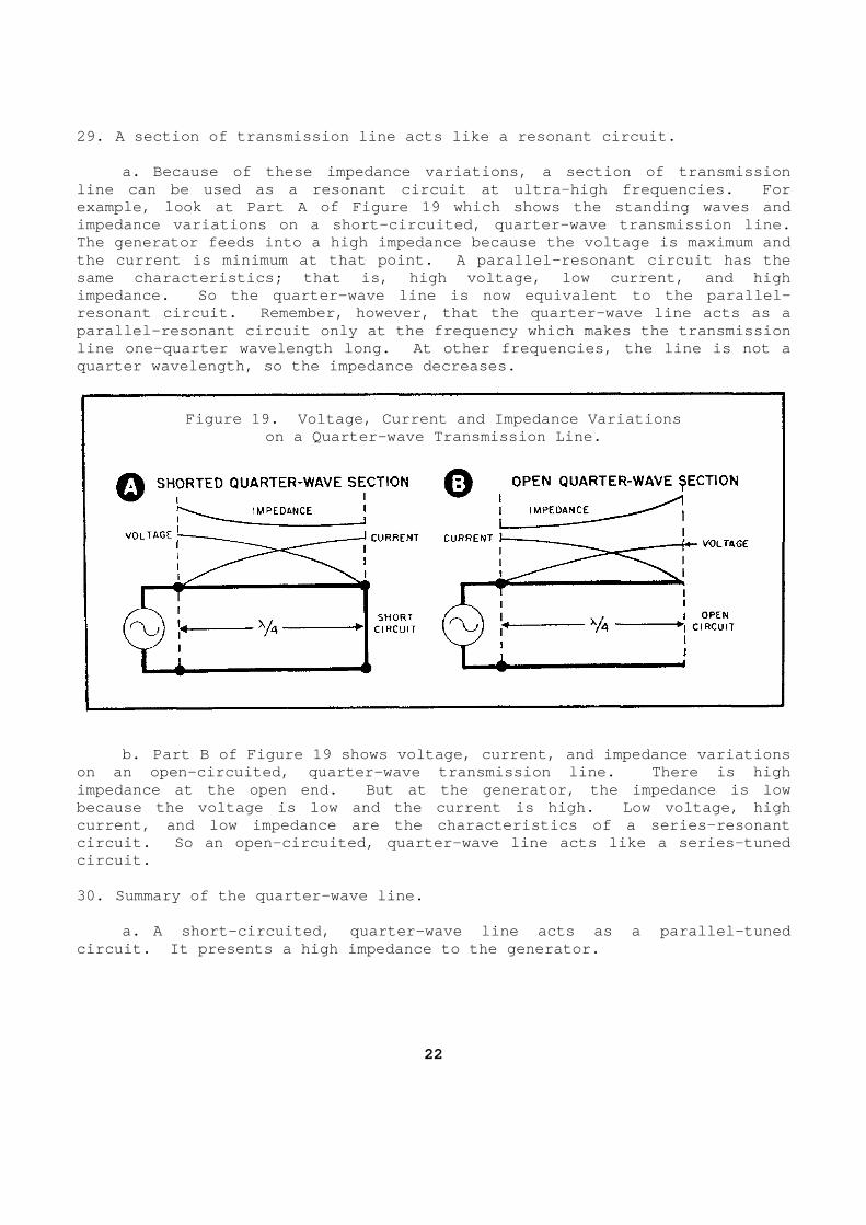
29. A section of transmission line acts like a reso nant circuit. a. Because of these impedance variations, a sectio n of transmission line can be used as a resonant circuit at ultra-hig h frequencies. For example, look at Part A of Figure 19 which shows th e standing waves and impedance variations on a short-circuited, quarter- wave transmission line. The generator feeds into a high impedance because t he voltage is maximum and the current is minimum at that point. A parallel-r esonant circuit has the same characteristics; that is, high voltage, low cu rrent, and high impedance. So the quarter-wave line is now equival ent to the parallel-resonant circuit. Remember, however, that the quar ter-wave line acts as a parallel-resonant circuit only at the frequency whi ch makes the transmission line one-quarter wavelength long. At other frequen cies, the line is not a quarter wavelength, so the impedance decreases.

Figure 19. Voltage, Current and Impedance Variatio ns

on a Quarter-wave Transmission Line. b. Part B of Figure 19 shows voltage, current, and impedance variations on an open-circuited, quarter-wave transmission lin e. There is high impedance at the open end. But at the generator, t he impedance is low because the voltage is low and the current is high. Low voltage, high current, and low impedance are the characteristics of a series-resonant circuit. So an open-circuited, quarter-wave line a cts like a series-tuned circuit. 30. Summary of the quarter-wave line. a. A short-circuited, quarter-wave line acts as a parallel-tuned circuit. It presents a high impedance to the gener ator.

22

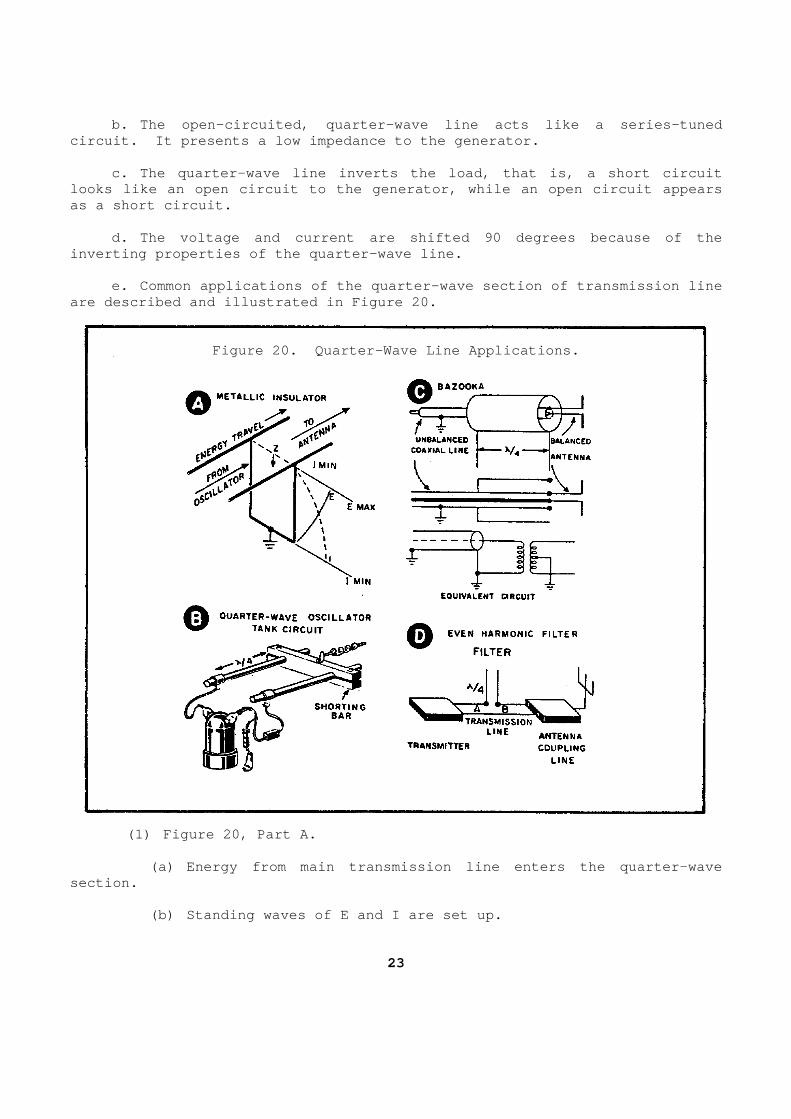
b. The open-circuited, quarter-wave line acts like a series-tuned circuit. It presents a low impedance to the genera tor. c. The quarter-wave line inverts the load, that is , a short circuit looks like an open circuit to the generator, while an open circuit appears as a short circuit. d. The voltage and current are shifted 90 degrees because of the inverting properties of the quarter-wave line. e. Common applications of the quarter-wave section of transmission line are described and illustrated in Figure 20.

Figure 20. Quarter-Wave Line Applications.

(1) Figure 20, Part A. (a) Energy from main transmission line enters the quarter-wave section. (b) Standing waves of E and I are set up.

23

(c) RF energy meets a high Z at the opening of the quarter-wave section. (d) Quarter-wave section also acts as a sturdy mec hanical support for the main line. (2) Figure 20, Part B. (a) A shorted quarter-wave section has the propert ies of a parallel-resonant circuit. (b) The oscillator is tuned by adjusting the movab le shorting bar. (3) Figure 20, Part C. (a) An antenna is usually balanced. Each side has the same impedance and voltage with respect to ground. (b) A coaxial line is unbalanced. The outside con ductor is at ground potential. (c) The bazooka removes the ground potential at th e point where the antenna is connected to the coaxial line. (4) Figure 20, Part D. (a) An open-end, quarter-wave section sets up a lo w Z at AB to the fundamental frequency. (b) RF energy at the fundamental frequency passes to the antenna. (c) The filter becomes a half-wave section at the second harmonic. It sets up a high impedance at AB. (d) The second harmonic does not pass on to the an tenna. 31. The half-wave section of transmission line. a. The half-wave section of a line is really an ex tension of the quarter-wave section. So, if you understand how th e quarter-wave section works, you will have little difficulty with the hal f-wave section. Figure 21 shows the standing-wave and impedance variations on a half-wave section of line. Notice that whatever conditions appear on the load end of the line are repeated at the generator or source end. For e xample, look at Part A of Figure 21 which shows the voltage,

24

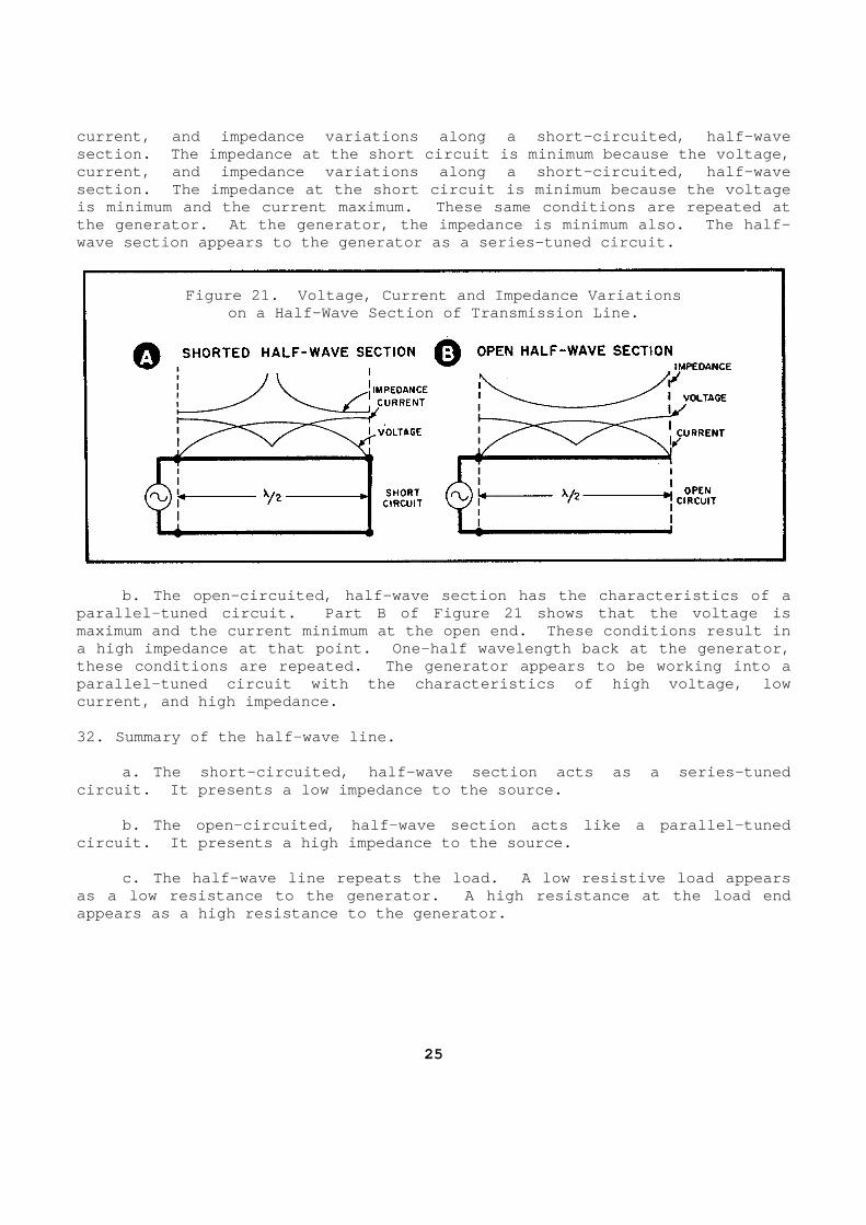
current, and impedance variations along a short-cir cuited, half-wave section. The impedance at the short circuit is min imum because the voltage, current, and impedance variations along a short-cir cuited, half-wave section. The impedance at the short circuit is min imum because the voltage is minimum and the current maximum. These same con ditions are repeated at the generator. At the generator, the impedance is minimum also. The half-wave section appears to the generator as a series-t uned circuit.

Figure 21. Voltage, Current and Impedance Variatio ns

on a Half-Wave Section of Transmission Line. b. The open-circuited, half-wave section has the c haracteristics of a parallel-tuned circuit. Part B of Figure 21 shows that the voltage is maximum and the current minimum at the open end. T hese conditions result in a high impedance at that point. One-half wavelengt h back at the generator, these conditions are repeated. The generator appea rs to be working into a parallel-tuned circuit with the characteristics of high voltage, low current, and high impedance. 32. Summary of the half-wave line. a. The short-circuited, half-wave section acts as a series-tuned circuit. It presents a low impedance to the source . b. The open-circuited, half-wave section acts like a parallel-tuned circuit. It presents a high impedance to the sourc e. c. The half-wave line repeats the load. A low res istive load appears as a low resistance to the generator. A high resis tance at the load end appears as a high resistance to the generator.

25

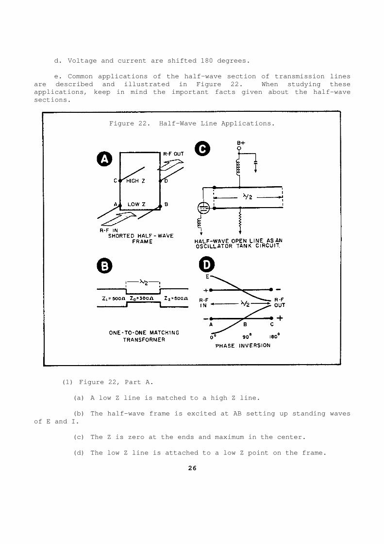
d. Voltage and current are shifted 180 degrees. e. Common applications of the half-wave section of transmission lines are described and illustrated in Figure 22. When s tudying these applications, keep in mind the important facts give n about the half-wave sections.

Figure 22. Half-Wave Line Applications.

(1) Figure 22, Part A. (a) A low Z line is matched to a high Z line. (b) The half-wave frame is excited at AB setting u p standing waves of E and I. (c) The Z is zero at the ends and maximum in the c enter. (d) The low Z line is attached to a low Z point on the frame.

26

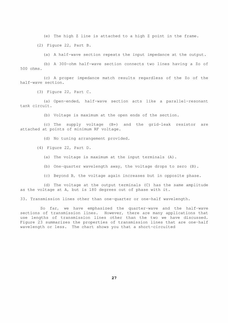
(e) The high Z line is attached to a high Z point in the frame. (2) Figure 22, Part B. (a) A half-wave section repeats the input impedanc e at the output. (b) A 300-ohm half-wave section connects two lines having a Zo of 500 ohms. (c) A proper impedance match results regardless of the Zo of the half-wave section. (3) Figure 22, Part C. (a) Open-ended, half-wave section acts like a para llel-resonant tank circuit. (b) Voltage is maximum at the open ends of the sec tion. (c) The supply voltage (B+) and the grid-leak resi stor are attached at points of minimum RF voltage. (d) No tuning arrangement provided. (4) Figure 22, Part D. (a) The voltage is maximum at the input terminals (A). (b) One-quarter wavelength away, the voltage drops to zero (B). (c) Beyond B, the voltage again increases but in o pposite phase. (d) The voltage at the output terminals (C) has th e same amplitude as the voltage at A, but is 180 degrees out of phas e with it. 33. Transmission lines other than one-quarter or on e-half wavelength. So far, we have emphasized the quarter-wave and t he half-wave sections of transmission lines. However, there are many applications that use lengths of transmission lines other than the tw o we have discussed. Figure 23 summarizes the properties of transmission lines that are one-half wavelength or less. The chart shows you that a sho rt-circuited

27

section of transmission line that is less than a qu arter wavelength can take the place of an inductor, at the ultra-high frequen cies. An actual coil having a specific amount of inductance would be too small to be practical at such high frequencies.

Figure 23. Properties of Transmission Lines One-Ha lf

Wavelength or Less. Learning Event 2: ARTIFICIAL TRANSMISSION LINES 1. General. a. A transmission line is used to guide RF energy from one place to another with a minimum loss of energy. In addition , sections of RF transmission lines are used as coils and capacitors . For example, an open circuited quarter-wave line acts as a coil and capa citor in series. An open-circuited, half-wave line acts as a coil and c apacitor connected in parallel. b. Since a transmission line acts like a combinati on of coils and capacitors, it follows that we can connect coils an d capacitors in arrangements that will act like transmission lines. We call this circuit arrangement of coils and capacitors artificial tran smission lines (ATL). c. Two major ATL uses we will discuss in this text are: (1) As pulse-forming networks (PFN), to form pulse s used in radar. (2) As delay lines to delay pulses. 2. Comparing real and artificial transmission lines .

28

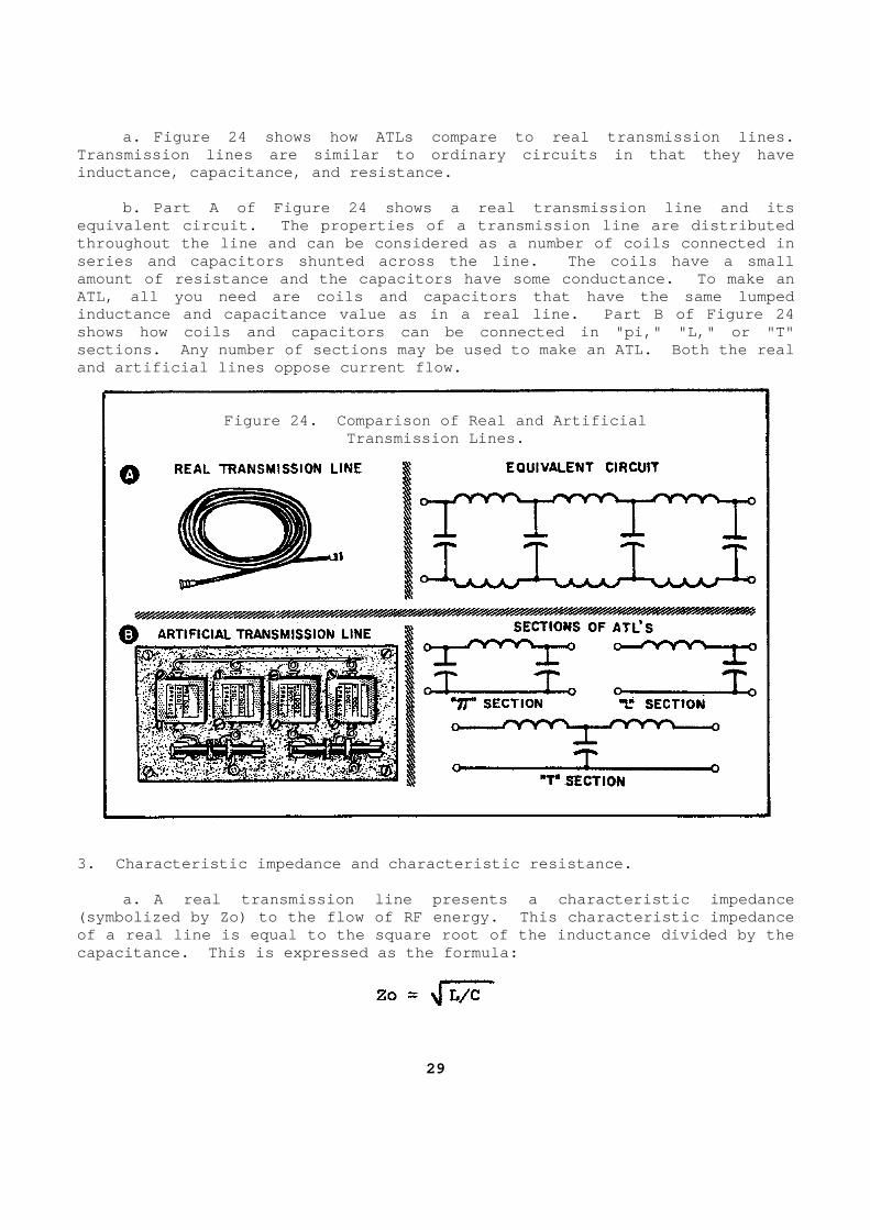
a. Figure 24 shows how ATLs compare to real transm ission lines. Transmission lines are similar to ordinary circuits in that they have inductance, capacitance, and resistance. b. Part A of Figure 24 shows a real transmission l ine and its equivalent circuit. The properties of a transmissi on line are distributed throughout the line and can be considered as a numb er of coils connected in series and capacitors shunted across the line. The coils have a small amount of resistance and the capacitors have some c onductance. To make an ATL, all you need are coils and capacitors that hav e the same lumped inductance and capacitance value as in a real line. Part B of Figure 24 shows how coils and capacitors can be connected in "pi," "L," or "T" sections. Any number of sections may be used to ma ke an ATL. Both the real and artificial lines oppose current flow.

Figure 24. Comparison of Real and Artificial

Transmission Lines. 3. Characteristic impedance and characteristic resi stance. a. A real transmission line presents a characteris tic impedance (symbolized by Zo) to the flow of RF energy. This characteristic impedance of a real line is equal to the square root of the i nductance divided by the capacitance. This is expressed as the formula:

29

b. Artificial transmission lines also present oppo sition to RF energy called characteristic resistance. We use the term characteristic resistance to indicate the impedance of an artificial transmis sion line. The symbol for characteristic resistance is Rc. As in a real line, the opposition is equal to the square root of the inductance divided by the capacitance. The formula is the same as for a real line:

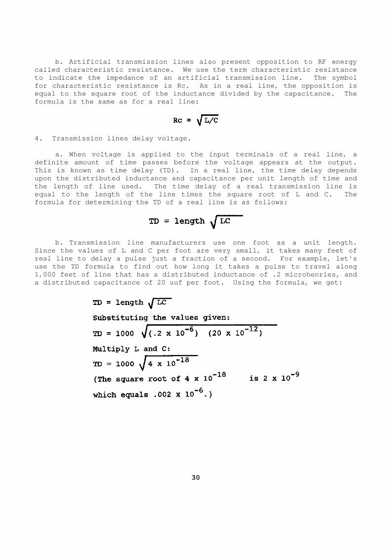
4. Transmission lines delay voltage. a. When voltage is applied to the input terminals of a real line, a definite amount of time passes before the voltage a ppears at the output. This is known as time delay (TD). In a real line, the time delay depends upon the distributed inductance and capacitance per unit length of time and the length of line used. The time delay of a real transmission line is equal to the length of the line times the square ro ot of L and C. The formula for determining the TD of a real line is as follows:

b. Transmission line manufacturers use one foot as a unit length. Since the values of L and C per foot are very small , it takes many feet of real line to delay a pulse just a fraction of a sec ond. For example, let's use the TD formula to find out how long it takes a pulse to travel along 1,000 feet of line that has a distributed inductanc e of .2 microhenries, and a distributed capacitance of 20 uuf per foot. Usin g the formula, we get:

30

The result is:

TD = 1000 x .002 x 10 -6 seconds or TD = 2 microseconds c. This example shows that the use of real line to delay a pulse 2 microseconds would be awkward to say the least. Ev en if you roll the 1,000 feet of transmission line to coil form, it will be very bulky. If you wanted to increase the delay, you would have to mak e the line even longer. You could not change the L and C without making the line longer because these are characteristics of the line. With artifi cial transmission lines, it's a different story. An ATL can be built to occ upy a small space and still have the same characteristics as several mile s of real transmission line. In other words, a combination of L and C com ponents (ATL) can be used to obtain the same time delay as that provided by a real transmission line of any given length. 5. An ATL can be substituted for a real line. a. The time delay you get from an ATL depends upon the lumped values of inductance and capacitance per section and the numb er of sections used. b. To find the time delay of an ATL, multiply the square root of the L and C per section by the number (N) of sections use d, using the formula: TD = . One coil and capacitor can be used instead of ma ny feet of line. To increase the delay, merely increase the values o f L and C, or add more sections. Three to eight sections are used for mos t radar applications. 6. Comparing characteristics. So far, you have learned that artificial transmis sion lines can be used as substitutes for real transmission lines for certain applications in radar and other RF systems. The major uses of ATL are as pulse-forming lines and delay lines. ATL have the same character istics as real transmission lines. A comparison of the characteri stics is given as a summary in Figure 25.

31

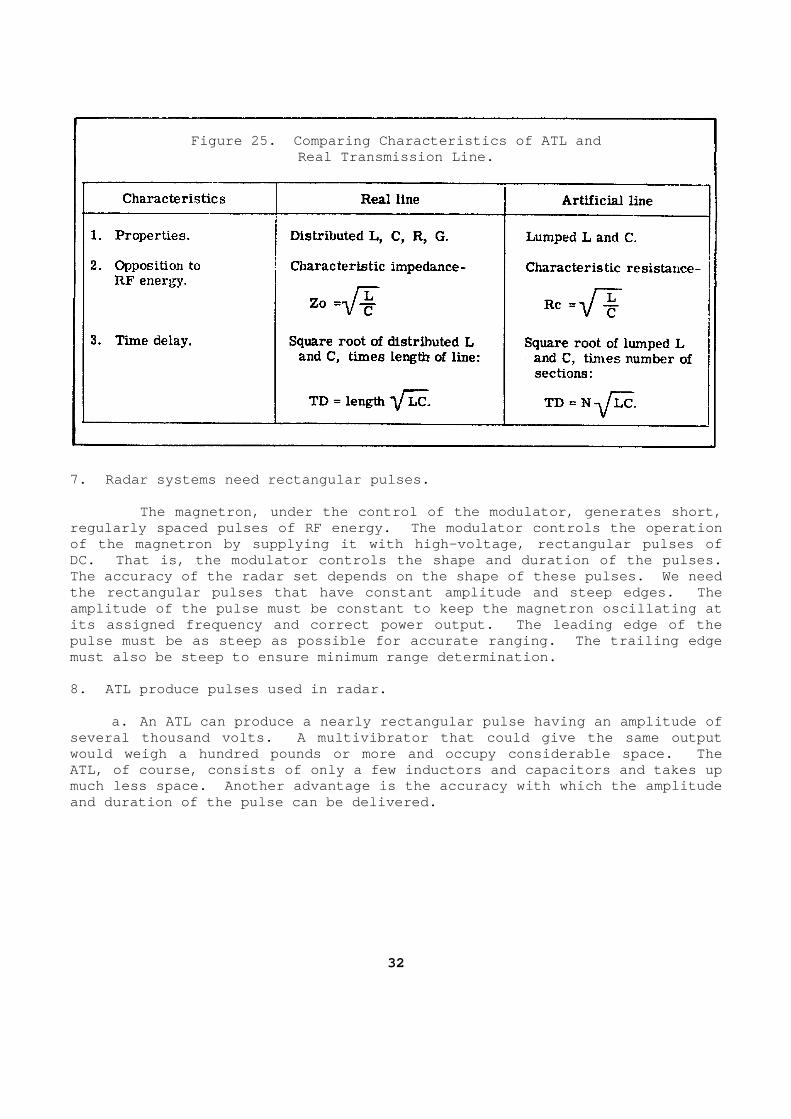
Figure 25. Comparing Characteristics of ATL and

Real Transmission Line. 7. Radar systems need rectangular pulses. The magnetron, under the control of the modulator , generates short, regularly spaced pulses of RF energy. The modulato r controls the operation of the magnetron by supplying it with high-voltage, rectangular pulses of DC. That is, the modulator controls the shape and duration of the pulses. The accuracy of the radar set depends on the shape of these pulses. We need the rectangular pulses that have constant amplitude and steep edges. The amplitude of the pulse must be constant to keep the magnetron oscillating at its assigned frequency and correct power output. T he leading edge of the pulse must be as steep as possible for accurate ran ging. The trailing edge must also be steep to ensure minimum range determin ation. 8. ATL produce pulses used in radar. a. An ATL can produce a nearly rectangular pulse h aving an amplitude of several thousand volts. A multivibrator that could give the same output would weigh a hundred pounds or more and occupy con siderable space. The ATL, of course, consists of only a few inductors an d capacitors and takes up much less space. Another advantage is the accuracy with which the amplitude and duration of the pulse can be delivered.

32

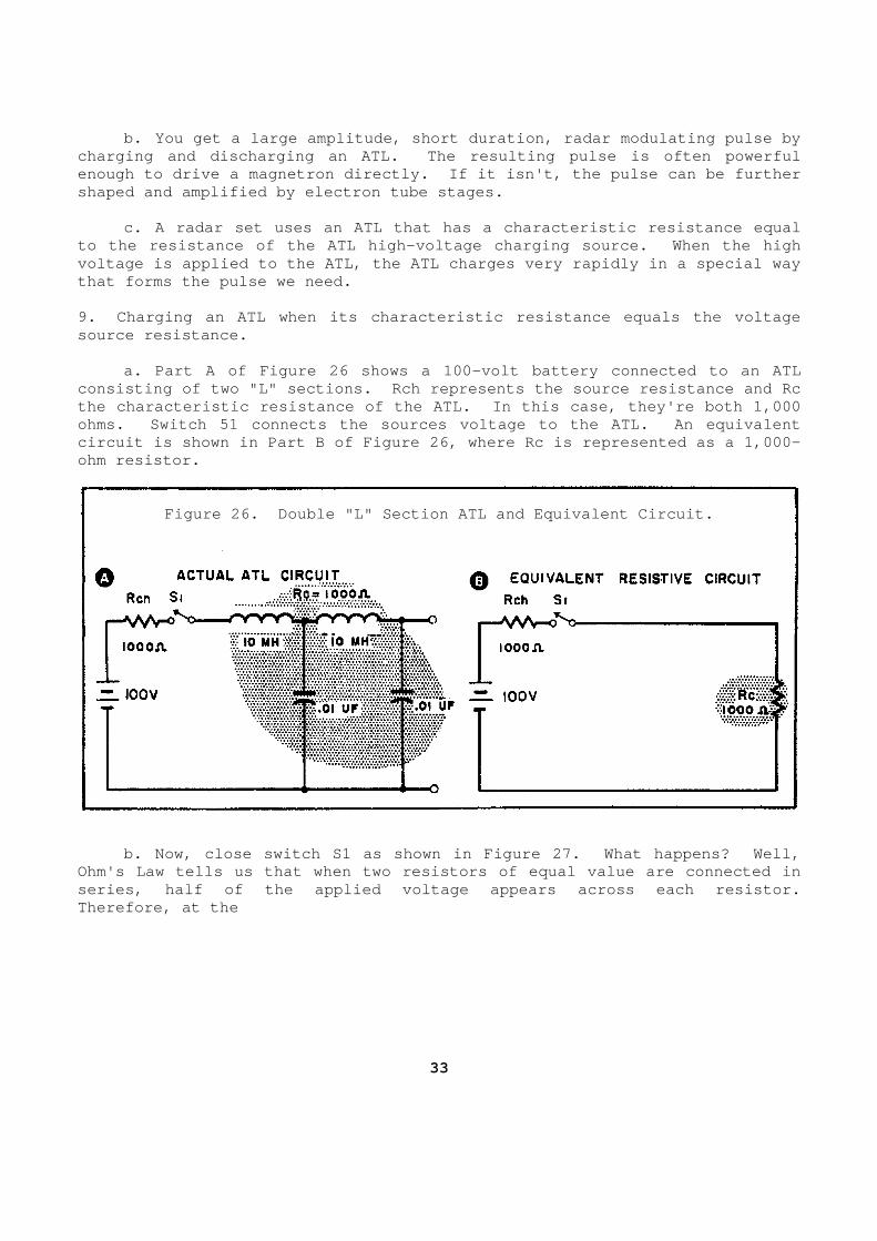
b. You get a large amplitude, short duration, rada r modulating pulse by charging and discharging an ATL. The resulting pul se is often powerful enough to drive a magnetron directly. If it isn't, the pulse can be further shaped and amplified by electron tube stages. c. A radar set uses an ATL that has a characterist ic resistance equal to the resistance of the ATL high-voltage charging source. When the high voltage is applied to the ATL, the ATL charges very rapidly in a special way that forms the pulse we need. 9. Charging an ATL when its characteristic resistan ce equals the voltage source resistance. a. Part A of Figure 26 shows a 100-volt battery co nnected to an ATL consisting of two "L" sections. Rch represents the source resistance and Rc the characteristic resistance of the ATL. In this case, they're both 1,000 ohms. Switch 51 connects the sources voltage to th e ATL. An equivalent circuit is shown in Part B of Figure 26, where Rc i s represented as a 1,000-ohm resistor.

Figure 26. Double "L" Section ATL and Equivalent C ircuit.

b. Now, close switch S1 as shown in Figure 27. Wh at happens? Well, Ohm's Law tells us that when two resistors of equal value are connected in series, half of the applied voltage appears across each resistor. Therefore, at the

33

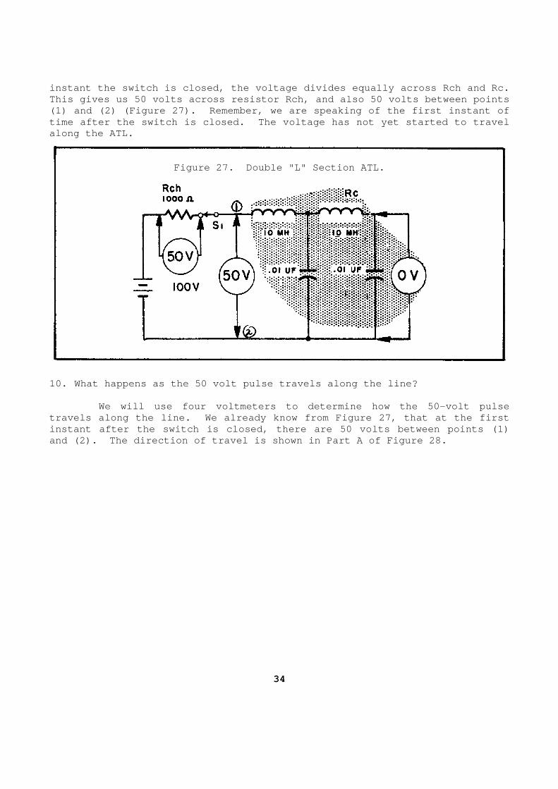
instant the switch is closed, the voltage divides e qually across Rch and Rc. This gives us 50 volts across resistor Rch, and als o 50 volts between points (1) and (2) (Figure 27). Remember, we are speaking of the first instant of time after the switch is closed. The voltage has n ot yet started to travel along the ATL.

Figure 27. Double "L" Section ATL.

10. What happens as the 50 volt pulse travels along the line? We will use four voltmeters to determine how the 50-volt pulse travels along the line. We already know from Figur e 27, that at the first instant after the switch is closed, there are 50 vo lts between points (1) and (2). The direction of travel is shown in Part A of Figure 28.

34

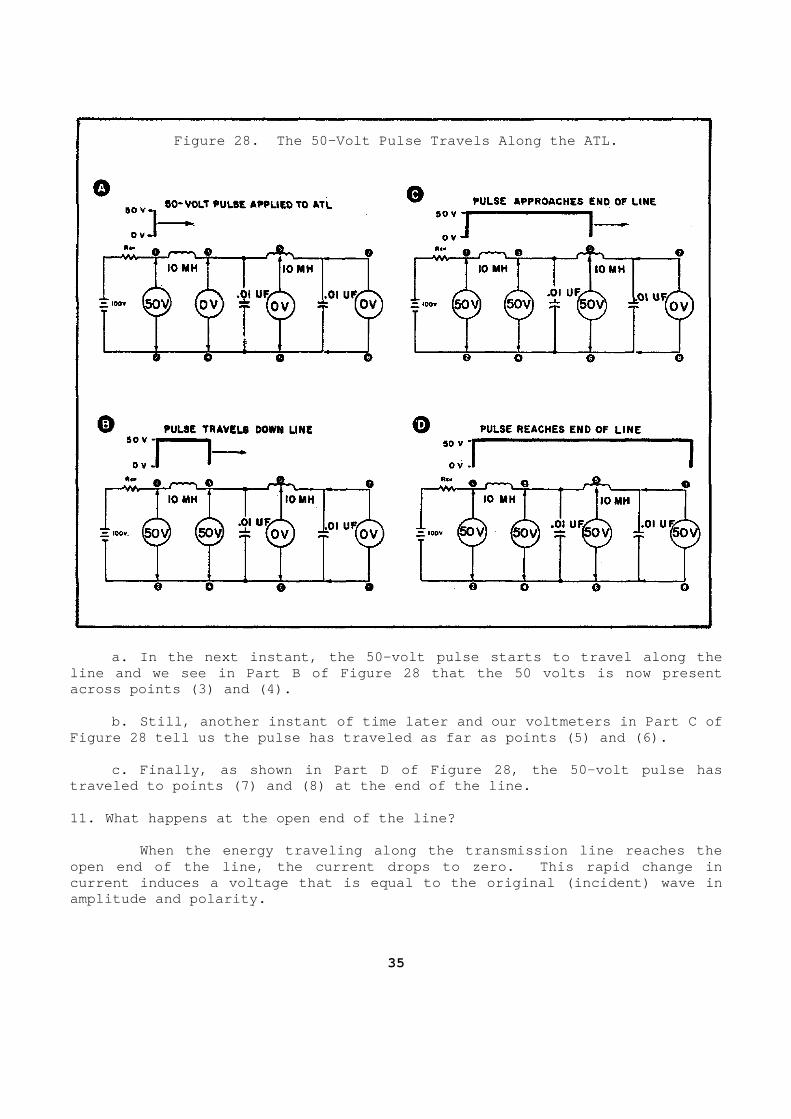
Figure 28. The 50-Volt Pulse Travels Along the ATL .

a. In the next instant, the 50-volt pulse starts t o travel along the line and we see in Part B of Figure 28 that the 50 volts is now present across points (3) and (4). b. Still, another instant of time later and our vo ltmeters in Part C of Figure 28 tell us the pulse has traveled as far as points (5) and (6). c. Finally, as shown in Part D of Figure 28, the 5 0-volt pulse has traveled to points (7) and (8) at the end of the li ne. 11. What happens at the open end of the line? When the energy traveling along the transmission line reaches the open end of the line, the current drops to zero. T his rapid change in current induces a voltage that is equal to the orig inal (incident) wave in amplitude and polarity.

35

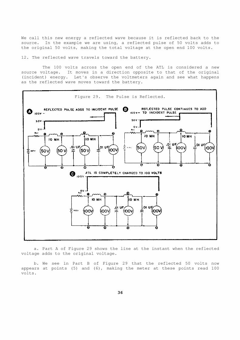
We call this new energy a reflected wave because it is reflected back to the source. In the example we are using, a reflected p ulse of 50 volts adds to the original 50 volts, making the total voltage at the open end 100 volts. 12. The reflected wave travels toward the battery. The 100 volts across the open end of the ATL is c onsidered a new source voltage. It moves in a direction opposite t o that of the original (incident) energy. Let's observe the voltmeters ag ain and see what happens as the reflected wave moves toward the battery.

Figure 29. The Pulse is Reflected.

a. Part A of Figure 29 shows the line at the insta nt when the reflected voltage adds to the original voltage. b. We see in Part B of Figure 29 that the reflecte d 50 volts now appears at points (5) and (6), making the meter at these points read 100 volts.

36

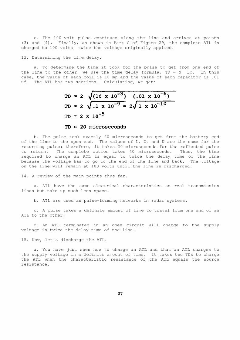
c. The 100-volt pulse continues along the line and arrives at points (3) and (4). Finally, as shown in Part C of Figure 29, the complete ATL is charged to 100 volts, twice the voltage originally applied. 13. Determining the time delay. a. To determine the time it took for the pulse to get from one end of the line to the other, we use the time delay formul a, TD = N LC. In this case, the value of each coil is 10 mh and the value of each capacitor is .01 uf. The ATL has two sections. Calculating, we get :

b. The pulse took exactly 20 microseconds to get f rom the battery end of the line to the open end. The values of L, C, a nd N are the same for the returning pulse; therefore, it takes 20 microsecond s for the reflected pulse to return. The complete action takes 40 microsecon ds. Thus, the time required to charge an ATL is equal to twice the del ay time of the line because the voltage has to go to the end of the lin e and back. The voltage on the line will remain at 100 volts until the line is discharged. 14. A review of the main points thus far. a. ATL have the same electrical characteristics as real transmission lines but take up much less space. b. ATL are used as pulse-forming networks in radar systems. c. A pulse takes a definite amount of time to trav el from one end of an ATL to the other. d. An ATL terminated in an open circuit will charg e to the supply voltage in twice the delay time of the line. 15. Now, let's discharge the ATL. a. You have just seen how to charge an ATL and tha t an ATL charges to the supply voltage in a definite amount of time. I t takes two TDs to charge the ATL when the characteristic resistance of the A TL equals the source resistance.

37

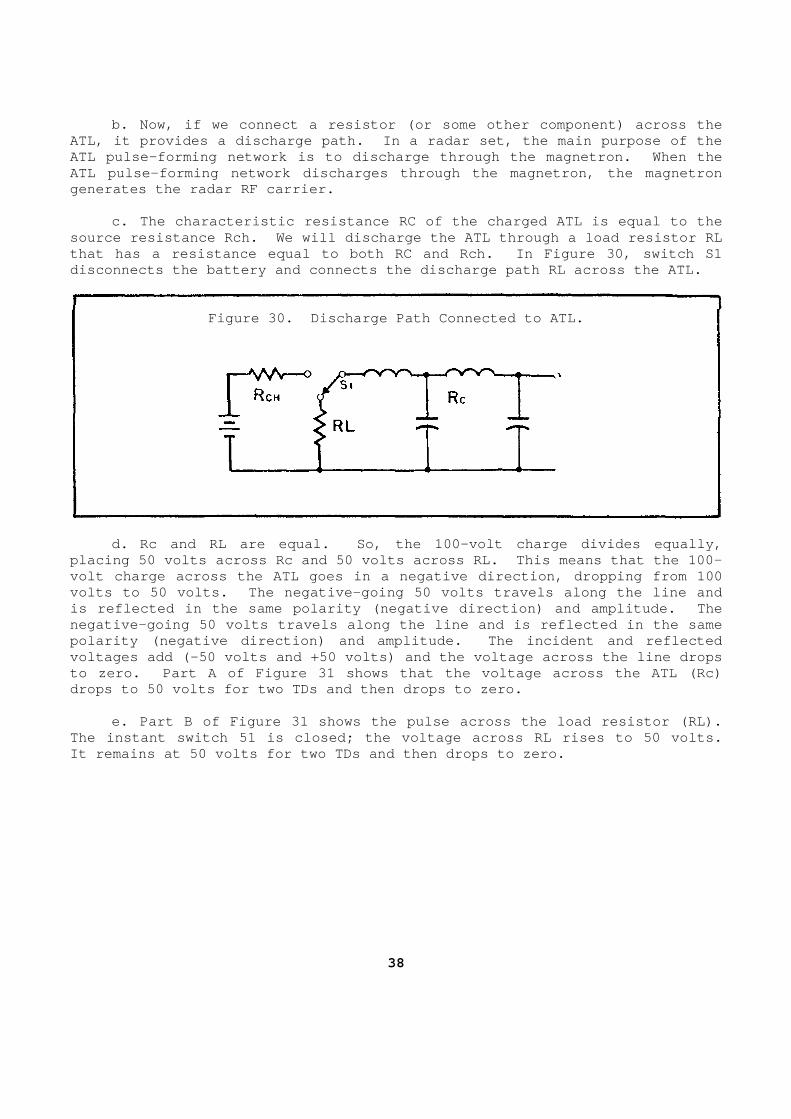
b. Now, if we connect a resistor (or some other co mponent) across the ATL, it provides a discharge path. In a radar set, the main purpose of the ATL pulse-forming network is to discharge through t he magnetron. When the ATL pulse-forming network discharges through the ma gnetron, the magnetron generates the radar RF carrier. c. The characteristic resistance RC of the charged ATL is equal to the source resistance Rch. We will discharge the ATL t hrough a load resistor RL that has a resistance equal to both RC and Rch. In Figure 30, switch S1 disconnects the battery and connects the discharge path RL across the ATL.

Figure 30. Discharge Path Connected to ATL.

d. Rc and RL are equal. So, the 100-volt charge d ivides equally, placing 50 volts across Rc and 50 volts across RL. This means that the 100-volt charge across the ATL goes in a negative direc tion, dropping from 100 volts to 50 volts. The negative-going 50 volts tra vels along the line and is reflected in the same polarity (negative directi on) and amplitude. The negative-going 50 volts travels along the line and is reflected in the same polarity (negative direction) and amplitude. The i ncident and reflected voltages add (-50 volts and +50 volts) and the volt age across the line drops to zero. Part A of Figure 31 shows that the voltag e across the ATL (Rc) drops to 50 volts for two TDs and then drops to zer o. e. Part B of Figure 31 shows the pulse across the load resistor (RL). The instant switch 51 is closed; the voltage across RL rises to 50 volts. It remains at 50 volts for two TDs and then drops t o zero.

38

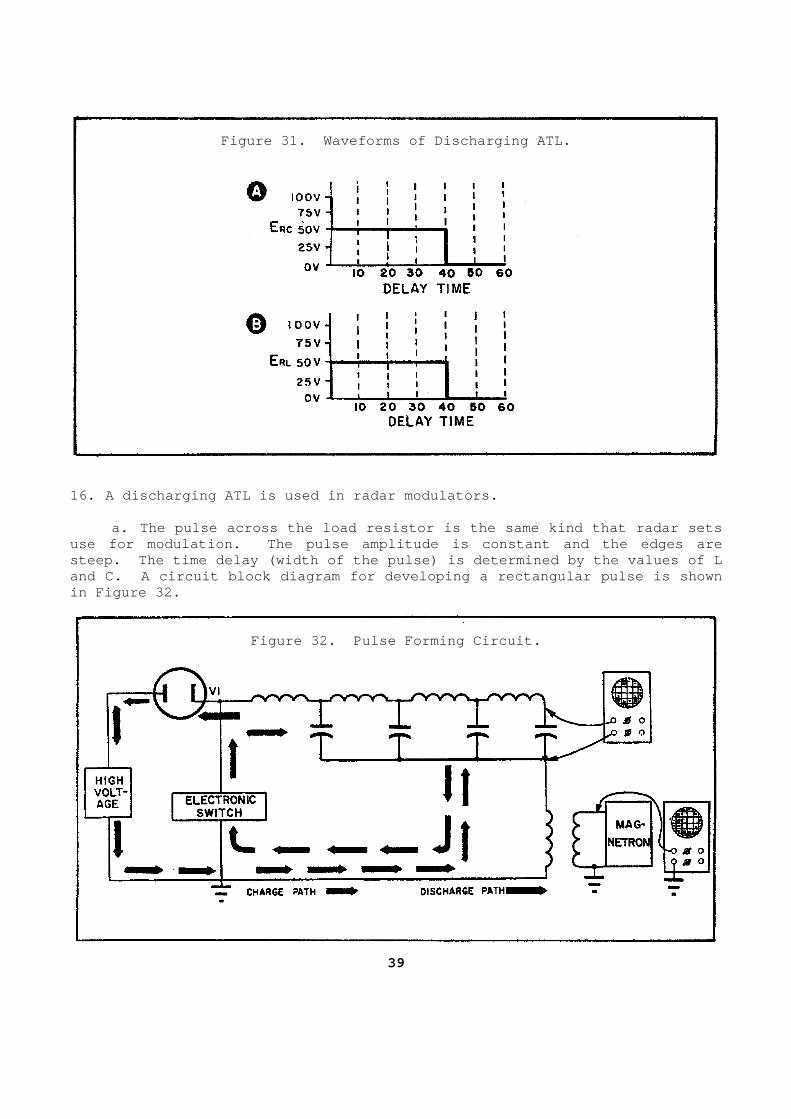
Figure 31. Waveforms of Discharging ATL.

16. A discharging ATL is used in radar modulators. a. The pulse across the load resistor is the same kind that radar sets use for modulation. The pulse amplitude is constan t and the edges are steep. The time delay (width of the pulse) is dete rmined by the values of L and C. A circuit block diagram for developing a re ctangular pulse is shown in Figure 32.

Figure 32. Pulse Forming Circuit.

39

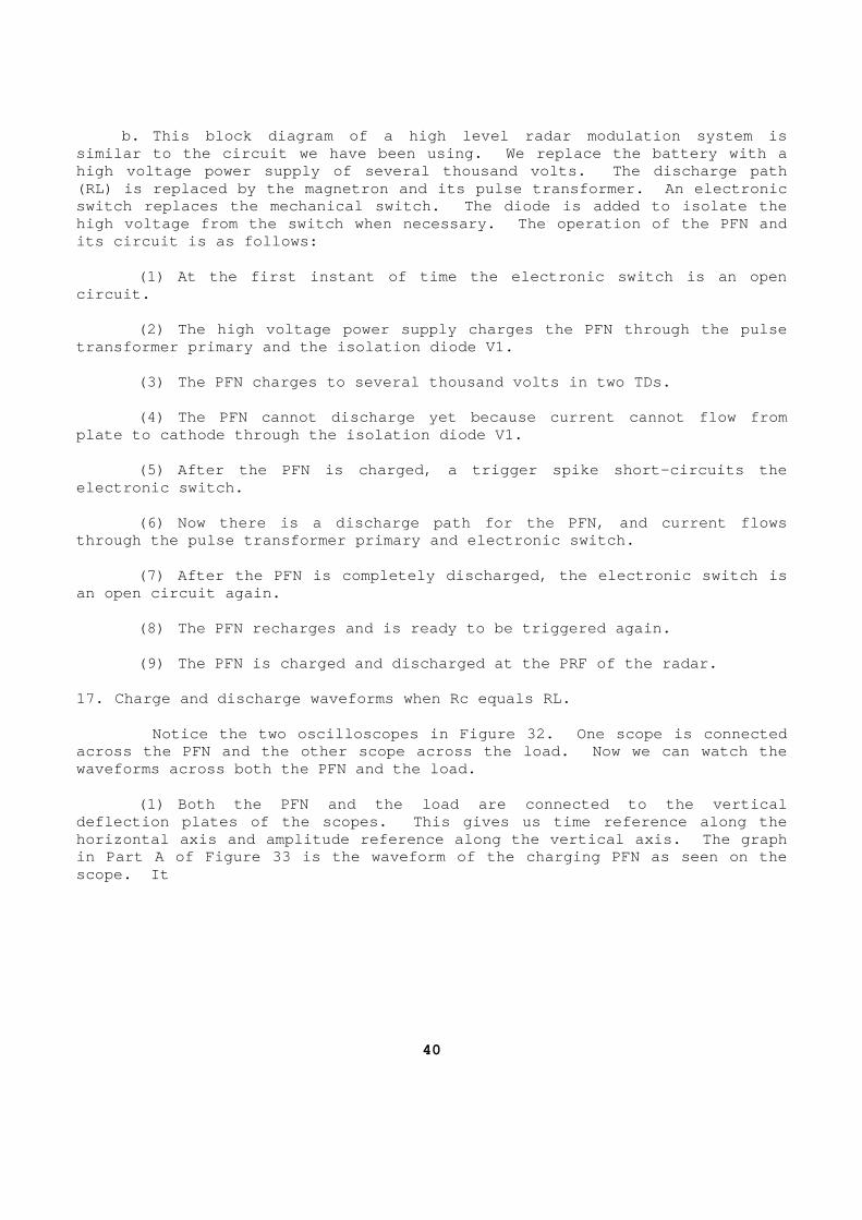
b. This block diagram of a high level radar modula tion system is similar to the circuit we have been using. We repl ace the battery with a high voltage power supply of several thousand volts . The discharge path (RL) is replaced by the magnetron and its pulse tra nsformer. An electronic switch replaces the mechanical switch. The diode i s added to isolate the high voltage from the switch when necessary. The o peration of the PFN and its circuit is as follows: (1) At the first instant of time the electronic sw itch is an open circuit. (2) The high voltage power supply charges the PFN through the pulse transformer primary and the isolation diode V1. (3) The PFN charges to several thousand volts in t wo TDs. (4) The PFN cannot discharge yet because current c annot flow from plate to cathode through the isolation diode V1. (5) After the PFN is charged, a trigger spike shor t-circuits the electronic switch. (6) Now there is a discharge path for the PFN, and current flows through the pulse transformer primary and electroni c switch. (7) After the PFN is completely discharged, the el ectronic switch is an open circuit again. (8) The PFN recharges and is ready to be triggered again. (9) The PFN is charged and discharged at the PRF o f the radar. 17. Charge and discharge waveforms when Rc equals R L. Notice the two oscilloscopes in Figure 32. One s cope is connected across the PFN and the other scope across the load. Now we can watch the waveforms across both the PFN and the load. (1) Both the PFN and the load are connected to the vertical deflection plates of the scopes. This gives us tim e reference along the horizontal axis and amplitude reference along the v ertical axis. The graph in Part A of Figure 33 is the waveform of the charg ing PFN as seen on the scope. It

40

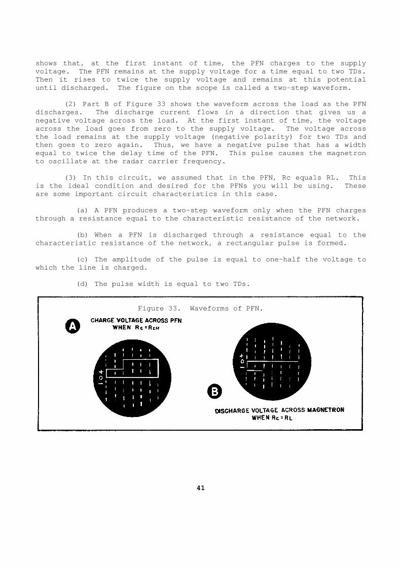
shows that, at the first instant of time, the PFN c harges to the supply voltage. The PFN remains at the supply voltage for a time equal to two TDs. Then it rises to twice the supply voltage and remai ns at this potential until discharged. The figure on the scope is calle d a two-step waveform. (2) Part B of Figure 33 shows the waveform across the load as the PFN discharges. The discharge current flows in a direc tion that gives us a negative voltage across the load. At the first ins tant of time, the voltage across the load goes from zero to the supply voltag e. The voltage across the load remains at the supply voltage (negative po larity) for two TDs and then goes to zero again. Thus, we have a negative pulse that has a width equal to twice the delay time of the PFN. This pul se causes the magnetron to oscillate at the radar carrier frequency. (3) In this circuit, we assumed that in the PFN, R c equals RL. This is the ideal condition and desired for the PFNs you will be using. These are some important circuit characteristics in this case. (a) A PFN produces a two-step waveform only when t he PFN charges through a resistance equal to the characteristic re sistance of the network. (b) When a PFN is discharged through a resistance equal to the characteristic resistance of the network, a rectang ular pulse is formed. (c) The amplitude of the pulse is equal to one-hal f the voltage to which the line is charged. (d) The pulse width is equal to two TDs.

Figure 33. Waveforms of PFN.

41

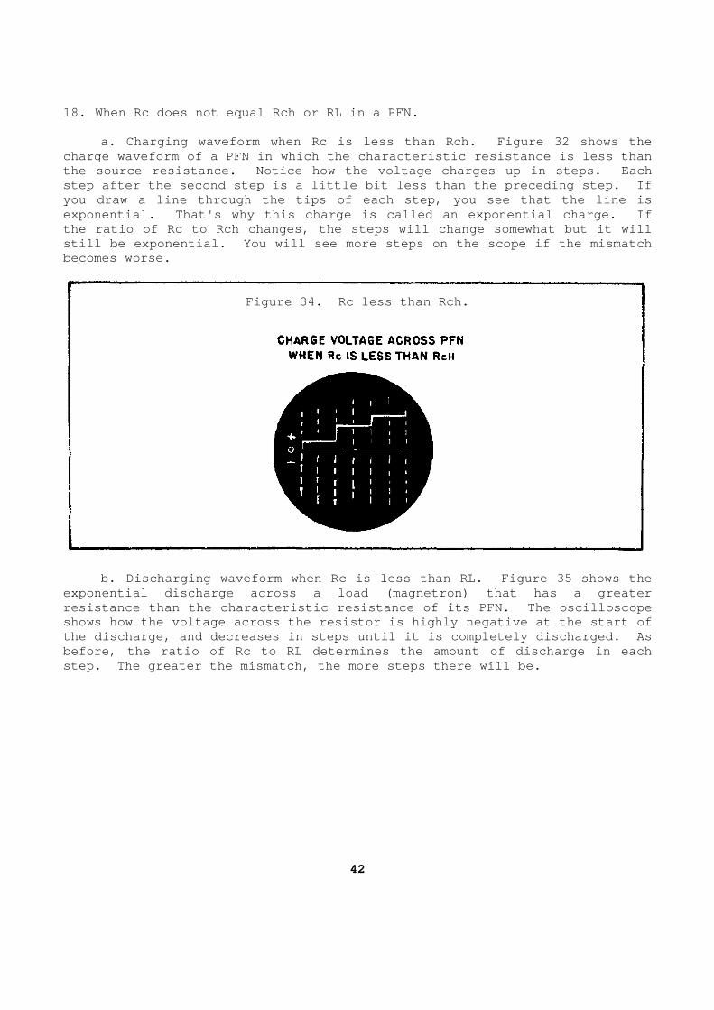
18. When Rc does not equal Rch or RL in a PFN. a. Charging waveform when Rc is less than Rch. Fi gure 32 shows the charge waveform of a PFN in which the characteristi c resistance is less than the source resistance. Notice how the voltage char ges up in steps. Each step after the second step is a little bit less tha n the preceding step. If you draw a line through the tips of each step, you see that the line is exponential. That's why this charge is called an e xponential charge. If the ratio of Rc to Rch changes, the steps will chan ge somewhat but it will still be exponential. You will see more steps on t he scope if the mismatch becomes worse.

Figure 34. Rc less than Rch.

b. Discharging waveform when Rc is less than RL. Figure 35 shows the exponential discharge across a load (magnetron) tha t has a greater resistance than the characteristic resistance of it s PFN. The oscilloscope shows how the voltage across the resistor is highly negative at the start of the discharge, and decreases in steps until it is c ompletely discharged. As before, the ratio of Rc to RL determines the amount of discharge in each step. The greater the mismatch, the more steps the re will be.

42

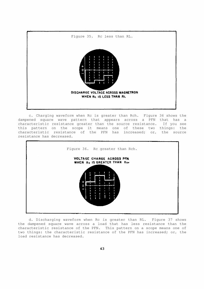
Figure 35. Rc less than RL.

c. Charging waveform when Rc is greater than Rch. Figure 36 shows the dampened square wave pattern that appears across a PFN that has a characteristic resistance greater than the source r esistance. If you see this pattern on the scope it means one of these two things: the characteristic resistance of the PFN has increased; or, the source resistance has decreased.

Figure 36. Rc greater than Rch.

d. Discharging waveform when Rc is greater than RL . Figure 37 shows the dampened square wave across a load that has les s resistance than the characteristic resistance of the PFN. This pattern on a scope means one of two things: the characteristic resistance of the PF N has increased; or, the load resistance has decreased.

43

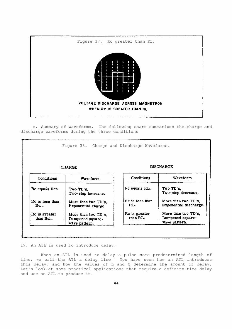
Figure 37. Rc greater than RL.

e. Summary of waveforms. The following chart summ arizes the charge and discharge waveforms during the three conditions

Figure 38. Charge and Discharge Waveforms.

19. An ATL is used to introduce delay. When an ATL is used to delay a pulse some predete rmined length of time, we call the ATL a delay line. You have seen how an ATL introduces this delay, and how the values of L and C determine the amount of delay. Let's look at some practical applications that requ ire a definite time delay and use an ATL to produce it.

44

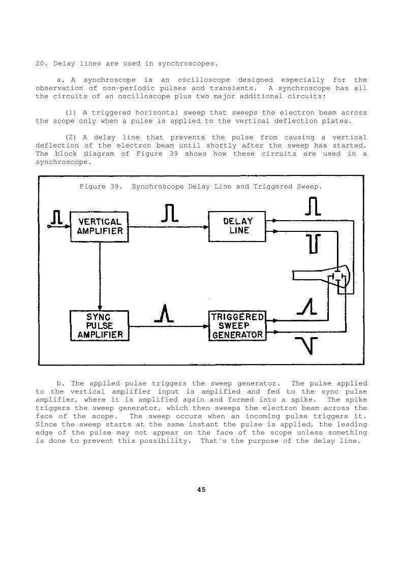
20. Delay lines are used in synchroscopes. a. A synchroscope is an oscilloscope designed espe cially for the observation of non-periodic pulses and transients. A synchroscope has all the circuits of an oscilloscope plus two major addi tional circuits: (1) A triggered horizontal sweep that sweeps the e lectron beam across the scope only when a pulse is applied to the verti cal deflection plates. (2) A delay line that prevents the pulse from caus ing a vertical deflection of the electron beam until shortly after the sweep has started. The block diagram of Figure 39 shows how these circ uits are used in a synchroscope.

Figure 39. Synchroscope Delay Line and Triggered S weep.

b. The applied pulse triggers the sweep generator. The pulse applied to the vertical amplifier input is amplified and fe d to the sync pulse amplifier, where it is amplified again and formed i nto a spike. The spike triggers the sweep generator, which then sweeps the electron beam across the face of the scope. The sweep occurs when an incomi ng pulse triggers it. Since the sweep starts at the same instant the puls e is applied, the leading edge of the pulse may not appear on the face of the scope unless something is done to prevent this possibility. That's the pu rpose of the delay line.

45

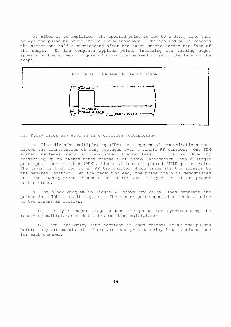
c. After it is amplified, the applied pulse is fed to a delay line that delays the pulse by about one-half a microsecond. The applied pulse reaches the screen one-half a microsecond after the sweep s tarts across the face of the scope. So the complete applied pulse, includin g its leading edge, appears on the screen. Figure 40 shows the delayed pulse on the face of the scope.

Figure 40. Delayed Pulse on Scope.

21. Delay lines are used in time division multiplex ing. a. Time division multiplexing (TDM) is a system of communications that allows the transmission of many messages over a sin gle RF carrier. One TDM system replaces many single-channel transmitters. This is done by converting up to twenty-three channels of audio inf ormation into a single pulse-position-modulated (PPM), time-division-multi plexed (TDM) pulse train. The train is then fed to an RF transmitter which tr ansmits the signals to the desired location. At the receiving end, the pu lse train is demodulated and the twenty-three channels of audio are relayed to their proper destinations. b. The block diagram in Figure 41 shows how delay lines separate the pulses in a TDM transmitting set. The master pulse generator feeds a pulse to two stages as follows: (1) The sync shaper stage widens the pulse for syn chronizing the receiving multiplexer with the transmitting multipl exer. (2) Then, the delay line sections in each channel delay the pulses before they are modulated. There are twenty-three delay line sections, one for each channel.

46

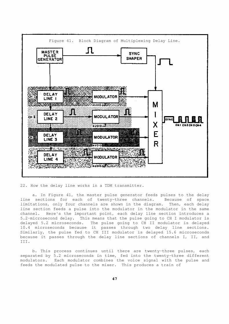
Figure 41. Block Diagram of Multiplexing Delay Lin e.

22. How the delay line works in a TDM transmitter. a. In Figure 41, the master pulse generator feeds pulses to the delay line sections for each of twenty-three channels. B ecause of space limitations, only four channels are shown in the di agram. Then, each delay line section feeds a pulse into the modulator in th e modulator in the same channel. Here's the important point, each delay li ne section introduces a 5.2-microsecond delay. This means that the pulse g oing to CH I modulator is delayed 5.2 microseconds. The pulse going to CH II modulator is delayed 10.4 microseconds because it passes through two del ay line sections. Similarly, the pulse fed to CH III modulator is del ayed 15.6 microseconds because it passes through the delay line sections o f channels I, II, and III. b. This process continues until there are twenty-t hree pulses, each separated by 5.2 microseconds in time, fed into the twenty-three different modulators. Each modulator combines the voice sign al with the pulse and feeds the modulated pulse to the mixer. This produ ces a train of

47

twenty-three independently modulated pulses which a re then impressed on a single RF carrier and transmitted. At the receivin g end of the system, a reverse process takes place and the pulses are demo dulated to produce the original voice signals.

48

PRACTICE EXERCISE (Performance-Oriented)

In each of the following exercises, select the ONE answer that BEST completes the statement or answers the question. I ndicate your solution by circling the letter opposite the correct answer in the subcourse booklet. 1. At radar and microwave frequencies, coaxial line sections are used in

preference to two-wire sections because their a. velocity factor is higher. b. radiation losses are lower. c. dielectric is more efficient. d. circuits can be balanced in respect to ground. 2. Although the electrical properties of a transmis sion line are

distributed evenly along the line, they can be repr esented as an infinite number of small values of series.

a. inductance and capacitance plus shunt resistanc e and conductance. b. resistance and conductance plus shunt inductanc e and capacitance. c. inductance and resistance plus shunt conductanc e and capacitance. d. conductance and capacitance plus shunt inductan ce and resistance.

49

3. Assume that a radar set is designed to use a fle xible coaxial cable with 4 characteristic impedance of 100 ohms and len gth of 10 meters to couple the RF energy from the transmitter to the an tenna. If only 5 meters of the cable are used when installing the ra dar set, the characteristic impedance of the flexible cable will be

a. 50 ohms. b. 100 ohms. c. 200 ohms. d. 400 ohms. 4. Assume that a coaxial transmission line is being used to transfer the

RF output of a radar transmitter to the radar anten na. Maximum power will be transferred from the magnetron to the anten na when the

a. coaxial line is terminated in a short circuit. b. standing wave ratio of the transmission line is greater than one. c. characteristic impedance of the transmission li ne matches the

impedance of the magnetron and antenna. d. impedances of the magnetron and the antenna are less than the

characteristic impedance of the transmission line. 5. Assume that a parallel-wire transmission line ha s been connected to an

antenna having a resistive input impedance of 600 o hms. If the characteristic impedance of the transmission line i s 500 ohms, what is the standing wave ratio of the voltage?

a. 0.5/1. b. 1.00/1. c. 1.20/1. d. 1.83/1.

50

6. A transmission line will have a maximum standing wave ratio when the transmission line is terminated in

a. a resistive load. b. an inductive load. c. a short or open circuit. d. an impedance equal to the characteristic impeda nce of the

transmission line. 7. Resonant lines are often called tuned lines whil e nonresonant lines

are called flat lines. What is one characteristic of tuned lines? a. Voltage is constant along the line. b. Reflected energy is present on the line. c. The voltage standing wave ratio is equal to one . d. The terminating impedance is equal to the chara cteristic

impedance of the line.

51

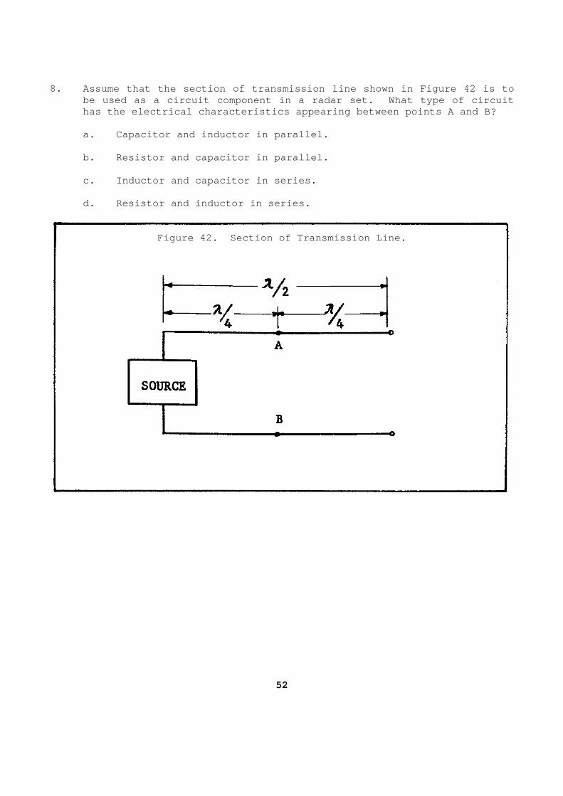
8. Assume that the section of transmission line sho wn in Figure 42 is to be used as a circuit component in a radar set. Wha t type of circuit has the electrical characteristics appearing betwee n points A and B?

a. Capacitor and inductor in parallel. b. Resistor and capacitor in parallel. c. Inductor and capacitor in series. d. Resistor and inductor in series.

Figure 42. Section of Transmission Line.

52

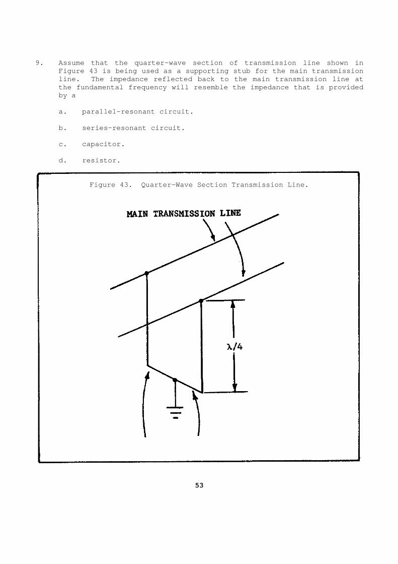
9. Assume that the quarter-wave section of transmis sion line shown in Figure 43 is being used as a supporting stub for th e main transmission line. The impedance reflected back to the main tra nsmission line at the fundamental frequency will resemble the impedan ce that is provided by a

a. parallel-resonant circuit. b. series-resonant circuit. c. capacitor. d. resistor.

Figure 43. Quarter-Wave Section Transmission Line.

53

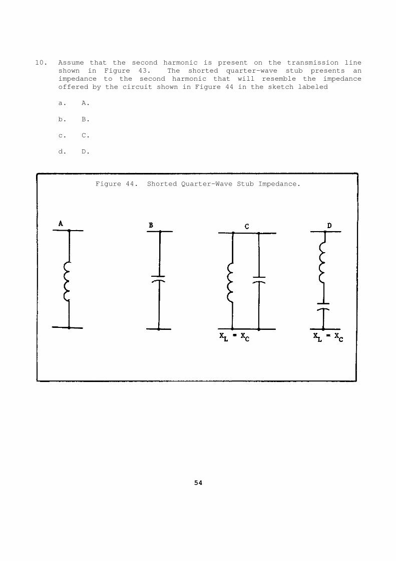
10. Assume that the second harmonic is present on t he transmission line shown in Figure 43. The shorted quarter-wave stub presents an impedance to the second harmonic that will resemble the impedance offered by the circuit shown in Figure 44 in the sk etch labeled

a. A. b. B. c. C. d. D.

Figure 44. Shorted Quarter-Wave Stub Impedance.

54

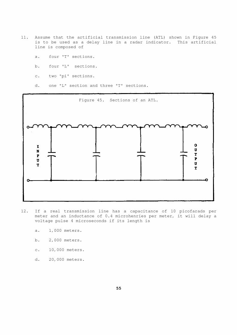
11. Assume that the artificial transmission line (A TL) shown in Figure 45 is to be used as a delay line in a radar indicator. This artificial line is composed of

a. four "T" sections. b. four "L" sections. c. two "pi" sections. d. one "L" section and three "T" sections.

Figure 45. Sections of an ATL.

12. If a real transmission line has a capacitance o f 10 picofarads per

meter and an inductance of 0.4 microhenries per met er, it will delay a voltage pulse 4 microseconds if its length is

a. 1,000 meters. b. 2,000 meters. c. 10,000 meters. d. 20,000 meters.

55

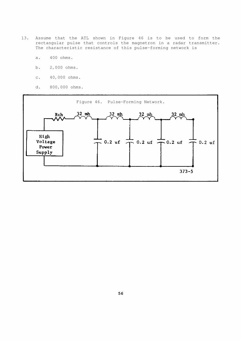
13. Assume that the ATL shown in Figure 46 is to be used to form the rectangular pulse that controls the magnetron in a radar transmitter. The characteristic resistance of this pulse-forming network is

a. 400 ohms. b. 2,000 ohms. c. 40,000 ohms. d. 800,000 ohms.

Figure 46. Pulse-Forming Network.

56

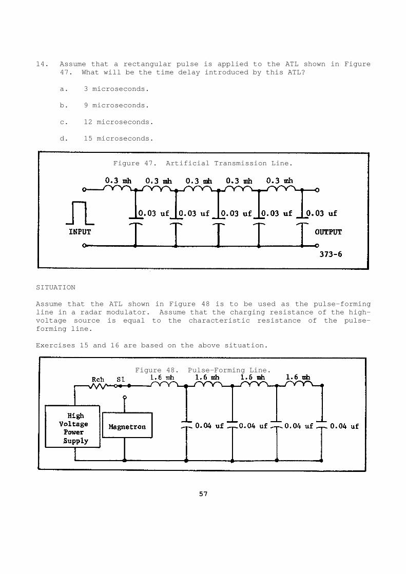
14. Assume that a rectangular pulse is applied to t he ATL shown in Figure 47. What will be the time delay introduced by this ATL?

a. 3 microseconds. b. 9 microseconds. c. 12 microseconds. d. 15 microseconds.

Figure 47. Artificial Transmission Line.

SITUATION Assume that the ATL shown in Figure 48 is to be use d as the pulse-forming line in a radar modulator. Assume that the chargin g resistance of the high-voltage source is equal to the characteristic resis tance of the pulse-forming line. Exercises 15 and 16 are based on the above situatio n.

Figure 48. Pulse-Forming Line.

57

15. The four-section ATL shown in Figure 48 will be fully charged after a. 8 microseconds. b. 16 microseconds. c. 32 microseconds. d. 64 microseconds. 16. The charging resistance is designed to be equal to the characteristic

resistance of the pulse-forming line shown in Figur e 48. What is the value of the charging resistance?

a. 200 ohms. b. 400 ohms. c. 600 ohms. d. 800 ohms.

58

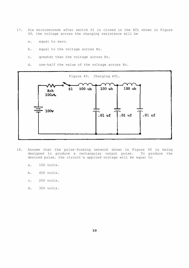
17. Six microseconds after switch S1 is closed in t he ATL shown in Figure 49, the voltage across the charging resistance will be

a. equal to zero. b. equal to the voltage across Rc. c. greater than the voltage across Rc. d. one-half the value of the voltage across Rc.

Figure 49. Charging ATL.

18. Assume that the pulse-forming network shown in Figure 50 is being

designed to produce a rectangular output pulse. To produce the desired pulse, the circuit's applied voltage will b e equal to

a. 100 volts. b. 400 volts. c. 200 volts. d. 300 volts.

59

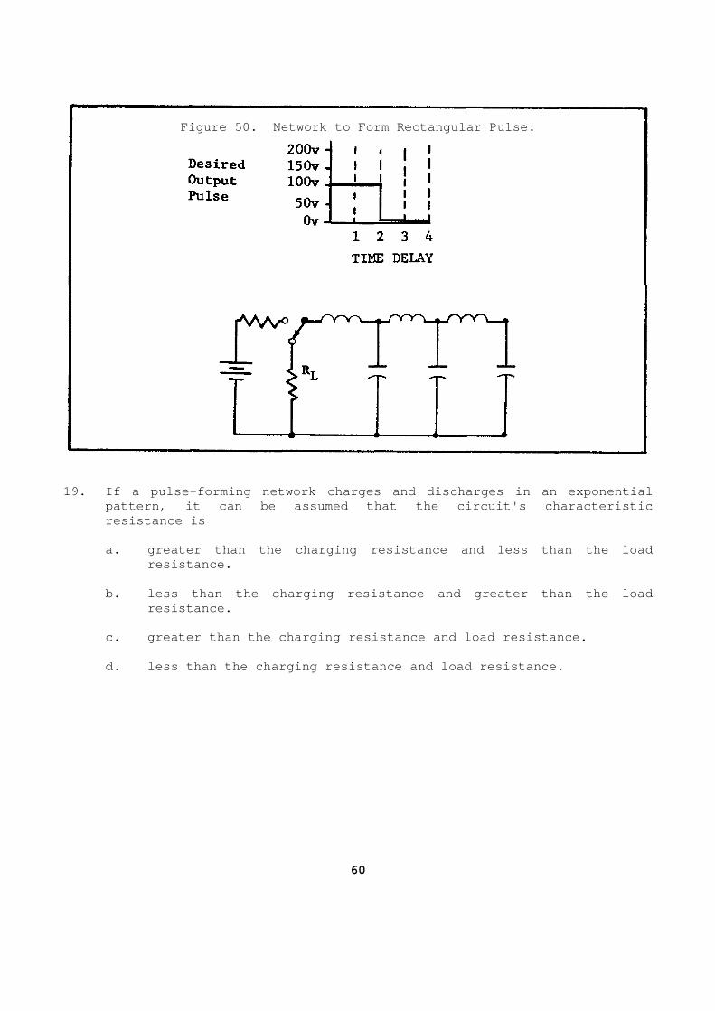
Figure 50. Network to Form Rectangular Pulse.

19. If a pulse-forming network charges and discharg es in an exponential

pattern, it can be assumed that the circuit's chara cteristic resistance is

a. greater than the charging resistance and less t han the load

resistance. b. less than the charging resistance and greater t han the load

resistance. c. greater than the charging resistance and load r esistance. d. less than the charging resistance and load resi stance.

60

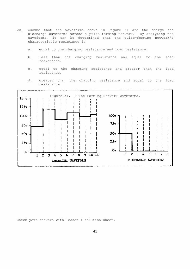
20. Assume that the waveforms shown in Figure 51 ar e the charge and discharge waveforms across a pulse-forming network. By analyzing the waveforms, it can be determined that the pulse-form ing network's characteristic resistance is

a. equal to the charging resistance and load resis tance. b. less than the charging resistance and equal to the load

resistance. c. equal to the charging resistance and greater th an the load

resistance. d. greater than the charging resistance and equal to the load

resistance.

Figure 51. Pulse-Forming Network Waveforms.

Check your answers with lesson 1 solution sheet.

61

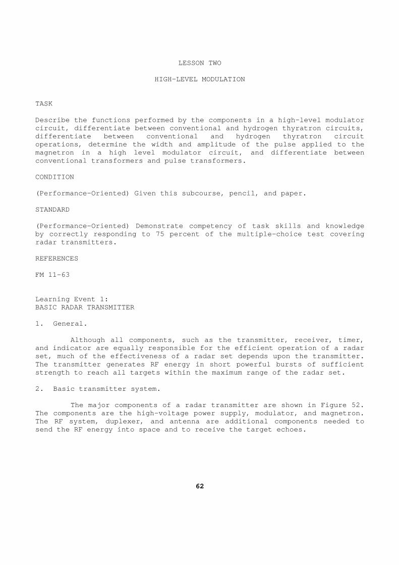
LESSON TWO

HIGH-LEVEL MODULATION TASK Describe the functions performed by the components in a high-level modulator circuit, differentiate between conventional and hyd rogen thyratron circuits, differentiate between conventional and hydrogen thy ratron circuit operations, determine the width and amplitude of th e pulse applied to the magnetron in a high level modulator circuit, and di fferentiate between conventional transformers and pulse transformers. CONDITION (Performance-Oriented) Given this subcourse, pencil , and paper. STANDARD (Performance-Oriented) Demonstrate competency of ta sk skills and knowledge by correctly responding to 75 percent of the multip le-choice test covering radar transmitters. REFERENCES FM 11-63 Learning Event 1: BASIC RADAR TRANSMITTER 1. General. Although all components, such as the transmitter, receiver, timer, and indicator are equally responsible for the effic ient operation of a radar set, much of the effectiveness of a radar set depen ds upon the transmitter. The transmitter generates RF energy in short powerf ul bursts of sufficient strength to reach all targets within the maximum ra nge of the radar set. 2. Basic transmitter system. The major components of a radar transmitter are s hown in Figure 52. The components are the high-voltage power supply, m odulator, and magnetron. The RF system, duplexer, and antenna are additional components needed to send the RF energy into space and to receive the ta rget echoes.

62

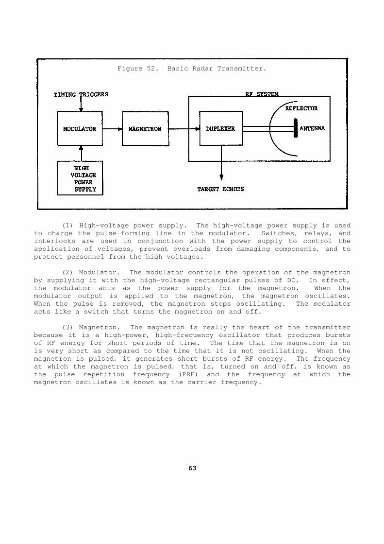
Figure 52. Basic Radar Transmitter.

(1) High-voltage power supply. The high-voltage p ower supply is used to charge the pulse-forming line in the modulator. Switches, relays, and interlocks are used in conjunction with the power s upply to control the application of voltages, prevent overloads from dam aging components, and to protect personnel from the high voltages. (2) Modulator. The modulator controls the operati on of the magnetron by supplying it with the high-voltage rectangular p ulses of DC. In effect, the modulator acts as the power supply for the magn etron. When the modulator output is applied to the magnetron, the m agnetron oscillates. When the pulse is removed, the magnetron stops osci llating. The modulator acts like a switch that turns the magnetron on and off. (3) Magnetron. The magnetron is really the heart of the transmitter because it is a high-power, high-frequency oscillat or that produces bursts of RF energy for short periods of time. The time t hat the magnetron is on is very short as compared to the time that it is no t oscillating. When the magnetron is pulsed, it generates short bursts of R F energy. The frequency at which the magnetron is pulsed, that is, turned o n and off, is known as the pulse repetition frequency (PRF) and the freque ncy at which the magnetron oscillates is known as the carrier freque ncy.

63

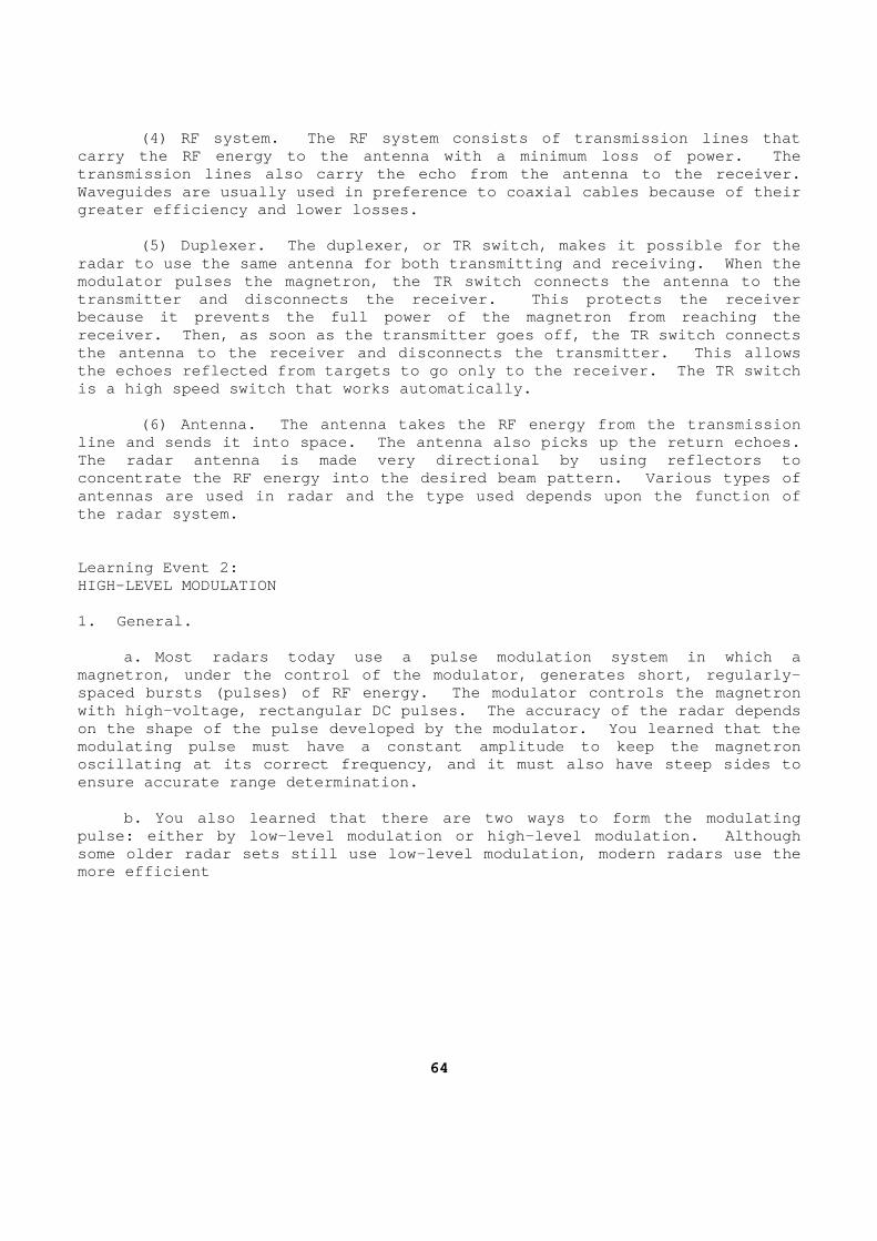
(4) RF system. The RF system consists of transmis sion lines that carry the RF energy to the antenna with a minimum l oss of power. The transmission lines also carry the echo from the ant enna to the receiver. Waveguides are usually used in preference to coaxia l cables because of their greater efficiency and lower losses. (5) Duplexer. The duplexer, or TR switch, makes i t possible for the radar to use the same antenna for both transmitting and receiving. When the modulator pulses the magnetron, the TR switch conne cts the antenna to the transmitter and disconnects the receiver. This pro tects the receiver because it prevents the full power of the magnetron from reaching the receiver. Then, as soon as the transmitter goes of f, the TR switch connects the antenna to the receiver and disconnects the tra nsmitter. This allows the echoes reflected from targets to go only to the receiver. The TR switch is a high speed switch that works automatically. (6) Antenna. The antenna takes the RF energy from the transmission line and sends it into space. The antenna also pic ks up the return echoes. The radar antenna is made very directional by using reflectors to concentrate the RF energy into the desired beam pat tern. Various types of antennas are used in radar and the type used depend s upon the function of the radar system. Learning Event 2: HIGH-LEVEL MODULATION 1. General. a. Most radars today use a pulse modulation system in which a magnetron, under the control of the modulator, gene rates short, regularly-spaced bursts (pulses) of RF energy. The modulator controls the magnetron with high-voltage, rectangular DC pulses. The accu racy of the radar depends on the shape of the pulse developed by the modulato r. You learned that the modulating pulse must have a constant amplitude to keep the magnetron oscillating at its correct frequency, and it must a lso have steep sides to ensure accurate range determination. b. You also learned that there are two ways to for m the modulating pulse: either by low-level modulation or high-level modulation. Although some older radar sets still use low-level modulatio n, modern radars use the more efficient

64

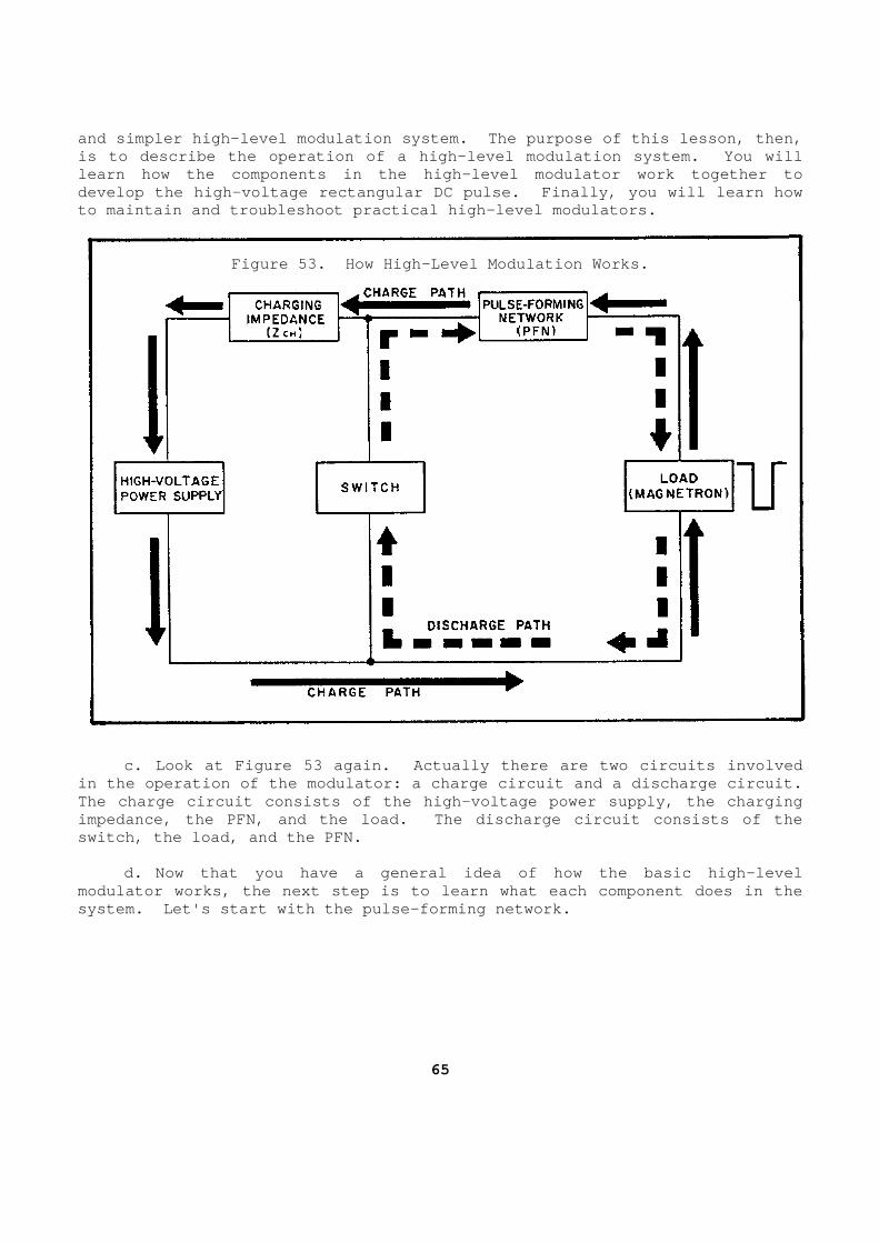
and simpler high-level modulation system. The purp ose of this lesson, then, is to describe the operation of a high-level modula tion system. You will learn how the components in the high-level modulato r work together to develop the high-voltage rectangular DC pulse. Fin ally, you will learn how to maintain and troubleshoot practical high-level m odulators.

Figure 53. How High-Level Modulation Works.

c. Look at Figure 53 again. Actually there are tw o circuits involved in the operation of the modulator: a charge circuit and a discharge circuit. The charge circuit consists of the high-voltage pow er supply, the charging impedance, the PFN, and the load. The discharge ci rcuit consists of the switch, the load, and the PFN. d. Now that you have a general idea of how the bas ic high-level modulator works, the next step is to learn what eac h component does in the system. Let's start with the pulse-forming network .

65

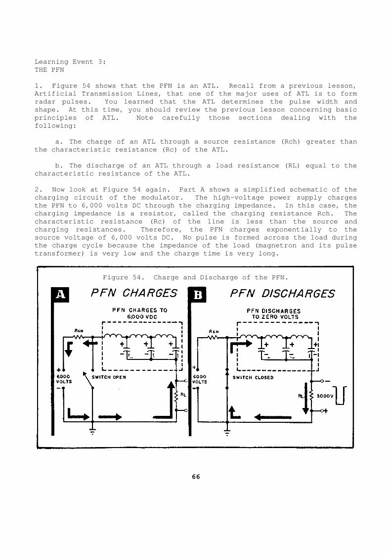
Learning Event 3: THE PFN 1. Figure 54 shows that the PFN is an ATL. Recall from a previous lesson, Artificial Transmission Lines, that one of the majo r uses of ATL is to form radar pulses. You learned that the ATL determines the pulse width and shape. At this time, you should review the previou s lesson concerning basic principles of ATL. Note carefully those sections d ealing with the following: a. The charge of an ATL through a source resistanc e (Rch) greater than the characteristic resistance (Rc) of the ATL. b. The discharge of an ATL through a load resistan ce (RL) equal to the characteristic resistance of the ATL. 2. Now look at Figure 54 again. Part A shows a sim plified schematic of the charging circuit of the modulator. The high-voltag e power supply charges the PFN to 6,000 volts DC through the charging impe dance. In this case, the charging impedance is a resistor, called the chargi ng resistance Rch. The characteristic resistance (Rc) of the line is less than the source and charging resistances. Therefore, the PFN charges e xponentially to the source voltage of 6,000 volts DC. No pulse is form ed across the load during the charge cycle because the impedance of the load (magnetron and its pulse transformer) is very low and the charge time is ver y long.

Figure 54. Charge and Discharge of the PFN.

66

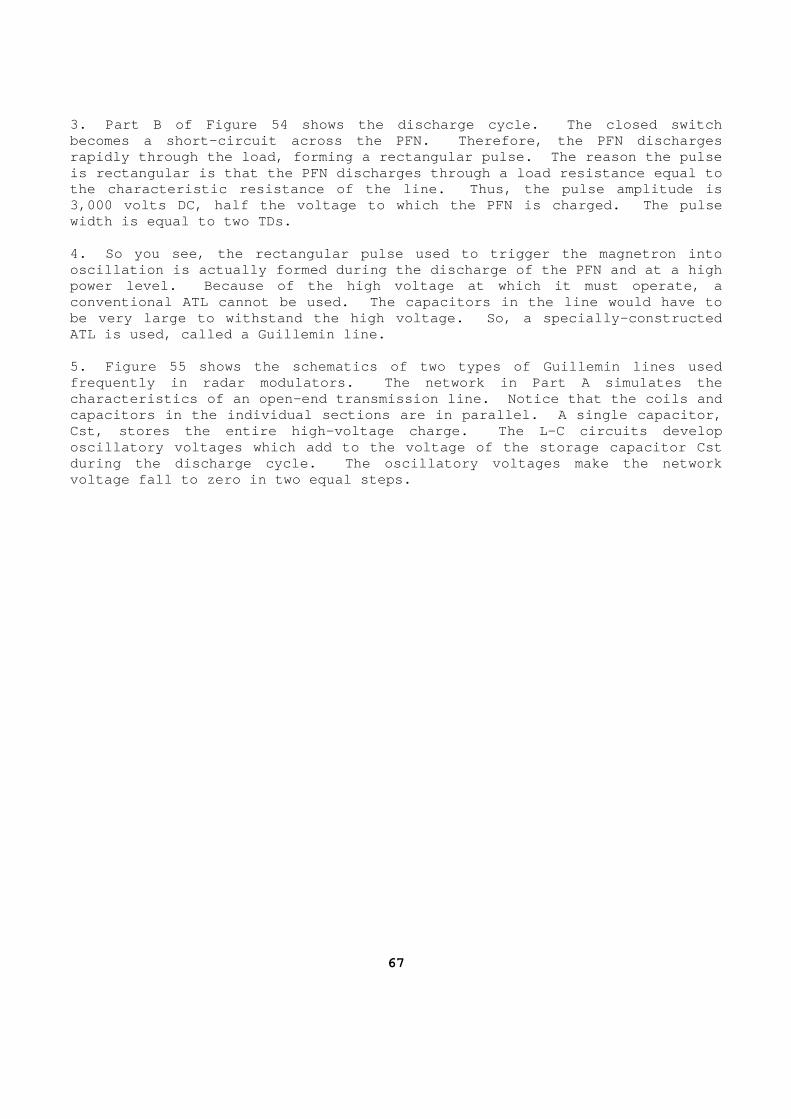
3. Part B of Figure 54 shows the discharge cycle. The closed switch becomes a short-circuit across the PFN. Therefore, the PFN discharges rapidly through the load, forming a rectangular pul se. The reason the pulse is rectangular is that the PFN discharges through a load resistance equal to the characteristic resistance of the line. Thus, t he pulse amplitude is 3,000 volts DC, half the voltage to which the PFN i s charged. The pulse width is equal to two TDs. 4. So you see, the rectangular pulse used to trigge r the magnetron into oscillation is actually formed during the discharge of the PFN and at a high power level. Because of the high voltage at which it must operate, a conventional ATL cannot be used. The capacitors in the line would have to be very large to withstand the high voltage. So, a specially-constructed ATL is used, called a Guillemin line. 5. Figure 55 shows the schematics of two types of G uillemin lines used frequently in radar modulators. The network in Par t A simulates the characteristics of an open-end transmission line. Notice that the coils and capacitors in the individual sections are in parall el. A single capacitor, Cst, stores the entire high-voltage charge. The L- C circuits develop oscillatory voltages which add to the voltage of th e storage capacitor Cst during the discharge cycle. The oscillatory voltag es make the network voltage fall to zero in two equal steps.

67

Figure 55. Two Types of Guillemin Lines

Used as Pulse-Forming Networks. 6. Part B of Figure 55 shows an open-end artificial transmission line with magnetic coupling between the coils. Mutual induct ance is used to remove undesirable oscillations on the top of the pulse. Notice that the line is actually a long solenoid with tap points for equal- value capacitors. The combination of all capacitors in parallel makes up the storage capacitor. This type of PFN is the one used most frequently in modern radar systems. 7. Pulse-forming networks are usually "potted," sea led in an oil-filled metal container. The oil is used for compact high voltage insulation. You can see, then, that there is no maintenance to be d one on the PFN. If one of the elements of the line fails, you must replace the entire line. 8. Brief review. a. Most modern radar sets use the high-level modul ation system in which the pulse is formed at a high power level. b. In high-level modulation, the pulse is formed b y discharging a pulse-forming line through a load resistance equal to the characteristic resistance of the line. c. The PFN determines the shape and width of the p ulse. d. The amplitude of the pulse is equal to one-half the voltage to which the line is charged. e. The pulse width is equal to two TDs. f. The PFN is discharged at the pulse repetition f requency of the radar.

68

g. A Guillemin line is a specially-constructed, pu lse-forming network. Learning Event 4: HYDROGEN THYRATRON SWITCH 1. The switch used to discharge the PFN is one of t he most critical components in the high-level modulator. Here are s ome reasons why. a. The switch must be nonconducting (off) during t he charge of the pulse-forming network. b. The switch must close very rapidly at the pulse repetition frequency of the radar. c. The switch resistance must be as small as possi ble during the discharge of the PFN. d. The switch must be capable of conducting high c urrents without damage. e. Some early radar sets used spark gaps to discha rge the PFN. Figure 56 shows two common types: a fixed spark gap and a rotary spark gap. (1) The two-electrode spark gap shown in Part A wo rks just like the spark plug in your car. During the charge of the P FN, the spark gap is an open circuit. Hence, its resistance is very large. As the PFN charges, the potential across the electrodes builds up rapidly. When the potential is large enough, the air between the electrodes breaks down (ionizes) and a spark jumps across the electrodes. This makes the resistance of the spark gap very small, and, thus, the PFN is short-circuit ed.

69

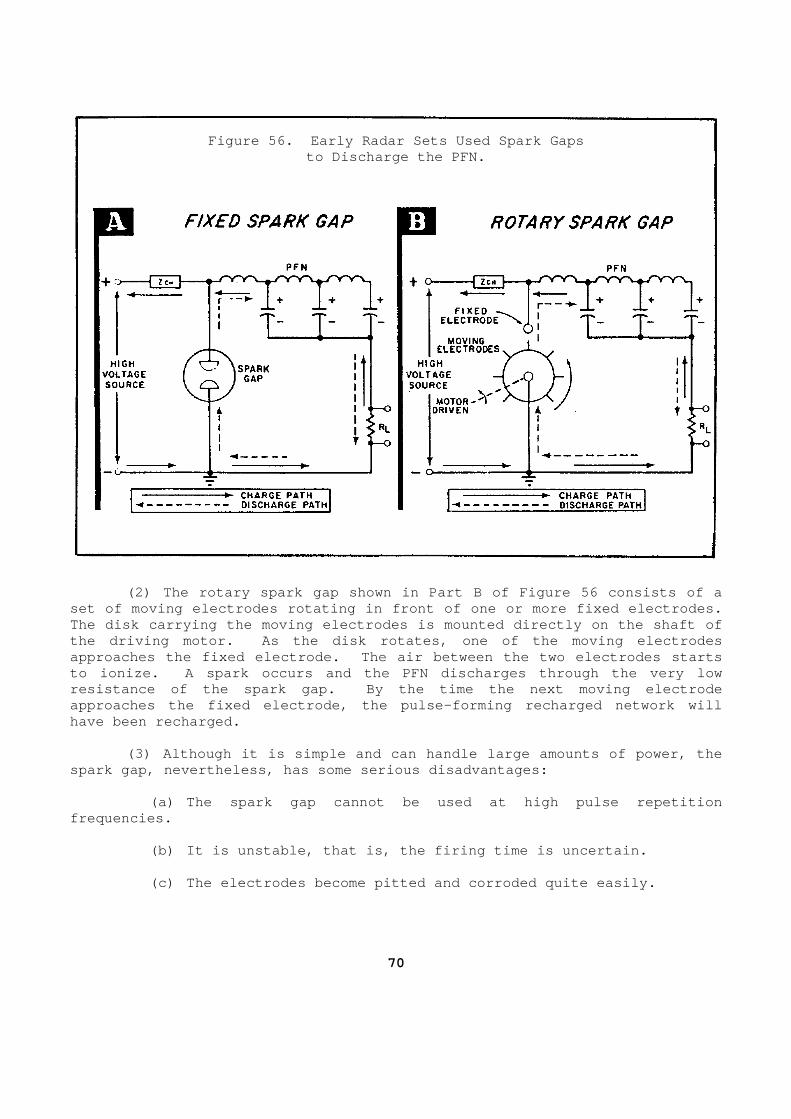
Figure 56. Early Radar Sets Used Spark Gaps

to Discharge the PFN. (2) The rotary spark gap shown in Part B of Figure 56 consists of a set of moving electrodes rotating in front of one o r more fixed electrodes. The disk carrying the moving electrodes is mounted directly on the shaft of the driving motor. As the disk rotates, one of the moving electrodes approaches the fixed electrode. The air between th e two electrodes starts to ionize. A spark occurs and the PFN discharges t hrough the very low resistance of the spark gap. By the time the next moving electrode approaches the fixed electrode, the pulse-forming r echarged network will have been recharged. (3) Although it is simple and can handle large amo unts of power, the spark gap, nevertheless, has some serious disadvant ages: (a) The spark gap cannot be used at high pulse rep etition frequencies. (b) It is unstable, that is, the firing time is un certain. (c) The electrodes become pitted and corroded quit e easily.

70

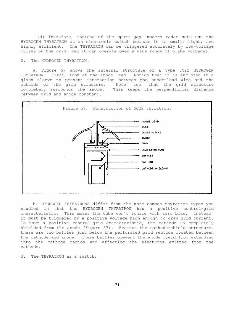
(4) Therefore, instead of the spark gap, modern ra dar sets use the HYDROGEN THYRATRON as an electronic switch because it is small, light, and highly efficient. The THYRATRON can be triggered a ccurately by low-voltage pulses on the grid, and it can operate over a wide range of plate voltages. 2. The HYDROGEN THYRATRON. a. Figure 57 shows the internal structure of a typ e 5C22 HYDROGEN THYRATRON. First, look at the anode lead. Notice that it is enclosed in a glass sleeve to prevent interaction between the ano de-lead wire and the outside of the grid structure. Note, too, that the grid structure completely surrounds the anode. This keeps the per pendicular distance between grid and anode constant.

Figure 57. Construction of 5C22 thyratron.

b. HYDROGEN THYRATRONS differ from the more common thyratron types you studied in that the HYDROGEN THYRATRON has a positi ve control-grid characteristic. This means the tube won't ionize w ith zero bias. Instead, it must be triggered by a positive voltage high eno ugh to draw grid current. To have a positive control-grid characteristic, the cathode is completely shielded from the anode (Figure 57). Besides the c athode-shield structure, there are two baffles just below the perforated gri d section located between the cathode and anode. These baffles prevent the a node field from extending into the cathode region and affecting the electrons emitted from the cathode. 3. The THYRATRON as a switch.

71

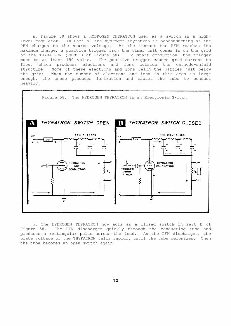
a. Figure 58 shows a HYDROGEN THYRATRON used as a switch in a high-level modulator. In Part A, the hydrogen thyratron is nonconducting as the PFN charges to the source voltage. At the instant the PFN reaches its maximum charge, a positive trigger from the timer u nit comes in on the grid of the THYRATRON (Part B of Figure 58). To start c onduction, the trigger must be at least 150 volts. The positive trigger c auses grid current to flow, which produces electrons and ions outside the cathode-shield structure. Some of these electrons and ions reach the baffles just below the grid: When the number of electrons and ions in this area is large enough, the anode produces ionization and causes th e tube to conduct heavily.

Figure 58. The HYDROGEN THYRATRON is an Electronic Switch.

b. The HYDROGEN THYRATRON now acts as a closed swi tch in Part B of Figure 58. The PFN discharges quickly through the conducting tube and produces a rectangular pulse across the load. As t he PFN discharges, the plate voltage of the THYRATRON falls rapidly until the tube deionizes. Then the tube becomes an open switch again.

72

c. Perhaps at this time, you are wondering why hyd rogen gas is used instead of some other gas, such as argon or mercury vapor. Hydrogen gas is used because it has a short deionization time compa red to the other gases. Also hydrogen allows high currents to pass through the tube without causing damage to the cathode. 4. Brief review. a. The switch discharges the pulse-forming network at the pulse-repetition frequency of the radar. b. Early radar sets used fixed and rotary spark ga ps as switches to discharge the pulse-forming network. c. Modern radar sets use the HYDROGEN THYRATRON as an electronic switch. d. The HYDROGEN THYRATRON is small, light, and hig hly efficient. Also, it can be triggered accurately. e. The HYDROGEN THYRATRON has a positive control-g rid characteristic. Grid current must flow first before the tube will i onize. f. Hydrogen gas is used because it will deionize q uickly and allow high current flow without damage to the cathode. Learning Event 5: CHARGING IMPEDANCE 1. Charging impedance isolates the high-voltage pow er supply from the closed switch while the PFN is discharging. In oth er words, the charging impedance prevents the closed switch from short-cir cuiting the source voltage. Isolation, then, is one of the primary pu rposes of the charging impedance. However, the charging impedance has ano ther important use, that of increasing the amplitude of the modulator pulse. a. For example, recall that the amplitude of the p ulse developed across the load is equal to half the voltage to which the PFN was charged. This means that if the PFN charges to 6,000 volts, then, upon discharging, the PFN will develop a 3,000-volt pulse across the load . Suppose, however, a pulse of 6,000 volts is needed across the load. On e way of getting the additional voltage is to use a 12,000-volt power su pply. The PFN, then, charges to 12,000 volts and, upon discharging, the PFN develops a 6,000-volt pulse across the load. However, this method is cos tly and inefficient.

73

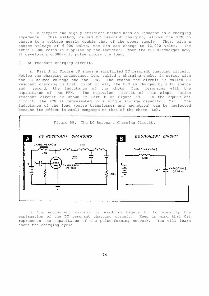
b. A simpler and highly efficient method uses an i nductor as a charging impedance. This method, called DC resonant chargin g, allows the PFN to charge to a voltage nearly double that of the power supply. Thus, with a source voltage of 6,000 volts, the PFN can charge t o 12,000 volts. The extra 6,000 volts is supplied by the inductor. Whe n the PFN discharges now, it develops a 6,000-volt pulse across the load. 2. DC resonant charging circuit. a. Part A of Figure 59 shows a simplified DC reson ant charging circuit. Notice the charging inductance, Lch, called a charg ing choke, in series with the DC source voltage and the PFN. The reason the circuit is called DC resonant charging is that, first of all, the PFN is charged by a DC source and, second, the inductance of the choke, Lch, reso nates with the capacitance of the PFN. The equivalent circuit of this simple series resonant circuit is shown in Part B of Figure 59. In the equivalent circuit, the PFN is represented by a single storage capacitor, Cst. The inductance of the load (pulse transformer and magne tron) can be neglected because its effect is small compared to that of the choke, Lch.

Figure 59. The DC Resonant Charging Circuit.

b. The equivalent circuit is used in Figure 60 to simplify the explanation of the DC resonant charging circuit. K eep in mind that Cst represents the capacitance of the pulse-forming net work. You will learn about the charging cycle

74

first and, then, the discharge cycle. Before start ing, assume a pulse has just been developed across the load. Hence, storag e capacitor Cst is fully discharged. Also, there is no current flowing thro ugh charging choke Lch. c. At the start of the charging cycle, storage cap acitor Cst begins to charge to the 6KV (6,000-volt) source. Current flo w through the choke in Part A of Figure 61 sets up a magnetic field. The charge cycle is slow at first because of the opposing effect of the choke. Remember, a coil produces an induced voltage which opposes changes i n current flow. Since current is increasing, the induced voltage produced by the expanding magnetic field opposes the supply voltage. d. Now, as Cst reaches its initial charge of 6KV, current flow starts to drop off, causing the magnetic field of the chok e to collapse. Once again, the self-inductance of the choke opposes thi s change in current flow. The collapsing magnetic field produces an induced v oltage which keeps current flowing in the same direction as before. P art B of Figure 60 shows that this induced voltage, which is 6KV, is in seri es with the power supply, and so aids the charging current. Notice, now that 12KV is applied to the storage capacitor instead of the 6KV at the start o f the cycle. Therefore, Cst charges to 12KV or double the voltage of the so urce. e. Part C of Figure 60 shows what happens in the c ircuit if the switch never closes. Cst won't stay charged because Lch a nd Cst form a resonant circuit. Therefore, capacitor voltage and inductor current vary sinusoidally as shown in Part C. Notice that capac itor voltage is maximum when inductor current is zero. (See dotted vertica l lines in Part C.) This means that the induced voltage of Lch is maximum wh en inductor current is zero. Recall that the amount of induced voltage de pends not only on the size of the inductor, but also on how fast the curr ent is changing. And, current changes fastest when it is going through ze ro. So Cst charges to twice the source voltage because of the additional induced voltage in series with the source voltage.

75

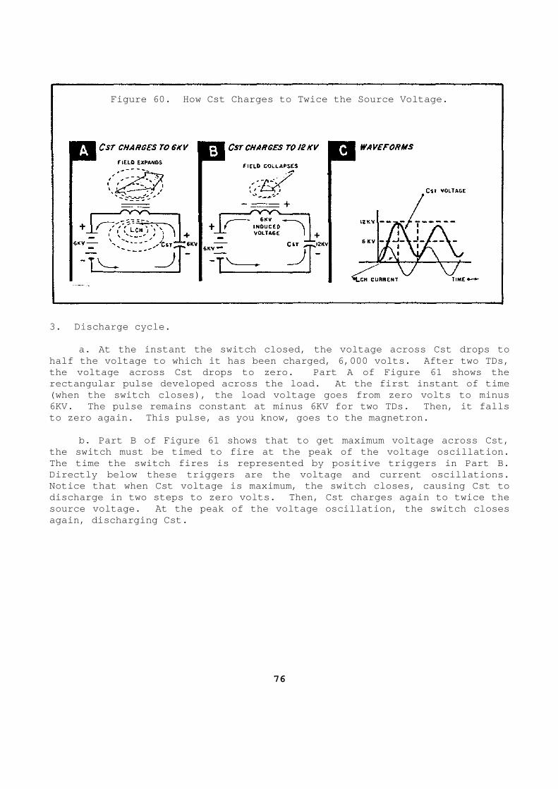
Figure 60. How Cst Charges to Twice the Source Vol tage.

3. Discharge cycle. a. At the instant the switch closed, the voltage a cross Cst drops to half the voltage to which it has been charged, 6,00 0 volts. After two TDs, the voltage across Cst drops to zero. Part A of Fi gure 61 shows the rectangular pulse developed across the load. At th e first instant of time (when the switch closes), the load voltage goes fro m zero volts to minus 6KV. The pulse remains constant at minus 6KV for t wo TDs. Then, it falls to zero again. This pulse, as you know, goes to th e magnetron. b. Part B of Figure 61 shows that to get maximum v oltage across Cst, the switch must be timed to fire at the peak of the voltage oscillation. The time the switch fires is represented by positiv e triggers in Part B. Directly below these triggers are the voltage and c urrent oscillations. Notice that when Cst voltage is maximum, the switch closes, causing Cst to discharge in two steps to zero volts. Then, Cst ch arges again to twice the source voltage. At the peak of the voltage oscilla tion, the switch closes again, discharging Cst.

76

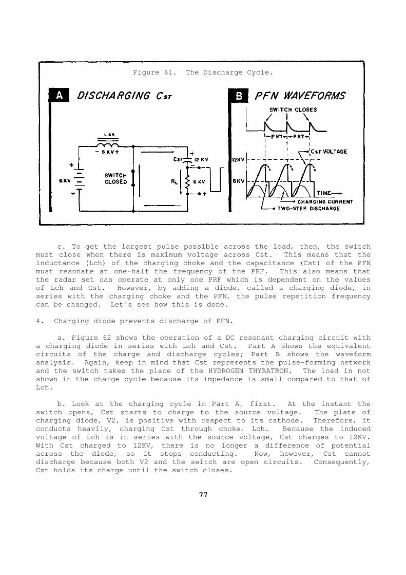
Figure 61. The Discharge Cycle.

c. To get the largest pulse possible across the lo ad, then, the switch must close when there is maximum voltage across Cst . This means that the inductance (Lch) of the charging choke and the capa citance (Cst) of the PFN must resonate at one-half the frequency of the PRF. This also means that the radar set can operate at only one PRF which is dependent on the values of Lch and Cst. However, by adding a diode, called a charging diode, in series with the charging choke and the PFN, the pul se repetition frequency can be changed. Let's see how this is done. 4. Charging diode prevents discharge of PFN. a. Figure 62 shows the operation of a DC resonant charging circuit with a charging diode in series with Lch and Cst. Part A shows the equivalent circuits of the charge and discharge cycles; Part B shows the waveform analysis. Again, keep in mind that Cst represents the pulse-forming network and the switch takes the place of the HYDROGEN THYR ATRON. The load in not shown in the charge cycle because its impedance is small compared to that of Lch. b. Look at the charging cycle in Part A, first. A t the instant the switch opens, Cst starts to charge to the source vo ltage. The plate of charging diode, V2, is positive with respect to its cathode. Therefore, it conducts heavily, charging Cst through choke, Lch. Because the induced voltage of Lch is in series with the source voltage , Cst charges to 12KV. With Cst charged to 12KV, there is no longer a diff erence of potential across the diode, so it stops conducting. Now, how ever, Cst cannot discharge because both V2 and the switch are open c ircuits. Consequently, Cst holds its charge until the switch closes.

77

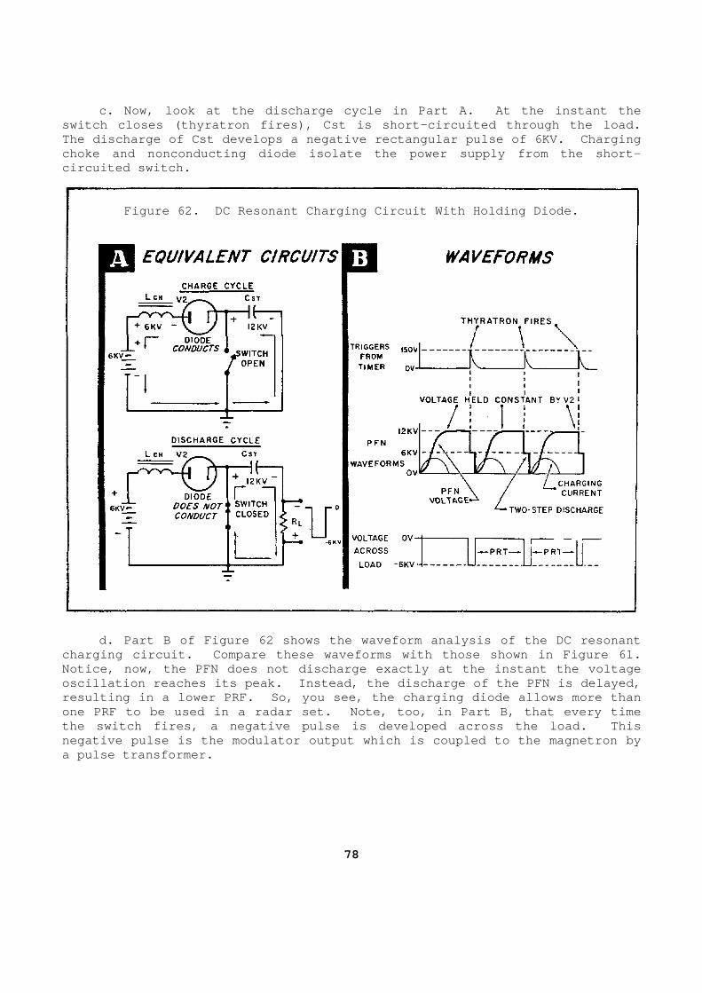
c. Now, look at the discharge cycle in Part A. At the instant the switch closes (thyratron fires), Cst is short-circu ited through the load. The discharge of Cst develops a negative rectangula r pulse of 6KV. Charging choke and nonconducting diode isolate the power sup ply from the short-circuited switch.

Figure 62. DC Resonant Charging Circuit With Holdi ng Diode.

d. Part B of Figure 62 shows the waveform analysis of the DC resonant charging circuit. Compare these waveforms with tho se shown in Figure 61. Notice, now, the PFN does not discharge exactly at the instant the voltage oscillation reaches its peak. Instead, the dischar ge of the PFN is delayed, resulting in a lower PRF. So, you see, the chargin g diode allows more than one PRF to be used in a radar set. Note, too, in P art B, that every time the switch fires, a negative pulse is developed acr oss the load. This negative pulse is the modulator output which is cou pled to the magnetron by a pulse transformer.

78

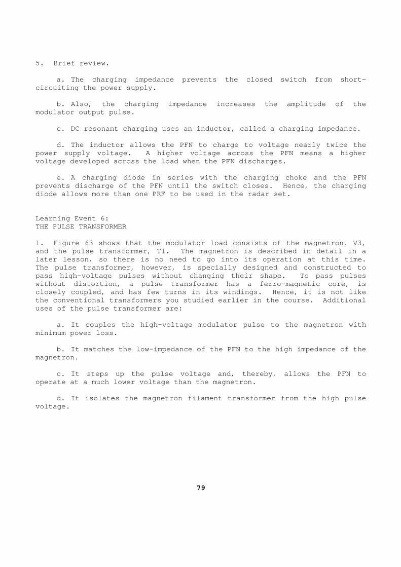
5. Brief review. a. The charging impedance prevents the closed swit ch from short-circuiting the power supply. b. Also, the charging impedance increases the ampl itude of the modulator output pulse. c. DC resonant charging uses an inductor, called a charging impedance. d. The inductor allows the PFN to charge to voltag e nearly twice the power supply voltage. A higher voltage across the PFN means a higher voltage developed across the load when the PFN disc harges. e. A charging diode in series with the charging ch oke and the PFN prevents discharge of the PFN until the switch clos es. Hence, the charging diode allows more than one PRF to be used in the ra dar set. Learning Event 6: THE PULSE TRANSFORMER 1. Figure 63 shows that the modulator load consists of the magnetron, V3, and the pulse transformer, T1. The magnetron is de scribed in detail in a later lesson, so there is no need to go into its op eration at this time. The pulse transformer, however, is specially design ed and constructed to pass high-voltage pulses without changing their sha pe. To pass pulses without distortion, a pulse transformer has a ferro -magnetic core, is closely coupled, and has few turns in its windings. Hence, it is not like the conventional transformers you studied earlier i n the course. Additional uses of the pulse transformer are: a. It couples the high-voltage modulator pulse to the magnetron with minimum power loss. b. It matches the low-impedance of the PFN to the high impedance of the magnetron. c. It steps up the pulse voltage and, thereby, all ows the PFN to operate at a much lower voltage than the magnetron. d. It isolates the magnetron filament transformer from the high pulse voltage.

79

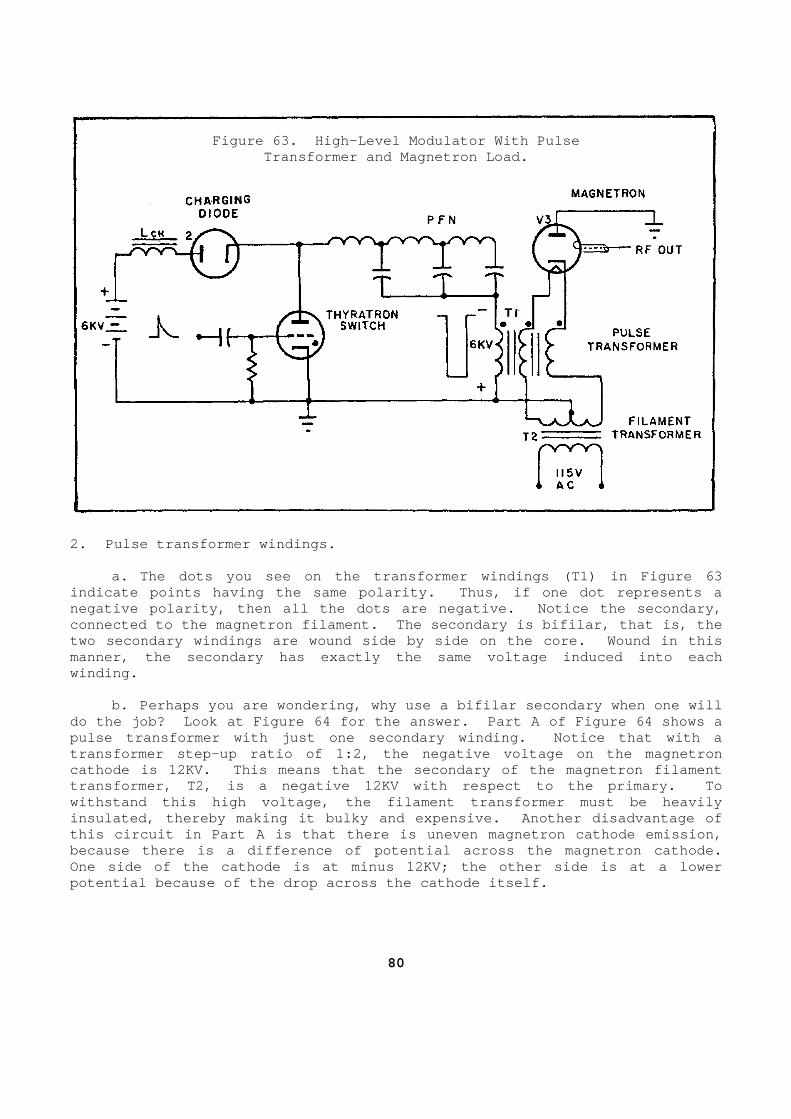
Figure 63. High-Level Modulator With Pulse

Transformer and Magnetron Load. 2. Pulse transformer windings. a. The dots you see on the transformer windings (T 1) in Figure 63 indicate points having the same polarity. Thus, if one dot represents a negative polarity, then all the dots are negative. Notice the secondary, connected to the magnetron filament. The secondary is bifilar, that is, the two secondary windings are wound side by side on th e core. Wound in this manner, the secondary has exactly the same voltage induced into each winding. b. Perhaps you are wondering, why use a bifilar se condary when one will do the job? Look at Figure 64 for the answer. Par t A of Figure 64 shows a pulse transformer with just one secondary winding. Notice that with a transformer step-up ratio of 1:2, the negative volt age on the magnetron cathode is 12KV. This means that the secondary of the magnetron filament transformer, T2, is a negative 12KV with respect to the primary. To withstand this high voltage, the filament transform er must be heavily insulated, thereby making it bulky and expensive. Another disadvantage of this circuit in Part A is that there is uneven magn etron cathode emission, because there is a difference of potential across t he magnetron cathode. One side of the cathode is at minus 12KV; the other side is at a lower potential because of the drop across the cathode it self.

80

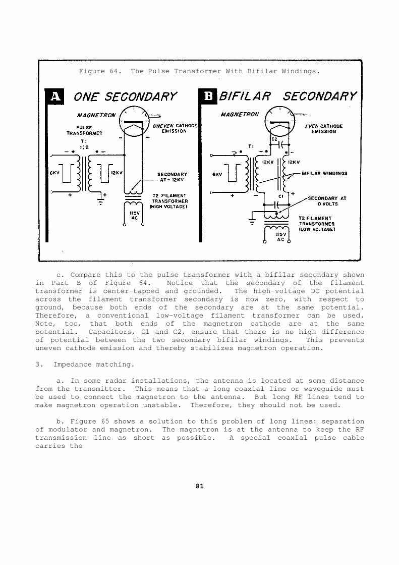
Figure 64. The Pulse Transformer With Bifilar Wind ings.

c. Compare this to the pulse transformer with a bi filar secondary shown in Part B of Figure 64. Notice that the secondary of the filament transformer is center-tapped and grounded. The hig h-voltage DC potential across the filament transformer secondary is now ze ro, with respect to ground, because both ends of the secondary are at t he same potential. Therefore, a conventional low-voltage filament tran sformer can be used. Note, too, that both ends of the magnetron cathode are at the same potential. Capacitors, C1 and C2, ensure that ther e is no high difference of potential between the two secondary bifilar wind ings. This prevents uneven cathode emission and thereby stabilizes magn etron operation. 3. Impedance matching. a. In some radar installations, the antenna is loc ated at some distance from the transmitter. This means that a long coaxi al line or waveguide must be used to connect the magnetron to the antenna. B ut long RF lines tend to make magnetron operation unstable. Therefore, they should not be used. b. Figure 65 shows a solution to this problem of l ong lines: separation of modulator and magnetron. The magnetron is at th e antenna to keep the RF transmission line as short as possible. A special coaxial pulse cable carries the

81

high-voltage modulator pulse to the magnetron. To prevent losses due to reflection of the pulse, the pulse cable must be te rminated in its characteristic impedance. However, the impedance o f the magnetron is high, approximately 1,000 ohms. So, it is not practical to build a pulse cable with a characteristic impedance of 1,000 ohms. Tha t is why we use a pulse transformer as an impedance-matching device.

Figure 65. Pulse Transformers Used as Impedance-Ma tching Devices.

c. Two pulse transformers, T1 and T2, are used to match impedances in the high-level modulator in Figure 65. Pulse trans former T1 couples the pulse cable to the modulator. Not only does T1 mat ch the impedance of the PFN and pulse cable, it also steps down the modulat or pulse voltage. Lowering the pulse voltage allows the use of a smal ler pulse cable with less high-voltage insulation. Pulse transformer T2 coup les the low-impedance pulse cable to the high-impedance magnetron. Also, T2 steps-up the pulse voltage and thus allows the PFN to operate at a low er voltage than the magnetron. 4. Brief review. a. The pulse transformer is a specially-designed t ransformer used to pass high-voltage pulses without distortion.

82

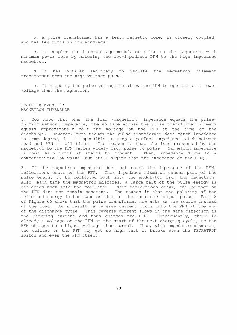
b. A pulse transformer has a ferro-magnetic core, is closely coupled, and has few turns in its windings. c. It couples the high-voltage modulator pulse to the magnetron with minimum power loss by matching the low-impedance PF N to the high impedance magnetron. d. It has bifilar secondary to isolate the magnetr on filament transformer from the high-voltage pulse. e. It steps up the pulse voltage to allow the PFN to operate at a lower voltage than the magnetron. Learning Event 7: MAGNETRON IMPEDANCE 1. You know that when the load (magnetron) impedanc e equals the pulse-forming network impedance, the voltage across the p ulse transformer primary equals approximately half the voltage on the PFN at the time of the discharge. However, even though the pulse transfor mer does match impedance to some degree, it is impossible to keep a perfect impedance match between load and PFN at all times. The reason is that the load presented by the magnetron to the PFN varies widely from pulse to pu lse. Magnetron impedance is very high until it starts to conduct. Then, imp edance drops to a comparatively low value (but still higher than the impedance of the PFN). 2. If the magnetron impedance does not match the im pedance of the PFN, reflections occur on the PFN. This impedance misma tch causes part of the pulse energy to be reflected back into the modulato r from the magnetron. Also, each time the magnetron misfires, a large par t of the pulse energy is reflected back into the modulator. When reflection s occur, the voltage on the PFN does not remain constant. The reason is th at the polarity of the reflected energy is the same as that of the modulat or output pulse. Part A of Figure 66 shows that the pulse transformer now a cts as the source instead of the load. As a result, a reverse current flows into the PFN at the end of the discharge cycle. This reverse current flows in the same direction as the charging current and thus charges the PFN. Con sequently, there is already a voltage on the PFN at the start of the ne xt charging cycle, so the PFN charges to a higher voltage than normal. Thus, with impedance mismatch, the voltage on the PFN may get so high that it brea ks down the THYRATRON switch and even the PFN itself.

83

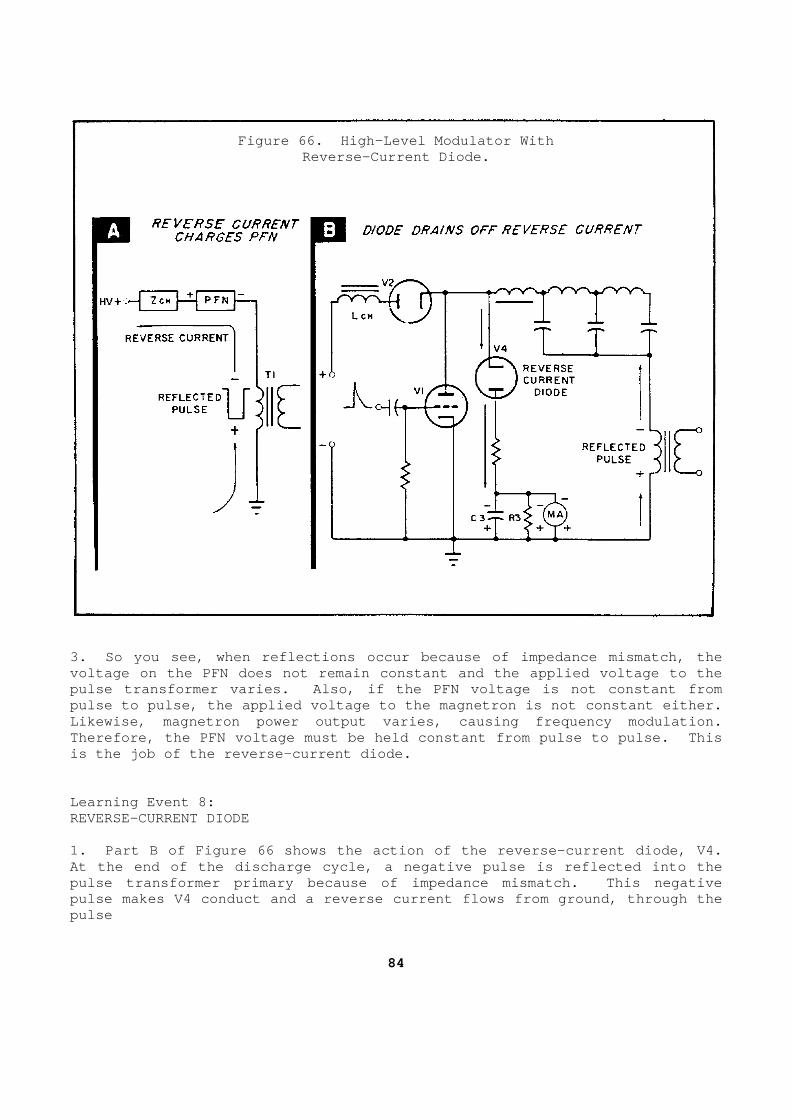
Figure 66. High-Level Modulator With

Reverse-Current Diode. 3. So you see, when reflections occur because of im pedance mismatch, the voltage on the PFN does not remain constant and the applied voltage to the pulse transformer varies. Also, if the PFN voltage is not constant from pulse to pulse, the applied voltage to the magnetro n is not constant either. Likewise, magnetron power output varies, causing fr equency modulation. Therefore, the PFN voltage must be held constant fr om pulse to pulse. This is the job of the reverse-current diode. Learning Event 8: REVERSE-CURRENT DIODE 1. Part B of Figure 66 shows the action of the reve rse-current diode, V4. At the end of the discharge cycle, a negative pulse is reflected into the pulse transformer primary because of impedance mism atch. This negative pulse makes V4 conduct and a reverse current flows from ground, through the pulse

84

transformer primary, out of the PFN, through V4 and into the reverse-current meter circuit. Oscillations within the PFN quickly reverse the voltage on the network. This reverse voltage is drained off b y V4. 2. The reverse current charges capacitor C3. When the short period of reverse-current flow is over, C3 discharges through R3. The RC time constant is long enough to maintain a stable curren t flow through reverse-current meter, M1. 3. Thus, the reverse-current action of V4 allows th e PFN to begin charging from the same potential each time. Hence, the modu lator output pulse is always kept at a constant level, thereby stabilizin g magnetron operation. 4. Figure 67 shows a basic high-level modulation sy stem with magnetron load. This circuit is not an actual high-level mod ulator, but it does give you some idea of how a practical high-level modulat or works. Follow the step-by-step circuit action below:

Figure 67. Review of High-Level Modulation.

a. At the first instant of time, the THYRATRON swi tch V2 and reverse-current diode V4 do not conduct. b. Therefore, the high-voltage power supply charge s the PFN through pulse transformer primary T1, charging diode V1 and charging choke Lch.

85

c. Lch and PFN form a series resonant circuit. He nce, the PFN charges to nearly twice the power supply voltage. d. When the PFN is fully charged, V1 stops conduct ing, thereby opening the charge circuit and preventing the PFN from disc harging through the load. Learning Event 9: THE DISCHARGE CYCLE 1. A positive trigger (Figure 68) from the timer ca uses the HYDROGEN THYRATRON to conduct heavily. Now there is a disch arge path for the PFN, and current flows through the pulse transformer pri mary and V2. 2. The PFN discharge develops a negative rectangula r pulse across the pulse transformer primary. The pulse amplitude is equal to nearly half the voltage on the PFN at the time of discharge. The p ulse width is equal to two TDs and depends on the PFN characteristics. 3. The pulse transformer couples this high-voltage pulse to the magnetron cathode. The magnetron oscillates for the duration of the pulse. 4. However, when the magnetron oscillates, it cause s an impedance mismatch between modulator and magnetron. Hence, a negative pulse is reflected into the pulse transformer primary. A reverse current f lows and charges the PFN. 5. Reverse-current diode V4 now conducts, draining the reverse charge off the PFN. This action of V4 keeps the PFN voltage c onstant from pulse to pulse. 6. When the PFN completely discharges, V2 deionizes and the charge cycle starts again. The HYDROGEN THYRATRON is triggered at the radar pulse-repetition frequency.

86

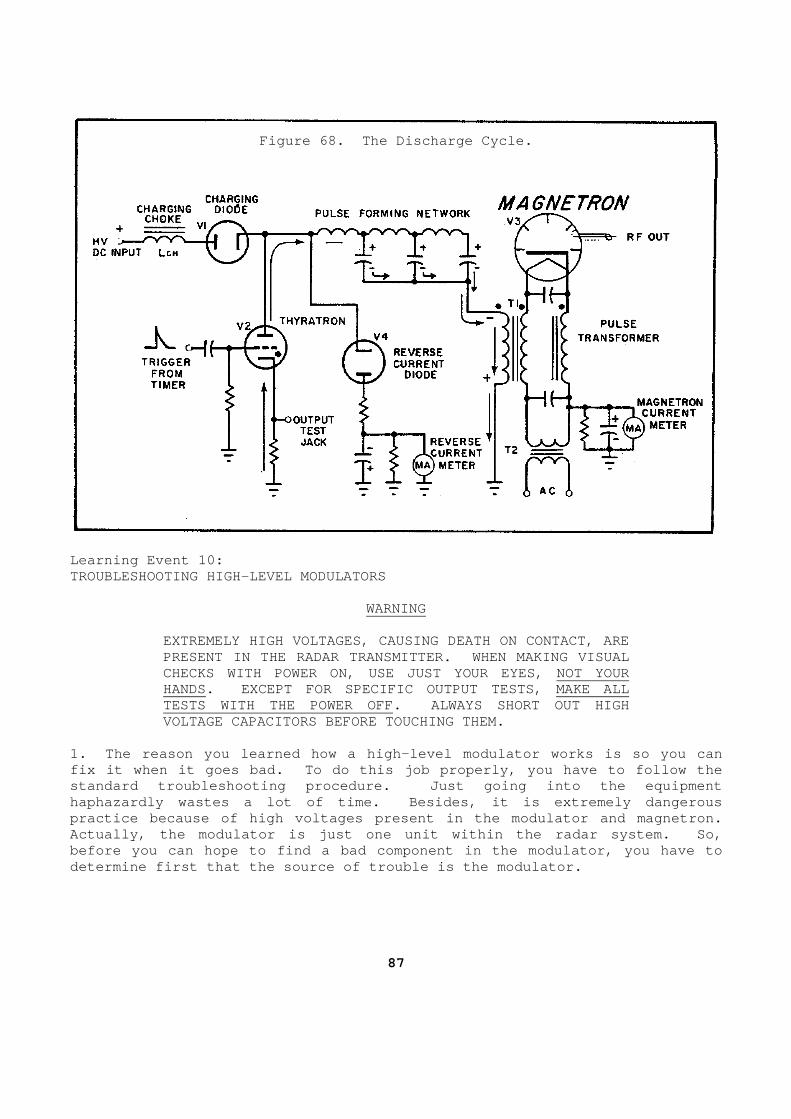
Figure 68. The Discharge Cycle.

Learning Event 10: TROUBLESHOOTING HIGH-LEVEL MODULATORS

WARNING

EXTREMELY HIGH VOLTAGES, CAUSING DEATH ON CONTACT, ARE PRESENT IN THE RADAR TRANSMITTER. WHEN MAKING VISU AL CHECKS WITH POWER ON, USE JUST YOUR EYES, NOT YOUR HANDS. EXCEPT FOR SPECIFIC OUTPUT TESTS, MAKE ALL TESTS WITH THE POWER OFF. ALWAYS SHORT OUT HIGH VOLTAGE CAPACITORS BEFORE TOUCHING THEM.

1. The reason you learned how a high-level modulato r works is so you can fix it when it goes bad. To do this job properly, you have to follow the standard troubleshooting procedure. Just going int o the equipment haphazardly wastes a lot of time. Besides, it is e xtremely dangerous practice because of high voltages present in the mo dulator and magnetron. Actually, the modulator is just one unit within the radar system. So, before you can hope to find a bad component in the modulator, you have to determine first that the source of trouble is the m odulator.

87

2. Trouble symptom. The first indication of troubl e in a particular circuit shows up in the operation of the equipment. The trouble can be due to improper operation of the equipment, an actual m alfunction within the equipment, or conditions outside the radar. Your j ob is to determine which of these conditions is causing the trouble. Theref ore, you must know how the equipment works and what the indications are fo r normal operation. For example, the radar operator complains: "No signals on the indicator, but receiver grass (noise) is normal." First, check th e settings of operator controls. Perhaps the radar operator is at fault. Next, check for proper meter readings, switch positions, panel lamps, and other devices built into the equipment. Knowing what each control does and what each meter or lamp indicates, helps you to troubleshoot quickly and ef ficiently. a. Sectionalization. Once you have verified the s ymptom, the next step is to analyze and evaluate the trouble symptom to d ecide which section of the radar is giving trouble. Here is where your kn owledge of equipment operation is important. For example, suppose durin g verification of the trouble symptom, you see that the magnetron-current meter reads zero. You know immediately that the trouble is in the transmi tting system. You also know that the timer, receiver, and indicator system s are operating properly because there is a sweep with normal receiver grass on the indicator. There is an input to the transmitting system, but no outp ut. Thus, you have sectionalized the trouble to the transmitting syste m just on the basis of your knowledge of the equipment. b. Localization. The next step is to localize the fault to either the magnetron or modulator. Once again, check the mete rs and indicating lamps to decide which stage is at fault. Suppose the rev erse-current meter reading is zero, but the high-voltage meter reading is higher than normal. These meter indications show that the modulator is not working. The THYRATRON is not loading the power supply and a pul se is not being developed to cause reverse current to flow. Now is the time to use a schematic and test equipment such as a synchroscope. Check for t he modulator output pulse at the test jack provided for this purpose. If the re is no modulator output, then you have localized the trouble to the modulator. c. Isolation. Isolating the faulty component is t he easiest step of all because there are so few components to check in the high-level modulator. Use the schematic diagram and voltage a nd resistance charts to isolate the faulty component quickly. But first ma ke a visual check of the modulator. Check for lighted filaments in the THYR ATRON,

88

charging diode, and reverse-current diode. Look fo r loose or broken connections, charred resistors, and loose or broken tubes. Check the tubes by substituting known good ones. Before replacing a component, make sure that the power is off. d. Elimination of the trouble. Your job is to rep air troubles. So take pride in your work by doing a neat repair job. Learn how to use your tools properly and efficiently. e. Test circuit. After repairing the trouble, mak e sure the circuit works by performing an operational check. f. So you see, the standard troubleshooting proced ure is both logical and systematic. It takes you where you want to go in the shortest time. Now, let's deal just with the modulator and see wha t can go wrong with it. 3. Trouble symptom. No modulator output pulse. Assume you've localized the trouble to the modula tor. The first step in troubleshooting the modulator is to check t he output pulse. You can do this easily by connecting a synchroscope to the test jack provided for this purpose. If there is no modulator output puls e, isolate the trouble by making the following checks: (1) Check the input trigger pulse to the THYRATRON . If the trigger is not present, the THYRATRON won't fire. Then, yo u will have to check the timer unit. If the trigger is present, measure its amplitude. If the amplitude is too low, the trigger will not fire the THYRATRON. (2) Check the modulator plate voltage. Usually, t here is a meter on the modulator panel for this purpose. If the meter indicates no modulator plate voltage, then check the output of the high-vo ltage power supply. (3) Look for lighted filaments in the THYRATRON an d charging diode. Replace the tubes with known good ones. (4) Check each of the components in the modulator. An open charging choke, PFN, or pulse transformer primary will cause loss of modulator output.

89

4. Trouble symptom. Modulator pulse present but di storted. If the modulator output pulse is present, check f or proper waveshape on the synchroscope. Examine it carefully for nega tive polarity, sharp leading and trailing edges, correct amplitude, and proper pulse width. If the modulator output pulse is distorted, isolate th e trouble by making the following checks: (1) Measure the pulse amplitude. If it is too low , check the components in the charge circuit. Check the high-v oltage power supply, the charging choke, PFN, and pulse transformer. Also c heck the THYRATRON; its conducting resistance may have increased. (2) Measure the pulse width. If the pulse width o r shape is not correct, check the PFN. (3) Check the trailing edge of the pulse. If ther e are too many oscillations following the pulse, check the reverse -current diode circuit. Replace the diode with a known good one. 5. Final Summary. a. A radar transmitter consists of two major units : modulator and magnetron. The modulator develops rectangular high -voltage DC pulses which cause the magnetron to generate bursts of RF energy . The modulating pulse may be formed either by low-level modulation or hig h-level modulation. This lesson describes the operation of a high-level modu lation system in which the pulse is formed at a high power level. b. A basic high-level modulator consists of a high -voltage DC power supply, a charging impedance, a pulse forming netwo rk, and a switch. At the first instant, the high-voltage power supply charge s the PFN to several thousand volts through the charging impedance. Aft er the PFN is fully charged, the switch closes, discharging the PFN thr ough the load (magnetron and its pulse transformer). c. Practical high-level modulators use DC resonant charging to increase the pulse amplitude and efficiency of the system. In DC resonant charging, the PFN is charged through a charging choke and cha rging diode. The charging choke allows the PFN to charge to a voltag e nearly twice the power supply voltage. The charging diode in series with the

90

charging choke prevents discharge of the PFN until the switch closes. The switch is a HYDROGEN THYRATRON, which is triggered at the PRF of the radar. When the THYRATRON fires, the PFN discharges throug h the pulse transformer primary, developing a negative DC pulse with an amp litude equal to half the voltage on the PFN. The pulse width is equal to tw o TDs and depends on the PFN characteristics.

91

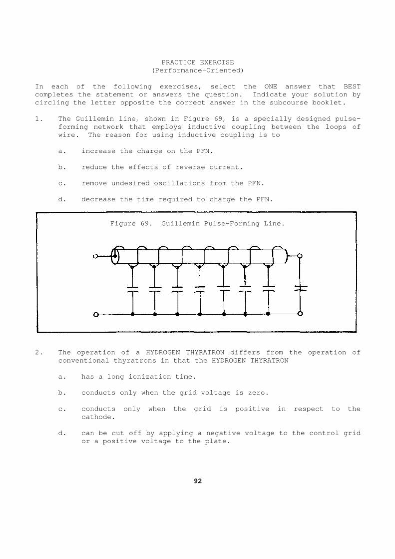
PRACTICE EXERCISE (Performance-Oriented)

In each of the following exercises, select the ONE answer that BEST completes the statement or answers the question. I ndicate your solution by circling the letter opposite the correct answer in the subcourse booklet. 1. The Guillemin line, shown in Figure 69, is a spe cially designed pulse-

forming network that employs inductive coupling bet ween the loops of wire. The reason for using inductive coupling is t o

a. increase the charge on the PFN. b. reduce the effects of reverse current. c. remove undesired oscillations from the PFN. d. decrease the time required to charge the PFN.

Figure 69. Guillemin Pulse-Forming Line.

2. The operation of a HYDROGEN THYRATRON differs fr om the operation of

conventional thyratrons in that the HYDROGEN THYRAT RON a. has a long ionization time. b. conducts only when the grid voltage is zero. c. conducts only when the grid is positive in resp ect to the

cathode. d. can be cut off by applying a negative voltage t o the control grid

or a positive voltage to the plate.

92

3. The HYDROGEN THYRATRON'S positive control grid c haracteristic is made possible by

a. using hydrogen gas. b. shielding the cathode from the plate. c. enclosing the plate wire in a glass sleeve. d. preventing interaction between the plate-lead w ire and the

outside of the grid structure. 4. If a DC resonant charging choke is used as the c harging impedance in a

high-level modulator, the choke is used to form a a. series-resonant circuit with the capacitance of the PFN. b. parallel-resonant circuit with the capacitance of the PFN. c. series-resonant circuit with the capacitance of the THYRATRON. d. parallel-resonant circuit with the capacitance of the pulse

transformer windings. 5. The necessity of timing a THYRATRON to conduct a t the instant when the

pulse-forming line is charged at its greatest poten tial is eliminated by

a. charging the pulse-forming line through a diode . b. DC resonance charging of the pulse-forming line . c. connecting a charging inductor across the circu it. d. using a HYDROGEN THYRATRON in conjunction with a Guillemin line.

93

6. The transmitter shown in Figure 65 uses two puls e transformers to transfer the modulator pulse to the magnetron. The reason for using a bifilar secondary winding on T2 is to

a. permit a 4:1 step-up of voltage. b. allow the use of a conventional filament transf ormer. c. reduce the effects of the changing magnetron im pedance. d. permit the use of a smaller pulse cable with le ss high-voltage

insulation. 7. The performance of a high-level modulator can be improved by coupling

the pulse from the modulator to the magnetron throu gh a pulse transformer. In addition, the use of a pulse trans former has the advantage of

a. eliminating the magnetron filament transformer. b. permitting higher voltages in the pulse-forming network. c. reducing the potential between cathode and grou nd of the

magnetron. d. eliminating the need for long transmission line s between the

transmitter and the antenna. 8. If the characteristic resistance of the PFN show n in Figure 65 is not

equal to the magnetron's impedance, the pulse appli ed to the magnetron will be distorted. This impedance mismatch will al so cause the PFN to

a. charge to a lower voltage on each succeeding ch arge cycle. b. charge to a higher voltage on each succeeding c harge cycle. c. produce a pulse that has a duration time of les s than two TDs. d. produce a voltage that will cause the thyratron to conduct

prematurely.

94

SITUATION Assume that the circuit shown in Figure 70 represen ts the schematic diagram of the transmitter in an air surveillance radar set . The high-level modulator uses an artificial transmission line that has a characteristic resistance of 1,000 ohms and time delay of 0.75 mic roseconds. Exercises 9 through 14 are based on the above situa tion.

95

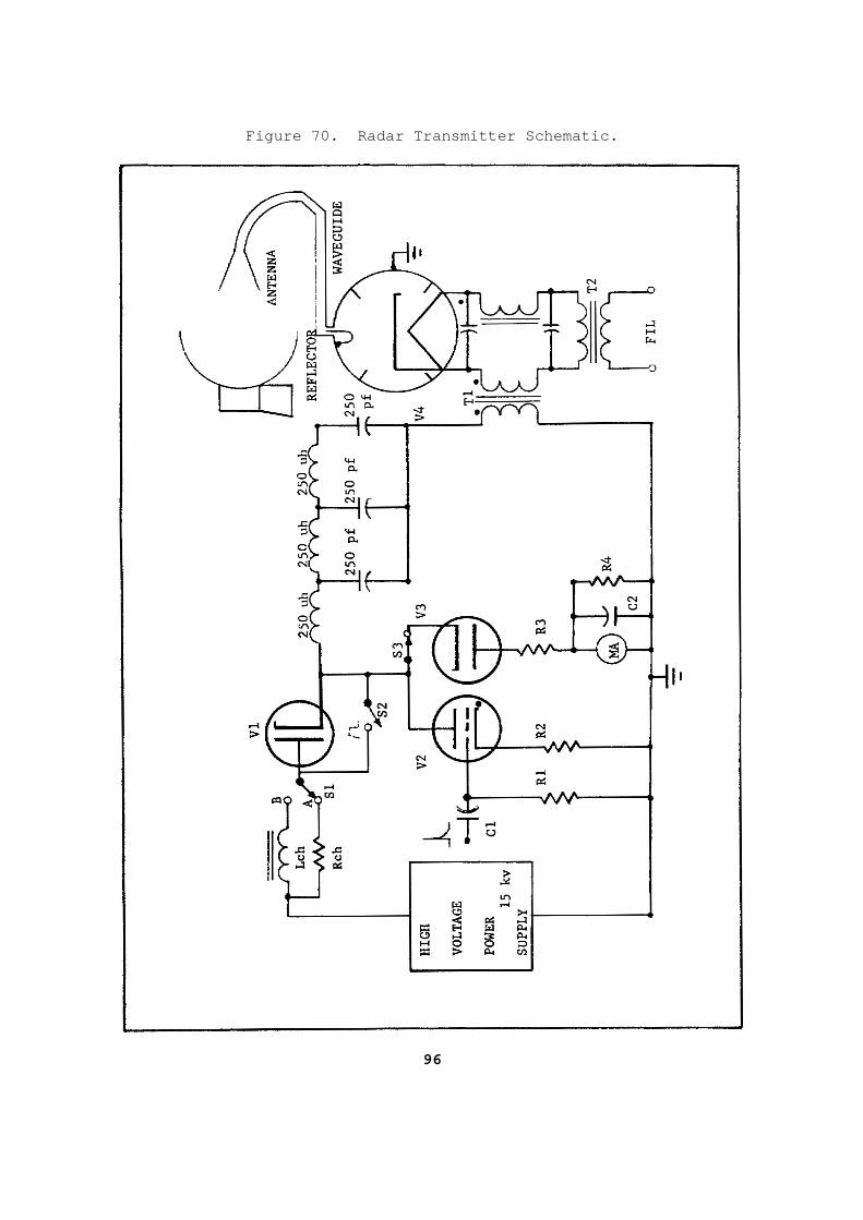
Figure 70. Radar Transmitter Schematic.

96

9. Assume that the load resistance of the high-leve l modulator shown in Figure 70 is equal to 1,000 ohms and that a positiv e trigger voltage causes tube V2 to conduct. The PFN will discharge and the amplitude of the pulse developed across the primary of transf ormer T1 will be a negative

a. 15 KV with a duration time of 1.5 microseconds. b. 15 KV with a duration time of 0.75 microseconds . c. 7.5 KV with a duration time of 1.5 microseconds . d. 7.5 KV with a duration time of 0.75 microsecond s. 10. The charging resistance Rch is used to control the charge time of the

pulse-forming network and to a. prevent the PFN from discharging before V2 cond ucts. b. control the duration of the voltage developed a cross T1. c. allow the PFN to charge to a voltage that is ap proximately twice

the power supply voltage. d. prevent tube V2 from short-circuiting the high- voltage power

supply during the discharge of the PFN. 11. The current flow through the switching tube V2 will cease when a. switch S3 is opened. b. a negative trigger is applied to the grid of V2 . c. the voltage across the pulse-forming network is zero. d. the pulse-forming network is completely charged to 15 KV.

97

12. If the milliammeter shown in the cathode circui t of V3 (Figure 70) indicates an abnormally high current reading, the p robable cause of this reading is

a. a change in the magnetron's impedance. b. a change in the value of Rch. c. an open charging resistance. d. a decrease in the pulse repetition frequency (P RF). 13. The network composed of C2 and R4 is used to fi lter the pulsating

current through V3 and to produce an average curren t reading on the milliammeter. Electron tube V3 will conduct when

a. V1 stops conducting. b. the PFN becomes fully charged. c. V2 is triggered by the positive timing pulse. d. the magnetron causes a negative pulse to be ref lected back into

the primary of T1. 14. When tube V2 conducts in the modulator circuit shown in Figure 70,

then pulse-forming network will discharge through a. the primary of T1, R2, and V2. b. the primary of T1, R4, R3, and V3. c. the primary of T1, high-voltage power supply, R ch, and V1. d. V1, Lch, high-voltage power supply, R4, C2, mil liammeter, R3, and

V3. SITUATION Assume that switch S1 is moved to position B in the circuit shown in Figure 70, and that the pulse repetition frequency of the radar set is 400 pulses per second. Exercises 15 through 20 are based on the above situ ation.

98

15. Assume that switch S2 is closed in the circuit shown in Figure 70. To produce the maximum output from the pulse-forming n etwork, the resonant frequency of the pulse-forming network cap acitance and Lch should be approximately

a. 100 Hz. b. 200 Hz. c. 400 Hz. d. 800 Hz. 16. If the pulse-forming network is allowed to char ge through the DC

resonant charging choke, the network will charge to approximately a. 15 KV and will produce an output pulse of appro ximately 7.5 KV. b. 15 KV and will produce an output pulse of appro ximately 15 KV. c. 30 KV and will produce an output pulse of appro ximately 15 KV. d. 30 KV and will produce an output pulse of appro ximately 30 KV. 17. The charging diode is used in conjunction with the DC resonant

charging choke to a. permit the use of more than one PRF. b. maintain a constant charge across the PFN from pulse to pulse. c. prevent the high-voltage power supply from bein g short circuited

when V3 conducts. d. allow the PFN to charge to a voltage that is ap proximately twice

the power supply voltage.

99

18. The pulse transformer used to couple the modula tor's output pulse to the magnetron is different from a conventional tran sformer in that its windings are designed to have

a. loose coupling and few turns. b. close coupling and few turns. c. loose coupling and many turns. d. close coupling and many turns. 19. The frequency at which the antenna shown in Fig ure 70 sends the RF

pulses into space is determined by the a. TD of the PFN. b. number of sections used in the PFN. c. resonant frequency of the magnetron. d. frequency of the positive triggers applied to V 2. 20. If the antenna shown in Figure 70 is to be used for both transmitting

and receiving, an additional section of waveguide w ill be connected to the existing waveguide. At the junction of the two waveguides, a component is placed which will allow one antenna to be used for both transmitting and receiving. This component is call ed

a. a relay. b. a duplexer. c. a thyratron. d. an interlock. Check your answers with lesson 2 solution sheet.

100

LESSON THREE

RESONANT CAVITIES AND MAGNETRONS TASK Describe resonant cavities and magnetron operations , recognize coupling and tuning techniques employed with resonant cavities a nd magnetrons, identify different types of magnetrons and describe their mo des of operation. CONDITION Given this lesson, pencil, and paper. STANDARD Demonstrate competency of task skills and knowledge by correctly responding to 75 percent of the multiple-choice test covering radar transmitters. REFERENCE TC 11-67 Learning Event 1: RESONANT CAVITIES 1. General. a. A coil and capacitor form a resonant circuit wh en connected together either in a series or parallel arrangement. The hi gher the resonant frequency you want, the smaller are the capacitor a nd coil that you need. Resonant circuits operating at ultra-high frequenci es (UHF) have extremely small values of inductance and capacitance. The va lues are so small in fact, that at about 500 megahertz, the use of coils and capacitors becomes impractical. So, instead of using a coil and capac itor at these UHF frequencies, we can use a section of transmission l ine as a resonant circuit. b. You learned in a previous lesson how a transmis sion line section serves as a resonant circuit. Transmission lines a re similar to resonant circuits, except that the inductance and capacitanc e are distributed instead of being lumped values. Just like ordinary resonan t circuit components,

101

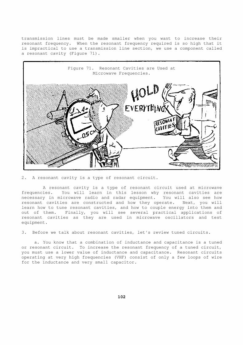
transmission lines must be made smaller when you wa nt to increase their resonant frequency. When the resonant frequency re quired is so high that it is impractical to use a transmission line section, we use a component called a resonant cavity (Figure 71).

Figure 71. Resonant Cavities are Used at

Microwave Frequencies. 2. A resonant cavity is a type of resonant circuit. A resonant cavity is a type of resonant circuit u sed at microwave frequencies. You will learn in this lesson why res onant cavities are necessary in microwave radio and radar equipment. You will also see how resonant cavities are constructed and how they oper ate. Next, you will learn how to tune resonant cavities, and how to cou ple energy into them and out of them. Finally, you will see several practic al applications of resonant cavities as they are used in microwave osc illators and test equipment. 3. Before we talk about resonant cavities, let's re view tuned circuits. a. You know that a combination of inductance and c apacitance is a tuned or resonant circuit. To increase the resonant freq uency of a tuned circuit, you must use a lower value of inductance and capaci tance. Resonant circuits operating at very high frequencies (VHF) consist of only a few loops of wire for the inductance and very small capacitor.

102

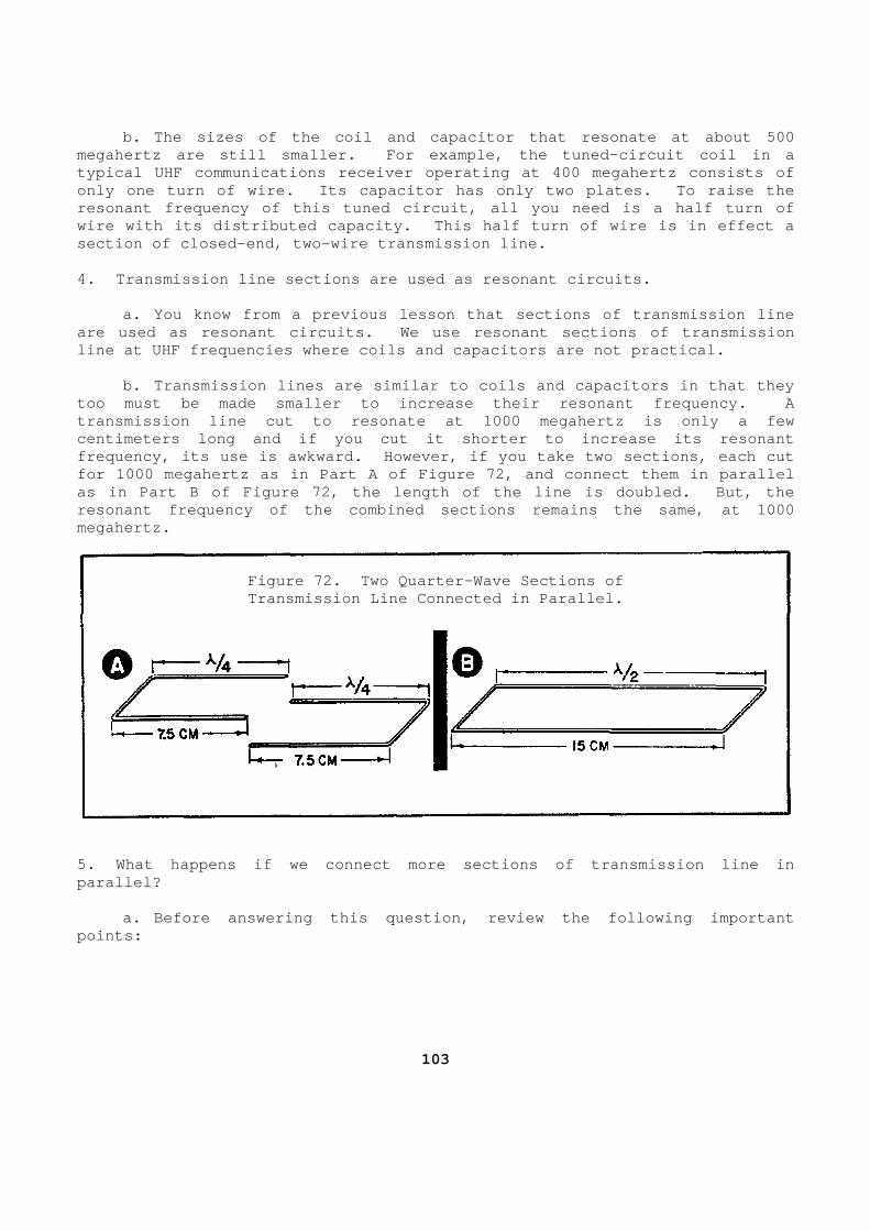
b. The sizes of the coil and capacitor that resona te at about 500 megahertz are still smaller. For example, the tune d-circuit coil in a typical UHF communications receiver operating at 40 0 megahertz consists of only one turn of wire. Its capacitor has only two plates. To raise the resonant frequency of this tuned circuit, all you n eed is a half turn of wire with its distributed capacity. This half turn of wire is in effect a section of closed-end, two-wire transmission line. 4. Transmission line sections are used as resonant circuits. a. You know from a previous lesson that sections o f transmission line are used as resonant circuits. We use resonant sec tions of transmission line at UHF frequencies where coils and capacitors are not practical. b. Transmission lines are similar to coils and cap acitors in that they too must be made smaller to increase their resonant frequency. A transmission line cut to resonate at 1000 megahertz is only a few centimeters long and if you cut it shorter to incre ase its resonant frequency, its use is awkward. However, if you tak e two sections, each cut for 1000 megahertz as in Part A of Figure 72, and c onnect them in parallel as in Part B of Figure 72, the length of the line i s doubled. But, the resonant frequency of the combined sections remains the same, at 1000 megahertz.

Figure 72. Two Quarter-Wave Sections of Transmission Line Connected in Parallel.

5. What happens if we connect more sections of tran smission line in parallel? a. Before answering this question, review the foll owing important points:

103

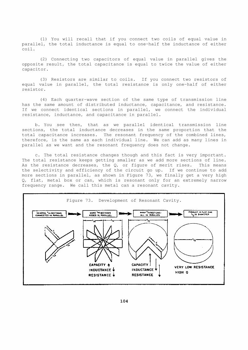
(1) You will recall that if you connect two coils of equal value in parallel, the total inductance is equal to one-half the inductance of either coil. (2) Connecting two capacitors of equal value in pa rallel gives the opposite result, the total capacitance is equal to twice the value of either capacitor. (3) Resistors are similar to coils. If you connec t two resistors of equal value in parallel, the total resistance is on ly one-half of either resistor. (4) Each quarter-wave section of the same type of transmission line has the same amount of distributed inductance, capa citance, and resistance. If we connect identical sections in parallel, we co nnect the individual resistance, inductance, and capacitance in parallel . b. You see then, that as we parallel identical tra nsmission line sections, the total inductance decreases in the sam e proportion that the total capacitance increases. The resonant frequenc y of the combined lines, therefore, is the same as each individual line. We can add as many lines in parallel as we want and the resonant frequency does not change. c. The total resistance changes though and this fa ct is very important. The total resistance keeps getting smaller as we ad d more sections of line. As the resistance decreases, the Q, or figure of me rit rises. This means the selectivity and efficiency of the circuit go up . If we continue to add more sections in parallel, as shown in Figure 73, w e finally get a very high Q, flat, metal box or can, which is resonant only f or an extremely narrow frequency range. We call this metal can a resonant cavity.

Figure 73. Development of Resonant Cavity.

104

6. Some characteristics of resonant cavities. a. You have seen that a resonant cavity is a space bounded by walls. When you excite the cavity by applying electrical e nergy to it, all the energy is contained inside the walls. b. When we apply energy to ordinary tuned circuits and transmission-line tuned circuits, we usually speak in terms of v oltage and current. But when we excite a resonant cavity, we cannot speak o nly in terms of voltage and current because most of the energy inside the w alls is contained in the electric and magnetic fields. There is some electr on flow, however, but it is limited to a thin layer of metal on the inside s urface of the walls. Sometimes, the inside surfaces of the walls are sil ver-plated or gold-plated to reduce heat losses due to resistance. Plating t he walls makes the Q of the cavity even higher, and cavities with a Q of 30 ,000 are not uncommon. There is no current flow on the outside of the cavi ty, so there is no radiation loss. Since current flows only on the in side walls, some cavities are made from nonconducting materials. The inside walls are then sprayed with a thin layer of metal, or covered with metal f oil. 7. Comparing resonant cavities with transmission li nes. a. Resonant cavities are similar to transmission l ines in two ways: (1) The fundamental resonant frequency of transmis sion lines and resonant cavities is determined by their size. (2) Transmission lines and resonant cavities can h ave different forms or shapes. b. Let's examine both of these similarities. 8. First, size determines resonant frequency. You know that the size of a transmission line det ermines its resonant frequency. For example, a one-quarter wav elength section of transmission line acts as a parallel resonant circu it, and it is the shortest length that oscillates. Similarly, the ar ea within the walls of a resonant cavity determine the resonant frequency. A resonant cavity must be at least one-half wavelength in dimension to oscill ate.

105

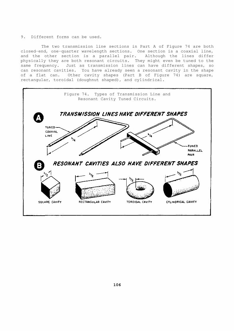
9. Different forms can be used. The two transmission line sections in Part A of F igure 74 are both closed-end, one-quarter wavelength sections. One s ection is a coaxial line, and the other section is a parallel pair. Although the lines differ physically they are both resonant circuits. They m ight even be tuned to the same frequency. Just as transmission lines can hav e different shapes, so can resonant cavities. You have already seen a res onant cavity in the shape of a flat can. Other cavity shapes (Part B of Figu re 74) are square, rectangular, toroidal (doughnut shaped), and cylind rical.

Figure 74. Types of Transmission Line and

Resonant Cavity Tuned Circuits.

106

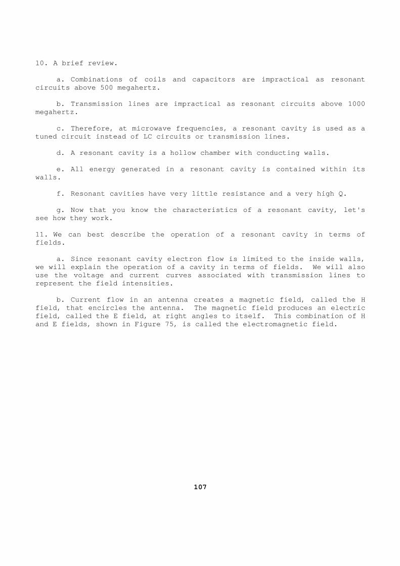
10. A brief review. a. Combinations of coils and capacitors are imprac tical as resonant circuits above 500 megahertz. b. Transmission lines are impractical as resonant circuits above 1000 megahertz. c. Therefore, at microwave frequencies, a resonant cavity is used as a tuned circuit instead of LC circuits or transmissio n lines. d. A resonant cavity is a hollow chamber with cond ucting walls. e. All energy generated in a resonant cavity is co ntained within its walls. f. Resonant cavities have very little resistance a nd a very high Q. g. Now that you know the characteristics of a reso nant cavity, let's see how they work. 11. We can best describe the operation of a resonan t cavity in terms of fields. a. Since resonant cavity electron flow is limited to the inside walls, we will explain the operation of a cavity in terms of fields. We will also use the voltage and current curves associated with transmission lines to represent the field intensities. b. Current flow in an antenna creates a magnetic f ield, called the H field, that encircles the antenna. The magnetic fi eld produces an electric field, called the E field, at right angles to itsel f. This combination of H and E fields, shown in Figure 75, is called the ele ctromagnetic field.

107

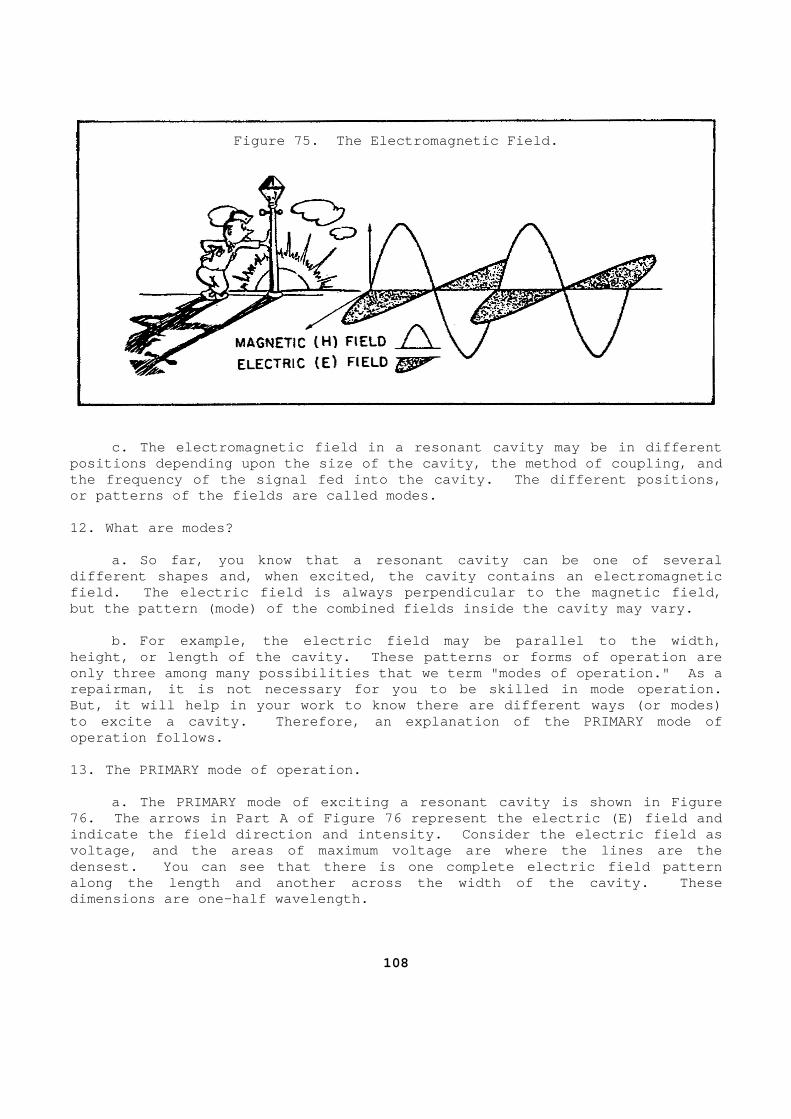
Figure 75. The Electromagnetic Field.

c. The electromagnetic field in a resonant cavity may be in different positions depending upon the size of the cavity, th e method of coupling, and the frequency of the signal fed into the cavity. T he different positions, or patterns of the fields are called modes. 12. What are modes? a. So far, you know that a resonant cavity can be one of several different shapes and, when excited, the cavity cont ains an electromagnetic field. The electric field is always perpendicular to the magnetic field, but the pattern (mode) of the combined fields insid e the cavity may vary. b. For example, the electric field may be parallel to the width, height, or length of the cavity. These patterns or forms of operation are only three among many possibilities that we term "m odes of operation." As a repairman, it is not necessary for you to be skille d in mode operation. But, it will help in your work to know there are di fferent ways (or modes) to excite a cavity. Therefore, an explanation of t he PRIMARY mode of operation follows. 13. The PRIMARY mode of operation. a. The PRIMARY mode of exciting a resonant cavity is shown in Figure 76. The arrows in Part A of Figure 76 represent th e electric (E) field and indicate the field direction and intensity. Consid er the electric field as voltage, and the areas of maximum voltage are where the lines are the densest. You can see that there is one complete el ectric field pattern along the length and another across the width of th e cavity. These dimensions are one-half wavelength.

108

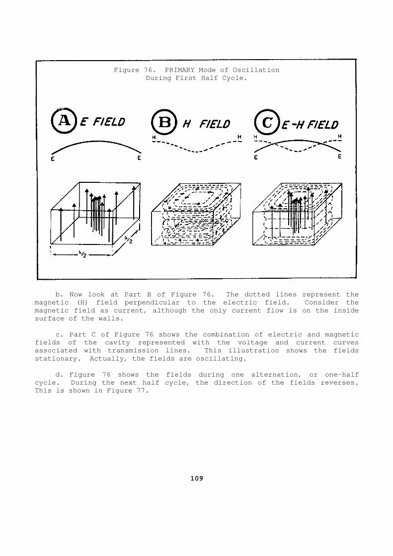
Figure 76. PRIMARY Mode of Oscillation

During First Half Cycle. b. Now look at Part B of Figure 76. The dotted li nes represent the magnetic (H) field perpendicular to the electric fi eld. Consider the magnetic field as current, although the only curren t flow is on the inside surface of the walls. c. Part C of Figure 76 shows the combination of el ectric and magnetic fields of the cavity represented with the voltage a nd current curves associated with transmission lines. This illustrat ion shows the fields stationary. Actually, the fields are oscillating. d. Figure 76 shows the fields during one alternati on, or one-half cycle. During the next half cycle, the direction o f the fields reverses. This is shown in Figure 77.

109

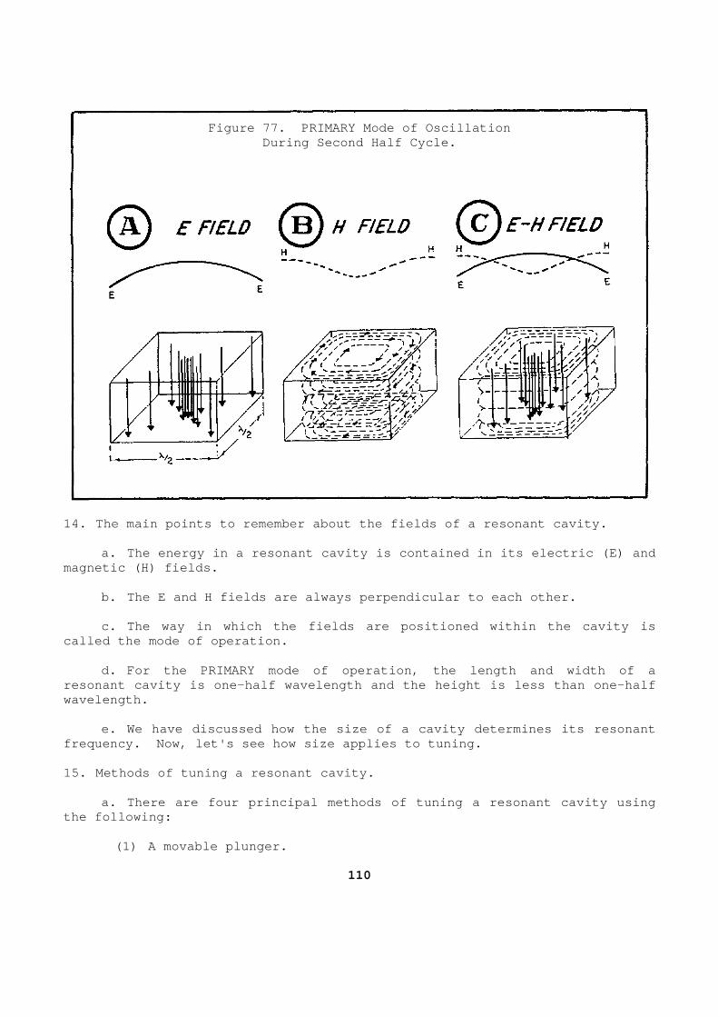
Figure 77. PRIMARY Mode of Oscillation

During Second Half Cycle. 14. The main points to remember about the fields of a resonant cavity. a. The energy in a resonant cavity is contained in its electric (E) and magnetic (H) fields. b. The E and H fields are always perpendicular to each other. c. The way in which the fields are positioned with in the cavity is called the mode of operation. d. For the PRIMARY mode of operation, the length a nd width of a resonant cavity is one-half wavelength and the heig ht is less than one-half wavelength. e. We have discussed how the size of a cavity dete rmines its resonant frequency. Now, let's see how size applies to tuni ng. 15. Methods of tuning a resonant cavity. a. There are four principal methods of tuning a re sonant cavity using the following: (1) A movable plunger.

110

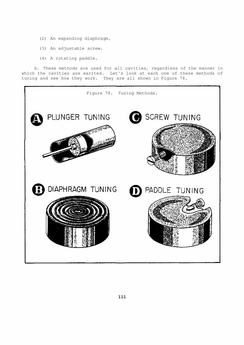
(2) An expanding diaphragm. (3) An adjustable screw. (4) A rotating paddle. b. These methods are used for all cavities, regard less of the manner in which the cavities are excited. Let's look at each one of these methods of tuning and see how they work. They are all shown i n Figure 78.

Figure 78. Tuning Methods.

111

16. First, plunger tuning. You see in Part A of Figure 78 that one wall of t he cavity is a movable plunger, resembling a piston in a cylinder. You adjust the plunger to change the size of the cavity. The effect is si milar to what happens when you change the length of a coil. Inserting th e plunger deeper reduces the cavity and inductance, causing the frequency to go up. If you withdraw the plunger, the inductance goes up and frequency g oes down. 17. Next, diaphragm tuning. An example of diaphragm tuning is shown in Part B of Figure 78. You see that one wall of the cavity is pleated. You ad just this wall, called a diaphragm, to reduce or increase the size of the ca vity. The effect is similar to what happens when you change the distanc e between the plates of a capacitor. If you make the distance between the di aphragm and the bottom of the cavity smaller, capacitance increases, causing the frequency to go down. If you make the distance larger, the capacitance go es down and frequency goes up. 18. Now, screw tuning. An example of screw tuning, sometimes called slug tuning, is shown in Part C of Figure 78. An adjustable screw is ins erted through one wall of the cavity. Turning the screw changes the inductan ce of the cavity. As you turn the screw so that it penetrates further into t he cavity, you confine the magnetic field to a smaller space, and reduce t he inductance. This increases the resonant frequency. As you turn the screw in the opposite direction, you shorten its extent into the cavity. This increases its inductance and the resonant frequency goes down. 19. Paddle tuning. Another method similar to screw tuning is paddle tuning. Part D of Figure 78 shows that one wall of the cavity has a p addle that you rotate. Turning the paddle to a position more nearly perpen dicular to the magnetic field lowers the cavity inductance and raises the c avity resonant frequency. Turning the paddle to a position more nearly parall el to the magnetic field raises the cavity inductance, and lowers the cavity resonant frequency. Both the screw and paddle methods of tuning compare to inserting a brass slug into an IF coil to adjust the inductance.

112

20. Summary of tuning methods. a. There are four principal methods of tuning a ca vity: using a plunger, a diaphragm, a screw, or a paddle. b. The plunger and diaphragm methods of tuning var y the size of the cavity to change its resonant frequency. c. The screw and paddle methods of tuning change t he resonant frequency of the cavity without varying the size. d. Now that you know the various methods used to t une resonant cavities, let's get back to the main purpose of res onant cavities, that is, to generate frequencies higher than 1000 megahertz. First of all, you know that a resonant cavity must be excited to make it o scillate, that is, energy must be fed to it from an external source. Once th e cavity is oscillating, we must couple the energy out of the cavity. There are three principle ways that energy is put into or removed from a cavity. You use the same methods for either operation. These three methods are desc ribed in the paragraphs that follow. 21. Loop coupling. a. A conductor in the shape of a loop is inserted into the area of maximum magnetic lines of force as shown in Part A of Figure 79. In effect, this method of coupling is comparable to coupling b etween the primary and secondary of a transformer as shown in Part B of Fi gure 79. When the loop is perpendicular to the lines of force, maximum ene rgy is transferred. This fact is also true of a transformer. The coils of t he transformer are parallel to each other, and the magnetic lines of f orce are perpendicular to the coils.

113

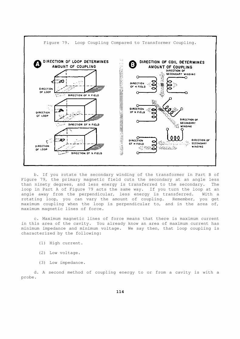
Figure 79. Loop Coupling Compared to Transformer C oupling.

b. If you rotate the secondary winding of the tran sformer in Part B of Figure 79, the primary magnetic field cuts the seco ndary at an angle less than ninety degrees, and less energy is transferred to the secondary. The loop in Part A of Figure 79 acts the same way. If you turn the loop at an angle away from the perpendicular, less energy is t ransferred. With a rotating loop, you can vary the amount of coupling. Remember, you get maximum coupling when the loop is perpendicular to, and in the area of, maximum magnetic lines of force. c. Maximum magnetic lines of force means that ther e is maximum current in this area of the cavity. You already know an ar ea of maximum current has minimum impedance and minimum voltage. We say then , that loop coupling is characterized by the following: (1) High current. (2) Low voltage. (3) Low impedance. d. A second method of coupling energy to or from a cavity is with a probe.

114

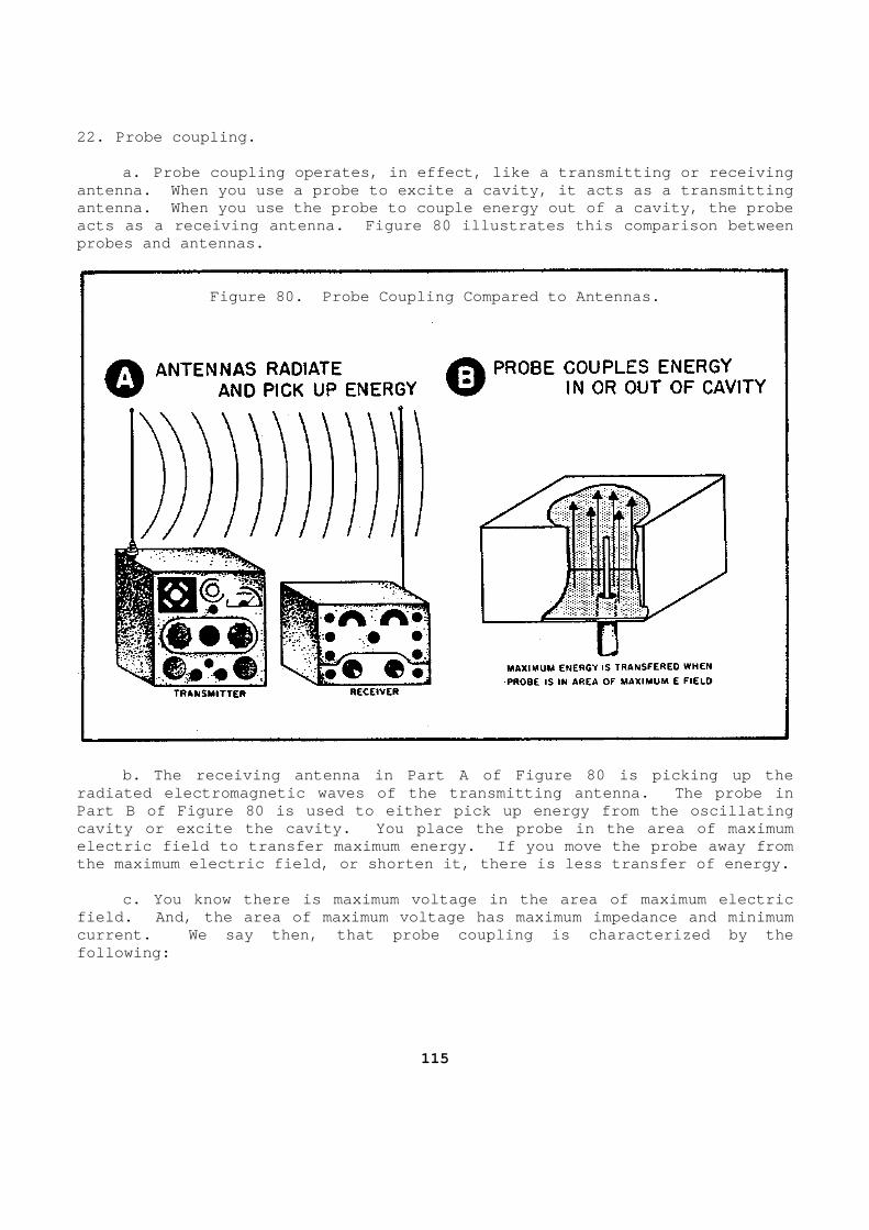
22. Probe coupling. a. Probe coupling operates, in effect, like a tran smitting or receiving antenna. When you use a probe to excite a cavity, it acts as a transmitting antenna. When you use the probe to couple energy o ut of a cavity, the probe acts as a receiving antenna. Figure 80 illustrates this comparison between probes and antennas.

Figure 80. Probe Coupling Compared to Antennas.

b. The receiving antenna in Part A of Figure 80 is picking up the radiated electromagnetic waves of the transmitting antenna. The probe in Part B of Figure 80 is used to either pick up energ y from the oscillating cavity or excite the cavity. You place the probe i n the area of maximum electric field to transfer maximum energy. If you move the probe away from the maximum electric field, or shorten it, there is less transfer of energy. c. You know there is maximum voltage in the area o f maximum electric field. And, the area of maximum voltage has maximu m impedance and minimum current. We say then, that probe coupling is chara cterized by the following:

115

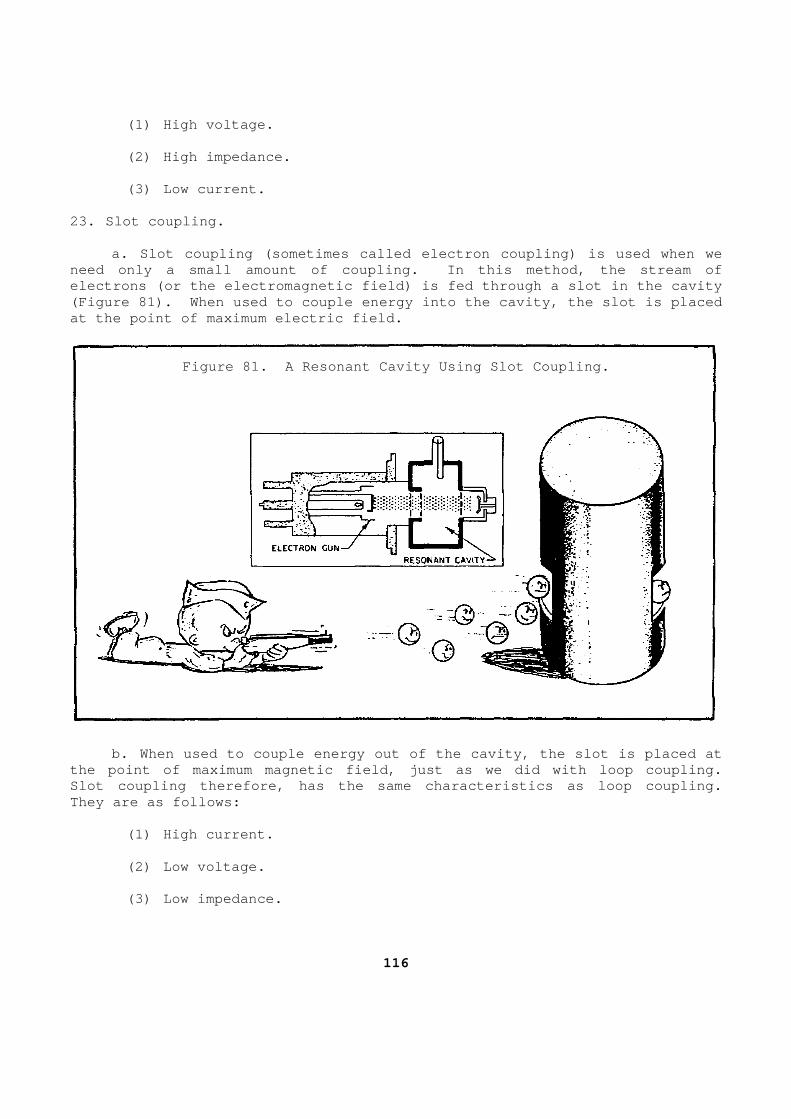
(1) High voltage. (2) High impedance. (3) Low current. 23. Slot coupling. a. Slot coupling (sometimes called electron coupli ng) is used when we need only a small amount of coupling. In this meth od, the stream of electrons (or the electromagnetic field) is fed thr ough a slot in the cavity (Figure 81). When used to couple energy into the c avity, the slot is placed at the point of maximum electric field.

Figure 81. A Resonant Cavity Using Slot Coupling.

b. When used to couple energy out of the cavity, t he slot is placed at the point of maximum magnetic field, just as we did with loop coupling. Slot coupling therefore, has the same characteristi cs as loop coupling. They are as follows: (1) High current. (2) Low voltage. (3) Low impedance.

116

24. Summary of coupling methods. a. The three principle means of coupling energy in to or out of a resonant cavity are called loop coupling, probe cou pling, and slot coupling. b. The loop is placed in the area of maximum magne tic field. c. The probe is placed in the area of maximum elec tric field. d. When coupling energy out of the cavity, the slo t is placed in the area of maximum magnetic field, but when coupling e nergy into the cavity, the slot is placed in the area of maximum electric field. e. So far, you have learned how a resonant cavity works, and why they are used at microwave frequencies. Now, let's look at some practical applications that you will run into as a repairman. 25. A resonant cavity is used in test equipment. a. A resonant cavity is used as a piece of radar t est equipment called an echo box. An echo box consists mainly of a high Q resonant cavity that oscillates when excited by a radar pulse. The ener gy picked up is used to check performance of the radar set. A typical echo box setup is shown in Figure 82.

117

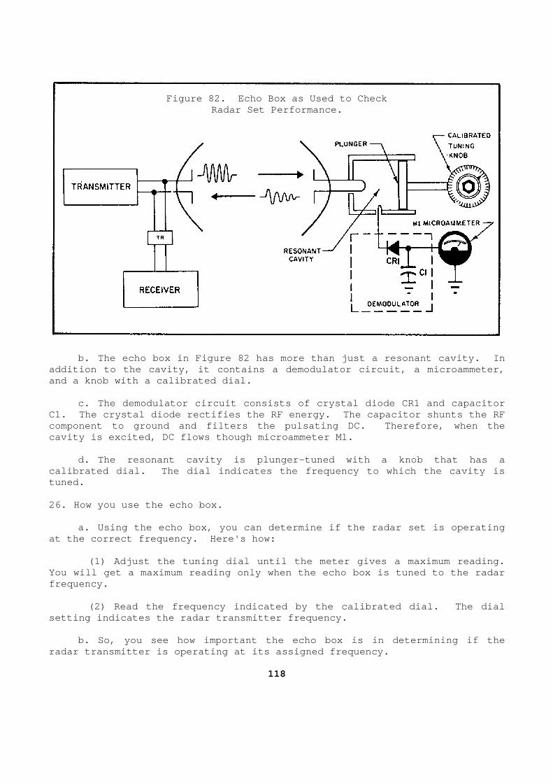
Figure 82. Echo Box as Used to Check

Radar Set Performance. b. The echo box in Figure 82 has more than just a resonant cavity. In addition to the cavity, it contains a demodulator c ircuit, a microammeter, and a knob with a calibrated dial. c. The demodulator circuit consists of crystal dio de CR1 and capacitor C1. The crystal diode rectifies the RF energy. Th e capacitor shunts the RF component to ground and filters the pulsating DC. Therefore, when the cavity is excited, DC flows though microammeter M1. d. The resonant cavity is plunger-tuned with a kno b that has a calibrated dial. The dial indicates the frequency to which the cavity is tuned. 26. How you use the echo box. a. Using the echo box, you can determine if the ra dar set is operating at the correct frequency. Here's how: (1) Adjust the tuning dial until the meter gives a maximum reading. You will get a maximum reading only when the echo b ox is tuned to the radar frequency. (2) Read the frequency indicated by the calibrated dial. The dial setting indicates the radar transmitter frequency. b. So, you see how important the echo box is in de termining if the radar transmitter is operating at its assigned freq uency.

118

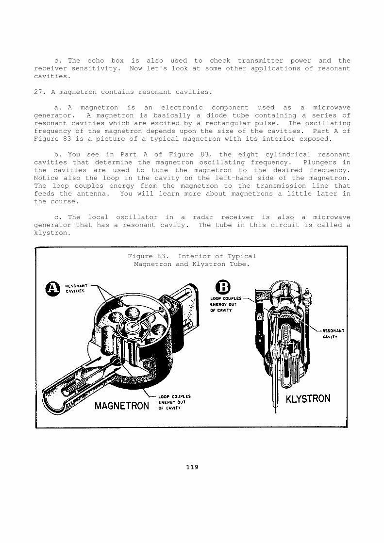
c. The echo box is also used to check transmitter power and the receiver sensitivity. Now let's look at some other applications of resonant cavities. 27. A magnetron contains resonant cavities. a. A magnetron is an electronic component used as a microwave generator. A magnetron is basically a diode tube c ontaining a series of resonant cavities which are excited by a rectangula r pulse. The oscillating frequency of the magnetron depends upon the size of the cavities. Part A of Figure 83 is a picture of a typical magnetron with its interior exposed. b. You see in Part A of Figure 83, the eight cylin drical resonant cavities that determine the magnetron oscillating f requency. Plungers in the cavities are used to tune the magnetron to the desired frequency. Notice also the loop in the cavity on the left-hand side of the magnetron. The loop couples energy from the magnetron to the t ransmission line that feeds the antenna. You will learn more about magne trons a little later in the course. c. The local oscillator in a radar receiver is als o a microwave generator that has a resonant cavity. The tube in this circuit is called a klystron.

Figure 83. Interior of Typical

Magnetron and Klystron Tube.

119

28. Klystrons have resonant cavities. Klystrons are similar to magnetrons in that they also use resonant cavities to produce microwave oscillations. Part B of Figure 83 shows the cavity of a typical klystron tube. One wall of the cavity is a diaphragm. You adjust the diaphragm to tune the cavity to the desired oscillator frequency. Notice the loop in the klystron cavity. Like the magnetron, the klystron uses loop coupling. You will learn more a bout klystron later on. 29. Final summary. You have learned in this lesson sheet why we use resonant cavities and some of their uses. The most important points to remember about resonant cavities are as follows: (1) A resonant cavity is used as a tuned circuit a t microwave frequencies. (2) A resonant cavity consists of a hollow chamber with conducting walls. (3) Resonant cavities have very low resistance and therefore have a very high Q. (4) Resonant cavities are made in various shapes, such as square, rectangular, toroidal (doughnut shaped), and cylind rical. (5) The energy in a resonant cavity is contained i n its electric (E) and magnetic (H) fields. (6) The combination of E and H fields is called th e electromagnetic field. (7) Four principle methods of tuning a resonant ca vity are with a plunger, a diaphragm, a screw, or a paddle. (8) Three principle methods of coupling energy to or from a resonant cavity are with a loop, a probe, or a slot. (9) Resonant cavities determine the resonant frequ ency of echo boxes, magnetrons, and klystrons.

120

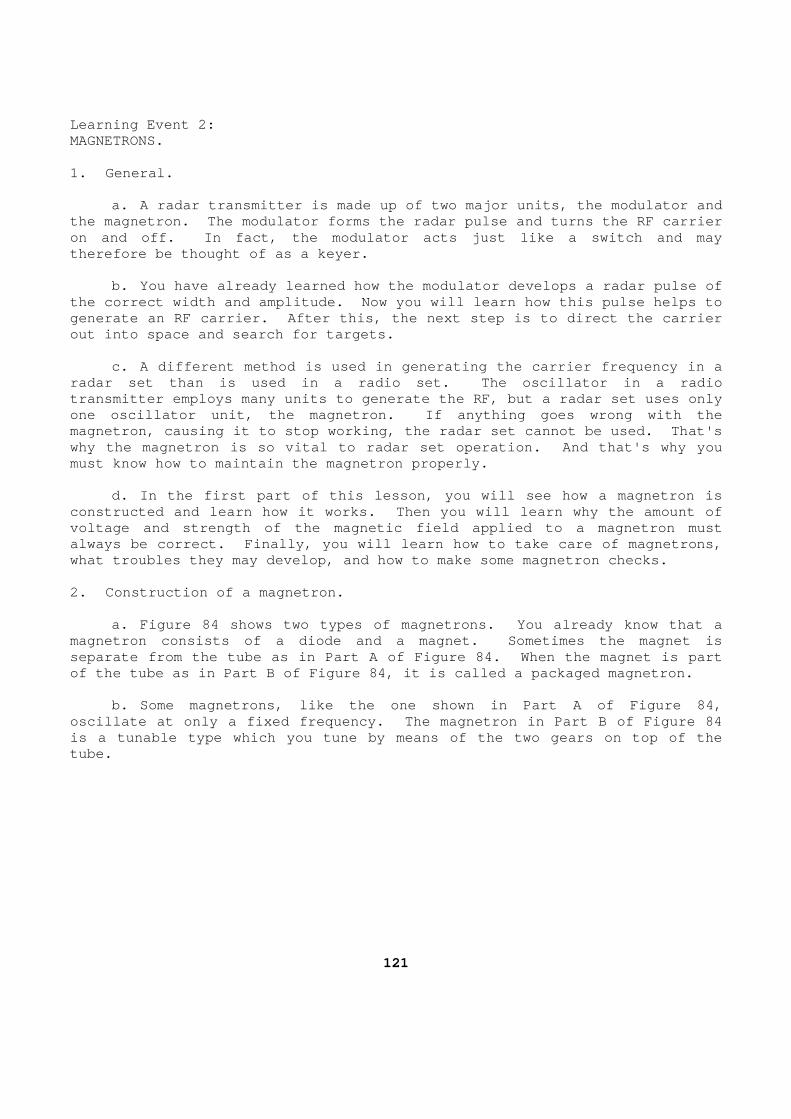
Learning Event 2: MAGNETRONS. 1. General. a. A radar transmitter is made up of two major uni ts, the modulator and the magnetron. The modulator forms the radar pulse and turns the RF carrier on and off. In fact, the modulator acts just like a switch and may therefore be thought of as a keyer. b. You have already learned how the modulator deve lops a radar pulse of the correct width and amplitude. Now you will lear n how this pulse helps to generate an RF carrier. After this, the next step is to direct the carrier out into space and search for targets. c. A different method is used in generating the ca rrier frequency in a radar set than is used in a radio set. The oscilla tor in a radio transmitter employs many units to generate the RF, but a radar set uses only one oscillator unit, the magnetron. If anything go es wrong with the magnetron, causing it to stop working, the radar se t cannot be used. That's why the magnetron is so vital to radar set operatio n. And that's why you must know how to maintain the magnetron properly. d. In the first part of this lesson, you will see how a magnetron is constructed and learn how it works. Then you will learn why the amount of voltage and strength of the magnetic field applied to a magnetron must always be correct. Finally, you will learn how to take care of magnetrons, what troubles they may develop, and how to make som e magnetron checks. 2. Construction of a magnetron. a. Figure 84 shows two types of magnetrons. You a lready know that a magnetron consists of a diode and a magnet. Someti mes the magnet is separate from the tube as in Part A of Figure 84. When the magnet is part of the tube as in Part B of Figure 84, it is called a packaged magnetron. b. Some magnetrons, like the one shown in Part A o f Figure 84, oscillate at only a fixed frequency. The magnetron in Part B of Figure 84 is a tunable type which you tune by means of the tw o gears on top of the tube.

121

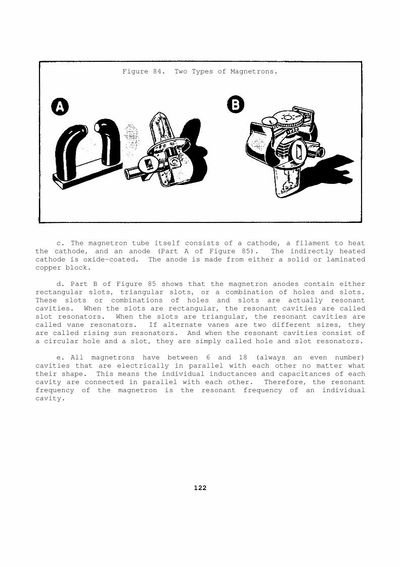
Figure 84. Two Types of Magnetrons.

c. The magnetron tube itself consists of a cathode , a filament to heat the cathode, and an anode (Part A of Figure 85). T he indirectly heated cathode is oxide-coated. The anode is made from ei ther a solid or laminated copper block. d. Part B of Figure 85 shows that the magnetron an odes contain either rectangular slots, triangular slots, or a combinati on of holes and slots. These slots or combinations of holes and slots are actually resonant cavities. When the slots are rectangular, the reso nant cavities are called slot resonators. When the slots are triangular, th e resonant cavities are called vane resonators. If alternate vanes are two different sizes, they are called rising sun resonators. And when the res onant cavities consist of a circular hole and a slot, they are simply called hole and slot resonators. e. All magnetrons have between 6 and 18 (always an even number) cavities that are electrically in parallel with eac h other no matter what their shape. This means the individual inductances and capacitances of each cavity are connected in parallel with each other. Therefore, the resonant frequency of the magnetron is the resonant frequenc y of an individual cavity.

122

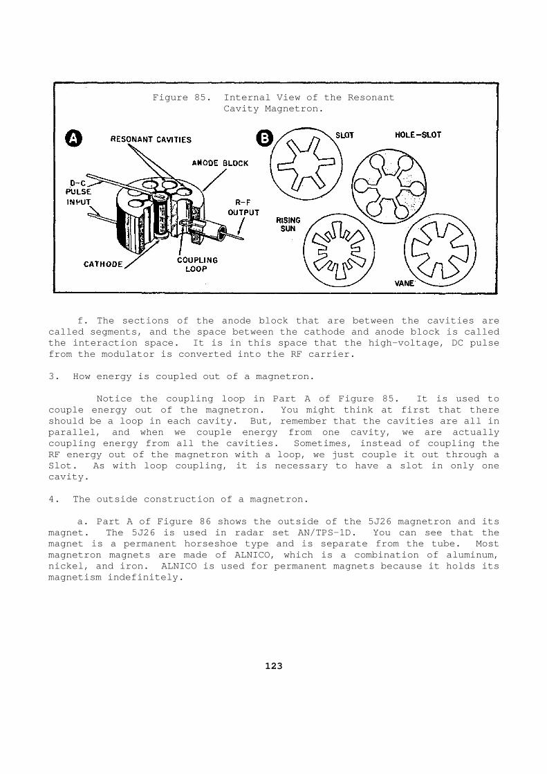
Figure 85. Internal View of the Resonant

Cavity Magnetron. f. The sections of the anode block that are betwee n the cavities are called segments, and the space between the cathode and anode block is called the interaction space. It is in this space that th e high-voltage, DC pulse from the modulator is converted into the RF carrier . 3. How energy is coupled out of a magnetron. Notice the coupling loop in Part A of Figure 85. It is used to couple energy out of the magnetron. You might thin k at first that there should be a loop in each cavity. But, remember tha t the cavities are all in parallel, and when we couple energy from one cavity , we are actually coupling energy from all the cavities. Sometimes, instead of coupling the RF energy out of the magnetron with a loop, we just couple it out through a Slot. As with loop coupling, it is necessary to ha ve a slot in only one cavity. 4. The outside construction of a magnetron. a. Part A of Figure 86 shows the outside of the 5J 26 magnetron and its magnet. The 5J26 is used in radar set AN/TPS-1D. You can see that the magnet is a permanent horseshoe type and is separat e from the tube. Most magnetron magnets are made of ALNICO, which is a co mbination of aluminum, nickel, and iron. ALNICO is used for permanent mag nets because it holds its magnetism indefinitely.

123

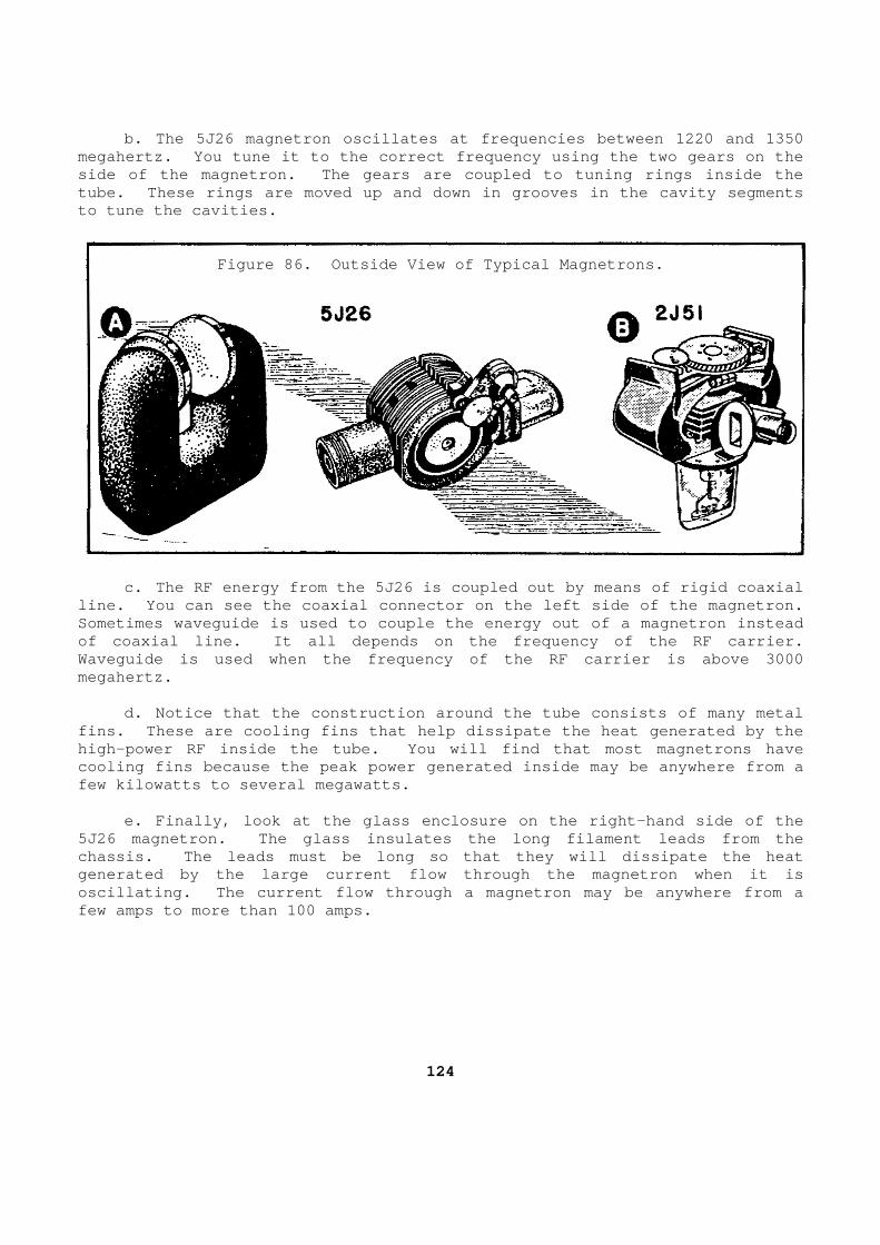
b. The 5J26 magnetron oscillates at frequencies be tween 1220 and 1350 megahertz. You tune it to the correct frequency us ing the two gears on the side of the magnetron. The gears are coupled to tu ning rings inside the tube. These rings are moved up and down in grooves in the cavity segments to tune the cavities.

Figure 86. Outside View of Typical Magnetrons.

c. The RF energy from the 5J26 is coupled out by m eans of rigid coaxial line. You can see the coaxial connector on the lef t side of the magnetron. Sometimes waveguide is used to couple the energy ou t of a magnetron instead of coaxial line. It all depends on the frequency o f the RF carrier. Waveguide is used when the frequency of the RF carr ier is above 3000 megahertz. d. Notice that the construction around the tube co nsists of many metal fins. These are cooling fins that help dissipate t he heat generated by the high-power RF inside the tube. You will find that most magnetrons have cooling fins because the peak power generated insid e may be anywhere from a few kilowatts to several megawatts. e. Finally, look at the glass enclosure on the rig ht-hand side of the 5J26 magnetron. The glass insulates the long filam ent leads from the chassis. The leads must be long so that they will dissipate the heat generated by the large current flow through the mag netron when it is oscillating. The current flow through a magnetron may be anywhere from a few amps to more than 100 amps.

124

f. Now, look at the 2J51 magnetron shown in Part B of Figure 86. You can see that the magnet for the 2J51 is part of the magnetron proper. So the 2J51 is called a packaged magnetron. Packaged magnetrons have an advantage over those having separate magnets in tha t they use a smaller magnet for a given field strength. There is no air gap between the pole pieces, so the magnetic lines of force are more con centrated. g. Another difference you will notice is that the 2J51 magnetron uses waveguide instead of rigid coaxial line to couple o ut the RF energy. The reason is that the 2J51 oscillates at frequencies b etween 8500 and 9600 megahertz. 5. Brief review on magnetron construction. a. A magnetron is a microwave oscillator that cons ists of a diode and a magnet. b. The magnet is either part of the magnetron prop er (packaged magnetron) or is separate. c. The diode section of the magnetron consists of a cathode, a filament to heat the cathode, and an anode. d. The cathode is oxide-coated and is indirectly h eated by the filament. e. The anode is a circular copper block containing six to eighteen resonant cavities. f. Magnetrons use loop coupling or slot coupling. g. RF energy is coupled out of the magnetron by co axial line or waveguide. h. The long filament leads of the magnetron are in sulated from the chassis by a glass enclosure. i. Now that you have seen typical magnetrons, let' s find out how they work. You are already familiar with other types of oscillators, so we will start by comparing these other types with magnetron s. This way you will get a better idea of magnetron operation. 6. Comparing magnetrons with other oscillators. A magnetron is like any oscillator in that it gen erates an alternating current at some particular frequency. Magnetrons differ from other oscillators in that their output

125

frequency (and usually their peak power) is very hi gh. A magnetron oscillator is actually a tube within a magnet. Eve n though magnetrons differ physically from other types of oscillators, they have the same basic requirements of a tuned circuit, tuned circuit exci tation, and regeneration. 7. All oscillators must have a tuned circuit. All oscillators have a tuned or resonant circuit that determines the oscillating frequency. In most applications at fre quencies below 500 megahertz, the tuned circuit is a coil and capacito r combination. At frequencies between 500 megahertz and 1000 megahert z, the tuned circuit is usually a section of transmission line. At frequen cies above 1000 megahertz the tuned circuit used most often is a resonant cav ity. Most magnetrons oscillate at frequencies above 1000 megahertz, and therefore they use resonant cavities as tuned circuits. 8. All oscillator tuned circuits must be excited. You know that an oscillator tuned circuit must be excited. That is, it must have some energy applied to it to start osc illations. For example, the coil and capacitor tuned circuit used with an o rdinary vacuum tube oscillator is excited by a surge of current. A tun ed circuit made of a section of transmission line is usually excited the same way. The resonant cavities of a magnetron oscillator, however, are ex cited by the fields built up by current flowing in their walls. You have alr eady seen in a previous lesson how a resonant cavity is shock-excited by an electromagnetic field. Well, magnetron cavities are excited in a similar m anner. 9. All oscillators need regeneration. a. One more requirement of an oscillator is regene ration. This means simply that we must reinforce the energy generated, or it will die out. Ordinary vacuum tube oscillators use positive feedb ack in which some of the output energy is fed back in phase with the input e nergy. The energy fed back adds to the input and keeps the oscillator wor king. This happens because the energy feedback is greater than the ene rgy being lost. b. A magnetron also needs regeneration to continue oscillating after it has been excited. Energy generated in the resonant cavities is reinforced by energy given off by electrons emitted from the m agnetron cathode. The electrons add their energy in phase with the oscill ating energy. Because the energy added is greater than the energy lost, o scillations don't die out.

126

c. Later in this lesson, you will learn exactly ho w a magnetron meets these three oscillator requirements of a tuned circ uit, tuned circuit excitation, and regeneration. 10. How a magnetron works. You know from examining the construction of a mag netron that it consists of a diode and permanent magnet. If we co mbine the qualities of a permanent magnet with the operation of a diode, you will get a good idea of how a magnetron works. We will start with the oper ation of a diode, next the magnet, and then put the two together. 11. Electron flow in diode tube. a. You know that a diode tube has two main element s: the cathode and the anode (plate). The cathode is coated with a ch emical substance such as thorium oxide, which emits electrons when heated. Electrons flow from the hot cathode to the anode only when the anode is at positive potential with respect to the cathode. The circuit action for ord inary diodes and magnetron diodes is the same, but the circuit arran gement is slightly different. The two arrangements are compared below . (1) In ordinary diode tube circuits, the cathode i s connected to negative voltage and is grounded. The anode is the n connected to the positive terminal of the same DC source. (2) In magnetron diode circuits, the cathode is st ill connected to negative voltage and the plate to positive voltage, but the plate is grounded instead of the cathode. b. The diode circuit action, of course, is still e xactly the same. Electrons flow from the heated cathode to the posit ive plate. Grounding the plate instead of the cathode does not affect the di ode circuit action. c. The magnetron anode actually forms the metal en velope of the tube. So, when the magnetron is bolted to a radar chassis , the anode becomes grounded. Electrons flow when the high voltage DC pulse is applied to the cathode (Figure 87). Grounding the anode this way prevents a shock hazard when the high-voltage pulse is applied to the magne tron.

127

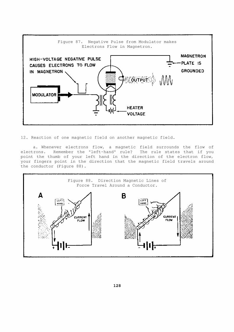
Figure 87. Negative Pulse from Modulator makes

Electrons Flow in Magnetron. 12. Reaction of one magnetic field on another magne tic field. a. Whenever electrons flow, a magnetic field surro unds the flow of electrons. Remember the "left-hand" rule? The rul e states that if you point the thumb of your left hand in the direction of the electron flow, your fingers point in the direction that the magnet ic field travels around the conductor (Figure 88).

Figure 88. Direction Magnetic Lines of

Force Travel Around a Conductor.

128

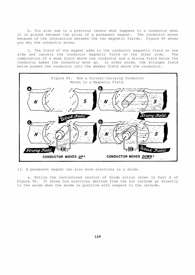
b. You also saw in a previous lesson what happens to a conductor when it is placed between the poles of a permanent magne t. The conductor moves because of the interaction between the two magnetic fields. Figure 89 shows you why the conductor moves. c. The field of the magnet adds to the conductor m agnetic field on one side and cancels the conductor magnetic field on th e other side. The combination of a weak field above the conductor and a strong field below the conductor makes the conductor move up. In other wo rds, the stronger field below pushes the conductor into the weaker field ab ove the conductor.

Figure 89. How a Current-Carrying Conductor

Moves in a Magnetic Field. 13. A permanent magnet can also move electrons in a diode. a. Notice the cartoonized version of diode action shown in Part A of Figure 90. It shows how electrons emitted from the hot cathode go directly to the anode when the anode is positive with respec t to the cathode.

129

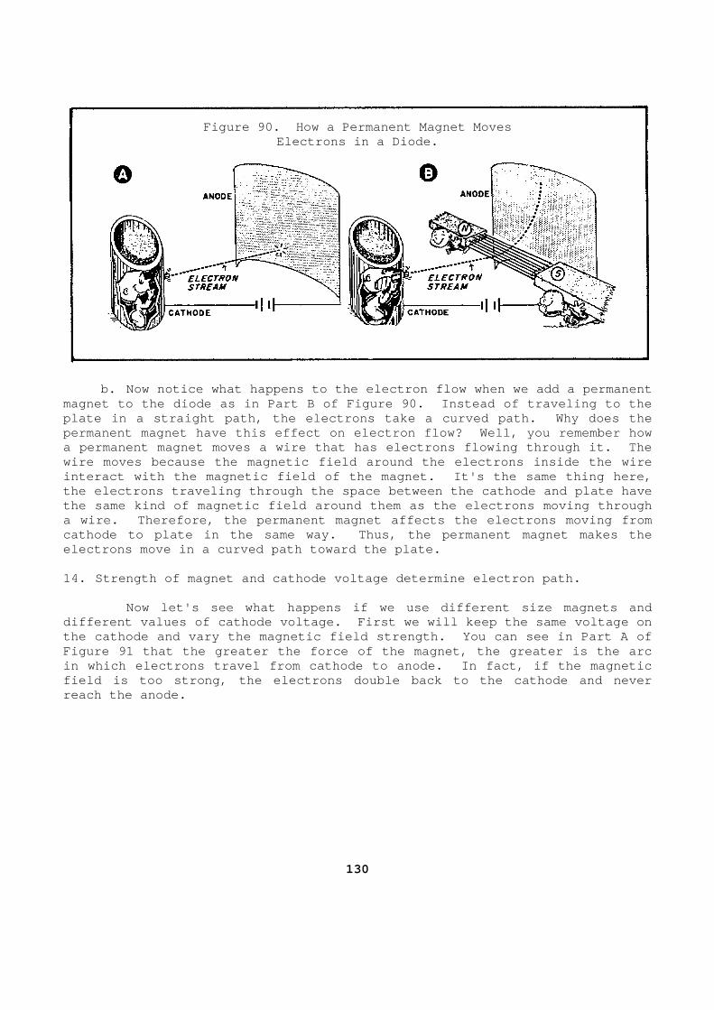
Figure 90. How a Permanent Magnet Moves

Electrons in a Diode. b. Now notice what happens to the electron flow wh en we add a permanent magnet to the diode as in Part B of Figure 90. Ins tead of traveling to the plate in a straight path, the electrons take a curv ed path. Why does the permanent magnet have this effect on electron flow? Well, you remember how a permanent magnet moves a wire that has electrons flowing through it. The wire moves because the magnetic field around the el ectrons inside the wire interact with the magnetic field of the magnet. It 's the same thing here, the electrons traveling through the space between t he cathode and plate have the same kind of magnetic field around them as the electrons moving through a wire. Therefore, the permanent magnet affects th e electrons moving from cathode to plate in the same way. Thus, the perman ent magnet makes the electrons move in a curved path toward the plate. 14. Strength of magnet and cathode voltage determin e electron path. Now let's see what happens if we use different si ze magnets and different values of cathode voltage. First we will keep the same voltage on the cathode and vary the magnetic field strength. You can see in Part A of Figure 91 that the greater the force of the magnet, the greater is the arc in which electrons travel from cathode to anode. I n fact, if the magnetic field is too strong, the electrons double back to t he cathode and never reach the anode.

130

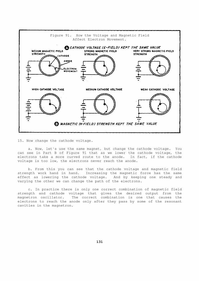
Figure 91. How the Voltage and Magnetic Field

Affect Electron Movement. 15. Now change the cathode voltage. a. Now, let's use the same magnet, but change the cathode voltage. You can see in Part B of Figure 91 that as we lower the cathode voltage, the electrons take a more curved route to the anode. I n fact, if the cathode voltage is too low, the electrons never reach the a node. b. From this you can see that the cathode voltage and magnetic field strength work hand in hand. Increasing the magneti c force has the same effect as lowering the cathode voltage. And by kee ping one steady and varying the other we can change the path of the ele ctrons. c. In practice there is only one correct combinati on of magnetic field strength and cathode voltage that gives the desired output from the magnetron oscillator. The correct combination is o ne that causes the electrons to reach the anode only after they pass b y some of the resonant cavities in the magnetron.

131

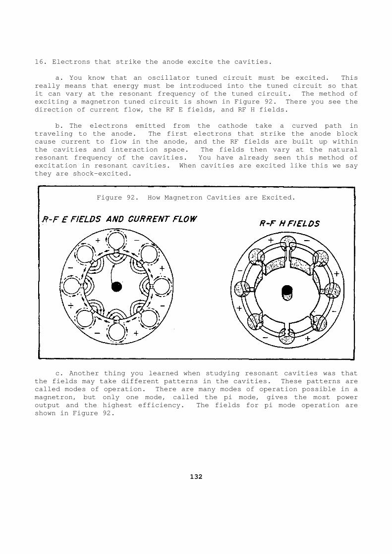
16. Electrons that strike the anode excite the cavi ties. a. You know that an oscillator tuned circuit must be excited. This really means that energy must be introduced into th e tuned circuit so that it can vary at the resonant frequency of the tuned circuit. The method of exciting a magnetron tuned circuit is shown in Figu re 92. There you see the direction of current flow, the RF E fields, and RF H fields. b. The electrons emitted from the cathode take a c urved path in traveling to the anode. The first electrons that s trike the anode block cause current to flow in the anode, and the RF fiel ds are built up within the cavities and interaction space. The fields the n vary at the natural resonant frequency of the cavities. You have alrea dy seen this method of excitation in resonant cavities. When cavities are excited like this we say they are shock-excited.

Figure 92. How Magnetron Cavities are Excited.

c. Another thing you learned when studying resonan t cavities was that the fields may take different patterns in the cavit ies. These patterns are called modes of operation. There are many modes of operation possible in a magnetron, but only one mode, called the pi mode, g ives the most power output and the highest efficiency. The fields for pi mode operation are shown in Figure 92.

132

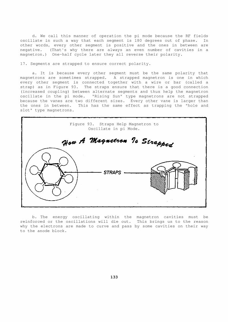
d. We call this manner of operation the pi mode be cause the RF fields oscillate in such a way that each segment is 180 de grees out of phase. In other words, every other segment is positive and th e ones in between are negative. (That's why there are always an even num ber of cavities in a magnetron.) One-half cycle later they all reverse their polarity. 17. Segments are strapped to ensure correct polarit y. a. It is because every other segment must be the s ame polarity that magnetrons are sometimes strapped. A strapped magn etron is one in which every other segment is connected together with a wi re or bar (called a strap) as in Figure 93. The straps ensure that the re is a good connection (increased coupling) between alternate segments and thus help the magnetron oscillate in the pi mode. "Rising Sun" type magnet rons are not strapped because the vanes are two different sizes. Every o ther vane is larger than the ones in between. This has the same effect as t rapping the "hole and slot" type magnetrons.

Figure 93. Straps Help Magnetron to

Oscillate in pi Mode. b. The energy oscillating within the magnetron cav ities must be reinforced or the oscillations will die out. This brings us to the reason why the electrons are made to curve and pass by som e cavities on their way to the anode block.

133

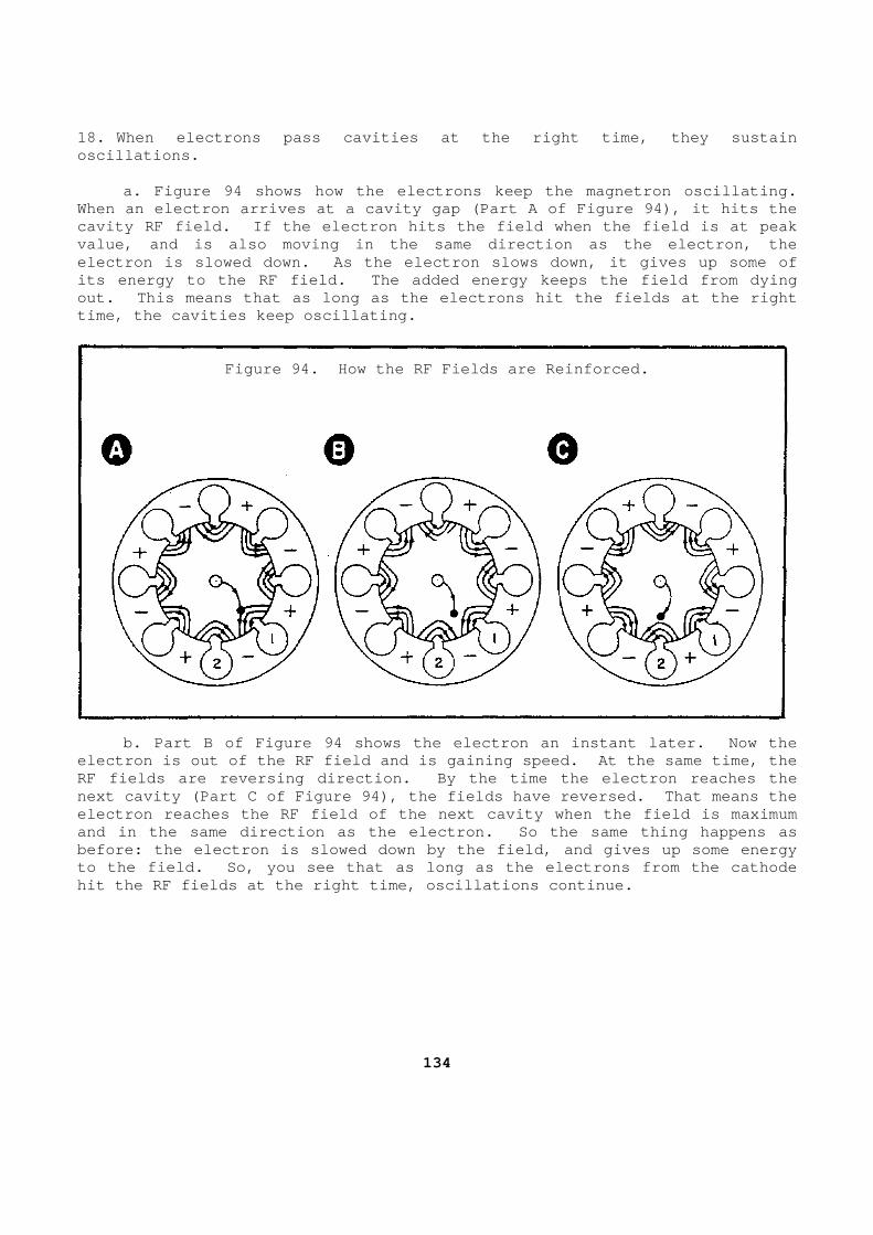
18. When electrons pass cavities at the right time, they sustain oscillations. a. Figure 94 shows how the electrons keep the magn etron oscillating. When an electron arrives at a cavity gap (Part A of Figure 94), it hits the cavity RF field. If the electron hits the field wh en the field is at peak value, and is also moving in the same direction as the electron, the electron is slowed down. As the electron slows dow n, it gives up some of its energy to the RF field. The added energy keeps the field from dying out. This means that as long as the electrons hit the fields at the right time, the cavities keep oscillating.

Figure 94. How the RF Fields are Reinforced.

b. Part B of Figure 94 shows the electron an insta nt later. Now the electron is out of the RF field and is gaining spee d. At the same time, the RF fields are reversing direction. By the time the electron reaches the next cavity (Part C of Figure 94), the fields have reversed. That means the electron reaches the RF field of the next cavity wh en the field is maximum and in the same direction as the electron. So the same thing happens as before: the electron is slowed down by the field, a nd gives up some energy to the field. So, you see that as long as the elec trons from the cathode hit the RF fields at the right time, oscillations c ontinue.

134

19. Finally, the electrons reach the anode. The electrons reach the anode only after they hav e taken a spiral path and given up some energy to the oscillating RF fields. Some electrons never reach the anode, but instead they return to t he cathode. Electrons that return to the cathode are lost. But when they hit the cathode, they cause it to get hotter. Most magnetrons therefore either have their filament voltage turned off or turned down after th ey have started oscillating If the filament voltage were kept at the full starting value, the combination of filament voltage heat and the he at from the returned electrons would damage the tube. 20. Summarizing electron movement. a. Electrons strike the anode block and shock exci te the resonant cavities. b. The RF fields in the cavities oscillate in such a way that alternate anode segments are of the same polarity and 180 deg rees out of phase with their neighboring cavities. c. Then the electrons pass the RF fields in phase and add their energy to the fields. d. The fields keep oscillating until the voltage a pplied to the cathode is removed and the electrons stop flowing. e. These four steps briefly state the operation of the magnetron. The most critical part of the operation is getting the electrons to pass the RI fields at the right time to keep the magnetron osci llating. 21. Cathode voltage and magnetic field make electro ns pass at the right time. a. You have already seen how the voltage across th e diode and the magnetic field of the magnet affect the electrons. The correct values of voltage and magnetic force make the electrons trave l in the right path. That path is the one where the electrons pass the R F fields so as to add their energy to them. If they don't add their ener gy in the right way, the magnetron will not oscillate at all, or it will ope rate erratically. This means then if the voltage or magnetic field change from the correct values, one of the following trouble symptoms will occur: (1) The magnetron will not oscillate at all. (2) The magnetron will oscillate at the wrong freq uency.

135

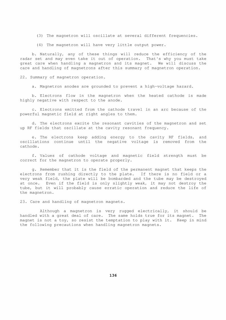
(3) The magnetron will oscillate at several differ ent frequencies. (4) The magnetron will have very little output pow er. b. Naturally, any of these things will reduce the efficiency of the radar set and may even take it out of operation. T hat's why you must take great care when handling a magnetron and its magnet . We will discuss the care and handling of magnetrons after this summary of magnetron operation. 22. Summary of magnetron operation. a. Magnetron anodes are grounded to prevent a high -voltage hazard. b. Electrons flow in the magnetron when the heated cathode is made highly negative with respect to the anode. c. Electrons emitted from the cathode travel in an arc because of the powerful magnetic field at right angles to them. d. The electrons excite the resonant cavities of t he magnetron and set up RF fields that oscillate at the cavity resonant frequency. e. The electrons keep adding energy to the cavity RF fields, and oscillations continue until the negative voltage is removed from the cathode. f. Values of cathode voltage and magnetic field st rength must be correct for the magnetron to operate properly. g. Remember that it is the field of the permanent magnet that keeps the electrons from rushing directly to the plate. If t here is no field or a very weak field, the plate will be bombarded and th e tube may be destroyed at once. Even if the field is only slightly weak, it may not destroy the tube, but it will probably cause erratic operation and reduce the life of the magnetron. 23. Care and handling of magnetron magnets. Although a magnetron is very rugged electrically, it should be handled with a great deal of care. The same holds true for its magnet. The magnet is not a toy, so resist the temptation to pl ay with it. Keep in mind the following precautions when handling magnetron m agnets.

136

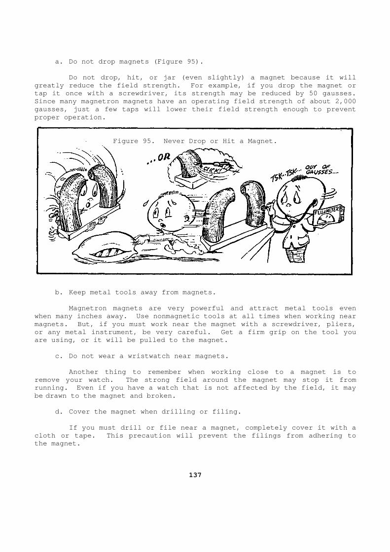
a. Do not drop magnets (Figure 95). Do not drop, hit, or jar (even slightly) a magnet because it will greatly reduce the field strength. For example, if you drop the magnet or tap it once with a screwdriver, its strength may be reduced by 50 gausses. Since many magnetron magnets have an operating fiel d strength of about 2,000 gausses, just a few taps will lower their field str ength enough to prevent proper operation.

Figure 95. Never Drop or Hit a Magnet.

b. Keep metal tools away from magnets. Magnetron magnets are very powerful and attract m etal tools even when many inches away. Use nonmagnetic tools at al l times when working near magnets. But, if you must work near the magnet wit h a screwdriver, pliers, or any metal instrument, be very careful. Get a fi rm grip on the tool you are using, or it will be pulled to the magnet. c. Do not wear a wristwatch near magnets. Another thing to remember when working close to a magnet is to remove your watch. The strong field around the mag net may stop it from running. Even if you have a watch that is not affe cted by the field, it may be drawn to the magnet and broken. d. Cover the magnet when drilling or filing. If you must drill or file near a magnet, complete ly cover it with a cloth or tape. This precaution will prevent the fi lings from adhering to the magnet.

137

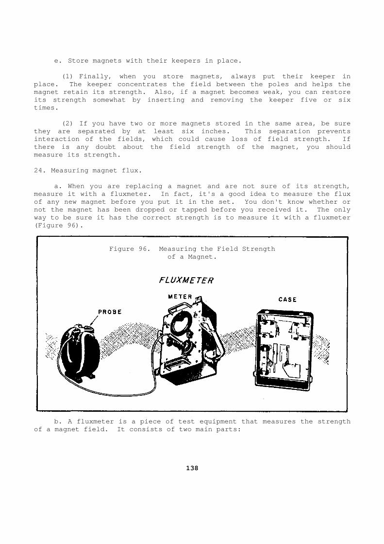
e. Store magnets with their keepers in place. (1) Finally, when you store magnets, always put th eir keeper in place. The keeper concentrates the field between t he poles and helps the magnet retain its strength. Also, if a magnet beco mes weak, you can restore its strength somewhat by inserting and removing the keeper five or six times. (2) If you have two or more magnets stored in the same area, be sure they are separated by at least six inches. This se paration prevents interaction of the fields, which could cause loss o f field strength. If there is any doubt about the field strength of the magnet, you should measure its strength. 24. Measuring magnet flux. a. When you are replacing a magnet and are not sur e of its strength, measure it with a fluxmeter. In fact, it's a good idea to measure the flux of any new magnet before you put it in the set. Yo u don't know whether or not the magnet has been dropped or tapped before yo u received it. The only way to be sure it has the correct strength is to me asure it with a fluxmeter (Figure 96).

Figure 96. Measuring the Field Strength

of a Magnet. b. A fluxmeter is a piece of test equipment that m easures the strength of a magnet field. It consists of two main parts:

138

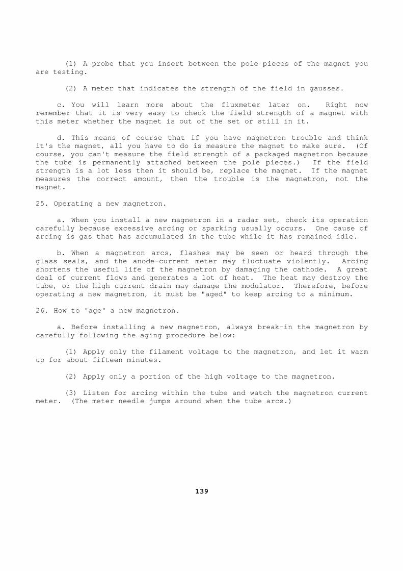
(1) A probe that you insert between the pole piece s of the magnet you are testing. (2) A meter that indicates the strength of the fie ld in gausses. c. You will learn more about the fluxmeter later o n. Right now remember that it is very easy to check the field st rength of a magnet with this meter whether the magnet is out of the set or still in it. d. This means of course that if you have magnetron trouble and think it's the magnet, all you have to do is measure the magnet to make sure. (Of course, you can't measure the field strength of a p ackaged magnetron because the tube is permanently attached between the pole p ieces.) If the field strength is a lot less then it should be, replace t he magnet. If the magnet measures the correct amount, then the trouble is th e magnetron, not the magnet. 25. Operating a new magnetron. a. When you install a new magnetron in a radar set , check its operation carefully because excessive arcing or sparking usua lly occurs. One cause of arcing is gas that has accumulated in the tube whil e it has remained idle. b. When a magnetron arcs, flashes may be seen or h eard through the glass seals, and the anode-current meter may fluctu ate violently. Arcing shortens the useful life of the magnetron by damagi ng the cathode. A great deal of current flows and generates a lot of heat. The heat may destroy the tube, or the high current drain may damage the modu lator. Therefore, before operating a new magnetron, it must be "aged" to kee p arcing to a minimum. 26. How to "age" a new magnetron. a. Before installing a new magnetron, always break -in the magnetron by carefully following the aging procedure below: (1) Apply only the filament voltage to the magnetr on, and let it warm up for about fifteen minutes. (2) Apply only a portion of the high voltage to th e magnetron. (3) Listen for arcing within the tube and watch th e magnetron current meter. (The meter needle jumps around when the tub e arcs.)

139

(4) Gradually increase the high voltage. (5) If arcing occurs, turn down the high voltage. (6) Wait a minute, and start turning the high volt age up again. (7) Continue this routine until arcing stops. b. Note that these steps provide only a general ou tline for aging a magnetron and should be used only when no instructi ons for the set are available. You should always follow instructions g iven in the TM for the particular set you're working with. c. It may take an hour or more before all arcing h as stopped and the magnetron has been "cleaned up" (free of gas). For tunately a magnetron can stand a considerable amount of arcing without any d amage, but you should hold it to a minimum. Remember that you hold the h igh-voltage down to keep the arcing down. d. Magnetron arcing is normal for new tubes and ol d tubes that need replacement. There are other more serious magnetro n troubles that you will run into. Let's see now what these other troubles are and find out what causes them. 27. Troubleshooting the magnetron. a. Before troubleshooting, you must know how the e quipment operates so you can recognize and analyze trouble symptoms as s oon as they occur. After recognizing the trouble symptom, the next step is s ectionalization. You sectionalize the trouble by first analyzing and eva luating the symptom. You will find that troubles causing faulty magnetron op eration usually occur in the RF and modulator sections of the radar set. b. When the cause for the magnetron operating at t he wrong frequency is in the RF section, we call the trouble magnetron pu lling. In other words, the magnetron is actually pulled off its correct os cillating frequency by some bad or mistuned component located somewhere be tween the magnetron and the antenna or even beyond the antenna. c. When the cause for faulty magnetron operation i s in a unit located ahead of the magnetron (the modulator), we call the trouble magnetron pushing. In other words, the magnetron is actually pushed off its correct oscillating frequency by some bad or mistuned compo nent located somewhere in or before the modulator.

140

d. Although magnetron pulling is more common than magnetron pushing, either trouble is likely to occur because magnetron operating requirements are so critical. 28. Magnetron pulling. a. The trouble is called magnetron pulling when th e frequency of the magnetron is changed (pulled off frequency) by a mi smatch somewhere past the magnetron. That is, the mismatch is either between the magnetron and the antenna, or it's caused by something beyond the ant enna. You will recall from a previous lesson, Transmission Lines, that a load must be matched to its generator circuit in order to get maximum power out. This is true also of magnetron loads. The load on a magnetron, of co urse, consists of all the RF components that follow it, including the antenna . Magnetrons also pull off frequency when the load is changed or mismatche d. The amount of frequency change and loss of power depends upon how great is the mismatch. b. Sometimes the mismatch is slight, and the frequ ency changes only slightly, and the power output remains almost the s ame. The radar receiver still picks up signals near the desired operating f requency because of its wide frequency response. But if the mismatch is mo re than just slight, the frequency will change more, and there will be even less power output. So even if the receiver still picks up echoes, the ech oes are weak. In an extreme case, the frequency change may be so great that the receiver will not respond at all to the echoes. c. You can see then, that anything that changes th e magnetron output impedance and causes a mismatch may be very harmful , and may even prevent the radar from functioning. 29. Causes of impedance mismatch between magnetron and antenna. a. The most common causes of mismatch between the magnetron and the antenna are as follows: (1) Dirt or moisture in the coaxial line or wavegu ide. (2) Dirt or moisture on the antenna. (3) Coaxial line or waveguide that is bent or dent ed. (4) Joints that are not soldered properly. (5) A defective rotating or coupling joint.

141

b. Most of these causes of magnetron pulling can b e avoided by proper care and preventive maintenance of the radar RF com ponents. 30. Causes of faulty operation beyond the antenna. a. Now, how about the causes of faulty magnetron o peration from something beyond the antenna? At first you might t hink that all troubles would have to be caused by something actually in th e set. That's usually true, but in the case of a radar transmitter, troub les can be caused by something that is not a physical part of the equipm ent. This happens because anything that changes the impedance of the load also effects the magnetron operation. b. The usual cause of mismatch from something beyo nd the antenna is a nearby object. The nearby object may be a building , another radar, a smokestack or anything else close enough to the ant enna to change its impedance. These types of mismatch can be avoided by selecting a good site for the radar set. c. Now, suppose there is no mismatch. The load im pedance remains constant at its correct value, but the magnetron is not operating correctly. Then, the trouble is probably magnetron pushing. 31. Magnetron pushing. a. As stated before, magnetron pushing occurs when the frequency of the magnetron is changed (pushed off frequency) by some thing before the magnetron. In other words, the trouble is somethin g that changes the current of the magnetron even though the load and m agnetic field are at the correct values. b. The most likely spot to look for the cause of t his trouble is in the modulator. Actually most magnetron pushing is caus ed by an improperly shaped pulse coming from the modulator. When the p ulse is not the right shape, the magnetron may oscillate in an undesired mode and at the wrong frequency. As with magnetron pulling, the output p ower drops and the frequency may change enough to make the receiver us eless.

142

32. Other magnetron troubles. a. Mode skip. Sometimes a magnetron does not fire (oscillate) every time the pulse is applied to the cathode. This hap pens when the pulse applied from the modulator isn't powerful enough. Of course when the magnetron doesn't fire, there is no output from the set, so the set receives fewer echoes. This means the set's average power o utput is reduced, and so is its effectiveness. When the magnetron fails to fire on each pulse, we call the trouble mode skip. b. Mode jump. If each pulse applied to the magnet ron isn't the same shape and amplitude, the magnetron may oscillate in different modes with different frequencies. This defect is called mode jump. c. Mode shift. Sometimes the magnetron may even c hange its mode of operation during a pulse, and we call this trouble mode shift. d. Mode jump and mode skip both result in less pow er being radiated from the radar set and poor efficiency. e. When a magnetron is not operating properly, it is not always easy to determine the exact trouble. However, it is easy t o determine if the output of the magnetron is correct by using a piece of tes t equipment called a spectrum analyzer. 33. Spectrum analysis. a. A radar modulator generates a rectangular pulse that modulates the RF carrier. The rectangular pulse is made up of th e fundamental frequency and many harmonics. Each harmonic modulates the ca rrier frequency producing a sum and difference frequency. These frequencies are called sidebands. Frequencies above the carrier make up the upper sid ebands, frequencies below the carrier make up the lower sidebands. Now, if w e plot the power of each frequency, we have a spectrum. b. A spectrum analyzer contains an oscilloscope th at shows the magnetron spectrum when the analyzer is connected t o the output of a radar transmitter. By checking the spectrum you tell whe ther or not the magnetron is operating correctly. When the magnetron is oper ating as it should, and the output of the transmitter is correct, the graph you see on the spectrum analyzer scope looks like the one in Part A of Figu re 94. So, if the output of the transmitter looks just like the one shown in Part A or is very similar to it, you know that the magnetron is opera ting correctly.

143

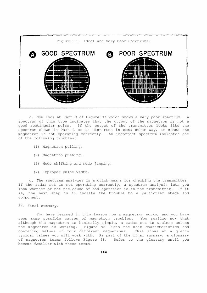
Figure 97. Ideal and Very Poor Spectrums.

c. Now look at Part B of Figure 97 which shows a v ery poor spectrum. A spectrum of this type indicates that the output of the magnetron is not a good rectangular pulse. If the output of the trans mitter looks like the spectrum shown in Part B or is distorted in some ot her way, it means the magnetron is not operating correctly. An incorrect spectrum indicates one of the following troubles: (1) Magnetron pulling. (2) Magnetron pushing. (3) Mode shifting and mode jumping. (4) Improper pulse width. d. The spectrum analyzer is a quick means for chec king the transmitter. If the radar set is not operating correctly, a spec trum analysis lets you know whether or not the cause of bad operation is i n the transmitter. If it is, the next step is to isolate the trouble to a pa rticular stage and component. 34. Final summary. You have learned in this lesson how a magnetron w orks, and you have seen some possible causes of magnetron troubles. Y ou realize now that although the magnetron is basically simple, a radar set is useless unless the magnetron is working. Figure 98 lists the main characteristics and operating values of four different magnetrons. Thi s shows at a glance typical values you will work with. As part of the final summary, a glossary of magnetron terms follows Figure 98. Refer to the glossary until you become familiar with these terms.

144

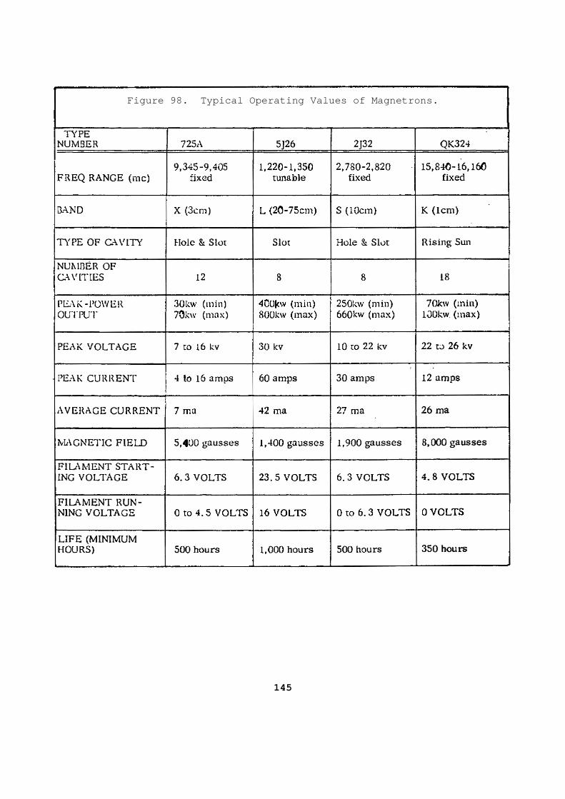
Figure 98. Typical Operating Values of Magnetrons.

145

35. Glossary of magnetron terms. a. Magnetron pulling - The frequency of the magnet ron changes because of a mismatch between the magnetron and the antenna . b. Magnetron pushing - The frequency of the magnet ron changes because of a faulty modulator. c. Mode skip - The magnetron does not fire on ever y pulse. d. Mode jump - The mode of operation changes from one pulse to the next pulse. e. Mode shift - The mode of operation changes duri ng the pulse. f. Packaged magnetron - A magnetron that has its m agnet as part of the magnetron proper. g. Magnetron arcing - Breakdown between the magnet ron cathode and anode caused by gasses. Arcing usually occurs in new tub es and in old tubes that need replacement. h. Magnetron aging - A break-in procedure used to "clean up" gasses in a magnetron. i. Fluxmeter - A meter that measures the flux dens ity of a magnet in terms of gauss. j. Spectrum analyzer - A test instrument used to s how the distribution of energy contained in the output of a pulsed magne tron.

146

PRACTICE EXERCISE (Performance-Oriented)

In each of the following exercises, select the ONE answer that BEST completes the statement or answers the question. I ndicate your solution by circling the letter opposite the correct answer in the subcourse booklet. 1. If a single-shorted quarter-wave section of tran smission line is

compared with two sections connected in parallel, i t is found that the two parallel sections have a

a. larger inductance, a smaller capacitance, and a larger

resistance. b. smaller inductance, a larger capacitance, and a larger

resistance. c. smaller inductance, a larger capacitance, and s maller resistance. d. larger inductance, a smaller capacitance, and s maller resistance. 2. When comparing the characteristics of parallel-c onnected, shorted,

quarter-wave sections of transmission lines to sing le quarter-wave sections, it is found that the cavity formed by the parallel section has

a. a higher resonant frequency and less selectivit y than the single

section. b. A lower resonant frequency and greater selectiv ity than the

single section. c. the same resonant frequency but less selectivit y than the single

section. d. the same resonant frequency but greater selecti vity than the

single section.

147

3. A resonant cavity that will operate in the PRIMA RY mode on a wavelength of 3 centimeters will have length, width , and height respectively of

a. L = 3 cm, W = 3 cm, H = 6 cm. b. L = 6 cm, W = 6 cm, H = 3 cm. c. L = 1.5 cm, W = 1.5 cm, H = 1.3 cm. d. L = .75 cm, W = .75 cm, H = 3.5 cm. 4. The electric and magnetic fields inside a resona nt cavity are always a. parallel to each other. b. perpendicular to each other. c. parallel to the coupling probes. d. perpendicular to the coupling probes. 5. The resonant cavity shown in Figure 99 uses slot coupling or electron

coupling to insert energy into the cavity. The ele ctric field developed in the cavity will be at its maximum stre ngth

a. at the center of the cavity, and the magnetic f ield will be at

its maximum strength on the edges of the cavity. b. at the center of the cavity, and the magnetic f ield will be at

its minimum strength on the edges of the cavity. c. on the edges of the cavity, and the magnetic fi eld will be at its

maximum strength in the center of the cavity. d. on the edges of the cavity, and the magnetic fi eld will be at its

minimum strength in the center of the cavity.

148

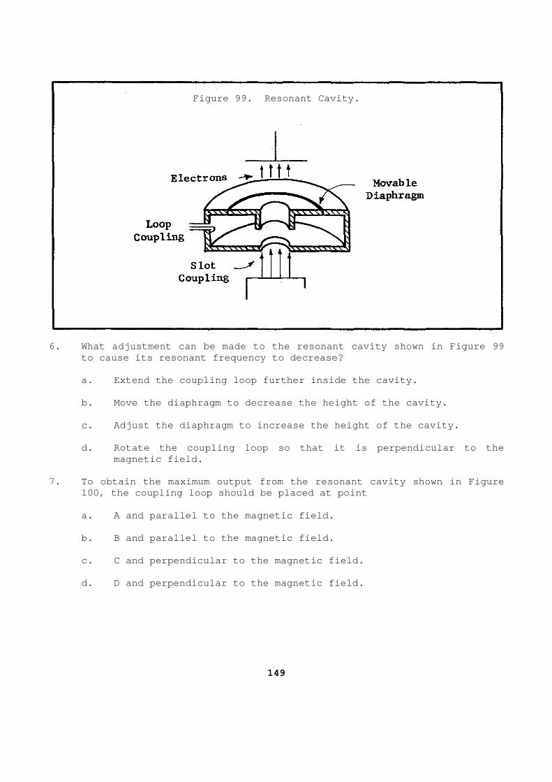
Figure 99. Resonant Cavity.

6. What adjustment can be made to the resonant cavi ty shown in Figure 99

to cause its resonant frequency to decrease? a. Extend the coupling loop further inside the cav ity. b. Move the diaphragm to decrease the height of th e cavity. c. Adjust the diaphragm to increase the height of the cavity. d. Rotate the coupling loop so that it is perpendi cular to the

magnetic field. 7. To obtain the maximum output from the resonant c avity shown in Figure

100, the coupling loop should be placed at point a. A and parallel to the magnetic field. b. B and parallel to the magnetic field. c. C and perpendicular to the magnetic field. d. D and perpendicular to the magnetic field.

149

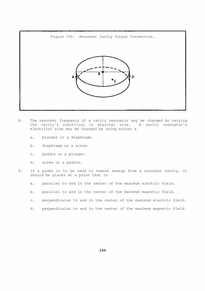
Figure 100. Resonant Cavity Output Connection.

8. The resonant frequency of a cavity resonator may be changed by varying

the cavity's electrical or physical size. A cavity resonator's electrical size may be changed by using either a

a. plunger or a diaphragm. b. diaphragm or a screw. c. paddle or a plunger. d. screw or a paddle. 9. If a probe is to be used to remove energy from a resonant cavity, it

should be places at a point that is a. parallel to and in the center of the maximum el ectric field. b. parallel to and in the center of the maximum ma gnetic field. c. perpendicular to and in the center of the maxim um electric field. d. perpendicular to and in the center of the maxim um magnetic field.

150

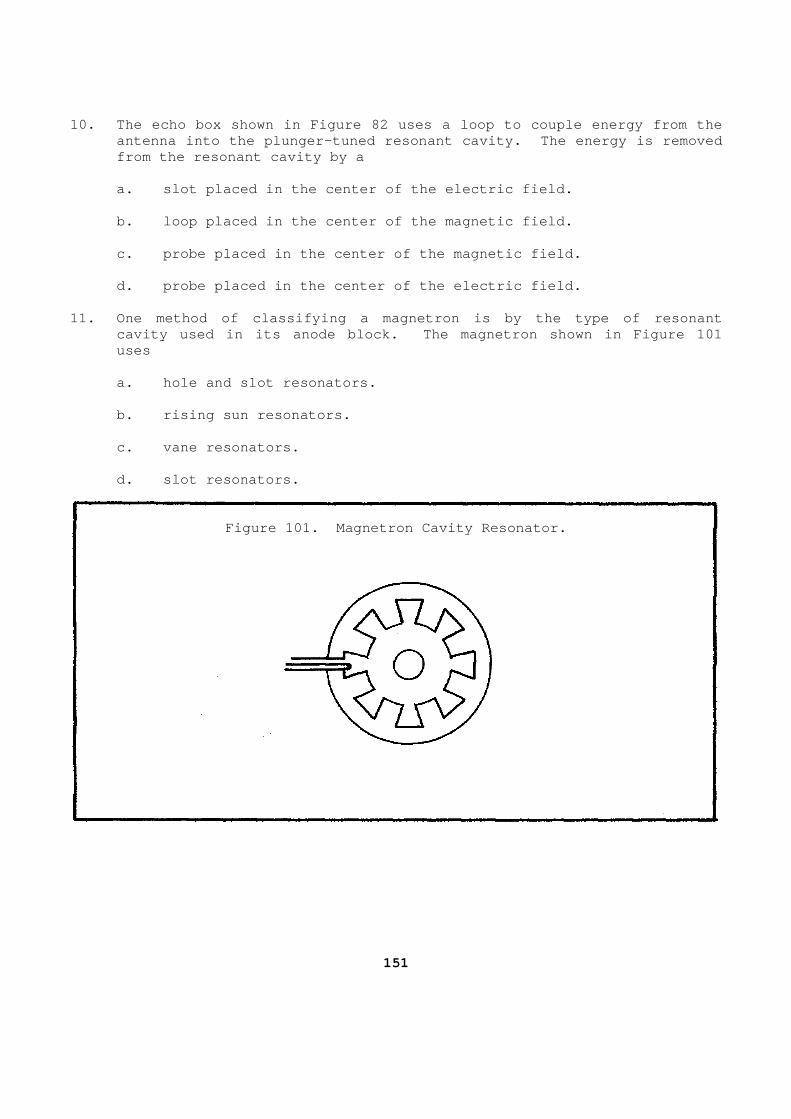
10. The echo box shown in Figure 82 uses a loop to couple energy from the antenna into the plunger-tuned resonant cavity. Th e energy is removed from the resonant cavity by a

a. slot placed in the center of the electric field . b. loop placed in the center of the magnetic field . c. probe placed in the center of the magnetic fiel d. d. probe placed in the center of the electric fiel d. 11. One method of classifying a magnetron is by the type of resonant

cavity used in its anode block. The magnetron show n in Figure 101 uses

a. hole and slot resonators. b. rising sun resonators. c. vane resonators. d. slot resonators.

Figure 101. Magnetron Cavity Resonator.

151

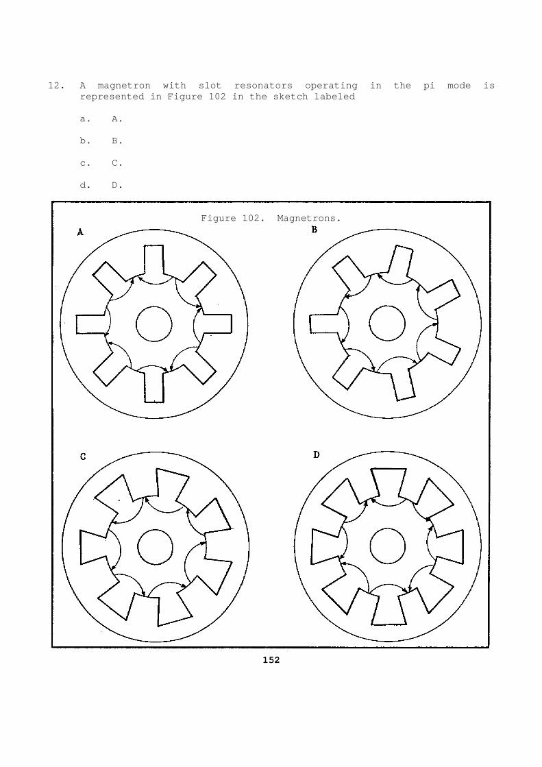
12. A magnetron with slot resonators operating in t he pi mode is represented in Figure 102 in the sketch labeled

a. A. b. B. c. C. d. D.

Figure 102. Magnetrons.

152

13. A magnetron differs from a conventional diode t ube in that it uses a permanent magnet to deflect the electron beam and i ts plate is at ground potential. The reason for grounding the pla te is to

a. prevent shock hazards. b. reduce magnetron pushing. c. permit the use of a conventional filament trans former for the

magnetron. d. reduce the strength of the electric field requi red for proper

operation. 14. The combination of the electric and magnetic fi elds causes the

electrons to take a twisting spiraling motion towar d the anode. The magnetron that has the greatest magnetic field stre ngth is represented in Figure 103 in the sketch labeled

a. A. b. B. c. C. d. D.

153

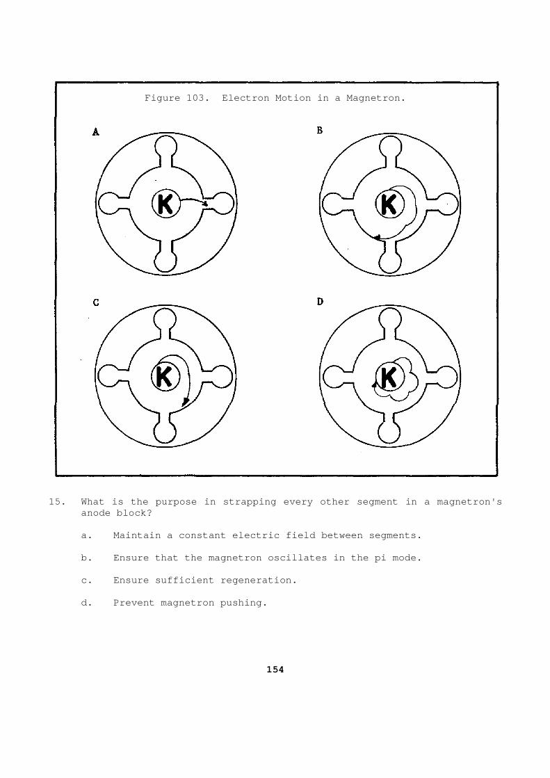
Figure 103. Electron Motion in a Magnetron.

15. What is the purpose in strapping every other se gment in a magnetron's

anode block? a. Maintain a constant electric field between segm ents. b. Ensure that the magnetron oscillates in the pi mode. c. Ensure sufficient regeneration. d. Prevent magnetron pushing.

154

16. The straps in a magnetron are designed to be on e-half wavelength long and will ensure that the magnetron operates properl y. The rising sun type magnetron does not require strapping because

a. the magnetic field ensures that the RF energy i n each slot is 180

degrees out of phase with the energy in the adjoini ng slot. b. it is not pulled off frequency by reflections i n the waveguide. c. every other vane is larger than the one in betw een. d. it does not operate in the pi mode. 17. The filament starting voltage for a QK324 magne tron is 4.8 volts and

the filament running voltage is zero. The reason f or using zero volts for the filament running voltage is that the

a. magnetron's frequency is fixed. b. modulator pulse provides filament voltage. c. filament is heated by degenerative electrons. d. pulse width of the modulator pulse is very narr ow. 18. For proper operation in a magnetron, the electr ons emitted by the

cathode must excite the cavities and also provide r egeneration for the cavities. Regeneration is provided by electrons in the magnetron shown in Figure 104, sketch labeled

a. A. b. B. c. C. d. D.

155

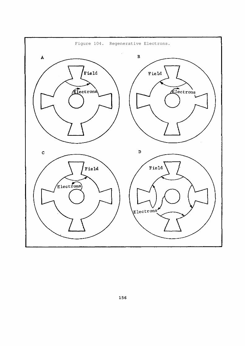
Figure 104. Regenerative Electrons.

156

19. A great deal of care should be taken when handl ing a magnetron magnet, so that

a. the magnetron will not require aging when insta lled in a radar

set. b. the magnetron will not be pulled off frequency. c. its field strength will not be reduced. d. tools will not become magnetized. 20. If the RF output of a magnetron is pulled off f requency, the probable

cause of the trouble is a. a dented section of waveguide. b. a distorted modulator pulse. c. an unstable timing trigger. d. a weak magnetic field.

Check your answers with lesson 3 Solution Sheet.

157

LESSON FOUR

ANTENNAS AND WAVEGUIDES TASK Describe how RF energy is transferred through waveg uides, recognize the various waveguide tuning and coupling devices, iden tify the various antennas and reflectors used in radar systems, and different iate between front and rear antenna feed systems. CONDITIONS (Performance-Oriented) Given this subcourse, pencil , and paper. STANDARD (Performance-Oriented) Demonstrate competency of ta sk skills and knowledge by correctly responding to 75 percent of the multip le-choice test covering radar transmitters. REFERENCES TC 11-67 FM 11-63 Learning Event 1: WAVEGUIDES 1. General. All transmission lines have power losses that inc rease as the applied frequency rises. In fact, at microwave fre quencies, ordinary RF transmission lines losses are so great that their u se is impractical. As a result, transmission engineers have devised a new t ransmission medium for guiding microwave energy from one place to another. They use waveguides as the transmission medium. Waveguides give much lowe r power losses at microwave frequencies than you would get using ordi nary RF transmission lines. Figure 105 shows waveguide directing energy to a radar antenna.

158

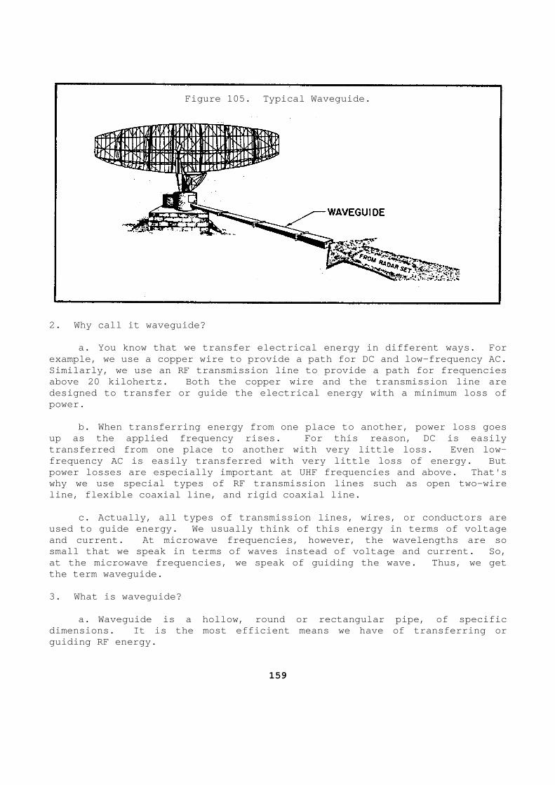
Figure 105. Typical Waveguide.

2. Why call it waveguide? a. You know that we transfer electrical energy in different ways. For example, we use a copper wire to provide a path for DC and low-frequency AC. Similarly, we use an RF transmission line to provid e a path for frequencies above 20 kilohertz. Both the copper wire and the t ransmission line are designed to transfer or guide the electrical energy with a minimum loss of power. b. When transferring energy from one place to anot her, power loss goes up as the applied frequency rises. For this reason , DC is easily transferred from one place to another with very lit tle loss. Even low-frequency AC is easily transferred with very little loss of energy. But power losses are especially important at UHF freque ncies and above. That's why we use special types of RF transmission lines s uch as open two-wire line, flexible coaxial line, and rigid coaxial line . c. Actually, all types of transmission lines, wire s, or conductors are used to guide energy. We usually think of this ene rgy in terms of voltage and current. At microwave frequencies, however, th e wavelengths are so small that we speak in terms of waves instead of vo ltage and current. So, at the microwave frequencies, we speak of guiding t he wave. Thus, we get the term waveguide. 3. What is waveguide? a. Waveguide is a hollow, round or rectangular pip e, of specific dimensions. It is the most efficient means we have of transferring or guiding RF energy.

159

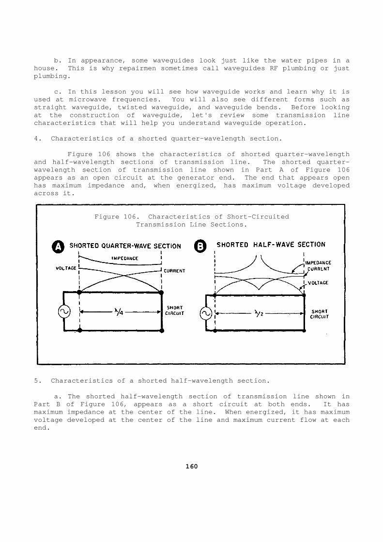
b. In appearance, some waveguides look just like t he water pipes in a house. This is why repairmen sometimes call wavegu ides RF plumbing or just plumbing. c. In this lesson you will see how waveguide works and learn why it is used at microwave frequencies. You will also see d ifferent forms such as straight waveguide, twisted waveguide, and waveguid e bends. Before looking at the construction of waveguide, let's review some transmission line characteristics that will help you understand waveg uide operation. 4. Characteristics of a shorted quarter-wavelength section. Figure 106 shows the characteristics of shorted q uarter-wavelength and half-wavelength sections of transmission line. The shorted quarter-wavelength section of transmission line shown in Pa rt A of Figure 106 appears as an open circuit at the generator end. T he end that appears open has maximum impedance and, when energized, has maxi mum voltage developed across it.

Figure 106. Characteristics of Short-Circuited

Transmission Line Sections.

5. Characteristics of a shorted half-wavelength sec tion. a. The shorted half-wavelength section of transmis sion line shown in Part B of Figure 106, appears as a short circuit at both ends. It has maximum impedance at the center of the line. When energized, it has maximum voltage developed at the center of the line and max imum current flow at each end.

160

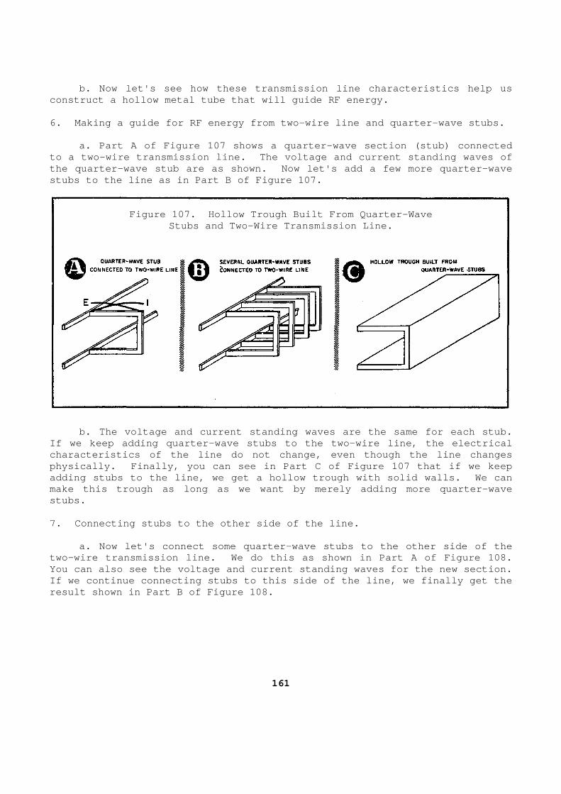
b. Now let's see how these transmission line chara cteristics help us construct a hollow metal tube that will guide RF en ergy. 6. Making a guide for RF energy from two-wire line and quarter-wave stubs. a. Part A of Figure 107 shows a quarter-wave secti on (stub) connected to a two-wire transmission line. The voltage and c urrent standing waves of the quarter-wave stub are as shown. Now let's add a few more quarter-wave stubs to the line as in Part B of Figure 107.

Figure 107. Hollow Trough Built From Quarter-Wave Stubs and Two-Wire Transmission Line.

b. The voltage and current standing waves are the same for each stub. If we keep adding quarter-wave stubs to the two-wir e line, the electrical characteristics of the line do not change, even tho ugh the line changes physically. Finally, you can see in Part C of Figu re 107 that if we keep adding stubs to the line, we get a hollow trough wi th solid walls. We can make this trough as long as we want by merely addin g more quarter-wave stubs. 7. Connecting stubs to the other side of the line. a. Now let's connect some quarter-wave stubs to th e other side of the two-wire transmission line. We do this as shown in Part A of Figure 108. You can also see the voltage and current standing w aves for the new section. If we continue connecting stubs to this side of the line, we finally get the result shown in Part B of Figure 108.

161

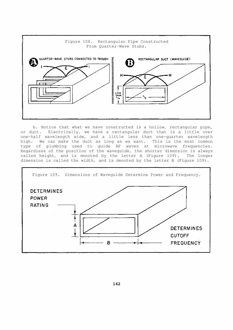
Figure 108. Rectangular Pipe Constructed

From Quarter-Wave Stubs.

b. Notice that what we have constructed is a hollo w, rectangular pipe, or duct. Electrically, we have a rectangular duct that is a little over one-half wavelength wide, and a little less than on e-quarter wavelength high. We can make the duct as long as we want. Th is is the most common type of plumbing used to guide RF waves at microwav e frequencies. Regardless of the position of the waveguide, the sh orter dimension is always called height, and is denoted by the letter A (Figu re 109). The longer dimension is called the width, and is denoted by th e letter B (Figure 109).

Figure 109. Dimensions of Waveguide Determine Powe r and Frequency.

162

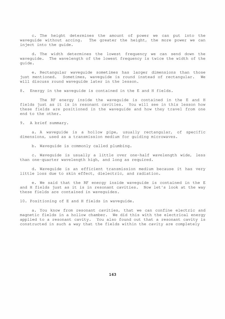
c. The height determines the amount of power we ca n put into the waveguide without arcing. The greater the height, the more power we can inject into the guide. d. The width determines the lowest frequency we ca n send down the waveguide. The wavelength of the lowest frequency is twice the width of the guide. e. Rectangular waveguide sometimes has larger dime nsions than those just mentioned. Sometimes, waveguide is round inst ead of rectangular. We will discuss round waveguide later in the lesson. 8. Energy in the waveguide is contained in the E an d H fields. The RF energy inside the waveguide is contained i n the E and H fields just as it is in resonant cavities. You wil l see in this lesson how these fields are positioned in the waveguide and ho w they travel from one end to the other. 9. A brief summary. a. A waveguide is a hollow pipe, usually rectangul ar, of specific dimensions, used as a transmission medium for guidi ng microwaves. b. Waveguide is commonly called plumbing. c. Waveguide is usually a little over one-half wav elength wide, less than one-quarter wavelength high, and long as requi red. d. Waveguide is an efficient transmission medium b ecause it has very little loss due to skin effect, dielectric, and rad iation. e. We said that the RF energy inside waveguide is contained in the E and H fields just as it is in resonant cavities. N ow let's look at the way these fields are contained in waveguides. 10. Positioning of E and H fields in waveguide. a. You know from resonant cavities, that we can co nfine electric and magnetic fields in a hollow chamber. We did this w ith the electrical energy applied to a resonant cavity. You also found out t hat a resonant cavity is constructed in such a way that the fields within th e cavity are completely

163

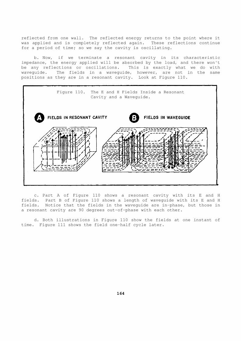
reflected from one wall. The reflected energy retu rns to the point where it was applied and is completely reflected again. The se reflections continue for a period of time; so we say the cavity is oscil lating. b. Now, if we terminate a resonant cavity in its c haracteristic impedance, the energy applied will be absorbed by t he load, and there won't be any reflections or oscillations. This is exactl y what we do with waveguide. The fields in a waveguide, however, are not in the same positions as they are in a resonant cavity. Look a t Figure 110.

Figure 110. The E and H Fields Inside a Resonant

Cavity and a Waveguide.

c. Part A of Figure 110 shows a resonant cavity wi th its E and H fields. Part B of Figure 110 shows a length of wav eguide with its E and H fields. Notice that the fields in the waveguide ar e in-phase, but those in a resonant cavity are 90 degrees out-of-phase with each other. d. Both illustrations in Figure 110 show the field s at one instant of time. Figure 111 shows the field one-half cycle la ter.

164

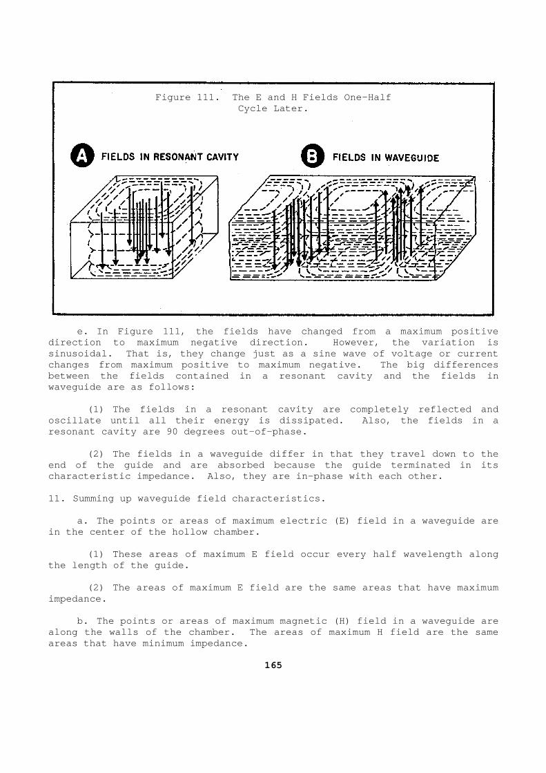
Figure 111. The E and H Fields One-Half

Cycle Later.

e. In Figure 111, the fields have changed from a m aximum positive direction to maximum negative direction. However, the variation is sinusoidal. That is, they change just as a sine wa ve of voltage or current changes from maximum positive to maximum negative. The big differences between the fields contained in a resonant cavity a nd the fields in waveguide are as follows: (1) The fields in a resonant cavity are completely reflected and oscillate until all their energy is dissipated. Al so, the fields in a resonant cavity are 90 degrees out-of-phase. (2) The fields in a waveguide differ in that they travel down to the end of the guide and are absorbed because the guide terminated in its characteristic impedance. Also, they are in-phase with each other. 11. Summing up waveguide field characteristics. a. The points or areas of maximum electric (E) fie ld in a waveguide are in the center of the hollow chamber. (1) These areas of maximum E field occur every hal f wavelength along the length of the guide. (2) The areas of maximum E field are the same area s that have maximum impedance. b. The points or areas of maximum magnetic (H) fie ld in a waveguide are along the walls of the chamber. The areas of maxim um H field are the same areas that have minimum impedance.

165

c. All of the fields are within the waveguide. d. The only current flow in waveguide is on the in side surface of the walls just as it is with resonant cavities. This i s one reason why waveguide is so efficient. e. We stated earlier that transmission lines have losses, due to skin effect, dielectric, and radiation. These losses ar e very slight with waveguide. Let's find out why. 12. Why waveguide has very low loss due to skin eff ect. a. When we transmit RF energy along a wire, the cu rrent flows on the outer edge of the wire. As we increase the applied frequency, the current flows more and more on just the outer edge (or circ umference) of the wire. We call this action skin effect. This means that, although the wire may be two inches in diameter, only one small section of t he wire is actually carrying current. b. The action of skin effect is the same as if we reduced the diameter of the wire or added resistance to it. This result s in heat being generated, and the electric power dissipated in the form of heat is loss. This is the reason, then, that wire has high losses due to skin effect at higher RF frequencies. c. In waveguide, current flows only along the insi de surface of the guide, but remember that waveguides have four solid walls to carry the current. Therefore, the current-carrying area is m uch greater in waveguide than in wire. This greater area has very little re sistance, so losses due to skin effect are very low. d. The inside walls of waveguide are sometimes sil verplated or gold-plated as they are in resonant cavities. Plating t he walls reduces any resistance the walls have and further decreases los ses due to skin effect. 13. Why waveguide has very low dielectric loss. a. You know that any two-wire or coaxial type tran smission line has some kind of insulation to keep the two wires apart . Any insulating material, such as rubber, plastic, or even air is a ctually a dielectric between the two conductors. So, there's always som e slight current flow through the dielectric. We call this slight curren t flow between the two conductors leakage current, and the resulting loss of energy is called dielectric loss.

166

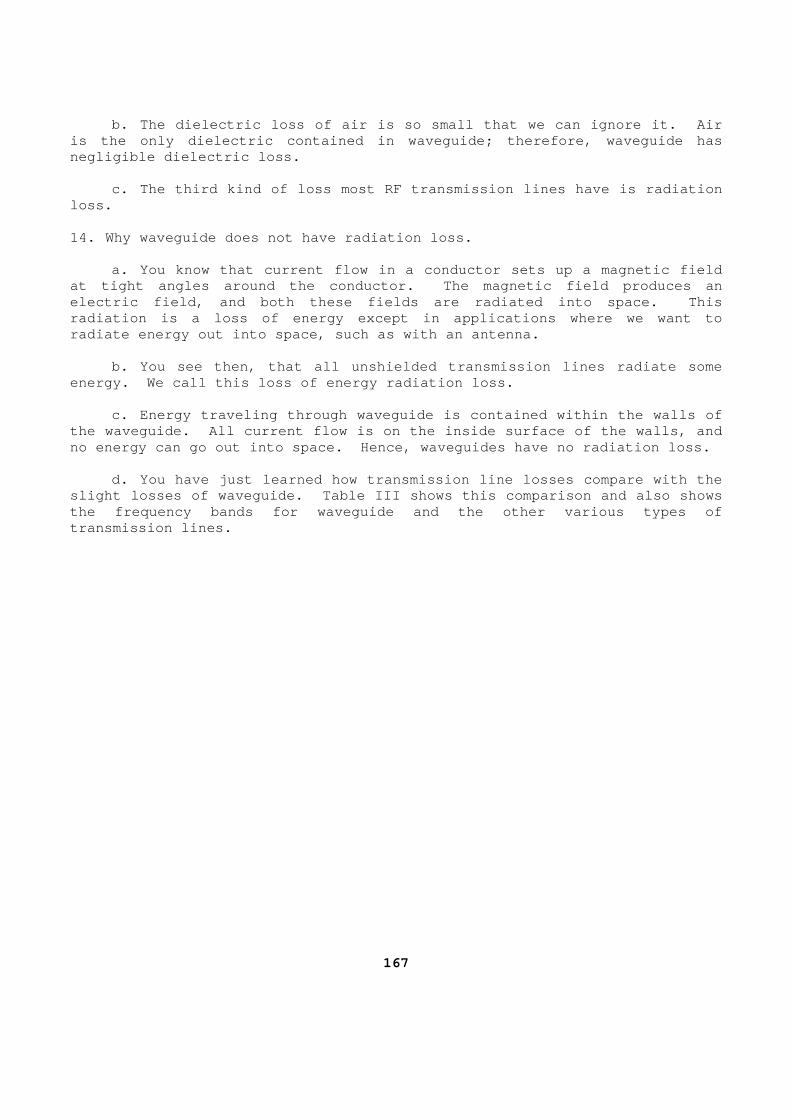
b. The dielectric loss of air is so small that we can ignore it. Air is the only dielectric contained in waveguide; ther efore, waveguide has negligible dielectric loss. c. The third kind of loss most RF transmission lin es have is radiation loss. 14. Why waveguide does not have radiation loss. a. You know that current flow in a conductor sets up a magnetic field at tight angles around the conductor. The magnetic field produces an electric field, and both these fields are radiated into space. This radiation is a loss of energy except in application s where we want to radiate energy out into space, such as with an ante nna. b. You see then, that all unshielded transmission lines radiate some energy. We call this loss of energy radiation loss . c. Energy traveling through waveguide is contained within the walls of the waveguide. All current flow is on the inside s urface of the walls, and no energy can go out into space. Hence, waveguides have no radiation loss. d. You have just learned how transmission line los ses compare with the slight losses of waveguide. Table III shows this c omparison and also shows the frequency bands for waveguide and the other var ious types of transmission lines.

167

Figure 112. Comparing Waveguide and Transmission L ines.

e. Now that you have learned how energy travels al ong waveguide and why waveguide is very efficient, let's see how you coup le energy into or out of waveguide. 15. Energy is usually coupled into waveguide with a probe. a. The most common method of coupling energy into waveguide is with a probe (Figure 113). This method is identical to pr obe coupling into a resonant cavity. That is, the probe is placed in t he waveguide at the center of the width (B dimension) and a quarter-wav elength from the end. This point gives maximum E field in the center of t he guide and maximum H field along the walls of the guide.

168

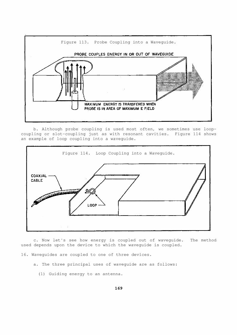
Figure 113. Probe Coupling into a Waveguide.

b. Although probe coupling is used most often, we sometimes use loop-coupling or slot-coupling just as with resonant cav ities. Figure 114 shows an example of loop coupling into a waveguide.

Figure 114. Loop Coupling into a Waveguide.

c. Now let's see how energy is coupled out of wave guide. The method used depends upon the device to which the waveguide is coupled. 16. Waveguides are coupled to one of three devices. a. The three principal uses of waveguide are as fo llows: (1) Guiding energy to an antenna.

169

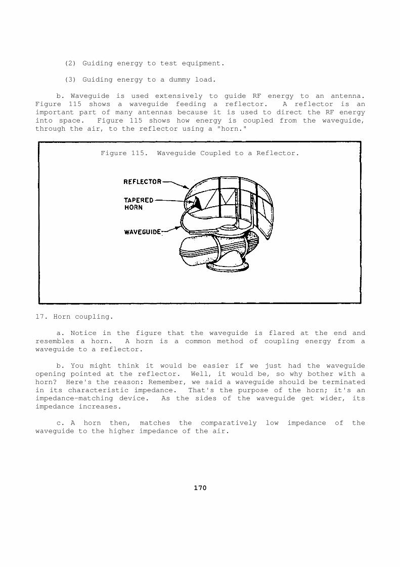
(2) Guiding energy to test equipment. (3) Guiding energy to a dummy load. b. Waveguide is used extensively to guide RF energ y to an antenna. Figure 115 shows a waveguide feeding a reflector. A reflector is an important part of many antennas because it is used to direct the RF energy into space. Figure 115 shows how energy is coupled from the waveguide, through the air, to the reflector using a "horn."

Figure 115. Waveguide Coupled to a Reflector.

17. Horn coupling. a. Notice in the figure that the waveguide is flar ed at the end and resembles a horn. A horn is a common method of cou pling energy from a waveguide to a reflector. b. You might think it would be easier if we just h ad the waveguide opening pointed at the reflector. Well, it would b e, so why bother with a horn? Here's the reason: Remember, we said a waveg uide should be terminated in its characteristic impedance. That's the purpos e of the horn; it's an impedance-matching device. As the sides of the wav eguide get wider, its impedance increases. c. A horn then, matches the comparatively low impe dance of the waveguide to the higher impedance of the air.

170

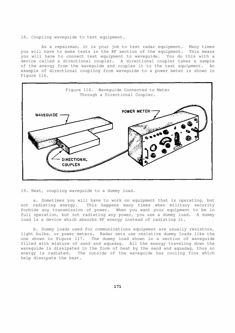
18. Coupling waveguide to test equipment. As a repairman, it is your job to test radar equi pment. Many times you will have to make tests in the RF section of th e equipment. This means you will have to connect test equipment to waveguid e. You do this with a device called a directional coupler. A directional coupler takes a sample of the energy from the waveguide and couples it to the test equipment. An example of directional coupling from waveguide to a power meter is shown in Figure 116.

Figure 116. Waveguide Connected to Meter

Through a Directional Coupler. 19. Next, coupling waveguide to a dummy load. a. Sometimes you will have to work on equipment th at is operating, but not radiating energy. This happens many times when military security forbids any transmission of power. When you want y our equipment to be in full operation, but not radiating any power, you us e a dummy load. A dummy load is a device which absorbs RF energy instead of radiating it. b. Dummy loads used for communications equipment a re usually resistors, light bulbs, or power meters. Radar sets use resis tive dummy loads like the one shown in Figure 117. The dummy load shown is a section of waveguide filled with mixture of sand and aquadag. All the e nergy traveling down the waveguide is dissipated in the form of heat by the sand and aquadag, thus no energy is radiated. The outside of the waveguide h as cooling fins which help dissipate the heat.

171

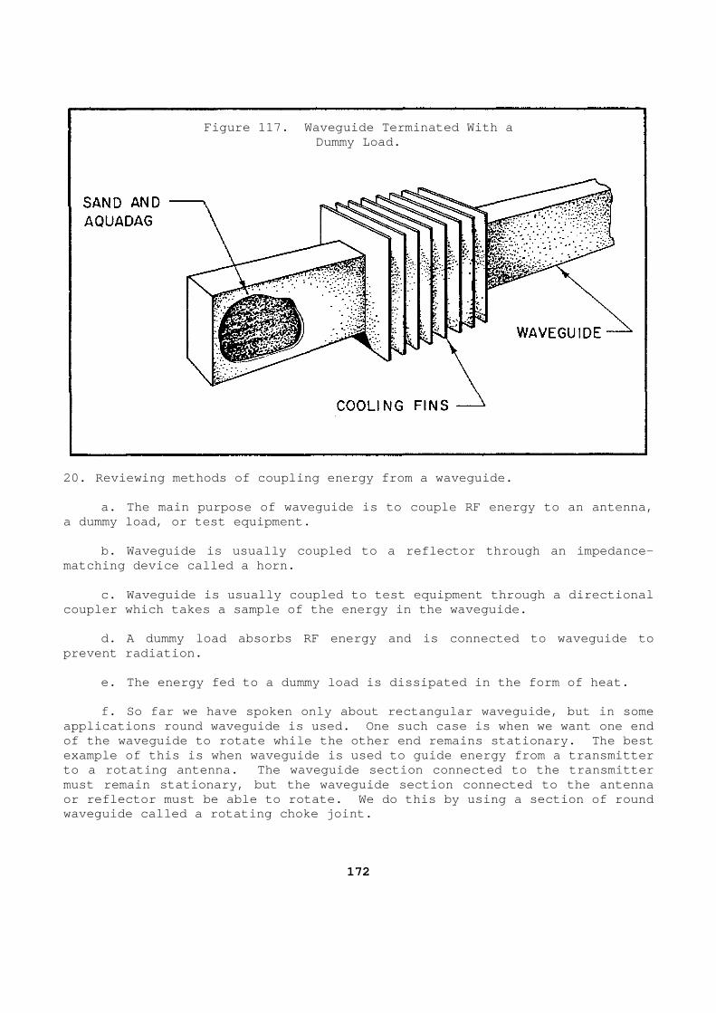
Figure 117. Waveguide Terminated With a

Dummy Load. 20. Reviewing methods of coupling energy from a wav eguide. a. The main purpose of waveguide is to couple RF e nergy to an antenna, a dummy load, or test equipment. b. Waveguide is usually coupled to a reflector thr ough an impedance-matching device called a horn. c. Waveguide is usually coupled to test equipment through a directional coupler which takes a sample of the energy in the w aveguide. d. A dummy load absorbs RF energy and is connected to waveguide to prevent radiation. e. The energy fed to a dummy load is dissipated in the form of heat. f. So far we have spoken only about rectangular wa veguide, but in some applications round waveguide is used. One such cas e is when we want one end of the waveguide to rotate while the other end rema ins stationary. The best example of this is when waveguide is used to guide energy from a transmitter to a rotating antenna. The waveguide section conne cted to the transmitter must remain stationary, but the waveguide section c onnected to the antenna or reflector must be able to rotate. We do this by using a section of round waveguide called a rotating choke joint.

172

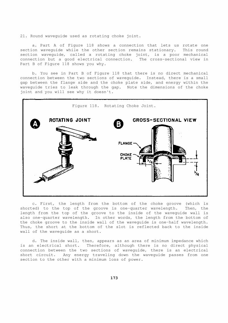
21. Round waveguide used as rotating choke joint. a. Part A of Figure 118 shows a connection that le ts us rotate one section waveguide while the other section remains s tationary. This round section waveguide, called a rotating choke joint, i s a poor mechanical connection but a good electrical connection. The c ross-sectional view in Part B of Figure 118 shows you why. b. You see in Part B of Figure 118 that there is n o direct mechanical connection between the two sections of waveguide. Instead, there is a small gap between the flange side and the choke plate sid e, and energy within the waveguide tries to leak through the gap. Note the dimensions of the choke joint and you will see why it doesn't.

Figure 118. Rotating Choke Joint.

c. First, the length from the bottom of the choke groove (which is shorted) to the top of the groove is one-quarter wa velength. Then, the length from the top of the groove to the inside of the waveguide wall is also one-quarter wavelength. In other words, the l ength from the bottom of the choke groove to the inside wall of the waveguid e is one-half wavelength. Thus, the short at the bottom of the slot is reflec ted back to the inside wall of the waveguide as a short. d. The inside wall, then, appears as an area of mi nimum impedance which is an electrical short. Therefore, although there is no direct physical connection between the two sections of waveguide, t here is an electrical short circuit. Any energy traveling down the waveg uide passes from one section to the other with a minimum loss of power.

173

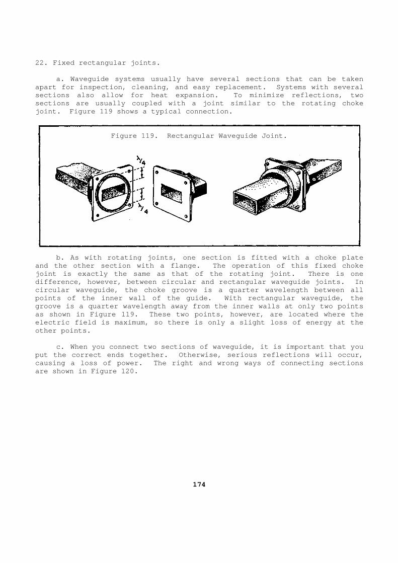
22. Fixed rectangular joints. a. Waveguide systems usually have several sections that can be taken apart for inspection, cleaning, and easy replacemen t. Systems with several sections also allow for heat expansion. To minimiz e reflections, two sections are usually coupled with a joint similar t o the rotating choke joint. Figure 119 shows a typical connection.

Figure 119. Rectangular Waveguide Joint.

b. As with rotating joints, one section is fitted with a choke plate and the other section with a flange. The operation of this fixed choke joint is exactly the same as that of the rotating j oint. There is one difference, however, between circular and rectangul ar waveguide joints. In circular waveguide, the choke groove is a quarter w avelength between all points of the inner wall of the guide. With rectan gular waveguide, the groove is a quarter wavelength away from the inner walls at only two points as shown in Figure 119. These two points, however, are located where the electric field is maximum, so there is only a sligh t loss of energy at the other points. c. When you connect two sections of waveguide, it is important that you put the correct ends together. Otherwise, serious reflections will occur, causing a loss of power. The right and wrong ways of connecting sections are shown in Figure 120.

174

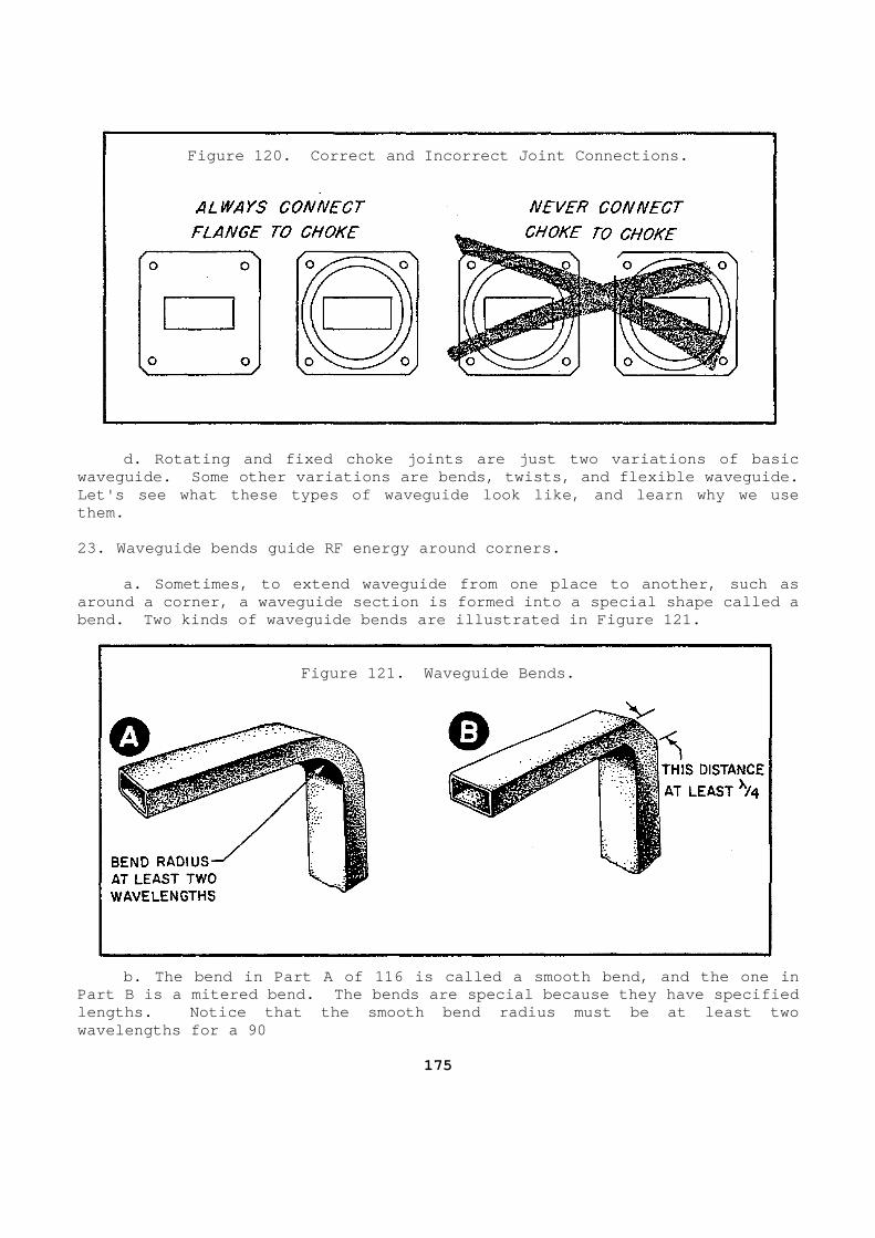
Figure 120. Correct and Incorrect Joint Connection s.

d. Rotating and fixed choke joints are just two va riations of basic waveguide. Some other variations are bends, twists , and flexible waveguide. Let's see what these types of waveguide look like, and learn why we use them. 23. Waveguide bends guide RF energy around corners. a. Sometimes, to extend waveguide from one place t o another, such as around a corner, a waveguide section is formed into a special shape called a bend. Two kinds of waveguide bends are illustrated in Figure 121.

Figure 121. Waveguide Bends.

b. The bend in Part A of 116 is called a smooth be nd, and the one in Part B is a mitered bend. The bends are special be cause they have specified lengths. Notice that the smooth bend radius must b e at least two wavelengths for a 90

175

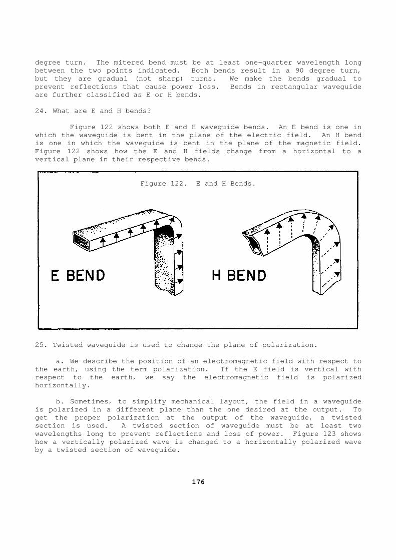
degree turn. The mitered bend must be at least one -quarter wavelength long between the two points indicated. Both bends resul t in a 90 degree turn, but they are gradual (not sharp) turns. We make th e bends gradual to prevent reflections that cause power loss. Bends i n rectangular waveguide are further classified as E or H bends. 24. What are E and H bends? Figure 122 shows both E and H waveguide bends. A n E bend is one in which the waveguide is bent in the plane of the ele ctric field. An H bend is one in which the waveguide is bent in the plane of the magnetic field. Figure 122 shows how the E and H fields change from a horizontal to a vertical plane in their respective bends.

Figure 122. E and H Bends.

25. Twisted waveguide is used to change the plane o f polarization. a. We describe the position of an electromagnetic field with respect to the earth, using the term polarization. If the E f ield is vertical with respect to the earth, we say the electromagnetic fi eld is polarized horizontally. b. Sometimes, to simplify mechanical layout, the f ield in a waveguide is polarized in a different plane than the one desi red at the output. To get the proper polarization at the output of the wa veguide, a twisted section is used. A twisted section of waveguide mu st be at least two wavelengths long to prevent reflections and loss of power. Figure 123 shows how a vertically polarized wave is changed to a hor izontally polarized wave by a twisted section of waveguide.

176

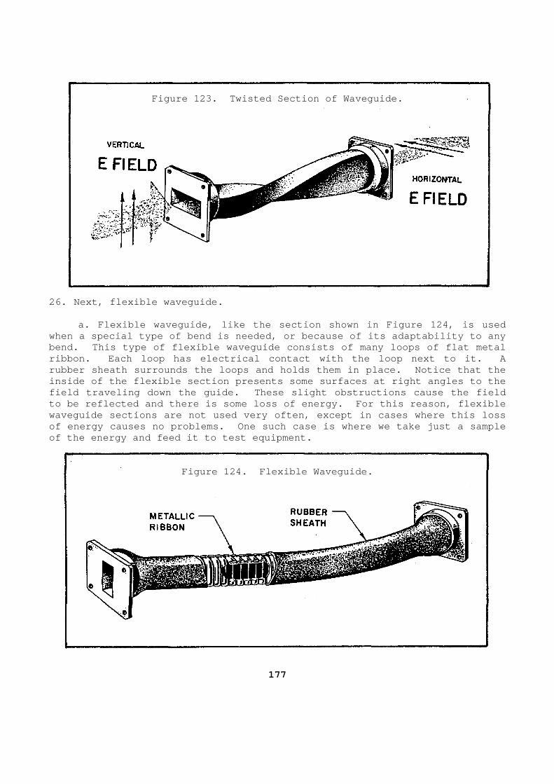
Figure 123. Twisted Section of Waveguide.

26. Next, flexible waveguide. a. Flexible waveguide, like the section shown in F igure 124, is used when a special type of bend is needed, or because o f its adaptability to any bend. This type of flexible waveguide consists of many loops of flat metal ribbon. Each loop has electrical contact with the loop next to it. A rubber sheath surrounds the loops and holds them in place. Notice that the inside of the flexible section presents some surfac es at right angles to the field traveling down the guide. These slight obstr uctions cause the field to be reflected and there is some loss of energy. For this reason, flexible waveguide sections are not used very often, except in cases where this loss of energy causes no problems. One such case is whe re we take just a sample of the energy and feed it to test equipment.

Figure 124. Flexible Waveguide.

177

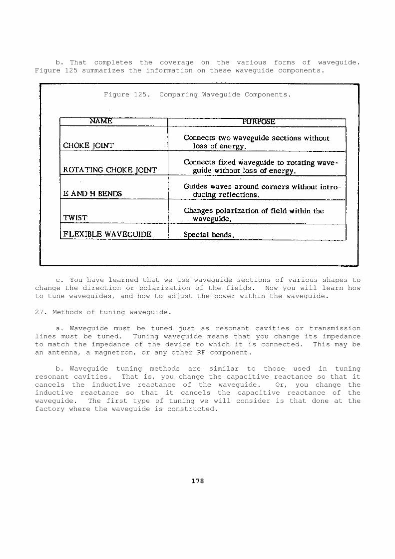
b. That completes the coverage on the various form s of waveguide. Figure 125 summarizes the information on these wave guide components.

Figure 125. Comparing Waveguide Components.

c. You have learned that we use waveguide sections of various shapes to change the direction or polarization of the fields. Now you will learn how to tune waveguides, and how to adjust the power wit hin the waveguide. 27. Methods of tuning waveguide. a. Waveguide must be tuned just as resonant caviti es or transmission lines must be tuned. Tuning waveguide means that y ou change its impedance to match the impedance of the device to which it is connected. This may be an antenna, a magnetron, or any other RF component. b. Waveguide tuning methods are similar to those u sed in tuning resonant cavities. That is, you change the capacit ive reactance so that it cancels the inductive reactance of the waveguide. Or, you change the inductive reactance so that it cancels the capaciti ve reactance of the waveguide. The first type of tuning we will consid er is that done at the factory where the waveguide is constructed.

178

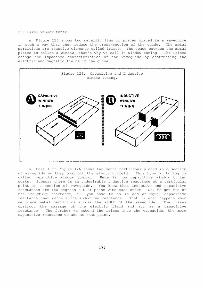
28. Fixed window tuner. a. Figure 126 shows two metallic fins or plates pl aced in a waveguide in such a way that they reduce the cross-section of the guide. The metal partitions are reactive elements called irises. Th e space between the metal plates is called a window; that's why we call it wi ndow tuning. The irises change the impedance characteristics of the wavegui de by obstructing the electric and magnetic fields in the guide.

Figure 126. Capacitive and Inductive

Window Tuning. b. Part A of Figure 126 shows two metal partitions placed in a section of waveguide so they obstruct the electric field. This type of tuning is called capacitive window tuning. Here is how capac itive window tuning works. Suppose there is an undesirable inductive r eactance at a particular point in a section of waveguide. You know that ind uctive and capacitive reactances are 180 degrees out of phase with each o ther. So, to get rid of the inductive reactance, all you have to do is add an equal capacitive reactance that cancels the inductive reactance. Th at is what happens when we place metal partitions across the width of the w aveguide. The irises obstruct the passage of the electric field and act as a capacitive reactance. The further we extend the irises into t he waveguide, the more capacitive reactance we add at that point.

179

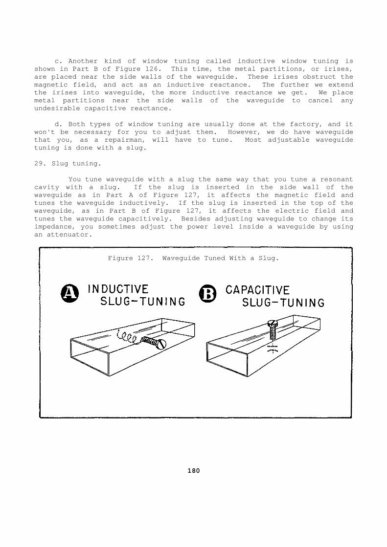
c. Another kind of window tuning called inductive window tuning is shown in Part B of Figure 126. This time, the meta l partitions, or irises, are placed near the side walls of the waveguide. T hese irises obstruct the magnetic field, and act as an inductive reactance. The further we extend the irises into waveguide, the more inductive react ance we get. We place metal partitions near the side walls of the wavegui de to cancel any undesirable capacitive reactance. d. Both types of window tuning are usually done at the factory, and it won't be necessary for you to adjust them. However , we do have waveguide that you, as a repairman, will have to tune. Most adjustable waveguide tuning is done with a slug. 29. Slug tuning. You tune waveguide with a slug the same way that you tune a resonant cavity with a slug. If the slug is inserted in the side wall of the waveguide as in Part A of Figure 127, it affects th e magnetic field and tunes the waveguide inductively. If the slug is in serted in the top of the waveguide, as in Part B of Figure 127, it affects t he electric field and tunes the waveguide capacitively. Besides adjustin g waveguide to change its impedance, you sometimes adjust the power level ins ide a waveguide by using an attenuator.

Figure 127. Waveguide Tuned With a Slug.

180

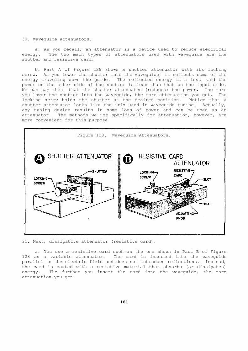
30. Waveguide attenuators. a. As you recall, an attenuator is a device used t o reduce electrical energy. The two main types of attenuators used wit h waveguide are the shutter and resistive card. b. Part A of Figure 128 shows a shutter attenuator with its locking screw. As you lower the shutter into the waveguide , it reflects some of the energy traveling down the guide. The reflected ene rgy is a loss, and the power on the other side of the shutter is less than that on the input side. We can say then, that the shutter attenuates (reduc es) the power. The more you lower the shutter into the waveguide, the more attenuation you get. The locking screw holds the shutter at the desired posi tion. Notice that a shutter attenuator looks like the iris used in wave guide tuning. Actually, any tuning device results in some loss of power and can be used as an attenuator. The methods we use specifically for at tenuation, however, are more convenient for this purpose.

Figure 128. Waveguide Attenuators.

31. Next, dissipative attenuator (resistive card). a. You use a resistive card such as the one shown in Part B of Figure 128 as a variable attenuator. The card is inserted into the waveguide parallel to the electric field and does not introdu ce reflections. Instead, the card is coated with a resistive material that a bsorbs (or dissipates) energy. The further you insert the card into the w aveguide, the more attenuation you get.

181

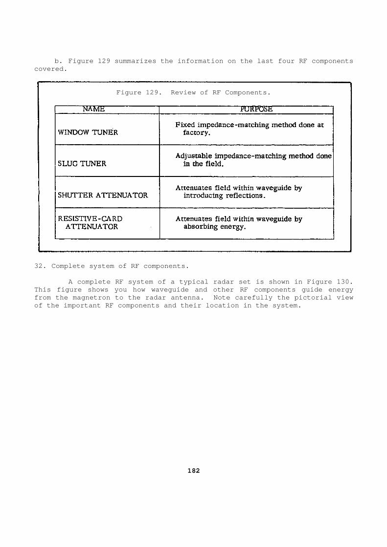
b. Figure 129 summarizes the information on the la st four RF components covered.

Figure 129. Review of RF Components.

32. Complete system of RF components. A complete RF system of a typical radar set is sh own in Figure 130. This figure shows you how waveguide and other RF co mponents guide energy from the magnetron to the radar antenna. Note care fully the pictorial view of the important RF components and their location i n the system.

182

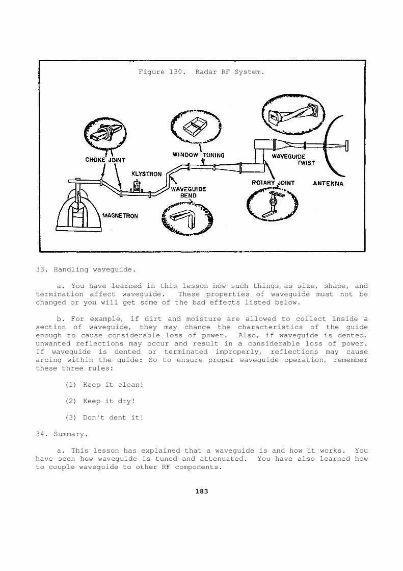
Figure 130. Radar RF System.

33. Handling waveguide. a. You have learned in this lesson how such things as size, shape, and termination affect waveguide. These properties of waveguide must not be changed or you will get some of the bad effects lis ted below. b. For example, if dirt and moisture are allowed t o collect inside a section of waveguide, they may change the character istics of the guide enough to cause considerable loss of power. Also, if waveguide is dented, unwanted reflections may occur and result in a cons iderable loss of power. If waveguide is dented or terminated improperly, re flections may cause arcing within the guide: So to ensure proper wavegu ide operation, remember these three rules: (1) Keep it clean! (2) Keep it dry! (3) Don't dent it! 34. Summary. a. This lesson has explained that a waveguide is a nd how it works. You have seen how waveguide is tuned and attenuated. Y ou have also learned how to couple waveguide to other RF components.

183

b. The most important points to remember about wav eguide are as follows: (1) Waveguide is a hollow pipe, usually rectangula r, used to guide microwave energy. (2) Waveguide is a very efficient transmission med ium because it has very little loss of energy. (3) Waveguide is used principally to guide microwa ve energy to antennas, test equipment, and dummy loads. (4) A choke joint is a device used to join two sec tions of waveguide. (5) Waveguide bends are smooth or mitered. (6) Twisted waveguide changes the plane of the fie ld within a waveguide. (7) Flexible waveguide is usually used when a loss of energy can be tolerated. (8) Waveguide must be tuned to prevent serious ref lections. (9) A shutter and resistive card are two types of waveguide attenuators. Learning Event 2: RADAR ANTENNAS 1. General. You know that radar operates on the echo principl e. The magnetron generates short regularly-spaced RF pulses when exc ited by short DC pulses from the modulator. These high-power RF pulses are transmitted into space in a narrow beam from a directional antenna (Figure 131). A target in the path of the radar beam sends back some of the RF en ergy in the form of echoes. The antenna intercepts these echoes and di rects them to a sensitive receiver and finally to the radar indicator.

184

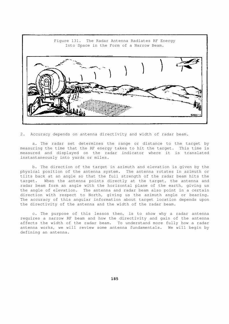
Figure 131. The Radar Antenna Radiates RF Energy

Into Space in the Form of a Narrow Beam. 2. Accuracy depends on antenna directivity and widt h of radar beam. a. The radar set determines the range or distance to the target by measuring the time that the RF energy takes to hit the target. This time is measured and displayed on the radar indicator where it is translated instantaneously into yards or miles. b. The direction of the target in azimuth and elev ation is given by the physical position of the antenna system. The anten na rotates in azimuth or tilts back at an angle so that the full strength of the radar beam hits the target. When the antenna points directly at the ta rget, the antenna and radar beam form an angle with the horizontal plane of the earth, giving us the angle of elevation. The antenna and radar beam also point in a certain direction with respect to North, giving us the azim uth angle or bearing. The accuracy of this angular information about targ et location depends upon the directivity of the antenna and the width of the radar beam. c. The purpose of this lesson then, is to show why a radar antenna requires a narrow RF beam and how the directivity a nd gain of the antenna affects the width of the radar beam. To understand more fully how a radar antenna works, we will review some antenna fundamen tals. We will begin by defining an antenna.

185

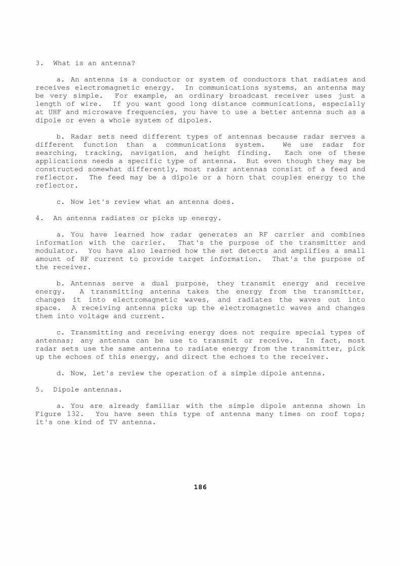
3. What is an antenna? a. An antenna is a conductor or system of conducto rs that radiates and receives electromagnetic energy. In communications systems, an antenna may be very simple. For example, an ordinary broadcast receiver uses just a length of wire. If you want good long distance com munications, especially at UHF and microwave frequencies, you have to use a better antenna such as a dipole or even a whole system of dipoles. b. Radar sets need different types of antennas bec ause radar serves a different function than a communications system. W e use radar for searching, tracking, navigation, and height finding . Each one of these applications needs a specific type of antenna. But even though they may be constructed somewhat differently, most radar antenn as consist of a feed and reflector. The feed may be a dipole or a horn that couples energy to the reflector. c. Now let's review what an antenna does. 4. An antenna radiates or picks up energy. a. You have learned how radar generates an RF carr ier and combines information with the carrier. That's the purpose o f the transmitter and modulator. You have also learned how the set detec ts and amplifies a small amount of RF current to provide target information. That's the purpose of the receiver. b. Antennas serve a dual purpose, they transmit en ergy and receive energy. A transmitting antenna takes the energy fr om the transmitter, changes it into electromagnetic waves, and radiates the waves out into space. A receiving antenna picks up the electromag netic waves and changes them into voltage and current. c. Transmitting and receiving energy does not requ ire special types of antennas; any antenna can be use to transmit or rec eive. In fact, most radar sets use the same antenna to radiate energy f rom the transmitter, pick up the echoes of this energy, and direct the echoes to the receiver. d. Now, let's review the operation of a simple dip ole antenna. 5. Dipole antennas. a. You are already familiar with the simple dipole antenna shown in Figure 132. You have seen this type of antenna man y times on roof tops; it's one kind of TV antenna.

186

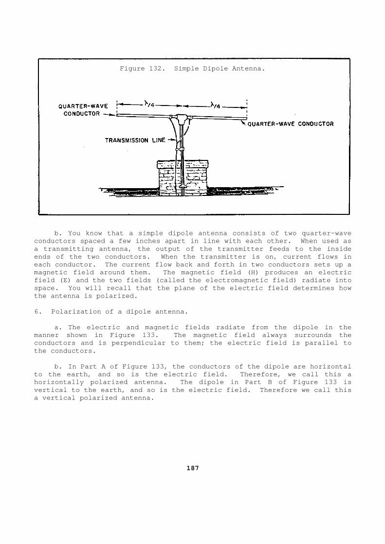
Figure 132. Simple Dipole Antenna.

b. You know that a simple dipole antenna consists of two quarter-wave conductors spaced a few inches apart in line with e ach other. When used as a transmitting antenna, the output of the transmitt er feeds to the inside ends of the two conductors. When the transmitter i s on, current flows in each conductor. The current flow back and forth in two conductors sets up a magnetic field around them. The magnetic field (H) produces an electric field (E) and the two fields (called the electromag netic field) radiate into space. You will recall that the plane of the elect ric field determines how the antenna is polarized. 6. Polarization of a dipole antenna. a. The electric and magnetic fields radiate from t he dipole in the manner shown in Figure 133. The magnetic field alw ays surrounds the conductors and is perpendicular to them; the electr ic field is parallel to the conductors. b. In Part A of Figure 133, the conductors of the dipole are horizontal to the earth, and so is the electric field. Theref ore, we call this a horizontally polarized antenna. The dipole in Part B of Figure 133 is vertical to the earth, and so is the electric field . Therefore we call this a vertical polarized antenna.

187

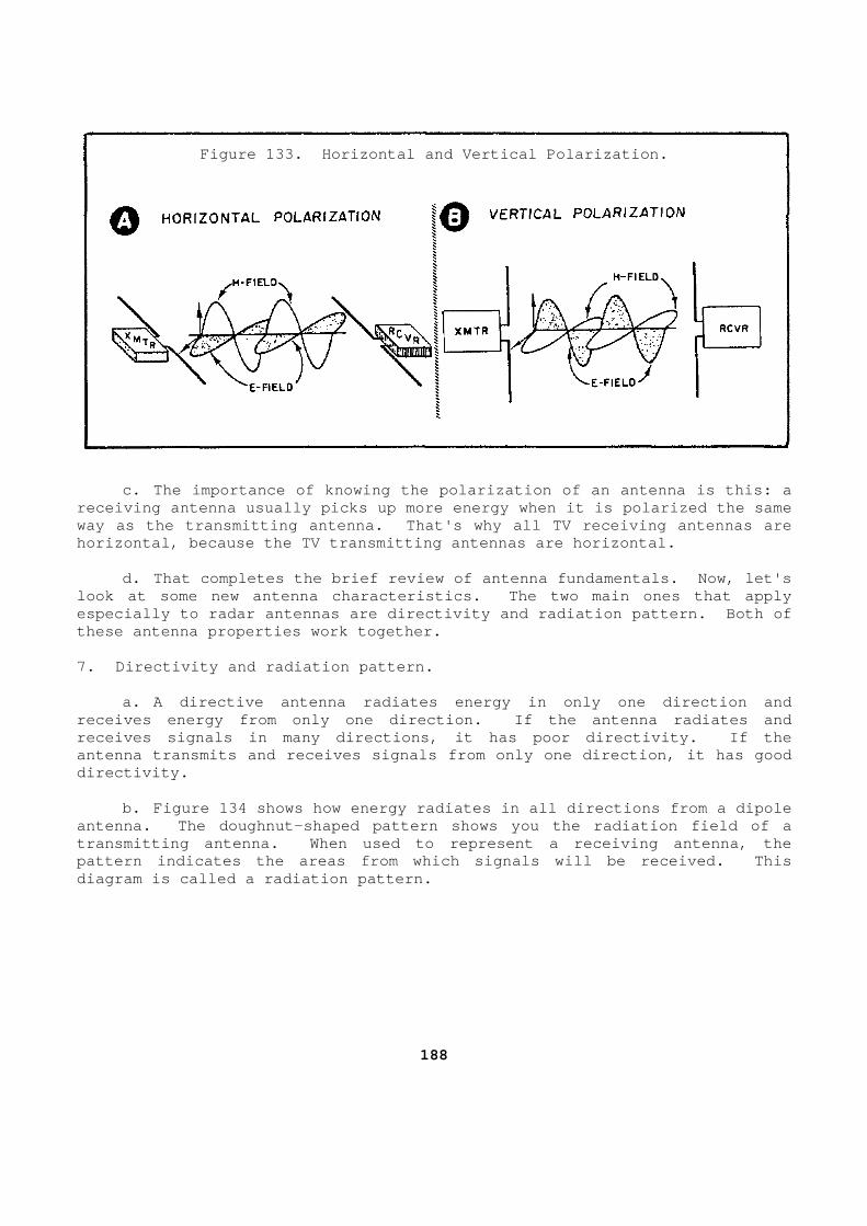
Figure 133. Horizontal and Vertical Polarization.

c. The importance of knowing the polarization of a n antenna is this: a receiving antenna usually picks up more energy when it is polarized the same way as the transmitting antenna. That's why all TV receiving antennas are horizontal, because the TV transmitting antennas ar e horizontal. d. That completes the brief review of antenna fund amentals. Now, let's look at some new antenna characteristics. The two main ones that apply especially to radar antennas are directivity and ra diation pattern. Both of these antenna properties work together. 7. Directivity and radiation pattern. a. A directive antenna radiates energy in only one direction and receives energy from only one direction. If the an tenna radiates and receives signals in many directions, it has poor di rectivity. If the antenna transmits and receives signals from only on e direction, it has good directivity. b. Figure 134 shows how energy radiates in all dir ections from a dipole antenna. The doughnut-shaped pattern shows you the radiation field of a transmitting antenna. When used to represent a rec eiving antenna, the pattern indicates the areas from which signals will be received. This diagram is called a radiation pattern.

188

Figure 134. Doughnut Radiation Pattern

of a Simple Dipole. c. A simple dipole has very poor directivity becau se it radiates in almost all directions. A simple dipole antenna is used, then, to radiate power in all directions. It is a very efficient an tenna for commercial radio and TV stations. d. Now suppose you want to transmit in only one di rection, or you want to receive from only one direction. For example, i f you are transmitting to ships out at sea, you want all the power from the t ransmitter to go out over the ocean. Can you do this using a dipole antenna? Yes, you can, by adding a reflector to the dipole. 8. Adding a reflector to the dipole makes the anten na directional. a. To make a dipole antenna directional, you merel y add an element called a reflector. A reflector may be nothing mor e than a conducting rod a little longer than one-half wavelength. Figure 135 shows a dipole with a reflector; it also shows the antenna radiation patt ern. b. The elements of an antenna that radiate or rece ive energy are called driven elements. Any other elements are called par asitic elements. Notice in Figure 135 that the dipole is the driven element , and the reflector is the parasitic element.

189

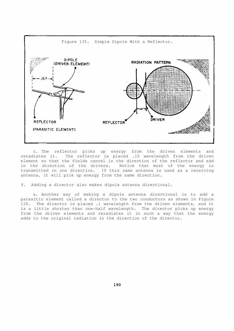
Figure 135. Simple Dipole With a Reflector.

c. The reflector picks up energy from the driven e lements and reradiates it. The reflector is placed .15 wavelen gth from the driven element so that the fields cancel in the direction of the reflector and add in the direction of the drivers. Notice that most of the energy is transmitted in one direction. If this same antenna is used as a receiving antenna, it will pick up energy from the same direc tion. 9. Adding a director also makes dipole antenna dire ctional. a. Another way of making a dipole antenna directio nal is to add a parasitic element called a director to the two cond uctors as shown in Figure 136. The director is placed .1 wavelength from the driven elements, and it is a little shorter than one-half wavelength. The director picks up energy from the driven elements and reradiates it in such a way that the energy adds to the original radiation in the direction of the director.

190

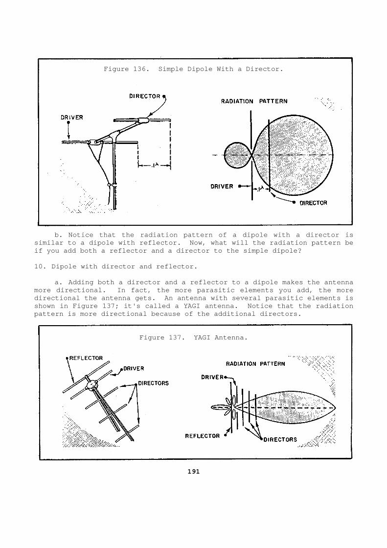
Figure 136. Simple Dipole With a Director.

b. Notice that the radiation pattern of a dipole w ith a director is similar to a dipole with reflector. Now, what will the radiation pattern be if you add both a reflector and a director to the s imple dipole? 10. Dipole with director and reflector. a. Adding both a director and a reflector to a dip ole makes the antenna more directional. In fact, the more parasitic elem ents you add, the more directional the antenna gets. An antenna with seve ral parasitic elements is shown in Figure 137; it's called a YAGI antenna. N otice that the radiation pattern is more directional because of the addition al directors.

Figure 137. YAGI Antenna.

191

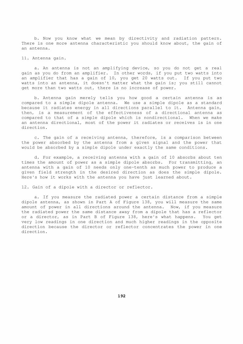
b. Now you know what we mean by directivity and ra diation pattern. There is one more antenna characteristic you should know about, the gain of an antenna. 11. Antenna gain. a. An antenna is not an amplifying device, so you do not get a real gain as you do from an amplifier. In other words, if you put two watts into an amplifier that has a gain of 10, you get 20 watt s out. If you put two watts into an antenna, it doesn't matter what the g ain is; you still cannot get more than two watts out, there is no increase o f power. b. Antenna gain merely tells you how good a certai n antenna is as compared to a simple dipole antenna. We use a simp le dipole as a standard because it radiates energy in all directions parall el to it. Antenna gain, then, is a measurement of the effectiveness of a di rectional antenna as compared to that of a simple dipole which is nondir ectional. When we make an antenna directional, most of the power it radiat es or receives is in one direction. c. The gain of a receiving antenna, therefore, is a comparison between the power absorbed by the antenna from a given sign al and the power that would be absorbed by a simple dipole under exactly the same conditions. d. For example, a receiving antenna with a gain of 10 absorbs about ten times the amount of power as a simple dipole absorb s. For transmitting, an antenna with a gain of 10 needs only one-tenth as m uch power to produce a given field strength in the desired direction as do es the simple dipole. Here's how it works with the antenna you have just learned about. 12. Gain of a dipole with a director or reflector. a. If you measure the radiated power a certain dis tance from a simple dipole antenna, as shown in Part A of Figure 138, y ou will measure the same amount of power in all directions around the antenn a. Now, if you measure the radiated power the same distance away from a di pole that has a reflector or a director, as in Part B of Figure 138, here's w hat happens. You get very low readings in one direction and much higher readings in the opposite direction because the director or reflector concent rates the power in one direction.

192

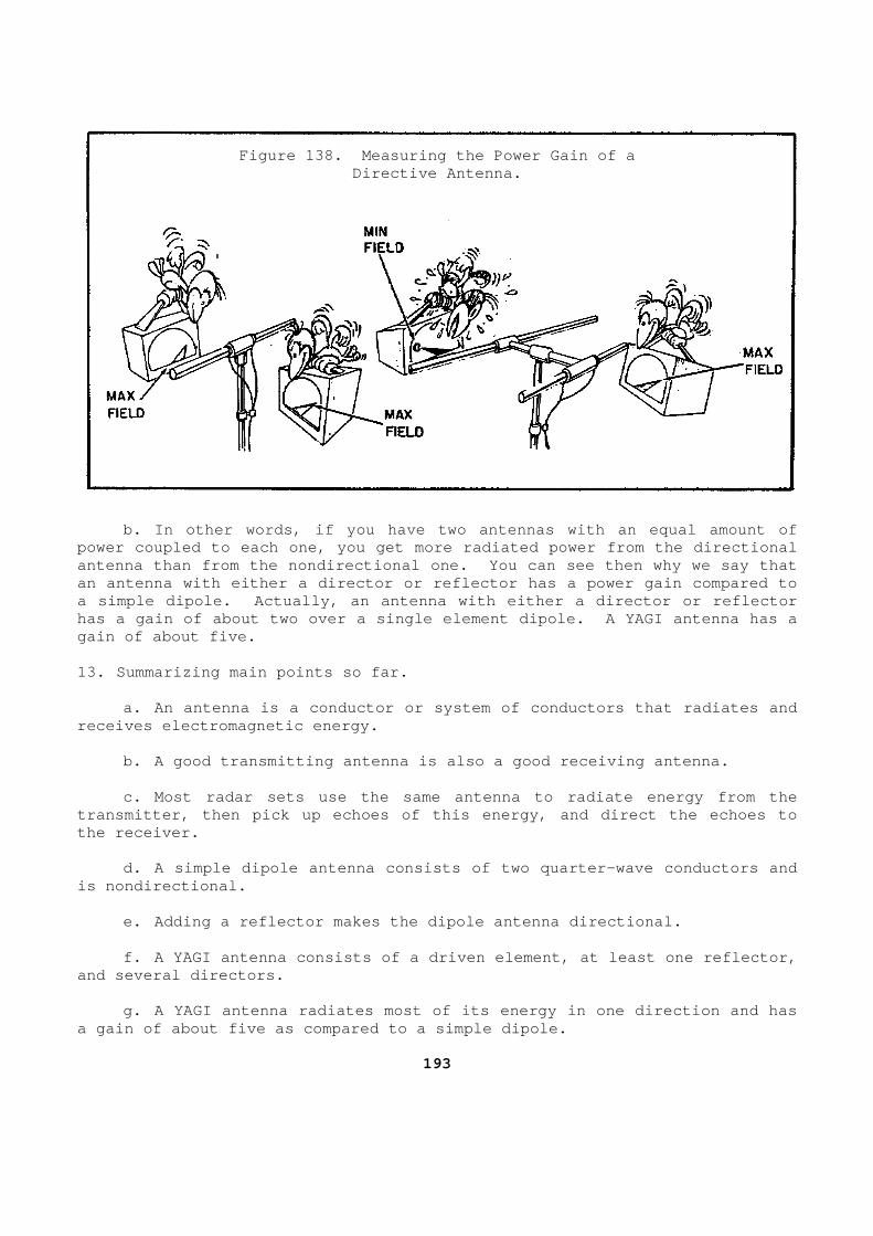
Figure 138. Measuring the Power Gain of a

Directive Antenna. b. In other words, if you have two antennas with a n equal amount of power coupled to each one, you get more radiated po wer from the directional antenna than from the nondirectional one. You can see then why we say that an antenna with either a director or reflector has a power gain compared to a simple dipole. Actually, an antenna with either a director or reflector has a gain of about two over a single element dipol e. A YAGI antenna has a gain of about five. 13. Summarizing main points so far. a. An antenna is a conductor or system of conducto rs that radiates and receives electromagnetic energy. b. A good transmitting antenna is also a good rece iving antenna. c. Most radar sets use the same antenna to radiate energy from the transmitter, then pick up echoes of this energy, an d direct the echoes to the receiver. d. A simple dipole antenna consists of two quarter -wave conductors and is nondirectional. e. Adding a reflector makes the dipole antenna dir ectional. f. A YAGI antenna consists of a driven element, at least one reflector, and several directors. g. A YAGI antenna radiates most of its energy in o ne direction and has a gain of about five as compared to a simple dipole .

193

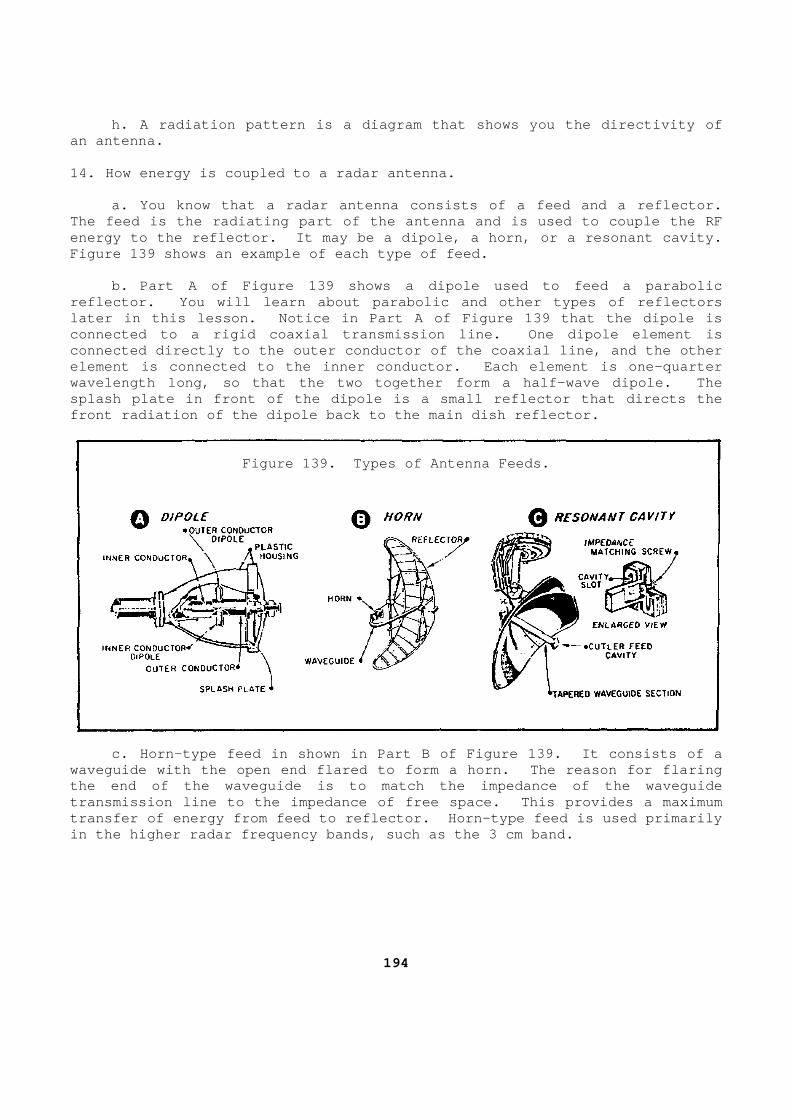
h. A radiation pattern is a diagram that shows you the directivity of an antenna. 14. How energy is coupled to a radar antenna. a. You know that a radar antenna consists of a fee d and a reflector. The feed is the radiating part of the antenna and i s used to couple the RF energy to the reflector. It may be a dipole, a hor n, or a resonant cavity. Figure 139 shows an example of each type of feed. b. Part A of Figure 139 shows a dipole used to fee d a parabolic reflector. You will learn about parabolic and othe r types of reflectors later in this lesson. Notice in Part A of Figure 1 39 that the dipole is connected to a rigid coaxial transmission line. On e dipole element is connected directly to the outer conductor of the co axial line, and the other element is connected to the inner conductor. Each element is one-quarter wavelength long, so that the two together form a ha lf-wave dipole. The splash plate in front of the dipole is a small refl ector that directs the front radiation of the dipole back to the main dish reflector.

Figure 139. Types of Antenna Feeds.

c. Horn-type feed in shown in Part B of Figure 139 . It consists of a waveguide with the open end flared to form a horn. The reason for flaring the end of the waveguide is to match the impedance of the waveguide transmission line to the impedance of free space. This provides a maximum transfer of energy from feed to reflector. Horn-ty pe feed is used primarily in the higher radar frequency bands, such as the 3 cm band.

194

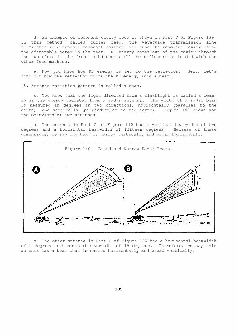
d. An example of resonant cavity feed is shown in Part C of Figure 139. In this method, called cutler feed, the waveguide t ransmission line terminates in a tunable resonant cavity. You tune the resonant cavity using the adjustable screw in the rear. RF energy comes out of the cavity through the two slots in the front and bounces off the refl ector as it did with the other feed methods. e. Now you know how RF energy is fed to the reflec tor. Next, let's find out how the reflector forms the RF energy into a beam. 15. Antenna radiation pattern is called a beam. a. You know that the light directed from a flashli ght is called a beam; so is the energy radiated from a radar antenna. Th e width of a radar beam is measured in degrees in two directions, horizonta lly (parallel to the earth), and vertically (perpendicular to the earth) . Figure 140 shows you the beamwidth of two antennas. b. The antenna in Part A of Figure 140 has a verti cal beamwidth of two degrees and a horizontal beamwidth of fifteen degre es. Because of these dimensions, we say the beam is narrow vertically an d broad horizontally.

Figure 140. Broad and Narrow Radar Beams.

c. The other antenna in Part B of Figure 140 has a horizontal beamwidth of 2 degrees and vertical beamwidth of 15 degrees. Therefore, we say this antenna has a beam that is narrow horizontally and broad vertically.

195

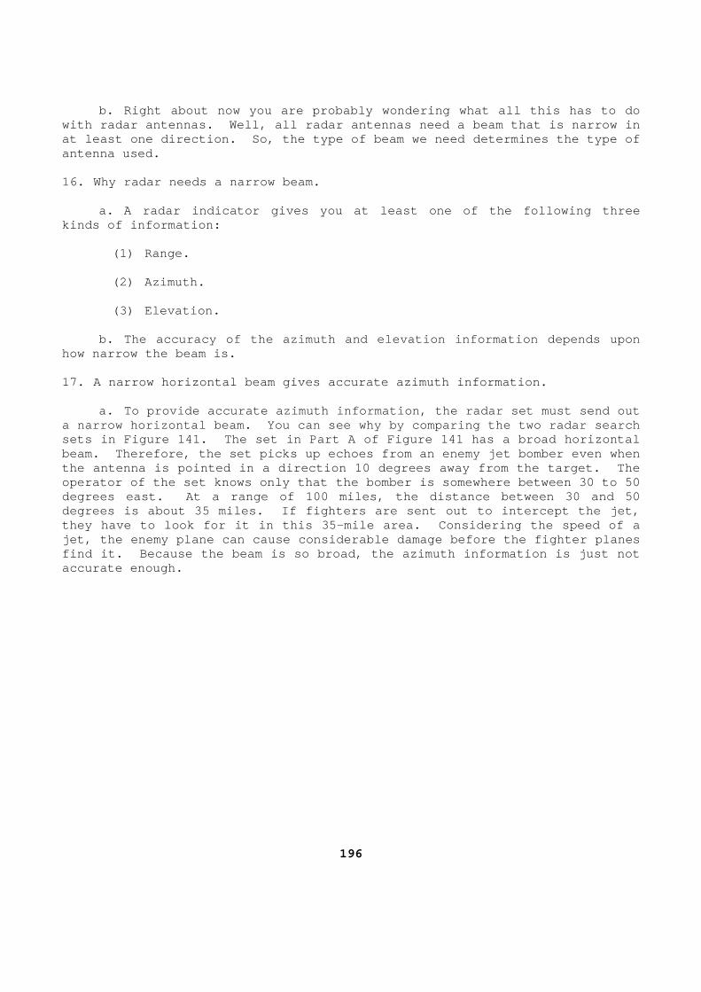
b. Right about now you are probably wondering what all this has to do with radar antennas. Well, all radar antennas need a beam that is narrow in at least one direction. So, the type of beam we ne ed determines the type of antenna used. 16. Why radar needs a narrow beam. a. A radar indicator gives you at least one of the following three kinds of information: (1) Range. (2) Azimuth. (3) Elevation. b. The accuracy of the azimuth and elevation infor mation depends upon how narrow the beam is. 17. A narrow horizontal beam gives accurate azimuth information. a. To provide accurate azimuth information, the ra dar set must send out a narrow horizontal beam. You can see why by compa ring the two radar search sets in Figure 141. The set in Part A of Figure 14 1 has a broad horizontal beam. Therefore, the set picks up echoes from an e nemy jet bomber even when the antenna is pointed in a direction 10 degrees aw ay from the target. The operator of the set knows only that the bomber is s omewhere between 30 to 50 degrees east. At a range of 100 miles, the distanc e between 30 and 50 degrees is about 35 miles. If fighters are sent ou t to intercept the jet, they have to look for it in this 35-mile area. Con sidering the speed of a jet, the enemy plane can cause considerable damage before the fighter planes find it. Because the beam is so broad, the azimuth information is just not accurate enough.

196

Figure 141. Broad and Narrow Horizontal Beams.

b. Now notice in Part B of Figure 141 how a narrow horizontal beam gives more accurate azimuth information. The indic ator tells the operator that the bomber is exactly 40 degrees east. Fighte rs directed to intercept an enemy jet using information from this set can he ad straight toward the target. c. Remember, then, that a radar set must have a na rrow horizontal beam to give accurate azimuth information. 18. A narrow vertical beam gives accurate height in formation. a. To provide accurate elevation information, the radar set must have a narrow vertical beam. You can see the reason by co mparing the two height-finding sets shown in Figure 142. Notice that the set in Part A of Figure 142 sends out a broad vertical beam. The beam is s o broad that even when the antenna is pointed at an angle of 40 degrees, i t picks up a plane that is at an angle of 15 degrees. The operator of the set knows, of course, that the enemy plane is there, but is not able to d etermine the exact height. If this information is used to aim and fir e antiaircraft guns automatically, the guns will miss the target becaus e of the inaccurate information.

197

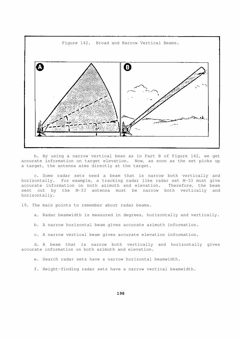
Figure 142. Broad and Narrow Vertical Beams.

b. By using a narrow vertical bean as in Part B of Figure 142, we get accurate information on target elevation. Now, as soon as the set picks up a target, the antenna aims directly at the target. c. Some radar sets need a beam that is narrow both vertically and horizontally. For example, a tracking radar like r adar set M-33 must give accurate information on both azimuth and elevation. Therefore, the beam sent out by the M-33 antenna must be narrow both ve rtically and horizontally. 19. The main points to remember about radar beams. a. Radar beamwidth is measured in degrees, horizon tally and vertically. b. A narrow horizontal beam gives accurate azimuth information. c. A narrow vertical beam gives accurate elevation information. d. A beam that is narrow both vertically and horiz ontally gives accurate information on both azimuth and elevation. e. Search radar sets have a narrow horizontal beam width. f. Height-finding radar sets have a narrow vertica l beamwidth.

198

g. Tracking radar sets have a beam that is narrow both vertically and horizontally. 20. Reflectors are used with radar antennas to prod uce correctly shaped beams. a. Radar sets operate in the microwave region of t he frequency spectrum. Microwave frequency wavelengths are so s mall that they act like light waves. That's why most sets use antenna refl ectors that work like light reflectors. There are four main types of ant ennas that you will work with, as follows: (1) Paraboloid (dish) (2) Orange peel. (3) Parabolic cylinder. (4) Metallic lens. b. The first three types of antennas get their nam es from the shape of their reflectors. The metallic lens type is actual ly a lens made of metal. 21. Radar reflectors work like light reflectors. a. Take a look at a flashlight and notice the refl ector surrounding the bulb. The reflector concentrates light from the bu lb into a narrow beam. Similarly, a radar reflector concentrates RF energy from the antenna into a narrow beam as shown in Figure 143. b. Without a reflector, light from the flashlight bulb would go out in all directions, and so would RF energy from the ant enna.

199

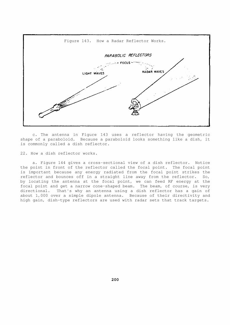
Figure 143. How a Radar Reflector Works.

c. The antenna in Figure 143 uses a reflector havi ng the geometric shape of a paraboloid. Because a paraboloid looks something like a dish, it is commonly called a dish reflector. 22. How a dish reflector works. a. Figure 144 gives a cross-sectional view of a di sh reflector. Notice the point in front of the reflector called the foca l point. The focal point is important because any energy radiated from the f ocal point strikes the reflector and bounces off in a straight line away f rom the reflector. So, by locating the antenna at the focal point, we can feed RF energy at the focal point and get a narrow cone-shaped beam. The beam, of course, is very directional. That's why an antenna using a dish re flector has a gain of about 1,000 over a simple dipole antenna. Because of their directivity and high gain, dish-type reflectors are used with radar sets that track targets.

200

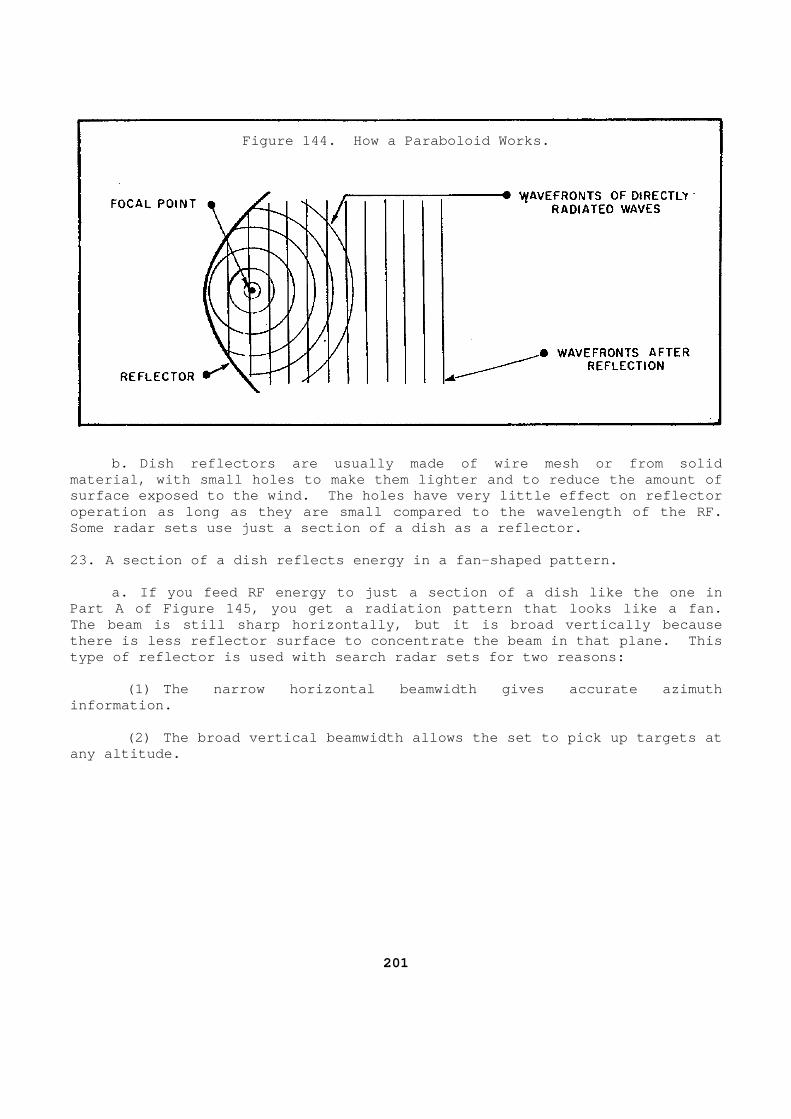
Figure 144. How a Paraboloid Works.

b. Dish reflectors are usually made of wire mesh o r from solid material, with small holes to make them lighter and to reduce the amount of surface exposed to the wind. The holes have very l ittle effect on reflector operation as long as they are small compared to the wavelength of the RF. Some radar sets use just a section of a dish as a r eflector. 23. A section of a dish reflects energy in a fan-sh aped pattern. a. If you feed RF energy to just a section of a di sh like the one in Part A of Figure 145, you get a radiation pattern t hat looks like a fan. The beam is still sharp horizontally, but it is bro ad vertically because there is less reflector surface to concentrate the beam in that plane. This type of reflector is used with search radar sets fo r two reasons: (1) The narrow horizontal beamwidth gives accurate azimuth information. (2) The broad vertical beamwidth allows the set to pick up targets at any altitude.

201

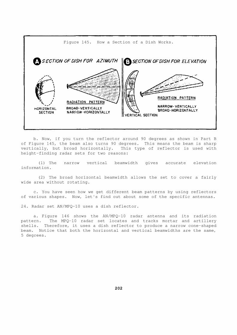
Figure 145. How a Section of a Dish Works.

b. Now, if you turn the reflector around 90 degree s as shown in Part B of Figure 145, the beam also turns 90 degrees. Thi s means the beam is sharp vertically, but broad horizontally. This type of r eflector is used with height-finding radar sets for two reasons: (1) The narrow vertical beamwidth gives accurate e levation information. (2) The broad horizontal beamwidth allows the set to cover a fairly wide area without rotating. c. You have seen how we get different beam pattern s by using reflectors of various shapes. Now, let's find out about some of the specific antennas. 24. Radar set AN/MPQ-10 uses a dish reflector. a. Figure 146 shows the AN/MPQ-10 radar antenna an d its radiation pattern. The MPQ-10 radar set locates and tracks m ortar and artillery shells. Therefore, it uses a dish reflector to pro duce a narrow cone-shaped beam. Notice that both the horizontal and vertical beamwidths are the same, 5 degrees.

202

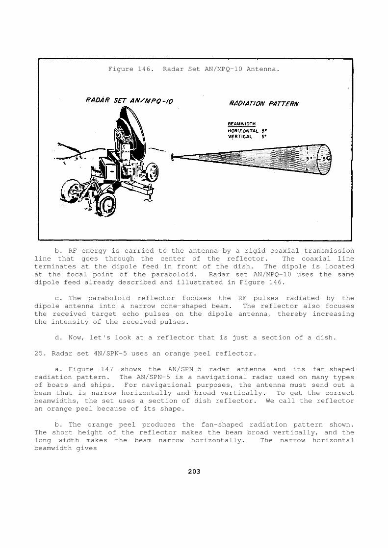
Figure 146. Radar Set AN/MPQ-10 Antenna.

b. RF energy is carried to the antenna by a rigid coaxial transmission line that goes through the center of the reflector. The coaxial line terminates at the dipole feed in front of the dish. The dipole is located at the focal point of the paraboloid. Radar set AN /MPQ-10 uses the same dipole feed already described and illustrated in Fi gure 146. c. The paraboloid reflector focuses the RF pulses radiated by the dipole antenna into a narrow cone-shaped beam. The reflector also focuses the received target echo pulses on the dipole anten na, thereby increasing the intensity of the received pulses. d. Now, let's look at a reflector that is just a s ection of a dish. 25. Radar set 4N/SPN-5 uses an orange peel reflecto r. a. Figure 147 shows the AN/SPN-5 radar antenna and its fan-shaped radiation pattern. The AN/SPN-5 is a navigational radar used on many types of boats and ships. For navigational purposes, the antenna must send out a beam that is narrow horizontally and broad vertical ly. To get the correct beamwidths, the set uses a section of dish reflecto r. We call the reflector an orange peel because of its shape. b. The orange peel produces the fan-shaped radiati on pattern shown. The short height of the reflector makes the beam br oad vertically, and the long width makes the beam narrow horizontally. The narrow horizontal beamwidth gives

203

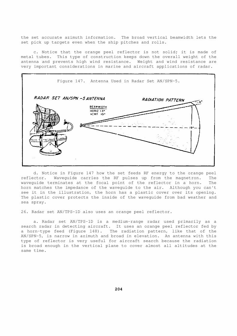
the set accurate azimuth information. The broad ve rtical beamwidth lets the set pick up targets even when the ship pitches and rolls. c. Notice that the orange peel reflector is not so lid; it is made of metal tubes. This type of construction keeps down the overall weight of the antenna and prevents high wind resistance. Weight and wind resistance are very important considerations in marine and aircraf t applications of radar.

Figure 147. Antenna Used in Radar Set AN/SPN-5.

d. Notice in Figure 147 how the set feeds RF energ y to the orange peel reflector. Waveguide carries the RF pulses up from the magnetron. The waveguide terminates at the focal point of the refl ector in a horn. The horn matches the impedance of the waveguide to the air. Although you can't see it in the illustration, the horn has a plastic cover over its opening. The plastic cover protects the inside of the wavegu ide from bad weather and sea spray. 26. Radar set AN/TPS-1D also uses an orange peel re flector. a. Radar set AN/TPS-1D is a medium-range radar use d primarily as a search radar in detecting aircraft. It uses an ora nge peel reflector fed by a horn-type feed (Figure 148). The radiation patte rn, like that of the AN/SPN-5, is narrow in azimuth and broad in elevati on. An antenna with this type of reflector is very useful for aircraft searc h because the radiation is broad enough in the vertical plane to cover almo st all altitudes at the same time.

204

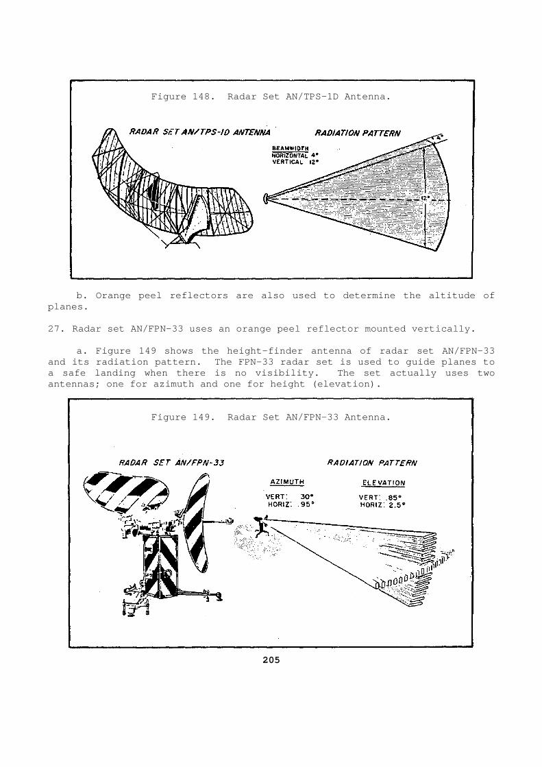
Figure 148. Radar Set AN/TPS-1D Antenna.

b. Orange peel reflectors are also used to determi ne the altitude of planes. 27. Radar set AN/FPN-33 uses an orange peel reflect or mounted vertically. a. Figure 149 shows the height-finder antenna of r adar set AN/FPN-33 and its radiation pattern. The FPN-33 radar set is used to guide planes to a safe landing when there is no visibility. The se t actually uses two antennas; one for azimuth and one for height (eleva tion).

Figure 149. Radar Set AN/FPN-33 Antenna.

205

b. The AN/FPN-33 height-finding antenna is similar to the AN/SPN-5 antenna. The big difference between the two antenn as is the way their reflectors are mounted. Notice in Figure 149 that the AN/FPN-33 height-finding reflector is mounted vertically to provide a narrow beamwidth. Remember that the antenna must have a narrow vertic al beamwidth to give accurate elevation information. c. The AN/FPN-33 uses waveguide to carry the RF pu lses from the magnetron to the reflector. The waveguide terminat es at the focal point in a horn. This horn has a plastic cover to protect t he waveguide from bad weather and moisture. The gain of this antenna is about 8,000 over a simple dipole. d. A third type of antenna that you will work with has a reflector called a parabolic cylinder. 28. Parabolic reflectors. a. A spherical wavefront spreads out as it travels , producing a pattern that is neither too sharp nor too directive. A pla in wavefront does not spread out because all of the wavefront moves forwa rd in the same direction. For a sharply defined radar beam, the need exists t o change the spherical wavefront from the antenna into a plain wavefront. A parabolic reflector accomplishes this. b. Radio waves behave similarly to light waves. B oth microwaves and light rays travel in straight lines and are focused and/or reflected. Figure 150 shows a point-radiation source placed at the focal point. The field leaves this antenna with a spherical wavefron t. As each part of the wavefront reaches the reflecting surface, it shifts 180 degrees in phase and moves outward at angles causing all parts of the fi eld to travel in parallel paths. Because of the shape of a parabolic surface , all paths from the focal point to the reflector and back to line XY ar e the same length. Therefore, all parts of the field arrive at line XY the same time after reflection.

206

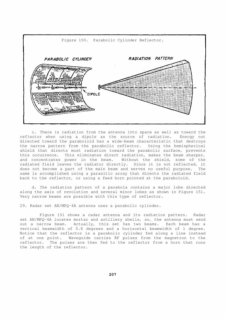
Figure 150. Parabolic Cylinder Reflector.

c. There is radiation from the antenna into space as well as toward the reflector when using a dipole as the source of radi ation. Energy not directed toward the paraboloid has a wide-beam char acteristic that destroys the narrow pattern from the parabolic reflector. U sing the hemispherical shield that directs most radiation toward the parab olic surface, prevents this occurrence. This eliminates direct radiation, makes the beam sharper, and concentrates power in the beam. Without the sh ield, some of the radiated field leaves the radiator directly. Since it is not reflected, it does not become a part of the main beam and serves no useful purpose. The same is accomplished using a parasitic array that d irects the radiated field back to the reflector, or using a feed horn pointed at the paraboloid. d. The radiation pattern of a parabola contains a major lobe directed along the axis of revolution and several minor lobe s as shown in Figure 151. Very narrow beams are possible with this type of re flector. 29. Radar set AN/MPQ-4A antenna uses a parabolic cy linder. Figure 151 shows a radar antenna and its radiatio n pattern. Radar set AN/MPQ-4A locates mortar and artillery shells, so, the antenna must send out a narrow beam. Actually, this set has two beam s. Each beam has a vertical beamwidth of 0.8 degrees and a horizontal beamwidth of 1 degree. Notice that the reflector is a parabolic cylinder f ed along a line instead of at one point. Waveguide carries RF pulses from the magnetron to the reflector. The pulses are then fed to the reflecto r from a horn that runs the length of the reflector.

207

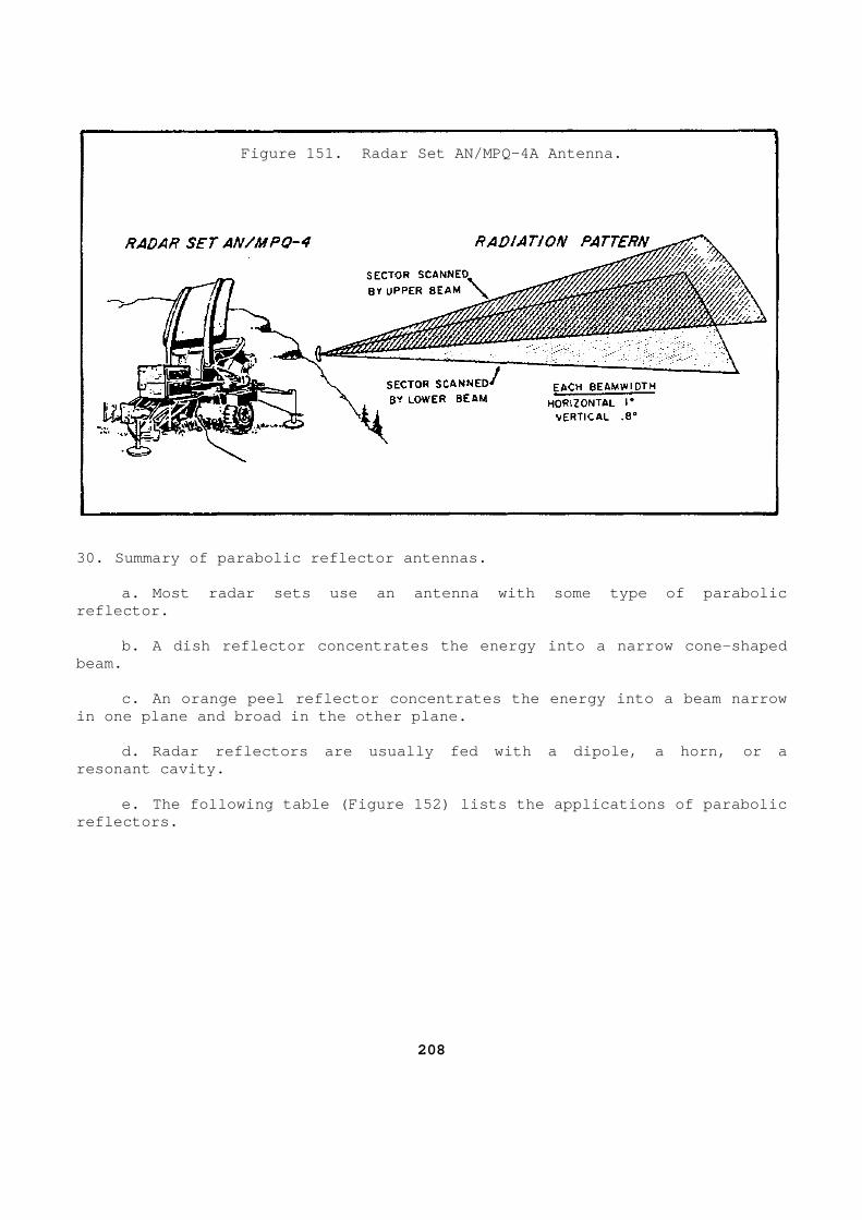
Figure 151. Radar Set AN/MPQ-4A Antenna.

30. Summary of parabolic reflector antennas. a. Most radar sets use an antenna with some type o f parabolic reflector. b. A dish reflector concentrates the energy into a narrow cone-shaped beam. c. An orange peel reflector concentrates the energ y into a beam narrow in one plane and broad in the other plane. d. Radar reflectors are usually fed with a dipole, a horn, or a resonant cavity. e. The following table (Figure 152) lists the appl ications of parabolic reflectors.

208

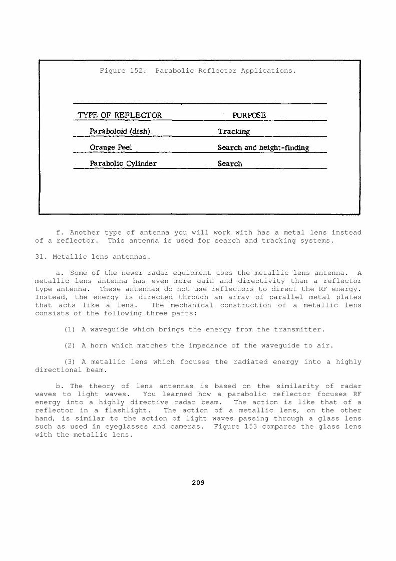
Figure 152. Parabolic Reflector Applications.

f. Another type of antenna you will work with has a metal lens instead of a reflector. This antenna is used for search an d tracking systems. 31. Metallic lens antennas. a. Some of the newer radar equipment uses the meta llic lens antenna. A metallic lens antenna has even more gain and direct ivity than a reflector type antenna. These antennas do not use reflectors to direct the RF energy. Instead, the energy is directed through an array of parallel metal plates that acts like a lens. The mechanical construction of a metallic lens consists of the following three parts: (1) A waveguide which brings the energy from the t ransmitter. (2) A horn which matches the impedance of the wave guide to air. (3) A metallic lens which focuses the radiated ene rgy into a highly directional beam. b. The theory of lens antennas is based on the sim ilarity of radar waves to light waves. You learned how a parabolic reflector focuses RF energy into a highly directive radar beam. The act ion is like that of a reflector in a flashlight. The action of a metalli c lens, on the other hand, is similar to the action of light waves passi ng through a glass lens such as used in eyeglasses and cameras. Figure 153 compares the glass lens with the metallic lens.

209

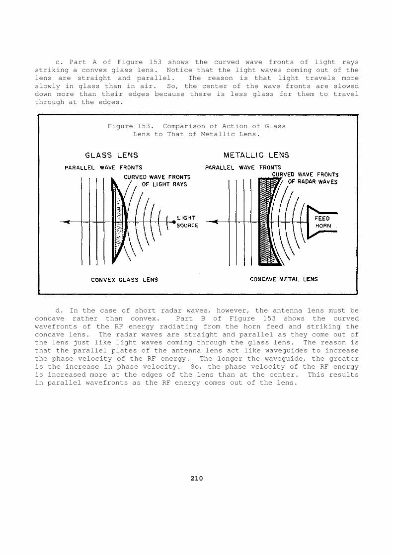
c. Part A of Figure 153 shows the curved wave fron ts of light rays striking a convex glass lens. Notice that the ligh t waves coming out of the lens are straight and parallel. The reason is that light travels more slowly in glass than in air. So, the center of the wave fronts are slowed down more than their edges because there is less gl ass for them to travel through at the edges.

Figure 153. Comparison of Action of Glass

Lens to That of Metallic Lens. d. In the case of short radar waves, however, the antenna lens must be concave rather than convex. Part B of Figure 153 s hows the curved wavefronts of the RF energy radiating from the horn feed and striking the concave lens. The radar waves are straight and par allel as they come out of the lens just like light waves coming through the g lass lens. The reason is that the parallel plates of the antenna lens act li ke waveguides to increase the phase velocity of the RF energy. The longer th e waveguide, the greater is the increase in phase velocity. So, the phase v elocity of the RF energy is increased more at the edges of the lens than at the center. This results in parallel wavefronts as the RF energy comes out o f the lens.

210

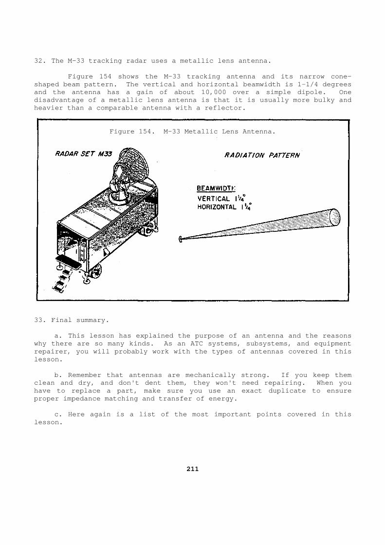
32. The M-33 tracking radar uses a metallic lens an tenna. Figure 154 shows the M-33 tracking antenna and it s narrow cone-shaped beam pattern. The vertical and horizontal b eamwidth is 1-1/4 degrees and the antenna has a gain of about 10,000 over a s imple dipole. One disadvantage of a metallic lens antenna is that it is usually more bulky and heavier than a comparable antenna with a reflector.

Figure 154. M-33 Metallic Lens Antenna.

33. Final summary. a. This lesson has explained the purpose of an ant enna and the reasons why there are so many kinds. As an ATC systems, su bsystems, and equipment repairer, you will probably work with the types of antennas covered in this lesson. b. Remember that antennas are mechanically strong. If you keep them clean and dry, and don't dent them, they won't need repairing. When you have to replace a part, make sure you use an exact duplicate to ensure proper impedance matching and transfer of energy. c. Here again is a list of the most important poin ts covered in this lesson.

211

(1) Target location in azimuth and elevation is gi ven by the physical position of the antenna. (2) Radar antennas must be highly directional so t hat they can give accurate angular information. (3) A radar antenna consists of a reflector and a feed. (4) RF energy is fed to the reflector by means of a dipole, horn, or resonant cavity. (5) The shape of the reflector depends upon the fu nction of the radar. (6) A parabolic or dish antenna, used with trackin g radars, focuses the RF energy into a narrow cone-shaped beam. (7) Parabolic cylinders and orange peel antennas a re used with search and height-finding radars. (8) An orange peel antenna used for search has a r adiation pattern that is narrow in azimuth and broad in elevation. (9) An orange peel antenna used for height-finding has a radiation pattern that is narrow in elevation and broad in az imuth. (10) A metallic lens is used with search and track ing radars. 34. Reflector feed systems. a. Conventional front feeds. In a front feed syst em, the transmission line (rigid coaxial line or waveguide) is led aroun d the edge of the antenna to the front, where it is terminated by a radiating device as shown in Figure 155.

212

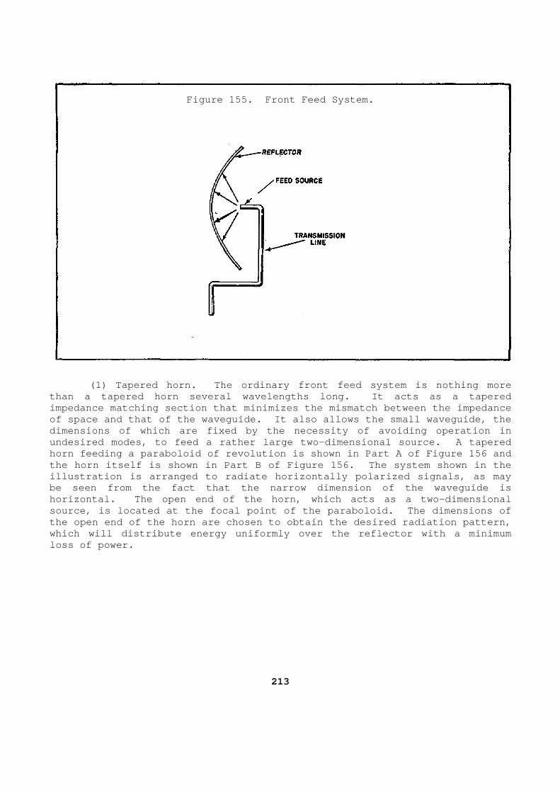
Figure 155. Front Feed System.

(1) Tapered horn. The ordinary front feed system is nothing more than a tapered horn several wavelengths long. It a cts as a tapered impedance matching section that minimizes the misma tch between the impedance of space and that of the waveguide. It also allows the small waveguide, the dimensions of which are fixed by the necessity of a voiding operation in undesired modes, to feed a rather large two-dimensi onal source. A tapered horn feeding a paraboloid of revolution is shown in Part A of Figure 156 and the horn itself is shown in Part B of Figure 156. The system shown in the illustration is arranged to radiate horizontally po larized signals, as may be seen from the fact that the narrow dimension of the waveguide is horizontal. The open end of the horn, which acts a s a two-dimensional source, is located at the focal point of the parabo loid. The dimensions of the open end of the horn are chosen to obtain the d esired radiation pattern, which will distribute energy uniformly over the ref lector with a minimum loss of power.

213

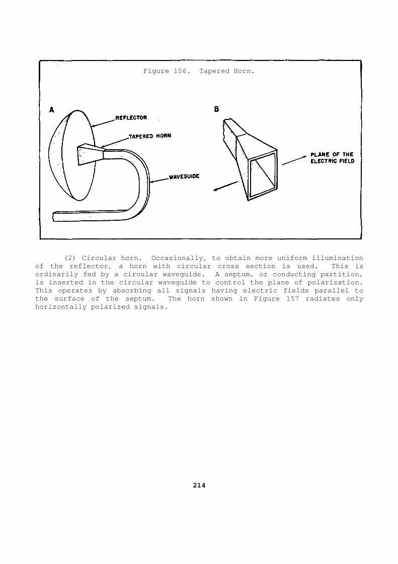
Figure 156. Tapered Horn.

(2) Circular horn. Occasionally, to obtain more u niform illumination of the reflector, a horn with circular cross sectio n is used. This is ordinarily fed by a circular waveguide. A septum, or conducting partition, is inserted in the circular waveguide to control th e plane of polarization. This operates by absorbing all signals having elect ric fields parallel to the surface of the septum. The horn shown in Figur e 157 radiates only horizontally polarized signals.

214

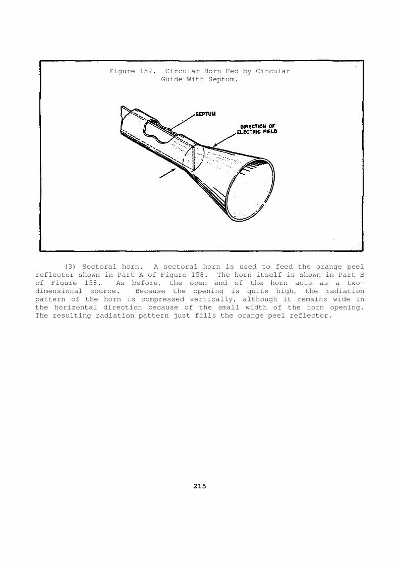
Figure 157. Circular Horn Fed by Circular

Guide With Septum. (3) Sectoral horn. A sectoral horn is used to fee d the orange peel reflector shown in Part A of Figure 158. The horn itself is shown in Part B of Figure 158. As before, the open end of the horn acts as a two-dimensional source. Because the opening is quite h igh, the radiation pattern of the horn is compressed vertically, altho ugh it remains wide in the horizontal direction because of the small width of the horn opening. The resulting radiation pattern just fills the oran ge peel reflector.

215

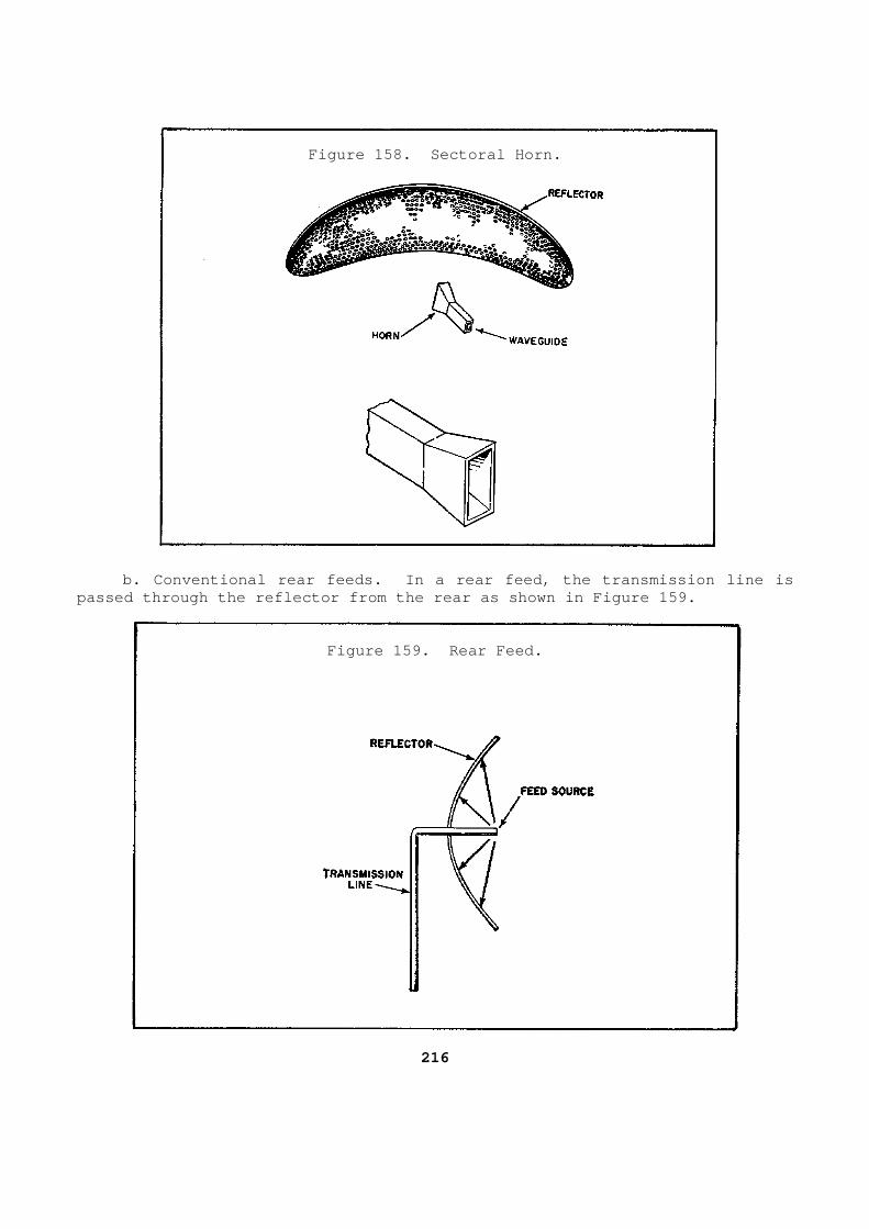
Figure 158. Sectoral Horn.

b. Conventional rear feeds. In a rear feed, the t ransmission line is passed through the reflector from the rear as shown in Figure 159.

Figure 159. Rear Feed.

216

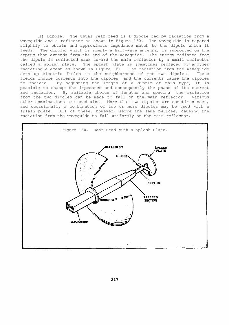
(1) Dipole. The usual rear feed is a dipole fed b y radiation from a waveguide and a reflector as shown in Figure 160. The waveguide is tapered slightly to obtain and approximate impedance match to the dipole which it feeds. The dipole, which is simply a half-wave ant enna, is supported on the septum that extends from the end of the waveguide. The energy radiated from the dipole is reflected back toward the main reflec tor by a small reflector called a splash plate. The splash plate is sometim es replaced by another radiating element as shown in Figure 161. The radi ation from the waveguide sets up electric fields in the neighborhood of the two dipoles. These fields induce currents into the dipoles, and the cu rrents cause the dipoles to radiate. By adjusting the length of a dipole of this type, it is possible to change the impedance and consequently t he phase of its current and radiation. By suitable choice of lengths and s pacing, the radiation from the two dipoles can be made to fall on the mai n reflector. Various other combinations are used also. More than two di poles are sometimes seen, and occasionally a combination of two or more dipol es may be used with a splash plate. All of these, however, serve the sam e purpose, causing the radiation from the waveguide to fall uniformly on t he main reflector.

Figure 160. Rear Feed With a Splash Plate.

217

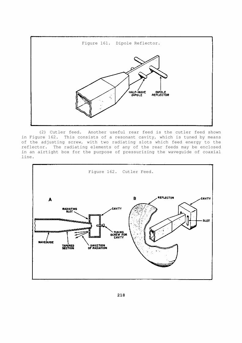
Figure 161. Dipole Reflector.

(2) Cutler feed. Another useful rear feed is the cutler feed shown in Figure 162. This consists of a resonant cavity, which is tuned by means of the adjusting screw, with two radiating slots wh ich feed energy to the reflector. The radiating elements of any of the re ar feeds may be enclosed in an airtight box for the purpose of pressurizing the waveguide of coaxial line.

Figure 162. Cutler Feed.

218

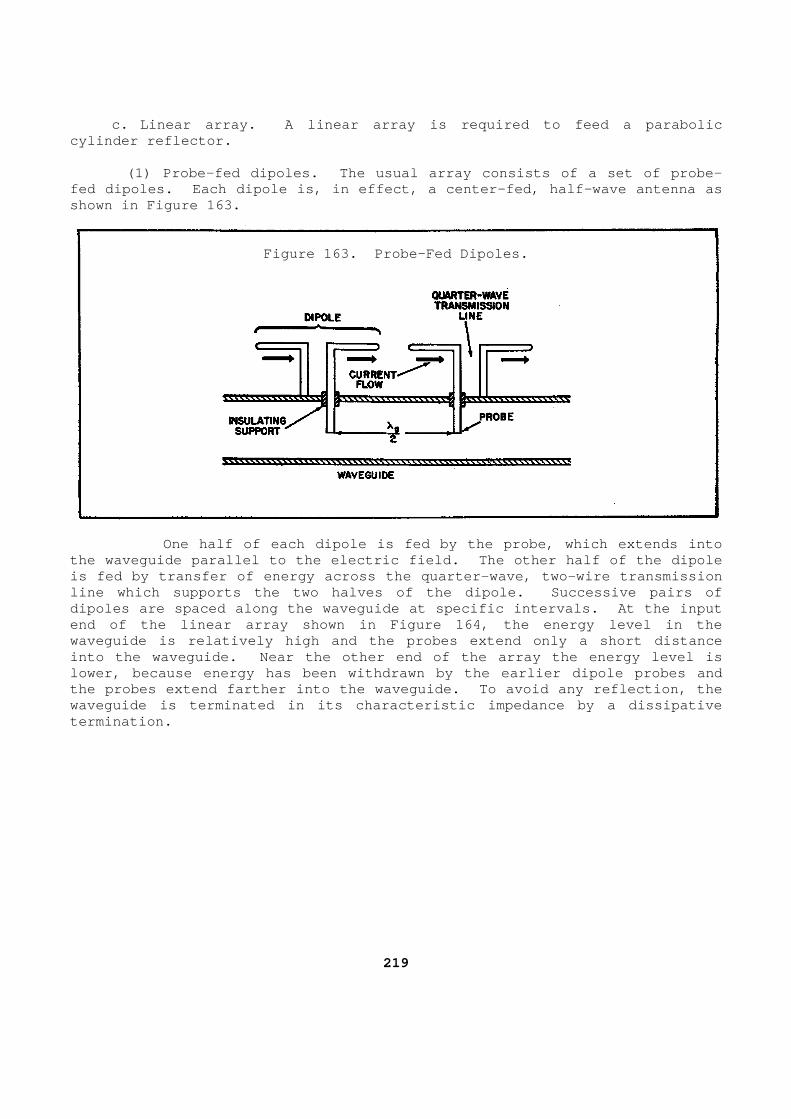
c. Linear array. A linear array is required to fe ed a parabolic cylinder reflector. (1) Probe-fed dipoles. The usual array consists o f a set of probe-fed dipoles. Each dipole is, in effect, a center-f ed, half-wave antenna as shown in Figure 163.

Figure 163. Probe-Fed Dipoles.

One half of each dipole is fed by the probe, whic h extends into the waveguide parallel to the electric field. The other half of the dipole is fed by transfer of energy across the quarter-wav e, two-wire transmission line which supports the two halves of the dipole. Successive pairs of dipoles are spaced along the waveguide at specific intervals. At the input end of the linear array shown in Figure 164, the en ergy level in the waveguide is relatively high and the probes extend only a short distance into the waveguide. Near the other end of the arra y the energy level is lower, because energy has been withdrawn by the ear lier dipole probes and the probes extend farther into the waveguide. To a void any reflection, the waveguide is terminated in its characteristic imped ance by a dissipative termination.

219

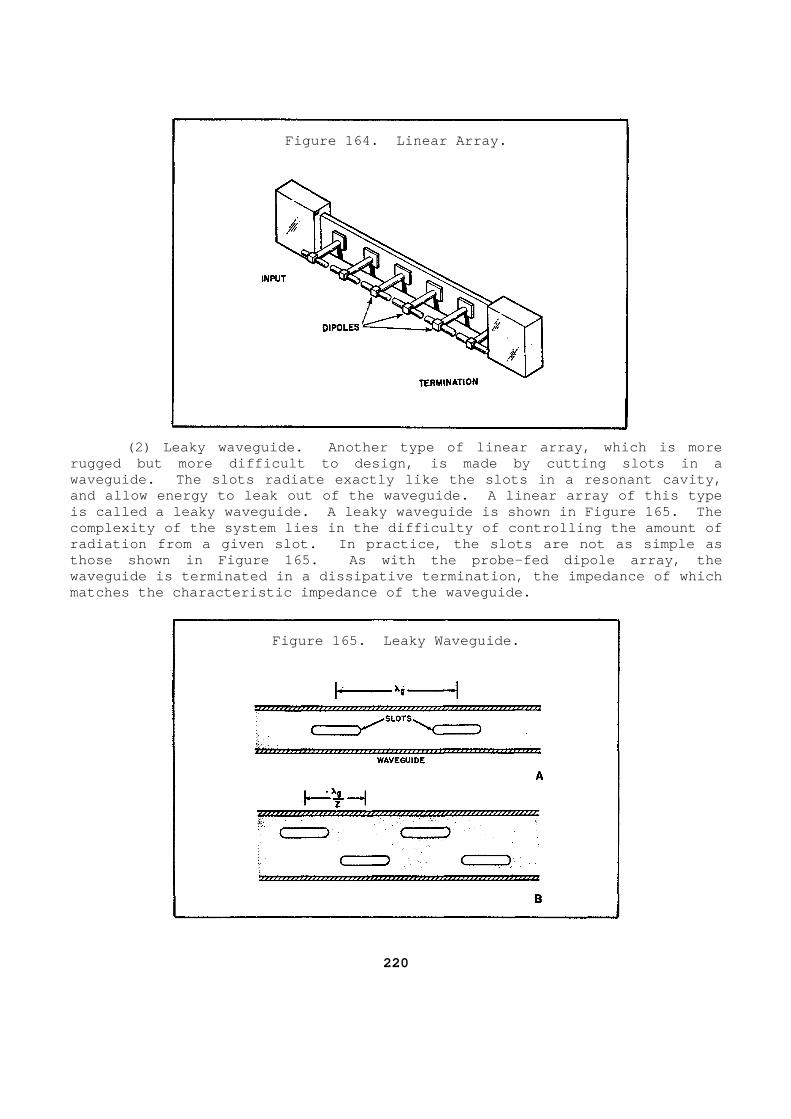
Figure 164. Linear Array.

(2) Leaky waveguide. Another type of linear array , which is more rugged but more difficult to design, is made by cut ting slots in a waveguide. The slots radiate exactly like the slot s in a resonant cavity, and allow energy to leak out of the waveguide. A l inear array of this type is called a leaky waveguide. A leaky waveguide is shown in Figure 165. The complexity of the system lies in the difficulty of controlling the amount of radiation from a given slot. In practice, the slot s are not as simple as those shown in Figure 165. As with the probe-fed d ipole array, the waveguide is terminated in a dissipative terminatio n, the impedance of which matches the characteristic impedance of the wavegui de.

Figure 165. Leaky Waveguide.

220

PRACTICE EXERCISE (Performance-Oriented)

In each of the following exercises, select the ONE answer that BEST completes the statement or answers the question. I ndicate your solution by circling the letter opposite the correct answer in the subcourse booklet. 1. The wavelength of the lowest frequency that can be sent down the

waveguide shown in Figure 130 is equal to a. the width of the waveguide. b. the height of the waveguide. c. twice the width of the waveguide. d. twice the height of the waveguide. 2. What determines the lowest frequency that a wave guide can handle? a. The length of the waveguide. b. The A dimension of the waveguide. c. The B dimension of the waveguide. d. The method of terminating the waveguide. 3. Waveguides and resonant cavities differ in the p ositioning of the E

and H fields and their terminations. The E and H f ields in a resonant cavity are

a. in phase while the E and H fields in a waveguid e are 90 degrees

out of phase. b. 90 degrees out of phase while the E and H field s in a waveguide

are in phase. c. 90 degrees out of phase while the E and H field s in a waveguide

are 180 degrees out of phase. d. 180 degrees out of phase while the E and H fiel ds in a waveguide

are 90 degrees out of phase.

221

4. Several methods of coupling are used to transfer energy into, or out of, waveguides. The device that is used to remove samples of energy from a waveguide and transfer these samples to asso ciated test equipment is a

a. directional coupler. b. dummy load. c. horn. d. loop. 5. If a rotating choke joint is used to couple two sections of waveguide

together, the two physical sections appear as one e lectrical section. Why does the choke joint make the two waveguide sec tions appear as one electrical section?

a. The choke joint appears as a half-wave open cir cuit to the

waveguides. b. The choke joint appears as a half-wave short ci rcuit to the

waveguides. c. The choke joint appears as a half-wave open cir cuit to the

waveguides. d. The choke joint appears as a quarter-wave short circuit to the

waveguides. 6. Twisted sections of waveguide must be at least t wo wavelengths long to

prevent reflections and loss of power. Twisted sec tions of waveguide are used primarily to

a. change the polarization of the waves. b. connect waveguides to directional couplers. c. connect fixed waveguides to rotating waveguides . d. match the load impedance to the characteristic impedance of the

waveguide.

222

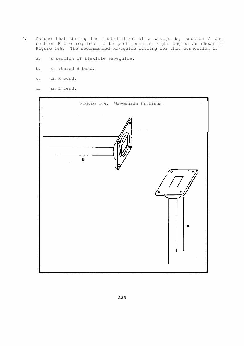
7. Assume that during the installation of a wavegui de, section A and section B are required to be positioned at right an gles as shown in Figure 166. The recommended waveguide fitting for this connection is

a. a section of flexible waveguide. b. a mitered H bend. c. an H bend. d. an E bend.

Figure 166. Waveguide Fittings.

223

8. Flexible sections of waveguide are used only whe n a special type of bend is needed. Flexible sections of waveguide are seldom used because they

a. have poor insulation. b. change the polarization of the wave. c. absorb energy in their resistive surfaces. d. cause reflections that result in a loss of powe r. 9. There are several devices used to match the load impedance to the

impedance of the waveguide. Some of these devices include the a. shutter, slug tuner, and horn. b. slug tuner, horn, and window tuner. c. window tuner, shutter, and resistive card. d. resistive card, window tuner, and slug tuner. 10. When test equipment is used to observe the tran smitted pulse spectrum,

the power level of the pulse must be reduced to pro tect the test equipment. The device that will reduce the power w ithout causing reflections in the waveguide is a

a. resistive card attenuator. b. shutter attenuator. c. window tuner. d. slug tuner.

224

11. The receiving antenna will absorb maximum energ y when the transmitting and receiving antennas are polarized identically. A horizontally polarized antenna is physically positioned

a. perpendicularly to the earth, and its electric field will be

perpendicular to the earth. b. perpendicularly to the earth, and its electric field will be

parallel to the earth. c. parallel to the earth, and its electric field w ill be

perpendicular to the earth. d. parallel to the earth, and its electric field w ill be parallel to

the earth. 12. A radar antenna system consists of a feed syste m and a reflector. The

reflector is used to a. permit the use of one antenna for both transmit ting and

receiving. b. change the polarization of the transmitted wave . c. allow the antenna to radiate in all directions. d. make the antenna directional. 13. Assume that the radar antenna shown in Figure 1 31 has a gain of 2,000.

This gain of 2,000 means that the radar antenna a. amplifies the RF power 2,000 times. b. absorbs 20 percent of the RF power. c. absorbs 2,000 times more power than a simple di pole. d. radiates 2,000 times more power than a simple d ipole. 14. A radar antenna consists of a feed and a reflec tor. The type of feed

that employs a resonant cavity to couple the RF ene rgy to the reflector is a

a. horn feed system. b. dipole feed system. c. cutler feed system. d. linear array of dipoles.

225

15. The type of radar beam that will provide accura te azimuth and elevation information is represented in SSTS 52011 in Figure

a. 154. b. 148. c. 140 B. d. 140 A. 16. The beam pattern shown in Part A of Figure 140 would provide a radar

set with accurate a. azimuth information. b. elevation information. c. azimuth and elevation information. d. azimuth, elevation, and range information. 17. The type of reflector that would produce the be am pattern shown in

Part B of Figure 140 can be described best as a a. paraboloid. b. metallic lens. c. vertically mounted orange peel. d. horizontally mounted orange peel. 18. All parabolic cylinders have one thing in commo n that makes them easy

to identify. That is, they are a. fed along a focal line rather than at a focal p oint. b. fed at a focal point rather than from a focal l ine. c. all identical in appearance. d. all fed from dipoles.

226

19. The antenna system show in Figure 167 uses a mo dified parabolic reflector to concentrate the RF energy into the des ired beam pattern. The antenna's feed system can be classified as a

a. rear feed system using a horn. b. front feed system using a horn. c. rear feed system using a dipole. d. front feed system using a dipole. 20. A radar antenna that uses a front feed system i s represented in Figure a. 139 C. b. 143. c. 149. d. 150.

227

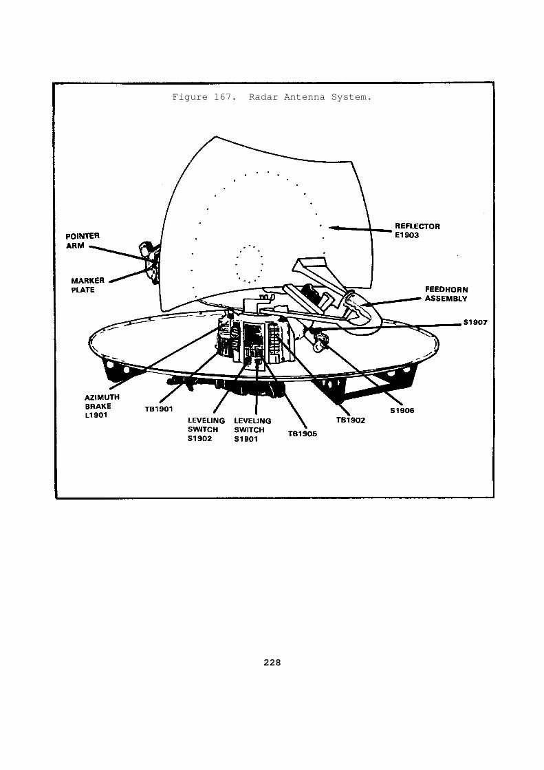
Figure 167. Radar Antenna System.

228

PRACTICE EXERCISE LESSON SOLUTIONS AV 5005 .............................. Radar Transm itters LESSON 1 .................................. Transmi ssion Lines 1. b--page 6, para 10d 2. c--page 8, para 12c, pg 7 3. b--page 10, para 15b 4. c--page 10, para 15b 5. c--page 18, SWR Formula 6. c--page 19, para 27b 7. b--page 19, para 27b 8. c--page 22, para 29b, page 28, fig 23 9. a--page 22, para 29a 10. d--page 22, para 29b A shorted quarter-wave stub will appear as a short ed half-wave stub to the second harmonic. Therefore, the impedance refl ected back to the transmission line will resemble the impedance offer ed by a series-resonant circuit. 11. a--page 29, para 2b, fig 24 12. b--page 30, para 46

229

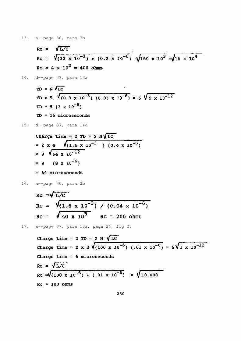
13. a--page 30, para 3b

14. d--page 37, para 13a

15. d--page 37, para 14d

16. a--page 30, para 3b

17. a--page 37, para 13a, page 34, fig 27

230

The charging resistance and the characteristic res istance of the circuit are equal and the ATL will be fully charged after 6 microseconds. Therefore, 6 microseconds after the voltage is appl ied, the voltage across the charging resistance will be equal to zero. 18. c--page 38, para 15d The pulse has a time duration of two TDs. Therefo re, the circuit will have an applied voltage equal to twice the amplitud e of the output pulse (2 x 100 = 200 volts). 19. d--page 42, para 18a, fig 34 20. d--page 43, para 18c, d LESSON 2 .................................. High-Le vel Modulation 1. c--page 68, para 6 2. c--page 71, para 2b 3. b--page 71, para 2b 4. a--page 74, para 2a 5. a--page 77, para 3c 6. b--page 81, para 2c 7. d--pages 81, 82, para 3b 8. b--page 83, para 2 9. c--page 66, para 2 When a pulse-forming network's characteristic resi stance is equal to its load resistance, the output pulse's amplitude w ill be equal to one-half the charge across the PFN. The PFN charges to twic e the input voltage. Amplitude = 30 kv/2 = 15 kv The pulse width will be equal to two TDs. Pulse width = 2 x 0.75 usec = 1.5 microseconds

231

10. d--page 73, para 1 11. c--pages 73, 76, para 3a 12. a--pages 83, 84 13. d--page 86 14. a--page 86 15. b--page 76 16. c--page 77 17. a--page 77 18. b--page 78 19. d--page 86 20. b--page 64 LESSON 3 .................................. Resonan t Cavities and Magnetrons 1. c--page 104 2. d--page 104 3. c--page 110, para 14d 4. b--page 110, para 14b 5. a--page 110, fig 77 6. b--page 112, para 17 7. d--page 113, para 21a a. Minimum output is obtained by placing a coupli ng loop at point A and parallel to the magnetic field. b. Minimum output obtained by placing the couplin g loop at point B because the magnetic field is minimum. c. The magnetic field is not at its maximum stren gth at point C; therefore, maximum output is not obtained. d. Maximum output is obtained by placing the coup ling loop at point D and placing it perpendicular to the magnetic field.

232

8. d--page 113, para 20c 9. a--page 115, para 22b 10. b--page 118, fig 82 11. c--pages 122, 123, fig 85 12. a--page 122, para e 13. a--page 127, para 11c 14. d--page 130, para 14, fig 91 15. b--page 133, para 17a 16. c--page 133, para 17a 17. c--page 135, para 19 18. a--page 134, para 18a 19. c--page 137, para a 20. a--page 141, para 29a(3) LESSON 4 .................................. Antenna s and Waveguides 1. c--page 163, para 7d 2. c--page 163, para 7d 3. b--page 164, para 10c 4. a--page 171, para 18 5. b--page 173, para 21c 6. a--page 176, para 25b 7. d--page 176, para 24, fig 122 8. d--page 177, para 26a 9. b--page 172, para 20b, page 180, para d 10. a--page 181, para 31a 11. d--page 187, para 66

233

12. d--page 199, para 20 13. c--page 192, para 11d 14. c--page 195, para 14d 15. a--page 211, para 32 16. b--page 197, para 18a 17. d--page 203, para 25 18. a--page 207, para 29 19. b--page 213, para (1), fig 155 20. c--page 205

234