Embed Size (px)
Citation preview

also in this issueBringing work home:
implications for BLS productivity
measures
The U.S. housing bubble and bust:
impacts on employment
M O N T H L Y L A B O R
R E V I E WU.S. Department of Labor U.S. Bureau of Labor Statistics
December 2010
U.S. Department of LaborHilda L. Solis, Secretary
U.S. Bureau of Labor StatisticsKeith Hall, Commissioner
The Monthly Labor Review is published monthly by the Bureau of Labor Statistics of the U.S. Department of Labor. The Review welcomes articles on employment and unemployment, compensation and working conditions, the labor force, labor-management relations, productivity and technology, occupational safety and health, demographic trends, and other economic developments.
The Review’s audience includes economists, statisticians, labor relations practitioners (lawyers, arbitrators, etc.), sociologists, and other professionals concerned with labor related issues. Because the Review presents topics in labor economics in less forbidding formats than some social science journals, its audience also includes laypersons who are interested in the topics, but are not professionally trained economists, statisticians, and so forth.
In writing articles for the Review, authors should aim at the generalists in the audience on the assumption that the specialist will understand. Authors should use the simplest exposition of the subject consonant with accuracy and adherence to scientific methods of data collection, analysis, and drawings of conclusions. Papers should be factual and analytical, not polemical in tone. Potential articles, as well as communications on editorial matters, should be submitted to:
Executive EditorMonthly Labor ReviewU.S. Bureau of Labor StatisticsRoom 2850Washington, DC 20212 Telephone: (202) 691–7911Fax: (202) 691–5908 E-mail: [email protected]
The Secretary of Labor has determined that the publication of this periodical is necessary in the transaction of the public business required by law of this Department.
The opinions, analysis, and conclusions put forth in articles written by non-BLS staff are solely the authors’ and do not necessarily reflect those of the Bureau of Labor Statistics or the Department of Labor.
Unless stated otherwise, articles appearing in this publication are in the public domain and may be reproduced without express permission from the Editor-in-Chief. Please cite the specific issue of the Monthly Labor Review as the source.
Links to non-BLS Internet sites are provided for your convenience and do not constitute an endorsement.
Information is available to sensory impaired individuals upon request:
Voice phone: (202) 691–5200Federal Relay Service: 1–800–877–8339 (toll free).
Cover Design by Bruce Boyd
BLS
BLS Regional OfficesNew EnglandConnecticutMaineMassachusettsNew HampshireRhode IslandVermontNew York–New JerseyNew JerseyNew YorkPuerto RicoU.S. Virgin IslandsMid–AtlanticPennsylvaniaDelawareDistrict of ColumbiaMarylandVirginiaWest VirginiaSoutheastAlabamaFloridaGeorgiaKentuckyMississippiNorth CarolinaSouth CarolinaTennesseeMidwestIllinoisIndianaIowaMichiganMinnesotaNebraskaNorth DakotaOhioSouth DakotaWisconsinSouthwestArkansasLouisianaNew MexicoOklahomaTexasMountain–PlainsColoradoKansasMissouriMontanaUtahWyomingWesternAlaskaArizonaCaliforniaHawaiiIdahoNevadaOregonWashington
JFK Federal BuildingRoom E-310Boston, MA 02203Phone: (617) 565–2327Fax: (617) 565–[email protected]
201 Varick Street, Room 808New York, NY 10014Phone: (646) 264–3600http://www.bls.gov/ro2/
Suite 610 East–The Curtis Center170 South Independence Mall WestPhiladelphia, PA 19106-3305Phone: (215) 597–3282
Room 7T5061 Forsyth St., S.W.Atlanta, GA 30303Phone: (404) 893–4222
Office of Economic Analysis and Information
J.C. Kluczynski Federal Office Building
Room 960230 South Dearborn StreetChicago, IL 60604Phone: (312) 353–1880Fax: (312) 353–1886
EA&I, Room 221 525 South Griffin StreetDallas, TX 75202Phone: (972) 850–4800
Two Pershing Square Building2300 Main Street, Suite 1190Kansas City, MO 64108Phone: (816) 285–7000
90 7th Street, Suite 14-100San Francisco, CA 94103Phone: (415) 625–2270Fax: (415) 625–2351
M O N T H L Y L A B O R
Volume 133, Number 12December 2010
The U.S. housing bubble and bust: impacts on employment 3Employment Projections data are used to estimate employment impactsresulting from the recent housing market cycleKathryn J. Byun
Bringing work home: implications for BLS productivity measures 18Those who bring work home work more hours, on average, than those who work only atthe workplace, but those who bring work home work fewer hours at the workplace itselfLucy P. Eldridge and Sabrina Wulff Pabilonia
ReportDuration of unemployment in States, 2007–09 36Sally L. Anderson
DepartmentsLabor month in review 2Précis 40 Book review 42Shiskin Award 44Errata: November 2009 issue 45Current labor statistics 46Index to volume 133 122
R E V I E W
Editor-in-Chief Michael D. Levi
Executive Editor William Parks II
Managing Editor Terry L. Schau
Editors Brian I. Baker Casey P. Homan
Book Review Editor James Titkemeyer
Design and LayoutCatherine D. Bowman Edith W. Peters
ContributorsJacob GalleyJohn KrantzMaureen Soyars
2 Monthly Labor Review • December 2010
Labor Month In Review
The December Review
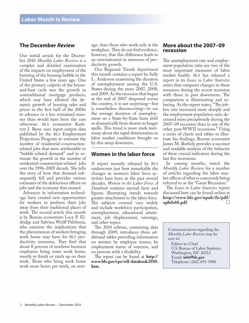
Our initial article for the Decem-ber 2010 Monthly Labor Review is a complex and detailed examination of the impacts on employment of the bursting of the housing bubble in the United States a few years ago. One of the primary culprits of the boom-and-bust cycle was the growth in nontraditional mortgage products, which may have allowed the dy-namic growth of housing sales and prices in the first half of the 2000s to advance in a less restrained man-ner than would have been the case otherwise. BLS economist Kath-ryn J. Byun uses input–output data published by the BLS Employment Projections Program to estimate the number of residential-construction-related jobs that were attributable to “bubble-related demand” and to es-timate the growth in the number of residential-construction-related jobs over the 1996–2005 decade. She tells the story of how that demand sub-sequently fell and provides various estimates of the deleterious effects on jobs and the economy that ensued.
Advances in information technol-ogy have created new opportunities for workers to perform their jobs away from their traditional places of work. The second article this month is by Bureau economists Lucy P. El-dridge and Sabrina Wulff Pabilonia, who examine the implications that the phenomenon of workers bringing work home may have for BLS pro-ductivity measures. They find that about 8 percent of nonfarm business employees bring some work home, mostly to finish or catch up on their work. Those who bring work home work more hours per week, on aver-
age, than those who work only at the workplace. They do not find evidence, however, that this difference leads to an overstatement in measures of pro-ductivity growth.
Our Regional Trends department this month contains a report by Sally L. Anderson examining the duration of unemployment among the U.S. States during the years 2007, 2008, and 2009. As the recession that began at the end of 2007 deepened across the country, it is not surprising—but is nonetheless disconcerting—to see the average duration of unemploy-ment on a State-by-State basis shift so dramatically from shorter to longer spells. This trend is more stark testi-mony about the rapid deterioration in labor market conditions brought on by this steep downturn.
Women in the labor force
A report recently released by BLS underscores just how remarkable the changes in women’s labor force ac-tivities have been in the past several decades. Women in the Labor Force: A Databook contains myriad facts and figures illustrating trends towards greater attachment to the labor force. The subjects covered vary widely and include workforce participation, unemployment, educational attain-ment, job displacement, earnings, and other topics.
The 2010 edition, containing data through 2009, introduces three ad-ditional tables providing information on women by employee tenure, by employment status of veterans, and on persons with a disability.
The report can be found at http://www.bls.gov/cps/wlf-databook2010.htm.
More about the 2007–09 recession
The unemployment rate and employ-ment-population ratio are two of the most important measures of labor market health. BLS has released a report in its Issues in Labor Statistics series that compares changes in these measures during the recent recession with those in past downturns. The comparison is illuminating and so-bering. As the report states, “The job-less rate increased more sharply and the employment-population ratio de-creased more precipitously during the 2007–09 recession than in any of the other post-WWII recessions.” Using a series of charts and tables to illus-trate his findings, Bureau economist James M. Borbely provides a succinct and readable analysis of the behavior of these crucial indicators during the last five recessions.
In coming months, watch the Monthly Labor Review for a number of articles regarding the labor mar-ket effects of what is commonly being referred to as the “Great Recession.”
The Issues in Labor Statistics report discussed here can be found online at http://www.bls.gov/opub/ils/pdf/opbils88.pdf.
Communications regarding the Monthly Labor Review may be sent to:
Editor-in-Chief U.S. Bureau of Labor Statistics Washington, DC 20212 Email: [email protected]: (202) 691-5900
Monthly Labor Review • December 2010 3
Housing Bubble and Bust
The U.S. housing bubble and bust: impacts on employmentEmployment Projections Program data are used to estimate employment impacts due to the recent housing market cycle, and alternative “nonbubble” demand scenarios indicate that at the peak of the bubble, in 2005, approximately 1.2 million to 1.7 million residential-construction-related jobs were attributable to “bubble-related demand”
Kathryn J. Byun
Kathryn J. Byun is an economist in the Division of Industry Employment Projections, Office of Occupational Statistics and Employment Projections, Bureau of Labor Statistics. E-mail: [email protected].
Several years ago, conditions in the U.S. economy—such as ease in the credit market—worked to create
a prime situation for the first national bubble in U.S. home prices since that which preceded the Great Depression.1 Generally, housing demand is restrained as prices rise in the market because buyers can no longer qualify for traditional loans. New “affordability” mortgage products considerably relaxed this restraint, thereby allowing the recent boom period to con-tinue much longer than previous expan-sionary periods. Nontraditional loans were increasingly granted with fewer require-ments for buyers to provide documenta-tion to verify that their income could sup-port the mortgage payment.2 Moreover, these loans were often granted with little or no down payment. Mortgage-backed securities also contributed to the bubble by increasingly financing these high-risk loans throughout the bubble years.
By late 2005, the rapid growth of in-vestment in residential structures had come to an end. Shortly thereafter, other indications of the oncoming bust became visible. First-time home buyers were in-
creasingly priced out of the market, mortgage rates rose by roughly 1 percent, affordability of homes decreased substantially, and speculators pulled out of the market. The market correc-tion has been much more abrupt than the onset of the bubble. Roughly a decade of growth of investment in residential structures was elimi-nated over just 3 years—from 2005 to 2008. Home prices, as measured by Robert Shiller’s real price index, have fallen considerably from their peak in 2006 to levels more consistent with earlier data. Whether or not the bottom of the cycle has been reached is not yet clear, as recent housing data remain relatively mixed.
The recent dynamic housing market cycle has had a considerable impact on the U.S. job market. Input–output (I–O) data published by the BLS Employment Projections Program (EPP) can be used to estimate the number of jobs related to residential construction spend-ing, employment that includes jobs in the con-struction sector and jobs in all the industries that supply intermediate products and services demanded by residential construction. On the basis of I–O calculations presented later in this article, EPP estimates that demand for resi-dential construction grew from supporting 5.5 million jobs, or 4.2 percent of all U.S. employ-
Housing Bubble and Bust
4 Monthly Labor Review • December 2010
ment, in 1996, to 7.4 million jobs, or 5.1 percent of total employment, at the peak of the cycle in 2005. As the housing market crashed, residential-construction-related employment fell substantially; it was at 4.5 mil-lion in 2008, accounting for only 3.0 percent of total U.S. jobs.
Not all of the employment growth during the ex-pansionary period is necessarily related to the bubble, as some increases would have been expected with an expanding population and normal economic growth. Given an alternative “nonbubble” demand scenario, I–O analysis allows one to estimate how much of the job growth was due to the bubble as opposed to “nor-mal” economic growth. The estimated alternative de-mand is necessarily an approximation. The uncertainty of the start date of the recent housing cycle makes de-termining “nonbubble” demand an even more difficult exercise at this time.
In order to account for the uncertainty of the timing of the bubble’s onset, two possible start dates of the housing market bubble are evaluated, 1996 and 2002, allowing for a range of estimated impacts. Two models are considered to estimate nonbubble demand: Be-cause BLS projections do not forecast business cycle ac-tivity and instead focus on long-run trends, previously published projections serve as one tool for approximat-ing nonbubble demand, and a naïve constant growth model serves as the second tool. Depending on the start date, the bubble is estimated to have contributed somewhere between 1.2 million and 1.7 million jobs in 2005, accounting for 0.8 percent to 1.2 percent of total U.S. employment. The housing market correction has also had a considerable effect on the U.S. job market. Residential-construction-related jobs are estimated to have been 1.7 million to 2.2 million fewer in 2008 than they would have been had there not been a bubble. Ac-cording to these estimates and the embedded assump-tions, the bust pulled down 2008 U.S. employment by 1.1 percent to 1.5 percent.
In the sections that follow, the housing bubble is an-alyzed through demand and price data. Construction sector employment data are discussed as inputs into EPP’s employment requirements table and as a com-monly cited measure of the employment impacts of the housing market. EPP’s methods are discussed, and estimates of “residential-construction-related employ-ment” during the recent boom-and-bust cycle are pre-sented. Finally, growth scenarios based on nonbubble demand are considered in order to estimate how the housing boom and bust have affected U.S. employment.
Bubble period
An economic bubble occurs when “trade is in high volumes at prices that are considerably at variance with intrinsic values.”3
The data discussed in this section show unusual growth and falloff in demand for housing and an unprecedented rise and decline in real home prices; behavior indicative of a bubble. Although the rise in demand in the U.S housing market that occurred through 2005 is now widely referred to as a bubble, when this bubble began is not yet apparent. This is still the subject of much debate and may never be clear, but certainly not until the trough is long past. However, in order to discuss the behavior and impacts of the housing bubble and crash, it is first necessary to come to some decision on when the bubble occurred.
Relying upon input–output analysis, the research presented in this article utilizes the measure of investment in residential structures, as calculated with Bureau of Economic Analysis (BEA) final-demand data, as the metric of the relative size of growth and decline over the housing bubble and bust.4 The final-demand data show that the climax of the bubble was in 2005, so that year will serve as the endpoint in this analysis. It should be noted, however, that other housing market mea-sures did not peak until 2006, including the price index and industry employment data, examined later.
In the demand data, the bubble’s starting point is much less apparent than its endpoint. The expansionary period started in 1991, but when this growth became a bubble is debatable. Many different start dates have been discussed, but years from the late 1990s and early 2000s are the most often suggested. Some people, including Thomas Lawler, an inde-pendent analyst who worked for Fannie Mae from 1984 to 2006, contend the bubble started in 2002. Lawler claims that, as the tech-stock bubble came to an end in 2000, investors fo-cused on real estate as an alternative investment vehicle. The low interest rates set by the Federal Reserve over the follow-ing few years provided further incentive for home buying. He further asserts that relaxed lending standards helped demand continue when prices reached levels that most people could not otherwise have afforded.5
Others contend the bubble began much earlier. For ex-ample, Dean Baker, codirector of the Center for Economic and Policy Research, argues the bubble started in 1997. Baker holds that the runup in demand and prices for housing was in large part due to the increased trade deficit and financial mar-ket deregulation in the 1990s.6 Robert Shiller has pointed out that prices, as measured by the Case–Shiller 10-city home price index, rose from 1995 to 2006, and he therefore refers to this as the boom period.7 As explained earlier, for the purpose of this article, two potential start dates will be examined, al-
Monthly Labor Review • December 2010 5
lowing for comparisons between a lengthier bubble and a shorter one: 1996, between the onset of the runup in prices and Baker’s asserted bubble start date, and 2002, as proposed by Lawler.
Measures of the bubble and bust
Several measures of the bubble and bust are presented here in order to compare data on the magnitude of growth and decline during the bubble and bust years. Although the price data offer important information regarding certain economic effects, residential-construction-relat-ed employment over the recent bubble and bust years has more closely tracked measurements related to the demand for homes than the prices paid for the homes. Regardless, I–O analysis dictates that final-demand data be used to gauge the magnitude of the bubble. Other demand-related estimates of housing market activity are presented here as comparative measures of the housing bubble and the bust. The alternative data sources offer measures of the relative size of the bubble and bust that are similar to those in the final-demand data. The simi-larity in data lends support to the use of final demand as an acceptable metric to gauge the impact of the housing
bubble and bust on U.S. employment.
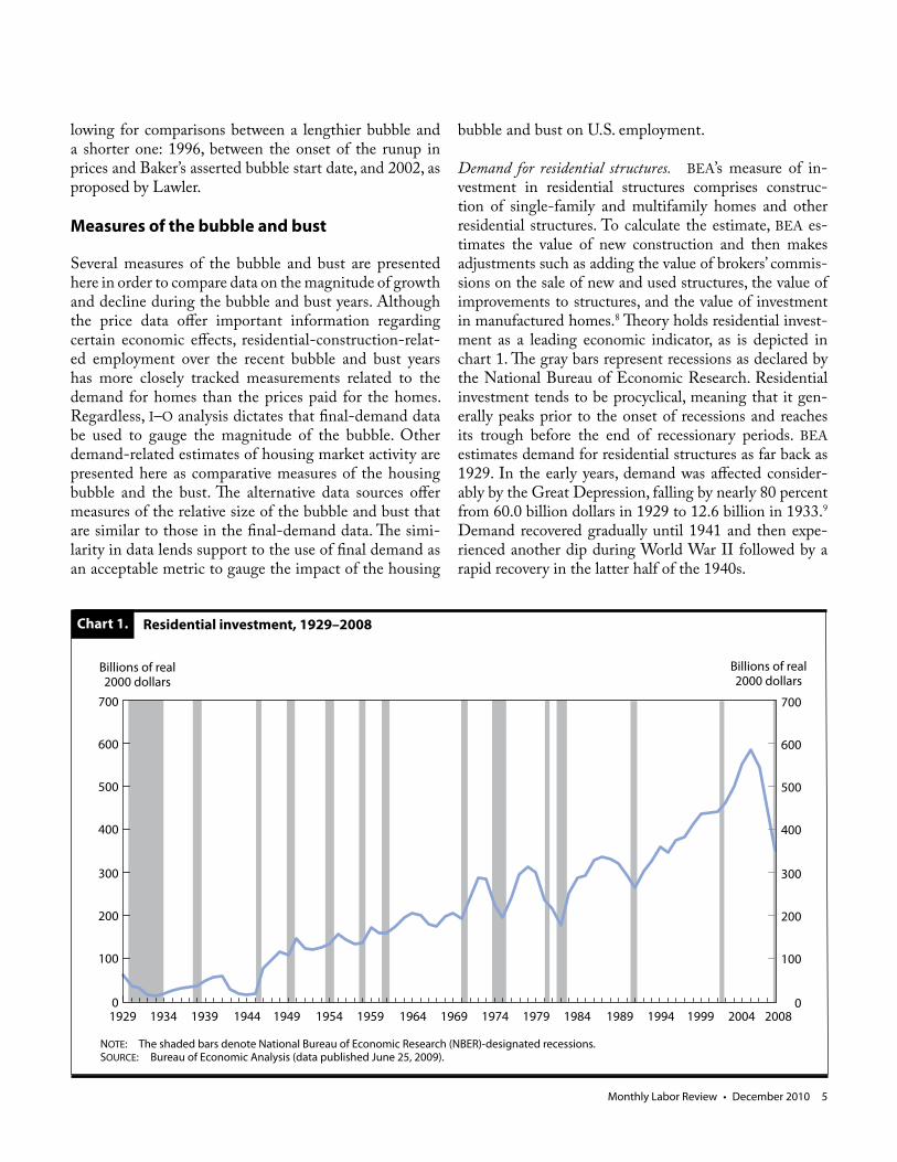
Demand for residential structures. BEA’s measure of in-vestment in residential structures comprises construc-tion of single-family and multifamily homes and other residential structures. To calculate the estimate, BEA es-timates the value of new construction and then makes adjustments such as adding the value of brokers’ commis-sions on the sale of new and used structures, the value of improvements to structures, and the value of investment in manufactured homes.8 Theory holds residential invest-ment as a leading economic indicator, as is depicted in chart 1. The gray bars represent recessions as declared by the National Bureau of Economic Research. Residential investment tends to be procyclical, meaning that it gen-erally peaks prior to the onset of recessions and reaches its trough before the end of recessionary periods. BEA estimates demand for residential structures as far back as 1929. In the early years, demand was affected consider-ably by the Great Depression, falling by nearly 80 percent from 60.0 billion dollars in 1929 to 12.6 billion in 1933.9 Demand recovered gradually until 1941 and then expe-rienced another dip during World War II followed by a rapid recovery in the latter half of the 1940s.
Chart 1. Residential investment, 1929–2008
1929 1934 1939 1944 1949 1954 1959 1964 1969 1974 1979 1984 1989 1994 1999 2004 2008
NOTE: The shaded bars denote National Bureau of Economic Research (NBER)-designated recessions.SOURCE: Bureau of Economic Analysis (data published June 25, 2009).
Billions of real 2000 dollars
Billions of real 2000 dollars
700
600
500
400
300
200
100
0
700
600
500
400
300
200
100
0
Housing Bubble and Bust
6 Monthly Labor Review • December 2010
Growth was somewhat more stable in the 1950s and 1960s, with more moderate declines during economic downturns. Its behavior then became more dynamic start-ing in the 1970s. Demand experienced peaks followed by troughs around the time of the 1970s oil crises and the energy crisis in 1979. Investment in residential construc-tion once again struggled during the “double-dip reces-sions” in 1980 and 1982 while buyers faced record-high mortgage rates. As the economy recuperated and interest rates declined, demand recovered until the onset of the savings and loan crisis in the late 1980s. Demand then continued to fall through the recession of 1990–91.
Residential construction then underwent an unprec-edented expansionary period that consisted of 14 years of positive growth over 1991–2005, with the exception of a slight decline over 1994–95. Growth in demand over the 1991–2005 period was more than double that of any other expansionary period in the U.S. housing market since 1950. For the first time in the post-World War II era, an expansionary period continued throughout a re-cession. In fact, some argue that appreciation in home prices stimulated consumer spending and thereby helped to keep the 2001 recession relatively short and shallow.10
Annual growth rates of demand over this expansionary
period were moderate given historical behavior; however, by 2005, 14 years of growth had left demand far above what would be expected given the long-run trend.
Demand more than doubled from 1991 to 2005, from 264.0 billion real dollars to 586.0 billion. Some of this expansion was to be expected as a result of normal cycli-cal activity. From 1996 (one of the years considered as a starting point for the bubble) to 2005, demand increased by 210.9 billion dollars, with average annual growth of 5.1 percent. More than half of the growth, 123.8 billion, oc-curred between 2002 and 2005, when demand grew much faster—by 8.2 percent annually. After the bubble period came to an end, in just 3 years demand fell back to 351.3 billion (the 2008 figure), near the 1995 level.
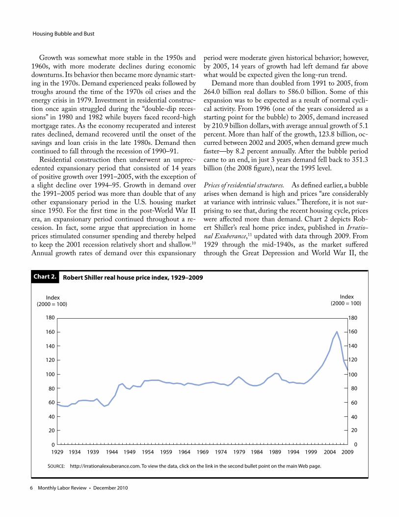
Prices of residential structures. As defined earlier, a bubble arises when demand is high and prices “are considerably at variance with intrinsic values.” Therefore, it is not sur-prising to see that, during the recent housing cycle, prices were affected more than demand. Chart 2 depicts Rob-ert Shiller’s real home price index, published in Irratio-nal Exuberance,11 updated with data through 2009. From 1929 through the mid-1940s, as the market suffered through the Great Depression and World War II, the
Chart 2.
180
160
140
120
100
80
60
40
20
0
Robert Shiller real house price index, 1929–2009
SOURCE: http://irrationalexuberance.com. To view the data, click on the link in the second bullet point on the main Web page.
Index(2000 = 100)
180
160
140
120
100
80
60
40
20
0
Index(2000 = 100)
1929 1934 1939 1944 1949 1954 1959 1964 1969 1974 1979 1984 1989 1994 1999 2004 2009
Monthly Labor Review • December 2010 7
Shiller real home price index stayed close to 60. During the mid-1940s, prices exhibited rapid growth, and the in-dex reached 86.6 in 1947. Prices then remained relatively stable through the late 1990s, with the exception of some cyclical activity in the late 1970s and late 1980s. Outside of the Great Depression and recent bubble period, home prices have closely followed changes to overall prices as measured by the Consumer Price Index. From 1996 to 2006, the Shiller real price index nearly doubled, from 87.0 to 160.6, with 65.7 percent of this growth occurring from 2002 to 2006. Prices quickly plunged thereafter, and the index was at 105.7 in 2009. This surge in growth fol-lowed by rapid decline is unprecedented in the history of U.S. real housing prices.
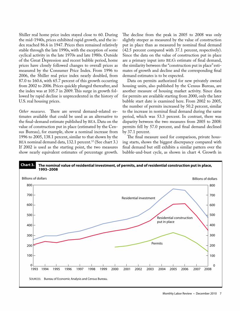
Other measures. There are several demand-related es-timates available that could be used as an alternative to the final-demand estimate published by BEA. Data on the value of construction put in place (estimated by the Cen-sus Bureau), for example, show a nominal increase from 1996 to 2005, 138.1 percent, similar to that shown by the BEA nominal demand data, 132.1 percent.12 (See chart 3.) If 2002 is used as the starting point, the two measures show nearly equivalent estimates of percentage growth.
The decline from the peak in 2005 to 2008 was only slightly steeper as measured by the value of construction put in place than as measured by nominal final demand (42.5 percent compared with 37.1 percent, respectively). Since the data on the value of construction put in place are a primary input into BEA’s estimate of final demand, the similarity between the “construction put in place” esti-mates of growth and decline and the corresponding final demand estimates is to be expected.
Data on permits authorized for new privately owned housing units, also published by the Census Bureau, are another measure of housing market activity. Since data for permits are available starting from 2000, only the later bubble start date is examined here. From 2002 to 2005, the number of permits increased by 50.2 percent, similar to the increase in nominal final demand during the same period, which was 53.3 percent. In contrast, there was disparity between the two measures from 2005 to 2008: permits fell by 57.0 percent, and final demand declined by 37.1 percent.
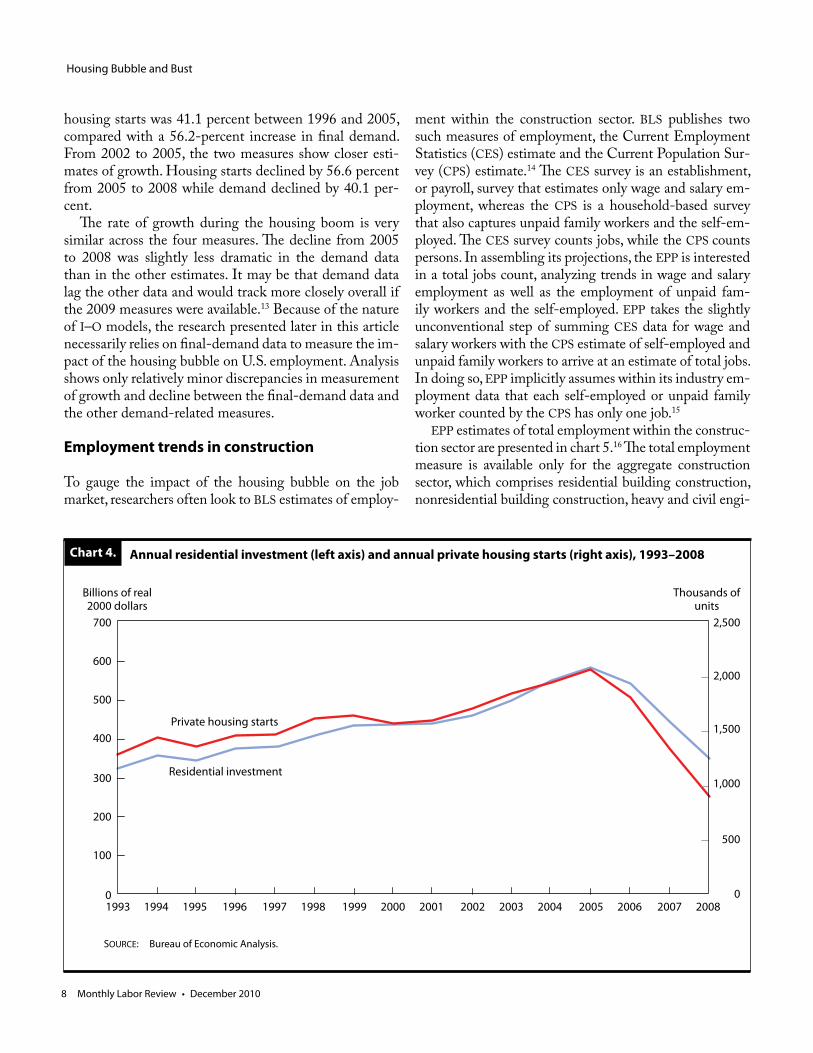
The final measure used for comparison, private hous-ing starts, shows the biggest discrepancy compared with final demand but still exhibits a similar pattern over the bubble-and-bust cycle, as shown in chart 4. Growth in
Chart 3.
Billions of dollars Billions of dollars
800
700
600
500
400
300
200
100
0
The nominal value of residential investment, of permits, and of residential construction put in place, 1993–2008
SOURCES: Bureau of Economic Analysis and Census Bureau.
1993 1994 1995 1996 1997 1998 1999 2000 2001 2002 2003 2004 2005 2006 2007 2008
800
700
600
500
400
300
200
100
0
Residential investment
Residential constructionput in place
Permits
Housing Bubble and Bust
8 Monthly Labor Review • December 2010
Chart 4.
Billions of real 2000 dollars
Thousands of units
700
600
500
400
300
200
100
0
Annual residential investment (left axis) and annual private housing starts (right axis), 1993–2008
SOURCE: Bureau of Economic Analysis.
Private housing starts
Residential investment
2,500
2,000
1,500
1,000
500
01993 1994 1995 1996 1997 1998 1999 2000 2001 2002 2003 2004 2005 2006 2007 2008
housing starts was 41.1 percent between 1996 and 2005, compared with a 56.2-percent increase in final demand. From 2002 to 2005, the two measures show closer esti-mates of growth. Housing starts declined by 56.6 percent from 2005 to 2008 while demand declined by 40.1 per-cent.
The rate of growth during the housing boom is very similar across the four measures. The decline from 2005 to 2008 was slightly less dramatic in the demand data than in the other estimates. It may be that demand data lag the other data and would track more closely overall if the 2009 measures were available.13 Because of the nature of I–O models, the research presented later in this article necessarily relies on final-demand data to measure the im-pact of the housing bubble on U.S. employment. Analysis shows only relatively minor discrepancies in measurement of growth and decline between the final-demand data and the other demand-related measures.
Employment trends in construction
To gauge the impact of the housing bubble on the job market, researchers often look to BLS estimates of employ-
ment within the construction sector. BLS publishes two such measures of employment, the Current Employment Statistics (CES) estimate and the Current Population Sur-vey (CPS) estimate.14 The CES survey is an establishment, or payroll, survey that estimates only wage and salary em-ployment, whereas the CPS is a household-based survey that also captures unpaid family workers and the self-em-ployed. The CES survey counts jobs, while the CPS counts persons. In assembling its projections, the EPP is interested in a total jobs count, analyzing trends in wage and salary employment as well as the employment of unpaid fam-ily workers and the self-employed. EPP takes the slightly unconventional step of summing CES data for wage and salary workers with the CPS estimate of self-employed and unpaid family workers to arrive at an estimate of total jobs. In doing so, EPP implicitly assumes within its industry em-ployment data that each self-employed or unpaid family worker counted by the CPS has only one job.15
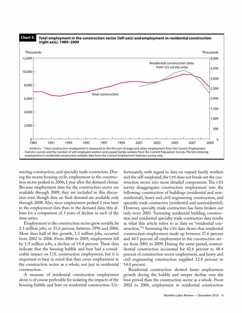
EPP estimates of total employment within the construc-tion sector are presented in chart 5.16 The total employment measure is available only for the aggregate construction sector, which comprises residential building construction, nonresidential building construction, heavy and civil engi-
Monthly Labor Review • December 2010 9
neering construction, and specialty trade contractors. Dur-ing the recent housing cycle, employment in the construc-tion sector peaked in 2006, 1 year after the demand climax. Because employment data for the construction sector are available through 2009, they are included in this discus-sion even though data on final demand are available only through 2008. Also, since employment peaked 1 year later in the employment data than in the demand data, this al-lows for a comparison of 3 years of decline in each of the time series.
Employment in the construction sector grew notably, by 2.3 million jobs, or 31.6 percent, between 1996 and 2006. More than half of this growth, 1.3 million jobs, occurred from 2002 to 2006. From 2006 to 2009, employment fell by 1.9 million jobs, a decline of 19.4 percent. These data indicate that the housing bubble and bust had a consid-erable impact on U.S. construction employment, but it is important to bear in mind that they cover employment in the construction sector as a whole, not just in residential construction.
A measure of residential construction employment alone is of course preferable for isolating the impacts of the housing bubble and bust on residential construction. Un-
fortunately, with regard to data on unpaid family workers and the self-employed, the CPS does not break out the con-struction sector into more detailed components. The CES survey disaggregates construction employment into the following: construction of buildings (residential and non-residential), heavy and civil engineering construction, and specialty trade contractors (residential and nonresidential). However, specialty trade contractors has been broken out only since 2001. Summing residential building construc-tion and residential specialty trade contractors data results in what this article refers to as data on “residential con-struction.”18 Summing the CES data shows that residential construction employment made up between 37.6 percent and 44.5 percent all employment in the construction sec-tor from 2001 to 2009. During the same period, nonresi-dential construction accounted for 42.6 percent to 48.4 percent of construction sector employment, and heavy and civil engineering construction supplied 12.8 percent to 14.0 percent.
Residential construction showed faster employment growth during the bubble and steeper decline over the bust period than the construction sector as a whole. From 2002 to 2006, employment in residential construction
Chart 5.
Thousands Thousands
12,000
10,000
8,000
6,000
4,000
2,000
0
Total employment in the construction sector (left axis) and employment in residential construction (right axis), 1989–2009
SOURCES: Total construction employment is measured as the the sum of wage and salary employment from the Current Employment Statistics survey and the number of self-employed workers and unpaid family workers from the Current Population Survey. The line showing employment in residential construction exhibits data from the Current Employment Statistics survey only.
1989 1991 1993 1995 1997 1999 2001 2003 2005 2007 2009
Total construction
Residential construction (data from CES survey only)
4,000
3,500
3,000
2,500
2,000
1,500
1,000
500
0
Housing Bubble and Bust
10 Monthly Labor Review • December 2010
increased by 26.6 percent, considerably faster than the 15.4-percent growth in the construction sector as a whole. Of the 1.3 million jobs added in construction, more than half—715,000—were in residential construction. From 2006 to 2009, wage and salary employment within resi-dential construction industries declined by 1.1 million, or 33.4 percent, while the total number of construction jobs fell by 1.9 million, or 19.4 percent.
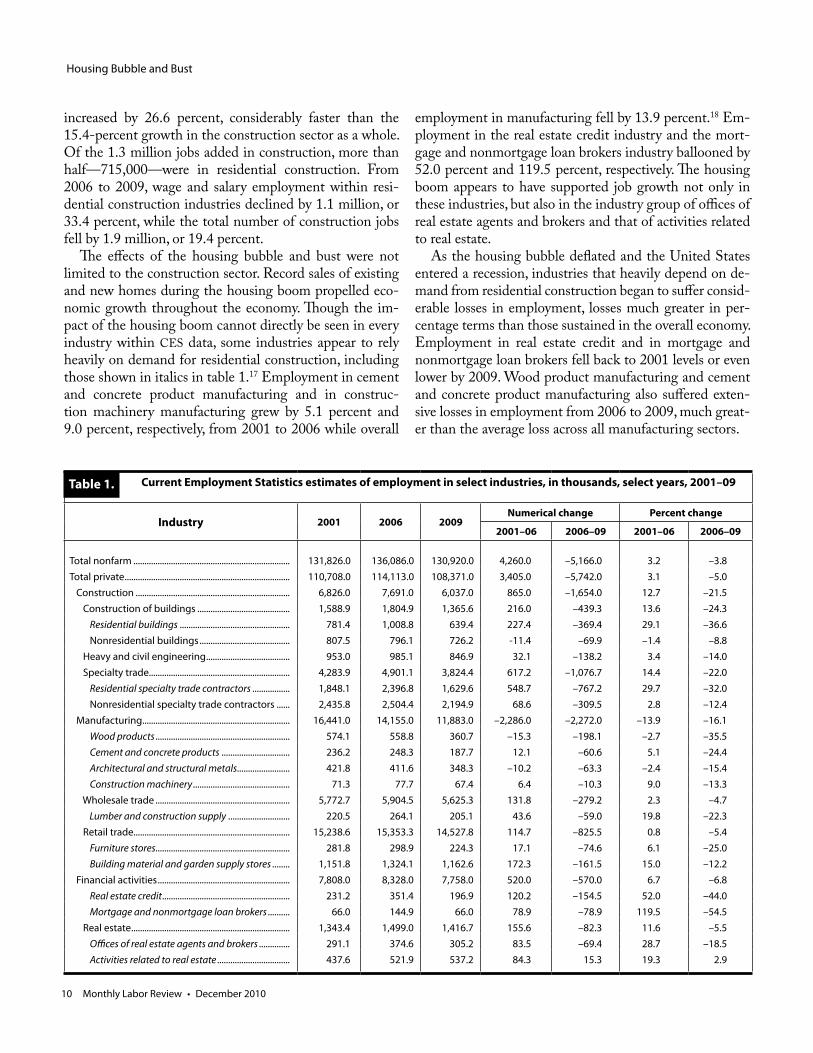
The effects of the housing bubble and bust were not limited to the construction sector. Record sales of existing and new homes during the housing boom propelled eco-nomic growth throughout the economy. Though the im-pact of the housing boom cannot directly be seen in every industry within CES data, some industries appear to rely heavily on demand for residential construction, including those shown in italics in table 1.17 Employment in cement and concrete product manufacturing and in construc-tion machinery manufacturing grew by 5.1 percent and 9.0 percent, respectively, from 2001 to 2006 while overall
employment in manufacturing fell by 13.9 percent.18 Em-ployment in the real estate credit industry and the mort-gage and nonmortgage loan brokers industry ballooned by 52.0 percent and 119.5 percent, respectively. The housing boom appears to have supported job growth not only in these industries, but also in the industry group of offices of real estate agents and brokers and that of activities related to real estate.
As the housing bubble deflated and the United States entered a recession, industries that heavily depend on de-mand from residential construction began to suffer consid-erable losses in employment, losses much greater in per-centage terms than those sustained in the overall economy. Employment in real estate credit and in mortgage and nonmortgage loan brokers fell back to 2001 levels or even lower by 2009. Wood product manufacturing and cement and concrete product manufacturing also suffered exten-sive losses in employment from 2006 to 2009, much great-er than the average loss across all manufacturing sectors.
Current Employment Statistics estimates of employment in select industries, in thousands, select years, 2001–09
Industry 2001 2006 2009Numerical change Percent change
2001–06 2006–09 2001–06 2006–09
Total nonfarm ....................................................................... 131,826.0 136,086.0 130,920.0 4,260.0 –5,166.0 3.2 –3.8Total private ........................................................................... 110,708.0 114,113.0 108,371.0 3,405.0 –5,742.0 3.1 –5.0 Construction ...................................................................... 6,826.0 7,691.0 6,037.0 865.0 –1,654.0 12.7 –21.5 Construction of buildings .......................................... 1,588.9 1,804.9 1,365.6 216.0 –439.3 13.6 –24.3 Residential buildings .................................................. 781.4 1,008.8 639.4 227.4 –369.4 29.1 –36.6 Nonresidential buildings ......................................... 807.5 796.1 726.2 -11.4 –69.9 –1.4 –8.8 Heavy and civil engineering ...................................... 953.0 985.1 846.9 32.1 –138.2 3.4 –14.0 Specialty trade................................................................ 4,283.9 4,901.1 3,824.4 617.2 –1,076.7 14.4 –22.0 Residential specialty trade contractors ................. 1,848.1 2,396.8 1,629.6 548.7 –767.2 29.7 –32.0 Nonresidential specialty trade contractors ...... 2,435.8 2,504.4 2,194.9 68.6 –309.5 2.8 –12.4 Manufacturing ................................................................... 16,441.0 14,155.0 11,883.0 –2,286.0 –2,272.0 –13.9 –16.1 Wood products ............................................................. 574.1 558.8 360.7 –15.3 –198.1 –2.7 –35.5 Cement and concrete products ............................... 236.2 248.3 187.7 12.1 –60.6 5.1 –24.4 Architectural and structural metals........................ 421.8 411.6 348.3 –10.2 –63.3 –2.4 –15.4 Construction machinery ............................................ 71.3 77.7 67.4 6.4 –10.3 9.0 –13.3 Wholesale trade ............................................................. 5,772.7 5,904.5 5,625.3 131.8 –279.2 2.3 –4.7 Lumber and construction supply ............................ 220.5 264.1 205.1 43.6 –59.0 19.8 –22.3 Retail trade....................................................................... 15,238.6 15,353.3 14,527.8 114.7 –825.5 0.8 –5.4 Furniture stores............................................................. 281.8 298.9 224.3 17.1 –74.6 6.1 –25.0 Building material and garden supply stores ........ 1,151.8 1,324.1 1,162.6 172.3 –161.5 15.0 –12.2 Financial activities ............................................................ 7,808.0 8,328.0 7,758.0 520.0 –570.0 6.7 –6.8 Real estate credit .......................................................... 231.2 351.4 196.9 120.2 –154.5 52.0 –44.0 Mortgage and nonmortgage loan brokers .......... 66.0 144.9 66.0 78.9 –78.9 119.5 –54.5 Real estate ........................................................................ 1,343.4 1,499.0 1,416.7 155.6 –82.3 11.6 –5.5 Offices of real estate agents and brokers .............. 291.1 374.6 305.2 83.5 –69.4 28.7 –18.5 Activities related to real estate ................................. 437.6 521.9 537.2 84.3 15.3 19.3 2.9
Table 1.
Monthly Labor Review • December 2010 11
Residential-construction-related employment
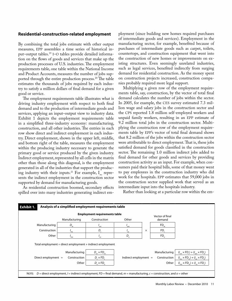
By combining the total jobs estimate with other output measures, EPP assembles a time series of historical in-put–output tables.19 I–O tables provide detailed informa-tion on the flows of goods and services that make up the production processes of U.S. industries. The employment requirements table, one table within the National Income and Product Accounts, measures the number of jobs sup-ported through the entire production process.20 The table estimates the thousands of jobs required by each indus-try to satisfy a million dollars of final demand for a given good or service.
The employment requirements table illustrates what is driving industry employment with respect to both final demand and to the production of intermediate goods and services, applying an input–output view to industry data. Exhibit 1 depicts the employment requirements table in a simplified three-industry economy: manufacturing, construction, and all other industries. The entries in each row show direct and indirect employment in each indus-try. Direct employment, shown in the upper left, middle, and bottom right of the table, measures the employment within the producing industry necessary to generate the primary good or service produced by the given industry. Indirect employment, represented by all cells in the matrix other than those along this diagonal, is the employment generated in all of the industries that support the produc-ing industry with their inputs.21 For example, Imc repre-sents the indirect employment in the construction sector supported by demand for manufacturing goods.
As residential construction boomed, secondary effects spilled over into many industries generating indirect em-
ployment (since building new homes required purchases of intermediate goods and services). Employment in the manufacturing sector, for example, benefited because of purchases of intermediate goods such as carpet, toilets, countertops, and construction equipment that went into the construction of new homes or improvements on ex-isting structures. Even seemingly unrelated industries, such as legal services, benefited indirectly from surging demand for residential construction. As the money spent on construction projects increased, construction compa-nies probably required more legal support.
Multiplying a given row of the employment require-ments table, say, construction, by the vector of total final demand calculates the number of jobs within the sector. In 2005, for example, the CES survey estimated 7.3 mil-lion wage and salary jobs in the construction sector and the CPS reported 1.8 million self-employed workers and unpaid family workers, resulting in an EPP estimate of 9.2 million total jobs in the construction sector. Multi-plying the construction row of the employment require-ments table by EPP’s vector of total final demand shows that 8.2 million of the jobs within the construction sector were attributable to direct employment. That is, these jobs satisfied demand for goods classified in the construction sector. The remaining 1.0 million indirect jobs added to final demand for other goods and services by providing construction activity as an input. For example, when con-sumers paid their hospital bills, some of that money went to pay employees in the construction industry who did work for the hospitals. EPP estimates that 59,000 jobs in the construction sector supplied work that served as an intermediate input into the hospitals industry.
Rather than looking at a particular row within the em-
Analysis of a simplified employment requirements table
Employment requirements tableVector of final
demandManufacturing Construction Other
Manufacturing Dm Icm Iom FDm
Construction Imc Dc Ioc × FDc
Other Imo Ico Do FDo
Total employment = direct employment + indirect employment
Manufacturing Dm × FDm Manufacturing (Icm × FDc) + (Iom × FDo)
Direct employment = Construction Dc × FDc Indirect employment = Construction (Imc × FDm) + (Ioc × FDo)
Other Do × FDo Other (Imo × FDm) + (Ico × FDc)
NOTE: D = direct employment, I = indirect employment, FD = final demand, m = manufacturing, c = construction, and o = other
Exhibit 1.
Housing Bubble and Bust
12 Monthly Labor Review • December 2010
ployment requirements table to break out sector employ-ment by what types of demand the industry in question is satisfying, one can analyze the table in its entirety to esti-mate how demand results in employment in all industries throughout the U.S. job market. Multiplying the employ-ment requirements matrix in its entirety by the column vector of final demand for investment in residential con-struction yields an estimate of what this article refers to as “residential-construction-related employment.” EPP’s analysis of direct and indirect employment includes data only for the construction sector as a whole. Determining employment impacts related specifically to demand for residential construction requires the assumption that the relationship of jobs to demand is the same for residential as for aggregate construction.
Because investment in residential construction requires purchases of many intermediate goods and services from
a variety of industries, the effects of the housing bubble spread throughout the economy. Construction output at-tributable to residential construction spending grew from 695.3 billion dollars in 1996, to 827.0 billion in 2002, to slightly over 1.0 trillion dollars in 2005. The purchases of intermediate goods and services for residential structures accounted for nearly half of this output. During the bust period, output related to residential construction demand fell, and it was at 600.2 billion in 2008.22
EPP estimates that output related to residential con-struction spending led to employment of 5.5 million in 1996. As the housing market expanded, related employ-ment grew to 6.0 million jobs in 2002. By the peak of the housing market, in 2005, it had increased to 7.4 million. Employment expanded by 1.8 million jobs, or by 33.4 percent, between 1996 and 2005, with 1.4 million of this growth occurring between 2002 and 2005. As the bubble burst, residential-construction-related employment fell to 4.5 million in 2008, 385,000 fewer jobs than in 1993, the earliest year of available data.
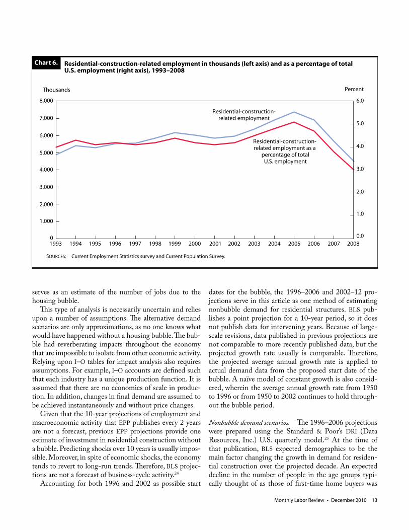
Residential construction spending supported an es-timated 4.0 percent to 4.4 percent of total employment within the United States from 1993 to 2000. By 2005, employment related to residential construction reached 5.1 percent of total U.S. employment; it then fell, reach-ing 3.0 percent in 2008. (See chart 6.) Since it makes up only a small portion of total employment, residential-construction-related employment usually has not had a considerable impact on overall employment change in the U.S. economy. It is interesting to note that, according to EPP’s estimates, in 2008 the decline in residential-con-struction-related employment—1.2 million—was greater than the overall net loss in employment in the U.S. econ-omy—804,000.
Employment growth attributable to the bubble
Not all of the residential-construction-related employ-ment growth during the bubble period was generated from the housing bubble, given that some increases would have been expected for reasons including population growth and continued expansion in the economy. I–O tables allow researchers to conduct an in-depth analysis of the economy-wide effects that a change in final demand has on industry output as well as employment.23 By esti-mating what demand would have been without a bubble, one can measure how many U.S. jobs there would have been under the alternative demand scenario. The differ-ence between the actual number of jobs and the number approximated under the scenario of nonbubble demand
The 2008–18 employment projections
Although this article is focused on the recent impacts of the housing bubble and bust, EPP’s 2008–18 projec-tions are briefly discussed as they relate to the housing market. EPP expects that construction will be the only sector among goods-producing sectors to show employ-ment growth over the projected period.1 Construction was more heavily affected by the 2007–09 recession than other goods-producing sectors and is therefore expected to show higher growth in the recovery period.
EPP anticipates demand for residential construction to recover to 581.6 billion dollars in 2018, very near the peak level of 586.0 billion in 2005. The projected level of demand is expected to support 6.2 million residential-construction-related jobs in 2018, near the 2003 level but not as high as the level in 2004 or 2005. EPP expects that residential-construction-related employment will climb back to 3.8 percent of total employment in 2018, higher than the 3.0 percent level of 2008 but lower than the 5.1 percent level of 2005 and slightly lower than the 1993 level. Sixty percent of the residential-construction-related jobs lost between 2005 and 2008, or 1.7 million, are anticipated to be recovered over the projection period.
Note
1 For more information on industry employment projec-tions, see Rose Woods, “Industry output and employment pro-jections to 2018,” Monthly Labor Review, November 2009, pp. 52–81.
Monthly Labor Review • December 2010 13
serves as an estimate of the number of jobs due to the housing bubble.
This type of analysis is necessarily uncertain and relies upon a number of assumptions. The alternative demand scenarios are only approximations, as no one knows what would have happened without a housing bubble. The bub-ble had reverberating impacts throughout the economy that are impossible to isolate from other economic activity. Relying upon I–O tables for impact analysis also requires assumptions. For example, I–O accounts are defined such that each industry has a unique production function. It is assumed that there are no economies of scale in produc-tion. In addition, changes in final demand are assumed to be achieved instantaneously and without price changes.
Given that the 10-year projections of employment and macroeconomic activity that EPP publishes every 2 years are not a forecast, previous EPP projections provide one estimate of investment in residential construction without a bubble. Predicting shocks over 10 years is usually impos-sible. Moreover, in spite of economic shocks, the economy tends to revert to long-run trends. Therefore, BLS projec-tions are not a forecast of business-cycle activity.24
Accounting for both 1996 and 2002 as possible start
dates for the bubble, the 1996–2006 and 2002–12 pro-jections serve in this article as one method of estimating nonbubble demand for residential structures. BLS pub-lishes a point projection for a 10-year period, so it does not publish data for intervening years. Because of large-scale revisions, data published in previous projections are not comparable to more recently published data, but the projected growth rate usually is comparable. Therefore, the projected average annual growth rate is applied to actual demand data from the proposed start date of the bubble. A naïve model of constant growth is also consid-ered, wherein the average annual growth rate from 1950 to 1996 or from 1950 to 2002 continues to hold through-out the bubble period.
Nonbubble demand scenarios. The 1996–2006 projections were prepared using the Standard & Poor’s DRI (Data Resources, Inc.) U.S. quarterly model.25 At the time of that publication, BLS expected demographics to be the main factor changing the growth in demand for residen-tial construction over the projected decade. An expected decline in the number of people in the age groups typi-cally thought of as those of first-time home buyers was
Residential-construction-related employment as a
percentage of total U.S. employment
Residential-construction-related employment
Chart 6.
Thousands Percent
8,000
7,000
6,000
5,000
4,000
3,000
2,000
1,000
0
Residential-construction-related employment in thousands (left axis) and as a percentage of total U.S. employment (right axis), 1993–2008
6.0
5.0
4.0
3.0
2.0
1.0
0.01993 1994 1995 1996 1997 1998 1999 2000 2001 2002 2003 2004 2005 2006 2007 2008
SOURCES: Current Employment Statistics survey and Current Population Survey.
Housing Bubble and Bust
14 Monthly Labor Review • December 2010
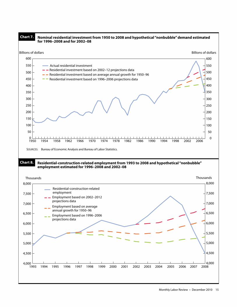
anticipated to hold growth to 0.8 percent annually over the projection period, in comparison with the 2.1 percent exhibited on average annually between 1950 and 1996. If the bubble did start in 1996 and the projections accurate-ly captured demand without the bubble, 86.0 percent of growth in demand for residential structures between 1996 and 2005, or 181.4 billion dollars, was attributable to the housing market bubble. In another scenario, if growth had continued at the 1950–96 average annual pace, the bubble contributed an estimated 134.9 billion dollars of invest-ment, 64.0 percent of growth, over the 1996–2006 period. (See chart 7.)
The 2002–12 projections were prepared by use of the macroeconomic model developed by Macroeconomic Advisers, LLC.26 EPP once again stated that demographics were expected to slow investment in residential structures. However, rapid growth during the late 1990s and early 2000s likely contributed to a projected annual growth rate of 2.1 percent from 2002 to 2012, higher than the rate projected for 1996–2006. The average annual growth rate from 1950 to 2002 was 2.2 percent, nearly equivalent to the 2002–12 projection. Because results based on the naïve constant growth model for 1950–2002 are nearly identical to those based on the 2002–12 projections, the constant growth model for 1950–2002 is not examined separately. If the bubble started in 2002, demand for resi-dential construction in 2005 was 93.3 billion dollars high-er than nonbubble demand as measured by the 2002–12 projections. According to this model, three quarters of the growth exhibited from 2002 to 2005 was attributable to the bubble.
From 2005 to 2008, demand for residential structures fell considerably as the market corrected for rapid growth during the boom years. In 2008, demand was only slightly higher than its 1995 level. All of the proposed models an-ticipated that demand for residential construction would be higher than it was in 2008. If the bubble began in 1996, on the basis of the 1996–2006 projections, demand would be expected to be 18.1 percent higher in 2008 than it actually was. On the basis of average annual growth from 1950 to 1996, growth would be expected to be 36.6 percent higher than it actually was. If the bubble started in 2002, demand would be projected to be 49.5 percent higher than it actually was.
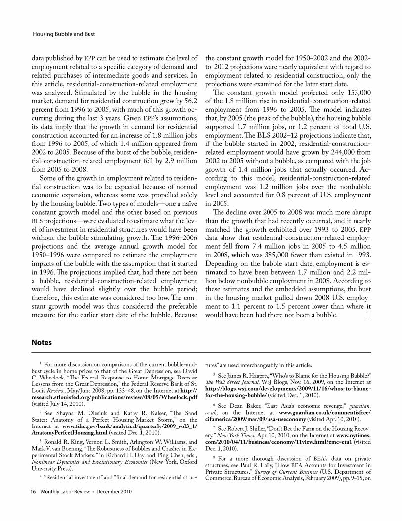
Related nonbubble employment. The alternative demand estimates were combined with data from the employment requirements table to estimate the impacts of the bubble and bust throughout the U.S. job market. (See chart 8.) On the basis of the 2002–12 projections, the number of
residential-construction-related jobs was approximated to be 1.2 million over the theoretical nonbubble level at the peak of the housing market in 2005. According to this estimate, 82.7 percent of the job growth between 2002 and 2005 was a result of the housing bubble. Also, the bubble is estimated to have increased U.S. employment by 0.8 percent in 2005.
If, however, the bubble started in 1996, the constant growth model implies that employment was 1.7 million over nonbubble residential-construction-related employ-ment and contributed 1.2 percent to the total number of U.S. jobs in 2005. According to the 1996–2006 projec-tions, employment was to stay relatively flat between 1996 and 2008, with a slight dip in the between years. In this nonbubble scenario, residential-construction-related em-ployment was expected to fall by 433,000 between 1996 and 2005.
The decline in nonbubble employment present in the 1996–2006 projections could be due to a number of fac-tors. The assumptions underlying I–O analysis may be having some impact here. For example, the production function may not have been the same without a bubble. Perhaps output was higher in relation to employment in the construction industry during the bubble than it would have been without a bubble. Alternatively, the projections could have underestimated nonbubble demand. Regard-less, because nonbubble residential-construction-related employment was expected to decline from 1996 to 2006, the results of this model are disregarded because they are considered to be too low.
By 2008, housing-related employment fell to 4.5 mil-lion and was accounting for only 3.0 percent of total U.S. jobs. If the bubble began in 1996, the naïve growth model expects that, if the market were not correcting for excess growth in the bubble years, residential-construction-re-lated employment would have been 1.7 million higher in 2008. If the bubble did not begin until 2002, it is approxi-mated that residential construction-related employment would have been 2.2 million higher in 2008. The bust in the housing market, according to these measures and the embedded assumptions, pulled down U.S. employment by 1.1 percent to 1.5 percent below where it would have been had there not been a bubble.
IN RECENT YEARS, THE HOUSING BOOM AND BUST have had a substantial impact on the U.S. job market. Be-cause the date of the onset of the bubble is not clear, this article considers two possible starting points, 1996 and 2002. Whereas industry employment data offer analysis of employment within the entire construction sector, I–O
Monthly Labor Review • December 2010 15
Chart 7.
Billions of dollars Billions of dollars
600
550
500
450
400
350
300
250
200
150
100
50
0
Nominal residential investment from 1950 to 2008 and hypothetical “nonbubble” demand estimated for 1996–2008 and for 2002–08
1950 1954 1958 1962 1966 1970 1974 1978 1982 1986 1990 1994 1998 2002 2006
SOURCES: Bureau of Economic Analysis and Bureau of Labor Statistics.
600
550
500
450
400
350
300
250
200
150
100
50
0
Actual residential investmentResidential investment based on 2002–12 projections dataResidential investment based on average annual growth for 1950–96Residential investment based on 1996–2006 projections data
Chart 8.
Thousands Thousands
8,000
7,500
7,000
6,500
6,000
5,500
5,000
4,500
4,000
Residential-construction-related employment from 1993 to 2008 and hypothetical “nonbubble” employment estimated for 1996–2008 and 2002–08
8,000
7,500
7,000
6,500
6,000
5,500
5,000
4,500
4,000
Employment based on 2002–2012 projections data
Employment based on average annual growth for 1950–96
Residential-construction-related employment
Employment based on 1996–2006 projections data
1993 1994 1995 1996 1997 1998 1999 2000 2001 2002 2003 2004 2005 2006 2007 2008
Housing Bubble and Bust
16 Monthly Labor Review • December 2010
data published by EPP can be used to estimate the level of employment related to a specific category of demand and related purchases of intermediate goods and services. In this article, residential-construction-related employment was analyzed. Stimulated by the bubble in the housing market, demand for residential construction grew by 56.2 percent from 1996 to 2005, with much of this growth oc-curring during the last 3 years. Given EPP’s assumptions, its data imply that the growth in demand for residential construction accounted for an increase of 1.8 million jobs from 1996 to 2005, of which 1.4 million appeared from 2002 to 2005. Because of the burst of the bubble, residen-tial-construction-related employment fell by 2.9 million from 2005 to 2008.
Some of the growth in employment related to residen-tial construction was to be expected because of normal economic expansion, whereas some was propelled solely by the housing bubble. Two types of models—one a naïve constant growth model and the other based on previous BLS projections—were evaluated to estimate what the lev-el of investment in residential structures would have been without the bubble stimulating growth. The 1996–2006 projections and the average annual growth model for 1950–1996 were compared to estimate the employment impacts of the bubble with the assumption that it started in 1996. The projections implied that, had there not been a bubble, residential-construction-related employment would have declined slightly over the bubble period; therefore, this estimate was considered too low. The con-stant growth model was thus considered the preferable measure for the earlier start date of the bubble. Because
the constant growth model for 1950–2002 and the 2002-to-2012 projections were nearly equivalent with regard to employment related to residential construction, only the projections were examined for the later start date.
The constant growth model projected only 153,000 of the 1.8 million rise in residential-construction-related employment from 1996 to 2005. The model indicates that, by 2005 (the peak of the bubble), the housing bubble supported 1.7 million jobs, or 1.2 percent of total U.S. employment. The BLS 2002–12 projections indicate that, if the bubble started in 2002, residential-construction-related employment would have grown by 244,000 from 2002 to 2005 without a bubble, as compared with the job growth of 1.4 million jobs that actually occurred. Ac-cording to this model, residential-construction-related employment was 1.2 million jobs over the nonbubble level and accounted for 0.8 percent of U.S. employment in 2005.
The decline over 2005 to 2008 was much more abrupt than the growth that had recently occurred, and it nearly matched the growth exhibited over 1993 to 2005. EPP data show that residential-construction-related employ-ment fell from 7.4 million jobs in 2005 to 4.5 million in 2008, which was 385,000 fewer than existed in 1993. Depending on the bubble start date, employment is es-timated to have been between 1.7 million and 2.2 mil-lion below nonbubble employment in 2008. According to these estimates and the embedded assumptions, the bust in the housing market pulled down 2008 U.S. employ-ment to 1.1 percent to 1.5 percent lower than where it would have been had there not been a bubble.
Notes
1 For more discussion on comparisons of the current bubble-and-bust cycle in home prices to that of the Great Depression, see David C. Wheelock, “The Federal Response to Home Mortgage Distress: Lessons from the Great Depression,” the Federal Reserve Bank of St. Louis Review, May/June 2008, pp. 133–48, on the Internet at http://research.stlouisfed.org/publications/review/08/05/Wheelock.pdf (visited July 14, 2010).
2 See Shayna M. Olesiuk and Kathy R. Kalser, “The Sand States: Anatomy of a Perfect Housing-Market Storm,” on the Internet at www.fdic.gov/bank/analytical/quarterly/2009_vol3_1/AnatomyPerfectHousing.html (visited Dec. 1, 2010).
3 Ronald R. King, Vernon L. Smith, Arlington W. Williams, and Mark V. van Boening, “The Robustness of Bubbles and Crashes in Ex-perimental Stock Markets,” in Richard H. Day and Ping Chen, eds., Nonlinear Dynamics and Evolutionary Economics (New York, Oxford University Press).
4 “Residential investment” and “final demand for residential struc-
tures” are used interchangeably in this article.5 See James R. Hagerty, “Who’s to Blame for the Housing Bubble?”
The Wall Street Journal, WSJ Blogs, Nov. 16, 2009, on the Internet at http://blogs.wsj.com/developments/2009/11/16/whos-to-blame-for-the-housing-bubble/ (visited Dec. 1, 2010).
6 See Dean Baker, “East Asia’s economic revenge,” guardian.co.uk, on the Internet at www.guardian.co.uk/commentisfree/cifamerica/2009/mar/09/usa-useconomy (visited Apr. 10, 2010).
7 See Robert J. Shiller, “Don’t Bet the Farm on the Housing Recov-ery,” New York Times, Apr. 10, 2010, on the Internet at www.nytimes.com/2010/04/11/business/economy/11view.html?emc=eta1 (visited Dec. 1, 2010).
8 For a more thorough discussion of BEA’s data on private structures, see Paul R. Lally, “How BEA Accounts for Investment in Private Structures,” Survey of Current Business (U.S. Department of Commerce, Bureau of Economic Analysis, February 2009), pp. 9–15, on
Monthly Labor Review • December 2010 17
the Internet at www.bea.gov/scb/pdf/2009/02%20February/0209_briefing_structures.pdf.
9 All dollar figures in this article, unless otherwise noted, are real values in year-2000 dollars. All BEA data in this article are consistent with figures published as of July of 2009 and with EPP’s 2008–18 pro-jections presented in this article.
10 See Frank E. Nothaft, “The Contribution of Home Value Ap-preciation to US Economic Growth,” Urban Policy and Research, March 2004, pp. 23–34, on the Internet at www.freddiemac.com/news/pdf/contribution_homevalue.pdf; and Kevin B. Moore and Michael G. Palumbo, The Finances of American Households in the Past Three Reces-sions: Evidence from the Survey of Consumer Finances (Washington, DC, Federal Reserve Board, Dec. 10, 2009), on the Internet at www.federalreserve.gov/pubs/feds/2010/201006/201006pap.pdf (visited Dec. 1, 2010).
11 Several other price indices are often cited when referencing the housing market, including the Case–Shiller 10 and 20, the Case–Shiller national, and the Federal Housing Finance Agency house price index, but these indexes have historical data going back no further than 1987. Note that, for the years 1987–2009, the Shiller real index is based on the Case–Shiller national index adjusted by the Consumer Price Index measurement of inflation. Earlier years are based on other price measures. For further information on the Shiller real index, see Robert J. Shiller, Irrational Exuberance, second edition (Princeton University Press, 2005); see also http://irrationalexuberance.com/ (visited Mar. 22, 2010).
12 Data on construction put in place and data on permits are not adjusted for changes in prices and are therefore compared with the nominal final-demand data published by BEA.
13 BEA implemented a comprehensive revision to its National In-come and Product Accounts in July of 2009. The estimates for 2009 are not comparable with earlier annual data as published by EPP because they were based upon BEA data as published before the comprehensive revision.
14 There are many differences between CPS and CES data, only a few of which are mentioned here. For a comparison between the two surveys, see www.bls.gov/bls/empsitquickguide.htm (visited July 19, 2010).
15 That is, EPP assumes that the count of self-employed and un-paid family workers is the equivalent of a jobs count. CPS data are also used by EPP to estimate wage and salary employment in industries for which the CES survey does not provide estimates, including the agricultural and private household industries.
16 The CPS program estimated data for 1983–2002 on the basis of the old Standard Industrial Classification (SIC) codes. Data for 2000–09 are based on the North American Industry Classification System (NAICS). (For 2000–02, data were calculated both within the framework of NAICS and within that of the SIC system.) The 1983–99 data were adjusted to account for the coding change.
17 The industries in table 1 were selected on the basis of those in-cluded in Matthew Miller, “A visual essay: post-recessionary employ-ment growth related to the housing market,” Monthly Labor Review,
October 2006, pp. 23–34. 18 Wood product manufacturing and architectural and structural
metals manufacturing did see slight declines in employment over 2001–06. However, these declines were minor in comparison with the loss of jobs in the overall manufacturing sector. Also, both showed much larger declines over 2006–09 than over 2001–06, suggesting that the housing bubble may have held onto jobs that otherwise would have been lost during this period.
19 BEA’s benchmark I–O accounts provide the most comprehensive picture available of transactions within the U.S. economy, but are pub-lished only once every 5 years. The 2002 benchmark I–O data, released in 2007, were the latest data available for EPP’s 2018 projections. On the basis of the 2002 benchmark I–O data, annual data from the Na-tional Income and Product Accounts, annual Census data, and data from a host of other sources, EPP estimates a historical time series of I–O data, currently 1993 to 2008. For detailed information regarding the 2002 benchmark I–O accounts, see Ricky L. Stewart, Jessica Brede Stone, and Mary L. Streitwieser, “U.S. Benchmark Input-Output Ac-counts, 2002,” Survey of Current Business (U.S. Department of Com-merce, Bureau of Economic Analysis, October 2007), pp. 19–48. For a more complete discussion of the methods used by EPP, see the BLS Handbook of Methods, chapter 13, on the Internet at www.bls.gov/opub/hom/homch13_a.htm (visited Apr. 5, 2010).
20 The employment requirements table is “import adjusted”; that is, it is modified to account only for the sales of domestically produced goods and services to final users because imported goods generally do not generate domestic employment.
21 All employees, direct and indirect, earn income that will gen-erally be spent on consumer goods and services, which, in turn, will generate a third type of employment called induced employment (also referred to as “income multiplier effects on employment”). The Bureau of Labor Statistics does not measure induced employment.
22 Estimating total output related to a specific category of final demand requires the assumption that the employment requirements table estimated for the economy as a whole also holds at the more detailed level.
23 See Mary L. Streitwieser, “A Primer on BEA’s Industry Ac-counts” (U.S. Department of Commerce, Bureau of Economic Analy-sis, June 2009), on the Internet at www.bea.gov/scb/pdf/2009/06%20June/0609_indyaccts_primer_a.pdf (visited Dec. 6, 2010).
24 The projections do, however, include in-house projections of the growth of the population, an important contributor to growth within the housing market. For more discussion on how BLS’s assumptions affected the 1996 to 2006 projections, see Ian Wyatt, “Evaluating the 1996–2006 employment projections,” Monthly Labor Review, October 2010, pp. 33–69.
25 For more information on the 1996–2006 projections, see Thom-as Boustead, “The U.S. economy to 2006,” Monthly Labor Review, No-vember 1997, pp. 6–22.
26 For more information on the 2002–12 projections, see Betty W. Su, “The U.S. economy to 2012: signs of growth,” Monthly Labor Re-view, February 2004, pp. 23–36.
18 Monthly Labor Review • December 2010
Measuring Productivity
Advances in information technology have created new opportunities for workers to perform their jobs away
from their traditional workplaces. One im-plication of this change—and the subject of an ongoing debate surrounding U.S. Bureau of Labor Statistics (BLS, the Bureau) pro-ductivity data—is that official estimates of productivity growth may be overstated be-cause estimates of hours worked may not include unpaid hours worked at home. To shed light on this debate, this article ex-amines two recent sources of data on U.S. workers who bring work home from their primary workplace: the 2003–08 Ameri-can Time Use Survey (ATUS) and the 1997, 2001, and 2004 May Current Population Survey (CPS) Work Schedules and Work at Home Supplement (CPS Supplement). The ATUS provides detailed information on time spent on work, work-related activities, and nonwork activities during a single day, as well as information on the locations of these activities. The CPS Supplement provides in-formation on the number of hours worked at home each week, information on whether or not workers had a formal arrangement to be paid for work at home, and reasons for working at home.
Recent research on work at home has fo-cused almost entirely on paid work done by
Lucy P. Eldridge is a senior economist in the Office of Productivity and Technol-ogy, Bureau of Labor Statistics. Sabrina Wulff Pabilonia is a research economist in the same office. Email: [email protected] or [email protected]
Lucy P. EldridgeandSabrina Wulff Pabilonia
Bringing work home: implicationsfor BLS productivity measures
About 8 percent of nonfarm business employees bring somework home, mostly to finish or catch up on their work; those who bring work home work more hours per week, on average, than those who work only at the workplace,but there is no evidence that this difference leadsto an overstatement in measures of productivity growth
those who have a formal arrangement to work at home. However, two papers pub-lished within the last 10 years have exam-ined unpaid work at home. Using the May 2001 CPS Work Schedules and Work at Home Supplement, Younghwan Song ex-amined the determinants of unpaid work at home for full-time wage and salary work-ers in the nonagricultural sector.1 He found that unpaid work at home is positively re-lated to education, the absence of overtime rates, being a team leader, efficiency wages, and greater earnings inequality within oc-cupation groups. Song attributed workers’ willingness to take on this additional unpaid work as an investment in their careers and future wage growth. In another study, Paul Callister and Sylvia Dixon used the 1999 New Zealand Time Use Survey and found that bringing work home was much more common than working exclusively from home.2 The majority of work at home lasted for less than 2 hours per day, and a signifi-cant proportion was done in the evenings after work and on weekends.
Although hours worked at home under a formal arrangement are important economi-cally, they almost certainly are included in official hours estimates; thus, their increased prevalence does not bias estimates of pro-ductivity growth. In contrast, when workers
Monthly Labor Review • December 2010 19
bring work home on an informal basis, it is more likely that the hours are worked off the clock and therefore are not included in these estimates. This study begins by explaining productivity measurement and discussing how unmeasured hours can affect estimates. Next, those who bring work home are defined and their characteristics and reasons for bringing work home evaluated. Then, the data are exam-ined to determine the amount of work brought home and whether those who bring work home work longer hours or are simply shifting the location of some of their work. Fi-nally, the study assesses whether BLS measures of hours and productivity capture the hours worked at home by those who bring work home from the workplace and, more im-portantly, whether unmeasured hours worked at home af-fect productivity trends.
Unmeasured hours and productivity growth
Labor productivity measures the difference between out-put growth and hours growth, and reflects many kinds of changes, including changes in the quantities of nonlabor inputs (that is, capital services, fuels, other intermediate materials, and purchased services) and changes in tech-nology, economies of scale, management techniques, and the skills of the labor force. The Bureau of Labor Statistics calculates labor productivity for the nonfarm business sec-tor by combining real output from the National Income and Product Accounts produced by the Bureau of Eco-nomic Analysis with BLS measures of hours worked for all persons. The primary source of data on hours is the average-weekly-hours-paid series for production work-ers in goods-producing industries and for nonsupervisory workers in service-providing industries.3 Data for these series are collected in the BLS Current Employment Sta-tistics (CES) survey, a monthly payroll survey of establish-ments that collects data on employment and hours paid for the pay period that includes the 12th of the month.4 Average weekly hours are adjusted to remove the hours of employees who work for nonprofit institutions and to convert the series to an hours-worked basis, using an hours-worked-to-hours-paid ratio estimated from the BLS National Compensation Survey.5 The hours-worked adjustment ensures that changes in vacation, holiday, and sick pay, which are viewed as changes in labor costs, do not affect growth in hours, but it does not adjust for hours worked off the clock.
Total hours worked by production and nonsupervisory employees are calculated as
(1)
where AWHP represents average weekly hours worked by production and nonsupervisory employees and NP is the employment of nonfarm business production and non-supervisory employees.
Average weekly hours worked by nonproduction and supervisory employees are estimated by applying a ratio adjustment from the CPS data to the production and non-supervisory hours data. The adjustment is the ratio of the average weekly hours worked by nonproduction and su-pervisory employees to the average weekly hours worked by production and nonsupervisory employees.6 This ratio (subsequently referred to as the CPS ratio), combined with the hours-worked series for production and nonsuper-visory employees and CES employment data, is used to calculate the total hours worked by nonproduction and supervisory employees as
(2)
where AWHNP and AWHP represent CPS measures of average weekly hours worked by nonproduction and su-pervisory employees and production and nonsupervisory employees, respectively, and NNP denotes the employ-ment of nonfarm business nonproduction and supervi-sory employees.
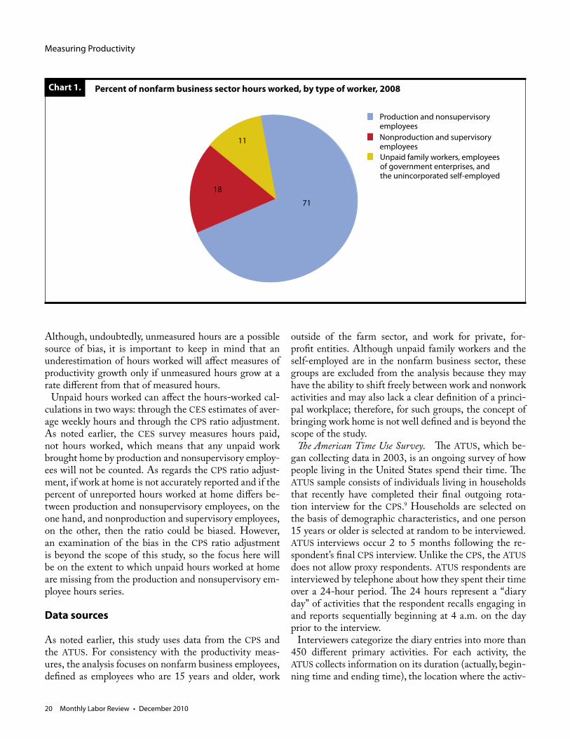
The Bureau constructs total hours worked by production and nonsupervisory employees and total hours worked by nonproduction and supervisory employees at the BLS-defined 14-sector level and then aggregates both measures to the level of all nonfarm business. Total hours worked by all persons in the nonfarm business sector are the sum of production and nonsupervisory employee hours, non-production and supervisory employee hours, and hours worked by unpaid family workers, employees of govern-ment enterprises, and the unincorporated self-employed.7 Chart 1 shows each group’s share of nonfarm business sec-tor hours worked in 2008. Production and nonsupervisory employees account for the majority of nonfarm business sector hours (71 percent), nonproduction and supervisory employee hours account for 18 percent, and the unincor-porated self-employed, unpaid family workers, and em-ployees of government enterprises make up the smallest share (11 percent).
Some critics have suggested that innovations in infor-mation technology have allowed many more workers the flexibility to work outside the traditional workplace and that these hours are not properly captured in official BLS productivity measures—in particular, the quarterly labor productivity estimates for the nonfarm business sector.8 ),52()()AWH( NH P
MP
MP
),52()(
AWHAWH)AWH( NPCPS
CPSNP
NP )( NHP
MP
M
CPS CPS
M
Measuring Productivity
20 Monthly Labor Review • December 2010
Chart 1. Percent of nonfarm business sector hours worked, by type of worker, 2008
Production and nonsupervisory employeesNonproduction and supervisory employees
Unpaid family workers, employees of government enterprises, and the unincorporated self-employed
11
18
Although, undoubtedly, unmeasured hours are a possible source of bias, it is important to keep in mind that an underestimation of hours worked will affect measures of productivity growth only if unmeasured hours grow at a rate different from that of measured hours.
Unpaid hours worked can affect the hours-worked cal-culations in two ways: through the CES estimates of aver-age weekly hours and through the CPS ratio adjustment. As noted earlier, the CES survey measures hours paid, not hours worked, which means that any unpaid work brought home by production and nonsupervisory employ-ees will not be counted. As regards the CPS ratio adjust-ment, if work at home is not accurately reported and if the percent of unreported hours worked at home differs be-tween production and nonsupervisory employees, on the one hand, and nonproduction and supervisory employees, on the other, then the ratio could be biased. However, an examination of the bias in the CPS ratio adjustment is beyond the scope of this study, so the focus here will be on the extent to which unpaid hours worked at home are missing from the production and nonsupervisory em-ployee hours series.
Data sources
As noted earlier, this study uses data from the CPS and the ATUS. For consistency with the productivity meas-ures, the analysis focuses on nonfarm business employees, defined as employees who are 15 years and older, work
outside of the farm sector, and work for private, for-profit entities. Although unpaid family workers and the self-employed are in the nonfarm business sector, these groups are excluded from the analysis because they may have the ability to shift freely between work and nonwork activities and may also lack a clear definition of a princi-pal workplace; therefore, for such groups, the concept of bringing work home is not well defined and is beyond the scope of the study.
The American Time Use Survey. The ATUS, which be-gan collecting data in 2003, is an ongoing survey of how people living in the United States spend their time. The ATUS sample consists of individuals living in households that recently have completed their final outgoing rota-tion interview for the CPS.9 Households are selected on the basis of demographic characteristics, and one person 15 years or older is selected at random to be interviewed. ATUS interviews occur 2 to 5 months following the re-spondent’s final CPS interview. Unlike the CPS, the ATUS does not allow proxy respondents. ATUS respondents are interviewed by telephone about how they spent their time over a 24-hour period. The 24 hours represent a “diary day” of activities that the respondent recalls engaging in and reports sequentially beginning at 4 a.m. on the day prior to the interview.
Interviewers categorize the diary entries into more than 450 different primary activities. For each activity, the ATUS collects information on its duration (actually, begin-ning time and ending time), the location where the activ-
71
Monthly Labor Review • December 2010 21
ity took place, and the people who were in the room with the respondent or who accompanied the respondent dur-ing the activity.10 Thus, it is possible to construct measures of hours worked that include time at work; time spent on work activities by location, such as at one’s usual work-place, at home, or in a restaurant; and interruptions of 15 minutes or longer that took place during the workday.11
Single-day diaries are thought to be more accurate than retrospective survey questions because time diaries have a shorter recall period and are less subject to aggregation bias (the sum of time spent in all activities must equal 1,440 minutes, and respondents do not have to add to-gether individual work episodes themselves).12 Also, time diary data should capture all work done by all persons, re-gardless of their usual work schedule.13 Finally, the ATUS updates the demographic and employment information that was collected in the CPS and asks respondents to re-port any activities during which children under 13 years were in their care. This request makes it possible to deter-mine when parents are working and simultaneously car-ing for a child.
The ATUS sample covers every day of the year, except for the days before major holidays. In 2003, there were 20,720 ATUS interviews. Beginning in December of that year, the sample size was reduced by 35 percent, yielding 13,973 completed diaries in 2004. From 2005 to 2008, approximately 13,000 diaries were completed each year, with the exception of 2007, when only 12,248 diaries were completed.
Because the study presented here is concerned primarily with unmeasured hours of work at home, the analysis was restricted to work done for a respondent’s main job. It is expected that those who are working at home on a second job are in fact being paid for those hours, and the hours would be captured in measured hours. Hours of work brought home from the primary job may be “extra hours,” not explicitly paid for and thus unmeasured. The restric-tion to the main job also allows a comparison of results from the ATUS with those from the CPS Supplement, be-cause the latter collects information about work at home only for the main job. This approach may slightly under-estimate work done at home, and thus unmeasured hours, to the extent that people combine work at their workplace with work at home on their second jobs. However, most second jobs are part time and, therefore, more likely to pay hourly and be captured in standard measures.
To analyze hours of work, the minutes spent on activities coded as “work at main job” were aggregated by location for each ATUS respondent, in order to construct measures of worktime both at the workplace and at the home. Reported
breaks of 15 or fewer minutes occurring at the workplace, as well as work-related travel (not commuting) occurring between episodes of work at a workplace, are included as worktime.14 From a productivity standpoint, short breaks are considered productive time.15
For this study, “bringing work home” is defined as bringing extra work home when home is not the primary workplace. Respondents whose diary day was a nonholi-day weekday are classified as those who bring work home if they report any minutes of work for their main job both at the workplace and at home on the same day. Respond-ents whose diary day was on a weekend day or a holiday are classified as those who bring work home if they report any minutes of work at home on their diary day. Unfor-tunately, it is not possible to distinguish whether those who worked exclusively at home on a weekend diary day were home-based workers, telecommuters, or traditional “nine-to-five” office workers who bring extra work home to do over the weekend. However, when the hours worked at home by this group are described later in the article, it will become clear that the group consists primarily of em-ployees who bring work home, rather than home-based workers. Because those who bring work home are identi-fied only according to work activities they engaged in on their diary day, the analysis using ATUS data is further restricted to nonfarm business employees who worked on their diary day. It is important to keep in mind that, be-cause the ATUS covers only a single day, it is impossible to identify people who bring work home if they do not do so on their diary day.
The CPS Work Schedules and Work at Home Supplement. The Work Schedules and Work at Home Supplement was collected as part of the May CPS in 1997, 2001, and 2004. Although changes in industry and occupational coding and changes in the sequence and wording of the questions on work at home limit the direct comparability of some data collected in 1997, data from all 3 years are included in the analyses, with limitations noted as they occur. As previously mentioned, the CPS supplement col-lected information only on whether respondents did any work at home as part of their main job. Wage and salary respondents who reported working at home were asked whether they had a formal agreement with their employer to be paid for work at home or whether they were just tak-ing (unpaid) work home.
The analysis focuses on those who reported that they were just taking work home, because their hours at home are the hours most likely to be unmeasured. Unfortunately, the questionnaire did not allow for the possibility that an
Measuring Productivity
22 Monthly Labor Review • December 2010
employee had a formal arrangement to be paid for work at home and also took unpaid work home.16 Respondents were asked their reasons for working at home, how fre-quently they worked at home, and the number of hours per week they worked at home. In 1997, respondents were asked for actual hours worked at home, whereas they were asked for usual hours in 2001 and 2004. The 2001 and 2004 respondents also were given a choice of “it varies” as a response for hours worked at home; therefore, it is not possible to determine a numerical measure of work hours for all respondents in these years. The analysis focuses only on workers who have positive weekly hours worked dur-ing the reference week.
ATUS and CPS Supplement matched data. CPS Supple-ment respondents in 2004 who were in their 5th through 8th months in the May CPS were eligible for an ATUS interview from July 2004 through January 2005. It is pos-sible to directly match 745 nonfarm business employees who (1) were in the same industry and occupation, (2) reported the same class of worker in both datasets, (3) did not change employers between their last month in the CPS and their ATUS interview, and (4) worked on their diary day. Of the 745 directly matched respondents, 93 reported in the CPS Supplement that they brought unpaid work home and 66 reported that they brought work home on their ATUS diary day. However, there are definitely limita-tions associated with the matched data. Some respond-ents to the Supplement questions answered that they did not do any work at home as part of their job, although their time diary clearly stated that they did some work at home. For example, of the 66 individuals who brought work home on their diary day, only 35 reported in the CPS Supplement that they had ever worked at home.17 This may be because the nature of their job changed between the time the CPS Supplement was conducted and the time the ATUS interviews took place, a period that could have been anywhere from 2 to 8 months. Alternatively, the CPS Supplement questions may have been misinterpreted by the respondents so that they answered affirmatively only if they brought work home on a regular basis, or answers may have been subject to proxy reporting bias; however, even self-respondents (as opposed to proxies) reported differently between surveys. The 2004 directly matched data indicate that 69 percent of those in the CPS Supple-ment who worked at home on their weekend or holiday diary day did not have a formal arrangement to be paid for such work. This finding provides additional evidence that most employees who worked at home on the weekend are not home-based or occasional telecommuters.
Who is bringing work home?
Many nonfarm business employees bring work home from the workplace. According to the 2004 ATUS diaries, 84 percent of nonfarm business employees who worked on their diary day worked exclusively in a workplace that day, 9 percent brought some of their work home, and 3 percent worked exclusively at home on weekdays.18 (See chart 2.)The 2004 CPS Supplement data show that approximately 12 percent of nonfarm business employees did some work at home. (See chart 2.) The CPS Supplement specifically asked those who responded that they did work at home whether they brought work home; 8 percent of employees reported bringing some work home in 2004, while 4 per-cent reported that they had a formal arrangement to be paid for work conducted at home. Because the ATUS cap-tures only a person’s diary day, some employees who bring work home on some days, but not their diary day, may be categorized as working only at a workplace or work-ing only at home. Therefore, the observed proportion of employees who bring work home is understated to some extent in the ATUS.19
Both datasets reveal that the characteristics of non-farm business employees who bring work home from the workplace are different from the characteristics of those who work exclusively in the workplace.20 Employees who bring work home from the workplace are more likely to be male, older, White, and married, to have a child and at least a bachelor’s degree, and to work in a management or professional occupation, compared with employees who work only in the workplace21 (see tables 1 and 2), and are less likely to be Black, Hispanic, part-time work-ers, or paid hourly.22 For example, according to the 2004 CPS Supplement, 63 percent of those who brought work home held at least a bachelor’s degree, whereas 19 per-cent of those who did no work at home held at least that same degree. Also, of those who brought work home, 15 percent reported being paid hourly, while 69 percent of nonfarm employees who did no work at home were paid hourly. Although 38 percent of those who brought work home worked in a management or professional occupa-tion, not all work brought home is done by white-collar office workers. For instance, the 2004 CPS Supplement found that, among nonfarm business employees who brought work home, 3 percent worked in construction and maintenance occupations. The data indicate that women were less likely than men to have brought work home. Gender-related differences such as this may sim-ply be capturing the fact that work may be less portable in traditionally female-dominated occupations and in-
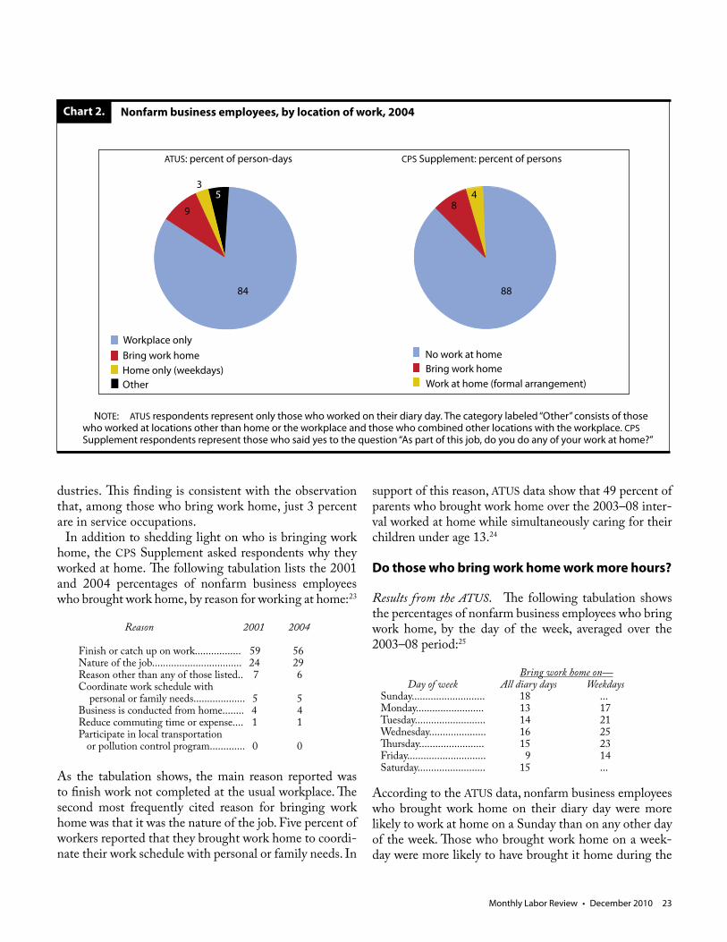
Monthly Labor Review • December 2010 23
Chart 2. Nonfarm business employees, by location of work, 2004
CPS Supplement: percent of persons
No work at home Bring work homeWork at home (formal arrangement)
NOTE: ATUS respondents represent only those who worked on their diary day. The category labeled “Other” consists of those who worked at locations other than home or the workplace and those who combined other locations with the workplace. CPS Supplement respondents represent those who said yes to the question “As part of this job, do you do any of your work at home?”
Workplace onlyBring work homeHome only (weekdays)Other
4
88
8
ATUS: percent of person-days
9
35
84
dustries. This finding is consistent with the observation that, among those who bring work home, just 3 percent are in service occupations.
In addition to shedding light on who is bringing work home, the CPS Supplement asked respondents why they worked at home. The following tabulation lists the 2001 and 2004 percentages of nonfarm business employees who brought work home, by reason for working at home:23
Reason 2001 2004
Finish or catch up on work................. 59 56Nature of the job................................. 24 29Reason other than any of those listed.. 7 6Coordinate work schedule with personal or family needs................... 5 5Business is conducted from home........ 4 4Reduce commuting time or expense.... 1 1Participate in local transportation or pollution control program............. 0 0
As the tabulation shows, the main reason reported was to finish work not completed at the usual workplace. The second most frequently cited reason for bringing work home was that it was the nature of the job. Five percent of workers reported that they brought work home to coordi-nate their work schedule with personal or family needs. In
support of this reason, ATUS data show that 49 percent of parents who brought work home over the 2003–08 inter-val worked at home while simultaneously caring for their children under age 13.24
Do those who bring work home work more hours?
Results from the ATUS. The following tabulation shows the percentages of nonfarm business employees who bring work home, by the day of the week, averaged over the 2003–08 period:25
Bring work home on— Day of week All diary days WeekdaysSunday........................... 18 ...Monday......................... 13 17Tuesday.......................... 14 21Wednesday..................... 16 25Thursday........................ 15 23Friday............................. 9 14Saturday......................... 15 ...
According to the ATUS data, nonfarm business employees who brought work home on their diary day were more likely to work at home on a Sunday than on any other day of the week. Those who brought work home on a week-day were more likely to have brought it home during the
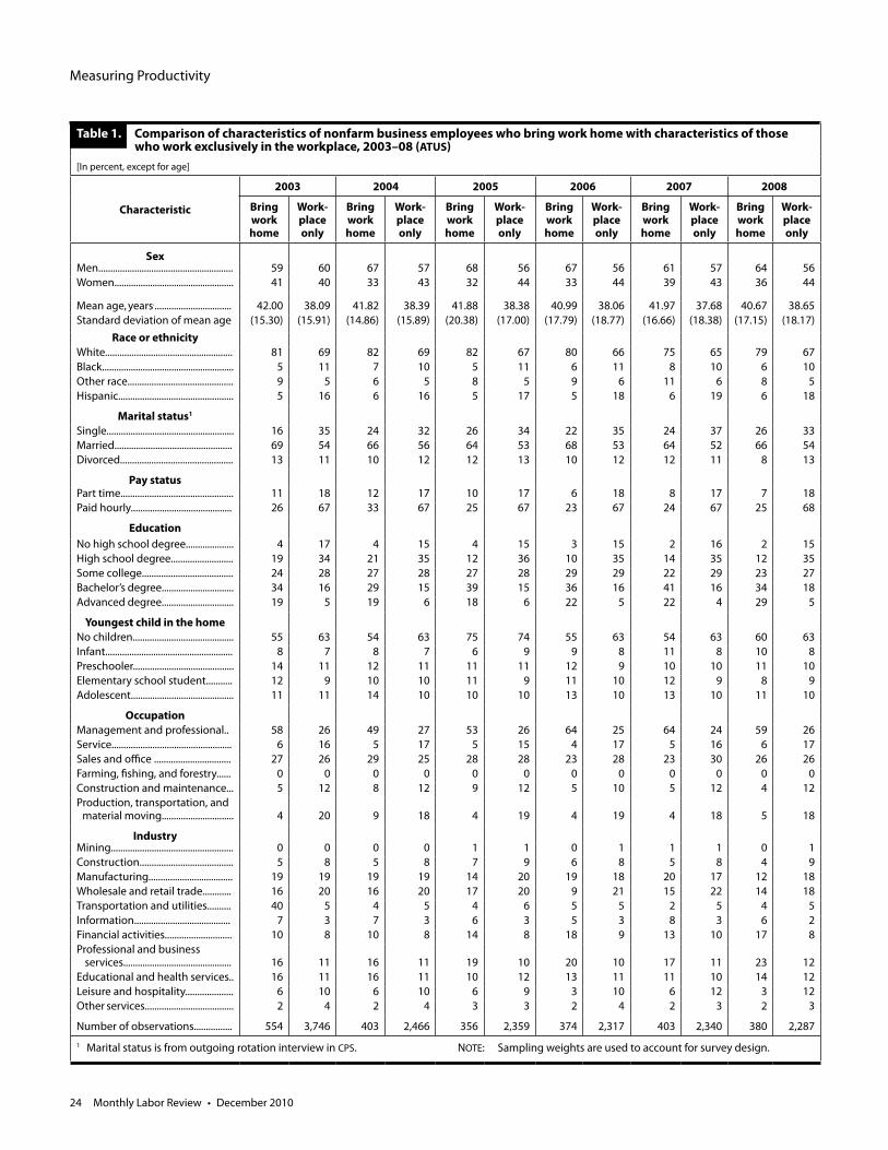
Measuring Productivity
24 Monthly Labor Review • December 2010
Table 1. Comparison of characteristics of nonfarm business employees who bring work home with characteristics of those who work exclusively in the workplace, 2003–08 (ATUS)[In percent, except for age]
Characteristic
2003 2004 2005 2006 2007 2008
Bring work home
Work-place only
Bring work home
Work-place only
Bring work home
Work-place only
Bring work home
Work-place only
Bring work home
Work-place only
Bring work home
Work-place only
SexMen........................................................ 59 60 67 57 68 56 67 56 61 57 64 56Women.................................................. 41 40 33 43 32 44 33 44 39 43 36 44
Mean age, years................................. 42.00 38.09 41.82 38.39 41.88 38.38 40.99 38.06 41.97 37.68 40.67 38.65Standard deviation of mean age (15.30) (15.91) (14.86) (15.89) (20.38) (17.00) (17.79) (18.77) (16.66) (18.38) (17.15) (18.17)
Race or ethnicityWhite..................................................... 81 69 82 69 82 67 80 66 75 65 79 67Black....................................................... 5 11 7 10 5 11 6 11 8 10 6 10Other race............................................ 9 5 6 5 8 5 9 6 11 6 8 5Hispanic................................................ 5 16 6 16 5 17 5 18 6 19 6 18
Marital status1
Single..................................................... 16 35 24 32 26 34 22 35 24 37 26 33Married................................................. 69 54 66 56 64 53 68 53 64 52 66 54Divorced............................................... 13 11 10 12 12 13 10 12 12 11 8 13
Pay statusPart time............................................... 11 18 12 17 10 17 6 18 8 17 7 18Paid hourly.......................................... 26 67 33 67 25 67 23 67 24 67 25 68
EducationNo high school degree.................... 4 17 4 15 4 15 3 15 2 16 2 15High school degree.......................... 19 34 21 35 12 36 10 35 14 35 12 35Some college...................................... 24 28 27 28 27 28 29 29 22 29 23 27Bachelor’s degree.............................. 34 16 29 15 39 15 36 16 41 16 34 18Advanced degree.............................. 19 5 19 6 18 6 22 5 22 4 29 5
Youngest child in the homeNo children.......................................... 55 63 54 63 75 74 55 63 54 63 60 63Infant..................................................... 8 7 8 7 6 9 9 8 11 8 10 8Preschooler.......................................... 14 11 12 11 11 11 12 9 10 10 11 10Elementary school student........... 12 9 10 10 11 9 11 10 12 9 8 9Adolescent........................................... 11 11 14 10 10 10 13 10 13 10 11 10
OccupationManagement and professional.. 58 26 49 27 53 26 64 25 64 24 59 26Service.................................................. 6 16 5 17 5 15 4 17 5 16 6 17Sales and office ................................ 27 26 29 25 28 28 23 28 23 30 26 26Farming, fishing, and forestry...... 0 0 0 0 0 0 0 0 0 0 0 0Construction and maintenance... 5 12 8 12 9 12 5 10 5 12 4 12Production, transportation, and material moving.............................. 4 20 9 18 4 19 4 19 4 18 5 18
IndustryMining................................................... 0 0 0 0 1 1 0 1 1 1 0 1Construction....................................... 5 8 5 8 7 9 6 8 5 8 4 9Manufacturing................................... 19 19 19 19 14 20 19 18 20 17 12 18Wholesale and retail trade............ 16 20 16 20 17 20 9 21 15 22 14 18Transportation and utilities.......... 40 5 4 5 4 6 5 5 2 5 4 5Information........................................ 7 3 7 3 6 3 5 3 8 3 6 2Financial activities............................ 10 8 10 8 14 8 18 9 13 10 17 8Professional and business services............................................. 16 11 16 11 19 10 20 10 17 11 23 12Educational and health services.. 16 11 16 11 10 12 13 11 11 10 14 12Leisure and hospitality.................... 6 10 6 10 6 9 3 10 6 12 3 12Other services..................................... 2 4 2 4 3 3 2 4 2 3 2 3
Number of observations................ 554 3,746 403 2,466 356 2,359 374 2,317 403 2,340 380 2,287
1 Marital status is from outgoing rotation interview in CPS. NOTE: Sampling weights are used to account for survey design.
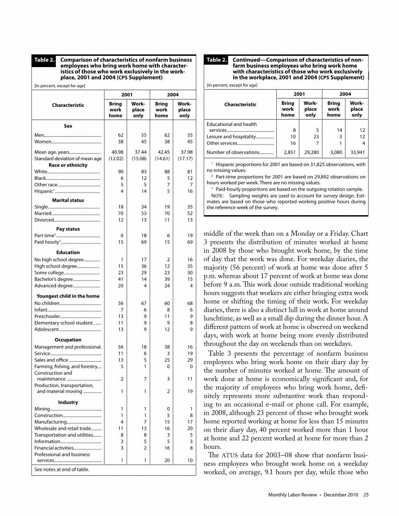
Monthly Labor Review • December 2010 25
middle of the week than on a Monday or a Friday. Chart 3 presents the distribution of minutes worked at home in 2008 by those who brought work home, by the time of day that the work was done. For weekday diaries, the majority (56 percent) of work at home was done after 5 p.m. whereas about 17 percent of work at home was done before 9 a.m. This work done outside traditional working hours suggests that workers are either bringing extra work home or shifting the timing of their work. For weekday diaries, there is also a distinct lull in work at home around lunchtime, as well as a small dip during the dinner hour. A different pattern of work at home is observed on weekend days, with work at home being more evenly distributed throughout the day on weekends than on weekdays.
Table 3 presents the percentage of nonfarm business employees who bring work home on their diary day by the number of minutes worked at home. The amount of work done at home is economically significant and, for the majority of employees who bring work home, defi-nitely represents more substantive work than respond-ing to an occasional e-mail or phone call. For example, in 2008, although 23 percent of those who brought work home reported working at home for less than 15 minutes on their diary day, 40 percent worked more than 1 hour at home and 22 percent worked at home for more than 2 hours.
The ATUS data for 2003–08 show that nonfarm busi-ness employees who brought work home on a weekday worked, on average, 9.1 hours per day, while those who
Table 2. Comparison of characteristics of nonfarm business employees who bring work home with character- istics of those who work exclusively in the work- place, 2001 and 2004 (CPS Supplement)[In percent, except for age]
Characteristic
2001 2004
Bring workhome
Work-place only
Bring workhome
Work-place only
Sex
Men..................................................... 62 55 62 55Women............................................... 38 45 38 45
Mean age, years............................. 40.98 37.44 42.45 37.98Standard deviation of mean age (12.02) (15.08) (14.61) (17.17)
Race or ethnicityWhite................................................. 90 83 88 81Black.................................................. 6 12 5 12Other race........................................ 5 5 7 7Hispanic1.......................................... 4 14 5 16
Marital statusSingle................................................ 18 34 19 35Married............................................. 70 53 70 52Divorced........................................... 12 13 11 13
Pay statusPart time2......................................... 6 18 6 19Paid hourly3..................................... 15 69 15 69
EducationNo high school degree............... 1 17 2 16High school degree..................... 15 36 12 35Some college................................. 23 29 23 30Bachelor’s degree......................... 41 14 39 15Advanced degree......................... 20 4 24 4
Youngest child in the homeNo children...................................... 56 67 60 68Infant.................................................. 7 6 8 6Preschooler...................................... 13 9 11 9Elementary school student.. ..... 11 9 9 8Adolescent....................................... 13 9 12 9
OccupationManagement and professional. 56 18 38 16Service................................................ 11 6 3 19Sales and office .............................. 13 5 25 29Farming, fishing, and forestry.... 5 1 0 0Construction and maintenance ................................ 2 7 3 11Production, transportation, and material moving ................. 1 1 2 19
IndustryMining................................................ 1 1 0 1Construction.................................... 1 1 5 8Manufacturing................................ 4 7 15 17Wholesale and retail trade.......... 11 13 16 20Transportation and utilities........ 8 8 3 5Information...................................... 3 5 5 3Financial activities.......................... 3 2 16 8Professional and business services............................................ 1 1 20 10
See notes at end of table.
Educational and health services............................................ 8 5 14 12Leisure and hospitality................. 10 23 3 12Other services.................................. 16 7 1 4
Number of observations............. 2,851 29,280 3,080 33,941
1 Hispanic proportions for 2001 are based on 31,825 observations, with no missing values.
2 Part-time proportions for 2001 are based on 29,892 observations on hours worked per week. There are no missing values.
3 Paid-hourly proportions are based on the outgoing rotation sample.NOTE: Sampling weights are used to account for survey design. Esti-
mates are based on those who reported working positive hours during the reference week of the survey.
Table 2. Continued—Comparison of characteristics of non- farm business employees who bring work home with characteristics of those who work exclusively in the workplace, 2001 and 2004 (CPS Supplement)[In percent, except for age]
Characteristic
2001 2004
Bring workhome
Work-place only
Bring workhome
Work-place only
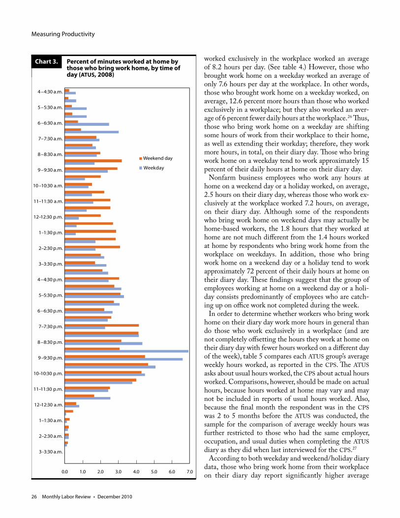
Measuring Productivity
26 Monthly Labor Review • December 2010
0.0 1.0 2.0 3.0 4.0 5.0 6.0 7.0
4–4:30 a.m.
5–5:30 a.m.
6–6:30 a.m.
7–7:30 a.m.
8–8:30 a.m.
9–9:30 a.m.
10–10:30 a.m.
11–11:30 a.m.
12–12:30 p.m.
1–1:30 p.m.
2–2:30 p.m.
3–3:30 p.m.
4–4:30 p.m.
5–5:30 p.m.
6–6:30 p.m.
7–7:30 p.m.
8–8:30 p.m.
9–9:30 p.m.
10–10:30 p.m.
11–11:30 p.m.
12–12:30 a.m.
1–1:30 a.m.
2–2:30 a.m.
3–3:30 a.m.
Weekday
Weekend day
worked exclusively in the workplace worked an average of 8.2 hours per day. (See table 4.) However, those who brought work home on a weekday worked an average of only 7.6 hours per day at the workplace. In other words, those who brought work home on a weekday worked, on average, 12.6 percent more hours than those who worked exclusively in a workplace; but they also worked an aver-age of 6 percent fewer daily hours at the workplace.26 Thus, those who bring work home on a weekday are shifting some hours of work from their workplace to their home, as well as extending their workday; therefore, they work more hours, in total, on their diary day. Those who bring work home on a weekday tend to work approximately 15 percent of their daily hours at home on their diary day.
Nonfarm business employees who work any hours at home on a weekend day or a holiday worked, on average, 2.5 hours on their diary day, whereas those who work ex-clusively at the workplace worked 7.2 hours, on average, on their diary day. Although some of the respondents who bring work home on weekend days may actually be home-based workers, the 1.8 hours that they worked at home are not much different from the 1.4 hours worked at home by respondents who bring work home from the workplace on weekdays. In addition, those who bring work home on a weekend day or a holiday tend to work approximately 72 percent of their daily hours at home on their diary day. These findings suggest that the group of employees working at home on a weekend day or a holi-day consists predominantly of employees who are catch-ing up on office work not completed during the week.
In order to determine whether workers who bring work home on their diary day work more hours in general than do those who work exclusively in a workplace (and are not completely offsetting the hours they work at home on their diary day with fewer hours worked on a different day of the week), table 5 compares each ATUS group’s average weekly hours worked, as reported in the CPS. The ATUS asks about usual hours worked, the CPS about actual hours worked. Comparisons, however, should be made on actual hours, because hours worked at home may vary and may not be included in reports of usual hours worked. Also, because the final month the respondent was in the CPS was 2 to 5 months before the ATUS was conducted, the sample for the comparison of average weekly hours was further restricted to those who had the same employer, occupation, and usual duties when completing the ATUS diary as they did when last interviewed for the CPS.27
According to both weekday and weekend/holiday diary data, those who bring work home from their workplace on their diary day report significantly higher average
Chart 3. Percent of minutes worked at home by those who bring work home, by time of day (ATUS, 2008)
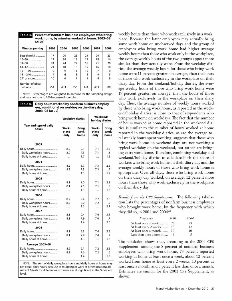
Monthly Labor Review • December 2010 27
Table 3. Percent of nonfarm business employees who bring work home, by minutes worked at home, 2003–08 (ATUS)
Minutes per day 2003 2004 2005 2006 2007 2008
Less than15................ 17 20 23 21 20 2316–30........................... 17 18 18 17 18 1631–60........................... 24 24 22 18 21 2061–120........................ 21 18 13 19 16 18121–180...................... 9 9 11 12 7 9181–240...................... 4 6 5 5 9 5241or more................ 10 6 7 9 8 8
Number of obser- vations...................... 554 403 356 374 403 380
NOTE: Percentages are weighted to account for the sampling design and may not sum to 100 because of rounding.
Table 4. Daily hours worked by nonfarm business employ- ees, conditional on working on the diary day, 2003–08 (ATUS)
Year and type of daily hours
Weekday diaries Weekend/holiday diaries
Work-place only
Bring work home
Work-place only
Bring work home
2003Daily hours..................................... 8.2 9.1 7.1 2.2 Daily workplace hours............ 8.2 7.3 7.1 .6 Daily hours at home............... .... 1.7 .... 1.5
2004Daily hours.................................... 8.2 8.7 7.3 2.6 Daily workplace hours........... 8.2 7.3 7.3 .9 Daily hours at home............... .... 1.3 .... 1.7
2005Daily hours.................................... 8.1 9.0 7.1 2.2 Daily workplace hours........... 8.1 7.5 7.1 .5 Daily hours at home............... .... 1.3 .... 1.6
2006Daily hours.................................... 8.2 9.4 7.2 2.6 Daily workplace hours........... 8.2 8.0 7.2 .5 Daily hours at home............... .... 1.3 .... 2.1
2007Daily hours..................................... 8.1 9.4 7.0 2.8 Daily workplace hours............ 8.1 7.9 7.0 .7 Daily hours at home................ .... 1.4 .... 2.0
2008Daily hours..................................... 8.1 9.3 7.4 2.5 Daily workplace hours............ 8.1 7.9 7.4 .7 Daily hours at home................ .... 1.3 .... 1.8
Average, 2003–08Daily hours..................................... 8.2 9.1 7.2 2.5 Daily workplace hours............ 8.2 7.6 7.2 .6 Daily hours at home................ .... 1.4 .... 1.8
NOTE: The sum of daily workplace hours and daily hours at home may not equal daily hours because of rounding or work at other locations. Re-sults of F-tests for differences in means are all significant at the 5-percent level.
weekly hours than those who work exclusively in a work-place. Because the latter employees may actually bring some work home on unobserved days and the group of employees who bring work home had higher average weekly hours than those who work only in the workplace, the average weekly hours of the two groups appear more similar than they actually were. From the weekday dia-ries, the average weekly hours for those who bring work home were 11 percent greater, on average, than the hours of those who work exclusively in the workplace on their diary day. From the weekend/holiday diaries, the aver-age weekly hours of those who bring work home were 19 percent greater, on average, than the hours of those who work exclusively in the workplace on their diary day. Thus, the average number of weekly hours worked by those who bring work home, as reported in the week-end/holiday diaries, is close to that of respondents who bring work home on weekdays. The fact that the number of hours worked at home reported in the weekend dia-ries is similar to the number of hours worked at home reported in the weekday diaries, as are the average to-tal weekly hours spent working, suggests that those who bring work home on weekend days are not working a typical workday on the weekend, but rather are bring-ing extra work home. Therefore, combining weekday and weekend/holiday diaries to calculate both the share of workers who bring work home on their diary day and the average weekly hours of those who bring work home is appropriate. Over all days, those who bring work home on their diary day worked, on average, 12 percent more hours than those who work exclusively in the workplace on their diary day.
Results from the CPS Supplement. The following tabula-tion lists the percentages of nonfarm business employees who brought work home, by the frequency with which they did so, in 2001 and 2004:28
Frequency 2001 2004At least once a week........... 71 73At least every 2 weeks........ 13 12At least once a month........ 10 10Less than once a month..... 6 5
The tabulation shows that, according to the 2004 CPS Supplement, among the 8 percent of nonfarm business employees who bring work home, 73 percent reported working at home at least once a week, about 12 percent worked from home at least every 2 weeks, 10 percent at least once a month, and 5 percent less than once a month. Estimates are similar for the 2001 CPS Supplement, as shown.
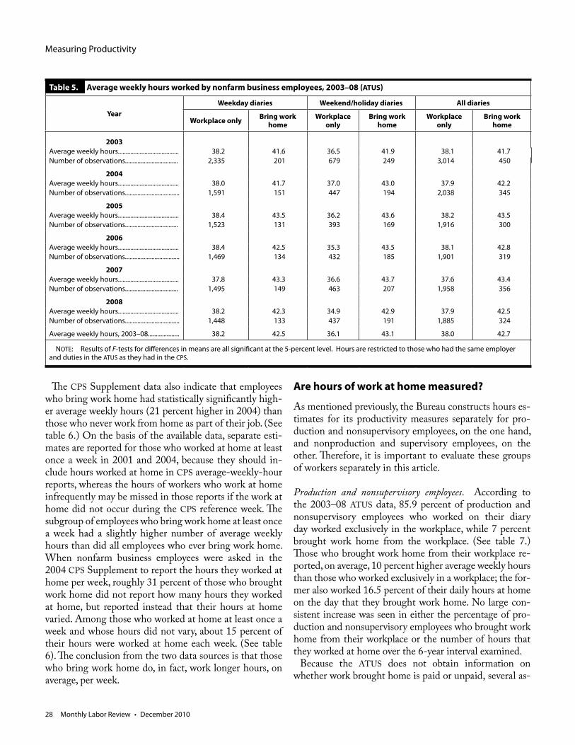
Measuring Productivity
28 Monthly Labor Review • December 2010
Table 5. Average weekly hours worked by nonfarm business employees, 2003–08 (ATUS)
YearWeekday diaries Weekend/holiday diaries All diaries
Workplace only Bring work home
Workplace only
Bring work home
Workplace only
Bring work home
2003Average weekly hours....................................... 38.2 41.6 36.5 41.9 38.1 41.7Number of observations.................................. 2,335 201 679 249 3,014 450
2004Average weekly hours....................................... 38.0 41.7 37.0 43.0 37.9 42.2Number of observations................................... 1,591 151 447 194 2,038 345
2005Average weekly hours....................................... 38.4 43.5 36.2 43.6 38.2 43.5Number of observations.................................. 1,523 131 393 169 1,916 300
2006Average weekly hours....................................... 38.4 42.5 35.3 43.5 38.1 42.8Number of observations................................... 1,469 134 432 185 1,901 319
2007Average weekly hours....................................... 37.8 43.3 36.6 43.7 37.6 43.4Number of observations.................................. 1,495 149 463 207 1,958 356
2008Average weekly hours....................................... 38.2 42.3 34.9 42.9 37.9 42.5Number of observations................................... 1,448 133 437 191 1,885 324
Average weekly hours, 2003–08.................... 38.2 42.5 36.1 43.1 38.0 42.7
NOTE: Results of F-tests for differences in means are all significant at the 5-percent level. Hours are restricted to those who had the same employer and duties in the ATUS as they had in the CPS.
The CPS Supplement data also indicate that employees who bring work home had statistically significantly high-er average weekly hours (21 percent higher in 2004) than those who never work from home as part of their job. (See table 6.) On the basis of the available data, separate esti-mates are reported for those who worked at home at least once a week in 2001 and 2004, because they should in-clude hours worked at home in CPS average-weekly-hour reports, whereas the hours of workers who work at home infrequently may be missed in those reports if the work at home did not occur during the CPS reference week. The subgroup of employees who bring work home at least once a week had a slightly higher number of average weekly hours than did all employees who ever bring work home. When nonfarm business employees were asked in the 2004 CPS Supplement to report the hours they worked at home per week, roughly 31 percent of those who brought work home did not report how many hours they worked at home, but reported instead that their hours at home varied. Among those who worked at home at least once a week and whose hours did not vary, about 15 percent of their hours were worked at home each week. (See table 6). The conclusion from the two data sources is that those who bring work home do, in fact, work longer hours, on average, per week.
Are hours of work at home measured?
As mentioned previously, the Bureau constructs hours es-timates for its productivity measures separately for pro-duction and nonsupervisory employees, on the one hand, and nonproduction and supervisory employees, on the other. Therefore, it is important to evaluate these groups of workers separately in this article.
Production and nonsupervisory employees. According to the 2003–08 ATUS data, 85.9 percent of production and nonsupervisory employees who worked on their diary day worked exclusively in the workplace, while 7 percent brought work home from the workplace. (See table 7.) Those who brought work home from their workplace re-ported, on average, 10 percent higher average weekly hours than those who worked exclusively in a workplace; the for-mer also worked 16.5 percent of their daily hours at home on the day that they brought work home. No large con-sistent increase was seen in either the percentage of pro-duction and nonsupervisory employees who brought work home from their workplace or the number of hours that they worked at home over the 6-year interval examined.
Because the ATUS does not obtain information on whether work brought home is paid or unpaid, several as-
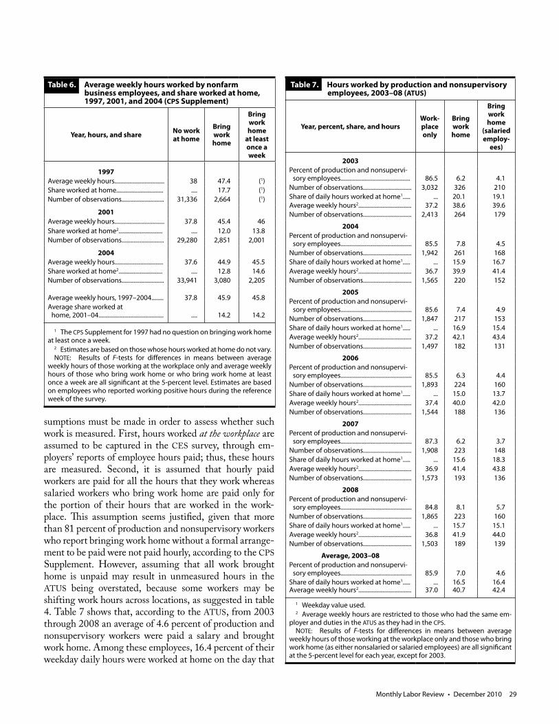
Monthly Labor Review • December 2010 29
Table 6. Average weekly hours worked by nonfarm business employees, and share worked at home, 1997, 2001, and 2004 (CPS Supplement)
Year, hours, and share No work at home
Bring work home
Bring work home
at least once a week
1997Average weekly hours................................. 38 47.4 (1)Share worked at home............................... .... 17.7 (1)Number of observations............................ 31,336 2,664 (1)
2001Average weekly hours................................. 37.8 45.4 46Share worked at home2............................. .... 12.0 13.8Number of observations............................ 29,280 2,851 2,001
2004Average weekly hours................................ 37.6 44.9 45.5Share worked at home2............................. .... 12.8 14.6Number of observations............................ 33,941 3,080 2,205
Average weekly hours, 1997–2004........ 37.8
45.9 45.8Average share worked at home, 2001–04........................................... .... 14.2 14.2
1 The CPS Supplement for 1997 had no question on bringing work home at least once a week.
2 Estimates are based on those whose hours worked at home do not vary. NOTE: Results of F-tests for differences in means between average
weekly hours of those working at the workplace only and average weekly hours of those who bring work home or who bring work home at least once a week are all significant at the 5-percent level. Estimates are based on employees who reported working positive hours during the reference week of the survey.
Table 7. Hours worked by production and nonsupervisory employees, 2003–08 (ATUS)
Year, percent, share, and hoursWork-place only
Bring work home
Bring work home
(salariedemploy-
ees)
2003Percent of production and nonsupervi- sory employees.............................................. 86.5 6.2 4.1Number of observations................................ 3,032 326 210Share of daily hours worked at home1..... ... 20.1 19.1Average weekly hours2................................... 37.2 38.6 39.6Number of observations................................ 2,413 264 179
2004Percent of production and nonsupervi- sory employees............................................... 85.5 7.8 4.5Number of observations................................ 1,942 261 168Share of daily hours worked at home1..... ... 15.9 16.7Average weekly hours2................................... 36.7 39.9 41.4Number of observations................................ 1,565 220 152
2005Percent of production and nonsupervi- sory employees............................................... 85.6 7.4 4.9Number of observations................................ 1,847 217 153Share of daily hours worked at home1..... ... 16.9 15.4Average weekly hours2................................... 37.2 42.1 43.4Number of observations................................ 1,497 182 131
2006Percent of production and nonsupervi- sory employees............................................... 85.5 6.3 4.4Number of observations................................ 1,893 224 160Share of daily hours worked at home1..... ... 15.0 13.7Average weekly hours2................................... 37.4 40.0 42.0Number of observations................................ 1,544 188 136
2007Percent of production and nonsupervi- sory employees............................................... 87.3 6.2 3.7Number of observations................................ 1,908 223 148Share of daily hours worked at home1..... ... 15.6 18.3Average weekly hours2................................... 36.9 41.4 43.8Number of observations................................ 1,573 193 136
2008Percent of production and nonsupervi- sory employees............................................... 84.8 8.1 5.7Number of observations................................ 1,865 223 160Share of daily hours worked at home1..... ... 15.7 15.1Average weekly hours2................................... 36.8 41.9 44.0Number of observations................................ 1,503 189 139
Average, 2003–08Percent of production and nonsupervi- sory employees............................................... 85.9 7.0 4.6Share of daily hours worked at home1..... ... 16.5 16.4Average weekly hours2................................... 37.0 40.7 42.4
1 Weekday value used.2 Average weekly hours are restricted to those who had the same em-
ployer and duties in the ATUS as they had in the CPS. NOTE: Results of F-tests for differences in means between average
weekly hours of those working at the workplace only and those who bring work home (as either nonsalaried or salaried employees) are all significant at the 5-percent level for each year, except for 2003.
sumptions must be made in order to assess whether such work is measured. First, hours worked at the workplace are assumed to be captured in the CES survey, through em-ployers’ reports of employee hours paid; thus, these hours are measured. Second, it is assumed that hourly paid workers are paid for all the hours that they work whereas salaried workers who bring work home are paid only for the portion of their hours that are worked in the work-place. This assumption seems justified, given that more than 81 percent of production and nonsupervisory workers who report bringing work home without a formal arrange-ment to be paid were not paid hourly, according to the CPS Supplement. However, assuming that all work brought home is unpaid may result in unmeasured hours in the ATUS being overstated, because some workers may be shifting work hours across locations, as suggested in table 4. Table 7 shows that, according to the ATUS, from 2003 through 2008 an average of 4.6 percent of production and nonsupervisory workers were paid a salary and brought work home. Among these employees, 16.4 percent of their weekday daily hours were worked at home on the day that
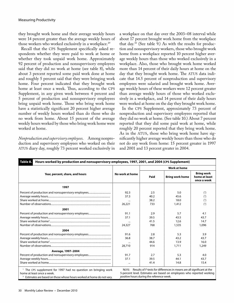
Measuring Productivity
30 Monthly Labor Review • December 2010
Table 8. Hours worked by production and nonsupervisory employees, 1997, 2001, and 2004 (CPS Supplement)
Year, percent, share, and hours No work at home
Work at home
Paid Bring work homeBring work
home at least once a week
1997
Percent of production and nonsupervisory employees................................... 92.3 2.5 5.0 (1) Average weekly hours.................................................................................................. 37.3 40.2 45.6 (1) Share worked at home................................................................................................. ... 38.2 18.0 (1)Number of observations.............................................................................................. 26,221 733 1,412 (1)
2001Percent of production and nonsupervisory employees.................................. 91.1 2.9 5.7 4.1Average weekly hours.................................................................................................. 37.1 39.5 43.5 43.7Share worked at home2............................................................................................... ... 41.5 12.6 14.7Number of observations............................................................................................. 24,327 768 1,535 1,096
2004Percent of production and nonsupervisory employees.................................... 91.6 2.8 5.3 3.9Average weekly hours.................................................................................................... 36.8 38.7 43.2 43.7Share worked at home2................................................................................................. ... 44.6 13.9 16.0Number of observations............................................................................................... 28,710 914 1,711 1,249
Average, 1997–2004Percent of production and nonsupervisory employees.................................... 91.7 2.7 5.3 4.0Average weekly hours................................................................................................... 37.1 39.5 44.1 43.7Share worked at home.................................................................................................. ... 41.4 14.8 15.4
.
1 The CPS supplement for 1997 had no question on bringing work home at least once a week.
2 Estimates are based on those whose hours worked at home do not vary.
NOTE: Results of F-tests for differences in means are all significant at the5-percent level. Estimates are based on employees who reported working positive hours during the reference week.
they brought work home and their average weekly hours were 14 percent greater than the average weekly hours of those workers who worked exclusively in a workplace.29
Recall that the CPS Supplement specifically asked re-spondents whether they were paid to work at home or whether they took unpaid work home. Approximately 92 percent of production and nonsupervisory employees said that they did no work at home (see table 8), while about 3 percent reported some paid work done at home and roughly 5 percent said that they were bringing work home. Four percent indicated that they brought work home at least once a week. Thus, according to the CPS Supplement, in any given week between 4 percent and 5 percent of production and nonsupervisory employees bring unpaid work home. Those who bring work home have a statistically significant 20 percent higher average number of weekly hours worked than do those who do no work from home. About 15 percent of the average weekly hours worked by those who bring work home were worked at home.
Nonproduction and supervisory employees. Among nonpro-duction and supervisory employees who worked on their ATUS diary day, roughly 73 percent worked exclusively in
a workplace on that day over the 2003–08 interval while about 17 percent brought work home from the workplace that day.30 (See table 9.) As with the results for produc-tion and nonsupervisory workers, those who brought work home from a workplace reported 10 percent higher aver-age weekly hours than those who worked exclusively in a workplace. Also, those who brought work home worked more than 14 percent of their daily hours at home on the day that they brought work home. The ATUS data indi-cate that 14.5 percent of nonproduction and supervisory employees were salaried and brought work home. Aver-age weekly hours of these workers were 12 percent greater than average weekly hours of those who worked exclu-sively in a workplace, and 14 percent of their daily hours were worked at home on the day they brought work home.
In the CPS Supplement, approximately 73 percent of nonproduction and supervisory employees reported that they did no work at home. (See table 10.) About 7 percent reported that they did some paid work at home, while roughly 20 percent reported that they bring work home. As in the ATUS, those who bring work home have sig-nificantly higher average weekly hours than those who do not do any work from home: 15 percent greater in 1997 and 2001 and 13 percent greater in 2004.
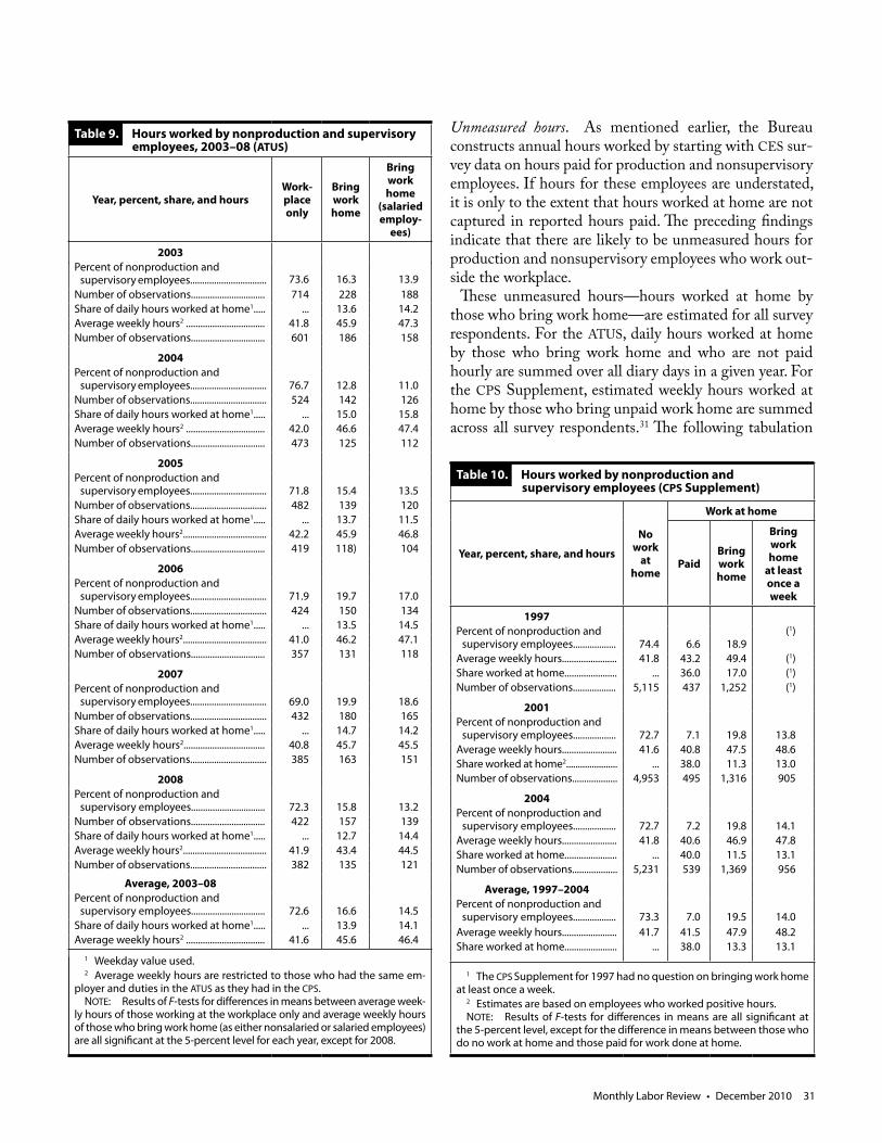
Monthly Labor Review • December 2010 31
Table 9. Hours worked by nonproduction and supervisory employees, 2003–08 (ATUS)
Year, percent, share, and hoursWork-place only
Bring work home
Bring work home
(salaried employ-
ees)
2003Percent of nonproduction and supervisory employees................................ 73.6 16.3 13.9Number of observations............................... 714 228 188Share of daily hours worked at home1..... ... 13.6 14.2Average weekly hours2 ................................. 41.8 45.9 47.3Number of observations............................... 601 186 158
2004Percent of nonproduction and supervisory employees................................ 76.7 12.8 11.0Number of observations................................ 524 142 126Share of daily hours worked at home1..... ... 15.0 15.8Average weekly hours2 ................................. 42.0 46.6 47.4Number of observations............................... 473 125 112
2005Percent of nonproduction and supervisory employees................................ 71.8 15.4 13.5Number of observations................................ 482 139 120Share of daily hours worked at home1..... ... 13.7 11.5Average weekly hours2................................... 42.2 45.9 46.8Number of observations............................... 419 118) 104
2006Percent of nonproduction and supervisory employees................................ 71.9 19.7 17.0Number of observations................................ 424 150 134Share of daily hours worked at home1..... ... 13.5 14.5Average weekly hours2................................... 41.0 46.2 47.1Number of observations............................... 357 131 118
2007Percent of nonproduction and supervisory employees................................ 69.0 19.9 18.6Number of observations................................ 432 180 165Share of daily hours worked at home1..... ... 14.7 14.2Average weekly hours2.................................. 40.8 45.7 45.5Number of observations................................ 385 163 151
2008Percent of nonproduction and supervisory employees............................... 72.3 15.8 13.2Number of observations............................... 422 157 139Share of daily hours worked at home1..... ... 12.7 14.4Average weekly hours2................................... 41.9 43.4 44.5Number of observations................................ 382 135 121
Average, 2003–08Percent of nonproduction and supervisory employees............................... 72.6 16.6 14.5Share of daily hours worked at home1..... ... 13.9 14.1Average weekly hours2 ................................. 41.6 45.6 46.4
1 Weekday value used.2 Average weekly hours are restricted to those who had the same em-
ployer and duties in the ATUS as they had in the CPS. NOTE: Results of F-tests for differences in means between average week-
ly hours of those working at the workplace only and average weekly hours of those who bring work home (as either nonsalaried or salaried employees) are all significant at the 5-percent level for each year, except for 2008.
Unmeasured hours. As mentioned earlier, the Bureau constructs annual hours worked by starting with CES sur-vey data on hours paid for production and nonsupervisory employees. If hours for these employees are understated, it is only to the extent that hours worked at home are not captured in reported hours paid. The preceding findings indicate that there are likely to be unmeasured hours for production and nonsupervisory employees who work out-side the workplace.
These unmeasured hours—hours worked at home by those who bring work home—are estimated for all survey respondents. For the ATUS, daily hours worked at home by those who bring work home and who are not paid hourly are summed over all diary days in a given year. For the CPS Supplement, estimated weekly hours worked at home by those who bring unpaid work home are summed across all survey respondents.31 The following tabulation
Table 10. Hours worked by nonproduction and supervisory employees (CPS Supplement)
Year, percent, share, and hours
No work
at home
Work at home
PaidBring work home
Bring work home
at least once a week
1997Percent of nonproduction and supervisory employees.................. 74.4 6.6 18.9
(1)
Average weekly hours....................... 41.8 43.2 49.4 (1)Share worked at home...................... ... 36.0 17.0 (1) Number of observations.................. 5,115 437 1,252 (1)
2001Percent of nonproduction and supervisory employees.................. 72.7 7.1 19.8 13.8Average weekly hours....................... 41.6 40.8 47.5 48.6Share worked at home2...................... ... 38.0 11.3 13.0Number of observations................... 4,953 495 1,316 905
2004Percent of nonproduction and supervisory employees.................. 72.7 7.2 19.8 14.1Average weekly hours....................... 41.8 40.6 46.9 47.8Share worked at home...................... ... 40.0 11.5 13.1Number of observations................... 5,231 539 1,369 956
Average, 1997–2004Percent of nonproduction and supervisory employees.................. 73.3 7.0 19.5 14.0Average weekly hours....................... 41.7 41.5 47.9 48.2Share worked at home...................... ... 38.0 13.3 13.1
1 The CPS Supplement for 1997 had no question on bringing work home at least once a week.
2 Estimates are based on employees who worked positive hours.NOTE: Results of F-tests for differences in means are all significant at
the 5-percent level, except for the difference in means between those who do no work at home and those paid for work done at home.
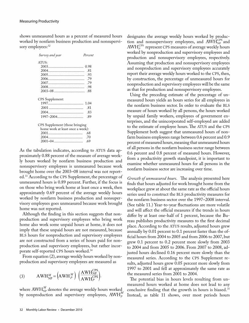
Measuring Productivity
32 Monthly Labor Review • December 2010
designates the average weekly hours worked by produc-tion and nonsupervisory employees, and AWHNP and AWHP represent CPS measures of average weekly hours worked by nonproduction and supervisory employees and production and nonsupervisory employees, respectively. Assuming that production and nonsupervisory employees and nonproduction and supervisory employees accurately report their average weekly hours worked to the CPS, then, by construction, the percentage of unmeasured hours for nonproduction and supervisory employees will be the same as that for production and nonsupervisory employees.
Using the preceding estimate of the percentage of un-measured hours yields an hours series for all employees in the nonfarm business sector. In order to evaluate the BLS measure of hours worked by all persons, the hours worked by unpaid family workers, employees of government en-terprises, and the unincorporated self-employed are added to the estimate of employee hours. The ATUS and the CPS Supplement both suggest that unmeasured hours of non-farm business employees range between 0.6 percent and 0.9 percent of measured hours, meaning that unmeasured hours of all persons in the nonfarm business sector range between 0.6 percent and 0.8 percent of measured hours. However, from a productivity growth standpoint, it is important to examine whether unmeasured hours for all persons in the nonfarm business sector are increasing over time.
Growth of unmeasured hours. The analysis presented here finds that hours adjusted for work brought home from the workplace grew at about the same rate as the official hours series used to construct the BLS productivity measures for the nonfarm business sector over the 1997–2008 interval. (See table 11.) Year-to-year fluctuations are more volatile and will affect the official measures if the trends in hours differ by at least one-half of 1 percent, because the Bu-reau publishes productivity measures to the first decimal place. According to the ATUS results, adjusted hours grew annually by 0.01 percent to 0.1 percent faster than the of-ficial hours from 2004 to 2005 and from 2006 to 2007, but grew 0.1 percent to 0.2 percent more slowly from 2003 to 2004 and from 2005 to 2006. From 2007 to 2008, ad-justed hours declined 0.16 percent more slowly than the measured series. According to the CPS Supplement re-sults, adjusted hours grew 0.05 percent more slowly from 1997 to 2001 and fell at approximately the same rate as the measured series from 2001 to 2004.
The potential bias in hours levels resulting from un-measured hours worked at home does not lead to any conclusive finding that the growth in hours is biased.35 Instead, as table 11 shows, over most periods hours
,CPS
CPSNP
NP AWHAWH
AWHAWH P
MP
M
shows unmeasured hours as a percent of measured hours worked by nonfarm business production and nonsupervi-sory employees:32
Survey and year Percent
ATUS: 2003...................................... 0.98 2004....................................... .81 2005....................................... .93 2006....................................... .79 2007....................................... .79 2008....................................... .98 2003–08 ................................. .88
CPS Supplement: 1997...................................... 1.04 2001 ..................................... .81 2004...................................... .83 1997–2004............................ .89
CPS Supplement (those bringing home work at least once a week): 2001..................................... .68 2004..................................... .70 2001–04 ............................... .69
As the tabulation indicates, according to ATUS data ap-proximately 0.88 percent of the measure of average week-ly hours worked by nonfarm business production and nonsupervisory employees is unmeasured because work brought home over the 2003–08 interval was not report-ed.33 According to the CPS Supplement, the percentage of unmeasured hours is 0.89 percent. Further, if the focus is on those who bring work home at least once a week, then approximately 0.69 percent of the average weekly hours worked by nonfarm business production and nonsuper-visory employees goes unmeasured because work brought home was not reported.
Although the finding in this section suggests that non-production and supervisory employees who bring work home also work some unpaid hours at home, it does not imply that these unpaid hours are not measured, because BLS hours for nonproduction and supervisory employees are not constructed from a series of hours paid for non-production and supervisory employees, but rather incor-porate self-reported CPS hours worked.34
From equation (2), average weekly hours worked by non-production and supervisory employees are measured as
(3)
where AWHNP denotes the average weekly hours worked by nonproduction and supervisory employees, AWHP M
M
CPS
CPS
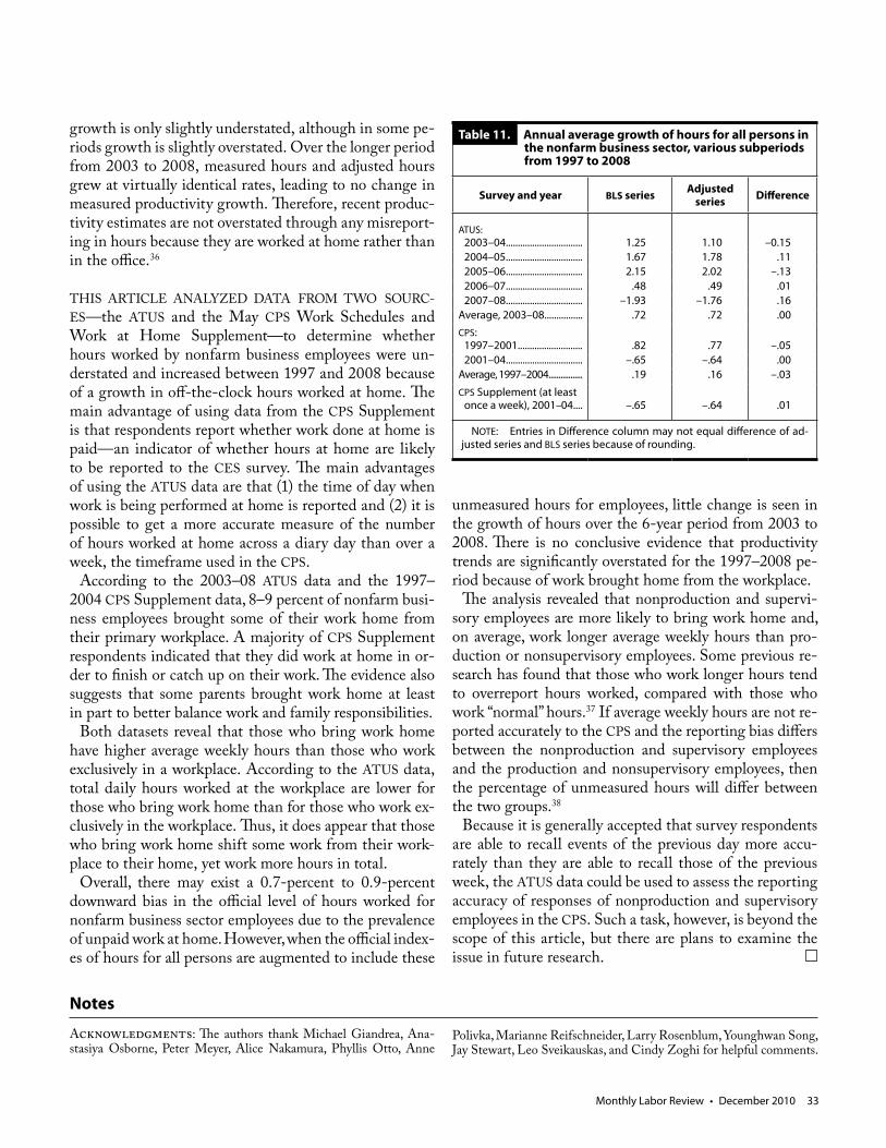
Monthly Labor Review • December 2010 33
Table 11. Annual average growth of hours for all persons in the nonfarm business sector, various subperiods from 1997 to 2008
Survey and year BLS series Adjusted series Difference
ATUS: 2003–04................................ 1.25 1.10 –0.15 2004–05................................ 1.67 1.78 .11 2005–06................................ 2.15 2.02 –.13 2006–07................................ .48 .49 .01 2007–08................................ –1.93 –1.76 .16Average, 2003–08................ .72 .72 .00CPS: 1997–2001........................... .82 .77 –.05 2001–04................................ –.65 –.64 .00Average, 1997–2004................. .19 .16 –.03
CPS Supplement (at least once a week), 2001–04.... –.65 –.64 .01
NOTE: Entries in Difference column may not equal difference of ad-justed series and BLS series because of rounding.
growth is only slightly understated, although in some pe-riods growth is slightly overstated. Over the longer period from 2003 to 2008, measured hours and adjusted hours grew at virtually identical rates, leading to no change in measured productivity growth. Therefore, recent produc-tivity estimates are not overstated through any misreport-ing in hours because they are worked at home rather than in the office.36
THIS ARTICLE ANALYZED DATA FROM TWO SOURC-ES—the ATUS and the May CPS Work Schedules and Work at Home Supplement—to determine whether hours worked by nonfarm business employees were un-derstated and increased between 1997 and 2008 because of a growth in off-the-clock hours worked at home. The main advantage of using data from the CPS Supplement is that respondents report whether work done at home is paid—an indicator of whether hours at home are likely to be reported to the CES survey. The main advantages of using the ATUS data are that (1) the time of day when work is being performed at home is reported and (2) it is possible to get a more accurate measure of the number of hours worked at home across a diary day than over a week, the timeframe used in the CPS.
According to the 2003–08 ATUS data and the 1997–2004 CPS Supplement data, 8–9 percent of nonfarm busi-ness employees brought some of their work home from their primary workplace. A majority of CPS Supplement respondents indicated that they did work at home in or-der to finish or catch up on their work. The evidence also suggests that some parents brought work home at least in part to better balance work and family responsibilities.
Both datasets reveal that those who bring work home have higher average weekly hours than those who work exclusively in a workplace. According to the ATUS data, total daily hours worked at the workplace are lower for those who bring work home than for those who work ex-clusively in the workplace. Thus, it does appear that those who bring work home shift some work from their work-place to their home, yet work more hours in total.
Overall, there may exist a 0.7-percent to 0.9-percent downward bias in the official level of hours worked for nonfarm business sector employees due to the prevalence of unpaid work at home. However, when the official index-es of hours for all persons are augmented to include these
unmeasured hours for employees, little change is seen in the growth of hours over the 6-year period from 2003 to 2008. There is no conclusive evidence that productivity trends are significantly overstated for the 1997–2008 pe-riod because of work brought home from the workplace.
The analysis revealed that nonproduction and supervi-sory employees are more likely to bring work home and, on average, work longer average weekly hours than pro-duction or nonsupervisory employees. Some previous re-search has found that those who work longer hours tend to overreport hours worked, compared with those who work “normal” hours.37 If average weekly hours are not re-ported accurately to the CPS and the reporting bias differs between the nonproduction and supervisory employees and the production and nonsupervisory employees, then the percentage of unmeasured hours will differ between the two groups.38
Because it is generally accepted that survey respondents are able to recall events of the previous day more accu-rately than they are able to recall those of the previous week, the ATUS data could be used to assess the reporting accuracy of responses of nonproduction and supervisory employees in the CPS. Such a task, however, is beyond the scope of this article, but there are plans to examine the issue in future research.
Notes
Acknowledgments: The authors thank Michael Giandrea, Ana-stasiya Osborne, Peter Meyer, Alice Nakamura, Phyllis Otto, Anne
Polivka, Marianne Reifschneider, Larry Rosenblum, Younghwan Song, Jay Stewart, Leo Sveikauskas, and Cindy Zoghi for helpful comments.
Measuring Productivity
34 Monthly Labor Review • December 2010
This article is an updated version of a publication by the Organization for Economic Cooperation and Development and includes 2007–08 ATUS data, as well as the 2008 major revision to BLS productivity data. (See Lucy Eldridge and Sabrina Wulff Pabilonia, “Are Those Who Bring Work Home Really Working Longer Hours? Implications for BLS Productivity Measures,” in Julien Dupont and Pierre Sollberger, eds., Productivity Measurement and Analysis: Proceedings from OECD Workshops (Neuchâtel, Switzerland, Swiss Federal Statistical Office, 2008), pp. 179–209.
1 Younghwan Song, “Unpaid Work at Home,” Industrial Relations: A Journal of Economy and Society, October 2009, pp. 578–88.
2 Paul Callister and Sylvia Dixon, “New Zealanders’ Working Time and Home Work Patterns: Evidence from the Time Use Survey,” New Zealand Department of Labour Occasional Paper No. 5, Aug. 1, 2001.
3 Production workers include working supervisors or group lead-ers who may be “in charge” of some employees, but whose supervisory functions are only incidental to their regular work. Nonsupervisory workers include every employee except those whose major responsibil-ity is to supervise, plan, or direct the work of others.
4 Another source of data on hours is the BLS CPS. However, the CES survey is preferred for productivity measurement because it samples 400,000 nonfarm establishments, more than 6 times the 60,000 households sampled in the CPS. In addition, the CES survey is benchmarked annually to levels based on administrative records of employees covered by State unemployment insurance tax records. There is no direct benchmark for CPS employment data. Adjustments to the survey’s underlying population base are made annually with intercensal estimates and every 10 years with the use of the decennial census. Also, hours data from establishments are more consistent with the measures of output used to produce productivity measures; output data are based on data collected from establishments. In addition, establishment data provide reliable reporting and coding on industries and thus are well suited for producing industry-level measures. Industry measures based on household reports tend to produce estimates with considerable variance, even in a survey as large as the CPS. Hence, the Bureau’s official measures by industry come from establishment surveys whenever possible. The CES survey began collecting data on earnings and hours for all employees in September 2005. An experimental series that includes these new data is available on the Internet at www.bls.gov/ces/cesaepp.htm. The Bureau is currently evaluating whether to start using this new series in its productivity statistics.
5 Prior to 2000, the annual Hours at Work Survey was used.6 The Bureau introduced this new method of constructing estimates
of hours for nonproduction and supervisory workers in August 2004. (See Lucy P. Eldridge, Marilyn E. Manser, and Phyllis Flohr Otto, “Alternative measures of supervisory employee hours and productivity growth,” Monthly Labor Review, April 2004, pp. 9–28.)
7 Average weekly hours for unpaid family workers, employees of government enterprises, and the unincorporated self-employed are obtained directly from the CPS. Employment counts for employees in agricultural services, forestry, and fishing come from the BLS Quarterly Census of Employment and Wages (formerly the ES-202 program), based on administrative records from the unemployment insurance system. The number of employees of government enterprises comes from the Bureau of Economic Analysis.
8 In this regard, Steven Roach argued that, as a result of the new portable technologies of the information age—laptops, cellular telephones, home fax machines, and pagers—many white-collar workers are working longer workdays than the official U.S. data show. (See Stephen Roach, The Boom for Whom: Revisiting America’s Technology Paradox, Morgan Stanley Dean Witter Special Economic
Study, Jan. 9, 1998.)9 The CPS collects information on the demographic characteristics
of all individuals in a household from a sample of about 60,000 households on a monthly basis. In addition, the CPS provides information on employment and hours worked by household members 15 years and older. Households are in the survey for 4 months, out for 8 months, and back in for another 4 months.
10 The ATUS does not report with whom a respondent spent time sleeping, grooming, on private activities, working, or taking a class; also excluded are activities the respondent refuses to classify by type and activities the respondent was unable to remember.
11 A workplace is the place where a person usually works. For example, a waitress probably would work in a restaurant, a teacher would work in a school, and an accountant might work in an office building. ATUS interviewers are trained to ask a respondent about work breaks of 15 minutes or longer any time the respondent reports that he or she worked. Beginning in January 2004, an automated question was introduced into the survey instrument. If a respondent reports working for more than 4 hours at one time, the interviewer automatically is prompted to ask, “Did you take any breaks of 15 minutes or longer?” If the respondent reports taking a break, the interviewer records the beginning and ending times and what was done on the break; if the respondent reports that he or she did not take any breaks, a solid work episode is recorded.
12 Suzanne M. Bianchi, John P. Robinson, and Melissa A. Milkie, Changing Rhythms of American Family Life (New York, Russell Sage, 2006).
13 Rachel Krantz-Kent, “Where People Worked, 2003 to 2007,” Is-sues in Labor Statistics, Summary 09–07 (U.S. Bureau of Labor Statis-tics, 2009).
14 Statistical testing excluding breaks and work-related travel yielded essentially the same results as the tests that included those activities.
15 See Edwin R. Dean and Michael J. Harper, “The BLS Productivity Measurement Program,” paper presented at the Conference on Research in Income and Wealth: New Directions in Productivity Research, Silver Spring, MD, March 20–21, 1998.
16 The 1997 CPS Supplement included a probing question later in the survey asking for the existence of additional unpaid hours; however, it is unclear how the information collected through this question may be appropriately analyzed.
17 These figures include those who were bringing a little work home on the weekend, as well as those who worked all day at home on their weekend diary day.
18 The distributions of work locations for other years are not statisti-cally different from the 2004 results.
19 Throughout this article, all ATUS estimates are weighted with the ATUS respondent final weight. The sample of nonfarm business em-ployees also is reweighted so that each day of the week is weighted the same in each of the analyses. All CPS Supplement estimates are weighted with the work schedules supplement weights.
20 Lucy Eldridge and Sabrina Wulff Pabilonia (see Eldridge and Pabilonia, “Are Those Who Bring Work Home?”) used the ATUS sample and a multinomial logit model to estimate the effect of de-mographic and job characteristics on the probability of bringing work home, compared with working exclusively in the workplace. Then they used the CPS Supplement to perform a similar analysis.
21 From this point forward, results are presented for combined week-day and weekend diaries. Separate analyses conducted for weekday dia-ries and weekend diaries yielded similar results.
Monthly Labor Review • December 2010 35
22 ATUS results may incorrectly categorize those who bring work home as working at the workplace only if they were not observed to bring work home on their diary day. As a result, the workplace-only cohort may be slightly “contaminated,” leading the two groups to ap-pear more similar than they actually are. The finding that these groups have different characteristics remains.
23 Note that the percentages shown are weighted to account for the sampling design. The reasons for working at home cited in the 1997 CPS Supplement are not comparable and, therefore, not reported here.
24 The 49-percent figure is calculated from secondary childcare meas-ures and does not imply that the child was in the same room while the parent was working. That is to say, the child may have been elsewhere in the home, but the parent was available if the child needed assistance.
25 The percentages are weighted to account for the sampling design.26 Those who worked for 2 or more hours at home on a weekday
worked, on average, 7.1 hours in the office on the same day, while their total hours were 9.9.
27 A comparison of usual hours reported in the ATUS and in the CPS reveals that the difference in hours reported was smaller for those who held similar jobs from the one survey to the other than for those who changed jobs between the two surveys.
28 The percentages are weighted to account for the sampling design.29 Those who brought work home on a weekend or holiday diary day
worked more than 70 percent of their hours at home.30 Numbers do not sum to 100 because workers could work in other
locations or exclusively at home.31 Weekly hours worked at home are estimated by multiplying av-
erage weekly hours by the share of hours worked at home. Shares of average weekly hours worked at home were calculated from data for those who reported actual hours worked at home; these shares were applied to the average weekly hours for all respondents who brought work home, yielding estimates of total hours worked at home for those who reported that their hours varied.
32 Measured hours are constructed as the sum of all hours worked, less unmeasured hours.
33 However, the quality of these additional hours worked at home may not be the same as the quality of those worked in the workplace,
especially if the workers are engaged in secondary childcare while working at home.
34 See equation (2).35 In a similar analysis, Eldridge found that a hypothetical hours se-
ries constructed by combining CPS average weekly hours with CES employment data produced slightly higher levels of hours, but hours showed a comparable trend from 2000 to 2003. (See Lucy P. Eldridge, “Hours Measures for Productivity Measurement and National Ac-counting,” paper presented to Paris Group on Measuring Hours of Work, Lisbon, September 29–October 1, 2004.
36 The results presented in this article are somewhat different from those arrived at in an earlier version, for two reasons. First, an improved method was used to adjust the weights in the ATUS data to account more accurately for differences in group selections. In addition, there was a major revision to the major sector productivity data on Sep-tember 2, 2009, that significantly changed the employment and hours series for 2003–06.
37 See, for example, John P. Robinson, Jonathan Gershuny, Kimberly Fisher, and Steven Martin, “Workweek Estimate: Diary Differences and Regression to the Mean,” presented at the International Asso-ciation for Time Use Research Annual Conference, Washington, DC, October 17–19, 2007; Steffen Otterbach and Alfonso Sousa-Poza, “How accurate are German work time data? A comparison between time-diary reports and stylized estimates,” Social Indicators Research, June 2009, pp. 325–29; and Jens Bonke, “Paid work and unpaid work: Diary information versus questionnaire information,” Social Indicators Research, February 2005, pp. 349–68.
38 Using the 2003–06 ATUS sample, Harley Frazis and Jay Stewart found that the CPS understates production and nonsupervisory work-ers’ hours worked on the main job by 1.2 hours per week. However, Frazis and Stewart also found that the CPS overstates production and nonsupervisory workers’ hours worked on all jobs by 0.2 hour per week, because of overreporting on second jobs, but that this small difference is not statistically significant. (See Harley Frazis and Jay Stewart, “Why Do BLS Hours Series Tell Different Stories about Trends in Hours Worked?” in Katharine G. Abraham, James R. Spletzer, and Michael J. Harper, eds., Labor in the New Economy, National Bureau of Economic Research Book Studies in Income and Wealth, vol. 71 (Chicago, University of Chicago Press, 2010), pp. 343–72.)
36 Monthly Labor Review • December 2010
Regional Trends
Duration of unemployment in States, 2007–09
Sally L. Anderson
Sally L. Anderson is an economist in the Division of Local Area Unemployment Statistics at the Bureau of Labor Statistics. E-mail: [email protected].
The U.S. Bureau of Labor Statis-tics (BLS) publishes statistics on
the duration of unemployment at the national level, derived from the Cur-rent Population Survey (CPS), on a monthly basis. Unemployed persons at the State level also can be classi-fied by duration. In this article, which utilizes CPS data at the State level, those jobless for a period of less than 5 weeks are referred to as short-term unemployed, while those jobless for 15 weeks or more are referred to as long-term unemployed.1
Duration of unemployment mea-sures are affected by economic cycles. In a strong economy, the largest share of the unemployed is generally found in the short-term category. The un-employed then would consist largely of the frictionally unemployed—those who are jobless for short periods as they are changing jobs. Increases in the number of short-term unemployed can indicate a weakening economy. If the economy continues to deteriorate over an extended period of time, and people continue to struggle to find jobs, the distribution of unemploy-ment by duration will begin to shift from short term to medium term and then finally to the long-term category.2
Recently, CPS annual average esti-mates for 2007–09 were tabulated for all States and the District of Columbia for the same unemployment duration categories that are published at the na-tional level. The estimation procedure used for the subnational sample-based
CPS data allows for the development of statistics on economic characteris-tics of the labor force, such as duration of unemployment, based on specific responses to the survey questionnaire.3 In contrast, the official statewide un-employment estimates from the Lo-cal Area Unemployment Statistics (LAUS) program are model-based measures and are designed to produce reliable total employment and unem-ployment estimates. Further break-downs of LAUS data by economic or demographic characteristics are not available.
When comparing duration across States, it is more revealing to look at the percent distributions within the different unemployment duration categories than the actual levels. This is due to the substantial differences across States in the size of their pop-ulation, labor force, and unemployed. This article focuses on percent distri-butions.
Duration in 2007
In 2007, the greatest proportion of unemployed, 35.9 percent of the total at the national level, was in the less- than-5-weeks range. Thirty-six States also recorded the largest percentages of their unemployed in the short-term category. Wyoming reported the highest share, 53.0 percent, followed closely by Utah, 52.2 percent. These two States were among those with the lowest unemployment rates for 2007. New Jersey and the District of Columbia registered the lowest pro-portions of their unemployment in the short-term category, 29.3 percent each.
Individuals unemployed for 15 weeks or longer accounted for 32.5 percent of unemployed persons in the United States in 2007. Nine States and the District of Columbia registered the largest percentages of their unemployed in the long-term category. Michigan, which recorded the highest unemployment rate for 2007, also had the highest share of its unemployment in the 15-weeks-or-longer category, 42.0 percent, fol-lowed by New York and the District of Columbia, 39.3 percent each. Wy-oming, at 16.1 percent, reported the lowest proportion of long-term un-employment. Two other Mountain division States also had shares below 20 percent—Idaho, 18.8 percent, and Utah, 18.9 percent.4
The BLS also produces estimates on the mean and median length of unemployment at both the national and State levels. The national mean duration of unemployment was 16.8 weeks in 2007. Among the States, Michigan recorded the highest mean, 20.7 weeks. Three other States had av-erage unemployment durations above 20 weeks: New York, 20.5 weeks, and Louisiana and Wisconsin, 20.1 weeks each. Wyoming recorded the lowest mean, 8.7 weeks.
The median unemployment dura-tion, which is the middle value within a distribution, can be a more represen-tative measure that is not influenced by a relatively small number of the very long-term unemployed (as the mean can be). The median length of time that a person was unemployed in the United States in 2007 was 8.5 weeks. Michigan and the District of Columbia recorded the highest me-
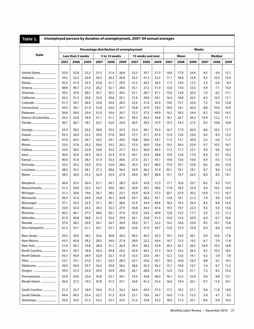
Monthly Labor Review • December 2010 37
Unemployed persons by duration of unemployment, 2007–09 annual averages
State
Percentage distribution of unemployment Weeks
Less than 5 weeks 5 to 14 weeks 15 weeks and over Mean Median
2007 2008 2009 2007 2008 2009 2007 2008 2009 2007 2008 2009 2007 2008 2009
United States ...................... 35.9 32.8 22.2 31.5 31.4 26.8 32.5 35.7 51.0 16.8 17.9 24.4 8.5 9.4 15.1
Alabama ............................... 34.5 32.2 20.9 30.3 26.3 26.6 35.2 41.5 52.5 17.1 18.8 23.8 9.2 10.3 15.9 Alaska..................................... 45.5 41.9 33.5 32.8 31.7 29.9 21.5 26.5 36.5 11.5 14.0 17.2 5.4 6.6 9.4 Arizona .................................. 48.8 40.7 21.0 26.2 32.1 28.0 25.1 27.2 51.0 13.0 13.6 23.3 4.9 7.1 15.0 Arkansas................................ 39.2 35.9 28.5 35.7 35.3 30.5 25.1 28.7 41.1 13.6 13.8 20.0 7.0 8.2 11.1 California .............................. 36.3 31.5 20.8 32.0 29.6 25.1 31.6 39.0 54.1 16.4 18.8 26.5 8.3 10.3 17.1 Colorado .............................. 41.5 34.7 26.4 32.8 34.4 28.2 25.6 31.0 45.4 14.0 15.7 22.0 7.2 9.0 12.8 Connecticut ........................ 34.4 30.1 21.9 31.8 32.0 24.7 33.8 37.9 53.3 18.0 19.1 26.0 8.8 10.0 16.9 Delaware ............................... 36.8 28.9 23.4 31.0 33.4 26.7 32.3 37.5 49.9 16.2 18.3 24.4 8.2 10.0 14.5 District of Columbia ......... 29.3 25.6 18.9 31.1 31.1 26.1 39.3 43.3 54.8 18.1 20.7 26.2 10.9 12.2 17.1 Florida .................................... 36.7 28.7 18.1 32.7 32.0 24.4 30.5 39.3 57.5 15.5 19.3 27.5 8.5 10.8 18.8
Georgia ................................. 35.9 28.5 20.3 30.8 33.5 24.5 33.3 38.1 55.3 16.7 17.9 26.0 8.6 10.5 17.7 Hawaii .................................... 43.3 36.0 22.2 29.0 37.0 30.4 27.7 27.1 47.4 15.4 13.6 23.0 6.4 8.3 13.5 Idaho ...................................... 47.6 44.5 29.7 33.5 29.1 26.6 18.8 26.6 43.7 11.5 12.1 20.9 5.2 6.4 11.7 Illinois .................................... 32.4 27.6 20.2 30.6 33.3 26.2 37.0 39.0 53.6 19.3 20.4 25.8 9.7 10.5 16.7 Indiana .................................. 32.0 30.5 22.9 34.8 33.5 27.7 33.2 36.0 49.3 17.5 17.7 22.7 9.0 9.6 14.2 Iowa ....................................... 36.0 42.6 30.3 34.3 32.5 31.0 29.7 25.0 38.8 13.9 12.6 17.0 8.0 6.1 10.2 Kansas ................................... 40.8 41.6 28.3 31.9 33.3 28.6 27.3 25.1 43.1 14.6 13.6 19.0 6.9 6.5 11.9 Kentucky .............................. 35.3 34.2 23.0 35.5 32.6 28.6 29.3 33.2 48.4 13.9 18.1 22.8 8.6 8.6 13.9 Louisiana............................... 38.0 35.2 28.1 27.2 28.6 34.4 34.9 36.2 37.4 20.1 19.1 18.1 8.7 9.6 11.0 Maine .................................... 38.5 36.0 23.3 32.4 33.4 27.8 29.0 30.7 48.9 15.1 14.7 22.3 8.0 8.3 14.1
Maryland .............................. 36.0 32.5 20.4 31.1 34.7 28.3 32.9 32.8 51.3 17.1 16.6 22.7 8.5 9.2 15.2 Massachusetts ................... 31.3 29.9 22.2 33.7 30.6 28.2 34.9 39.5 49.6 17.8 18.3 23.9 9.4 10.5 14.4 Michigan .............................. 31.3 28.8 19.6 26.7 28.3 23.1 42.0 42.9 57.3 20.7 22.9 30.2 10.9 11.1 19.7 Minnesota ........................... 36.4 31.6 24.0 33.8 30.1 30.8 29.7 38.2 45.1 13.8 19.1 21.3 7.9 9.9 12.9 Mississippi ........................... 37.1 35.5 22.3 31.1 30.1 28.0 31.9 34.4 49.6 18.4 19.5 24.3 8.3 8.8 14.3 Missouri ................................ 33.9 32.4 24.5 29.2 33.3 27.9 36.8 34.3 47.6 19.5 19.7 22.3 9.5 9.3 13.6 Montana ............................... 46.2 46.1 27.3 28.6 30.1 31.9 25.0 23.6 40.9 12.8 12.5 17.7 5.4 5.5 11.3 Nebraska ............................... 41.9 40.8 28.8 31.9 33.4 29.9 26.1 25.8 41.3 13.0 13.4 20.0 6.9 6.7 10.6 Nevada ................................. 37.0 28.2 20.9 34.1 34.7 26.9 29.0 37.1 52.2 14.2 16.6 23.9 8.5 10.7 15.8 New Hampshire ................. 41.2 35.1 21.7 34.1 33.1 28.6 24.6 31.9 49.7 12.9 15.4 23.9 6.9 8.6 14.4
New Jersey .......................... 29.3 29.0 18.5 32.6 30.8 26.2 38.2 40.3 55.3 19.1 19.4 28.1 9.9 10.6 17.8 New Mexico ........................ 43.5 43.8 29.2 28.5 34.0 27.4 28.0 22.2 43.4 14.7 13.5 19.2 6.7 5.9 11.8 New York .............................. 31.8 30.7 19.8 28.9 31.1 26.4 39.3 38.2 53.9 20.5 20.1 26.5 10.0 10.2 16.8 North Carolina .................... 34.3 29.7 18.6 30.3 29.8 24.2 35.4 40.5 57.2 16.3 19.2 26.3 9.2 10.3 18.5 North Dakota ..................... 43.3 43.9 39.9 32.8 32.7 31.0 23.5 23.6 29.1 12.2 12.6 14.1 6.2 5.9 7.8 Ohio ........................................ 33.7 33.1 21.6 33.1 33.3 28.3 33.1 33.6 50.1 18.3 16.8 24.2 8.8 9.2 14.5 Oklahoma ............................ 39.0 34.9 29.7 32.4 29.9 28.2 28.6 35.3 42.2 15.7 19.0 19.7 7.4 8.7 11.2 Oregon ................................. 39.4 37.3 23.9 34.4 33.9 29.0 26.1 28.8 47.0 12.9 15.2 21.1 7.2 8.2 13.2
Pennsylvania ...................... 32.8 34.0 23.6 33.8 32.1 30.1 33.4 33.8 46.3 16.1 15.5 22.8 9.0 8.8 13.1 Rhode Island ...................... 30.4 27.2 19.5 35.8 31.5 25.1 34.0 41.2 55.4 16.6 19.4 26.1 9.7 11.6 18.1
South Carolina ................... 31.3 25.7 18.4 34.4 31.3 24.2 34.4 43.0 57.4 17.5 19.2 27.1 9.4 11.8 19.6
South Dakota ...................... 44.4 49.3 32.4 32.7 31.3 32.9 23.1 19.6 34.7 16.0 11.6 15.3 5.9 4.7 9.5 Tennessee ............................ 35.6 33.5 21.3 33.2 32.7 25.5 31.2 33.8 53.2 18.0 17.3 25.1 8.6 9.0 16.2
Table 1.
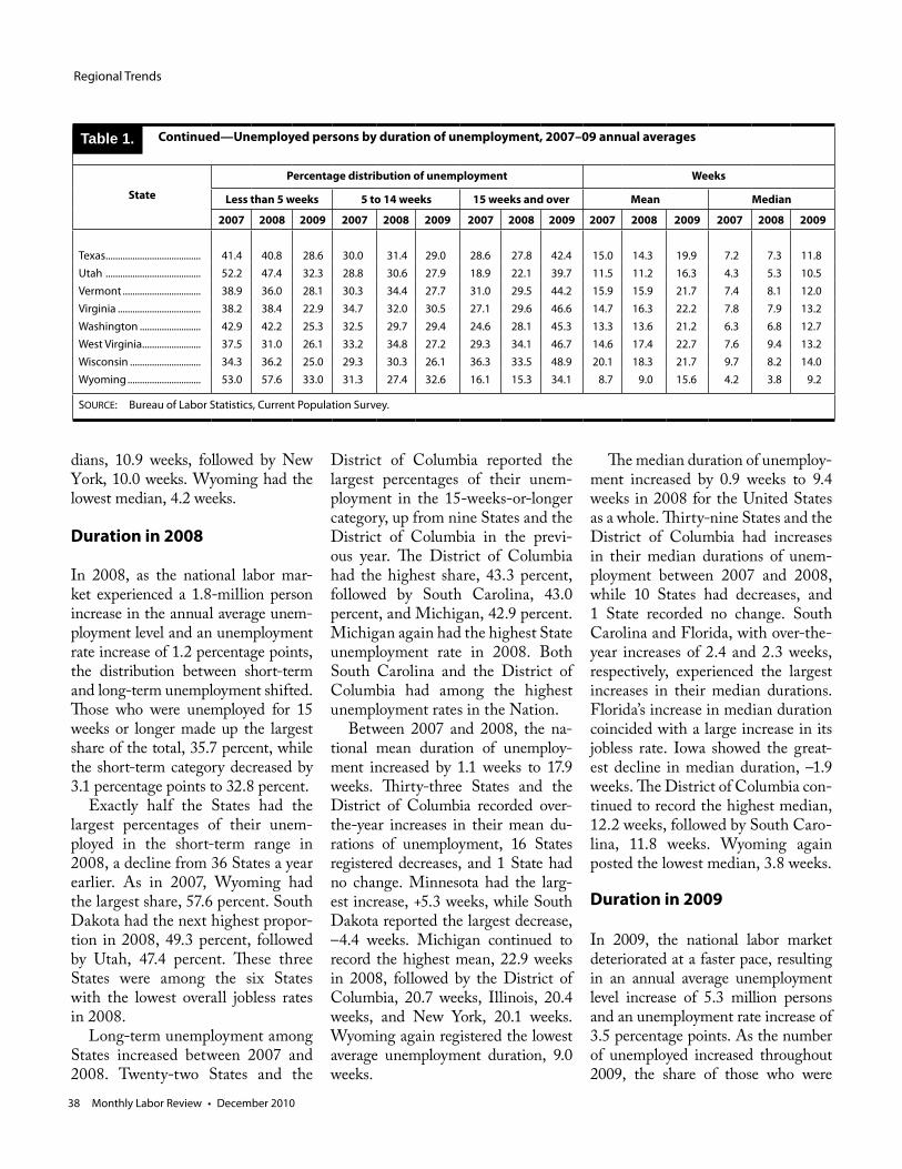
Regional Trends
38 Monthly Labor Review • December 2010
Continued—Unemployed persons by duration of unemployment, 2007–09 annual averages
State
Percentage distribution of unemployment Weeks
Less than 5 weeks 5 to 14 weeks 15 weeks and over Mean Median
2007 2008 2009 2007 2008 2009 2007 2008 2009 2007 2008 2009 2007 2008 2009
Texas ....................................... 41.4 40.8 28.6 30.0 31.4 29.0 28.6 27.8 42.4 15.0 14.3 19.9 7.2 7.3 11.8 Utah ....................................... 52.2 47.4 32.3 28.8 30.6 27.9 18.9 22.1 39.7 11.5 11.2 16.3 4.3 5.3 10.5 Vermont ................................ 38.9 36.0 28.1 30.3 34.4 27.7 31.0 29.5 44.2 15.9 15.9 21.7 7.4 8.1 12.0 Virginia .................................. 38.2 38.4 22.9 34.7 32.0 30.5 27.1 29.6 46.6 14.7 16.3 22.2 7.8 7.9 13.2 Washington ......................... 42.9 42.2 25.3 32.5 29.7 29.4 24.6 28.1 45.3 13.3 13.6 21.2 6.3 6.8 12.7 West Virginia ........................ 37.5 31.0 26.1 33.2 34.8 27.2 29.3 34.1 46.7 14.6 17.4 22.7 7.6 9.4 13.2 Wisconsin ............................. 34.3 36.2 25.0 29.3 30.3 26.1 36.3 33.5 48.9 20.1 18.3 21.7 9.7 8.2 14.0 Wyoming .............................. 53.0 57.6 33.0 31.3 27.4 32.6 16.1 15.3 34.1 8.7 9.0 15.6 4.2 3.8 9.2
SOURCE: Bureau of Labor Statistics, Current Population Survey.
Table 1.
dians, 10.9 weeks, followed by New York, 10.0 weeks. Wyoming had the lowest median, 4.2 weeks.
Duration in 2008
In 2008, as the national labor mar-ket experienced a 1.8-million person increase in the annual average unem-ployment level and an unemployment rate increase of 1.2 percentage points, the distribution between short-term and long-term unemployment shifted. Those who were unemployed for 15 weeks or longer made up the largest share of the total, 35.7 percent, while the short-term category decreased by 3.1 percentage points to 32.8 percent.
Exactly half the States had the largest percentages of their unem-ployed in the short-term range in 2008, a decline from 36 States a year earlier. As in 2007, Wyoming had the largest share, 57.6 percent. South Dakota had the next highest propor-tion in 2008, 49.3 percent, followed by Utah, 47.4 percent. These three States were among the six States with the lowest overall jobless rates in 2008.
Long-term unemployment among States increased between 2007 and 2008. Twenty-two States and the
District of Columbia reported the largest percentages of their unem-ployment in the 15-weeks-or-longer category, up from nine States and the District of Columbia in the previ-ous year. The District of Columbia had the highest share, 43.3 percent, followed by South Carolina, 43.0 percent, and Michigan, 42.9 percent. Michigan again had the highest State unemployment rate in 2008. Both South Carolina and the District of Columbia had among the highest unemployment rates in the Nation.
Between 2007 and 2008, the na-tional mean duration of unemploy-ment increased by 1.1 weeks to 17.9 weeks. Thirty-three States and the District of Columbia recorded over-the-year increases in their mean du-rations of unemployment, 16 States registered decreases, and 1 State had no change. Minnesota had the larg-est increase, +5.3 weeks, while South Dakota reported the largest decrease, –4.4 weeks. Michigan continued to record the highest mean, 22.9 weeks in 2008, followed by the District of Columbia, 20.7 weeks, Illinois, 20.4 weeks, and New York, 20.1 weeks. Wyoming again registered the lowest average unemployment duration, 9.0 weeks.
The median duration of unemploy-ment increased by 0.9 weeks to 9.4 weeks in 2008 for the United States as a whole. Thirty-nine States and the District of Columbia had increases in their median durations of unem-ployment between 2007 and 2008, while 10 States had decreases, and 1 State recorded no change. South Carolina and Florida, with over-the-year increases of 2.4 and 2.3 weeks, respectively, experienced the largest increases in their median durations. Florida’s increase in median duration coincided with a large increase in its jobless rate. Iowa showed the great-est decline in median duration, –1.9 weeks. The District of Columbia con-tinued to record the highest median, 12.2 weeks, followed by South Caro-lina, 11.8 weeks. Wyoming again posted the lowest median, 3.8 weeks.
Duration in 2009
In 2009, the national labor market deteriorated at a faster pace, resulting in an annual average unemployment level increase of 5.3 million persons and an unemployment rate increase of 3.5 percentage points. As the number of unemployed increased throughout 2009, the share of those who were
Monthly Labor Review • December 2010 39
without a job for 15 weeks or longer jumped 15.3 percentage points from 2008. Those considered long-term unemployed constituted 51.0 percent of the total, while the short-term cat-egory decreased by 10.6 percentage points to 22.2 percent.
Only one State, North Dakota, had the largest proportion of its un-employed in the short-term range in 2009, a drastic decline from 25 States a year earlier. In North Dakota, 39.9 percent of the unemployed were job-less for 5 weeks or less. This State also posted the lowest 2009 annual aver-age unemployment rate in the Na-tion, 4.3 percent.
Forty-nine States and the Dis-trict of Columbia reported the larg-est shares of their unemployed in the 15-weeks-or-longer category in 2009. Fifteen of those States and the District of Columbia recorded higher proportions than that of the Nation, 51.0 percent. Florida recorded the highest share among the States, 57.5 percent, followed closely by South Carolina, 57.4 percent, Michigan, 57.3 percent, and North Carolina, 57.2 percent. These States experi-enced some of the highest annual average unemployment rates in 2009, with Michigan recording the highest rate, 13.6 percent.
In 2009, the United States expe-rienced a substantial increase in the
national mean duration of jobless-ness, which rose 6.5 weeks over the year to 24.4 weeks. Forty-nine States and the District of Columbia experi-enced over-the-year increases in their mean durations of unemployment, with Arizona recording the largest increase, +9.7 weeks, followed closely by Hawaii, +9.4 weeks. Only one State, Louisiana, had a small decline, –1.0 week. As nearly all States regis-tered increases in their average dura-tions of joblessness, 39 States and the District of Columbia posted increases of 5.0 weeks or more between 2008 and 2009. Michigan, once again, re-corded the highest mean, 30.2 weeks, while North Dakota recorded the lowest, 14.1 weeks.
The median length of time a per-son was jobless at the national level in 2009 was 15.1 weeks, up from 9.4 weeks a year earlier. All 50 States and the District of Columbia had increas-es in their median durations of unem-ployment between 2008 and 2009 of at least 1.4 weeks. Michigan had the largest increase, +8.6 weeks, followed by two other States with increases of at least 8.0 weeks: North Carolina, +8.2 weeks, and Florida, +8.0 weeks. Michigan and Florida also recorded the highest and the third highest medians in the Nation, 19.7 weeks and 18.8 weeks, respectively. Three other States reported median dura-
tions above 18.0 weeks: South Caro-lina, 19.6 weeks, North Carolina, 18.5 weeks, and Rhode Island, 18.1 weeks. In contrast, North Dakota, at 7.8 weeks, was the only State to post a median duration of joblessness below 9.2 weeks in 2009.
Notes1 Many data users consider long-term un-
employment to be 27 weeks or more, while some data users consider 15 weeks or more to be long term. For the purposes of this ar-ticle, short-term unemployment is defined as less than 5 weeks, medium term as 5 to 14 weeks, and long-term joblessness as 15 weeks or more. This article focuses on short-term and long-term unemployment.
2 The duration of unemployment repre-sents the length of time (through the current reference week) that individuals classified as unemployed have been looking for work and refers to job searches in continuous progress rather than the duration of a completed spell.
3 Statewide estimates on the economic char-acteristics of the unemployed (e.g., duration of unemployment) are based on annual aver-ages of monthly data obtained from the CPS and are, therefore, subject to sampling error. For more information on using and interpret-ing CPS subnational data, see “Notes on Using Current Population Survey (CPS) Subnational Data,” on the Internet at www.bls.gov/gps/notescps.htm. For additional information and sampling error tables, see the appendices of the Geographic Profile of Employment and Unemployment publications, on the Internet at www.bls.gov/opub/gp/laugp.htm.
4 The Mountain division, located in the West region, is composed of eight States: Arizona, Colorado, Idaho, Montana, Nevada, New Mexico, Utah, and Wyoming.
40 Monthly Labor Review • December 2010
Précis
Assimilating activities of immigrants
Many studies have been conducted focusing on the results of assimila-tion by immigrants into a native cul-ture; however, few have examined the activities involved in the process of assimilation. Daniel S. Hamer-mesh and Stephen J. Trejo use data from the American Time Use Sur-vey (ATUS) to explore the process of assimilation by U.S. immigrants in their working paper titled “How Do Immigrants Spend Time?: The Pro-cess of Assimilation” (NBER Work-ing Paper 16430, October 2010).
The researchers began by con-structing a model in which they classified certain activities as as-similating activities and others as nonassimilating activities. Assimi-lating activities are defined as those which advance immigrants’ famil-iarity with and absorption into their new country’s culture: for example, learning English and working and shopping outside of one’s ethnic community. The researchers classi-fied the ATUS categories of purchas-ing, education, and market work as assimilating activities. Care for others, eating/drinking, household activities (household production), personal care, other leisure, social-izing/television watching, and orga-nizational/civic/religious activities were classified as nonassimilating activities. The researchers viewed performing activities that entail overcoming language barriers and cultural obstacles as fixed costs that lead to an increased level of utility in the future.
Plugging the ATUS data into Hamermesh and Trejo’s model generates some interesting results.
Natives’ rate of participation in as-similating activities was 1.5 percent higher than that of immigrants, pri-marily driven by a disparity in par-ticipation levels in purchasing ac-tivities. However, contingent upon his or her participation in an assimi-lating activity, an immigrant tends to spend more time performing that activity. Specifically, in comparison with their native counterparts, those immigrants who engaged in pur-chasing activities spent 10.9 percent more time on these activities, and those immigrants who engaged in market work spent 4.0 percent time doing it. On average, conditional on immigrants’ participation in an activity, they spent 5.7 percent more time than natives on assimilating activities and 1.2 percent less time on non-assimilating activities.
Interestingly, very similar results were observed when applying the model to data from the Australian Time Use Survey, after accounting for methodological differences be-tween the surveys.
Ultimately, Hamermesh and Trejo postulate that there are high costs to assimilating: they involve leaving the familiarity of one’s own cultural and economic mindset and adopting the customs of a new country. These high costs are a barrier to assimila-tion, causing some immigrants to choose not to assimilate. But those who do take part in assimilating ac-tivities tend to spend more time on them than natives.
Optimism leads to improved labor market outcomes
Is the glass half full or half empty?
This common question is a litmus test that categorizes a person as one of two personality types: optimist or pessimist. Economists Ron Kaniel, Cade Massey, and David T. Robin-son believe that the answer to this question tells a lot about a person—including how he or she may fare in the labor market.
In their recent National Bureau of Economic Research (NBER) study entitled “The Importance of Being An Optimist: Evidence from Labor Markets” (NBER Working Paper 16328, September 2010) the authors explore how optimism shapes the economic behavior and labor market outcomes of a panel of MBA students at a major U.S. university. Specifi-cally, the authors focus on disposi-tional optimism, a personality trait associated with people who believe that good things tend to happen to them more often than bad things. The authors focus on dispositional optimism because uncertainty is central to economic choice; when making a decision that may yield an uncertain future, an optimist places more weight on positive outcomes than a pessimist does.
The authors calculated dispo-sitional optimism by measuring generalized expectations of the fu-ture, observing job search behavior during the MBA program, analyz-ing admissions records and data on classroom performance, and admin-istering surveys designed to capture the perceptions of other students. In addition, the authors followed up with alumni two years after they graduated to learn about their post-MBA job-market experience.
With their study, the authors find strong evidence to suggest that op-timists outperform their peers in the job market. They found that

Monthly Labor Review • December 2010 41
increase in the probability of being promoted.
The authors hypothesize that optimism has a large effect on cir-cumstance because it affects many interactions and decisions through-out the day, every day. They also note that dispositional optimists are more resilient when receiving negative feedback and have an easier time maintaining the complex bal-ance between abandoning a goal and staying the course.
optimists place less importance on the job search process. Of the MBA students surveyed, 38 percent said getting a job after graduation was more important than making friends or earning good grades in the pro-gram. Optimists were significantly less likely to place the greatest im-portance on getting a job.
Optimists are generally more ef-ficient in their job searches. The authors found a strong negative cor-relation between optimism and the
number of jobs applied for through on-campus recruiting, regardless of controls for various demographic and other characteristics.
Optimists have higher search yields and receive job offers more quickly. The median student gets one offer for every six bids, but on average, optimism leads to a 10-per-cent greater search efficiency. More-over, optimism has a strong positive effect on getting a promotion; opti-mism translates to a 5- to 10-percent
Where are you publishing your research?�e Monthly Labor Review welcomes articles on the labor force, labor-management relations, business conditions, industry productivity, compensation, occupational safety and health, demographic trends, and other economic developments. Papers should be factual and analytical, not polemical, in tone. For guidelines on how to submit papers, go towww.bls.gov/opub/mlr/guidelines.htm. Potential articles, as well as comments onmaterial published in the Review, should besubmitted to:
Executive EditorMonthly Labor ReviewU.S. Bureau of Labor StatisticsRoom 2850Washington, DC 20212Telephone: (202) 691–7911Fax: (202) 691–5908 E-mail: [email protected]
42 Monthly Labor Review • December 2010
Book Review
A race to the bottom
NAFTA and Labor in North America. By Norman Caulfield, Champaign, IL, University of Illinois Press, 2010, 264 pp., $70/cloth; $25/paperback.
With a recession having just ended in March 1991 and its effects still fresh in the minds of the voters, the state of the economy became the primary focus of the United States presidential election of 1992. One particularly contentious issue was whether the proposed North Ameri-can Free Trade Agreement (NAFTA) would prove to be beneficial or det-rimental to the working class citi-zens of the United States. In what must be considered the single most famous quote associated with the NAFTA debate, Ross Perot warned that, if NAFTA were ratified, “there will be a giant sucking sound going south” as U.S. industries head across the Mexican border in search of cheap labor. Nearly 20 years later, the question naturally arises: Did Perot’s prediction turn out to be true?
While it is not the purpose of Norman Caulfield’s book to answer this specific question, NAFTA and Labor in North American neverthe-less sheds light on this issue in the course of articulating a broader narrative. Two other qualifications deserve mention. In reference to the book’s title, the scope of the work en-compasses economic forces that are more general than those associated with NAFTA alone. Furthermore, the book is largely concerned with only a subset of the total labor force rather than its entirety. The content of the book is, therefore, more accu-rately described as a characterization of the effects of globalization upon
organized labor in North America. And as Caulfield argues, these ef-fects have been negative.
The book begins with a historical overview of the rise of organized labor in North America from 1850 to 1970. Out of tumultuous begin-nings, the first few decades of the 20th century saw unions grow rap-idly and win important political and legal victories. Notwithstanding the occasional setbacks unions suffered throughout the 1920s and 1930s, the decades immediately following World War II would represent a “golden age” for organized labor and the economies of North America as well. By the mid-1950s, union density in Canada and the U.S. would climb to one-third of non-agricultural employment. Unions in Mexico also experienced gains in terms of greater representation in political and economic matters dur-ing this period.
According to Caulfield, this period of prosperity was made possible be-cause international trade was insig-nificant, implying that production and economic policies were directed predominantly toward the domes-tic economy. Under the conditions of limited foreign competition and strong economic growth, unions were in an advantageous position to bargain for higher wages and ben-efits and better working conditions. The recessions, declining profits, and increased foreign competition of the 1970s would transform the political and economic landscape to the detriment of unions. In the 1980s, the three North Ameri-can countries elected conservative, market-oriented political leaders all of whom sought to expand interna-tional trade, reduce social spending, and deregulate or privatize industry.
Within this neoliberal framework, organized labor would suffer de-clines in compensation, working conditions, and workers’ rights.
NAFTA is characterized as the logical next step in the expansion of global capitalism. Of greater impor-tance to the present discussion is the North American Agreement on La-bor Cooperation (NAALC). As a side agreement to NAFTA, the NAALC was designed to monitor violations against each country’s labor laws and settle labor disputes. Caulfield reports an extensive list of violations filed with the NAALC that includes dangerous working conditions, gen-der discrimination, preventing the organization of labor, and paying illegally low wages, to name a few. The NAALC has been mostly ineffec-tive, according to Caulfield, because it has no coercive power. Ironically, the NAALC has had an effect exactly the opposite of its intended purpose. Tasked with monitoring violations and ensuring that the letter of the law was observed, an unintended in-centive was created to reduce the le-gal rights of workers for the purpose of reducing labor costs, attracting investment, and avoiding NAALC censure in what Caulfield describes as a “race to the bottom.”
The response to globalization by unions has been to align their in-terests with firms and accept con-cessionary bargaining. Caulfield accuses union leaders across many industries of partnering with man-agement to help rollback the gains previously won by unions. Under the threat of plant closures, declining union membership, and a shrinking base of union dues, labor leaders ap-pear to have placed their own self-interest above the collective interests of the rank and file. Within some
Monthly Labor Review • December 2010 43
industries, union leaders were given official corporate positions and stew-ardship over union funds, which placed them in the debt of firms. Moreover, the shifting of health care costs from firms to unions through Voluntary Employees’ Beneficiary Associations (VEBAs) has made some unions large share-holders of the same corporations in which they are organized, thereby creating an interest in reducing la-bor costs to maximize the value of the VEBA. Accordingly, Caulfield finds the response by union leaders to be completely ineffective, if not wholly contemptible.
In the concluding chapter, several prescriptions are offered for the fu-ture direction of organized labor. Caulfield advocates that workers organize internationally, but inde-pendently of the established trade unions. Labor is urged to promote equal rights for all migrant work-ers. Lastly, workers are encouraged to seek not only economic gains, but greater political influence as well.
Acknowledging Caulfield’s in-tended purpose, this reviewer be-lieves it is fair to raise a few broader issues of relevance to the general arguments presented in the book. The first issue concerns the interpre-tation of trends in manufacturing employment. Caulfield’s discussion is framed squarely in terms of the impact of globalization on unions specifically within manufactur-ing industries, which makes logical sense because the manufacturing industries are at greatest risk of crossing international borders. Is globalization to blame for the loss of U.S. manufacturing jobs? Current Employment Statistics data for the
U.S. reveals that manufacturing as a share of total non-farm employ-ment has exhibited a continuous, uninterrupted decline from 35 per-cent in 1945 to 9 percent in 2009. Even during the prosperous years between 1945 and 1970, manufac-turing’s share of total employment decreased by 10 percent. At the same time, U.S. manufacturing out-put steadily increased. While this reviewer does not dispute the fact that U.S. manufacturing jobs have moved abroad, Caulfield seems to suggest that technology is the great-er long-run threat to manufacturing employment, both here and abroad. If productivity continues to increase through technological advances, it is conceivable that only 2 percent of total employment will be needed to manufacture everything society needs in the future. In this scenario, it would be neither possible nor de-sirable to prevent the secular decline of manufacturing employment in this reviewer’s opinion.
A second issue of relevance con-cerns the organizational strategy of unions. If globalization is prompting firms to move abroad, maybe labor unions should give up attempting to preserve jobs in those industries that are subject to intense competi-tive pressures and relatively easy to relocate. As long as goods, services, and financial capital are free to cross international borders, pressing for higher wages in some industries (e.g. manufacturing) will likely not be successful. Unions might find greater success in organizing indus-tries that produce goods or services that are prohibitively expensive to trade internationally. The service sector has weathered the general
decline in union density far better than manufacturing and this can be explained in part by the cost of im-porting services.
These issues aside, Caulfield’s book can be praised as a detailed, well-researched historical portrayal of the effects of globalization on labor unions in North America. Moreover, as the former director of research for the Secretariat of the Commission for Labor Cooperation, he presents an authoritative account of the labor law violations occurring since the inception of NAFTA and of the Commission for Labor Coop-eration’s inefficacy in resolving these violations. Overall, the presentation is accurate and balanced.
NAFTA and Labor in North America will likely find its greatest apprecia-tion within academia, primarily as a supplemental text in economics courses. It would be useful in labor economics courses that empha-size the study of organized labor. The book is equally well-suited for courses in international economics as it can provide a counterbalance to the welfare arguments made in favor of free trade agreements that too often ignore the impacts on los-ers from these arrangements. This is not to say, however, that the book will not appeal to the general public. Interested readers will find it ac-cessible and readable. Members of labor unions who are interested in the future of organized labor should perhaps regard this book as required reading.
—John Kenneth KrantzEconomist
Utah Department of Workforce Services
Salt Lake City, UT

44 Monthly Labor Review • December 2010
Nominations Sought for 2011 Julius Shiskin Award
Nominations are invited for the annual Julius Shiskin Memorial Award for Economic Statistics. The Award is given in recognition of unusually original and important contributions in the development of economic statistics or in the use of statistics in interpreting the economy. Contributions are recog-nized for statistical research, development of statistical tools, application of information technology techniques, use of economic statistical programs, management of statistical programs, or developing public understanding of measurement issues. The Award was established in 1980 by the Washington Statistical Society (WSS) and is now cosponsored by the WSS, the National Association for Business Economics, and the Business and Economics Statistics Section of the American Statistical Asso-ciation (ASA). The 2010 award recipient was Dr. Dale W. Jorgenson for for his contributions to the measurement of productivity, innovation, capital, human capital, poverty, and for his leadership in the integration of the U.S. National Accounts.
Because the program was initiated many years ago, statisticians and economists often ask, “Who was Julius Shiskin?” At the time of his death in 1978, “Julie” was the Commissioner for the Bureau of Labor Statistics (BLS) and earlier served as the Chief Statistician at the Office of Management and Budget (OMB), and the Chief Economic Statistician and Assistant Director of the Census Bureau. Throughout his career, he was known as an innovator. At Census he was instrumental in developing an electronic computer method for seasonal adjustment. In 1961, he published Signals of Recession and Recovery, which laid the groundwork for the calculation of monthly economic indicators, and he developed the monthly Census report Business Conditions Digest to disseminate them to the public. In 1969, he was appointed Chief Statistician at OMB where he developed the policies and procedures that govern the release of key economic indicators (Statistical Policy Directive Number 3), and origi-nated a Social Indicators report. In 1973, he was selected to head BLS where he was instrumental in preserving the integrity and independence of the BLS labor force data and directed the most compre-hensive revision in the history of the Consumer Price Index (CPI), which included a new CPI for all urban consumers.
Nominations for the 2011 award are now being accepted. Individuals and groups in the public or private sector from any country can be nominated. The award will be presented with an honorarium of $1000 plus additional recognition from the sponsors. A nomination form and a list of all previous recipients are available on the ASA Website at www.amstat.org/sections/bus_econ/shiskin.html.
For questions or more information, please contact Steven Paben, Julius Shiskin Award Committee Secretary, via e-mail at [email protected] or call 202-691-6147. Completed nominations must be received by March 15, 2011.
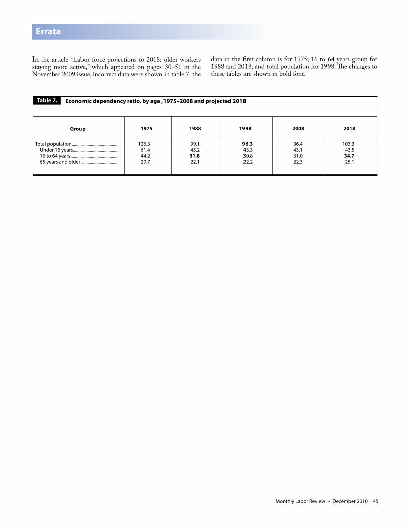
Monthly Labor Review • December 2010 45
Errata
In the article “Labor force projections to 2018: older workers staying more active,” which appeared on pages 30–51 in the November 2009 issue, incorrect data were shown in table 7: the
data in the first column is for 1975; 16 to 64 years group for 1988 and 2018; and total population for 1998. The changes to these tables are shown in bold font.
Total population ........................................... 126.3 99.1 96.3 96.4 103.3 Under 16 years.......................................... 61.4 45.2 43.3 43.1 43.5 16 to 64 years ............................................ 44.2 31.8 30.8 31.0 34.7 65 years and older ................................... 20.7 22.1 22.2 22.3 25.1
Table 7.
Group 1975 1988 20081998
Economic dependency ratio, by age ,1975–2008 and projected 2018
2018
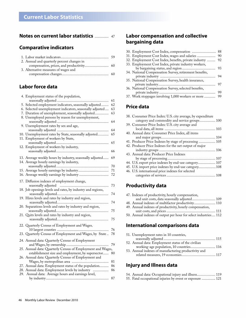
46 Monthly Labor Review December 2010
Current Labor Statistics
Notes on current labor statistics ............... 47
Comparative indicators
1. Labor market indicators .................................................... 59 2. Annual and quarterly percent changes in compensation, prices, and productivity .......................... 60 3. Alternative measures of wages and compensation changes ................................................... 60
Labor force data
4. Employment status of the population, seasonally adjusted ........................................................ 61 5. Selected employment indicators, seasonally adjusted ........ 62 6. Selected unemployment indicators, seasonally adjusted .... 63 7. Duration of unemployment, seasonally adjusted ............... 63 8. Unemployed persons by reason for unemployment, seasonally adjusted ........................................................ 64 9. Unemployment rates by sex and age, seasonally adjusted ........................................................ 6410. Unemployment rates by State, seasonally adjusted ............ 6511. Employment of workers by State, seasonally adjusted ......................................................... 6512. Employment of workers by industry, seasonally adjusted ......................................................... 66
13. Average weekly hours by industry, seasonally adjusted ...... 6914. Average hourly earnings by industry, seasonally adjusted ......................................................... 7015. Average hourly earnings by industry ................................. 7116. Average weekly earnings by industry ................................ 72
17. Diffusion indexes of employment change, seasonally adjusted ..................................................... 7318. Job openings levels and rates, by industry and regions, seasonally adjusted........................................................ 7419. Hires levels and rates by industry and region, seasonally adjusted........................................................ 7420. Separations levels and rates by industry and region, seasonally adjusted......................................................... 7521. Quits levels and rates by industry and region, seasonally adjusted........................................................ 7522. Quarterly Census of Employment and Wages, 10 largest counties ........................................................ 7623. Quarterly Census of Employment and Wages, by State .. 78
24. Annual data: Quarterly Census of Employment and Wages, by ownership .............................................. 7925. Annual data: Quarterly Census of Employment and Wages, establishment size and employment, by supersector ...... 8026. Annual data: Quarterly Census of Employment and Wages, by metropolitan area ........................................ 8127. Annual data: Employment status of the population.......... 8628. Annual data: Employment levels by industry ................. 8629. Annual data: Average hours and earnings level, by industry .................................................................... 87
Labor compensation and collectivebargaining data
30. Employment Cost Index, compensation .......................... 8831. Employment Cost Index, wages and salaries .................... 9032. Employment Cost Index, benefits, private industry ......... 9233. Employment Cost Index, private industry workers, by bargaining status, and region .................................... 9334. National Compensation Survey, retirement benefits, private industry ............................................................ 9435. National Compensation Survey, health insurance, private industry .............................................................. 9736. National Compensation Survey, selected benefits, private industry ............................................................. 9937. Work stoppages involving 1,000 workers or more ............ 99
Price data
38. Consumer Price Index: U.S. city average, by expenditure category and commodity and service groups ................. 10039. Consumer Price Index: U.S. city average and local data, all items ....................................................... 10340. Annual data: Consumer Price Index, all items and major groups........................................................... 10441. Producer Price Indexes by stage of processing .................. 105 42. Producer Price Indexes for the net output of major industry groups ............................................................. 10643. Annual data: Producer Price Indexes by stage of processing .................................................... 10744. U.S. export price indexes by end-use category................... 10745. U.S. import price indexes by end-use category................... 10846. U.S. international price indexes for selected categories of services ..................................................... 108
Productivity data
47. Indexes of productivity, hourly compensation, and unit costs, data seasonally adjusted ......................... 10948. Annual indexes of multifactor productivity ....................... 11049. Annual indexes of productivity, hourly compensation, unit costs, and prices ..................................................... 11150. Annual indexes of output per hour for select industries .... 112
International comparisons data
51. Unemployment rates in 10 countries, seasonally adjusted ........................................................ 11552. Annual data: Employment status of the civilian working-age population, 10 countries........................... 11653. Annual indexes of manufacturing productivity and related measures, 19 economies..................................... 117
Injury and Illness data
54. Annual data: Occupational injury and illness................... . 11955. Fatal occupational injuries by event or exposure .............. . 121
Monthly Labor Review • December 2010 47
1979. Detailed data on the occupational injury
and illness series are published in Occupa-tional Injuries and Illnesses in the United States, by Industry, a BLS annual bulletin.
Finally, the Monthly Labor Review carries analytical articles on annual and longer term developments in labor force, employment, and unemployment; employee compensation and collective bargaining; prices; productiv-ity; international comparisons; and injury and illness data.
Symbolsn.e.c. = not elsewhere classified.n.e.s. = not elsewhere specified. p = preliminary. To increase the timeliness of some series, preliminary figures are issued based on representative but incomplete returns. r = revised. Generally, this revision reflects the availability of later data, but also may reflect other adjustments.
Comparative Indicators(Tables 1–3)
Comparative indicators tables provide an overview and comparison of major bls sta-tistical series. Consequently, although many of the included series are available monthly, all measures in these comparative tables are presented quarterly and annually.
Labor market indicators include em-ployment measures from two major surveys and information on rates of change in compensation provided by the Employment Cost Index (ECI) program. The labor force participation rate, the employment-popula-tion ratio, and unemployment rates for major demographic groups based on the Current Population (“household”) Survey are pre-sented, while measures of employment and average weekly hours by major industry sec-tor are given using nonfarm payroll data. The Employment Cost Index (compensation), by major sector and by bargaining status, is chosen from a variety of BLS compensation and wage measures because it provides a comprehensive measure of employer costs for hiring labor, not just outlays for wages, and it is not affected by employment shifts among occupations and industries.
Data on changes in compensation, pric-es, and productivity are presented in table 2. Measures of rates of change of compensation and wages from the Employment Cost Index
values) are described as “real,” “constant,” or “1982” dollars.
Sources of information
Data that supplement the tables in this sec-tion are published by the Bureau in a variety of sources. Definitions of each series and notes on the data are contained in later sec-tions of these Notes describing each set of data. For detailed descriptions of each data series, see BLS Handbook of Methods, Bulletin 2490. Users also may wish to consult Major Programs of the Bureau of Labor Statistics, Report 919. News releases provide the lat-est statistical information published by the Bureau; the major recurring releases are published according to the schedule appear-ing on the back cover of this issue.
More information about labor force, employment, and unemployment data and the household and establishment surveys underlying the data are available in the Bureau’s monthly publication, Employment and Earnings. Historical unadjusted and seasonally adjusted data from the household survey are available on the Internet:
www.bls.gov/cps/Historically comparable unadjusted and sea-sonally adjusted data from the establishment survey also are available on the Internet:
www.bls.gov/ces/Additional information on labor force data for areas below the national level are pro-vided in the BLS annual report, Geographic Profile of Employment and Unemployment.
For a comprehensive discussion of the Employment Cost Index, see Employment Cost Indexes and Levels, 1975–95, BLS Bul-letin 2466. The most recent data from the Employee Benefits Survey appear in the fol-lowing Bureau of Labor Statistics bulletins: Employee Benefits in Medium and Large Firms; Employee Benefits in Small Private Establish-ments; and Employee Benefits in State and Local Governments.
More detailed data on consumer and producer prices are published in the monthly periodicals, The CPI Detailed Report and Pro-ducer Price Indexes. For an overview of the 1998 revision of the CPI, see the December 1996 issue of the Monthly Labor Review. Ad-ditional data on international prices appear in monthly news releases.
Listings of industries for which produc-tivity indexes are available may be found on the Internet:
www.bls.gov/lpc/
For additional information on inter-national comparisons data, see Interna-tional Comparisons of Unemployment, Bulletin
This section of the Review presents the principal statistical series collected and calculated by the Bureau of Labor Statistics: series on labor force; employment; unem-ployment; labor compensation; consumer, producer, and international prices; produc-tivity; international comparisons; and injury and illness statistics. In the notes that follow, the data in each group of tables are briefly described; key definitions are given; notes on the data are set forth; and sources of ad-ditional information are cited.
General notesThe following notes apply to several tables in this section:
Seasonal adjustment. Certain monthly and quarterly data are adjusted to eliminate the effect on the data of such factors as cli-matic conditions, industry production sched-ules, opening and closing of schools, holiday buying periods, and vacation practices, which might prevent short-term evaluation of the statistical series. Tables containing data that have been adjusted are identified as “season-ally adjusted.” (All other data are not season-ally adjusted.) Seasonal effects are estimated on the basis of current and past experiences. When new seasonal factors are computed each year, revisions may affect seasonally adjusted data for several preceding years.
Seasonally adjusted data appear in tables 1–14, 17–21, 48, and 52. Seasonally adjusted labor force data in tables 1 and 4–9 and sea-sonally adjusted establishment survey data shown in tables 1, 12–14, and 17 usually are revised in the March issue of the Review. A brief explanation of the seasonal adjustment methodology appears in “Notes on the data.”
Revisions in the productivity data in table 54 are usually introduced in the September issue. Seasonally adjusted indexes and per-cent changes from month-to-month and quarter-to-quarter are published for numer-ous Consumer and Producer Price Index series. However, seasonally adjusted indexes are not published for the U.S. average All-Items CPI. Only seasonally adjusted percent changes are available for this series.
Adjustments for price changes. Some data—such as the “real” earnings shown in table 14—are adjusted to eliminate the effect of changes in price. These adjustments are made by dividing current-dollar values by the Consumer Price Index or the appropriate component of the index, then multiplying by 100. For example, given a current hourly wage rate of $3 and a current price index number of 150, where 1982 = 100, the hourly rate expressed in 1982 dollars is $2 ($3/150 x 100 = $2). The $2 (or any other resulting
Notes on Current Labor Statistics
48 Monthly Labor Review • December 2010
Current Labor Statistics
program are provided for all civilian nonfarm workers (excluding Federal and household workers) and for all private nonfarm workers. Measures of changes in consumer prices for all urban consumers; producer prices by stage of processing; overall prices by stage of pro-cessing; and overall export and import price indexes are given. Measures of productivity (output per hour of all persons) are provided for major sectors.
Alternative measures of wage and com-pensation rates of change, which reflect the overall trend in labor costs, are summarized in table 3. Differences in concepts and scope, related to the specific purposes of the series, contribute to the variation in changes among the individual measures.
Notes on the data
Definitions of each series and notes on the data are contained in later sections of these notes describing each set of data.
Employment and Unemployment Data(Tables 1; 4–29)
Household survey data
Description of the seriesEmployment data in this section are ob-tained from the Current Population Survey, a program of personal interviews conducted monthly by the Bureau of the Census for the Bureau of Labor Statistics. The sample consists of about 60,000 households selected to represent the U.S. population 16 years of age and older. Households are interviewed on a rotating basis, so that three-fourths of the sample is the same for any 2 consecutive months.
Definitions
Employed persons include (1) all those who worked for pay any time during the week which includes the 12th day of the month or who worked unpaid for 15 hours or more in a family-operated enterprise and (2) those who were temporarily absent from their regular jobs because of illness, vacation, industrial dispute, or similar reasons. A person working at more than one job is counted only in the job at which he or she worked the greatest number of hours.
Unemployed persons are those who did not work during the survey week, but were available for work except for temporary illness and had looked for jobs within the preceding 4 weeks. Persons who did not look for work
ally adjusted data usually are revised for only the most recent 5 years. In July, new seasonal adjustment factors, which incorporate the experience through June, are produced for the July–December period, but no revisions are made in the historical data.
FOR ADDITIONAL INFORMATION on national household survey data, contact the Division of Labor Force Statistics: (202) 691–6378.
Establishment survey data
Description of the series
Employment, hours, and earnings data in this section are compiled from payroll records reported monthly on a voluntary basis to the Bureau of Labor Statistics and its co-operating State agencies by about 160,000 businesses and government agencies, which represent approximately 400,000 individual worksites and represent all industries except agriculture. The active CES sample covers approximately one-third of all nonfarm payroll workers. Industries are classified in accordance with the 2007 North American Industry Classification System. In most industries, the sampling probabilities are based on the size of the establishment; most large establishments are therefore in the sample. (An establishment is not necessarily a firm; it may be a branch plant, for example, or warehouse.) Self-employed persons and others not on a regular civilian payroll are outside the scope of the survey because they are excluded from establishment records. This largely accounts for the difference in employment figures between the household and establishment surveys.
Definitions
An establishment is an economic unit which produces goods or services (such as a factory or store) at a single location and is engaged in one type of economic activity.
Employed persons are all persons who received pay (including holiday and sick pay) for any part of the payroll period including the 12th day of the month. Persons holding more than one job (about 5 percent of all persons in the labor force) are counted in each establishment which reports them.
Production workers in the goods-produc-ing industries cover employees, up through the level of working supervisors, who engage directly in the manufacture or construction of the establishment’s product. In private ser-vice-providing industries, data are collected for nonsupervisory workers, which include most employees except those in executive, managerial, and supervisory positions. Those
because they were on layoff are also counted among the unemployed. The unemployment rate represents the number unemployed as a percent of the civilian labor force.
The civilian labor force consists of all employed or unemployed persons in the civil-ian noninstitutional population. Persons not in the labor force are those not classified as employed or unemployed. This group includes discouraged workers, defined as persons who want and are available for a job and who have looked for work sometime in the past 12 months (or since the end of their last job if they held one within the past 12 months), but are not currently looking, because they believe there are no jobs available or there are none for which they would qualify. The civil-ian noninstitutional population comprises all persons 16 years of age and older who are not inmates of penal or mental institutions, sanitariums, or homes for the aged, infirm, or needy. The civilian labor force partici-pation rate is the proportion of the civilian noninstitutional population that is in the labor force. The employment-population ratio is employment as a percent of the civil-ian noninstitutional population.
Notes on the data
From time to time, and especially after a de-cennial census, adjustments are made in the Current Population Survey figures to correct for estimating errors during the intercensal years. These adjustments affect the compa-rability of historical data. A description of these adjustments and their effect on the various data series appears in the Explana-tory Notes of Employment and Earnings. For a discussion of changes introduced in January 2003, see “Revisions to the Current Popula-tion Survey Effective in January 2003” in the February 2003 issue of Employment and Earnings (available on the BLS Web site at www.bls.gov/cps/rvcps03.pdf).
Effective in January 2003, BLS began using the X-12 ARIMA seasonal adjustment program to seasonally adjust national labor force data. This program replaced the X-11 ARIMA program which had been used since January 1980. See “Revision of Seasonally Adjusted Labor Force Series in 2003,” in the February 2003 issue of Employment and Earnings (available on the BLS Web site at www.bls.gov/cps/cpsrs.pdf) for a discussion of the introduction of the use of X-12 ARIMA for seasonal adjustment of the labor force data and the effects that it had on the data.
At the beginning of each calendar year, historical seasonally adjusted data usually are revised, and projected seasonal adjust-ment factors are calculated for use during the January–June period. The historical season-
Monthly Labor Review • December 2010 49
lished as preliminary in January and February and as final in March.
FOR ADDITIONAL INFORMATION on establishment survey data, contact the Di-vision of Current Employment Statistics: (202) 691–6555.
Unemployment data by State
Description of the series
Data presented in this section are obtained from the Local Area Unemployment Statis-tics (LAUS) program, which is conducted in cooperation with State employment security agencies.
Monthly estimates of the labor force, employment, and unemployment for States and sub-State areas are a key indicator of lo-cal economic conditions, and form the basis for determining the eligibility of an area for benefits under Federal economic assistance programs such as the Job Training Partner-ship Act. Seasonally adjusted unemployment rates are presented in table 10. Insofar as pos-sible, the concepts and definitions underlying these data are those used in the national estimates obtained from the CPS.
Notes on the data
Data refer to State of residence. Monthly data for all States and the District of Colum-bia are derived using standardized procedures established by BLS. Once a year, estimates are revised to new population controls, usually with publication of January estimates, and benchmarked to annual average CPS levels.
FOR ADDITIONAL INFORMATION on data in this series, call (202) 691–6392 (table 10) or (202) 691–6559 (table 11).
Quarterly Census ofEmployment and Wages
Description of the series
Employment, wage, and establishment data in this section are derived from the quarterly tax reports submitted to State employment security agencies by private and State and local government employers subject to State unemployment insurance (ui) laws and from Federal, agencies subject to the Unemploy-ment Compensation for Federal Employees (ucfe) program. Each quarter, State agen-cies edit and process the data and send the information to the Bureau of Labor Statistics.
The Quarterly Census of Employment and Wages (QCEW) data, also referred as ES-202 data, are the most complete enumeration of employment and wage information by
probability-based sample design. The indus-try-coding update included reconstruction of historical estimates in order to preserve time series for data users. Normally 5 years of seasonally adjusted data are revised with each benchmark revision. However, with this release, the entire new time series history for all CES data series were re-seasonally adjusted due to the NAICS conversion, which resulted in the revision of all CES time series.
Also in June 2003, the CES program in-troduced concurrent seasonal adjustment for the national establishment data. Under this methodology, the first preliminary estimates for the current reference month and the revised estimates for the 2 prior months will be updated with concurrent factors with each new release of data. Concurrent seasonal adjustment incorporates all available data, including first preliminary estimates for the most current month, in the adjustment process. For additional information on all of the changes introduced in June 2003, see the June 2003 issue of Employment and Earnings and “Recent changes in the national Current Employment Statistics survey,” Monthly La-bor Review, June 2003, pp. 3–13.
Revisions in State data (table 11) oc-curred with the publication of January 2003 data. For information on the revisions for the State data, see the March and May 2003 issues of Employment and Earnings, and “Re-cent changes in the State and Metropolitan Area CES survey,” Monthly Labor Review, June 2003, pp. 14–19.
Beginning in June 1996, the BLS uses the X-12-ARIMA methodology to season-ally adjust establishment survey data. This procedure, developed by the Bureau of the Census, controls for the effect of varying survey intervals (also known as the 4- versus 5-week effect), thereby providing improved measurement of over-the-month changes and underlying economic trends. Revisions of data, usually for the most recent 5-year period, are made once a year coincident with the benchmark revisions.
In the establishment survey, estimates for the most recent 2 months are based on incomplete returns and are published as pre-liminary in the tables (12–17 in the Review). When all returns have been received, the estimates are revised and published as “final” (prior to any benchmark revisions) in the third month of their appearance. Thus, De-cember data are published as preliminary in January and February and as final in March. For the same reasons, quarterly establish-ment data (table 1) are preliminary for the first 2 months of publication and final in the third month. Fourth-quarter data are pub-
workers mentioned in tables 11–16 include production workers in manufacturing and natural resources and mining; construction workers in construction; and nonsupervi-sory workers in all private service-providing industries. Production and nonsupervisory workers account for about four-fifths of the total employment on private nonagricultural payrolls.
Earnings are the payments production or nonsupervisory workers receive during the survey period, including premium pay for overtime or late-shift work but exclud-ing irregular bonuses and other special payments. Real earnings are earnings adjusted to reflect the effects of changes in consumer prices. The deflator for this series is derived from the Consumer Price Index for Urban Wage Earners and Clerical Workers (CPI-W).
Hours represent the average weekly hours of production or nonsupervisory workers for which pay was received, and are different from standard or scheduled hours. Overtime hours represent the portion of average weekly hours which was in excess of regular hours and for which overtime premiums were paid.
The Diffusion Index represents the percent of industries in which employment was rising over the indicated period, plus one-half of the industries with unchanged employment; 50 percent indicates an equal balance between industries with increasing and decreasing employment. In line with Bureau practice, data for the 1-, 3-, and 6-month spans are seasonally adjusted, while those for the 12-month span are unadjusted. Table 17 provides an index on private non-farm employment based on 278 industries, and a manufacturing index based on 84 industries. These indexes are useful for mea-suring the dispersion of economic gains or losses and are also economic indicators.
Notes on the data
With the release of data for January 2010, the CES program introduced its annual revision of national estimates of employment, hours, and earnings from the monthly survey of nonfarm establishments. Each year, the CES survey realigns its sample-based estimates to incorporate universe counts of employ-ment—a process known as benchmarking. Comprehensive counts of employment, or benchmarks, are derived primarily from un-employment insurance (UI) tax reports that nearly all employers are required to file with State Workforce Agencies. With the release in June 2003, CES completed the transition from its original quota sample design to a
50 Monthly Labor Review • December 2010
Current Labor Statistics
industry at the national, State, metropolitan area, and county levels. They have broad eco-nomic significance in evaluating labor market trends and major industry developments.
Definitions
In general, the Quarterly Census of Employ-ment and Wages monthly employment datarepresent the number of covered workers who worked during, or received pay for, the pay period that included the 12th day of the month. Covered private industry em-ployment includes most corporate officials, executives, supervisory personnel, profes-sionals, clerical workers, wage earners, piece workers, and part-time workers. It excludes proprietors, the unincorporated self-em-ployed, unpaid family members, and certain farm and domestic workers. Certain types of nonprofit employers, such as religious organizations, are given a choice of coverage or exclusion in a number of States. Workers in these organizations are, therefore, reported to a limited degree.
Persons on paid sick leave, paid holiday, paid vacation, and the like, are included. Persons on the payroll of more than one firm during the period are counted by each ui-subject employer if they meet the employ-ment definition noted earlier. The employ-ment count excludes workers who earned no wages during the entire applicable pay period because of work stoppages, temporary layoffs, illness, or unpaid vacations.
Federal employment data are based on reports of monthly employment and quar-terly wages submitted each quarter to State agencies for all Federal installations with employees covered by the Unemployment Compensation for Federal Employees (ucfe) program, except for certain national security agencies, which are omitted for security rea-sons. Employment for all Federal agencies for any given month is based on the number of persons who worked during or received pay for the pay period that included the 12th of the month.
An establishment is an economic unit, such as a farm, mine, factory, or store, that produces goods or provides services. It is typically at a single physical location and engaged in one, or predominantly one, type of economic activity for which a single indus-trial classification may be applied. Occasion-ally, a single physical location encompasses two or more distinct and significant activities. Each activity should be reported as a separate establishment if separate records are kept and the various activities are classified under different NAICS industries.
Most employers have only one estab-lishment; thus, the establishment is the
predominant reporting unit or statistical entity for reporting employment and wages data. Most employers, including State and local governments who operate more than one establishment in a State, file a Multiple Worksite Report each quarter, in addition to their quarterly ui report. The Multiple Worksite Report is used to collect separate employment and wage data for each of the employer’s establishments, which are not detailed on the ui report. Some very small multi-establishment employers do not file a Multiple Worksite Report. When the total employment in an employer’s secondary establishments (all establishments other than the largest) is 10 or fewer, the employer generally will file a consolidated report for all establishments. Also, some employers either cannot or will not report at the establishment level and thus aggregate establishments into one consolidated unit, or possibly several units, though not at the establishment level.
For the Federal Government, the report-ing unit is the installation: a single location at which a department, agency, or other gov-ernment body has civilian employees. Federal agencies follow slightly different criteria than do private employers when breaking down their reports by installation. They are permit-ted to combine as a single statewide unit: 1) all installations with 10 or fewer workers, and 2) all installations that have a combined total in the State of fewer than 50 workers. Also, when there are fewer than 25 workers in all secondary installations in a State, the secondary installations may be combined and reported with the major installation. Last, if a Federal agency has fewer than five employees in a State, the agency headquarters office (regional office, district office) serving each State may consolidate the employment and wages data for that State with the data re-ported to the State in which the headquarters is located. As a result of these reporting rules, the number of reporting units is always larger than the number of employers (or govern-ment agencies) but smaller than the number of actual establishments (or installations).
Data reported for the first quarter are tabulated into size categories ranging from worksites of very small size to those with 1,000 employees or more. The size category is determined by the establishment’s March employment level. It is important to note that each establishment of a multi-establishment firm is tabulated separately into the appropri-ate size category. The total employment level of the reporting multi-establishment firm is not used in the size tabulation.
Covered employers in most States report total wages paid during the calendar quarter, regardless of when the services were per-formed. A few State laws, however, specify
that wages be reported for, or based on the period during which services are performed rather than the period during which com-pensation is paid. Under most State laws or regulations, wages include bonuses, stock options, the cash value of meals and lodging, tips and other gratuities, and, in some States, employer contributions to certain deferred compensation plans such as 401(k) plans.
Covered employer contributions for old-age, survivors, and disability insurance (oasdi), health insurance, unemployment in-surance, workers’ compensation, and private pension and welfare funds are not reported as wages. Employee contributions for the same purposes, however, as well as money withheld for income taxes, union dues, and so forth, are reported even though they are deducted from the worker’s gross pay.
Wages of covered Federal workers rep-resent the gross amount of all payrolls for all pay periods ending within the quarter. This includes cash allowances, the cash equivalent of any type of remuneration, severance pay, withholding taxes, and retirement deduc-tions. Federal employee remuneration gener-ally covers the same types of services as for workers in private industry.
Average annual wage per employee for any given industry are computed by divid-ing total annual wages by annual average employment. A further division by 52 yields average weekly wages per employee. Annual pay data only approximate annual earnings because an individual may not be employed by the same employer all year or may work for more than one employer at a time.
Average weekly or annual wage is af-fected by the ratio of full-time to part-time workers as well as the number of individuals in high-paying and low-paying occupations. When average pay levels between States and industries are compared, these factors should be taken into consideration. For example, industries characterized by high proportions of part-time workers will show average wage levels appreciably less than the weekly pay levels of regular full-time employees in these industries. The opposite effect characterizes industries with low proportions of part-time workers, or industries that typically schedule heavy weekend and overtime work. Average wage data also may be influenced by work stoppages, labor turnover rates, retroactive payments, seasonal factors, bonus payments, and so on.
Notes on the data
Beginning with the release of data for 2007, publications presenting data from the Cov-ered Employment and Wages program have
Monthly Labor Review • December 2010 51
switched to the 2007 version of the North American Industry Classification System (NAICS) as the basis for the assignment and tabulation of economic data by industry. NAICS is the product of a cooperative effort on the part of the statistical agencies of the United States, Canada, and Mexico. Due to difference in NAICS and Standard Industrial Classification (SIC) structures, industry data for 2001 is not comparable to the SIC-based data for earlier years.
Effective January 2001, the program began assigning Indian Tribal Councils and related establishments to local government ownership. This BLS action was in response to a change in Federal law dealing with the way Indian Tribes are treated under the Federal Unemployment Tax Act. This law requires federally recognized Indian Tribes to be treat-ed similarly to State and local governments. In the past, the Covered Employment and Wage (CEW) program coded Indian Tribal Councils and related establishments in the private sector. As a result of the new law, CEW data reflects significant shifts in employment and wages between the private sector and local government from 2000 to 2001. Data also reflect industry changes. Those accounts previously assigned to civic and social organi-zations were assigned to tribal governments. There were no required industry changes for related establishments owned by these Tribal Councils. These tribal business establishments continued to be coded according to the eco-nomic activity of that entity.
To insure the highest possible quality of data, State employment security agencies verify with employers and update, if neces-sary, the industry, location, and ownership classification of all establishments on a 3-year cycle. Changes in establishment classifica-tion codes resulting from the verification process are introduced with the data reported for the first quarter of the year. Changes resulting from improved employer reporting also are introduced in the first quarter. For these reasons, some data, especially at more detailed geographic levels, may not be strictly comparable with earlier years.
County definitions are assigned according to Federal Information Processing Standards Publications as issued by the National In-stitute of Standards and Technology. Areas shown as counties include those designated as independent cities in some jurisdictions and, in Alaska, those areas designated by the Census Bureau where counties have not been created. County data also are presented for the New England States for comparative purposes, even though townships are the more common designation used in New England (and New Jersey).
The Office of Management and Budget (OMB) defines metropolitan areas for use in Federal statistical activities and updates these definitions as needed. Data in this table use metropolitan area criteria established by OMB in definitions issued June 30, 1999 (OMB Bulletin No. 99-04). These definitions reflect information obtained from the 1990 Decennial Census and the 1998 U.S. Census Bureau population estimate. A complete list of metropolitan area definitions is available from the National Technical Information Service (NTIS), Document Sales, 5205 Port Royal Road, Springfield, Va. 22161, tele-phone 1-800-553-6847.
OMB defines metropolitan areas in terms of entire counties, except in the six New Eng-land States where they are defined in terms of cities and towns. New England data in this table, however, are based on a county concept defined by OMB as New England County Metropolitan Areas (NECMA) because coun-ty-level data are the most detailed available from the Quarterly Census of Employment and Wages. The NECMA is a county-based alternative to the city- and town-based metro-politan areas in New England. The NECMA for a Metropolitan Statistical Area (MSA) include: (1) the county containing the first-named city in that MSA title (this county may include the first-named cities of other MSA, and (2) each additional county having at least half its population in the MSA in which first-named cities are in the county identified in step 1. The NECMA is officially defined areas that are meant to be used by statistical programs that cannot use the regular metropolitan area definitions in New England.
For additional information on the covered employment and wage data, contact the Division of Administrative Statistics and Labor Turnover at (202) 691–6567.
Job Openings and Labor Turnover Survey
Description of the series
Data for the Job Openings and Labor Turnover Survey (JOLTS) are collected and compiled from a sample of 16,000 business establishments. Each month, data are col-lected for total employment, job openings, hires, quits, layoffs and discharges, and other separations. The JOLTS program covers all private nonfarm establishments such as fac-tories, offices, and stores, as well as Federal, State, and local government entities in the 50 States and the District of Columbia. The JOLTS sample design is a random sample drawn from a universe of more than eight mil-
lion establishments compiled as part of the operations of the Quarterly Census of Em-ployment and Wages, or QCEW, program. This program includes all employers subject to State unemployment insurance (UI) laws and Federal agencies subject to Unemployment Compensation for Federal Employees (UCFE).
The sampling frame is stratified by own-ership, region, industry sector, and size class. Large firms fall into the sample with virtual certainty. JOLTS total employment estimates are controlled to the employment estimates of the Current Employment Statistics (CES) survey. A ratio of CES to JOLTS employment is used to adjust the levels for all other JOLTS data elements. Rates then are computed from the adjusted levels.
The monthly JOLTS data series begin with December 2000. Not seasonally adjusted data on job openings, hires, total separa-tions, quits, layoffs and discharges, and other separations levels and rates are available for the total nonfarm sector, 16 private industry divisions and 2 government divisions based on the North American Industry Classifica-tion System (NAICS), and four geographic regions. Seasonally adjusted data on job openings, hires, total separations, and quits levels and rates are available for the total nonfarm sector, selected industry sectors, and four geographic regions.
Definitions
Establishments submit job openings infor-mation for the last business day of the reference month. A job opening requires that (1) a specific position exists and there is work available for that position; and (2) work could start within 30 days regardless of whether a suitable candidate is found; and (3) the employer is actively recruiting from outside the establishment to fill the position. Included are full-time, part-time, permanent, short-term, and seasonal openings. Active recruiting means that the establishment is taking steps to fill a position by advertising in newspapers or on the Internet, posting help-wanted signs, accepting applications, or using other similar methods.
Jobs to be filled only by internal transfers, promotions, demotions, or recall from layoffs are excluded. Also excluded are jobs with start dates more than 30 days in the future, jobs for which employees have been hired but have not yet reported for work, and jobs to be filled by employees of temporary help agen-cies, employee leasing companies, outside contractors, or consultants. The job openings rate is computed by dividing the number of job openings by the sum of employment and job openings, and multiplying that quotient
52 Monthly Labor Review • December 2010
Current Labor Statistics
by 100.Hires are the total number of additions
to the payroll occurring at any time during the reference month, including both new and rehired employees and full-time and part-time, permanent, short-term and seasonal employees, employees recalled to the location after a layoff lasting more than 7 days, on-call or intermittent employees who returned to work after having been formally separated, and transfers from other locations. The hires count does not include transfers or promo-tions within the reporting site, employees returning from strike, employees of temporary help agencies or employee leasing companies, outside contractors, or consultants. The hires rate is computed by dividing the number of hires by employment, and multiplying that quotient by 100.
Separations are the total number of terminations of employment occurring at any time during the reference month, and are reported by type of separation—quits, layoffs and discharges, and other separations. Quits are voluntary separations by employees (except for retirements, which are reported as other separations). Layoffs and discharges are involuntary separations initiated by the employer and include layoffs with no intent to rehire, formal layoffs lasting or expected to last more than 7 days, discharges resulting from mergers, downsizing, or closings, firings or other discharges for cause, terminations of permanent or short-term employees, and terminations of seasonal employees. Other separations include retirements, transfers to other locations, deaths, and separations due to disability. Separations do not include transfers within the same location or employees on strike.
The separations rate is computed by di-viding the number of separations by employ-ment, and multiplying that quotient by 100. The quits, layoffs and discharges, and other separations rates are computed similarly, dividing the number by employment and multiplying by 100.
Notes on the dataThe JOLTS data series on job openings, hires, and separations are relatively new. The full sample is divided into panels, with one panel enrolled each month. A full complement of panels for the original data series based on the 1987 Standard Industrial Classification (SIC) system was not completely enrolled in the survey until January 2002. The supple-mental panels of establishments needed to create NAICS estimates were not completely enrolled until May 2003. The data collected up until those points are from less than a
full sample. Therefore, estimates from earlier months should be used with caution, as fewer sampled units were reporting data at that time.
In March 2002, BLS procedures for collect-ing hires and separations data were revised to address possible underreporting. As a result, JOLTS hires and separations estimates for months prior to March 2002 may not be comparable with estimates for March 2002 and later.
The Federal Government reorganization that involved transferring approximately 180,000 employees to the new Department of Homeland Security is not reflected in the JOLTS hires and separations estimates for the Federal Government. The Office of Personnel Management’s record shows these transfers were completed in March 2003. The inclusion of transfers in the JOLTS definitions of hires and separations is intended to cover ongoing movements of workers between establishments. The Department of Home-land Security reorganization was a massive one-time event, and the inclusion of these intergovernmental transfers would distort the Federal Government time series.
Data users should note that seasonal adjustment of the JOLTS series is conducted with fewer data observations than is cus-tomary. The historical data, therefore, may be subject to larger than normal revisions. Because the seasonal patterns in economic data series typically emerge over time, the standard use of moving averages as seasonal filters to capture these effects requires longer series than are currently available. As a result, the stable seasonal filter option is used in the seasonal adjustment of the JOLTS data. When calculating seasonal factors, this filter takes an average for each calendar month after detrending the series. The stable seasonal filter assumes that the seasonal factors are fixed; a necessary assumption until sufficient data are available. When the stable seasonal filter is no longer needed, other program fea-tures also may be introduced, such as outlier adjustment and extended diagnostic testing. Additionally, it is expected that more series, such as layoffs and discharges and additional industries, may be seasonally adjusted when more data are available.
JOLTS hires and separations estimates cannot be used to exactly explain net changes in payroll employment. Some reasons why it is problematic to compare changes in payroll employment with JOLTS hires and separa-tions, especially on a monthly basis, are: (1) the reference period for payroll employment is the pay period including the 12th of the month, while the reference period for hires and separations is the calendar month; and (2) payroll employment can vary from month
to month simply because part-time and on-call workers may not always work during the pay period that includes the 12th of the month. Additionally, research has found that some reporters systematically underreport separations relative to hires due to a num-ber of factors, including the nature of their payroll systems and practices. The shortfall appears to be about 2 percent or less over a 12-month period.
FOR ADDITIONAL INFORMATION on the Job Openings and Labor Turnover Survey, contact the Division of Administra-tive Statistics and Labor Turnover at (202) 961–5870.
Compensation andWage Data(Tables 1–3; 30–37)
The National Compensation Survey (NCS) produces a variety of compensation data. These include: The Employment Cost Index (ECI) and NCS benefit measures of the incidence and provisions of selected employee benefit plans. Selected samples of these measures appear in the following tables. NCS also compiles data on occupational wages and the Employer Costs for Employee Compensation (ECEC).
Employment Cost Index
Description of the seriesThe Employment Cost Index (ECI) is a quarterly measure of the rate of change in compensation per hour worked and includes wages, salaries, and employer costs of em-ployee benefits. It is a Laspeyres Index that uses fixed employment weights to measure change in labor costs free from the influence of employment shifts among occupations and industries.
The ECI provides data for the civilian economy, which includes the total private nonfarm economy excluding private house-holds, and the public sector excluding the Federal government. Data are collected each quarter for the pay period including the 12th day of March, June, September, and December.
Sample establishments are classified by industry categories based on the 2007 North American Classification System (NAICS). Within a sample establishment, specific job categories are selected and classified into about 800 occupations according to the 2000 Standard Occupational Classification (SOC) System. Individual occupations are com-bined to represent one of ten intermediate
Monthly Labor Review • December 2010 53
aggregations, such as professional and related occupations, or one of five higher level aggre-gations, such as management, professional, and related occupations.
Fixed employment weights are used each quarter to calculate the most aggregate series—civilian, private, and State and local government. These fixed weights are also used to derive all of the industry and occupational series indexes. Beginning with the March 2006 estimates, 2002 fixed employment weights from the Bureau’s Occupational Employment Statistics survey were intro-duced. From March 1995 to December 2005, 1990 employment counts were used. These fixed weights ensure that changes in these indexes reflect only changes in compensation, not employment shifts among industries or occupations with different levels of wages and compensation. For the series based on bargaining status, census region and division, and metropolitan area status, fixed employ-ment data are not available. The employment weights are reallocated within these series each quarter based on the current eci sample. The indexes for these series, consequently, are not strictly comparable with those for aggre-gate, occupational, and industry series.
Definitions
Total compensation costs include wages, salaries, and the employer’s costs for em-ployee benefits.
Wages and salaries consist of earnings before payroll deductions, including produc-tion bonuses, incentive earnings, commis-sions, and cost-of-living adjustments.
Benefits include the cost to employers for paid leave, supplemental pay (includ- ing nonproduction bonuses), insurance, retirement and savings plans, and legally required benefits (such as Social Security, workers’ compensation, and unemployment insurance).
Excluded from wages and salaries and employee benefits are such items as payment-in-kind, free room and board, and tips.
Notes on the data
The ECI data in these tables reflect the con-version to the 2002 North American Industry Classification System (NAICS) and the 2000 Standard Occupational Classifica-tion (SOC) system. The NAICS and SOC data shown prior to 2006 are for informational purposes only. ECI series based on NAICS and SOC became the official BLS estimates starting in March 2006.
The ECI for changes in wages and salaries in the private nonfarm economy was pub-
lished beginning in 1975. Changes in total compensation cost—wages and salaries and benefits combined—were published begin-ning in 1980. The series of changes in wages and salaries and for total compensation in the State and local government sector and in the civilian nonfarm economy (excluding Federal employees) were published begin-ning in 1981. Historical indexes (December 2005=100) are available on the Internet: www.bls.gov/ect/
ADDITIONAL INFORMATION on the Employment Cost Index is available at www.bls.gov/ncs/ect/home.htm or by telephone at (202) 691–6199.
National Compensation Survey Benefit Measures
Description of the series
NCS benefit measures of employee benefits are published in two separate reports. The annual summary provides data on the in-cidence of (access to and participation in) selected benefits and provisions of paid holidays and vacations, life insurance plans, and other selected benefit programs. Data on percentages of establishments offering major employee benefits, and on the employer and employee shares of contributions to medical care premiums also are presented. Selected benefit data appear in the following tables. A second publication, published later, contains more detailed information about health and retirement plans.
Definitions
Employer-provided benefits are benefits that are financed either wholly or partly by the employer. They may be sponsored by a union or other third party, as long as there is some employer financing. However, some benefits that are fully paid for by the employ-ee also are included. For example, long-term care insurance paid entirely by the employee are included because the guarantee of insur-ability and availability at group premium rates are considered a benefit.
Employees are considered as having ac-cess to a benefit plan if it is available for their use. For example, if an employee is permitted to participate in a medical care plan offered by the employer, but the employee declines to do so, he or she is placed in the category with those having access to medical care.
Employees in contributory plans are considered as participating in an insurance or retirement plan if they have paid required contributions and fulfilled any applicable
service requirement. Employees in noncontr-ibutory plans are counted as participating regardless of whether they have fulfilled the service requirements.
Defined benefit pension plans use pre-determined formulas to calculate a retirement benefit (if any), and obligate the employer to provide those benefits. Benefits are generally based on salary, years of service, or both.
Defined contribution plans generally specify the level of employer and employee contributions to a plan, but not the formula for determining eventual benefits. Instead, individual accounts are set up for par-ticipants, and benefits are based on amounts credited to these accounts.
Tax-deferred savings plans are a type of defined contribution plan that allow partici-pants to contribute a portion of their salary to an employer-sponsored plan and defer income taxes until withdrawal.
Flexible benefit plans allow employees to choose among several benefits, such as life insurance, medical care, and vacation days, and among several levels of coverage within a given benefit.
Notes on the data
ADDITIONAL INFORMATION ON THE NCS benefit measures is available at www.bls.gov/ncs/ebs/home.htm or by telephone at (202) 691–6199.
Work stoppages
Description of the series
Data on work stoppages measure the number and duration of major strikes or lockouts (involving 1,000 workers or more) occurring during the month (or year), the number of workers involved, and the amount of work time lost because of stoppage. These data are presented in table 37.
Data are largely from a variety of pub-lished sources and cover only establishments directly involved in a stoppage. They do not measure the indirect or secondary effect of stoppages on other establishments whose employees are idle owing to material short-ages or lack of service.
Definitions
Number of stoppages: The number of strikes and lockouts involving 1,000 work-ers or more and lasting a full shift or longer.
Workers involved: The number of work-ers directly involved in the stoppage.
Number of days idle: The aggregatenumber of workdays lost by workers involved
54 Monthly Labor Review • December 2010
Current Labor Statistics
in the stoppages.Days of idleness as a percent of esti-
mated working time: Aggregate workdays lost as a percent of the aggregate number of standard workdays in the period multiplied by total employment in the period.
Notes on the dataThis series is not comparable with the one terminated in 1981 that covered strikes in-volving six workers or more.
ADDITIONAL INFORMATION on work stop-pages data is available at www. bls.gov/cba/home.htm or by telephone at (202) 691–6199.
Price Data(Tables 2; 38–46)
Price data are gathered by the Bureau of Labor Statistics from retail and pri- mary markets in the United States. Price indexes are given in relation to a base pe-riod—December 2003 = 100 for many Pro-ducer Price Indexes (unless otherwise noted), 1982–84 = 100 for many Consumer Price Indexes (unless otherwise noted), and 1990 = 100 for International Price Indexes.
Consumer Price Indexes
Description of the series
The Consumer Price Index (CPI) is a measure of the average change in the prices paid by urban consumers for a fixed market basket of goods and services. The CPI is calculated monthly for two population groups, one consisting only of urban households whose primary source of income is derived from the employment of wage earners and clerical workers, and the other consisting of all urban households. The wage earner index (CPI-W) is a continuation of the historic index that was introduced well over a half-century ago for use in wage negotiations. As new uses were developed for the CPI in recent years, the need for a broader and more representative index became apparent. The all-urban consumer index (CPI-U), introduced in 1978, is represen-tative of the 1993–95 buying habits of about 87 percent of the noninstitutional population of the United States at that time, compared with 32 percent represented in the CPI-W. In addition to wage earners and clerical workers, the CPI-U covers professional, managerial, and technical workers, the self-employed, short-term workers, the unemployed, retirees, and others not in the labor force.
The CPI is based on prices of food, clothing, shelter, fuel, drugs, transportation fares, doctors’ and dentists’ fees, and other goods and services that people buy for day-to-day living. The quantity and quality of these items are kept essentially unchanged between major revisions so that only price changes will be measured. All taxes directly associated with the purchase and use of items are included in the index.
Data collected from more than 23,000 retail establishments and 5,800 housing units in 87 urban areas across the country are used to de-velop the “U.S. city average.” Separate estimates for 14 major urban centers are presented in table 39. The areas listed are as indicated in footnote 1 to the table. The area indexes measure only the average change in prices for each area since the base period, and do not indicate differences in the level of prices among cities.
Notes on the data
In January 1983, the Bureau changed the way in which homeownership costs are meaured for the CPI-U. A rental equivalence method replaced the asset-price approach to homeown-ership costs for that series. In January 1985, the same change was made in the CPI-W. The central purpose of the change was to separate shelter costs from the investment component of homeownership so that the index would reflect only the cost of shelter services provided by owner-occupied homes. An updated CPI-U and CPI-W were introduced with release of the January 1987 and January 1998 data.
FOR ADDITIONAL INFORMATION, con-tact the Division of Prices and Price Indexes: (202) 691–7000.
Producer Price Indexes
Description of the series
Producer Price Indexes (PPI) measure ave-rage changes in prices received by domestic producers of commodities in all stages of processing. The sample used for calculating these indexes currently contains about 3,200 commodities and about 80,000 quotations per month, selected to represent the movement of prices of all commodities produced in the manufacturing; agriculture, forestry, and fish-ing; mining; and gas and electricity and public utilities sectors. The stage-of-processing structure of PPI organizes products by class of buyer and degree of fabrication (that is, finished goods, intermediate goods, and crude materials). The traditional commodity struc-ture of PPI organizes products by similarity of end use or material composition. The industry and product structure of PPI organizes data in accordance with the North American Indus-
try Classification System and product codes developed by the U.S. Census Bureau.
To the extent possible, prices used in calculating Producer Price Indexes apply to the first significant commercial transaction in the United States from the production or central marketing point. Price data are generally collected monthly, primarily by mail questionnaire. Most prices are obtained directly from producing companies on a vol-untary and confidential basis. Prices gener-ally are reported for the Tuesday of the week containing the 13th day of the month.
Since January 1992, price changes for the various commodities have been averaged together with implicit quantity weights rep-resenting their importance in the total net selling value of all commodities as of 1987. The detailed data are aggregated to obtain indexes for stage-of-processing groupings, commodity groupings, durability-of-product groupings, and a number of special composite groups. All Producer Price Index data are subject to revi-sion 4 months after original publication.
FOR ADDITIONAL INFORMATION, con-tact the Division of Industrial Prices and Price Indexes: (202) 691–7705.
International Price Indexes
Description of the series
The International Price Program produces monthly and quarterly export and import price indexes for nonmilitary goods and services traded between the United States and the rest of the world. The export price index provides a measure of price change for all products sold by U.S. residents to foreign buyers. (“Residents” is defined as in the national income accounts; it includes corporations, businesses, and individuals, but does not require the organizations to be U.S. owned nor the individuals to have U.S. citi-zenship.) The import price index provides a measure of price change for goods purchased from other countries by U.S. residents.
The product universe for both the import and export indexes includes raw materials, agricultural products, semifinished manu-factures, and finished manufactures, includ-ing both capital and consumer goods. Price data for these items are collected primarily by mail questionnaire. In nearly all cases, the data are collected directly from the ex-porter or importer, although in a few cases, prices are obtained from other sources.
To the extent possible, the data gathered refer to prices at the U.S. border for exports and at either the foreign border or the U.S. border for imports. For nearly all products, the prices refer to transactions completed during
Monthly Labor Review • December 2010 55
the first week of the month. Survey respon-dents are asked to indicate all discounts, allow-ances, and rebates applicable to the reported prices, so that the price used in the calculation of the indexes is the actual price for which the product was bought or sold.
In addition to general indexes of prices for U.S. exports and imports, indexes are also published for detailed product categories of ex-ports and imports. These categories are defined according to the five-digit level of detail for the Bureau of Economic Analysis End-use Clas-sification, the three-digit level for the Standard International Trade Classification (SITC), and the four-digit level of detail for the Harmo-nized System. Aggregate import indexes by country or region of origin are also available.
BLS publishes indexes for selected cat-egories of internationally traded services, calculated on an international basis and on a balance-of-payments basis.
Notes on the data
The export and import price indexes are weighted indexes of the Laspeyres type. The trade weights currently used to compute both indexes relate to 2000.
Because a price index depends on the same items being priced from period to period, it is necessary to recognize when a product’s specifications or terms of transaction have been modified. For this reason, the Bureau’s questionnaire requests detailed descriptions of the physical and functional characteristics of the products being priced, as well as informa-tion on the number of units bought or sold, discounts, credit terms, packaging, class of buyer or seller, and so forth. When there are changes in either the specifications or terms of transaction of a product, the dollar value of each change is deleted from the total price change to obtain the “pure” change. Once this value is determined, a linking procedure is employed which allows for the continued repricing of the item.
FOR ADDITIONAL INFORMATION, con-tact the Division of International Prices: (202) 691–7155.
Productivity Data
(Tables 2; 47–50)
Business and major sectors
Description of the series
The productivity measures relate real output to real input. As such, they encompass a fam-ily of measures which include single-factor input measures, such as output per hour,
output per unit of labor input, or output per unit of capital input, as well as measures of multifactor productivity (output per unit of combined labor and capital inputs). The Bureau indexes show the change in output relative to changes in the various inputs. The measures cover the business, nonfarm business, manufacturing, and nonfinancial corporate sectors.
Corresponding indexes of hourly com-pensation, unit labor costs, unit nonlabor payments, and prices are also provided.
Definitions
Output per hour of all persons (labor pro-ductivity) is the quantity of goods and services produced per hour of labor input. Output per unit of capital services (capital productivity) is the quantity of goods and services produced per unit of capital services input. Multifactor productivity is the quantity of goods and services produced per combined inputs. For private business and private nonfarm business, inputs include labor and capital units. For manufacturing, inputs include labor, capital, energy, nonenergy materials, and purchased business services.
Compensation per hour is total com-pensation divided by hours at work. Total compensation equals the wages and salaries of employees plus employers’ contributions for social insurance and private benefit plans, plus an estimate of these payments for the self-employed (except for nonfinancial corpo-rations in which there are no self-employed). Real compensation per hour is compensation per hour deflated by the change in the Con-sumer Price Index for All Urban Consumers.
Unit labor costs are the labor compensa-tion costs expended in the production of a unit of output and are derived by dividing compensation by output. Unit nonlabor payments include profits, depreciation, interest, and indirect taxes per unit of output. They are computed by subtracting compensa-tion of all persons from current-dollar value of output and dividing by output.
Unit nonlabor costs contain all the com-ponents of unit nonlabor payments except unit profits.
Unit profits include corporate profits with inventory valuation and capital con-sumption adjustments per unit of output.
Hours of all persons are the total hours at work of payroll workers, self-employed persons, and unpaid family workers.
Labor inputs are hours of all persons adjusted for the effects of changes in the education and experience of the labor force.
Capital services are the flow of services from the capital stock used in production. It
is developed from measures of the net stock of physical assets—equipment, structures, land, and inventories—weighted by rental prices for each type of asset.
Combined units of labor and capital inputs are derived by combining changes in labor and capital input with weights which represent each component’s share of total cost. Combined units of labor, capital, energy, materials, and purchased business services are similarly derived by combining changes in each input with weights that represent each input’s share of total costs. The indexes for each input and for combined units are based on changing weights which are averages of the shares in the current and preceding year (the Tornquist index-number formula).
Notes on the data
Business sector output is an annually-weighted index constructed by excluding from real gross domestic product (GDP) the following outputs: general government, nonprofit institutions, paid employees of private households, and the rental value of owner-occupied dwellings. Nonfarm busi-ness also excludes farming. Private business and private nonfarm business further exclude government enterprises. The measures are supplied by the U.S. Department of Com-merce’s Bureau of Economic Analysis. Annual estimates of manufacturing sectoral output are produced by the Bureau of Labor Statistics. Quarterly manufacturing output indexes from the Federal Reserve Board are adjusted to these annual output measures by the BLS. Compensation data are developed from data of the Bureau of Economic Analy-sis and the Bureau of Labor Statistics. Hours data are developed from data of the Bureau of Labor Statistics.
The productivity and associated cost measures in tables 47–50 describe the rela-tionship between output in real terms and the labor and capital inputs involved in its production. They show the changes from period to period in the amount of goods and services produced per unit of input.
Although these measures relate output to hours and capital services, they do not measure the contributions of labor, capital, or any other specific factor of production. Rather, they reflect the joint effect of many influences, including changes in technology; shifts in the composition of the labor force; capital investment; level of output; changes in the utilization of capacity, energy, material, and research and development; the organi-zation of production; managerial skill; and characteristics and efforts of the work force.
56 Monthly Labor Review • December 2010
Current Labor Statistics
FOR ADDITIONAL INFORMATION on this productivity series, contact the Division of Productivity Research: (202) 691–5606.
Industry productivity measures
Description of the series
The BLS industry productivity indexes mea-sure the relationship between output and inputs for selected industries and industry groups, and thus reflect trends in industry ef-ficiency over time. Industry measures include labor productivity, multifactor productivity, compensation, and unit labor costs.
The industry measures differ in method-ology and data sources from the productivity measures for the major sectors because the industry measures are developed indepen-dently of the National Income and Product Accounts framework used for the major sector measures.
DefinitionsOutput per hour is derived by dividing an index of industry output by an index of labor input. For most industries, output indexes are derived from data on the value of indus-try output adjusted for price change. For the remaining industries, output indexes are derived from data on the physical quantity of production.
The labor input series is based on the hours of all workers or, in the case of some transportation industries, on the number of employees. For most industries, the series consists of the hours of all employees. For some trade and services industries, the series also includes the hours of partners, propri-etors, and unpaid family workers.
Unit labor costs represent the labor com-pensation costs per unit of output produced, and are derived by dividing an index of labor compensation by an index of output. Labor compensation includes payroll as well as supplemental payments, including both legally required expenditures and payments for voluntary programs.
Multifactor productivity is derived by dividing an index of industry output by an in-dex of combined inputs consumed in produc-ing that output. Combined inputs include capital, labor, and intermediate purchases. The measure of capital input represents the flow of services from the capital stock used in production. It is developed from measures of the net stock of physical assets—equip-ment, structures, land, and inventories. The measure of intermediate purchases is a combination of purchased materials, services,
fuels, and electricity.
Notes on the data
The industry measures are compiled from data produced by the Bureau of Labor Statis-tics and the Census Bureau, with additional data supplied by other government agencies, trade associations, and other sources.
FOR ADDITIONAL INFORMATION on this series, contact the Division of Industry Productivity Studies: (202) 691–5618, or visit the Web site at: www.bls.gov/lpc/home.htm
International Comparisons(Tables 51–53)
Labor force and unemployment
Description of the series
Tables 51 and 52 present comparative mea-sures of the labor force, employment, and unemployment adjusted to U.S. concepts for the United States, Canada, Australia, Japan, and six European countries. The Bureau adjusts the figures for these selected countries, for all known major definitional differences, to the extent that data to pre-pare adjustments are available. Although precise comparability may not be achieved, these adjusted figures provide a better basis for international comparisons than the figures regularly published by each country. For further information on adjustments and comparability issues, see Constance Sorrentino, “International unemployment rates: how comparable are they?” Monthly Labor Review, June 2000, pp. 3–20, avail-able on the Internet at www.bls.gov/opub/mlr/2000/06/art1full.pdf.
Definitions
For the principal U.S. definitions of the labor force, employment, and unemployment, see the Notes section on Employment and Un-employment Data: Household survey data.
Notes on the data
Foreign-country data are adjusted as closely as possible to the U.S. definitions. Primary areas of adjustment address conceptual dif-ferences in upper age limits and defini-tions of employment and unemployment, provided that reliable data are available to make these adjustments. Adjustments are made where applicable to include employed and unemployed persons above upper age limits and to exclude active duty military
from employment figures, although a small number of career military may be included in some European countries. Adjustments are made to exclude unpaid family workers who worked fewer than 15 hours per week from employment figures; U.S. concepts do not include them in employment, whereas most foreign countries include all unpaid family workers regardless of the number of hours worked. Adjustments are made to include full-time students seeking work and available for work as unemployed when they are classified as not in the labor force.
Where possible, lower age limits are based on the age at which compulsory schooling ends in each country, rather than based on the U.S. standard of 16. Lower age limits have ranged between 13 and 16 over the years covered; currently, the lower age limits are either 15 or 16 in all 10 countries.
Some adjustments for comparability are not made because data are unavailable for adjustment purposes. For example, no adjustments to unemployment are usually made for deviations from U.S. concepts in the treatment of persons waiting to start a new job or passive job seekers. These con-ceptual differences have little impact on the measures. Furthermore, BLS studies have concluded that no adjustments should be made for persons on layoff who are counted as employed in some countries because of their strong job attachment as evidenced by, for example, payment of salary or the exis-tence of a recall date. In the United States, persons on layoff have weaker job attachment and are classified as unemployed.
The annual labor force measures are obtained from monthly, quarterly, or con-tinuous household surveys and may be cal-culated as averages of monthly or quarterly data. Quarterly and monthly unemployment rates are based on household surveys. For some countries, they are calculated by ap-plying annual adjustment factors to current published data and, therefore, are less pre-cise indicators of unemployment under U.S. concepts than the annual figures.
The labor force measures may have breaks in series over time due to changes in surveys, sources, or estimation methods. Breaks are noted in data tables.
For up-to-date information on adjust-ments and breaks in series, see the Introduc-tion and Appendix B. Country Notes in International Comparisons of Annual Labor Force Statistics, Adjusted to U.S. Concepts, 10 Countries, 1997–2009, on the Internet at www.bls.gov/ilc/flscomparelf.htm, and the Notes for Table 1 in the monthly report In-ternational Unemployment Rates and Employ-ment Indexes, Seasonally Adjusted, 2008–2010,
Monthly Labor Review • December 2010 57
on the Internet at www.bls.gov/ilc/intl_un-employment_rates_monthly.htm.
Manufacturing productivity and labor costs
Description of the seriesTable 53 presents comparative indexes of manufactur ing output per hour (labor productivity), output, total hours, compensation per hour, and unit labor costs for 19 countries. These measures are trend comparisons—that is, series that measure changes over time—rather than level comparisons. BLS does not recommend using these series for level comparisons because of technical problems.
BLS constructs the comparative indexes from three basic aggregate measures—output, total labor hours, and total compensation. The hours and compensation measures refer to employees (wage and salary earners) in Belgium and Taiwan. For all other economies, the measures refer to all employed persons, including employees, self-employed persons, and unpaid family workers. The data for recent years are based on the United Nations System of National Accounts 1993 (SNA 93). Manufacturing is generally defined according to the International Standard Industrial Classification (ISIC). However, the measures for France include parts of mining as well. For the United States and Canada, manufacturing is defined according to the North American Industry Classification System (NAICS 97).
Definitions
Output. For most economies, the output measures are real value added in manufac-turing from national accounts. However, output for Japan prior to 1970 and for the Netherlands prior to 1960 are indexes of industrial production. The manufacturing value added measures for the United King-dom are essentially identical to their indexes of industrial production.
For the United States, the output mea-sure is a chain-weighted index of real value added produced by the Bureau of Economic Analysis. BLS uses this series here to pre-serve international comparability. However, for its domestic industry measures, shown in tables 47–50 in this section, BLS uses a different output measures called “sectoral output,” which is gross output less intra-sector transactions.
Total hours refer to hours worked in all economies. The measures are developed from
statistics of manufacturing employment and average hours. For most other economies, recent years’ aggregate hours series are obtained from national statistical offices, usually from national accounts. However, for some economies and for earlier years, BLS calculates the aggregate hours series using employment figures published with the national accounts, or other comprehen-sive employment series, and data on average hours worked.
Hourly compensation is total compensa-tion divided by total hours. Total compensa-tion includes all payments in cash or in-kind made directly to employees plus employer expenditures for legally required insurance programs and contractual and private ben-efit plans. For Australia, Canada, France, Singapore, and Sweden, compensation is increased to account for important taxes on payroll or employment. For the Czech Re-public, Finland, and the United Kingdom, compensation is reduced in certain years to account for subsidies.
Labor productivity is defined as real output per hour worked. Although the la-bor productivity measure presented in this release relates output to the hours worked of persons employed in manufacturing, it does not measure the specific contributions of labor as a single factor of production. Rather, it reflects the joint effects of many influences, including new technology, capital investment, capacity utilization, energy use, and managerial skills, as well as the skills and efforts of the workforce.
Unit labor costs are defined as the cost of labor input required to produce one unit of output. They are computed as compensation in nominal terms divided by real output.
Notes on the data
The measures for recent years may be based on current indicators of manufacturing out-put (such as industrial production indexes), employment, average hours, and hourly com-pensation until national accounts and other statistics used for the long-term measures become available. For more in-depth infor-mation on sources and methods, see http://www.bls.gov/news.release/prod4.toc.htm.
FOR ADDITIONAL INFORMATION on in-ternational comparisons, contact the Division of International Labor Comparisons: (202) 691–5654 or [email protected].
Occupational Injury and Illness Data(Tables 54–55)
Survey of Occupational Injuries and Illnesses
Description of the series
The Survey of Occupational Injuries and Illnesses collects data from employers about their workers’ job-related nonfatal injuries and illnesses. The information that employers provide is based on records that they maintain under the Occupational Safety and Health Act of 1970. Self-employed individuals, farms with fewer than 11 employees, employers regulated by other Federal safety and health laws, and Federal, State, and local government agencies are excluded from the survey.
The survey is a Federal-State cooperative program with an independent sample select-ed for each participating State. A stratified random sample with a Neyman allocation is selected to represent all private industries in the State. The survey is stratified by Stan-dard Industrial Classification and size of employment.
Definitions
Under the Occupational Safety and Health Act, employers maintain records of nonfatal work-related injuries and illnesses that in-volve one or more of the following: loss of consciousness, restriction of work or motion, transfer to another job, or medical treatment other than first aid.
Occupational injury is any injury such as a cut, fracture, sprain, or amputation that results from a work-related event or a single, in-stantaneous exposure in the work environment.
Occupational illness is an abnormal condition or disorder, other than one result-ing from an occupational injury, caused by exposure to factors associated with employ-ment. It includes acute and chronic illnesses or disease which may be caused by inhalation, absorption, ingestion, or direct contact.
Lost workday injuries and illnesses are cases that involve days away from work, or days of restricted work activity, or both.
Lost workdays include the number of workdays (consecutive or not) on which the employee was either away from work or at work in some restricted capacity, or both, because of an occupational injury or illness. BLS measures of the number and incidence rate of lost workdays were discontinued be-ginning with the 1993 survey. The number of days away from work or days of restricted work activity does not include the day of injury or onset of illness or any days on which the employee would not have worked, such as a Federal holiday, even though able to work.
58 Monthly Labor Review • December 2010
Current Labor Statistics
Incidence rates are computed as the number of injuries and/or illnesses or lost work days per 100 full-time workers.
Notes on the data
The definitions of occupational injuries and illnesses are from Recordkeeping Guidelines for Occupational Injuries and Illnesses (U.S. Department of Labor, Bureau of Labor Sta-tistics, September 1986).
Estimates are made for industries and employment size classes for total recordable cases, lost workday cases, days away from work cases, and nonfatal cases without lost workdays. These data also are shown sepa-rately for injuries. Illness data are available for seven categories: occupational skin dis-eases or disorders, dust diseases of the lungs, respiratory conditions due to toxic agents, poisoning (systemic effects of toxic agents), disorders due to physical agents (other than toxic materials), disorders associated with repeated trauma, and all other occupational illnesses.
The survey continues to measure the number of new work-related illness cases which are recognized, diagnosed, and re-ported during the year. Some conditions, for example, long-term latent illnesses caused by exposure to carcinogens, often are dif-ficult to relate to the workplace and are not adequately recognized and reported. These long-term latent illnesses are believed to be understated in the survey’s illness measure. In contrast, the overwhelming majority of the reported new illnesses are those which are easier to directly relate to workplace activity (for example, contact dermatitis and carpal tunnel syndrome).
Most of the estimates are in the form of incidence rates, defined as the number of injuries and illnesses per 100 equivalent full-time workers. For this purpose, 200,000 employee hours represent 100 employee years (2,000 hours per employee). Full detail on the available measures is presented in the annual bulletin, Occupational Injuries and
Illnesses: Counts, Rates, and Characteristics.Comparable data for more than 40 States
and territories are available from the bls Office of Safety, Health and Working Con-ditions. Many of these States publish data on State and local government employees in addition to private industry data.
Mining and railroad data are furnished to BLS by the Mine Safety and Health Administration and the Federal Railroad Administration. Data from these organiza-tions are included in both the national and State data published annually.
With the 1992 survey, BLS began pub-lishing details on serious, nonfatal incidents resulting in days away from work. Included are some major characteristics of the injured and ill workers, such as occupation, age, gender, race, and length of service, as well as the circumstances of their injuries and illnesses (nature of the disabling condition, part of body affected, event and exposure, and the source directly producing the con-dition). In general, these data are available nationwide for detailed industries and for individual States at more aggregated in-dustry levels.
FOR ADDITIONAL INFORMATION on oc-cupational injuries and illnesses, contact the Office of Occupational Safety, Health and Working Conditions at (202) 691–6180, or access the Internet at: www.bls. gov/iif/.
Census of Fatal Occupational Injuries
The Census of Fatal Occupational Injuries compiles a complete roster of fatal job-relat-ed injuries, including detailed data about the fatally injured workers and the fatal events. The program collects and cross checks fatality information from multiple sources, including death certificates, State and Federal workers’ compensation reports, Occupational Safety and Health Administration and Mine Safety and Health Administration records, medical examiner and autopsy reports, media ac-
counts, State motor vehicle fatality records, and follow-up questionnaires to employers.
In addition to private wage and salary workers, the self-employed, family mem-bers, and Federal, State, and local govern-ment workers are covered by the program. To be included in the fatality census, the decedent must have been employed (that is working for pay, compensation, or profit) at the time of the event, engaged in a legal work activity, or present at the site of the incident as a requirement of his or her job.
DefinitionA fatal work injury is any intentional or unintentional wound or damage to the body resulting in death from acute exposure to energy, such as heat or electricity, or kinetic energy from a crash, or from the absence of such essentials as heat or oxygen caused by a specific event or incident or series of events within a single workday or shift. Fatalities that occur during a person’s commute to or from work are excluded from the census, as well as work-related illnesses,which can be difficult to identify due to long latency periods.
Notes on the dataTwenty-eight data elements are collected, coded, and tabulated in the fatality program, including information about the fatally injured worker, the fatal incident, and the machinery or equipment involved. Summary worker demographic data and event char-acteristics are included in a national news release that is available about 8 months after the end of the reference year. The Census of Fatal Occupational Injuries was initiated in 1992 as a joint Federal-State effort. Most States issue summary information at the time of the national news release. FOR ADDITIONAL INFORMATION on the Census of Fatal Occupational Injuries contact the BLS Office of Safety, Health, and Working Conditions at (202) 691–6175, or the Internet at: www.bls.gov/iif/
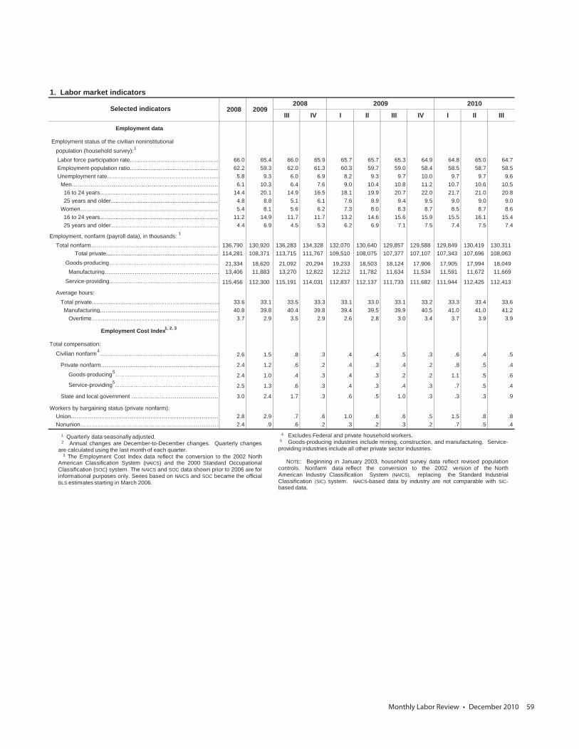
Monthly Labor Review • December 2010 59
1. Labor market indicators2008 2009 2010
III IV I II III IV I II III
Employment data
Employment status of the civilian noninstitutional population (household survey):1
Labor force participation rate........................................................ 66.0 65.4 66.0 65.9 65.7 65.7 65.3 64.9 64.8 65.0 64.7 Employment-population ratio........................................................ 62.2 59.3 62.0 61.3 60.3 59.7 59.0 58.4 58.5 58.7 58.5 Unemployment rate………………………………………………….… 5.8 9.3 6.0 6.9 8.2 9.3 9.7 10.0 9.7 9.7 9.6 Men………………………………………………..…….….………… 6.1 10.3 6.4 7.6 9.0 10.4 10.8 11.2 10.7 10.6 10.5 16 to 24 years........................................................................... 14.4 20.1 14.9 16.5 18.1 19.9 20.7 22.0 21.7 21.0 20.8 25 years and older.................................................................... 4.8 8.8 5.1 6.1 7.6 8.9 9.4 9.5 9.0 9.0 9.0 Women……………………………………………….….…………… 5.4 8.1 5.6 6.2 7.3 8.0 8.3 8.7 8.5 8.7 8.6 16 to 24 years........................................................................... 11.2 14.9 11.7 11.7 13.2 14.6 15.6 15.9 15.5 16.1 15.4 25 years and older.................................................................... 4.4 6.9 4.5 5.3 6.2 6.9 7.1 7.5 7.4 7.5 7.4
Employment, nonfarm (payroll data), in thousands: 1
Total nonfarm…………………….................................................... 136,790 130,920 136,283 134,328 132,070 130,640 129,857 129,588 129,849 130,419 130,311 Total private....................................................................... 114,281 108,371 113,715 111,767 109,510 108,075 107,377 107,107 107,343 107,696 108,063 Goods-producing……………………………………………….………….. 21,334 18,620 21,092 20,294 19,233 18,503 18,124 17,906 17,905 17,994 18,049 Manufacturing………….………………..………………………… 13,406 11,883 13,270 12,822 12,212 11,782 11,634 11,534 11,591 11,672 11,669 Service-providing……………………………………………….…………..…115,456 112,300 115,191 114,031 112,837 112,137 111,733 111,682 111,944 112,425 112,413
Average hours: Total private........................................………….......................... 33.6 33.1 33.5 33.3 33.1 33.0 33.1 33.2 33.3 33.4 33.6 Manufacturing………...…………………………………………… 40.8 39.8 40.4 39.8 39.4 39.5 39.9 40.5 41.0 41.0 41.2 Overtime……..………….………………...……………………… 3.7 2.9 3.5 2.9 2.6 2.8 3.0 3.4 3.7 3.9 3.9
Employment Cost Index1, 2, 3
Total compensation:
Civilian nonfarm4……………………………….…………………………….…… 2.6 1.5 .8 .3 .4 .4 .5 .3 .6 .4 .5
Private nonfarm……………...............………............................... 2.4 1.2 .6 .2 .4 .3 .4 .2 .8 .5 .4
Goods-producing5……………………………………………….………… 2.4 1.0 .4 .3 .4 .3 .2 .2 1.1 .5 .6
Service-providing5……………………………………………….………… 2.5 1.3 .6 .3 .4 .3 .4 .3 .7 .5 .4
State and local government ……………….……………………… 3.0 2.4 1.7 .3 .6 .5 1.0 .3 .3 .3 .9
Workers by bargaining status (private nonfarm): Union…………………………………………………………………… 2.8 2.9 .7 .6 1.0 .6 .6 .5 1.5 .8 .8 Nonunion………………………………………………………………… 2.4 .9 .6 .2 .3 .2 .3 .2 .7 .5 .4
Selected indicators 2009
1 Quarterly data seasonally adjusted.2 Annual changes are December-to-December changes. Quarterly changes
are calculated using the last month of each quarter.3 The Employment Cost Index data reflect the conversion to the 2002 North
American Classification System (NAICS) and the 2000 Standard OccupationalClassification (SOC) system. The NAICS and SOC data shown prior to 2006 are forinformational purposes only. Series based on NAICS and SOC became the officialBLS estimates starting in March 2006.
4 Excludes Federal and private household workers.5 Goods-producing industries include mining, construction, and manufacturing. Service-
providing industries include all other private sector industries.
NOTE: Beginning in January 2003, household survey data reflect revised populationcontrols. Nonfarm data reflect the conversion to the 2002 version of the NorthAmerican Industry Classification System (NAICS), replacing the Standard IndustrialClassification (SIC) system. NAICS-based data by industry are not comparable with SIC-based data.
2008
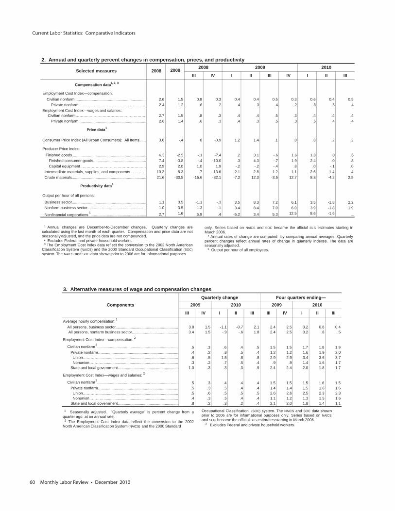
Current Labor Statistics: Comparative Indicators
60 Monthly Labor Review • December 2010
2. Annual and quarterly percent changes in compensation, prices, and productivity2008 2009 2010
III IV I II III IV I II III
Compensation data1, 2, 3
Employment Cost Index—compensation: Civilian nonfarm................................................................... 2.6 1.5 0.8 0.3 0.4 0.4 0.5 0.3 0.6 0.4 0.5 Private nonfarm............................................................... 2.4 1.2 .6 .2 .4 .3 .4 .2 .8 .5 .4 Employment Cost Index—wages and salaries: Civilian nonfarm………………………………………………. 2.7 1.5 .8 .3 .4 .4 .5 .3 .4 .4 .4 Private nonfarm............................................................... 2.6 1.4 .6 .3 .4 .3 .5 .3 .5 .4 .4
Price data1
Consumer Price Index (All Urban Consumers): All Items...... 3.8 -.4 0 -3.9 1.2 1.4 .1 .0 .8 .2 .2
Producer Price Index: Finished goods..................................................................... 6.3 -2.5 -.1 -7.4 .2 3.1 -.6 1.6 1.8 .0 .6 Finished consumer goods................................................. 7.4 -3.8 -.4 -10.0 .3 4.3 -.7 1.9 2.4 .0 .8 Capital equipment…………………………………………… 2.9 2.0 1.0 1.9 -.2 -.2 -.4 .8 .0 -.1 .0 Intermediate materials, supplies, and components………… 10.3 -8.3 .7 -13.6 -2.1 2.8 1.2 1.1 2.6 1.4 .4 Crude materials..................................................................... 21.6 -30.5 -15.6 -32.1 -7.2 12.3 -3.5 12.7 8.8 -4.2 2.5
Productivity data4
Output per hour of all persons:
Business sector..................................................................... 1.1 3.5 -1.1 -.3 3.5 8.3 7.2 6.1 3.5 -1.8 2.2 Nonfarm business sector....................................................... 1.0 3.5 -1.3 -.1 3.4 8.4 7.0 6.0 3.9 -1.8 1.9
Nonfinancial corporations 5……………….…………...……………… 2.7 1.6 5.9 .4 -5.2 3.4 5.3 12.5 8.6 -1.6 _
Selected measures 2008 2009
1 Annual changes are December-to-December changes. Quarterly changes arecalculated using the last month of each quarter. Compensation and price data are notseasonally adjusted, and the price data are not compounded.
2 Excludes Federal and private household workers.3 The Employment Cost Index data reflect the conversion to the 2002 North American
Classification System (NAICS) and the 2000 Standard Occupational Classification (SOC)system. The NAICS and SOC data shown prior to 2006 are for informational purposes
only. Series based on NAICS and SOC became the official BLS estimates starting inMarch 2006.
4 Annual rates of change are computed by comparing annual averages. Quarterlypercent changes reflect annual rates of change in quarterly indexes. The data areseasonally adjusted.
5 Output per hour of all employees.
3. Alternative measures of wage and compensation changesQuarterly change Four quarters ending—
Components 2009 2010 2009 2010
III IV I II III III IV I II III
Average hourly compensation:1
All persons, business sector.......................................................... 3.8 1.5 -1.1 -0.7 2.1 2.4 2.5 3.2 0.8 0.4 All persons, nonfarm business sector........................................... 3.4 1.5 -.9 -.6 1.8 2.4 2.5 3.2 .8 .5
Employment Cost Index—compensation: 2
Civilian nonfarm3……….………………………………………….…………..… .5 .3 .6 .4 .5 1.5 1.5 1.7 1.8 1.9
Private nonfarm…....................................................................... .4 .2 .8 .5 .4 1.2 1.2 1.6 1.9 2.0 Union………….......................................................................... .6 .5 1.5 .8 .8 2.9 2.9 3.4 3.6 3.7 Nonunion………….................................................................... .3 .2 .7 .5 .4 .9 .9 1.4 1.6 1.7 State and local government…..................................................... 1.0 .3 .3 .3 .9 2.4 2.4 2.0 1.8 1.7
Employment Cost Index—wages and salaries: 2
Civilian nonfarm3……….………………………………………….…………..… .5 .3 .4 .4 .4 1.5 1.5 1.5 1.6 1.5
Private nonfarm…....................................................................... .5 .3 .5 .4 .4 1.4 1.4 1.5 1.6 1.6 Union………….......................................................................... .5 .6 .5 .5 .5 2.6 2.6 2.5 2.3 2.3 Nonunion………….................................................................... .4 .3 .5 .4 .4 1.1 1.2 1.3 1.5 1.6 State and local government…..................................................... .8 .2 .3 .2 .4 2.1 2.0 1.8 1.4 1.1
Occupational Classification (SOC) system. The NAICS and SOC data shownprior to 2006 are for informational purposes only. Series based on NAICSand SOC became the official BLS estimates starting in March 2006.
3 Excludes Federal and private household workers.
1 Seasonally adjusted. "Quarterly average" is percent change from aquarter ago, at an annual rate.
2 The Employment Cost Index data reflect the conversion to the 2002North American Classification System (NAICS) and the 2000 Standard
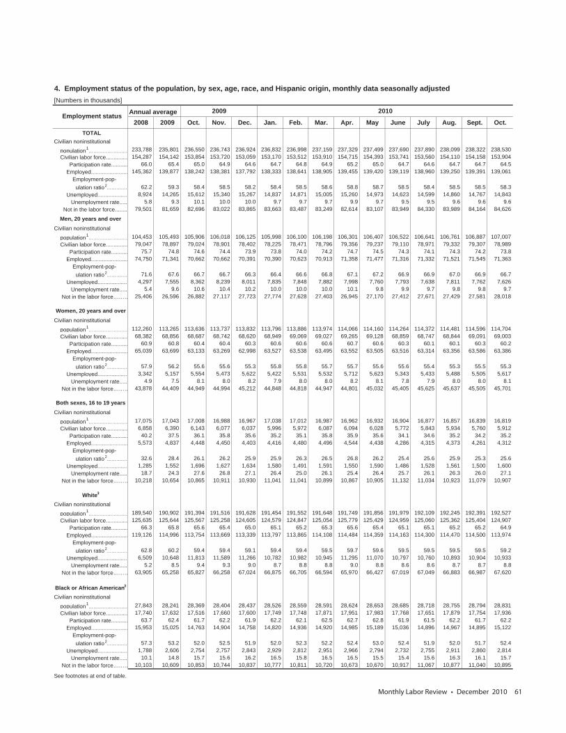
Monthly Labor Review • December 2010 61
4. Employment status of the population, by sex, age, race, and Hispanic origin, monthly data seasonally adjusted[Numbers in thousands]
Annual average 2009 2010
2008 2009 Oct. Nov. Dec. Jan. Feb. Mar. Apr. May June July Aug. Sept. Oct. TOTAL
Civilian noninstitutional
population1……………………. 233,788 235,801 236,550 236,743 236,924 236,832 236,998 237,159 237,329 237,499 237,690 237,890 238,099 238,322 238,530
Civilian labor force.............. 154,287 154,142 153,854 153,720 153,059 153,170 153,512 153,910 154,715 154,393 153,741 153,560 154,110 154,158 153,904 Participation rate........... 66.0 65.4 65.0 64.9 64.6 64.7 64.8 64.9 65.2 65.0 64.7 64.6 64.7 64.7 64.5 Employed........................ 145,362 139,877 138,242 138,381 137,792 138,333 138,641 138,905 139,455 139,420 139,119 138,960 139,250 139,391 139,061 Employment-pop- ulation ratio2…………… 62.2 59.3 58.4 58.5 58.2 58.4 58.5 58.6 58.8 58.7 58.5 58.4 58.5 58.5 58.3 Unemployed................... 8,924 14,265 15,612 15,340 15,267 14,837 14,871 15,005 15,260 14,973 14,623 14,599 14,860 14,767 14,843 Unemployment rate..... 5.8 9.3 10.1 10.0 10.0 9.7 9.7 9.7 9.9 9.7 9.5 9.5 9.6 9.6 9.6 Not in the labor force........ 79,501 81,659 82,696 83,022 83,865 83,663 83,487 83,249 82,614 83,107 83,949 84,330 83,989 84,164 84,626
Men, 20 years and overCivilian noninstitutional
population1……………………. 104,453 105,493 105,906 106,018 106,125 105,998 106,100 106,198 106,301 106,407 106,522 106,641 106,761 106,887 107,007
Civilian labor force.............. 79,047 78,897 79,024 78,901 78,402 78,225 78,471 78,796 79,356 79,237 79,110 78,971 79,332 79,307 78,989 Participation rate........... 75.7 74.8 74.6 74.4 73.9 73.8 74.0 74.2 74.7 74.5 74.3 74.1 74.3 74.2 73.8 Employed........................ 74,750 71,341 70,662 70,662 70,391 70,390 70,623 70,913 71,358 71,477 71,316 71,332 71,521 71,545 71,363 Employment-pop- ulation ratio2…………… 71.6 67.6 66.7 66.7 66.3 66.4 66.6 66.8 67.1 67.2 66.9 66.9 67.0 66.9 66.7 Unemployed................... 4,297 7,555 8,362 8,239 8,011 7,835 7,848 7,882 7,998 7,760 7,793 7,638 7,811 7,762 7,626 Unemployment rate..... 5.4 9.6 10.6 10.4 10.2 10.0 10.0 10.0 10.1 9.8 9.9 9.7 9.8 9.8 9.7 Not in the labor force……… 25,406 26,596 26,882 27,117 27,723 27,774 27,628 27,403 26,945 27,170 27,412 27,671 27,429 27,581 28,018
Women, 20 years and overCivilian noninstitutional
population1……………………. 112,260 113,265 113,636 113,737 113,832 113,796 113,886 113,974 114,066 114,160 114,264 114,372 114,481 114,596 114,704
Civilian labor force.............. 68,382 68,856 68,687 68,742 68,620 68,949 69,069 69,027 69,265 69,128 68,859 68,747 68,844 69,091 69,003 Participation rate........... 60.9 60.8 60.4 60.4 60.3 60.6 60.6 60.6 60.7 60.6 60.3 60.1 60.1 60.3 60.2 Employed........................ 65,039 63,699 63,133 63,269 62,998 63,527 63,538 63,495 63,552 63,505 63,516 63,314 63,356 63,586 63,386 Employment-pop- ulation ratio2…………… 57.9 56.2 55.6 55.6 55.3 55.8 55.8 55.7 55.7 55.6 55.6 55.4 55.3 55.5 55.3 Unemployed................... 3,342 5,157 5,554 5,473 5,622 5,422 5,531 5,532 5,712 5,623 5,343 5,433 5,488 5,505 5,617 Unemployment rate..... 4.9 7.5 8.1 8.0 8.2 7.9 8.0 8.0 8.2 8.1 7.8 7.9 8.0 8.0 8.1 Not in the labor force……… 43,878 44,409 44,949 44,994 45,212 44,848 44,818 44,947 44,801 45,032 45,405 45,625 45,637 45,505 45,701
Both sexes, 16 to 19 yearsCivilian noninstitutional
population1……………………. 17,075 17,043 17,008 16,988 16,967 17,038 17,012 16,987 16,962 16,932 16,904 16,877 16,857 16,839 16,819
Civilian labor force.............. 6,858 6,390 6,143 6,077 6,037 5,996 5,972 6,087 6,094 6,028 5,772 5,843 5,934 5,760 5,912 Participation rate........... 40.2 37.5 36.1 35.8 35.6 35.2 35.1 35.8 35.9 35.6 34.1 34.6 35.2 34.2 35.2 Employed........................ 5,573 4,837 4,448 4,450 4,403 4,416 4,480 4,496 4,544 4,438 4,286 4,315 4,373 4,261 4,312 Employment-pop- ulation ratio2…………… 32.6 28.4 26.1 26.2 25.9 25.9 26.3 26.5 26.8 26.2 25.4 25.6 25.9 25.3 25.6 Unemployed................... 1,285 1,552 1,696 1,627 1,634 1,580 1,491 1,591 1,550 1,590 1,486 1,528 1,561 1,500 1,600 Unemployment rate..... 18.7 24.3 27.6 26.8 27.1 26.4 25.0 26.1 25.4 26.4 25.7 26.1 26.3 26.0 27.1 Not in the labor force……… 10,218 10,654 10,865 10,911 10,930 11,041 11,041 10,899 10,867 10,905 11,132 11,034 10,923 11,079 10,907
White3
Civilian noninstitutional
population1……………………. 189,540 190,902 191,394 191,516 191,628 191,454 191,552 191,648 191,749 191,856 191,979 192,109 192,245 192,391 192,527
Civilian labor force.............. 125,635 125,644 125,567 125,258 124,605 124,579 124,847 125,054 125,779 125,429 124,959 125,060 125,362 125,404 124,907 Participation rate........... 66.3 65.8 65.6 65.4 65.0 65.1 65.2 65.3 65.6 65.4 65.1 65.1 65.2 65.2 64.9 Employed........................ 119,126 114,996 113,754 113,669 113,339 113,797 113,865 114,108 114,484 114,359 114,163 114,300 114,470 114,500 113,974 Employment-pop- ulation ratio2…………… 62.8 60.2 59.4 59.4 59.1 59.4 59.4 59.5 59.7 59.6 59.5 59.5 59.5 59.5 59.2 Unemployed................... 6,509 10,648 11,813 11,589 11,266 10,782 10,982 10,945 11,295 11,070 10,797 10,760 10,893 10,904 10,933 Unemployment rate..... 5.2 8.5 9.4 9.3 9.0 8.7 8.8 8.8 9.0 8.8 8.6 8.6 8.7 8.7 8.8 Not in the labor force……… 63,905 65,258 65,827 66,258 67,024 66,875 66,705 66,594 65,970 66,427 67,019 67,049 66,883 66,987 67,620
Black or African American3
Civilian noninstitutional
population1……………………. 27,843 28,241 28,369 28,404 28,437 28,526 28,559 28,591 28,624 28,653 28,685 28,718 28,755 28,794 28,831
Civilian labor force.............. 17,740 17,632 17,516 17,660 17,600 17,749 17,748 17,871 17,951 17,983 17,768 17,651 17,879 17,754 17,936 Participation rate........... 63.7 62.4 61.7 62.2 61.9 62.2 62.1 62.5 62.7 62.8 61.9 61.5 62.2 61.7 62.2 Employed........................ 15,953 15,025 14,763 14,904 14,758 14,820 14,936 14,920 14,985 15,189 15,036 14,896 14,967 14,895 15,122 Employment-pop- ulation ratio2…………… 57.3 53.2 52.0 52.5 51.9 52.0 52.3 52.2 52.4 53.0 52.4 51.9 52.0 51.7 52.4 Unemployed................... 1,788 2,606 2,754 2,757 2,843 2,929 2,812 2,951 2,966 2,794 2,732 2,755 2,911 2,860 2,814 Unemployment rate..... 10.1 14.8 15.7 15.6 16.2 16.5 15.8 16.5 16.5 15.5 15.4 15.6 16.3 16.1 15.7 Not in the labor force……… 10,103 10,609 10,853 10,744 10,837 10,777 10,811 10,720 10,673 10,670 10,917 11,067 10,877 11,040 10,895
See footnotes at end of table.
Employment status
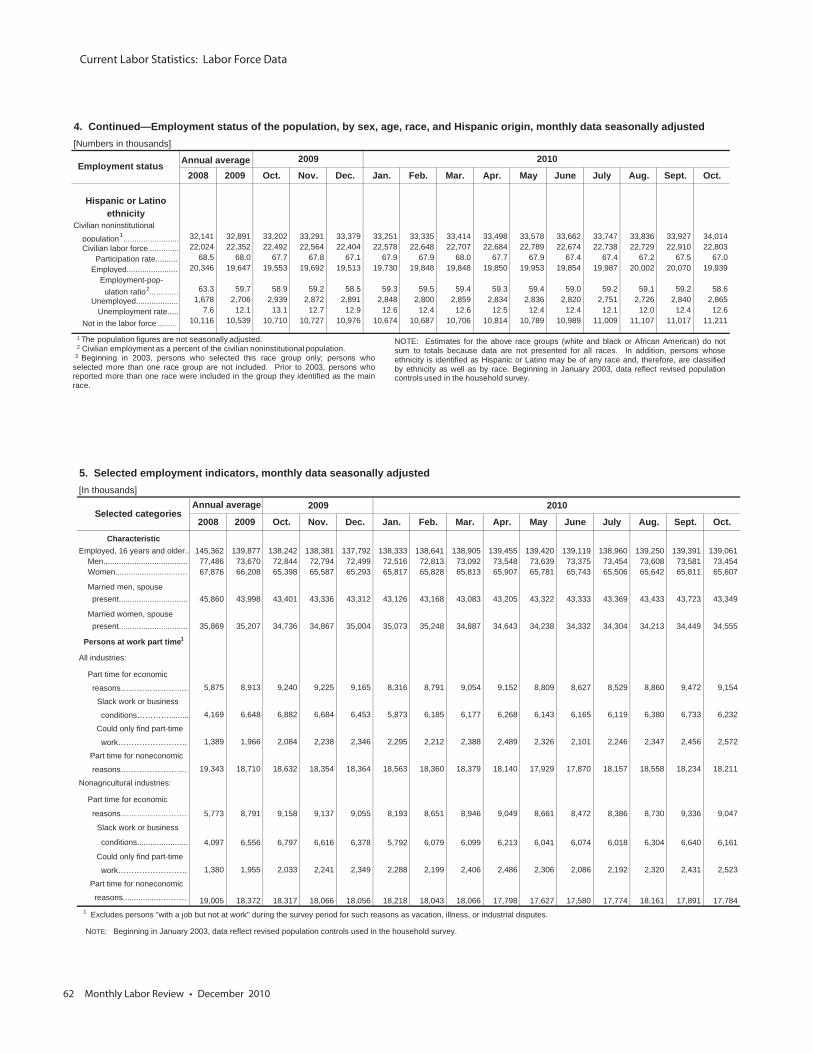
Current Labor Statistics: Labor Force Data
62 Monthly Labor Review • December 2010
4. Continued—Employment status of the population, by sex, age, race, and Hispanic origin, monthly data seasonally adjusted [Numbers in thousands]
Annual average 2009 2010
2008 2009 Oct. Nov. Dec. Jan. Feb. Mar. Apr. May June July Aug. Sept. Oct.
Hispanic or Latinoethnicity
Civilian noninstitutional
population1……………………. 32,141 32,891 33,202 33,291 33,379 33,251 33,335 33,414 33,498 33,578 33,662 33,747 33,836 33,927 34,014
Civilian labor force.............. 22,024 22,352 22,492 22,564 22,404 22,578 22,648 22,707 22,684 22,789 22,674 22,738 22,729 22,910 22,803 Participation rate........... 68.5 68.0 67.7 67.8 67.1 67.9 67.9 68.0 67.7 67.9 67.4 67.4 67.2 67.5 67.0 Employed........................ 20,346 19,647 19,553 19,692 19,513 19,730 19,848 19,848 19,850 19,953 19,854 19,987 20,002 20,070 19,939 Employment-pop- ulation ratio2…………… 63.3 59.7 58.9 59.2 58.5 59.3 59.5 59.4 59.3 59.4 59.0 59.2 59.1 59.2 58.6 Unemployed................... 1,678 2,706 2,939 2,872 2,891 2,848 2,800 2,859 2,834 2,836 2,820 2,751 2,726 2,840 2,865 Unemployment rate..... 7.6 12.1 13.1 12.7 12.9 12.6 12.4 12.6 12.5 12.4 12.4 12.1 12.0 12.4 12.6
Not in the labor force………… 10,116 10,539 10,710 10,727 10,976 10,674 10,687 10,706 10,814 10,789 10,989 11,009 11,107 11,017 11,211
1 The population figures are not seasonally adjusted.2 Civilian employment as a percent of the civilian noninstitutional population.
3 Beginning in 2003, persons who selected this race group only; persons whoselected more than one race group are not included. Prior to 2003, persons whoreported more than one race were included in the group they identified as the mainrace.
NOTE: Estimates for the above race groups (white and black or African American) do notsum to totals because data are not presented for all races. In addition, persons whoseethnicity is identified as Hispanic or Latino may be of any race and, therefore, are classifiedby ethnicity as well as by race. Beginning in January 2003, data reflect revised populationcontrols used in the household survey.
Employment status
5. Selected employment indicators, monthly data seasonally adjusted [In thousands]
2009 2010
2008 2009 Oct. Nov. Dec. Jan. Feb. Mar. Apr. May June July Aug. Sept. Oct.
CharacteristicEmployed, 16 years and older.. 145,362 139,877 138,242 138,381 137,792 138,333 138,641 138,905 139,455 139,420 139,119 138,960 139,250 139,391 139,061 Men....................................... 77,486 73,670 72,844 72,794 72,499 72,516 72,813 73,092 73,548 73,639 73,375 73,454 73,608 73,581 73,454 Women............................…… 67,876 66,208 65,398 65,587 65,293 65,817 65,828 65,813 65,907 65,781 65,743 65,506 65,642 65,811 65,607
Married men, spouse present................................ 45,860 43,998 43,401 43,336 43,312 43,126 43,168 43,083 43,205 43,322 43,333 43,369 43,433 43,723 43,349
Married women, spouse present................................ 35,869 35,207 34,736 34,867 35,004 35,073 35,248 34,887 34,643 34,238 34,332 34,304 34,213 34,449 34,555
Persons at work part time1
All industries:
Part time for economic
reasons…………………….… 5,875 8,913 9,240 9,225 9,165 8,316 8,791 9,054 9,152 8,809 8,627 8,529 8,860 9,472 9,154
Slack work or business
conditions…………......... 4,169 6,648 6,882 6,684 6,453 5,873 6,185 6,177 6,268 6,143 6,165 6,119 6,380 6,733 6,232
Could only find part-time
work……………………… 1,389 1,966 2,084 2,238 2,346 2,295 2,212 2,388 2,489 2,326 2,101 2,246 2,347 2,456 2,572
Part time for noneconomic
reasons……………………… 19,343 18,710 18,632 18,354 18,364 18,563 18,360 18,379 18,140 17,929 17,870 18,157 18,558 18,234 18,211
Nonagricultural industries:
Part time for economic
reasons…………………….… 5,773 8,791 9,158 9,137 9,055 8,193 8,651 8,946 9,049 8,661 8,472 8,386 8,730 9,336 9,047
Slack work or business
conditions....................... 4,097 6,556 6,797 6,616 6,378 5,792 6,079 6,099 6,213 6,041 6,074 6,018 6,304 6,640 6,161
Could only find part-time
work……………………… 1,380 1,955 2,033 2,241 2,349 2,288 2,199 2,406 2,486 2,306 2,086 2,192 2,320 2,431 2,523
Part time for noneconomic
reasons.................………… 19,005 18,372 18,317 18,066 18,056 18,218 18,043 18,066 17,798 17,627 17,580 17,774 18,161 17,891 17,7841 Excludes persons "with a job but not at work" during the survey period for such reasons as vacation, illness, or industrial disputes.
NOTE: Beginning in January 2003, data reflect revised population controls used in the household survey.
Annual averageSelected categories
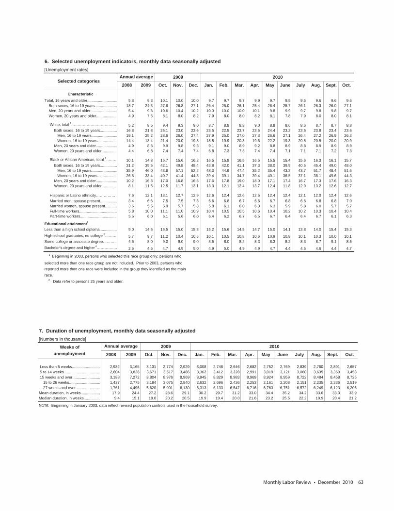
Monthly Labor Review • December 2010 63
6. Selected unemployment indicators, monthly data seasonally adjusted [Unemployment rates]
2009 2010
2008 2009 Oct. Nov. Dec. Jan. Feb. Mar. Apr. May June July Aug. Sept. Oct.
CharacteristicTotal, 16 years and older............................ 5.8 9.3 10.1 10.0 10.0 9.7 9.7 9.7 9.9 9.7 9.5 9.5 9.6 9.6 9.6 Both sexes, 16 to 19 years..................... 18.7 24.3 27.6 26.8 27.1 26.4 25.0 26.1 25.4 26.4 25.7 26.1 26.3 26.0 27.1 Men, 20 years and older......................... 5.4 9.6 10.6 10.4 10.2 10.0 10.0 10.0 10.1 9.8 9.9 9.7 9.8 9.8 9.7 Women, 20 years and older................... 4.9 7.5 8.1 8.0 8.2 7.9 8.0 8.0 8.2 8.1 7.8 7.9 8.0 8.0 8.1
White, total 1……………………………… 5.2 8.5 9.4 9.3 9.0 8.7 8.8 8.8 9.0 8.8 8.6 8.6 8.7 8.7 8.8 Both sexes, 16 to 19 years................ 16.8 21.8 25.1 23.0 23.6 23.5 22.5 23.7 23.5 24.4 23.2 23.5 23.8 23.4 23.6 Men, 16 to 19 years........................ 19.1 25.2 28.6 26.0 27.4 27.9 25.0 27.0 27.3 26.6 27.1 26.4 27.2 26.9 26.3 Women, 16 to 19 years.................. 14.4 18.4 21.4 20.0 19.8 18.8 19.9 20.3 19.6 22.2 19.3 20.5 20.5 20.0 20.9 Men, 20 years and older.................... 4.9 8.8 9.9 9.8 9.3 9.1 9.0 8.9 9.2 8.8 8.9 8.8 8.9 8.9 8.9 Women, 20 years and older.............. 4.4 6.8 7.4 7.4 7.4 6.8 7.3 7.3 7.4 7.4 7.1 7.1 7.1 7.2 7.3
Black or African American, total 1……… 10.1 14.8 15.7 15.6 16.2 16.5 15.8 16.5 16.5 15.5 15.4 15.6 16.3 16.1 15.7 Both sexes, 16 to 19 years................ 31.2 39.5 42.1 49.8 48.4 43.8 42.0 41.1 37.3 38.0 39.9 40.6 45.4 49.0 48.0 Men, 16 to 19 years........................ 35.9 46.0 43.6 57.1 52.2 48.3 44.9 47.4 35.2 35.4 43.2 43.7 51.7 48.4 51.6 Women, 16 to 19 years.................. 26.8 33.4 40.7 41.4 44.8 39.4 39.1 34.7 39.4 40.1 36.5 37.1 38.1 49.6 44.3 Men, 20 years and older.................... 10.2 16.3 17.0 16.8 16.6 17.6 17.8 19.0 18.0 17.1 17.4 16.7 17.3 17.6 16.3 Women, 20 years and older.............. 8.1 11.5 12.5 11.7 13.1 13.3 12.1 12.4 13.7 12.4 11.8 12.9 13.2 12.6 12.7
Hispanic or Latino ethnicity……………… 7.6 12.1 13.1 12.7 12.9 12.6 12.4 12.6 12.5 12.4 12.4 12.1 12.0 12.4 12.6 Married men, spouse present................ 3.4 6.6 7.5 7.5 7.3 6.6 6.8 6.7 6.6 6.7 6.8 6.6 6.8 6.8 7.0 Married women, spouse present........... 3.6 5.5 5.9 5.7 5.8 5.8 6.1 6.0 6.3 6.3 5.9 5.8 6.0 5.7 5.7 Full-time workers................................... 5.8 10.0 11.1 11.0 10.9 10.4 10.5 10.5 10.6 10.4 10.2 10.2 10.3 10.4 10.4 Part-time workers.................................. 5.5 6.0 6.1 5.6 6.0 6.4 6.2 6.7 6.5 6.7 6.4 6.4 6.7 6.1 6.3
Educational attainment2
Less than a high school diploma................ 9.0 14.6 15.5 15.0 15.3 15.2 15.6 14.5 14.7 15.0 14.1 13.8 14.0 15.4 15.3High school graduates, no college 3……… 5.7 9.7 11.2 10.4 10.5 10.1 10.5 10.8 10.6 10.9 10.8 10.1 10.3 10.0 10.1 Some college or associate degree……….. 4.6 8.0 9.0 9.0 9.0 8.5 8.0 8.2 8.3 8.3 8.2 8.3 8.7 9.1 8.5Bachelor's degree and higher 4……………. 2.6 4.6 4.7 4.9 5.0 4.9 5.0 4.9 4.9 4.7 4.4 4.5 4.6 4.4 4.7
1 Beginning in 2003, persons who selected this race group only; persons who
selected more than one race group are not included. Prior to 2003, persons who reported more than one race were included in the group they identified as the main race.
2 Data refer to persons 25 years and older.
Annual averageSelected categories
7. Duration of unemployment, monthly data seasonally adjusted [Numbers in thousands]
Weeks of 2009 2010unemployment 2008 2009 Oct. Nov. Dec. Jan. Feb. Mar. Apr. May June July Aug. Sept. Oct.
Less than 5 weeks........................... 2,932 3,165 3,131 2,774 2,929 3,008 2,748 2,646 2,682 2,752 2,769 2,839 2,760 2,891 2,657 5 to 14 weeks.................................. 2,804 3,828 3,671 3,517 3,486 3,362 3,412 3,228 2,991 3,019 3,121 3,060 3,635 3,350 3,458 15 weeks and over.......................... 3,188 7,272 8,804 8,976 8,969 8,945 8,829 8,983 8,969 8,924 8,959 8,722 8,484 8,458 8,725 15 to 26 weeks............................. 1,427 2,775 3,184 3,075 2,840 2,632 2,696 2,436 2,253 2,161 2,208 2,151 2,235 2,336 2,519 27 weeks and over....................... 1,761 4,496 5,620 5,901 6,130 6,313 6,133 6,547 6,716 6,763 6,751 6,572 6,249 6,123 6,206Mean duration, in weeks................... 17.9 24.4 27.2 28.6 29.1 30.2 29.7 31.2 33.0 34.4 35.2 34.2 33.6 33.3 33.9Median duration, in weeks............... 9.4 15.1 19.0 20.2 20.5 19.9 19.4 20.0 21.6 23.2 25.5 22.2 19.9 20.4 21.2
NOTE: Beginning in January 2003, data reflect revised population controls used in the household survey.
Annual average
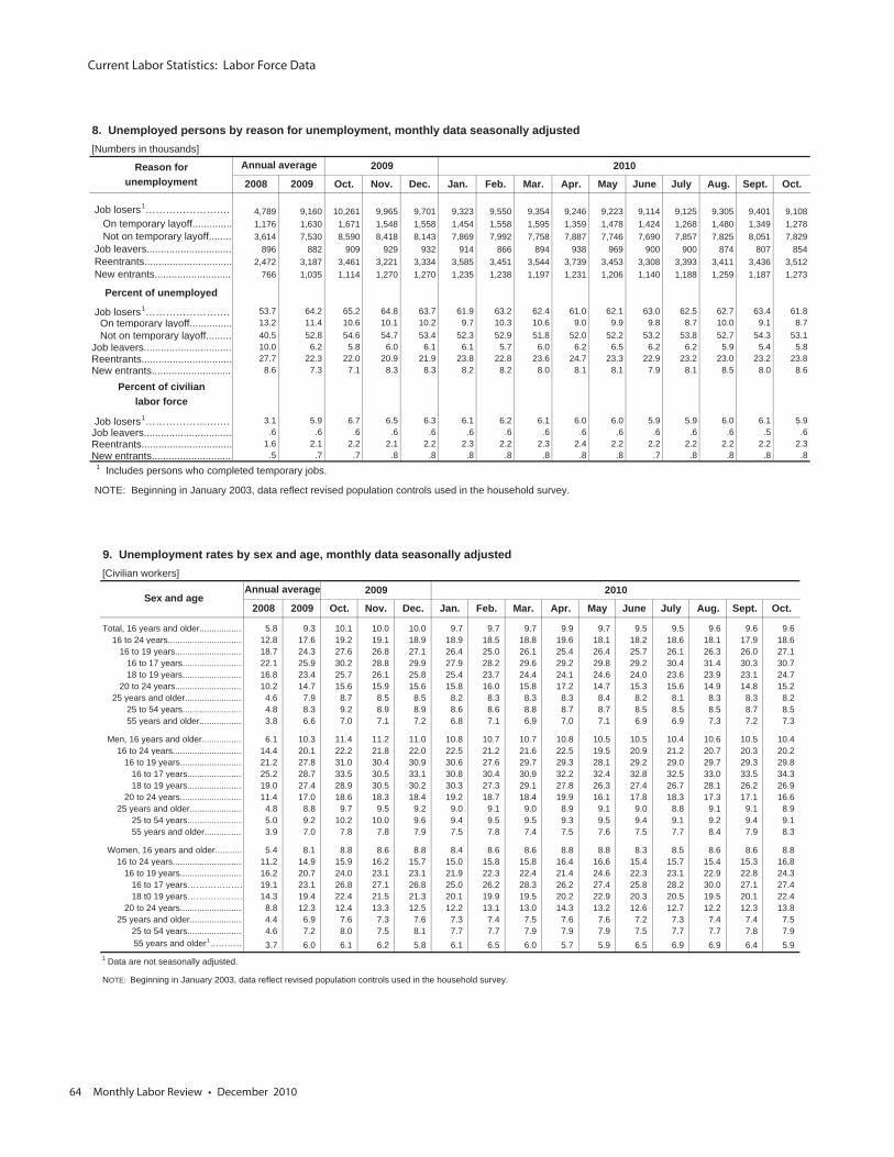
Current Labor Statistics: Labor Force Data
64 Monthly Labor Review • December 2010
8. Unemployed persons by reason for unemployment, monthly data seasonally adjusted [Numbers in thousands]
Reason for 2009 2010unemployment 2008 2009 Oct. Nov. Dec. Jan. Feb. Mar. Apr. May June July Aug. Sept. Oct.
Job losers1…………………….… 4,789 9,160 10,261 9,965 9,701 9,323 9,550 9,354 9,246 9,223 9,114 9,125 9,305 9,401 9,108 On temporary layoff.............. 1,176 1,630 1,671 1,548 1,558 1,454 1,558 1,595 1,359 1,478 1,424 1,268 1,480 1,349 1,278 Not on temporary layoff........ 3,614 7,530 8,590 8,418 8,143 7,869 7,992 7,758 7,887 7,746 7,690 7,857 7,825 8,051 7,829 Job leavers.............................. 896 882 909 929 932 914 866 894 938 969 900 900 874 807 854 Reentrants............................... 2,472 3,187 3,461 3,221 3,334 3,585 3,451 3,544 3,739 3,453 3,308 3,393 3,411 3,436 3,512 New entrants........................... 766 1,035 1,114 1,270 1,270 1,235 1,238 1,197 1,231 1,206 1,140 1,188 1,259 1,187 1,273
Percent of unemployed
Job losers1…………………….… 53.7 64.2 65.2 64.8 63.7 61.9 63.2 62.4 61.0 62.1 63.0 62.5 62.7 63.4 61.8 On temporary layoff............... 13.2 11.4 10.6 10.1 10.2 9.7 10.3 10.6 9.0 9.9 9.8 8.7 10.0 9.1 8.7 Not on temporary layoff......... 40.5 52.8 54.6 54.7 53.4 52.3 52.9 51.8 52.0 52.2 53.2 53.8 52.7 54.3 53.1Job leavers............................... 10.0 6.2 5.8 6.0 6.1 6.1 5.7 6.0 6.2 6.5 6.2 6.2 5.9 5.4 5.8Reentrants................................ 27.7 22.3 22.0 20.9 21.9 23.8 22.8 23.6 24.7 23.3 22.9 23.2 23.0 23.2 23.8New entrants............................ 8.6 7.3 7.1 8.3 8.3 8.2 8.2 8.0 8.1 8.1 7.9 8.1 8.5 8.0 8.6
Percent of civilianlabor force
Job losers1…………………….… 3.1 5.9 6.7 6.5 6.3 6.1 6.2 6.1 6.0 6.0 5.9 5.9 6.0 6.1 5.9Job leavers............................... .6 .6 .6 .6 .6 .6 .6 .6 .6 .6 .6 .6 .6 .5 .6Reentrants................................ 1.6 2.1 2.2 2.1 2.2 2.3 2.2 2.3 2.4 2.2 2.2 2.2 2.2 2.2 2.3New entrants............................ .5 .7 .7 .8 .8 .8 .8 .8 .8 .8 .7 .8 .8 .8 .8 1 Includes persons who completed temporary jobs.
NOTE: Beginning in January 2003, data reflect revised population controls used in the household survey.
Annual average
9. Unemployment rates by sex and age, monthly data seasonally adjusted [Civilian workers]
2009 2010
2008 2009 Oct. Nov. Dec. Jan. Feb. Mar. Apr. May June July Aug. Sept. Oct.
Total, 16 years and older.................. 5.8 9.3 10.1 10.0 10.0 9.7 9.7 9.7 9.9 9.7 9.5 9.5 9.6 9.6 9.6 16 to 24 years............................... 12.8 17.6 19.2 19.1 18.9 18.9 18.5 18.8 19.6 18.1 18.2 18.6 18.1 17.9 18.6 16 to 19 years............................ 18.7 24.3 27.6 26.8 27.1 26.4 25.0 26.1 25.4 26.4 25.7 26.1 26.3 26.0 27.1 16 to 17 years......................... 22.1 25.9 30.2 28.8 29.9 27.9 28.2 29.6 29.2 29.8 29.2 30.4 31.4 30.3 30.7 18 to 19 years......................... 16.8 23.4 25.7 26.1 25.8 25.4 23.7 24.4 24.1 24.6 24.0 23.6 23.9 23.1 24.7 20 to 24 years............................ 10.2 14.7 15.6 15.9 15.6 15.8 16.0 15.8 17.2 14.7 15.3 15.6 14.9 14.8 15.2 25 years and older........................ 4.6 7.9 8.7 8.5 8.5 8.2 8.3 8.3 8.3 8.4 8.2 8.1 8.3 8.3 8.2 25 to 54 years......................... 4.8 8.3 9.2 8.9 8.9 8.6 8.6 8.8 8.7 8.7 8.5 8.5 8.5 8.7 8.5 55 years and older.................. 3.8 6.6 7.0 7.1 7.2 6.8 7.1 6.9 7.0 7.1 6.9 6.9 7.3 7.2 7.3
Men, 16 years and older................. 6.1 10.3 11.4 11.2 11.0 10.8 10.7 10.7 10.8 10.5 10.5 10.4 10.6 10.5 10.4 16 to 24 years............................. 14.4 20.1 22.2 21.8 22.0 22.5 21.2 21.6 22.5 19.5 20.9 21.2 20.7 20.3 20.2 16 to 19 years.......................... 21.2 27.8 31.0 30.4 30.9 30.6 27.6 29.7 29.3 28.1 29.2 29.0 29.7 29.3 29.8 16 to 17 years....................... 25.2 28.7 33.5 30.5 33.1 30.8 30.4 30.9 32.2 32.4 32.8 32.5 33.0 33.5 34.3 18 to 19 years....................... 19.0 27.4 28.9 30.5 30.2 30.3 27.3 29.1 27.8 26.3 27.4 26.7 28.1 26.2 26.9 20 to 24 years.......................... 11.4 17.0 18.6 18.3 18.4 19.2 18.7 18.4 19.9 16.1 17.8 18.3 17.3 17.1 16.6 25 years and older...................... 4.8 8.8 9.7 9.5 9.2 9.0 9.1 9.0 8.9 9.1 9.0 8.8 9.1 9.1 8.9 25 to 54 years....................... 5.0 9.2 10.2 10.0 9.6 9.4 9.5 9.5 9.3 9.5 9.4 9.1 9.2 9.4 9.1 55 years and older................ 3.9 7.0 7.8 7.8 7.9 7.5 7.8 7.4 7.5 7.6 7.5 7.7 8.4 7.9 8.3
Women, 16 years and older........... 5.4 8.1 8.8 8.6 8.8 8.4 8.6 8.6 8.8 8.8 8.3 8.5 8.6 8.6 8.8 16 to 24 years............................. 11.2 14.9 15.9 16.2 15.7 15.0 15.8 15.8 16.4 16.6 15.4 15.7 15.4 15.3 16.8 16 to 19 years.......................... 16.2 20.7 24.0 23.1 23.1 21.9 22.3 22.4 21.4 24.6 22.3 23.1 22.9 22.8 24.3 16 to 17 years………………… 19.1 23.1 26.8 27.1 26.8 25.0 26.2 28.3 26.2 27.4 25.8 28.2 30.0 27.1 27.4 18 t0 19 years………………… 14.3 19.4 22.4 21.5 21.3 20.1 19.9 19.5 20.2 22.9 20.3 20.5 19.5 20.1 22.4 20 to 24 years.......................... 8.8 12.3 12.4 13.3 12.5 12.2 13.1 13.0 14.3 13.2 12.6 12.7 12.2 12.3 13.8 25 years and older...................... 4.4 6.9 7.6 7.3 7.6 7.3 7.4 7.5 7.6 7.6 7.2 7.3 7.4 7.4 7.5 25 to 54 years....................... 4.6 7.2 8.0 7.5 8.1 7.7 7.7 7.9 7.9 7.9 7.5 7.7 7.7 7.8 7.9
55 years and older1………… 3.7 6.0 6.1 6.2 5.8 6.1 6.5 6.0 5.7 5.9 6.5 6.9 6.9 6.4 5.9 1 Data are not seasonally adjusted.
NOTE: Beginning in January 2003, data reflect revised population controls used in the household survey.
Annual averageSex and age
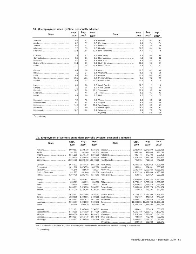
Monthly Labor Review • December 2010 65
10. Unemployment rates by State, seasonally adjusted
StateSept.2009
Aug.2010p
Sept.2010p State
Sept.2009
Aug.2010p
Sept.2010p
Alabama............................………………… 10.7 9.2 8.9 Missouri……………………………………… 9.7 9.3 9.3 Alaska........................................................ 8.3 7.7 7.7 Montana..................................................... 6.5 7.4 7.4 Arizona............................…………………… 9.4 9.7 9.7 Nebraska............................………………… 4.8 4.6 4.6 Arkansas.................................................... 7.5 7.5 7.7 Nevada...................................................... 12.7 14.4 14.4 California............................………………… 12.1 12.4 12.4 New Hampshire............................………… 6.7 5.7 5.5
Colorado.................................................... 7.7 8.1 8.2 New Jersey................................................ 9.8 9.6 9.4 Connecticut............................……………… 8.6 9.1 9.1 New Mexico............................……………… 7.8 8.3 8.2 Delaware................................................... 8.4 8.4 8.3 New York................................................... 8.8 8.3 8.3 District of Columbia............................…… 11.1 9.9 9.8 North Carolina............................…………… 10.9 9.7 9.7 Florida........................................................ 11.2 11.8 11.9 North Dakota............................................. 4.3 3.7 3.7
Georgia............................………………… 10.1 10.0 9.9 Ohio............................……………………… 10.7 10.1 10.0 Hawaii........................................................ 7.0 6.4 6.4 Oklahoma.................................................. 6.9 7.0 6.9 Idaho............................……………………… 8.7 8.9 9.0 Oregon............................…………………… 11.0 10.6 10.5 Illinois......................................................... 10.8 10.1 9.9 Pennsylvania............................................. 8.6 9.2 9.0 Indiana............................…………………… 10.1 10.2 10.1 Rhode Island............................…………… 12.0 11.8 11.5
Iowa............................……………………… 6.4 6.8 6.7 South Carolina............................………… 12.2 11.1 11.0 Kansas....................................................... 7.0 6.5 6.6 South Dakota............................................. 4.7 4.5 4.4 Kentucky............................………………… 10.8 10.0 10.1 Tennessee............................……………… 10.8 9.6 9.4 Louisiana................................................... 7.3 7.6 7.8 Texas......................................................... 8.1 8.3 8.1 Maine............................…………………… 8.1 8.0 7.7 Utah............................……………………… 6.7 7.4 7.5
Maryland............................………………… 7.3 7.3 7.4 Vermont............................………………… 6.8 6.0 5.8 Massachusetts........................................... 9.0 8.8 8.4 Virginia....................................................... 6.8 6.9 6.8 Michigan............................………………… 14.4 13.1 13.0 Washington............................……………… 9.2 9.0 9.1 Minnesota.................................................. 7.9 7.0 7.0 West Virginia............................................. 8.7 8.8 9.1 Mississippi............................……………… 10.0 10.0 9.8 Wisconsin............................……………… 8.8 7.9 7.8
Wyoming.................................................... 7.3 6.8 6.8p = preliminary
11. Employment of workers on nonfarm payrolls by State, seasonally adjusted
State Sept.2009
Aug.2010p
Sept.2010p State Sept.
2009Aug.2010p
Sept.2010p
Alabama............................………… 2,090,657 2,102,719 2,116,041 Missouri……………………………… 3,025,653 2,979,390 2,986,013 Alaska............................................. 361,782 362,940 362,839 Montana......................................... 498,168 497,080 496,753 Arizona............................…………… 3,141,228 3,174,778 3,184,833 Nebraska............................………… 981,446 975,704 973,852 Arkansas........................................ 1,370,170 1,340,954 1,340,139 Nevada........................................... 1,374,355 1,351,703 1,345,677 California............................………… 18,186,700 18,228,402 18,243,523 New Hampshire............................… 741,805 739,556 743,334
Colorado......................................... 2,675,921 2,656,425 2,661,096 New Jersey..................................... 4,535,232 4,510,012 4,501,934 Connecticut............................……… 1,891,862 1,878,770 1,887,678 New Mexico............................…… 956,361 954,601 955,485 Delaware........................................ 431,145 422,019 422,234 New York........................................ 9,681,483 9,659,324 9,668,201 District of Columbia........................ 331,777 331,846 331,038 North Carolina............................… 4,521,728 4,491,689 4,480,643 Florida............................................ 9,197,435 9,231,401 9,244,061 North Dakota.................................. 364,261 367,817 368,133
Georgia............................………… 4,738,422 4,667,647 4,665,021 Ohio............................……………… 5,943,505 5,926,232 5,920,082 Hawaii............................................. 635,921 634,911 634,592 Oklahoma....................................... 1,776,947 1,756,990 1,756,867 Idaho............................…………… 749,904 755,998 756,377 Oregon............................…………… 1,950,054 1,963,843 1,969,403 Illinois............................................. 6,600,891 6,624,550 6,636,991 Pennsylvania.................................. 6,393,308 6,363,778 6,364,974 Indiana............................…………… 3,145,379 3,120,208 3,120,354 Rhode Island............................…… 570,062 572,105 570,985
Iowa............................……………… 1,674,621 1,671,904 1,674,347 South Carolina............................… 2,175,832 2,148,303 2,152,822 Kansas........................................... 1,522,030 1,490,391 1,492,225 South Dakota.................................. 445,787 442,919 443,117 Kentucky............................………… 2,078,142 2,067,873 2,077,480 Tennessee............................……… 3,004,527 3,037,440 3,047,916 Louisiana........................................ 2,066,717 2,098,960 2,109,275 Texas.............................................. 11,990,835 12,128,738 12,139,139 Maine............................…………… 703,495 693,879 693,954 Utah............................……………… 1,355,259 1,351,894 1,353,756
Maryland............................………… 2,972,191 2,947,668 2,954,805 Vermont............................………… 358,431 355,824 356,075 Massachusetts............................... 3,473,310 3,475,329 3,477,026 Virginia........................................... 4,161,458 4,168,751 4,170,705 Michigan............................………… 4,866,356 4,831,009 4,826,432 Washington............................……… 3,523,760 3,536,807 3,540,211 Minnesota....................................... 2,963,834 2,956,479 2,957,148 West Virginia.................................. 794,159 773,780 775,906 Mississippi............................……… 1,288,977 1,296,590 1,302,666 Wisconsin............................……… 3,058,942 3,029,737 3,031,807
Wyoming........................................ 294,053 290,923 291,675
NOTE: Some data in this table may differ from data published elsewhere because of the continual updating of the database.p = preliminary
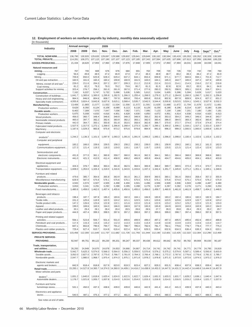
Current Labor Statistics: Labor Force Data
66 Monthly Labor Review • December 2010
12. Employment of workers on nonfarm payrolls by industry, monthly data seasonally adjusted[In thousands]
2009 2010
2008 2009 Oct. Nov. Dec. Jan. Feb. Mar. Apr. May June July Aug. Sept.p Oct.p
TOTAL NONFARM................. 136,790 130,920 129,633 129,697 129,588 129,602 129,641 129,849 130,162 130,594 130,419 130,353 130,352 130,328 130,500 TOTAL PRIVATE........................ 114,281 108,371 107,115 107,190 107,107 107,123 107,185 107,343 107,584 107,635 107,696 107,813 107,956 108,068 108,228GOODS-PRODUCING……………… 21,334 18,620 17,993 17,960 17,906 17,876 17,848 17,905 17,972 17,993 17,994 18,031 18,048 18,038 18,041
Natural resources and mining…………..……….......…… 767 700 669 676 676 684 691 702 709 720 726 733 742 749 760 Logging.................................... 56.6 49.8 48.5 47.2 46.9 47.0 47.2 48.3 48.9 48.7 48.2 48.3 48.2 47.2 46.9 Mining.......................................... 709.8 650.0 620.8 628.4 629.4 637.2 644.1 653.4 659.8 671.1 677.7 684.6 694.1 701.8 712.7 Oil and gas extraction…………… 160.5 161.6 160.4 160.2 159.8 160.9 161.5 163.0 164.1 165.3 164.7 165.0 167.2 167.8 169.8
Mining, except oil and gas 1…… 226.0 211.6 204.3 207.2 207.7 209.3 211.2 212.8 212.4 213.3 214.1 214.5 216.0 217.3 218.8 Coal mining…………………… 81.2 82.2 79.3 79.3 79.2 79.6 80.7 81.3 81.5 82.8 82.9 83.2 83.5 84.1 84.8 Support activities for mining…… 323.4 276.7 256.1 261.0 261.9 267.0 271.4 277.6 283.3 292.5 298.9 305.1 310.9 316.7 324.1 Construction................................ 7,162 6,037 5,747 5,732 5,696 5,636 5,585 5,612 5,634 5,605 5,596 5,594 5,628 5,617 5,620 Construction of buildings........... 1,641.7 1,365.6 1,300.0 1,295.9 1,282.5 1,266.3 1,255.4 1,268.5 1,278.3 1,271.2 1,264.9 1,260.3 1,260.7 1,262.3 1,256.8 Heavy and civil engineering…… 964.5 846.9 804.6 808.7 797.9 800.8 793.4 800.8 810.8 802.8 807.9 809.9 824.3 827.2 831.2 Speciality trade contractors....... 4,555.8 3,824.4 3,642.8 3,627.6 3,615.1 3,568.4 3,535.7 3,542.5 3,544.4 3,530.8 3,523.5 3,524.1 3,543.1 3,527.9 3,532.3 Manufacturing.............................. 13,406 11,883 11,577 11,552 11,534 11,556 11,572 11,591 11,629 11,668 11,672 11,704 11,678 11,672 11,661 Production workers................ 9,629 8,350 8,124 8,108 8,089 8,113 8,118 8,129 8,159 8,188 8,196 8,214 8,187 8,180 8,166 Durable goods........................... 8,463 7,309 7,070 7,047 7,036 7,062 7,071 7,095 7,123 7,159 7,166 7,201 7,180 7,185 7,181 Production workers................ 5,975 5,008 4,833 4,816 4,801 4,828 4,830 4,850 4,872 4,901 4,914 4,938 4,916 4,920 4,913 Wood products.......................... 456.0 360.7 348.4 348.6 348.9 348.3 348.9 350.2 352.9 353.3 354.2 349.2 346.5 344.8 343.7 Nonmetallic mineral products 465.0 397.7 382.2 382.6 383.9 382.2 383.1 382.5 383.4 386.0 384.5 383.3 382.6 383.8 383.2 Primary metals.......................... 442.0 364.7 350.1 350.8 351.8 353.5 358.9 362.8 366.7 370.0 372.7 374.0 373.9 374.8 374.4 Fabricated metal products......... 1,527.5 1,317.5 1,272.1 1,268.0 1,266.8 1,268.4 1,273.3 1,282.7 1,290.1 1,300.2 1,306.1 1,316.1 1,317.1 1,321.0 1,320.7 Machinery………..................... 1,187.6 1,029.3 983.8 975.9 973.2 975.6 979.8 984.9 991.0 996.3 999.3 1,000.5 1,000.0 1,000.8 1,001.9 Computer and electronic
products1……………………… 1,244.2 1,136.3 1,101.5 1,097.9 1,093.3 1,091.6 1,091.9 1,093.2 1,093.1 1,096.0 1,098.0 1,100.4 1,102.6 1,103.4 1,102.2 Computer and peripheral
equipment.............................. 183.2 166.0 159.6 159.5 158.3 158.2 158.2 158.0 158.1 158.9 159.2 160.1 161.2 161.3 162.0 Communications equipment… 127.3 121.4 119.3 118.3 119.0 118.1 118.7 119.7 119.5 120.5 121.5 121.4 122.4 122.6 123.3
Semiconductors and electronic components.......... 431.8 377.0 361.1 360.8 359.7 360.0 361.6 362.3 364.1 365.1 366.4 368.0 369.8 368.6 368.1 Electronic instruments………. 441.0 421.3 413.5 411.4 408.9 408.2 406.9 405.9 404.6 404.7 404.6 405.0 404.1 406.0 403.8
Electrical equipment and appliances............................... 424.3 376.7 365.6 363.4 361.8 362.5 364.5 365.9 368.2 369.7 369.5 372.4 372.4 373.7 374.3 Transportation equipment......... 1,608.0 1,353.0 1,326.3 1,318.0 1,316.6 1,343.6 1,333.6 1,337.2 1,342.4 1,351.7 1,345.8 1,371.2 1,351.1 1,349.1 1,348.6
Furniture and related products.....……………………… 479.6 385.7 364.6 365.8 363.9 361.0 361.2 359.9 360.5 360.1 361.6 358.6 358.4 357.3 355.9 Miscellaneous manufacturing 628.9 587.0 575.6 576.1 575.6 575.1 575.5 575.3 575.1 575.6 574.0 575.1 575.0 576.2 575.9 Nondurable goods..................... 4,943 4,574 4,507 4,505 4,498 4,494 4,501 4,496 4,506 4,509 4,506 4,503 4,498 4,487 4,480 Production workers................ 3,653 3,341 3,291 3,292 3,288 3,285 3,288 3,279 3,287 3,287 3,282 3,276 3,271 3,260 3,253 Food manufacturing.................. 1,480.9 1,459.0 1,462.0 1,457.4 1,455.6 1,450.6 1,455.0 1,456.0 1,459.7 1,460.9 1,461.8 1,461.9 1,458.7 1,454.2 1,448.5
Beverages and tobacco products………………………… 198.4 187.7 187.8 185.3 183.6 182.3 184.1 184.9 183.9 183.2 182.4 180.6 182.0 182.9 184.7 Textile mills……………………… 151.2 125.6 119.9 122.5 124.2 121.1 123.5 123.1 123.6 123.5 123.6 123.9 122.7 122.8 123.2 Textile product mills................... 147.2 126.6 123.6 122.8 122.1 121.6 122.0 121.8 122.5 123.2 123.2 123.2 122.0 121.5 120.0 Apparel…………………………. 199.0 169.6 163.5 164.0 166.0 168.9 167.9 165.9 165.8 164.9 163.9 163.8 163.9 163.2 164.0 Leather and allied products....... 33.1 29.4 28.1 28.4 28.4 28.5 28.6 28.5 27.7 28.3 28.8 28.4 29.3 29.2 29.7 Paper and paper products......... 444.9 407.4 399.3 398.5 397.6 397.2 398.8 397.2 399.0 399.0 398.7 397.4 398.0 397.8 397.5
Printing and related support activities………………………… 594.1 523.8 506.7 501.4 501.0 499.6 499.9 496.0 497.2 497.3 495.5 495.6 492.6 490.0 488.8 Petroleum and coal products..... 117.4 115.3 115.3 115.2 112.3 113.3 113.6 113.4 114.8 113.8 113.9 113.5 113.6 113.4 114.7 Chemicals.................................. 847.1 802.8 790.5 794.7 791.2 788.7 785.0 782.5 781.7 782.1 779.6 778.7 778.4 777.7 775.3 Plastics and rubber products.. 729.4 627.4 610.7 614.8 616.4 622.4 622.4 626.5 630.4 632.6 634.3 636.4 636.3 634.3 633.1SERVICE-PROVIDING................... 115,456 112,300 111,640 111,737 111,682 111,726 111,793 111,944 112,190 112,601 112,425 112,322 112,304 112,290 112,459
PRIVATE SERVICE- PROVIDING……………………… 92,947 89,751 89,122 89,230 89,201 89,247 89,337 89,438 89,612 89,642 89,702 89,782 89,908 90,030 90,187
Trade, transportation, and utilities................................ 26,293 24,949 24,670 24,678 24,653 24,666 24,667 24,714 24,741 24,742 24,741 24,771 24,779 24,795 24,819 Wholesale trade......................... 5,942.7 5,625.3 5,574.5 5,568.3 5,564.0 5,556.3 5,559.5 5,570.8 5,576.2 5,575.2 5,579.9 5,587.1 5,589.4 5,593.9 5,603.9 Durable goods………………….. 3,052.0 2,827.0 2,787.0 2,775.0 2,766.7 2,761.9 2,764.3 2,765.4 2,768.1 2,772.2 2,767.6 2,776.6 2,776.6 2,781.3 2,785.7 Nondurable goods…………… 2,047.7 1,980.0 1,968.7 1,975.4 1,974.3 1,975.1 1,971.8 1,978.2 1,978.8 1,971.5 1,973.9 1,972.6 1,974.5 1,973.2 1,976.3
Electronic markets and agents and brokers…………… 842.9 818.4 818.8 817.9 823.0 819.3 823.4 827.2 829.3 831.5 838.4 837.9 838.3 839.4 841.9 Retail trade................................. 15,283.1 14,527.8 14,365.7 14,374.5 14,360.0 14,409.1 14,416.2 14,438.9 14,453.3 14,447.5 14,431.3 14,442.4 14,448.8 14,444.9 14,457.9 Motor vehicles and parts
dealers1……………………… 1,831.2 1,640.0 1,618.6 1,620.4 1,624.0 1,622.5 1,622.7 1,626.4 1,631.0 1,633.3 1,631.7 1,628.2 1,636.1 1,640.4 1,647.6 Automobile dealers.................. 1,176.7 1,021.8 1,005.7 1,007.8 1,014.0 1,013.6 1,014.0 1,015.3 1,016.9 1,014.5 1,016.5 1,015.2 1,019.4 1,021.7 1,027.0
Furniture and home furnishings stores.................... 531.1 450.0 437.3 438.6 439.0 439.8 440.6 442.9 441.4 441.2 441.3 439.9 437.8 440.3 443.4
Electronics and appliance stores....................................... 540.5 487.1 475.3 477.2 477.2 481.0 481.5 482.0 479.5 480.3 479.6 480.2 483.7 486.5 491.1
See notes at end of table.
Annual averageIndustry
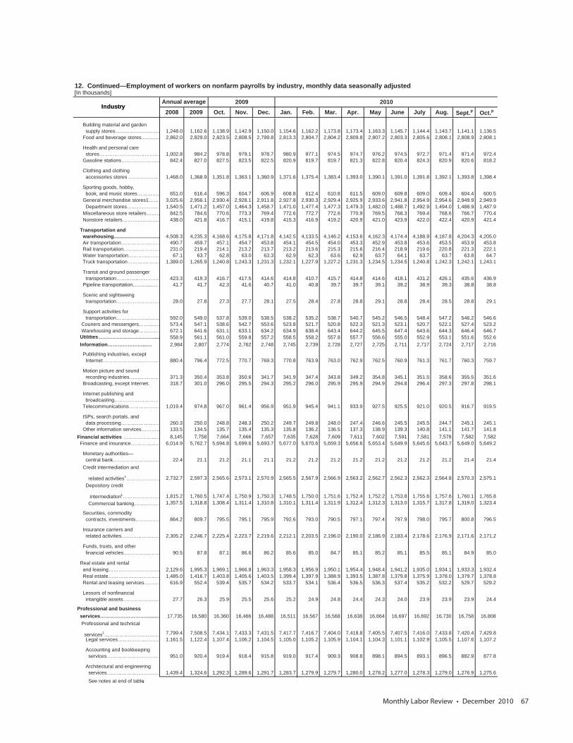
Monthly Labor Review • December 2010 67
12. Continued—Employment of workers on nonfarm payrolls by industry, monthly data seasonally adjusted[In thousands]
2009 2010
2008 2009 Oct. Nov. Dec. Jan. Feb. Mar. Apr. May June July Aug. Sept.p Oct.p
Building material and garden supply stores................................ 1,248.0 1,162.6 1,138.9 1,142.9 1,150.0 1,154.6 1,162.2 1,173.8 1,173.4 1,163.3 1,145.7 1,144.4 1,143.7 1,141.1 1,136.5 Food and beverage stores............. 2,862.0 2,829.0 2,823.5 2,808.5 2,799.8 2,813.3 2,804.7 2,804.2 2,809.8 2,807.2 2,803.3 2,805.6 2,808.1 2,808.9 2,808.1
Health and personal care stores……………………………… 1,002.8 984.2 978.8 979.1 978.7 980.9 977.1 974.5 974.7 976.2 974.5 972.7 971.4 971.4 972.4 Gasoline stations…………………… 842.4 827.0 827.5 823.5 822.5 820.9 819.7 819.7 821.3 822.8 820.4 824.3 820.9 820.6 818.2
Clothing and clothing accessories stores ………………… 1,468.0 1,368.9 1,351.8 1,363.1 1,360.9 1,371.6 1,375.4 1,383.4 1,393.0 1,390.1 1,391.0 1,391.8 1,392.1 1,393.8 1,398.4
Sporting goods, hobby, book, and music stores…………… 651.0 616.4 596.3 604.7 606.9 608.8 612.4 610.8 611.5 609.0 609.8 609.0 609.4 604.4 600.5 General merchandise stores1……… 3,025.6 2,956.1 2,930.4 2,928.1 2,911.8 2,927.8 2,930.3 2,929.4 2,925.9 2,933.6 2,941.8 2,954.9 2,954.6 2,949.9 2,949.9 Department stores………………… 1,540.5 1,471.2 1,457.0 1,464.3 1,458.7 1,471.0 1,477.4 1,477.3 1,479.3 1,482.0 1,488.7 1,492.9 1,494.0 1,488.9 1,487.9 Miscellaneous store retailers……… 842.5 784.6 770.6 773.3 769.4 772.6 772.7 772.6 770.9 769.5 768.3 769.4 768.6 766.7 770.4 Nonstore retailers…………………… 438.0 421.8 416.7 415.1 419.8 415.3 416.9 419.2 420.9 421.0 423.9 422.0 422.4 420.9 421.4
Transportation and warehousing................................. 4,508.3 4,235.3 4,168.6 4,175.8 4,171.8 4,142.5 4,133.5 4,146.2 4,153.6 4,162.3 4,174.4 4,188.9 4,187.8 4,204.3 4,205.0 Air transportation…………….……… 490.7 459.7 457.1 454.7 453.8 454.1 454.5 454.0 453.3 452.9 453.8 453.6 453.5 453.9 453.8 Rail transportation……...…………… 231.0 219.4 214.1 213.2 213.7 213.2 213.6 215.3 215.6 216.4 218.9 219.6 220.8 221.3 222.1 Water transportation………...……… 67.1 63.7 62.8 63.0 63.3 62.9 62.3 63.6 62.9 63.7 64.1 63.7 63.7 63.8 64.7 Truck transportation………..……… 1,389.0 1,265.9 1,240.8 1,243.3 1,231.3 1,232.1 1,227.9 1,227.2 1,231.3 1,234.5 1,234.5 1,240.8 1,242.3 1,242.1 1,243.1
Transit and ground passenger transportation………...…………… 423.3 419.3 416.7 417.5 414.6 414.8 410.7 415.7 414.8 414.6 418.1 431.2 426.1 435.6 436.9 Pipeline transportation………...…… 41.7 41.7 42.3 41.6 40.7 41.0 40.8 39.7 39.7 39.1 39.2 38.9 39.3 38.8 38.8
Scenic and sightseeing transportation…….………………… 28.0 27.8 27.3 27.7 28.1 27.5 28.4 27.8 28.8 29.1 28.8 28.4 28.5 28.8 29.1
Support activities for transportation………………..…… 592.0 549.0 537.8 539.0 538.5 538.2 535.2 538.7 540.7 545.2 546.5 548.4 547.2 546.2 546.6 Couriers and messengers……...…… 573.4 547.1 538.6 542.7 553.6 523.8 521.7 520.8 522.3 521.3 523.1 520.7 522.1 527.4 523.2 Warehousing and storage………… 672.1 641.6 631.1 633.1 634.2 634.9 638.4 643.4 644.2 645.5 647.4 643.6 644.3 646.4 646.7
Utilities………………………….………..... 558.9 561.1 561.0 559.8 557.2 558.5 558.2 557.8 557.7 556.6 555.0 552.9 553.1 551.6 552.6 Information…………………...…. 2,984 2,807 2,774 2,762 2,748 2,745 2,739 2,728 2,727 2,725 2,711 2,717 2,724 2,717 2,716
Publishing industries, except Internet…………………...………… 880.4 796.4 772.5 770.7 769.3 770.8 763.9 763.0 762.9 762.5 760.9 761.3 761.7 760.3 759.7
Motion picture and sound recording industries……...………… 371.3 350.4 353.8 350.6 341.7 341.9 347.4 343.8 349.2 354.8 345.1 351.5 358.6 355.5 351.6 Broadcasting, except Internet. 318.7 301.0 296.0 295.5 294.3 295.2 296.0 295.9 295.9 294.9 294.8 296.4 297.3 297.8 298.1
Internet publishing and broadcasting………………...……… Telecommunications………….…… 1,019.4 974.8 967.0 961.4 956.9 951.9 945.4 941.1 933.9 927.5 925.5 921.0 920.5 916.7 919.5
ISPs, search portals, and data processing………..………… 260.3 250.0 248.8 248.3 250.2 249.7 249.8 248.0 247.4 246.6 245.5 245.5 244.7 245.1 245.1 Other information services………… 133.5 134.5 135.7 135.4 135.3 135.8 136.2 136.5 137.3 138.9 139.3 140.8 141.1 141.7 141.8 Financial activities ………………..… 8,145 7,758 7,664 7,666 7,657 7,635 7,628 7,609 7,611 7,602 7,591 7,581 7,578 7,582 7,582 Finance and insurance……………..… 6,014.9 5,762.7 5,694.8 5,699.6 5,693.7 5,677.0 5,670.6 5,659.3 5,656.6 5,653.4 5,649.9 5,645.6 5,643.7 5,649.0 5,649.2
Monetary authorities— central bank…………………..…… 22.4 21.1 21.2 21.1 21.1 21.2 21.2 21.2 21.2 21.2 21.2 21.2 21.2 21.4 21.4 Credit intermediation and
related activities 1………………… 2,732.7 2,597.3 2,565.6 2,573.1 2,570.9 2,565.5 2,567.9 2,566.9 2,563.2 2,562.7 2,562.3 2,562.3 2,564.8 2,570.3 2,575.1 Depository credit
intermediation 1…………………… 1,815.2 1,760.5 1,747.4 1,750.9 1,750.3 1,748.5 1,750.0 1,751.6 1,752.4 1,752.2 1,753.8 1,755.6 1,757.6 1,760.1 1,765.8 Commercial banking..…………… 1,357.5 1,318.8 1,308.4 1,311.4 1,310.8 1,310.1 1,311.4 1,311.9 1,312.4 1,312.3 1,313.0 1,315.7 1,317.8 1,319.0 1,323.4
Securities, commodity contracts, investments…………… 864.2 809.7 795.5 795.1 795.9 792.6 793.0 790.5 797.1 797.4 797.9 798.0 795.7 800.8 796.5
Insurance carriers and related activities………………...… 2,305.2 2,246.7 2,225.4 2,223.7 2,219.6 2,212.1 2,203.5 2,196.0 2,190.0 2,186.9 2,183.4 2,178.6 2,176.9 2,171.6 2,171.2
Funds, trusts, and other financial vehicles…………….…… 90.5 87.8 87.1 86.6 86.2 85.6 85.0 84.7 85.1 85.2 85.1 85.5 85.1 84.9 85.0
Real estate and rental and leasing………………………..… 2,129.6 1,995.3 1,969.1 1,966.8 1,963.3 1,958.3 1,956.9 1,950.1 1,954.4 1,948.4 1,941.2 1,935.0 1,934.1 1,933.3 1,932.4 Real estate……………………….… 1,485.0 1,416.7 1,403.8 1,405.6 1,403.5 1,399.4 1,397.9 1,388.9 1,393.5 1,387.8 1,379.8 1,375.9 1,378.0 1,379.7 1,378.8 Rental and leasing services……… 616.9 552.4 539.4 535.7 534.2 533.7 534.1 536.4 536.5 536.3 537.4 535.2 532.2 529.7 529.2
Lessors of nonfinancial intangible assets………………..… 27.7 26.3 25.9 25.5 25.6 25.2 24.9 24.8 24.4 24.3 24.0 23.9 23.9 23.9 24.4
Professional and business services…………………………...… 17,735 16,580 16,360 16,466 16,488 16,511 16,567 16,568 16,638 16,664 16,697 16,692 16,730 16,758 16,808 Professional and technical
services1…………………………… 7,799.4 7,508.5 7,434.1 7,433.3 7,431.5 7,417.7 7,416.7 7,404.0 7,418.8 7,405.5 7,407.5 7,416.0 7,433.8 7,420.4 7,429.8 Legal services……………..……… 1,161.5 1,122.4 1,107.4 1,106.2 1,104.5 1,105.0 1,105.2 1,105.9 1,104.1 1,104.3 1,101.1 1,102.9 1,105.5 1,107.6 1,107.2
Accounting and bookkeeping services…………………………… 951.0 920.4 919.4 918.4 915.8 919.0 917.4 909.3 908.8 898.1 894.5 893.1 896.5 882.9 877.8
Architectural and engineering services…………………………… 1,439.4 1,324.6 1,292.3 1,289.6 1,291.7 1,283.7 1,279.9 1,279.7 1,280.0 1,278.2 1,277.0 1,278.3 1,279.0 1,276.9 1,275.6 See notes at end of table.
Annual averageIndustryIndustry
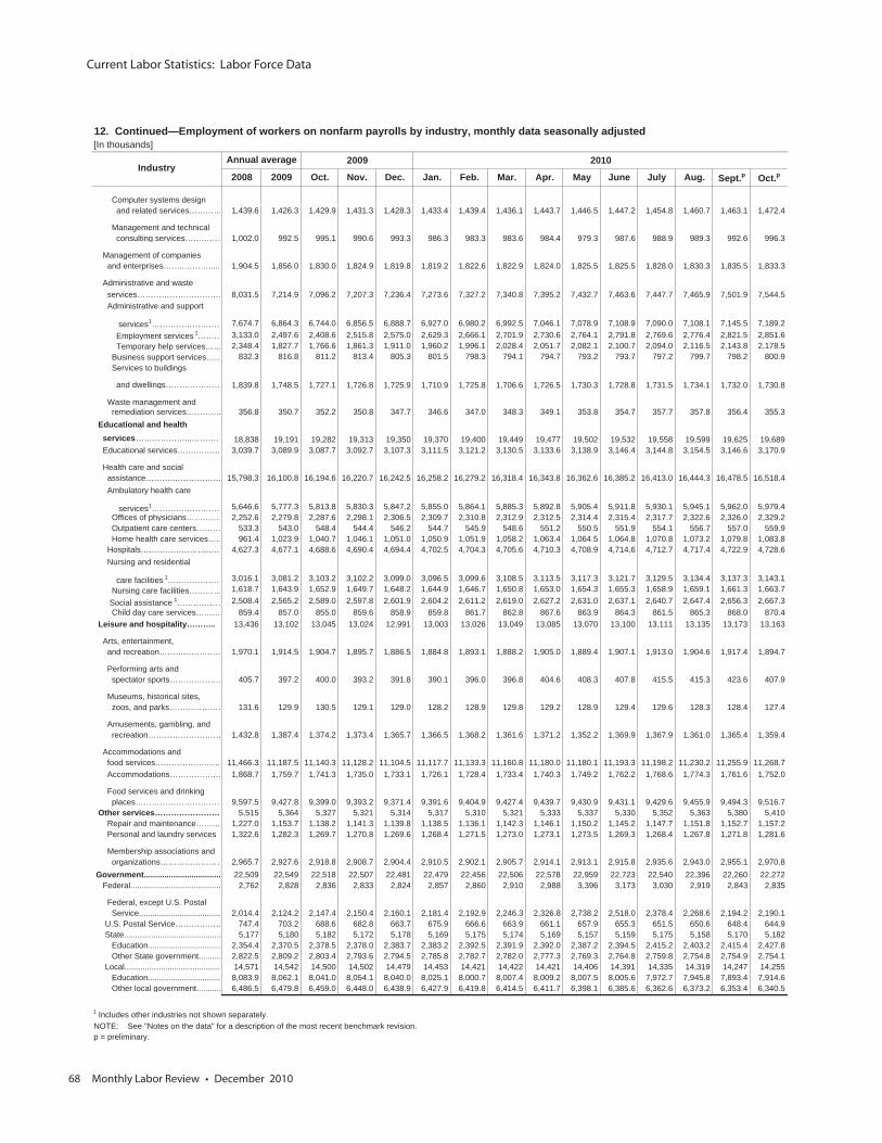
Current Labor Statistics: Labor Force Data
68 Monthly Labor Review • December 2010
12. Continued—Employment of workers on nonfarm payrolls by industry, monthly data seasonally adjusted[In thousands]
2009 2010
2008 2009 Oct. Nov. Dec. Jan. Feb. Mar. Apr. May June July Aug. Sept.p Oct.p
Computer systems design and related services………… 1,439.6 1,426.3 1,429.9 1,431.3 1,428.3 1,433.4 1,439.4 1,436.1 1,443.7 1,446.5 1,447.2 1,454.8 1,460.7 1,463.1 1,472.4
Management and technical consulting services…………… 1,002.0 992.5 995.1 990.6 993.3 986.3 983.3 983.6 984.4 979.3 987.6 988.9 989.3 992.6 996.3
Management of companies and enterprises……..………..... 1,904.5 1,856.0 1,830.0 1,824.9 1,819.8 1,819.2 1,822.6 1,822.9 1,824.0 1,825.5 1,825.5 1,828.0 1,830.3 1,835.5 1,833.3
Administrative and waste services…………………………… 8,031.5 7,214.9 7,096.2 7,207.3 7,236.4 7,273.6 7,327.2 7,340.8 7,395.2 7,432.7 7,463.6 7,447.7 7,465.9 7,501.9 7,544.5 Administrative and support
services1……………………… 7,674.7 6,864.3 6,744.0 6,856.5 6,888.7 6,927.0 6,980.2 6,992.5 7,046.1 7,078.9 7,108.9 7,090.0 7,108.1 7,145.5 7,189.2 Employment services 1……… 3,133.0 2,497.6 2,408.6 2,515.8 2,575.0 2,629.3 2,666.1 2,701.9 2,730.6 2,764.1 2,791.8 2,769.6 2,776.4 2,821.5 2,851.6 Temporary help services…… 2,348.4 1,827.7 1,766.6 1,861.3 1,911.0 1,960.2 1,996.1 2,028.4 2,051.7 2,082.1 2,100.7 2,094.0 2,116.5 2,143.8 2,178.5 Business support services…… 832.3 816.8 811.2 813.4 805.3 801.5 798.3 794.1 794.7 793.2 793.7 797.2 799.7 798.2 800.9 Services to buildings
and dwellings………………… 1,839.8 1,748.5 1,727.1 1,726.8 1,725.9 1,710.9 1,725.8 1,706.6 1,726.5 1,730.3 1,728.8 1,731.5 1,734.1 1,732.0 1,730.8
Waste management and remediation services…………. 356.8 350.7 352.2 350.8 347.7 346.6 347.0 348.3 349.1 353.8 354.7 357.7 357.8 356.4 355.3 Educational and health services………………...………. 18,838 19,191 19,282 19,313 19,350 19,370 19,400 19,449 19,477 19,502 19,532 19,558 19,599 19,625 19,689 Educational services…….……… 3,039.7 3,089.9 3,087.7 3,092.7 3,107.3 3,111.5 3,121.2 3,130.5 3,133.6 3,138.9 3,146.4 3,144.8 3,154.5 3,146.6 3,170.9
Health care and social assistance……….……………… 15,798.3 16,100.8 16,194.6 16,220.7 16,242.5 16,258.2 16,279.2 16,318.4 16,343.8 16,362.6 16,385.2 16,413.0 16,444.3 16,478.5 16,518.4 Ambulatory health care
services1……………………… 5,646.6 5,777.3 5,813.8 5,830.3 5,847.2 5,855.0 5,864.1 5,885.3 5,892.8 5,905.4 5,911.8 5,930.1 5,945.1 5,962.0 5,979.4 Offices of physicians…………… 2,252.6 2,279.8 2,287.6 2,298.1 2,306.5 2,309.7 2,310.8 2,312.9 2,312.5 2,314.4 2,315.4 2,317.7 2,322.6 2,326.0 2,329.2 Outpatient care centers……… 533.3 543.0 548.4 544.4 546.2 544.7 545.9 548.6 551.2 550.5 551.9 554.1 556.7 557.0 559.9 Home health care services…… 961.4 1,023.9 1,040.7 1,046.1 1,051.0 1,050.9 1,051.9 1,058.2 1,063.4 1,064.5 1,064.8 1,070.8 1,073.2 1,079.8 1,083.8 Hospitals………………………… 4,627.3 4,677.1 4,688.6 4,690.4 4,694.4 4,702.5 4,704.3 4,705.6 4,710.3 4,708.9 4,714.6 4,712.7 4,717.4 4,722.9 4,728.6 Nursing and residential
care facilities 1………………… 3,016.1 3,081.2 3,103.2 3,102.2 3,099.0 3,096.5 3,099.6 3,108.5 3,113.5 3,117.3 3,121.7 3,129.5 3,134.4 3,137.3 3,143.1 Nursing care facilities………… 1,618.7 1,643.9 1,652.9 1,649.7 1,648.2 1,644.9 1,646.7 1,650.8 1,653.0 1,654.3 1,655.3 1,658.9 1,659.1 1,661.3 1,663.7
Social assistance 1……………… 2,508.4 2,565.2 2,589.0 2,597.8 2,601.9 2,604.2 2,611.2 2,619.0 2,627.2 2,631.0 2,637.1 2,640.7 2,647.4 2,656.3 2,667.3 Child day care services……… 859.4 857.0 855.0 859.6 858.9 859.8 861.7 862.8 867.6 863.9 864.3 861.5 865.3 868.0 870.4 Leisure and hospitality……….. 13,436 13,102 13,045 13,024 12,991 13,003 13,026 13,049 13,085 13,070 13,100 13,111 13,135 13,173 13,163
Arts, entertainment, and recreation……….…….…… 1,970.1 1,914.5 1,904.7 1,895.7 1,886.5 1,884.8 1,893.1 1,888.2 1,905.0 1,889.4 1,907.1 1,913.0 1,904.6 1,917.4 1,894.7
Performing arts and spectator sports………………… 405.7 397.2 400.0 393.2 391.8 390.1 396.0 396.8 404.6 408.3 407.8 415.5 415.3 423.6 407.9
Museums, historical sites, zoos, and parks………………… 131.6 129.9 130.5 129.1 129.0 128.2 128.9 129.8 129.2 128.9 129.4 129.6 128.3 128.4 127.4
Amusements, gambling, and recreation……………………… 1,432.8 1,387.4 1,374.2 1,373.4 1,365.7 1,366.5 1,368.2 1,361.6 1,371.2 1,352.2 1,369.9 1,367.9 1,361.0 1,365.4 1,359.4
Accommodations and food services…………………… 11,466.3 11,187.5 11,140.3 11,128.2 11,104.5 11,117.7 11,133.3 11,160.8 11,180.0 11,180.1 11,193.3 11,198.2 11,230.2 11,255.9 11,268.7 Accommodations………………. 1,868.7 1,759.7 1,741.3 1,735.0 1,733.1 1,726.1 1,728.4 1,733.4 1,740.3 1,749.2 1,762.2 1,768.6 1,774.3 1,761.6 1,752.0
Food services and drinking places…………………………… 9,597.5 9,427.8 9,399.0 9,393.2 9,371.4 9,391.6 9,404.9 9,427.4 9,439.7 9,430.9 9,431.1 9,429.6 9,455.9 9,494.3 9,516.7 Other services…………………… 5,515 5,364 5,327 5,321 5,314 5,317 5,310 5,321 5,333 5,337 5,330 5,352 5,363 5,380 5,410 Repair and maintenance……… 1,227.0 1,153.7 1,138.2 1,141.3 1,139.8 1,138.5 1,136.1 1,142.3 1,146.1 1,150.2 1,145.2 1,147.7 1,151.8 1,152.7 1,157.2 Personal and laundry services 1,322.6 1,282.3 1,269.7 1,270.8 1,269.6 1,268.4 1,271.5 1,273.0 1,273.1 1,273.5 1,269.3 1,268.4 1,267.8 1,271.8 1,281.6
Membership associations and organizations…………………… 2,965.7 2,927.6 2,918.8 2,908.7 2,904.4 2,910.5 2,902.1 2,905.7 2,914.1 2,913.1 2,915.8 2,935.6 2,943.0 2,955.1 2,970.8 Government.................................. 22,509 22,549 22,518 22,507 22,481 22,479 22,456 22,506 22,578 22,959 22,723 22,540 22,396 22,260 22,272 Federal........................................ 2,762 2,828 2,836 2,833 2,824 2,857 2,860 2,910 2,988 3,396 3,173 3,030 2,919 2,843 2,835
Federal, except U.S. Postal Service.................................... 2,014.4 2,124.2 2,147.4 2,150.4 2,160.1 2,181.4 2,192.9 2,246.3 2,326.8 2,738.2 2,518.0 2,378.4 2,268.6 2,194.2 2,190.1 U.S. Postal Service……………… 747.4 703.2 688.6 682.8 663.7 675.9 666.6 663.9 661.1 657.9 655.3 651.5 650.6 648.4 644.9 State........................................... 5,177 5,180 5,182 5,172 5,178 5,169 5,175 5,174 5,169 5,157 5,159 5,175 5,158 5,170 5,182 Education................................ 2,354.4 2,370.5 2,378.5 2,378.0 2,383.7 2,383.2 2,392.5 2,391.9 2,392.0 2,387.2 2,394.5 2,415.2 2,403.2 2,415.4 2,427.8 Other State government.......... 2,822.5 2,809.2 2,803.4 2,793.6 2,794.5 2,785.8 2,782.7 2,782.0 2,777.3 2,769.3 2,764.8 2,759.8 2,754.8 2,754.9 2,754.1 Local........................................... 14,571 14,542 14,500 14,502 14,479 14,453 14,421 14,422 14,421 14,406 14,391 14,335 14,319 14,247 14,255 Education................................ 8,083.9 8,062.1 8,041.0 8,054.1 8,040.0 8,025.1 8,000.7 8,007.4 8,009.2 8,007.5 8,005.6 7,972.7 7,945.8 7,893.4 7,914.6 Other local government........... 6,486.5 6,479.8 6,459.0 6,448.0 6,438.9 6,427.9 6,419.8 6,414.5 6,411.7 6,398.1 6,385.6 6,362.6 6,373.2 6,353.4 6,340.5
1 Includes other industries not shown separately.NOTE: See "Notes on the data" for a description of the most recent benchmark revision. p = preliminary.
Annual averageIndustry
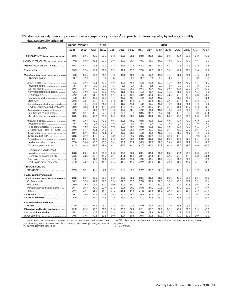
Monthly Labor Review • December 2010 69
13. Average weekly hours of production or nonsupervisory workers 1 on private nonfarm payrolls, by industry, monthly data seasonally adjusted
2009 2010
2008 2009 Oct. Nov. Dec. Jan. Feb. Mar. Apr. May June July Aug. Sept.p Oct.p
TOTAL PRIVATE………………………… 33.6 33.1 33.0 33.2 33.2 33.3 33.2 33.3 33.4 33.5 33.4 33.4 33.5 33.5 33.6
GOODS-PRODUCING……………………… 40.2 39.2 39.1 39.7 39.6 40.0 39.4 40.1 40.5 40.5 40.2 40.3 40.5 40.7 40.6
Natural resources and mining…………… 45.1 43.3 42.8 43.0 43.4 44.2 43.6 44.2 44.7 45.4 44.8 44.8 45.5 44.6 44.3
Construction………………………………… 38.5 37.6 36.9 37.8 37.5 37.9 37.0 37.8 38.7 38.1 38.2 38.2 38.6 39.0 38.8
Manufacturing……………………............. 40.8 39.8 40.0 40.5 40.5 40.9 40.5 41.0 41.2 41.5 41.0 41.1 41.1 41.2 41.2 Overtime hours.................................. 3.7 2.9 3.2 3.4 3.4 3.6 3.5 3.7 3.8 3.9 3.9 3.8 3.8 3.9 3.9
Durable goods..…………………............ 41.1 39.9 40.1 40.6 40.6 40.9 40.6 41.2 41.4 41.7 41.3 41.4 41.3 41.4 41.5 Overtime hours.................................. 3.7 2.7 3.0 3.2 3.3 3.5 3.4 3.7 3.8 3.9 3.9 3.9 3.8 3.9 3.9 Wood products..................................... 38.6 37.4 37.6 38.2 38.2 39.2 38.3 39.4 39.7 40.0 38.8 38.4 38.5 39.3 39.3 Nonmetallic mineral products............... 42.1 40.9 40.8 41.9 40.2 41.4 40.0 41.3 41.7 41.7 41.5 41.5 41.6 41.7 42.1 Primary metals..................................... 42.2 40.7 41.0 42.4 42.7 42.9 42.9 43.2 43.9 44.2 43.6 43.6 43.6 43.8 44.0 Fabricated metal products................... 41.3 39.4 39.5 39.9 40.1 40.5 40.4 41.0 41.2 41.7 41.4 41.6 41.6 41.7 41.4 Machinery………………………………… 42.3 40.1 40.0 40.6 41.0 41.2 41.0 41.7 41.8 42.2 42.1 42.2 42.3 42.5 42.5 Computer and electronic products…… 41.0 40.4 40.5 41.0 40.8 41.1 41.0 41.2 41.1 41.2 40.7 41.1 41.1 40.9 40.9 Electrical equipment and appliances… 40.9 39.3 39.4 40.0 40.5 40.8 39.7 41.2 41.5 41.3 41.7 41.4 41.7 41.0 41.6 Transportation equipment.................... 41.9 41.2 41.9 42.4 42.5 42.5 42.4 42.9 42.9 43.2 42.8 42.9 42.6 42.7 43.0 Furniture and related products……….. 38.1 37.7 38.2 37.9 37.8 37.8 37.5 38.5 38.7 38.7 38.1 38.2 38.2 38.5 38.4 Miscellaneous manufacturing.............. 38.9 38.5 38.7 39.3 38.9 38.8 38.7 38.8 38.8 39.4 38.7 38.8 38.3 38.5 38.3
Nondurable goods.................................. 40.4 39.8 40.0 40.3 40.4 40.8 40.2 40.8 40.9 41.1 40.5 40.7 40.9 41.0 40.9 Overtime hours.................................. 3.7 3.2 3.4 3.6 3.6 3.7 3.6 3.7 3.9 4.0 3.8 3.7 3.9 3.9 4.0 Food manufacturing............................… 40.5 40.0 40.0 40.5 40.5 40.9 40.4 40.8 40.8 40.9 40.5 40.7 40.8 41.2 40.7 Beverage and tobacco products.......... 38.8 35.7 36.1 34.6 34.7 35.4 35.0 36.0 35.5 38.2 36.4 38.0 39.0 38.4 40.5 Textile mills……………………………… 38.7 37.7 38.8 40.1 39.4 40.5 39.7 41.3 42.4 42.5 41.1 41.6 41.7 41.5 40.3 Textile product mills…………………… 38.6 37.9 38.3 37.6 38.9 39.8 39.2 39.5 39.2 39.1 37.8 38.3 38.0 39.0 39.3 Apparel................................................. 36.4 36.0 36.0 36.3 36.2 36.7 36.1 36.2 36.4 35.9 36.3 35.9 36.9 36.4 37.1 Leather and allied products.................. 37.6 33.6 35.0 35.6 36.2 38.3 37.9 38.3 38.6 38.6 38.9 39.4 39.7 39.9 39.2 Paper and paper products……………… 42.9 41.8 42.2 42.4 42.1 42.9 42.1 42.7 42.8 43.2 42.5 42.8 42.9 43.0 42.9
Printing and related support activities............................................. 38.3 38.0 38.2 38.3 38.2 38.2 38.0 38.1 38.6 38.8 38.5 38.4 38.5 38.5 38.2 Petroleum and coal products…………… 44.6 43.4 42.2 41.7 42.7 42.4 42.0 43.1 43.9 43.5 42.5 42.5 43.3 43.3 44.4 Chemicals………………………………… 41.5 41.4 41.7 42.1 42.7 42.8 41.8 42.2 42.1 42.3 41.5 41.7 42.2 42.1 42.3 Plastics and rubber products…………… 41.0 40.2 40.7 41.0 41.4 41.5 41.4 42.2 42.6 42.8 42.0 41.7 41.7 41.7 41.6
PRIVATE SERVICE- PROVIDING……………………………… 32.3 32.1 32.0 32.1 32.1 32.2 32.1 32.2 32.2 32.3 32.2 32.3 32.3 32.3 32.4
Trade, transportation, and utilities.......………………....................... 33.2 32.9 32.9 33.0 32.9 33.1 33.0 33.1 33.2 33.3 33.3 33.5 33.5 33.4 33.5 Wholesale trade........………………....... 38.2 37.6 37.4 37.6 37.6 37.7 37.7 37.8 37.9 38.0 37.8 38.0 38.1 38.2 38.1 Retail trade………………………………… 30.0 29.9 29.9 30.0 30.0 30.1 30.0 30.1 30.1 30.2 30.1 30.4 30.3 30.1 30.2 Transportation and warehousing……… 36.4 36.0 36.3 36.4 36.2 36.4 36.2 36.8 37.1 37.1 37.4 37.5 37.5 37.6 37.7 Utilities……………………………………… 42.7 42.1 41.7 41.6 41.4 41.4 41.6 41.6 41.8 42.2 42.2 42.2 42.3 42.2 43.0 Information………………………………… 36.7 36.6 36.4 36.7 36.5 36.6 36.5 36.5 36.5 36.6 36.6 36.3 36.4 36.2 36.4 Financial activities………………………… 35.8 36.1 36.0 36.1 35.9 36.1 36.0 36.1 36.2 36.2 36.3 36.1 36.4 36.3 36.3
Professional and business services…………………………………… 34.8 34.7 34.6 34.8 34.8 34.9 34.8 35.0 35.0 35.1 35.0 35.1 35.1 35.2 35.3 Education and health services…………… 32.5 32.3 32.2 32.2 32.3 32.3 32.2 32.1 32.2 32.2 32.2 32.1 32.2 32.2 32.3 Leisure and hospitality…………………… 25.2 24.8 24.6 24.9 24.8 24.8 24.8 25.0 24.9 24.8 24.7 24.8 24.8 24.7 24.9 Other services……………........................ 30.8 30.5 30.5 30.5 30.5 30.7 30.6 30.8 30.8 30.9 30.7 30.9 30.9 30.9 30.9
Annual averageIndustry
1 Data relate to production workers in natural resources and mining andmanufacturing, construction workers in construction, and nonsupervisory workers inthe service-providing industries.
NOTE: See "Notes on the data" for a description of the most recent benchmarkrevision.p = preliminary.
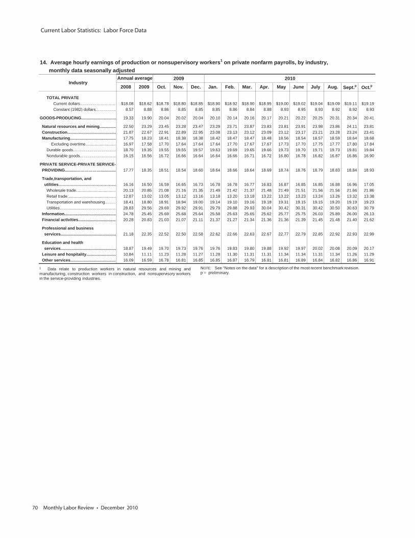
Current Labor Statistics: Labor Force Data
70 Monthly Labor Review • December 2010
14. Average hourly earnings of production or nonsupervisory workers 1 on private nonfarm payrolls, by industry, monthly data seasonally adjusted
2009 2010
2008 2009 Oct. Nov. Dec. Jan. Feb. Mar. Apr. May June July Aug. Sept.p Oct.p
TOTAL PRIVATE Current dollars……………………… $18.08 $18.62 $18.78 $18.80 $18.85 $18.90 $18.92 $18.90 $18.95 $19.00 $19.02 $19.04 $19.09 $19.11 $19.19 Constant (1982) dollars…………… 8.57 8.88 8.86 8.85 8.85 8.85 8.86 8.84 8.88 8.93 8.95 8.93 8.92 8.92 8.93
GOODS-PRODUCING............................... 19.33 19.90 20.04 20.02 20.04 20.10 20.14 20.16 20.17 20.21 20.22 20.25 20.31 20.34 20.41
Natural resources and mining............... 22.50 23.29 23.45 23.28 23.47 23.29 23.71 23.87 23.83 23.81 23.91 23.98 23.86 24.11 23.81 Construction........................................... 21.87 22.67 22.91 22.89 22.95 23.08 23.13 23.12 23.09 23.12 23.17 23.21 23.28 23.24 23.41 Manufacturing......................................... 17.75 18.23 18.41 18.38 18.38 18.42 18.47 18.47 18.48 18.56 18.54 18.57 18.59 18.64 18.68 Excluding overtime........................... 16.97 17.58 17.70 17.64 17.64 17.64 17.70 17.67 17.67 17.73 17.70 17.75 17.77 17.80 17.84 Durable goods…………………………… 18.70 19.35 19.55 19.55 19.57 19.63 19.69 19.65 19.66 19.73 19.70 19.71 19.73 19.81 19.84 Nondurable goods……………………… 16.15 16.56 16.72 16.66 16.64 16.64 16.66 16.71 16.72 16.80 16.78 16.82 16.87 16.86 16.90
PRIVATE SERVICE-PRIVATE SERVICE- PROVIDING..........……………….............. 17.77 18.35 18.51 18.54 18.60 18.64 18.66 18.64 18.69 18.74 18.76 18.79 18.83 18.84 18.93
Trade,transportation, and utilities………………………………….... 16.16 16.50 16.59 16.65 16.73 16.78 16.78 16.77 16.83 16.87 16.85 16.85 16.88 16.96 17.05 Wholesale trade.................................... 20.13 20.85 21.08 21.16 21.35 21.49 21.42 21.37 21.48 21.49 21.51 21.56 21.56 21.66 21.86 Retail trade........................................... 12.87 13.02 13.05 13.12 13.16 13.18 13.20 13.18 13.22 13.22 13.23 13.24 13.26 13.32 13.38 Transportation and warehousing……… 18.41 18.80 18.91 18.94 19.00 19.14 19.10 19.16 19.18 19.31 19.15 19.15 19.20 19.19 19.23 Utilities…………………………………… 28.83 29.56 29.69 29.92 29.91 29.79 29.88 29.93 30.04 30.42 30.31 30.42 30.50 30.63 30.79 Information.............................................. 24.78 25.45 25.69 25.68 25.64 25.58 25.63 25.65 25.62 25.77 25.75 26.03 25.89 26.00 26.13 Financial activities.................................. 20.28 20.83 21.03 21.07 21.11 21.37 21.27 21.34 21.36 21.36 21.39 21.45 21.48 21.40 21.62
Professional and business services................................................. 21.18 22.35 22.52 22.50 22.58 22.62 22.66 22.63 22.67 22.77 22.79 22.85 22.92 22.93 22.99
Education and health services................................................. 18.87 19.49 19.70 19.73 19.76 19.76 19.83 19.80 19.88 19.92 19.97 20.02 20.08 20.09 20.17 Leisure and hospitality.......................... 10.84 11.11 11.23 11.28 11.27 11.28 11.30 11.31 11.31 11.34 11.34 11.31 11.34 11.26 11.29 Other services......................................... 16.09 16.59 16.78 16.81 16.85 16.85 16.87 16.79 16.81 16.81 16.89 16.84 16.82 16.86 16.91
Annual averageIndustry
1 Data relate to production workers in natural resources and mining andmanufacturing, construction workers in construction, and nonsupervisory workersin the service-providing industries.
NOTE: See "Notes on the data" for a description of the most recent benchmark revision. p = preliminary.
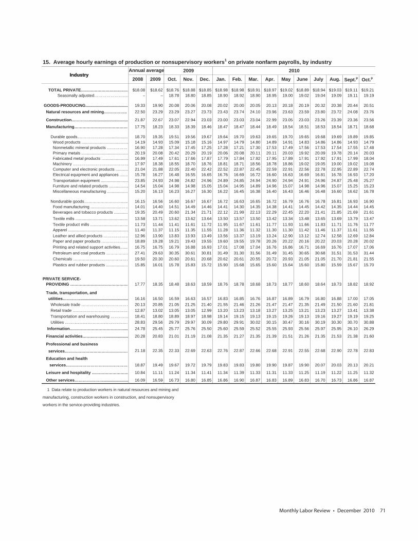
Monthly Labor Review • December 2010 71
15. Average hourly earnings of production or nonsupervisory workers 1 on private nonfarm payrolls, by industry2009 2010
2008 2009 Oct. Nov. Dec. Jan. Feb. Mar. Apr. May June July Aug. Sept.p Oct.p
TOTAL PRIVATE……………………………… $18.08 $18.62 $18.76 $18.88 $18.85 $18.98 $18.98 $18.91 $18.97 $19.02 $18.89 $18.94 $19.03 $19.11 $19.21 Seasonally adjusted……………………. – – 18.78 18.80 18.85 18.90 18.92 18.90 18.95 19.00 19.02 19.04 19.09 19.11 19.19
GOODS-PRODUCING...................................... 19.33 19.90 20.08 20.06 20.08 20.02 20.00 20.05 20.13 20.18 20.19 20.32 20.38 20.44 20.51 Natural resources and mining…………….. 22.50 23.29 23.29 23.27 23.73 23.43 23.74 24.10 23.96 23.63 23.59 23.80 23.72 24.08 23.76
Construction.………….................................. 21.87 22.67 23.07 22.94 23.03 23.00 23.03 23.04 22.99 23.05 23.03 23.26 23.39 23.36 23.56
Manufacturing…………………………………… 17.75 18.23 18.33 18.39 18.46 18.47 18.47 18.44 18.49 18.54 18.51 18.53 18.54 18.71 18.68
Durable goods..………………….................. 18.70 19.35 19.51 19.56 19.67 19.64 19.70 19.63 19.65 19.70 19.65 19.68 19.69 19.89 19.85 Wood products ......................................... 14.19 14.93 15.09 15.18 15.16 14.97 14.79 14.80 14.89 14.91 14.83 14.86 14.86 14.93 14.79 Nonmetallic mineral products ……………… 16.90 17.28 17.34 17.45 17.25 17.28 17.21 17.30 17.53 17.49 17.56 17.53 17.54 17.55 17.48 Primary metals ......................................... 20.19 20.08 20.42 20.29 20.19 20.06 20.08 20.11 20.11 20.03 19.92 20.09 19.78 20.14 20.03 Fabricated metal products ….................... 16.99 17.49 17.61 17.66 17.87 17.79 17.84 17.92 17.95 17.89 17.91 17.92 17.91 17.99 18.04 Machinery …………..……………………… 17.97 18.38 18.55 18.70 18.76 18.81 18.71 18.56 18.78 18.86 19.02 19.05 19.00 19.02 19.08 Computer and electronic products ........... 21.04 21.88 22.05 22.40 22.42 22.52 22.87 22.45 22.59 22.91 22.56 22.78 22.95 22.89 22.74 Electrical equipment and appliances ........ 15.78 16.27 16.48 16.55 16.65 16.76 16.69 16.72 16.60 16.63 16.69 16.81 16.78 16.93 17.20 Transportation equipment ........................ 23.85 24.93 24.98 24.82 24.96 24.89 24.85 24.94 24.90 24.94 24.91 24.96 24.87 25.48 25.27 Furniture and related products ................. 14.54 15.04 14.98 14.98 15.05 15.04 14.95 14.89 14.96 15.07 14.98 14.96 15.07 15.25 15.23 Miscellaneous manufacturing ................... 15.20 16.13 16.23 16.27 16.30 16.22 16.45 16.38 16.40 16.43 16.46 16.48 16.60 16.62 16.78
Nondurable goods………………………...... 16.15 16.56 16.60 16.67 16.67 16.72 16.63 16.65 16.72 16.79 16.76 16.78 16.81 16.93 16.90 Food manufacturing ...........................…… 14.01 14.40 14.51 14.49 14.46 14.41 14.30 14.35 14.38 14.41 14.45 14.42 14.35 14.44 14.45 Beverages and tobacco products ............. 19.35 20.49 20.60 21.34 21.71 22.12 21.99 22.13 22.29 22.45 22.20 21.41 21.85 21.69 21.61 Textile mills .............................................. 13.58 13.71 13.62 13.62 13.64 13.50 13.57 13.50 13.42 13.34 13.48 13.65 13.69 13.79 13.47 Textile product mills ................................. 11.73 11.44 11.41 11.61 11.72 11.95 11.67 11.61 11.77 11.93 11.66 11.83 11.71 11.76 11.77 Apparel ..................................................... 11.40 11.37 11.15 11.35 11.55 11.28 11.36 11.32 11.30 11.30 11.42 11.46 11.37 11.61 11.55 Leather and allied products ……………… 12.96 13.90 13.83 13.93 13.49 13.56 13.37 13.19 13.24 12.90 13.12 12.74 12.58 12.69 12.84 Paper and paper products ………………… 18.89 19.28 19.21 19.43 19.55 19.60 19.55 19.78 20.26 20.22 20.16 20.22 20.03 20.28 20.02 Printing and related support activities…... 16.75 16.75 16.79 16.88 16.93 17.01 17.08 17.04 16.76 16.86 16.71 16.69 16.76 17.07 17.06 Petroleum and coal products ……………… 27.41 29.63 30.35 30.61 30.81 31.49 31.30 31.56 31.49 31.45 30.65 30.68 31.51 31.53 31.44 Chemicals …………………………………… 19.50 20.30 20.60 20.61 20.68 20.62 20.61 20.55 20.72 20.93 21.05 21.05 21.70 21.81 21.55 Plastics and rubber products .................... 15.85 16.01 15.78 15.83 15.72 15.90 15.68 15.65 15.60 15.64 15.60 15.80 15.59 15.67 15.70
PRIVATE SERVICE- PROVIDING ……………………………………. 17.77 18.35 18.48 18.63 18.59 18.76 18.78 18.68 18.73 18.77 18.60 18.64 18.73 18.82 18.92
Trade, transportation, and utilities…….…….......................................... 16.16 16.50 16.59 16.63 16.57 16.83 16.85 16.76 16.87 16.89 16.79 16.80 16.88 17.00 17.05 Wholesale trade ……………………………… 20.13 20.85 21.05 21.25 21.40 21.55 21.46 21.26 21.47 21.47 21.35 21.49 21.50 21.60 21.81 Retail trade …………………………………… 12.87 13.02 13.05 13.05 12.99 13.20 13.23 13.18 13.27 13.25 13.21 13.23 13.27 13.41 13.38 Transportation and warehousing …………… 18.41 18.80 18.89 18.97 18.98 19.14 19.15 19.13 19.15 19.26 19.13 19.16 19.27 19.19 19.25 Utilities ………..…..….………..……………… 28.83 29.56 29.79 29.97 30.09 29.80 29.91 30.02 30.15 30.47 30.16 30.19 30.30 30.70 30.88 Information…………………………………..... 24.78 25.45 25.77 25.76 25.50 25.60 25.59 25.52 25.55 25.93 25.56 25.97 25.95 26.10 26.29
Financial activities……..……….................... 20.28 20.83 21.01 21.19 21.08 21.35 21.27 21.35 21.39 21.51 21.26 21.35 21.53 21.38 21.60
Professional and business services………………………………………… 21.18 22.35 22.33 22.69 22.63 22.76 22.87 22.66 22.68 22.91 22.55 22.68 22.90 22.78 22.83
Education and health services………………………………………… 18.87 19.49 19.67 19.72 19.79 19.83 19.83 19.80 19.90 19.87 19.90 20.07 20.03 20.13 20.21
Leisure and hospitality ……………………… 10.84 11.11 11.24 11.34 11.41 11.34 11.39 11.33 11.31 11.33 11.25 11.19 11.22 11.25 11.32
Other services…………………...................... 16.09 16.59 16.73 16.80 16.85 16.86 16.90 16.87 16.83 16.89 16.83 16.70 16.73 16.86 16.87
1 Data relate to production workers in natural resources and mining and
manufacturing, construction workers in construction, and nonsupervisory
workers in the service-providing industries.
Annual averageIndustryIndustry
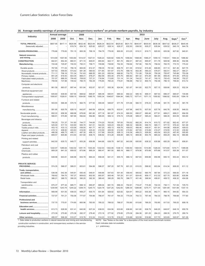
Current Labor Statistics: Labor Force Data
72 Monthly Labor Review • December 2010
16. Average weekly earnings of production or nonsupervisory workers 1 on private nonfarm payrolls, by industry2009
2008 2009 Oct. Nov. Dec. Jan. Feb. Mar. Apr. May June July Aug. Sept.p Oct.p
TOTAL PRIVATE…………………
GOODS-PRODUCING………………
Natural resources and mining
CONSTRUCTION Manufacturing………………………
PRIVATE SERVICE- PROVIDING…………....................
Trade, transportation, and utilities………………………
Information…………………………
Financial activities…………………
Professional and business services………………
Education and……………………… health services……………………
Leisure and hospitality……………
Other services………………………
Annual average 2010Industry
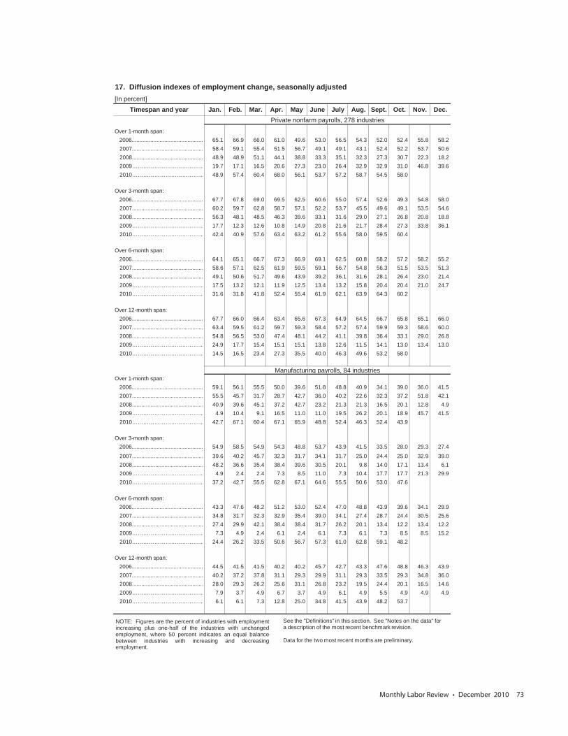
Monthly Labor Review • December 2010 73
17. Diffusion indexes of employment change, seasonally adjusted [In percent]
Timespan and year Jan. Feb. Mar. Apr. May June July Aug. Sept. Oct. Nov. Dec.Private nonfarm payrolls, 278 industries
Over 1-month span: 2006............................................... 65.1 66.9 66.0 61.0 49.6 53.0 56.5 54.3 52.0 52.4 55.8 58.2 2007.............................................. 58.4 59.1 55.4 51.5 56.7 49.1 49.1 43.1 52.4 52.2 53.7 50.6 2008.............................................. 48.9 48.9 51.1 44.1 38.8 33.3 35.1 32.3 27.3 30.7 22.3 18.2 2009………………………………… 19.7 17.1 16.5 20.6 27.3 23.0 26.4 32.9 32.9 31.0 46.8 39.6 2010………………………………… 48.9 57.4 60.4 68.0 56.1 53.7 57.2 58.7 54.5 58.0
Over 3-month span: 2006............................................... 67.7 67.8 69.0 69.5 62.5 60.6 55.0 57.4 52.6 49.3 54.8 58.0 2007.............................................. 60.2 59.7 62.8 58.7 57.1 52.2 53.7 45.5 49.6 49.1 53.5 54.6 2008.............................................. 56.3 48.1 48.5 46.3 39.6 33.1 31.6 29.0 27.1 26.8 20.8 18.8 2009………………………………… 17.7 12.3 12.6 10.8 14.9 20.8 21.6 21.7 28.4 27.3 33.8 36.1 2010………………………………… 42.4 40.9 57.6 63.4 63.2 61.2 55.6 58.0 59.5 60.4
Over 6-month span: 2006............................................... 64.1 65.1 66.7 67.3 66.9 69.1 62.5 60.8 58.2 57.2 58.2 55.2 2007.............................................. 58.6 57.1 62.5 61.9 59.5 59.1 56.7 54.8 56.3 51.5 53.5 51.3 2008.............................................. 49.1 50.6 51.7 49.6 43.9 39.2 36.1 31.6 28.1 26.4 23.0 21.4 2009………………………………… 17.5 13.2 12.1 11.9 12.5 13.4 13.2 15.8 20.4 20.4 21.0 24.7 2010………………………………… 31.6 31.8 41.8 52.4 55.4 61.9 62.1 63.9 64.3 60.2
Over 12-month span: 2006............................................... 67.7 66.0 66.4 63.4 65.6 67.3 64.9 64.5 66.7 65.8 65.1 66.0 2007.............................................. 63.4 59.5 61.2 59.7 59.3 58.4 57.2 57.4 59.9 59.3 58.6 60.0 2008.............................................. 54.8 56.5 53.0 47.4 48.1 44.2 41.1 39.8 36.4 33.1 29.0 26.8 2009………………………………… 24.9 17.7 15.4 15.1 15.1 13.8 12.6 11.5 14.1 13.0 13.4 13.0 2010………………………………… 14.5 16.5 23.4 27.3 35.5 40.0 46.3 49.6 53.2 58.0
Manufacturing payrolls, 84 industries
Over 1-month span: 2006............................................... 59.1 56.1 55.5 50.0 39.6 51.8 48.8 40.9 34.1 39.0 36.0 41.5 2007.............................................. 55.5 45.7 31.7 28.7 42.7 36.0 40.2 22.6 32.3 37.2 51.8 42.1 2008.............................................. 40.9 39.6 45.1 37.2 42.7 23.2 21.3 21.3 16.5 20.1 12.8 4.9 2009………………………………… 4.9 10.4 9.1 16.5 11.0 11.0 19.5 26.2 20.1 18.9 45.7 41.5 2010………………………………… 42.7 67.1 60.4 67.1 65.9 48.8 52.4 46.3 52.4 43.9
Over 3-month span: 2006............................................... 54.9 58.5 54.9 54.3 48.8 53.7 43.9 41.5 33.5 28.0 29.3 27.4
2007.............................................. 39.6 40.2 45.7 32.3 31.7 34.1 31.7 25.0 24.4 25.0 32.9 39.0 2008.............................................. 48.2 36.6 35.4 38.4 39.6 30.5 20.1 9.8 14.0 17.1 13.4 6.1 2009………………………………… 4.9 2.4 2.4 7.3 8.5 11.0 7.3 10.4 17.7 17.7 21.3 29.9 2010………………………………… 37.2 42.7 55.5 62.8 67.1 64.6 55.5 50.6 53.0 47.6
Over 6-month span: 2006............................................... 43.3 47.6 48.2 51.2 53.0 52.4 47.0 48.8 43.9 39.6 34.1 29.9 2007.............................................. 34.8 31.7 32.3 32.9 35.4 39.0 34.1 27.4 28.7 24.4 30.5 25.6 2008.............................................. 27.4 29.9 42.1 38.4 38.4 31.7 26.2 20.1 13.4 12.2 13.4 12.2 2009………………………………… 7.3 4.9 2.4 6.1 2.4 6.1 7.3 6.1 7.3 8.5 8.5 15.2 2010………………………………… 24.4 26.2 33.5 50.6 56.7 57.3 61.0 62.8 59.1 48.2
Over 12-month span: 2006............................................... 44.5 41.5 41.5 40.2 40.2 45.7 42.7 43.3 47.6 48.8 46.3 43.9 2007.............................................. 40.2 37.2 37.8 31.1 29.3 29.9 31.1 29.3 33.5 29.3 34.8 36.0 2008.............................................. 28.0 29.3 26.2 25.6 31.1 26.8 23.2 19.5 24.4 20.1 16.5 14.6 2009………………………………… 7.9 3.7 4.9 6.7 3.7 4.9 6.1 4.9 5.5 4.9 4.9 4.9 2010………………………………… 6.1 6.1 7.3 12.8 25.0 34.8 41.5 43.9 48.2 53.7
See the "Definitions" in this section. See "Notes on the data" for a description of the most recent benchmark revision.
Data for the two most recent months are preliminary.
NOTE: Figures are the percent of industries with employmentincreasing plus one-half of the industries with unchangedemployment, where 50 percent indicates an equal balancebetween industries with increasing and decreasingemployment.
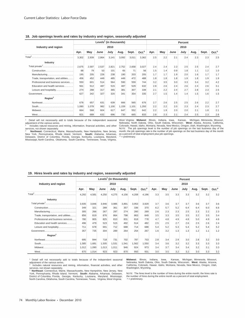
Current Labor Statistics: Labor Force Data
74 Monthly Labor Review • December 2010
18. Job openings levels and rates by industry and region, seasonally adjustedLevels1 (in thousands) Percent
Industry and region 2010 2010
Apr. May June July Aug. Sept. Oct.p Apr. May June July Aug. Sept. Oct.p
Total2……………………………………………… 3,302 2,939 2,864 3,141 3,092 3,011 3,362 2.5 2.2 2.1 2.4 2.3 2.3 2.5
IndustryTotal private2………………………………… 2,675 2,597 2,537 2,821 2,752 2,658 3,027 2.4 2.4 2.3 2.5 2.5 2.4 2.7
Construction……………………………… 88 79 53 101 65 71 56 1.5 1.4 0.9 1.8 1.1 1.2 1.0Manufacturing…………………………… 195 205 226 238 190 203 205 1.7 1.7 1.9 2.0 1.6 1.7 1.7Trade, transportation, and utilities……… 456 452 449 485 449 472 488 1.8 1.8 1.8 1.9 1.8 1.9 1.9Professional and business services…… 550 601 514 564 590 559 744 3.2 3.5 3.0 3.3 3.4 3.2 4.2Education and health services………… 561 512 487 515 487 529 632 2.8 2.6 2.4 2.6 2.4 2.6 3.1Leisure and hospitality…………………… 274 288 317 365 381 307 339 2.1 2.2 2.4 2.7 2.8 2.3 2.5
Government………………………………… 627 342 327 320 341 354 335 2.7 1.5 1.4 1.4 1.5 1.6 1.5
Region3
Northeast………………………………… 678 657 631 639 666 565 676 2.7 2.6 2.5 2.5 2.6 2.2 2.7South……………………………………… 1,080 1,078 982 1,100 1,159 1,101 1,293 2.2 2.2 2.0 2.3 2.4 2.3 2.7Midwest…………………………………… 664 568 604 617 647 552 642 2.2 1.9 2.0 2.0 2.1 1.8 2.1
West……………………………………… 821 689 632 696 730 665 833 2.8 2.3 2.1 2.4 2.5 2.3 2.8
1 Detail will not necessarily add to totals because of the independent seasonaladjustment of the various series.2 Includes natural resources and mining, information, financial activities, and otherservices, not shown separately.3 Northeast: Connecticut, Maine, Massachusetts, New Hampshire, New Jersey,New York, Pennsylvania, Rhode Island, Vermont; South: Alabama, Arkansas,Delaware, District of Columbia, Florida, Georgia, Kentucky, Louisiana, Maryland,Mississippi, North Carolina, Oklahoma, South Carolina, Tennessee, Texas, Virginia,
West Virginia; Midwest: Illinois, Indiana, Iowa, Kansas, Michigan, Minnesota, Missouri,Nebraska, North Dakota, Ohio, South Dakota, Wisconsin; West: Alaska, Arizona, California,Colorado, Hawaii, Idaho, Montana, Nevada, New Mexico, Oregon, Utah, Washington, Wyoming.NOTE: The job openings level is the number of job openings on the last business day of themonth; the job openings rate is the number of job openings on the last business day of the monthas a percent of total employment plus job openings.P = preliminary.
19. Hires levels and rates by industry and region, seasonally adjustedLevels1 (in thousands) Percent
Industry and region 2010 2010
Apr. May June July Aug. Sept. Oct.p Apr. May June July Aug. Sept. Oct.p
Total2……………………………………………… 4,292 4,581 4,250 4,275 4,156 4,208 4,196 3.3 3.5 3.3 3.3 3.2 3.2 3.2
IndustryTotal private2………………………………… 3,935 3,846 3,946 3,985 3,891 3,953 3,929 3.7 3.6 3.7 3.7 3.6 3.7 3.6
Construction……………………………… 349 321 289 361 357 336 370 6.2 5.7 5.2 6.4 6.4 6.0 6.6Manufacturing…………………………… 305 266 267 297 274 260 269 2.6 2.3 2.3 2.5 2.3 2.2 2.3Trade, transportation, and utilities……… 856 819 876 864 798 863 849 3.5 3.3 3.5 3.5 3.2 3.5 3.4Professional and business services…… 780 805 825 810 831 818 778 4.7 4.8 4.9 4.8 5.0 4.9 4.6Education and health services………… 496 479 523 515 492 514 482 2.5 2.5 2.7 2.6 2.5 2.6 2.4Leisure and hospitality…………………… 711 678 691 712 688 714 688 5.4 5.2 5.3 5.4 5.2 5.4 5.2
Government………………………………… 357 735 304 289 264 254 267 1.6 3.2 1.3 1.3 1.2 1.1 1.2
Region3
Northeast………………………………… 695 844 718 731 702 787 753 2.8 3.4 2.9 3.0 2.8 3.2 3.0South……………………………………… 1,585 1,681 1,505 1,531 1,541 1,562 1,550 3.4 3.6 3.2 3.2 3.3 3.3 3.3Midwest…………………………………… 1,012 1,090 1,013 1,011 946 924 973 3.4 3.7 3.4 3.4 3.2 3.1 3.3
West……………………………………… 870 1,014 923 923 870 950 931 3.0 3.5 3.2 3.2 3.0 3.3 3.2
1 Detail will not necessarily add to totals because of the independent seasonaladjustment of the various series.2 Includes natural resources and mining, information, financial activities, and otherservices, not shown separately.3 Northeast: Connecticut, Maine, Massachusetts, New Hampshire, New Jersey, NewYork, Pennsylvania, Rhode Island, Vermont; South: Alabama, Arkansas, Delaware,District of Columbia, Florida, Georgia, Kentucky, Louisiana, Maryland, Mississippi,North Carolina, Oklahoma, South Carolina, Tennessee, Texas, Virginia, West Virginia;
Midwest: Illinois, Indiana, Iowa, Kansas, Michigan, Minnesota, Missouri,Nebraska, North Dakota, Ohio, South Dakota, Wisconsin; West: Alaska, Arizona,California, Colorado, Hawaii, Idaho, Montana, Nevada, New Mexico, Oregon, Utah,Washington, Wyoming.
NOTE: The hires level is the number of hires during the entire month; the hires rate isthe number of hires during the entire month as a percent of total employment.p = preliminary.
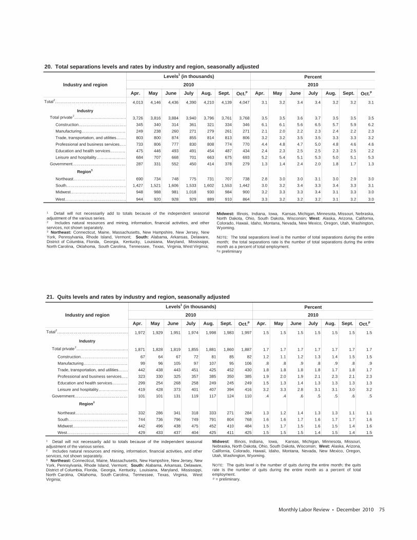
Monthly Labor Review • December 2010 75
20. Total separations levels and rates by industry and region, seasonally adjustedLevels1 (in thousands) Percent
Industry and region 2010 2010
Apr. May June July Aug. Sept. Oct.p Apr. May June July Aug. Sept. Oct.p
Total2……………………………………………… 4,013 4,146 4,436 4,390 4,210 4,139 4,047 3.1 3.2 3.4 3.4 3.2 3.2 3.1
IndustryTotal private2………………………………… 3,726 3,816 3,884 3,940 3,796 3,761 3,768 3.5 3.5 3.6 3.7 3.5 3.5 3.5
Construction……………………………… 345 340 314 361 321 334 346 6.1 6.1 5.6 6.5 5.7 5.9 6.2Manufacturing…………………………… 249 238 260 271 279 261 271 2.1 2.0 2.2 2.3 2.4 2.2 2.3Trade, transportation, and utilities……… 803 800 874 855 814 813 806 3.2 3.2 3.5 3.5 3.3 3.3 3.2Professional and business services…… 733 806 777 830 808 774 770 4.4 4.8 4.7 5.0 4.8 4.6 4.6Education and health services………… 475 446 493 491 454 487 434 2.4 2.3 2.5 2.5 2.3 2.5 2.2Leisure and hospitality…………………… 684 707 668 701 663 675 693 5.2 5.4 5.1 5.3 5.0 5.1 5.3
Government………………………………… 287 331 552 450 414 378 279 1.3 1.4 2.4 2.0 1.8 1.7 1.3
Region3
Northeast………………………………… 690 734 748 775 731 707 738 2.8 3.0 3.0 3.1 3.0 2.9 3.0South……………………………………… 1,427 1,521 1,606 1,533 1,602 1,553 1,442 3.0 3.2 3.4 3.3 3.4 3.3 3.1Midwest…………………………………… 948 988 981 1,018 930 984 900 3.2 3.3 3.3 3.4 3.1 3.3 3.0
West……………………………………… 944 920 928 929 889 910 864 3.3 3.2 3.2 3.2 3.1 3.2 3.0
1 Detail will not necessarily add to totals because of the independent seasonaladjustment of the various series.2 Includes natural resources and mining, information, financial activities, and otherservices, not shown separately.3 Northeast: Connecticut, Maine, Massachusetts, New Hampshire, New Jersey, NewYork, Pennsylvania, Rhode Island, Vermont; South: Alabama, Arkansas, Delaware,District of Columbia, Florida, Georgia, Kentucky, Louisiana, Maryland, Mississippi,North Carolina, Oklahoma, South Carolina, Tennessee, Texas, Virginia, West Virginia;
Midwest: Illinois, Indiana, Iowa, Kansas, Michigan, Minnesota, Missouri, Nebraska,North Dakota, Ohio, South Dakota, Wisconsin; West: Alaska, Arizona, California,Colorado, Hawaii, Idaho, Montana, Nevada, New Mexico, Oregon, Utah, Washington,Wyoming.
NOTE: The total separations level is the number of total separations during the entiremonth; the total separations rate is the number of total separations during the entiremonth as a percent of total employment.p= preliminary
21. Quits levels and rates by industry and region, seasonally adjustedLevels1 (in thousands) Percent
Industry and region 2010 2010
Apr. May June July Aug. Sept. Oct.p Apr. May June July Aug. Sept. Oct.p
Total2……………………………………………… 1,972 1,929 1,951 1,974 1,998 1,983 1,997 1.5 1.5 1.5 1.5 1.5 1.5 1.5
Industry
Total private2………………………………… 1,871 1,828 1,819 1,855 1,881 1,860 1,887 1.7 1.7 1.7 1.7 1.7 1.7 1.7
Construction……………………………… 67 64 67 72 81 85 82 1.2 1.1 1.2 1.3 1.4 1.5 1.5Manufacturing…………………………… 99 96 105 97 107 95 106 .8 .8 .9 .8 .9 .8 .9Trade, transportation, and utilities……… 442 438 443 451 425 452 430 1.8 1.8 1.8 1.8 1.7 1.8 1.7Professional and business services…… 323 330 325 357 385 350 385 1.9 2.0 1.9 2.1 2.3 2.1 2.3Education and health services………… 299 254 268 258 249 245 249 1.5 1.3 1.4 1.3 1.3 1.3 1.3Leisure and hospitality…………………… 419 428 373 401 407 394 416 3.2 3.3 2.8 3.1 3.1 3.0 3.2
Government………………………………… 101 101 131 119 117 124 110 .4 .4 .6 .5 .5 .6 .5
Region3
Northeast………………………………… 332 286 341 318 333 271 284 1.3 1.2 1.4 1.3 1.3 1.1 1.1South……………………………………… 744 736 796 749 791 804 768 1.6 1.6 1.7 1.6 1.7 1.7 1.6Midwest…………………………………… 442 496 438 475 452 410 484 1.5 1.7 1.5 1.6 1.5 1.4 1.6West……………………………………… 429 433 437 404 425 411 425 1.5 1.5 1.5 1.4 1.5 1.4 1.5
1 Detail will not necessarily add to totals because of the independent seasonaladjustment of the various series.2 Includes natural resources and mining, information, financial activities, and otherservices, not shown separately.3 Northeast: Connecticut, Maine, Massachusetts, New Hampshire, New Jersey, NewYork, Pennsylvania, Rhode Island, Vermont; South: Alabama, Arkansas, Delaware,District of Columbia, Florida, Georgia, Kentucky, Louisiana, Maryland, Mississippi,North Carolina, Oklahoma, South Carolina, Tennessee, Texas, Virginia, WestVirginia;
Midwest: Illinois, Indiana, Iowa, Kansas, Michigan, Minnesota, Missouri,Nebraska, North Dakota, Ohio, South Dakota, Wisconsin; West: Alaska, Arizona,California, Colorado, Hawaii, Idaho, Montana, Nevada, New Mexico, Oregon,Utah, Washington, Wyoming.
NOTE: The quits level is the number of quits during the entire month; the quitsrate is the number of quits during the entire month as a percent of totalemployment.p = preliminary.
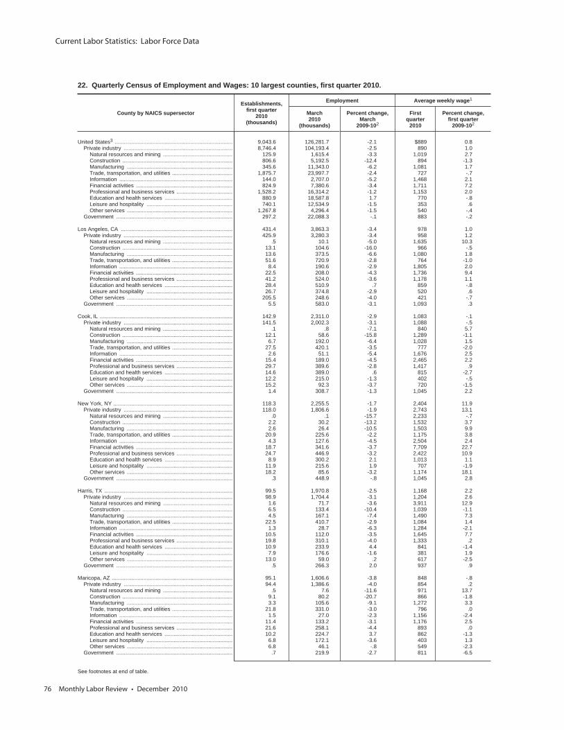
Current Labor Statistics: Labor Force Data
76 Monthly Labor Review • December 2010
22. Quarterly Census of Employment and Wages: 10 largest counties, first quarter 2010.
County by NAICS supersectorEstablishments,
first quarter2010
(thousands)
Employment Average weekly wage1
March2010
(thousands)
Percent change,March
2009-102
Firstquarter
2010
Percent change,first quarter
2009-102
United States3 .............................................................................. 9,043.6 126,281.7 -2.1 $889 0.8Private industry ........................................................................ 8,746.4 104,193.4 -2.5 890 1.0
Natural resources and mining .............................................. 125.9 1,615.4 -3.3 1,019 2.7Construction ......................................................................... 806.6 5,192.5 -12.4 894 -1.3Manufacturing ...................................................................... 345.6 11,343.0 -6.2 1,081 1.7Trade, transportation, and utilities ........................................ 1,875.7 23,997.7 -2.4 727 -.7Information ........................................................................... 144.0 2,707.0 -5.2 1,468 2.1Financial activities ................................................................ 824.9 7,380.6 -3.4 1,711 7.2Professional and business services ..................................... 1,528.2 16,314.2 -1.2 1,153 2.0Education and health services ............................................. 880.9 18,587.8 1.7 770 -.8Leisure and hospitality ......................................................... 740.1 12,534.9 -1.5 353 .6Other services ...................................................................... 1,267.8 4,296.4 -1.5 540 -.4
Government ............................................................................. 297.2 22,088.3 -.1 883 -.2
Los Angeles, CA .......................................................................... 431.4 3,863.3 -3.4 978 1.0Private industry ........................................................................ 425.9 3,280.3 -3.4 958 1.2
Natural resources and mining .............................................. .5 10.1 -5.0 1,635 10.3Construction ......................................................................... 13.1 104.6 -16.0 966 -.5Manufacturing ...................................................................... 13.6 373.5 -6.6 1,080 1.8Trade, transportation, and utilities ........................................ 51.6 720.9 -2.8 764 -1.0Information ........................................................................... 8.4 190.6 -2.9 1,805 2.0Financial activities ................................................................ 22.5 208.0 -4.3 1,736 9.4Professional and business services ..................................... 41.2 524.0 -3.6 1,178 1.1Education and health services ............................................. 28.4 510.9 .7 859 -.8Leisure and hospitality ......................................................... 26.7 374.8 -2.9 520 .6Other services ...................................................................... 205.5 248.6 -4.0 421 -.7
Government ............................................................................. 5.5 583.0 -3.1 1,093 .3
Cook, IL ........................................................................................ 142.9 2,311.0 -2.9 1,083 -.1Private industry ........................................................................ 141.5 2,002.3 -3.1 1,088 -.5
Natural resources and mining .............................................. .1 .8 -7.1 840 5.7Construction ......................................................................... 12.1 58.6 -15.8 1,289 -1.1Manufacturing ...................................................................... 6.7 192.0 -6.4 1,028 1.5Trade, transportation, and utilities ........................................ 27.5 420.1 -3.5 777 -2.0Information ........................................................................... 2.6 51.1 -5.4 1,676 2.5Financial activities ................................................................ 15.4 189.0 -4.5 2,465 2.2Professional and business services ..................................... 29.7 389.6 -2.8 1,417 .9Education and health services ............................................. 14.6 389.0 .6 815 -2.7Leisure and hospitality ......................................................... 12.2 215.0 -1.3 402 -.5Other services ...................................................................... 15.2 92.3 -3.7 720 -1.5
Government ............................................................................. 1.4 308.7 -1.3 1,045 2.2
New York, NY ............................................................................... 118.3 2,255.5 -1.7 2,404 11.9Private industry ........................................................................ 118.0 1,806.6 -1.9 2,743 13.1
Natural resources and mining .............................................. .0 .1 -15.7 2,233 -.7Construction ......................................................................... 2.2 30.2 -13.2 1,532 3.7Manufacturing ...................................................................... 2.6 26.4 -10.5 1,503 9.9Trade, transportation, and utilities ........................................ 20.9 225.6 -2.2 1,175 3.8Information ........................................................................... 4.3 127.6 -4.5 2,504 2.4Financial activities ................................................................ 18.7 341.6 -3.7 7,709 22.7Professional and business services ..................................... 24.7 446.9 -3.2 2,422 10.9Education and health services ............................................. 8.9 300.2 2.1 1,013 1.1Leisure and hospitality ......................................................... 11.9 215.6 1.9 707 -1.9Other services ...................................................................... 18.2 85.6 -3.2 1,174 18.1
Government ............................................................................. .3 448.9 -.8 1,045 2.8
Harris, TX ..................................................................................... 99.5 1,970.8 -2.5 1,168 2.2Private industry ........................................................................ 98.9 1,704.4 -3.1 1,204 2.6
Natural resources and mining .............................................. 1.6 71.7 -3.6 3,911 12.9Construction ......................................................................... 6.5 133.4 -10.4 1,039 -1.1Manufacturing ...................................................................... 4.5 167.1 -7.4 1,490 7.3Trade, transportation, and utilities ........................................ 22.5 410.7 -2.9 1,084 1.4Information ........................................................................... 1.3 28.7 -6.3 1,284 -2.1Financial activities ................................................................ 10.5 112.0 -3.5 1,645 7.7Professional and business services ..................................... 19.8 310.1 -4.0 1,333 .2Education and health services ............................................. 10.9 233.9 4.4 841 -1.4Leisure and hospitality ......................................................... 7.9 176.6 -1.6 381 1.9Other services ...................................................................... 13.0 59.0 .2 617 -2.5
Government ............................................................................. .5 266.3 2.0 937 .9
Maricopa, AZ ................................................................................ 95.1 1,606.6 -3.8 848 -.8Private industry ........................................................................ 94.4 1,386.6 -4.0 854 .2
Natural resources and mining .............................................. .5 7.6 -11.6 971 13.7Construction ......................................................................... 9.1 80.2 -20.7 866 -1.8Manufacturing ...................................................................... 3.3 105.6 -9.1 1,272 3.3Trade, transportation, and utilities ........................................ 21.8 331.0 -3.0 796 .0Information ........................................................................... 1.5 27.0 -2.3 1,156 -2.4Financial activities ................................................................ 11.4 133.2 -3.1 1,176 2.5Professional and business services ..................................... 21.6 258.1 -4.4 893 .0Education and health services ............................................. 10.2 224.7 3.7 862 -1.3Leisure and hospitality ......................................................... 6.8 172.1 -3.6 403 1.3Other services ...................................................................... 6.8 46.1 -.8 549 -2.3
Government ............................................................................. .7 219.9 -2.7 811 -6.5
See footnotes at end of table.
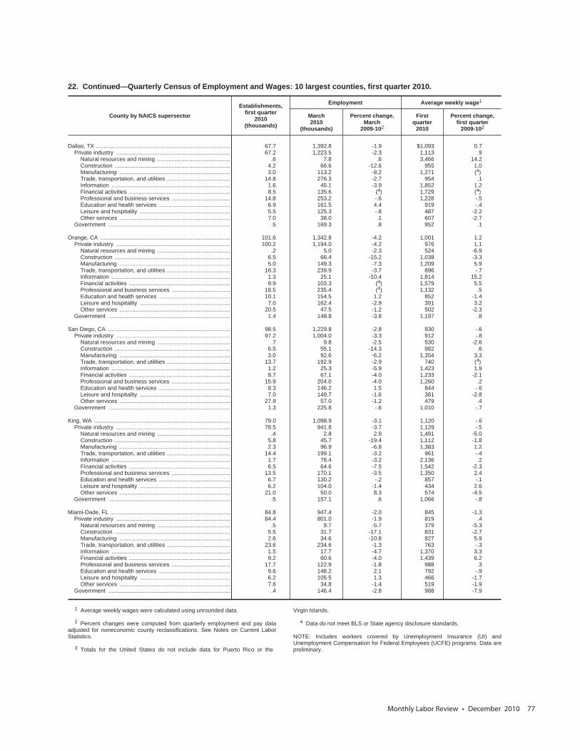
Monthly Labor Review • December 2010 77
22. Continued—Quarterly Census of Employment and Wages: 10 largest counties, first quarter 2010.
County by NAICS supersectorEstablishments,
first quarter2010
(thousands)
Employment Average weekly wage1
March2010
(thousands)
Percent change,March
2009-102
Firstquarter
2010
Percent change,first quarter
2009-102
Dallas, TX ..................................................................................... 67.7 1,392.8 -1.9 $1,093 0.7Private industry ........................................................................ 67.2 1,223.5 -2.3 1,113 .9
Natural resources and mining .............................................. .6 7.8 .6 3,466 14.2Construction ......................................................................... 4.2 66.6 -12.6 955 1.0Manufacturing ...................................................................... 3.0 113.2 -8.2 1,271 (4)Trade, transportation, and utilities ........................................ 14.8 276.3 -2.7 954 .1Information ........................................................................... 1.6 45.1 -3.9 1,852 1.2Financial activities ................................................................ 8.5 135.6 (4) 1,729 (4)Professional and business services ..................................... 14.8 253.2 -.6 1,228 -.5Education and health services ............................................. 6.9 161.5 4.4 919 -.4Leisure and hospitality ......................................................... 5.5 125.3 -.8 487 -2.2Other services ...................................................................... 7.0 38.0 .1 607 -2.7
Government ............................................................................. .5 169.3 .8 952 .1
Orange, CA .................................................................................. 101.6 1,342.8 -4.2 1,001 1.2Private industry ........................................................................ 100.2 1,194.0 -4.2 976 1.1
Natural resources and mining .............................................. .2 5.0 -2.3 524 -6.9Construction ......................................................................... 6.5 66.4 -15.2 1,038 -3.3Manufacturing ...................................................................... 5.0 149.3 -7.3 1,209 5.9Trade, transportation, and utilities ........................................ 16.3 239.9 -3.7 896 -.7Information ........................................................................... 1.3 25.1 -10.4 1,814 15.2Financial activities ................................................................ 9.9 103.3 (4) 1,579 5.5Professional and business services ..................................... 18.5 235.4 (4) 1,132 .5Education and health services ............................................. 10.1 154.5 1.2 852 -1.4Leisure and hospitality ......................................................... 7.0 162.4 -2.9 391 3.2Other services ...................................................................... 20.5 47.5 -1.2 502 -2.3
Government ............................................................................. 1.4 148.8 -3.8 1,197 .8
San Diego, CA ............................................................................. 98.5 1,229.8 -2.8 930 -.6Private industry ........................................................................ 97.2 1,004.0 -3.3 912 -.8
Natural resources and mining .............................................. .7 9.8 -2.5 530 -2.6Construction ......................................................................... 6.5 55.1 -14.3 982 .6Manufacturing ...................................................................... 3.0 92.6 -6.2 1,354 3.3Trade, transportation, and utilities ........................................ 13.7 192.9 -2.9 740 (4)Information ........................................................................... 1.2 25.3 -5.9 1,423 1.9Financial activities ................................................................ 8.7 67.1 -4.0 1,233 -2.1Professional and business services ..................................... 15.9 204.0 -4.0 1,260 .2Education and health services ............................................. 8.3 146.2 1.5 844 -.6Leisure and hospitality ......................................................... 7.0 149.7 -1.6 381 -2.8Other services ...................................................................... 27.9 57.0 -1.2 479 .4
Government ............................................................................. 1.3 225.8 -.6 1,010 -.7
King, WA ...................................................................................... 79.0 1,098.9 -3.1 1,120 -.6Private industry ........................................................................ 78.5 941.8 -3.7 1,129 -.5
Natural resources and mining .............................................. .4 2.8 2.9 1,491 -5.0Construction ......................................................................... 5.8 45.7 -19.4 1,112 -1.8Manufacturing ...................................................................... 2.3 96.9 -6.8 1,383 1.2Trade, transportation, and utilities ........................................ 14.4 199.1 -3.2 961 -.4Information ........................................................................... 1.7 78.4 -3.2 2,136 .2Financial activities ................................................................ 6.5 64.6 -7.5 1,542 -2.3Professional and business services ..................................... 13.5 170.1 -3.5 1,350 2.4Education and health services ............................................. 6.7 130.2 -.2 857 -.1Leisure and hospitality ......................................................... 6.2 104.0 -1.4 434 2.6Other services ...................................................................... 21.0 50.0 8.3 574 -4.5
Government ............................................................................. .5 157.1 .6 1,066 -.8
Miami-Dade, FL ............................................................................ 84.8 947.4 -2.0 845 -1.3Private industry ........................................................................ 84.4 801.0 -1.9 819 .4
Natural resources and mining .............................................. .5 9.7 -5.7 379 -5.3Construction ......................................................................... 5.5 31.7 -17.1 831 -2.7Manufacturing ...................................................................... 2.6 34.6 -10.8 827 5.9Trade, transportation, and utilities ........................................ 23.6 234.6 -1.3 763 -.3Information ........................................................................... 1.5 17.7 -4.7 1,370 3.3Financial activities ................................................................ 9.2 60.6 -4.0 1,439 6.2Professional and business services ..................................... 17.7 122.9 -1.8 988 .3Education and health services ............................................. 9.6 148.2 2.1 792 -.9Leisure and hospitality ......................................................... 6.2 105.5 1.3 466 -1.7Other services ...................................................................... 7.6 34.8 -1.4 519 -1.9
Government ............................................................................. .4 146.4 -2.8 988 -7.9
1 Average weekly wages were calculated using unrounded data.
2 Percent changes were computed from quarterly employment and pay dataadjusted for noneconomic county reclassifications. See Notes on Current LaborStatistics.
3 Totals for the United States do not include data for Puerto Rico or the
Virgin Islands.
4 Data do not meet BLS or State agency disclosure standards.
NOTE: Includes workers covered by Unemployment Insurance (UI) andUnemployment Compensation for Federal Employees (UCFE) programs. Data arepreliminary.
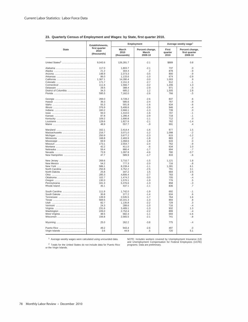
Current Labor Statistics: Labor Force Data
78 Monthly Labor Review • December 2010
23. Quarterly Census of Employment and Wages: by State, first quarter 2010.
StateEstablishments,
first quarter2010
(thousands)
Employment Average weekly wage1
March2010
(thousands)
Percent change,March
2009-10
Firstquarter
2010
Percent change,first quarter
2009-10
United States2 ................................... 9,043.6 126,281.7 -2.1 $889 0.8
Alabama ............................................ 117.0 1,803.7 -2.1 737 .0Alaska ............................................... 21.2 304.4 .2 878 -.9Arizona .............................................. 148.9 2,373.3 -3.5 800 -.9Arkansas ........................................... 86.0 1,133.6 -1.0 674 -2.9California ........................................... 1,367.1 14,280.4 -3.0 1,003 .9Colorado ........................................... 171.7 2,151.3 -2.7 912 -.1Connecticut ....................................... 111.6 1,566.7 -3.2 1,206 1.3Delaware ........................................... 28.5 388.4 -2.9 971 -.5District of Columbia ........................... 34.3 685.2 1.2 1,505 2.8Florida ............................................... 595.5 7,162.0 -2.6 766 -.5
Georgia ............................................. 269.0 3,728.2 -2.6 837 .6Hawaii ............................................... 39.3 585.6 -2.4 767 -.9Idaho ................................................. 55.3 591.8 -1.6 634 -.6Illinois ................................................ 376.9 5,406.6 -2.6 946 -.4Indiana .............................................. 160.2 2,666.1 -1.3 739 .0Iowa .................................................. 94.0 1,410.0 -1.6 707 -.1Kansas .............................................. 87.8 1,286.4 -2.9 718 -.1Kentucky ........................................... 109.2 1,690.8 -1.1 712 .0Louisiana ........................................... 128.6 1,827.6 -2.1 762 -1.4Maine ................................................ 48.9 557.7 -.9 691 .4
Maryland ........................................... 162.1 2,414.4 -1.6 977 1.5Massachusetts .................................. 216.7 3,071.0 -1.2 1,098 -.2Michigan ............................................ 250.9 3,677.2 -2.3 815 -1.2Minnesota ......................................... 168.8 2,493.9 -1.8 883 .2Mississippi ......................................... 69.9 1,068.6 -1.8 633 .0Missouri ............................................. 173.1 2,554.7 -2.4 762 -.9Montana ............................................ 42.2 411.0 -.6 634 1.0Nebraska ........................................... 59.4 880.4 -1.7 694 -.7Nevada .............................................. 73.9 1,097.8 -4.6 780 -3.7New Hampshire ................................ 47.7 589.9 -1.7 833 -.6
New Jersey ....................................... 269.6 3,710.7 -1.5 1,121 1.8New Mexico ...................................... 54.2 777.3 -2.0 716 -.8New York .......................................... 586.1 8,239.4 -1.1 1,281 6.1North Carolina ................................... 250.8 3,752.2 -2.5 791 3.1North Dakota ..................................... 25.8 347.2 1.5 684 2.5Ohio .................................................. 285.3 4,806.4 -2.7 783 -.8Oklahoma .......................................... 102.7 1,474.2 -3.0 705 -.4Oregon .............................................. 130.3 1,570.1 -1.9 776 .5Pennsylvania ..................................... 341.3 5,376.6 -1.3 858 -.3Rhode Island ..................................... 35.1 437.1 -1.1 836 .7
South Carolina .................................. 111.9 1,742.0 -1.9 692 -.1South Dakota .................................... 30.8 377.2 -1.4 634 .6Tennessee ........................................ 139.9 2,535.5 -1.7 764 1.6Texas ................................................ 569.5 10,101.3 -1.3 893 .8Utah .................................................. 82.7 1,135.8 -2.2 729 .3Vermont ............................................ 24.3 288.6 -1.0 716 -.4Virginia .............................................. 231.6 3,489.1 -1.3 932 1.3Washington ....................................... 226.0 2,752.4 -2.2 899 -.4West Virginia ..................................... 48.5 682.3 -1.1 693 -1.6Wisconsin .......................................... 156.8 2,565.5 -2.1 741 -.8
Wyoming ........................................... 25.0 262.2 -3.8 775 -.4
Puerto Rico ....................................... 49.2 943.4 -2.6 497 .0Virgin Islands .................................... 3.6 44.9 .5 720 5.1
1 Average weekly wages were calculated using unrounded data.
2 Totals for the United States do not include data for Puerto Ricoor the Virgin Islands.
NOTE: Includes workers covered by Unemployment Insurance (UI)and Unemployment Compensation for Federal Employees (UCFE)programs. Data are preliminary.
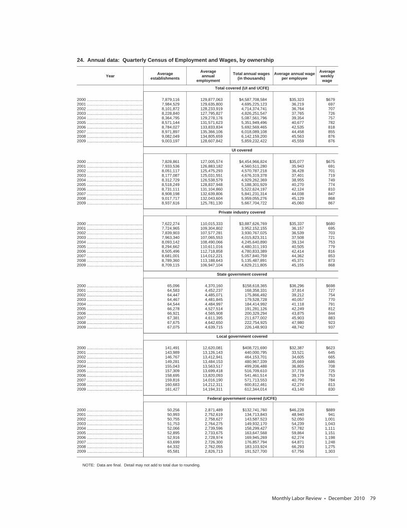
Monthly Labor Review • December 2010 79
24. Annual data: Quarterly Census of Employment and Wages, by ownership
Year Averageestablishments
Averageannual
employmentTotal annual wages
(in thousands)Average annual wage
per employeeAverageweeklywage
Total covered (UI and UCFE)
2000 .................................................. 7,879,116 129,877,063 $4,587,708,584 $35,323 $679 2001 .................................................. 7,984,529 129,635,800 4,695,225,123 36,219 697 2002 .................................................. 8,101,872 128,233,919 4,714,374,741 36,764 707 2003 .................................................. 8,228,840 127,795,827 4,826,251,547 37,765 726 2004 .................................................. 8,364,795 129,278,176 5,087,561,796 39,354 757 2005 .................................................. 8,571,144 131,571,623 5,351,949,496 40,677 782 2006 .................................................. 8,784,027 133,833,834 5,692,569,465 42,535 818 2007 .................................................. 8,971,897 135,366,106 6,018,089,108 44,458 855 2008 .................................................. 9,082,049 134,805,659 6,142,159,200 45,563 876 2009 .................................................. 9,003,197 128,607,842 5,859,232,422 45,559 876
UI covered
2000 .................................................. 7,828,861 127,005,574 $4,454,966,824 $35,077 $675 2001 .................................................. 7,933,536 126,883,182 4,560,511,280 35,943 691 2002 .................................................. 8,051,117 125,475,293 4,570,787,218 36,428 701 2003 .................................................. 8,177,087 125,031,551 4,676,319,378 37,401 719 2004 .................................................. 8,312,729 126,538,579 4,929,262,369 38,955 749 2005 .................................................. 8,518,249 128,837,948 5,188,301,929 40,270 774 2006 .................................................. 8,731,111 131,104,860 5,522,624,197 42,124 810 2007 .................................................. 8,908,198 132,639,806 5,841,231,314 44,038 847 2008 .................................................. 9,017,717 132,043,604 5,959,055,276 45,129 868 2009 .................................................. 8,937,616 125,781,130 5,667,704,722 45,060 867
Private industry covered
2000 .................................................. 7,622,274 110,015,333 $3,887,626,769 $35,337 $680 2001 .................................................. 7,724,965 109,304,802 3,952,152,155 36,157 695 2002 .................................................. 7,839,903 107,577,281 3,930,767,025 36,539 703 2003 .................................................. 7,963,340 107,065,553 4,015,823,311 37,508 721 2004 .................................................. 8,093,142 108,490,066 4,245,640,890 39,134 753 2005 .................................................. 8,294,662 110,611,016 4,480,311,193 40,505 779 2006 .................................................. 8,505,496 112,718,858 4,780,833,389 42,414 816 2007 .................................................. 8,681,001 114,012,221 5,057,840,759 44,362 853 2008 .................................................. 8,789,360 113,188,643 5,135,487,891 45,371 873 2009 .................................................. 8,709,115 106,947,104 4,829,211,805 45,155 868
State government covered
2000 .................................................. 65,096 4,370,160 $158,618,365 $36,296 $698 2001 .................................................. 64,583 4,452,237 168,358,331 37,814 727 2002 .................................................. 64,447 4,485,071 175,866,492 39,212 754 2003 .................................................. 64,467 4,481,845 179,528,728 40,057 770 2004 .................................................. 64,544 4,484,997 184,414,992 41,118 791 2005 .................................................. 66,278 4,527,514 191,281,126 42,249 812 2006 .................................................. 66,921 4,565,908 200,329,294 43,875 844 2007 .................................................. 67,381 4,611,395 211,677,002 45,903 883 2008 .................................................. 67,675 4,642,650 222,754,925 47,980 923 2009 .................................................. 67,075 4,639,715 226,148,903 48,742 937
Local government covered
2000 .................................................. 141,491 12,620,081 $408,721,690 $32,387 $623 2001 .................................................. 143,989 13,126,143 440,000,795 33,521 645 2002 .................................................. 146,767 13,412,941 464,153,701 34,605 665 2003 .................................................. 149,281 13,484,153 480,967,339 35,669 686 2004 .................................................. 155,043 13,563,517 499,206,488 36,805 708 2005 .................................................. 157,309 13,699,418 516,709,610 37,718 725 2006 .................................................. 158,695 13,820,093 541,461,514 39,179 753 2007 .................................................. 159,816 14,016,190 571,713,553 40,790 784 2008 .................................................. 160,683 14,212,311 600,812,461 42,274 813 2009 .................................................. 161,427 14,194,311 612,344,014 43,140 830
Federal government covered (UCFE)
2000 .................................................. 50,256 2,871,489 $132,741,760 $46,228 $889 2001 .................................................. 50,993 2,752,619 134,713,843 48,940 941 2002 .................................................. 50,755 2,758,627 143,587,523 52,050 1,001 2003 .................................................. 51,753 2,764,275 149,932,170 54,239 1,043 2004 .................................................. 52,066 2,739,596 158,299,427 57,782 1,111 2005 .................................................. 52,895 2,733,675 163,647,568 59,864 1,151 2006 .................................................. 52,916 2,728,974 169,945,269 62,274 1,198 2007 .................................................. 63,699 2,726,300 176,857,794 64,871 1,248 2008 .................................................. 64,332 2,762,055 183,103,924 66,293 1,275 2009 .................................................. 65,581 2,826,713 191,527,700 67,756 1,303
NOTE: Data are final. Detail may not add to total due to rounding.
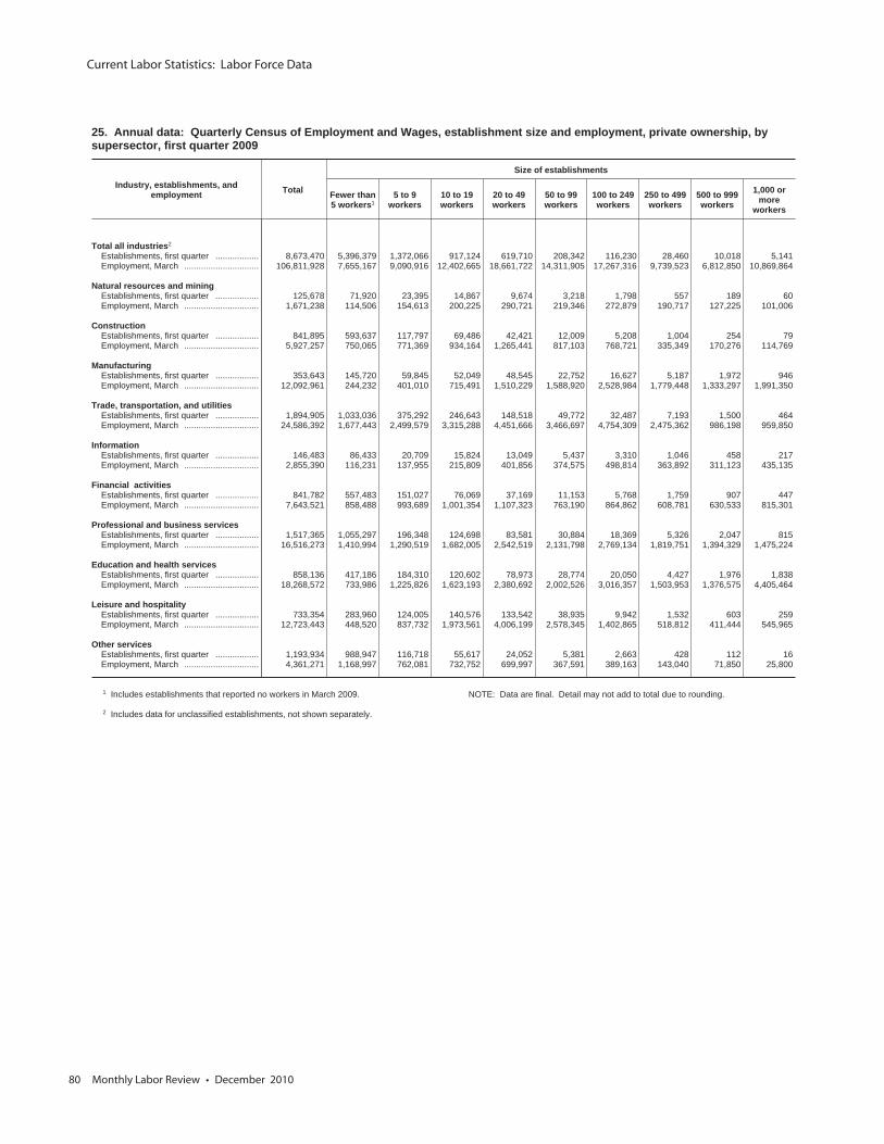
Current Labor Statistics: Labor Force Data
80 Monthly Labor Review • December 2010
25. Annual data: Quarterly Census of Employment and Wages, establishment size and employment, private ownership, bysupersector, first quarter 2009
Industry, establishments, andemployment Total
Size of establishments
Fewer than5 workers1
5 to 9workers
10 to 19workers
20 to 49workers
50 to 99workers
100 to 249workers
250 to 499workers
500 to 999workers
1,000 ormore
workers
Total all industries2
Establishments, first quarter .................. 8,673,470 5,396,379 1,372,066 917,124 619,710 208,342 116,230 28,460 10,018 5,141Employment, March ............................... 106,811,928 7,655,167 9,090,916 12,402,665 18,661,722 14,311,905 17,267,316 9,739,523 6,812,850 10,869,864
Natural resources and miningEstablishments, first quarter .................. 125,678 71,920 23,395 14,867 9,674 3,218 1,798 557 189 60Employment, March ............................... 1,671,238 114,506 154,613 200,225 290,721 219,346 272,879 190,717 127,225 101,006
ConstructionEstablishments, first quarter .................. 841,895 593,637 117,797 69,486 42,421 12,009 5,208 1,004 254 79Employment, March ............................... 5,927,257 750,065 771,369 934,164 1,265,441 817,103 768,721 335,349 170,276 114,769
ManufacturingEstablishments, first quarter .................. 353,643 145,720 59,845 52,049 48,545 22,752 16,627 5,187 1,972 946Employment, March ............................... 12,092,961 244,232 401,010 715,491 1,510,229 1,588,920 2,528,984 1,779,448 1,333,297 1,991,350
Trade, transportation, and utilitiesEstablishments, first quarter .................. 1,894,905 1,033,036 375,292 246,643 148,518 49,772 32,487 7,193 1,500 464Employment, March ............................... 24,586,392 1,677,443 2,499,579 3,315,288 4,451,666 3,466,697 4,754,309 2,475,362 986,198 959,850
InformationEstablishments, first quarter .................. 146,483 86,433 20,709 15,824 13,049 5,437 3,310 1,046 458 217Employment, March ............................... 2,855,390 116,231 137,955 215,809 401,856 374,575 498,814 363,892 311,123 435,135
Financial activitiesEstablishments, first quarter .................. 841,782 557,483 151,027 76,069 37,169 11,153 5,768 1,759 907 447Employment, March ............................... 7,643,521 858,488 993,689 1,001,354 1,107,323 763,190 864,862 608,781 630,533 815,301
Professional and business servicesEstablishments, first quarter .................. 1,517,365 1,055,297 196,348 124,698 83,581 30,884 18,369 5,326 2,047 815Employment, March ............................... 16,516,273 1,410,994 1,290,519 1,682,005 2,542,519 2,131,798 2,769,134 1,819,751 1,394,329 1,475,224
Education and health servicesEstablishments, first quarter .................. 858,136 417,186 184,310 120,602 78,973 28,774 20,050 4,427 1,976 1,838Employment, March ............................... 18,268,572 733,986 1,225,826 1,623,193 2,380,692 2,002,526 3,016,357 1,503,953 1,376,575 4,405,464
Leisure and hospitalityEstablishments, first quarter .................. 733,354 283,960 124,005 140,576 133,542 38,935 9,942 1,532 603 259Employment, March ............................... 12,723,443 448,520 837,732 1,973,561 4,006,199 2,578,345 1,402,865 518,812 411,444 545,965
Other servicesEstablishments, first quarter .................. 1,193,934 988,947 116,718 55,617 24,052 5,381 2,663 428 112 16Employment, March ............................... 4,361,271 1,168,997 762,081 732,752 699,997 367,591 389,163 143,040 71,850 25,800
1 Includes establishments that reported no workers in March 2009.
2 Includes data for unclassified establishments, not shown separately.
NOTE: Data are final. Detail may not add to total due to rounding.
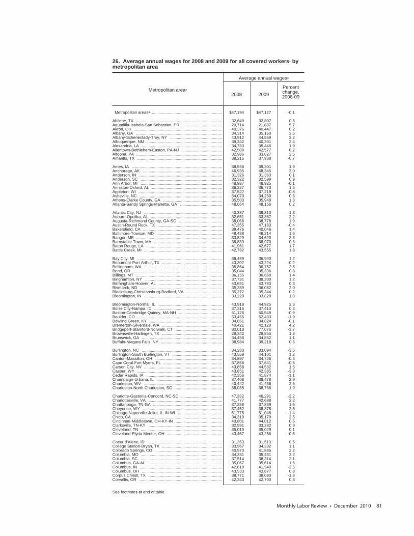
Monthly Labor Review • December 2010 81
26. Average annual wages for 2008 and 2009 for all covered workers1 bymetropolitan area
Metropolitan area2
Average annual wages3
2008 2009Percentchange,2008-09
Metropolitan areas4 .............................................................. $47,194 $47,127 -0.1
Abilene, TX ............................................................................ 32,649 32,807 0.5Aguadilla-Isabela-San Sebastian, PR ................................... 20,714 21,887 5.7Akron, OH .............................................................................. 40,376 40,447 0.2Albany, GA ............................................................................ 34,314 35,160 2.5Albany-Schenectady-Troy, NY .............................................. 43,912 44,859 2.2Albuquerque, NM ................................................................... 39,342 40,301 2.4Alexandria, LA ....................................................................... 34,783 35,446 1.9Allentown-Bethlehem-Easton, PA-NJ .................................... 42,500 42,577 0.2Altoona, PA ............................................................................ 32,986 33,827 2.5Amarillo, TX ........................................................................... 38,215 37,938 -0.7
Ames, IA ................................................................................ 38,558 39,301 1.9Anchorage, AK ...................................................................... 46,935 48,345 3.0Anderson, IN .......................................................................... 31,326 31,363 0.1Anderson, SC ........................................................................ 32,322 32,599 0.9Ann Arbor, MI ........................................................................ 48,987 48,925 -0.1Anniston-Oxford, AL .............................................................. 36,227 36,773 1.5Appleton, WI .......................................................................... 37,522 37,219 -0.8Asheville, NC ......................................................................... 34,070 34,259 0.6Athens-Clarke County, GA .................................................... 35,503 35,948 1.3Atlanta-Sandy Springs-Marietta, GA ..................................... 48,064 48,156 0.2
Atlantic City, NJ ..................................................................... 40,337 39,810 -1.3Auburn-Opelika, AL ............................................................... 32,651 33,367 2.2Augusta-Richmond County, GA-SC ...................................... 38,068 38,778 1.9Austin-Round Rock, TX ......................................................... 47,355 47,183 -0.4Bakersfield, CA ...................................................................... 39,476 40,046 1.4Baltimore-Towson, MD .......................................................... 48,438 49,214 1.6Bangor, ME ............................................................................ 33,829 34,620 2.3Barnstable Town, MA ............................................................ 38,839 38,970 0.3Baton Rouge, LA ................................................................... 41,961 42,677 1.7Battle Creek, MI ..................................................................... 42,782 43,555 1.8
Bay City, MI ........................................................................... 36,489 36,940 1.2Beaumont-Port Arthur, TX ..................................................... 43,302 43,224 -0.2Bellingham, WA ..................................................................... 35,864 36,757 2.5Bend, OR ............................................................................... 35,044 35,336 0.8Billings, MT ............................................................................ 36,155 36,660 1.4Binghamton, NY .................................................................... 37,731 38,200 1.2Birmingham-Hoover, AL ........................................................ 43,651 43,783 0.3Bismarck, ND ......................................................................... 35,389 36,082 2.0Blacksburg-Christiansburg-Radford, VA ................................ 35,272 35,344 0.2Bloomington, IN ..................................................................... 33,220 33,828 1.8
Bloomington-Normal, IL ......................................................... 43,918 44,925 2.3Boise City-Nampa, ID ............................................................ 37,315 37,410 0.3Boston-Cambridge-Quincy, MA-NH ...................................... 61,128 60,549 -0.9Boulder, CO ........................................................................... 53,455 52,433 -1.9Bowling Green, KY ................................................................ 34,861 34,824 -0.1Bremerton-Silverdale, WA ..................................................... 40,421 42,128 4.2Bridgeport-Stamford-Norwalk, CT ......................................... 80,018 77,076 -3.7Brownsville-Harlingen, TX ..................................................... 28,342 28,855 1.8Brunswick, GA ....................................................................... 34,458 34,852 1.1Buffalo-Niagara Falls, NY ...................................................... 38,984 39,218 0.6
Burlington, NC ....................................................................... 34,283 33,094 -3.5Burlington-South Burlington, VT ............................................ 43,559 44,101 1.2Canton-Massillon, OH ........................................................... 34,897 34,726 -0.5Cape Coral-Fort Myers, FL .................................................... 37,866 37,641 -0.6Carson City, NV ..................................................................... 43,858 44,532 1.5Casper, WY ........................................................................... 43,851 42,385 -3.3Cedar Rapids, IA ................................................................... 42,356 41,874 -1.1Champaign-Urbana, IL .......................................................... 37,408 38,478 2.9Charleston, WV ..................................................................... 40,442 41,436 2.5Charleston-North Charleston, SC .......................................... 38,035 38,766 1.9
Charlotte-Gastonia-Concord, NC-SC .................................... 47,332 46,291 -2.2Charlottesville, VA ................................................................. 41,777 42,688 2.2Chattanooga, TN-GA ............................................................. 37,258 37,839 1.6Cheyenne, WY ...................................................................... 37,452 38,378 2.5Chicago-Naperville-Joliet, IL-IN-WI ....................................... 51,775 51,048 -1.4Chico, CA .............................................................................. 34,310 35,179 2.5Cincinnati-Middletown, OH-KY-IN ......................................... 43,801 44,012 0.5Clarksville, TN-KY ................................................................. 32,991 33,282 0.9Cleveland, TN ........................................................................ 35,010 35,029 0.1Cleveland-Elyria-Mentor, OH ................................................. 43,467 43,256 -0.5
Coeur d’Alene, ID .................................................................. 31,353 31,513 0.5College Station-Bryan, TX ..................................................... 33,967 34,332 1.1Colorado Springs, CO ........................................................... 40,973 41,885 2.2Columbia, MO ........................................................................ 34,331 35,431 3.2Columbia, SC ........................................................................ 37,514 38,314 2.1Columbus, GA-AL .................................................................. 35,067 35,614 1.6Columbus, IN ......................................................................... 42,610 41,540 -2.5Columbus, OH ....................................................................... 43,533 43,877 0.8Corpus Christi, TX ................................................................. 38,771 38,090 -1.8Corvallis, OR ......................................................................... 42,343 42,700 0.8
See footnotes at end of table.
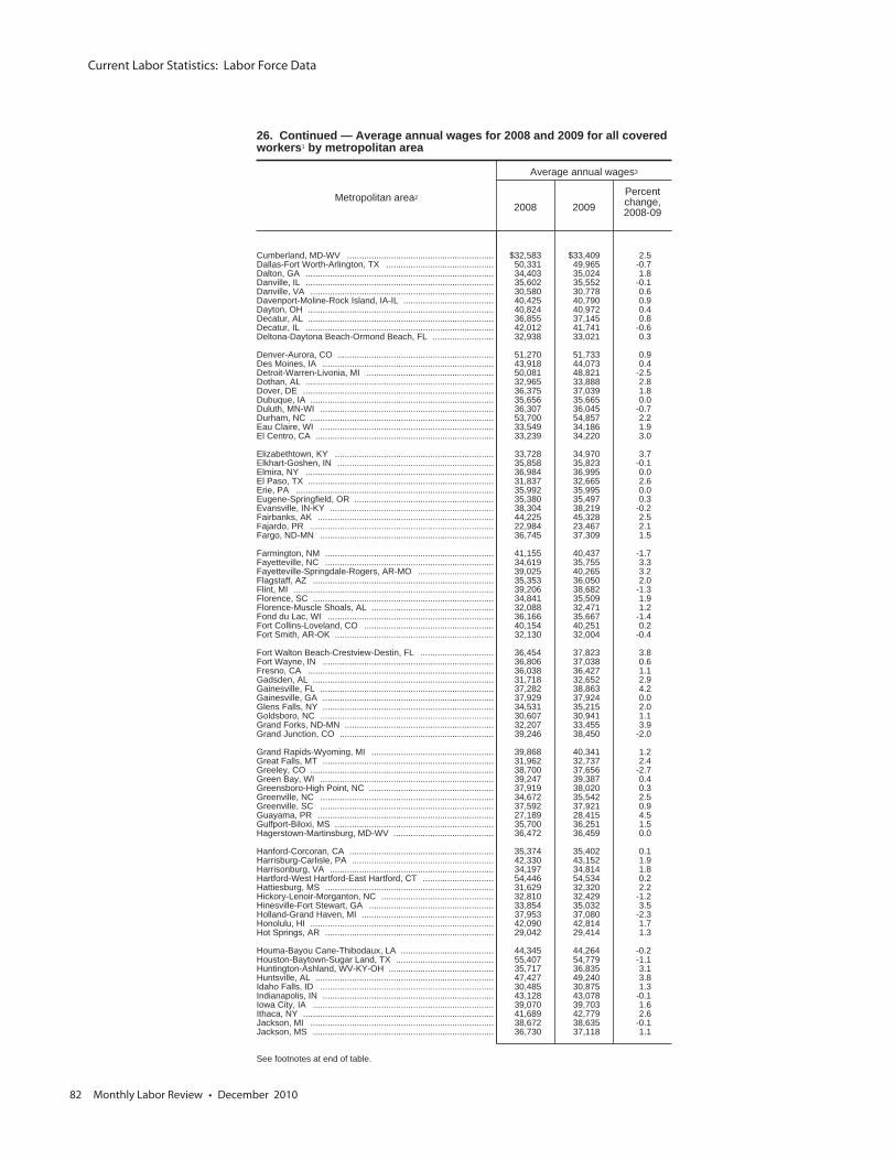
Current Labor Statistics: Labor Force Data
82 Monthly Labor Review • December 2010
26. Continued — Average annual wages for 2008 and 2009 for all coveredworkers1 by metropolitan area
Metropolitan area2
Average annual wages3
2008 2009Percentchange,2008-09
Cumberland, MD-WV ............................................................ $32,583 $33,409 2.5Dallas-Fort Worth-Arlington, TX ............................................ 50,331 49,965 -0.7Dalton, GA ............................................................................. 34,403 35,024 1.8Danville, IL ............................................................................. 35,602 35,552 -0.1Danville, VA ........................................................................... 30,580 30,778 0.6Davenport-Moline-Rock Island, IA-IL ..................................... 40,425 40,790 0.9Dayton, OH ............................................................................ 40,824 40,972 0.4Decatur, AL ............................................................................ 36,855 37,145 0.8Decatur, IL ............................................................................. 42,012 41,741 -0.6Deltona-Daytona Beach-Ormond Beach, FL ......................... 32,938 33,021 0.3
Denver-Aurora, CO ................................................................ 51,270 51,733 0.9Des Moines, IA ...................................................................... 43,918 44,073 0.4Detroit-Warren-Livonia, MI .................................................... 50,081 48,821 -2.5Dothan, AL ............................................................................. 32,965 33,888 2.8Dover, DE .............................................................................. 36,375 37,039 1.8Dubuque, IA ........................................................................... 35,656 35,665 0.0Duluth, MN-WI ....................................................................... 36,307 36,045 -0.7Durham, NC ........................................................................... 53,700 54,857 2.2Eau Claire, WI ....................................................................... 33,549 34,186 1.9El Centro, CA ......................................................................... 33,239 34,220 3.0
Elizabethtown, KY ................................................................. 33,728 34,970 3.7Elkhart-Goshen, IN ................................................................ 35,858 35,823 -0.1Elmira, NY ............................................................................. 36,984 36,995 0.0El Paso, TX ............................................................................ 31,837 32,665 2.6Erie, PA ................................................................................. 35,992 35,995 0.0Eugene-Springfield, OR ......................................................... 35,380 35,497 0.3Evansville, IN-KY ................................................................... 38,304 38,219 -0.2Fairbanks, AK ........................................................................ 44,225 45,328 2.5Fajardo, PR ........................................................................... 22,984 23,467 2.1Fargo, ND-MN ....................................................................... 36,745 37,309 1.5
Farmington, NM ..................................................................... 41,155 40,437 -1.7Fayetteville, NC ..................................................................... 34,619 35,755 3.3Fayetteville-Springdale-Rogers, AR-MO ............................... 39,025 40,265 3.2Flagstaff, AZ .......................................................................... 35,353 36,050 2.0Flint, MI .................................................................................. 39,206 38,682 -1.3Florence, SC .......................................................................... 34,841 35,509 1.9Florence-Muscle Shoals, AL .................................................. 32,088 32,471 1.2Fond du Lac, WI .................................................................... 36,166 35,667 -1.4Fort Collins-Loveland, CO ..................................................... 40,154 40,251 0.2Fort Smith, AR-OK ................................................................. 32,130 32,004 -0.4
Fort Walton Beach-Crestview-Destin, FL .............................. 36,454 37,823 3.8Fort Wayne, IN ...................................................................... 36,806 37,038 0.6Fresno, CA ............................................................................ 36,038 36,427 1.1Gadsden, AL .......................................................................... 31,718 32,652 2.9Gainesville, FL ....................................................................... 37,282 38,863 4.2Gainesville, GA ...................................................................... 37,929 37,924 0.0Glens Falls, NY ...................................................................... 34,531 35,215 2.0Goldsboro, NC ....................................................................... 30,607 30,941 1.1Grand Forks, ND-MN ............................................................. 32,207 33,455 3.9Grand Junction, CO ............................................................... 39,246 38,450 -2.0
Grand Rapids-Wyoming, MI .................................................. 39,868 40,341 1.2Great Falls, MT ...................................................................... 31,962 32,737 2.4Greeley, CO ........................................................................... 38,700 37,656 -2.7Green Bay, WI ....................................................................... 39,247 39,387 0.4Greensboro-High Point, NC ................................................... 37,919 38,020 0.3Greenville, NC ....................................................................... 34,672 35,542 2.5Greenville, SC ....................................................................... 37,592 37,921 0.9Guayama, PR ........................................................................ 27,189 28,415 4.5Gulfport-Biloxi, MS ................................................................. 35,700 36,251 1.5Hagerstown-Martinsburg, MD-WV ......................................... 36,472 36,459 0.0
Hanford-Corcoran, CA ........................................................... 35,374 35,402 0.1Harrisburg-Carlisle, PA .......................................................... 42,330 43,152 1.9Harrisonburg, VA ................................................................... 34,197 34,814 1.8Hartford-West Hartford-East Hartford, CT ............................. 54,446 54,534 0.2Hattiesburg, MS ..................................................................... 31,629 32,320 2.2Hickory-Lenoir-Morganton, NC .............................................. 32,810 32,429 -1.2Hinesville-Fort Stewart, GA ................................................... 33,854 35,032 3.5Holland-Grand Haven, MI ...................................................... 37,953 37,080 -2.3Honolulu, HI ........................................................................... 42,090 42,814 1.7Hot Springs, AR ..................................................................... 29,042 29,414 1.3
Houma-Bayou Cane-Thibodaux, LA ...................................... 44,345 44,264 -0.2Houston-Baytown-Sugar Land, TX ........................................ 55,407 54,779 -1.1Huntington-Ashland, WV-KY-OH ........................................... 35,717 36,835 3.1Huntsville, AL ......................................................................... 47,427 49,240 3.8Idaho Falls, ID ....................................................................... 30,485 30,875 1.3Indianapolis, IN ...................................................................... 43,128 43,078 -0.1Iowa City, IA .......................................................................... 39,070 39,703 1.6Ithaca, NY .............................................................................. 41,689 42,779 2.6Jackson, MI ........................................................................... 38,672 38,635 -0.1Jackson, MS .......................................................................... 36,730 37,118 1.1
See footnotes at end of table.
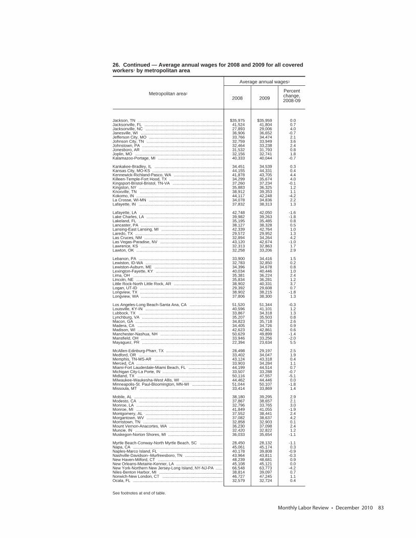
Monthly Labor Review • December 2010 83
26. Continued — Average annual wages for 2008 and 2009 for all coveredworkers1 by metropolitan area
Metropolitan area2
Average annual wages3
2008 2009Percentchange,2008-09
Jackson, TN ........................................................................... $35,975 $35,959 0.0Jacksonville, FL ..................................................................... 41,524 41,804 0.7Jacksonville, NC .................................................................... 27,893 29,006 4.0Janesville, WI ........................................................................ 36,906 36,652 -0.7Jefferson City, MO ................................................................. 33,766 34,474 2.1Johnson City, TN ................................................................... 32,759 33,949 3.6Johnstown, PA ....................................................................... 32,464 33,238 2.4Jonesboro, AR ....................................................................... 31,532 31,793 0.8Joplin, MO ............................................................................. 32,156 32,741 1.8Kalamazoo-Portage, MI ......................................................... 40,333 40,044 -0.7
Kankakee-Bradley, IL ............................................................ 34,451 34,539 0.3Kansas City, MO-KS .............................................................. 44,155 44,331 0.4Kennewick-Richland-Pasco, WA ........................................... 41,878 43,705 4.4Killeen-Temple-Fort Hood, TX ............................................... 34,299 35,674 4.0Kingsport-Bristol-Bristol, TN-VA ............................................ 37,260 37,234 -0.1Kingston, NY .......................................................................... 35,883 36,325 1.2Knoxville, TN ......................................................................... 38,912 39,353 1.1Kokomo, IN ............................................................................ 44,117 42,248 -4.2La Crosse, WI-MN ................................................................. 34,078 34,836 2.2Lafayette, IN .......................................................................... 37,832 38,313 1.3
Lafayette, LA ......................................................................... 42,748 42,050 -1.6Lake Charles, LA ................................................................... 39,982 39,263 -1.8Lakeland, FL .......................................................................... 35,195 35,485 0.8Lancaster, PA ........................................................................ 38,127 38,328 0.5Lansing-East Lansing, MI ...................................................... 42,339 42,764 1.0Laredo, TX ............................................................................. 29,572 29,952 1.3Las Cruces, NM ..................................................................... 32,894 34,264 4.2Las Vegas-Paradise, NV ....................................................... 43,120 42,674 -1.0Lawrence, KS ........................................................................ 32,313 32,863 1.7Lawton, OK ............................................................................ 32,258 33,206 2.9
Lebanon, PA .......................................................................... 33,900 34,416 1.5Lewiston, ID-WA .................................................................... 32,783 32,850 0.2Lewiston-Auburn, ME ............................................................ 34,396 34,678 0.8Lexington-Fayette, KY ........................................................... 40,034 40,446 1.0Lima, OH ............................................................................... 35,381 36,224 2.4Lincoln, NE ............................................................................ 35,834 36,281 1.2Little Rock-North Little Rock, AR ........................................... 38,902 40,331 3.7Logan, UT-ID ......................................................................... 29,392 29,608 0.7Longview, TX ......................................................................... 38,902 38,215 -1.8Longview, WA ........................................................................ 37,806 38,300 1.3
Los Angeles-Long Beach-Santa Ana, CA ............................. 51,520 51,344 -0.3Louisville, KY-IN .................................................................... 40,596 41,101 1.2Lubbock, TX .......................................................................... 33,867 34,318 1.3Lynchburg, VA ....................................................................... 35,207 35,503 0.8Macon, GA ............................................................................. 34,823 35,718 2.6Madera, CA ........................................................................... 34,405 34,726 0.9Madison, WI ........................................................................... 42,623 42,861 0.6Manchester-Nashua, NH ....................................................... 50,629 49,899 -1.4Mansfield, OH ........................................................................ 33,946 33,256 -2.0Mayaguez, PR ....................................................................... 22,394 23,634 5.5
McAllen-Edinburg-Pharr, TX .................................................. 28,498 29,197 2.5Medford, OR .......................................................................... 33,402 34,047 1.9Memphis, TN-MS-AR ............................................................ 43,124 43,318 0.4Merced, CA ............................................................................ 33,903 34,284 1.1Miami-Fort Lauderdale-Miami Beach, FL .............................. 44,199 44,514 0.7Michigan City-La Porte, IN ..................................................... 33,507 33,288 -0.7Midland, TX ........................................................................... 50,116 47,557 -5.1Milwaukee-Waukesha-West Allis, WI .................................... 44,462 44,446 0.0Minneapolis-St. Paul-Bloomington, MN-WI ........................... 51,044 50,107 -1.8Missoula, MT ......................................................................... 33,414 33,869 1.4
Mobile, AL .............................................................................. 38,180 39,295 2.9Modesto, CA .......................................................................... 37,867 38,657 2.1Monroe, LA ............................................................................ 32,796 33,765 3.0Monroe, MI ............................................................................ 41,849 41,055 -1.9Montgomery, AL .................................................................... 37,552 38,441 2.4Morgantown, WV ................................................................... 37,082 38,637 4.2Morristown, TN ...................................................................... 32,858 32,903 0.1Mount Vernon-Anacortes, WA ............................................... 36,230 37,098 2.4Muncie, IN ............................................................................. 32,420 32,822 1.2Muskegon-Norton Shores, MI ................................................ 36,033 35,654 -1.1
Myrtle Beach-Conway-North Myrtle Beach, SC .................... 28,450 28,132 -1.1Napa, CA ............................................................................... 45,061 45,174 0.3Naples-Marco Island, FL ....................................................... 40,178 39,808 -0.9Nashville-Davidson--Murfreesboro, TN ................................. 43,964 43,811 -0.3New Haven-Milford, CT ......................................................... 48,239 48,681 0.9New Orleans-Metairie-Kenner, LA ......................................... 45,108 45,121 0.0New York-Northern New Jersey-Long Island, NY-NJ-PA ...... 66,548 63,773 -4.2Niles-Benton Harbor, MI ........................................................ 38,814 39,097 0.7Norwich-New London, CT ..................................................... 46,727 47,245 1.1Ocala, FL ............................................................................... 32,579 32,724 0.4
See footnotes at end of table.
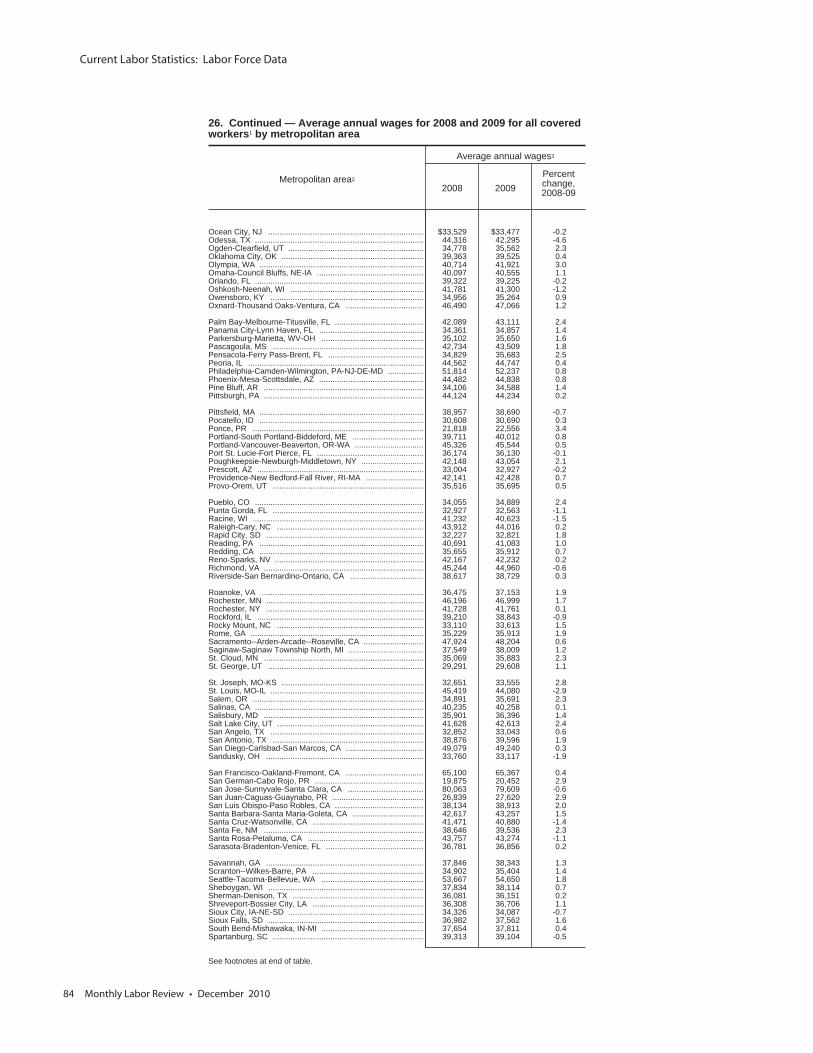
Current Labor Statistics: Labor Force Data
84 Monthly Labor Review • December 2010
26. Continued — Average annual wages for 2008 and 2009 for all coveredworkers1 by metropolitan area
Metropolitan area2
Average annual wages3
2008 2009Percentchange,2008-09
Ocean City, NJ ...................................................................... $33,529 $33,477 -0.2Odessa, TX ............................................................................ 44,316 42,295 -4.6Ogden-Clearfield, UT ............................................................. 34,778 35,562 2.3Oklahoma City, OK ................................................................ 39,363 39,525 0.4Olympia, WA .......................................................................... 40,714 41,921 3.0Omaha-Council Bluffs, NE-IA ................................................ 40,097 40,555 1.1Orlando, FL ............................................................................ 39,322 39,225 -0.2Oshkosh-Neenah, WI ............................................................ 41,781 41,300 -1.2Owensboro, KY ..................................................................... 34,956 35,264 0.9Oxnard-Thousand Oaks-Ventura, CA ................................... 46,490 47,066 1.2
Palm Bay-Melbourne-Titusville, FL ........................................ 42,089 43,111 2.4Panama City-Lynn Haven, FL ............................................... 34,361 34,857 1.4Parkersburg-Marietta, WV-OH .............................................. 35,102 35,650 1.6Pascagoula, MS .................................................................... 42,734 43,509 1.8Pensacola-Ferry Pass-Brent, FL ........................................... 34,829 35,683 2.5Peoria, IL ............................................................................... 44,562 44,747 0.4Philadelphia-Camden-Wilmington, PA-NJ-DE-MD ................ 51,814 52,237 0.8Phoenix-Mesa-Scottsdale, AZ ............................................... 44,482 44,838 0.8Pine Bluff, AR ........................................................................ 34,106 34,588 1.4Pittsburgh, PA ........................................................................ 44,124 44,234 0.2
Pittsfield, MA .......................................................................... 38,957 38,690 -0.7Pocatello, ID .......................................................................... 30,608 30,690 0.3Ponce, PR ............................................................................. 21,818 22,556 3.4Portland-South Portland-Biddeford, ME ................................ 39,711 40,012 0.8Portland-Vancouver-Beaverton, OR-WA ............................... 45,326 45,544 0.5Port St. Lucie-Fort Pierce, FL ................................................ 36,174 36,130 -0.1Poughkeepsie-Newburgh-Middletown, NY ............................ 42,148 43,054 2.1Prescott, AZ ........................................................................... 33,004 32,927 -0.2Providence-New Bedford-Fall River, RI-MA .......................... 42,141 42,428 0.7Provo-Orem, UT .................................................................... 35,516 35,695 0.5
Pueblo, CO ............................................................................ 34,055 34,889 2.4Punta Gorda, FL .................................................................... 32,927 32,563 -1.1Racine, WI ............................................................................. 41,232 40,623 -1.5Raleigh-Cary, NC .................................................................. 43,912 44,016 0.2Rapid City, SD ....................................................................... 32,227 32,821 1.8Reading, PA .......................................................................... 40,691 41,083 1.0Redding, CA .......................................................................... 35,655 35,912 0.7Reno-Sparks, NV ................................................................... 42,167 42,232 0.2Richmond, VA ........................................................................ 45,244 44,960 -0.6Riverside-San Bernardino-Ontario, CA ................................. 38,617 38,729 0.3
Roanoke, VA ......................................................................... 36,475 37,153 1.9Rochester, MN ....................................................................... 46,196 46,999 1.7Rochester, NY ....................................................................... 41,728 41,761 0.1Rockford, IL ........................................................................... 39,210 38,843 -0.9Rocky Mount, NC .................................................................. 33,110 33,613 1.5Rome, GA .............................................................................. 35,229 35,913 1.9Sacramento--Arden-Arcade--Roseville, CA ........................... 47,924 48,204 0.6Saginaw-Saginaw Township North, MI .................................. 37,549 38,009 1.2St. Cloud, MN ........................................................................ 35,069 35,883 2.3St. George, UT ...................................................................... 29,291 29,608 1.1
St. Joseph, MO-KS ................................................................ 32,651 33,555 2.8St. Louis, MO-IL ..................................................................... 45,419 44,080 -2.9Salem, OR ............................................................................. 34,891 35,691 2.3Salinas, CA ............................................................................ 40,235 40,258 0.1Salisbury, MD ........................................................................ 35,901 36,396 1.4Salt Lake City, UT .................................................................. 41,628 42,613 2.4San Angelo, TX ..................................................................... 32,852 33,043 0.6San Antonio, TX .................................................................... 38,876 39,596 1.9San Diego-Carlsbad-San Marcos, CA ................................... 49,079 49,240 0.3Sandusky, OH ....................................................................... 33,760 33,117 -1.9
San Francisco-Oakland-Fremont, CA ................................... 65,100 65,367 0.4San German-Cabo Rojo, PR ................................................. 19,875 20,452 2.9San Jose-Sunnyvale-Santa Clara, CA .................................. 80,063 79,609 -0.6San Juan-Caguas-Guaynabo, PR ......................................... 26,839 27,620 2.9San Luis Obispo-Paso Robles, CA ........................................ 38,134 38,913 2.0Santa Barbara-Santa Maria-Goleta, CA ................................ 42,617 43,257 1.5Santa Cruz-Watsonville, CA .................................................. 41,471 40,880 -1.4Santa Fe, NM ........................................................................ 38,646 39,536 2.3Santa Rosa-Petaluma, CA .................................................... 43,757 43,274 -1.1Sarasota-Bradenton-Venice, FL ............................................ 36,781 36,856 0.2
Savannah, GA ....................................................................... 37,846 38,343 1.3Scranton--Wilkes-Barre, PA .................................................. 34,902 35,404 1.4Seattle-Tacoma-Bellevue, WA .............................................. 53,667 54,650 1.8Sheboygan, WI ...................................................................... 37,834 38,114 0.7Sherman-Denison, TX ........................................................... 36,081 36,151 0.2Shreveport-Bossier City, LA .................................................. 36,308 36,706 1.1Sioux City, IA-NE-SD ............................................................. 34,326 34,087 -0.7Sioux Falls, SD ...................................................................... 36,982 37,562 1.6South Bend-Mishawaka, IN-MI .............................................. 37,654 37,811 0.4Spartanburg, SC .................................................................... 39,313 39,104 -0.5
See footnotes at end of table.
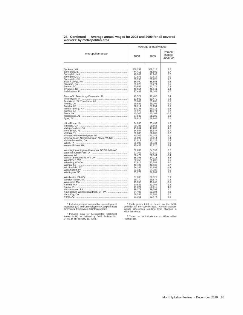
Monthly Labor Review • December 2010 85
26. Continued — Average annual wages for 2008 and 2009 for all coveredworkers1 by metropolitan area
Metropolitan area2
Average annual wages3
2008 2009Percentchange,2008-09
Spokane, WA ......................................................................... $36,792 $38,112 3.6Springfield, IL ......................................................................... 44,416 45,602 2.7Springfield, MA ...................................................................... 40,969 41,248 0.7Springfield, MO ...................................................................... 32,971 33,615 2.0Springfield, OH ...................................................................... 33,158 33,725 1.7State College, PA .................................................................. 38,050 38,658 1.6Stockton, CA .......................................................................... 39,075 39,274 0.5Sumter, SC ............................................................................ 30,842 31,074 0.8Syracuse, NY ......................................................................... 40,554 41,141 1.4Tallahassee, FL ..................................................................... 37,433 38,083 1.7
Tampa-St. Petersburg-Clearwater, FL .................................. 40,521 41,480 2.4Terre Haute, IN ...................................................................... 33,562 33,470 -0.3Texarkana, TX-Texarkana, AR .............................................. 35,002 35,288 0.8Toledo, OH ............................................................................ 39,686 39,098 -1.5Topeka, KS ............................................................................ 36,714 37,651 2.6Trenton-Ewing, NJ ................................................................. 60,135 59,313 -1.4Tucson, AZ ............................................................................ 39,973 40,071 0.2Tulsa, OK ............................................................................... 40,205 40,108 -0.2Tuscaloosa, AL ...................................................................... 37,949 38,309 0.9Tyler, TX ................................................................................ 38,817 38,845 0.1
Utica-Rome, NY ..................................................................... 34,936 35,492 1.6Valdosta, GA ......................................................................... 29,288 29,661 1.3Vallejo-Fairfield, CA ............................................................... 45,264 47,287 4.5Vero Beach, FL ...................................................................... 36,557 35,937 -1.7Victoria, TX ............................................................................ 39,888 38,608 -3.2Vineland-Millville-Bridgeton, NJ ............................................. 40,709 41,145 1.1Virginia Beach-Norfolk-Newport News, VA-NC ..................... 38,696 39,614 2.4Visalia-Porterville, CA ............................................................ 32,018 32,125 0.3Waco, TX ............................................................................... 35,698 36,731 2.9Warner Robins, GA ............................................................... 40,457 41,820 3.4
Washington-Arlington-Alexandria, DC-VA-MD-WV ............... 62,653 64,032 2.2Waterloo-Cedar Falls, IA ....................................................... 37,363 37,919 1.5Wausau, WI ........................................................................... 36,477 36,344 -0.4Weirton-Steubenville, WV-OH ............................................... 35,356 34,113 -3.5Wenatchee, WA ..................................................................... 30,750 31,200 1.5Wheeling, WV-OH ................................................................. 32,915 33,583 2.0Wichita, KS ............................................................................ 40,423 40,138 -0.7Wichita Falls, TX .................................................................... 34,185 33,698 -1.4Williamsport, PA .................................................................... 33,340 34,188 2.5Wilmington, NC ...................................................................... 35,278 36,204 2.6
Winchester, VA-WV ............................................................... 37,035 38,127 2.9Winston-Salem, NC ............................................................... 39,770 39,874 0.3Worcester, MA ....................................................................... 45,955 45,743 -0.5Yakima, WA ........................................................................... 30,821 31,366 1.8Yauco, PR ............................................................................. 19,821 20,619 4.0York-Hanover, PA .................................................................. 39,379 39,798 1.1Youngstown-Warren-Boardman, OH-PA ............................... 34,403 33,704 -2.0Yuba City, CA ........................................................................ 36,538 37,289 2.1Yuma, AZ ............................................................................... 31,351 32,474 3.6
1 Includes workers covered by UnemploymentInsurance (UI) and Unemployment Compensationfor Federal Employees (UCFE) programs.
2 Includes data for Metropolitan StatisticalAreas (MSA) as defined by OMB Bulletin No.04-03 as of February 18, 2004.
3 Each year’s total is based on the MSAdefinition for the specific year. Annual changesinclude differences resulting from changes inMSA definitions.
4 Totals do not include the six MSAs withinPuerto Rico.
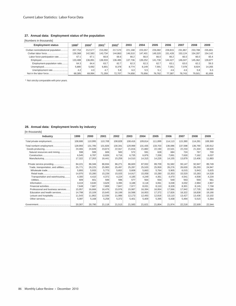
Current Labor Statistics: Labor Force Data
86 Monthly Labor Review • December 2010
27. Annual data: Employment status of the population [Numbers in thousands]
Employment status 19991 20001 20011 20021 2003 2004 2005 2006 2007 2008 2009
Civilian noninstitutional population........... 207,753 212,577 215,092 217,570 221,168 223,357 226,082 228,815 231,867 233,788 235,801 Civilian labor force............................…… 139,368 142,583 143,734 144,863 146,510 147,401 149,320 151,428 153,124 154,287 154,142 Labor force participation rate............... 67.1 67.1 66.8 66.6 66.2 66.0 66.0 66.2 66.0 66.0 65.4 Employed............................………… 133,488 136,891 136,933 136,485 137,736 139,252 141,730 144,427 146,047 145,362 139,877 Employment-population ratio.......... 64.3 64.4 63.7 62.7 62.3 62.3 62.7 63.1 63.0 62.2 59.3 Unemployed............................……… 5,880 5,692 6,801 8,378 8,774 8,149 7,591 7,001 7,078 8,924 14,265 Unemployment rate........................ 4.2 4.0 4.7 5.8 6.0 5.5 5.1 4.6 4.6 5.8 9.3 Not in the labor force............................… 68,385 69,994 71,359 72,707 74,658 75,956 76,762 77,387 78,743 79,501 81,659
1 Not strictly comparable with prior years.
28. Annual data: Employment levels by industry [In thousands]
Industry 1999 2000 2001 2002 2003 2004 2005 2006 2007 2008 2009
Total private employment............................… 108,686 110,995 110,708 108,828 108,416 109,814 111,899 114,113 115,380 114,281 108,369
Total nonfarm employment…………………… 128,993 131,785 131,826 130,341 129,999 131,435 133,703 136,086 137,598 136,790 130,912 Goods-producing............................………… 24,465 24,649 23,873 22,557 21,816 21,882 22,190 22,531 22,233 21,334 18,620 Natural resources and mining................. 598 599 606 583 572 591 628 684 724 767 700 Construction............................…………… 6,545 6,787 6,826 6,716 6,735 6,976 7,336 7,691 7,630 7,162 6,037 Manufacturing............................………… 17,322 17,263 16,441 15,259 14,510 14,315 14,226 14,155 13,879 13,406 11,883
Private service-providing.......................... 84,221 86,346 86,834 86,271 86,600 87,932 89,709 91,582 93,147 92,947 89,749 Trade, transportation, and utilities.......... 25,771 26,225 25,983 25,497 25,287 25,533 25,959 26,276 26,630 26,293 24,947 Wholesale trade............................……… 5,893 5,933 5,773 5,652 5,608 5,663 5,764 5,905 6,015 5,943 5,625 Retail trade............................………… 14,970 15,280 15,239 15,025 14,917 15,058 15,280 15,353 15,520 15,283 14,528 Transportation and warehousing......... 4,300 4,410 4,372 4,224 4,185 4,249 4,361 4,470 4,541 4,508 4,234 Utilities............................……………… 609 601 599 596 577 564 554 549 553 559 561 Information............................…………… 3,419 3,630 3,629 3,395 3,188 3,118 3,061 3,038 3,032 2,984 2,807 Financial activities............................…… 7,648 7,687 7,808 7,847 7,977 8,031 8,153 8,328 8,301 8,145 7,758 Professional and business services…… 15,957 16,666 16,476 15,976 15,987 16,394 16,954 17,566 17,942 17,735 16,580 Education and health services………… 14,798 15,109 15,645 16,199 16,588 16,953 17,372 17,826 18,322 18,838 19,190 Leisure and hospitality…………………… 11,543 11,862 12,036 11,986 12,173 12,493 12,816 13,110 13,427 13,436 13,102 Other services…………………………… 5,087 5,168 5,258 5,372 5,401 5,409 5,395 5,438 5,494 5,515 5,364
Government…………………………………… 20,307 20,790 21,118 21,513 21,583 21,621 21,804 21,974 22,218 22,509 22,544
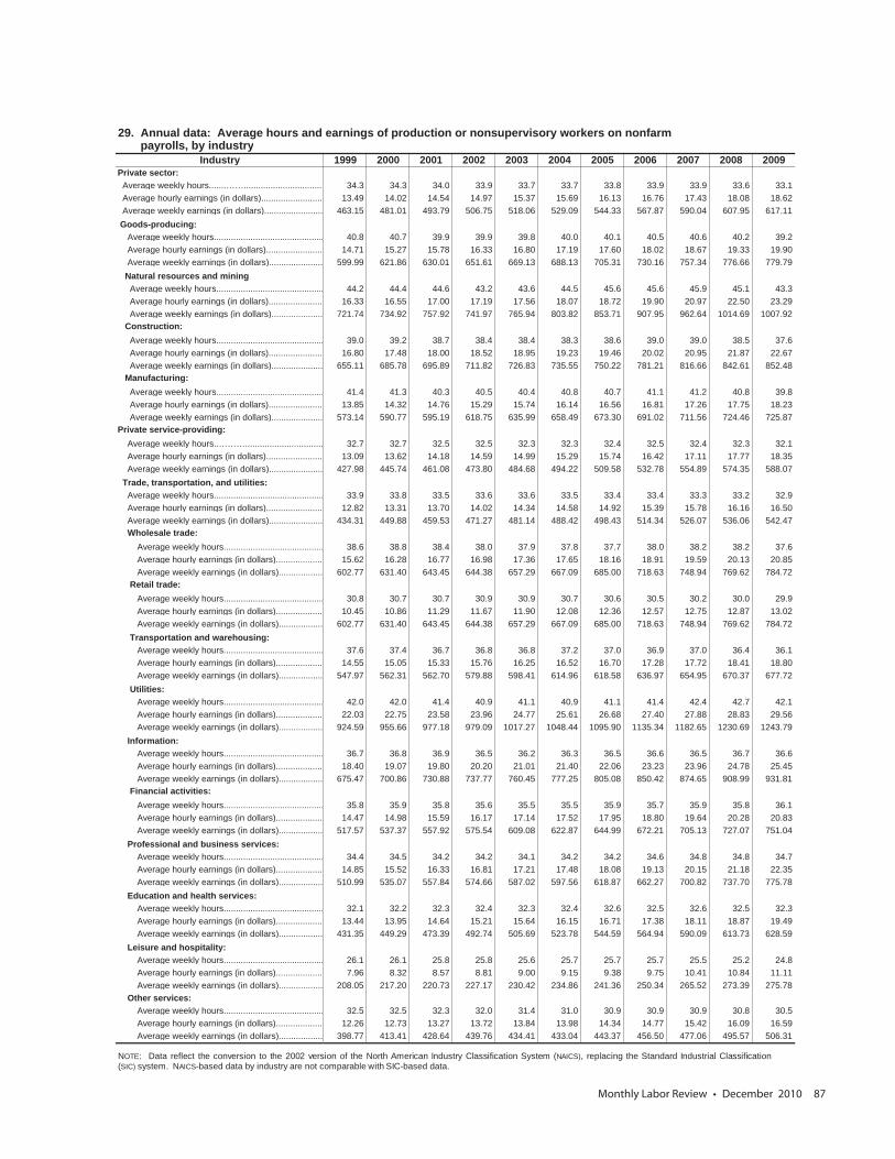
Monthly Labor Review • December 2010 87
29. Annual data: Average hours and earnings of production or nonsupervisory workers on nonfarm payrolls, by industry
Industry 1999 2000 2001 2002 2003 2004 2005 2006 2007 2008 2009Private sector: Average weekly hours.......……................................ 34.3 34.3 34.0 33.9 33.7 33.7 33.8 33.9 33.9 33.6 33.1 Average hourly earnings (in dollars)......................... 13.49 14.02 14.54 14.97 15.37 15.69 16.13 16.76 17.43 18.08 18.62 Average weekly earnings (in dollars)........................ 463.15 481.01 493.79 506.75 518.06 529.09 544.33 567.87 590.04 607.95 617.11 Goods-producing: Average weekly hours............................................. 40.8 40.7 39.9 39.9 39.8 40.0 40.1 40.5 40.6 40.2 39.2 Average hourly earnings (in dollars)....................... 14.71 15.27 15.78 16.33 16.80 17.19 17.60 18.02 18.67 19.33 19.90 Average weekly earnings (in dollars)...................... 599.99 621.86 630.01 651.61 669.13 688.13 705.31 730.16 757.34 776.66 779.79 Natural resources and mining Average weekly hours............................................ 44.2 44.4 44.6 43.2 43.6 44.5 45.6 45.6 45.9 45.1 43.3 Average hourly earnings (in dollars)...................... 16.33 16.55 17.00 17.19 17.56 18.07 18.72 19.90 20.97 22.50 23.29 Average weekly earnings (in dollars)..................... 721.74 734.92 757.92 741.97 765.94 803.82 853.71 907.95 962.64 1014.69 1007.92 Construction: Average weekly hours............................................ 39.0 39.2 38.7 38.4 38.4 38.3 38.6 39.0 39.0 38.5 37.6 Average hourly earnings (in dollars)...................... 16.80 17.48 18.00 18.52 18.95 19.23 19.46 20.02 20.95 21.87 22.67 Average weekly earnings (in dollars)..................... 655.11 685.78 695.89 711.82 726.83 735.55 750.22 781.21 816.66 842.61 852.48 Manufacturing: Average weekly hours............................................ 41.4 41.3 40.3 40.5 40.4 40.8 40.7 41.1 41.2 40.8 39.8 Average hourly earnings (in dollars)...................... 13.85 14.32 14.76 15.29 15.74 16.14 16.56 16.81 17.26 17.75 18.23 Average weekly earnings (in dollars)..................... 573.14 590.77 595.19 618.75 635.99 658.49 673.30 691.02 711.56 724.46 725.87Private service-providing: Average weekly hours..………................................ 32.7 32.7 32.5 32.5 32.3 32.3 32.4 32.5 32.4 32.3 32.1 Average hourly earnings (in dollars)....................... 13.09 13.62 14.18 14.59 14.99 15.29 15.74 16.42 17.11 17.77 18.35 Average weekly earnings (in dollars)...................... 427.98 445.74 461.08 473.80 484.68 494.22 509.58 532.78 554.89 574.35 588.07 Trade, transportation, and utilities: Average weekly hours............................................. 33.9 33.8 33.5 33.6 33.6 33.5 33.4 33.4 33.3 33.2 32.9 Average hourly earnings (in dollars)....................... 12.82 13.31 13.70 14.02 14.34 14.58 14.92 15.39 15.78 16.16 16.50 Average weekly earnings (in dollars)...................... 434.31 449.88 459.53 471.27 481.14 488.42 498.43 514.34 526.07 536.06 542.47 Wholesale trade: Average weekly hours......................................... 38.6 38.8 38.4 38.0 37.9 37.8 37.7 38.0 38.2 38.2 37.6 Average hourly earnings (in dollars)................... 15.62 16.28 16.77 16.98 17.36 17.65 18.16 18.91 19.59 20.13 20.85 Average weekly earnings (in dollars).................. 602.77 631.40 643.45 644.38 657.29 667.09 685.00 718.63 748.94 769.62 784.72 Retail trade: Average weekly hours......................................... 30.8 30.7 30.7 30.9 30.9 30.7 30.6 30.5 30.2 30.0 29.9 Average hourly earnings (in dollars)................... 10.45 10.86 11.29 11.67 11.90 12.08 12.36 12.57 12.75 12.87 13.02 Average weekly earnings (in dollars).................. 602.77 631.40 643.45 644.38 657.29 667.09 685.00 718.63 748.94 769.62 784.72 Transportation and warehousing: Average weekly hours......................................... 37.6 37.4 36.7 36.8 36.8 37.2 37.0 36.9 37.0 36.4 36.1 Average hourly earnings (in dollars)................... 14.55 15.05 15.33 15.76 16.25 16.52 16.70 17.28 17.72 18.41 18.80 Average weekly earnings (in dollars).................. 547.97 562.31 562.70 579.88 598.41 614.96 618.58 636.97 654.95 670.37 677.72 Utilities: Average weekly hours......................................... 42.0 42.0 41.4 40.9 41.1 40.9 41.1 41.4 42.4 42.7 42.1 Average hourly earnings (in dollars)................... 22.03 22.75 23.58 23.96 24.77 25.61 26.68 27.40 27.88 28.83 29.56 Average weekly earnings (in dollars).................. 924.59 955.66 977.18 979.09 1017.27 1048.44 1095.90 1135.34 1182.65 1230.69 1243.79 Information: Average weekly hours......................................... 36.7 36.8 36.9 36.5 36.2 36.3 36.5 36.6 36.5 36.7 36.6 Average hourly earnings (in dollars)................... 18.40 19.07 19.80 20.20 21.01 21.40 22.06 23.23 23.96 24.78 25.45 Average weekly earnings (in dollars).................. 675.47 700.86 730.88 737.77 760.45 777.25 805.08 850.42 874.65 908.99 931.81 Financial activities: Average weekly hours......................................... 35.8 35.9 35.8 35.6 35.5 35.5 35.9 35.7 35.9 35.8 36.1 Average hourly earnings (in dollars)................... 14.47 14.98 15.59 16.17 17.14 17.52 17.95 18.80 19.64 20.28 20.83 Average weekly earnings (in dollars).................. 517.57 537.37 557.92 575.54 609.08 622.87 644.99 672.21 705.13 727.07 751.04 Professional and business services: Average weekly hours......................................... 34.4 34.5 34.2 34.2 34.1 34.2 34.2 34.6 34.8 34.8 34.7 Average hourly earnings (in dollars)................... 14.85 15.52 16.33 16.81 17.21 17.48 18.08 19.13 20.15 21.18 22.35 Average weekly earnings (in dollars).................. 510.99 535.07 557.84 574.66 587.02 597.56 618.87 662.27 700.82 737.70 775.78 Education and health services: Average weekly hours......................................... 32.1 32.2 32.3 32.4 32.3 32.4 32.6 32.5 32.6 32.5 32.3 Average hourly earnings (in dollars)................... 13.44 13.95 14.64 15.21 15.64 16.15 16.71 17.38 18.11 18.87 19.49 Average weekly earnings (in dollars).................. 431.35 449.29 473.39 492.74 505.69 523.78 544.59 564.94 590.09 613.73 628.59 Leisure and hospitality: Average weekly hours......................................... 26.1 26.1 25.8 25.8 25.6 25.7 25.7 25.7 25.5 25.2 24.8 Average hourly earnings (in dollars)................... 7.96 8.32 8.57 8.81 9.00 9.15 9.38 9.75 10.41 10.84 11.11 Average weekly earnings (in dollars).................. 208.05 217.20 220.73 227.17 230.42 234.86 241.36 250.34 265.52 273.39 275.78 Other services: Average weekly hours......................................... 32.5 32.5 32.3 32.0 31.4 31.0 30.9 30.9 30.9 30.8 30.5 Average hourly earnings (in dollars)................... 12.26 12.73 13.27 13.72 13.84 13.98 14.34 14.77 15.42 16.09 16.59 Average weekly earnings (in dollars).................. 398.77 413.41 428.64 439.76 434.41 433.04 443.37 456.50 477.06 495.57 506.31
NOTE: Data reflect the conversion to the 2002 version of the North American Industry Classification System (NAICS), replacing the Standard Industrial Classification(SIC) system. NAICS-based data by industry are not comparable with SIC-based data.
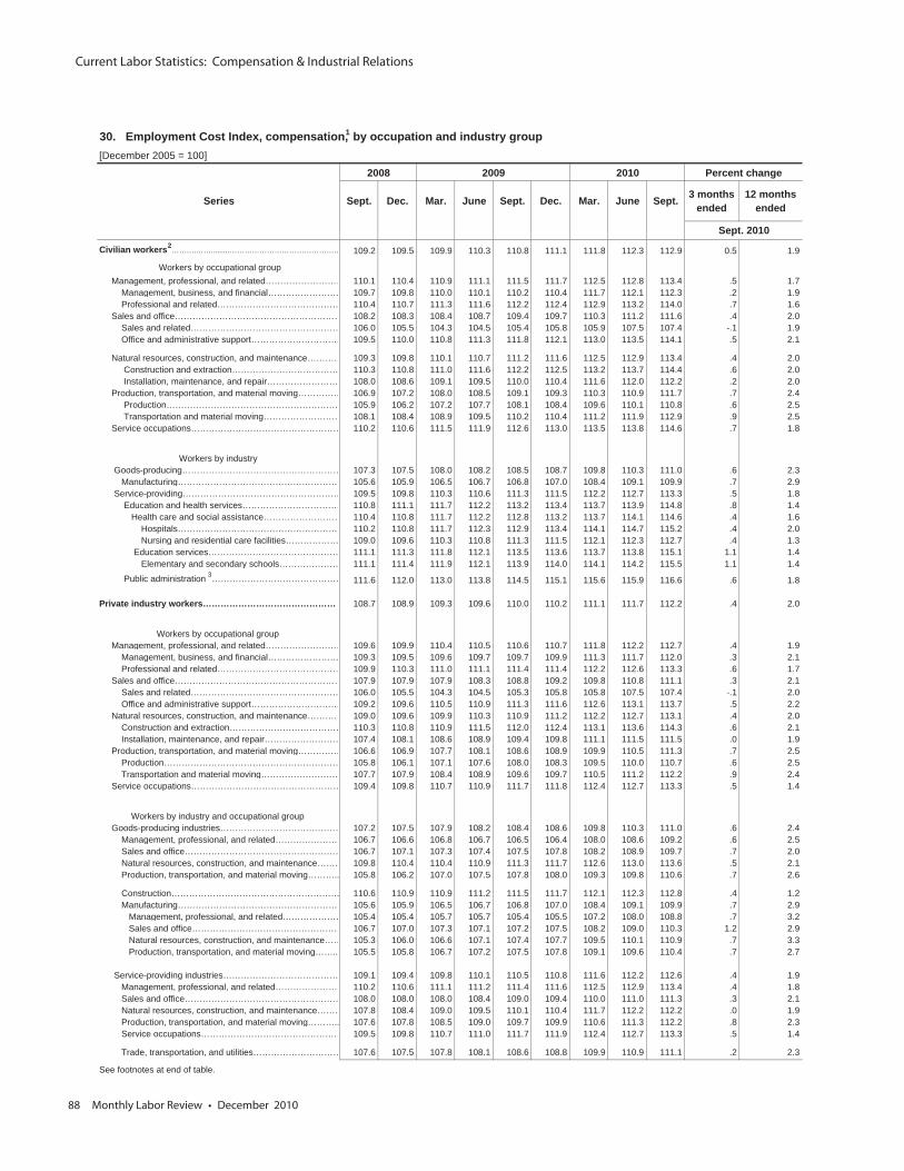
Current Labor Statistics: Compensation & Industrial Relations
88 Monthly Labor Review • December 2010
30. Employment Cost Index, compensation,1 by occupation and industry group[December 2005 = 100]
2008 2009 2010 Percent change
Series Sept. Dec. Mar. June Sept. Dec. Mar. June Sept. 3 monthsended
12 monthsended
Sept. 2010
Civilian workers2……….…….........…………………………………….… 109.2 109.5 109.9 110.3 110.8 111.1 111.8 112.3 112.9 0.5 1.9
Workers by occupational group Management, professional, and related……………………… 110.1 110.4 110.9 111.1 111.5 111.7 112.5 112.8 113.4 .5 1.7 Management, business, and financial…………………… 109.7 109.8 110.0 110.1 110.2 110.4 111.7 112.1 112.3 .2 1.9 Professional and related…………………………………… 110.4 110.7 111.3 111.6 112.2 112.4 112.9 113.2 114.0 .7 1.6 Sales and office………………………………………………… 108.2 108.3 108.4 108.7 109.4 109.7 110.3 111.2 111.6 .4 2.0 Sales and related…………………………………………… 106.0 105.5 104.3 104.5 105.4 105.8 105.9 107.5 107.4 -.1 1.9 Office and administrative support………………………… 109.5 110.0 110.8 111.3 111.8 112.1 113.0 113.5 114.1 .5 2.1
Natural resources, construction, and maintenance………… 109.3 109.8 110.1 110.7 111.2 111.6 112.5 112.9 113.4 .4 2.0 Construction and extraction……………………………… 110.3 110.8 111.0 111.6 112.2 112.5 113.2 113.7 114.4 .6 2.0 Installation, maintenance, and repair…………………… 108.0 108.6 109.1 109.5 110.0 110.4 111.6 112.0 112.2 .2 2.0 Production, transportation, and material moving…………… 106.9 107.2 108.0 108.5 109.1 109.3 110.3 110.9 111.7 .7 2.4 Production…………………………………………………… 105.9 106.2 107.2 107.7 108.1 108.4 109.6 110.1 110.8 .6 2.5 Transportation and material moving……………………… 108.1 108.4 108.9 109.5 110.2 110.4 111.2 111.9 112.9 .9 2.5 Service occupations…………………………………………… 110.2 110.6 111.5 111.9 112.6 113.0 113.5 113.8 114.6 .7 1.8
Workers by industry Goods-producing……………………………………………… 107.3 107.5 108.0 108.2 108.5 108.7 109.8 110.3 111.0 .6 2.3 Manufacturing………………………………………………… 105.6 105.9 106.5 106.7 106.8 107.0 108.4 109.1 109.9 .7 2.9 Service-providing……………………………………………… 109.5 109.8 110.3 110.6 111.3 111.5 112.2 112.7 113.3 .5 1.8 Education and health services…………………………… 110.8 111.1 111.7 112.2 113.2 113.4 113.7 113.9 114.8 .8 1.4 Health care and social assistance……………………… 110.4 110.8 111.7 112.2 112.8 113.2 113.7 114.1 114.6 .4 1.6 Hospitals………………………………………………… 110.2 110.8 111.7 112.3 112.9 113.4 114.1 114.7 115.2 .4 2.0 Nursing and residential care facilities……………… 109.0 109.6 110.3 110.8 111.3 111.5 112.1 112.3 112.7 .4 1.3 Education services……………………………………… 111.1 111.3 111.8 112.1 113.5 113.6 113.7 113.8 115.1 1.1 1.4 Elementary and secondary schools………………… 111.1 111.4 111.9 112.1 113.9 114.0 114.1 114.2 115.5 1.1 1.4
Public administration 3……………………………………… 111.6 112.0 113.0 113.8 114.5 115.1 115.6 115.9 116.6 .6 1.8
Private industry workers……………………………………… 108.7 108.9 109.3 109.6 110.0 110.2 111.1 111.7 112.2 .4 2.0
Workers by occupational group Management, professional, and related……………………… 109.6 109.9 110.4 110.5 110.6 110.7 111.8 112.2 112.7 .4 1.9 Management, business, and financial…………………… 109.3 109.5 109.6 109.7 109.7 109.9 111.3 111.7 112.0 .3 2.1 Professional and related…………………………………… 109.9 110.3 111.0 111.1 111.4 111.4 112.2 112.6 113.3 .6 1.7 Sales and office………………………………………………… 107.9 107.9 107.9 108.3 108.8 109.2 109.8 110.8 111.1 .3 2.1 Sales and related…………………………………………… 106.0 105.5 104.3 104.5 105.3 105.8 105.8 107.5 107.4 -.1 2.0 Office and administrative support………………………… 109.2 109.6 110.5 110.9 111.3 111.6 112.6 113.1 113.7 .5 2.2 Natural resources, construction, and maintenance………… 109.0 109.6 109.9 110.3 110.9 111.2 112.2 112.7 113.1 .4 2.0 Construction and extraction………………………………… 110.3 110.8 110.9 111.5 112.0 112.4 113.1 113.6 114.3 .6 2.1 Installation, maintenance, and repair……………………… 107.4 108.1 108.6 108.9 109.4 109.8 111.1 111.5 111.5 .0 1.9 Production, transportation, and material moving…………… 106.6 106.9 107.7 108.1 108.6 108.9 109.9 110.5 111.3 .7 2.5 Production…………………………………………………… 105.8 106.1 107.1 107.6 108.0 108.3 109.5 110.0 110.7 .6 2.5 Transportation and material moving……………………… 107.7 107.9 108.4 108.9 109.6 109.7 110.5 111.2 112.2 .9 2.4 Service occupations…………………………………………… 109.4 109.8 110.7 110.9 111.7 111.8 112.4 112.7 113.3 .5 1.4
Workers by industry and occupational group Goods-producing industries…………………………………… 107.2 107.5 107.9 108.2 108.4 108.6 109.8 110.3 111.0 .6 2.4 Management, professional, and related…………………… 106.7 106.6 106.8 106.7 106.5 106.4 108.0 108.6 109.2 .6 2.5 Sales and office……………………………………………… 106.7 107.1 107.3 107.4 107.5 107.8 108.2 108.9 109.7 .7 2.0 Natural resources, construction, and maintenance……… 109.8 110.4 110.4 110.9 111.3 111.7 112.6 113.0 113.6 .5 2.1 Production, transportation, and material moving……….. 105.8 106.2 107.0 107.5 107.8 108.0 109.3 109.8 110.6 .7 2.6
Construction………………………………………………… 110.6 110.9 110.9 111.2 111.5 111.7 112.1 112.3 112.8 .4 1.2 Manufacturing………………………………………………… 105.6 105.9 106.5 106.7 106.8 107.0 108.4 109.1 109.9 .7 2.9 Management, professional, and related………………… 105.4 105.4 105.7 105.7 105.4 105.5 107.2 108.0 108.8 .7 3.2 Sales and office…………………………………………… 106.7 107.0 107.3 107.1 107.2 107.5 108.2 109.0 110.3 1.2 2.9 Natural resources, construction, and maintenance…… 105.3 106.0 106.6 107.1 107.4 107.7 109.5 110.1 110.9 .7 3.3 Production, transportation, and material moving…….. 105.5 105.8 106.7 107.2 107.5 107.8 109.1 109.6 110.4 .7 2.7
Service-providing industries………………………………… 109.1 109.4 109.8 110.1 110.5 110.8 111.6 112.2 112.6 .4 1.9 Management, professional, and related…………………… 110.2 110.6 111.1 111.2 111.4 111.6 112.5 112.9 113.4 .4 1.8 Sales and office……………………………………………… 108.0 108.0 108.0 108.4 109.0 109.4 110.0 111.0 111.3 .3 2.1 Natural resources, construction, and maintenance……… 107.8 108.4 109.0 109.5 110.1 110.4 111.7 112.2 112.2 .0 1.9 Production, transportation, and material moving……….. 107.6 107.8 108.5 109.0 109.7 109.9 110.6 111.3 112.2 .8 2.3 Service occupations………………………………………… 109.5 109.8 110.7 111.0 111.7 111.9 112.4 112.7 113.3 .5 1.4
Trade, transportation, and utilities………………………… 107.6 107.5 107.8 108.1 108.6 108.8 109.9 110.9 111.1 .2 2.3
See footnotes at end of table.
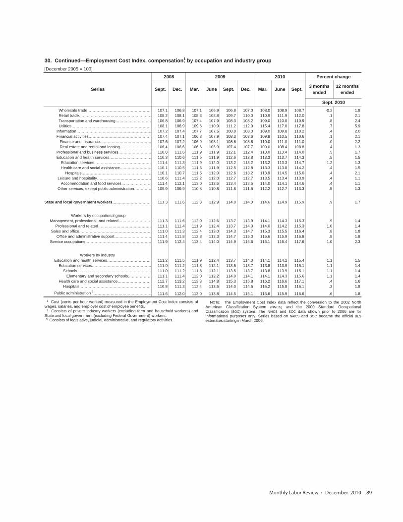
Monthly Labor Review • December 2010 89
30. Continued—Employment Cost Index, compensation,1 by occupation and industry group[December 2005 = 100]
2008 2009 2010 Percent change
Series Sept. Dec. Mar. June Sept. Dec. Mar. June Sept. 3 monthsended
12 monthsended
Sept. 2010 Wholesale trade…………………………………………… 107.1 106.8 107.1 106.9 106.8 107.0 108.0 108.9 108.7 -0.2 1.8 Retail trade………………………………………………… 108.2 108.1 108.3 108.8 109.7 110.0 110.9 111.9 112.0 .1 2.1 Transportation and warehousing……………………… 106.8 106.9 107.4 107.9 108.3 108.2 109.0 110.0 110.9 .8 2.4 Utilities……………………………………………………… 108.1 108.9 109.6 110.9 111.2 112.0 115.4 117.0 117.8 .7 5.9 Information………………………………………………… 107.2 107.4 107.7 107.5 108.0 108.3 109.0 109.8 110.2 .4 2.0 Financial activities………………………………………… 107.4 107.1 106.8 107.9 108.3 108.6 109.8 110.5 110.6 .1 2.1 Finance and insurance………………………………… 107.6 107.2 106.9 108.1 108.6 108.8 110.0 111.0 111.0 .0 2.2 Real estate and rental and leasing…………………… 106.4 106.6 106.6 106.9 107.4 107.7 109.0 108.4 108.8 .4 1.3 Professional and business services……………………… 110.8 111.6 111.9 111.9 112.1 112.4 113.0 113.4 114.0 .5 1.7 Education and health services…………………………… 110.3 110.6 111.5 111.9 112.6 112.8 113.3 113.7 114.3 .5 1.5 Education services……………………………………… 111.4 111.3 111.9 112.0 113.2 113.2 113.2 113.3 114.7 1.2 1.3 Health care and social assistance…………………… 110.1 110.5 111.5 111.9 112.5 112.8 113.3 113.8 114.2 .4 1.5 Hospitals……………………………………………… 110.1 110.7 111.5 112.0 112.6 113.2 113.9 114.5 115.0 .4 2.1 Leisure and hospitality…………………………………… 110.6 111.4 112.2 112.0 112.7 112.7 113.5 113.4 113.9 .4 1.1 Accommodation and food services…………………… 111.4 112.1 113.0 112.6 113.4 113.5 114.0 114.1 114.6 .4 1.1 Other services, except public administration…………… 109.9 109.9 110.8 110.8 111.8 111.5 112.2 112.7 113.3 .5 1.3
State and local government workers………………………… 111.3 111.6 112.3 112.9 114.0 114.3 114.6 114.9 115.9 .9 1.7
Workers by occupational group Management, professional, and related……………………… 111.3 111.6 112.0 112.6 113.7 113.9 114.1 114.3 115.3 .9 1.4 Professional and related…………………………………… 111.1 111.4 111.9 112.4 113.7 114.0 114.0 114.2 115.3 1.0 1.4 Sales and office………………………………………………… 111.0 111.3 112.4 113.0 114.3 114.7 115.3 115.5 116.4 .8 1.8 Office and administrative support………………………… 111.4 111.8 112.8 113.3 114.7 115.0 115.6 115.9 116.8 .8 1.8 Service occupations…………………………………………… 111.9 112.4 113.4 114.0 114.9 115.6 116.1 116.4 117.6 1.0 2.3
Workers by industry Education and health services……………………………… 111.2 111.5 111.9 112.4 113.7 114.0 114.1 114.2 115.4 1.1 1.5 Education services……………………………………… 111.0 111.2 111.8 112.1 113.5 113.7 113.8 113.9 115.1 1.1 1.4 Schools………………………………………………… 111.0 111.2 111.8 112.1 113.5 113.7 113.8 113.9 115.1 1.1 1.4 Elementary and secondary schools……………… 111.1 111.4 112.0 112.2 114.0 114.1 114.1 114.3 115.6 1.1 1.4 Health care and social assistance……………………… 112.7 113.2 113.3 114.8 115.3 115.8 116.2 116.6 117.1 .4 1.6 Hospitals………………………………………………… 110.8 111.3 112.4 113.5 114.0 114.5 115.2 115.8 116.1 .3 1.8
Public administration 3……………………………………… 111.6 112.0 113.0 113.8 114.5 115.1 115.6 115.9 116.6 .6 1.8
1 Cost (cents per hour worked) measured in the Employment Cost Index consists ofwages, salaries, and employer cost of employee benefits.
2 Consists of private industry workers (excluding farm and household workers) andState and local government (excluding Federal Government) workers.3 Consists of legislative, judicial, administrative, and regulatory activities.
NOTE: The Employment Cost Index data reflect the conversion to the 2002 NorthAmerican Classification System (NAICS) and the 2000 Standard OccupationalClassification (SOC) system. The NAICS and SOC data shown prior to 2006 are forinformational purposes only. Series based on NAICS and SOC became the official BLSestimates starting in March 2006.
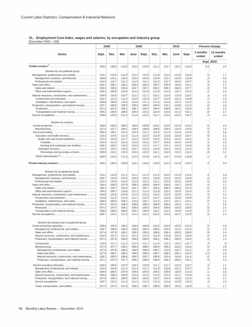
Current Labor Statistics: Compensation & Industrial Relations
90 Monthly Labor Review • December 2010
31. Employment Cost Index, wages and salaries, by occupation and industry group[December 2005 = 100]
2008 2009 2010 Percent change
Series Sept. Dec. Mar. June Sept. Dec. Mar. June Sept. 3 monthsended
12 monthsended
Sept. 2010Civilian workers1
……….…….........…………………………………….… 109.3 109.6 110.0 110.4 110.9 111.2 111.7 112.2 112.6 0.4 1.5
Workers by occupational group Management, professional, and related……………………… 110.1 110.5 111.0 111.2 111.5 111.8 112.5 112.8 113.4 .5 1.7 Management, business, and financial…………………… 109.8 110.1 110.4 110.5 110.6 110.9 112.1 112.6 112.8 .2 2.0 Professional and related…………………………………… 110.3 110.7 111.2 111.5 112.1 112.2 112.7 113.0 113.7 .6 1.4 Sales and office………………………………………………… 108.1 108.1 108.1 108.6 109.2 109.7 109.9 110.8 111.1 .3 1.7 Sales and related…………………………………………… 106.3 105.6 104.3 104.7 105.7 106.2 106.2 108.0 107.7 -.3 1.9 Office and administrative support………………………… 109.3 109.8 110.6 111.2 111.6 111.9 112.3 112.7 113.3 .5 1.5
Natural resources, construction, and maintenance………… 109.9 110.6 110.7 111.2 111.7 112.1 112.6 112.9 113.2 .3 1.3 Construction and extraction……………………………… 110.7 111.3 111.4 111.8 112.3 112.7 112.8 113.3 113.8 .4 1.3 Installation, maintenance, and repair…………………… 108.8 109.6 110.0 110.5 111.1 111.5 112.3 112.4 112.5 .1 1.3 Production, transportation, and material moving…………… 107.7 108.0 108.5 109.0 109.6 109.9 110.1 110.6 111.3 .6 1.6 Production…………………………………………………… 107.2 107.5 108.2 108.7 109.2 109.4 109.8 110.1 110.6 .5 1.3 Transportation and material moving……………………… 108.2 108.5 108.8 109.5 110.2 110.4 110.6 111.2 112.1 .8 1.7 Service occupations…………………………………………… 109.9 110.3 111.2 111.6 112.4 112.7 113.0 113.2 113.7 .4 1.2
Workers by industry Goods-producing……………………………………………… 108.6 109.0 109.2 109.5 109.8 110.1 110.5 110.9 111.5 .5 1.5 Manufacturing………………………………………………… 107.4 107.7 108.1 108.4 108.6 108.9 109.4 110.0 110.6 .5 1.8 Service-providing……………………………………………… 109.4 109.7 110.2 110.5 111.1 111.4 111.9 112.4 112.9 .4 1.6 Education and health services…………………………… 110.2 110.5 111.0 111.4 112.3 112.6 112.8 113.0 113.7 .6 1.2 Health care and social assistance……………………… 110.4 110.9 111.7 112.2 112.8 113.2 113.6 114.0 114.3 .3 1.3 Hospitals………………………………………………… 110.5 111.3 112.0 112.6 113.2 113.7 114.0 114.6 114.9 .3 1.5 Nursing and residential care facilities……………… 109.1 109.7 110.3 110.9 111.4 111.7 112.1 112.3 112.6 .3 1.1 Education services……………………………………… 110.0 110.2 110.5 110.7 111.8 112.0 112.2 112.3 113.2 .8 1.3 Elementary and secondary schools………………… 109.9 110.1 110.4 110.5 112.0 112.1 112.3 112.5 113.4 .8 1.2
Public administration 2……………………………………… 109.9 110.4 111.3 112.3 112.8 113.3 113.7 113.9 113.8 -.1 .9
Private industry workers……………………………………… 109.1 109.4 109.8 110.1 110.6 110.9 111.4 111.9 112.4 .4 1.6
Workers by occupational group Management, professional, and related……………………… 110.1 110.5 111.1 111.1 111.3 111.5 112.5 112.9 113.4 .4 1.9 Management, business, and financial…………………… 109.7 110.0 110.3 110.3 110.4 110.8 112.0 112.6 112.8 .2 2.2 Professional and related…………………………………… 110.4 110.9 111.6 111.8 112.1 112.1 112.8 113.2 113.9 .6 1.6 Sales and office………………………………………………… 108.0 108.0 107.9 108.3 109.0 109.4 109.6 110.7 110.9 .2 1.7 Sales and related…………………………………………… 106.4 105.7 104.3 104.7 105.7 106.2 106.2 108.0 107.8 -.2 2.0 Office and administrative support………………………… 109.2 109.7 110.6 111.1 111.4 111.8 112.2 112.6 113.3 .6 1.7 Natural resources, construction, and maintenance………… 109.8 110.5 110.6 111.0 111.6 112.0 112.5 112.8 113.1 .3 1.3 Construction and extraction………………………………… 110.8 111.5 111.4 111.7 112.3 112.7 112.9 113.3 113.9 .5 1.4 Installation, maintenance, and repair……………………… 108.5 109.3 109.7 110.2 110.7 111.2 112.1 112.1 112.1 .0 1.3 Production, transportation, and material moving…………… 107.5 107.8 108.3 108.8 109.4 109.6 109.8 110.3 111.1 .7 1.6 Production…………………………………………………… 107.2 107.4 108.1 108.5 109.0 109.3 109.6 110.0 110.5 .5 1.4 Transportation and material moving……………………… 108.0 108.3 108.5 109.2 109.9 110.1 110.2 110.8 111.8 .9 1.7 Service occupations…………………………………………… 109.7 110.1 111.0 111.2 112.1 112.3 112.6 112.7 113.3 .5 1.1
Workers by industry and occupational group Goods-producing industries…………………………………… 108.6 109.0 109.2 109.5 109.8 110.0 110.5 110.9 111.5 .5 1.5 Management, professional, and related…………………… 108.7 108.8 109.3 109.3 109.4 109.4 110.5 111.0 111.5 .5 1.9 Sales and office……………………………………………… 107.6 107.9 108.1 108.3 108.4 108.8 108.4 108.9 109.9 .9 1.4 Natural resources, construction, and maintenance……… 110.5 111.3 111.1 111.4 111.9 112.3 112.6 112.9 113.5 .5 1.4 Production, transportation, and material moving……….. 107.3 107.6 108.0 108.5 108.9 109.1 109.4 109.9 110.4 .5 1.4
Construction………………………………………………… 110.6 111.1 111.2 111.4 111.7 111.9 112.1 112.2 112.7 .4 .9 Manufacturing………………………………………………… 107.4 107.7 108.1 108.4 108.6 108.9 109.4 110.0 110.6 .5 1.8 Management, professional, and related………………… 107.6 107.8 108.4 108.5 108.6 108.7 110.0 110.7 111.2 .5 2.4 Sales and office…………………………………………… 107.6 108.1 108.2 108.2 108.3 108.7 108.3 109.1 110.4 1.2 1.9 Natural resources, construction, and maintenance…… 108.1 109.0 108.8 109.2 109.7 109.9 110.4 110.9 111.4 .5 1.5 Production, transportation, and material moving…….. 107.1 107.3 107.7 108.2 108.6 108.9 109.2 109.6 110.1 .5 1.4
Service-providing industries………………………………… 109.3 109.6 110.0 110.3 110.8 111.1 111.7 112.3 112.7 .4 1.7 Management, professional, and related…………………… 110.3 110.8 111.4 111.5 111.7 111.9 112.8 113.2 113.7 .4 1.8 Sales and office……………………………………………… 108.0 108.0 107.9 108.3 109.0 109.5 109.8 110.9 111.0 .1 1.8 Natural resources, construction, and maintenance……… 108.6 109.3 109.9 110.5 111.2 111.6 112.5 112.7 112.6 -.1 1.3 Production, transportation, and material moving……….. 107.8 108.1 108.6 109.3 110.0 110.2 110.4 110.9 111.9 .9 1.7 Service occupations………………………………………… 109.7 110.1 111.0 111.3 112.2 112.3 112.6 112.8 113.3 .4 1.0
Trade, transportation, and utilities………………………… 107.5 107.4 107.8 108.2 108.7 108.9 109.5 110.5 110.6 .1 1.7
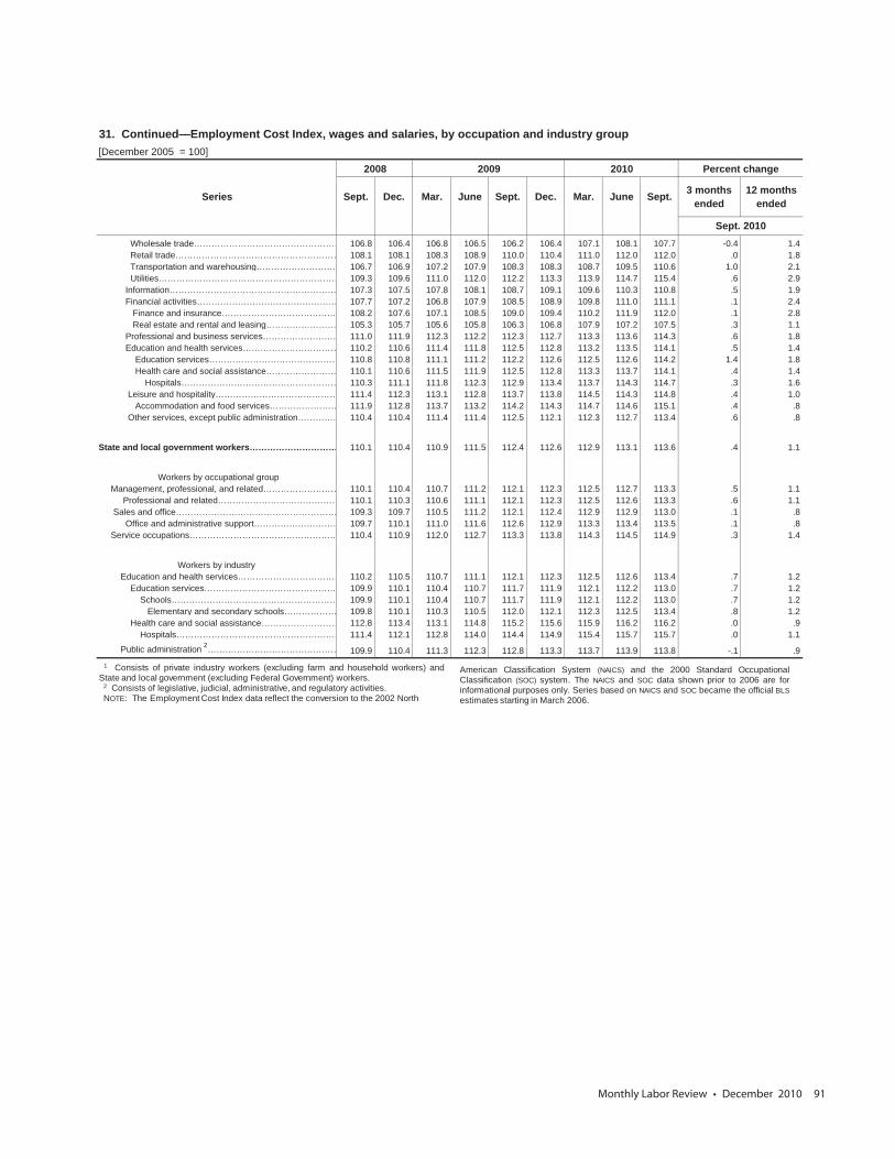
Monthly Labor Review • December 2010 91
31. Continued—Employment Cost Index, wages and salaries, by occupation and industry group[December 2005 = 100]
2008 2009 2010 Percent change
Series Sept. Dec. Mar. June Sept. Dec. Mar. June Sept. 3 monthsended
12 monthsended
Sept. 2010 Wholesale trade…………………………………………… 106.8 106.4 106.8 106.5 106.2 106.4 107.1 108.1 107.7 -0.4 1.4 Retail trade………………………………………………… 108.1 108.1 108.3 108.9 110.0 110.4 111.0 112.0 112.0 .0 1.8 Transportation and warehousing……………………… 106.7 106.9 107.2 107.9 108.3 108.3 108.7 109.5 110.6 1.0 2.1 Utilities……………………………………………………… 109.3 109.6 111.0 112.0 112.2 113.3 113.9 114.7 115.4 .6 2.9 Information………………………………………………… 107.3 107.5 107.8 108.1 108.7 109.1 109.6 110.3 110.8 .5 1.9 Financial activities………………………………………… 107.7 107.2 106.8 107.9 108.5 108.9 109.8 111.0 111.1 .1 2.4 Finance and insurance………………………………… 108.2 107.6 107.1 108.5 109.0 109.4 110.2 111.9 112.0 .1 2.8 Real estate and rental and leasing…………………… 105.3 105.7 105.6 105.8 106.3 106.8 107.9 107.2 107.5 .3 1.1 Professional and business services……………………… 111.0 111.9 112.3 112.2 112.3 112.7 113.3 113.6 114.3 .6 1.8 Education and health services…………………………… 110.2 110.6 111.4 111.8 112.5 112.8 113.2 113.5 114.1 .5 1.4 Education services……………………………………… 110.8 110.8 111.1 111.2 112.2 112.6 112.5 112.6 114.2 1.4 1.8 Health care and social assistance…………………… 110.1 110.6 111.5 111.9 112.5 112.8 113.3 113.7 114.1 .4 1.4 Hospitals……………………………………………… 110.3 111.1 111.8 112.3 112.9 113.4 113.7 114.3 114.7 .3 1.6 Leisure and hospitality…………………………………… 111.4 112.3 113.1 112.8 113.7 113.8 114.5 114.3 114.8 .4 1.0 Accommodation and food services…………………… 111.9 112.8 113.7 113.2 114.2 114.3 114.7 114.6 115.1 .4 .8 Other services, except public administration…………… 110.4 110.4 111.4 111.4 112.5 112.1 112.3 112.7 113.4 .6 .8
State and local government workers………………………… 110.1 110.4 110.9 111.5 112.4 112.6 112.9 113.1 113.6 .4 1.1
Workers by occupational group Management, professional, and related……………………… 110.1 110.4 110.7 111.2 112.1 112.3 112.5 112.7 113.3 .5 1.1 Professional and related…………………………………… 110.1 110.3 110.6 111.1 112.1 112.3 112.5 112.6 113.3 .6 1.1 Sales and office………………………………………………… 109.3 109.7 110.5 111.2 112.1 112.4 112.9 112.9 113.0 .1 .8 Office and administrative support………………………… 109.7 110.1 111.0 111.6 112.6 112.9 113.3 113.4 113.5 .1 .8 Service occupations…………………………………………… 110.4 110.9 112.0 112.7 113.3 113.8 114.3 114.5 114.9 .3 1.4
Workers by industry Education and health services……………………………… 110.2 110.5 110.7 111.1 112.1 112.3 112.5 112.6 113.4 .7 1.2 Education services……………………………………… 109.9 110.1 110.4 110.7 111.7 111.9 112.1 112.2 113.0 .7 1.2 Schools………………………………………………… 109.9 110.1 110.4 110.7 111.7 111.9 112.1 112.2 113.0 .7 1.2 Elementary and secondary schools……………… 109.8 110.1 110.3 110.5 112.0 112.1 112.3 112.5 113.4 .8 1.2 Health care and social assistance……………………… 112.8 113.4 113.1 114.8 115.2 115.6 115.9 116.2 116.2 .0 .9 Hospitals………………………………………………… 111.4 112.1 112.8 114.0 114.4 114.9 115.4 115.7 115.7 .0 1.1
Public administration 2……………………………………… 109.9 110.4 111.3 112.3 112.8 113.3 113.7 113.9 113.8 -.1 .91 Consists of private industry workers (excluding farm and household workers) and
State and local government (excluding Federal Government) workers.2 Consists of legislative, judicial, administrative, and regulatory activities.NOTE: The Employment Cost Index data reflect the conversion to the 2002 North
American Classification System (NAICS) and the 2000 Standard OccupationalClassification (SOC) system. The NAICS and SOC data shown prior to 2006 are forinformational purposes only. Series based on NAICS and SOC became the official BLSestimates starting in March 2006.
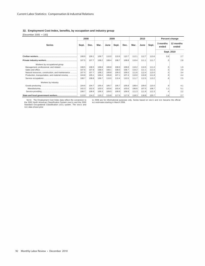
Current Labor Statistics: Compensation & Industrial Relations
92 Monthly Labor Review • December 2010
32. Employment Cost Index, benefits, by occupation and industry group[December 2005 = 100]
2008 2009 2010 Percent change
Series Sept. Dec. Mar. June Sept. Dec. Mar. June Sept. 3 monthsended
12 monthsended
Sept. 2010
Civilian workers…………………………………………………. 108.9 109.1 109.7 110.0 110.6 110.7 112.1 112.7 113.6 0.8 2.7
Private industry workers………………………………………… 107.5 107.7 108.2 108.4 108.7 108.8 110.4 111.1 111.7 .5 2.8
Workers by occupational group Management, professional, and related……………………… 108.5 108.5 108.8 108.8 108.9 108.8 110.2 110.5 111.0 .5 1.9 Sales and office………………………………………………… 107.6 107.8 108.0 108.1 108.5 108.7 110.2 111.1 111.6 .5 2.9 Natural resources, construction, and maintenance………… 107.5 107.7 108.2 108.8 109.3 109.5 111.6 112.4 113.0 .5 3.4 Production, transportation, and material moving…………… 104.8 105.1 106.4 106.8 107.1 107.4 110.0 110.8 111.8 .9 4.4 Service occupations…………………………………………… 108.7 108.8 109.7 110.0 110.4 110.5 111.7 112.5 113.2 .6 2.5
Workers by industry Goods-producing……………………………………………… 104.6 104.7 105.4 105.7 105.7 105.8 108.4 109.0 110.0 .9 4.1 Manufacturing………………………………………………… 102.3 102.5 103.5 103.6 103.4 103.6 106.6 107.5 108.7 1.1 5.1 Service-providing……………………………………………… 108.7 108.9 109.3 109.5 109.9 109.9 111.3 111.9 112.3 .4 2.2
State and local government workers………………………… 113.9 114.2 115.2 115.8 117.5 117.9 118.3 118.8 120.7 1.6 2.7
NOTE: The Employment Cost Index data reflect the conversion tothe 2002 North American Classification System (NAICS) and the 2000Standard Occupational Classification (SOC) system. The NAICS andSOC data shown prior
to 2006 are for informational purposes only. Series based on NAICS and SOC became the officialBLS estimates starting in March 2006.
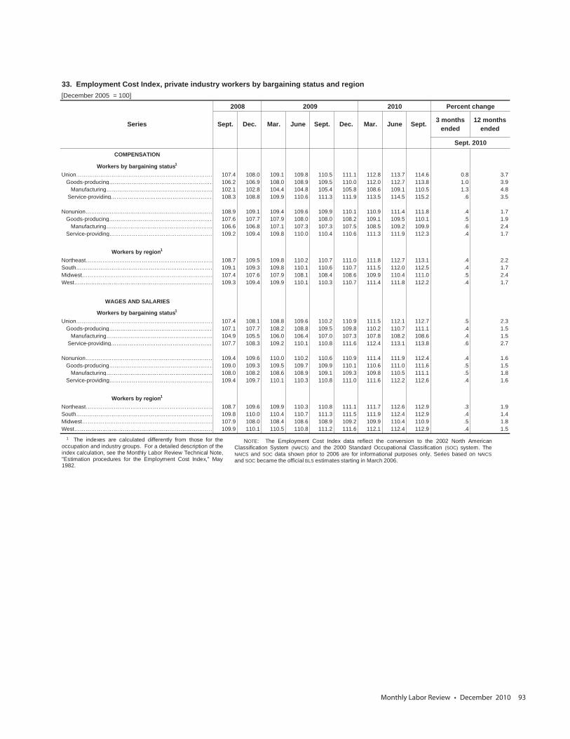
Monthly Labor Review • December 2010 93
33. Employment Cost Index, private industry workers by bargaining status and region[December 2005 = 100]
2008 2009 2010 Percent change
Series Sept. Dec. Mar. June Sept. Dec. Mar. June Sept. 3 monthsended
12 monthsended
Sept. 2010
COMPENSATION
Workers by bargaining status1
Union………………………………………………………………… 107.4 108.0 109.1 109.8 110.5 111.1 112.8 113.7 114.6 0.8 3.7 Goods-producing………………………………………………… 106.2 106.9 108.0 108.9 109.5 110.0 112.0 112.7 113.8 1.0 3.9 Manufacturing………………………………………………… 102.1 102.8 104.4 104.8 105.4 105.8 108.6 109.1 110.5 1.3 4.8 Service-providing………………………………………………… 108.3 108.8 109.9 110.6 111.3 111.9 113.5 114.5 115.2 .6 3.5
Nonunion…………………………………………………………… 108.9 109.1 109.4 109.6 109.9 110.1 110.9 111.4 111.8 .4 1.7 Goods-producing………………………………………………… 107.6 107.7 107.9 108.0 108.0 108.2 109.1 109.5 110.1 .5 1.9 Manufacturing………………………………………………… 106.6 106.8 107.1 107.3 107.3 107.5 108.5 109.2 109.9 .6 2.4 Service-providing………………………………………………… 109.2 109.4 109.8 110.0 110.4 110.6 111.3 111.9 112.3 .4 1.7
Workers by region1
Northeast…………………………………………………………… 108.7 109.5 109.8 110.2 110.7 111.0 111.8 112.7 113.1 .4 2.2South………………………………………………………………… 109.1 109.3 109.8 110.1 110.6 110.7 111.5 112.0 112.5 .4 1.7Midwest……………………………………………………………… 107.4 107.6 107.9 108.1 108.4 108.6 109.9 110.4 111.0 .5 2.4West………………………………………………………………… 109.3 109.4 109.9 110.1 110.3 110.7 111.4 111.8 112.2 .4 1.7
WAGES AND SALARIES
Workers by bargaining status1
Union………………………………………………………………… 107.4 108.1 108.8 109.6 110.2 110.9 111.5 112.1 112.7 .5 2.3 Goods-producing………………………………………………… 107.1 107.7 108.2 108.8 109.5 109.8 110.2 110.7 111.1 .4 1.5 Manufacturing………………………………………………… 104.9 105.5 106.0 106.4 107.0 107.3 107.8 108.2 108.6 .4 1.5 Service-providing………………………………………………… 107.7 108.3 109.2 110.1 110.8 111.6 112.4 113.1 113.8 .6 2.7
Nonunion…………………………………………………………… 109.4 109.6 110.0 110.2 110.6 110.9 111.4 111.9 112.4 .4 1.6 Goods-producing………………………………………………… 109.0 109.3 109.5 109.7 109.9 110.1 110.6 111.0 111.6 .5 1.5 Manufacturing………………………………………………… 108.0 108.2 108.6 108.9 109.1 109.3 109.8 110.5 111.1 .5 1.8 Service-providing………………………………………………… 109.4 109.7 110.1 110.3 110.8 111.0 111.6 112.2 112.6 .4 1.6
Workers by region1
Northeast…………………………………………………………… 108.7 109.6 109.9 110.3 110.8 111.1 111.7 112.6 112.9 .3 1.9South………………………………………………………………… 109.8 110.0 110.4 110.7 111.3 111.5 111.9 112.4 112.9 .4 1.4Midwest……………………………………………………………… 107.9 108.0 108.4 108.6 108.9 109.2 109.9 110.4 110.9 .5 1.8West………………………………………………………………… 109.9 110.1 110.5 110.8 111.2 111.6 112.1 112.4 112.9 .4 1.5
1 The indexes are calculated differently from those for theoccupation and industry groups. For a detailed description of theindex calculation, see the Monthly Labor Review Technical Note,"Estimation procedures for the Employment Cost Index," May1982.
NOTE: The Employment Cost Index data reflect the conversion to the 2002 North AmericanClassification System (NAICS) and the 2000 Standard Occupational Classification (SOC) system. TheNAICS and SOC data shown prior to 2006 are for informational purposes only. Series based on NAICSand SOC became the official BLS estimates starting in March 2006.
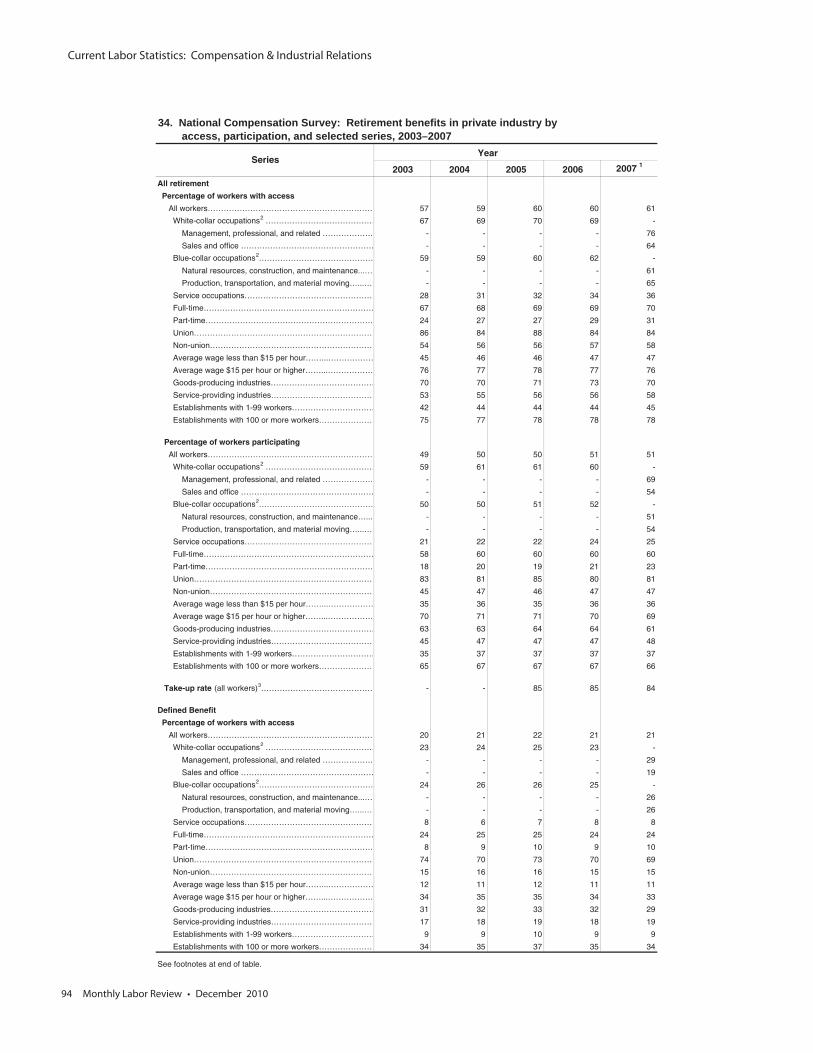
Current Labor Statistics: Compensation & Industrial Relations
94 Monthly Labor Review • December 2010
access, participation, and selected series, 2003–2007
2003 2004 2005 2006 2007 1
All retirement
Percentage of workers with access
All workers……………………………………………………… 57 59 60 60 61
White-collar occupations2 …………………………………… 67 69 70 69 -
Management, professional, and related ………………. - - - - 76
Sales and office …………………………………………… - - - - 64
Blue-collar occupations2……………………………………… 59 59 60 62 -
Natural resources, construction, and maintenance...… - - - - 61
Production, transportation, and material moving…...… - - - - 65
Service occupations…………………………………………… 28 31 32 34 36
Full-time………………………………………………………… 67 68 69 69 70
Part-time……………………………………………………… 24 27 27 29 31
Union…………………………………………………………… 86 84 88 84 84
Non-union……………………………………………………… 54 56 56 57 58
Average wage less than $15 per hour……...……………… 45 46 46 47 47
Average wage $15 per hour or higher……...……………… 76 77 78 77 76
Goods-producing industries………………………………… 70 70 71 73 70
Service-providing industries………………………………… 53 55 56 56 58
Establishments with 1-99 workers…………………………… 42 44 44 44 45
Establishments with 100 or more workers………………… 75 77 78 78 78
Percentage of workers participating
All workers……………………………………………………… 49 50 50 51 51
White-collar occupations2 …………………………………… 59 61 61 60 -
Management, professional, and related ………………. - - - - 69
Sales and office …………………………………………… - - - - 54
Blue-collar occupations2……………………………………… 50 50 51 52 -
Natural resources, construction, and maintenance…... - - - - 51
Production, transportation, and material moving…...… - - - - 54
Service occupations…………………………………………… 21 22 22 24 25
Full-time………………………………………………………… 58 60 60 60 60
Part-time……………………………………………………… 18 20 19 21 23
Union…………………………………………………………… 83 81 85 80 81
Non-union……………………………………………………… 45 47 46 47 47
Average wage less than $15 per hour……...……………… 35 36 35 36 36
Average wage $15 per hour or higher……...……………… 70 71 71 70 69
Goods-producing industries………………………………… 63 63 64 64 61
Service-providing industries………………………………… 45 47 47 47 48
Establishments with 1-99 workers…………………………… 35 37 37 37 37
Establishments with 100 or more workers………………… 65 67 67 67 66
Take-up rate (all workers)3…………………………………… - - 85 85 84
Defined Benefit
Percentage of workers with access
All workers……………………………………………………… 20 21 22 21 21
White-collar occupations2 …………………………………… 23 24 25 23 -
Management, professional, and related ………………. - - - - 29
Sales and office …………………………………………… - - - - 19
Blue-collar occupations2……………………………………… 24 26 26 25 -
Natural resources, construction, and maintenance...… - - - - 26
Production, transportation, and material moving…...… - - - - 26
Service occupations…………………………………………… 8 6 7 8 8
Full-time………………………………………………………… 24 25 25 24 24
Part-time……………………………………………………… 8 9 10 9 10
Union…………………………………………………………… 74 70 73 70 69
Non-union……………………………………………………… 15 16 16 15 15
Average wage less than $15 per hour……...……………… 12 11 12 11 11
Average wage $15 per hour or higher……...……………… 34 35 35 34 33
Goods-producing industries………………………………… 31 32 33 32 29
Service-providing industries………………………………… 17 18 19 18 19
Establishments with 1-99 workers…………………………… 9 9 10 9 9
Establishments with 100 or more workers………………… 34 35 37 35 34
See footnotes at end of table.
34. National Compensation Survey: Retirement benefits in private industry by
SeriesYear
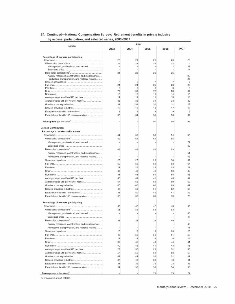
Monthly Labor Review • December 2010 95
by access, participation, and selected series, 2003–2007
2003 2004 2005 2006 2007 1
Percentage of workers participating All workers……………………………………………………… 20 21 21 20 20 White-collar occupations2 …………………………………… 22 24 24 22 - Management, professional, and related ………………. - - - - 28 Sales and office …………………………………………… - - - - 17 Blue-collar occupations2…………………………………… 24 25 26 25 - Natural resources, construction, and maintenance...… - - - - 25 Production, transportation, and material moving…...… - - - - 25 Service occupations………………………………………… 7 6 7 7 7 Full-time……………………………………………………… 24 24 25 23 23 Part-time……………………………………………………… 8 9 9 8 9 Union…………………………………………………………… 72 69 72 68 67 Non-union……………………………………………………… 15 15 15 14 15 Average wage less than $15 per hour……...……………… 11 11 11 10 10
Average wage $15 per hour or higher……...……………… 33 35 34 33 32
Goods-producing industries………………………………… 31 31 32 31 28
Service-providing industries………………………………… 16 18 18 17 18
Establishments with 1-99 workers………………………… 8 9 9 9 9
Establishments with 100 or more workers………………… 33 34 36 33 32
Take-up rate (all workers)3…………………………………… - - 97 96 95
Defined Contribution
Percentage of workers with access
All workers……………………………………………………… 51 53 53 54 55
White-collar occupations2 …………………………………… 62 64 64 65 -
Management, professional, and related ………………. - - - - 71
Sales and office …………………………………………… - - - - 60
Blue-collar occupations2…………………………………… 49 49 50 53 -
Natural resources, construction, and maintenance...… - - - - 51
Production, transportation, and material moving…...… - - - - 56
Service occupations………………………………………… 23 27 28 30 32
Full-time……………………………………………………… 60 62 62 63 64
Part-time……………………………………………………… 21 23 23 25 27
Union…………………………………………………………… 45 48 49 50 49
Non-union……………………………………………………… 51 53 54 55 56
Average wage less than $15 per hour……...……………… 40 41 41 43 44
Average wage $15 per hour or higher……...……………… 67 68 69 69 69
Goods-producing industries………………………………… 60 60 61 63 62
Service-providing industries………………………………… 48 50 51 52 53
Establishments with 1-99 workers………………………… 38 40 40 41 42
Establishments with 100 or more workers………………… 65 68 69 70 70
Percentage of workers participating
All workers……………………………………………………… 40 42 42 43 43
White-collar occupations2 …………………………………… 51 53 53 53 -
Management, professional, and related ………………. - - - - 60
Sales and office …………………………………………… - - - - 47
Blue-collar occupations2…………………………………… 38 38 38 40 -
Natural resources, construction, and maintenance...… - - - - 40
Production, transportation, and material moving…...… - - - - 41
Service occupations………………………………………… 16 18 18 20 20
Full-time……………………………………………………… 48 50 50 51 50
Part-time……………………………………………………… 14 14 14 16 18
Union…………………………………………………………… 39 42 43 44 41
Non-union……………………………………………………… 40 42 41 43 43
Average wage less than $15 per hour……...……………… 29 30 29 31 30
Average wage $15 per hour or higher……...……………… 57 59 59 58 57
Goods-producing industries………………………………… 49 49 50 51 49
Service-providing industries………………………………… 37 40 39 40 41
Establishments with 1-99 workers………………………… 31 32 32 33 33
Establishments with 100 or more workers………………… 51 53 53 54 53
Take-up rate (all workers)3…………………………………… - - 78 79 77
See footnotes at end of table.
34. Continued—National Compensation Survey: Retirement benefits in private industry
SeriesYear
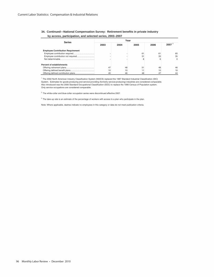
Current Labor Statistics: Compensation & Industrial Relations
96 Monthly Labor Review • December 2010
by access, participation, and selected series, 2003–2007
2003 2004 2005 2006 2007 1
Employee Contribution Requirement Employee contribution required………………………… - - 61 61 65 Employee contribution not required……………………… - - 31 33 35 Not determinable…………………………………………… - - 8 6 0
Percent of establishments Offering retirement plans…………………………………… 47 48 51 48 46 Offering defined benefit plans……………………………… 10 10 11 10 10 Offering defined contribution plans………………………. 45 46 48 47 44
1 The 2002 North American Industry Classification System (NAICS) replaced the 1987 Standard Industrial Classification (SIC) System. Estimates for goods-producing and service-providing (formerly service-producing) industries are considered comparable. Also introduced was the 2000 Standard Occupational Classification (SOC) to replace the 1990 Census of Population system. Only service occupations are considered comparable.
2 The white-collar and blue-collar occupation series were discontinued effective 2007.
3 The take-up rate is an estimate of the percentage of workers with access to a plan who participate in the plan. Note: Where applicable, dashes indicate no employees in this category or data do not meet publication criteria.
34. Continued—National Compensation Survey: Retirement benefits in private industry
SeriesYear
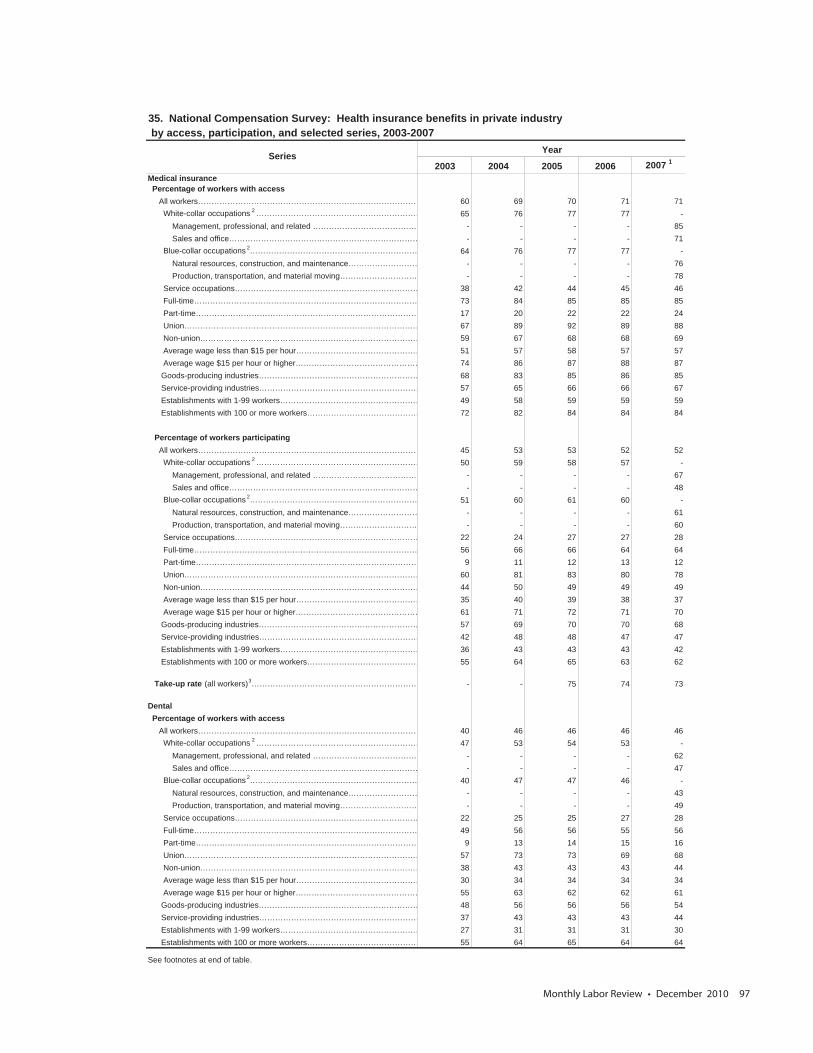
Monthly Labor Review • December 2010 97
by access, participation, and selected series, 2003-2007
2003 2004 2005 2006 2007 1
Medical insurance Percentage of workers with access All workers………………………………………………………………………… 60 69 70 71 71 White-collar occupations 2 ……………………………………………………… 65 76 77 77 - Management, professional, and related ………………………………… - - - - 85 Sales and office……………………………………………………………… - - - - 71 Blue-collar occupations 2……………………………………………………… 64 76 77 77 - Natural resources, construction, and maintenance……………………… - - - - 76 Production, transportation, and material moving………………………… - - - - 78 Service occupations…………………………………………………………… 38 42 44 45 46 Full-time………………………………………………………………………… 73 84 85 85 85 Part-time………………………………………………………………………… 17 20 22 22 24 Union……………………………………………………………………………… 67 89 92 89 88 Non-union………………………………………………………………………… 59 67 68 68 69 Average wage less than $15 per hour………………………………………… 51 57 58 57 57 Average wage $15 per hour or higher………………………………………… 74 86 87 88 87 Goods-producing industries…………………………………………………… 68 83 85 86 85 Service-providing industries…………………………………………………… 57 65 66 66 67 Establishments with 1-99 workers……………………………………………… 49 58 59 59 59 Establishments with 100 or more workers…………………………………… 72 82 84 84 84
Percentage of workers participating All workers………………………………………………………………………… 45 53 53 52 52 White-collar occupations 2 ……………………………………………………… 50 59 58 57 - Management, professional, and related ………………………………… - - - - 67 Sales and office……………………………………………………………… - - - - 48 Blue-collar occupations 2……………………………………………………… 51 60 61 60 - Natural resources, construction, and maintenance……………………… - - - - 61 Production, transportation, and material moving………………………… - - - - 60 Service occupations…………………………………………………………… 22 24 27 27 28 Full-time………………………………………………………………………… 56 66 66 64 64 Part-time………………………………………………………………………… 9 11 12 13 12 Union……………………………………………………………………………… 60 81 83 80 78 Non-union………………………………………………………………………… 44 50 49 49 49 Average wage less than $15 per hour………………………………………… 35 40 39 38 37 Average wage $15 per hour or higher………………………………………… 61 71 72 71 70 Goods-producing industries…………………………………………………… 57 69 70 70 68 Service-providing industries…………………………………………………… 42 48 48 47 47 Establishments with 1-99 workers……………………………………………… 36 43 43 43 42 Establishments with 100 or more workers…………………………………… 55 64 65 63 62
Take-up rate (all workers)3……………………………………………………… - - 75 74 73
Dental Percentage of workers with access All workers………………………………………………………………………… 40 46 46 46 46 White-collar occupations 2 ……………………………………………………… 47 53 54 53 - Management, professional, and related ………………………………… - - - - 62 Sales and office……………………………………………………………… - - - - 47 Blue-collar occupations 2……………………………………………………… 40 47 47 46 - Natural resources, construction, and maintenance……………………… - - - - 43 Production, transportation, and material moving………………………… - - - - 49 Service occupations…………………………………………………………… 22 25 25 27 28 Full-time………………………………………………………………………… 49 56 56 55 56 Part-time………………………………………………………………………… 9 13 14 15 16 Union……………………………………………………………………………… 57 73 73 69 68 Non-union………………………………………………………………………… 38 43 43 43 44 Average wage less than $15 per hour………………………………………… 30 34 34 34 34 Average wage $15 per hour or higher………………………………………… 55 63 62 62 61 Goods-producing industries…………………………………………………… 48 56 56 56 54 Service-providing industries…………………………………………………… 37 43 43 43 44 Establishments with 1-99 workers……………………………………………… 27 31 31 31 30 Establishments with 100 or more workers…………………………………… 55 64 65 64 64
See footnotes at end of table.
35. National Compensation Survey: Health insurance benefits in private industry
Series Year
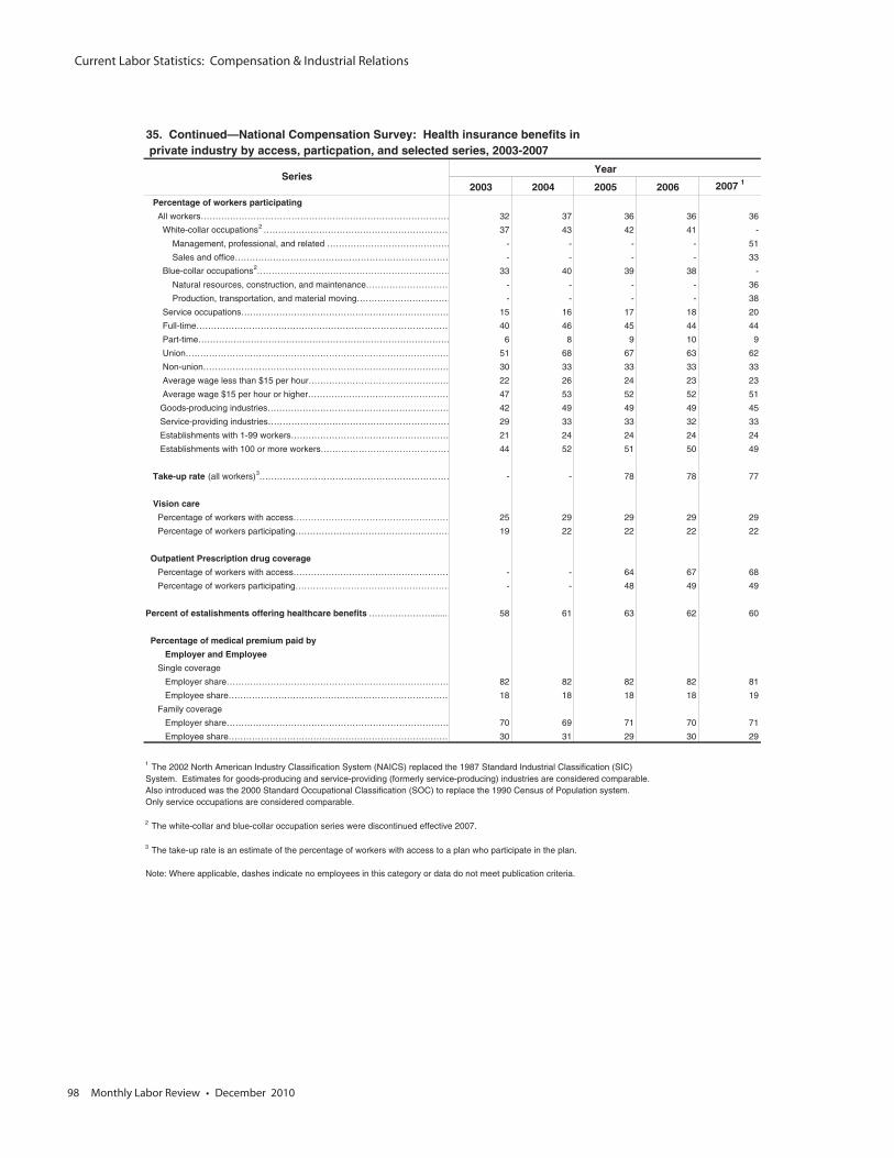
Current Labor Statistics: Compensation & Industrial Relations
98 Monthly Labor Review • December 2010
private industry by access, particpation, and selected series, 2003-2007
2003 2004 2005 2006 2007 1
Percentage of workers participating
All workers…………………………………………………………………………… 32 37 36 36 36
White-collar occupations2 ……………………………………………………… 37 43 42 41 -
Management, professional, and related …………………………………… - - - - 51
Sales and office………………………………………………………………… - - - - 33
Blue-collar occupations2………………………………………………………… 33 40 39 38 -
Natural resources, construction, and maintenance………………………… - - - - 36
Production, transportation, and material moving…………………………… - - - - 38
Service occupations……………………………………………………………… 15 16 17 18 20
Full-time…………………………………………………………………………… 40 46 45 44 44
Part-time…………………………………………………………………………… 6 8 9 10 9
Union……………………………………………………………………………… 51 68 67 63 62
Non-union………………………………………………………………………… 30 33 33 33 33
Average wage less than $15 per hour………………………………………… 22 26 24 23 23
Average wage $15 per hour or higher………………………………………… 47 53 52 52 51
Goods-producing industries……………………………………………………… 42 49 49 49 45
Service-providing industries……………………………………………………… 29 33 33 32 33
Establishments with 1-99 workers……………………………………………… 21 24 24 24 24
Establishments with 100 or more workers……………………………………… 44 52 51 50 49
Take-up rate (all workers)3………………………………………………………… - - 78 78 77
Vision care
Percentage of workers with access……………………………………………… 25 29 29 29 29
Percentage of workers participating……………………………………………… 19 22 22 22 22
Outpatient Prescription drug coverage
Percentage of workers with access……………………………………………… - - 64 67 68
Percentage of workers participating……………………………………………… - - 48 49 49
Percent of estalishments offering healthcare benefits …………………......… 58 61 63 62 60
Percentage of medical premium paid by
Employer and Employee
Single coverage
Employer share…………………………………………………………………… 82 82 82 82 81
Employee share………………………………………………………………… 18 18 18 18 19
Family coverage
Employer share…………………………………………………………………… 70 69 71 70 71
Employee share………………………………………………………………… 30 31 29 30 29
1 The 2002 North American Industry Classification System (NAICS) replaced the 1987 Standard Industrial Classification (SIC) System. Estimates for goods-producing and service-providing (formerly service-producing) industries are considered comparable. Also introduced was the 2000 Standard Occupational Classification (SOC) to replace the 1990 Census of Population system. Only service occupations are considered comparable.
2 The white-collar and blue-collar occupation series were discontinued effective 2007.
3 The take-up rate is an estimate of the percentage of workers with access to a plan who participate in the plan. Note: Where applicable, dashes indicate no employees in this category or data do not meet publication criteria.
35. Continued—National Compensation Survey: Health insurance benefits in
SeriesYear
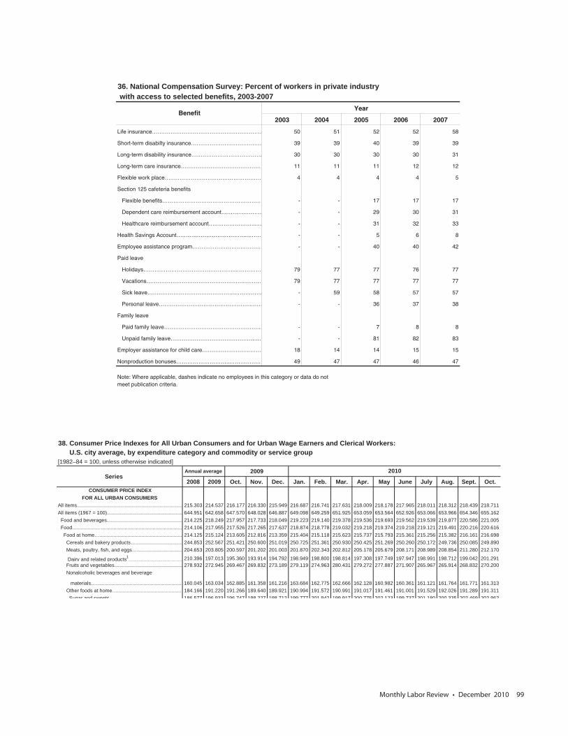
Monthly Labor Review • December 2010 99
with access to selected benefits, 2003-2007
2003 2004 2005 2006 2007
Life insurance…………………………………………………… 50 51 52 52 58
Short-term disabilty insurance………………………………… 39 39 40 39 39
Long-term disability insurance………………………………… 30 30 30 30 31
Long-term care insurance……………………………………… 11 11 11 12 12
Flexible work place……………………………………………… 4 4 4 4 5
Section 125 cafeteria benefits
Flexible benefits……………………………………………… - - 17 17 17
Dependent care reimbursement account…………..……… - - 29 30 31
Healthcare reimbursement account……………………...… - - 31 32 33
Health Savings Account………………………………...……… - - 5 6 8
Employee assistance program……………………….………… - - 40 40 42
Paid leave
Holidays…………………………………………...…………… 79 77 77 76 77
Vacations……………………………………………..……… 79 77 77 77 77
Sick leave………………………………………..…………… - 59 58 57 57
Personal leave…………………………………………..…… - - 36 37 38
Family leave
Paid family leave…………………………………………….… - - 7 8 8
Unpaid family leave………………………………………..… - - 81 82 83
Employer assistance for child care…………………….……… 18 14 14 15 15
Nonproduction bonuses………………………...……………… 49 47 47 46 47
Note: Where applicable, dashes indicate no employees in this category or data do not meet publication criteria.
36. National Compensation Survey: Percent of workers in private industry
YearBenefit
38. Consumer Price Indexes for All Urban Consumers and for Urban Wage Earners and Clerical Workers: U.S. city average, by expenditure category and commodity or service group[1982–84 = 100, unless otherwise indicated]
2009
2008 2009 Oct. Nov. Dec. Jan. Feb. Mar. Apr. May June July Aug. Sept. Oct.CONSUMER PRICE INDEX
FOR ALL URBAN CONSUMERSAll items........................................................................... 215.303 214.537 216.177 216.330 215.949 216.687 216.741 217.631 218.009 218.178 217.965 218.011 218.312 218.439 218.711All items (1967 = 100)...................................................... 644.951 642.658 647.570 648.028 646.887 649.098 649.259 651.925 653.059 653.564 652.926 653.066 653.966 654.346 655.162 Food and beverages...................................................... 214.225 218.249 217.957 217.733 218.049 219.223 219.140 219.378 219.536 219.693 219.562 219.539 219.877 220.586 221.005 Food..................…......................................................... 214.106 217.955 217.526 217.265 217.637 218.874 218.778 219.032 219.218 219.374 219.218 219.121 219.491 220.216 220.616 Food at home…........................................................... 214.125 215.124 213.605 212.816 213.359 215.404 215.118 215.623 215.737 215.793 215.361 215.256 215.382 216.161 216.698 Cereals and bakery products…................................. 244.853 252.567 251.421 250.600 251.019 250.725 251.361 250.930 250.425 251.269 250.260 250.172 249.736 250.085 249.890 Meats, poultry, fish, and eggs…................................ 204.653 203.805 200.597 201.202 201.003 201.870 202.343 202.812 205.178 205.679 208.171 208.989 208.854 211.280 212.170
Dairy and related products1……….…………………………210.396 197.013 195.360 193.914 194.792 198.949 198.800 198.814 197.308 197.749 197.947 198.991 198.712 199.042 201.291
Fruits and vegetables…............................................. 278.932 272.945 269.467 269.832 273.189 279.119 274.963 280.431 279.272 277.887 271.907 265.967 265.914 268.832 270.200 Nonalcoholic beverages and beverage
materials….............................................................. 160.045 163.034 162.885 161.358 161.216 163.684 162.775 162.666 162.128 160.982 160.361 161.121 161.764 161.771 161.313 Other foods at home…............................................... 184.166 191.220 191.266 189.640 189.921 190.994 191.572 190.991 191.017 191.461 191.001 191.529 192.026 191.289 191.311
Sugar and sweets 186 577 196 933 196 747 198 227 198 712 199 777 201 942 199 917 200 775 202 123 199 737 201 180 200 335 202 469 202 962
Annual average 2010Series
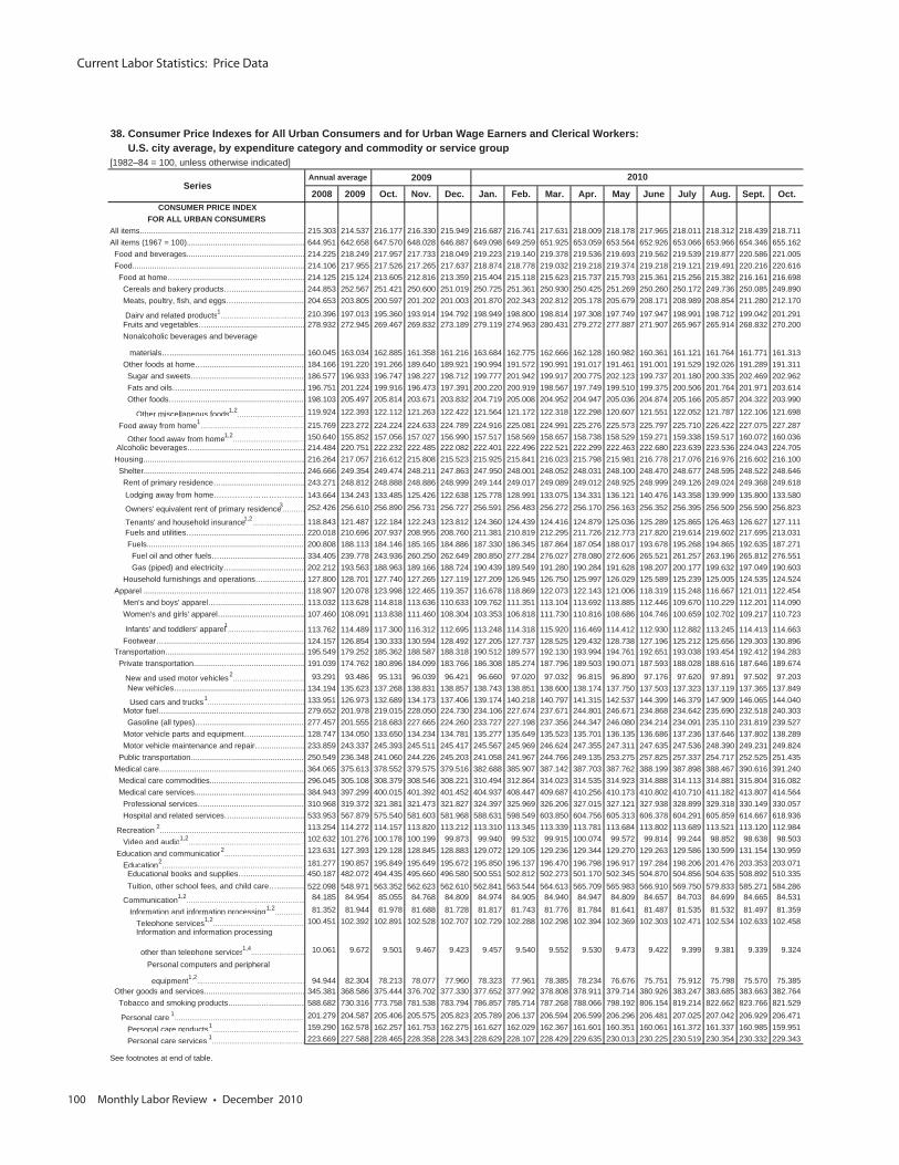
Current Labor Statistics: Price Data
100 Monthly Labor Review • December 2010
38. Consumer Price Indexes for All Urban Consumers and for Urban Wage Earners and Clerical Workers: U.S. city average, by expenditure category and commodity or service group[1982–84 = 100, unless otherwise indicated]
2009
2008 2009 Oct. Nov. Dec. Jan. Feb. Mar. Apr. May June July Aug. Sept. Oct.CONSUMER PRICE INDEX
FOR ALL URBAN CONSUMERSAll items........................................................................... 215.303 214.537 216.177 216.330 215.949 216.687 216.741 217.631 218.009 218.178 217.965 218.011 218.312 218.439 218.711All items (1967 = 100)...................................................... 644.951 642.658 647.570 648.028 646.887 649.098 649.259 651.925 653.059 653.564 652.926 653.066 653.966 654.346 655.162 Food and beverages...................................................... 214.225 218.249 217.957 217.733 218.049 219.223 219.140 219.378 219.536 219.693 219.562 219.539 219.877 220.586 221.005 Food..................…......................................................... 214.106 217.955 217.526 217.265 217.637 218.874 218.778 219.032 219.218 219.374 219.218 219.121 219.491 220.216 220.616 Food at home…........................................................... 214.125 215.124 213.605 212.816 213.359 215.404 215.118 215.623 215.737 215.793 215.361 215.256 215.382 216.161 216.698 Cereals and bakery products…................................. 244.853 252.567 251.421 250.600 251.019 250.725 251.361 250.930 250.425 251.269 250.260 250.172 249.736 250.085 249.890 Meats, poultry, fish, and eggs…................................ 204.653 203.805 200.597 201.202 201.003 201.870 202.343 202.812 205.178 205.679 208.171 208.989 208.854 211.280 212.170
Dairy and related products1……….…………………………210.396 197.013 195.360 193.914 194.792 198.949 198.800 198.814 197.308 197.749 197.947 198.991 198.712 199.042 201.291
Fruits and vegetables…............................................. 278.932 272.945 269.467 269.832 273.189 279.119 274.963 280.431 279.272 277.887 271.907 265.967 265.914 268.832 270.200 Nonalcoholic beverages and beverage
materials….............................................................. 160.045 163.034 162.885 161.358 161.216 163.684 162.775 162.666 162.128 160.982 160.361 161.121 161.764 161.771 161.313 Other foods at home…............................................... 184.166 191.220 191.266 189.640 189.921 190.994 191.572 190.991 191.017 191.461 191.001 191.529 192.026 191.289 191.311 Sugar and sweets…................................................. 186.577 196.933 196.747 198.227 198.712 199.777 201.942 199.917 200.775 202.123 199.737 201.180 200.335 202.469 202.962 Fats and oils…......................................................... 196.751 201.224 199.916 196.473 197.391 200.220 200.919 198.567 197.749 199.510 199.375 200.506 201.764 201.971 203.614 Other foods…........................................................... 198.103 205.497 205.814 203.671 203.832 204.719 205.008 204.952 204.947 205.036 204.874 205.166 205.857 204.322 203.990
Other miscellaneous foods1,2……….………………… 119.924 122.393 122.112 121.263 122.422 121.564 121.172 122.318 122.298 120.607 121.551 122.052 121.787 122.106 121.698
Food away from home 1……….………………………………… 215.769 223.272 224.224 224.633 224.789 224.916 225.081 224.991 225.276 225.573 225.797 225.710 226.422 227.075 227.287
Other food away from home1,2……….…………………… 150.640 155.852 157.056 157.027 156.990 157.517 158.569 158.657 158.738 158.529 159.271 159.338 159.517 160.072 160.036
Alcoholic beverages….................................................. 214.484 220.751 222.232 222.485 222.082 222.401 222.496 222.521 222.299 222.463 222.680 223.639 223.536 224.043 224.705 Housing.......................................................................... 216.264 217.057 216.612 215.808 215.523 215.925 215.841 216.023 215.798 215.981 216.778 217.076 216.976 216.602 216.100 Shelter...............…....................................................... 246.666 249.354 249.474 248.211 247.863 247.950 248.001 248.052 248.031 248.100 248.470 248.677 248.595 248.522 248.646 Rent of primary residence…...................................... 243.271 248.812 248.888 248.886 248.999 249.144 249.017 249.089 249.012 248.925 248.999 249.126 249.024 249.368 249.618 Lodging away from home………………………………143.664 134.243 133.485 125.426 122.638 125.778 128.991 133.075 134.331 136.121 140.476 143.358 139.999 135.800 133.580
Owners' equivalent rent of primary residence 3………. 252.426 256.610 256.890 256.731 256.727 256.591 256.483 256.272 256.170 256.163 256.352 256.395 256.509 256.590 256.823
Tenants' and household insurance 1,2……….…………… 118.843 121.487 122.184 122.243 123.812 124.360 124.439 124.416 124.879 125.036 125.289 125.865 126.463 126.627 127.111
Fuels and utilities…................................................... 220.018 210.696 207.937 208.955 208.760 211.381 210.819 212.295 211.726 212.773 217.820 219.614 219.602 217.695 213.031 Fuels...............…...................................................... 200.808 188.113 184.146 185.165 184.886 187.330 186.345 187.864 187.054 188.017 193.678 195.268 194.865 192.635 187.271 Fuel oil and other fuels…....................................... 334.405 239.778 243.936 260.250 262.649 280.850 277.284 276.027 278.080 272.606 265.521 261.257 263.196 265.812 276.551 Gas (piped) and electricity….................................. 202.212 193.563 188.963 189.166 188.724 190.439 189.549 191.280 190.284 191.628 198.207 200.177 199.632 197.049 190.603 Household furnishings and operations…................... 127.800 128.701 127.740 127.265 127.119 127.209 126.945 126.750 125.997 126.029 125.589 125.239 125.005 124.535 124.524 Apparel .......................................................................... 118.907 120.078 123.998 122.465 119.357 116.678 118.869 122.073 122.143 121.006 118.319 115.248 116.667 121.011 122.454 Men's and boys' apparel…......................................... 113.032 113.628 114.818 113.636 110.633 109.762 111.351 113.104 113.692 113.885 112.446 109.670 110.229 112.201 114.090 Women's and girls' apparel….................................... 107.460 108.091 113.838 111.460 108.304 103.353 106.818 111.730 110.816 108.686 104.746 100.659 102.702 109.217 110.723
Infants' and toddlers' apparel 1……….………………………113.762 114.489 117.300 116.312 112.695 113.248 114.318 115.920 116.469 114.412 112.930 112.882 113.245 114.413 114.663 Footwear…................................................................ 124.157 126.854 130.333 130.594 128.492 127.205 127.737 128.525 129.432 128.738 127.196 125.212 125.656 129.303 130.896 Transportation................................................................ 195.549 179.252 185.362 188.587 188.318 190.512 189.577 192.130 193.994 194.761 192.651 193.038 193.454 192.412 194.283 Private transportation...............…................................ 191.039 174.762 180.896 184.099 183.766 186.308 185.274 187.796 189.503 190.071 187.593 188.028 188.616 187.646 189.674
New and used motor vehicles 2……….…………………… 93.291 93.486 95.131 96.039 96.421 96.660 97.020 97.032 96.815 96.890 97.176 97.620 97.891 97.502 97.203 New vehicles…........................................................ 134.194 135.623 137.268 138.831 138.857 138.743 138.851 138.600 138.174 137.750 137.503 137.323 137.119 137.365 137.849
Used cars and trucks1……….………………………………133.951 126.973 132.689 134.173 137.406 139.174 140.218 140.797 141.315 142.537 144.399 146.379 147.909 146.065 144.040
Motor fuel…............................................................... 279.652 201.978 219.015 228.050 224.730 234.106 227.674 237.671 244.801 246.671 234.868 234.642 235.690 232.518 240.303 Gasoline (all types)…............................................... 277.457 201.555 218.683 227.665 224.260 233.727 227.198 237.356 244.347 246.080 234.214 234.091 235.110 231.819 239.527 Motor vehicle parts and equipment…........................ 128.747 134.050 133.650 134.234 134.781 135.277 135.649 135.523 135.701 136.135 136.686 137.236 137.646 137.802 138.289 Motor vehicle maintenance and repair…................... 233.859 243.337 245.393 245.511 245.417 245.567 245.969 246.624 247.355 247.311 247.635 247.536 248.390 249.231 249.824 Public transportation...............….................................. 250.549 236.348 241.060 244.226 245.203 241.058 241.967 244.766 249.135 253.275 257.825 257.337 254.717 252.525 251.435 Medical care................................................................... 364.065 375.613 378.552 379.575 379.516 382.688 385.907 387.142 387.703 387.762 388.199 387.898 388.467 390.616 391.240 Medical care commodities...............…......................... 296.045 305.108 308.379 308.546 308.221 310.494 312.864 314.023 314.535 314.923 314.888 314.113 314.881 315.804 316.082 Medical care services...............…................................ 384.943 397.299 400.015 401.392 401.452 404.937 408.447 409.687 410.256 410.173 410.802 410.710 411.182 413.807 414.564 Professional services…............................................. 310.968 319.372 321.381 321.473 321.827 324.397 325.969 326.206 327.015 327.121 327.938 328.899 329.318 330.149 330.057 Hospital and related services…................................. 533.953 567.879 575.540 581.603 581.968 588.631 598.549 603.850 604.756 605.313 606.378 604.291 605.859 614.667 618.936
Recreation 2……….………………………………………….………113.254 114.272 114.157 113.820 113.212 113.310 113.345 113.339 113.781 113.684 113.802 113.689 113.521 113.120 112.984
Video and audio1,2……….………………………………………102.632 101.276 100.178 100.199 99.873 99.940 99.532 99.915 100.074 99.572 99.814 99.244 98.852 98.638 98.503
Education and communication2……….……………………… 123.631 127.393 129.128 128.845 128.883 129.072 129.105 129.236 129.344 129.270 129.263 129.586 130.599 131.154 130.959
Education2……….………………………………………….………181.277 190.857 195.849 195.649 195.672 195.850 196.137 196.470 196.798 196.917 197.284 198.206 201.476 203.353 203.071
Educational books and supplies…........................... 450.187 482.072 494.435 495.660 496.580 500.551 502.812 502.273 501.170 502.345 504.870 504.856 504.635 508.892 510.335 Tuition, other school fees, and child care…............. 522.098 548.971 563.352 562.623 562.610 562.841 563.544 564.613 565.709 565.983 566.910 569.750 579.833 585.271 584.286
Communication1,2……….……………………………………… 84.185 84.954 85.055 84.768 84.809 84.974 84.905 84.940 84.947 84.809 84.657 84.703 84.699 84.665 84.531
Information and information processing1,2……….…… 81.352 81.944 81.978 81.688 81.728 81.817 81.743 81.776 81.784 81.641 81.487 81.535 81.532 81.497 81.359
Telephone services1,2……….…………………………… 100.451 102.392 102.891 102.528 102.707 102.729 102.288 102.298 102.394 102.369 102.303 102.471 102.534 102.633 102.458
Information and information processing
other than telephone services1,4……….…………… 10.061 9.672 9.501 9.467 9.423 9.457 9.540 9.552 9.530 9.473 9.422 9.399 9.381 9.339 9.324
Personal computers and peripheral
equipment1,2……….…………………………………… 94.944 82.304 78.213 78.077 77.960 78.323 77.961 78.385 78.234 76.676 75.751 75.912 75.798 75.570 75.385
Other goods and services.............................................. 345.381 368.586 375.444 376.702 377.330 377.652 377.992 378.808 378.911 379.714 380.926 383.247 383.685 383.663 382.764 Tobacco and smoking products...............…................ 588.682 730.316 773.758 781.538 783.794 786.857 785.714 787.268 788.066 798.192 806.154 819.214 822.662 823.766 821.529
Personal care 1……….………………………………………….…201.279 204.587 205.406 205.575 205.823 205.789 206.137 206.594 206.599 206.296 206.481 207.025 207.042 206.929 206.471
Personal care products1……….…………………………… 159.290 162.578 162.257 161.753 162.275 161.627 162.029 162.367 161.601 160.351 160.061 161.372 161.337 160.985 159.951
Personal care services 1……….…………………………… 223.669 227.588 228.465 228.358 228.343 228.629 228.107 228.429 229.635 230.013 230.225 230.519 230.354 230.332 229.343
See footnotes at end of table.
Annual average 2010Series
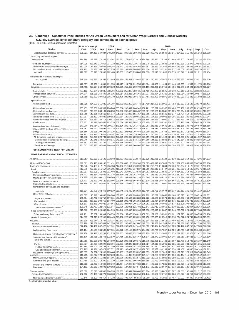
Monthly Labor Review • December 2010 101
38. Continued—Consumer Price Indexes for All Urban Consumers and for Urban Wage Earners and Clerical Workers U.S. city average, by expenditure category and commodity or service group[1982–84 = 100, unless otherwise indicated]
2009 20102008 2009 Oct. Nov. Dec. Jan. Feb. Mar. Apr. May June July Aug. Sept. Oct.
Miscellaneous personal services...............….... 338.921 344.469 347.834 348.792 348.697 349.605 350.780 352.028 352.779 353.522 353.941 354.533 355.429 355.964 356.508
Commodity and service group: Commodities...........…............................................ 174.764 169.698 172.252 173.061 172.572 173.646 173.419 174.798 175.333 175.333 173.899 173.503 173.925 174.282 175.225
Food and beverages…......................................... 214.225 218.249 217.957 217.733 218.049 219.223 219.140 219.378 219.536 219.693 219.562 219.539 219.877 220.586 221.005 Commodities less food and beverages…............. 153.034 144.395 148.037 149.245 148.441 149.439 149.162 150.953 151.621 151.559 149.648 149.116 149.558 149.761 150.882 Nondurables less food and beverages…............ 196.192 178.959 185.759 187.776 185.689 187.484 186.882 190.674 192.335 192.201 188.237 187.006 187.890 188.770 191.332 Apparel …......................................................... 118.907 120.078 123.998 122.465 119.357 116.678 118.869 122.073 122.143 121.006 118.319 115.248 116.667 121.011 122.454
Non durables less food, beverages, and apparel…................................................. 248.809 219.592 228.344 232.649 231.169 235.821 233.447 237.683 240.381 240.876 236.028 235.935 236.498 235.211 238.530
Durables….......................................................... 110.877 109.859 110.684 111.159 111.477 111.731 111.753 111.694 111.450 111.454 111.443 111.555 111.587 111.174 110.966 Services….............................................................. 255.498 259.154 259.844 259.323 259.055 259.459 259.792 260.196 260.420 260.756 261.756 262.241 262.421 262.320 261.927
Rent of shelter3……….…………………………………… 257.152 259.924 260.035 258.704 258.303 258.382 258.435 258.489 258.457 258.525 258.910 259.115 259.015 258.934 259.054
Transportation services….................................... 244.074 251.031 254.449 255.935 256.014 255.216 256.365 257.337 258.384 259.325 260.525 261.054 260.944 260.577 261.625 Other services….................................................. 295.780 303.992 307.011 306.740 306.436 306.916 307.171 307.451 308.493 308.870 309.349 310.033 311.443 311.802 311.375
Special indexes: All items less food…............................................ 215.528 214.008 215.986 216.207 215.703 216.362 216.440 217.430 217.839 218.010 217.788 217.857 218.147 218.179 218.431
All items less shelter…........................................ 205.453 203.301 205.567 206.286 205.888 206.892 206.948 208.181 208.722 208.932 208.486 208.469 208.925 209.133 209.467 All items less medical care…............................... 207.777 206.555 208.131 208.250 207.860 208.499 208.432 209.301 209.669 209.841 209.605 209.664 209.952 210.001 210.257 Commodities less food…..................................... 155.310 147.071 150.663 151.847 151.052 152.035 151.767 153.516 154.163 154.106 152.247 151.754 152.182 152.395 153.508 Nondurables less food…..................................... 197.297 181.453 187.939 189.852 187.864 189.578 189.015 192.601 194.159 194.041 190.306 189.196 190.025 190.885 193.344 Nondurables less food and apparel…................. 244.443 218.687 226.717 230.622 229.250 233.498 231.353 235.198 237.626 238.090 233.711 233.710 234.212 233.089 236.158 Nondurables…..................................................... 205.901 198.548 202.058 203.035 202.064 203.588 203.219 205.409 206.393 206.391 204.157 203.471 204.111 204.920 206.518
Services less rent of shelter 3……….………………… 273.000 278.064 279.545 280.014 279.896 280.730 281.432 282.297 282.851 283.541 285.371 286.238 286.775 286.640 285.588
Services less medical care services…................ 244.987 248.122 248.692 248.075 247.793 248.023 248.178 248.531 248.733 249.087 250.094 250.605 250.766 250.516 250.066 Energy….............................................................. 236.666 193.126 199.198 204.026 202.301 208.026 204.455 209.999 212.977 214.363 211.660 212.372 212.663 210.003 210.947 All items less energy…........................................ 214.751 218.433 219.624 219.291 219.048 219.287 219.708 220.133 220.252 220.298 220.336 220.316 220.619 221.030 221.236 All items less food and energy…....................... 215.572 219.235 220.731 220.384 220.025 220.086 220.602 221.059 221.166 221.193 221.265 221.258 221.551 221.907 222.079 Commodities less food and energy….............. 140.246 142.041 143.857 143.871 143.383 143.125 143.711 144.399 144.169 143.888 143.376 142.864 143.206 143.866 144.028 Energy commodities...................................... 284.352 205.281 221.749 231.226 228.186 238.069 231.735 241.239 248.165 249.680 238.032 237.602 238.702 235.797 243.784 Services less energy….................................... 261.017 265.875 267.081 266.488 266.237 266.519 266.967 267.248 267.587 267.829 268.308 268.655 268.903 269.034 269.208
CONSUMER PRICE INDEX FOR URBAN
WAGE EARNERS AND CLERICAL WORKERS
All items.................................................................... 211.053 209.630 211.549 212.003 211.703 212.568 212.544 213.525 213.958 214.124 213.839 213.898 214.205 214.306 214.623
All items (1967 = 100)............................................... 628.661 624.423 630.140 631.491 630.600 633.176 633.105 636.025 637.316 637.809 636.962 637.138 638.052 638.353 639.296 Food and beverages................................................ 213.546 217.480 217.123 216.853 217.186 218.354 218.299 218.502 218.730 218.844 218.730 218.784 219.175 219.817 220.199 Food..................….................................................. 213.376 217.118 216.654 216.305 216.679 217.900 217.837 218.066 218.319 218.427 218.291 218.276 218.696 219.376 219.736 Food at home….................................................... 213.017 213.908 212.396 211.488 212.041 214.049 213.839 214.291 214.498 214.501 214.143 214.212 214.392 215.058 215.511 Cereals and bakery products….......................... 245.472 253.214 252.049 251.376 251.570 251.195 251.757 251.493 251.031 251.920 250.742 250.670 250.327 250.654 250.429 Meats, poultry, fish, and eggs…......................... 204.255 203.394 200.210 200.709 200.623 201.411 202.139 202.540 204.878 205.228 207.883 208.784 208.676 211.109 211.978
Dairy and related products1……….……………………209.773 195.679 194.120 192.695 193.546 197.663 197.583 197.370 195.958 196.490 196.663 197.782 197.651 197.812 199.890
Fruits and vegetables…...................................... 276.759 270.562 267.084 267.049 270.279 276.025 271.974 277.347 276.727 275.080 269.040 263.715 263.946 266.461 267.466 Nonalcoholic beverages and beverage
materials…....................................................... 159.324 162.598 162.456 160.619 160.745 163.439 162.524 162.499 161.721 160.694 159.938 160.862 161.353 161.210 160.678 Other foods at home…....................................... 183.637 190.519 190.630 188.868 189.197 190.354 190.831 190.232 190.299 190.643 190.164 190.675 191.226 190.318 190.351 Sugar and sweets…......................................... 185.494 195.702 195.752 197.031 197.258 198.694 200.880 198.720 199.665 200.979 198.560 199.857 198.872 200.971 201.469 Fats and oils….................................................. 197.512 202.003 200.759 197.400 198.165 200.741 201.356 198.808 198.454 200.054 199.676 200.656 201.786 202.118 203.670 Other foods…................................................... 198.303 205.573 205.929 203.664 203.972 204.957 205.117 205.081 205.048 205.031 204.877 205.206 206.021 204.234 203.935
Other miscellaneous foods 1,2……….…………… 120.348 122.753 122.676 121.647 122.796 122.051 121.482 122.543 122.712 120.869 121.830 122.217 121.804 122.164 121.806
Food away from home 1……….……………………………215.613 223.383 224.382 224.815 224.940 225.015 225.168 225.072 225.395 225.657 225.846 225.707 226.481 227.188 227.412
Other food away from home 1,2……….………………149.731 155.607 156.909 156.853 156.830 157.670 158.826 159.023 159.088 158.901 159.601 159.725 159.866 160.755 160.988
Alcoholic beverages…........................................... 214.579 221.325 222.555 223.445 223.168 223.565 223.621 223.452 223.305 223.515 223.718 224.772 224.749 224.828 225.531
Housing.................................................................... 211.839 213.144 212.734 212.327 212.142 212.529 212.401 212.604 212.368 212.518 213.469 213.743 213.603 213.294 212.681 Shelter...............…................................................ 239.128 242.637 242.804 242.159 241.991 242.019 242.002 242.019 241.987 241.964 242.253 242.396 242.295 242.338 242.513 Rent of primary residence…............................... 242.196 247.401 247.422 247.361 247.465 247.574 247.448 247.555 247.474 247.352 247.389 247.442 247.250 247.589 247.823
Lodging away from home 2……….…………………… 143.164 135.163 134.586 127.061 124.222 127.150 130.571 134.632 135.793 137.067 142.529 145.768 140.967 136.488 134.787
Owners' equivalent rent of primary residence 3… 228.758 232.499 232.761 232.635 232.603 232.463 232.354 232.179 232.108 232.068 232.235 232.271 232.373 232.472 232.680
Tenants' and household insurance 1,2……….…… 119.136 121.935 122.761 122.830 124.415 125.299 125.367 125.374 125.872 126.051 126.345 126.950 127.526 127.718 128.130
Fuels and utilities…........................................... 217.883 209.595 206.732 207.530 207.329 209.691 209.171 210.775 210.326 211.426 217.007 218.770 218.703 216.787 211.649 Fuels...............….............................................. 197.537 186.229 182.227 182.994 182.701 184.843 183.918 185.557 184.918 185.946 192.105 193.671 193.259 191.066 185.262 Fuel oil and other fuels…................................ 331.784 243.003 246.153 262.340 265.130 284.061 281.157 279.384 280.770 274.630 267.671 263.269 264.904 267.283 278.516 Gas (piped) and electricity….......................... 200.265 191.981 187.473 187.572 187.125 188.607 187.730 189.595 188.837 190.233 197.258 199.162 198.640 196.143 189.313 Household furnishings and operations…............ 123.635 124.632 123.995 123.448 123.187 123.339 123.097 122.859 121.979 122.019 121.720 121.273 120.912 120.560 120.643 Apparel ................................................................... 118.735 119.847 123.642 122.228 118.984 116.310 118.607 121.347 121.293 120.267 117.630 114.464 115.600 119.942 121.587 Men's and boys' apparel…................................. 113.490 114.340 115.381 114.091 110.856 109.893 111.575 113.032 113.538 113.838 112.359 109.313 110.005 111.901 113.618 Women's and girls' apparel…............................. 107.489 107.602 113.290 111.039 107.819 102.860 106.496 110.885 109.783 107.882 103.952 99.600 101.483 108.532 110.474
Infants' and toddlers' apparel1……….……………… 116.266 117.202 119.949 119.272 115.754 117.028 117.789 119.644 120.106 117.881 116.509 116.291 116.066 116.688 117.250
Footwear…......................................................... 124.102 127.183 130.596 130.682 128.637 127.267 127.843 128.172 129.112 128.647 127.034 125.317 125.535 128.436 129.851
Transportation.......................................................... 195.692 176.729 183.506 186.928 186.839 189.544 188.406 191.294 193.320 194.079 191.587 192.051 192.657 191.517 193.553 Private transportation...............…......................... 192.492 173.491 180.271 183.680 183.565 186.457 185.268 188.146 190.106 190.768 188.088 188.577 189.261 188.152 190.259
New and used motor vehicles 2……….……………… 92.146 91.308 93.414 94.338 95.072 95.464 95.819 95.900 95.780 95.988 96.467 97.003 97.389 96.860 96.402
See footnotes at end of table.
Annual averageSeries
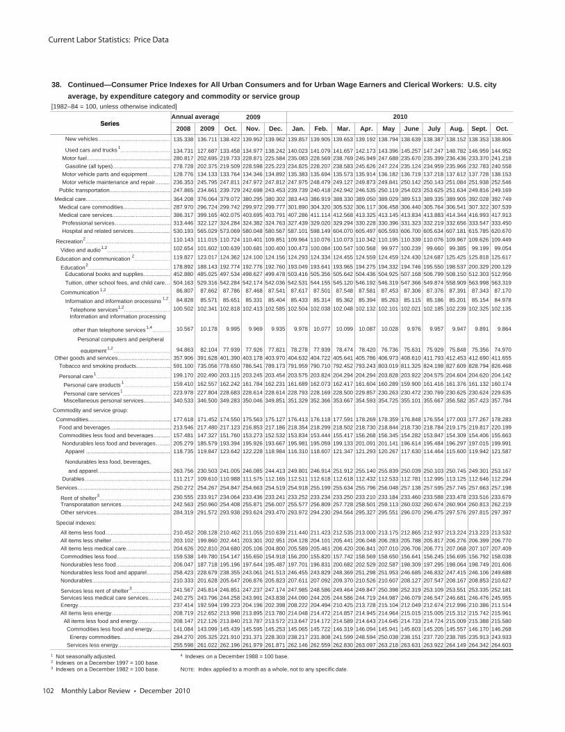
Current Labor Statistics: Price Data
102 Monthly Labor Review • December 2010
38. Continued—Consumer Price Indexes for All Urban Consumers and for Urban Wage Earners and Clerical Workers: U.S. city average, by expenditure category and commodity or service group[1982–84 = 100, unless otherwise indicated]
2009
2008 2009 Oct. Nov. Dec. Jan. Feb. Mar. Apr. May June July Aug. Sept. Oct. New vehicles…............................................ 135.338 136.711 138.422 139.952 139.962 139.857 139.905 139.653 139.192 138.794 138.639 138.387 138.152 138.353 138.806
Used cars and trucks 1……….……………………134.731 127.687 133.458 134.977 138.242 140.023 141.079 141.657 142.173 143.396 145.257 147.247 148.782 146.959 144.952
Motor fuel…................................................... 280.817 202.695 219.733 228.871 225.584 235.083 228.569 238.769 245.949 247.688 235.670 235.399 236.436 233.370 241.218 Gasoline (all types)….................................. 278.728 202.375 219.509 228.598 225.223 234.825 228.207 238.583 245.626 247.224 235.124 234.959 235.966 232.783 240.558 Motor vehicle parts and equipment…............ 128.776 134.133 133.764 134.346 134.892 135.383 135.694 135.573 135.914 136.182 136.719 137.218 137.612 137.728 138.153 Motor vehicle maintenance and repair…....... 236.353 245.795 247.811 247.972 247.812 247.975 248.479 249.127 249.873 249.841 250.142 250.143 251.084 251.938 252.546 Public transportation...............…..................... 247.865 234.661 239.729 242.698 243.453 239.739 240.418 242.942 246.535 250.119 254.023 253.625 251.634 249.816 249.169 Medical care....................................................... 364.208 376.064 379.072 380.295 380.302 383.443 386.919 388.330 389.050 389.029 389.513 389.335 389.905 392.028 392.749 Medical care commodities...............…............ 287.970 296.724 299.742 299.972 299.777 301.890 304.320 305.532 306.117 306.458 306.440 305.764 306.541 307.322 307.539 Medical care services...............…................... 386.317 399.165 402.075 403.695 403.791 407.286 411.114 412.568 413.325 413.145 413.834 413.883 414.344 416.993 417.913 Professional services…................................. 313.446 322.127 324.284 324.382 324.763 327.439 329.020 329.294 330.228 330.396 331.323 332.219 332.656 333.547 333.450 Hospital and related services…..................... 530.193 565.029 573.069 580.048 580.567 587.101 598.149 604.070 605.497 605.593 606.700 605.634 607.181 615.785 620.670
Recreation2……….……………………………………… 110.143 111.015 110.724 110.401 109.851 109.964 110.076 110.073 110.342 110.195 110.339 110.076 109.967 109.626 109.449
Video and audio1,2……….……………………………102.654 101.602 100.639 100.681 100.400 100.473 100.084 100.547 100.568 99.977 100.239 99.660 99.385 99.199 99.054
Education and communication 2……….……………119.827 123.017 124.362 124.100 124.156 124.293 124.334 124.455 124.559 124.459 124.430 124.687 125.425 125.818 125.617
Education2……….………………………………………178.892 188.143 192.774 192.776 192.760 193.049 193.641 193.965 194.275 194.332 194.746 195.550 198.537 200.329 200.129
Educational books and supplies….............. 452.880 485.025 497.534 498.627 499.478 503.416 505.356 505.642 504.436 504.925 507.168 506.799 508.150 512.303 512.956 Tuition, other school fees, and child care… 504.163 529.316 542.284 542.174 542.036 542.531 544.155 545.120 546.192 546.319 547.366 549.874 558.909 563.998 563.319
Communication 1,2……….…………………………… 86.807 87.662 87.786 87.468 87.541 87.617 87.501 87.548 87.581 87.453 87.306 87.376 87.391 87.343 87.170
Information and information processing 1,2… 84.828 85.571 85.651 85.331 85.404 85.433 85.314 85.362 85.394 85.263 85.115 85.186 85.201 85.154 84.978
Telephone services1,2……….………………… 100.502 102.341 102.818 102.413 102.585 102.504 102.038 102.048 102.132 102.101 102.021 102.185 102.239 102.325 102.135
Information and information processing
other than telephone services1,4……….… 10.567 10.178 9.995 9.969 9.935 9.978 10.077 10.099 10.087 10.028 9.976 9.957 9.947 9.891 9.864
Personal computers and peripheral
equipment 1,2……….……………………… 94.863 82.104 77.939 77.926 77.821 78.278 77.939 78.474 78.420 76.736 75.631 75.929 75.848 75.356 74.970
Other goods and services.................................. 357.906 391.628 401.390 403.178 403.970 404.632 404.722 405.641 405.786 406.973 408.610 411.793 412.453 412.690 411.655 Tobacco and smoking products...............….... 591.100 735.056 778.650 786.541 789.173 791.959 790.710 792.452 793.243 803.019 811.325 824.198 827.609 828.794 826.468
Personal care1……….………………………………… 199.170 202.490 203.115 203.245 203.454 203.575 203.824 204.294 204.294 203.828 203.922 204.575 204.604 204.620 204.142
Personal care products 1……….………………… 159.410 162.557 162.242 161.784 162.231 161.689 162.073 162.417 161.604 160.289 159.900 161.416 161.376 161.132 160.174
Personal care services1……….………………… 223.978 227.804 228.683 228.614 228.614 228.793 228.169 228.500 229.857 230.263 230.472 230.769 230.625 230.624 229.635
Miscellaneous personal services...............… 340.533 346.500 349.283 350.046 349.851 351.329 352.366 353.667 354.593 354.725 355.101 355.667 356.582 357.423 357.784
Commodity and service group: Commodities...........…....................................... 177.618 171.452 174.550 175.563 175.127 176.413 176.118 177.591 178.269 178.359 176.848 176.554 177.003 177.267 178.283 Food and beverages….................................... 213.546 217.480 217.123 216.853 217.186 218.354 218.299 218.502 218.730 218.844 218.730 218.784 219.175 219.817 220.199 Commodities less food and beverages…........ 157.481 147.327 151.760 153.273 152.532 153.834 153.444 155.417 156.268 156.345 154.282 153.847 154.309 154.406 155.663 Nondurables less food and beverages…...... 205.279 185.579 193.394 195.926 193.667 195.981 195.059 199.133 201.091 201.141 196.614 195.484 196.297 197.015 199.991 Apparel …................................................... 118.735 119.847 123.642 122.228 118.984 116.310 118.607 121.347 121.293 120.267 117.630 114.464 115.600 119.942 121.587
Nondurables less food, beverages, and apparel…............................................ 263.756 230.503 241.005 246.085 244.413 249.801 246.914 251.912 255.140 255.839 250.039 250.103 250.745 249.301 253.167 Durables….................................................... 111.217 109.610 110.988 111.575 112.165 112.511 112.618 112.618 112.432 112.533 112.781 112.995 113.125 112.646 112.294 Services…......................................................... 250.272 254.267 254.847 254.663 254.519 254.918 255.199 255.634 255.796 256.048 257.138 257.595 257.745 257.663 257.198
Rent of shelter3……….……………………………… 230.555 233.917 234.064 233.436 233.241 233.252 233.234 233.250 233.210 233.184 233.460 233.588 233.478 233.516 233.679
Transporatation services…............................ 242.563 250.960 254.408 255.871 256.007 255.577 256.809 257.728 258.501 259.113 260.032 260.674 260.904 260.813 262.219 Other services…............................................. 284.319 291.572 293.938 293.624 293.470 293.972 294.230 294.564 295.327 295.551 296.070 296.475 297.576 297.815 297.397
Special indexes:
All items less food…....................................... 210.452 208.128 210.462 211.055 210.639 211.440 211.423 212.535 213.000 213.175 212.865 212.937 213.224 213.223 213.532 All items less shelter…................................... 203.102 199.860 202.441 203.301 202.951 204.128 204.101 205.441 206.048 206.283 205.788 205.817 206.276 206.399 206.770 All items less medical care…......................... 204.626 202.810 204.680 205.106 204.800 205.589 205.461 206.420 206.841 207.010 206.706 206.771 207.068 207.107 207.409 Commodities less food…............................... 159.538 149.780 154.147 155.650 154.918 156.200 155.820 157.742 158.569 158.650 156.641 156.245 156.695 156.792 158.038 Nondurables less food…................................ 206.047 187.718 195.196 197.644 195.487 197.701 196.831 200.682 202.529 202.587 198.309 197.295 198.064 198.749 201.606 Nondurables less food and apparel…............ 258.423 228.679 238.355 243.061 241.513 246.455 243.829 248.369 251.298 251.953 246.685 246.832 247.415 246.106 249.688 Nondurables…............................................... 210.333 201.628 205.647 206.876 205.823 207.611 207.092 209.370 210.526 210.607 208.127 207.547 208.167 208.853 210.627
Services less rent of shelter 3……….…………… 241.567 245.814 246.851 247.237 247.174 247.985 248.586 249.464 249.847 250.398 252.319 253.109 253.551 253.335 252.181
Services less medical care services…........... 240.275 243.796 244.258 243.991 243.838 244.090 244.205 244.586 244.719 244.987 246.079 246.547 246.681 246.476 245.955 Energy…........................................................ 237.414 192.594 199.223 204.196 202.398 208.222 204.494 210.425 213.728 215.104 212.049 212.674 212.996 210.386 211.514 All items less energy…................................... 208.719 212.652 213.998 213.895 213.780 214.048 214.472 214.857 214.945 214.964 215.015 215.005 215.312 215.742 215.961 All items less food and energy….................. 208.147 212.126 213.840 213.787 213.572 213.647 214.172 214.589 214.643 214.645 214.733 214.724 215.009 215.388 215.580 Commodities less food and energy…........ 141.084 143.099 145.439 145.595 145.253 145.065 145.722 146.319 146.094 145.941 145.603 145.205 145.557 146.170 146.268 Energy commodities................................. 284.270 205.325 221.910 231.371 228.303 238.217 231.808 241.599 248.594 250.038 238.151 237.720 238.785 235.913 243.933 Services less energy…............................... 255.598 261.022 262.196 261.979 261.871 262.146 262.559 262.830 263.097 263.218 263.631 263.922 264.149 264.342 264.603
Annual average 2010Series
1 Not seasonally adjusted.2 Indexes on a December 1997 = 100 base.3 Indexes on a December 1982 = 100 base.
4 Indexes on a December 1988 = 100 base.
NOTE: Index applied to a month as a whole, not to any specific date.
Series
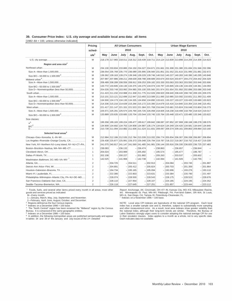
Monthly Labor Review • December 2010 103
39. Consumer Price Index: U.S. city average and available local area data: all items[1982–84 = 100, unless otherwise indicated]
Pricing All Urban Consumers Urban Wage Earners
sched- 2010 2010
ule1 May June July Aug. Sept. Oct. May June July Aug. Sept. Oct.
U.S. city average…………………………………………… M 218.178 217.965 218.011 218.312 218.439 218.711 214.124 213.839 213.898 214.205 214.306 214.623
Region and area size2
Northeast urban……….………………………………………….……… M 234.130 233.834 233.885 234.150 234.027 234.671 231.661 231.308 231.380 231.694 231.566 232.396 Size A—More than 1,500,000........................................... M 236.054 235.769 235.770 236.089 235.995 236.560 231.851 231.552 231.615 231.995 231.881 232.672
Size B/C—50,000 to 1,500,0003……….………………………… M 139.362 139.163 139.274 139.348 139.229 139.746 140.510 140.227 140.283 140.390 140.295 140.848
Midwest urban4……….………………………………………….……… M 207.987 207.886 208.211 208.639 208.788 208.689 203.674 203.524 203.877 204.273 204.442 204.329
Size A—More than 1,500,000........................................... M 208.489 208.289 208.556 208.912 209.253 209.182 203.330 203.063 203.363 203.593 203.946 203.906
Size B/C—50,000 to 1,500,0003……….………………………… M 133.772 133.845 134.130 134.375 134.275 134.074 133.797 133.845 134.136 134.426 134.361 134.093
Size D—Nonmetropolitan (less than 50,000)…………..... M 204.026 203.749 203.992 204.985 205.100 205.565 201.974 201.654 201.950 202.896 203.086 203.548 South urban…….….............................................................. M 211.423 211.232 210.988 211.308 211.775 212.026 208.920 208.640 208.440 208.740 209.155 209.376 Size A—More than 1,500,000........................................... M 213.101 213.121 212.696 212.947 213.493 213.589 211.065 210.985 210.592 210.831 211.393 211.409
Size B/C—50,000 to 1,500,0003……….………………………… M 134.500 134.173 134.130 134.335 134.658 134.890 133.621 133.227 133.227 133.420 133.680 133.923
Size D—Nonmetropolitan (less than 50,000)…………..... M 214.336 215.216 214.639 215.266 215.172 215.390 214.679 215.416 214.840 215.354 215.346 215.451 West urban…….…............................................................... M 221.417 221.147 221.331 221.523 221.384 221.708 216.044 215.681 215.824 216.048 215.804 216.273 Size A—More than 1,500,000........................................... M 225.571 225.291 225.574 225.790 225.726 226.058 218.605 218.238 218.499 218.784 218.524 219.017
Size B/C—50,000 to 1,500,0003……….………………………… M 133.889 133.635 133.685 133.704 133.544 133.745 133.764 133.448 133.471 133.480 133.346 133.622
Size classes:
A5 M 199.358 199.183 199.224 199.477 199.617 199.842 198.087 197.852 197.908 198.168 198.278 198.576
B/C3……………………….….………………………………………….… M 134.909 134.692 134.753 134.908 134.987 135.174 134.624 134.349 134.420 134.581 134.644 134.840
D…………….…………...................................................... M 210.739 211.094 210.882 211.606 211.524 211.831 209.097 209.374 209.161 209.863 209.864 210.160
Selected local areas6
Chicago–Gary–Kenosha, IL–IN–WI………………………….. M 212.984 212.186 212.535 212.784 213.339 213.332 206.774 205.834 206.307 206.338 206.897 206.894Los Angeles–Riverside–Orange County, CA……….………… M 226.438 225.877 225.991 226.373 226.048 226.794 218.787 218.222 218.367 218.752 218.427 219.339
New York, NY–Northern NJ–Long Island, NY–NJ–CT–PA… M 241.075 240.817 241.147 241.569 241.485 241.981 236.144 235.916 236.330 236.820 236.725 237.483
Boston–Brockton–Nashua, MA–NH–ME–CT……….………… 1 238.083 – 236.132 – 236.474 – 238.863 – 236.657 – 236.844 –Cleveland–Akron, OH…………………………………………… 1 204.024 – 203.989 – 205.492 – 195.574 – 195.477 – 196.787 –Dallas–Ft Worth, TX…….……………………………………… 1 202.108 – 200.227 – 201.882 – 205.263 – 203.537 – 205.602 –
Washington–Baltimore, DC–MD–VA–WV 7……….…………… 1 142.025 – 141.966 – 142.738 – 142.064 – 141.926 – 142.755 –
Atlanta, GA……………………..………………………………… 2 – 204.725 – 204.511 – 202.913 – 204.084 – 203.745 – 201.887Detroit–Ann Arbor–Flint, MI…………………………………… 2 – 204.891 – 205.412 – 205.824 – 200.703 – 201.359 – 201.864Houston–Galveston–Brazoria, TX……………………………… 2 – 194.734 – 195.165 – 195.094 – 192.696 – 193.276 – 193.110Miami–Ft. Lauderdale, FL……………...……………………… 2 – 222.390 – 222.803 – 223.631 – 220.384 – 220.790 – 221.497Philadelphia–Wilmington–Atlantic City, PA–NJ–DE–MD…… 2 – 228.074 – 228.500 – 228.543 – 228.175 – 228.523 – 228.676San Francisco–Oakland–San Jose, CA…….………………… 2 – 228.110 – 227.954 – 228.107 – 224.185 – 224.195 – 224.352Seattle–Tacoma–Bremerton, WA………………...…………… 2 – 226.118 – 227.645 – 227.251 – 221.857 – 223.444 – 223.112
1 Foods, fuels, and several other items priced every month in all areas; most othergoods and services priced as indicated:M—Every month.1—January, March, May, July, September, and November.2—February, April, June, August, October, and December.
2 Regions defined as the four Census regions.3 Indexes on a December 1996 = 100 base.4 The "North Central" region has been renamed the "Midwest" region by the CensusBureau. It is composed of the same geographic entities.5 Indexes on a December 1986 = 100 base.6 In addition, the following metropolitan areas are published semiannually and appearin tables 34 and 39 of the January and July issues of the CPI Detailed
Report: Anchorage, AK; Cincinnatti, OH–KY–IN; Kansas City, MO–KS; Milwaukee–Racine,WI; Minneapolis–St. Paul, MN–WI; Pittsburgh, PA; Port-land–Salem, OR–WA; St Louis,MO–IL; San Diego, CA; Tampa–St. Petersburg–Clearwater, FL.7 Indexes on a November 1996 = 100 base.
NOTE: Local area CPI indexes are byproducts of the national CPI program. Each localindex has a smaller sample size and is, therefore, subject to substantially more samplingand other measurement error. As a result, local area indexes show greater volatility thanthe national index, although their long-term trends are similar. Therefore, the Bureau ofLabor Statistics strongly urges users to consider adopting the national average CPI for usein their escalator clauses. Index applies to a month as a whole, not to any specific date.Dash indicates data not available.
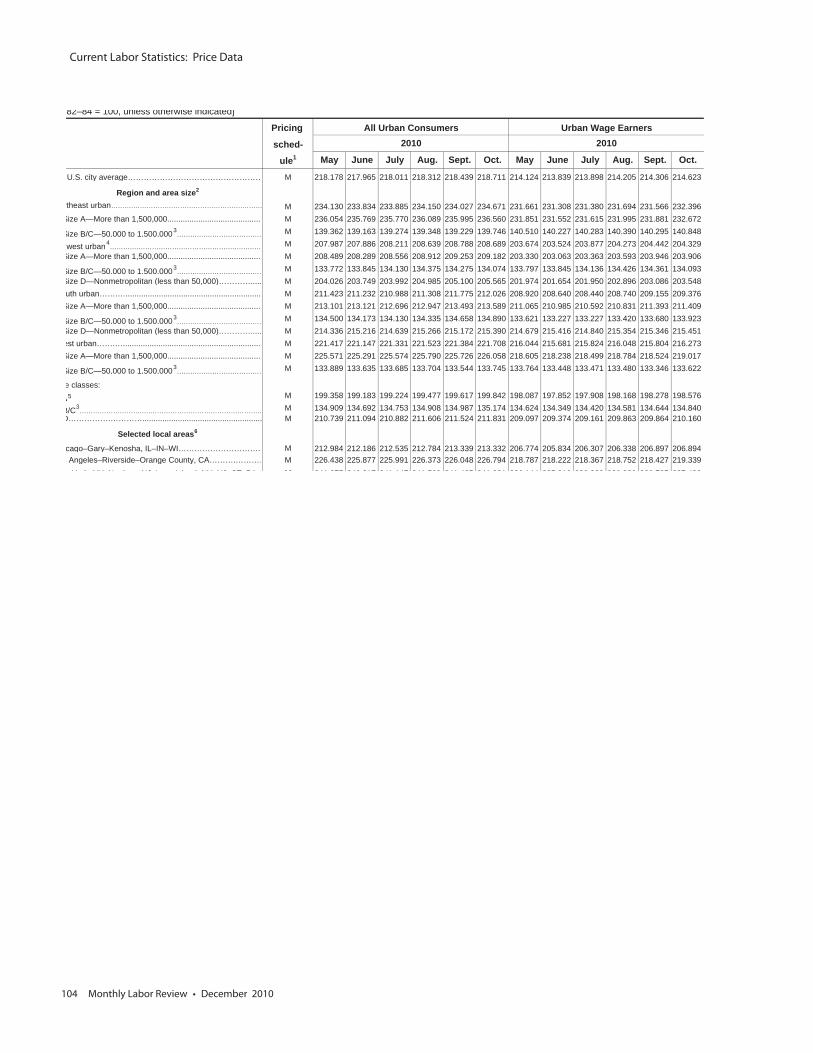
Current Labor Statistics: Price Data
104 Monthly Labor Review • December 2010
82–84 = 100, unless otherwise indicated]
Pricing All Urban Consumers Urban Wage Earners
sched- 2010 2010
ule1 May June July Aug. Sept. Oct. May June July Aug. Sept. Oct.
U.S. city average…………………………………………… M 218.178 217.965 218.011 218.312 218.439 218.711 214.124 213.839 213.898 214.205 214.306 214.623
Region and area size2
rtheast urban……….………………………………………….……… M 234.130 233.834 233.885 234.150 234.027 234.671 231.661 231.308 231.380 231.694 231.566 232.396Size A—More than 1,500,000........................................... M 236.054 235.769 235.770 236.089 235.995 236.560 231.851 231.552 231.615 231.995 231.881 232.672
Size B/C—50,000 to 1,500,0003……….………………………… M 139.362 139.163 139.274 139.348 139.229 139.746 140.510 140.227 140.283 140.390 140.295 140.848
west urban4……….………………………………………….……… M 207.987 207.886 208.211 208.639 208.788 208.689 203.674 203.524 203.877 204.273 204.442 204.329
Size A—More than 1,500,000........................................... M 208.489 208.289 208.556 208.912 209.253 209.182 203.330 203.063 203.363 203.593 203.946 203.906
Size B/C—50,000 to 1,500,0003……….………………………… M 133.772 133.845 134.130 134.375 134.275 134.074 133.797 133.845 134.136 134.426 134.361 134.093
Size D—Nonmetropolitan (less than 50,000)…………..... M 204.026 203.749 203.992 204.985 205.100 205.565 201.974 201.654 201.950 202.896 203.086 203.548uth urban…….….............................................................. M 211.423 211.232 210.988 211.308 211.775 212.026 208.920 208.640 208.440 208.740 209.155 209.376
Size A—More than 1,500,000........................................... M 213.101 213.121 212.696 212.947 213.493 213.589 211.065 210.985 210.592 210.831 211.393 211.409
Size B/C—50,000 to 1,500,0003……….………………………… M 134.500 134.173 134.130 134.335 134.658 134.890 133.621 133.227 133.227 133.420 133.680 133.923
Size D—Nonmetropolitan (less than 50,000)…………..... M 214.336 215.216 214.639 215.266 215.172 215.390 214.679 215.416 214.840 215.354 215.346 215.451est urban…….…............................................................... M 221.417 221.147 221.331 221.523 221.384 221.708 216.044 215.681 215.824 216.048 215.804 216.273Size A—More than 1,500,000........................................... M 225.571 225.291 225.574 225.790 225.726 226.058 218.605 218.238 218.499 218.784 218.524 219.017
Size B/C—50,000 to 1,500,0003……….………………………… M 133.889 133.635 133.685 133.704 133.544 133.745 133.764 133.448 133.471 133.480 133.346 133.622
e classes:
A5 M 199.358 199.183 199.224 199.477 199.617 199.842 198.087 197.852 197.908 198.168 198.278 198.576
B/C3……………………….….………………………………………….… M 134.909 134.692 134.753 134.908 134.987 135.174 134.624 134.349 134.420 134.581 134.644 134.840
D…………….…………...................................................... M 210.739 211.094 210.882 211.606 211.524 211.831 209.097 209.374 209.161 209.863 209.864 210.160
Selected local areas6
cago–Gary–Kenosha, IL–IN–WI………………………….. M 212.984 212.186 212.535 212.784 213.339 213.332 206.774 205.834 206.307 206.338 206.897 206.894s Angeles–Riverside–Orange County, CA……….………… M 226.438 225.877 225.991 226.373 226.048 226.794 218.787 218.222 218.367 218.752 218.427 219.339
Y k NY N th NJ L I l d NY NJ CT PA M 241 075 240 817 241 147 241 569 241 485 241 981 236 144 235 916 236 330 236 820 236 725 237 483
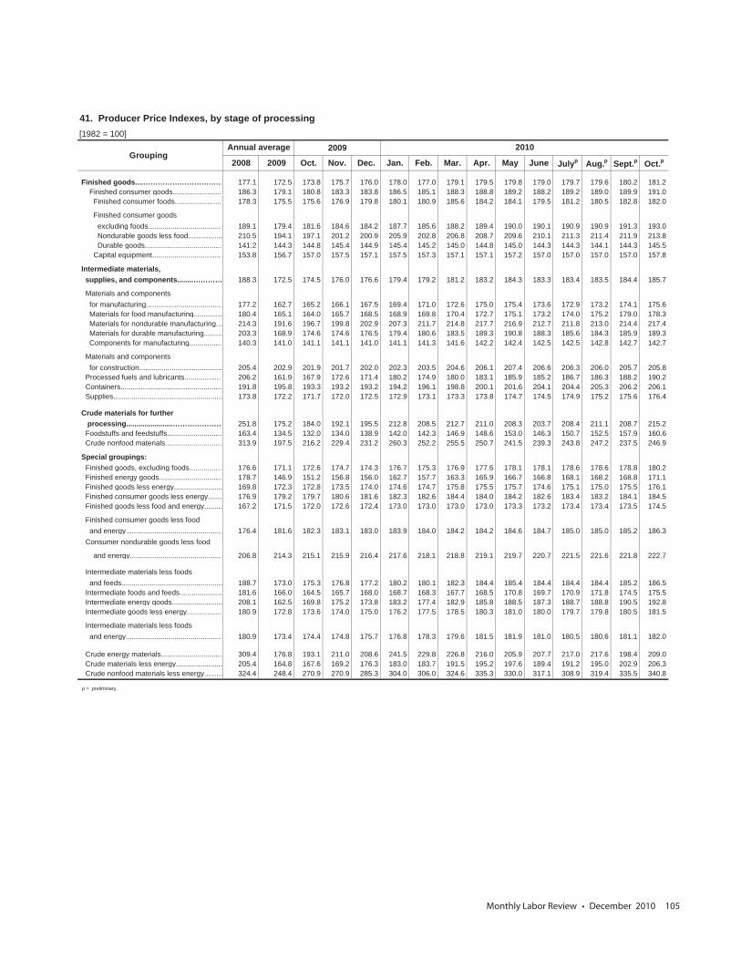
Monthly Labor Review • December 2010 105
41. Producer Price Indexes, by stage of processing[1982 = 100]
2009
2008 2009 Oct. Nov. Dec. Jan. Feb. Mar. Apr. May June Julyp Aug.p Sept.p Oct.p
Finished goods....…………………………… 177.1 172.5 173.8 175.7 176.0 178.0 177.0 179.1 179.5 179.8 179.0 179.7 179.6 180.2 181.2 Finished consumer goods......................... 186.3 179.1 180.8 183.3 183.8 186.5 185.1 188.3 188.8 189.2 188.2 189.2 189.0 189.9 191.0 Finished consumer foods........................ 178.3 175.5 175.6 176.9 179.8 180.1 180.9 185.6 184.2 184.1 179.5 181.2 180.5 182.8 182.0
Finished consumer goods excluding foods..................................... 189.1 179.4 181.6 184.6 184.2 187.7 185.6 188.2 189.4 190.0 190.1 190.9 190.9 191.3 193.0 Nondurable goods less food................. 210.5 194.1 197.1 201.2 200.9 205.9 202.8 206.8 208.7 209.6 210.1 211.3 211.4 211.9 213.8 Durable goods...................................... 141.2 144.3 144.8 145.4 144.9 145.4 145.2 145.0 144.8 145.0 144.3 144.3 144.1 144.3 145.5 Capital equipment................................... 153.8 156.7 157.0 157.5 157.1 157.5 157.3 157.1 157.1 157.2 157.0 157.0 157.0 157.0 157.8
Intermediate materials, supplies, and components........………… 188.3 172.5 174.5 176.0 176.6 179.4 179.2 181.2 183.2 184.3 183.3 183.4 183.5 184.4 185.7
Materials and components for manufacturing...................................... 177.2 162.7 165.2 166.1 167.5 169.4 171.0 172.6 175.0 175.4 173.6 172.9 173.2 174.1 175.6 Materials for food manufacturing.............. 180.4 165.1 164.0 165.7 168.5 168.9 169.8 170.4 172.7 175.1 173.2 174.0 175.2 179.0 178.3 Materials for nondurable manufacturing... 214.3 191.6 196.7 199.8 202.9 207.3 211.7 214.8 217.7 216.9 212.7 211.8 213.0 214.4 217.4 Materials for durable manufacturing......... 203.3 168.9 174.6 174.6 176.5 179.4 180.6 183.5 189.3 190.8 188.3 185.6 184.3 185.9 189.3 Components for manufacturing................ 140.3 141.0 141.1 141.1 141.0 141.1 141.3 141.6 142.2 142.4 142.5 142.5 142.8 142.7 142.7
Materials and components for construction......................................... 205.4 202.9 201.9 201.7 202.0 202.3 203.5 204.6 206.1 207.4 206.6 206.3 206.0 205.7 205.8 Processed fuels and lubricants................... 206.2 161.9 167.9 172.6 171.4 180.2 174.9 180.0 183.1 185.9 185.2 186.7 186.3 188.2 190.2 Containers.................................................. 191.8 195.8 193.3 193.2 193.2 194.2 196.1 198.8 200.1 201.6 204.1 204.4 205.3 206.2 206.1 Supplies...................................................... 173.8 172.2 171.7 172.0 172.5 172.9 173.1 173.3 173.8 174.7 174.5 174.9 175.2 175.6 176.4
Crude materials for further processing.......................………………… 251.8 175.2 184.0 192.1 195.5 212.8 208.5 212.7 211.0 208.3 203.7 208.4 211.1 208.7 215.2 Foodstuffs and feedstuffs........................... 163.4 134.5 132.0 134.0 138.9 142.0 142.3 146.9 148.6 153.0 146.3 150.7 152.5 157.9 160.6 Crude nonfood materials............................ 313.9 197.5 216.2 229.4 231.2 260.3 252.2 255.5 250.7 241.5 239.3 243.8 247.2 237.5 246.9
Special groupings: Finished goods, excluding foods................ 176.6 171.1 172.6 174.7 174.3 176.7 175.3 176.9 177.6 178.1 178.1 178.6 178.6 178.8 180.2 Finished energy goods............................... 178.7 146.9 151.2 156.8 156.0 162.7 157.7 163.3 165.9 166.7 166.8 168.1 168.2 168.8 171.1 Finished goods less energy........................ 169.8 172.3 172.8 173.5 174.0 174.6 174.7 175.8 175.5 175.7 174.6 175.1 175.0 175.5 176.1 Finished consumer goods less energy....... 176.9 179.2 179.7 180.6 181.6 182.3 182.6 184.4 184.0 184.2 182.6 183.4 183.2 184.1 184.5 Finished goods less food and energy......... 167.2 171.5 172.0 172.6 172.4 173.0 173.0 173.0 173.0 173.3 173.2 173.4 173.4 173.5 174.5
Finished consumer goods less food and energy................................................ 176.4 181.6 182.3 183.1 183.0 183.9 184.0 184.2 184.2 184.6 184.7 185.0 185.0 185.2 186.3 Consumer nondurable goods less food
and energy.............................................. 206.8 214.3 215.1 215.9 216.4 217.6 218.1 218.8 219.1 219.7 220.7 221.5 221.6 221.8 222.7
Intermediate materials less foods and feeds.................................................. 188.7 173.0 175.3 176.8 177.2 180.2 180.1 182.3 184.4 185.4 184.4 184.4 184.4 185.2 186.5 Intermediate foods and feeds..................... 181.6 166.0 164.5 165.7 168.0 168.7 168.3 167.7 168.5 170.8 169.7 170.9 171.8 174.5 175.5 Intermediate energy goods......................... 208.1 162.5 169.8 175.2 173.8 183.2 177.4 182.9 185.8 188.5 187.3 188.7 188.8 190.5 192.8 Intermediate goods less energy.................. 180.9 172.8 173.6 174.0 175.0 176.2 177.5 178.5 180.3 181.0 180.0 179.7 179.8 180.5 181.5
Intermediate materials less foods and energy................................................ 180.9 173.4 174.4 174.8 175.7 176.8 178.3 179.6 181.5 181.9 181.0 180.5 180.6 181.1 182.0
Crude energy materials.............................. 309.4 176.8 193.1 211.0 208.6 241.5 229.8 226.8 216.0 205.9 207.7 217.0 217.6 198.4 209.0 Crude materials less energy....................... 205.4 164.8 167.6 169.2 176.3 183.0 183.7 191.5 195.2 197.6 189.4 191.2 195.0 202.9 206.3 Crude nonfood materials less energy......... 324.4 248.4 270.9 270.9 285.3 304.0 306.0 324.6 335.3 330.0 317.1 308.9 319.4 335.5 340.8
p = preliminary.
Annual average 2010Grouping
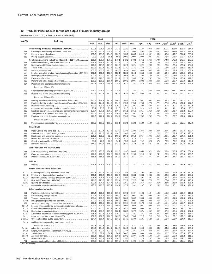
Current Labor Statistics: Price Data
106 Monthly Labor Review • December 2010
42. Producer Price Indexes for the net output of major industry groups[December 2003 = 100, unless otherwise indicated]
2009
Oct. Nov. Dec. Jan. Feb. Mar. Apr. May June Julyp Aug.p Sept.p Oct.p
Total mining industries (December 1984=100)............................. 192.3 206.7 208.4 231.3 222.3 219.8 213.4 204.9 204.8 210.1 212.0 203.6 214.3211 Oil and gas extraction (December 1985=100) ............................. 210.8 233.5 235.5 271.6 257.3 250.9 240.0 226.8 226.7 235.4 238.0 222.2 238.0212 Mining, except oil and gas…………………………………………… 189.7 191.6 194.2 196.9 195.8 200.5 201.3 200.1 199.0 198.8 199.7 204.8 208.0213 Mining support activities……………………………………………… 99.1 99.1 99.1 99.3 100.0 100.4 100.6 100.7 101.1 101.5 101.6 102.7 104.8
Total manufacturing industries (December 1984=100)................ 168.9 170.7 170.8 173.1 172.2 173.9 175.2 176.1 174.8 174.8 175.2 175.5 177.1311 Food manufacturing (December 1984=100)………………………… 168.3 169.1 171.2 172.2 172.4 172.6 173.6 175.8 174.6 175.5 175.8 178.2 178.1312 Beverage and tobacco manufacturing........................................... 120.6 121.3 121.3 121.8 122.0 122.4 122.1 123.5 123.9 123.5 123.6 123.5 124.9313 Textile mills.................................................................................... 112.1 112.4 112.4 112.6 113.2 114.1 114.6 115.3 115.7 116.0 116.4 116.6 117.0315 Apparel manufacturing………………………………...……………… 103.7 103.6 103.6 103.5 103.4 103.3 103.6 103.5 103.5 103.3 103.5 103.2 103.6316 Leather and allied product manufacturing (December 1984=100) 153.3 152.9 152.8 153.1 153.6 154.0 155.3 155.8 155.9 156.4 156.9 157.4 158.5321 Wood products manufacturing……………………………………… 102.7 103.0 103.5 103.6 105.6 107.3 110.0 112.5 109.3 109.7 108.0 107.2 106.8322 Paper manufacturing..................................................................... 121.7 122.0 122.0 121.9 122.8 124.2 125.1 126.7 128.0 128.7 129.3 130.0 129.7323 Printing and related support activities........................................... 109.2 109.3 109.4 109.2 109.3 109.4 109.5 109.5 109.8 110.0 109.7 109.9 110.3324 Petroleum and coal products manufacturing 240.8 258.4 254.3 275.6 261.0 278.2 287.8 292.0 280.4 278.6 282.8 282.0 295.5
(December 1984=100)………………………………….…………
325 Chemical manufacturing (December 1984=100)…………………… 225.0 225.4 227.3 228.7 231.3 232.0 234.1 233.4 232.6 233.8 234.1 234.5 236.6326 Plastics and rubber products manufacturing 161.5 161.9 162.0 162.3 163.1 164.3 165.6 166.2 167.1 166.7 166.5 166.7 166.7
(December 1984=100)………….…………………………………
331 Primary metal manufacturing (December 1984=100)……………… 180.7 179.9 182.2 186.5 188.1 191.8 198.7 200.5 198.8 194.3 192.7 196.2 200.7332 Fabricated metal product manufacturing (December 1984=100)… 174.1 174.1 174.2 174.4 175.0 175.6 176.3 177.0 177.1 177.3 177.6 177.3 177.2333 Machinery manufacturing………………………..…………………… 120.1 120.2 120.3 120.2 120.2 120.2 120.4 120.4 120.3 120.5 120.7 120.8 120.9334 Computer and electronic products manufacturing………………… 91.9 91.8 91.7 91.5 91.5 91.6 91.4 91.3 91.1 91.1 91.1 90.8 90.2335 Electrical equipment, appliance, and components manufacturing 129.7 130.1 130.5 130.7 131.1 131.1 131.7 131.9 131.8 131.6 131.7 131.2 132.4336 Transportation equipment manufacturing…………………………… 110.2 110.6 110.2 110.8 110.7 110.3 110.3 110.3 109.9 109.8 109.8 109.8 110.7337 Furniture and related product manufacturing 176.7 176.4 176.4 176.2 176.0 176.4 176.9 176.7 177.3 178.1 177.7 177.5 177.6
(December 1984=100)………………………………………………
339 Miscellaneous manufacturing………………………………………… 111.6 111.8 112.0 112.1 112.1 112.5 112.6 112.6 112.7 113.2 113.1 113.1 113.3
Retail trade
441 Motor vehicle and parts dealers……………………………………… 122.1 122.4 121.5 123.9 123.8 123.9 124.4 123.9 123.9 123.6 124.6 125.4 125.7442 Furniture and home furnishings stores……………………………… 121.8 121.5 121.1 120.0 120.9 120.3 121.7 121.7 120.5 120.7 122.5 120.9 120.8443 Electronics and appliance stores…………………………………… 106.0 109.0 92.3 103.2 105.8 101.0 105.4 104.1 105.3 108.1 106.7 104.4 101.8446 Health and personal care stores……………………………………… 138.7 140.0 139.0 138.7 141.0 141.8 142.1 142.5 143.1 142.2 127.6 128.7 128.2447 Gasoline stations (June 2001=100)………………………………… 61.9 77.8 82.9 74.1 75.3 64.3 74.1 82.8 67.6 73.9 76.2 69.8 69.8454 Nonstore retailers……………………………………………………… 144.1 143.4 145.0 142.9 154.7 144.5 142.8 142.7 138.7 141.4 136.3 140.8 139.9
Transportation and warehousing
481 Air transportation (December 1992=100)…………………………… 188.5 193.3 194.7 199.6 199.5 203.2 205.8 202.9 208.0 209.3 208.5 195.6 201.9483 Water transportation…………………………………………………… 116.8 118.3 118.3 120.0 121.5 119.8 121.0 123.1 124.1 129.9 129.9 128.4 128.7491 Postal service (June 1989=100)……………………………………… 186.8 186.8 186.8 187.7 187.7 187.7 187.7 187.7 187.7 187.7 187.7 187.7 187.7
Utilities 221 Utilities…………………………………………………………………… 128.8 128.9 129.4 132.2 133.0 132.2 131.0 131.3 134.5 136.9 139.1 135.9 132.1
Health care and social assistance
6211 Office of physicians (December 1996=100)………………………… 127.4 127.5 127.6 128.5 128.6 128.9 129.0 129.0 129.7 129.6 129.9 130.0 130.66215 Medical and diagnostic laboratories………………………………… 108.3 108.0 108.0 108.3 108.2 108.2 108.2 108.2 108.3 108.3 108.4 108.4 108.66216 Home health care services (December 1996=100)………………… 128.8 128.8 128.8 129.2 129.3 129.3 129.3 129.3 129.3 129.3 129.5 129.6 129.9622 Hospitals (December 1992=100)…………………………………… 171.2 171.3 171.5 172.4 172.7 172.9 173.0 172.8 172.9 173.4 173.7 173.4 173.9
6231 Nursing care facilities………………………………………………… 123.8 124.1 124.4 125.3 125.2 125.4 125.4 125.4 125.0 126.0 125.9 125.8 126.262321 Residential mental retardation facilities……………………………… 125.6 125.6 127.1 128.1 127.9 128.1 128.7 128.7 129.5 128.6 130.1 129.9 131.3
Other services industries
511 Publishing industries, except Internet ……………………………… 111.4 109.8 109.7 110.3 110.2 110.4 110.3 110.4 110.2 110.2 110.3 110.4 110.3515 Broadcasting, except Internet………………………………………… 103.5 104.9 104.6 105.0 104.0 106.3 108.7 109.5 113.5 109.1 109.1 108.4 112.2517 Telecommunications…………………………………………………… 101.1 100.8 100.9 100.8 100.6 100.5 100.2 100.8 100.9 100.9 101.3 101.3 101.55182 Data processing and related services……………………………… 101.0 100.6 100.6 100.7 100.7 100.7 100.8 100.8 100.8 100.7 100.8 100.7 101.8523 Security, commodity contracts, and like activity…………………… 116.4 116.0 116.5 117.2 115.7 116.1 117.6 121.2 119.7 116.1 117.4 119.7 122.0
53112 Lessors or nonresidental buildings (except miniwarehouse)……… 109.5 109.3 109.9 109.5 109.1 108.8 108.7 109.6 109.5 109.4 109.7 109.4 109.75312 Offices of real estate agents and brokers…………………………… 102.0 102.0 101.9 101.7 101.0 100.8 100.6 100.3 100.1 99.6 99.8 99.1 99.15313 Real estate support activities………………………………………… 107.4 107.3 109.3 108.1 108.3 107.9 107.4 106.9 106.9 107.0 106.6 107.0 107.35321 Automotive equipment rental and leasing (June 2001=100)……… 135.8 132.3 129.8 130.2 134.3 132.2 133.1 128.9 134.2 144.6 136.2 135.4 134.75411 Legal services (December 1996=100)……………………………… 166.6 166.6 166.8 169.6 170.0 170.0 171.5 171.5 171.5 171.9 172.2 172.2 172.3
541211 Offices of certified public accountants……………………………… 114.7 115.4 114.0 113.6 114.3 113.6 113.7 112.9 112.7 113.3 113.0 114.0 113.6
5413 Architectural, engineering, and related services
(December 1996=100)……………………………………………… 142.8 142.8 143.0 142.9 142.7 143.1 143.1 143.2 143.6 143.7 143.6 143.6 143.954181 Advertising agencies…………………………………………………… 104.6 104.7 104.7 104.8 104.8 104.8 104.8 104.8 104.8 104.8 104.8 105.1 105.05613 Employment services (December 1996=100)……………………… 123.2 122.8 122.8 123.9 123.6 123.7 124.5 124.9 125.2 125.5 125.8 125.8 126.0
56151 Travel agencies………………………………………………………… 98.5 98.1 98.1 98.1 100.3 100.4 100.4 100.4 100.6 100.7 100.8 100.8 100.556172 Janitorial services……………………………………………………… 110.3 110.5 110.5 110.6 110.2 110.4 110.5 110.6 110.6 110.2 110.8 111.2 111.15621 Waste collection………………………………………………………… 116.9 117.1 116.1 116.0 115.5 117.1 117.9 118.7 118.6 118.5 118.8 119.1 119.1721 Accommodation (December 1996=100)…………………………… 141.8 139.8 137.2 139.3 140.6 140.3 140.5 140.8 141.2 143.7 142.1 140.1 142.0
p = preliminary.
2010IndustryNAICS
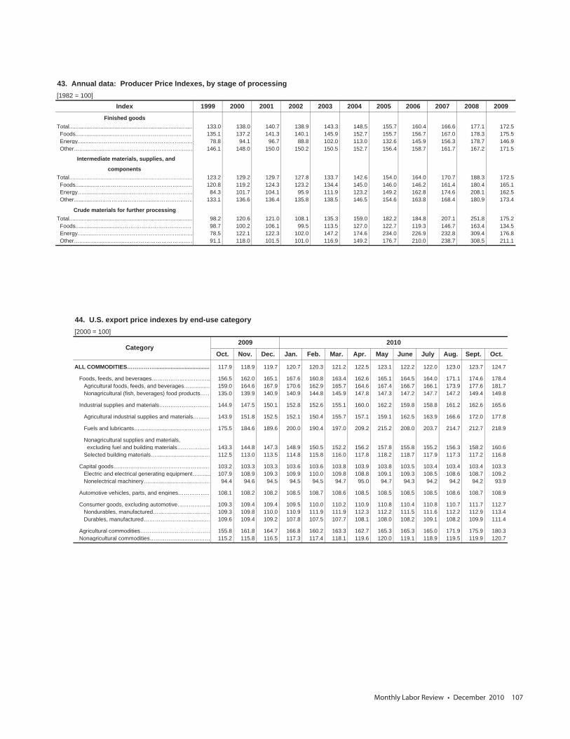
Monthly Labor Review • December 2010 107
43. Annual data: Producer Price Indexes, by stage of processing [1982 = 100]
Index 1999 2000 2001 2002 2003 2004 2005 2006 2007 2008 2009
Finished goodsTotal............................................................................... 133.0 138.0 140.7 138.9 143.3 148.5 155.7 160.4 166.6 177.1 172.5 Foods............................…………………………….…… 135.1 137.2 141.3 140.1 145.9 152.7 155.7 156.7 167.0 178.3 175.5 Energy............……………………………………….….… 78.8 94.1 96.7 88.8 102.0 113.0 132.6 145.9 156.3 178.7 146.9 Other…...............................………………………….…… 146.1 148.0 150.0 150.2 150.5 152.7 156.4 158.7 161.7 167.2 171.5
Intermediate materials, supplies, and
componentsTotal............................................................................... 123.2 129.2 129.7 127.8 133.7 142.6 154.0 164.0 170.7 188.3 172.5 Foods............……………………………………….….… 120.8 119.2 124.3 123.2 134.4 145.0 146.0 146.2 161.4 180.4 165.1 Energy…...............................………………………….… 84.3 101.7 104.1 95.9 111.9 123.2 149.2 162.8 174.6 208.1 162.5 Other.................…………...………..........………….…… 133.1 136.6 136.4 135.8 138.5 146.5 154.6 163.8 168.4 180.9 173.4
Crude materials for further processingTotal............................................................................... 98.2 120.6 121.0 108.1 135.3 159.0 182.2 184.8 207.1 251.8 175.2 Foods............................…………………………….…… 98.7 100.2 106.1 99.5 113.5 127.0 122.7 119.3 146.7 163.4 134.5 Energy............……………………………………….….… 78.5 122.1 122.3 102.0 147.2 174.6 234.0 226.9 232.8 309.4 176.8 Other…...............................………………………….…… 91.1 118.0 101.5 101.0 116.9 149.2 176.7 210.0 238.7 308.5 211.1
44. U.S. export price indexes by end-use category [2000 = 100]
2009 2010
Oct. Nov. Dec. Jan. Feb. Mar. Apr. May June July Aug. Sept. Oct.
ALL COMMODITIES…………….................................... 117.9 118.9 119.7 120.7 120.3 121.2 122.5 123.1 122.2 122.0 123.0 123.7 124.7
Foods, feeds, and beverages……………...…………… 156.5 162.0 165.1 167.6 160.8 163.4 162.6 165.1 164.5 164.0 171.1 174.6 178.4 Agricultural foods, feeds, and beverages…............. 159.0 164.6 167.9 170.6 162.9 165.7 164.6 167.4 166.7 166.1 173.9 177.6 181.7 Nonagricultural (fish, beverages) food products…… 135.0 139.9 140.9 140.9 144.8 145.9 147.8 147.3 147.2 147.7 147.2 149.4 149.8
Industrial supplies and materials……………...………… 144.9 147.5 150.1 152.8 152.6 155.1 160.0 162.2 159.8 158.8 161.2 162.6 165.6
Agricultural industrial supplies and materials…........ 143.9 151.8 152.5 152.1 150.4 155.7 157.1 159.1 162.5 163.9 166.6 172.0 177.8
Fuels and lubricants…...............................………… 175.5 184.6 189.6 200.0 190.4 197.0 209.2 215.2 208.0 203.7 214.7 212.7 218.9
Nonagricultural supplies and materials, excluding fuel and building materials…………...… 143.3 144.8 147.3 148.9 150.5 152.2 156.2 157.8 155.8 155.2 156.3 158.2 160.6 Selected building materials…...............................… 112.5 113.0 113.5 114.8 115.8 116.0 117.8 118.2 118.7 117.9 117.3 117.2 116.8
Capital goods……………...…………………………….… 103.2 103.3 103.3 103.6 103.6 103.8 103.9 103.8 103.5 103.4 103.4 103.4 103.3 Electric and electrical generating equipment…........ 107.9 108.9 109.3 109.9 110.0 109.8 108.8 109.1 109.3 108.5 108.6 108.7 109.2 Nonelectrical machinery…...............................……… 94.4 94.6 94.5 94.5 94.5 94.7 95.0 94.7 94.3 94.2 94.2 94.2 93.9
Automotive vehicles, parts, and engines……………... 108.1 108.2 108.2 108.5 108.7 108.6 108.5 108.5 108.5 108.5 108.6 108.7 108.9
Consumer goods, excluding automotive……………... 109.3 109.4 109.4 109.5 110.0 110.2 110.9 110.8 110.4 110.8 110.7 111.7 112.7 Nondurables, manufactured…...............................… 109.3 109.8 110.0 110.9 111.9 111.9 112.3 112.2 111.5 111.6 112.2 112.9 113.4 Durables, manufactured…………...………..........…… 109.6 109.4 109.2 107.8 107.5 107.7 108.1 108.0 108.2 109.1 108.2 109.9 111.4
Agricultural commodities……………...………………… 155.8 161.8 164.7 166.8 160.2 163.3 162.7 165.3 165.3 165.0 171.9 175.9 180.3 Nonagricultural commodities……………...…………… 115.2 115.8 116.5 117.3 117.4 118.1 119.6 120.0 119.1 118.9 119.5 119.9 120.7
Category
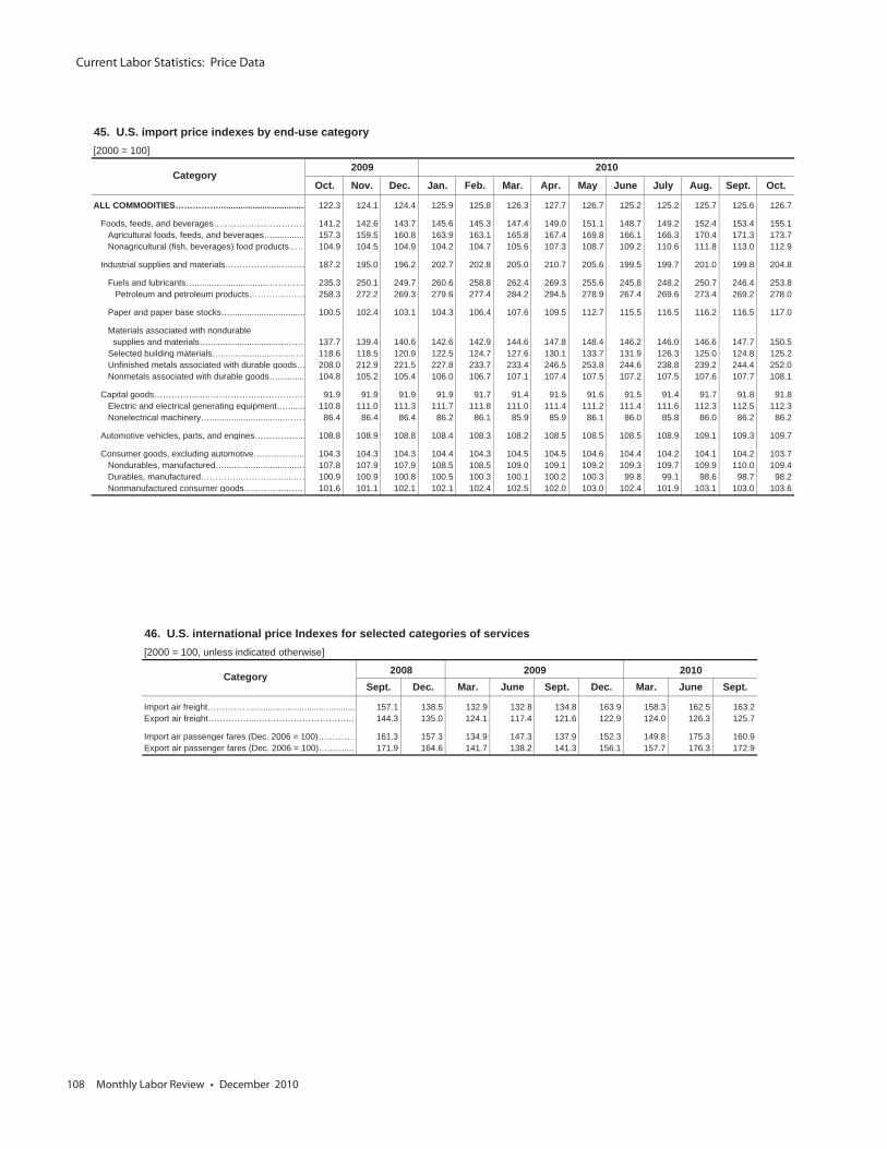
Current Labor Statistics: Price Data
108 Monthly Labor Review • December 2010
45. U.S. import price indexes by end-use category[2000 = 100]
2009 2010
Oct. Nov. Dec. Jan. Feb. Mar. Apr. May June July Aug. Sept. Oct.
ALL COMMODITIES…………….................................... 122.3 124.1 124.4 125.9 125.8 126.3 127.7 126.7 125.2 125.2 125.7 125.6 126.7
Foods, feeds, and beverages……………...…………… 141.2 142.6 143.7 145.6 145.3 147.4 149.0 151.1 148.7 149.2 152.4 153.4 155.1 Agricultural foods, feeds, and beverages…............. 157.3 159.5 160.8 163.9 163.1 165.8 167.4 169.8 166.1 166.3 170.4 171.3 173.7 Nonagricultural (fish, beverages) food products…… 104.9 104.5 104.9 104.2 104.7 105.6 107.3 108.7 109.2 110.6 111.8 113.0 112.9
Industrial supplies and materials……………...………… 187.2 195.0 196.2 202.7 202.8 205.0 210.7 205.6 199.5 199.7 201.0 199.8 204.8
Fuels and lubricants…...............................………… 235.3 250.1 249.7 260.6 258.8 262.4 269.3 255.6 245.8 248.2 250.7 246.4 253.8 Petroleum and petroleum products…………...…… 258.3 272.2 269.3 279.6 277.4 284.2 294.5 278.9 267.4 269.6 273.4 269.2 278.0
Paper and paper base stocks…............................... 100.5 102.4 103.1 104.3 106.4 107.6 109.5 112.7 115.5 116.5 116.2 116.5 117.0
Materials associated with nondurable supplies and materials…...............................……… 137.7 139.4 140.6 142.6 142.9 144.6 147.8 148.4 146.2 146.0 146.6 147.7 150.5 Selected building materials…...............................… 118.6 118.5 120.9 122.5 124.7 127.6 130.1 133.7 131.9 126.3 125.0 124.8 125.2 Unfinished metals associated with durable goods… 208.0 212.9 221.5 227.8 233.7 233.4 246.5 253.8 244.6 238.8 239.2 244.4 252.0 Nonmetals associated with durable goods…........... 104.8 105.2 105.4 106.0 106.7 107.1 107.4 107.5 107.2 107.5 107.6 107.7 108.1
Capital goods……………...…………………………….… 91.9 91.9 91.9 91.9 91.7 91.4 91.5 91.6 91.5 91.4 91.7 91.8 91.8 Electric and electrical generating equipment…........ 110.8 111.0 111.3 111.7 111.8 111.0 111.4 111.2 111.4 111.6 112.3 112.5 112.3 Nonelectrical machinery…...............................……… 86.4 86.4 86.4 86.2 86.1 85.9 85.9 86.1 86.0 85.8 86.0 86.2 86.2
Automotive vehicles, parts, and engines……………... 108.8 108.9 108.8 108.4 108.3 108.2 108.5 108.5 108.5 108.9 109.1 109.3 109.7
Consumer goods, excluding automotive……………... 104.3 104.3 104.3 104.4 104.3 104.5 104.5 104.6 104.4 104.2 104.1 104.2 103.7 Nondurables, manufactured…...............................… 107.8 107.9 107.9 108.5 108.5 109.0 109.1 109.2 109.3 109.7 109.9 110.0 109.4 Durables, manufactured…………...………..........…… 100.9 100.9 100.8 100.5 100.3 100.1 100.2 100.3 99.8 99.1 98.6 98.7 98.2 Nonmanufactured consumer goods…………...……… 101.6 101.1 102.1 102.1 102.4 102.5 102.0 103.0 102.4 101.9 103.1 103.0 103.6
Category
46. U.S. international price Indexes for selected categories of services [2000 = 100, unless indicated otherwise]
2008 2009 2010Sept. Dec. Mar. June Sept. Dec. Mar. June Sept.
Import air freight……………........................................... 157.1 138.5 132.9 132.8 134.8 163.9 158.3 162.5 163.2Export air freight……………...…………………………… 144.3 135.0 124.1 117.4 121.6 122.9 124.0 126.3 125.7
Import air passenger fares (Dec. 2006 = 100)…………… 161.3 157.3 134.9 147.3 137.9 152.3 149.8 175.3 160.9Export air passenger fares (Dec. 2006 = 100)…............ 171.9 164.6 141.7 138.2 141.3 156.1 157.7 176.3 172.9
Category
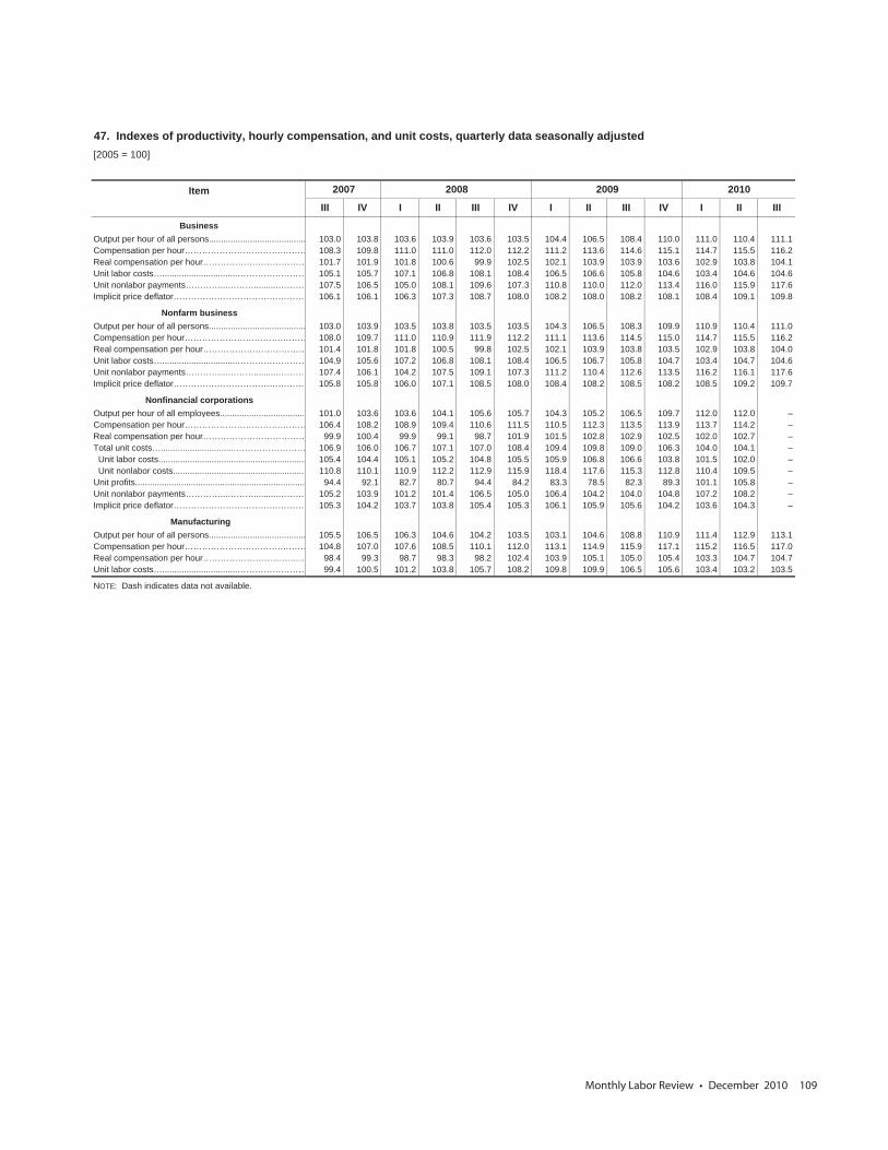
Monthly Labor Review • December 2010 109
47. Indexes of productivity, hourly compensation, and unit costs, quarterly data seasonally adjusted [2005 = 100]
Item 2007 2008 2009 2010
III IV I II III IV I II III IV I II III
BusinessOutput per hour of all persons........................................ 103.0 103.8 103.6 103.9 103.6 103.5 104.4 106.5 108.4 110.0 111.0 110.4 111.1Compensation per hour…………………………….……… 108.3 109.8 111.0 111.0 112.0 112.2 111.2 113.6 114.6 115.1 114.7 115.5 116.2Real compensation per hour……………………………… 101.7 101.9 101.8 100.6 99.9 102.5 102.1 103.9 103.9 103.6 102.9 103.8 104.1Unit labor costs…...............................…………………… 105.1 105.7 107.1 106.8 108.1 108.4 106.5 106.6 105.8 104.6 103.4 104.6 104.6Unit nonlabor payments…………...………..........……… 107.5 106.5 105.0 108.1 109.6 107.3 110.8 110.0 112.0 113.4 116.0 115.9 117.6Implicit price deflator……………………………………… 106.1 106.1 106.3 107.3 108.7 108.0 108.2 108.0 108.2 108.1 108.4 109.1 109.8
Nonfarm businessOutput per hour of all persons........................................ 103.0 103.9 103.5 103.8 103.5 103.5 104.3 106.5 108.3 109.9 110.9 110.4 111.0Compensation per hour…………………………….……… 108.0 109.7 111.0 110.9 111.9 112.2 111.1 113.6 114.5 115.0 114.7 115.5 116.2Real compensation per hour……………………………… 101.4 101.8 101.8 100.5 99.8 102.5 102.1 103.9 103.8 103.5 102.9 103.8 104.0Unit labor costs…...............................…………………… 104.9 105.6 107.2 106.8 108.1 108.4 106.5 106.7 105.8 104.7 103.4 104.7 104.6Unit nonlabor payments…………...………..........……… 107.4 106.1 104.2 107.5 109.1 107.3 111.2 110.4 112.6 113.5 116.2 116.1 117.6Implicit price deflator……………………………………… 105.8 105.8 106.0 107.1 108.5 108.0 108.4 108.2 108.5 108.2 108.5 109.2 109.7
Nonfinancial corporationsOutput per hour of all employees................................... 101.0 103.6 103.6 104.1 105.6 105.7 104.3 105.2 106.5 109.7 112.0 112.0 –Compensation per hour…………………………….……… 106.4 108.2 108.9 109.4 110.6 111.5 110.5 112.3 113.5 113.9 113.7 114.2 –Real compensation per hour……………………………… 99.9 100.4 99.9 99.1 98.7 101.9 101.5 102.8 102.9 102.5 102.0 102.7 –Total unit costs…...............................…………………… 106.9 106.0 106.7 107.1 107.0 108.4 109.4 109.8 109.0 106.3 104.0 104.1 – Unit labor costs............................................................. 105.4 104.4 105.1 105.2 104.8 105.5 105.9 106.8 106.6 103.8 101.5 102.0 – Unit nonlabor costs...................................................... 110.8 110.1 110.9 112.2 112.9 115.9 118.4 117.6 115.3 112.8 110.4 109.5 –Unit profits...................................................................... 94.4 92.1 82.7 80.7 94.4 84.2 83.3 78.5 82.3 89.3 101.1 105.8 –Unit nonlabor payments…………...………..........……… 105.2 103.9 101.2 101.4 106.5 105.0 106.4 104.2 104.0 104.8 107.2 108.2 –Implicit price deflator……………………………………… 105.3 104.2 103.7 103.8 105.4 105.3 106.1 105.9 105.6 104.2 103.6 104.3 –
ManufacturingOutput per hour of all persons........................................ 105.5 106.5 106.3 104.6 104.2 103.5 103.1 104.6 108.8 110.9 111.4 112.9 113.1Compensation per hour…………………………….……… 104.8 107.0 107.6 108.5 110.1 112.0 113.1 114.9 115.9 117.1 115.2 116.5 117.0Real compensation per hour……………………………… 98.4 99.3 98.7 98.3 98.2 102.4 103.9 105.1 105.0 105.4 103.3 104.7 104.7Unit labor costs…...............................…………………… 99.4 100.5 101.2 103.8 105.7 108.2 109.8 109.9 106.5 105.6 103.4 103.2 103.5
NOTE: Dash indicates data not available.
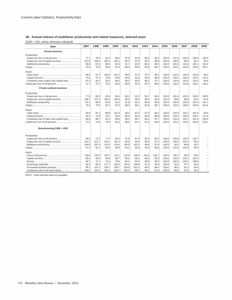
Current Labor Statistics: Productivity Data
110 Monthly Labor Review • December 2010
48. Annual indexes of multifactor productivity and related measures, selected years[2005 = 100, unless otherwise indicated]
Item 1997 1998 1999 2000 2001 2002 2003 2004 2005 2006 2007 2008 2009
Private businessProductivity: Output per hour of all persons......…………….............. 77.1 79.5 82.3 85.2 87.9 91.9 95.5 98.3 100.0 101.0 102.9 105.0 109.0 Output per unit of capital services……………………… 107.6 106.4 105.2 103.1 99.2 97.8 98.2 99.8 100.0 100.0 99.3 96.7 92.3 Multifactor productivity…………………………………… 86.6 87.9 89.5 91.0 91.7 93.9 96.4 99.0 100.0 100.5 101.0 101.1 101.9Output…...............................………………………….…… 75.3 79.2 83.6 87.4 88.2 90.0 92.8 96.7 100.0 103.1 105.5 105.4 101.7
Inputs: Labor input................................................................... 95.5 97.7 100.0 101.2 99.5 97.5 97.1 98.1 100.0 102.3 103.5 102.0 95.0 Capital services…………...………..........………….…… 70.0 74.4 79.5 84.8 89.0 92.0 94.5 96.9 100.0 103.1 106.2 109.1 110.3 Combined units of labor and capital input……………… 87.0 90.1 93.4 96.0 96.2 95.8 96.2 97.7 100.0 102.6 104.4 104.3 99.9Capital per hour of all persons.......................…………… 71.7 74.7 78.2 82.6 88.6 94.0 97.3 98.5 100.0 101.0 103.6 108.7 118.2
Private nonfarm business
Productivity: Output per hour of all persons........……………………… 77.6 80.0 82.6 85.4 88.1 92.2 95.7 98.4 100.0 101.0 102.9 105.0 109.0 Output per unit of capital services……………………… 108.7 107.3 105.9 103.5 99.5 98.0 98.2 99.9 100.0 99.8 98.9 96.1 91.6 Multifactor productivity…………………………………… 87.1 88.4 89.9 91.3 91.9 94.2 96.5 99.0 100.0 100.4 100.9 101.0 101.7Output…...............................………………………….…… 75.3 79.3 83.7 87.5 88.4 90.1 92.8 96.7 100.0 103.2 105.6 105.5 101.6
Inputs: Labor input................................................................... 94.9 97.2 99.8 101.0 99.4 97.4 97.0 98.1 100.0 102.5 103.7 101.9 94.9 Capital services…………...………..........………….…… 69.3 73.9 79.1 84.5 88.8 91.9 94.5 96.8 100.0 103.4 106.8 109.7 111.0 Combined units of labor and capital input……………… 86.5 89.7 93.2 95.8 96.1 95.7 96.2 97.7 100.0 102.8 104.7 104.4 100.0Capital per hour of all persons......………………………… 71.4 74.5 78.0 82.5 88.6 94.1 97.4 98.5 100.0 101.2 104.0 109.3 119.1
Manufacturing [1996 = 100]
Productivity: Output per hour of all persons...………………………… 69.5 73.3 77.0 80.4 81.9 87.9 93.4 95.5 100.0 100.8 105.0 104.7 – Output per unit of capital services……………………… 101.2 101.7 102.1 102.3 95.9 94.6 95.3 97.2 100.0 100.6 101.9 96.4 – Multifactor productivity…………………………………… 104.6 107.3 110.5 110.0 105.9 102.3 99.8 97.9 100.0 99.3 96.8 93.2 –Output…...............................………………………….…… 87.4 92.1 95.9 98.9 94.2 93.9 94.9 96.6 100.0 101.5 104.0 99.4 –
Inputs: – Hours of all persons..................................................... 125.8 125.5 124.7 123.1 115.0 106.9 101.6 101.1 100.0 100.7 99.0 95.0 – Capital services…………...………..........………….…… 86.4 90.5 93.9 96.7 98.3 99.2 99.6 99.3 100.0 100.9 102.1 103.2 – Energy……………….………......................................... 68.7 72.1 75.4 78.6 85.4 92.9 98.0 98.3 100.0 100.2 103.1 108.6 – Nonenergy materials.................................................... 92.4 95.4 117.7 128.4 140.3 108.6 97.0 90.8 100.0 92.2 97.7 95.2 – Purchased business services....................................... 96.1 102.3 108.7 106.7 100.0 101.0 99.3 98.5 100.0 98.3 91.3 86.4 – Combined units of all factor inputs…………...………... 104.5 104.1 105.1 103.7 102.0 98.7 98.1 91.8 100.0 98.4 97.6 92.3 –
NOTE: Dash indicates data not available.
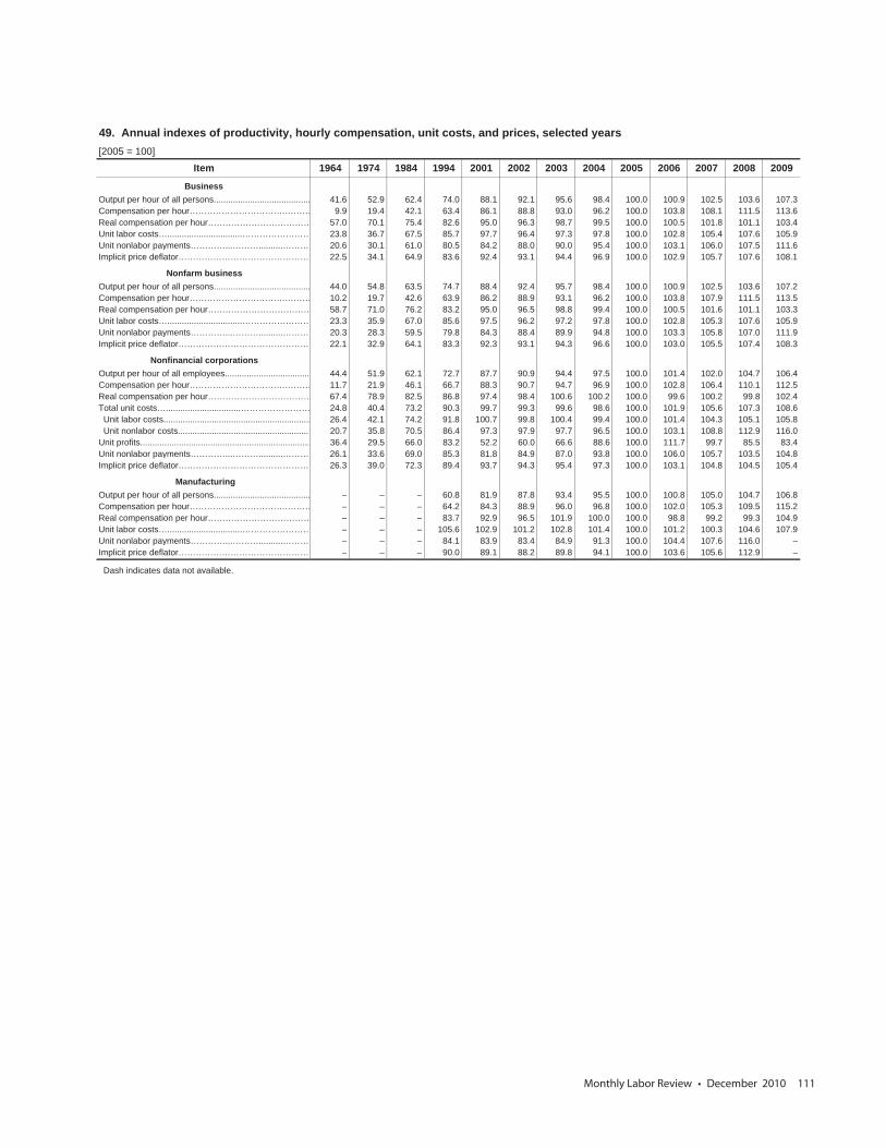
Monthly Labor Review • December 2010 111
49. Annual indexes of productivity, hourly compensation, unit costs, and prices, selected years [2005 = 100]
Item 1964 1974 1984 1994 2001 2002 2003 2004 2005 2006 2007 2008 2009
BusinessOutput per hour of all persons........................................ 41.6 52.9 62.4 74.0 88.1 92.1 95.6 98.4 100.0 100.9 102.5 103.6 107.3Compensation per hour…………………………….……… 9.9 19.4 42.1 63.4 86.1 88.8 93.0 96.2 100.0 103.8 108.1 111.5 113.6Real compensation per hour……………………………… 57.0 70.1 75.4 82.6 95.0 96.3 98.7 99.5 100.0 100.5 101.8 101.1 103.4Unit labor costs…...............................…………………… 23.8 36.7 67.5 85.7 97.7 96.4 97.3 97.8 100.0 102.8 105.4 107.6 105.9Unit nonlabor payments…………...………..........……… 20.6 30.1 61.0 80.5 84.2 88.0 90.0 95.4 100.0 103.1 106.0 107.5 111.6Implicit price deflator……………………………………… 22.5 34.1 64.9 83.6 92.4 93.1 94.4 96.9 100.0 102.9 105.7 107.6 108.1
Nonfarm businessOutput per hour of all persons........................................ 44.0 54.8 63.5 74.7 88.4 92.4 95.7 98.4 100.0 100.9 102.5 103.6 107.2Compensation per hour…………………………….……… 10.2 19.7 42.6 63.9 86.2 88.9 93.1 96.2 100.0 103.8 107.9 111.5 113.5Real compensation per hour……………………………… 58.7 71.0 76.2 83.2 95.0 96.5 98.8 99.4 100.0 100.5 101.6 101.1 103.3Unit labor costs…...............................…………………… 23.3 35.9 67.0 85.6 97.5 96.2 97.2 97.8 100.0 102.8 105.3 107.6 105.9Unit nonlabor payments…………...………..........……… 20.3 28.3 59.5 79.8 84.3 88.4 89.9 94.8 100.0 103.3 105.8 107.0 111.9Implicit price deflator……………………………………… 22.1 32.9 64.1 83.3 92.3 93.1 94.3 96.6 100.0 103.0 105.5 107.4 108.3
Nonfinancial corporationsOutput per hour of all employees................................... 44.4 51.9 62.1 72.7 87.7 90.9 94.4 97.5 100.0 101.4 102.0 104.7 106.4Compensation per hour…………………………….……… 11.7 21.9 46.1 66.7 88.3 90.7 94.7 96.9 100.0 102.8 106.4 110.1 112.5Real compensation per hour……………………………… 67.4 78.9 82.5 86.8 97.4 98.4 100.6 100.2 100.0 99.6 100.2 99.8 102.4Total unit costs…...............................…………………… 24.8 40.4 73.2 90.3 99.7 99.3 99.6 98.6 100.0 101.9 105.6 107.3 108.6 Unit labor costs............................................................. 26.4 42.1 74.2 91.8 100.7 99.8 100.4 99.4 100.0 101.4 104.3 105.1 105.8 Unit nonlabor costs...................................................... 20.7 35.8 70.5 86.4 97.3 97.9 97.7 96.5 100.0 103.1 108.8 112.9 116.0Unit profits...................................................................... 36.4 29.5 66.0 83.2 52.2 60.0 66.6 88.6 100.0 111.7 99.7 85.5 83.4Unit nonlabor payments…………...………..........……… 26.1 33.6 69.0 85.3 81.8 84.9 87.0 93.8 100.0 106.0 105.7 103.5 104.8Implicit price deflator……………………………………… 26.3 39.0 72.3 89.4 93.7 94.3 95.4 97.3 100.0 103.1 104.8 104.5 105.4
ManufacturingOutput per hour of all persons........................................ – – – 60.8 81.9 87.8 93.4 95.5 100.0 100.8 105.0 104.7 106.8Compensation per hour…………………………….……… – – – 64.2 84.3 88.9 96.0 96.8 100.0 102.0 105.3 109.5 115.2Real compensation per hour……………………………… – – – 83.7 92.9 96.5 101.9 100.0 100.0 98.8 99.2 99.3 104.9Unit labor costs…...............................…………………… – – – 105.6 102.9 101.2 102.8 101.4 100.0 101.2 100.3 104.6 107.9Unit nonlabor payments…………...………..........……… – – – 84.1 83.9 83.4 84.9 91.3 100.0 104.4 107.6 116.0 –Implicit price deflator……………………………………… – – – 90.0 89.1 88.2 89.8 94.1 100.0 103.6 105.6 112.9 –
Dash indicates data not available.
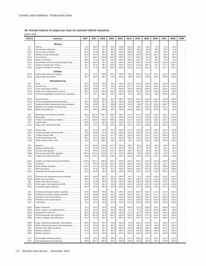
Current Labor Statistics: Productivity Data
112 Monthly Labor Review • December 2010
50. Annual indexes of output per hour for selected NAICS industries[2002=100]
NAICS Industry 1987 1997 2000 2001 2002 2003 2004 2005 2006 2007 2008 2009
Mining21 Mining…………………………………………………. 75.0 88.3 97.8 94.9 100.0 102.8 94.0 85.0 77.0 71.2 69.0 -
211 Oil and gas extraction………………………………… 64.9 81.0 96.7 96.6 100.0 105.9 90.0 86.6 80.9 78.7 71.6 -2111 Oil and gas extraction………………………………… 64.9 81.0 96.7 96.6 100.0 105.9 90.0 86.6 80.9 78.7 71.6 -212 Mining, except oil and gas…………………………… 62.3 90.2 95.3 98.5 100.0 102.8 104.9 104.3 101.1 94.4 93.7 -
2121 Coal mining……………………………………………. 51.7 89.7 103.9 102.5 100.0 101.7 101.6 96.7 89.5 90.6 85.4 -2122 Metal ore mining………………………………………… 50.5 72.1 85.7 93.8 100.0 103.3 101.5 97.2 90.7 77.0 74.4 -2123 Nonmetallic mineral mining and quarrying………… 84.3 96.0 92.1 96.5 100.0 104.3 109.4 115.2 116.8 103.8 103.9 -213 Support activities for mining…………………………… 76.1 97.0 99.7 104.5 100.0 121.9 141.6 104.1 87.1 117.7 145.7 -
2131 Support activities for mining…………………………… 76.1 97.0 99.7 104.5 100.0 121.9 141.6 104.1 87.1 117.7 145.7 -
Utilities2211 Power generation and supply………………………… 63.7 97.2 103.9 103.4 100.0 102.1 104.4 111.1 112.1 110.1 105.6 -2212 Natural gas distribution………………………………… 58.7 86.6 98.1 95.4 100.0 98.9 102.5 105.9 103.2 103.8 104.6 -
Manufacturing311 Food…………………………………………………. 81.0 86.9 93.5 95.4 100.0 101.5 101.0 106.2 104.1 101.9 101.4 -
3111 Animal food……………………………………………… 58.6 70.4 77.0 92.0 100.0 117.7 104.6 119.5 108.2 110.2 103.5 -3112 Grain and oilseed milling……………………………… 66.0 80.8 91.7 97.3 100.0 100.5 104.9 106.6 102.3 105.6 101.8 -3113 Sugar and confectionery products…………………… 80.4 92.5 102.3 100.3 100.0 100.4 107.3 120.4 113.5 103.4 95.5 -3114 Fruit and vegetable preserving and specialty……… 73.1 78.7 88.7 95.7 100.0 97.2 99.5 103.3 98.0 105.5 103.1 -
3115 Dairy products…………………………………………… 77.4 94.4 89.6 92.2 100.0 104.0 101.8 101.8 100.7 100.6 108.6 -3116 Animal slaughtering and processing………………… 90.1 93.0 95.7 96.0 100.0 99.9 100.4 109.7 109.4 106.3 109.0 -3117 Seafood product preparation and packaging………. 72.5 58.9 82.7 89.8 100.0 101.8 96.5 110.5 122.0 100.7 87.8 -3118 Bakeries and tortilla manufacturing…………………… 85.5 87.5 96.6 98.4 100.0 97.9 100.1 104.3 103.8 101.4 93.8 -3119 Other food products…………………………………… 87.5 89.7 100.8 94.5 100.0 104.8 106.1 102.9 102.8 95.1 96.4 -
312 Beverages and tobacco products…………………… 94.3 121.1 106.7 108.3 100.0 111.4 114.7 120.8 113.1 110.1 107.4 -3121 Beverages……………………………………………… 77.2 100.5 91.1 93.1 100.0 110.8 115.4 120.9 112.6 113.4 113.6 -3122 Tobacco and tobacco products……………………… 107.2 149.3 143.0 146.6 100.0 116.7 121.5 136.5 138.1 137.7 119.8 -313 Textile mills……………………………………………… 59.8 81.3 86.3 89.4 100.0 111.1 113.0 122.9 122.2 126.0 124.0 -
3131 Fiber, yarn, and thread mills…………………………… 50.0 75.2 75.6 82.5 100.0 112.1 116.7 108.8 105.5 116.4 117.9 -
3132 Fabric mills……………………………………………… 56.0 82.5 90.2 91.4 100.0 114.0 115.3 133.0 140.7 143.2 150.8 -3133 Textile and fabric finishing mills……………………… 76.5 83.6 87.2 91.0 100.0 104.1 104.5 113.3 102.4 101.2 86.4 -314 Textile product mills…………………………………… 82.0 91.3 101.2 97.7 100.0 102.8 115.1 121.3 111.2 100.3 97.2 -
3141 Textile furnishings mills………………………………… 85.7 94.1 100.2 97.9 100.0 105.7 115.3 119.1 108.4 101.9 99.2 -3149 Other textile product mills……………………………… 78.8 93.2 105.9 99.0 100.0 98.1 116.4 128.3 120.9 104.9 104.5 -
315 Apparel…………………………………………………. 73.1 100.3 116.9 117.2 100.0 106.7 94.2 94.4 86.0 56.5 55.4 -3151 Apparel knitting mills…………………………………… 71.3 92.8 100.4 97.3 100.0 93.2 83.7 97.8 97.7 65.1 62.9 -3152 Cut and sew apparel…………………………………… 70.4 99.6 119.2 119.7 100.0 109.7 96.4 91.9 82.4 52.9 52.1 -3159 Accessories and other apparel……………………… 129.9 132.2 129.8 137.4 100.0 105.8 95.8 109.8 96.3 74.0 74.0 -316 Leather and allied products…………………………… 83.9 119.1 133.8 138.5 100.0 104.9 128.4 129.4 133.7 128.8 133.4 -
3161 Leather and hide tanning and finishing……………… 138.4 153.7 135.8 140.1 100.0 103.1 135.7 142.4 127.8 165.0 160.6 -3162 Footwear………………………………………………… 77.3 99.3 123.8 132.9 100.0 105.9 110.0 115.9 122.4 110.7 130.8 -3169 Other leather products………………………………… 116.7 134.7 142.6 140.2 100.0 109.2 163.7 160.8 182.3 166.6 158.6 -321 Wood products………………………………………… 83.1 87.5 90.2 91.7 100.0 101.6 102.2 107.6 110.9 111.9 109.6 -
3211 Sawmills and wood preservation……………………… 67.3 86.9 90.9 90.6 100.0 108.3 103.9 108.3 113.4 108.4 112.2 -
3212 Plywood and engineered wood products…………… 90.3 90.4 89.6 95.1 100.0 96.7 92.3 99.6 105.5 109.0 104.7 -3219 Other wood products…………………………………… 89.9 87.3 90.4 90.9 100.0 100.7 106.5 111.5 113.2 116.5 112.5 -322 Paper and paper products…………………………… 75.5 87.9 93.5 93.8 100.0 104.4 108.1 108.6 109.9 114.0 113.4 -
3221 Pulp, paper, and paperboard mills…………………… 61.9 75.6 88.2 90.4 100.0 106.2 110.4 110.2 110.9 114.0 114.6 -3222 Converted paper products…………………………… 84.4 94.8 96.0 95.3 100.0 104.0 107.5 108.8 110.5 115.7 114.3 -
323 Printing and related support activities………………… 87.6 88.8 94.8 95.1 100.0 100.3 103.7 109.1 111.7 117.4 119.1 -3231 Printing and related support activities………………… 87.6 88.8 94.8 95.1 100.0 100.3 103.7 109.1 111.7 117.4 119.1 -324 Petroleum and coal products………………………… 60.8 85.6 96.8 94.9 100.0 102.0 105.9 106.2 104.3 106.3 103.2 -
3241 Petroleum and coal products………………………… 60.8 85.6 96.8 94.9 100.0 102.0 105.9 106.2 104.3 106.3 103.2 -325 Chemicals……………………………………………… 75.0 87.4 92.9 91.9 100.0 101.3 105.3 109.4 109.1 116.3 108.5 -
3251 Basic chemicals………………………………………… 76.1 80.2 94.6 87.6 100.0 108.5 121.8 129.6 134.1 156.0 132.4 -3252 Resin, rubber, and artificial fibers…………………… 62.9 81.2 89.0 86.3 100.0 97.7 97.3 103.4 105.5 108.1 98.9 -3253 Agricultural chemicals………………………………… 80.8 100.6 92.8 89.9 100.0 110.4 121.0 139.2 134.7 140.0 138.5 -3254 Pharmaceuticals and medicines……………………… 89.6 102.8 98.3 101.8 100.0 103.0 103.6 107.0 107.5 104.2 102.8 -3255 Paints, coatings, and adhesives……………………… 81.6 91.4 90.5 97.3 100.0 106.1 109.7 111.2 106.7 105.5 101.3 -
3256 Soap, cleaning compounds, and toiletries…………… 68.2 80.4 82.3 84.6 100.0 92.8 102.6 110.2 111.5 135.2 127.7 -3259 Other chemical products and preparations………… 62.3 82.6 98.1 90.9 100.0 98.6 96.2 96.0 91.5 102.3 103.1 -326 Plastics and rubber products………………………… 67.3 82.7 91.1 92.8 100.0 103.8 105.9 108.7 108.6 107.9 102.2 -
3261 Plastics products……………………………………… 67.3 80.8 90.7 92.4 100.0 103.9 105.8 108.5 106.8 105.1 100.0 -3262 Rubber products………………………………………… 71.3 93.2 94.8 95.5 100.0 103.5 106.4 109.4 114.2 118.8 109.8 -
327 Nonmetallic mineral products………………………… 83.6 95.1 98.6 95.6 100.0 107.1 105.3 111.6 110.7 112.7 107.6 -3271 Clay products and refractories………………………… 90.6 102.7 108.5 99.1 100.0 109.5 116.0 122.0 122.2 119.9 118.2 -
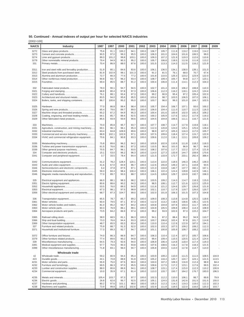
Monthly Labor Review • December 2010 113
50. Continued - Annual indexes of output per hour for selected NAICS industries[2002=100]
NAICS Industry 1987 1997 2000 2001 2002 2003 2004 2005 2006 2007 2008 2009
3272 Glass and glass products……………………………… 75.6 91.1 100.2 94.1 100.0 106.7 105.7 111.8 119.2 119.0 114.2 -3273 Cement and concrete products……………………… 90.5 97.0 99.3 95.5 100.0 106.3 101.0 104.6 101.6 106.5 99.0 -3274 Lime and gypsum products…………………………… 89.3 101.2 99.8 103.1 100.0 109.3 107.2 121.9 119.3 112.6 110.6 -3279 Other nonmetallic mineral products………………… 79.4 94.9 90.3 95.2 100.0 105.7 106.8 118.5 112.8 111.8 113.2 -331 Primary metals………………………………………… 70.4 86.9 88.0 87.6 100.0 101.5 113.3 114.3 112.5 116.2 121.9 -
3311 Iron and steel mills and ferroalloy production……… 51.9 80.1 84.6 83.6 100.0 106.1 136.5 134.1 138.0 139.1 151.0 -3312 Steel products from purchased steel………………… 81.9 102.9 99.1 101.3 100.0 91.2 81.5 76.1 68.0 70.7 67.4 -3313 Alumina and aluminum production…………………… 72.7 80.3 77.5 77.2 100.0 101.8 110.5 125.3 123.2 123.9 122.0 -3314 Other nonferrous metal production…………………… 90.8 93.7 96.2 93.4 100.0 108.7 109.4 105.7 94.8 117.7 123.1 -3315 Foundries………………………………………………… 69.4 85.5 88.7 91.2 100.0 100.4 106.8 111.4 114.1 112.3 104.3 -
332 Fabricated metal products…………………………… 78.3 90.1 94.7 94.5 100.0 102.7 101.4 104.3 106.2 108.8 110.3 -3321 Forging and stamping………………………………… 68.8 80.4 97.8 97.3 100.0 106.6 112.3 116.2 118.1 124.2 124.4 -3322 Cutlery and handtools………………………………… 76.1 88.1 93.4 97.3 100.0 99.2 90.9 95.4 97.2 105.4 102.0 -3323 Architectural and structural metals…………………… 83.5 94.0 95.6 95.5 100.0 103.4 98.7 103.5 106.5 107.0 106.1 -3324 Boilers, tanks, and shipping containers……………… 86.7 100.6 95.2 95.0 100.0 103.7 96.0 99.3 101.0 104.7 102.5 -
3325 Hardware………………………………………………… 77.0 86.8 99.4 98.4 100.0 105.7 104.4 106.7 107.1 93.0 100.2 -3326 Spring and wire products……………………………… 65.4 79.6 89.7 89.0 100.0 106.0 104.4 111.0 110.7 111.5 116.3 -3327 Machine shops and threaded products……………… 65.2 87.2 94.9 95.3 100.0 100.4 101.6 100.9 102.0 105.3 109.2 -3328 Coating, engraving, and heat treating metals……… 64.1 85.7 89.4 92.5 100.0 100.2 105.9 117.6 115.2 117.9 119.3 -3329 Other fabricated metal products……………………… 85.5 93.9 93.9 90.6 100.0 104.5 104.8 106.5 111.1 116.7 121.5 -
333 Machinery……………………………………………… 70.0 85.8 95.7 93.7 100.0 107.7 108.7 114.7 117.9 119.8 118.1 -3331 Agriculture, construction, and mining machinery…… 69.1 96.1 96.1 95.3 100.0 112.3 120.8 124.0 125.1 125.6 128.4 -3332 Industrial machinery…………………………………… 63.4 84.8 109.9 89.6 100.0 98.9 107.3 105.3 116.3 117.0 105.7 -3333 Commercial and service industry machinery………… 88.9 102.1 102.9 97.1 100.0 107.5 109.6 118.4 127.4 115.7 122.9 -3334 HVAC and commercial refrigeration equipment…… 70.6 84.1 90.8 93.3 100.0 109.6 112.0 116.1 113.1 109.8 109.2 -
3335 Metalworking machinery……………………………… 75.8 89.6 96.2 94.2 100.0 103.9 102.9 110.9 111.8 118.2 118.3 -3336 Turbine and power transmission equipment………… 61.5 76.6 88.1 97.3 100.0 110.5 96.6 101.0 96.9 96.7 94.0 -3339 Other general purpose machinery…………………… 70.5 84.7 96.1 93.5 100.0 108.2 107.6 117.7 122.2 127.4 121.9 -334 Computer and electronic products…………………… 15.1 53.0 96.2 96.3 100.0 114.0 127.3 133.9 144.7 159.9 170.6 -
3341 Computer and peripheral equipment………………… 3.7 33.5 78.4 84.4 100.0 121.5 133.9 172.7 233.1 292.4 388.4 -
3342 Communications equipment…………………………… 31.2 78.2 128.4 120.1 100.0 113.4 122.0 118.5 146.3 146.2 139.3 -3343 Audio and video equipment…………………………… 41.6 67.0 84.9 86.7 100.0 112.6 155.8 149.2 147.1 110.8 93.5 -3344 Semiconductors and electronic components………… 6.4 37.8 87.5 87.1 100.0 121.0 133.8 140.7 137.7 160.1 167.1 -3345 Electronic instruments………………………………… 59.3 84.4 98.4 100.4 100.0 106.1 122.4 124.4 128.8 142.9 146.1 -3346 Magnetic media manufacturing and reproduction…… 77.0 89.7 93.3 88.7 100.0 114.5 128.8 129.7 124.9 132.7 158.3 -
335 Electrical equipment and appliances………………… 66.0 88.1 98.3 98.2 100.0 103.5 109.2 114.3 114.7 118.3 115.0 -3351 Electric lighting equipment…………………………… 80.6 88.6 90.2 94.3 100.0 98.5 108.1 112.7 121.6 122.5 125.0 -3352 Household appliances………………………………… 53.5 76.0 89.3 94.9 100.0 111.6 121.2 124.6 129.7 126.8 121.9 -3353 Electrical equipment…………………………………… 67.3 98.1 97.5 98.9 100.0 102.1 110.7 117.9 119.7 126.0 120.7 -3359 Other electrical equipment and components………… 68.7 87.3 104.7 99.0 100.0 102.0 101.8 106.3 101.5 107.3 104.8 -
336 Transportation equipment……………………………… 65.5 78.7 85.7 89.2 100.0 109.0 108.3 113.8 114.8 125.5 118.6 -3361 Motor vehicles…………………………………………… 60.4 79.5 87.1 87.3 100.0 112.0 113.2 118.5 130.6 135.1 122.5 -3362 Motor vehicle bodies and trailers……………………… 81.0 95.2 93.7 84.2 100.0 103.8 104.8 107.8 103.3 111.7 105.3 -3363 Motor vehicle parts……………………………………… 60.3 76.9 86.1 88.1 100.0 104.8 105.5 109.8 108.4 114.3 108.9 -3364 Aerospace products and parts………………………… 73.5 84.2 86.9 97.4 100.0 99.2 93.9 102.6 97.3 115.2 104.7 -
3365 Railroad rolling stock…………………………………… 38.0 68.5 81.1 86.3 100.0 94.1 87.2 88.4 95.2 94.9 110.7 -3366 Ship and boat building………………………………… 73.3 76.6 94.4 93.3 100.0 103.7 106.8 102.4 97.8 101.7 114.8 -3369 Other transportation equipment……………………… 48.7 65.5 83.3 83.4 100.0 110.0 110.4 112.8 122.9 187.0 194.1 -337 Furniture and related products………………………… 75.9 88.7 91.3 92.0 100.0 102.0 103.3 107.5 109.2 108.2 112.3 -
3371 Household and institutional furniture………………… 77.3 89.3 92.7 94.7 100.0 101.1 100.8 105.9 109.7 108.2 113.3 -
3372 Office furniture and fixtures…………………………… 74.0 86.3 86.9 84.7 100.0 106.3 110.4 112.4 107.2 105.7 106.6 -3379 Other furniture related products……………………… 77.4 89.6 90.2 94.8 100.0 99.4 109.4 115.5 120.5 121.4 124.4 -339 Miscellaneous manufacturing………………………… 64.5 79.3 92.6 94.0 100.0 106.9 106.4 114.8 118.4 117.4 119.3 -
3391 Medical equipment and supplies……………………… 57.7 76.6 90.3 93.8 100.0 107.6 108.6 116.2 117.8 118.3 121.5 -3399 Other miscellaneous manufacturing………………… 71.8 83.1 96.0 94.7 100.0 105.8 104.6 113.0 117.8 114.7 114.0 -
Wholesale trade42 Wholesale trade………………………………………… 59.2 80.9 94.4 95.4 100.0 103.9 109.2 110.0 111.5 111.0 108.5 104.9 423 Durable goods………………………………………… 44.1 70.8 88.8 91.8 100.0 105.2 116.4 120.7 124.7 124.1 121.5 113.5
4231 Motor vehicles and parts……………………………… 55.9 75.0 87.5 90.0 100.0 103.0 107.2 109.3 116.9 112.4 98.9 84.4 4232 Furniture and furnishings……………………………… 69.5 86.3 97.0 95.5 100.0 109.6 117.5 117.2 123.1 117.6 99.5 102.4 4233 Lumber and construction supplies…………………… 88.0 80.6 86.9 94.1 100.0 108.7 115.1 117.4 115.0 112.3 110.2 100.9 4234 Commercial equipment………………………………… 10.0 35.9 67.1 81.4 100.0 113.3 133.7 150.7 164.2 176.7 193.0 196.5
4235 Metals and minerals…………………………………… 105.4 103.7 97.3 97.7 100.0 102.3 112.2 110.0 106.1 98.7 89.8 79.9 4236 Electric goods…………………………………………… 26.8 62.6 95.7 92.5 100.0 105.1 124.5 131.8 142.6 151.5 151.5 155.0 4237 Hardware and plumbing……………………………… 80.2 97.6 101.1 98.0 100.0 105.3 112.3 114.2 119.3 119.0 112.3 102.3 4238 Machinery and supplies……………………………… 73.9 99.8 105.2 102.6 100.0 102.9 111.8 119.5 122.0 116.0 120.3 103.7
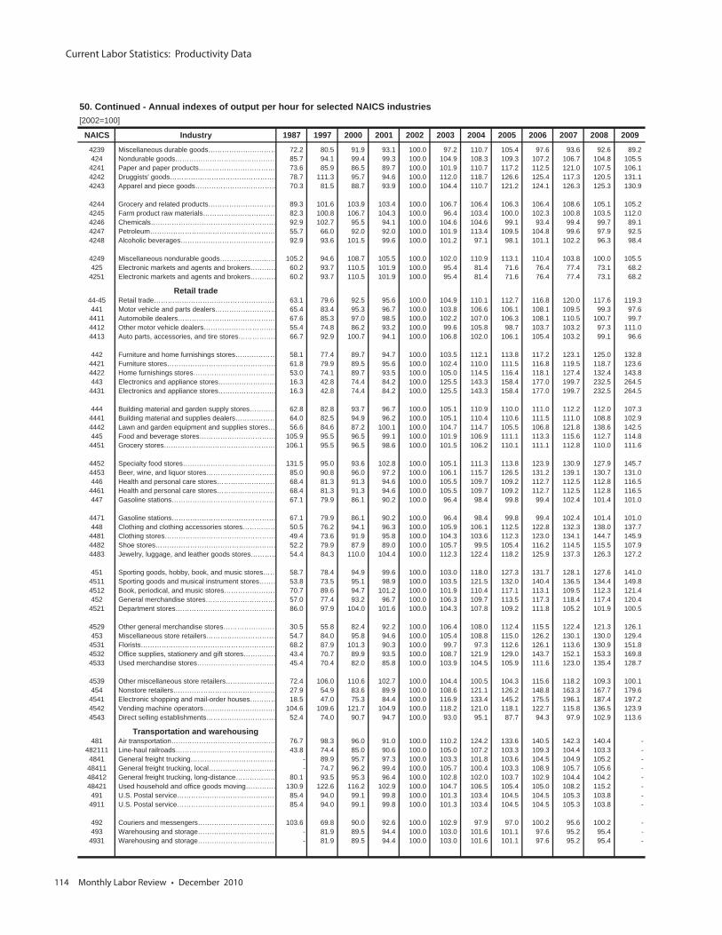
Current Labor Statistics: Productivity Data
114 Monthly Labor Review • December 2010
50. Continued - Annual indexes of output per hour for selected NAICS industries[2002=100]
NAICS Industry 1987 1997 2000 2001 2002 2003 2004 2005 2006 2007 2008 2009
4239 Miscellaneous durable goods………………………… 72.2 80.5 91.9 93.1 100.0 97.2 110.7 105.4 97.6 93.6 92.6 89.2 424 Nondurable goods……………………………………… 85.7 94.1 99.4 99.3 100.0 104.9 108.3 109.3 107.2 106.7 104.8 105.5
4241 Paper and paper products…………………………… 73.6 85.9 86.5 89.7 100.0 101.9 110.7 117.2 112.5 121.0 107.5 106.1 4242 Druggists' goods………………………………………… 78.7 111.3 95.7 94.6 100.0 112.0 118.7 126.6 125.4 117.3 120.5 131.1 4243 Apparel and piece goods……………………………… 70.3 81.5 88.7 93.9 100.0 104.4 110.7 121.2 124.1 126.3 125.3 130.9
4244 Grocery and related products………………………… 89.3 101.6 103.9 103.4 100.0 106.7 106.4 106.3 106.4 108.6 105.1 105.2 4245 Farm product raw materials…………………………… 82.3 100.8 106.7 104.3 100.0 96.4 103.4 100.0 102.3 100.8 103.5 112.0 4246 Chemicals……………………………………………… 92.9 102.7 95.5 94.1 100.0 104.6 104.6 99.1 93.4 99.4 99.7 89.1 4247 Petroleum……………………………………………… 55.7 66.0 92.0 92.0 100.0 101.9 113.4 109.5 104.8 99.6 97.9 92.5 4248 Alcoholic beverages…………………………………… 92.9 93.6 101.5 99.6 100.0 101.2 97.1 98.1 101.1 102.2 96.3 98.4
4249 Miscellaneous nondurable goods…………………… 105.2 94.6 108.7 105.5 100.0 102.0 110.9 113.1 110.4 103.8 100.0 105.5 425 Electronic markets and agents and brokers………… 60.2 93.7 110.5 101.9 100.0 95.4 81.4 71.6 76.4 77.4 73.1 68.2
4251 Electronic markets and agents and brokers………… 60.2 93.7 110.5 101.9 100.0 95.4 81.4 71.6 76.4 77.4 73.1 68.2
Retail trade44-45 Retail trade……………………………………………… 63.1 79.6 92.5 95.6 100.0 104.9 110.1 112.7 116.8 120.0 117.6 119.3 441 Motor vehicle and parts dealers……………………… 65.4 83.4 95.3 96.7 100.0 103.8 106.6 106.1 108.1 109.5 99.3 97.6
4411 Automobile dealers…………………………………… 67.6 85.3 97.0 98.5 100.0 102.2 107.0 106.3 108.1 110.5 100.7 99.7 4412 Other motor vehicle dealers…………………………… 55.4 74.8 86.2 93.2 100.0 99.6 105.8 98.7 103.7 103.2 97.3 111.0 4413 Auto parts, accessories, and tire stores……………… 66.7 92.9 100.7 94.1 100.0 106.8 102.0 106.1 105.4 103.2 99.1 96.6
442 Furniture and home furnishings stores……………… 58.1 77.4 89.7 94.7 100.0 103.5 112.1 113.8 117.2 123.1 125.0 132.8 4421 Furniture stores………………………………………… 61.8 79.9 89.5 95.6 100.0 102.4 110.0 111.5 116.8 119.5 118.7 123.6 4422 Home furnishings stores……………………………… 53.0 74.1 89.7 93.5 100.0 105.0 114.5 116.4 118.1 127.4 132.4 143.8 443 Electronics and appliance stores……………………… 16.3 42.8 74.4 84.2 100.0 125.5 143.3 158.4 177.0 199.7 232.5 264.5
4431 Electronics and appliance stores……………………… 16.3 42.8 74.4 84.2 100.0 125.5 143.3 158.4 177.0 199.7 232.5 264.5
444 Building material and garden supply stores………… 62.8 82.8 93.7 96.7 100.0 105.1 110.9 110.0 111.0 112.2 112.0 107.3 4441 Building material and supplies dealers……………… 64.0 82.5 94.9 96.2 100.0 105.1 110.4 110.6 111.5 111.0 108.8 102.9 4442 Lawn and garden equipment and supplies stores… 56.6 84.6 87.2 100.1 100.0 104.7 114.7 105.5 106.8 121.8 138.6 142.5 445 Food and beverage stores…………………………… 105.9 95.5 96.5 99.1 100.0 101.9 106.9 111.1 113.3 115.6 112.7 114.8
4451 Grocery stores………………………………………… 106.1 95.5 96.5 98.6 100.0 101.5 106.2 110.1 111.1 112.8 110.0 111.6
4452 Specialty food stores…………………………………… 131.5 95.0 93.6 102.8 100.0 105.1 111.3 113.8 123.9 130.9 127.9 145.7 4453 Beer, wine, and liquor stores………………………… 85.0 90.8 96.0 97.2 100.0 106.1 115.7 126.5 131.2 139.1 130.7 131.0 446 Health and personal care stores……………………… 68.4 81.3 91.3 94.6 100.0 105.5 109.7 109.2 112.7 112.5 112.8 116.5
4461 Health and personal care stores……………………… 68.4 81.3 91.3 94.6 100.0 105.5 109.7 109.2 112.7 112.5 112.8 116.5 447 Gasoline stations……………………………………… 67.1 79.9 86.1 90.2 100.0 96.4 98.4 99.8 99.4 102.4 101.4 101.0
4471 Gasoline stations……………………………………… 67.1 79.9 86.1 90.2 100.0 96.4 98.4 99.8 99.4 102.4 101.4 101.0 448 Clothing and clothing accessories stores…………… 50.5 76.2 94.1 96.3 100.0 105.9 106.1 112.5 122.8 132.3 138.0 137.7
4481 Clothing stores………………………………………… 49.4 73.6 91.9 95.8 100.0 104.3 103.6 112.3 123.0 134.1 144.7 145.9 4482 Shoe stores……………………………………………… 52.2 79.9 87.9 89.0 100.0 105.7 99.5 105.4 116.2 114.5 115.5 107.9 4483 Jewelry, luggage, and leather goods stores………… 54.4 84.3 110.0 104.4 100.0 112.3 122.4 118.2 125.9 137.3 126.3 127.2
451 Sporting goods, hobby, book, and music stores…… 58.7 78.4 94.9 99.6 100.0 103.0 118.0 127.3 131.7 128.1 127.6 141.0 4511 Sporting goods and musical instrument stores……… 53.8 73.5 95.1 98.9 100.0 103.5 121.5 132.0 140.4 136.5 134.4 149.8 4512 Book, periodical, and music stores…………………… 70.7 89.6 94.7 101.2 100.0 101.9 110.4 117.1 113.1 109.5 112.3 121.4 452 General merchandise stores………………………… 57.0 77.4 93.2 96.7 100.0 106.3 109.7 113.5 117.3 118.4 117.4 120.4
4521 Department stores……………………………………… 86.0 97.9 104.0 101.6 100.0 104.3 107.8 109.2 111.8 105.2 101.9 100.5
4529 Other general merchandise stores…………………… 30.5 55.8 82.4 92.2 100.0 106.4 108.0 112.4 115.5 122.4 121.3 126.1 453 Miscellaneous store retailers………………………… 54.7 84.0 95.8 94.6 100.0 105.4 108.8 115.0 126.2 130.1 130.0 129.4
4531 Florists…………………………………………………. 68.2 87.9 101.3 90.3 100.0 99.7 97.3 112.6 126.1 113.6 130.9 151.8 4532 Office supplies, stationery and gift stores…………… 43.4 70.7 89.9 93.5 100.0 108.7 121.9 129.0 143.7 152.1 153.3 169.8 4533 Used merchandise stores……………………………… 45.4 70.4 82.0 85.8 100.0 103.9 104.5 105.9 111.6 123.0 135.4 128.7
4539 Other miscellaneous store retailers…………………… 72.4 106.0 110.6 102.7 100.0 104.4 100.5 104.3 115.6 118.2 109.3 100.1 454 Nonstore retailers……………………………………… 27.9 54.9 83.6 89.9 100.0 108.6 121.1 126.2 148.8 163.3 167.7 179.6
4541 Electronic shopping and mail-order houses………… 18.5 47.0 75.3 84.4 100.0 116.9 133.4 145.2 175.5 196.1 187.4 197.2 4542 Vending machine operators…………………………… 104.6 109.6 121.7 104.9 100.0 118.2 121.0 118.1 122.7 115.8 136.5 123.9 4543 Direct selling establishments………………………… 52.4 74.0 90.7 94.7 100.0 93.0 95.1 87.7 94.3 97.9 102.9 113.6
Transportation and warehousing481 Air transportation……………………………………… 76.7 98.3 96.0 91.0 100.0 110.2 124.2 133.6 140.5 142.3 140.4 -
482111 Line-haul railroads……………………………………… 43.8 74.4 85.0 90.6 100.0 105.0 107.2 103.3 109.3 104.4 103.3 -4841 General freight trucking………………………………… - 89.9 95.7 97.3 100.0 103.3 101.8 103.6 104.5 104.9 105.2 -48411 General freight trucking, local………………………… - 74.7 96.2 99.4 100.0 105.7 100.4 103.3 108.9 105.7 105.6 -48412 General freight trucking, long-distance……………… 80.1 93.5 95.3 96.4 100.0 102.8 102.0 103.7 102.9 104.4 104.2 -48421 Used household and office goods moving…………… 130.9 122.6 116.2 102.9 100.0 104.7 106.5 105.4 105.0 108.2 115.2 -491 U.S. Postal service……………………………………… 85.4 94.0 99.1 99.8 100.0 101.3 103.4 104.5 104.5 105.3 103.8 -
4911 U.S. Postal service……………………………………… 85.4 94.0 99.1 99.8 100.0 101.3 103.4 104.5 104.5 105.3 103.8 -
492 Couriers and messengers……………………………… 103.6 69.8 90.0 92.6 100.0 102.9 97.9 97.0 100.2 95.6 100.2 -493 Warehousing and storage……………………………… - 81.9 89.5 94.4 100.0 103.0 101.6 101.1 97.6 95.2 95.4 -
4931 Warehousing and storage……………………………… - 81.9 89.5 94.4 100.0 103.0 101.6 101.1 97.6 95.2 95.4 -
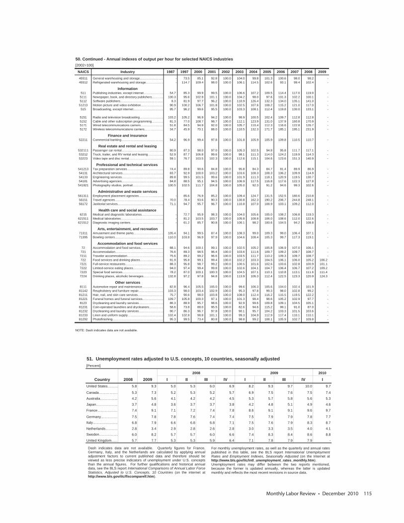
Monthly Labor Review • December 2010 115
50. Continued - Annual indexes of output per hour for selected NAICS industries[2002=100]
NAICS Industry 1987 1997 2000 2001 2002 2003 2004 2005 2006 2007 2008 2009
49311 General warehousing and storage…………………… - 73.5 85.1 92.8 100.0 104.0 99.8 101.3 100.6 98.0 98.2 -49312 Refrigerated warehousing and storage……………… - 114.7 109.4 98.0 100.0 106.1 114.5 102.6 93.1 99.4 102.4 -
Information511 Publishing industries, except internet………………… 54.7 85.3 99.9 99.5 100.0 106.6 107.2 109.5 114.4 117.0 119.0 -
5111 Newspaper, book, and directory publishers………… 100.3 95.6 102.9 101.1 100.0 104.2 98.0 97.6 101.3 102.2 100.1 -5112 Software publishers…………………………………… 8.3 81.9 97.7 96.2 100.0 110.9 126.4 132.3 134.0 135.1 141.0 -51213 Motion picture and video exhibition…………………… 90.9 100.2 106.7 101.8 100.0 102.5 107.6 108.2 115.2 121.0 117.0 -515 Broadcasting, except internet………………………… 95.7 96.2 99.6 95.5 100.0 103.3 108.1 112.4 119.8 130.0 133.1 -
5151 Radio and television broadcasting…………………… 103.2 105.2 96.9 94.2 100.0 98.9 100.5 102.4 109.7 112.8 112.8 -5152 Cable and other subscription programming………… 81.3 77.0 108.7 98.7 100.0 112.1 123.9 131.0 137.9 160.8 170.9 -5171 Wired telecommunications carriers…………………… 51.8 84.5 94.9 92.0 100.0 105.7 110.4 112.3 116.6 122.8 126.7 -5172 Wireless telecommunications carriers……………… 34.7 45.9 70.1 88.0 100.0 110.5 132.3 171.7 185.1 195.1 231.9 -
Finance and insurance52211 Commercial banking…………………………………… 54.2 96.9 99.4 97.8 100.0 101.8 105.9 105.9 109.8 110.5 110.7 -
Real estate and rental and leasing532111 Passenger car rental…………………………………… 80.9 87.3 98.0 97.0 100.0 105.3 102.5 94.8 95.8 111.7 117.1 -53212 Truck, trailer, and RV rental and leasing…………… 52.9 87.7 106.8 99.6 100.0 98.1 111.3 114.0 124.2 119.9 114.3 -53223 Video tape and disc rental…………………………… 59.1 76.7 103.5 102.3 100.0 112.6 115.1 104.6 123.6 151.3 140.9 -
Professional and technical services 541213 Tax preparation services……………………………… 74.4 89.8 90.6 84.8 100.0 95.8 84.3 84.7 81.4 89.9 86.9 -54131 Architectural services…………………………………… 83.7 92.9 100.0 103.2 100.0 103.6 108.3 108.3 106.2 109.9 114.9 -54133 Engineering services…………………………………… 89.8 99.5 101.5 99.6 100.0 101.9 111.3 118.1 120.9 119.5 130.7 -54181 Advertising agencies…………………………………… 84.8 88.5 95.1 94.5 100.0 106.9 117.5 116.8 117.6 122.3 127.8 -
541921 Photography studios, portrait………………………… 100.5 102.5 111.7 104.8 100.0 105.0 92.3 91.2 94.6 99.3 102.6 -
Administrative and waste services561311 Employment placement agencies…………………… - 85.6 76.9 85.2 100.0 109.4 124.7 131.5 152.5 180.6 210.8 -56151 Travel agencies………………………………………… 70.0 78.4 93.6 90.3 100.0 130.8 162.3 190.2 206.7 244.8 248.1 -56172 Janitorial services……………………………………… 71.1 94.7 95.7 96.7 100.0 110.8 107.0 108.9 103.1 109.2 112.0 -
Health care and social assistance6215 Medical and diagnostic laboratories………………… - 72.7 95.9 98.3 100.0 104.0 105.6 105.0 108.2 106.8 119.3 -
621511 Medical laboratories…………………………………… - 81.2 103.5 103.7 100.0 105.8 108.8 106.0 108.6 112.0 122.6 -621512 Diagnostic imaging centers…………………………… - 61.2 85.7 90.8 100.0 100.1 98.2 100.6 104.5 94.2 108.8 -
Arts, entertainment, and recreation71311 Amusement and theme parks………………………… 105.4 94.1 99.5 87.4 100.0 108.3 99.0 109.3 99.0 106.4 107.1 -71395 Bowling centers………………………………………… 110.0 103.8 96.9 97.9 100.0 104.6 108.4 105.3 99.7 117.3 119.1 -
Accommodation and food services72 Accommodation and food services…………………… 88.1 94.6 100.1 99.1 100.0 102.5 105.2 105.8 106.9 107.0 106.1 -721 Accommodation………………………………………… 76.6 89.3 98.5 96.4 100.0 103.6 111.6 109.7 109.2 109.7 108.7 -
7211 Traveler accommodation……………………………… 75.6 89.2 99.2 96.6 100.0 103.5 111.7 110.2 109.3 109.7 108.7 -722 Food services and drinking places…………………… 91.9 95.8 99.1 99.4 100.0 102.2 103.3 104.5 106.1 106.0 105.2 106.2
7221 Full-service restaurants………………………………… 88.3 95.8 98.7 99.2 100.0 100.5 101.6 102.6 103.6 102.8 100.9 101.1 7222 Limited-service eating places………………………… 94.0 97.4 99.4 99.8 100.0 102.6 104.1 104.7 106.4 106.7 107.2 109.2 7223 Special food services…………………………………… 78.2 87.0 100.1 100.3 100.0 104.5 107.1 110.1 110.8 113.1 111.6 111.4 7224 Drinking places, alcoholic beverages………………… 132.8 97.2 97.8 94.8 100.0 113.9 106.3 112.4 122.5 123.3 120.9 124.3
Other services8111 Automotive repair and maintenance………………… 82.8 96.4 105.5 105.0 100.0 99.6 106.3 105.6 104.0 102.4 101.9 -81142 Reupholstery and furniture repair…………………… 103.3 98.0 103.4 102.9 100.0 95.3 97.8 99.3 98.0 102.8 99.2 -81211 Hair, nail, and skin care services……………………… 75.7 90.6 98.0 103.8 100.0 108.0 112.4 116.2 115.5 119.5 122.2 -81221 Funeral homes and funeral services………………… 109.7 105.8 100.3 97.1 100.0 101.3 98.4 98.6 105.2 102.9 97.7 -8123 Drycleaning and laundry services…………………… 86.3 88.9 95.7 98.6 100.0 92.9 99.6 109.8 109.1 104.5 105.1 -81231 Coin-operated laundries and drycleaners…………… 58.6 73.8 88.0 95.5 100.0 82.6 94.6 115.2 99.1 91.0 87.0 -81232 Drycleaning and laundry services…………………… 90.7 86.3 96.7 97.8 100.0 90.1 95.7 104.2 103.3 101.5 103.6 -81233 Linen and uniform supply……………………………… 102.4 102.8 98.8 101.1 100.0 99.3 104.9 112.9 117.4 110.1 110.1 -81292 Photofinishing…………………………………………… 95.3 99.5 73.4 80.8 100.0 98.8 99.2 108.1 105.9 102.7 109.8 -
NOTE: Dash indicates data are not available.
51. Unemployment rates adjusted to U.S. concepts, 10 countries, seasonally adjusted[Percent]
2008 2009 2010
Country 2008 2009 I II III IV I II III IV IUnited States……… 5.8 9.3 5.0 5.3 6.0 6.9 8.2 9.3 9.7 10.0 9.7
Canada……………… 5.3 7.3 5.2 5.3 5.2 5.7 6.9 7.5 7.6 7.5 7.4
Australia…………… 4.2 5.6 4.1 4.2 4.2 4.5 5.3 5.7 5.8 5.6 5.3
Japan………………… 3.7 4.8 3.6 3.7 3.7 3.8 4.2 4.8 5.1 4.9 4.6
France……………… 7.4 9.1 7.1 7.2 7.4 7.8 8.6 9.1 9.1 9.6 9.7
Germany…………… 7.5 7.8 7.8 7.6 7.4 7.4 7.5 7.9 7.9 7.8 7.7Italy………………… 6.8 7.9 6.6 6.8 6.8 7.1 7.5 7.6 7.9 8.3 8.7
Netherlands………… 2.8 3.4 2.9 2.8 2.6 2.8 3.0 3.3 3.5 4.0 4.1Sweden……………… 6.0 8.2 5.7 5.7 6.0 6.6 7.4 8.3 8.4 8.6 8.8
United Kingdom…… 5.7 7.7 5.3 5.3 5.9 6.4 7.1 7.8 7.9 7.9 -
Dash indicates data are not available. Quarterly figures for France,Germany, Italy, and the Netherlands are calculated by applying annualadjustment factors to current published data and therefore should beviewed as less precise indicators of unemployment under U.S. conceptsthan the annual figures. For further qualifications and historical annualdata, see the BLS report International Comparisons of Annual Labor ForceStatistics, Adjusted to U.S. Concepts, 10 Countries (on the internet athttp://www.bls.gov/ilc/flscomparelf.htm).
For monthly unemployment rates, as well as the quarterly and annual ratespublished in this table, see the BLS report International UnemploymentRates and Employment Indexes, Seasonally Adjusted (on the Internet athttp://www.bls.gov/ilc/intl_unemployment_rates_monthly.htm).Unemployment rates may differ between the two reports mentioned,because the former is updated annually, whereas the latter is updatedmonthly and reflects the most recent revisions in source data.
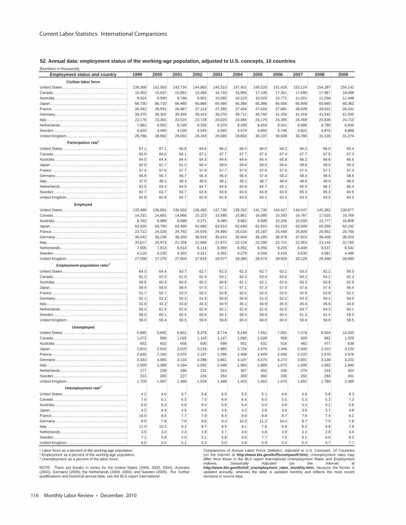
Current Labor Statistics: International Comparisons
116 Monthly Labor Review • December 2010
52. Annual data: employment status of the working-age population, adjusted to U.S. concepts, 10 countries[Numbers in thousands]
Employment status and country 1999 2000 2001 2002 2003 2004 2005 2006 2007 2008 2009Civilian labor force
United States……………………………………………… 139,368 142,583 143,734 144,863 146,510 147,401 149,320 151,428 153,124 154,287 154,142Canada…………………………………………………… 15,403 15,637 15,891 16,366 16,733 16,955 17,108 17,351 17,696 17,987 18,098Australia…………………………………………………… 9,414 9,590 9,746 9,901 10,085 10,213 10,529 10,771 11,021 11,254 11,448Japan……………………………………………………… 66,730 66,710 66,480 65,866 65,495 65,366 65,386 65,556 65,909 65,660 65,362France……………………………………………………… 26,342 26,591 26,867 27,113 27,285 27,424 27,616 27,881 28,028 28,021 28,331Germany…………………………………………………… 39,375 39,302 39,459 39,413 39,276 39,711 40,760 41,250 41,416 41,542 41,545Italy………………………………………………………… 23,176 23,361 23,524 23,728 24,020 24,084 24,179 24,395 24,459 24,836 24,710Netherlands……………………………………………… 7,881 8,052 8,199 8,345 8,379 8,439 8,459 8,541 8,686 8,780 8,846Sweden…………………………………………………… 4,429 4,490 4,530 4,545 4,565 4,579 4,693 4,746 4,822 4,875 4,888United Kingdom…………………………………………… 28,786 28,962 29,092 29,343 29,565 29,802 30,137 30,599 30,780 31,126 31,274
Participation rate1
United States……………………………………………… 67.1 67.1 66.8 66.6 66.2 66.0 66.0 66.2 66.0 66.0 65.4Canada…………………………………………………… 65.9 66.0 66.1 67.1 67.7 67.7 67.4 67.4 67.7 67.9 67.3Australia…………………………………………………… 64.0 64.4 64.4 64.3 64.6 64.6 65.4 65.8 66.2 66.6 66.5Japan……………………………………………………… 62.0 61.7 61.2 60.4 59.9 59.6 59.5 59.6 59.8 59.5 59.3France……………………………………………………… 57.4 57.6 57.7 57.8 57.7 57.5 57.4 57.5 57.4 57.1 57.3Germany…………………………………………………… 56.9 56.7 56.7 56.4 56.0 56.4 57.6 58.2 58.4 58.5 58.6Italy………………………………………………………… 47.9 48.1 48.3 48.5 49.1 49.1 48.7 48.9 48.6 49.0 48.4Netherlands……………………………………………… 62.5 63.4 64.0 64.7 64.6 64.8 64.7 65.1 65.9 66.2 66.4Sweden…………………………………………………… 62.7 63.7 63.7 63.9 63.9 63.6 64.8 64.9 65.3 65.3 64.6United Kingdom…………………………………………… 62.8 62.8 62.7 62.9 62.9 63.0 63.1 63.5 63.3 63.5 63.3
EmployedUnited States……………………………………………… 133,488 136,891 136,933 136,485 137,736 139,252 141,730 144,427 146,047 145,362 139,877Canada…………………………………………………… 14,331 14,681 14,866 15,223 15,586 15,861 16,080 16,393 16,767 17,025 16,769Australia…………………………………………………… 8,762 8,989 9,088 9,271 9,485 9,662 9,998 10,255 10,539 10,777 10,809Japan……………………………………………………… 63,920 63,790 63,460 62,650 62,510 62,640 62,910 63,210 63,509 63,250 62,242France……………………………………………………… 23,712 24,326 24,792 24,976 24,990 25,016 25,187 25,446 25,806 25,951 25,755Germany…………………………………………………… 36,042 36,236 36,350 36,018 35,615 35,604 36,185 36,978 37,815 38,406 38,324Italy………………………………………………………… 20,617 20,973 21,359 21,666 21,972 22,124 22,290 22,721 22,953 23,144 22,765Netherlands……………………………………………… 7,605 7,813 8,014 8,114 8,069 8,052 8,056 8,205 8,408 8,537 8,542Sweden…………………………………………………… 4,116 4,230 4,303 4,311 4,301 4,279 4,334 4,416 4,530 4,581 4,486United Kingdom…………………………………………… 27,058 27,375 27,604 27,815 28,077 28,380 28,674 28,929 29,129 29,346 28,880
Employment-population ratio2
United States……………………………………………… 64.3 64.4 63.7 62.7 62.3 62.3 62.7 63.1 63.0 62.2 59.3Canada…………………………………………………… 61.3 62.0 61.9 62.4 63.1 63.3 63.4 63.6 64.2 64.2 62.3Australia…………………………………………………… 59.6 60.3 60.0 60.2 60.8 61.1 62.1 62.6 63.3 63.8 62.8Japan……………………………………………………… 59.4 59.0 58.4 57.5 57.1 57.1 57.3 57.5 57.6 57.4 56.4France……………………………………………………… 51.7 52.7 53.3 53.2 52.8 52.5 52.3 52.5 52.9 52.8 52.1Germany…………………………………………………… 52.1 52.2 52.2 51.5 50.8 50.6 51.2 52.2 53.3 54.1 54.0I l 42 6 43 2 43 8 44 3 44 9 45 1 44 9 45 5 45 6 45 6 44 6Italy………………………………………………………… 42.6 43.2 43.8 44.3 44.9 45.1 44.9 45.5 45.6 45.6 44.6Netherlands……………………………………………… 60.3 61.5 62.6 62.9 62.2 61.8 61.6 62.5 63.7 64.3 64.1Sweden…………………………………………………… 58.3 60.1 60.5 60.6 60.2 59.5 59.9 60.4 61.3 61.4 59.3United Kingdom…………………………………………… 59.0 59.4 59.5 59.6 59.8 60.0 60.0 60.0 59.9 59.9 58.5
UnemployedUnited States……………………………………………… 5,880 5,692 6,801 8,378 8,774 8,149 7,591 7,001 7,078 8,924 14,265Canada…………………………………………………… 1,072 956 1,026 1,143 1,147 1,093 1,028 958 929 962 1,329Australia…………………………………………………… 652 602 658 630 599 551 531 516 482 477 638Japan……………………………………………………… 2,810 2,920 3,020 3,216 2,985 2,726 2,476 2,346 2,400 2,410 3,120France……………………………………………………… 2,630 2,265 2,075 2,137 2,295 2,408 2,429 2,435 2,222 2,070 2,576Germany…………………………………………………… 3,333 3,065 3,110 3,396 3,661 4,107 4,575 4,272 3,601 3,136 3,222Italy………………………………………………………… 2,559 2,388 2,164 2,062 2,048 1,960 1,889 1,673 1,506 1,692 1,945Netherlands……………………………………………… 277 239 186 231 310 387 402 336 278 243 304Sweden…………………………………………………… 313 260 227 234 264 300 360 330 292 294 401United Kingdom…………………………………………… 1,728 1,587 1,489 1,528 1,488 1,423 1,463 1,670 1,652 1,780 2,395
Unemployment rate3
United States……………………………………………… 4.2 4.0 4.7 5.8 6.0 5.5 5.1 4.6 4.6 5.8 9.3Canada…………………………………………………… 7.0 6.1 6.5 7.0 6.9 6.4 6.0 5.5 5.3 5.3 7.3Australia…………………………………………………… 6.9 6.3 6.8 6.4 5.9 5.4 5.0 4.8 4.4 4.2 5.6Japan……………………………………………………… 4.2 4.4 4.5 4.9 4.6 4.2 3.8 3.6 3.6 3.7 4.8France……………………………………………………… 10.0 8.5 7.7 7.9 8.4 8.8 8.8 8.7 7.9 7.4 9.1Germany…………………………………………………… 8.5 7.8 7.9 8.6 9.3 10.3 11.2 10.4 8.7 7.5 7.8Italy………………………………………………………… 11.0 10.2 9.2 8.7 8.5 8.1 7.8 6.9 6.2 6.8 7.9Netherlands……………………………………………… 3.5 3.0 2.3 2.8 3.7 4.6 4.8 3.9 3.2 2.8 3.4Sweden…………………………………………………… 7.1 5.8 5.0 5.1 5.8 6.6 7.7 7.0 6.1 6.0 8.2United Kingdom…………………………………………… 6.0 5.5 5.1 5.2 5.0 4.8 4.9 5.5 5.4 5.7 7.7
Comparisons of Annual Labor Force Statistics, Adjusted to U.S. Concepts, 10 Countries(on the internet at http://www.bls.gov/ilc/flscomparelf.htm). Unemployment rates maydiffer from those in the BLS report International Unemployment Rates and EmploymentIndexes, Seasonally Adjusted (on the Internet athttp://www.bls.gov/ilc/intl_unemployment_rates_monthly.htm), because the former isupdated annually, whereas the latter is updated monthly and reflects the most recentrevisions in source data.
1 Labor force as a percent of the working-age population.2 Employment as a percent of the working-age population.3 Unemployment as a percent of the labor force.
NOTE: There are breaks in series for the United States (2000, 2003, 2004), Australia(2001), Germany (2005), the Netherlands (2000, 2003), and Sweden (2005). For furtherqualifications and historical annual data, see the BLS report International
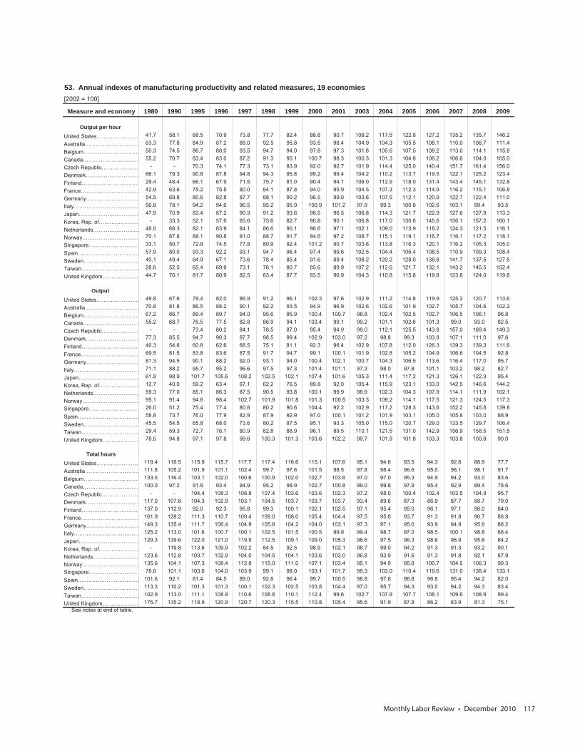
Monthly Labor Review • December 2010 117
53. Annual indexes of manufacturing productivity and related measures, 19 economies
Measure and economy 1980 1990 1995 1996 1997 1998 1999 2000 2001 2003 2004 2005 2006 2007 2008 2009
Output per hour
Output
Total hours
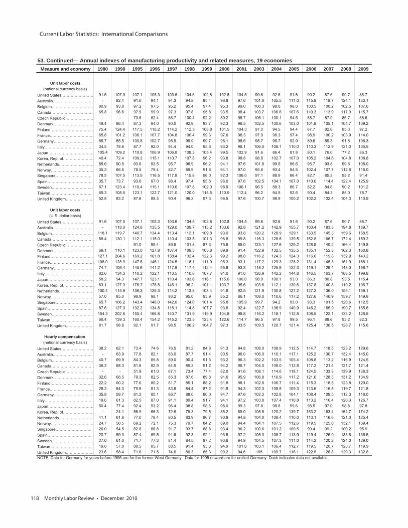
Current Labor Statistics: International Comparisons
118 Monthly Labor Review • December 2010
53. Continued— Annual indexes of manufacturing productivity and related measures, 19 economiesMeasure and economy 1980 1990 1995 1996 1997 1998 1999 2000 2001 2003 2004 2005 2006 2007 2008 2009
Unit labor costs
Unit labor costs
Hourly compensation
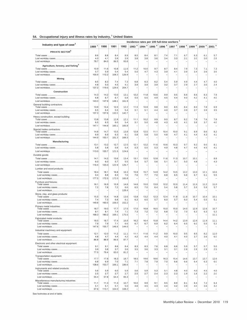
Monthly Labor Review • December 2010 119
54. Occupational injury and illness rates by industry, 1 United StatesIncidence rates per 100 full-time workers 3
1989 1 1990 1991 1992 1993 4 1994 4 1995 4 1996 4 1997 4 1998 4 1999 4 2000 4 2001 4
PRIVATE SECTOR5
Total cases ............................…………………………. 8.6 8.8 8.4 8.9 8.5 8.4 8.1 7.4 7.1 6.7 6.3 6.1 5.7 Lost workday cases..................................................... 4.0 4.1 3.9 3.9 3.8 3.8 3.6 3.4 3.3 3.1 3.0 3.0 2.8 Lost workdays........………........................................... 78.7 84.0 86.5 93.8 – – – – – – – – –
Agriculture, forestry, and fishing5
Total cases ............................…………………………. 10.9 11.6 10.8 11.6 11.2 10.0 9.7 8.7 8.4 7.9 7.3 7.1 7.3 Lost workday cases..................................................... 5.7 5.9 5.4 5.4 5.0 4.7 4.3 3.9 4.1 3.9 3.4 3.6 3.6 Lost workdays........………........................................... 100.9 112.2 108.3 126.9 – – – – – – – – –
Mining Total cases ............................…………………………. 8.5 8.3 7.4 7.3 6.8 6.3 6.2 5.4 5.9 4.9 4.4 4.7 4.0
Lost workday cases..................................................... 4.8 5.0 4.5 4.1 3.9 3.9 3.9 3.2 3.7 2.9 2.7 3.0 2.4 Lost workdays........………........................................... 137.2 119.5 129.6 204.7 – – – – – – – – –
Construction Total cases ............................…………………………. 14.3 14.2 13.0 13.1 12.2 11.8 10.6 9.9 9.5 8.8 8.6 8.3 7.9
Lost workday cases..................................................... 6.8 6.7 6.1 5.8 5.5 5.5 4.9 4.5 4.4 4.0 4.2 4.1 4.0 Lost workdays........………........................................... 143.3 147.9 148.1 161.9 – – – – – – – – – General building contractors: Total cases ............................…………………………. 13.9 13.4 12.0 12.2 11.5 10.9 9.8 9.0 8.5 8.4 8.0 7.8 6.9
Lost workday cases..................................................... 6.5 6.4 5.5 5.4 5.1 5.1 4.4 4.0 3.7 3.9 3.7 3.9 3.5 Lost workdays........………........................................... 137.3 137.6 132.0 142.7 – – – – – – – – – Heavy construction, except building: Total cases ............................…………………………. 13.8 13.8 12.8 12.1 11.1 10.2 9.9 9.0 8.7 8.2 7.8 7.6 7.8
Lost workday cases..................................................... 6.5 6.3 6.0 5.4 5.1 5.0 4.8 4.3 4.3 4.1 3.8 3.7 4.0 Lost workdays........………........................................... 147.1 144.6 160.1 165.8 – – – – – – – – – Special trades contractors: Total cases ............................…………………………. 14.6 14.7 13.5 13.8 12.8 12.5 11.1 10.4 10.0 9.1 8.9 8.6 8.2
Lost workday cases..................................................... 6.9 6.9 6.3 6.1 5.8 5.8 5.0 4.8 4.7 4.1 4.4 4.3 4.1 Lost workdays........………........................................... 144.9 153.1 151.3 168.3 – – – – – – – – –
Manufacturing Total cases ............................…………………………. 13.1 13.2 12.7 12.5 12.1 12.2 11.6 10.6 10.3 9.7 9.2 9.0 8.1
Lost workday cases..................................................... 5.8 5.8 5.6 5.4 5.3 5.5 5.3 4.9 4.8 4.7 4.6 4.5 4.1 Lost workdays........………........................................... 113.0 120.7 121.5 124.6 – – – – – – – – – Durable goods:
Total cases ............................…………………………. 14.1 14.2 13.6 13.4 13.1 13.5 12.8 11.6 11.3 10.7 10.1 – 8.8 Lost workday cases..................................................... 6.0 6.0 5.7 5.5 5.4 5.7 5.6 5.1 5.1 5.0 4.8 – 4.3 Lost workdays........………........................................... 116.5 123.3 122.9 126.7 – – – – – – – – – Lumber and wood products:
Total cases ............................………………………… 18.4 18.1 16.8 16.3 15.9 15.7 14.9 14.2 13.5 13.2 13.0 12.1 10.6 Lost workday cases.................................................. 9.4 8.8 8.3 7.6 7.6 7.7 7.0 6.8 6.5 6.8 6.7 6.1 5.5 Lost workdays........………........................................ 177.5 172.5 172.0 165.8 – – – – – – – – – Furniture and fixtures: Total cases ............................………………………… 16.1 16.9 15.9 14.8 14.6 15.0 13.9 12.2 12.0 11.4 11.5 11.2 11.0
Lost workday cases.................................................. 7.2 7.8 7.2 6.6 6.5 7.0 6.4 5.4 5.8 5.7 5.9 5.9 5.7 Lost workdays........………........................................ – – – 128.4 – – – – – – – – – Stone, clay, and glass products: Total cases ............................………………………… 15.5 15.4 14.8 13.6 13.8 13.2 12.3 12.4 11.8 11.8 10.7 10.4 10.1
Lost workday cases.................................................. 7.4 7.3 6.8 6.1 6.3 6.5 5.7 6.0 5.7 6.0 5.4 5.5 5.1 Lost workdays........………........................................ 149.8 160.5 156.0 152.2 – – – – – – – – – Primary metal industries: Total cases ............................………………………… 18.7 19.0 17.7 17.5 17.0 16.8 16.5 15.0 15.0 14.0 12.9 12.6 10.7
Lost workday cases.................................................. 8.1 8.1 7.4 7.1 7.3 7.2 7.2 6.8 7.2 7.0 6.3 6.3 5.3 Lost workdays........………........................................ 168.3 180.2 169.1 175.5 – – – – – – – – 11.1 Fabricated metal products: Total cases ............................………………………… 18.5 18.7 17.4 16.8 16.2 16.4 15.8 14.4 14.2 13.9 12.6 11.9 11.1
Lost workday cases.................................................. 7.9 7.9 7.1 6.6 6.7 6.7 6.9 6.2 6.4 6.5 6.0 5.5 5.3 Lost workdays........………........................................ 147.6 155.7 146.6 144.0 – – – – – – – – – Industrial machinery and equipment:
Total cases ............................………………………… 12.1 12.0 11.2 11.1 11.1 11.6 11.2 9.9 10.0 9.5 8.5 8.2 11.0 Lost workday cases.................................................. 4.8 4.7 4.4 4.2 4.2 4.4 4.4 4.0 4.1 4.0 3.7 3.6 6.0 Lost workdays........………........................................ 86.8 88.9 86.6 87.7 – – – – – – – – – Electronic and other electrical equipment: Total cases ............................………………………… 9.1 9.1 8.6 8.4 8.3 8.3 7.6 6.8 6.6 5.9 5.7 5.7 5.0
Lost workday cases.................................................. 3.9 3.8 3.7 3.6 3.5 3.6 3.3 3.1 3.1 2.8 2.8 2.9 2.5 Lost workdays........………........................................ 77.5 79.4 83.0 81.2 – – – – – – – – – Transportation equipment: Total cases ............................………………………… 17.7 17.8 18.3 18.7 18.5 19.6 18.6 16.3 15.4 14.6 13.7 13.7 12.6
Lost workday cases.................................................. 6.8 6.9 7.0 7.1 7.1 7.8 7.9 7.0 6.6 6.6 6.4 6.3 6.0 Lost workdays........………........................................ 138.6 153.7 166.1 186.6 – – – – – – – – – Instruments and related products: Total cases ............................………………………… 5.6 5.9 6.0 5.9 5.6 5.9 5.3 5.1 4.8 4.0 4.0 4.5 4.0
Lost workday cases.................................................. 2.5 2.7 2.7 2.7 2.5 2.7 2.4 2.3 2.3 1.9 1.8 2.2 2.0 Lost workdays........………........................................ 55.4 57.8 64.4 65.3 – – – – – – – – – Miscellaneous manufacturing industries: Total cases ............................………………………… 11.1 11.3 11.3 10.7 10.0 9.9 9.1 9.5 8.9 8.1 8.4 7.2 6.4
Lost workday cases.................................................. 5.1 5.1 5.1 5.0 4.6 4.5 4.3 4.4 4.2 3.9 4.0 3.6 3.2 Lost workdays........………........................................ 97.6 113.1 104.0 108.2 – – – – – – – – –
See footnotes at end of table.
Industry and type of case 2
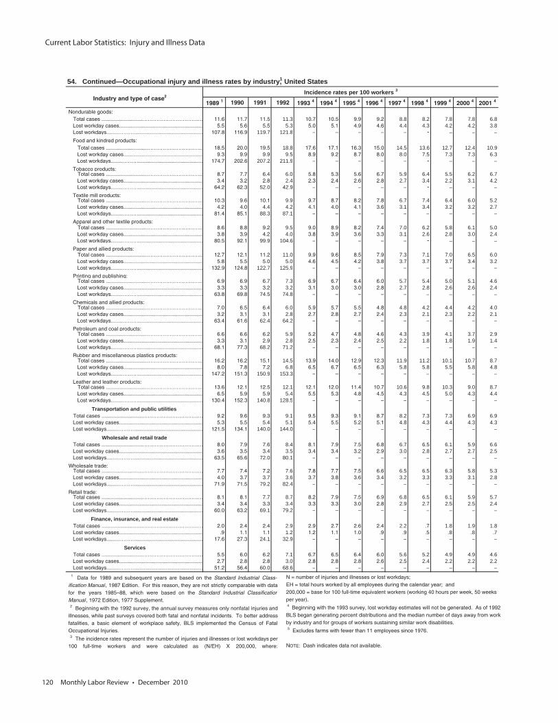
Current Labor Statistics: Injury and Illness Data
120 Monthly Labor Review • December 2010
54. Continued—Occupational injury and illness rates by industry,1 United StatesIncidence rates per 100 workers 3
1989 1 1990 1991 1992 1993 4 1994 4 1995 4 1996 4 1997 4 1998 4 1999 4 2000 4 2001 4
Nondurable goods: Total cases ............................…………………………..… 11.6 11.7 11.5 11.3 10.7 10.5 9.9 9.2 8.8 8.2 7.8 7.8 6.8
Lost workday cases......................................................... 5.5 5.6 5.5 5.3 5.0 5.1 4.9 4.6 4.4 4.3 4.2 4.2 3.8 Lost workdays........………............................................... 107.8 116.9 119.7 121.8 – – – – – - – – – Food and kindred products: Total cases ............................………………………….. 18.5 20.0 19.5 18.8 17.6 17.1 16.3 15.0 14.5 13.6 12.7 12.4 10.9
Lost workday cases...................................................... 9.3 9.9 9.9 9.5 8.9 9.2 8.7 8.0 8.0 7.5 7.3 7.3 6.3 Lost workdays........………............................................ 174.7 202.6 207.2 211.9 – – – – – - – – – Tobacco products: Total cases ............................………………………….. 8.7 7.7 6.4 6.0 5.8 5.3 5.6 6.7 5.9 6.4 5.5 6.2 6.7
Lost workday cases...................................................... 3.4 3.2 2.8 2.4 2.3 2.4 2.6 2.8 2.7 3.4 2.2 3.1 4.2 Lost workdays........………............................................ 64.2 62.3 52.0 42.9 – – – – – - – – – Textile mill products: Total cases ............................………………………….. 10.3 9.6 10.1 9.9 9.7 8.7 8.2 7.8 6.7 7.4 6.4 6.0 5.2
Lost workday cases...................................................... 4.2 4.0 4.4 4.2 4.1 4.0 4.1 3.6 3.1 3.4 3.2 3.2 2.7 Lost workdays........………............................................ 81.4 85.1 88.3 87.1 – – – – – – – – – Apparel and other textile products: Total cases ............................………………………….. 8.6 8.8 9.2 9.5 9.0 8.9 8.2 7.4 7.0 6.2 5.8 6.1 5.0
Lost workday cases...................................................... 3.8 3.9 4.2 4.0 3.8 3.9 3.6 3.3 3.1 2.6 2.8 3.0 2.4 Lost workdays........………............................................ 80.5 92.1 99.9 104.6 – – – – – - – – – Paper and allied products: Total cases ............................………………………….. 12.7 12.1 11.2 11.0 9.9 9.6 8.5 7.9 7.3 7.1 7.0 6.5 6.0
Lost workday cases...................................................... 5.8 5.5 5.0 5.0 4.6 4.5 4.2 3.8 3.7 3.7 3.7 3.4 3.2 Lost workdays........………............................................ 132.9 124.8 122.7 125.9 – – – – – – – – – Printing and publishing: Total cases ............................………………………….. 6.9 6.9 6.7 7.3 6.9 6.7 6.4 6.0 5.7 5.4 5.0 5.1 4.6
Lost workday cases...................................................... 3.3 3.3 3.2 3.2 3.1 3.0 3.0 2.8 2.7 2.8 2.6 2.6 2.4 Lost workdays........………............................................ 63.8 69.8 74.5 74.8 – – – – – – – – – Chemicals and allied products: Total cases ............................………………………….. 7.0 6.5 6.4 6.0 5.9 5.7 5.5 4.8 4.8 4.2 4.4 4.2 4.0
Lost workday cases...................................................... 3.2 3.1 3.1 2.8 2.7 2.8 2.7 2.4 2.3 2.1 2.3 2.2 2.1 Lost workdays........………............................................ 63.4 61.6 62.4 64.2 – – – – – – – – – Petroleum and coal products: Total cases ............................………………………….. 6.6 6.6 6.2 5.9 5.2 4.7 4.8 4.6 4.3 3.9 4.1 3.7 2.9
Lost workday cases...................................................... 3.3 3.1 2.9 2.8 2.5 2.3 2.4 2.5 2.2 1.8 1.8 1.9 1.4 Lost workdays........………............................................ 68.1 77.3 68.2 71.2 – – – – – – – – – Rubber and miscellaneous plastics products: Total cases ............................………………………….. 16.2 16.2 15.1 14.5 13.9 14.0 12.9 12.3 11.9 11.2 10.1 10.7 8.7
Lost workday cases...................................................... 8.0 7.8 7.2 6.8 6.5 6.7 6.5 6.3 5.8 5.8 5.5 5.8 4.8 Lost workdays........………............................................ 147.2 151.3 150.9 153.3 – – – – – – – – – Leather and leather products: Total cases ............................………………………….. 13.6 12.1 12.5 12.1 12.1 12.0 11.4 10.7 10.6 9.8 10.3 9.0 8.7
Lost workday cases...................................................... 6.5 5.9 5.9 5.4 5.5 5.3 4.8 4.5 4.3 4.5 5.0 4.3 4.4 Lost workdays........………............................................ 130.4 152.3 140.8 128.5 – – – – – – – – –
Transportation and public utilities Total cases ............................…………………………..… 9.2 9.6 9.3 9.1 9.5 9.3 9.1 8.7 8.2 7.3 7.3 6.9 6.9
Lost workday cases......................................................... 5.3 5.5 5.4 5.1 5.4 5.5 5.2 5.1 4.8 4.3 4.4 4.3 4.3 Lost workdays........………............................................... 121.5 134.1 140.0 144.0 – – – – – – – – –
Wholesale and retail trade Total cases ............................…………………………..… 8.0 7.9 7.6 8.4 8.1 7.9 7.5 6.8 6.7 6.5 6.1 5.9 6.6
Lost workday cases......................................................... 3.6 3.5 3.4 3.5 3.4 3.4 3.2 2.9 3.0 2.8 2.7 2.7 2.5 Lost workdays........………............................................... 63.5 65.6 72.0 80.1 – – – – – – – – – Wholesale trade: Total cases ............................…………………………..… 7.7 7.4 7.2 7.6 7.8 7.7 7.5 6.6 6.5 6.5 6.3 5.8 5.3
Lost workday cases......................................................... 4.0 3.7 3.7 3.6 3.7 3.8 3.6 3.4 3.2 3.3 3.3 3.1 2.8 Lost workdays........………............................................... 71.9 71.5 79.2 82.4 – – – – – – – – – Retail trade: Total cases ............................…………………………..… 8.1 8.1 7.7 8.7 8.2 7.9 7.5 6.9 6.8 6.5 6.1 5.9 5.7
Lost workday cases......................................................... 3.4 3.4 3.3 3.4 3.3 3.3 3.0 2.8 2.9 2.7 2.5 2.5 2.4 Lost workdays........………............................................... 60.0 63.2 69.1 79.2 – – – – – – – – –
Finance, insurance, and real estate Total cases ............................…………………………..… 2.0 2.4 2.4 2.9 2.9 2.7 2.6 2.4 2.2 .7 1.8 1.9 1.8
Lost workday cases......................................................... .9 1.1 1.1 1.2 1.2 1.1 1.0 .9 .9 .5 .8 .8 .7 Lost workdays........………............................................... 17.6 27.3 24.1 32.9 – – – – – – – – –
Services Total cases ............................…………………………..… 5.5 6.0 6.2 7.1 6.7 6.5 6.4 6.0 5.6 5.2 4.9 4.9 4.6
Lost workday cases......................................................... 2.7 2.8 2.8 3.0 2.8 2.8 2.8 2.6 2.5 2.4 2.2 2.2 2.2 Lost workdays........………............................................... 51.2 56.4 60.0 68.6 – – – – – – – – –
Industry and type of case2
1 Data for 1989 and subsequent years are based on the Standard Industrial Class-ification Manual , 1987 Edition. For this reason, they are not strictly comparable with datafor the years 1985–88, which were based on the Standard Industrial ClassificationManual , 1972 Edition, 1977 Supplement.2 Beginning with the 1992 survey, the annual survey measures only nonfatal injuries and
illnesses, while past surveys covered both fatal and nonfatal incidents. To better addressfatalities, a basic element of workplace safety, BLS implemented the Census of FatalOccupational Injuries.3 The incidence rates represent the number of injuries and illnesses or lost workdays per
100 full-time workers and were calculated as (N/EH) X 200,000, where:
N = number of injuries and illnesses or lost workdays; EH = total hours worked by all employees during the calendar year; and200,000 = base for 100 full-time equivalent workers (working 40 hours per week, 50 weeks per year). 4 Beginning with the 1993 survey, lost workday estimates will not be generated. As of 1992,BLS began generating percent distributions and the median number of days away from work by industry and for groups of workers sustaining similar work disabilities.
5 Excludes farms with fewer than 11 employees since 1976.
NOTE: Dash indicates data not available.
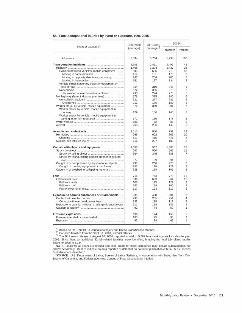
Monthly Labor Review • December 2010 121
55. Fatal occupational injuries by event or exposure, 1996-2005
Event or exposure1 1996-2000(average)
2001-2005(average)2
20053
Number Percent
All events ............................................................... 6,094 5,704 5,734 100
Transportation incidents ................................................ 2,608 2,451 2,493 43Highway ........................................................................ 1,408 1,394 1,437 25
Collision between vehicles, mobile equipment ......... 685 686 718 13Moving in same direction ...................................... 117 151 175 3Moving in opposite directions, oncoming .............. 247 254 265 5Moving in intersection ........................................... 151 137 134 2
Vehicle struck stationary object or equipment onside of road ............................................................. 264 310 345 6
Noncollision ............................................................... 372 335 318 6Jack-knifed or overturned--no collision ................. 298 274 273 5
Nonhighway (farm, industrial premises) ........................ 378 335 340 6Noncollision accident ................................................ 321 277 281 5
Overturned ............................................................ 212 175 182 3Worker struck by vehicle, mobile equipment ................ 376 369 391 7
Worker struck by vehicle, mobile equipment inroadway .................................................................. 129 136 140 2
Worker struck by vehicle, mobile equipment inparking lot or non-road area .................................... 171 166 176 3
Water vehicle ................................................................ 105 82 88 2Aircraft ........................................................................... 263 206 149 3
Assaults and violent acts ............................................... 1,015 850 792 14Homicides ..................................................................... 766 602 567 10
Shooting .................................................................... 617 465 441 8Suicide, self-inflicted injury ............................................ 216 207 180 3
Contact with objects and equipment ............................ 1,005 952 1,005 18Struck by object ............................................................ 567 560 607 11
Struck by falling object .............................................. 364 345 385 7Struck by rolling, sliding objects on floor or groundlevel ......................................................................... 77 89 94 2
Caught in or compressed by equipment or objects ....... 293 256 278 5Caught in running equipment or machinery .............. 157 128 121 2
Caught in or crushed in collapsing materials ................ 128 118 109 2
Falls .................................................................................. 714 763 770 13Fall to lower level .......................................................... 636 669 664 12
Fall from ladder ......................................................... 106 125 129 2Fall from roof ............................................................. 153 154 160 3Fall to lower level, n.e.c. ........................................... 117 123 117 2
Exposure to harmful substances or environments ..... 535 498 501 9Contact with electric current .......................................... 290 265 251 4
Contact with overhead power lines ........................... 132 118 112 2Exposure to caustic, noxious, or allergenic substances 112 114 136 2Oxygen deficiency ......................................................... 92 74 59 1
Fires and explosions ...................................................... 196 174 159 3Fires--unintended or uncontrolled ................................. 103 95 93 2Explosion ...................................................................... 92 78 65 1
1 Based on the 1992 BLS Occupational Injury and Illness Classification Manual.2 Excludes fatalities from the Sept. 11, 2001, terrorist attacks.3 The BLS news release of August 10, 2006, reported a total of 5,702 fatal work injuries for calendar year
2005. Since then, an additional 32 job-related fatalities were identified, bringing the total job-related fatalitycount for 2005 to 5,734.
NOTE: Totals for all years are revised and final. Totals for major categories may include subcategories notshown separately. Dashes indicate no data reported or data that do not meet publication criteria. N.e.c. means"not elsewhere classified."
SOURCE: U.S. Department of Labor, Bureau of Labor Statistics, in cooperation with State, New York City,District of Columbia, and Federal agencies, Census of Fatal Occupational Injuries.
122 Monthly Labor Review • December 2010
Index to Volume 133January 2010 to December 2010
American Time Use Survey
Time-use surveys: issues in data collection on multitasking. Aug. 2010, pp. 17–31.
Bringing work home: implications for BLS productivity measures. Dec. 2010, pp. 18–35.
Census of Fatal Occupational Injuries Fatal occupational injuries at road construction sites, 2003–07. Nov. 2010, pp. 37–40.
Compensation costs Compensation of residential and nonresidential construction
workers. Apr. 2010, pp. 31–45.Labor costs in India’s organized manufacturing sector. May 2010,
pp. 3–22.Compensation costs in manufacturing across industries and
countries, 1975–2007. June 2010, pp. 32–54.
Construction Compensation of residential and nonresidential construction
workers. Apr. 2010, pp. 31–45.The U.S. housing bubble and bust: impacts on employment. Dec.
2010, pp. 3–17.
Consumer Expenditure Survey
Out-of-pocket health care expenditures: a comparison. Feb. 2010, pp. 3–19.
New expenditure data in the PSID: comparisons with the CE. Feb. 2010, pp. 29–39.
Consumer Expenditure Survey Microdata Users’ Workshop, July 2009. Apr. 2010, pp. 46–49.
Consumer expenditures Out-of-pocket health care expenditures: a comparison. Feb. 2010,
pp. 3–19.New expenditure data in the PSID: comparisons with the CE. Feb.
2010, pp. 29–39.Household expenditures on children, 2007–08. Sep. 2010, pp. 3–16.
Consumer Expenditures Survey Household expenditures on children, 2007–08. Sep. 2010, pp. 3–16.
Consumer Price Index
Producing disease-based price indexes. Feb. 2010, pp. 20–28.PPI and CPI seasonal adjustment: an update. July 2010, pp. 10–20.
Current Employment Statistics Payroll employment in 2009: job losses continue. Mar. 2010, pp.
23–33.New all-employee hours and earnings from the CES survey. Mar.
2010, pp. 34–40.
All-employee hours and earnings for States and metropolitan areas Mar. 2010, pp. 41–50.
The composition of the unemployed and long-term unemployed in tough labor markets. Oct. 2010, pp. 3–18.
Current Population Survey Union membership attrition Jan. 2010, pp. 74–76.The labor market in 2009: recession drags on. Mar. 2010, pp. 3–22.The early 2000s: a period of declining teen summer employment
rates. May 2010, pp. 23–35.Employment and earnings of recent veterans: data from the CPS. July
2010, pp. 3–9.Multiple jobholding during the 2000s. July 2010, pp. 21–32.Multiple jobholding in States in 2009. July 2010, pp. 33–34.Self-employment in the United States. Sep. 2010, pp. 17–32.The composition of the unemployed and long-term unemployed in
tough labor markets. Oct. 2010, pp. 3–18.The impact of the 2007–09 recession on workers with disabilities.
Oct. 2010, pp. 19–30.Disability and occupational projections. Oct. 2010, pp. 31–87.The Nation’s underemployed in the “Great Recession” of 2007–09.
Nov. 2010, pp. 3–15.Reversals in the patterns of women’s labor supply in the U.S., 1977–
2009. Nov. 2010, pp. 16–36.Bringing work home: implications for BLS productivity measures.
Dec. 2010, pp. 18–35.Duration of unemployment in States, 2007–09. Dec. 2010, pp. 36–39.
Disability
The impact of the 2007–09 recession on workers with disabilities. Oct. 2010, pp. 19–30.
Disability and occupational projections. Oct. 2010, pp. 31–87.
Earnings and wages
New all-employee hours and earnings from the CES survey. Mar. 2010, pp. 34–40.
All-employee hours and earnings for States and metropolitan areas Mar. 2010, pp. 41–50.
Compensation of residential and nonresidential construction workers. Apr. 2010, pp. 31–45.
Job openings, hires, and separations fall during the recession. May 2010, pp. 36–44.
Employment and earnings of recent veterans: data from the CPS. July 2010, pp. 3–9.
Economic development and growth Industry shifts over the decade put Philadelphia on a new road to job
growth. Apr. 2010, pp. 3–18.
Monthly Labor Review • December 2010 123
Employment
Crash and reboot: Silicon Valley high-tech employment and wages, 2000–08. Jan. 2010, pp. 59–73.
Industry shifts over the decade put Philadelphia on a new road to job growth. Apr. 2010, pp. 3–18.
The early 2000s: a period of declining teen summer employment rates. May 2010, pp. 23–35.
Job openings, hires, and separations fall during the recession. May 2010, pp. 36–44.
Employment and earnings of recent veterans: data from the CPS. July 2010, pp. 3–9.
The expanding role of temporary help services from 1990 to 2008. Aug. 2010, pp. 3–16.
The composition of the unemployed and long-term unemployed in tough labor markets. Oct. 2010, pp. 3–18.
The Nation’s underemployed in the “Great Recession” of 2007–09. Nov. 2010, pp. 3–15.
The U.S. housing bubble and bust: impacts on employment. Dec. 2010, pp. 3–17.
Employment Projections
Evaluating the 1996–2006 employment projections. Sep. 2010, pp. 33–69.
Disability and occupational projections. Oct. 2010, pp. 31–87.The U.S. housing bubble and bust: impacts on employment. Dec.
2010, pp. 3–17.
Health care
Out-of-pocket health care expenditures: a comparison. Feb. 2010, pp. 3–19.
New expenditure data in the PSID: comparisons with the CE. Feb. 2010, pp. 29–39.
Home-based work
Bringing work home: implications for BLS productivity measures. Dec. 2010, pp. 18–35.
Hours of work
New all-employee hours and earnings from the CES survey. Mar. 2010, pp. 34–40.
All-employee hours and earnings for States and metropolitan areas Mar. 2010, pp. 41–50.
Housing
The U.S. housing bubble and bust: impacts on employment. Dec. 2010, pp. 3–17.
India
Labor costs in India’s organized manufacturing sector. May 2010, pp. 3–22.
Industry studies
The expanding role of temporary help services from 1990 to 2008. Aug. 2010, pp. 3–16.
International comparisons
Labor costs in India’s organized manufacturing sector. May 2010, pp. 3–22.
Compensation costs in manufacturing across industries and countries, 1975–2007. June 2010, pp. 32–54.
International Labor Comparisons
Labor costs in India’s organized manufacturing sector. May 2010, pp. 3–22.
Effects of imported intermediate inputs on productivity. June 2010, pp. 3–15.
Compensation costs in manufacturing across industries and countries, 1975–2007. June 2010, pp. 32–54.
International Price Program
IPP 2008 year in review. Apr. 2010, pp. 19–30.Job creationJob openings, hires, and separations fall during the recession. May
2010, pp. 36–44.
Job Openings and Labor Turnover
Job openings, hires, and separations fall during the recession. May 2010, pp. 36–44.
Labor force
Reversals in the patterns of women’s labor supply in the U.S., 1977–2009. Nov. 2010, pp. 16–36.
The U.S. housing bubble and bust: impacts on employment. Dec. 2010, pp. 3–17.
Labor law
State labor legislation enacted in 2009. Jan. 2010, pp. 3–36.Changes in State unemployment insurance legislation in 2009. Jan.
2010, pp. 37–58.
Labor market
The labor market in 2009: recession drags on. Mar. 2010, pp. 3–22.Payroll employment in 2009: job losses continue. Mar. 2010, pp.
23–33.Job openings, hires, and separations fall during the recession. May
2010, pp. 36–44.
Labor organizations
Union membership attrition Jan. 2010, pp. 74–76.
Labor Productivity and Costs
Effects of imported intermediate inputs on productivity. June 2010, pp. 3–15.
Nonmanufacturing industry contributions to multifactor productivity, 1987–2006. June 2010, pp. 16–31.
Compensation costs in manufacturing across industries and countries, 1975–2007. June 2010, pp. 32–54.
Bringing work home: implications for BLS productivity measures. Dec. 2010, pp. 18–35.
Manufacturing
Labor costs in India’s organized manufacturing sector. May 2010, pp. 3–22.
Multifactor Productivity Effects of imported intermediate inputs on productivity. June 2010, pp. 3–15.
Nonmanufacturing industry contributions to multifactor productivity, 1987–2006. June 2010, pp. 16–31.
Multiple jobholders
Multiple jobholding during the 2000s. July 2010, pp. 21–32.Multiple jobholding in States in 2009. July 2010, pp. 33–34.
124 Monthly Labor Review • December 2010
National Compensation Survey
Compensation of residential and nonresidential construction workers. Apr. 2010, pp. 31–45.
Occupational Employment Statistics
Revising the Standard Occupational Classification system for 2010,. Aug. 2010, pp. 32–41.
Occupational safety and health
Fatal occupational injuries at road construction sites, 2003–07. Nov. 2010, pp. 37–40.
Occupations
Revising the Standard Occupational Classification system for 2010. Aug. 2010, pp. 32–41.
Part-time work
The Nation’s underemployed in the “Great Recession” of 2007–09. Nov. 2010, pp. 3–15.
Prices
Producing disease-based price indexes. Feb. 2010, pp. 20–28.
IPP
2008 year in review. Apr. 2010, pp. 19–30.PPI and CPI seasonal adjustment: an update. July 2010, pp. 10–20.
Producer Price Index
PPI and CPI seasonal adjustment: an update. July 2010, pp. 10–20.
Productivity
Effects of imported intermediate inputs on productivity. June 2010, pp. 3–15.
Nonmanufacturing industry contributions to multifactor productivity, 1987–2006. June 2010, pp. 16–31.
Bringing work home: implications for BLS productivity measures. Dec. 2010, pp. 18–35.
Projections
Evaluating the 1996–2006 employment projections. Sep. 2010, pp. 33–69.
Disability and occupational projections. Oct. 2010, pp. 31–87.
Quarterly Census of Employment and Wages
Crash and reboot: Silicon Valley high-tech employment and wages, 2000–08. Jan. 2010, pp. 59–73.
Industry shifts over the decade put Philadelphia on a new road to job growth. Apr. 2010, pp. 3–18.
The expanding role of temporary help services from 1990 to 2008. Aug. 2010, pp. 3–16.
Recession
The composition of the unemployed and long-term unemployed in tough labor markets. Oct. 2010, pp. 3–18.
The Nation’s underemployed in the “Great Recession” of 2007–09. Nov. 2010, pp. 3–15.
Regional economics
Crash and reboot: Silicon Valley high-tech employment and wages, 2000–08. Jan. 2010, pp. 59–73.
The expanding role of temporary help services from 1990 to 2008.
Aug. 2010, pp. 3–16.Duration of unemployment in States, 2007–09. Dec. 2010, pp. 36–39.
Seasonal employment
The early 2000s: a period of declining teen summer employment rates. May 2010, pp. 23–35.
Self-employment
Self-employment in the United States. Sep. 2010, pp. 17–32.
Standard Occupational Classification
Revising the Standard Occupational Classification system for 2010. Aug. 2010, pp. 32–41.
State government
State labor legislation enacted in 2009. Jan. 2010, pp. 3–36.Changes in State unemployment insurance legislation in 2009. Jan.
2010, pp. 37–58.
Statistical programs and methods
Consumer Expenditure Survey Microdata Users’ Workshop, July 2009. Apr. 2010, pp. 46–49.
PPI and CPI seasonal adjustment: an update. July 2010, pp. 10–20.Revising the Standard Occupational Classification system for 2010.
Aug. 2010, pp. 32–41.
Time use
Time-use surveys: issues in data collection on multitasking. Aug. 2010, pp. 17–31.
Unemployment
The composition of the unemployed and long-term unemployed in tough labor markets. Oct. 2010, pp. 3–18.
The Nation’s underemployed in the “Great Recession” of 2007–09. Nov. 2010, pp. 3–15.
Duration of unemployment in States, 2007–09. Dec. 2010, pp. 36–39.
Unemployment insurance
Changes in State unemployment insurance legislation in 2009. Jan. 2010, pp. 37–58.
Veterans
Employment and earnings of recent veterans: data from the CPS. July 2010, pp. 3–9.
Women
Reversals in the patterns of women’s labor supply in the U.S., 1977–2009. Nov. 2010, pp. 16–36.
Workplace injuries and illnesses
Fatal occupational injuries at road construction sites, 2003–07. Nov. 2010, pp. 37–40.
Youth
The early 2000s: a period of declining teen summer employment rates. May 2010, pp. 23–35.
DEPARTMENTSBook reviews. Each issue.Current Labor Statistics. Each issue.Labor month in review. Each issue.

Monthly Labor Review • December 2010 125
Précis. Each issue. Program reports. Mar. and Apr. issues.Regional trends. July and Dec. issues.Research summary. Jan. issue.Workplace safety and health. Nov. issue.
BOOK REVIEWS (Listed by author of book)Angrist, Joshua D. and Jorn-Steffan Pischke. Mostly Harmless
Econometrics: An Empiricist’s Companion. Mar. 2010, p. 52.Applebaum, Eileen, Annette D. Bernhardt, and Richard J. Murnane.
Low-Wage America: How Employers are Reshaping Opportunity in the Workplace. Oct. 2010, pp.90–92.
Bamber, Greg, Jody Hoffer Gittell, Thomas A. Kochan, and Andrew von Nordenflycht. Up in the Air: How airlines can improve performance by engaging their employees. Nov. 2010, pp. 43–44.
Bernhardt, Annette D., Eileen Applebaum, and Richard J. Murnane. Low-Wage America: How Employers are Reshaping Opportunity in the Workplace. Oct. 2010, pp.90–92.
Caulfield, Norman. NAFTA and Labor in North America. Dec. 2010, pp. 42–43.
Gittell, Jody Hoffer, Greg Bamber, Thomas A. Kochan, and Andrew von Nordenflycht. Up in the Air: How airlines can improve performance by engaging their employees. Nov. 2010, pp. 43–44.
Hawthorne, Fran. Pension Dumping: The Reasons, the Wreckage, the Stakes for Wall Street. Jan. 2010, pp. 78–79.
Kleiner, Morris M. Licensing Occupations: Ensuring Quality or Restricting Competition? June 2010, p. 56.
Klier, Thomas and James Rubenstein. Who Really Made Your Car?: Restructuring and Geographic Change in the Auto Industry. Sep. 2010, pp. 72–73.
Kochan, Thomas A., Greg Bamber, Jody Hoffer Gittell, and Andrew von Nordenflycht. Up in the Air: How airlines can improve performance by engaging their employees. Nov. 2010, pp. 43–44.
MacLaury, Judson. To Advance Their Opportunities: Federal Policies Towards African American Workers From World War I to the Civil Rights Act of 1964. Apr. 2010, pp. 52–53.
McCloskey, Deirdre N. and Stephen T. Ziliak. The Cult of Statistical Significance: How the Standard Error Costs Us Jobs, Justice, and Lives. Feb. 2010, pp. 41–42.
Murnane, Richard J., Eileen Applebaum, and Annette D. Bernhardt. Low-Wage America: How Employers are Reshaping Opportunity in the Workplace. Oct. 2010, pp.90–92.
Pischke, Jorn-Steffan and Joshua D. Angrist. Mostly Harmless Econometrics: An Empiricist’s Companion. Mar. 2010, p. 52.
Rubenstein, James and Thomas Klier. Who Really Made Your Car?: Restructuring and Geographic Change in the Auto Industry. Sep. 2010, pp. 72–73.
Seefeldt, Kristin S. Working After Welfare: How Women Balance Jobs and Family in the Wake of Welfare Reform. May 2010, pp. 47–48.
Stockhammer, Engelbert. The Rise of Unemployment in Europe: A Keynesian Approach. Aug. 44–45.
von Nordenflycht, Andrew, Greg Bamber, Jody Hoffer Gittell, and Thomas A. Kochan. Up in the Air: How airlines can improve performance by engaging their employees. Nov. 2010, pp. 43–44.
Zaniello, Tom. The Cinema of Globalization: A Guide to Films about the New Economic Order. July 2010, p. 36.
Ziliak, Stephen T. and Deirdre N. McCloskey. The Cult of Statistical Significance: How the Standard Error Costs Us Jobs, Justice, and Lives. Feb. 2010, pp. 41–42.
AUTHORSAli, Mohammad, Douglas Kruse, andLisa Schur. Disability and
occupational projections. Oct. 2010, pp. 31–87.Allegretto, Sylvia and Devon Lynch. The composition of the
unemployed and long-term unemployed in tough labor markets. Oct. 2010, pp. 3–18.
Anderson, Sally L. Duration of unemployment in States, 2007–09. Dec. 2010, pp. 36–39.
Ayres, Mary Ellen. Book review. May 2010, pp. 47–48.Barker, Megan M. and Adam A. Hadi. Payroll employment in 2009:
job losses continue. Mar. 2010, pp. 23–33.Barsky, Carl. Book review. Nov. 2010, pp. 43–44.Bennion, Edwin. IPP 2008 year in review. Apr. 2010, pp. 19–30.Bergman, Bruce. Book review. Feb. 2010, pp. 41–42.Bibler, Adam. Book review. Sep. 2010, pp. 72–73.Bradley, Ralph, Elaine Cardenas, Daniel H. Ginsburg, Lyubov
Rozental, and Frankie Velez. Producing disease-based price indexes. Feb. 2010, pp. 20–28.
Brand, Horst. Book review. Oct. 2010, pp. 90–92.Byun, Kathryn J. The U.S. housing bubble and bust: impacts on
employment. Dec. 2010, pp. 3–17.Campbell, Jim. Multiple jobholding in States in 2009. July 2010, pp.
33–34.Cardenas, Elaine, Ralph Bradley, Daniel H. Ginsburg, Lyubov
Rozental, and Frankie Velez. Producing disease-based price indexes. Feb. 2010, pp. 20–28.
Chaison, Gary. Union membership attrition. Jan. 2010, pp. 74–76.Charles, Kerwin Kofi, Geng Li, Robert F. Schoeni, and Sheldon
Danziger. New expenditure data in the PSID: comparisons with the CE. Feb. 2010, pp. 29–39.
Clinton, Angela, John Coughlan, and Brian Dahlin. New all-employee hours and earnings from the CES survey. Mar. 2010, pp. 34–40.
Cosca, Theresa and Alissa Emmel. Revising the Standard Occupational Classification system for 2010. Aug. 2010, pp. 32–41.
Coughlan, John, Angela Clinton, and Brian Dahlin. New all-employee hours and earnings from the CES survey. Mar. 2010, pp. 34–40.
Dahlin, Brian, Angela Clinton, and John Coughlan. New all-employee hours and earnings from the CES survey. Mar. 2010, pp. 34–40.
Danziger, Sheldon, Geng Li, Robert F. Schoeni, and Kerwin Kofi Charles. New expenditure data in the PSID: comparisons with the CE. Feb. 2010, pp. 29–39.
DeAntonio, Dante. All-employee hours and earnings for States and metropolitan areas Mar. 2010, pp. 41–50.
deWolf, Mark and Katherine Klemmer. Job openings, hires, and separations fall during the recession. May 2010, pp. 36–44.
Drago, Robert W. and Jay C. Stewart. Time-use surveys: issues in data collection on multitasking. Aug. 2010, pp. 17–31.
Dutton, Bridget, John J. Fitzpatrick, Jr., and James L. Perine. State labor legislation enacted in 2009. Jan. 2010, pp. 3–36.
Eldridge, Lucy P. and Michael J. Harper. Effects of imported intermediate inputs on productivity. June 2010, pp. 3–15.
Eldridge, Lucy P. and Sabrina Wulff Pabilonia. Bringing work home: implications for BLS productivity measures. Dec. 2010, pp. 18–35.
Emmel, Alissa and Theresa Cosca. Revising the Standard Occupational Classification system for 2010. Aug. 2010, pp. 32–41.
Faluszczak, Mary. Book review. July 2010, p. 36.Fitzpatrick, Jr., John J., James L. Perine, and Bridget Dutton. State
labor legislation enacted in 2009. Jan. 2010, pp. 3–36.

126 Monthly Labor Review • December 2010
Foster, Ann C. Out-of-pocket health care expenditures: a comparison. Feb. 2010, pp. 3–19.
Ginsburg, Daniel H., Ralph Bradley, Elaine Cardenas, Lyubov Rozental, and Frankie Velez. Producing disease-based price indexes. Feb. 2010, pp. 20–28.
Hadi, Adam A. and Megan M. Barker. Payroll employment in 2009: job losses continue. Mar. 2010, pp. 23–33.
Harper, Michael J. and Lucy P. Eldridge. Effects of imported intermediate inputs on productivity. June 2010, pp. 3–15.
Harper, Michael J., Bhavani Khandrika, Randal Kinoshita, and Steven Rosenthal. Nonmanufacturing industry contributions to multifactor productivity, 1987–2006. June 2010, pp. 16–31.
Haub, Carl, Jessica R. Sincavage, and O.P. Sharma. Labor costs in India’s organized manufacturing sector. May 2010, pp. 3–22.
Hertwig, Ralf. Book review. Aug. 2010, pp. 44–45.Hipple, Steven F. Multiple jobholding during the 2000s. July 2010,
pp. 21–32.Hipple, Steven F. Self-employment in the United States. Sep. 2010,
pp. 17–32.Hipple, Steven. The labor market in 2009: recession drags on. Mar.
2010, pp. 3–22.Holden, Richard, Tian Luo, and Amar Mann. The expanding role of
temporary help services from 1990 to 2008. Aug. 2010, pp. 3–16.Kaye, H. Stephen. The impact of the 2007–09 recession on workers
with disabilities. Oct. 2010, pp. 19–30.Khandrika, Bhavani, Michael J. Harper, Randal Kinoshita, and
Steven Rosenthal. Nonmanufacturing industry contributions to multifactor productivity, 1987–2006. June 2010, pp. 16–31.
Khatiwada, Ishwar and Andrew Sum. The Nation’s underemployed in the “Great Recession” of 2007–09. Nov. 2010, pp. 3–15.
Kinoshita, Randal, Michael J. Harper, Bhavani Khandrika, and Steven Rosenthal. Nonmanufacturing industry contributions to multifactor productivity, 1987–2006. June 2010, pp. 16–31.
Kirchmer, Jacob and Elizabeth Zamora. Compensation costs in manufacturing across industries and countries, 1975–2007. June 2010, pp. 32–54.
Klemmer, Katherine and Mark deWolf. Job openings, hires, and separations fall during the recession. May 2010, pp. 36–44.
Krantz, John Kenneth. Book review. Dec. 2010, pp. 42–43.Kruse, Douglas, Lisa Schur, and Mohammad Ali. Disability and
occupational projections. Oct. 2010, pp. 31–87.Lancaster, Loryn. Changes in State unemployment insurance
legislation in 2009. Jan. 2010, pp. 37–58.Li, Geng, Robert F. Schoeni, Sheldon Danziger, and Kerwin Kofi
Charles. New expenditure data in the PSID: comparisons with the CE. Feb. 2010, pp. 29–39.
Luo, Tian and Amar Mann. Crash and reboot: Silicon Valley high-tech employment and wages, 2000–08. Jan. 2010, pp. 59–73.
Luo, Tian, Amar Mann, and Richard Holden. The expanding role of temporary help services from 1990 to 2008. Aug. 2010, pp. 3–16.
Lynch, Devon and Sylvia Allegretto. The composition of the unemployed and long-term unemployed in tough labor markets. Oct. 2010, pp. 3–18.
Macunovich, Diane J. Reversals in the patterns of women’s labor supply in the U.S., 1977–2009. Nov. 2010, pp. 16–36.
Mann, Amar and Tian Luo. Crash and reboot: Silicon Valley high-tech employment and wages, 2000–08. Jan. 2010, pp. 59–73.
Mann, Amar, Tian Luo, and Richard Holden. The expanding role of
temporary help services from 1990 to 2008. Aug. 2010, pp. 3–16.Mitchell, David. Book review. Mar. 2010, p. 52.Moehrle, Thomas. Compensation of residential and nonresidential
construction workers. Apr. 2010, pp. 31–45.Morisi, Teresa L. The early 2000s: a period of declining teen summer
employment rates. May 2010, pp. 23–35.Muri, Steven M., Jonathan C. Weinhagen, and Jeffrey S. Wilson.
PPI and CPI seasonal adjustment: an update. July 2010, pp. 10–20.Nilsen, Diane and Gerald Perrins. Industry shifts over the decade put
Philadelphia on a new road to job growth. Apr. 2010, pp. 3–18.Omori, Megumi. Household expenditures on children, 2007–08.
Sep. 2010, pp. 3–16.Pabilonia, Sabrina Wulff and Lucy P. Eldridge. Bringing work home:
implications for BLS productivity measures. Dec. 2010, pp. 18–35.Paulin, Geoffrey D. Consumer Expenditure Survey Microdata Users’
Workshop, July 2009. Apr. 2010, pp. 46–49.Pegula, Stephen. Fatal occupational injuries at road construction
sites, 2003–07. Nov. 2010, pp. 37–40.Perine, James L., John J. Fitzpatrick, Jr., and Bridget Dutton. State
labor legislation enacted in 2009. Jan. 2010, pp. 3–36.Perrins, Gerald and Diane Nilsen. Industry shifts over the decade put
Philadelphia on a new road to job growth. Apr. 2010, pp. 3–18.Ramey, Alice. Book review. June 2010, p. 56.Rosenthal, Steven, Michael J. Harper, Bhavani Khandrika, and
Randal Kinoshita. Nonmanufacturing industry contributions to multifactor productivity, 1987–2006. June 2010, pp. 16–31.
Rozental, Lyubov, Ralph Bradley, Elaine Cardenas, Daniel H. Ginsburg, and Frankie Velez. Producing disease-based price indexes. Feb. 2010, pp. 20–28
Schoeni, Robert F., Geng Li, Sheldon Danziger, and Kerwin Kofi Charles. New expenditure data in the PSID: comparisons with the CE. Feb. 2010, pp. 29–39.
Schur, Lisa, Douglas Kruse, and Mohammad Ali. Disability and occupational projections. Oct. 2010, pp. 31–87.
Sharma, O.P., Jessica R. Sincavage, and Carl Haub. Labor costs in India’s organized manufacturing sector. May 2010, pp. 3–22.
Sincavage, Jessica R., Carl Haub, and O.P. Sharma. Labor costs in India’s organized manufacturing sector. May 2010, pp. 3–22.
Stewart, Jay C. and Robert W. Drago. Time-use surveys: issues in data collection on multitasking. Aug. 2010, pp. 17–31.
Sum, Andrew and Ishwar Khatiwada. The Nation’s underemployed in the “Great Recession” of 2007–09. Nov. 2010, pp. 3–15.
Velez, Frankie, Ralph Bradley, Elaine Cardenas, Daniel H. Ginsburg, and Lyubov Rozental. Producing disease-based price indexes. Feb. 2010, pp. 20–28.
Walker, James A. Employment and earnings of recent veterans: data from the CPS. July 2010, pp. 3–9.
Wasser, Solidelle. Book review. Apr. 2010, pp. 52–53.Weinhagen, Jonathan C., Jeffrey S. Wilson, and Steven M. Muri.
PPI and CPI seasonal adjustment: an update. July 2010, pp. 10–20.Wilson, Jeffrey S., Jonathan C. Weinhagen, and Steven M. Muri.
PPI and CPI seasonal adjustment: an update. July 2010, pp. 10–20.Wyatt, Ian D. Evaluating the 1996–2006 employment projections.
Sep. 2010, pp. 33–69.Yi, Song. Book review. Jan. 2010, pp. 78–79.Zamora, Elizabeth and Jacob Kirchmer. Compensation costs in
manufacturing across industries and countries, 1975–2007. June 2010, pp. 32–54.