Seediscussions,stats,andauthorprofilesforthispublicationat:http://www.researchgate.net/publication/263377627

U.S.IOOScoastalandoceanmodelingtestbed:Inter‐modelevaluationoftides,waves,andhurricanesurgeintheGulfofMexico

ARTICLE·OCTOBER2013

DOI:10.1002/jgrc.20376

CITATIONS

4

DOWNLOADS

76

VIEWS

148

29AUTHORS,INCLUDING:

AronRoland

TechnicalUniversityDarmstadtandBGSIT&…

48PUBLICATIONS396CITATIONS

SEEPROFILE

RichardSignell

UnitedStatesGeologicalSurvey

91PUBLICATIONS2,349CITATIONS

SEEPROFILE

JaneM.Smith

USArmyCorpsofEngineers

118PUBLICATIONS790CITATIONS

SEEPROFILE

MarkDPowell

HWindScientific,LLC

87PUBLICATIONS2,371CITATIONS

SEEPROFILE

Availablefrom:RichardA.Luettich,Jr.

Retrievedon:14July2015

U.S. IOOS coastal and ocean modeling testbed: Inter-modelevaluation of tides, waves, and hurricane surge in the Gulf of Mexico

P. C. Kerr,1 A. S. Donahue,1 J. J. Westerink,1 R. A. Luettich Jr.,2 L. Y. Zheng,3 R. H. Weisberg,3 Y. Huang,3

H. V. Wang,4 Y. Teng,4 D. R. Forrest,4 A. Roland,5 A. T. Haase,6 A. W. Kramer,6 A. A. Taylor,6 J. R. Rhome,7

J. C. Feyen,8 R. P. Signell,9 J. L. Hanson,10 M. E. Hope,1 R. M. Estes,1 R. A. Dominguez,1 R. P. Dunbar,1

L. N. Semeraro,1 H. J. Westerink,1 A. B. Kennedy,1 J. M. Smith,11 M. D. Powell,12 V. J. Cardone,13

and A. T. Cox13

Received 15 March 2013; revised 22 July 2013; accepted 23 August 2013; published 8 October 2013.

[1] A Gulf of Mexico performance evaluation and comparison of coastal circulation andwave models was executed through harmonic analyses of tidal simulations, hindcasts ofHurricane Ike (2008) and Rita (2005), and a benchmarking study. Three unstructuredcoastal circulation models (ADCIRC, FVCOM, and SELFE) validated with similar skillon a new common Gulf scale mesh (ULLR) with identical frictional parameterization andforcing for the tidal validation and hurricane hindcasts. Coupled circulation and wavemodels, SWANþADCIRC and WWMIIþSELFE, along with FVCOM loosely coupledwith SWAN, also validated with similar skill. NOAA’s official operational forecast stormsurge model (SLOSH) was implemented on local and Gulf scale meshes with the samewind stress and pressure forcing used by the unstructured models for hindcasts of Ike andRita. SLOSH’s local meshes failed to capture regional processes such as Ike’s forerunnerand the results from the Gulf scale mesh further suggest shortcomings may be due to acombination of poor mesh resolution, missing internal physics such as tides and nonlinearadvection, and SLOSH’s internal frictional parameterization. In addition, these modelswere benchmarked to assess and compare execution speed and scalability for aprototypical operational simulation. It was apparent that a higher number ofcomputational cores are needed for the unstructured models to meet similar operationalimplementation requirements to SLOSH, and that some of them could benefit fromimproved parallelization and faster execution speed.

Citation: Kerr, P. C., et al. (2013), U.S. IOOS coastal and ocean modeling testbed: Inter-model evaluation of tides, waves, andhurricane surge in the Gulf of Mexico, J. Geophys. Res. Oceans, 118, 5129–5172, doi:10.1002/jgrc.20376.

Additional supporting information may be found in the online version of this article.1Department of Civil and Environmental Engineering and Earth Sciences, University of Notre Dame, South Bend, Indiana, USA.2Institute of Marine Sciences, University of North Carolina at Chapel Hill, Chapel Hill, North Carolina, USA.3College of Marine Science, University of South Florida, St. Petersburg, Florida, USA.4Virginia Institute of Marine Science, College of William and Mary, Williamsburg, Virginia, USA.5Institute for Hydraulic and Water Resources Engineering, Darmstadt University of Technology, Darmstadt, Germany.6Meteorological Development Lab, National Weather Service, National Oceanic and Atmospheric Administration, Silver Spring, Maryland, USA.7National Weather Service, National Oceanic and Atmospheric Administration, Miami, Florida, USA.8National Ocean Service, National Oceanic and Atmospheric Administration, Silver Spring, Maryland, USA.9Woods Hole Science Center, United States Geological Survey, Woods Hole, Massachusetts, USA.10Engineer Research Development Center, United States Army Corps of Engineers, Vicksburg, Mississippi, USA.11Coastal and Hydraulics Laboratory, U.S. Army Engineer Research and Development Center, Vicksburg, Mississippi, USA.12Atlantic Oceanographic and Meteorological Labs, Hurricane Research Division, National Oceanic and Atmospheric Administration, Tallahassee,

Florida, USA.13Ocean Weather, Inc., New Canaan, Connecticut, USA.

Corresponding author: P. C. Kerr, Department of Civil and Environmental Engineering and Earth Sciences, University of Notre Dame, 156 FitzpatrickHall, South Bend, IN 46556, USA. (PCorbittKerr@gmail.com)

©2013. The Authors. Journal of Geophysical Research: Oceans published by Wiley on behalf of the American Geophysical Union.2169-9275/13/10.1002/jgrc.20376

5129

JOURNAL OF GEOPHYSICAL RESEARCH: OCEANS, VOL. 118, 5129–5172, doi:10.1002/jgrc.20376, 2013

1. Introduction

[2] Storm surge is the phenomenon of rising coastalwater levels due to the cumulative effect of processes suchas wind-driven setup and currents, geostrophic effects,wave setup, wave runup and breaking, atmospheric pres-sure changes, precipitation (freshwater flooding), and astro-nomical tides. The National Hurricane Center officiallydescribes storm surge as the difference between water lev-els during the storm (referred to as storm tide) and pre-dicted astronomical tides. This is not to say thatastronomical tides do not influence storm surge, but ratherthat storm surge is considered an abnormal rise of watergenerated by a storm over and above astronomically pre-dicted levels. The resulting high water, powerful currents,erosive velocities, and saline intrusion along the nearshoreand shallow inland areas across the shore and via the con-duit of bays, wetlands, rivers, and channels pose a signifi-cant threat to human life, infrastructure, and freshwaterecosystems. The trend of population and infrastructuregrowth in low-lying coastal areas, combined with the pro-jection for increased flood susceptibility [Mousavi et al.,2010; Ning et al., 2012] due to changes in storm climatol-ogy and sea level rise, suggests a mounting necessity toadvance our understanding of coastal storm surge andimprove our risk assessment and forecasting abilities.

[3] Significant progress has been made over the pasthalf century to understand storm evolution and coastalflooding processes. Outside the broad objective of under-standing these physical processes, the two primary practi-cal uses for coastal storm surge models are operationalforecasting and design/risk analysis. Operational forecast-ing requires an ensemble approach of modeling variantpredictions in storm track and characteristics, that must beexecuted on a consistently stable basis within a short win-dow of simulation time and provide realistic results thatcan be processed and interpreted quickly. Operationalforecasts are used by emergency managers and by thepublic to ensure that risk and loss of life are minimized.Because the overwhelming controlling factors in opera-tional forecasting are ‘‘time’’ and ‘‘robustness/stability,’’metrics such as skill, resolution, and geographic range areoften sacrificed so that a high number of probabilisticstorm variants can be simulated. Design and risk analysis,on the other hand, has a primary objective of designingcoastal protection structures and assessing risk that driveslocal development as well as government subsidized floodinsurance. Accuracy and resolution are essential, and sim-ulation time is of secondary concern. Design and riskanalysis also takes an ensemble approach to storm surgemodeling, but instead of modeling the variants of a singlepredicted storm, a suite of hypothetical storms are mod-eled, so that all contingencies are addressed. One objec-tive of design/risk analysis is to predict flood potentialstatistically. A recurrence interval measure, known as theBase Flood Elevation (BFE), is a measure by which floodrisk reduction systems, bridges, levees, and other struc-tures are designed. Both operational forecasting anddesign/risk analysis use composites of maximum stormsurge water levels, referred to as the Maximum Envelopeof high Water (MEOW) for a single storm and the Maxi-mum of the Maximum (MOM) for a suite of probabilisticstorms.

[4] The National Weather Service (NWS) uses SLOSH(Sea, Lake, and Overland Surges from Hurricanes) as its of-ficial operational forecast model [Jelesnianski et al., 1992].Developed in the late 1960s and formalized in the 1980s,SLOSH uses a best track file to inform its own internalwind model and is applied via an ensemble approach onsmall structured curvilinear meshes overlapping the coast-line [Forbes and Rhome, 2012; Glahn et al., 2009; Taylorand Glahn, 2008]. While there have been improvements tothe SLOSH model in terms of features such as barriers and1-D channels, the core of the computational model has seenvery little change since its inception. Recent studies,including this one and studies by Blain et al. [1994] andMorey et al. [2006], have noted the deficiency of usingsmall domains that cannot capture large-scale processesand suggest using larger meshes for improved accuracy. Inaddition, the use of a structured mesh, regardless if it is cur-vilinear, limits the ability for localized resolution; andtherefore potentially hampers accuracy in SLOSH.

[5] In the last decade, there has been rapid developmentand application of unstructured mesh circulation and wavemodels. Unlike structured models, unstructured modelshave the advantage of being able to provide coarser resolu-tion at the Gulf scale and finer resolution at the coastalfloodplain and channel scale without unnecessary andcostly resolution throughout the Gulf; thus unstructuredmesh models can simultaneously address the domain sizeand mesh resolution issues that have hampered the accu-racy of the SLOSH model. A number of unstructured meshcoastal circulation and wave models have recently comeinto widespread use. The United States Army Corps ofEngineers (USACE) used the ADvanced CIRCulation(ADCIRC) model [Luettich et al., 1992; Westerink et al.,2008] to evaluate and design improvements for the NewOrleans Flood Risk Reduction System and the FederalEmergency Management Agency (FEMA) applies thismodel to evaluate coastal flood risk which is used to de-velop flood insurance rate maps [USACE, 2009; FEMA,2009]. There has been a recent progression toward opera-tional applications of prevalent unstructured mesh circula-tion and/or wave models including: the tightly coupledSimulating WAves Nearshore (SWAN) [Booij et al., 1999;Zijlema, 2010] and ADCIRC model (SWANþADCIRC)[Dietrich et al., 2011a]; the Finite Volume Coastal OceanModel (FVCOM) [Chen et al., 2003]; the Semi-implicitEulerian Lagrangian Finite Element model (SELFE)[Zhang and Baptista, 2008]; and the tightly coupled WindWave Model II (WWMII) and SELFE models(WWMIIþSELFE) [Roland et al., 2009, 2012].

[6] The ADCIRC-based Extratropical Surge and TideOperational Forecast System model (ESTOFS) is used toforecast tides and extratropical surges by the NationalWeather Service [http://www.opc.ncep.noaa.gov/estofs/estofs_surge_info.shtml]. The SWANþADCIRC model isused by the Advanced Surge Guidance System (ASGS),which focuses on providing operational advisory servicesfor impending hurricane events [Fleming et al., 2008]. Thescope of ASGS currently includes the Gulf of Mexico andAtlantic seaboard, and it has been used to provide forecast-ing for Hurricanes Irene (2011), Isaac (2012), and Sandy(2012), as well as the Gulf oil spill [Dietrich et al., 2012a].FVCOM is a component of the Northeast Coastal Ocean

KERR ET AL.: IOOS TESTBED: INTER-MODEL EVALUATION

5130

Forecast System (NECOFS) and is used extensively toforecast tides and extratropical storm events along thenortheast coast of the United States, in particular within theGulf of Maine region [http://www.neracoos.org/datatools/forecast/oceanforecasts]. The SELFE model is currently inuse for forecasting in the Columbia River Estuary as thecore ocean prediction model for the Columbia River Estu-ary Operational Forecast System (CREOFS) [http://tide-sandcurrents.noaa.gov/ofs/creofs/creofs.html].

[7] One aim of the Southeastern Universities ResearchAssociation (SURA)-led U.S. Integrated Ocean ObservingSystem (IOOS)-funded Coastal and Ocean ModelingTestbed (COMT) is to evaluate and improve models al-ready in operational use as well as facilitating the transitionof additional models to operational use. This inter-modelcomparison was initiated as part of that objective, so thatthe skill and behavior of leading coastal and ocean modelsat simulating tropical cyclone waves and surge could beassessed and the implementation requirements necessaryfor these models to migrate to operational use be identified.With that purpose in mind, three widely used unstructuredcoastal and ocean circulation models, ADCIRC, FVCOM,and SELFE, were selected for use on a new common Gulfof Mexico mesh created specifically for the Testbed. Wavesare an integral aspect of hurricanes that can contribute towater levels, coastal erosion, and forces on structures, sosimulations were also performed with tightly coupled waveand circulation models such as SWANþADCIRC andWWMIIþSELFE and FVCOM loosely coupled [Huang etal., 2010] with SWAN. In addition to the unstructuredmodels, NOAA’s official operational forecast storm surgemodel, SLOSH, was also included in this study.

[8] To ensure uniformity in the inter-model comparison,the unstructured models were implemented with identicalfrictional parameterization and forcing for each of thestudy’s simulations. For consistency, SLOSH was alsosimulated with the same forcing as the unstructured mod-els, but due to model constraints continued to use its owninternal bottom friction formulation. Whereas the unstruc-tured models were run on the same Gulf scale mesh,SLOSH used its local and Gulf scale meshes so that theeffects of domain size for SLOSH could be formallyaddressed. Behavioral response to domain size and meshselection is important to understand in order to improveSLOSH’s operational implementation, especially consider-ing the recommendations presented by Morey et al. [2006].

[9] Keeping with the objective of operational forecastingpotential, models included in this study were benchmarkedon the Texas Advanced Computing Cluster’s (TACC)Ranger to assess and compare execution speed and scal-ability for a prototypical operational simulation. In addi-tion, the number of computational cores needed for theunstructured mesh models to match SLOSH’s operationalexecution speed (i.e., wall clock time) was estimated.

[10] Tides contribute to overall water levels and currentsduring a hurricane, and therefore this study included aninter-model tidal comparison to assess the ability for eachof these models to simulate the relatively low-energy proc-esses of tidal dynamics in the Gulf. Tides propagate intothe Gulf of Mexico from the Atlantic Ocean through theStraits of Florida and from the Caribbean Sea through theYucatan Channel and are also generated internally in the

Gulf through gravitational tidal potential forcing [Wester-ink et al., 2008]. The dominant tidal signals in the basin arediurnal ; however, resonance along the continental shelvesadjacent to Florida, western Louisiana, and Texas canlocally amplify the semidiurnal tides [Reid, 1990; DiMarcoand Reid, 1998; Gouillon et al., 2010]. Tidal validationstudies have been conducted individually for ADCIRC[Mukai et al., 2002; Bunya et al., 2010], for FVCOM[Chen et al., 2011], and for SELFE [Bertin et al., 2012;Cho et al., 2012]; however, no study has yet comprehen-sively compared the skill of these three models for thesame mesh and tidal forcing. Tides-only simulations wereconducted for ADCIRC, FVCOM, and SELFE, and theresults of the tidal harmonic decomposition were then com-pared with tidal harmonic constituent data from 59 NOAAstations located throughout the Gulf of Mexico. It was notpossible to include SLOSH in the tidal validation sinceSLOSH is unable to simulate tides itself ; instead tides aregenerated within SLOSH by a synthesis of tidal constituentdata gathered from an ADCIRC-based National OceanService EC2001 database [Mukai et al., 2002].

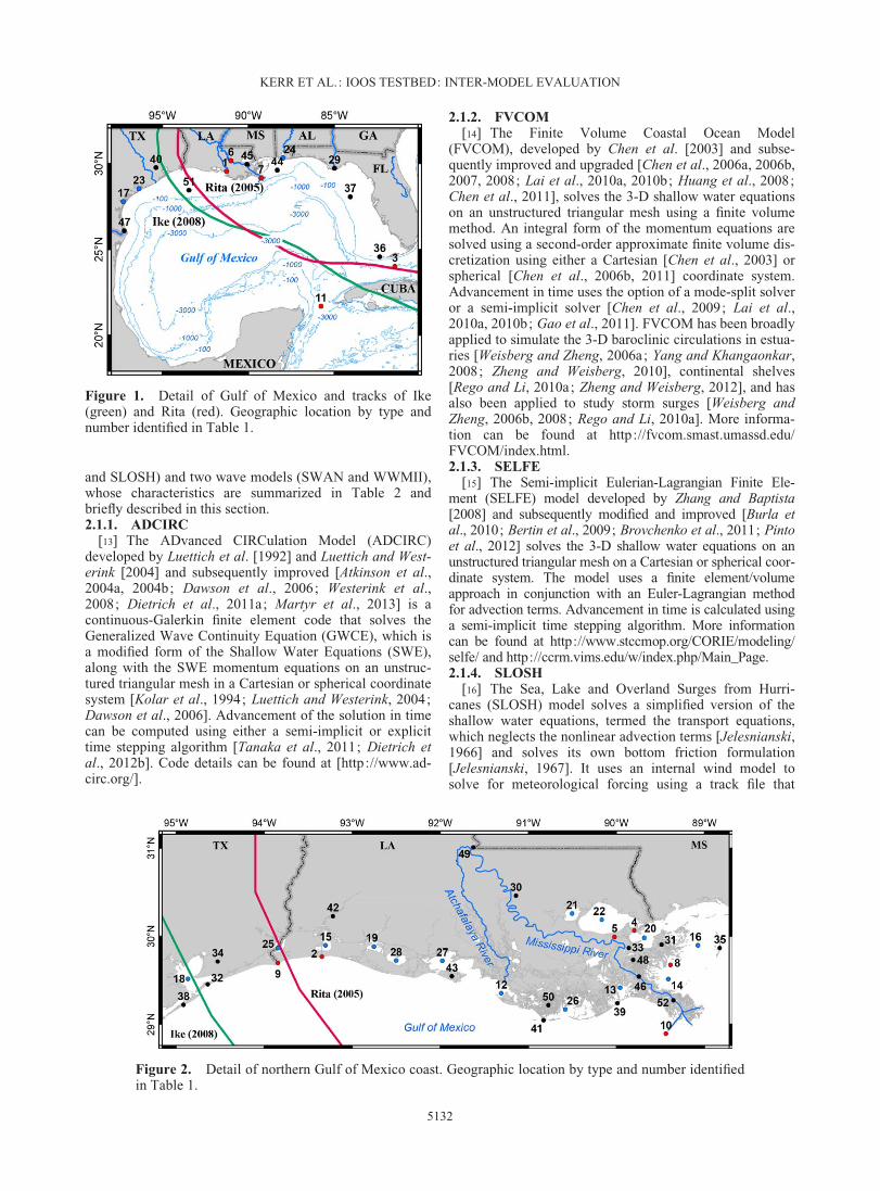
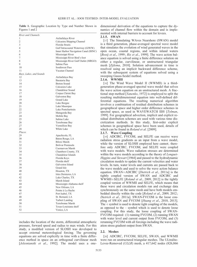
[11] For the inter-model evaluation of skill and behaviorin simulating Atlantic-based tropical cyclones, two Gulf ofMexico hurricanes were selected for analysis: HurricaneRita (2005) and Hurricane Ike (2008). The tracks of thesetwo hurricanes along with many of the points of interestdescribed in this study can be found in Figures 1 and 2 andTable 1. These storms were selected for their large-scaleimpacts on the Louisiana-Texas coastline, unique individ-ual characteristics, and wealth of recorded wave and waterlevel data. Ike, while of similar strength, track, and forwardspeed as Rita, exhibited significantly different surge proc-esses due to its large size. Ike’s steady track across the Gulfcombined with its unusually large wind field created astrong shore-parallel shelf current driven by shore-parallelwinds in the 36 h before landfall. This current caused thelargest ever recorded geostrophic setup or ‘‘forerunner’’surge along the Texas-Louisiana coast filling coastal lakesand bays by up to 2 m before Ike made landfall [Kennedyet al., 2011]. In addition to the ‘‘forerunner,’’ Ike’s relevantsurge processes included: the generation of surge bysteady, moderate winds in southeastern Louisiana and theinfluence (or lack thereof) of marshes in the region in theimpedance of storm surge over extended time scales ; theassociated capture of surge by the protruding MississippiRiver Delta and the surface gradient and associated cur-rents created along the edge of Delta; the propagation of acoherent free wave down the Texas continental shelf ; peakstorm surge driven by strong shore normal winds; and atrapped resonant wave on the continental shelf caused bythe recession of surge onto the shelf [Hope et al., 2013].Circulation models, ADCIRC, FVCOM, SELFE, andSLOSH, along with the tightly coupled circulation andwave models, SWANþADCIRC and WWMIIþSELFE,and the loosely coupled FVCOM with SWAN, wereapplied to hindcast these storms.

2. Methods

2.1. Computational Wave and Current Models

[12] This study compares the behavior and performanceof four circulation models (ADCIRC, FVCOM, SELFE,

KERR ET AL.: IOOS TESTBED: INTER-MODEL EVALUATION

5131

and SLOSH) and two wave models (SWAN and WWMII),whose characteristics are summarized in Table 2 andbriefly described in this section.2.1.1. ADCIRC

[13] The ADvanced CIRCulation Model (ADCIRC)developed by Luettich et al. [1992] and Luettich and West-erink [2004] and subsequently improved [Atkinson et al.,2004a, 2004b; Dawson et al., 2006; Westerink et al.,2008; Dietrich et al., 2011a; Martyr et al., 2013] is acontinuous-Galerkin finite element code that solves theGeneralized Wave Continuity Equation (GWCE), which isa modified form of the Shallow Water Equations (SWE),along with the SWE momentum equations on an unstruc-tured triangular mesh in a Cartesian or spherical coordinatesystem [Kolar et al., 1994; Luettich and Westerink, 2004;Dawson et al., 2006]. Advancement of the solution in timecan be computed using either a semi-implicit or explicittime stepping algorithm [Tanaka et al., 2011; Dietrich etal., 2012b]. Code details can be found at [http://www.ad-circ.org/].

2.1.2. FVCOM[14] The Finite Volume Coastal Ocean Model

(FVCOM), developed by Chen et al. [2003] and subse-quently improved and upgraded [Chen et al., 2006a, 2006b,2007, 2008; Lai et al., 2010a, 2010b; Huang et al., 2008;Chen et al., 2011], solves the 3-D shallow water equationson an unstructured triangular mesh using a finite volumemethod. An integral form of the momentum equations aresolved using a second-order approximate finite volume dis-cretization using either a Cartesian [Chen et al., 2003] orspherical [Chen et al., 2006b, 2011] coordinate system.Advancement in time uses the option of a mode-split solveror a semi-implicit solver [Chen et al., 2009; Lai et al.,2010a, 2010b; Gao et al., 2011]. FVCOM has been broadlyapplied to simulate the 3-D baroclinic circulations in estua-ries [Weisberg and Zheng, 2006a; Yang and Khangaonkar,2008; Zheng and Weisberg, 2010], continental shelves[Rego and Li, 2010a; Zheng and Weisberg, 2012], and hasalso been applied to study storm surges [Weisberg andZheng, 2006b, 2008; Rego and Li, 2010a]. More informa-tion can be found at http://fvcom.smast.umassd.edu/FVCOM/index.html.2.1.3. SELFE

[15] The Semi-implicit Eulerian-Lagrangian Finite Ele-ment (SELFE) model developed by Zhang and Baptista[2008] and subsequently modified and improved [Burla etal., 2010; Bertin et al., 2009; Brovchenko et al., 2011; Pintoet al., 2012] solves the 3-D shallow water equations on anunstructured triangular mesh on a Cartesian or spherical coor-dinate system. The model uses a finite element/volumeapproach in conjunction with an Euler-Lagrangian methodfor advection terms. Advancement in time is calculated usinga semi-implicit time stepping algorithm. More informationcan be found at http://www.stccmop.org/CORIE/modeling/selfe/ and http://ccrm.vims.edu/w/index.php/Main_Page.2.1.4. SLOSH

[16] The Sea, Lake and Overland Surges from Hurri-canes (SLOSH) model solves a simplified version of theshallow water equations, termed the transport equations,which neglects the nonlinear advection terms [Jelesnianski,1966] and solves its own bottom friction formulation[Jelesnianski, 1967]. It uses an internal wind model tosolve for meteorological forcing using a track file that

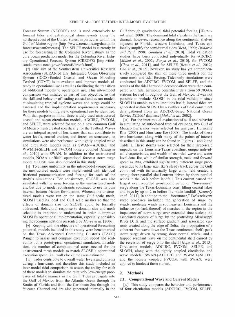
Figure 1. Detail of Gulf of Mexico and tracks of Ike(green) and Rita (red). Geographic location by type andnumber identified in Table 1.

Figure 2. Detail of northern Gulf of Mexico coast. Geographic location by type and number identifiedin Table 1.

KERR ET AL.: IOOS TESTBED: INTER-MODEL EVALUATION

5132

includes the location of the storm, differential atmosphericpressure, forward speed and radius to max winds. For thisstudy, a modified version of SLOSH was developed toaccept external meteorological forcing. The governingequations are solved explicitly in time with a finite differ-ence method in space on an orthogonal curvilinear mesh[Jelesnianski et al., 1992]. The model uses a one-

dimensional derivation of the equations to capture the dy-namics of channel flow within the domain and is imple-mented with internal barriers to account for levees.2.1.5. SWAN

[17] The Simulating WAves Nearshore (SWAN) modelis a third generation, phase-averaged spectral wave modelthat simulates the evolution of wind generated waves in theopen ocean, coastal regions, and within inland waters[Booij et al., 1999; Ris et al., 1999]. The wave action bal-ance equation is solved using a finite difference solution oneither a regular, curvilinear, or unstructured triangularmesh [Zijlema, 2010]. Solution advancement in time isresolved using an implicit backward difference scheme,with the subsequent system of equations solved using asweeping Gauss-Seidel method.2.1.6. WWMII

[18] The Wind Wave Model II (WWMII) is a third-generation phase-averaged spectral wave model that solvesthe wave action equation on an unstructured mesh. A frac-tional step method [Yanenko, 1972] is employed to split theresulting multidimensional equation into well-defined dif-ferential equations. The resulting numerical algorithminvolves a combination of residual distribution schemes ingeographical space and higher order difference schemes inspectral space, as used in WAVEWATCH IIIVR [Tolman,1999]. For geographical advection, implicit and explicit re-sidual distribution schemes are used with various time dis-cretization methods. In this study, first-order explicitschemes in geographical space have been used, details ofwhich can be found in Roland et al. [2009].2.1.7. Wave Coupling

[19] ADCIRC, FVCOM, and SELFE can receive waveradiation stress gradients as an input from a wave model,while the version of SLOSH employed here cannot; there-fore only ADCIRC, FVCOM, and SELFE were coupledwith wave models. Wave radiation stresses are determinedwithin the wave models according to the theory of Longuet-Higgins and Stewart [1964] and passed to the hydrodynamiccirculation models to update the current velocities and waterlevels. In turn, water levels and currents are passed back tothe wave models and used to solve the wave action balanceequation. SWANþADCIRC [Dietrich et al., 2011a] is thetightly coupled version of SWAN and ADCIRC andWWMIIþSELFE [Roland et al., 2009, 2012] is the tightlycoupled version of WWMII and SELFE, which means thatthese wave and circulation models run and exchange datasynchronously on the same mesh and have both models em-bedded directly within the code [Roland et al., 2009, 2012;Dietrich et al., 2011a]. SWAN-FVCOM is the loose cou-pling of SWAN and FVCOM [Huang et al., 2010, 2013].Theþ symbol is used to denote tight coupling of the models,as opposed to the – symbol which is used to denote loosecoupling. For this study, the loose coupling of SWAN-FVCOM required: (1) running FVCOM, (2) running SWANwith water level and current output from FVCOM, and (3)rerunning FVCOM with all forcings including the wave radi-ation stress gradient output from SWAN.

2.2. Meshes

[20] ADCIRC, FVCOM, SELFE, SWAN, and WWMIIwere run on unstructured triangular meshes. The ULtralite-Levee-Removed (ULLR) mesh, a 417,642 nodes (826,866

Table 1. Geographic Location by Type and Number Shown inFigures 1 and 2

River and Channels1 Atchafalaya River2 Calcasieu Shipping Channel3 Florida Straits4 Gulf Intracoastal Waterway (GIWW)5 Inner Harbor Navigation Canal (IHNC)6 Mississippi River7 Mississippi River Bird’s foot8 Mississippi River Gulf Outlet (MRGO)9 Sabine Pass10 Southwest Pass11 Yucatan ChannelBays, Lakes, and Sounds12 Atchafalaya Bay13 Barataria Bay14 Breton Sound15 Calcasieu Lake16 Chandeleur Sound17 Corpus Christi Bay18 Galveston Bay19 Grand Lake20 Lake Borgne21 Lake Maurepas22 Lake Pontchartrain23 Matagorda Bay24 Mobile Bay25 Sabine Lake26 Terrebonne Bay27 Vermillion Bay28 White LakePlaces29 Apachicola, FL30 Baton Rouge, LA31 Biloxi Marsh32 Bolivar Peninsula33 Caernarvon Marsh34 Chambers County, TX35 Chandeleur Islands36 Florida Keys37 Florida shelf38 Galveston Island39 Grand Isle40 Houston, TX41 Isles Dernieres, LA42 Lake Charles, TX43 Marsh Island44 Mississippi-Alabama shelf45 New Orleans, LA46 Pointe �a La Hache47 Port Isabel, TX48 St. Bernard, LA49 Tarbert Landing50 Terrebonne Marsh51 Texas-Louisiana shelf52 Venice, LA

KERR ET AL.: IOOS TESTBED: INTER-MODEL EVALUATION

5133

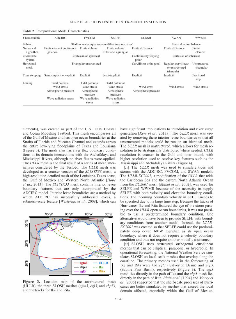
elements), was created as part of the U.S. IOOS Coastaland Ocean Modeling Testbed. This mesh encompasses allof the Gulf of Mexico and has open ocean boundaries at theStraits of Florida and Yucatan Channel and extends acrossthe entire low-lying floodplains of Texas and Louisiana(Figure 3). The mesh also has river flux boundary condi-tions at its domain intersections with the Atchafalaya andMississippi Rivers, although no river fluxes were applied.The ULLR mesh is the final result of a series of mesh alter-natives considered by the Testbed. The ULLR mesh wasdeveloped as a coarser version of the SL18TX33 mesh, ahigh-resolution detailed mesh of the Louisiana-Texas coast,the Gulf of Mexico and Western North Atlantic [Hopeet al., 2013]. The SL18TX33 mesh contains interior leveeboundary features that are only incorporated by theADCIRC model. Interior levee boundaries are a method bywhich ADCIRC has successfully addressed levees, asubmesh-scale feature [Westerink et al., 2008], which can

have significant implications to inundation and river surgegeneration [Kerr et al., 2013a]. The ULLR mesh was cre-ated by removing these interior levee boundaries so that allunstructured models could be run on an identical mesh.The ULLR mesh is unstructured, which allows for mesh re-solution to be strategically distributed where needed. ULLRresolution is coarser in the Gulf and finer inland, withhigher resolution used to resolve key features such as theMississippi and Atchafalaya Rivers (Figure 4).

[21] The ULLR mesh was used to simulate tides andstorms with the ADCIRC, FVCOM, and SWAN models.The ULLR-EC2001, a modification of the ULLR that addsthe Caribbean Sea and the eastern North Atlantic Oceanfrom the EC2001 mesh [Mukai et al., 2002], was used forSELFE and WWMII because of the necessity to supplySELFE with both velocity and elevation boundary condi-tions. The incoming boundary velocity in SELFE needs tobe specified due to its large time step. Because the tracks ofHurricanes Ike and Rita featured the eye of the storm pass-ing over the ULLR open ocean boundaries, it was not possi-ble to use a predetermined boundary condition. Onealternative would have been to provide SELFE with bound-ary conditions from another model. Instead, the ULLR-EC2001 was created so that SELFE could use the predomi-nately deep ocean 60�W meridian as its open oceanboundary, where it does not require a velocity boundarycondition and thus not require another model’s assistance.

[22] SLOSH uses structured orthogonal curvilinearmeshes that can be elliptical, parabolic, or hyperbolic. Inoperational forecasting, the National Weather Service sim-ulates SLOSH on local-scale meshes that overlap along thecoastline. The primary meshes used in the forecasting ofIke and Rita were the egl3 (Galveston Basin) and ebp3(Sabine Pass Basin), respectively (Figure 3). The egl3mesh lies directly in the path of Ike and the ebp3 mesh liesdirectly in the path of Rita. Blain et al. [1994] and Morey etal. [2006] suggested that the shelf-scale processes of hurri-canes are better simulated by meshes that exceed the localdomain affected, especially within the Gulf of Mexico.

Figure 3. Location map of the unstructured mesh(ULLR), the three SLOSH meshes (egm3, egl3, and ebp3),and the tracks for Ike and Rita.

Table 2. Computational Model Characteristics

Characteristic ADCIRC FVCOM SELFE SLOSH SWAN WWMII

Solves Shallow water equations (modified in some cases) Spectral action balanceNumerical

algorithmFinite element continuous

galerkinFinite volume Finite volume

Eulerian-LagrangianFinite difference Finite difference Finite

elementCoordinate

systemCartesian or spherical Continuously varying

polarCartesian or spherical

Horizontalmesh

Triangular unstructured Curvilinear orthogonal Regular, curvilinearor unstructuredtriangular

Unstructuredtriangular

Time stepping Semi-implicit or explicit Explicit Semi-implicit Explicit Implicit Fractionalstep

Forcing Tidal potential Tidal potential Tidal potentialWind stress Wind stress Wind stress Wind stress Wind stress Wind stress

Atmospheric pressure Atmosphericpressure

Atmosphericpressure

Atmospheric pressure

Wave radiation stress Wave radiationstress

Wave radiationstress

KERR ET AL.: IOOS TESTBED: INTER-MODEL EVALUATION

5134

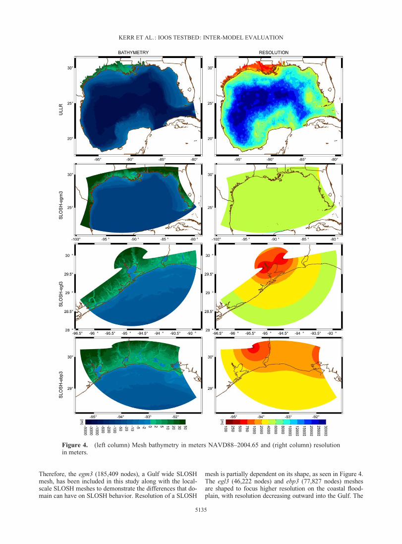
Therefore, the egm3 (185,409 nodes), a Gulf wide SLOSHmesh, has been included in this study along with the local-scale SLOSH meshes to demonstrate the differences that do-main can have on SLOSH behavior. Resolution of a SLOSH

mesh is partially dependent on its shape, as seen in Figure 4.The egl3 (46,222 nodes) and ebp3 (77,827 nodes) meshesare shaped to focus higher resolution on the coastal flood-plain, with resolution decreasing outward into the Gulf. The

Figure 4. (left column) Mesh bathymetry in meters NAVD88–2004.65 and (right column) resolutionin meters.

KERR ET AL.: IOOS TESTBED: INTER-MODEL EVALUATION

5135

egm3 mesh encompasses most of the Gulf of Mexico andhas relatively constant resolution across its domain.

[23] Unstructured meshes provide the ability to applyresolution where needed; whereas structured meshes,even those that are curvilinear, are more limited, espe-cially in rate of transition between resolution. The ULLRmesh’s resolution ranges from 8 to 30 km in the Gulf, 2–8km on the shelf, 500–2000 m on the floodplain, and 100–500 m in the rivers. The resolution of the egm3 mesh isfairly constant between 4 and 6 km over the Gulf, shelf,floodplain, and channel scales, due to its structured na-ture; this is in contrast to the unstructured ULLR meshwhich is coarser in the Gulf and finer inland. The egl3 andebp3 meshes have more variation in their resolution thanthe egm3 mesh and their resolution ranges from 500 to4000 m, although most of the resolution at the shoreline isbetween 1000 and 2000 m. Comparatively, the resolutionalong the coastline for the ULLR, egl3, and ebp3 meshesare similar, whereas the resolution at the coastline for theegm3 mesh is much coarser. The overall range of resolu-tion for each of the meshes are : ULLR (100–31,000 m),egl3 (80–2700 m), ebp3 (80–1600 m), and egm3 (1900–4000 m).

2.3. Bathymetry, Topography

[24] The bathymetry and topography used for the devel-opment of the ULLR mesh matches that used by Hope et al.[2013] in their synoptic study of Ike and Dietrich et al.[2011b] in their synoptic study of Gustav. The bathymetryand topography of the ULLR, ebp3, egl3, and egm3 meshesare shown in Figure 4. Depth in the egm3 is limited to 182m due to limits built into SLOSH. This is in stark contrastto the depth of the ULLR, which reaches the actual depthsof over 4000 m in the center of the Gulf.

[25] Topographic and bathymetric data is referenced tothe North American Vertical Datum of 1988 (NAVD88).Initial water levels are raised by 0.134 m to update eleva-tions to the NAVD88 2004.65 epoch, and increased by anadditional amount, the steric, prior to simulation. The stericreflects the seasonal variability of the of the sea level in theGulf of Mexico, due to thermal expansion and contraction,salinity, winds, ocean currents, seasonal river runoff, andother factors. The steric for Rita was 0.146 m which resultsin a total adjustment of 0.28 m [Bunya et al., 2010]. For Ikethe steric is 0.142 m and the total adjustment is 0.276 m[Hope et al., 2013].

2.4. Friction

[26] A spatially varying Manning’s n bottom frictionwas applied for each of the unstructured circulation models.Manning’s n values were derived from land-use databasesas described by Dietrich et al. [2011b]. Capturing frictioncorrectly on the continental shelf is essential to developingthe shore-parallel current that preceded Ike and caused thegeostrophic setup [Kennedy et al., 2011; Kerr et al.,2013b; Hope et al., 2013]. This required some of the mod-els to remove lower drag coefficient limits from their bot-tom friction formulations, so that Ike’s forerunner coulddevelop. Unlike the unstructured mesh model’s implemen-tation of the Manning’s formula, SLOSH uses its own in-ternal bottom friction formulation which is mildly depthdependent and is not spatially varying.

[27] Jelesnianski [1966, 1967] studied the effects ofincluding or not including a bottom stress formulation inSLOSH, and concluded that a dissipation mechanism wasessential for modeling slow-moving storms, shore-parallelstorms, or storms with extended duration on the continentalshelf, because it was necessary to control large amplituderesurgences and/or initialization phenomena that werecaused by the case with no bottom friction. Thus friction ispartially used in the SLOSH model to control numericalstability and initialization phenomena with its internal pa-rameters empirically set to match peak surge levels.

2.5. Tidal Forcing

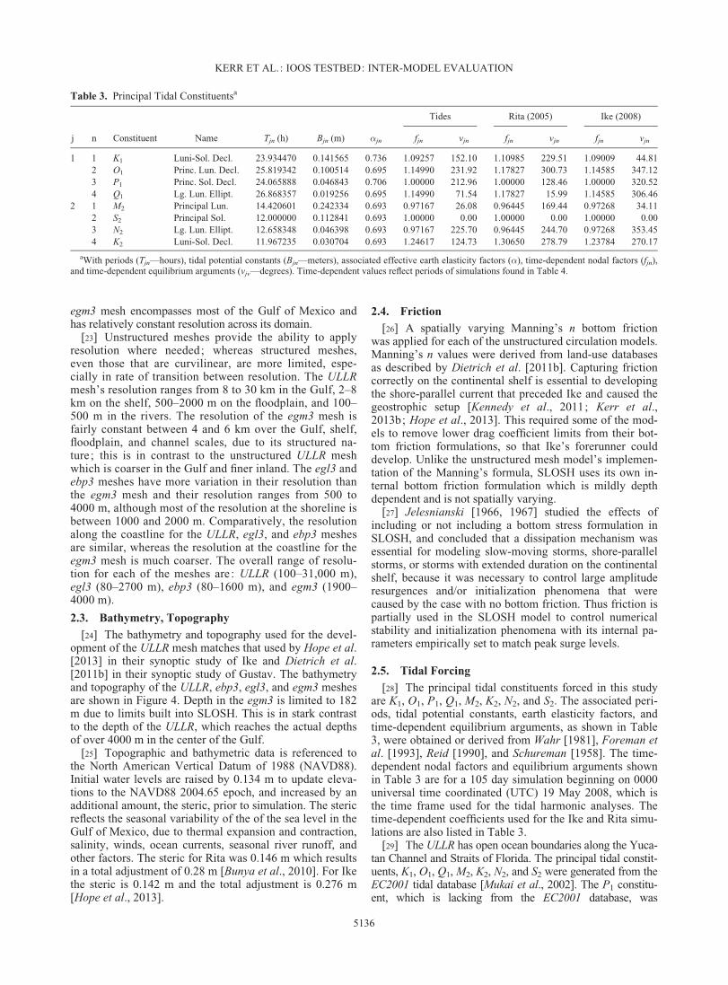
[28] The principal tidal constituents forced in this studyare K1, O1, P1, Q1, M2, K2, N2, and S2. The associated peri-ods, tidal potential constants, earth elasticity factors, andtime-dependent equilibrium arguments, as shown in Table3, were obtained or derived from Wahr [1981], Foreman etal. [1993], Reid [1990], and Schureman [1958]. The time-dependent nodal factors and equilibrium arguments shownin Table 3 are for a 105 day simulation beginning on 0000universal time coordinated (UTC) 19 May 2008, which isthe time frame used for the tidal harmonic analyses. Thetime-dependent coefficients used for the Ike and Rita simu-lations are also listed in Table 3.

[29] The ULLR has open ocean boundaries along the Yuca-tan Channel and Straits of Florida. The principal tidal constit-uents, K1, O1, Q1, M2, K2, N2, and S2 were generated from theEC2001 tidal database [Mukai et al., 2002]. The P1 constitu-ent, which is lacking from the EC2001 database, was

Table 3. Principal Tidal Constituentsa

j n Constituent Name Tjn (h) Bjn (m) �jn

Tides Rita (2005) Ike (2008)

fjn vjn fjn vjn fjn vjn

1 1 K1 Luni-Sol. Decl. 23.934470 0.141565 0.736 1.09257 152.10 1.10985 229.51 1.09009 44.812 O1 Princ. Lun. Decl. 25.819342 0.100514 0.695 1.14990 231.92 1.17827 300.73 1.14585 347.123 P1 Princ. Sol. Decl. 24.065888 0.046843 0.706 1.00000 212.96 1.00000 128.46 1.00000 320.524 Q1 Lg. Lun. Ellipt. 26.868357 0.019256 0.695 1.14990 71.54 1.17827 15.99 1.14585 306.46

2 1 M2 Principal Lun. 14.420601 0.242334 0.693 0.97167 26.08 0.96445 169.44 0.97268 34.112 S2 Principal Sol. 12.000000 0.112841 0.693 1.00000 0.00 1.00000 0.00 1.00000 0.003 N2 Lg. Lun. Ellipt. 12.658348 0.046398 0.693 0.97167 225.70 0.96445 244.70 0.97268 353.454 K2 Luni-Sol. Decl. 11.967235 0.030704 0.693 1.24617 124.73 1.30650 278.79 1.23784 270.17

aWith periods (Tjn—hours), tidal potential constants (Bjn—meters), associated effective earth elasticity factors (�), time-dependent nodal factors (fjn),and time-dependent equilibrium arguments (vjv—degrees). Time-dependent values reflect periods of simulations found in Table 4.

KERR ET AL.: IOOS TESTBED: INTER-MODEL EVALUATION

5136

generated by averaging the FES2004 [Lyard et al., 2006] andTPXO7.2 [Egbert et al., 1994; Egbert and Erofeeva, 2002]tidal atlases. The ULLR-EC2001 open ocean boundary, whichis located along the 60�W meridian, was forced with the K1,O1, P1, Q1, M2, K2, N2, and S2 tidal constituents generatedfrom the FES95.2 tidal atlas [Le Provost et al., 1994, 1995].

[30] SLOSH does not simulate tides, so there was notidal forcing to apply. For the hurricane analyses, tidal sig-nals from ADCIRC were superimposed onto SLOSH waterlevels. For each cell and output step, the water level fromthe nearest ADCIRC node to the center of each SLOSHcell was added to that SLOSH cell’s water level. Thismethod is not ideal due to the difference in meshes, and isfurther compounded by the difference in resolution, withthe SLOSH meshes being typically coarser than the ULLR.At several stations spatial misalignment between theSLOSH cell center point and the actual station was appa-rent. This was noticed because SLOSH-interpolated resultshad an erroneously high tidal signal, whereas at the samestation, ADCIRC had a weaker but more correct tidal sig-nal. The superposition of the tidal signal on the surge leveldoes not replicate the nonlinear and mass contributions oftidal dynamics that are included in the unstructured meshmodels that dynamically simulate both the tides and surge.

2.6. Meteorological Forcing

[31] OceanWeather Inc. (OWI) structured and data-assimilated wind and pressure fields were used in this studyto hindcast Rita [Bunya et al., 2010] and Ike [Hope et al.,2013]. As described by Bunya et al. [2010], hindcast windfields were defined objectively using analyzed measurementsfrom anemometers, airborne and land-based Doppler radar,airborne stepped-frequency microwave radiometers, buoys,ships, aircraft, coastal stations, and satellite measurements.Hindcast winds are based on the blending of an inner corewind field (transformed to 30 min averaged sustainedwinds), such as the TC96 mesoscale models [Thompson andCardone, 1996] solutions for Rita and the NOAA HurricaneResearch Wind Analysis System (H�WIND) [Powell et al.,1996, 1998, 2010] for Ike, with Gulf scale winds using theInteractive Objective Kinematic Analysis (IOKA) system[Cox et al., 1995; Cardone and Cox, 2009].

[32] H�WIND analyses had a 3 h frequency and includedthe use of improved terrain conversions [Vickery et al.,2009] and high-resolution tower data from Texas Tech Uni-versity and the Florida Coastal Monitoring Program. TheH�WIND analyses of Ike also included the deployment ofstepped-frequency microwave radiometers aboard the AirForce Hurricane Hunter Aircraft [Uhlhorn et al., 2007],which increased the availability of high radial resolutionsurface winds since the Katrina wind field post analysis[Ebersole et al., 2007]. Peripheral winds were derived fromthe National Centers for Environmental Prediction-National Center for Atmospheric Research (NCEP-NCAR)reanalysis project [Kalnay et al., 1996]. The IOKA systemalso includes the injection of local marine data, adjustmentto a consistent 10 m elevation, 30 min sustained windspeed, marine exposure, and neutral stability. Finally,Lagrangian-based interpolation is used to produce struc-tured wind fields every 15 min. This included for Rita a sin-gle structured grid spaced at 0.05� and for Ike a Gulf scale0.1� grid and a local scale 0.015� grid near landfall. Sea

level atmospheric pressure fields for both Rita and Ike werederived using the widely adopted radial-based parametricmodel developed by Holland [1980] and assigned to thesame structured grids as the wind fields.

[33] The methodology used by ADCIRC to employ anOWI wind field includes: (1) converting 30 min averagedsustained winds to 10 min averaged sustained winds; (2)accounting for canopy cover; (3) applying a directionalreduction factor to account for surface roughness [Bunyaet al., 2010]; and (4) increasing winds to full marine windsas roughness elements are inundated. In this study, asector-based directional wind drag law, which is datadriven and wind speed limited, is applied in ADCIRC tocompute its drag coefficient. The drag law was developedby Powell et al. [2003] and Powell [2006], and previouslyapplied by Dietrich et al. [2011b] and Hope et al. [2013].FVCOM, SELFE, and SLOSH models do not include thesesophisticated wind reduction factors, so in order to performa consistent comparison, wind stress (not wind velocity)was output from an ADCIRC hindcast on the SL18TX33mesh [Hope et al., 2013] and converted to a structured for-mat so that it could be applied to SELFE, FVCOM, andSLOSH. Each model then employed approximately thesame wind stress and pressure, therefore essentially usingthe wind stress physics built into ADCIRC.

[34] The wave models, SWAN and WWMII, were sup-plied with the OWI 30 min winds. SWANþADCIRC usedthe sector-based drag law to compute its wind-wave dragcoefficient, whereas the wind-wave computations inSWAN-FVCOM and WWMIIþSELFE applied Wu’s draglaw [Wu et al., 1982] with a modified cap for the SWAN-FVCOM simulations [Huang et al., 2013].

2.7. Wave Parameters

[35] Identical wave parameters were used in SWAN andWWMII. Wave direction was discretized into 36 regularbins and wave frequency was logarithmically distributedinto 50 bins with a range of 0.035–0.9635 Hz. The Komenformulation as modified by Rogers et al. [2003] was used forwhite capping. Wave breaking due to depth was determinedspectrally according to the model of Battjes and Janssen[1978] with a breaking parameter of �¼ 0.73 [Battjes andStive, 1985]. For SWANþADCIRC, the spectral and direc-tional speeds were set with a Courant-Friedrichs-Lewy(CFL) condition of 0.25 to limit spurious refractions [Die-trich et al., 2012c]. Bottom friction is applied via a JointNorth Sea Wave Project (JONSWAP) formulation with aCfjon ¼ 0:019m2=s 3, as recommended by Kerr et al.[2013b] for the muddy bottom of the LATEX shelf.

2.8. Summary of TESTBED Simulations

[36] A total of 21 simulations were performed as part ofthis study (Table 4). The inter-model comparison includedtidal harmonic analyses and hindcasts of Rita and Ike. Thetidal simulations were performed using ADCIRC, FVCOM,and SELFE. The hurricane hindcasts were performed usingcirculation models (ADCIRC, FVCOM, SELFE, andSLOSH) and coupled wave and circulation models(SWANþADCIRC, SWAN-FVCOM, and WWMIIþSELFE). The unstructured models were all run on theULLR mesh (the exception being ULLR-EC2001 forSELFE and WWMIIþSELFE); whereas SLOSH was run

KERR ET AL.: IOOS TESTBED: INTER-MODEL EVALUATION

5137

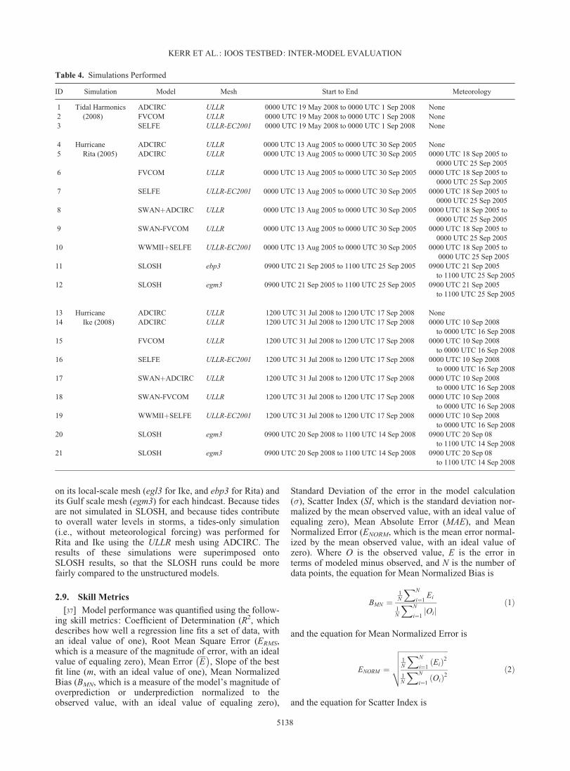
on its local-scale mesh (egl3 for Ike, and ebp3 for Rita) andits Gulf scale mesh (egm3) for each hindcast. Because tidesare not simulated in SLOSH, and because tides contributeto overall water levels in storms, a tides-only simulation(i.e., without meteorological forcing) was performed forRita and Ike using the ULLR mesh using ADCIRC. Theresults of these simulations were superimposed ontoSLOSH results, so that the SLOSH runs could be morefairly compared to the unstructured models.

2.9. Skill Metrics

[37] Model performance was quantified using the follow-ing skill metrics: Coefficient of Determination (R2, whichdescribes how well a regression line fits a set of data, withan ideal value of one), Root Mean Square Error (ERMS,which is a measure of the magnitude of error, with an idealvalue of equaling zero), Mean Error E

� �, Slope of the best

fit line (m, with an ideal value of one), Mean NormalizedBias (BMN, which is a measure of the model’s magnitude ofoverprediction or underprediction normalized to theobserved value, with an ideal value of equaling zero),

Standard Deviation of the error in the model calculation(�), Scatter Index (SI, which is the standard deviation nor-malized by the mean observed value, with an ideal value ofequaling zero), Mean Absolute Error (MAE), and MeanNormalized Error (ENORM, which is the mean error normal-ized by the mean observed value, with an ideal value ofzero). Where O is the observed value, E is the error interms of modeled minus observed, and N is the number ofdata points, the equation for Mean Normalized Bias is

BMN ¼1N

XN

i¼1Ei

1N

XN

i¼1jOij

ð1Þ

and the equation for Mean Normalized Error is

ENORM ¼

ffiffiffiffiffiffiffiffiffiffiffiffiffiffiffiffiffiffiffiffiffiffiffiffiffiffiffi1N

XN

i¼1Eið Þ2

1N

XN

i¼1Oið Þ2

vuuut ð2Þ

and the equation for Scatter Index is

Table 4. Simulations Performed

ID Simulation Model Mesh Start to End Meteorology

1 Tidal Harmonics(2008)

ADCIRC ULLR 0000 UTC 19 May 2008 to 0000 UTC 1 Sep 2008 None2 FVCOM ULLR 0000 UTC 19 May 2008 to 0000 UTC 1 Sep 2008 None3 SELFE ULLR-EC2001 0000 UTC 19 May 2008 to 0000 UTC 1 Sep 2008 None

4 HurricaneRita (2005)

ADCIRC ULLR 0000 UTC 13 Aug 2005 to 0000 UTC 30 Sep 2005 None5 ADCIRC ULLR 0000 UTC 13 Aug 2005 to 0000 UTC 30 Sep 2005 0000 UTC 18 Sep 2005 to

0000 UTC 25 Sep 20056 FVCOM ULLR 0000 UTC 13 Aug 2005 to 0000 UTC 30 Sep 2005 0000 UTC 18 Sep 2005 to

0000 UTC 25 Sep 20057 SELFE ULLR-EC2001 0000 UTC 13 Aug 2005 to 0000 UTC 30 Sep 2005 0000 UTC 18 Sep 2005 to

0000 UTC 25 Sep 20058 SWANþADCIRC ULLR 0000 UTC 13 Aug 2005 to 0000 UTC 30 Sep 2005 0000 UTC 18 Sep 2005 to

0000 UTC 25 Sep 20059 SWAN-FVCOM ULLR 0000 UTC 13 Aug 2005 to 0000 UTC 30 Sep 2005 0000 UTC 18 Sep 2005 to

0000 UTC 25 Sep 200510 WWMIIþSELFE ULLR-EC2001 0000 UTC 13 Aug 2005 to 0000 UTC 30 Sep 2005 0000 UTC 18 Sep 2005 to

0000 UTC 25 Sep 200511 SLOSH ebp3 0900 UTC 21 Sep 2005 to 1100 UTC 25 Sep 2005 0900 UTC 21 Sep 2005

to 1100 UTC 25 Sep 200512 SLOSH egm3 0900 UTC 21 Sep 2005 to 1100 UTC 25 Sep 2005 0900 UTC 21 Sep 2005

to 1100 UTC 25 Sep 2005

13 HurricaneIke (2008)

ADCIRC ULLR 1200 UTC 31 Jul 2008 to 1200 UTC 17 Sep 2008 None14 ADCIRC ULLR 1200 UTC 31 Jul 2008 to 1200 UTC 17 Sep 2008 0000 UTC 10 Sep 2008

to 0000 UTC 16 Sep 200815 FVCOM ULLR 1200 UTC 31 Jul 2008 to 1200 UTC 17 Sep 2008 0000 UTC 10 Sep 2008

to 0000 UTC 16 Sep 200816 SELFE ULLR-EC2001 1200 UTC 31 Jul 2008 to 1200 UTC 17 Sep 2008 0000 UTC 10 Sep 2008

to 0000 UTC 16 Sep 200817 SWANþADCIRC ULLR 1200 UTC 31 Jul 2008 to 1200 UTC 17 Sep 2008 0000 UTC 10 Sep 2008

to 0000 UTC 16 Sep 200818 SWAN-FVCOM ULLR 1200 UTC 31 Jul 2008 to 1200 UTC 17 Sep 2008 0000 UTC 10 Sep 2008

to 0000 UTC 16 Sep 200819 WWMIIþSELFE ULLR-EC2001 1200 UTC 31 Jul 2008 to 1200 UTC 17 Sep 2008 0000 UTC 10 Sep 2008

to 0000 UTC 16 Sep 200820 SLOSH egm3 0900 UTC 20 Sep 2008 to 1100 UTC 14 Sep 2008 0900 UTC 20 Sep 08

to 1100 UTC 14 Sep 200821 SLOSH egm3 0900 UTC 20 Sep 2008 to 1100 UTC 14 Sep 2008 0900 UTC 20 Sep 08

to 1100 UTC 14 Sep 2008

KERR ET AL.: IOOS TESTBED: INTER-MODEL EVALUATION

5138

SI ¼

ffiffiffiffiffiffiffiffiffiffiffiffiffiffiffiffiffiffiffiffiffiffiffiffiffiffiffiffiffiffiffiffiffiffiffiffiffi1N

XN

i¼1Ei � E� �2

1N

XN

i¼1jOij

vuuut ð3Þ

[38] In the statistical analyses of water levels and highwater marks, it was found that the number of stations andpoints in the time series which wetted varied for all themodels. In some previous hurricane validation studies, drystations and dry time series points were omitted. While thismethod may be appropriate for a single model validation, itbecame apparent that there are problems to that methodwhen applying it for the comparison of multiple models.One example of a problem is that if one model wetted onestation but the results were poor, and another model did notwet that station at all, then the model that did wet the sta-tion would be penalized with poor statistics. Another prob-lem is that if stations are omitted that were not wetted byall models then the richness of the statistical set would besorely depleted.

[39] To counter the problem of a disproportionate num-ber of wet and dry points between the models, one solutionis to replace dry points with a common equalizer, the ba-thymetry. Because the bathymetry represents the minimumwater level obtainable at any point in the mesh, dry valueswere replaced with the ground surface elevation, and com-mon statistical sets were obtained. This method is referredto in this study as Topo-Substitution (TS). To compareboth approaches, the statistical analyses are presented withboth the TS method and the Wet-Only method. The Wet-Only method refers to the method of using only those sta-tions or points that wetted in the statistical analysis andomitting the rest.

3. Tidal Simulations

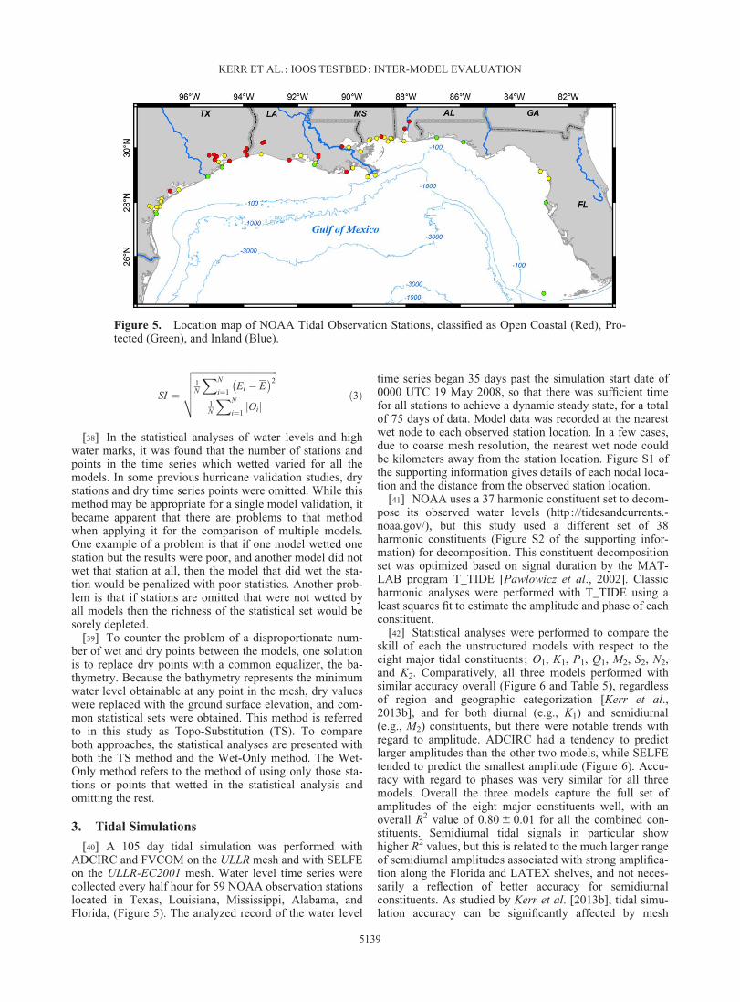
[40] A 105 day tidal simulation was performed withADCIRC and FVCOM on the ULLR mesh and with SELFEon the ULLR-EC2001 mesh. Water level time series werecollected every half hour for 59 NOAA observation stationslocated in Texas, Louisiana, Mississippi, Alabama, andFlorida, (Figure 5). The analyzed record of the water level

time series began 35 days past the simulation start date of0000 UTC 19 May 2008, so that there was sufficient timefor all stations to achieve a dynamic steady state, for a totalof 75 days of data. Model data was recorded at the nearestwet node to each observed station location. In a few cases,due to coarse mesh resolution, the nearest wet node couldbe kilometers away from the station location. Figure S1 ofthe supporting information gives details of each nodal loca-tion and the distance from the observed station location.

[41] NOAA uses a 37 harmonic constituent set to decom-pose its observed water levels (http://tidesandcurrents.-noaa.gov/), but this study used a different set of 38harmonic constituents (Figure S2 of the supporting infor-mation) for decomposition. This constituent decompositionset was optimized based on signal duration by the MAT-LAB program T_TIDE [Pawlowicz et al., 2002]. Classicharmonic analyses were performed with T_TIDE using aleast squares fit to estimate the amplitude and phase of eachconstituent.

[42] Statistical analyses were performed to compare theskill of each the unstructured models with respect to theeight major tidal constituents ; O1, K1, P1, Q1, M2, S2, N2,and K2. Comparatively, all three models performed withsimilar accuracy overall (Figure 6 and Table 5), regardlessof region and geographic categorization [Kerr et al.,2013b], and for both diurnal (e.g., K1) and semidiurnal(e.g., M2) constituents, but there were notable trends withregard to amplitude. ADCIRC had a tendency to predictlarger amplitudes than the other two models, while SELFEtended to predict the smallest amplitude (Figure 6). Accu-racy with regard to phases was very similar for all threemodels. Overall the three models capture the full set ofamplitudes of the eight major constituents well, with anoverall R2 value of 0.80 6 0.01 for all the combined con-stituents. Semidiurnal tidal signals in particular showhigher R2 values, but this is related to the much larger rangeof semidiurnal amplitudes associated with strong amplifica-tion along the Florida and LATEX shelves, and not neces-sarily a reflection of better accuracy for semidiurnalconstituents. As studied by Kerr et al. [2013b], tidal simu-lation accuracy can be significantly affected by mesh

Figure 5. Location map of NOAA Tidal Observation Stations, classified as Open Coastal (Red), Pro-tected (Green), and Inland (Blue).

KERR ET AL.: IOOS TESTBED: INTER-MODEL EVALUATION

5139

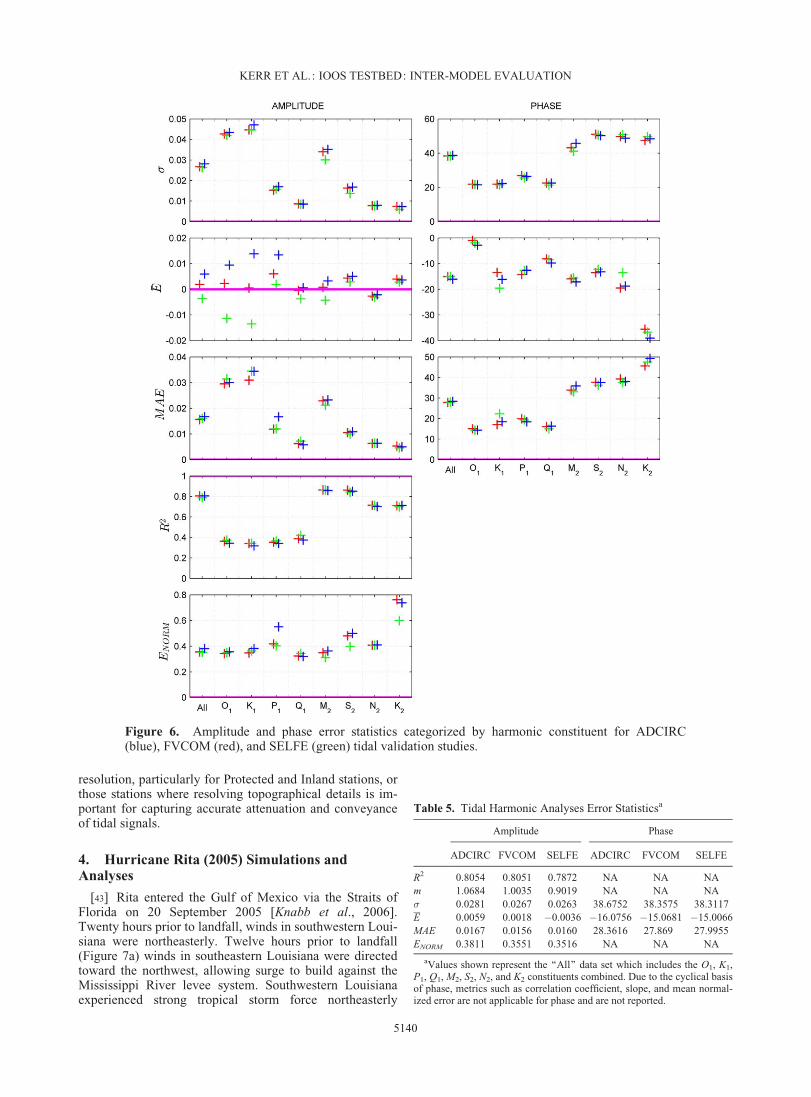
resolution, particularly for Protected and Inland stations, orthose stations where resolving topographical details is im-portant for capturing accurate attenuation and conveyanceof tidal signals.

4. Hurricane Rita (2005) Simulations andAnalyses

[43] Rita entered the Gulf of Mexico via the Straits ofFlorida on 20 September 2005 [Knabb et al., 2006].Twenty hours prior to landfall, winds in southwestern Loui-siana were northeasterly. Twelve hours prior to landfall(Figure 7a) winds in southeastern Louisiana were directedtoward the northwest, allowing surge to build against theMississippi River levee system. Southwestern Louisianaexperienced strong tropical storm force northeasterly

Table 5. Tidal Harmonic Analyses Error Statisticsa

Amplitude Phase

ADCIRC FVCOM SELFE ADCIRC FVCOM SELFE

R2 0.8054 0.8051 0.7872 NA NA NAm 1.0684 1.0035 0.9019 NA NA NA� 0.0281 0.0267 0.0263 38.6752 38.3575 38.3117E 0.0059 0.0018 �0.0036 �16.0756 �15.0681 �15.0066MAE 0.0167 0.0156 0.0160 28.3616 27.869 27.9955ENORM 0.3811 0.3551 0.3516 NA NA NA

aValues shown represent the ‘‘All’’ data set which includes the O1, K1,P1, Q1, M2, S2, N2, and K2 constituents combined. Due to the cyclical basisof phase, metrics such as correlation coefficient, slope, and mean normal-ized error are not applicable for phase and are not reported.

Figure 6. Amplitude and phase error statistics categorized by harmonic constituent for ADCIRC(blue), FVCOM (red), and SELFE (green) tidal validation studies.

KERR ET AL.: IOOS TESTBED: INTER-MODEL EVALUATION

5140

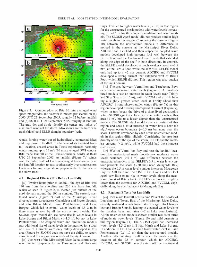
winds, forcing water out of hydraulically connected lakesand bays prior to landfall. To the west of its eventual land-fall location, coastal areas in Texas experienced northerlywinds ranging up to 25 m/s (10 min averaged OWI winds).Rita made landfall at the Texas-Louisiana border at 0740UTC 24 September 2005. At landfall (Figure 7b) windsover the entire state of Louisiana ranged from southerly atthe landfall location to east-southeasterly over southeasternLouisiana forcing surge shore perpendicular to the east ofthe storm track.

4.1. Regional Effects (12 h Before Landfall)

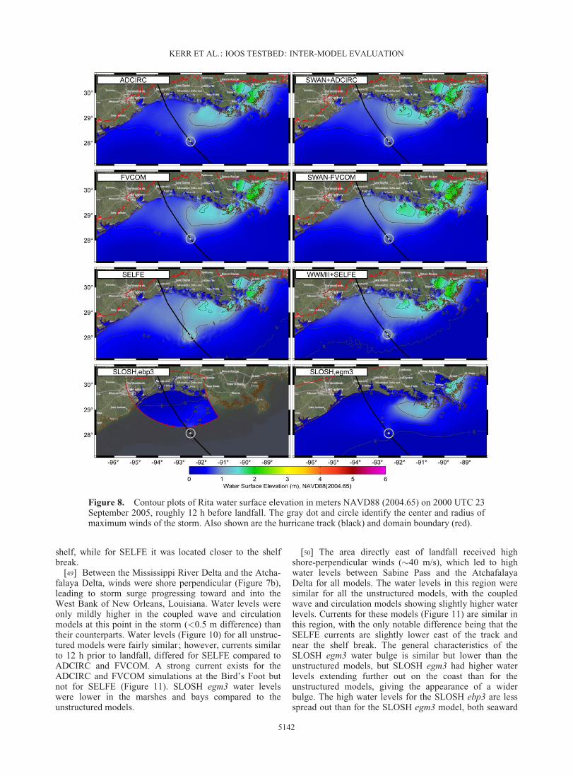
[44] Twelve hours prior to landfall, the eye of Rita was170 km from the shoreline and 220 km from landfall,which as seen in Figure 8, is located just outside of theebp3 domain around the 100 m contour. The easterly sus-tained winds (Figure 7) east of the Mississippi Riverdirected storm surge across Chandeleur and Breton Sounds,and into Biloxi Marsh, Lake Pontchartrain, and LakeBorgne, which led to overall water levels of 1.5–2 m inthese areas as seen by all the unstructured models. TheSLOSH egm3 model did see some rise in water levels inLake Borgne and Biloxi Marsh (1–1.5 m), but not in LakePontchartrain. The coupled wave and circulation modelssaw additional rise of water levels in the marshes for a totalof 1.5–2 m. Currents were only mildly developed in thisarea (Figure 9). SLOSH does not have the ability to reportcurrents and this region was outside of the ebp3 domain.

[45] Just west of the Mississippi River Delta, storm surgewas directed perpendicular to Terrebonne and Barataria

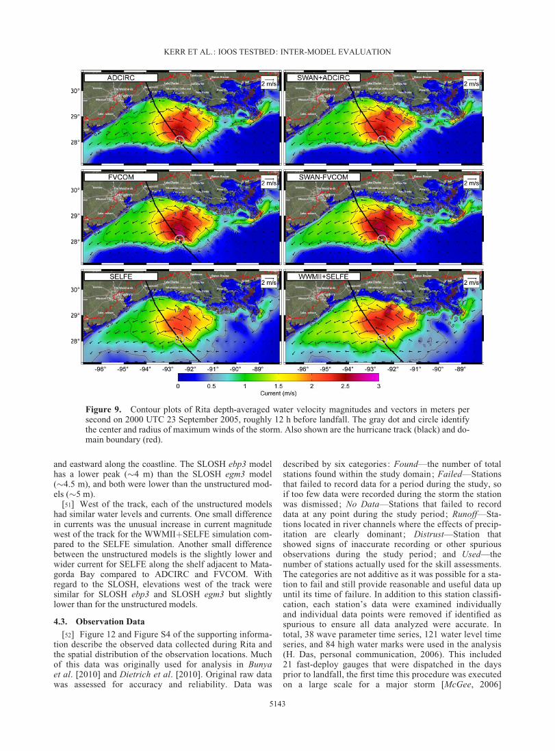
Bays. This led to higher water levels (�1 m) in that regionfor the unstructured mesh models with water levels increas-ing to 1–1.5 m for the coupled circulation and wave mod-els. The SLOSH egm3 model did not produce similar highwater levels in this region. Comparing the currents (Figure10) between the unstructured models, a difference isnoticed in the currents at the Mississippi River Delta.ADCIRC and FVCOM and their respective coupled wavemodels developed high currents (>2 m/s) between theBird’s Foot and the Continental shelf break that extendedalong the edge of the shelf in both directions. In contrast,the SELFE model developed a much weaker current (�1.5m/s) at the Bird’s Foot, while the WWMIIþSELFE modelonly had up to a �2 m/s current. ADCIRC and FVCOMdeveloped a strong current that extended west of Bird’sFoot, which SELFE did not. This region was also outsideof the ebp3 domain.

[46] The area between Vermillion and Terrebonne Baysexperienced increased water levels (Figure 8). All unstruc-tured models saw an increase in water levels near Trinityand Ship Shoals (�1.5 m), with FVCOM and SELFE hav-ing a slightly greater water level at Trinity Shoal thanADCIRC. Strong shore-parallel winds (Figure 7a) in thisregion developed a strong shore-parallel current (Figure 9),which in turn began the drive of a short-lived geostrophicsetup. SLOSH egm3 developed a rise in water levels in thisarea (1 m), but to a lesser degree than the unstructuredmodels. The SLOSH ebp3 model covers a portion of thisregion and sees a mild increase in water levels near theebp3 open ocean boundary (�0.5 m) but none near theshore. Currents developed by each of the unstructured mod-els in this region differ slightly. Considering the area justdirectly north of the eye of the storm, SELFE had the weak-est currents (�2 m/s), while FVCOM had the strongest(�2.5 m/s).

[47] West of Vermillion Bay and near the landfall loca-tion, the unstructured mesh models saw moderate waterlevels nearshore (0.5–1 m). One difference between theunstructured models is that SELFE’s 0.5 m water level con-tour parallels the shore (�50 km) near Matagorda Bay,whereas the 0.5 m water level contour intersects MatagordaBay for ADCIRC and FVCOM. SLOSH ebp3 and SLOSHegm3 saw little or no rise in water levels along the near-shore. West of Rita’s track, SELFE’s currents are slightlylower than the currents for ADCIRC and FVCOM, espe-cially along the shelf adjacent to Matagorda Bay.

4.2. Regional Effects (At Landfall)

[48] Rita made landfall near Sabine Pass at the border ofLouisiana and Texas. East of the Mississippi River Delta,easterly sustained winds forced storm surge into Chande-leur and Breton Sounds, leading to elevated water levels inthe marshes, bays, and lakes (�2 m Lake Pontchartrain).All the unstructured models showed similar results in termsof moderate water levels (Figure 10) and mild currents inthis region (Figure 11). The SLOSH egm3 had increasedwater levels (1.5–2 m) in Biloxi Marsh and Lake Borgne.In addition, SLOSH had a much lower water level in LakePontchartrain (0.5–1.0 m) than the unstructured models.Another differentiating result between the models is thelocation of the 0.5 m contour, which for ADCIRC,FVCOM, and SLOSH, was located off the continental

Figure 7. Contour plots of Rita 10 min averaged windspeed magnitudes and vectors in meters per second on (a)2000 UTC 23 September 2005, roughly 12 before landfalland (b) 0800 UTC 24 September 2005, roughly at landfall.The gray dot and circle identify the center and radius ofmaximum winds of the storm. Also shown are the hurricanetrack (black) and ULLR domain boundary (red).

KERR ET AL.: IOOS TESTBED: INTER-MODEL EVALUATION

5141

shelf, while for SELFE it was located closer to the shelfbreak.

[49] Between the Mississippi River Delta and the Atcha-falaya Delta, winds were shore perpendicular (Figure 7b),leading to storm surge progressing toward and into theWest Bank of New Orleans, Louisiana. Water levels wereonly mildly higher in the coupled wave and circulationmodels at this point in the storm (<0.5 m difference) thantheir counterparts. Water levels (Figure 10) for all unstruc-tured models were fairly similar; however, currents similarto 12 h prior to landfall, differed for SELFE compared toADCIRC and FVCOM. A strong current exists for theADCIRC and FVCOM simulations at the Bird’s Foot butnot for SELFE (Figure 11). SLOSH egm3 water levelswere lower in the marshes and bays compared to theunstructured models.

[50] The area directly east of landfall received highshore-perpendicular winds (�40 m/s), which led to highwater levels between Sabine Pass and the AtchafalayaDelta for all models. The water levels in this region weresimilar for all the unstructured models, with the coupledwave and circulation models showing slightly higher waterlevels. Currents for these models (Figure 11) are similar inthis region, with the only notable difference being that theSELFE currents are slightly lower east of the track andnear the shelf break. The general characteristics of theSLOSH egm3 water bulge is similar but lower than theunstructured models, but SLOSH egm3 had higher waterlevels extending further out on the coast than for theunstructured models, giving the appearance of a widerbulge. The high water levels for the SLOSH ebp3 are lessspread out than for the SLOSH egm3 model, both seaward

Figure 8. Contour plots of Rita water surface elevation in meters NAVD88 (2004.65) on 2000 UTC 23September 2005, roughly 12 h before landfall. The gray dot and circle identify the center and radius ofmaximum winds of the storm. Also shown are the hurricane track (black) and domain boundary (red).

KERR ET AL.: IOOS TESTBED: INTER-MODEL EVALUATION

5142

and eastward along the coastline. The SLOSH ebp3 modelhas a lower peak (�4 m) than the SLOSH egm3 model(�4.5 m), and both were lower than the unstructured mod-els (�5 m).

[51] West of the track, each of the unstructured modelshad similar water levels and currents. One small differencein currents was the unusual increase in current magnitudewest of the track for the WWMIIþSELFE simulation com-pared to the SELFE simulation. Another small differencebetween the unstructured models is the slightly lower andwider current for SELFE along the shelf adjacent to Mata-gorda Bay compared to ADCIRC and FVCOM. Withregard to the SLOSH, elevations west of the track weresimilar for SLOSH ebp3 and SLOSH egm3 but slightlylower than for the unstructured models.

4.3. Observation Data

[52] Figure 12 and Figure S4 of the supporting informa-tion describe the observed data collected during Rita andthe spatial distribution of the observation locations. Muchof this data was originally used for analysis in Bunyaet al. [2010] and Dietrich et al. [2010]. Original raw datawas assessed for accuracy and reliability. Data was

described by six categories : Found—the number of totalstations found within the study domain; Failed—Stationsthat failed to record data for a period during the study, soif too few data were recorded during the storm the stationwas dismissed ; No Data—Stations that failed to recorddata at any point during the study period; Runoff—Sta-tions located in river channels where the effects of precip-itation are clearly dominant ; Distrust—Station thatshowed signs of inaccurate recording or other spuriousobservations during the study period; and Used—thenumber of stations actually used for the skill assessments.The categories are not additive as it was possible for a sta-tion to fail and still provide reasonable and useful data upuntil its time of failure. In addition to this station classifi-cation, each station’s data were examined individuallyand individual data points were removed if identified asspurious to ensure all data analyzed were accurate. Intotal, 38 wave parameter time series, 121 water level timeseries, and 84 high water marks were used in the analysis(H. Das, personal communication, 2006). This included21 fast-deploy gauges that were dispatched in the daysprior to landfall, the first time this procedure was executedon a large scale for a major storm [McGee, 2006]

Figure 9. Contour plots of Rita depth-averaged water velocity magnitudes and vectors in meters persecond on 2000 UTC 23 September 2005, roughly 12 h before landfall. The gray dot and circle identifythe center and radius of maximum winds of the storm. Also shown are the hurricane track (black) and do-main boundary (red).

KERR ET AL.: IOOS TESTBED: INTER-MODEL EVALUATION

5143

Collected observation data from Rita stretches from KeyWest, Florida, to the south Texas coast incorporatinginland, floodplain, coastal, and deep water locations. Themajority of locations are found in extreme eastern Texasand southern and southwest Louisiana characterizingsurge in the highly dynamic area near landfall.

4.4. Waves

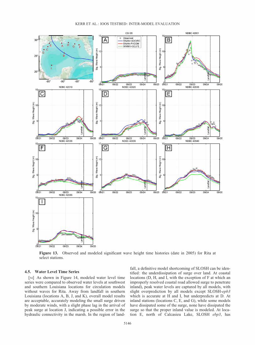
[53] Comparisons of SWANþADCIRC, SWAN-FVCOM, and WWMIIþSELFE to measured significantwave heights are shown in Figure 13. As expected,SWANþADCIRC and SWAN-FVCOM perform similarlyand accurately with slight differences likely caused by the

variation in wind drag formulations between thewave models. A small departure is seen betweenWWMIIþSELFE and the two other models. This departureappears to be spatially dependent with departures seen atstations further from the track. Table 6 lists the resultsof a statistical analysis of wave model performance.WWMIIþSELFE has a large negative BMN for significantwave height and also has the lowest R2 for peak period.Aside from this, all models perform comparably across allwave parameters with the exception of the large wavedirection E for SWAN-FVCOM. See Figure S5 of the sup-porting information for a comparison of wave characteristicperformance categorized by data source.

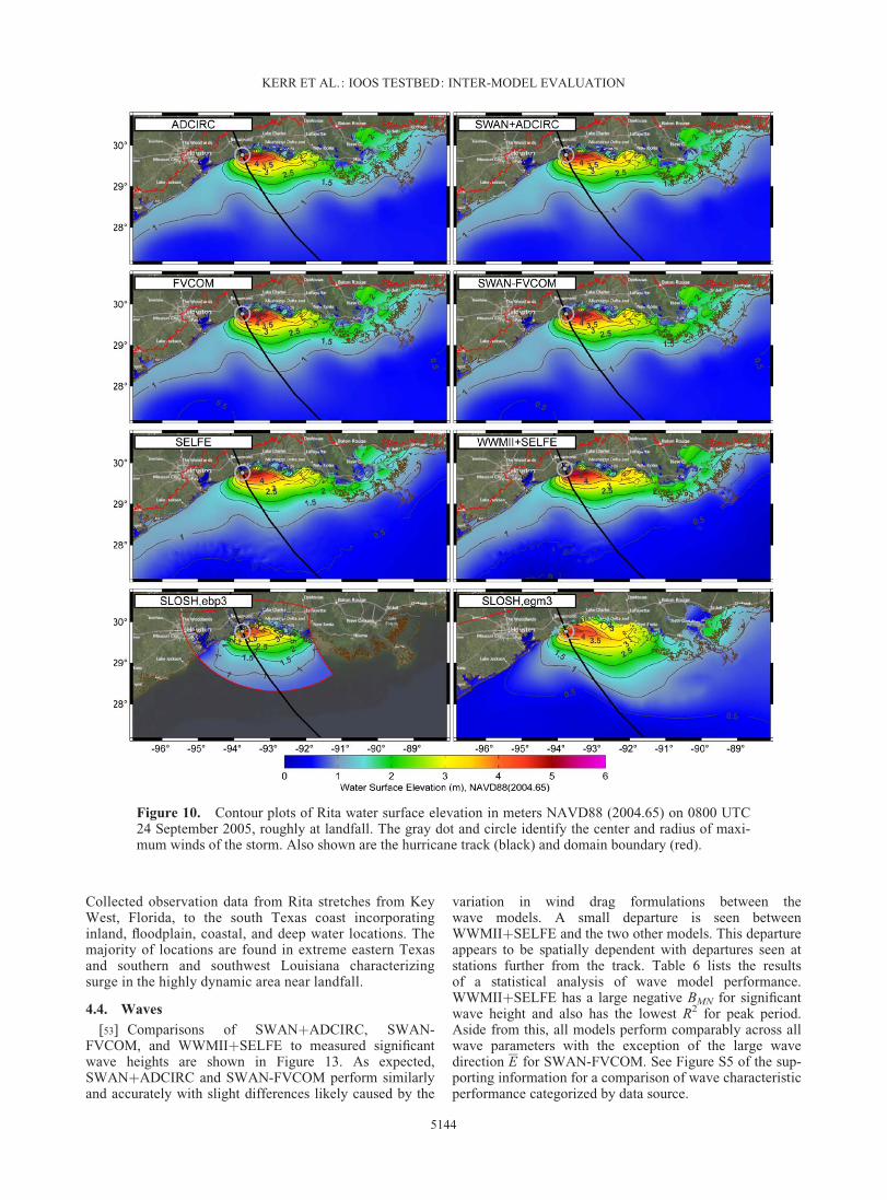
Figure 10. Contour plots of Rita water surface elevation in meters NAVD88 (2004.65) on 0800 UTC24 September 2005, roughly at landfall. The gray dot and circle identify the center and radius of maxi-mum winds of the storm. Also shown are the hurricane track (black) and domain boundary (red).

KERR ET AL.: IOOS TESTBED: INTER-MODEL EVALUATION

5144

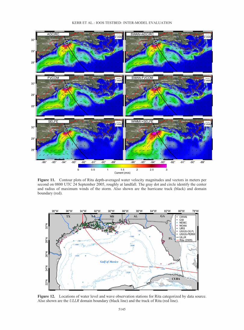
Figure 11. Contour plots of Rita depth-averaged water velocity magnitudes and vectors in meters persecond on 0800 UTC 24 September 2005, roughly at landfall. The gray dot and circle identify the centerand radius of maximum winds of the storm. Also shown are the hurricane track (black) and domainboundary (red).

Figure 12. Locations of water level and wave observation stations for Rita categorized by data source.Also shown are the ULLR domain boundary (black line) and the track of Rita (red line).

KERR ET AL.: IOOS TESTBED: INTER-MODEL EVALUATION

5145

4.5. Water Level Time Series

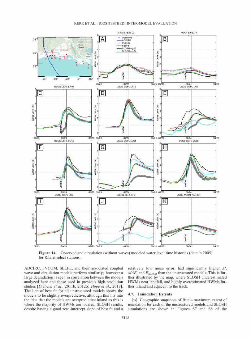
[54] As shown in Figure 14, modeled water level timeseries were compared to observed water levels at southwestand southern Louisiana locations for circulation modelswithout waves for Rita. Away from landfall in southernLouisiana (locations A, B, J, and K), overall model resultsare acceptable, accurately modeling the small surge drivenby moderate winds, with a slight phase lag in the arrival ofpeak surge at location J, indicating a possible error in thehydraulic connectivity in the marsh. In the region of land-

fall, a definitive model shortcoming of SLOSH can be iden-tified: the underdissipation of surge over land. At coastallocations (D, H, and I, with the exception of F at which animproperly resolved coastal road allowed surge to penetrateinland), peak water levels are captured by all models, withslight overprediction by all models except SLOSH-epb3which is accurate at H and I, but underpredicts at D. Atinland stations (locations C, E, and G), while some modelshave dissipated some of the surge, none have dissipated thesurge so that the proper inland value is modeled. At loca-tion E, north of Calcasieu Lake, SLOSH ebp3, has

Figure 13. Observed and modeled significant wave height time histories (date in 2005) for Rita atselect stations.

KERR ET AL.: IOOS TESTBED: INTER-MODEL EVALUATION

5146

dissipated surge to its proper level ; however, the large lagin time of arrival of peak surge indicates improper modelphysics in the region.

[55] Modeled water level time series were also comparedto observed water levels at southwest and southern Louisi-ana locations for coupled wave and circulation models forRita (Figure 15). Almost identical behavior is seen betweenthe coupled waves and circulation models presented in Fig-ure 15 as the circulation only models show in Figure 14,with the exception of Stations A and B, which showimprovement with the addition of waves in southeasternLouisiana. Peak water levels at the coast are accuratelycaptured, however at inland stations little to no dissipationis seen as the addition of wave radiation stress gradientsincrease water levels in wave breaking and inland areas.

[56] Analyzing the statistics of model performance toobserved data (Table 6 and Figure S6 of the supporting in-formation) confirms much of what was identified in the pre-vious figures. Based on BMN and E, SLOSH tends tooverpredict water levels. In fact, almost without exceptionall models tend to be overpredictive based on BMN and E.This explains the deterioration of results when wave mod-els are coupled to the circulation models. Because the cir-culation models are already statistically overpredictive,when wave radiation stress gradients are added, water lev-els can be expected to increase in inland areas, thus makingalready overpredictive models more overpredictive. Whilean increase in E and BMN values is seen when adding thewave models, the change is small and the coupled wave

and circulation models would still be classified as accurate.In general, ADCIRC is the top statistical performer; how-ever, the differences between the unstructured models aresmall and all unstructured mesh simulations can be classi-fied as accurate. A large separation is seen between thestructured and unstructured models. SLOSH egm3 per-forms better than SLOSH ebp3 ; however, the low numberof stations analyzed in the ebp3 domain limits its statisticalset in comparison to the other models. The lack of inlandattenuation can seen by the Topo-Substitution method (TS)water level BMN statistics for USGS-PERM stations (SeeFigure S6 of the supporting information). USGS-PERMstations are located primarily in inland areas such as chan-nels and lakes and the high values for BMN produced by allmodels quantifies this overestimation. Compare this tomodel performance at coastal stations (CRMS, CSI,NOAA, and USGS-DEPL), where BMN values are muchcloser to zero, indicating better model performance. It is tobe noted that the number of locations at which model com-parisons were made differs from model to model, particu-larly between the structured and unstructured models.

4.6. High Water Marks

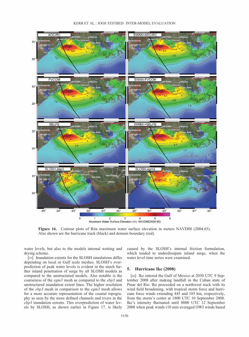
[57] As shown in Figure 16, the maximum modeledwater levels during Rita were compared for each modeland those water levels compared to measured high watermarks (HWMs) spatially in Figure 17 and correlatively inFigure 18 with the statistics of these HWM comparisonspresented in Table 7. Qualitatively and quantitatively,

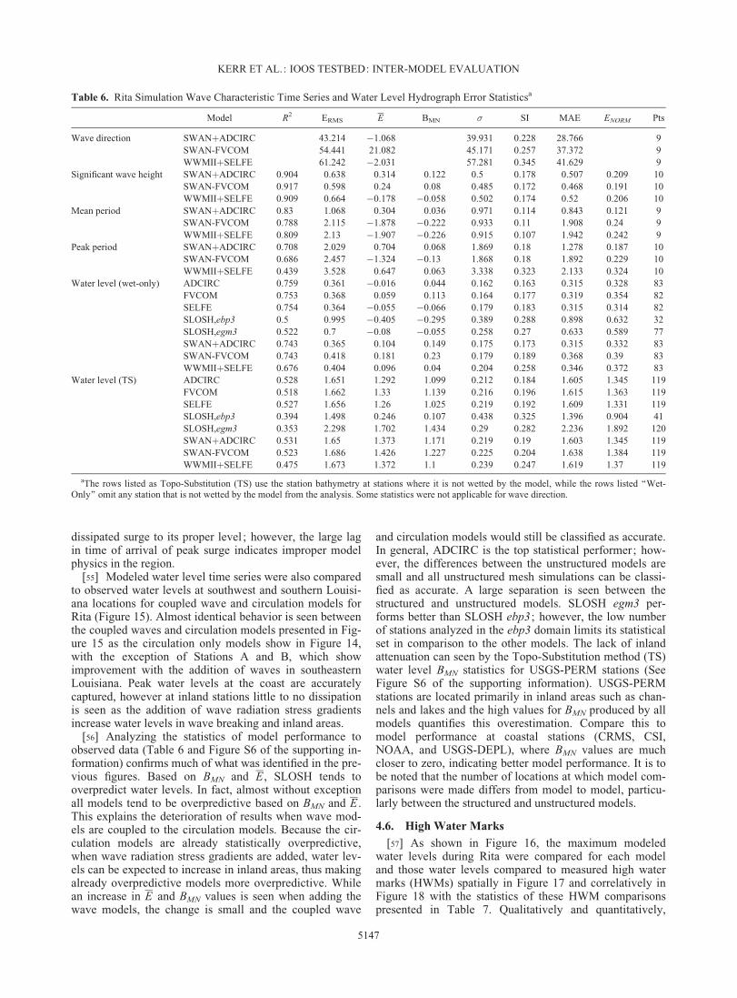
Table 6. Rita Simulation Wave Characteristic Time Series and Water Level Hydrograph Error Statisticsa

Model R2 ERMS E BMN � SI MAE ENORM Pts

Wave direction SWANþADCIRC 43.214 �1.068 39.931 0.228 28.766 9SWAN-FVCOM 54.441 21.082 45.171 0.257 37.372 9WWMIIþSELFE 61.242 �2.031 57.281 0.345 41.629 9

Significant wave height SWANþADCIRC 0.904 0.638 0.314 0.122 0.5 0.178 0.507 0.209 10SWAN-FVCOM 0.917 0.598 0.24 0.08 0.485 0.172 0.468 0.191 10WWMIIþSELFE 0.909 0.664 �0.178 �0.058 0.502 0.174 0.52 0.206 10

Mean period SWANþADCIRC 0.83 1.068 0.304 0.036 0.971 0.114 0.843 0.121 9SWAN-FVCOM 0.788 2.115 �1.878 �0.222 0.933 0.11 1.908 0.24 9WWMIIþSELFE 0.809 2.13 �1.907 �0.226 0.915 0.107 1.942 0.242 9

Peak period SWANþADCIRC 0.708 2.029 0.704 0.068 1.869 0.18 1.278 0.187 10SWAN-FVCOM 0.686 2.457 �1.324 �0.13 1.868 0.18 1.892 0.229 10WWMIIþSELFE 0.439 3.528 0.647 0.063 3.338 0.323 2.133 0.324 10

Water level (wet-only) ADCIRC 0.759 0.361 �0.016 0.044 0.162 0.163 0.315 0.328 83FVCOM 0.753 0.368 0.059 0.113 0.164 0.177 0.319 0.354 82SELFE 0.754 0.364 �0.055 �0.066 0.179 0.183 0.315 0.314 82SLOSH,ebp3 0.5 0.995 �0.405 �0.295 0.389 0.288 0.898 0.632 32SLOSH,egm3 0.522 0.7 �0.08 �0.055 0.258 0.27 0.633 0.589 77SWANþADCIRC 0.743 0.365 0.104 0.149 0.175 0.173 0.315 0.332 83SWAN-FVCOM 0.743 0.418 0.181 0.23 0.179 0.189 0.368 0.39 83WWMIIþSELFE 0.676 0.404 0.096 0.04 0.204 0.258 0.346 0.372 83

Water level (TS) ADCIRC 0.528 1.651 1.292 1.099 0.212 0.184 1.605 1.345 119FVCOM 0.518 1.662 1.33 1.139 0.216 0.196 1.615 1.363 119SELFE 0.527 1.656 1.26 1.025 0.219 0.192 1.609 1.331 119SLOSH,ebp3 0.394 1.498 0.246 0.107 0.438 0.325 1.396 0.904 41SLOSH,egm3 0.353 2.298 1.702 1.434 0.29 0.282 2.236 1.892 120SWANþADCIRC 0.531 1.65 1.373 1.171 0.219 0.19 1.603 1.345 119SWAN-FVCOM 0.523 1.686 1.426 1.227 0.225 0.204 1.638 1.384 119WWMIIþSELFE 0.475 1.673 1.372 1.1 0.239 0.247 1.619 1.37 119

aThe rows listed as Topo-Substitution (TS) use the station bathymetry at stations where it is not wetted by the model, while the rows listed ‘‘Wet-Only’’ omit any station that is not wetted by the model from the analysis. Some statistics were not applicable for wave direction.

KERR ET AL.: IOOS TESTBED: INTER-MODEL EVALUATION

5147

ADCIRC, FVCOM, SELFE, and their associated coupledwave and circulation models perform similarly; however alarge degradation is seen in correlation between the modelsanalyzed here and those used in previous high-resolutionstudies [Dietrich et al., 2011b, 2012b; Hope et al., 2013].The line of best fit for all unstructured models shows themodels to be slightly overpredictive, although this fits intothe idea that the models are overpredictive inland as this iswhere the majority of HWMs are located. SLOSH results,despite having a good zero-intercept slope of best fit and a

relatively low mean error, had significantly higher SI,MAE, and ENORM than the unstructured models. This is fur-ther illustrated by the map, where SLOSH underestimatedHWMs near landfall, and highly overestimated HWMs fur-ther inland and adjacent to the track.

4.7. Inundation Extents

[58] Geographic snapshots of Rita’s maximum extent ofinundation for each of the unstructured models and SLOSHsimulations are shown in Figures S7 and S8 of the

Figure 14. Observed and circulation (without waves) modeled water level time histories (date in 2005)for Rita at select stations.

KERR ET AL.: IOOS TESTBED: INTER-MODEL EVALUATION

5148

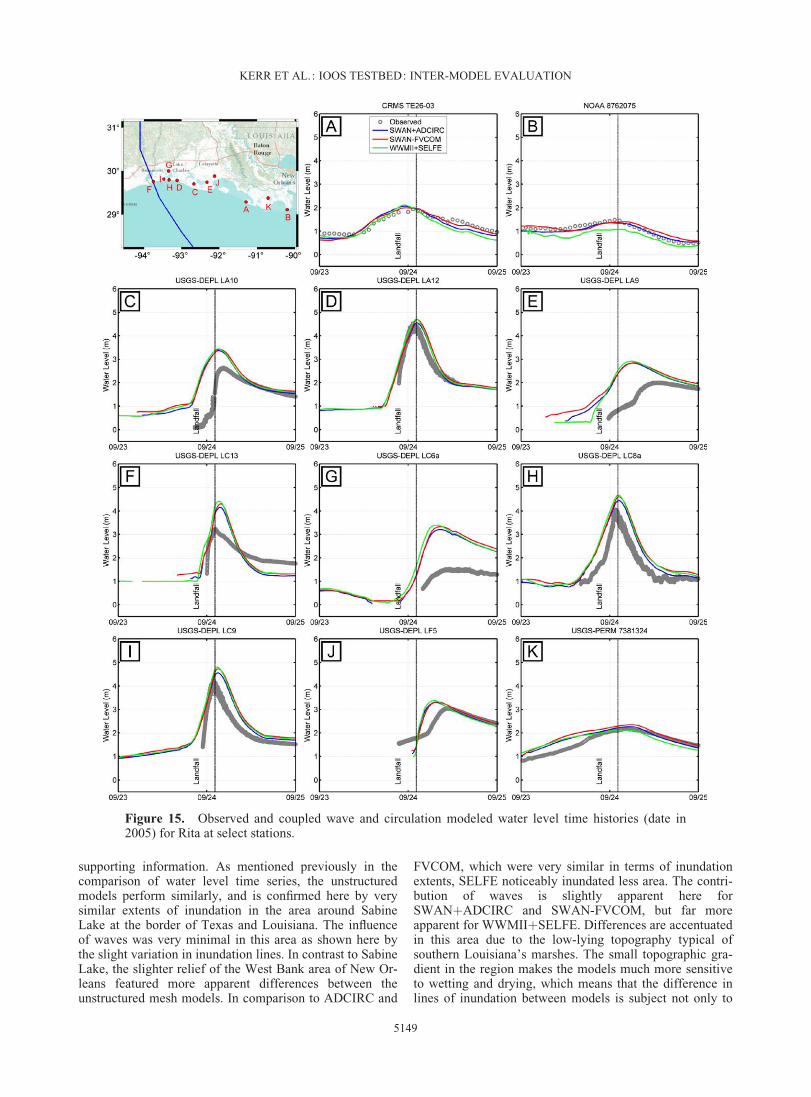
supporting information. As mentioned previously in thecomparison of water level time series, the unstructuredmodels perform similarly, and is confirmed here by verysimilar extents of inundation in the area around SabineLake at the border of Texas and Louisiana. The influenceof waves was very minimal in this area as shown here bythe slight variation in inundation lines. In contrast to SabineLake, the slighter relief of the West Bank area of New Or-leans featured more apparent differences between theunstructured mesh models. In comparison to ADCIRC and

FVCOM, which were very similar in terms of inundationextents, SELFE noticeably inundated less area. The contri-bution of waves is slightly apparent here forSWANþADCIRC and SWAN-FVCOM, but far moreapparent for WWMIIþSELFE. Differences are accentuatedin this area due to the low-lying topography typical ofsouthern Louisiana’s marshes. The small topographic gra-dient in the region makes the models much more sensitiveto wetting and drying, which means that the difference inlines of inundation between models is subject not only to

Figure 15. Observed and coupled wave and circulation modeled water level time histories (date in2005) for Rita at select stations.

KERR ET AL.: IOOS TESTBED: INTER-MODEL EVALUATION

5149

water levels, but also to the models internal wetting anddrying scheme.

[59] Inundation extents for the SLOSH simulations differdepending on local or Gulf scale meshes. SLOSH’s over-prediction of peak water levels is evident in the much fur-ther inland penetration of surge by all SLOSH models ascompared to the unstructured models. Also notable is thecoarseness of the egm3 mesh as compared to the ebp3 andunstructured inundation extent lines. The higher resolutionof the ebp3 mesh in comparison to the egm3 mesh allowsfor a more accurate representation of the coastal topogra-phy as seen by the more defined channels and rivers in theebp3 inundation extents. This overprediction of water lev-els by SLOSH, as shown earlier in Figure 17, is likely

caused by the SLOSH’s internal friction formulation,which tended to underdissipate inland surge, when thewater level time series were examined.

5. Hurricane Ike (2008)

[60] Ike entered the Gulf of Mexico at 2030 UTC 9 Sep-tember 2008 after making landfall in the Cuban state ofPinar del Rio. Ike proceeded on a northwest track with itswind field broadening, with tropical storm force and hurri-cane force winds extending 445 and 185 km, respectively,from the storm’s center at 1800 UTC 10 September 2008.Ike’s intensity fluctuated until 0000 UTC 12 September2008 when peak winds (10 min averaged OWI winds based

Figure 16. Contour plots of Rita maximum water surface elevation in meters NAVD88 (2004.65).Also shown are the hurricane track (black) and domain boundary (red).

KERR ET AL.: IOOS TESTBED: INTER-MODEL EVALUATION

5150

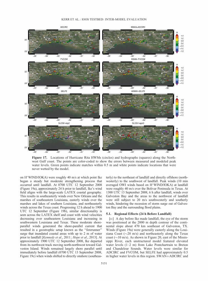
on H�WIND/IOKA) were roughly 40 m/s at which point Ikebegan a steady but moderate strengthening process thatoccurred until landfall. At 0700 UTC 12 September 2008(Figure 19a), approximately 24 h prior to landfall, Ike’s windfield aligns with the large-scale LATEX coastal geography.This results in southeasterly winds over New Orleans and themarshes of southeastern Louisiana, easterly winds over themarshes and lakes of southern Louisiana, and northeasterlywinds across the Texas coast. Progressing 12 h ahead to 1900UTC 12 September (Figure 19b), similar directionality isseen across the LATEX shelf and coast with wind velocitiesdecreasing over southeastern Louisiana and increasing insouthwestern Louisiana and Texas. These moderate shore-parallel winds generated the shore-parallel current thatresulted in a geostrophic setup known as the ‘‘forerunner’’surge that inundated coastal areas with up to 2 m of waterprior to landfall [Kennedy et al., 2011; Hope et al., 2013]. Atapproximately 1900 UTC 12 September 2008, Ike departedfrom its northwest track moving north-northwest toward Gal-veston Island. Winds remained largely shore parallel untilimmediately before landfall (0700 UTC 13 September 2008,Figure 19c) when winds shifted to directly onshore (southeas-

terly) to the northeast of landfall and directly offshore (north-westerly) to the southwest of landfall. Peak winds (10 minaveraged OWI winds based on H�WIND/IOKA) at landfallwere roughly 40 m/s over the Bolivar Peninsula in Texas. At1300 UTC 13 September 2008, 6 h after landfall, winds overGalveston Bay and the areas to the northwest of landfallwere still subject to 20 m/s southwesterly and southerlywinds, hindering the recession of storm surge out of Galves-ton Bay and the surrounding flood plains.

5.1. Regional Effects (24 h Before Landfall)

[61] A day before Ike made landfall, the eye of the stormwas positioned at the 2000 m depth contour of the conti-nental slope about 470 km southeast of Galveston, TX.Winds (Figure 19a) were generally easterly along the Loui-siana Coast (�20 m/s) and northeasterly along the Texascoast (�10 m/s). As shown in Figure 20, east of the Missis-sippi River, each unstructured model featured elevatedwater levels (1–2 m) from Lake Pontchartrain to Bretonand Chandeleur Sounds. Water levels were similar forADCIRC and FVCOM, but SELFE had approximately 0.5m higher water levels in this region. SWANþADCIRC and

Figure 17. Locations of Hurricane Rita HWMs (circles) and hydrographs (squares) along the North-west Gulf coast. The points are color-coded to show the errors between measured and modeled peakwater levels. Green points indicate matches within 0.5 m and white points indicate locations that werenever wetted by the model.

KERR ET AL.: IOOS TESTBED: INTER-MODEL EVALUATION

5151

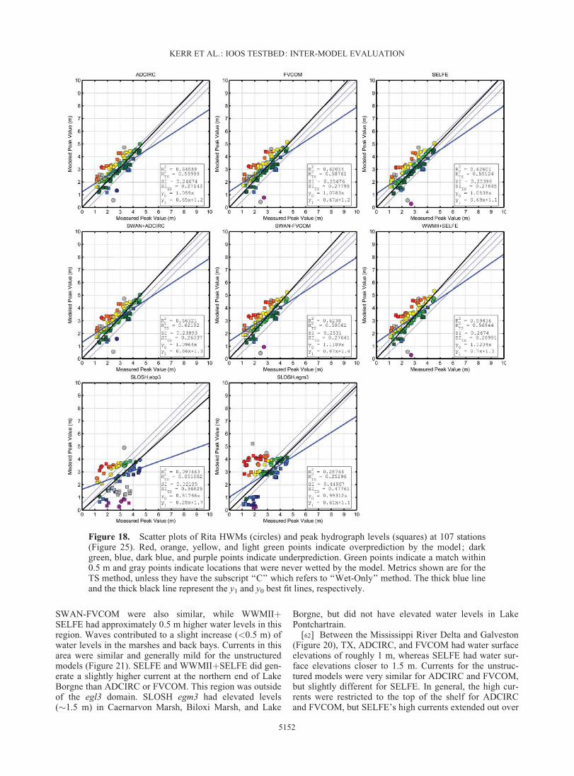
SWAN-FVCOM were also similar, while WWMIIþSELFE had approximately 0.5 m higher water levels in thisregion. Waves contributed to a slight increase (<0.5 m) ofwater levels in the marshes and back bays. Currents in thisarea were similar and generally mild for the unstructuredmodels (Figure 21). SELFE and WWMIIþSELFE did gen-erate a slightly higher current at the northern end of LakeBorgne than ADCIRC or FVCOM. This region was outsideof the egl3 domain. SLOSH egm3 had elevated levels(�1.5 m) in Caernarvon Marsh, Biloxi Marsh, and Lake

Borgne, but did not have elevated water levels in LakePontchartrain.

[62] Between the Mississippi River Delta and Galveston(Figure 20), TX, ADCIRC, and FVCOM had water surfaceelevations of roughly 1 m, whereas SELFE had water sur-face elevations closer to 1.5 m. Currents for the unstruc-tured models were very similar for ADCIRC and FVCOM,but slightly different for SELFE. In general, the high cur-rents were restricted to the top of the shelf for ADCIRCand FVCOM, but SELFE’s high currents extended out over

Figure 18. Scatter plots of Rita HWMs (circles) and peak hydrograph levels (squares) at 107 stations(Figure 25). Red, orange, yellow, and light green points indicate overprediction by the model; darkgreen, blue, dark blue, and purple points indicate underprediction. Green points indicate a match within0.5 m and gray points indicate locations that were never wetted by the model. Metrics shown are for theTS method, unless they have the subscript ‘‘C’’ which refers to ‘‘Wet-Only’’ method. The thick blue lineand the thick black line represent the y1 and y0 best fit lines, respectively.

KERR ET AL.: IOOS TESTBED: INTER-MODEL EVALUATION

5152

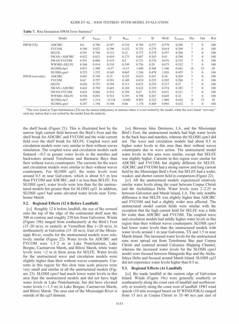
the shelf break (Figure 21). This is illustrated best by thenarrow high current field between the Bird’s Foot and theshelf break for ADCIRC and FVCOM and the wide currentfield over the shelf break for SELFE. Coupled wave andcirculation models were very similar to their without wavessimulation. The coupled wave and circulation models eachfeatured �0.5 m greater water levels in the marshes andbackwaters around Terrebonne and Barataria Bays thantheir without waves counterparts. The currents for the waveand circulation models were similar to their without wavescounterparts. For SLOSH egl3, the water levels werearound 0.5 m near Galveston, which is about 0.5 m lessthan FVCOM and ADCIRC, and 1 m less than SELFE. ForSLOSH egm3, water levels were less than for the unstruc-tured models but greater than for SLOSH egl3. In addition,SLOSH egm3 had some elevated water levels near Terre-bonne Marsh.

5.2. Regional Effects (12 h Before Landfall)

[63] Roughly 12 h before landfall, the eye of Ike crossedonto the top of the edge of the continental shelf near the300 m contour and roughly 230 km from Galveston. Winds(Figure 19b) ranged from southeasterly at the Bird’s Foot(15–20 m/s), to easterly at Vermillion Bay (�20 m/s), tonortheasterly at Galveston (15–20 m/s). East of the Missis-sippi River, results for the unstructured models were rela-tively similar (Figure 22). Water levels for ADCIRC andFVCOM were 1.5–2 m in Lake Pontchartrain, LakeBorgne, Caernarvon Marsh, and Biloxi Marsh, while waterlevels were �2 m in these areas for SELFE. Water levelsfor the unstructured wave and circulation models wereslightly higher than their without waves counterparts. Cur-rents in this region for this slow time scale process werevery small and similar in all the unstructured models (Fig-ure 23). SLOSH egm3 had much lower water levels in thisarea than the unstructured models and did not have highwater levels in Lake Pontchartrain, but did have elevatedwater levels (�1.5 m) in Lake Borgne, Caernarvon Marsh,and Biloxi Marsh. The area east of the Mississippi River isoutside of the egl3 domain.

[64] Between Isles Dernieres, LA, and the MississippiBird’s Foot, the unstructured models had high water levelsin the back bays and marshes, whereas the SLOSH egm3 didnot. The wave and circulation models had about 0.5 mhigher water levels in this area than their without wavescounterparts due to wave action. The unstructured modelwater levels in this area were similar, except that SELFEwas slightly higher. Currents in this region were similar forADCIRC and FVCOM, but slightly different for SELFE.ADCIRC and FVCOM had a strong narrow and long currentfield by the Mississippi Bird’s Foot, but SELFE had a wider,weaker, and shorter current field in comparison (Figure 22).

[65] All the unstructured models experienced relativelysimilar water levels along the coast between Corpus Christiand the Atchafalaya Delta. Water levels were 2–2.25 mbetween Galveston and Marsh Island, LA. The only notabledifference is that SELFE was slightly higher than ADCIRCand FVCOM and had a slightly wider area affected. Theunstructured model current fields were similar with theexception that the high current field for SELFE was a littlebit wider than ADCIRC and FVCOM. The coupled waveand circulation models had mildly higher water levels in thisregion than their without waves counterparts. SLOSH egm3had lower water levels than the unstructured models withwater levels around 1 m near Galveston, TX and 1.5 m nearMarsh Island. The increased water levels for the unstructuredruns were spread out from Terrebonne Bay past CorpusChristi and centered around Calcasieu Shipping Channel,whereas the increased water levels for the SLOSH egm3model were focused between Matagorda Bay and the Atcha-falaya Delta and focused around Marsh Island. SLOSH egl3did not experience water levels higher than 0.5 m.

5.3. Regional Effects (At Landfall)

[66] Ike made landfall at the eastern edge of GalvestonIsland. Winds (Figure 19c) were generally southerly orsoutheasterly along the coast east of landfall and northwest-erly or westerly along the coast west of landfall. OWI windspeeds (10 min averaged based on H�WIND/IOKA) rangedfrom 15 m/s at Corpus Christi to 35–40 m/s just east of

Table 7. Rita Simulation HWM Error Statisticsa

Model R2 ERMS E BMN � SI MAE ENORM Dry Out Wet

HWM (TS) ADCIRC 0.6 0.786 0.347 0.134 0.708 0.271 0.578 0.286 7 0 100FVCOM 0.588 0.823 0.396 0.152 0.725 0.278 0.614 0.299 7 0 100SELFE 0.591 0.788 0.312 0.12 0.727 0.278 0.557 0.286 7 0 100SWANþADCIRC 0.622 0.821 0.454 0.175 0.687 0.263 0.61 0.299 7 0 100SWAN-FVCOM 0.591 0.886 0.519 0.2 0.721 0.276 0.676 0.322 7 0 100WWMIIþSELFE 0.568 0.914 0.518 0.199 0.756 0.29 0.675 0.332 7 0 100SLOSH,ebp3 0.051 1.308 �0.37 �0.13 1.048 0.368 1.106 0.441 16 33 58SLOSH,egm3 0.253 1.252 0.169 0.065 1.246 0.478 1.026 0.455 3 0 104

HWM (wet-only) ADCIRC 0.641 0.749 0.33 0.125 0.653 0.247 0.54 0.269 7 0 100FVCOM 0.62 0.797 0.391 0.149 0.674 0.255 0.585 0.286 7 0 100SELFE 0.626 0.752 0.294 0.111 0.672 0.254 0.517 0.27 7 0 100SWANþADCIRC 0.663 0.789 0.445 0.169 0.632 0.239 0.574 0.283 7 0 100SWAN-FVCOM 0.624 0.866 0.524 0.199 0.67 0.253 0.651 0.311 7 0 100WWMIIþSELFE 0.594 0.892 0.514 0.195 0.708 0.267 0.645 0.32 7 0 100SLOSH,ebp3 0.097 1.214 �0.124 �0.045 0.893 0.322 1.009 0.416 16 33 58SLOSH,egm3 0.287 1.194 0.104 0.04 1.178 0.449 0.985 0.432 3 0 104

aThe rows listed as Topo-Substitution (TS) use the station bathymetry at stations where it is not wetted by the model, while the rows listed ‘‘wet-only’’omit any station that is not wetted by the model from the analysis.

KERR ET AL.: IOOS TESTBED: INTER-MODEL EVALUATION

5153

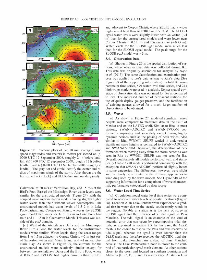
Galveston, to 20 m/s at Vermillion Bay, and 15 m/s at theBird’s Foot. East of the Mississippi River water levels weresimilar for the unstructured models (Figure 24), with thecoupled wave and circulation models having slightly higherwater levels than their without waves counterparts. Theunstructured models had water levels of 1.5–2 m in LakePontchartrain and Caernarvon Marsh, whereas the SLOSHegm3 model had water levels of 0.5 m in Lake Pontchar-train and 1�1.5 m in Caernarvon Marsh. This area was out-side of the egl3 domain.

[67] West of the Atchafalaya Delta and the MississippiRiver Bird’s Foot, the water levels for the unstructuredmodels were similar. Water levels along the coast rangedfrom 1 to 1.5 m adjacent to Corpus Christi, �5 m just eastof Galveston, �2 m near Marsh Island, and �1 m near Bar-ataria Bay. As shown in Figure 25, the currents for theunstructured models were relatively similar except forbetween the Atchafalaya Delta and the Bird’s Foot, whereADCIRC and FVCOM had higher currents than SELFE,

and adjacent to Corpus Christi, where SELFE had a widerhigh current field than ADCIRC and FVCOM. The SLOSHegm3 water levels were slightly lower near Galveston (�4m) than for the unstructured models and were lower nearCorpus Christi (�0.75 m) and Barataria Bay (�0.75 m).Water levels for the SLOSH egl3 model were much lessthan for the SLOSH egm3 model. The peak surge for theSLOSH egl3 model was �3 m.

5.4. Observation Data

[68] Shown in Figure 26 is the spatial distribution of sta-tions, where observational data was collected during Ike.This data was originally assembled for analysis by Hopeet al. [2013]. The same classification and examination pro-cess was applied to Ike’s data as was to Rita’s data (SeeFigure S9 of the supporting information). In total 81 waveparameter time series, 579 water level time series, and 243high water marks were used in analysis. Denser spatial cov-erage of observation data was obtained for Ike as comparedto Rita. The increased number of permanent stations, theuse of quick-deploy gauges prestorm, and the fortificationof existing gauges allowed for a much larger number ofobservations to be obtained.

5.5. Waves

[69] As shown in Figure 27, modeled significant waveheights were compared to measured data in the Gulf ofMexico and on the LATEX shelf. Similar to Rita, at moststations, SWANþADCIRC and SWAN-FVCOM per-formed comparably and accurately except during highlydynamic periods such as the passing of peak winds. Alsosimilar to Rita, WWMIIþSELFE tended to underpredictsignificant wave heights as compared to SWANþADCIRCand SWAN-FVCOM; however, the deterioration of per-formance when moving away from the storm center as wasseen in Rita by WWMIIþSELFE was not seen for Ike.Overall, qualitatively all models performed well, and statis-tically (Table 8) all models performed comparably with theexception that SWANþADCIRC performed slightly betterin some categories. The differences, however, were slightand can likely be attributed to the different approaches towind drag used by the wave models. See Figure S10 of thesupporting information for a comparison of wave character-istic performance categorized by data source.

5.6. Water Level Time Series

[70] Circulation model water level time series were com-pared to observed water levels at coastal locations (Figure28). Location A, in Lake Pontchartrain experienced a grad-ual rise in water due to the steady southeasterly winds inthe region. Notable at station A is the lack of surge inSLOSH egm3 and the presence of a tidal signal in PassManchac. The tidal signal is an example of the kind ofpotential error that can occur by superimposing tidal sig-nals, as explained in section 2.5. In this case, the ULLRmesh is too coarse to resolve the Pass and thus receives notidal signal, whereas the egm3 is even coarser than theULLR mesh and therefore receives the ADCIRC tidal sig-nal from Lake Pontchartrain instead of Pass Manchacbecause the Lake Pontchartrain node is closer to the cent-roid of that particular egm3 mesh element. At other stationscloser to the coast and located in southern Louisiana andAlabama (B, C, D, E, and F) results vary. At station E in

Figure 19. Contour plots of Ike 10 min averaged windspeed magnitudes and vectors in meters per second on (a)0700 UTC 12 September 2008, roughly 24 h before land-fall, (b) 1900 UTC 12 September 2008, roughly 12 h beforelandfall, and (c) 0700 UTC 13 September 2008, roughly atlandfall. The gray dot and circle identify the center and ra-dius of maximum winds of the storm. Also shown are thehurricane track (black) and ULLR domain boundary (red).

KERR ET AL.: IOOS TESTBED: INTER-MODEL EVALUATION

5154

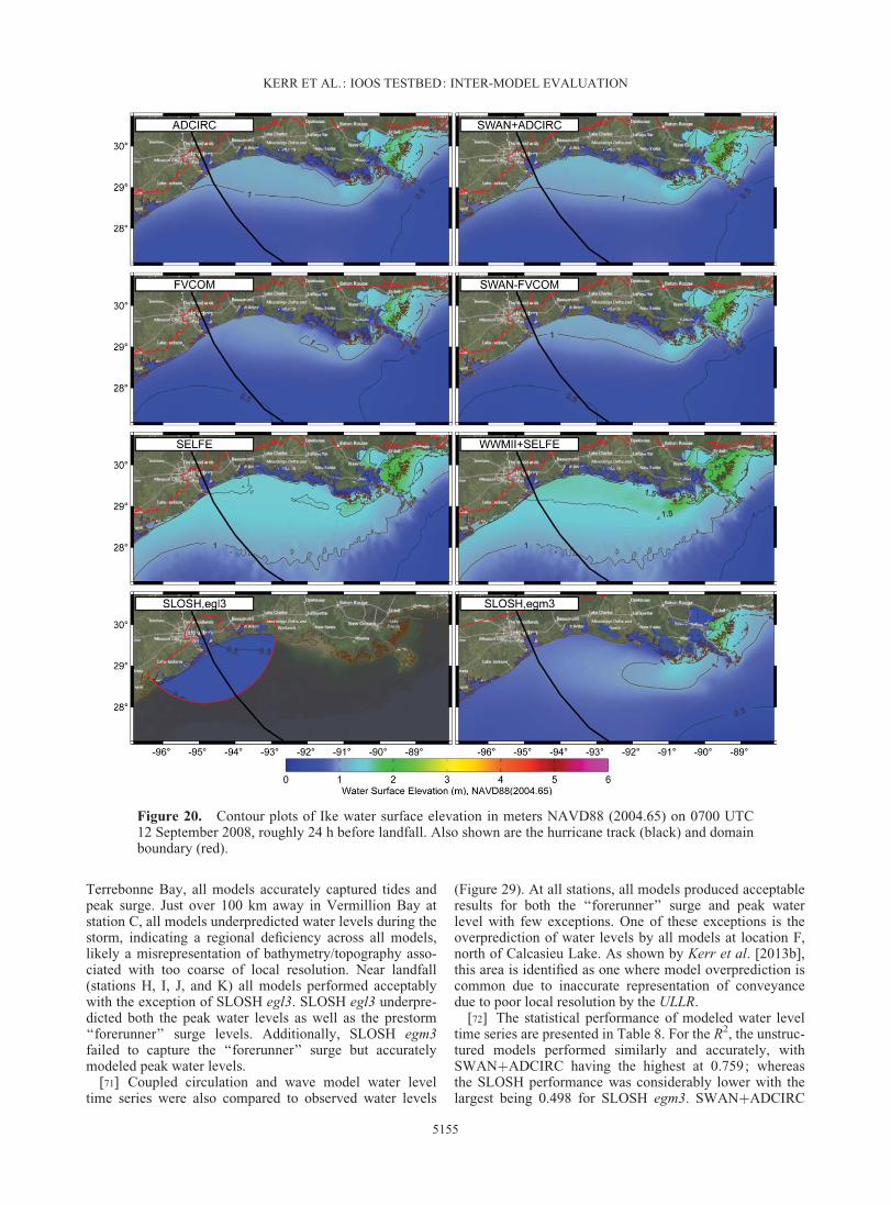
Terrebonne Bay, all models accurately captured tides andpeak surge. Just over 100 km away in Vermillion Bay atstation C, all models underpredicted water levels during thestorm, indicating a regional deficiency across all models,likely a misrepresentation of bathymetry/topography asso-ciated with too coarse of local resolution. Near landfall(stations H, I, J, and K) all models performed acceptablywith the exception of SLOSH egl3. SLOSH egl3 underpre-dicted both the peak water levels as well as the prestorm‘‘forerunner’’ surge levels. Additionally, SLOSH egm3failed to capture the ‘‘forerunner’’ surge but accuratelymodeled peak water levels.

[71] Coupled circulation and wave model water leveltime series were also compared to observed water levels

(Figure 29). At all stations, all models produced acceptableresults for both the ‘‘forerunner’’ surge and peak waterlevel with few exceptions. One of these exceptions is theoverprediction of water levels by all models at location F,north of Calcasieu Lake. As shown by Kerr et al. [2013b],this area is identified as one where model overprediction iscommon due to inaccurate representation of conveyancedue to poor local resolution by the ULLR.

[72] The statistical performance of modeled water leveltime series are presented in Table 8. For the R2, the unstruc-tured models performed similarly and accurately, withSWANþADCIRC having the highest at 0.759; whereasthe SLOSH performance was considerably lower with thelargest being 0.498 for SLOSH egm3. SWANþADCIRC

Figure 20. Contour plots of Ike water surface elevation in meters NAVD88 (2004.65) on 0700 UTC12 September 2008, roughly 24 h before landfall. Also shown are the hurricane track (black) and domainboundary (red).

KERR ET AL.: IOOS TESTBED: INTER-MODEL EVALUATION

5155

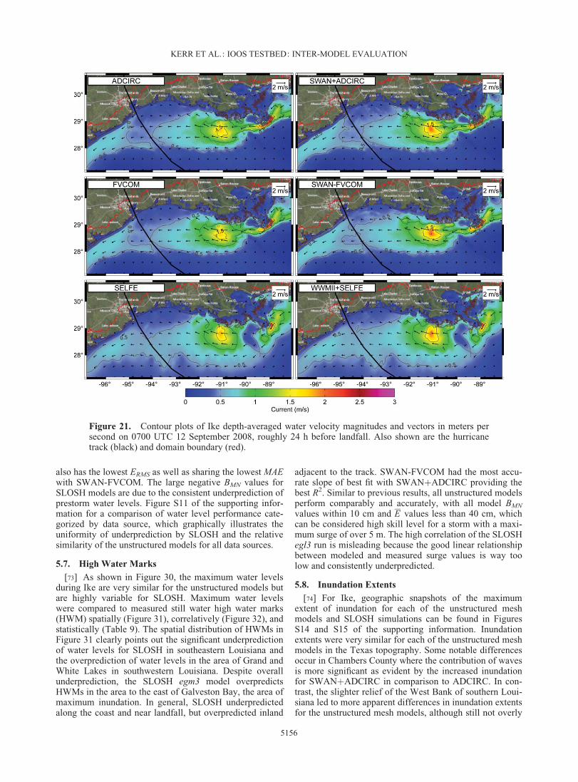
also has the lowest ERMS as well as sharing the lowest MAEwith SWAN-FVCOM. The large negative BMN values forSLOSH models are due to the consistent underprediction ofprestorm water levels. Figure S11 of the supporting infor-mation for a comparison of water level performance cate-gorized by data source, which graphically illustrates theuniformity of underprediction by SLOSH and the relativesimilarity of the unstructured models for all data sources.

5.7. High Water Marks

[73] As shown in Figure 30, the maximum water levelsduring Ike are very similar for the unstructured models butare highly variable for SLOSH. Maximum water levelswere compared to measured still water high water marks(HWM) spatially (Figure 31), correlatively (Figure 32), andstatistically (Table 9). The spatial distribution of HWMs inFigure 31 clearly points out the significant underpredictionof water levels for SLOSH in southeastern Louisiana andthe overprediction of water levels in the area of Grand andWhite Lakes in southwestern Louisiana. Despite overallunderprediction, the SLOSH egm3 model overpredictsHWMs in the area to the east of Galveston Bay, the area ofmaximum inundation. In general, SLOSH underpredictedalong the coast and near landfall, but overpredicted inland

adjacent to the track. SWAN-FVCOM had the most accu-rate slope of best fit with SWANþADCIRC providing thebest R2. Similar to previous results, all unstructured modelsperform comparably and accurately, with all model BMN

values within 10 cm and E values less than 40 cm, whichcan be considered high skill level for a storm with a maxi-mum surge of over 5 m. The high correlation of the SLOSHegl3 run is misleading because the good linear relationshipbetween modeled and measured surge values is way toolow and consistently underpredicted.

5.8. Inundation Extents

[74] For Ike, geographic snapshots of the maximumextent of inundation for each of the unstructured meshmodels and SLOSH simulations can be found in FiguresS14 and S15 of the supporting information. Inundationextents were very similar for each of the unstructured meshmodels in the Texas topography. Some notable differencesoccur in Chambers County where the contribution of wavesis more significant as evident by the increased inundationfor SWANþADCIRC in comparison to ADCIRC. In con-trast, the slighter relief of the West Bank of southern Loui-siana led to more apparent differences in inundation extentsfor the unstructured mesh models, although still not overly

Figure 21. Contour plots of Ike depth-averaged water velocity magnitudes and vectors in meters persecond on 0700 UTC 12 September 2008, roughly 24 h before landfall. Also shown are the hurricanetrack (black) and domain boundary (red).

KERR ET AL.: IOOS TESTBED: INTER-MODEL EVALUATION

5156

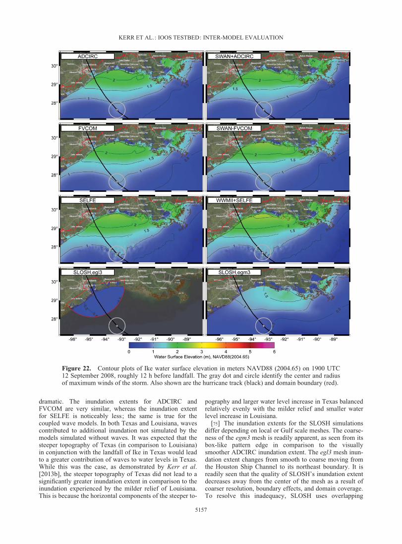
dramatic. The inundation extents for ADCIRC andFVCOM are very similar, whereas the inundation extentfor SELFE is noticeably less; the same is true for thecoupled wave models. In both Texas and Louisiana, wavescontributed to additional inundation not simulated by themodels simulated without waves. It was expected that thesteeper topography of Texas (in comparison to Louisiana)in conjunction with the landfall of Ike in Texas would leadto a greater contribution of waves to water levels in Texas.While this was the case, as demonstrated by Kerr et al.[2013b], the steeper topography of Texas did not lead to asignificantly greater inundation extent in comparison to theinundation experienced by the milder relief of Louisiana.This is because the horizontal components of the steeper to-

pography and larger water level increase in Texas balancedrelatively evenly with the milder relief and smaller waterlevel increase in Louisiana.

[75] The inundation extents for the SLOSH simulationsdiffer depending on local or Gulf scale meshes. The coarse-ness of the egm3 mesh is readily apparent, as seen from itsbox-like pattern edge in comparison to the visuallysmoother ADCIRC inundation extent. The egl3 mesh inun-dation extent changes from smooth to coarse moving fromthe Houston Ship Channel to its northeast boundary. It isreadily seen that the quality of SLOSH’s inundation extentdecreases away from the center of the mesh as a result ofcoarser resolution, boundary effects, and domain coverage.To resolve this inadequacy, SLOSH uses overlapping

Figure 22. Contour plots of Ike water surface elevation in meters NAVD88 (2004.65) on 1900 UTC12 September 2008, roughly 12 h before landfall. The gray dot and circle identify the center and radiusof maximum winds of the storm. Also shown are the hurricane track (black) and domain boundary (red).

KERR ET AL.: IOOS TESTBED: INTER-MODEL EVALUATION

5157

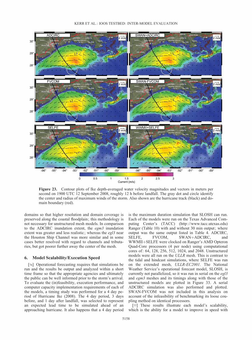
domains so that higher resolution and domain coverage ispreserved along the coastal floodplain; this methodology isnot necessary for unstructured mesh models. In comparisonto the ADCIRC inundation extent, the egm3 inundationextent was greater and less realistic ; whereas the egl3 nearthe Houston Ship Channel was more similar and in somecases better resolved with regard to channels and tributa-ries, but got poorer further away the center of the mesh.

6. Model Scalability/Execution Speed

[76] Operational forecasting requires that simulations berun and the results be output and analyzed within a shorttime frame so that the appropriate agencies and ultimatelythe public can be well informed prior to the storm’s arrival.To evaluate the (in)feasibility, execution performance, andcomputer capacity implementation requirements of each ofthe models, a timing study was performed for a 4 day pe-riod of Hurricane Ike (2008). The 4 day period, 3 daysbefore, and 1 day after landfall, was selected to representan expected lead time to be simulated ahead of anapproaching hurricane. It also happens that a 4 day period

is the maximum duration simulation that SLOSH can run.Each of the models were run on the Texas Advanced Com-puting Center’s (TACC) (http://www.tacc.utexas.edu)Ranger (Table 10) with and without 30 min output; whereoutput was the same output listed in Table 4. ADCIRC,SELFE, FVCOM, SWANþADCIRC, andWWMIIþSELFE were clocked on Ranger’s AMD OpteronQuad-Core processors (4 per node) using computationalcores of: 64, 128, 256, 512, 1024, and 2048. Unstructuredmodels were all run on the ULLR mesh. This is contrast tothe tidal and hindcast simulations, where SELFE was runon the extended mesh, ULLR-EC2001. The NationalWeather Service’s operational forecast model, SLOSH, iscurrently not parallelized, so it was run in serial on the egl3and egm3 meshes and its timings along with those of theunstructured models are plotted in Figure 33. A serialADCIRC simulation was also performed and plotted.SWAN-FVCOM was not included in this analysis onaccount of the infeasibility of benchmarking its loose cou-pling method on identical processors.

[77] These results illustrate each model’s scalability,which is the ability for a model to improve in speed with

Figure 23. Contour plots of Ike depth-averaged water velocity magnitudes and vectors in meters persecond on 1900 UTC 12 September 2008, roughly 12 h before landfall. The gray dot and circle identifythe center and radius of maximum winds of the storm. Also shown are the hurricane track (black) and do-main boundary (red).

KERR ET AL.: IOOS TESTBED: INTER-MODEL EVALUATION

5158

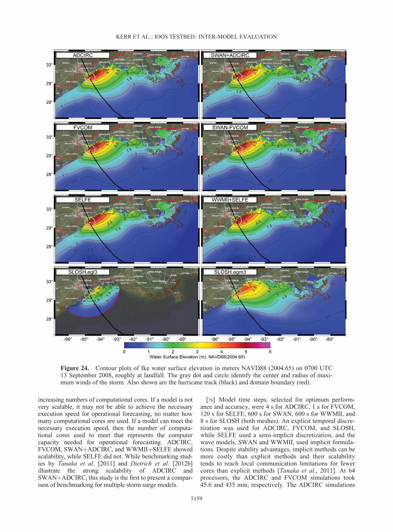
increasing numbers of computational cores. If a model is notvery scalable, it may not be able to achieve the necessaryexecution speed for operational forecasting, no matter howmany computational cores are used. If a model can meet thenecessary execution speed, then the number of computa-tional cores used to meet that represents the computercapacity needed for operational forecasting. ADCIRC,FVCOM, SWANþADCIRC, and WWMIIþSELFE showedscalability, while SELFE did not. While benchmarking stud-ies by Tanaka et al. [2011] and Dietrich et al. [2012b]illustrate the strong scalability of ADCIRC andSWANþADCIRC, this study is the first to present a compar-ison of benchmarking for multiple storm surge models.

[78] Model time steps, selected for optimum perform-ance and accuracy, were 4 s for ADCIRC, 1 s for FVCOM,120 s for SELFE, 600 s for SWAN, 600 s for WWMII, and8 s for SLOSH (both meshes). An explicit temporal discre-tization was used for ADCIRC, FVCOM, and SLOSH,while SELFE used a semi-implicit discretization, and thewave models, SWAN and WWMII, used implicit formula-tions. Despite stability advantages, implicit methods can bemore costly than explicit methods and their scalabilitytends to reach local communication limitations for fewercores than explicit methods [Tanaka et al., 2011]. At 64processors, the ADCIRC and FVCOM simulations took45.6 and 435 min, respectively. The ADCIRC simulations

Figure 24. Contour plots of Ike water surface elevation in meters NAVD88 (2004.65) on 0700 UTC13 September 2008, roughly at landfall. The gray dot and circle identify the center and radius of maxi-mum winds of the storm. Also shown are the hurricane track (black) and domain boundary (red).

KERR ET AL.: IOOS TESTBED: INTER-MODEL EVALUATION

5159

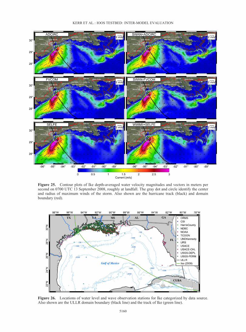
Figure 25. Contour plots of Ike depth-averaged water velocity magnitudes and vectors in meters persecond on 0700 UTC 13 September 2008, roughly at landfall. The gray dot and circle identify the centerand radius of maximum winds of the storm. Also shown are the hurricane track (black) and domainboundary (red).

Figure 26. Locations of water level and wave observation stations for Ike categorized by data source.Also shown are the ULLR domain boundary (black line) and the track of Ike (green line).

KERR ET AL.: IOOS TESTBED: INTER-MODEL EVALUATION

5160

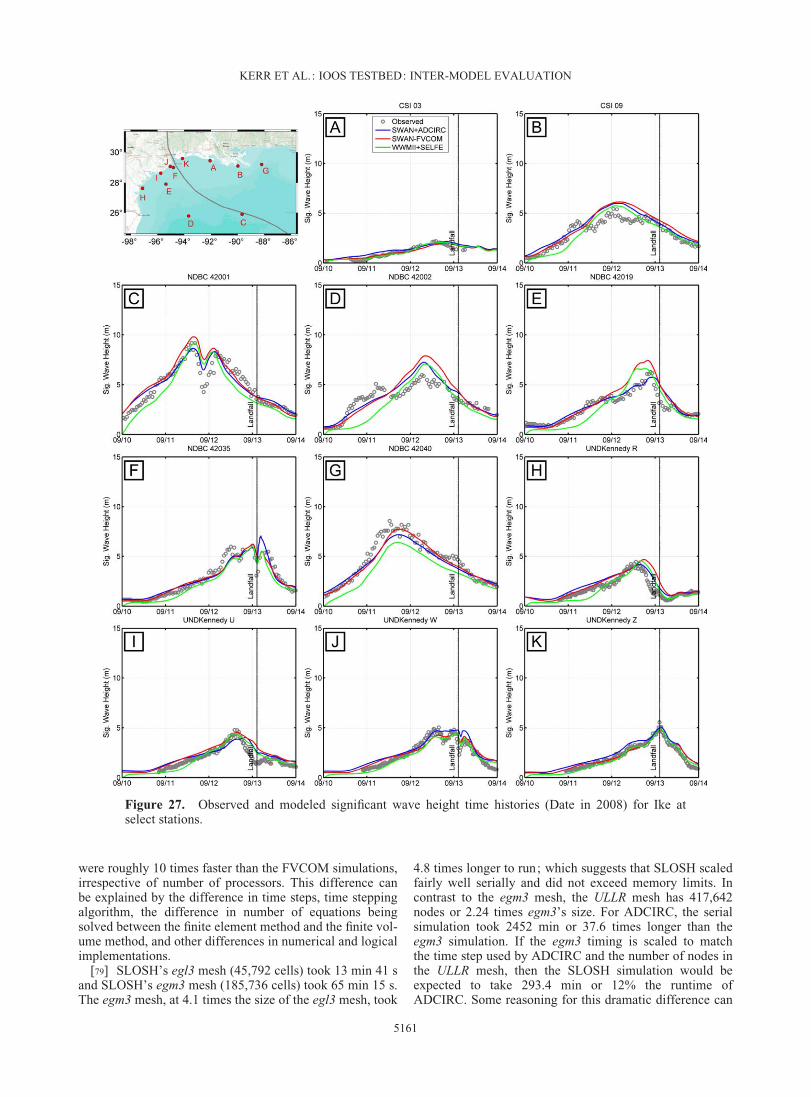
were roughly 10 times faster than the FVCOM simulations,irrespective of number of processors. This difference canbe explained by the difference in time steps, time steppingalgorithm, the difference in number of equations beingsolved between the finite element method and the finite vol-ume method, and other differences in numerical and logicalimplementations.

[79] SLOSH’s egl3 mesh (45,792 cells) took 13 min 41 sand SLOSH’s egm3 mesh (185,736 cells) took 65 min 15 s.The egm3 mesh, at 4.1 times the size of the egl3 mesh, took

4.8 times longer to run; which suggests that SLOSH scaledfairly well serially and did not exceed memory limits. Incontrast to the egm3 mesh, the ULLR mesh has 417,642nodes or 2.24 times egm3’s size. For ADCIRC, the serialsimulation took 2452 min or 37.6 times longer than theegm3 simulation. If the egm3 timing is scaled to matchthe time step used by ADCIRC and the number of nodes inthe ULLR mesh, then the SLOSH simulation would beexpected to take 293.4 min or 12% the runtime ofADCIRC. Some reasoning for this dramatic difference can

Figure 27. Observed and modeled significant wave height time histories (Date in 2008) for Ike atselect stations.

KERR ET AL.: IOOS TESTBED: INTER-MODEL EVALUATION

5161

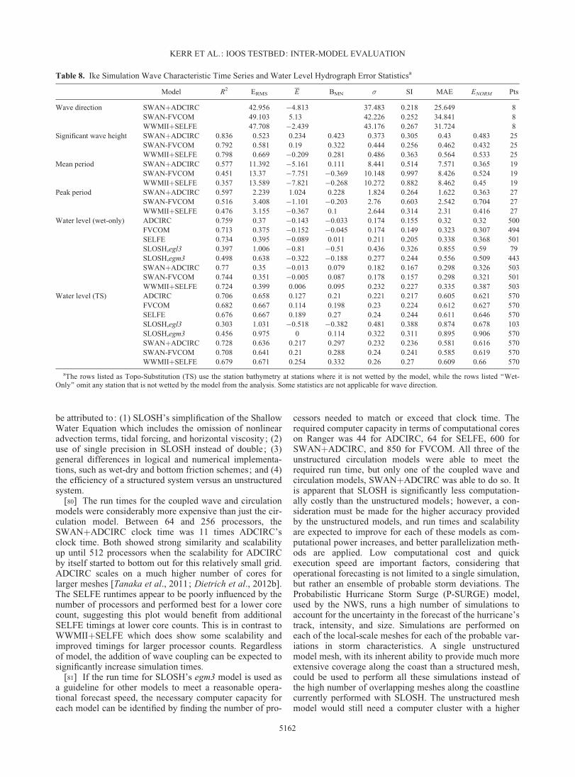
be attributed to: (1) SLOSH’s simplification of the ShallowWater Equation which includes the omission of nonlinearadvection terms, tidal forcing, and horizontal viscosity; (2)use of single precision in SLOSH instead of double; (3)general differences in logical and numerical implementa-tions, such as wet-dry and bottom friction schemes; and (4)the efficiency of a structured system versus an unstructuredsystem.

[80] The run times for the coupled wave and circulationmodels were considerably more expensive than just the cir-culation model. Between 64 and 256 processors, theSWANþADCIRC clock time was 11 times ADCIRC’sclock time. Both showed strong similarity and scalabilityup until 512 processors when the scalability for ADCIRCby itself started to bottom out for this relatively small grid.ADCIRC scales on a much higher number of cores forlarger meshes [Tanaka et al., 2011; Dietrich et al., 2012b].The SELFE runtimes appear to be poorly influenced by thenumber of processors and performed best for a lower corecount, suggesting this plot would benefit from additionalSELFE timings at lower core counts. This is in contrast toWWMIIþSELFE which does show some scalability andimproved timings for larger processor counts. Regardlessof model, the addition of wave coupling can be expected tosignificantly increase simulation times.

[81] If the run time for SLOSH’s egm3 model is used asa guideline for other models to meet a reasonable opera-tional forecast speed, the necessary computer capacity foreach model can be identified by finding the number of pro-

cessors needed to match or exceed that clock time. Therequired computer capacity in terms of computational coreson Ranger was 44 for ADCIRC, 64 for SELFE, 600 forSWANþADCIRC, and 850 for FVCOM. All three of theunstructured circulation models were able to meet therequired run time, but only one of the coupled wave andcirculation models, SWANþADCIRC was able to do so. Itis apparent that SLOSH is significantly less computation-ally costly than the unstructured models; however, a con-sideration must be made for the higher accuracy providedby the unstructured models, and run times and scalabilityare expected to improve for each of these models as com-putational power increases, and better parallelization meth-ods are applied. Low computational cost and quickexecution speed are important factors, considering thatoperational forecasting is not limited to a single simulation,but rather an ensemble of probable storm deviations. TheProbabilistic Hurricane Storm Surge (P-SURGE) model,used by the NWS, runs a high number of simulations toaccount for the uncertainty in the forecast of the hurricane’strack, intensity, and size. Simulations are performed oneach of the local-scale meshes for each of the probable var-iations in storm characteristics. A single unstructuredmodel mesh, with its inherent ability to provide much moreextensive coverage along the coast than a structured mesh,could be used to perform all these simulations instead ofthe high number of overlapping meshes along the coastlinecurrently performed with SLOSH. The unstructured meshmodel would still need a computer cluster with a higher

Table 8. Ike Simulation Wave Characteristic Time Series and Water Level Hydrograph Error Statisticsa

Model R2 ERMS E BMN � SI MAE ENORM Pts

Wave direction SWANþADCIRC 42.956 �4.813 37.483 0.218 25.649 8SWAN-FVCOM 49.103 5.13 42.226 0.252 34.841 8WWMIIþSELFE 47.708 �2.439 43.176 0.267 31.724 8

Significant wave height SWANþADCIRC 0.836 0.523 0.234 0.423 0.373 0.305 0.43 0.483 25SWAN-FVCOM 0.792 0.581 0.19 0.322 0.444 0.256 0.462 0.432 25WWMIIþSELFE 0.798 0.669 �0.209 0.281 0.486 0.363 0.564 0.533 25

Mean period SWANþADCIRC 0.577 11.392 �5.161 0.111 8.441 0.514 7.571 0.365 19SWAN-FVCOM 0.451 13.37 �7.751 �0.369 10.148 0.997 8.426 0.524 19WWMIIþSELFE 0.357 13.589 �7.821 �0.268 10.272 0.882 8.462 0.45 19

Peak period SWANþADCIRC 0.597 2.239 1.024 0.228 1.824 0.264 1.622 0.363 27SWAN-FVCOM 0.516 3.408 �1.101 �0.203 2.76 0.603 2.542 0.704 27WWMIIþSELFE 0.476 3.155 �0.367 0.1 2.644 0.314 2.31 0.416 27

Water level (wet-only) ADCIRC 0.759 0.37 �0.143 �0.033 0.174 0.155 0.32 0.32 500FVCOM 0.713 0.375 �0.152 �0.045 0.174 0.149 0.323 0.307 494SELFE 0.734 0.395 �0.089 0.011 0.211 0.205 0.338 0.368 501SLOSH,egl3 0.397 1.006 �0.81 �0.51 0.436 0.326 0.855 0.59 79SLOSH,egm3 0.498 0.638 �0.322 �0.188 0.277 0.244 0.556 0.509 443SWANþADCIRC 0.77 0.35 �0.013 0.079 0.182 0.167 0.298 0.326 503SWAN-FVCOM 0.744 0.351 �0.005 0.087 0.178 0.157 0.298 0.321 501WWMIIþSELFE 0.724 0.399 0.006 0.095 0.232 0.227 0.335 0.387 503

Water level (TS) ADCIRC 0.706 0.658 0.127 0.21 0.221 0.217 0.605 0.621 570FVCOM 0.682 0.667 0.114 0.198 0.23 0.224 0.612 0.627 570SELFE 0.676 0.667 0.189 0.27 0.24 0.244 0.611 0.646 570SLOSH,egl3 0.303 1.031 �0.518 �0.382 0.481 0.388 0.874 0.678 103SLOSH,egm3 0.456 0.975 0 0.114 0.322 0.311 0.895 0.906 570SWANþADCIRC 0.728 0.636 0.217 0.297 0.232 0.236 0.581 0.616 570SWAN-FVCOM 0.708 0.641 0.21 0.288 0.24 0.241 0.585 0.619 570WWMIIþSELFE 0.679 0.671 0.254 0.332 0.26 0.27 0.609 0.66 570

aThe rows listed as Topo-Substitution (TS) use the station bathymetry at stations where it is not wetted by the model, while the rows listed ‘‘Wet-Only’’ omit any station that is not wetted by the model from the analysis. Some statistics are not applicable for wave direction.

KERR ET AL.: IOOS TESTBED: INTER-MODEL EVALUATION

5162

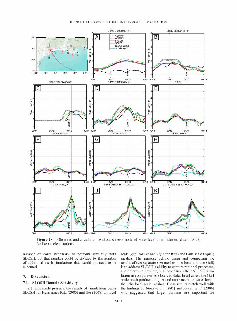
number of cores necessary to perform similarly withSLOSH, but that number could be divided by the numberof additional mesh simulations that would not need to beexecuted.

7. Discussion

7.1. SLOSH Domain Sensitivity

[82] This study presents the results of simulations usingSLOSH for Hurricanes Rita (2005) and Ike (2008) on local

scale (egl3 for Ike and ebp3 for Rita) and Gulf scale (egm3)meshes. The purpose behind using and comparing theresults of two separate size meshes, one local and one Gulf,is to address SLOSH’s ability to capture regional processes,and determine how regional processes affect SLOSH’s so-lution in comparison to observed data. In all cases, the Gulfscale mesh produced higher and more accurate water levelsthan the local-scale meshes. These results match well withthe findings by Blain et al. [1994] and Morey et al. [2006]who suggested that larger domains are important for

Figure 28. Observed and circulation (without waves) modeled water level time histories (date in 2008)for Ike at select stations.

KERR ET AL.: IOOS TESTBED: INTER-MODEL EVALUATION

5163

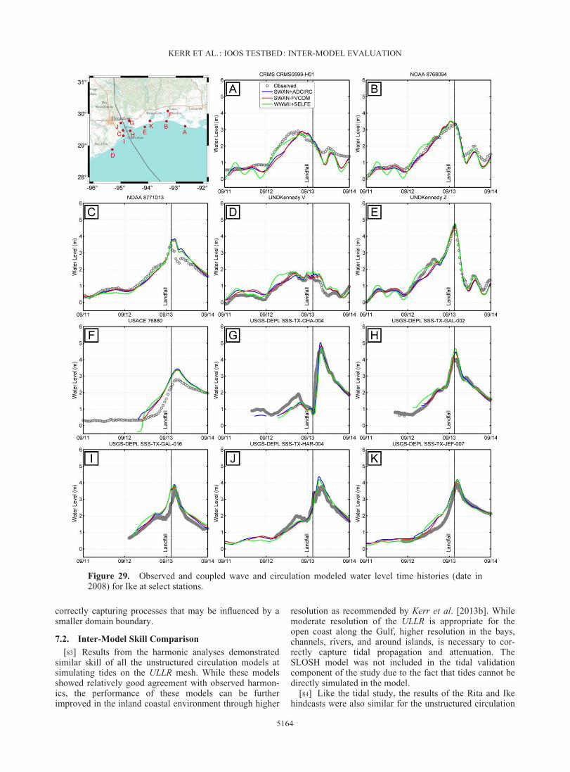
correctly capturing processes that may be influenced by asmaller domain boundary.

7.2. Inter-Model Skill Comparison

[83] Results from the harmonic analyses demonstratedsimilar skill of all the unstructured circulation models atsimulating tides on the ULLR mesh. While these modelsshowed relatively good agreement with observed harmon-ics, the performance of these models can be furtherimproved in the inland coastal environment through higher

resolution as recommended by Kerr et al. [2013b]. Whilemoderate resolution of the ULLR is appropriate for theopen coast along the Gulf, higher resolution in the bays,channels, rivers, and around islands, is necessary to cor-rectly capture tidal propagation and attenuation. TheSLOSH model was not included in the tidal validationcomponent of the study due to the fact that tides cannot bedirectly simulated in the model.

[84] Like the tidal study, the results of the Rita and Ikehindcasts were also similar for the unstructured circulation

Figure 29. Observed and coupled wave and circulation modeled water level time histories (date in2008) for Ike at select stations.

KERR ET AL.: IOOS TESTBED: INTER-MODEL EVALUATION

5164

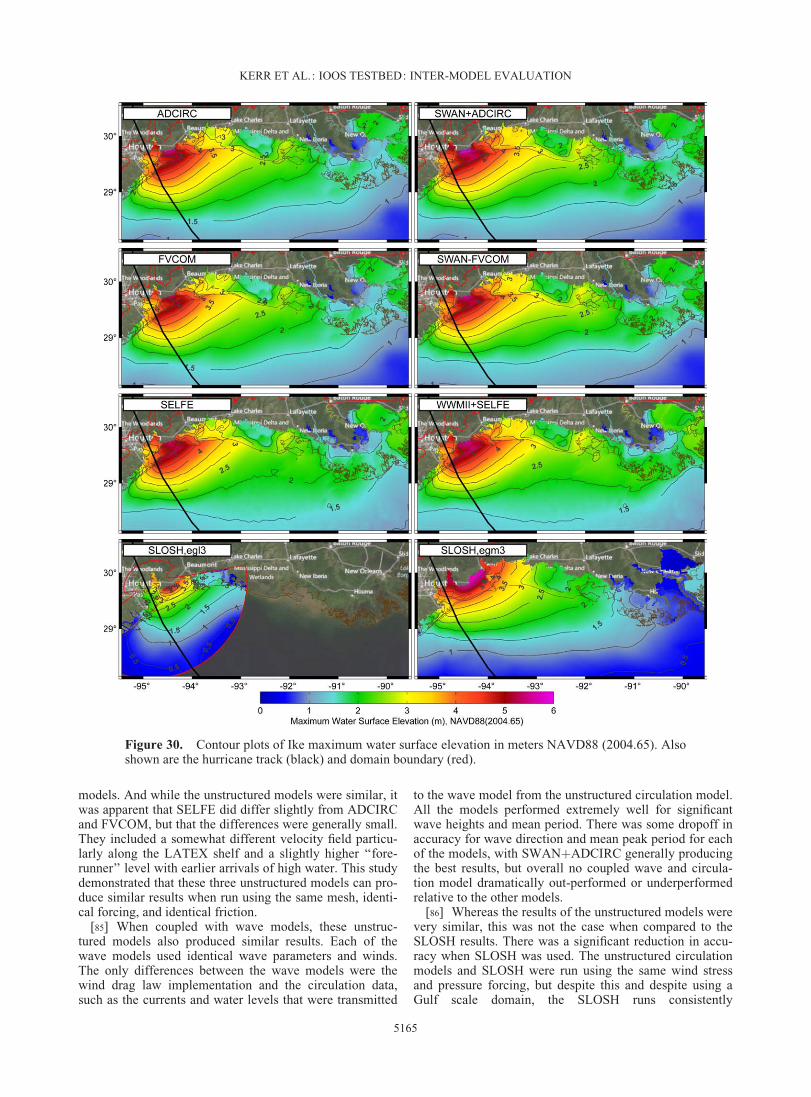
models. And while the unstructured models were similar, itwas apparent that SELFE did differ slightly from ADCIRCand FVCOM, but that the differences were generally small.They included a somewhat different velocity field particu-larly along the LATEX shelf and a slightly higher ‘‘fore-runner’’ level with earlier arrivals of high water. This studydemonstrated that these three unstructured models can pro-duce similar results when run using the same mesh, identi-cal forcing, and identical friction.

[85] When coupled with wave models, these unstruc-tured models also produced similar results. Each of thewave models used identical wave parameters and winds.The only differences between the wave models were thewind drag law implementation and the circulation data,such as the currents and water levels that were transmitted

to the wave model from the unstructured circulation model.All the models performed extremely well for significantwave heights and mean period. There was some dropoff inaccuracy for wave direction and mean peak period for eachof the models, with SWANþADCIRC generally producingthe best results, but overall no coupled wave and circula-tion model dramatically out-performed or underperformedrelative to the other models.

[86] Whereas the results of the unstructured models werevery similar, this was not the case when compared to theSLOSH results. There was a significant reduction in accu-racy when SLOSH was used. The unstructured circulationmodels and SLOSH were run using the same wind stressand pressure forcing, but despite this and despite using aGulf scale domain, the SLOSH runs consistently

Figure 30. Contour plots of Ike maximum water surface elevation in meters NAVD88 (2004.65). Alsoshown are the hurricane track (black) and domain boundary (red).

KERR ET AL.: IOOS TESTBED: INTER-MODEL EVALUATION

5165

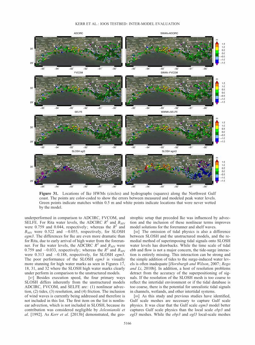
underperformed in comparison to ADCIRC, FVCOM, andSELFE. For Rita water levels, the ADCIRC R2 and BMN

were 0.759 and 0.044, respectively; whereas the R2 andBMN were 0.522 and �0.055, respectively, for SLOSHegm3. The differences for Ike are even more dramatic thanfor Rita, due to early arrival of high water from the forerun-ner. For Ike water levels, the ADCIRC R2 and BMN were0.759 and �0.033, respectively; whereas the R2 and BMN

were 0.313 and �0.188, respectively, for SLOSH egm3.The poor performance of the SLOSH egm3 is visuallymore stunning for high water marks as seen in Figures 17,18, 31, and 32 where the SLOSH high water marks clearlyunder perform in comparison to the unstructured models.

[87] Besides execution speed, the four primary waysSLOSH differs inherently from the unstructured modelsADCIRC, FVCOM, and SELFE are: (1) nonlinear advec-tion, (2) tides, (3) resolution, and (4) friction. The inclusionof wind waves is currently being addressed and therefore isnot included in this list. The first item on the list is nonlin-ear advection, which is not included in SLOSH, because itscontribution was considered negligible by Jelesnianski etal. [1992]. As Kerr et al. [2013b] demonstrated, the geo-

strophic setup that preceded Ike was influenced by advec-tion and the inclusion of these nonlinear terms improvesmodel solutions for the forerunner and shelf waves.

[88] The omission of tidal physics is also a differencebetween SLOSH and the unstructured models, and the re-medial method of superimposing tidal signals onto SLOSHwater levels has drawbacks. While the time scale of tidalebb and flow is not a major concern, the tide-surge interac-tion is entirely missing. This interaction can be strong andthe simple addition of tides to the surge-induced water lev-els is often inadequate [Horsburgh and Wilson, 2007; Regoand Li, 2010b]. In addition, a host of resolution problemsdetract from the accuracy of the superpositioning of sig-nals. If the resolution of the SLOSH mesh is too coarse toreflect the intertidal environment or if the tidal database istoo coarse, there is the potential for unrealistic tidal signalsin channels, wetlands, and other intertidal systems.

[89] As this study and previous studies have identified,Gulf scale meshes are necessary to capture Gulf scalephysics. It was clear that the Gulf scale egm3 model bettercaptures Gulf scale physics than the local scale ebp3 andegl3 meshes. While the ebp3 and egl3 local-scale meshes

Figure 31. Locations of Ike HWMs (circles) and hydrographs (squares) along the Northwest Gulfcoast. The points are color-coded to show the errors between measured and modeled peak water levels.Green points indicate matches within 0.5 m and white points indicate locations that were never wettedby the model.

KERR ET AL.: IOOS TESTBED: INTER-MODEL EVALUATION

5166

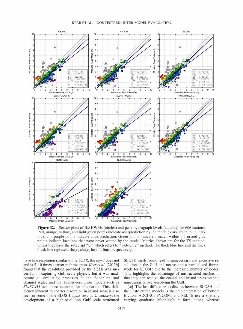
have fine resolution similar to the ULLR, the egm3 does notand is 5–10 times coarser in these areas. Kerr et al. [2013b]found that the resolution provided by the ULLR was suc-cessful in capturing Gulf scale physics, but it was inad-equate at simulating processes at the floodplain andchannel scale; and that higher-resolution models such asSL18TX33 are more accurate for inundation. This defi-ciency inherent to coarser resolution in inland areas is alsoseen in some of the SLOSH egm3 results. Ultimately, thedevelopment of a high-resolution Gulf scale structured

SLOSH mesh would lead to unnecessary and excessive re-solution in the Gulf and necessitate a parallelized frame-work for SLOSH due to the increased number of nodes.This highlights the advantage of unstructured meshes inthat they can resolve the coastal and inland areas withoutunnecessarily over-resolving the Gulf.

[90] The last difference to discuss between SLOSH andthe unstructured models is the implementation of bottomfriction. ADCIRC, FVCOM, and SELFE use a spatiallyvarying quadratic Manning’s n formulation; whereas

Figure 32. Scatter plots of Ike HWMs (circles) and peak hydrograph levels (squares) for 606 stations.Red, orange, yellow, and light green points indicate overprediction by the model; dark green, blue, darkblue, and purple points indicate underprediction. Green points indicate a match within 0.5 m and graypoints indicate locations that were never wetted by the model. Metrics shown are for the TS method,unless they have the subscript ‘‘C’’ which refers to ‘‘wet-Only’’ method. The thick blue line and the thickblack line represent the y1 and y0 best fit lines, respectively.

KERR ET AL.: IOOS TESTBED: INTER-MODEL EVALUATION

5167

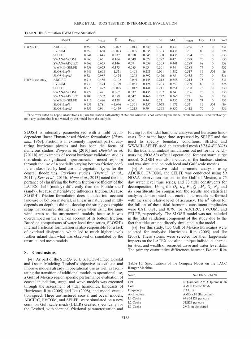
SLOSH is internally parameterized with a mild depth-dependent linear Ekman-based friction formulation [Platz-man, 1963]. Friction is an extremely important part of cap-turing hurricane physics and has been the focus ofnumerous studies. Bunya et al. [2010] and Dietrich et al.[2011b] are examples of recent hurricane validation studiesthat identified significant improvements in model responsethrough the use of a spatially varying bottom friction coef-ficient classified by land-use and vegetation types for thecoastal floodplains. Previous studies [Dietrich et al.,2011b; Kerr et al., 2013b; Hope et al., 2013] noted the im-portance of classifying the bottom friction coefficient of theLATEX shelf (muddy) differently than the Florida shelf(sandy), because material-type influences friction. BecauseSLOSH’s friction formulation does not take into accountland-use or bottom material, is linear in nature, and mildlydepends on depth, it did not develop the strong geostrophicsetup that occurred during Ike, even when using the samewind stress as the unstructured models, because it wasoverdamped on the shelf on account of its bottom friction.Based on comparisons of water level time series, SLOSH’sinternal frictional formulation is also responsible for a lackof overland dissipation, which led to much higher levelsfurther inland than what was observed or simulated by theunstructured mesh models.

8. Conclusions

[91] As part of the SURA-led U.S. IOOS-funded Coastaland Ocean Modeling Testbed’s objective to evaluate andimprove models already in operational use as well as facili-tating the transition of additional models to operational use,a Gulf of Mexico region specific performance evaluation ofcoastal inundation, surge, and wave models was executedthrough the assessment of tidal harmonics, hindcasts ofHurricanes Rita (2005) and Ike (2008), and model execu-tion speed. Three unstructured coastal and ocean models,ADCIRC, FVCOM, and SELFE, were simulated on a newcommon Gulf scale mesh (ULLR) created specifically forthe Testbed, with identical frictional parameterization and

forcing for the tidal harmonic analyses and hurricane hind-casts. Due to the large time steps used by SELFE and theneed to specify boundary conditions, SELFE andWWMIIþSELFE used an extended mesh (ULLR-EC2001)for the tidal and hindcast simulations but not for the bench-marking. NOAA’s official operational forecast storm surgemodel, SLOSH was also included in the hindcast studiesand was simulated on both local and Gulf scale meshes.

[92] A comparative tidal harmonic analysis usingADCIRC, FVCOM, and SELFE was conducted using 59NOAA observation stations in the Gulf of Mexico, a 75day water level time series, and 38 tidal constituents fordecomposition. Using the O1, K1, P1, Q1, M2, S2, N2, andK2 constituents for comparison, the results and statisticalanalyses demonstrated that each of the models performedwith the same relative level of accuracy. The R2 values forthe full set of these tidal harmonic constituent amplitudeswere 0.81, 0.81, and 0.79, for ADCIRC, FVCOM, andSELFE, respectively. The SLOSH model was not includedin the tidal validation component of the study due to thefact that tides are not directly simulated in the model.

[93] For this study, two Gulf of Mexico hurricanes wereselected for analysis: Hurricanes Rita (2005) and Ike(2008). These storms were selected for their large-scaleimpacts on the LATEX coastline, unique individual charac-teristics, and wealth of recorded wave and water level data.The primary quantitative differences between Ike and Rita

Table 9. Ike Simulation HWM Error Statisticsa

Model R2 ERMS E BMN � SI MAE ENORM Dry Out Wet

HWM (TS) ADCIRC 0.553 0.649 �0.027 �0.013 0.649 0.31 0.439 0.286 75 0 531FVCOM 0.55 0.638 �0.073 �0.035 0.635 0.303 0.436 0.281 80 0 526SELFE 0.541 0.645 0.037 0.018 0.645 0.308 0.435 0.284 76 0 530SWAN-FVCOM 0.567 0.63 0.104 0.049 0.622 0.297 0.42 0.278 76 0 530SWANþADCIRC 0.568 0.655 0.146 0.07 0.639 0.305 0.441 0.289 68 0 538WWMIIþSELFE 0.558 0.653 0.173 0.083 0.63 0.301 0.44 0.288 74 0 532SLOSH,egl3 0.646 1.698 �1.551 �0.498 0.283 0.091 1.582 0.517 16 504 86SLOSH,egm3 0.52 0.987 �0.424 �0.203 0.892 0.426 0.85 0.435 70 0 536

HWM (wet-only) ADCIRC 0.716 0.486 �0.102 �0.049 0.445 0.212 0.358 0.214 75 0 531FVCOM 0.73 0.474 �0.129 �0.061 0.426 0.203 0.353 0.209 80 0 526SELFE 0.715 0.472 �0.025 �0.012 0.441 0.211 0.351 0.208 76 0 530SWAN-FVCOM 0.722 0.47 0.067 0.032 0.435 0.207 0.34 0.206 76 0 530SWANþADCIRC 0.703 0.502 0.089 0.042 0.466 0.222 0.365 0.221 68 0 538WWMIIþSELFE 0.716 0.486 0.128 0.061 0.44 0.21 0.357 0.215 74 0 532SLOSH,egl3 0.651 1.781 �1.646 �0.501 0.257 0.078 1.673 0.52 16 504 86SLOSH,egm3 0.555 0.961 �0.459 �0.213 0.794 0.368 0.837 0.412 70 0 536

aThe rows listed as Topo-Substitution (TS) use the station bathymetry at stations where it is not wetted by the model, while the rows listed ‘‘wet-only’’omit any station that is not wetted by the model from the analysis.

Table 10. Specifications of the Compute Nodes on the TACCRanger Machine

Node Sun Blade �6420

CPU 4 Quad-core AMD Opteron 8356Core AMD Opteron 8356Frequency 2.3 GHzArchitecture AMD K10 (Barcelona)L1-Cache 64þ64 KB per coreL2-Cache 512KB per coreL3-Cache 2MB on die shared

KERR ET AL.: IOOS TESTBED: INTER-MODEL EVALUATION

5168

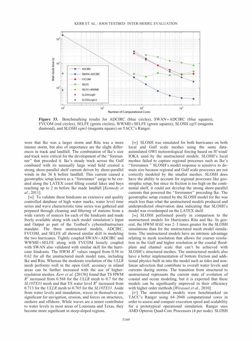
were that Ike was a larger storm and Rita was a moreintense storm, but also of importance are the slight differ-ences in track and landfall. The combination of Ike’s sizeand track were critical for the development of the ‘‘forerun-ner’’ that preceded it. Ike’s steady track across the Gulfcombined with its unusually large wind field created astrong shore-parallel shelf current driven by shore-parallelwinds in the 36 h before landfall. This current caused ageostrophic setup known as a ‘‘forerunner’’ surge to be cre-ated along the LATEX coast filling coastal lakes and baysreaching up to 2 m before Ike made landfall [Kennedy etal., 2011].

[94] To validate these hindcasts an extensive and qualitycontrolled database of high water marks, water level timeseries and wave characteristic time series was gathered andprepared through cleaning and filtering of stations from awide variety of sources for each of the hindcasts and madefreely available along with each model simulation’s Inputand Output as part of the Testbed’s cyberinfrastructuremandate. The three unstructured models, ADCIRC,FVCOM, and SELFE all showed similar skill in modelingthe two hurricanes. Tightly coupled SWANþADCIRC andWWMIIþSELFE along with FVCOM loosely coupledwith SWAN also validated with similar skill for the hurri-cane hindcasts. The HWM R2 values ranged from 0.56 to0.62 for all the unstructured mesh model runs, includingIke and Rita. Whereas the moderate resolution of the ULLRmesh performs well in the open Gulf, accuracy in inlandareas can be further increased with the use of higher-resolution meshes. Kerr et al. [2013b] found that TS HWMR2 increased from 0.568 for the ULLR mesh to 0.7 for theSL18TX33 mesh and that TS water level R2 increased from0.713 for the ULLR mesh to 0.765 for the SL18TX33. Asidefrom water levels and inundation, waves in themselves aresignificant for navigation, erosion, and forces on structures,onshore and offshore. While waves are a minor contributorto water levels in most areas of Louisiana and Texas, theybecome more significant in steep-sloped regions.

[95] SLOSH was simulated for both hurricanes on bothlocal and Gulf scale meshes using the same data-assimilated OWI meteorological forcing based on H�wind/IOKA used by the unstructured models. SLOSH’s localmeshes failed to capture regional processes such as Ike’s‘‘forerunner.’’ SLOSH’s model response is sensitive to do-main size because regional and Gulf scale processes are notcorrectly modeled by the smaller meshes. SLOSH doeshave the ability to account for regional processes like geo-strophic setup, but since its friction is too high on the conti-nental shelf, it could not develop the strong shore-parallelcurrents that powered the ‘‘forerunner’’ preceding Ike. Thegeostrophic setup created by the SLOSH model for Ike wasmuch less than what the unstructured models produced andunderpredicted observation data indicating that SLOSH’smodel was overdamped on the LATEX shelf.

[96] SLOSH performed poorly in comparison to theunstructured models for Hurricanes Rita and Ike. In gen-eral, the HWM MAE was 2–3 times greater for the SLOSHsimulations than for the unstructured mesh model simula-tions. The unstructured models have an intrinsic advantagerelating to mesh resolution that allows for coarser resolu-tion in the Gulf and higher resolution at the coastal flood-plain and channel scale that can’t be achieved withSLOSH’s structured meshes. The unstructured models alsohave a better implementation of bottom friction and addi-tional physics built in into the model such as tides and non-linear advection that contribute to overall water levels andcurrents during storms. The transition from structured tounstructured represents the current state of evolution ofcoastal and ocean modeling, but it is expected that thesemodels can be significantly improved in their efficiencywith higher order methods [Wirasaet et al., 2010].

[97] The unstructured models were benchmarked onTACC’s Ranger using 64–2048 computational cores inorder to assess and compare execution speed and scalabilityfor a prototypical operational simulation. Ranger usesAMD Opteron Quad-Core Processors (4 per node). SLOSH

Figure 33. Benchmarking results for ADCIRC (blue circles), SWANþADCIRC (blue squares),FVCOM (red circles), SELFE (green circles), WWMIIþSELFE (green squares), SLOSH egl3 (magentadiamond), and SLOSH egm3 (magenta square) on TACC’s Ranger.

KERR ET AL.: IOOS TESTBED: INTER-MODEL EVALUATION

5169

in its serial framework was also benchmarked and used torepresent the speed necessary for the unstructured modelsto meet operational implementation requirements. Each ofthe unstructured models was capable of matching or beat-ing the timing of the SLOSH egm3 simulation, but a highernumber of computational cores are needed in comparisonto the single core used by SLOSH. It was also apparent thatSELFE was not scalable and that it could benefit fromeffective parallelization. The coupling of wave models tostorm surge models does significantly increase timings andcomputational cost. For example, in order for ADCIRC andSWANþADCIRC to meet the same timing as SLOSH onRanger, they would require 44 and 600 cores, respectively.While SLOSH is significantly less computationally costlythan the unstructured models, the unstructured mesh mod-els deliver a significantly higher accuracy in water leveland inundation. Run times and scalability are expected toimprove for each of these models as computational powerincreases and more efficient high-order algorithms and par-allelization methods are developed and applied.

[98] Acknowledgments. This project was supported by NOAAvia the U.S. IOOS Office (award: NA10NOS0120063 andNA11NOS0120141) and was managed by the Southeastern UniversitiesResearch Association. In addition, this work used the Extreme Science andEngineering Discovery Environment (XSEDE), which is supported byNational Science Foundation grant OCI-1053575.

ReferencesAtkinson, J., J. Westerink, and R. Luettich Jr. (2004a), Two-dimensional

dispersion analyses of finite element approximations to the shallow waterequations, Int. J. Numer. Methods Fluids, 45(7), 715–749.

Atkinson, J., J. Westerink, and J. Hervouet (2004b), Similarities betweenthe quasi-bubble and the generalized wave continuity equation solutionsto the shallow water equations, Int. J. Numer. Methods Fluids, 45(7),689–714.

Battjes, J., and J. Janssen (1978), Energy loss and setup due to breaking ofrandom waves, paper presented at the 16th International Conference onCoastal Engineering, Hamburg, Germany.

Battjes, J., and M. Stive (1985), Calibration and verification of a dissipationmodel for random breaking waves, J. Geophys. Res., 90(C5), 9159–9167.

Bertin, X., A. Oliveira, and A. B. Fortunato (2009), Simulating morphody-namics with unstructured grids: Description and validation of a model-ing system for coastal applications, Ocean Modell., 28(1), 75–87.

Bertin, X., N. Bruneau, J.-F. Breilh, A. B. Fortunato, and M. Karpytchev(2012), Importance of wave age and resonance in storm surges: The caseXynthia, Bay of Biscay, Ocean Modell., 42, 16–30, doi:10.1016/j.ocemod.2011.11.001.

Blain, C., J. Westerink, and R. Luettich Jr. (1994), The influence of domainsize on the response characteristics of a hurricane storm surge model, J.Geophys. Res., 99(C9), 18,467–18,479.

Booij, N., R. Ris, and L. Holthuijsen (1999), A third-generation wavemodel for coastal regions: 1. Model description and validation, J. Geo-phys. Res., 104(C4), 7649–7666.

Brovchenko, I., V. Maderich, and K. Terletska (2011), Numerical simula-tions of 3D structure of currents in the region of deep canyons on the eastcoast of the Black Sea, Int. J. Comput. Civil Struct. Eng., 7(2), 47–53.

Bunya, S., et al. (2010), A high-resolution coupled riverine flow, tide,wind, wind wave, and storm surge model for southern Louisiana andMississippi. Part I : Model development and validation, Mon. WeatherRev., 138(2), 345–377.

Burla, M., A. M. Baptista, Y. Zhang, and S. Frolov (2010), Seasonal andinterannual variability of the Columbia River plume: A perspectiveenabled by multiyear simulation databases, J. Geophys. Res., 115,C00B16, doi:10.1029/2008JC004964.

Cardone, V., and A. Cox (2009), Tropical cyclone wind field forcing forsurge models: Critical issues and sensitivities, Nat. hazards, 51(1),29–47.

Chen, C., H. Liu, and R. C. Beardsley (2003), An unstructured grid, finite-volume, three-dimensional, primitive equations ocean model: Applica-tion to coastal ocean and estuaries, J. Atmos. Oceanic Technol., 20(1),159–186.

Chen, C., R. C. Beardsley, and G. Cowles (2006a), An unstructured grid,finite-volume coastal ocean model: FVCOM user manual, School forMarine Science and Technology/University of Massachusetts Dartmouth(SMAST/UMASSD).

Chen, C., R. C. Beardsley, and G. Cowles (2006b), An unstructured grid,finite-volume coastal ocean model (FVCOM) system, Special issue enti-tled ‘‘Advances in computational oceanography,’’ Oceanography, 19(1),78–89.

Chen, C., H. Huang, R. C. Beardsley, H. Liu, Q. Xu, and G. Cowles (2007),A finite volume numerical approach for coastal ocean circulation stud-ies: Comparisons with finite difference models, J. Geophys. Res., 112,C03018, doi:10.1029/2006JC003485.

Chen, C., J. Qi, C. Li, R. C. Beardsley, H. Lin, R. Walker, and K. Gates(2008), Complexity of the flooding/drying process in an estuarine tidal-creek salt-marsh system: An application of FVCOM, J. Geophys. Res.,113, C07052, doi:10.1029/2007JC004328.

Chen, C., G. Gao, J. Qi, A. Proshutinsky, R. C. Beardsley, Z. Kowalik, H.Lin, and G. Cowles (2009), A new high-resolution unstructured grid fi-nite volume Arctic Ocean model (AO-FVCOM): An application for tidalstudies, J. Geophys. Res., 114, C08017, doi:10.1029/2008JC004941.

Chen, C., H. Huang, R. C. Beardsley, Q. Xu, R. Limeburner, G. W. Cowles,Y. Sun, J. Qi, and H. Lin (2011), Tidal dynamics in the Gulf of Maineand New England shelf: An application of FVCOM, J. Geophys. Res.,116, C12010, doi:10.1029/2011JC007054.

Cho, K.-H., H. V. Wang, J. Shen, A. Valle-Levinson, and Y. cheng Teng(2012), A modeling study on the response of Chesapeake Bay to hurri-cane events of Floyd and Isabel, Ocean Modell., 4950, 22–46,doi:10.1016/j.ocemod.2012.02.005.

Cox, A. T., J. Greenwood, V. Cardone, and V. Swail (1995), An interactiveobjective kinematic analysis system, in Fourth International Workshopon Wave Hindcasting and Forecasting, pp. 109–118, Atmos. Environ.Serv., Banff, Alberta, Canada.

Dawson, C., J. J. Westerink, J. C. Feyen, and D. Pothina (2006), Continu-ous, discontinuous and coupled discontinuous–continuous galerkin finiteelement methods for the shallow water equations, Int. J. Numer. MethodsFluids, 52(1), 63–88.

Dietrich, J., et al. (2010), A high-resolution coupled riverine flow, tide,wind, wind wave, and storm surge model for southern Louisiana andMississippi. Part II : Synoptic description and analysis of hurricanesKatrina and Rita, Mon. Weather Rev., 138(2), 378–404.

Dietrich, J., M. Zijlema, J. Westerink, L. Holthuijsen, C. Dawson, R. Luet-tich Jr., R. Jensen, J. Smith, G. Stelling, and G. Stone (2011a), Modelinghurricane waves and storm surge using integrally-coupled, scalable com-putations, Coastal Eng., 58(1), 45–65.

Dietrich, J., et al. (2011b), Hurricane Gustav (2008) waves and stormsurge: Hindcast, synoptic analysis, and validation in southern Louisiana,Mon. Weather Rev., 139(8), 2488–2522.

Dietrich, J., et al. (2012a), Surface trajectories of oil transport along thenorthern coastline of the Gulf of Mexico, Cont. Shelf Res., 41(1), 17–47,doi:10.1016/j.csr.2012.03.015.

Dietrich, J., S. Tanaka, J. Westerink, C. Dawson, R. Luettich, M. Zijlema,L. Holthuijsen, J. Smith, L. Westerink, and H. Westerink (2012b), Per-formance of the unstructured-mesh, SWANþADCIRC model in com-puting hurricane waves and surge, J. Sci. Comput., 52(2), 468–497,doi:10.1007/s10915-011-9555-6.

Dietrich, J., et al. (2012c), Limiters for spectral propagation velocities inSWAN, Ocean Modell., 70, 85–102, doi:10.1016/j.ocemod.2012.11.005.

DiMarco, S. F., and R. O. Reid (1998), Characterization of the principaltidal current constituents on the Texas-Louisiana shelf, J. Geophys. Res.,103(C2), 3093–3109, doi:10.1029/97JC03289.

Ebersole, B., J. Westerink, D. Resio, and R. Dean (2007), Performanceevaluation of the New Orleans and southeast Louisiana hurricane protec-tion system, volume IV–the storm, Final report of the interagency per-formance evaluation task force, technical report, 263 pp., U.S. ArmyCorps of Eng., Washington, D. C.

Egbert, G. D., and S. Y. Erofeeva (2002), Efficient inverse modeling of bar-otropic ocean tides, J. Atmos. Oceanic Technol., 19(2), 183–204.

Egbert, G. D., A. F. Bennett, and M. G. Foreman (1994), TOPEX/Poseidontides estimated using a global inverse model, J. Geophys. Res., 99(C12),24,821–24,852.

KERR ET AL.: IOOS TESTBED: INTER-MODEL EVALUATION

5170

FEMA (2009), Flood Insurance Study: Southeastern Parishes, Louisiana:Offshore Water Levels and Waves, U.S. Army Corps of Engineers, NewOrleans, La.

Fleming, J., C. Fulcher, R. Luettich, B. Estrade, G. Allen, and H. Winer(2008), A real time storm surge forecasting system using ADCIRC, inEstuarine and Coastal Modeling X, edited by M. Spaulding, pp. 373–392, Am. Soc. Civ. Eng., Reston, Va.

Forbes, C., and J. Rhome (2012), An automated operational storm surgeprediction system for the national hurricane center, in Estuarine andCoastal Modeling, edited by M. Spaulding, pp. 213–229, Am. Soc. Civ.Eng., Reston, Va.

Foreman, M., R. Walters, and R. Henry (1993), A model for simulatingcurrents in eastern Juan de Fuca Strait and the southern Strait ofGeorgia, in Proceedings of OCEANS’93. Engineering in Harmony withOcean, Oceanic Engineering Society, IEEE Council on OceanicEngineering, Victoria, B. C., C12, 28,629–28,651, doi:10.1109/OCEANS.1993.325987.

Gao, G., C. Chen, J. Qi, and R. C. Beardsley (2011), An unstructured-grid,finite-volume sea ice model: Development, validation, and application,J. Geophys. Res., 116, C00D04, doi:10.1029/2010JC006688.

Glahn, B., A. Taylor, N. Nurkowski, and W. Shaffer (2009), The role of theSLOSH model in national weather service storm surge forecasting, Natl.Weather Dig., 33(1), 3–14.

Gouillon, F., S. L. Morey, D. S. Dukhovskoy, and J. J. O’Brien (2010),Forced tidal response in the Gulf of Mexico, J. Geophys. Res., 115,C10050, doi:10.1029/2010JC006122.

Holland, G. J. (1980), An analytic model of the wind and pressure profilesin hurricanes, Mon. Weather Rev., 108(8), 1212–1218.

Hope, M. E., et al. (2013), Hindcast and validation of Hurricane Ike (2008)waves, forerunner, and storm surge, J. Geophys. Res. Oceans, in Press.

Horsburgh, K., and C. Wilson (2007), Tide-surge interaction and its role inthe distribution of surge residuals in the North Sea, J. Geophys. Res.,112, C08003, doi:10.1029/2006JC004033.

Huang, H., C. Chen, G. W. Cowles, C. D. Winant, R. C. Beardsley, K. S.Hedstrom, and D. B. Haidvogel (2008), FVCOM validation experi-ments: Comparisons with roms for three idealized barotropic test prob-lems, J. Geophys. Res., 113, C07042, doi:10.1029/2007JC004557.

Huang, Y., R. H. Weisberg, and L. Zheng (2010), Coupling of surge andwaves for an Ivan-like hurricane impacting the Tampa Bay, Floridaregion, J. Geophys. Res., 115, C12009, doi:10.1029/2009JC006090.

Huang, Y., R. H. Weisberg, L. Zheng, and M. Zijlema (2013), Gulf of Mex-ico hurricane wave simulations using SWAN: Bulk formula based dragcoefficient sensitivity for Hurricane Ike, J. Geophys. Res. Oceans,doi:10.1002/jgrc.20283, in press.

Jelesnianski, C. P. (1966), Numerical computations of storm surges withoutbottom stress, Mon. Weather Rev., 94(6), 379–394.

Jelesnianski, C. P. (1967), Numerical computations of storm surges withbottom stress, Mon. Weather Rev., 95(11), 740–756.

Jelesnianski, C. P., J. Chen, and W. A. Shaffer (1992), SLOSH: Sea, Lake,and Overland Surges from Hurricanes, U.S. Dep. of Commer., Natl. Oce-anic and Atmos. Admin., Natl. Weather Serv., Silver Spring, Md.

Kalnay, E., et al. (1996), The NCEP/NCAR 40-year reanalysis project,Bull. Am. Meteorol. Soc., 77(3), 437–471.

Kennedy, A. B., U. Gravois, B. C. Zachry, J. J. Westerink, M. E. Hope, J.C. Dietrich, M. D. Powell, A. T. Cox, R. A. Luettich Jr., and R. G. Dean(2011), Origin of the Hurricane Ike forerunner surge, Geophys. Res.Lett., 38, L08608, doi:10.1029/2011GL047090.

Kerr, P., et al. (2013a), Surge generation mechanisms in the lower Missis-sippi River and discharge dependency, J. Waterway Port Coastal OceanEng., 139(4), 326–335, doi:10.1061/(ASCE)WW.1943–5460.000018.

Kerr, P. C., R. Martyr, A. Donahue, M. Hope, J. Westerink, R. Luettich Jr.,J. Dietrich, C. Dawson, and H. Westerink (2013b), U.S. IOOS coastaland ocean modeling testbed: Evaluation of tide, wave, and hurricanesurge response sensitivities to mesh resolution and friction in the Gulf ofMexico, J. Geophys. Res. Oceans, doi:10.1002/jgrc.20305, in press.

Knabb, R. D., D. P. Brown, and J. Rhome (2006), Tropical cyclone report,Hurricane Rita, 18–26 Sep 2005, report, Natl. Hurricane Cent., Miami.

Kolar, R., W. Gray, J. Westerink, and R. Luettich Jr. (1994), Shallow watermodeling in spherical coordinates: Equation formulation, numericalimplementation, and application, J. Hydraul. Res., 32(1), 3–24.

Lai, Z., C. Chen, G. W. Cowles, and R. C. Beardsley (2010a), A nonhydro-static version of FVCOM: 1. Validation experiments, J. Geophys. Res.,115, C11010, doi:10.1029/2009JC005525.

Lai, Z., C. Chen, G. W. Cowles, and R. C. Beardsley (2010b), A nonhydro-static version of FVCOM: 2. Mechanistic study of tidally generated non-

linear internal waves in Massachusetts Bay, J. Geophys. Res., 115,C12049, doi:10.1029/2010JC006331.

Le Provost, C., M. Genco, F. Lyard, P. Vincent, and P. Canceil (1994),Spectroscopy of the world ocean tides from a finite element hydrody-namic model, J. Geophys. Res., 99(C12), 24,777–24,797.

Le Provost, C., A. Bennett, and D. Cartwright (1995), Ocean tides for andfrom TOPEX/Poseidon, Science, 267, 639–639.

Longuet-Higgins, M. S., and R. Stewart (1964), Radiation stresses in waterwaves; a physical discussion, with applications, Deep Sea Res. Ocean-ogr. Abstr., 11(4), 529–562.

Luettich, R., Jr., J. Westerink, and N. W. Scheffner (1992), ADCIRC: Anadvanced three-dimensional circulation model for shelves, coasts, andestuaries. Report 1. Theory and methodology of ADCIRC-2ddi andADCIRC-3dl, Dredging Research Program Tech. Rep. DRP-92-6, 137pp., U.S. Army Engineers Waterways Experiment Station, Vicksburg,Miss.

Luettich, R. A., and J. J. Westerink (2004), Formulation and NumericalImplementation of the 2D/3D ADCIRC Finite Element Model Version44. XX. http://www.unc.edu/ims/adcirc/publications/2004/2004_Luettich.pdf.

Lyard, F., F. Lefevre, T. Letellier, and O. Francis (2006), Modelling theglobal ocean tides: Modern insights from FES2004, Ocean Dyn., 56(5),394–415.

Martyr, R., et al. (2013), Simulating hurricane storm surge in the lowerMississippi River under varying flow conditions, J. Hydraul. Eng.,139(5), 492–501, doi:10.1061/(ASCE)HY.1943–7900.0000699.

McGee, B. D. (2006), Hurricane Rita Surge Data, Southwestern Louisianaand Southeastern Texas, September to November 2005, Data Ser. 220,U.S. Dep. of the Interior, U.S. Geol. Surv., Reston, Va.

Morey, S. L., S. Baig, M. A. Bourassa, D. S. Dukhovskoy, and J. J. O’Brien(2006), Remote forcing contribution to storm-induced sea level rise dur-ing Hurricane Dennis, Geophys. Res. Lett., 33, L19603, doi:10.1029/2006GL027021.

Mousavi, M., J. Irish, A. Frey, F. Olivera, and B. Edge (2010),Global warming and hurricanes: The potential impact of hurricane inten-sification and sea level rise on coastal flooding, Clim. Change, 104,575–597.

Mukai, A., J. Westerink, R. Luettich Jr., and D. Mark (2002), Eastcoast2001, a tidal constituent database for western North Atlantic, Gulf ofMexico, and Caribbean Sea, Tech. Rep. ERDC/CHL TR-02-24, 201 pp.,US Army Eng. Res. and Dev. Cent., Coastal and Hydraulics Lab., Vicks-burg, Miss.

Ning, L., K. Emanuel, M. Openheimer, and E. Vanmarcke (2012),Physically based assessment of hurricane surge threat under climatechange, Nat. Clim. Change, 2(6), 462–467, doi:10.1038/nclimate1389.

Pawlowicz, R., B. Beardsley, and S. Lentz (2002), Classical tidal harmonicanalysis including error estimates in Matlab using T_TIDE, Comput.Geosci., 28(8), 929–937.

Pinto, L., A. Fortunato, Y. Zhang, A. Oliveira, and F. Sancho (2012),Development and validation of a three-dimensional morphodynamicmodelling system for non-cohesive sediments, Ocean Modell., 5758,1–14, doi:10.1016/j.ocemod.2012.08.005.

Platzman, G. W. (1963), The dynamica prediction of wind tides on LakeErie, Meterol. Monogr., 4(26), 44.

Powell, M. (2006), Drag coefficient distribution and wind speed depend-ence in tropical cyclones, final report to the National Oceanic andAtmospheric Administration (NOAA) Joint Hurricane Testbed (JHT)program, technical report, Atl. Oceanogr. and Meteorol. Lab., Miami,Fla.

Powell, M. D., S. H. Houston, and T. A. Reinhold (1996), HurricaneAndrew’s landfall in South Florida. Part I: Standardizing measurementsfor documentation of surface wind fields, Weather Forecasting, 11(3),304–328.

Powell, M. D., S. H. Houston, L. R. Amat, and N. Morisseau-Leroy (1998),The HRD real-time hurricane wind analysis system, J. Wind Eng. Ind.Aerodyn., 77, 53–64.

Powell, M. D., P. J. Vickery, and T. A. Reinhold (2003), Reduced dragcoefficient for high wind speeds in tropical cyclones, Nature, 422(6929),279–283.

Powell, M. D., et al. (2010), Reconstruction of Hurricane Katrina’swind fields for storm surge and wave hindcasting, Ocean Eng., 37(1),26–36.

Rego, J. L., and C. Li (2010a), Storm surge propagation in Galveston Bayduring Hurricane Ike, J. Mar. Syst., 82(4), 265–279.

KERR ET AL.: IOOS TESTBED: INTER-MODEL EVALUATION

5171

Rego, J. L., and C. Li (2010b), Nonlinear terms in storm surge predictions:Effect of tide and shelf geometry with case study from Hurricane Rita, J.Geophys. Res., 115, C06020, doi:10.1029/2009JC005285.

Reid, R. (1990), Tides and Storm Surges, Handbook of Coastal and OceanEngineering, Volume 1—Wave Phenomena and Coastal Structures, GulfPubl., Houston, Tex.

Ris, R., L. Holthuijsen, and N. Booij (1999), A third-generation wavemodel for coastal regions: 2. Verification, J. Geophys. Res., 104(C4),7667–7681.

Rogers, W. E., P. A. Hwang, and D. W. Wang (2003), Investigation ofwave growth and decay in the SWAN model: Three regional-scale appli-cations, J. Phys. Oceanogr., 33(2), 366–389.

Roland, A., A. Cucco, C. Ferrarin, T.-W. Hsu, J.-M. Liau, S.-H. Ou, G.Umgiesser, and U. Zanke (2009), On the development and verification ofa 2-D coupled wave-current model on unstructured meshes, J. Mar.Syst., 78, S244–S254.

Roland, A., Y. J. Zhang, H. V. Wang, Y. Meng, Y.-C. Teng, V. Maderich,I. Brovchenko, M. Dutour-Sikiric, and U. Zanke (2012), A fully coupled3D wave-current interaction model on unstructured grids, J. Geophys.Res., 117, C00J33, doi:10.1029/2012JC007952.

Schureman, P. (1958), Manual of harmonic analysis and prediction of tides,Special Publication 98, U.S. Dept. of Commer., Coast and GeodeticSurv., Washington, D. C.

Tanaka, S., S. Bunya, J. Westerink, C. Dawson, and R. Luettich (2011),Scalability of an unstructured grid continuous galerkin based hurricanestorm surge model, J. Sci. Comput., 46(3), 329–358.

Taylor, A., and B. Glahn (2008), Probablistic guidance for hurricane stormsurge, Preprints, 19th Conference on Probability and Statistics, New Or-leans, LA, Amer. Meteor. Soc., 7.4.

Thompson, E. F., and V. J. Cardone (1996), Practical modeling of hurricanesurface wind fields, J. Waterway Port Coastal Ocean Eng., 122(4), 195–205.

Tolman, H. (1999), User Manual and System Documentation ofWAVEWATCH-III Version 1.18., NOAA/NWS/NCEP/OMB, Tech.Note 166, 110 pp. [Available at http://polar.ncep.noaa.gov/mmab/papers/tn166/OMB_166.pdf.]

Uhlhorn, E. W., P. G. Black, J. L. Franklin, M. Goodberlet, J. Carswell, andA. S. Goldstein (2007), Hurricane surface wind measurements from anoperational stepped frequency microwave radiometer, Mon. WeatherRev., 135(9), 3070–3085.

USACE (2009), Hydraulics and hydrology appendix, Louisiana coastalprotection and restoration final technical report, U.S. Army Corps ofEng., New Orleans, La.

Vickery, P. J., D. Wadhera, M. D. Powell, and Y. Chen (2009), A hurricaneboundary layer and wind field model for use in engineering applications,J. Appl. Meteorol. Climatol., 48(2), 381–405.

Wahr, J. M. (1981), Body tides on an elliptical, rotating, elastic and ocean-less earth, Geophys. J. R. Astron. Soc., 64(3), 677–703.

Weisberg, R. H., and L. Zheng (2006a), Circulation of Tampa Bay driven bybuoyancy, tides, and winds, as simulated using a finite volume coastalocean model, J. Geophys. Res., 111, C01005, doi:10.1029/2005JC003067.

Weisberg, R. H., and L. Zheng (2006b), Hurricane storm surge simulationsfor Tampa Bay, Estuaries Coasts, 29(6), 899–913.

Weisberg, R. H., and L. Zheng (2008), Hurricane storm surge simulationscomparing three-dimensional with two-dimensional formulations basedon an ivan-like storm over the Tampa Bay, Florida region, J. Geophys.Res., 113, C12001, doi:10.1029/2008JC005115.

Westerink, J. J., R. A. Luettich, J. C. Feyen, J. H. Atkinson, C. Dawson, H. J.Roberts, M. D. Powell, J. P. Dunion, E. J. Kubatko, and H. Pourtaheri(2008), A basin-to channel-scale unstructured grid hurricane storm surgemodel applied to southern Louisiana, Mon. Weather Rev., 136(3), 833–864.

Wirasaet, D., S. Tanaka, E. J. Kubatko, J. J. Westerink, and C. Dawson(2010), A performance comparison of nodal discontinuous galerkinmethods on triangles and quadrilaterals, Int. J. Numer. Methods Fluids,64(10-12), 1336–1362, doi:10.1002/fld.2376.

Wu, J. (1982), Wind-stress coefficients over sea surface from breeze to hur-ricane, J. Geophys. Res., 87(C12), 9704–9706.

Yanenko, N. (1972), The Method of Fractional Steps, 160 pp., Springer,New York.

Yang, Z., and T. Khangaonkar (2008), Modeling of salt intrusion, intertidalmixing, and circulation in a braided estuary, J. Coastal Res., 52, 171–180.

Zhang, Y., and A. M. Baptista (2008), Selfe: A semi-implicit eulerian–lagrangian finite-element model for cross-scale ocean circulation, OceanModell., 21(3), 71–96.

Zheng, L., and R. H. Weisberg (2010), Rookery Bay and Naples Bay circu-lation simulations: Applications to tides and fresh water inflow regula-tion, Ecol. Modell., 221(7), 986–996, doi:10.1016/j.ecolmodel.2009.01.024.

Zheng, L., and R. H. Weisberg (2012), Modeling the west Florida coastalocean by downscaling from the deep ocean, across the continental shelfand into the estuaries, Ocean Modell., 48, 10–29, doi:10.1016/j.ocemod.2012.02.002.

Zijlema, M. (2010), Computation of wind-wave spectra in coastal waterswith SWAN on unstructured grids, Coastal Eng., 57(3), 267–277.

KERR ET AL.: IOOS TESTBED: INTER-MODEL EVALUATION

5172