Journal of Policy Modeling 30 (2008) 603–618

Available online at www.sciencedirect.com

U.S. Labor supply and demand in the long run

Dale W. Jorgenson a,∗, Richard J. Goettle b, Mun S. Ho c,Daniel T. Slesnick d, Peter J. Wilcoxen e

a Department of Economics, Harvard University, Cambridge, MA 02138, USAb Department of Economics, Northeastern University, Boston, MA 02115-5000, USA

c Institute for Quantitative Social Science, Harvard University, Cambridge, MA 02138, USAd Department of Economics, University of Texas at Austin, Austin, TX 78712, USA

e The Maxwell School, Syracuse University, Syracuse, NY 13244, USA

Available online 9 May 2008

Abstract

In this paper we model U.S. labor supply and demand over the next 25 years. Despite the anticipatedaging of the population, moderate population growth will provide growing supplies of labor well into the21st century. Improvements in labor quality due to greater education and experience will also continue forsome time, but will eventually disappear. Productivity growth for the U.S. economy will be below long-termhistorical averages, but labor-using technical change will be a stimulus to the growth of labor demand. Year-to-year changes in economic activity will be primarily the consequence of capital accumulation. However,the driving forces of economic growth over the long term will be demography and technology.© 2008 Society for Policy Modeling. Published by Elsevier Inc. All rights reserved.

Keywords: Labor supply; Labor demand; Household preferences; Demographic transition

1. Introduction

In this paper, we model U.S. labor supply and demand in considerable detail in order tocapture the enormous heterogeneity of the labor force and its evolution over the next 25 years.We represent labor supplies for a large number of demographic groups as responses to pricesof leisure and consumption of goods and services. The price of leisure is an after-tax wage rate,while the prices of goods and services reflect the supply prices of the industries that produce them.By including demographic characteristics among the determinants of household preferences, we

∗ Corresponding author. Tel.: +1 617 495 4661; fax: +1 617 495 4660.E-mail address: djorgenson@harvard.edu (D.W. Jorgenson).

0161-8938/$ – see front matter © 2008 Society for Policy Modeling. Published by Elsevier Inc. All rights reserved.doi:10.1016/j.jpolmod.2008.04.008

604 D.W. Jorgenson et al. / Journal of Policy Modeling 30 (2008) 603–618

incorporate the expected demographic transition into our long-run projections of the U.S. labormarket.

The U.S. population will be growing older and elderly households have very different patternsof labor supply and consumption. Our projections thus incorporate the expected fall in the supplyof labor per capita. These changes in labor supply patterns are the consequence of populationaging, rather than wage and income effects. Despite the anticipated aging of the U.S. population,moderate population growth will provide growing supplies of labor well into the 21st century.Improvements in the quality of U.S. labor input, defined as increased average levels of educationalattainment and experience, will also continue for some time, but will gradually disappear overthe next quarter century.

We represent labor demand for each of 35 industrial sectors of the U.S. economy as a responseto the prices of productive inputs: labor, capital, and intermediate goods and services. In addition,labor demand is driven by changes in technology. Technical change generates productivity growthwithin each industry. Rates of productivity growth differ widely among industries, ranging fromthe blistering pace of advance in computers and electronic components to the gradual decline inconstruction and petroleum refining. In addition, changes in technology may be biased. Labor-saving technical change reduces demand for labor for given input prices, while labor-using changeincreases labor demand.

Productivity growth for the U.S. economy as a whole will be below long-term historicalaverages. However, productivity growth in information technology equipment and software willcontinue to outpace productivity growth in the rest of the economy. The output of the U.S. economywill continue to shift toward industries with high rates of productivity growth. Labor input biasesof technical change are substantial in many industries. Labor-using, rather than labor-saving,biases predominate. Labor-using technical change will continue to be a stimulus to the growth oflabor demand and differences in the biases for different industries will play an important role inthe reallocation of labor.

We incorporate the determinants of long-term labor supply and demand into a model of U.S.economic growth. We refer to this model as IGEM1 for Inter-temporal General EquilibriumModel. Markets for labor, capital, and the output of the economy equilibrate through the pricesystem at each point of time. In the labor market, for example, wage rates determine the laborsupplied by the current population and the labor demanded by employers in the many sectors ofthe economy. In the model and the U.S. economy year-to-year changes in the level of economicactivity are primarily the consequence of the accumulation of capital. However, over a quartercentury the driving forces of economic growth are demography and technology—as encapsulatedin the neo-classical theory of economic growth.

In IGEM, capital formation is determined by the equilibration of saving and investment. Wemodel household saving at the level of the individual household. Consumption, labor supply, andsaving for each household are chosen to maximize a utility function, defined on the stream of futureconsumption of goods and leisure, subject to an inter-temporal budget constraint. The forward-looking character of savings decisions allows changes in future prices and rates of return to affectcurrent labor supply. The availability of capital input in the U.S. economy is the consequence ofpast investment. This backward-looking feature of capital accumulation links current markets ofcapital input to past investment decisions.

1 Detailed information about earlier versions of IGEM and a survey of applications are available in Jorgenson (1998).

D.W. Jorgenson et al. / Journal of Policy Modeling 30 (2008) 603–618 605

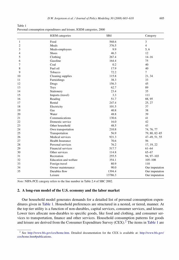
Table 1Personal consumption expenditures and leisure, IGEM categories, 2000

IGEM categories $Bil Category

1 Food 568.6 32 Meals 376.5 43 Meals-employees 9.9 5, 64 Shoes 46.3 125 Clothing 267.4 14–166 Gasoline 164.4 757 Coal 0.2 408 Fuel oil 17.9 409 Tobacco 72.2 7

10 Cleaning supplies 115.8 21, 3411 Furnishings 38.3 3312 Drugs 156.3 4513 Toys 62.7 8914 Stationery 23.4 3515 Imports (travel) 3.3 11116 Reading 51.7 88, 9517 Rental 247.4 25, 2718 Electricity 101.5 3719 Gas 40.8 3820 Water 48.8 3921 Communications 130.6 4122 Domestic service 16.0 4223 Other household 48.5 4324 Own transportation 210.8 74, 76, 7725 Transportation 56.9 79, 80, 82–8526 Medical services 921.3 47–49, 51, 5527 Health Insurance 70.6 5628 Personal services 76.2 17, 19, 2229 Financial services 517.7 61–6430 Other services 114.8 65–6731 Recreation 255.5 94, 97–10332 Education and welfare 354.1 105–10833 Foreign travel 80.9 11034 Owner maintenance 90.0 Our imputation35 Durables flow 1394.4 Our imputation

Leisure 13786.3 Our imputation

Note: NIPA-PCE category refers to the line number in Table 2.4 of SBC 2002.

2. A long-run model of the U.S. economy and the labor market

Our household model generates demands for a detailed list of personal consumption expen-ditures given in Table 1. Household preferences are structured in a nested, or tiered, manner. Atthe top tier utility is a function of non-durables, capital services, consumer services, and leisure.Lower tiers allocate non-durables to specific goods, like food and clothing, and consumer ser-vices to transportation, finance and other services. Household consumption patterns for goodsand leisure are derived from the Consumer Expenditure Survey (CEX).2 The items in Table 1 are

2 See http://www.bls.gov/cex/home.htm. Detailed documentation for the CEX is available at: http://www.bls.gov/cex/home.htm#publications.

606 D.W. Jorgenson et al. / Journal of Policy Modeling 30 (2008) 603–618

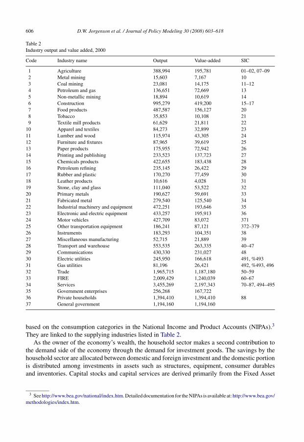
Table 2Industry output and value added, 2000

Code Industry name Output Value-added SIC

1 Agriculture 388,994 195,781 01–02, 07–092 Metal mining 15,603 7,167 103 Coal mining 23,081 14,175 11–124 Petroleum and gas 136,651 72,669 135 Non-metallic mining 18,894 10,619 146 Construction 995,279 419,200 15–177 Food products 487,587 156,127 208 Tobacco 35,853 10,108 219 Textile mill products 61,629 21,811 22

10 Apparel and textiles 84,273 32,899 2311 Lumber and wood 115,974 43,305 2412 Furniture and fixtures 87,965 39,619 2513 Paper products 175,955 72,942 2614 Printing and publishing 233,523 137,723 2715 Chemicals products 422,655 183,438 2816 Petroleum refining 235,145 26,422 2917 Rubber and plastic 170,270 77,459 3018 Leather products 10,616 4,028 3119 Stone, clay and glass 111,040 53,522 3220 Primary metals 190,627 59,691 3321 Fabricated metal 279,540 125,540 3422 Industrial machinery and equipment 472,251 193,646 3523 Electronic and electric equipment 433,257 195,913 3624 Motor vehicles 427,709 83,072 37125 Other transportation equipment 186,241 87,121 372–37926 Instruments 183,293 104,351 3827 Miscellaneous manufacturing 52,715 21,889 3928 Transport and warehouse 553,535 263,335 40–4729 Communications 430,330 231,027 4830 Electric utilities 245,950 166,618 491, %49331 Gas utilities 81,196 26,421 492, %493, 49632 Trade 1,965,715 1,187,180 50–5933 FIRE 2,009,429 1,240,039 60–6734 Services 3,455,269 2,197,343 70–87, 494–49535 Government enterprises 256,268 167,72236 Private households 1,394,410 1,394,410 8837 General government 1,194,160 1,194,160

based on the consumption categories in the National Income and Product Accounts (NIPAs).3

They are linked to the supplying industries listed in Table 2.As the owner of the economy’s wealth, the household sector makes a second contribution to

the demand side of the economy through the demand for investment goods. The savings by thehousehold sector are allocated between domestic and foreign investment and the domestic portionis distributed among investments in assets such as structures, equipment, consumer durablesand inventories. Capital stocks and capital services are derived primarily from the Fixed Asset

3 See http://www.bea.gov/national/index.htm. Detailed documentation for the NIPAs is available at: http://www.bea.gov/methodologies/index.htm.

D.W. Jorgenson et al. / Journal of Policy Modeling 30 (2008) 603–618 607

Accounts of the Bureau of Economic Analysis,4 which include information on investment by60 asset categories. Data on labor input by industry are derived from detailed demographic andwage data in the annual Current Population Surveys and the decennial Censuses of Population,as described by Jorgenson, Ho, and Stiroh (2005).

We separate the production sector in IGEM into 35 individual industries. The complete list isgiven in Table 2, together with the value of each industry’s output in 2000 and the correspondingStandard Industrial Classification codes. Each industry produces output from labor, capital, andintermediate inputs, using a technology that allows for substitution among these inputs. Althoughtechnology can be represented by means of a production function, we find it much more convenientto use a dual approach, based on a price function that gives the price of output of each sectoras a function of the prices of inputs. Technologies are structured in a nested or tiered mannerwith intermediate inputs divided between energy and materials; both energy and materials arefurther sub-divided among inputs that correspond to the 35 commodity groups produced by the35 industries.

Our representation of the technology in each sector includes the rate and biases of technicalchange. The rate of technical change captures improvements in productivity or growth in outputper unit of input. The biases of technical change correspond to increases or decreases in theshares of inputs in the value of output, holding input prices constant. The evolution of patternsof production reflects both price-induced substitution among inputs and the impact of changes intechnology. We project the historical patterns of technical change represented in our database inorder to incorporate future changes in technology into the demand for inputs of labor, capital, andintermediate goods and services.

The production of each commodity by one or more of the 35 U.S. domestic industries isaugmented by imports of that commodity from the rest of the world to generate the U.S. domesticsupply. This supply is allocated to U.S. industries as an intermediate input and to final demand forconsumption by U.S. households and governments, investments by U.S. businesses, households,and governments, and net exports. Since imports are not perfect substitutes for commoditiesproduced domestically, we also model the substitution between imports and domestic productionexplicitly. The rest of the world absorbs exports from the U.S. and the net flow of resources ineach period is governed by an exogenously specified current account deficit.

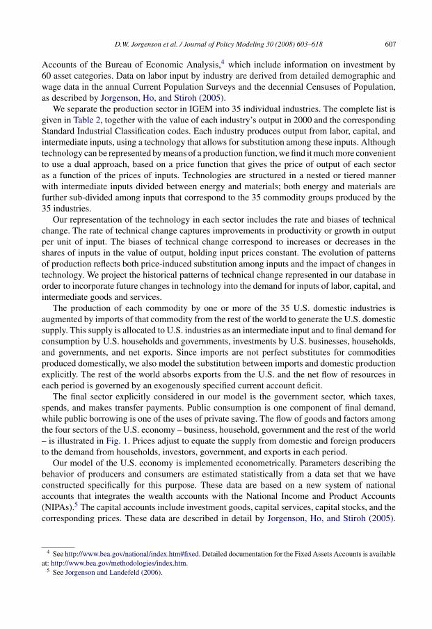
The final sector explicitly considered in our model is the government sector, which taxes,spends, and makes transfer payments. Public consumption is one component of final demand,while public borrowing is one of the uses of private saving. The flow of goods and factors amongthe four sectors of the U.S. economy – business, household, government and the rest of the world– is illustrated in Fig. 1. Prices adjust to equate the supply from domestic and foreign producersto the demand from households, investors, government, and exports in each period.

Our model of the U.S. economy is implemented econometrically. Parameters describing thebehavior of producers and consumers are estimated statistically from a data set that we haveconstructed specifically for this purpose. These data are based on a new system of nationalaccounts that integrates the wealth accounts with the National Income and Product Accounts(NIPAs).5 The capital accounts include investment goods, capital services, capital stocks, and thecorresponding prices. These data are described in detail by Jorgenson, Ho, and Stiroh (2005).

4 See http://www.bea.gov/national/index.htm#fixed. Detailed documentation for the Fixed Assets Accounts is availableat: http://www.bea.gov/methodologies/index.htm.

5 See Jorgenson and Landefeld (2006).

608 D.W. Jorgenson et al. / Journal of Policy Modeling 30 (2008) 603–618

Fig. 1. Flow of goods and factors in IGEM.

Similar data have recently been released for members of the European Union by the EU KLEMSproject.6

3. Exogenous variables in the projections

Our model of the U.S. economy simulates the future growth and structure of the economy overthe intermediate term of 25 years. The time path of model outcomes is conditional on projectionsof exogenous variables. Among the most important of these variables are the total population,the time endowment of the working-age population, the overall government deficit, the currentaccount deficit, world prices and government tax policies. Many of these are developed frompublished sources, “official” and otherwise. In addition, we project the evolution of technologyin each of the 35 industries that make up the production sector of the model. These variables areprojected from the historical data set that underlies the production model and its estimation.

The key exogenous variables that describe the growth and composition of the U.S. populationare population projections by sex and individual year of age from the U.S. Bureau of the Census.7

During the sample period the population is allocated to educational attainment categories usingdata from the Current Population Survey8 in a way that is parallel to our calculation of labor

6 See http://www.euklems.net/. This data set was released on 15 March 2007, and is described in “Use IT or Lose It,”The Economist, May 19–25, 2007, p. 82.

7 See: http://www.census.gov/popest/estimates.php. Historical data are taken from: http://www.census.gov/popest/archives/. These population data are revised to match the latest censuses (e.g., 1981 data is revised to be consistentwith the 1990 Census).

8 See http://www.census.gov/cps/.

D.W. Jorgenson et al. / Journal of Policy Modeling 30 (2008) 603–618 609

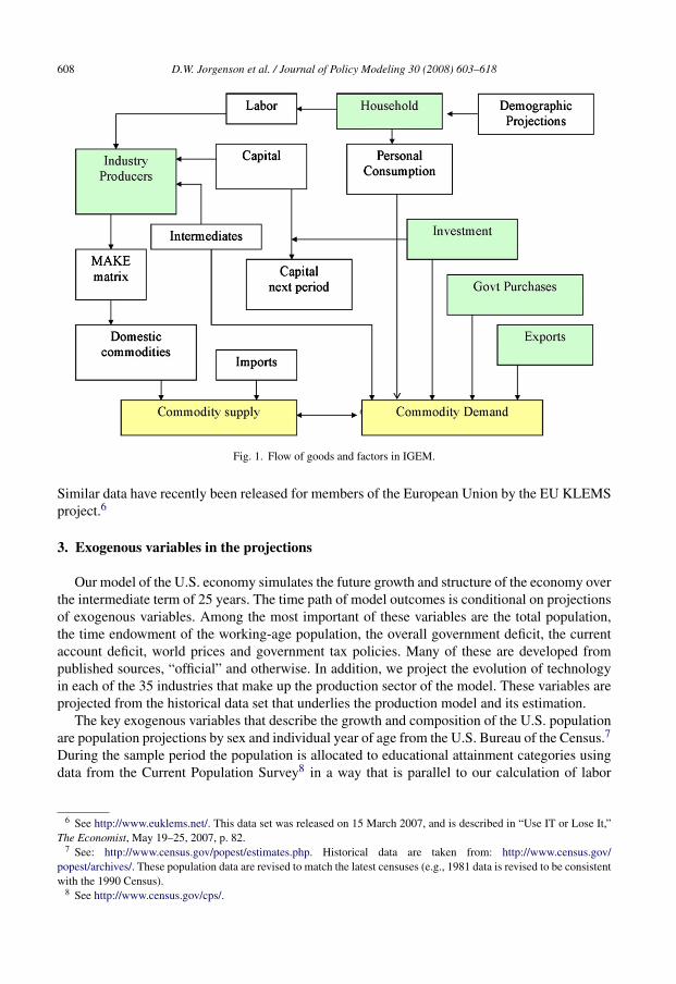
Fig. 2. Sources of growth.

input. Each adult is given a time endowment of 14 h a day to be used for work and leisure. Thenumber of hours for each sex–age–education category is weighted by labor compensation ratesand aggregated to form the national time endowment presented in Fig. 2.

Our projections use Census Bureau forecasts by sex and age. We assume that the educationalattainment of those aged 35 or younger will be the same as in the last year of the sample period;that is, a person who becomes 22 years old in 2014 will have the same chance of having a BAdegree as a person in 2004. Those aged 55 and over carry their education attainment with themas they age; that is, the educational distribution of 70 year olds in 2014 is the same as that of60 year olds in 2004. Those between 35 and 55 have a complex adjustment that is a mixture ofthese two assumptions to allow a smooth improvement of educational attainment that is consistentwith the observed profile in 2004. The result of these calculations, shown in Fig. 2, is that theU.S. population is expected to grow at just under 1% per year through 2030, reaching a level inexcess of 365 million. The gradually slowing improvement in the average level of educationalattainment implies that the time endowment grows at a modestly faster rate of around 1% through2030.

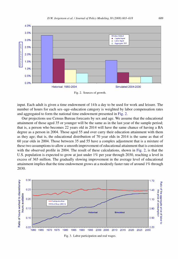
Fig. 3. Labor participation and real wages.

610 D.W. Jorgenson et al. / Journal of Policy Modeling 30 (2008) 603–618

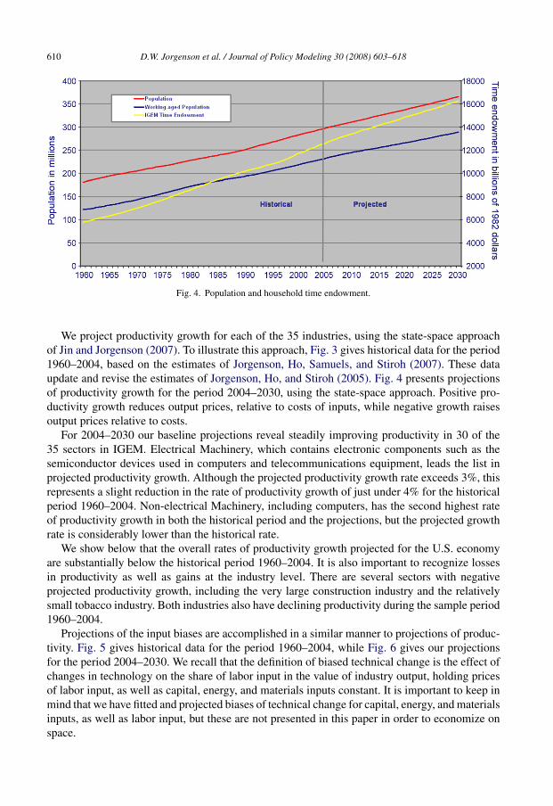
Fig. 4. Population and household time endowment.

We project productivity growth for each of the 35 industries, using the state-space approachof Jin and Jorgenson (2007). To illustrate this approach, Fig. 3 gives historical data for the period1960–2004, based on the estimates of Jorgenson, Ho, Samuels, and Stiroh (2007). These dataupdate and revise the estimates of Jorgenson, Ho, and Stiroh (2005). Fig. 4 presents projectionsof productivity growth for the period 2004–2030, using the state-space approach. Positive pro-ductivity growth reduces output prices, relative to costs of inputs, while negative growth raisesoutput prices relative to costs.

For 2004–2030 our baseline projections reveal steadily improving productivity in 30 of the35 sectors in IGEM. Electrical Machinery, which contains electronic components such as thesemiconductor devices used in computers and telecommunications equipment, leads the list inprojected productivity growth. Although the projected productivity growth rate exceeds 3%, thisrepresents a slight reduction in the rate of productivity growth of just under 4% for the historicalperiod 1960–2004. Non-electrical Machinery, including computers, has the second highest rateof productivity growth in both the historical period and the projections, but the projected growthrate is considerably lower than the historical rate.

We show below that the overall rates of productivity growth projected for the U.S. economyare substantially below the historical period 1960–2004. It is also important to recognize lossesin productivity as well as gains at the industry level. There are several sectors with negativeprojected productivity growth, including the very large construction industry and the relativelysmall tobacco industry. Both industries also have declining productivity during the sample period1960–2004.

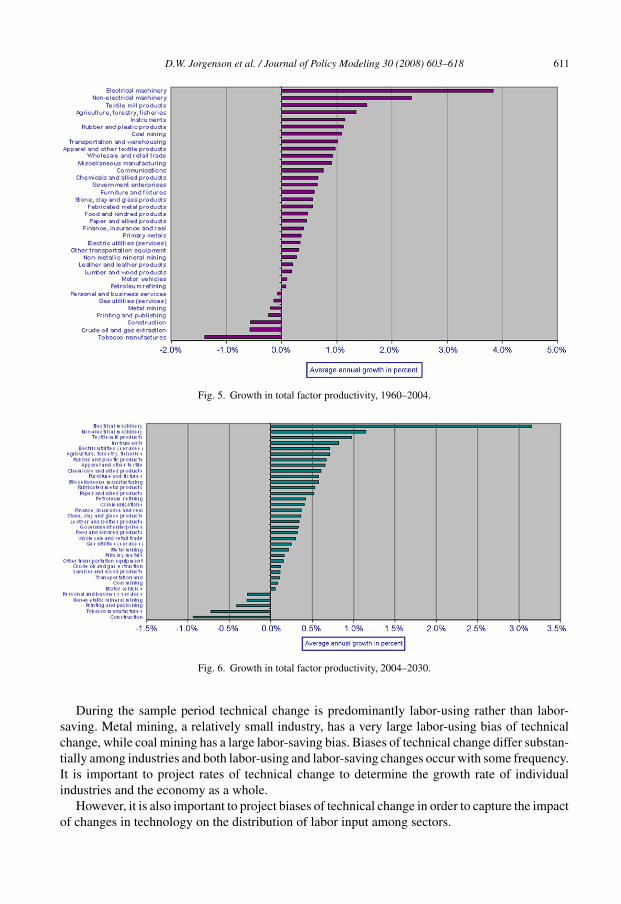
Projections of the input biases are accomplished in a similar manner to projections of produc-tivity. Fig. 5 gives historical data for the period 1960–2004, while Fig. 6 gives our projectionsfor the period 2004–2030. We recall that the definition of biased technical change is the effect ofchanges in technology on the share of labor input in the value of industry output, holding pricesof labor input, as well as capital, energy, and materials inputs constant. It is important to keep inmind that we have fitted and projected biases of technical change for capital, energy, and materialsinputs, as well as labor input, but these are not presented in this paper in order to economize onspace.

D.W. Jorgenson et al. / Journal of Policy Modeling 30 (2008) 603–618 611

Fig. 5. Growth in total factor productivity, 1960–2004.

Fig. 6. Growth in total factor productivity, 2004–2030.

During the sample period technical change is predominantly labor-using rather than labor-saving. Metal mining, a relatively small industry, has a very large labor-using bias of technicalchange, while coal mining has a large labor-saving bias. Biases of technical change differ substan-tially among industries and both labor-using and labor-saving changes occur with some frequency.It is important to project rates of technical change to determine the growth rate of individualindustries and the economy as a whole.

However, it is also important to project biases of technical change in order to capture the impactof changes in technology on the distribution of labor input among sectors.

612 D.W. Jorgenson et al. / Journal of Policy Modeling 30 (2008) 603–618

Fig. 7. Labor input biases, 1960–2004.

Two other important assumptions that determine the shape of the economy are the governmentand trade deficits. Our projection of the government deficit follows the forecasts of the Congres-sional Budget Office for the next 10 years and then is set on course to a zero balance by 2030.9 Thecurrent account deficit is assumed to shrink steadily, relative to the GDP, so that it also reachesa sustainable balance by 2030. These simplifying assumptions allow the simulation the producea smooth time path. The government and current account deficits are determinants of long rungrowth to the extent that they influence capital formation, but are substantially less important thanthe exogenous demographic and technology variables we have described.

4. Projection of U.S. economic growth

Our baseline path for the economy generates a labor force participation rate, defined as the ratioof labor input to the time endowment. We have used this to extrapolate the ratio of hours worked todiscretionary hours available from the working age population. The participation rate presented inFig. 7 reached a peak in 2000, before the shallow recession of 2001 and the “jobless” recovery thatfollowed. The historical data from 1960 to 1990 show substantial gains in participation. No suchgains in participation are in prospect for the next quarter century. At the same time, projectionsbeginning in 2004 do not suggest a large decline in labor force participation.

It is important to keep in mind that the rate of population growth will be declining throughout theprojection period 2004–2030. The working age population will be growing at a very similar rateto the population as a whole during our projection period. During the historical period 1960–2004the working age population grew considerably more rapidly than the population. Finally, the timeendowment, which adjusts the population for changes in composition by educational attainmentand experience, will continue to grow more rapidly than the working age population. However,changes in composition will gradually disappear as average levels of education and experiencestabilize.

Real wages, defined as the ratio of the price of labor input to the price of consumption goods andservices, are also presented in Fig. 7. Contrary to historical trends often described in the business

9 See http://www.cbo.gov/showdoc.cfm.

D.W. Jorgenson et al. / Journal of Policy Modeling 30 (2008) 603–618 613

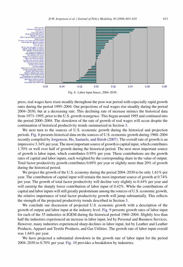
Fig. 8. Labor input biases, 2004–2030.

press, real wages have risen steadily throughout the post-war period with especially rapid growthrates during the period 1995–2004. Our projections of real wages rise steadily during the period2004–2030, but at a decreasing rate. This declining rate of increase mimics the historical datafrom 1973–1995, prior to the U.S. growth resurgence. This began around 1995 and continued intothe period 2000–2004. The slowdown of the rate of growth of real wages will occur despite thecontinuation of historical productivity trends summarized in Section 3.

We next turn to the sources of U.S. economic growth during the historical and projectionperiods. Fig. 8 presents historical data on the sources of U.S. economic growth during 1960–2004recently compiled by Jorgenson, Ho, Samuels, and Stiroh (2007). The overall rate of growth is animpressive 3.34% per year. The most important source of growth is capital input, which contributes1.70% or well over half of growth during the historical period. The next most important sourceof growth is labor input, which contributes 0.95% per year. These contributions are the growthrates of capital and labor inputs, each weighted by the corresponding share in the value of output.Total factor productivity growth contributes 0.69% per year or slightly more than 20% of growthduring the historical period.

We project the growth of the U.S. economy during the period 2004–2030 to be only 1.61% peryear. The contribution of capital input will remain the most important source of growth at 0.74%per year. The growth of total factor productivity will decline very slightly to 0.44% per year andwill outstrip the sharply lower contribution of labor input of 0.42%. While the contributions ofcapital and labor inputs will still greatly predominate among the sources of U.S. economic growth,the relative importance of total factor productivity growth will jump substantially. This reflectsthe strength of the projected productivity trends described in Section 3.

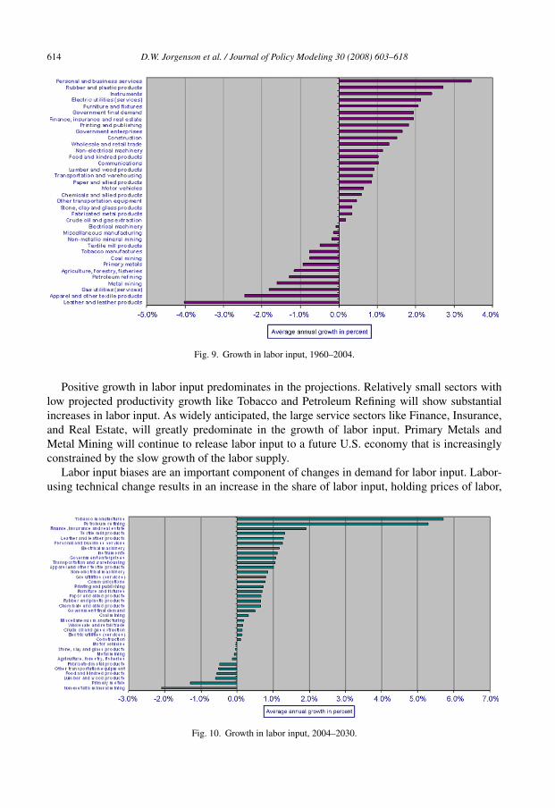
We conclude our discussion of projected U.S. economic growth with a description of thegrowth of output and labor input at the industry level. Fig. 9 presents growth rates of labor inputfor each of the 35 industries in IGEM during the historical period 1960–2004. Slightly less thanhalf the industries experienced an increase in labor input, led by Personal and Business Services.However, many industries experienced sharp declines in labor input, led by Leather and LeatherProducts, Apparel and Textile Products, and Gas Utilities. The growth rate of labor input overallwas 1.64% per year.

We have projected a substantial slowdown in the growth rate of labor input for the period2004–2030 to 0.70% per year. Fig. 10 provides a breakdown by industries.

614 D.W. Jorgenson et al. / Journal of Policy Modeling 30 (2008) 603–618

Fig. 9. Growth in labor input, 1960–2004.

Positive growth in labor input predominates in the projections. Relatively small sectors withlow projected productivity growth like Tobacco and Petroleum Refining will show substantialincreases in labor input. As widely anticipated, the large service sectors like Finance, Insurance,and Real Estate, will greatly predominate in the growth of labor input. Primary Metals andMetal Mining will continue to release labor input to a future U.S. economy that is increasinglyconstrained by the slow growth of the labor supply.

Labor input biases are an important component of changes in demand for labor input. Labor-using technical change results in an increase in the share of labor input, holding prices of labor,

Fig. 10. Growth in labor input, 2004–2030.

D.W. Jorgenson et al. / Journal of Policy Modeling 30 (2008) 603–618 615

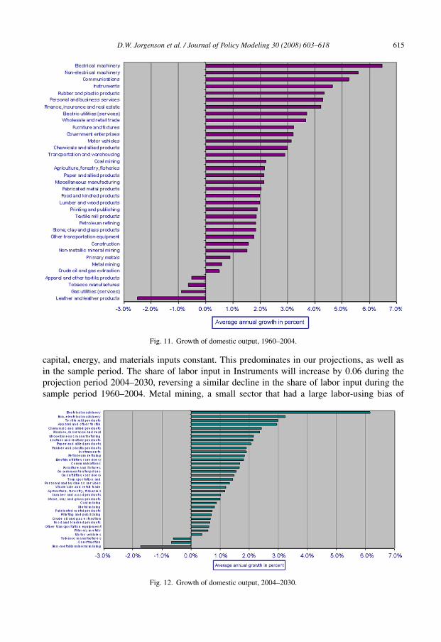
Fig. 11. Growth of domestic output, 1960–2004.

capital, energy, and materials inputs constant. This predominates in our projections, as well asin the sample period. The share of labor input in Instruments will increase by 0.06 during theprojection period 2004–2030, reversing a similar decline in the share of labor input during thesample period 1960–2004. Metal mining, a small sector that had a large labor-using bias of

Fig. 12. Growth of domestic output, 2004–2030.

616 D.W. Jorgenson et al. / Journal of Policy Modeling 30 (2008) 603–618

technical change during the sample period, has a smaller labor-using bias during the projectionperiod. Biases of technical change are an important component of labor input demand, along withthe steady rise in the price of labor input relative to other inputs.

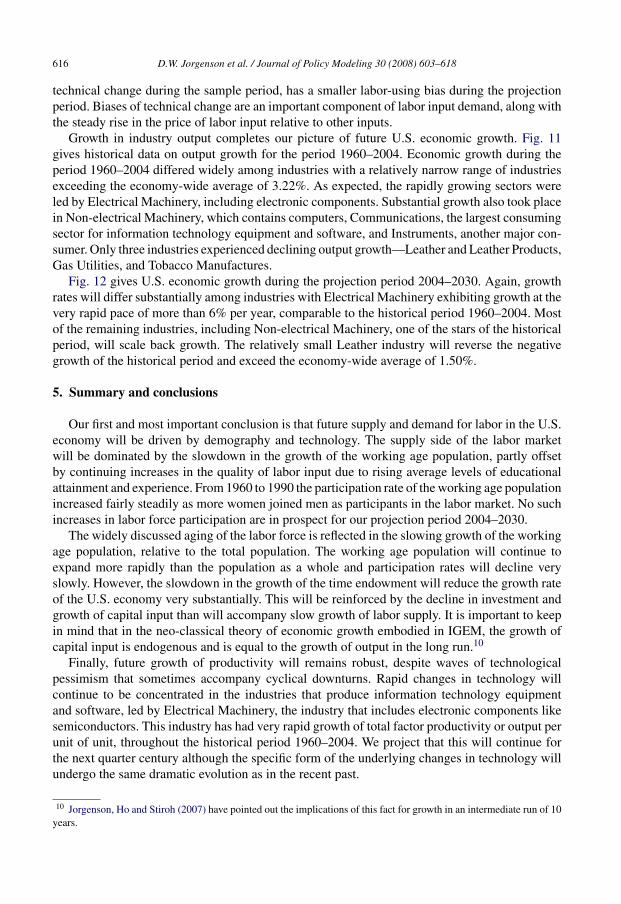
Growth in industry output completes our picture of future U.S. economic growth. Fig. 11gives historical data on output growth for the period 1960–2004. Economic growth during theperiod 1960–2004 differed widely among industries with a relatively narrow range of industriesexceeding the economy-wide average of 3.22%. As expected, the rapidly growing sectors wereled by Electrical Machinery, including electronic components. Substantial growth also took placein Non-electrical Machinery, which contains computers, Communications, the largest consumingsector for information technology equipment and software, and Instruments, another major con-sumer. Only three industries experienced declining output growth—Leather and Leather Products,Gas Utilities, and Tobacco Manufactures.

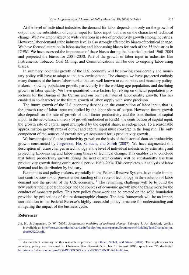
Fig. 12 gives U.S. economic growth during the projection period 2004–2030. Again, growthrates will differ substantially among industries with Electrical Machinery exhibiting growth at thevery rapid pace of more than 6% per year, comparable to the historical period 1960–2004. Mostof the remaining industries, including Non-electrical Machinery, one of the stars of the historicalperiod, will scale back growth. The relatively small Leather industry will reverse the negativegrowth of the historical period and exceed the economy-wide average of 1.50%.

5. Summary and conclusions

Our first and most important conclusion is that future supply and demand for labor in the U.S.economy will be driven by demography and technology. The supply side of the labor marketwill be dominated by the slowdown in the growth of the working age population, partly offsetby continuing increases in the quality of labor input due to rising average levels of educationalattainment and experience. From 1960 to 1990 the participation rate of the working age populationincreased fairly steadily as more women joined men as participants in the labor market. No suchincreases in labor force participation are in prospect for our projection period 2004–2030.

The widely discussed aging of the labor force is reflected in the slowing growth of the workingage population, relative to the total population. The working age population will continue toexpand more rapidly than the population as a whole and participation rates will decline veryslowly. However, the slowdown in the growth of the time endowment will reduce the growth rateof the U.S. economy very substantially. This will be reinforced by the decline in investment andgrowth of capital input than will accompany slow growth of labor supply. It is important to keepin mind that in the neo-classical theory of economic growth embodied in IGEM, the growth ofcapital input is endogenous and is equal to the growth of output in the long run.10

Finally, future growth of productivity will remains robust, despite waves of technologicalpessimism that sometimes accompany cyclical downturns. Rapid changes in technology willcontinue to be concentrated in the industries that produce information technology equipmentand software, led by Electrical Machinery, the industry that includes electronic components likesemiconductors. This industry has had very rapid growth of total factor productivity or output perunit of unit, throughout the historical period 1960–2004. We project that this will continue forthe next quarter century although the specific form of the underlying changes in technology willundergo the same dramatic evolution as in the recent past.

10 Jorgenson, Ho and Stiroh (2007) have pointed out the implications of this fact for growth in an intermediate run of 10years.

D.W. Jorgenson et al. / Journal of Policy Modeling 30 (2008) 603–618 617

At the level of individual industries the demand for labor depends not only on the growth ofoutput and the substitution of capital input for labor input, but also on the character of technicalchange. We have emphasized the wide variations in rates of productivity growth among industries.However, labor demand at the industry level is also strongly affected by biases of technical change.We have focused attention in labor-saving and labor-using biases for each of the 35 industries inIGEM. We have assessed the importance of these biases during the historical period 1960–2004and projected the biases for 2004–2030. Part of the growth of labor input in industries likeInstruments, Tobacco, Coal Mining, and Communications will be due to ongoing labor-usingbiases.

In summary, potential growth of the U.S. economy will be slowing considerably and mone-tary policy will have to adapt to the new environment. The changes we have projected embodymany features of the future labor market that are well known to economists and monetary policy-makers—slowing population growth, particularly for the working age population, and declininggrowth in labor quality. We have quantified these factors by relying on official population pro-jections for the Bureau of the Census and our own estimates of labor quality growth. This hasenabled us to characterize the future growth of labor supply with some precision.

The future growth of the U.S. economy depends on the contribution of labor input, that is,the growth rate of labor input multiplied by the labor share of output. However, future growthalso depends on the rate of growth of total factor productivity and the contribution of capitalinput. In the neo-classical theory of growth embodied in IGEM, the contribution of capital input,the growth rate of capital input multiplied by the capital share, is endogenous. To a reasonableapproximation growth rates of output and capital input must converge in the long run. The onlycomponent of the sources of growth not yet accounted for is productivity growth.

We have projected future productivity growth on the basis of the historical data on productivitygrowth constructed by Jorgenson, Ho, Samuels, and Stiroh (2007). We have augmented thisdescription of future changes in technology at the level of individual industries by estimating andprojecting labor-saving and labor-using biases of technical change. This enables us to concludethat future productivity growth during the next quarter century will be substantially less thanproductivity growth during our historical period 1960–2004. This completes our analysis of labordemand and its distribution by industry.

Economists and policy-makers, especially in the Federal Reserve System, have made impor-tant contributions to our present understanding of the role of technology in the evolution of labordemand and the growth of the U.S. economy.11 The remaining challenge will be to build thenew understanding of technology and the sources of economic growth into the framework for theconduct of monetary policy. This new policy framework can be erected on the solid foundationprovided by projections of future demographic change. The new framework will be an impor-tant addition to the Federal Reserve’s highly successful policy structure for understanding andmitigating the impact of the business cycle.

References

Jin, H., & Jorgenson, D. W. (2007). Econometric modeling of technical change, February 3. An electronic versionis available at: http://post.economics.harvard.edu/faculty/jorgenson/papers/EconometricModelingTechChangehuijindraft070203.pdf.

11 An excellent summary of this research is provided by Oliner, Sichel, and Stiroh (2007). The implications formonetary policy are discussed in Chairman Ben Bernanke’s in his 31 August 2006, speech on “Productivity”http://www.federalreserve.gov/BOARDDOCS/Speeches/2006/20060831/default.htm.

618 D.W. Jorgenson et al. / Journal of Policy Modeling 30 (2008) 603–618

Jorgenson, D. W. (1998). Energy, the environment and economic growth. Cambridge: The MIT Press.Jorgenson, D. W., Ho, M. S., & Stiroh, K. J. (2005). Information technology and the American growth resurgence.

Cambridge: The MIT Press.Jorgenson, D. W., Ho, M. S., Samuels, J. D., & Stiroh, K. J. (2007). Industry origins of the American productivity

resurgence, economic systems research, forthcoming. An electronic version is available at: http://post.economics.harvard.edu/faculty/jorgenson/papers/IndustryOriginsAmerProdResurg 100206.pdf.

Jorgenson, D. W., Ho, & Stiroh, K. J. (2007). A retrospective look at the U.S. productivity growth resurgence. Jour-nal of Economic Perspectives, forthcoming. An electronic version is available at: http://post.economics.harvard.edu/faculty/jorgenson/papers/RetroProdGrowthResurg 070203.pdf

Jorgenson, Dale W., & Landefeld, J. Steven. (2006). Blueprint for an Expanded and Integrated U.S. National Accounts:Review, Assessment and Next Steps. In Dale W. Jorgenson, J. Steven Landefeld, & William D. Nordhaus (Eds.), ANew Architecture for the U.S. National Accounts (pp. 13–112). Chicago: University of Chicago Press.

Oliner, S. D., Sichel, D. E., & Stiroh, K. J. (2007), Explaining a productivity decade. Brookings Eco-nomic Papers, forthcoming. An electronic version is available at: http://www.brookings.edu/es/commentary/journals/bpea macro/forum/agenda.htm.