Embed Size (px)
Citation preview
USNTPS-FTM-No. 107
U.S. NAVAL TEST PILOT SCHOOL
FLIGHT TEST MANUAL
ROTARY WING STABILITY AND CONTROL
Approved for public release; distribution is unlimited.
NAVAL AIR WARFARE CENTERPATUXENT RIVER, MARYLAND
Revised 31 December 1995

U.S. NAVAL TEST PILOT SCHOOL
FLIGHT TEST MANUAL
USNTPS-FTM-No. 107
ROTARY WING STABILITY AND CONTROL
This Flight Test Manual, published under the authority of the Commanding Officer, U.S.Naval Test Pilot School, is intended primarily as a text for the pilots, engineers and flightofficers attending the school. Additionally, it is intended to serve as a reference documentfor those engaged in flight testing. Corrections and update recommendations to this manualare welcome and may be submitted to:
Commanding OfficerU.S. Naval Test Pilot School22783 Cedar Point RoadPatuxent River, MD 20670-5304
31 December 1995
TABLE OF CONTENTS
ROTARY WING STABILITY AND CONTROL
CHAPTER PAGE
1 INTRODUCTION 1
2 PILOT FLYING QUALITIES EVALUATIONS 2
3 OPEN LOOP TESTING 3
4 ROTOR CHARACTERISTICS 4
5 FLIGHT CONTROL SYSTEM CHARACTERISTICS 5
6 FORWARD FLIGHT LONGITUDINAL STABILITY, CONTROL,
AND FLYING QUALITIES 6
7 FORWARD FLIGHT LATERAL-DIRECTIONAL STABILITY,
CONTROL, AND FLYING QUALITIES 7
8 HOVER AND LOW AIRSPEED STABILITY, CONTROL, AND
FLYING QUALITIES 8
9 COUPLED LONGITUDINAL AND LATERAL-DIRECTIONAL
STABILITY, CONTROL, AND FLYING QUALITIES 9
10 SUDDEN ENGINE FAILURES, AUTOROTATIVE FLIGHT,
AND AUTOROTATIVE LANDINGS 10
APPENDIX
I GLOSSARY I
II REFERENCES II
III FIGURES III
IV TABLES IV
V EQUATIONS V
VI RATING SCALES VI
VII MILITARY SPECIFICATION, HELICOPTER FLYING AND
GROUND HANDLING QUALITIES; GENERAL
REQUIREMENT FOR, MIL-H-8501A VII
VIII AUTOMATIC FLIGHT CONTROL SYSTEM ASSESSMENT VIII
1.i
CHAPTER ONE
INTRODUCTION
PAGE
1.1 OBJECTIVE 1.1
1.2 ORGANIZATION 1.2
1.2.1 Manual Organization 1.2
1.2.2 Chapter Organization 1.4
1.3 EFFECTIVE TEST PLANNING 1.4
1.4 RESPONSIBILITIES OF TEST PILOT AND FLIGHT TEST ENGINEER 1.5
1.4.1 The Test Pilot 1.5
1.4.2 The Flight Test Engineer 1.6
1.5 STABILITY AND CONTROL SYLLABUS 1.7
1.5.1 Overview 1.7
1.5.2 Flight Briefings 1.8
1.5.3 Demonstration Flights 1.8
1.5.4 Practice Flights 1.9
1.5.5 Exercise Flights 1.9
1.5.6 Reports 1.9
1.5.7 Progress Evaluation Flight 1.10
1.6 FLIGHT SAFETY 1.11
1.6.1 Incremental Build-Up 1.11
1.6.2 Unusual Attitude Recovery 1.11
1.6.3 Teetering Rotor System Aircraft 1.11
1.6.3.1 Recovery From Nose High Unusual Attitude 1.11
1.6.3.2 Recovery From Nose Low Unusual Attitude 1.12
1.6.3.3 Recovery From an Unusual Roll Attitude 1.12
1.6.3.4 Recovery From Low Normal Acceleration Maneuver 1.12
ROTARY WING STABILITY AND CONTROL
1.ii
1.6.4 Articulated Rotor System Aircraft 1.13
1.6.4.1 Recovery From a Nose High Unusual Attitude 1.13
1.6.4.2 Recovery From a Nose Low Unusual Attitude 1.13
1.6.4.3 Recovery From an Unusual Roll Attitude 1.13
1.7 GLOSSARY 1.14
1.7.1 Notations 1.14
1.8 REFERENCES 1.14
1.1
CHAPTER ONE
INTRODUCTION
1.1 OBJECTIVE
The Rotary Wing Stability and Control Flight Test Manual (FTM) is intended to
serve as a practical and easy to use reference guide for the planning, execution, and
reporting of flight testing rotary wing aircraft for stability, control, and flying qualities. The
FTM is intended for use as a primary instructional tool at the U.S. Naval Test Pilot School
(USNTPS) and as a reference document for those conducting relatedhelicopter flight
testing at the Naval Air Warfare Center Aircraft Division (NAWCAD) or similar
organizations interested in rotary wing flight testing. It is not intended to be a substitute for
helicopter stability and control textbooks. Rather, the FTM summarizes applicable theory to
the extent necessary to permit an understanding of the concepts, techniques, and
procedures involved in successful flight testing. The FTM is directed at test pilots and flight
test engineers (FTE); it deals with the more practical and prominent features of stability and
control issues, sometimes sacrificing exactness or completeness in the interest of clarity and
brevity.
The FTM does not replace the Naval Air Warfare Center Aircraft Division Report
Writing Handbook. The FTM contains examples of stability, control, and flying qualities
parameters discussed in narrative and graphic format. It contains discussions of the effect
on mission performance and suitability of the various parameters, and a discussionof
specification compliance where applicable. The examples in this manual show trends
extracted from current helicopters and are in the format used at USNTPS.
This FTM, since it is a text for USNTPS, contains information relative to
operations at USNTPS and NAWCAD; however, it does not contain information relative to
the scope of a particular USNTPS syllabus exercise or to the reporting requirements for a
particular exercise. Detailed information for each flight exercise will vary from time to time
as resources and personnel change and will be briefed separately to each individual class.
ROTARY WING STABILITY AND CONTROL
1.2
1.2 ORGANIZATION
1.2.1 Manual Organization
The FTM is organized to simplify access to desired information. Although there is
some cross referencing, in general, each chapter stands as a discrete unit. Discussions of
flight test techniques are presented together with pertinent background analytic
presentations. Most of the information is generic in nature although specific examples are
given where appropriate. The contents are organized in a classical grouping and follow the
stability and control syllabus at USNTPS.
The FTM puts in perspective flying qualities testing relative to open loop statics and
dynamics documentation typical of Military Specification (MilSpec) compliance testing.
Chapter 1, Introduction, is an overview of the FTM.
Chapter 2, Pilot Flying Qualities Evaluations, details the pilot flying qualities
evaluation process (closed loop flight testing) and establishes piloted flying qualities as the
focus of supportive stability and control open loop flight testing. Evaluating mission
relevant tasks using Handling Qualities Ratings (HANDLING QUALITIES RATING) is
discussed.
Chapter 3, Open Loop Testing, outlines the various elements in open loop testing:
the specialized test inputs for statics and dynamics testing, a summary of data reduction
techniques, and the context for presenting results of open loop testing such as MilSpec. In
the open loop system, the pilot interfaces within closed loop testing, including the
augmented aircraft characteristics and the control system characteristics. Open loop testing
is aimed at determining the transfer characteristics of these elements.
Chapter 4, Rotor Characteristics, contains stability and control theory without any
discussion of test techniques or procedures. The purpose of this chapter is to reacquaint the
reader with the rotor characteristics which provide control of the helicopter. No attempt is
made to develop rigorously the various equations which govern the stability and control of
the rotor. Rather the terminology, reference systems, and equations are presented with a
discussion of the factors which influence the results. Simplifying assumptions are made
and discussed.
INTRODUCTION
1.3
Chapter 5, Flight Control System Characteristics, covers helicopter control system
mechanical characteristics with emphases on the irreversible control system. Understanding
and documenting the flight control system characteristics is fundamental toany flying
qualities or closed loop flight evaluation. Since the flight control system is part of the
control loop, the test pilot must have a detailed understanding of the components of the
flight control system and their function. The understanding begins with a thorough flight
control system description and proceeds with documenting the flight control system
characteristics. Test methods, data requirements, and data presentation are addressed.
Chapter 6, Forward Flight Longitudinal Stability, Control, and Flying Qualities,
covers longitudinal characteristics in powered forward flight above 35 kn. The lateral-
directional responses of the helicopter are constrained to minimize interference with the
longitudinal characteristics. Coupling between these axes is ignored in the analytic
discussions. Cross axis coupling is explicitly treated in Chapter 9. Chapter 6 details the
various elements which comprise the longitudinal open loop characteristics, how to test for
these elements, and how they yield particular flying qualities.
Chapter 7, Forward Flight Lateral-Directional Stability, Control, and Flying
Qualities, is the lateral-directional equivalent of Chapter 6. Lateral-directional characteristics
in powered forward flight above 35 kn are discussed. Coupling between the longitudinal
and lateral-directional axis is constrained.
Chapter 8, Hover and Low Airspeed Stability, Control, and Flying Qualities,
covers the longitudinal and lateral-directional characteristics in the low speed regime, from
hover to about 35 kn. The focus is on in and out of ground effect (IGE, OGE)
characteristics for hover and vertical maneuvering. The upper end of the relative wind
spectrum encompasses translational velocities. Takeoff and landing characteristics are
included.
To simplify discussion, the longitudinal and lateral-directional characteristics are
treated as decoupled wherever practical. For example, the lateral-directional responses of
the helicopter are constrained to minimize their influence on the longitudinal characteristics.
Chapter 9, Coupled Longitudinal and Lateral-DirectionalStability, Control, and
Flying Qualities, aggregates the important coupling effects between the pitch, roll, and yaw
ROTARY WING STABILITY AND CONTROL
1.4
axes dependent on attitude, rate, acceleration, or control coupling. This chapter discusses
stability, control, and flying qualities when longitudinal and lateral-directional coupling is
present for hover, low airspeed, and forward flight. Because of the helicopter’s asymmetric
configuration, coupling is a significant factor in assessing mission related flying qualities in
all phases of flight. Understanding and developing meaningful test procedures and
documenting any undesirable coupling effects on flying qualities is essential in evaluating a
helicopter's ability to perform its mission.
Chapter 10, Sudden Engine Failures, Autorotative Flight, and Autorotative
Landings, deals with the theory of autorotative flight and the flight test techniques pertinent
to this flight regime. This chapter discusses helicopter stability, control, and flying qualities
during engine failure, autorotation entry, steady autorotative flight, and landing following a
successful autorotation. Although the emphasis is on flying qualities, knowledge of
helicopter performance requirements and power deficits is essential to understanding the
total autorotation evaluation starting with engine failure and ending with a satisfactory
landing. Flying qualities and performance characteristics are both required in analyzing and
testing autorotation capability.
1.2.2 Chapter Organization
Each chapter has the same internal organization where possible. Following the
chapter introduction, the second section gives the purpose of the test. The third section is a
review of the applicable theory. The fourth section discusses the test methods and
techniques, data requirements, and safety precautions applicable to those methods. The
fifth section discusses data reduction. The sixth section pertains to the data analysis. The
seventh section covers relevant mission suitability aspects of the stability, control, and
flying qualities parameters. The eighth section discusses specification compliance. The
ninth section is a glossary of terms introduced in the chapter. Finally, the tenth section lists
applicable references.
1.3 EFFECTIVE TEST PLANNING
In order to plan a test program effectively, a sound understanding of the theoretical
background of the tests to be performed is necessary. This knowledge helps the test team
establish the optimum scope of tests, choose appropriate test techniques and data reduction
methods, and present the test results effectively. Time and money are scarce resources;
INTRODUCTION
1.5
therefore, test data should be obtained with a minimum expenditure of both. Proper
application of theory ensures the tests will be performed at the proper conditions, with
appropriate techniques, and using efficient data reduction methods.
1.4 RESPONSIBILITIES OF TEST PILOT AND FLIGHT TEST
ENGINEER
Almost every flight test and evaluation team will be composed of one or more test
pilots and one or more project engineers. Team members bring together the necessary
expertise in qualitative testing (flying qualities evaluation) and quantitative evaluation
(knowledge of theory, instrumentation, and specifications). To perform the necessary tests
and evaluations, the test pilot must have knowledge of theory, test methods, data
requirements, data analysis, instrumentation, and specifications. The FTE must possess a
thorough knowledge of the pilot tasks required to perform a total mission in order to
participate fully in the planning and execution of the test and evaluation program.
1.4.1 The Test Pilot
The competent test pilot must be highly proficient to obtain accurate data. He must
have well developed observation and perception powers to recognize problems and adverse
characteristics. He must have the ability to analyze test results so that he understands them
and can explain the significance of his findings. To fulfill these expectations, he must
possess a superior knowledge of:
1. The test helicopter and rotary wing aircraft in general.
2. The total mission of the aircraft and the individual pilot tasks required to
accomplish the mission.
3. Theory and associated test techniques required for qualitative testing and
quantitative evaluation.
4. Specifications relevant to the evaluation program.
5. Technical report writing.
The test pilot must understand the test aircraft in detail, particularly the flight control
system, to do a creditable job of stability and control testing. He must consider the effects
of external configuration changes on flying qualities. The successful test pilot should have
flight experience in many different types of aircraft. By observing diverse characteristics
exhibited by a variety of aircraft, the test pilot can make accurate and precise assessments of
ROTARY WING STABILITY AND CONTROL
1.6
design concepts. Further, by flying many different types, he develops adaptability. When
flight test time is limited by monetary and time considerations, the ability to adapt is
invaluable.
The test pilot must understand clearly the total mission of the helicopter. The test
pilot must know the specific operational requirements on which the design was based, the
detail specification under which the design was developed, and other planning documents.
Knowledge of the individual pilot tasks required for total mission accomplishment is
derived from recent operational experience. Additionally, he can gain knowledge of the
individual pilot tasks from talking with other pilots, studying operational and tactical
manuals, and visiting replacement pilot training squadrons.
A qualified engineering test pilot executes a flight test task and evaluates the validity
of the results to determine whether he needs to repeat the test. Often the test pilot is the best
judge of an invalid test point and can save the test team wasted effort. The test pilot's
knowledge of theory, test techniques, relevant specifications, and technical report writing
may be gained through formal education or practical experience. The most effective and
efficient method is through formal study with practical application at an established test
pilot school such as the USNTPS. This education provides a common ground for the test
pilot and FTE to converse in technical terms concerning stability, control, and flying
qualities phenomena.
1.4.2 The Flight Test Engineer
The successful FTE must have general knowledge of the same items for which the
test pilot is mainly responsible. Additionally, he must possess superior knowledge of:
1. Instrumentation requirements.
2. Planning and coordination aspects of the flight test program.
3. Data acquisition, reduction, and presentation.
4. Technical report writing.
These skills are necessary for the FTE to form an efficient team with the test pilot
for the planning, executing, analyzing, and reporting process.
INTRODUCTION
1.7
Normally, the FTE is responsible for determining the test instrumentation. This
involves determining the ranges, sensitivities, frequency response required, and developing
an instrumentation specification or planning document. In the context of flying qualities
testing, the FTE assists the test pilots with establishing the appropriate evaluation tasks, the
standard of performance (desired/adequate), and the pilot comment cards. For open loop
stability testing, the FTE must determine the pertinent test inputs necessary to generate time
histories which can be reduced to yield the desired stability parameters and control
sensitivities.
The FTE is in the best position to coordinate all aspects of the program because he
does not fly in the test aircraft often and is available in the project office. The coordination
involves aiding in the preparation and revision of the test plan and coordinating the order in
which flights will be conducted. Normally, the FTE prepares all test flight cards and
participates in all flight briefings and debriefings.
A great deal of the engineer's time will be spent working with flight and ground test
data. He must review preliminary data from wind tunnel studies and existing flight tests.
From this data, critical areas may be determined prior to actualmilitary flight testing.
During the flight tests, the engineer may monitor and aid in the acquisition of data through
telemetry facilities and radio, or by flying in the test aircraft. Following completion of flight
tests, the engineer coordinates data reduction, data analysis, and data presentation.
The FTE uses his knowledge of technical report writing to participate in the
preparation of the report. Usually, the FTE and the test pilot will proofread the entire
manuscript.
1.5 STABILITY AND CONTROL SYLLABUS
1.5.1 Overview
The stability and control syllabus at USNTPS consists of academic instruction,
flight briefings, demonstration flights, practice flights, exercise flights, reports, and
evaluation flights. The stability and control phase of instruction concludes in an individual
evaluation flight. The final exercise at USNTPS is a simulated Navy Developmental Test
ROTARY WING STABILITY AND CONTROL
1.8
IIA (DT IIA). This exercise incorporates all the performance, stability, control, flying
qualities, and airborne systems instruction into the total evaluation of an airborne weapon
system.
The stability and control syllabus includes exercises in flight control systems,
mechanical characteristics, hover and low airspeed stability and control, forward flight
stability and control, and autorotative flight. The syllabus is presented in a step-by-step,
building block approach which allows concentration on specific objectives and
fundamentals. Unfortunately, this approach focuses on individual characteristics at the
expense of evaluating the total weapon system. Progress through the syllabus must be
made with the end objective in mind, the evaluation of the helicopter as a weapon system in
the mission environment. The details of the current syllabus is contained in U.S. Naval
Test Pilot School Notice 1542.
1.5.2 Flight Briefings
To form the basis of the applicable theory, each exercise in the stability and control
syllabus is preceded by academic instruction. Printed and oral flight briefings are presented
by the principal instructor for the exercise. The flight briefing gives specific details of the
exercise and the exercise requirements. The flight briefing covers the purpose, references,
test conditions, method of test to be used, the scope of test, test planning, and report
requirements. The briefing also covers the applicable safety requirements for the exercise as
well as administrative and support requirements.
1.5.3 Demonstration Flights
The demonstration flight is preceded by thorough briefings including: theory, test
techniques, analysis of test results in terms of mission accomplishment and specification
requirements, and data presentation methods. The student must prepare for the
demonstration flight by review of briefing notes, appropriate technical literature, and
relevant specifications. Thorough preparation is essential for maximum benefit.
The demonstration flight crew consists of one or more students and an instructor,
with the students sharing airborne instructional time. If the students are not qualified in the
demonstration aircraft, the instructor pilot may handle all preflight, ground operations,
takeoffs, and landings. The students are required to know the operational characteristics of
the demonstration aircraft. In flight, the instructor will demonstrate both qualitative and
INTRODUCTION
1.9
quantitative test techniques, use of special instrumentation, and data recording procedures.
After the student observes and understands each technique, he has the opportunity to
practice until attaining a reasonable level of proficiency. Throughout the demonstration
flight, the instructor discusses the significance of each test, implications of results, and
variations in the test techniques appropriate for other type helicopters. Students are
encouraged to ask questions during the flight; many points are explained or demonstrated
easier in flight than on the ground. A thorough post flight discussion between instructor
and students completes the demonstration flight. During the debrief, the data obtained in
flight are plotted and analyzed.
1.5.4 Practice Flights
Each student is afforded the opportunity to practice the test methods and techniques
in flight after the demonstration flights and prior to the exercise or data flight. The purpose
of the practice flights is to gain proficiency in the test techniques, data acquisition, and crew
coordination necessary for safe and efficient flight testing.
1.5.5 Exercise Flights
Each student will fly one or more flights as part of each exercise. The student is
expected to plan the flight, have the plan approved, and fly the flight in accordance with the
plan. The purpose of the flight is to gather both quantitative and qualitative data as part of
an overall flying qualities evaluation. The primary inflight objective is safe and efficient
flight testing. Under no conditions will flight safety be compromised.
1.5.6 Reports
A fundamental purpose of USNTPS is developing the test pilot/FTE’s ability to
report test results in clear, concise, unambiguous technical terms. After completing the
exercise flight, the student reduces the data. Data reduction transposes the format of data
gathered during flight to data used for engineering analysis. The student analyzes the data
for both mission suitability and specification compliance. The data are presented in the
proper format and a report is prepared. The report process combines factual data gathered
from ground and flight tests and analysis of its effect on mission suitability. The report
conclusions answers the questions implicit in the purpose of the test.

ROTARY WING STABILITY AND CONTROL
1.10
Theory should be used as the foundation for data analysis and technical reporting of
test results. However, theory is often misused to explain why something desirable or
undesirable happened. The question, “What caused the occurrence?” often receives more
attention than reporting the actual occurrence and its impact on mission suitability. The
cause may be completely irrelevant. For example, a helicopter exhibiting stable longitudinal
maneuvering stability with a forward center of gravity (CG) is unstable with an aft CG.
Such a trend is not unusual and no theoretical discussion is in order. A statement as to the
degree of instability uncovered and its significance to mission suitability or safety of flight
is needed.
1.5.7 Progress Evaluation Flight
The progress evaluation flight is both an evaluation exercise and an instructional
flight. It is a check flight on the phase of study just completed. A numerical grade will be
assigned by the instructor.
One student and one instructor comprise the flight crew. The student develops a
flight plan considering the real or simulated aircraft mission and appropriate specification
requirements. The student conducts the flight briefing, including the mission, a brief flight
control system description, discussion of test techniques, and specification requirements.
As the student demonstrates his knowledge of qualitative and quantitative test
techniques in flight, he is expected to comment on the impact of the results on the real or
simulated mission. The instructor will comment on validity of the results obtained, errors
or omissions in test procedures, and may demonstrate variations in test techniques not
introduced previously. The instructor may ask the student to perform a flying qualities
evaluation of a mission task. The student is expected to define the task, the expected
performance, evaluate the workload and pilot compensation, and assign a Handling
Qualities Rating.
During the debrief the student presents, analyzes, and discusses the test results. The
discussion includes the influence of the results on aircraft mission suitability.
INTRODUCTION
1.11
1.6 FLIGHT SAFETY
1.6.1 Incremental Build-Up
The concept of incremental build-up is one of the most important practical and
philosophical approaches to flight testing. Build-up is the process of proceeding from the
known to the unknown in an incremental, methodical pattern. Flight tests should be
structured with build-up in mind. Testing begins with the best documented, least hazardous
data points and proceeds toward the desired end points, always conscious of the aircraft,
pilot, and evaluation limits. There should be no surprises in flight test. In the event a data
point yields an unexpected result or a series of data points creates an unexpected trend,
evaluation stops until the results are analyzed and explained.
1.6.2 Unusual Attitude Recovery
For USNTPS purposes, the term Unusual Attitude refers to the in flight pitch, roll,
and yaw attitudes and/or rates resulting from an intentional control input commanding the
aircraft to deviate from its trimmed flight condition. Applicable recovery procedures depend
upon the aircraft being flown and the severity of the maneuver being executed. At all times
the pilot must remain in the loop actively flying the aircraft and analyzing the aircraft
response.
Recommended pilot recovery techniques from unusual attitudes for aircraft
currently operated at USNTPS are delineated below.
1.6.3 Teetering Rotor System Aircraft
1.6.3.1 RECOVERY FROM NOSE HIGH UNUSUAL ATTITUDE
As the pitch attitude reaches the nose up limit or the data point is complete, yaw and
roll right. The amount of right lateral cyclic will depend on the roll induced by the yaw rate.
The goal of this recovery is to roll out to the right of the initial heading, accelerating nose
down toward the trim airspeed. If the yaw rate appears to be excessive, apply left pedal to
slow the response. As the yaw rate diminishes, add left lateral cyclic to roll wings level and
fly away smoothly. If the pitch rate appears to be excessive or if the absolute allowable
pitch up attitude is going to be exceeded, a small amount of forward cyclic may be added at
the beginning of the recovery to slow the pitch rate. Do not attempt to stop the pitch rate, a
ROTARY WING STABILITY AND CONTROL
1.12
low normal acceleration condition may result. If a small amount of forward cyclic and right
pedal are applied simultaneously, it is likely that the resulting yaw rate will be greater than
the yaw rate had the forward cyclic not been added.
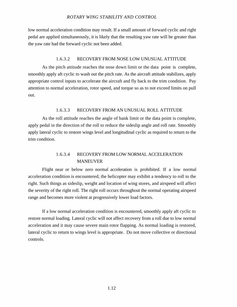
1.6.3.2 RECOVERY FROM NOSE LOW UNUSUAL ATTITUDE
As the pitch attitude reaches the nose down limit or the data point is complete,
smoothly apply aft cyclic to wash out the pitch rate. As the aircraft attitude stabilizes, apply
appropriate control inputs to accelerate the aircraft and fly back to the trim condition. Pay
attention to normal acceleration, rotor speed, and torque so as to not exceed limits on pull
out.
1.6.3.3 RECOVERY FROM AN UNUSUAL ROLL ATTITUDE
As the roll attitude reaches the angle of bank limit or the data point is complete,
apply pedal in the direction of the roll to reduce the sideslip angle and roll rate. Smoothly
apply lateral cyclic to restore wings level and longitudinal cyclic as required to return to the
trim condition.
1.6.3.4 RECOVERY FROM LOW NORMAL ACCELERATION
MANEUVER
Flight near or below zero normal acceleration is prohibited. If a low normal
acceleration condition is encountered, the helicopter may exhibit a tendency to roll to the
right. Such things as sideslip, weight and location of wing stores, and airspeed will affect
the severity of the right roll. The right roll occurs throughout the normal operating airspeed
range and becomes more violent at progressively lower load factors.
If a low normal acceleration condition is encountered, smoothly apply aft cyclic to
restore normal loading. Lateral cyclic will not affect recovery from a roll due to low normal
acceleration and it may cause severe main rotor flapping. As normal loading is restored,
lateral cyclic to return to wings level is appropriate. Do not move collective or directional
controls.
INTRODUCTION
1.13
1.6.4 Articulated Rotor System Aircraft
1.6.4.1 RECOVERY FROM A NOSE HIGH UNUSUAL ATTITUDE
Once sufficient data has been obtained, or no later than reaching the nose up limit,
apply a slight forward cyclic stick input to stop the pitch rate. Once the pitch rate has been
arrested, continue with forward cyclic to return the pitch attitude to slightly below the
horizon to regain airspeed. In the more extreme pitch up attitudes, the recovery can be
expedited by rolling slightly and applying pedal in the direction of cyclic to yaw the aircraft
back to or below the horizon. For the roll, follow the direction the aircraft is tending to
roll, if any. If the pitch is straight up, consider rolling right for US type rotors and left for
those rotating in the opposite direction. When recovering from a nose high unusual attitude
in a hover, apply up collective to arrest any undesirable rate of descent only after the pitch
attitude has been returned to the horizon.
Horizontal stabilizers on some helicopters are programmed as a function of
airspeed. The nose high recovery in forward flight needs to be quick enough so as to not
attain low airspeed and risk further nose up pitch as the aircraft potentially settles by the
tail.
In any recovery, pay particular attention to parameters such as normal acceleration
limits, torque changes, onset of blade stall, and rotor speed.
1.6.4.2 RECOVERY FROM A NOSE LOW UNUSUAL ATTITUDE
Recovery techniques are the same as those described in Section 1.6.3.2 for the
teetering rotor system aircraft.
1.6.4.3 RECOVERY FROM AN UNUSUAL ROLL ATTITUDE
Recovery techniques are the same as those described in Section 1.6.3.3 for the
teetering rotor system aircraft.
ROTARY WING STABILITY AND CONTROL
1.14
1.7 GLOSSARY
1.7.1 Notations
CG Center of gravity
DT IIA Developmental Test IIA
FTE Flight Test Engineer
FTM Flight Test Manual
HQR Handling Qualities Rating
IGE In ground effect
kn Knots
MilSpec Military Specification
NAWCAD Naval Air Warfare Center Aircraft Division
OGE Out of ground effect
USNTPS U.S. Naval Test Pilot School
1.8 REFERENCES
1. NATC Instruction 5213.3F,Report Writing Handbook, NAWCAD,
Patuxent River, MD, 16 August 1984.
2. U.S. Naval Test Pilot School Notice 1542, Subj: Academic, Flight and
Report Curriculum for Class --, U.S. Naval Test Pilot School, Patuxent River, MD.
ROTARY WING STABILITY AND CONTROL
CHAPTER TWO
PILOT FLYING QUALITIES EVALUATIONS
PAGE2.1 INTRODUCTION 2.1
2.1.1 Stability, Control, and Flying Qualities Testing 2.1
2.1.2 Closed Loop and Open Loop Testing 2.2
2.1.2.1 The Concept of Controllability 2.3
2.2 PURPOSE OF TEST 2.5
2.3 THEORY 2.6
2.3.1 Flying Qualities 2.6
2.3.2 Mission and Role 2.6
2.3.3 Task 2.7
2.3.4 Performance 2.8
2.3.4.1 Desired Performance 2.8
2.3.4.2 Adequate Performance 2.8
2.3.5 Compensation 2.9
2.3.6 Workload 2.9
2.3.7 Environment 2.9
2.3.8 Composite or Specific Ratings 2.10
2.3.9 Handling Qualities Rating Scale 2.10
2.3.10 Additional Rating Scales 2.15
2.4 TEST METHODS AND TECHNIQUES 2.18
2.4.1 General 2.18
2.4.2 Test Planning 2.19
2.4.3 Test Techniques 2.19
2.4.4 Data Required 2.20
2.4.5 Safety Considerations/ Risk Management 2.21
2.4.6 Special Factors Affecting Evaluation in Helicopters 2.21
PILOT FLYING QUALITIES EVALUATIONS
2.5 DATA PRESENTATION 2.22
2.6 GLOSSARY 2.22
2.6.1 Notations 2.22
2.7 REFERENCES 2.23

ROTARY WING STABILITY AND CONTROL
CHAPTER TWO
FIGURES
PAGE
2.1 Closed Loop Control System 2.2
2.2 Open Loop Control System 2.3
2.3 Control Movement Required in Changing From One Steady State FlightCondition to Another 2.4
2.4 Typical Patterns of Pilot Attention Required as a Function of AircraftStability and Control Characteristics 2.5
PILOT FLYING QUALITIES EVALUATIONS
CHAPTER TWO
TABLES
PAGE
2.I Relationship Between Role, Flight Segments, and Tasks 2.7
2.II Handling Qualities Rating Scale 2.11
2.III PIO Rating Scale 2.16
2.IV Turbulence Rating Scale 2.17
2.V Vibration Rating Scale 2.18

ROTARY WING STABILITY AND CONTROL
CHAPTER TWO
PILOT FLYING QUALITIES EVALUATIONS
2.1 INTRODUCTION
The objective of aircraft service suitability test and evaluation (whether flight,
ground, or laboratory testing) is to determine the aircraft’s capability to accomplish the
assigned mission in a combat environment. Performance testing provides answers to
many questions such as how high, fast, and for how long. Stability, control, and flying
qualities testing determines the pilot’s ability to employ the aircraft in the mission
environment. Can the pilot place the aircraft in the proper location on the battlefield for
sufficient duration to bring its mission systems to bear?
The answer to this question can be determined through flying actual missions in a
combat environment and evaluating performance. While this method will provide the
answers, it may not be cost effective and there may not be a handy combat environment.
Flying qualities testing is a controlled, quantifiable method of evaluating and reporting
mission suitability of an aircraft.
To understand flying qualities testing, it is helpful to compare and contrast flying
qualities testing with stability and control testing.
2.1.1 Stability, Control, and Flying Qualities Testing
Flying qualities determine the ease and accuracy of accomplishing the tasks or
maneuvers which constitute an aircraft's mission. Flying qualities are the result of a closed
loop or pilot-in-the-loop control concept where the pilot actively makes control inputs to
accomplish a desired task. The stability and control characteristics directly affect the
aircraft’s flying qualities. The stability and control characteristics link the cockpit flight
controls, through the flight control system, to the aircraft aerodynamic response
characteristics which the pilot desires to control. Flying qualities are pilot perceived results
of how easily and accurately an aircraft is commanded to perform assigned mission tasks.

PILOT FLYING QUALITIES EVALUATIONS
The contributing elements of stability and control are measurable characteristics of
the helicopter system which influence pilot perceived flying qualities. What matters is the
ease and accuracy with which the pilot can perform particulartasks with a helicopter.
Stability and control characteristics are the objective design parameters implemented to
achieve flying quality objectives.
Flying qualities evaluations are closed loop tests where the pilot actively
manipulates the flight controls to accomplish a task; stability and control characteristics are
evaluated through open loop test.
2.1.2 Closed Loop and Open Loop Testing
Stability, control, and flying qualities testing consists of both closed loop testing
and open loop testing. Closed loop testing consists of performing mission relevant flight
tasks and evaluating the resulting man-machine performance. Closed loop testing (Figure
2.1) consists of a maneuver requirement, the pilot input through the flight control system to
achieve the maneuver requirement, the aircraft reaction in accordance with its aerodynamic
characteristics, and the response. The pilot observes the response through a feedback path
and determines the error between the desired and actual response. If an error exists, the
pilot provides additional inputs to reduce or eliminate the error. Additionally, the
environment provides inputs to the aircraft through external disturbances. This closed loop
process continues until the error is zero or until another maneuver is required. As long as
the environment provides external disturbances, an error exists and the pilot continues the
inputs to null the error.
FlightControlSystem
ManeuverRequirement
ResponsePilot Aircraft S & C
Characteristics
Environmental InfluencesExternal Disturbances
Figure 2.1Closed Loop Control System
ROTARY WING STABILITY AND CONTROL
The process of performing closed loop flight evaluations, where the pilot actively
manages the flight controls to accomplish a desired task in a real or simulated mission
environment, is termed flying qualities testing.
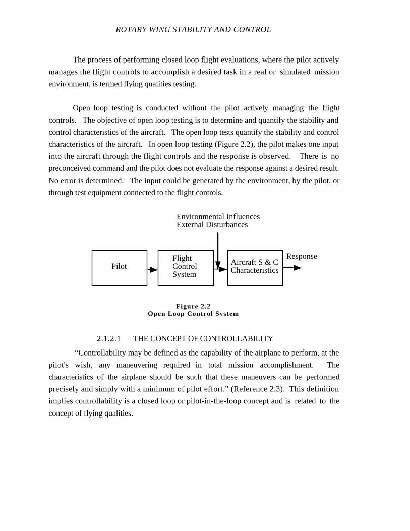
Open loop testing is conducted without the pilot actively managing the flight
controls. The objective of open loop testing is to determine and quantify the stability and
control characteristics of the aircraft. The open loop tests quantify the stability and control
characteristics of the aircraft. In open loop testing (Figure 2.2), the pilot makes one input
into the aircraft through the flight controls and the response is observed. There is no
preconceived command and the pilot does not evaluate the response against a desired result.
No error is determined. The input could be generated by the environment, by the pilot, or
through test equipment connected to the flight controls.
2.1.2.1 THE CONCEPT OF CONTROLLABILITY
“Controllability may be defined as the capability of the airplane to perform, at the
pilot's wish, any maneuvering required in total mission accomplishment. The
characteristics of the airplane should be such that these maneuvers can be performed
precisely and simply with a minimum of pilot effort.” (Reference 2.3). This definition
implies controllability is a closed loop or pilot-in-the-loop concept and is related to the
concept of flying qualities.
FlightControlSystem
ResponsePilot Aircraft S & C
Characteristics
Environmental InfluencesExternal Disturbances
Figure 2.2Open Loop Control System
PILOT FLYING QUALITIES EVALUATIONS
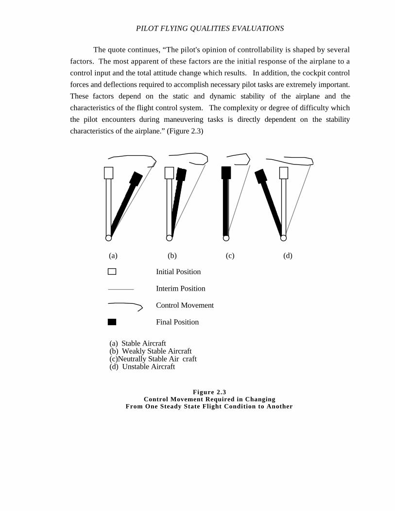
The quote continues, “The pilot's opinion of controllability is shaped by several
factors. The most apparent of these factors are the initial response of the airplane to a
control input and the total attitude change which results. In addition, the cockpit control
forces and deflections required to accomplish necessary pilot tasks are extremely important.
These factors depend on the static and dynamic stability of the airplane and the
characteristics of the flight control system. The complexity or degree of difficulty which
the pilot encounters during maneuvering tasks is directly dependent on the stability
characteristics of the airplane.” (Figure 2.3)
Initial Position
Interim Position
Control Movement
(a) Stable Aircraft(b) Weakly Stable Aircraft(c)Neutrally Stable Air craft(d) Unstable Aircraft
(a) (b) (c) (d)
Final Position
Figure 2.3Control Movement Required in Changing
From One Steady State Flight Condition to Another
ROTARY WING STABILITY AND CONTROL
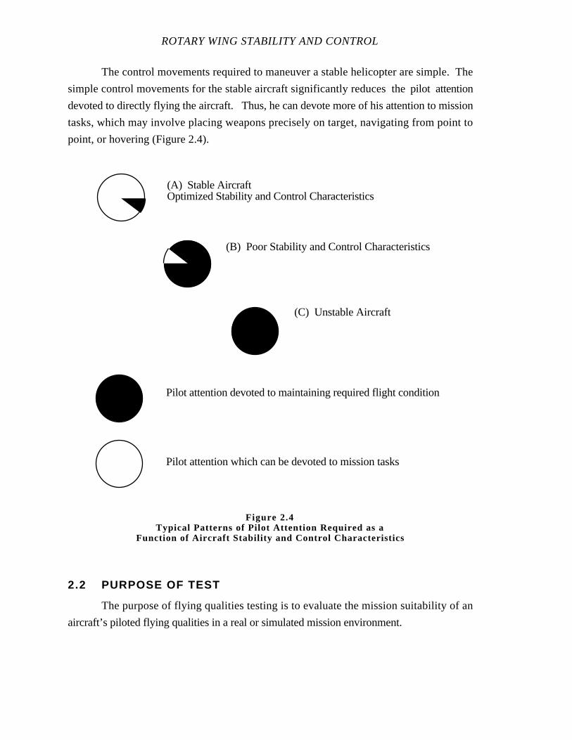
The control movements required to maneuver a stable helicopter are simple. The
simple control movements for the stable aircraft significantly reduces the pilot attention
devoted to directly flying the aircraft. Thus, he can devote more of his attention to mission
tasks, which may involve placing weapons precisely on target, navigating from point to
point, or hovering (Figure 2.4).
2.2 PURPOSE OF TEST
The purpose of flying qualities testing is to evaluate the mission suitability of an
aircraft’s piloted flying qualities in a real or simulated mission environment.
Pilot attention devoted to maintaining required flight condition
Pilot attention which can be devoted to mission tasks
(A) Stable AircraftOptimized Stability and Control Characteristics
(B) Poor Stability and Control Characteristics
(C) Unstable Aircraft
Figure 2.4Typical Patterns of Pilot Attention Required as a
Function of Aircraft Stability and Control Characte ristics
PILOT FLYING QUALITIES EVALUATIONS
2.3 THEORY
Pilot flying qualities evaluation is based on the principle of selecting mission
representative tasks, performing the tasks in a simulated mission environment, observing
the pilot workload required to accomplish the task, and determining if the performance and
workload are acceptable for the mission.
2.3.1 Flying Qualities
Flying qualities are defined as, “Those qualities or characteristics of an aircraft that
govern the ease and precision with which a pilot is able to perform the tasks required in
support of an aircraft role.” (Reference 2.3). Generally, the definition of flying qualities is
the same as handling qualities. Either term is used throughout the Flight Test Manual.
Piloted flying qualities are a qualitative evaluation which is controlled and quantified
as much as possible. However, the evaluation requires the subjective judgement of a
trained pilot.
Flying qualities are a comprehensive pilot evaluation of the workload required to
accomplish a task. Factors which influence a pilot's evaluation of flying qualities are the
aircraft stability and control characteristics, flight control system, cockpit interface (displays
and controls), the environment (weather conditions, visibility, turbulence), total mission
requirements, and stress. The pilot’s evaluation may be affected by the displays which
form part of the feedback loop. The aircraft stability and control characteristics may not
change but the piloting tasks can be affected by a change in any element of the control loop
(Figure 2.1). To understand the flying qualities evaluation process and communicate the
results clearly, the following related concepts must be understood.
2.3.2 Mission and Role
The mission and role of an aircraft are defined in the operational requirements
documents and the aircraft specification. The mission of the aircraft is defined as, “The
composite of pilot-vehicle functions that must be performed to fulfill operational
requirements. May be specified for a role, complete flight, flight phase, or a flight
subphase.” (Reference 2.3). The important element in the definition of mission is
operational requirements. The term mission refers to the operational environment in which
ROTARY WING STABILITY AND CONTROL
the aircraft is intended to be used. The role of the aircraft is defined as, “The function or
purpose that defines the primary use of an aircraft.” (Reference 2.3). The role of the
aircraft defines only the general use of the aircraft.
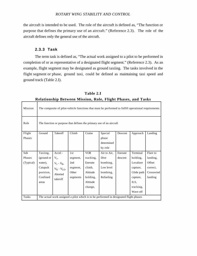
2.3.3 Task
The term task is defined as, “The actual work assigned to a pilot to be performed in
completion of or as representative of a designated flight segment.” (Reference 2.3). As an
example, flight segment may be designated as ground taxiing. The tasks involved in the
flight segment or phase, ground taxi, could be defined as maintaining taxi speed and
ground track (Table 2.I).
Table 2.I
Relationship Between Mission, Role, Flight Phases, and Tasks
Mission The composite of pilot-vehicle functions that must be performed to fulfill operational requirements
Role The function or purpose that defines the primary use of an aircraft
Flight
Phases
Ground Takeoff Climb Cruise Special
phase
determined
by role
Descent Approach Landing
Sub
Phases
(Typical)
Taxiing,
(ground or
water),
Catapult
position,
Confined
areas
Accel -
V1,
V1 - VR,
VR - VLO,
Aborted
takeoff
1st
segment,
2nd
segment,
Other
segments
VOR
tracking,
Enroute
climb,
Altitude
holding,
Altitude
change,
Air to Air,
Dive
bombing,
Low level
bombing,
Refueling
Enroute
descent
Terminal
holding,
Localizer
capture,
Glide path
capture,
ILS,
tracking,
Wave off
Flare to
landing,
Offset
correct,
Crosswind
landing
Tasks The actual work assigned a pilot which is to be performed in designated flight phases
PILOT FLYING QUALITIES EVALUATIONS
2.3.4 Performance
Flying qualities performance is defined as, “The precision of control with respect to
aircraft movement that a pilot is able to achieve in performing a task.” (Reference 2.3).
Performance is a quantifiable measure. For the example task of maintaining ground track,
performance is quantified as maintaining taxi line and runway center line between the main
landing gear.
The evaluation process involves judgement of pilot workload relative to degree of
performance. The degree of precision is defined initially by the test team prior to the
evaluation. Two degrees of precision are necessary for the process of assigning flying
qualities ratings, desired and adequate performance.
2.3.4.1 DESIRED PERFORMANCE
Desired performance is the level of performance required to accomplish the task
successfully in all mission environments. In the ground taxiing example, desired
performance may be defined as maintaining nose gear on taxi line and runway center line
within ± 5 ft. The degree of precision required for desired performance is determined
from operational requirements. Our example aircraft may be required to operate in
confined areas where taxi space is severely limited. In this environment, a high degree of
precision in taxiing is required. Achieving desired performance indicates the task can be
performed in the complete mission environment.
2.3.4.2 ADEQUATE PERFORMANCE
Adequate performance is a lower level of performance achievable only with the
application of a higher level of pilot workload. Adequate performance is determined from
operational requirements as well. Adequate performance indicates the task can be
performed in a portion of the mission environment, but not in the complete environment.
In our example, adequate taxi performance may be defined as maintaining nose gear on taxi
line and runway center line ± 10 ft. Therefore, the aircraft could not be taxied in confined
areas where the degree of precision required is ± 5 ft.

ROTARY WING STABILITY AND CONTROL
2.3.5 Compensation
Compensation is defined as, “The measure of additional pilot effort and attention
required to maintain a given level of performance in the face of less favorable or deficient
characteristics.” (Reference 2.3). In our taxiing example, the compensation necessary to
maintain desired performance could be described as the frequency and magnitude of
directional control activity when attempting a straight ahead taxi.
2.3.6 Workload
The total pilot workload consists of workload due to compensation foraircraft
deficiencies plus workload due to the task. In the taxi example, the total workload could
be described as the frequency and magnitude of directional control activity required to
initiate a taxi turn while maintaining desired performance. Generally, when describing a
task, the evaluation pilot describes the total workload as follows:
“Maintaining directional control during ground taxi in calm wind conditions
over level prepared surfaces with the nose wheel ± 5 ft of the desired taxi
line was easy, requiring ± 1/4 in directional control inputs every 8 to 10 s.”
In this example, the pilot described the task, the environment, the desired performance, and
the pilot workload.
2.3.7 Environment
The environment, both inside and outside the cockpit, influences the pilot's ability
and workload required to complete the task. The internal environment is the sum of the
tasks the pilot must perform simultaneously to accomplish the mission. It is one task to
taxi the aircraft without performing other functions and another task to taxi the aircraft
while tuning radios, making radio calls, and copying clearances. The taxi task can be
significantly different when taxiing on a smooth, level, prepared surface in calm winds as
compared to taxiing on unprepared surfaces or in gusty crosswinds.
Such conditions as day, night, Visual Meteorological Conditions (VMC),
Instrument Meteorological Conditions (IMC), and turbulence level are environmental
factors that affect visual cues, disturbance levels, and pilot workload. These factors affect
pilot opinion of flying qualities and they should be specified in the test conditions.
PILOT FLYING QUALITIES EVALUATIONS
Evaluating the task in a realistic operational environment minimizes the test pilot’s
extrapolation of his qualitative assessment. Generally, it is impractical to reproduce the
environment in full fidelity. When some aspects of the environment are unavailable for the
test program, it might be beneficial to introduce carefully designed, artificial aspects to
approximate the operational environment and reduce extrapolation. For example, the test
pilot might be required to perform a secondary task simultaneous with the evaluation task.
Performing the secondary task simulates a realistic high stress environment.
2.3.8 Composite or Specific Ratings
Since the purpose of piloted flying qualities evaluations is to determine mission
suitability of an aircraft, we may be tempted to assign an overall evaluation to the aircraft
for the complete mission, but this composite approach is not practical. The complete
mission is composed of many different flight phase, sub-phases, and tasks; each performed
in different environments. Therefore, little useful information can be communicated about
specific aircraft capabilities by assigning one rating. Similarly, if an entire flight phase is
evaluated, there is little likelihood of the evaluation being performed in the same
environment with the aircraft in the same state.
On the other hand, a separate, distinct task can be evaluated under one set of
environmental conditions. Evaluating the aircraft for the complete mission using separate
tasks, involves specifying and evaluating all the tasks which constitute the complete
mission. Obviously, resources are not available to complete a flight test program of such
magnitude. Therefore, task selection must consider the most important, critical, and
representative tasks for the aircraft’s mission.
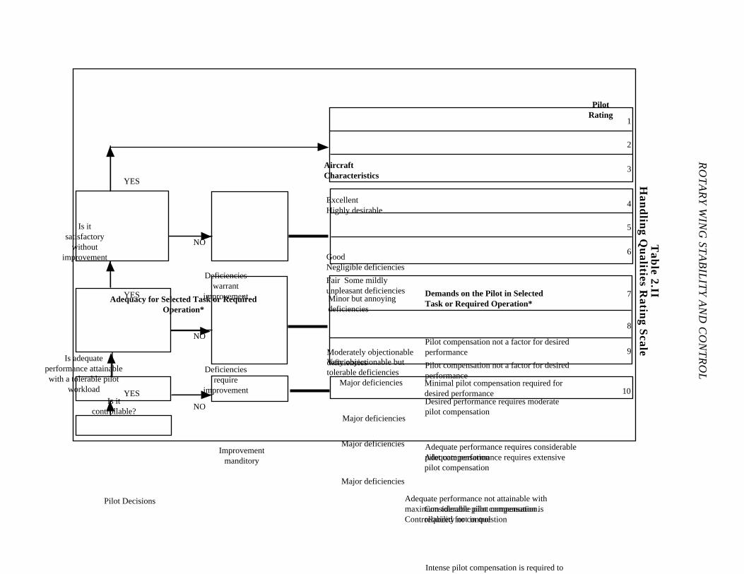
2.3.9 Handling Qualities Rating Scale
Having defined the elements which are the foundation of the Handling Qualities Rating
(HQR) scale, let us examine the scale and the pilot decisions required to use the scale
(Table 2.II). The pilot, having defined the mission (selected the task, established the
performance requirements, both desired and adequate, and determined the environment),
performs the task. The pilot uses the maximum compensation necessary to obtain desired
performance. If the desired performance is obtained easily, the pilot uses a lower level of
compensation and total workload to accomplish the task; he does not interact frequently in
the aircraft control loop. If the pilot does not achieve the desired performance, he must
RO
TA
RY
WIN
G S
TA
BIL
ITY
AN
D C
ON
TR
OL
Ta
ble
2.II
Ha
nd
ling
Qu
alitie
s Ra
ting
Sca
le
Adequacy for Selected Task or RequiredOperation*
AircraftCharacteristics
Demands on the Pilot in SelectedTask or Required Operation*
PilotRating
Pilot Decisions
YES
Is adequateperformance attainablewith a tolerable pilot
workload
Deficienciesrequire
improvement
Is itsatisfactory
withoutimprovement
YES
YES
NO
NO
Deficiencieswarrant
improvement
Improvementmanditory
Is itcontrollable?
10
Major deficiencies
Adequate performance not attainable withmaximum tolerable pilot compensation.Controllability not in question
Major deficiencies
7
Intense pilot compensation is required toretain control
Major deficiencies
9
Major deficiencies
Considerable pilot compensation isrequired for control
8
Minor but annoyingdeficiencies
Desired performance requires moderatepilot compensation
4
Moderately objectionabledeficiencies
Adequate performance requires considerablepilot compensation
5
Very objectionable buttolerable deficiencies
Adequate performance requires extensivepilot compensation
6
Fair Some mildlyunpleasant deficiencies
Minimal pilot compensation required fordesired performance
3
GoodNegligible deficiencies
Pilot compensation not a factor for desiredperformance
2
ExcellentHighly desirable
Pilot compensation not a factor for desiredperformance
1
NO
PILOT FLYING QUALITIES EVALUATIONS
increase his compensation trying to obtain desired performance. He may have to reduce
the time spent on auxiliary or supporting tasks and direct his entire concentration to
achieving desired performance for the evaluation task.
The pilot must maintain situational awareness at all times and operate the aircraft
safely. If the pilot is unable to achieve desired performance with appropriate compensation
(some auxiliary tasks cannot be ignored), he attempts to achieve adequate performance.
Again the level of compensation used is that required to achieve adequate performance.
This discussion assumes the pilot can control the aircraft and is able to perform the task. If
controllability is in question, the pilot must direct all his attention to basic aircraft control
and is unable to perform any mission tasks.
While the pilot performs the task, he describes task performance, compensation,
and total workload. The pilot makes his comments using the simplest piloting terms
possible. Do not analyze the results or aircraft response in complex stability and control
terminology. Keep the comments simple and direct. The comments should be recorded
concurrent with performing the task and shortly after task completion; ideally, recorded on
a voice recorder and summarized on kneeboard cards. Comments should include a
description of the environment at the time of task performance.
Immediately after task completion and after making all relevant comments, the pilot
assigns the HQR. Starting at the lower left hand corner of the HQR scale (Table 2.II), the
pilot enters the decision matrix. The pilot follows the decision matrix, moving upward and
branching to the right until he assigns a HQR.
Is it “Controllable”?
To control is to exercise direction of, to command, or to regulate. The
determination as to whether the airplane is controllable must be made within the framework
of the defined mission or intended use. An example of the considerations of this decision
would be the evaluation of an aircraft’s handling qualities during which the evaluation pilot
encounters a situation in which he can maintain control only with complete and undivided
attention. The aircraft is “controllable” in this situation in the sense that the pilot can
maintain control only by restricting the tasks and maneuvers he is called upon to perform
and by giving the configuration undivided attention. However, to answer, “Yes, it is
controllable in the flight phase or task,” the pilot must be able to retain control in all mission
ROTARY WING STABILITY AND CONTROL
oriented tasks and other required operations without sacrificing effort and attention to his
overall duties. If the final overall answer to these questions is no, the pilot will assign an
HQR-10.
A major division in the rating scale is made between HQR-9 and HQR-10. If
control is or will be lost, the rating is 10. If control is or can be maintained, the rating is 9
or below. A rating of 9.5 is not permitted; therefore, a decision on control must be made
here.
Is adequateperformanceattainablewith atolerablepilot workload?
There are really two questions asked here. First, is adequate performance
attainable? If the pilot attains at least the adequate tolerance, the answer to the first part is
yes. However, if adequate performance cannot be achieved, the answer is no. The
second part of the question is, “Is the workload tolerable while attaining adequate
performance?” Tolerable workload describes the capability to perform auxiliary tasks such
as communication, navigation, and maintaining situational awareness. The pilot must be
able to complete auxiliary tasks in addition to the evaluation task to maintain safe flight
conditions. The pilot may consider that the designated flight phase or task can be
accomplished but the effort, concentration, and workload required are of such magnitude
that the pilot rejects the aircraft for this phase of its intended use. If the answer to either of
the two questions is “No”, then the aircraft is not suitable for the purpose, though it is
controllable.
An HQR-7 states that adequate performance is not attainable with maximum
tolerable pilot compensation, but controllability is not in question. The pilot workload is
beyond what is tolerable although adequate performance may have been attained. The
pilot’s workload requires a major portion of his attention, butthe issue is not one of
controllability.
An HQR-8 is applied to a piloting requirement which can only be done with a
minimum of cockpit duties. Considerable pilot compensation is then required for control
of the task.
PILOT FLYING QUALITIES EVALUATIONS
An HQR-9 may enter the dangerous control area being just controllable with
complete attention to the task at hand. Intense pilot compensation is required to retain
control. The rating appears similar to the HQR-10, but the pilot has already determined that
it was controllable.
Is it satisfactorywithoutimprovement?
The next major question to be answered is “Is it satisfactory without improvement?”
If the answer is yes, the pilot’s definition might be that it isn’t perfect, or even good, but
that it is good enough to not require changes at least in this model. It meets a standard; it
has sufficient goodness; it’s of a kind to meet all pilot demands for the intended use. If the
answer to this question is no, the implication is that adequate or desired performance can be
achieved only with a workload which impacts the pilot’s capability to perform auxiliary, or
secondary, tasks simultaneously with the evaluation task. In this case, a deficiency exists
which warrants improvement and the pilot selects the rating which best describes the
situation.
HQR-4 means the desired level of performance was reached but with some work
categorized as moderate pilot compensation. The aircraft characteristic is minorbut
annoying to the piloting task. If challenged enough, pilots can achieve desired levels of
performance but the workload seems more than moderate. The words for an HQR-5 may
better describe the workload although desired performance was attained. A division
between desired and adequate occurs within this major section of the scale. At times it
appears an HQR-5 is a better rating for a desired performance level. Discussions over
many years have lead to two approaches. One allows an HQR-4.5 when a desired level of
performance is attained but the workload is higher than described. The other allows an
HQR-5 to be assigned to a desired level of performance at higher than described workload.
Assigning an HQR-6 to a desired level of performance is too extreme and normally means
the task and tolerances need to be better defined.
When desired performance is not attainable, an HQR-5 or 6 is the rating assigned
within the major division. The pilot has determined that the characteristic is not satisfactory
and the desired level of performance is not attainable. The rating now rests on the words
for demands on the pilot and/or aircraft characteristics. Both should be considered when
ROTARY WING STABILITY AND CONTROL
choosing the rating. For the demands on the pilot, adequate performance requires
considerable (HQR-5) or extensive (HQR-6) pilot compensation. For the aircraft,the
deficiencies are moderately objectionable (HQR-5) or very objectionable but tolerable
(HQR-6).
Yes,it is satisfactorywithoutimprovement.
If task performance is satisfactory without improvement, desired performance was
attained. The pilot selects the rating which best describes the situation. “Excellent, Highly
desirable. Pilot compensation not a factor for desired performance,” HQR-1. This rating
is selected if the pilot makes one control input, the desired performance is achieved without
error, and additional pilot inputs are not required. “Good Negligible deficiencies. Pilot
compensation not a factor for desired performance,” HQR-2. This rating implies that
desired performance was not achieved on the first pilot input, but subsequent inputs were
very minimal. “Fair, Some mildly unpleasant deficiencies. Minimal pilot compensation
required for desired performance,” HQR-3. This rating implies that a deficiency exists but
its correction is not required to accomplish the mission.
Half ratings are discouraged! The rating scale is broad enough to cover
contingencies from highly desirable flying qualities to situations where control will be lost.
Specifically, half ratings are not permitted between major decision points. HQRs assigned
by trained test pilots to well defined tasks with defined performance in the same
environment are repeatable. The HQRs are repeatable for the same test pilot over time or
for different test pilots. Studies show the average standard deviation for well constructed
flying qualities evaluations using HQRs is less than one.
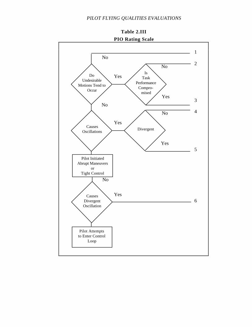
2.3.10 Additional Rating Scales
An aid to assist the pilot describing performance, workload, and environment is the
Pilot Induced Oscillation (PIO) rating scale (Table 2.III). This rating scale helps to classify
the susceptibility of the task to PIO.
PILOT FLYING QUALITIES EVALUATIONS
Table 2.III
PIO Rating Scale
Pilot InitiatedAbrupt Maneuvers
orTight Control
Yes
Pilot Attemptsto Enter Control
Loop
CausesDivergentOscillation
Yes
No
6
5
CausesOscillations
Divergent
IsTask
PerformanceCompro-
mised
DoUndesirable
Motions Tend toOccur
Yes
No 4
3Yes
No
No
No
1
2
Yes

ROTARY WING STABILITY AND CONTROL
The Turbulence Rating Scale (Table 2.IV) is a tool used to describe the
environment. This scale, extracted from the Flight Information Handbook (Reference 2.1),
describes conditions which exist during task performance.
Table 2.IV
Turbulence Rating Scale
INTENSITY AIRCRAFT REACTION REACTION INSIDE AIRCRAFT
LIGHT
Turbulence
Chop
Turbulence that momentarily causesslight, erratic changes in altitudeand/or attitude.
Turbulence that causes slight, rapidand somewhat rhythmic changes inaltitude or attitude
Occupants may feel a slight strainagainst seat belts or shoulder straps.Unsecured objects may be displacedslightly. Food service may beconducted and little or no difficulty isencounter in walking.
MODERATE
Turbulence
Chop
Turbulence that causes changes inaltitude and/or attitude, but with theaircraft remaining in positive controlat all times. It usually causesvariations in indicated airspeed.
Turbulence that causes rapid bumps orjolts without appreciable changes inaircraft altitude or attitude.
Occupants feel definite strains againstseat belts or shoulder straps.Unsecured objects are dislodged. Foodservice and walking are difficult.
SEVERE
Turbulence Turbulence that causes large, abruptchanges in altitude and/or attitude. Itusually causes large variations inindicated airspeed. Aircraft may bemomentarily out of control.
Occupants are forced violentlyagainst seat belts or shoulder straps.Unsecured objects are tossed about.Food service and walking areimpossible.
EXTREME
Turbulence Turbulence in which the aircraft isviolently tossed about and ispractically impossible to control. Itmay cause structural damage.
FREQUENCY DEFINITION
Occasional Less than 1/3 of the time
Intermittent 1/3 to 2/3 of the time
Continuous More than 2/3 of the time

PILOT FLYING QUALITIES EVALUATIONS
The Vibration Rating Scale (Table 2.V) is another rating scale the pilot uses to
describe the environment. This scale classifies, quantifies,and communicates in-flight
observations.
Table 2.V
Vibration Rating Scale
Degree of Vibration Description Pilot Rating
No Vibration 0
Slight Not apparent to experienced aircrew fully occupied
by their tasks, but noticeable if their attention is
directed to it or if not otherwise occupied.
1
2
3
Moderate Experienced aircrew are aware of the vibration but it
does not affect their work, at least over a short
period.
4
5
6
Severe Vibration is immediately apparent to experienced
aircrew even when fully occupied. Performance of
primary task is affected or tasks can be done only
with difficulty.
7
8
9
Intolerable Sole preoccupation of aircrew is to reduce vibration. 10
Based on the Subjective Vibration Assessment Scale developed by the Aeroplane andArmament Experimental Establishment, Boscombe Down, England.
2.4 TEST METHODS AND TECHNIQUES
2.4.1 General
Since the objective of flying qualities evaluations is communicating the test pilot's
qualitative assessment of the aircraft mission suitability, an orderly process should be
observed. As is true for any communication, format should be standardized so data
gathered by different pilots can be compared with the least chance of misinterpretation. The
guidelines to accomplish the evaluation process are outlined in subsequent sections.
ROTARY WING STABILITY AND CONTROL
2.4.2 Test Planning
During the planning stage, the test team refers to specifications and requirements
documents to determine the aircraft mission. The team determines the environment in
which the aircraft will operate and which they will use for task evaluation. The team
determines the mission representative tasks for evaluation and the priority for task
evaluation. The team establishes the performance tolerances required for task completion,
both desired and adequate. The team relies on fleet experienced pilots to guide task and
performance selection.
Following mission definition, task selection, and performance tolerance
determination, the team prepares the flight test data cards. The flight test data cards detail
the specific task/maneuver sequences for the pilot evaluation. Usually an optimistic
approach is taken in planning, including more tasks than can be accomplished during the
evaluation. However, the tasks are prioritized and sequenced in a logical manner. The
sequence is arranged for the most efficient use of the flight time.
The data card is used to prompt the pilot for all desired information. In general,
cards that solicit narrative responses as opposed to one word answers are preferred.
2.4.3 Test Techniques
Following the flight test data card, the test pilot executes the evaluation tasks. The
pilot performs the tasks with the same level of aggressiveness applicable to the mission
environment. The test pilot uses the HQR Scale, PIO Rating Scale, Turbulence Rating
Scale, and Vibration Rating Scale to quantify his observations. All are recorded on the
data card.
The test pilot makes comments extemporaneously while performing the evaluation
tasks. The data card lists items of interest. Generally, the pilot refers to the data card after
finishing the task and completes his observations. The substance of evaluation data lies in
the pilot comments.
Recording comments and rating data simultaneously is both difficult and time
consuming while performing the evaluation tasks. Therefore, it is advantageous to carry
some form of voice recorder on board. A voice activated unit is most efficient.
PILOT FLYING QUALITIES EVALUATIONS
The following summarizes the evaluation process.
1. Fly the task/maneuver as planned.
2. Observe both the vehicle's responses and the nature of control inputs, relate
the two in the closed control loop. What the aircraft did and how the pilot responded?
3. Make extemporaneous comments of pertinent observations during task
performance.
4. Use plain piloting language to describe direct observations not technical or
engineering language (e.g., frequency, damping, etc.). Do not interpret the results.
5. Be complete in comments, when the voice tape is transcribed leave no room
for doubt about in-flight comments.
6. Refer to the data card at task completion and ensure all items are covered.
7. Assign a HQR using the rating scale each time. Assign the HQR as soon
as the task is completed, while everything is in perspective. Complete the data card.
Review the rating. If a change in rating is considered, justify it. Summarize the primary
reasons for the rating.
8. Describe any pertinent environmental factors such as weather, turbulence,
etc., which qualify the evaluation.
As soon as feasible, the test pilot conducts a debrief with the flight test team. He
transcribes his comments from the voice tape and data cards and clarifies any confusion in
the comments while the evaluation is fresh in his mind. The transcription is accomplished
with one of the test engineers and put into a format for analysis.
2.4.4 Data Required
The data required for a piloted flying qualities evaluation are task definition,
definition of desired and adequate performance, actual performance achieved, task
environment, pilot compensation and total workload required for the task, HQR, any
additional numerical ratings assigned to clarify the HQR and the transcribed pilot
comments. These data are obtained from the flight test data cards and the voice recorder.
ROTARY WING STABILITY AND CONTROL
2.4.5 Safety Considerations/Risk Management
The principal consideration for flight test is flight safety. A test pilot or flight test
crew can become so absorbed in performing, observing, and recording a task evaluation
that basic aircraft control, situational awareness and flight discipline are lost. Under no
circumstances is task evaluation more important than maintaining safe operating conditions.
If flight safety is compromised, stop the evaluation. Regain basic flight discipline,
situational awareness, and flight safety before continuing. If the task cannot be
accomplished without further compromise, stop the evaluation and replan the flight on the
ground.
2.4.6 Special Factors Affecting Evaluation in Helicopters
A number of factors peculiar to helicopters influence the evaluation process. The
following list contains some factors which should be considered in planning and executing
helicopter flight test.
1. Ambient vibration levels, primarily from the rotor system.
2. Cockpit field of view downward for ground reference maneuvers.
3. The accelerations perceived by the pilot due to seat location relative to the
center of gravity may be particularly important in terms of the cues the pilot senses in
closed loop tasks.
4. Tail cone or nose boom strike by the rotor.
5. Tip path plane dynamics due, for example, to a particular aerodynamic
loading.
6. Effectiveness of RPM governor. For particular tests, the governor
characteristics may need to be accommodated to satisfy test requirements.
7. Control and motion coupling. Pilots may be required to suppress such
coupling.
8. Control nonlinearities. Open-loop testing should account for such
possibilities.
PILOT FLYING QUALITIES EVALUATIONS
2.5 DATA PRESENTATION
The data are presented in narrative format in the results and discussion section of
the report. A sample narrative presentation is a follows:
"Maintaining directional control during ground taxi in calm wind conditions
over level prepared surfaces with the nose wheel ± 5 ft of the desired taxi
line was easy, requiring ± 1/4 in directional control inputs every 8 to 10 s
(HQR 3)."
Piloted flying qualities evaluation data for a large number of mission tasks may be
summarized in tabular format and included in an appendix. Data for the same task
performed under different environmental conditions, or by different pilots, may be
summarized in tabular format. Comparative data are best presented in graphical format.
Preserve the perspective that flying qualities data is bottom line information and the
results of open loop testing, including Military Specification compliance testing, supports
this bottom line. Present the closed loop or handling qualities results first. Use the open
loop data to support the pilot qualitative evaluation. Too often the quantitative testing
results are presented. The flying qualities or qualitative data is presented in less detail or in
a less definitive format. This form of presentation can misdirect the emphasis.
Furthermore, it does not provide the proper focus for the open loop data. We are interested
in open loop data primarily for their explanatory function with respect to the observed
flying qualities.
2.6 GLOSSARY
2.6.1 Notations
ft Foot
HQR Handling Qualities Rating
IMC Instrument Meteorological Conditions
PIO Pilot Induced Oscillation
s Second
VMC Visual Meteorological Conditions
ROTARY WING STABILITY AND CONTROL
2.7 REFERENCES
1. Flight Information Handbook, DOD Flight Information Publication,
Defense Mapping Agency Aerospace Center, St. Louis, MO, 23 August, 1990.
2. Naval Test Pilot School Flight Test Manual,Fixed Wing Stability and
Control, Theory and Flight Test Techniques, USNTPS-FTM-No.103, U. S. Naval Test
Pilot School, Patuxent River, MD, 1 January, 1975, Revised 1 November, 1981.
3. NASA Technical Note, NASA TN D-5153, “The Use of Piloted Rating In
The Evaluation Of Aircraft Handling Qualities”, National Aeronauticsand Space
Administration, Washington, D.C., April, 1969.
CHAPTER THREE
OPEN LOOP TESTING
PAGE3.1 INTRODUCTION 3.1
3.2 PURPOSE 3.1
3.3 THEORY 3.2
3.3.1 General 3.2
3.3.2 Stability 3.2
3.3.2.1 Static Stability 3.2
3.3.2.2 Dynamic Stability 3.3
3.3.3 Damping 3.4
3.3.4 Control Response 3.4
3.3.5 Second Order System 3.5
3.3.6 First Order Systems 3.15
3.4 TEST METHODS AND TECHNIQUES 3.18
3.4.1 General 3.18
3.4.2 Trim 3.18
3.4.3 Input Shape 3.18
3.4.4 Input Amplitude 3.19
3.4.5 Quickness of Input 3.20
3.4.6 Excitation Methods 3.20
3.4.7 Test Technique 3.21
3.4.8 Data Required 3.22
3.4.9 Test Criteria 3.22
3.4.10 Data Requirements 3.22
3.4.11 Safety Considerations/Risk Management 3.22
3.5 DATA REDUCTION 3.23
3.5.1 General 3.23
3.5.2 Data Presentation 3.26
ROTARY WING STABILITY AND CONTROL
3.6 DATA ANALYSIS 3.26
3.7 MISSION SUITABILITY 3.26
3.8 SPECIFICATION COMPLIANCE 3.26
3.9 GLOSSARY 3.27
3.9.1 Notations and Definitions 3.27
3.9.2 Greek Symbols 3.28
3.10 REFERENCES 3.28
OPEN LOOP TESTING
CHAPTER THREE
FIGURES
PAGE
3.1 Spring Mass Damper System 3.6
3.2 The Complex Plane 3.9
3.3 Effect of Increasing Spring Constant 3.10
3.4 Time Histories of First and Second Order Systems 3.11
3.5 Relationship of Root Location on Complex Plane to Motion Characteristics 3.14
3.6 Zw Root Location on Complex Plane 3.16
3.7 Typical Stable First Order Response 3.17
3.8 Examples of Test Inputs for Determination of Open Loop Dynamics 3.19
3.9 Graphic Method for Determining T1/2 and C1/2 3.24
3.10 Graphic Solution for Damping Ratio 3.25

ROTARY WING STABILITY AND CONTROL
CHAPTER THREE
EQUATIONS
PAGEm˙x + Bx + Kx = 0 eq 3.1 3.7
λ2 + Bm λ + Km = 0
eq 3.2 3.7
λ1,2
= - B2m
± ( B2m)
2
- Kmeq 3.3 3.8
x(t) = C1 e
λ1t + C
2 e
λ2t
eq 3.4 3.8
x(t) = Ae-ζωnt
sin ωn 1 -ζ2 t
eq 3.5 3.9
BCRIT
= 2m (Km)
12
eq 3.6 3.10
ωn = (Km)
12
eq 3.7 3.12
ζ = BB
CRIT eq 3.8 3.13
λ2 + 2 ωn ζλ + ωn
2 = 0eq 3.9 3.13
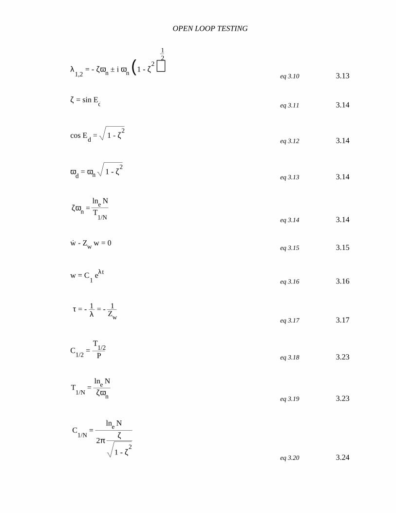
OPEN LOOP TESTING
λ1,2
= - ζωn ± i ωn (1 - ζ2)
12
eq 3.10 3.13
ζ = sin Ed eq 3.11 3.14
cos Ed = 1 - ζ
2
eq 3.12 3.14
ωd = ωn 1 - ζ
2
eq 3.13 3.14
ζωn = lne N
T1/N eq 3.14 3.14
w. - Zw w = 0
eq 3.15 3.15
w = C1 eλt
eq 3.16 3.16
τ = - 1λ
= - 1Zw eq 3.17 3.17
C1/2
= P
T1/2
eq 3.18 3.23
T1/N
= lne N
ζωn eq 3.19 3.23
C1/N
= lne N
2πζ
1 - ζ2
eq 3.20 3.24
CHAPTER THREE
OPEN LOOP TESTING
3.1 INTRODUCTION
The major reason for conducting flying qualities evaluations is to determine if the
pilot-aircraft combination can perform safely and precisely the tasks required for the
mission. This determination can be made by the pure qualitative approach to stability and
control testing via flying qualities evaluation or closed loop testing. However, the flying
qualities evaluation is only part of the complete test program. Open loop testing is
conducted to quantify the stability and control parameters and support the test pilot’s
qualitative evaluation. A balance between qualitative pilot opinion and quantitative testing
must be achieved in any stability and control test and evaluation program.
The open loop system the pilot interfaces with in closed loop testing includes the
augmented aircraft characteristics and the control system characteristics. Open loop testing
is aimed at determining the transfer characteristics of these elements.
3.2 PURPOSE
The purpose of open loop testing is to quantify stability and control evaluations.
Specific objectives of open loop testing are:
1. Substantiate the pilot's qualitative opinion.
2. Document characteristics of the aircraft-control system combination.
3. Provide data for comparing the aircraft characteristics with others and for
formulating future designs.
4. Provide baseline data for expansion of flight and center of gravity envelope.
5. Determine compliance or noncompliance with specifications.
6. Provide data for predictive closed loop analysis.
7. Provide data for simulator applications.

ROTARY WING STABILITY AND CONTROL
3.3 THEORY
3.3.1 General
To exhibit satisfactory flying qualities, the aircraft must possess a balance of both
stability and control. The optimum blend depends on the aircraft’s mission. A degree of
stability is necessary to reduce pilot workload. However, too much stability can degrade
the pilot's ability to maneuver the aircraft. An optimum blend of stability and control is one
goal of the aircraft designer. When the optimum mix of stability and control is attained, the
aircraft flying qualities enhance the pilot’s ability to perform the mission.
Stability and control can be viewed as opposite ends of a spectrum, with stability on
one end and control on the other. While both characteristics are desirable, too much of one
degrades the contributions of the other. A helicopter with a high degree of stability is easy
to fly straight and level but is difficult to maneuver quickly and precisely. On the other
hand, a helicopter which responds quickly to control inputs may lack sufficient stability for
flight in instrument conditions. Static and dynamic stability partially determine the pilot's
ability to control the aircraft. While static instability about any axis is generally
undesirable, excessively strong positive static stability can degrade maneuverability to an
unacceptable degree. For some tasks, neutral static stability is acceptable or even desirable.
The optimum level of static stability depends on the specific mission oriented tasks of the
aircraft.
3.3.2 Stability
The helicopter is a dynamic system. It is a body in motion under the influence of
forces and moments producing or changing motion. In order to investigate the motion of
the helicopter, it is necessary to establish a condition of equilibrium between opposing
forces and moments. When the equilibrium condition is achieved, the stability
characteristics can be determined.
3.3.2.1 STATIC STABILITY
Static stability is the sum of the forces and moments following a disturbance from
an equilibrium flight condition. The helicopter is statically stable (positive static stability) if
forces and moments are generated to restore the aircraft toward equilibrium. The helicopter
is statically unstable (negative static stability) if the sum of forces and moments following a
OPEN LOOP TESTING
disturbance from an equilibrium flight condition cause a further divergence from
equilibrium. The helicopter has neutral static stability if the forces and moments following
a disturbance from an equilibrium flight condition cause the helicopter to continue in the
direction of the disturbance without diverging from or converging toward equilibrium.
Static stability is represented by the initial response of the aircraft when disturbed from an
equilibrium flight condition. The aircraft has positive static stability if the initial response is
toward the equilibrium flight condition. The aircraft has negative static stability if the initial
response is away from the equilibrium condition. If the aircraft continues in the direction
of the disturbance without a return toward or away from the equilibrium flight condition,
the aircraft has neutral static stability.
Static stability characteristics must be investigated at equilibrium flight conditions in
which all forces and moments are in balance. In wind tunnel tests, the forces and moments
produced by a disturbance from an equilibrium flight condition can be measured directly.
The direct in flight measurement of static stability parameters is not feasible inmany
instances. Therefore, the flight test team measures parameters which give indications of
static stability. These indications are adequate to establish the mission effectiveness of the
aircraft and are more meaningful to the pilot than the numerical value of actual static
stability parameters. For example, static longitudinal stability is evaluated through the
longitudinal control displacement required to counter or balance an off trim airspeed
condition, not by measuring directly the moment produced by the off trim airspeed
condition.
3.3.2.2 DYNAMIC STABILITY
Dynamic stability is the response of the aircraft over time after the initial reaction to
a disturbance from an equilibrium flight condition. The time history of the aircraft response
can be either oscillatory or aperiodic. The time history response can be either convergent,
neutral, or divergent. The aircraft has positive dynamic stability if the response converges
to the initial equilibrium flight condition. If the response diverges from the initial
equilibrium flight condition, the aircraft has negative dynamic stability. The response can
be aperiodic and convergent (positive dynamic stability), aperiodic and divergent (negative
dynamic stability), oscillatory and convergent (positive dynamic stability), or oscillatory
and divergent (negative dynamic stability). With neutral dynamic stability, the response
neither converges or diverges. The true oscillatory neutral response is seldom found in
ROTARY WING STABILITY AND CONTROL
aircraft dynamic responses. Static stability determines the initial response of the aircraft. If
the aircraft has negative static stability, the initial response is away from trim and the
dynamic response is aperiodic divergent.
As the pilot changes from one equilibrium flight condition to another, one or more
of the aircraft's dynamic modes of motion are excited. Changes are initiated by pilot inputs
which excite these dynamic modes. These modes of motion can be excited by external
perturbations as well. The study of the characteristics of these modes of motion is the
study of dynamics.
Time history parameters of the aircraft modes of motion define the dynamic stability
characteristics. The most important parameters are the frequency and damping ratio of the
motion. The frequency of the motion is the number of cycles per unit time and is a measure
of the quickness of the motion. The term natural frequency,ωn, used in analytical
discussions, is the frequency the motion exhibits with no damping. However, the pilot
observes the damped frequency, ωd, usually referred to simply as frequency, ω.
3.3.3 Damping
Positive damping is the characteristic which causes progressive diminishing of the
amplitudes or rates of the transient motion. Damping is a measure of the subsidence of the
motion. Because it is observable by the pilot, the term damping ratio, ζ, is used rather than
damping to describe the subsidence of an oscillatory motion. Both frequency and damping
ratio are characteristics of a system response which affect flying qualities. For example, if
the damping ratio is too low, aircraft motion is a nuisance when excited by pilot inputs or
by atmospheric disturbances. If the damping ratio is too high, the aircraft response to
control input appears sluggish. Desirable values of these characteristics depend on an
aircraft’s mission. The corresponding characteristic of a first order response is the time
constant,τ, defined as the time to reach 63.2 % of the steady state value.
3.3.4 Control Response
The pilot controls the helicopter through the dynamic modes of motion. The pilot
first excites the dynamic mode, allows the helicopter to respond, and as the helicopter
reaches the desired flight condition, the pilot suppresses the dynamic mode.
OPEN LOOP TESTING
Control response testing is the evaluation of aircraft response following step
displacement of a flight control. Control response testing is open loop testing of the
dynamic response of the aircraft. Aircraft responses are often assumed to be either first or
second order dynamic responses for data reduction purposes.
In discussions of control response, several terms are used. Control power is a
measure of the moment produced per unit of control displacement. Typical units for
control power are lbf in/in control displacement or Newton meter/% control displacement.
Control sensitivity is the initial angular acceleration produced by a unit step control
displacement. Typical units for control sensitivity are deg/s2/in control displacement.
Attitude control effectiveness (attitude control response) is the change in aircraft attitude
achieved in one second following a unit step control displacement. Typical units for
attitude control effectiveness are deg/in control displacement. Rate control effectiveness
(rate control response) is the angular rate achieved one second following a unit step control
displacement. Typical units for rate control effectiveness are deg/s/in control displacement.
3.3.5 Second Order System
A helicopter in flight can be represented by a mass restrained by springs, which are
comparable to static stability, and dampers which are comparable to aerodynamic damping
(Figure 3.1). For simplicity, consider a single degree of freedom to yield the equivalent
spring-mass-damper system in Figure 3.1 (b).
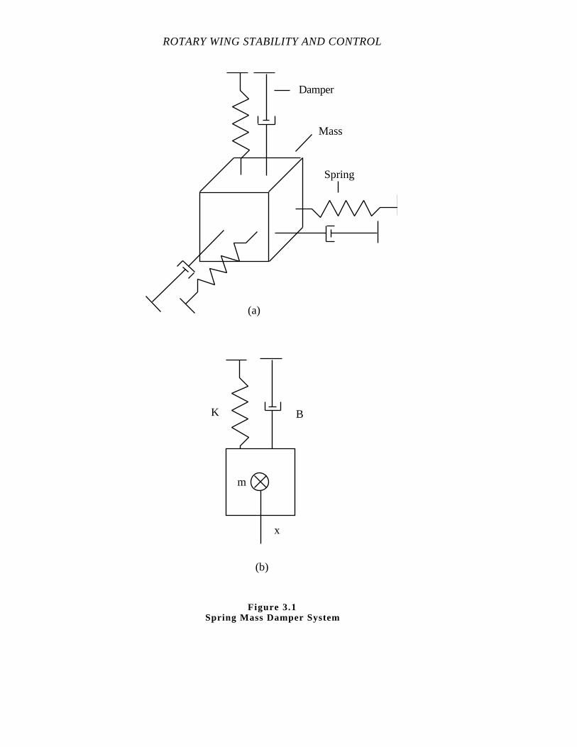
ROTARY WING STABILITY AND CONTROL
K B
m
x
Damper
Mass
Spring
(a)
(b)
Figure 3.1Spring Mass Damper System
OPEN LOOP TESTING
The solution of the equation of motion for the system represented in Figure 3.1 (b)
provides a useful insight into the solution of the more complex equations of motion of the
helicopter. If the mass, m, is displaced from equilibrium an amount, x, and released, the
subsequent free response of the system is described by the following second order linear
homogeneous differential equation:
m˙x + Bx + Kx = 0 eq 3.1
Where:
B - Damping constant
K - Spring constant
m - Mass
x - Displacement
˙x - Acceleration
x - Velocity.
At the moment of release, the spring exerts a force, Kx, in the direction to restore
the mass to its equilibrium position. After release, the viscous damper force opposing the
motion is Bx . The inertia force is m˙x. The characteristic equation can be written as:
λ2 + Bm λ + Km = 0
eq 3.2
Where:
B - Damping constant
K - Spring constant
λ - Characteristic root
m - Mass.
ROTARY WING STABILITY AND CONTROL
Solving the characteristic equation yields the following roots:
λ1,2
= - B2m
± ( B2m)
2
- Kmeq 3.3
Where:
B - Damping constant
K - Spring constant
λ1,2 - Characteristic roots
m - Mass.
The corresponding time responses are as follows:
1. If,B
2m
2
>K
m, λ1 and λ2 are real roots and the time response is a
combination of first order (non-oscillatory) exponential responses of the form:
x(t) = C1 e
λ1t + C
2 e
λ2t
eq 3.4
Where:
C1 and C2 - Constants affected by initial conditions of the motion
e - Base of natural logarithm
λ1,2 - Characteristic roots
t - Time
x - Displacement.
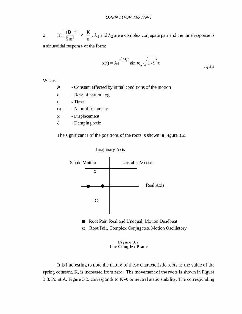
OPEN LOOP TESTING
2. If,B
2m
2
<K
m, λ1 and λ2 are a complex conjugate pair and the time response is
a sinusoidal response of the form:
x(t) = Ae-ζωnt
sin ωn 1 -ζ2 t
eq 3.5
Where:
Α - Constant affected by initial conditions of the motion
e - Base of natural log
t - Time
ωn - Natural frequency
x - Displacement
ζ - Damping ratio.
The significance of the positions of the roots is shown in Figure 3.2.
It is interesting to note the nature of these characteristic roots as the value of the
spring constant, K, is increased from zero. The movement of the roots is shown in Figure
3.3. Point A, Figure 3.3, corresponds to K=0 or neutral static stability. The corresponding
Imaginary Axis
Unstable MotionStable Motion
Real Axis
Root Pair, Real and Unequal, Motion Deadbeat
Root Pair, Complex Conjugates, Motion Oscillatory
Figure 3.2The Complex Plane
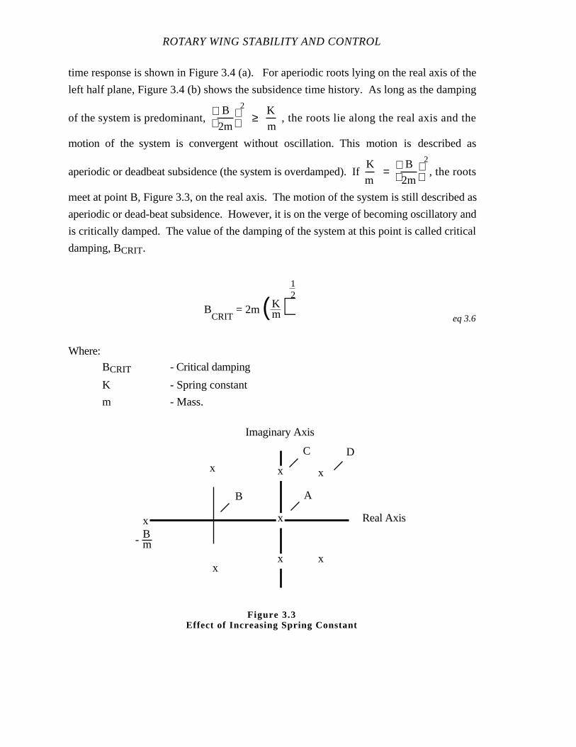
ROTARY WING STABILITY AND CONTROL
time response is shown in Figure 3.4 (a). For aperiodic roots lying on the real axis of the
left half plane, Figure 3.4 (b) shows the subsidence time history. As long as the damping
of the system is predominant, B
2m
2
≥K
m , the roots lie along the real axis and the
motion of the system is convergent without oscillation. This motion is described as
aperiodic or deadbeat subsidence (the system is overdamped). If K
m=
B
2m
2
, the roots
meet at point B, Figure 3.3, on the real axis. The motion of the system is still described as
aperiodic or dead-beat subsidence. However, it is on the verge of becoming oscillatory and
is critically damped. The value of the damping of the system at this point is called critical
damping, BCRIT.
BCRIT
= 2m (Km)
12
eq 3.6
Where:
BCRIT - Critical damping
K - Spring constant
m - Mass.
Imaginary Axis
Real Axis
x
x
x
x
x
x
xx
B A
C D
- Bm
Figure 3.3Effect of Increasing Spring Constant

OPEN LOOP TESTING
Time
Dis
plac
emen
t
Time
Dis
plac
emen
t
Time
Dis
plac
emen
t
Time
Dis
plac
emen
t
Time
Dis
plac
emen
t
(f) Oscillatory divergentPositive static, negative dynamic
(g) Aperiodic DivergentNegative static, negative dynamic
(a) Neutral Static StabilityNeutral static, neutral dynamic
(b) Aperiodic convergent (Deadbeat)Positive static, positive dynamic
ζ > 0
ζ < 0
(d) Oscillatory ConvergentPositive Static, positive dynamic
(c) ζ = 0.7
Initial Disturbance
Time(e) Undamped OscillationPositive static, neutral dynamic
ζ = 0
Dis
plac
emen
t
Time
Dis
plac
emen
t
Figure 3.4Time Histories of First and Second Order Systems
ROTARY WING STABILITY AND CONTROL
If the spring constant is increased further such that K
m>
B
2m
2
, the solutions to
the equation of motion are composed of real and imaginary parts. The roots split at point
B, Figure 3.3, the real part remains constant and as K increases, the imaginary part
becomes larger. The motion of the system is now oscillatory and the frequency increases
as K increases. However, for all values of K, the motion is damped after the disturbing
force is removed.
The measure of the strength of the system to seek an equilibrium condition is called
the system stiffness and is directly related to the square of the system frequency when
damping is not present. This frequency is called the natural frequency, ωn. It is usually a
computed number since most systems have damping and the measured system frequency
will be the damped natural frequency, ωd. The natural frequency for the spring-mass-
damper system is expressed as follows:
ωn = (Km)
12
eq 3.7
Where:
K - Spring constant
m - Mass
ωn - Natural frequency.
The level of dynamic stability of a second order system is generally expressed in
terms of the damping ratio, ζ. It is the ratio of the real system damping constant to the
damping constant which makes the system critically damped and is related to the number of
overshoots in free response:
OPEN LOOP TESTING
ζ = BB
CRIT eq 3.8
Where:
B - Damping constant
BCRIT - Critical damping
ζ - Damping ratio.
The characteristic equation for the spring-mass-damper system, written in terms of
natural frequency and damping ratio, is as follows:
λ2 + 2 ωn ζλ + ωn
2 = 0eq 3.9
The two roots of the equation are:
λ1,2
= - ζωn ± i ωn (1 - ζ2)
12
eq 3.10
Where:
i - Imaginary index
λ1,2 - Characteristic roots
ωn - Natural frequency
ζ - Damping ratio.
These roots plotted on the complex plane are shown in Figure 3.5. Several
important relationships are also presented:
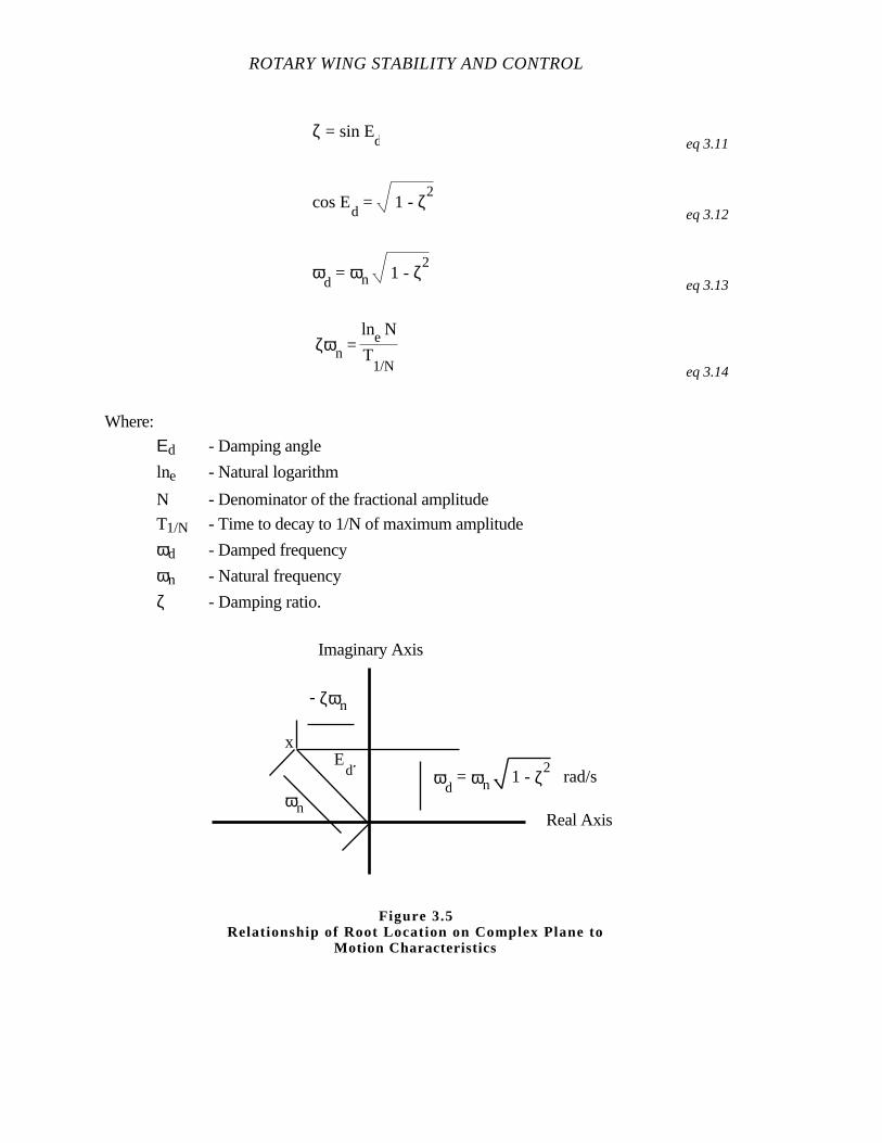
ROTARY WING STABILITY AND CONTROL
ζ = sin Ed eq 3.11
cos Ed = 1 - ζ
2
eq 3.12
ωd = ωn 1 - ζ
2
eq 3.13
ζωn = lne N
T1/N eq 3.14
Where:
Εd - Damping angle
lne - Natural logarithm
N - Denominator of the fractional amplitude
T1/N - Time to decay to 1/N of maximum amplitude
ωd - Damped frequency
ωn - Natural frequency
ζ - Damping ratio.
Imaginary Axis
Real Axis
x
ωn
ωd
= ωn 1 - ζ2E
d
- ζωn
rad/s
Figure 3.5Relationship of Root Location on Complex Plane to
Motion Characteristics
OPEN LOOP TESTING
As the complex pair of roots separate vertically from the real axis, there is a point of
interest where the damping angle, Ed = 45˚, andζ ≈ 0.7. The corresponding time
response is shown in Figure 3.4 (c). The oscillation has essentially one noticeable
overshoot. This situation is considered to be the best compromise between quickness of
initial response and minimum oscillation about steady state. Beyond this root location, ζ <
0.7 and Figure 3.4 (d) applies.
If the characteristics of the system yield roots in location C on Figure 3.3, the time
response is a constant amplitude oscillation as shown in Figure 3.4 (e). If the roots fall in
position D on Figure 3.3, the response is a divergent oscillation as shown in Figure 3.4 (f).
3.3.6 First Order Systems
A first order system is described by a first order linear homogeneous differential
equation. A mass whose motion is restrained by only viscous damping is a typical
example. With no stiffness, the variable is velocity not displacement. The heave mode of a
helicopter in a hover is a first order system with the following characteristic equation:
w. - Zw w = 0
eq 3.15
Where:
w - Translational velocity component along z axis
Zw - Vertical force due to vertical velocity
w - Linear acceleration along the z axis.
It has a real root λ = Zw where Zw, a negative number, yields the root location on
Figure 3.6.
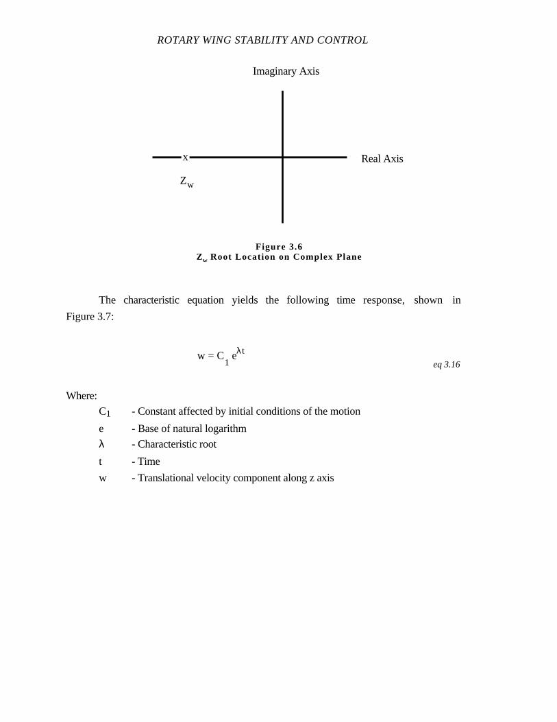
ROTARY WING STABILITY AND CONTROL
The characteristic equation yields the following time response, shown in
Figure 3.7:
w = C1 eλt
eq 3.16
Where:
C1 - Constant affected by initial conditions of the motion
e - Base of natural logarithm
λ - Characteristic root
t - Time
w - Translational velocity component along z axis
Imaginary Axis
Real Axisx
Zw
Figure 3.6Zw Root Location on Complex Plane

OPEN LOOP TESTING
The time required to reach 63.2 % of a steady state first order response is called the
time constant, τ:
τ = - 1λ
= - 1Zw eq 3.17
Where:
λ - Characteristic root
τ - Time constant
Zw - Vertical force due to vertical velocity.
The time constant is a function of heave damping; the greater the damping, the
shorter the time constant. It takes about 5 τ ’s for the response to approximate steady state.
From a piloting viewpoint, τ relates to how quickly the response reaches steady state.
If the first order root, λ, is a positive number, it appears on the real axis in the right
half of the complex plane. Systems with negative static stability yield an aperiodic
divergent response as shown in Figure 3.4(g) when released from an initial off trim
condition. The pertinent time history parameter is the time to double amplitude, Td,
expressed as: Td = 0.69/ λ.
Time - sτ = - 1Zw
0.632 wsswssV
eloc
ity
Figure 3.7Typical Stable First Order Response
ROTARY WING STABILITY AND CONTROL
3.4 TEST METHODS AND TECHNIQUES
3.4.1 General
Open loop dynamics data are obtained to clarify specific closed loop evaluation
information, to document control system or aircraft response characteristics, or to check
compliance with military specifications. The use determines the specific data to be acquired
and the applicable flight conditions. The test pilot must be aware of the specific flight
conditions and variable constraints to obtain useful open loop data.
3.4.2 Trim
The pilot must establish stabilized initial conditions to provide adequate reference
for time histories. The initial conditions can be achieved either by trimming all control
forces to zero (establishing a trim condition) or by holding the control fixed against the
control force while maintaining equilibrium flight conditions. If the pilot intends to make a
precise control input to create the disturbance from equilibrium conditions, the pilot trims
all control forces to zero. If the pilot intends to use a control release from an off trim
condition to create the disturbance, the pilot stabilizes at the equilibrium conditions by
holding the off trim control forces.
3.4.3 Input Shape
Whether an input is a step, pulse, or doublet (Figure 3.8) depends on several
factors including the nature of the response mode to be excited, whether it is to be excited
selectively, the data reduction technique, and sometimes on specific data constraints. For
the pulse and doublet, the controls must be returned to the initial trim position. For
doublets, the test pilot makes a symmetrical input. The controls are returned to trim to
eliminate any moment generated by the control displacement and to record the free response
(without a forcing function) after the initial disturbance. Generally, step inputs are used for
first order responses; while steps, pulses, and doublets are used for second order
responses.

OPEN LOOP TESTING
3.4.4 Input Amplitude
The appropriate input size is a function of the data desired. The input must be large
enough to yield readable data with adequate signal to noise ratio. If the input is too large,
nonlinearities of aerodynamics with airspeed might distort the data. Additionally, if the
input size is large, the aircraft can reach a test limit without the pilot observing the complete
response. On the other hand, it is desirable to correspond open loop data to realistic input
Time
Con
trol
Dis
plac
emen
t
Time
Con
trol
Dis
plac
emen
t
Time
Con
trol
Dis
plac
emen
t
Time
Con
trol
Dis
plac
emen
t
TimeC
ontr
olD
ispl
acem
ent
Time
Con
trol
Dis
plac
emen
t
(a) Step Input
(b) Pulse Input
(c) Doublet Input
Ideal Input Practical Real Input
Figure 3.8Examples of Test Inputs for Determination of Open Loop Dynamics

ROTARY WING STABILITY AND CONTROL
size used to perform the closed loop tasks. The test team must explicitly consider input
size. Because flight safety is always a constraint on input size, proper build up procedures
must be followed.
3.4.5 Quickness of Input
The input frequency should maximize the disturbance at the response frequency.
To approximate the natural frequency the pilot should make a series of sinusoidal,
symmetrical control doublet inputs. Start at a low frequency and observe the response.
Increase the frequency of the input and observe the response. Increase the frequency until
the largest response is observed. Typically, bracketing the largest observed response with
a low frequency and a high frequency will permit the pilot to find the correct input
frequency. Once the input frequency is determined, use this frequency for the subsequent
control inputs.
3.4.6 Excitation Methods
1. Natural excitation. No conscious excitation. Controls fixed without pilot
input. Imperfect trim conditions or atmospheric disturbances may excite an aperiodic
divergent mode or a lightly damped oscillatory mode. This is an unsatisfactory excitation
technique if no response is obtained, but usually indicates a desirable aircraft characteristic.
2. Artificial excitation. Use the longitudinal control to accelerate or decelerate
to an airspeed faster or slower than trim. Then smoothly return the control to the original
trim position and record the aircraft motion. An off trim airspeed variation of 5-15 kn is
normally used to excite the motion.
3. The method of excitation can determine the type of response documented.
Natural disturbances resulting in a long term response are desirable but these responses are
usually contaminated by another disturbance before the motion is completed. This
contamination makes quantifying the mode of motion difficult.
4. Artificial methods are used to obtain time histories from engineering data.
The excitation method chosen should result in an aircraft response similar to a response
following a natural disturbance.
OPEN LOOP TESTING
3.4.7 Test Technique
The longitudinal long term response in forward flight is used to illustrate the flight
test techniques required for open loop dynamic evaluations. Subsequent chapters present
the techniques applicable to a specific axis, mode of motion, and flight condition.
1. Stabilize at the desired trim airspeed and reduce all control forces to zero.
Do not retrim control forces or move the collective during the test.
2. Record trim condition. Assure you can return and hold the controls at trim
after exciting the response.
3. Determine if a long term response is excited by a natural disturbance. With
the controls either fixed or free, note the open loop aircraft response. If no aircraft
response is observed, an artificial excitation is used.
4. Excite the aircraft using a control input. Try several different methods in
order to find the most representative aircraft response. Do not retrim any control forces and
keep the collective constant during response.
5. If aircraft is flown hands off, obtain a control free response following
excitation. Controls should be released at trim conditions so the subsequent control
motions include the effect of attitude changes and gravity force acting on thecontrols
during the response.
6. Record the resulting mode of motion using cockpit data and automatic
recording system. Cockpit displayed boom airspeed is recorded at selected increments of
time. Start the stop watch at the completion of the excitation or at a predetermined airspeed.
The zero time reference point is arbitrary. Use time intervals small enough to define the
shape of irregular responses.
7. The resulting mode of motion may not be a classical single axis response.
Use lateral cyclic and directional pedals as necessary to maintain a single axis response for
the initial excitation. If the lateral-directional inputs are significant, record a time history of
the aircraft response with all controls fixed.
8. For hand held data, a plot of airspeed at regular intervals (5-10 s) adequately
defines the response. An alternate method is to record peak (maximum and minimum)
airspeeds and determine the period by timing the response as the helicopter passes through
the trim airspeed.
ROTARY WING STABILITY AND CONTROL
3.4.8 Data Required
Time history of aircraft response to natural and/or artificial excitation with controls
fixed and/or free. Parameters of interest are: Vo, boom and aircraft system, HPo, α, θ, q,
control positions. If the excitation produces a coupled response which is not suppressed
by the pilot, the attitudes and rates in the other axis are also of interest.
3.4.9 Test Criteria
1. Balanced (ball centered), wings level, unaccelerated trim condition.
2. All flight controls forces trimmed to zero.
3. Control returned exactly to trim following artificial excitation.
4. HPo ± 1000 ft.
3.4.10 Data Requirements
1. Stabilize 5 s minimum prior to recording data.
2. Record sufficient data to include three complete cycles or until a test limit is
reached.
3. NR ± 1 % at trim.
3.4.11 Safety Considerations/Risk Management
Aircraft and test attitude, rate, and acceleration limits must be established prior to
test and strictly followed during the test. Artificial excitation and control displacement
limits must be specified. Control displacement must follow proper build up techniques,
progressing from small inputs to the test limit in small increments. Prior to the test,
applicable recovery techniques must be reviewed and understood. The flight crew must
practice the recovery techniques in a controlled build up manner until comfortable with the
procedures.
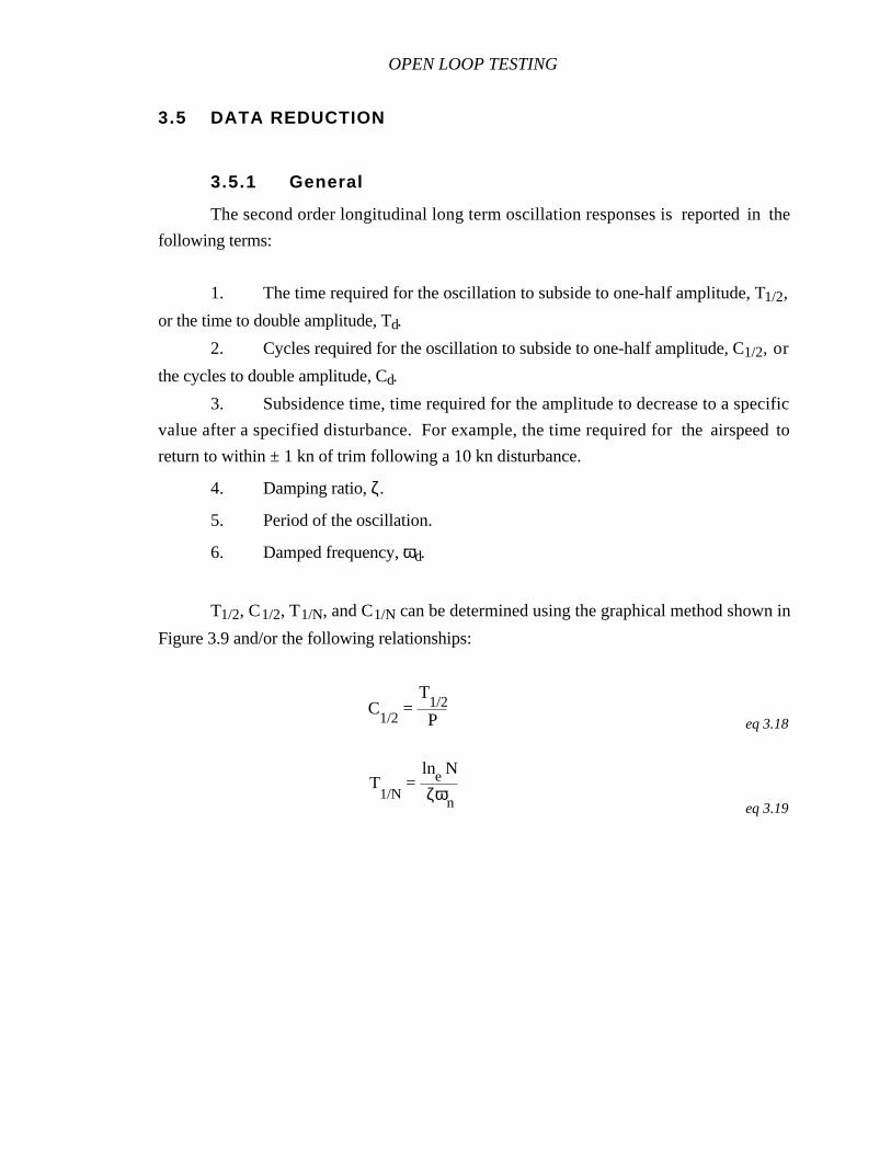
OPEN LOOP TESTING
3.5 DATA REDUCTION
3.5.1 General
The second order longitudinal long term oscillation responses is reported in the
following terms:
1. The time required for the oscillation to subside to one-half amplitude, T1/2,
or the time to double amplitude, Td.
2. Cycles required for the oscillation to subside to one-half amplitude, C1/2, or
the cycles to double amplitude, Cd.
3. Subsidence time, time required for the amplitude to decrease to a specific
value after a specified disturbance. For example, the time required for the airspeed to
return to within ± 1 kn of trim following a 10 kn disturbance.
4. Damping ratio, ζ.
5. Period of the oscillation.
6. Damped frequency, ωd.
T1/2, C1/2, T1/N, and C1/N can be determined using the graphical method shown in
Figure 3.9 and/or the following relationships:
C1/2
= P
T1/2
eq 3.18
T1/N
= lne N
ζωn eq 3.19
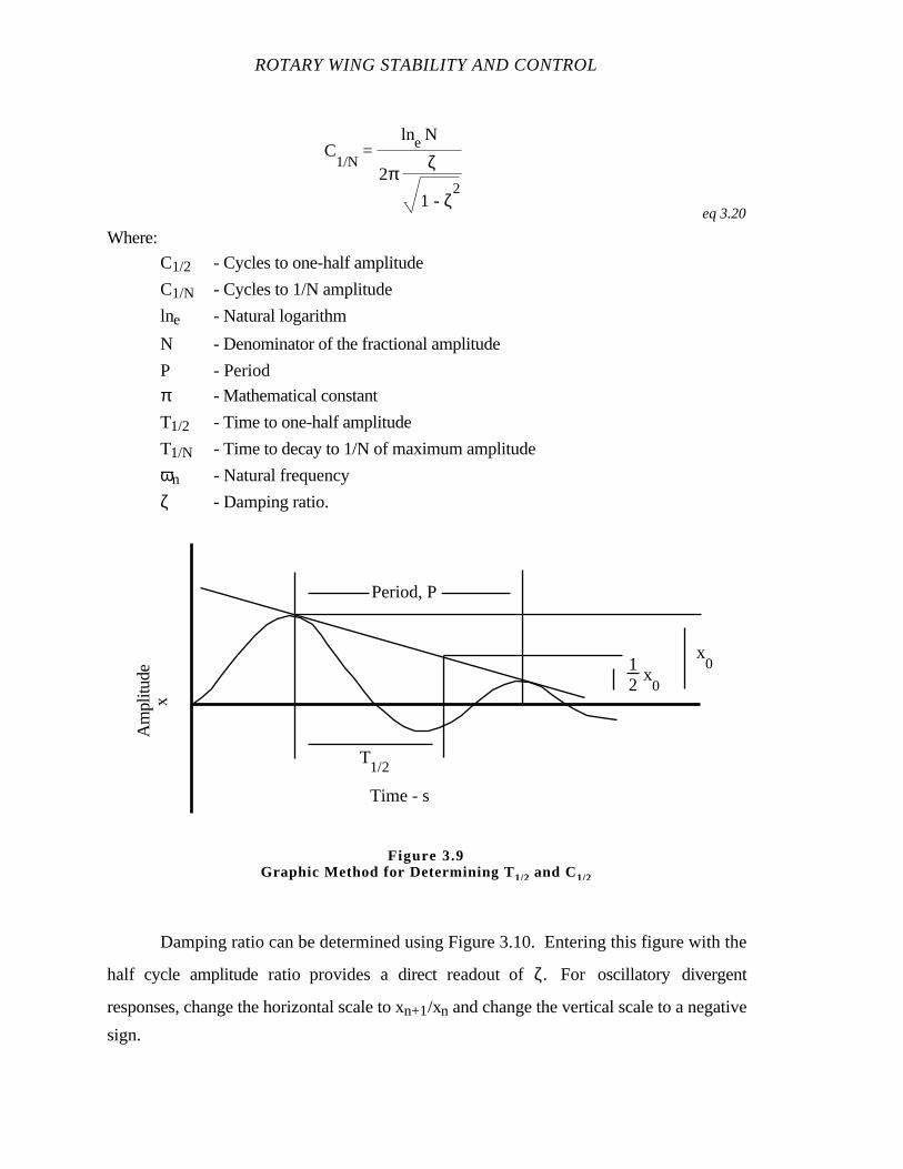
ROTARY WING STABILITY AND CONTROL
C1/N
= lne N
2πζ
1 - ζ2
eq 3.20
Where:
C1/2 - Cycles to one-half amplitude
C1/N - Cycles to 1/N amplitude
lne - Natural logarithm
N - Denominator of the fractional amplitude
P - Period
π - Mathematical constant
T1/2 - Time to one-half amplitude
T1/N - Time to decay to 1/N of maximum amplitude
ωn - Natural frequency
ζ - Damping ratio.
Damping ratio can be determined using Figure 3.10. Entering this figure with the
half cycle amplitude ratio provides a direct readout ofζ. For oscillatory divergent
responses, change the horizontal scale to xn+1/xn and change the vertical scale to a negative
sign.
Period, P
T1/2
Time - s
Am
plitu
dex
12
x0
x0
Figure 3.9Graphic Method for Determining T 1/2 and C1/2
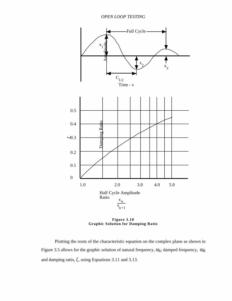
OPEN LOOP TESTING
Plotting the roots of the characteristic equation on the complex plane as shown in
Figure 3.5 allows for the graphic solution of natural frequency, ωn; damped frequency, ωd;
and damping ratio, ζ, using Equations 3.11 and 3.13.
Dam
ping
Rat
io
ζ
0
0.1
0.2
0.3
0.4
0.5
2.0 3.0 4.0 5.0
Half Cycle AmplitudeRatio
xn+1
xn
Am
plitu
de, x
Time - s
C1/2
x1
x2 x
3
Full Cycle
1.0
Figure 3.10Graphic Solution for Damping Ratio
ROTARY WING STABILITY AND CONTROL
3.5.2 Data Presentation
1. Present an annotated time history of airspeed or altitude. Other parameters
which can be plotted are pitch attitude or altitude deviations. Annotate the time history with
the following engineering characteristics as appropriate: C1/2, Cd, T1/2, Td, ωd, period,
andζ.
2. Tables are used to summarize the engineering characteristics for several test
conditions.
3.6 DATA ANALYSIS
In addition to the quantitative data reduction and presentation, the test pilot
associates the open loop tests with the closed loop evaluation tasks discussed in Chapter 2.
The following questions guide this association.
1. How easily excited is the long term response?
2. How does this motion influence the pilot's ability to perform mission tasks?
The significance of the long term response is the manner in which it degrades or helps the
pilot perform a specific task. Evaluate the pilot effort required to suppress or correct
airspeed, attitude, and altitude variations about trim.
3. Can precise pitch attitude and airspeed changes be made?
3.7 MISSION SUITABILITY
Open loop testing supports the pilot qualitative evaluations made using closed loop
test techniques. Mission suitability considerations are based on the closed loop flying
qualities evaluations discussed in Chapter 2. The qualitative results of the open loop test
support pilot opinion of mission suitability.
3.8 SPECIFICATION COMPLIANCE
Specification requirements are generally contained in military specification
documents which put limits on open loop parameters as a function of flying qualities levels.
Applicable documents are MIL-H-8501A for helicopters and the detailed or prime item
specifications for each model helicopter. Subsequent chapters present the specification
requirements relevant for that chapter.
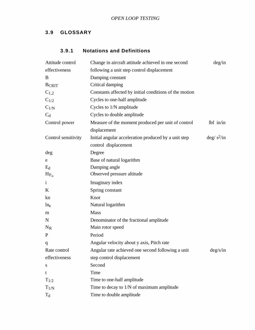
OPEN LOOP TESTING
3.9 GLOSSARY
3.9.1 Notations and Definitions
Attitude control Change in aircraft attitude achieved in one second deg/in
effectiveness following a unit step control displacement
B Damping constant
BCRIT Critical damping
C1,2 Constants affected by initial conditions of the motion
C1/2 Cycles to one-half amplitude
C1/N Cycles to 1/N amplitude
Cd Cycles to double amplitude
Control power Measure of the moment produced per unit of control lbf in/in
displacement
Control sensitivity Initial angular acceleration produced by a unit step deg/ s2/in
control displacement
deg Degree
e Base of natural logarithm
Ed Damping angleHPo Observed pressure altitude
i Imaginary index
K Spring constant
kn Knot
lne Natural logarithm
m Mass
N Denominator of the fractional amplitude
NR Main rotor speed
P Period
q Angular velocity about y axis, Pitch rate
Rate control Angular rate achieved one second following a unit deg/s/in
effectiveness step control displacement
s Second
t Time
T1/2 Time to one-half amplitude
T1/N Time to decay to 1/N of maximum amplitude
Td Time to double amplitude
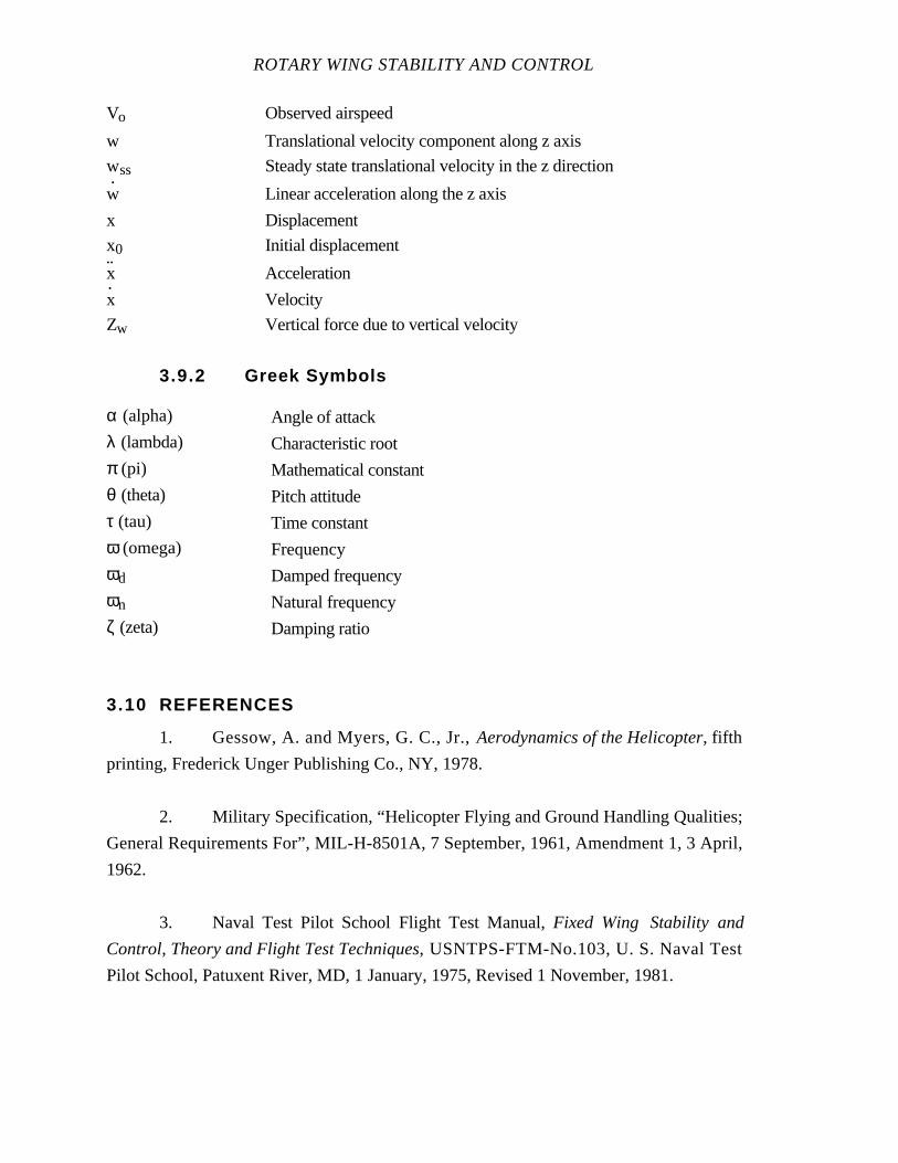
ROTARY WING STABILITY AND CONTROL
Vo Observed airspeed
w Translational velocity component along z axis
wss Steady state translational velocity in the z direction
w Linear acceleration along the z axis
x Displacement
x0 Initial displacement
x Acceleration
x Velocity
Zw Vertical force due to vertical velocity
3.9.2 Greek Symbols
α (alpha) Angle of attack
λ (lambda) Characteristic root
π (pi) Mathematical constant
θ (theta) Pitch attitude
τ (tau) Time constant
ω (omega) Frequency
ωd Damped frequency
ωn Natural frequency
ζ (zeta) Damping ratio
3.10 REFERENCES
1. Gessow, A. and Myers, G. C., Jr., Aerodynamics of the Helicopter, fifth
printing, Frederick Unger Publishing Co., NY, 1978.
2. Military Specification, “Helicopter Flying and Ground Handling Qualities;
General Requirements For”, MIL-H-8501A, 7 September, 1961, Amendment 1, 3 April,
1962.
3. Naval Test Pilot School Flight Test Manual,Fixed Wing Stability and
Control, Theory and Flight Test Techniques, USNTPS-FTM-No.103, U. S. Naval Test
Pilot School, Patuxent River, MD, 1 January, 1975, Revised 1 November, 1981.
OPEN LOOP TESTING
4. Naval Test Pilot School Flight Test Manual,Helicopter Stability and
Control, USNTPS-FTM-No. 101, U. S. Naval Test Pilot School, Patuxent River, MD, 10
June 1968, reprinted February 1978.
5. Naval Test Pilot School Flight Test Manual,Helicopter Stability and
Control, Theory and Flight Test Techniques, USNTPS-FTM-No. 105, U. S. Naval Test
Pilot School, Patuxent River, MD, November 1983, Preliminary Edition.
6. Prouty, R. W., Practical Helicopter Aerodynamics, PJS Publications, Inc.,
1982.
7. Prouty, Raymond W.,Helicopter Performance, Stability, and Control,
PWS Publishers, Boston, MA, 1986.
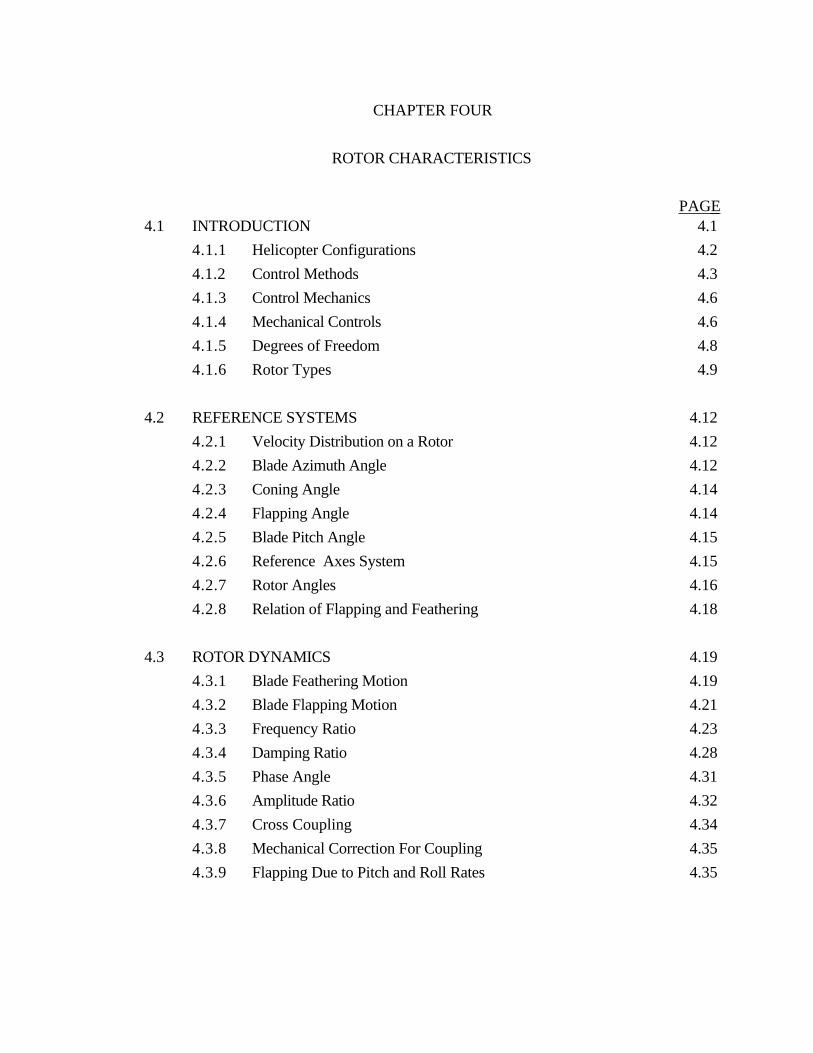
CHAPTER FOUR
ROTOR CHARACTERISTICS
PAGE4.1 INTRODUCTION 4.1
4.1.1 Helicopter Configurations 4.2
4.1.2 Control Methods 4.3
4.1.3 Control Mechanics 4.6
4.1.4 Mechanical Controls 4.6
4.1.5 Degrees of Freedom 4.8
4.1.6 Rotor Types 4.9
4.2 REFERENCE SYSTEMS 4.12
4.2.1 Velocity Distribution on a Rotor 4.12
4.2.2 Blade Azimuth Angle 4.12
4.2.3 Coning Angle 4.14
4.2.4 Flapping Angle 4.14
4.2.5 Blade Pitch Angle 4.15
4.2.6 Reference Axes System 4.15
4.2.7 Rotor Angles 4.16
4.2.8 Relation of Flapping and Feathering 4.18
4.3 ROTOR DYNAMICS 4.19
4.3.1 Blade Feathering Motion 4.19
4.3.2 Blade Flapping Motion 4.21
4.3.3 Frequency Ratio 4.23
4.3.4 Damping Ratio 4.28
4.3.5 Phase Angle 4.31
4.3.6 Amplitude Ratio 4.32
4.3.7 Cross Coupling 4.34
4.3.8 Mechanical Correction For Coupling 4.35
4.3.9 Flapping Due to Pitch and Roll Rates 4.35
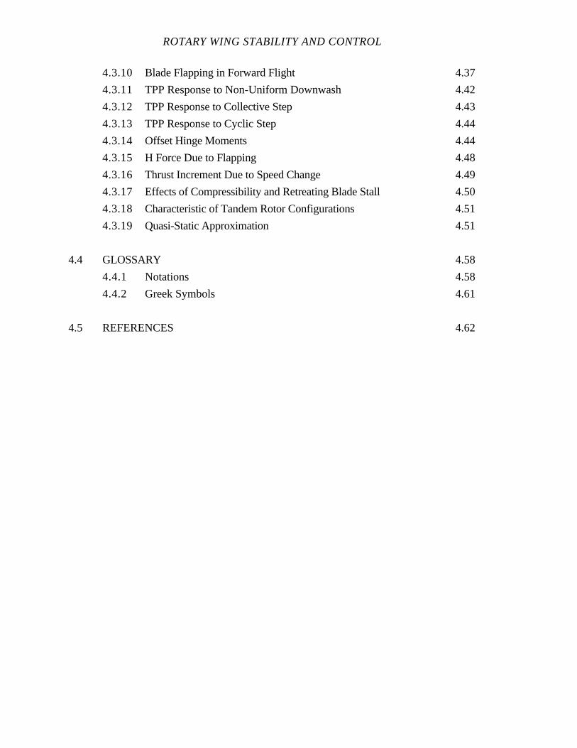
ROTARY WING STABILITY AND CONTROL
4.3.10 Blade Flapping in Forward Flight 4.37
4.3.11 TPP Response to Non-Uniform Downwash 4.42
4.3.12 TPP Response to Collective Step 4.43
4.3.13 TPP Response to Cyclic Step 4.44
4.3.14 Offset Hinge Moments 4.44
4.3.15 H Force Due to Flapping 4.48
4.3.16 Thrust Increment Due to Speed Change 4.49
4.3.17 Effects of Compressibility and Retreating Blade Stall 4.50
4.3.18 Characteristic of Tandem Rotor Configurations 4.51
4.3.19 Quasi-Static Approximation 4.51
4.4 GLOSSARY 4.58
4.4.1 Notations 4.58
4.4.2 Greek Symbols 4.61
4.5 REFERENCES 4.62
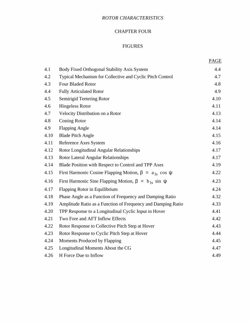
ROTOR CHARACTERISTICS
CHAPTER FOUR
FIGURES
PAGE
4.1 Body Fixed Orthogonal Stability Axis System 4.4
4.2 Typical Mechanism for Collective and Cyclic Pitch Control 4.7
4.3 Four Bladed Rotor 4.8
4.4 Fully Articulated Rotor 4.9
4.5 Semirigid Teetering Rotor 4.10
4.6 Hingeless Rotor 4.11
4.7 Velocity Distribution on a Rotor 4.13
4.8 Coning Rotor 4.14
4.9 Flapping Angle 4.14
4.10 Blade Pitch Angle 4.15
4.11 Reference Axes System 4.16
4.12 Rotor Longitudinal Angular Relationships 4.17
4.13 Rotor Lateral Angular Relationships 4.17
4.14 Blade Position with Respect to Control and TPP Axes 4.19
4.15 First Harmonic Cosine Flapping Motion, β = a1s cos ψ 4.22
4.16 First Harmonic Sine Flapping Motion, β = b1s sin ψ 4.23
4.17 Flapping Rotor in Equilibrium 4.24
4.18 Phase Angle as a Function of Frequency and Damping Ratio 4.32
4.19 Amplitude Ratio as a Function of Frequency and Damping Ratio 4.33
4.20 TPP Response to a Longitudinal Cyclic Input in Hover 4.41
4.21 Two Fore and AFT Inflow Effects 4.42
4.22 Rotor Response to Collective Pitch Step at Hover 4.43
4.23 Rotor Response to Cyclic Pitch Step at Hover 4.44
4.24 Moments Produced by Flapping 4.45
4.25 Longitudinal Moments About the CG 4.47
4.26 H Force Due to Inflow 4.49
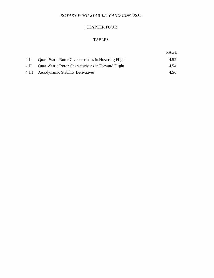
ROTARY WING STABILITY AND CONTROL
CHAPTER FOUR
TABLES
PAGE
4.I Quasi-Static Rotor Characteristics in Hovering Flight 4.52
4.II Quasi-Static Rotor Characteristics in Forward Flight 4.54
4.III Aerodynamic Stability Derivatives 4.56
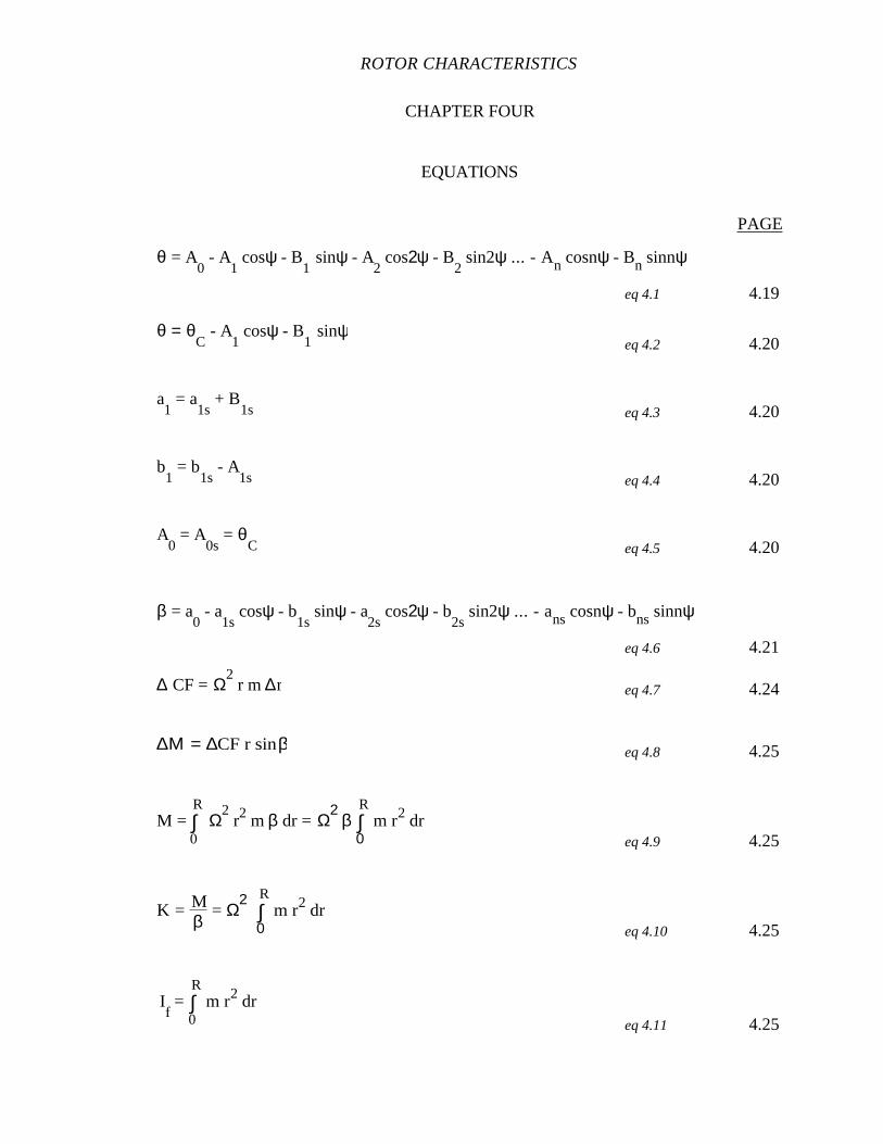
ROTOR CHARACTERISTICS
CHAPTER FOUR
EQUATIONS
PAGE
θ = A0 - A
1 cosψ - B
1 sinψ - A
2 cos2ψ - B
2 sin2ψ ... - An cosnψ - Bn sinnψ
eq 4.1 4.19
θ = θC
- A1 cosψ - B
1 sinψ
eq 4.2 4.20
a1 = a
1s + B
1s eq 4.3 4.20
b1 = b
1s - A
1s eq 4.4 4.20
A0 = A
0s = θ
C eq 4.5 4.20
β = a0 - a
1s cosψ - b
1s sinψ - a
2s cos2ψ - b
2s sin2ψ ... - ans cosnψ - bns sinnψ
eq 4.6 4.21
∆ CF = Ω2 r m ∆r eq 4.7 4.24
∆Μ = ∆CF r sinβ eq 4.8 4.25
M = ∫0
RΩ
2 r2 m β dr = Ω
2 β ∫
0
R m r2 dr
eq 4.9 4.25
K = Mβ
= Ω2 ∫
0
R m r2 dr
eq 4.10 4.25
If = ∫
0
R m r2 dr
eq 4.11 4.25
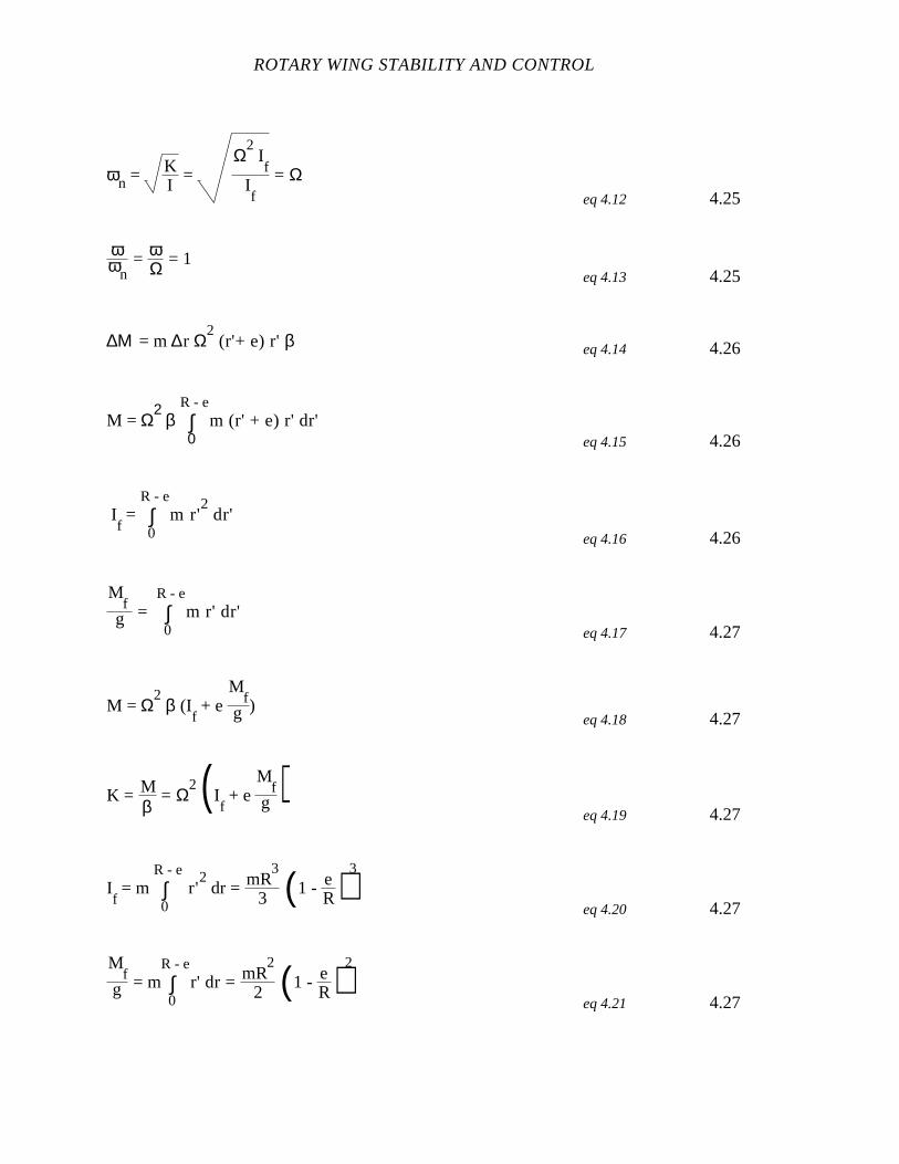
ROTARY WING STABILITY AND CONTROL
ωn = KI
= Ω
2 I
fIf
= Ωeq 4.12 4.25
ωωn
= ωΩ = 1eq 4.13 4.25
∆Μ = m ∆r Ω2 (r'+ e) r' β eq 4.14 4.26
M = Ω2 β ∫
0
R - em (r' + e) r' dr'
eq 4.15 4.26
If = ∫
0
R - em r'
2 dr'
eq 4.16 4.26
Mf
g = ∫0
R - em r' dr'
eq 4.17 4.27
M = Ω2
β (If + e
Mf
g )eq 4.18 4.27
K = Mβ
= Ω2 ( I
f + e
Mf
g )eq 4.19 4.27
If = m ∫
0
R - e r'
2 dr = mR
3
3 (1 - eR)
3
eq 4.20 4.27
Mf
g = m ∫0
R - er' dr = mR
2
2 (1 - eR)
2
eq 4.21 4.27

ROTOR CHARACTERISTICS
ωn = KIf
= Ω 1 + eM
fg I
f
= Ω 1 +
32
eR
1 - eR eq 4.22 4.27
ωωn
= ωΩ = 1 +
32
eR
1 - eR eq 4.23 4.27
I f˙β + Bβ + K β = 0 eq 4.24 4.28
β = - B2I
f
± ( B2I
f)
2
- KIf eq 4.25 4.29
BCRIT
= 2If (K
If)
12
eq 4.26 4.29
ζ = BB
CRIT eq 4.27 4.29
MA
= ∫0
R - e r'
ρ2
a c r' β. (r' + e) Ω dr
eq 4.28 4.29
B = 2M
A
∂β. =
cρaR4
8 (1 - eR)
4
Ω ( 1 + e3R
1 - eR
)eq 4.29 4.29
ζ = γ16 (1 - e
R)4( 1 + e
3R
1 - eR
) 1ωn / Ω
eq 4.30 4.30
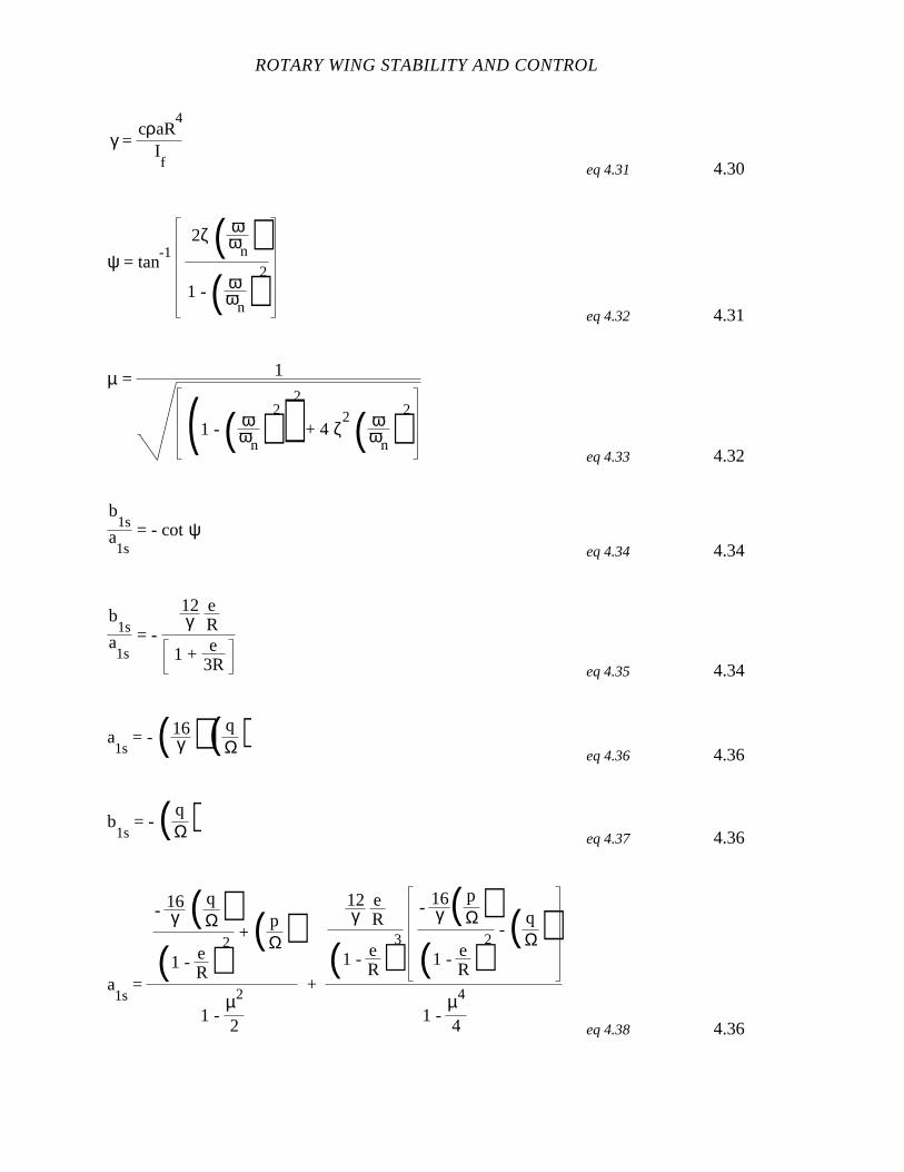
ROTARY WING STABILITY AND CONTROL
γ = cρaR
4
If eq 4.31 4.30
ψ = tan-1
2ζ ( ωωn)
1 - ( ωωn)
2
eq 4.32 4.31
µ = 1
(1 - ( ωωn)
2)2
+ 4 ζ2 ( ω
ωn)2
eq 4.33 4.32
b1s
a1s
= - cotψeq 4.34 4.34
b1s
a1s
= -
12γ
eR
1 + e3R eq 4.35 4.34
a1s
= - ( 16γ ) ( q
Ω)eq 4.36 4.36
b1s
= - ( qΩ)
eq 4.37 4.36
a1s
=
- 16γ ( q
Ω)(1 - e
R)2
+ ( pΩ)
1 - µ2
2
+
12γ
eR
(1 - eR)
3
- 16γ ( p
Ω)(1 - e
R)2
- ( qΩ)
1 - µ4
4 eq 4.38 4.36

b1s
=
- 16γ ( p
Ω)(1 - e
R)2
+ ( qΩ)
1 - µ2
2
+
12γ
eR
(1 - eR)
3
- 16γ ( q
Ω)(1 - e
R)2
- ( pΩ)
1 - µ4
4 eq 4.39 4.36
µ = VΩR eq 4.40 4.36
β = a0 - a
1s cos ψ - b
1s sin ψ
eq 4.41 4.37
a0 =
γ8
θC(1 + µ2) + 4
3λ -
MW
IΩ2
eq 4.42 4.38
a1s
= - B1s
1 + 32
µ2
1 - µ2
2
+
83
θC
µ + 2 λ µ
1 - µ2
2 eq 4.43 4.38
b1s
= A1s
+
43
µ a0
1 + µ2
2 eq 4.44 4.38
λ = V sin αs - vi
ΩR eq 4.45 4.38
-FS
hub on blade
+ ∫e
RdT cos β = ∫
e
Rβ..
(r - e) dmeq 4.46 4.45
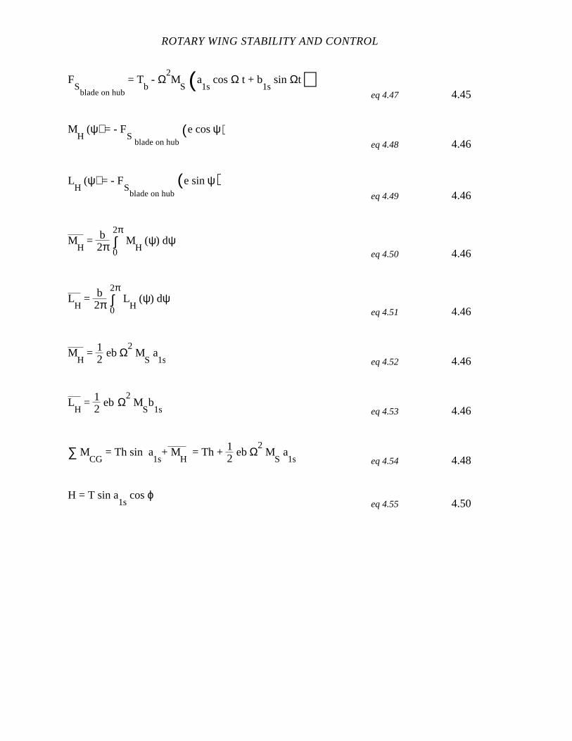
ROTARY WING STABILITY AND CONTROL
FS
blade on hub
= Tb - Ω
2M
S (a1s
cos Ω t + b1s
sin Ωt)eq 4.47 4.45
MH
(ψ) = - FS
blade on hub(e cos ψ)
eq 4.48 4.46
LH
(ψ) = - FS
blade on hub(e sin ψ)
eq 4.49 4.46
MH
= b2π ∫
0
2π M
H (ψ) dψ
eq 4.50 4.46
LH
= b2π ∫
0
2π L
H (ψ) dψ
eq 4.51 4.46
MH
= 12
eb Ω2 M
S a
1s eq 4.52 4.46
LH
= 12
ebΩ2 M
Sb
1s eq 4.53 4.46
∑ MCG
= Th sin a1s
+ MH
= Th + 12
eb Ω2 M
S a
1s eq 4.54 4.48
H = T sin a1s
cos ϕeq 4.55 4.50

CHAPTER FOUR
ROTOR CHARACTERISTICS
4.1 INTRODUCTION
Throughout the development of the helicopter, three fundamental problems faced
the developers: reducing structural and engine weight sufficiently to provide a useful
payload capability; counteracting rotor torque; and controlling the helicopter. The purpose
of this chapter is to reacquaint the reader with the rotor characteristics whichprovide
control of the helicopter. No attempt is made to develop rigorously the various equations
which govern the stability and control of the rotor. Rather the terminology, reference
systems, and equations are presented with a discussion of the factors which influence the
results. Simplifying assumptions are made and discussed. References, containing
complete development of the equations, are listed at the end of the chapter for those readers
who wish further clarification.
The stability and control of the helicopter depends on the net effect of all the forces
and moments applied to the helicopter from control inputs, helicopter motion, or external
sources. The early development of rotary wing aircraft was slowed by the inherent stability
and control problems of the single rigid rotor configuration. The basic difficulty was lift
dissymmetry caused by a blade rotating with a constant pitch angle in forward flight,
developing greater lift when advancing in the direction of motion than when retreating.
Thus, the rigid rotor applies a rolling moment to the aircraft.
The problem of the lift dissymmetry in forward flight can be addressed in two
ways. This problem was first solved by the introduction of blade flapping hinges which
prevented the transmission of blade flapping moments to the aircraft. The unbalanced
cyclic flapping moments resulted in a once per revolution blade flapping motion. The once
per revolution blade flapping tended to make the aerodynamic lift and flapping moments on
the blades approximately equal to the average values obtained with a rigid rotor.
ROTARY WING STABILITY AND CONTROL
The second method of overcoming lift dissymmetry in forward flight is through
cyclic feathering of the blades; decreasing pitch on the advancing blades and increasing
pitch on the retreating blade. In this case, the blades can be rigidly attached to the rotor
shaft or incorporate flapping hinges. Hingeless blades flap relative to the rotor shaft and
produce effects analogous to those obtained with flapping hinges.
The purpose of this chapter is understanding the flapping and feathering action of
the rotor and how the pilot interacts to control the rotor. We begin the chapter with a
review of various helicopter configurations.
4.1.1 Helicopter Configurations
There are five main types of helicopter configurations. Each type is presented along
with its unique characteristics, advantages, and disadvantages.
The single rotor helicopter is the configuration most widely used. The major
advantage is relative simplicity of one main rotor and one tail rotor. The single rotor
helicopter can be powered by one or more engines combined through one transmission.
The tail rotor typically uses about 8 to 10% of the total power available in a hover and 3 to
4% in forward flight. The simplicity and savings in weight make this method of countering
rotor torque attractive. The few disadvantages of the single rotor configuration include the
close proximity of the tail rotor to the ground, the relatively restrictive center of gravity
(CG) range, and smaller payload capacity. These disadvantages have been overcome with
advances in propulsion and materials, allowing design of larger multi-blade, multi-engine
single rotor helicopters.
The tip driven rotor provides a simple solution to the problem of countering rotor
torque. The rotor is powered at the tips rather than by the shaft, eliminating torque applied
to the fuselage. The advantages are the elimination of the tail rotor and main transmission.
The disadvantages are caused by the requirements of tip propulsion.
Coaxial rotors such as the Advancing Blade Concept (ABC) incorporate
counterrotating main rotors to eliminate rotor torque to the fuselage. The advantage is the
elimination of the tail rotor. The disadvantage is the weight and complexity of the rotor and
hub. The interaction of the rotor flow causes vibration problems as well.

ROTOR CHARACTERISTICS
Side by side rotors offer the advantage of elimination of the tail rotor and a
reduction in power required in forward flight since each rotor operates in relatively
undisturbed air. The disadvantage is high fuselage parasite drag, greater weight, and
complexity of rotor control systems.
Tandem rotors offer the advantage of large payload capability, larger CG range, and
relatively clean fuselage design. The disadvantage is some increase in power required in
forward flight due to the influence of the front rotor on the rear rotor.
Multi-rotors offer the advantage of increased lift capability and simplicity of control
through varying thrust of each rotor. The disadvantages are large size and high weight.
A special type of helicopter configuration is the compound aircraft such as the
V-22. This design offers the advantages of high speed flight while retaining vertical/short
takeoff and landing capability. The disadvantages lie in overall complexity of design.
For the purpose of understanding rotor characteristics in this chapter, the discussion
concentrates on the single rotor configuration with some discussion as applicable to the
tandem rotor configuration.
4.1.2 Control Methods
To control the helicopter in flight, the forces and moments about all three axes of
the helicopter must be controlled. This involves controlling three forces and three
moments. Figure 4.1 presents a body fixed reference axis system and shows the usual
convention for positive values. This orthogonal axis system is depicted initially aligned
with the relative wind.
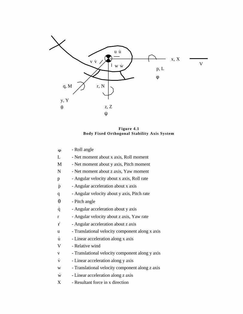
φ - Roll angle
L - Net moment about x axis, Roll moment
M - Net moment about y axis, Pitch moment
N - Net moment about z axis, Yaw moment
p - Angular velocity about x axis, Roll rate
p - Angular acceleration about x axis
q - Angular velocity about y axis, Pitch rate
θ - Pitch angle
q - Angular acceleration about y axis
r - Angular velocity about z axis, Yaw rate
r - Angular acceleration about z axis
u - Translational velocity component along x axis
u - Linear acceleration along x axis
V - Relative wind
v - Translational velocity component along y axis
v - Linear acceleration along y axis
w - Translational velocity component along z axis
w - Linear acceleration along z axis
X - Resultant force in x direction
u
wv
p, L
r, Nq, M
x, X
y, Yz, Z
u.
v.
w. V
φ
ψθ
Figure 4.1Body Fixed Orthogonal Stabil i ty Axis System
ROTARY WING STABILITY AND CONTROL
x - Orthogonal direction along longitudinal axis of the aircraft
Y - Resultant force in y direction
y - Orthogonal direction along lateral axis of the aircraft
ψ - Yaw angle
Z - Resultant force in z direction
z - Orthogonal direction along vertical axis of the aircraft.
Controlling the forces and moments in six independent degrees of freedom require
six independent controls. The six required controls would be extremely cumbersome.
Coupling the controls reduces the number of independent controls and provides a
manageable control system. The sacrifice is complete freedom of controlling position and
attitude. The degrees of freedom necessary to control the helicopter are reduced to four and
controls are provided for each.
Vertical control is required to fix the helicopter vertically. Vertical control is
provided through the collective control to increase/decrease the pitch of the rotor and
increase/decrease thrust.
Directional control is used to fix the attitude of the helicopter about the z axis.
Directional control is used to point the helicopter or if required by configuration, counteract
main rotor torque. The directional control mechanism varies with configuration.
Lateral control is provided through control of both forces and moments. The lateral
control produces a rolling moment about the CG which tilts the helicopter. However, the
tilt of the thrust vector also produces a lateral or side force, depending on the configuration.
Longitudinal control consists of controlling both longitudinal forces and moments.
In a tandem configuration, the longitudinal control is accomplished by controlling the thrust
of the rotors independently or by tilting the rotors. Rotor tilt is reserved usually for
trimming.
Control coupling or the application of control in one axis producing a force or
moment in another axis is undesirable, unless the control coupling is designed to counteract
aerodynamic coupling. The sources of aerodynamic coupling are introduced in subsequent
sections and the requirement for control coupling or pilot action is discussed. Chapter 8
concentrates on coupling and the impact on stability and control.
ROTOR CHARACTERISTICS
4.1.3 Control Mechanics
Longitudinal and lateral control of the main rotor is exercised through tilting the
thrust vector or by producing moments about the rotor hub. The pilot controls the rotor
through cyclic pitch change. The cyclic pitch change is accomplished by the linkage from
the cockpit flight control to the swashplate. The outer rotating race of the swashplate is
connected through pitch change linkage to the pitch change horn. The pitch change horn
controls the blade pitch or feathering through the feathering bearing. For rotors without
flapping hinge offset or effective flapping offset, the tilt of the swashplate produces blade
flapping as well as tip path plane (TPP) and thrust vector tilt. For rotors with flapping
hinge offset or effective flapping offset, blade flapping produces a moment about the rotor
hub as well as a tilt of the TPP and thrust vector.
4.1.4 Mechanical Controls
The two primary main rotor controls in a conventional helicopter are the collective
and cyclic pitch controls. The pilot uses the collective pitch control to increase or decrease
the average pitch angle of all the blades, controlling the helicopter vertically. The cyclic
pitch control is used to change the pitch of the individual blades in relation to the feathering
axis sinusoidally, once each revolution. One per revolution cyclic pitch change causes
blade flapping, resulting in a tilt of the TPP and the thrust vector. The resulting tilt of the
thrust vector produces pitching and rolling moments as well as longitudinal and lateral
forces. A typical mechanism for collective and cyclic pitch control is illustrated in Figure
4.2. Cyclic pitch mechanisms customarily incorporate a swashplate and pitch change
mechanisms as shown in Figure 4.3. Cyclic pitch change mechanisms usually are
designed for a one to one relationship between the swashplate angle and the amplitude of
cyclic feathering introduced to the rotor.
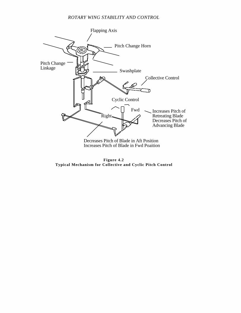
ROTARY WING STABILITY AND CONTROL
Collective Control
Cyclic Control
FwdRight
Decreases Pitch of Blade in Aft PositionIncreases Pitch of Blade in Fwd Poaition
Increases Pitch ofRetreating BladeDecreases Pitch ofAdvancing Blade
Flapping Axis
Swashplate
Pitch Change Horn
Pitch ChangeLinkage
Figure 4.2Typical Mechanism for Collective and Cyclic Pitch Control
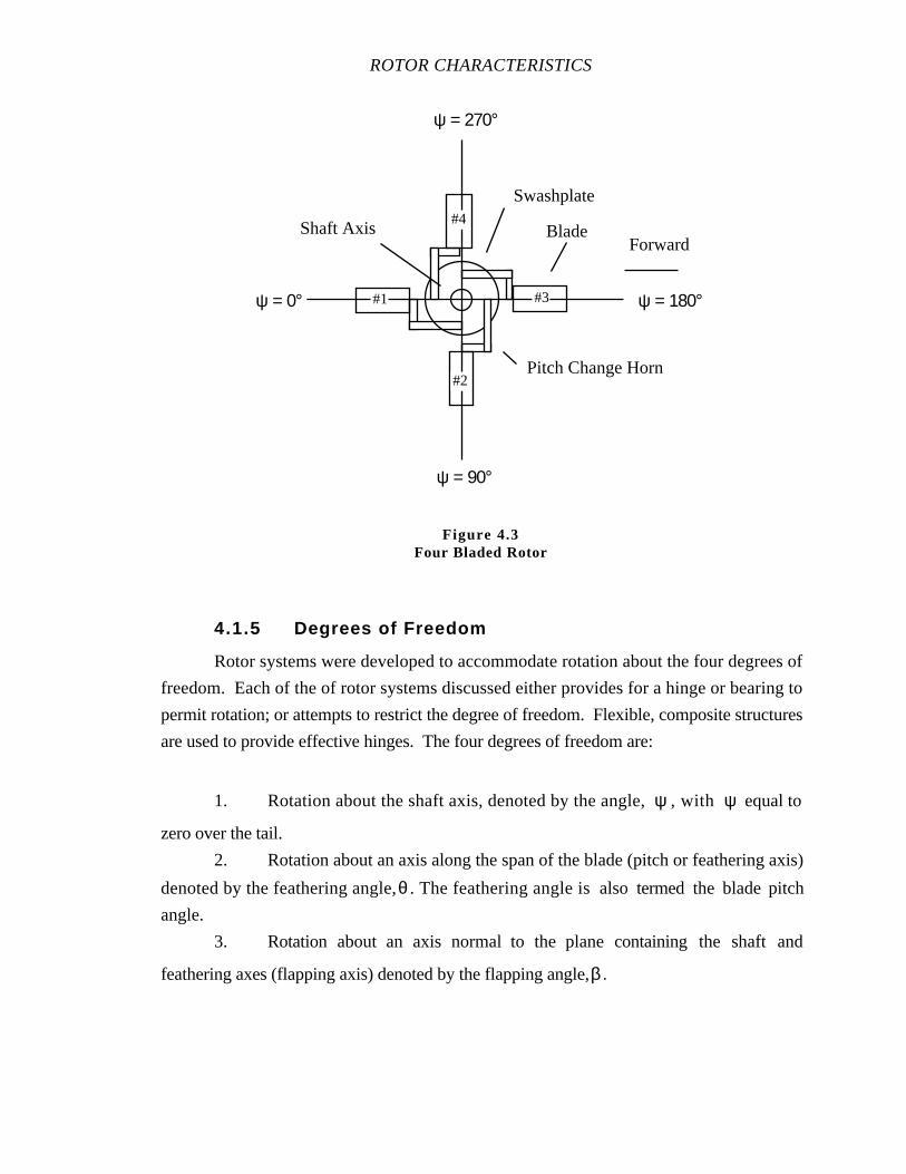
ROTOR CHARACTERISTICS
4.1.5 Degrees of Freedom
Rotor systems were developed to accommodate rotation about the four degrees of
freedom. Each of the of rotor systems discussed either provides for a hinge or bearing to
permit rotation; or attempts to restrict the degree of freedom. Flexible, composite structures
are used to provide effective hinges. The four degrees of freedom are:
1. Rotation about the shaft axis, denoted by the angle, ψ , with ψ equal to
zero over the tail.
2. Rotation about an axis along the span of the blade (pitch or feathering axis)
denoted by the feathering angle,θ . The feathering angle is also termed the blade pitch
angle.
3. Rotation about an axis normal to the plane containing the shaft and
feathering axes (flapping axis) denoted by the flapping angle,β.
#1
#2
#3
#4
ψ = 0°
ψ = 90°
ψ = 180°
ψ = 270°
ForwardBlade
Swashplate
Pitch Change Horn
Shaft Axis
Figure 4.3Four Bladed Rotor

ROTARY WING STABILITY AND CONTROL
4. Rotation about an axis parallel to the shaft (lead-lag axis) denoted by the
lead-lag angle, ζ . Lead-lag motion is important for the study of vibration, rotor loads, and
ground resonance but has little effect on stability and control. For this reason, lead-lag
motion is not discussed in this chapter.
4.1.6 Rotor Types
Conventional helicopter rotor systems have blades hinged at or near the center of
rotation to permit the blades freedom to flap up and down as they rotate. The two systems
of articulation widely used are the fully articulated rotor and the semirigid or teetering rotor.
The fully articulated system incorporates three or more blades, each blade
individually hinged near the hub as shown in Figure 4.4. The offset of the flapping hinge
axis from the axis of rotation (shaft axis) effects the moments the rotor applies to the
aircraft. The flapping frequency of the rotor blades, as well as the speed and phasing of
their response to control inputs, depend on the flapping hinge offset. In addition to
flapping motion, the articulated system incorporates lead-lag hinges which permit in-plane
motion of the blade. The lag degree of freedom is ordinarily of secondary importance from
the stability and control standpoint. Control of the rotor is accomplished by rotating the
blade about the blade feathering axis.
Axis of Rotationor Shaft Axis
Hub
Blade FlappingAxis
Lead-LagAxis
Blade Feathering Axis
Figure 4.4Fully Articulated Rotor
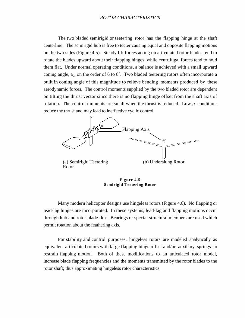
ROTOR CHARACTERISTICS
The two bladed semirigid or teetering rotor has the flapping hinge at the shaft
centerline. The semirigid hub is free to teeter causing equal and opposite flapping motions
on the two sides (Figure 4.5). Steady lift forces acting on articulated rotor blades tend to
rotate the blades upward about their flapping hinges, while centrifugal forces tend to hold
them flat. Under normal operating conditions, a balance is achieved with a small upward
coning angle, a0, on the order of 6 to 8˚. Two bladed teetering rotors often incorporate a
built in coning angle of this magnitude to relieve bending moments produced by these
aerodynamic forces. The control moments supplied by the two bladed rotor are dependent
on tilting the thrust vector since there is no flapping hinge offset from the shaft axis of
rotation. The control moments are small when the thrust is reduced. Low g conditions
reduce the thrust and may lead to ineffective cyclic control.
Many modern helicopter designs use hingeless rotors (Figure 4.6). No flapping or
lead-lag hinges are incorporated. In these systems, lead-lag and flapping motions occur
through hub and rotor blade flex. Bearings or special structural members are used which
permit rotation about the feathering axis.
For stability and control purposes, hingeless rotors are modeled analytically as
equivalent articulated rotors with large flapping hinge offset and/or auxiliary springs to
restrain flapping motion. Both of these modifications to an articulated rotor model,
increase blade flapping frequencies and the moments transmitted by the rotor blades to the
rotor shaft; thus approximating hingeless rotor characteristics.
(a) Semirigid TeeteringRotor
(b) Underslung Rotor
Flapping Axis
Figure 4.5Semirigid Teetering Rotor

ROTARY WING STABILITY AND CONTROL
Changing blade pitch about the feathering axis is the usual method of rotor control.
Blade feathering hinges are usually located near the blade one-quarter chord to reduce blade
pitching moments about the feathering axis. Another method of cyclic pitch change is
structural twisting of the blade using a small, movable flap near the blade tip to control the
twisting motion (Kaman rotor).
Various combinations of rotors and fixed airfoil surfaces are used in helicopters to
improve performance (compound helicopter, X wing, retractable rotor, coaxial rotor, and
tilt rotor). Auxiliary forward thrust devices are necessary with many of these
configurations and each one has its own stability and control characteristics and problems.
In general, the role of the rotors and lifting surfaces changes with the flight regime.
Typical helicopter rotor control techniques are applicable in low airspeed flight. However,
auxiliary airplane type controls are required in high speed flight because the rotors are
unloaded (ABC) or transitioned (V-22) to delay compressibility effects and retreating blade
stall.
Figure 4.6Hingless Rotor
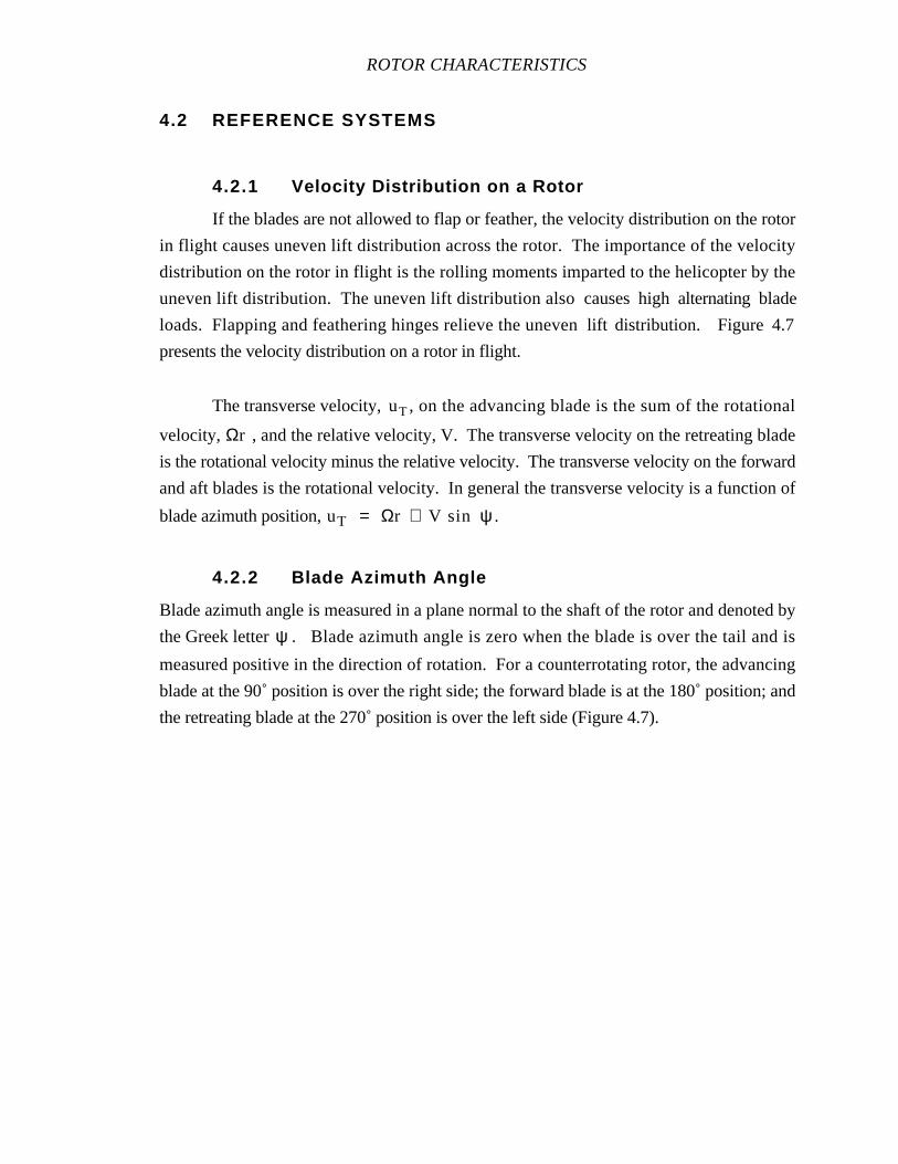
ROTOR CHARACTERISTICS
4.2 REFERENCE SYSTEMS
4.2.1 Velocity Distribution on a Rotor
If the blades are not allowed to flap or feather, the velocity distribution on the rotor
in flight causes uneven lift distribution across the rotor. The importance of the velocity
distribution on the rotor in flight is the rolling moments imparted to the helicopter by the
uneven lift distribution. The uneven lift distribution also causes high alternating blade
loads. Flapping and feathering hinges relieve the uneven lift distribution. Figure 4.7
presents the velocity distribution on a rotor in flight.
The transverse velocity, uT , on the advancing blade is the sum of the rotational
velocity, Ωr , and the relative velocity, V. The transverse velocity on the retreating blade
is the rotational velocity minus the relative velocity. The transverse velocity on the forward
and aft blades is the rotational velocity. In general the transverse velocity is a function of
blade azimuth position, uT = Ωr + V sin ψ .
4.2.2 Blade Azimuth Angle
Blade azimuth angle is measured in a plane normal to the shaft of the rotor and denoted by
the Greek letter ψ . Blade azimuth angle is zero when the blade is over the tail and is
measured positive in the direction of rotation. For a counterrotating rotor, the advancing
blade at the 90˚ position is over the right side; the forward blade is at the 180˚ position; and
the retreating blade at the 270˚ position is over the left side (Figure 4.7).

ROTARY WING STABILITY AND CONTROL
uT = Ωr
uT = Ωr
Relative VelocityDue to forwardMotion
Region of Reversed Flow
(ψ = 180˚)
Retreating Blade
Aft Blade (ψ = 0 )
(ψ = 90 )Advancing Blade
Forward Blade
(ψ = 270˚)
Ω
uT
= Ωr + V
V
V
V
uT
= Ωr - V
Figure 4.7Velocity Distribution on a Rotor
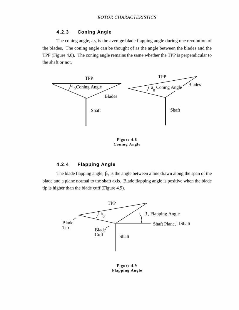
ROTOR CHARACTERISTICS
4.2.3 Coning Angle
The coning angle, a0, is the average blade flapping angle during one revolution of
the blades. The coning angle can be thought of as the angle between the blades and the
TPP (Figure 4.8). The coning angle remains the same whether the TPP is perpendicular to
the shaft or not.
4.2.4 Flapping Angle
The blade flapping angle, β , is the angle between a line drawn along the span of the
blade and a plane normal to the shaft axis. Blade flapping angle is positive when the blade
tip is higher than the blade cuff (Figure 4.9).
Shaft
Blades
a0
Shaft
Bladesa0
TPP TPP
Coning AngleConing Angle
Figure 4.8Coning Angle
Shaft
BladeTip
a0
TPP
β , Flapping Angle
Shaft Plane, ⊥ ShaftBladeCuff
Figure 4.9Flapping Angle
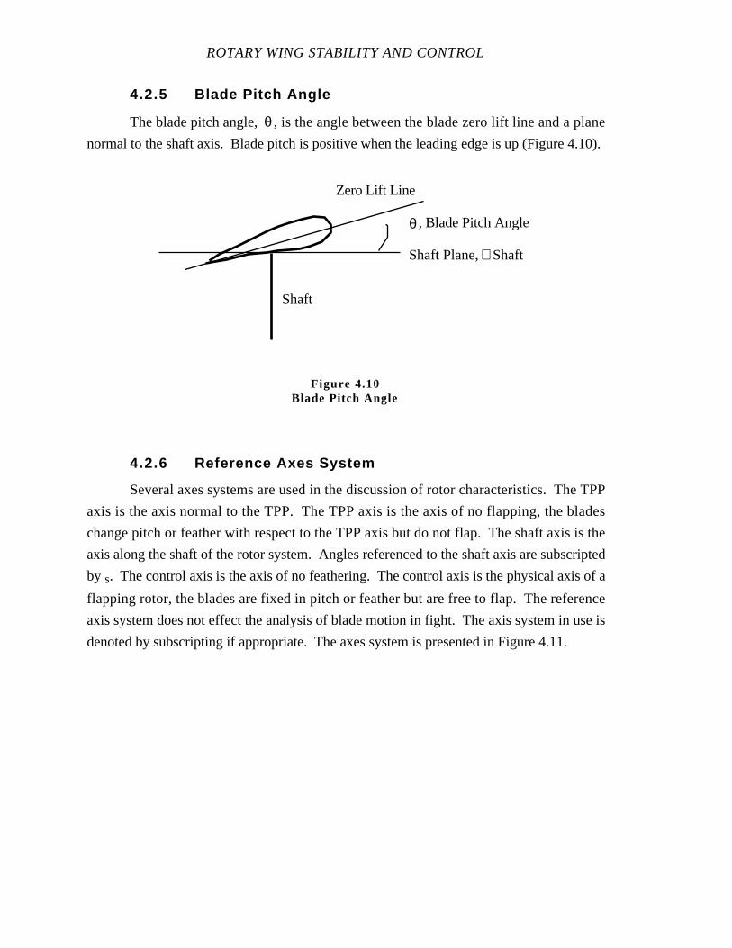
ROTARY WING STABILITY AND CONTROL
4.2.5 Blade Pitch Angle
The blade pitch angle, θ , is the angle between the blade zero lift line and a plane
normal to the shaft axis. Blade pitch is positive when the leading edge is up (Figure 4.10).
4.2.6 Reference Axes System
Several axes systems are used in the discussion of rotor characteristics. The TPP
axis is the axis normal to the TPP. The TPP axis is the axis of no flapping, the blades
change pitch or feather with respect to the TPP axis but do not flap. The shaft axis is the
axis along the shaft of the rotor system. Angles referenced to the shaft axis are subscripted
by s. The control axis is the axis of no feathering. The control axis is the physical axis of a
flapping rotor, the blades are fixed in pitch or feather but are free to flap. The reference
axis system does not effect the analysis of blade motion in fight. The axis system in use is
denoted by subscripting if appropriate. The axes system is presented in Figure 4.11.
Shaft
Zero Lift Line
θ , Blade Pitch Angle
Shaft Plane, ⊥ Shaft
Figure 4.10Blade Pitch Angle

ROTOR CHARACTERISTICS
4.2.7 Rotor Angles
Just as with the reference axes system, the rotor angles are defined to aid the
discussion of rotor characteristics. Figure 4.12 presents the rotor longitudinal angular
relationships. Figure 4.13 presents the rotor lateral angular relationships. The angles
referenced to the shaft plane (plane ⊥ to the shaft axis) are subscripted with an s.
The longitudinal tilt of the TPP in relation to the shaft is the longitudinal flapping
angle, a1s. The longitudinal flapping angle is generated by longitudinal cyclic or external
aerodynamic inputs. The longitudinal flapping angle is positive when the blade flaps up at
ψ = 180° .
TPP
TPP Axis, Axis of no Flapping
Shaft Axis
Control Axis, Axis of no Feathering
Perpendicular to Flight Path
a1
a1s
B1s
αs
α
V
Figure 4.11Reference Axes System
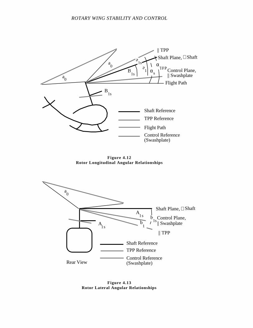
ROTARY WING STABILITY AND CONTROL
Flight Path
Control Plane, || Swashplate
Shaft Plane, ⊥ Shaft
|| TPP
a1s
a1
a0
a0 α
TPPαs
B1s
B1s
Shaft Reference
TPP Reference
Flight Path
Control Reference (Swashplate)
Figure 4.12Rotor Longitudinal Angular Relationships
Control Plane, || Swashplate
Shaft Plane, ⊥ Shaft
|| TPP
Shaft Reference
TPP Reference
Control Reference (Swashplate)
a0
A1s
b1s
Rear View
A1s
b1
Figure 4.13Rotor Lateral Angular Relationships

ROTOR CHARACTERISTICS
The longitudinal cyclic pitch angle, B1s, is the angle between the shaft plane and the
control plane or swashplate.
The lateral tilt of the TPP in relation to the shaft is the lateral flapping angle, b1s.
The lateral flapping angle is generated by lateral cyclic or external aerodynamic inputs. The
lateral flapping angle is positive when the blade flaps down at ψ = 90° .
The lateral cyclic pitch angle, A1s, is the angle between the shaft plane and the
control plane or swashplate.
4.2.8 Relation of Flapping and Feathering
An observer riding on the control axis (axis of no feathering) and rotating with the
blades observes the blade flap up and down each revolution, but they are fixed in pitch.
Likewise, an observer riding on the TPP axis (axis of no flapping) and rotating with the
blades observes the blades change pitch (feather) each revolution, but do not flap at all.
The relation of flapping and feathering is shown in Figure 4.14.
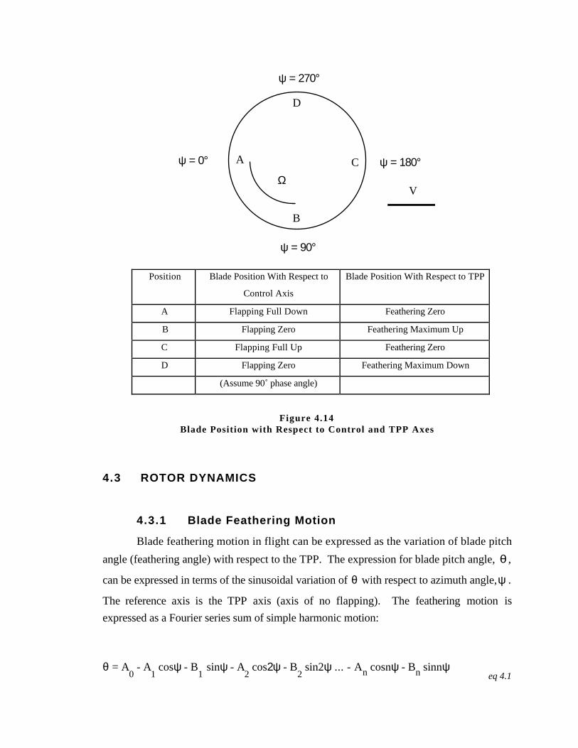
ψ = 0°
ψ = 90°
ψ = 180°
ψ = 270°
Ω
A
B
C
D
V
Position Blade Position With Respect to
Control Axis
Blade Position With Respect to TPP
A Flapping Full Down Feathering Zero
B Flapping Zero Feathering Maximum Up
C Flapping Full Up Feathering Zero
D Flapping Zero Feathering Maximum Down
(Assume 90˚ phase angle)
4.3 ROTOR DYNAMICS
4.3.1 Blade Feathering Motion
Blade feathering motion in flight can be expressed as the variation of blade pitch
angle (feathering angle) with respect to the TPP. The expression for blade pitch angle, θ ,
can be expressed in terms of the sinusoidal variation of θ with respect to azimuth angle,ψ .
The reference axis is the TPP axis (axis of no flapping). The feathering motion is
expressed as a Fourier series sum of simple harmonic motion:
θ = A0 - A
1 cosψ - B
1 sinψ - A
2 cos2ψ - B
2 sin2ψ ... - An cosnψ - Bn sinnψ
eq 4.1
Figure 4.14Blade Position with Respect to Control and TPP Axes
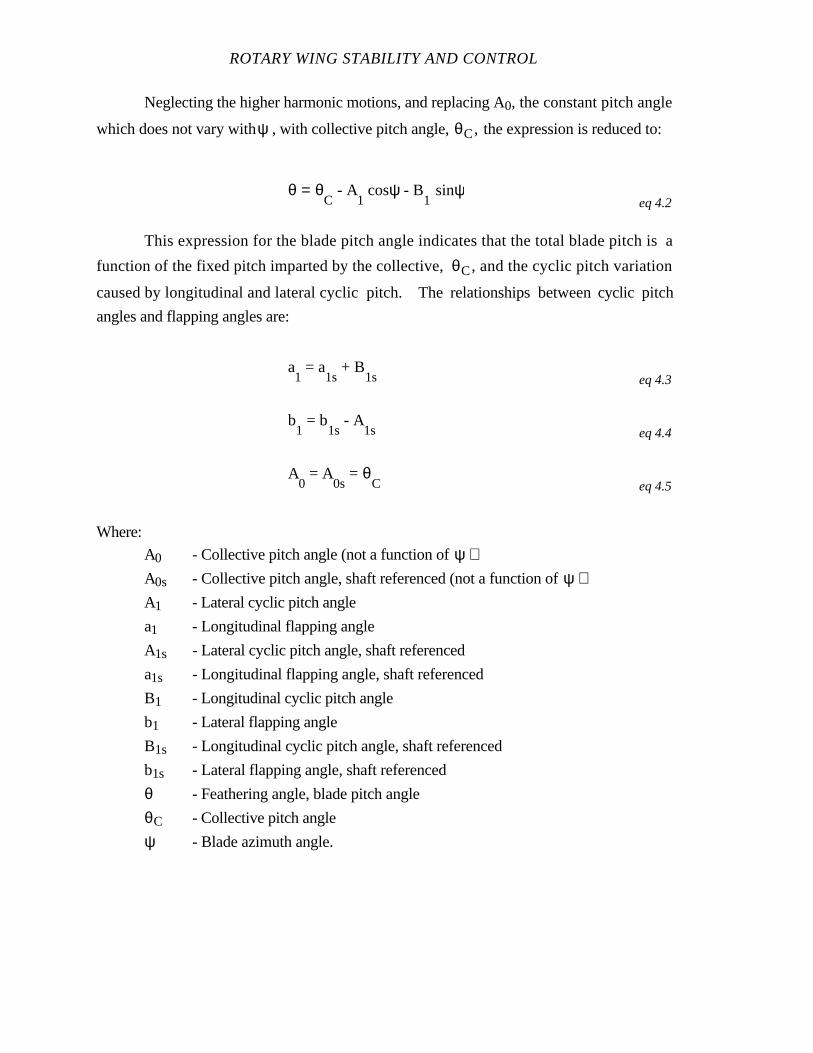
ROTARY WING STABILITY AND CONTROL
Neglecting the higher harmonic motions, and replacing A0, the constant pitch angle
which does not vary withψ , with collective pitch angle, θC, the expression is reduced to:
θ = θC
- A1 cosψ - B
1 sinψ
eq 4.2
This expression for the blade pitch angle indicates that the total blade pitch is a
function of the fixed pitch imparted by the collective, θC, and the cyclic pitch variation
caused by longitudinal and lateral cyclic pitch. The relationships between cyclic pitch
angles and flapping angles are:
a1 = a
1s + B
1s eq 4.3
b1 = b
1s - A
1s eq 4.4
A0 = A
0s = θ
C eq 4.5
Where:
A0 - Collective pitch angle (not a function of ψ )A0s - Collective pitch angle, shaft referenced (not a function of ψ )A1 - Lateral cyclic pitch angle
a1 - Longitudinal flapping angle
A1s - Lateral cyclic pitch angle, shaft referenced
a1s - Longitudinal flapping angle, shaft referenced
B1 - Longitudinal cyclic pitch angle
b1 - Lateral flapping angle
B1s - Longitudinal cyclic pitch angle, shaft referenced
b1s - Lateral flapping angle, shaft referenced
θ - Feathering angle, blade pitch angle
θC - Collective pitch angle
ψ - Blade azimuth angle.
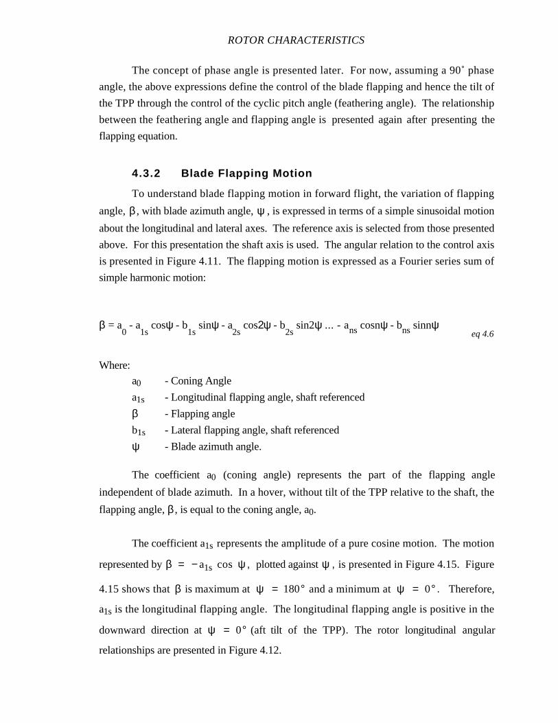
ROTOR CHARACTERISTICS
The concept of phase angle is presented later. For now, assuming a 90˚ phase
angle, the above expressions define the control of the blade flapping and hence the tilt of
the TPP through the control of the cyclic pitch angle (feathering angle). The relationship
between the feathering angle and flapping angle is presented again after presenting the
flapping equation.
4.3.2 Blade Flapping Motion
To understand blade flapping motion in forward flight, the variation of flapping
angle,β , with blade azimuth angle, ψ , is expressed in terms of a simple sinusoidal motion
about the longitudinal and lateral axes. The reference axis is selected from those presented
above. For this presentation the shaft axis is used. The angular relation to the control axis
is presented in Figure 4.11. The flapping motion is expressed as a Fourier series sum of
simple harmonic motion:
β = a0 - a
1s cosψ - b
1s sinψ - a
2s cos2ψ - b
2s sin2ψ ... - ans cosnψ - bns sinnψ
eq 4.6
Where:
a0 - Coning Angle
a1s - Longitudinal flapping angle, shaft referenced
β - Flapping angle
b1s - Lateral flapping angle, shaft referenced
ψ - Blade azimuth angle.
The coefficient a0 (coning angle) represents the part of the flapping angle
independent of blade azimuth. In a hover, without tilt of the TPP relative to the shaft, the
flapping angle, β , is equal to the coning angle, a0.
The coefficient a1s represents the amplitude of a pure cosine motion. The motion
represented by β = − a1s cos ψ , plotted against ψ , is presented in Figure 4.15. Figure
4.15 shows that β is maximum at ψ = 180° and a minimum at ψ = 0° . Therefore,
a1s is the longitudinal flapping angle. The longitudinal flapping angle is positive in the
downward direction atψ = 0° (aft tilt of the TPP). The rotor longitudinal angular
relationships are presented in Figure 4.12.
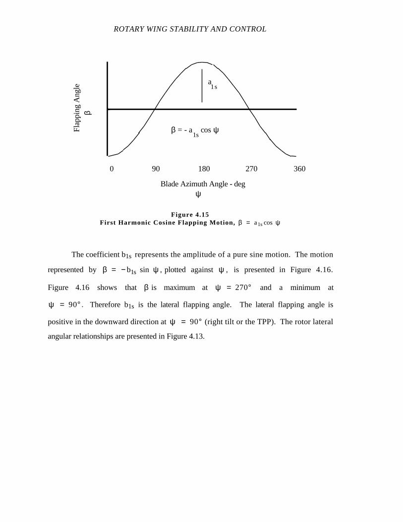
ROTARY WING STABILITY AND CONTROL
The coefficient b1s represents the amplitude of a pure sine motion. The motion
represented byβ = − b1s sin ψ , plotted againstψ , is presented in Figure 4.16.
Figure 4.16 shows thatβ is maximum at ψ = 270° and a minimum at
ψ = 90° . Therefore b1s is the lateral flapping angle. The lateral flapping angle is
positive in the downward direction at ψ = 90° (right tilt or the TPP). The rotor lateral
angular relationships are presented in Figure 4.13.
β = - a1s
cosψ
Blade Azimuth Angle - degψ
0 90 180 270 360
Fla
ppin
g A
ngle
βa1s
Figure 4.15First Harmonic Cosine Flapping Motion, β = a1scos ψ
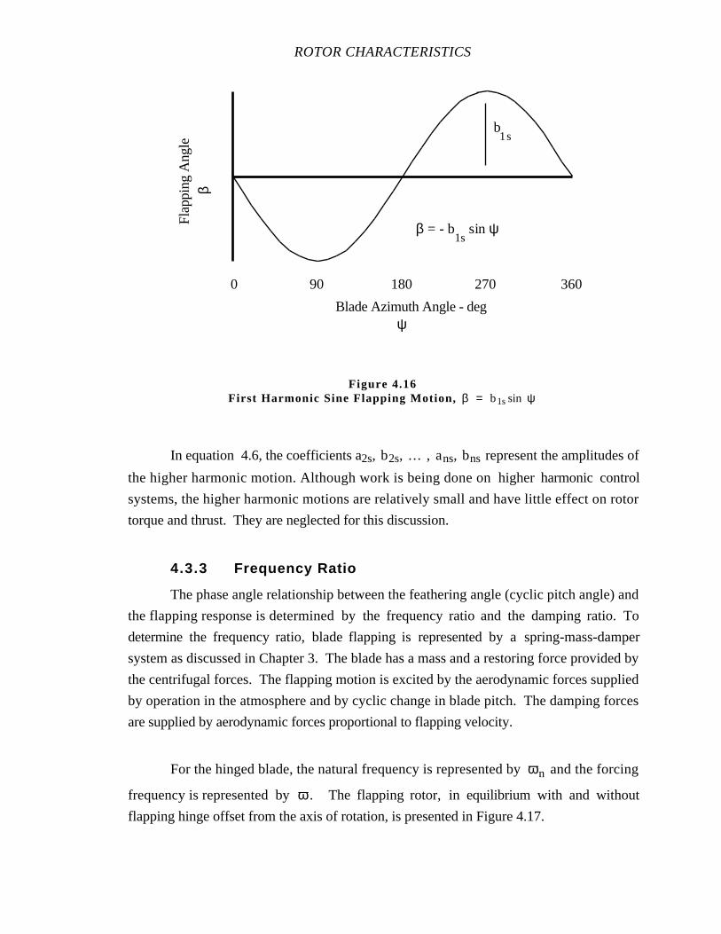
ROTOR CHARACTERISTICS
In equation 4.6, the coefficients a2s, b2s, ... , ans, bns represent the amplitudes of
the higher harmonic motion. Although work is being done on higher harmonic control
systems, the higher harmonic motions are relatively small and have little effect on rotor
torque and thrust. They are neglected for this discussion.
4.3.3 Frequency Ratio
The phase angle relationship between the feathering angle (cyclic pitch angle) and
the flapping response is determined by the frequency ratio and the damping ratio. To
determine the frequency ratio, blade flapping is represented by a spring-mass-damper
system as discussed in Chapter 3. The blade has a mass and a restoring force provided by
the centrifugal forces. The flapping motion is excited by the aerodynamic forces supplied
by operation in the atmosphere and by cyclic change in blade pitch. The damping forces
are supplied by aerodynamic forces proportional to flapping velocity.
For the hinged blade, the natural frequency is represented by ωn and the forcing
frequency is represented byω . The flapping rotor, in equilibrium with and without
flapping hinge offset from the axis of rotation, is presented in Figure 4.17.
Fla
ppin
g A
ngle
β
Blade Azimuth Angle - degψ
0 90 180 270 360
b1s
β = - b1s
sin ψ
Figure 4.16First Harmonic Sine Flapping Motion, β = b1ssin ψ
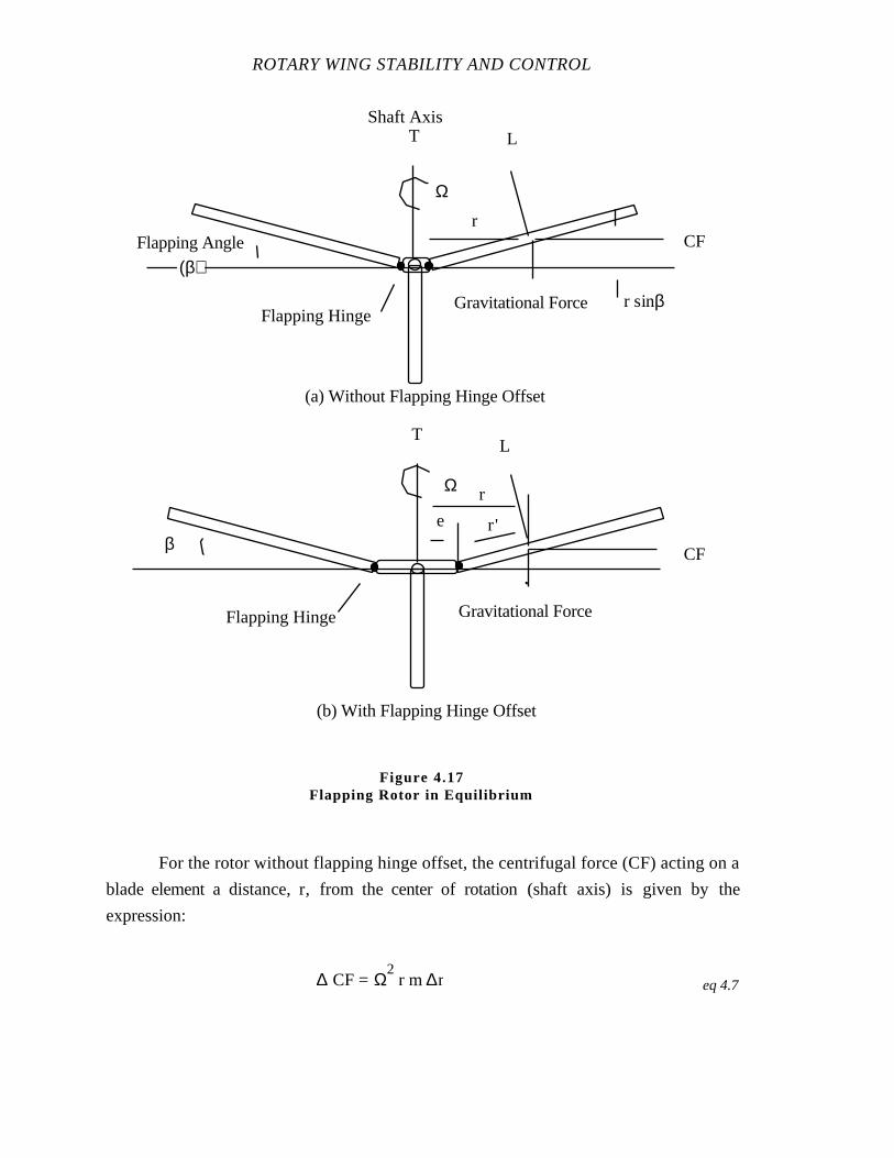
ROTARY WING STABILITY AND CONTROL
For the rotor without flapping hinge offset, the centrifugal force (CF) acting on a
blade element a distance, r, from the center of rotation (shaft axis) is given by the
expression:
∆ CF = Ω2 r m ∆r eq 4.7
Shaft Axis
Gravitational Force
Ω
(a) Without Flapping Hinge Offset
rFlapping Angle
(β)
r sinβ
(b) With Flapping Hinge Offset
r'
Ω
eβ
Gravitational Force
r
LT
Flapping Hinge
CF
LT
CF
Flapping Hinge
Figure 4.17Flapping Rotor in Equilibrium
ROTOR CHARACTERISTICS
The restoring moment due to this centrifugal force is given by:
∆Μ = ∆CF r sinβ eq 4.8
Using a small angle assumption, sinβ = β, the total moment is given by
integrating with respect to r from 0 to R, the rotor radius, is:
M = ∫0
RΩ
2 r2 m β dr = Ω
2 β ∫
0
R m r2 dr
eq 4.9
The spring constant for the equivalent spring-mass-damper system is:
K = Mβ
= Ω2 ∫
0
R m r2 dr
eq 4.10
The moment of inertia about the flapping hinge is defined as:
If = ∫
0
R m r2 dr
eq 4.11
Substituting into the equation for natural frequency of a spring-mass-damper, ωn ,
the natural frequency of a rotor without spring offset is given by:
ωn = KI
= Ω
2 I
fIf
= Ωeq 4.12
The frequency ratio of a rotor without hinge offset is given by:
ωωn
= ωΩ = 1eq 4.13

ROTARY WING STABILITY AND CONTROL
Where:
β - Flapping angle
CF - Centrifugal force
Ι - Moment of inertia
If - Moment of inertia about flapping hinge
Κ - Spring constant
M - Moment
m - Mass
R - Rotor radius
r - Radius along blade
Ω - Rotor angular velocity
ω - Frequency
ωn - Natural frequency.
The expression for the frequency ratio of a rotor without hinge offset says for a
rotor without flapping hinge offset, the frequency ratio is 1; and the natural frequency is the
same as the rotor angular velocity, Ω.
For the rotor with flapping hinge offset, the restoring moment due to the centrifugal
force acting on a blade mass element at a distance r' from the flapping hinge such that r = e
+ r', is given by:
∆Μ = m ∆r Ω2 (r'+ e) r' β eq 4.14
Using a small angle assumption, sinβ = β, the total moment is given by
integrating with respect to r from 0 to R - e:
M = Ω2 β ∫
0
R - em (r' + e) r' dr'
eq 4.15
However:
If = ∫
0
R - em r'
2 dr'
eq 4.16
ROTOR CHARACTERISTICS
And:
Mf
g = ∫0
R - em r' dr'
eq 4.17Thus:
M = Ω2
β (If + e
Mf
g )eq 4.18
The spring constant for the equivalent spring-mass-damper system is:
K = Mβ
= Ω2 ( I
f + e
Mf
g )eq 4.19
The moment of inertia about the flapping hinge is defined as:
If = m ∫
0
R - e r'
2 dr = mR
3
3 (1 - eR)
3
eq 4.20
And:
Mf
g = m ∫0
R - er' dr = mR
2
2 (1 - eR)
2
eq 4.21
Substituting into the equation for natural frequency of a spring-mass-damper, ωn ,
the natural frequency of a rotor without spring offset is given by:
ωn = KIf
= Ω 1 + eM
fg I
f
= Ω 1 +
32
eR
1 - eR eq 4.22
The frequency ratio of a rotor with hinge offset is given by:
ωωn
= ωΩ = 1 +
32
eR
1 - eR eq 4.23
ROTARY WING STABILITY AND CONTROL
Where:
β - Flapping angle
CF - Centrifugal force
e - Flapping hinge offset
g - Gravity
Ι - Moment of inertia
If - Moment of inertia about flapping hinge
Κ - Spring constant
M - Moment
m - Mass
Mf - Moment about flapping hinge
R - Rotor radius
r - Radius along blade
r' - Radius along blade outboard of flapping hinge
Ω - Rotor angular velocity
ω - Frequency
ωn - Natural frequency.
The expression for frequency ratio for a rotor with flapping hinge offset says the
frequency ratio is not 1; but, is a function of the flapping hinge offset. The natural
frequency of the flapping motion is greater than the rotational frequency. For a rotor with a
5% hinge offset, the frequency ratio is 1.04. The influence of frequency ratio on phase
angle is discussed later.
4.3.4 Damping Ratio
The damping ratio in combination with the frequency ratio determine the phase
angle. The damping ratio of the rotor in motion is found from the equivalent spring-mass-
damper system. The linear differential equation for the flapping motion is expressed as:
I f˙β + Bβ + K β = 0 eq 4.24
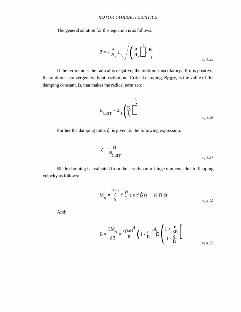
ROTOR CHARACTERISTICS
The general solution for this equation is as follows:
β = - B2I
f
± ( B2I
f)
2
- KIf eq 4.25
If the term under the radical is negative, the motion is oscillatory. If it is positive,
the motion is convergent without oscillation. Critical damping, BCRIT, is the value of the
damping constant, B, that makes the radical term zero:
BCRIT
= 2If (K
If)
12
eq 4.26
Further the damping ratio, ζ, is given by the following expression:
ζ = BB
CRIT eq 4.27
Blade damping is evaluated from the aerodynamic hinge moments due to flapping
velocity as follows:
MA
= ∫0
R - e r'
ρ2
a c r' β. (r' + e) Ω dr
eq 4.28
And:
B = 2M
A
∂β. =
cρaR4
8 (1 - eR)
4
Ω ( 1 + e3R
1 - eR
)eq 4.29
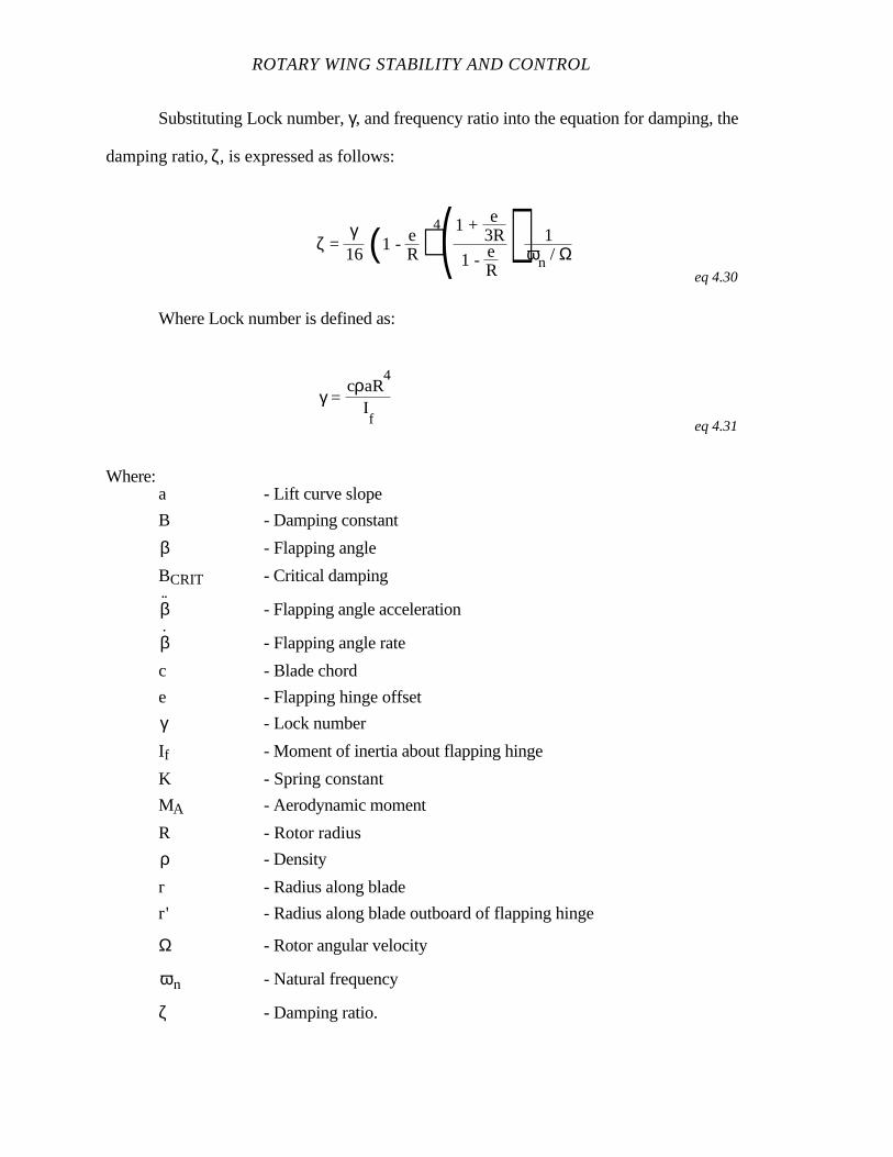
ROTARY WING STABILITY AND CONTROL
Substituting Lock number, γ, and frequency ratio into the equation for damping, the
damping ratio, ζ, is expressed as follows:
ζ = γ16 (1 - e
R)4( 1 + e
3R
1 - eR
) 1ωn / Ω
eq 4.30
Where Lock number is defined as:
γ = cρaR
4
If eq 4.31
Where:a - Lift curve slope
B - Damping constant
β - Flapping angle
BCRIT - Critical damping
˙β - Flapping angle acceleration
β - Flapping angle rate
c - Blade chord
e - Flapping hinge offset
γ - Lock number
If - Moment of inertia about flapping hinge
K - Spring constant
MA - Aerodynamic moment
R - Rotor radius
ρ - Density
r - Radius along blade
r' - Radius along blade outboard of flapping hinge
Ω - Rotor angular velocity
ωn - Natural frequency
ζ - Damping ratio.
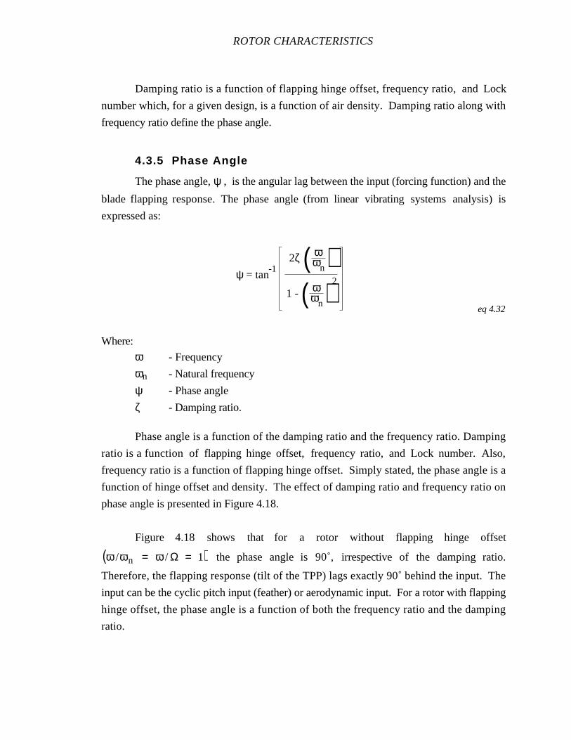
ROTOR CHARACTERISTICS
Damping ratio is a function of flapping hinge offset, frequency ratio, and Lock
number which, for a given design, is a function of air density. Damping ratio along with
frequency ratio define the phase angle.
4.3.5 Phase Angle
The phase angle, ψ , is the angular lag between the input (forcing function) and the
blade flapping response. The phase angle (from linear vibrating systems analysis) is
expressed as:
ψ = tan-1
2ζ ( ωωn)
1 - ( ωωn)
2
eq 4.32
Where:
ω - Frequency
ωn - Natural frequency
ψ - Phase angle
ζ - Damping ratio.
Phase angle is a function of the damping ratio and the frequency ratio. Damping
ratio is a function of flapping hinge offset, frequency ratio, and Lock number. Also,
frequency ratio is a function of flapping hinge offset. Simply stated, the phase angle is a
function of hinge offset and density. The effect of damping ratio and frequency ratio on
phase angle is presented in Figure 4.18.
Figure 4.18 shows that for a rotor without flapping hinge offset
ω /ωn = ω / Ω = 1( ) the phase angle is 90˚, irrespective of the damping ratio.
Therefore, the flapping response (tilt of the TPP) lags exactly 90˚ behind the input. The
input can be the cyclic pitch input (feather) or aerodynamic input. For a rotor with flapping
hinge offset, the phase angle is a function of both the frequency ratio and the damping
ratio.
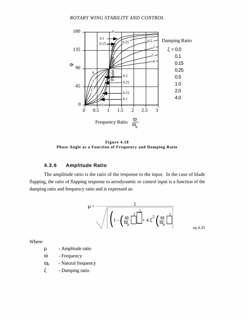
ROTARY WING STABILITY AND CONTROL
4.3.6 Amplitude Ratio
The amplitude ratio is the ratio of the response to the input. In the case of blade
flapping, the ratio of flapping response to aerodynamic or control input is a function of the
damping ratio and frequency ratio and is expressed as:
µ = 1
(1 - ( ωωn)
2)2
+ 4 ζ2 ( ω
ωn)2
eq 4.33
Where:
µ - Amplitude ratio
ω - Frequency
ωn - Natural frequency
ζ - Damping ratio.
0
45
90
135
180
0 0.5 1 1.5 2 2.5 3
4
2
1
0.50.250.15
0.1
0
4
2
1
0.25
0.5
0.15
0.1
0
Frequency Ratioωωn
Pha
se A
ngle
- d
eg
ψ
ζ = 0.0 0.1 0.15 0.25 0.5 1.0 2.0 4.0
Damping Ratio
Figure 4.18Phase Angle as a Function of Frequency and Damping Ratio
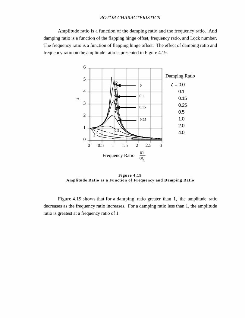
ROTOR CHARACTERISTICS
Amplitude ratio is a function of the damping ratio and the frequency ratio. And
damping ratio is a function of the flapping hinge offset, frequency ratio, and Lock number.
The frequency ratio is a function of flapping hinge offset. The effect of damping ratio and
frequency ratio on the amplitude ratio is presented in Figure 4.19.
Figure 4.19 shows that for a damping ratio greater than 1, the amplitude ratio
decreases as the frequency ratio increases. For a damping ratio less than 1, the amplitude
ratio is greatest at a frequency ratio of 1.
0
1
2
3
4
5
6
0 0.5 1 1.5 2 2.5 3
42 1 0.5
0.25
0.15
0.1
0 ζ = 0.0 0.1 0.15 0.25 0.5 1.0 2.0 4.0
Damping Ratio
Frequency Ratioωωn
Am
plitu
de R
atio
µ
Figure 4.19Amplitude Ratio as a Function of Frequency and Damping Ratio
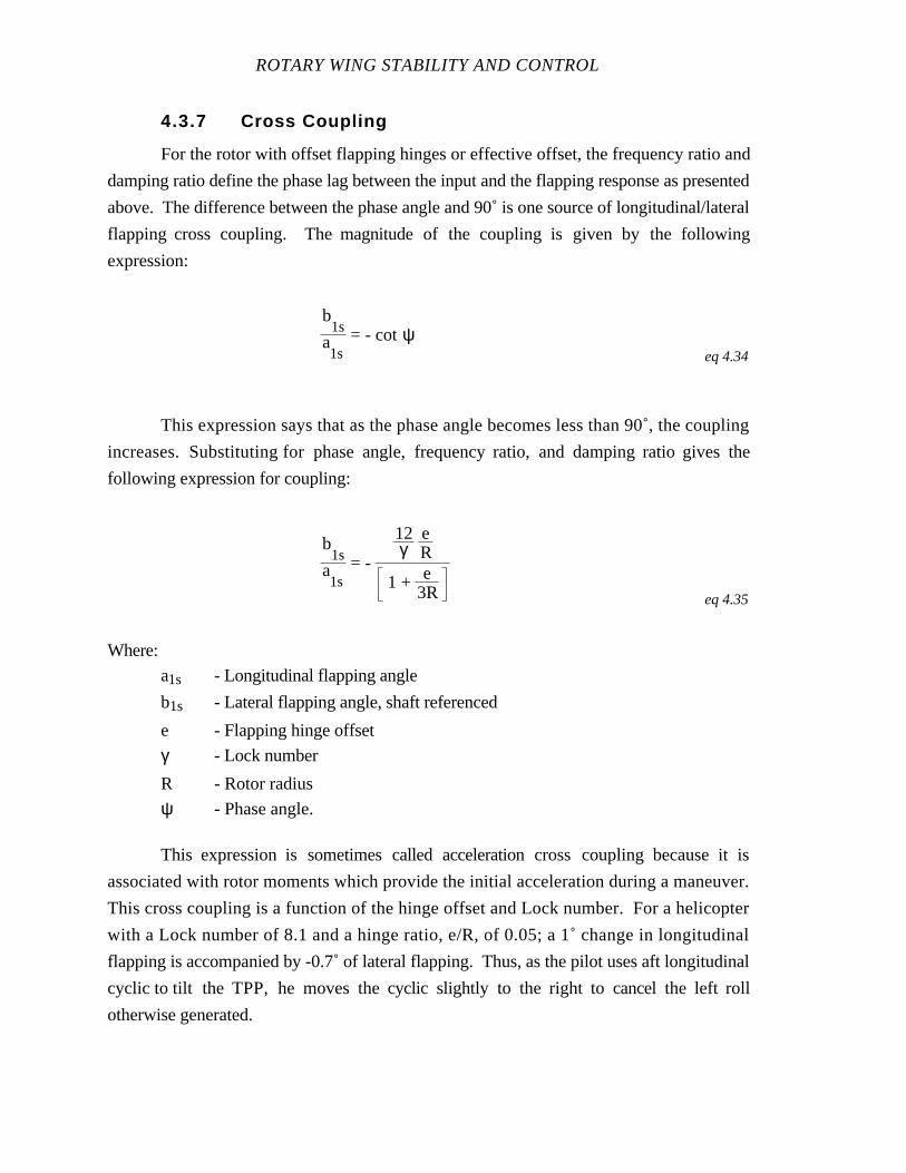
ROTARY WING STABILITY AND CONTROL
4.3.7 Cross Coupling
For the rotor with offset flapping hinges or effective offset, the frequency ratio and
damping ratio define the phase lag between the input and the flapping response as presented
above. The difference between the phase angle and 90˚ is one source of longitudinal/lateral
flapping cross coupling. The magnitude of the coupling is given by the following
expression:
b1s
a1s
= - cotψeq 4.34
This expression says that as the phase angle becomes less than 90˚, the coupling
increases. Substituting for phase angle, frequency ratio, and damping ratio gives the
following expression for coupling:
b1s
a1s
= -
12γ
eR
1 + e3R eq 4.35
Where:
a1s - Longitudinal flapping angle
b1s - Lateral flapping angle, shaft referenced
e - Flapping hinge offset
γ - Lock number
R - Rotor radius
ψ - Phase angle.
This expression is sometimes called acceleration cross coupling because it is
associated with rotor moments which provide the initial acceleration during a maneuver.
This cross coupling is a function of the hinge offset and Lock number. For a helicopter
with a Lock number of 8.1 and a hinge ratio, e/R, of 0.05; a 1˚ change in longitudinal
flapping is accompanied by -0.7˚ of lateral flapping. Thus, as the pilot uses aft longitudinal
cyclic to tilt the TPP, he moves the cyclic slightly to the right to cancel the left roll
otherwise generated.

ROTOR CHARACTERISTICS
4.3.8 Mechanical Correction for Coupling
The effect of phase angle on coupling due to control input is compensated for by
changing the angular alignment between the control input and the swashplate. If the phase
angle is constant, the angular alignment of the longitudinal and lateral inputs can correct for
the angle. However, the phase angle is not constant but a function of Lock number,
damping ratio, and frequency ratio. Thus, the designer has to make a compromise in
establishing the angular alignment of the flight controls and the swashplate.
4.3.9 Flapping Due to Pitch and Roll Rates
The rotating rotor produces damping moments when the helicopter is subjected to
pitch and roll rates. The damping produced by the tilt of the TPP lags behind the motion of
the shaft by an amount proportional to the pitch or roll rate. The aerodynamic forces on the
blade tend to stabilize the TPP with respect to the shaft. The TPP, attached to a shaft which
is tilting, follows the shaft. To maintain a steady nose up pitch rate, the air load on the
advancing blade is higher than on the retreating blade. This asymmetry is generated by
downward flapping velocity with respect to the shaft at ψ = 90° and an upward velocity
at ψ = 270° . The maximum flapping amplitude with respect to the shaft is down at
ψ = 180° and up at ψ = 0° . The TPP follows the motion of the shaft at a lag angle
that is proportional to the pitch rate and the rotor moment of inertia.
During a steady nose up pitch rate, some lateral flapping is generated because of the
decreased angle of attack at ψ = 180° and the increase at ψ = 0° . The change in angle
of attack is caused by the pitch rate. This difference in angle of attack is compensated for
by the lateral flapping which produces enough flapping velocity at these two blade locations
to cancel out the effect of the pitch rate. The longitudinal and lateral flapping caused by a
pure pitch rate is a source of cross coupling applicable to rotors with and without flapping
hinge offset.

ROTARY WING STABILITY AND CONTROL
The expression for rate cross coupling for a hovering rotor without hinge offset
experiencing only a pitch rate is given by the following simplified expression:
a1s
= - ( 16γ ) ( q
Ω)eq 4.36
b1s
= - ( qΩ)
eq 4.37
The complete equations for rate cross coupling are expressed as:
a1s
=
- 16γ ( q
Ω)(1 - e
R)2
+ ( pΩ)
1 - µ2
2
+
12γ
eR
(1 - eR)
3
- 16γ ( p
Ω)(1 - e
R)2
- ( qΩ)
1 - µ4
4 eq 4.38
b1s
=
- 16γ ( p
Ω)(1 - e
R)2
+ ( qΩ)
1 - µ2
2
+
12γ
eR
(1 - eR)
3
- 16γ ( q
Ω)(1 - e
R)2
- ( pΩ)
1 - µ4
4 eq 4.39
With the advance ratio, µ, defined as:
µ = VΩR eq 4.40
Where:
a1s - Longitudinal flapping angle, shaft referenced
b1s - Lateral flapping angle, shaft referenced
e - Flapping hinge offset
γ - Lock number
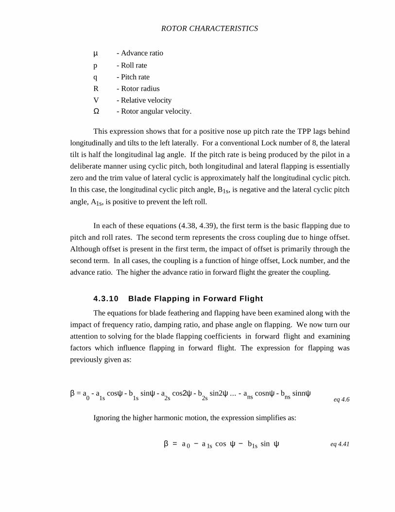
ROTOR CHARACTERISTICS
µ - Advance ratio
p - Roll rate
q - Pitch rate
R - Rotor radius
V - Relative velocity
Ω - Rotor angular velocity.
This expression shows that for a positive nose up pitch rate the TPP lags behind
longitudinally and tilts to the left laterally. For a conventional Lock number of 8, the lateral
tilt is half the longitudinal lag angle. If the pitch rate is being produced by the pilot in a
deliberate manner using cyclic pitch, both longitudinal and lateral flapping is essentially
zero and the trim value of lateral cyclic is approximately half the longitudinal cyclic pitch.
In this case, the longitudinal cyclic pitch angle, B1s, is negative and the lateral cyclic pitch
angle, A1s, is positive to prevent the left roll.
In each of these equations (4.38, 4.39), the first term is the basic flapping due to
pitch and roll rates. The second term represents the cross coupling due to hinge offset.
Although offset is present in the first term, the impact of offset is primarily through the
second term. In all cases, the coupling is a function of hinge offset, Lock number, and the
advance ratio. The higher the advance ratio in forward flight the greater the coupling.
4.3.10 Blade Flapping in Forward Flight
The equations for blade feathering and flapping have been examined along with the
impact of frequency ratio, damping ratio, and phase angle on flapping. We now turn our
attention to solving for the blade flapping coefficients in forward flight and examining
factors which influence flapping in forward flight. The expression for flapping was
previously given as:
β = a0 - a
1s cosψ - b
1s sinψ - a
2s cos2ψ - b
2s sin2ψ ... - ans cosnψ - bns sinnψ
eq 4.6
Ignoring the higher harmonic motion, the expression simplifies as:
β = a0 − a1s cos ψ − b1s sin ψ eq 4.41
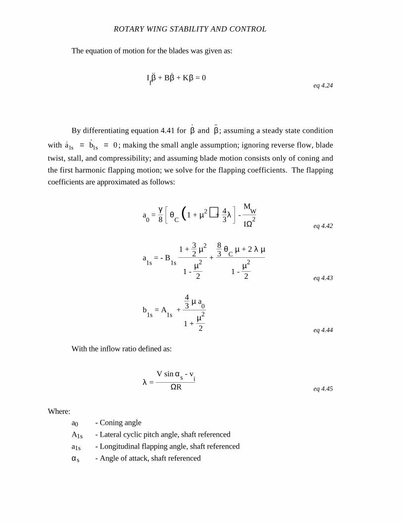
ROTARY WING STABILITY AND CONTROL
The equation of motion for the blades was given as:
Ifβ.. + Bβ
. + Kβ = 0
eq 4.24
By differentiating equation 4.41 for β and ˙β ; assuming a steady state condition
with a1s = b1s = 0; making the small angle assumption; ignoring reverse flow, blade
twist, stall, and compressibility; and assuming blade motion consists only of coning and
the first harmonic flapping motion; we solve for the flapping coefficients. The flapping
coefficients are approximated as follows:
a0 =
γ8
θC(1 + µ2) + 4
3λ -
MW
IΩ2
eq 4.42
a1s
= - B1s
1 + 32
µ2
1 - µ2
2
+
83
θC
µ + 2 λ µ
1 - µ2
2 eq 4.43
b1s
= A1s
+
43
µ a0
1 + µ2
2 eq 4.44
With the inflow ratio defined as:
λ = V sin αs - vi
ΩR eq 4.45
Where:
a0 - Coning angle
A1s - Lateral cyclic pitch angle, shaft referenced
a1s - Longitudinal flapping angle, shaft referenced
αs - Angle of attack, shaft referenced
ROTOR CHARACTERISTICS
Β - Damping constant
β - Flapping angle˙β - Flapping angle acceleration
β - Flapping angle rate
B1s - Longitudinal cyclic pitch angle, shaft referenced
b1s - Lateral flapping angle, shaft referenced
γ - Lock number
Ι - Moment of inertia
If - Moment of inertia about flapping hinge
Κ - Spring constant
λ - Inflow ratio
µ - Advance ratio
MW - Moment due to weight
θC - Collective pitch angle
R - Rotor radius
V - Relative velocity
vi - Induced velocity
Ω - Rotor angular velocity
ψ - Blade azimuth angle.
Typically, the second term in the expression for a0,MW
IΩ2 ,is neglected because the
weight of the blades is relatively small.
Several important relationships are contained in the above expressions. The coning
angle, a0, is a function of Lock number, advance ratio, and inflow ratio. The coning angle
increases as forward flight speed increases and as inflow increases.
Longitudinal flapping angle (a1s) is a function of the longitudinal cyclic pitch angle
(B1s). In accordance with the established sign convention, aft longitudinal cyclic pitch
angle(-B1s) produces aft longitudinal flapping (+a1s) and aft tilt of the TPP.
ROTARY WING STABILITY AND CONTROL
Longitudinal flapping angle is a function of the advance ratio; as forward speed
increases, a given ∆B1s produces increased ∆a1s. In forward flight, the increase in a1s due
to µ, produces an increase in control power. Also, through the second term, as forward
speed is increased for a fixed B1s, the longitudinal flapping increases and the TPP tilts aft
or blows back contributing to speed stability (Mu ).
Longitudinal flapping angle is a function of collective pitch angle,θ C. Increased
θ C produces increaseda1s. An increase in collective produces an increase in a1sand the
TPP tilts aft. The increase in a1sdue to collective is the reason forward cyclic is required as
the collective is increased during termination of an approach.
Longitudinal flapping angle is a function of inflow ratio. Increased inflow such as
caused by a vertical gust produces increaseda1s. Therefore, in a vertical gust the TPP tilts
aft.
Lateral flapping angle (b1s) is a function of lateral cyclic pitch angle (A1s). In
accordance with the established sign convention, right lateral cyclic pitch (+A1s) produces
right flapping (+b1s) and right tilt of the TPP.
Lateral flapping angle is a function of the advance ratio. Increased forward speed
produces increased lateral flapping and right tilt of the TPP. However, increased forward
speed does not produce an increase in control power as is the case for longitudinal cyclic.
Lateral flapping is not a function of θ C. However, increased collective produces
increased coning, a0, thereby increasing lateral flapping, resulting in a right tilt of the TPP.
Lateral flapping is not a function of inflow ratio. However coning is a function of
inflow ratio. A vertical gust increases coning, a0, thereby increasing lateral flapping,
resulting in a right tilt of the TPP.
Figure 4.20 presents the TPP and blade flapping response to a longitudinal cyclic
input in a hover. The representation is for a rotor system at a hover with a 90˚ phase angle.
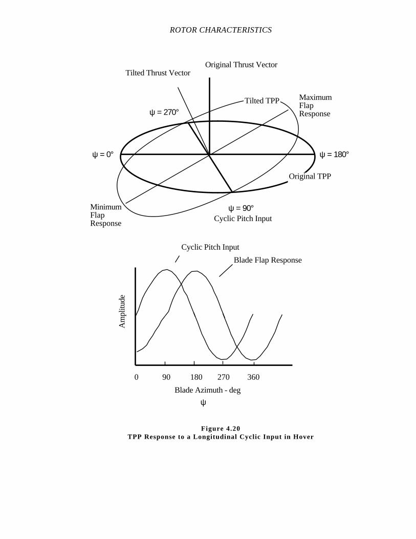
ROTOR CHARACTERISTICS
Tilted Thrust VectorOriginal Thrust Vector
Original TPP
Tilted TPP
ψ = 0°
ψ = 90°
ψ = 180°
ψ = 270°
MinimumFlapResponse
MaximumFlapResponse
Am
plitu
de
Cyclic Pitch Input
Blade Flap Response
0 90 180 270 360
Blade Azimuth - deg
ψ
Cyclic Pitch Input
Figure 4.20TPP Response to a Longitudinal Cyclic Input in Hover

ROTARY WING STABILITY AND CONTROL
As the TPP responds to a longitudinal cyclic input in hover, each blade of a multi-
bladed rotor has the same flapping angle at a given azimuth position and lies in the new
TPP. The new TPP is oriented with the maximum upward displacement 90˚ after the cyclic
pitch input (phase angle = 90˚). Furthermore, the magnitude of the flapping (and TPP tilt)
is equal to the magnitude of the cyclic control input. Since the thrust vector is
perpendicular to the TPP, a moment is generated about the helicopter CG proportional to
the product of mast height and TPP tilt.
4.3.11 TPP Response to Non-Uniform Downwash
The fore/aft variation of inflow is indicated schematically on Figure 4.21. A downwash
variation from zero at the front of the disk, to maximum at the aft edge of the disk, is
obtained by adding a uniform downwash to one varying linearly, with an up value at the
front of the disk, and a down value at the aft edge of the disk. Figure 4.21 also shows the
flow relative to a rotor blade with coning. A similar relative velocity situation exists. There
is an up flow relative to a blade at the front of the disk and a down flow relative to the blade
at the trailing edge of the disk. These velocities, normal to the TPP, change the effective
blade angles of attack. The angle of attack is increased at the front of the rotor disk and
decreased at the rear of the disk. The TPP tilts to the right if the pilot makes no
compensating control inputs. This effect is most critical in the low airspeed transition
region. In this region, the downwash effect is considerably larger than that due to coning.
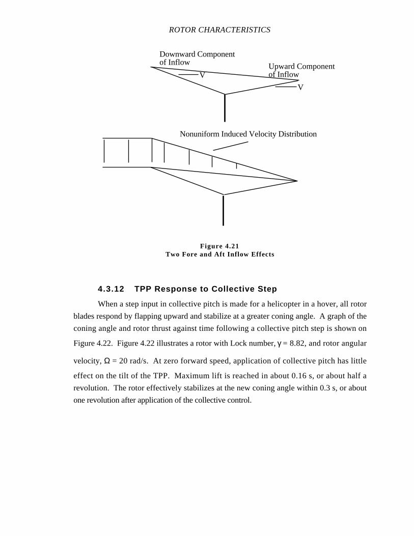
ROTOR CHARACTERISTICS
4.3.12 TPP Response to Collective Step
When a step input in collective pitch is made for a helicopter in a hover, all rotor
blades respond by flapping upward and stabilize at a greater coning angle. A graph of the
coning angle and rotor thrust against time following a collective pitch step is shown on
Figure 4.22. Figure 4.22 illustrates a rotor with Lock number, γ = 8.82, and rotor angular
velocity, Ω = 20 rad/s. At zero forward speed, application of collective pitch has little
effect on the tilt of the TPP. Maximum lift is reached in about 0.16 s, or about half a
revolution. The rotor effectively stabilizes at the new coning angle within 0.3 s, or about
one revolution after application of the collective control.
Nonuniform Induced Velocity Distribution
Upward Componentof Inflow
Downward Componentof Inflow
V
V
Figure 4.21Two Fore and Aft Inflow Effects
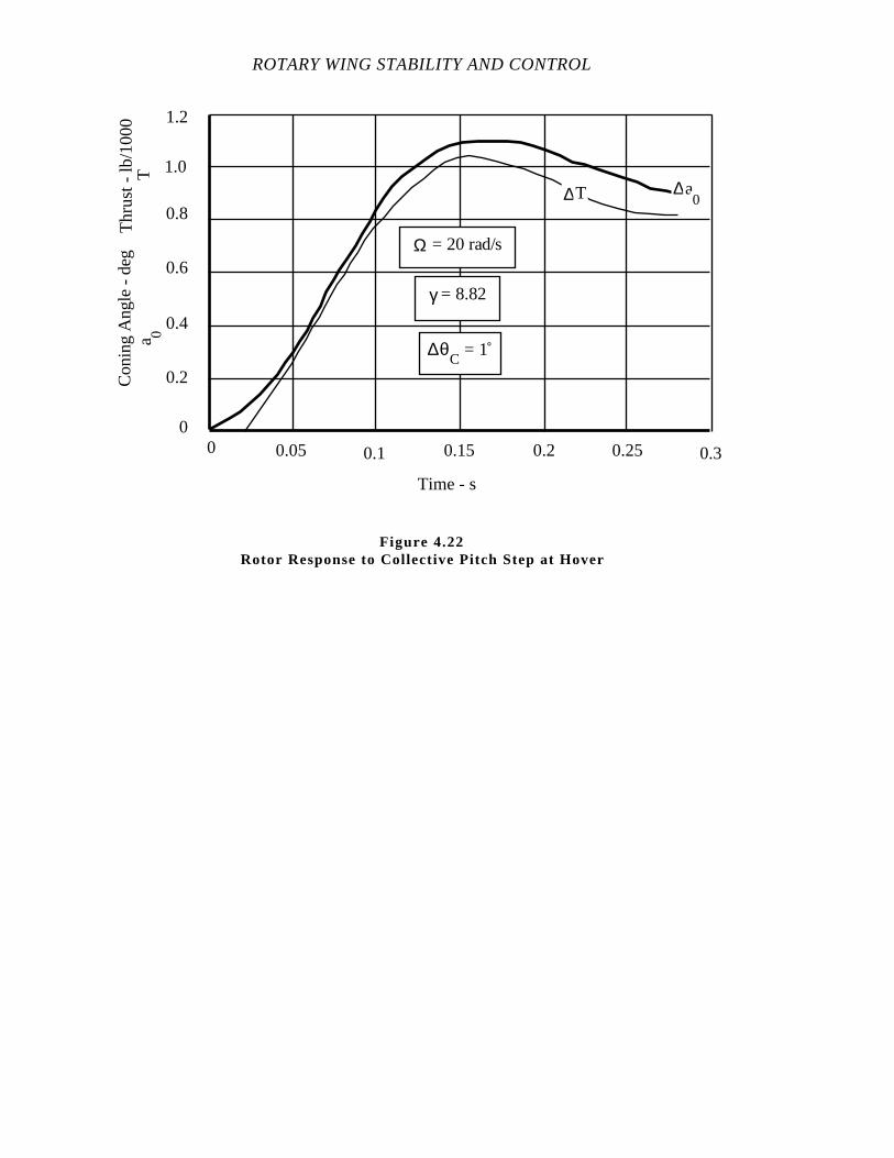
ROTARY WING STABILITY AND CONTROL
0
0.2
0.4
0.6
0.8
1.0
1.2
0 0.05 0.1 0.15 0.2 0.25 0.3
Ω = 20 rad/s
γ = 8.82
∆θC
= 1
∆T
Time - s
Con
ing
Ang
le -
deg
a 0
Thr
ust -
lb/1
000
T
∆a0
Figure 4.22Rotor Response to Collective Pitch Step at Hover
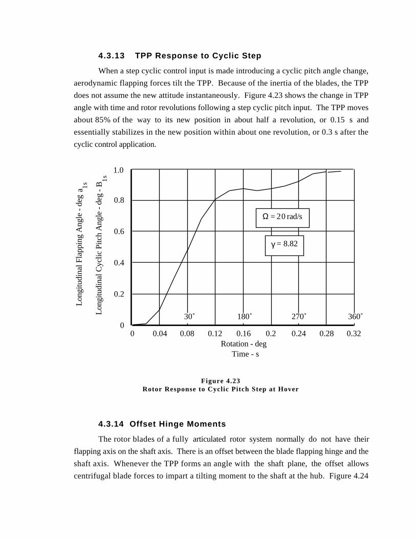
4.3.13 TPP Response to Cyclic Step
When a step cyclic control input is made introducing a cyclic pitch angle change,
aerodynamic flapping forces tilt the TPP. Because of the inertia of the blades, the TPP
does not assume the new attitude instantaneously. Figure 4.23 shows the change in TPP
angle with time and rotor revolutions following a step cyclic pitch input. The TPP moves
about 85% of the way to its new position in about half a revolution, or 0.15 s and
essentially stabilizes in the new position within about one revolution, or 0.3 s after the
cyclic control application.
4.3.14 Offset Hinge Moments
The rotor blades of a fully articulated rotor system normally do nothave their
flapping axis on the shaft axis. There is an offset between the blade flapping hinge and the
shaft axis. Whenever the TPP forms an angle with theshaft plane, the offset allows
centrifugal blade forces to impart a tilting moment to the shaft at the hub. Figure 4.24
0
0.2
0.4
0.6
0.8
1.0
0 0.04 0.08 0.12 0.16 0.2 0.24 0.28 0.32
Time - sRotation - deg
30˚ 180˚ 270˚
Ω = 20 rad/s
γ = 8.82
360˚Long
itudi
nal C
yclic
Pitc
h A
ngle
- d
eg
-B
1s
a 1sLo
ngitu
dina
l Fla
ppin
g A
ngle
- d
eg
Figure 4.23Rotor Response to Cyclic Pitch Step at Hover
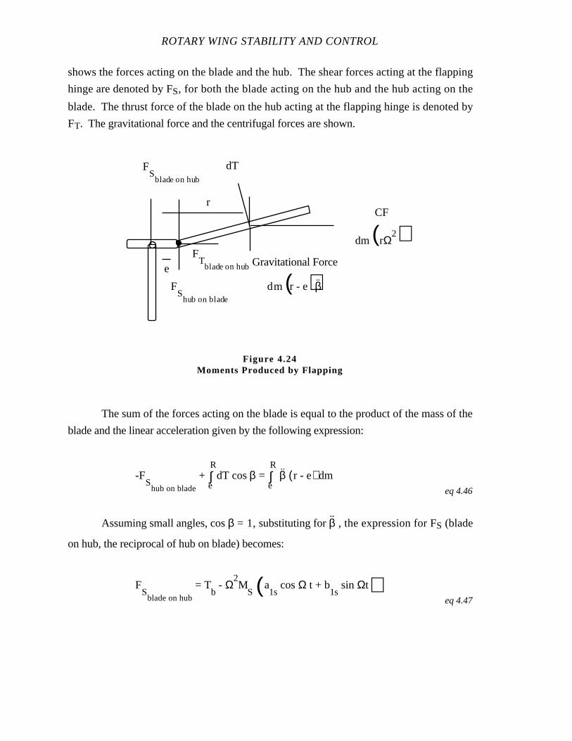
ROTARY WING STABILITY AND CONTROL
shows the forces acting on the blade and the hub. The shear forces acting at the flapping
hinge are denoted by FS, for both the blade acting on the hub and the hub acting on the
blade. The thrust force of the blade on the hub acting at the flapping hinge is denoted by
FT. The gravitational force and the centrifugal forces are shown.
The sum of the forces acting on the blade is equal to the product of the mass of the
blade and the linear acceleration given by the following expression:
-FS
hub on blade
+ ∫e
RdT cos β = ∫
e
Rβ..
(r - e) dmeq 4.46
Assuming small angles, cos β = 1, substituting for β , the expression for FS (blade
on hub, the reciprocal of hub on blade) becomes:
FS
blade on hub
= Tb - Ω
2M
S (a1s
cos Ω t + b1s
sin Ωt)eq 4.47
eGravitational Force
rCF
dT
FS
hub on blade
FT
blade on hub
FS
blade on hub
dm(rΩ2)
dm(r - e)β..
Figure 4.24Moments Produced by Flapping
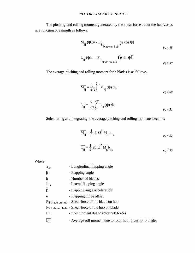
ROTOR CHARACTERISTICS
The pitching and rolling moment generated by the shear force about the hub varies
as a function of azimuth as follows:
MH
(ψ) = - FS
blade on hub(e cos ψ)
eq 4.48
LH
(ψ) = - FS
blade on hub(e sin ψ)
eq 4.49
The average pitching and rolling moment for b blades is as follows:
MH
= b2π ∫
0
2π M
H (ψ) dψ
eq 4.50
LH
= b2π ∫
0
2π L
H (ψ) dψ
eq 4.51
Substituting and integrating, the average pitching and rolling moments become:
MH
= 12
eb Ω2 M
S a
1s eq 4.52
LH
= 12
ebΩ2 M
Sb
1s eq 4.53
Where:a1s - Longitudinal flapping angle
β - Flapping angle
b - Number of bladesb1s - Lateral flapping angle
β - Flapping angle acceleration
e - Flapping hinge offset
FS blade on hub- Shear force of the blade on hub
FS hub on blade- Shear force of the hub on blade
LH - Roll moment due to rotor hub forces
LH—
- Average roll moment due to rotor hub forces for b blades
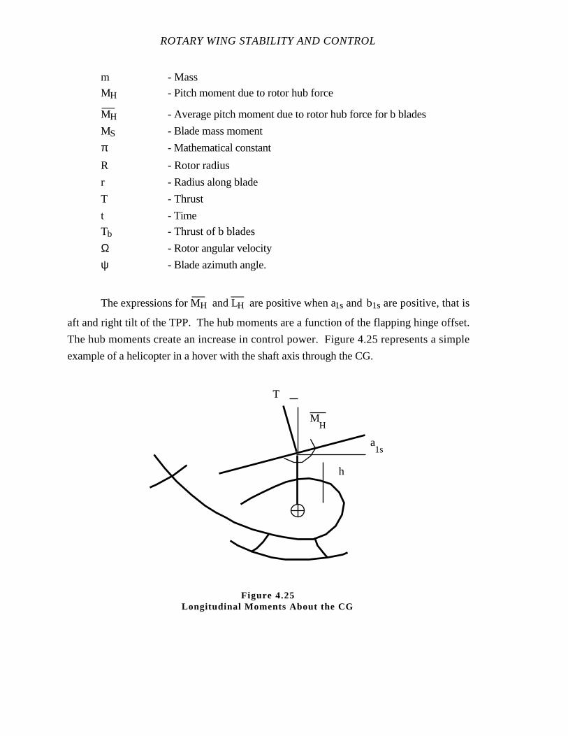
ROTARY WING STABILITY AND CONTROL
m - Mass
MH - Pitch moment due to rotor hub force
MH—
- Average pitch moment due to rotor hub force for b blades
MS - Blade mass moment
π - Mathematical constant
R - Rotor radius
r - Radius along blade
T - Thrust
t - Time
Tb - Thrust of b blades
Ω - Rotor angular velocity
ψ - Blade azimuth angle.
The expressions for MH—
and LH—
are positive when a1s and b1s are positive, that is
aft and right tilt of the TPP. The hub moments are a function of the flapping hinge offset.
The hub moments create an increase in control power. Figure 4.25 represents a simple
example of a helicopter in a hover with the shaft axis through the CG.
h
T
a1s
MH
Figure 4.25Longitudinal Moments About the CG

ROTOR CHARACTERISTICS
In this simple example, assuming small angles, the sum of the moments about the
CG is as follows:
∑ MCG
= Th sin a1s
+ MH
= Th + 12
eb Ω2 M
S a
1s eq 4.54
Where:
a1s - Longitudinal flapping angle
b - Number of blades
e - Flapping hinge offset
h - Height of hub above CG
MCG - Moment about CG
MH—
- Average pitch moment due to rotor hub force for b blades
MS - Blade mass moment
T - Thrust
Ω - Rotor angular velocity.
The expression for the moment about the CG shows an increase in the MCG and
control power due to the hub moment produced by the flapping hinge offset.
4.3.15 H Force Due to Flapping
Rotor thrust is often assumed to be perpendicular to the TPP; however, the effect of
inflow produces forces which act parallel to the shaft plane ( ⊥ to the shaft). Figure 4.26
represents a helicopter hovering with aft tilt of the TPP due to the CG being ahead of the
shaft.
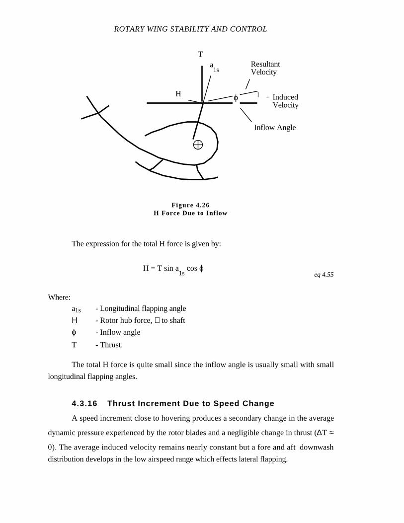
ROTARY WING STABILITY AND CONTROL
The expression for the total H force is given by:
H = T sin a1s
cos ϕeq 4.55
Where:
a1s - Longitudinal flapping angle
Η - Rotor hub force, ⊥ to shaft
ϕ - Inflow angle
T - Thrust.
The total H force is quite small since the inflow angle is usually small with small
longitudinal flapping angles.
4.3.16 Thrust Increment Due to Speed Change
A speed increment close to hovering produces a secondary change in the average
dynamic pressure experienced by the rotor blades and a negligible change in thrust (∆T ≈
0). The average induced velocity remains nearly constant but a fore and aft downwash
distribution develops in the low airspeed range which effects lateral flapping.
ResultantVelocity
InducedVelocity
ϕH
T
Inflow Angle
a1s
Figure 4.26H Force Due to Inflow
ROTOR CHARACTERISTICS
In forward flight, a thrust increment is produced by an increase in forward speed.
The thrust increment is due to several factors whose relative magnitudes depends on the
initial trim speed. An increase in average dynamic pressure in conjunction with collective
pitch increases thrust. Decreased induced velocity with a forward speed increment
increases the effective angle of attack of the blade sections and their lift. However, at
higher forward speeds, the TPP is tilted forward so a speed increment produces a
downward flow normal to the disk reducing the effective blade angle of attack and thrust.
Typical thrust changes with speed increments are positive for low trim speeds, but become
negative for high trim speeds (TPP tilted forward).
4.3.17 Effects of Compressibility and Retreating Blade
There are several ways compressibility effects handling qualities in high speed
flight. Noise and vibration caused by compressibility are an annoyance to the pilot and
often provide a high speed limitation on the helicopter. The possibility of encountering
blade flapping or pitching flutter increases when blade aerodynamic characteristics are
modified by compressibility. Although these instabilities may not be encountered,
vibrations are amplified at flight conditions close to flutter.
The most significant effect of compressibility on handling qualities arises from large
changes in the blade section pitching moment coefficient as a function of angle of attack.
Since the local Mach number varies with blade azimuth angle, these changes cause large
cyclic variations in pitching moments and result in corresponding twisting of the blades. A
cyclic twisting of the blades has the same effect as a cyclic control input. Consequently,
blade flapping occurs and undesirable pitching and/or rolling moments are applied to the
helicopter. The pilot must apply cyclic control inputs to compensate for these undesirable
moments. Blade pitching moments due to compressibility cause an additional problem for
helicopters without irreversible controls where they result in forces being fed back through
the control system.
Retreating blade stall is another phenomenon which tends to occur concurrently
with advancing blade compressibility problems in high speed flight. While forward speed
adds to the relative velocity of the advancing blade, it subtracts from the speed of the
retreating blade. At high forward speeds a substantial portion of the rotor disc may be
stalled, or operating in reverse flow. Figure 4.7 indicates therelative velocity of the
ROTARY WING STABILITY AND CONTROL
advancing and retreating blades. The edge of the circular region on the retreating blade side
of the rotor disc shows the outer limits of the reverse flow region. Since the boundary of
this region corresponds to relative airspeed equal to zero, the region over which the blades
are stalled is considerably higher.
The diameter of the reverse flow region is V/Ω at any forward speed; therefore,
some portion of the rotor disc is operating in reverse flow. At low airspeeds, the effects
are small because a substantial portion of the reverse flow region encompasses the inboard
blade root region and because the contribution of the inboard blade sections to the total
blade forces is small. At high speeds, this reverse flow region typically extends over 50%
or more of the retreating blade radius, causing substantial loss of lift and undesirable
pitching and rolling moments.
4.3.18 Characteristics of Tandem Rotor Configuration
Some aspects of stability and control of tandem rotor configurations are simpler
than single rotor helicopters. The aircraft is supported by the thrust of two rotors. The
thrust of each rotor is controlled through the conventional use of collective blade pitch.
Aircraft pitching moment is produced through the use of differential collective between the
fore and aft rotor. Yawing moment is produced by tilting the front rotor to the opposite
side laterally from the rear rotor. Rolling moment is generated by tilting both rotors
laterally in the same direction.
On the other hand, the analysis of the response of a tandem configuration to vehicle
motions is complicated by the interference effects between the two rotors and between the
rotors and the airframe. The significant effects of tandem rotors on the various stability
derivatives of the vehicles, the corresponding aircraft dynamics, and the important
differences from single rotor helicopters are covered at the end of the pertinent chapters.
4.3.19 Quasi-Static Approximation
Figures 4.22 and 4.23 indicate typical rotor responses to step collective and cyclic
control inputs. In both cases, the rotor stabilizes in a new TPP within one revolution, or
approximately 0.3 s. This suggests that dynamic blade responses have little effect on the
flight dynamics of the helicopter because the time constants and periods of both the long
term and short term flight dynamic response modes are much longer. Consequently, a
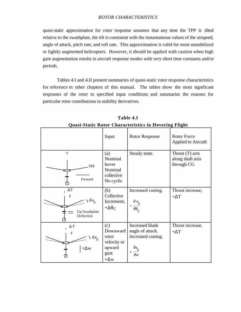
ROTOR CHARACTERISTICS
quasi-static approximation for rotor response assumes that any time the TPP is tilted
relative to the swashplate, the tilt is consistent with the instantaneous values of the airspeed,
angle of attack, pitch rate, and roll rate. This approximation is valid for most unstabilized
or lightly augmented helicopters. However, it should be applied with caution when high
gain augmentation results in aircraft response modes with very short time constants and/or
periods.
Tables 4.I and 4.II present summaries of quasi-static rotor response characteristics
for reference in other chapters of this manual. The tables show the most significant
responses of the rotor to specified input conditions and summarize the reasons for
particular rotor contributions to stability derivatives.
Table 4.I
Quasi-Static Rotor Characteristics in Hovering Flight
Input Rotor Response Rotor ForceApplied to Aircraft
T
TPP
Forward
(a)NominalhoverNominalcollectiveNo cyclic
Steady state. Thrust (T) actsalong shaft axisthrough CG
T
∆T
Up SwashplateDeflection
∆a0
(b)CollectiveIncrement,+∆θC
Increased coning.
+∂ a
0
∂θC
Thrust increase,+∆T
T
∆ T
∆a0
+∆w
(c)Downwardrotorvelocity orupwardgust+∆w
Increased bladeangle of attack.Increased coning.
+∂a
0
∂w
Thrust increase,+∆T
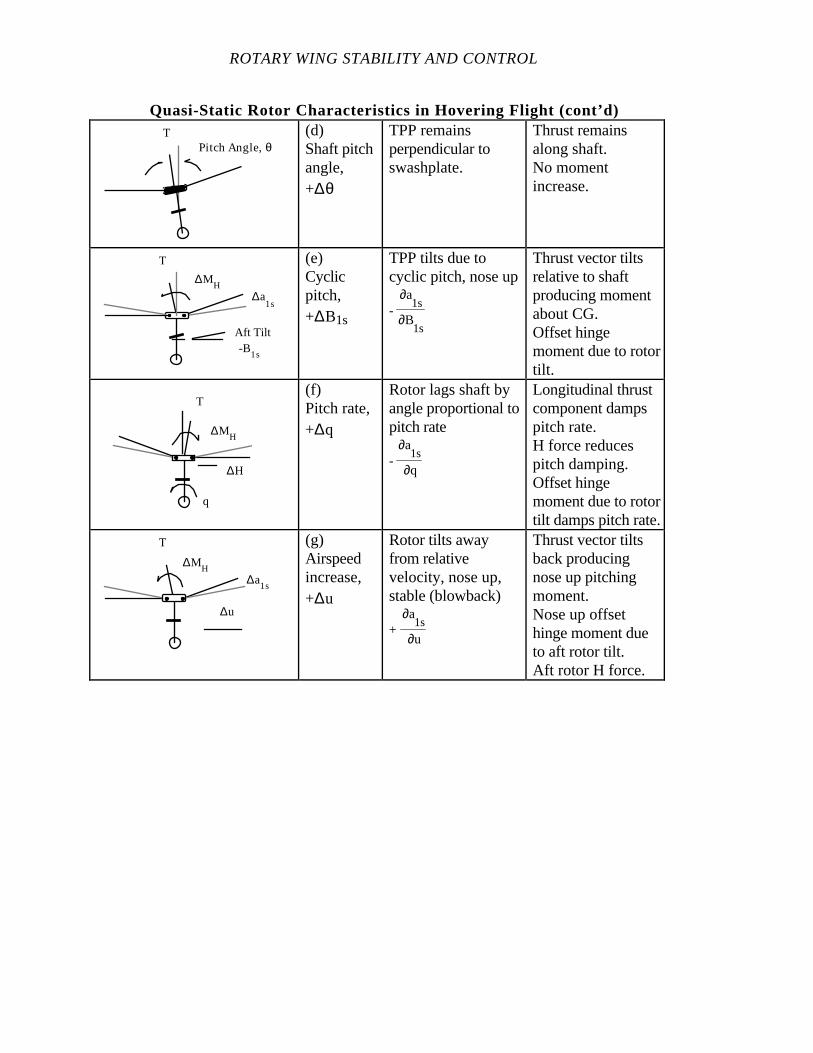
ROTARY WING STABILITY AND CONTROL
Quasi-Static Rotor Characteristics in Hovering Flight (cont’d)T
Pitch Angle,θ(d)Shaft pitchangle,+∆θ
TPP remainsperpendicular toswashplate.
Thrust remainsalong shaft.No momentincrease.
T
-B1s
∆a1s
∆MH
Aft Tilt
(e)Cyclicpitch,+∆B1s
TPP tilts due tocyclic pitch, nose up
-∂a
1s
∂B1s
Thrust vector tiltsrelative to shaftproducing momentabout CG.Offset hingemoment due to rotortilt.
T
q
∆MH
∆H
(f)Pitch rate,+∆q
Rotor lags shaft byangle proportional topitch rate
-∂a
1s
∂q
Longitudinal thrustcomponent dampspitch rate.H force reducespitch damping.Offset hingemoment due to rotortilt damps pitch rate.
T
∆u
∆MH
∆a1s
(g)Airspeedincrease,+∆u
Rotor tilts awayfrom relativevelocity, nose up,stable (blowback)
+∂a
1s
∂u
Thrust vector tiltsback producingnose up pitchingmoment.Nose up offsethinge moment dueto aft rotor tilt.Aft rotor H force.
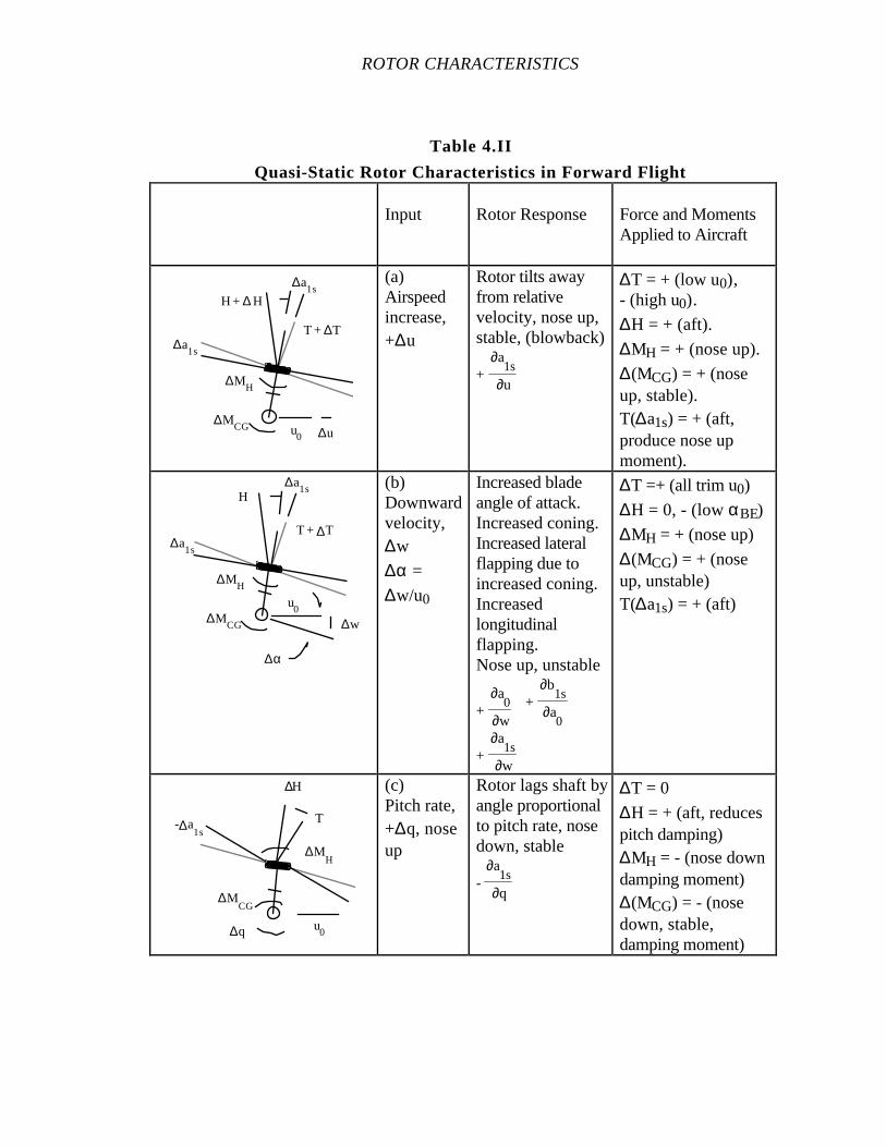
ROTOR CHARACTERISTICS
Table 4.II
Quasi-Static Rotor Characteristics in Forward Flight
Input Rotor Response Force and MomentsApplied to Aircraft
∆a1s
∆a1s
T + ∆T
u0 ∆u
H + ∆ H
∆MCG
∆MH
(a)Airspeedincrease,+∆u
Rotor tilts awayfrom relativevelocity, nose up,stable, (blowback)
+∂a
1s
∂u
∆T = + (low u0),- (high u0).
∆H = + (aft).
∆MH = + (nose up).
∆(MCG) = + (noseup, stable).T(∆a1s) = + (aft,produce nose upmoment).
∆a1s
∆a1s
T + ∆T
u0
∆MCG ∆w
H
∆α
∆MH
(b)Downwardvelocity,∆w
∆α =
∆w/u0
Increased bladeangle of attack.Increased coning.Increased lateralflapping due toincreased coning.Increasedlongitudinalflapping.Nose up, unstable
+∂a
0
∂w+
∂b1s
∂a0
+∂a
1s
∂w
∆T =+ (all trim u0)
∆H = 0, - (low αBE)
∆MH = + (nose up)
∆(MCG) = + (noseup, unstable)T(∆a1s) = + (aft)
u0
∆MCG
∆q
T-∆a1s
∆H
∆MH
(c)Pitch rate,+∆q, noseup
Rotor lags shaft byangle proportionalto pitch rate, nosedown, stable
-∂a
1s
∂q
∆T = 0
∆H = + (aft, reducespitch damping)∆MH = - (nose downdamping moment)∆(MCG) = - (nosedown, stable,damping moment)
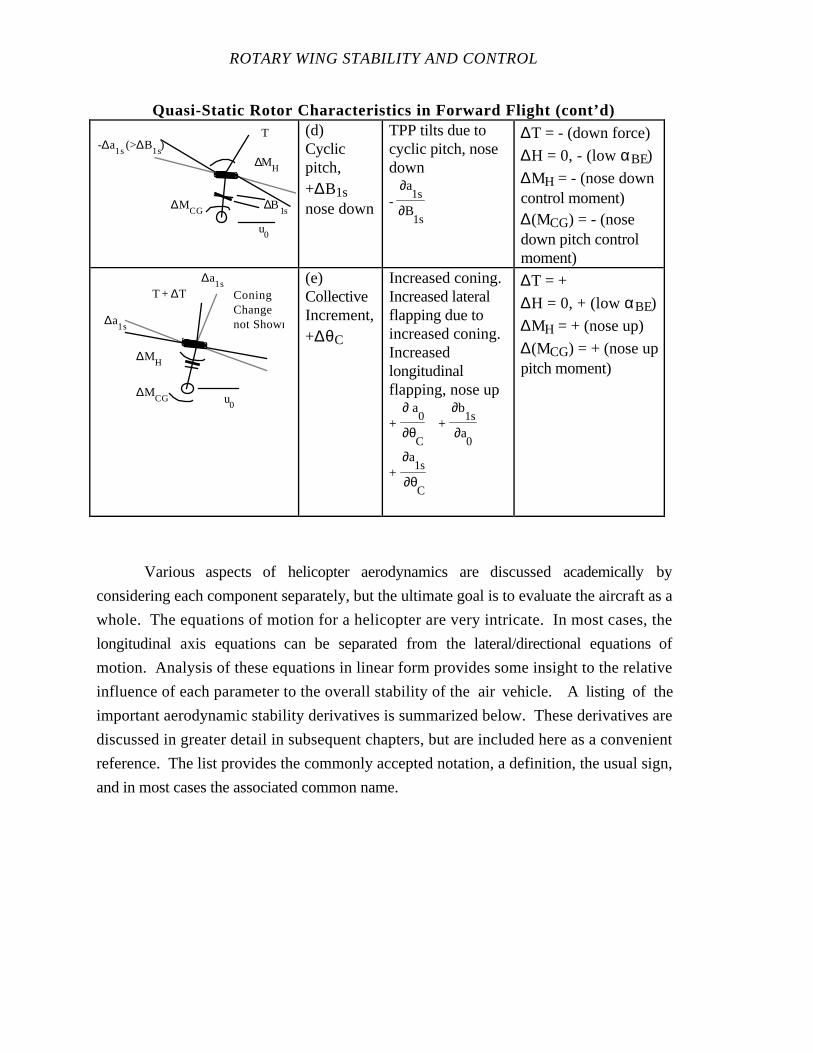
ROTARY WING STABILITY AND CONTROL
Quasi-Static Rotor Characteristics in Forward Flight (cont’d)
u0
∆MCG
T
∆MH
∆B1s
-∆a1s
(>∆B1s
)(d)Cyclicpitch,+∆B1snose down
TPP tilts due tocyclic pitch, nosedown
-∂a
1s
∂B1s
∆T = - (down force)
∆H = 0, - (low αBE)
∆MH = - (nose downcontrol moment)∆(MCG) = - (nosedown pitch controlmoment)
∆a1s
∆a1s
u0
∆MCG
∆MH
T + ∆T ConingChangenot Shown
(e)CollectiveIncrement,+∆θC
Increased coning.Increased lateralflapping due toincreased coning.Increasedlongitudinalflapping, nose up
+∂ a
0
∂θC
+∂b
1s
∂a0
+∂a
1s
∂θC
∆T = +
∆H = 0, + (low αBE)
∆MH = + (nose up)
∆(MCG) = + (nose uppitch moment)
Various aspects of helicopter aerodynamics are discussed academically by
considering each component separately, but the ultimate goal is to evaluate the aircraft as a
whole. The equations of motion for a helicopter are very intricate. In most cases, the
longitudinal axis equations can be separated from the lateral/directional equations of
motion. Analysis of these equations in linear form provides some insight to the relative
influence of each parameter to the overall stability of the air vehicle. A listing of the
important aerodynamic stability derivatives is summarized below. These derivatives are
discussed in greater detail in subsequent chapters, but are included here as a convenient
reference. The list provides the commonly accepted notation, a definition, the usual sign,
and in most cases the associated common name.
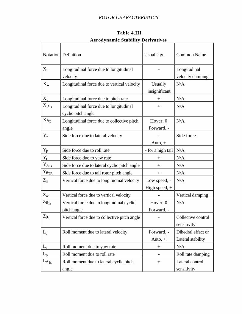
ROTOR CHARACTERISTICS
Table 4.III
Aerodynamic Stability Derivatives
Notation Definition Usual sign Common Name
Xu Longitudinal force due to longitudinal
velocity
- Longitudinal
velocity damping
Xw Longitudinal force due to vertical velocity Usually
insignificant
N/A
Xq Longitudinal force due to pitch rate + N/AXB1s Longitudinal force due to longitudinal
cyclic pitch angle
+ N/A
XθC Longitudinal force due to collective pitch
angle
Hover, 0
Forward, -
N/A
Yv Side force due to lateral velocity -
Auto, +
Side force
Yp Side force due to roll rate - for a high tail N/A
Yr Side force due to yaw rate + N/AYA1s Side force due to lateral cyclic pitch angle + N/AYθTR Side force due to tail rotor pitch angle + N/A
Zu Vertical force due to longitudinal velocity Low speed, -
High speed, +
N/A
Zw Vertical force due to vertical velocity - Vertical dampingZB1s Vertical force due to longitudinal cyclic
pitch angle
Hover, 0
Forward, -
N/A
ZθC Vertical force due to collective pitch angle - Collective control
sensitivity
Lv Roll moment due to lateral velocity Forward, -
Auto, +
Dihedral effect or
Lateral stability
Lr Roll moment due to yaw rate + N/A
Lp Roll moment due to roll rate - Roll rate dampingLA1s Roll moment due to lateral cyclic pitch
angle
+ Lateral control
sensitivity
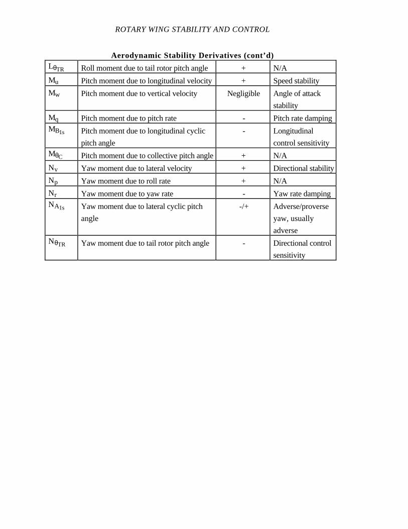
ROTARY WING STABILITY AND CONTROL
Aerodynamic Stability Derivatives (cont’d)LθTR Roll moment due to tail rotor pitch angle + N/A
Mu Pitch moment due to longitudinal velocity + Speed stability
Mw Pitch moment due to vertical velocity Negligible Angle of attack
stability
Mq Pitch moment due to pitch rate - Pitch rate dampingMB1s Pitch moment due to longitudinal cyclic
pitch angle
- Longitudinal
control sensitivityMθC Pitch moment due to collective pitch angle + N/A
Nv Yaw moment due to lateral velocity + Directional stability
Np Yaw moment due to roll rate + N/A
Nr Yaw moment due to yaw rate - Yaw rate dampingNA1s Yaw moment due to lateral cyclic pitch
angle
-/+ Adverse/proverse
yaw, usually
adverseNθTR Yaw moment due to tail rotor pitch angle - Directional control
sensitivity
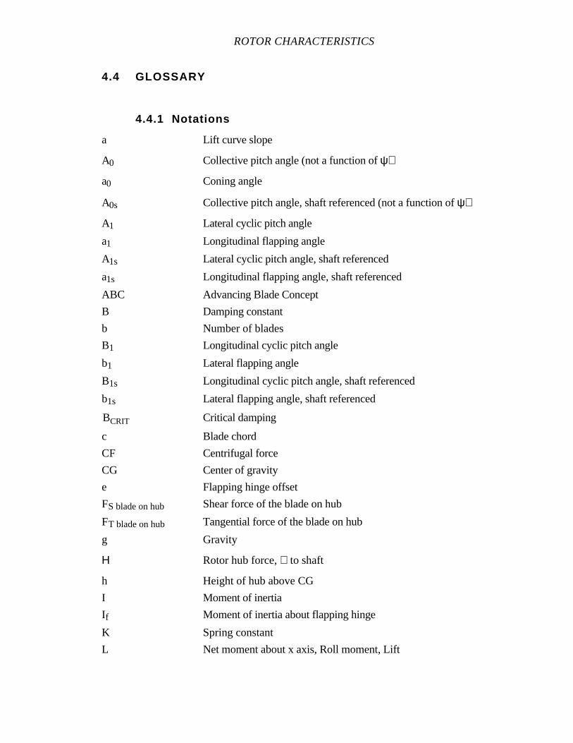
ROTOR CHARACTERISTICS
4.4 GLOSSARY
4.4.1 Notations
a Lift curve slope
A0 Collective pitch angle (not a function of ψ)
a0 Coning angle
A0s Collective pitch angle, shaft referenced (not a function of ψ)
A1 Lateral cyclic pitch angle
a1 Longitudinal flapping angle
A1s Lateral cyclic pitch angle, shaft referenced
a1s Longitudinal flapping angle, shaft referenced
ABC Advancing Blade Concept
B Damping constant
b Number of blades
B1 Longitudinal cyclic pitch angle
b1 Lateral flapping angle
B1s Longitudinal cyclic pitch angle, shaft referenced
b1s Lateral flapping angle, shaft referenced
BCRIT Critical damping
c Blade chord
CF Centrifugal force
CG Center of gravity
e Flapping hinge offset
FS blade on hub Shear force of the blade on hub
FT blade on hub Tangential force of the blade on hub
g Gravity
Η Rotor hub force, ⊥ to shaft
h Height of hub above CG
I Moment of inertia
If Moment of inertia about flapping hinge
K Spring constant
L Net moment about x axis, Roll moment, Lift
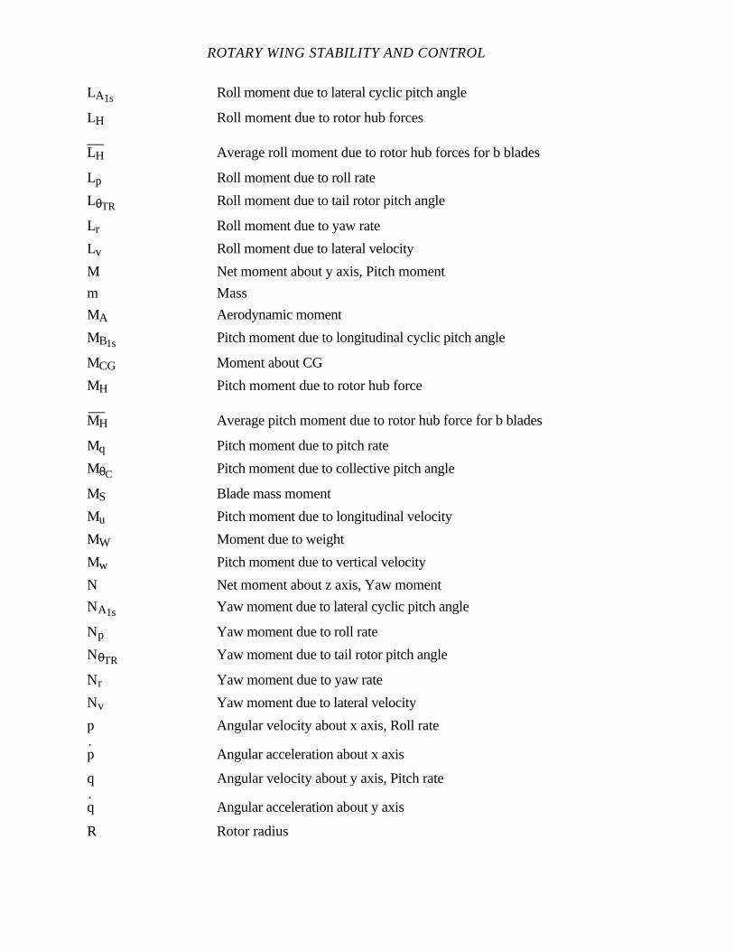
ROTARY WING STABILITY AND CONTROL
LA1s Roll moment due to lateral cyclic pitch angle
LH Roll moment due to rotor hub forces
LH—
Average roll moment due to rotor hub forces for b blades
Lp Roll moment due to roll rate
LθTR Roll moment due to tail rotor pitch angle
Lr Roll moment due to yaw rate
Lv Roll moment due to lateral velocity
M Net moment about y axis, Pitch moment
m Mass
MA Aerodynamic moment
MB1s Pitch moment due to longitudinal cyclic pitch angle
MCG Moment about CG
MH Pitch moment due to rotor hub force
MH—
Average pitch moment due to rotor hub force for b blades
Mq Pitch moment due to pitch rate
MθC Pitch moment due to collective pitch angle
MS Blade mass moment
Mu Pitch moment due to longitudinal velocity
MW Moment due to weight
Mw Pitch moment due to vertical velocity
N Net moment about z axis, Yaw moment
NA1s Yaw moment due to lateral cyclic pitch angle
Np Yaw moment due to roll rate
NθTR Yaw moment due to tail rotor pitch angle
Nr Yaw moment due to yaw rate
Nv Yaw moment due to lateral velocity
p Angular velocity about x axis, Roll rate
p Angular acceleration about x axis
q Angular velocity about y axis, Pitch rate
q Angular acceleration about y axis
R Rotor radius
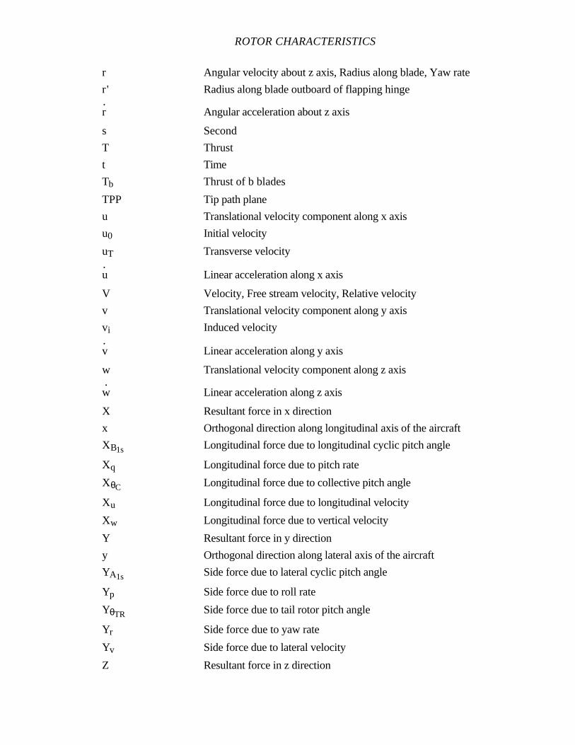
ROTOR CHARACTERISTICS
r Angular velocity about z axis, Radius along blade, Yaw rate
r' Radius along blade outboard of flapping hinge
r Angular acceleration about z axis
s Second
T Thrust
t Time
Tb Thrust of b blades
TPP Tip path plane
u Translational velocity component along x axis
u0 Initial velocity
uT Transverse velocity
u Linear acceleration along x axis
V Velocity, Free stream velocity, Relative velocity
v Translational velocity component along y axis
vi Induced velocity
v Linear acceleration along y axis
w Translational velocity component along z axis
w Linear acceleration along z axis
X Resultant force in x direction
x Orthogonal direction along longitudinal axis of the aircraft
XB1s Longitudinal force due to longitudinal cyclic pitch angle
Xq Longitudinal force due to pitch rate
XθC Longitudinal force due to collective pitch angle
Xu Longitudinal force due to longitudinal velocity
Xw Longitudinal force due to vertical velocity
Y Resultant force in y direction
y Orthogonal direction along lateral axis of the aircraft
YA1s Side force due to lateral cyclic pitch angle
Yp Side force due to roll rate
YθTR Side force due to tail rotor pitch angle
Yr Side force due to yaw rate
Yv Side force due to lateral velocity
Z Resultant force in z direction
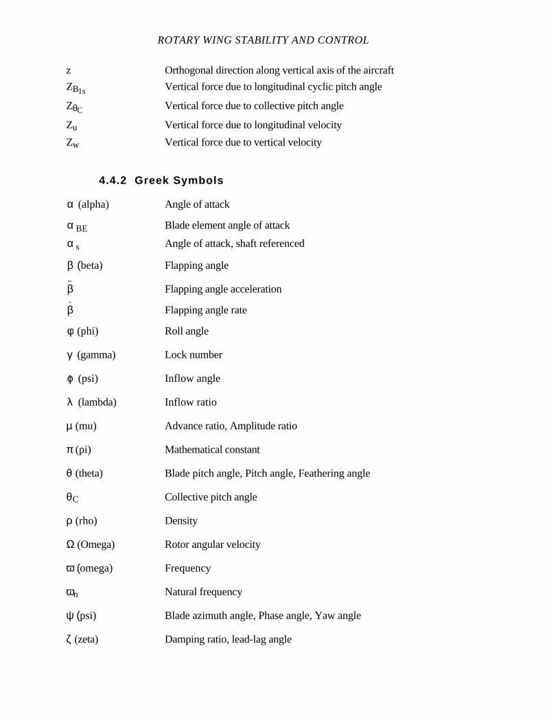
ROTARY WING STABILITY AND CONTROL
z Orthogonal direction along vertical axis of the aircraft
ZB1s Vertical force due to longitudinal cyclic pitch angle
ZθC Vertical force due to collective pitch angle
Zu Vertical force due to longitudinal velocity
Zw Vertical force due to vertical velocity
4.4.2 Greek Symbols
α (alpha) Angle of attack
α BE Blade element angle of attack
α s Angle of attack, shaft referenced
β (beta) Flapping angle
˙β Flapping angle acceleration
β Flapping angle rate
φ (phi) Roll angle
γ (gamma) Lock number
ϕ (psi) Inflow angle
λ (lambda) Inflow ratio
µ (mu) Advance ratio, Amplitude ratio
π (pi) Mathematical constant
θ (theta) Blade pitch angle, Pitch angle, Feathering angle
θC Collective pitch angle
ρ (rho) Density
Ω (Omega) Rotor angular velocity
ω (omega) Frequency
ωn Natural frequency
ψ (psi) Blade azimuth angle, Phase angle, Yaw angle
ζ (zeta) Damping ratio, lead-lag angle
ROTOR CHARACTERISTICS
4.5 REFERENCES
1. Bramwell, A. R. S., Helicopter Dynamics, Edward Arnold (Publishers)
Ltd., London, England, 1976.
2. Gessow, A. and Myers, G. C., Jr., Aerodynamics of the Helicopter, fifth
printing, Fredrick Unger Publishing Co., NY, 1978.
3. Naval Test Pilot School Flight Test Manual,Helicopter Stability and
Control, USNTPS-FTM-No. 101, U. S. Naval Test Pilot School, Patuxent River, MD, 10
June 1968, reprinted February 1978.
4. Naval Test Pilot School Flight Test Manual,Helicopter Stability and
Control, Theory and Flight Test Techniques, USNTPS-FTM-No. 105, U. S. Naval Test
Pilot School, Patuxent River, MD, November 1983, Preliminary Edition.
5. Prouty, Raymond W.,Helicopter Performance, Stability, and Control,
PWS Publishers, Boston, MA, 1986.
CHAPTER FIVE
FLIGHT CONTROL SYSTEM CHARACTERISTICS
PAGE
5.1 INTRODUCTION 5.1
5.2 PURPOSE OF TEST 5.2
5.3 THEORY 5.2
5.3.1 Control Rigging 5.2
5.3.2 Control Envelope 5.2
5.3.3 Control Mixing 5.3
5.4 IRREVERSIBLE CONTROL SYSTEMS 5.4
5.4.1 Trim Systems 5.4
5.4.1.1 Friction Systems 5.4
5.4.1.2 Electro-Mechanical Systems 5.4
5.4.1.3 Force Versus Displacement 5.5
5.4.1.4 Force Gradient 5.7
5.4.1.5 Limit Control Force 5.7
5.4.1.6 Beeper Trim System 5.8
5.4.1.7 Beeper Trim Rates 5.8
5.4.1.8 Trim Lag 5.10
5.4.1.9 Trim Envelope 5.10
5.4.1.10 Control Jump 5.11
5.4.1.11 Trim System Freeplay 5.12
5.4.2 Friction 5.13
5.4.3 Trim Control Displacement Band 5.13
5.4.4 Breakout 5.14
5.4.5 Breakout Plus Friction 5.16
5.4.6 Control Mass Imbalance 5.18
5.4.7 Control Force Coupling 5.18
5.4.8 Control Centering 5.18
5.4.9 Control Dynamics 5.19
5.4.10 Total System Freeplay 5.19
ROTARY WING STABILITY AND CONTROL
5.4.11 Viscous Dampers 5.19
5.4.11.1 Parallel Damper 5.20
5.4.11.2 Series Damper 5.20
5.4.12 Transient Control Forces 5.21
5.4.13 AFCS Inputs 5.21
5.5 REVERSIBLE CONTROL SYSTEMS 5.22
5.5.1 General 5.22
5.5.2 Degraded Flight Control System Operation 5.23
5.6 TEST METHODS AND TECHNIQUES 5.24
5.6.1 General 5.24
5.6.2 Ground Testing 5.25
5.6.2.1 Control Envelope and Control Mixing 5.25
5.6.2.1.1 Data Required 5.25
5.6.2.2 Force Versus Displacement 5.26
5.6.2.2.1 Data Required 5.26
5.6.2.3 Trim System 5.27
5.6.2.3.1 Data Required 5.28
5.6.2.4 Control Jump, Centering, and Dynamics 5.28
5.6.2.4.1 Data Required 5.29
5.6.2.5 Control Force Coupling 5.30
5.6.2.5.1 Data Required 5.30
5.6.2.6 Total System Freeplay 5.31
5.6.2.6.1 Data Required 5.31
5.6.2.7 Viscous Damper Characteristics and Transient Forces 5.32
5.6.2.7.1 Data Required 5.32
5.6.2.8 AFCS Inputs 5.33
5.6.3 In Flight Testing 5.34
5.6.3.1 Data Required 5.34
5.6.4 Safety Considerations/Risk Management 5.34
5.7 DATA REDUCTION 5.36
5.8 DATA ANALYSIS 5.36
FLIGHT CONTROL SYSTEM CHARACTERISTICS
5.9 MISSION SUITABILITY 5.36
5.10 SPECIFICATION COMPLIANCE 5.36
5.11 GLOSSARY 5.38
5.11.1 Notations 5.38
5.12 REFERENCES 5.38
ROTARY WING STABILITY AND CONTROL
CHAPTER FIVE
FIGURES
PAGE
5.1 Cyclic Control Envelope 5.3
5.2 Representative Mechanical Trim System 5.6
5.3 Control Characteristics with Trim System 5.7
5.4 Static Longitudinal Stability 5.9
5.5 Cyclic Control Trim Envelope 5.11
5.6 Control Characteristics with Trim System Freeplay 5.12
5.7 Control Characteristics with Friction 5.14
5.8 Control Characteristics with Breakout 5.15
5.9 Control Characteristics with Trim System Freeplay and Breakout 5.17
5.10 Parallel and Series Dampers 5.20
5.11 Lateral Cyclic Force Displacement Characteristics 5.27
5.12 Control Jump 5.29
5.13 Control Dynamics 5.30
5.14 Control Force Coupling 5.31
5.15 Viscous Damper Characteristics 5.33

FLIGHT CONTROL SYSTEM CHARACTERISTICS
CHAPTER FIVE
TABLES
PAGE
5.I Representative Flight Control System Characteristics 5.35
CHAPTER FIVE
FLIGHT CONTROL SYSTEM CHARACTERISTICS
5.1 INTRODUCTION
Since flight control systems are one element in the aircraft control loop, flight
control system characteristics are very important to the pilot. The pilot interacts with the
flight control system in maneuvering the aircraft to accomplish mission tasks. Pilot activity
in the control loop depends on the flight control system characteristics, the aircraft stability
and control characteristics, mission tasks, and atmospheric disturbances. Pilot opinion of
aircraft flying qualities is influenced by the flight control system characteristics. A pilot
working very hard to fly the aircraft is critical of the flight control system characteristics.
Understanding and documenting the flight control system characteristics is
fundamental to any flying qualities or closed loop flight evaluation. Since the flight control
system is part of the control loop, the test pilot must have a detailed understanding of the
components of the flight control system and their function. The understanding begins with
a thorough flight control system description and proceeds with documenting the flight
control system characteristics.
Helicopter flight control systems are grouped into two general categories,
irreversible and reversible. An irreversible control system has integral hydraulic or electro-
mechanical power servos. These servos are an irreversible link between the cockpit flight
controls and the aerodynamic control surfaces. Reversible control systems incorporate
mechanical advantage or dynamic balancing to reduce the cockpit flight control forces
without isolating the cockpit flight controls from the aerodynamic control surface loads.
The flight control system characteristics of an irreversible system can be tailored to provide
a wide range of force, displacement, and pilot assist characteristics; while the reversible
system is not as flexible. The ease of flying a helicopter with a reversible flight control
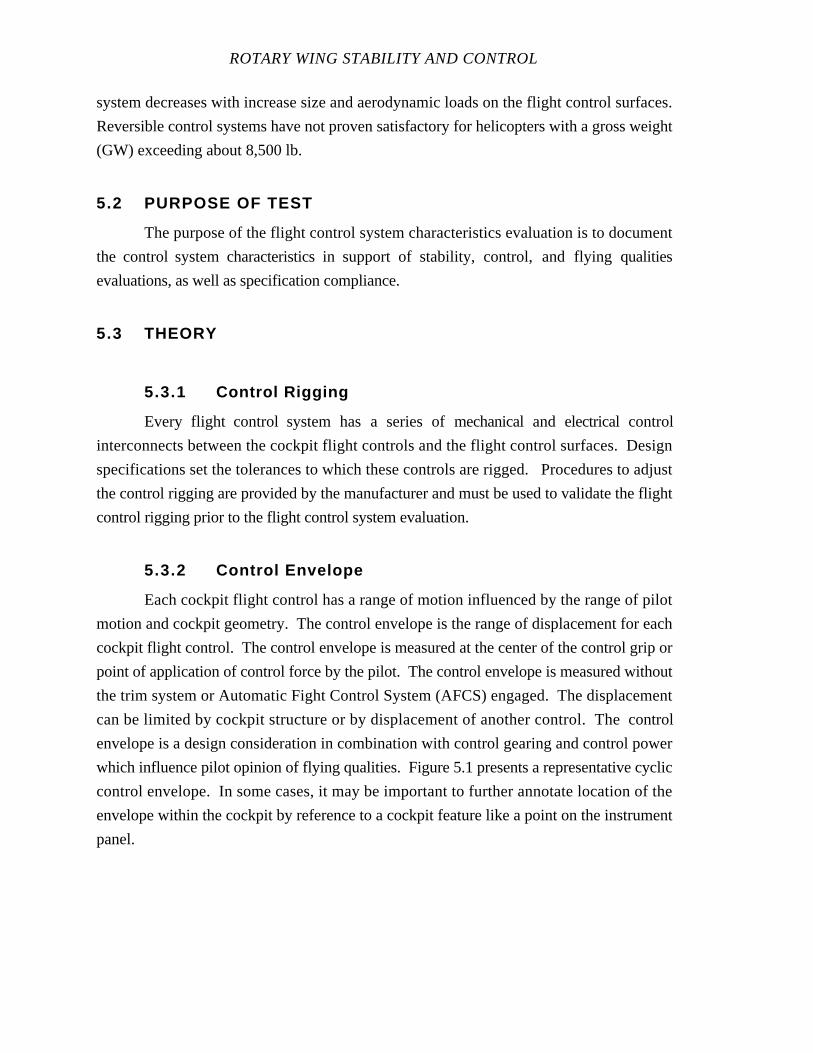
ROTARY WING STABILITY AND CONTROL
system decreases with increase size and aerodynamic loads on the flight control surfaces.
Reversible control systems have not proven satisfactory for helicopters with a gross weight
(GW) exceeding about 8,500 lb.
5.2 PURPOSE OF TEST
The purpose of the flight control system characteristics evaluation is to document
the control system characteristics in support of stability, control, and flying qualities
evaluations, as well as specification compliance.
5.3 THEORY
5.3.1 Control Rigging
Every flight control system has a series of mechanical and electrical control
interconnects between the cockpit flight controls and the flight control surfaces. Design
specifications set the tolerances to which these controls are rigged. Procedures to adjust
the control rigging are provided by the manufacturer and must be used to validate the flight
control rigging prior to the flight control system evaluation.
5.3.2 Control Envelope
Each cockpit flight control has a range of motion influenced by the range of pilot
motion and cockpit geometry. The control envelope is the range of displacement for each
cockpit flight control. The control envelope is measured at the center of the control grip or
point of application of control force by the pilot. The control envelope is measured without
the trim system or Automatic Fight Control System (AFCS) engaged. The displacement
can be limited by cockpit structure or by displacement of another control. The control
envelope is a design consideration in combination with control gearing and control power
which influence pilot opinion of flying qualities. Figure 5.1 presents a representative cyclic
control envelope. In some cases, it may be important to further annotate location of the
envelope within the cockpit by reference to a cockpit feature like a point on the instrument
panel.
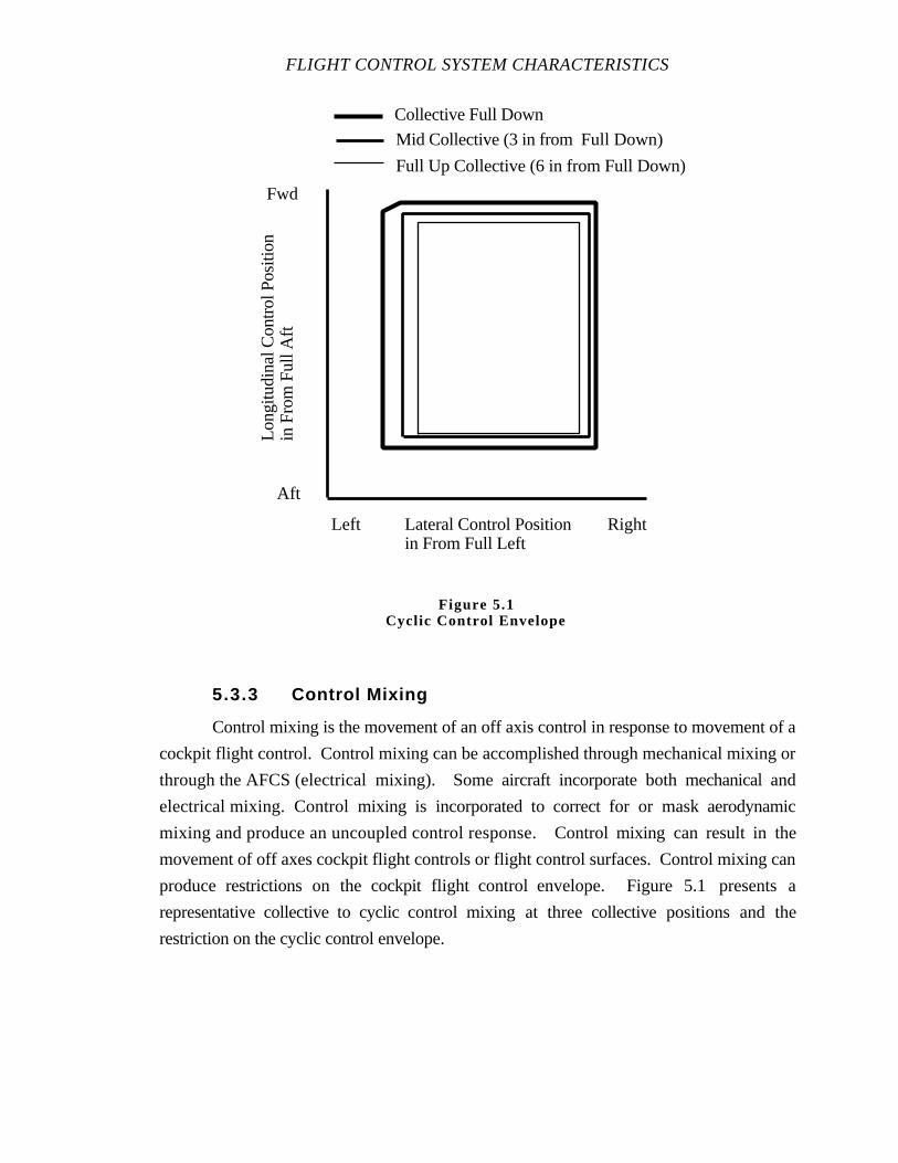
FLIGHT CONTROL SYSTEM CHARACTERISTICS
5.3.3 Control Mixing
Control mixing is the movement of an off axis control in response to movement of a
cockpit flight control. Control mixing can be accomplished through mechanical mixing or
through the AFCS (electrical mixing). Some aircraft incorporate bothmechanical and
electrical mixing. Control mixing is incorporated to correct for or mask aerodynamic
mixing and produce an uncoupled control response. Controlmixing can result in the
movement of off axes cockpit flight controls or flight control surfaces. Control mixing can
produce restrictions on the cockpit flight control envelope. Figure 5.1 presents a
representative collective to cyclic control mixing at three collective positionsand the
restriction on the cyclic control envelope.
Aft
Fwd
Long
itudi
nal C
ontr
ol P
ositi
onin
Fro
m F
ull A
ft
Lateral Control Positionin From Full Left
Left Right
Collective Full Down
Mid Collective (3 in from Full Down)
Full Up Collective (6 in from Full Down)
Figure 5.1Cyclic Control Envelope
ROTARY WING STABILITY AND CONTROL
5.4 IRREVERSIBLE CONTROL SYSTEMS
Irreversible systems isolate the aerodynamic loads on the flight control surfaces
from the cockpit flight controls. In such systems, there is no aerodynamically supplied
force when the cockpit flight control is moved from one position to another. The absence
of control force produces two problems. The first problem is the inability to release the
control and perform other cockpit duties without the control moving due to the force of
gravity or vibratory loads. The second problem is the absence of a cockpit flight control
force cue which the pilot uses to sense displacement of the control from trim. A
requirement exists to provide artificial cockpit flight control retention and force cues.
5.4.1 Trim Systems
Trim systems are incorporated into the flight control system to overcome the two
problems of an irreversible control system. Trim systems provide for cockpit flight control
centering, trim retention, and provide forces cues to control displacement from trim.
5.4.1.1 FRICTION SYSTEMS
Adjustable control friction is a simple flight control system trim device. Such
devices normally have an adjustment through which the coefficient of sliding friction is
varied, thereby adjusting the friction force in the flight control system. An example is the
friction collar on the UH-60A collective control. Friction can be adjusted so that friction
force is equal to or greater than any force in the control system tending to move the control
from trim. For example, with all friction off, the pilot exerts a 4 lb lift force on the
collective control to balance the gravity force acting on the control. If the collective control
is released, the collective moves downward due to the gravity force. If the pilot increases
the collective friction to 4 lb, the collective does not move when it is released. To raise the
collective the pilot must exert 8 lb of lift force. To lower the collective, a few ounces of
downward force is required. Precise control inputs are difficult with high friction forces.
For this reason, there is a practical limit to the application of a variable friction trim device.
5.4.1.2 ELECTRO-MECHANICAL SYSTEMS
The spring and clutch combination is representative of mechanical trim systems
which provide an artificial force gradient, control centering, and trim capability. A
simplified system is presented in Figure 5.2. Zero force is exerted on the control in Figure
5.2 (a) at the initial trim condition. The control is displaced from trim in Figure 5.2 (b) and
FLIGHT CONTROL SYSTEM CHARACTERISTICS
the spring is extended, exerting a force opposing the control displacement. In Figure 5.2
(c), the pilot activated a momentary trim release, disengaging the clutch and producing a
sudden reduction of the opposing force. The pilot can fly with zero force (momentary trim
release activated) or fly against a force, trimming as necessary.
Most trim systems incorporate switches to activate/deactivate and momentarily
disengage the system. This capability is provided in case of malfunction or situations when
the pilot does not desire to fly against a force. Current irreversible control helicopter trim
systems use electro-mechanical or hydraulic servos to provide the force gradient and
centering capabilities. An example is the SH-60 aircraft which uses electro-mechanical
servos in the yaw and collective axis, and hydraulic servos in the pitch and roll axis. In all
axes, the trim system is controlled through the AFCS system. The pilot must know what
type of system is producing the force and trim characteristics to design and apply effective
test procedures and document deficiencies.
5.4.1.3 FORCE VERSUS DISPLACEMENT
The trim system provides control centering and force cues for displacement from
the trim position. The force versus displacement of the cockpit flight control is measured at
the center of the cockpit flight control grip or the point of application of control force.
Figure 5.3 presents a representative force versus control displacement curve. The
helicopter force versus displacement characteristics should be approximately linear, without
discontinuities or reversals, and symmetrical for displacement in both directions. The
forces should be accommodated to the control axis and physiological capabilities of the
pilot population. For a conventional center cyclic control, the forces in the longitudinal axis
should be harmonious with those in the lateral cyclic axis. Additionally, for a multi-axis
controller, the forces should be harmonious in all control axes and directions.

ROTARY WING STABILITY AND CONTROL
Cockpit Flight Control
Flight Control Rod
Spring
(a) Initial Trim, No Force
Clutch
(b) Control Displaced, Spring Extended, Force on Cockpit Flight Control
Control Displaced
(c) Momentary Trim Release Activated, ClutchDisengaged, No Force on Cockpit Control
Figure 5.2Representative Mechanical Trim System
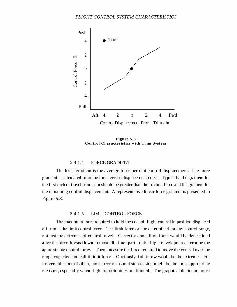
FLIGHT CONTROL SYSTEM CHARACTERISTICS
5.4.1.4 FORCE GRADIENT
The force gradient is the average force per unit control displacement. The force
gradient is calculated from the force versus displacement curve. Typically, the gradient for
the first inch of travel from trim should be greater than the friction force and the gradient for
the remaining control displacement. A representative linear force gradient is presented in
Figure 5.3.
5.4.1.5 LIMIT CONTROL FORCE
The maximum force required to hold the cockpit flight control in position displaced
off trim is the limit control force. The limit force can be determined for any control range,
not just the extremes of control travel. Correctly done, limit force would be determined
after the aircraft was flown in most all, if not part, of the flight envelope to determine the
approximate control throw. Then, measure the force required to move the control over the
range expected and call it limit force. Obviously, full throw would be the extreme. For
irreversible controls then, limit force measured stop to stop might be the most appropriate
measure, especially when flight opportunities are limited. The graphical depiction most
0
2
4
2
4
0 2 424
Push
Pull
Con
trol
For
ce -
lb
Aft Fwd
Control Displacement From Trim - in
Trim
Figure 5.3Control Characteristics with Trim System

ROTARY WING STABILITY AND CONTROL
often presented for the Mil-H-8501A shows limit force as measured from the center of the
control throw, although the description in paragraph 3.2.6 of the spec does not require
measurement from center. When discussing limit force, it would be very important to
cover the range measured. For spec compliance, the general agreement would be to use
the forces measured from the center of control range out to each control throw extreme. A
discussion of limit force for a control trimmed to one extreme of travel and force measured
to the other extreme should be included, but not related, to specification requirements.
5.4.1.6 BEEPER TRIM SYSTEM
A beeper trim capability can be added to a trim system to provide vernier force
adjustments. These systems are operated in two ways. One, to trim out control forces
opposed by the pilot; or two, to move the cockpit flight control. The control switch for a
beeper trim system should be located on the flight control being trimmed and oriented in the
direction of control displacement. A beeper trim for pedals would be most conveniently
mounted on the collective. The beeper trim system may have the capability of selecting
single or multiple speeds. The beeper trim system should provide precise selection of
control position as well as rapidly adjusting the control position and force required for
maneuvering flight.
5.4.1.7 BEEPER TRIM RATES
The beeper trim rate is the cockpit flight control displacement per unit engagement time of
the beeper trim switch. The trim rate is measured at the cockpit flight control. Satisfactory
beeper trim rates for the longitudinal, lateral, and directional controls depend in part on the
slope of the control position gradients. Figure 5.4 (a) illustrates an aircraft with nearly
neutral static stability as indicated by the shallow control position versus airspeed gradient.
The beeper trim system in an aircraft with a shallow control position gradient must be
capable of small, precise control displacements. A slight error in trim control position
results in a large error in trim speed and the pilot must continuously retrim. Figure 5.4 (b)
depicts a steep control position gradient. This type of gradient requires the beeper trim to
operate at a fast rate to achieve modest airspeed changes in a satisfactory time period.
Figure 5.4 (c) illustrates both near neutral and steep control position gradients in one
aircraft. Slow speed maneuvering in this aircraft uses a momentary trim release system or
one with a high beeper trim rate. Trimming at high speed is accomplished with a slow trim
rate. Selection of the proper trim system in such an aircraft is not easy. A slow trim rate
used in conjunction with a shallow control position gradient may give the illusion of
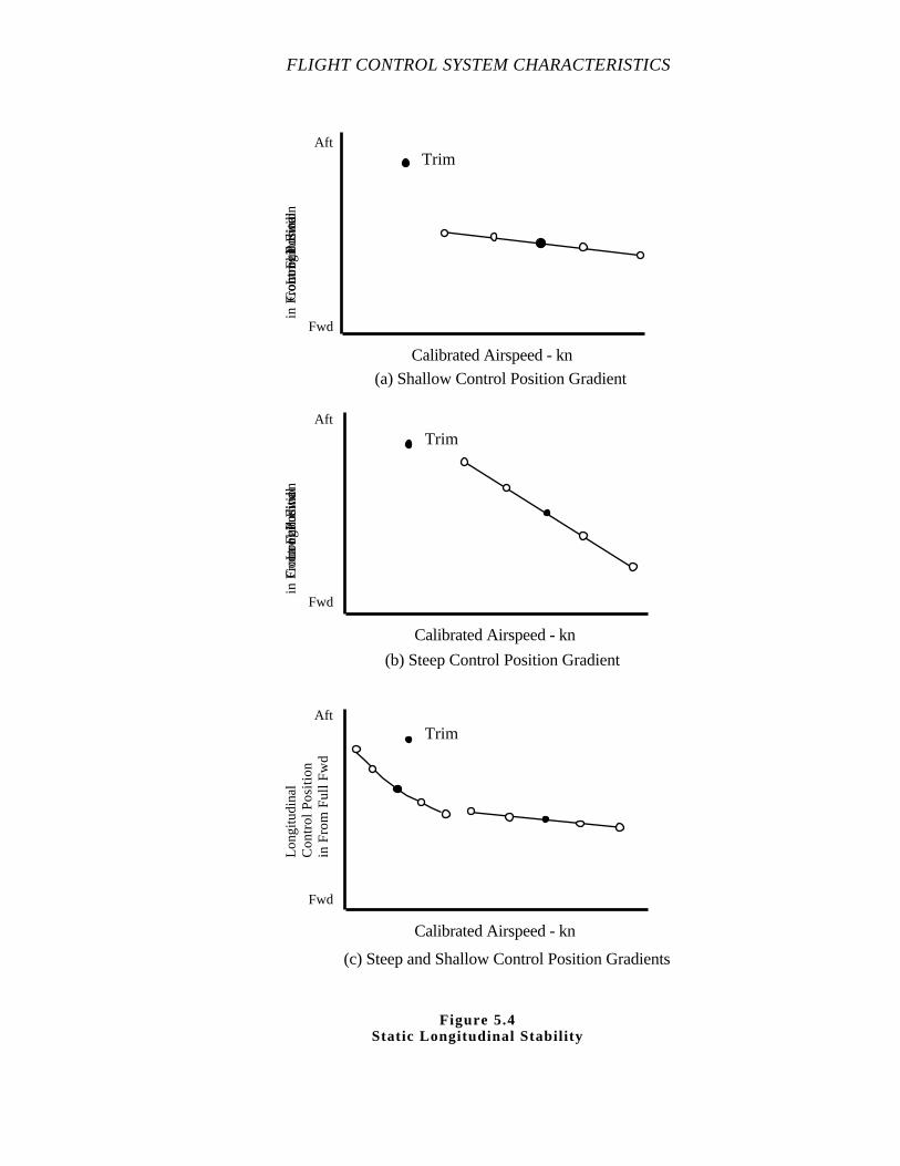
FLIGHT CONTROL SYSTEM CHARACTERISTICS
Calibrated Airspeed - kn
Trim
Calibrated Airspeed - kn
Trim
Calibrated Airspeed - kn
Trim
(a) Shallow Control Position Gradient
(b) Steep Control Position Gradient
(c) Steep and Shallow Control Position Gradients
Aft
Fwd
Long
itudi
nal
Co
ntr
ol P
osi
tion
in F
rom
Fu
ll F
wd
Aft
Fwd
Long
itudi
nal
Co
ntr
ol P
osi
tion
in F
rom
Fu
ll F
wd
Aft
Fwd
Long
itudi
nal
Co
ntr
ol P
osi
tion
in F
rom
Fu
ll F
wd
Figure 5.4Static Longitudinal Stabil ity
ROTARY WING STABILITY AND CONTROL
increased positive static stability. This occurs because the pilotsenses the time he is
activating the beeper trim and the change in the control force or control position. Force or
position is integrated with respect to time to produce a control cue similar to the cue
provided by a steeper control position gradient.
5.4.1.8 TRIM LAG
Trim lag is the time delay between activation of the beeper trim switch and
movement of the cockpit flight control. Trim lag is problematic when it is large enough to
produce unpredictable results in response to beeper trim activation. Lags on the order of
0.3 to 0.5 s are generally unacceptable. If a pilot momentarily activates the beeper trim
switch attempting to make a fine trim adjustment and there is no response in the trim
system, the next input will be too long and will overshoot the desired displacement. Trim
lag is particularly bothersome during Instrument Meteorological Condition (IMC)
operations and is generally undesirable for all precise trim operations.
5.4.1.9 TRIM ENVELOPE
The trim envelope is the maximum control displacement wherein the cockpit flight
control forces can be reduced to zero using the trim system. The control envelope
determined using the momentary trim release is the trim release envelope. The control
envelope determined using the beeper trim is the beeper trim envelope. The two trim
envelopes may not be the same. Further, the trim envelopes may not be the same as the
control envelope without the trim system engaged. Although most trim systems are capable
of trimming forces to zero from one flight control stop to the other, there are some systems
which have limits and do not provide a stop to stop trimming capability. In some cases, the
trim limit is due to a design deficiency; however, in other situations the trim limit is
purposely designed into the control system. A restricted trim envelope can be used to warn
the pilot he is approaching the control displacement limit. Some aircraft use this technique
to prevent the collective control from being trimmed full down. This low limit reminds the
pilot not to operate on the ground with full down collective which helps to prevent droop
stop pounding. Figure 5.5 presents a representative cyclic control trim envelope.

FLIGHT CONTROL SYSTEM CHARACTERISTICS
5.4.1.10 CONTROL JUMP
Control jump is the undesired movement of the cockpit flight control that occurs
when the momentary trim release is activated while holding a force against the trim system.
Control jump is a function of displacement, force gradient, friction band, viscous dampers,
and trim release characteristics. If upon activating the trim release, the trim force drops to
zero faster than the pilot can relax his applied force, a force imbalance exists for a fraction
of a second. The force imbalance results in undesired motion of the cockpit flight control.
Although light forces do not produce significant problems, pre-trim forces of 3 lb or more
result in small, rapid movement of the cockpit flight control. The end result is the control is
displaced from the desired trim position, requiring retrimming the undesired motion.
Aft
Fwd
Long
itudi
nal C
ontr
ol P
ositi
onin
from
Ful
l Aft
Lateral Control Positionin from Full Left
Left Right
Control Envelope Collective Full DownTrim Release Envelope, Collective Full Down
Beeper Trim Envelope, Collective Full Down
Figure 5.5Cyclic Control Trim Envelope
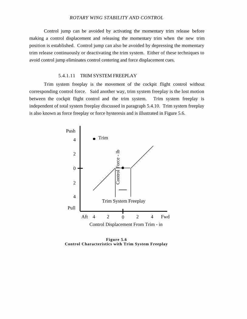
ROTARY WING STABILITY AND CONTROL
Control jump can be avoided by activating the momentary trim release before
making a control displacement and releasing the momentary trim when the new trim
position is established. Control jump can also be avoided by depressing the momentary
trim release continuously or deactivating the trim system. Either of these techniques to
avoid control jump eliminates control centering and force displacement cues.
5.4.1.11 TRIM SYSTEM FREEPLAY
Trim system freeplay is the movement of the cockpit flight control without
corresponding control force. Said another way, trim system freeplay is the lost motion
between the cockpit flight control and the trim system. Trim system freeplay is
independent of total system freeplay discussed in paragraph 5.4.10. Trim system freeplay
is also known as force freeplay or force hysteresis and is illustrated in Figure 5.6.
0
2
4
2
4
0 2 424
Push
Pull
Con
trol
For
ce -
lb
Aft Fwd
Control Displacement From Trim - in
Trim
Trim System Freeplay
Figure 5.6Control Characteristics with Trim System Freeplay
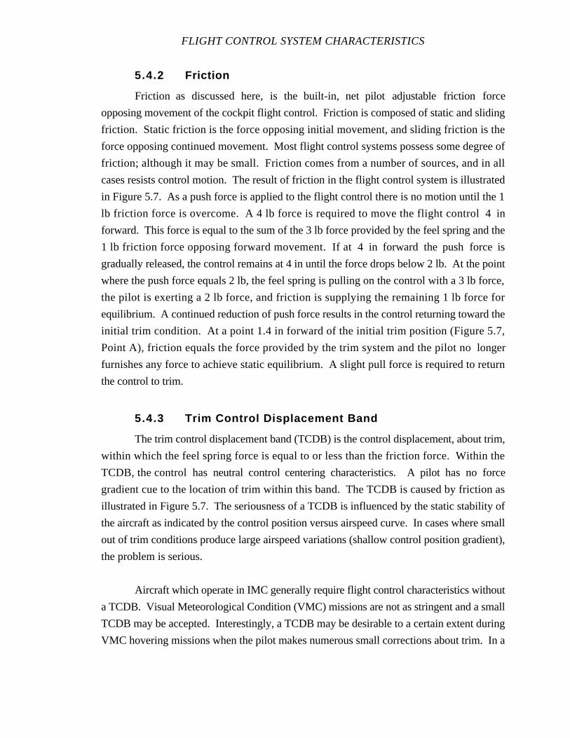
FLIGHT CONTROL SYSTEM CHARACTERISTICS
5.4.2 Friction
Friction as discussed here, is the built-in, net pilot adjustable friction force
opposing movement of the cockpit flight control. Friction is composed of static and sliding
friction. Static friction is the force opposing initial movement, and sliding friction is the
force opposing continued movement. Most flight control systems possess some degree of
friction; although it may be small. Friction comes from a number of sources, and in all
cases resists control motion. The result of friction in the flight control system is illustrated
in Figure 5.7. As a push force is applied to the flight control there is no motion until the 1
lb friction force is overcome. A 4 lb force is required to move the flight control 4 in
forward. This force is equal to the sum of the 3 lb force provided by the feel spring and the
1 lb friction force opposing forward movement. If at 4 in forward the push force is
gradually released, the control remains at 4 in until the force drops below 2 lb. At the point
where the push force equals 2 lb, the feel spring is pulling on the control with a 3 lb force,
the pilot is exerting a 2 lb force, and friction is supplying the remaining 1 lb force for
equilibrium. A continued reduction of push force results in the control returning toward the
initial trim condition. At a point 1.4 in forward of the initial trim position (Figure 5.7,
Point A), friction equals the force provided by the trim system and the pilot no longer
furnishes any force to achieve static equilibrium. A slight pull force is required to return
the control to trim.
5.4.3 Trim Control Displacement Band
The trim control displacement band (TCDB) is the control displacement, about trim,
within which the feel spring force is equal to or less than the friction force. Within the
TCDB, the control has neutral control centering characteristics. A pilot has no force
gradient cue to the location of trim within this band. The TCDB is caused by friction as
illustrated in Figure 5.7. The seriousness of a TCDB is influenced by the static stability of
the aircraft as indicated by the control position versus airspeed curve. In cases where small
out of trim conditions produce large airspeed variations (shallow control position gradient),
the problem is serious.
Aircraft which operate in IMC generally require flight control characteristics without
a TCDB. Visual Meteorological Condition (VMC) missions are not as stringent and a small
TCDB may be accepted. Interestingly, a TCDB may be desirable to a certain extent during
VMC hovering missions when the pilot makes numerous small corrections about trim. In a
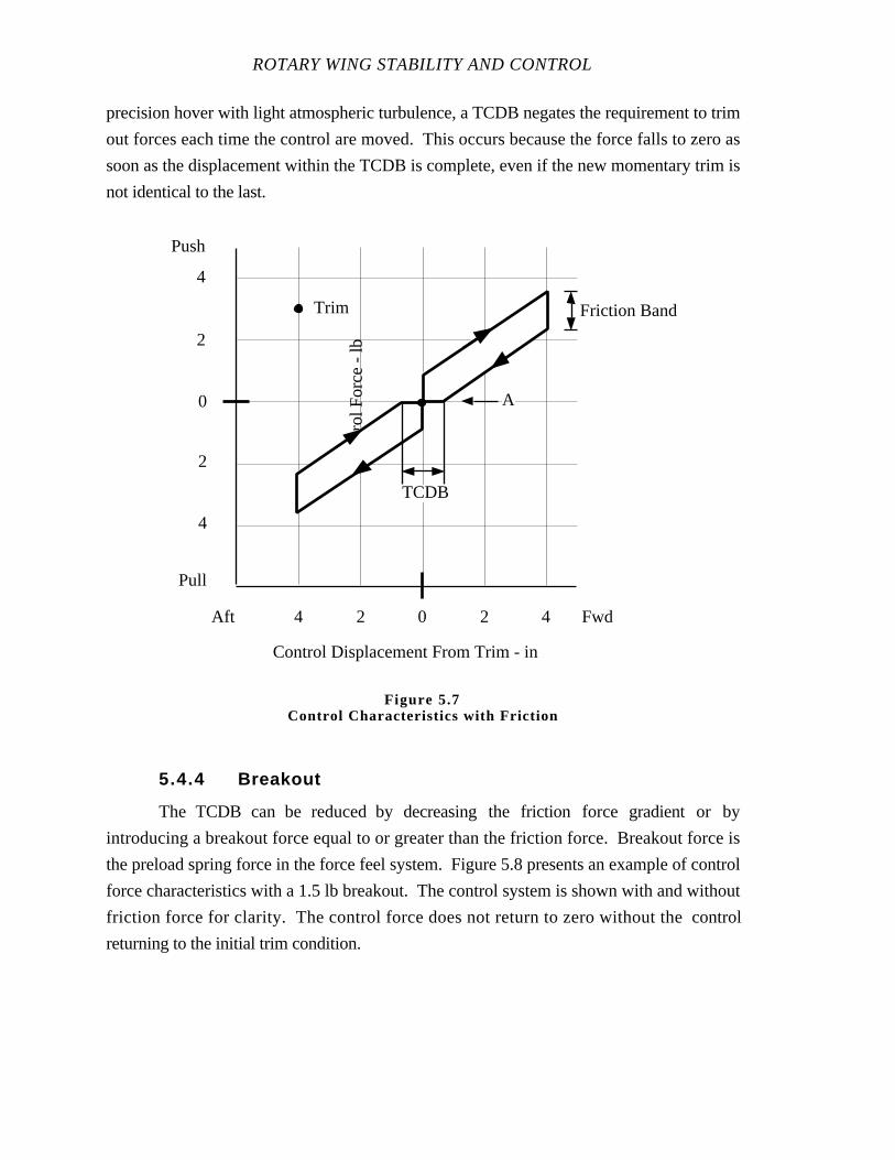
ROTARY WING STABILITY AND CONTROL
precision hover with light atmospheric turbulence, a TCDB negates the requirement to trim
out forces each time the control are moved. This occurs because the force falls to zero as
soon as the displacement within the TCDB is complete, even if the new momentary trim is
not identical to the last.
5.4.4 Breakout
The TCDB can be reduced by decreasing the friction force gradient or by
introducing a breakout force equal to or greater than the friction force. Breakout force is
the preload spring force in the force feel system. Figure 5.8 presents an example of control
force characteristics with a 1.5 lb breakout. The control system is shown with and without
friction force for clarity. The control force does not return to zero without the control
returning to the initial trim condition.
Pull
Aft
0
2
4
Push
Fwd
Control Displacement From Trim - in
Friction Band
2
4
04 2 2 4
Con
trol
For
ce -
lb
Trim
TCDB
A
Figure 5.7Control Characteristics with Friction
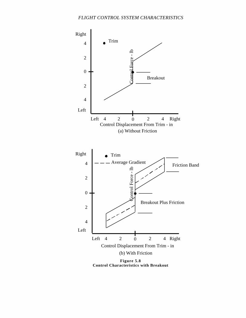
FLIGHT CONTROL SYSTEM CHARACTERISTICS
0
2
4
2
4
0 2 424
Right
Left
Left Right
Control Displacement From Trim - in
Trim
(b) With Friction
Breakout Plus Friction
Friction BandAverage Gradient
Con
trol
For
ce -
lb
0
2
4
2
4
0 2 424
Right
Left
Con
trol
For
ce -
lb
Left RightControl Displacement From Trim - in
Trim
(a) Without Friction
Breakout
Figure 5.8Control Characteristics with Breakout
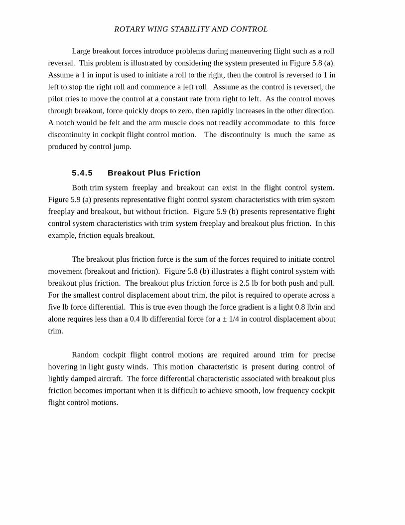
ROTARY WING STABILITY AND CONTROL
Large breakout forces introduce problems during maneuvering flight such as a roll
reversal. This problem is illustrated by considering the system presented in Figure 5.8 (a).
Assume a 1 in input is used to initiate a roll to the right, then the control is reversed to 1 in
left to stop the right roll and commence a left roll. Assume as the control is reversed, the
pilot tries to move the control at a constant rate from right to left. As the control moves
through breakout, force quickly drops to zero, then rapidly increases in the other direction.
A notch would be felt and the arm muscle does not readily accommodate to this force
discontinuity in cockpit flight control motion. The discontinuity is much the same as
produced by control jump.
5.4.5 Breakout Plus Friction
Both trim system freeplay and breakout can exist in the flight control system.
Figure 5.9 (a) presents representative flight control system characteristics with trim system
freeplay and breakout, but without friction. Figure 5.9 (b) presents representative flight
control system characteristics with trim system freeplay and breakout plus friction. In this
example, friction equals breakout.
The breakout plus friction force is the sum of the forces required to initiate control
movement (breakout and friction). Figure 5.8 (b) illustrates a flight control system with
breakout plus friction. The breakout plus friction force is 2.5 lb for both push and pull.
For the smallest control displacement about trim, the pilot is required to operate across a
five lb force differential. This is true even though the force gradient is a light 0.8 lb/in and
alone requires less than a 0.4 lb differential force for a ± 1/4 in control displacement about
trim.
Random cockpit flight control motions are required around trim for precise
hovering in light gusty winds. This motion characteristic is present during control of
lightly damped aircraft. The force differential characteristic associated with breakout plus
friction becomes important when it is difficult to achieve smooth, low frequency cockpit
flight control motions.
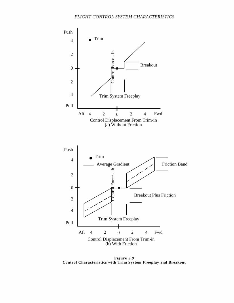
FLIGHT CONTROL SYSTEM CHARACTERISTICS
0
2
4
2
4
0 2 424
Push
Pull
Con
trol
For
ce -
lbAft Fwd
Trim
Breakout
Trim System Freeplay
0
2
4
2
4
0 2 424
Push
Pull
Con
trol
For
ce -
lb
Aft Fwd
Control Displacement From Trim-in(b) With Friction
Trim
Friction Band
Breakout Plus Friction
Trim System Freeplay
Average Gradient
Control Displacement From Trim-in(a) Without Friction
Figure 5.9Control Characteristics with Trim System Freeplay and Breakout

ROTARY WING STABILITY AND CONTROL
5.4.6 Control Mass Imbalance
Control mass imbalance can produce discontinuities in the breakout plus friction
force. This problem normally is related to light breakout plus friction, light force gradient,
heavy control stick, forward cyclic displacement, and nose down aircraft attitude. In some
flight situations, the longitudinal flight control can be inclined up to 20˚ with respect to the
earth. The inclined control mass, acted upon by gravity, produces a moment about the
control pivot point. The moment produces an equivalent force at the pilot's grip.
Equivalent forces of more than 1 lb are not uncommon. The force due to control stick mass
tends to overcome the push breakout plus friction force, while it adds to the initial pull
breakout plus friction force. There are cases where the longitudinal flight control moved
forward after being trimmed and released for hands off flight. This control motion
produced a nose down longitudinal divergence when the aircraft actually had a moderately
damped oscillatory long term characteristic.
5.4.7 Control Force Coupling
Control force coupling is the force introduced in one cockpit flight control or axis
when a second cockpit flight control is moved. Control force coupling can be intentional or
unintentional. Force coupling is intentionally designed into an aircraft to offset a severe
trim change or some other unusual characteristic. In one irreversible system, an
unintentional control force characteristic was introduced in the longitudinal control system
when the collective was raised or lowered, as a result of a control force per g augmentation
system, providing the pilot with false force cues.
5.4.8 Control Centering
Many flight control system characteristics prevent the cockpit flight control from
returning to a trim condition. The motion of the cockpit flight control following a
displacement from trim is referred to as control centering. If the control moves unassisted
towards its initial trim position, the control has positive control centering. If the control
returns precisely to trim, the control has absolute control centering. If the control moves
away from trim, the control has negative control centering. If the control does not move
following the displacement from trim, the control has neutral control centering.

FLIGHT CONTROL SYSTEM CHARACTERISTICS
5.4.9 Control Dynamics
The motion of the cockpit flight control when dynamically disturbed from trim is
referred to as control dynamics. The disturbance can be a displacement and sudden release,
or a control rap. Control dynamics are important if the pilot inadvertently releases or raps
the control. If the control dynamics are not well dampened, the resultant motion of the
cockpit flight control could impart undesired aircraft motion.
5.4.10 Total System Freeplay
Total system freeplay is the movement of the cockpit flight control without
movement of the corresponding flight control surface. Total system freeplay is the lost
motion between the cockpit flight control and the control surface. Total system freeplay is
also referred to as position freeplay or position hysteresis. Freeplay comes from several
sources including: hydraulic system friction, sloppy control linkages, and control washouts
due to AFCS inputs. If control freeplay is ± 1/4 in or more, the pilot can experience
controllability problems. Total system freeplay is independent of trim system freeplay.
5.4.11 Viscous Dampers
Cockpit flight control rate damping is used to restrict the rateof cockpit flight
control movement by incorporating viscous dampers in the control system. Viscous
dampers are incorporated to prevent pilot induced oscillation (PIO), or otherwise prevent
unpleasant characteristics related to rate of cockpit control movement. For example, a
collective viscous damper was used in an aircraft because of a serious collective to pitch
attitude dynamic coupling problem. In another situation, a damper was installed in the
lateral cyclic control system of a tandem rotor helicopter to prevent pilot induced excitation
of a lateral bending mode. A third common application is found in the directional control
system of helicopters equipped with an antitorque tail rotor. The damper in this installation
is intended to prevent unintentional overstressing of the tail boom.
The flight control system characteristics produced by viscous dampers can enhance
or detract from flying qualities depending on the combined effects of the damper
characteristics and the force gradient system. Rate damping gives the pilot a feel for how
fast he is moving the control, and tends to take some of the jerkiness out of the control
motion. When added to a system which has light breakout plus friction force and a light
force gradient, a damper can provide an acceptable control system. Adding a rate damper
to already high forces can be unacceptable. Rate damping of a control can reduce the
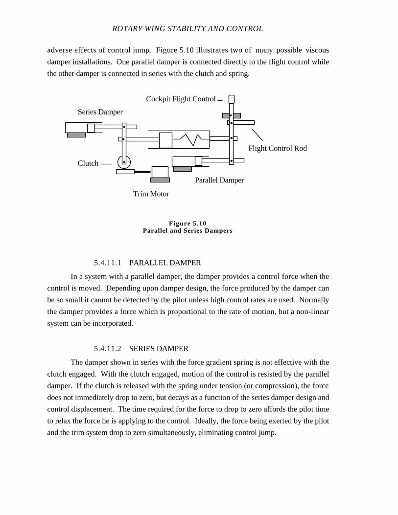
ROTARY WING STABILITY AND CONTROL
adverse effects of control jump. Figure 5.10 illustrates two of many possible viscous
damper installations. One parallel damper is connected directly to the flight control while
the other damper is connected in series with the clutch and spring.
5.4.11.1 PARALLEL DAMPER
In a system with a parallel damper, the damper provides a control force when the
control is moved. Depending upon damper design, the force produced by the damper can
be so small it cannot be detected by the pilot unless high control rates are used. Normally
the damper provides a force which is proportional to the rate of motion, but a non-linear
system can be incorporated.
5.4.11.2 SERIES DAMPER
The damper shown in series with the force gradient spring is not effective with the
clutch engaged. With the clutch engaged, motion of the control is resisted by the parallel
damper. If the clutch is released with the spring under tension (or compression), the force
does not immediately drop to zero, but decays as a function of the series damper design and
control displacement. The time required for the force to drop to zero affords the pilot time
to relax the force he is applying to the control. Ideally, the force being exerted by the pilot
and the trim system drop to zero simultaneously, eliminating control jump.
Cockpit Flight Control
Flight Control Rod
Clutch
Series Damper
Parallel Damper
Trim Motor
Figure 5.10Parallel and Series Dampers
FLIGHT CONTROL SYSTEM CHARACTERISTICS
5.4.12 Transient Control Forces
Transient control forces are the forces developed in a control system as the result of
control velocity or some auxiliary control system force input. Transient control forces
associated with rate of control motion are, in general, the result of viscous damper action,
friction, or a servo system which cannot produce the rate or motion demanded by the pilot.
The servo problem is not uncommon and can be identified by the sharpness of the transient
force when it occurs. The hydraulic servo is limited by design and flow rate to support a
maximum flight load and rate of control motion. A servo stalls or squeals when its capacity
is exceeded due to maximum load or rate of motion, severely restricting aircraft control.
5.4.13 AFCS Inputs
Airspeed, sideslip, altitude, and normal acceleration among other flight parameters
can be measured in flight and used to provide flight control system cues to the pilot. One
application provides the pilot with increased maneuvering stability (control displacement
and force per g), or in the case of airspeed, allow control free constant airspeed flight. The
signals from the respective sensors are fed to a trim motor through the AFCS. For
example, if an aircraft is trimmed at some airspeed then displaced by a gust into a nose
down attitude, an airspeed transducer senses an increase in speed as the aircraft accelerates.
The speed signal is fed to a trim motor to move the longitudinal control aft producing a
corresponding pitch up of the aircraft. If the pilot is holding the control and does not let it
move, he exerts a push force which is a force cue to an off trim condition. Depending
upon sensitivity, the sensors may transmit random forces into the flight control system in
response to gust or dynamic and static pressure changes. Such random forces are
annoying to the pilot. Longitudinal control force per g may be troublesome with respect to
random forces produced as a result of the basic aircraft gust response. If the random or
transient forces are bothersome over a long term, the pilot becomes insensitive to the
control force characteristics. Other essential longitudinal force cues may be disregarded or
downgraded in the process.
ROTARY WING STABILITY AND CONTROL
5.5 REVERSIBLE CONTROL SYSTEMS
5.5.1 General
Reversible control systems are used when the flight control loads are low, and
mechanical gearing is sufficient to obtain the desired control force characteristics. The
reversible system is attractive because of low maintainability and high reliability. Some
aircraft with irreversible systems provide an emergency capability to fly with a degraded
system.
The reversible control system provides for direct control of the aerodynamic flight
control surfaces. This system may incorporate a simple spring trim system to assist in
reducing control forces once the control is fixed at a trim position. A large friction force
may be required to assist in holding the control against the flight loads. The combined
force with the friction inherent in a mechanical control system, often makes flight
maneuvers difficult to perform precisely. If the aircraft has weak positive or negative static
stability, the pilot workload may become excessive in light turbulence. There is no reason
to expect any of the force cues necessary for IMC flight operations. Therefore, do not
expect a reversible control system to provide anything more than an emergency IMC
capability. An exceptionally stable and responsive aircraft may possess some IMC transit
or cruise capability under ideal conditions with good flight instruments.
The forces experienced in a reversible control system are difficult to measure
repeatedly in flight because of the nature of their source. Most of these forces result from
blade pitching moments transmitted into the flight control system. These forces vary with
flight conditions. Measurement of the control characteristics, such as positionversus
force, are difficult to attain qualitatively. A ground evaluation is also inappropriate for
characteristics influenced by aerodynamic loads since the flight condition is not relateable.
In some cases, aerodynamics balances, mechanical control balances, or springs are used to
reduce flight loads transmitted to the cockpit flight controls. These artifacts are designed to
minimize the forces transmitted from the flight control surface to the cockpit flight control
for a given flight condition. Such counterbalances are usually insufficient during
operations on one side of the design flight condition; and overcorrect during operations on
the other side of the design flight condition. Thus control forces exist during off design
operation.
FLIGHT CONTROL SYSTEM CHARACTERISTICS
Vibratory feedback from the rotor system may cause the cockpit flight controls to
move. Such motion may be reduced in flight by increasing control friction or changing the
operating conditions. Neither of these solutions is satisfactory.
5.5.2 Degraded Flight Control System Operation
Helicopters normally employ double or triple redundancy in flight control system
augmentation. Primary hydraulic servos should be double redundant; and hydraulic
pressure and supply systems should be at least double redundant. Augmented flight
control systems which incorporate AFCS inputs should provide double redundant sensors
and processors as well as error checking routines. Additionally, many flight control
systems separate the pilot assist and boost functions from the primary flight control servos
to increase reliability.
However reliable the flight control system, failures can occur. Some helicopters
with irreversible flight control systems cannot be flown with a total failure of the flight
control hydraulic boost system. However, most helicopters can be flown with a partial
failure. When an irreversible flight control system is operated with a partial failure, the
pilot generally changes his mode of control manipulations. This is because he has lost the
advantages normally afforded by the flight control system, and acquired one with standing
control forces, high friction, control force coupling, control freeplay, and other undesirable
characteristics.
The ability of a pilot to transition into or accommodate a degraded flight control
system operation is extremely important. Transition time and success attained after
transition is related to how much the control characteristics differ with the degraded flight
control system. When the change is severe, the result will be correspondingly poor unless
the pilot has gained proficiency in flying the aircraft in a degraded mode.
In many cases, the problem of controlling the aircraft after a servo system failure is
compounded by the simultaneous loss of stability and control augmentation. This
compound failure can be more serious than a boost only failure. When there is a serious
degradation of aircraft stability due to a servo system failure, it becomes important to have
acceptable unaugmented flight control system characteristics.
ROTARY WING STABILITY AND CONTROL
5.6 TEST METHODS AND TECHNIQUES
5.6.1 General
Prior to any flight control system characteristics, flying qualities, or stability and
control evaluation, the flight control system rigging must be verified and documented in
accordance with the published maintenance practices for the aircraft. In addition to the
primary flight control rigging check, auxiliary or secondary flight controls such as
mechanically or automatically movable horizontal tails must be checked. The checks may
involve inducing artificial signals to various sensors such as airspeed, normal or lateral
acceleration, and turn rate.
The evaluation of flight control system characteristics involve measuring forces,
displacements, and time. Typical flight test instrumentation used for stability and control
evaluations provide cockpit control positions. Some instrumentation packages may include
cockpit control force data as well. The instrumentation package may provide cockpit as
well as recorded data, and may be capable of recording static as well as dynamic data.
Cockpit flight control position can be recorded and displayed as units of
displacement or percent of total displacement. In either case, the control position data must
be calibrated to displacement at the center of the cockpit flight control grip or point of
application of pilot control force. Similarly, the control force data must be calibrated to the
point of application of pilot control force.
If the cockpit flight control position and force data are manually recorded, the
position data are measured along the arc described by the control grip, and the force must
be applied normal to the control motion. If the total control displacement is small, the
displacement along the arc can be approximated by the linear displacement.
Although several automatic devices are available for measuring cockpit flight
control force and displacement on the ground, the following discussion assumes the use of
a hand held force gauge and instrumented control position data.
FLIGHT CONTROL SYSTEM CHARACTERISTICS
The irreversible flight control system is quantitatively tested on the ground, and
qualitatively evaluated in flight. The impact of flight control system characteristics on
flying qualities is evaluated in flight. If appropriate, additional quantitative data may be
obtained to support any deficiencies observed in flight.
Reversible flight control systems are evaluated primarily in flight. Some
characteristics which do not depend on the effect of aerodynamic loads can be evaluated on
the ground. Knowledge of the flight control system determines whether on deck or in
flight evaluations are appropriate.
If the flight control system can be powered by external hydraulic and electrical
power, ground tests of irreversible flight control systems are conducted without the engines
or rotors turning. Another option for powering the flight control system is an on board
auxiliary power unit (APU). If the APU can provide full hydraulic and electrical power, it
may be used for ground tests. The least desirable method of powering the flight control
system for ground tests is through turning the engines and rotor system. Turning engines
and rotors restrict the control displacement due to droop stop pounding, rotor-fuselage
interference, aircraft loads, or aircraft roll over. In all cases, the ground evaluation is
conducted with the rotors spread. No matter what method is used to power the flight
control system, all applicable restrictions such as ground operating time or temperature
must be observed.
5.6.2 Ground Testing
5.6.2.1 CONTROL ENVELOPE AND CONTROL MIXING
The control envelope of each cockpit flight control is determined without the trim
system activated. The control envelope for one control is determined with the other
controls centered or at minimum displacement. If control mixing is present, the control
envelope is determined with the off axis control displaced at several locations throughout its
available range. Control envelope and control mixing data are presented in Figure 5.1.
5.6.2.1.1 Data Required
Cockpit flight control positions.
ROTARY WING STABILITY AND CONTROL
5.6.2.2 FORCE VERSUS DISPLACEMENT
The force versus displacement characteristics for the flight control trim system are
determined from a representative trim position. The cockpit flight control is positioned at a
representative trim position, or approximate center of the available control envelope by use
of the momentary trim release. The force gauge is applied perpendicular to the
displacement of the control grip. The force is applied at the center of the grip or at the point
of pilot force application. The force is increased slowly, recording the force and
displacement to the edge of the control envelope. At the edge of the envelope the force is
slowly relaxed, recording the force and displacement as the control returns toward the trim
position. The process is repeated in the opposite direction.
Several important points must be made. As the force is first applied, the force at
which the control first moves is the breakout plus friction force. The difference in the force
between the force at the edge of the control envelope and the force at which the control
begins to move toward trim is the friction band or twice the friction force. If the control
does not return to trim with zero force applied, apply a force in the opposite direction to
return the control to trim. Always apply force in one direction as the control is moved
away from or toward trim. If you allow the control to move in the opposite direction, you
may contaminate the data since you are operating through the friction band.
Limit control force is determined from centered control to each extreme for
specification compliance. If any discontinuities are noted in the force gradient, the limit
force is determined for the discontinuities. Limit control force data are presented in
narrative and tabular format (Table 5.I). The limit control force is also determined by
trimming the control to one extreme of travel and measuring the force after the control is
displaced to the other extreme of travel.
Representative force versus displacement data are presented in Figure 5.11.
Annotate the breakout plus friction, the friction band at the edge of the control envelope, the
average gradient for the first inch of travel, the average gradient for the remainder of travel,
the TCDB, specification limits, freeplay, and total control travel.
5.6.2.2.1 Data Required
Cockpit flight control position and force.

FLIGHT CONTROL SYSTEM CHARACTERISTICS
5.6.2.3 TRIM SYSTEM
Evaluate the trim system freeplay by making small displacements around trim. If
the control can be displaced with negligible force, record the freeplay. Trim system
freeplay is annotated on the force versus displacement curve (Figure 5.11) and presented in
narrative and tabular format (Table 5.I).
Lateral Control Position - in From TrimLeft Right
0 2 4 6 82468
0
2
4
6
2
4
6
Late
ral C
ockp
it C
ontr
ol F
orce
-lb
Right
Left 8
8 Total Control Travel 13.9 inAverage Gradient, 1st inch 1.7 lb/in Right 1.6 lb/in LeftAverage Gradient, Remaining 0.4 lb/in Right 0.4 lb/in LeftBreakout Plus Friction 1.3 lb Right 1.2 lb LeftTrim System Freeplay 0.2 inTotal Freeplay 0.1 inTrim Control Displacement Band 0.5 inFriction Band 1.1 lb Right 1.0 lb LeftAverage GradientMIL-H-8501AA
Figure 5.11Lateral Cyclic Force Displacement Characteristics
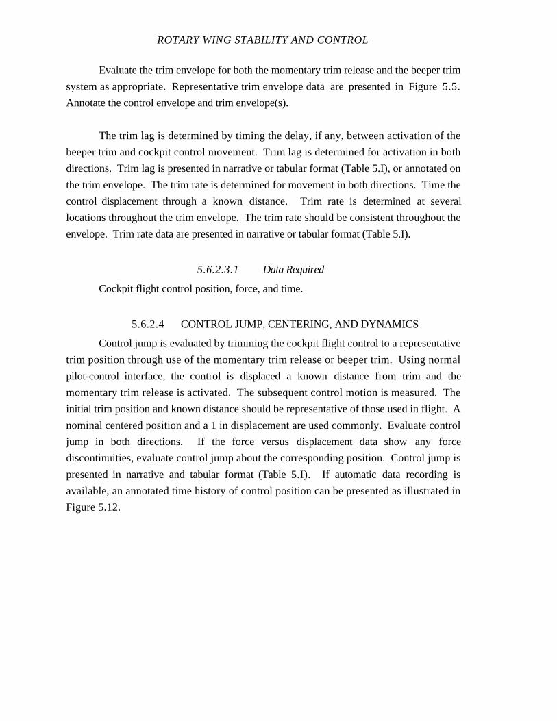
ROTARY WING STABILITY AND CONTROL
Evaluate the trim envelope for both the momentary trim release and the beeper trim
system as appropriate. Representative trim envelope data are presented in Figure 5.5.
Annotate the control envelope and trim envelope(s).
The trim lag is determined by timing the delay, if any, between activation of the
beeper trim and cockpit control movement. Trim lag is determined for activation in both
directions. Trim lag is presented in narrative or tabular format (Table 5.I), or annotated on
the trim envelope. The trim rate is determined for movement in both directions. Time the
control displacement through a known distance. Trim rate is determined at several
locations throughout the trim envelope. The trim rate should be consistent throughout the
envelope. Trim rate data are presented in narrative or tabular format (Table 5.I).
5.6.2.3.1 Data Required
Cockpit flight control position, force, and time.
5.6.2.4 CONTROL JUMP, CENTERING, AND DYNAMICS
Control jump is evaluated by trimming the cockpit flight control to a representative
trim position through use of the momentary trim release or beeper trim. Using normal
pilot-control interface, the control is displaced a known distance from trim and the
momentary trim release is activated. The subsequent control motion is measured. The
initial trim position and known distance should be representative of those used in flight. A
nominal centered position and a 1 in displacement are used commonly. Evaluate control
jump in both directions. If the force versus displacement data show any force
discontinuities, evaluate control jump about the corresponding position. Control jump is
presented in narrative and tabular format (Table 5.I). If automatic data recording is
available, an annotated time history of control position can be presented as illustrated in
Figure 5.12.
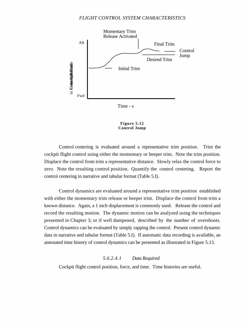
FLIGHT CONTROL SYSTEM CHARACTERISTICS
Control centering is evaluated around a representative trim position. Trim the
cockpit flight control using either the momentary or beeper trim. Note the trim position.
Displace the control from trim a representative distance. Slowly relax the control force to
zero. Note the resulting control position. Quantify the control centering. Report the
control centering in narrative and tabular format (Table 5.I).
Control dynamics are evaluated around a representative trim position established
with either the momentary trim release or beeper trim. Displace the control from trim a
known distance. Again, a 1 inch displacement is commonly used. Release the control and
record the resulting motion. The dynamic motion can be analyzed using the techniques
presented in Chapter 3; or if well dampened, described by the number of overshoots.
Control dynamics can be evaluated by simply rapping the control. Present control dynamic
data in narrative and tabular format (Table 5.I). If automatic data recording is available, an
annotated time history of control dynamics can be presented as illustrated in Figure 5.13.
5.6.2.4.1 Data Required
Cockpit flight control position, force, and time. Time histories are useful.
Time - s
Initial Trim
Desired Trim
Final Trim
Momentary TrimRelease Activated
ControlJump
Long
itudi
nal
Co
ntr
ol P
osi
tion
in F
rom
Fu
ll F
wd
Aft
Fwd
Figure 5.12Control Jump
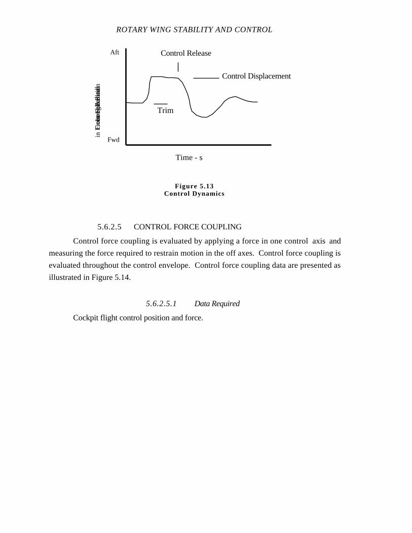
ROTARY WING STABILITY AND CONTROL
5.6.2.5 CONTROL FORCE COUPLING
Control force coupling is evaluated by applying a force in one control axis and
measuring the force required to restrain motion in the off axes. Control force coupling is
evaluated throughout the control envelope. Control force coupling data are presented as
illustrated in Figure 5.14.
5.6.2.5.1 Data Required
Cockpit flight control position and force.
Time - s
Trim
Control Release
Control Displacement
Long
itudi
nal
Co
ntr
ol P
osi
tion
in F
rom
Fu
ll F
wd
Aft
Fwd
Figure 5.13Control Dynamics
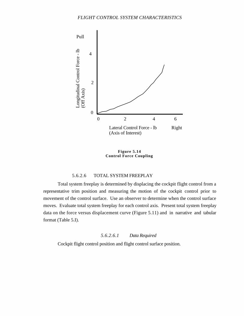
FLIGHT CONTROL SYSTEM CHARACTERISTICS
5.6.2.6 TOTAL SYSTEM FREEPLAY
Total system freeplay is determined by displacing the cockpit flight control from a
representative trim position and measuring the motion of the cockpit control prior to
movement of the control surface. Use an observer to determine when the control surface
moves. Evaluate total system freeplay for each control axis. Present total system freeplay
data on the force versus displacement curve (Figure 5.11) and in narrative and tabular
format (Table 5.I).
5.6.2.6.1 Data Required
Cockpit flight control position and flight control surface position.
0
2
4
0 42
Pull
RightLateral Control Force - lb(Axis of Interest)
Long
itudi
nal C
ontr
ol F
orce
- lb
(Off
Axi
s)
6
Figure 5.14Control Force Coupling
ROTARY WING STABILITY AND CONTROL
5.6.2.7 VISCOUS DAMPER CHARACTERISTICS AND
TRANSIENT FORCES
Viscous damper characteristics are evaluated by determining the control rate by
timing control displacements with a stop watch, and recording the corresponding force
exerted on the control. Apply a constant force to the control and observe the steady state
rate of motion. To eliminate the influence of breakout, displace the control from a
representative trim position prior to starting the test. Restrain the control in this position
and apply a small force to the control in a direction to move the control away from trim.
When the applied force is at the desired level, release the control and allow the control to
acquire a velocity. Hold the applied force constant as the control moves and time the
control movement through a known distance. Repeat the test for increasing force levels
until the maximum rate of interest is tested. A time history can be used to determine the rate
of motion. Present viscous damper data as a plot of rate versus force (Figure 5.15) or in
narrative and tabular format (Table 5.I).
Rapid control displacements which produce transient control forces can be
evaluated by making step control inputs and recording the resultant force and displacement
time histories. The time constant of the force increase and decay is determined from the
time history and used to quantify this characteristic. If time history data are not available,
measure the time required for the force to increase or drop to an apparent steady state value
(determined by the pilot's feel) after the control motion has started or stopped. Transient
force decay characteristics are related to the magnitude of the control motion and the peak
rate of motion, so these parameters are reported with the above data. Report transient force
characteristics data in narrative or tabular format (Table 5.I).
5.6.2.7.1 Data Required
Cockpit flight control position, force, and time.
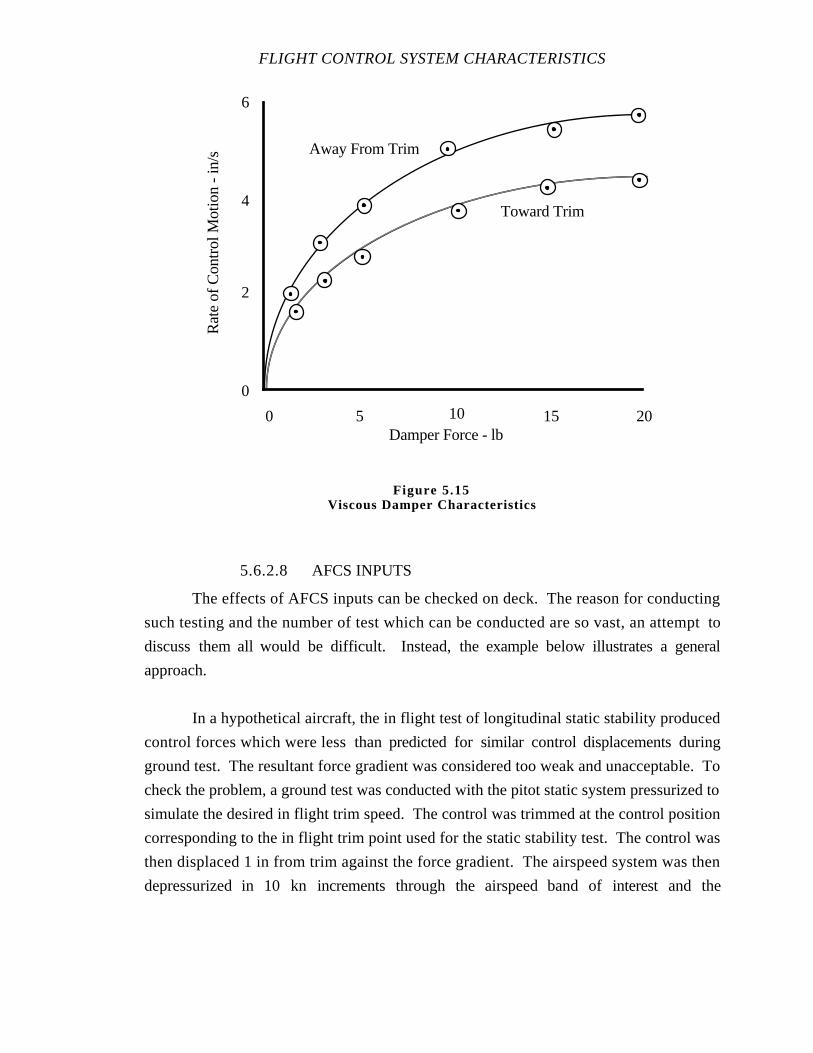
FLIGHT CONTROL SYSTEM CHARACTERISTICS
5.6.2.8 AFCS INPUTS
The effects of AFCS inputs can be checked on deck. The reason for conducting
such testing and the number of test which can be conducted are so vast, an attempt to
discuss them all would be difficult. Instead, the example below illustrates a general
approach.
In a hypothetical aircraft, the in flight test of longitudinal static stability produced
control forces which were less than predicted for similar control displacements during
ground test. The resultant force gradient was considered too weak and unacceptable. To
check the problem, a ground test was conducted with the pitot static system pressurized to
simulate the desired in flight trim speed. The control was trimmed at the control position
corresponding to the in flight trim point used for the static stability test. The control was
then displaced 1 in from trim against the force gradient. The airspeed system was then
depressurized in 10 kn increments through the airspeed band of interest and the
Damper Force - lb
Rat
e of
Con
trol
Mot
ion
- in
/s
0 5 10 15 20
0
2
4
6
Away From Trim
Toward Trim
Figure 5.15Viscous Damper Characteristics

ROTARY WING STABILITY AND CONTROL
corresponding forces for the 1 in displacement were recorded. This test was repeated for 2
in aft and 1 and 2 in forward control displacement. The ground test data were compared to
the in flight data and revealed an undesired AFCS input into the flight control system.
5.6.3 In Flight Testing
In flight evaluation of flight control system characteristics is performed to validate
the results of the ground evaluation and to determine the effects of the control
characteristics on flight parameters. Trim system characteristics such as freeplay, lag, and
rate are evaluated for the effect on parameters such as airspeed, bank angle, or heading
while performing representative mission tasks. Control jump and control dynamics are
evaluated for the effect on aircraft dynamics. The limit control force is evaluated from one
representative trim position to another.
In flight evaluation of the reversible flight control system is conducted in an
environment with representative aerodynamic flight control loads. All control force versus
displacement tests must be conducted for small displacements. Departure from the
representative trim positions cause a change in the aerodynamicloads. Therefore, all
displacements must be small changes from a trim condition. Control force data are difficult
to record precisely in flight especially if there isa high vibration level in the cockpit.
Regardless, all ground tests can be adapted for in flight use staying within the constraints
of small displacements and the flight control envelope.
5.6.3.1 DATA REQUIRED
Cockpit flight control position, force, and time.
5.6.4 Safety Considerations/Risk Management
All ground tests must observe the operating limits of the ground power systems
whether they are external or internal to the aircraft. Any ground test conducted with the
rotors turning must use limited control displacements and rates to avoid rotor to airframe or
rotor to ground contact or high aircraft structural load. Inflight tests are limited by the
normal flight envelope. Displacements and rates may be limited. Normal build up
procedures for force, displacement, or rate must be followed.
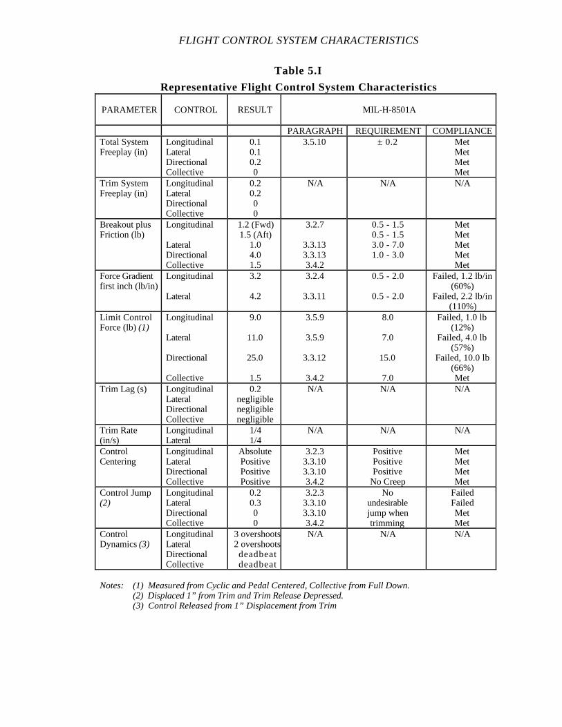
FLIGHT CONTROL SYSTEM CHARACTERISTICS
Table 5.I
Representative Flight Control System Characteristics
PARAMETER CONTROL RESULT MIL-H-8501A
PARAGRAPH REQUIREMENT COMPLIANCETotal SystemFreeplay (in)
LongitudinalLateralDirectionalCollective
0.10.10.20
3.5.10 ± 0.2 MetMetMetMet
Trim SystemFreeplay (in)
LongitudinalLateralDirectionalCollective
0.20.200
N/A N/A N/A
Breakout plusFriction (lb)
Longitudinal
LateralDirectionalCollective
1.2 (Fwd)1.5 (Aft)
1.04.01.5
3.2.7
3.3.133.3.133.4.2
0.5 - 1.50.5 - 1.53.0 - 7.01.0 - 3.0
MetMetMetMetMet
Force Gradientfirst inch (lb/in)
Longitudinal
Lateral
3.2
4.2
3.2.4
3.3.11
0.5 - 2.0
0.5 - 2.0
Failed, 1.2 lb/in(60%)
Failed, 2.2 lb/in(110%)
Limit ControlForce (lb) (1)
Longitudinal
Lateral
Directional
Collective
9.0
11.0
25.0
1.5
3.5.9
3.5.9
3.3.12
3.4.2
8.0
7.0
15.0
7.0
Failed, 1.0 lb(12%)
Failed, 4.0 lb(57%)
Failed, 10.0 lb(66%)Met
Trim Lag (s) LongitudinalLateralDirectionalCollective
0.2negligiblenegligiblenegligible
N/A N/A N/A
Trim Rate(in/s)
LongitudinalLateral
1/41/4
N/A N/A N/A
ControlCentering
LongitudinalLateralDirectionalCollective
AbsolutePositivePositivePositive
3.2.33.3.103.3.103.4.2
PositivePositivePositive
No Creep
MetMetMetMet
Control Jump(2)
LongitudinalLateralDirectionalCollective
0.20.300
3.2.33.3.103.3.103.4.2
Noundesirablejump whentrimming
FailedFailedMetMet
ControlDynamics (3)
LongitudinalLateralDirectionalCollective
3 overshoots2 overshootsd e a d b e a t d e a d b e a t
N/A N/A N/A
Notes: (1) Measured from Cyclic and Pedal Centered, Collective from Full Down.(2) Displaced 1” from Trim and Trim Release Depressed.(3) Control Released from 1” Displacement from Trim
ROTARY WING STABILITY AND CONTROL
5.7 DATA REDUCTION
The data reduction required for flight control system characteristic evaluations
consists of calibrating the control position and control force data to the center of the cockpit
flight control grip or the point of application of pilot control force. The data obtained from
the flight test instrumentation, whether recorded or displayed in the cockpit, and the hand
held data are corrected in accordance with this calibration. Inflight data are corrected as
required for position error and instrument corrections. Data are presented in consistent
units of measure and if control position data are presented as percent of total travel, a
correlation between percent and units of displacement is presented.
5.8 DATA ANALYSIS
Flight control system characteristics data analysis consists principally of comparing
the test results to the specification requirements and theimpact on mission suitability.
Quantitative data analysis techniques are not required.
5.9 MISSION SUITABILITY
While the majority of the flight control system evaluation is conducted statically on
the ground, the impact of the characteristics must be evaluated inflight during representative
mission maneuvers. Armed with a detailed knowledge of the flight control system and its
characteristics, the test pilot can assess and report their impact during flying qualities
evaluations.
5.10 SPECIFICATION COMPLIANCE
MIL-H-8501A, “Helicopter Flying and Ground Handling Qualities; General
Requirements For”, contains general requirements for flight control system characteristics.
Additionally, each aircraft specification or other procurement documents may contain
additional or supplementary requirements. Research the specifications thoroughly to
ensure contractual compliance and a complete evaluation. The following list identifies the
paragraph number in MIL-H-8501A and a short description of the requirement.
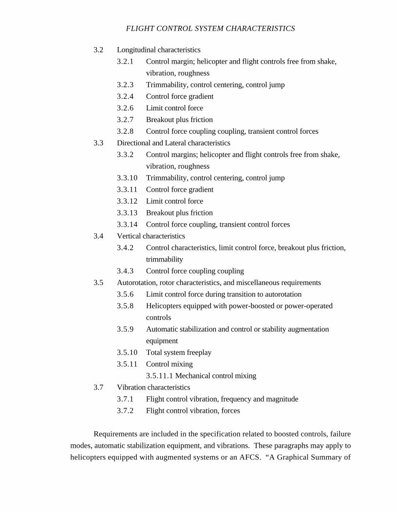
FLIGHT CONTROL SYSTEM CHARACTERISTICS
3.2 Longitudinal characteristics
3.2.1 Control margin; helicopter and flight controls free from shake,
vibration, roughness
3.2.3 Trimmability, control centering, control jump
3.2.4 Control force gradient
3.2.6 Limit control force
3.2.7 Breakout plus friction
3.2.8 Control force coupling coupling, transient control forces
3.3 Directional and Lateral characteristics
3.3.2 Control margins; helicopter and flight controls free from shake,
vibration, roughness
3.3.10 Trimmability, control centering, control jump
3.3.11 Control force gradient
3.3.12 Limit control force
3.3.13 Breakout plus friction
3.3.14 Control force coupling, transient control forces
3.4 Vertical characteristics
3.4.2 Control characteristics, limit control force, breakout plus friction,
trimmability
3.4.3 Control force coupling coupling
3.5 Autorotation, rotor characteristics, and miscellaneous requirements
3.5.6 Limit control force during transition to autorotation
3.5.8 Helicopters equipped with power-boosted or power-operated
controls
3.5.9 Automatic stabilization and control or stability augmentation
equipment
3.5.10 Total system freeplay
3.5.11 Control mixing
3.5.11.1 Mechanical control mixing
3.7 Vibration characteristics
3.7.1 Flight control vibration, frequency and magnitude
3.7.2 Flight control vibration, forces
Requirements are included in the specification related to boosted controls, failure
modes, automatic stabilization equipment, and vibrations. These paragraphs may apply to
helicopters equipped with augmented systems or an AFCS. “A Graphical Summary of
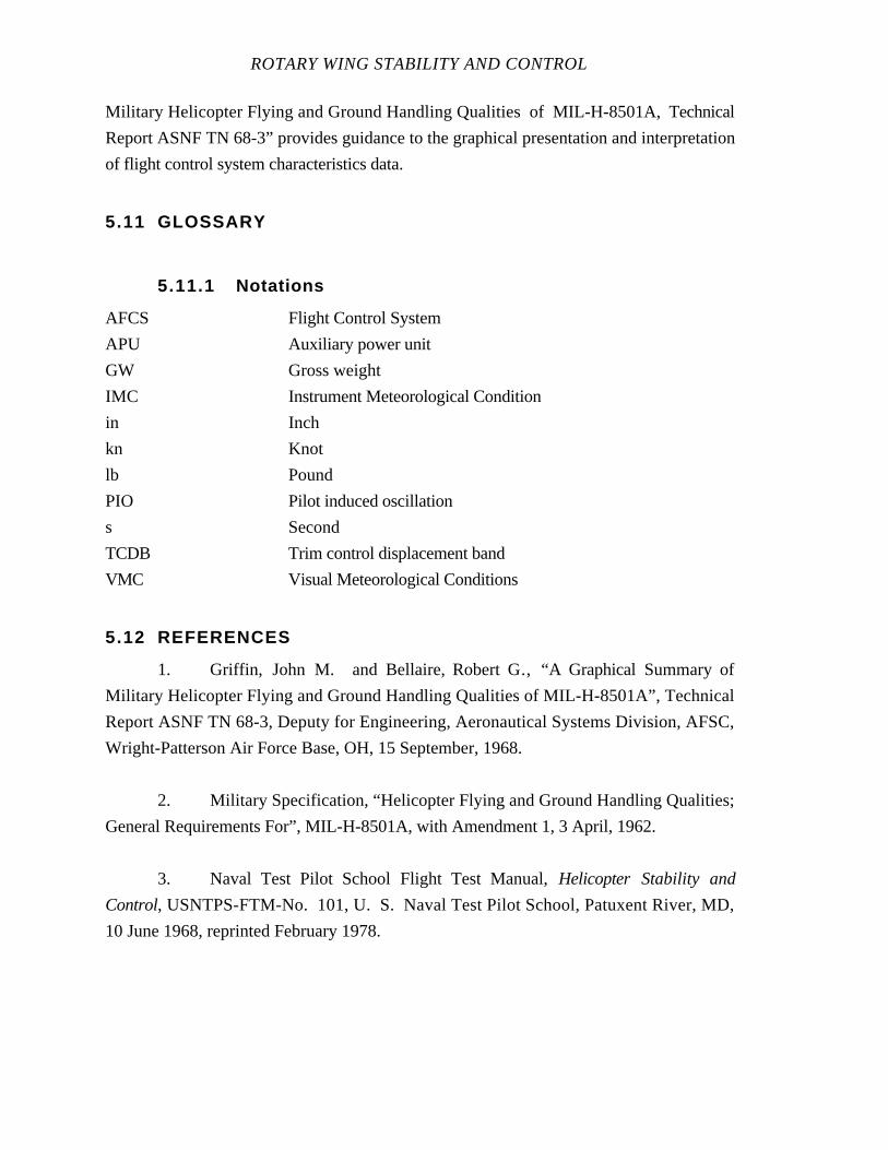
ROTARY WING STABILITY AND CONTROL
Military Helicopter Flying and Ground Handling Qualities of MIL-H-8501A, Technical
Report ASNF TN 68-3” provides guidance to the graphical presentation and interpretation
of flight control system characteristics data.
5.11 GLOSSARY
5.11.1 Notations
AFCS Flight Control System
APU Auxiliary power unit
GW Gross weight
IMC Instrument Meteorological Condition
in Inch
kn Knot
lb Pound
PIO Pilot induced oscillation
s Second
TCDB Trim control displacement band
VMC Visual Meteorological Conditions
5.12 REFERENCES
1. Griffin, John M. and Bellaire, Robert G., “A Graphical Summary of
Military Helicopter Flying and Ground Handling Qualities of MIL-H-8501A”, Technical
Report ASNF TN 68-3, Deputy for Engineering, Aeronautical Systems Division, AFSC,
Wright-Patterson Air Force Base, OH, 15 September, 1968.
2. Military Specification, “Helicopter Flying and Ground Handling Qualities;
General Requirements For”, MIL-H-8501A, with Amendment 1, 3 April, 1962.
3. Naval Test Pilot School Flight Test Manual,Helicopter Stability and
Control, USNTPS-FTM-No. 101, U. S. Naval Test Pilot School, Patuxent River, MD,
10 June 1968, reprinted February 1978.

FLIGHT CONTROL SYSTEM CHARACTERISTICS
4. Naval Test Pilot School Flight Test Manual,Helicopter Stability and
Control, Theory and Flight Test Techniques, USNTPS-FTM-No. 105, U. S. Naval Test
Pilot School, Patuxent River, MD, November 1983, Preliminary Edition.
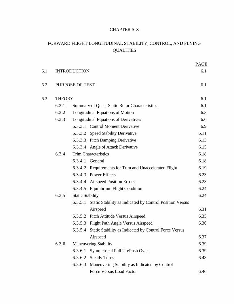
CHAPTER SIX
FORWARD FLIGHT LONGITUDINAL STABILITY, CONTROL, AND FLYING
QUALITIES
PAGE
6.1 INTRODUCTION 6.1
6.2 PURPOSE OF TEST 6.1
6.3 THEORY 6.1
6.3.1 Summary of Quasi-Static Rotor Characteristics 6.1
6.3.2 Longitudinal Equations of Motion 6.3
6.3.3 Longitudinal Equations of Derivatives 6.6
6.3.3.1 Control Moment Derivative 6.9
6.3.3.2 Speed Stability Derivative 6.11
6.3.3.3 Pitch Damping Derivative 6.13
6.3.3.4 Angle of Attack Derivative 6.15
6.3.4 Trim Characteristics 6.18
6.3.4.1 General 6.18
6.3.4.2 Requirements for Trim and Unaccelerated Flight 6.19
6.3.4.3 Power Effects 6.23
6.3.4.4 Airspeed Position Errors 6.23
6.3.4.5 Equilibrium Flight Condition 6.24
6.3.5 Static Stability 6.24
6.3.5.1 Static Stability as Indicated by Control Position Versus
Airspeed 6.31
6.3.5.2 Pitch Attitude Versus Airspeed 6.35
6.3.5.3 Flight Path Angle Versus Airspeed 6.36
6.3.5.4 Static Stability as Indicated by Control Force Versus
Airspeed 6.37
6.3.6 Maneuvering Stability 6.39
6.3.6.1 Symmetrical Pull Up/Push Over 6.39
6.3.6.2 Steady Turns 6.43
6.3.6.3 Maneuvering Stability as Indicated by Control
Force Versus Load Factor 6.46
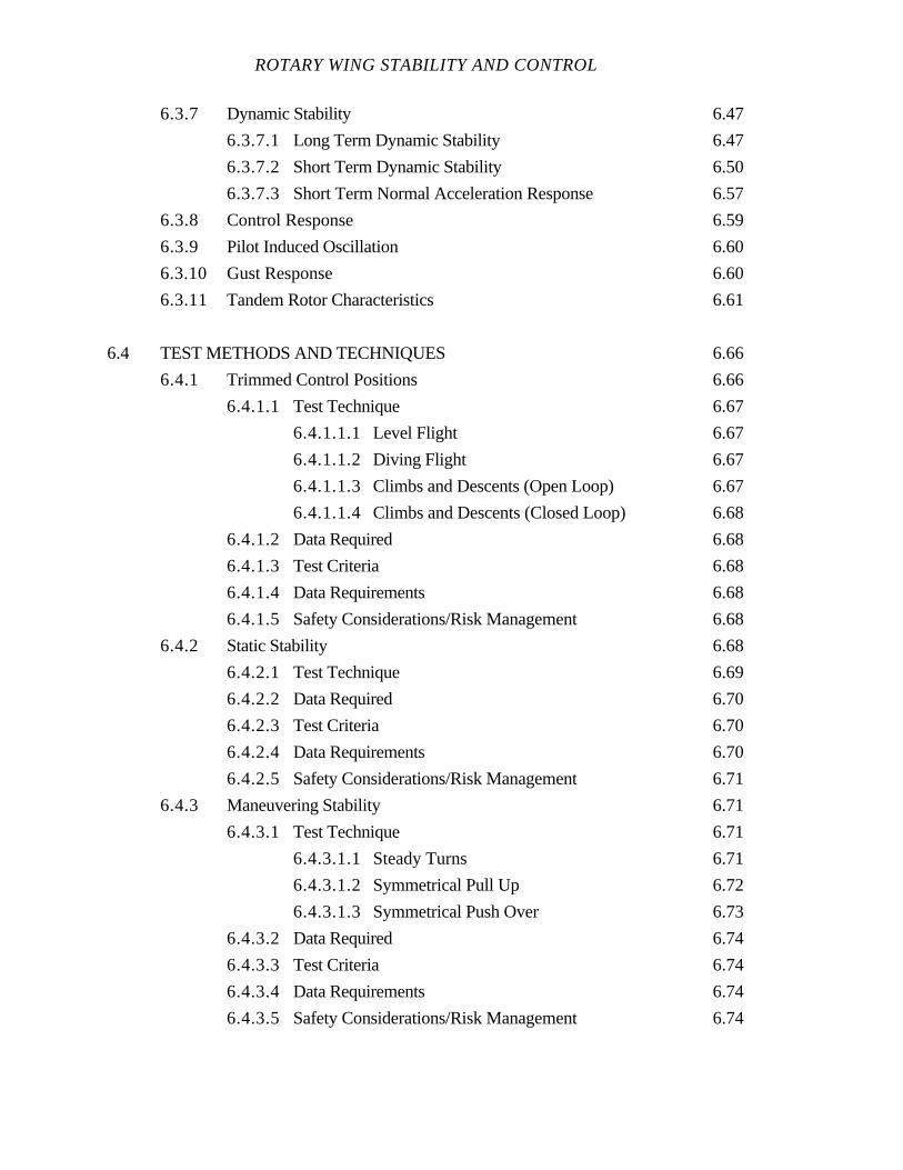
ROTARY WING STABILITY AND CONTROL
6.3.7 Dynamic Stability 6.47
6.3.7.1 Long Term Dynamic Stability 6.47
6.3.7.2 Short Term Dynamic Stability 6.50
6.3.7.3 Short Term Normal Acceleration Response 6.57
6.3.8 Control Response 6.59
6.3.9 Pilot Induced Oscillation 6.60
6.3.10 Gust Response 6.60
6.3.11 Tandem Rotor Characteristics 6.61
6.4 TEST METHODS AND TECHNIQUES 6.66
6.4.1 Trimmed Control Positions 6.66
6.4.1.1 Test Technique 6.67
6.4.1.1.1 Level Flight 6.67
6.4.1.1.2 Diving Flight 6.67
6.4.1.1.3 Climbs and Descents (Open Loop) 6.67
6.4.1.1.4 Climbs and Descents (Closed Loop) 6.68
6.4.1.2 Data Required 6.68
6.4.1.3 Test Criteria 6.68
6.4.1.4 Data Requirements 6.68
6.4.1.5 Safety Considerations/Risk Management 6.68
6.4.2 Static Stability 6.68
6.4.2.1 Test Technique 6.69
6.4.2.2 Data Required 6.70
6.4.2.3 Test Criteria 6.70
6.4.2.4 Data Requirements 6.70
6.4.2.5 Safety Considerations/Risk Management 6.71
6.4.3 Maneuvering Stability 6.71
6.4.3.1 Test Technique 6.71
6.4.3.1.1 Steady Turns 6.71
6.4.3.1.2 Symmetrical Pull Up 6.72
6.4.3.1.3 Symmetrical Push Over 6.73
6.4.3.2 Data Required 6.74
6.4.3.3 Test Criteria 6.74
6.4.3.4 Data Requirements 6.74
6.4.3.5 Safety Considerations/Risk Management 6.74
FORWARD FLIGHT LONGITUDINAL STABILITY, CONTROL,
AND FLYING QUALITIES
6.4.4 Long Term Dynamic Stability 6.75
6.4.4.1 Excitation Methods 6.75
6.4.4.2 Test Technique 6.77
6.4.4.3 Data Required 6.78
6.4.4.4 Test Criteria 6.78
6.4.4.5 Data Requirements 6.78
6.4.4.6 Safety Considerations/Risk Management 6.78
6.4.5 Short Term Dynamic Stability 6.78
6.4.5.1 Excitation Methods 6.79
6.4.5.2 Test Technique 6.79
6.4.5.3 Data Required 6.80
6.4.5.4 Test Criteria 6.80
6.4.5.5 Data Requirements 6.80
6.4.5.6 Safety Considerations/Risk Management 6.80
6.4.6 Control Response 6.80
6.4.6.1 Test Technique 6.82
6.4.6.2 Data Required 6.82
6.4.6.3 Test Criteria 6.83
6.4.6.4 Data Requirements 6.83
6.4.6.5 Safety Considerations/Risk Management 6.83
6.4.7 Gust Response 6.83
6.4.7.1 Excitation Methods 6.84
6.4.7.2 Test Technique 6.84
6.4.7.3 Data Required 6.84
6.4.7.4 Test Criteria 6.84
6.4.7.5 Data Requirements 6.85
6.4.7.6 Safety Considerations/Risk Management 6.85
6.5 DATA REDUCTION 6.85
6.5.1 Trimmed Control Positions 6.85
6.5.2 Static Stability 6.87
6.5.3 Maneuvering Stability 6.88
6.5.4 Long Term Dynamic Stability 6.89
6.5.5 Short Term Dynamic Stability 6.90

ROTARY WING STABILITY AND CONTROL
6.5.6 Control Response 6.90
6.5.7 Gust Response 6.92
6.6 DATA ANALYSIS 6.94
6.6.1 Trimmed Control Positions 6.94
6.6.2 Static Stability 6.94
6.6.3 Maneuvering Stability 6.95
6.6.4 Long Term Dynamic Stability 6.95
6.6.5 Short Term Dynamic Stability 6.96
6.6.6 Control Response 6.96
6.6.7 Gust Response 6.97
6.7 MISSION SUITABILITY 6.97
6.8 SPECIFICATION COMPLIANCE 6.98
6.9 GLOSSARY 6.99
6.9.1 Notations 6.99
6.9.2 Greek Symbols 6.102
6.10 REFERENCES 6.103
FORWARD FLIGHT LONGITUDINAL STABILITY, CONTROL,
AND FLYING QUALITIES
CHAPTER SIX
FIGURES
PAGE
6.1 Forces and Moments Acting on the Helicopter 6.7
6.2 Control Force and Moment Derivatives 6.10
6.3 Forces and Moments Contributing to Pitch Damping 6.14
6.4 Factors Affecting Angle of Attack Derivative 6.17
6.5 Parameters Involved in Trim 6.19
6.6 Longitudinal Trimmed Flight Control Positions Versus Power 6.24
6.7 Static Stability Examples 6.33
6.8 Destabilizing Effect of Reduced Rotor Downwash 6.34
6.9 Static Stability as Indicated by Longitudinal Control Position Versus
Airspeed 6.35
6.10 Flight Path Angle Versus Airspeed 6.36
6.11 Static Stability as Indicated by Control Force Versus Airspeed 6.38
6.12 Relationships Between Variables in Steady Coordinated Turn 6.44
6.13 Helicopter Long Term Response 6.50
6.14 Pitch Rate Response to Step Cyclic Input 6.56
6.15 Normal Acceleration Response to Step Input in Cyclic Pitch 6.58
6.16 Longitudinal Control of a Tandem Rotor Helicopter 6.62
6.17 Factors Affecting Longitudinal Stability of a Tandem Helicopter 6.65
6.18 Time Histories Produced by Various Levels of Excitation 6.76
6.19 Measurement of Step Control Response Characteristics 6.81
6.20 Trimmed Control Positions 6.86
6.21 Static Longitudinal Stability 6.87
6.22 Maneuvering Stability 6.88
6.23 Long Term Dynamic Response 6.89
6.24 Short Term Response 6.90
6.25 Control Response Characteristics 6.91
6.26 Gust Response Characteristics 6.93
ROTARY WING STABILITY AND CONTROL
CHAPTER SIX
TABLES
PAGE
6.I Quasi-Static Rotor Characteristics in Forward Flight 6.2
6.II Sets of Independent Variables for Trim in Steady Rectilinear Flight 6.21
6.III Analogy of Long Term Response and Spring Mass Damper 6.49
6.IV Analogy of Short Term Response and Spring Mass Damper 6.52
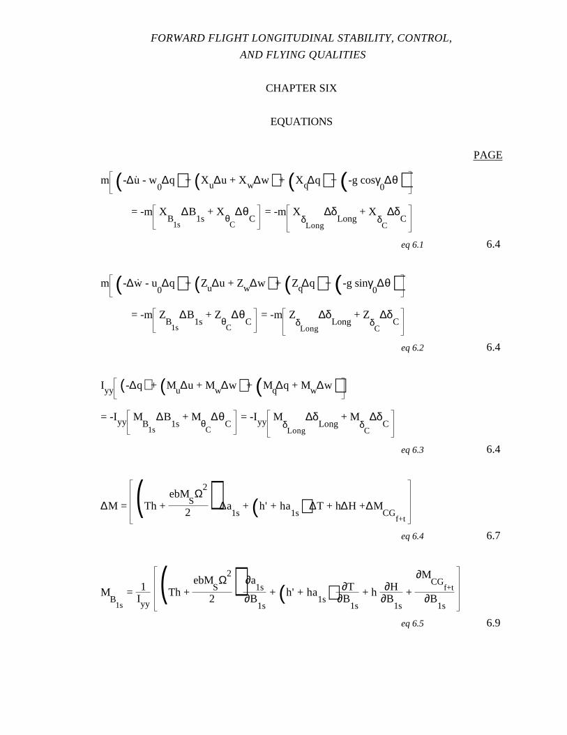
FORWARD FLIGHT LONGITUDINAL STABILITY, CONTROL,
AND FLYING QUALITIES
CHAPTER SIX
EQUATIONS
PAGE
m (-∆u. - w
0∆q) + (Xu∆u + Xw∆w) + (Xq∆q) + (-g cosγ
0∆θ)
= -m XB
1s
∆B1s
+ XθC
∆θC
= -m XδLong
∆δLong
+ XδC
∆δC
eq 6.1 6.4
m (-∆w. - u
0∆q) + (Zu∆u + Zw∆w) + (Zq∆q) + (-g sinγ
0∆θ)
= -m ZB
1s
∆B1s
+ ZθC
∆θC
= -m ZδLong
∆δLong
+ ZδC
∆δC
eq 6.2 6.4
Iyy (-∆q) + (Mu∆u + Mw∆w) + (Mq∆q + Mw∆w)= -Iyy M
B1s
∆B1s
+ MθC
∆θC
= -Iyy MδLong
∆δLong
+ MδC
∆δC
eq 6.3 6.4
∆M = (Th + ebM
SΩ
2
2) ∆a
1s + (h' + ha
1s) ∆T + h∆H +∆MCG
f+t
eq 6.4 6.7
MB
1s
= 1Iyy
(Th + ebM
SΩ
2
2) ∂a
1s∂B
1s
+ (h' + ha1s) ∂T
∂B1s
+ h ∂H∂B
1s
+
∂MCG
f+t
∂B1s
eq 6.5 6.9

ROTARY WING STABILITY AND CONTROL
Mu = 1Iyy
(Th + ebM
SΩ
2
2) ∂a
1s∂u
+ (h' + ha1s) ∂T
∂u + h ∂H
∂u +
∂MCG
f+t
∂u
eq 6.6 6.11
Mq = 1Iyy
(Th + ebM
SΩ
2
2) ∂a
1s∂q
+ (h' + ha1s) ∂T
∂q + h ∂H
∂q +
∂MCG
f+t
∂q
eq 6.7 6.13
Mw = 1Iyy
(Th + ebM
SΩ
2
2) ∂a
1s∂w
+ (h' + ha1s) ∂T
∂w + h ∂H
∂w +
∂MCG
f+t
∂w
eq 6.8 6.15
Xu Xw -g 0
Zu Zw 0 0
Mu Mw 0 0
0 - 1u
01 -1
∆u∆w
∆θ∆γ
= -
XB
1s
ZB
1s
MB
1s
0
∆B1s
-
XθC
ZθC
MθC
0
∆θC
eq 6.9 6.26
XB
1s
Xw - g 0
ZB
1s
Zw 0 0
MB
1s
Mw 0 0
0 - 1u
01 -1
∆B1s
∆w
∆θ∆γ
= -
Xu
Zu
Mu
0
∆u -
XθC
ZθC
MθC
0
∆θC
eq 6.10 6.26
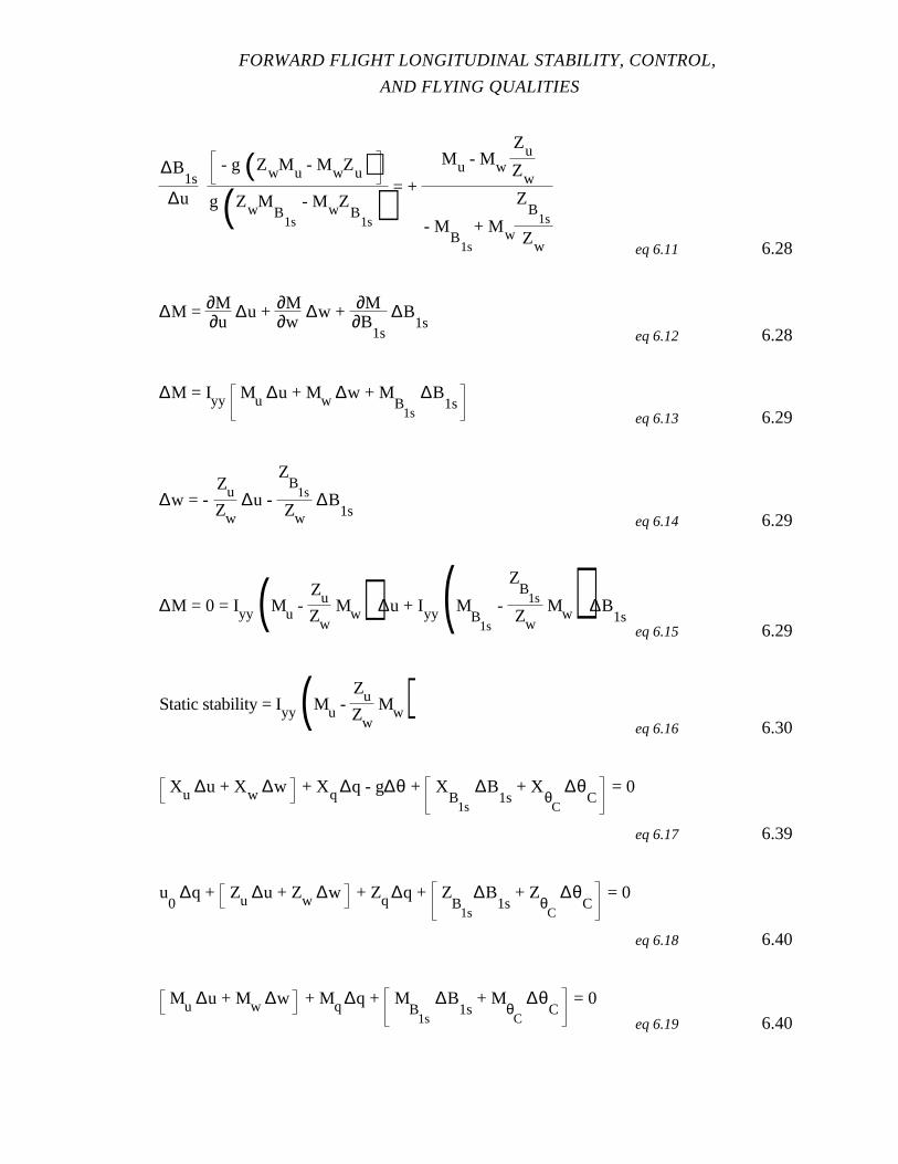
FORWARD FLIGHT LONGITUDINAL STABILITY, CONTROL,
AND FLYING QUALITIES
∆B1s
∆u
- g (ZwMu - MwZu)g(ZwM
B1s
- MwZB
1s) = +
Mu - Mw
Zu
Zw
- MB
1s
+ Mw
ZB
1s
Zw eq 6.11 6.28
∆M = ∂M∂u
∆u + ∂M∂w
∆w + ∂M∂B
1s
∆B1s
eq 6.12 6.28
∆M = Iyy Mu ∆u + Mw ∆w + MB
1s
∆B1s
eq 6.13 6.29
∆w = - ZuZw
∆u -
ZB
1s
Zw∆B
1seq 6.14 6.29
∆M = 0 = Iyy (Mu - ZuZw
Mw) ∆u + Iyy (MB
1s
-
ZB
1s
Zw Mw) ∆B
1seq 6.15 6.29
Static stability = Iyy (Mu - ZuZw
Mw)eq 6.16 6.30
Xu ∆u + Xw ∆w + Xq∆q - g∆θ + XB
1s
∆B1s
+ XθC
∆θC
= 0
eq 6.17 6.39
u0
∆q + Zu ∆u + Zw ∆w + Zq∆q + ZB
1s
∆B1s
+ ZθC
∆θC
= 0
eq 6.18 6.40
Mu ∆u + Mw ∆w + Mq∆q + MB
1s
∆B1s
+ MθC
∆θC
= 0
eq 6.19 6.40
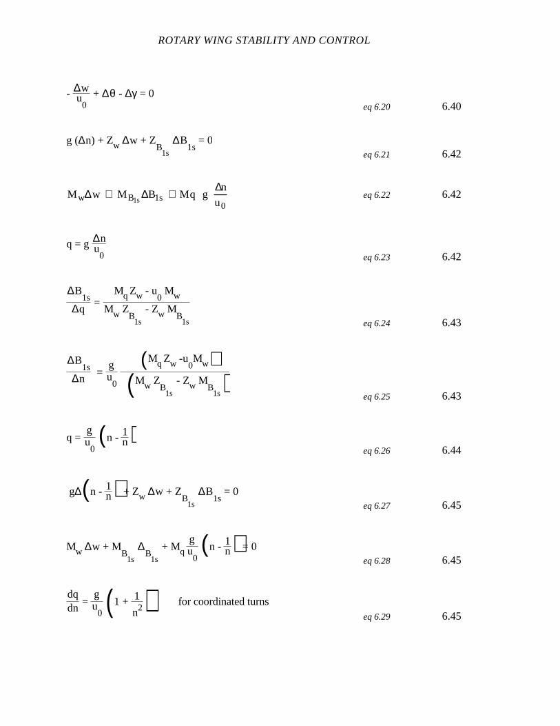
ROTARY WING STABILITY AND CONTROL
- ∆wu
0 + ∆θ - ∆γ = 0
eq 6.20 6.40
g (∆n) + Zw ∆w + ZB
1s
∆B1s
= 0eq 6.21 6.42
M w∆w + MB1s∆B1s + Mq g
∆n
u0eq 6.22 6.42
q = g ∆nu
0 eq 6.23 6.42
∆B1s
∆q =
Mq Zw - u0 Mw
Mw ZB
1s
- Zw MB
1s eq 6.24 6.43
∆B1s
∆n =
gu
0
(Mq Zw -u0Mw)
(Mw ZB
1s
- Zw MB
1s) eq 6.25 6.43
q = gu
0(n - 1n)
eq 6.26 6.44
g∆(n - 1n) + Zw ∆w + ZB
1s
∆B1s
= 0eq 6.27 6.45
Mw ∆w + MB
1s
∆B
1s
+ Mqgu
0(n - 1n) = 0
eq 6.28 6.45
dqdn
= gu
0 (1 + 1
n2) for coordinated turnseq 6.29 6.45
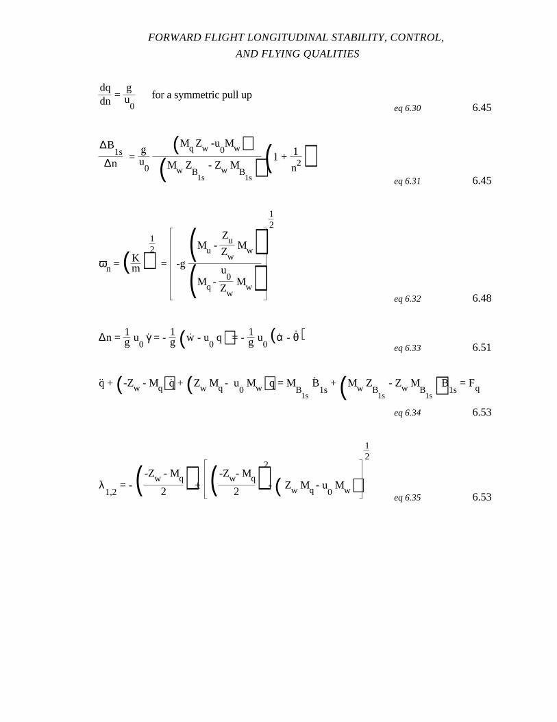
FORWARD FLIGHT LONGITUDINAL STABILITY, CONTROL,
AND FLYING QUALITIES
dqdn
= gu
0for a symmetric pull up
eq 6.30 6.45
∆B1s
∆n =
gu
0
(Mq Zw -u0Mw)
(Mw ZB
1s
- Zw MB
1s) (1 + 1
n2)eq 6.31 6.45
ωn = (Km)
12
= -g(Mu -
ZuZw
Mw)(Mq -
u0
Zw Mw)
12
eq 6.32 6.48
∆n = 1g u0
γ. = - 1g (w. - u
0 q) = - 1g u
0(α. - θ
. )eq 6.33 6.51
q.. + (-Zw - Mq)q
. + (Zw Mq - u0
Mw)q = MB
1s
B.
1s + (Mw Z
B1s
- Zw MB
1s)B1s
= Fq
eq 6.34 6.53
λ1,2
= - ( -Zw - Mq
2 ) ± ( -Zw- Mq
2 )2
- ( Zw Mq - u0 Mw)
12
eq 6.35 6.53
CHAPTER SIX
FORWARD FLIGHT LONGITUDINAL STABILITY,
CONTROL, AND FLYING QUALITIES
6.1 INTRODUCTION
This chapter discusses helicopter stability, control, and flying qualities in forward
flight. The objective is understanding and documenting the helicopter's suitability for
performing specific mission-oriented tasks. This chapter discusses open loop and closed
loop response characteristics, and the test techniques used to assess and document the
characteristics.
6.2 PURPOSE OF TEST
The purpose of these tests is to evaluate the forward flight longitudinal stability,
control, and flying qualities of the helicopter. The engineering tests included in the
evaluation are:
1. Trimmed flight control positions.
2. Static stability.
3. Maneuvering stability.
4. Long term dynamic stability.
5. Short term dynamic stability.
6. Control response.
7. Gust response.
6.3 THEORY
6.3.1 Summary of Quasi-Static Rotor Characteristics
The basic rotor characteristics are discussed in Chapter 4 along with the dynamic
responses to various inputs. The presentations indicated a quasi-static approximation for
rotor responses is satisfactory for the discussion of helicopter stability, control, and flying
qualities.
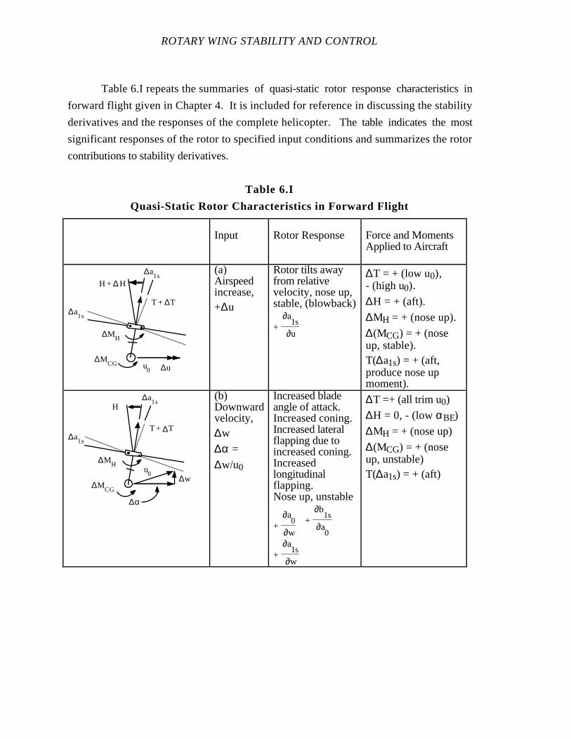
ROTARY WING STABILITY AND CONTROL
Table 6.I repeats the summaries of quasi-static rotor response characteristics in
forward flight given in Chapter 4. It is included for reference in discussing the stability
derivatives and the responses of the complete helicopter. The table indicates the most
significant responses of the rotor to specified input conditions and summarizes the rotor
contributions to stability derivatives.
Table 6.I
Quasi-Static Rotor Characteristics in Forward Flight
Input Rotor Response Force and MomentsApplied to Aircraft
∆a1s
∆a1s
T + ∆T
u0 ∆u
H + ∆ H
∆MCG
∆MH
(a)Airspeedincrease,+∆u
Rotor tilts awayfrom relativevelocity, nose up,stable, (blowback)
+∂a
1s
∂u
∆T = + (low u0),- (high u0).
∆H = + (aft).
∆MH = + (nose up).
∆(MCG) = + (noseup, stable).T(∆a1s) = + (aft,produce nose upmoment).
∆a1s
∆a1s
T + ∆T
u0
∆MCG
∆w
H
∆α
∆MH
(b)Downwardvelocity,∆w
∆α =
∆w/u0
Increased bladeangle of attack.Increased coning.Increased lateralflapping due toincreased coning.Increasedlongitudinalflapping.Nose up, unstable
+∂a
0
∂w+
∂b1s
∂a0
+∂a
1s
∂w
∆T =+ (all trim u0)
∆H = 0, - (low αBE)
∆MH = + (nose up)
∆(MCG) = + (noseup, unstable)T(∆a1s) = + (aft)
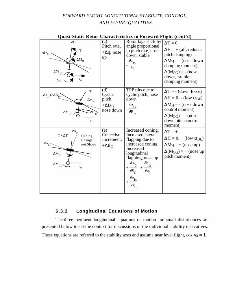
FORWARD FLIGHT LONGITUDINAL STABILITY, CONTROL,
AND FLYING QUALITIES
Quasi-Static Rotor Characteristics in Forward Flight (cont’d)
u0
∆MCG
∆q
T-∆a1s
∆H
∆MH
(c)Pitch rate,+∆q, noseup
Rotor lags shaft byangle proportionalto pitch rate, nosedown, stable
-∂a
1s
∂q
∆T = 0
∆H = + (aft, reducespitch damping)∆MH = - (nose downdamping moment)∆(MCG) = - (nosedown, stable,damping moment)
u0
∆MCG
T
∆MH
∆B1s
-∆a1s
(>∆B1s
)(d)Cyclicpitch,+∆B1snose down
TPP tilts due tocyclic pitch, nosedown
-∂a
1s
∂B1s
∆T = - (down force)
∆H = 0, - (low αBE)
∆MH = - (nose downcontrol moment)∆(MCG) = - (nosedown pitch controlmoment)
∆a1s
∆a1s
u0
∆MCG
∆MH
T + ∆T ConingChangenot Shown
(e)CollectiveIncrement,+∆θC
Increased coning.Increased lateralflapping due toincreased coning.Increasedlongitudinalflapping, nose up
+∂ a
0
∂θC
+∂b
1s
∂a0
+∂a
1s
∂θC
∆T = +
∆H = 0, + (low αBE)
∆MH = + (nose up)
∆(MCG) = + (nose uppitch moment)
6.3.2 Longitudinal Equations of Motion
The three pertinent longitudinal equations of motion for small disturbances are
presented below to set the context for discussions of the individual stability derivatives.
These equations are referred to the stability axes and assume near level flight, cos γ0 ≈ 1.
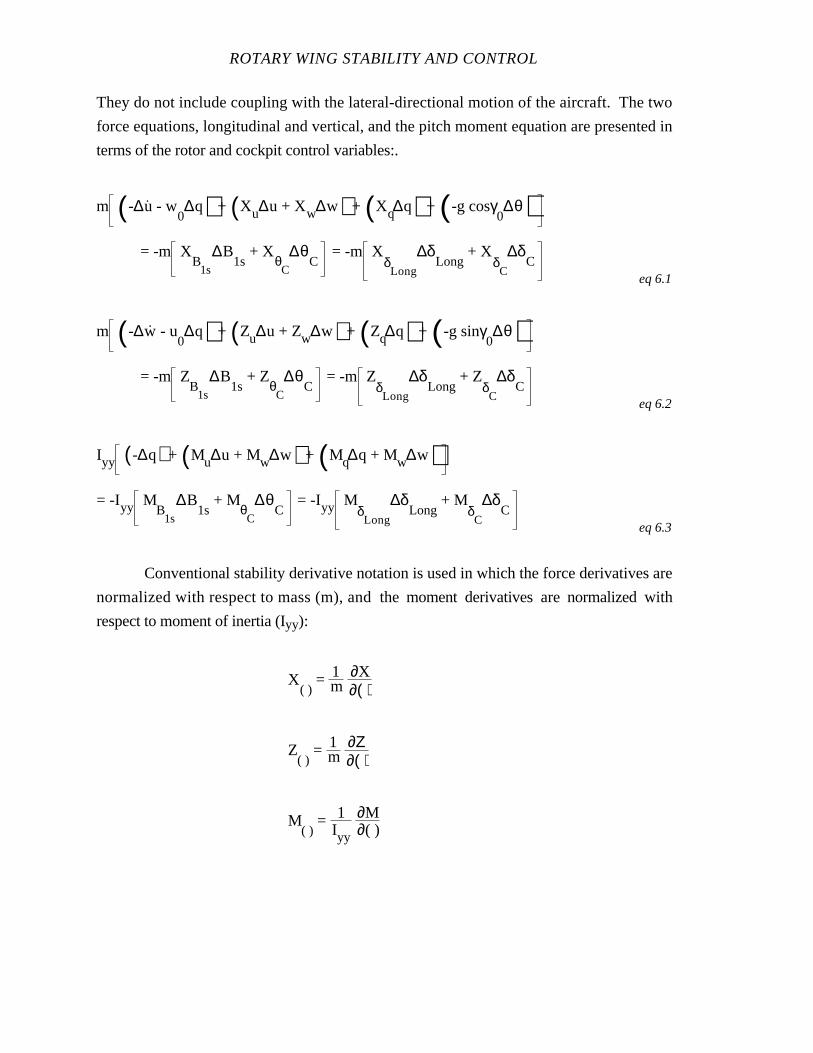
ROTARY WING STABILITY AND CONTROL
They do not include coupling with the lateral-directional motion of the aircraft. The two
force equations, longitudinal and vertical, and the pitch moment equation are presented in
terms of the rotor and cockpit control variables:.
m (-∆u. - w
0∆q) + (Xu∆u + Xw∆w) + (Xq∆q) + (-g cosγ
0∆θ)
= -m XB
1s
∆B1s
+ XθC
∆θC
= -m XδLong
∆δLong
+ XδC
∆δC
eq 6.1
m (-∆w. - u
0∆q) + (Zu∆u + Zw∆w) + (Zq∆q) + (-g sinγ
0∆θ)
= -m ZB
1s
∆B1s
+ ZθC
∆θC
= -m ZδLong
∆δLong
+ ZδC
∆δC
eq 6.2
Iyy (-∆q) + (Mu∆u + Mw∆w) + (Mq∆q + Mw∆w)= -Iyy M
B1s
∆B1s
+ MθC
∆θC
= -Iyy MδLong
∆δLong
+ MδC
∆δC
eq 6.3
Conventional stability derivative notation is used in which the force derivatives are
normalized with respect to mass (m), and the moment derivatives are normalized with
respect to moment of inertia (Iyy):
X( )
= 1m∂X∂( )
Z( )
= 1m∂Ζ∂( )
M( )
= 1Iyy
∂M∂( )

FORWARD FLIGHT LONGITUDINAL STABILITY, CONTROL,
AND FLYING QUALITIES
Where:
B1s - Longitudinal cyclic pitch angle, shaft referenced
C - Collective control
LONG - Longitudinal control
g - Gravity
0 - Initial flight path angle
I yy - Moment of inertia about y axis, pitch moment of inertia
m - Mass
M B1s- Pitch moment due to longitudinal cyclic pitch angle
M q - Pitch moment due to pitch rate
MθC- Pitch moment due to collective pitch angle
M u - Pitch moment due to longitudinal velocity
M w - Pitch moment due to vertical velocity
M w - Pitch moment due to vertical acceleration
θ - Pitch angle
q - Pitch rate
θC - Collective pitch angle
u - Translational velocity component along x axis
u0 - Initial velocity
u - Linear acceleration along x axis
w - Translational velocity component along z axis
w0 - Initial velocity component along z axis
w - Linear acceleration along z axis
X B1s- Longitudinal force due to longitudinal cyclic pitch angle
X q - Longitudinal force due to pitch rate
Xθ C- Longitudinal force due to collective pitch angle
X u - Longitudinal force due to longitudinal velocity
X w - Longitudinal force due to vertical velocity
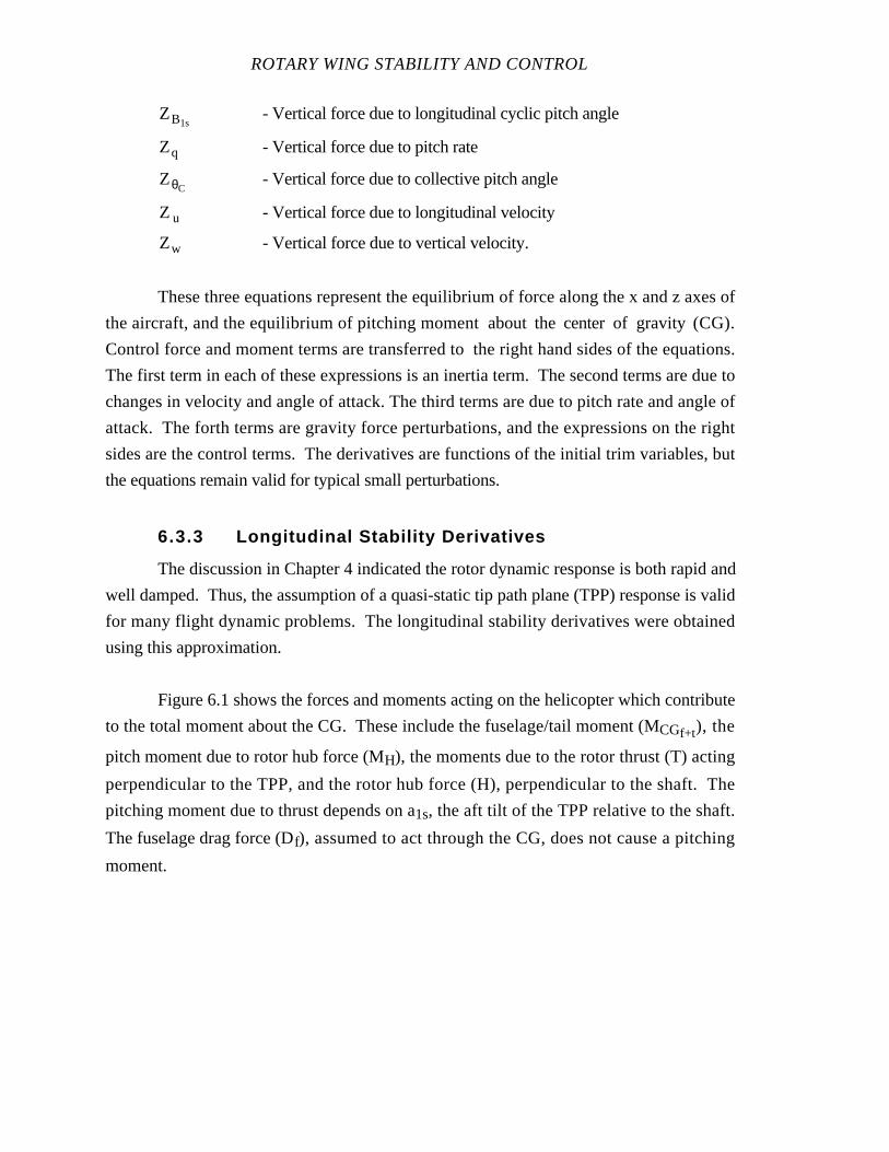
ROTARY WING STABILITY AND CONTROL
ZB1s- Vertical force due to longitudinal cyclic pitch angle
Zq - Vertical force due to pitch rate
ZθC- Vertical force due to collective pitch angle
Z u - Vertical force due to longitudinal velocity
Zw - Vertical force due to vertical velocity.
These three equations represent the equilibrium of force along the x and z axes of
the aircraft, and the equilibrium of pitching moment about the center of gravity (CG).
Control force and moment terms are transferred to the right hand sides of the equations.
The first term in each of these expressions is an inertia term. The second terms are due to
changes in velocity and angle of attack. The third terms are due to pitch rate and angle of
attack. The forth terms are gravity force perturbations, and the expressions on the right
sides are the control terms. The derivatives are functions of the initial trim variables, but
the equations remain valid for typical small perturbations.
6.3.3 Longitudinal Stability Derivatives
The discussion in Chapter 4 indicated the rotor dynamic response is both rapid and
well damped. Thus, the assumption of a quasi-static tip path plane (TPP) response is valid
for many flight dynamic problems. The longitudinal stability derivatives were obtained
using this approximation.
Figure 6.1 shows the forces and moments acting on the helicopter which contribute
to the total moment about the CG. These include the fuselage/tail moment (MCGf+t), the
pitch moment due to rotor hub force (MH), the moments due to the rotor thrust (T) acting
perpendicular to the TPP, and the rotor hub force (H), perpendicular to the shaft. The
pitching moment due to thrust depends on a1s, the aft tilt of the TPP relative to the shaft.
The fuselage drag force (Df), assumed to act through the CG, does not cause a pitching
moment.
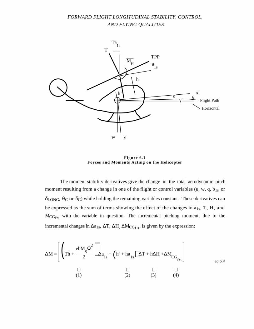
FORWARD FLIGHT LONGITUDINAL STABILITY, CONTROL,
AND FLYING QUALITIES
The moment stability derivatives give the change in thetotal aerodynamic pitch
moment resulting from a change in one of the flight or control variables (u, w, q, b1s or
δLONG, θC or δC) while holding the remaining variables constant. These derivatives can
be expressed as the sum of terms showing the effect of the changes in a1s, T, H, and
MCGf+t with the variable in question. The incremental pitching moment, due to the
incremental changes in ∆a1s, ∆T, ∆H, ∆MCGf+t, is given by the expression:
∆M = (Th + ebM
SΩ
2
2) ∆a
1s + (h' + ha
1s) ∆T + h∆H +∆MCG
f+t eq 6.4
⇑ ⇑ ⇑ ⇑(1) (2) (3) (4)
h
a1s
MH
h'
T
Ta1s
zw
x
TPP
Horizontal
θγ
αFlight Path
Figure 6.1Forces and Moments Acting on the Helicopter
ROTARY WING STABILITY AND CONTROL
Where:
a1s - Longitudinal flapping angle, shaft referenced
b - Number of blades
e - Flapping hinge offset
H - Rotor hub force, ⊥ to shaft
h - Height of hub above CG
h' - Longitudinal distance between the rotor shaft and the CG
M - Net moment about y axis, Pitch moment
MCG f + t - Pitch moment due to the aerodynamic forces on the fuselage/tail
MS - Blade mass moment
T - Thrust
Ω - Rotor angular velocity.
The physical explanation for the four terms is as follows:
(1) Term proportional to aft tilt of TPP (∆a1s):
Th∆a1s, Moment caused by aft thrust component due to TPP tilt. (Depends on
height, h, of rotor above CG).
ebMSΩ2
2 ∆a1s, Offset hinge moment corresponding to aft TPP tilt.
(2) Term proportional to thrust (∆T):
(h' + ha1s), Moment arm from CG to line of action of thrust at trim condition.
(Depends on height of rotor above CG, distance between rotor shaft and CG, and trim
value of a1s).
(3) Term proportional to rotor H force (∆H). (Depends on height of rotor
above CG).
(4) Term including pitching moment due to fuselage/tail.
Each of the stability derivatives discussed in the following section are treated as the
sum of four terms corresponding to the four terms above.
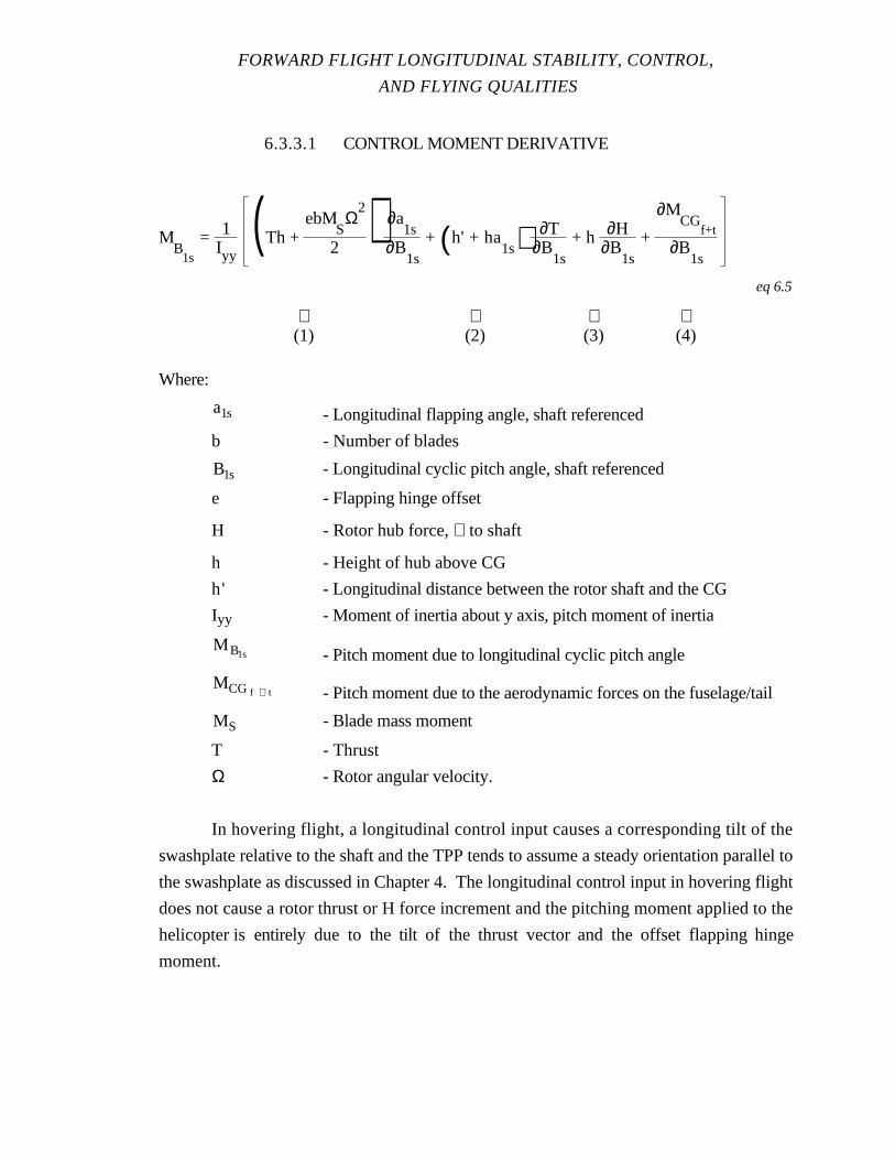
FORWARD FLIGHT LONGITUDINAL STABILITY, CONTROL,
AND FLYING QUALITIES
6.3.3.1 CONTROL MOMENT DERIVATIVE
MB
1s
= 1Iyy
(Th + ebM
SΩ
2
2) ∂a
1s∂B
1s
+ (h' + ha1s) ∂T
∂B1s
+ h ∂H∂B
1s
+
∂MCG
f+t
∂B1s
eq 6.5
⇑ ⇑ ⇑ ⇑(1) (2) (3) (4)
Where:
a1s - Longitudinal flapping angle, shaft referenced
b - Number of blades
B1s - Longitudinal cyclic pitch angle, shaft referenced
e - Flapping hinge offset
H - Rotor hub force, ⊥ to shaft
h - Height of hub above CG
h' - Longitudinal distance between the rotor shaft and the CG
Iyy - Moment of inertia about y axis, pitch moment of inertia
M B1s - Pitch moment due to longitudinal cyclic pitch angle
MCG f + t - Pitch moment due to the aerodynamic forces on the fuselage/tail
MS - Blade mass moment
T - Thrust
Ω - Rotor angular velocity.
In hovering flight, a longitudinal control input causes a corresponding tilt of the
swashplate relative to the shaft and the TPP tends to assume a steady orientation parallel to
the swashplate as discussed in Chapter 4. The longitudinal control input in hovering flight
does not cause a rotor thrust or H force increment and the pitching moment applied to the
helicopter is entirely due to the tilt of the thrust vector and the offset flapping hinge
moment.
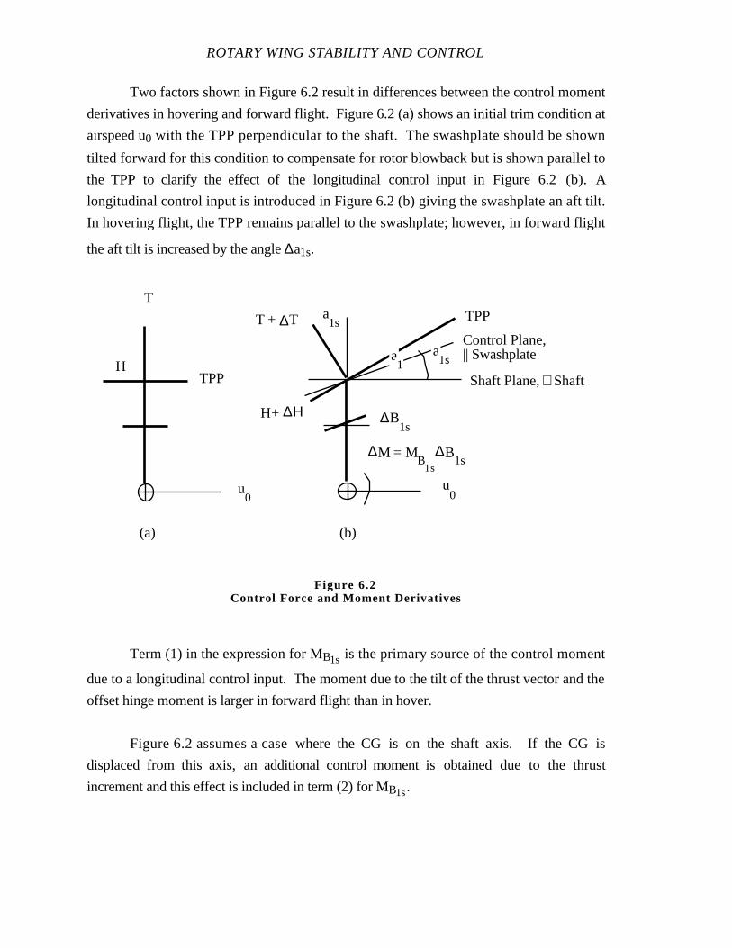
ROTARY WING STABILITY AND CONTROL
Two factors shown in Figure 6.2 result in differences between the control moment
derivatives in hovering and forward flight. Figure 6.2 (a) shows an initial trim condition at
airspeed u0 with the TPP perpendicular to the shaft. The swashplate should be shown
tilted forward for this condition to compensate for rotor blowback but is shown parallel to
the TPP to clarify the effect of the longitudinal control input in Figure 6.2 (b). A
longitudinal control input is introduced in Figure 6.2 (b) giving the swashplate an aft tilt.
In hovering flight, the TPP remains parallel to the swashplate; however, in forward flight
the aft tilt is increased by the angle ∆a1s.
Term (1) in the expression for MB1s is the primary source of the control moment
due to a longitudinal control input. The moment due to the tilt of the thrust vector and the
offset hinge moment is larger in forward flight than in hover.
Figure 6.2 assumes a case where the CG is on the shaft axis. If the CG is
displaced from this axis, an additional control moment is obtained due to the thrust
increment and this effect is included in term (2) for MB1s.
Control Plane, || Swashplate
Shaft Plane, ⊥ Shaft
TPP
u0
∆B1s
a1sa
1
T + ∆T a1s
H+ ∆Η
T
H
u0
TPP
(a) (b)
∆M = MB
1s
∆B1s
Figure 6.2Control Force and Moment Derivatives

FORWARD FLIGHT LONGITUDINAL STABILITY, CONTROL,
AND FLYING QUALITIES
Term (3) in the expression for MB1s is small because the control input causes little
change in H force. Term (4) could give a contribution to the derivative if control inputs
influenced the flow sufficiently to cause changes in the interference of the rotor with the
fuselage or tail. However, this term is usually negligible.
6.3.3.2 SPEED STABILITY DERIVATIVE
Mu = 1Iyy
(Th + ebM
SΩ
2
2) ∂a
1s∂u
+ (h' + ha1s) ∂T
∂u + h ∂H
∂u +
∂MCG
f+t
∂u
eq 6.6
⇑ ⇑ ⇑ ⇑(1) (2) (3) (4)
Where:
a1s - Longitudinal flapping angle, shaft referenced
b - Number of blades
e - Flapping hinge offset
H - Rotor hub force, ⊥ to shaft
h - Height of hub above CG
h' - Longitudinal distance between the rotor shaft and the CG
I yy - Moment of inertia about y axis, pitch moment of inertia
MCG f + t - Pitch moment due to the aerodynamic forces on the
fuselage/tail
MS - Blade mass moment
M u - Pitch moment due to longitudinal velocity
T - Thrust
u - Translational velocity component along x axis
Ω - Rotor angular velocity.
ROTARY WING STABILITY AND CONTROL
The primary contribution of the rotor to the speed stability derivative (Mu) is given
by term (1) which shows the effect of rotor blowback or aft tilt with increasing speed. This
causes a positive or nose up pitching moment due to the combined effects of an offset hinge
moment and the aft tilt of the thrust vector. The increased rotor profile drag with a speed
increment also produces a positive nose up pitching moment (Term (3)). Terms (1) and (3)
depend on the height of the rotor above the CG, but not on the fore and aft location of the
CG. The change in rotor thrust with speed contributes a pitching moment depending on the
fore and aft CG location and the product of the rotor tilt at trim and the rotor height. This
term changes sign at high speed where the thrust variation with speed changes sign. In
general, the change in thrust is small compared to the contribution due to rotor blowback.
The combined effect of the fuselage/tail on Mu, term (4), is strongly dependent on
the tail incidence and the tail load at the trim condition. Negative incidence at trim produces
a stabilizing down load. The down load becomes larger with a speed increase producing a
nose up pitching moment. Conversely, an up load at trim makes a negative contribution to
the speed stability derivative. However, a tail down load to obtain a positive increment in
Mu results in some performance penalty.
Another problem with a horizontal tail is adverse interference with the main rotor or
fuselage which may be encountered during some flight conditions. The induced velocities
at the tail generated by the main rotor tend to be destabilizing. Downwash angle at the tail
can be increased with increased speed due to main rotorwake impingement. The tail
effective angle is increased, increasing tail lift and producing a negative or nose down
moment. Other problems arise for flight conditions where the fuselage disturbs the flow at
the tail. It may be impossible to find a tail location which avoids all interference
difficulties. When a satisfactory tail location cannot be found for the desired Mu, it may be
necessary to augment the aircraft to provide the desired airspeed variation with longitudinal
control position.
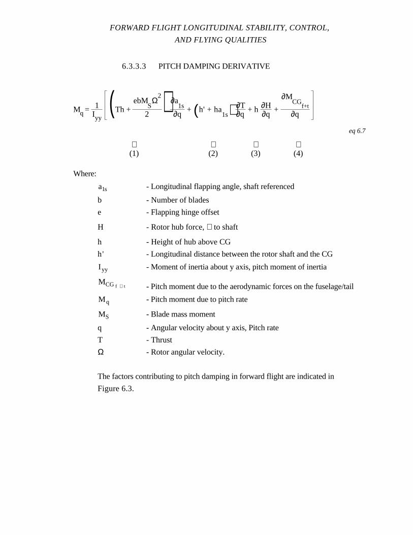
FORWARD FLIGHT LONGITUDINAL STABILITY, CONTROL,
AND FLYING QUALITIES
6.3.3.3 PITCH DAMPING DERIVATIVE
Mq = 1Iyy
(Th + ebM
SΩ
2
2) ∂a
1s∂q
+ (h' + ha1s) ∂T
∂q + h ∂H
∂q +
∂MCG
f+t
∂q
eq 6.7
⇑ ⇑ ⇑ ⇑(1) (2) (3) (4)
Where:
a1s - Longitudinal flapping angle, shaft referenced
b - Number of blades
e - Flapping hinge offset
H - Rotor hub force, ⊥ to shaft
h - Height of hub above CG
h' - Longitudinal distance between the rotor shaft and the CG
I yy - Moment of inertia about y axis, pitch moment of inertia
MCG f + t - Pitch moment due to the aerodynamic forces on the fuselage/tail
M q - Pitch moment due to pitch rate
MS - Blade mass moment
q - Angular velocity about y axis, Pitch rate
T - Thrust
Ω - Rotor angular velocity.
The factors contributing to pitch damping in forward flight are indicated in
Figure 6.3.
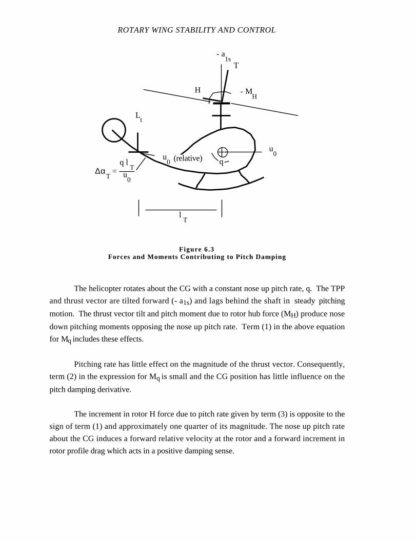
ROTARY WING STABILITY AND CONTROL
The helicopter rotates about the CG with a constant nose up pitch rate, q. The TPP
and thrust vector are tilted forward (- a1s) and lags behind the shaft in steady pitching
motion. The thrust vector tilt and pitch moment due to rotor hub force (MH) produce nose
down pitching moments opposing the nose up pitch rate. Term (1) in the above equation
for Mq includes these effects.
Pitching rate has little effect on the magnitude of the thrust vector. Consequently,
term (2) in the expression for Mq is small and the CG position has little influence on the
pitch damping derivative.
The increment in rotor H force due to pitch rate given by term (3) is opposite to the
sign of term (1) and approximately one quarter of its magnitude. The nose up pitch rate
about the CG induces a forward relative velocity at the rotor and a forward increment in
rotor profile drag which acts in a positive damping sense.
u0
q
lT
u0 (relative)
T
- a1s
- MH
H
∆αT
=q l
Tu
0
Lt
Figure 6.3Forces and Moments Contributing to Pitch Damping
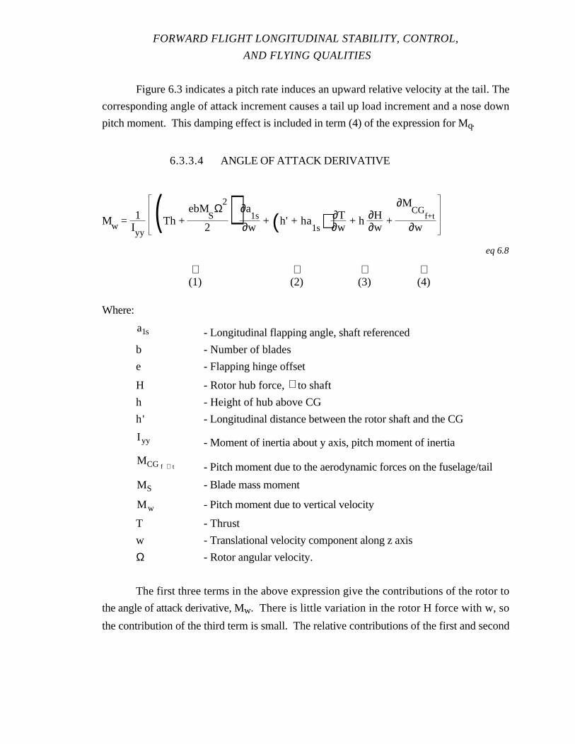
FORWARD FLIGHT LONGITUDINAL STABILITY, CONTROL,
AND FLYING QUALITIES
Figure 6.3 indicates a pitch rate induces an upward relative velocity at the tail. The
corresponding angle of attack increment causes a tail up load increment and a nose down
pitch moment. This damping effect is included in term (4) of the expression for Mq.
6.3.3.4 ANGLE OF ATTACK DERIVATIVE
Mw = 1Iyy
(Th + ebM
SΩ
2
2) ∂a
1s∂w
+ (h' + ha1s) ∂T
∂w + h ∂H
∂w +
∂MCG
f+t
∂w
eq 6.8
⇑ ⇑ ⇑ ⇑(1) (2) (3) (4)
Where:
a1s - Longitudinal flapping angle, shaft referenced
b - Number of blades
e - Flapping hinge offset
H - Rotor hub force, ⊥ to shaft
h - Height of hub above CG
h' - Longitudinal distance between the rotor shaft and the CG
I yy - Moment of inertia about y axis, pitch moment of inertia
MCG f + t - Pitch moment due to the aerodynamic forces on the fuselage/tail
MS - Blade mass moment
M w - Pitch moment due to vertical velocity
T - Thrust
w - Translational velocity component along z axis
Ω - Rotor angular velocity.
The first three terms in the above expression give the contributions of the rotor to
the angle of attack derivative, Mw. There is little variation in the rotor H force with w, so
the contribution of the third term is small. The relative contributions of the first and second
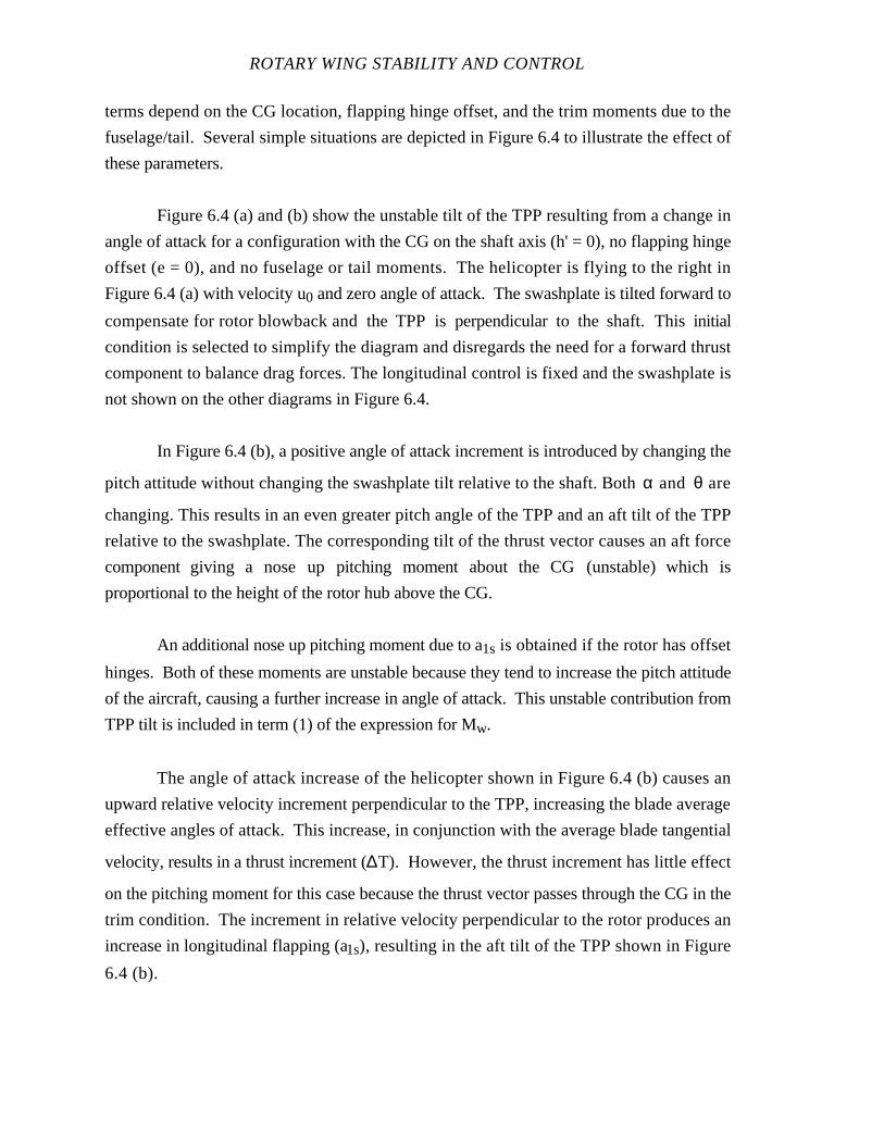
ROTARY WING STABILITY AND CONTROL
terms depend on the CG location, flapping hinge offset, and the trim moments due to the
fuselage/tail. Several simple situations are depicted in Figure 6.4 to illustrate the effect of
these parameters.
Figure 6.4 (a) and (b) show the unstable tilt of the TPP resulting from a change in
angle of attack for a configuration with the CG on the shaft axis (h' = 0), no flapping hinge
offset (e = 0), and no fuselage or tail moments. The helicopter is flying to the right in
Figure 6.4 (a) with velocity u0 and zero angle of attack. The swashplate is tilted forward to
compensate for rotor blowback and the TPP is perpendicular tothe shaft. This initial
condition is selected to simplify the diagram and disregards the need for a forward thrust
component to balance drag forces. The longitudinal control is fixed and the swashplate is
not shown on the other diagrams in Figure 6.4.
In Figure 6.4 (b), a positive angle of attack increment is introduced by changing the
pitch attitude without changing the swashplate tilt relative to the shaft. Both α and θ are
changing. This results in an even greater pitch angle of the TPP and an aft tilt of the TPP
relative to the swashplate. The corresponding tilt of the thrust vector causes an aft force
component giving a nose up pitching moment about the CG (unstable) which is
proportional to the height of the rotor hub above the CG.
An additional nose up pitching moment due to a1s is obtained if the rotor has offset
hinges. Both of these moments are unstable because they tend to increase the pitch attitude
of the aircraft, causing a further increase in angle of attack. This unstable contribution from
TPP tilt is included in term (1) of the expression for Mw.
The angle of attack increase of the helicopter shown in Figure 6.4 (b) causes an
upward relative velocity increment perpendicular to the TPP, increasing the blade average
effective angles of attack. This increase, in conjunction with the average blade tangential
velocity, results in a thrust increment (∆T). However, the thrust increment has little effect
on the pitching moment for this case because the thrust vector passes through the CG in the
trim condition. The increment in relative velocity perpendicular to the rotor produces an
increase in longitudinal flapping (a1s), resulting in the aft tilt of the TPP shown in Figure
6.4 (b).
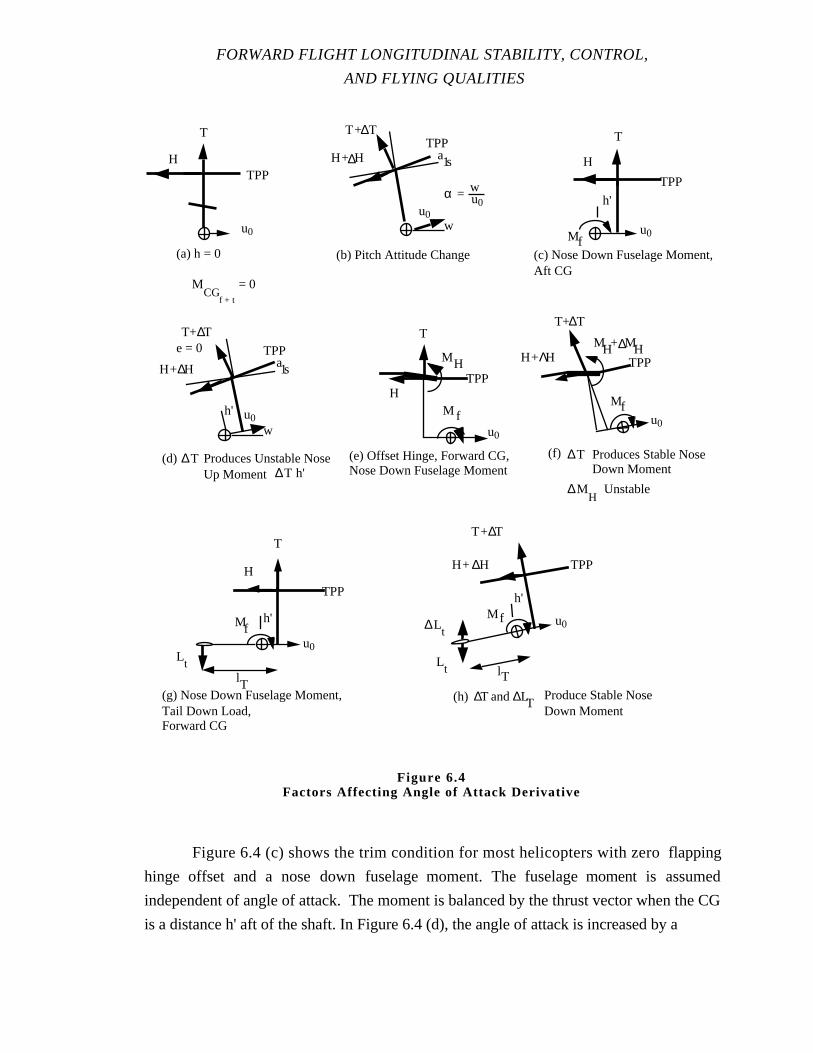
FORWARD FLIGHT LONGITUDINAL STABILITY, CONTROL,
AND FLYING QUALITIES
Figure 6.4 (c) shows the trim condition for most helicopters with zero flapping
hinge offset and a nose down fuselage moment. The fuselage moment is assumed
independent of angle of attack. The moment is balanced by the thrust vector when the CG
is a distance h' aft of the shaft. In Figure 6.4 (d), the angle of attack is increased by a
(a) h = 0
e = 0
TPP
T
H
u0
MCG
= 0f + t
(b) Pitch Attitude Change
TPPa1s
w
α = w
T+∆T
H+∆H
u0
u0
(c) Nose Down Fuselage Moment,Aft CG
TPP
H
h'
Mfu0
T
(e) Offset Hinge, Forward CG,Nose Down Fuselage Moment
TPP
T
HM f
MH
u0
TPP
Mf
MH+∆MH
T+∆T
(f) ∆T Produces Stable NoseDown Moment
∆MH
Unstable
H+ΛH
u0
TPPa1s
T+∆T
H+∆H
w
h'
(d) ∆T Produces Unstable NoseUp Moment ∆T h'
u0
(g) Nose Down Fuselage Moment,Tail Down Load,Forward CG
TPP
T
H
h'Mf
lT
Lt
u0
TPP
h'M f
lT
(h) Produce Stable NoseDown Moment
∆LT∆T and
H+ ∆H
T+∆T
Lt
∆Lt
u0
Figure 6.4Factors Affecting Angle of Attack Derivative
ROTARY WING STABILITY AND CONTROL
change in aircraft pitch attitude. The destabilizing pitching moment due to TPP tilt (Figure
6.4 (b)) is also present in this case. The thrust increment (∆T) due to the angle of attack
change acting at a moment arm (h') gives an additional unstable nose up moment about the
CG included by term (2) in the expression for Mw.
Figure 6.4 (e) shows the trim condition for a configuration with offset flapping
hinges and the same nose down fuselage moment in Figure 6.4 (c). In this case,
equilibrium is obtained with a forward CG location and the line of action of the thrust
vector passing aft of the CG. Figure 6.4 (f) shows this configuration with an increased
angle of attack. The thrust increment now produces a nose down or stabilizing pitching
moment about the CG. This effect, included in term (2) of the equation for Mw, makes a
stabilizing contribution to the angle of attack derivative.
Figure 6.4 (g) shows the initial trim condition with the fuselage moment balanced
by a horizontal tail down load. Figure 6.4 (h) shows this configuration with an increased
pitch attitude. The increase in the angle of attack of the tail gives a tail up load and a nose
down stabilizing pitch moment. Term (4) in the expression for Mw is negative or
stabilizing for this configuration.
6.3.4 Trim Characteristics
6.3.4.1 GENERAL
Longitudinal control position changes are required normally to achieve changes in
rate of climb, descent, and forward airspeed. There are additional requirements for
longitudinal trim changes during operations from in and out of ground effect. Investigation
of trim changes is an important element of the helicopter's overall flying qualities
evaluation. Trim changes refer to flight conditions where power is adjusted to obtain the
desired flight path. The power adjustment is the element which makes trimmed control
positions significantly different from the static longitudinal stability.
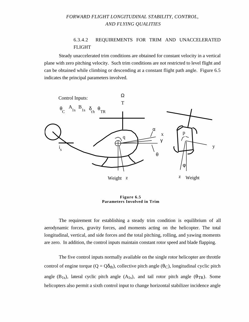
FORWARD FLIGHT LONGITUDINAL STABILITY, CONTROL,
AND FLYING QUALITIES
6.3.4.2 REQUIREMENTS FOR TRIM AND UNACCELERATED
FLIGHT
Steady unaccelerated trim conditions are obtained for constant velocity in a vertical
plane with zero pitching velocity. Such trim conditions are not restricted to level flight and
can be obtained while climbing or descending at a constant flight path angle. Figure 6.5
indicates the principal parameters involved.
The requirement for establishing a steady trim condition is equilibrium of all
aerodynamic forces, gravity forces, and moments acting on the helicopter. The total
longitudinal, vertical, and side forces and the total pitching, rolling, and yawing moments
are zero. In addition, the control inputs maintain constant rotor speed and blade flapping.
The five control inputs normally available on the single rotor helicopter are throttle
control of engine torque (Q = Qδth), collective pitch angle (θC), longitudinal cyclic pitch
angle (B1s), lateral cyclic pitch angle (A1s), and tail rotor pitch angle (θTR). Some
helicopters also permit a sixth control input to change horizontal stabilizer incidence angle
z
x
Weight
q
T
is
α
θ
Ω
γ
z
y
Weight
φ
p
θTR
θC
A1s
B1s δ
th
Control Inputs:
Figure 6.5Parameters Involved in Trim
ROTARY WING STABILITY AND CONTROL
(is). These controls may not be independent. In many helicopters, linkage between the
collective pitch and throttle controls are incorporated. In some helicopters, the stabilizer
incidence is linked to the cyclic or collective pitch controls.
The aerodynamic forces and moments acting on the helicopter in steady flight
conditions are determined by the six control input variables in conjunction with the rotor
speed, the aircraft velocity components (u, v, w), and the aircraft angular velocity
components (p, q, r). Although the forces and moments depend on the rotor downwash,
longitudinal flapping, and lateral flapping; these variables are not considered in the present
discussion of trim because they are determined by the control and flight path variables
during steady flight conditions. Furthermore, the rotor response parameters are not
ordinarily measured or monitored by the pilot. Pitch angle (θ) and roll angle (φ), shown on
Figure 6.5 define the direction of the gravity force with respect to aircraft axes. The flight
path angle (γ) is shown since it is an important variable in both maneuvering and non-
maneuvering tasks. Thus, a total of 16 variables are involved in trimming the helicopter:
Ω, V, α, β, p, q, r, θ, φ, γ, Q(δth), θC, B1s, A1s, θTR, and is. Establishing a steady
flight condition requires satisfying three conditions for equilibrium of force components,
three conditions for equilibrium of moment components, and a condition for equilibrium of
torque acting on the rotor. The kinematics of the situation provides an eighth condition
relating the vertical velocity (or flight path angle), the aircraft attitude, and angle of attack.
The 16 variables and eight general conditions involved, require the pilot to select eight
independent variables to establish a steady flight condition. The need for specific values
for some of the variables is obvious and generally they are selected intuitively. The
following discussion provides examples of the complete selection of the eight independent
variables to emphasize the constraints which exist in trimming the aircraft.
When steady rectilinear flight is required, the three angular velocities are zero. The
five remaining independent variables could be control positions. However, a stabilized
flight condition is not reached with arbitrarily selected control inputs unless the aircraft is
statically and dynamically stable and not performance limited. Some of these five
independent variables need not be control inputs and could be flight parameters. In this
case, the pilot manipulates the controls as dependent variables to obtain the desired flight
parameters.
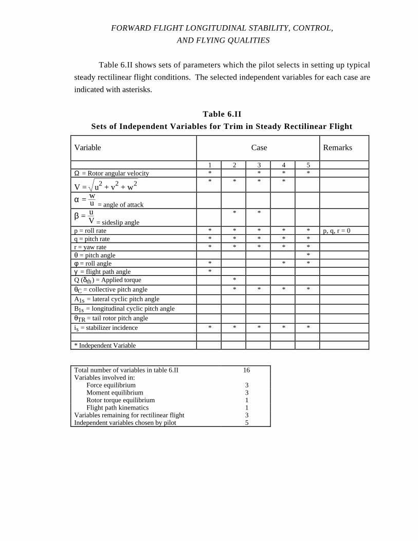
FORWARD FLIGHT LONGITUDINAL STABILITY, CONTROL,
AND FLYING QUALITIES
Table 6.II shows sets of parameters which the pilot selects in setting up typical
steady rectilinear flight conditions. The selected independent variables for each case are
indicated with asterisks.
Table 6.II
Sets of Independent Variables for Trim in Steady Rectilinear Flight
Variable Case Remarks
1 2 3 4 5Ω = Rotor angular velocity * * * *
V = u2 + v2 + w2 * * * *
α = wu = angle of attack
β = uV = sideslip angle
* *
p = roll rate * * * * * p, q, r = 0q = pitch rate * * * * *r = yaw rate * * * * *θ = pitch angle *φ = roll angle * * *γ = flight path angle *Q (δth) = Applied torque *
θC = collective pitch angle * * * *
A1s = lateral cyclic pitch angle
B1s = longitudinal cyclic pitch angle
θTR = tail rotor pitch angle
is = stabilizer incidence * * * * *
* Independent Variable
Total number of variables in table 6.II 16Variables involved in:
Force equilibrium 3Moment equilibrium 3Rotor torque equilibrium 1Flight path kinematics 1
Variables remaining for rectilinear flight 3Independent variables chosen by pilot 5
ROTARY WING STABILITY AND CONTROL
Table 6.II, Case 1 is the typical forward flight trim condition encountered in routine
non-maneuvering tasks. Independent variables for this case include rotor speed, flight
velocity, flight path angle, and roll angle. The fifth arbitrarily selected variable is stabilizer
incidence which is assumed to be constant as with a fixed stabilizer.
All other control variables for Case 1 are dependent variables. The pilot cannot
choose them arbitrarily but manipulates the controls until he finds the proper input values
for Q(δth), θC, A1s, B1s, and θTR to attain the desired velocity, climb angle, and roll
angle. If the helicopter incorporates a rotor speed governor, the pilot is relieved of using
the throttle to control rotor speed. The pilot accepts whatever values are obtained for the
remaining dependent flight parameters. For example, when the stabilizer angle is fixed, the
pilot cannot independently control the pitch angle. Also when the pilot chooses to fly with
zero roll angle, he may be forced to fly with a nonzero sideslip angle. If instead he chose
to fly with zero sideslip, he may have to fly with some bank angle.
Table 6.II, Case 2 corresponds to a test procedure used to obtain control position
versus airspeed gradients to investigate static stability. Collective pitch and throttle are held
constant at the initial trim positions. The pilot determines the longitudinal cyclic pitch angle
required to stabilize at a new rectilinear flight condition differing from the original by a
small speed increment. The speed increment is an arbitrarily selected independent variable
for this test and longitudinal cyclic is a dependent variable. Pitch angle and flight path
angle are dependent variables.
The complete definition of the longitudinal control position versus airspeed gradient
test requires defining the lateral-directional control manipulations. In Case 2, sideslip angle
is an independent variable, and lateral cyclic pitch angle and tail rotor pitch angle are
dependent variables adjusted to obtain the desired sideslip.
Table 6.II, Case 3 corresponds to another test procedure which might be used in
obtaining longitudinal control position versus airspeed gradients. In this case, rotor speed
is an independent constant variable. This is accomplished by controlling the dependent
variable, torque, via throttle adjustments. Comparatively small changes in rotor speed are
obtained in tests corresponding to Case 2 and only small differences in results are expected
using Case 2 or Case 3 techniques.
FORWARD FLIGHT LONGITUDINAL STABILITY, CONTROL,
AND FLYING QUALITIES
An alternative trim technique used in static stability tests is indicated by Case 4.
This case differs from Case 3 because roll angle is treated as an independent variable rather
than sideslip. Thus, Case 4 tests are flown with zero roll angle but with some sideslip.
Case 5 presents a technique commonly used for static longitudinal stability tests.
Case 5 differs from Case 4 because pitch attitude is an independent variable which the pilot
controls, and airspeed is a resulting dependent variable which the pilot accepts.
Although the collective pitch is constant for longitudinal control position gradients,
both collective pitch and longitudinal cyclic are used to change trim conditions during non-
maneuvering tasks. The Case 1 technique is applicable for changing trim speed in level
flight while maintaining constant rotor speed. The primary control inputs are changes in
longitudinal cyclic and collective pitch. However, small adjustments in throttle and lateral-
directional controls might be required to hold the rotor speed and roll angle constant.
6.3.4.3 POWER EFFECTS
Power effects can produce three trim problems: reduction of control margin;
nonlinear trim requirements; and excessive control displacement during normal
maneuvering. All three of these problems are depicted in Figure 6.6.
Figure 6.6 indicates less than 3% control margin is available in a descent. There are
two discontinuities in the high power portion of the curve. Almost 90% of the available
longitudinal control envelope is required during the transition from autorotation to a full
power climb.
6.3.4.4 AIRSPEED POSITION ERRORS
The example in Figure 6.6 represents a constant indicated airspeed situation.
Indicated airspeed is used because the pilot flies the helicopter by reference to indicated
airspeed. Some of the undesirable aspects of the curve may be the direct result of airspeed
position error with power. This fact does not excuse the characteristic, the pilot cannot be
concerned with position errors during operational flight conditions.
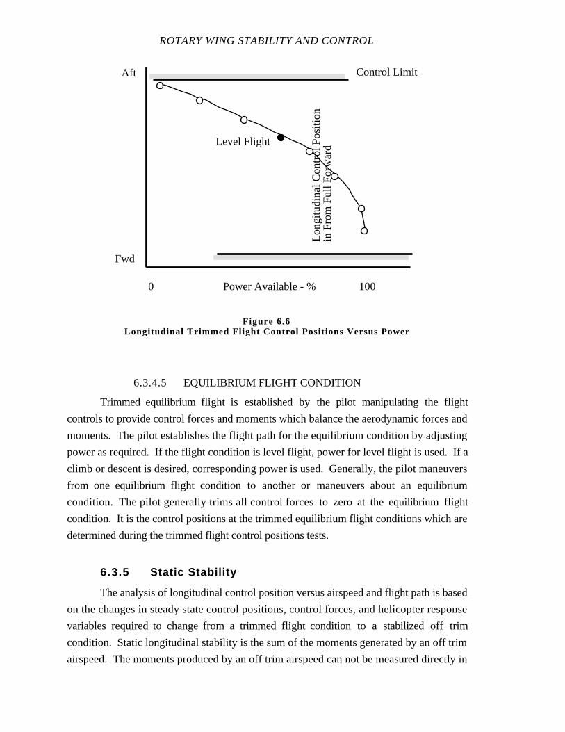
ROTARY WING STABILITY AND CONTROL
Longitudinal Trimmed Flight Control Positions Versu s Power
6.3.4.5 EQUILIBRIUM FLIGHT CONDITION
Trimmed equilibrium flight is established by the pilot manipulating theflight
controls to provide control forces and moments which balance the aerodynamic forces and
moments. The pilot establishes the flight path for the equilibrium condition by adjusting
power as required. If the flight condition is level flight, power for level flight is used. If a
climb or descent is desired, corresponding power is used. Generally, the pilot maneuvers
from one equilibrium flight condition to another or maneuvers about an equilibrium
condition. The pilot generally trims all control forces to zero at the equilibrium flight
condition. It is the control positions at the trimmed equilibrium flight conditions which are
determined during the trimmed flight control positions tests.
6.3.5 Static Stability
The analysis of longitudinal control position versus airspeed and flight path is based
on the changes in steady state control positions, control forces, and helicopter response
variables required to change from a trimmed flight condition to a stabilized off trim
condition. Static longitudinal stability is the sum of the moments generated by an off trim
airspeed. The moments produced by an off trim airspeed can not be measured directly in
Aft
Fwd
Long
itudi
nal C
ontr
ol P
ositi
onin
Fro
m F
ull F
orw
ard
Power Available - %0 100
Control Limit
Level Flight
Figure 6.6
FORWARD FLIGHT LONGITUDINAL STABILITY, CONTROL,
AND FLYING QUALITIES
flight. The helicopter can be maneuvered into an off trim equilibrium flight condition by
providing an opposing moment generated by longitudinal control displacement. The
moment produced by the longitudinal control displacement can not be measured directly in
flight. The longitudinal control displacement from trim can be measured. Therefore, static
stability is indicated by the gradient of longitudinal control position versus airspeed.
A large number of variables are required to define trim for a helicopter without
explicitly including variables describing blade motions. The variables controlled by the
pilot are independent and the remaining variables are dependent. The independent variables
for each case of Table 6.II should be kept in mind when specifying flight test procedures to
insure repeatable results. However, several simplifying assumptions are made to reduce
the number of variables considered in this section.
Rotor speed (Ω), for helicopters in powered flight with rotor speed governors, is
assumed constant. Consequently, it is unnecessary to include throttle position or applied
rotor torque as variables. The tail incidence angle (is) is assumed fixed. Finally, any
coupling of longitudinal with lateral-directional forces and moments and/or control inputs
are not considered. After making the above assumptions, the remaining variables from
table 6.II are: V= u2+w2 , α = w/u, θ, θC, B1s, and γ.
Tests for static stability are initiated from trimmed conditions in level, climbing or
descending flight. All perturbation variables (∆u, ∆w, and ∆θ) are zero at the original
rectilinear trimmed flight condition. The pilot can disturb the aircraft from trim by
longitudinal control input. Following the control input, a statically and dynamically stable
aircraft undergoes a transient response and stabilizes at a new steady rectilinear flight
condition with longitudinal speed increment, angle of attack increment, and pitch angle
increment. If the aircraft is unstable, the pilot may establish a new momentary equilibrium
condition to obtain flight test data by manipulating the controls until the time rate of changes
of the perturbation variables are zero.
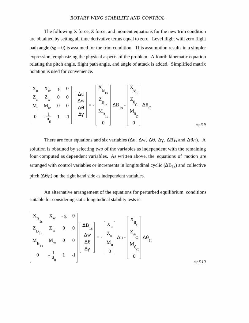
ROTARY WING STABILITY AND CONTROL
The following X force, Z force, and moment equations for the new trim condition
are obtained by setting all time derivative terms equal to zero. Level flight with zero flight
path angle (γ0 = 0) is assumed for the trim condition. This assumption results in a simpler
expression, emphasizing the physical aspects of the problem. A fourth kinematic equation
relating the pitch angle, flight path angle, and angle of attack is added. Simplified matrix
notation is used for convenience.
Xu Xw -g 0
Zu Zw 0 0
Mu Mw 0 0
0 - 1u
01 -1
∆u∆w
∆θ∆γ
= -
XB
1s
ZB
1s
MB
1s
0
∆B1s
-
XθC
ZθC
MθC
0
∆θC
eq 6.9
There are four equations and six variables (∆u, ∆w, ∆θ, ∆γ, ∆B1s and ∆θC). A
solution is obtained by selecting two of the variables as independent with the remaining
four computed as dependent variables. As written above, the equations of motion are
arranged with control variables or increments in longitudinal cyclic (∆B1s) and collective
pitch (∆θC) on the right hand side as independent variables.
An alternative arrangement of the equations for perturbed equilibrium conditions
suitable for considering static longitudinal stability tests is:
XB
1s
Xw - g 0
ZB
1s
Zw 0 0
MB
1s
Mw 0 0
0 - 1u
01 -1
∆B1s
∆w
∆θ∆γ
= -
Xu
Zu
Mu
0
∆u -
XθC
ZθC
MθC
0
∆θC
eq 6.10

FORWARD FLIGHT LONGITUDINAL STABILITY, CONTROL,
AND FLYING QUALITIES
Where:
B1s - Longitudinal cyclic pitch angle, shaft referenced
g - Gravity
γ - Flight path angle
M B1s- Pitch moment due to longitudinal cyclic pitch angle
MθC- Pitch moment due to collective pitch angle
M u - Pitch moment due to longitudinal velocity
M w - Pitch moment due to vertical velocity
θ - Pitch angle
θC - Collective pitch angle
u - Translational velocity component along x axis
u0 - Initial velocity
w - Translational velocity component along z axis
X B1s- Longitudinal force due to longitudinal cyclic pitch angle
Xθ C- Longitudinal force due to collective pitch angle
X u - Longitudinal force due to longitudinal velocity
X w - Longitudinal force due to vertical velocity
ZB1s- Vertical force due to longitudinal cyclic pitch angle
ZθC- Vertical force due to collective pitch angle
Z u - Vertical force due to longitudinal velocity
Zw - Vertical force due to vertical velocity.
In evaluating static stability through the longitudinal control position versus
airspeed gradient, the speed increment (∆u) and collective pitch increment (∆θC) are the
independent variables. The test technique requires collective pitch fixed at the original trim
value so there is no increment in collective (∆θC = 0). The longitudinal cyclic input is a
dependent variable with the value of∆B1s sufficient to stabilize at the desired speed
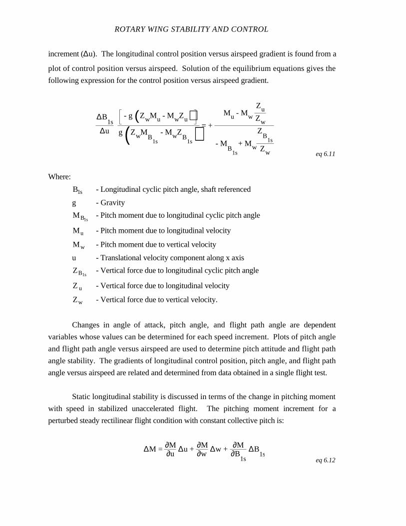
ROTARY WING STABILITY AND CONTROL
increment (∆u). The longitudinal control position versus airspeed gradient is found from a
plot of control position versus airspeed. Solution of the equilibrium equations gives the
following expression for the control position versus airspeed gradient.
∆B1s
∆u
- g (ZwMu - MwZu)g(ZwM
B1s
- MwZB
1s) = +
Mu - Mw
Zu
Zw
- MB
1s
+ Mw
ZB
1s
Zw eq 6.11
Where:
B1s - Longitudinal cyclic pitch angle, shaft referenced
g - Gravity
M B1s- Pitch moment due to longitudinal cyclic pitch angle
M u - Pitch moment due to longitudinal velocity
M w - Pitch moment due to vertical velocity
u - Translational velocity component along x axis
ZB1s- Vertical force due to longitudinal cyclic pitch angle
Z u - Vertical force due to longitudinal velocity
Zw - Vertical force due to vertical velocity.
Changes in angle of attack, pitch angle, and flight path angle are dependent
variables whose values can be determined for each speed increment. Plots of pitch angle
and flight path angle versus airspeed are used to determine pitch attitude and flight path
angle stability. The gradients of longitudinal control position, pitch angle, and flight path
angle versus airspeed are related and determined from data obtained in a single flight test.
Static longitudinal stability is discussed in terms of the change in pitching moment
with speed in stabilized unaccelerated flight. The pitching moment incrementfor a
perturbed steady rectilinear flight condition with constant collective pitch is:
∆M = ∂M∂u
∆u + ∂M∂w
∆w + ∂M∂B
1s
∆B1s
eq 6.12
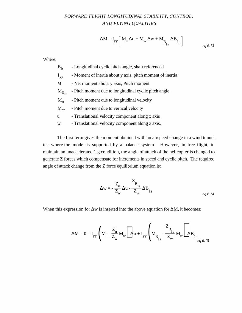
FORWARD FLIGHT LONGITUDINAL STABILITY, CONTROL,
AND FLYING QUALITIES
∆M = Iyy Mu ∆u + Mw ∆w + MB
1s
∆B1s
eq 6.13
Where:
B1s - Longitudinal cyclic pitch angle, shaft referenced
I yy - Moment of inertia about y axis, pitch moment of inertia
M - Net moment about y axis, Pitch moment
M B1s- Pitch moment due to longitudinal cyclic pitch angle
M u - Pitch moment due to longitudinal velocity
M w - Pitch moment due to vertical velocity
u - Translational velocity component along x axis
w - Translational velocity component along z axis.
The first term gives the moment obtained with an airspeed change in a wind tunnel
test where the model is supported by a balance system. However, in free flight, to
maintain an unaccelerated 1 g condition, the angle of attack of the helicopter is changed to
generate Z forces which compensate for increments in speed and cyclic pitch. The required
angle of attack change from the Z force equilibrium equation is:
∆w = - ZuZw
∆u -
ZB
1s
Zw∆B
1seq 6.14
When this expression for ∆w is inserted into the above equation for ∆M, it becomes:
∆M = 0 = Iyy (Mu - ZuZw
Mw) ∆u + Iyy (MB
1s
-
ZB
1s
Zw Mw) ∆B
1seq 6.15
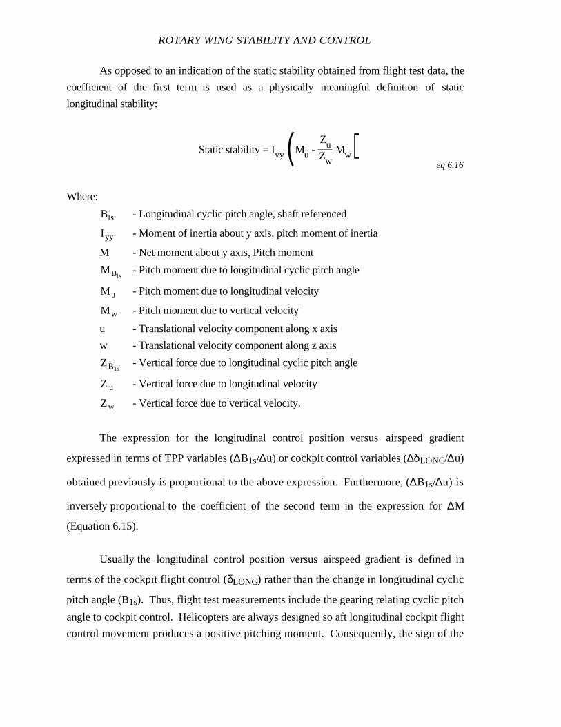
ROTARY WING STABILITY AND CONTROL
As opposed to an indication of the static stability obtained from flight test data, the
coefficient of the first term is used as a physically meaningful definition of static
longitudinal stability:
Static stability = Iyy (Mu - ZuZw
Mw)eq 6.16
Where:
B1s - Longitudinal cyclic pitch angle, shaft referenced
I yy - Moment of inertia about y axis, pitch moment of inertia
M - Net moment about y axis, Pitch moment
M B1s- Pitch moment due to longitudinal cyclic pitch angle
M u - Pitch moment due to longitudinal velocity
M w - Pitch moment due to vertical velocity
u - Translational velocity component along x axis
w - Translational velocity component along z axis
ZB1s- Vertical force due to longitudinal cyclic pitch angle
Z u - Vertical force due to longitudinal velocity
Zw - Vertical force due to vertical velocity.
The expression for the longitudinal control position versus airspeed gradient
expressed in terms of TPP variables (∆B1s/∆u) or cockpit control variables (∆δLONG/∆u)
obtained previously is proportional to the above expression. Furthermore, (∆B1s/∆u) is
inversely proportional to the coefficient of the second term in the expression for∆M
(Equation 6.15).
Usually the longitudinal control position versus airspeed gradient is defined in
terms of the cockpit flight control (δLONG) rather than the change in longitudinal cyclic
pitch angle (B1s). Thus, flight test measurements include the gearing relating cyclic pitch
angle to cockpit control. Helicopters are always designed so aft longitudinal cockpit flight
control movement produces a positive pitching moment. Consequently, the sign of the
FORWARD FLIGHT LONGITUDINAL STABILITY, CONTROL,
AND FLYING QUALITIES
longitudinal control position versus airspeed gradient is a reliable indication of the
helicopter’s static stability. However, the magnitude of the gradient does not show the
degree of static stability because control effectiveness and gearing are included.
6.3.5.1 STATIC STABILITY AS INDICATED BY CONTROL
POSITION VERSUS AIRSPEED
When a statically stable helicopter is given a speed increment above the trim speed,
it has an initial tendency for nose up pitching motion which tilts the thrust vector aft and
slows the helicopter. Static instability leads to an aperiodic divergent response.
Control position versus airspeed curves are referred to a particular trim airspeed.
Therefore, the first step in performing a static stability evaluation is to establish a steady
trimmed condition. Tests are conducted in wings level, steady heading, ball centered,
collective fixed, unaccelerated flight. Any changes in power and rotor speed depend on the
rotor speed governor. Ordinarily, these quantities are nearly constant in static stability
tests.
The longitudinal control position data are recorded at the initial trim position and at
incremental speeds above and below the trim speed. Data are taken at stabilized,
equilibrium conditions. The pilot makes a small forward longitudinal cyclic control input to
increase airspeed. The pilot observes the resulting decrease in pitch angle. If the helicopter
has positive static stability, the helicopter will start to pitch up, returning toward the trim
airspeed. The pilot makes additional longitudinal control inputs to maintain a fixed pitch
attitude, allowing airspeed to stabilize at the increased value. If the helicopter has negative
static stability, the pitch attitude will continue to decrease. The pilot uses aft longitudinal
control to maintain the pitch attitude, allowing airspeed to stabilize. The pilot achieves the
change in airspeed by flying a fixed pitch attitude, allowing airspeed to stabilize.
Vertical motion or angle of attack have little effect on small speed changes near zero
airspeed or hovering flight since the coupling derivatives are small or zero. A more
complicated situation exists when the initial trim is in forward flight. Then the Z forces due
to speed change (Zu) and control inputs (ZB1s) are no longer zero. They must be balanced
ROTARY WING STABILITY AND CONTROL
by forces due to angle of attack changes (Zw) to maintain one g flight. Pitching moments
result from changes in angle of attack (Mw) and affect the control displacement versus
airspeed variation of the helicopter.
Figure 6.7 depicts longitudinal control position and horizontal stabilizer load for
several configurations having different static stability characteristics.
Forward longitudinal control displacement is required to stabilize at a higher
airspeed for a helicopter with positive static stability (Figure 6.7 (a)). The nose down
pitching moment due to forward longitudinal control displacement balances thespeed
stability of the rotor due to blowback.
Figure 6.7 (b) differs from Figure 6.7 (a) because the negative tail incidence results
in a down load at the initial trim condition. The speed increment causes an increase in the
down load and a corresponding nose up pitching moment. Thus, the longitudinal control is
moved further forward for equilibrium.
Figure 6.7 (c) has positive tail incidence and tail up load. This up load becomes
larger with increasing speed causing a nose down pitching moment which is exactly equal
in magnitude to the nose up pitch moment due to the rotor. Consequently, Figure 6.7 (c)
depicts a neutrally stable configuration where equilibrium is maintained with a 10 kn speed
increment without changing longitudinal control position.
Figure 6.7 (d) depicts a configuration with greater positive tail incidence. The
larger tail up load with increased speed produces a larger nose down moment than the
stable nose up moment contributed by the rotor. The pilot uses aft longitudinal control
displacement to achieve equilibrium at the higher speed, indicating negative static stability.
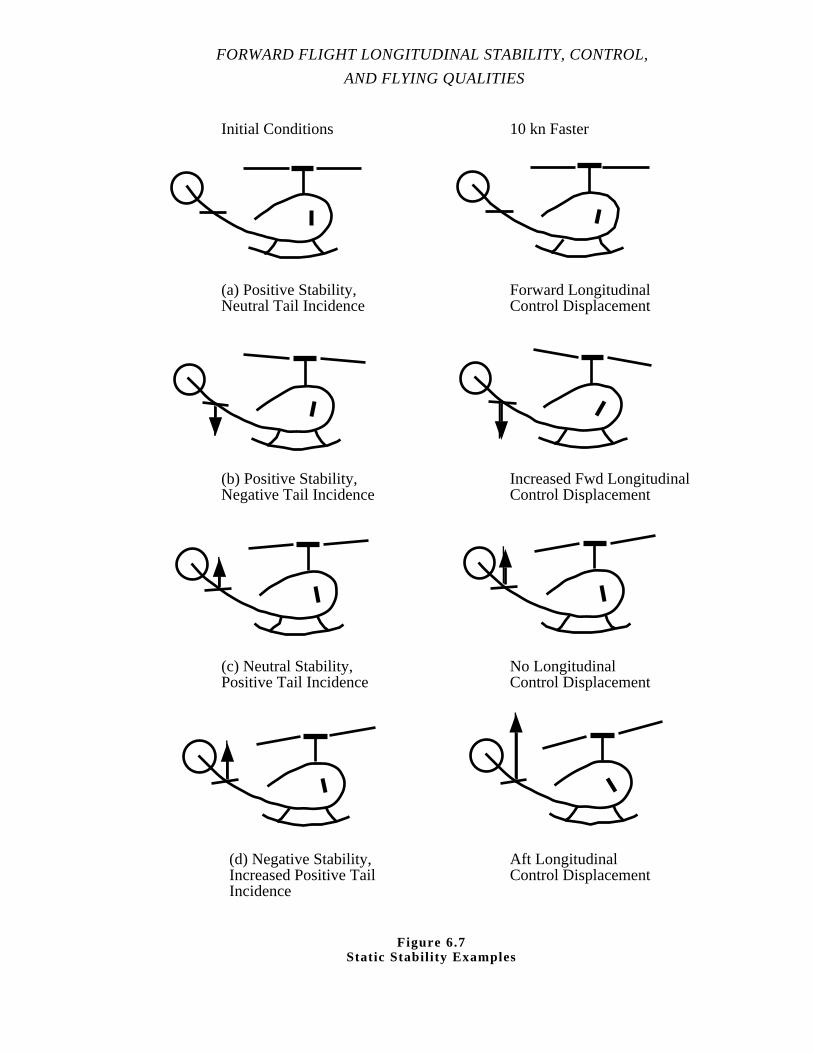
FORWARD FLIGHT LONGITUDINAL STABILITY, CONTROL,
AND FLYING QUALITIES
Initial Conditions 10 kn Faster
(a) Positive Stability,Neutral Tail Incidence
(b) Positive Stability,Negative Tail Incidence
(c) Neutral Stability,Positive Tail Incidence
(d) Negative Stability,Increased Positive TailIncidence
Forward LongitudinalControl Displacement
Increased Fwd LongitudinalControl Displacement
No LongitudinalControl Displacement
Aft LongitudinalControl Displacement
Figure 6.7Static Stabil i ty Examples
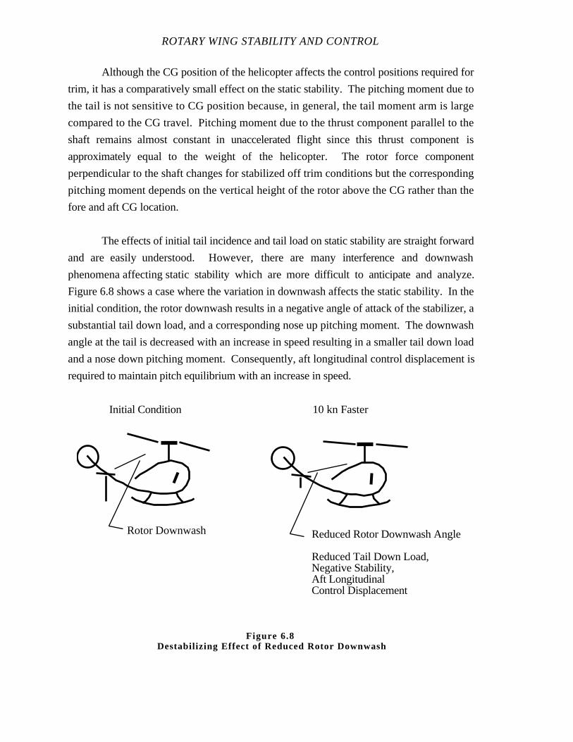
ROTARY WING STABILITY AND CONTROL
Although the CG position of the helicopter affects the control positions required for
trim, it has a comparatively small effect on the static stability. The pitching moment due to
the tail is not sensitive to CG position because, in general, the tail moment arm is large
compared to the CG travel. Pitching moment due to the thrust component parallel to the
shaft remains almost constant in unaccelerated flight since this thrust component is
approximately equal to the weight of the helicopter. The rotor force component
perpendicular to the shaft changes for stabilized off trim conditions but the corresponding
pitching moment depends on the vertical height of the rotor above the CG rather than the
fore and aft CG location.
The effects of initial tail incidence and tail load on static stability are straight forward
and are easily understood. However, there are many interference and downwash
phenomena affecting static stability which are more difficult to anticipate and analyze.
Figure 6.8 shows a case where the variation in downwash affects the static stability. In the
initial condition, the rotor downwash results in a negative angle of attack of the stabilizer, a
substantial tail down load, and a corresponding nose up pitching moment. The downwash
angle at the tail is decreased with an increase in speed resulting in a smaller tail down load
and a nose down pitching moment. Consequently, aft longitudinal control displacement is
required to maintain pitch equilibrium with an increase in speed.
Initial Condition 10 kn Faster
Rotor Downwash Reduced Rotor Downwash Angle
Reduced Tail Down Load,Negative Stability,Aft LongitudinalControl Displacement
Figure 6.8 Destabilizing Effect of Reduced Rotor Downwash
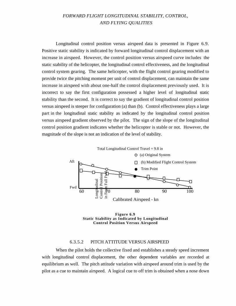
FORWARD FLIGHT LONGITUDINAL STABILITY, CONTROL,
AND FLYING QUALITIES
Longitudinal control position versus airspeed data is presented in Figure 6.9.
Positive static stability is indicated by forward longitudinal control displacement with an
increase in airspeed. However, the control position versus airspeed curve includes the
static stability of the helicopter, the longitudinal control effectiveness, and the longitudinal
control system gearing. The same helicopter, with the flight control gearing modified to
provide twice the pitching moment per unit of control displacement, can maintain the same
increase in airspeed with about one-half the control displacement previously used. It is
incorrect to say the first configuration possessed a higher level of longitudinal static
stability than the second. It is correct to say the gradient of longitudinal control position
versus airspeed is steeper for configuration (a) than (b). Control effectiveness plays a large
part in the longitudinal static stability as indicated by thelongitudinal control position
versus airspeed gradient observed by the pilot. The sign of the slope of the longitudinal
control position gradient indicates whether the helicopter is stable or not. However, the
magnitude of the slope is not an indication of the level of stability.
6.3.5.2 PITCH ATTITUDE VERSUS AIRSPEED
When the pilot holds the collective fixed and establishes a steady speed increment
with longitudinal control displacement, the other dependent variables are recorded at
equilibrium as well. The pitch attitude variation with airspeed around trim is used by the
pilot as a cue to maintain airspeed. A logical cue to off trim is obtained when a nose down
Calibrated Airspeed - kn
80 90 1007060
Aft
Fwd
Total Longitudinal Control Travel = 9.8 in
Trim Point
(a) Original System
(b) Modified Flight Control System
Long
itudi
nal
Con
trol
Pos
ition
in F
rom
Ful
l Fw
d
Figure 6.9Static Stability as Indicated by Longitudinal
Control Position Versus Airspeed
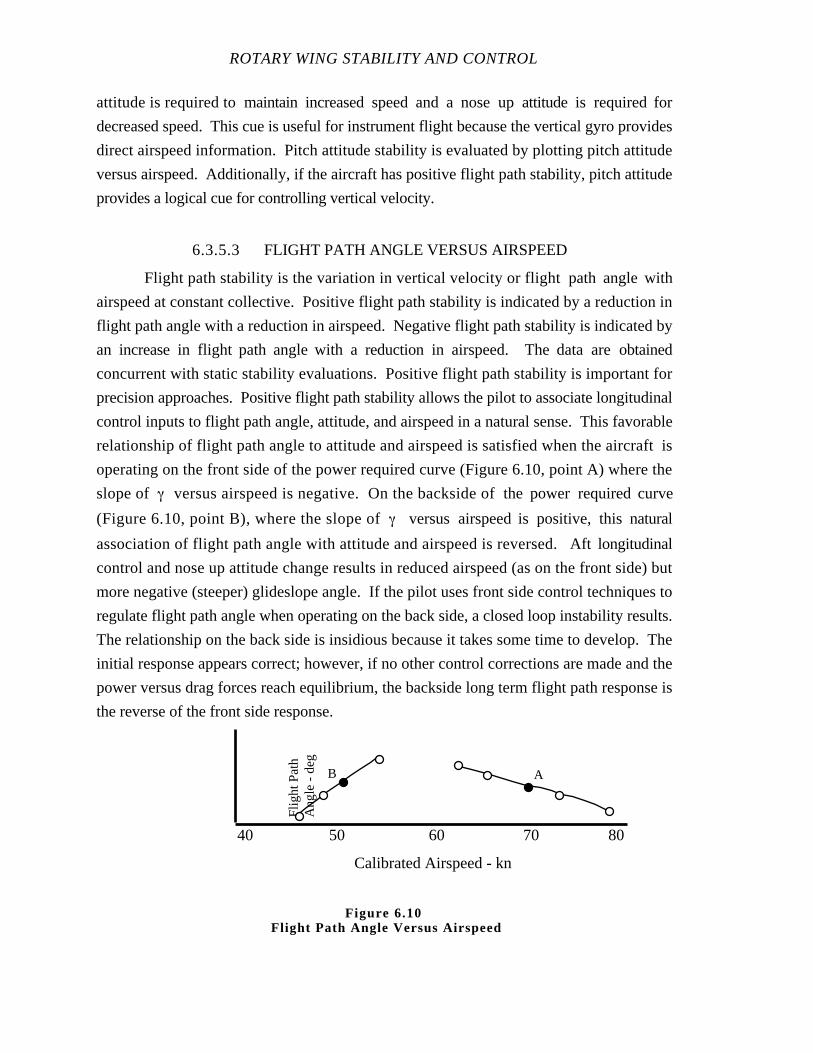
ROTARY WING STABILITY AND CONTROL
attitude is required to maintain increased speed and a nose up attitude is required for
decreased speed. This cue is useful for instrument flight because the vertical gyro provides
direct airspeed information. Pitch attitude stability is evaluated by plotting pitch attitude
versus airspeed. Additionally, if the aircraft has positive flight path stability, pitch attitude
provides a logical cue for controlling vertical velocity.
6.3.5.3 FLIGHT PATH ANGLE VERSUS AIRSPEED
Flight path stability is the variation in vertical velocity or flight path angle with
airspeed at constant collective. Positive flight path stability is indicated by a reduction in
flight path angle with a reduction in airspeed. Negative flight path stability is indicated by
an increase in flight path angle with a reduction in airspeed. The data are obtained
concurrent with static stability evaluations. Positive flight path stability is important for
precision approaches. Positive flight path stability allows the pilot to associate longitudinal
control inputs to flight path angle, attitude, and airspeed in a natural sense. This favorable
relationship of flight path angle to attitude and airspeed is satisfied when the aircraft is
operating on the front side of the power required curve (Figure 6.10, point A) where the
slope of versus airspeed is negative. On the backside of thepower required curve
(Figure 6.10, point B), where the slope of versus airspeed is positive, this natural
association of flight path angle with attitude and airspeed is reversed. Aft longitudinal
control and nose up attitude change results in reduced airspeed (as on the front side) but
more negative (steeper) glideslope angle. If the pilot uses front side control techniques to
regulate flight path angle when operating on the back side, a closed loop instability results.
The relationship on the back side is insidious because it takes some time to develop. The
initial response appears correct; however, if no other control corrections are made and the
power versus drag forces reach equilibrium, the backside long term flight path response is
the reverse of the front side response.
Calibrated Airspeed - kn
60 70 805040
Flig
ht P
ath
Ang
le -
deg
AB
Figure 6.10 Flight Path Angle Versus Airspeed
FORWARD FLIGHT LONGITUDINAL STABILITY, CONTROL,
AND FLYING QUALITIES
6.3.5.4 STATIC STABILITY AS INDICATED BY CONTROL FORCE
VERSUS AIRSPEED
The static stability of the helicopter is indicated by the longitudinal control position
versus airspeed gradient. This variation of control position versus airspeed provides a cue
to the pilot to off trim airspeed conditions. If the pilot desires to increase his airspeed, he
moves the longitudinal control forward to accelerate. If the helicopter has positive static
stability, he maintains a forward longitudinal control displacement at the increased airspeed.
The control displacement is a cue to the pilot to the off trim airspeed condition. The force
required to maintain the control displacement also provides a cue to the off trim condition.
In a helicopter with an irreversible flight control system incorporating an artificial
trim system, the control force variation with airspeed is determined by the control position
versus airspeed curve and the control force versus displacement characteristics of the
control system. The control force versus airspeed curve is generated by cross plotting the
control position versus airspeed curve with the control force versus displacement curve,
indicated schematically on Figure 6.11 for control systems with various combinations of
control force gradient, breakout force, and friction.
A linear control position versus airspeed curve is assumed for stabilized flight
conditions close to the original trim position. When the cockpit force versus displacement
curve is also linear, a linear force versus airspeed curve is obtained about the original trim.
A negative slope of this force versus airspeed (like a negative slope of the control position
versus airspeed curve) provides an indication of positive static stability to the pilot.
Positive static stability is indicated by increasing push force for increasing airspeed.
The force feel system gradients must harmonize with the control position gradient in
order to obtain good flying qualities. High force gradients are inappropriate for a helicopter
which requires large control deflections to make small airspeed changes. The pilot
generally senses forces on the cyclic control more acutely than displacement and thus
cockpit control forces provide an indication of the control position and a cue to off trim
conditions.

ROTARY WING STABILITY AND CONTROL
Static Stability as Indicated by Control Force Versus Airspeed
Aft
Fwd
Static Stability as Indicatedby Longitudinal Control Position
Versus Airspeed
Calibrated Airspeed - knLo
ngitu
dina
lC
ontr
ol P
ositi
on -
in F
rom
Ful
l Fw
d
Trim Point
Calibrated Airspeed - kn
Pull
Push
Calibrated Airspeed - kn
Pull
Push
Calibrated Airspeed - kn
Pull
Push
Pull
Push
Long
itudi
nal
Con
trol
For
ce -
lb
Longitudinal Control Position -in From Trim
Aft Fwd
Pull
Push
Long
itudi
nal
Con
trol
For
ce -
lb
Longitudinal Control Position -in From Trim
Aft Fwd
Pull
Push
Long
itudi
nal
Con
trol
For
ce -
lb
Longitudinal Control Position -in From Trim
Aft Fwd
Control Force VersusDisplacement
Static Stability as Indicated byLongitudinal Control Force Versus
Airspeed Obtained from Cross Plot ofControl Position Versus Airspeed andControl Force Versus Displacement
Figure 6.11
FORWARD FLIGHT LONGITUDINAL STABILITY, CONTROL,
AND FLYING QUALITIES
Control force versus airspeed gradients can be measured in flight as well as being
obtained by a cross plot. In flight measurements are necessary to obtain accurate results for
helicopters with reversible flight control systems. In this case, the flight dynamic and
control system characteristics are coupled together. Wide variations in control force
gradients are found in different flight conditions and may provide inconsistent cues to the
pilot.
6.3.6 Maneuvering Stability
Maneuvering stability is the sum of the forces and moments acting on the helicopter
due to a disturbance in normal acceleration. As in static stability, the forces and moments
acting on the helicopter due to a disturbance can not be measured directly in flight. The
forces and moments due to a disturbance in load factor are balanced by longitudinal control
forces and moments. The longitudinal control displacement from trim is a measure of the
maneuvering stability. A helicopter with positive maneuvering stability tends to return to
one g flight following a disturbance. Positive maneuvering stability is indicated by aft
longitudinal control displacement from trim for increasing g. A helicopter with negative
maneuvering stability tends to depart in g when disturbed. Negative maneuvering stability
is indicated by forward longitudinal control displacement from trim with increasing g.
6.3.6.1 SYMMETRICAL PULL UP/PUSH OVER
The linearized form of the longitudinal equations of motion used in discussing static
stability are used to obtain a physical understanding of maneuvering stability as indicated
by the longitudinal control position versus load factor gradient. In steady accelerated flight
as in rectilinear flight, the acceleration time derivatives ∆u, ∆w , and ∆q are zero, but the
aircraft has a constant pitch rate (∆q). When terms in the equation which include ∆q are
retained, the linearized X force, Z force, and pitching momentequations are as listed
below. The kinematic relationship between the variables∆w, ∆θ , and ∆γ remains
unchanged.
Xu ∆u + Xw ∆w + Xq∆q - g∆θ + XB
1s
∆B1s
+ XθC
∆θC
= 0
eq 6.17

ROTARY WING STABILITY AND CONTROL
u0
∆q + Zu ∆u + Zw ∆w + Zq∆q + ZB
1s
∆B1s
+ ZθC
∆θC
= 0
eq 6.18
Mu ∆u + Mw ∆w + Mq∆q + MB
1s
∆B1s
+ MθC
∆θC
= 0
eq 6.19
- ∆wu
0 + ∆θ - ∆γ = 0
eq 6.20
Where:
B1s - Longitudinal cyclic pitch angle, shaft referenced
g - Gravity
γ - Flight path angle
M B1s- Pitch moment due to longitudinal cyclic pitch angle
M q - Pitch moment due to pitch rate
MθC- Pitch moment due to collective pitch angle
M u - Pitch moment due to longitudinal velocity
M w - Pitch moment due to vertical velocity
θ - Pitch angle
q - Angular velocity about y axis, Pitch rate
θC - Collective pitch angle
u - Translational velocity component along x axis
u0 - Initial velocity
w - Translational velocity component along z axis
X B1s- Longitudinal force due to longitudinal cyclic pitch angle
X q - Longitudinal force due to pitch rate
Xθ C- Longitudinal force due to collective pitch angle
X u - Longitudinal force due to longitudinal velocity
X w - Longitudinal force due to vertical velocity
ZB1s- Vertical force due to longitudinal cyclic pitch angle
Zq - Vertical force due to pitch rate
FORWARD FLIGHT LONGITUDINAL STABILITY, CONTROL,
AND FLYING QUALITIES
ZθC- Vertical force due to collective pitch angle
Z u - Vertical force due to longitudinal velocity
Zw - Vertical force due to vertical velocity.
The variables ∆u and ∆w are zero prior to a disturbance in g. The equations
provide conditions which must be satisfied in steady accelerated longitudinal flight close to
the original trim condition.
The u0 ∆q( ) term in the above equation gives the upward acceleration in the -z
direction resulting in flight path curvature. The M q ∆q( ) term is the pitch damping moment
while the Xq ∆q( ) and Zq ∆q( ) terms in the first two equations give the X and Z forces
due to pitch rate.
The angle, θ, is the second of three Euler angles (ψ, θ, and φ) used to define the
orientation of the aircraft relative to earth fixed axes. Hence, the Euler angle∆θ and
angular velocity about the pitch body axis (∆q) are treated as separate variables. This is
clearly the case in a steady turn where both body axis, q, and Euler θ can be constant. In a
constant g, wings level, pullout maneuver, a particular ∆θ (near the bottom of the arc) is
required to satisfy the equations for the perturbed motion as shown in the following
discussion. However,∆θ appears in the X force equation where it determines the
component of the gravity force along the flight path which tends to give the aircraft a small
forward or aft acceleration. Test results are not sensitive to small errors in ∆θ, provided
they are obtained at the desired test velocity.
There are seven perturbation variables (∆B1s, ∆w, ∆θ, ∆γ, ∆u, ∆θC, and ∆q) in
this system of four equations. Three variables must be treated as independent before the
remaining four variables are determined.
ROTARY WING STABILITY AND CONTROL
Collective pitch is fixed at the trim value; therefore, ∆θC = 0 . Maneuvering tasks
are accomplished rapidly before appreciable velocity changes can occur. Consequently, ∆u
is assumed to be zero, requiring the pilot to obtain data at the specified test airspeed. The
third independent variable is steady pitch rate or the corresponding incremental load factor.
Longitudinal cyclic pitch, ∆B1s, is one of the dependent variables and the pilot must
adjust the longitudinal control position to obtain a steady pitch rate or load factor at the test
airspeed. The z axis velocity component (∆w), the pitch angle (∆θ), and the flight path
angle (∆γ) are dependent variables which are determined when the pilot adjusts the
longitudinal control to obtain a stabilized load factor.
The above discussion emphasizes there are a number of independent and dependent
variables involved in tests under steady accelerated flight conditions. However, an
expression for the acceleration trim gradient can be obtained using only the Z force and
pitching moment equations since they do not involve two of the variables, ∆θ and ∆γ.
Neglecting the small contribution of Zq and substituting for u0∆q , the case where ∆u and
∆θC are zero, the Z force and pitching moment equations are:
g (∆n) + Zw ∆w + ZB
1s
∆B1s
= 0eq 6.21
Mw ∆w + MB
1s
∆B1s
+ Mq g∆nu
0 = 0
eq 6.22
Where:
q = g ∆nu
0 eq 6.23

FORWARD FLIGHT LONGITUDINAL STABILITY, CONTROL,
AND FLYING QUALITIES
The longitudinal control position versus pitch rate gradientand the longitudinal
control position versus load factor gradient obtained by a simultaneous solution of these
equations are as follows:
∆B1s
∆q =
Mq Zw - u0 Mw
Mw ZB
1s
- Zw MB
1s eq 6.24
∆B1s
∆n =
gu
0
(Mq Zw -u0Mw)
(Mw ZB
1s
- Zw MB
1s) eq 6.25
Where:
B1s - Longitudinal cyclic pitch angle, shaft referenced
g - Gravity
M B1s- Pitch moment due to longitudinal cyclic pitch angle
M q - Pitch moment due to pitch rate
M u - Pitch moment due to longitudinal velocity
M w - Pitch moment due to vertical velocity
n - Normal acceleration, Normal load factor
q - Angular velocity about y axis, Pitch rate
u0 - Initial velocity
w - Translational velocity component along z axis
ZB1s- Vertical force due to longitudinal cyclic pitch angle
Zw - Vertical force due to vertical velocity.
6.3.6.2 STEADY TURNS
The preceding discussion investigated maneuver stability as indicated by
longitudinal control position versus normal acceleration obtained in cyclic pull ups with
constant collective. Although steady pitch rates and angles of attack can be obtained using
this procedure, the change in flight path angle and X gravity force component eventually
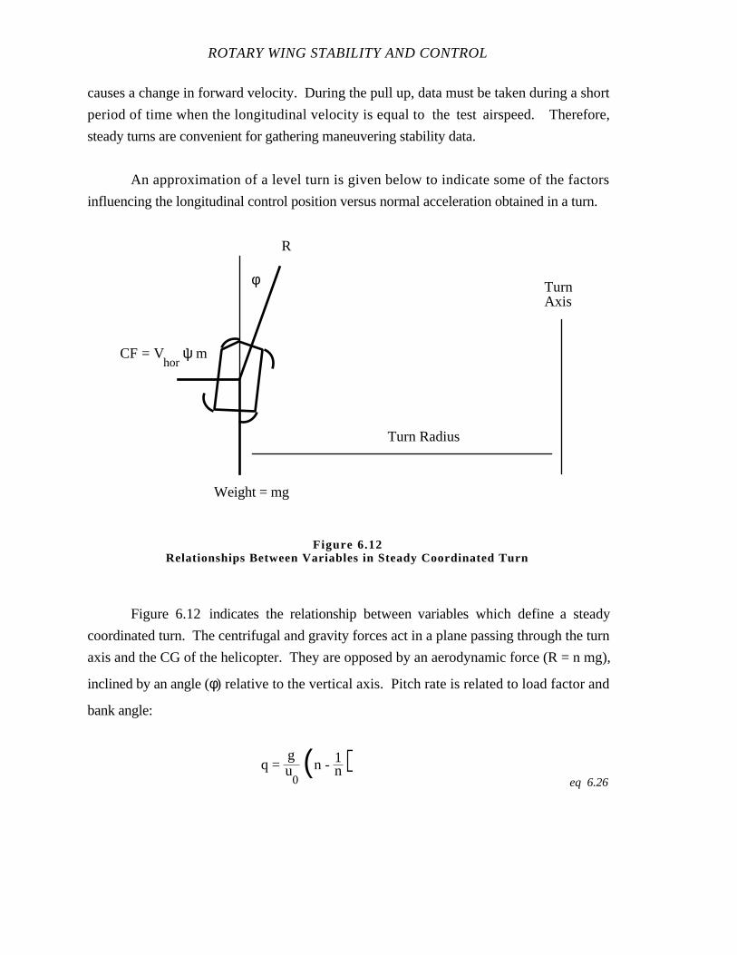
ROTARY WING STABILITY AND CONTROL
causes a change in forward velocity. During the pull up, data must be taken during a short
period of time when the longitudinal velocity is equal to the test airspeed. Therefore,
steady turns are convenient for gathering maneuvering stability data.
An approximation of a level turn is given below to indicate some of the factors
influencing the longitudinal control position versus normal acceleration obtained in a turn.
Figure 6.12 indicates the relationship between variables which define a steady
coordinated turn. The centrifugal and gravity forces act in a plane passing through the turn
axis and the CG of the helicopter. They are opposed by an aerodynamic force (R = n mg),
inclined by an angle (φ) relative to the vertical axis. Pitch rate is related to load factor and
bank angle:
q = gu
0(n - 1n)
eq 6.26
R
Weight = mg
TurnAxis
Turn Radius
CF = Vhor
ψ. m
φ
Figure 6.12Relationships Between Variables in Steady Coordinated Turn
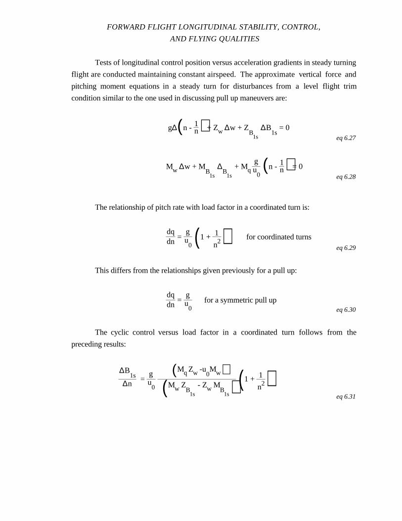
FORWARD FLIGHT LONGITUDINAL STABILITY, CONTROL,
AND FLYING QUALITIES
Tests of longitudinal control position versus acceleration gradients in steady turning
flight are conducted maintaining constant airspeed. The approximate vertical force and
pitching moment equations in a steady turn for disturbances from a level flight trim
condition similar to the one used in discussing pull up maneuvers are:
g∆(n - 1n) + Zw ∆w + ZB
1s
∆B1s
= 0eq 6.27
Mw ∆w + MB
1s
∆B
1s
+ Mqgu
0(n - 1n) = 0
eq 6.28
The relationship of pitch rate with load factor in a coordinated turn is:
dqdn
= gu
0 (1 + 1
n2) for coordinated turnseq 6.29
This differs from the relationships given previously for a pull up:
dqdn
= gu
0for a symmetric pull up
eq 6.30
The cyclic control versus load factor in a coordinated turn follows from the
preceding results:
∆B1s
∆n =
gu
0
(Mq Zw -u0Mw)
(Mw ZB
1s
- Zw MB
1s) (1 + 1
n2)eq 6.31
ROTARY WING STABILITY AND CONTROL
Where:
B1s - Longitudinal cyclic pitch angle, shaft referenced
g - Gravity
M B1s- Pitch moment due to longitudinal cyclic pitch angle
M q - Pitch moment due to pitch rate
M w - Pitch moment due to vertical velocity
n - Normal acceleration, Normal load factor
q - Angular velocity about y axis, Pitch rate
u0 - Initial velocity
ZB1s- Vertical force due to longitudinal cyclic pitch angle
Zw - Vertical force due to vertical velocity.
The above expression for the cyclic pitch versus load factor gradient obtained in a
coordinated turn with constant collective pitch differs from the one obtained for steady pull
ups. As indicated, the gradient (dq/dn) is different in the two cases. The gradient of B1s/n
if multiplied by the factor (1 + 1/n2). At n ≈ 1, the local gradient in a steady turn is
approximately twice the gradient in a steady pull up. At high n, the local gradient in a
steady turn approaches the local gradient in a pull up.
6.3.6.3 MANEUVERING STABILITY AS INDICATED BY
CONTROL FORCE VERSUS LOAD FACTOR
Longitudinal control force versus load factor is a cue to the pilot to off trim load
factor just as the longitudinal control force versus airspeed is a cue to off trim airspeed.
When a longitudinal control position versus normal load factor curve is obtained for a
helicopter with an irreversible control system, corresponding control force versus normal
load factor curves are constructed by cross plotting cockpit flight control force versus
displacement data. For a reversible flight control system, control force versus load factor
data can be measured in flight. Positive maneuvering stability is indicated by increasing
pull force for increasing load factor. Negative maneuvering stability is indicated by
increasing push force for increasing load factor.
Trim systems which give a satisfactory control force versus airspeed gradient may
provide an insufficient control force versus normal load factor gradient. Therefore, a bob
weight or other flight control system artifact might be used to provide the desired control
FORWARD FLIGHT LONGITUDINAL STABILITY, CONTROL,
AND FLYING QUALITIES
force versus load factor gradient. The bob weight does not change the control force versus
airspeed gradient. However, a bungee spring may be required to counteract the bob weight
under static conditions. Bob weights are not used widely in helicopters because of inherent
drawbacks such as longitudinal control forces generated by vertical accelerations due to
collective pitch inputs and inputs fed into the control system by turbulence.
Some helicopter trim systems introduce control forces proportional to pitch rate as a
pilot cue in maneuvering flight and incorporate a minimum pitch rate limit so control forces
are not affected by aircraft responses to small gust inputs.
6.3.7 Dynamic Stability
Dynamic stability is the helicopter motion over time following a disturbance. Both
control response and gust response depend on the basic vehicle dynamics and are not
independent considerations from the test pilot's viewpoint. One other distinction between
the two responses might be mentioned. Control inputs generally do notcontain high
frequency components exciting blade dynamic response. Therefore, high frequency modes
involving blade dynamics are ignored in considering control responses. On the other hand,
the gust response may include high frequency dynamics.
6.3.7.1 LONG TERM DYNAMIC STABILITY
The significance of static stability on the nature of the long term response in
forward flight is determined from an approximate second order equation for the
longitudinal velocity (u). The longitudinal equations of motion are approximated on the
basis the helicopter has a slow aperiodic or a low frequency oscillatory long term response,
and the uncoupled u velocity response is much slower than the uncoupled w velocity or q =
responses. This approximation is generally true for augmented helicopters and also for
most unaugmented helicopters. However, the simplified formulas developed for the long
term mode cannot be applied for cases having comparatively slow w and θ responses.
Thus w and θ should be close to their quasi-static values, wQS andθ QS, obtained by
solving the equations of motion assuming w and θ are zero as a first approximation. The
time derivatives dwQS / dt and dθ QS/dt are substituted into the equations as a second
approximation for w and˙θ .
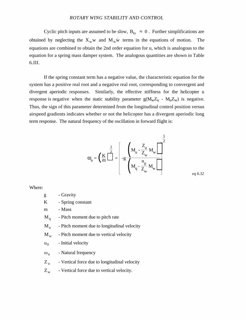
ROTARY WING STABILITY AND CONTROL
Cyclic pitch inputs are assumed to be slow, B1s ≈ 0 . Further simplifications are
obtained by neglecting the Xww and Mww terms in the equations of motion. The
equations are combined to obtain the 2nd order equation for u, which is analogous to the
equation for a spring mass damper system. The analogous quantities are shown in Table
6.III.
If the spring constant term has a negative value, the characteristic equation for the
system has a positive real root and a negative real root, corresponding to convergent and
divergent aperiodic responses. Similarly, the effective stiffness for the helicopter u
response is negative when the static stability parameter g(MwZu - MuZw) is negative.
Thus, the sign of this parameter determined from the longitudinal control position versus
airspeed gradients indicates whether or not the helicopter has a divergent aperiodic long
term response. The natural frequency of the oscillation in forward flight is:
ωn = (Km)
12
= -g(Mu -
ZuZw
Mw)(Mq -
u0
Zw Mw)
12
eq 6.32
Where:
g - Gravity
K - Spring constant
m - Mass
M q - Pitch moment due to pitch rate
M u - Pitch moment due to longitudinal velocity
M w - Pitch moment due to vertical velocity
u0 - Initial velocity
n - Natural frequency
Z u - Vertical force due to longitudinal velocity
Zw - Vertical force due to vertical velocity.
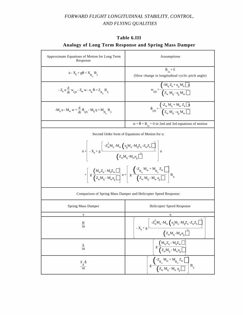
FORWARD FLIGHT LONGITUDINAL STABILITY, CONTROL,
AND FLYING QUALITIES
Table 6.III
Analogy of Long Term Response and Spring Mass Damper
Approximate Equations of Motion for Long TermResponse
Assumptions
u. - Xu + gθ = XB
1s
B1s
B.
1s = 0
(Slow change in longitudinal cyclic pitch angle)
- Zu u ddt
wQS
- Zw w - u0
θ. = Z
B1s
B1s
wQS
= ( -Mq Zu + u
0 Mu) u
(Zw Mq - u0 Mw)
-Mu u - Mw w + ddt
θ.
QS - Mq q = M
B1s
B1s
θ.
QS =
( -Zw Mu + Mw Zu) u
(Zw Mq - u0 Mw)w. = θ
.. = B
1s = 0 in 2nd and 3rd equations of motion
Second Order form of Equations of Motion for u:
u.. + - Xu + g
-Zw2Mu -Mw (u
0Mu -MqZu -ZwZu)
(ZwMq -Mwu0)
2 u.
+ g(MwZu - MuZw)(ZwMq - Mwu
0) u = g
( -ZB
1s
Mw + MB
1s
Zw)(Zw Mq - Mw u
0) B
1s
Comparison of Spring Mass Damper and Helicopter Speed Response:
Spring Mass Damper Helicopter Speed Response
x u
Bm - Xu + g
-Zw2Mu -Mw (u
0Mu -MqZu -ZwZu)
(ZwMq -Mwu0)
2
km g
(MwZu - MuZw)(ZwMq - Mwu
0)
Fδ
δ
mg( -Z
B1s
Mw + MB
1s
Zw)(Zw Mq - Mw u
0) B
1s
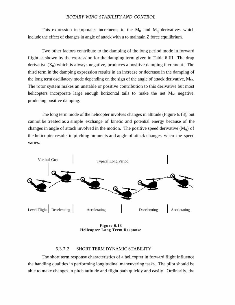
ROTARY WING STABILITY AND CONTROL
This expression incorporates increments to the Mu and Mq derivatives which
include the effect of changes in angle of attack with u to maintain Z force equilibrium.
Two other factors contribute to the damping of the long period mode in forward
flight as shown by the expression for the damping term given in Table 6.III. The drag
derivative (Xu) which is always negative, produces a positive damping increment. The
third term in the damping expression results in an increase or decrease in the damping of
the long term oscillatory mode depending on the sign of the angle of attack derivative, Mw.
The rotor system makes an unstable or positive contribution to this derivative but most
helicopters incorporate large enough horizontal tails to make the net Mw negative,
producing positive damping.
The long term mode of the helicopter involves changes in altitude (Figure 6.13), but
cannot be treated as a simple exchange of kinetic and potential energy because of the
changes in angle of attack involved in the motion. The positive speed derivative (Mu) of
the helicopter results in pitching moments and angle of attack changes when the speed
varies.
6.3.7.2 SHORT TERM DYNAMIC STABILITY
The short term response characteristics of a helicopter in forward flight influence
the handling qualities in performing longitudinal maneuvering tasks. The pilot should be
able to make changes in pitch attitude and flight path quickly and easily. Ordinarily, the
Level Flight
Vertical Gust
Decelerating Accelerating Decelerating Accelerating
Typical Long Period
Figure 6.13Helicopter Long Term Response
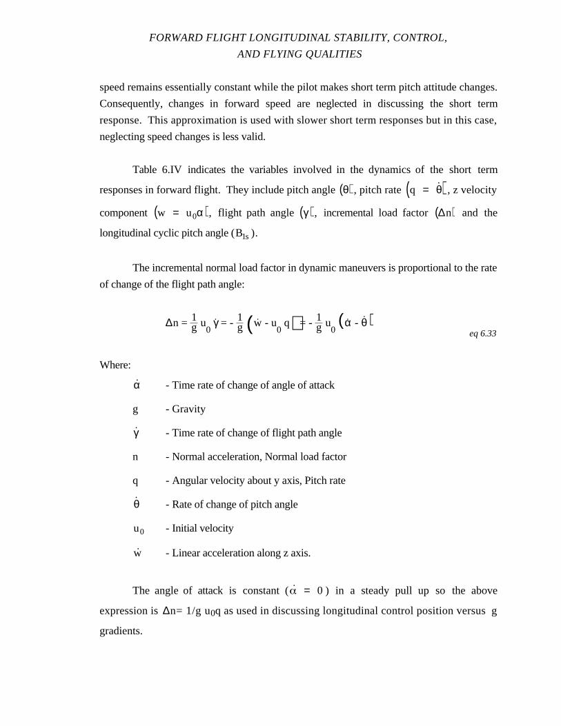
FORWARD FLIGHT LONGITUDINAL STABILITY, CONTROL,
AND FLYING QUALITIES
speed remains essentially constant while the pilot makes short term pitch attitude changes.
Consequently, changes in forward speed are neglected in discussing the short term
response. This approximation is used with slower short term responses but in this case,
neglecting speed changes is less valid.
Table 6.IV indicates the variables involved in the dynamics of the short term
responses in forward flight. They include pitch angle θ( ) , pitch rate q = θ ( ) , z velocity
component w = u0α( ), flight path angle γ( ) , incremental load factor∆n( ) and the
longitudinal cyclic pitch angle (B1s).
The incremental normal load factor in dynamic maneuvers is proportional to the rate
of change of the flight path angle:
∆n = 1g u0
γ. = - 1g (w. - u
0 q) = - 1g u
0(α. - θ
. )eq 6.33
Where:
α - Time rate of change of angle of attack
g - Gravity
γ - Time rate of change of flight path angle
n - Normal acceleration, Normal load factor
q - Angular velocity about y axis, Pitch rate
θ - Rate of change of pitch angle
u0 - Initial velocity
w - Linear acceleration along z axis.
The angle of attack is constant (˙ = 0 ) in a steady pull up so the above
expression is ∆n= 1/g u0q as used in discussing longitudinal control position versus g
gradients.
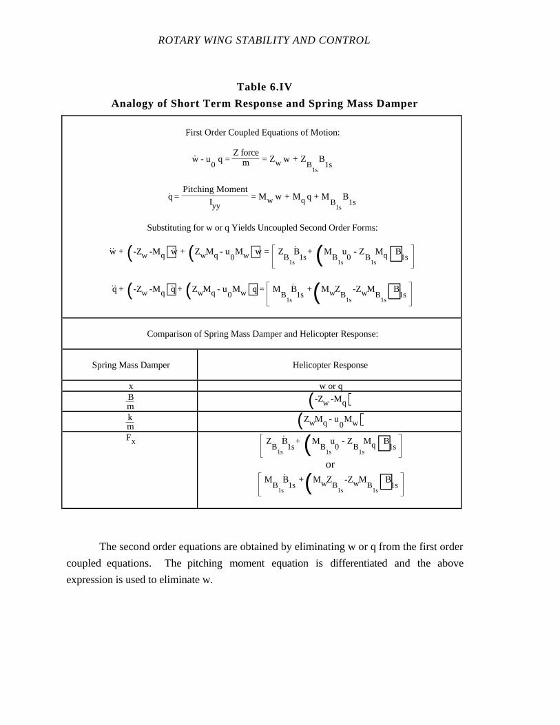
ROTARY WING STABILITY AND CONTROL
Table 6.IV
Analogy of Short Term Response and Spring Mass Damper
First Order Coupled Equations of Motion:
w. - u
0 q =
Z forcem = Zw w + Z
B1s
B1s
q. =
Pitching Moment
Iyy = Mw w + Mq q + M
B1s
B1s
Substituting for w or q Yields Uncoupled Second Order Forms:
w. .
+ ( -Zw -Mq)w. + (ZwMq - u0
Mw)w = ZB
1s
B.1s
+ (MB
1s
u0 - Z
B1s
Mq)B1s
q. . + ( -Zw -Mq)q
. + (ZwMq - u0
Mw)q = MB
1s
B.1s
+(MwZB
1s
-ZwMB
1s)B1s
Comparison of Spring Mass Damper and Helicopter Response:
Spring Mass Damper Helicopter Response
x w or qBm ( -Zw -Mq)km (ZwMq - u0
Mw)Fx Z
B1s
B.1s
+ (MB
1s
u0 - Z
B1s
Mq)B1s
orM
B1s
B.1s
+(MwZB
1s
-ZwMB
1s)B1s
The second order equations are obtained by eliminating w or q from the first order
coupled equations. The pitching moment equation is differentiated and the above
expression is used to eliminate w.

FORWARD FLIGHT LONGITUDINAL STABILITY, CONTROL,
AND FLYING QUALITIES
q.. + (-Zw - Mq)q
. + (Zw Mq - u0
Mw)q = MB
1s
B.
1s + (Mw Z
B1s
- Zw MB
1s)B1s
= Fq
eq 6.34
Where:
B1s - Longitudinal cyclic pitch angle, shaft referenced
Fq - Pitch input
M B1s- Pitch moment due to longitudinal cyclic pitch angle
M q - Pitch moment due to pitch rate
M w - Pitch moment due to vertical velocity
q - Angular velocity about y axis, Pitch rate
˙q - Second time derivative of pitch rate
q - Angular acceleration about y axis
u0 - Initial velocity
ZB1s- Vertical force due to longitudinal cyclic pitch angle
Zw - Vertical force due to vertical velocity.
The short term response of the helicopter, like the response of the spring mass
damper system, is aperiodic if the characteristic roots are real and is oscillatory if the roots
are complex numbers. The solution for the two roots of the short term mode areas
follows:
λ1,2
= - ( -Zw - Mq
2 ) ± ( -Zw- Mq
2 )2
- ( Zw Mq - u0 Mw)
12
eq 6.35
Where:
- Characteristic root
Mq - Pitch moment due to pitch rate
Mw - Pitch moment due to vertical velocity
u0 - Initial velocity
Zw - Vertical force due to vertical velocity.
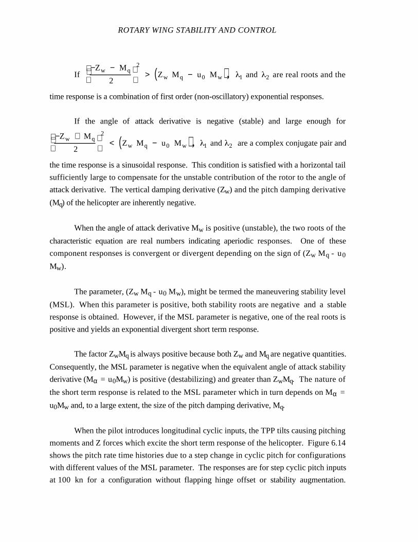
ROTARY WING STABILITY AND CONTROL
If−Zw − Mq
2
2
> Zw Mq − u0 Mw( ), 1 and 2 are real roots and the
time response is a combination of first order (non-oscillatory) exponential responses.
If the angle of attack derivative is negative (stable) and large enough for
−Zw + Mq
2
2
< Zw Mq − u0 Mw( ) , 1 and 2 are a complex conjugate pair and
the time response is a sinusoidal response. This condition is satisfied with a horizontal tail
sufficiently large to compensate for the unstable contribution of the rotor to the angle of
attack derivative. The vertical damping derivative (Zw) and the pitch damping derivative
(Mq) of the helicopter are inherently negative.
When the angle of attack derivative Mw is positive (unstable), the two roots of the
characteristic equation are real numbers indicating aperiodic responses. One of these
component responses is convergent or divergent depending on the sign of (Zw Mq - u0
Mw).
The parameter, (Zw Mq - u0 Mw), might be termed the maneuvering stability level
(MSL). When this parameter is positive, both stability roots are negative and a stable
response is obtained. However, if the MSL parameter is negative, one of the real roots is
positive and yields an exponential divergent short term response.
The factor ZwMq is always positive because both Zw and Mq are negative quantities.
Consequently, the MSL parameter is negative when the equivalent angle of attack stability
derivative (Mα = u0Mw) is positive (destabilizing) and greater than ZwMq. The nature of
the short term response is related to the MSL parameter which in turn depends on Mα =
u0Mw and, to a large extent, the size of the pitch damping derivative, Mq.
When the pilot introduces longitudinal cyclic inputs, the TPP tilts causing pitching
moments and Z forces which excite the short term response of the helicopter. Figure 6.14
shows the pitch rate time histories due to a step change in cyclic pitch for configurations
with different values of the MSL parameter. The responses are for step cyclic pitch inputs
at 100 kn for a configuration without flapping hinge offset or stability augmentation.
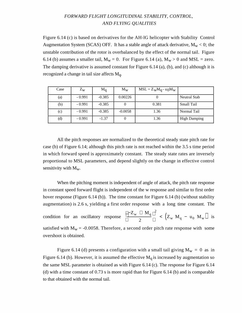
FORWARD FLIGHT LONGITUDINAL STABILITY, CONTROL,
AND FLYING QUALITIES
Figure 6.14 (c) is based on derivatives for the AH-lG helicopter with Stability Control
Augmentation System (SCAS) OFF. It has a stable angle of attack derivative, Mw < 0; the
unstable contribution of the rotor is overbalanced by the effect of the normal tail. Figure
6.14 (b) assumes a smaller tail, Mw = 0. For Figure 6.14 (a), Mw > 0 and MSL = zero.
The damping derivative is assumed constant for Figure 6.14 (a), (b), and (c) although it is
recognized a change in tail size affects Mq.
Case Zw Mq Mw MSL = ZwMq - u0Mw
(a) - 0.991 -0.385 0.00226 0 Neutral Stab
(b) - 0.991 -0.385 0 0.381 Small Tail
(c) - 0.991 -0.385 -0.0058 1.36 Normal Tail
(d) - 0.991 -1.37 0 1.36 High Damping
All the pitch responses are normalized to the theoretical steady state pitch rate for
case (b) of Figure 6.14; although this pitch rate is not reached within the 3.5 s time period
in which forward speed is approximately constant. The steady state rates are inversely
proportional to MSL parameters, and depend slightly on the change in effective control
sensitivity with Mw.
When the pitching moment is independent of angle of attack, the pitch rate response
in constant speed forward flight is independent of the w response and similar to first order
hover response (Figure 6.14 (b)). The time constant for Figure 6.14 (b) (without stability
augmentation) is 2.6 s, yielding a first order response with a long time constant. The
condition for an oscillatory response−Zw + Mq
2
2
< Zw Mq − u0 Mw( ) is
satisfied with Mw = -0.0058. Therefore, a second order pitch rate response with some
overshoot is obtained.
Figure 6.14 (d) presents a configuration with a small tail giving Mw = 0 as in
Figure 6.14 (b). However, it is assumed the effective Mq is increased by augmentation so
the same MSL parameter is obtained as with Figure 6.14 (c). The response for Figure 6.14
(d) with a time constant of 0.73 s is more rapid than for Figure 6.14 (b) and is comparable
to that obtained with the normal tail.
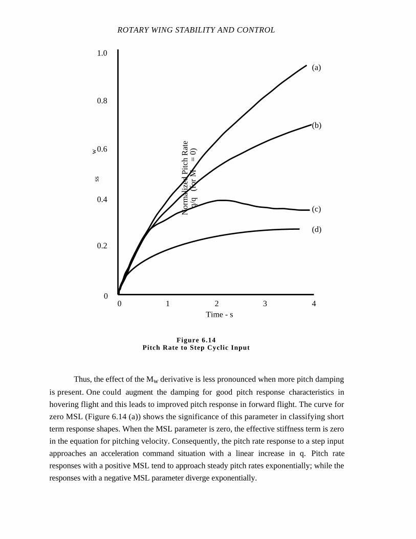
ROTARY WING STABILITY AND CONTROL
Thus, the effect of the Mw derivative is less pronounced when more pitch damping
is present. One could augment the damping for good pitch response characteristics in
hovering flight and this leads to improved pitch response in forward flight. The curve for
zero MSL (Figure 6.14 (a)) shows the significance of this parameter in classifying short
term response shapes. When the MSL parameter is zero, the effective stiffness term is zero
in the equation for pitching velocity. Consequently, the pitch rate response to a step input
approaches an acceleration command situation with a linear increase in q. Pitch rate
responses with a positive MSL tend to approach steady pitch rates exponentially; while the
responses with a negative MSL parameter diverge exponentially.
Time - s1 2 3 40
0
0.2
0.4
0.6
0.8
1.0
(b)
(c)
(d)
(a)
Nor
mal
ized
Pitc
h R
ate
q/q
(fo
r M
=
0)
ssw
Figure 6.14Pitch Rate to Step Cyclic Input
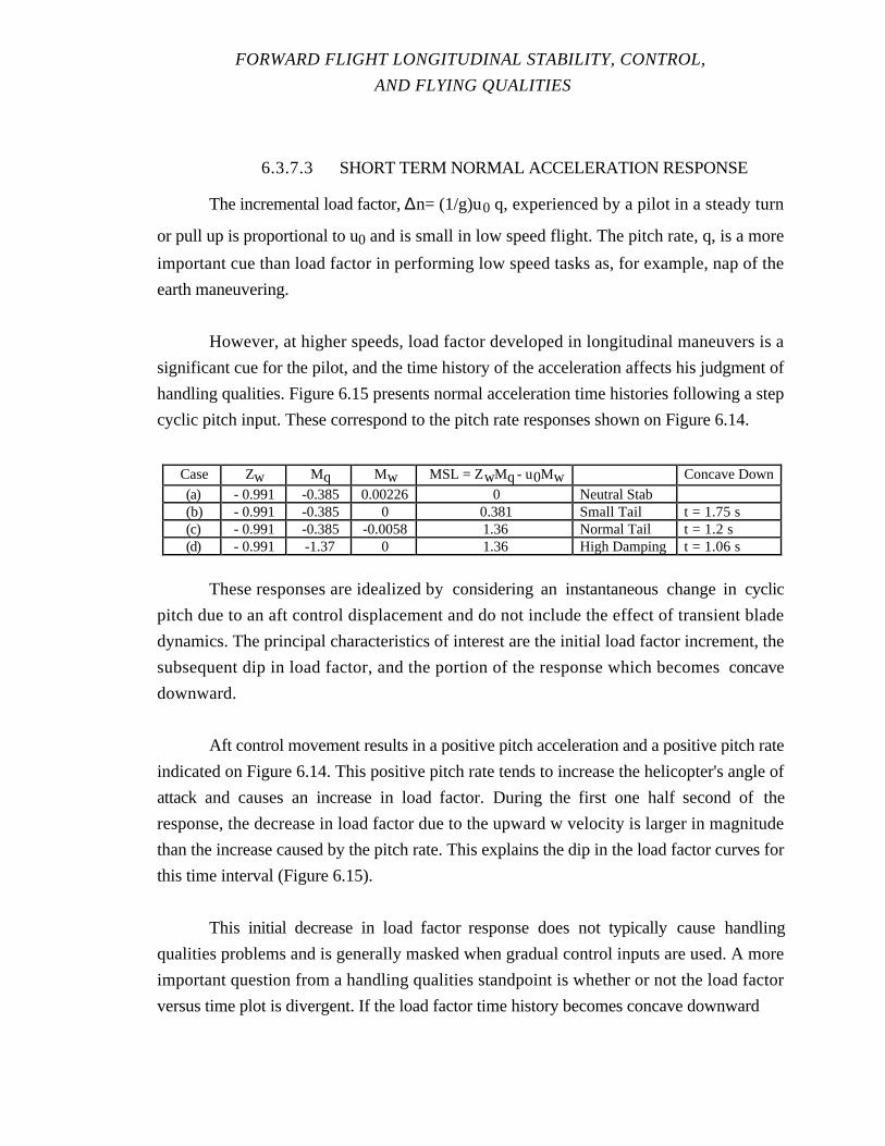
FORWARD FLIGHT LONGITUDINAL STABILITY, CONTROL,
AND FLYING QUALITIES
6.3.7.3 SHORT TERM NORMAL ACCELERATION RESPONSE
The incremental load factor, ∆n= (1/g)u0 q, experienced by a pilot in a steady turn
or pull up is proportional to u0 and is small in low speed flight. The pitch rate, q, is a more
important cue than load factor in performing low speed tasks as, for example, nap of the
earth maneuvering.
However, at higher speeds, load factor developed in longitudinal maneuvers is a
significant cue for the pilot, and the time history of the acceleration affects his judgment of
handling qualities. Figure 6.15 presents normal acceleration time histories following a step
cyclic pitch input. These correspond to the pitch rate responses shown on Figure 6.14.
Case Zw Mq Mw MSL = ZwMq - u0Mw Concave Down
(a) - 0.991 -0.385 0.00226 0 Neutral Stab(b) - 0.991 -0.385 0 0.381 Small Tail t = 1.75 s(c) - 0.991 -0.385 -0.0058 1.36 Normal Tail t = 1.2 s(d) - 0.991 -1.37 0 1.36 High Damping t = 1.06 s
These responses are idealized by considering an instantaneous change in cyclic
pitch due to an aft control displacement and do not include the effect of transient blade
dynamics. The principal characteristics of interest are the initial load factor increment, the
subsequent dip in load factor, and the portion of the response which becomes concave
downward.
Aft control movement results in a positive pitch acceleration and a positive pitch rate
indicated on Figure 6.14. This positive pitch rate tends to increase the helicopter's angle of
attack and causes an increase in load factor. During the first one half second of the
response, the decrease in load factor due to the upward w velocity is larger in magnitude
than the increase caused by the pitch rate. This explains the dip in the load factor curves for
this time interval (Figure 6.15).
This initial decrease in load factor response does not typically cause handling
qualities problems and is generally masked when gradual control inputs are used. A more
important question from a handling qualities standpoint is whether or not the load factor
versus time plot is divergent. If the load factor time history becomes concave downward
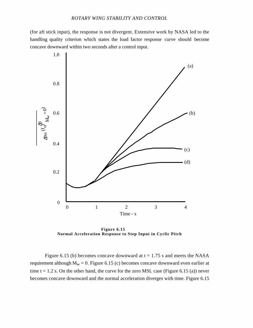
ROTARY WING STABILITY AND CONTROL
(for aft stick input), the response is not divergent. Extensive work by NASA led to the
handling quality criterion which states the load factor response curve should become
concave downward within two seconds after a control input.
Normal Acceleration Response to Step Input in Cyclic Pitch
Figure 6.15 (b) becomes concave downward at t = 1.75 s and meets the NASA
requirement although Mw = 0. Figure 6.15 (c) becomes concave downward even earlier at
time t = 1.2 s. On the other hand, the curve for the zero MSL case (Figure 6.15 (a)) never
becomes concave downward and the normal acceleration diverges with time. Figure 6.15
Time - s1 2 3 40
0
0.2
0.4
0.6
0.8
1.0
(b)
(c)
(d)
(a)
∆n∆n
ss(f
orM
w=
0)
Figure 6.15
FORWARD FLIGHT LONGITUDINAL STABILITY, CONTROL,
AND FLYING QUALITIES
(d) is for the same MSL value as for curve (c) but with Mw = 0 and a more negative pitch
damping derivative. The normal load factor response curve for this case becomes concave
downward at t = 1.06 s.
The preceding discussion of the short term response started by assuming the u
velocity component remains constant and no coupling exists with lateral and directional
degrees of freedom. Analysis of the complete system requires consideration of the
additional degrees of freedom with their corresponding equations of motion and results in
additional characteristic frequencies and natural response modes. However, for the more
complete case, the general motions for small disturbances from trim condition can be
described by considering several elemental first and secondorder spring mass damper
models. The time history of each of the flight variables resulting from a control input is the
sum of several terms, each proportional to the response in one of the spring mass damper
models used to represent the helicopter.
6.3.8 Control Response
Helicopter response to cockpit control inputs is termed control response. The short
and long term responses of the helicopter are key ingredients of both control response and
gust response. It suffices here to list those characteristics which are additional when
considering pilot inputs. Helicopter designs include increasing use of augmentation and
digital flight controls. The effects of these systems should be considered in the total control
response.
Feed forward control loops may include the control boost system. The feedback
loop may consist of pure gain on a response feedback signal such as pitch rate or both gain
and dynamics from filters, etc. All elements directly in the control signal path such as the
force feel system, any pertinent nonlinearities and stabilization loop feed forward elements
affect the total control response directly. Elements in this path are sometimes called control
augmentation. On the other hand, elements within the stabilization loop function as
stability augmentation. An evaluation of the adequacy of control response in the context of
operational tasks, therefore, implicitly includes a consideration of the effects of all pilot
command path elements, in addition to the basic or stability augmented dynamics of the
helicopter. The evaluation considers predictability of the total control response as well as
adequate control sensitivity.
ROTARY WING STABILITY AND CONTROL
6.3.9 Pilot Induced Oscillation
Some helicopters exhibit pilot induced oscillation (PIO) tendencies when carrying
out mission related pitch tasks requiring tight closed loop control. For example, in a
conventional gun run task, the pilot uses the short term response to bring the aircraft into
alignment with the target. This is accomplished by a series of short rapid inputs to correct
for errors in attitude.
If the pilot makes a correction to bring the nose on target and the short term
response and control system combination is such that the harder he tries to zero the tracking
error, the poorer his closed loop performance and more oscillatory than the open loop
response, he is in a PIO. If he persists, he is worse off than if he backed off in the closed
loop. The existence of PIO tendencies is examined by the test pilot throughout the
operating envelope.
6.3.10 Gust Response
A distinction can be made between the gust and short term responses of the
helicopter. Pitch attitude and pitch rate changes are usually considered in characterizing the
short term response. Although the pilot uses the short term response mode to make
corrections for pitch attitude or rate changes resulting from encountering turbulence, this is
not the complete gust response.
The evaluation of the gust response amounts to a subjective pilot judgment of the
helicopter ride qualities when flying through turbulence. This judgment is influenced by
the aircraft linear and angular accelerations due to turbulence and the location of the pilot
relative to the CG. The time variations of these quantities influence the judgment of ride
qualities.
The aerodynamic forces due to turbulence simultaneously excite responses of the
rotor blade and fuselage structural modes as well as the short term and other rigid body
modes. The pilot's judgment is based on the total perceived response.
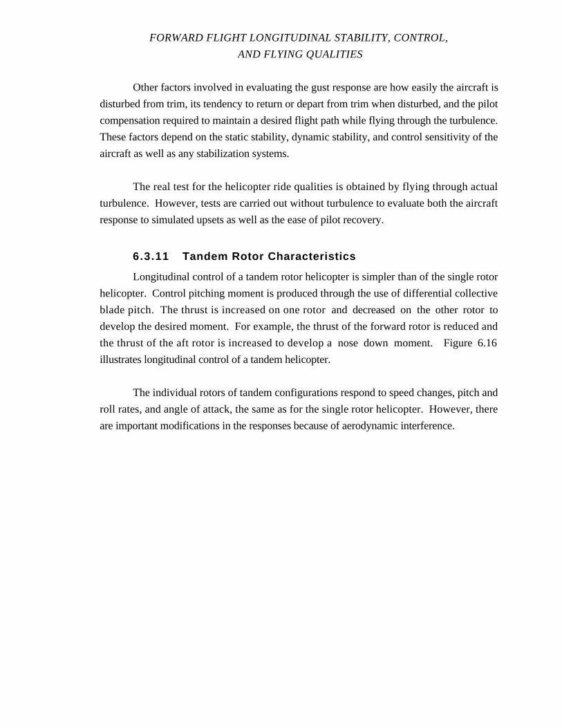
FORWARD FLIGHT LONGITUDINAL STABILITY, CONTROL,
AND FLYING QUALITIES
Other factors involved in evaluating the gust response are how easily the aircraft is
disturbed from trim, its tendency to return or depart from trim when disturbed, and the pilot
compensation required to maintain a desired flight path while flying through the turbulence.
These factors depend on the static stability, dynamic stability, and control sensitivity of the
aircraft as well as any stabilization systems.
The real test for the helicopter ride qualities is obtained by flying through actual
turbulence. However, tests are carried out without turbulence to evaluate both the aircraft
response to simulated upsets as well as the ease of pilot recovery.
6.3.11 Tandem Rotor Characteristics
Longitudinal control of a tandem rotor helicopter is simpler than of the single rotor
helicopter. Control pitching moment is produced through the use of differential collective
blade pitch. The thrust is increased on one rotor and decreased on the other rotor to
develop the desired moment. For example, the thrust of the forward rotor is reduced and
the thrust of the aft rotor is increased to develop a nose down moment. Figure 6.16
illustrates longitudinal control of a tandem helicopter.
The individual rotors of tandem configurations respond to speed changes, pitch and
roll rates, and angle of attack, the same as for the single rotor helicopter. However, there
are important modifications in the responses because of aerodynamic interference.
ROTARY WING STABILITY AND CONTROL
Figure 6.16Longitudinal Control of a Tandem Rotor Helicopter
Weight
(a) Equilibrium
Weight(b) Nose Down Moment
Weight
(c) Nose up Moment
Increased Collective,Increased Thrust
Decreased Collective,Decreased Thrust
Decreased Collective,Decreased Thrust
Increased Collective,Increased Thrust
FORWARD FLIGHT LONGITUDINAL STABILITY, CONTROL,
AND FLYING QUALITIES
Figure 6.17 indicates some of the factors affecting the longitudinal stability of the
tandem helicopter. The nature of the configuration is such that the pitching moment of
inertia is much greater than a single rotor helicopter. However, this characteristic is offset
by the higher control power and pitch damping of most tandem designs. The higher
control power of the tandem configurations arises from the use of differential collective
pitch on the front and rear rotors. Some control systems combine longitudinal cyclic pitch
with differential collective pitch to obtain increased control power.
Figure 6.17 (a) indicates the major source of pitch damping of the tandem. For the
case shown, the pitching velocity produces an upward increment of flow through the front
rotor disc, and a downward increment of flow through the rear rotor disc. Ahigher
average blade angle of attack of the front rotor increases its thrust; while the average blade
angle of attack and thrust of the rear rotor are decreased. The damping moments about the
CG produced by these changes in thrust are considerably larger than the moments due to
the TPP inclination, which is the primary source of pitchdamping of the single rotor
helicopter.
A helicopter has positive static stability if an increase in speed results in a nose up
pitching moment in opposition to the speed change. The aft tilting of the individual TPPs
and thrust vectors due to a speed increment has a stabilizing effect. Unlike the single rotor
helicopter, the speed stability of the tandem helicopter is affected appreciably by the CG
location. The rate of change of thrust on the front and rear rotors with forward speed can
be different because of differences in the trim values of collective pitch. A favorable speed
stability condition is obtained with a forward CG location.
Tandem helicopters encounter some problems in handling qualities due to pitching
moments which change with forward speed. In hovering, the downwash from both rotors
moves straight down and there is negligible interaction. As forward speed is increased, the
downwash on the forward rotor affects the flow over the rear rotor and consequently
reduces its lift. This results in a nose up pitching moment as the speed is first increased.
After moderate speed is gained, at an advance ratio of about 0.1, further increases in speed
tend to decrease the downwash from the front rotor on the rear rotor. The rear rotor lift is
increased by further speed increases. This latter condition sometimes results in an unstable
change in pitching moment with speed. At high speeds the downwash becomes small
enough to be unimportant from the speed stability standpoint.
ROTARY WING STABILITY AND CONTROL
Figure 6.17 (c) indicates a means to adjust the speed stability of the tandem
helicopter by the use of swashplate dihedral. A dihedral of the type indicated could be
obtained by appropriate rigging of the control system or by tilting of the shafts of the two
rotors. For the configuration shown, a forward speed increment producesan upflow
through the front rotor disc increasing the average blade angle of attack and a down flow
through the rear rotor decreasing the average angle of attack of the rear rotor. The net result
is an up thrust increment on the front rotor and a down thrust increment on the rear rotor
giving an aft pitching moment. An outward tilting of the rotors has an opposite effect,
decreasing the speed stability of the tandem helicopter. Since adjustments of the dihedral
changes the speed stability, it also provides a convenient means of controlling the
frequency of the long period oscillation.
The angle of attack stability characteristics of the tandem helicopter are indicated on
Figure 6.17 (d) and (e). Although a nose up increment in moment is a stable change in
moment with forward speed, it represents an unstable change in moment with angle of
attack. Aft tilting of the TPPs of the individual rotors with increasing pitch attitude results
in unstable pitching moments similar to a single rotor configuration. These unstable
moments can be compensated for by proper positioning of the CG because the angle of
attack stability of the tandem helicopter, like the airplane, depends on the CG position
relative to the aerodynamic center. When downwash effects are neglected, the aerodynamic
center is midway between the rotor shafts. For this condition, an increase in fuselage angle
of attack results in equal increments of thrust on the front and rear rotors and a resultant
thrust increment acting at the aerodynamic center. This thrust increment produces a stable
nose down pitching moment if the CG is forward of the aerodynamic center as indicated on
Figure 6.17 (d). A second beneficial effect of a forward CG location is an unloading of the
rear rotor, reducing the likelihood of rear rotor tip stalling which has a destabilizing
influence.
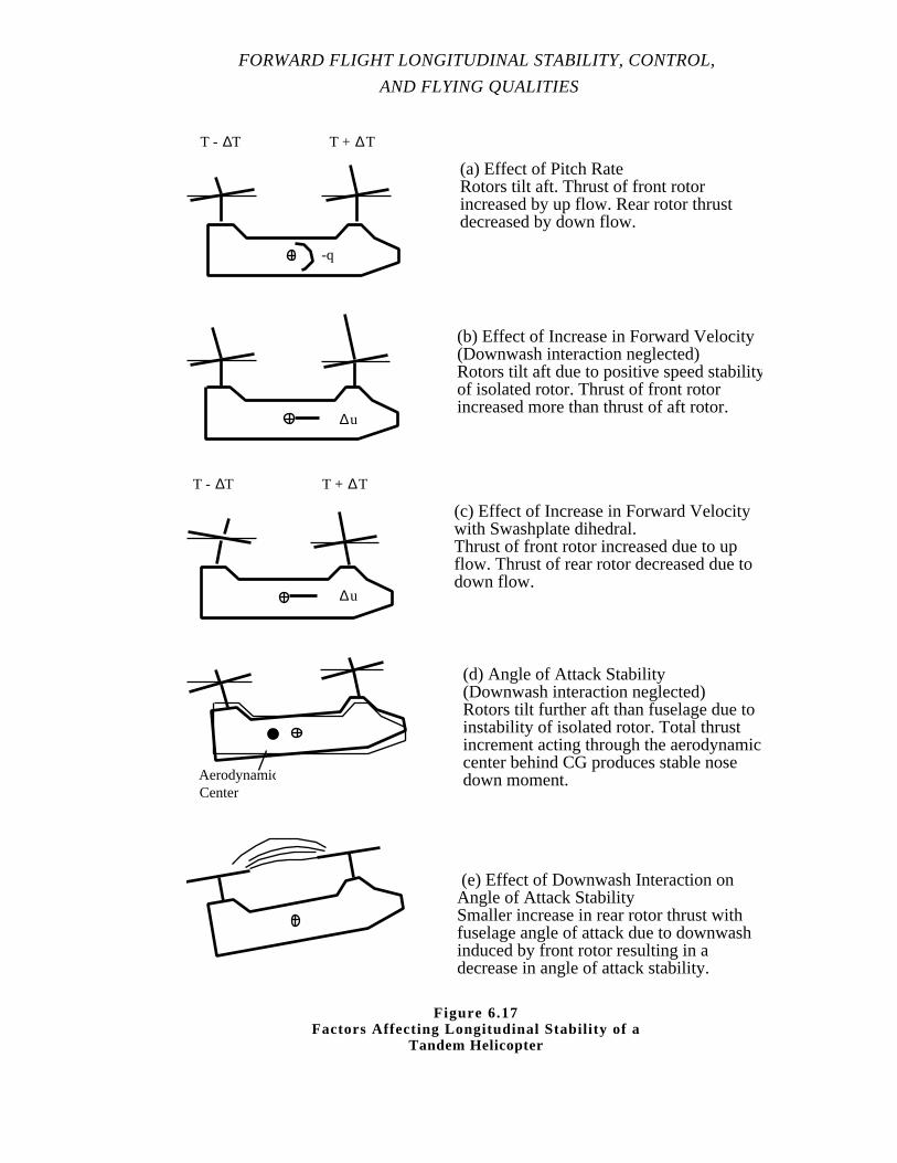
FORWARD FLIGHT LONGITUDINAL STABILITY, CONTROL,
AND FLYING QUALITIES
(a) Effect of Pitch RateRotors tilt aft. Thrust of front rotorincreased by up flow. Rear rotor thrustdecreased by down flow.
T + ∆TT - ∆T
-q
(b) Effect of Increase in Forward Velocity(Downwash interaction neglected)Rotors tilt aft due to positive speed stabilityof isolated rotor. Thrust of front rotorincreased more than thrust of aft rotor.
∆u
(c) Effect of Increase in Forward Velocitywith Swashplate dihedral.Thrust of front rotor increased due to upflow. Thrust of rear rotor decreased due todown flow.
T + ∆TT - ∆T
∆u
(e) Effect of Downwash Interaction onAngle of Attack StabilitySmaller increase in rear rotor thrust withfuselage angle of attack due to downwashinduced by front rotor resulting in adecrease in angle of attack stability.
(d) Angle of Attack Stability(Downwash interaction neglected)Rotors tilt further aft than fuselage due toinstability of isolated rotor. Total thrustincrement acting through the aerodynamiccenter behind CG produces stable nosedown moment.Aerodynamic
Center
Figure 6.17Factors Affecting Longitudinal Stability of a
Tandem Helicopter
ROTARY WING STABILITY AND CONTROL
The downwash induced by the front rotor at the rear rotor has an unfavorable effect
on angle of attack stability as well as on speed stability and is largely responsible for the
unsatisfactory maneuvering characteristics of some tandemconfigurations (Figure 6.17
(e)). An increase in front rotor angle gives a large front rotor thrust and a corresponding
increase in downwash induced at the rear rotor. The average blade angle of attack of the
rear rotor is changed less than the front rotor because of this downwash giving a smaller
increment in rear rotor thrust. Thus, the lift curve slope of the rear rotor is less than the
front rotor and this difference results in a decrease in angle of attack stability.
6.4 TEST METHODS AND TECHNIQUES
A thorough knowledge and understanding of the flight control system operation is
important when designing the test conditions for flying qualities evaluations. Generally,
the Stability Augmentation System (SAS) does not impact the results of the trimmed flight
control positions and the static stability tests. However, if the Automatic Flight Control
System (AFCS) system incorporates a device similar to the pitch bias actuator found in the
SH-60 series aircraft, the AFCS can effect the trimmed flight control positions as well as
the apparent static stability. In most helicopters, the AFCS does effect the dynamic and
control response results. For this reason, the stability, control, and flying qualities test are
flown with the AFCS fully operational in the mission representative manner. If time
permits, the test can be repeated with the AFCS in alternate configurations, simulating
possible pilot selected options or system degradation. Further, the tests can be performed
with the AFCS secured, simulating total system failure and documenting the unaugmented
helicopter responses, possibly for flight simulator development.
6.4.1 Trimmed Control Positions
The purpose of the test is an evaluation of the variation in control positions with
changes in power and airspeed, the control margins, the ease of trimming the flight control
forces to zero, and the qualitative evaluation of the importance of trim changes to the
piloting task. The entire airspeed envelope is evaluated to VNE and the complete power
range is evaluated from autorotation to maximum power. For level flight, the helicopter is
established in trimmed, wings level, unaccelerated flight, and the data are recorded. The
airspeed is varied approximately 10 kn and the test is repeated.
FORWARD FLIGHT LONGITUDINAL STABILITY, CONTROL,
AND FLYING QUALITIES
For climbs and descents, one or more mission representative airspeeds are used.
The helicopter is stabilized on airspeed and the power is varied from autorotation to
maximum available. Airspeed remains constant while the power is varied. At least 5
power increments are used. The entire test is repeated at another airspeed. Usually, the
airspeed for maximum rate of climb, or minimum rate of descent is evaluated. If large
control displacements are observed when making a power change, the test can be
conducted open loop with all controls fixed except for power. The resulting attitude and
rate changes show the aircraft response which the pilot must counteract to maintain wings
level, unaccelerated flight conditions. The results of the open loop test is used to relate the
possible helicopter excursions when performing constant airspeed climbs and descents.
6.4.1.1 TEST TECHNIQUE
1. Establish wings level, unaccelerated, trimmed flight. Record the initial trim
conditions.
2. Assign a Handling Qualities Rating (HQR) and Vibration Assessment
Rating (VAR) to each data point.
3. Use the force trim and AFCS in a mission representative manner.
6.4.1.1.1 Level Flight
1. This data can be obtained concurrently with level flight performance testing.
2. Investigate entire airspeed profile (40 kn to VH).
6.4.1.1.2 Diving Flight
1. If VNE is greater than VH, fix the collective at maximum power and dive the
aircraft to obtain control position data at the higher airspeeds.
2. Control margins are particularly important.
6.4.1.1.3 Climbs and Descents (Open Loop)
1. Collective changes are made and the aircraft response observed without
making any other control inputs.
2. Tests are conducted controls fixed and free.

ROTARY WING STABILITY AND CONTROL
6.4.1.1.4 Climbs and Descents (Closed loop)
1. Establish wings level, unaccelerated flight at the desired trim airspeed.
2. Vary power incrementally from autorotation to the maximum available.
3. Normally five increments define a satisfactory curve.
4. Altitude range, ±1000 ft about target.
6.4.1.2 DATA REQUIRED
Control positions, Vo, HPo, θ, φ, Q, NR, fuel counts (FC), HQR, and VAR.
6.4.1.3 TEST CRITERIA
1. Stabilized, wings level, ball centered, unaccelerated flight.
2. No vertical velocity (level flight).
3. Constant vertical velocity (climb and descent).
4. All control forces trimmed to zero.
6.4.1.4 DATA REQUIREMENTS
1. Stabilize 15 s prior to recording data.
2. Record 10 s data.
3. HPo ± 1000 ft of the target test altitude.
4. Vv, level flight, ±10 fpm, climb and descent, stabilized ± 25 fpm.
5. NR ± 1%.
6.4.1.5 SAFETY CONSIDERATIONS/RISK MANAGEMENT
Observe normal operating limitations. Use incremental build up procedures when
approaching any envelope boundary. Conduct tests at a safe operating altitude over terrain
suitable for forced landings. Maintain proper lookout procedures. Consider using a chase
aircraft and sole use airspace.
6.4.2 Static Stability
The purpose of this test is to evaluate the static stability or the change in the total
longitudinal moment generated by off trim airspeed changes. Static stability is the initial
tendency of an aircraft to return or to depart from equilibrium if disturbed. Static stability is
indicated by the variation of the longitudinal control position with airspeed. Positive static
FORWARD FLIGHT LONGITUDINAL STABILITY, CONTROL,
AND FLYING QUALITIES
stability is indicated by increasing forward longitudinal control displacement with
increasing airspeed. Since the fuselage/rotor system forces and moments can not be
measured directly in flight, the purpose of this test is to determine the control positions and
forces necessary to balance the pitching moments caused by airspeed variations from trim.
The test is accomplished by establishing a wings level, ball centered, unaccelerated
trim condition. Without changing the collective position, trim settings, or rotor speed, the
airspeed is varied and stabilized at incremental airspeed faster and slower then trim. The
airspeed around trim is most important. Small 2 to 3 kn increments are used around trim.
As airspeed is varied from trim, larger 5 kn increments are used. At each stabilized flight
condition, lateral and directional controls are used to maintain wings level, ball centered
flight. Collective is maintained constant. A stabilized climb or descent is accepted and
altitude is maintained within ± 1000 ft of the test altitude. Alternating test points faster and
slower than trim are used to remain within the test altitude band. If power must be changed
to return to the test altitude, record all engine parameters and collective control position. Do
not retrim the collective. When the test altitude is reestablished, return the collective control
to trim.
The airspeed increments are arbitrary. It is not important to establish precisely a 3
or 5 kn increment. It is important to be in stabilized flight. A suggested procedure is to
make maximum use of attitude flying by reference outside the cockpit. A good instrument
scan is necessary. From the initial trim position, displace the longitudinal control forward,
decreasing the pitch attitude slightly. As the helicopter accelerates, observe the pitch
attitude. As it begins to change, apply forward control (Assuming positive static stability)
to maintain a constant pitch attitude. When airspeed stabilizes, establish equilibrium flight
conditions. Do not try to chase the airspeed indicator. Attempt to move the control in one
direction to avoid operating through any force hysteresis band.
6.4.2.1 TEST TECHNIQUE
1. Stabilize at the initial trim airspeed and reduce all control forces to zero.
Do not retrim control forces or adjust engine controls during the test.
2. Record the trim data.
ROTARY WING STABILITY AND CONTROL
3. Stabilize at airspeeds slower and faster than the trim airspeed. Do not retrim
control forces or adjust the collective and engine controls. Generally airspeed variations of
±20 kn in 5 kn increments is acceptable. However, use ± 2 kn increments close to the trim
airspeed.
4. Stabilize at each speed increment for 15 s and record data for approximately
10 s. Make qualitative comments on the force and displacement cues at theoff trim
conditions.
5. Hold attitude constant once a desired speed change is achieved. Pitch
attitude change provides a cue to off trim conditions.
6. Repeat the procedure until the airspeed range is completed. Alternate
airspeeds faster and slower than trim to remain in the altitude band.
7. If it is necessary to adjust altitude to remain within the test band, note the
collective position, torque, and Ng, before moving the collective. Do not retrim any control
forces. The test is continued after the collective control is returned to the original trim
position.
6.4.2.2 DATA REQUIRED
Longitudinal control position, longitudinal control force, Vo, Vv, θ, Q, NR, FC,
HPo, To.
6.4.2.3 TEST CRITERIA
1. Wings level, ball centered, unaccelerated flight.
2. Collective fixed.
3. No retrimming.
6.4.2.4 DATA REQUIREMENTS
1. Stabilize 15 s prior to taking data.
2. Record 10 s stabilized data.
3. Vo ± 1 kn.
4. Wings level, φ ± 1˚.
FORWARD FLIGHT LONGITUDINAL STABILITY, CONTROL,
AND FLYING QUALITIES
5. Ball centered.
6. HPo ± 1000 ft of the target test altitude.
7. NR ± 0.5%.
6.4.2.5 SAFETY CONSIDERATIONS/RISK MANAGEMENT
Observe normal operating limitations. Use incremental build up procedures when
approaching any envelope boundary. Conduct tests at a safe operating altitude over terrain
suitable for forced landings. Maintain proper lookout procedures. Consider using a chase
aircraft and using sole use airspace.
6.4.3 Maneuvering Stability
The maneuver stability test is a variation on the static longitudinal stability test. In
both cases, longitudinal control inputs are used to stabilize the aircraft at off trim
conditions. The static stability evaluation is conducted at 1.0 g and the airspeed is varied.
In maneuvering stability tests the trim airspeed is maintained and the normal acceleration is
varied. The maneuvering stability or pitching moment change with change in load factor is
determined from the variation of the longitudinal control position and control force with
normal acceleration obtained in stabilized conditions with constant airspeed and collective.
Three test techniques are used to cover the load factor envelope of the aircraft:
steady turns, symmetrical pull-ups, and symmetrical pushovers. Symmetrical pull-ups and
symmetrical pushovers encompass both the target cyclic and target “g” test methods.
6.4.3.1 TEST TECHNIQUE
6.4.3.1.1 Steady Turns
1. Stabilize in ball centered, coordinated level flight at the desired trim
airspeed.
2. Reduce all control forces to zero and do not retrim the forces during the
tests. Fix the collective position.
3. Record trim data.

ROTARY WING STABILITY AND CONTROL
4. Establish the desired bank angle, stabilizing on trim airspeed with a constant
g. Do not retrim the control forces and maintain fixed collective. Accept any resultant
climb or descent. Start the test at an altitude which permits a stabilized condition within the
test altitude band.
5. Record data when the airspeed, bank angle, and normal acceleration are
stabilized.
6. Repeat at incrementally increasing bank angles (15°, 30°, 45°, 60°) until the
maximum load factor or a predetermined flight limit is reached. These are target bank
angle, exact bank angles are not required. Evaluate turns in both directions.
7. Note collective position, torque and Ng,. Do not retrim the collective.
Climb if required to stay in the altitude band and reset collective to the trim position before
continuing the test.
6.4.3.1.2 Symmetrical Pull Up
The symmetrical pull up test technique requires considerable practice and proper
timing to yield satisfactory results. Exercise caution with this method because an aircraft
with neutral or unstable maneuvering stability characteristics continues to increase g when
the longitudinal control is held against the control fixture.
1. Stabilize in ball centered, coordinated level flight at the desired trim
airspeed.
2. Reduce all control forces to zero and fix the collective, noting its position.
3. If a control fixture is used, establish the fixture increment and place the
fixture behind the cyclic. Start with a small increment which corresponds to a low value of
normal acceleration.
4. Decelerate below the trim airspeed.
5. Lower the nose below the trim attitude to accelerate toward the trim
airspeed.
6. Prior to reaching the trim airspeed, rapidly displace the longitudinal control
and hold the control against the fixture. If a fixture is not used, displace the cyclic to obtain
the desired g level.
7. The aircraft must pass through the trimmed attitude, wings level, stable g,
and on trim airspeed.
FORWARD FLIGHT LONGITUDINAL STABILITY, CONTROL,
AND FLYING QUALITIES
8. Voice procedures for cockpit coordination are as follows: “Data on. Stand-
by for a (displacement magnitude), (direction of input), (control) input on three. Thousand
one, thousand two, thousand three.” The input is executed on three. Example, “Data on,
stand-by for a one inch aft longitudinal control input on three. Thousand one, thousand
two, thousand three.”
9. Turn on the automatic data recording prior to setting the fixture.
10. Use incremental increases in cyclic displacement (fixture increment) and
repeat the procedure until the desired normal acceleration range is obtained or a
predetermined limit is reached.
11. As the displacement and g level increase, it is necessary to decelerate more
and use a lower nose attitude during the acceleration phase. This technique requires
practice and crew coordination. Satisfactory results can be obtained through practice.
12. Announce the recovery to allow the copilot to remove the fixture.
6.4.3.1.3 Symmetrical Push Over
The symmetrical push over test technique requires considerable practice and proper
timing to yield satisfactory results. Exercise caution with this method because an aircraft
with neutral or unstable maneuvering stability characteristics continues to decrease g if the
longitudinal control is held against a fixture.
1. Stabilize in wings level, ball centered, coordinated level flight at the desired
trim airspeed.
2. Reduce all control forces to zero and fix the collective.
3. If a control fixture is used, establish the fixture increment and place the
fixture in front of the cyclic. Start with a small increment which corresponds to a small
change of normal acceleration.
4. Accelerate to an airspeed faster than trim.
5. Raise the nose above the horizon and allow the airspeed to decrease toward
trim.
6. Prior to reaching the trim airspeed, rapidly displace and hold the cyclic
against the fixture. If a fixture is not used, displace the cyclic to obtain the desired g level.
7. The aircraft must pass through horizontal with wings level, steady g, and on
trim airspeed.
ROTARY WING STABILITY AND CONTROL
8. Increase the cyclic displacement (fixture increment) and repeat the procedure
until the desired normal acceleration range is obtained or a predetermined limit is reached.
9. As the displacement and g level increase it becomes necessary to accelerate
to a higher airspeed, and use a more nose high attitude during the deceleration phase.
10. Use cockpit voice procedures similar to pull ups for crew coordination.
6.4.3.2 DATA REQUIRED
Longitudinal control position, longitudinal control force, g, Vo, φ for steady turn
method, Vv, θ, FC, HPo, To, Q, NR.
6.4.3.3 TEST CRITERIA
1. Ball centered, balanced flight.
2. Collective fixed.
3. Constant bank angle.
4. Constant airspeed.
5. Data valid only as aircraft passes through the trimmed pitch attitude with
constant g and control displacement for pull up and push over methods.
6.4.3.4 DATA REQUIREMENTS
1. Stabilize 15 s prior to taking data.
2. Record 10 s stabilized data.
3. Load factor, ± 0.05 g.
4. Vo ± 2 kn.
5. φ ± 2 .
6. Ball centered.
7. HPo± 1000 ft of the target test altitude.
8. NR ± 1.0%.
6.4.3.5 SAFETY CONSIDERATIONS/RISK MANAGEMENT
Observe normal operating limitations. Use incremental build up procedures.
Conduct test at a safe operating altitude over terrain suitable for forced landings. Maintain
proper lookout procedures. Consider using a chase aircraft and sole use airspace. If a
FORWARD FLIGHT LONGITUDINAL STABILITY, CONTROL,
AND FLYING QUALITIES
chase is used, ensure adequate separation is maintained throughout these maneuvers.
Consider positioning the chase at the minimum altitude of the test band for low altitude
recovery radio calls.
Maintain situational awareness. Wear parachutes when conducting maneuvering
stability tests, particularly if aircraft limits are expected to be approached. The crew must
be trained in the proper use and care of these devices.
Control fixtures can be as much of a hazard as they are a help. Brief, coordinate,
and practice the use of control fixtures. There have been instances in which the control
fixture was not properly removed at the appropriate time and/or the fixture became jammed
in the control system, causing an exciting recovery from the maneuver. Preparation is the
key.
6.4.4 Long Term Dynamic Stability
The purpose of this test is to evaluate the helicopter's long term airspeed and
altitude variations as a function of time. The long term response is a nuisance mode of
motion which must be suppressed by the pilot or Automatic Flight Control System
(AFCS). Tests include a qualitative determination of the difficulty of suppressing the long
term response, and conversely the ease of excitation. The test consists of recording the
response of the aircraft to off trim conditions resulting from turbulence or disturbances
introduced by the pilot. The test is conducted to determine the response in the longitudinal
axis. Use the lateral and directional controls to obtain a single axis response. If the
workload in the off axis is high or the aircraft is flown hands off, obtain a control fixed and
free response.
6.4.4.1 EXCITATION METHODS
1. No conscious excitation. Controls fixed without pilot inputs. Imperfect
trim conditions or atmospheric disturbance may excite a lightly damped mode. This is an
unsatisfactory excitation technique if no response is obtained, but indicates a desirable
aircraft characteristic.
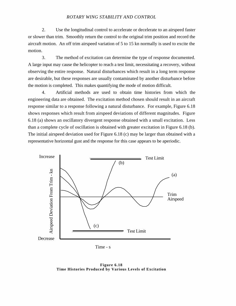
ROTARY WING STABILITY AND CONTROL
2. Use the longitudinal control to accelerate or decelerate to an airspeed faster
or slower than trim. Smoothly return the control to the original trim position and record the
aircraft motion. An off trim airspeed variation of 5 to 15 kn normally is used to excite the
motion.
3. The method of excitation can determine the type of response documented.
A large input may cause the helicopter to reach a test limit, necessitating a recovery, without
observing the entire response. Natural disturbances which result in a long term response
are desirable, but these responses are usually contaminated by another disturbance before
the motion is completed. This makes quantifying the mode of motion difficult.
4. Artificial methods are used to obtain time histories from which the
engineering data are obtained. The excitation method chosen should result in an aircraft
response similar to a response following a natural disturbance. For example, Figure 6.18
shows responses which result from airspeed deviations of different magnitudes. Figure
6.18 (a) shows an oscillatory divergent response obtained with a small excitation. Less
than a complete cycle of oscillation is obtained with greater excitation in Figure 6.18 (b).
The initial airspeed deviation used for Figure 6.18 (c) may be larger than obtained with a
representative horizontal gust and the response for this case appears to be aperiodic.
Airs
peed
Dev
iatio
n F
rom
Trim
- k
n
Increase
Decrease
Time - s
(b)
(c)
(a)
Test Limit
Test Limit
TrimAirspeed
Figure 6.18Time Histories Produced by Various Levels of Excitation

FORWARD FLIGHT LONGITUDINAL STABILITY, CONTROL,
AND FLYING QUALITIES
6.4.4.2 TEST TECHNIQUE
1. Stabilize at the desired trim airspeed (these tests can be conducted at
trimmed conditions other than level flight), and reduce all control forces to zero. Do not
retrim control forces or move the collective during the test.
2. Record trim conditions. Assure the ability to return the control to trim after
exciting the response.
3. Determine if a long term response results from a natural disturbance. With
the controls either fixed or free, note the open loop aircraft response. If no aircraft
response is observed, an artificial excitation is used.
4. Excite the aircraft using an artificial input. It may be necessary to try several
different inputs to find the most representative aircraft response Do not retrim any control
forces and keep the collective constant during the response.
5. If the aircraft is flown hands off, obtain control free responses following the
excitation. The controls are released at trim so the subsequent control motions indicate the
effect of attitude changes and gravity force acting during the response.
6. Record the resulting mode of motion using cockpit data and automatic
recording systems. Cockpit displayed airspeed or altitude is recorded at selected time
increments. Start the stop watch at the completion of the excitation or at a predetermined
airspeed. The zero time reference point is arbitrary. Use small enough time intervals to
define the shape of irregular responses.
7. The resulting mode of motion may not be a classical single axis response.
Use lateral cyclic and directional control as necessary to maintain a single axis response for
the initial excitation. If you find the lateral-directional inputs are significant, record a time
history of the aircraft response with all controls fixed.
8. For hand held data, a plot of airspeed at regular intervals (5 to 10 s)
adequately defines the response. An alternate method is to record peak (maximum and
minimum) airspeeds and determine the period by timing the response as the helicopter
passes through the trim airspeed.
ROTARY WING STABILITY AND CONTROL
6.4.4.3 DATA REQUIRED
Vo, HPo, Vv, θ, FC, To, Q, NR, cockpit control positions.
Following the excitation, record airspeed, altitude, or pitch attitude as a function of
time. Use automatic recording systems to simplify this task.
6.4.4.4 TEST CRITERIA
1. Ball centered, balanced flight.
2. Longitudinal control fixed (at trim) and/or free.
3. Collective fixed.
6.4.4.5 DATA REQUIREMENTS
1. Stabilize 15 s prior to taking data.
2. Trim Vo ± 2 kn.
3. HPo ± 1000 ft of the target test altitude.
4. φ ± 2˚.
5. Ball centered.
6.4.4.6 SAFETY CONSIDERATIONS/RISK MANAGEMENT
Observe the normal operating limitations. A thorough knowledge of airspeed and
attitude limitations is essential. Recovery must be initiated in sufficient time to prevent limit
overshoot. Conduct tests at a safe operating altitude over terrain suitable for forced
landings. Maintain proper lookout procedures. Consider using a chase aircraft and sole
use airspace. Wear parachutes.
6.4.5 Short Term Dynamic Stability
The longitudinal short term mode is the mechanism used to make pitch attitude
changes. Only small pitch attitude changes from unaccelerated flight conditions are
classified under short term dynamic stability. Short term longitudinal responses resulting
from gust inputs are evaluated and discussed under the classification of gust responses.
The purpose of the test is to determine the characteristics of the short term response due to
longitudinal control inputs and to evaluate the pilot's ability to make small attitude changes.
FORWARD FLIGHT LONGITUDINAL STABILITY, CONTROL,
AND FLYING QUALITIES
6.4.5.1 EXCITATION METHODS
The following excitation methods are used for longitudinal short term dynamic
tests:
1. Pulse and doublet type cyclic inputs are used to evaluate the short term
response.
2. Doublet inputs minimize inadvertent excitation of the long term response. A
pulse input causes an attitude and airspeed change which tends to initiate a long term
response and contaminate the short term response data.
3. A frequency sweep is accomplished first by applying sinusoidal inputs of
constant amplitude at a series of frequencies and observing the pitch response. The short
term frequency is found by starting with a low frequency input and increasing the input
frequency while comparing the pitch attitude response. The short term frequency is
indicated by a maximum amplitude of the pitch response to the inputs. Data are taken using
doublets at the noted short term frequency with sufficient amplitude to disturb the pitch
attitude.
4. Mission suitability tasks, such as changing the gun-target line, are evaluated
using the required closed loop inputs.
6.4.5.2 TEST TECHNIQUE
1. Establish trim conditions and record trim data.
2. Conduct a frequency sweep at the trim airspeed to determine the short term
frequency.
3. Make a doublet input at this frequency and record a time history of the pitch
attitude response. Control fixtures and control position indicators are helpful for making
good doublet inputs.
4. Investigate the ease or difficulty in making small, precise pitch attitude
changes. The attitude indicator and/or grease pencil marks on the windscreen are helpful.
Determine if pilot corrections are required for overshoots in pitch, which might compound
problems of establishing a target line.
5. Many helicopters are well damped. Do not waste time trying to document a
problem which does not exist.
ROTARY WING STABILITY AND CONTROL
6.4.5.3 DATA REQUIRED
Vo, HPo, Vv, θ, FC, To, Q, NR, cockpit control positions. Time history of pitch
attitude response to the excitation.
6.4.5.4 TEST CRITERIA
1. Wings level, ball centered, balanced flight.
2. Collective fixed.
6.4.5.5 DATA REQUIREMENTS
1. Stabilize 15 s prior to taking data.
2. Trim Vo ± 2 kn.
3. HPo ± 1000 ft of the target test altitude.
6.4.5.6 SAFETY CONSIDERATIONS/RISK MANAGEMENT
Observe normal operating limitations. Conduct tests at a safe operating altitude
over terrain suitable for forced landings. Maintain proper lookout procedures. Maintain
situational awareness. Consider using a chase aircraft and sole use airspace. Wear
parachutes.
A thorough knowledge of airspeed and attitude limitations is essential. Recovery
must be initiated in sufficient time to prevent exceeding a test limit. The use of control
fixtures must be thoroughly briefed and practiced.
6.4.6 Control Response
Static and maneuvering stability tests are primarily concerned with evaluating the
stability characteristics which keep the helicopter at a trim condition and the cues provided
to the pilot of an off trim condition. Control response testing involves evaluating the
aircraft response caused by rotor system moments generated from cyclic, pedal, and
collective inputs. The purpose of these tests is to evaluate the aircraft response to flight
control input. The tests are conducted by applying control step inputs of incrementally
increasing size against a fixture and recording a time history of the aircraft response.
Definitions of control response terms are shown on Figure 6.19.
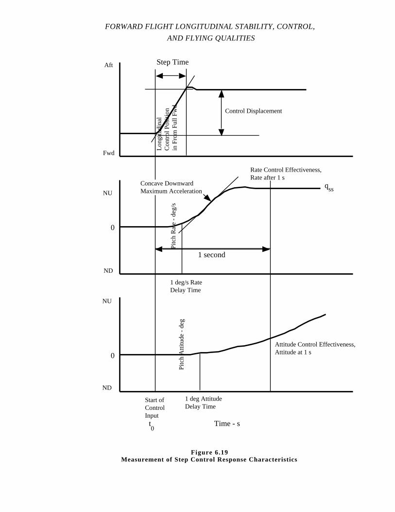
FORWARD FLIGHT LONGITUDINAL STABILITY, CONTROL,
AND FLYING QUALITIES
Time - s
Step Time
Control Displacement
Pitc
h R
ate
- de
g/s
Fwd
NU
ND
0
qss
1 second
Rate Control Effectiveness,Rate after 1 s
Attitude Control Effectiveness,Attitude at 1 s
1 deg AttitudeDelay Time
1 deg/s RateDelay Time
t0
Start ofControlInput
Pitc
h A
ttitu
de -
deg
0
NU
ND
Aft
Long
itudi
nal
Con
trol
Pos
ition
in F
rom
Ful
l Fw
dConcave DownwardMaximum Acceleration
Figure 6.19Measurement of Step Control Response Characteristics

ROTARY WING STABILITY AND CONTROL
6.4.6.1 TEST TECHNIQUE
1. Stabilize in wings level, ball centered, coordinated flight at the desired trim
conditions. Maintain constant collective during the control response. Record trim data.
2. Set the control fixture for the desired displacement magnitude and direction.
The control input direction and size is verbally and visually (if possible) verified between
the pilot and copilot/engineer. Start with small displacements and always use an
incremental buildup procedure.
3. A suggested voice procedure is: “Data ON, standby for a (displacement
magnitude), (direction of input), (control) input on three. Thousand one, thousand two,
thousand three.” For example: “Data ON, standby for a one inch forward longitudinal step
input on three. Thousand one, thousand two, thousand three.”
4. Turn ON the data system prior to the countdown, allowing the initial
conditions to be recorded.
5. After the countdown, a crisp step input is made against the fixture. Hold
the input control rigidly against the fixture while maintaining all other controls fixed. When
making cyclic inputs, use only wrist action and not the entire arm.
6. Do not attempt to decouple responses in other axes. The response lasts only
seconds and attempts to decouple usually result in contaminating the desired response.
7. Hold the input control fixed and initiate recovery when a steady state rate is
obtained or a predetermined flight limit is reached. When you have the required data or a
limit is approached, recover and secure the automatic data recorder.
8. Restabilize at the trim conditions and repeat the procedure for incrementally
larger inputs until the desired control input magnitude is obtained, or a predetermined flight
limit is reached.
9. An incremental buildup in step input size is mandatory. Practice and
experience are necessary for good results.
6.4.6.2 DATA REQUIRED
Vo, HPo, θ, FC, To, Q, NR, cockpit control positions, control input size and
direction.
Automatic recording systems are required for data collection. A time history of the
longitudinal control position, pitch attitude, pitch rate, and pitch acceleration are the
minimum essential data traces.
FORWARD FLIGHT LONGITUDINAL STABILITY, CONTROL,
AND FLYING QUALITIES
6.4.6.3 TEST CRITERIA
1. Wings level, ball centered, balanced flight.
2. Collective fixed.
6.4.6.4 DATA REQUIREMENTS
1. Stabilize 15 s prior to taking data.
2. Trim Vo ± 2 kn.
3. HPo ± 1000 ft of the target test altitude.
4. The data system must be capable of recording data with a 10 Hz frequency
response.
6.4.6.5 SAFETY CONSIDERATIONS/RISK MANAGEMENT
Observe normal operating limitations. Conduct tests at a safe operating altitude
over terrain suitable for forced landings. Maintainproper lookout doctrine. Maintain
situational awareness. Consider using a chase aircraft and sole use airspace. Wear
parachutes.
A thorough knowledge of airspeed and attitude limitations is essential. Initiate
recovery in sufficient time to prevent exceeding a test limit. The use of the control fixture
must be thoroughly briefed and practiced.
Observe the response during the maneuver; however, analyze theresponse and
make comments both oral and written after the recovery is complete.
6.4.7 Gust Response
Gust response is a dynamic mode of motion which is treated in a separate category
in the discussion and evaluation of flight dynamics. In general terms, the gust response
relates to the quality of the ride. This encompasses the combination of instantaneous linear
and angular acceleration changes during and immediately following flying through an
atmospheric disturbance. Different characteristics are emphasized in the evaluation of the
short term and gust responses. Pitch attitude and pitch rate changes are of primary
ROTARY WING STABILITY AND CONTROL
importance for the short term dynamic response. Gust responses could result in pitch rate
and attitude changes. The pilot could correct using the short term longitudinal mode but
this is just one consideration with the gust response. The gust response evaluation includes
determining the difficulty of maintaining a desired flight path in turbulence.
6.4.7.1 EXCITATION METHODS
1. Flight in actual turbulence is the best method of evaluation.
2. Pulse inputs of varying magnitudes and duration can be used to simulate
gusts. Using a one inch control deflection for one half second as required by MIL-H-
8501A could give excessive response with high hinge offset.
3. Simulated gusts can also be obtained by making inputs directlyinto the
flight control system using the automatic flight control systems.
6.4.7.2 TEST TECHNIQUE
1. Record flight through natural turbulence.
2. If natural turbulence is not available, pulse inputs in the longitudinal axis are
substituted. Generally, a one inch aft longitudinal pulse input held for one-half second is
acceptable. Following the pulse, maintain controls fixed and record the resulting aircraft
response.
6.4.7.3 DATA REQUIRED
Vo, HPo, Vv, θ, FC, To, Q, NR, cockpit control positions.
Following the excitation, record airspeed, altitude, pitch attitude, pitch rate, and CG
normal acceleration as a function of time. Automatic recording systems are required to
obtain meaningful test data. AFCS or SAS actuator time histories indicate the system
response and show how close the system is to saturation.
6.4.7.4 TEST CRITERIA
1. Wings level, ball centered, balanced flight.
2. Collective fixed.
FORWARD FLIGHT LONGITUDINAL STABILITY, CONTROL,
AND FLYING QUALITIES
6.4.7.5 DATA REQUIREMENTS
1. Controls fixed for natural excitation.
2. For pulse excitation:
a. Trim Vo ± 2 kn.
b. HPo ± 1000 ft of the target test altitude.
c. φ ± 3 degrees bank angle.
d. Pulse duration 0.5 s ± 0.1 s.
6.4.7.6 SAFETY CONSIDERATIONS/RISK MANAGEMENT
Observe normal operating limitations. Conduct tests at a safe operating altitude
over terrain suitable for forced landings. Maintain proper lookout procedures. Maintain
situational awareness. Consider using a chase aircraft and sole use airspace. Wear
parachutes.
A thorough knowledge of airspeed and attitude limitations is essential. Initiate
recovery in sufficient time to prevent exceeding a test limit. The use of the control fixture
must be thoroughly briefed and practiced.
6.5 DATA REDUCTION
Data reduction requirements for these tests are limited to application of instrument
corrections to the recorded data. Airspeed and altitude data are corrected for both
instrument and position errors. Automatic data recording systems normally include total
instrumentation system corrections in reducing a flight tape (or telemetry) raw data into
engineering units. Most quantitative information required for longitudinal flying qualities
tests is read from time histories of selected data parameters.
6.5.1 Trimmed Control Positions
Plot longitudinal cyclic position versus calibrated airspeed (Figure 6.20).
Normally, pitch attitude, lateral, directional, and collective control positions are presented
as well.
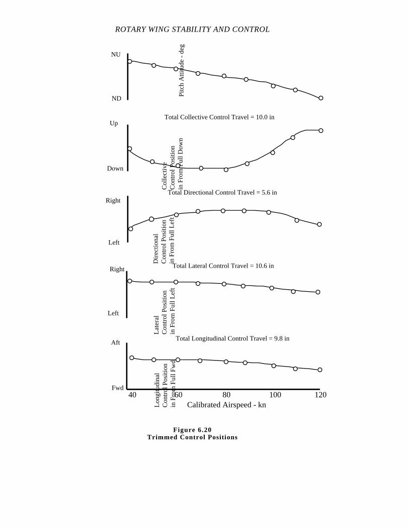
ROTARY WING STABILITY AND CONTROL
Calibrated Airspeed - kn80 100 1206040
Late
ral
Con
trol
Pos
ition
in F
rom
Ful
l Lef
t
Aft
Fwd
Long
itudi
nal
Con
trol
Pos
ition
in F
rom
Ful
l Fw
d
Dire
ctio
nal
Con
trol
Pos
ition
in F
rom
Ful
l Lef
t
Right
Left
Col
lect
ive
Con
trol
Pos
ition
in F
rom
Ful
l Dow
n
Left
Right
Down
Up
Pitc
h A
ttitu
de -
deg
ND
NU
Total Collective Control Travel = 10.0 in
Total Directional Control Travel = 5.6 in
Total Lateral Control Travel = 10.6 in
Total Longitudinal Control Travel = 9.8 in
Figure 6.20Trimmed Control Positions
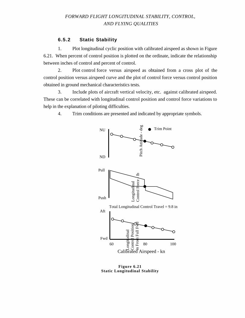
FORWARD FLIGHT LONGITUDINAL STABILITY, CONTROL,
AND FLYING QUALITIES
6.5.2 Static Stability
1. Plot longitudinal cyclic position with calibrated airspeed as shown in Figure
6.21. When percent of control position is plotted on the ordinate, indicate the relationship
between inches of control and percent of control.
2. Plot control force versus airspeed as obtained from a cross plot of the
control position versus airspeed curve and the plot of control force versus control position
obtained in ground mechanical characteristics tests.
3. Include plots of aircraft vertical velocity, etc. against calibrated airspeed.
These can be correlated with longitudinal control position and control force variations to
help in the explanation of piloting difficulties.
4. Trim conditions are presented and indicated by appropriate symbols.
Calibrated Airspeed - kn
Aft
Fwd
Long
itudi
nal
Con
trol
Pos
ition
in F
rom
Ful
l Fw
d
Pull
Push
Long
itudi
nal
Con
trol
For
ce -
lbP
itch
Atti
tude
- d
eg
NU
ND
Trim Point
80 10060
Total Longitudinal Control Travel = 9.8 in
Figure 6.21Static Longitudinal Stabil ity
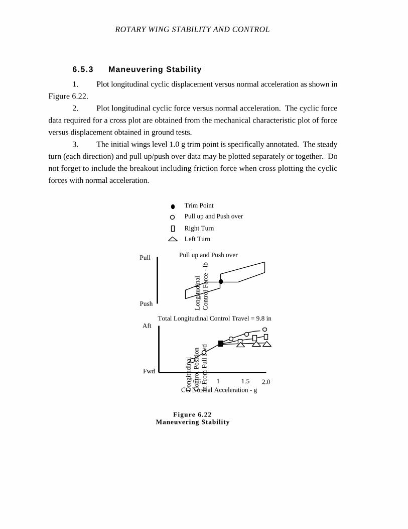
ROTARY WING STABILITY AND CONTROL
6.5.3 Maneuvering Stability
1. Plot longitudinal cyclic displacement versus normal acceleration as shown in
Figure 6.22.
2. Plot longitudinal cyclic force versus normal acceleration. The cyclic force
data required for a cross plot are obtained from the mechanical characteristic plot of force
versus displacement obtained in ground tests.
3. The initial wings level 1.0 g trim point is specifically annotated. The steady
turn (each direction) and pull up/push over data may be plotted separately or together. Do
not forget to include the breakout including friction force when cross plotting the cyclic
forces with normal acceleration.
Aft
Fwd
Long
itudi
nal
Con
trol
Pos
ition
in F
rom
Ful
l Fw
d
Pull
Push
Long
itudi
nal
Con
trol
For
ce -
lb
1 2.0
Total Longitudinal Control Travel = 9.8 in
Pull up and Push over
Pull up and Push over
Right Turn
Left Turn
Trim Point
1.50.5CG Normal Acceleration - g
Figure 6.22Maneuvering Stability
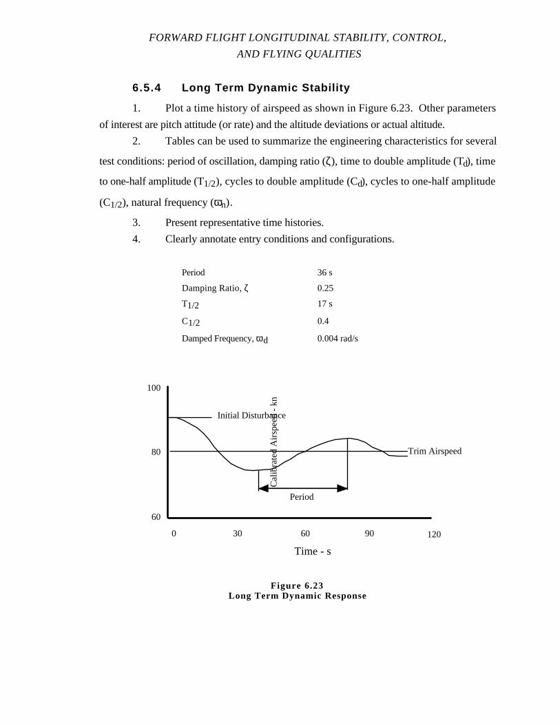
FORWARD FLIGHT LONGITUDINAL STABILITY, CONTROL,
AND FLYING QUALITIES
6.5.4 Long Term Dynamic Stability
1. Plot a time history of airspeed as shown in Figure 6.23. Other parameters
of interest are pitch attitude (or rate) and the altitude deviations or actual altitude.
2. Tables can be used to summarize the engineering characteristics for several
test conditions: period of oscillation, damping ratio (ζ), time to double amplitude (Td), time
to one-half amplitude (T1/2), cycles to double amplitude (Cd), cycles to one-half amplitude
(C1/2), natural frequency (ωn).
3. Present representative time histories.
4. Clearly annotate entry conditions and configurations.
Period 36 s
Damping Ratio, ζ 0.25
T1/2 17 s
C1/2 0.4
Damped Frequency, ωd 0.004 rad/s
Time - s
Cal
ibra
ted
Airs
peed
- k
n
Initial Disturbance
Period
80
100
60
30 60 90 1200
Trim Airspeed
Figure 6.23Long Term Dynamic Response
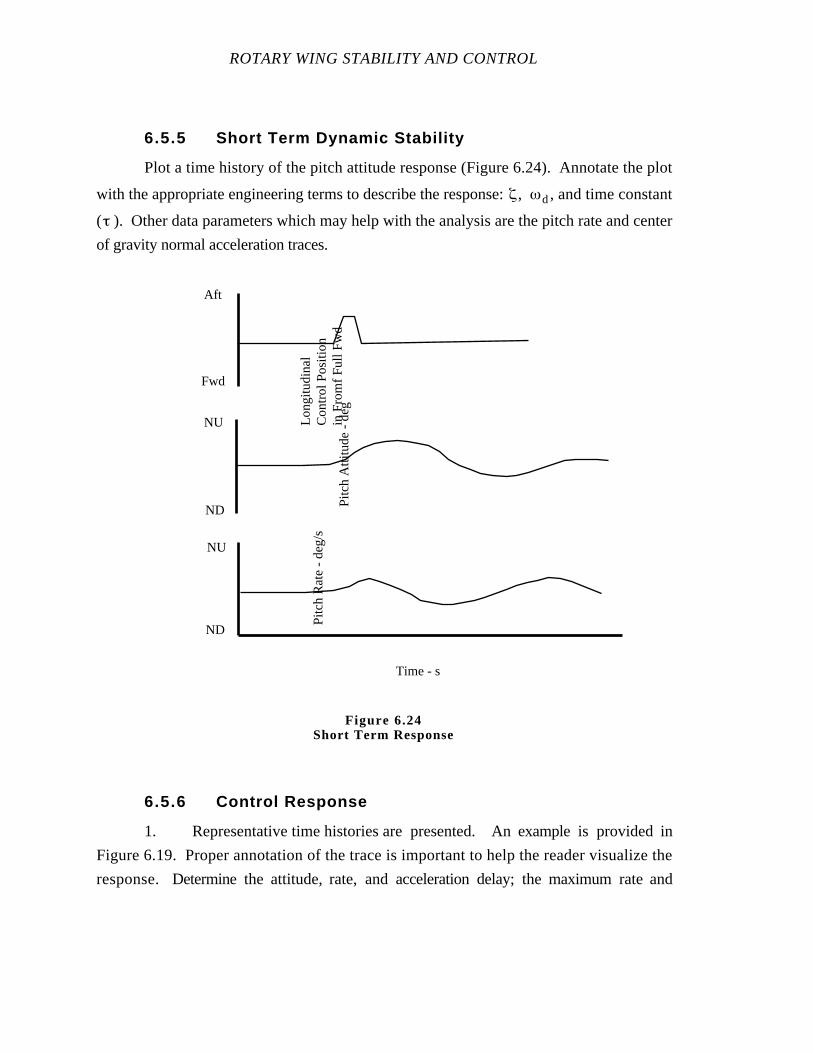
ROTARY WING STABILITY AND CONTROL
6.5.5 Short Term Dynamic Stability
Plot a time history of the pitch attitude response (Figure 6.24). Annotate the plot
with the appropriate engineering terms to describe the response: , d, and time constant
( ). Other data parameters which may help with the analysis are the pitch rate and center
of gravity normal acceleration traces.
6.5.6 Control Response
1. Representative time histories are presented. An example is provided in
Figure 6.19. Proper annotation of the trace is important to help the reader visualize the
response. Determine the attitude, rate, and acceleration delay; the maximum rate and
Long
itudi
nal
Con
trol
Pos
ition
in F
rom
f Ful
l Fw
d
Fwd
Aft
Pitc
h A
ttitu
de -
deg
ND
NU
Time - s
NU
ND
Pitc
h R
ate
- de
g/s
Figure 6.24Short Term Response

FORWARD FLIGHT LONGITUDINAL STABILITY, CONTROL,
AND FLYING QUALITIES
acceleration; the time to 63% of steady state rate; and the attitude change after 1 s. Note the
time at which the step input was made and the time at which a recovery was initiated.
Present a summary of control response characteristics (Figure 6.25).
2. Tables are helpful in presenting data from various responses.
0 1 212
NU
ND
Longitudinal Control Input - in
Atti
tude
Cha
nge
Afte
r 1
s -
deg
Max
imum
Ang
ular
Acc
eler
atio
n -
deg/
s/sNU
ND
ND
NU
Max
imum
Pitc
hR
ate
- de
g/s
Tim
e to
63%
Max
imum
Rat
e -
s
0
1
2
-10
0
10
40
-40
0
10
-10
0
AftFwd
Figure 6.25Control Response Characteristics
ROTARY WING STABILITY AND CONTROL
6.5.7 Gust Response
1. Cockpit data of airspeed and attitude changes suffice for qualitative
evaluations. The g meter in the cockpit does not display accurately the short duration
accelerations felt by the pilot.
2. A time history of the pilot seat acceleration or the aircraft CG acceleration
can be useful when shown with the flight control displacements and attitude changes
(Figure 6.26).
3. Time histories of the stability system actuator positions may also be
included.
4. Qualitative observations are the principal data obtained in the test.
Quantitative data are used to reinforce qualitative comments.
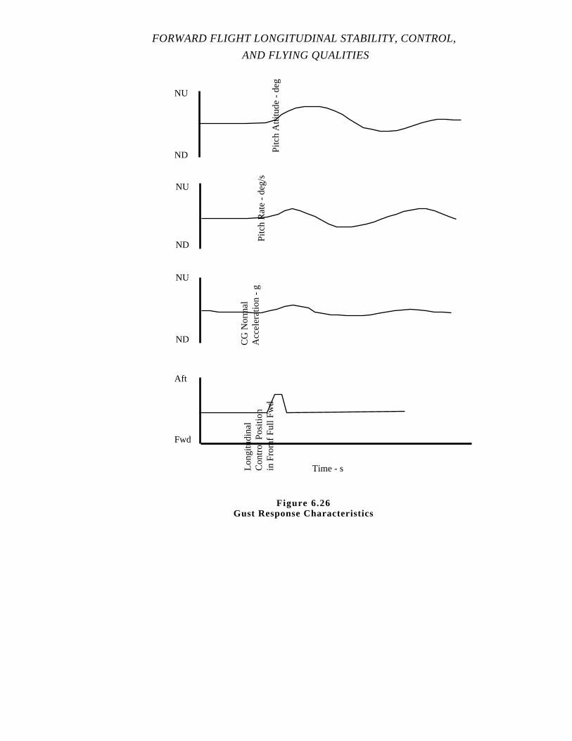
FORWARD FLIGHT LONGITUDINAL STABILITY, CONTROL,
AND FLYING QUALITIES
Pitc
h A
ttitu
de -
deg
ND
NU
NU
ND
Pitc
h R
ate
- de
g/s
Time - sLong
itudi
nal
Con
trol
Pos
ition
in F
rom
f Ful
l Fw
d
Fwd
Aft
ND
NU
CG
Nor
mal
Acc
eler
atio
n -
g
Figure 6.26Gust Response Characteristics

ROTARY WING STABILITY AND CONTROL
6.6 DATA ANALYSIS
6.6.1 Trimmed Control Positions
The following considerations are generally included in the analysis oftrimmed
control position in forward flight data:
1. Were there adequate control margins?
2. Was forward cyclic required with increasing airspeed?
3. Are the control position changes with changes in power excessive?
4. Could forces be trimmed to zero?
5. What were pitch attitude changes with airspeed?
6. Was field-of-view adequate?
7. Were there objectionable vibrations?
8. Was there coupling between the pitch, yaw and roll axes?
9. Could small precise collective changes be made?
6.6.2 Static Stability
The following considerations are generally included in the analysis of static
longitudinal stability test data:
1. Positive static stability is indicated by forward longitudinal cyclic position
and forces with increasing airspeed.
2. Positive static stability causes the aircraft to tend to return to trim following
a disturbance. The force and position provide cues to off trim airspeed. Does the data
substantiate the pilot's qualitative opinion concerning ease of trimming the aircraft?
3. Is there a trim speed band within which there are no force or displacement
cues for off trim conditions?
4. Discuss gradients (in/kn, lb/kn) and not the strength of the static stability.
The longitudinal cyclic position required is not only a function of the pitching moments
being generated, but also is influenced by the control system characteristics.

FORWARD FLIGHT LONGITUDINAL STABILITY, CONTROL,
AND FLYING QUALITIES
6.6.3 Maneuvering Stability
The following considerations are generally included in the analysis of maneuvering
stability test data:
1. Positive maneuvering stability is indicated by an aft longitudinal cyclic
displacement with increasing normal acceleration. What is the sign of the stability and how
is it indicated?
2. The cyclic forces and displacements provide a physical cue to the pilot of
normal acceleration and pitch rate (turn rate). Were these cues available and what is your
opinion of their value?
3. Was there any tendency to exceed the g envelope of the aircraft? This might
limit the usable g envelope.
6.6.4 Long Term Dynamic Stability
The following considerations are generally included in the analysis of long term
dynamic stability test data:
1. How easy or difficult was it to excite the long term response?
2. In engineering terms, how do you describe the aircraft mode of motion?
Use the period, damping ratio, time to half amplitude and time to double amplitude to tell
the reader what you saw.
3. How does this motion influence the pilot's ability to perform mission tasks?
The significance of the long term response is how it degrades or helps the pilot perform a
specific task. An evaluation is made of the pilot effort required to suppress or correct the
airspeed, attitude, and altitude variations about trim.
ROTARY WING STABILITY AND CONTROL
6.6.5 Short Term Dynamic Stability
The following considerations are generally included in the analysis of short term
dynamic stability test data:
1. Can the pilot make small precise pitch attitude changes?
2. In reference to the time history of the pitch attitude change, the discussion
includes the number of pitch oscillations (overshoots), the frequency and magnitude of the
cyclic inputs required to obtain the desired performance, the excitation of other modes of
motion, and the approximate damping ratio if an estimate (or analysis) can be obtained.
3. Time histories of mission tasks are sometimes helpful in discussing problem
areas.
6.6.6 Control Response
The following considerations are generally included in the analysis of longitudinal
control response test data:
1. An abundance of quantitative data can be taken from the response time
histories. The parameters chosen and presented support your opinion of how well or
poorly the aircraft responds to control inputs. Parameters which define the amount of
control moment available are: rate control effectiveness; attitude control effectiveness; and
steady state angular velocity. Quantities which can be used in discussing the quality of the
response or how it got to the observed steady state rate are the: angular accelerations delay
time; initial angular acceleration; inflection time; and response time constant. Use these data
as an integral part of your discussions.
2. Did the aircraft respond adequately to perform the assigned task?
a. Were the steady state rates adequate?
b. Was the response predictable?
c. Was the response consistent?
d. Were there any over controlling problems?

FORWARD FLIGHT LONGITUDINAL STABILITY, CONTROL,
AND FLYING QUALITIES
6.6.7 Gust Response
The following considerations are generally included in the analysis of gust response
test data:
1. How could the ride be described? Jerky, smooth, loping, etc.? Was the
ride comfortable or uncomfortable?
2. What were the pitch, roll, and yaw attitude changes and airspeed changes?
3. Did the aircraft tend to return to the original trim condition?
4. How much pilot effort was required to return the aircraft to the trim
condition?
6.7 MISSION SUITABILITY
The suitability of the test aircraft for the intended mission is the ultimate reason for
conducting any handling qualities test. Each of the specific tests, detailed in the previous
sections, provides some information in accessing suitability. Longitudinal trimmed control
positions in forward flight provides detailed information about control margins, linearities,
discontinuities and gradients which assist the pilot in determining overall suitability. Static
longitudinal stability characteristics are good indicators of pilot workload requirements to
maintain a desired forward flight speed and the tendencies of the aircraft once disturbed.
Maneuvering stability characteristics determine many aspects of the pilot qualitative
comments relative to aggressive flight path changes. The long term dynamicstability
character in large part determines cruise flying qualities. Short term dynamics in the
longitudinal axis are a big factor in how quickly and accurately the pilot can point the
aircraft in high gain tasks such as aerial refueling or target tracking. Control response tests
quantitatively document the pilots qualitative comments concerning aircraft responsiveness.
Gust response evaluation indicates how the crew and passengers like the ride quality.
In addition to the engineering tests, the test pilot investigates how the helicopter is
intended to be used and closely duplicates these mission tasks. Generally, knowledge of
engineering maneuver shortcomings allows the test team to design operational scenarios
which also reflect the poor characteristics. The mission of the aircraft determines the
maneuvers required to be flown. Cargo helicopters require close attention to straight and

ROTARY WING STABILITY AND CONTROL
level cruise tasks (long term dynamic stability); while attackaircraft may need special
consideration for tracking tasks (short term dynamic stability) and maneuverability
(maneuvering stability). Each test program requires a unique set of mission maneuvers.
The most important aspect of mission suitability testing is to keep the operator in
mind. How the test vehicle will be used in the field, and who will be operating the aircraft
are important factors to consider.
6.8 SPECIFICATION COMPLIANCE
General guidelines for helicopter handling qualities in the hovering and low
airspeed flight regime are contained in MIL-H-8501A. Military specifications are only a
guide. The following list identifies the paragraph number in MIL-H-8501A and a short
description of the requirement.
3.2 Longitudinal characteristics
3.2.1 Longitudinal control margin; controls and helicopter shake,
vibration, roughness
3.2.2 Hovering turns on a spot
3.2.3 Longitudinal trimmability, control jump
3.2.4 Longitudinal control force gradient
3.2.5 Quick stop, rapid acceleration
3.2.6 Limit control force
3.2.7 Breakout force
3.2.8 Control coupling
3.2.9 Control response
3.2.10 Static longitudinal stability
3.2.10.1 Critical center of gravity
3.2.10.2 Trim change in climbs and descents
3.2.11 Dynamic longitudinal stability
3.2.11.1 Dynamic control response
3.2.11.2 Gust response
3.2.12 Control response, normal acceleration
3.2.13 Control power
3.2.14 Control response damping

FORWARD FLIGHT LONGITUDINAL STABILITY, CONTROL,
AND FLYING QUALITIES
Additional requirements are included in the military specification which relate to
boosted controls, failure modes, automatic stabilization equipment, and vibrations. Some
of these paragraphs may apply to specific helicopters equipped with advanced flight control
systems or highly augmented systems.
MIL-H-8501A is old and under most circumstances supplemented with additional
detailed specifications listed in the procurement documents. These must be researched
thoroughly and carefully to ensure contractual compliance and a complete evaluation.
A new military specification has been under development for years, but to this date
not finalized. This new specification may include frequency domain tests to evaluate higher
order aircraft flight control systems expected in future helicopters.
6.9 GLOSSARY
6.9.1 Notations
A1s Lateral cyclic pitch angle, shaft referenced
a1s Longitudinal flapping angle, shaft referenced
AFCS Automatic Flight Control System
B Damping constant
b Number of blades
B1s Longitudinal cyclic pitch angle, shaft referenced
b1s Lateral flapping angle, shaft referenced
B 1s Time rate of change of longitudinal cyclic pitch angle, shaft
referenced
C1/2 Cycles to one-half amplitude
Cd Cycles to double amplitude
CF Centrifugal force
CG Center of gravity
Df Fuselage drag force
e Base of natural logarithm, flapping hinge offset
FC Fuel count
Fq Pitch input
ROTARY WING STABILITY AND CONTROL
Fx Force in the x direction
g Gravity
H Rotor hub force, ⊥ to shaft
h Height of hub above CG
h' Longitudinal distance between the rotor shaft and the CGHPo Observed pressure altitude
HQR Handling Qualities Rating
Hz Hertz (cycles per second)
in Inch
is Stabilizer incidenceIyy Moment of inertia about y axis, pitch moment of inertia
K Spring constant
kn Knot
Lt Tail lift
lt Distance from the tail to the CG
M Net moment about y axis, Pitch moment
m Mass
Mα Pitch moment due to angle of attackMB1s Pitch moment due to longitudinal cyclic pitch angle
MCG Moment about CGMCGf+t Pitch moment due to the aerodynamic forces on the fuselage/tail
MH Pitch moment due to rotor hub force
MH—
Average pitch moment due to rotor hub force for b blades
Mq Pitch moment due to pitch rateMθC Pitch moment due to collective pitch angle
MS Blade mass moment
MSL Maneuvering stability level
Mu Pitch moment due to longitudinal velocity
Mw Pitch moment due to vertical velocity
Mw Pitch moment due to vertical acceleration
n Normal acceleration, Normal load factor
Ng Engine gas generator speed
NR Main rotor speed
nss Steady state normal acceleration
p Angular velocity about x axis, Roll rate
FORWARD FLIGHT LONGITUDINAL STABILITY, CONTROL,
AND FLYING QUALITIES
PIO Pilot induced oscillation
Q Engine torque
q Angular velocity about y axis, Pitch rate
qss Steady state pitch rate
˙q Second time derivative of pitch rate
q Angular acceleration about y axis
R Resultant aerodynamic force
r Angular velocity about z axis, Radius along blade, Yaw rate
rad Radian
s Second
SAS Stability Augmentation System
SCAS Stability Control Augmentation System
T Thrust
t Time
T1/2 Time to one-half amplitude
Td Time to double amplitude
To Observed temperature
TPP Tip path plane
u Translational velocity component along x axis
u0 Initial velocity
˙u Time rate of change of linear acceleration along x axis
u Linear acceleration along x axis
V Velocity, Free stream velocity, Relative velocity
VAR Vibration Assessment Rating
VH Maximum level flight airspeed
Vhor Velocity in the horizontal plane
VNE Velocity never exceed
Vo Observed airspeed
Vv Vertical velocity
w Translational velocity component along z axis
w0 Initial velocity component along z axis
wQS Quasi-static vertical velocity
˙w Time rate of change of linear acceleration along z axis
w Linear acceleration along z axis
X Resultant force in x direction

ROTARY WING STABILITY AND CONTROL
x Orthogonal direction along longitudinal axis of the aircraft; Distance
along x axisXB1s Longitudinal force due to longitudinal cyclic pitch angle
Xq Longitudinal force due to pitch rateXθC Longitudinal force due to collective pitch angle
Xu Longitudinal force due to longitudinal velocity
Xw Longitudinal force due to vertical velocity
˙x Time rate of change of velocity in x direction, Acceleration along x
axis
x Time rate of change of x, Velocity in x direction
y Orthogonal direction along lateral axis of the aircraft
Z Resultant force in z direction
z Orthogonal direction along vertical axis of the aircraftZB1s Vertical force due to longitudinal cyclic pitch angle
Zq Vertical force due to pitch rateZθC Vertical force due to collective pitch angle
Zu Vertical force due to longitudinal velocity
Zw Vertical force due to vertical velocity
6.9.2 Greek Symbols
α (alpha) Angle of attack
αBE Blade element angle of attack
αT Tail angle of attack
˙ Time rate of change of angle of attack
β (beta) Flapping angle, Sideslip angle
δ (delta) Control
δC Collective control
δLONG Longitudinal control
δth Throttle control
δ Rate of change of control
φ (phi) Roll angle
γ (gamma) Flight path angle
γ0 Initial flight path angle˙ Time rate of change of flight path angle
λ (lambda) Characteristic root
FORWARD FLIGHT LONGITUDINAL STABILITY, CONTROL,
AND FLYING QUALITIES
θ (theta) Pitch angle, shaft angle
θC Collective pitch angle
θTR Tail rotor pitch angle
θ Pitch acceleration
θ Rate of change of pitch angle
θ QS Quasi-static rate of change of pitch angle
τ (tau) Time constant
ωd (omega) Damped frequency
ωn Natural frequency
ψ (psi) Blade azimuth angle, Phase angle, Yaw angle
ζ (zeta) Damping ratio
Ω (Omega) Rotor angular velocity
6.10 REFERENCES
1. Johnson, W.Helicopter Theory, Princeton University Pres., 1980.
2. Military Specification, "Helicopter Flying and Ground Handling Qualities;
General Requirements For", MIL-H-8501A, with Amendment 1, 3 April, 1962.
3. Naval Test Pilot School Flight Test Manual,Helicopter Stability and
Control, USNTPS-FTM-No. 101, U. S. Naval Test Pilot School, Patuxent River, MD, 10
June 1968, reprinted February 1978.
4. Naval Test Pilot School Flight Test Manual,Helicopter Stability and
Control, Theory and Flight Test Techniques, USNTPS-FTM-No. 105, U. S. Naval Test
Pilot School, Patuxent River, MD, November 1983, Preliminary Edition.
5. Prouty, R. W., Practical Helicopter Aerodynamics, PJS Publications, Inc.,
1982.

ROTARY WING STABILITY AND CONTROL
6. Prouty, Raymond W.,Helicopter Performance, Stability, and Control,
PWS Publishers, Boston, MA, 1986.
7. Wiesner, W. and Kohler, G., Tail Rotor Performance in Presence of Main
Rotor, Ground, and Winds, J.A.H.S., Vol. 15, No. 3, July 1974.
CHAPTER SEVEN
FORWARD FLIGHT LATERAL-DIRECTIONAL STABILITY, CONTROL, AND
FLYING QUALITIES
PAGE
7.1 INTRODUCTION 7.1
7.2 PURPOSE OF TEST 7.2
7.3 THEORY 7.2
7.3.1 Summary of Quasi-Static Rotor Characteristics 7.2
7.3.2 Equations of Motion 7.4
7.3.3 Lateral-Directional Derivatives 7.7
7.3.3.1 Yaw Moment Due to Lateral Velocity, Directional
Stability 7.11
7.3.3.2 Yaw Moments Due to Yaw Rate, Yaw Damping 7.14
7.3.3.3 Yaw Moment Due to Roll Rate 7.16
7.3.3.4 Yaw Moment Due to Tail Rotor Pitch Angle, Directional
Control 7.18
7.3.3.5 Yaw Moment Due to Lateral Cyclic Pitch Angle 7.20
7.3.3.6 Roll Moment Due to Lateral Velocity, Dihedral Effect 7.22
7.3.3.7 Roll Moment Due to Yaw Rate 7.24
7.3.3.8 Roll Moment Due to Roll Rate, Roll Damping 7.26
7.3.3.9 Roll Moment Due to Lateral Cyclic Pitch Angle,
Lateral Control 7.28
7.3.3.10 Roll Moment Due to Tail Rotor Pitch Angle 7.30
7.3.3.11 Side Force Due to Lateral Velocity 7.32
7.3.3.12 Side Force Due to Yaw Rate 7.33
7.3.3.13 Side Force Due to Roll Rate 7.35
7.3.3.14 Side Force Due to Lateral Control 7.36
7.3.3.15 Side Force Due to Directional Control 7.38
7.3.3.16 Summary of Fuselage/Tail, Main Rotor, and Tail
Rotor Contributions 7.40
7.3.4 Trimmed Control Positions 7.41
ROTARY WING STABILITY AND CONTROL
7.3.5 Static Stability 7.43
7.3.5.1 Steady Lateral-Directional Characteristics 7.44
7.3.5.2 Inherent Sideslip in Forward Flight 7.44
7.3.5.3 Airspeed Position Errors in Sideslips 7.44
7.3.5.4 Steady Heading Sideslips (SHSS) 7.45
7.3.5.5 One Control Rolls 7.54
7.3.5.6 Steady Turning Flight 7.56
7.3.5.6.1 Cyclic Only Turns 7.58
7.3.5.6.2 Pedal Only Turns 7.64
7.3.5.6.3 Coordinated Turns 7.70
7.3.6 Dynamic Stability 7.71
7.3.6.1 Roll Mode 7.72
7.3.6.2 Spiral Stability 7.73
7.3.6.3 Lateral-Directional Oscillation 7.76
7.3.7 Control Response 7.83
7.3.8 Tandem Rotor Characteristics 7.85
7.3.8.1 Stability Derivatives 7.85
7.3.8.2 Dynamic Response Modes of the Unaugmented Tandem 7.88
7.4 TEST METHODS AND TECHNIQUES 7.90
7.4.1 Trimmed Control Positions 7.90
7.4.1.1 Test Technique 7.91
7.4.1.1.1 Level Flight 7.91
7.4.1.1.2 Diving Flight 7.91
7.4.1.1.3 Steady Turns 7.92
7.4.1.1.4 Climbs and Descents (Closed Loop) 7.92
7.4.1.2 Data Required 7.92
7.4.1.3 Test Criteria 7.92
7.4.1.4 Data Requirements 7.92
7.4.1.5 Safety Considerations/Risk Management 7.93
7.4.2 Static Lateral-Directional Stability (SHSS) 7.93
7.4.2.1 Test Technique 7.94
7.4.2.2 Data Required 7.95
7.4.2.3 Test Criteria 7.95
7.4.2.4 Data Requirements 7.96
7.4.2.5 Safety Considerations/Risk Management 7.96

FORWARD FLIGHT LATERAL-DIRECTIONAL STABILITY, CONTROL,
AND FLYING QUALITIES
7.4.3 Turns on One Control (TOOC) 7.97
7.4.3.1 Cyclic Only Turns 7.97
7.4.3.1.1 Test Technique 7.98
7.4.3.1.2 Data Required 7.98
7.4.3.1.3 Test Criteria 7.98
7.4.3.1.4 Data Requirements 7.99
7.4.3.1.5 Safety Considerations/Risk Management 7.99
7.4.3.2 Pedal Only Turns 7.99
7.4.3.2.1 Test Technique 7.99
7.4.3.2.2 Data Required 7.100
7.4.3.2.3 Test Criteria 7.100
7.4.3.2.4 Data Requirements 7.100
7.4.3.2.5 Safety Considerations/Risk Management 7.100
7.4.4 Spiral Stability 7.100
7.4.4.1 Test Technique 7.101
7.4.4.2 Data Required 7.101
7.4.4.3 Test Criteria 7.102
7.4.4.4 Data Requirements 7.102
7.4.4.5 Safety Considerations/Risk Management 7.102
7.4.5 Lateral-Directional Oscillation 7.102
7.4.5.1 Excitation Methods 7.102
7.4.5.2 Test Technique 7.103
7.4.5.3 Data Required 7.104
7.4.5.4 Test Criteria 7.104
7.4.5.5 Data Requirements 7.104
7.4.5.6 Safety Considerations/Risk Management 7.104
7.4.6 Control Response 7.104
7.4.6.1 Test Technique 7.105
7.4.6.2 Data Required 7.106
7.4.6.3 Test Criteria 7.106
7.4.6.4 Data Requirements 7.106
7.4.6.5 Safety Considerations/Risk Management 7.106
7.4.7 Gust Response 7.107
7.4.7.1 Test Technique 7.108
ROTARY WING STABILITY AND CONTROL
7.4.7.2 Data Required 7.108
7.4.7.3 Test Criteria 7.108
7.4.7.4 Data Requirements 7.108
7.4.7.5 Safety Considerations/Risk Management 7.109
7.5 DATA REDUCTION 7.109
7.5.1 First Order Systems 7.109
7.5.2 Second Order Systems 7.113
7.5.3 Trimmed Control Positions 7.115
7.5.4 Static Lateral-Directional Stability (SHSS) 7.117
7.5.5 Cyclic Only Turns 7.117
7.5.6 Pedal Only Turns 7.117
7.5.7 Spiral Stability 7.117
7.5.8 Lateral-Directional Oscillation 7.119
7.5.9 Control Response 7.119
7.5.10 Gust Response 7.121
7.6 DATA ANALYSIS 7.121
7.6.1 Trimmed Control Positions 7.121
7.6.2 Static Lateral-Directional Stability 7.121
7.6.2.1 Turns on One Control 7.122
7.6.3 Spiral Stability 7.122
7.6.4 Lateral-Directional Oscillation 7.122
7.6.5 Control Response 7.123
7.6.6 Gust Response 7.123
7.7 MISSION SUITABILITY 7.123
7.8 SPECIFICATION COMPLIANCE 7.124
7.9 GLOSSARY 7.125
7.9.1 Notations 7.125
7.9.2 Greek Symbols 7.129
7.10 REFERENCES 7.130
FORWARD FLIGHT LATERAL-DIRECTIONAL STABILITY, CONTROL,
AND FLYING QUALITIES
CHAPTER SEVEN
FIGURES
PAGE
7.1 Forces and Moments Contributing to Lateral-Directional Stability Derivatives 7.8
7.2 Loss of Directional Stability Due to Fuselage/Tail Rotor Interference 7.12
7.3 Flow Field at Tail Rotor 7.13
7.4 Directional Stability Versus Airspeed 7.14
7.5 Yaw Damping Versus Airspeed 7.16
7.6 Yaw Moment Due to Roll Rate Versus Airspeed 7.17
7.7 Directional Control Versus Airspeed 7.19
7.8 Yaw Due to Lateral Cyclic Versus Airspeed 7.21
7.9 Unstable Dihedral Effect Due to Fuselage Side Forces 7.23
7.10 Roll Moment Due to Lateral Velocity Versus Airspeed 7.24
7.11 Roll Moment Due to Yaw Rate Versus Airspeed 7.26
7.12 Roll Damping Versus Airspeed 7.28
7.13 Lateral Control Versus Airspeed 7.30
7.14 Roll Moment Due to Yaw Control Versus Airspeed 7.31
7.15 Side Force Due to Lateral Velocity Versus Airspeed 7.33
7.16 Side Force Due to Yaw Rate Versus Airspeed 7.34
7.17 Side Force Due to Roll Rate Versus Airspeed 7.36
7.18 Side Force Due to Lateral Control Versus Airspeed 7.38
7.19 Side Force Due to Directional Control Versus Airspeed 7.39
7.20 Trimmed Pedal Position Versus Airspeed for Rectilinear Flight 7.43
7.21 Static Lateral-Directional Stability 7.48
7.22 Trim Conditions in Steady Sideslips 7.49
7.23 Cyclic Only Turn of Directionally and Spirally Stable Helicopter 7.59
7.24 Pedal Only Turn of Directionally and Spirally Stable Helicopter 7.68
7.25 Simplified Coordinated Turning Flight 7.70
7.26 Source of Dihedral Effect, Roll Damping, and Roll Due to Yaw for the
Tandem Helicopter 7.86
7.27 Example Sideslip Envelope 7.97
7.28 First Order Response 7.110
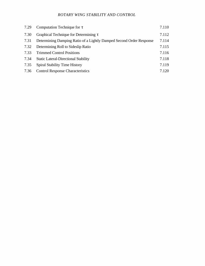
ROTARY WING STABILITY AND CONTROL
7.29 Computation Technique for τ 7.110
7.30 Graphical Technique for Determining τ 7.112
7.31 Determining Damping Ratio of a Lightly Damped Second Order Response 7.114
7.32 Determining Roll to Sideslip Ratio 7.115
7.33 Trimmed Control Positions 7.116
7.34 Static Lateral-Directional Stability 7.118
7.35 Spiral Stability Time History 7.119
7.36 Control Response Characteristics 7.120
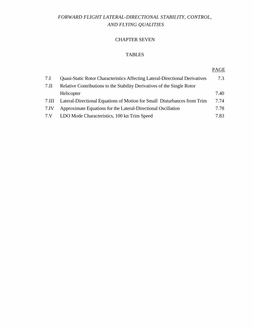
FORWARD FLIGHT LATERAL-DIRECTIONAL STABILITY, CONTROL,
AND FLYING QUALITIES
CHAPTER SEVEN
TABLES
PAGE
7.I Quasi-Static Rotor Characteristics Affecting Lateral-Directional Derivatives 7.3
7.II Relative Contributions to the Stability Derivatives of the Single Rotor
Helicopter 7.40
7.III Lateral-Directional Equations of Motion for Small Disturbances from Trim 7.74
7.IV Approximate Equations for the Lateral-Directional Oscillation 7.78
7.V LDO Mode Characteristics, 100 kn Trim Speed 7.83

ROTARY WING STABILITY AND CONTROL
CHAPTER SEVEN
EQUATIONS
PAGE
v. - Yv∆v -Yr∆r +u
0∆r -Yp∆p -gφ = Y
A1s
∆A1s
+ YθTR
∆θTR
= YδLAT
∆δLAT
+ YδPED
∆δPED
eq 7.1 7.4
p. - Lv∆v - Lr∆r - Lp∆p = L
A1s
∆A1s
+ LθTR
∆θTR
= LδLAT
∆δLAT
+ LδPED
∆δPED
eq 7.2 7.5
r. - Nv∆v - Np∆p - Nr∆r = N
A1s
∆A1s
+ NθTR
∆θTR
= NδLAT
∆δLAT
+ NδPED
∆δPED
eq 7.3 7.5
∆Y = T ∆b1s
+ b1s
∆T + ∆YR
+ ∆TTR
+ ∆Yf+t eq 7.4 7.9
∆L = (Th + 12
ebMSΩ
2)∆b
1s + hb
1s∆T + h∆Y
R + h
TR∆T
TR + ∆L
f+t
eq 7.5 7.9
∆N = Th'∆b1s
+ h'b1s
∆T + h'∆YR
- lt∆T
TR + ∆N
f+t + ∆Q
MR eq 7.6 7.9
Nv = 1Izz
Th'∂b
1s∂v
+ h'b1s
∂T∂v
+ h' ∂Y
R∂v
- lt
∂TTR
∂v +
∂Nf+t
∂v +
∂QMR
∂v
eq 7.7 7.11
Nv ≈ 1Izz
-lt
∂TTR
∂v +
∂Nf+t
∂veq 7.8 7.11
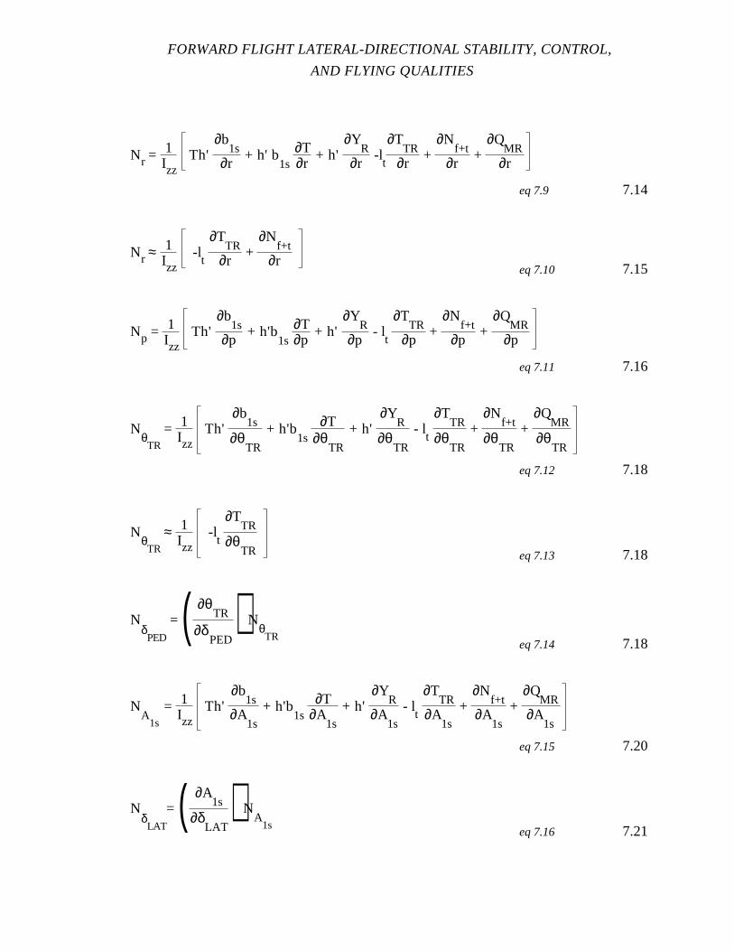
FORWARD FLIGHT LATERAL-DIRECTIONAL STABILITY, CONTROL,
AND FLYING QUALITIES
Nr = 1Izz
Th'∂b
1s∂r
+ h' b1s
∂T∂r
+ h' ∂Y
R∂r
-lt
∂TTR
∂r +
∂Nf+t
∂r +
∂QMR
∂r
eq 7.9 7.14
Nr ≈ 1Izz
-lt
∂TTR
∂r +
∂Nf+t
∂req 7.10 7.15
Np = 1Izz
Th'∂b
1s∂p
+ h'b1s
∂T∂p
+ h' ∂Y
R∂p
- lt
∂TTR
∂p +
∂Nf+t
∂p +
∂QMR
∂p
eq 7.11 7.16
NθTR
= 1Izz
Th'∂b
1s
∂θTR
+ h'b1s
∂T∂θ
TR
+ h' ∂Y
R
∂θTR
- lt
∂TTR
∂θTR
+ ∂N
f+t
∂θTR
+ ∂Q
MR
∂θTR
eq 7.12 7.18
NθTR
≈ 1Izz
-lt
∂TTR
∂θTR eq 7.13 7.18
NδPED
= ( ∂θTR
∂δPED
) NθTR
eq 7.14 7.18
NA
1s
= 1Izz
Th'∂b
1s∂A
1s
+ h'b1s
∂T∂A
1s
+ h' ∂Y
R∂A
1s
- lt
∂TTR
∂A1s
+ ∂N
f+t∂A
1s
+ ∂Q
MR∂A
1s
eq 7.15 7.20
NδLAT
= ( ∂A1s
∂δLAT
) NA
1seq 7.16 7.21
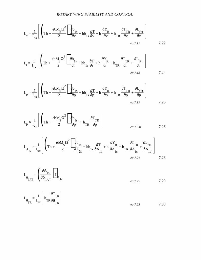
ROTARY WING STABILITY AND CONTROL
Lv = 1Ixx
(Th + ebM
SΩ
2
2) ∂b
1s∂v
+ hb1s
∂T∂v
+ h ∂Y
R∂v
+ hTR
∂TTR
∂v +
∂Lf+t
∂v
eq 7.17 7.22
Lr = 1Ixx
(Th + ebM
SΩ
2
2) ∂b
1s∂r
+ hb1s
∂T∂r
+ h ∂Y
R∂r
+ hTR
∂TTR
∂r +
∂Lf+t
∂r
eq 7.18 7.24
Lp = 1Ixx
(Th + ebM
SΩ
2
2) ∂b
1s∂p
+ hb1s
∂T∂p
+ h ∂Y
R∂p
+ hTR
∂TTR
∂p +
∂Lf+t
∂p
eq 7.19 7.26
Lp ≈ 1Ixx
(Th + ebM
SΩ
2
2) ∂b
1s∂p
+ hTR
∂TTR
∂peq 7. 20 7.26
LA
1s
= 1Ixx
(Th + ebM
SΩ
2
2) ∂b
1s∂A
1s
+ hb1s
∂T∂A
1s
+ h ∂Y
R∂A
1s
+ hTR
∂TTR
∂A1s
+ ∂L
f+t∂A
1s
eq 7.21 7.28
LδLAT
= ( ∂A1s
∂δLAT
)LA
1seq 7.22 7.29
LθTR
= 1Ixx
hTR
∂TTR
∂θTR eq 7.23 7.30
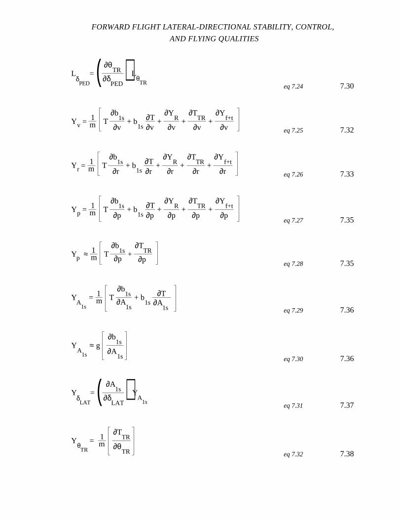
FORWARD FLIGHT LATERAL-DIRECTIONAL STABILITY, CONTROL,
AND FLYING QUALITIES
LδPED
= ( ∂θTR
∂δPED
) LθTR
eq 7.24 7.30
Yv = 1m T
∂b1s
∂v + b
1s∂T∂v
+ ∂Y
R
∂v +
∂TTR
∂v +
∂Yf+t
∂v eq 7.25 7.32
Yr = 1m T
∂b1s
∂r + b
1s∂T∂r
+ ∂Y
R
∂r +
∂TTR
∂r +
∂Yf+t
∂r eq 7.26 7.33
Yp = 1m T
∂b1s
∂p + b
1s∂T∂p
+ ∂Y
R
∂p +
∂TTR
∂p +
∂Yf+t
∂peq 7.27 7.35
Yp ≈ 1m T
∂b1s
∂p +
∂TTR
∂p eq 7.28 7.35
YA
1s
= 1m T∂b
1s∂A
1s
+ b1s
∂T∂A
1s
eq 7.29 7.36
YA
1s
≈ g ∂b
1s
∂A1s eq 7.30 7.36
YδLAT
= ( ∂A1s
∂δLAT
) YA
1seq 7.31 7.37
YθTR
= 1m
∂TTR
∂θTR eq 7.32 7.38
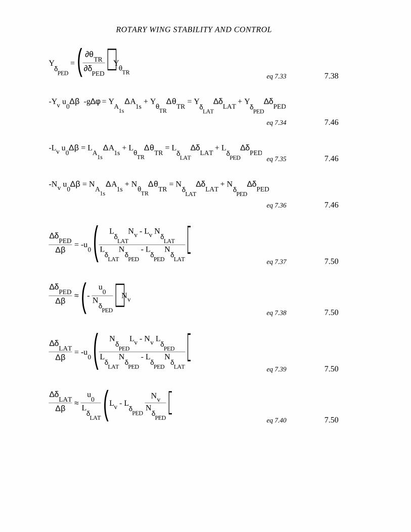
ROTARY WING STABILITY AND CONTROL
YδPED
= ( ∂θTR
∂δPED
) YθTR
eq 7.33 7.38
-Yv u0∆β -g∆φ = Y
A1s
∆A1s
+ YθTR
∆θTR
= YδLAT
∆δLAT
+ YδPED
∆δPED
eq 7.34 7.46
-Lv u0∆β = L
A1s
∆A1s
+ LθTR
∆θTR
= LδLAT
∆δLAT
+ LδPED
∆δPED
eq 7.35 7.46
-Nv u0∆β = N
A1s
∆A1s
+ NθTR
∆θTR
= NδLAT
∆δLAT
+ NδPED
∆δPED
eq 7.36 7.46
∆δPED
∆β = -u
0 ( LδLAT
Nv - Lv NδLAT
LδLAT
NδPED
- LδPED
NδLAT
)eq 7.37 7.50
∆δPED
∆β≈ (-
u0
NδPED
) Nv
eq 7.38 7.50
∆δLAT
∆β = -u
0 ( NδPED
Lv - Nv LδPED
LδLAT
NδPED
- LδPED
NδLAT
)eq 7.39 7.50
∆δLAT
∆β≈
u0
LδLAT
(Lv - LδPED
NvN
δPED
)eq 7.40 7.50
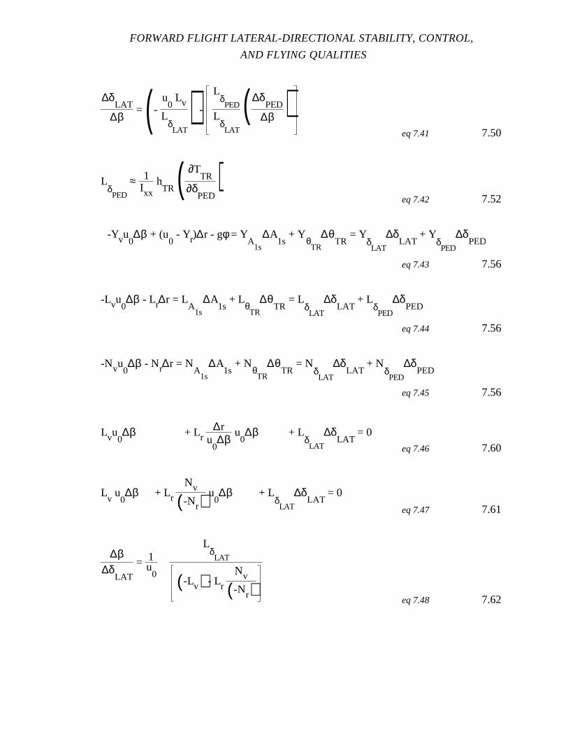
FORWARD FLIGHT LATERAL-DIRECTIONAL STABILITY, CONTROL,
AND FLYING QUALITIES
∆δLAT
∆β = (-
u0 Lv
LδLAT
) -
LδPED
LδLAT
(∆δPED
∆β )eq 7.41 7.50
LδPED
≈ 1Ixx
hTR ( ∂T
TR
∂δPED
)eq 7.42 7.52
-Yvu0∆β + (u
0 - Yr)∆r - gφ = Y
A1s
∆A1s
+ YθTR
∆θTR
= YδLAT
∆δLAT
+ YδPED
∆δPED
eq 7.43 7.56
-Lvu0∆β - Lr∆r = L
A1s
∆A1s
+ LθTR
∆θTR
= LδLAT
∆δLAT
+ LδPED
∆δPED
eq 7.44 7.56
-Nvu0∆β - Nr∆r = N
A1s
∆A1s
+ NθTR
∆θTR
= NδLAT
∆δLAT
+ NδPED
∆δPED
eq 7.45 7.56
Lvu0∆β + Lr
∆ru
0∆β
u0∆β + L
δLAT
∆δLAT
= 0
eq 7.46 7.60
Lv
u0∆β + Lr
Nv
(-Nr) u
0∆β + L
δLAT
∆δLAT
= 0
eq 7.47 7.61
∆β∆δ
LAT
= 1u
0
LδLAT
(-Lv) - Lr
Nv
(-Nr)eq 7.48 7.62

ROTARY WING STABILITY AND CONTROL
∆β∆δ
LAT
= 1u
0
(-Nr) LδLAT
(LvNr - LrNv) eq 7.49 7.63
∆r∆δ
LAT
= ∆ru
0∆β
u0∆β
∆δLAT
=
NvLδLAT
(LvNr - LrNv) eq 7.50 7.63
Lv uo∆β + Lr∆r + LδPED
∆δPED
= 0eq 7.51 7.64
Nvu0∆β + Nr ∆r + N
δPED
∆δPED
= 0eq 7.52 7.64
(u0∆β)
∆r =
Lr
(-Lv) eq 7.53 7.65
Nv
Lr
(-Lv)∆r - (-Nr) ∆r + N
δPED
∆δPED
= 0
eq 7.54 7.66
∆r∆δ
PED
=
(-Lv)NδPED
LvNr - LrNv eq 7.55 7.66
u0∆β
∆δPED
=
LrNδPED
LvNr - LrNv eq 7.56 7.66
∆r∆δ
PED
=
(-Lv) NδPED
1 - ( LδPED
NδPED
)(NvLv
)LvNr - LrNv eq 7.57 7.69
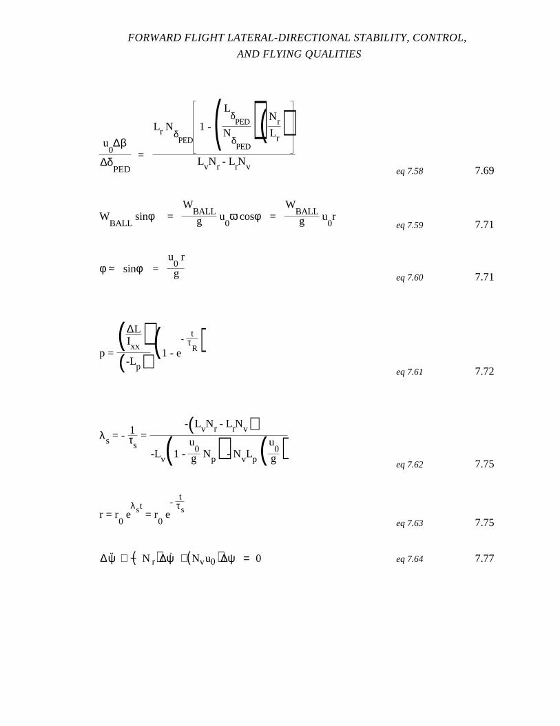
FORWARD FLIGHT LATERAL-DIRECTIONAL STABILITY, CONTROL,
AND FLYING QUALITIES
u0∆β
∆δPED
=
Lr NδPED
1 - ( LδPED
NδPED
)(NrLr
)LvNr - LrNv eq 7.58 7.69
WBALL
sinφ =W
BALLg u
0ω cosφ =
WBALLg u
0r
eq 7.59 7.71
φ ≈ sinφ =u
0 r
g eq 7.60 7.71
p = (∆L
Ixx )(-Lp)
(1 - e-
tτR)
eq 7.61 7.72
λs = - 1τs =
-(LvNr - LrNv)-Lv(1 -
u0
g Np) - NvLp ( u0
g )eq 7.62 7.75
r = r0 e
λst = r0 e
-t
τs
eq 7.63 7.75
∆ ˙ψ + −N r( )∆ψ + Nvu0( )∆ψ = 0 eq 7.64 7.77
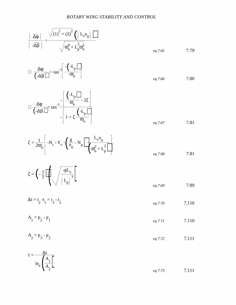
ROTARY WING STABILITY AND CONTROL
∆φ
-∆β =
(1)2 + (2)
2 ( Lvu0 )
ωn4 + Lp
2ωn
2
eq 7.65 7.79
∠ ∆φ
(-∆β) = tan-1
-(-Lp)-ωn
eq 7.66 7.80
∠ ∆φ
(-∆β) = tan-1
-(-Lp)
ωn - 2ζ
- 1 + ζ(-Lp)
ωn eq 7.67 7.81
ζ = 12ωn
-Nr - Yv -( gu
0 - Np) Lvu
0
(ωn2 + Lp
2)eq 7.68 7.81
ζ = (- 12)( -gLv
Lp
3)eq 7.69 7.89
∆t = t2 -t
1 = t
3 - t
2 eq 7.70 7.110
A1 = p
2 - p
1 eq 7.71 7.110
A2 = p
3 - p
2 eq 7.72 7.111
τ = ∆t
lne(A1
A2)
eq 7.73 7.111
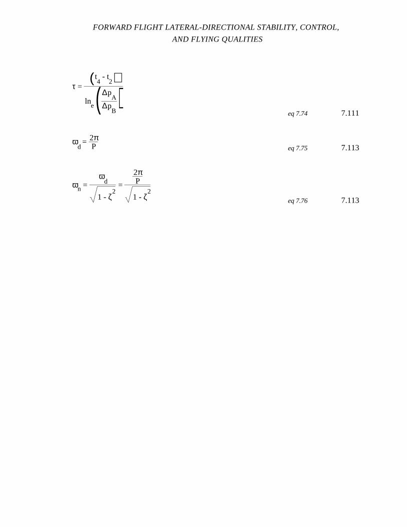
FORWARD FLIGHT LATERAL-DIRECTIONAL STABILITY, CONTROL,
AND FLYING QUALITIES
τ = ( t
4 - t
2)ln
e(∆pA
∆pB)
eq 7.74 7.111
ωd = 2π
P eq 7.75 7.113
ωn = ω
d
1 - ζ2 =
2πP
1 - ζ2
eq 7.76 7.113

CHAPTER SEVEN
FORWARD FLIGHT LATERAL-DIRECTIONAL STABILITY, CONTROL, AND
FLYING QUALITIES
7.1 INTRODUCTION
This chapter presents the analytic background and flight test techniques associated
with the lateral-directional stability, control, and flying qualities of helicopters in powered
forward flight above transitional speeds. The objective of the analytic development is to
provide an understanding of the factors affecting pilot opinion of the helicopter flying
qualities while performing mission tasks.
Discussion of lateral-directional characteristics involvessome greater complexity
than the previous longitudinal chapter because two rotational axes are involved, including
considerable coupling between them. In addition, many of these characteristics are a
function of forward speed.
The subject matter is divided into the following topic areas: lateral-directional
stability derivatives, trim characteristics, characteristics in static or steady flight conditions,
dynamics, control response, and gust response. The chapter concentrates on the single
rotor helicopter with some discussion of the lateral-directional characteristics of the tandem.
Lateral control of a helicopter rotor is achieved in a manner identical to longitudinal
control. However, because the fuselage roll moment of inertia is less than the pitch
moment of inertia, the gearing ratio between the lateral cyclic control and the swashplate is
normally less than in the longitudinal control system. In some flight conditions, the thrust
vector is tilted laterally to balance side forces on the fuselage developed as the result of
lateral velocity and tail rotor thrust. The control gearing, moment of inertia, side force
characteristic, and lateral speed stability together provide lateral control characteristics in
forward flight different than for the longitudinal axis.
The side force characteristic, analogous to longitudinal drag, is normally a larger
contribution to the lateral force equation than drag is in the longitudinal equation. The tail
rotor, of a single rotor helicopter, always provides a significant side force and the fuselage
lateral flat plate area is greater than the frontal flat plate area. The tandem helicopter does
ROTARY WING STABILITY AND CONTROL
not have a tail rotor, but the fuselage tends to produce higher drag in response to lateral
velocity because of its size and shape. Generally, in both the single main rotor and tandem
rotor configurations, there are no surfaces generating roll moments which are equivalent to
the longitudinal moments produced by the horizontal stabilizer. Therefore, any roll
moments generated by the rotor, as it is tilted to balance the lateral force equation, results in
a substantial bank angle. However, the tail rotor and/or vertical tail provide forces
stabilizing yaw motion analogous to the action of the horizontal tail in restraining pitch
motion.
7.2 PURPOSE OF TEST
The purpose of these tests is to evaluate the helicopter forward flight lateral-
directional stability, control, and flying qualities. The tests included in the evaluation are:
1. Mechanical Characteristics
2. Trimmed control positions.
3. Static stability.
4. Dynamic stability.
5. Spiral stability.
6. Control response.
7. Gust response.
7.3 THEORY
7.3.1 Summary of Quasi-Static Rotor Characteristics
The basic rotor characteristics presented in Chapter 4 indicate a quasi-static
approximation for rotor responses which is satisfactory for helicopter stability, control, and
flying qualities analysis. Table 7.I presents the summaries of quasi-static lateral rotor
response characteristics in forward flight. It is included for reference in discussing the
stability derivatives and the helicopter’s response. The table summarizes the rotor
contributions to stability derivatives by indicating the most significant rotor responses.

FORWARD FLIGHT LATERAL-DIRECTIONAL STABILITY, CONTROL,
AND FLYING QUALITIES
Table 7.I
Quasi-Static Rotor Characteristics Affecting Lateral-Directional Derivatives
Perturbation RotorResponse
Force andMoments Appliedto Aircraft
∆ L
∆ LH
hTR
∆b1s
T∆YR
TTR
+ ∆TTR
∆V
(Cockpit Perspective)
(a)Left LateralVelocityincrease,∆v(-)
Rotor tilts awayfrom relativevelocity, righttilt, stable,(blowback)
∂b1s
∂v (+)
T∆b1s right
∆YR right
∆LH right
∆TTR right
TTR∆ T
TR∆p
T∆L
H ∆ b1s
∆ L
∆YR
(b)Right RollRate∆p(+)
Rotor tilts awayfrom roll
∂b1s
∂v (-)
T∆b1s left,provides rolldamping∆YR left, increasesroll damping∆LH left, increasesroll damping∆TTR left,increases rolldamping
∆TT/R
∆r
lt
(c)Yaw rate,∆r, right (+)
∆TTR, l t , right,
provides yawdamping moment.
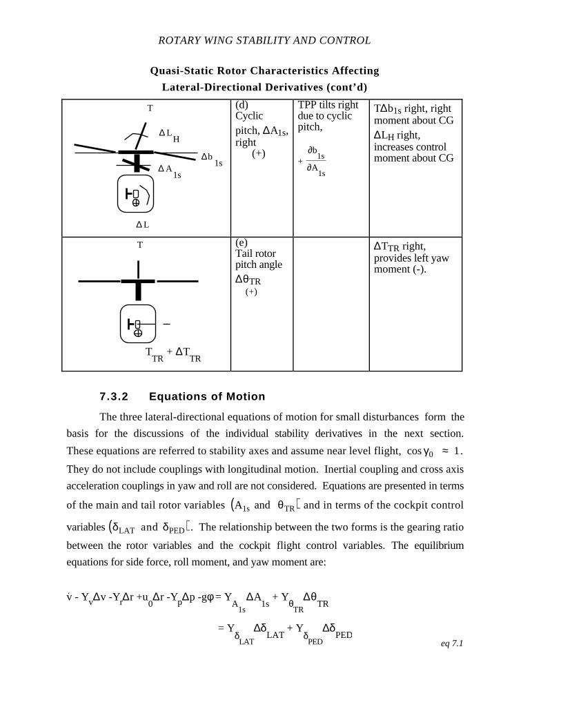
ROTARY WING STABILITY AND CONTROL
Quasi-Static Rotor Characteristics Affecting
Lateral-Directional Derivatives (cont’d)
∆ L
∆ LH
∆b1s
T
∆ A1s
(d)Cyclicpitch,∆A1s,right (+)
TPP tilts rightdue to cyclicpitch,
+∂b
1s
∂A1s
T∆b1s right, rightmoment about CG∆LH right,increases controlmoment about CG
T
TTR
+ ∆TTR
(e)Tail rotorpitch angle∆θTR (+)
∆TTR right,provides left yawmoment (-).
7.3.2 Equations of Motion
The three lateral-directional equations of motion for small disturbances form the
basis for the discussions of the individual stability derivatives in the next section.
These equations are referred to stability axes and assume near level flight, cosγ0 ≈ 1.
They do not include couplings with longitudinal motion. Inertial coupling and cross axis
acceleration couplings in yaw and roll are not considered. Equations are presented in terms
of the main and tail rotor variables A1s and θTR( ) and in terms of the cockpit control
variables δLAT and δPED( ) . The relationship between the two forms is the gearing ratio
between the rotor variables and the cockpit flight control variables. The equilibrium
equations for side force, roll moment, and yaw moment are:
v. - Yv∆v -Yr∆r +u
0∆r -Yp∆p -gφ = Y
A1s
∆A1s
+ YθTR
∆θTR
= YδLAT
∆δLAT
+ YδPED
∆δPED
eq 7.1
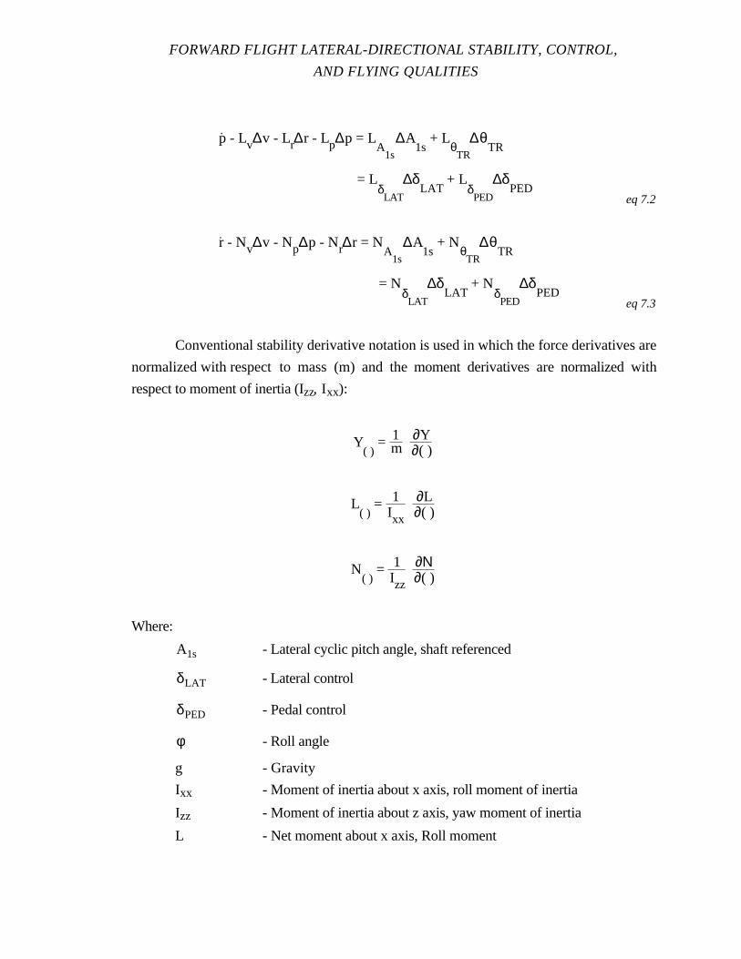
FORWARD FLIGHT LATERAL-DIRECTIONAL STABILITY, CONTROL,
AND FLYING QUALITIES
p. - Lv∆v - Lr∆r - Lp∆p = L
A1s
∆A1s
+ LθTR
∆θTR
= LδLAT
∆δLAT
+ LδPED
∆δPED
eq 7.2
r. - Nv∆v - Np∆p - Nr∆r = N
A1s
∆A1s
+ NθTR
∆θTR
= NδLAT
∆δLAT
+ NδPED
∆δPED
eq 7.3
Conventional stability derivative notation is used in which the force derivatives are
normalized with respect to mass (m) and the moment derivatives are normalized with
respect to moment of inertia (Izz, Ixx):
Y( )
= 1m∂Y∂( )
L( )
= 1Ixx
∂L∂( )
N( )
= 1Izz
∂Ν∂( )
Where:
A1s - Lateral cyclic pitch angle, shaft referenced
δLAT - Lateral control
δPED - Pedal control
φ - Roll angle
g - Gravity
Ixx - Moment of inertia about x axis, roll moment of inertia
Izz - Moment of inertia about z axis, yaw moment of inertia
L - Net moment about x axis, Roll moment
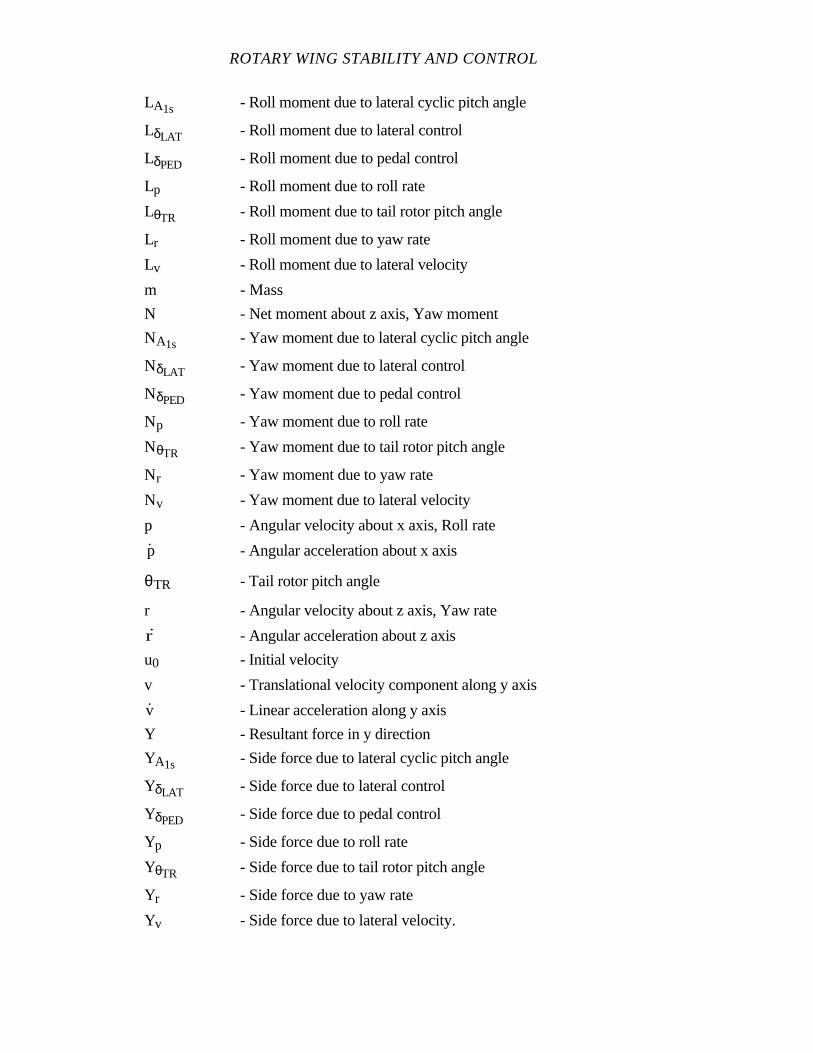
ROTARY WING STABILITY AND CONTROL
LA1s - Roll moment due to lateral cyclic pitch angle
LδLAT - Roll moment due to lateral control
LδPED - Roll moment due to pedal control
Lp - Roll moment due to roll rate
LθTR - Roll moment due to tail rotor pitch angle
Lr - Roll moment due to yaw rate
Lv - Roll moment due to lateral velocity
m - Mass
N - Net moment about z axis, Yaw moment
NA1s - Yaw moment due to lateral cyclic pitch angle
NδLAT - Yaw moment due to lateral control
NδPED - Yaw moment due to pedal control
Np - Yaw moment due to roll rate
NθTR - Yaw moment due to tail rotor pitch angle
Nr - Yaw moment due to yaw rate
Nv - Yaw moment due to lateral velocity
p - Angular velocity about x axis, Roll rate
p - Angular acceleration about x axis
θTR - Tail rotor pitch angle
r - Angular velocity about z axis, Yaw rate
r - Angular acceleration about z axis
u0 - Initial velocity
v - Translational velocity component along y axis
v - Linear acceleration along y axis
Y - Resultant force in y direction
YA1s - Side force due to lateral cyclic pitch angle
YδLAT - Side force due to lateral control
YδPED - Side force due to pedal control
Yp - Side force due to roll rate
YθTR - Side force due to tail rotor pitch angle
Yr - Side force due to yaw rate
Yv - Side force due to lateral velocity.
FORWARD FLIGHT LATERAL-DIRECTIONAL STABILITY, CONTROL,
AND FLYING QUALITIES
7.3.3 Lateral-Directional Derivatives
The quasi-static tip path plane (TPP) motion presented in Section 7.3.1 is adequate
for explaining most helicopter stability and control problems because the rotor blade
dynamic responses are rapid and well damped. This quasi-static approximation expresses
the TPP variables in terms of the rigid body motions of the helicopter and incorporate their
influence on the overall stability derivatives. The derivatives which have the greatest
influence on stability and control characteristics are discussed in this section.
Figure 7.1 shows the forces and moments acting on the helicopter which contribute
to the side force, roll moment, and yaw moment about the center of gravity (CG).
The forces include the lateral thrust component ≈ T∆b1s( ),the rotor side force YR( ) which
acts parallel to the TPP, the side force on the fuselage/tail Yf + t( ) , and tail rotor thrust
TTR( ) . The diagram indicates the roll moment due to the fuselage/tail Lf + t( ), and due to
the offset flapping hinge (LH). There are roll moments about the CG due to the rotor YR
force and side component of rotor thrust, both acting through a moment arm (h), and due to
the tail rotor thrust acting through the arm hTR.
The torque of the main rotor (QMR) and the yaw moment due to the fuselage/tail
N f + t( ) are indicated. Yaw moments are produced by the tail rotor thrust acting through
the arm (lt) and by the main rotor side forces acting through the arm h'. The CG is
assumed in the xz plane of the helicopter.
The lateral-directional stability derivatives give the change in the total aerodynamic side
force, roll moment, and yaw moment resulting from a change in one of the lateral-
directional flight or control variables v, p, r, θTR (or δPED), and A1s (or δLAT) while
holding the remaining variables constant. These derivatives are expressed as a sum of
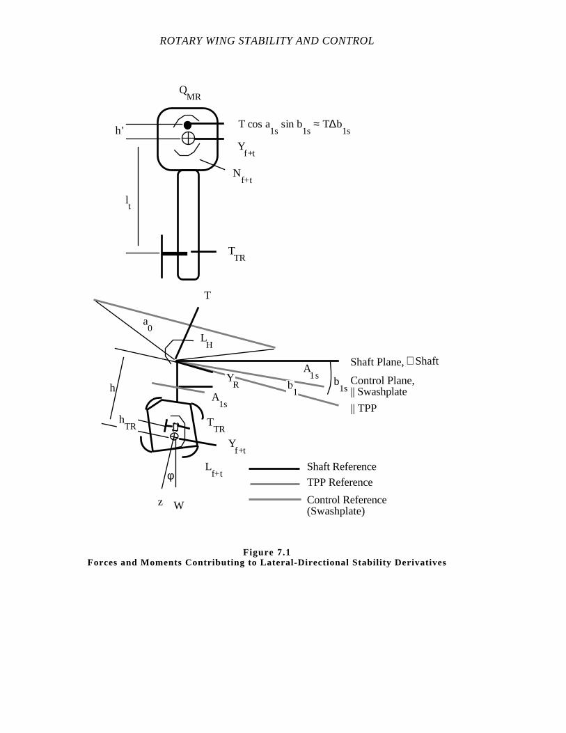
ROTARY WING STABILITY AND CONTROL
Control Plane, || Swashplate
Shaft Plane, ⊥ Shaft
|| TPP
a0
A1s
b1sb
1
Shaft Reference
TPP Reference
Control Reference (Swashplate)
h
TTR
T
LH
YR
Yf+t
Lf+t
Wz
φ
lt
h'
TTR
QMR
Nf+t
Yf+t
A1s
T cos a1s
sin b1s
≈ T∆b1s
hTR
Figure 7.1Forces and Moments Contributing to Lateral-Directional Stability Derivatives
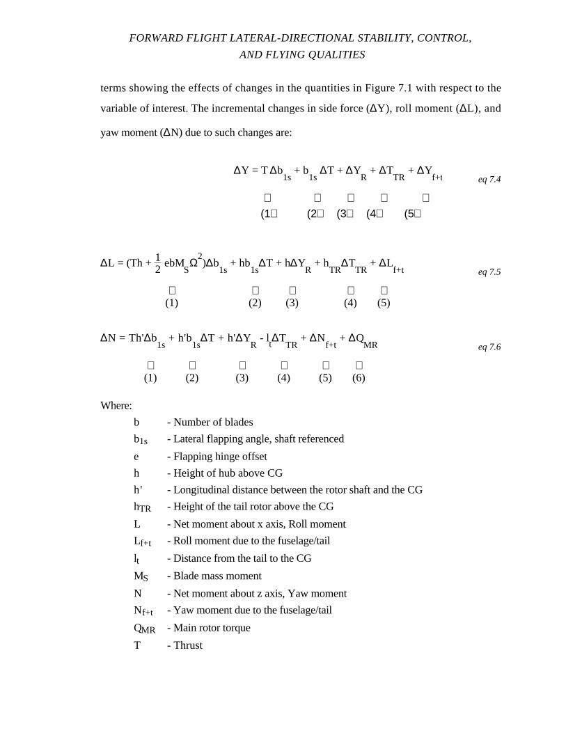
FORWARD FLIGHT LATERAL-DIRECTIONAL STABILITY, CONTROL,
AND FLYING QUALITIES
terms showing the effects of changes in the quantities in Figure 7.1 with respect to the
variable of interest. The incremental changes in side force (∆Y), roll moment (∆L), and
yaw moment (∆N) due to such changes are:
∆Y = T ∆b1s
+ b1s
∆T + ∆YR
+ ∆TTR
+ ∆Yf+t eq 7.4
⇑ ⇑ ⇑ ⇑ ⇑(1) (2) (3) (4) (5)
∆L = (Th + 12
ebMSΩ
2)∆b
1s + hb
1s∆T + h∆Y
R + h
TR∆T
TR + ∆L
f+t eq 7.5
⇑ ⇑ ⇑ ⇑ ⇑(1) (2) (3) (4) (5)
∆N = Th'∆b1s
+ h'b1s
∆T + h'∆YR
- lt∆T
TR + ∆N
f+t + ∆Q
MR eq 7.6
⇑ ⇑ ⇑ ⇑ ⇑ ⇑(1) (2) (3) (4) (5) (6)
Where:
b - Number of blades
b1s - Lateral flapping angle, shaft referenced
e - Flapping hinge offset
h - Height of hub above CG
h' - Longitudinal distance between the rotor shaft and the CG
hTR - Height of the tail rotor above the CG
L - Net moment about x axis, Roll moment
Lf+t - Roll moment due to the fuselage/tail
lt - Distance from the tail to the CG
MS - Blade mass moment
N - Net moment about z axis, Yaw moment
Nf+t - Yaw moment due to the fuselage/tail
QMR - Main rotor torque
T - Thrust
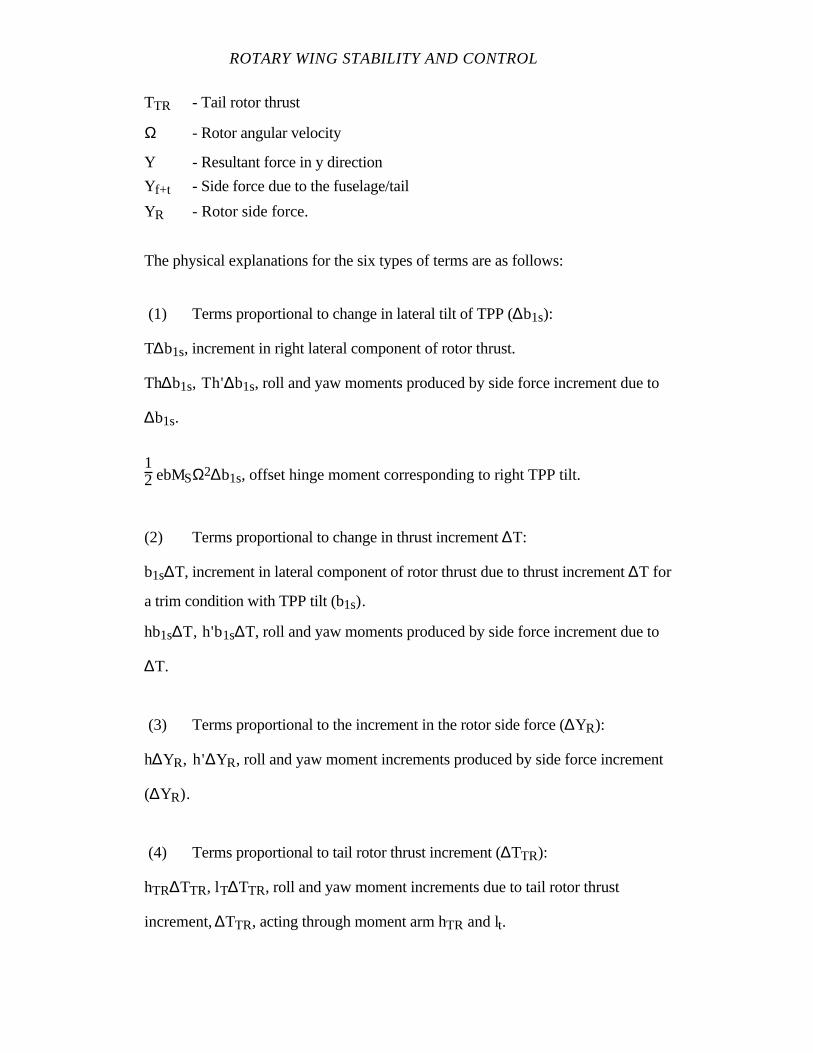
ROTARY WING STABILITY AND CONTROL
TTR - Tail rotor thrust
Ω - Rotor angular velocity
Y - Resultant force in y direction
Yf+t - Side force due to the fuselage/tail
YR - Rotor side force.
The physical explanations for the six types of terms are as follows:
(1) Terms proportional to change in lateral tilt of TPP (∆b1s):
T∆b1s, increment in right lateral component of rotor thrust.
Th∆b1s, Th'∆b1s, roll and yaw moments produced by side force increment due to
∆b1s.
12 ebMSΩ2∆b1s, offset hinge moment corresponding to right TPP tilt.
(2) Terms proportional to change in thrust increment ∆T:
b1s∆T, increment in lateral component of rotor thrust due to thrust increment ∆T for
a trim condition with TPP tilt (b1s).
hb1s∆T, h'b1s∆T, roll and yaw moments produced by side force increment due to
∆T.
(3) Terms proportional to the increment in the rotor side force (∆YR):
h∆YR, h'∆YR, roll and yaw moment increments produced by side force increment
(∆YR).
(4) Terms proportional to tail rotor thrust increment (∆TTR):
hTR∆TTR, lT∆TTR, roll and yaw moment increments due to tail rotor thrust
increment,∆TTR, acting through moment arm hTR and lt.

FORWARD FLIGHT LATERAL-DIRECTIONAL STABILITY, CONTROL,
AND FLYING QUALITIES
(5) Terms proportional to increments in the aerodynamic forces acting on the
fuselage/tail.
(6) Increment in yaw moment due to a change in main rotor torque.
The distance of the CG aft of the rotor shaft (h') is usually small for conventional
helicopters and is assumed zero to simplify the discussion of the yaw moment derivatives.
A further simplification is made by assuming constant collective, thereby neglecting the
type (2) terms for the variation in side force, roll moment, and yaw moment produced by
thrust changes.
The values of the stability derivatives as a function of airspeed for the BO-105, the
OH-6A, and the CH-53D are presented at the end of each subsection.
7.3.3.1 YAW MOMENT DUE TO LATERAL VELOCITY,
DIRECTIONAL STABILITY
Nv = 1Izz
Th'∂b
1s∂v
+ h'b1s
∂T∂v
+ h' ∂Y
R∂v
- lt
∂TTR
∂v +
∂Nf+t
∂v +
∂QMR
∂veq 7.7
⇑ ⇑ ⇑ ⇑ ⇑ ⇑
(1) (2) (3) (4) (5) (6)
Nv ≈ 1Izz
-lt
∂TTR
∂v +
∂Nf+t
∂veq 7. 8
⇑ ⇑
(4) (5)
Where:
b1s - Lateral flapping angle, shaft referenced
h' - Longitudinal distance between the rotor shaft and the CG
Izz - Moment of inertia about z axis, yaw moment of inertia
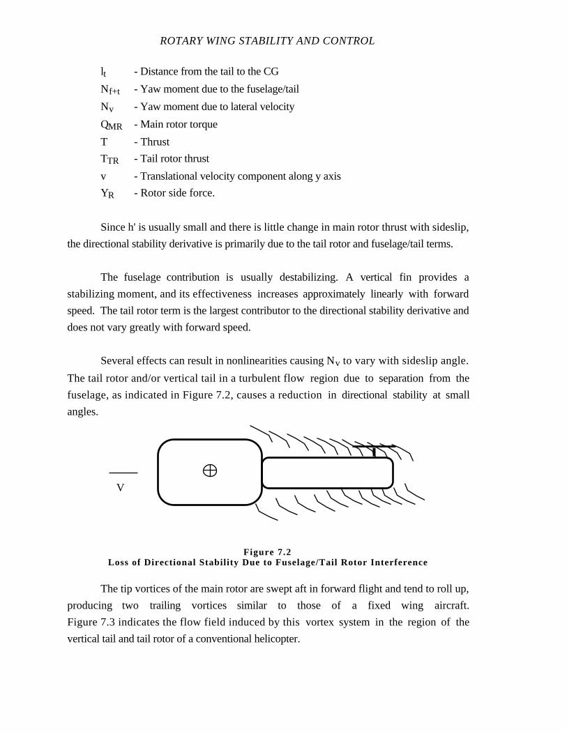
ROTARY WING STABILITY AND CONTROL
lt - Distance from the tail to the CG
Nf+t - Yaw moment due to the fuselage/tail
Nv - Yaw moment due to lateral velocity
QMR - Main rotor torque
T - Thrust
TTR - Tail rotor thrust
v - Translational velocity component along y axis
YR - Rotor side force.
Since h' is usually small and there is little change in main rotor thrust with sideslip,
the directional stability derivative is primarily due to the tail rotor and fuselage/tail terms.
The fuselage contribution is usually destabilizing. A vertical fin provides a
stabilizing moment, and its effectiveness increases approximately linearly with forward
speed. The tail rotor term is the largest contributor to the directional stability derivative and
does not vary greatly with forward speed.
Several effects can result in nonlinearities causing Nv to vary with sideslip angle.
The tail rotor and/or vertical tail in a turbulent flow region due to separation from the
fuselage, as indicated in Figure 7.2, causes a reduction in directional stability at small
angles.
The tip vortices of the main rotor are swept aft in forward flight and tend to roll up,
producing two trailing vortices similar to those of a fixed wing aircraft.
Figure 7.3 indicates the flow field induced by this vortex system in the region of the
vertical tail and tail rotor of a conventional helicopter.
V
Figure 7.2Loss of Directional Stability Due to Fuselage/Tail Rotor Interference
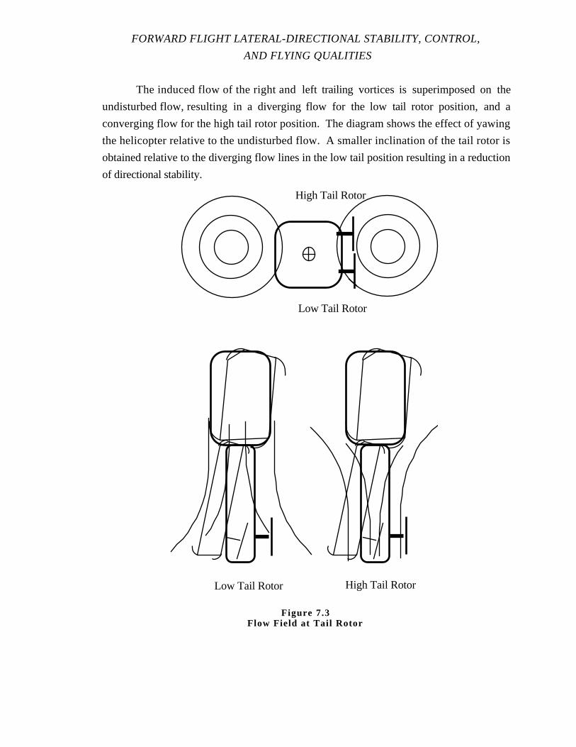
FORWARD FLIGHT LATERAL-DIRECTIONAL STABILITY, CONTROL,
AND FLYING QUALITIES
The induced flow of the right and left trailing vortices is superimposed on the
undisturbed flow, resulting in a diverging flow for the low tail rotor position, and a
converging flow for the high tail rotor position. The diagram shows the effect of yawing
the helicopter relative to the undisturbed flow. A smaller inclination of the tail rotor is
obtained relative to the diverging flow lines in the low tail position resulting in a reduction
of directional stability.
High Tail Rotor
Low Tail Rotor
Low Tail Rotor High Tail Rotor
Figure 7.3Flow Field at Tail Rotor
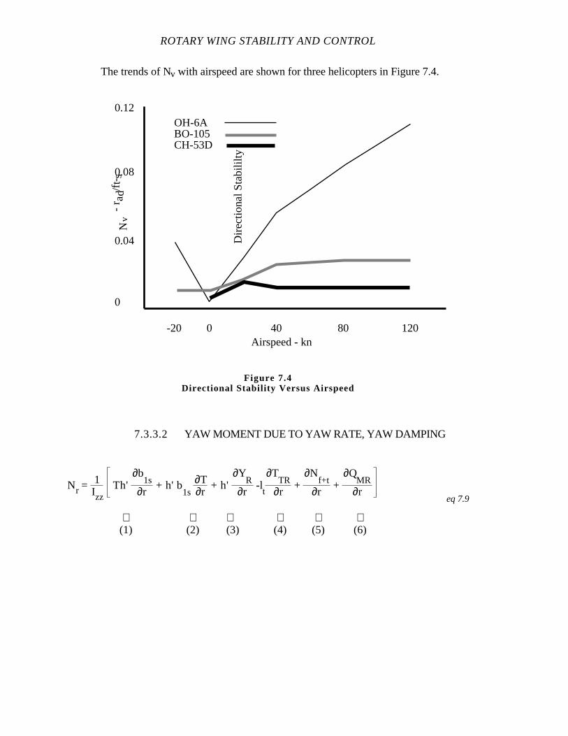
ROTARY WING STABILITY AND CONTROL
The trends of Nv with airspeed are shown for three helicopters in Figure 7.4.
7.3.3.2 YAW MOMENT DUE TO YAW RATE, YAW DAMPING
Nr = 1Izz
Th'∂b
1s∂r
+ h' b1s
∂T∂r
+ h' ∂Y
R∂r
-lt
∂TTR
∂r +
∂Nf+t
∂r +
∂QMR
∂req 7.9
⇑ ⇑ ⇑ ⇑ ⇑ ⇑(1) (2) (3) (4) (5) (6)
0 40 80 120-20Airspeed - kn
0
0.04
0.08
0.12
Dire
ctio
nal S
tabi
lilty
Nv
-r a
d/f t
- sOH-6ABO-105CH-53D
Figure 7.4Directional Stability Versus Airspeed
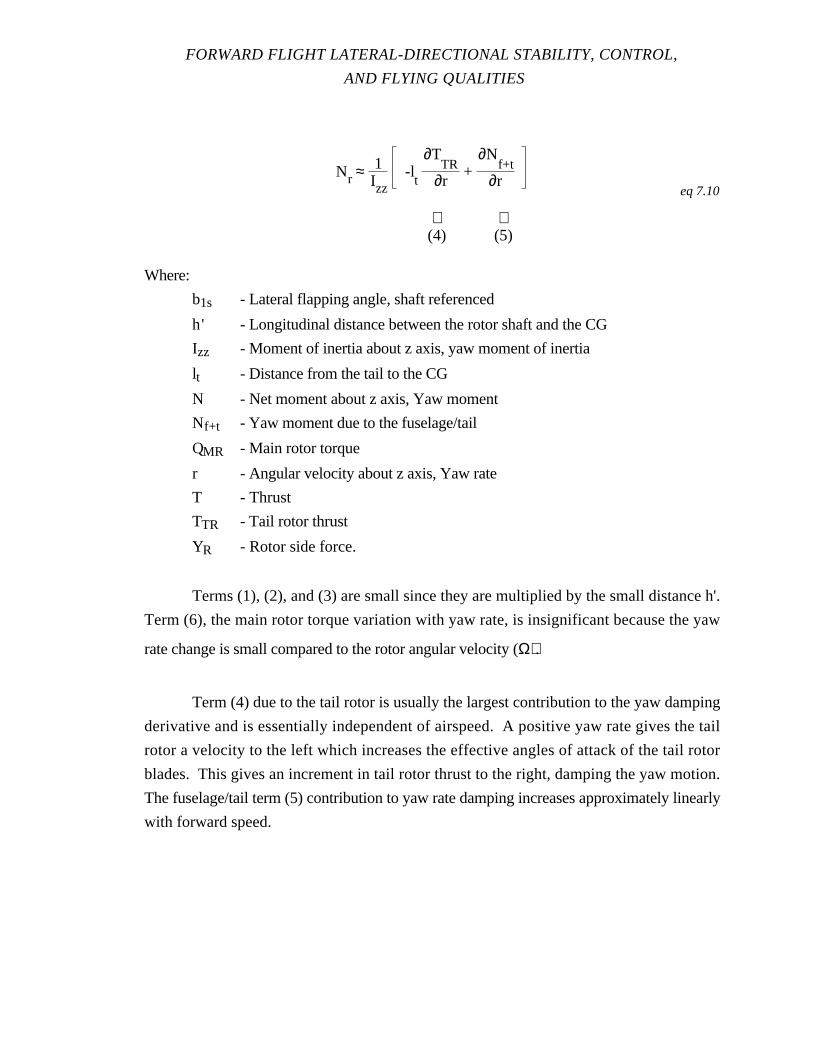
FORWARD FLIGHT LATERAL-DIRECTIONAL STABILITY, CONTROL,
AND FLYING QUALITIES
Nr ≈ 1Izz
-lt
∂TTR
∂r +
∂Nf+t
∂req 7.10
⇑ ⇑(4) (5)
Where:
b1s - Lateral flapping angle, shaft referenced
h' - Longitudinal distance between the rotor shaft and the CG
Izz - Moment of inertia about z axis, yaw moment of inertia
lt - Distance from the tail to the CG
N - Net moment about z axis, Yaw moment
Nf+t - Yaw moment due to the fuselage/tail
QMR - Main rotor torque
r - Angular velocity about z axis, Yaw rate
T - Thrust
TTR - Tail rotor thrust
YR - Rotor side force.
Terms (1), (2), and (3) are small since they are multiplied by the small distance h'.
Term (6), the main rotor torque variation with yaw rate, is insignificant because the yaw
rate change is small compared to the rotor angular velocity (Ω).
Term (4) due to the tail rotor is usually the largest contribution to the yaw damping
derivative and is essentially independent of airspeed. A positive yaw rate gives the tail
rotor a velocity to the left which increases the effective angles of attack of the tail rotor
blades. This gives an increment in tail rotor thrust to the right, damping the yaw motion.
The fuselage/tail term (5) contribution to yaw rate damping increases approximately linearly
with forward speed.
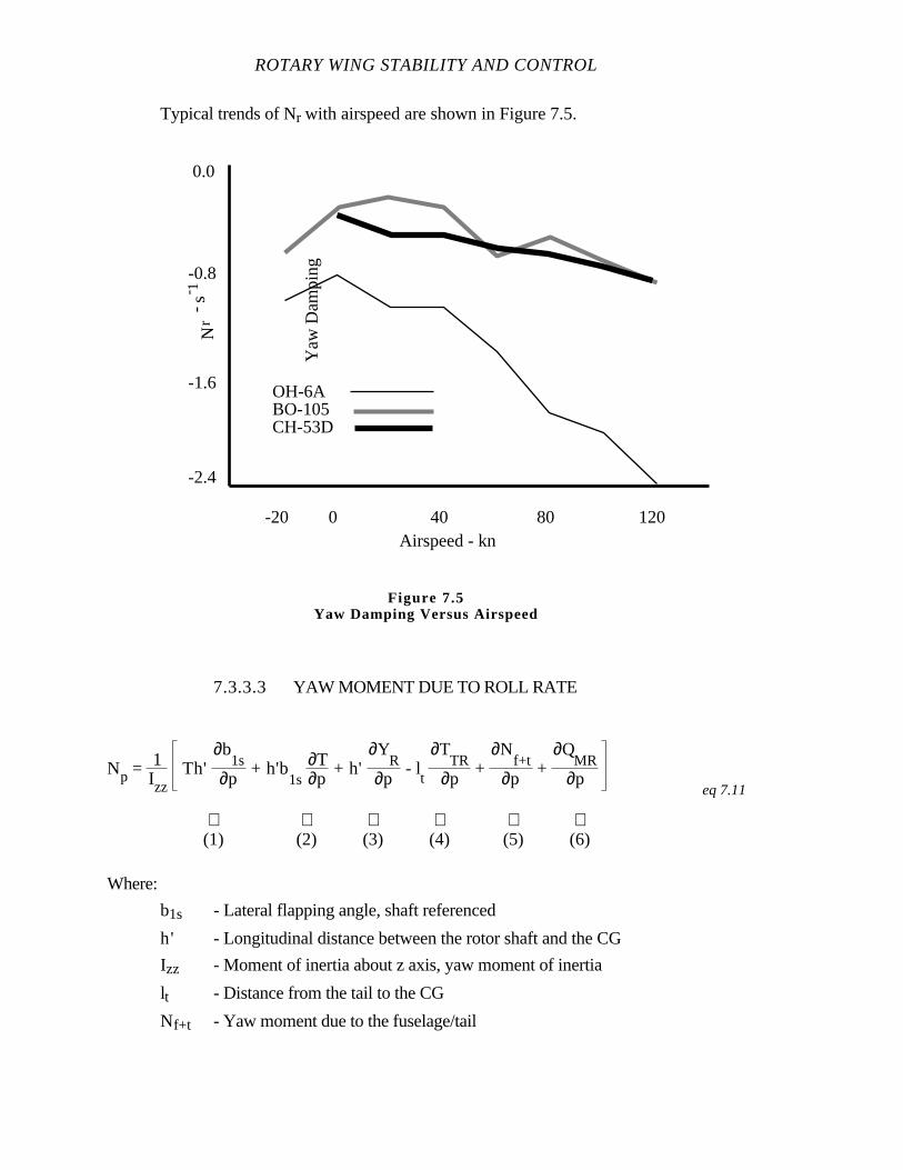
ROTARY WING STABILITY AND CONTROL
Typical trends of Nr with airspeed are shown in Figure 7.5.
7.3.3.3 YAW MOMENT DUE TO ROLL RATE
Np = 1Izz
Th'∂b
1s∂p
+ h'b1s
∂T∂p
+ h' ∂Y
R∂p
- lt
∂TTR
∂p +
∂Nf+t
∂p +
∂QMR
∂peq 7.11
⇑ ⇑ ⇑ ⇑ ⇑ ⇑(1) (2) (3) (4) (5) (6)
Where:
b1s - Lateral flapping angle, shaft referenced
h' - Longitudinal distance between the rotor shaft and the CG
Izz - Moment of inertia about z axis, yaw moment of inertia
lt - Distance from the tail to the CG
Nf+t - Yaw moment due to the fuselage/tail
0 40 80 120-20Airspeed - kn
-2.4
0.0
-0.8
-1.6
Nr
- s- 1
Yaw
Dam
ping
OH-6ABO-105CH-53D
Figure 7.5Yaw Damping Versus Airspeed
FORWARD FLIGHT LATERAL-DIRECTIONAL STABILITY, CONTROL,
AND FLYING QUALITIES
Np - Yaw moment due to roll rate
p - Angular velocity about x axis, Roll rate
QMR - Main rotor torque
T - Thrust
TTR - Tail rotor thrust
YR - Rotor side force.
Since the quantity h' is small, terms (1), (2), and (3) have little effect.
High vertical fins and high tail rotor thrust lines might make ∂Nf + t / ∂p positive and
∂TTR / ∂p negative. Thus the tail rotor contributions to NP tends to be positive and is
essentially constant since ∂TTR / ∂p is not strongly affected by speed.
Trends of Np with airspeed are shown in Figure 7.6.
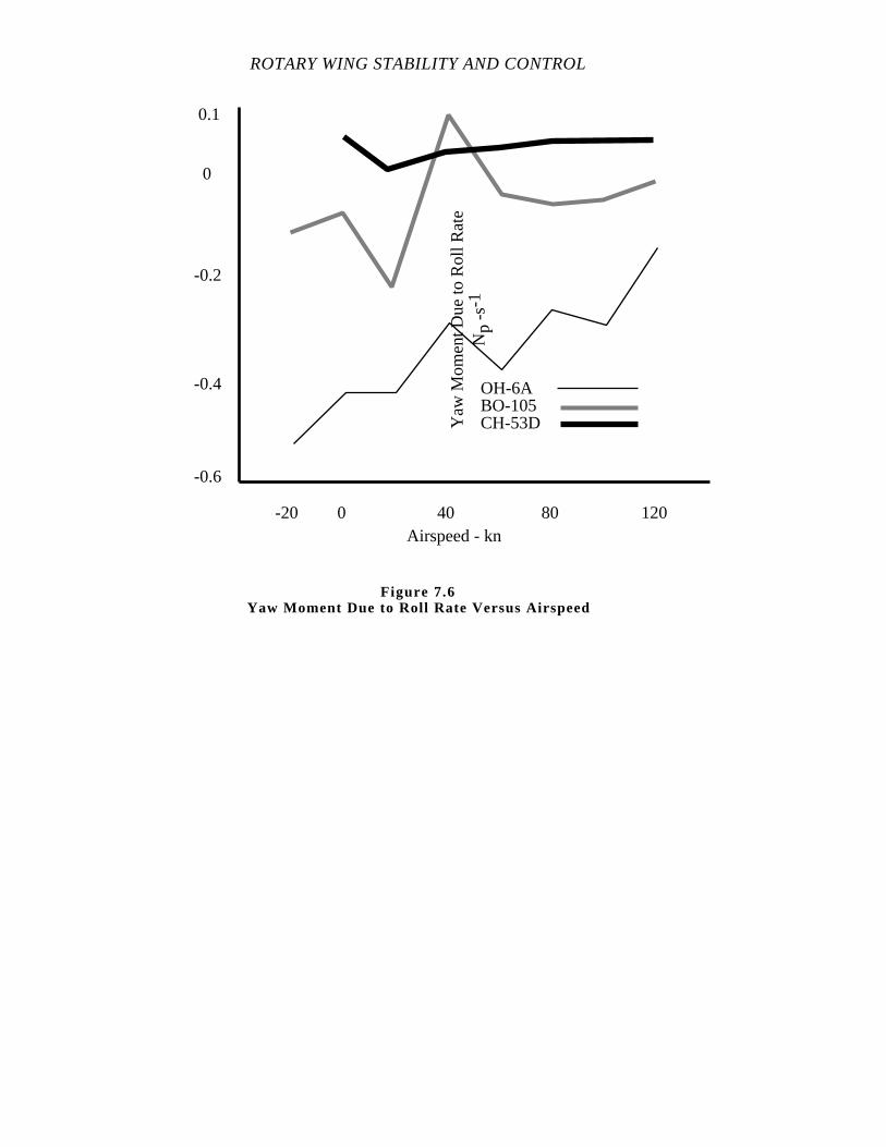
ROTARY WING STABILITY AND CONTROL
0 40 80 120-20Airspeed - kn
0
-0.2
-0.4
-0.6
0.1
OH-6ABO-105CH-53DY
aw M
omen
t Due
to R
oll R
ate
Np
-s-1
Figure 7.6Yaw Moment Due to Roll Rate Versus Airspeed
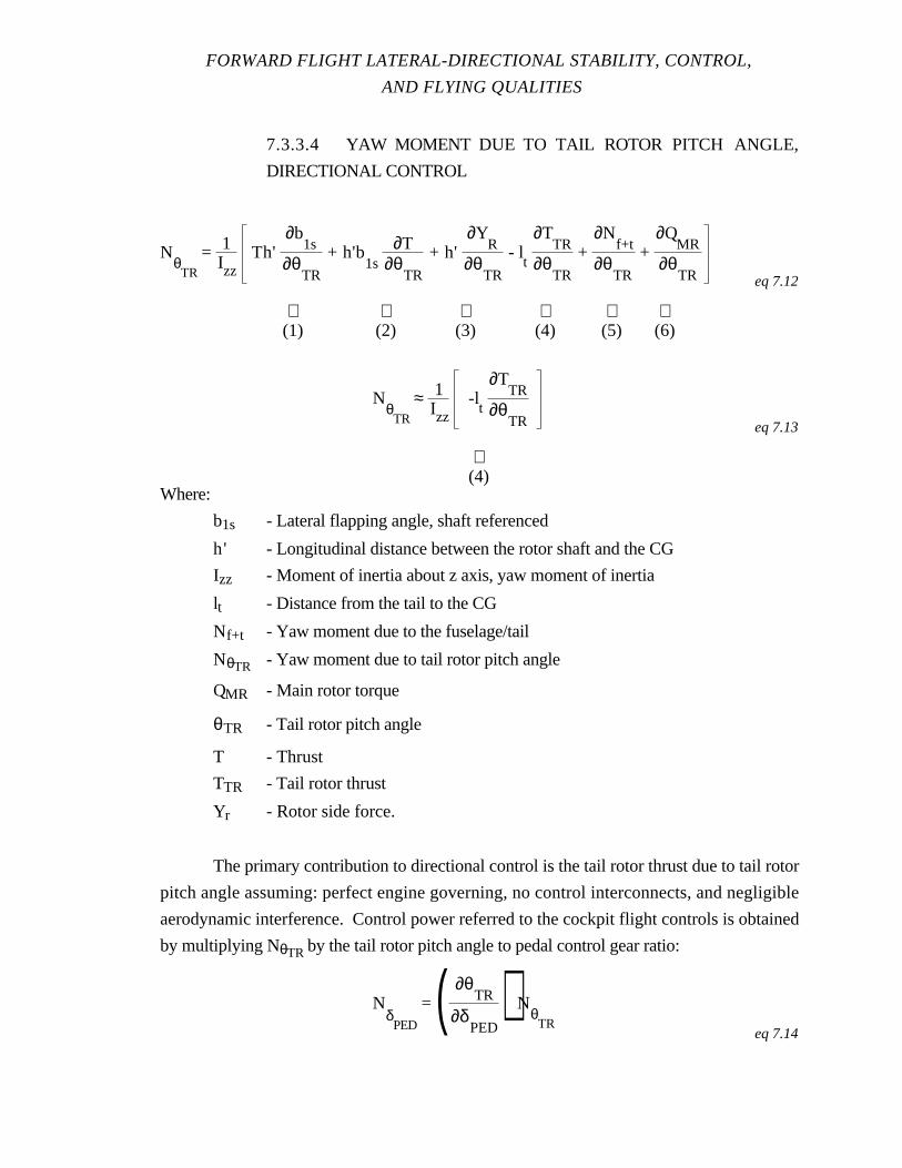
FORWARD FLIGHT LATERAL-DIRECTIONAL STABILITY, CONTROL,
AND FLYING QUALITIES
7.3.3.4 YAW MOMENT DUE TO TAIL ROTOR PITCH ANGLE,
DIRECTIONAL CONTROL
NθTR
= 1Izz
Th'∂b
1s
∂θTR
+ h'b1s
∂T∂θ
TR
+ h' ∂Y
R
∂θTR
- lt
∂TTR
∂θTR
+ ∂N
f+t
∂θTR
+ ∂Q
MR
∂θTR eq 7.12
⇑ ⇑ ⇑ ⇑ ⇑ ⇑(1) (2) (3) (4) (5) (6)
NθTR
≈ 1Izz
-lt
∂TTR
∂θTR eq 7.13
⇑(4)
Where:
b1s - Lateral flapping angle, shaft referenced
h' - Longitudinal distance between the rotor shaft and the CG
Izz - Moment of inertia about z axis, yaw moment of inertia
lt - Distance from the tail to the CG
Nf+t - Yaw moment due to the fuselage/tail
NθTR - Yaw moment due to tail rotor pitch angle
QMR - Main rotor torque
θTR - Tail rotor pitch angle
T - Thrust
TTR - Tail rotor thrust
Yr - Rotor side force.
The primary contribution to directional control is the tail rotor thrust due to tail rotor
pitch angle assuming: perfect engine governing, no control interconnects, and negligible
aerodynamic interference. Control power referred to the cockpit flight controls is obtained
by multiplying NθTR by the tail rotor pitch angle to pedal control gear ratio:
NδPED
= ( ∂θTR
∂δPED
) NθTR
eq 7.14
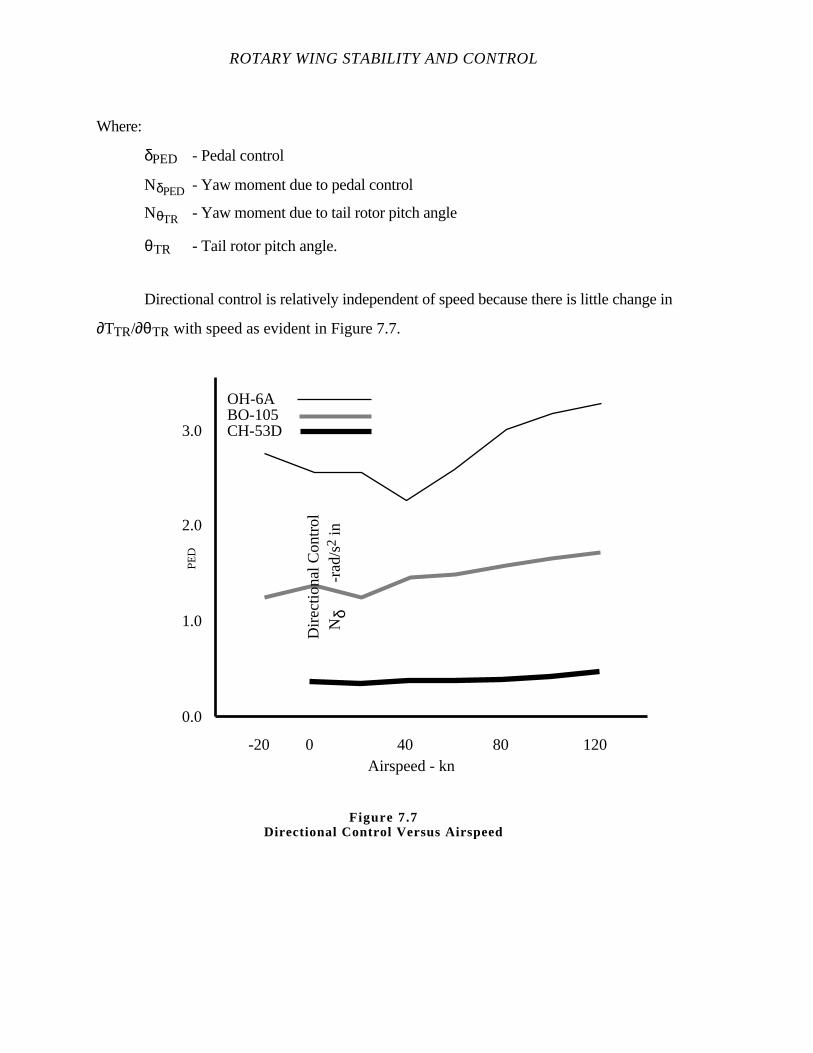
ROTARY WING STABILITY AND CONTROL
Where:
δPED - Pedal control
NδPED - Yaw moment due to pedal control
NθTR - Yaw moment due to tail rotor pitch angle
θTR - Tail rotor pitch angle.
Directional control is relatively independent of speed because there is little change in
∂TTR/∂θTR with speed as evident in Figure 7.7.
0 40 80 120-20Airspeed - kn
0.0
1.0
2.0
3.0
OH-6ABO-105CH-53D
Dire
ctio
nal C
ontr
olN
δ
-r
ad/s2
in
PED
Figure 7.7Directional Control Versus Airspeed
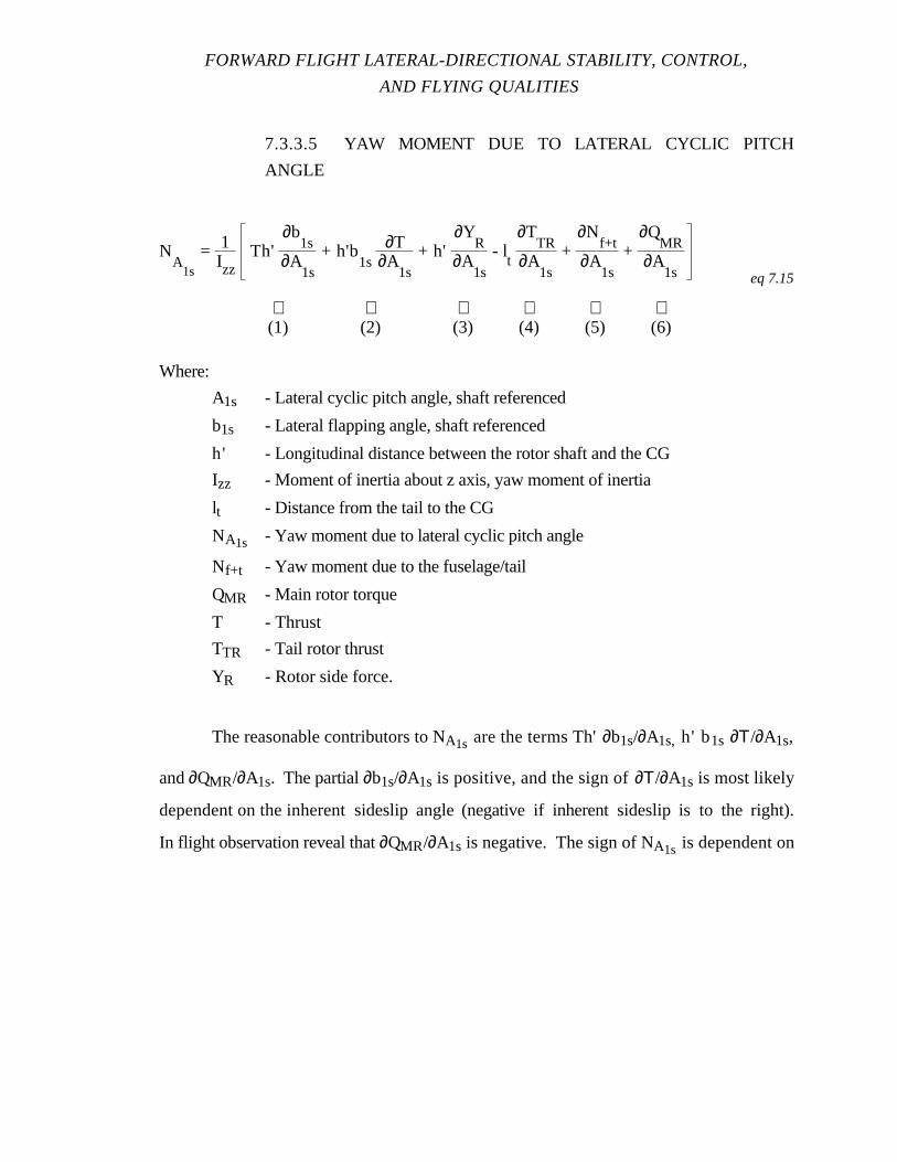
FORWARD FLIGHT LATERAL-DIRECTIONAL STABILITY, CONTROL,
AND FLYING QUALITIES
7.3.3.5 YAW MOMENT DUE TO LATERAL CYCLIC PITCH
ANGLE
NA
1s
= 1Izz
Th'∂b
1s∂A
1s
+ h'b1s
∂T∂A
1s
+ h' ∂Y
R∂A
1s
- lt
∂TTR
∂A1s
+ ∂N
f+t∂A
1s
+ ∂Q
MR∂A
1s eq 7.15
⇑ ⇑ ⇑ ⇑ ⇑ ⇑(1) (2) (3) (4) (5) (6)
Where:
A1s - Lateral cyclic pitch angle, shaft referenced
b1s - Lateral flapping angle, shaft referenced
h' - Longitudinal distance between the rotor shaft and the CG
Izz - Moment of inertia about z axis, yaw moment of inertia
lt - Distance from the tail to the CG
NA1s - Yaw moment due to lateral cyclic pitch angle
Nf+t - Yaw moment due to the fuselage/tail
QMR - Main rotor torque
T - Thrust
TTR - Tail rotor thrust
YR - Rotor side force.
The reasonable contributors to NA1s are the terms Th' ∂b1s/∂A1s, h' b1s ∂Τ/∂A1s,
and∂QMR/∂A1s. The partial ∂b1s/∂A1s is positive, and the sign of ∂Τ/∂A1s is most likely
dependent on the inherent sideslip angle (negative if inherent sideslip is to the right).
In flight observation reveal that ∂QMR/∂A1s is negative. The sign of NA1s is dependent on
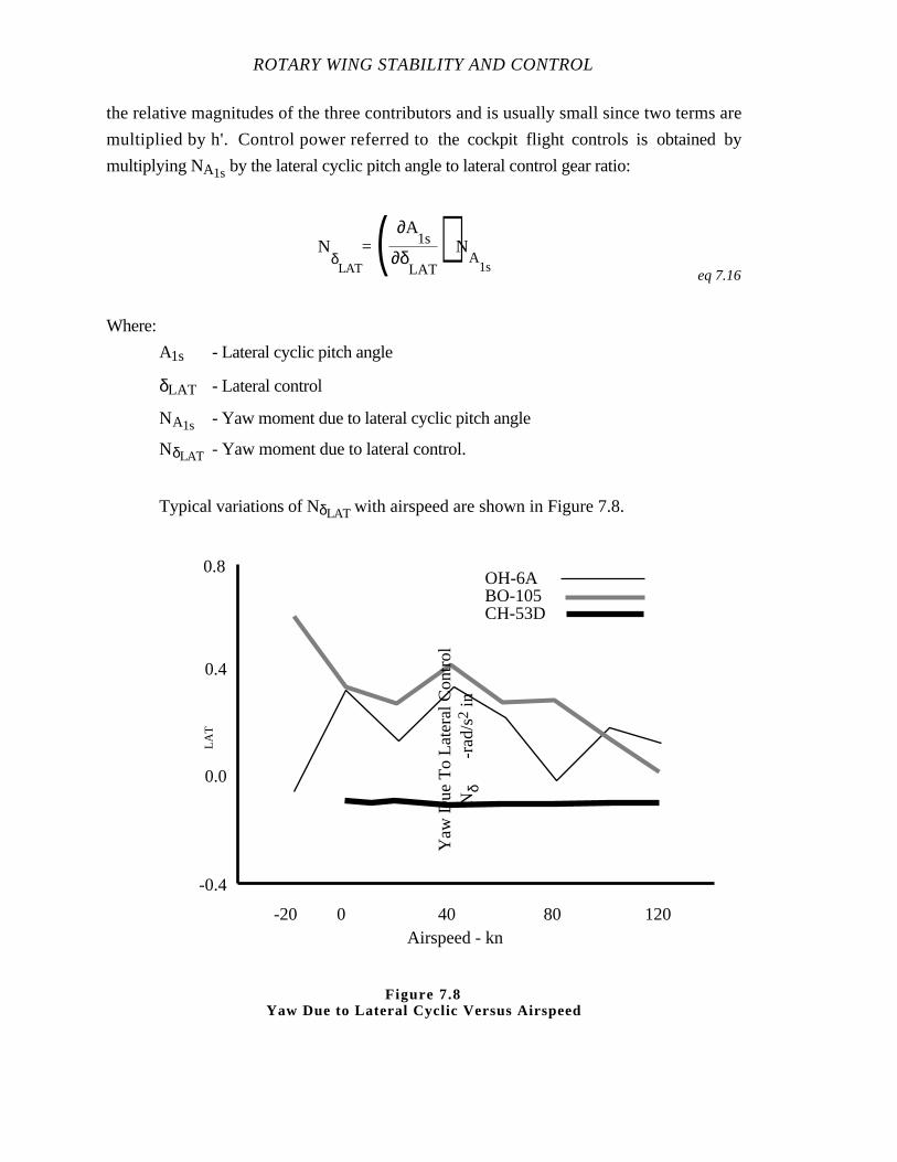
ROTARY WING STABILITY AND CONTROL
the relative magnitudes of the three contributors and is usually small since two terms are
multiplied by h'. Control power referred to the cockpit flight controls is obtained by
multiplying NA1s by the lateral cyclic pitch angle to lateral control gear ratio:
NδLAT
= ( ∂A1s
∂δLAT
) NA
1seq 7.16
Where:
A1s - Lateral cyclic pitch angle
δLAT - Lateral control
NA1s - Yaw moment due to lateral cyclic pitch angle
NδLAT - Yaw moment due to lateral control.
Typical variations of NδLAT with airspeed are shown in Figure 7.8.
0 40 80 120-20Airspeed - kn
-0.4
0.0
0.4
0.8OH-6ABO-105CH-53D
Yaw
Due
To
Late
ral C
ontr
olN
δ
-ra
d/s2
in
LAT
Figure 7.8Yaw Due to Lateral Cyclic Versus Airspeed
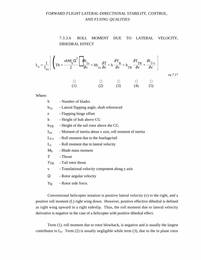
FORWARD FLIGHT LATERAL-DIRECTIONAL STABILITY, CONTROL,
AND FLYING QUALITIES
7.3.3.6 ROLL MOMENT DUE TO LATERAL VELOCITY,
DIHEDRAL EFFECT
Lv = 1Ixx
(Th + ebM
SΩ
2
2) ∂b
1s∂v
+ hb1s
∂T∂v
+ h ∂Y
R∂v
+ hTR
∂TTR
∂v +
∂Lf+t
∂v
eq 7.17
⇑ ⇑ ⇑ ⇑ ⇑(1) (2) (3) (4) (5)
Where:
b - Number of blades
b1s - Lateral flapping angle, shaft referenced
e - Flapping hinge offset
h - Height of hub above CG
hTR - Height of the tail rotor above the CG
Ixx - Moment of inertia about x axis, roll moment of inertia
Lf+t - Roll moment due to the fuselage/tail
Lv - Roll moment due to lateral velocity
MS - Blade mass moment
T - Thrust
TTR - Tail rotor thrust
v - Translational velocity component along y axis
Ω - Rotor angular velocity
YR - Rotor side force.
Conventional helicopter notation is positive lateral velocity (v) to the right, and a
positive roll moment (L) right wing down. However, positive effective dihedral is defined
as right wing upward in a right sideslip. Thus, the roll moment due to lateral velocity
derivative is negative in the case of a helicopter with positive dihedral effect.
Term (1), roll moment due to rotor blowback, is negative and is usually the largest
contributor to Lv. Term (2) is usually negligible while term (3), due to the in plane rotor
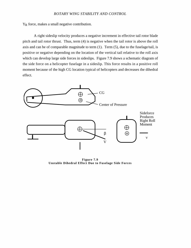
ROTARY WING STABILITY AND CONTROL
YR force, makes a small negative contribution.
A right sideslip velocity produces a negative increment in effective tail rotor blade
pitch and tail rotor thrust. Thus, term (4) is negative when the tail rotor is above the roll
axis and can be of comparable magnitude to term (1). Term (5), due to the fuselage/tail, is
positive or negative depending on the location of the vertical tail relative to the roll axis
which can develop large side forces in sideslips. Figure 7.9 shows a schematic diagram of
the side force on a helicopter fuselage in a sideslip. This force results in a positive roll
moment because of the high CG location typical of helicopters and decreases the dihedral
effect.
β
Vv
CG
Center of Pressure
SideforceProducesRight RollMoment
Figure 7.9Unstable Dihedral Effect Due to Fuselage Side Forces
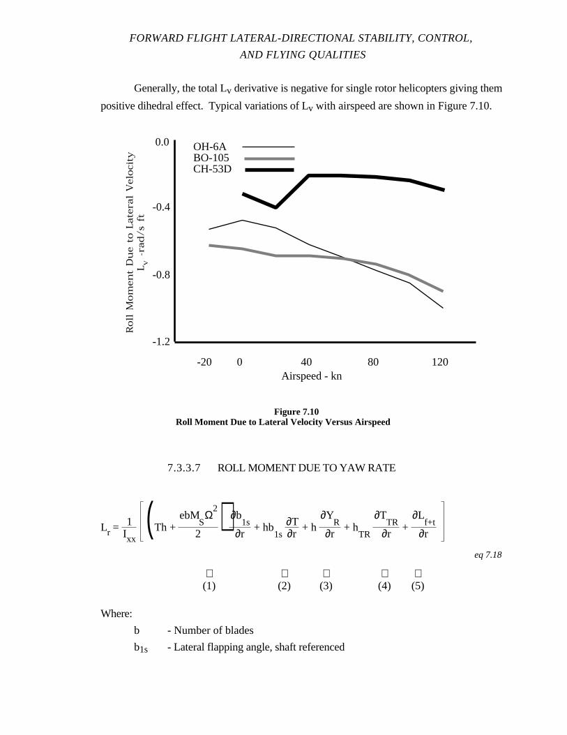
FORWARD FLIGHT LATERAL-DIRECTIONAL STABILITY, CONTROL,
AND FLYING QUALITIES
Generally, the total Lv derivative is negative for single rotor helicopters giving them
positive dihedral effect. Typical variations of Lv with airspeed are shown in Figure 7.10.
7.3.3.7 ROLL MOMENT DUE TO YAW RATE
Lr = 1Ixx
(Th + ebM
SΩ
2
2) ∂b
1s∂r
+ hb1s
∂T∂r
+ h ∂Y
R∂r
+ hTR
∂TTR
∂r +
∂Lf+t
∂r
eq 7.18
⇑ ⇑ ⇑ ⇑ ⇑(1) (2) (3) (4) (5)
Where:
b - Number of blades
b1s - Lateral flapping angle, shaft referenced
0 40 80 120-20Airspeed - kn
0.0
-0.4
-0.8
-1.2
OH-6ABO-105CH-53D
Roll M
oment
Due to
Latera
l Velo
cityL v
-rad/s
ft
Figure 7.10Roll Moment Due to Lateral Velocity Versus Airspeed
ROTARY WING STABILITY AND CONTROL
e - Flapping hinge offset
h - Height of hub above CG
hTR - Height of the tail rotor above the CG
Ixx - Moment of inertia about x axis, roll moment of inertia
Lf+t - Roll moment due to the fuselage/tail
Lr - Roll moment due to yaw rate
MS - Blade mass moment
r - Angular velocity about z axis, Yaw rate
T - Thrust
TTR - Tail rotor thrust
Ω - Rotor angular velocity
YR - Rotor side force.
The partial ∂b1s/ ∂r is dependent on longitudinal CG position. The partial ∂T/ ∂r
is dependent on both longitudinal CG position and the trim value of b1s. The contributions
involving these partials are normally not significant.
The fuselage probably does not make any significant contribution except with a
large, high vertical tail or if wings are present. The primary contributor for typical
helicopter configurations is the tail rotor. Typical variations of Lr with airspeed are shown
in Figure 7.11.
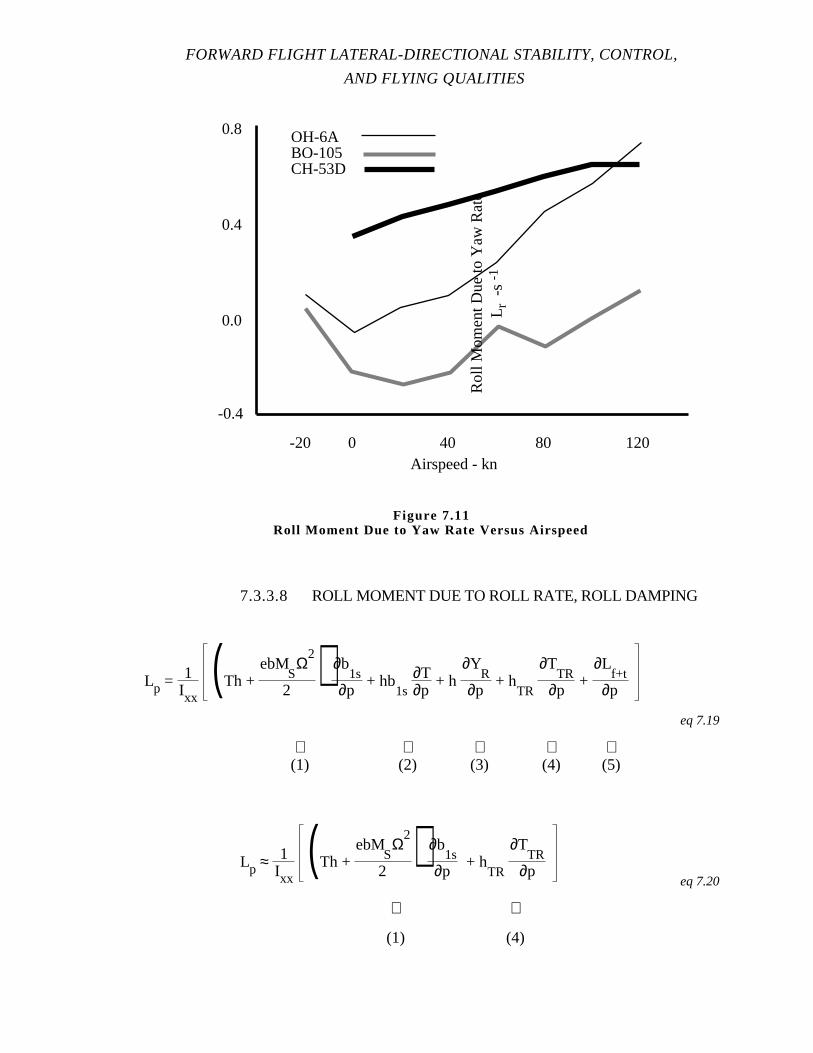
FORWARD FLIGHT LATERAL-DIRECTIONAL STABILITY, CONTROL,
AND FLYING QUALITIES
7.3.3.8 ROLL MOMENT DUE TO ROLL RATE, ROLL DAMPING
Lp = 1Ixx
(Th + ebM
SΩ
2
2) ∂b
1s∂p
+ hb1s
∂T∂p
+ h ∂Y
R∂p
+ hTR
∂TTR
∂p +
∂Lf+t
∂p
eq 7.19
⇑ ⇑ ⇑ ⇑ ⇑(1) (2) (3) (4) (5)
Lp ≈ 1Ixx
(Th + ebM
SΩ
2
2) ∂b
1s∂p
+ hTR
∂TTR
∂peq 7.20
⇑ ⇑
(1) (4)
0 40 80 120-20Airspeed - kn
-0.4
0.0
0.4
0.8 OH-6ABO-105CH-53D
Rol
l Mom
ent D
ue to
Yaw
Rat
eL
r -s
-1
Figure 7.11Roll Moment Due to Yaw Rate Versus Airspeed
ROTARY WING STABILITY AND CONTROL
Where:
b - Number of blades
b1s - Lateral flapping angle, shaft referenced
e - Flapping hinge offset
h - Height of hub above CG
hTR - Height of the tail rotor above the CG
Ixx - Moment of inertia about x axis, roll moment of inertia
Lf+t - Roll moment due to the fuselage/tail
Lp - Roll moment due to roll rate
MS - Blade mass moment
p - Angular velocity about x axis, Roll rate
T - Thrust
TTR - Tail rotor thrust
Ω - Rotor angular velocity
YR - Rotor side force.
Term (1) is the largest contributor to roll damping and is due to TPP tilt resulting
from flapping introduced by the roll rate. The tail rotor forces due to the lateral velocity
induced by the roll are the source for term (4), and are significant depending on the height
of the tail rotor above the roll axis. There is little change in thrust due to roll rate, rotor side
force due to roll rate, and roll moment due to the fuselage/tail due to roll rate; therefore
terms (2), (3), and (5) can be neglected, and Equation 7.19 can be approximated by
Equation 7.20. Term (1) is nearly independent of airspeed. The thrust variation with
lateral velocity at the tail rotor is also nearly constant with airspeed. However, the lateral
velocity at the tail and the roll moment due to tail rotor thrust both depend on hTR. This
distance is a function of the roll axis orientation which may vary for different forward flight
conditions when the equations of motion are referred to stability axes.
Typical values of Lp as a function of airspeed are shown in Figure 7.12. Lp is
essentially independent of airspeed.
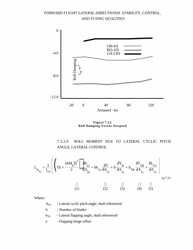
FORWARD FLIGHT LATERAL-DIRECTIONAL STABILITY, CONTROL,
AND FLYING QUALITIES
7.3.3.9 ROLL MOMENT DUE TO LATERAL CYCLIC PITCH
ANGLE, LATERAL CONTROL
LA
1s
= 1Ixx
(Th + ebM
SΩ
2
2) ∂b
1s∂A
1s
+ hb1s
∂T∂A
1s
+ h ∂Y
R∂A
1s
+ hTR
∂TTR
∂A1s
+ ∂L
f+t∂A
1s
eq 7.21
⇑ ⇑ ⇑ ⇑ ⇑(1) (2) (3) (4) (5)
Where:
A1s - Lateral cyclic pitch angle, shaft referenced
b - Number of blades
b1s - Lateral flapping angle, shaft referenced
e - Flapping hinge offset
0 40 80 120-20Airspeed - kn
0
-4.0
-8.0
-12.0
OH-6ABO-105CH-53D
Rol
l Dam
ping
Lp
-s-1
Figure 7.12Roll Damping Versus Airspeed
ROTARY WING STABILITY AND CONTROL
h - Height of hub above CG
hTR - Height of the tail rotor above the CG
Ixx - Moment of inertia about x axis, roll moment of inertia
LA1s - Roll moment due to lateral cyclic pitch angle
Lf+t - Roll moment due to the fuselage/tail
MS - Blade mass moment
T - Thrust
TTR - Tail rotor thrust
Ω - Rotor angular velocity
YR - Rotor side force.
The lateral control derivative is predominantly caused by term (1) which is
proportional to the change in TPP tilt with lateral cyclic pitch angle input (∂b1s/∂A1s). The
lateral tilt has little influence on the flow through the rotor disk, its effect primarily being to
tilt the TPP laterally relative to the shaft. Thus, LA1s is little affected by the initial trim
speed.
The control power referred to the cockpit flight controls is obtained by multiplying
LA1s by the lateral cyclic pitch angle to lateral control gear ratio:
LδLAT
= ( ∂A1s
∂δLAT
)LA
1seq 7.22
Where:
A1s - Lateral cyclic pitch angle, shaft referenced
δLAT - Lateral control
LA1s - Roll moment due to lateral cyclic pitch angle
LδLAT - Roll moment due to lateral control.
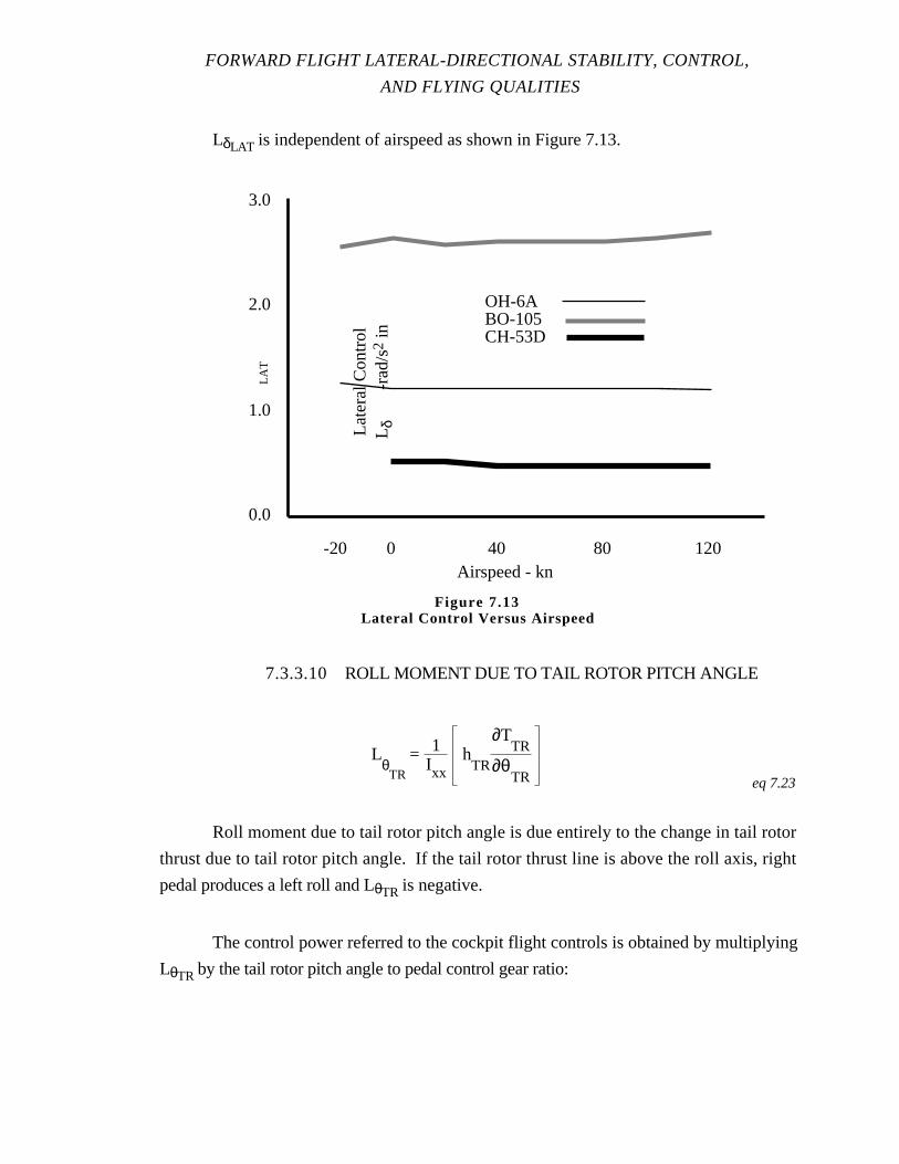
FORWARD FLIGHT LATERAL-DIRECTIONAL STABILITY, CONTROL,
AND FLYING QUALITIES
LδLAT is independent of airspeed as shown in Figure 7.13.
7.3.3.10 ROLL MOMENT DUE TO TAIL ROTOR PITCH ANGLE
LθTR
= 1Ixx
hTR
∂TTR
∂θTR eq 7.23
Roll moment due to tail rotor pitch angle is due entirely to the change in tail rotor
thrust due to tail rotor pitch angle. If the tail rotor thrust line is above the roll axis, right
pedal produces a left roll and LθTR is negative.
The control power referred to the cockpit flight controls is obtained by multiplying
LθTR by the tail rotor pitch angle to pedal control gear ratio:
0 40 80 120-20Airspeed - kn
0.0
1.0
2.0
3.0
OH-6ABO-105CH-53D
Late
ral C
ontr
olL
δ
-r
ad/s2
in
LAT
Figure 7.13Lateral Control Versus Airspeed
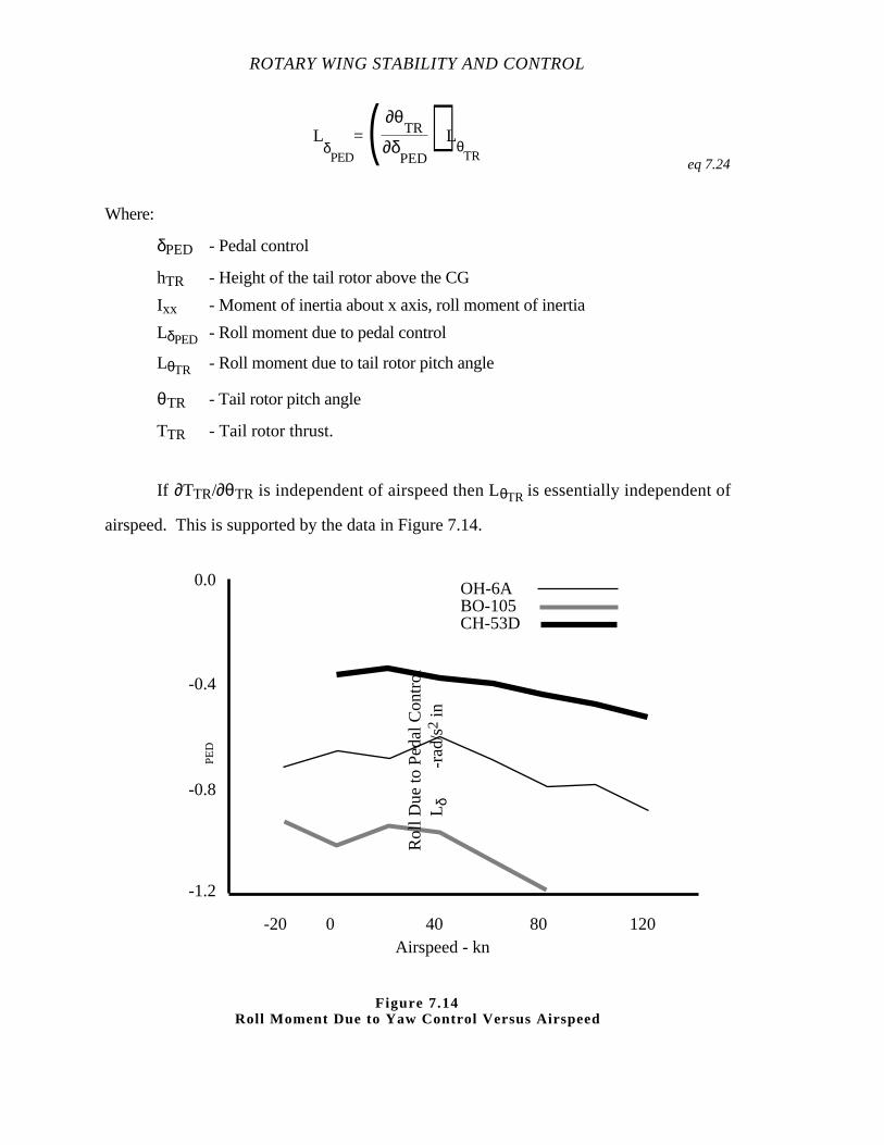
ROTARY WING STABILITY AND CONTROL
LδPED
= ( ∂θTR
∂δPED
) LθTR
eq 7.24
Where:
δPED - Pedal control
hTR - Height of the tail rotor above the CG
Ixx - Moment of inertia about x axis, roll moment of inertia
LδPED - Roll moment due to pedal control
LθTR - Roll moment due to tail rotor pitch angle
θTR - Tail rotor pitch angle
TTR - Tail rotor thrust.
If ∂TTR/∂θTR is independent of airspeed then LθTR is essentially independent of
airspeed. This is supported by the data in Figure 7.14.
0 40 80 120-20Airspeed - kn
0.0
-0.4
-0.8
-1.2
OH-6ABO-105CH-53D
Rol
l Due
to P
edal
Con
trol
Lδ
-rad
/s2 in
PE
D
Figure 7.14Roll Moment Due to Yaw Control Versus Airspeed
FORWARD FLIGHT LATERAL-DIRECTIONAL STABILITY, CONTROL,
AND FLYING QUALITIES
7.3.3.11 SIDE FORCE DUE TO LATERAL VELOCITY
Yv = 1m T
∂b1s
∂v + b
1s∂T∂v
+ ∂Y
R
∂v +
∂TTR
∂v +
∂Yf+t
∂v eq 7.25
⇑ ⇑ ⇑ ⇑ ⇑(1) (2) (3) (4) (5)
Where:
b1s - Lateral flapping angle, shaft referenced
m - Mass
T - Thrust
TTR - Tail rotor thrust
v - Translational velocity component along y axis
Yf+t - Side force due to the fuselage/tail
YR - Rotor side force
Yv - Side force due to lateral velocity.
Term (2) is dependent on the initial TPP tilt at trim but is usually insignificant. The
in plane rotor force contribution (Term (3) is also small. Term (1) due to the increment in
lateral tilt of the TPP and term (4) due to the change in tail rotor thrust with lateral velocity
are of comparable magnitude, and do not vary much with trim speed. Term (5) is
proportional to the product of the dynamic pressure and sideslip angle. Consequently, term
(5) varies with trim speed causing a considerable variation in the total derivative through the
speed range. The overall variation of Yv with speed is presented in Figure 7.15.
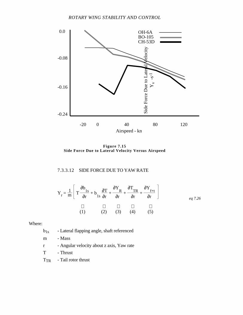
ROTARY WING STABILITY AND CONTROL
7.3.3.12 SIDE FORCE DUE TO YAW RATE
Yr = 1m T
∂b1s
∂r + b
1s∂T∂r
+ ∂Y
R
∂r +
∂TTR
∂r +
∂Yf+t
∂r eq 7.26
⇑ ⇑ ⇑ ⇑ ⇑(1) (2) (3) (4) (5)
Where:
b1s - Lateral flapping angle, shaft referenced
m - Mass
r - Angular velocity about z axis, Yaw rate
T - Thrust
TTR - Tail rotor thrust
0 40 80 120-20Airspeed - kn
0.0
-0.08
-0.16
-0.24
OH-6ABO-105CH-53D
Sid
e F
orce
Due
to L
ater
al V
eloc
ityY
v -
s-1
Figure 7.15Side Force Due to Lateral Velocity Versus Airspeed
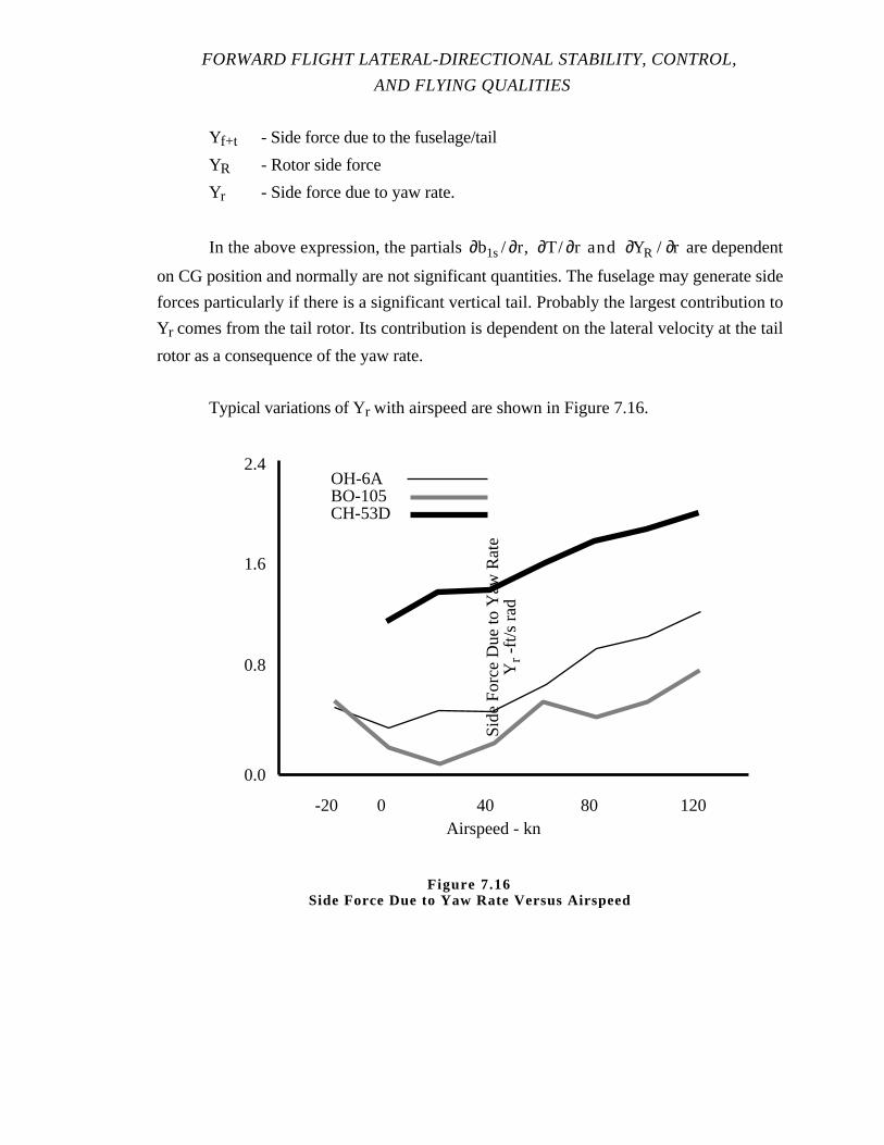
FORWARD FLIGHT LATERAL-DIRECTIONAL STABILITY, CONTROL,
AND FLYING QUALITIES
Yf+t - Side force due to the fuselage/tail
YR - Rotor side force
Yr - Side force due to yaw rate.
In the above expression, the partials ∂b1s/ ∂r, ∂T/ ∂r and ∂YR / ∂r are dependent
on CG position and normally are not significant quantities. The fuselage may generate side
forces particularly if there is a significant vertical tail. Probably the largest contribution to
Yr comes from the tail rotor. Its contribution is dependent on the lateral velocity at the tail
rotor as a consequence of the yaw rate.
Typical variations of Yr with airspeed are shown in Figure 7.16.
0 40 80 120-20Airspeed - kn
0.0
0.8
1.6
2.4OH-6ABO-105CH-53D
Sid
e F
orce
Due
to Y
aw R
ate
Yr -
ft/s
rad
Figure 7.16Side Force Due to Yaw Rate Versus Airspeed
ROTARY WING STABILITY AND CONTROL
7.3.3.13 SIDE FORCE DUE TO ROLL RATE
Yp = 1m T
∂b1s
∂p + b
1s∂T∂p
+ ∂Y
R
∂p +
∂TTR
∂p +
∂Yf+t
∂peq 7.27
The significant quantities in the above expression are T ∂b1s/∂p and ∂TTR/∂p. An
approximation for Yp is:
Yp ≈ 1m T
∂b1s
∂p +
∂TTR
∂p eq 7.28
Where:
b1s - Lateral flapping angle, shaft referenced
m - Mass
p - Angular velocity about x axis, Roll rate
T - Thrust
TTR - Tail rotor thrust
Yf+t - Side force due to the fuselage/tail
Yp - Side force due to roll rate
YR - Rotor side force.
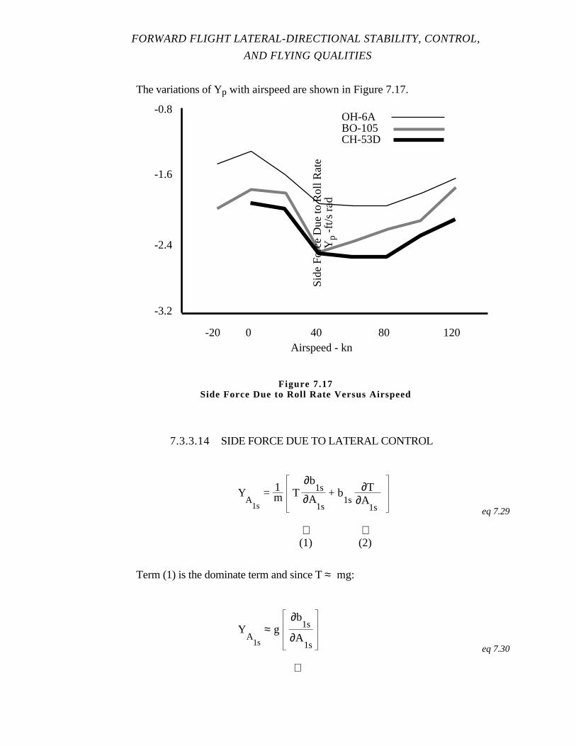
FORWARD FLIGHT LATERAL-DIRECTIONAL STABILITY, CONTROL,
AND FLYING QUALITIES
The variations of Yp with airspeed are shown in Figure 7.17.
7.3.3.14 SIDE FORCE DUE TO LATERAL CONTROL
YA
1s
= 1m T∂b
1s∂A
1s
+ b1s
∂T∂A
1s
eq 7.29
⇑ ⇑(1) (2)
Term (1) is the dominate term and since T ≈ mg:
YA
1s
≈ g ∂b
1s
∂A1s eq 7.30
⇑
0 40 80 120-20Airspeed - kn
-0.8
-1.6
-2.4
-3.2
OH-6ABO-105CH-53D
Sid
e F
orce
Due
to R
oll R
ate
Yp
-ft/s
rad
Figure 7.17Side Force Due to Roll Rate Versus Airspeed

ROTARY WING STABILITY AND CONTROL
(1)
The control power referred to the cockpit flight controls is the product of YA1s and
the lateral cyclic pitch angle to lateral control gear ratio:
YδLAT
= ( ∂A1s
∂δLAT
) YA
1seq 7.31
Where:
A1s - Lateral cyclic pitch angle, shaft referenced
b1s - Lateral flapping angle, shaft referenced
δLAT - Lateral control
g - Gravity
m - Mass
T - Thrust
YA1s - Side force due to lateral cyclic pitch angle
YδLAT - Side force due to lateral control.
The side force due to lateral control input is primarily due to the resulting lateral tilt
of the TPP and thrust vector. The variations of YδLAT with speed are indicated in Figure
7.18.

FORWARD FLIGHT LATERAL-DIRECTIONAL STABILITY, CONTROL,
AND FLYING QUALITIES
7.3.3.15 SIDE FORCE DUE TO DIRECTIONAL CONTROL
YθTR
= 1m
∂TTR
∂θTR eq 7.32
⇑
(4)
The control power referred to the cockpit flight controls is the product of YθTR and
the tail rotor pitch angle to pedal control gear ratio:
YδPED
= ( ∂θTR
∂δPED
) YθTR
eq 7.33
0 40 80 120-20Airspeed - kn
0.0
0.4
0.8
1.2OH-6ABO-105CH-53D
Sid
e F
orce
Due
to L
ater
al C
ontr
olY
δ
-f
t/s2
in
LAT
Figure 7.18Side Force Due to Lateral Control Versus Airspeed
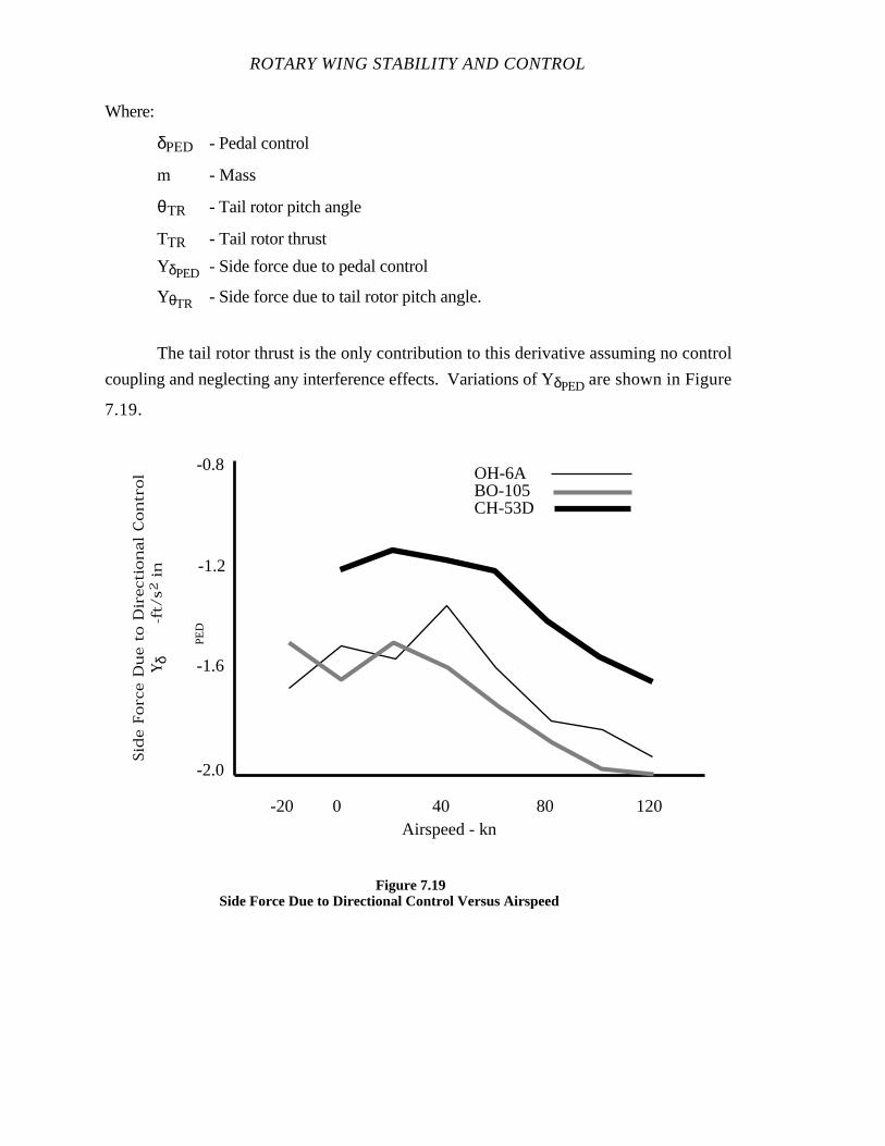
ROTARY WING STABILITY AND CONTROL
Where:
δPED - Pedal control
m - Mass
θTR - Tail rotor pitch angle
TTR - Tail rotor thrust
YδPED - Side force due to pedal control
YθTR - Side force due to tail rotor pitch angle.
The tail rotor thrust is the only contribution to this derivative assuming no control
coupling and neglecting any interference effects. Variations of YδPED are shown in Figure
7.19.
0 40 80 120-20Airspeed - kn
-0.8
-1.2
-1.6
-2.0
OH-6ABO-105CH-53D
Side F
orce D
ue to D
irection
al Cont
rolY δ
-ft/
s2 in
PE
D
Figure 7.19Side Force Due to Directional Control Versus Airspeed
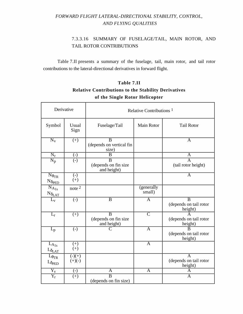
FORWARD FLIGHT LATERAL-DIRECTIONAL STABILITY, CONTROL,
AND FLYING QUALITIES
7.3.3.16 SUMMARY OF FUSELAGE/TAIL, MAIN ROTOR, AND
TAIL ROTOR CONTRIBUTIONS
Table 7.II presents a summary of the fuselage, tail, main rotor, and tail rotor
contributions to the lateral-directional derivatives in forward flight.
Table 7.II
Relative Contributions to the Stability Derivatives
of the Single Rotor Helicopter
Derivative Relative Contributions 1
Symbol UsualSign
Fuselage/Tail Main Rotor Tail Rotor
Nv (+) B(depends on vertical fin
size)
A
Nr (-) B ANp (-) B
(depends on fin sizeand height)
A(tail rotor height)
NθTRNδPED
(-)(+)
A
NA1sNδLAT
note2 (generallysmall)
Lv (-) B A B(depends on tail rotor
height)Lr (+) B
(depends on fin sizeand height)
C A(depends on tail rotor
height)Lp (-) C A B
(depends on tail rotorheight)
LA1sLδLAT
(+)(+)
A
LθTRLδPED
(-)(+)(+)(-)
A(depends on tail rotor
height)Yv (-) A A AYr (+) B
(depends on fin size)A

ROTARY WING STABILITY AND CONTROL
Relative Contributions to the Stability Derivatives
of the Single Rotor Helicopter (cont’d)
Yp (-) B(depends on fin size
and height)
A(depends on tail rotor
height)YA1sYδLAT
(+)(+)
A
YθTRYδPED
(+)(-)
A
Notes: (1) A is the highest contributor(2) Depends on the relative strengths of three factors
7.3.4 Trimmed Control Positions
An important part of helicopter flight testing is determining the trimmed flight
control positions throughout the flight envelope. A complete investigation requires a large
number of flight tests involving a multidimensional matrix of possible flight conditions. A
practical approach is to determine the trimmed control positions when important parameters
are changed. Gross weight, altitude, airspeed, rotor speed, as well as powered and
autorotational flight are all factors which can have a significant effect on trimmed control
positions and control margins. The effect of these parameters is evaluated during rectilinear
and turning flight.
The effect of airspeed and torque on trimmed pedal position is considered as an
example. Figure 7.20 (a) presents typical plots of pedal position versus airspeed for four
different constant rotor torque conditions. At a given airspeed, when a greater torque is
applied to the rotor, a greater left pedal displacement is required, producing a greater right
tail rotor thrust to maintain equilibrium.
The trimmed flight conditions for different forward velocities along each of the
constant torque curves correspond to a variation in descending, level, and climbing flight.
Considerable flight testing is required to determine a family of constant torque curves.
Consequently, an abbreviated program incorporates a series of level flight airspeeds. This
results in a level flight pedal position versus airspeed curve shown on Figure 7.20. Similar
plots could be made for constant rates of descent or climb covering the entire speed range to
VNE.
The definition of the test corresponding to the plot of pedal position versus airspeed
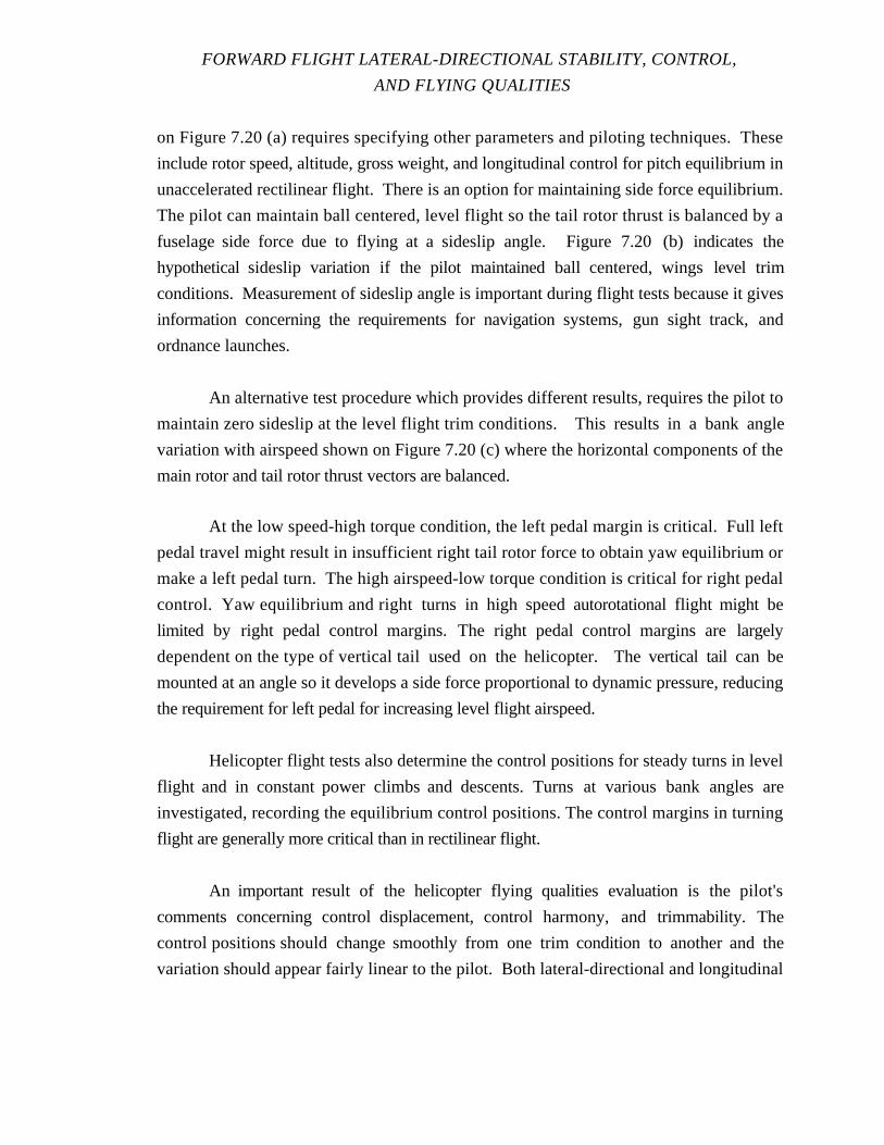
FORWARD FLIGHT LATERAL-DIRECTIONAL STABILITY, CONTROL,
AND FLYING QUALITIES
on Figure 7.20 (a) requires specifying other parameters and piloting techniques. These
include rotor speed, altitude, gross weight, and longitudinal control for pitch equilibrium in
unaccelerated rectilinear flight. There is an option for maintaining side force equilibrium.
The pilot can maintain ball centered, level flight so the tail rotor thrust is balanced by a
fuselage side force due to flying at a sideslip angle. Figure 7.20 (b) indicates the
hypothetical sideslip variation if the pilot maintained ball centered, wings level trim
conditions. Measurement of sideslip angle is important during flight tests because it gives
information concerning the requirements for navigation systems, gun sight track, and
ordnance launches.
An alternative test procedure which provides different results, requires the pilot to
maintain zero sideslip at the level flight trim conditions. This results in a bank angle
variation with airspeed shown on Figure 7.20 (c) where the horizontal components of the
main rotor and tail rotor thrust vectors are balanced.
At the low speed-high torque condition, the left pedal margin is critical. Full left
pedal travel might result in insufficient right tail rotor force to obtain yaw equilibrium or
make a left pedal turn. The high airspeed-low torque condition is critical for right pedal
control. Yaw equilibrium and right turns in high speed autorotational flight might be
limited by right pedal control margins. The right pedal control margins are largely
dependent on the type of vertical tail used on the helicopter. The vertical tail can be
mounted at an angle so it develops a side force proportional to dynamic pressure, reducing
the requirement for left pedal for increasing level flight airspeed.
Helicopter flight tests also determine the control positions for steady turns in level
flight and in constant power climbs and descents. Turns at various bank angles are
investigated, recording the equilibrium control positions. The control margins in turning
flight are generally more critical than in rectilinear flight.
An important result of the helicopter flying qualities evaluation is the pilot's
comments concerning control displacement, control harmony, and trimmability. The
control positions should change smoothly from one trim condition to another and the
variation should appear fairly linear to the pilot. Both lateral-directional and longitudinal
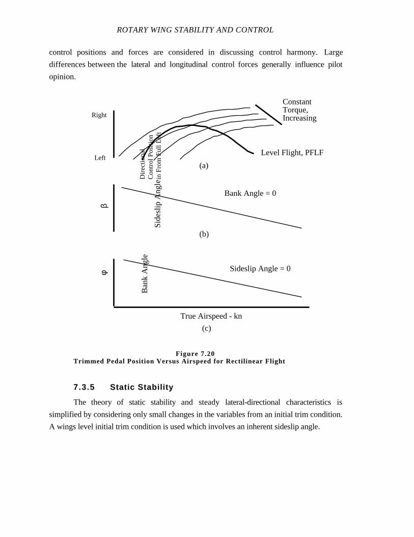
ROTARY WING STABILITY AND CONTROL
control positions and forces are considered in discussing control harmony. Large
differences between the lateral and longitudinal control forces generally influence pilot
opinion.
Trimmed Pedal Position Versus Airspeed for Rectilinear Flight
7.3.5 Static Stability
The theory of static stability and steady lateral-directional characteristics is
simplified by considering only small changes in the variables from an initial trim condition.
A wings level initial trim condition is used which involves an inherent sideslip angle.
True Airspeed - kn
Dire
ctio
nal
Con
trol
Pos
ition
in F
rom
Ful
l Lef
tLeft
Right
Sid
eslip
Ang
le
β
Ban
k A
ngle
φ
Bank Angle = 0
Sideslip Angle = 0
(a)
(b)
(c)
ConstantTorque,Increasing
Level Flight, PFLF
Figure 7.20
FORWARD FLIGHT LATERAL-DIRECTIONAL STABILITY, CONTROL,
AND FLYING QUALITIES
7.3.5.1 STEADY LATERAL-DIRECTIONAL CHARACTERISTICS
Four different steady conditions are used in flight tests for the evaluation of
helicopter lateral-directional flight characteristics. The steady heading sideslip is used to
evaluate static lateral-directional stability and side force characteristics through flight control
positions and bank angle. The remaining steady conditions obtained in turning flight
include pedal only turns, lateral cyclic only turns, and coordinated turns.
7.3.5.2 INHERENT SIDESLIP IN FORWARD FLIGHT
A typical U.S. single rotor helicopter in wings level, coordinated, equilibrium flight
is normally flying in a right sideslip. This sideslip is required to achieve a balance between
the side force contribution of tail rotor thrust and fuselage-main rotor side forces. The
sideslip angle required to achieve the balance in side forces is the inherent sideslip angle.
Increasing main rotor torque by going from level to climbing flight, or by increasing gross
weight increases the inherent sideslip angle. In addition, a decrease in airspeed at constant
main rotor torque may have the same effect; since the tail rotor force is constant, a larger
sideslip angle is required at the slower airspeeds to develop the same fuselage side forces.
Important effects associated with the inherent sideslip angle are demonstrated in
flight. The static lateral-directional stability can be dissimilar on either side of the inherent
sideslip angle. Such a condition results in dissimilar helicopter response to right and left
disturbances from trimmed flight.
A second problem area is mission oriented. In terms of dead reckoning navigation,
the effects of an inherent sideslip angle can not be separated from the effects of a
crosswind. The pilot generally has no way of knowing the sideslip angle. When Doppler
ground speed and drift angle are furnished, the combined effects of wind and inherent
sideslip are displayed as though caused by crosswind alone.
Thirdly, the variation in inherent sideslip angle with power and airspeed may
introduce a significant lateral control task during accelerations and decelerations.
7.3.5.3 AIRSPEED POSITION ERRORS IN SIDESLIPS
Indicated airspeed in sideslips is subject to position error, particularly at slow
speeds. Large variations in airspeed position errors with small variations in sideslip angles
ROTARY WING STABILITY AND CONTROL
may present a problem in forward flight. For example, a fictitious helicopter has a 10 kn
position error with each 5˚ of sideslip. If this helicopter is disturbed in yaw by a gust or
increase in power, the helicopter yaws right and left, and the airspeed never seems to
stabilize. Efforts by the pilot to maintain airspeed may keep the helicopter disturbed in
yaw, perpetuating the indicated airspeed problems.
Several procedures are used to alleviate the problems of airspeed position errors in
helicopter flight tests. Airspeed calibration tests are conducted and corrected airspeed
flown in subsequent data flights. The pitot static source can be located on a swivel on the
end of a boom so it aligns with the airflow. Another method for avoiding position error
due to sideslip in forward flight is use of a trailing bomb towed behind the helicopter.
Omni-directional helicopter airspeed systems are available which are generally free
of sideslip position errors. They provide the body axes components of the level flight
airspeed, u and v, as well as the total airspeed.
7.3.5.4 STEADY HEADING SIDESLIPS (SHSS)
One of the conventional methods for evaluating helicopter static lateral-directional
characteristics is to obtain data at stabilized steady heading sideslip conditions. The tests
are conducted at a series of sideslip angles about a specified trim point. Collective pitch is
fixed and flight path velocity is maintained by longitudinal cyclic control inputs. The
normal initial trim point in forward flight is a steady heading, wings level, balanced
condition.
The principal characteristics evaluated in steady heading sideslip tests are the
combined effects of dihedral effect, directional static stability, and the side force variation
with sideslip. The term effective dihedral means “not necessarily caused by dihedral” and
is used to refer to the total helicopter roll moment due to sideslip and tail rotor thrust as
reflected by the lateral control displacement required to maintain a steady heading sideslip.

FORWARD FLIGHT LATERAL-DIRECTIONAL STABILITY, CONTROL,
AND FLYING QUALITIES
The lateral-directional equations of motion reduce to the following for steady
rectilinear flight where v = p = r = p = r = 0 :
-Yv u0∆β -g∆φ = Y
A1s
∆A1s
+ YθTR
∆θTR
= YδLAT
∆δLAT
+ YδPED
∆δPED
eq 7.34
-Lv u0∆β = L
A1s
∆A1s
+ LθTR
∆θTR
= LδLAT
∆δLAT
+ LδPED
∆δPED
eq 7.35
-Nv u0∆β = N
A1s
∆A1s
+ NθTR
∆θTR
= NδLAT
∆δLAT
+ NδPED
∆δPED
eq 7.36
Where:
A1s - Lateral cyclic
β - Sideslip angle
δLAT - Lateral control
δPED - Pedal control
φ - Roll angle
g - Gravity
LA1s - Roll moment due to lateral cyclic pitch angle
LδLAT - Roll moment due to lateral control
LδPED - Roll moment due to pedal control
LθTR - Roll moment due to tail rotor pitch angle
Lv - Roll moment due to lateral velocity
NA1s - Yaw moment due to lateral cyclic pitch angle
NδLAT - Yaw moment due to lateral control
NδPED - Yaw moment due to pedal control
NθTR - Yaw moment due to tail rotor pitch angle
Nv - Yaw moment due to lateral velocity
θTR - Tail rotor pitch angle
ROTARY WING STABILITY AND CONTROL
u0 - Initial velocity
YA1s - Side force due to lateral cyclic pitch angle
YδLAT - Side force due to lateral control
YδPED - Side force due to pedal control
YθTR - Side force due to tail rotor pitch angle
Yv - Side force due to lateral velocity.
These three equations represent the static equilibrium of side forces, roll moments,
and yaw moments acting on the helicopter. The sideslip angle ∆β = ∆v/ ∆u0( ) , roll
angle (∆φ), lateral cyclic pitch angle ∆A1s( ) , lateral control ∆δLAT( ) , tail rotor pitch angle
∆θTR( ) , and pedal control ∆δPED( ) are all increments from their trim values. The above
equations only apply for steady conditions close to the original trim condition. The
dynamic motions involved in going from a trim condition to a stabilized off trim condition
are not considered.
Since there are three equations for static lateral-directional equilibrium involving
four variables ∆β, ∆φ, ∆δLAT , and ∆δPED, the pilot can select one variable arbitrarily
(∆β). He manipulates the lateral ∆δLAT( ) and pedal control (∆δPED) until he achieves a
steady heading sideslip condition. The steady sideslip results in the helicopter rolling to the
bank angle required for equilibrium. Representative data for stabilized off trim points at a
series of sideslip angles are presented in Figure 7.21.
Figure 7.22 presents schematic diagrams helpful in visualizing the combinations of
control positions and helicopter attitudes which occur in steady heading sideslips.
According to the linearized small disturbance theory, the plots of the lateral-
directional variables obtained in steady heading sideslips versus sideslip angle should fall
on straight lines as indicated on Figure 7.22. Thus, the gradients (∆δLAT/∆β, ∆δPED/∆β,
and∆φ/∆β) are computed from the data obtained at each selected increment in sideslip.
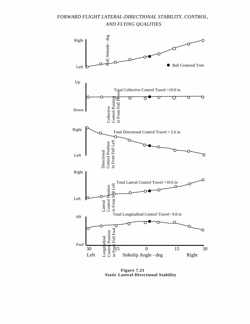
FORWARD FLIGHT LATERAL-DIRECTIONAL STABILITY, CONTROL,
AND FLYING QUALITIES
Sideslip Angle - degLeft Right0 15 301530
Late
ral
Con
trol
Pos
ition
in F
rom
Ful
l Lef
t
Aft
Fwd
Long
itudi
nal
Con
trol
Pos
ition
in F
rom
Ful
l Fw
d
Dire
ctio
nal
Con
trol
Pos
ition
in F
rom
Ful
l Lef
t
Right
Left
Col
lect
ive
Con
trol
Pos
ition
in F
rom
Ful
l Dow
n
Left
Right
Down
Up
Rol
l Atti
tude
- d
eg
Left
Right
Total Collective Control Travel =10.0 in
Total Directional Control Travel = 5.6 in
Total Lateral Control Travel =10.6 in
Total Longitudinal Control Travel= 9.8 in
Ball Centered Trim
Figure 7.21 Static Lateral-Directional Stability

ROTARY WING STABILITY AND CONTROL
Sideslip Angle - degLeft Right0 10 201020
Late
ral
Con
trol
Pos
ition
in F
rom
Ful
l Lef
t
Dire
ctio
nal
Con
trol
Pos
ition
in F
rom
Ful
l Lef
t
Right
Left
Left
Right
Rol
l Atti
tude
- d
eg
Left
RightSide ForceCharacteristics
0
Directional Stability
Effective Dihedral
Right SideslipLeft Sideslip
W
Figure 7.22Trim Conditions in Steady Sideslips

FORWARD FLIGHT LATERAL-DIRECTIONAL STABILITY, CONTROL,
AND FLYING QUALITIES
The roll and yaw moment equations are solved simultaneously for ∆δPED/∆β and
∆δLAT/∆β since bank angle (∆φ) does not appear in these two equations. The resulting
expressions are given below along with the simplified forms obtained assuming yaw
moment is not generated by lateral control:
∆δPED
∆β = -u
0 ( LδLAT
Nv - Lv NδLAT
LδLAT
NδPED
- LδPED
NδLAT
)eq 7.37
If NδLAT is assumed to be zero, Eq 7.37 reduces to:
∆δPED
∆β≈ (-
u0
NδPED
) Nv
eq 7.38
∆δLAT
∆β = -u
0 ( NδPED
Lv - Nv LδPED
LδLAT
NδPED
- LδPED
NδLAT
)eq 7.39
If NδLAT is assumed to be zero, Eq 7.39 reduces to:
∆δLAT
∆β≈
u0
LδLAT
(Lv - LδPED
NvN
δPED
)eq 7.40
or:
∆δLAT
∆β = (-
u0 Lv
LδLAT
) -
LδPED
LδLAT
(∆δPED
∆β )eq 7.41
ROTARY WING STABILITY AND CONTROL
Where:
β - Sideslip angle
δLAT - Lateral control
δPED - Pedal control
LδLAT - Roll moment due to lateral control
LδPED - Roll moment due to pedal control
Lv - Roll moment due to lateral velocity
NδLAT - Yaw moment due to lateral control
NδPED - Yaw moment due to pedal control
Nv - Yaw moment due to lateral velocity
u0 - Initial velocity.
Static lateral-directional stability is the sum of the moments generated by an off trim
lateral airspeed or sideslip. The moments produced by an off trim sideslip can not be
measured directly in flight. The helicopter is maneuvered into an off trim equilibrium flight
condition by providing an opposing moment generated by lateral and pedal control. The
moment produced by the lateral and pedal control can not be measured directly in flight.
However, the lateral and pedal control displacement from trim can be measured.
Therefore, static lateral-directional stability is indicated by the gradient of lateral and pedal
control position versus sideslip. The gradient of pedal control with sideslip indicates the
sign of the directional stability. The gradient of the lateral control with sideslip indicates the
sign of the lateral stability or effective dihedral.
Control systems are designed so a right pedal displacement produces a positive or
nose right yaw moment (NδPED is positive). Consequently, the above expression for
∆δPED/∆β provides a negative pedal displacement versus sideslip gradient, indicating the
yaw moment due to lateral velocity, static directional stability, is positive. A right sideslip
produces a nose right yaw moment rotating the nose of the helicopter to the right and
reducing the sideslip angle. In a steady heading sideslip, the yaw angle is maintained by
the control moment due to left pedal displacement as indicated in Figure 7.22. Although
the slope of the pedal control versus sideslip curve indicates the sign of the static directional
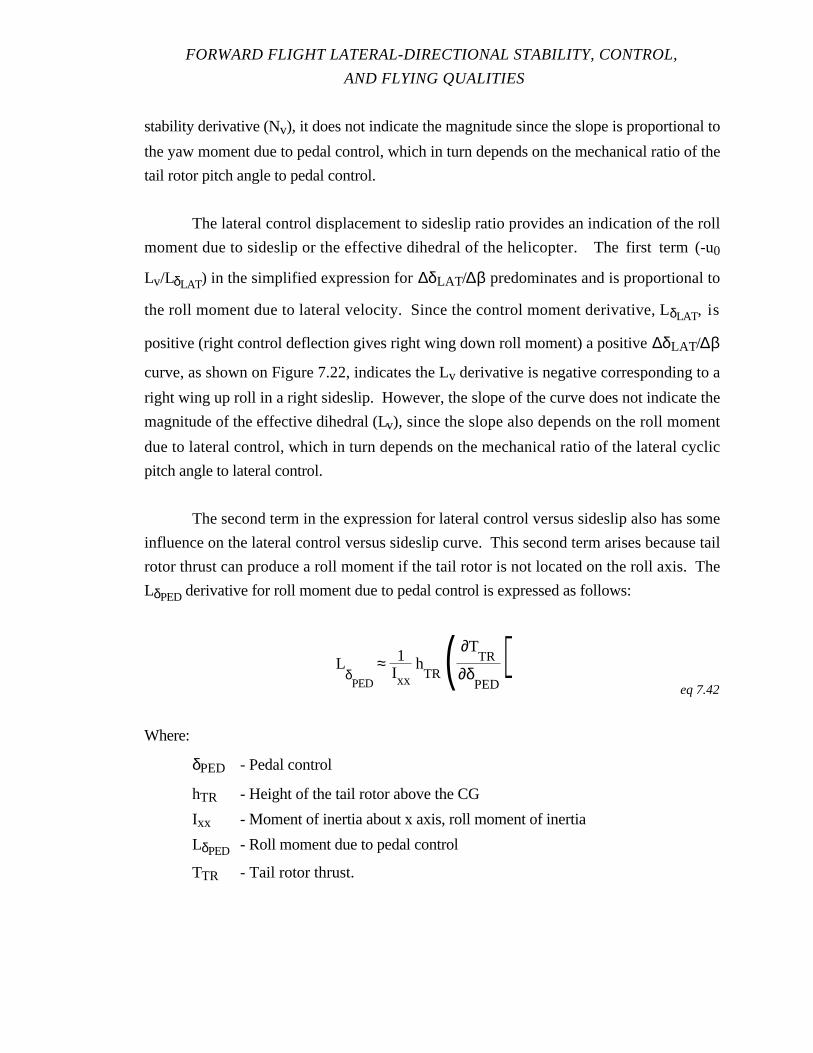
FORWARD FLIGHT LATERAL-DIRECTIONAL STABILITY, CONTROL,
AND FLYING QUALITIES
stability derivative (Nv), it does not indicate the magnitude since the slope is proportional to
the yaw moment due to pedal control, which in turn depends on the mechanical ratio of the
tail rotor pitch angle to pedal control.
The lateral control displacement to sideslip ratio provides an indication of the roll
moment due to sideslip or the effective dihedral of the helicopter. The first term (-u0
Lv/LδLAT) in the simplified expression for ∆δLAT/∆β predominates and is proportional to
the roll moment due to lateral velocity. Since the control moment derivative, LδLAT, is
positive (right control deflection gives right wing down roll moment) a positive ∆δLAT/∆β
curve, as shown on Figure 7.22, indicates the Lv derivative is negative corresponding to a
right wing up roll in a right sideslip. However, the slope of the curve does not indicate the
magnitude of the effective dihedral (Lv), since the slope also depends on the roll moment
due to lateral control, which in turn depends on the mechanical ratio of the lateral cyclic
pitch angle to lateral control.
The second term in the expression for lateral control versus sideslip also has some
influence on the lateral control versus sideslip curve. This second term arises because tail
rotor thrust can produce a roll moment if the tail rotor is not located on the roll axis. The
LδPED derivative for roll moment due to pedal control is expressed as follows:
LδPED
≈ 1Ixx
hTR ( ∂T
TR
∂δPED
)eq 7.42
Where:
δPED - Pedal control
hTR - Height of the tail rotor above the CG
Ixx - Moment of inertia about x axis, roll moment of inertia
LδPED - Roll moment due to pedal control
TTR - Tail rotor thrust.
ROTARY WING STABILITY AND CONTROL
The right yaw moment due to a right pedal displacement is produced by a tail rotor
thrust to the left or a negative increment in TTR, consequently, (∂TTR/∂δPED) is a negative
quantity. For most configurations, the tail rotor is located above the roll axis so hTR is
positive. In this case, LδPED is negative or a right pedal input produces a left wing down
roll moment. Also (-LδPED/LδLAT) is positive since LδLAT is positive. On the other hand,
∆δPED/∆β is usually negative in steady heading sideslips for configurations with positive
directional stability. For most configurations then, the roll moment generated in a SHSS
by the tail rotor is into the sideslip and must be balanced by cyclic into the sideslip. This
additional cyclic requirement contributes to the “effective dihedral” of the vehicle. The term
“dihedral effect” refers to the derivative Lv in which the roll due to pilot generated tail rotor
inputs is not considered.
The resultant of the aerodynamic forces acting on the helicopter when flying in a
steady heading sideslip is in equilibrium with the vertical weight force as depicted in Figure
7.22. The aerodynamic forces are divided into those acting on the main rotor, those acting
on the tail rotor, and those acting on the fuselage/tail surface. When the resultant
aerodynamic force has a lateral component (a force parallel to the y body axis), equilibrium
of the aerodynamic forces with the gravity force is obtained when the helicopter has a bank
angle.
When there is no sideslip, there is still a tail rotor force producing a yaw moment to
balance the torque on the main rotor. Consequently, the resultant aerodynamic force has a
lateral component along the aircraft y body axis to the right which requires a negative bank
angle for equilibrium, as depicted in Figure 7.22, for zero sideslip angle. Another way of
describing this equilibrium is the left horizontal component of rotor thrust is in equilibrium
with the right horizontal component of tail rotor thrust. In this case, the tail rotor thrust acts
at the CG which is the case if the tail rotor were on the roll axis.
Left or right side forces act on the fuselage and vertical tail depending on whether
the helicopter has a right or left sideslip, respectively. A right sideslip generates a left
fuselage side force to balance the right tail rotor force. At the inherent sideslip angle where
the side forces are balanced, the helicopter can fly with zero bank angle. In the case shown
on Figure 7.22, the inherent sideslip angle is approximately 5˚.
FORWARD FLIGHT LATERAL-DIRECTIONAL STABILITY, CONTROL,
AND FLYING QUALITIES
A further increase in right sideslip with the corresponding increase in left fuselage
side force leads to a resultant aerodynamic side force to the left which requires a right bank
angle for equilibrium. Similarly, a left sideslip introduces a side force to the right and
requires a left bank angle for equilibrium.
Tail rotor thrust is also changed by lateral velocity which results in a change in the
effective angles of attack of the tail rotor blades. However, to maintainyaw moment
equilibrium, the pilot introduces a pedal input which changes tail rotor pitch to maintain an
approximately constant tail rotor force as the helicopter is placed in steady heading
sideslips.
The main rotor is affected by lateral velocity. The principal effect is TPP tilt or
blow back resulting in a corresponding lateral tilt of the thrust vector and a roll moment
about the CG. However, to maintain roll moment equilibrium in the steady heading
sideslip, the pilot makes a lateral control input.
The bank angle versus sideslip variation in steady heading sideslips is determined
primarily by the variation of fuselage/tail side forces with sideslip angle. The relationship
of bank angle to sideslip is used to make a qualitative determination of the strength of
sideforces. The bank angle at which the pilot can feel the sideslip can be used to assist in
determining the strength of sideforce.
7.3.5.5 ONE CONTROL ROLLS
During flight evaluation of the Static Lateral Directional flight characteristics of
helicopters, stabilized, one control turns are conducted as a way of gaining clues towards
the stable or unstable nature of the spiral mode. The following paragraph is included to
deal with the unsteady portion, that is to say the portion of a one control turn when angle of
bank is being generated (p, r, p ≠ 0) . Once steady turning flight is achieved,
(p = r = p = 0) , paragraph 7.5.5.6 should be used to aid in the analysis of this condition.
Some significant observations can be made immediately following and shortly after
a one control input is made to initiate a one control turn. During this transient portion of the
maneuver, information is available about adverse/proverse yaw and roll due to pedal as
well as the relative strength of the effective dihedral and directional stability. Understand
ROTARY WING STABILITY AND CONTROL
that these are transient maneuvers in which most of the flight variables are changing with
time. For this reason, there are no simplified governing equations for these tests and they
are therefore conducted in a qualitative fashion and can be reviewed after the flight history
plots.
When performing a lateral cyclic only roll, if there is a significant amount of
adverse or proverse yaw present in the test vehicle, there will be an immediate yaw
response to cyclic application. For adverse yaw, the yaw will be in the direction opposing
the turn (Nlat
−) while for proverse, the response will be into the turn (Nlat
+) . If
there is a large amount of yaw due to roll rate (Np), then as the roll rate builds, there could
be confusion between this rate coupling and the control coupling, adverseyaw. This
ambiguity is exacerbated by short roll mode time constants. Once a sideslip perturbation
from inherent is established, the willingness of the sideslip to return towards inherent is
considered a measure of the relative strength of directional stability (Nv).
Pedal only rolls are conducted by using the directional pedals to generate a sideslip.
Upon initiation of the maneuver, if there is a significant amount of roll due to pedal (Lδped)
present in the test vehicle, there will be an immediate roll response to the pedal application.
After the target amount of sideslip has been generated, roll acceleration in response to that
sideslip is considered an indication of the relative strength ofeffective dihedral. Roll
acceleration is qualitatively hard to perceive, so roll rate resulting from a given sideslip is
often substituted as the measure of dihedral strength. If there is a large amount of roll
damping in the test vehicle, the low steady rate reached following the pedal application
could mask otherwise strong effective dihedral.

FORWARD FLIGHT LATERAL-DIRECTIONAL STABILITY, CONTROL,
AND FLYING QUALITIES
7.3.5.6 STEADY TURNING FLIGHT
By definition, steady turning flight requires a constant roll angle (φ) and a constant turn rate
about a vertical axis ψ ( ) . The time derivatives of lateral velocity, roll rate, and yaw rate are
zero as in steady heading sideslips v = p = r = 0( ) . However, the angular velocities
about the aircraft body axes are not zero and are approximated by the following expressions
in the case of steady level turns:
p ~– 0 roll rate
q ~– ψ sinφ pitch rate
r = ψ rate of change of yaw attitude ≈ turn rate
Using the above assumptions, the lateral-directional equations of motion for small
disturbances reduce to the following for steady turning flight:
-Yvu0∆β + (u
0 - Yr)∆r - gφ = Y
A1s
∆A1s
+ YθTR
∆θTR
= YδLAT
∆δLAT
+ YδPED
∆δPED
eq 7.43
-Lvu0∆β - Lr∆r = L
A1s
∆A1s
+ LθTR
∆θTR
= LδLAT
∆δLAT
+ LδPED
∆δPED
eq 7.44
-Nvu0∆β - Nr∆r = N
A1s
∆A1s
+ NθTR
∆θTR
= NδLAT
∆δLAT
+ NδPED
∆δPED
eq 7.45
Where:
A1s - Lateral cyclic pitch angle, shaft referenced
β - Sideslip angle
δLAT - Lateral control
δPED - Pedal control
φ - Roll angle
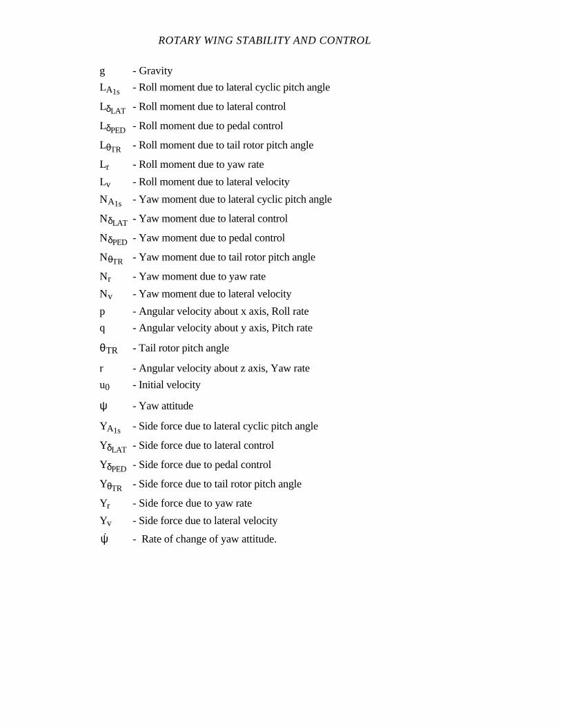
ROTARY WING STABILITY AND CONTROL
g - Gravity
LA1s - Roll moment due to lateral cyclic pitch angle
LδLAT - Roll moment due to lateral control
LδPED - Roll moment due to pedal control
LθTR - Roll moment due to tail rotor pitch angle
Lr - Roll moment due to yaw rate
Lv - Roll moment due to lateral velocity
NA1s - Yaw moment due to lateral cyclic pitch angle
NδLAT - Yaw moment due to lateral control
NδPED - Yaw moment due to pedal control
NθTR - Yaw moment due to tail rotor pitch angle
Nr - Yaw moment due to yaw rate
Nv - Yaw moment due to lateral velocity
p - Angular velocity about x axis, Roll rate
q - Angular velocity about y axis, Pitch rate
θTR - Tail rotor pitch angle
r - Angular velocity about z axis, Yaw rate
u0 - Initial velocity
ψ - Yaw attitude
YA1s - Side force due to lateral cyclic pitch angle
YδLAT - Side force due to lateral control
YδPED - Side force due to pedal control
YθTR - Side force due to tail rotor pitch angle
Yr - Side force due to yaw rate
Yv - Side force due to lateral velocity
ψ - Rate of change of yaw attitude.
FORWARD FLIGHT LATERAL-DIRECTIONAL STABILITY, CONTROL,
AND FLYING QUALITIES
These equations for side force, roll moment, and yaw moment equilibrium are valid
for nearly level turns at constant flight path velocity. It is assumed longitudinal control
inputs are used to maintain constant speed. The discussion is simplified by assuming
lateral control does not produce yaw moments.
The set of variables (∆β = ∆v/u0 = sideslip angle, r = roll rate, φ = roll angle A1s =
lateral cyclic pitch angle, and θTR = tail rotor pitch angle) which provide a solution for the
equations of motion are the incremental changes from an initial trimmed rectilinear
condition to a steady off trim turning flight condition. The time history of the variables
going from a trimmed rectilinear flight condition to steady turning flight is not considered.
7.3.5.6.1 Cyclic Only Turns
Figure 7.23 depicts a helicopter making an approximately level, cyclic only, right
turn. The helicopter was disturbed from an initial condition in which the tail rotor thrust
was balanced by a fuselage side force generated by flying at the inherent sideslip angle. As
a result there is no initial lateral tilt of the main rotor thrust vector. The diagram shows the
changes in forces acting on the helicopter resulting from a steady turn. For simplicity, the
rotor thrust is assumed to act along the shaft axis neglecting any rotor side forces due to
turning. The diagram corresponds to a helicopter with stable spiral characteristics.
The helicopter is banked to the right so the thrust vector has a horizontal component
to the right. This right thrust component balances the sum of the centrifugal force due to
turning and the horizontal component of the aerodynamic side force on the fuselage/tail
acting to the left.
The resultant of the weight and centrifugal force in Figure 7.23 has a lateral
component acting to the right along the y body axis of the helicopter, and the pilot feels a
force tending to push him towards the right or lower side of the seat in this uncoordinated
turn.
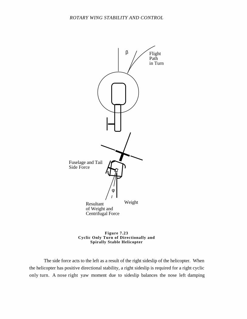
ROTARY WING STABILITY AND CONTROL
The side force acts to the left as a result of the right sideslip of the helicopter. When
the helicopter has positive directional stability, a right sideslip is required for a right cyclic
only turn. A nose right yaw moment due to sideslip balances the nose left damping
β FlightPathin Turn
WeightResultantof Weight andCentrifugal Force
Fuselage and TailSide Force
φ
Figure 7.23Cyclic Only Turn of Directionally and
Spirally Stable Helicopter
FORWARD FLIGHT LATERAL-DIRECTIONAL STABILITY, CONTROL,
AND FLYING QUALITIES
moment generated by the turn rate to the right. This equilibrium is expressed by the yaw
moment equation for a steady turn which reduces to the following form for this cyclic only
case:
-Nvu0∆β - Nr∆r = 0
Assumptions:
∆δPED = 0 (No pedal input)
NδLAT = 0 (No yaw moment due to lateral cyclic)
It follows the yaw rate to lateral velocity ratio is:
∆ru
0∆β
= Nv
(-Nr)
Where:
β - Sideslip angle
NδLAT - Yaw moment due to lateral control
Nr - Yaw moment due to yaw rate
Nv - Yaw moment due to lateral velocity
r - Angular velocity about z axis, Yaw rate
u0 - Initial velocity.
The yaw moment due to yaw rate is inherently negative so the quantity (-Nr) is
positive. The ratio of yaw rate to sideslip angle is positive for a helicopter with positive
directional stability.
There are roll moments acting on the helicopter shown in Figure 7.23 because of its
lateral velocity and yaw rate. These are balanced by the roll moment due to lateral control
required for a steady turn. The equilibrium zero roll moment is expressed as follows:
ROTARY WING STABILITY AND CONTROL
Lvu0∆β + Lr
∆ru
0∆β
u0∆β + L
δLAT
∆δLAT
= 0
eq 7.46
or:
Lv
u0∆β + Lr
Nv
(-Nr) u
0∆β + L
δLAT
∆δLAT
= 0
eq 7.47
⇑ ⇑ ⇑
Roll moment Roll moment Roll moment
due to sideslip due to yaw rate due to lateral control
Where:
β - Sideslip angle
δLAT - Lateral control
LδLAT - Roll moment due to lateral control
Lr - Roll moment due to yaw rate
Lv - Roll moment due to lateral velocity
NδLAT - Yaw moment due to lateral control
Nr - Yaw moment due to yaw rate
Nv - Yaw moment due to lateral velocity
r - Angular velocity about z axis, Yaw rate
u0 - Initial velocity.
The yaw rate to lateral velocity ratio ∆r/u0∆β = Nv/(-Nr) required for yaw moment
equilibrium is introduced explicitly in the second form of the roll moment equilibrium
equation.
Helicopter control systems are designed so a right lateral control deflection
produces a right wing down roll moment. Thus, the LδLAT derivative is positive and the
last term gives a positive roll moment for a positive control deflection. On the other hand,
existing helicopters generally exhibit positive effective dihedral or negative Lv. Thus, the
first term gives a negative roll moment for a positive sideslip.
FORWARD FLIGHT LATERAL-DIRECTIONAL STABILITY, CONTROL,
AND FLYING QUALITIES
The Nr derivative is negative corresponding to positive yaw damping, while the Nv
derivative is positive for a configuration with positive directional stability. The sign of the
roll moment due to yaw rate derivative, Lr, is dependent on the location of the tail rotor and
vertical tail. A positive yaw rate results in a left velocity increment at the tail rotor and an
incremental tail rotor force to the right. This gives a positive increment in roll moment for a
tail rotor above the roll axis corresponding to a positive Lr. The second term in the
equation produces a positive roll moment for a configuration with directional stability and a
tail rotor and tail combination above the roll axis. This is the roll moment generated by the
yaw rate required for yaw moment equilibrium and is proportional to the ∆r/u0∆β ratio in
the turn. This moment has the opposite sign to the moment due to the dihedral effect for a
configuration with positive directional stability and a positive Lr. The combined moments
due to sideslip and yaw rate are balanced by the moment due to lateral control.
The following expression for the sideslip-lateral control ratio in a cyclic only turn is
obtained by rearranging the roll moment equilibrium equation:
∆β∆δ
LAT
= 1u
0
LδLAT
(-Lv) - Lr
Nv
(-Nr)eq 7.48
Where:
β - Sideslip angle
δLAT - Lateral control
LδLAT - Roll moment due to lateral control
Lr - Roll moment due to yaw rate
Lv - Roll moment due to lateral velocity
Nr - Yaw moment due to yaw rate
Nv - Yaw moment due to lateral velocity
u0 - Initial velocity.
ROTARY WING STABILITY AND CONTROL
The influence of the roll moment due to sideslip, or dihedral effect, is present in the
first term in the denominator. The second term in the denominator introduces the effect of
the roll moment due to yaw rate. The first term due to dihedral effect is always positive,
while the second term due to yaw rate makes a negative contribution to the denominator
when Lr and Nv are positive. The second term is more important for configurations with
high directional stability which results in high yaw rate to sideslip ratio in cyclic only turns.
The above expression for the ratio of sideslip to lateral control deflection is
rearranged giving:
∆β∆δ
LAT
= 1u
0
(-Nr) LδLAT
(LvNr - LrNv) eq 7.49
The denominator of the right hand side is the spiral stability parameter (LvNr -
LrNv).
The yaw rate to lateral control ratio in a cyclic only turn follows from the
expressions for the ∆r/u0∆β and ∆β/∆δLAT ratios:
∆r∆δ
LAT
= ∆ru
0∆β
u0∆β
∆δLAT
=
NvLδLAT
(LvNr - LrNv) eq 7.50
Where:
β - Sideslip angle
δLAT - Lateral control
L δLAT - Roll moment due to lateral control
Lr - Roll moment due to yaw rate
Lv - Roll moment due to lateral velocity
Nr - Yaw moment due to yaw rate
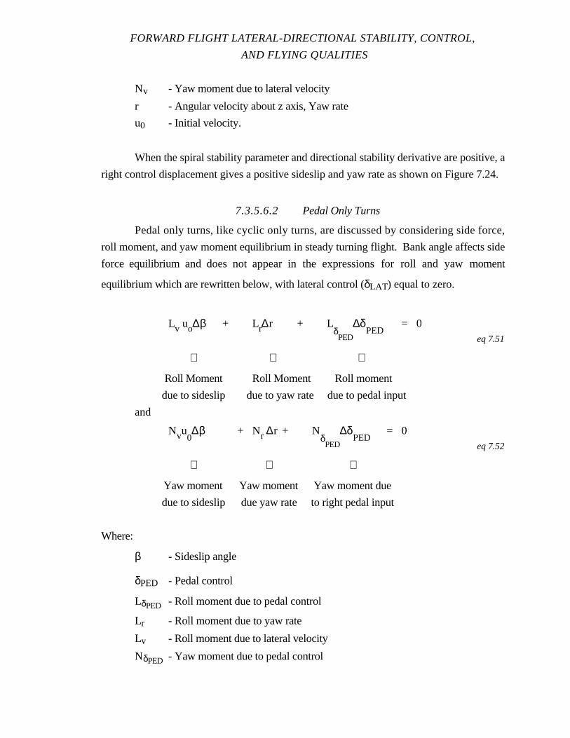
FORWARD FLIGHT LATERAL-DIRECTIONAL STABILITY, CONTROL,
AND FLYING QUALITIES
Nv - Yaw moment due to lateral velocity
r - Angular velocity about z axis, Yaw rate
u0 - Initial velocity.
When the spiral stability parameter and directional stability derivative are positive, a
right control displacement gives a positive sideslip and yaw rate as shown on Figure 7.24.
7.3.5.6.2 Pedal Only Turns
Pedal only turns, like cyclic only turns, are discussed by considering side force,
roll moment, and yaw moment equilibrium in steady turning flight. Bank angle affects side
force equilibrium and does not appear in the expressions for roll and yaw moment
equilibrium which are rewritten below, with lateral control (δLAT) equal to zero.
Lv uo∆β + Lr∆r + LδPED
∆δPED
= 0eq 7.51
⇑ ⇑ ⇑
Roll Moment Roll Moment Roll moment
due to sideslip due to yaw rate due to pedal input
and
Nvu0∆β + Nr ∆r + N
δPED
∆δPED
= 0eq 7.52
⇑ ⇑ ⇑
Yaw moment Yaw moment Yaw moment due
due to sideslip due yaw rate to right pedal input
Where:
β - Sideslip angle
δPED - Pedal control
LδPED - Roll moment due to pedal control
Lr - Roll moment due to yaw rate
Lv - Roll moment due to lateral velocity
NδPED - Yaw moment due to pedal control

ROTARY WING STABILITY AND CONTROL
Nr - Yaw moment due to yaw rate
Nv - Yaw moment due to lateral velocity
r - Angular velocity about z axis, Yaw rate
u0 - Initial velocity.
The quantities highlighted by arrows are positive for a conventional helicopter. The
sideslip velocity (u0∆β), yaw rate (∆r) and pedal displacement (∆δPED) in these equations
are the incremental changes from an initial trimmed rectilinear flight condition.
The pilot selects one of the three variables in the roll and yaw moment equations;
the other variables, or their ratios with respect to the selected variable, are determined from
the equilibrium conditions. For example, if he desires a particular turn rate, he adjusts
pedal control until the turn rate is established. The pilot accepts the corresponding sideslip
determined from the roll and yaw moment equilibrium and the bank angle necessary to
achieve side force equilibrium.
There is usually some control moment coupling in helicopters so a lateral control
displacement, or pedal displacement, might result in both roll and yaw moments. The yaw
moment due to lateral control deflection is generally small and is neglected in considering
cyclic only turns. An analogous assumption for pedal only turns neglects the roll moment
due to pedal control corresponding to a configuration with the tail rotor on the roll axis.
This configuration is considered first, subsequent discussion shows the characteristics
obtained when a pedal input causes both roll and yaw moments.
When LδPED = 0, the roll moment due to sideslip is equal and opposite to the roll
moment due to yaw rate. This condition is satisfied when the sideslip to yaw rate ratio is:
(u0∆β)
∆r =
Lr
(-Lv) eq 7.53
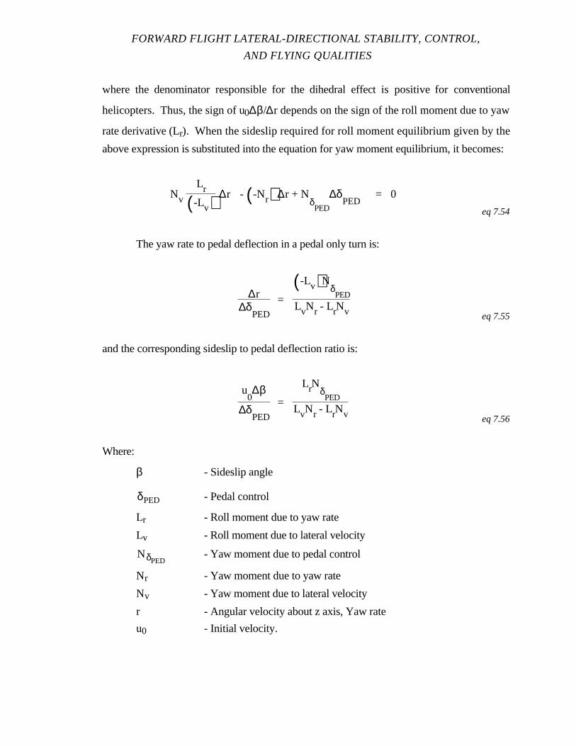
FORWARD FLIGHT LATERAL-DIRECTIONAL STABILITY, CONTROL,
AND FLYING QUALITIES
where the denominator responsible for the dihedral effect is positive for conventional
helicopters. Thus, the sign of u0∆β/∆r depends on the sign of the roll moment due to yaw
rate derivative (Lr). When the sideslip required for roll moment equilibrium given by the
above expression is substituted into the equation for yaw moment equilibrium, it becomes:
Nv
Lr
(-Lv)∆r - (-Nr) ∆r + N
δPED
∆δPED
= 0
eq 7.54
The yaw rate to pedal deflection in a pedal only turn is:
∆r∆δ
PED
=
(-Lv)NδPED
LvNr - LrNv eq 7.55
and the corresponding sideslip to pedal deflection ratio is:
u0∆β
∆δPED
=
LrNδPED
LvNr - LrNv eq 7.56
Where:
β - Sideslip angle
δPED - Pedal control
Lr - Roll moment due to yaw rate
Lv - Roll moment due to lateral velocity
NδPED- Yaw moment due to pedal control
Nr - Yaw moment due to yaw rate
Nv - Yaw moment due to lateral velocity
r - Angular velocity about z axis, Yaw rate
u0 - Initial velocity.
ROTARY WING STABILITY AND CONTROL
The denominator in the above expressions is the spiral stability parameter (LvNr -
LrNv) which appeared in the corresponding expressions for cyclic only turns. The same
expression is obtained in the two cases because the spiral stability of the helicopter depends
on the coupling between yaw rate and sideslip and not on the control input.
When the spiral stability parameter is positive (Figure 7.24) a steady right turn is
obtained with a right pedal displacement (pedal input is required in the direction of turn). If
the pilot required a left pedal input to obtain temporary equilibrium in a right turn, it
indicates the spiral stability parameter is negative. Thus, one method used to evaluate the
spiral stability is to observe the ∆r/∆δPED ratio in pedal only turn.
The yaw moment balance on Figure 7.24 is used to determine the initial tendency of
a helicopter to return to, or depart from, a steady turn when disturbed from equilibrium and
thus the spiral stability. Assuming the helicopter originally is stabilized in a pedal only
turn, if the pedal input is reduced, the corresponding yaw moment is reduced.
Consequently, there is a nose left yaw moment tending to increase sideslip. An increase in
sideslip results in a side force to the left, decreasing the turn rate and a roll moment due to
dihedral effect decreasing the bank angle. Consequently, where (LvNr -LrNv) > 0, the
initial tendency of the helicopter when disturbed is to return to its original steady turn
condition.
The configuration in Figure 7.24 has positive directional stability as well as spiral
stability, and the side force at the vertical tail is assumed to act above the roll axis so Lr is
positive. The helicopter is banked to the right giving a right horizontal thrust component to
balance the horizontal component of the aerodynamic side force and the centrifugal force
due to turning. The positive roll moment due to yaw rate is balanced by the negative
dihedral effect. Since the roll moment due to lateral velocity derivative (Lv) is negative, the
helicopter has a positive or right sideslip which is obtained with a nose left yaw angle
relative to the turning flight path.
There is a negative yaw damping moment tending to damp the positive yaw rate due
to turning toward the right. This is partially compensated by the positive yaw moment due
to right sideslip.

FORWARD FLIGHT LATERAL-DIRECTIONAL STABILITY, CONTROL,
AND FLYING QUALITIES
The yaw moment due to a right pedal input is required to obtain yaw moment
equilibrium. If the spiral stability is negative, a left pedal displacement is required to hold
the right turn. In this case, a reduction in left pedal causes a nose right yaw moment
increment and a reduction in sideslip. There is a reduction in dihedral effect roll moment
and left side force, both of which cause a steeper bank and tighter turn.
β FlightPathin Turn
Weight
Fuselage and TailSide Force
CentrifugalForce
Lr Lv
Nv
NδPED Nr
V
ResultantWeight andCentrifugalForce
Figure 7.24Pedal Only Turn of Directionally and Spirally Stable Helicopter
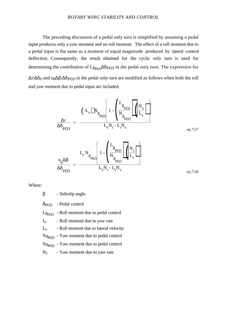
ROTARY WING STABILITY AND CONTROL
The preceding discussion of a pedal only turn is simplified by assuming a pedal
input produces only a yaw moment and no roll moment. The effect of a roll moment due to
a pedal input is the same as a moment of equal magnitude produced by lateral control
deflection. Consequently, the result obtained for the cyclic only turn is used for
determining the contribution of LδPED∆δPED in the pedal only turn. The expression for
∆r/∆δ0 and u0∆β/∆δPED in the pedal only turn are modified as follows when both the roll
and yaw moment due to pedal input are included.
∆r∆δ
PED
=
(-Lv) NδPED
1 - ( LδPED
NδPED
)(NvLv
)LvNr - LrNv eq 7.57
u0∆β
∆δPED
=
Lr NδPED
1 - ( LδPED
NδPED
)(NrLr
)LvNr - LrNv eq 7.58
Where:
β - Sideslip angle
δPED - Pedal control
LδPED - Roll moment due to pedal control
Lr - Roll moment due to yaw rate
Lv - Roll moment due to lateral velocity
NδPED - Yaw moment due to pedal control
NδPED - Yaw moment due to pedal control
Nr - Yaw moment due to yaw rate
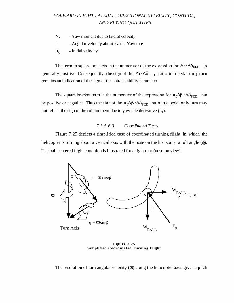
FORWARD FLIGHT LATERAL-DIRECTIONAL STABILITY, CONTROL,
AND FLYING QUALITIES
Nv - Yaw moment due to lateral velocity
r - Angular velocity about z axis, Yaw rate
u0 - Initial velocity.
The term in square brackets in the numerator of the expression for ∆r/ ∆δPED is
generally positive. Consequently, the sign of the ∆r/ ∆δPED ratio in a pedal only turn
remains an indication of the sign of the spiral stability parameter.
The square bracket term in the numerator of the expression for u0∆β /∆δPED can
be positive or negative. Thus the sign of the u0∆β /∆δPED ratio in a pedal only turn may
not reflect the sign of the roll moment due to yaw rate derivative (Lr).
7.3.5.6.3 Coordinated Turns
Figure 7.25 depicts a simplified case of coordinated turning flight in which the
helicopter is turning about a vertical axis with the nose on the horizon at a roll angle (φ).
The ball centered flight condition is illustrated for a right turn (nose-on view).
The resolution of turn angular velocity (ω) along the helicopter axes gives a pitch
ω
φ
q = ω sinφTurn Axis W
BALLF
R
φ
r = ω cosφ
WBALLg u
0ω
Figure 7.25Simplified Coordinated Turning Flight

ROTARY WING STABILITY AND CONTROL
rate (q = ω sin φ), a yaw rate (r = ω cos φ), and no roll rate.
Three forces are shown on a hypothetical ball used for turn coordination. They are,
the weight force (WBALL ), the centrifugal force due to the curved flight path in the turn
(WBALL /g u0 ω), and the reaction force (FR) from the ball race.
The race reaction force is in the z direction in the ball centered condition, while the y
components of the weight and centrifugal forces are balanced for equilibrium:
WBALL
sinφ =W
BALLg u
0ω cosφ =
WBALLg u
0r
eq 7.59
φ ≈ sinφ =u
0 r
g eq 7.60
Where:
φ - Roll angle
g - Gravity
r - Angular velocity about z axis, Yaw rate
u0 - Initial velocity
ω - Turn angular velocity
WBALL - Weight of the ball.
In discussing cyclic only and pedal only turns, it was shown that side force
equilibrium is obtained by flying at the proper bank angle. In the case of coordinated turns,
the bank angle is related to the yaw rate by the above expression. In this case, the pedal
and lateral control inputs are adjusted until side force equilibrium is obtained at the proper
bank angle.
7.3.6 Dynamic Stability
Lateral-directional dynamics are discussed neglecting coupling with longitudinal
dynamics. The lateral-directional dynamics of the unaugmented helicopter is represented
by fourth order equations of motion leading to a characteristic equation with four roots.
Two of these roots are usually real and correspond to the first order roll and spiral mode
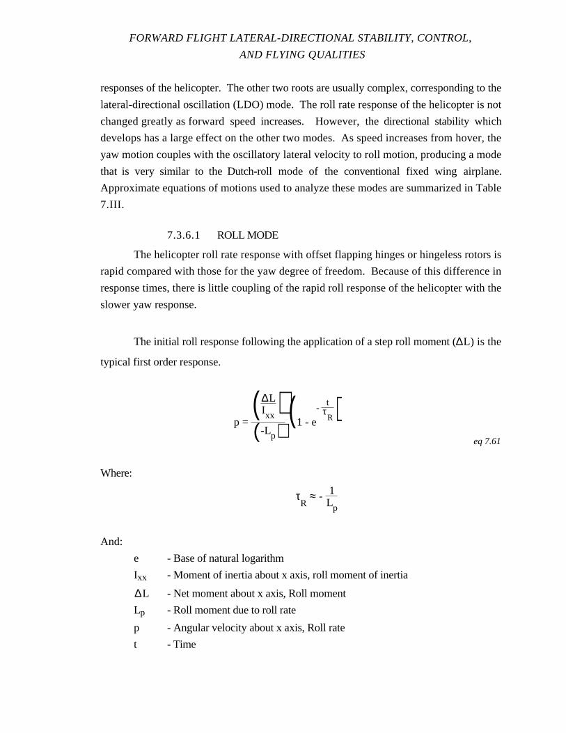
FORWARD FLIGHT LATERAL-DIRECTIONAL STABILITY, CONTROL,
AND FLYING QUALITIES
responses of the helicopter. The other two roots are usually complex, corresponding to the
lateral-directional oscillation (LDO) mode. The roll rate response of the helicopter is not
changed greatly as forward speed increases. However, the directional stability which
develops has a large effect on the other two modes. As speed increases from hover, the
yaw motion couples with the oscillatory lateral velocity to roll motion, producing a mode
that is very similar to the Dutch-roll mode of the conventional fixed wing airplane.
Approximate equations of motions used to analyze these modes are summarized in Table
7.III.
7.3.6.1 ROLL MODE
The helicopter roll rate response with offset flapping hinges or hingeless rotors is
rapid compared with those for the yaw degree of freedom. Because of this difference in
response times, there is little coupling of the rapid roll response of the helicopter with the
slower yaw response.
The initial roll response following the application of a step roll moment (∆L) is the
typical first order response.
p = (∆L
Ixx )(-Lp)
(1 - e-
tτR)
eq 7.61
Where:
τR
≈ - 1Lp
And:
e - Base of natural logarithm
Ixx - Moment of inertia about x axis, roll moment of inertia
∆L - Net moment about x axis, Roll moment
Lp - Roll moment due to roll rate
p - Angular velocity about x axis, Roll rate
t - Time
ROTARY WING STABILITY AND CONTROL
τR - Roll mode time constant.
The inherent or augmented roll damping derivative (Lp), is negative giving an
exponentially damped roll rate response. This roll rate response mode does not vary
greatly with trim airspeed because the roll damping derivative remains approximately
constant.
The preceding approximate formulas are not valid when the effective damping
derivative is small, for example when there is a stronger effect of yaw and sideslip motions
on the roll response mode.
7.3.6.2 SPIRAL STABILITY
The long term lateral-directional dynamics or spiral stability in forward flight affects
pilot workload in steady turns. It also affects workload in straight and level trimmed flight.
An approximate form of the lateral-directional equations of motion in Table 7.III is used in
discussing the spiral mode and relating it to steady turns. The discussion is for pedal
control inputs, but the resultant character spiral mode is independent of the way the mode is
excited. The yaw moment due to pedal displacement is included on the right hand side of
the yaw equation only. The roll moments and side forces due to pedal inputs usually are of
secondary importance and are neglected to simplify the following discussion.
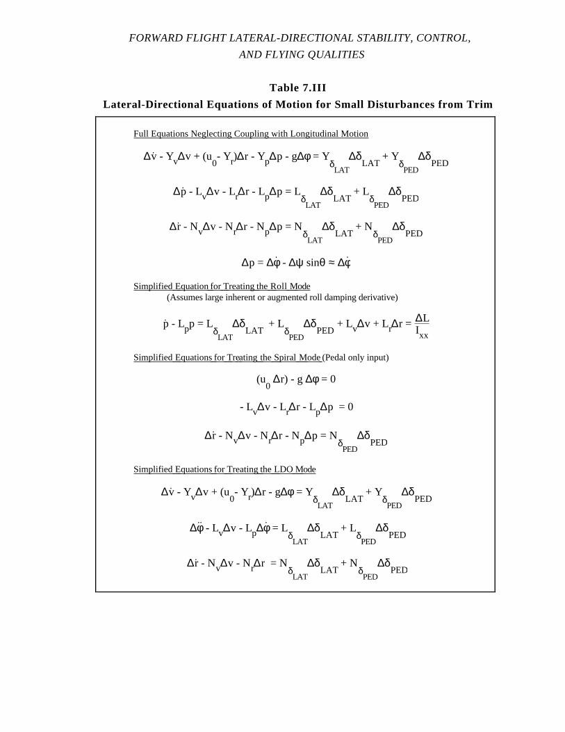
FORWARD FLIGHT LATERAL-DIRECTIONAL STABILITY, CONTROL,
AND FLYING QUALITIES
Table 7.III
Lateral-Directional Equations of Motion for Small Disturbances from Trim
Full Equations Neglecting Coupling with Longitudinal Motion
∆v. - Yv∆v + (u
0- Yr)∆r - Yp∆p - g∆φ = Y
δLAT
∆δLAT
+ YδPED
∆δPED
∆p. - Lv∆v - Lr∆r - Lp∆p = L
δLAT
∆δLAT
+ LδPED
∆δPED
∆r. - Nv∆v - Nr∆r - Np∆p = N
δLAT
∆δLAT
+ NδPED
∆δPED
∆p = ∆φ. - ∆ψ. sinθ ≈ ∆φ
.
Simplified Equationfor TreatingtheRoll Mode(Assumes large inherent or augmented roll damping derivative)
p. - Lpp = L
δLAT
∆δLAT
+ LδPED
∆δPED
+ Lv∆v + Lr∆r = ∆LIxx
Simplified Equationsfor Treating theSpiral Mode(Pedal only input)
(u0
∆r) - g ∆φ = 0
- Lv∆v - Lr∆r - Lp∆p = 0
∆r. - Nv∆v - Nr∆r - Np∆p = N
δPED
∆δPED
Simplified Equationsfor TreatingtheLDO Mode
∆v. - Yv∆v + (u
0- Yr)∆r - g∆φ = Y
δLAT
∆δLAT
+ YδPED
∆δPED
∆φ.. - Lv∆v - Lp∆φ
. = L
δLAT
∆δLAT
+ LδPED
∆δPED
∆r. - Nv∆v - Nr∆r = N
δLAT
∆δLAT
+ NδPED
∆δPED

ROTARY WING STABILITY AND CONTROL
The simplification of the equations of motion are in part based on the assumption the spiral
mode response is much slower than the other lateral-directional responses of the helicopter.
The spiral root and corresponding time constant is:
λs = - 1τs =
-(LvNr - LrNv)-Lv(1 -
u0
g Np) - NvLp ( u0
g )eq 7.62
Where:
δPED - Pedal control
g - Gravity
Lp - Roll moment due to roll rate
Lr - Roll moment due to yaw rate
λs - Spiral mode root
Lv - Roll moment due to lateral velocityNδPED - Yaw moment due to pedal control
Np - Yaw moment due to roll rate
Nr - Yaw moment due to yaw rate
Nv - Yaw moment due to lateral velocity
r - Angular velocity about z axis, Yaw rate
r - Angular acceleration about z axis
τs - Spiral mode time constant
u0 - Initial velocity
v - Translational velocity component along y axis.
The time solution for the first order spiral mode response is:
r = r0 e
λst = r0 e
-t
τs
eq 7.63
FORWARD FLIGHT LATERAL-DIRECTIONAL STABILITY, CONTROL,
AND FLYING QUALITIES
Where:
e - Base of natural logarithm
λs - Spiral mode root
r - Angular velocity about z axis, Yaw rate
r0 - Initial angular velocity about z axis, Yaw rate
t - Time
τs Spiral mode time constant.
An aperiodic divergent spiral mode response is obtained when the spiral root, λs, is
positive. The denominator in the expression for the spiral root is positive with
configurations having positive directional stability (Nv > 0). In this case, the sign of the
spiral root depends upon the sign of the spiral stability parameter (LvNr -LrNv) in the
numerator. This same parameter was discussed in connection with steady turning flight.
The product LvNr is typically positive for configurations with positive yaw damping and
positive dihedral effect. Configurations with high tail rotor and vertical tails have a positive
roll moment due to yaw rate derivative (Lr); therefore, the spiral stability parameter is
negative with large, positive directional stability producing a divergent spiral mode. The
discussion in Section 7.3.5.6.1 and 7.3.5.6.2 indicated how the sign of the spiral stability
root is estimated in steady turns. The spiral mode is observed by introducing a bank angle,
then carefully returning the controls to their respective level flight trim positions. The time-
to-one-half (T1/2) or time-to-double (T2) bank amplitude is then determined.
7.3.6.3 LATERAL-DIRECTIONAL OSCILLATION
The LDO mode of the helicopter changes character going from hovering to forward
flight. In hovering flight, where the helicopter has little directional stability, an oscillatory
mode is obtained which primarily involves lateral velocity and roll motions. In forward
flight, the directional stability of the typical helicopter results in the oscillatory roll/yaw
mode. Generally, the frequency of the LDO is determined by coupling between the lateral
velocity and yaw motions, while the coupling with the roll motion has a significant effect
on its damping. The amplitude and phase of the roll to sideslip ratio in the LDO mode may
influence the pilot’s evaluation of lateral-directional handling qualities. To simplify
understanding of the LDO motion, a particular case without roll motion in the mode is
considered first. This is then generalized to include roll motions.
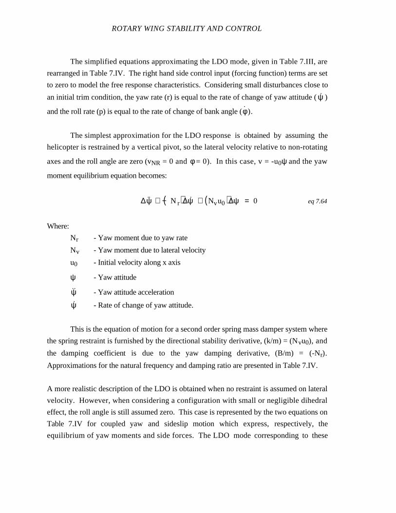
ROTARY WING STABILITY AND CONTROL
The simplified equations approximating the LDO mode, given in Table 7.III, are
rearranged in Table 7.IV. The right hand side control input (forcing function) terms are set
to zero to model the free response characteristics. Considering small disturbances close to
an initial trim condition, the yaw rate (r) is equal to the rate of change of yaw attitude (ψ )
and the roll rate (p) is equal to the rate of change of bank angle (φ ).
The simplest approximation for the LDO response is obtained by assuming the
helicopter is restrained by a vertical pivot, so the lateral velocity relative to non-rotating
axes and the roll angle are zero (vNR = 0 and φ = 0). In this case, v = -u0ψ and the yaw
moment equilibrium equation becomes:
∆ ˙ψ + −N r( )∆ψ + Nvu0( )∆ψ = 0 eq 7.64
Where:
Nr - Yaw moment due to yaw rate
Nv - Yaw moment due to lateral velocity
u0 - Initial velocity along x axis
ψ - Yaw attitude
˙ψ - Yaw attitude acceleration
ψ - Rate of change of yaw attitude.
This is the equation of motion for a second order spring mass damper system where
the spring restraint is furnished by the directional stability derivative, (k/m) = (Nvu0), and
the damping coefficient is due to the yaw damping derivative, (B/m) = (-Nr).
Approximations for the natural frequency and damping ratio are presented in Table 7.IV.
A more realistic description of the LDO is obtained when no restraint is assumed on lateral
velocity. However, when considering a configuration with small or negligible dihedral
effect, the roll angle is still assumed zero. This case is represented by the two equations on
Table 7.IV for coupled yaw and sideslip motion which express, respectively, the
equilibrium of yaw moments and side forces. The LDO mode corresponding to these

FORWARD FLIGHT LATERAL-DIRECTIONAL STABILITY, CONTROL,
AND FLYING QUALITIES
Table 7.IV
Approximate Equations for the Lateral-Directional Oscillation
SimplifiedEquationsfor theLDO
∆v. - Yv∆v + (u
0 - Yr)∆ψ. - g∆φ = 0
∆φ.. - Lv∆v - Lp∆φ
. = 0
∆ψ.. - Nr∆ψ. - Nv∆v - Np∆φ. = 0
∆ψ.. + (-Nr)∆ψ. + (Nvu0)∆ψ - Nv∆v
NR - Np∆φ
. = 0
(Yaw equation referred to non-rotating axes)
HelicopterAssumedPivotedattheCG (φ = vNR = 0)
∆ψ.. + (-Nr) ∆ψ. + (Nvu0) ∆ψ = 0
ωn ≈ Nvu0
ζ ≈ 12ωn
(-Nr)
CoupledEquationsfor YawandSideslipMotions (φ = 0)
(∆ψ.. Nr ∆ψ. ) - Nv ∆v = 0
∆v. - Yv∆v + (u
0 - Yr)∆ψ. = 0
Separate ψ andv Equationsfor CoupledMotion (φ = 0)
∆ψ.. + (-Nr - Yv)∆ψ. + Nvu0 + (YvNr - NvYr) ∆ψ = 0
∆v.. + (-Nr - Yv)∆v
. + Nvu
0 + (YvNr - NvYr) ∆v = 0
ωn ≈ Nvu0 (YvNr - NvYr)
ζ ≈ 12ωn
(-Nr -Yv)
ω = ωn 1 - ζ2
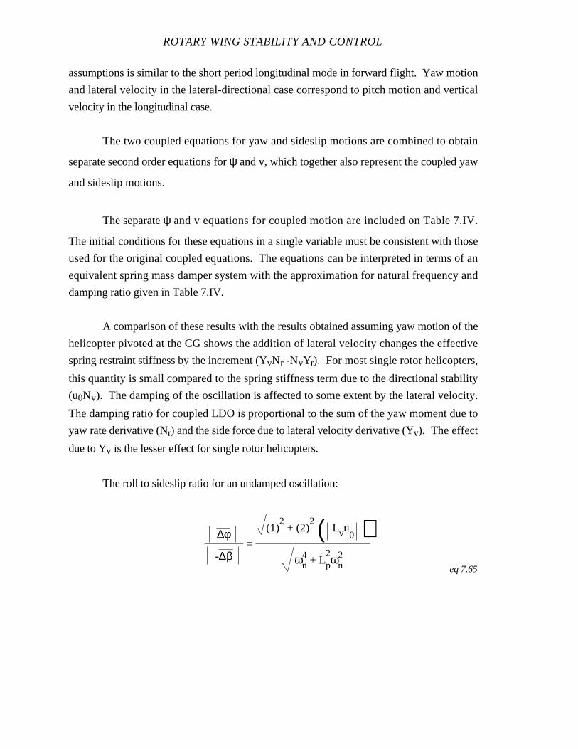
ROTARY WING STABILITY AND CONTROL
assumptions is similar to the short period longitudinal mode in forward flight. Yaw motion
and lateral velocity in the lateral-directional case correspond to pitch motion and vertical
velocity in the longitudinal case.
The two coupled equations for yaw and sideslip motions are combined to obtain
separate second order equations for ψ and v, which together also represent the coupled yaw
and sideslip motions.
The separate ψ and v equations for coupled motion are included on Table 7.IV.
The initial conditions for these equations in a single variable must be consistent with those
used for the original coupled equations. The equations can be interpreted in terms of an
equivalent spring mass damper system with the approximation for natural frequency and
damping ratio given in Table 7.IV.
A comparison of these results with the results obtained assuming yaw motion of the
helicopter pivoted at the CG shows the addition of lateral velocity changes the effective
spring restraint stiffness by the increment (YvNr -NvYr). For most single rotor helicopters,
this quantity is small compared to the spring stiffness term due to the directional stability
(u0Nv). The damping of the oscillation is affected to some extent by the lateral velocity.
The damping ratio for coupled LDO is proportional to the sum of the yaw moment due to
yaw rate derivative (Nr) and the side force due to lateral velocity derivative (Yv). The effect
due to Yv is the lesser effect for single rotor helicopters.
The roll to sideslip ratio for an undamped oscillation:
∆φ
-∆β =
(1)2 + (2)
2 ( Lvu0 )
ωn4 + Lp
2ωn
2
eq 7.65

FORWARD FLIGHT LATERAL-DIRECTIONAL STABILITY, CONTROL,
AND FLYING QUALITIES
And the phase angle (∠) between the roll and sideslip:
∠ ∆φ
(-∆β) = tan-1
-(-Lp)-ωn
eq 7.66
Where:
(1)−ωn −Lvu0( )ωn
4 + L p2ω n
2( )
(2)− −Lpωn( ) −Lvu0( )
ωn4 + Lp
2ωn2( )
β - Sideslip angle
e - Base of natural logarithm
φ - Roll angle
i - Imaginary index
Lp - Roll moment due to roll rate
Lv - Roll moment due to lateral velocity
t - Time
u0 - Initial velocity along x axis
ωn - Natural frequency.
The ratio of ∆φ is presented relative to (-∆β) rather than to (∆β) because (-∆β) ≈
∆ψ tends to produce a positive roll moment via the dihedral effect. The expression for
phase angle for sinusoidal motion is approximately correct for lightly damped LDO modes.

ROTARY WING STABILITY AND CONTROL
When the damping ratio is larger a better estimate for the phase angle is obtained by a
similar derivatation using ∆φ = ∆φ (- ωn + iωn (1 - ζ2 t)0.5):
∠ ∆φ
(-∆β) = tan-1
-(-Lp)
ωn - 2ζ
- 1 + ζ(-Lp)
ωn eq 7.67
Where:
β - Sideslip angle
φ - Roll angle
Lp - Roll moment due to roll rate
ωn - Natural frequency
ζ - Damping ratio.
The equation given on Table 7.IV for the helicopter pivoted about the CG was
obtained by neglecting the lateral velocity term and roll rate term in the yaw equation of
motion. The change in response characteristics obtained when these terms are included is
found using approximate expressions obtained for ∆vNR and ∆φ in a neutrally stable LDO.
These approximations make it possible to obtain expression for the neglected terms as
linear functions of ∆ψ and ∆ψ ; thus, determining how the neglected terms affect the
response characteristics. The corrections have little effect on the LDO mode frequencies for
typical single rotor helicopters whose tail rotors and vertical stabilizers provide adequate
directional stability. However, an appreciable correction to the LDO mode damping ratio is
required as a result of the roll motion:
ζ = 12ωn
-Nr - Yv -( gu
0 - Np) Lvu
0
(ωn2 + Lp
2)eq 7.68
Where:

FORWARD FLIGHT LATERAL-DIRECTIONAL STABILITY, CONTROL,
AND FLYING QUALITIES
g - Gravity
Lp - Roll moment due to roll rate
Lv - Roll moment due to lateral velocity
Np - Yaw moment due to roll rate
Nr - Yaw moment due to yaw rate
u0 - Initial velocity along x axis
ωn - Natural frequency
Yv - Side force due to lateral velocity
ζ - Damping ratio.
The first two terms within the brackets of the above expression give the damping
ratio when roll in neglected, while the third term gives the correction due to the roll
response. The yaw moment due to roll rate derivative (Np) obtained when the equations
are rearranged to eliminate inertia couplings is usually a somewhat larger negative number.
Thus, a positive sign is obtained for the (g/u0 -Np) factor in the third term. The second
factor in the third term is equal to the real part or in phase part of the ∆φ/(-∆β) ratio which
is usually negative. Thus, the correction due to the roll response is negative, tending to
reduce the LDO mode damping ratio. This correction is larger when the dihedral effect is
increased and is reduced by an increase in roll damping.
Several approximate formulas are presented in this section as an aid to
understanding the affect of various parameters on the response characteristics of the LDO
mode of the single rotor helicopter. Table 7.V summarizes the LDO mode data for five
unaugmented helicopters using the approximate equations. These results were computed
from data in reference 7.1 for a 100 kn trim condition. Frequency and damping ratios
obtained from the approximate formulas are compared with those obtained in reference 7.1
for coupled six degree of freedom analysis.
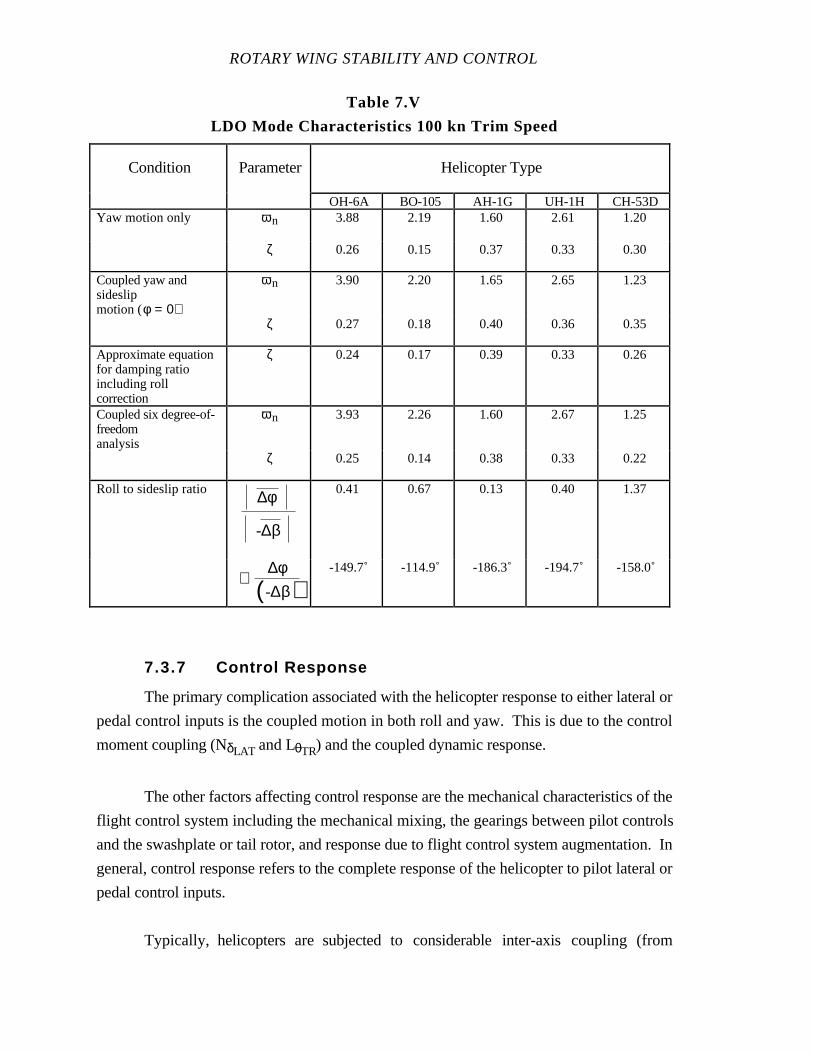
ROTARY WING STABILITY AND CONTROL
Table 7.V
LDO Mode Characteristics 100 kn Trim Speed
Condition Parameter Helicopter Type
OH-6A BO-105 AH-1G UH-1H CH-53DYaw motion only ωn 3.88 2.19 1.60 2.61 1.20
ζ 0.26 0.15 0.37 0.33 0.30
Coupled yaw andsideslipmotion (φ = 0)
ωn 3.90 2.20 1.65 2.65 1.23
ζ 0.27 0.18 0.40 0.36 0.35
Approximate equationfor damping ratioincluding rollcorrection
ζ 0.24 0.17 0.39 0.33 0.26
Coupled six degree-of-freedomanalysis
ωn 3.93 2.26 1.60 2.67 1.25
ζ 0.25 0.14 0.38 0.33 0.22
Roll to sideslip ratio ∆φ
-∆β
0.41 0.67 0.13 0.40 1.37
∠ ∆φ
(-∆β)-149.7˚ -114.9˚ -186.3˚ -194.7˚ -158.0˚
7.3.7 Control Response
The primary complication associated with the helicopter response to either lateral or
pedal control inputs is the coupled motion in both roll and yaw. This is due to the control
moment coupling (NδLAT and LθTR) and the coupled dynamic response.
The other factors affecting control response are the mechanical characteristics of the
flight control system including the mechanical mixing, the gearings between pilot controls
and the swashplate or tail rotor, and response due to flight control system augmentation. In
general, control response refers to the complete response of the helicopter to pilot lateral or
pedal control inputs.
Typically, helicopters are subjected to considerable inter-axis coupling (from
FORWARD FLIGHT LATERAL-DIRECTIONAL STABILITY, CONTROL,
AND FLYING QUALITIES
longitudinal to lateral-directional, not just roll to yaw). Hence, the control responses in roll
or yaw is dependent on how the pilot chooses to regulate coupled longitudinal motions.
The question is how much such undesired motions affect task performance and/or
workload, and how dependent the answer is on pilot aggressiveness. The aggressiveness
is of interest because the number of dynamic modes excited by a control input is a function
of the frequency content of the excitation. This is of interest for Automatic Flight Control
System (AFCS) operation both ON and OFF. The AFCS may include rate dampers and
devices to cancel the coupling from the control input. Inherently included in the test pilot's
task is an assessment of workload created by any requirement to use coordinated control
inputs such as pedal inputs accompanying the lateral control to minimize the excitation of
unwanted motions during a lateral-directional task.
The coordinated control workload is a function of the size, direction, and timing of
the pedal input required to accompany the lateral cyclic to accomplish particular tasks.
Associated with this consideration is how natural the coordinated inputs are to the pilot.
Helicopter pilots generally are adept at using their feet in maneuvering tasks and there is a
spectrum of coordinated inputs which require relatively little extra mental or physical
workload, while outside this spectrum, significant workload increases occur. For
example, pedal input at the same time and in the same direction as a lateral control input
may feel natural. Coordinating for proverse yaw or for a delayed yaw is more difficult.
The overall response to any control input can be divided into the initial response and
the longer term response. For a lateral cyclic input, the initial response is composed of the
desired roll motion and the undesirable aspect, yaw moment due to lateral control (NδLAT,
adverse or proverse). For a given NδLAT, the level of the undesirable motion is a function
of the magnitude and abruptness of the lateral control input (δLAT). This yaw may confuse
the pilot in a directional control task since the lateral input is generally used to effect a
heading change or lateral pipper placement. Another undesired by product is a yaw
moment due to roll rate (Np) which occurs soon after the lateral control input, but later than
the NδLAT. The particular combination of these two yaw motions have a significant effect
on the predictability of directional response initiated by a lateral cyclic input and on the
ability of the pilot to suppress these motions using pedal inputs. For pedal only turns, yaw
ROTARY WING STABILITY AND CONTROL
motions may cause some undesired roll motions on top of the commanded roll via dihedral
effect. The test pilot must assess the workload such distortion produces for particular
piloting tasks.
The longer term response is dominated by the characteristics of the LDO mode,
primarily damping ratio, and by the effects of the pilot's attempts to control residual
undesired motions while performing a closed loop task. Furthermore, the spiral mode may
significantly affect the steady state lateral cyclic or pedal inputs for a desired bank angle.
The discussion applies equally for helicopters with an AFCS where the specific
purpose of augmentation: control shaping (modify the effective NδLAT or LδPED) or stability
augmentation (yaw damper or roll damper) is to remove the undesirable distortions which
interfere with task performance. Even with augmentation, the outcome may be less than
perfect. The test pilot assesses the augmentation gains/shaping as well as the effects of
AFCS failure on mission performance.
7.3.8 Tandem Rotor Characteristics
7.3.8.1 STABILITY DERIVATIVES
Figure 7.26 indicates the principal effects contributing to the lateral-directional
derivatives of the tandem helicopter recognized early in the development of this
configuration. They are presented on the basis of the individual rotor characteristics
discussed in Chapter 4.
The diagrams on Figure 7.26 are simplified by not picturing the front and rear
rotors; however, the thrust vectors are shown which correspond to the TPP tilt due to
disturbances from trim conditions by an incremental lateral velocity, roll rate, or yaw rate.
A lateral velocity to the left causes both the front and rear thrust vectors to tilt to the
right. This tilt is another example of the stable speed response of the isolated rotor tilting
away from the relative wind. The roll moment due to sideslip or effective dihedral is
because the rotors are above the CG and a right tilt produces a right roll moment.
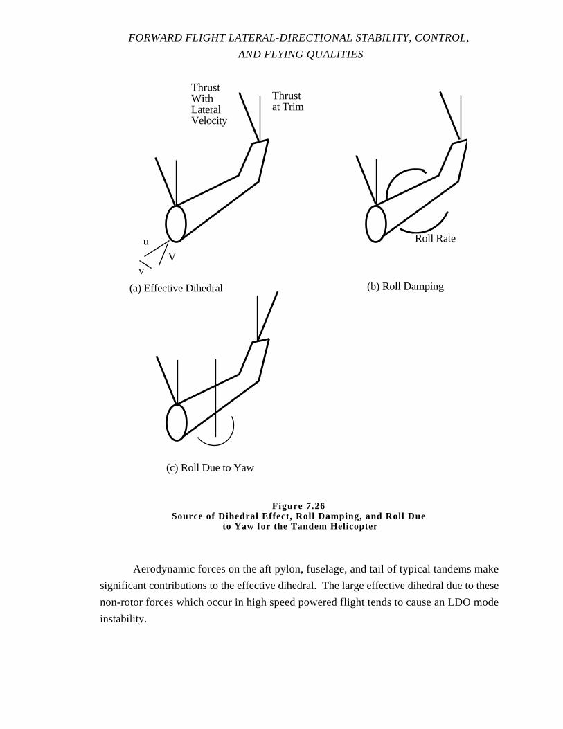
FORWARD FLIGHT LATERAL-DIRECTIONAL STABILITY, CONTROL,
AND FLYING QUALITIES
Aerodynamic forces on the aft pylon, fuselage, and tail of typical tandems make
significant contributions to the effective dihedral. The large effective dihedral due to these
non-rotor forces which occur in high speed powered flight tends to cause an LDO mode
instability.
V
u
v
Thrustat Trim
ThrustWithLateralVelocity
(a) Effective Dihedral (b) Roll Damping
Roll Rate
(c) Roll Due to Yaw
Figure 7.26Source of Dihedral Effect, Roll Damping, and Roll Due
to Yaw for the Tandem Helicopter
ROTARY WING STABILITY AND CONTROL
The tandem helicopter has a side force due to the lateral velocity derivative resulting
from the sum of the side force contributions by the two rotors and the fuselage/tail. The
lateral tilt of a rotor due to lateral velocity is proportional to the average blade angle of
attack. If the CG of the tandem is forward of the midpoint between the two rotors, the
forward rotor thrust is greater than the thrust of the rear rotor to trim the helicopter.
Consequently, the average blade angle of attack is greater for the forward rotor than for the
rear rotor; therefore, the forward rotor has a larger lateral tilt and side force than the rear
rotor in response to an increment in lateral velocity. The side forces on the two rotors
produce a net unstable yaw moment about the forward CG in the direction tending to rotate
the tandem away from the lateral velocity.
The tail rotor of the single rotor helicopter tends to give that configuration inherent
directional stability which is increased by the addition of a vertical tail located toward the
rear of the tail boom where it has a long moment arm generating yaw moments. Vertical
tails added to tandems are less effective because of the comparatively short moment arms
from the CG, usually located near the middle of the helicopter. As a result, marginal
directional stability is often a major deficiency of unaugmented tandem helicopters. This
problem is accentuated in nose up autorotational flight where aerodynamic flow
disturbances and interferences reduce the contributions of the aft pylon and vertical tail to
directional stability.
A roll velocity of the helicopter to the left, indicated on Figure 7.26, results in a tilt
of the TPPs to the right. There are small relative lateral velocities at the rotors due to roll
rate about the CG and the vertical moment arms of the two rotors. These lateral velocities
result in a small increment in the TPP tilt due to roll rate. If one rotor is higher than the
other, this effect results in a small yaw moment due to roll rate.
The third diagram on Figure 7.26 indicates the rotor tilt produced by a yaw velocity
about the CG. The tilt in the thrust vectors give thrust components opposing the yaw
motion and are responsible for the yaw damping.
If the rear rotor is higher than the front rotor, as indicated in Figure 7.26, the lateral
component of the rear rotor thrust due to yaw rate produces a greater roll moment about the
CG than the front rotor, and a net roll moment due to yaw velocity results. The
FORWARD FLIGHT LATERAL-DIRECTIONAL STABILITY, CONTROL,
AND FLYING QUALITIES
aerodynamic forces due to yaw rate acting on the aft pylon and vertical surfaces mounted
above the CG also make a positive contribution to the roll moment due to yaw rate
derivative.
Roll control of the tandem helicopter is achieved by applying lateral cyclic pitch to
the front and rear rotors and is analogous to the single rotor helicopter. The resulting tilt of
the forward and aft TPP introduce rotor side forces and offset hinge roll moments.
Yaw control is accomplished by differential lateral cyclic pitch introduced by pedal
inputs. The tandem helicopter can employ various combinations of lateral cyclic and
differential cyclic of the two rotors to make turns about any desired turning axis.
However, if the resulting motion causes different lateral velocities at the forward and aft
rotors, a thrust difference can develop between the rotors causing cross coupling with the
helicopter longitudinal responses.
7.3.8.2 DYNAMIC RESPONSE MODES OF THE UNAUGMENTED
TANDEM
In hovering flight there is little coupling between yaw and lateral motions of the
tandem helicopter. The yaw rate response of the hovering tandem is more sluggish than the
single rotor helicopter both because of the tandem's large yaw moment of inertia and the
low yaw damping provided by the thrust vector tilt of the forward and aft rotors in
response to their lateral velocities generated by yaw rate.
The spiral mode is usually a slowly convergent mode for the unaugmented tandem
helicopter. The tandem helicopter is usually free of spiral instability because of its low
directional stability. Consequently, when the helicopter is disturbed in bank angle, the
predominant effect of any sideslip angle which develops in the subsequent motion is to
produce dihedral effect roll moments tending to bring the bank angle to the wing's level
trim condition rather than producing yaw moments leading to an ever steepening inward
spiraling flight path.
The roll rate response mode of the tandem is quite similar to the single rotor
helicopter. Coupling effects are small and roll motion predominates in this first order
subsidence mode in both hovering and forward flight. Tandem helicopters tend to have
somewhat longer roll rate response times than single rotor helicopters with similar rotor
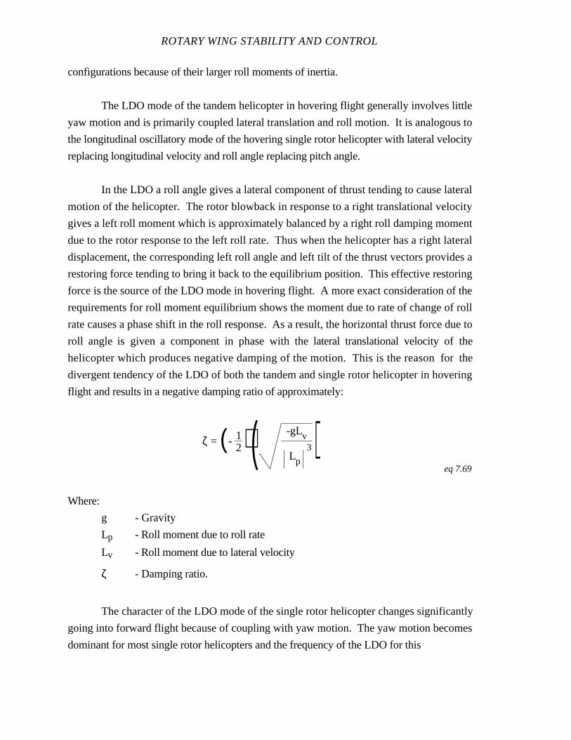
ROTARY WING STABILITY AND CONTROL
configurations because of their larger roll moments of inertia.
The LDO mode of the tandem helicopter in hovering flight generally involves little
yaw motion and is primarily coupled lateral translation and roll motion. It is analogous to
the longitudinal oscillatory mode of the hovering single rotor helicopter with lateral velocity
replacing longitudinal velocity and roll angle replacing pitch angle.
In the LDO a roll angle gives a lateral component of thrust tending to cause lateral
motion of the helicopter. The rotor blowback in response to a right translational velocity
gives a left roll moment which is approximately balanced by a right roll damping moment
due to the rotor response to the left roll rate. Thus when the helicopter has a right lateral
displacement, the corresponding left roll angle and left tilt of the thrust vectors provides a
restoring force tending to bring it back to the equilibrium position. This effective restoring
force is the source of the LDO mode in hovering flight. A more exact consideration of the
requirements for roll moment equilibrium shows the moment due to rate of change of roll
rate causes a phase shift in the roll response. As a result, the horizontal thrust force due to
roll angle is given a component in phase with the lateral translational velocity of the
helicopter which produces negative damping of the motion. This is the reason for the
divergent tendency of the LDO of both the tandem and single rotor helicopter in hovering
flight and results in a negative damping ratio of approximately:
ζ = (- 12)( -gLv
Lp
3)eq 7.69
Where:
g - Gravity
Lp - Roll moment due to roll rate
Lv - Roll moment due to lateral velocity
ζ - Damping ratio.
The character of the LDO mode of the single rotor helicopter changes significantly
going into forward flight because of coupling with yaw motion. The yaw motion becomes
dominant for most single rotor helicopters and the frequency of the LDO for this
FORWARD FLIGHT LATERAL-DIRECTIONAL STABILITY, CONTROL,
AND FLYING QUALITIES
configuration is primarily determined by the yaw stiffness provided by the directional
stability derivative.
The LDO mode of the tandem helicopter is changed less than the single rotor
helicopter going into forward flight because of the small directional stability derivative.
The coupling of yaw motion remains comparatively small. The phase shift due to roll
moments are still destabilizing. However, in low speed forward flight, aerodynamic forces
on the rotor pylons and fixed surface add to the roll damping derivative and tend to stabilize
the motion.
The small yaw motion which is present in the LDO mode of the tandem can
contribute to the instability of the mode. The destabilizing effect on this oscillatory mode is
dependent on the directional stability derivative. A more divergent LDO mode is found in
high speed flight where the tandem's directional stability is usually negative. This is the
most significant deficiency of the lateral-directional handling qualities of the unaugmented
tandem helicopter. Although negative directional stability increases the instability of the
LDO mode, it does not generally result in an aperiodic divergence. The yaw motion is a
secondary effect in this mode and the effective stiffness of the tandem's LDO mode is
largely determined by the dihedral mechanism rather than by the directional stability.
7.4 TEST METHODS AND TECHNIQUES
7.4.1 Trimmed Control Positions
The purpose of this test is to evaluate the variation in control positions with changes
in power, airspeed, and bank angle; control margins; the ease of trimming the flight control
forces to zero; and the qualitative importance of trim changes to the piloting task. The
entire airspeed envelope is evaluated to VNE and the complete power range is evaluated
from autorotation to maximum power. For level flight, the helicopter is established in
trimmed, wings level, unaccelerated flight, and the data are recorded. The airspeed is
varied approximately 10 kn and the test is repeated.
For climbs and descents, one or more mission representative airspeeds are used.
The helicopter is stabilized on airspeed and the power is varied from autorotation to
maximum available. Airspeed remains constant while the power is varied incrementally.

ROTARY WING STABILITY AND CONTROL
At least 5 power increments are used. The climb and descent test is repeated at another
airspeed. Usually, the airspeed for maximum rate of climb, or minimum rate of descent is
evaluated. If large control displacements are observed while making a power change, the
test can be conducted open loop with all controls fixed except for power. The resulting
attitude and rate changes show the helicopter response which the pilot must counteract to
maintain wings level, unaccelerated flight conditions. The results of the open loop test are
used to relate the possible helicopter excursions when performing constant airspeed climbs
and descents.
“If large excursions are seen in the pedal positions while making power changes especially
in full power climbs and minimum power descents, turns at these conditions should be
considered to determine if any additional margin of control is required. For example, in
US built helos, low power descents require right pedal and a right turn at this condition
may require more right pedal. The reverse would be true in high power climb.”
7.4.1.1 TEST TECHNIQUE
1. Establish wings level, ball centered, unaccelerated, trimmed flight. Record
the initial trim conditions.
2. Assign a Handling Qualities Rating (HQR) and Vibration Assessment
Rating (VAR) to each data point.
3. Use the force trim and AFCS in a mission representative manner.
4. Gather data in steady rectilinear flight, varying airspeed; steady turning
flight, varying bank angle while maintaining altitude and airspeed; and climb and descent,
varying power while maintaining constant airspeed.
7.4.1.1.1 Level Flight
1. This data can be obtained concurrently with level flight performance testing.
2. Investigate entire airspeed profile (30 kn to VH).
7.4.1.1.2 Diving Flight
1. If VNE is greater than VH, fix the collective at maximum power and dive the
aircraft to obtain control position data at the higher airspeeds.
2. Control margins are particularly important.
FORWARD FLIGHT LATERAL-DIRECTIONAL STABILITY, CONTROL,
AND FLYING QUALITIES
7.4.1.1.3 Steady Turns
1. Establish wings level, ball centered, unaccelerated, trimmed flight at a
mission representative airspeed. Record the initial trim conditions.
2. Vary roll attitude, establishing trimmed incremental bank angles both left
and right. Adjust collective as necessary to maintain altitude and airspeed.
3. Incrementally increase bank angle to the test limit.
4. Repeat the bank angle series at another mission representative airspeed as
desired.
7.4.1.1.4 Climbs and Descents (Closed Loop)
1. Establish wings level, unaccelerated flight at the desired trim airspeed with
collective control position at incremental power settings.
2. Vary power incrementally from autorotation to the maximum available.
3. Normally five increments define a satisfactory curve.
4. Altitude range, ±1000 ft about target.
5. If near a margin in high power climb or auto, check that a turn doesn’t
decrease the margin.
7.4.1.2 DATA REQUIRED
Control positions, Vo, HPo, To, Vv (climb and descent) θ, φ, β, Q, NR, fuel
counts (FC), HQR, and VAR.
7.4.1.3 TEST CRITERIA
1. Stabilized, wings level (level flight), ball centered flight.
2. No vertical velocity (level flight).
3. Constant vertical velocity (climb and descent).
4. All control forces trimmed to zero.
7.4.1.4 DATA REQUIREMENTS
1. Stabilize 15 s prior to recording data.
2. Record 10 s data.
3. HPo ± 1000 ft of the target test altitude.
ROTARY WING STABILITY AND CONTROL
4. Vv level flight, ±10 fpm; climb and descent, stabilized ± 25 fpm.
5. NR ± 1%.
6. Vo ± 1 kn.
7. φ ± 2˚.
7.4.1.5 SAFETY CONSIDERATIONS/RISK MANAGEMENT
Observe normal operating limitations, including acceleration and bank angle
limitations. Use incremental build up procedures when approaching any envelope
boundary. Conduct tests at a safe operating altitude over terrain suitable for forced
landings. Maintain proper lookout procedures. Consider using a chase aircraft and sole
use airspace.
7.4.2 Static Lateral-Directional Stability (SHSS)
The purpose of this test is to evaluate the static lateral-directional stability or the
change in the total lateral-directional restoring moments generated by off trim lateral
velocity (sideslip angles). Static stability is indicated by the initial tendency of a helicopter
to return to or depart from equilibrium if disturbed. Positive static stability is indicated by
the tendency to return toward the original trimmed condition.
Directional static stability is indicated by the variation of pedal control with sideslip.
Positive static directional stability is indicated by increasing left pedal control displacement
with increasing right sideslip. Since the forces and moments can not be measured directly
in flight, the purpose of this test is to determine the control forces and positions necessary
to balance the directional moments caused by sideslip variations from the inherent trim
sideslip. Cockpit control position versus sideslip angle indicates the sign butnot the
magnitude of static stability since the slope in proportional to the yaw moment due to pedal
control, which in turn depends on the mechanical ratio of tail rotor pitch angle to pedal
control.
Lateral static stability (effective dihedral) is indicated by the variation of lateral
control with sideslip. Positive effective dihedral is indicated by increasing right lateral
control displacement with increasing right sideslip. Since the forces and moments can not
be measured directly in flight, the purpose of this test is to determine the control forces and
positions necessary to balance the roll moments caused by sideslip variations from the
FORWARD FLIGHT LATERAL-DIRECTIONAL STABILITY, CONTROL,
AND FLYING QUALITIES
inherent trim sideslip. Cockpit control position versus sideslip angle indicates the sign but
not the magnitude of static stability since the slope is proportional to the roll moment due to
lateral control, which in turn depends on the mechanical ratio of the lateral cyclic pitch angle
to lateral control.
Side force is indicated by the variation in bank angle with sideslip. The lateral
component of the gravity vector provides a cue to the pilot that he is in out of balanced
flight. The sideslip angle and the corresponding bank angle at which the pilot
proprioceptively recognizes the out of balanced flight condition is a measure of the strength
of the side force cue. Ideally, a small sideslip angle produces a side force cue to the pilot
that he is in out of balanced flight. Conclusions are drawn on the aircraft characteristics of
sideforce and not sideforce cues to the pilot.
The test is accomplished by establishing a wings level, ball centered, unaccelerated
trim condition. Without changing the collective position, trim, or rotor speed, the sideslip
is varied and stabilized at incremental sideslips. The sideslip around trim is most
important. Small 2 to 3˚ increments are used around trim. As sideslip increases from trim,
larger 5˚ increments are used. At each stabilized flight condition, lateral and directional
controls are used to maintain steady, non-turning flight. The longitudinal control is used to
maintain constant boom airspeed. Collective is maintained constant. A stabilized climb or
descent is accepted and altitude is maintained within ± 1000 ft of the test altitude. If power
must be changed to return to the test altitude, record all engine parameters and collective
control position to assist in returning to trim. Do not retrim the collective. When the test
altitude is reestablished, return the collective control to trim.
7.4.2.1 TEST TECHNIQUE
1. Stabilize at the initial trim airspeed in ball-centered, wings level,
unaccelerated flight and reduce all control forces to zero. Do not retrim control forces or
adjust engine controls during the test.
2. Record trim conditions.
3. Smoothly yaw the helicopter to the desired sideslip angle for the next data
point while simultaneously adding lateral cyclic to prevent the helicopter from turning.
Generally 5˚ sideslip variations are acceptable; however, around the inherent trim sideslip,
use 2 to 3˚ sideslip variations. Use longitudinal control to maintain trim airspeed as

ROTARY WING STABILITY AND CONTROL
indicated by the boom airspeed. Selecting a prominent landmark along the original flight
path is helpful in assuring a straight flight path.
4. Stabilize at each sideslip increment for 15 s and record data for
approximately 10 s. Make qualitative comments on the control force, control displacement,
and side force (bank angle) cues at the off trim conditions. Note the sideslip angle at which
the pilot proprioceptively is aware of the side force and out of balanced flight condition.
5. Collect the data at incremental sideslip angles both left and right covering the
allowable range. Obtain data at zero bank angle and ball centered, and zero sideslip angle.
6. Good in flight visibility with a defined horizon and long straight line land
features decrease the pilot effort required to conduct this test. Strong winds at the test
altitude make the task more difficult.
7. If it is necessary to adjust altitude to remain within the test band, note the
collective position, torque, and Ng, before moving the collective. Do not retrim any control
forces. The test is continued after the collective control is returned to the original trim
position.
8. Determine if airspeed errors need to be accounted for by yawing to a given
sideslip and observing airspeed. If a change is noted, yaw the aircraft back to trim. If the
airspeed returns to trim, fly the off airspeed when in a slip as you have an airspeed error in
sideslip. If the airspeed did not return to trim airspeed when sideslip was removed, you
must make adjustments in longitudinal control in the face of sideslip to hold the original
airspeed.
7.4.2.2 DATA REQUIRED
Control positions, control force, Vo, Vv, φ, β, θ, Q, NR, FC, HPo, To.
7.4.2.3 TEST CRITERIA
1. Wings level, ball centered, unaccelerated flight at trim.
2. Constant heading, no turning.
3. Collective fixed.
4. No retrimming.

FORWARD FLIGHT LATERAL-DIRECTIONAL STABILITY, CONTROL,
AND FLYING QUALITIES
7.4.2.4 DATA REQUIREMENTS
1. Stabilize 15 s prior to taking data.
2. Record 10 s stabilized data.
3. Vo ± 1 kn.
4. Stabilized sideslip, β ± 0.5˚.
5. Steady heading, ψ ± 1˚.
6. HPo ± 1000 ft of the target test altitude.
7. NR ± 0.5%.
7.4.2.5 SAFETY CONSIDERATIONS/RISK MANAGEMENT
Observe normal operating limitations. Use incremental build up procedures when
approaching any envelope boundary. Maintain proper lookout procedures. Consider using
a chase aircraft and using sole use airspace. In most cases the sideslip envelope for the
helicopter as a function of calibrated airspeed must be obtained from the airframe
manufacturer or other competent authority (Figure 7.27). These limits are normally not
published in documents readily available to the test team. A well written safety of flight
release may be the source for this data.
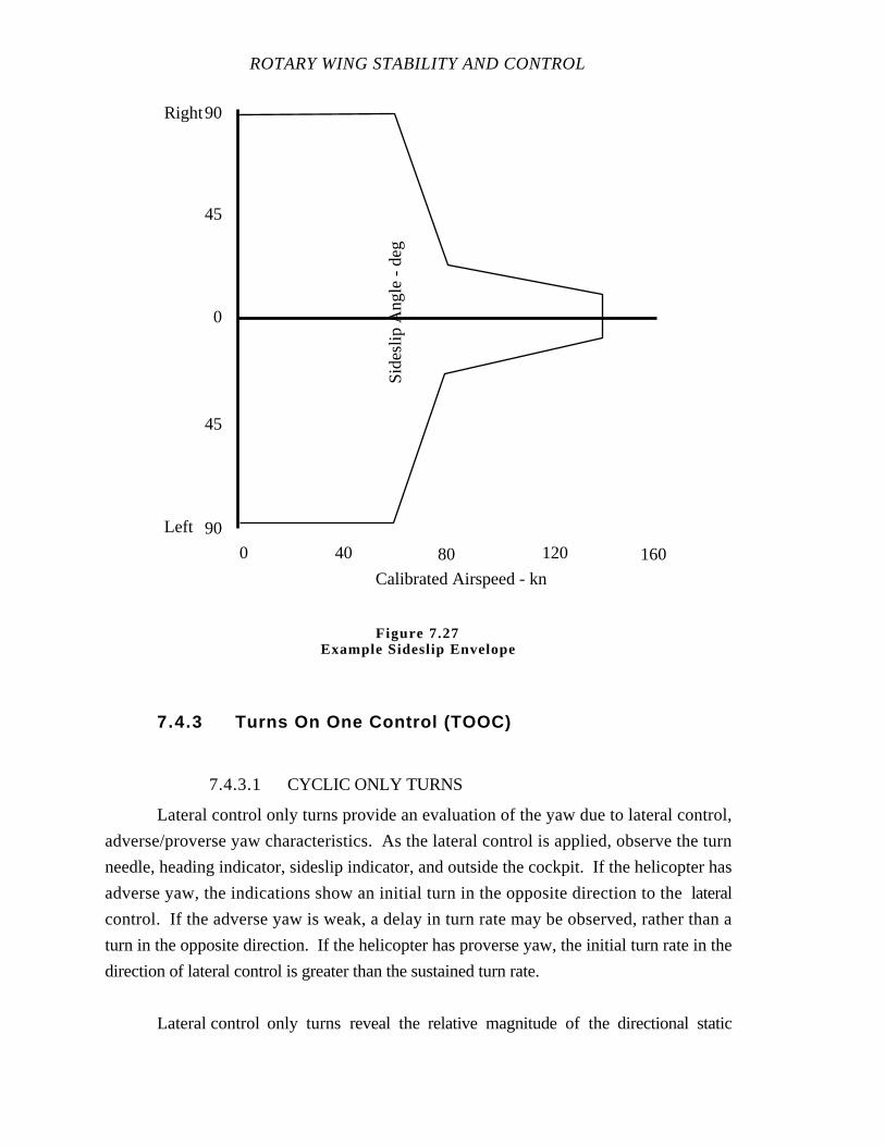
ROTARY WING STABILITY AND CONTROL
7.4.3 Turns On One Control (TOOC)
7.4.3.1 CYCLIC ONLY TURNS
Lateral control only turns provide an evaluation of the yaw due to lateral control,
adverse/proverse yaw characteristics. As the lateral control is applied, observe the turn
needle, heading indicator, sideslip indicator, and outside the cockpit. If the helicopter has
adverse yaw, the indications show an initial turn in the opposite direction to the lateral
control. If the adverse yaw is weak, a delay in turn rate may be observed, rather than a
turn in the opposite direction. If the helicopter has proverse yaw, the initial turn rate in the
direction of lateral control is greater than the sustained turn rate.
Lateral control only turns reveal the relative magnitude of the directional static
0 40 80 120 160
Calibrated Airspeed - kn
Sid
eslip
Ang
le -
deg
Right
Left
0
45
90
45
90
Figure 7.27Example Sideslip Envelope
FORWARD FLIGHT LATERAL-DIRECTIONAL STABILITY, CONTROL,
AND FLYING QUALITIES
stability. Assuming adverse/proverse yaw is present, if the sideslip angle during the steady
roll remains at the inherent sideslip or quickly returns toward the inherent sideslip angle,
the helicopter exhibits relatively strong directional stability. If the sideslip angle does not
return toward the inherent sideslip, the directional stability is relatively weak.
Lateral control only turns provide a secondary indication of the spiralstability.
Once a stabilized bank angle is established, the lateral control deflection from trim provides
an indication of the character of the spiral mode. If the control is displaced into the bank
angle, the spiral is positive or convergent. If the control is displaced away from the bank
angle, the spiral mode is negative or divergent.
7.4.3.1.1 Test Technique
1. Trim the helicopter at desired airspeed in ball-centered, wings level,
unaccelerated flight. Record the trim conditions including inherent sideslip angle.
2. Smoothly apply lateral cyclic to establish the desired roll rate and ultimately
the roll attitude. Do not move directional controls.
3. Observe the turn needle, heading indicator, sideslip indicator, and outside
the cockpit while displacing the lateral cyclic.
4. Observe the turn needle, heading indicator, sideslip indicator, and outside
the cockpit when the bank angle and turn rate are steady.
5. Repeat for both left and right turns at desired bank angles.
6. Repeat for faster and slower rate of control application inan attempt to
generate sideslip.
7. Assign an HQR for capturing and maintaining bank angle or turn rate.
7.4.3.1.2 Data Required
Control positions, initial and final lateral control position, Vo, Vv, φ, β, θ, Q, NR,
FC, HPo, To, HQR.
7.4.3.1.3 Test Criteria
1. Wings level, ball centered, unaccelerated flight at trim.
2. Collective and pedal control fixed.
3. No retrimming.
ROTARY WING STABILITY AND CONTROL
7.4.3.1.4 Data Requirements
1. Stabilize 15 s at trim.
2. Record 10 s stabilized data.
3. Vo ± 1 kn.
4. Stabilized bank angle, φ ± 1˚.
5. HPo ± 1000 ft of the target test altitude.
6. NR ± 0.5%.
7.4.3.1.5 Safety Considerations/Risk Management
Lateral cyclic only turn tests are generally low risk. Observe normal flight test
precautions and operating limits. No additional considerations peculiar to this test method
are required.
7.4.3.2 PEDAL ONLY TURNS
Directional control only turns reveal the relative magnitude of the effective dihedral.
If a relatively small sideslip angle results in a large roll rate in the opposite direction, the
helicopter exhibits relatively strong effective dihedral. If a large sideslip angle is required
to generate a roll in the opposite direction, the helicopter exhibits relatively weak positive
effective dihedral. If a sideslip angle results in a roll in the direction of the sideslip, the
helicopter exhibits negative effective dihedral.
7.4.3.2.1 Test Technique
1. Trim the helicopter at the desired airspeed in ball-centered, wings level,
unaccelerated flight. Record trim conditions.
2. Smoothly apply directional control to change sideslip angle. Do not move
the lateral control.
3. Observe the roll response during application of directional control.
4. When bank angle and turn rate are steady, record thedirectional control
displacement and sideslip angle.
5. Repeat for both left and right directional control displacements and desired
bank angles.
FORWARD FLIGHT LATERAL-DIRECTIONAL STABILITY, CONTROL,
AND FLYING QUALITIES
7.4.3.2.2 Data Required
Control positions, initial and final pedal control position, Vo, Vv, φ, β, θ, Q, NR,
FC, HPo, To, HQR.
7.4.3.2.3 Test Criteria
1. Wings level, ball centered, unaccelerated flight at trim.
2. Collective and lateral control fixed.
3. No retrimming.
7.4.3.2.4 Data Requirements
1. Stabilize 15 s prior to taking data.
2. Record 10 s stabilized data.
3. Vo ± 1 kn.
4. Stabilized bank angle, φ ± 1˚.
5. HPo ± 1000 ft of the target test altitude.
6. NR ± 0.5%.
7.4.3.2.5 Safety Considerations/Risk Management
Directional only turn tests are generally low risk. Observe normal flight test
precautions and operating limits. No additional considerations peculiar to this test method
are required.
7.4.4 Spiral Stability
The purpose of this test is to determine the helicopter response to bank angle
deviations from trim.

ROTARY WING STABILITY AND CONTROL
7.4.4.1 TEST TECHNIQUE
During turns on one control tests, a look into the spiral was accomplished. For
cyclic only turns, the position of the control when the angle of bank was steady was an
indication of the spiral mode. Likewise, the pedal position during pedal only turns when
the bank angle was steady, also gave an indication of the spiral. The following test will
quantify the spiral mode.
1. Trim the helicopter in wings level, steady heading, coordinated flight at the
desired test conditions.
2. Use lateral cyclic to establish the desired bank angle, smoothly return the
lateral cyclic to trim, and observe the helicopter response. Since the spiral mode is usually
weak, the response is easily contaminated if the controls are not returned exactly to trim.
3. Use a range of bank angles from 5˚ to approximately 20˚ unless
significantly larger bank angles are routinely experienced in accomplishing the mission of
the helicopter.
4. If the effective dihedral of the helicopter is sufficient to achieve the desired
bank angle, the alternate method uses directional controls to develop a sideslip angle. Hold
sideslip until the helicopter rolls to the desired bank angle. For tail rotor helicopters, the
rate of directional control application should not create a roll moment due to change in tail
rotor thrust. Lateral control is fixed throughout the evaluation at the initial trim position.
Since the spiral mode is usually weak, the response is easily contaminated if the controls
are not returned exactly to trim.
5. Record a time history of the response or record the bank angle at selected
time intervals to generate a plot of bank angle as a function of time.
6. Repeat steps 1 through 7 as required to evaluate increasingly larger bank
angles both left and right.
7.4.4.2 DATA REQUIRED
Control positions, initial and final lateral or directional control positions, Vo, Vv,
φ, β, θ, Q, NR, FC, HPo, To.
Hand recorded or automatic time history of bank angle versus time.
7.4.4.3 TEST CRITERIA
FORWARD FLIGHT LATERAL-DIRECTIONAL STABILITY, CONTROL,
AND FLYING QUALITIES
1. Wings level, ball centered, unaccelerated flight at trim.
2. Controls fixed except for the excitation control.
3. Excitation control returned exactly to trim.
4. No retrimming.
7.4.4.4 DATA REQUIREMENTS
1. Stabilize 15 s prior to returning excitation control to trim.
2. Vo ± 1 kn.
3. HPo ± 1000 ft of the target test altitude.
4. NR ± 0.5%.
7.4.4.5 SAFETY CONSIDERATIONS/RISK MANAGEMENT
Spiral stability tests are generally low risk. Observe normal flight test precautions
and operating limits. No additional considerations peculiar to this test method are required.
7.4.5 Lateral-Directional Oscillation
The purpose of this test is to document the variation of bank angle and sideslip
during the LDO. The LDO is a nuisance mode of motion and when excited is suppressed
by the pilot or AFCS. Tests include a qualitative determination of the ease of exciting and
the difficulty of suppressing the LDO. The test basically consists of recording the transient
responses of the helicopter resulting from a disturbance from a trim introduced by
turbulence or a pilot input.
7.4.5.1 EXCITATION METHODS
1. No conscious pilot inputs. Imperfect trim conditions or atmospheric
disturbance may excite an aperiodic divergent mode or lightly damped oscillatory mode. If
no significant response is obtained, it could indicate a desirable helicopter characteristic
particularly for flight in turbulence.
2. Pilot excitation.
a. Release from steady-heading sideslip. This is generally the
preferred technique because it closely resembles conditions encountered in flight. The
technique requires that the cyclic and directional controls are simultaneously returned to the
ROTARY WING STABILITY AND CONTROL
trim conditions. Control system mechanical characteristics often complicate this
requirement. These difficulties can be overcome with use of control fixtures.
b. Release from pedal driven LDO. After trimming the helicopter at the
desired conditions, drive the helicopter in yaw with a sinusoidal pedal input. Identify the
damped frequency of the yaw oscillation. After exciting the yaw oscillation, stop the
sinusoidal input with the directional control at the trim position and observe (record) the
helicopter response.
c. Pedal doublet. At the frequency determined from pedal driven LDO,
apply a doublet and observe the helicopter response after the input is stopped.
d. Lateral cyclic or collective pulse. Secondary test techniques used to
create a transient sideslip angle include a lateral cyclic pulse or a collective pulse input. The
lateral cyclic pulse technique is applicable where the adverse/proverse yaw characteristics
are appreciable and AFCS provides no heading hold or coordinated turn feature. The
collective pulse technique is applicable for tail rotor configured helicopter.
7.4.5.2 TEST TECHNIQUE
1. Stabilize at the desired trim airspeed and reduce all control forces to zero.
Subsequently, do not retrim control forces. Assure you can return and maintain the
controls at the trim position after exciting the response.
2. Record trim condition.
3. First determine if a LDO results from a natural disturbance. With the
controls either fixed or free, note the open loop helicopter response. If no helicopter
response is observed, use an artificial excitation.
4. Excite the helicopter response using one of the artificial methods.
5. If the helicopter is operationally flown hands off, obtain controls free
responses following excitation. Controls are released at trim so the subsequent response
indicates the effect of control motions.
6. Record the resulting motion using cockpit data and automatic recording
system.
7. The effects of various degraded AFCS modes should be considered and
investigated if warranted.
FORWARD FLIGHT LATERAL-DIRECTIONAL STABILITY, CONTROL,
AND FLYING QUALITIES
7.4.5.3 DATA REQUIRED
β, φ, θ, Vo, HPo, Vv, FC, To, Q, NR, and cockpit control positions.
Time history of the helicopter response to excitation. Attitudes θ, φ, and β( ) ,
rates (q, p, and r), and control positions. Estimate the φ /β ratio, period, and damping.
7.4.5.4 TEST CRITERIA
1. Ball centered, balanced flight at trim.
2. Longitudinal, lateral, and pedal controls fixed (at trim) and/or free.
3. Collective fixed.
7.4.5.5 DATA REQUIREMENTS
1. Trim Vo ± 2 kn.
2. HPo ± 1000 ft of the target test altitude.
3. NR ± 0.5%.
7.4.5.6 SAFETY CONSIDERATIONS/RISK MANAGEMENT
Observe normal operating limitations. Knowledge of airspeed and attitude
limitations is essential. Initiate recovery in sufficient time to prevent exceeding any limits.
Maintain proper lookout procedures. Consider using a chase aircraft, sole use airspace,
and wearing parachutes.
Sideslip limits for the particular test airspeed can be exceeded. Degraded AFCS
functions, if investigated, can exhibit surprising oscillatory responses and must be
approached cautiously.
7.4.6 Control Response
Static and maneuvering stability tests are primarily concerned with evaluating the
stability characteristics which keep the helicopter at a trim condition and the cues provided
to the pilot of an off-trim condition. Control response testing involves evaluating the
helicopter response generated from cyclic, pedal, and collective inputs. Response to
ROTARY WING STABILITY AND CONTROL
control input depends on mechanical characteristics, static stability, dynamic stability, and
the control characteristics of the helicopter. The tests are conducted by applying step
control inputs of increasing magnitude against a fixture and recording a time history of the
helicopter response.
7.4.6.1 TEST TECHNIQUE
1. Stabilize in wings level, coordinated flight at the desired trim conditions.
The collective should be held constant during control response tests.
2. Set the control fixture for the desired displacement magnitude, direction,
and axis. The control input direction and size is verbally and visually (if able) verified
between the pilot and copilot/engineer. Start with small displacements.
3. The voice procedures are: “Data ON, standby for a (displacement
magnitude), (direction of input), (control) input on three; thousand one, thousand two,
thousand three.” For example: “Data ON, standby for a one inch, right lateral input on
three; thousand one, thousand two, thousand three.”
4. An automatic data recording system is required to record accurately
helicopter responses and is activated prior to the countdown to record the initial trim
conditions.
5. After the count down, a step input is made against the fixture. The input
control is held rigidly against the fixture while maintaining all other controls fixed. When
making cyclic inputs, a crisp quick input is obtained using only wrist action and not the
entire arm. When making pedal inputs, relax the other foot so the input is made by one
foot only.
6. Do not attempt to decouple responses in other axes. The response lasts only
for a couple of seconds and attempts to decouple usually result in contaminating the
response.
7. Hold the input control fixed and make recovery when a steady state rate is
obtained, or a predetermined flight limit is reached. Recover when you have the data you
need or a limit is approached.
8. Restabilize at the trim conditions and repeat the procedure until the desired
range of control input is achieved or a predetermined flight limit is reached.
9. Use incremental buildup in step input size. Do not overpower the person
holding your fixture.
10. Perform appropriate lateral-directional tasks for the test helicopter's mission
to assess the mission suitability of the control response. Test control inputs outlined in the
FORWARD FLIGHT LATERAL-DIRECTIONAL STABILITY, CONTROL,
AND FLYING QUALITIES
previous steps document control response characteristics. However, the qualitative
evaluation of mission tasks produces the bottom line whether the control responses are
enhancing or detracting to mission performance and corresponding pilot workload.
7.4.6.2 DATA REQUIRED
Vo, HPo, FC, To, Q, NR, cockpit control positions, control input size and
direction.
Automatic recording systems are required for data collection. A time history of the
control position, attitude (φ, ψ, and β), rate (p and r), and acceleration (p and r ) are the
minimum essential data elements.
7.4.6.3 TEST CRITERIA
1. Wings level, ball centered, balanced flight at trim.
2. Collective and off axis controls fixed.
7.4.6.4 DATA REQUIREMENTS
1. Stabilize 15 s at trim prior to input.
2. Trim Vo ± 2 kn.
3. HPo ± 1000 ft of the target test altitude.
4. NR ± 0.5%.
7.4.6.5 SAFETY CONSIDERATIONS/RISK MANAGEMENT
Observe normal operating limitations. Maintain proper lookout doctrine. Maintain
situational awareness. Consider using a chase aircraft, sole use airspace, and wearing a
parachute.
A thorough knowledge of airspeed and attitude limitations is essential. Initiate
recovery in sufficient time to prevent exceeding a test limit. Use a control fixture to obtain
consistent inputs. Brief and practice use of the control fixture. Brief and rehearse recovery
procedures.
ROTARY WING STABILITY AND CONTROL
Aircraft attitude limits could be exceeded during these tests. Exercise care when
approaching limit conditions. Cautious, incremental buildup is important.
7.4.7 Gust Response
The lateral-directional gust response is assessed in terms of effect on tasks
performance and ride quality which may in turn contribute to crew fatigue or distraction.
Pertinent factors may include the initial motions induced by the gusts, the degree of residual
upset requiring pilot recovery, and the induced dynamic motions the pilot might have to
subdue.
The initial upset likely triggers one or more of the dynamic modes ofmotion.
Explicit testing for the dynamic modes is conducted under carefully controlled conditions
using test inputs designed to excite dynamic modes selectively to permit documentation.
However, in the majority of operational circumstances, turbulence may excite more
dynamic modes than selective test inputs. Hence, the pilot may contend with both short
term and long term gust motions. In both cases, since the gust induced motions are a
hindrance to a particular piloting task, the time for the disturbance to reach negligible levels
is the pilot's key concern. Adequate total damping in any motion is the key factor. The
quicker the undesired motions disappear, the lower the requirement for pilot intervention,
and the lower the pilot's workload. However, there are tasks when the actual number of
overshoots in the undesired motions becomes a dominant factor. The relative importance
of short term versus longer term gust induced motions is primarily determined by the
specific nature of a given piloting task.
Because of the simultaneous mode excitation produced by turbulence, the
subsequent interaction between longitudinal and lateral-directional disturbances may result
in a residual upset from the original trim from which the pilot must recover after the
oscillatory dynamic modes are suppressed.
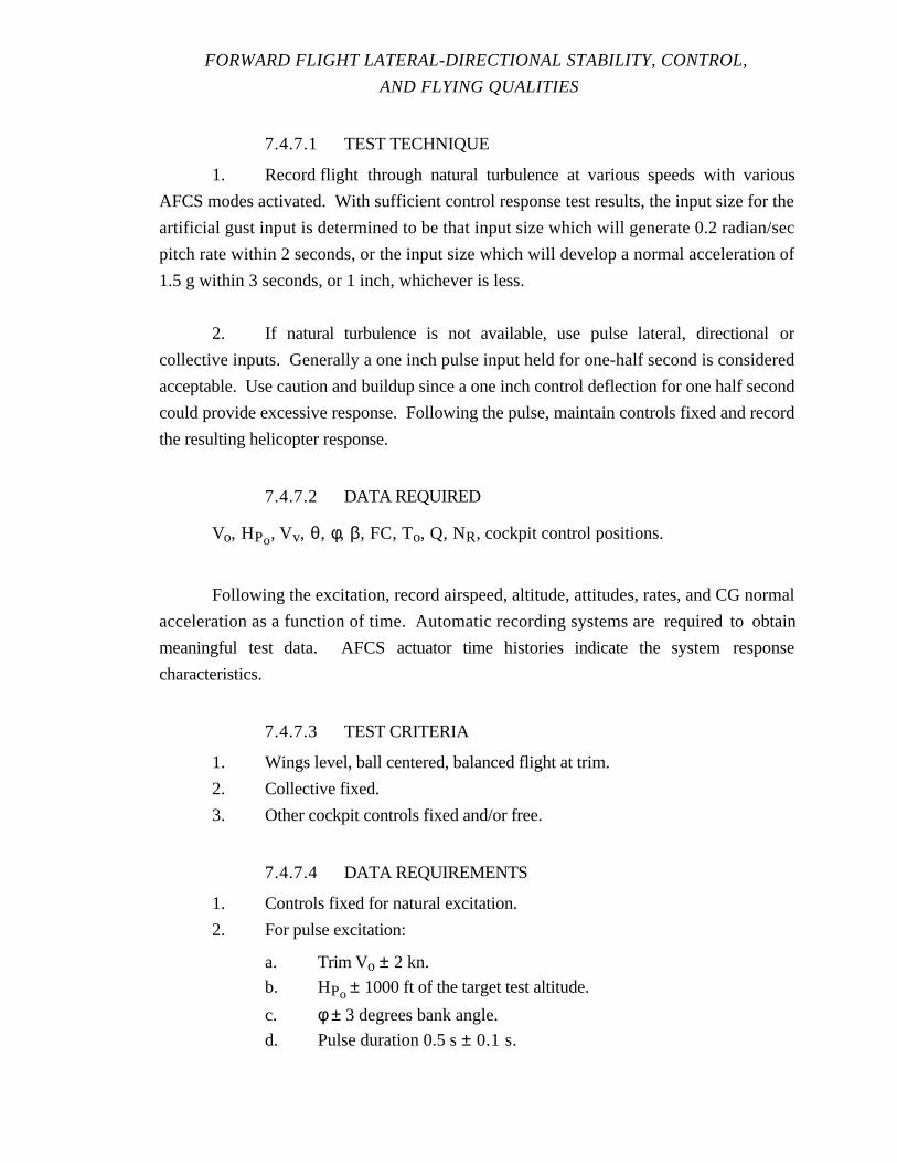
FORWARD FLIGHT LATERAL-DIRECTIONAL STABILITY, CONTROL,
AND FLYING QUALITIES
7.4.7.1 TEST TECHNIQUE
1. Record flight through natural turbulence at various speeds with various
AFCS modes activated. With sufficient control response test results, the input size for the
artificial gust input is determined to be that input size which will generate 0.2 radian/sec
pitch rate within 2 seconds, or the input size which will develop a normal acceleration of
1.5 g within 3 seconds, or 1 inch, whichever is less.
2. If natural turbulence is not available, use pulse lateral, directional or
collective inputs. Generally a one inch pulse input held for one-half second is considered
acceptable. Use caution and buildup since a one inch control deflection for one half second
could provide excessive response. Following the pulse, maintain controls fixed and record
the resulting helicopter response.
7.4.7.2 DATA REQUIRED
Vo, HPo, Vv, θ, φ, β, FC, To, Q, NR, cockpit control positions.
Following the excitation, record airspeed, altitude, attitudes, rates, and CG normal
acceleration as a function of time. Automatic recording systems are required to obtain
meaningful test data. AFCS actuator time histories indicate the system response
characteristics.
7.4.7.3 TEST CRITERIA
1. Wings level, ball centered, balanced flight at trim.
2. Collective fixed.
3. Other cockpit controls fixed and/or free.
7.4.7.4 DATA REQUIREMENTS
1. Controls fixed for natural excitation.
2. For pulse excitation:
a. Trim Vo ± 2 kn.
b. HPo ± 1000 ft of the target test altitude.
c. φ ± 3 degrees bank angle.
d. Pulse duration 0.5 s ± 0.1 s.

ROTARY WING STABILITY AND CONTROL
7.4.7.5 SAFETY CONSIDERATIONS/RISK MANAGEMENT
If these tests are conducted well within an established flight envelope, consider
normal operating limitations. Maintain situational awareness and proper lookout
procedures. This is particularly important when control fixtures are involved. Consider
using a chase, sole use airspace, and wearing a parachute. A thorough knowledge of
airspeed and attitude limitations is essential. Initiate recovery in sufficient time to prevent
exceeding limits. Brief and practice use of the control fixture.
Approach flight into known turbulence cautiously. Comparison with known chase
aircraft gust response characteristics may be of some benefit. Consider saturation of AFCS
and AFCS capabilities to deal with the turbulence.
7.5 DATA REDUCTION
Data reduction requires the application of instrument corrections to the hand
recorded data. Airspeed and altitude data are corrected for both instrument and position
errors. Automatic data recording systems normally include total instrumentation system
corrections in the process used to change a flight tape (or telemetry) raw data into
engineering units. Most quantitative information required for lateral-directional flying
qualities tests is read from time histories of selected data parameters. The specific data
elements as well as general definitions are included in each test technique section.
Specific data reduction procedures are discussed for the two most common types of
dynamic time history responses. Roll control response time histories may resemble a
classical first order response, while the LDO is typically a lightly damped second order
response. These two procedures encompass most of the commonly expected test results.
Non-classical responses may require characterization by other data reduction techniques.
7.5.1 First Order Systems
A high quality time history of the response of interest is required to determine the
first order time constant (τ). Additional data are read directly from the time history. The
time constant is usually used to describe a first order convergent response as shown in
Figure 7.28.
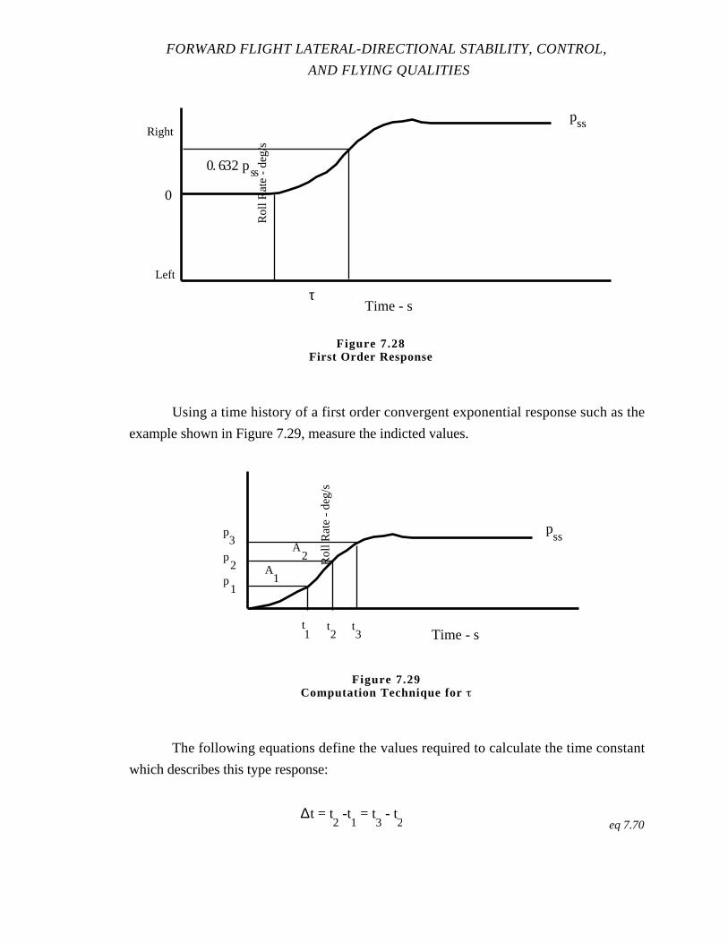
FORWARD FLIGHT LATERAL-DIRECTIONAL STABILITY, CONTROL,
AND FLYING QUALITIES
Using a time history of a first order convergent exponential response such as the
example shown in Figure 7.29, measure the indicted values.
The following equations define the values required to calculate the time constant
which describes this type response:
∆t = t2 -t
1 = t
3 - t
2 eq 7.70
Time - s
Rol
l Rat
e -
deg/
sRight
Left
0
0. 632 pss
pss
τ
Figure 7.28First Order Response
Time - s
Rol
l Rat
e -
deg/
s
pss
t1
t2
t3
p1
p2
p3
A1
A2
Figure 7.29Computation Technique for
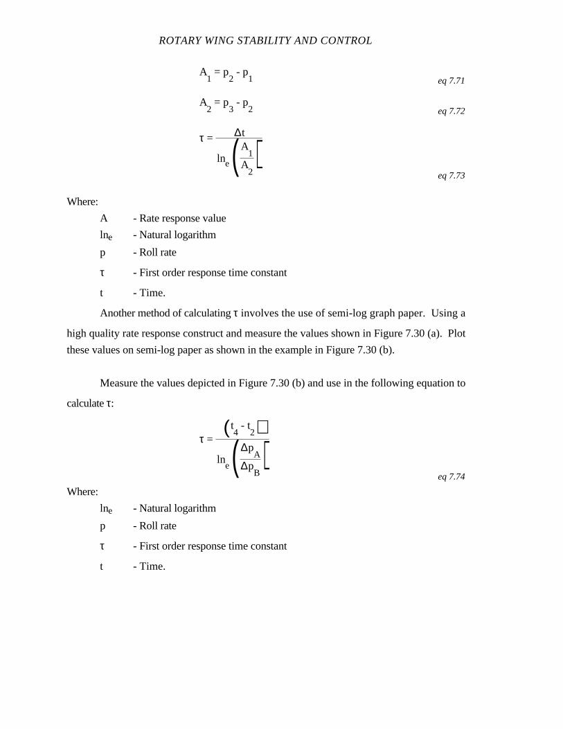
ROTARY WING STABILITY AND CONTROL
A1 = p
2 - p
1 eq 7.71
A2 = p
3 - p
2 eq 7.72
τ = ∆t
lne(A1
A2)
eq 7.73
Where:
A - Rate response value
lne - Natural logarithm
p - Roll rate
τ - First order response time constant
t - Time.
Another method of calculating τ involves the use of semi-log graph paper. Using a
high quality rate response construct and measure the values shown in Figure 7.30 (a). Plot
these values on semi-log paper as shown in the example in Figure 7.30 (b).
Measure the values depicted in Figure 7.30 (b) and use in the following equation to
calculateτ:
τ = ( t
4 - t
2)ln
e(∆pA
∆pB)
eq 7.74
Where:
lne - Natural logarithm
p - Roll rate
τ - First order response time constant
t - Time.
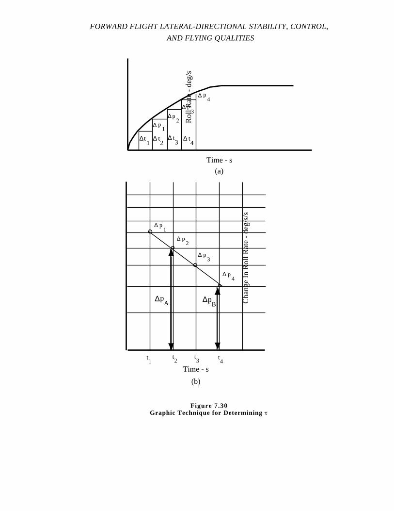
FORWARD FLIGHT LATERAL-DIRECTIONAL STABILITY, CONTROL,
AND FLYING QUALITIES
Time - s
(a)
Time - s
(b)
Cha
nge
In R
oll R
ate
- de
g/s/
s
t1
t2
t3 t
4
∆ p1
∆ p2
∆ p3
∆ p4
∆pA ∆p
B
Rol
l Rat
e -
deg/
s
∆ t1
∆ t2
∆ t3
∆ t4
∆ p1
∆ p2
∆ p3
∆ p4
Figure 7.30Graphic Technique for Determining
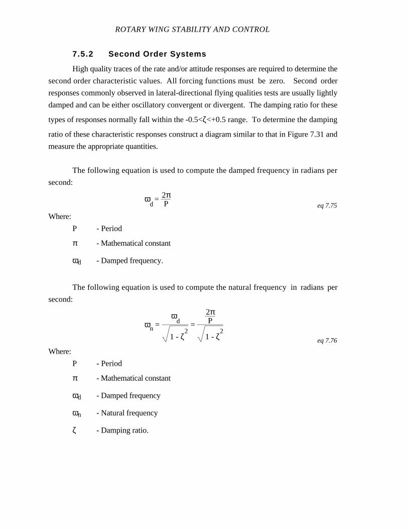
ROTARY WING STABILITY AND CONTROL
7.5.2 Second Order Systems
High quality traces of the rate and/or attitude responses are required to determine the
second order characteristic values. All forcing functions must be zero. Second order
responses commonly observed in lateral-directional flying qualities tests are usually lightly
damped and can be either oscillatory convergent or divergent. The damping ratio for these
types of responses normally fall within the -0.5<ζ<+0.5 range. To determine the damping
ratio of these characteristic responses construct a diagram similar to that in Figure 7.31 and
measure the appropriate quantities.
The following equation is used to compute the damped frequency in radians per
second:
ωd = 2π
P eq 7.75
Where:
P - Period
π - Mathematical constant
ωd - Damped frequency.
The following equation is used to compute the natural frequency in radians per
second:
ωn = ω
d
1 - ζ2 =
2πP
1 - ζ2
eq 7.76
Where:
P - Period
π - Mathematical constant
ωd - Damped frequency
ωn - Natural frequency
ζ - Damping ratio.
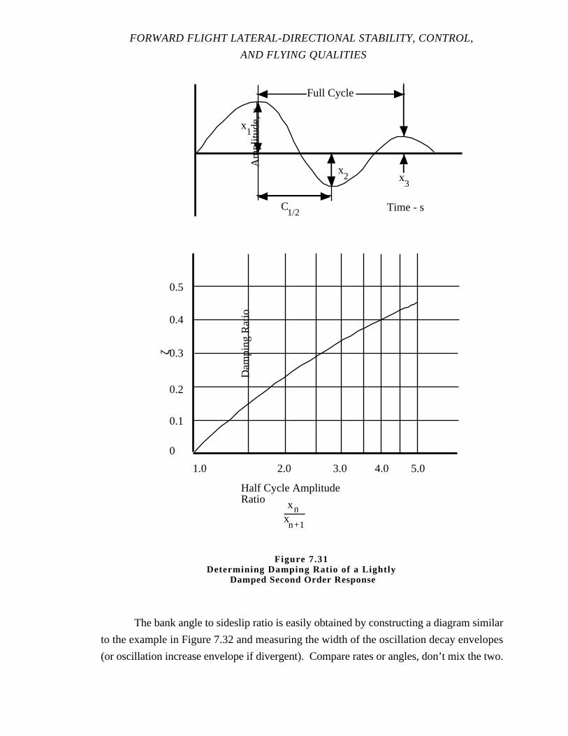
FORWARD FLIGHT LATERAL-DIRECTIONAL STABILITY, CONTROL,
AND FLYING QUALITIES
The bank angle to sideslip ratio is easily obtained by constructing a diagram similar
to the example in Figure 7.32 and measuring the width of the oscillation decay envelopes
(or oscillation increase envelope if divergent). Compare rates or angles, don’t mix the two.
0
0.1
0.2
0.3
0.4
0.5
2.0 3.0 4.0 5.0
Half Cycle AmplitudeRatio
xn+1
xn
Am
plitu
de, x
Time - sC1/2
x1
x2 x
3
Full Cycle
1.0
Dam
ping
Rat
io
ζ
Figure 7.31Determining Damping Ratio of a Lightly
Damped Second Order Response
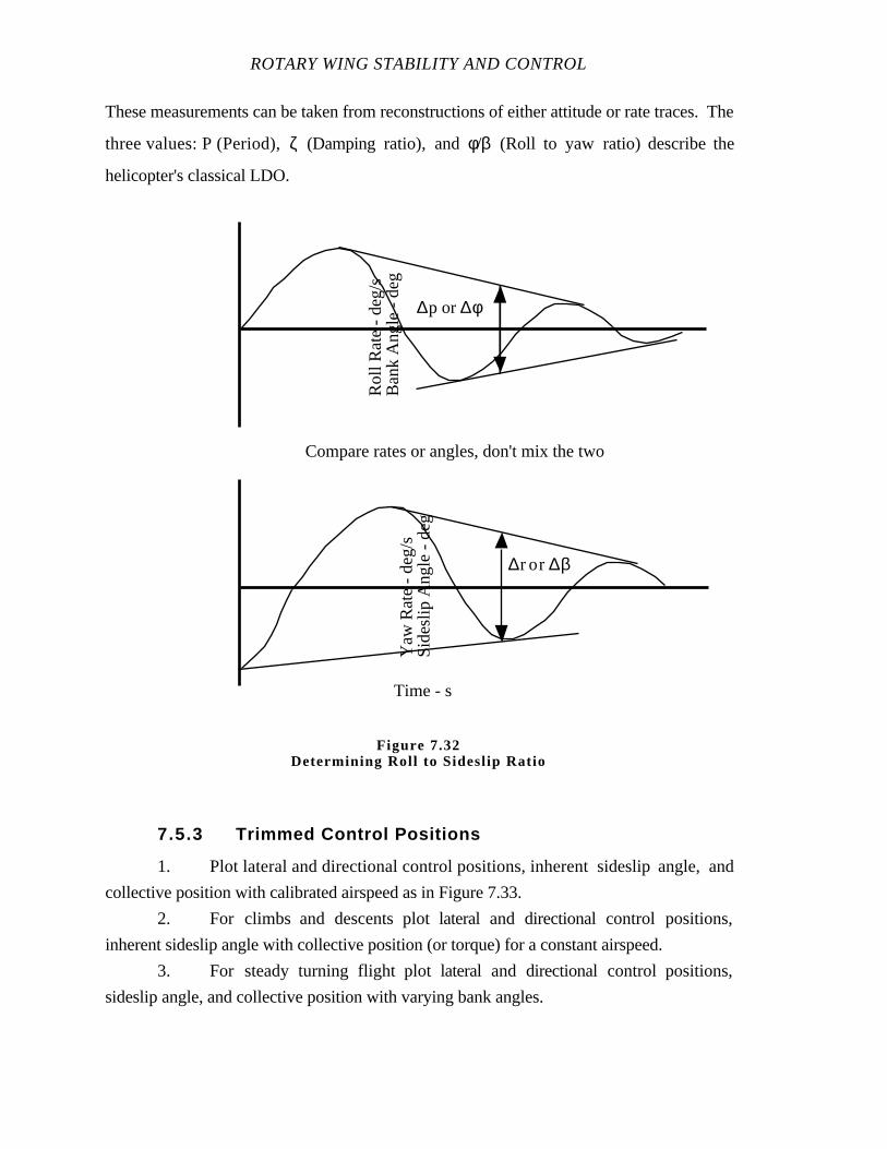
ROTARY WING STABILITY AND CONTROL
These measurements can be taken from reconstructions of either attitude or rate traces. The
three values: P (Period), ζ (Damping ratio), andφ/β (Roll to yaw ratio) describe the
helicopter's classical LDO.
7.5.3 Trimmed Control Positions
1. Plot lateral and directional control positions, inherent sideslip angle, and
collective position with calibrated airspeed as in Figure 7.33.
2. For climbs and descents plot lateral and directional control positions,
inherent sideslip angle with collective position (or torque) for a constant airspeed.
3. For steady turning flight plot lateral and directional control positions,
sideslip angle, and collective position with varying bank angles.
Rol
l Rat
e -
deg/
sB
ank
Ang
le -
deg
Yaw
Rat
e -
deg/
sS
ides
lip A
ngle
- d
eg
∆p or ∆φ
Time - s
∆r or ∆β
Compare rates or angles, don't mix the two
Figure 7.32Determining Roll to Sideslip Ratio

FORWARD FLIGHT LATERAL-DIRECTIONAL STABILITY, CONTROL,
AND FLYING QUALITIES
True Airspeed - kn80 100 1206040
Late
ral
Con
trol
Pos
ition
in F
rom
Ful
l Lef
t
Aft
Fwd
Long
itudi
nal
Con
trol
Pos
ition
in F
rom
Ful
l Fw
d
Dire
ctio
nal
Con
trol
Pos
ition
in F
rom
Ful
l Lef
t
Right
Left
Col
lect
ive
Con
trol
Pos
ition
in F
rom
Ful
l Dow
n
Left
Right
Down
Up
Sid
eslip
Ang
le -
deg
Left
Right
Total Collective Control Travel =10.0 in
Total Directional Control Travel = 5.6 in
Total Lateral Control Travel =10.6 in
Total Longitudinal Control Travel= 9.8 in
Trim Ball Centered
Figure 7.33Trimmed Control Positions
ROTARY WING STABILITY AND CONTROL
7.5.4 Static Lateral-Directional Stability (SHSS)
Static lateral-directional data obtained from SHSS are presented in graphic form
(Figure 7.34), plotting helicopter control positions, and roll attitude versus sideslip angles
for a given airspeed. If pitch attitude or vertical velocities are significant they are presented.
Either zero sideslip or ball centered is the trim point, depending on whether engineering
results or mission relative results are being presented. In either case, the trim point should
be annotated.
7.5.5 Cyclic Only Turns
Cyclic only turn data are generally presented in narrative form to support the
discussion of static lateral-directional stability. Include a discussion of the pilot workload
in performing cyclic only turns. Assess and report on the workload associated with
capturing and maintaining bank angle. Assess the workload associated with maintaining
ball centered. Report on the yaw due to lateral control, adverse/proverse yaw, and what
effect, if any, this had on the workload associated with capturing and maintaining a bank
angle. The behavior of BETA during the initial part of the roll should be discussed as an
indication of the strength of directional stability and related to the results of pedal
requirements found in steady heading sideslip.
7.5.6 Pedal Only Turns
Pedal only turn data are generally presented in narrative form to support the
discussion of static lateral-directional stability. Assess and report on the workload
associated with capturing and maintaining bank angle. The behavior of the aircraft in roll
due to pedal input and the presence of BETA should be addressed and related to the
strength of effective dihedral and cyclic requirements found in steady heading sideslips.
7.5.7 Spiral Stability
Spiral stability data are presented with a properly annotated time history as shown
in Figure 7.35. Report the spiral stability characteristics as convergent, divergent or
neutral. Include time to half/double amplitude (T1/2, Td). Results for left versus right bank
angles may not be the same.
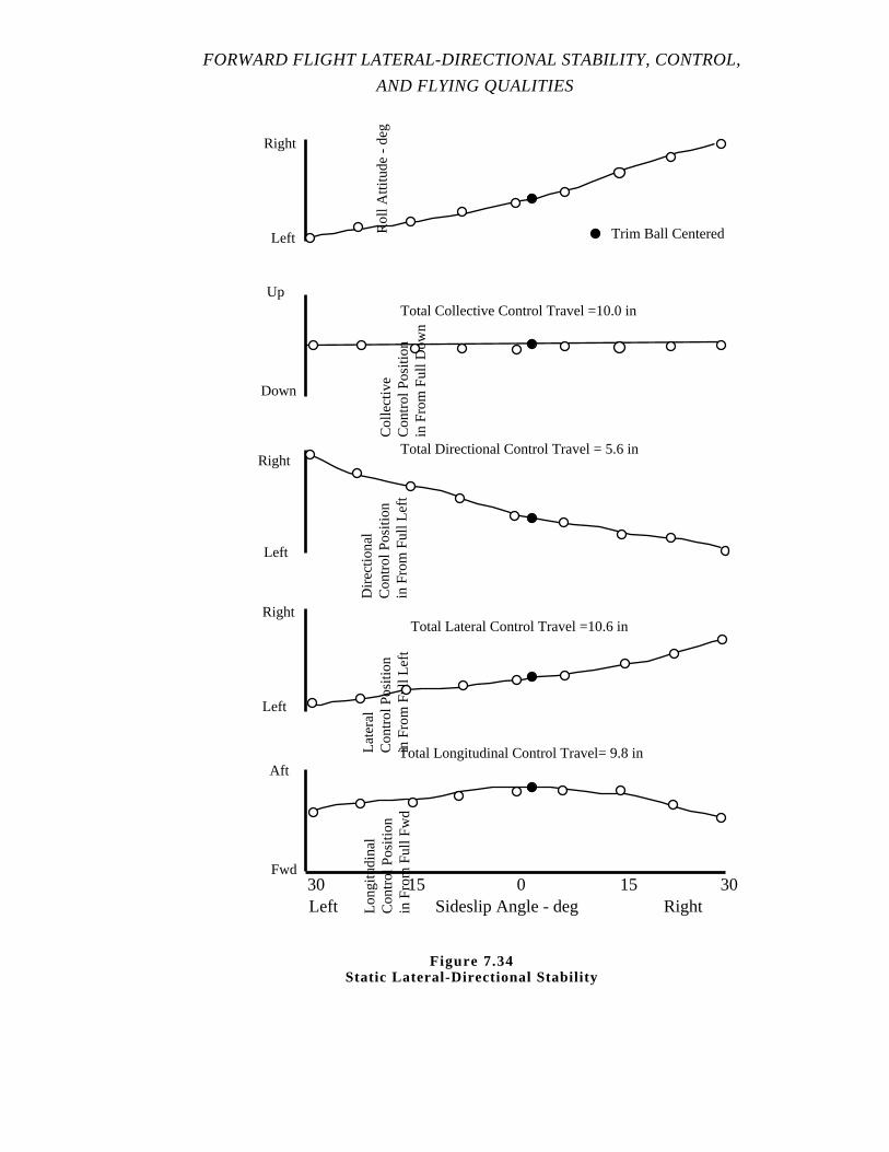
FORWARD FLIGHT LATERAL-DIRECTIONAL STABILITY, CONTROL,
AND FLYING QUALITIES
Sideslip Angle - degLeft Right0 15 301530
Late
ral
Con
trol
Pos
ition
in F
rom
Ful
l Lef
t
Aft
Fwd
Long
itudi
nal
Con
trol
Pos
ition
in F
rom
Ful
l Fw
d
Dire
ctio
nal
Con
trol
Pos
ition
in F
rom
Ful
l Lef
t
Right
Left
Col
lect
ive
Con
trol
Pos
ition
in F
rom
Ful
l Dow
n
Left
Right
Down
Up
Rol
l Atti
tude
- d
eg
Left
Right
Total Collective Control Travel =10.0 in
Total Directional Control Travel = 5.6 in
Total Lateral Control Travel =10.6 in
Total Longitudinal Control Travel= 9.8 in
Trim Ball Centered
Figure 7.34Static Lateral-Directional Stability
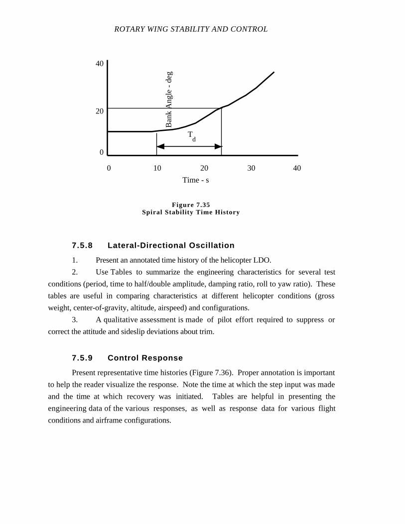
ROTARY WING STABILITY AND CONTROL
7.5.8 Lateral-Directional Oscillation
1. Present an annotated time history of the helicopter LDO.
2. Use Tables to summarize the engineering characteristics for severaltest
conditions (period, time to half/double amplitude, damping ratio, roll to yaw ratio). These
tables are useful in comparing characteristics at different helicopter conditions (gross
weight, center-of-gravity, altitude, airspeed) and configurations.
3. A qualitative assessment is made of pilot effort required to suppress or
correct the attitude and sideslip deviations about trim.
7.5.9 Control Response
Present representative time histories (Figure 7.36). Proper annotation is important
to help the reader visualize the response. Note the time at which the step input was made
and the time at which recovery was initiated. Tables are helpful in presenting the
engineering data of the various responses, as well as response data for various flight
conditions and airframe configurations.
Ban
k A
ngle
- d
eg
0
20
40
Time - s
0 10 20 30 40
Td
Figure 7.35Spiral Stabil i ty Time History
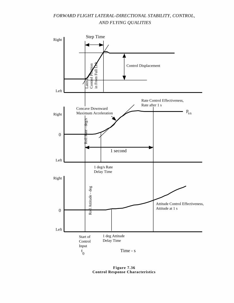
FORWARD FLIGHT LATERAL-DIRECTIONAL STABILITY, CONTROL,
AND FLYING QUALITIES
Time - s
Step Time
Control Displacement
Rol
l Rat
e -
deg/
sLeft
Right
Left
0
1 second
Rate Control Effectiveness,Rate after 1 s
Attitude Control Effectiveness,Attitude at 1 s
1 deg AttitudeDelay Time
1 deg/s RateDelay Time
t0
Start ofControlInput
Rol
l Atti
tude
- d
eg
0
Right
Left
Right
Late
ral
Con
trol
Pos
ition
in F
rom
Ful
l Lef
t
pss
Concave DownwardMaximum Acceleration
Figure 7.36Control Response Characteristics
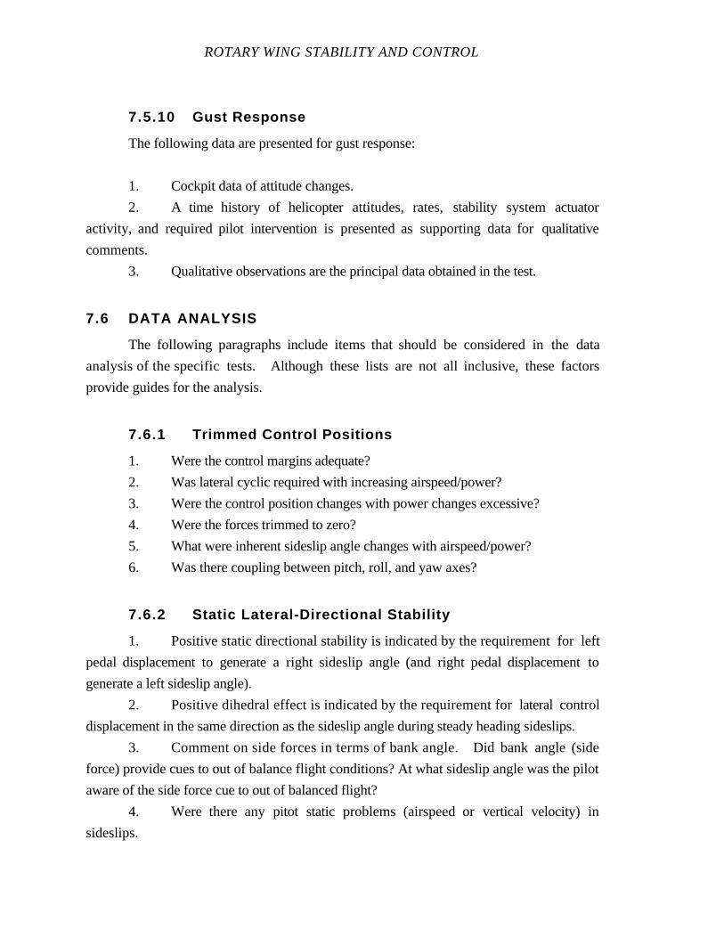
ROTARY WING STABILITY AND CONTROL
7.5.10 Gust Response
The following data are presented for gust response:
1. Cockpit data of attitude changes.
2. A time history of helicopter attitudes, rates, stability system actuator
activity, and required pilot intervention is presented as supporting data for qualitative
comments.
3. Qualitative observations are the principal data obtained in the test.
7.6 DATA ANALYSIS
The following paragraphs include items that should be considered in the data
analysis of the specific tests. Although these lists are not all inclusive, these factors
provide guides for the analysis.
7.6.1 Trimmed Control Positions
1. Were the control margins adequate?
2. Was lateral cyclic required with increasing airspeed/power?
3. Were the control position changes with power changes excessive?
4. Were the forces trimmed to zero?
5. What were inherent sideslip angle changes with airspeed/power?
6. Was there coupling between pitch, roll, and yaw axes?
7.6.2 Static Lateral-Directional Stability
1. Positive static directional stability is indicated by the requirement for left
pedal displacement to generate a right sideslip angle (and right pedal displacement to
generate a left sideslip angle).
2. Positive dihedral effect is indicated by the requirement for lateral control
displacement in the same direction as the sideslip angle during steady heading sideslips.
3. Comment on side forces in terms of bank angle. Did bank angle(side
force) provide cues to out of balance flight conditions? At what sideslip angle was the pilot
aware of the side force cue to out of balanced flight?
4. Were there any pitot static problems (airspeed or vertical velocity) in
sideslips.
FORWARD FLIGHT LATERAL-DIRECTIONAL STABILITY, CONTROL,
AND FLYING QUALITIES
7.6.2.1 TURNS ON ONE CONTROL
1. What does the lateral control only turns reveal about the relative magnitude
of the directional stability of the helicopter? If the sideslip angle during the steady state turn
returns to the inherent sideslip angle, the helicopter exhibits strong directional stability. Is
adverse/proverse yaw present? Does it cause an increase in pilot workload for coordinated
turns.
2. In addition to testing for directional stability, a limited examination of the
spiral mode of the helicopter can be obtained during lateral cyclic only and pedal only turns.
The requirement for lateral cyclic displacement into the turn after a steady state turn rate is
established is indicative of a convergent spiral mode. If cyclic or pedal position during
steady state turn is the same as trim, neutral spiral mode is indicated. A requirement for
cyclic or pedal displacement away from the turn during steady state turns is indicative of a
divergent spiral mode. Cyclic or pedal displacement during turns on one control is only
one portion of a spiral mode evaluation.
3. What does the directional control only turns reveal about the relative
magnitude of the effective dihedral of the helicopter? If a relatively small sideslip angle
results in a large roll rate in the opposite direction, the helicopter exhibits strong effective
dihedral.
7.6.3 Spiral Stability
1. Did the spiral stability characteristics vary with airspeed and power?
2. What is the impact of the spiral stability characteristics on mission
performance and pilot workload?
7.6.4 Lateral-Directional Oscillation
1. How easily is the LDO excited by atmospheric turbulence?
2. Is the LDO excited by normal pilot control motions?
3. What is the φ/β ratio?
4. How well damped is the LDO?
5. What is the frequency of the LDO?
6. Is the LDO disturbing or distracting to the pilot, crew members, or
passengers?
ROTARY WING STABILITY AND CONTROL
7. If the helicopter can be flown with various AFCS modes selected, are the
characteristics of the LDO appreciably different?
8. Can the pilot damp the LDO or does pilot interaction further aggravate the
situation?
9. What are the pilot workload implications of this nuisance mode?
7.6.5 Control Response
1. Quantitative data are taken from the response time histories. The parameters
chosen and presented support pilot opinion of the helicopter response to control inputs.
Parameters which define the control moment available are the rate control effectiveness,
attitude control effectiveness, and the steady-state angular velocity. Quantities which are
used in discussing the quality of the response are the angular accelerations delay time,
initial angular acceleration, inflection time, and response time constant. Use these data as
an integral part of your discussions.
2. Did the helicopter respond adequately to perform the assigned task?
a. Were the steady-state rates adequate?
b. Was the response predictable?
c. Was the response consistent?
d. Were there any over controlling problems?
e. Were off axis responses observed?
7.6.6 Gust Response
1. Discuss the effects of varying levels of turbulence on task performance.
Did workload increase? Describe the ride quality.
2. What were the pitch, roll and yaw attitude changes? Airspeed changes?
3. Did the helicopter tend to return to the original trim condition?
4. How much pilot effort was required to return the helicopter to thetrim
condition?
5. Were any of the helicopter modes of motion excited?
7.7 MISSION SUITABILITY
The suitability of the test helicopter for the intended mission is the ultimate reason
for conducting any handling qualities test. Each of the specific tests provides some
information in accessing that suitability. Lateral-directional trimmed control positions
FORWARD FLIGHT LATERAL-DIRECTIONAL STABILITY, CONTROL,
AND FLYING QUALITIES
provides information about control margins, linearities, discontinuities, and gradients
which assist the pilot in determining overall suitability. Static lateral-directional stability
characteristics are good indicators of pilot workload required to maintain a desired forward
flight trim condition and the motion of the helicopter once disturbed. Spiral stability
characteristics is an indicator of the pilot workload required to maintain a trimmed wings
level condition. Short term lateral-directional dynamics area big factor in how much
difficulty the pilot will have maneuvering the helicopter in roll and yaw during high gain
tasks. Coupled lateral-directional short term dynamics are most often found objectionable.
Control response tests quantitatively document the pilots qualitative comments concerning
helicopter responsiveness.
In addition to the engineering tests discussed the test pilot should investigate how
the helicopter is intended to be used and duplicate mission tasks. Generally, knowledge of
engineering shortcomings allow the test team to design operational scenarios which reflect
the poor characteristics. Each test program and helicopter require a unique set of mission
maneuvers. The most important aspect of mission suitability testing is to keep the operator
in mind. Consider how the test helicopter is used in the field and who will be operating the
helicopter.
7.8 SPECIFICATION COMPLIANCE
General guidelines for lateral-directional helicopter handling qualities in forward
flight are contained in applicable paragraphs of MIL-H-8501A. Readthe specification
carefully to understand each requirement. Remember the military specifications are only a
guide which leave some room for interpretation for individual systems and situations. The
following list identifies the MIL-H-8501A paragraph number and a short description of the
requirement.
3.3 Directional and Lateral characteristics.
3.3.8 Directional control for autorotation
3.3.9 Directional stability and effective dihedral
3.3.9.1 Turns on one control
3.3.9.2 Adverse yaw
3.3.10 Trimmability, control jump
3.3.11 Control force gradients
ROTARY WING STABILITY AND CONTROL
3.3.12 Limit forces
3.3.13 Breakout forces
3.3.14 Control coupling
3.3.15 Lateral control response, over control
3.3.16 Lateral and directional control response
3.3.17 Lateral trim with power effects
3.5.9 Automatic stabilization system
3.5.10 Total control system freeplay
3.5.11 Mechanical coupling
3.5.11.1 Mixing
3.6.1 Instrument flight characteristics
3.6.1.1 Control power
3.6.1.2 Lateral directional oscillation IFR
3.6.2 Lateral directional stability IFR
3.7.1 Vibrations
3.7.2 Vibrations
3.7.3 Mechanical Instability
Additional requirements are included in the military specification relating to boosted
controls, failure modes, automatic stabilization equipment, and vibrations. Some of these
paragraphs may apply to specific helicopters equipped with an AFCS.
7.9 GLOSSARY
7.9.1 Notations
A Rate response value
A1s Lateral cyclic pitch angle, shaft referenced
AFCS Automatic Flight Control System
B Damping constant
b Number of blades
b1s Lateral flapping angle, shaft referenced
C1/2 Cycles to one-half amplitude
CG Center of gravity
e Base of natural logarithm, flapping hinge offset
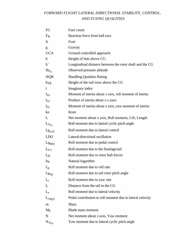
FORWARD FLIGHT LATERAL-DIRECTIONAL STABILITY, CONTROL,
AND FLYING QUALITIES
FC Fuel count
FR Reaction force from ball race
ft Foot
g Gravity
GCA Ground controlled approach
h Height of hub above CG
h' Longitudinal distance between the rotor shaft and the CG
HPo Observed pressure altitude
HQR Handling Qualities Rating
hTR Height of the tail rotor above the CG
i Imaginary index
Ixx Moment of inertia about x axis, roll moment of inertia
Ixz Product of inertia about x z axes
Izz Moment of inertia about z axis, yaw moment of inertia
kn Knot
L Net moment about x axis, Roll moment, Lift, Length
LA1s Roll moment due to lateral cyclic pitch angle
LδLAT Roll moment due to lateral control
LDO Lateral-directional oscillation
LδPED Roll moment due to pedal control
Lf+t Roll moment due to the fuselage/tail
LH Roll moment due to rotor hub forces
lne Natural logarithm
Lp Roll moment due to roll rate
LθTR Roll moment due to tail rotor pitch angle
Lr Roll moment due to yaw rate
lt Distance from the tail to the CG
Lv Roll moment due to lateral velocity
LvPED Pedal contribution to roll moment due to lateral velocity
m Mass
MS Blade mass moment
N Net moment about z axis, Yaw moment
NA1s Yaw moment due to lateral cyclic pitch angle
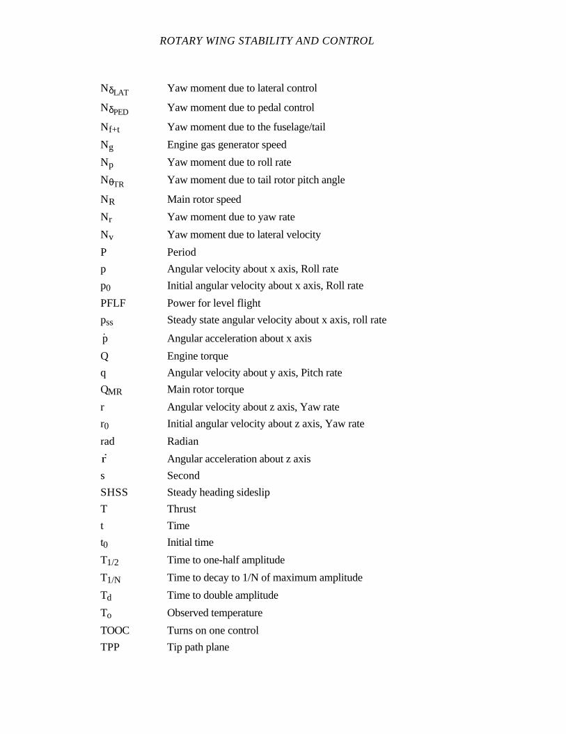
ROTARY WING STABILITY AND CONTROL
NδLAT Yaw moment due to lateral control
NδPED Yaw moment due to pedal control
Nf+t Yaw moment due to the fuselage/tail
Ng Engine gas generator speed
Np Yaw moment due to roll rate
NθTR Yaw moment due to tail rotor pitch angle
NR Main rotor speed
Nr Yaw moment due to yaw rate
Nv Yaw moment due to lateral velocity
P Period
p Angular velocity about x axis, Roll rate
p0 Initial angular velocity about x axis, Roll rate
PFLF Power for level flight
pss Steady state angular velocity about x axis, roll rate
p Angular acceleration about x axis
Q Engine torque
q Angular velocity about y axis, Pitch rate
QMR Main rotor torque
r Angular velocity about z axis, Yaw rate
r0 Initial angular velocity about z axis, Yaw rate
rad Radian
r Angular acceleration about z axis
s Second
SHSS Steady heading sideslip
T Thrust
t Time
t0 Initial time
T1/2 Time to one-half amplitude
T1/N Time to decay to 1/N of maximum amplitude
Td Time to double amplitude
To Observed temperature
TOOC Turns on one control
TPP Tip path plane
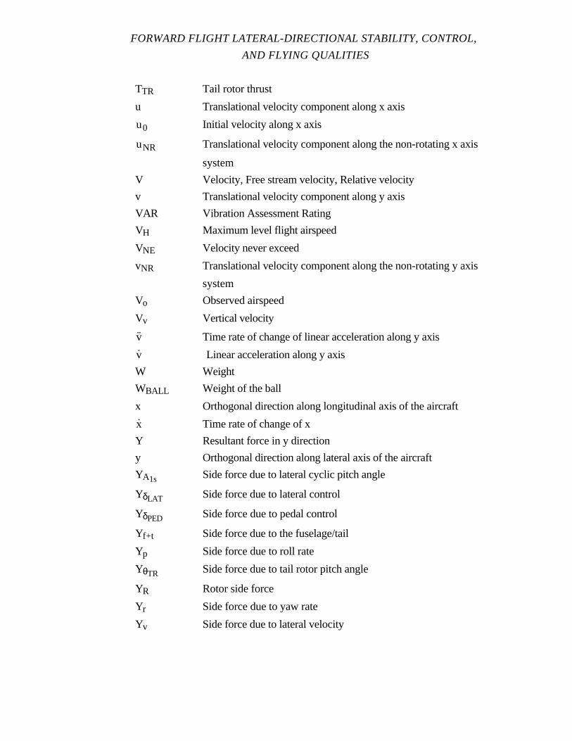
FORWARD FLIGHT LATERAL-DIRECTIONAL STABILITY, CONTROL,
AND FLYING QUALITIES
TTR Tail rotor thrust
u Translational velocity component along x axis
u0 Initial velocity along x axis
uNR Translational velocity component along the non-rotating x axis
system
V Velocity, Free stream velocity, Relative velocity
v Translational velocity component along y axis
VAR Vibration Assessment Rating
VH Maximum level flight airspeed
VNE Velocity never exceed
vNR Translational velocity component along the non-rotating y axis
system
Vo Observed airspeed
Vv Vertical velocity
˙v Time rate of change of linear acceleration along y axis
v Linear acceleration along y axis
W Weight
WBALL Weight of the ball
x Orthogonal direction along longitudinal axis of the aircraft
x Time rate of change of x
Y Resultant force in y direction
y Orthogonal direction along lateral axis of the aircraft
YA1s Side force due to lateral cyclic pitch angle
YδLAT Side force due to lateral control
YδPED Side force due to pedal control
Yf+t Side force due to the fuselage/tail
Yp Side force due to roll rate
YθTR Side force due to tail rotor pitch angle
YR Rotor side force
Yr Side force due to yaw rate
Yv Side force due to lateral velocity
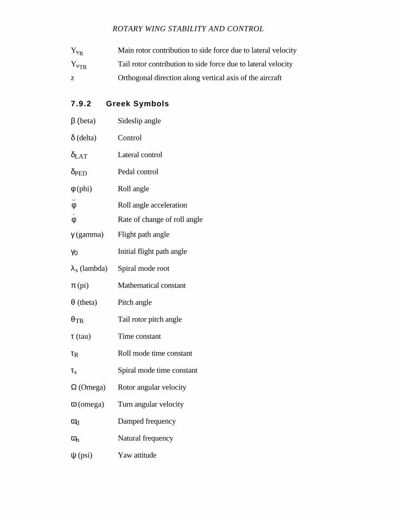
ROTARY WING STABILITY AND CONTROL
YvR Main rotor contribution to side force due to lateral velocity
YvTR Tail rotor contribution to side force due to lateral velocity
z Orthogonal direction along vertical axis of the aircraft
7.9.2 Greek Symbols
β (beta) Sideslip angle
δ (delta) Control
δLAT Lateral control
δPED Pedal control
φ (phi) Roll angle
˙φ Roll angle acceleration
φ Rate of change of roll angle
γ (gamma) Flight path angle
γ0 Initial flight path angle
λs (lambda) Spiral mode root
π (pi) Mathematical constant
θ (theta) Pitch angle
θTR Tail rotor pitch angle
τ (tau) Time constant
τR Roll mode time constant
τs Spiral mode time constant
Ω (Omega) Rotor angular velocity
ω (omega) Turn angular velocity
ωd Damped frequency
ωn Natural frequency
ψ (psi) Yaw attitude
FORWARD FLIGHT LATERAL-DIRECTIONAL STABILITY, CONTROL,
AND FLYING QUALITIES
˙ψ Yaw attitude acceleration
ψ Rate of change of yaw attitude
ζ (zeta) Damping ratio
7.10 REFERENCES
1. Bramwell, A. R. S., Helicopter Dynamics, Edward Arnold (Publishers)
Ltd., London, England, 1976.
2. Gessow, A. and Myers, G. C., Jr., Aerodynamics of the Helicopter, fifth
printing, Frederick Unger Publishing Co., NY, 1978.
3. Johnson, W., Helicopter Theory, Princeton University Pres., 1980.
4. Hall, W. G., "A Collection of Flight Test Data Reduction Techniques",
CAL No. 177, Technical Report, Cornell Aeronautical Laboratory, Inc., Buffalo, NY,
June 1971.
5. Military Specification, "Helicopter Flying and Ground Handling Qualities;
General Requirements For", MIL-H-8501A, with Amendment 1, 3 April, 1962.
6. Naval Test Pilot School Flight Test Manual,Helicopter Stability and
Control, USNTPS-FTM-No. 101, U. S. Naval Test Pilot School, Patuxent River, MD, 10
June 1968, reprinted February 1978.
7. Naval Test Pilot School Flight Test Manual,Helicopter Stability and
Control, Theory and Flight Test Techniques, USNTPS-FTM-No. 105, U. S. Naval Test
Pilot School, Patuxent River, MD, November 1983, Preliminary Edition.
8. Prouty, R. W., Practical Helicopter Aerodynamics, PJS Publications, Inc.,
1982.
ROTARY WING STABILITY AND CONTROL
9. Prouty, Raymond W.,Helicopter Performance, Stability, and Control,
PWS Publishers, Boston, MA, 1986.
10. Wiesner, W. and Kohler, G., Tail Rotor Performance in Presence of Main
Rotor, Ground, and Winds, J.A.H.S., Vol. 15, No. 3, July 1974.
11. Wolowicz, C. H., "Considerations in the Determination of Stability and
Control Derivatives and Dynamic Characteristics from Flight Data", AGARD Report 549-
Part I, NASA Flight Research Center, AFB, CA, 1966.
CHAPTER EIGHT
HOVER AND LOW AIRSPEED STABILITY, CONTROL, AND FLYING QUALITIES
PAGE
8.1 INTRODUCTION 8.1
8.2 PURPOSE OF TEST 8.1
8.3 THEORY 8.1
8.3.1 Summary of Quasi-Static Rotor Characteristics 8.2
8.3.2 Linearized Equations of Motion 8.2
8.3.2.1 Longitudinal 8.4
8.3.2.2 Lateral-Directional 8.6
8.3.3 Stability Derivatives 8.8
8.3.4 Z Force Equation Derivatives 8.9
8.3.5 X Force and Pitching Moment Equation Derivatives 8.9
8.3.6 Side Force and Rolling Moment Equation Derivatives 8.10
8.3.7 Yawing Moment Equation Derivatives 8.11
8.3.8 Trim and Static Stability 8.11
` 8.3.8.1 Hover Attitude 8.12
8.3.8.2 Trim and Power Changes During Translational Flight 8.14
8.3.8.3 Rotor Blowback and Nonuniform Inflow Distribution
Over Rotor Disk 8.15
8.3.8.4 Downwash Impingement on Fuselage, Tail,
and Horizontal Stabilizer 8.18
8.3.8.5 Tail Rotor Thrust Changes in Sideward Flight 8.18
8.3.8.6 Interference of Main Rotor Tip Vortices with Tail Rotor
and Fixed Stabilizer Surfaces 8.21
8.3.8.7 Reduction of Power Required IGE 8.21
8.3.8.8 Influence of Ground Vortices on Trim Control Positions 8.22
8.3.8.9 Static Stability 8.26
ROTARY WING STABILITY AND CONTROL
8.3.9 Turn on a Spot 8.29
8.3.9.1 Directional Control 8.29
8.3.9.2 Bank and Height Control 8.31
8.3.9.3 Longitudinal Control 8.32
8.3.10 Long Term Dynamic Stability 8.33
8.3.11 First Order Representation of Vertical Velocity, Pitch Rate,
Roll Rate, and Yaw Rate Responses 8.36
8.3.12 Control Response 8.44
8.3.13 Vertical Response IGE 8.46
8.4 TEST METHODS AND TECHNIQUES 8.48
8.4.1 General 8.48
8.4.2 Trimmed Control Positions 8.49
8.4.2.1 Test Technique 8.49
8.4.2.2 Data Required 8.50
8.4.2.3 Test Criteria 8.50
8.4.2.4 Data Requirements 8.50
8.4.2.5 Safety Considerations/Risk Management 8.51
8.4.3 Critical Azimuth 8.51
8.4.4 Turn on a Spot 8.51
8.4.4.1 Test Technique 8.52
8.4.4.2 Data Required 8.52
8.4.4.3 Test Criteria 8.52
8.4.4.4 Data Requirements 8.53
8.4.5 Static Stability 8.53
8.4.5.1 Test Technique 8.54
8.4.5.2 Data Required 8.54
8.4.5.3 Test Criteria 8.54
8.4.5.4 Data Requirements 8.55
8.4.6 Long Term Dynamic Stability 8.55
8.4.6.1 Test Technique 8.56
8.4.6.2 Data Required 8.56
8.4.6.3 Test Criteria 8.56
8.4.6.4 Data Requirements 8.57
8.4.6.5 Safety Considerations/Risk Management 8.57

HOVER AND LOW AIRSPEED STABILITY, CONTROL, AND FLYING QUALITIES
8.4.7 Control Response 8.57
8.4.7.1 Test Technique 8.57
8.4.7.2 Data Required 8.58
8.4.7.3 Test Criteria 8.58
8.4.7.4 Data Requirements 8.58
8.4.7.5 Safety Considerations/Risk Management 8.58
8.4.8 Departures and Approaches 8.59
8.4.8.1 Test Technique 8.59
8.4.8.2 Data Required 8.59
8.4.8.3 Test Criteria 8.60
8.5 DATA REDUCTION 8.60
8.5.1 General 8.60
8.5.2 Trimmed Control Positions 8.60
8.5.3 Critical Azimuth 8.60
8.5.4 Turn on a Spot 8.60
8.5.5 Static Stability 8.65
8.5.6 Long Term Dynamic Stability 8.65
8.5.7 Control Response 8.65
8.6 DATA ANALYSIS 8.70
8.6.1 General 8.70
8.6.2 Trimmed Control Positions 8.70
8.6.3 Critical Azimuth 8.70
8.6.4 Turn on a Spot 8.71
8.6.5 Static Stability 8.71
8.6.6 Long Term Dynamic Stability 8.71
8.6.7 Control Response 8.72
8.7 MISSION SUITABILITY 8.72
8.8 SPECIFICATION COMPLIANCE 8.72

ROTARY WING STABILITY AND CONTROL
8.9 GLOSSARY 8.75
8.9.1 Notations 8.75
8.9.2 Greek Symbols 8.78
8.10 REFERENCES 8.79
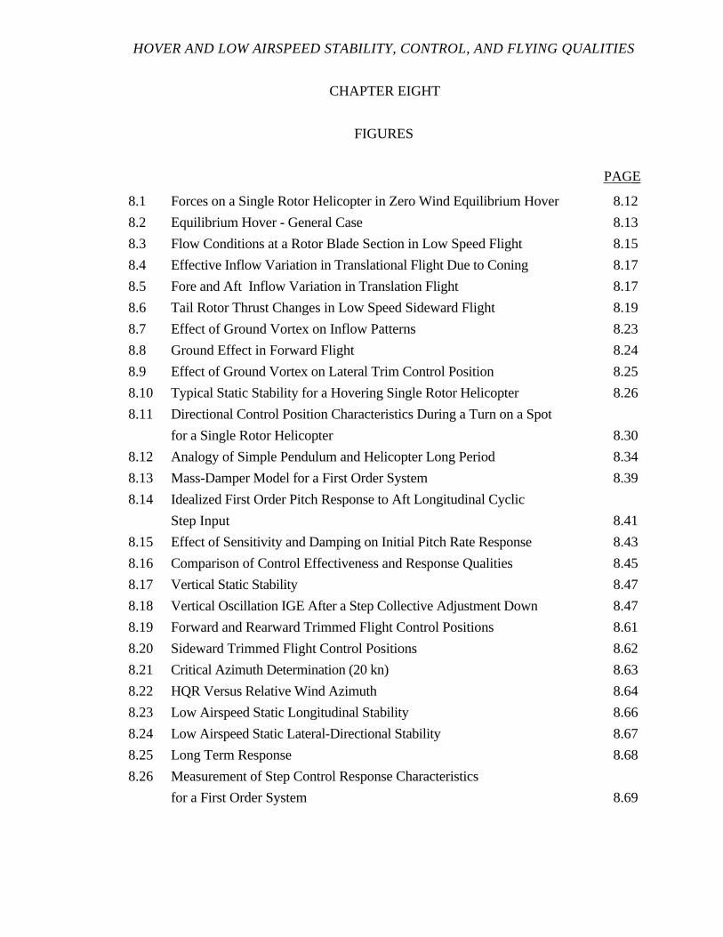
HOVER AND LOW AIRSPEED STABILITY, CONTROL, AND FLYING QUALITIES
CHAPTER EIGHT
FIGURES
PAGE
8.1 Forces on a Single Rotor Helicopter in Zero Wind Equilibrium Hover 8.12
8.2 Equilibrium Hover - General Case 8.13
8.3 Flow Conditions at a Rotor Blade Section in Low Speed Flight 8.15
8.4 Effective Inflow Variation in Translational Flight Due to Coning 8.17
8.5 Fore and Aft Inflow Variation in Translation Flight 8.17
8.6 Tail Rotor Thrust Changes in Low Speed Sideward Flight 8.19
8.7 Effect of Ground Vortex on Inflow Patterns 8.23
8.8 Ground Effect in Forward Flight 8.24
8.9 Effect of Ground Vortex on Lateral Trim Control Position 8.25
8.10 Typical Static Stability for a Hovering Single Rotor Helicopter 8.26
8.11 Directional Control Position Characteristics During a Turn on a Spot
for a Single Rotor Helicopter 8.30
8.12 Analogy of Simple Pendulum and Helicopter Long Period 8.34
8.13 Mass-Damper Model for a First Order System 8.39
8.14 Idealized First Order Pitch Response to Aft Longitudinal Cyclic
Step Input 8.41
8.15 Effect of Sensitivity and Damping on Initial Pitch Rate Response 8.43
8.16 Comparison of Control Effectiveness and Response Qualities 8.45
8.17 Vertical Static Stability 8.47
8.18 Vertical Oscillation IGE After a Step Collective Adjustment Down 8.47
8.19 Forward and Rearward Trimmed Flight Control Positions 8.61
8.20 Sideward Trimmed Flight Control Positions 8.62
8.21 Critical Azimuth Determination (20 kn) 8.63
8.22 HQR Versus Relative Wind Azimuth 8.64
8.23 Low Airspeed Static Longitudinal Stability 8.66
8.24 Low Airspeed Static Lateral-Directional Stability 8.67
8.25 Long Term Response 8.68
8.26 Measurement of Step Control Response Characteristics
for a First Order System 8.69
ROTARY WING STABILITY AND CONTROL
CHAPTER EIGHT
TABLES
PAGE
8.I Quasi-Static Rotor Characteristics in Hovering Flight 8.3
8.II First Order System Parameters 8.37
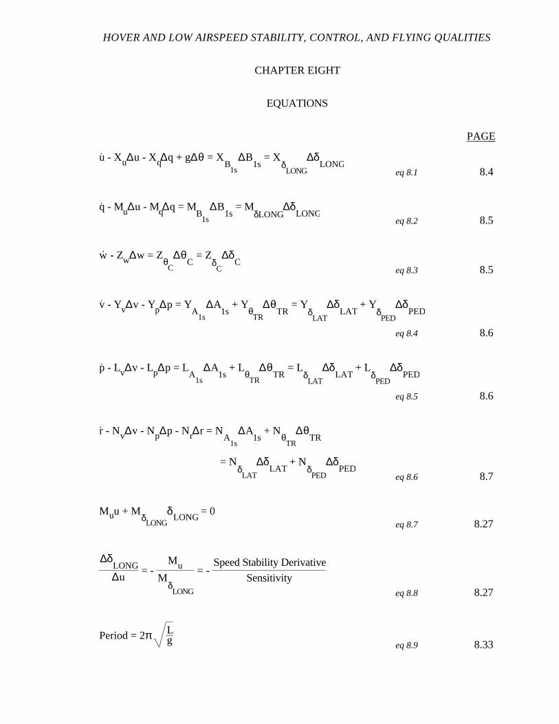
HOVER AND LOW AIRSPEED STABILITY, CONTROL, AND FLYING QUALITIES
CHAPTER EIGHT
EQUATIONS
PAGE
u. - Xu∆u - Xq∆q + g∆θ = X
B1s
∆B1s
= XδLONG
∆δLONG
eq 8.1 8.4
q. - Mu∆u - Mq∆q = M
B1s
∆B1s
= MδLONG
∆δLONG
eq 8.2 8.5
w. - Zw∆w = Z
θC
∆θC
= ZδC
∆δC
eq 8.3 8.5
v. - Yv∆v - Yp∆p = Y
A1s
∆A1s
+ YθTR
∆θTR
= YδLAT
∆δLAT
+ YδPED
∆δPED
eq 8.4 8.6
p. - Lv∆v - Lp∆p = L
A1s
∆A1s
+ LθTR
∆θTR
= LδLAT
∆δLAT
+ LδPED
∆δPED
eq 8.5 8.6
r. - Nv∆v - Np∆p - Nr∆r = N
A1s
∆A1s
+ NθTR
∆θTR
= NδLAT
∆δLAT
+ NδPED
∆δPED
eq 8.6 8.7
Muu + MδLONG
δLONG
= 0eq 8.7 8.27
∆δLONG∆u
= - Mu
MδLONG
= - Speed Stability Derivative
Sensitivityeq 8.8 8.27
Period = 2π Lg eq 8.9 8.33
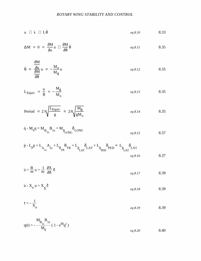
ROTARY WING STABILITY AND CONTROL
u ≅ x ≅ L θ eq 8.10 8.33
∆M = 0 =∂M
∂uu +
∂M
∂θ θ eq 8.11 8.35
θ =
∂M
∂u∂M∂θ
u = −M u
M θ u eq 8.12 8.35
L Equiv =u
θ = −
Mθ M u
eq 8.13 8.35
Period = 2πLEquiv
g= 2π
Mθ gMu
eq 8.14 8.35
.q - Mqq = M
B1sB
1s = M
δLONGδ
LONGeq 8.15 8.37
p. - Lpp = L
A1s
A1s
+ LθTR
θTR
= LδLAT
δLAT
+ LδPED
δPED
≈ LδLAT
δLAT
eq 8.16 8.37
u. = Bm u = 1
m∂X∂δ
δeq 8.17 8.39
u. - Xu u = X
δδ
eq 8.18 8.39
τ = - 1Xu eq 8.19 8.39
q(t) = - Mq
MB1s
B1s
( 1 - eMqt )eq 8.20 8.40
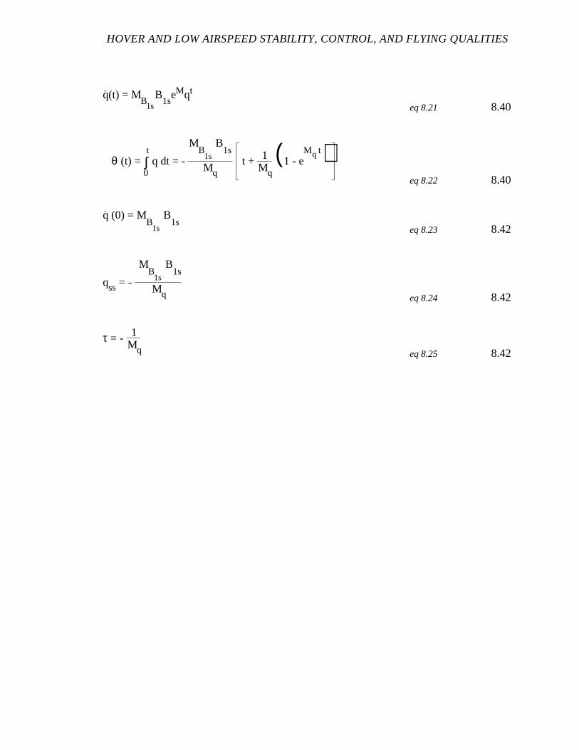
HOVER AND LOW AIRSPEED STABILITY, CONTROL, AND FLYING QUALITIES
.q(t) = M
B1sB
1seMqt
eq 8.21 8.40
θ (t) = ∫0
t q dt = -
MB
1s
B1s
Mqt + 1
Mq
(1 - eMq t)
eq 8.22 8.40
q. (0) = M
B1s
B1s
eq 8.23 8.42
qss = -
MB
1s
B1s
Mq eq 8.24 8.42
τ = - 1Mq eq 8.25 8.42
CHAPTER EIGHT
HOVER AND LOW AIRSPEED STABILITY, CONTROL,
AND FLYING QUALITIES
8.1 INTRODUCTION
This chapter discusses stability, control, and flying qualities in the hover and low
airspeed flight regime. The helicopter possess the unique capability of vertical and low
airspeed flight. The greatest tactical advantage of helicopter employment relies on this
unique capability. Therefore, a large part of the helicopter mission is conducted in the
hover and low airspeed regime. Understanding, testing, and documenting the flying
qualities in this flight regime is critical to the success of the helicopter and the test program.
8.2 PURPOSE OF TEST
The purpose of these tests is to evaluate the hover and low airspeed stability,
control, and flying qualities of the helicopter. The tests included in the evaluation are:
1. Trim control positions.
2. Critical azimuth.
3. Turn on a spot.
4. Static stability.
5. Long term dynamic stability.
6. Control response.
7. Mission maneuvers.
8.3 THEORY
The linear analysis of the helicopter response to control inputs and other
disturbances provides a valuable indication of important handling qualities characteristics.
A number of the stability derivatives are zero or negligible in the hovering regime resulting
ROTARY WING STABILITY AND CONTROL
in a simplification of the equations of motion and a decoupling of some of the degrees of
freedom. The linearized equations used in the discussion of low airspeed stability and
control are the basis for the theory presented in this chapter.
8.3.1 Summary of Quasi-Static Rotor Characteristics
The rotor characteristics are presented in Chapter 4 along with rotor response to
various inputs. Those discussions indicated a quasi-static approximation for rotor response
is satisfactory for most discussions of helicopter stability, control, and flying qualities.
Table 8.I repeats the summaries of quasi-static rotor response characteristics given
in Chapter 4 for hovering flight. The table indicates the most significant quasi-static
responses of the rotor to specified input conditions and summarizes the effects responsible
for particular rotor contributions to stability derivatives.
The diagrams on Table 8.I show only longitudinal inputs and responses. Similar
diagrams are applicable for lateral inputs and responses with pitch angle (θ) replaced by roll
angle (φ), aft longitudinal cyclic pitch angle −B1s( ) replaced by right lateral cyclic pitch
angle (A1s), aft longitudinal flapping angle (a1s) replaced by right lateral flapping angle
(b1s), pitch rate (q) replaced by roll rate (p), and translational velocity component along x
axis (u) replaced by translational velocity component along y axis (v).
8.3.2 Linearized Equations of Motion
The set of linearized longitudinal and lateral-directional equations of motion which
are the basis for discussing hovering and low airspeed flight dynamics are presented
below. Coupling terms between these two sets of equations are omitted. Some qualitative
discussions of the coupling effects are included in this chapter and further considered in
Chapter 9. Equations are presented in terms of the main and tail rotor variables (A1s, B1s,
θC, and θTR) and in terms of the cockpit control variables (δLONG, δLAT, δC, and δPED).
The relationship between the two forms is the gearing ratio between the rotor variables and
the cockpit flight control variables.
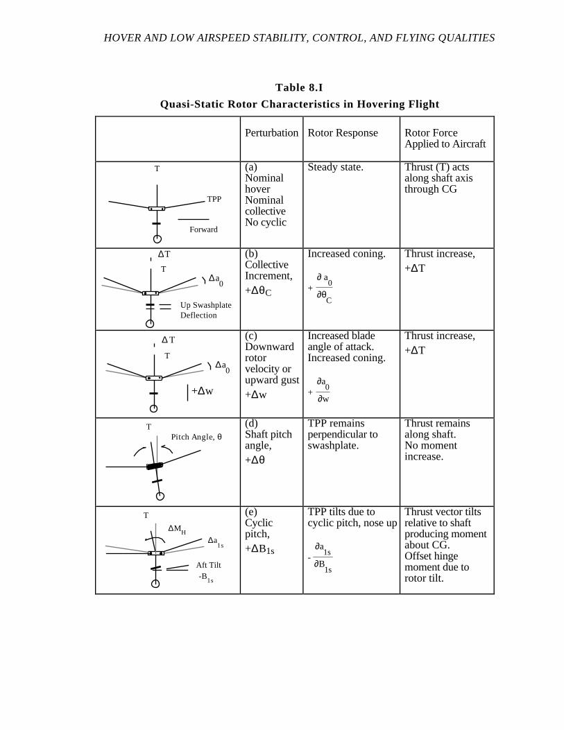
HOVER AND LOW AIRSPEED STABILITY, CONTROL, AND FLYING QUALITIES
Table 8.I
Quasi-Static Rotor Characteristics in Hovering Flight
Perturbation Rotor Response Rotor ForceApplied to Aircraft
T
TPP
Forward
(a)NominalhoverNominalcollectiveNo cyclic
Steady state. Thrust (T) actsalong shaft axisthrough CG
T
∆T
Up SwashplateDeflection
∆a0
(b)CollectiveIncrement,+∆θC
Increased coning.
+∂ a
0
∂θC
Thrust increase,+∆T
T
∆ T
∆a0
+∆w
(c)Downwardrotorvelocity orupward gust+∆w
Increased bladeangle of attack.Increased coning.
+∂a
0
∂w
Thrust increase,+∆T
T Pitch Angle,θ
(d)Shaft pitchangle,+∆θ
TPP remainsperpendicular toswashplate.
Thrust remainsalong shaft.No momentincrease.
T
-B1s
∆a1s
∆MH
Aft Tilt
(e)Cyclicpitch,+∆B1s
TPP tilts due tocyclic pitch, nose up
-∂a
1s
∂B1s
Thrust vector tiltsrelative to shaftproducing momentabout CG.Offset hingemoment due torotor tilt.
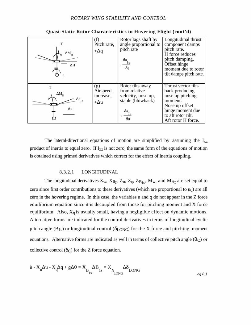
ROTARY WING STABILITY AND CONTROL
Quasi-Static Rotor Characteristics in Hovering Flight (cont’d)
T
q
∆MH
∆H
(f)Pitch rate,+∆q
Rotor lags shaft byangle proportional topitch rate
-∂a
1s
∂q
Longitudinal thrustcomponent dampspitch rate.H force reducespitch damping.Offset hingemoment due to rotortilt damps pitch rate.
T
∆u
∆MH
∆a1s
(g)Airspeedincrease,+∆u
Rotor tilts awayfrom relativevelocity, nose up,stable (blowback)
+∂a
1s
∂u
Thrust vector tiltsback producingnose up pitchingmoment.Nose up offsethinge moment dueto aft rotor tilt.Aft rotor H force.
The lateral-directional equations of motion are simplified by assuming the Ixz
product of inertia to equal zero. If Ixz is not zero, the same form of the equations of motion
is obtained using primed derivatives which correct for the effect of inertia coupling.
8.3.2.1 LONGITUDINAL
The longitudinal derivatives Xw, XθC, Zu, Zq, ZB1s, Mw, and MθC are set equal to
zero since first order contributions to these derivatives (which are proportional to u0) are all
zero in the hovering regime. In this case, the variables u and q do not appear in the Z force
equilibrium equation since it is decoupled from those for pitching moment and X force
equilibrium. Also, Xq is usually small, having a negligible effect on dynamic motions.
Alternative forms are indicated for the control derivatives in terms of longitudinal cyclic
pitch angle (B1s) or longitudinal control (δLONG) for the X force and pitching moment
equations. Alternative forms are indicated as well in terms of collective pitch angle (θC) or
collective control (δC) for the Z force equation.
u. - Xu∆u - Xq∆q + g∆θ = X
B1s
∆B1s
= XδLONG
∆δLONG
eq 8.1
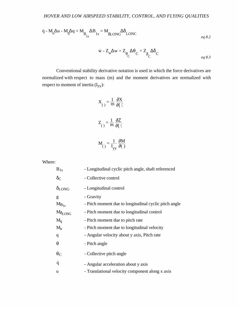
HOVER AND LOW AIRSPEED STABILITY, CONTROL, AND FLYING QUALITIES
q. - Mu∆u - Mq∆q = M
B1s
∆B1s
= MδLONG
∆δLONG
eq 8.2
w. - Zw∆w = Z
θC
∆θC
= ZδC
∆δC
eq 8.3
Conventional stability derivative notation is used in which the force derivatives are
normalized with respect to mass (m) and the moment derivatives are normalized with
respect to moment of inertia (Iyy):
X( )
= 1m∂X∂( )
Z( )
= 1m∂Ζ∂( )
M( )
= 1Iyy
∂M∂( )
Where:
B1s - Longitudinal cyclic pitch angle, shaft referenced
δC - Collective control
δLONG - Longitudinal control
g - Gravity
MB1s - Pitch moment due to longitudinal cyclic pitch angle
MδLONG - Pitch moment due to longitudinal control
Mq - Pitch moment due to pitch rate
Mu - Pitch moment due to longitudinal velocity
q - Angular velocity about y axis, Pitch rate
θ - Pitch angle
θC - Collective pitch angle
q - Angular acceleration about y axis
u - Translational velocity component along x axis
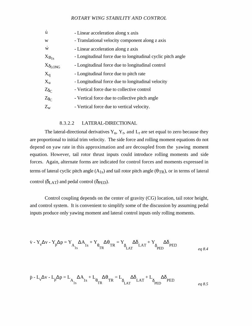
ROTARY WING STABILITY AND CONTROL
u - Linear acceleration along x axis
w - Translational velocity component along z axis
w - Linear acceleration along z axis
XB1s - Longitudinal force due to longitudinal cyclic pitch angle
XδLONG - Longitudinal force due to longitudinal control
Xq - Longitudinal force due to pitch rate
Xu - Longitudinal force due to longitudinal velocity
ZδC - Vertical force due to collective control
ZθC - Vertical force due to collective pitch angle
Zw - Vertical force due to vertical velocity.
8.3.2.2 LATERAL-DIRECTIONAL
The lateral-directional derivatives Yu, Yr, and Lr are set equal to zero because they
are proportional to initial trim velocity. The side force and rolling moment equations do not
depend on yaw rate in this approximation and are decoupled from the yawing moment
equation. However, tail rotor thrust inputs could introduce rolling moments and side
forces. Again, alternate forms are indicated for control forces and moments expressed in
terms of lateral cyclic pitch angle (A1s) and tail rotor pitch angle (θTR), or in terms of lateral
control (δLAT) and pedal control (δPED).
Control coupling depends on the center of gravity (CG) location, tail rotor height,
and control system. It is convenient to simplify some of the discussion by assuming pedal
inputs produce only yawing moment and lateral control inputs only rolling moments.
v. - Yv∆v - Yp∆p = Y
A1s
∆A1s
+ YθTR
∆θTR
= YδLAT
∆δLAT
+ YδPED
∆δPED
eq 8.4
p. - Lv∆v - Lp∆p = L
A1s
∆A1s
+ LθTR
∆θTR
= LδLAT
∆δLAT
+ LδPED
∆δPED
eq 8.5
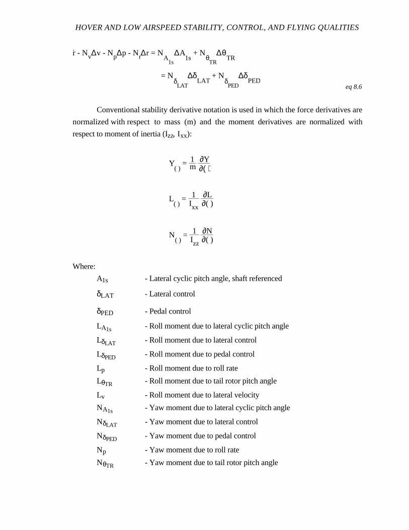
HOVER AND LOW AIRSPEED STABILITY, CONTROL, AND FLYING QUALITIES
r. - Nv∆v - Np∆p - Nr∆r = N
A1s
∆A1s
+ NθTR
∆θTR
= NδLAT
∆δLAT
+ NδPED
∆δPED
eq 8.6
Conventional stability derivative notation is used in which the force derivatives are
normalized with respect to mass (m) and the moment derivatives are normalized with
respect to moment of inertia (Izz, Ixx):
Y( )
= 1m∂Y∂( )
L( )
= 1Ixx
∂L∂( )
N( )
= 1Izz
∂N∂( )
Where:
A1s - Lateral cyclic pitch angle, shaft referenced
δLAT - Lateral control
δPED - Pedal control
LA1s - Roll moment due to lateral cyclic pitch angle
LδLAT - Roll moment due to lateral control
LδPED - Roll moment due to pedal control
Lp - Roll moment due to roll rate
LθTR - Roll moment due to tail rotor pitch angle
Lv - Roll moment due to lateral velocity
NA1s - Yaw moment due to lateral cyclic pitch angle
NδLAT - Yaw moment due to lateral control
NδPED - Yaw moment due to pedal control
Np - Yaw moment due to roll rate
NθTR - Yaw moment due to tail rotor pitch angle
ROTARY WING STABILITY AND CONTROL
Nr - Yaw moment due to yaw rate
Nv - Yaw moment due to lateral velocity
p - Angular velocity about x axis, Roll rate
p - Angular acceleration about x axis
θTR - Tail rotor pitch angle
r - Angular velocity about z axis, Yaw rate
r - Angular acceleration about z axis
v - Translational velocity component along y axis
v - Linear acceleration along y axis
YA1s - Side force due to lateral cyclic pitch angle
YδLAT - Side force due to lateral control
YδPED - Side force due to pedal control
Yp - Side force due to roll rate
YθTR - Side force due to tail rotor pitch angle
Yv - Side force due to lateral velocity.
8.3.3 Stability Derivatives
There are a number of nonlinear aerodynamic phenomena which influence the
flying characteristics of a helicopter in hovering flight. For example, changes in the
downwash impingement on the fuselage, or movement of rotor tip trailing vortices in
relationship to the tail rotor, both result in forces and moments being applied to the
helicopter.
However, in considering flight dynamics, it is convenient to use the linear
equations of motion presented above. These contain constant derivatives corresponding to
the initial trim conditions. Such equations give a satisfactory indication of the dynamic
characteristics which are important from the handling qualities standpoint although they
may not explain all trim changes and response peculiarities. Forces and moments due to
the main rotor and the tail rotor make the dominant contributions to the derivatives in the
linear equations of motion.
HOVER AND LOW AIRSPEED STABILITY, CONTROL, AND FLYING QUALITIES
8.3.4 Z Force Equation Derivatives
Table 8.I (b) indicates a main rotor collective pitch input results in increased rotor
thrust and coning. This is the source of the vertical force due to collective pitch angle
derivative (ZθC) which is negative because the z axis is directed downward. The magnitude
of the corresponding collective control derivative (ZδC) is determined by the gearing used in
the control system. The downward motion of the helicopter shown in Table 8.I (c)
produces positive increments in effective blade angles of attack and increased thrust. This
is the source of the Zw damping derivative which like ZθC is negative because of the z axis
sign convention.
8.3.5 X Force and Pitching Moment Equation Derivatives
The largest contributions to the derivatives in the X force and pitching moment
equations result from the aft tilt of the thrust vector and tip path plane (TPP) relative to the
shaft. Table 8.I (e) indicates aft longitudinal cyclic pitch results in an aft thrust component
responsible for the X force due to longitudinal cyclic pitch angle derivative (XB1s), and the
corresponding X force due to longitudinal control derivative (XδLONG). The pitch moment
about the CG due to the aft thrust component and offset hinge moment both contribute to
the pitch moment due to longitudinal cyclic pitch angle derivative (MB1s). This
corresponds to the pitch moment due to longitudinal control derivative (MδLONG) when
referred to cockpit controls. The usual sign convention results in XB1s and XδLONG being
positive while MB1s and MδLONG are negative.
Table 8.I (f) depicts the TPP lag when the shaft and hub have a nose up pitch rate.
The resulting nose down pitch moment about the CG due to the forward thrust component
and the offset hinge moment provide the principal contributions to the pitch moment due to
pitch rate derivative (Mq). However, an H force due to blade induced drag acts in a
direction tending to reduce the magnitude of Mq.
Table 8.I (g) shows the aft TPP tilt or blowback due to an increase in velocity (∆u).
This results in an aft thrust component and offset hinge moment in large part responsible
for the speed stability derivative (Mu) in hovering flight. The fuselage profile drag does not
ROTARY WING STABILITY AND CONTROL
contribute to Mu for a zero airspeed trim condition. However, the blade profile drag due to
the combination of speed caused by shaft rotation and aircraft translational velocity result in
contributions to the Xu and Mu derivatives.
8.3.6 Side Force and Rolling Moment Equation Derivatives
Rotor forces and moments contribute to the derivatives in the Y force and rolling
moment equations analogous to those in the X force and pitching moment equations. The
analogous derivative pairs are Xu and Yv, Xq and Yp, XB1s and YA1s, XδLONG and YδLAT,
Mu and Lv, Mq and Lp, MB1s and LA1s, and MδLONG and LδLAT.
Tail rotor force increments also contribute to the Y force and rolling moment
derivatives. First order tail rotor effects are due to changes in the axial thrust of the tail
rotor rather than to changes in the direction of the tail rotor thrust. Lateral velocity of the
helicopter ∆v( ) produces a relative axial velocity at the tail rotor analogous to the relative
axial velocity at the main rotor produced by a downward velocity of the helicopter (∆w).
The change in tail rotor thrust due to ∆v is a source of the side force due to lateral velocity
derivative Yv( ) . This tail rotor thrust increment contributes to the rolling moment due to
lateral velocity derivative Lv( ) depending on the height of the tail rotor relative to the
aircraft CG.
Aircraft roll rate also induces axial velocity at the tail rotor if the tail rotor is
displaced from the roll axis. The resulting tail rotor thrust increment effects the roll
moment due to roll rate derivative (Lp), as well as the side force due to roll rate derivative
(Yp).
The side force due to tail rotor pitch angle derivative (YθTR) results from the change
in tail rotor thrust with blade pitch angle, and is analogous to the ZθC derivative of the main
rotor. There is a corresponding rolling moment due to tail rotor pitch derivative (LθTR)
whose magnitude depends on the displacement of the tail rotor from the roll axis. Lateral
control derivatives can be referred to lateral cyclic pitch angle (A1s) and tail rotor pitch angle
(θTR), or to the cockpit lateral control (δLAT) and pedal control (δPED).
8.3.7 Yawing Moment Equation Derivatives
HOVER AND LOW AIRSPEED STABILITY, CONTROL, AND FLYING QUALITIES
When the main rotor thrust vector is aligned with the CG at the initial zero airspeed
trim condition, the derivatives in the yawing moment equation are primarily due to the tail
rotor. The tail rotor thrust increment due to lateral velocity produces a yawing moment
about the CG, and contributes to the yaw moment due to lateral velocity derivative (Nv).
Similarly, a yaw rate about the CG results in an axial velocity at the tail rotor and a tail rotor
thrust increment which produces a yawing moment about the CG. This is the primary
source of the yaw moment due to yaw rate derivative (Nr) in the case of the single rotor
helicopter.
If the tail rotor is displaced from the roll axis, a roll rate causes an axial velocity
change at the tail rotor and a corresponding tail rotor thrust increment. This results in an
increase in the yaw moment due to roll rate derivative (Np), which introduces coupling
between the yawing and rolling moment equations.
The main rotor force increments which effect the derivatives in the Y force equation
also effect the derivatives in the yawing moment equation when the main rotor is displaced
from the CG. Under these conditions, there is a yaw moment due to lateral cyclic pitch
angle derivative (NA1s). However, the predominant yawing moments used for directional
control in hovering flight are introduced by changes in tail rotor pitch via pedal control
producing yaw moment due to tail rotor pitch angle (NθTR). Directional control derivatives
can be referred to lateral cyclic pitch angle (A1s) and tail rotor pitch angle (θTR), or to the
cockpit lateral control (δLAT) and pedal control (δPED).
8.3.8 Trim and Static Stability
A number of aerodynamic effects influence trimmed control positions in hovering
and low airspeed flight both in and out of ground effect (IGE, OGE). The important
effects are discussed to provide background concerning possible sources of difficulty in
obtaining and holding trimmed flight conditions. It is difficult to generalize the relative
importance of these and other aerodynamic effects encountered with various helicopter
configurations.
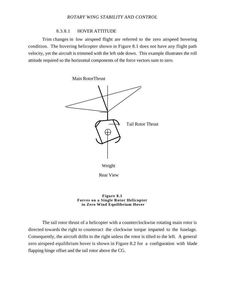
ROTARY WING STABILITY AND CONTROL
8.3.8.1 HOVER ATTITUDE
Trim changes in low airspeed flight are referred to the zero airspeed hovering
condition. The hovering helicopter shown in Figure 8.1 does not have any flight path
velocity, yet the aircraft is trimmed with the left side down. This example illustrates the roll
attitude required so the horizontal components of the force vectors sum to zero.
The tail rotor thrust of a helicopter with a counterclockwise rotating main rotor is
directed towards the right to counteract the clockwise torque imparted to the fuselage.
Consequently, the aircraft drifts to the right unless the rotor is tilted to the left. A general
zero airspeed equilibrium hover is shown in Figure 8.2 for a configuration with blade
flapping hinge offset and the tail rotor above the CG.
Rear View
Weight
Tail Rotor Thrust
Main RotorThrust
Figure 8.1Forces on a Single Rotor Helicopter
in Zero Wind Equilibrium Hover
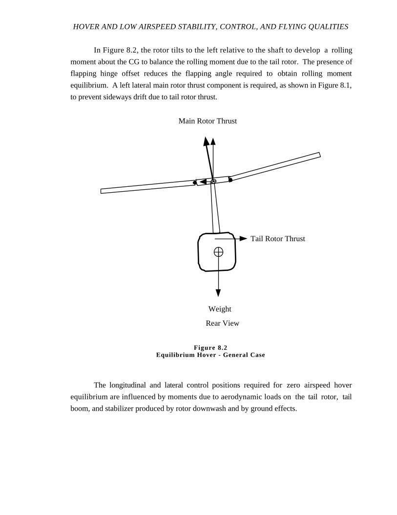
HOVER AND LOW AIRSPEED STABILITY, CONTROL, AND FLYING QUALITIES
In Figure 8.2, the rotor tilts to the left relative to the shaft to develop a rolling
moment about the CG to balance the rolling moment due to the tail rotor. The presence of
flapping hinge offset reduces the flapping angle required to obtain rolling moment
equilibrium. A left lateral main rotor thrust component is required, as shown in Figure 8.1,
to prevent sideways drift due to tail rotor thrust.
The longitudinal and lateral control positions required for zero airspeed hover
equilibrium are influenced by moments due to aerodynamic loads on the tail rotor, tail
boom, and stabilizer produced by rotor downwash and by ground effects.
Rear View
Weight
Tail Rotor Thrust
Main Rotor Thrust
Figure 8.2Equilibrium Hover - General Case
ROTARY WING STABILITY AND CONTROL
8.3.8.2 TRIM AND POWER CHANGES DURING
TRANSLATIONAL FLIGHT
When a helicopter hovering OGE translates into low airspeed flight, adjustments are
required in cyclic pitch, collective pitch, engine power, and tail rotor thrust to maintain
trim. Cyclic pitch is used to compensate for rotor blowback and to keep the TPP
approximately horizontal and the main rotor thrust vector approximately vertical. The small
increase in parasite drag at low translational velocity is balanced by a small inclination of
the thrust vector.
The speed change results in an increase in thrust if the collective pitch is held fixed.
After lowering the collective pitch to maintain constant thrust and prevent the helicopter
from climbing, there is a corresponding decrease in the blade section induced drag and the
torque required to drive the rotor. Consequently, engine power is reduced to prevent an
increase in rotor speed. Less tail rotor thrust is required to counter the decreased main rotor
torque. Pedal inputs are used to keep this translational velocity to yaw coupling from
changing the heading of the aircraft. The tail rotor pitch adjustments made by the pilot
depend on whether the translational velocity is forward, aft, right, or left, since these
motions have different effects on tail rotor thrust as well as different power requirements.
The effect of trim and power changes in translational flight result from changes in
the average downwash velocity. A qualitative argument, according to the vortex theory,
states the downward velocity at the rotor plane results from a superposition of the velocities
induced by the system of vortices which are generated by the rotor. In forward flight, the
higher velocity of the rotor relative to the undisturbed air mass causes the wake vortices to
move away from the rotor more rapidly and, therefore, induce smaller velocities at the
rotor.
Figure 8.3 depicts flow conditions at a typical blade section of a rotor in hovering
or low airspeed flight. The blade section is shown rotating in a horizontal plane. The
downward perpendicular flow component (uP) is entirely due to the induced velocities
caused by the vorticity in the wake of the rotor. The transverse velocity component is
approximately equal to the velocity due to shaft rotation. The resultant of these two
components is the total relative velocity at the blade section which has a inflow angle (ϕ)
relative to the horizontal rotor disk.
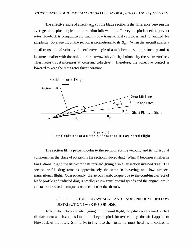
HOVER AND LOW AIRSPEED STABILITY, CONTROL, AND FLYING QUALITIES
The effective angle of attack (αeff ) of the blade section is the difference between the
average blade pitch angle and the section inflow angle. The cyclic pitch used to prevent
rotor blowback is comparatively small at low translational velocities and is omitted for
simplicity. Average lift on the section is proportional to its αeff . When the aircraft attains a
small translational velocity, the effective angle of attack becomes larger since uP and ϕ
become smaller with the reduction in downwash velocity induced by the wake vortices.
Thus, rotor thrust increases at constant collective. Therefore, the collective control is
lowered to keep the main rotor thrust constant.
The section lift is perpendicular to the section relative velocity and its horizontal
component in the plane of rotation is the section induced drag. When ϕ becomes smaller in
translational flight, the lift vector tilts forward giving a smaller section induced drag. The
section profile drag remains approximately the same in hovering and low airspeed
translational flight. Consequently, the aerodynamic torque due to the combined effect of
blade profile and induced drag is smaller at low translational speeds and the engine torque
and tail rotor reaction torque is reduced to trim the aircraft.
8.3.8.3 ROTOR BLOWBACK AND NONUNIFORM INFLOW
DISTRIBUTION OVER ROTOR DISK
To trim the helicopter when going into forward flight, the pilot uses forward control
displacement which applies longitudinal cyclic pitch for overcoming the aft flapping or
blowback of the rotor. Similarly, in flight to the right, he must hold right control to
Zero Lift Line
Shaft Plane, ⊥ Shaft
θ, Blade Pitchαeff
uPu
T
ϕ
Section Lift
Section Induced Drag
Figure 8.3Flow Conditions at a Rotor Blade Section in Low Speed Flight
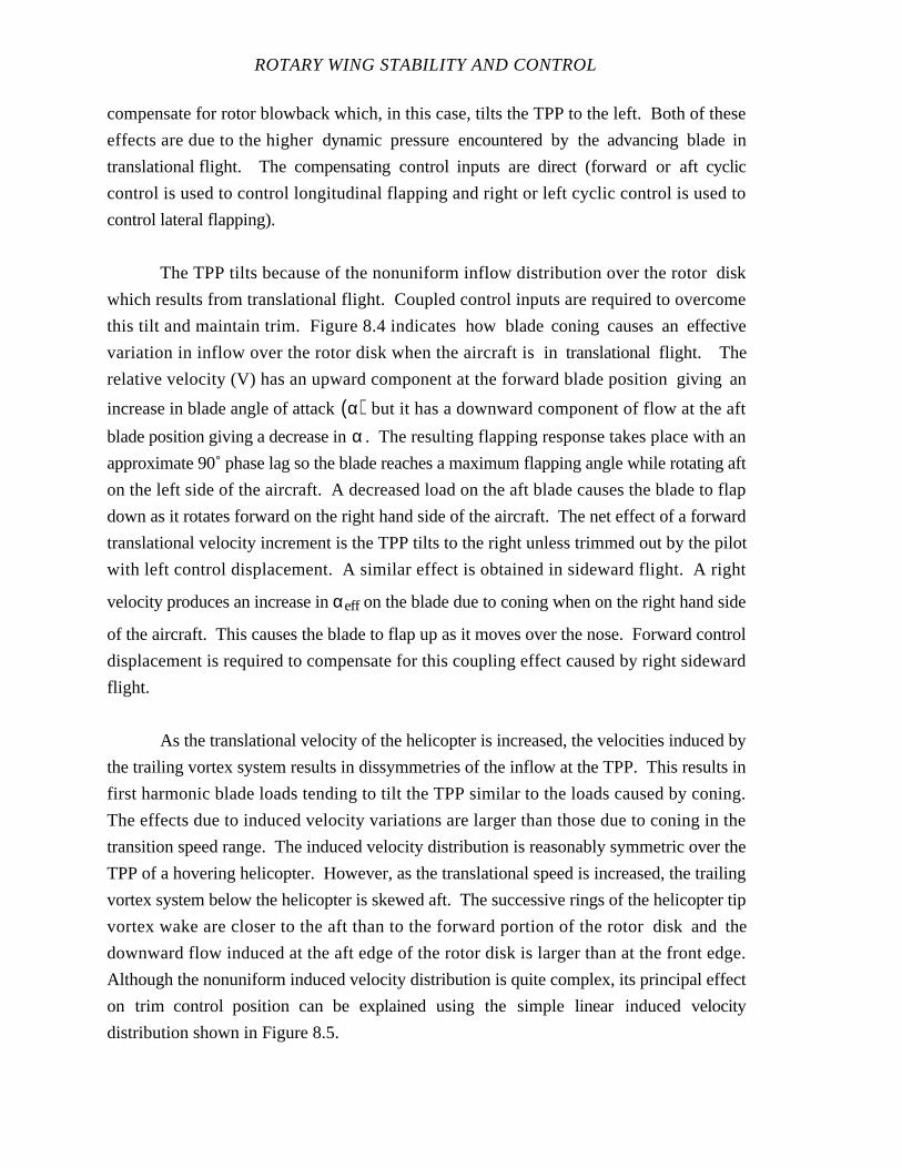
ROTARY WING STABILITY AND CONTROL
compensate for rotor blowback which, in this case, tilts the TPP to the left. Both of these
effects are due to the higher dynamic pressure encountered by theadvancing blade in
translational flight. The compensating control inputs are direct (forward or aft cyclic
control is used to control longitudinal flapping and right or left cyclic control is used to
control lateral flapping).
The TPP tilts because of the nonuniform inflow distribution over the rotor disk
which results from translational flight. Coupled control inputs are required to overcome
this tilt and maintain trim. Figure 8.4 indicates how blade coning causes an effective
variation in inflow over the rotor disk when the aircraft is in translational flight. The
relative velocity (V) has an upward component at the forward blade position giving an
increase in blade angle of attack α( ) but it has a downward component of flow at the aft
blade position giving a decrease in α . The resulting flapping response takes place with an
approximate 90˚ phase lag so the blade reaches a maximum flapping angle while rotating aft
on the left side of the aircraft. A decreased load on the aft blade causes the blade to flap
down as it rotates forward on the right hand side of the aircraft. The net effect of a forward
translational velocity increment is the TPP tilts to the right unless trimmed out by the pilot
with left control displacement. A similar effect is obtained in sideward flight. A right
velocity produces an increase in αeff on the blade due to coning when on the right hand side
of the aircraft. This causes the blade to flap up as it moves over the nose. Forward control
displacement is required to compensate for this coupling effect caused by right sideward
flight.
As the translational velocity of the helicopter is increased, the velocities induced by
the trailing vortex system results in dissymmetries of the inflow at the TPP. This results in
first harmonic blade loads tending to tilt the TPP similar to the loads caused by coning.
The effects due to induced velocity variations are larger than those due to coning in the
transition speed range. The induced velocity distribution is reasonably symmetric over the
TPP of a hovering helicopter. However, as the translational speed is increased, the trailing
vortex system below the helicopter is skewed aft. The successive rings of the helicopter tip
vortex wake are closer to the aft than to the forward portion of the rotor disk and the
downward flow induced at the aft edge of the rotor disk is larger than at the front edge.
Although the nonuniform induced velocity distribution is quite complex, its principal effect
on trim control position can be explained using the simple linear induced velocity
distribution shown in Figure 8.5.
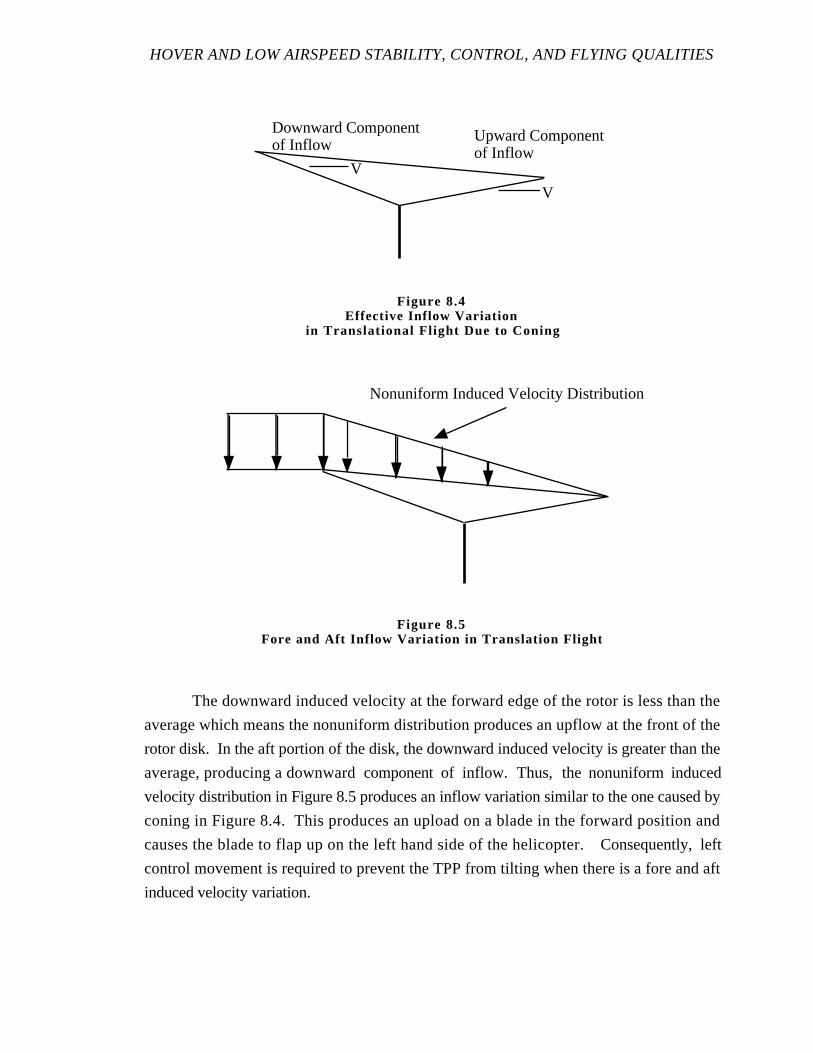
HOVER AND LOW AIRSPEED STABILITY, CONTROL, AND FLYING QUALITIES
The downward induced velocity at the forward edge of the rotor is less than the
average which means the nonuniform distribution produces an upflow at the front of the
rotor disk. In the aft portion of the disk, the downward induced velocity is greater than the
average, producing a downward component of inflow. Thus, the nonuniform induced
velocity distribution in Figure 8.5 produces an inflow variation similar to the one caused by
coning in Figure 8.4. This produces an upload on a blade in the forward position and
causes the blade to flap up on the left hand side of the helicopter. Consequently, left
control movement is required to prevent the TPP from tilting when there is a fore and aft
induced velocity variation.
Upward Componentof Inflow
Downward Componentof Inflow
V
V
Figure 8.4Effective Inflow Variation
in Translational Flight Due to Coning
Nonuniform Induced Velocity Distribution
Figure 8.5Fore and Aft Inflow Variation in Translation Flight

ROTARY WING STABILITY AND CONTROL
The critical nonuniform induced velocity conditions occur in the transition region.
At higher speeds the TPP and thrust vector are inclined forward giving a forward horizontal
force component to balance the higher parasite drag of the aircraft. Consequently, a
component of translational velocity adds to the total downward inflow and the variation of
the induced velocity over the rotor disk is a smaller percentage of the total downward flow
through the rotor disk.
8.3.8.4 DOWNWASH IMPINGEMENT ON FUSELAGE, TAIL, AND
HORIZONTAL STABILIZER
When the pilot goes from one stabilized condition to another in hovering flight, low
airspeed forward or aft flight, climb, or descent, changes occur in the fuselage attitude,
TPP tilt relative to the shaft, and the direction of the relative velocity vector.
Corresponding shifts in the main rotor wake position change the downwash impingement
on the fuselage, tail boom, and horizontal stabilizer. The aerodynamic moments applied to
the aircraft as a result of changes in downwash impingement might cause large and
discontinuous control position changes. These effects are very dependent on the particular
configuration involved.
A fixed stabilizer located in an aft position could be clear of the rotor downwash in
hovering flight. However, in low airspeed forward flight, the downwash trails further aft
where it can influence the stabilizer, causing an abrupt nose up pitching moment and
requiring forward cyclic control to trim the aircraft. If the stabilizer is located at a forward
position, a download acts on the stabilizer due to downwash impingement both in hovering
and low airspeed forward flight. However, in aft flight, the downwash moves forward
producing a nose down pitching moment requiring aft cyclic control to maintain trim. A
high stabilizer position in the T-tail design eliminates most trim problems due to
interference but could be subject to downwash impingement in forward or climbing flight.
8.3.8.5 TAIL ROTOR THRUST CHANGES IN SIDEWARD FLIGHT
Figure 8.6 depicts some of the factors causing tailrotor thrust changes in low
airspeed sideward flight and the compensating pilot control positions required to maintain
trim. Left pedal is forward in a hover to provide tail rotor pitch and thrust to the right
which balances the main rotor torque. No cyclic control displacement is shown while

HOVER AND LOW AIRSPEED STABILITY, CONTROL, AND FLYING QUALITIES
hovering. The tail rotor is at the same height as the CG. In this case, the thrust vector is
aligned with the shaft and the aircraft is rolled to the left so the tail rotor thrust is balanced
by the lateral component of the weight force.
Lateral velocity produces changes in theαeff and thrust of the tail rotor
corresponding to the main rotor changes obtained with vertical velocity. The tail rotor
thrust change is in the same direction as the change in relative sideward velocity, creating a
damping force similar to the vertical damping force generated by the main rotor when given
a vertical velocity. Both of these rotor damping forces can be generated without forward
motion of the aircraft.
A right sideward velocity causes a relative velocity to the left of the tail rotor and
incremental tail rotor thrust to the left. This left tail rotor thrust produces a stable yawing
moment, yawing the aircraft to the right into the relativewind. A left pedal input is
Left Sideward Flight Hover Right Sideward Flight
MainRotorThrust
MainRotorThrust
Tail RotorThrust
FuselageDrag
FuselageDrag
Left PedalCyclic Neutral
Right PedalLeft, Aft Cyclic
More Left PedalRight, Forward Cyclic
MainRotorTorque
Figure 8.6Tail Rotor Thrust Changes in Low Speed Sideward Flight
ROTARY WING STABILITY AND CONTROL
required to increase tail rotor pitch and tail rotor thrust to the right to prevent this yawing
motion. Left sideward velocity causes an increase in tail rotor thrust to the right which is
balanced by right pedal input.
However, several factors lead to unsymmetrical directional control for sideward
flight to the left or right. A reduction in main rotor power required and torque is obtained
with translational velocity to the right or left. Therefore, less tail rotor thrust is required to
react main rotor torque and results in a right pedal increment in both cases.
Another source of control dissymmetry for sideward flight is the possibility of the
tail rotor entering the vortex ring state. This occurs in left sideward flight with a high
enough relative velocity to the right to exceed the induced velocity of the tail rotor to the
left. In this case, an abrupt loss in tail rotor thrust is obtained and a left pedal input is
required to obtain trim.
Figure 8.6 indicates changes in trimmed cyclic control positions as well as changes
in pedal position in going into sideward flight. Right cyclic control deflection is shown for
right sideward flight. The lateral cyclic compensates for the lateral blowback of the rotor
which tilts the TPP to the left. Similarly, left cyclic control displacement is required in left
sideward flight to prevent the TPP tilting to the right. Some change in trimmed roll angle is
required so lateral components of the gravity force balance fuselage or tail boom drag
caused by sideward velocity.
In right sideward flight, there is an upward flow increment for a blade on the right
hand side because of coning and lower induced velocity at the right edge of the rotor disk.
These same effects cause a downward flow on the blades rotating through the left hand side
The resulting increase in blade lift on the right hand side and decrease on the left hand side
causes the blades to flap up at the front of the disk and down at the aft. Forward control
displacement is used to compensate for this flapping. The opposite effect in left sideward
flight is compensated by aft cyclic displacement.
HOVER AND LOW AIRSPEED STABILITY, CONTROL, AND FLYING QUALITIES
8.3.8.6 INTERFERENCE OF MAIN ROTOR TIP VORTICES WITH
TAIL ROTOR AND FIXED STABILIZER SURFACES
Tail rotor thrust changes occur when the aircraft attitude changes due to variations
in its CG and flight path. Corresponding changes in control position are required to
maintain trim. The moments due to the rotor downwash are not only caused by the general
change in flow direction at the stabilizer and tail rotor, but also by the strong local velocity
fields induced by vortices carried with the flow.
If the trailing vortex passes below and parallel to the tail rotor the induced velocity
on the tail rotor is to the left. This decreases the αeff of the blades of a conventional tail
rotor whose thrust is directed to the right. Thus, the tail rotor thrust is increased with a left
pedal input to maintain yawing moment equilibrium. If the trailing vortex passes above the
tail rotor, the direction of the induced velocity at the tail rotor is to the right increasing the
right tail rotor thrust. Right pedal input is required to trim the aircraft.
In general, the effects of blade tip trailing vortices are irregular and are difficult to
predict or explain. The interaction is dependent on the direction of rotation of the tail rotor
and whether it is a tractor or pusher type. In any case, the test pilot should document any
combination of control positions and maneuvers leading to objectionable changes in trim.
8.3.8.7 REDUCTION OF POWER REQUIRED IGE
A change in aerodynamic flow pattern around the helicopter takes place when the
helicopter transitions from OGE to IGE. When operating IGE, the downwash flow
direction changes near the ground. The downwash region expands in diameter as it moves
downward and the flow moves outward parallel to the ground. The induced velocity
through the rotor is reduced because of the ground boundary conditions. The reduction in
induced velocity produces an increase in thrust. To counter the increase in thrust, the pilot
lowers the collective. A corresponding pedal input is made to counter the reduced torque
on the fuselage. There is usually a change in the pressures acting on the bottom of the
fuselage IGE. These usually do not have a significant effect on the required thrust but can
introduce pitching moments affecting the trim of the aircraft.
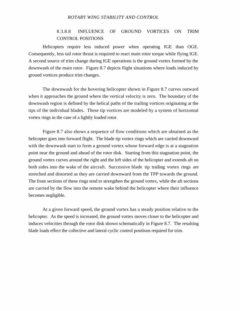
ROTARY WING STABILITY AND CONTROL
8.3.8.8 INFLUENCE OF GROUND VORTICES ON TRIM
CONTROL POSITIONS
Helicopters require less induced power when operating IGE than OGE.
Consequently, less tail rotor thrust is required to react main rotor torque while flying IGE.
A second source of trim change during IGE operations is the ground vortex formed by the
downwash of the main rotor. Figure 8.7 depicts flight situations where loads induced by
ground vortices produce trim changes.
The downwash for the hovering helicopter shown in Figure 8.7 curves outward
when it approaches the ground where the vertical velocity is zero. The boundary of the
downwash region is defined by the helical paths of the trailing vortices originating at the
tips of the individual blades. These tip vortices are modeled by a system of horizontal
vortex rings in the case of a lightly loaded rotor.
Figure 8.7 also shows a sequence of flow conditions which are obtained as the
helicopter goes into forward flight. The blade tip vortex rings which are carried downward
with the downwash start to form a ground vortex whose forward edge is at a stagnation
point near the ground and ahead of the rotor disk. Starting from this stagnation point, the
ground vortex curves around the right and the left sides of the helicopter and extends aft on
both sides into the wake of the aircraft. Successive blade tip trailing vortex rings are
stretched and distorted as they are carried downward from the TPP towards the ground.
The front sections of these rings tend to strengthen the ground vortex, while the aft sections
are carried by the flow into the remote wake behind the helicopter where their influence
becomes negligible.
At a given forward speed, the ground vortex has a steady position relative to the
helicopter. As the speed is increased, the ground vortex moves closer to the helicopter and
induces velocities through the rotor disk shown schematically in Figure 8.7. The resulting
blade loads effect the collective and lateral cyclic control positions required for trim.
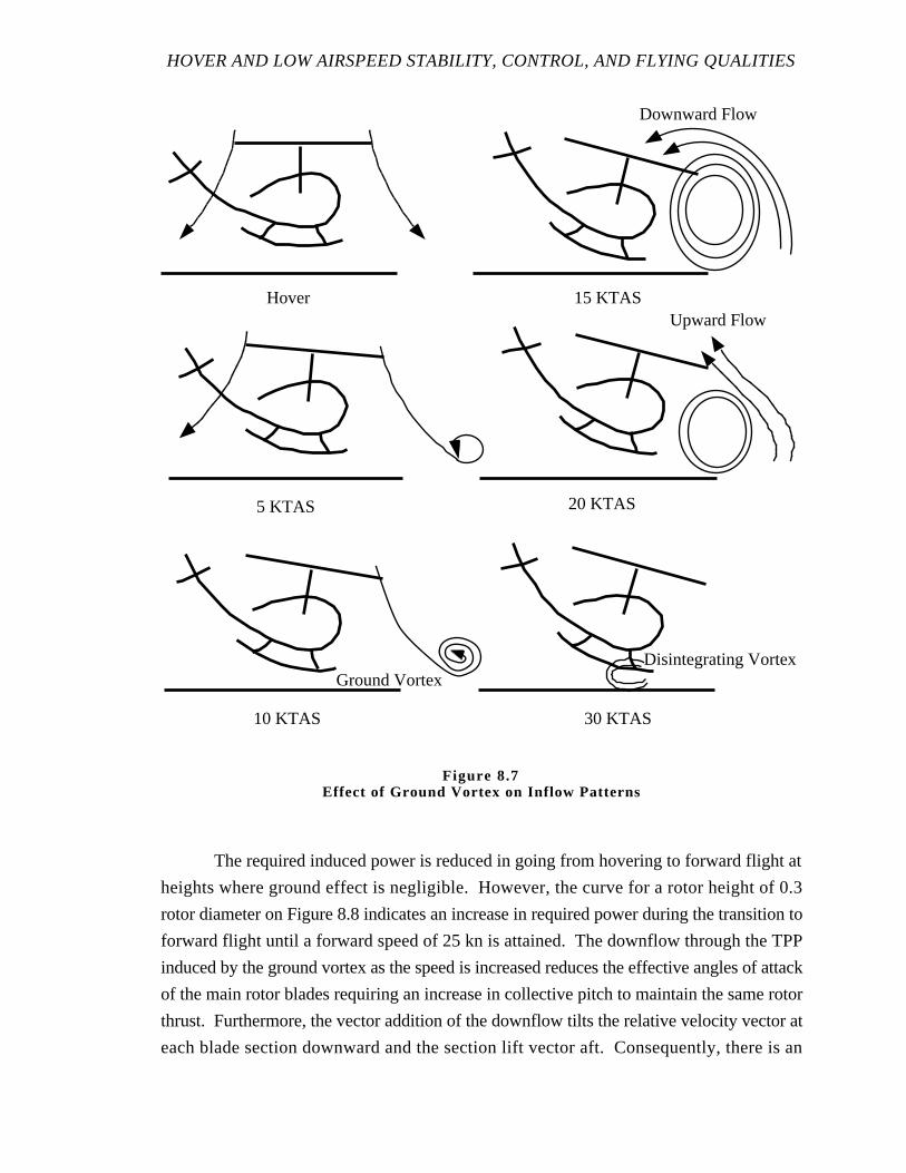
HOVER AND LOW AIRSPEED STABILITY, CONTROL, AND FLYING QUALITIES
The required induced power is reduced in going from hovering to forward flight at
heights where ground effect is negligible. However, the curve for a rotor height of 0.3
rotor diameter on Figure 8.8 indicates an increase in required power during the transition to
forward flight until a forward speed of 25 kn is attained. The downflow through the TPP
induced by the ground vortex as the speed is increased reduces the effective angles of attack
of the main rotor blades requiring an increase in collective pitch to maintain the same rotor
thrust. Furthermore, the vector addition of the downflow tilts the relative velocity vector at
each blade section downward and the section lift vector aft. Consequently, there is an
Hover
5 KTAS
10 KTAS
15 KTAS
20 KTAS
30 KTAS
Downward Flow
Upward Flow
Disintegrating VortexGround Vortex
Figure 8.7Effect of Ground Vortex on Inflow Patterns
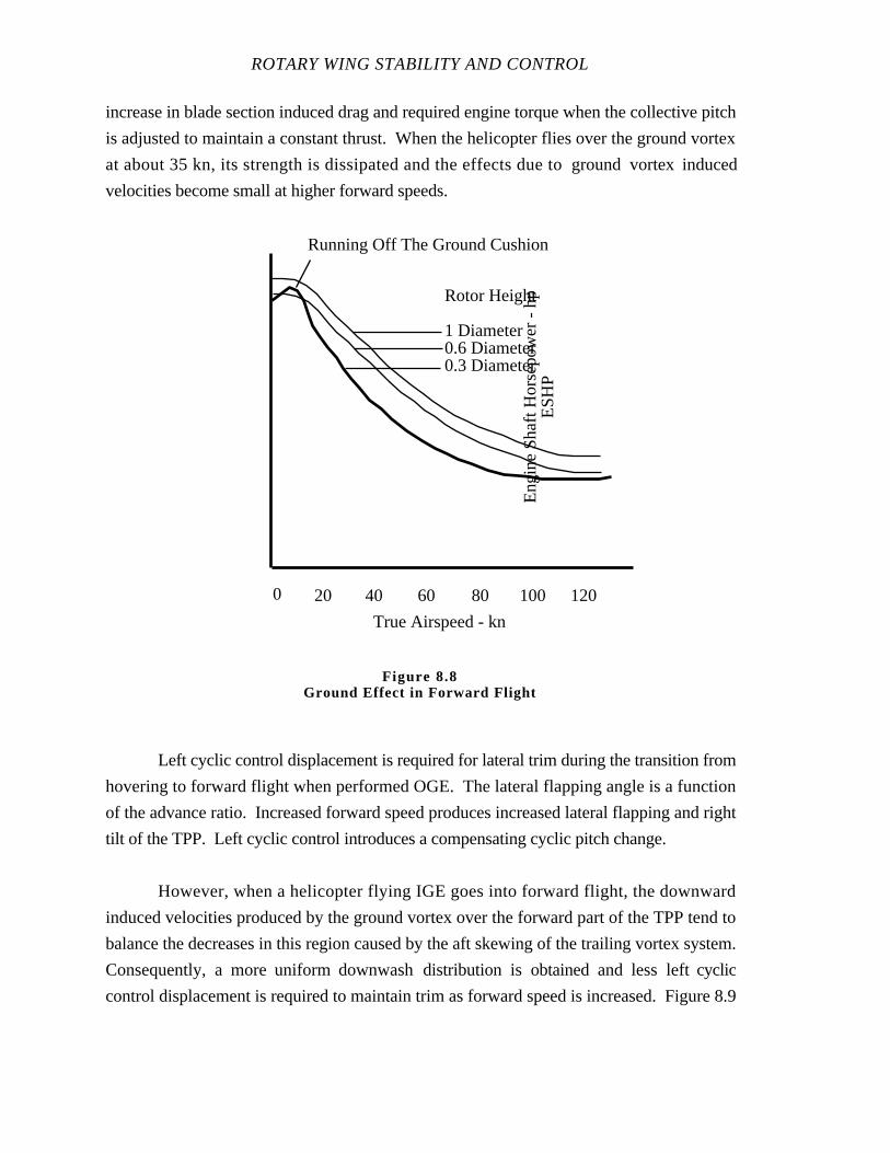
ROTARY WING STABILITY AND CONTROL
increase in blade section induced drag and required engine torque when the collective pitch
is adjusted to maintain a constant thrust. When the helicopter flies over the ground vortex
at about 35 kn, its strength is dissipated and the effects due to ground vortex induced
velocities become small at higher forward speeds.
Left cyclic control displacement is required for lateral trim during the transition from
hovering to forward flight when performed OGE. The lateral flapping angle is a function
of the advance ratio. Increased forward speed produces increased lateral flapping and right
tilt of the TPP. Left cyclic control introduces a compensating cyclic pitch change.
However, when a helicopter flying IGE goes into forward flight, the downward
induced velocities produced by the ground vortex over the forward part of the TPP tend to
balance the decreases in this region caused by the aft skewing of the trailing vortex system.
Consequently, a more uniform downwash distribution is obtained and less left cyclic
control displacement is required to maintain trim as forward speed is increased. Figure 8.9
Eng
ine
Sha
ft H
orse
pow
er -
hp
ES
HP
20 40 60 80 100 120
Rotor Height
1 Diameter0.6 Diameter0.3 Diameter
Running Off The Ground Cushion
0
True Airspeed - kn
Figure 8.8Ground Effect in Forward Flight
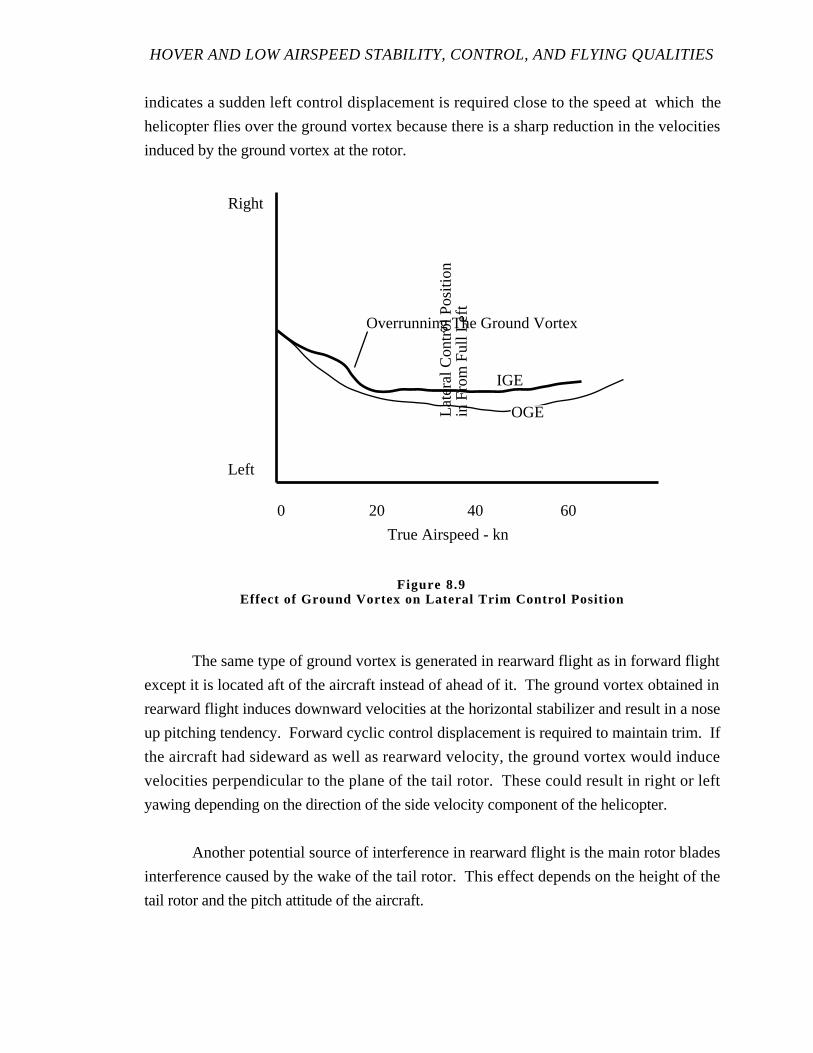
HOVER AND LOW AIRSPEED STABILITY, CONTROL, AND FLYING QUALITIES
indicates a sudden left control displacement is required close to the speed at which the
helicopter flies over the ground vortex because there is a sharp reduction in the velocities
induced by the ground vortex at the rotor.
The same type of ground vortex is generated in rearward flight as in forward flight
except it is located aft of the aircraft instead of ahead of it. The ground vortex obtained in
rearward flight induces downward velocities at the horizontal stabilizer and result in a nose
up pitching tendency. Forward cyclic control displacement is required to maintain trim. If
the aircraft had sideward as well as rearward velocity, the ground vortex would induce
velocities perpendicular to the plane of the tail rotor. These could result in right or left
yawing depending on the direction of the side velocity component of the helicopter.
Another potential source of interference in rearward flight is the main rotor blades
interference caused by the wake of the tail rotor. This effect depends on the height of the
tail rotor and the pitch attitude of the aircraft.
Late
ral C
ontr
ol P
ositi
onin
Fro
m F
ull L
eft
Left
Right
0 20 40 60
OGE
IGE
Overrunning The Ground Vortex
True Airspeed - kn
Figure 8.9Effect of Ground Vortex on Lateral Trim Control Pos ition
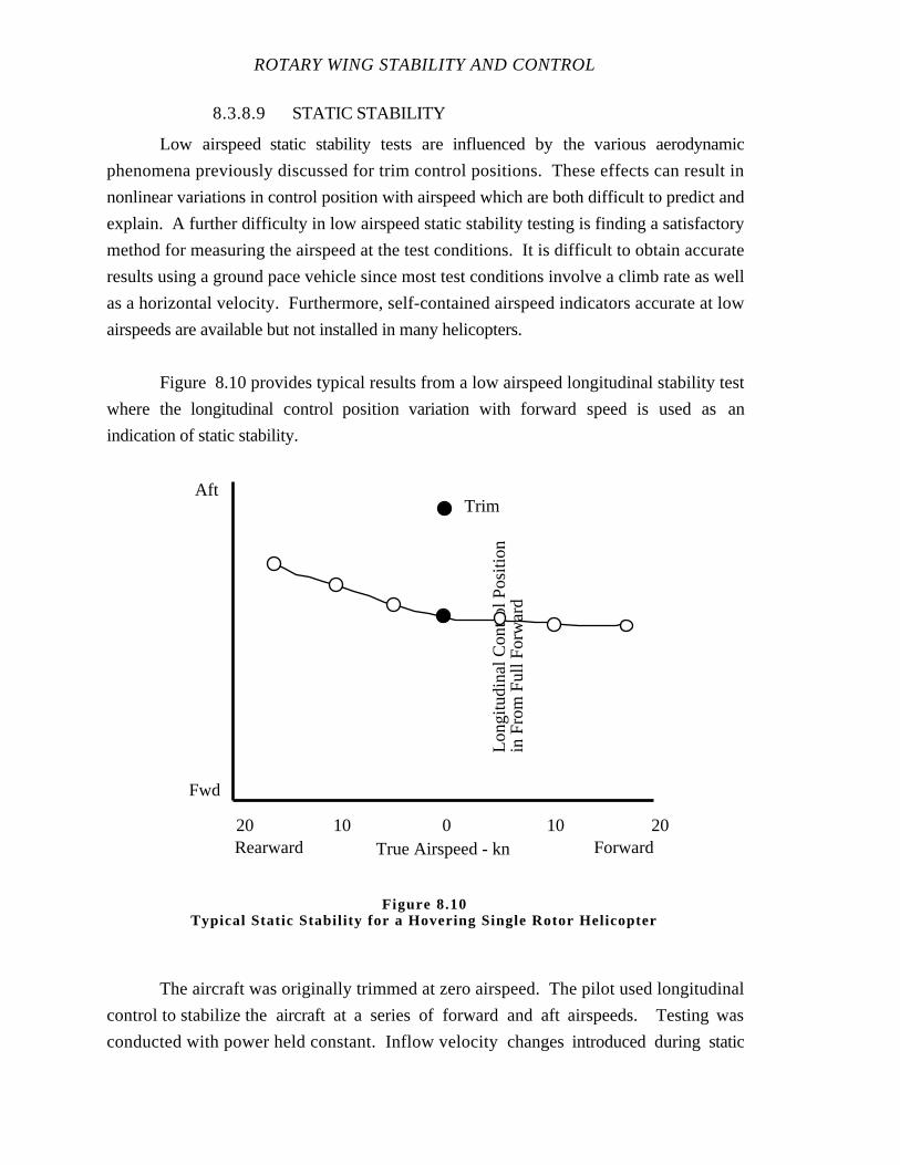
ROTARY WING STABILITY AND CONTROL
8.3.8.9 STATIC STABILITY
Low airspeed static stability tests are influenced by the various aerodynamic
phenomena previously discussed for trim control positions. These effects can result in
nonlinear variations in control position with airspeed which are both difficult to predict and
explain. A further difficulty in low airspeed static stability testing is finding a satisfactory
method for measuring the airspeed at the test conditions. It is difficult to obtain accurate
results using a ground pace vehicle since most test conditions involve a climb rate as well
as a horizontal velocity. Furthermore, self-contained airspeed indicators accurate at low
airspeeds are available but not installed in many helicopters.
Figure 8.10 provides typical results from a low airspeed longitudinal stability test
where the longitudinal control position variation with forward speed is used as an
indication of static stability.
The aircraft was originally trimmed at zero airspeed. The pilot used longitudinal
control to stabilize the aircraft at a series of forward and aft airspeeds. Testing was
conducted with power held constant. Inflow velocity changes introduced during static
True Airspeed - knRearward Forward0 10 201020
Long
itudi
nal C
ontr
ol P
ositi
onin
Fro
m F
ull F
orw
ard
Aft
Fwd
Trim
Figure 8.10Typical Static Stabil ity for a Hovering Single Rotor Helicopter
HOVER AND LOW AIRSPEED STABILITY, CONTROL, AND FLYING QUALITIES
stability flight testing tend to cause variations in the thrust developed for a fixed collective
setting. Depending upon the aircraft power management system, this variation in thrust
produces various combinations of rotor speed and engine output power with the collective
fixed. Although changes occur, the collective fixed method is used to eliminate one
additional variable.
The pilot suppresses lateral and directional responses when performing static
longitudinal stability tests as he does during longitudinal maneuvers. Similarly,
longitudinal control displacement is used to suppress pitching motion in the investigation of
low airspeed lateral and directional stability similar to steady heading sideslips.
The pitching moment equation for hovering flight reduces to the following for a
stabilized flight condition:
Muu + MδLONG
δLONG
= 0eq 8.7
The static longitudinal stability as indicated by the longitudinal control position
variation with airspeed shown below is proportional to Mu:
∆δLONG∆u
= - Mu
MδLONG
= - Speed Stability Derivative
Sensitivityeq 8.8
Where:
δLONG - Longitudinal control
MδLONG - Pitch moment due to longitudinal control
Mu - Pitch moment due to longitudinal velocity
u - Translational velocity component along x axis.
Mu is entirely due to the pitching moment produced by rotor blowback in the case
of an idealized hovering helicopter. However, changes in downwash impingement on the
fuselage and the interaction effects involving the blade tip vortices can cause large shifts in
the control positions required to stabilize when speed is changed.
ROTARY WING STABILITY AND CONTROL
In forward flight, the variation in control position with velocity depends on the lift
and pitching moment variation with angle of attack. A speed change from a trimmed
forward flight condition produces a lift increment and an angle of attack adjustment is
required to stabilize the aircraft. The corresponding pitching moment due to angle of attack
change is balanced by a longitudinal cyclic pitch input and this effects the observed forward
flight static stability.
The situation is simplified near a zero airspeed hover where the vertical forces due
to speed change are negligible so little coupling is obtained between forward and vertical
motions. However, the reduction in the average induced velocity of the rotor, obtained as
the speed is increased, causes the aircraft to develop greater lift and a vertical velocity.
A plot of control position versus airspeed, such as shown in Figure 8.10, is useful
in considering handling qualities even if the causes for the nonlinearities in the curve are
unknown. In this example, the data indicate substantial forward speed changes are
experienced with little forward cyclic control required. Conversely, small rearward speed
changes require significant aft displacement of the cyclic control.
Often control position versus airspeed plots are not obtained for the low airspeed
range because of the difficulties in airspeed measurement. However, it is important to
obtain at least a qualitative evaluation of static stability for all directions of flight from a zero
airspeed hovering condition. These data are particularly valuable for determining the effect
of inadvertent relative wind change caused by ambient winds and gusts, particularly when
hovering over a spot. A head-on gust results in the aircraft experiencing an airspeed greater
than trim. In the example given, very little forward longitudinal control is required to
compensate for a 5 kn speed change. The slope is almost neutral or flat. A neutral slope
means that if the wind did change, as on a light gusty day, the aircraft could be stabilized
without large force or displacement requirements. Tests have indicated precision hover
handling qualities in gusty weather are degraded by an increase in the speed stability
derivative.
HOVER AND LOW AIRSPEED STABILITY, CONTROL, AND FLYING QUALITIES
8.3.9 Turn on a Spot
A turn over a fixed spot on the ground is a frequently required operational task and
is evaluated in flying qualities tests. Some differences may be noted when comparing these
results with qualitative and quantitative results obtained during sideward and rearward
flight evaluations.
8.3.9.1 DIRECTIONAL CONTROL
One significant difference between sideward flight and a turn on the spot is the
power required. In sideward flight, a significant amount of collective to yaw coupling is
caused by the change in power required and main rotor torque associated with the lateral
velocity change. There is not such a significant main rotor torque change during a turn on a
spot. The collective to yaw coupling is considerably less for a turn on a spot.
The directional control requirements of a single rotor helicopter are normally of
primary interest during a turn on a spot in a wind. The most important characteristics are
revealed by the shape of the control position curve and the control margin at the critical
azimuth. Three example plots of directional control variation with sideslip angle are
presented in Figure 8.11.
Figure 8.11 (a) depicts a fairly typical pattern with control reversals occurring at a
relative wind of 90˚ and 270˚. Maximum left pedal is required at 90˚ when the relative
wind from the right decreases the αeff and thrust of the tail rotor. Maximum right pedal is
required at 270˚ where the wind increases the tail rotor thrust. The significance of the
reversals from a handling qualities standpoint is the requirement for the pilot to use
nonlinear pedal displacement in controlling the aircraft. In addition, should the aircraft turn
past the azimuth corresponding to the reversal, the pilot must operate in an unstable control
gradient region. Operations on either side of the reversal are easier than operations at the
point of reversal.
Critical azimuth is the heading of the relative wind which causes a minimum control
margin in any axis. Control margin is defined as the moment available to maneuver the
aircraft beyond that required to hold the azimuth position; however, it is satisfactory to
report the control position margin as long as the data are properly labeled and discussed. A
critical azimuth exists for all controls, even the collective if total θC available is a problem.
In Figure 8.11 (a), the critical azimuth is 90˚ (right cross wind).
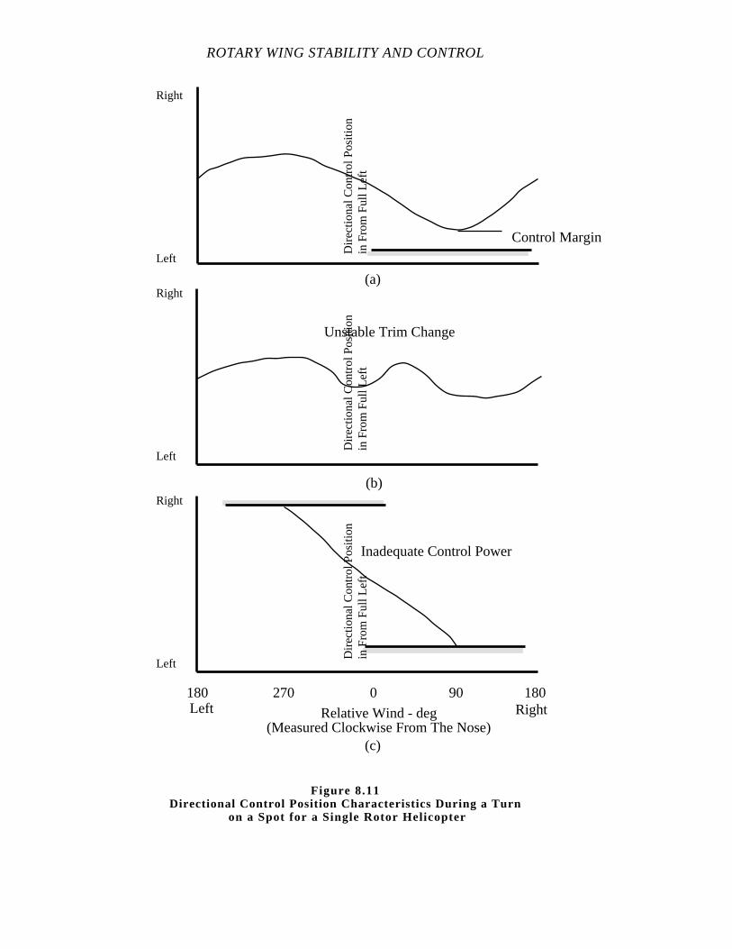
ROTARY WING STABILITY AND CONTROL
Dire
ctio
nal C
ontr
ol P
ositi
onin
Fro
m F
ull L
eft
Left
Right
Control Margin
(a)
(b)
Unstable Trim ChangeD
irect
iona
l Con
trol
Pos
ition
in F
rom
Ful
l Lef
t
Left
Right
Relative Wind - deg(Measured Clockwise From The Nose)
Left Right90 180180 270
Inadequate Control Power
(c)
Dire
ctio
nal C
ontr
ol P
ositi
onin
Fro
m F
ull L
eft
Left
Right
0
Figure 8.11Directional Control Position Characteristics During a Turn
on a Spot for a Single Rotor Helicopter
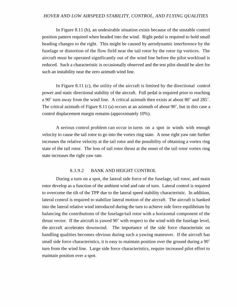
HOVER AND LOW AIRSPEED STABILITY, CONTROL, AND FLYING QUALITIES
In Figure 8.11 (b), an undesirable situation exists because of the unstable control
position pattern required when headed into the wind. Right pedal is required to hold small
heading changes to the right. This might be caused by aerodynamic interference by the
fuselage or distortion of the flow field near the tail rotor by the rotor tip vortices. The
aircraft must be operated significantly out of the wind line before the pilot workload is
reduced. Such a characteristic is occasionally observed and the test pilot should be alert for
such an instability near the zero azimuth wind line.
In Figure 8.11 (c), the utility of the aircraft is limited by the directional control
power and static directional stability of the aircraft. Full pedal is required prior to reaching
a 90˚ turn away from the wind line. A critical azimuth then exists at about 80˚ and 285˚.
The critical azimuth of Figure 8.11 (a) occurs at an azimuth of about 90˚, but in this case a
control displacement margin remains (approximately 10%).
A serious control problem can occur in turns on a spot in winds withenough
velocity to cause the tail rotor to go into the vortex ring state. A nose right yaw rate further
increases the relative velocity at the tail rotor and the possibility of obtaining a vortex ring
state of the tail rotor. The loss of tail rotor thrust at the onset of the tail rotor vortex ring
state increases the right yaw rate.
8.3.9.2 BANK AND HEIGHT CONTROL
During a turn on a spot, the lateral side force of the fuselage, tail rotor, and main
rotor develop as a function of the ambient wind and rate of turn. Lateral control is required
to overcome the tilt of the TPP due to the lateral speed stability characteristic. In addition,
lateral control is required to stabilize lateral motion of the aircraft. The aircraft is banked
into the lateral relative wind introduced during the turn to achieve side force equilibrium by
balancing the contributions of the fuselage/tail rotor with a horizontal component of the
thrust vector. If the aircraft is yawed 90˚ with respect to the wind with the fuselage level,
the aircraft accelerates downwind. The importance of the side force characteristic on
handling qualities becomes obvious during such a yawing maneuver. If the aircraft has
small side force characteristics, it is easy to maintain position over the ground during a 90˚
turn from the wind line. Large side force characteristics, require increased pilot effort to
maintain position over a spot.
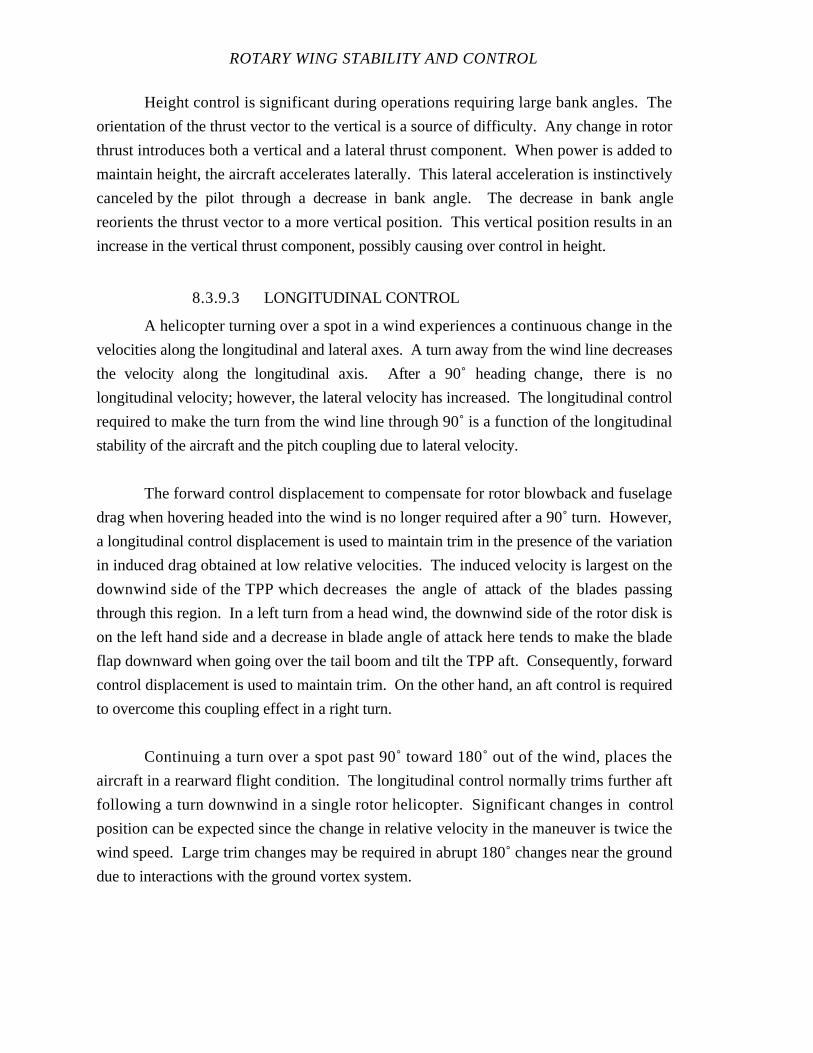
ROTARY WING STABILITY AND CONTROL
Height control is significant during operations requiring large bank angles. The
orientation of the thrust vector to the vertical is a source of difficulty. Any change in rotor
thrust introduces both a vertical and a lateral thrust component. When power is added to
maintain height, the aircraft accelerates laterally. This lateral acceleration is instinctively
canceled by the pilot through a decrease in bank angle. The decrease in bank angle
reorients the thrust vector to a more vertical position. This vertical position results in an
increase in the vertical thrust component, possibly causing over control in height.
8.3.9.3 LONGITUDINAL CONTROL
A helicopter turning over a spot in a wind experiences a continuous change in the
velocities along the longitudinal and lateral axes. A turn away from the wind line decreases
the velocity along the longitudinal axis. After a 90˚ heading change, there is no
longitudinal velocity; however, the lateral velocity has increased. The longitudinal control
required to make the turn from the wind line through 90˚ is a function of the longitudinal
stability of the aircraft and the pitch coupling due to lateral velocity.
The forward control displacement to compensate for rotor blowback and fuselage
drag when hovering headed into the wind is no longer required after a 90˚ turn. However,
a longitudinal control displacement is used to maintain trim in the presence of the variation
in induced drag obtained at low relative velocities. The induced velocity is largest on the
downwind side of the TPP which decreases the angle of attack ofthe blades passing
through this region. In a left turn from a head wind, the downwind side of the rotor disk is
on the left hand side and a decrease in blade angle of attack here tends to make the blade
flap downward when going over the tail boom and tilt the TPP aft. Consequently, forward
control displacement is used to maintain trim. On the other hand, an aft control is required
to overcome this coupling effect in a right turn.
Continuing a turn over a spot past 90˚ toward 180˚ out of the wind, places the
aircraft in a rearward flight condition. The longitudinal control normally trims further aft
following a turn downwind in a single rotor helicopter. Significant changes in control
position can be expected since the change in relative velocity in the maneuver is twice the
wind speed. Large trim changes may be required in abrupt 180˚ changes near the ground
due to interactions with the ground vortex system.
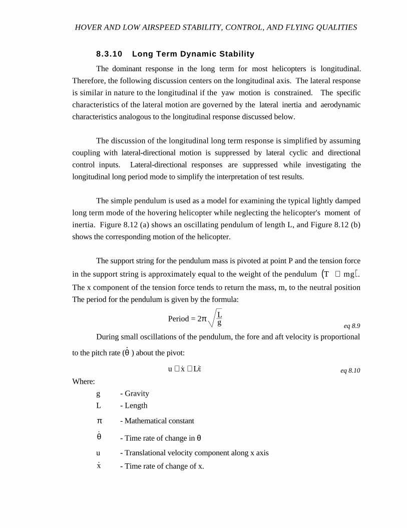
HOVER AND LOW AIRSPEED STABILITY, CONTROL, AND FLYING QUALITIES
8.3.10 Long Term Dynamic Stability
The dominant response in the long term for most helicopters is longitudinal.
Therefore, the following discussion centers on the longitudinal axis. The lateral response
is similar in nature to the longitudinal if the yaw motion is constrained. The specific
characteristics of the lateral motion are governed by the lateral inertia and aerodynamic
characteristics analogous to the longitudinal response discussed below.
The discussion of the longitudinal long term response is simplified by assuming
coupling with lateral-directional motion is suppressed by lateral cyclic and directional
control inputs. Lateral-directional responses are suppressed while investigating the
longitudinal long period mode to simplify the interpretation of test results.
The simple pendulum is used as a model for examining the typical lightly damped
long term mode of the hovering helicopter while neglecting the helicopter's moment of
inertia. Figure 8.12 (a) shows an oscillating pendulum of length L, and Figure 8.12 (b)
shows the corresponding motion of the helicopter.
The support string for the pendulum mass is pivoted at point P and the tension force
in the support string is approximately equal to the weight of the pendulum T≅ mg( ).The x component of the tension force tends to return the mass, m, to the neutral position
The period for the pendulum is given by the formula:
Period = 2π Lg eq 8.9
During small oscillations of the pendulum, the fore and aft velocity is proportional
to the pitch rate (θ ) about the pivot:
u ≅ .x ≅ L
.θ eq 8.10
Where:
g - Gravity
L - Length
π - Mathematical constant
θ - Time rate of change in θ
u - Translational velocity component along x axis
x - Time rate of change of x.

ROTARY WING STABILITY AND CONTROL
θ
u
String Tension = T = mg
x
L
Pivot Point
(a)
u = 0 u < umax
u = umax
u < umax
u = 0
Thrust
Virtual Pivot
(b)
Initial Position,TPP Shaft⊥
θmax
θmax
θmax
θ.
= 0θ.
= 0 θ.
< θ.maxθ
.< θ
.max θ
.= θ
.max
Figure 8.12Analogy of Simple Pendulum and Helicopter Long Period

HOVER AND LOW AIRSPEED STABILITY, CONTROL, AND FLYING QUALITIES
In Figure 8.12 (b), the string tension force is replaced by the rotor thrust force (T =
mg) acting parallel to the shaft towards a virtual pivot point. At the initial position, the
helicopter has a nose down pitch angle θ = -θmax and the pitch rate θ ( ) and forward
velocity (u) are both zero. The shaft is tilted forward and the TPP is perpendicular to the
shaft. This gives a forward tilt of the thrust vector, causing the helicopter to accelerate to
the right.
When the helicopter develops a forward velocity, the TPP tilts aft. This produces a
nose up pitching moment. However, if the helicopter has zero moment of inertia, any
pitching moment causes an infinite nose up pitching acceleration.
Consequently, a nose up pitch rate develops instantaneously and the forward rotor
tilt due to lag exactly cancels the aft tilt due to the forward speed increment. The TPP
remains perpendicular to the shaft as indicated in the diagram and the pitch rate at any
forward speed makes the total pitching moment on the helicopter equal to zero. That is:
∆M = 0 =∂M
∂uu +
∂M
∂θ θ eq 8.11
θ =
∂M
∂u∂M∂θ
u = −M u
M θ u eq 8.12
The above linear relationship holds during long period oscillations for a
configuration assumed to have zero moment of inertia. This long period motion can be
described as the oscillation about a virtual pivot point of a pendulum with equivalent length:
L Equiv =u
θ = −
Mθ M u
eq 8.13
The period for this long term oscillation is obtained from the analogy with the
simple pendulum:
Period = 2πLEquiv
g= 2π
Mθ gMu
eq 8.14
ROTARY WING STABILITY AND CONTROL
Where:
g - Gravity
- Lequiv Equivalent length
M - Net moment about y axis, Pitch moment
Mθ - Pitch moment due to time rate of change of pitch angle
Mu - Pitch moment due to longitudinal velocity
π - Mathematical constant
θ - Pitch angle
θ - Time rate of change in θ
u - Translational velocity component along x axis.
In sinusoidal oscillations, the moment of inertia about the pitch axis is small at the
low frequency of the long term oscillation. This is the basis for assuming it negligible
compared to the aerodynamic pitching moment in the preceding discussion. However, a
more accurate analysis, including non-zero moment of inertia, shows the rotor tilt due to
velocity and pitch rate do not exactly balance. The residual pitching moments usually cause
an unstable long period mode of the basic helicopter in hovering flight.
8.3.11 First Order Representation of Vertical Velocity, Pitch
Rate, Roll Rate, and Yaw Rate Responses
The first order equations used to approximate the initial vertical velocity OGE, pitch
rate, roll rate, and yaw rate responses in hovering flight are presented in Table 8.II.

HOVER AND LOW AIRSPEED STABILITY, CONTROL, AND FLYING QUALITIES
Table 8.II
First Order System Parameters
NormalizedDamping
TimeConstant
ControlVariable
ControlSensitivity
Mass DamperModel
Bm = - Xu
1(B/m) = - 1
Xu
δ Xδ
Vertical VelocityResponse Mode
-Zw
(- Zw)1 θC or δC
ZθC
Pitch RateResponse Mode
-Mq
(- Mq)1 B1s or δLONG
MB1s orMδLONG
Yaw RateResponse Mode
-Nr
(- Nr)1 θTR or δPED
NθTR or NδPED
Roll RateResponse Mode
-Lp
(- Lp)1 A1s or δLAT
LA1s or LδLAT
The longitudinal velocity develops more slowly than the pitch rate in the initial
response to a longitudinal control input, and the lateral velocity develops more slowly than
the roll rate in response to a lateral control input. Consequently, there is a period of time
during which the pitching moment due to longitudinal velocity has a negligible effect on the
pitching moment equilibrium, and similarly there is a period when the moment due to lateral
velocity has a negligible effect on the rolling moment equilibrium. When the terms due to
linear velocity changes are neglected, the pitching and rolling moment equilibrium
equations for hovering and low airspeed flight become:
.q - Mqq = M
B1sB
1s = M
δLONGδ
LONGeq 8.15
p. - Lpp = L
A1s
A1s
+ LθTR
θTR
= LδLAT
δLAT
+ LδPED
δPED
≈ LδLAT
δLAT
eq 8.16
ROTARY WING STABILITY AND CONTROL
Where:
A1s - Lateral cyclic pitch angle, shaft referenced
B1s - Longitudinal cyclic pitch angle, shaft referenced
δLAT - Lateral control
δLONG - Longitudinal control
δPED - Pedal control
LA1s - Roll moment due to lateral cyclic pitch angle
LδLAT - Roll moment due to lateral control
LδPED - Roll moment due to pedal control
Lp - Roll moment due to roll rate
LθTR - Roll moment due to tail rotor pitch angle
MB1s - Pitch moment due to longitudinal cyclic pitch angle
MδLONG - Pitch moment due to longitudinal control
Mq - Pitch moment due to pitch rate
p - Angular velocity about x axis, Roll rate
p - Angular acceleration about x axis
q - Angular velocity about y axis, Pitch rate
θTR - Tail rotor pitch angle
q - Angular acceleration about y axis.
The rolling moment due to pedal input is assumed zero as a simple approximation.
These first order equations for pitch rate and roll rate, as well as the equations for vertical
velocity and yaw rate, in hovering flight are represented by an equivalent mass-damper
system as shown schematically in Figure 8.13.
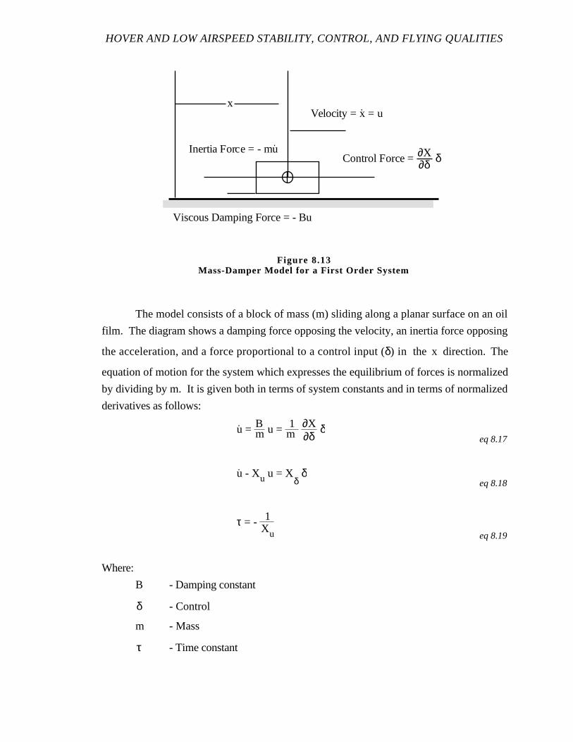
HOVER AND LOW AIRSPEED STABILITY, CONTROL, AND FLYING QUALITIES
The model consists of a block of mass (m) sliding along a planar surface on an oil
film. The diagram shows a damping force opposing the velocity, an inertia force opposing
the acceleration, and a force proportional to a control input (δ) in the x direction. The
equation of motion for the system which expresses the equilibrium of forces is normalized
by dividing by m. It is given both in terms of system constants and in terms of normalized
derivatives as follows:
u. = Bm u = 1
m∂X∂δ
δeq 8.17
u. - Xu u = X
δδ
eq 8.18
τ = - 1Xu eq 8.19
Where:
B - Damping constant
δ - Control
m - Mass
τ - Time constant
x
Inertia Force = - mu.
Control Force =∂X∂δ δ
Velocity = x.
= u
Viscous Damping Force = - Bu
Figure 8.13Mass-Damper Model for a First Order System
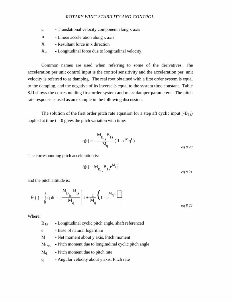
ROTARY WING STABILITY AND CONTROL
u - Translational velocity component along x axis
u - Linear acceleration along x axis
X - Resultant force in x direction
Xu - Longitudinal force due to longitudinal velocity.
Common names are used when referring to some of the derivatives. The
acceleration per unit control input is the control sensitivity and the acceleration per unit
velocity is referred to as damping. The real root obtained with a first order system is equal
to the damping, and the negative of its inverse is equal to the system time constant. Table
8.II shows the corresponding first order system and mass-damper parameters. The pitch
rate response is used as an example in the following discussion.
The solution of the first order pitch rate equation for a step aft cyclic input (-B1s)
applied at time t = 0 gives the pitch variation with time:
q(t) = - Mq
MB1s
B1s
( 1 - eMqt )eq 8.20
The corresponding pitch acceleration is:
.q(t) = M
B1sB
1seMqt
eq 8.21
and the pitch attitude is:
θ (t) = ∫0
t q dt = -
MB
1s
B1s
Mqt + 1
Mq
(1 - eMq t)
eq 8.22
Where:
B1s - Longitudinal cyclic pitch angle, shaft referenced
e - Base of natural logarithm
M - Net moment about y axis, Pitch moment
MB1s - Pitch moment due to longitudinal cyclic pitch angle
Mq - Pitch moment due to pitch rate
q - Angular velocity about y axis, Pitch rate
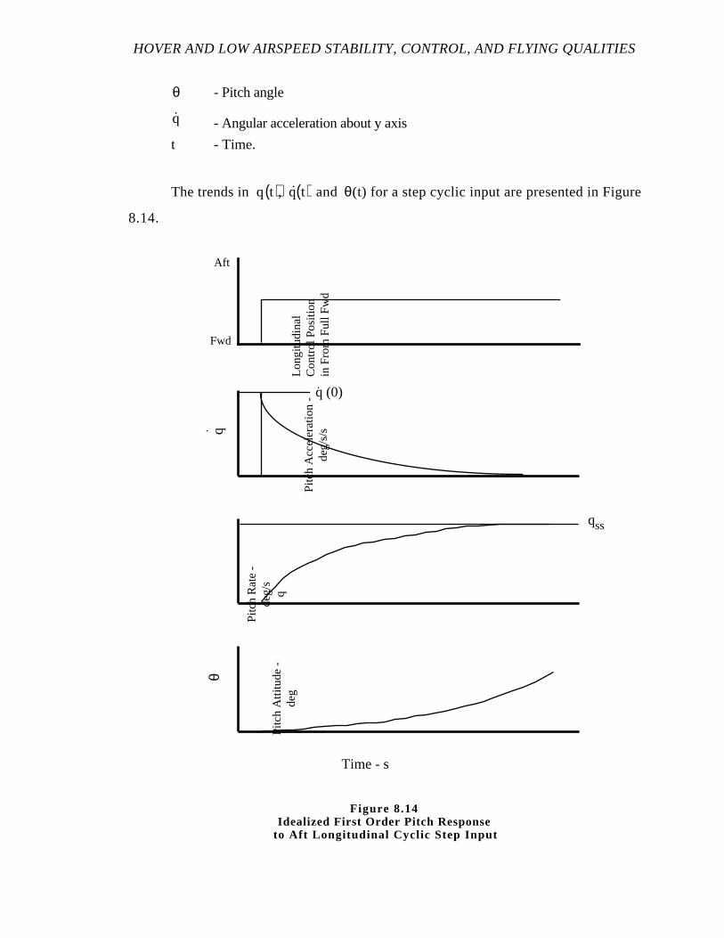
HOVER AND LOW AIRSPEED STABILITY, CONTROL, AND FLYING QUALITIES
θ - Pitch angle
q - Angular acceleration about y axis
t - Time.
The trends in q t( ), q t( ) and θ(t) for a step cyclic input are presented in Figure
8.14.
Time - s
qss
Pitc
h R
ate
-de
g/s
q
q.
(0)
Long
itudi
nal
Con
trol
Pos
ition
in F
rom
Ful
l Fw
d
q.
Pitc
h A
ccel
erat
ion
-de
g/s/
s
θ
Pitc
h A
ttitu
de -
deg
Fwd
Aft
Figure 8.14Idealized First Order Pitch Response
to Aft Longitudinal Cyclic Step Input
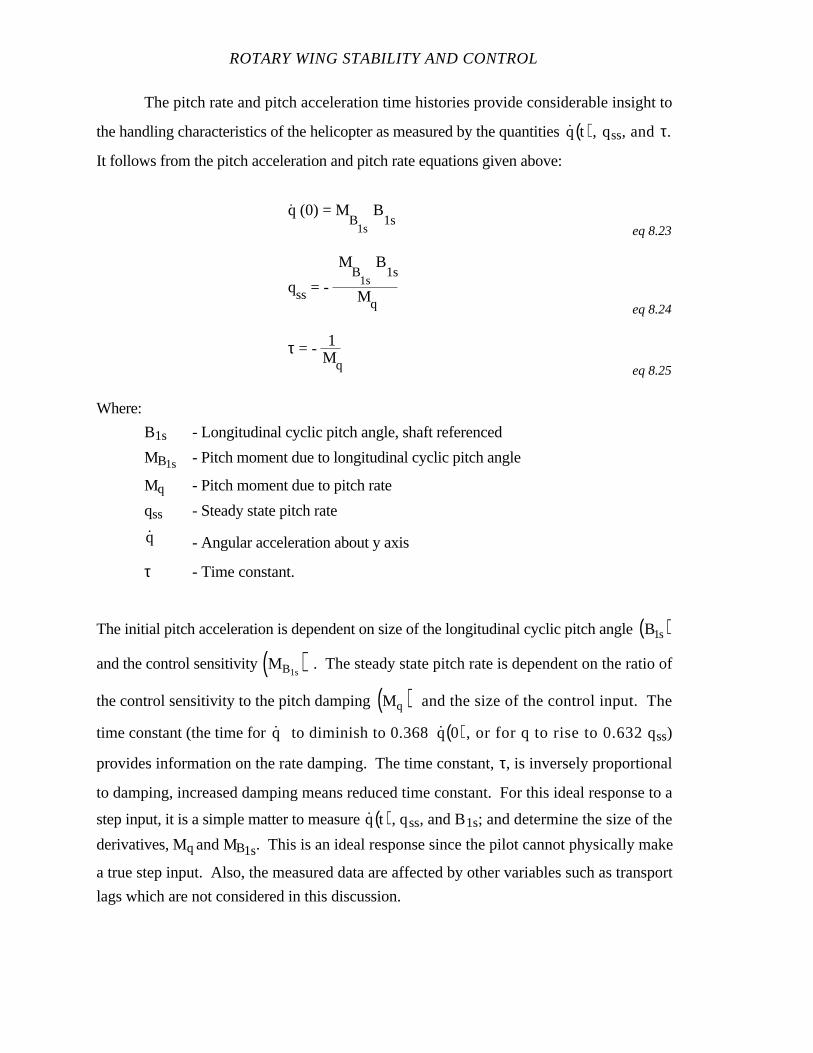
ROTARY WING STABILITY AND CONTROL
The pitch rate and pitch acceleration time histories provide considerable insight to
the handling characteristics of the helicopter as measured by the quantities q t( ), qss, and τ.
It follows from the pitch acceleration and pitch rate equations given above:
q. (0) = M
B1s
B1s
eq 8.23
qss = -
MB
1s
B1s
Mq eq 8.24
τ = - 1Mq eq 8.25
Where:
B1s - Longitudinal cyclic pitch angle, shaft referenced
MB1s - Pitch moment due to longitudinal cyclic pitch angle
Mq - Pitch moment due to pitch rate
qss - Steady state pitch rate
q - Angular acceleration about y axis
τ - Time constant.
The initial pitch acceleration is dependent on size of the longitudinal cyclic pitch angle B1s( )and the control sensitivity MB1s( ) . The steady state pitch rate is dependent on the ratio of
the control sensitivity to the pitch damping Mq( ) and the size of the control input. The
time constant (the time for q to diminish to 0.368 q 0( ) , or for q to rise to 0.632 qss)
provides information on the rate damping. The time constant, τ, is inversely proportional
to damping, increased damping means reduced time constant. For this ideal response to a
step input, it is a simple matter to measure q t( ), qss, and B1s; and determine the size of the
derivatives, Mq and MB1s. This is an ideal response since the pilot cannot physically make
a true step input. Also, the measured data are affected by other variables such as transport
lags which are not considered in this discussion.
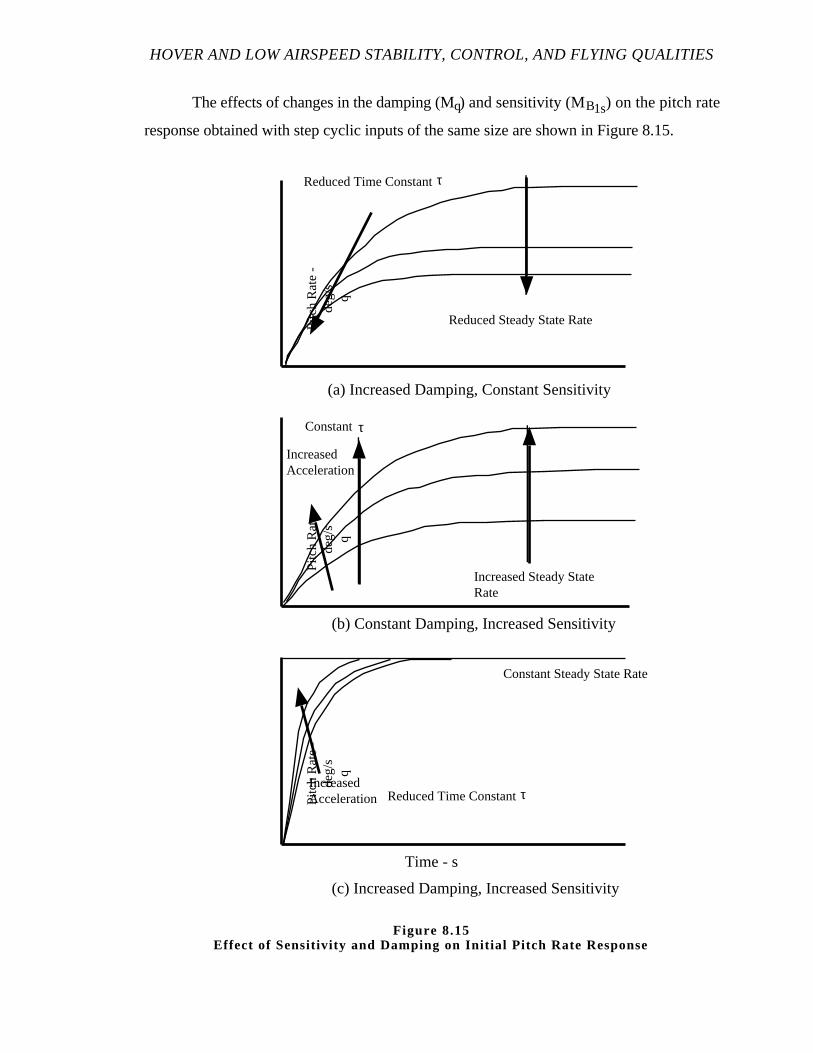
HOVER AND LOW AIRSPEED STABILITY, CONTROL, AND FLYING QUALITIES
The effects of changes in the damping (Mq) and sensitivity (MB1s) on the pitch rate
response obtained with step cyclic inputs of the same size are shown in Figure 8.15.
Pitc
h R
ate
-de
g/s
q
Pitc
h R
ate
-de
g/s
q
Pitc
h R
ate
-de
g/s
q
(a) Increased Damping, Constant Sensitivity
Reduced Steady State Rate
(b) Constant Damping, Increased Sensitivity
Constantτ
Increased Steady StateRate
IncreasedAcceleration
(c) Increased Damping, Increased Sensitivity
Constant Steady State Rate
IncreasedAcceleration
τReduced Time Constant
τReduced Time Constant
Time - s
Figure 8.15Effect of Sensitivity and Damping on Init ial Pitch Rate Response
ROTARY WING STABILITY AND CONTROL
For a constant MB1s, Figure 8.15 (a) shows increased damping (Mq) reduces the
steady state rate and shortens the time constant.
For a constant Mq, Figure 8.15 (b) shows increased control sensitivity (MB1s)
increases the initial pitch acceleration and steady state rate, while the time constant is
unchanged.
For a constant ratio of control sensitivity to damping (MB1s/ Mq), Figure 8.15 (c)
shows increased damping and sensitivity increases the initial pitch acceleration and shortens
the time constant, while the steady state rate remains constant.
8.3.12 Control Response
The discussion in the preceding section used a first order system approximation for
initial helicopter responses. The effect of control sensitivity and damping on the responses
was presented. This section relates these results to the concepts of control effectiveness
and response quality.
Attitude control effectiveness is the change in aircraft attitude achieved per time
period (usually one second) following a unit step control displacement. Rate control
effectiveness is the angular rate achieved per time period (usually one second) following a
unit step control displacement. The concept of control effectiveness is illustrated using the
pitch responses in Figure 8.16, for two different helicopters, with different levels of both
damping and sensitivity. The rate control effectiveness of the two configurations is equal at
a time of 1.25 s, and the attitude control effectiveness is equal at 2 s.
The response quality is determined by the pilot's judgment of the overall response
which is influenced to a large extent by:
1. Control sensitivity.
2. Damping.
3. Response lags.
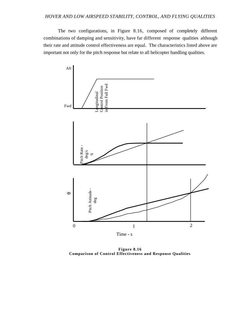
HOVER AND LOW AIRSPEED STABILITY, CONTROL, AND FLYING QUALITIES
The two configurations, in Figure 8.16, composed of completely different
combinations of damping and sensitivity, have far different response qualities although
their rate and attitude control effectiveness are equal. The characteristics listed above are
important not only for the pitch response but relate to all helicopter handling qualities.
Time - s
0 1 2
Long
itudi
nal
Con
trol
Pos
ition
in F
rom
Ful
l Fw
dFwd
Aftθ
Pitc
h A
ttitu
de -
deg
Pitc
h R
ate
-de
g/s
q
Figure 8.16Comparison of Control Effectiveness and Response Qualities
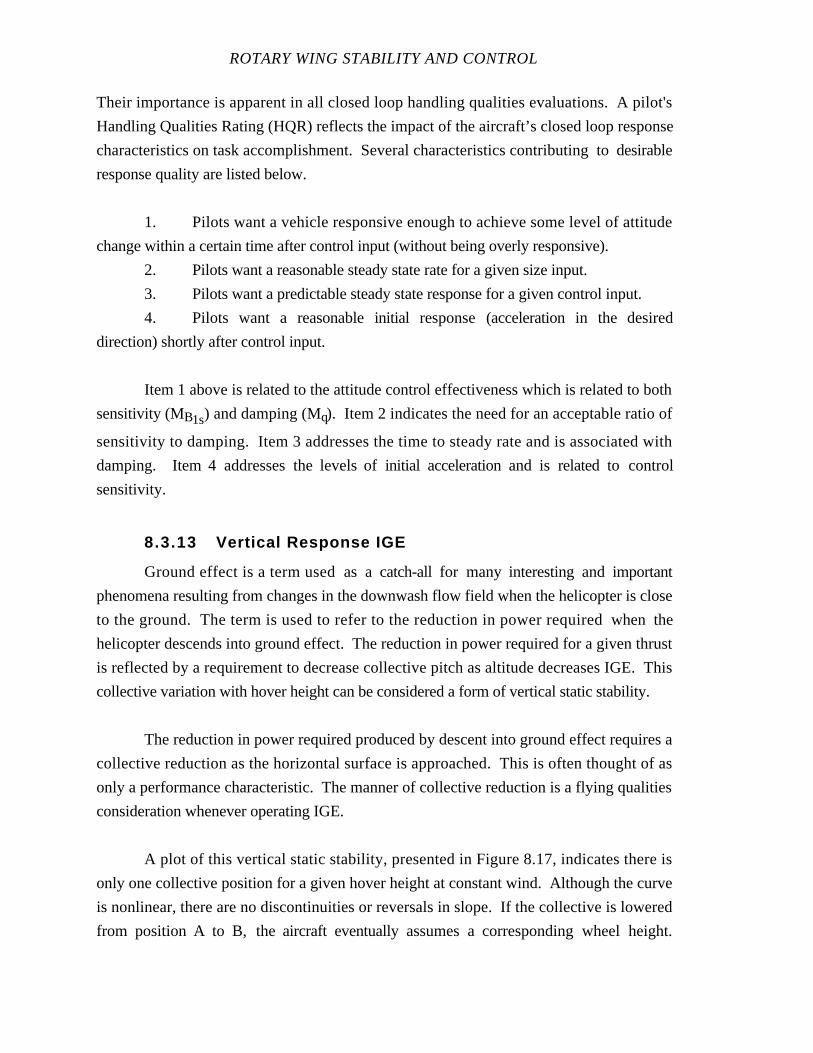
ROTARY WING STABILITY AND CONTROL
Their importance is apparent in all closed loop handling qualities evaluations. A pilot's
Handling Qualities Rating (HQR) reflects the impact of the aircraft’s closed loop response
characteristics on task accomplishment. Several characteristics contributing to desirable
response quality are listed below.
1. Pilots want a vehicle responsive enough to achieve some level of attitude
change within a certain time after control input (without being overly responsive).
2. Pilots want a reasonable steady state rate for a given size input.
3. Pilots want a predictable steady state response for a given control input.
4. Pilots want a reasonable initial response (acceleration in the desired
direction) shortly after control input.
Item 1 above is related to the attitude control effectiveness which is related to both
sensitivity (MB1s) and damping (Mq). Item 2 indicates the need for an acceptable ratio of
sensitivity to damping. Item 3 addresses the time to steady rate and is associated with
damping. Item 4 addresses the levels of initial acceleration and is related to control
sensitivity.
8.3.13 Vertical Response IGE
Ground effect is a term used as a catch-all for many interesting and important
phenomena resulting from changes in the downwash flow field when the helicopter is close
to the ground. The term is used to refer to the reduction in power required when the
helicopter descends into ground effect. The reduction in power required for a given thrust
is reflected by a requirement to decrease collective pitch as altitude decreases IGE. This
collective variation with hover height can be considered a form of vertical static stability.
The reduction in power required produced by descent into ground effect requires a
collective reduction as the horizontal surface is approached. This is often thought of as
only a performance characteristic. The manner of collective reduction is a flying qualities
consideration whenever operating IGE.
A plot of this vertical static stability, presented in Figure 8.17, indicates there is
only one collective position for a given hover height at constant wind. Although the curve
is nonlinear, there are no discontinuities or reversals in slope. If the collective is lowered
from position A to B, the aircraft eventually assumes a corresponding wheel height.
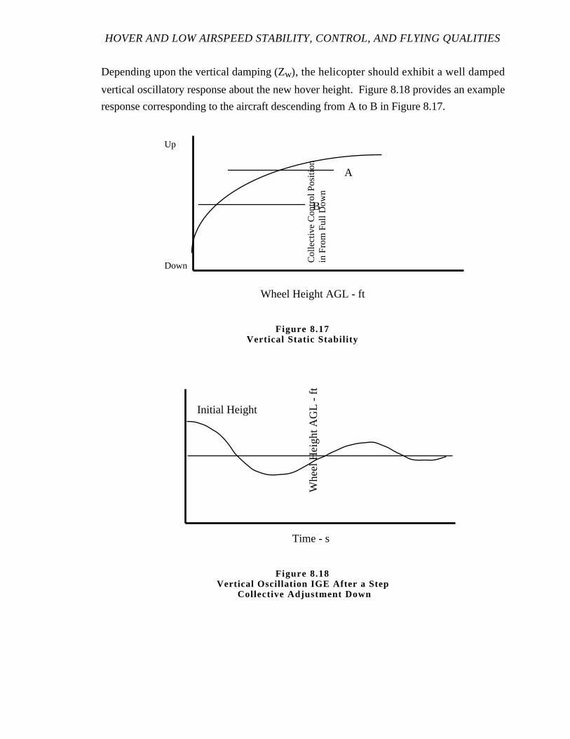
HOVER AND LOW AIRSPEED STABILITY, CONTROL, AND FLYING QUALITIES
Depending upon the vertical damping (Zw), the helicopter should exhibit a well damped
vertical oscillatory response about the new hover height. Figure 8.18 provides an example
response corresponding to the aircraft descending from A to B in Figure 8.17.
Wheel Height AGL - ft
A
B
Col
lect
ive
Con
trol
Pos
ition
in F
rom
Ful
l Dow
n
Up
Down
Figure 8.17Vertical Static Stabil ity
Whe
el H
eigh
t AG
L -
ft
Initial Height
Time - s
Figure 8.18Vertical Oscillation IGE After a Step
Collective Adjustment Down
ROTARY WING STABILITY AND CONTROL
In addition to the increase in thrust descending IGE, a substantial portion of the
IGE vertical static stability is supplied by the pressure pattern under the fuselage. This
phenomenon is so strong on some aircraft a considerable pitching moment is developed as
a result. This moment must be countered with longitudinal control input to zero drift and
avoid undesirable landing attitudes. This pressure pattern characteristic may provide
desirable or undesirable results varying with gross weight, power, wind, and ground
speed. The pattern may be unstable and introduce a random disturbance in pitch. A wide
variety of ground effects characteristics are possible.
Tandem rotor helicopters have a particular problem in pitch control during vertical
descents into ground effect. The forward and aft rotors normally do not experience the
same increase in thrust during a decrease in hover height. Thus, as the aircraft descends
into ground effect, the thrust of the individual rotors change in an unequal fashion
producing a longitudinal pitching moment away from the more effective rotor. As the
tandem helicopter descends into ground effect, the pilot may not perceive the actual vertical
motion of the aircraft CG. He may see the combined vertical and pitching response as the
vertical motion of the aircraft.
8.4 TEST METHODS AND TECHNIQUES
8.4.1 General
The tests generally included in an evaluation of low airspeed handling qualities are:
trim control positions in low airspeed flight, critical azimuth determination, turn on a spot,
static stability, long term dynamic response, control response, and departures and
approaches.
Most low airspeed tests require calm winds to quantify accurately the aircraft
handling characteristics. A test limit of 3 to 5 kn true wind speed is the norm. When
winds are present, the velocity is vectorially included in the data presentation to establish
aircraft operating limits. During periods of steady wind conditions, turn on a spot data are
collected and various mission maneuvers are qualitatively and quantitatively evaluated.
HOVER AND LOW AIRSPEED STABILITY, CONTROL, AND FLYING QUALITIES
Low airspeed velocity is measured in a variety of ways. The most common method
is formation flight with a ground pace vehicle. Other methods include use of low airspeed
sensing systems, Doppler ground speed systems, and inertial systems. All these systems
are calibrated prior to test and all, except the low airspeed systems, depend on adjustment
for the local wind speed and direction.
Qualitative evaluation of the helicopter is accomplished with a full and complete
understanding of the intended mission. HQRs are assigned with respect to pilot workload,
adequate and desired performance, and the test conditions. For instance, an attack
helicopter pilot may need to maintain aircraft heading within 3˚ to fire effectively a
particular weapon system. The attack pilot heading control criteria may be too strict for the
utility mission. These judgments require operational experience and influence the HQRs
assigned to a particular maneuver.
8.4.2 Trimmed Control Positions
The purpose of this test is to determine the control margins and handling qualities in
simulated crosswind, downwind, and low airspeed forward flight. The qualitative
evaluation of trim changes is an integral part of the test. The test is accomplished by flying
formation on a ground pace vehicle having a calibrated airspeed system. The helicopter is
flown at a constant height AGL. Winds should be less than 3 kn. Quantitative data are
collected in forward, rearward, and sideward trimmed IGE flight. The entire low airspeed
envelope of the helicopter is investigated. Sideward and rearward flight to the maximum
allowable velocity, as determined by control position and control power margins; and
forward flight to approximately 50 kn are conducted. Airspeed increments of
approximately 5 kn are used. A ground observer records the ambient wind information and
relays this information to the crew of the pace vehicle. The crew of the pace vehicle uses
the ambient wind information along with runway heading to determine aircraft heading and
pace vehicle speed for each test point.
8.4.2.1 TEST TECHNIQUE
1. Establish a zero drift, unaccelerated, trimmed hover on the test heading.
Record the initial trim conditions.
2. The pace vehicle establishes the next test speed. The aircraft stabilizes in
formation on the pace vehicle. The standoff distance is sufficiently close to detect small,
relative motions; but far enough to avoid downwash interference.

ROTARY WING STABILITY AND CONTROL
3. When all relative motion is stopped, the flight control forces trimmed to
zero, and the helicopter on heading at the correct altitude, data are recorded.
4. Assign an HQR and Vibration Assessment Rating (VAR) to each data point.
5. The pace vehicle establishes the next test speed and the process is repeated.
6. Use the force trim and Automatic Flight Control System (AFCS) in a
mission representative manner.
7. Fly all test points for the same direction (forward, rearward, sideward) in
the same geographical direction.
8.4.2.2 DATA REQUIRED
Cockpit. Run number, control positions, heading, airspeed from low airspeed
system (if available), ground speed (if available), fuel counts (FC), Q, NR, θ, φ, HQR,
and VAR.
Ground station. Run number, wind direction, wind speed, To, and HPo.
8.4.2.3 TEST CRITERIA
1. No relative motion between helicopter and pace vehicle.
2. Stabilized, unaccelerated flight.
3. No vertical climb/descent.
4. Constant height AGL.
5. Minimum control movement.
6. All control forces trimmed to zero.
8.4.2.4 DATA REQUIREMENTS
1. Stabilize 15 s prior to recording data.
2. Record 10 s data.
3. Altitude ± 5 ft.
4. Vertical speed 0.
5. NR ± 1%.
6. Heading ± 2˚.
HOVER AND LOW AIRSPEED STABILITY, CONTROL, AND FLYING QUALITIES
8.4.2.5 SAFETY CONSIDERATIONS/RISK MANAGEMENT
Trimmed control positions in low airspeed flight require operating close to the
ground and pace vehicle at relatively high speed. The helicopter can experience large pitch
or roll attitudes reducing field of view. Three different groups of people are involved: the
helicopter crew, the pace vehicle crew, and the ground wind observer operating in close
proximity. Terminating from high speed sideward, rearward, and forward flight close to
the ground must be briefed and practiced. Emergency procedures for engine failure, engine
control failure, and flight control system failures must be briefed. Procedures for
terminating a data point must be briefed. All participants must maintain spatial awareness
and conduct test operations clear of airport hazards and traffic.
8.4.3 Critical Azimuth
The purpose of this test is an evaluation of the control margins and pilot workload
with changes in airspeed and relative wind azimuth. The qualitative evaluation of trim
changes and pilot workload is an integral part of this test. Data are collected simultaneously
with trimmed control positions in low airspeed flight. Of specific interest are the control
margins and pilot workload to accomplish the task of hovering the helicopter within
predetermined tolerances at various wind speeds and directions. The techniques, data,
criteria, and safety considerations for trimmed control positions apply to critical azimuth.
Critical azimuth data are gathered in relative wind azimuth increments of 30˚ to 45˚; unless
a region of particular interest is identified and then as little as 15˚ increments are common.
Critical azimuth data are gathered for at least one airspeed, but a range of speeds can be
used.
8.4.4 Turn on a Spot
In conducting this test, a steady hovering condition is established heading into a
wind of known velocity. The aircraft is then turned to the right or left through a small
heading angle. Records are taken of control positions, attitudes, and rates after the aircraft
is stabilized on the new heading. Altitude and position over the ground are maintained
constant. Tests are continued at small increments in heading (15˚) until data are obtained
for a full 360˚ turn. Several different ambient wind speeds are used to document fully the
handling characteristics. The test team must be prepared to take advantage of all ambient
wind for data collection opportunities. A ground wind observer is used to record wind
information.
ROTARY WING STABILITY AND CONTROL
Constant yaw rate turns to the right, or the left, are used to obtain pilot evaluations
of handling qualities in turns over a spot. A continuous record of this maneuver,
considering the piloting task and performance criteria, indicates how well the aircraft is
controlled. Pilot workload is determined by examining the control patterns required to
perform the turn.
8.4.4.1 TEST TECHNIQUE
1. Establish a zero drift, unaccelerated, trimmed hover on the test heading.
Record the initial trim conditions.
2. Establish a zero drift, unaccelerated, trimmed hover on the new test
heading.
3. Trim the flight control forces to zero, stabilize on heading at the correct
altitude, and record data.
4. Minimize control movement during data recording.
5. Assign an HQR and VAR to each data point.
6. Use the force trim and AFCS in a mission representative manner.
7. Complete the 360˚ turn.
8.4.4.2 DATA REQUIRED
Cockpit. Run number, control positions, heading, airspeed from low airspeed
system (if available), fuel counts (FC), Q, NR, θ, φ, HQR, and VAR.
Ground station. Run number, wind direction, wind speed, To, and HPo.
8.4.4.3 TEST CRITERIA
1. Stabilized, unaccelerated, zero drift flight.
2. No vertical climb/descent.
3. Constant height AGL.
4. Minimum control movement.
5. All control forces trimmed to zero.
HOVER AND LOW AIRSPEED STABILITY, CONTROL, AND FLYING QUALITIES
8.4.4.4 DATA REQUIREMENTS
1. Stabilize 15 s prior to recording data.
2. Record 10 s data.
3. Altitude ± 5 ft.
4. Vertical speed 0.
5. NR ± 1%.
6. Heading ± 2˚.
8.4.5 Static Stability
The purpose of this test is to evaluate the static stability or total restoring moment
generated by off trim conditions in the longitudinal, lateral, and directional axes. Data are
collected during forward, rearward, and sideward collective fixed flight about zero trimmed
airspeed. A 10 kn variation about trim is used. Data are collected with the collective fixed
at the zero airspeed value. Static stability is indicated by the initial tendency of the aircraft
to return to or depart from equilibrium if disturbed.
Static stability is indicated by pilot control displacement and/or control force
required to generate balancing pitching, rolling, or yawing moments when the aircraft is
stabilized at off trim conditions. Cyclic displacement in the direction of movement is
required to hold an off trim condition in an aircraft possessing positive longitudinal or
lateral static stability. Positive directional stability is indicated by directional control
displacement opposite to the direction of sideward flight (increasing left pedal with
increasing right sideward flight). No variation in control positions with speed is obtained if
the aircraft is neutrally stable. Cyclic displacement opposite the direction of movement is
required to hold an off trim condition in an aircraft with negative longitudinal and lateral
static stability. Directional control displacement in the direction of sideward flight indicates
negative directional static stability (right pedal applied with right lateral flight). Calm wind
conditions are required to accomplish this test.
The test technique for evaluating the low airspeed static stability of the helicopter are
broken into two portions, longitudinal and lateral/directional.
ROTARY WING STABILITY AND CONTROL
8.4.5.1 TEST TECHNIQUE
1. Longitudinal static stability.
a. Establish a zero drift, unaccelerated, trimmed hover on the test
heading. Record the initial trim conditions.
b. Accelerate approximately 2 to 3 kn forward, collective fixed at the
zero airspeed trim position, do not retrim, stabilize airspeed, and record data.
c. Repeat step b to achieve a 10 kn band.
d. Repeat steps a, b, and c for rearward flight.
2. Lateral and directional static stability.
a. Establish a zero drift, unaccelerated, trimmed hover on the test
heading. Record the initial trim conditions.
b. Accelerate the aircraft sideways 2 to 3 kn, collective fixed at the zero
airspeed trim positions, do not retrim, stabilize airspeed, ensuring no forward or aft drift
and relative wind azimuth equal 90˚ or 270˚. Record data.
c. Repeat step b until total velocity is approximately 10 kn.
d. Repeat steps a, b, and c for lateral flight in the other direction.
8.4.5.2 DATA REQUIRED
Cockpit. Run number, control positions, heading, airspeed from low airspeed
system (if available), ground speed (if available), fuel counts (FC), Q, NR, θ, φ, HQR,
and VAR.
Ground station. Run number, wind direction, wind speed, To, and HPo.
8.4.5.3 TEST CRITERIA
1. Stabilized, unaccelerated flight.
2. Constant collective.
3. Minimum control movement.
4. Do not retrim.
HOVER AND LOW AIRSPEED STABILITY, CONTROL, AND FLYING QUALITIES
8.4.5.4 DATA REQUIREMENTS
1. Stabilize 15 s prior to recording data.
2. Record 10 s data.
3. Heading ± 2˚.
8.4.6 Long Term Dynamic Stability
The purpose of this test is to evaluate the long term response (change in attitude,
airspeed, and altitude) of the aircraft as a function of time. This is a nuisance mode
generally suppressed by the pilot or AFCS. The tests should include a qualitative
determination of the difficulty of suppressing the long term response and the ease of
excitation. The test basically consists of recording the response of the aircraft to off trim
conditions resulting from turbulence or disturbances introduced by the pilot. Calm
atmospheric conditions are required to accomplish this test.
Static stability influences the low airspeed long term dynamic stability of the
helicopter. Negative static stability results in an aperiodic divergent response. Positive
static stability causes an oscillatory response which may be convergent, or divergent,
depending on damping. Higher damping results in fewer overshoots and a more
convergent oscillation. Also, angle of attack variations are more significant for the long
term helicopter mode than for the airplane phugoid mode.
Often the low airspeed long term response can be excited without conscious input.
With the controls fixed and no pilot inputs, an imperfect trim condition, or atmospheric
disturbance, may excite an aperiodic divergent mode or a lightly damped oscillatory mode.
This is an unsatisfactory technique if no response is obtained, but indicates a desirable
aircraft characteristic.
If maintaining control fixed fails to produce a long term response, use the
longitudinal control to increase, or decrease, the pitch attitude of the hovering helicopter.
Then smoothly return the control to the original trim position and record the aircraft motion.
An off trim attitude variation of 5 to 10˚ is used to excite the motion. Natural disturbances
which result in a long term response are desirable but these responses are usually
contaminated by another disturbance before the motion is completed. This makes
quantifying the mode of motion difficult.

ROTARY WING STABILITY AND CONTROL
Artificial excitation using the longitudinal control to generate an off trim pitch
attitude condition is used to stimulate the response and obtain time histories from which
engineering data are obtained. The excitation method chosen should result in an aircraft
response similar to a response following a natural disturbance.
8.4.6.1 TEST TECHNIQUE
1. Establish a zero drift, unaccelerated, trimmed OGE hover. Do not retrim
control forces or move the collective during the test. Record the initial trim conditions.
2. Determine if a long term response results from a natural disturbance. With
the controls either fixed or free, note the open loop aircraft response. If no aircraft
response is observed, use an artificial excitation.
3. Excite the aircraft long term response using an aft longitudinal control input
to establish a 5 to 10˚ off trim pitch condition. Return the control exactly to trim. Conduct
several tests to find the most representative aircraft responses to include in the report. Do
not retrim any control forces and keep the collective constant during the response.
4. If the aircraft is flown hands off during normal operations, obtain control
free responses following excitation. The controls are released at trim so the subsequent
control motions indicate the effect of attitude changes and gravity force acting on the
controls during the response.
5. Record the resulting mode of motion using cockpit data and automatic
recording systems. Cockpit displayed attitudes are recorded at selected time increments.
The stop watch is started at the completion of the excitation or at a predetermined attitude.
The zero time reference point is arbitrary. Use small time intervals to define the shape of
irregular responses.
8.4.6.2 DATA REQUIRED
A time history of aircraft attitudes, rates, control positions, heading, airspeed from
low airspeed system (if available), FC, Q, NR, To, HPo, and VAR.
8.4.6.3 TEST CRITERIA
1. Stabilized, unaccelerated flight at trim.
2. All control forces trimmed to zero.
3. Collective fixed.
4. Do not retrim.
HOVER AND LOW AIRSPEED STABILITY, CONTROL, AND FLYING QUALITIES
8.4.6.4 DATA REQUIREMENTS
1. Stabilize 15 s prior to recording trim data.
2. Record 2 complete cycles or until a test limit is reached.
8.4.6.5 SAFETY CONSIDERATIONS/RISK MANAGEMENT
Be prepared for large attitude excursions. Brief and practice unusual attitude
recoveries, using appropriate build up. Be prepared for coupled responses. Operate
outside the avoid area of the helicopter's height velocity diagram. Maintain situational and
height awareness. Be prepared for power settling.
8.4.7 Control Response
The purpose of these tests is to evaluate the aircraft response to flight control input.
The tests are conducted by applying control step inputs of incrementally increasing size
against a fixture, and recording a time history of the aircraft response.
8.4.7.1 TEST TECHNIQUE
1. Establish a zero drift, unaccelerated, trimmed hover at the desired altitude.
Normally control step inputs are accomplished OGE above the height velocity diagram
avoid area.
2. Set the control fixture for the desired displacement and position for the
desired input direction. The control input direction and size is verbally and visually (if
able) verified between the pilot and copilot/engineer. Start with small displacements and
increase incrementally.
3. Voice procedures for cockpit coordination are as follows: “Data on. Stand-
by for a (displacement magnitude), (direction of input), (control) input on three. Thousand
one, thousand two, thousand three.” The input is executed on three. Example, “Data on,
stand-by for a one inch right lateral cyclic input on three. Thousand one, thousand two,
thousand three.”
4. Hold the control input fixed. Recover when a steady state rate is obtained
or a predetermined flight limit is reached. A common error during these tests is to hold the
point longer than required, allowing the aircraft to reach an uncomfortable or even
dangerous attitude or rate.
ROTARY WING STABILITY AND CONTROL
5. When the maneuver is complete, announce the recovery so the control
fixture can be quickly and completely removed.
6. Repeat steps 1 through 5 for subsequent data points until the desired control
displacement is achieved or a predetermined flight limit is reached.
7. Qualitatively assess the attitude control effectiveness, rate control
effectiveness, and the predictability of the control response.
Test limits on bank attitude can prevent achieving steady state roll rates. If the test
helicopter can achieve high roll rates but the test program is restricted to low roll attitude
excursions, the test pilot must recover prior to achieving steady state roll rate. In this case,
a false start technique might be is used. In this technique, the test pilot establishes a bank
attitude in the direction opposite to the test input. Make the step input in the desired
direction from the banked control position. The use of the false start technique permits a
greater roll attitude change and longer time to elapse prior to recovery at a test attitude limit.
This technique may permit the helicopter to reach steady state roll rate.
8.4.7.2 DATA REQUIRED
A time history of aircraft attitudes, rates, control positions, heading, airspeed from
low airspeed system (if available), FC, Q, NR, To, HPo, and VAR.
8.4.7.3 TEST CRITERIA
1. Stabilized, unaccelerated flight at trim.
2. All control forces trimmed to zero.
3. Off axis controls fixed.
8.4.7.4 DATA REQUIREMENTS
1. Stabilize 15 s prior to recording data.
2. Record data until steady state rate is achieved or until a test limit is reached.
8.4.7.5 SAFETY CONSIDERATIONS/RISK MANAGEMENT
The considerations for trimmed control positions and long term response generally
apply for control response as well. Additionally, all tests have attitude or rate limits which
must be observed. You are operating close to the ground, rates or attitudes which may be
HOVER AND LOW AIRSPEED STABILITY, CONTROL, AND FLYING QUALITIES
appropriate for forward flight may not be appropriate for the low airspeed regime. Input
size must follow logical build up procedures, usually starting with 1/4 in. Remember you
don’t have to find the absolute end point, if the trend is rapidly approaching a limit, don’t
proceed.
8.4.8 Departures and Approaches
The approach to a hover from forward flight uses a descent/deceleration schedule
which is repeated over and over again. This schedule can be investigated as a series of
fixed trim points. These points are chosen to represent the center and/or extremes of the
approach airspeed/altitude envelope. The scope of the test may include repeating the
investigation for various types of approach. The following are of interest:
1. Normal approach to a hover.
2. Normal approach to a running landing.
3. Confined area approach to a hover.
4. Precautionary single engine approach.
5. Precision approach to a spot, when thrust to weight precludes a hover.
8. Level flight deceleration (quick stop).
These tests are generally qualitative but if a problem is suspected, time history
recordings of the maneuver are used to document the objectionable characteristic.
8.4.8.1 TEST TECHNIQUE
Various approach and departure techniques are investigated. The approaches
include steep approach, normal approaches, running landings, and confined area
approaches. The departures include: normal take-offs, vertical departures, obstacle
clearance take-offs, IGE accelerations to a climb speed, and rolling take-offs.
8.4.8.2 DATA REQUIRED
Qualitative remarks and HQR. A time history is used to document undesirable
characteristics. The time history includes aircraft attitudes, rates, control positions,
heading, altitude, airspeed from low airspeed system (if available), ground speed (if
available), FC, Q, NR and VAR. Ambient wind and weather conditions are recorded.

ROTARY WING STABILITY AND CONTROL
8.4.8.3 TEST CRITERIA
Use standard flight techniques for the approaches and departures.
8.5 DATA REDUCTION
8.5.1 General
Data reduction for low airspeed handling qualities tests involves applying the
appropriate instrumentation corrections and plotting a number of control positions, aircraft
attitudes, rates, and HQRs versus airspeed. Few analytical techniques are needed. Control
response is the one exception and is discussed.
8.5.2 Trimmed Control Positions
Instrument corrected control positions and aircraft attitudes are plotted as shown in
Figures 8.19 and 8.20. Engineering judgement is applied to determine which aircraft
attitudes to depict when the relative wind azimuth is not from a cardinal direction.
Additional parameters are shown if a problem is detected and requires discussion.
8.5.3 Critical Azimuth
Critical azimuth data are presented in two ways. First, the trimmed control position
data plotted are plotted as a function of relative wind azimuth. An example is provided in
Figure 8.21. Additionally, the HQRs and/or VARs obtained during the trimmed control
position tests are plotted versus wind azimuth as shown in Figure 8.22. The figure should
be further annotated with cross hatched areas depicting what caused the higher numbers.
VARs are plotted and annotated similarly. The figure could also be expanded to include
areas of restricted field of view, excessive attitude, etc.
8.5.4 Turn on a Spot
Turn on a spot data are reduced and presented similar to trimmed control position
data. The data presented are similar to that depicted in Figures 8.21 and 8.22. Minor
differences between turn on a spot and trimmed control position data are usually attributable
to the cues the pilot has available in conducting these two test techniques.
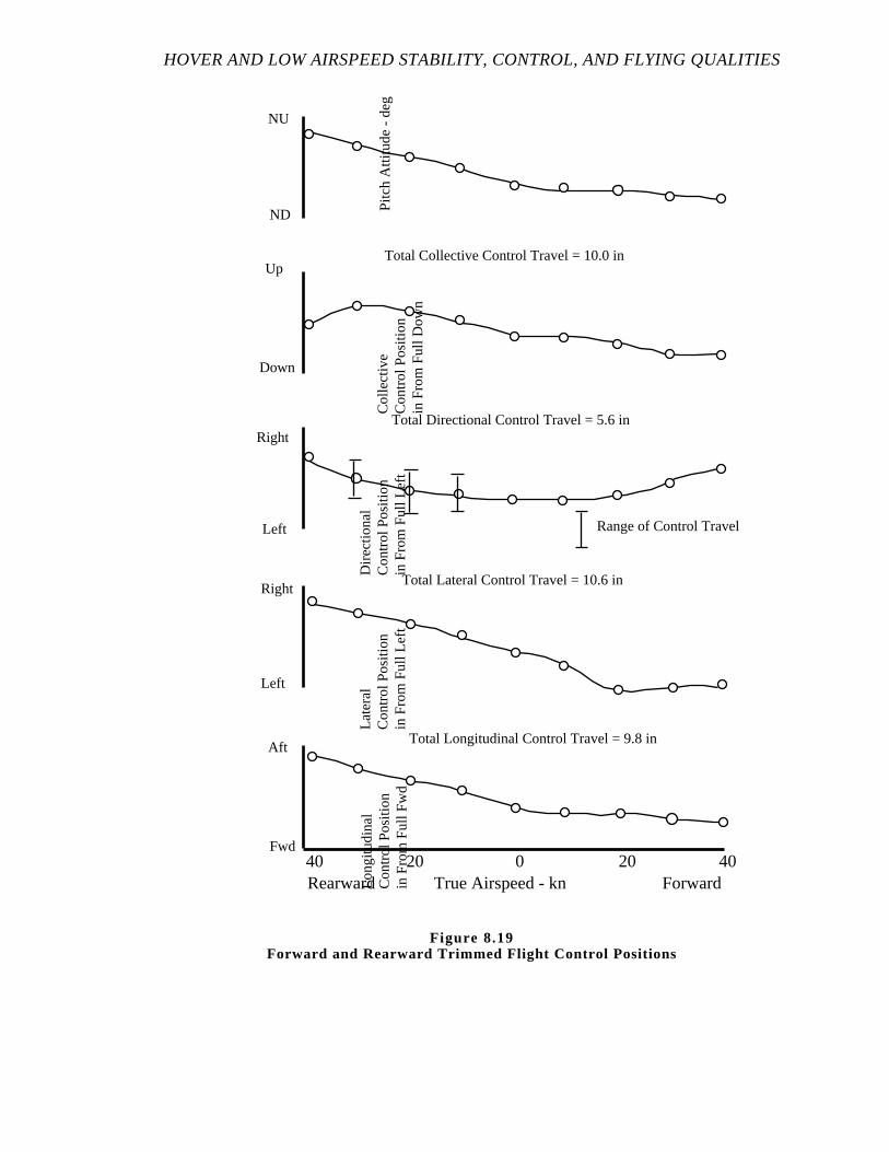
HOVER AND LOW AIRSPEED STABILITY, CONTROL, AND FLYING QUALITIES
True Airspeed - knRearward Forward0 20 402040
Late
ral
Con
trol
Pos
ition
in F
rom
Ful
l Lef
t
Aft
Fwd
Long
itudi
nal
Con
trol
Pos
ition
in F
rom
Ful
l Fw
d
Dire
ctio
nal
Con
trol
Pos
ition
in F
rom
Ful
l Lef
t
Right
Left
Col
lect
ive
Con
trol
Pos
ition
in F
rom
Ful
l Dow
n
Left
Right
Down
Up
Pitc
h A
ttitu
de -
deg
ND
NU
Range of Control Travel
Total Collective Control Travel = 10.0 in
Total Directional Control Travel = 5.6 in
Total Lateral Control Travel = 10.6 in
Total Longitudinal Control Travel = 9.8 in
Figure 8.19Forward and Rearward Trimmed Flight Control Positio ns
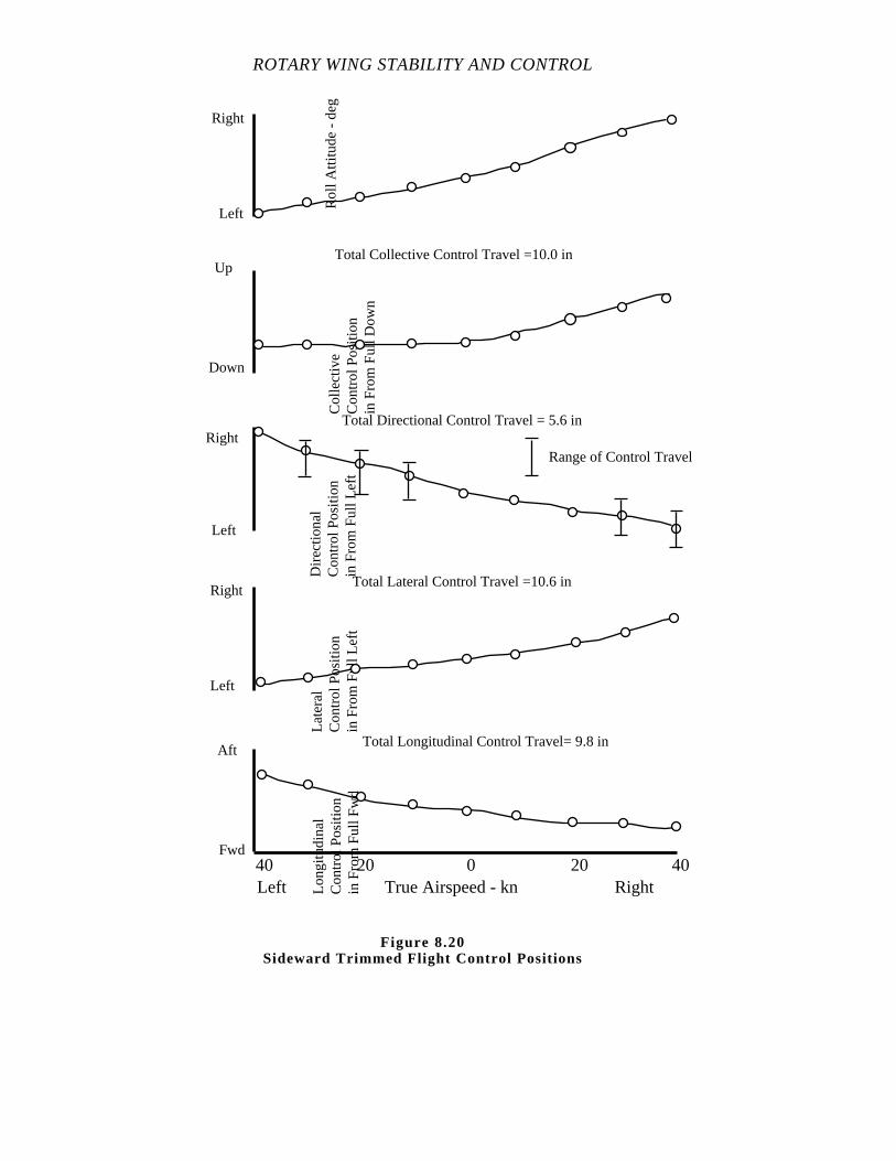
ROTARY WING STABILITY AND CONTROL
True Airspeed - knLeft Right0 20 402040
Late
ral
Con
trol
Pos
ition
in F
rom
Ful
l Lef
t
Aft
Fwd
Long
itudi
nal
Con
trol
Pos
ition
in F
rom
Ful
l Fw
d
Dire
ctio
nal
Con
trol
Pos
ition
in F
rom
Ful
l Lef
t
Right
Left
Col
lect
ive
Con
trol
Pos
ition
in F
rom
Ful
l Dow
n
Left
Right
Down
Up
Rol
l Atti
tude
- d
eg
Left
Right
Range of Control Travel
Total Collective Control Travel =10.0 in
Total Directional Control Travel = 5.6 in
Total Lateral Control Travel =10.6 in
Total Longitudinal Control Travel= 9.8 in
Figure 8.20Sideward Trimmed Flight Control Positions
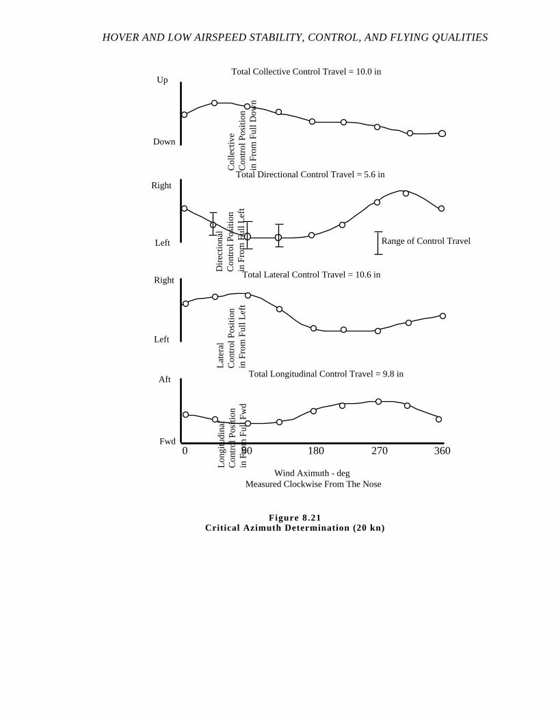
HOVER AND LOW AIRSPEED STABILITY, CONTROL, AND FLYING QUALITIES
180 270 360900
Late
ral
Con
trol
Pos
ition
in F
rom
Ful
l Lef
t
Aft
Fwd
Long
itudi
nal
Con
trol
Pos
ition
in F
rom
Ful
l Fw
d
Dire
ctio
nal
Con
trol
Pos
ition
in F
rom
Ful
l Lef
t
Right
Left
Col
lect
ive
Con
trol
Pos
ition
in F
rom
Ful
l Dow
nLeft
Right
Down
Up
Range of Control Travel
Total Collective Control Travel = 10.0 in
Total Directional Control Travel = 5.6 in
Total Lateral Control Travel = 10.6 in
Total Longitudinal Control Travel = 9.8 in
Wind Aximuth - deg Measured Clockwise From The Nose
Figure 8.21Critical Azimuth Determination (20 kn)
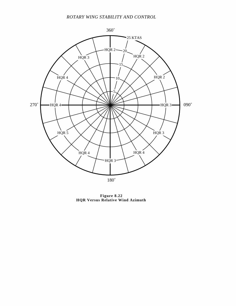
ROTARY WING STABILITY AND CONTROL
360˚
090˚
180˚
270˚
HQR 5
5
10
20
15
25 KTAS
HQR 2
HQR 2
HQR 3
HQR 3
HQR 3
HQR 4HQR 4
HQR 4
HQR 3
HQR 4
HQR 2
Figure 8.22HQR Versus Relative Wind Azimuth
HOVER AND LOW AIRSPEED STABILITY, CONTROL, AND FLYING QUALITIES
8.5.5 Static Stability
Low airspeed static stability is separated generally into longitudinal characteristics
and lateral/directional characteristics. Control position and aircraft attitude data are plotted
versus airspeeds about trim as shown in Figures 8.23 and 8.24. Note that the trim might
not be at zero airspeed depending on the wind conditions at the time of testing.
8.5.6 Long Term Dynamic Stability
Present a representative time history of the aircraft response to a disturbance in the
longitudinal axis. Annotate important and descriptive parameters such asτ, Damped
frequency (ωd), Cycles to one-half amplitude (C1/2), Cycles to double amplitude (Cd),
Time to one-half amplitude (T1/2), and Time to double amplitude (Td). Other parameters of
interest are pitch, roll, and yaw rates. Sample data are presented in Figure 8.25.
Tables are used to summarize the engineering characteristics for several test
conditions (period C1/2, Cd, T1/2, Td, τ, ωd).
8.5.7 Control Response
Time histories are scaled to distinguish the appropriate responses. Present
representative time histories of a 1 in input if available. Proper annotation of the trace is
important to assist the reader in visualizing the response. Definitions of control response
terms are shown in Figure 8.26. Tables and graphs are used to summarize engineering
data for the various responses.
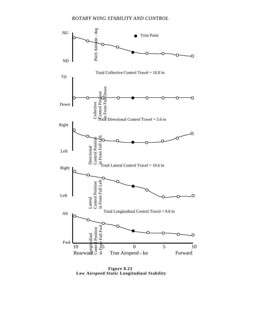
ROTARY WING STABILITY AND CONTROL
True Airspeed - knRearward Forward0 5 10510
Late
ral
Con
trol
Pos
ition
in F
rom
Ful
l Lef
t
Aft
Fwd
Long
itudi
nal
Con
trol
Pos
ition
in F
rom
Ful
l Fw
d
Dire
ctio
nal
Con
trol
Pos
ition
in F
rom
Ful
l Lef
t
Right
Left
Col
lect
ive
Con
trol
Pos
ition
in F
rom
Ful
l Dow
n
Left
Right
Down
Up
Pitc
h A
ttitu
de -
deg
ND
NU
Total Collective Control Travel = 10.0 in
Total Directional Control Travel = 5.6 in
Total Lateral Control Travel = 10.6 in
Total Longitudinal Control Travel = 9.8 in
Trim Point
Figure 8.23 Low Airspeed Static Longitudinal Stability
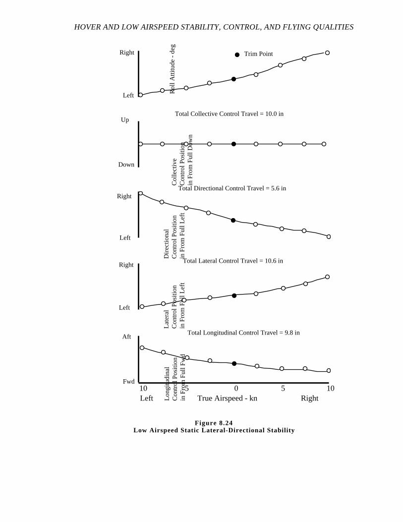
HOVER AND LOW AIRSPEED STABILITY, CONTROL, AND FLYING QUALITIES
True Airspeed - knLeft Right0 5 10510
Late
ral
Con
trol
Pos
ition
in F
rom
Ful
l Lef
t
Aft
Fwd
Long
itudi
nal
Con
trol
Pos
ition
in F
rom
Ful
l Fw
d
Dire
ctio
nal
Con
trol
Pos
ition
in F
rom
Ful
l Lef
t
Right
Left
Col
lect
ive
Con
trol
Pos
ition
in F
rom
Ful
l Dow
n
Left
Right
Down
Up
Rol
l Atti
tude
- d
eg
Left
Right
Total Collective Control Travel = 10.0 in
Total Directional Control Travel = 5.6 in
Total Lateral Control Travel = 10.6 in
Total Longitudinal Control Travel = 9.8 in
Trim Point
Figure 8.24Low Airspeed Static Lateral-Directional Stability

ROTARY WING STABILITY AND CONTROL
Left
Right
Pitc
h A
ttitu
de -
deg
ND
NU
Time - s
NU
ND
Pitc
h R
ate
- de
g/s
Hea
ding
- d
eg
Yaw
Rat
e -
deg/
s
Right
Left
Long
itudi
nal
Con
trol
Pos
ition
in F
rom
f Ful
l Fw
d
Fwd
Aft
τ = 19 s
ζ = 0.085
ωd
= 0.33 rad/s
C1/2
= 1.36
T1/2
= 25 s
Figure 8.25Long Term Response
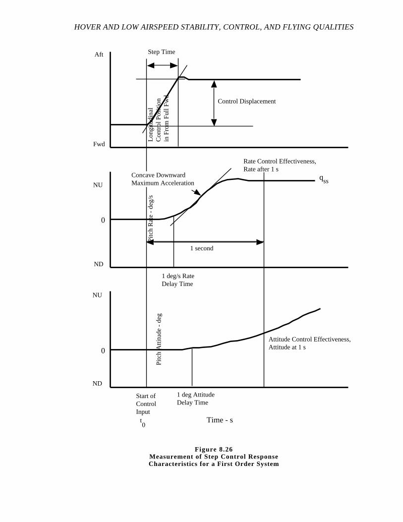
HOVER AND LOW AIRSPEED STABILITY, CONTROL, AND FLYING QUALITIES
Time - s
Step Time
Control Displacement
Pitc
h R
ate
- de
g/s
Fwd
NU
ND
0
qss
1 second
Rate Control Effectiveness,Rate after 1 s
Concave DownwardMaximum Acceleration
Attitude Control Effectiveness,Attitude at 1 s
1 deg AttitudeDelay Time
1 deg/s RateDelay Time
t0
Start ofControlInput
Pitc
h A
ttitu
de -
deg
0
NU
ND
Aft
Long
itudi
nal
Con
trol
Pos
ition
in F
rom
Ful
l Fw
d
Figure 8.26Measurement of Step Control ResponseCharacteristics for a First Order System
ROTARY WING STABILITY AND CONTROL
8.6 DATA ANALYSIS
8.6.1 General
Low airspeed handling qualities are difficult to portray in a pure quantitative
manner. The pilot qualitative comments are the most important product of these
evaluations. The engineering evaluations are conducted to isolate unsatisfactory or
acceptable characteristics. Accurate documentation of the low airspeed flight regime is
necessary because the helicopter operates in this environment much of the time.
8.6.2 Trimmed Control Positions
Low airspeed trimmed flight control positions are essentially analogous to hovering
(zero ground speed) in a wind of equal velocity from the relative azimuth of the direction of
flight. The analysis should include:
1. Were the control margins adequate? Greater than 10% control position or
control power margin?
2. Were control movements required in the usual sense (forward cyclic for
forward airspeed, right lateral cyclic for right lateral flight)?
3. Were the control position changes with power or airspeed excessive?
4. Could the control forces be trimmed to zero?
5. What were the aircraft attitude changes with airspeed?
6. Was field-of-view adequate?
7. Were the vibrations objectionable?
8. Was there any objectionable coupling between pitch, roll, and yaw?
8.6.3 Critical Azimuth
Critical azimuth determination is an extension of low airspeed trimmed flight control
positions and is therefore analogous to hovering in winds of the velocities and azimuths
tested. Critical azimuths for a particular aircraft may be based on control margin remaining,
pitch, roll or yaw excursions, excessive pitch or roll attitudes, excessively large or frequent
control inputs, or high vibration levels. Critical azimuth data analysis should include:
1. What was the limiting factor?
2. For which axis was it most objectionable?
HOVER AND LOW AIRSPEED STABILITY, CONTROL, AND FLYING QUALITIES
3. Were the control margins adequate?
4. Were the control position changes with variation in azimuth excessive?
5. Could the control forces be trimmed to zero?
6. Was field-of-view adequate?
7. Were the vibrations objectionable?
8. Were pitch or roll attitudes excessive?
9. Are these characteristics suitable for the intended mission?
8.6.4 Turn on a Spot
Turn on a spot data analysis is identical to the evaluation of trimmed control
positions and critical azimuth except the pilot must understand different station keeping
cues were used in collecting the two sets of information.
8.6.5 Static Stability
Analysis of low airspeed static stability data should consider the following
questions:
1. Were the control position gradients positive, neutral, or negative?
2. Did the pilot have force cues to an off trim condition?
3. Are the characteristics suitable for the mission?
8.6.6 Long Term Dynamic Stability
Analysis of the long term response should consider the following questions:
1. How easy or difficult was the long term response excited?
2. Using the methods presented in Chapter 3, discuss the response
characteristics (period C1/2, Cd, T1/2, Td, τ, ωd).
3. How does this motion influence the pilot's ability to perform mission tasks?
ROTARY WING STABILITY AND CONTROL
8.6.7 Control Response
An abundance of quantitative data can be taken from the response time histories.
Parameters which define the response are: rate control effectiveness; attitude control
effectiveness; steady-state rate, maximum rate, maximum acceleration, initial acceleration,
acceleration delay, and time constant. The following considerations are an integral part of
control response and effectiveness discussions.
1. Was the steady-state rate adequate?
2. Was the response predictable?
3. Was the response consistent?
4. Were there any over control problems?
5. Was the response suitable for the mission?
8.7 MISSION SUITABILITY
Mission suitability is a very important part of the low airspeed evaluation. The
helicopter's unique capabilities in this flight regime provide many potential operational uses
if the handling qualities and performance of the vehicle are adequate. Before mission
suitability is accessed, a detailed clear understanding of the intendedmission must be
provided. Additionally, the pilot's experience in conducting similar mission maneuvers is
considered. The test pilot must research the mission tasks to establish evaluation
maneuvers and determine performance criteria. The mission maneuvers vary greatly with
aircraft type, intended use and expected operational environment. Potential maneuvers
include everything from sling load operations to rocket firing.
A key element in conducting a mission suitability evaluation is experience. Ensure
all operational aspects are considered. Engineering tests conducted in the low airspeed
regime provide invaluable insight into the reasons for unfavorable comments relative to
operational tasks.
8.8 SPECIFICATION COMPLIANCE
General guidelines for helicopter handling qualities in the hovering and low
airspeed flight regime are contained in MIL-H-8501A. Military specifications are only a
guide. The following list identifies the paragraph number in MIL-H-8501A and a short
description of the requirement.
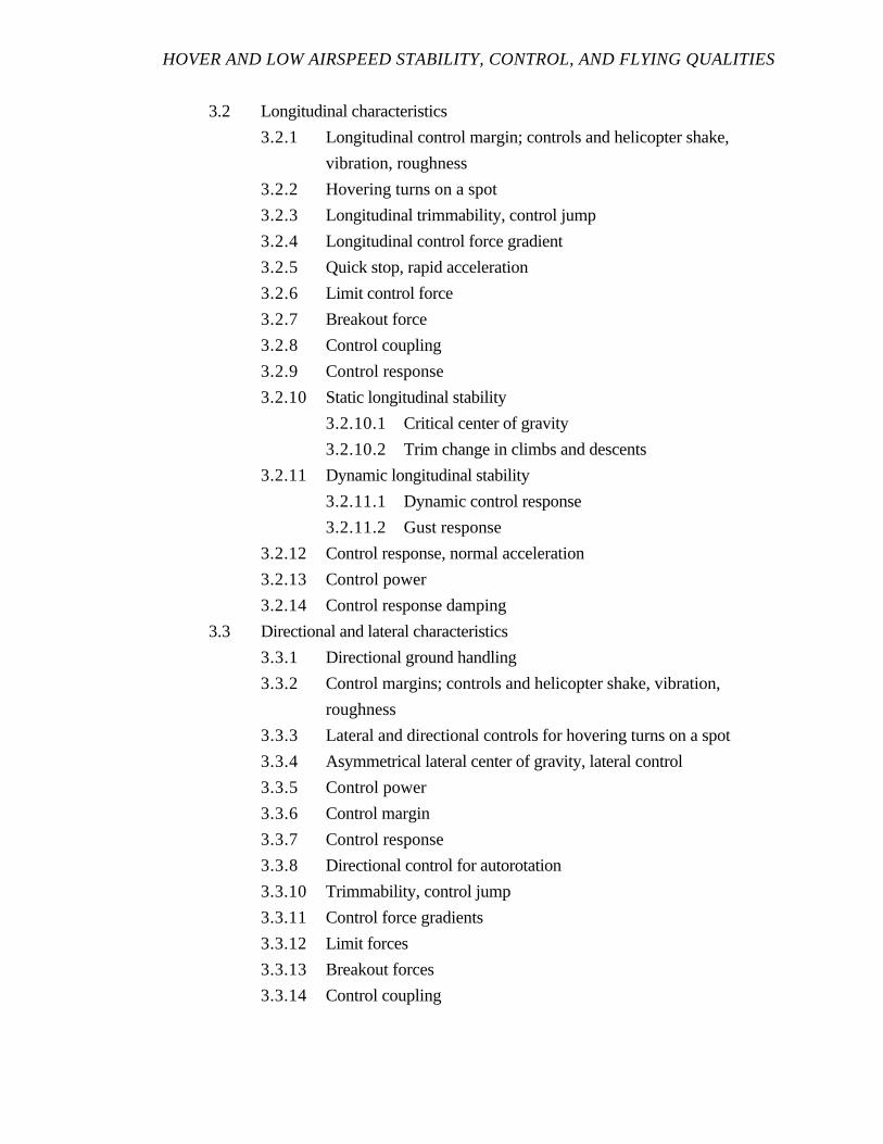
HOVER AND LOW AIRSPEED STABILITY, CONTROL, AND FLYING QUALITIES
3.2 Longitudinal characteristics
3.2.1 Longitudinal control margin; controls and helicopter shake,
vibration, roughness
3.2.2 Hovering turns on a spot
3.2.3 Longitudinal trimmability, control jump
3.2.4 Longitudinal control force gradient
3.2.5 Quick stop, rapid acceleration
3.2.6 Limit control force
3.2.7 Breakout force
3.2.8 Control coupling
3.2.9 Control response
3.2.10 Static longitudinal stability
3.2.10.1 Critical center of gravity
3.2.10.2 Trim change in climbs and descents
3.2.11 Dynamic longitudinal stability
3.2.11.1 Dynamic control response
3.2.11.2 Gust response
3.2.12 Control response, normal acceleration
3.2.13 Control power
3.2.14 Control response damping
3.3 Directional and lateral characteristics
3.3.1 Directional ground handling
3.3.2 Control margins; controls and helicopter shake, vibration,
roughness
3.3.3 Lateral and directional controls for hovering turns on a spot
3.3.4 Asymmetrical lateral center of gravity, lateral control
3.3.5 Control power
3.3.6 Control margin
3.3.7 Control response
3.3.8 Directional control for autorotation
3.3.10 Trimmability, control jump
3.3.11 Control force gradients
3.3.12 Limit forces
3.3.13 Breakout forces
3.3.14 Control coupling
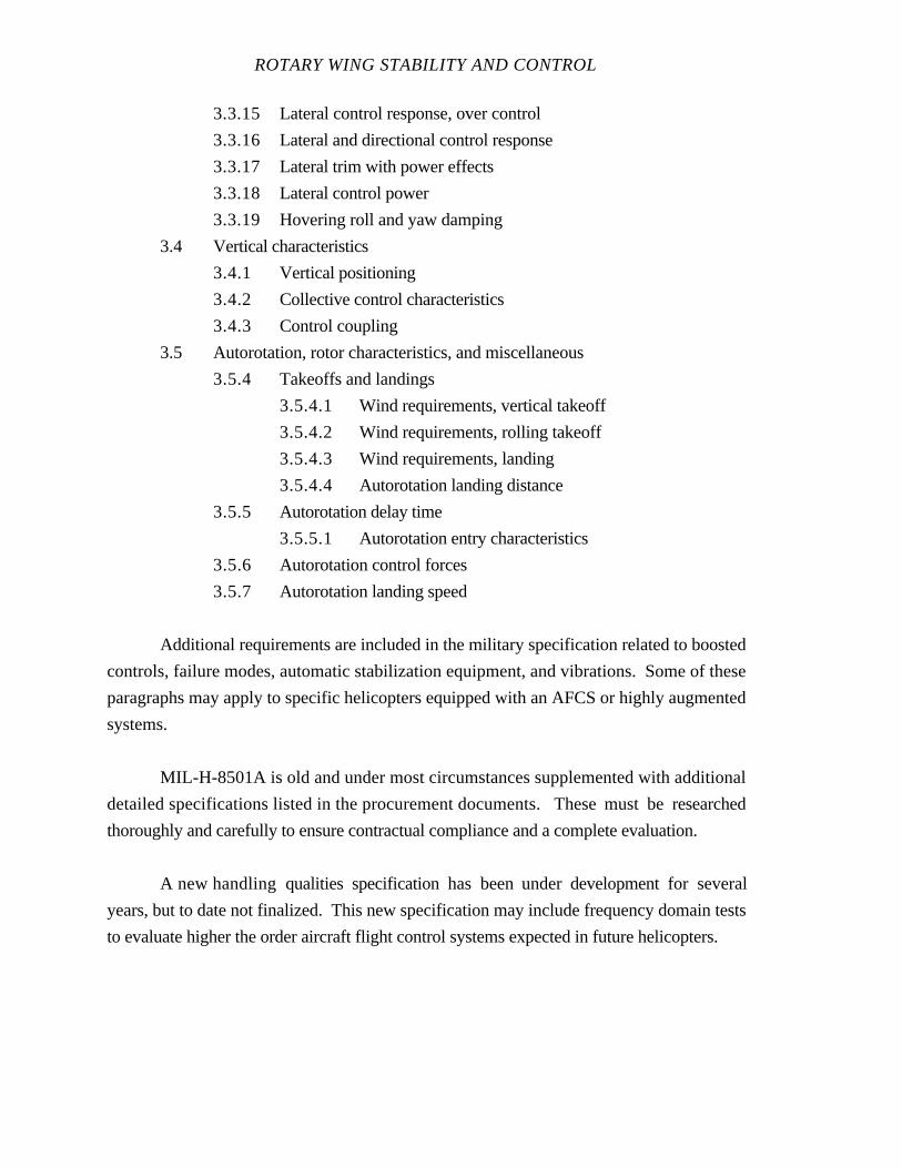
ROTARY WING STABILITY AND CONTROL
3.3.15 Lateral control response, over control
3.3.16 Lateral and directional control response
3.3.17 Lateral trim with power effects
3.3.18 Lateral control power
3.3.19 Hovering roll and yaw damping
3.4 Vertical characteristics
3.4.1 Vertical positioning
3.4.2 Collective control characteristics
3.4.3 Control coupling
3.5 Autorotation, rotor characteristics, and miscellaneous
3.5.4 Takeoffs and landings
3.5.4.1 Wind requirements, vertical takeoff
3.5.4.2 Wind requirements, rolling takeoff
3.5.4.3 Wind requirements, landing
3.5.4.4 Autorotation landing distance
3.5.5 Autorotation delay time
3.5.5.1 Autorotation entry characteristics
3.5.6 Autorotation control forces
3.5.7 Autorotation landing speed
Additional requirements are included in the military specification related to boosted
controls, failure modes, automatic stabilization equipment, and vibrations. Some of these
paragraphs may apply to specific helicopters equipped with an AFCS or highly augmented
systems.
MIL-H-8501A is old and under most circumstances supplemented with additional
detailed specifications listed in the procurement documents. These must be researched
thoroughly and carefully to ensure contractual compliance and a complete evaluation.
A new handling qualities specification has been under developmentfor several
years, but to date not finalized. This new specification may include frequency domain tests
to evaluate higher the order aircraft flight control systems expected in future helicopters.
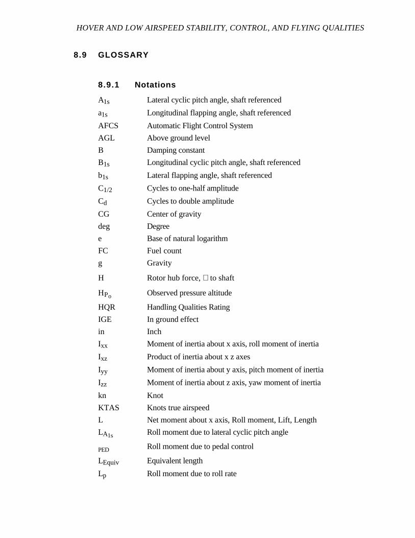
HOVER AND LOW AIRSPEED STABILITY, CONTROL, AND FLYING QUALITIES
8.9 GLOSSARY
8.9.1 Notations
A1s Lateral cyclic pitch angle, shaft referenced
a1s Longitudinal flapping angle, shaft referenced
AFCS Automatic Flight Control System
AGL Above ground level
B Damping constant
B1s Longitudinal cyclic pitch angle, shaft referenced
b1s Lateral flapping angle, shaft referenced
C1/2 Cycles to one-half amplitude
Cd Cycles to double amplitude
CG Center of gravity
deg Degree
e Base of natural logarithm
FC Fuel count
g Gravity
H Rotor hub force, ⊥ to shaft
HPo Observed pressure altitude
HQR Handling Qualities Rating
IGE In ground effect
in Inch
Ixx Moment of inertia about x axis, roll moment of inertia
Ixz Product of inertia about x z axes
Iyy Moment of inertia about y axis, pitch moment of inertia
Izz Moment of inertia about z axis, yaw moment of inertia
kn Knot
KTAS Knots true airspeed
L Net moment about x axis, Roll moment, Lift, Length
LA1s Roll moment due to lateral cyclic pitch angle
PED Roll moment due to pedal control
LEquiv Equivalent length
Lp Roll moment due to roll rate

ROTARY WING STABILITY AND CONTROL
LθTR Roll moment due to tail rotor pitch angle
Lr Roll moment due to yaw rate
Lv Roll moment due to lateral velocity
M Net moment about y axis, Pitch moment
m Mass
MB1s Pitch moment due to longitudinal cyclic pitch angle
MδLONG Pitch moment due to longitudinal control
Mq Pitch moment due to pitch rate
MθC Pitch moment due to collective pitch angle
Mθ Pitch moment due to time rate of change of pitch angle
Mu Pitch moment due to longitudinal velocity
Mw Pitch moment due to vertical velocity
N Net moment about z axis, Yaw moment
NA1s Yaw moment due to lateral cyclic pitch angle
NδLAT Yaw moment due to lateral control
NδPED Yaw moment due to pedal control
Np Yaw moment due to roll rate
NθTR Yaw moment due to tail rotor pitch angle
NR Main rotor speed
Nr Yaw moment due to yaw rate
Nv Yaw moment due to lateral velocity
OGE Out of ground effect
p Angular velocity about x axis, Roll rate
p Angular acceleration about x axis
Q Engine torque
q Angular velocity about y axis, Pitch rate
qss Steady state pitch rate
q Angular acceleration about y axis
r Angular velocity about z axis, Yaw rate
r Angular acceleration about z axis
s Second
T Thrust
t Time
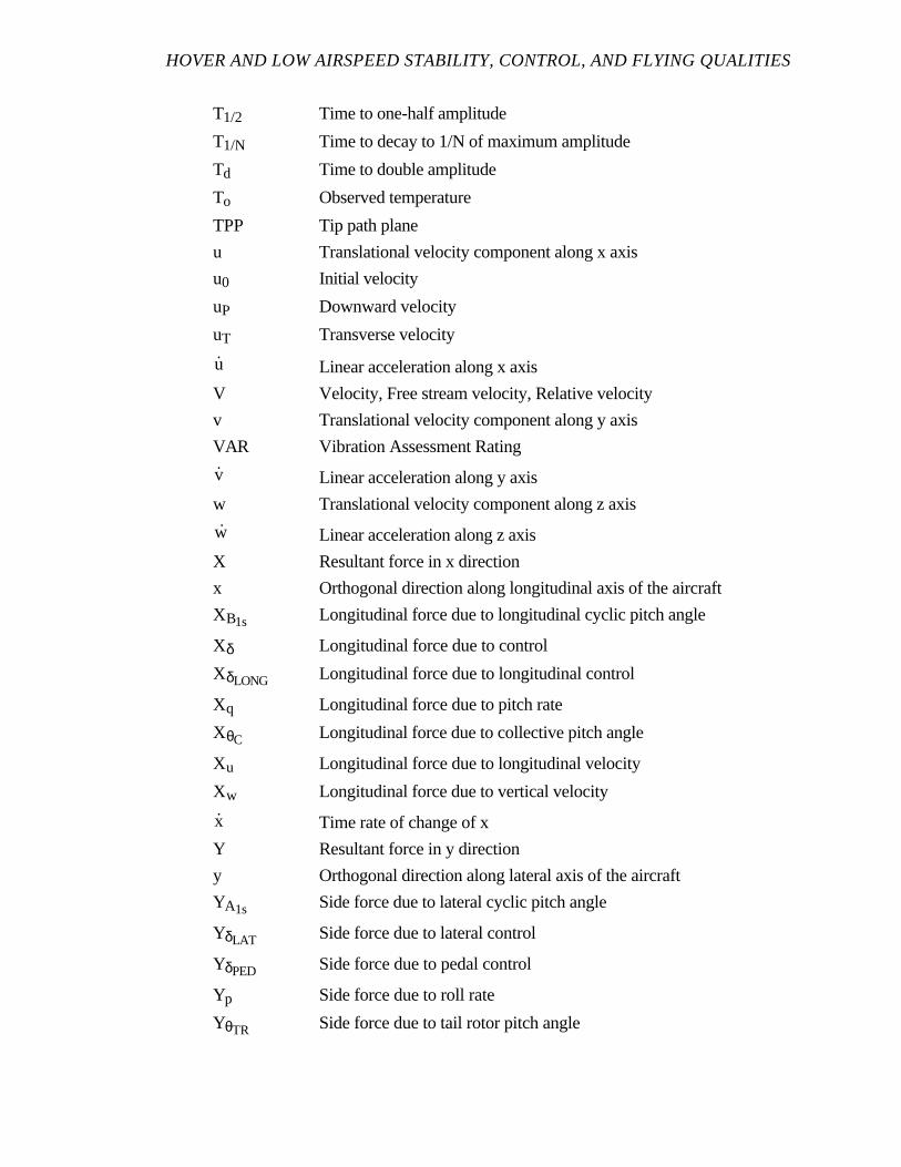
HOVER AND LOW AIRSPEED STABILITY, CONTROL, AND FLYING QUALITIES
T1/2 Time to one-half amplitude
T1/N Time to decay to 1/N of maximum amplitude
Td Time to double amplitude
To Observed temperature
TPP Tip path plane
u Translational velocity component along x axis
u0 Initial velocity
uP Downward velocity
uT Transverse velocity
u Linear acceleration along x axis
V Velocity, Free stream velocity, Relative velocity
v Translational velocity component along y axis
VAR Vibration Assessment Rating
v Linear acceleration along y axis
w Translational velocity component along z axis
w Linear acceleration along z axis
X Resultant force in x direction
x Orthogonal direction along longitudinal axis of the aircraft
XB1s Longitudinal force due to longitudinal cyclic pitch angle
Xδ Longitudinal force due to control
XδLONG Longitudinal force due to longitudinal control
Xq Longitudinal force due to pitch rate
XθC Longitudinal force due to collective pitch angle
Xu Longitudinal force due to longitudinal velocity
Xw Longitudinal force due to vertical velocity
x Time rate of change of x
Y Resultant force in y direction
y Orthogonal direction along lateral axis of the aircraft
YA1s Side force due to lateral cyclic pitch angle
YδLAT Side force due to lateral control
YδPED Side force due to pedal control
Yp Side force due to roll rate
YθTR Side force due to tail rotor pitch angle

ROTARY WING STABILITY AND CONTROL
Yr Side force due to yaw rate
Yu Side force due to longitudinal velocity
Yv Side force due to lateral velocity
Z Resultant force in z direction
z Orthogonal direction along vertical axis of the aircraft
ZB1s Vertical force due to longitudinal cyclic pitch angle
ZδC Vertical force due to collective control
Zq Vertical force due to pitch rate
ZθC Vertical force due to collective pitch angle
Zu Vertical force due to longitudinal velocity
Zw Vertical force due to vertical velocity
8.9.2 Greek Symbols
α (alpha) Angle of attack
αeff Effective angle of attack
δ (delta) Control
δC Collective control
δLAT Lateral control
δLONG Longitudinal control
δPED Pedal control
φ (phi) Roll angle
ϕ (psi) Inflow angle
π (pi) Mathematical constant
θ (theta) Pitch angle, shaft angle
θC Collective pitch angle
θmax Maximum pitch angle
θTR Tail rotor pitch angle
θ Time rate of change in θ
HOVER AND LOW AIRSPEED STABILITY, CONTROL, AND FLYING QUALITIES
θ max Maximum time rate of change in θ
τ (tau) Time constant
ωd (omega) Damped frequency
ζ (zeta) Damping ratio
8.10 REFERENCES
1. Griffin, John M. and Bellaire, Robert G., “A Graphical Summary of
Military Helicopter Flying and Ground Handling Qualities of MIL-H-8501A”, Technical
Report ASNF TN 68-3, Deputy for Engineering, Aeronautical Systems Division, AFSC,
Wright-Patterson Air Force Base, OH, 15 September, 1968.
2. Johnson, W., Helicopter Theory, Princeton University Pres., 1980.
3. Military Specification, "Helicopter Flying and Ground Handling Qualities;
General Requirements For", MIL-H-8501A, with Amendment 1, 3 April, 1962.
4. Naval Test Pilot School Flight Test Manual,Helicopter Stability and
Control, USNTPS-FTM-No. 101, U. S. Naval Test Pilot School, Patuxent River, MD, 10
June 1968, reprinted February 1978.
5. Naval Test Pilot School Flight Test Manual,Helicopter Stability and
Control, Theory and Flight Test Techniques, USNTPS-FTM-No. 105, U. S. Naval Test
Pilot School, Patuxent River, MD, November 1983, Preliminary Edition.
6. Prouty, R. W., Practical Helicopter Aerodynamics, PJS Publications, Inc.,
1982.
7. Prouty, Raymond W.,Helicopter Performance, Stability, and Control,
PWS Publishers, Boston, MA, 1986.
8. Wiesner, W. and Kohler, G., “Tail Rotor Performance in Presence of Main
Rotor, Ground, and Winds”, J.A.H.S., Vol. 15, No. 3, July 1974.

CHAPTER NINE
COUPLED LONGITUDINAL AND LATERAL-DIRECTIONAL STABILITY,
CONTROL, AND FLYING QUALITIES
PAGE
9.1 INTRODUCTION 9.1
9.1.1 Definition of Coupling 9.1
9.2 PURPOSE OF TEST 9.1
9.3 THEORY 9.2
9.3.1 Dominant Coupling Derivatives 9.4
9.3.2 Coupling Derivative Origins 9.7
9.3.2.1 Roll Moment Due to Longitudinal Velocity 9.8
9.3.2.2 Roll Moment Due to Vertical Velocity 9.9
9.3.2.3 Roll Moment Due to Pitch Rate 9.13
9.3.2.4 Roll Moment Due to Longitudinal Cyclic Pitch Angle 9.14
9.3.2.5 Roll Moment Due to Collective Pitch Angle 9.14
9.3.2.6 Roll Moment Due to Tail Rotor Pitch Angle 9.15
9.3.2.7 Pitch Moment Due to Lateral Velocity 9.15
9.3.2.8 Pitch Moment Due to Roll Rate 9.16
9.3.2.9 Pitch Moment Due to Collective Pitch Angle 9.16
9.3.2.10 Pitch Moment Due to Lateral Cyclic Pitch Angle 9.17
9.3.2.11 Pitch Moment Due to Vertical Velocity 9.17
9.3.2.12 Yaw Moment Due to Vertical Velocity 9.18
9.3.2.13 Yaw Moment Due to Roll Rate 9.20
9.3.2.14 Yaw Moment Due to Lateral Cyclic Pitch Angle 9.20
9.3.2.15 Yaw Moment Due to Longitudinal Cyclic Pitch Angle 9.21
9.3.2.16 Yaw Moment Due to Collective Pitch Angle 9.22
9.3.2.17 Yaw Moment Due to Lateral Velocity 9.23
9.3.3 Coupling Perception 9.24
9.3.4 Moments of Inertia 9.25
ROTARY WING STABILITY AND CONTROL
9.3.5 Control Versus Aerodynamic Coupling 9.26
9.3.5.1 Longitudinal and Lateral Cyclic Input Phasing 9.26
9.3.5.2 Mechanical Control Mixing 9.26
9.4 TEST METHODS AND TECHNIQUES 9.28
9.4.1 Trimmed Control Positions 9.28
9.4.1.1 Hover and Low Airspeed 9.29
9.4.1.1.1 Test Technique 9.31
9.4.1.1.2 Data Required 9.32
9.4.1.1.3 Test Criteria 9.32
9.4.1.1.4 Data Requirements 9.33
9.4.1.2 Forward Flight 9.33
9.4.1.2.1 Test Technique 9.33
9.4.1.2.2 Data Required 9.33
9.4.1.2.3 Test Criteria 9.34
9.4.1.2.4 Data Requirements 9.34
9.4.1.3 Steady Turns 9.34
9.4.1.3.1 Test Technique 9.35
9.4.1.3.2 Data Required 9.35
9.4.1.3.3 Test Criteria 9.36
9.4.1.3.4 Data Requirement 9.36
9.4.2 Steady Pull Ups/Push Overs 9.36
9.4.2.1 Test Technique 9.38
9.4.2.2 Data Required 9.38
9.4.2.3 Test Criteria 9.38
9.4.2.4 Data Requirements 9.39
9.4.3 Steady Heading Sideslips 9.39
9.4.4 Control Response 9.39
9.4.4.1 Longitudinal Control Response 9.40
9.4.4.1.1 Test Technique 9.42
9.4.4.1.2 Data Required 9.42
9.4.4.1.3 Test Criteria 9.42
9.4.4.1.4 Data Requirements 9.42
9.4.4.2 Lateral Control Response 9.42
9.4.4.2.1 Test Technique 9.43
9.4.4.2.2 Data Required 9.43
COUPLED LONGITUDINAL AND LATERAL-DIRECTIONAL STABILITY,
CONTROL, AND FLYING QUALITIES
9.4.4.2.3 Test Criteria 9.43
9.4.4.2.4 Data Requirements 9.45
9.4.4.3 Directional Control Response 9.45
9.4.4.3.1 Test Technique 9.45
9.4.4.3.2 Data Required 9.45
9.4.4.3.3 Test Criteria 9.46
9.4.4.3.4 Data Requirements 9.46
9.4.4.4 Vertical Control Response 9.47
9.4.4.4.1 Test Technique 9.47
9.4.4.4.2 Data Required 9.47
9.4.4.4.3 Test Criteria 9.47
9.4.4.4.4 Data Requirements 9.49
9.4.5 Longitudinal Long Term Coupling 9.50
9.4.5.1 Excitation Methods 9.54
9.4.5.2 Test Technique 9.55
9.4.5.3 Data Required 9.55
9.4.5.4 Test Criteria 9.56
9.4.5.5 Data Requirements 9.56
9.4.6 Spiral Motion Coupling 9.56
9.4.6.1 Excitation Methods 9.57
9.4.6.2 Test Technique 9.57
9.4.6.3 Data Required 9.58
9.4.6.4 Test Criteria 9.58
9.4.6.5 Data Requirements 9.58
9.4.7 Lateral-Directional Oscillation Coupling 9.59
9.4.7.1 Excitation Methods 9.59
9.4.7.2 Test Technique 9.60
9.4.7.3 Data Required 9.61
9.4.7.4 Test Criteria 9.61
9.4.7.5 Data Requirements 9.61
9.4.8 Cyclic Only Turns 9.61
9.4.8.1 Test Technique 9.62
9.4.8.2 Data Required 9.63
ROTARY WING STABILITY AND CONTROL
9.4.8.3 Test Criteria 9.63
9.4.8.4 Data Requirements 9.63
9.4.9 Pedal Only Turns 9.63
9.4.9.1 Test Technique 9.64
9.4.9.2 Data Required 9.65
9.4.9.3 Test Criteria 9.65
9.4.9.4 Data Requirements 9.65
9.5 DATA REDUCTION 9.65
9.5.1 Trimmed Control Positions 9.66
9.5.1.1 Hover and Low Airspeed 9.66
9.5.1.2 Forward Flight 9.66
9.5.1.3 Steady Turns 9.66
9.5.2 Steady Pull Ups/Push Overs 9.67
9.5.3 Steady Heading Sideslips 9.67
9.5.4 Control Response 9.68
9.5.5 Longitudinal Long Term Coupling 9.68
9.5.6 Spiral Motion Coupling 9.68
9.5.7 Lateral-Directional Oscillation Coupling 9.68
9.5.8 Cyclic Only Turns 9.69
9.5.9 Pedal Only Turns 9.69
9.6 DATA ANALYSIS 9.69
9.6.1 Trimmed Control Positions 9.69
9.6.1.1 Hover and Low Airspeed 9.69
9.6.1.2 Forward Flight 9.70
9.6.1.3 Steady Turns 9.71
9.6.2 Steady Pull Ups/Push Overs 9.71
9.6.3 Steady Heading Sideslips 9.71
9.6.4 Control Response 9.72
9.6.5 Longitudinal Long Term Coupling 9.75
9.6.6 Spiral Motion Coupling 9.75
9.6.7 Lateral-Directional Oscillation Coupling 9.76
9.6.8 Cyclic Only Turns 9.76
9.6.9 Pedal Only Turns 9.77
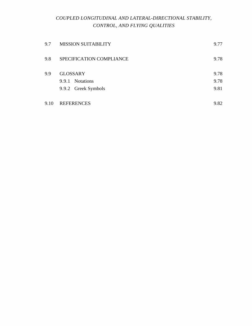
COUPLED LONGITUDINAL AND LATERAL-DIRECTIONAL STABILITY,
CONTROL, AND FLYING QUALITIES
9.7 MISSION SUITABILITY 9.77
9.8 SPECIFICATION COMPLIANCE 9.78
9.9 GLOSSARY 9.78
9.9.1 Notations 9.78
9.9.2 Greek Symbols 9.81
9.10 REFERENCES 9.82
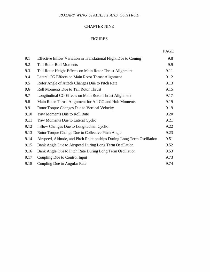
ROTARY WING STABILITY AND CONTROL
CHAPTER NINE
FIGURES
PAGE
9.1 Effective Inflow Variation in Translational Flight Due to Coning 9.8
9.2 Tail Rotor Roll Moments 9.9
9.3 Tail Rotor Height Effects on Main Rotor Thrust Alignment 9.11
9.4 Lateral CG Effects on Main Rotor Thrust Alignment 9.12
9.5 Rotor Angle of Attack Changes Due to Pitch Rate 9.13
9.6 Roll Moments Due to Tail Rotor Thrust 9.15
9.7 Longitudinal CG Effects on Main Rotor Thrust Alignment 9.17
9.8 Main Rotor Thrust Alignment for Aft CG and Hub Moments 9.19
9.9 Rotor Torque Changes Due to Vertical Velocity 9.19
9.10 Yaw Moments Due to Roll Rate 9.20
9.11 Yaw Moments Due to Lateral Cyclic 9.21
9.12 Inflow Changes Due to Longitudinal Cyclic 9.22
9.13 Rotor Torque Change Due to Collective Pitch Angle 9.23
9.14 Airspeed, Altitude, and Pitch Relationships During Long Term Oscillation 9.51
9.15 Bank Angle Due to Airspeed During Long Term Oscillation 9.52
9.16 Bank Angle Due to Pitch Rate During Long Term Oscillation 9.53
9.17 Coupling Due to Control Input 9.73
9.18 Coupling Due to Angular Rate 9.74
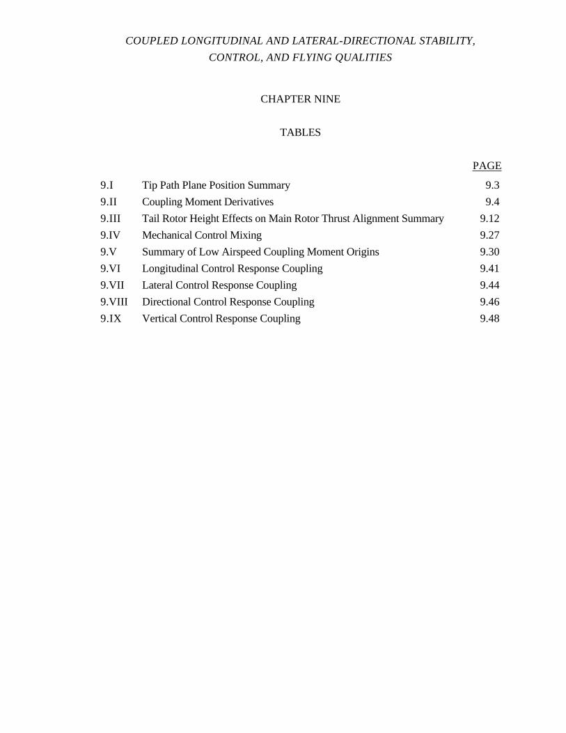
COUPLED LONGITUDINAL AND LATERAL-DIRECTIONAL STABILITY,
CONTROL, AND FLYING QUALITIES
CHAPTER NINE
TABLES
PAGE
9.I Tip Path Plane Position Summary 9.3
9.II Coupling Moment Derivatives 9.4
9.III Tail Rotor Height Effects on Main Rotor Thrust Alignment Summary 9.12
9.IV Mechanical Control Mixing 9.27
9.V Summary of Low Airspeed Coupling Moment Origins 9.30
9.VI Longitudinal Control Response Coupling 9.41
9.VII Lateral Control Response Coupling 9.44
9.VIII Directional Control Response Coupling 9.46
9.IX Vertical Control Response Coupling 9.48
CHAPTER NINE
COUPLED LONGITUDINAL AND LATERAL-DIRECTIONAL
STABILITY, CONTROL, AND FLYING QUALITIES
9.1 INTRODUCTION
Previous chapters address helicopter stability, control, and flying qualities topics
when coupling between aircraft axes is considered negligible or when the pilot suppresses
coupling through manipulation of the flight controls. Helicopters, particularly single rotor
vehicles, have highly non symmetric configurations and are subject to trim and response
coupling between axes. This chapter discusses stability, control, and flying qualities when
longitudinal and lateral-directional coupling is present for hover, low airspeed, and forward
flight. Because of the helicopter’s asymmetric configuration, coupling is a significant factor
in assessing mission related flying qualities in all phases of flight. Understanding,
developing meaningful test procedures, and documenting any undesirable coupling effects
on flying qualities is essential in evaluating a helicopter's ability to perform its mission.
9.1.1 Definition of Coupling
Providing a comprehensive, all inclusive definition is a difficult undertaking;
however, a working definition of coupling is:
“Coupling is the generation of a force along or moment about an aircraft axis
resulting from forces, moments, or disturbances associated with another axis.”
9.2 PURPOSE OF TEST
The purpose of these tests is to evaluate pilot requirements to compensate for
coupling in trimmed steady flight and to suppress coupling in short and long term dynamic
situations. As a minimum, coupling evaluations include:
1. Trim control positions for equilibrium in hover, low airspeed, and forward
flight.
ROTARY WING STABILITY AND CONTROL
2. Trim control positions to maintain steady non-rectilinear flight such as
forward flight turns.
3. Control positions required to perform long term flight condition changes
such as level accelerations, transition to climb, and diving accelerations for ordnance
delivery.
4. Short term, off axis aircraft responses to rapid control inputs.
9.3 THEORY
Linear analysis of helicopter characteristics is used to gain insight into uncoupled
helicopter characteristics. Linear analysis remains a valid tool to investigate the origins and
effects of coupling. The cross-axis derivatives previously neglected, or assumed
suppressed by pilot control inputs, provide the basis for understanding coupling.
Chapter 4 gives insight to the various control and flight condition effects on tip path
plane (TPP) longitudinal flapping angle (a1s) and lateral flapping angle (b1s). In summary,
a1s increases (aft tilt of TPP) are related to negative B1s changes (aft cyclic control
movement), airspeed or advance ratio (µ) increases, increased collective pitch (θC),
negative inflow (λ) changes (upward through rotor), positive roll rates (p), and negative
pitch rates (q). The b1s increases (right tilt of TPP) result from positive A1s changes (right
cyclic control movement), airspeed (µ) increases with a conned rotor, negative pitch rates,
and negative roll rates. The coning angle (a0) represents a balance between blade thrust
forces and blade inertial or centrifugal forces due to rotational velocity. These contributions
to TPP position were developed based on longitudinal translation of the helicopter. In
lateral translation the same types of TPP tilt occurs in an axissystem shifted by 90˚.
Table 9.I summarizes control, airspeed, inflow, and aircraft angular rate contributions to
TPP tilt for longitudinal and lateral translation flight. A review of Table 9.I reveals several
instances where disturbances along or about one axis causes changes with respect to
another axis, or coupling.

COUPLED LONGITUDINAL AND LATERAL-DIRECTIONAL STABILITY,
CONTROL, AND FLYING QUALITIES
Table 9.I
Tip Path Plane Position Summary
PARAMETER FLIGHT CONDITION/TPP TILT INTRODUCED
Forward Translation Right Translationa1s change b1s change a1schange b1schange
Airspeedincrease
Aft tilt Right tilt Aft tilt Left tilt
Inflowdecrease (Upflow)
Aft tilt, no effectin hover
Right tilt duringconing increase,no effect inhover
Aft tilt duringconing increase,no effect inhover
Left tilt, no effectin hover
+B1s * Forward tilt No effect Forward tilt No effect+A1s * No effect Right tilt No effect Right tilt
+θCAft tilt, no effectin hover
Right tilt duringconing increase,no effect inhover
Aft tilt duringconing increase,no effect inhover
Left tilt, no effectin hover
+q (Nose up) Forward tilt Left tilt Forward tilt Left tilt+p (Right) Aft tilt Left tilt Aft tilt Left Tilt* Valid for rotor with zero flapping hinge offset and no flapping springs
Chapter 4 also summarizes the effects of hinge offset on rotor hub moments, and
the shift in cyclic control phasing resulting from the difference between the natural flapping
frequency and the rotor rotational frequency (forcing function frequency). The shift in
cyclic control phasing results in lateral tilt with longitudinal cyclic changes (and vice versa)
if the helicopter designer does not reorient the swashplate inputs to blade pitch. As shown
in Chapter 4, the cyclic phase shift with flapping hinge offset is dependent on blade flap
damping (Lock number/density altitude). The hub moments available through flapping
hinge offset provide one method of trimming the helicopter for equilibrium or steady flight
in conditions where the rotor thrust axis is not aligned through the helicopter center of
gravity (CG). Thrust offset from the CG can result in cross axis response when thrust
changes occur.
The configuration of the single rotor helicopter plays a significant part in inter-axis
response or coupling. Main rotor torque changes and tail rotor vertical position are
substantial contributors. For example, main rotor torque changes resulting from collective
and inflow change produce yawing moments. High tail rotor thrust lines produce roll
moments with directional control inputs.
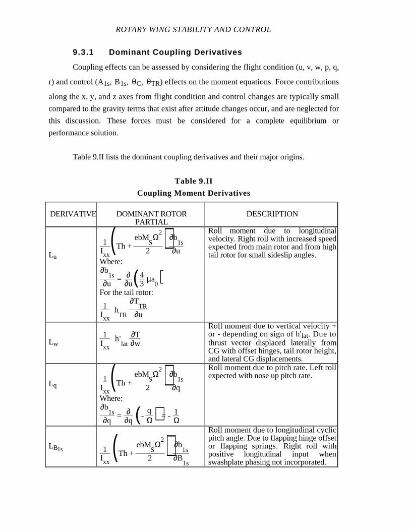
ROTARY WING STABILITY AND CONTROL
9.3.1 Dominant Coupling Derivatives
Coupling effects can be assessed by considering the flight condition (u, v, w, p, q,
r) and control (A1s, B1s, θC, θTR) effects on the moment equations. Force contributions
along the x, y, and z axes from flight condition and control changes are typically small
compared to the gravity terms that exist after attitude changes occur, and are neglected for
this discussion. These forces must be considered for a complete equilibrium or
performance solution.
Table 9.II lists the dominant coupling derivatives and their major origins.
Table 9.II
Coupling Moment Derivatives
DERIVATIVE DOMINANT ROTORPARTIAL
DESCRIPTION
Lu
1Ixx
(Th + ebM
SΩ
2
2)∂b
1s∂u
Where:∂b
1s∂u
= ∂∂u( 4
3µa
0)For the tail rotor:
1Ixx
hTR
∂TTR
∂u
Roll moment due to longitudinalvelocity. Right roll with increased speedexpected from main rotor and from hightail rotor for small sideslip angles.
Lw1
Ixx h'
lat∂T∂w
Roll moment due to vertical velocity +or - depending on sign of h'lat. Due tothrust vector displaced laterally fromCG with offset hinges, tail rotor height,and lateral CG displacements.
Lq1
Ixx(Th +
ebMSΩ
2
2)∂b
1s∂q
Where:∂b
1s∂q
= ∂∂q (-
qΩ) = - 1Ω
Roll moment due to pitch rate. Left rollexpected with nose up pitch rate.
LB1s 1Ixx
(Th + ebM
SΩ
2
2) ∂b
1s∂B
1s
Roll moment due to longitudinal cyclicpitch angle. Due to flapping hinge offsetor flapping springs. Right roll withpositive longitudinal input whenswashplate phasing not incorporated.
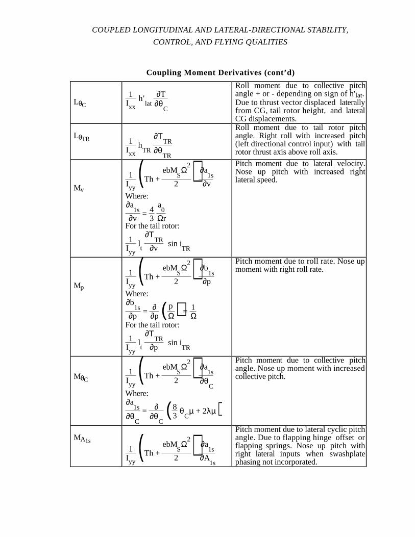
COUPLED LONGITUDINAL AND LATERAL-DIRECTIONAL STABILITY,
CONTROL, AND FLYING QUALITIES
Coupling Moment Derivatives (cont’d)
LθC
1Ixx
h'lat
∂T∂θ
C
Roll moment due to collective pitchangle + or - depending on sign of h'lat.Due to thrust vector displaced laterallyfrom CG, tail rotor height, and lateralCG displacements.
LθTR 1Ixx
hTR
∂ΤTR
∂θTR
Roll moment due to tail rotor pitchangle. Right roll with increased pitch(left directional control input) with tailrotor thrust axis above roll axis.
Mv
1Iyy
(Th + ebM
SΩ
2
2) ∂a
1s∂v
Where:∂a
1s∂v
= 43
a0
ΩrFor the tail rotor:
1Iyy
lt
∂ΤTR
∂v sin i
TR
Pitch moment due to lateral velocity.Nose up pitch with increased rightlateral speed.
Mp
1Iyy
(Th + ebM
SΩ
2
2) ∂b
1s∂p
Where:∂b
1s∂p
= ∂∂p ( p
Ω) = 1ΩFor the tail rotor:
1Iyy
lt
∂ΤTR
∂p sin i
TR
Pitch moment due to roll rate. Nose upmoment with right roll rate.
MθC1
Iyy(Th +
ebMSΩ
2
2) ∂a
1s
∂θC
Where:∂a
1s
∂θC
= ∂∂θ
C( 8
3θ
Cµ + 2λµ)
Pitch moment due to collective pitchangle. Nose up moment with increasedcollective pitch.
MA1s
1Iyy
(Th + ebM
SΩ
2
2) ∂a
1s∂A
1s
Pitch moment due to lateral cyclic pitchangle. Due to flapping hinge offset orflapping springs. Nose up pitch withright lateral inputs when swashplatephasing not incorporated.

ROTARY WING STABILITY AND CONTROL
Coupling Moment Derivatives (cont’d)
MθTR 1Iyy
lt
∂ΤTR
∂θTR
sin iTR
Pitch moment due to tail rotor pitchangle. Due to inclination of tail rotorthrust vector out of vertical plane.
Nw 1Izz
∂QMR
∂w
Yaw moment due to vertical velocity.Nose left moment with increased(downward) vertical speed, torquedecreases as inflow increases.
Np1Izz
lt
∂ΤTR
∂pWhere:∂T
TR∂p
= hTR
∂TTR
∂v
Yaw moment due to roll rate. Noseright moment with right roll rate whentail rotor thrust axis above roll axis.
NA1s 1Izz
Th' ∂b
1s∂A
1s
Yaw moment due to lateral cyclic pitchangle. Adverse/proverse yaw, adverseis nose left yaw moment with rightlateral control input.
NB1s1Izz
∂QMR
∂B1s
alternatively,
1Izz
∂QMR
∂wrotor
∂wrotor
∂B1s
Yaw moment due to longitudinal cyclicpitch angle. Nose right moment withforward longitudinal input.
NθC1Izz
∂QMR
∂θC
Yaw moment due to collective pitchangle. Nose right moment withincreased collective pitch.
Where:
a0 - Coning angle
A1s - Lateral cyclic pitch angle, shaft referenced
a1s - Longitudinal flapping angle, shaft referenced
b - Number of blades
B1s - Longitudinal cyclic pitch angle, shaft referenced
b1s - Lateral flapping angle, shaft referenced
e - Flapping hinge offset
h - Height of hub above CG
h'lat - Lateral distance between the rotor shaft and the CG
hTR - Height of the tail rotor above CG
iTR - Tail rotor inclination out of vertical plane
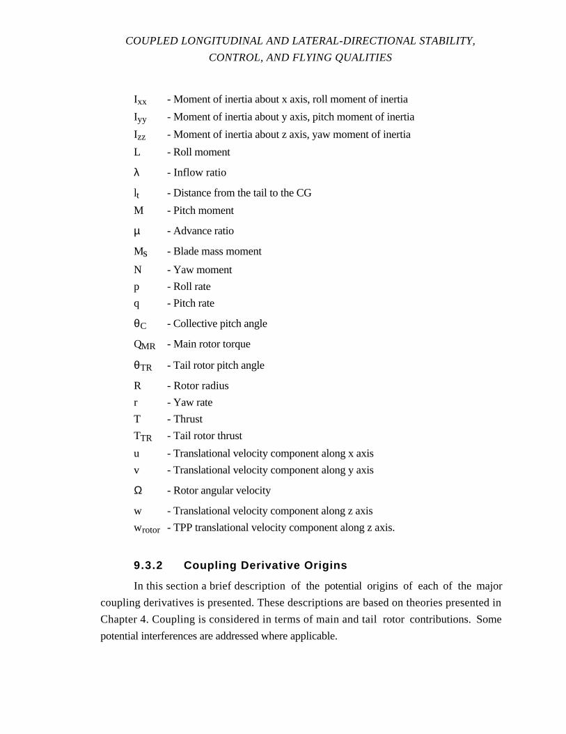
COUPLED LONGITUDINAL AND LATERAL-DIRECTIONAL STABILITY,
CONTROL, AND FLYING QUALITIES
Ixx - Moment of inertia about x axis, roll moment of inertia
Iyy - Moment of inertia about y axis, pitch moment of inertia
Izz - Moment of inertia about z axis, yaw moment of inertia
L - Roll moment
λ - Inflow ratio
lt - Distance from the tail to the CG
M - Pitch moment
µ - Advance ratio
Ms - Blade mass moment
N - Yaw moment
p - Roll rate
q - Pitch rate
θC - Collective pitch angle
QMR - Main rotor torque
θTR - Tail rotor pitch angle
R - Rotor radius
r - Yaw rate
T - Thrust
TTR - Tail rotor thrust
u - Translational velocity component along x axis
v - Translational velocity component along y axis
Ω - Rotor angular velocity
w - Translational velocity component along z axis
wrotor - TPP translational velocity component along z axis.
9.3.2 Coupling Derivative Origins
In this section a brief description of the potential origins of each ofthe major
coupling derivatives is presented. These descriptions are based on theories presented in
Chapter 4. Coupling is considered in terms of main and tail rotor contributions. Some
potential interferences are addressed where applicable.
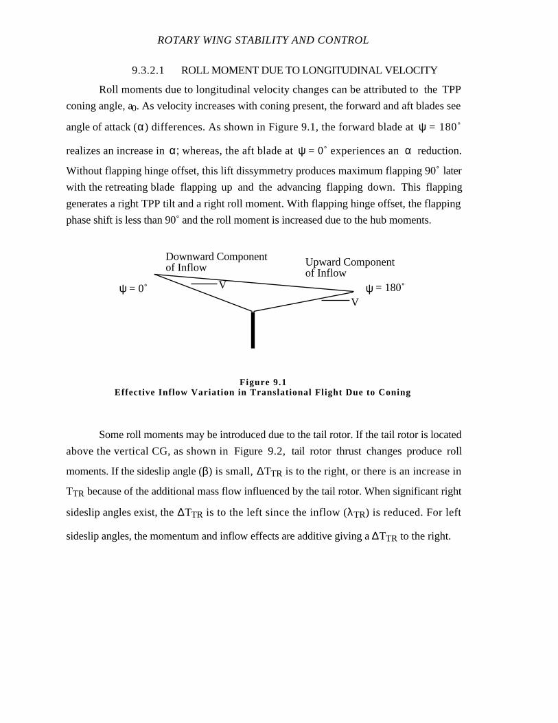
ROTARY WING STABILITY AND CONTROL
9.3.2.1 ROLL MOMENT DUE TO LONGITUDINAL VELOCITY
Roll moments due to longitudinal velocity changes can be attributed to the TPP
coning angle, a0. As velocity increases with coning present, the forward and aft blades see
angle of attack (α) differences. As shown in Figure 9.1, the forward blade at ψ = 180˚
realizes an increase in α; whereas, the aft blade at ψ = 0˚ experiences an α reduction.
Without flapping hinge offset, this lift dissymmetry produces maximum flapping 90˚ later
with the retreating blade flapping up and the advancing flapping down. This flapping
generates a right TPP tilt and a right roll moment. With flapping hinge offset, the flapping
phase shift is less than 90˚ and the roll moment is increased due to the hub moments.
Some roll moments may be introduced due to the tail rotor. If the tail rotor is located
above the vertical CG, as shown in Figure 9.2, tail rotor thrust changes produce roll
moments. If the sideslip angle (β) is small, ∆TTR is to the right, or there is an increase in
TTR because of the additional mass flow influenced by the tail rotor. When significant right
sideslip angles exist, the ∆TTR is to the left since the inflow (λTR) is reduced. For left
sideslip angles, the momentum and inflow effects are additive giving a ∆TTR to the right.
Upward Componentof Inflow
Downward Componentof Inflow
V
Vψ = 0˚ ψ = 180˚
Figure 9.1Effective Inflow Variation in Translational Flight Due to Coning
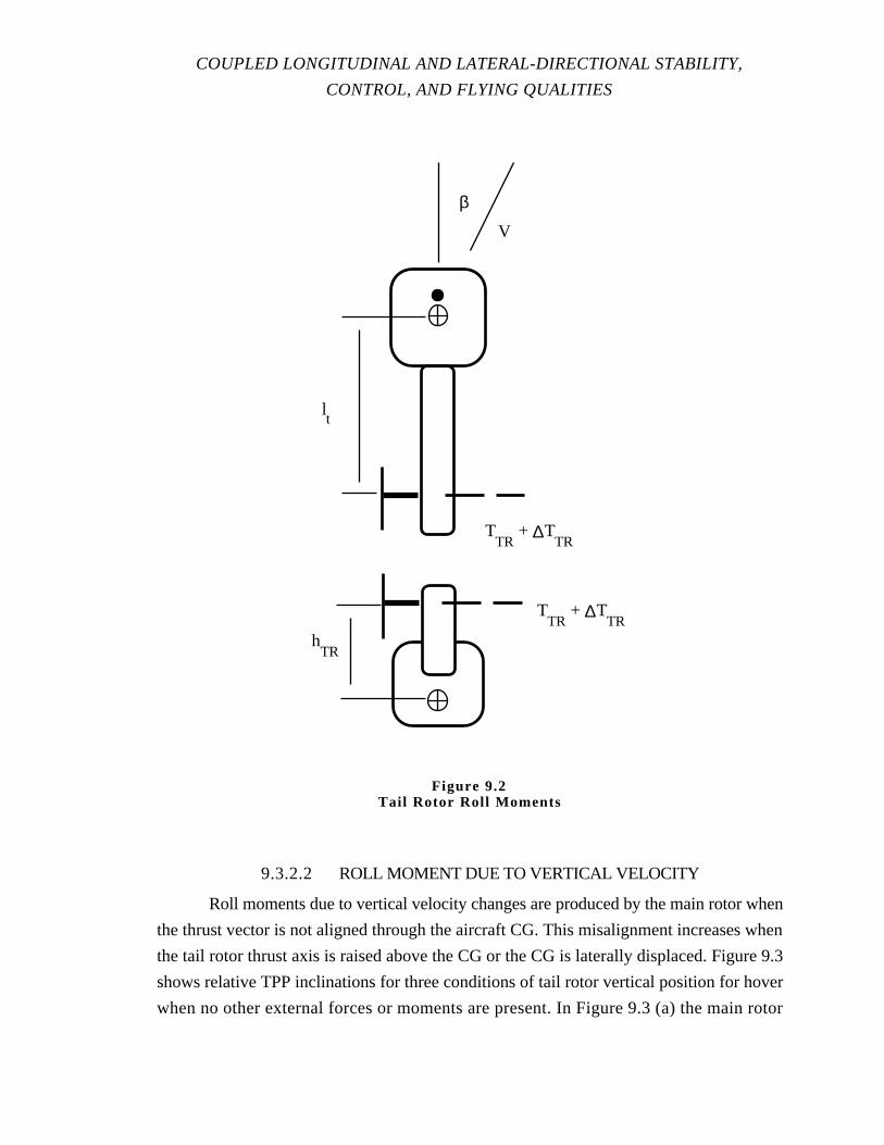
COUPLED LONGITUDINAL AND LATERAL-DIRECTIONAL STABILITY,
CONTROL, AND FLYING QUALITIES
9.3.2.2 ROLL MOMENT DUE TO VERTICAL VELOCITY
Roll moments due to vertical velocity changes are produced by the main rotor when
the thrust vector is not aligned through the aircraft CG. This misalignment increases when
the tail rotor thrust axis is raised above the CG or the CG is laterally displaced. Figure 9.3
shows relative TPP inclinations for three conditions of tail rotor vertical position for hover
when no other external forces or moments are present. In Figure 9.3 (a) the main rotor
lt
β
V
TTR
+ ∆TTR
hTR
TTR
+ ∆TTR
Figure 9.2Tail Rotor Roll Moments

ROTARY WING STABILITY AND CONTROL
thrust (T), TTR and weight (W) all act through the CG and produce no moments. The main
rotor thrust balances the weight component (W cosφ) and the weight component (W sin φ)
balances the TTR. For Figure 9.3 (b), left TPP tilt is required to balance the tail rotor
moment (hTTR). The left TPP tilt also produces a hub moment to the left.The lateral
component of T and the TTR are balanced by the weight component (W sinφ). The
moments produced by TTR are balanced by the hub moment and the thrust axis offset (right
of CG). In Figure 9.3 (c) the helicopter is level laterally and the TTR is balanced by
T sinb1s. The higher tail rotor location produces larger right roll moments which are
balanced by the component Tsinb1s and the hub moment. As shown in Figure 9.3, the
trend for increased tail rotor height is increased right bank angle and left TPP tilt. If hub
moments are not available, the left tilt of the TPP with higher tail rotors is accentuated since
greater thrust induced roll moments are required to counter tail rotor roll moments.
Although Figure 9.3 is for hover, the concept applies to all flight regimes. Table 9.III
summarizes the conditions depicted in Figure 9.3. The greatertail rotor heights cause
increased main rotor thrust misalignment with the CG.
Thrust changes occur from vertical velocity changes producing roll moments
proportional to the distance from the CG to the main rotor thrust axis. Thrust changes result
from rotor inflow variations with vertical speed.
Lateral CG displacement from the main rotor shaft with flapping hinge offset is
depicted in Figure 9.4 for hover. Tail rotor thrust is assumed to act through the CG for
simplification. As shown, the helicopter requires increased bank angle in the direction of
the CG displacement. The rotor thrust produces a left roll moment which is balanced by the
hub moment LH. Vertical velocity changes with the attendant thrust change cause roll
moments in the direction of thrust change.
A secondary contribution to the roll moment in forward flight exists since the thrust
changes cause coning changes. These coning changes produce lateral TPP tilt of magnitude
4/3 µa0. The coning changes are transient in nature and subside as the inflow changes
during the subsequent helicopter response.
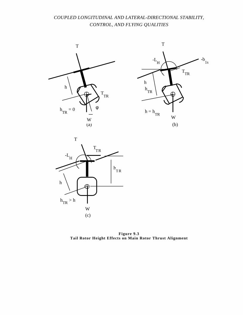
COUPLED LONGITUDINAL AND LATERAL-DIRECTIONAL STABILITY,
CONTROL, AND FLYING QUALITIES
hTR
h
T
TTR
h
T
TTR
h
T
φ
(a)
hTR
= 0
TTR
W W
(b)
-LH
-b1s
h = hTR
-LH
hTR
hTR
> h
(c)W
Figure 9.3Tail Rotor Height Effects on Main Rotor Thrust Alig nment
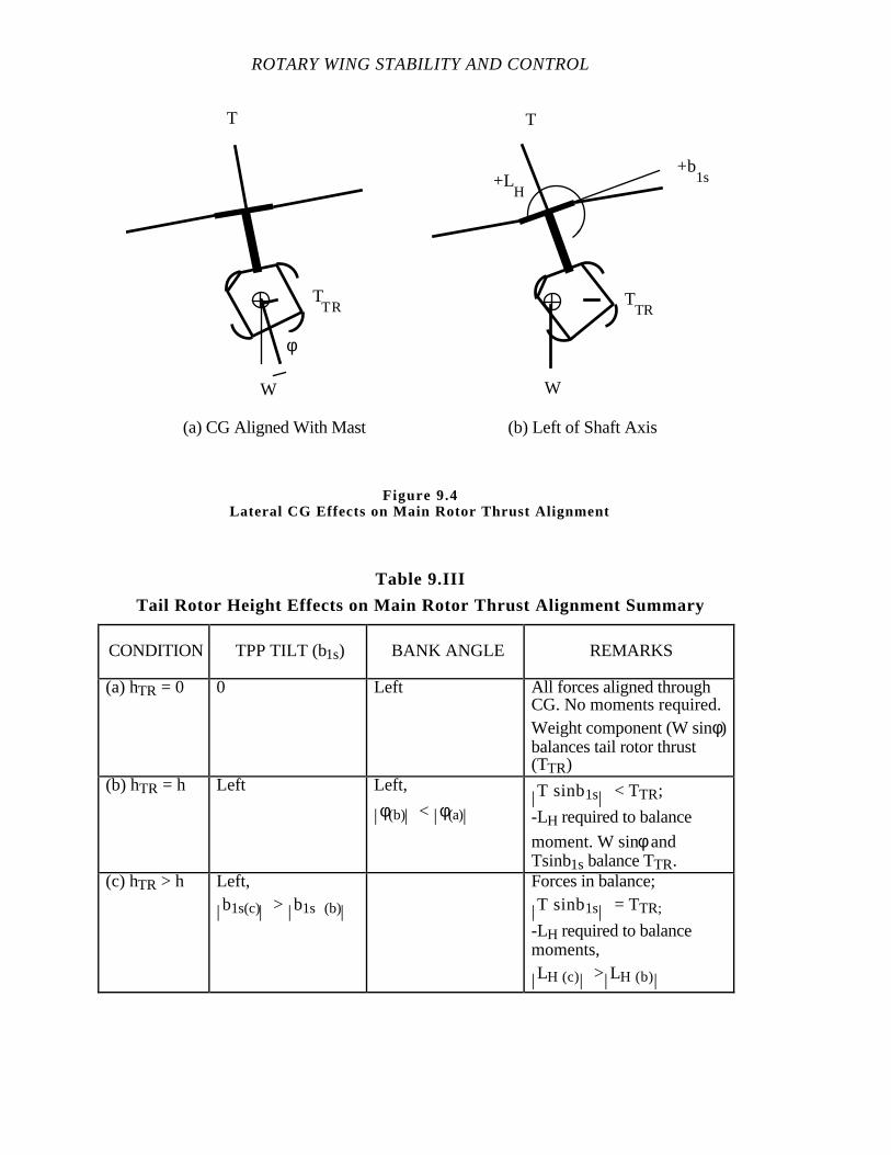
ROTARY WING STABILITY AND CONTROL
Table 9.III
Tail Rotor Height Effects on Main Rotor Thrust Alig nment Summary
CONDITION TPP TILT (b1s) BANK ANGLE REMARKS
(a) hTR = 0 0 Left All forces aligned throughCG. No moments required.Weight component (W sinφ)balances tail rotor thrust(TTR)
(b) hTR = h Left Left,
| |φ(b) < | |φ(a)| |T sinb1s < TTR;
-LH required to balance
moment. W sinφ andTsinb1s balance TTR.
(c) hTR > h Left,
| |b1s(c) > | |b1s (b)
Forces in balance;
| |T sinb1s = TTR;
-LH required to balancemoments,
| |LH (c) >| |LH (b)
T
TTR
T
φ
(a) CG Aligned With Mast
TTR
W W
(b) Left of Shaft Axis
+b1s+L
H
Figure 9.4Lateral CG Effects on Main Rotor Thrust Alignment
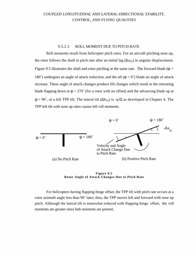
COUPLED LONGITUDINAL AND LATERAL-DIRECTIONAL STABILITY,
CONTROL, AND FLYING QUALITIES
9.3.2.3 ROLL MOMENT DUE TO PITCH RATE
Roll moments result from helicopter pitch rates. For an aircraft pitching nose up,
the rotor follows the shaft in pitch rate after an initial lag (∆a1s) in angular displacement.
Figure 9.5 illustrates the shaft and rotor pitching at the same rate. The forward blade (ψ =
180˚) undergoes an angle of attack reduction, and the aft (ψ = 0˚) blade an angle of attack
increase. These angle of attack changes produce lift changes which result in the retreating
blade flapping down at ψ = 270˚ (for a rotor with no offset) and the advancing blade up at
ψ = 90˚, or a left TPP tilt. The lateral tilt (∆b1s) is -q/Ω as developed in Chapter 4. The
TPP left tilt with nose up rates causes left roll moments.
For helicopters having flapping hinge offset, the TPP tilt with pitch rate occurs at a
rotor azimuth angle less than 90˚ later; thus, the TPP moves left and forward with nose up
pitch. Although the lateral tilt is somewhat reduced with flapping hinge offset, the roll
moments are greater since hub moments are present.
ψ = 0˚
ψ = 0˚
ψ = 180˚
ψ = 180˚
-∆a1s
Velocity and Angleof Attack Change Dueto Pitch Rate
(a) No Pitch Rate (b) Positive Pitch Rate
Figure 9.5Rotor Angle of Attack Changes Due to Pitch Rate
ROTARY WING STABILITY AND CONTROL
9.3.2.4 ROLL MOMENT DUE TO LONGITUDINAL CYCLIC PITCH
ANGLE
A rotor without flapping hinge offset normally is rigged so longitudinal cyclic
control movements produce the maximum cyclic pitch changes at blade azimuth positions
of 90˚ and 270˚. This rigging configuration is a natural fallout of the 90˚ phase shift which
occurs for an oscillatory system forced at its natural frequency. When flapping hinge offset
or flapping springs are used, the blade natural flapping frequency becomes greater than the
blade rotating frequency. The result is a phase shift of less than 90˚. The magnitude of this
shift depends on the frequency ratio (ω/ωn) and blade damping which is affected by Lock
number or density altitude. The frequency ratio is dependent on both spring stiffness and
rotor speed when flapping springs are used, and only on the offset dimension when
flapping hinge offset is present.
During design of the helicopter, efforts are made to phase the cyclic pitch inputs to
account for flapping phase shifts less than 90˚. For example, if the sea level phase shift for
a rotor with flapping hinge offset is 84˚, the swashplate to pitch change rigging might be
such that longitudinal cyclic control movements produce maximum cyclic pitch changes at
rotor azimuths of 96˚ and 276˚. The same logic is used for lateral controls. By properly
phasing the swashplate, flapping responses for pure longitudinal control inputs are purely
longitudinal, and lateral control inputs, purely lateral.
If the helicopter designer did not consider rotor phasing requirements, or if the
helicopter is operated off design (density altitude for flapping hinge offset; density altitude
and rotor speed for flapping springs), roll moments are generated with longitudinal control
movements. In the case of the 84˚ phase angle example, failure to compensate results in a
roll moment 10.5% of the pitch moment. The roll acceleration could be higher considering
differences in aircraft moments of inertia. Moment of inertia effects are addressed in a
subsequent section.
9.3.2.5 ROLL MOMENT DUE TO COLLECTIVE PITCH ANGLE
Roll moments due to collective pitch changes have the same origins as the roll
moment due to vertical speed changes. The difference is the mechanics of thrust and coning
change due to collective pitch rather than vertical velocity.

COUPLED LONGITUDINAL AND LATERAL-DIRECTIONAL STABILITY,
CONTROL, AND FLYING QUALITIES
9.3.2.6 ROLL MOMENT DUE TO TAIL ROTOR PITCH ANGLE
Roll moments due to tail rotor pitch angle changes occur when the tail rotor thrust
axis does not pass through the helicopter CG. Figure 9.6 illustrates this concept for a tail
rotor mounted above the CG. If a left directional control input is made to produce a left
yawing moment, tail rotor thrust (∆TTR) is increased to the right. The increased tail rotor
thrust results in right roll moments in addition to the desired left yaw moment.
9.3.2.7 PITCH MOMENT DUE TO LATERAL VELOCITY
The origins of the pitch moment due to the main rotor are analogous to the roll
moment origins. Therefore, the description of coupled pitching moment origins is
presented in less detail.
The pitch moment due to lateral velocity results from rotor coning. The rotor
flapping equations developed in Chapter 4 can be reoriented for sideward flight. An
increase in right sideward flight velocity causes an aft TPP tilt through the coning term
similar to the increase in forward velocity producing a right TPP tilt increment. The aft tilt
of the TPP with right translational velocities results in nose up pitching moments.
hTR
TTR
+ ∆TTR
Figure 9.6Roll Moments Due to Tail Rotor Thrust
ROTARY WING STABILITY AND CONTROL
Pitch moments due to lateral velocity also result when the tail rotor is inclined out of
the vertical plane. Tail rotor thrust changes caused by lateral velocity have components in
the vertical direction thereby producing pitching moments. For a tail rotor providing an
upward thrust component, an increase in right lateral velocity results in a decrease in tail
rotor thrust and a nose up pitch.
9.3.2.8 PITCH MOMENT DUE TO ROLL RATE
The pitching moment due to roll rate results from increased blade angle of attack
changes on the downward blade and reduced angle of attack for the upward blade of a
rolling rotor. The maximum flapping caused by the blade angle of attack changes occurs
90˚ later in rotor azimuth when flapping hinge offset or flapping springs are not used, and
less than 90˚ later when flapping hinge offset/flapping springs are incorporated. Thus a
rotor experiencing a right roll rate experiences aft TPP tilt (∆a1s) of magnitude p/Ω.
Pitch moments due to roll rate result when the tail rotor is inclined out of the vertical
plane. When the helicopter is rolling to the right with a high tail rotor, the inflow change at
the tail rotor reduces its thrust. For an upward canted tail rotor, the tail rotor thrust has a
vertical component and a thrust reduction produces a nose up pitch moment.
9.3.2.9 PITCH MOMENT DUE TO COLLECTIVE PITCH ANGLE
In hover, pitch moments due to collective pitch angle are present when the thrust
axis is not aligned with the helicopter CG. Figure 9.7 shows a hovering helicopter with
flapping hinge offset and with no external forces or moments involved. If the CG is aligned
longitudinally beneath the rotor shaft, the helicopter hovers as shown in Figure 9.7 (a)
without longitudinal cyclic input or TPP tilt. As the CG is moved aft, forward cyclic and
forward TPP tilt are required for equilibrium. A nose down hub moment (-MH) is balanced
by a nose up moment due to thrust. An increase in thrust from an up collective movement
results in a nose up pitching moment.
In forward flight, the location of the thrust axis relative to the longitudinal CG
location causes pitching moments with collective changes. In addition, the flapping
equations developed in Chapter 4 show an aft TPP tilt (∆a1s) associated with collective
pitch increases given by 8/3 ∆θCµ.
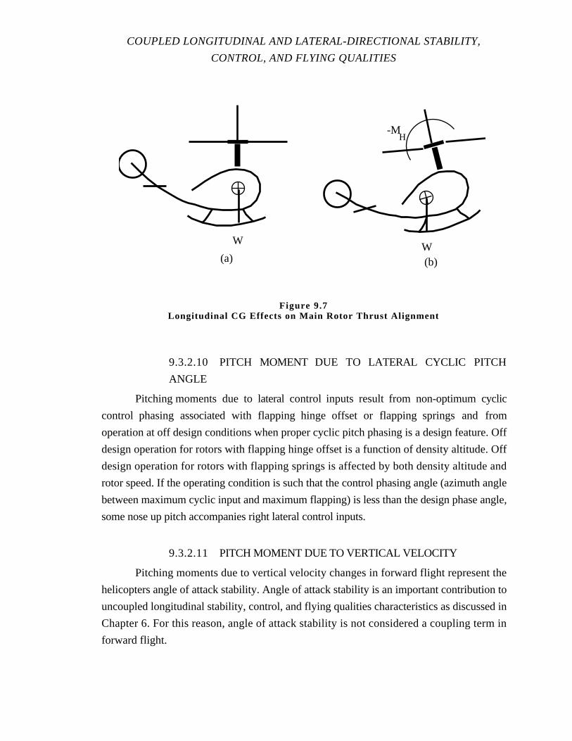
COUPLED LONGITUDINAL AND LATERAL-DIRECTIONAL STABILITY,
CONTROL, AND FLYING QUALITIES
9.3.2.10 PITCH MOMENT DUE TO LATERAL CYCLIC PITCH
ANGLE
Pitching moments due to lateral control inputs result from non-optimum cyclic
control phasing associated with flapping hinge offset or flapping springs and from
operation at off design conditions when proper cyclic pitch phasing is a design feature. Off
design operation for rotors with flapping hinge offset is a function of density altitude. Off
design operation for rotors with flapping springs is affected by both density altitude and
rotor speed. If the operating condition is such that the control phasing angle (azimuth angle
between maximum cyclic input and maximum flapping) is less than the design phase angle,
some nose up pitch accompanies right lateral control inputs.
9.3.2.11 PITCH MOMENT DUE TO VERTICAL VELOCITY
Pitching moments due to vertical velocity changes in forward flight represent the
helicopters angle of attack stability. Angle of attack stability is an important contribution to
uncoupled longitudinal stability, control, and flying qualities characteristics as discussed in
Chapter 6. For this reason, angle of attack stability is not considered a coupling term in
forward flight.
WW
-MH
(a) (b)
Figure 9.7Longitudinal CG Effects on Main Rotor Thrust Alignm ent
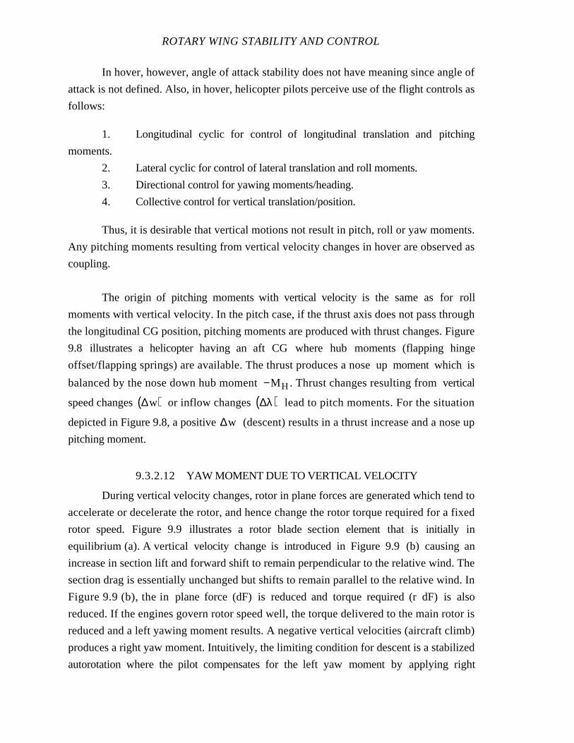
ROTARY WING STABILITY AND CONTROL
In hover, however, angle of attack stability does not have meaning since angle of
attack is not defined. Also, in hover, helicopter pilots perceive use of the flight controls as
follows:
1. Longitudinal cyclic for control of longitudinal translation and pitching
moments.
2. Lateral cyclic for control of lateral translation and roll moments.
3. Directional control for yawing moments/heading.
4. Collective control for vertical translation/position.
Thus, it is desirable that vertical motions not result in pitch, roll or yaw moments.
Any pitching moments resulting from vertical velocity changes in hover are observed as
coupling.
The origin of pitching moments with vertical velocity is the same as for roll
moments with vertical velocity. In the pitch case, if the thrust axis does not pass through
the longitudinal CG position, pitching moments are produced with thrust changes. Figure
9.8 illustrates a helicopter having an aft CG where hub moments (flapping hinge
offset/flapping springs) are available. The thrust produces a nose up moment which is
balanced by the nose down hub moment −M H . Thrust changes resulting from vertical
speed changes ∆w( ) or inflow changes ∆λ( ) lead to pitch moments. For the situation
depicted in Figure 9.8, a positive ∆w (descent) results in a thrust increase and a nose up
pitching moment.
9.3.2.12 YAW MOMENT DUE TO VERTICAL VELOCITY
During vertical velocity changes, rotor in plane forces are generated which tend to
accelerate or decelerate the rotor, and hence change the rotor torque required for a fixed
rotor speed. Figure 9.9 illustrates a rotor blade section element that is initially in
equilibrium (a). A vertical velocity change is introduced in Figure 9.9(b) causing an
increase in section lift and forward shift to remain perpendicular to the relative wind. The
section drag is essentially unchanged but shifts to remain parallel to the relative wind. In
Figure 9.9 (b), the in plane force (dF) is reduced and torque required (r dF) is also
reduced. If the engines govern rotor speed well, the torque delivered to the main rotor is
reduced and a left yawing moment results. A negative vertical velocities (aircraft climb)
produces a right yaw moment. Intuitively, the limiting condition for descent is a stabilized
autorotation where the pilot compensates for the left yaw moment by applying right
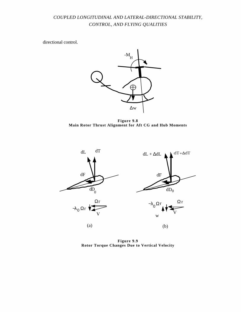
COUPLED LONGITUDINAL AND LATERAL-DIRECTIONAL STABILITY,
CONTROL, AND FLYING QUALITIES
directional control.
-MH
∆w
Figure 9.8Main Rotor Thrust Alignment for Aft CG and Hub Mome nts
dTdL
dF
dD0
Ωr
V−λ0 Ωr
dF
dD0
Ω r
V
−λ Ω0r
w
(a) (b)
dL + ∆dL dT + ∆dT
Figure 9.9Rotor Torque Changes Due to Vertical Velocity
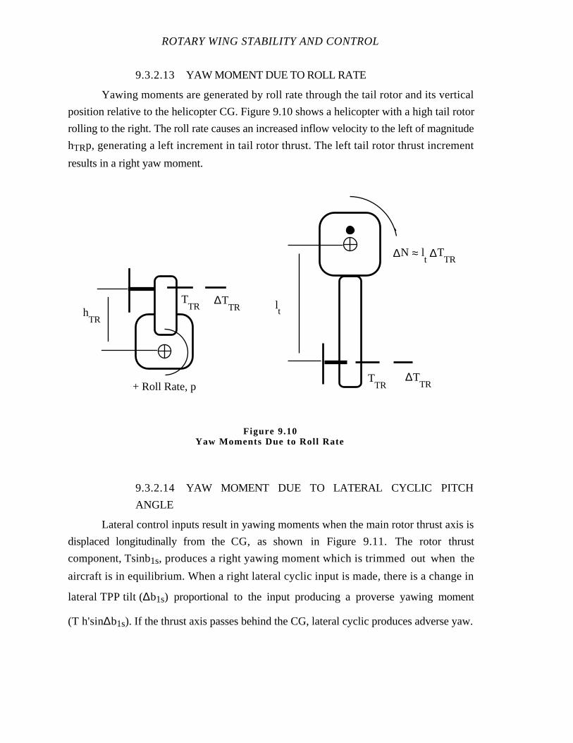
ROTARY WING STABILITY AND CONTROL
9.3.2.13 YAW MOMENT DUE TO ROLL RATE
Yawing moments are generated by roll rate through the tail rotor and its vertical
position relative to the helicopter CG. Figure 9.10 shows a helicopter with a high tail rotor
rolling to the right. The roll rate causes an increased inflow velocity to the left of magnitude
hTRp, generating a left increment in tail rotor thrust. The left tail rotor thrust increment
results in a right yaw moment.
9.3.2.14 YAW MOMENT DUE TO LATERAL CYCLIC PITCH
ANGLE
Lateral control inputs result in yawing moments when the main rotor thrust axis is
displaced longitudinally from the CG, as shown in Figure 9.11. The rotor thrust
component, Tsinb1s, produces a right yawing moment which is trimmed outwhen the
aircraft is in equilibrium. When a right lateral cyclic input is made, there is a change in
lateral TPP tilt (∆b1s) proportional to the input producing a proverse yawing moment
(T h'sin∆b1s). If the thrust axis passes behind the CG, lateral cyclic produces adverse yaw.
lt
∆TTR
TTR
∆N ≈ lt∆T
TR
hTR
TTR
∆TTR
+ Roll Rate, p
Figure 9.10Yaw Moments Due to Roll Rate
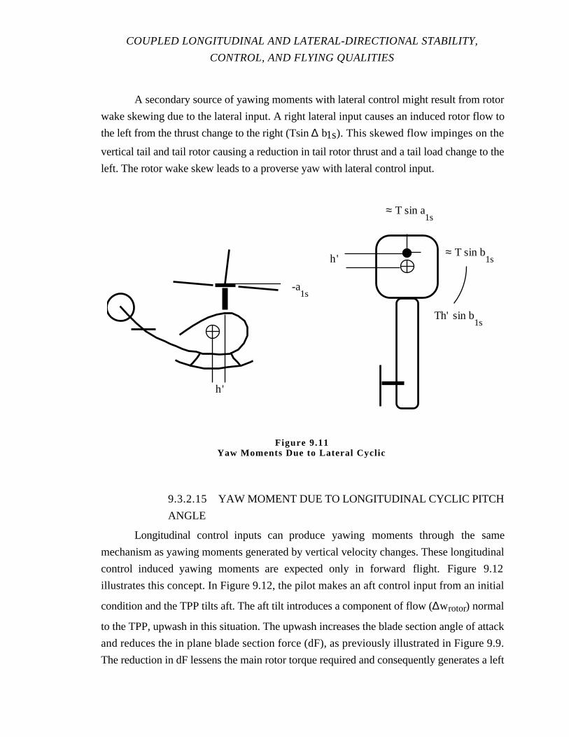
COUPLED LONGITUDINAL AND LATERAL-DIRECTIONAL STABILITY,
CONTROL, AND FLYING QUALITIES
A secondary source of yawing moments with lateral control might result from rotor
wake skewing due to the lateral input. A right lateral input causes an induced rotor flow to
the left from the thrust change to the right (Tsin ∆ b1s). This skewed flow impinges on the
vertical tail and tail rotor causing a reduction in tail rotor thrust and a tail load change to the
left. The rotor wake skew leads to a proverse yaw with lateral control input.
9.3.2.15 YAW MOMENT DUE TO LONGITUDINAL CYCLIC PITCH
ANGLE
Longitudinal control inputs can produce yawing moments through the same
mechanism as yawing moments generated by vertical velocity changes. These longitudinal
control induced yawing moments are expected only in forward flight. Figure 9.12
illustrates this concept. In Figure 9.12, the pilot makes an aft control input from an initial
condition and the TPP tilts aft. The aft tilt introduces a component of flow (∆wrotor) normal
to the TPP, upwash in this situation. The upwash increases the blade section angle of attack
and reduces the in plane blade section force (dF), as previously illustrated in Figure 9.9.
The reduction in dF lessens the main rotor torque required and consequently generates a left
h'
h'
≈ T sin a1s
≈ T sin b1s
Th' sin b1s
-a1s
Figure 9.11Yaw Moments Due to Lateral Cyclic
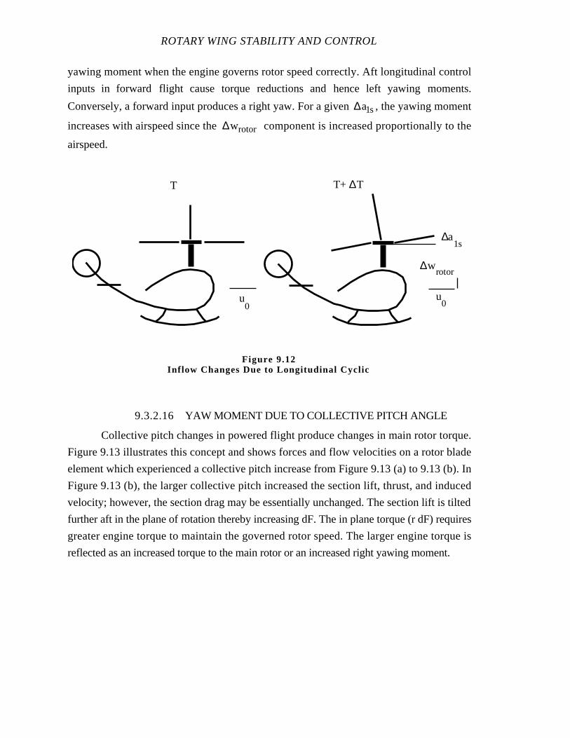
ROTARY WING STABILITY AND CONTROL
yawing moment when the engine governs rotor speed correctly. Aft longitudinal control
inputs in forward flight cause torque reductions and hence left yawing moments.
Conversely, a forward input produces a right yaw. For a given ∆a1s, the yawing moment
increases with airspeed since the ∆wrotor component is increased proportionally to the
airspeed.
9.3.2.16 YAW MOMENT DUE TO COLLECTIVE PITCH ANGLE
Collective pitch changes in powered flight produce changes in main rotor torque.
Figure 9.13 illustrates this concept and shows forces and flow velocities on a rotor blade
element which experienced a collective pitch increase from Figure 9.13 (a) to 9.13 (b). In
Figure 9.13 (b), the larger collective pitch increased the section lift, thrust, and induced
velocity; however, the section drag may be essentially unchanged. The section lift is tilted
further aft in the plane of rotation thereby increasing dF. The in plane torque (r dF) requires
greater engine torque to maintain the governed rotor speed. The larger engine torque is
reflected as an increased torque to the main rotor or an increased right yawing moment.
u0
T
u0
∆wrotor
T+ ∆T
∆a1s
Figure 9.12Inflow Changes Due to Longitudinal Cyclic
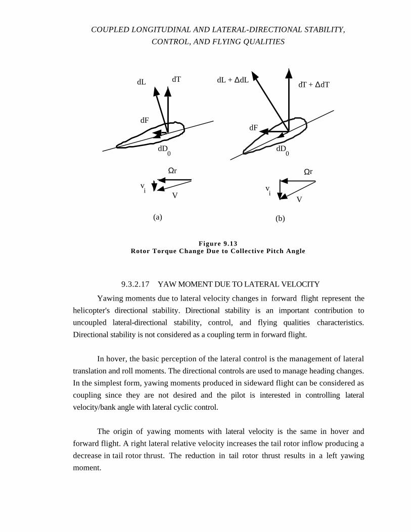
COUPLED LONGITUDINAL AND LATERAL-DIRECTIONAL STABILITY,
CONTROL, AND FLYING QUALITIES
9.3.2.17 YAW MOMENT DUE TO LATERAL VELOCITY
Yawing moments due to lateral velocity changes in forwardflight represent the
helicopter's directional stability. Directional stability is an important contribution to
uncoupled lateral-directional stability, control, and flying qualities characteristics.
Directional stability is not considered as a coupling term in forward flight.
In hover, the basic perception of the lateral control is the management of lateral
translation and roll moments. The directional controls are used to manage heading changes.
In the simplest form, yawing moments produced in sideward flight can be considered as
coupling since they are not desired and the pilot is interested in controlling lateral
velocity/bank angle with lateral cyclic control.
The origin of yawing moments with lateral velocity is the same in hover and
forward flight. A right lateral relative velocity increases the tail rotor inflow producing a
decrease in tail rotor thrust. The reduction in tail rotor thrust results in aleft yawing
moment.
dTdL
dF
dD0
Ωr
V
dF
dD0
Ωr
V
dT + ∆dTdL + ∆dL
(a) (b)
vi v
i
Figure 9.13Rotor Torque Change Due to Collective Pitch Angle
ROTARY WING STABILITY AND CONTROL
9.3.3 Coupling Perception
Section 9.3.2 considered the moments resulting from translational velocity (u, v,
w), rotational rates (p, q), and control inputs (A1s, B1s, θTR, θC). The moments generated
and the aircraft angular acceleration depend on the time development of the flight
parameters and control inputs. As an example, consider a helicopter with roll moments
produced by longitudinal cyclic, pitch rate, and longitudinal velocity. A forward control
input instantaneously produces nose down pitch acceleration and roll acceleration
(conceivably right roll). The pilot senses an immediate cross axis response. As the pitch
rate develops, an additional roll moment is generated. In addition, the developing right roll
rate produces roll damping which causes the roll acceleration to diminish or the roll rate to
stabilize. The roll moment with pitch rate reduces the stabilizing effect, and the pilot might
perceive a continuing of the roll acceleration. As airspeed increases, some time later a
further right roll moment is generated and a follow-on right roll acceleration results.
Obviously other moments and responses occur due to the effect of other stability derivative
contributions. Accelerations might be generated immediately or some time later as other
flight parameters change. If for example, the pilot makes a forward longitudinal control
input without control coupling (LB1s) present, a single axis (pitch) response is initially
perceived, but some time later, after the pitch rate developed, a roll to the right is
manifested. Roll control coupling might at first be expected, but further analysis indicates a
lag or delay in the roll tendency. This delay cues the evaluator that the coupling present is
not control related.
For systems with short term response approximated by first order responses, as
discussed in Chapter 8, further confusion could exist. Consider a first order response with
a very short time constant. The uncoupled response to a longitudinal control input is the
generation of a steady pitch rate almost immediately after the control input. The presence of
roll due to pitch rate coupling causes the total roll acceleration to be sensed shortly after the
longitudinal input. In this situation, the evaluator might be hard pressed to sort out whether
the roll response was caused by the control input or the pitch rate.
Coupling effects may be masked by the feeding of coupling effects from axis to
axis. To illustrate this concept, consider a helicopter that exhibits first order pitch and roll
response characteristics. Assume the helicopter has no cross axis control coupling, and
moderate response time constants. The pilot makes a forward longitudinal input and a pitch
rate develops. This pitch rate causes flapping in roll and some time later right roll rates are
COUPLED LONGITUDINAL AND LATERAL-DIRECTIONAL STABILITY,
CONTROL, AND FLYING QUALITIES
introduced. The right roll rates produce nose up longitudinal flapping which reduces the
pitch rate and also reduces the right flapping and roll moment. The system exhibits
coupling, but the continued cross axis effects tend to some extent to reduce the degree of
coupling felt.
9.3.4 Moments of Inertia
The flying qualities evaluator is typically not interestedin, or sensitive to, the
magnitudes of the moments, but rather to the angular accelerations and rates produced by
these moments. In the simplest form, a moment produces an angular acceleration with the
magnitude directly proportional to the size of the moment and inversely proportional to
helicopter moment of inertia (Ixx or Iyy or Izz). Although not true in all cases, the
conventional helicopter layout leads to relative moments of inertia such that the pitch (Iyy)
and yaw (Izz) moments of inertia are about the same magnitude, while the roll inertia (Ixx)
may be approximately 20% of the pitch inertia. Two examples are used to show the effects
of moment of inertia on the coupling observed.
For the first example, consider the roll moment with longitudinal cyclic. It was
argued for a control phase shift of 84˚, 10.5% of the pitching moment generated by a
longitudinal input is experienced in roll if the designer neglected phase shift requirements.
If moments of inertia were that such Ixx equaled 20% Iyy, then the roll acceleration is
52.5% of the pitch acceleration, or the total acceleration response occurs approximately 30˚
off the desired axis.
As the second example, consider a helicopter that is first subjected to a pitch rate
and then to the same magnitude roll rate. In this case, the roll moment due to pitch rate and
the pitch moment due to roll rate is the same size. When relative moments of inertia are
considered (Ixx equal approximately 20% Iyy), the roll acceleration due to the pitch rate
would be five times the pitch acceleration due to roll rate. The evaluator might be sensitive
to the roll coupling present, but unconcerned or even unaware of the pitch coupling.
Moments of inertia differences between axes may influence significantly the pilot's
perception of cross axis aerodynamic or control coupling.
ROTARY WING STABILITY AND CONTROL
9.3.5 Control Versus Aerodynamic Coupling
9.3.5.1 LONGITUDINAL AND LATERAL CYCLIC INPUT
PHASING
Cyclic control coupling may exist when flapping hinge offset or flapping springs
are incorporated in the design. The origin of this coupling is the phase shift between the
rotor azimuth for control input and the azimuth for maximum flapping. The phase shift is
less than 90˚ because the rotating or forcing frequency is less than the natural flapping
frequency. The designer can compensate for the control coupling by mechanically
introducing the correct azimuth position for cyclic blade pitch inputs. This mechanical
azimuth correction is a function of Lock number or density altitude for offset flapping
hinges, and a function of both Lock number and rotor speed for flapping springs. Thus,
correcting for cyclic control coupling is possible; however, the correction is valid for a
single design condition (density altitude or density altitude/rotor speed).
When mechanical cyclic control phasing is used, compensation for rotor coupling
due to angular rates and translational velocities is not achieved. To illustrate, a rotor with
flapping hinge offset is subjected to a nose up pitch rate. This rotor in a short time pitches
at the same rate as the rotor shaft, but lags behind the shaft in pitch angular displacement by
the angle (∆a1s). The flapping caused by pitch rate results in left tilt and some aft tilt of the
rotor. The left TPP tilt results in the normal roll coupling, and the aft tilt produces an
additional pitch rate damping contribution. The designer's use of mechanical phasing for
cyclic inputs does not affect the flapping phasing resulting from other disturbances such as
angular rates (p, q) and velocities (u, v, w).
9.3.5.2 MECHANICAL CONTROL MIXING
Various helicopter configurations incorporate combinations of longitudinal shaft tilt,
lateral shaft tilt, and tail inclination out of the vertical plane. Forward longitudinal shaft tilt
is used to provide an optimum cruise attitude and reduce longitudinal cyclic requirements at
higher airspeeds. Left lateral shaft tilt can optimize the interplay between cyclic inputs, hub
moments, and tail rotor vertical position to attain a laterally level hover. Tail rotor
inclination from vertical provides a vertical upwards component of tail rotor thrust to
improve performance and may expand aft CG limits.
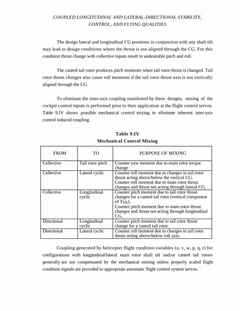
COUPLED LONGITUDINAL AND LATERAL-DIRECTIONAL STABILITY,
CONTROL, AND FLYING QUALITIES
The design lateral and longitudinal CG positions in conjunction with any shaft tilt
may lead to design conditions where the thrust is not aligned through the CG. For this
condition thrust change with collective inputs result in undesirable pitch and roll.
The canted tail rotor produces pitch moments when tail rotor thrust is changed. Tail
rotor thrust changes also cause roll moments if the tail rotor thrust axis is not vertically
aligned through the CG.
To eliminate the inter-axis coupling manifested by these designs, mixing of the
cockpit control inputs is performed prior to their application at the flight control servos.
Table 9.IV shows possible mechanical control mixing to eliminate inherent inter-axis
control induced coupling.
Table 9.IV
Mechanical Control Mixing
FROM TO PURPOSE OF MIXING
Collective Tail rotor pitch Counter yaw moment due to main rotor torquechange
Collective Lateral cyclic Counter roll moment due to changes in tail rotorthrust acting above/below the vertical CG.Counter roll moment due to main rotor thrustchanges and thrust not acting through lateral CG.
Collective Longitudinalcyclic
Counter pitch moment due to tail rotor thrustchanges for a canted tail rotor (vertical componentof TTR).Counter pitch moment due to main rotor thrustchanges and thrust not acting through longitudinalCG.
Directional Longitudinalcyclic
Counter pitch moment due to tail rotor thrustchange for a canted tail rotor.
Directional Lateral cyclic Counter roll moment due to changes in tail rotorthrust acting above/below roll axis.
Coupling generated by helicopter flight condition variables (u, v, w, p, q, r) for
configurations with longitudinal/lateral main rotor shaft tilt and/or canted tail rotors
generally are not compensated by the mechanical mixing unless properly scaled flight
condition signals are provided to appropriate automatic flight control system servos.
ROTARY WING STABILITY AND CONTROL
9.4 TEST METHODS AND TECHNIQUES
In general, there are no clearly defined methods for evaluating helicopter response
coupling. Existing specifications for helicopters and VSTOL (Vertical/short takeoff and
landing) aircraft (MIL-H-8501A and MIL-F-83300) are very general regarding coupling.
MIL-H-8501A states:
“For all operating conditions, longitudinal, lateral, directional, or vertical control
motions shall not produce adverse response of the helicopter due to mechanical coupling in
the control system”.
MIL-F-83300 states:
“Control inputs or aircraft motions about a given aircraft axis shall not induce
objectionable control forces or aircraft motions about any other axis.”
“The application of any cockpit control input necessary to meet any pitch, roll or
yaw performance requirement of this specification shallnot result in any objectionable
aircraft attitudes or angular rates about the axes not under consideration.”
Limits on what is “adverse” or “objectionable” are not quantified. Any evaluation of
coupling effects on mission suitability/acceptability is subjective. Coupling assessments are
normally not standard elements in helicopter flying qualities programs, but result because
of some peculiarity or difficulty encountered during conduct of other standard tests or
during performance of mission related maneuvers.
New helicopters are evaluated to support development and acceptance testing of
operational flight trainers (OFT). Data are used to compare OFT and aircraft characteristics
in efforts to ensure OFT fidelity. Naturally, documentation of coupling, even if not
“adverse” or “objectionable”, is required to provide acceptable flying qualities fidelity.
9.4.1 Trimmed Control Positions
Trimmed control position information is obtained during equilibrium flight. Data are
obtained during any situation desired (level flight, climb, descent, and dive) as long as the
aircraft is in rectilinear flight at a steady speed. Data are obtained over an airspeed range at
COUPLED LONGITUDINAL AND LATERAL-DIRECTIONAL STABILITY,
CONTROL, AND FLYING QUALITIES
selected airspeed intervals, at constant airspeed for various power settings, or at a given
airspeed and power setting for various sideslip angles. For these equilibrium conditions, all
angular rates (p, q, r) are zero; therefore, the coupling quantities (Mp, Lq, Np) are
neglected. Other coupling terms are omitted if specific items are constrained during the test.
For example, if control position data are obtained during constant airspeed climbs and
descents, u is zero and therefore Lu is not considered.
Steady state testing involve equilibrium or steady, non equilibrium conditions. An
example of steady non equilibrium flight is the steady turn discussed under maneuvering
stability testing in Chapter 6. In a steady turn, all flight parameters except heading (and
possibly altitude) are stable and the only acceleration involved is in the vertical axis. In a
steady turn, trim control position data are meaningful in terms of the control positions
required to trim the other axis to equilibrium. For this reason, coupling in steady turning
flight is addressed under trim control position testing.
During any equilibrium or steady state test, coupling parameters are changing as
each data point is obtained over the range of test variables. To illustrate, trimmed control
position data for level flight are obtained as collective is adjusted to maintain power for
level flight, and the other controls are manipulated for trimmed wings level, ball centered
flight. Any control position coupling, as well as speed coupling (Mv, Lu), are inherent in
the data. If the main rotor cyclic control phasing is correct, such that LB1s and MA1s are not
involved, the coupling arising from aerodynamics and geometry such as LθTR, MθC, NA1s
and NθC may exist. It may be impossible to sort out any one effect.
Control coupling resulting from incorrect cyclic control phasing (LB1s and MA1s)
are perceived during control response testing and are omitted from equilibrium tests for
simplicity. This does not mean cyclic control coupling does not exist in equilibrium data.
9.4.1.1 HOVER AND LOW AIRSPEED
Hover and low airspeed trimmed control position (TCP) data are normally obtained
at constant altitude during fore/aft translations and sideward translations, vertical
translation, and during translation with the relative wind from various azimuths (critical
azimuth). Table 9.V summarizes the main and tail rotor coupling which exist and the effect

ROTARY WING STABILITY AND CONTROL
of each type. The individual stability derivative effect reflects the expected result if no other
aerodynamic or control terms change. Obviously, during data acquisition all or most of the
stability derivatives are involved.
Table 9.V
Summary of Low Airspeed Coupling Moment Origins
FLIGHTREGIME
STABILITYDERIVATIVE
EFFECT
Lu Right roll in forward flight, left roll in aft flight.LθC Depends on main rotor thrust offset from lateral
CG. Normally with symmetrical lateral CG, rotorthrust acts to right of the lateral CG for high tailrotors; therefore, left roll with up collective.
LθTR For tail rotor above the roll axis, increased leftdirectional control produces right roll.
Forward/afttranslation
MθC Depends on main rotor thrust offset fromlongitudinal CG. For thrust acting forward of CG,up collective produces nose up pitch. For thrustacting aft of CG, up collective produces nose downpitch.
Nu Left yaw in forward and aft flight.NθC Right yaw with up collective, left yaw with down
collectiveLθC, LθTR, MθC,NθC
Same effects as for forward/aft translation.
Sidewardtranslation
Mv Nose up pitch with right translation, nose downpitch with left translation.
Nv Right yaw in right sideward flight, left yaw in leftsideward flight.
LθC, LθTR, MθC,NθC
Same effects as for forward/aft translation.
Vertical flight Lw Depends on main rotor thrust offset from lateralCG. Normally with symmetrical lateral CG, rotorthrust acts to right of CG for a high tail rotor;therefore, left roll in descent and right roll in climb.
Mw Depends on main rotor thrust offset fromlongitudinal CG. For thrust acting forward of CG,descent produces nose up pitch. For thrust actingaft of CG, descent produces nose down pitch.
Nw Right yaw in climb, left yaw in descent.
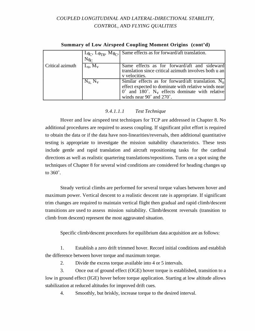
COUPLED LONGITUDINAL AND LATERAL-DIRECTIONAL STABILITY,
CONTROL, AND FLYING QUALITIES
Summary of Low Airspeed Coupling Moment Origins (cont’d)
LθC, LθTR, MθC,NθC
Same effects as for forward/aft translation.
Critical azimuth Lu, Mv Same effects as for forward/aft and sidewardtranslation since critical azimuth involves both u anv velocities.
Nu, Nv Similar effects as for forward/aft translation. Nueffect expected to dominate with relative winds near0˚ and 180˚. Nv effects dominate with relativewinds near 90˚ and 270˚.
9.4.1.1.1 Test Technique
Hover and low airspeed test techniques for TCP are addressed in Chapter 8. No
additional procedures are required to assess coupling. If significant pilot effort is required
to obtain the data or if the data have non-linearities/reversals, then additional quantitative
testing is appropriate to investigate the mission suitability characteristics. These tests
include gentle and rapid translation and aircraft repositioning tasks for thecardinal
directions as well as realistic quartering translations/repositions. Turns on a spot using the
techniques of Chapter 8 for several wind conditions are considered for heading changes up
to 360˚.
Steady vertical climbs are performed for several torque values between hover and
maximum power. Vertical descent to a realistic descent rate is appropriate. If significant
trim changes are required to maintain vertical flight then gradual and rapid climb/descent
transitions are used to assess mission suitability. Climb/descent reversals (transition to
climb from descent) represent the most aggravated situation.
Specific climb/descent procedures for equilibrium data acquisition are as follows:
1. Establish a zero drift trimmed hover. Record initial conditions and establish
the difference between hover torque and maximum torque.
2. Divide the excess torque available into 4 or 5 intervals.
3. Once out of ground effect (OGE) hover torque is established, transition to a
low in ground effect (IGE) hover before torque application. Starting at low altitude allows
stabilization at reduced altitudes for improved drift cues.
4. Smoothly, but briskly, increase torque to the desired interval.
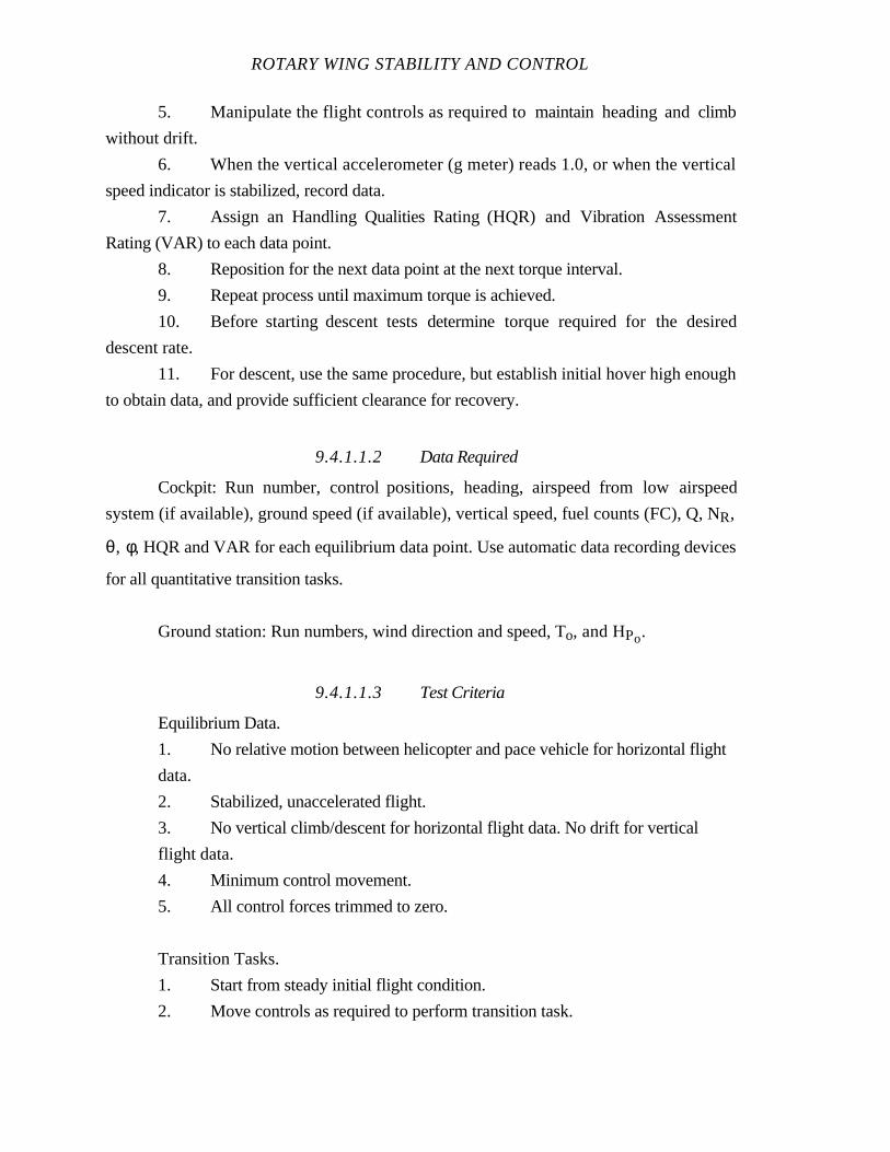
ROTARY WING STABILITY AND CONTROL
5. Manipulate the flight controls as required to maintain heading and climb
without drift.
6. When the vertical accelerometer (g meter) reads 1.0, or when the vertical
speed indicator is stabilized, record data.
7. Assign an Handling Qualities Rating (HQR) and Vibration Assessment
Rating (VAR) to each data point.
8. Reposition for the next data point at the next torque interval.
9. Repeat process until maximum torque is achieved.
10. Before starting descent tests determine torque required for the desired
descent rate.
11. For descent, use the same procedure, but establish initial hover high enough
to obtain data, and provide sufficient clearance for recovery.
9.4.1.1.2 Data Required
Cockpit: Run number, control positions, heading, airspeed from low airspeed
system (if available), ground speed (if available), vertical speed, fuel counts (FC), Q, NR,
θ, φ, HQR and VAR for each equilibrium data point. Use automatic data recording devices
for all quantitative transition tasks.
Ground station: Run numbers, wind direction and speed, To, and HPo.
9.4.1.1.3 Test Criteria
Equilibrium Data.
1. No relative motion between helicopter and pace vehicle for horizontal flight
data.
2. Stabilized, unaccelerated flight.
3. No vertical climb/descent for horizontal flight data. No drift for vertical
flight data.
4. Minimum control movement.
5. All control forces trimmed to zero.
Transition Tasks.
1. Start from steady initial flight condition.
2. Move controls as required to perform transition task.
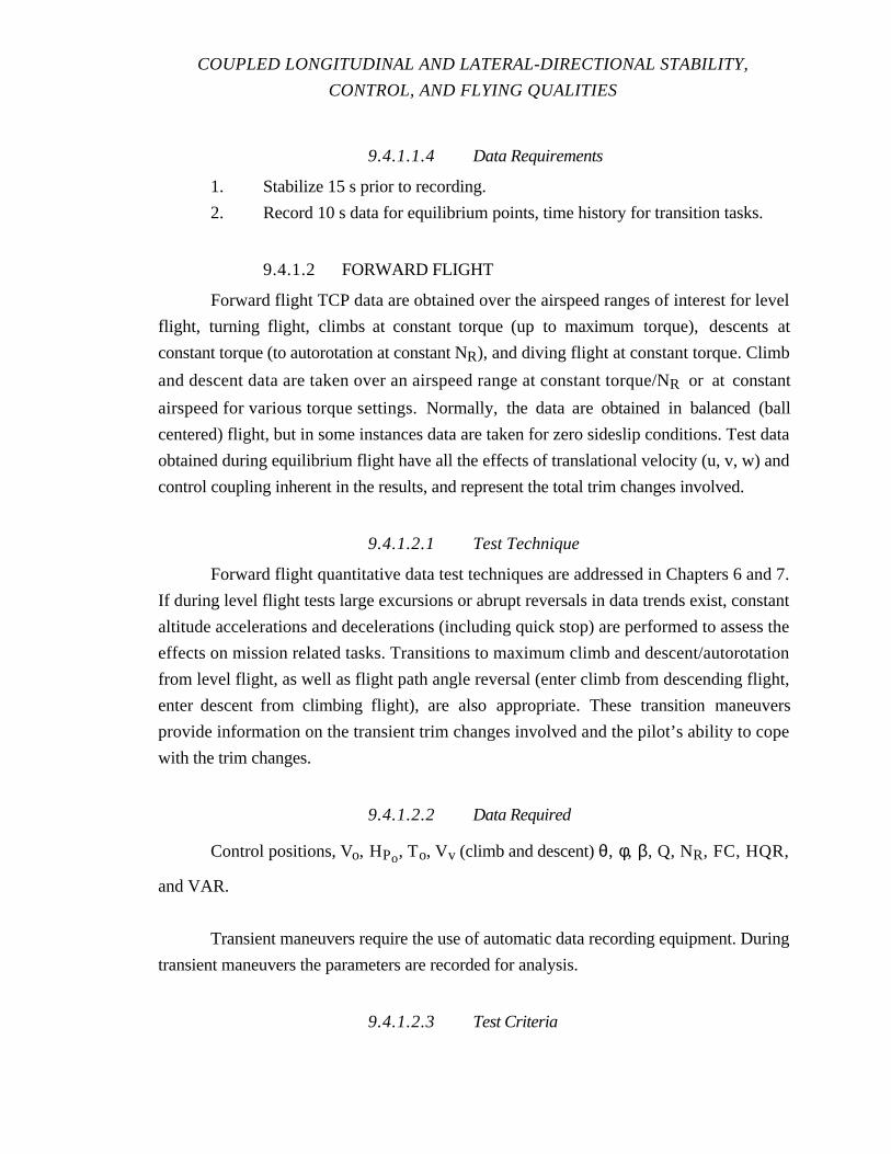
COUPLED LONGITUDINAL AND LATERAL-DIRECTIONAL STABILITY,
CONTROL, AND FLYING QUALITIES
9.4.1.1.4 Data Requirements
1. Stabilize 15 s prior to recording.
2. Record 10 s data for equilibrium points, time history for transition tasks.
9.4.1.2 FORWARD FLIGHT
Forward flight TCP data are obtained over the airspeed ranges of interest for level
flight, turning flight, climbs at constant torque (up to maximum torque), descents at
constant torque (to autorotation at constant NR), and diving flight at constant torque. Climb
and descent data are taken over an airspeed range at constant torque/NR or at constant
airspeed for various torque settings. Normally, the data are obtained inbalanced (ball
centered) flight, but in some instances data are taken for zero sideslip conditions. Test data
obtained during equilibrium flight have all the effects of translational velocity (u, v, w) and
control coupling inherent in the results, and represent the total trim changes involved.
9.4.1.2.1 Test Technique
Forward flight quantitative data test techniques are addressed in Chapters 6 and 7.
If during level flight tests large excursions or abrupt reversals in data trends exist, constant
altitude accelerations and decelerations (including quick stop) are performed to assess the
effects on mission related tasks. Transitions to maximum climb and descent/autorotation
from level flight, as well as flight path angle reversal (enter climb from descending flight,
enter descent from climbing flight), are also appropriate. These transition maneuvers
provide information on the transient trim changes involved and the pilot’s ability to cope
with the trim changes.
9.4.1.2.2 Data Required
Control positions, Vo, HPo, To, Vv (climb and descent) θ, φ, β, Q, NR, FC, HQR,
and VAR.
Transient maneuvers require the use of automatic data recording equipment. During
transient maneuvers the parameters are recorded for analysis.
9.4.1.2.3 Test Criteria
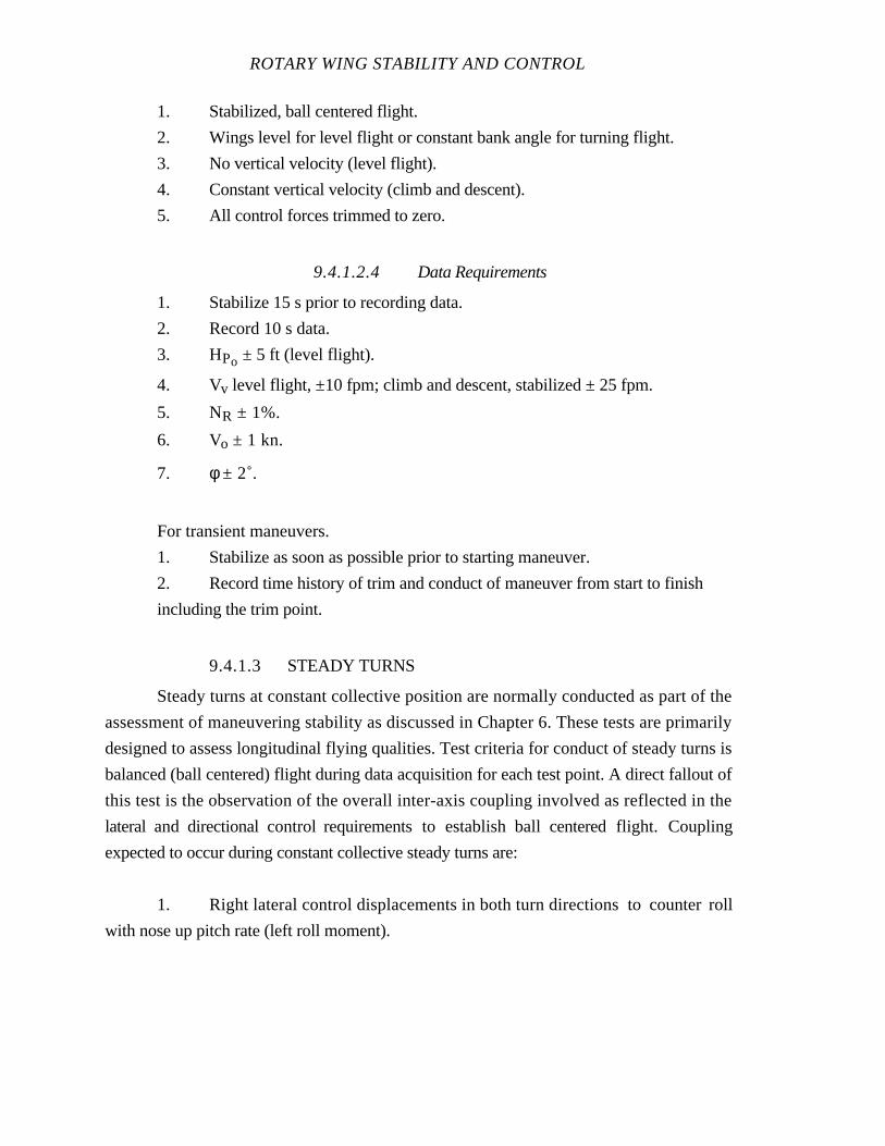
ROTARY WING STABILITY AND CONTROL
1. Stabilized, ball centered flight.
2. Wings level for level flight or constant bank angle for turning flight.
3. No vertical velocity (level flight).
4. Constant vertical velocity (climb and descent).
5. All control forces trimmed to zero.
9.4.1.2.4 Data Requirements
1. Stabilize 15 s prior to recording data.
2. Record 10 s data.
3. HPo ± 5 ft (level flight).
4. Vv level flight, ±10 fpm; climb and descent, stabilized ± 25 fpm.
5. NR ± 1%.
6. Vo ± 1 kn.
7. φ ± 2˚.
For transient maneuvers.
1. Stabilize as soon as possible prior to starting maneuver.
2. Record time history of trim and conduct of maneuver from start to finish
including the trim point.
9.4.1.3 STEADY TURNS
Steady turns at constant collective position are normally conducted as part of the
assessment of maneuvering stability as discussed in Chapter 6. These tests are primarily
designed to assess longitudinal flying qualities. Test criteria for conduct of steady turns is
balanced (ball centered) flight during data acquisition for each test point. A direct fallout of
this test is the observation of the overall inter-axis coupling involved as reflected in the
lateral and directional control requirements to establish ball centered flight. Coupling
expected to occur during constant collective steady turns are:
1. Right lateral control displacements in both turn directions to counter roll
with nose up pitch rate (left roll moment).
COUPLED LONGITUDINAL AND LATERAL-DIRECTIONAL STABILITY,
CONTROL, AND FLYING QUALITIES
2. Lateral control displacements to counter roll moments due to thrust changes
when the thrust is not laterally aligned through the CG. The direction of required control
displacement depends on thrust axis orientation (left or right of CG). This effect is similar
for left and right turns.
3. Lateral control displacements to counter roll moments due to lateral velocity
(dihedral effect) if changes in sideslip angle are required for balanced flight.
4. Lateral control displacements to counter roll moments due to tail rotor thrust
changes associated with directional control inputs (yaw damping and directional stability).
5. Directional control inputs to counter directional stability and yaw damping
effects. The directional control requirements may be different for left and right turns.
6. Directional control inputs to counter rotor torque changes.
Steady turns are conducted at constant altitude and constant airspeed. These terms
represent operational conditions reflective of Search and Rescue (SAR) and Antisubmarine
Warfare (ASW) search patterns, and holding patterns during landing zone reconnaissance.
The constant altitude steady turns give similar insight to the lateral and directional control
requirements as determined during constant collective turns. The constant altitude turns are
not maneuvering stability tests since the collective position is being varied, but they do give
insight to additional coupling obtained with collective movement. Increased collective
required to maintain altitude during turns results in increased aft rotor tilt. This aft tilt may
result in a shallowing of the longitudinal control position/force gradient with load factor,
even to the condition where the gradient becomes neutral or negative.
9.4.1.3.1 Test Technique
Techniques for conducting constant collective steady turns are described in Chapter
6. The technique for constant altitude turns is described in Chapter 7. Lateral, directional,
and collective control forces are trimmed to zero at the pilot's discretion.
9.4.1.3.2 Data Required
All control positions, longitudinal control force, g, Vo, bank angle, pitch attitude,
turn direction, sideslip angle (if available), HQR, VAR, Vv, FC, HPo, To, Q, and NR.
ROTARY WING STABILITY AND CONTROL
9.4.1.3.3 Test Criteria
1. Ball centered, balanced flight.
2. Collective fixed/varied depending on test.
3. Constant bank angle/pitch attitude.
4. Constant airspeed.
5. Steady load factor.
9.4.1.3.4 Data Requirement
1. Stabilize 15 s prior to taking data.
2. Record 10 s stabilized data.
3. Trim Vo ± 1 kn.
4. Ball centered, ± 1/4 ball.
5. HPo ± 5 ft (level flight).
6. NR ± 1%.
7. Vv level flight, ±10 fpm; climb and descent, stabilized ± 25 fpm.
9.4.2 Steady Pull Ups/Push Overs
Steady symmetrical pull ups and push overs at constant collective position are
normally conducted as part of the assessment of maneuvering stability. Maneuvering
stability testing is discussed in Sections 6.4. Test criteria for the conduct of pull ups and
push overs requires ball centered, balanced flight during the test. Inter-axis coupling may
exist during pull ups and push overs and is reflected in the lateral and direction control
requirements to counter trim changes and maintain balanced flight. Expected coupling:
1. Right lateral control to counter left roll moments with nose up pitch rate
(pull up), left lateral control with nose down pitch rate (push over).
2. Lateral control displacements to counter roll moments due to thrust changes
when the thrust is not laterally aligned through the CG. The direction of required control
displacement depends on thrust axis orientation (left or right CG). This effect is opposite
for pull ups and push overs.
3. Lateral control displacements to counter roll moments due to lateral velocity
if changes in sideslip angle are introduced by main rotor torque changes.
4. Lateral control displacement to counter roll moments due to tail rotor thrust
changes associated with directional control inputs.
COUPLED LONGITUDINAL AND LATERAL-DIRECTIONAL STABILITY,
CONTROL, AND FLYING QUALITIES
5. Directional control inputs to counter main rotor torque changes. Directional
control requirements may be in opposite directions for pull ups and push overs. Right
directional control inputs are expected in pull ups. When rapid longitudinal inputs are used
during pull ups and push overs, roll coupling associated with non optimum cyclic input
phasing may exist. If this coupling is present, it is observed as an immediate roll tendency.
Collective inputs may be used to change load factor as in a bob up or bob down
maneuver. These maneuvers are operationally representative in terms of low altitude terrain
following, vertical repositioning in formation flight/aerial refueling, and recovery from low
power diving flight. Collective maneuvering gives insight to the collective ability to
produce load factor as well as coupling involved with collective movement. The coupling
perceived depends on the final aircraft response the pilot desires. For example, the pilot
may desire to hold heading and pitch attitude during formation flight, whereas during a
diving pullout or terrain following he might be interested in coordinated (ball centered)
flight and some use of pitch attitude change in his control of flight path angles. In either
case, expected coupling include:
1. Nose up pitching moments with up collective input due to aft TPP tilt.
2. Nose up or down pitching moments with up collective when the thrust axis
is not longitudinally aligned with the CG. The thrust axis could pass on either side of the
CG depending on aircraft loading and external forces and moments (tail loads). These
pitching moment result from changes in thrust magnitude.
3. Heading/sideslip changes due to yaw moments from collective inputs
(torque changes).
4. Roll moments from lateral flapping associated with coning (thrust changes).
These moments are to the left for collective increases.
5. Roll moments from aircraft dihedral effect when sideslip changes occur.
6. Roll moments from tail rotor thrust changes associated with directional
control inputs used to control heading/sideslip.
7. Roll moments from thrust changes when the thrust axis is not laterally
aligned with the CG.
ROTARY WING STABILITY AND CONTROL
9.4.2.1 TEST TECHNIQUE
Steady symmetrical pull up and push over test procedures for longitudinal control
inputs are provided in Section 6.4. No adjustments to these techniques are required to
investigate coupling, unless significant coupling is present. The pull ups and push overs
can be performed with the other controls fixed to assess the degree of coupling.
The collective bob up or bob down technique is as follows:
1. Stabilize in ball-centered, coordinated flight at the desired trim airspeed.
2. Reduce all control forces to zero.
3. Rapidly increase or decrease collective pitch. If a control fixture is used,
establish the fixture increment and place the fixture appropriately. Start with small
increments and use a build up procedure.
4. Manipulate the other controls to maintain the desired flight condition (pitch
attitude, or heading, or bank angle, etc.).
5. Repeat the procedure until the predetermined limit (load factor, torque,
control margin, etc) is reached.
9.4.2.2 DATA REQUIRED
Longitudinal, lateral, and directional control positions, longitudinal control force, g,
Vo, bank angle, pitch attitude, HQR, VAR, size of longitudinal or collective input, FC,
HPo, To, Q, and NR for coordinated cyclic control pull up/push over flight maneuvers. For
uncoordinated cyclic only pull up/push over tests (lateral and directional controls fixed) and
for collective bob up and bob down maneuvers, time histories of the data parameters as
well as collective position, pitch rate, roll rate, yaw rate, heading and sideslip angle.
9.4.2.3 TEST CRITERIA
1. Ball centered, balanced flight for coordinated maneuvers.
2. Constant bank angle for coordinated maneuvers.
3. Lateral cyclic and directional control fixed for uncoordinated maneuvers.
4. Collective fixed for cyclic pull ups/push overs.
5. Constant airspeed.
6. Load factor data are valid only as the aircraft passes through the trimmed
pitch attitude during cyclic pull ups/push overs.

COUPLED LONGITUDINAL AND LATERAL-DIRECTIONAL STABILITY,
CONTROL, AND FLYING QUALITIES
9.4.2.4 DATA REQUIREMENTS
1. Record steady trim data when on airspeed, on attitude.
2. Trim Vo ± 2 kn.
3. Ball centered for coordinated maneuvers, ± 1/4 ball.
4. HPo ± 1000 ft of the target test attitude.
5. NR ± 1%.
9.4.3 Steady Heading Sideslips
Steady heading sideslip tests are performed to assess static lateral-directional flying
qualities. The only meaningful insight to coupling obtained from steady heading sideslip
tests is of pitching moments resulting from lateral velocity changes. Main rotor TPP
longitudinal tilt is expected when the lateral velocity is changed. The longitudinal tilt is a
function of coning and the magnitude of the lateral velocity change. During steady heading
sideslip tests an aft TPP tilt is expected in right sideslips and forward tilt in left sideslips.
These moments, if unchecked, produce pitch attitude and airspeed excursions. During
conduct of steady heading sideslips, forward cyclic control inputs in right sideslips, and aft
cyclic inputs in left sideslips are normally required to maintain airspeed.
Test techniques, data required, test criteria, data requirements, and Safety
Considerations/Risk Management for steady heading sideslip testing are given in Section
7.4.
9.4.4 Control Response
Control response tests are normally conducted for all four controls (longitudinal,
lateral, directional, and vertical) in each direction. The purpose of control response testing
is to investigate the primary axis helicopter response to abrupt (step) control inputs. In the
simplest form, the responses achieved give insight to the aircraft damping and the pilots
ability to establish angular rates and attitude changes. Control response tests are performed
using single axis control inputs, with the control positions for the other axes fixed. The
control response data are obtained during the first several seconds immediately following
the control step.
ROTARY WING STABILITY AND CONTROL
Control response testing provides an excellent avenue to investigate short term
coupling. This short term coupling plays a significant role in the pilot's perception of his
ability to rapidly and accurately perform flight path changes. Since the response is short
term in nature, the slower developing responses such as airspeed changes with longitudinal
control steps and lateral velocity changes with lateral control steps are neglected.
For the purpose of discussing coupling, it is assumed the pilot uses the cockpit
controls as follows:
1. Longitudinal cyclic to control pitch attitude, pitch rate, and airspeed.
2. Lateral cyclic to control bank angle, roll rate, and lateral velocity.
3. Directional control for heading and yaw rate.
4. Vertical/Collective control for altitude or vertical speed.
With this simplified control approach, off axis responses which occur are
considered as coupling. Generally the coupling which occurs is not desirable. For example,
a left directional control input is made in forward flight on a helicopter with a high tail
rotor. This directional input produces a left yaw acceleration (desired uncoupled response),
an initial right roll which tries to turn the aircraft right (undesired coupled response), and
with time a right sideslip causing left roll and left turn (desired coupled response).
Hover and forward flight control response and the resultant coupling may or may
not be similar. Consequently control response testing is usually performed in hover and at
several representative forward flight airspeeds.
9.4.4.1 LONGITUDINAL CONTROL RESPONSE
Potential coupling expected during longitudinal control response testing is
summarized in Table 9.VI. There is no simple response. The coupling evaluator should be
aware of the timing of the perceived response, its magnitude, and how other quantities are
changing. The timing of the perceived response is an indicator of whether the coupling is
control input related, rate related, or a secondary effect. When an acceleration is observed
immediately following a control input, it is probably control related. If the response is
delayed, it is probably rate related or a secondary effect such as the dihedral characteristic.
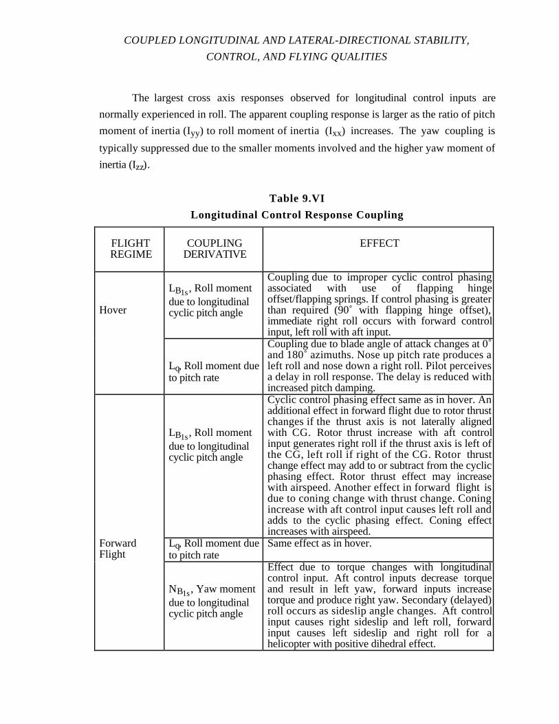
COUPLED LONGITUDINAL AND LATERAL-DIRECTIONAL STABILITY,
CONTROL, AND FLYING QUALITIES
The largest cross axis responses observed for longitudinal control inputs are
normally experienced in roll. The apparent coupling response is larger as the ratio of pitch
moment of inertia (Iyy) to roll moment of inertia (Ixx) increases. The yaw coupling is
typically suppressed due to the smaller moments involved and the higher yaw moment of
inertia (Izz).
Table 9.VI
Longitudinal Control Response Coupling
FLIGHTREGIME
COUPLINGDERIVATIVE
EFFECT
Hover
LB1s, Roll momentdue to longitudinalcyclic pitch angle
Coupling due to improper cyclic control phasingassociated with use of flapping hingeoffset/flapping springs. If control phasing is greaterthan required (90˚ with flapping hinge offset),immediate right roll occurs with forward controlinput, left roll with aft input.
Lq, Roll moment dueto pitch rate
Coupling due to blade angle of attack changes at 0˚and 180˚ azimuths. Nose up pitch rate produces aleft roll and nose down a right roll. Pilot perceivesa delay in roll response. The delay is reduced withincreased pitch damping.
LB1s, Roll momentdue to longitudinalcyclic pitch angle
Cyclic control phasing effect same as in hover. Anadditional effect in forward flight due to rotor thrustchanges if the thrust axis is not laterally alignedwith CG. Rotor thrust increase with aft controlinput generates right roll if the thrust axis is left ofthe CG, left roll if right of the CG. Rotor thrustchange effect may add to or subtract from the cyclicphasing effect. Rotor thrust effect may increasewith airspeed. Another effect in forward flight isdue to coning change with thrust change. Coningincrease with aft control input causes left roll andadds to the cyclic phasing effect. Coning effectincreases with airspeed.
ForwardFlight
Lq, Roll moment dueto pitch rate
Same effect as in hover.
NB1s, Yaw momentdue to longitudinalcyclic pitch angle
Effect due to torque changes with longitudinalcontrol input. Aft control inputs decrease torqueand result in left yaw, forward inputs increasetorque and produce right yaw. Secondary (delayed)roll occurs as sideslip angle changes. Aft controlinput causes right sideslip and left roll, forwardinput causes left sideslip and right roll for ahelicopter with positive dihedral effect.
ROTARY WING STABILITY AND CONTROL
9.4.4.1.1 Test Technique
Longitudinal control response test techniques are described in Section 8.4 for hover
and Section 6.4 for forward flight.
9.4.4.1.2 Data Required
Hover.
A time history of aircraft attitudes, rates, control positions, heading, airspeed from
low airspeed system (if available), FC, Q, NR, To, HPo, and VAR.
Forward Flight.
Vo, HPo, θ, FC, To, Q, NR, cockpit control positions, control input size and
direction.
Automatic recording systems are required for data collection. A time history of the
longitudinal control position, attitudes, rates, and accelerations are essential data elements.
9.4.4.1.3 Test Criteria
1. Stabilized, unaccelerated flight at trim.
2. All control forces trimmed to zero.
3. Off axis controls fixed.
9.4.4.1.4 Data Requirements
1. Stabilize 15 s prior to recording data.
2. Trim Vo ± 1 kn.
3. Record data until steady state rate is achieved or until a test limit is reached.
9.4.4.2 LATERAL CONTROL RESPONSE
Potential coupling expected during lateral control response testing is summarized in
Table 9.VII. As in the longitudinal case, there is no simple, expected response. The
coupling evaluator should be aware of the timing of the perceived response, its magnitude
and how other quantities are changing. The timing of the perceived response is indicative of
COUPLED LONGITUDINAL AND LATERAL-DIRECTIONAL STABILITY,
CONTROL, AND FLYING QUALITIES
whether the coupling is control input related, rate related, or a secondary effect. When an
acceleration is observed immediately following a control input it is probably control related.
If the response is delayed, it is probably rate related or a secondary effect.
The cross axis responses observed in pitch and yaw with lateral control inputs are
normally significantly less than the roll coupling observed for other control inputs. Pitch
and yaw moments of inertia (Iyy and Izz) tend to be substantially larger than the roll
moment of inertia (Ixx). These greater moments of inertia reduce the cross axis
accelerations resulting from lateral control inputs and roll rates.
9.4.4.2.1 Test Technique
Lateral control response test techniques are described in Section 8.4 for
hover and Section 7.4 for forward flight.
9.4.4.2.2 Data Required
Hover.
Control positions, all angular accelerations, pitch rate, roll rate, yaw rate, pitch
attitude, bank angle, heading, FC, To, Q, NR, HPo, control input size and direction.
Forward Flight.
All hover data plus load factor, airspeed, sideslip and Vv. All data except FC and To
are measured in time history form. Measure and record the Automatic Flight Control
System (AFCS) control movements.
Certain data requirements listed are not expected to be affected during lateral control
response testing. These data are measured regardless to verify that coupling does not exist.
9.4.4.2.3 Test Criteria
1. Airspeed, altitude stabilized.
2. Ball centered in forward flight.
3. Longitudinal, directional, and collective controls fixed.
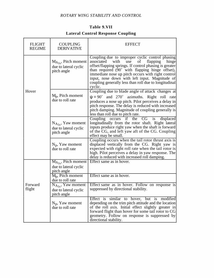
ROTARY WING STABILITY AND CONTROL
Table 9.VII
Lateral Control Response Coupling
FLIGHTREGIME
COUPLINGDERIVATIVE
EFFECT
MA1s, Pitch momentdue to lateral cyclicpitch angle
Coupling due to improper cyclic control phasingassociated with use of flapping hingeoffset/flapping springs. If control phasing is greaterthan required (90˚ with flapping hinge offset),immediate nose up pitch occurs with right controlinput, nose down with left input. Magnitude ofcoupling generally less than roll due to longitudinalcyclic.
HoverMp, Pitch momentdue to roll rate
Coupling due to blade angle of attack changes atψ = 90˚ and 270˚ azimuths. Right roll rateproduces a nose up pitch. Pilot perceives a delay inpitch response. The delay is reduced with increasedpitch damping. Magnitude of coupling generally isless than roll due to pitch rate.
NA1s, Yaw momentdue to lateral cyclicpitch angle
Coupling occurs if the CG is displacedlongitudinally from the rotor shaft. Right lateralinputs produce right yaw when the shaft is forwardof the CG, and left yaw aft of the CG. Couplingeffect may be small.
Np, Yaw momentdue to roll rate
Coupling occurs when the tail rotor thrust axis isdisplaced vertically from the CG. Right yaw isexpected with right roll rate when the tail rotor ishigh. Pilot perceives a delay in yaw response. Thedelay is reduced with increased roll damping.
MA1s, Pitch momentdue to lateral cyclicpitch angle
Effect same as in hover.
Mp, Pitch momentdue to roll rate
Effect same as in hover.
Forwardflight
NA1s, Yaw momentdue to lateral cyclicpitch angle
Effect same as in hover. Follow on response issuppressed by directional stability.
Np, Yaw momentdue to roll rate
Effect is similar to hover, but is modifieddepending on the trim pitch attitude and the locationof the roll axis. Initial effect slightly greater inforward flight than hover for some tail rotor to CGgeometry. Follow on response is suppressed bydirectional stability.

COUPLED LONGITUDINAL AND LATERAL-DIRECTIONAL STABILITY,
CONTROL, AND FLYING QUALITIES
9.4.4.2.4 Data Requirements
1. Stabilize 15 s prior to taking data.
2. Trim Vo ± 1 kn.
3. HPo ± 1000 ft of the target test altitude.
9.4.4.3 DIRECTIONAL CONTROL RESPONSE
Potential coupling expected during directional control response testing is
summarized in Table 9.VIII. In general, coupling in roll due to directional control changes
is tail rotor height dependent. If the tail rotor is high, initial right roll with left directional
control is expected, followed by a reduction in roll response as yaw rate develops. In
forward flight the final bank angle change may be in the opposite direction (in the direction
of directional control) when dihedral effect is positive. The coupling evaluator should be
aware of the timing of the perceived response, its magnitude and how other quantities (yaw
rate and sideslip) are changing. The timing of the perceived response gives insight to
whether the coupling is control input related or a secondary effect. When an acceleration is
observed immediately following a control input, it is probably control related. If the
response is delayed, it is probably rate related or a secondary dihedral effect.
9.4.4.3.1 Test Technique
Directional control response test techniques are described in Section 8.4 for hover,
and Section 7.4 for forward flight.
9.4.4.3.2 Data Required
Hover.
Control positions, all angular accelerations, pitch rate, roll rate, yaw rate, pitch
attitude, bank angle, heading, FC, To, Q, NR, HPo, control input size and direction.
Forward Flight.
All hover data plus, load factor, airspeed, sideslip, and Vv.
All data except FC and To are measured in time history form. Measure and record
the AFCS control movements.
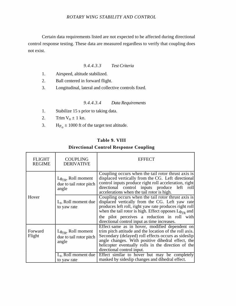
ROTARY WING STABILITY AND CONTROL
Certain data requirements listed are not expected to be affected during directional
control response testing. These data are measured regardless to verify that coupling does
not exist.
9.4.4.3.3 Test Criteria
1. Airspeed, altitude stabilized.
2. Ball centered in forward flight.
3. Longitudinal, lateral and collective controls fixed.
9.4.4.3.4 Data Requirements
1. Stabilize 15 s prior to taking data.
2. Trim Vo ± 1 kn.
3. HPo ± 1000 ft of the target test altitude.
Table 9. VIII
Directional Control Response Coupling
FLIGHTREGIME
COUPLINGDERIVATIVE
EFFECT
LθTR, Roll momentdue to tail rotor pitchangle
Coupling occurs when the tail rotor thrust axis isdisplaced vertically from the CG. Left directionalcontrol inputs produce right roll acceleration, rightdirectional control inputs produce left rollaccelerations when the tail rotor is high.
HoverLr, Roll moment dueto yaw rate
Coupling occurs when the tail rotor thrust axis isdisplaced vertically from the CG. Left yaw rateproduces left roll, right yaw rate produces right rollwhen the tail rotor is high. Effect opposes LθTR andthe pilot perceives a reduction in roll withdirectional control input as time increases.
ForwardFlight
LθTR, Roll momentdue to tail rotor pitchangle
Effect same as in hover, modified dependent ontrim pitch attitude and the location of the roll axis.Secondary (delayed) roll effects occurs as sideslipangle changes. With positive dihedral effect, thehelicopter eventually rolls in the direction of thedirectional control input.
Lr, Roll moment dueto yaw rate
Effect similar to hover but may be completelymasked by sideslip changes and dihedral effect.
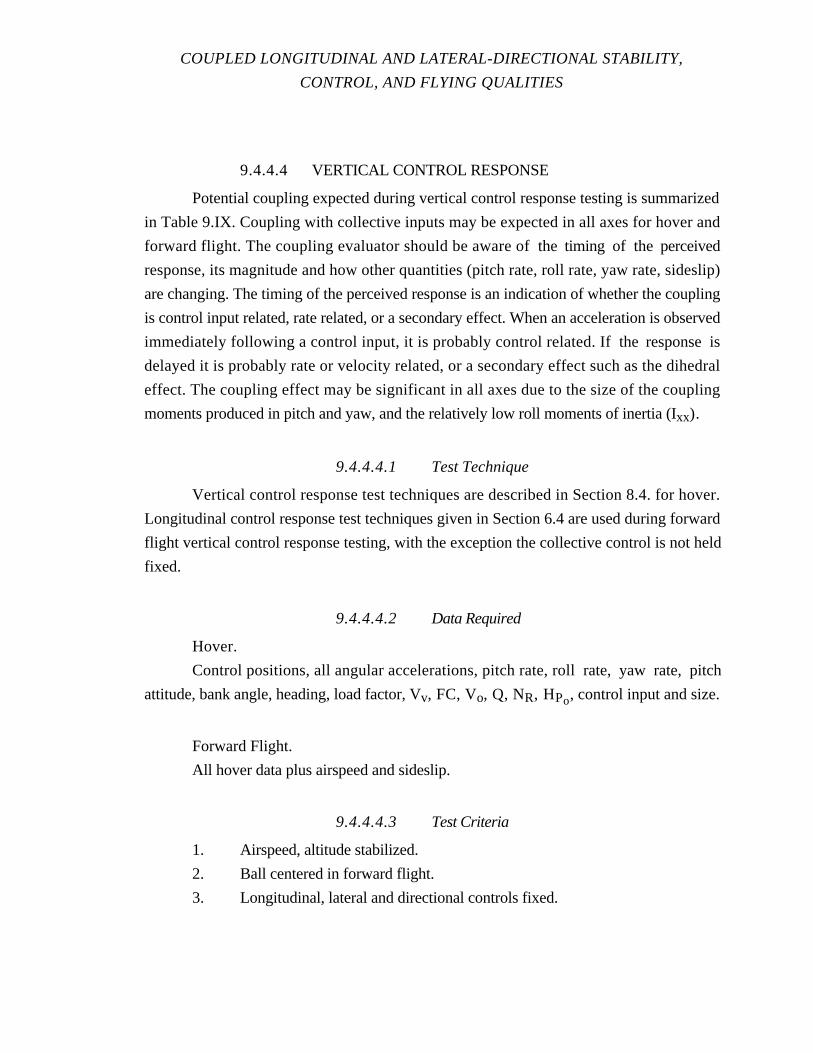
COUPLED LONGITUDINAL AND LATERAL-DIRECTIONAL STABILITY,
CONTROL, AND FLYING QUALITIES
9.4.4.4 VERTICAL CONTROL RESPONSE
Potential coupling expected during vertical control response testing is summarized
in Table 9.IX. Coupling with collective inputs may be expected in all axes for hover and
forward flight. The coupling evaluator should be aware of the timing of the perceived
response, its magnitude and how other quantities (pitch rate, roll rate, yaw rate, sideslip)
are changing. The timing of the perceived response is an indication of whether the coupling
is control input related, rate related, or a secondary effect. When an acceleration is observed
immediately following a control input, it is probably control related. If the response is
delayed it is probably rate or velocity related, or a secondary effect such as the dihedral
effect. The coupling effect may be significant in all axes due to the size of the coupling
moments produced in pitch and yaw, and the relatively low roll moments of inertia (Ixx).
9.4.4.4.1 Test Technique
Vertical control response test techniques are described in Section 8.4. for hover.
Longitudinal control response test techniques given in Section 6.4 are used during forward
flight vertical control response testing, with the exception the collective control is not held
fixed.
9.4.4.4.2 Data Required
Hover.
Control positions, all angular accelerations, pitch rate, roll rate, yaw rate, pitch
attitude, bank angle, heading, load factor, Vv, FC, Vo, Q, NR, HPo, control input and size.
Forward Flight.
All hover data plus airspeed and sideslip.
9.4.4.4.3 Test Criteria
1. Airspeed, altitude stabilized.
2. Ball centered in forward flight.
3. Longitudinal, lateral and directional controls fixed.
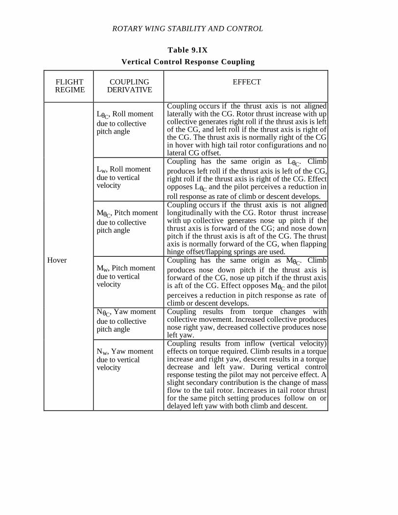
ROTARY WING STABILITY AND CONTROL
Table 9.IX
Vertical Control Response Coupling
FLIGHTREGIME
COUPLINGDERIVATIVE
EFFECT
LθC, Roll momentdue to collectivepitch angle
Coupling occurs if the thrust axis is not alignedlaterally with the CG. Rotor thrust increase with upcollective generates right roll if the thrust axis is leftof the CG, and left roll if the thrust axis is right ofthe CG. The thrust axis is normally right of the CGin hover with high tail rotor configurations and nolateral CG offset.
Lw, Roll momentdue to verticalvelocity
Coupling has the same origin as LθC. Climbproduces left roll if the thrust axis is left of the CG,right roll if the thrust axis is right of the CG. Effectopposes LθC and the pilot perceives a reduction inroll response as rate of climb or descent develops.
MθC, Pitch momentdue to collectivepitch angle
Coupling occurs if the thrust axis is not alignedlongitudinally with the CG. Rotor thrust increasewith up collective generates nose up pitch if thethrust axis is forward of the CG; and nose downpitch if the thrust axis is aft of the CG. The thrustaxis is normally forward of the CG, when flappinghinge offset/flapping springs are used.
HoverMw, Pitch momentdue to verticalvelocity
Coupling has the same origin as MθC. Climbproduces nose down pitch if the thrust axis isforward of the CG, nose up pitch if the thrust axisis aft of the CG. Effect opposes MθC and the pilotperceives a reduction in pitch response as rate ofclimb or descent develops.
NθC, Yaw momentdue to collectivepitch angle
Coupling results from torque changes withcollective movement. Increased collective producesnose right yaw, decreased collective produces noseleft yaw.
Nw, Yaw momentdue to verticalvelocity
Coupling results from inflow (vertical velocity)effects on torque required. Climb results in a torqueincrease and right yaw, descent results in a torquedecrease and left yaw. During vertical controlresponse testing the pilot may not perceive effect. Aslight secondary contribution is the change of massflow to the tail rotor. Increases in tail rotor thrustfor the same pitch setting produces follow on ordelayed left yaw with both climb and descent.
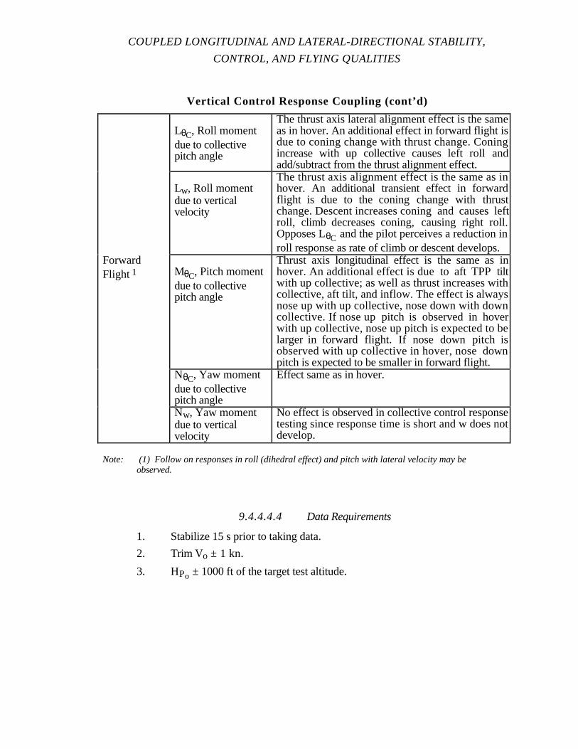
COUPLED LONGITUDINAL AND LATERAL-DIRECTIONAL STABILITY,
CONTROL, AND FLYING QUALITIES
Vertical Control Response Coupling (cont’d)
LθC, Roll momentdue to collectivepitch angle
The thrust axis lateral alignment effect is the sameas in hover. An additional effect in forward flight isdue to coning change with thrust change. Coningincrease with up collective causes left roll andadd/subtract from the thrust alignment effect.
Lw, Roll momentdue to verticalvelocity
The thrust axis alignment effect is the same as inhover. An additional transient effect in forwardflight is due to the coning change with thrustchange. Descent increases coning and causes leftroll, climb decreases coning, causing right roll.Opposes LθC and the pilot perceives a reduction inroll response as rate of climb or descent develops.
ForwardFlight 1 MθC, Pitch moment
due to collectivepitch angle
Thrust axis longitudinal effect is the same as inhover. An additional effect is due to aft TPP tiltwith up collective; as well as thrust increases withcollective, aft tilt, and inflow. The effect is alwaysnose up with up collective, nose down with downcollective. If nose up pitch is observed in hoverwith up collective, nose up pitch is expected to belarger in forward flight. If nose down pitch isobserved with up collective in hover, nose downpitch is expected to be smaller in forward flight.
NθC, Yaw momentdue to collectivepitch angle
Effect same as in hover.
Nw, Yaw momentdue to verticalvelocity
No effect is observed in collective control responsetesting since response time is short and w does notdevelop.
Note: (1) Follow on responses in roll (dihedral effect) and pitch with lateral velocity may be observed.
9.4.4.4.4 Data Requirements
1. Stabilize 15 s prior to taking data.
2. Trim Vo ± 1 kn.
3. HPo ± 1000 ft of the target test altitude.
ROTARY WING STABILITY AND CONTROL
9.4.5 Longitudinal Long Term Coupling
The longitudinal long term mode is typically a low frequency oscillatory motion or
an aperiodic divergent motion for helicopters. The oscillatory mode may be convergent or
divergent. For either the oscillatory or divergent modes, the motion consists of an
interchange of airspeed and altitude at modest pitch rates. Classically the long term mode is
considered to be uncoupled in roll and yaw.
Coupling may appear during investigation of long term characteristics if it is not
actively suppressed by pilot inputs. As airspeed variations occur about the nominal trim
airspeed, roll moments are expected. These roll moment (Lu) contributions, acting through
coning and airspeed changes, generate right roll tendencies during higher than trim airspeed
conditions, and left roll tendencies for slower airspeeds. Additionally, when airspeeds are
slower than trim (aircraft pitching down) or faster than trim (aircraft pitching up), some roll
with pitch rate is expected. The roll with airspeed and roll with pitch rate work to some
degree to cancel each other. Figure 9.14 illustrates the airspeed, attitude, and pitch
relationships for an undamped long term oscillation. This figure shows that the two roll
contributions are opposed. For very low frequency (long period) oscillations with low
pitch rates, the roll with airspeed term dominates. For higher frequency oscillations, the
roll with pitch rate contributions may have a stronger influence. Figures 9.15 and 9.16
illustrate the phasing of bank angle with airspeed and altitude. Figure 9.15 illustrates roll
with airspeed only coupling, and Figure 9.16 is for roll with pitch rate only coupling.
Comparing figures 9.15 and 9.16, the phasing of the bank angle excursions is dependent
on the dominant form of coupling encountered. The actual phasing of the bank angle
changes during long term longitudinal motions depends on the relative magnitudes of each
contribution.

COUPLED LONGITUDINAL AND LATERAL-DIRECTIONAL STABILITY,
CONTROL, AND FLYING QUALITIES
Time - s
Alti
tude
AboveTrim
BelowTrim
1
2
3
4
1. Trim Airspeed, No Roll Due to Airspeed Maximum Nose Down Attitude, No Pitch Rate
2. Maximum Airspeed, Maximum Right Roll Due to Airspeed Maximum Nose Up Pitch Rate, Maximum Left Roll Due to Pitch Rate
3. Trim Airspeed, No Roll Due to Airspeed Maximum Nose Up Attitude, No Pitch Rate
4. Minimum Airspeed, Maximum Left Roll Due to Airspeed Maximum Nose Down Pitch Rate, Maximum Right Roll Due to Pitch Rate
Figure 9.14Airspeed, Altitude, and Pitch Relationships
During Long Term Oscillation
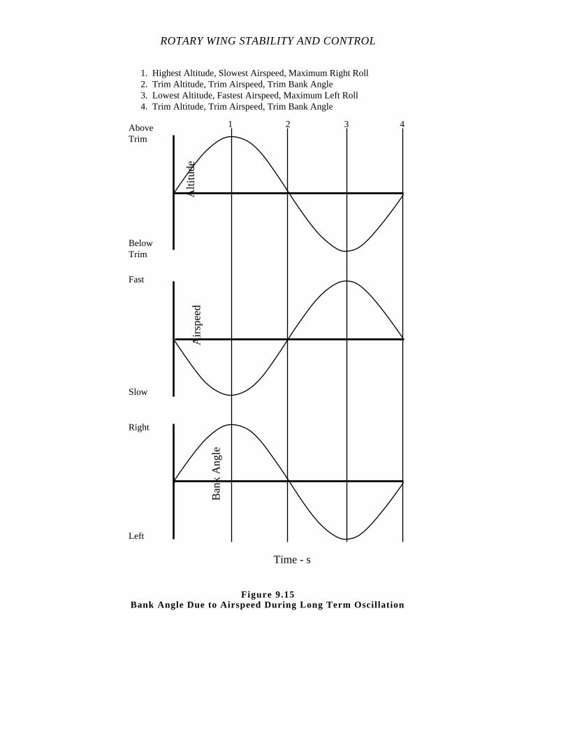
ROTARY WING STABILITY AND CONTROL
Alti
tude
AboveTrim
BelowTrim
Airs
peed
Fast
Slow
Right
Left
Ban
k A
ngle
1 2 3
Time - s
4
1. Highest Altitude, Slowest Airspeed, Maximum Right Roll2. Trim Altitude, Trim Airspeed, Trim Bank Angle3. Lowest Altitude, Fastest Airspeed, Maximum Left Roll4. Trim Altitude, Trim Airspeed, Trim Bank Angle
Figure 9.15Bank Angle Due to Airspeed During Long Term Oscillation
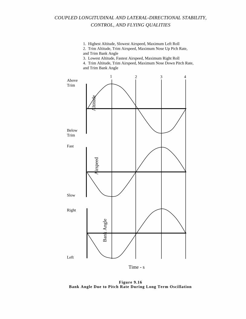
COUPLED LONGITUDINAL AND LATERAL-DIRECTIONAL STABILITY,
CONTROL, AND FLYING QUALITIES
Alti
tude
AboveTrim
BelowTrim
Airs
peed
Fast
Slow
Right
Left
Ban
k A
ngle
1 2 3
1. Highest Altitude, Slowest Airspeed, Maximum Left Roll2. Trim Altitude, Trim Airspeed, Maximum Nose Up Pich Rate,and Trim Bank Angle3. Lowest Altitude, Fastest Airspeed, Maximum Right Roll4. Trim Altitude, Trim Airspeed, Maximum Nose Down Pitch Rate,and Trim Bank Angle
Time - s
4
Figure 9.16Bank Angle Due to Pitch Rate During Long Term Oscillation
ROTARY WING STABILITY AND CONTROL
If bank angle excursions are allowed to develop during testing of long term
oscillations, then sideslip angle changes can be expected through introduction of spiral
mode effects. The spiral mode may be convergent or divergent.
During investigation of longitudinal long term oscillatory modes of motion, the
evaluator may observe rolling and yawing motions superimposed on the classical pitch
motion with the controls fixed or free.
When the longitudinal long term motion is aperiodic the aircraft is statically unstable
(normally with weak pitch rates) and the dynamics involve what appear to be spiral mode
characteristics. Statically unstable helicopters exhibit rolling motions as airspeed changes
occur. When airspeed increases during the divergence, right roll will be observed as the
helicopter pitches down and accelerates. When the airspeed decreases, the roll tendency is
to the left. The pilot may measure the controls required to counter roll tendencies, or may
investigate the motions with controls free. Obviously, if the controls are free, there may be
an interaction between the longitudinal and spiral modes.
9.4.5.1 EXCITATION METHODS
1. No conscious excitation. Controls fixed and no pilot inputs. Imperfect trim
conditions or atmospheric disturbance may excite an aperiodic divergent mode or a lightly
damped oscillatory mode. This is an unsatisfactory excitation technique if no response is
obtained, but usually indicates a desirable aircraft characteristic.
2. Use the longitudinal control to accelerate or decelerate to an airspeed faster
or slower than trim. Then smoothly return the control to the original trim position and
record the aircraft motion. An off trim airspeed variation of 5 to 15 kn is normally used to
excite the motion.
3. The method of excitation can determine the type of response documented.
Natural disturbances which result in a long term response are desirable but these responses
are usually contaminated by another disturbance before the motion is completed. This
makes quantifying the mode of motion difficult.
COUPLED LONGITUDINAL AND LATERAL-DIRECTIONAL STABILITY,
CONTROL, AND FLYING QUALITIES
9.4.5.2 TEST TECHNIQUE
1. Stabilize at the desired trim airspeed (these tests can be conducted at
trimmed conditions other than level flight) and reduce all control forces to zero. Do not
retrim control forces or move the collective during the test.
2. Record trim conditions. Assure the ability of returning to trim control
positions and of holding them after exciting the response.
3. Determine if a long term response results from a natural disturbance. With
the controls either fixed or free, note the open loop aircraft response. If no aircraft
response is observed, an artificial excitation is used.
4. Excite the aircraft using one or all of the artificial methods discussed above.
Try several different methods to find the most representative aircraft responses to include in
the report. Do not retrim any control forces and keep the collective constant during the
response.
5. If the aircraft is flown with controls free (hands off), obtain responses
following the excitation. The controls are released at trim so the subsequent control
motions indicate the effect of attitude changes and gravity force acting during the response.
6. Record the resulting mode of motion using cockpit data and automatic
recording systems. Cockpit displayed airspeed, altitude, and attitudes are recorded at
selected increments of time. Start the stop watch at the completion of the excitation or at a
predetermined airspeed. The zero time reference point is arbitrary. Small enough time
intervals are used to define the shape of irregular responses.
7. The resulting mode of motion may not be a classical single axis response.
Use lateral cyclic and directional controls as necessary to maintain a single axis response
for the initial excitation. If you find the lateral-directional inputs are significant, record a
time history of the aircraft response with all controls free.
8. For hand held data, a plot of airspeed at regular intervals (5 to 10 s)
adequately defines the response. An alternate method is to record peak (maximum and
minimum) airspeeds, and determine the period by timing the response as the helicopter
passes through the trim airspeed.
9.4.5.3 DATA REQUIRED
Vo, HPo, Vv, θ, φ, heading, HQR, VAR, FC, To, Q, NR, and cockpit control
positions.
ROTARY WING STABILITY AND CONTROL
Following the excitation, record airspeed, altitude, and attitudes as a function of
time. Use automatic recording systems to simplify this task.
9.4.5.4 TEST CRITERIA
1. Ball centered, balanced flight.
2. Controls fixed (at trim) and/or free.
3. Collective fixed.
9.4.5.5 DATA REQUIREMENTS
1. Stabilize 15 s prior to taking data.
2. Trim Vo ± 1 kn.
3. HPo ± 1000 ft of the target test altitude.
9.4.6 Spiral Motion Coupling
The helicopter spiral mode is typically a slowly developing long term aperiodic
motion which may be stable, neutral or unstable. The spiral mode characteristics are
defined by the time history of the bank angle after the helicopter is disturbed in bank angle.
Tests are conducted normally at constant airspeed by using the longitudinal control as
required to maintain airspeed. If airspeed is not maintained then other effects may be
superimposed. When the bank angle is disturbed, naturally or artificially, sideslip is
generated, usually in the direction of bank. One of the effects of the sideslip change is the
generation of a directional stability yawing moment(nose right for right wing down).
Because of the bank angle, the yaw moment produces a nose down attitude change tending
to accelerate the helicopter longitudinally. When this acceleration is unchecked by the pilot,
additional roll moments are produced as well as pitch moments. The pitch moments may
be stabilizing or destabilizing, as evidenced by the longitudinal control or force gradient
measured during static longitudinal stability tests. With a longitudinally statically unstable
aircraft, airspeed increases persist and a further right roll results when starting from an
initial right bank, and a reduction in left bank angle when starting from initial left roll.
Disturbances of the long term divergence mode produce a stabilizing effect for spiral
stability tests initiated from left bank angles, and destabilizing from initial right bank
angles.
COUPLED LONGITUDINAL AND LATERAL-DIRECTIONAL STABILITY,
CONTROL, AND FLYING QUALITIES
For helicopters having positive longitudinal static stability characteristics nose up
pitching moments with airspeed increases excite the long term oscillatory longitudinal
motion and a coupling between the spiral and longitudinal modes is evident.
During spiral stability testing, the pilot should be aware of coupling. He may wish
to maintain airspeed with longitudinal cyclic and measure the control required to hold
airspeed. Since spiral and long term longitudinal motions are nuisance modes which may
require periodic suppression during conduct of some tasks, the pilot investigates the
constrained motion (hold airspeed during spiral tests) as well as the free motion. By
allowing the interplay between modes, the evaluator can assess expected aircraft motions
and the degree to which pilot attention is required if distracted by other mission related
tasks.
9.4.6.1 EXCITATION METHODS
1. No conscious excitation. Controls fixed and no pilot inputs. Imperfect trim
conditions or atmospheric disturbance may excite an aperiodic divergent mode or a lightly
damped oscillatory mode. This is an unsatisfactory excitation technique if no response is
obtained, but usually indicates a desirable aircraft characteristic.
2. Use the lateral or directional control to establish a 5˚ to 10˚ bank angle.
Then smoothly return the control to the original trim position and record the aircraft motion.
9.4.6.2 TEST TECHNIQUE
1. Trim the helicopter in wings level, steady heading, coordinated flight at the
desired test conditions.
2. Use directional controls to develop a sideslip angle. Hold sideslip until the
helicopter rolls to the desired bank angle.
3. For tail rotor helicopters, the rate of directional control application should
not create a roll moment due to change in tail rotor thrust. Lateral control is fixed
throughout the evaluation at the initial trim position.
4. Use a range of bank angles from 5˚ to approximately 20˚ unless
significantly larger bank angles are routinely experienced in accomplishing the mission of
the helicopter.
ROTARY WING STABILITY AND CONTROL
5. After the bank angle is established, smoothly return the directional controls
to the trim position and observe the helicopter response.
6. If the effective dihedral of the helicopter is not sufficient to achieve the
desired bank angle, the alternate method is to fix the directional controls at trim, use lateral
cyclic to establish the desired bank angle, smoothly return the lateral cyclic to trim, and
observe the helicopter response. Since the spiral mode is usually weak, the response is
easily contaminated if the controls are not returned exactly to trim.
7. Record a time history of the response or record the bank angle at selected
time intervals to generate a plot of bank angle as a function of time.
8. Repeat steps 1 through 7 as required to evaluate increasingly larger bank
angles both left and right.
9.4.6.3 DATA REQUIRED
Control positions, initial and final lateral or directional control positions, Vo, Vv,
φ, β, θ, Q, NR, FC, HPo, and To.
Hand recorded or automatic time history of bank angle versus time.
9.4.6.4 TEST CRITERIA
1. Wings level, ball centered, unaccelerated flight at trim.
2. Controls fixed except for the excitation control.
3. Excitation control returned exactly to trim.
4. No retrimming.
9.4.6.5 DATA REQUIREMENTS
1. Stabilize 15 s prior to returning excitation control to trim.
2. Vo ± 1 kn.
3. HPo ± 1000 ft of the target test altitude.
4. NR ± 0.5%.

COUPLED LONGITUDINAL AND LATERAL-DIRECTIONAL STABILITY,
CONTROL, AND FLYING QUALITIES
9.4.7 Lateral-Directional Oscillation Coupling
The helicopter lateral-directional oscillation (LDO) mode is typically a relatively
short term, positively damped, oscillatory motion with a period of 3 to 5 s. Depending on
the relative sizes of stability derivatives involved, the motion may be flat with little or no
roll involved or a combination of yawing, sideslipping, and rolling. In the classical LDO,
pitch attitude and airspeed excursions are minimal. Since the conventional helicopter has a
non symmetric configuration, coupling of the LDO into pitching motions can be expected.
Potential contributions to pitch motions are the pitch moment due to lateral velocity (Mv) or
sideslip, and the pitch moment due to roll rate (Mp). When the sideslip angle is to the right
a nose up moment is provided from the rotor coning. Left sideslips cause a nose down
moment. Roll moments (accelerations) and subsequent roll rates result from the dihedral
effect as sideslip changes, and from roll moment due to yaw rate (Lr). The initial
development of pitch response due to lateral velocity and roll rate are through the short term
longitudinal mode of motion. When the LDO is heavily damped, minimal pitch excursions
are observed. For lightly damped LDOs, pitching motions at the LDO frequency can
become apparent. These pitch motions with lightly damped LDOs aggravate tracking
precision to a greater degree than poor LDO damping. If the LDO is low frequency, the
pitch attitude excursions may generate commensurate airspeed changes.
Long term pitching motions are possible after complete subsidence of the LDO,
whether heavily or lightly damped. Just as for uncoupled dynamics, the short term motion
through minor airspeed or attitude changes provides the energy required to initiate long
term dynamics. These residual longitudinal dynamics and spiral characteristics can be
coupled, leading to increased pilot effort to suppress undesired motions.
9.4.7.1 EXCITATION METHODS
1. No conscious pilot inputs. Imperfect trim conditions or atmospheric
disturbance may excite an aperiodic divergent mode or lightly damped oscillatory mode. If
no significant response is obtained, it could indicate a desirable helicopter characteristic
particularly for flight in turbulence.
ROTARY WING STABILITY AND CONTROL
2. Pilot excitation.
a. Release from steady-heading sideslip. This is generally the
preferred technique because it closely resembles conditions encountered in flight. The
technique requires that the cyclic and directional controls are simultaneously returned to the
trim conditions. Control system mechanical characteristics often complicate this
requirement. These difficulties can be overcome with use of control fixtures.
b. Release from pedal driven LDO. After trimming the helicopter at the
desired conditions, drive the helicopter in yaw with a sinusoidal pedal input. Identify the
damped frequency of the yaw oscillation. After exciting the yaw oscillation, stop the
sinusoidal input with the directional control at the trim position and observe (record) the
helicopter response.
c. Lateral cyclic or collective pulse. Secondary test techniques used to
create a transient sideslip angle include a lateral cyclic pulse or a collective pulse input. The
lateral cyclic pulse technique is applicable where the adverse/proverse yaw characteristics
are appreciable and AFCS provides no heading hold or coordinated turn feature. The
collective pulse technique is applicable for tail rotor configured helicopter.
9.4.7.2 TEST TECHNIQUE
1. Stabilize at the desired trim airspeed and reduce all control forces to zero.
Subsequently, do not retrim control forces. Assure you can return and maintain the
controls at the trim position after exciting the response.
2. Record trim condition.
3. First determine if a LDO results from a natural disturbance. With the
controls either fixed or free, note the open loop helicopter response. If no helicopter
response is observed, use an artificial excitation.
4. Excite the helicopter response using one of the artificial methods.
5. If the helicopter is operationally flown hands off, obtain controls free
responses following excitation. Controls are released at trim so the subsequent response
indicates the effect of control motions.
6. Record the resulting motion using cockpit data and automatic recording
system.
7. The effects of various degraded AFCS modes should be considered and
investigated if warranted.
COUPLED LONGITUDINAL AND LATERAL-DIRECTIONAL STABILITY,
CONTROL, AND FLYING QUALITIES
9.4.7.3 DATA REQUIRED
β, φ, θ, Vo, HPo, Vv, FC, To, Q, NR, and cockpit control positions.
Time history of the helicopter response to excitation. Attitudes (θ, φ, and β), rates
(q, p, and r), and control positions. Estimate the φ/β ratio, period, and damping.
9.4.7.4 TEST CRITERIA
1. Ball centered, balanced flight at trim.
2. Longitudinal, lateral, and pedal controls fixed (at trim) and/or free.
3. Collective fixed.
9.4.7.5 DATA REQUIREMENTS
1. Trim Vo ± 2 kn.
2. HPo ± 1000 ft of the target test altitude.
3. NR ± 0.5%.
9.4.8 Cyclic Only Turns
Cyclic only turns are used to give insight to several lateral-directional handling
qualities characteristics. Once the turn is established (steady turn), cyclic opposite the turn
or cyclic into the turn may be required. Opposite cyclic is an indicator of an unstable spiral
mode if the lateral control gradient in steady heading sideslip is in the proper sense, right
lateral control in right sideslip. Cyclic into the turn indicates just the opposite. During turn
entry, either smooth gradual or abrupt lateral control inputs are used. For the smooth
entry, insight is gained to the helicopter's overall ability to maintain coordinated flight. The
abrupt input provides information about the control response and the degree to which
coupling effects are manifested. The main coupling expected is the yaw moment due to
lateral cyclic pitch angle (NA1s). The sign of NA1s is dependent on longitudinal CG
position relative to the rotor shaft. When the CG is aft of the shaft, right lateral control
inputs are expected to produce proverse right yaw moments. An additional contribution to
ROTARY WING STABILITY AND CONTROL
proverse yaw results from rotor wake skew (rotor side wash to the left with right control)
and its effect on tail rotor thrust and fin loads. Adverse yaw is expected with forward CG
locations. During abrupt lateral control inputs with associated yaw moments, the pilot
observes simultaneous roll and yaw accelerations. When yaw is in the adverse sense a
false start (yaw away from roll) or hesitation in the development of yaw rate is experienced.
With proverse yaw immediate roll and yaw acceleration in the same direction are evident.
Yaw with lateral cyclic is considered a coupling term. At first observation it appears
proverse yaw is desirable. In reality, too much coupling in either direction is undesirable.
With significant adverse yaw an excessive delay in the generation of yaw rate or turn rate
may exist. In extreme cases too much proverse yaw can result in the pilot driving the LDO
mode unstable during high gain closed loop control of bank angle.
During abrupt lateral control induced bank angle changes, information from the
degree of uncoordinated (ball not centered) flight which occurs reflects qualitatively the
adequacy of the aircraft directional stability.
Pilot attention while conducting lateral control only turns is directed to initial
yawing accelerations, initial ball position, transient side force cues, follow-on ball
movement and lateral control requirements in the stabilized turn. If serious lack of
coordination exists, pilot ability to provide coordination through directional control inputs
is assessed. When significant adverse or proverse yaw tendencies are observed, tight pilot
in the loop tasks such as precise bank angle captures, abrupt roll outs from established
turns, and roll reversals are evaluated for mission suitability.
9.4.8.1 TEST TECHNIQUE
1. Stabilize at the desired trim airspeed and reduce all control forces to zero.
Maintain longitudinal, directional and collective controls fixed during initial tests.
2. Record trim conditions.
3. Starting with slower, more gradual lateral control inputs, establish left and
right turns to predetermined bank angles.
4. Increase initial control application rate up to step inputs of predetermined
sizes, with follow-on lateral inputs to establish desired bank angle. A control fixture is
used to size inputs. Review methods in Section 7.4 for use of control fixtures.
5. If significant yaw excursions are observed during initial tests, attempt to
coordinate with directional control.
COUPLED LONGITUDINAL AND LATERAL-DIRECTIONAL STABILITY,
CONTROL, AND FLYING QUALITIES
6. Perform tests of bank angle capture, roll reversals, etc., if warranted.
7. Record time histories of representative aircraft responses, as desired for
documentation purposes.
9.4.8.2 DATA REQUIRED
Control positions θ, φ, β, p, q, r, Vo, HPo, FC, To, Q, NR, size and direction of
inputs.
Use automatic recording systems.
9.4.8.3 TEST CRITERIA
1. Ball centered, balanced flight at trim.
2. Longitudinal, directional and collective controls fixed. Directional control
movement as required when evaluating coordination efforts.
9.4.8.4 DATA REQUIREMENTS
1. Stabilize 15 s prior to taking data.
2. Trim Vo ± 2 kn.
3. HPo ± 1000 ft from the target test altitude.
4. Ball centered, ± 1/4 ball, for trim.
9.4.9 Pedal Only Turns
Pedal only turns are used to provide information about several lateral-directional
handling qualities characteristics. Once the turn is established (steady turn), pedal opposite
the turn or pedal into the turn may be required. Opposite pedal indicates an unstable spiral
mode if the directional control gradient in steady heading sideslips indicates positive
directional stability. It is highly unlikely the directional control gradient is in the unstable
direction. Pedal into the turn indicates a stable spiral mode. During turn entry and bank
angle capture either smooth gradual or abrupt directional control inputs are used. For the
smooth entry, insight is obtained about the pilot's ability to induce and stop roll by use of
the directional controls. The abrupt input provides information about the yaw control
response and the degree to which coupling occurs. Coupling of roll with directional

ROTARY WING STABILITY AND CONTROL
control inputs is expected when the tail rotor thrust axis is not aligned with the vertical CG.
For helicopters with high tail rotors, a left directional control input causes immediate left
yaw and right roll accelerations. The roll acceleration in time may produce a bank angle
change attempting to turn the aircraft in a direction opposite to the control input.
When the helicopter has positive dihedral effect, a left roll moment is generated as
right sideslip increases and this left roll moment eventually arrests the roll due to directional
control, and the aircraft rolls in the direction of turn. The initial roll away from the desired
direction of turn is interpreted as coupling or at least a distinct hesitation in the production
of roll rates, and attitude changes in the intended direction.
In extreme cases with inadequate dihedral effect, the helicopter may initially roll
away from the heading change and maintain a left yawed and right banked condition with
little or no ground track change, or may even continue to roll away from the intended
direction of turn.
During abrupt directional control induced turns, the immediate response gives
insight to the roll with directional control involved and the follow on roll after sideslip
develops (insight about the level of dihedral effect).
Pilot attention while conducting directional control only turns is directed to initial
roll accelerations, rates, and attitude changes, follow on roll tendencies, anticipation
required to establish the desired bank angle using directional control only, and the final
directional control required (pedal into or opposite the turn) for the steady turning
condition. Recovery to zero bank flight from steady turns using directional control only
can also be used to assess coupling and dihedral effect.
9.4.9.1 TEST TECHNIQUE
1. Stabilize at the desired trim airspeed and reduce all control forces to zero.
Maintain longitudinal, lateral and collective controls fixed.
2. Record trim conditions.
3. Starting with slower, more gradual directional control inputs, establish left
and right turns to predetermined bank angles.
4. Increase initial control application rate up to step inputs of predetermined
sizes. A control fixture is used to size inputs. Review methods of Section 7.4 for use of
control fixtures.
COUPLED LONGITUDINAL AND LATERAL-DIRECTIONAL STABILITY,
CONTROL, AND FLYING QUALITIES
5. Perform tests to look at initial turn capability, bank angle capture, turn
reversals, etc.
6. Record time histories of representative aircraft responses as desired for
documentation purposes.
9.4.9.2 DATA REQUIRED
Control positions θ, φ, β, p, q, r, Vo, HPo, FC, To, Q, NR, size and direction of
inputs.
Use automatic recording systems.
9.4.9.3 TEST CRITERIA
1. Ball centered, balanced flight at trim.
2. Longitudinal, lateral and collective controls fixed.
9.4.9.4 DATA REQUIREMENTS
1. Stabilize 15 s prior to taking data.
2. Trim Vo ± 2 kn.
3. HPo ± 1000 ft of the target test altitude.
4. Ball centered, ± 1/4 ball, for trim.
9.5 DATA REDUCTION
Data reduction requirements for these tests are limited to the application of
instrument corrections to recorded data. Airspeed and altitude data are corrected for both
instrument and position errors in forward flight. Automatic data recording systems
normally include total instrumentation system corrections in the process used to change a
flight tape (or telemetry) raw data into engineering units. Most quantitative information
required for plotted data are read from time histories of selected data parameters. In some
instances, time histories are used in dynamic tests to show the overall response and the
interrelation/timing of parameter changes. Time histories are appropriately annotated to
show the phenomena leading to the final assessment/conclusions drawn from aircraft
responses.
ROTARY WING STABILITY AND CONTROL
9.5.1 Trimmed Control Positions
9.5.1.1 HOVER AND LOW AIRSPEED
Plot all control positions, pitch attitude, banks angles, torque (optimal), versus
relative true wind velocity (longitudinal, lateral and vertical translation) or wind direction
(critical azimuth) for all stabilized data points.
Provide time histories of all control positions, velocity if available (Doppler, or low
airspeed system), aircraft attitudes and angular rates, load factor torque (optional) to show
unsuitable characteristics obtained during translation/repositioning dynamic tests. Time
histories of suitable characteristics are optional.
Plots and time histories include tabulations of weight, CG, pressure altitude,
ambient temperature, height above ground level, AFCS operating mode, and NR.
9.5.1.2 FORWARD FLIGHT
Plot all control positions, pitch attitude, bank angle, sideslip, and torque (optional)
versus calibrated airspeed for all stabilized data points.
Provide time histories of all control positions, airspeed, altitude, aircraft attitudes
and angular rates, load factor, sideslip, torque, and NR to show unsuitable characteristics
obtained during dynamic transition (climb, descent, acceleration, deceleration, etc.) tests.
Time histories of suitable characteristics are optional.
Plots and time histories include tabulations of weight, CG, pressure altitude (not
required if shown on time history) ambient temperature, AFCS operating mode and NR
(not required if shown on time history).
9.5.1.3 STEADY TURNS
Plot all control positions, pitch attitude, bank angle, sideslip, torque, rate of descent
(constant collective turns), versus load factor. Distinguish between left and right turns.
Plot calibrated airspeed to show quality of airspeed control.

COUPLED LONGITUDINAL AND LATERAL-DIRECTIONAL STABILITY,
CONTROL, AND FLYING QUALITIES
Tabulate weight, CG, pressure altitude, airspeed (if not plotted), ambient
temperature, AFCS operating mode and NR.
9.5.2 Steady Pull Ups/Push Overs
Plot all control positions, pitch rate, sideslip, torque versus load factor for all ball
centered pull up and push over data points obtained with longitudinal cyclic inputs.
Provide time histories of all control positions, pitch attitude, bank angle, heading,
all angular rates, load factor, torque, and sideslip for:
1. Cyclic pull ups/push overs where excessive amount of pilot effort was
required to maintain balanced flight.
2. Cyclic pull ups/push overs which were intentionally not coordinated with
other controls if undesirable characteristics exist.
3. Collective pull ups/push overs which required excessive amount of pilot
effort to obtain required response (coordinated flight, or constant heading, or constant pitch
attitude, etc.).
Plots and time histories include tabulations of weight, CG, pressure altitude,
ambient temperature, AFCS operating mode and NR.
9.5.3 Steady Heading Sideslips
Plot all control positions, pitch attitude, bank angle, rate of climb or descent versus
sideslip angle.
Plots include tabulations of weight, CG, pressure altitude, AFCS operating mode,
torque and NR.
ROTARY WING STABILITY AND CONTROL
9.5.4 Control Response
Provide time histories of all control positions, all angular accelerations, all angular
rates, pitch attitude, bank angle, heading, load factor, airspeed, altitude, torque, AFCS
positions (optional), sideslip, and NR. Time history parameters are selectively eliminated if
certain coupling responses are not observed.
Tabulations of weight, CG, ambient temperature, and AFCS operating mode are
included. Chapters 6, 7 and 8 address additional required annotations on time histories.
9.5.5 Longitudinal Long Term Coupling
Provide time histories of all control positions, pitch attitude, bank angle, heading,
all angular rates (optional if rates are low), airspeed, altitude, load factor (optional), and
sideslip. Time histories involving pilot control manipulation to maintain coordinated flight
and time histories of aircraft response with controls fixed and free are appropriate.
Tabulations of weight, CG, ambient temperature, AFCS operating mode, torque,
and NR are included.
9.5.6 Spiral Motion Coupling
Provide time histories of all control positions, pitch attitude, bank angle, heading,
all angular rates (optional if rates are low), airspeed, altitude, load factor (optional), and
sideslip. Time histories involving pilot longitudinal control manipulation to maintain
airspeed, and time histories of aircraft response with controls fixed and free are
appropriate.
Tabulations of weight, CG, ambient temperature, AFCS operating mode, torque,
and NR are included.
9.5.7 Lateral-Directional Oscillation Coupling
Provide time histories of all control positions, pitch attitude, bank angle, heading,
all angular rates (pitch rate optional), and sideslip. Time histories involving pilot
longitudinal control manipulation to maintain pitch attitude, and time histories of aircraft
response with controls fixed and free are appropriate.
COUPLED LONGITUDINAL AND LATERAL-DIRECTIONAL STABILITY,
CONTROL, AND FLYING QUALITIES
Tabulations of weight, CG, ambient temperature, AFCS operating mode, torque,
and NR are included.
9.5.8 Cyclic Only Turns
Time histories of the more abrupt lateral control inputs for turn entries, bank angle
captures, and roll reversals are presented to show undesirable aircraft characteristics.
Provide time histories of all control positions, pitch attitude, bank angle, heading, all
angular rates (pitch rate optional), load factor (optional), and sideslip.
Tabulations of weight, CG, airspeed, altitude, ambient temperature, AFCS
operating mode, torque, and NR are included.
9.5.9 Pedal Only Turns
Time histories of the more abrupt directional control inputs for turn entries, bank
angle captures, turn roll outs, heading reversals, etc. for representative responses are
presented to show undesirable aircraft characteristics. Provide time histories of all control
positions, pitch attitude, bank angle, heading, all angular rates (pitch rate optional), load
factor (optional), and sideslip.
Tabulations of weight, CG, airspeed, altitude, ambient temperature, AFCS
operating mode, torque, and NR are included.
9.6 DATA ANALYSIS
9.6.1 Trimmed Control Positions
9.6.1.1 HOVER AND LOW AIRSPEED
Low airspeed trimmed flight control positions are essentially analogous to hovering
(zero ground speed) in a wind of equal velocity. The analysis includes:
1. Were there any limiting factors?
ROTARY WING STABILITY AND CONTROL
2. For which axis was the limiting factor most objectionable?
3. Were the control margins adequate? Greater than 10% control position or
control power margin?
4. Were control movements required in the usual sense (forward cyclic for
forward airspeed, right lateral cyclic for right lateral flight)?
5. Were the control position changes with power, airspeed, or azimuth
excessive?
6. Could the control forces be trimmed to zero?
7. What were the aircraft attitude changes with airspeed, rate of climb? Were
they objectionable?
8. Was field-of-view adequate?
9. Were the vibrations objectionable?
10. Was there any objectionable coupling between pitch, roll, and yaw?
11. Could the pilot keep up with trim changes/coupling during dynamic
situations?
12. Are these characteristics suitable for the intended mission?
9.6.1.2 FORWARD FLIGHT
The following considerations are generally included in the analysis oftrimmed
control position in forward flight data:
1. Were there adequate control margins?
2. Was forward cyclic required with increasing airspeed?
3. Are the control position changes with changes in airspeed and power
excessive?
4. Were there significant non linearities or abrupt reversals in data trends?
5. Could forces be trimmed to zero?
6. What were pitch attitude changes with airspeed?
7. Was field-of-view adequate?
8. Were there objectionable vibrations?
9. What was the coupling between the pitch, yaw and roll axes?
10. Could small precise collective changes be made?
11. Could the pilot keep up with trim changes and coupling during dynamic
situations?
COUPLED LONGITUDINAL AND LATERAL-DIRECTIONAL STABILITY,
CONTROL, AND FLYING QUALITIES
9.6.1.3 STEADY TURNS
The following considerations are generally included in the analysis of steady turn
test data:
1. What was the basic longitudinal stability?
2. What was the effect of power addition in constant altitude turns on
longitudinal control position gradients?
3. What longitudinal force/position cues were available at increased load
factors?
4. What trim changes/coupling were involved in other axes?
5. Could the trim changes be easily compensated?
6. What pitch attitudes were required to maintain airspeed?
7. Was field-of-view adequate?
8. Were vibrations objectionable?
9.6.2 Steady Pull Ups/Push Overs
The following considerations are generally included in the analysis of steady pull
ups/push overs:
1. What was the basic longitudinal stability?
2. What longitudinal force and position cues were available at increased load
factors during cyclic induced pull up/push overs?
3. What trim changes and coupling were involved in other axes during cyclic
and collective induced pull ups/push overs?
4. Could the trim changes be easily compensated?
5. Were vibrations objectionable?
9.6.3 Steady Heading Sideslips
The following are normally included in the analysis of steady heading sideslips:
1. What were the lateral and directional control gradients? Were they adequate?
2. What was the bank angle gradient? Did it provide sufficient cues to prevent
cross control trimming.

ROTARY WING STABILITY AND CONTROL
3. What pitch attitudes and longitudinal control inputs were required to
maintain airspeed?
4. Were control and attitude gradients linear and aircraft cross control changes
predictable?
5. Was the field-of-view adequate?
6. Were the vibrations objectionable?
9.6.4 Control Response
An abundance of quantitative data are taken from the response time histories.
Parameters which define the response are: rate control effectiveness; attitude control
effectiveness; steady-state rate, maximum rate, maximum acceleration, initial acceleration,
acceleration delay, and time constant. The following considerations are an integral part of
control response and effectiveness discussions.
1. Was the steady-state rate adequate?
2. Was the response predictable?
3. Was the response consistent?
4. Were there any over control problems?
5. What coupling was observed between axes?
6. Was the coupling immediate or did it appear delayed?
7. Was the coupling desirable or undesirable?
8. What pilot efforts were required to compensate for undesired coupling?
9. What vibrations were introduced?
10. Was the response suitable for the mission?
Figures 9.17 and 9.18 illustrate the expected trends when an off axis response is
due to the control input (Figure 9.17) or due to subsequent rate or secondary effects
(Figure 9.18). As shown, the pitch accelerations (maximum slope of angular rate) occur at
nearly the same time shortly after the input is made if the off axis response is control
generated. When the off axis coupling is related to the angular rate a distinct lag is involved
in the development of the off axis acceleration, and the development of off axis angular rate
is delayed.
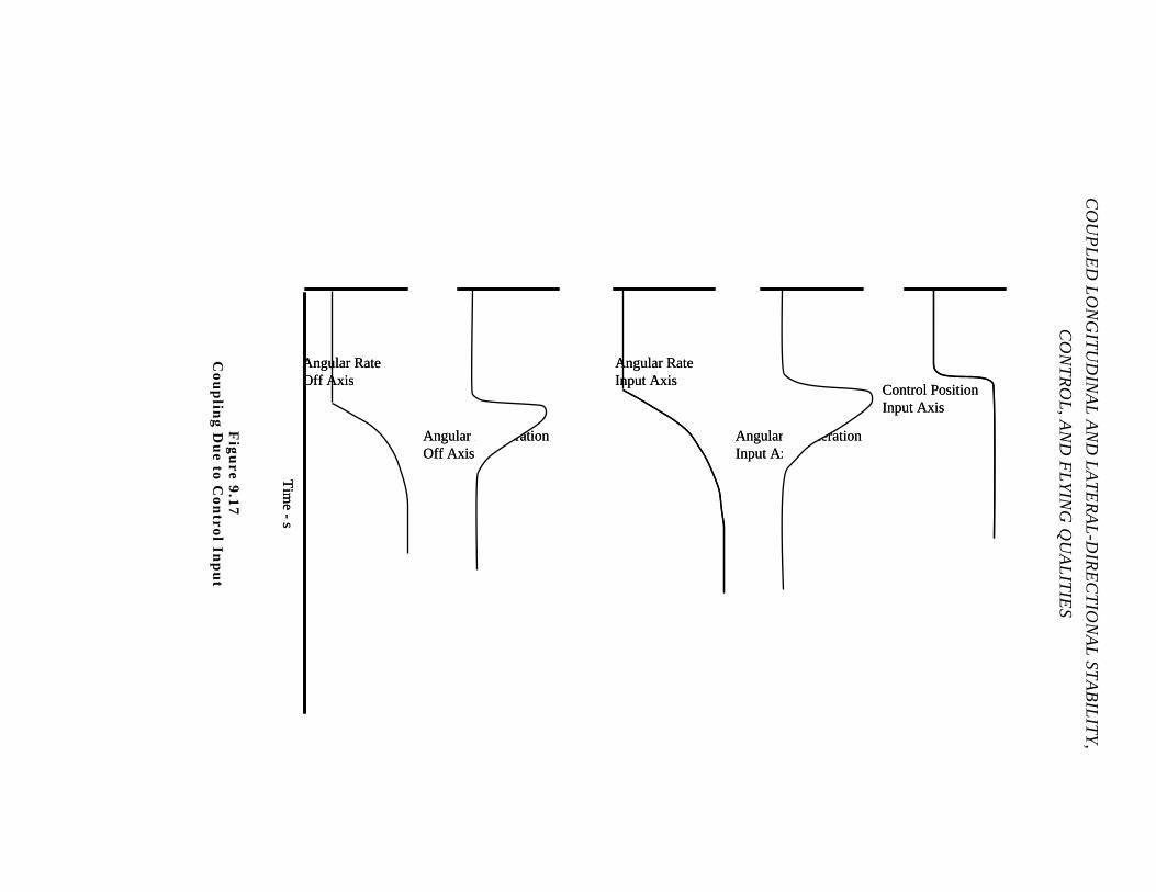
CO
UP
LE
D L
ON
GIT
UD
INA
L A
ND
LA
TE
RA
L-D
IRE
CT
ION
AL
ST
AB
ILIT
Y,
CO
NT
RO
L, A
ND
FL
YIN
G Q
UA
LIT
IES
Tim
e - s
Control PositionInput Axis
Angular AccelerationInput Axis
Angular RateInput Axis
Angular AccelerationOff Axis
Angular RateOff Axis
Tim
e - s
Control PositionInput Axis
Angular AccelerationInput Axis
Angular RateInput Axis
Angular AccelerationOff Axis
Angular RateOff Axis
Fig
ure
9.1
7C
ou
plin
g D
ue
to C
on
trol In
pu
t
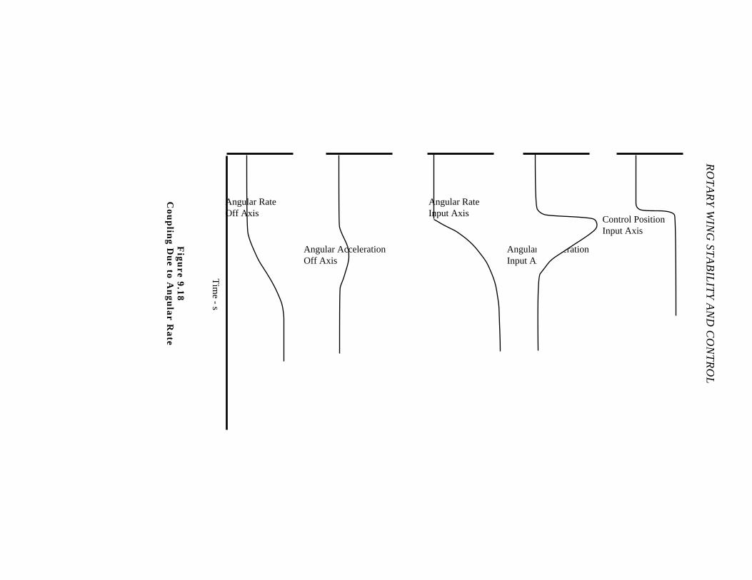
RO
TA
RY
WIN
G S
TA
BIL
ITY
AN
D C
ON
TR
OL
Tim
e - s
Control PositionInput Axis
Angular AccelerationInput Axis
Angular RateInput Axis
Angular AccelerationOff Axis
Angular RateOff Axis
Fig
ure
9.1
8C
ou
plin
g D
ue
to A
ng
ula
r Ra
te

COUPLED LONGITUDINAL AND LATERAL-DIRECTIONAL STABILITY,
CONTROL, AND FLYING QUALITIES
9.6.5 Longitudinal Long Term Coupling
The longitudinal long term motion is a nuisance mode, particularly when lightly
damped or when statically or dynamically unstable. The following considerations are
generally included in the analysis of the longitudinal long term motion:
1. How easy or difficult was it to excite the long term response?
2. In engineering terms, how do you describe the uncoupled aircraft mode of
motion? Use the period, damping ratio, time to half amplitude or time to double amplitude
to tell the reader what you saw.
3. What coupling or off axis trim changes exist?
4. What were controls fixed and free responses?
5. Are off axis motions more or less significant than the single axis motion?
6. How do the coupled and uncoupled motions influence the pilot's ability to
perform mission tasks? The significance of the response is the level to which it degrades
or helps the pilot perform a specific task. An evaluation is made of the pilot effort required
to suppress or correct the airspeed, attitude, and altitude variations about trim.
9.6.6 Spiral Motion Coupling
The spiral mode of motion is a nuisance mode, particularly when neutrally stable or
unstable. The following considerations are generally included in the analysis of the spiral
mode:
1. To what extent do natural disturbances or other motions excite the spiral
mode?
2. In engineering terms, how do you describe the uncoupled aircraft mode of
motion? Use the time to half amplitude or time to double amplitude to tell the reader what
you saw.
3. What coupling or off axis trim changes occur?
4. What were the controls fixed and free responses?
5. Were airspeed changes significant or dangerous?
6. Are off axis motions more or less significant than the basic spiral motions?
7. How does the motion influence the pilot's ability to perform mission tasks?

ROTARY WING STABILITY AND CONTROL
The significance of the response is the level to which it degrades or helps the pilot perform
a specific task. An evaluation is made of the pilot effort required to suppress or correct the
airspeed, attitude, and altitude variations from trim.
9.6.7 Lateral-Directional Oscillation Coupling
The following considerations are generally included in the analysis of lateral-
directional oscillation (LDO) characteristics:
1. How easily is the LDO excited during other mission tasks?
2. What is the basic character of the LDO in terms of frequency, damping
ratio, cycles or time to half amplitude, yawing motion or rolling motion or combination of
both?
3. Does pitch coupling exist?
4. What is pilot effort required to suppress the LDO and cross axis coupling?
5. Does the LDO degenerate into spiral or longitudinal long term motions?
6. Can the LDO mode be driven unstable with tight pilot in the loop bank angle
control tasks?
7. How does the motion influence the pilot's ability to perform mission tasks?
9.6.8 Cyclic Only Turns
The following considerations are generally included in the analysis of lateral cyclic
only turns:
1. Did the aircraft initially yaw opposite to the control input or display
excessive hesitation in developing turn in the direction of roll?
2. To what degree was transient uncoordinated (ball out) motion observed?
3. Could steady bank angles be obtained precisely and quickly ?
4. What direction of lateral control was required in the established turn?
5. What was the level of coordination (ball position) in the established turn?
6. What were the roll out responses?
7. Was the LDO excited? To what extent?
8. Could the turn be coordinated easily if desired?
COUPLED LONGITUDINAL AND LATERAL-DIRECTIONAL STABILITY,
CONTROL, AND FLYING QUALITIES
9.6.9 Pedal Only Turns
The following considerations are generally included in the analysis of directional
control only turns:
1. Did the aircraft initially roll opposite to the control input or display excessive
hesitation in developing roll in the direction of yaw?
2. Could steady bank angles be obtained with a reasonable degree of
directional control input leading?
3. What direction of directional control was required in the established turn?
4. What was the level of coordination (ball position) in the established turn?
5. Could roll out from the established turn be accomplished with directional
control only?
6. Was the LDO excited? To what extent?
7. Did the LDO excitation significantly affect desired performance?
9.7 MISSION SUITABILITY
Mission suitability is the ultimate reason for conducting any handling qualities
evaluation. The helicopter's unique capabilities in the low airspeed regime and its forward
flight capabilities provide many potential operational uses if the handling qualities and
performance of the vehicle are adequate. Before mission suitability is accessed, a detailed
clear understanding of the intended mission is developed. Additionally, the pilot's
experience in conducting similar mission maneuvers is considered. The test pilot
researches the mission tasks to establish evaluation maneuvers and determine performance
criteria. The mission maneuvers vary greatly with aircraft type, use, and operational
environment. Potential maneuvers include everything from sling load operations to rocket
firing.
Chapters 6, 7, and 8 address test procedures to evaluate handling qualities
suitability when the inter-axis coupling is neglected or easily overcome. The test pilot now
assesses mission effectiveness of the vehicle when all the considerations of the previous
chapters are included, with the realization that the aircraft is asymmetrically configured and
naturally exhibits coupled responses.
ROTARY WING STABILITY AND CONTROL
In addition to the engineering tests, the test pilot investigates how the helicopter is
used and closely duplicates these mission tasks. Knowledge of coupling origins and
measurement of coupling phenomena allows the test team to design operational scenarios
which reflect the effects of undesirable coupling characteristics. Inter-axis coupling can
aggravate long term dynamics and require significant compensation in short term
maneuvering. The mission of the aircraft determines the maneuvers flown. Cargo
helicopters require close attention to straight and level cruise tasks (long term dynamic
stability) as well as maneuvering in confined areas. Attack aircraft may need special
consideration for tracking tasks and maneuverability. Each test program requires a unique
set of mission maneuvers.
The most important aspect of mission suitability testing is to keep the operator in
mind. How the test vehicle is used in the field, and who is operating the aircraft are
important factors to consider.
9.8 SPECIFICATION COMPLIANCE
Requirements for helicopter handling qualities are contained in MIL-H-8501A.
Coupling requirements stated in MIL-H-8501A are very brief and are contained in
paragraph 3.5.16. Paragraph 3.5.11.1 of MIL-H-8501Aallows for mechanical control
mixing to the extent "... no adverse limitations in control power shall exist with any
possible combination of control inputs...".
9.9 GLOSSARY
9.9.1 Notations
a0 Coning angle
A1s Lateral cyclic pitch angle, shaft referenced
a1s Longitudinal flapping angle, shaft referenced
AFCS Automatic Flight Control System
ASW Anti-submarine warfare
b Number of blades
B1s Longitudinal cyclic pitch angle, shaft referenced
b1s Lateral flapping angle, shaft referenced
dD0 Blade element profile drag
COUPLED LONGITUDINAL AND LATERAL-DIRECTIONAL STABILITY,
CONTROL, AND FLYING QUALITIES
dF Blade element torque force
dL Blade element lift
dT Blade element thrust
e Flapping hinge offset
F Force
FC Fuel count
g Gravity
h Height of hub above CG
h' Longitudinal distance between the rotor shaft and the CG
h'lat Lateral distance between the rotor shaft and the CG
HPo Observed pressure altitude
HQR Handling Qualities Rating
hTR Height of the tail rotor above the CG
IGE In ground effect
iTR Tail rotor inclination out of vertical plane
Ixx Moment of inertia about x axis, roll moment of inertia
Iyy Moment of inertia about y axis, pitch moment of inertia
Izz Moment of inertia about z axis, yaw moment of inertia
L Net moment about x axis, Roll moment
LB1s Roll moment due to longitudinal cyclic pitch angle
LDO Lateral-directional oscillation
LH Roll moment due to rotor hub forces
Lq Roll moment due to pitch rate
LθC Roll moment due to collective pitch angle
LθTR Roll moment due to tail rotor pitch angle
Lr Roll moment due to yaw rate
lt Distance from the tail to the CG
Lu Roll moment due to longitudinal velocity
Lw Roll moment due to vertical velocity
M Net moment about y axis, Pitch moment
MA1s Pitch moment due to lateral cyclic pitch angle
MH Pitch moment due to rotor hub force
ROTARY WING STABILITY AND CONTROL
Mp Pitch moment due to roll rate
MθC Pitch moment due to collective pitch angle
MθTR Pitch moment due to tail rotor pitch angle
MS Blade mass moment
Mv Pitch moment due to lateral velocity
Mw Pitch moment due to vertical velocity
N Net moment about z axis, Yaw moment
NA1s Yaw moment due to lateral cyclic pitch angle
NB1s Yaw moment due to longitudinal cyclic pitch angle
Np Yaw moment due to roll rate
NθC Yaw moment due to collective pitch angle
NR Main rotor speed
Nu Yaw moment due to longitudinal velocity
Nv Yaw moment due to lateral velocity
Nw Yaw moment due to vertical velocity
OFT Operational flight trainer
OGE Out of ground effect
p Angular velocity about x axis, Roll rate
p Angular acceleration about x axis
Q Engine torque
q Angular velocity about y axis, Pitch rate
QMR Main rotor torque
q Angular acceleration about y axis, Pitch acceleration
R Rotor radius
r Angular velocity about z axis, Radius along blade, Yaw rate
r Angular acceleration about z axis, Yaw acceleration
SAR Search and rescue
T Thrust
t Time
TCP Trim control position
To Observed temperature
TPP Tip path plane
TTR Tail rotor thrust
COUPLED LONGITUDINAL AND LATERAL-DIRECTIONAL STABILITY,
CONTROL, AND FLYING QUALITIES
u Translational velocity component along x axis
u0 Initial velocity
u Linear acceleration along x axis
V Velocity, Free stream velocity, Relative velocity
v Translational velocity component along y axis
VAR Vibration Assessment Rating
vi Induced velocity at hover
Vo Observed airspeed
VSTOL Vertical/short takeoff and landing
Vv Vertical velocity
v Linear acceleration along y axis
W Weight
w Translational velocity component along z axis
wrotor TPP translational velocity along z axis
w Linear acceleration along z axis
x Orthogonal direction along longitudinal axis of the aircraft; Distance
along x axis
y Orthogonal direction along lateral axis of the aircraft
z Orthogonal direction along vertical axis of the aircraft
9.9.2 Greek Symbols
α (alpha) Angle of attack
β (beta) Flapping angle, Sideslip angle
φ (phi) Roll angle
λ (lambda) Inflow ratio
λTR Tail rotor inflow ratio
µ (mu) Advance ratio
θ (theta) Pitch angle
θC Collective pitch angle
ROTARY WING STABILITY AND CONTROL
θTR Tail rotor pitch angle
ω (omega) Forcing frequency
ωn Natural frequency
ψ (psi) Blade azimuth angle, Phase angle, Yaw angle
Ω (Omega) Rotor angular velocity
9.10 REFERENCES
1. Johnson, W., Helicopter Theory, Princeton University Pres. 1980.
2. Military Specification, “Flying Qualities of Piloted V/STOL Aircraft”, MIL-
F-83300, 31 December 1970.
3. Military Specification, “Helicopter Flying and Ground Handling Qualities;
General Requirements For” MIL-H-8501A, with Amendment 1, 3 April, 1962.
4. Prouty, Raymond W.,Helicopter Performance, Stability, and Control,
PWS Publishers, Boston, MA, 1986.
5. U. S. Naval Test Pilot School Flight Test Manual,Rotary Wing
Performance, USNTPS-FTM-No. 106 USNTPS, Patuxent River, MD, 31 December
1987.
CHAPTER TEN
SUDDEN ENGINE FAILURES, AUTOROTATIVE FLIGHT, AND AUTOROTATIVE
LANDINGS
PAGE
10.1 INTRODUCTION 10.1
10.2 PURPOSE 10.1
10.3 THEORY 10.2
10.3.1 Engine Failure 10.2
10.3.1.1 Rotor Speed Decay 10.2
10.3.1.2 Thrust Decay 10.5
10.3.1.3 Yaw Response 10.5
10.3.1.3.1 Hover 10.9
10.3.1.3.2 Level Forward Flight 10.14
10.3.1.4 Roll Response 10.17
10.3.1.4.1 Hover 10.17
10.3.1.4.2 Level Forward Flight 10.18
10.3.1.5 Pitch Response 10.18
10.3.1.5.1 Hover 10.18
10.3.1.5.2 Level Forward Flight 10.19
10.3.1.6 Climb Versus Descent 10.23
10.3.1.7 Desired Pitch and Roll Responses 10.23
10.3.1.8 Multi-Engine Operation 10.25
10.3.1.9 Engine Failure Warning 10.29
10.3.1.9.1 Natural Warning 10.29
10.3.1.9.2 Artificial Warning 10.29
10.3.2 Steady Autorotation 10.30
10.3.2.1 Rotor Equilibrium 10.30
10.3.2.2 Rate of Descent 10.32
10.3.2.3 Minimum Collective Pitch 10.34
10.3.2.4 Optimum Autorotative Airspeeds 10.34
ROTARY WING STABILITY AND CONTROL
10.3.2.5 Trimmed Control Positions, Static, and Dynamic
Stability 10.35
10.3.2.6 Cyclic and Collective Maneuvering 10.35
10.3.2.7 Rotor Speed Control 10.37
10.3.3 Transition to Autorotation Following Power Loss 10.37
10.3.3.1 Available Delay and Pilot Reaction Times 10.38
10.3.3.2 Controls Fixed Natural Response 10.40
10.3.3.3 Response to Collective Input 10.40
10.3.3.3.1 Hover 10.40
10.3.3.3.2 Forward Flight 10.41
10.3.3.4 Response to Longitudinal Cyclic Input 10.41
10.3.3.4.1 Hover 10.41
10.3.3.4.2 Forward Flight 10.41
10.3.3.5 Control Reversal 10.42
10.3.3.6 Response to Lateral Cyclic Input 10.45
10.3.3.7 Response to Directional Control Input 10.45
10.3.3.8 Response in Rearward Flight 10.46
10.3.3.9 Control Inputs at Low Load Factors 10.46
10.3.4 Autorotative Landing 10.46
10.3.4.1 Landing From Steady Autorotative Descent 10.48
10.3.4.1.1 Rotor Speed Increase During Flare 10.48
10.3.4.1.2 Landing 10.50
10.3.4.1.3 Full Flare Landing 10.50
10.3.4.1.4 Modified Full Flare Landing 10.51
10.3.4.1.5 Vertical Landing 10.51
10.3.4.1.6 Run-On Landing 10.51
10.3.4.1.7 Blade Stall 10.52
10.3.4.2 Height-Velocity Diagram 10.53
10.3.4.2.1 Maximum Height for Low Hover 10.54
10.3.4.2.2 Slow Speed Low Boundary 10.58
10.3.4.2.3 Minimum Height for High Hover
and Slow Speed High Boundary 10.58
SUDDEN ENGINE FAILURES, AUTOROTATIVE FLIGHT,
AND AUTOROTATIVE LANDINGS
10.3.4.2.4 Slow Speed Knee 10.58
10.3.4.2.5 Maximum Touchdown Speed 10.59
10.3.4.2.6 High Speed Region 10.59
10.4 Test Methods and Techniques 10.60
10.4.1 Flare and Landing 10.61
10.4.1.1 Test Technique 10.62
10.4.1.2 Data Required 10.62
10.4.1.3 Test Criteria 10.63
10.4.1.4 Data Requirements 10.63
10.4.1.5 Safety Considerations/Risk Management 10.63
10.4.2 Response to Engine Failure and Pilot Inputs 10.64
10.4.2.1 Test Technique 10.65
10.4.2.2 Data Required 10.66
10.4.2.3 Test Criteria 10.66
10.4.2.4 Data Requirements 10.66
10.4.2.5 Safety Considerations/Risk Management 10.67
10.4.3 Height-Velocity Diagram 10.67
10.4.3.1 Test Technique 10.71
10.4.3.2 Data Required 10.71
10.4.3.3 Test Criteria 10.72
10.4.3.4 Data Requirements 10.72
10.4.3.5 Safety Considerations/Risk Management 10.72
10.5 DATA REDUCTION 10.73
10.5.1 Steady Autorotation 10.73
10.5.2 Flare and Landing 10.73
10.5.3 Response to Engine Failure and Pilot Inputs 10.74
10.5.4 Height-Velocity Diagram 10.78
10.6 DATA ANALYSIS 10.79
10.6.1 Steady Autorotation 10.79
10.6.2 Flare and Landing 10.80
ROTARY WING STABILITY AND CONTROL
10.6.3 Response to Engine Failure and Pilot Inputs 10.81
10.6.4 Height-Velocity Diagram 10.81
10.7 MISSION SUITABILITY 10.82
10.8 SPECIFICATION COMPLIANCE 10.82
10.9 GLOSSARY 10.83
10.9.1 Notations 10.83
10.9.2 Greek Symbols 10.85
10.10 REFERENCES 10.86
SUDDEN ENGINE FAILURES, AUTOROTATIVE FLIGHT,
AND AUTOROTATIVE LANDINGS
CHAPTER TEN
FIGURES
PAGE
10.1 Rotor Blade Section Velocities 10.3
10.2 Rotor Speed Decay for Typical Light Helicopters 10.6
10.3 Rotor Speed Decay for Typical Medium Helicopters 10.7
10.4 Rotor Speed Decay for Typical Heavy Helicopters 10.8
10.5 Determination of Directional Control Sensitivity 10.10
10.6 Pedal Position Versus Tail Rotor Thrust Coefficient 10.12
10.7 Pedal Position Versus Main Rotor Torque Coefficient 10.13
10.8 Pedal Position Versus Tail Rotor Thrust 10.13
10.9 Pedal Position Versus Main Rotor Torque 10.14
10.10 Level Flight Power/Torque Required 10.16
10.11 Rotor Pitch Moment Changes at Aft CG 10.21
10.12 Rotor Pitch Moment Changes at Forward CG 10.21
10.13 Aft TPP Tilt with Increased Advance Ratio 10.22
10.14 Rotor Upwash Due to Aft and Left Tilt 10.24
10.15 Accelerating in Plane Rotor Forces 10.25
10.16 Power Train Response to Limited Partial Power Loss 10.27
10.17 Power Train Response to Extreme Partial Power Loss 10.28
10.18 Rotor Blade Section Autorotative Equilibrium 10.31
10.19 Effects of Weight/Density Altitude on Rate of Descent at Constant
Rotor Speed 10.33
10.20 Estimation of Airspeed for Best Glide Ratio 10.35
10.21 Longitudinal Cyclic Control Reversal 10.44
10.22 Rotor Acceleration During Cyclic Flare 10.49
10.23 Generic Height-Velocity Diagram 10.53
10.24 Simulated Power Failure Test Sequence 10.65
10.25 Height-Velocity Diagram Low Speed Area Test Sequence 10.69
10.26 Height Velocity Diagram High Speed Area Test Sequence 10.70
10.27 Autorotative Touchdown of a Single Rotor Helicopter 10.74
10.28 Simulated Engine Failure of Single Engine Helicopter 10.75
ROTARY WING STABILITY AND CONTROL
10.29 Rotor Speed Decay Characteristics 10.76
10.30 Delay Time for Fixed Rotor Speed Change 10.77
10.31 Load Factor Changes During Decay and Recovery 10.77
10.32 Simulated Engine Failure and Landing 10.78
10.33 Tested Height-Velocity Diagram 10.79
SUDDEN ENGINE FAILURES, AUTOROTATIVE FLIGHT,
AND AUTOROTATIVE LANDINGS
CHAPTER TEN
TABLES
PAGE
10.I Height-Velocity Diagram Descriptions 10.54
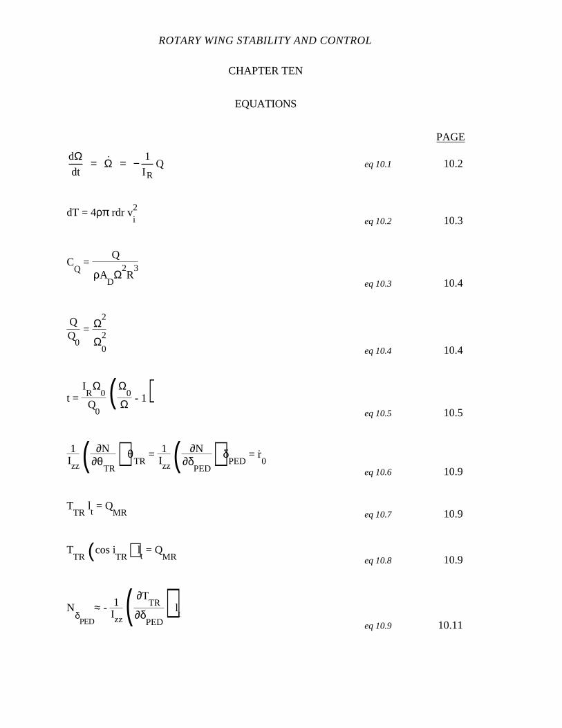
ROTARY WING STABILITY AND CONTROL
CHAPTER TEN
EQUATIONS
PAGE
dΩdt
= Ω = −1
I RQ eq 10.1 10.2
dT = 4ρπ rdr vi2
eq 10.2 10.3
CQ
= Q
ρAD
Ω2R
3
eq 10.3 10.4
0
= Ω2
Ω0
2
eq 10.4 10.4
t = IR
Ω0
Q0
(Ω0
Ω - 1)eq 10.5 10.5
1Izz( ∂N
∂θTR
) θTR
= 1Izz( ∂N
∂δPED
) δPED
= r.0
eq 10.6 10.9
TTR
lt = Q
MR eq 10.7 10.9
TTR (cos i
TR) lt = Q
MR eq 10.8 10.9
NδPED
≈ - 1Izz( ∂T
TR
∂δPED
) lt
eq 10.9 10.11
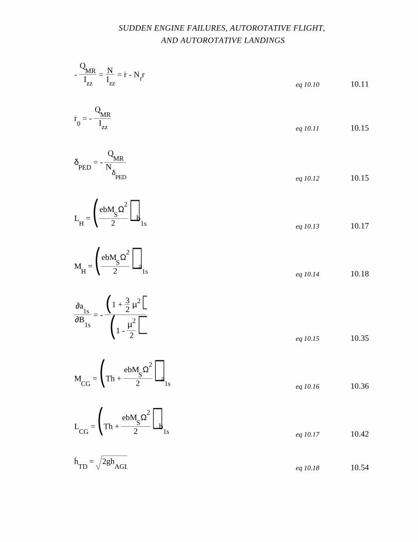
SUDDEN ENGINE FAILURES, AUTOROTATIVE FLIGHT,
AND AUTOROTATIVE LANDINGS
-Q
MRIzz
= NIzz
= r. - Nrr
eq 10.10 10.11
r.0 = -
QMRIzz eq 10.11 10.15
δPED
= - Q
MRN
δPED eq 10.12 10.15
LH
= ( ebMSΩ
2
2) b
1s eq 10.13 10.17
MH
= ( ebMSΩ
2
2) a
1s eq 10.14 10.18
∂a1s
∂B1s
= - (1 + 3
2µ2)
(1 - µ2
2 )eq 10.15 10.35
MCG
= (Th + ebM
SΩ
2
2) a
1s eq 10.16 10.36
LCG
= (Th + ebM
SΩ
2
2) b
1s eq 10.17 10.42
h.TD
= 2ghAGL eq 10.18 10.54
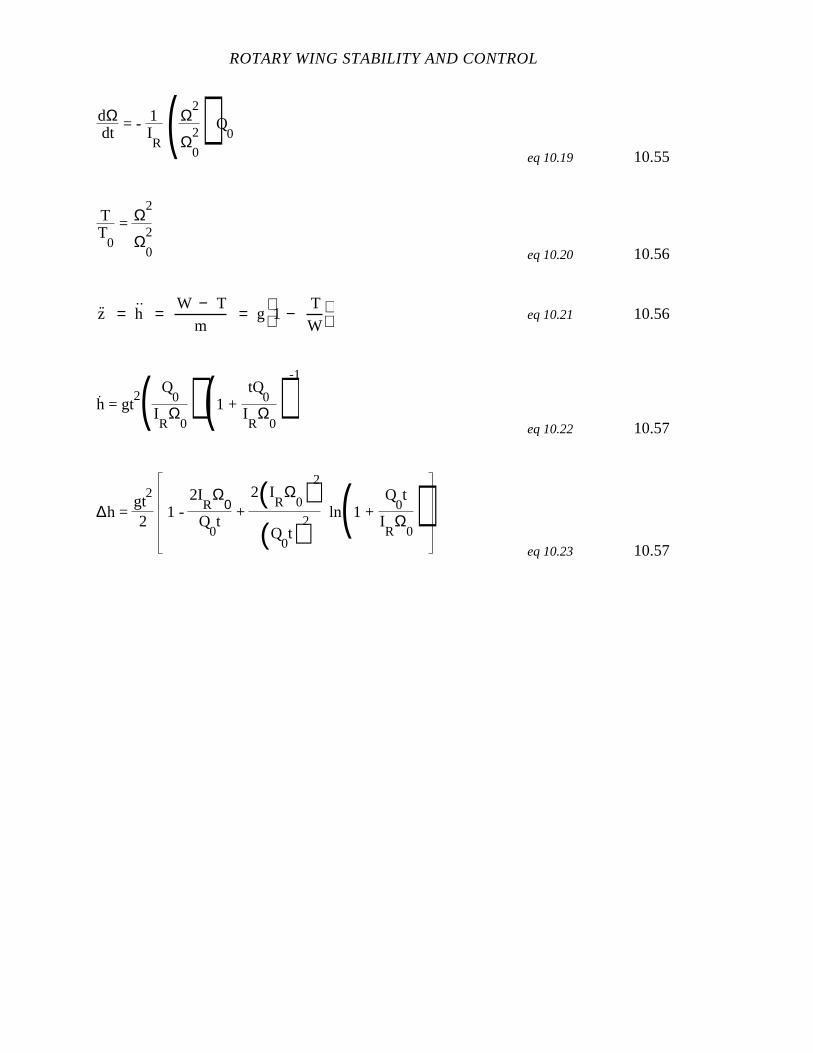
ROTARY WING STABILITY AND CONTROL
dΩdt
= - 1IR (Ω
2
Ω0
2) Q0
eq 10.19 10.55
TT
0
= Ω2
Ω0
2
eq 10.20 10.56
˙z = ˙h =W − T
m= g 1 −
T
W
eq 10.21 10.56
h. = gt
2( Q0
IR
Ω0) (1 +
tQ0
IR
Ω0)
-1
eq 10.22 10.57
∆h = gt
2
21 -
2IR
Ω0
Q0t
+ 2( I
RΩ
0)2
(Q0t)2
ln(1 + Q
0t
IR
Ω0)
eq 10.23 10.57
CHAPTER TEN
SUDDEN ENGINE FAILURES, AUTOROTATIVE FLIGHT,
AND AUTOROTATIVE LANDINGS
10.1 INTRODUCTION
This chapter discusses helicopter stability, control, and flying qualities during
engine failure, autorotation entry, steady autorotative flight, and landing following a
successful autorotation. Although the emphasis is on flying qualities, knowledge of
helicopter performance requirements and power deficits is essential to understanding the
autorotation evaluation starting with engine failure and ending with a satisfactory landing.
Flying qualities and performance characteristics are both required to analyze and test
autorotation capability.
10.2 PURPOSE
The purpose of these tests is to evaluate the handling qualities of the helicopter from
engine failure to completion of the landing. Tests are conducted to evaluate the following
characteristics:
1. Engine failure and autorotation entry.
2. Steady autorotative flight.
3. Autorotative landings.
Tests investigate the effects of flight condition (hover, low airspeed, and forward
flight), power setting (climb, level, and descent), and altitude. Further testing may be
conducted to assess the effects of parameters such as gross weight (GW) and center of
gravity (CG).
ROTARY WING STABILITY AND CONTROL
10.3 THEORY
10.3.1 Engine Failure
Sudden engine failures for single rotor helicopters in powered flight result in large
unbalanced moments on both the rotor and airframe. In time these moments produce rotor
speed changes and attitude excursions resulting in aircraft deviations from the original flight
condition. The pilot eventually responds to these excursions with control inputs to bring
the helicopter back under control, establish the steady autorotative glide, and perform the
landing maneuver.
10.3.1.1 ROTOR SPEED DECAY
At the time of power loss there is a decelerating torque on the drive train
proportional to the engine power that was being delivered to the main rotor, tail rotor,
accessories, and to overcome mechanical losses in the drive train. The decelerating torque
produces a drive train deceleration given by:
dΩdt
= Ω = −1
I RQ eq 10.1
Where:
IR - Rotor rotational moment of inertia
Q - Torque
t - Time
Ω - Rotor angular velocity
Ω - Rotor angular acceleration.
If flight conditions (airspeed, rate of climb/descent) are constant over the time
interval of interest, the time for rotor decay to some prescribed percentage of the initial
value can be predicted. Consider the main rotor for a hovering helicopter. Figure 10.1
shows the geometry of a rotor blade section at two different rotational speeds for the same
collective pitch angle.
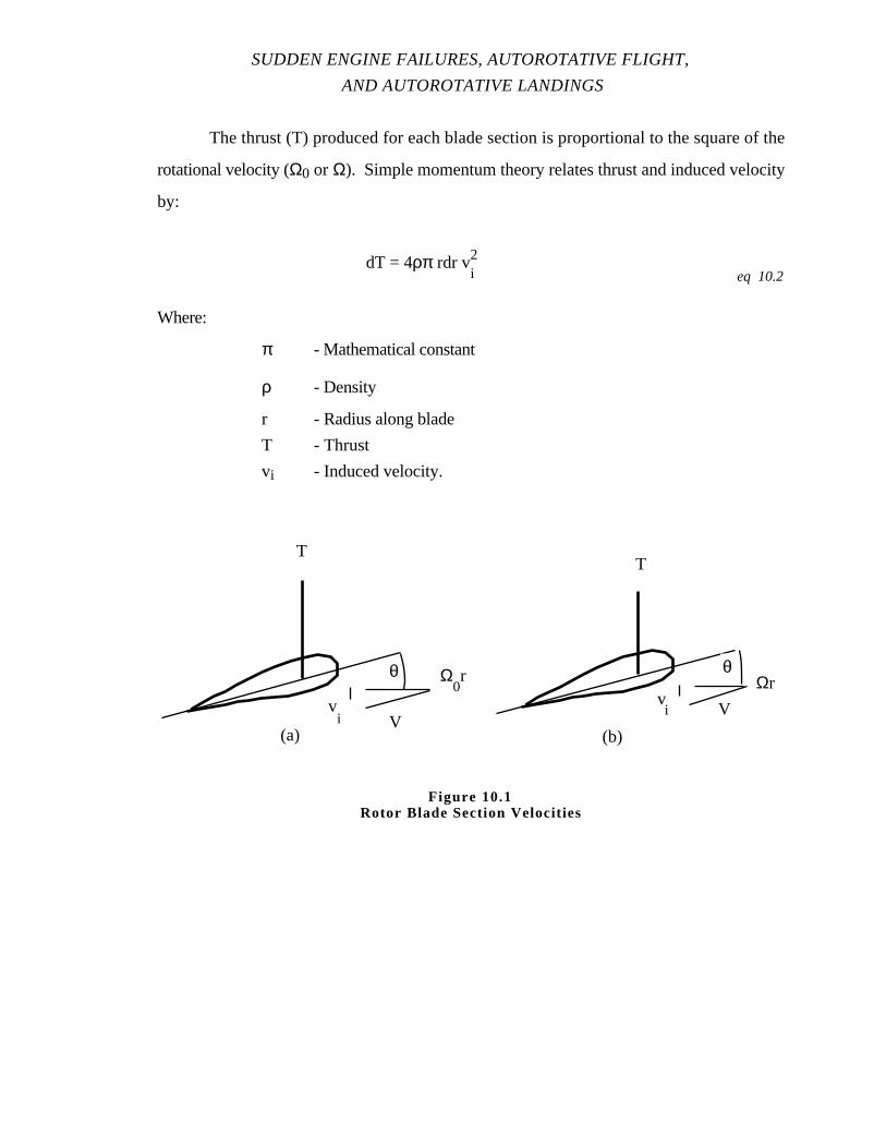
SUDDEN ENGINE FAILURES, AUTOROTATIVE FLIGHT,
AND AUTOROTATIVE LANDINGS
The thrust (T) produced for each blade section is proportional to the square of the
rotational velocity (Ω0 or Ω). Simple momentum theory relates thrust and induced velocity
by:
dT = 4ρπ rdr vi2
eq 10.2
Where:
π - Mathematical constant
ρ - Density
r - Radius along blade
T - Thrust
vi - Induced velocity.
V
Ωr
V
(a) (b)
TT
θ θ
vi
vi
Ω0r
Figure 10.1Rotor Blade Section Velocities
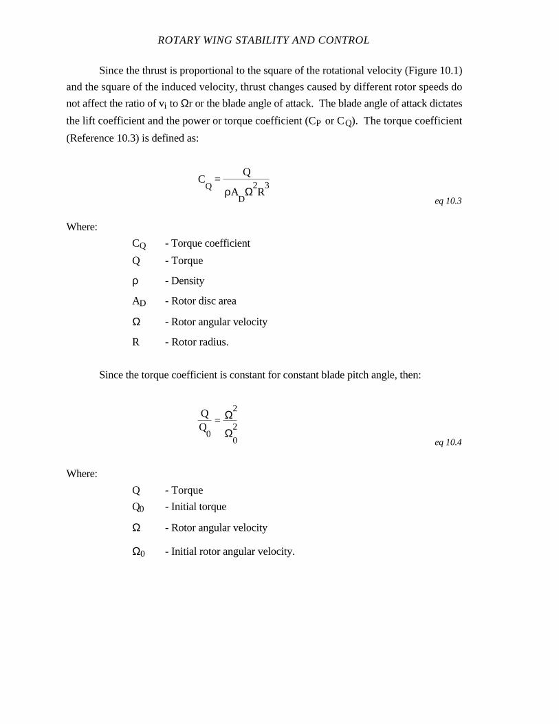
ROTARY WING STABILITY AND CONTROL
Since the thrust is proportional to the square of the rotational velocity (Figure 10.1)
and the square of the induced velocity, thrust changes caused by different rotor speeds do
not affect the ratio of vi to Ωr or the blade angle of attack. The blade angle of attack dictates
the lift coefficient and the power or torque coefficient (CP or CQ). The torque coefficient
(Reference 10.3) is defined as:
CQ
= Q
ρAD
Ω2R
3
eq 10.3
Where:
CQ - Torque coefficient
Q - Torque
ρ - Density
AD - Rotor disc area
Ω - Rotor angular velocity
R - Rotor radius.
Since the torque coefficient is constant for constant blade pitch angle, then:
0
= Ω2
Ω0
2
eq 10.4
Where:
Q - Torque
Q0 - Initial torque
Ω - Rotor angular velocity
Ω0 - Initial rotor angular velocity.
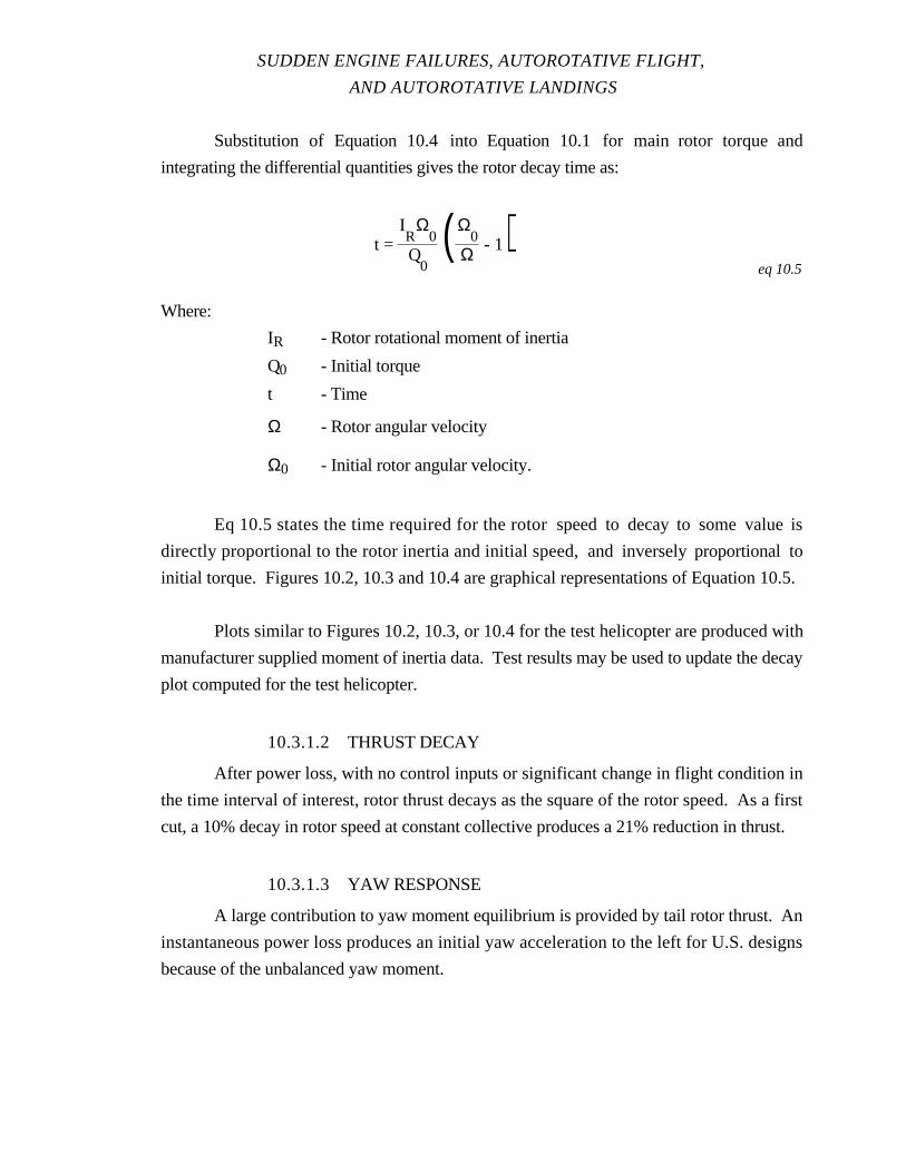
SUDDEN ENGINE FAILURES, AUTOROTATIVE FLIGHT,
AND AUTOROTATIVE LANDINGS
Substitution of Equation 10.4 into Equation 10.1 for main rotor torque and
integrating the differential quantities gives the rotor decay time as:
t = IR
Ω0
Q0
(Ω0
Ω - 1)eq 10.5
Where:
IR - Rotor rotational moment of inertia
Q0 - Initial torque
t - Time
Ω - Rotor angular velocity
Ω0 - Initial rotor angular velocity.
Eq 10.5 states the time required for the rotor speed to decay tosome value is
directly proportional to the rotor inertia and initial speed, and inversely proportional to
initial torque. Figures 10.2, 10.3 and 10.4 are graphical representations of Equation 10.5.
Plots similar to Figures 10.2, 10.3, or 10.4 for the test helicopter are produced with
manufacturer supplied moment of inertia data. Test results may be used to update the decay
plot computed for the test helicopter.
10.3.1.2 THRUST DECAY
After power loss, with no control inputs or significant change in flight condition in
the time interval of interest, rotor thrust decays as the square of the rotor speed. As a first
cut, a 10% decay in rotor speed at constant collective produces a 21% reduction in thrust.
10.3.1.3 YAW RESPONSE
A large contribution to yaw moment equilibrium is provided by tail rotor thrust. An
instantaneous power loss produces an initial yaw acceleration to the left for U.S. designs
because of the unbalanced yaw moment.
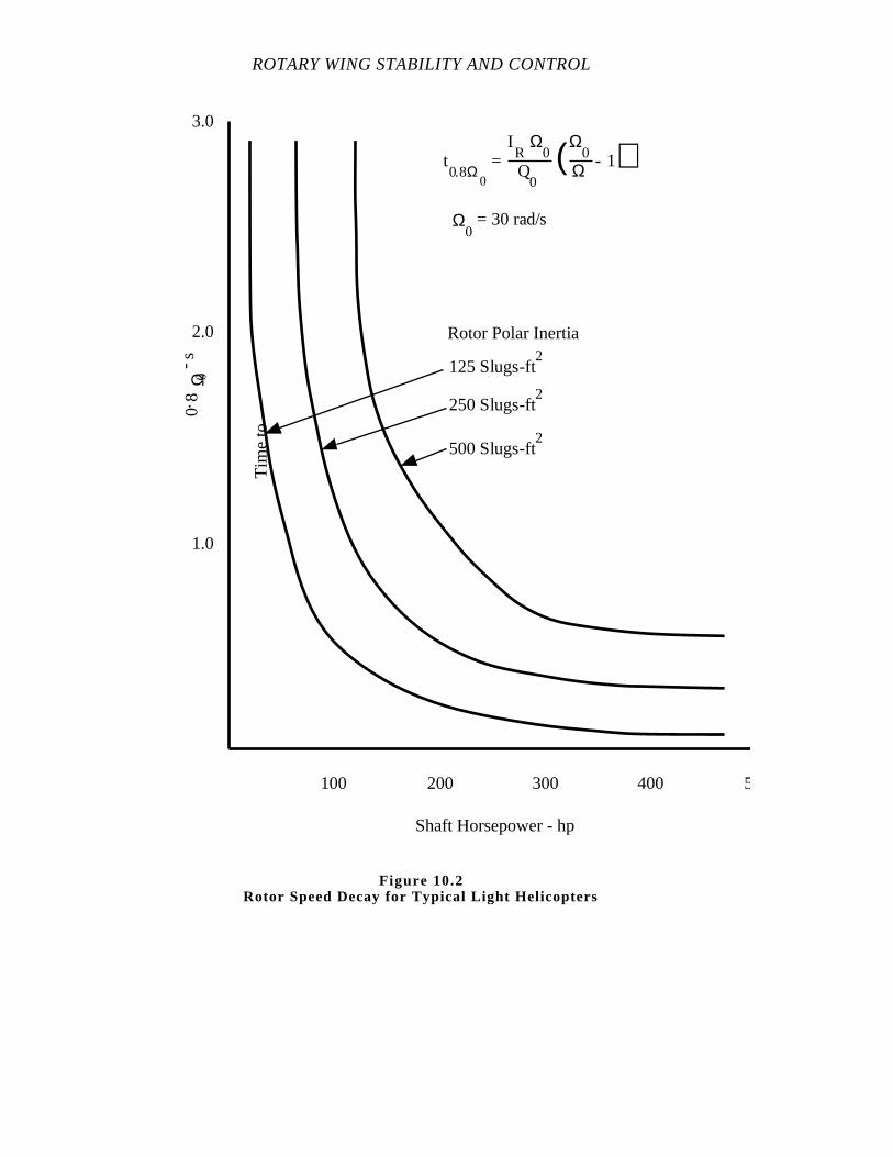
ROTARY WING STABILITY AND CONTROL
100 200 300 400 500
1.0
2.0
3.0
Rotor Polar Inertia
125 Slugs-ft2
250 Slugs-ft2
500 Slugs-ft2
Ω0
= 30 rad/s
0.8
Ω 0- s
Tim
e to
Shaft Horsepower - hp
t0.8Ω
0
=IR
Ω0
Q0
(Ω0
Ω - 1)
Figure 10.2Rotor Speed Decay for Typical Light Helicopters
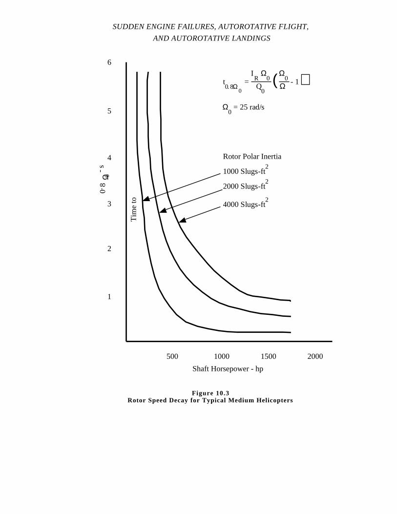
SUDDEN ENGINE FAILURES, AUTOROTATIVE FLIGHT,
AND AUTOROTATIVE LANDINGS
500 1000 1500 2000
2
6
Rotor Polar Inertia
0.8
Ω 0- s
Tim
e to
Shaft Horsepower - hp
Ω0
= 25 rad/s
1000 Slugs-ft2
2000 Slugs-ft2
4000 Slugs-ft2
1
3
4
5
t0. 8Ω
0
=IR
Ω0
Q0
(Ω0
Ω - 1)
Figure 10.3Rotor Speed Decay for Typical Medium Helicopters
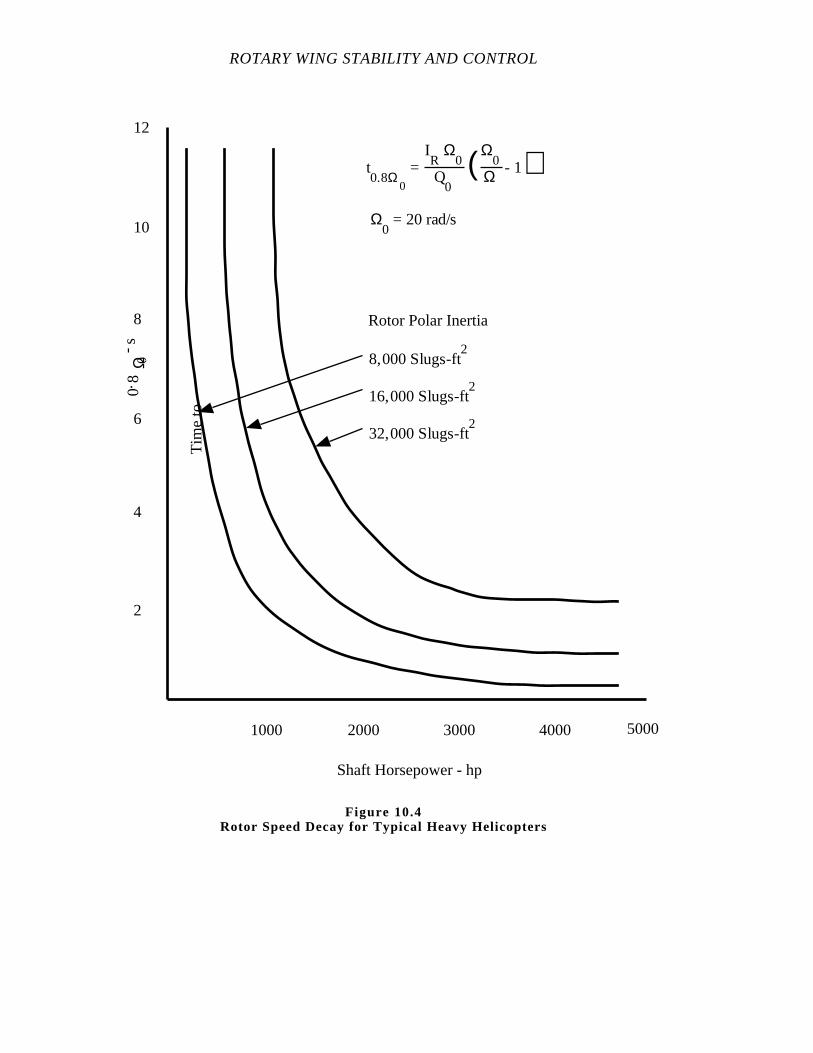
ROTARY WING STABILITY AND CONTROL
1000 2000 3000 4000 5000
4
8
12
Rotor Polar Inertia
0.8
Ω 0- s
Tim
e to
Shaft Horsepower - hp
8,000 Slugs-ft2
16,000 Slugs-ft2
32,000 Slugs-ft2
Ω0
= 20 rad/s
2
6
10
t0.8Ω
0
=IR
Ω0
Q0
(Ω0
Ω - 1)
Figure 10.4Rotor Speed Decay for Typical Heavy Helicopters
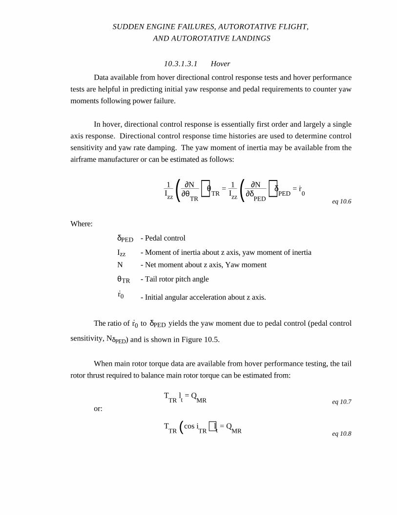
SUDDEN ENGINE FAILURES, AUTOROTATIVE FLIGHT,
AND AUTOROTATIVE LANDINGS
10.3.1.3.1 Hover
Data available from hover directional control response tests and hover performance
tests are helpful in predicting initial yaw response and pedal requirements to counter yaw
moments following power failure.
In hover, directional control response is essentially first order and largely a single
axis response. Directional control response time histories are used to determine control
sensitivity and yaw rate damping. The yaw moment of inertia may be available from the
airframe manufacturer or can be estimated as follows:
1Izz( ∂N
∂θTR
) θTR
= 1Izz( ∂N
∂δPED
) δPED
= r.0
eq 10.6
Where:
δPED - Pedal control
Izz - Moment of inertia about z axis, yaw moment of inertia
N - Net moment about z axis, Yaw moment
θTR - Tail rotor pitch angle
r0 - Initial angular acceleration about z axis.
The ratio of r0 to δPED yields the yaw moment due to pedal control (pedal control
sensitivity, NδPED) and is shown in Figure 10.5.
When main rotor torque data are available from hover performance testing, the tail
rotor thrust required to balance main rotor torque can be estimated from:
TTR
lt = Q
MR eq 10.7or:
TTR (cos i
TR) lt = Q
MR eq 10.8
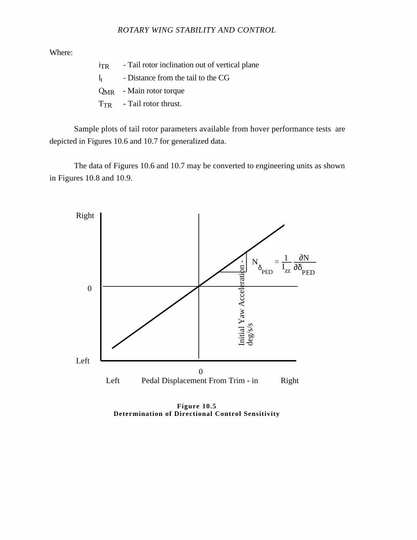
ROTARY WING STABILITY AND CONTROL
Where:
iTR - Tail rotor inclination out of vertical plane
lt - Distance from the tail to the CG
QMR - Main rotor torque
TTR - Tail rotor thrust.
Sample plots of tail rotor parameters available from hover performance tests are
depicted in Figures 10.6 and 10.7 for generalized data.
The data of Figures 10.6 and 10.7 may be converted to engineering units as shown
in Figures 10.8 and 10.9.
Left RightPedal Displacement From Trim - in0
0
Right
Left
Initi
al Y
aw A
ccel
erat
ion
-de
g/s/
s
NδPED
= 1Izz
∂N∂δ
PED
Figure 10.5Determination of Directional Control Sensitivity
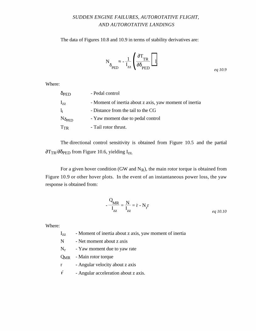
SUDDEN ENGINE FAILURES, AUTOROTATIVE FLIGHT,
AND AUTOROTATIVE LANDINGS
The data of Figures 10.8 and 10.9 in terms of stability derivatives are:
NδPED
≈ - 1Izz( ∂T
TR
∂δPED
) lt
eq 10.9
Where:
δPED - Pedal control
Izz - Moment of inertia about z axis, yaw moment of inertia
lt - Distance from the tail to the CG
NδPED - Yaw moment due to pedal control
TTR - Tail rotor thrust.
The directional control sensitivity is obtained from Figure 10.5 and the partial
∂TTR/∂δPED from Figure 10.6, yielding Izz.
For a given hover condition (GW and NR), the main rotor torque is obtained from
Figure 10.9 or other hover plots. In the event of an instantaneous power loss, the yaw
response is obtained from:
-Q
MRIzz
= NIzz
= r. - Nrr
eq 10.10
Where:
Izz - Moment of inertia about z axis, yaw moment of inertia
N - Net moment about z axis
Nr - Yaw moment due to yaw rate
QMR - Main rotor torque
r - Angular velocity about z axis
r - Angular acceleration about z axis.
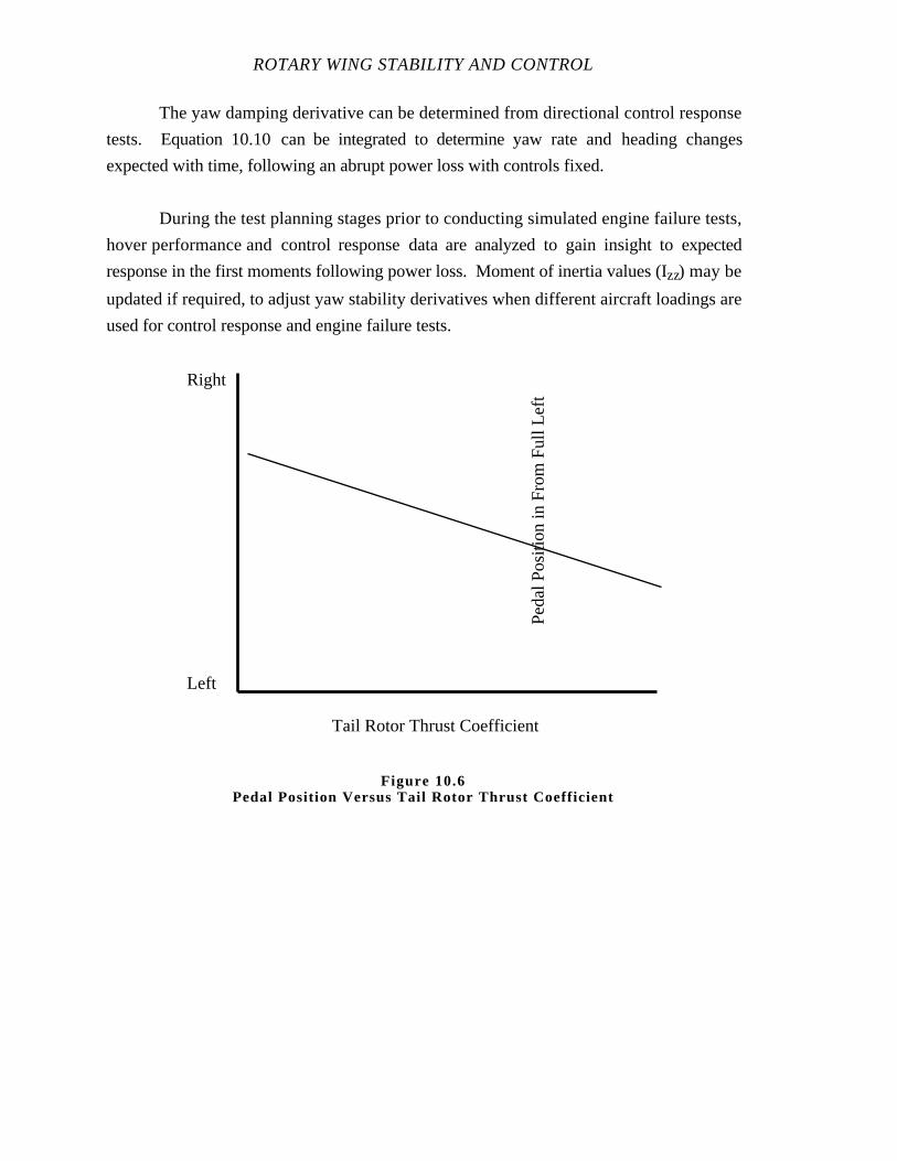
ROTARY WING STABILITY AND CONTROL
The yaw damping derivative can be determined from directional control response
tests. Equation 10.10 can be integrated to determine yaw rate and heading changes
expected with time, following an abrupt power loss with controls fixed.
During the test planning stages prior to conducting simulated engine failure tests,
hover performance and control response data are analyzed to gain insight to expected
response in the first moments following power loss. Moment of inertia values (Izz) may be
updated if required, to adjust yaw stability derivatives when different aircraft loadings are
used for control response and engine failure tests.
Ped
al P
ositi
on in
Fro
m F
ull L
eft
Left
Right
Tail Rotor Thrust Coefficient
Figure 10.6Pedal Position Versus Tail Rotor Thrust Coefficient
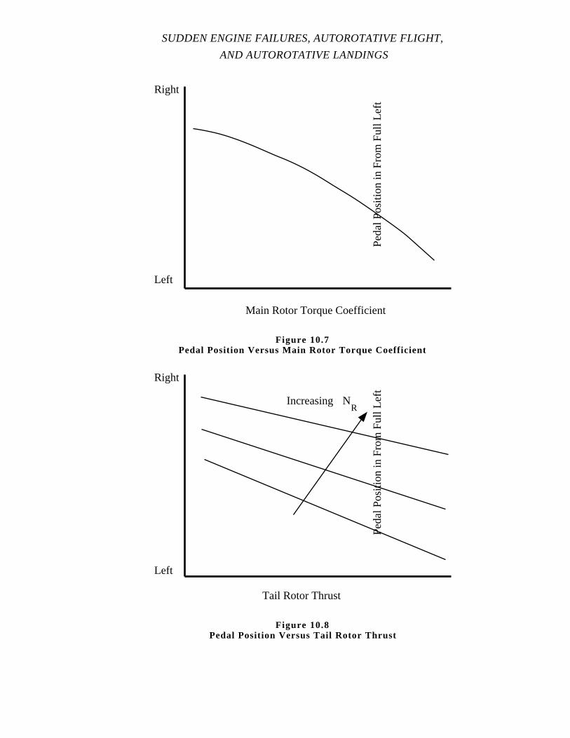
SUDDEN ENGINE FAILURES, AUTOROTATIVE FLIGHT,
AND AUTOROTATIVE LANDINGS
Ped
al P
ositi
on in
Fro
m F
ull L
eft
Left
Right
Main Rotor Torque Coefficient
Figure 10.7Pedal Position Versus Main Rotor Torque Coefficient
Ped
al P
ositi
on in
Fro
m F
ull L
eft
Left
Right
Tail Rotor Thrust
Increasing NR
Figure 10.8Pedal Position Versus Tail Rotor Thrust
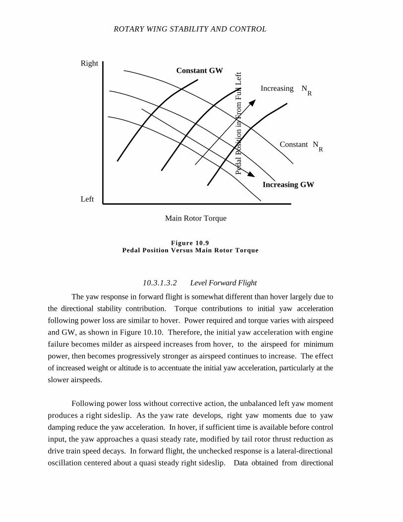
ROTARY WING STABILITY AND CONTROL
10.3.1.3.2 Level Forward Flight
The yaw response in forward flight is somewhat different than hover largely due to
the directional stability contribution. Torque contributions to initial yaw acceleration
following power loss are similar to hover. Power required and torque varies with airspeed
and GW, as shown in Figure 10.10. Therefore, the initial yaw acceleration with engine
failure becomes milder as airspeed increases from hover, to the airspeed for minimum
power, then becomes progressively stronger as airspeed continues to increase. The effect
of increased weight or altitude is to accentuate the initial yaw acceleration, particularly at the
slower airspeeds.
Following power loss without corrective action, the unbalanced left yaw moment
produces a right sideslip. As the yaw rate develops, right yaw moments due to yaw
damping reduce the yaw acceleration. In hover, if sufficient time is available before control
input, the yaw approaches a quasi steady rate, modified by tail rotor thrust reduction as
drive train speed decays. In forward flight, the unchecked response is a lateral-directional
oscillation centered about a quasi steady right sideslip. Data obtained from directional
Ped
al P
ositi
on in
Fro
m F
ull L
eft
Left
Right
Main Rotor Torque
Constant NR
Constant GW
Increasing NR
Increasing GW
Figure 10.9Pedal Position Versus Main Rotor Torque
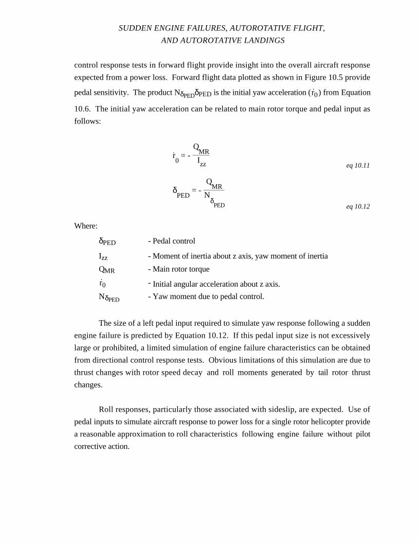
SUDDEN ENGINE FAILURES, AUTOROTATIVE FLIGHT,
AND AUTOROTATIVE LANDINGS
control response tests in forward flight provide insight into the overall aircraft response
expected from a power loss. Forward flight data plotted as shown in Figure 10.5 provide
pedal sensitivity. The product NδPEDδPED is the initial yaw acceleration (r0) from Equation
10.6. The initial yaw acceleration can be related to main rotor torque and pedal input as
follows:
r.0 = -
QMRIzz eq 10.11
δPED
= - Q
MRN
δPED eq 10.12
Where:
δPED - Pedal control
Izz - Moment of inertia about z axis, yaw moment of inertia
QMR - Main rotor torque
r0 - Initial angular acceleration about z axis.
NδPED - Yaw moment due to pedal control.
The size of a left pedal input required to simulate yaw response following a sudden
engine failure is predicted by Equation 10.12. If this pedal input size is not excessively
large or prohibited, a limited simulation of engine failure characteristics can be obtained
from directional control response tests. Obvious limitations of this simulation are due to
thrust changes with rotor speed decay and roll moments generated bytail rotor thrust
changes.
Roll responses, particularly those associated with sideslip, are expected. Use of
pedal inputs to simulate aircraft response to power loss for a single rotor helicopter provide
a reasonable approximation to roll characteristics following engine failure without pilot
corrective action.
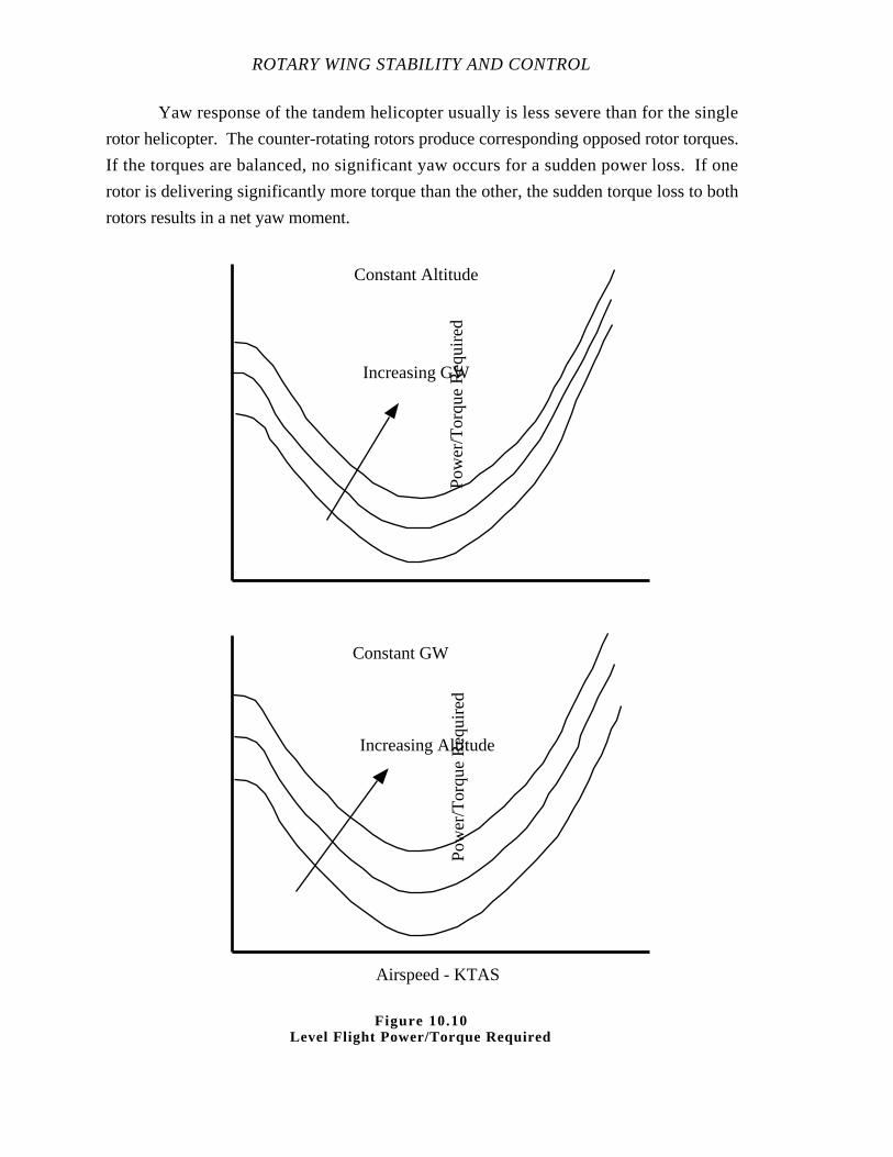
ROTARY WING STABILITY AND CONTROL
Yaw response of the tandem helicopter usually is less severe than for the single
rotor helicopter. The counter-rotating rotors produce corresponding opposed rotor torques.
If the torques are balanced, no significant yaw occurs for a sudden power loss. If one
rotor is delivering significantly more torque than the other, the sudden torque loss to both
rotors results in a net yaw moment.
Increasing GW
Constant Altitude
Pow
er/T
orqu
e R
equi
red
Pow
er/T
orqu
e R
equi
red
Constant GW
Increasing Altitude
Airspeed - KTAS
Figure 10.10Level Flight Power/Torque Required
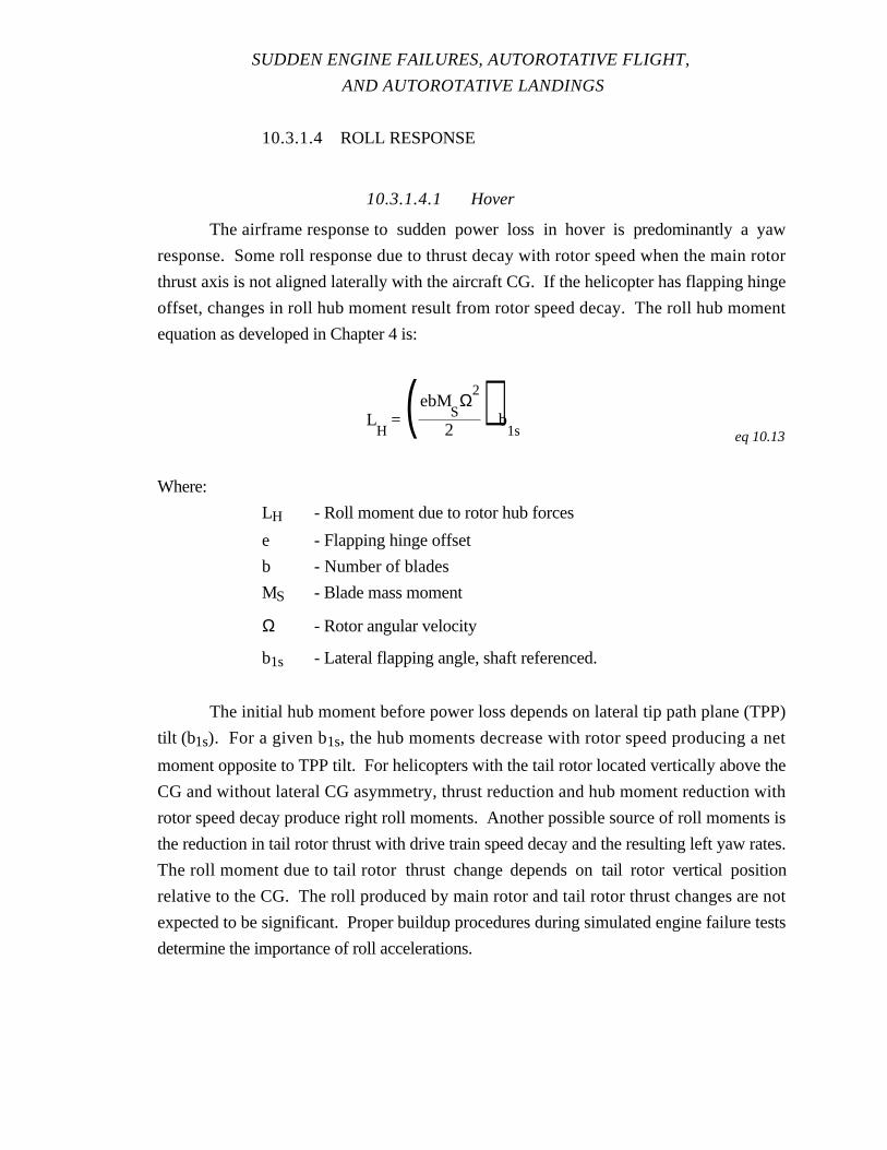
SUDDEN ENGINE FAILURES, AUTOROTATIVE FLIGHT,
AND AUTOROTATIVE LANDINGS
10.3.1.4 ROLL RESPONSE
10.3.1.4.1 Hover
The airframe response to sudden power loss in hover is predominantly a yaw
response. Some roll response due to thrust decay with rotor speed when the main rotor
thrust axis is not aligned laterally with the aircraft CG. If the helicopter has flapping hinge
offset, changes in roll hub moment result from rotor speed decay. The roll hub moment
equation as developed in Chapter 4 is:
LH
= ( ebMSΩ
2
2) b
1s eq 10.13
Where:
LH - Roll moment due to rotor hub forces
e - Flapping hinge offset
b - Number of blades
MS - Blade mass moment
Ω - Rotor angular velocity
b1s - Lateral flapping angle, shaft referenced.
The initial hub moment before power loss depends on lateral tip path plane (TPP)
tilt (b1s). For a given b1s, the hub moments decrease with rotor speed producing a net
moment opposite to TPP tilt. For helicopters with the tail rotor located vertically above the
CG and without lateral CG asymmetry, thrust reduction and hub moment reduction with
rotor speed decay produce right roll moments. Another possible source of roll moments is
the reduction in tail rotor thrust with drive train speed decay and the resulting left yaw rates.
The roll moment due to tail rotor thrust change depends on tail rotor verticalposition
relative to the CG. The roll produced by main rotor and tail rotor thrust changes are not
expected to be significant. Proper buildup procedures during simulated engine failure tests
determine the importance of roll accelerations.
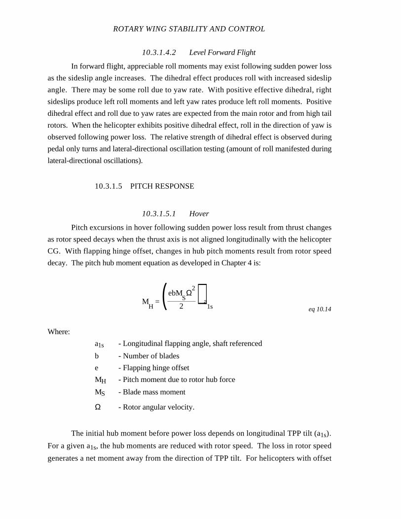
ROTARY WING STABILITY AND CONTROL
10.3.1.4.2 Level Forward Flight
In forward flight, appreciable roll moments may exist following sudden power loss
as the sideslip angle increases. The dihedral effect produces roll with increased sideslip
angle. There may be some roll due to yaw rate. With positive effective dihedral, right
sideslips produce left roll moments and left yaw rates produce left roll moments. Positive
dihedral effect and roll due to yaw rates are expected from the main rotor and from high tail
rotors. When the helicopter exhibits positive dihedral effect, roll in the direction of yaw is
observed following power loss. The relative strength of dihedral effect is observed during
pedal only turns and lateral-directional oscillation testing (amount of roll manifested during
lateral-directional oscillations).
10.3.1.5 PITCH RESPONSE
10.3.1.5.1 Hover
Pitch excursions in hover following sudden power loss result from thrust changes
as rotor speed decays when the thrust axis is not aligned longitudinally with the helicopter
CG. With flapping hinge offset, changes in hub pitch moments result from rotor speed
decay. The pitch hub moment equation as developed in Chapter 4 is:
MH
= ( ebMSΩ
2
2) a
1s eq 10.14
Where:
a1s - Longitudinal flapping angle, shaft referenced
b - Number of blades
e - Flapping hinge offset
MH - Pitch moment due to rotor hub force
MS - Blade mass moment
Ω - Rotor angular velocity.
The initial hub moment before power loss depends on longitudinal TPP tilt (a1s).
For a given a1s, the hub moments are reduced with rotor speed. The loss in rotor speed
generates a net moment away from the direction of TPP tilt. For helicopters with offset
SUDDEN ENGINE FAILURES, AUTOROTATIVE FLIGHT,
AND AUTOROTATIVE LANDINGS
flapping hinges, displacement of the thrust vector longitudinally from the CG causes the
thrust moments and hub moments to be in opposite directions. As thrust and hub moments
decrease with rotor speed decay, their changes are opposing. For example, when the CG
is aft of the shaft, TPP tilt is forward and the thrust axis passes ahead of the CG. Rotor
speed loss reduces the thrust producing a nose down moment and also reduces the hub
moment producing a nose up moment. The onset of any pitch accelerations lag the yaw
accelerations since they depend on rotor speed changes and require a finite amount of time
to develop. As in roll, in the first few moments following power loss, significant pitch
moments are not anticipated.
10.3.1.5.2 Level Forward Flight
Thrust decay and hub moment contributions in forward flight have the same origins
as in hover. Additional considerations are:
1. Fuselage aerodynamics (tail loads) and their effects on thrust axis
longitudinal orientation with respect to the CG.
2. Blowback effects.
3. Sideslip generated pitch moments.
4. Trim lateral TPP position.
Fuselage aerodynamics contribute to the trimmed a1s. If significant tail down loads
exist in trimmed forward flight, additional forward a1s is required to balance tail loads. Tail
down loads work to favor the hub moment changes with rotor speed decay for aft CG
positions, and to favor the thrust effect for forward CG position. Figures 10.11 and 10.12
depict these concepts.
For the aft CG case (Figure 10.11), increase in tail down load requires forward
TPP tilt for equilibrium with the thrust vector through the CG. For the forward CG
(Figure 10.12), the increase in tail down load increases the forward tilt for equilibrium with
the TPP aligned with the shaft when the tail load is present. Some differences in aircraft
pitch attitude (and trim tail loads) exist between the helicopters represented in Figures 10.11
and 10.12, but analysis of these differences is not required to illustrate the basic trends. In
Figure 10.11 (aft CG), the thrust and the hub moments both decrease with rotor speed
decay. When the tail load is present, loss of rotor speed only affects the hub moment
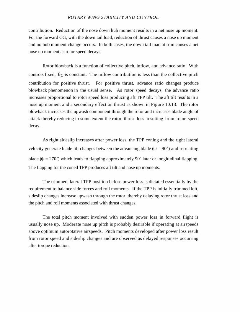
ROTARY WING STABILITY AND CONTROL
contribution. Reduction of the nose down hub moment results in a net nose up moment.
For the forward CG, with the down tail load, reduction of thrust causes a nose up moment
and no hub moment change occurs. In both cases, the down tail load at trim causes a net
nose up moment as rotor speed decays.
Rotor blowback is a function of collective pitch, inflow, and advance ratio. With
controls fixed, θC is constant. The inflow contribution is less than the collective pitch
contribution for positive thrust. For positive thrust, advance ratio changes produce
blowback phenomenon in the usual sense. As rotor speed decays, the advance ratio
increases proportional to rotor speed loss producing aft TPP tilt. The aft tilt results in a
nose up moment and a secondary effect on thrust as shown in Figure 10.13. The rotor
blowback increases the upwash component through the rotor and increases blade angle of
attack thereby reducing to some extent the rotor thrust lossresulting from rotor speed
decay.
As right sideslip increases after power loss, the TPP coning and the right lateral
velocity generate blade lift changes between the advancing blade (ψ = 90˚) and retreating
blade (ψ = 270˚) which leads to flapping approximately 90˚ later or longitudinal flapping.
The flapping for the coned TPP produces aft tilt and nose up moments.
The trimmed, lateral TPP position before power loss is dictated essentially by the
requirement to balance side forces and roll moments. If the TPP is initially trimmed left,
sideslip changes increase upwash through the rotor, thereby delaying rotor thrust loss and
the pitch and roll moments associated with thrust changes.
The total pitch moment involved with sudden power loss in forward flight is
usually nose up. Moderate nose up pitch is probably desirable if operating at airspeeds
above optimum autorotative airspeeds. Pitch moments developed after power loss result
from rotor speed and sideslip changes and are observed as delayed responses occurring
after torque reduction.
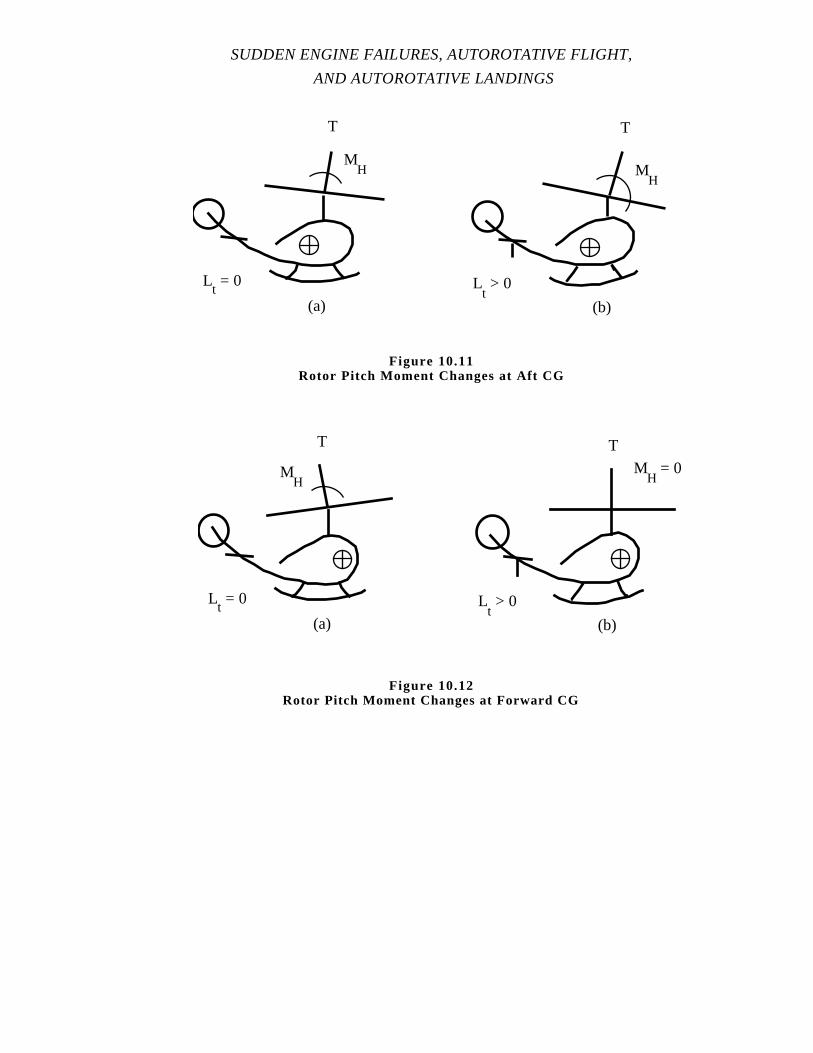
SUDDEN ENGINE FAILURES, AUTOROTATIVE FLIGHT,
AND AUTOROTATIVE LANDINGS
Lt= 0 L
t> 0
MH M
H
T T
(a) (b)
Figure 10.11Rotor Pitch Moment Changes at Aft CG
Lt= 0 L
t> 0
MH
T T
(a) (b)
MH
= 0
Figure 10.12Rotor Pitch Moment Changes at Forward CG
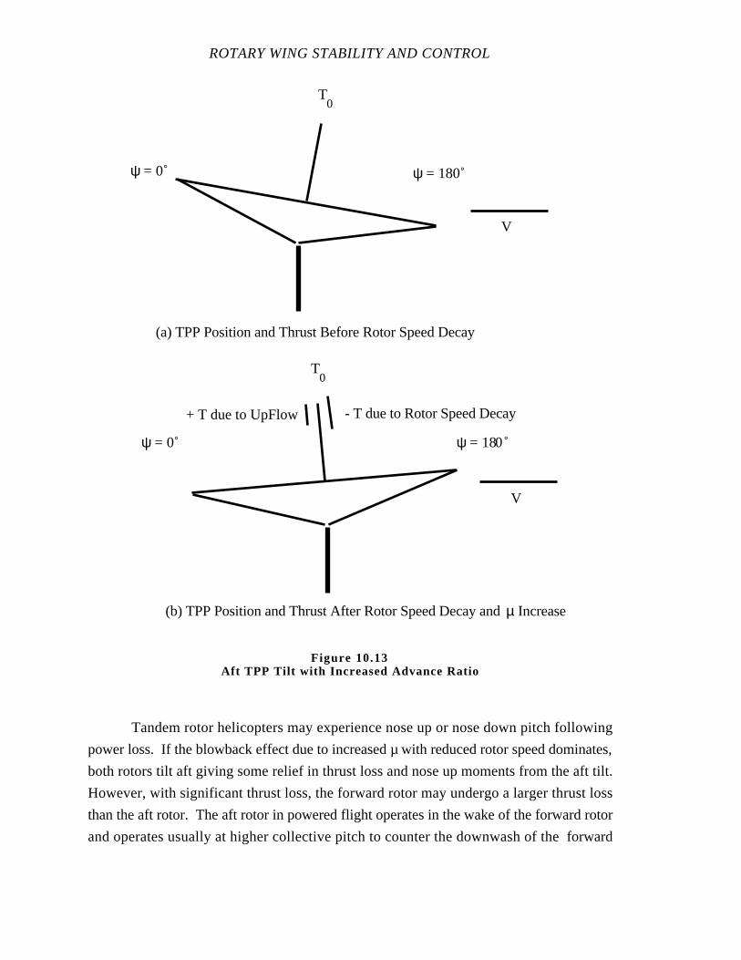
ROTARY WING STABILITY AND CONTROL
Tandem rotor helicopters may experience nose up or nose down pitch following
power loss. If the blowback effect due to increased µ with reduced rotor speed dominates,
both rotors tilt aft giving some relief in thrust loss and nose up moments from the aft tilt.
However, with significant thrust loss, the forward rotor may undergo a larger thrust loss
than the aft rotor. The aft rotor in powered flight operates in the wake of the forward rotor
and operates usually at higher collective pitch to counter the downwash of the forward
ψ = 0˚ ψ = 180˚
(a) TPP Position and Thrust Before Rotor Speed Decay
ψ = 0˚ ψ = 180˚
(b) TPP Position and Thrust After Rotor Speed Decay and Increaseµ
T0
T0
- T due to Rotor Speed Decay+ T due to UpFlow
V
V
Figure 10.13Aft TPP Tilt with Increased Advance Ratio
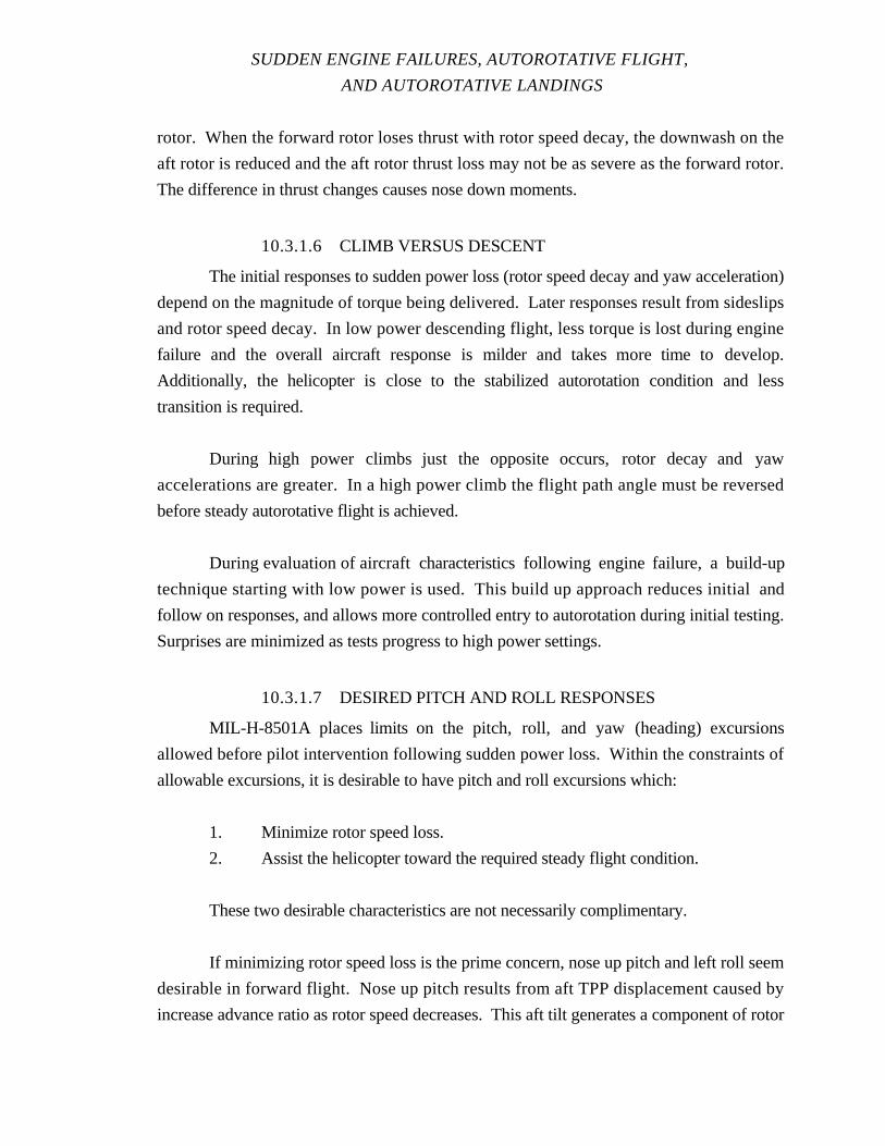
SUDDEN ENGINE FAILURES, AUTOROTATIVE FLIGHT,
AND AUTOROTATIVE LANDINGS
rotor. When the forward rotor loses thrust with rotor speed decay, the downwash on the
aft rotor is reduced and the aft rotor thrust loss may not be as severe as the forward rotor.
The difference in thrust changes causes nose down moments.
10.3.1.6 CLIMB VERSUS DESCENT
The initial responses to sudden power loss (rotor speed decay and yaw acceleration)
depend on the magnitude of torque being delivered. Later responses result from sideslips
and rotor speed decay. In low power descending flight, less torque is lost during engine
failure and the overall aircraft response is milder and takes more time to develop.
Additionally, the helicopter is close to the stabilized autorotation condition and less
transition is required.
During high power climbs just the opposite occurs, rotor decay and yaw
accelerations are greater. In a high power climb the flight path angle must be reversed
before steady autorotative flight is achieved.
During evaluation of aircraft characteristics following engine failure, a build-up
technique starting with low power is used. This build up approach reduces initial and
follow on responses, and allows more controlled entry to autorotation during initial testing.
Surprises are minimized as tests progress to high power settings.
10.3.1.7 DESIRED PITCH AND ROLL RESPONSES
MIL-H-8501A places limits on the pitch, roll, and yaw (heading) excursions
allowed before pilot intervention following sudden power loss. Within the constraints of
allowable excursions, it is desirable to have pitch and roll excursions which:
1. Minimize rotor speed loss.
2. Assist the helicopter toward the required steady flight condition.
These two desirable characteristics are not necessarily complimentary.
If minimizing rotor speed loss is the prime concern, nose up pitch and left roll seem
desirable in forward flight. Nose up pitch results from aft TPP displacement caused by
increase advance ratio as rotor speed decreases. This aft tilt generates a component of rotor
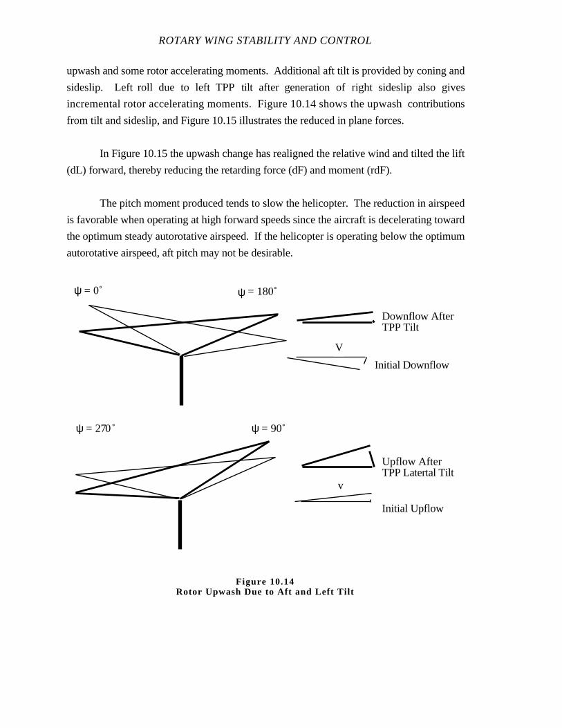
ROTARY WING STABILITY AND CONTROL
upwash and some rotor accelerating moments. Additional aft tilt is provided by coning and
sideslip. Left roll due to left TPP tilt after generation of right sideslip also gives
incremental rotor accelerating moments. Figure 10.14 shows the upwash contributions
from tilt and sideslip, and Figure 10.15 illustrates the reduced in plane forces.
In Figure 10.15 the upwash change has realigned the relative wind and tilted the lift
(dL) forward, thereby reducing the retarding force (dF) and moment (rdF).
The pitch moment produced tends to slow the helicopter. The reduction in airspeed
is favorable when operating at high forward speeds since the aircraft is decelerating toward
the optimum steady autorotative airspeed. If the helicopter is operating below the optimum
autorotative airspeed, aft pitch may not be desirable.
ψ = 0˚ ψ = 180˚
V
Initial Downflow
Downflow AfterTPP Tilt
v
Initial Upflow
Upflow AfterTPP Latertal Tilt
ψ = 270˚ ψ = 90˚
Figure 10.14Rotor Upwash Due to Aft and Left Tilt
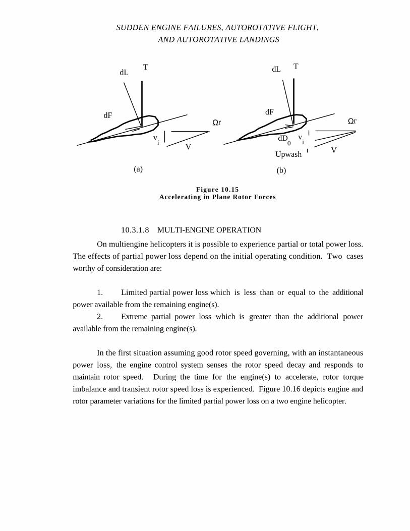
SUDDEN ENGINE FAILURES, AUTOROTATIVE FLIGHT,
AND AUTOROTATIVE LANDINGS
10.3.1.8 MULTI-ENGINE OPERATION
On multiengine helicopters it is possible to experience partial or total power loss.
The effects of partial power loss depend on the initial operating condition. Two cases
worthy of consideration are:
1. Limited partial power loss which is less than or equal to the additional
power available from the remaining engine(s).
2. Extreme partial power loss which is greater than the additional power
available from the remaining engine(s).
In the first situation assuming good rotor speed governing, with an instantaneous
power loss, the engine control system senses the rotor speed decay and responds to
maintain rotor speed. During the time for the engine(s) to accelerate, rotor torque
imbalance and transient rotor speed loss is experienced. Figure 10.16 depicts engine and
rotor parameter variations for the limited partial power loss on a two engine helicopter.
Ωr
(a) (b)
T T
vi
vi
Ωr
Upwash
dF
dD0
dF
dL dL
V V
Figure 10.15Accelerating in Plane Rotor Forces
ROTARY WING STABILITY AND CONTROL
Transient yaw, roll, and pitch responses previously discussed are observed, but
with the onset of additional torque from the remaining engine(s), the transient responses
diminish and the aircraft returns to a quasi steady condition. In the steady condition,
sideslip, bank angle, and airspeed disturbances may have occurred exciting long term
dynamic responses.
When the power loss is greater than can be absorbed by the remaining engine(s),
the engine controls sense rotor speed loss and respond with maximum power available. At
maximum power, insufficient power is available to restore full rotor speed. In this
situation, there are transient rotor speed losses and a final or steady reduction in rotor
speed. Characteristic transient conditions following extreme power loss are shown in
Figure 10.17 for a two engine helicopter.
Transient yaw, roll, and pitch responses are observed which are greater than those
for the limited partial power loss. As the remaining engine(s) absorb the torque deficits,
the transient response diminishes. In the steady condition, trim changes/aircraft responses
are proportional to the net torque deficit and the steady loss of rotor speed.
Use of pedal control response data to simulate the anticipated aircraft response
following a sudden power loss may not be as useful in evaluating airframe response to
partial power loss since additional forces and moments are present as the other engine(s)
assume the load.
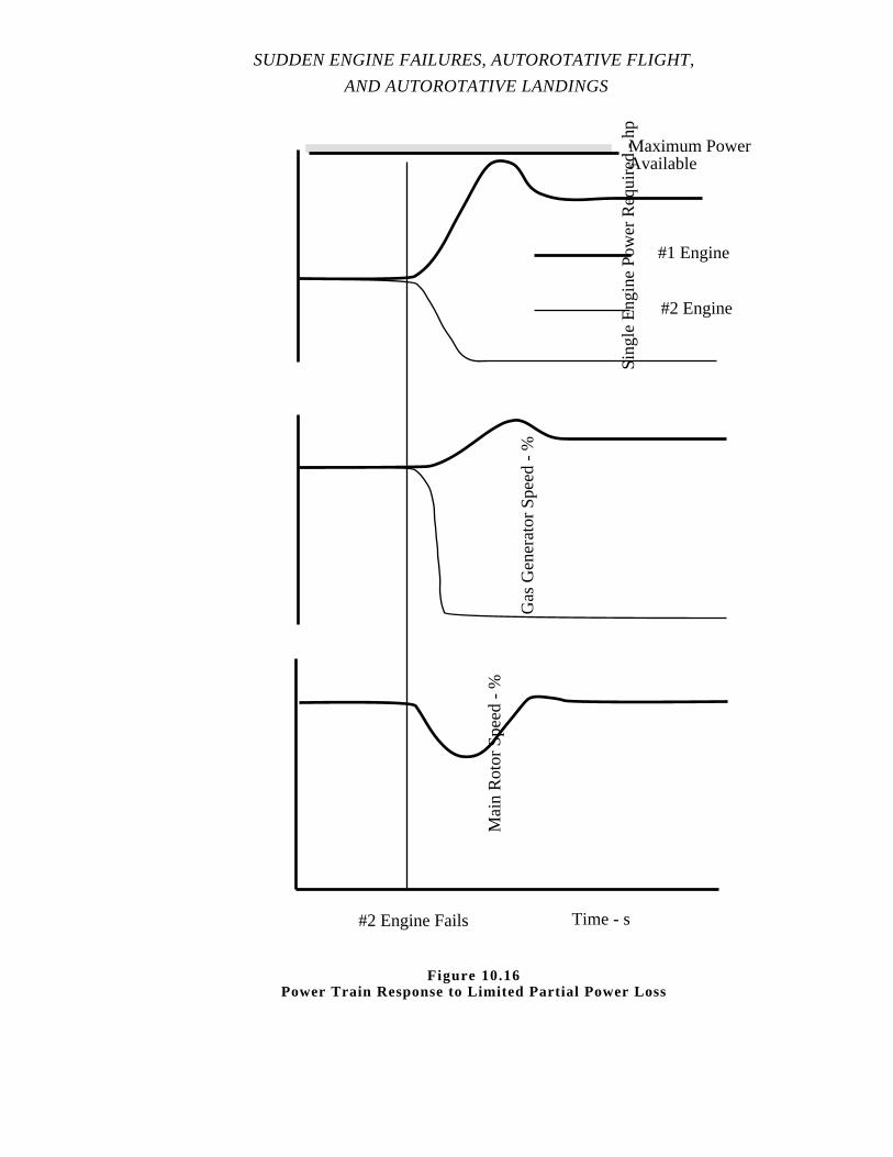
SUDDEN ENGINE FAILURES, AUTOROTATIVE FLIGHT,
AND AUTOROTATIVE LANDINGS
Sin
gle
Eng
ine
Pow
er R
equi
red
- hp
#1 Engine
#2 Engine
Gas
Gen
erat
or S
peed
- %
Mai
n R
otor
Spe
ed -
%
Time - s#2 Engine Fails
Maximum PowerAvailable
Figure 10.16Power Train Response to Limited Partial Power Loss
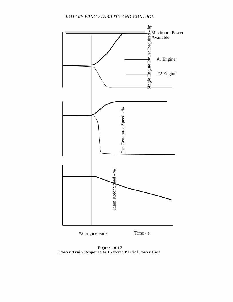
ROTARY WING STABILITY AND CONTROL
Sin
gle
Eng
ine
Pow
er R
equi
red
- hp
#1 Engine
#2 Engine
Gas
Gen
erat
or S
peed
- %
Mai
n R
otor
Spe
ed -
%
Time - s#2 Engine Fails
Maximum PowerAvailable
Figure 10.17Power Train Response to Extreme Partial Power Loss
SUDDEN ENGINE FAILURES, AUTOROTATIVE FLIGHT,
AND AUTOROTATIVE LANDINGS
10.3.1.9 ENGINE FAILURE WARNING
10.3.1.9.1 Natural Warning
Natural warning of an engine failure can be provided by engine noise, rotor speed
noise, acceleration, or attitude variations. Engine noise may be a poor cue in a helicopter
equipped with turbo-shaft engines due to masking of engine noise by transmission and
other noises. If engine noise reduction does not provide adequatewarning of engine
failure, acceleration/attitude change or the sound of rotor speed decay may provide a
warning. Attitude change (except yaw in a hovering single rotor helicopter) may not be a
good warning for two reasons. First, Automatic Flight Control Systems (AFCS) tend to
limit attitude excursions. Second, the attitude changes due toengine failure are often
masked by turbulent atmospheric conditions or, are similar in nature to AFCS or hydraulic
hardovers. The natural warning must be unambiguous. If the pilot is required to determine
the exact nature of the problem, the warning effectiveness is lost.
Low power descent or decelerating maneuvers make unambiguous natural warning
unlikely. The pilot of an aircraft in a low power condition may not know he has a power
failure until after he increases collective to terminate the low power maneuver.
Additionally, some transient rotor droop is not unusual. The pilot may neglect the natural
aural warning due to rotor speed decay until a severe loss in rotor speed is experienced.
10.3.1.9.2 Artificial Warning
Artificial warning devices are installed in most aircraft to improve engine failure
warning characteristics but many of them have common deficiencies. These deficiencies
include a capability to be deactivated, false activation during ground and flight operations,
and warning which is related to a low rotor speed and not a power failure. More
sophisticated systems provide different audible tone warnings for engine power
malfunctions and low rotor speed indications. A warning device which produces false
indications is ineffective.
ROTARY WING STABILITY AND CONTROL
10.3.2 Steady Autorotation
Following a power failure, attaining and maintaining steady state or quasi steady
autorotative flight is a primary goal. The recovery of autorotative rotor speed and descent
airspeed, is considered under the category of steady autorotative flight. The pilot attempts
to acquire the optimum possible conditions for an autorotative flare and landing during
autorotative flight.
Autorotative performance theory provides an understanding of rotor response to
variations in collective pitch, cyclic pitch, and inflow velocity as well as the effects of
weight, density altitude, and maneuvering on steady state autorotative characteristics.
10.3.2.1 ROTOR EQUILIBRIUM
Rotor equilibrium is obtained when net drive train torque and torque required are
balanced. Figure 10.18 presents some simplified diagrams to illustrate a few of the many
possible operating states which are applicable to blade elements of an autorotating rotor.
In Figure 10.18 (b), the pro and anti-autorotation torque vectors are equal and the
rotor angular velocity is constant. In Figure 10.18 (c) the rotor speed is increased and the
inflow velocity constant. This produces an increased blade element speed, increased drag,
and decreased angle of attack. The reduced angle of attack causes the blade element lift
vector (dL) to tilt toward the trailing edge. Since the anti-torque vector is greater than the
pro-torque vector, the rotor decelerates. In Figure 10.18 (d), the blade angle of attack is
decreased and the inflow velocity is increased by a reduction of thrust and induced velocity.
The result of these changes is rotational acceleration of the rotor. After the rotor in Figure
10.18 (d) stabilizes, the steady state condition resembles Figure 10.18 (e).
The blade elements along a twisted, autorotating rotor blade are all operating under
approximately the same inflow conditions (at low forward speeds). The outer elements are
operating at the highest tangential velocities and lowest angle of attack. The result of the
above conditions is anti-rotational blade element forces over the outer portion of a rotor
while the inner portion produces the predominance of pro-autorotational blade element
forces.
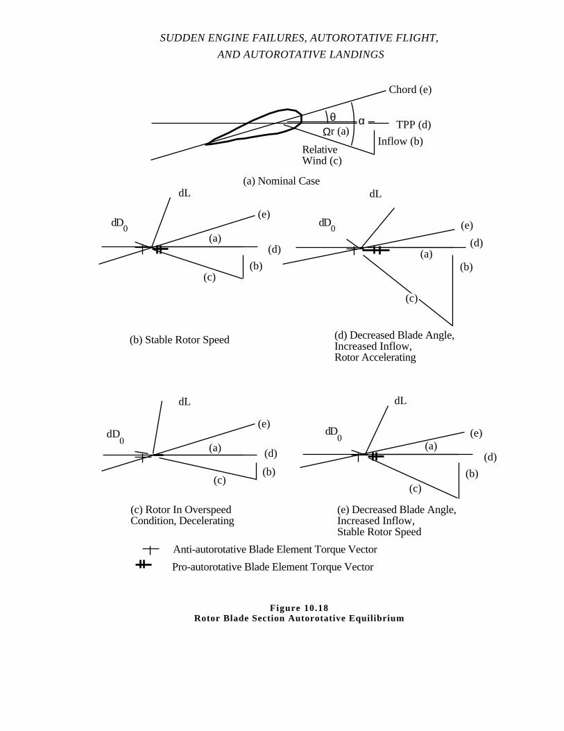
SUDDEN ENGINE FAILURES, AUTOROTATIVE FLIGHT,
AND AUTOROTATIVE LANDINGS
TPP (d)
Chord (e)
Inflow (b)RelativeWind (c)
θ αΩr (a)
(d)
(e)
(b) (c)
(a)
dL
(d)
(e)
(b)
(c)
(a)
dL
(b) Stable Rotor Speed (d) Decreased Blade Angle,Increased Inflow,Rotor Accelerating
(d)
(e)
(b) (c)
(a)
dL
(d)
(e)
(b) (c)
(a)
dL
(c) Rotor In OverspeedCondition, Decelerating
(e) Decreased Blade Angle,Increased Inflow,Stable Rotor Speed
Anti-autorotative Blade Element Torque Vector
Pro-autorotative Blade Element Torque Vector
(a) Nominal Case
dD0
dD0
dD0
dD0
Figure 10.18Rotor Blade Section Autorotative Equilibrium
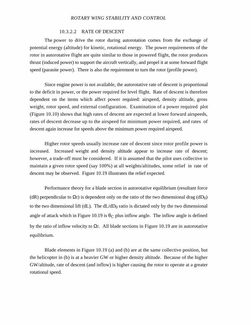
ROTARY WING STABILITY AND CONTROL
10.3.2.2 RATE OF DESCENT
The power to drive the rotor during autorotation comes from the exchange of
potential energy (altitude) for kinetic, rotational energy. The power requirements of the
rotor in autorotative flight are quite similar to those in powered flight, the rotor produces
thrust (induced power) to support the aircraft vertically, and propel it at some forward flight
speed (parasite power). There is also the requirement to turn the rotor (profile power).
Since engine power is not available, the autorotative rate of descent is proportional
to the deficit in power, or the power required for level flight. Rate of descent is therefore
dependent on the items which affect power required: airspeed, density altitude, gross
weight, rotor speed, and external configuration. Examination of a power required plot
(Figure 10.10) shows that high rates of descent are expected at lower forward airspeeds,
rates of descent decrease up to the airspeed for minimum power required, and rates of
descent again increase for speeds above the minimum power required airspeed.
Higher rotor speeds usually increase rate of descent since rotor profile power is
increased. Increased weight and density altitude appear to increase rate of descent;
however, a trade-off must be considered. If it is assumed that the pilot uses collective to
maintain a given rotor speed (say 100%) at all weights/altitudes, some relief in rate of
descent may be observed. Figure 10.19 illustrates the relief expected.
Performance theory for a blade section in autorotative equilibrium (resultant force
(dR) perpendicular to Ωr) is dependent only on the ratio of the two dimensional drag (dD0)
to the two dimensional lift (dL). The dL/dD0 ratio is dictated only by the two dimensional
angle of attack which in Figure 10.19 is θC plus inflow angle. The inflow angle is defined
by the ratio of inflow velocity to Ωr. All blade sections in Figure 10.19 are in autorotative
equilibrium.
Blade elements in Figure 10.19 (a) and (b) are at the same collective position, but
the helicopter in (b) is at a heavier GW or higher density altitude. Because of the higher
GW/altitude, rate of descent (and inflow) is higher causing the rotor to operate at a greater
rotational speed.
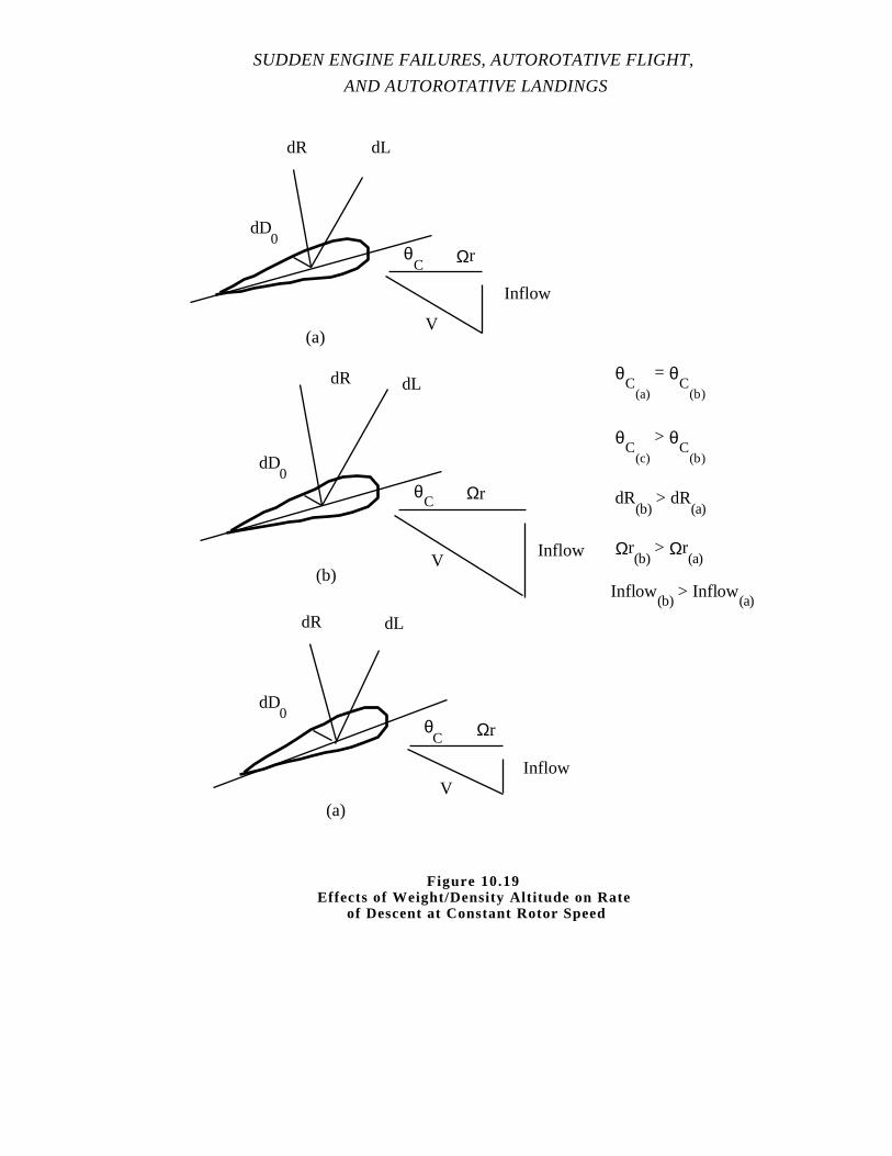
SUDDEN ENGINE FAILURES, AUTOROTATIVE FLIGHT,
AND AUTOROTATIVE LANDINGS
(a)
Ωr
Inflow
dR dL
dD0
θC
(b)
Ωr
Inflow
dR dL
dD0
θC
(a)
Ωr
Inflow
dR dL
dD0
θC
θC
(a)
= θC
(b)
θC
(c)
> θC
(b)
dR(b)
> dR(a)
Ωr(b)
> Ωr(a)
Inflow(b)
> Inflow(a)
V
V
V
Figure 10.19Effects of Weight/Density Altitude on Rate
of Descent at Constant Rotor Speed
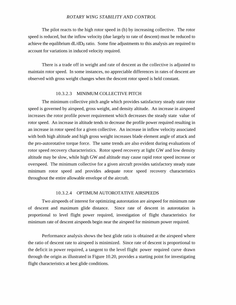
ROTARY WING STABILITY AND CONTROL
The pilot reacts to the high rotor speed in (b) by increasing collective. The rotor
speed is reduced, but the inflow velocity (due largely to rate of descent) must be reduced to
achieve the equilibrium dL/dD0 ratio. Some fine adjustments to this analysis are required to
account for variations in induced velocity required.
There is a trade off in weight and rate of descent as the collective is adjusted to
maintain rotor speed. In some instances, no appreciable differences in rates of descent are
observed with gross weight changes when the descent rotor speed is held constant.
10.3.2.3 MINIMUM COLLECTIVE PITCH
The minimum collective pitch angle which provides satisfactory steady state rotor
speed is governed by airspeed, gross weight, and density altitude. An increase in airspeed
increases the rotor profile power requirement which decreases the steady state value of
rotor speed. An increase in altitude tends to decrease the profile power required resulting in
an increase in rotor speed for a given collective. An increase in inflow velocity associated
with both high altitude and high gross weight increases blade element angle of attack and
the pro-autorotative torque force. The same trends are also evident during evaluations of
rotor speed recovery characteristics. Rotor speed recovery at light GW and low density
altitude may be slow, while high GW and altitude may cause rapid rotor speed increase or
overspeed. The minimum collective for a given aircraft provides satisfactory steady state
minimum rotor speed and provides adequate rotor speed recovery characteristics
throughout the entire allowable envelope of the aircraft.
10.3.2.4 OPTIMUM AUTOROTATIVE AIRSPEEDS
Two airspeeds of interest for optimizing autorotation are airspeed for minimum rate
of descent and maximum glide distance. Since rate of descent in autorotation is
proportional to level flight power required, investigation of flight characteristicsfor
minimum rate of descent airspeeds begin near the airspeed for minimum power required.
Performance analysis shows the best glide ratio is obtained at the airspeed where
the ratio of descent rate to airspeed is minimized. Since rate of descent is proportional to
the deficit in power required, a tangent to the level flight power required curve drawn
through the origin as illustrated in Figure 10.20, provides a starting point for investigating
flight characteristics at best glide conditions.
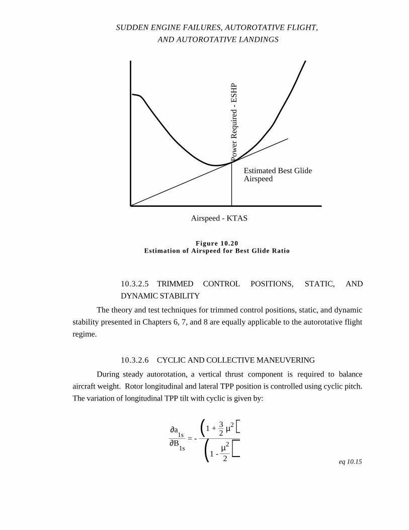
SUDDEN ENGINE FAILURES, AUTOROTATIVE FLIGHT,
AND AUTOROTATIVE LANDINGS
10.3.2.5 TRIMMED CONTROL POSITIONS, STATIC, AND
DYNAMIC STABILITY
The theory and test techniques for trimmed control positions, static, and dynamic
stability presented in Chapters 6, 7, and 8 are equally applicable to the autorotative flight
regime.
10.3.2.6 CYCLIC AND COLLECTIVE MANEUVERING
During steady autorotation, a vertical thrust component is required to balance
aircraft weight. Rotor longitudinal and lateral TPP position is controlled using cyclic pitch.
The variation of longitudinal TPP tilt with cyclic is given by:
∂a1s
∂B1s
= - (1 + 3
2µ2)
(1 - µ2
2 )eq 10.15
Airspeed - KTAS
Estimated Best GlideAirspeed
Pow
er R
equi
red
- E
SH
PFigure 10.20
Estimation of Airspeed for Best Glide Ratio
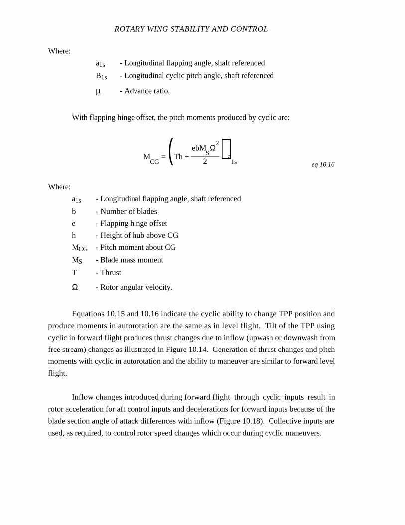
ROTARY WING STABILITY AND CONTROL
Where:
a1s - Longitudinal flapping angle, shaft referenced
B1s - Longitudinal cyclic pitch angle, shaft referenced
µ - Advance ratio.
With flapping hinge offset, the pitch moments produced by cyclic are:
MCG
= (Th + ebM
SΩ
2
2) a
1s eq 10.16
Where:
a1s - Longitudinal flapping angle, shaft referenced
b - Number of blades
e - Flapping hinge offset
h - Height of hub above CG
MCG - Pitch moment about CG
MS - Blade mass moment
T - Thrust
Ω - Rotor angular velocity.
Equations 10.15 and 10.16 indicate the cyclic ability to change TPP position and
produce moments in autorotation are the same as in level flight. Tilt of the TPP using
cyclic in forward flight produces thrust changes due to inflow (upwash or downwash from
free stream) changes as illustrated in Figure 10.14. Generation of thrust changes and pitch
moments with cyclic in autorotation and the ability to maneuver are similar to forward level
flight.
Inflow changes introduced during forward flight through cyclic inputs result in
rotor acceleration for aft control inputs and decelerations for forward inputs because of the
blade section angle of attack differences with inflow (Figure 10.18). Collective inputs are
used, as required, to control rotor speed changes which occur during cyclic maneuvers.
SUDDEN ENGINE FAILURES, AUTOROTATIVE FLIGHT,
AND AUTOROTATIVE LANDINGS
Collective only maneuvers produce thrust changes (possibly coupling with pitch
moments) and rotor speed changes. Collective maneuvers are limited generally to
maintaining rotor speed within an acceptable range.
10.3.2.7 ROTOR SPEED CONTROL
Steady state autorotative rotor speed is controlled largely by collective application.
Rotor accelerating/decelerating moments depend on collective position and inflow. Rotor
acceleration/deceleration is dictated by the size of the in plane moment and the rotor's
rotational moment of inertia. Low inertia rotors accelerate rapidly and high inertia rotors
accelerate slowly for a given in plane moment.
When rotor speed recovery is extremely rapid the pilot may experience a rotor speed
control problem. The pilot may be required to manage rotor speed in deference to other
emergency procedures. This problem may be aggravated at high density altitude, high
GW, and following a severe loss of rotor speed which precipitates a high rate of descent.
This excess rate of descent may tend to induce rotor overspeed requiring additional pilot
manipulation of the collective. Precise, small, continuous collective inputs may be required
to manage rotor speed for low inertia rotors.
When rotor speed recovery is sluggish, the pilot may have difficulty determining
how much collective input is required to effect a final rotor speed change. If severe rotor
speed loss is encountered, electrical systems, AFCS, and conceivably hydraulic systems
may be lost. If the pilot is distracted with controlling attitude or reengaging systems (such
as AFCS), an overspeed may occur. The high inertia rotor system is basically a lightly
damped first order system which may require large pilot inputs to achieve desired rotor
acceleration, followed by periodic pilot inputs to modify the acceleration and some
collective leading to establish the final rotor speed.
10.3.3 Transition To Autorotation Following Power Loss
There is a finite period of time between a power failure and pilot response referred
to as pilot reaction time. The magnitude of pilot reaction time varies with circumstances, as
does the maximum allowable delay time which can be tolerated. The acceptability of either
pilot reaction time or the available delay time cannot be determined independently, they
must be considered collectively. The predictability and complexity of the recovery control
ROTARY WING STABILITY AND CONTROL
inputs is an important aspect in both reaction time and delay time and can be a limiting
factor. An elementary evaluation of pilot response to a total power failure is accomplished
readily when the elements of the above factors are considered separately with continual
awareness of their interdependency.
10.3.3.1 AVAILABLE DELAY AND PILOT REACTION TIMES
A total power failure with controls fixed produces a rotor speed decay resulting in a
loss of thrust as well as angular accelerations about all axes and linear acceleration along all
axes. When control inputs are made by the pilot to enter an autorotation, the result is a
reversal in rotor speed decay and possibly a decrease in normal acceleration. The length of
time the controls can remain fixed during a transition is equal to the time required for
divergence of one or more characteristics as follows:
1. Minimum tolerable rotor speed.
2. Attitude or angular rate or combination of attitude and angular rate which
does not afford 100% probability for a successful recovery.
3. Conditions that do not allow the pilot to move the flight controls as rapidly
as required without producing acceleration or blade flapping exceeding structural limits.
When operations are conducted in close proximity to the ground an additional
consideration for defining divergence is in order. It is possible to make a safe transition
into an autorotative flight condition which does not provide the combinations of rotor
speed, airspeed, and rate of descent which allows a sufficient margin for a safe landing. In
such cases a modification to the definition of divergence is required to insure the minimum
performance margin required for the degree of landing safety desired. For example, the
minimum rotor speed for an entry at 100 ft Above Ground Level (AGL) and 10 kn may be
higher than the minimum rotor speed for the same entry at 1000 ft AGL. Problems related
to retreating blade stall, structural interference, etc. are analyzed in the same fashion as
discussed above for ground clearance. Divergence with respect to structuralintegrity
should be predicted by the manufacturer, and realistic margins added for safety.
Pilot reaction time varies from pilot to pilot; but as a rule, the variations are
minimal. The reaction times of interest are those following pilot sensation of aural, visual,
vestibular, and proprioceptor cues resulting from engine failure. The response time of a
SUDDEN ENGINE FAILURES, AUTOROTATIVE FLIGHT,
AND AUTOROTATIVE LANDINGS
pilot, is a function of a certain number of defined delays or lags. The elements of pilot
response time are receptor delays, transmission delays, central process delays, muscle
latency, and activation time.
Studies indicate that when all factors including initial aircraft responses (motion,
aural warning, etc.) are considered, the minimum probable pilot reaction time to a sudden
unexpected power loss is about one second.
Receptor delays are a function of the operator's vigilance, the type of stimulation,
and the intensity and quality of the sensation. Reaction times are shortest for auditory cues,
with proprioceptory cues next, and visual cues producing the longest reaction times.
Transmission delays involve signal passage to/from the brain. The central process delays
involve detection, recognition, discrimination, identification, thinking, planning, and the
decision making processes. When there is more than one stimulus, each of which requires
a particular, correct response, there is usually a significant increase in the central process
delay time. The muscle latency and activation time refers to the time required to obtain
muscle action once the transmission of the command from the brain is complete.
The helicopter's mission may dictate the requirement for anextremely effective
engine failure warning characteristic and/or an extremely long available delay time. Pilots
are often required to concentrate on flight instruments, fire control systems, or other special
and demanding mission tasks. The relatively simple tasks of visual flight rules (VFR)
formation flying and terrain avoidance requires pilot attention outside the cockpit and also
tends to reduce pilot awareness of power failure cues. When a pilot is involved in a special
mission task, a finite period of time is required to switch from the mission task to the
control task required for transition into autorotative flight.
Many helicopters have altitude and attitude hold features. Some have a collective
control hold system. These systems promote hands off flight. When engine failure is
recognized during hands off flight, a finite period of time is required to move hands and
feet back to the flight controls.
ROTARY WING STABILITY AND CONTROL
10.3.3.2 CONTROLS FIXED NATURAL RESPONSE
To some extent, the natural helicopter response to power loss is in the favorable
direction for establishing steady autorotation. Loss of thrust associated with rotor speed
decay provides an acceleration downward which eventually produces rate of descent which
is required for steady autorotation. Additionally, in forward flight, pitch up tendencies and
right sideslips (left TPP tilt), with resulting inflow changes, decrease rotor speed decay.
10.3.3.3 RESPONSE TO COLLECTIVE INPUT
The collective is usually the primary control for autorotative entry. A few
noteworthy exceptions include sudden power losses at low wheel heights and sudden
power losses at high tip speed ratios. These exceptions involve the use of longitudinal
cyclic and are related to limited areas of operation discussed later.
10.3.3.3.1 Hover
When the collective is lowered in hovering flight there is an immediate decrease in
normal acceleration as the direct result of decreased thrust. The decreased collective pitch
significantly decreases the power required to turn the rotor, hence a decrease in the power
deficit. The decreased power deficit diminishes rotor speed decay and allows the rotor
speed to stabilize and increase as the flow up through the rotor establishes a predominance
of pro-autorotative blade element torque. When the collective is decreased, after a hovering
engine failure, the rate of collective motion, in part, determines the rotor speed lost during
transition. The faster the motion to full down, the higher the minimum rotor speed and in
some cases the higher the recovered steady state value. Slow decreases in collective pitch
provide a smoother entry and reduce vertical velocity obtained during the first few seconds.
The large loss in rotor speed, associated with slow rates of collective reduction can be
regained and may not be significant unless there is insufficient altitude remaining.
Downward collective movement combined with reduced rotor speed decreases
cyclic control effectiveness. Equation 10.16 shows pitch moments generated byTPP
movement are reduced as both rotor speed and thrust are reduced. Likewise the ability to
produce roll moments is decreased.

SUDDEN ENGINE FAILURES, AUTOROTATIVE FLIGHT,
AND AUTOROTATIVE LANDINGS
10.3.3.3.2 Forward Flight
In forward flight, the rate and magnitude of collective movement becomes more
significant since control effectiveness is reduced. Rotor speed decay may not be arrested
and blade flapping limits may be encountered. When the collective is lowered in forward
flight the TPP tilts forward or flaps down at ψ = 180˚. After the TPP flaps forward
because of collective reduction, it tilts further forward in response to its inherent angle of
attack instability. The total effect of lowering the collective is a nose down pitch moment,
increased flow down through the rotor, a subsequent reduction in normal acceleration, and
continual loss of rotor speed. In addition, the forward flapping of the TPP can present a
structural clearance problem in terms of droop stop clearance or mast strikes for semirigid
rotors.
10.3.3.4 RESPONSE TO LONGITUDINAL CYCLIC INPUT
10.3.3.4.1 Hover
Significant longitudinal control inputs following power loss are required usually to
accelerate to a more favorable airspeed and rate of descent combination prior to initiation of
the landing flare. Cyclic effectiveness to produce pitch moments is reduced because of
rotor speed decay and thrust losses.
10.3.3.4.2 Forward Flight
Forward longitudinal cyclic control input in forward flight cause the TPP to flap
forward driving the rotor angle of attack more negative. This forward tilt of the TPP
increases the flow down through the rotor resulting in a decrease in rotor pro-autorotative
blade element torque. The down flow increases the forward flapping due to the rotor's
inherent angle of attack instability. The net effect of forward cyclic is a nose down pitch
moment, increased flow down through the rotor, a reduction in normal acceleration,
continued loss of rotor speed, and an increase in rate of descent. The forward flapping
with increased down flow significantly increases at higher airspeeds. If a pilot over
controls the aircraft, significant time can elapse between full down collective and attaining
satisfactory autorotative rotor speed. The low rotor speed and large potential dive angle
combine to exaggerate the rapid increase in rate of descent.

ROTARY WING STABILITY AND CONTROL
The flapping response to control inputs and down flow changes has the potential to
produce droop stop or mast strikes. The TPP to fuselage clearance margins for forward
control inputs is reduced as the CG moves aft.
At higher forward airspeeds, an initial aft cyclic input may be required following
sudden power loss. Aft control inputs provide a rotor up flow and pro-autorotative rotor
torque moments, increase load factor, improve cyclic control effectiveness, and reduce
concern for droop stop pounding/mast strikes.
10.3.3.5 CONTROL REVERSAL
Equations developed in Chapter 4 for rotor contributions to roll and pitch moments
with flapping hinge offset are:
MCG
= (Th + ebM
SΩ
2
2) a
1s eq 10.16
LCG
= (Th + ebM
SΩ
2
2) b
1s eq 10.17
Where:
a1s - Longitudinal flapping angle, shaft referenced
b - Number of blades
b1s - Lateral flapping angle, shaft referenced
e - Flapping hinge offset
h - Height of hub above CG
LCG - Roll moment about CG
MCG - Pitch moment about CG
MS - Blade mass moment
T - Thrust
Ω - Rotor angular velocity.
SUDDEN ENGINE FAILURES, AUTOROTATIVE FLIGHT,
AND AUTOROTATIVE LANDINGS
These equations indicate that moments generated by a1s and b1s are dependent on
thrust and rotor speed. When thrust and/or rotor speed are significantly reduced, there is a
reduction in the moment generated by a given TPP tilt. If the rotor thrust approaches zero
(zero load factor), moments are produced by only the hub moment term (ebMS Ω2/2). If
negative thrust is encountered (load factor less than zero) the thrust and hub moment terms
oppose each other until at some negative load factor, no moments are produced. Further
reductions in load factor (for a given Ω) causes the sign of the moments to reverse and the
helicopter experiences control reversal. Control reversal implies that forward control inputs
produce nose up moments and right control input yield left roll moments. Figure 10.21
illustrates this concept. Figure 10.21 (a) shows the helicopter in 1.0 g flight.
Figure 10.21 (b) through (e) show reduction of thrust until at (e) a large negative
thrust exists. For simplification, longitudinal TPP position and rotor speed are maintained
constant. As thrust decreases the total rotor moment available is reduced (but still has the
proper sign) until at (e) the thrust moment and hub moment are opposite, and equal and no
moments are therefore available. In (e) the thrust moment is greater than the hub moment.
If the pilot moves the longitudinal control at (e) TPP movement is in the proper sense (aft
tilt for aft input), but the thrust moment dominates. In case (e), an aft control input tilts the
TPP aft, producing a nose up hub moment and a nose down thrust moment, which is
stronger than the hub moment. The result is a net nose down pitch moment for an aft
control input, or a reversal in the control sense (control reversal).
If the helicopter is not equipped with flapping hinge offset or flapping springs,
control reversal can be expected as soon as the thrust (or load factor) goes negative.
Similarly, the same conditions results in lateral control reversal.
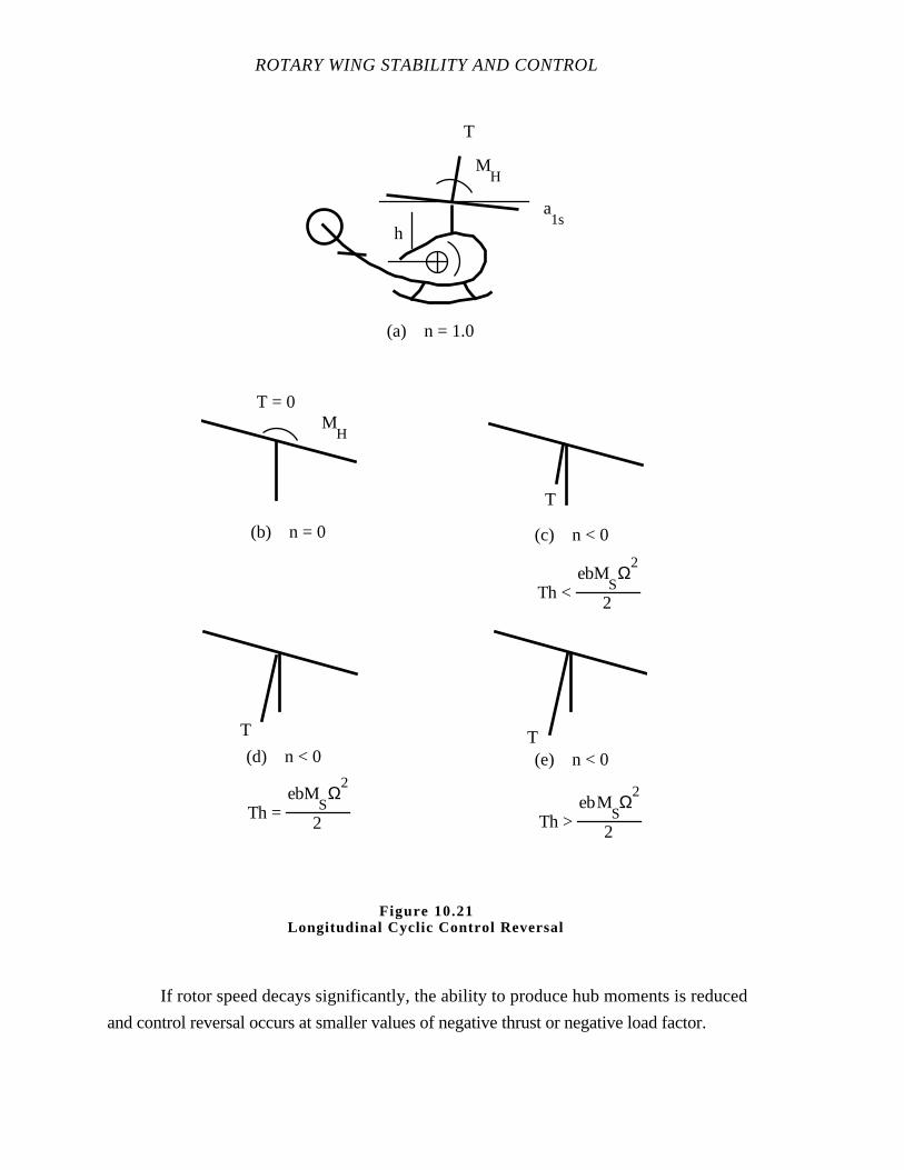
ROTARY WING STABILITY AND CONTROL
If rotor speed decays significantly, the ability to produce hub moments is reduced
and control reversal occurs at smaller values of negative thrust or negative load factor.
MH
T
(a) n = 1.0
a1s
h
T = 0
(b) n = 0
MH
(c) n < 0
Th <ebM
SΩ
2
2
Th =ebM
SΩ
2
2 Th >ebM
SΩ
2
2
T
(d) n < 0 (e) n < 0
T T
Figure 10.21Longitudinal Cyclic Control Reversal

SUDDEN ENGINE FAILURES, AUTOROTATIVE FLIGHT,
AND AUTOROTATIVE LANDINGS
Cautious use of down collective and forward cyclic control inputs during forward
flight power loss tests is imperative (particularly at higher airspeeds), to prevent aggravated
loss of rotor speed, excessive forward flapping, excessive nose down pitch
attitudes/descent rates and control reversal.
10.3.3.6 RESPONSE TO LATERAL CYCLIC INPUT
It is extremely difficult to predict the lateral cyclic inputs required during entry into
autorotative flight. The most probable input is to the right, as this tends to counter the
predominate roll away from the right sideslip (experienced during power loss in a single
rotor helicopter). One interesting aspect of lateral inputs is the effect these inputs have on
aircraft response when the collective motion lags the lateral control displacement. Lateral
inputs used to keep the aircraft wings level as a sideslip angle develops result in
approximately a steady heading sideslip. When the response of the aircraft to rapid down
collective or forward control motion is compared for steady heading balanced flight and
steady heading sideslip flight, the sideslip entry may exhibit a more violent characteristic.
When down collective or forward control inputs are made rapidly there is a reduction (or
reversal) in lateral control effectiveness. In addition, the TPP tilts left because of the
reduced coning (low thrust). The relatively small lateral aircraft moment of inertia may
contribute to the severity of the situation allowing comparatively large roll angular
acceleration to develop.
10.3.3.7 RESPONSE TO DIRECTIONAL CONTROL INPUT
Directional control inputs are very important during recovery from sudden power
loss. The application of right pedal reduces the tail rotor thrust. This reduction in thrust is
accompanied by an immediate reduction in tail rotor torque. The reduction in tail rotor
torque effectively reduces the total power train torque deficiency. For extreme right
sideslips the tail rotor itself may be approaching an autorotative state and provide some
initial torque to the system as the right pedal is applied.
ROTARY WING STABILITY AND CONTROL
A second major effect of corrective directional control inputs is to reduce sideslip
angles both before and after the collective is lowered. The rapid or timely application of the
proper control greatly reduces the possibility of divergence in yaw and roll.
One potential adverse effect of right pedal inputs is the incremental left roll moment
produced for a helicopter configured with a high tail rotor.
10.3.3.8 RESPONSE IN REARWARD FLIGHT
An engine failure during rearward flight can result in a very difficult situation from
a lateral and directional controllability aspect. Such an engine failure in a single rotor
helicopter usually results in a rapid yaw to the left, due first to the decrease in main rotor
torque, then later due to directional stability. If a substantial yaw rate develops before there
is a pilot response, right yaw control may be insufficient to prevent a rapid 180˚ turn to the
left. A rapid turn to the left during rearward flight also results in an almost instantaneous
introduction of a lateral wind component at the left side of the rotor. A rotor which exhibits
high positive dihedral effect produces a rapid roll away from the lateral velocity. The roll
due to sideslip can be reduced by anticipation of the problem and roll into the direction of
yaw.
10.3.3.9 CONTROL INPUTS AT LOW LOAD FACTORS
Control inputs at low load factors may be introduced by the pilot or by the AFCS.
At low load factors the cyclic control effectiveness is reduced. For single rotor helicopters
this loss in effectiveness is felt in pitch and roll, and for the tandem configurations, in roll
and yaw. When the pilot or AFCS makes inputs at reduced load factor with little or no
aircraft response, the tendency is to make larger inputs. If the rotor thrust is then restored
rapidly, the effects of these control inputs can be excessive. Cautious use of flight controls
in low g flight is mandatory.
10.3.4 Autorotative Landing
A successful autorotative landing is only possible after an entry into some form of
autorotative, descending flight. The definition of a successful landing is generally
established by the procuring agency, while the test activity is left to determine what limits
are imposed on operations to assure such landings. The success of an autorotative flare
and landing are strongly dependent upon energy transfers, rotor performance
characteristics, and landing gear design. The nature of the parameters being tested denotes
SUDDEN ENGINE FAILURES, AUTOROTATIVE FLIGHT,
AND AUTOROTATIVE LANDINGS
a performance type test is in order; but, the emergency nature of the entire task and the
dynamic aspects of maneuvers, dictates that stability and control tests must be conducted.
A clever approach is to conduct a stability and control type test while paying strict attention
to performance.
There are a number of very important performance characteristics which must be
monitored and understood. These characteristics are related to the power required for level
flight, the kinetic energy of the rotor, the kinetic energy of the aircraft, the rate of descent,
and the potential energy of the aircraft at the instant the landing flare is commenced. The
ability to decrease the horizontal and vertical velocities is related to the rotor energy and the
thrust produced by the rotor during energy transfers. The energy not absorbed and used by
the rotor during the landing phase is absorbed by the landing gear.
Touch down conditions required in a successful landing reflect the landing surface
characteristics expected. Different airspeed/rate of descent combinations are allowable
when landing on a smooth prepared surface rather than a plowed field.
Landings are considered from several possible flight conditions as follows:
1. Steady autorotative descent.
2. Low above ground level (AGL) altitude hovers.
3. High AGL altitude hovers.
4. Intermediate AGL altitude flight at low airspeed.
5. Low AGL altitude flight with low to high airspeeds.
In situations 2 through 5, it is probable that no steady autorotative flight condition
exists prior to landing; rather, the pilot must use the helicopter and rotor energy available to
him to execute the successful landing. Situations 2 through 5 give rise to the concept of the
Height-Velocity Diagram (H-V diagram) sometimes referred to as the Dead Man's Curve.
ROTARY WING STABILITY AND CONTROL
10.3.4.1 LANDING FROM STEADY AUTOROTATIVE DESCENT
Landing from steady autorotative descent usually involves a flare phase to retard
rate of descent and airspeed. The flare is executed usually with cyclic and some possible
collective adjustments to control rotor speed and descent rate. Rotor speed usually
increases during the cyclic flare with rotor speed increase dependent on the rate of flare and
the airspeed at flare commencement.
10.3.4.1.1 Rotor Speed Increase During Flare
The origin of rotor speed increases during an autorotative flareis illustrated in
Figure 10.22. In Figure 10.22, the aircraft is descending at essentially constant conditions
when the pilot makes an aft cyclic input.
The cyclic input tilts the TPP aft thereby increasing the rotor angle of attack and
thrust and providing nose up pitch moments. After the helicopter pitches to some
predetermined attitude, the pilot adjusts cyclic pitch to maintain this attitude, while ground
speed and rate of descent decrease due to the increased thrust. In the flared attitude, the
rotor senses increased angle of attack (or upwash) equivalent to an increased rate of
descent. Increased rate of descent provides pro-autorotative rotor moments or rotor
acceleration torque.
If the flare rate is high, ballooning (climbing) may result, and down collective may
be required to control ballooning. High flare rates or high pitch attitudes may also lead to
rotor overspeeding which must be controlled with collective. Optimization of flare
technique may be required to keep all parameters within satisfactory bounds.
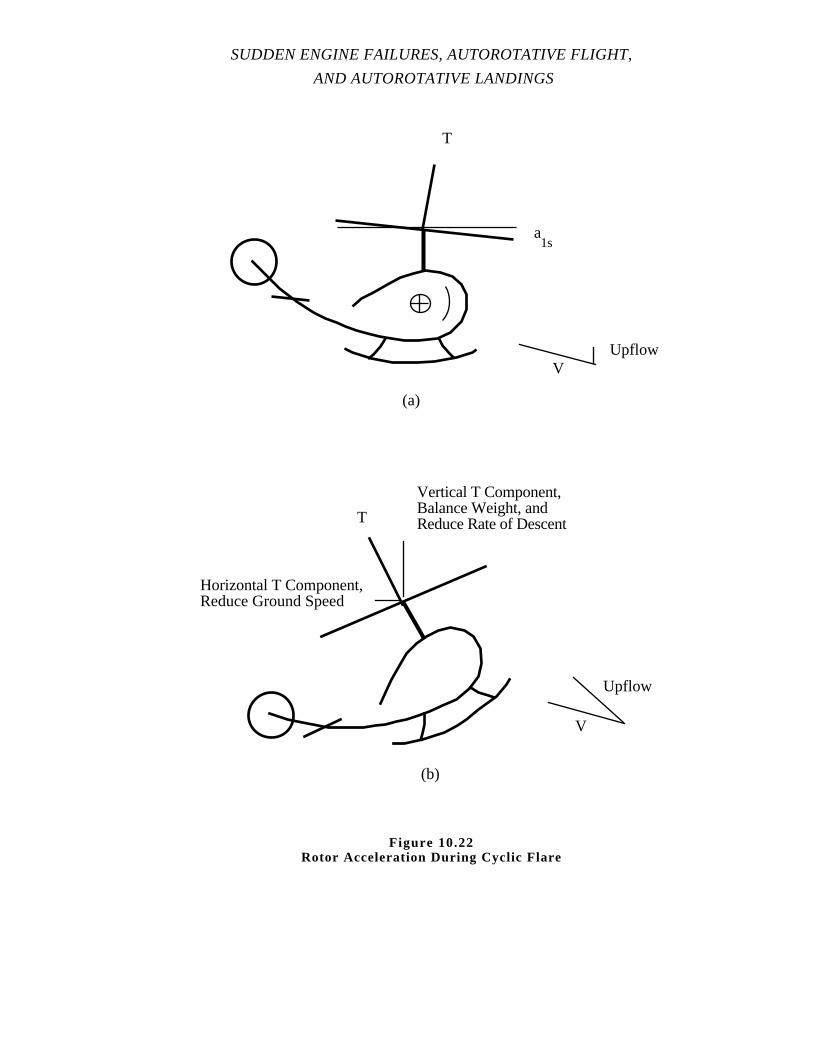
SUDDEN ENGINE FAILURES, AUTOROTATIVE FLIGHT,
AND AUTOROTATIVE LANDINGS
T
(a)
a1s
UpflowV
T
Upflow
V
Vertical T Component,Balance Weight, andReduce Rate of Descent
Horizontal T Component,Reduce Ground Speed
(b)
Figure 10.22Rotor Acceleration During Cyclic Flare
ROTARY WING STABILITY AND CONTROL
10.3.4.1.2 Landing
Aircraft attitude is adjusted between the flare phase and touch down to obtain the
required/desired touchdown attitude. The required touchdown attitude may be nose up (tail
wheel first landing for aircraft so configured) to near level for three point landing or for
landing skid configured helicopters. Landing attitudes involve structural considerations
(tail wheel/tail boom loads), ability to control pitch rate after a nose high touchdown, and
uncontrolled TPP flapping (structural or ground interference) associated with high rates of
descent and low rotor speeds at touchdown.
Adjustments to aircraft attitude in preparation for landing are essentially cyclic
maneuvers. When the flare is terminated rotor speed may be high (desirable), but the
accelerating moments achieved during the flare are lost or reduced and rotor speed decays.
The available energy stored in the rotor is dissipated using collective pitch inputs to cushion
the landing and obtain acceptable touchdown descent rates. The use of increased collective
naturally increases the rotor speed decay rate.
10.3.4.1.3 Full Flare Landing
The full flare autorotative landing is the most difficult to perform. The term full
flare refers to a landing where airspeed and ground speed are zero on touchdown. The
conditions are achieved by conducting a continuous decelerating flare from some higher
airspeed. The degree of difficulty actually experienced during this maneuver is dependent
upon many obvious factors such as atmosphere, rate of descent, aircraft size, field of view,
etc. The pilot may be required to modify the control technique because of aircraft structural
limits. Some considerations are fear of tail rotor to ground contact, main rotor to structure
interference, landing gear failure or upset due to lateral drift. The ability to land tail wheel
first generally eases the demand for pilot proficiency, while any consideration which
requires a near level landing tends to increase the degree of difficulty.
The full flare landing has greater practical application than any other type of
landing. This landing is used to obtain the best results on touchdown over the vast
majority of surfaces available; water, rough terrain, marsh land, and wooded areas. The
goal is to touchdown at a zero ground speed to prevent upset.
SUDDEN ENGINE FAILURES, AUTOROTATIVE FLIGHT,
AND AUTOROTATIVE LANDINGS
10.3.4.1.4 Modified Full Flare Landing
A full flare landing is not always required to achieve the desired goal of a zero
ground speed touchdown. Winds of 5 to 10 kn are representative of the minimum surface
winds on any given day. In addition, ground speeds of up to about 5 kn (sum of lateral
and longitudinal components) provide touchdown safety comparable to that attained with
zero ground speed. A modified full flare landing is then defined as a full flare type landing
where the touchdown ground speed does not exceed 5 kn and the touchdown calibrated
airspeed does not exceed 10 kn.
10.3.4.1.5 Vertical Landing
A vertical landing is required usually when power is lost in a hover. Like the full
flare landing it alludes to zero wind and zero ground speed conditions. A landing of this
type is accomplished by the use of collective only, to cushion landing impact. This type
landing also has a modified category which refers to ground contact when either the values
of horizontal drift (ground speed) or calibrated airspeeds exceed about 5 kn. The overall
success of vertical landing lies in pilot skill and the structural strength of the landing gear.
10.3.4.1.6 Run-On Landing
The run-on landing is one where there is either no requirement or capability to attain
a near zero ground speed. Touchdown is achieved at calibrated airspeeds greater than 10
kn and/or ground speeds in excess of 5 kn. There are three major variations to this landing;
cyclic only flare, collective only flare and coordinated cyclic-collective flare. The
coordinated cyclic-collective maneuver is the most universally used in autorotative landing
techniques and may result in either a tail first or a flat attitude touchdown. The cyclic only
maneuver requires the tail wheel or tail skag to touchdown first and sustain some of the
aircraft weight while the main mounts fall through as thrust is lost on the main rotor. The
collective only run-on landing is required when a flare is either not possible or not practical
(low altitude). The cyclic is used to attain and maintain the desired landing attitude but the
collective is the only control used to reduce sink rate and select the landing point.
Run-on landings, as a rule, require the least pilot skill to accomplish a satisfactory
touchdown attitude and impact velocity. The success of the landing is dependent upon the
landing surface, landing gear configuration and pilot skill in controlling the aircraft through

ROTARY WING STABILITY AND CONTROL
the ground run out. Two of the problems expected during a water landing are tucking and
loss of directional control. A soft surface such as mud or soft sod may produce enough
sliding friction to separate the landing gear from the aircraft. If the run-on ground speed is
sufficiently high and initial touchdown is on one main mount or end of a skid, a dynamic
pitch-roll-yaw bounce may ensue. This type of gyration may turn an otherwise routine
landing into one with damage.
Helicopters which may be configured with different landing gear depending on the
type of terrain or landing surface in use should be tested with each gear configuration and
landing surface combination. An example is a helicopter configured with either skid gear
for use on land or float gear for use on land and water. For a helicopter with different
external configurations, not only must the autorotative landings be evaluated, the transition
into autorotative flight and the steady state autorotation must be evaluated for each
configuration.
The effect of gear type on the run -on landing must be evaluated. Additionally use
of wheel brakes, collective lowering for braking, and control margins during the run-on
landing must be evaluated. Pedal control and margins are especially important during the
run-on landing. The helicopter must be aligned in the direction of run-out during the
landing to reduce the change of roll over.
10.3.4.1.7 Blade Stall
The potential for blade stall during the autorotative flare and landing phases is a
concern. Stall is related to blade section angle of attack which is a combination of collective
input, rotor speed, airspeed, flapping, and inflow (upwash) contributions. High upwash
values in the flare, aft TPP tilt (downward flapping on retreating blade) and reduced total
velocity on the retreating blade during forward flight flares are all conducive to stall
production. High collective positions, low rotor speeds and high descent rates can induce
stall in the landing. Stall results in thrust losses, reduced cyclic effectiveness to produce
moments, increased downward acceleration and aggravated rotor speed decay associated
with increased blade drag coefficients.

SUDDEN ENGINE FAILURES, AUTOROTATIVE FLIGHT,
AND AUTOROTATIVE LANDINGS
10.3.4.2 HEIGHT-VELOCITY DIAGRAM
The H-V diagram serves to define those conditions for which a successful
autorotative landing is not possible. Operation inside the H-V diagram boundaries should
be avoided or minimized based on operational requirements. Figure 10.23 represents a
generic H-V diagram. Points A and B represent conditions 2 and 3, respectively, of
section 10.3.4.1, and ranges A-C-B and D-E-F, conditions 4 and 5, respectively.
Table 10.I defines the boundaries of Figure 10.23.
Airspeed - KTAS
VLimit
Hei
ght A
GL
- ft
B
C
A D
E
F
Avoid
Avoid
Figure 10.23Generic Height-Velocity Diagram
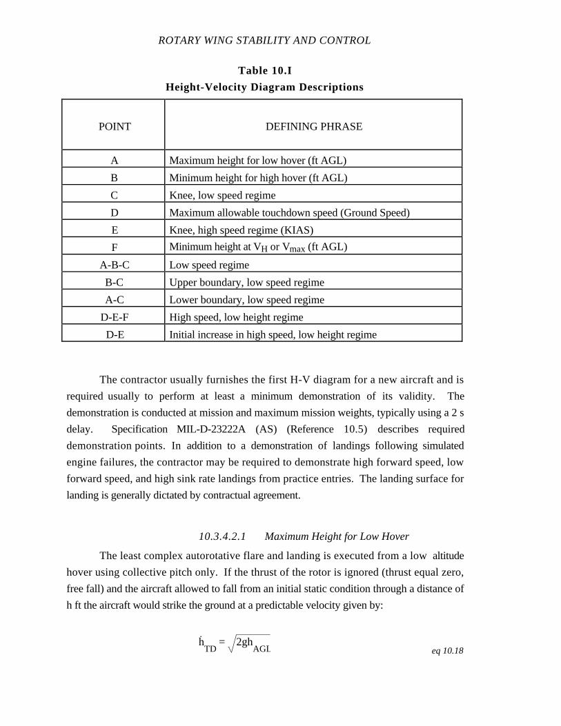
ROTARY WING STABILITY AND CONTROL
Table 10.I
Height-Velocity Diagram Descriptions
POINT DEFINING PHRASE
A Maximum height for low hover (ft AGL)
B Minimum height for high hover (ft AGL)
C Knee, low speed regime
D Maximum allowable touchdown speed (Ground Speed)
E Knee, high speed regime (KIAS)
F Minimum height at VH or Vmax (ft AGL)
A-B-C Low speed regime
B-C Upper boundary, low speed regime
A-C Lower boundary, low speed regime
D-E-F High speed, low height regime
D-E Initial increase in high speed, low height regime
The contractor usually furnishes the first H-V diagram for a new aircraft and is
required usually to perform at least a minimum demonstration of its validity. The
demonstration is conducted at mission and maximum mission weights, typically using a 2 s
delay. Specification MIL-D-23222A (AS) (Reference 10.5) describes required
demonstration points. In addition to a demonstration of landingsfollowing simulated
engine failures, the contractor may be required to demonstrate high forward speed, low
forward speed, and high sink rate landings from practice entries. The landing surface for
landing is generally dictated by contractual agreement.
10.3.4.2.1 Maximum Height for Low Hover
The least complex autorotative flare and landing is executed from a low altitude
hover using collective pitch only. If the thrust of the rotor is ignored (thrust equal zero,
free fall) and the aircraft allowed to fall from an initial static condition through a distance of
h ft the aircraft would strike the ground at a predictable velocity given by:
h.TD
= 2ghAGL eq 10.18
SUDDEN ENGINE FAILURES, AUTOROTATIVE FLIGHT,
AND AUTOROTATIVE LANDINGS
Where:
g - Gravity
hAGL - Height above ground level
hTD - Vertical velocity at touchdown.
By specifying the limit sink speed (hTD ), the free fall limit height is calculated.
For example, if the design limit sink speed were 15 ft/s (900 fpm), the limit height is
approximately 3.5 ft. This estimation of the maximum height for a vertical landing is
extremely conservative since it does not account for rotor thrust being produced.
Rotor thrust effects are examined by considering the collective fixed autorotation as
rotor speed decays. Lowering the collective following power loss may not always be
desirable since thrust reduction with collective input may lead to excessive rates of descent
at touchdown, even though collective reduction lowers the rotor speed decay rate. The
fixed collective setting is maintained until limit sink speed (hTD ) is obtained. The pilot
then increases collective rapidly to achieve thrust equal weight (zero vertical acceleration)
and continues to smoothly increase collective (maintaining thrust equal weight) until
touchdown is achieved just prior to reaching the collective up limit or rotor stall. For this
model, rotor speed bleeds off according to:
dΩdt
= - 1IR (Ω
2
Ω0
2) Q0
eq 10.19
Where:
IR - Rotor rotational moment of inertia
Q0 - Initial torque
t - Time
Ω - Rotor angular velocity
Ω0 - Initial rotor angular velocity.
ROTARY WING STABILITY AND CONTROL
Because rotor speed decays, the thrust is given by:
TT
0
= Ω2
Ω0
2
eq 10.20
Where:
T - Thrust
T0 - Initial thrust
Ω - Rotor angular velocity
Ω0 - Initial rotor angular velocity.
The concept of Equation 10.20 was developed in section 10.3.1.1. The vertical
acceleration is obtained from:
˙z = ˙h =W − T
m= g 1 −
T
W
eq 10.21
Where:
g - Gravity
˙h - Vertical acceleration
m - Mass
T - Thrust
W - Weight
˙z - Acceleration along z axis.
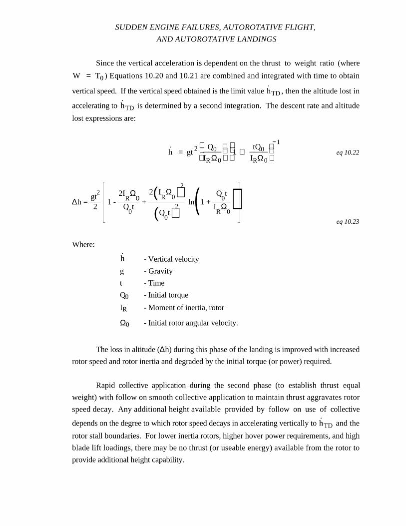
SUDDEN ENGINE FAILURES, AUTOROTATIVE FLIGHT,
AND AUTOROTATIVE LANDINGS
Since the vertical acceleration is dependent on the thrust to weight ratio (where
W = T0) Equations 10.20 and 10.21 are combined and integrated with time to obtain
vertical speed. If the vertical speed obtained is the limit value hTD , then the altitude lost in
accelerating to hTD is determined by a second integration. The descent rate and altitude
lost expressions are:
h = gt2 Q0
IRΩ0
1 +
tQ0
IRΩ0
−1
eq 10.22
∆h = gt
2
21 -
2IR
Ω0
Q0t
+ 2( I
RΩ
0)2
(Q0t)2
ln(1 + Q
0t
IR
Ω0)
eq 10.23
Where:
h - Vertical velocity
g - Gravity
t - Time
Q0 - Initial torque
IR - Moment of inertia, rotor
Ω0 - Initial rotor angular velocity.
The loss in altitude (∆h) during this phase of the landing is improved with increased
rotor speed and rotor inertia and degraded by the initial torque (or power) required.
Rapid collective application during the second phase (to establish thrust equal
weight) with follow on smooth collective application to maintain thrust aggravates rotor
speed decay. Any additional height available provided by follow on useof collective
depends on the degree to which rotor speed decays in accelerating vertically to hTD and the
rotor stall boundaries. For lower inertia rotors, higher hover power requirements, and high
blade lift loadings, there may be no thrust (or useable energy) available from the rotor to
provide additional height capability.
ROTARY WING STABILITY AND CONTROL
10.3.4.2.2 Slow Speed Low Boundary
As speed increases from the low hover point there is some decrease in power
required. The forward entry from the lower boundary probably provides improved rotor
decay characteristics due to the lower torque required but little or no cyclic flare is generally
possible and the landing consists of a collect flare at near entry speed. The forward speed
landing may give the pilot better field of view than in hover, but the forward speed and low
rotor speed may become critical on the roll out. Very little down collective, if any, is used
between power loss and touchdown when on, or below, the lower boundary.
10.3.4.2.3 Minimum Height for High Hover and Slow
Speed High Boundary
At the high hover condition, sufficient altitude (potential energy) is available to
convert to airspeed (kinetic energy) thereby reducing power required and providing energy
to the rotor lost during rotor speed decay. Studies indicate the minimum height for high
hover is related to the airspeed defined for the low speed knee (section 10.3.4.2.5). The
minimum height for high hover with a 2 s delay generally is in the range of 500 to 800 ft.
Entry at the minimum height for high hover generally requires down collective to
minimize rotor speed loss, a significant dive angle to obtain forward speed, and a rapid
flare prior to touchdown. Pilot judgement for airspeed and flare, becomes crucial to the
successful accomplishment of this maneuver. As height decreases and airspeed increases,
the requirement to dive decreases. In fact, as the entry altitude approaches that of the low
speed knee, a significant dive is not possible and there is, in some cases, a significant
change in pilot technique for control of the collective. The collective may not reach full
down because of the vertical acceleration and ground proximity.
10.3.4.2.4 Slow Speed Knee
The slow speed knee represents an area of the curve with all the bad features of the
upper and lower boundaries. The landing from this area probably results in a touchdown at
a speed not much less than the entry speed. The flare must come soon after a rate of
descent is established. The rate of descent is controlled (established) by the pilot by either a
slight dive, a small decrease in collective or a combination of the two. The time between
power failure and landing may be only a few seconds.
SUDDEN ENGINE FAILURES, AUTOROTATIVE FLIGHT,
AND AUTOROTATIVE LANDINGS
Analytical studies, backed up with actual aircraft data, indicate the airspeed for the
low speed knee is related to the airspeed for minimum power required in level flight and the
helicopter gross weight. The same study predicts the minimum high hover altitude as a
function of the airspeed for the slow speed knee, but data indicate that high hover altitude
results are optimistic, i.e. the altitudes predicted are too low. Typically, the low speed knee
with a 2 s delay time occurs in the range of 40 to 60 kn and 120 to 150 ft.
10.3.4.2.5 Maximum Touchdown Speed
The maximum touchdown speed in the high speed region is limited by landing gear
design, etc. and is certainly tied to the landing surface characteristics. The touchdown is
covered under autorotative landings. The ability to control direction of motion on the
ground and stop the aircraft is important when landing in unprepared areas.
10.3.4.2.6 High Speed Region
The initial H-V curve rise in the high speed region is required to allow for some
flare capability. The flare is needed here to slow to the maximum touchdown speed. The
landing attitude (level or tail wheel first) somewhat governs the shape of this curve as does
the flare capability of the aircraft. As speed increases toward limit speed, there is a
tendency for some aircraft to lose a significant amount of altitude during rotor decay
(controls fixed). In addition, an extended level autorotative deceleration (or pull up) from
near VH may be a difficult piloting task. This is especially true of entries at speeds in
excess of about 90 kn. Decelerations or pull ups are considered from a ground clearance
standpoint during pitch attitude changes. Practice is required usually to develop pilot
proficiency for the successful accomplishment of a near VH entry. The engine
characteristics of some aircraft offset some of the value gained from practicing this entry, in
that the static power during push over (after cyclic only flare when needles are not split)
may be enough to reduce rotor speed decay. However, in a real situation rotor speed decay
is extreme and drastically changes the technique required to land. The constant altitude
wind up turn or climbing turn may be a good way to decelerate in some high speed
situations, as it allows rapid change in rotor angle of attack (increased upwash) to recover
rotor speed loss. This turning maneuver may be required when obstacles do not allow a
straight ahead deceleration.
ROTARY WING STABILITY AND CONTROL
10.4 TEST METHODS AND TECHNIQUES
Helicopter flying qualities following sudden power loss through completion of a
successful landing reflect the performance capabilities of the aircraft and the ease with
which the pilot can attain and maintain optimum performance. Tests generally included in
autorotative flying qualities evaluations are designed to investigate aircraft responses to
engine failure, warnings provided, aircraft response to pilot inputs during the transition to
autorotation, steady autorotative flight characteristics, and the pilot’s ability to flare and
land safely.
Before conducting any autorotative testing, perform a data search of contractor and
government test results for the type aircraft to be tested, and other similar aircraft. This
search includes assessment of:
1. Trimmed control position data in hover, low speed flight, vertical
climbs/descents, and forward flight climbs/descents.
2. Control positions to counter trim changes associated with transition
maneuvers for the above conditions.
3. Control response (and coupling) data for all axes in hover and forward
flight.
4. Rotor acceleration/deceleration tendencies as indicated by changes in torque
required during longitudinal control response tests and maneuvering stability tests (constant
collective turns).
Consider using build up simulation maneuvers. Examples are:
1. Directional control response type tests to simulate torque changes and
aircraft response following sudden power loss.
2. Conduct of autorotative flares, transitions from flare to landing attitude, and
limited collective increase to a simulated runway at a safe altitude AGL. This simulation
provides insight to rotor acceleration in the flare, rotor decay during landing attitude
transition, and rotor decay associated with collective increases, as well as a rough
indication of altitude lost from flare initiation to start of the collective increase.
SUDDEN ENGINE FAILURES, AUTOROTATIVE FLIGHT,
AND AUTOROTATIVE LANDINGS
Autorotation testing is accomplished usually in the following order:
1. Steady state autorotation performance (rate of descent with airspeed) and
flying qualities (trimmed control positions, autorotation turns, etc.) evaluations.
2. Flare and landing characteristics.
3. Simulated engine failures characteristics.
4. H-V diagram investigation.
Steady state autorotation test techniques are addressed in reference 10.9 and
Chapters 6 and 7, and are not repeated in this section. Flare and landing characteristics are
conducted before throttle chops and H-V diagram tests in the event unforeseen problems
exist after the throttle chop requiring an actual autorotation. H-V diagram tests are
conducted last to benefit from knowledge gained during flare, landing, and throttle chop
tests.
Subjective evaluation of the autorotative flying qualities is accomplished with a
complete understanding of mission requirements. Handling Qualities Ratings (HQRs) are
assigned with respect to pilot workload and attaining adequate and desired performance for
the test conditions.
10.4.1 Flare and Landing
The purpose of these tests is to determine the optimum flare attitude and rate
required to maximize rotor speed and maintain ground speed and descent rate within
acceptable limits, to determine cyclic control requirements to establish the desired landing
attitude, and to determine collective application requirements to effect a satisfactory
autorotative landing.
The effect of different landing gear configurations on the touchdown and landing
run as well as use of braking, either wheel brakes or collective lowering for braking, along
with control margins during the flare and landing are evaluated.

ROTARY WING STABILITY AND CONTROL
10.4.1.1 TEST TECHNIQUE
1. At a safe altitude, practice power recoveries from autorotation at minimum
rate of descent airspeed and several increasing flare attitudes. Investigate faster and slower
airspeeds at each flare attitude.
2. At a safe altitude, practice simulated flares and landings from full
autorotation at minimum rate of descent airspeed and several increasing flare attitudes and
flare rates. Vary rotor speed for each entry. Investigate faster and slower airspeeds at each
flare condition. Pay close attention to rotor speed changes, airspeed, altitude lost during
flare and simulated landing, aircraft responses/trim changes which provide useful cues or
which cause concern, and note the field of view.
3. Establish stabilized autorotation at the optimum conditions (airspeed, rotor
speed) in preparation for actual autorotative flare/landing.
4. At a predetermined height based on contractor tests and/or altitude
simulations, flare at the optimum rate to the optimum attitude.
5. As ground speed decreases to a comfortable level, establish a landing
attitude and complete the landing.
6. Repeat tests systematically varying approach airspeed, flare characteristics,
approach rotor speed, flare altitude, attitude, and touchdown ground speed. During these
systematic variations, change only one parameter at a time and use small incremental
changes initially to establish the trend produced by each variation.
7. Once the optimum flare and landing requirements are determined,
investigate the effect of braking on the landing run. Vary the use of wheel brakes and
collective lowering for braking.
8. Evaluate each available landing gear and landing surface combination for the
helicopter’s mission.
10.4.1.2 DATA REQUIRED
Cockpit. Run number; approach airspeed; flare attitude; flare altitude, flare rate
(low, medium, high); approach, maximum and touchdown rotor speeds; touchdown
ground speed (estimate if not available); fuel count (FC); roll out distance; tower ambient
conditions.
Ground personnel if used. Run number, wind speed and direction, temperature,
pressure.
SUDDEN ENGINE FAILURES, AUTOROTATIVE FLIGHT,
AND AUTOROTATIVE LANDINGS
Ground station (telemetry). Control positions, attitudes, rates, load factor,
airspeed, altitude (radar altitude if available), rotor speed. Use of ground station personnel
observing data real time is recommended to provide information on exact pitch rate, pitch
attitude, control margins, and rotor speeds during build up to the test limits.
10.4.1.3 TEST CRITERIA
1. Stabilized autorotation (airspeed, rotor speed) prior to flare initiation.
2. Forces initially trimmed to zero (optional).
10.4.1.4 DATA REQUIREMENTS
1. Stabilize as soon as possible before reaching flare altitude.
2. Start automatic recording of data 10 s prior to initiating flare. Record data
until aircraft is on the ground.
3. Approach airspeed ± 1 kn.
4. Approach rotor speed ± 1%.
5. Flare altitude ± 5 ft.
6. Wind < 5 kn, ± 20° of the landing heading.
10.4.1.5 SAFETY CONSIDERATIONS/RISK MANAGEMENT
This test involves operation in an extreme situation where ground contact conditions
are controlled. Execute a power recovery at any time the situation does not feel right. In
the event a power recovery is required, engine response may be sluggish. When the engine
engages the rotor, abrupt torque and heading changes may occur. Tail boom/tail wheel first
landings at high pitch attitudes may lead to asymmetric main gear/skid touchdown and a
subsequent pitch, roll, yaw bounce and/or nose tuck and/or lateral drift. After touchdown,
heading control is reduced with low rotor speed. Ability to rapidly reposition TPP angle is
reduced with low drive train speeds. Adequate fire fighting, crash rescue, and emergency
medical treatment facilities should be available based on risk level. Follow careful build up
procedures to investigate the use of braking during the landing run to avoid unexpected
helicopter attitude changes on the deck.
ROTARY WING STABILITY AND CONTROL
10.4.2 Response to Engine Failure and Pilot Inputs
The purpose of this test is to evaluate aircraft response to sudden powerloss,
effectiveness of warning cues, available time for the pilot to take corrective action, initial
pilot actions required, and follow up pilot actions required to transition to a steady or quasi
steady autorotative condition. Tests are initiated at a safe altitude, usually 2000 to 3000 ft
AGL. Desired end points are those associated with high power flight and representative
power loss situations, i.e. total power loss in a single engine aircraft, or loss of one or
more engines simultaneously in multiengine helicopters. Test techniques discussed in this
section are designed to provide for a logical build up to end point conditions. Power loss is
simulated by abrupt step input of the engine power control from the flight condition to the
ground idle condition.
Engine deceleration (and torque loss) for this simulation is governed by the fuel
control scheduling characteristics and may not be representative of actual lost power
conditions (instantaneous failure of engine power turbine drive shaft or fuel starvation).
Actual engine shut downs usually are not performed since they limit the power recovery
option.
Abrupt power control movement involves coordinated efforts between flight crew
members and ground station personnel similar to control response testing. These tests
involve control response type inputs using the engine power control and voice procedures
to establish cockpit coordination.
A systematic build up is necessary to eliminate surprises. Figure 10.24 illustrates a
possible built up sequence. Point 1 is the starting point and is selected since steady
autorotations and autorotative flares/landings were conducted starting at this airspeed.
Once Point 2 is achieved two paths are available, 2 to 3A or 2 to 3B. Either path is
acceptable. If Path 2 to 3B is chosen, side paths (airspeed variations at constant torque)
ending at the level flight curve are considered. An alternate path similar to Path 2 to 3A on
the back side of the power curve is also realistic. Operation on the back side of the power
curve provides information used later during H-V diagram investigations, which are
conducted at lower entry altitudes.
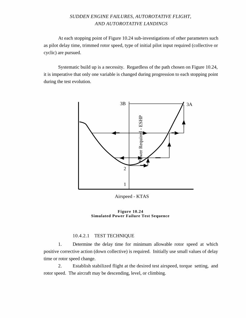
SUDDEN ENGINE FAILURES, AUTOROTATIVE FLIGHT,
AND AUTOROTATIVE LANDINGS
At each stopping point of Figure 10.24 sub-investigations of other parameters such
as pilot delay time, trimmed rotor speed, type of initial pilot input required (collective or
cyclic) are pursued.
Systematic build up is a necessity. Regardless of the path chosen on Figure 10.24,
it is imperative that only one variable is changed during progression to each stopping point
during the test evolution.
10.4.2.1 TEST TECHNIQUE
1. Determine the delay time for minimum allowable rotor speed at which
positive corrective action (down collective) is required. Initially use small values of delay
time or rotor speed change.
2. Establish stabilized flight at the desired test airspeed, torque setting, and
rotor speed. The aircraft may be descending, level, or climbing.
Airspeed - KTAS
Pow
er R
equi
red
- E
SH
P
1
2
3B 3A
Figure 10.24Simulated Power Failure Test Sequence
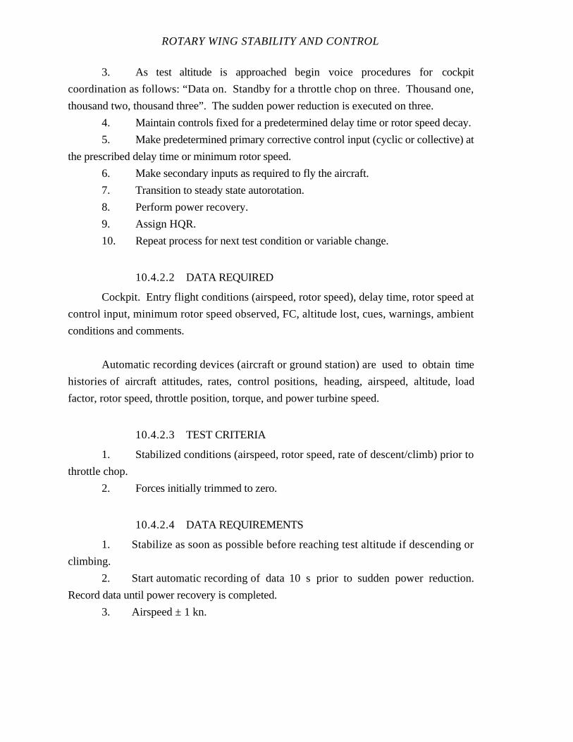
ROTARY WING STABILITY AND CONTROL
3. As test altitude is approached begin voice procedures for cockpit
coordination as follows: “Data on. Standby for a throttle chop on three. Thousand one,
thousand two, thousand three”. The sudden power reduction is executed on three.
4. Maintain controls fixed for a predetermined delay time or rotor speed decay.
5. Make predetermined primary corrective control input (cyclic or collective) at
the prescribed delay time or minimum rotor speed.
6. Make secondary inputs as required to fly the aircraft.
7. Transition to steady state autorotation.
8. Perform power recovery.
9. Assign HQR.
10. Repeat process for next test condition or variable change.
10.4.2.2 DATA REQUIRED
Cockpit. Entry flight conditions (airspeed, rotor speed), delay time, rotor speed at
control input, minimum rotor speed observed, FC, altitude lost, cues, warnings, ambient
conditions and comments.
Automatic recording devices (aircraft or ground station) are used to obtain time
histories of aircraft attitudes, rates, control positions, heading, airspeed, altitude, load
factor, rotor speed, throttle position, torque, and power turbine speed.
10.4.2.3 TEST CRITERIA
1. Stabilized conditions (airspeed, rotor speed, rate of descent/climb) prior to
throttle chop.
2. Forces initially trimmed to zero.
10.4.2.4 DATA REQUIREMENTS
1. Stabilize as soon as possible before reaching test altitude if descending or
climbing.
2. Start automatic recording of data 10 s prior to sudden power reduction.
Record data until power recovery is completed.
3. Airspeed ± 1 kn.
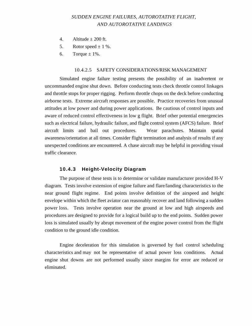
SUDDEN ENGINE FAILURES, AUTOROTATIVE FLIGHT,
AND AUTOROTATIVE LANDINGS
4. Altitude ± 200 ft.
5. Rotor speed ± 1 %.
6. Torque ± 1%.
10.4.2.5 SAFETY CONSIDERATIONS/RISK MANAGEMENT
Simulated engine failure testing presents the possibility of an inadvertent or
uncommanded engine shut down. Before conducting tests check throttle control linkages
and throttle stops for proper rigging. Perform throttle chops on the deck before conducting
airborne tests. Extreme aircraft responses are possible. Practice recoveries from unusual
attitudes at low power and during power applications. Be cautious of control inputs and
aware of reduced control effectiveness in low g flight. Brief other potential emergencies
such as electrical failure, hydraulic failure, and flight control system (AFCS) failure. Brief
aircraft limits and bail out procedures. Wear parachutes. Maintain spatial
awareness/orientation at all times. Consider flight termination and analysis of results if any
unexpected conditions are encountered. A chase aircraft may be helpful in providing visual
traffic clearance.
10.4.3 Height-Velocity Diagram
The purpose of these tests is to determine or validate manufacturer provided H-V
diagram. Tests involve extension of engine failure and flare/landing characteristics to the
near ground flight regime. End points involve definition of the airspeed and height
envelope within which the fleet aviator can reasonably recover and land following a sudden
power loss. Tests involve operation near the ground at low and high airspeeds and
procedures are designed to provide for a logical build up to the end points. Sudden power
loss is simulated usually by abrupt movement of the engine power control from the flight
condition to the ground idle condition.
Engine deceleration for this simulation is governed by fuel control scheduling
characteristics and may not be representative of actual power loss conditions. Actual
engine shut downs are not performed usually since margins for error are reduced or
eliminated.

ROTARY WING STABILITY AND CONTROL
Abrupt power control movements, the potential for violent aircraft reactions, close
to ground operation and the limited time available to perform the correct actions necessitate
close coordination of flight crew members and ground station personnel. Voice procedures
to coordinate activities are mandatory.
A systematic build up is necessary to provide safety margins and eliminate
surprises. Figure 10.25 illustrates the possible build up sequences employed during
investigation of the low speed area of the H-V Diagram.
In Figure 10.25, either point 1 or 4 is an acceptable starting point. Point 1
represents a very low hover, or even possibly an on the ground point with thrust greater
than zero but less than the aircraft weight (light on the landing gear). Point 4 represents a
safe condition as determined by engine failure tests at altitude.
Path 1 to 2 develops the maximum height for a safe vertical hovering autorotation.
Path 2 to 3 involves the landing technique of a collective increase near touchdown and
run-on landing with some ground speed.
Path 4 to 5 represents a build up of decreasing airspeed and increasing power
required until point 5 is reached. Intervals along this path are reduced as point 5 is
approached. Once point 5 is obtained, either path 5 to 7 or 5 to 7A is acceptable. Paths 5
to 7/7A represent conditions where the initial pilot reactions are down collective to reduce
rotor decay and forward cyclic to increase airspeed to arrive at an acceptable rotor speed
and flight path combination for flare/landing.
Figure 10.26 proposes potential sequences to investigate the high speed area of the
H-V diagram. Point 1, 7 or 8 are all acceptable starting conditions. Point 5 is the
maximum allowable landing ground speed.
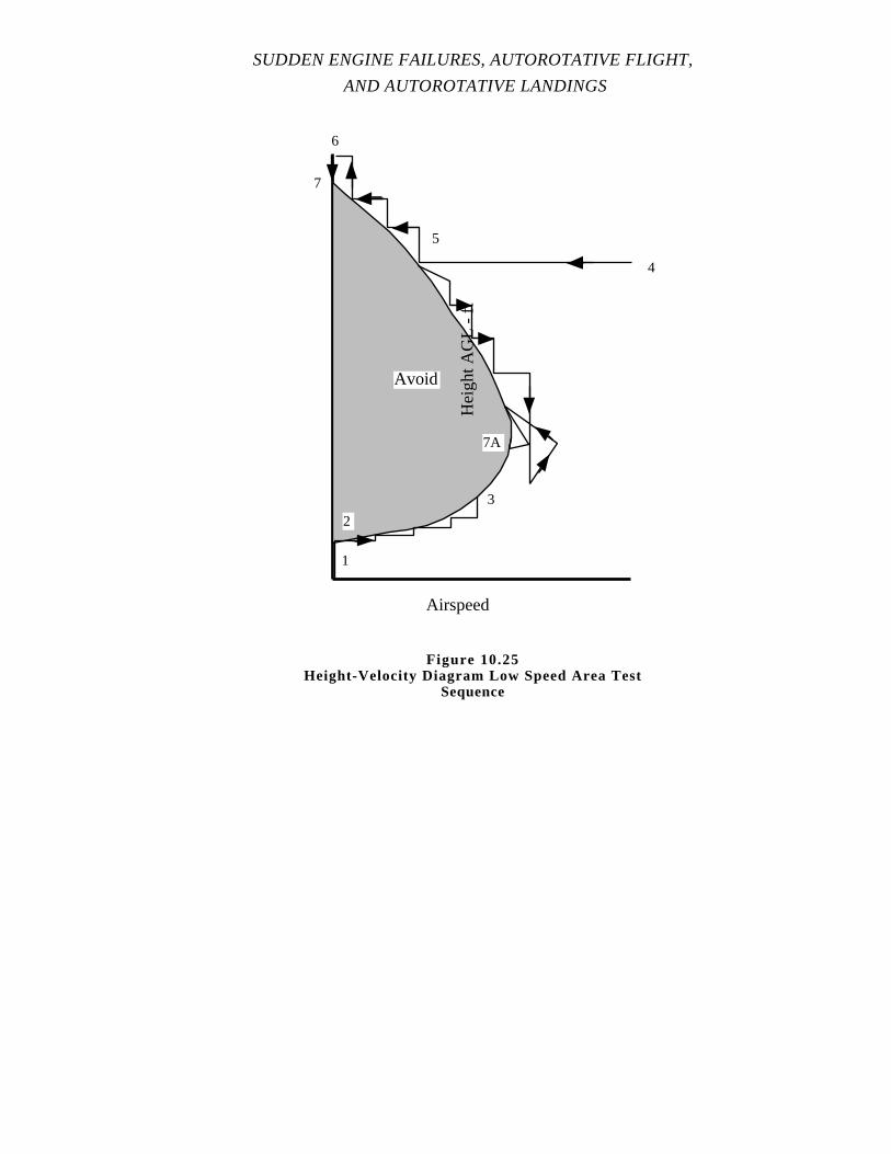
SUDDEN ENGINE FAILURES, AUTOROTATIVE FLIGHT,
AND AUTOROTATIVE LANDINGS
Avoid
Airspeed
Hei
ght A
GL
- ft
1
2
3
4
5
6
7
7A
Figure 10.25Height-Velocity Diagram Low Speed Area Test
Sequence
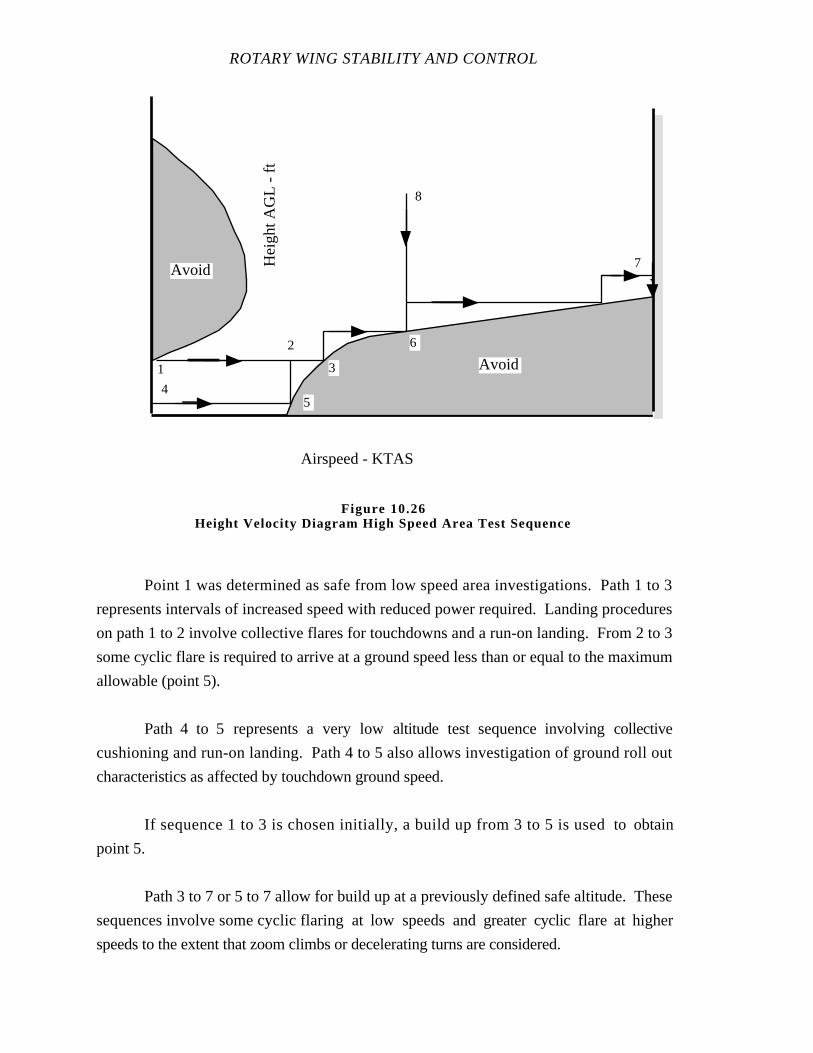
ROTARY WING STABILITY AND CONTROL
Point 1 was determined as safe from low speed area investigations. Path 1 to 3
represents intervals of increased speed with reduced power required. Landing procedures
on path 1 to 2 involve collective flares for touchdowns and a run-on landing. From 2 to 3
some cyclic flare is required to arrive at a ground speed less than or equal to the maximum
allowable (point 5).
Path 4 to 5 represents a very low altitude test sequence involving collective
cushioning and run-on landing. Path 4 to 5 also allows investigation of ground roll out
characteristics as affected by touchdown ground speed.
If sequence 1 to 3 is chosen initially, a build up from 3 to 5 is used to obtain
point 5.
Path 3 to 7 or 5 to 7 allow for build up at a previously defined safe altitude. These
sequences involve some cyclic flaring at low speeds and greater cyclic flare at higher
speeds to the extent that zoom climbs or decelerating turns are considered.
Airspeed - KTAS
Hei
ght A
GL
- ft
Avoid1
2
3
45
6
7
8
Avoid
Figure 10.26Height Velocity Diagram High Speed Area Test Sequence
SUDDEN ENGINE FAILURES, AUTOROTATIVE FLIGHT,
AND AUTOROTATIVE LANDINGS
Starting point 8 represents a predetermined safe airspeed and attitude combination
obtained either from engine failure tests at altitude or H-V diagram investigation for the low
speed area. If point 8 is chosen as a starting point a build up is used to approach point 5
from point 6.
At each stopping point investigation of effects such as delay time and initial rotor
speed are performed.
Careful review of flare/landing and engine failure data are performed prior to
starting H-V diagram testing.
10.4.3.1 TEST TECHNIQUE
1. Determine the delay time or minimum rotor speed allowable at which
appropriate positive corrective action (down collective, cyclic flare, or push over) is taken.
Initially use small values of delay time or rotor speed change.
2. Establish stabilized conditions at the desired test speed (airspeed or ground
speed), altitude, and rotor speed. Record stabilized conditions.
3. Initiate voice procedures for cockpit coordination as follows: “Data on.
Standby for a throttle chop on three. Thousand one, thousand two, thousand three”. The
throttle chop is executed on three.
4. Maintain controls fixed for a predetermined delay time or rotor speed decay.
5. Make predetermined primary corrective control input at prescribed delay time or
minimum rotor speed.
6. Make secondary inputs as required to fly the aircraft and transition to
flare/landing.
7. Assign an HQR to the task of completing a successful landing.
8. Repeat process for next the test condition or variable change.
10.4.3.2 DATA REQUIRED
Cockpit. Airspeed/ground speed, altitude, rotor speed, delay time, rotor speed at
control input, minimum rotor speed, cues, warnings, ground roll, fuel remaining, ambient
conditions, HQR, FC, and comments.
ROTARY WING STABILITY AND CONTROL
Automatic recording devices (aircraft or ground station are used to obtain time
histories of aircraft attitudes, rates, control positions, heading, airspeed, altitude (radar),
load factor, rotor speed, throttle position, torque, and power turbine speed.
10.4.3.3 TEST CRITERIA
1. Stabilized flight prior to throttle chop.
2. Forces initially trimmed to zero.
3. Constant altitude, no rate of climb or descent.
10.4.3.4 DATA REQUIREMENTS
1. Stabilize as soon as possible before recording data.
2. Start automatic recording of data 10 s prior to throttle chop. Record data
until ground run is complete.
3. Airspeed/ground speed ± 1 kn.
4. Altitude ± 5 ft above 50 ft AGL, ± 10% altitude below 50 ft AGL.
5. Rotor speed ± 1 %.
6. Wind < 3 kn.
7. Torque as required for level flight.
10.4.3.5 SAFETY CONSIDERATIONS/RISK MANAGEMENT
Simulated engine failure testing always presents the possibility of an inadvertent or
uncommanded engine shut down. Before conducting these testscheck throttle control
linkage rigging and perform ground throttle chops. Be cautious of control inputs and
aware of reduced effectiveness of control inputs in low g flight. Tests involve operation in
an extreme situation where ground contact conditions must be controlled. Execute a power
recovery if a safe autorotative landing is doubtful. In the event a power recovery is
required, engine response from ground idle may be sluggish. When the engine engages the
rotor, abrupt torque and heading changes may occur. Consider power recovery practice in
the low speed environment. At ground contact, tail wheel first landings at high pitch
attitudes may result in asymmetric main gear/skid touchdown and a subsequent pitch, roll,
yaw bounce and/or nose tuck and/or lateral drift. After touchdown, heading control is
reduced with low rotor speed. Ability to rapidly reposition TPP angle is reduced with low
rotor speed. Maintain spatial awareness/orientation and conduct operations clear of airport
hazards and traffic.
SUDDEN ENGINE FAILURES, AUTOROTATIVE FLIGHT,
AND AUTOROTATIVE LANDINGS
10.5 DATA REDUCTION
Data reduction for steady state autorotative flying qualities involves presentation of
selected dependent variables (control positions, attitudes, etc.) as functions of pertinent
independent variable (airspeed or main rotor speed). Dynamic characteristics are
represented usually in time history form with appropriate annotations. Some graphical data
presentations for dynamic characteristics may be warranted. Automatic data recording
systems usually include total instrumentation system corrections in the process used to
change a flight or telemetry tape raw data into engineering units.
Label all graphs and time histories to show configuration, GW, CG, ambient
conditions, AFCS status, and other appropriate constants.
10.5.1 Steady Autorotation
Data reduction requirements and methods for steady autorotation are outlined in
Chapters 6 and 7 for longitudinal and lateral-directional tests respectively.
10.5.2 Flare and Landing
Present time histories showing complete flare, landing, and landing run for
appropriate parameters and maneuvers. Annotate flare initiation, maximum flare attitude,
maximum rotor speed, control inputs to achieve landing attitude, touchdown, and
termination of landing run. A sample time history showing the touchdown and roll out
phase of an autorotative landing is presented in Figure 10.27.
Consider graphical presentations of parameters showing trends or limiting
conditions, such as maximum rotor speed with flare rate for a fixed flare attitude to show
overspeed tendencies, or touchdown rotor speed with flare height. Make graphical
presentations to illustrate points of interest.

ROTARY WING STABILITY AND CONTROL
10.5.3 Response to Engine Failure and Pilot Inputs
Present time histories from initiation of simulated engine failure to steady
autorotative flight. Annotate throttle reduction, pilot reaction (delay time), minimum rotor
speed, any approaches to control, attitude or load factor limitations, occurrence of any
highly desirable or undesirable characteristics. A sample time history is shown in Figure
10.28.
Time - s
0 1 2 3 4
Pitch Attitude
Pitc
h A
ttitu
de-
deg
NU
0Collective Control
Col
lect
ive
Con
trol
Pos
ition
in F
rom
Ful
l Dow
n
Lateral Control
Late
ral C
ontr
olP
ositi
on -
inF
rom
Ful
l Lef
t
Left
Right
Longitudinal Control
Long
itudi
nal C
ontr
olP
ositi
on -
in F
rom
Aft
Fwd
Dn
Up
Load FactorLoad
Fac
tor
- g
Tail WheelTouchdown
Main WheelTouchdown
Figure 10.27Autorotative Touchdown of a Single Rotor Helicopter

SUDDEN ENGINE FAILURES, AUTOROTATIVE FLIGHT,
AND AUTOROTATIVE LANDINGS
Time - s0 2 4 6 8
Pitch Attitude
Pitc
h A
ttitu
de-
deg
NU
ND
Collective Control
Col
lect
ive
Con
trol
Po
sitio
n in
Fro
m
Ful
l Dow
nLa
tera
l Con
trol
Po
sitio
n -
inF
rom
Fu
ll L
eft
Left
Right
Longitudinal Control
Long
itudi
nal C
ontr
olP
osi
tion
- in
Fro
mF
ull
AftAft
Fwd
Dn
Up
Rol
l Atti
tude
- d
eg
0
Hea
ding
- d
eg
Dire
ctio
nal C
ontr
olP
osi
tion
- in
Fro
m
Ful
l Lef
t
Right
Left
Alti
tude
- ft
Airs
peed
- K
IAS
Thr
ottle
Po
sitio
n
Mai
n R
otor
Spe
ed -
%
Roll Attitude
Lateral Control
Left
Right Heading
Directional Control
Altitude
Collective Lowered
Figure 10.28Simulated Engine Failure of Single Engine Helicopter
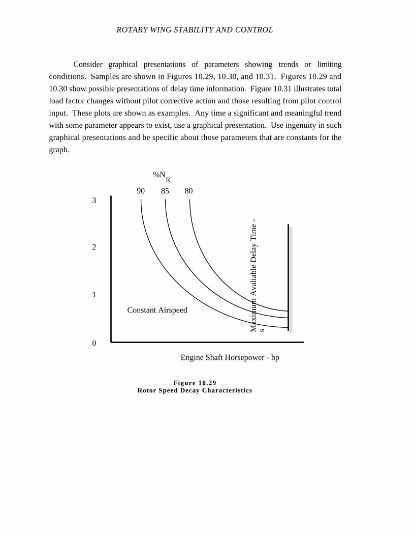
ROTARY WING STABILITY AND CONTROL
Consider graphical presentations of parameters showing trends or limiting
conditions. Samples are shown in Figures 10.29, 10.30, and 10.31. Figures 10.29 and
10.30 show possible presentations of delay time information. Figure 10.31 illustrates total
load factor changes without pilot corrective action and those resulting from pilot control
input. These plots are shown as examples. Any time a significant and meaningful trend
with some parameter appears to exist, use a graphical presentation. Use ingenuity in such
graphical presentations and be specific about those parameters that are constants for the
graph.
Engine Shaft Horsepower - hp
0
1
2
3
%NR
90 8085
Constant Airspeed
Max
imum
Ava
liabl
e D
elay
Tim
e -
s
Figure 10.29Rotor Speed Decay Characteristics
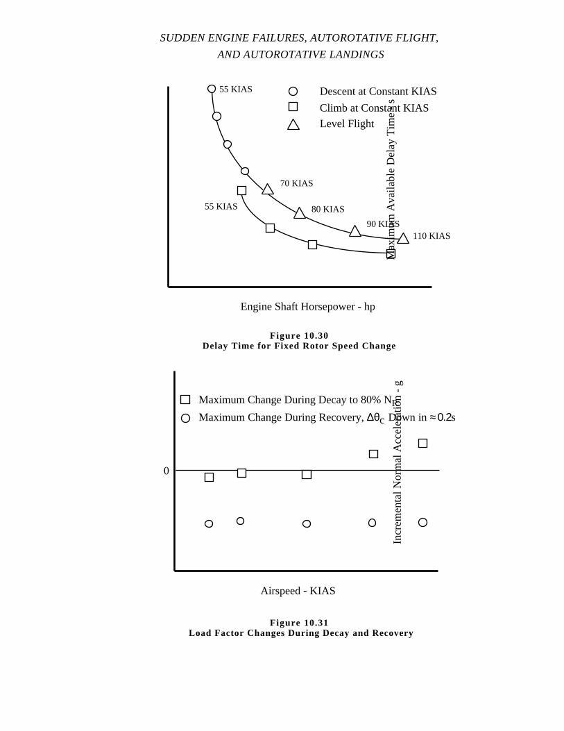
SUDDEN ENGINE FAILURES, AUTOROTATIVE FLIGHT,
AND AUTOROTATIVE LANDINGS
Engine Shaft Horsepower - hp
Descent at Constant KIAS
Climb at Constant KIAS
Level Flight
55 KIAS
70 KIAS
80 KIAS
90 KIAS110 KIAS
55 KIAS
Max
imum
Ava
ilabl
e D
elay
Tim
e -
s
Figure 10.30Delay Time for Fixed Rotor Speed Change
Airspeed - KIAS
0
Maximum Change During Decay to 80% NRIn
crem
enta
l Nor
mal
Acc
eler
atio
n -
g
Maximum Change During Recovery, ∆θc Down in ≈ 0.2s
Figure 10.31 Load Factor Changes During Decay and Recovery
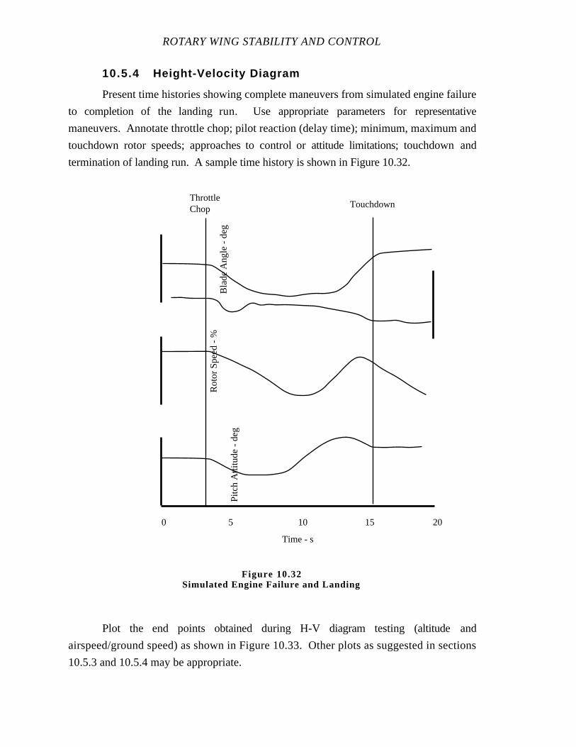
ROTARY WING STABILITY AND CONTROL
10.5.4 Height-Velocity Diagram
Present time histories showing complete maneuvers from simulated engine failure
to completion of the landing run. Use appropriate parameters for representative
maneuvers. Annotate throttle chop; pilot reaction (delay time); minimum, maximum and
touchdown rotor speeds; approaches to control or attitude limitations; touchdown and
termination of landing run. A sample time history is shown in Figure 10.32.
Plot the end points obtained during H-V diagram testing (altitude and
airspeed/ground speed) as shown in Figure 10.33. Other plots as suggested in sections
10.5.3 and 10.5.4 may be appropriate.
Time - s
0 5 10 15 20
Bla
de A
ngle
- d
egR
otor
Spe
ed -
%
Pitc
h A
ttitu
de -
deg
ThrottleChop Touchdown
Figure 10.32Simulated Engine Failure and Landing
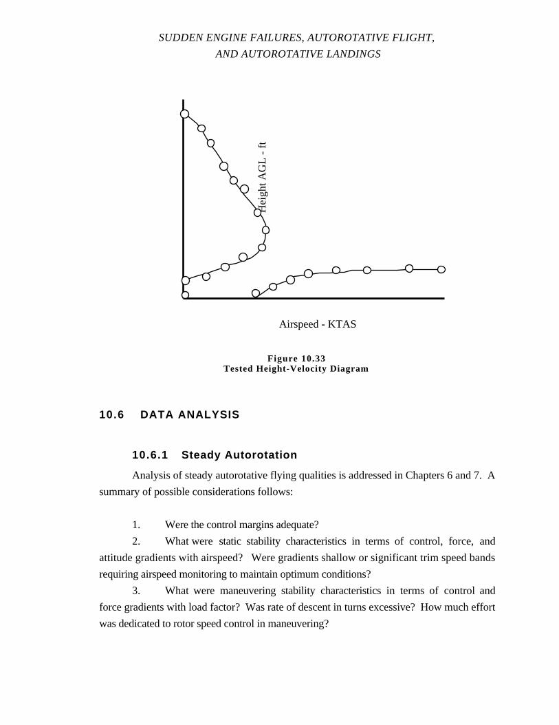
SUDDEN ENGINE FAILURES, AUTOROTATIVE FLIGHT,
AND AUTOROTATIVE LANDINGS
10.6 DATA ANALYSIS
10.6.1 Steady Autorotation
Analysis of steady autorotative flying qualities is addressed in Chapters 6 and 7. A
summary of possible considerations follows:
1. Were the control margins adequate?
2. What were static stability characteristics in terms of control, force, and
attitude gradients with airspeed? Were gradients shallow or significant trim speed bands
requiring airspeed monitoring to maintain optimum conditions?
3. What were maneuvering stability characteristics in terms of control and
force gradients with load factor? Was rate of descent in turns excessive? How much effort
was dedicated to rotor speed control in maneuvering?
Airspeed - KTAS
Hei
ght A
GL
- ft
Figure 10.33Tested Height-Velocity Diagram
ROTARY WING STABILITY AND CONTROL
4. Did longitudinal long term and spiral motions require close monitoring of
airspeed and attitude?
5. Were static lateral-directional characteristics usual? What were rate of
descent changes in steady heading sideslip?
6. What is optimum rotor speed for steady state autorotation?
10.6.2 Flare and Landing
The following considerations are generally included in analysis of autorotative flare
and landing test data:
1. Were control response characteristics adequate to make precise predictable
attitude changes during flare and recovery to landing attitude?
2. How did rotor speed build in the flare?
3. Were there outside cues to rotor speed build up (rotor sound)?
4. Was rotor speed control a problem?
5. How effective was flare in arresting ground speed and rate of descent? Did
the aircraft tend to mush or balloon?
6. How critical was flare initiation altitude on safe landing parameters?
7. How much collective/rotor speed was available for landing?
8. What were landing attitudes and touchdown speeds?
9. What were field of view and altitude cues at landing?
10. What were the landing run characteristics and were there problems with
asymmetric touchdown, bounce, tuck, TPP control, or heading control? Do these
characteristics warrant further tests on other surfaces? What were the landing run distances
and were they excessive for the mission?
11. Were there indications of approach to stall as indicated by vibration, control
feedback, or loss of TPP control?
SUDDEN ENGINE FAILURES, AUTOROTATIVE FLIGHT,
AND AUTOROTATIVE LANDINGS
10.6.3 Response to Engine Failure and Pilot Inputs
The following considerations are generally included in the analysis of engine failure
and pilot response to engine failure test data:
1. What warning was provided and what was the timing and effectiveness of the
warning?
2. What were the initial yaw, roll, and pitch responses to engine failure? Were
these responses in excess of specification requirements?
3. What time is available delay time for the pilot to take corrective action? What
parameter dictates available delay time?
4. How much rotor speed is lost before pilot input and what was the minimum
rotor speed experienced?
5. Were aircraft systems (electrical, hydraulic, AFCS) lost and what was the
significance of these losses?
6. What is the sequence, rate, direction, and magnitude of pilot inputs required?
7. What was the control response/effectiveness during recovery and were
coupled responses a problem?
8. Are structural limits such as load factor or excessive flapping a cause for
concern?
9. How long did it take to regain rotor speed and lost systems? Are transients
involved as systems come back on line? Is restoration of desired/acceptable rotor speed
easily controlled?
10. Were pilot actions required to restore lost systems? Are transients involved?
11. How much altitude was lost between engine failure and (a) recovery of
acceptable rotor speed and (b) establishment of stabilized autorotation?
10.6.4 Height-Velocity Diagram
Height velocity diagram investigation is basically a combination of response to
engine failure, effects of pilot inputs, and flare/landing characteristics. The combined
considerations of sections 10.6.2 and 10.6.3 are addressed during H-V diagram testing.
ROTARY WING STABILITY AND CONTROL
10.7 MISSION SUITABILITY
The suitability of the test aircraft for the intended mission is the ultimate reason for
conducting usual handling qualities testing. However, in the event of a sudden power loss
the aircraft is permanently out of the mission and mission suitability reverts to the pilot's
ability to save the personnel involved and possibly the airframe.
Engine failure testing from occurrence to landing result in defining those actions
which result in a safe landing. To define these actions the test team must be aware of the
flight environment, the flight tasks, and the internal and external information available to
the operator during conduct of the task.
Engineering and quantitative information should be included in the NATOPS
manual for all mission phases to allow meaningful practice in lost power situations.
The most important aspects of autorotative handling qualities is to keep the operator
and his required flight and landing area environment in mind.
10.8 SPECIFICATION COMPLIANCE
Guidelines for helicopter handling qualities during engine failure, recovery, steady
autorotation and landing are contained in MIL-H-8501A. Military specifications are guides
to acceptability and are used in conjunction with mission requirements. Paragraphs 3.2
(Longitudinal characteristics) and 3.3 (Directional and lateralcharacteristics), and
subparagraphs of 3.2 and 3.3, address autorotative flying qualities covered in Chapters 6
and 7 of this manual. These requirements are not repeated here. The following list
identifies those paragraphs of MIL-H-8501A which specifically address autorotation
requirements.
SUDDEN ENGINE FAILURES, AUTOROTATIVE FLIGHT,
AND AUTOROTATIVE LANDINGS
3.5 Autorotation, rotor characteristics, and miscellaneous requirements.
3.5.4.3 Paved surface landings to at least 35 kn.
3.5.4.4 Stopping distance.
3.5.4.5 Water landings.
3.5.5 Autorotation entry.
3.5.5.1 Attitude changes and delay time following sudden
power reduction.
3.5.6 Control forces during transition to autorotation.
3.5.7 Landings at speeds of 15 kn or less.
3.5.9(e)(2) Control margins in steady heading sideslips.
Additional requirements are included in MIL-H-8501 which relate to boosted
controls failure modes, and automatic stabilizationequipment. These requirements are
considered in view of the real potential to lose systems during low rotor speed conditions.
MIL-H-8501A is supplemented with additional detailed specifications listed in the
procurement documents. These should be researched to ensure contractual compliance and
a complete evaluation.
10.9 GLOSSARY
10.9.1 Notations
a1s Longitudinal flapping angle, shaft referenced
AD Rotor disc area
AFCS Automatic Flight Control System
AGL Above ground level
b Number of blades
B1s Longitudinal cyclic pitch angle, shaft referenced
b1s Lateral flapping angle, shaft referenced
CG Center of gravity
CP Power coefficient
CQ Torque coefficient
dD0 Blade element profile drag
dF Blade element torque force
ROTARY WING STABILITY AND CONTROL
dL Blade element lift
dR Blade element resultant aerodynamic force
e Flapping hinge offset
ESHP Engine shaft horsepower
F Force
FC Fuel count
g Gravity
GW Gross weight
h Height of hub above CG
H-V Height -Velocity
hAGL Height above ground level
HQR Handling Qualities Rating
˙h Vertical acceleration
h Vertical velocity
hTD Vertical velocity at touchdown
IR Rotor rotational moment of inertia
iTR Tail rotor inclination out of vertical plane
Izz Moment of inertia about z axis, yaw moment of inertia
KIAS Knots indicated airspeed
KTAS Knots true airspeed
L Lift
LCG Roll moment about CG
LH Roll moment due to rotor hub forces
Lr Roll moment due to yaw rate
Lt Tail lift
lt Distance from the tail to the CG
Lv Roll moment due to lateral velocity
m Mass
MCG Moment about CG
MH Pitch moment due to rotor hub force
MS Blade mass moment
N Net moment about z axis, Yaw moment
NδPED Yaw moment due to pedal control
NR Main rotor speed
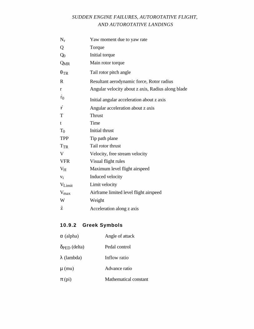
SUDDEN ENGINE FAILURES, AUTOROTATIVE FLIGHT,
AND AUTOROTATIVE LANDINGS
Nr Yaw moment due to yaw rate
Q Torque
Q0 Initial torque
QMR Main rotor torque
θTR Tail rotor pitch angle
R Resultant aerodynamic force, Rotor radius
r Angular velocity about z axis, Radius along blade
r0 Initial angular acceleration about z axis
r Angular acceleration about z axis
T Thrust
t Time
T0 Initial thrust
TPP Tip path plane
TTR Tail rotor thrust
V Velocity, free stream velocity
VFR Visual flight rules
VH Maximum level flight airspeed
vi Induced velocity
VLimit Limit velocity
Vmax Airframe limited level flight airspeed
W Weight
˙z Acceleration along z axis
10.9.2 Greek Symbols
α (alpha) Angle of attack
δPED (delta) Pedal control
λ (lambda) Inflow ratio
µ (mu) Advance ratio
π (pi) Mathematical constant
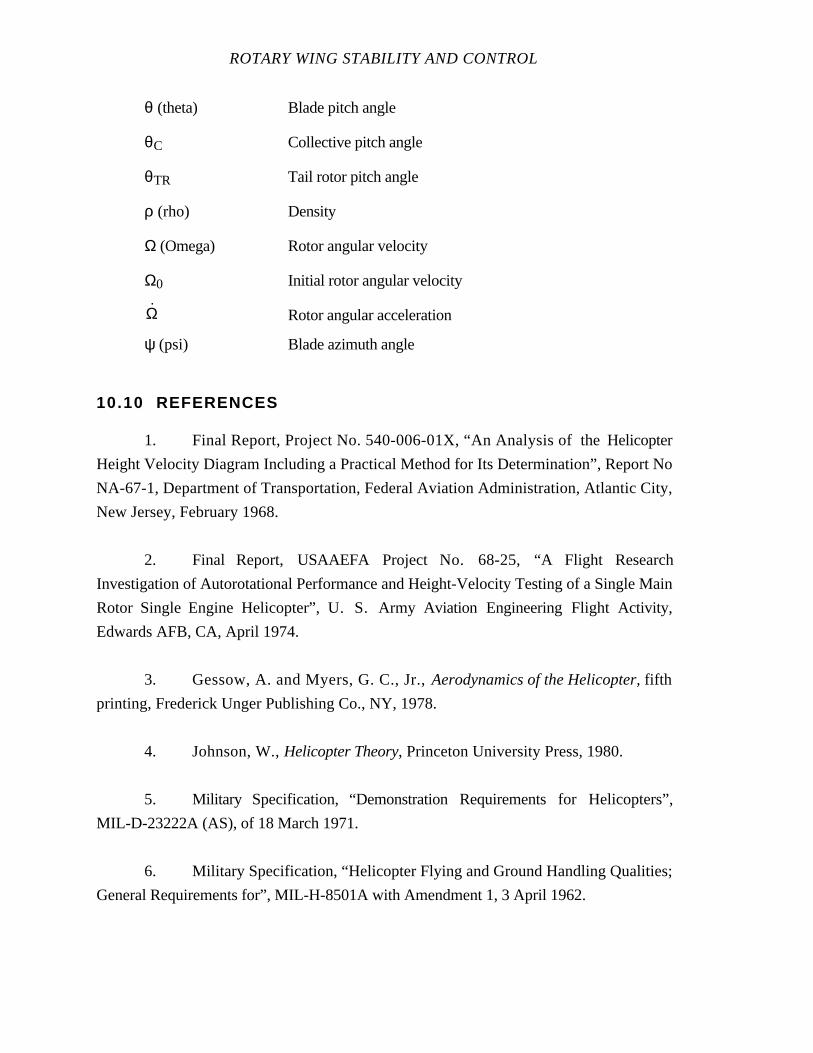
ROTARY WING STABILITY AND CONTROL
θ (theta) Blade pitch angle
θC Collective pitch angle
θTR Tail rotor pitch angle
ρ (rho) Density
Ω (Omega) Rotor angular velocity
Ω0 Initial rotor angular velocity
Ω Rotor angular acceleration
ψ (psi) Blade azimuth angle
10.10 REFERENCES
1. Final Report, Project No. 540-006-01X, “An Analysis of the Helicopter
Height Velocity Diagram Including a Practical Method for Its Determination”, Report No
NA-67-1, Department of Transportation, Federal Aviation Administration, Atlantic City,
New Jersey, February 1968.
2. Final Report, USAAEFA Project No. 68-25, “A Flight Research
Investigation of Autorotational Performance and Height-Velocity Testing of a Single Main
Rotor Single Engine Helicopter”, U. S. Army Aviation Engineering Flight Activity,
Edwards AFB, CA, April 1974.
3. Gessow, A. and Myers, G. C., Jr., Aerodynamics of the Helicopter, fifth
printing, Frederick Unger Publishing Co., NY, 1978.
4. Johnson, W., Helicopter Theory, Princeton University Press, 1980.
5. Military Specification, “Demonstration Requirements for Helicopters”,
MIL-D-23222A (AS), of 18 March 1971.
6. Military Specification, “Helicopter Flying and Ground Handling Qualities;
General Requirements for”, MIL-H-8501A with Amendment 1, 3 April 1962.
SUDDEN ENGINE FAILURES, AUTOROTATIVE FLIGHT,
AND AUTOROTATIVE LANDINGS
7. Naval Test Pilot School Flight Test Manual,Helicopter Stability and
Control, USNTPS-FTM-No. 101, U. S. Naval Test Pilot School, Patuxent River, MD, 10
June 1968, reprinted February 1978.
8. Prouty, Raymond W.,Helicopter Performance, Stability, and Control,
PWS Publishers, Boston, MA, 1986.
9. U.S. Naval Test Pilot School Flight Test Manual,Rotary Wing
Performance, USNTPS-FTM-No. 106, U. S. Naval Test Pilot School, Patuxent River,
MD, 31 December 1987.

APPENDIX I
GLOSSARY
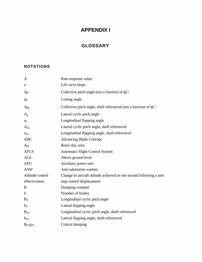
APPENDIX I
GLOSSARY
NOTATIONS
A Rate response value
a Lift curve slope
A0 Collective pitch angle (not a function of ψ)
a0 Coning angle
A0s Collective pitch angle, shaft referenced (not a function of ψ)
A1 Lateral cyclic pitch angle
a1 Longitudinal flapping angle
A1s Lateral cyclic pitch angle, shaft referenced
a1s Longitudinal flapping angle, shaft referenced
ABC Advancing Blade Concept
AD Rotor disc area
AFCS Automatic Flight Control System
AGL Above ground level
APU Auxiliary power unit
ASW Anti-submarine warfare
Attitude control Change in aircraft attitude achieved in one second following a unit
effectiveness step control displacement
B Damping constant
b Number of blades
B1 Longitudinal cyclic pitch angle
b1 Lateral flapping angle
B1s Longitudinal cyclic pitch angle, shaft referenced
b1s Lateral flapping angle, shaft referenced
BCRIT Critical damping
GLOSSARY
B 1s Time rate of change of longitudinal cyclic pitch angle, shaft
referenced
c Blade chord
C1,2 Constants affected by initial conditions of the motion
C1/2 Cycles to one-half amplitude
C1/N Cycles to 1/N amplitude
Cd Cycles to double amplitude
CF Centrifugal force
CG Center of gravity
Control power Measure of the moment produced per unit of control
displacement
Control sensitivity Initial angular acceleration produced by a unit step control
displacement
CP Power coefficient
CQ Torque coefficient
dD0 Blade element profile drag
deg Degree
Df Fuselage drag force
dF Blade element torque force
dL Blade element lift
dR Blade element resultant aerodynamic force
DT IIA Developmental Test IIA
dT Blade element thrust
e Base of natural logarithm, flapping hinge offset
Ed Damping angle
ESHP Engine shaft horsepower
F Force
FC Fuel count
Fq Pitch input
FR Reaction force from ball race
FS blade on hub Shear force of the blade on hub
FT blade on hub Tangential force of the blade on hub
ft Foot
FTE Flight Test Engineer
FTM Flight Test Manual
Fx Force in the x direction
g Gravity
GCA Ground controlled approach
GW Gross weight
H Rotor hub force, ⊥ to shaft
h Height of hub above CG
h' Longitudinal distance between the rotor shaft and the CG
h'lat Lateral distance between the rotor shaft and the CG
H-V Height -Velocity
hAGL Height above ground level
HPo Observed pressure altitude
HQR Handling Qualities Rating
hTR Height of the tail rotor above the CG
Hz Hertz (cycles per second)
˙h Vertical acceleration
h Vertical velocity
hTD Vertical velocity at touchdown
I Moment of inertia
i Imaginary index
If Moment of inertia about flapping hinge
IGE In ground effect
IMC Instrument Meteorological Conditions
in Inch
IR Rotor rotational moment of inertia
is Stabilizer incidence
iTR Tail rotor inclination out of vertical plane
Ixx Moment of inertia about x axis, roll moment of inertia
Ixz Product of inertia about x z axes
Iyy Moment of inertia about y axis, pitch moment of inertia
Izz Moment of inertia about z axis, yaw moment of inertia
K Spring constant
KIAS Knots indicated airspeed
kn Knot
GLOSSARY
KTAS Knots true airspeed
L Net moment about x axis, Roll moment, Lift, Length
LA1s Roll moment due to lateral cyclic pitch angle
lb Pound
LB1s Roll moment due to longitudinal cyclic pitch angle
LCG Roll moment about CG
LδLAT Roll moment due to lateral control
LDO Lateral-directional oscillation
LδPED Roll moment due to pedal control
LEquiv Equivalent length
Lf+t Roll moment due to the fuselage/tail
LH Roll moment due to rotor hub forces
L H Average roll moment due to rotor hub forces for b blades
lne Natural logarithm
Lp Roll moment due to roll rate
Lq Roll moment due to pitch rate
LθC Roll moment due to collective pitch angle
LθTR Roll moment due to tail rotor pitch angle
Lr Roll moment due to yaw rate
Lt Tail lift
lt Distance from the tail to the CG
Lu Roll moment due to longitudinal velocity
Lv Roll moment due to lateral velocity
LvPED Pedal contribution to roll moment due to lateral velocity
Lw Roll moment due to vertical velocity
M Net moment about y axis, Pitch moment
m Mass
MA Aerodynamic moment
Mα Pitch moment due to angle of attack
MA1s Pitch moment due to lateral cyclic pitch angle
MB1s Pitch moment due to longitudinal cyclic pitch angle
MCG Moment about CG
MCGf+t Pitch moment due to the aerodynamic forces on the fuselage/tail
MδLONG Pitch moment due to longitudinal control
MH Pitch moment due to rotor hub force
M H Average pitch moment due to rotor hub force for b blades
MilSpec Military Specification
Mp Pitch moment due to roll rate
Mq Pitch moment due to pitch rate
MθC Pitch moment due to collective pitch angle
MθTR Pitch moment due to tail rotor pitch angle
M θ Pitch moment due to time rate of change of pitch angle
MS Blade mass moment
MSL Maneuvering stability level
Mu Pitch moment due to longitudinal velocity
Mv Pitch moment due to lateral velocity
MW Moment due to weight
Mw Pitch moment due to vertical velocity
M w Pitch moment due to vertical acceleration
N Net moment about z axis, Yaw moment, Denominator of the
fractional amplitude
n Normal acceleration, Normal load factor
NA1s Yaw moment due to lateral cyclic pitch angle
NAWCAD Naval Air Warfare Center Aircraft Division
NB1s Yaw moment due to longitudinal cyclic pitch angle
NδLAT Yaw moment due to lateral control
NδPED Yaw moment due to pedal control
Nf+t Yaw moment due to the fuselage/tail
Ng Engine gas generator speed
Np Yaw moment due to roll rate
NθC Yaw moment due to collective pitch angle
NθTR Yaw moment due to tail rotor pitch angle
NR Main rotor speed
Nr Yaw moment due to yaw rate
nss Steady state normal acceleration
Nu Yaw moment due to longitudinal velocity

GLOSSARY
Nv Yaw moment due to lateral velocity
Nw Yaw moment due to vertical velocity
OFT Operational flight trainer
OGE Out of ground effect
P Period
p Angular velocity about x axis, Roll rate
p0 Initial angular velocity about x axis, Roll rate
PFLF Power for level flight
PIO Pilot Induced Oscillation
pss Steady state angular velocity about x axis, roll rate
p Angular acceleration about x axis
Q Engine torque, Torque
q Angular velocity about y axis, Pitch rate
Q0 Initial torque
QMR Main rotor torque
qss Steady state pitch rate
θTR Tail rotor pitch angle
˙q Second time derivative of pitch rate
q Angular acceleration about y axis, Pitch acceleration
R Resultant aerodynamic force, Rotor radius
r Angular velocity about z axis, Radius along blade, Yaw rate
r' Radius along blade outboard of flapping hinge
r0 Initial angular velocity about z axis, Yaw rate
r0 Initial angular acceleration about z axis
rad Radian
Rate control Angular rate achieved one second following a unit step control
effectiveness displacement
r Angular acceleration about z axis, Yaw acceleration
s Second
SAR Search and rescue
SAS Stability Augmentation System
SCAS Stability Control Augmentation System
SHSS Steady heading sideslip
T Thrust

t Time
T0 Initial thrust
t0 Initial time
T1/2 Time to one-half amplitude
T1/N Time to decay to 1/N of maximum amplitude
Tb Thrust of b blades
TCDB Trim control displacement band
TCP Trim control position
Td Time to double amplitude
To Observed temperature
TOOC Turns on one control
TPP Tip path plane
TTR Tail rotor thrust
u Translational velocity component along x axis
u0 Initial velocity, Initial velocity along x axis
uNR Translational velocity component along the non-rotating x axis
system
uP Downward velocity
USNTPS U.S. Naval Test Pilot School
uT Transverse velocity
˙u Time rate of change of linear acceleration along x axis
u Linear acceleration along x axis
V Velocity, Free stream velocity, Relative velocity
v Translational velocity component along y axis
VAR Vibration Assessment Rating
VFR Visual flight rules
VH Maximum level flight airspeed
Vhor Velocity in the horizontal plane
vi Induced velocity, Induced velocity at hover
VLimit Limit velocity
Vmax Airframe limited level flight airspeed
VMC Visual Meteorological Conditions
VNE Velocity never exceed
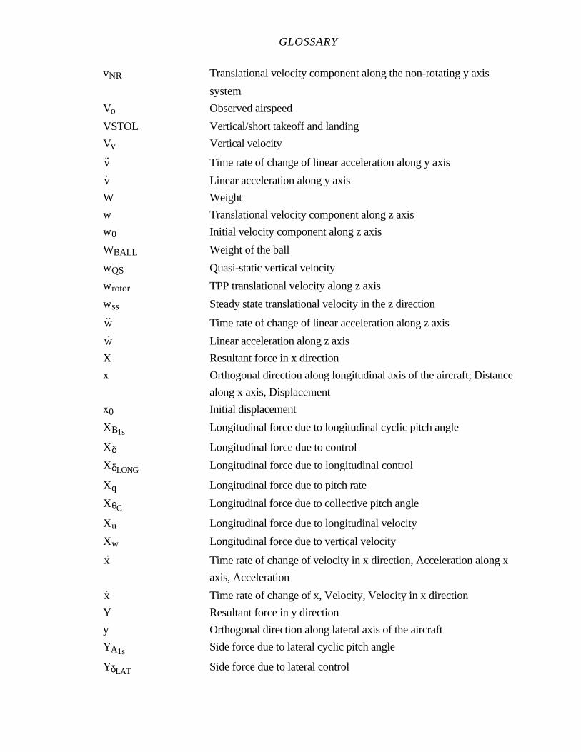
GLOSSARY
vNR Translational velocity component along the non-rotating y axis
system
Vo Observed airspeed
VSTOL Vertical/short takeoff and landing
Vv Vertical velocity
˙v Time rate of change of linear acceleration along y axis
v Linear acceleration along y axis
W Weight
w Translational velocity component along z axis
w0 Initial velocity component along z axis
WBALL Weight of the ball
wQS Quasi-static vertical velocity
wrotor TPP translational velocity along z axis
wss Steady state translational velocity in the z direction
˙w Time rate of change of linear acceleration along z axis
w Linear acceleration along z axis
X Resultant force in x direction
x Orthogonal direction along longitudinal axis of the aircraft; Distance
along x axis, Displacement
x0 Initial displacement
XB1s Longitudinal force due to longitudinal cyclic pitch angle
Xδ Longitudinal force due to control
XδLONG Longitudinal force due to longitudinal control
Xq Longitudinal force due to pitch rate
XθC Longitudinal force due to collective pitch angle
Xu Longitudinal force due to longitudinal velocity
Xw Longitudinal force due to vertical velocity
˙x Time rate of change of velocity in x direction, Acceleration along x
axis, Acceleration
x Time rate of change of x, Velocity, Velocity in x direction
Y Resultant force in y direction
y Orthogonal direction along lateral axis of the aircraft
YA1s Side force due to lateral cyclic pitch angle
YδLAT Side force due to lateral control
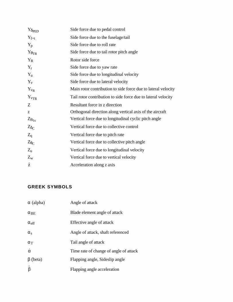
YδPED Side force due to pedal control
Yf+t Side force due to the fuselage/tail
Yp Side force due to roll rate
YθTR Side force due to tail rotor pitch angle
YR Rotor side force
Yr Side force due to yaw rate
Yu Side force due to longitudinal velocity
Yv Side force due to lateral velocity
YvR Main rotor contribution to side force due to lateral velocity
YvTR Tail rotor contribution to side force due to lateral velocity
Z Resultant force in z direction
z Orthogonal direction along vertical axis of the aircraft
ZB1s Vertical force due to longitudinal cyclic pitch angle
ZδC Vertical force due to collective control
Zq Vertical force due to pitch rate
ZθC Vertical force due to collective pitch angle
Zu Vertical force due to longitudinal velocity
Zw Vertical force due to vertical velocity
˙z Acceleration along z axis
GREEK SYMBOLS
α (alpha) Angle of attack
αBE Blade element angle of attack
αeff Effective angle of attack
αs Angle of attack, shaft referenced
αT Tail angle of attack
α Time rate of change of angle of attack
β (beta) Flapping angle, Sideslip angle
˙β Flapping angle acceleration
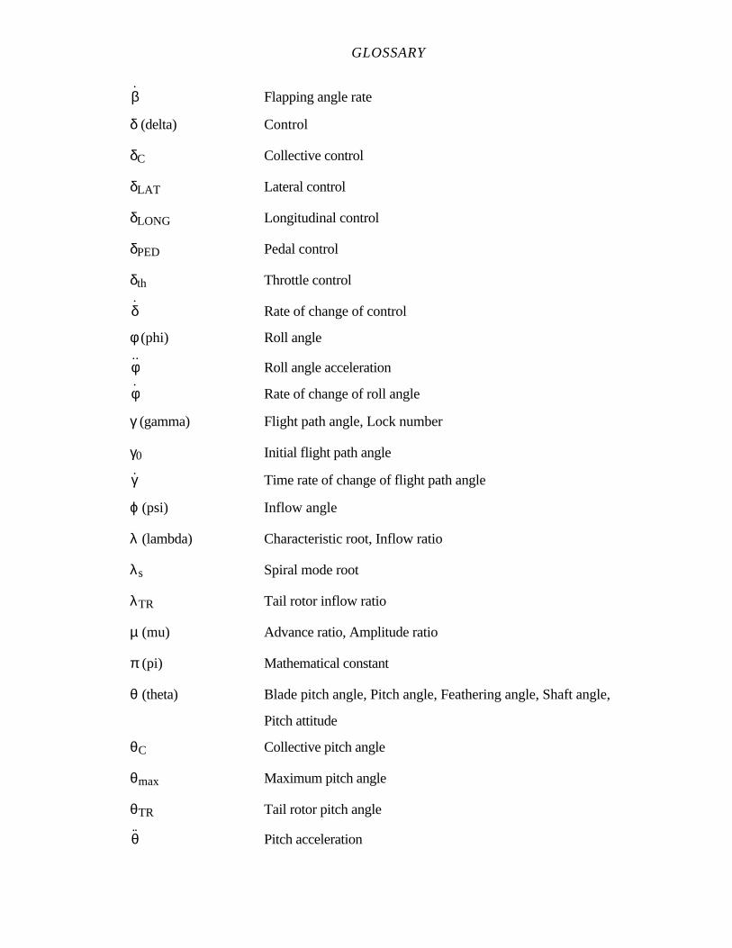
GLOSSARY
β Flapping angle rate
δ (delta) Control
δC Collective control
δLAT Lateral control
δLONG Longitudinal control
δPED Pedal control
δth Throttle control
δ Rate of change of control
φ (phi) Roll angle
˙φ Roll angle acceleration
φ Rate of change of roll angle
γ (gamma) Flight path angle, Lock number
γ0 Initial flight path angle
γ Time rate of change of flight path angle
ϕ (psi) Inflow angle
λ (lambda) Characteristic root, Inflow ratio
λs Spiral mode root
λTR Tail rotor inflow ratio
µ (mu) Advance ratio, Amplitude ratio
π (pi) Mathematical constant
θ (theta) Blade pitch angle, Pitch angle, Feathering angle, Shaft angle,
Pitch attitude
θC Collective pitch angle
θmax Maximum pitch angle
θTR Tail rotor pitch angle
˙θ Pitch acceleration
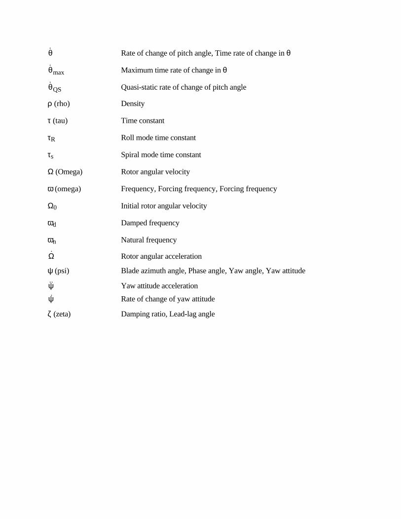
θ Rate of change of pitch angle, Time rate of change in θ
θ max Maximum time rate of change in θ
θ QS Quasi-static rate of change of pitch angle
ρ (rho) Density
τ (tau) Time constant
τR Roll mode time constant
τs Spiral mode time constant
Ω (Omega) Rotor angular velocity
ω (omega) Frequency, Forcing frequency, Forcing frequency
Ω0 Initial rotor angular velocity
ωd Damped frequency
ωn Natural frequency
Ω Rotor angular acceleration
ψ (psi) Blade azimuth angle, Phase angle, Yaw angle, Yaw attitude
˙ψ Yaw attitude acceleration
ψ Rate of change of yaw attitude
ζ (zeta) Damping ratio, Lead-lag angle

II
APPENDIX II
REFERENCES
II.1
APPENDIX II
REFERENCES
CHAPTER 1
1. NATC Instruction 5213.3F, Report Writing Handbook,
NAVAIRTESTCEN, Patuxent River, MD, 16 August 1984.
2. U.S. Naval Test Pilot School Notice 1542, Subj: Academic, Flight and
Report Curriculum for Class --, U.S. Naval Test Pilot School, Patuxent River, MD.
CHAPTER 2
1. Flight Information Handbook, DOD Flight Information Publication,
Defense Mapping Agency Aerospace Center, St. Louis, MO, 23 August, 1990.
2. Naval Test Pilot School Flight Test Manual,Fixed Wing Stability and
Control, Theory and Flight Test Techniques, USNTPS-FTM-No.103, U. S. Naval Test
Pilot School, Patuxent River, MD, 1 January, 1975, Revised 1 November, 1981.
3. NASA Technical Note, NASA TN D-5153, “The Use of Piloted Rating In
The Evaluation Of Aircraft Handling Qualities”, National Aeronauticsand Space
Administration, Washington, D.C., April, 1969.
CHAPTER 3
1. Gessow, A. and Myers, G. C., Jr., Aerodynamics of the Helicopter, fifth
printing, Frederick Unger Publishing Co., NY, 1978.
2. Military Specification, “Helicopter Flying and Ground Handling Qualities;
General Requirements For”, MIL-H-8501A, 7 September, 1961, Amendment 1, 3 April,
1962.
ROTARY WING STABILITY AND CONTROL
II.2
3. Naval Test Pilot School Flight Test Manual,Fixed Wing Stability and
Control, Theory and Flight Test Techniques, USNTPS-FTM-No.103, U. S. Naval Test
Pilot School, Patuxent River, MD, 1 January, 1975, Revised 1 November, 1981.
4. Naval Test Pilot School Flight Test Manual,Helicopter Stability and
Control, USNTPS-FTM-No. 101, U. S. Naval Test Pilot School, Patuxent River, MD, 10
June 1968, reprinted February 1978.
5. Naval Test Pilot School Flight Test Manual,Helicopter Stability and
Control, Theory and Flight Test Techniques, USNTPS-FTM-No. 105, U. S. Naval Test
Pilot School, Patuxent River, MD, November 1983, Preliminary Edition.
6. Prouty, R. W., Practical Helicopter Aerodynamics, PJS Publications, Inc.,
1982.
7. Prouty, Raymond W.,Helicopter Performance, Stability, and Control,
PWS Publishers, Boston, MA, 1986.
CHAPTER 4
1. Bramwell, A. R. S., Helicopter Dynamics, Edward Arnold (Publishers)
Ltd., London, England, 1976.
2. Gessow, A. and Myers, G. C., Jr., Aerodynamics of the Helicopter, fifth
printing, Fredrick Unger Publishing Co., NY, 1978.
3. Naval Test Pilot School Flight Test Manual,Helicopter Stability and
Control, USNTPS-FTM-No. 101, U. S. Naval Test Pilot School, Patuxent River, MD, 10
June 1968, reprinted February 1978.
4. Naval Test Pilot School Flight Test Manual,Helicopter Stability and
Control, Theory and Flight Test Techniques, USNTPS-FTM-No. 105, U. S. Naval Test
Pilot School, Patuxent River, MD, November 1983, Preliminary Edition.
5. Prouty, Raymond W.,Helicopter Performance, Stability, and Control,
PWS Publishers, Boston, MA, 1986.
REFERENCES
II.3
CHAPTER 5
1. Griffin, John M. and Bellaire, Robert G., “A Graphical Summary of
Military Helicopter Flying and Ground Handling Qualities of MIL-H-8501A”, Technical
Report ASNF TN 68-3, Deputy for Engineering, Aeronautical Systems Division, AFSC,
Wright-Patterson Air Force Base, OH, 15 September, 1968.
2. Military Specification, “Helicopter Flying and Ground Handling Qualities;
General Requirements For”, MIL-H-8501A, with Amendment 1, 3 April, 1962.
3. Naval Test Pilot School Flight Test Manual,Helicopter Stability and
Control, USNTPS-FTM-No. 101, U. S. Naval Test Pilot School, Patuxent River, MD,
10 June 1968, reprinted February 1978.
4. Naval Test Pilot School Flight Test Manual,Helicopter Stability and
Control, Theory and Flight Test Techniques, USNTPS-FTM-No. 105, U. S. Naval Test
Pilot School, Patuxent River, MD, November 1983, Preliminary Edition.
CHAPTER 6
1. Johnson, W.Helicopter Theory, Princeton University Pres., 1980.
2. Military Specification, "Helicopter Flying and Ground Handling Qualities;
General Requirements For", MIL-H-8501A, with Amendment 1, 3 April, 1962.
3. Naval Test Pilot School Flight Test Manual,Helicopter Stability and
Control, USNTPS-FTM-No. 101, U. S. Naval Test Pilot School, Patuxent River, MD, 10
June 1968, reprinted February 1978.
4. Naval Test Pilot School Flight Test Manual,Helicopter Stability and
Control, Theory and Flight Test Techniques, USNTPS-FTM-No. 105, U. S. Naval Test
Pilot School, Patuxent River, MD, November 1983, Preliminary Edition.
5. Prouty, R. W., Practical Helicopter Aerodynamics, PJS Publications, Inc.,
1982.
II.4
6. Prouty, Raymond W.,Helicopter Performance, Stability, and Control,
PWS Publishers, Boston, MA, 1986.
7. Wiesner, W. and Kohler, G., Tail Rotor Performance in Presence of Main
Rotor, Ground, and Winds, J.A.H.S., Vol. 15, No. 3, July 1974.
CHAPTER 7
1. Bramwell, A. R. S., Helicopter Dynamics, Edward Arnold (Publishers)
Ltd., London, England, 1976.
2. Gessow, A. and Myers, G. C., Jr., Aerodynamics of the Helicopter, fifth
printing, Frederick Unger Publishing Co., NY, 1978.
3. Johnson, W., Helicopter Theory, Princeton University Pres., 1980.
4. Hall, W. G., "A Collection of Flight Test Data Reduction Techniques",
CAL No. 177, Technical Report, Cornell Aeronautical Laboratory, Inc., Buffalo, NY,
June 1971.
5. Military Specification, "Helicopter Flying and Ground Handling Qualities;
General Requirements For", MIL-H-8501A, with Amendment 1, 3 April, 1962.
6. Naval Test Pilot School Flight Test Manual, Helicopter Stability and
Control, USNTPS-FTM-No. 101, U. S. Naval Test Pilot School, Patuxent River, MD, 10
June 1968, reprinted February 1978.
7. Naval Test Pilot School Flight Test Manual, Helicopter Stability and
Control, Theory and Flight Test Techniques, USNTPS-FTM-No. 105, U. S. Naval Test
Pilot School, Patuxent River, MD, November 1983, Preliminary Edition.
8. Prouty, R. W., Practical Helicopter Aerodynamics, PJS Publications, Inc.,
1982.

II.5
9. Prouty, Raymond W.,Helicopter Performance, Stability, and Control,
PWS Publishers, Boston, MA, 1986.
10. Wiesner, W. and Kohler, G., Tail Rotor Performance in Presence of Main
Rotor, Ground, and Winds, J.A.H.S., Vol. 15, No. 3, July 1974.
11. Wolowicz, C. H., "Considerations in the Determination of Stability and
Control Derivatives and Dynamic Characteristics from Flight Data", AGARD Report 549-
Part I, NASA Flight Research Center, AFB, CA, 1966.
CHAPTER 8
1. Griffin, John M. and Bellaire, Robert G., “A Graphical Summary of
Military Helicopter Flying and Ground Handling Qualities of MIL-H-8501A”, Technical
Report ASNF TN 68-3, Deputy for Engineering, Aeronautical Systems Division, AFSC,
Wright-Patterson Air Force Base, OH, 15 September, 1968.
2. Johnson, W., Helicopter Theory, Princeton University Pres., 1980.
3. Military Specification, "Helicopter Flying and Ground Handling Qualities;
General Requirements For", MIL-H-8501A, with Amendment 1, 3 April, 1962.
4. Naval Test Pilot School Flight Test Manual, Helicopter Stability and
Control, USNTPS-FTM-No. 101, U. S. Naval Test Pilot School, Patuxent River, MD, 10
June 1968, reprinted February 1978.
5. Naval Test Pilot School Flight Test Manual, Helicopter Stability and
Control, Theory and Flight Test Techniques, USNTPS-FTM-No. 105, U. S. Naval Test
Pilot School, Patuxent River, MD, November 1983, Preliminary Edition.
6. Prouty, R. W., Practical Helicopter Aerodynamics, PJS Publications, Inc.,
1982.
7. Prouty, Raymond W.,Helicopter Performance, Stability, and Control,
PWS Publishers, Boston, MA, 1986.

ROTARY WING STABILITY AND CONTROL
II.6
8. Wiesner, W. and Kohler, G., “Tail Rotor Performance in Presence of Main
Rotor, Ground, and Winds”, J.A.H.S., Vol. 15, No. 3, July 1974.
CHAPTER 9
1. Johnson, W., Helicopter Theory, Princeton University Pres. 1980.
2. Military Specification, “Flying Qualities of Piloted V/STOL Aircraft”, MIL-
F-83300, 31 December 1970.
3. Military Specification, “Helicopter Flying and Ground Handling Qualities;
General Requirements For” MIL-H-8501A, with Amendment 1, 3 April, 1962.
4. Prouty, Raymond W.,Helicopter Performance, Stability, and Control,
PWS Publishers, Boston, MA, 1986.
5. U. S. Naval Test Pilot School Flight Test Manual, Rotary Wing
Performance, USNTPS-FTM-No. 106 USNTPS, Patuxent River, MD, 31 December
1987.
CHAPTER 10
1. Final Report, Project No. 540-006-01X, “An Analysis of the Helicopter
Height Velocity Diagram Including a Practical Method for Its Determination”, Report No
NA-67-1, Department of Transportation, Federal Aviation Administration, Atlantic City,
New Jersey, February 1968.
2. Final Report, USAAEFA Project No. 68-25, “A Flight Research
Investigation of Autorotational Performance and Height-Velocity Testing of a Single Main
Rotor Single Engine Helicopter”, U. S. Army Aviation Engineering Flight Activity,
Edwards AFB, CA, April 1974.
3. Gessow, A. and Myers, G. C., Jr., Aerodynamics of the Helicopter, fifth
printing, Frederick Unger Publishing Co., NY, 1978.
REFERENCES
II.7
4. Johnson, W., Helicopter Theory, Princeton University Press, 1980.
5. Military Specification, “Demonstration Requirements for Helicopters”,
MIL-D-23222A (AS), of 18 March 1971.
6. Military Specification, “Helicopter Flying and Ground Handling Qualities;
General Requirements for”, MIL-H-8501A with Amendment 1, 3 April 1962.
7. Naval Test Pilot School Flight Test Manual, Helicopter Stability and
Control, USNTPS-FTM-No. 101, U. S. Naval Test Pilot School, Patuxent River, MD, 10
June 1968, reprinted February 1978.
8. Prouty, Raymond W.,Helicopter Performance, Stability, and Control,
PWS Publishers, Boston, MA, 1986.
9. U.S. Naval Test Pilot School Flight Test Manual, Rotary Wing
Performance, USNTPS-FTM-No. 106, U. S. Naval Test Pilot School, Patuxent River,
MD, 31 December 1987.

III
APPENDIX III
FIGURES

III.1
APPENDIX III
FIGURES
PAGE
CHAPTER 2
2.1 Closed Loop Control System 2.2
2.2 Open Loop Control System 2.3
2.3 Control Movement Required in Changing From One Steady State Flight
Condition to Another 2.4
2.4 Typical Patterns of Pilot Attention Required as a Function of Aircraft
Stability and Control Characteristics 2.5
CHAPTER 3
3.1 Spring Mass Damper System 3.6
3.2 The Complex Plane 3.9
3.3 Effect of Increasing Spring Constant 3.10
3.4 Time Histories of First and Second Order Systems 3.11
3.5 Relationship of Root Location on Complex Plane to Motion Characteristics 3.14
3.6 Zw Root Location on Complex Plane 3.16
3.7 Typical Stable First Order Response 3.17
3.8 Examples of Test Inputs for Determination of Open Loop Dynamics 3.19
3.9 Graphic Method for Determining T1/2 and C1/2 3.24
3.10 Graphic Solution for Damping Ratio 3.25
CHAPTER 4
4.1 Body Fixed Orthogonal Stability Axis System 4.4
4.2 Typical Mechanism for Collective and Cyclic Pitch Control 4.7
4.3 Four Bladed Rotor 4.8
4.4 Fully Articulated Rotor 4.9
4.5 Semirigid Teetering Rotor 4.10
ROTARY WING STABILITY AND CONTROL
III.2
4.6 Hingeless Rotor 4.11
4.7 Velocity Distribution on a Rotor 4.13
4.8 Coning Rotor 4.14
4.9 Flapping Angle 4.14
4.10 Blade Pitch Angle 4.15
4.11 Reference Axes System 4.16
4.12 Rotor Longitudinal Angular Relationships 4.17
4.13 Rotor Lateral Angular Relationships 4.17
4.14 Blade Position with Respect to Control and TPP Axes 4.19
4.15 First Harmonic Cosine Flapping Motion, β = a1s cos ψ 4.22
4.16 First Harmonic Sine Flapping Motion, β = b1s sin ψ 4.23
4.17 Flapping Rotor in Equilibrium 4.24
4.18 Phase Angle as a Function of Frequency and Damping Ratio 4.32
4.19 Amplitude Ratio as a Function of Frequency and Damping Ratio 4.33
4.20 TPP Response to a Longitudinal Cyclic Input in Hover 4.41
4.21 Two Fore and AFT Inflow Effects 4.42
4.22 Rotor Response to Collective Pitch Step at Hover 4.43
4.23 Rotor Response to Cyclic Pitch Step at Hover 4.44
4.24 Moments Produced by Flapping 4.45
4.25 Longitudinal Moments About the CG 4.47
4.26 H Force Due to Inflow 4.49
CHAPTER 5
5.1 Cyclic Control Envelope 5.3
5.2 Representative Mechanical Trim System 5.6
5.3 Control Characteristics with Trim System 5.7
5.4 Static Longitudinal Stability 5.9
5.5 Cyclic Control Trim Envelope 5.11
5.6 Control Characteristics with Trim System Freeplay 5.12
5.7 Control Characteristics with Friction 5.14
5.8 Control Characteristics with Breakout 5.15
5.9 Control Characteristics with Trim System Freeplay and Breakout 5.17
5.10 Parallel and Series Dampers 5.20
5.11 Lateral Cyclic Force Displacement Characteristics 5.27
5.12 Control Jump 5.29
FIGURES
III.3
5.13 Control Dynamics 5.30
5.14 Control Force Coupling 5.31
5.15 Viscous Damper Characteristics 5.33
CHAPTER 6
6.1 Forces and Moments Acting on the Helicopter 6.7
6.2 Control Force and Moment Derivatives 6.10
6.3 Forces and Moments Contributing to Pitch Damping 6.14
6.4 Factors Affecting Angle of Attack Derivative 6.17
6.5 Parameters Involved in Trim 6.19
6.6 Longitudinal Trimmed Flight Control Positions Versus Power 6.24
6.7 Static Stability Examples 6.33
6.8 Destabilizing Effect of Reduced Rotor Downwash 6.34
6.9 Static Stability as Indicated by Longitudinal Control Position Versus
Airspeed 6.35
6.10 Flight Path Angle Versus Airspeed 6.36
6.11 Static Stability as Indicated by Control Force Versus Airspeed 6.38
6.12 Relationships Between Variables in Steady Coordinated Turn 6.44
6.13 Helicopter Long Term Response 6.50
6.14 Pitch Rate Response to Step Cyclic Input 6.56
6.15 Normal Acceleration Response to Step Input in Cyclic Pitch 6.58
6.16 Longitudinal Control of a Tandem Rotor Helicopter 6.62
6.17 Factors Affecting Longitudinal Stability of a Tandem Helicopter 6.65
6.18 Time Histories Produced by Various Levels of Excitation 6.76
6.19 Measurement of Step Control Response Characteristics 6.81
6.20 Trimmed Control Positions 6.86
6.21 Static Longitudinal Stability 6.87
6.22 Maneuvering Stability 6.88
6.23 Long Term Dynamic Response 6.89
6.24 Short Term Response 6.90
6.25 Control Response Characteristics 6.91
6.26 Gust Response Characteristics 6.93
ROTARY WING STABILITY AND CONTROL
III.4
CHAPTER 7
7.1 Forces and Moments Contributing to Lateral-Directional Stability Derivatives 7.8
7.2 Loss of Directional Stability Due to Fuselage/Tail Rotor Interference 7.12
7.3 Flow Field at Tail Rotor 7.13
7.4 Directional Stability Versus Airspeed 7.14
7.5 Yaw Damping Versus Airspeed 7.16
7.6 Yaw Moment Due to Roll Rate Versus Airspeed 7.17
7.7 Directional Control Versus Airspeed 7.19
7.8 Yaw Due to Lateral Cyclic Versus Airspeed 7.21
7.9 Unstable Dihedral Effect Due to Fuselage Side Forces 7.23
7.10 Roll Moment Due to Lateral Velocity Versus Airspeed 7.24
7.11 Roll Moment Due to Yaw Rate Versus Airspeed 7.26
7.12 Roll Damping Versus Airspeed 7.28
7.13 Lateral Control Versus Airspeed 7.30
7.14 Roll Moment Due to Yaw Control Versus Airspeed 7.31
7.15 Side Force Due to Lateral Velocity Versus Airspeed 7.33
7.16 Side Force Due to Yaw Rate Versus Airspeed 7.34
7.17 Side Force Due to Roll Rate Versus Airspeed 7.36
7.18 Side Force Due to Lateral Control Versus Airspeed 7.38
7.19 Side Force Due to Directional Control Versus Airspeed 7.39
7.20 Trimmed Pedal Position Versus Airspeed for Rectilinear Flight 7.43
7.21 Static Lateral-Directional Stability 7.48
7.22 Trim Conditions in Steady Sideslips 7.49
7.23 Cyclic Only Turn of Directionally and Spirally Stable Helicopter 7.59
7.24 Pedal Only Turn of Directionally and Spirally Stable Helicopter 7.68
7.25 Simplified Coordinated Turning Flight 7.70
7.26 Source of Dihedral Effect, Roll Damping, and Roll Due to Yaw for the
Tandem Helicopter 7.86
7.27 Example Sideslip Envelope 7.97
7.28 First Order Response 7.110
7.29 Computation Technique for τ 7.110
7.30 Graphical Technique for Determining τ 7.112
7.31 Determining Damping Ratio of a Lightly Damped Second Order Response 7.114
7.32 Determining Roll to Sideslip Ratio 7.115
7.33 Trimmed Control Positions 7.116
FIGURES
III.5
7.34 Static Lateral-Directional Stability 7.118
7.35 Spiral Stability Time History 7.119
7.36 Control Response Characteristics 7.120
CHAPTER 8
8.1 Forces on a Single Rotor Helicopter in Zero Wind Equilibrium Hover 8.12
8.2 Equilibrium Hover - General Case 8.13
8.3 Flow Conditions at a Rotor Blade Section in Low Speed Flight 8.15
8.4 Effective Inflow Variation in Translational Flight Due to Coning 8.17
8.5 Fore and Aft Inflow Variation in Translation Flight 8.17
8.6 Tail Rotor Thrust Changes in Low Speed Sideward Flight 8.19
8.7 Effect of Ground Vortex on Inflow Patterns 8.23
8.8 Ground Effect in Forward Flight 8.24
8.9 Effect of Ground Vortex on Lateral Trim Control Position 8.25
8.10 Typical Static Stability for a Hovering Single Rotor Helicopter 8.26
8.11 Directional Control Position Characteristics During a Turn on a Spot
for a Single Rotor Helicopter 8.30
8.12 Analogy of Simple Pendulum and Helicopter Long Period 8.34
8.13 Mass-Damper Model for a First Order System 8.39
8.14 Idealized First Order Pitch Response to Aft Longitudinal Cyclic
Step Input 8.41
8.15 Effect of Sensitivity and Damping on Initial Pitch Rate Response 8.43
8.16 Comparison of Control Effectiveness and Response Qualities 8.45
8.17 Vertical Static Stability 8.47
8.18 Vertical Oscillation IGE After a Step Collective Adjustment Down 8.47
8.19 Forward and Rearward Trimmed Flight Control Positions 8.61
8.20 Sideward Trimmed Flight Control Positions 8.62
8.21 Critical Azimuth Determination (20 kn) 8.63
8.22 HQR Versus Relative Wind Azimuth 8.64
8.23 Low Airspeed Static Longitudinal Stability 8.66
8.24 Low Airspeed Static Lateral-Directional Stability 8.67
8.25 Long Term Response 8.68
8.26 Measurement of Step Control Response Characteristics 8.69
ROTARY WING STABILITY AND CONTROL
III.6
CHAPTER 9
9.1 Effective Inflow Variation in Translational Flight Due to Coning 9.8
9.2 Tail Rotor Roll Moments 9.9
9.3 Tail Rotor Height Effects on Main Rotor Thrust Alignment 9.11
9.4 Lateral CG Effects on Main Rotor Thrust Alignment 9.12
9.5 Rotor Angle of Attack Changes Due to Pitch Rate 9.13
9.6 Roll Moments Due to Tail Rotor Thrust 9.15
9.7 Longitudinal CG Effects on Main Rotor Thrust Alignment 9.17
9.8 Main Rotor Thrust Alignment for Aft CG and Hub Moments 9.19
9.9 Rotor Torque Changes Due to Vertical Velocity 9.19
9.10 Yaw Moments Due to Roll Rate 9.20
9.11 Yaw Moments Due to Lateral Cyclic 9.21
9.12 Inflow Changes Due to Longitudinal Cyclic 9.22
9.13 Rotor Torque Change Due to Collective Pitch Angle 9.23
9.14 Airspeed, Altitude, and Pitch Relationships During Long Term Oscillation 9.51
9.15 Bank Angle Due to Airspeed During Long Term Oscillation 9.52
9.16 Bank Angle Due to Pitch Rate During Long Term Oscillation 9.53
9.17 Coupling Due to Control Input 9.73
9.18 Coupling Due to Angular Rate 9.74
CHAPTER 10
10.1 Rotor Blade Section Velocities 10.3
10.2 Rotor Speed Decay for Typical Light Helicopters 10.6
10.3 Rotor Speed Decay for Typical Medium Helicopters 10.7
10.4 Rotor Speed Decay for Typical Heavy Helicopters 10.8
10.5 Determination of Directional Control Sensitivity 10.10
10.6 Pedal Position Versus Tail Rotor Thrust Coefficient 10.12
10.7 Pedal Position Versus Main Rotor Torque Coefficient 10.13
10.8 Pedal Position Versus Tail Rotor Thrust 10.13
10.9 Pedal Position Versus Main Rotor Torque 10.14
10.10 Level Flight Power/Torque Required 10.16
10.11 Rotor Pitch Moment Changes at Aft CG 10.21
10.12 Rotor Pitch Moment Changes at Forward CG 10.21
10.13 Aft TPP Tilt with Increased Advance Ratio 10.22
10.14 Rotor Upwash Due to Aft and Left Tilt 10.24
FIGURES
III.7
10.15 Accelerating in Plane Rotor Forces 10.25
10.16 Power Train Response to Limited Partial Power Loss 10.27
10.17 Power Train Response to Extreme Partial Power Loss 10.28
10.18 Rotor Blade Section Autorotative Equilibrium 10.31
10.19 Effects of Weight/Density Altitude on Rate of Descent at Constant
Rotor Speed 10.33
10.20 Estimation of Airspeed for Best Glide Ratio 10.35
10.21 Longitudinal Cyclic Control Reversal 10.44
10.22 Rotor Acceleration During Cyclic Flare 10.49
10.23 Generic Height-Velocity Diagram 10.53
10.24 Simulated Power Failure Test Sequence 10.65
10.25 Height-Velocity Diagram Low Speed Area Test Sequence 10.69
10.26 Height Velocity Diagram High Speed Area Test Sequence 10.70
10.27 Autorotative Touchdown of a Single Rotor Helicopter 10.74
10.28 Simulated Engine Failure of Single Engine Helicopter 10.75
10.29 Rotor Speed Decay Characteristics 10.76
10.30 Delay Time for Fixed Rotor Speed Change 10.77
10.31 Load Factor Changes During Decay and Recovery 10.77
10.32 Simulated Engine Failure and Landing 10.78
10.33 Tested Height-Velocity Diagram 10.79

IV
APPENDIX IV
TABLES

IV.1
APPENDIX IV
TABLES
PAGE
CHAPTER 2
2.I Relationship Between Role, Flight Segments, and Tasks 2.7
2.II Handling Qualities Rating Scale 2.11
2.III Pio Rating Scale 2.16
2.IV Turbulence Rating Scale 2.17
2.V Vibration Rating Scale 2.18
CHAPTER 4
4.I Quasi-Static Rotor Characteristics in Hovering Flight 4.52
4.II Quasi-Static Rotor Characteristics in Forward Flight 4.54
4.III Aerodynamic Stability Derivatives 4.56
CHAPTER 5
5.I Representative Flight Control System Characteristics 5.35
CHAPTER 6
6.I Quasi-Static Rotor Characteristics in Forward Flight 6.2
6.II Sets of Independent Variables for Trim in Steady Rectilinear Flight 6.21
6.III Analogy of Long Term Response and Spring Mass Damper 6.49
6.IV Analogy of Short Term Response and Spring Mass Damper 6.52
CHAPTER 7
7.I Quasi-Static Rotor Characteristics Affecting Lateral-Directional Derivatives 7.3
7.II Relative Contributions to the Stability Derivatives of the Single Rotor
Helicopter 7.40
ROTARY WING STABILITY AND CONTROL
IV.2
7.III Lateral-Directional Equations of Motion for Small Disturbances from Trim 7.74
7.IV Approximate Equations for the Lateral-Directional Oscillation 7.78
7.V LDO Mode Characteristics, 100 kn Trim Speed 7.83
CHAPTER 8
8.I Quasi-Static Rotor Characteristics in Hovering Flight 8.3
8.II First Order System Parameters 8.37
CHAPTER 9
9.I Tip Path Plane Position Summary 9.3
9.II Coupling Moment Derivatives 9.4
9.III Tail Rotor Height Effects on Main Rotor Thrust Alignment Summary 9.12
9.IV Mechanical Control Mixing 9.27
9.V Summary of Low Airspeed Coupling Moment Origins 9.30
9.VI Longitudinal Control Response Coupling 9.41
9.VII Lateral Control Response Coupling 9.44
9.VIII Directional Control Response Coupling 9.46
9.IX Vertical Control Response Coupling 9.48
CHAPTER 10
10.I Height-Velocity Diagram Descriptions 10.51

V
APPENDIX V
EQUATIONS
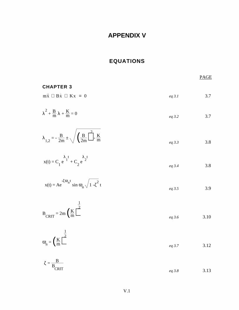
V.1
APPENDIX V
EQUATIONS
PAGE
CHAPTER 3
m˙x + Bx + Kx = 0 eq 3.1 3.7
λ2 + Bm λ + Km = 0
eq 3.2 3.7
λ1,2
= - B2m
± ( B2m)
2
- Kmeq 3.3 3.8
x(t) = C1 e
λ1t + C
2 e
λ2t
eq 3.4 3.8
x(t) = Ae-ζωnt
sin ωn 1 -ζ2 t
eq 3.5 3.9
BCRIT
= 2m (Km)
12
eq 3.6 3.10
ωn = (Km)
12
eq 3.7 3.12
ζ = BB
CRIT eq 3.8 3.13
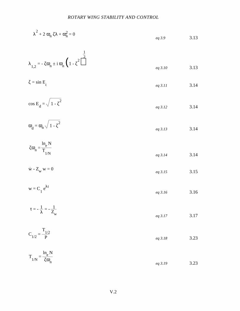
ROTARY WING STABILITY AND CONTROL
V.2
λ2 + 2 ωn ζλ + ωn
2 = 0eq 3.9 3.13
λ1,2
= - ζωn ± i ωn (1 - ζ2)
12
eq 3.10 3.13
ζ = sin Ed eq 3.11 3.14
cos Ed = 1 - ζ
2
eq 3.12 3.14
ωd = ωn 1 - ζ
2
eq 3.13 3.14
ζωn = lne N
T1/N eq 3.14 3.14
w. - Zw w = 0
eq 3.15 3.15
w = C1 eλt
eq 3.16 3.16
τ = - 1λ
= - 1Zw eq 3.17 3.17
C1/2
= P
T1/2
eq 3.18 3.23
T1/N
= lne N
ζωn eq 3.19 3.23
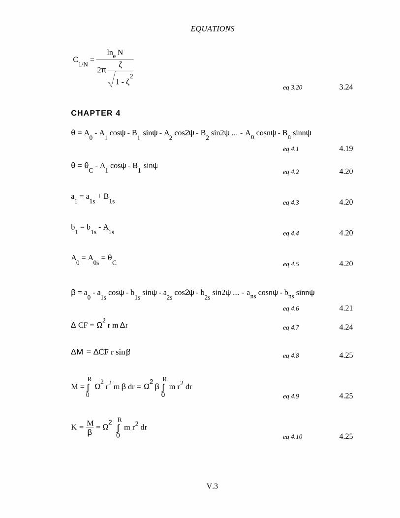
EQUATIONS
V.3
C1/N
= lne N
2πζ
1 - ζ2
eq 3.20 3.24
CHAPTER 4
θ = A0 - A
1 cosψ - B
1 sinψ - A
2 cos2ψ - B
2 sin2ψ ... - An cosnψ - Bn sinnψ
eq 4.1 4.19
θ = θC
- A1 cosψ - B
1 sinψ
eq 4.2 4.20
a1 = a
1s + B
1s eq 4.3 4.20
b1 = b
1s - A
1s eq 4.4 4.20
A0 = A
0s = θ
C eq 4.5 4.20
β = a0 - a
1s cosψ - b
1s sinψ - a
2s cos2ψ - b
2s sin2ψ ... - ans cosnψ - bns sinnψ
eq 4.6 4.21
∆ CF = Ω2 r m ∆r eq 4.7 4.24
∆Μ = ∆CF r sinβ eq 4.8 4.25
M = ∫0
RΩ
2 r2 m β dr = Ω
2 β ∫
0
R m r2 dr
eq 4.9 4.25
K = Mβ
= Ω2 ∫
0
R m r2 dr
eq 4.10 4.25
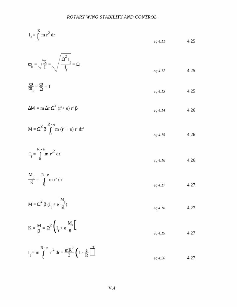
ROTARY WING STABILITY AND CONTROL
V.4
If = ∫
0
R m r2 dr
eq 4.11 4.25
ωn = KI
= Ω
2 I
fIf
= Ωeq 4.12 4.25
ωωn
= ωΩ = 1eq 4.13 4.25
∆Μ = m ∆r Ω2 (r'+ e) r' β eq 4.14 4.26
M = Ω2 β ∫
0
R - em (r' + e) r' dr'
eq 4.15 4.26
If = ∫
0
R - em r'
2 dr'
eq 4.16 4.26
Mf
g = ∫0
R - em r' dr'
eq 4.17 4.27
M = Ω2
β (If + e
Mf
g )eq 4.18 4.27
K = Mβ
= Ω2 ( I
f + e
Mf
g )eq 4.19 4.27
If = m ∫
0
R - e r'
2 dr = mR
3
3 (1 - eR)
3
eq 4.20 4.27
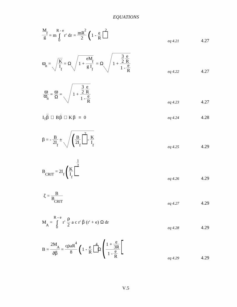
EQUATIONS
V.5
Mf
g = m ∫0
R - er' dr = mR
2
2 (1 - eR)
2
eq 4.21 4.27
ωn = KIf
= Ω 1 + eM
fg I
f
= Ω 1 +
32
eR
1 - eR eq 4.22 4.27
ωωn
= ωΩ = 1 +
32
eR
1 - eR eq 4.23 4.27
I f˙β + Bβ + K β = 0 eq 4.24 4.28
β = - B2I
f
± ( B2I
f)
2
- KIf eq 4.25 4.29
BCRIT
= 2If (K
If)
12
eq 4.26 4.29
ζ = BB
CRIT eq 4.27 4.29
MA
= ∫0
R - e r'
ρ2
a c r' β. (r' + e) Ω dr
eq 4.28 4.29
B = 2M
A
∂β. =
cρaR4
8 (1 - eR)
4
Ω ( 1 + e3R
1 - eR
)eq 4.29 4.29
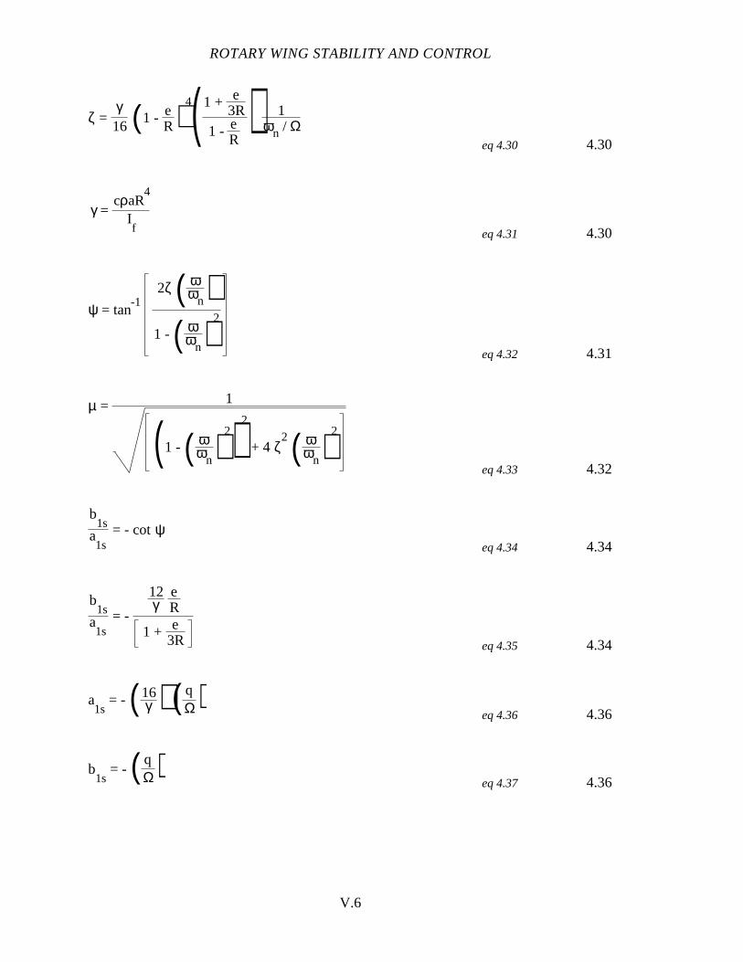
ROTARY WING STABILITY AND CONTROL
V.6
ζ = γ16 (1 - e
R)4( 1 + e
3R
1 - eR
) 1ωn / Ω
eq 4.30 4.30
γ = cρaR
4
If eq 4.31 4.30
ψ = tan-1
2ζ ( ωωn)
1 - ( ωωn)
2
eq 4.32 4.31
µ = 1
(1 - ( ωωn)
2)2
+ 4 ζ2 ( ω
ωn)2
eq 4.33 4.32
b1s
a1s
= - cotψeq 4.34 4.34
b1s
a1s
= -
12γ
eR
1 + e3R eq 4.35 4.34
a1s
= - ( 16γ ) ( q
Ω)eq 4.36 4.36
b1s
= - ( qΩ)
eq 4.37 4.36
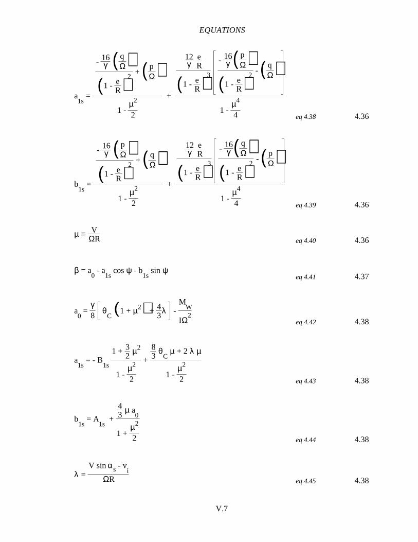
EQUATIONS
V.7
a1s
=
- 16γ ( q
Ω)(1 - e
R)2
+ ( pΩ)
1 - µ2
2
+
12γ
eR
(1 - eR)
3
- 16γ ( p
Ω)(1 - e
R)2
- ( qΩ)
1 - µ4
4 eq 4.38 4.36
b1s
=
- 16γ ( p
Ω)(1 - e
R)2
+ ( qΩ)
1 - µ2
2
+
12γ
eR
(1 - eR)
3
- 16γ ( q
Ω)(1 - e
R)2
- ( pΩ)
1 - µ4
4 eq 4.39 4.36
µ = VΩR eq 4.40 4.36
β = a0 - a
1s cos ψ - b
1s sin ψ
eq 4.41 4.37
a0 =
γ8
θC(1 + µ2) + 4
3λ -
MW
IΩ2
eq 4.42 4.38
a1s
= - B1s
1 + 32
µ2
1 - µ2
2
+
83
θC
µ + 2 λ µ
1 - µ2
2 eq 4.43 4.38
b1s
= A1s
+
43
µ a0
1 + µ2
2 eq 4.44 4.38
λ = V sin αs - vi
ΩR eq 4.45 4.38
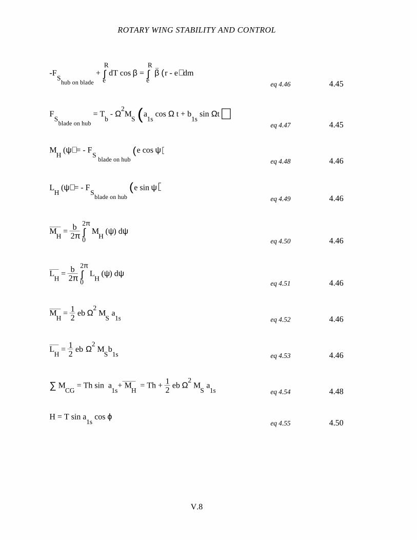
ROTARY WING STABILITY AND CONTROL
V.8
-FS
hub on blade
+ ∫e
RdT cos β = ∫
e
Rβ..
(r - e) dmeq 4.46 4.45
FS
blade on hub
= Tb - Ω
2M
S (a1s
cos Ω t + b1s
sin Ωt)eq 4.47 4.45
MH
(ψ) = - FS
blade on hub(e cos ψ)
eq 4.48 4.46
LH
(ψ) = - FS
blade on hub(e sin ψ)
eq 4.49 4.46
MH
= b2π ∫
0
2π M
H (ψ) dψ
eq 4.50 4.46
LH
= b2π ∫
0
2π L
H (ψ) dψ
eq 4.51 4.46
MH
= 12
eb Ω2 M
S a
1s eq 4.52 4.46
LH
= 12
ebΩ2 M
Sb
1s eq 4.53 4.46
∑ MCG
= Th sin a1s
+ MH
= Th + 12
eb Ω2 M
S a
1s eq 4.54 4.48
H = T sin a1s
cos ϕeq 4.55 4.50
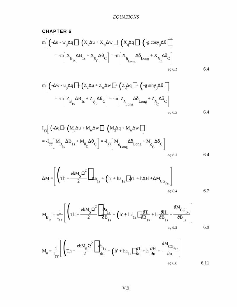
EQUATIONS
V.9
CHAPTER 6
m (-∆u. - w
0∆q) + (Xu∆u + Xw∆w) + (Xq∆q) + (-g cosγ
0∆θ)
= -m XB
1s
∆B1s
+ XθC
∆θC
= -m XδLong
∆δLong
+ XδC
∆δC
eq 6.1 6.4
m (-∆w. - u
0∆q) + (Zu∆u + Zw∆w) + (Zq∆q) + (-g sinγ
0∆θ)
= -m ZB
1s
∆B1s
+ ZθC
∆θC
= -m ZδLong
∆δLong
+ ZδC
∆δC
eq 6.2 6.4
Iyy (-∆q) + (Mu∆u + Mw∆w) + (Mq∆q + Mw∆w)= -Iyy M
B1s
∆B1s
+ MθC
∆θC
= -Iyy MδLong
∆δLong
+ MδC
∆δC
eq 6.3 6.4
∆M = (Th + ebM
SΩ
2
2) ∆a
1s + (h' + ha
1s) ∆T + h∆H +∆MCG
f+t
eq 6.4 6.7
MB
1s
= 1Iyy
(Th + ebM
SΩ
2
2) ∂a
1s∂B
1s
+ (h' + ha1s) ∂T
∂B1s
+ h ∂H∂B
1s
+
∂MCG
f+t
∂B1s
eq 6.5 6.9
Mu = 1Iyy
(Th + ebM
SΩ
2
2) ∂a
1s∂u
+ (h' + ha1s) ∂T
∂u + h ∂H
∂u +
∂MCG
f+t
∂u
eq 6.6 6.11
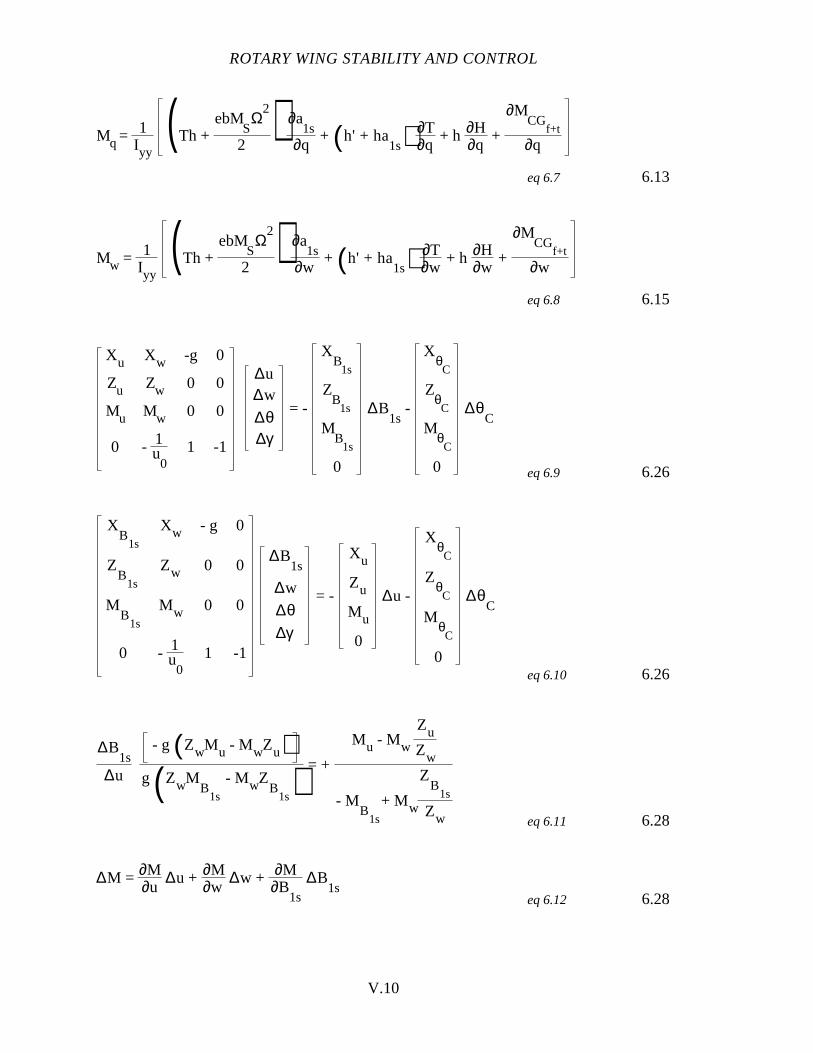
ROTARY WING STABILITY AND CONTROL
V.10
Mq = 1Iyy
(Th + ebM
SΩ
2
2) ∂a
1s∂q
+ (h' + ha1s) ∂T
∂q + h ∂H
∂q +
∂MCG
f+t
∂q
eq 6.7 6.13
Mw = 1Iyy
(Th + ebM
SΩ
2
2) ∂a
1s∂w
+ (h' + ha1s) ∂T
∂w + h ∂H
∂w +
∂MCG
f+t
∂w
eq 6.8 6.15
Xu Xw -g 0
Zu Zw 0 0
Mu Mw 0 0
0 - 1u
01 -1
∆u∆w
∆θ∆γ
= -
XB
1s
ZB
1s
MB
1s
0
∆B1s
-
XθC
ZθC
MθC
0
∆θC
eq 6.9 6.26
XB
1s
Xw - g 0
ZB
1s
Zw 0 0
MB
1s
Mw 0 0
0 - 1u
01 -1
∆B1s
∆w
∆θ∆γ
= -
Xu
Zu
Mu
0
∆u -
XθC
ZθC
MθC
0
∆θC
eq 6.10 6.26
∆B1s
∆u
- g (ZwMu - MwZu)g(ZwM
B1s
- MwZB
1s) = +
Mu - Mw
Zu
Zw
- MB
1s
+ Mw
ZB
1s
Zw eq 6.11 6.28
∆M = ∂M∂u
∆u + ∂M∂w
∆w + ∂M∂B
1s
∆B1s
eq 6.12 6.28
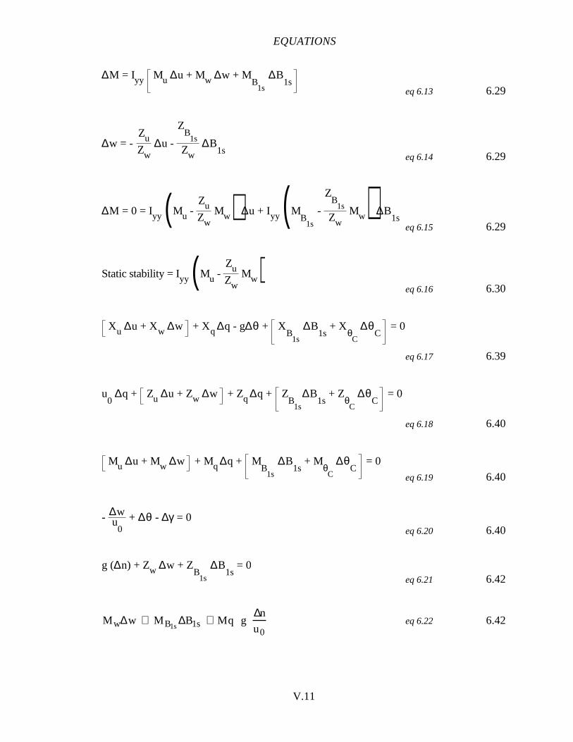
EQUATIONS
V.11
∆M = Iyy Mu ∆u + Mw ∆w + MB
1s
∆B1s
eq 6.13 6.29
∆w = - ZuZw
∆u -
ZB
1s
Zw∆B
1seq 6.14 6.29
∆M = 0 = Iyy (Mu - ZuZw
Mw) ∆u + Iyy (MB
1s
-
ZB
1s
Zw Mw) ∆B
1seq 6.15 6.29
Static stability = Iyy (Mu - ZuZw
Mw)eq 6.16 6.30
Xu ∆u + Xw ∆w + Xq∆q - g∆θ + XB
1s
∆B1s
+ XθC
∆θC
= 0
eq 6.17 6.39
u0
∆q + Zu ∆u + Zw ∆w + Zq∆q + ZB
1s
∆B1s
+ ZθC
∆θC
= 0
eq 6.18 6.40
Mu ∆u + Mw ∆w + Mq∆q + MB
1s
∆B1s
+ MθC
∆θC
= 0
eq 6.19 6.40
- ∆wu
0 + ∆θ - ∆γ = 0
eq 6.20 6.40
g (∆n) + Zw ∆w + ZB
1s
∆B1s
= 0eq 6.21 6.42
M w∆w + MB1s∆B1s + Mq g
∆n
u0eq 6.22 6.42
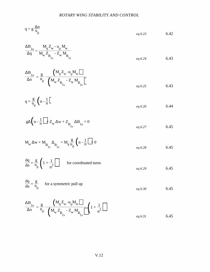
ROTARY WING STABILITY AND CONTROL
V.12
q = g ∆nu
0 eq 6.23 6.42
∆B1s
∆q =
Mq Zw - u0 Mw
Mw ZB
1s
- Zw MB
1s eq 6.24 6.43
∆B1s
∆n =
gu
0
(Mq Zw -u0Mw)
(Mw ZB
1s
- Zw MB
1s) eq 6.25 6.43
q = gu
0(n - 1n)
eq 6.26 6.44
g∆(n - 1n) + Zw ∆w + ZB
1s
∆B1s
= 0eq 6.27 6.45
Mw ∆w + MB
1s
∆B
1s
+ Mqgu
0(n - 1n) = 0
eq 6.28 6.45
dqdn
= gu
0 (1 + 1
n2) for coordinated turnseq 6.29 6.45
dqdn
= gu
0for a symmetric pull up
eq 6.30 6.45
∆B1s
∆n =
gu
0
(Mq Zw -u0Mw)
(Mw ZB
1s
- Zw MB
1s) (1 + 1
n2)eq 6.31 6.45
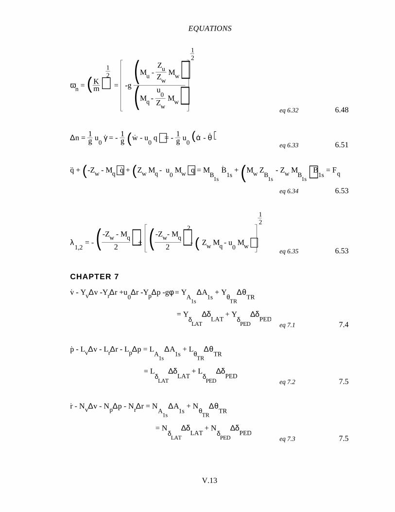
EQUATIONS
V.13
ωn = (Km)
12
= -g(Mu -
ZuZw
Mw)(Mq -
u0
Zw Mw)
12
eq 6.32 6.48
∆n = 1g u0
γ. = - 1g (w. - u
0 q) = - 1g u
0(α. - θ
. )eq 6.33 6.51
q.. + (-Zw - Mq)q
. + (Zw Mq - u0
Mw)q = MB
1s
B.
1s + (Mw Z
B1s
- Zw MB
1s)B1s
= Fq
eq 6.34 6.53
λ1,2
= - ( -Zw - Mq
2 ) ± ( -Zw- Mq
2 )2
- ( Zw Mq - u0 Mw)
12
eq 6.35 6.53
CHAPTER 7
v. - Yv∆v -Yr∆r +u
0∆r -Yp∆p -gφ = Y
A1s
∆A1s
+ YθTR
∆θTR
= YδLAT
∆δLAT
+ YδPED
∆δPED
eq 7.1 7.4
p. - Lv∆v - Lr∆r - Lp∆p = L
A1s
∆A1s
+ LθTR
∆θTR
= LδLAT
∆δLAT
+ LδPED
∆δPED
eq 7.2 7.5
r. - Nv∆v - Np∆p - Nr∆r = N
A1s
∆A1s
+ NθTR
∆θTR
= NδLAT
∆δLAT
+ NδPED
∆δPED
eq 7.3 7.5
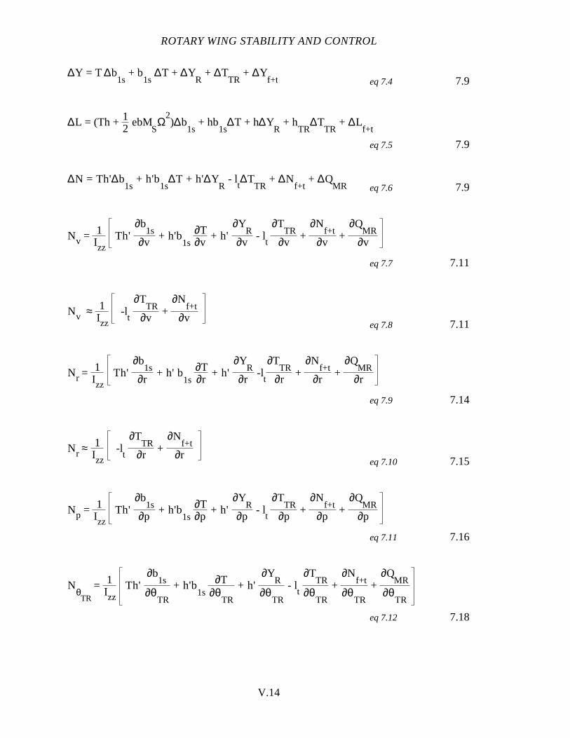
ROTARY WING STABILITY AND CONTROL
V.14
∆Y = T ∆b1s
+ b1s
∆T + ∆YR
+ ∆TTR
+ ∆Yf+t eq 7.4 7.9
∆L = (Th + 12
ebMSΩ
2)∆b
1s + hb
1s∆T + h∆Y
R + h
TR∆T
TR + ∆L
f+t
eq 7.5 7.9
∆N = Th'∆b1s
+ h'b1s
∆T + h'∆YR
- lt∆T
TR + ∆N
f+t + ∆Q
MR eq 7.6 7.9
Nv = 1Izz
Th'∂b
1s∂v
+ h'b1s
∂T∂v
+ h' ∂Y
R∂v
- lt
∂TTR
∂v +
∂Nf+t
∂v +
∂QMR
∂v
eq 7.7 7.11
Nv ≈ 1Izz
-lt
∂TTR
∂v +
∂Nf+t
∂veq 7.8 7.11
Nr = 1Izz
Th'∂b
1s∂r
+ h' b1s
∂T∂r
+ h' ∂Y
R∂r
-lt
∂TTR
∂r +
∂Nf+t
∂r +
∂QMR
∂r
eq 7.9 7.14
Nr ≈ 1Izz
-lt
∂TTR
∂r +
∂Nf+t
∂req 7.10 7.15
Np = 1Izz
Th'∂b
1s∂p
+ h'b1s
∂T∂p
+ h' ∂Y
R∂p
- lt
∂TTR
∂p +
∂Nf+t
∂p +
∂QMR
∂p
eq 7.11 7.16
NθTR
= 1Izz
Th'∂b
1s
∂θTR
+ h'b1s
∂T∂θ
TR
+ h' ∂Y
R
∂θTR
- lt
∂TTR
∂θTR
+ ∂N
f+t
∂θTR
+ ∂Q
MR
∂θTR
eq 7.12 7.18
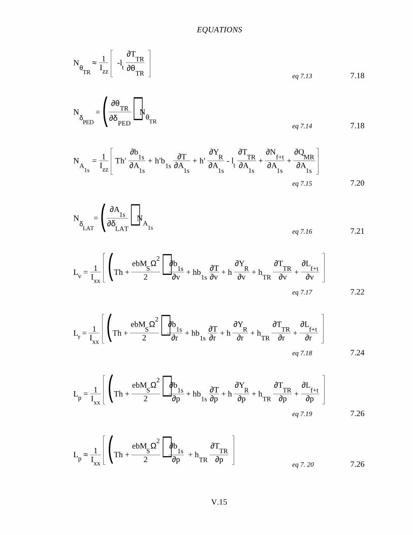
EQUATIONS
V.15
NθTR
≈ 1Izz
-lt
∂TTR
∂θTR eq 7.13 7.18
NδPED
= ( ∂θTR
∂δPED
) NθTR
eq 7.14 7.18
NA
1s
= 1Izz
Th'∂b
1s∂A
1s
+ h'b1s
∂T∂A
1s
+ h' ∂Y
R∂A
1s
- lt
∂TTR
∂A1s
+ ∂N
f+t∂A
1s
+ ∂Q
MR∂A
1s
eq 7.15 7.20
NδLAT
= ( ∂A1s
∂δLAT
) NA
1seq 7.16 7.21
Lv = 1Ixx
(Th + ebM
SΩ
2
2) ∂b
1s∂v
+ hb1s
∂T∂v
+ h ∂Y
R∂v
+ hTR
∂TTR
∂v +
∂Lf+t
∂v
eq 7.17 7.22
Lr = 1Ixx
(Th + ebM
SΩ
2
2) ∂b
1s∂r
+ hb1s
∂T∂r
+ h ∂Y
R∂r
+ hTR
∂TTR
∂r +
∂Lf+t
∂r
eq 7.18 7.24
Lp = 1Ixx
(Th + ebM
SΩ
2
2) ∂b
1s∂p
+ hb1s
∂T∂p
+ h ∂Y
R∂p
+ hTR
∂TTR
∂p +
∂Lf+t
∂p
eq 7.19 7.26
Lp ≈ 1Ixx
(Th + ebM
SΩ
2
2) ∂b
1s∂p
+ hTR
∂TTR
∂peq 7. 20 7.26

ROTARY WING STABILITY AND CONTROL
V.16
LA
1s
= 1Ixx
(Th + ebM
SΩ
2
2) ∂b
1s∂A
1s
+ hb1s
∂T∂A
1s
+ h ∂Y
R∂A
1s
+ hTR
∂TTR
∂A1s
+ ∂L
f+t∂A
1s
eq 7.21 7.28
LδLAT
= ( ∂A1s
∂δLAT
)LA
1seq 7.22 7.29
LθTR
= 1Ixx
hTR
∂TTR
∂θTR eq 7.23 7.30
LδPED
= ( ∂θTR
∂δPED
) LθTR
eq 7.24 7.30
Yv = 1m T
∂b1s
∂v + b
1s∂T∂v
+ ∂Y
R
∂v +
∂TTR
∂v +
∂Yf+t
∂v eq 7.25 7.32
Yr = 1m T
∂b1s
∂r + b
1s∂T∂r
+ ∂Y
R
∂r +
∂TTR
∂r +
∂Yf+t
∂r eq 7.26 7.33
Yp = 1m T
∂b1s
∂p + b
1s∂T∂p
+ ∂Y
R
∂p +
∂TTR
∂p +
∂Yf+t
∂peq 7.27 7.35
Yp ≈ 1m T
∂b1s
∂p +
∂TTR
∂p eq 7.28 7.35
YA
1s
= 1m T∂b
1s∂A
1s
+ b1s
∂T∂A
1s
eq 7.29 7.36
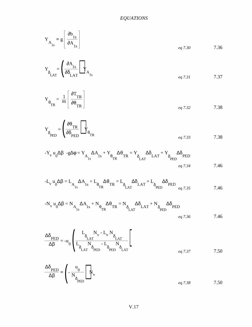
EQUATIONS
V.17
YA
1s
≈ g ∂b
1s
∂A1s eq 7.30 7.36
YδLAT
= ( ∂A1s
∂δLAT
) YA
1seq 7.31 7.37
YθTR
= 1m
∂TTR
∂θTR eq 7.32 7.38
YδPED
= ( ∂θTR
∂δPED
) YθTR
eq 7.33 7.38
-Yv u0∆β -g∆φ = Y
A1s
∆A1s
+ YθTR
∆θTR
= YδLAT
∆δLAT
+ YδPED
∆δPED
eq 7.34 7.46
-Lv u0∆β = L
A1s
∆A1s
+ LθTR
∆θTR
= LδLAT
∆δLAT
+ LδPED
∆δPED
eq 7.35 7.46
-Nv u0∆β = N
A1s
∆A1s
+ NθTR
∆θTR
= NδLAT
∆δLAT
+ NδPED
∆δPED
eq 7.36 7.46
∆δPED
∆β = -u
0 ( LδLAT
Nv - Lv NδLAT
LδLAT
NδPED
- LδPED
NδLAT
)eq 7.37 7.50
∆δPED
∆β≈ (-
u0
NδPED
) Nv
eq 7.38 7.50
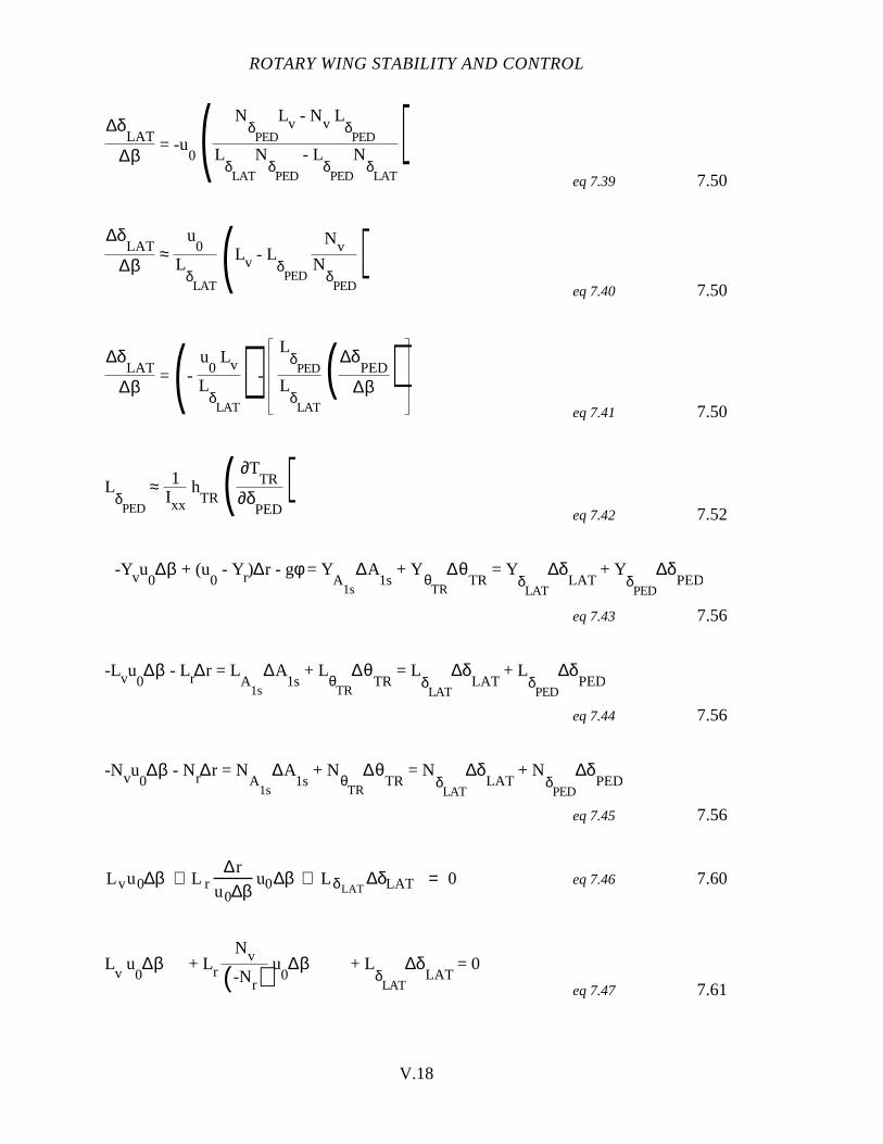
ROTARY WING STABILITY AND CONTROL
V.18
∆δLAT
∆β = -u
0 ( NδPED
Lv - Nv LδPED
LδLAT
NδPED
- LδPED
NδLAT
)eq 7.39 7.50
∆δLAT
∆β≈
u0
LδLAT
(Lv - LδPED
NvN
δPED
)eq 7.40 7.50
∆δLAT
∆β = (-
u0 Lv
LδLAT
) -
LδPED
LδLAT
(∆δPED
∆β )eq 7.41 7.50
LδPED
≈ 1Ixx
hTR ( ∂T
TR
∂δPED
)eq 7.42 7.52
-Yvu0∆β + (u
0 - Yr)∆r - gφ = Y
A1s
∆A1s
+ YθTR
∆θTR
= YδLAT
∆δLAT
+ YδPED
∆δPED
eq 7.43 7.56
-Lvu0∆β - Lr∆r = L
A1s
∆A1s
+ LθTR
∆θTR
= LδLAT
∆δLAT
+ LδPED
∆δPED
eq 7.44 7.56
-Nvu0∆β - Nr∆r = N
A1s
∆A1s
+ NθTR
∆θTR
= NδLAT
∆δLAT
+ NδPED
∆δPED
eq 7.45 7.56
L vu0∆β + L r∆r
u0∆βu0∆β + LδLAT
∆δLAT = 0 eq 7.46 7.60
Lv
u0∆β + Lr
Nv
(-Nr) u
0∆β + L
δLAT
∆δLAT
= 0
eq 7.47 7.61
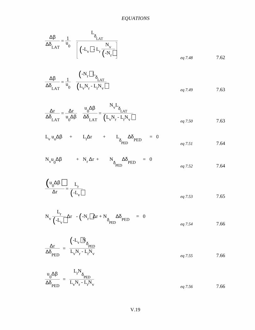
EQUATIONS
V.19
∆β∆δ
LAT
= 1u
0
LδLAT
(-Lv) - Lr
Nv
(-Nr)eq 7.48 7.62
∆β∆δ
LAT
= 1u
0
(-Nr) LδLAT
(LvNr - LrNv) eq 7.49 7.63
∆r∆δ
LAT
= ∆ru
0∆β
u0∆β
∆δLAT
=
NvLδLAT
(LvNr - LrNv) eq 7.50 7.63
Lv uo∆β + Lr∆r + LδPED
∆δPED
= 0eq 7.51 7.64
Nvu0∆β + Nr ∆r + N
δPED
∆δPED
= 0eq 7.52 7.64
(u0∆β)
∆r =
Lr
(-Lv) eq 7.53 7.65
Nv
Lr
(-Lv)∆r - (-Nr) ∆r + N
δPED
∆δPED
= 0
eq 7.54 7.66
∆r∆δ
PED
=
(-Lv)NδPED
LvNr - LrNv eq 7.55 7.66
u0∆β
∆δPED
=
LrNδPED
LvNr - LrNv eq 7.56 7.66
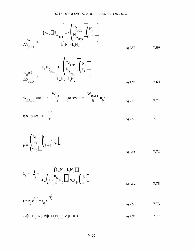
ROTARY WING STABILITY AND CONTROL
V.20
∆r∆δ
PED
=
(-Lv) NδPED
1 - ( LδPED
NδPED
)(NvLv
)LvNr - LrNv eq 7.57 7.69
u0∆β
∆δPED
=
Lr NδPED
1 - ( LδPED
NδPED
)(NrLr
)LvNr - LrNv eq 7.58 7.69
WBALL
sinφ =W
BALLg u
0ω cosφ =
WBALLg u
0r
eq 7.59 7.71
φ ≈ sinφ =u
0 r
g eq 7.60 7.71
p = (∆L
Ixx )(-Lp)
(1 - e-
tτR)
eq 7.61 7.72
λs = - 1τs =
-(LvNr - LrNv)-Lv(1 -
u0
g Np) - NvLp ( u0
g )eq 7.62 7.75
r = r0 e
λst = r0 e
-t
τs
eq 7.63 7.75
∆ ˙ψ + −N r( )∆ψ + Nvu0( )∆ψ = 0 eq 7.64 7.77

EQUATIONS
V.21
∆φ
-∆β =
(1)2 + (2)
2 ( Lvu0 )
ωn4 + Lp
2ωn
2
eq 7.65 7.79
∠ ∆φ
(-∆β) = tan-1
-(-Lp)-ωn
eq 7.66 7.80
∠ ∆φ
(-∆β) = tan-1
-(-Lp)
ωn - 2ζ
- 1 + ζ(-Lp)
ωn eq 7.67 7.81
ζ = 12ωn
-Nr - Yv -( gu
0 - Np) Lvu
0
(ωn2 + Lp
2)eq 7.68 7.81
ζ = (- 12)( -gLv
Lp
3)eq 7.69 7.89
∆t = t2 -t
1 = t
3 - t
2 eq 7.70 7.110
A1 = p
2 - p
1 eq 7.71 7.110
A2 = p
3 - p
2 eq 7.72 7.111

ROTARY WING STABILITY AND CONTROL
V.22
τ = ∆t
lne(A1
A2)
eq 7.73 7.111
τ = ( t
4 - t
2)ln
e(∆pA
∆pB)
eq 7.74 7.111
ωd = 2π
P eq 7.75 7.113
ωn = ω
d
1 - ζ2 =
2πP
1 - ζ2
eq 7.76 7.113
CHAPTER 8
u. - Xu∆u - Xq∆q + g∆θ = X
B1s
∆B1s
= XδLONG
∆δLONG
eq 8.1 8.4
q. - Mu∆u - Mq∆q = M
B1s
∆B1s
= MδLONG
∆δLONG
eq 8.2 8.5
w. - Zw∆w = Z
θC
∆θC
= ZδC
∆δC
eq 8.3 8.5
v. - Yv∆v - Yp∆p = Y
A1s
∆A1s
+ YθTR
∆θTR
= YδLAT
∆δLAT
+ YδPED
∆δPED
eq 8.4 8.6
p. - Lv∆v - Lp∆p = L
A1s
∆A1s
+ LθTR
∆θTR
= LδLAT
∆δLAT
+ LδPED
∆δPED
eq 8.5 8.6
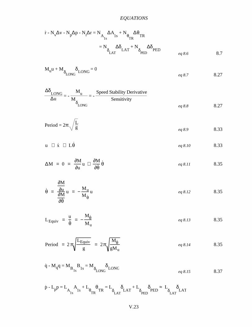
EQUATIONS
V.23
r. - Nv∆v - Np∆p - Nr∆r = N
A1s
∆A1s
+ NθTR
∆θTR
= NδLAT
∆δLAT
+ NδPED
∆δPED
eq 8.6 8.7
Muu + MδLONG
δLONG
= 0eq 8.7 8.27
∆δLONG∆u
= - Mu
MδLONG
= - Speed Stability Derivative
Sensitivityeq 8.8 8.27
Period = 2π Lg eq 8.9 8.33
u ≅ x ≅ L θ eq 8.10 8.33
∆M = 0 =∂M
∂uu +
∂M
∂θ θ eq 8.11 8.35
θ =
∂M
∂u∂M∂θ
u = −M u
M θ u eq 8.12 8.35
L Equiv =u
θ = −
Mθ M u
eq 8.13 8.35
Period = 2πLEquiv
g= 2π
Mθ gMu
eq 8.14 8.35
.q - Mqq = M
B1sB
1s = M
δLONGδ
LONGeq 8.15 8.37
p. - Lpp = L
A1s
A1s
+ LθTR
θTR
= LδLAT
δLAT
+ LδPED
δPED
≈ LδLAT
δLAT
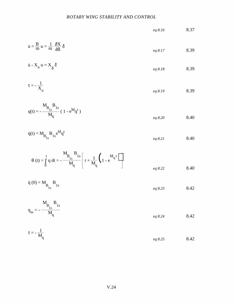
ROTARY WING STABILITY AND CONTROL
V.24
eq 8.16 8.37
u. = Bm u = 1
m∂X∂δ
δeq 8.17 8.39
u. - Xu u = X
δδ
eq 8.18 8.39
τ = - 1Xu eq 8.19 8.39
q(t) = - Mq
MB1s
B1s
( 1 - eMqt )eq 8.20 8.40
.q(t) = M
B1sB
1seMqt
eq 8.21 8.40
θ (t) = ∫0
t q dt = -
MB
1s
B1s
Mqt + 1
Mq
(1 - eMq t)
eq 8.22 8.40
q. (0) = M
B1s
B1s
eq 8.23 8.42
qss = -
MB
1s
B1s
Mq eq 8.24 8.42
τ = - 1Mq eq 8.25 8.42
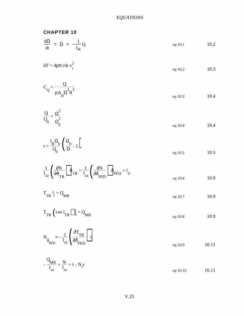
EQUATIONS
V.25
CHAPTER 10
dΩdt
= Ω = −1
I RQ eq 10.1 10.2
dT = 4ρπ rdr vi2
eq 10.2 10.3
CQ
= Q
ρAD
Ω2R
3
eq 10.3 10.4
0
= Ω2
Ω0
2
eq 10.4 10.4
t = IR
Ω0
Q0
(Ω0
Ω - 1)eq 10.5 10.5
1Izz( ∂N
∂θTR
) θTR
= 1Izz( ∂N
∂δPED
) δPED
= r.0
eq 10.6 10.9
TTR
lt = Q
MR eq 10.7 10.9
TTR (cos i
TR) lt = Q
MR eq 10.8 10.9
NδPED
≈ - 1Izz( ∂T
TR
∂δPED
) lt
eq 10.9 10.11
-Q
MRIzz
= NIzz
= r. - Nrr
eq 10.10 10.11
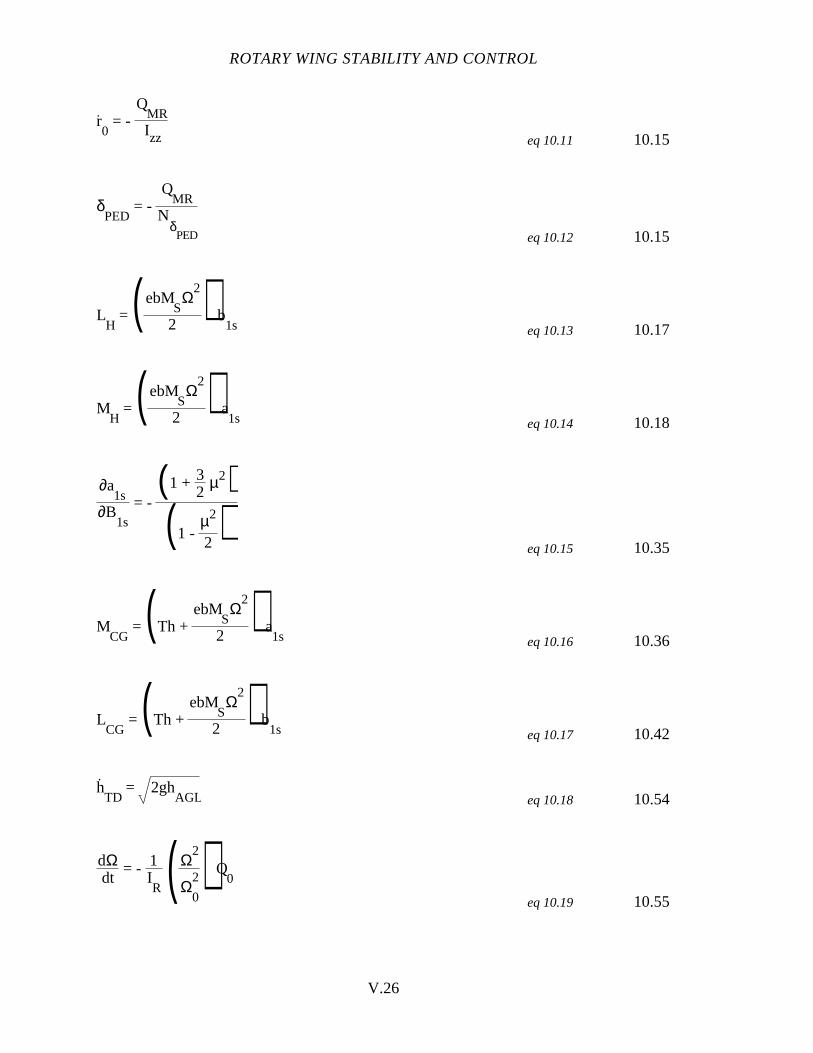
ROTARY WING STABILITY AND CONTROL
V.26
r.0 = -
QMRIzz eq 10.11 10.15
δPED
= - Q
MRN
δPED eq 10.12 10.15
LH
= ( ebMSΩ
2
2) b
1s eq 10.13 10.17
MH
= ( ebMSΩ
2
2) a
1s eq 10.14 10.18
∂a1s
∂B1s
= - (1 + 3
2µ2)
(1 - µ2
2 )eq 10.15 10.35
MCG
= (Th + ebM
SΩ
2
2) a
1s eq 10.16 10.36
LCG
= (Th + ebM
SΩ
2
2) b
1s eq 10.17 10.42
h.TD
= 2ghAGL eq 10.18 10.54
dΩdt
= - 1IR (Ω
2
Ω0
2) Q0
eq 10.19 10.55
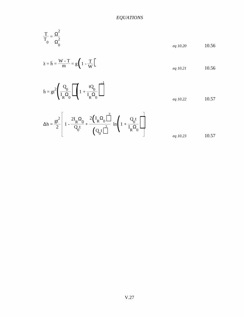
EQUATIONS
V.27
TT
0
= Ω2
Ω0
2
eq 10.20 10.56
z.. = h
.. =
W - Tm = g(1 - T
W)eq 10.21 10.56
h. = gt
2( Q0
IR
Ω0) (1 +
tQ0
IR
Ω0)
-1
eq 10.22 10.57
∆h = gt
2
21 -
2IR
Ω0
Q0t
+ 2( I
RΩ
0)2
(Q0t)2
ln(1 + Q
0t
IR
Ω0)
eq 10.23 10.57
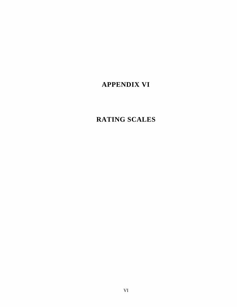
VI
APPENDIX VI
RATING SCALES
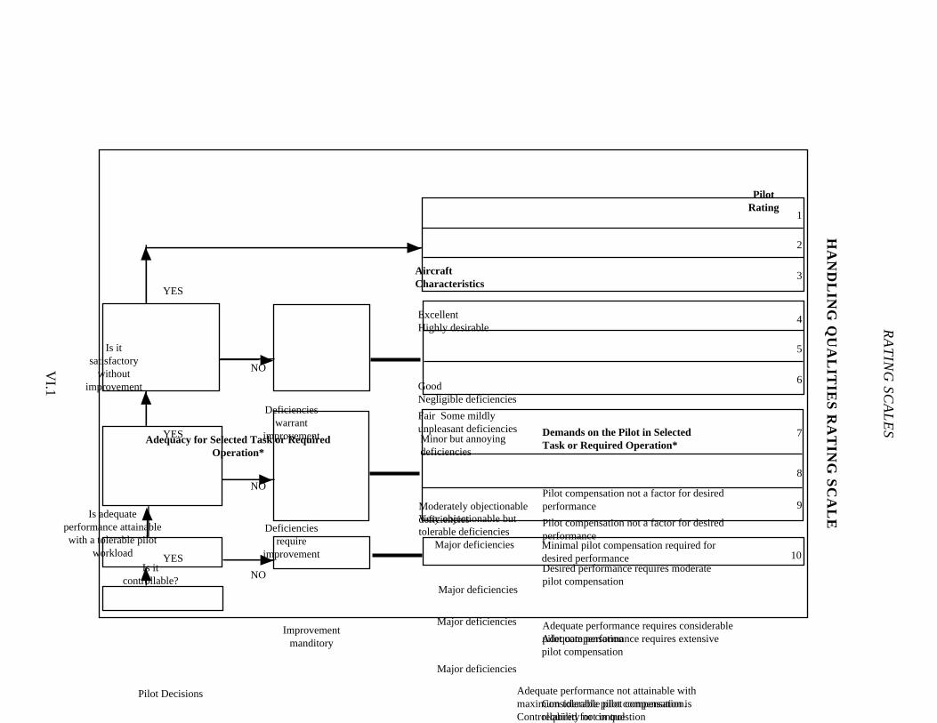
RA
TIN
G S
CA
LE
S
VI.1
HA
ND
LIN
G Q
UA
LIT
IES
RA
TIN
G S
CA
LE
Adequacy for Selected Task or RequiredOperation*
AircraftCharacteristics
Demands on the Pilot in SelectedTask or Required Operation*
PilotRating
Pilot Decisions
YES
Is adequateperformance attainablewith a tolerable pilot
workload
Deficienciesrequire
improvement
Is itsatisfactory
withoutimprovement
YES
YES
NO
NO
Deficiencieswarrant
improvement
Improvementmanditory
Is itcontrollable?
10
Major deficiencies
Adequate performance not attainable withmaximum tolerable pilot compensation.Controllability not in question
Major deficiencies
7
Major deficiencies
9
Major deficiencies
Considerable pilot compensation isrequired for control
8
Minor but annoyingdeficiencies
Desired performance requires moderatepilot compensation
4
Moderately objectionabledeficiencies
Adequate performance requires considerablepilot compensation
5
Very objectionable buttolerable deficiencies
Adequate performance requires extensivepilot compensation
6
Fair Some mildlyunpleasant deficiencies
Minimal pilot compensation required fordesired performance
3
GoodNegligible deficiencies
Pilot compensation not a factor for desiredperformance
2
ExcellentHighly desirable
Pilot compensation not a factor for desiredperformance
1
NO
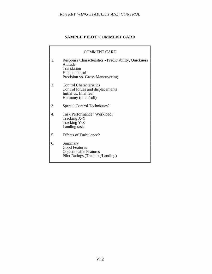
ROTARY WING STABILITY AND CONTROL
VI.2
SAMPLE PILOT COMMENT CARD
COMMENT CARD
1. Response Characteristics - Predictability, QuicknessAttitudeTranslationHeight controlPrecision vs. Gross Maneuvering
2. Control CharacteristicsControl forces and displacementsInitial vs. final feelHarmony (pitch/roll)
3. Special Control Techniques?
4. Task Performance? Workload?Tracking X-YTracking Y-ZLanding task
5. Effects of Turbulence?
6. SummaryGood FeaturesObjectionable FeaturesPilot Ratings (Tracking/Landing)
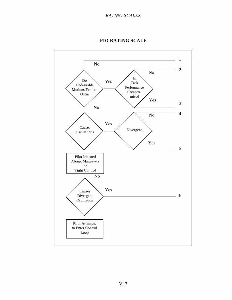
RATING SCALES
VI.3
PIO RATING SCALE
Pilot InitiatedAbrupt Maneuvers
orTight Control
Yes
Pilot Attemptsto Enter Control
Loop
CausesDivergentOscillation
Yes
No
6
5
CausesOscillations
Divergent
IsTask
PerformanceCompro-
mised
DoUndesirable
Motions Tend toOccur
Yes
No 4
3Yes
No
No
No
1
2
Yes
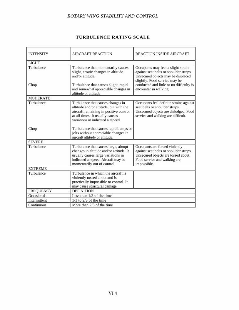
ROTARY WING STABILITY AND CONTROL
VI.4
TURBULENCE RATING SCALE
INTENSITY AIRCRAFT REACTION REACTION INSIDE AIRCRAFT
LIGHTTurbulence
Chop
Turbulence that momentarily causesslight, erratic changes in altitudeand/or attitude.
Turbulence that causes slight, rapidand somewhat appreciable changes inaltitude or attitude
Occupants may feel a slight strainagainst seat belts or shoulder straps.Unsecured objects may be displacedslightly. Food service may beconducted and little or no difficulty isencounter in walking
MODERATETurbulence
Chop
Turbulence that causes changes inaltitude and/or attitude, but with theaircraft remaining in positive controlat all times. It usually causesvariations in indicated airspeed.
Turbulence that causes rapid bumps orjolts without appreciable changes inaircraft altitude or attitude.
Occupants feel definite strains againstseat belts or shoulder straps.Unsecured objects are dislodged. Foodservice and walking are difficult.
SEVERETurbulence Turbulence that causes large, abrupt
changes in altitude and/or attitude. Itusually causes large variations inindicated airspeed. Aircraft may bemomentarily out of control
Occupants are forced violentlyagainst seat belts or shoulder straps.Unsecured objects are tossed about.Food service and walking areimpossible.
EXTREMETurbulence Turbulence in which the aircraft is
violently tossed about and ispractically impossible to control. Itmay cause structural damage.
FREQUENCY DEFINITIONOccasional Less than 1/3 of the timeIntermittent 1/3 to 2/3 of the timeContinuous More than 2/3 of the time

RATING SCALES
VI.5
VIBRATION RATING SCALE
Degree of Vibration Description Pilot Rating
No Vibration 0Slight Not apparent to experienced aircrew fully occupied
by their tasks, but noticeable if their attention isdirected to it or if not otherwise occupied.
123
Moderate Experienced aircrew are aware of the vibration but itdoes not affect their work, at least over a shortperiod.
456
Severe Vibration is immediately apparent to experiencedaircrew even when fully occupied. Performance ofprimary task is affected or tasks can be done onlywith difficulty.
789
Intolerable Sole preoccupation of aircrew is to reduce vibration. 10
Based on the Subjective Vibration Assessment Scale developed by the AeroplaneandArmament Experimental Establishment, Boscombe Down, England.
VII
APPENDIX VII
MILITARY SPECIFICATION, HELICOPTERFLYING AND GROUND HANDLING
QUALITIES; GENERAL REQUIREMENT FOR,MIL-H-8501A
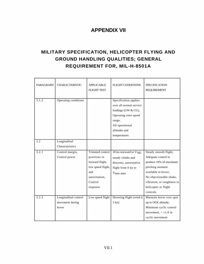
VII.1
APPENDIX VII
MILITARY SPECIFICATION, HELICOPTER FLYING AND
GROUND HANDLING QUALITIES; GENERAL
REQUIREMENT FOR, MIL-H-8501A
PARAGRAPH CHARACTERISTIC APPLICABLE
FLIGHT TEST
FLIGHT CONDITIONS SPECIFICATION
REQUIREMENT
3.1.2 Operating conditions Specification applies
over all normal service
loadings (GW & CG),
Operating rotor speed
range,
All operational
altitudes and
temperatures
3.2 Longitudinal
Characteristics
3.2.1 Control margin,
Control power
Trimmed control
positions in
forward flight,
low speed flight,
and
autorotation,
Control
response
30 kn rearward to VNE,
steady climbs and
descents, autorotative
flight from 0 kn to
Vmax auto
Steady smooth flight;
Adequate control to
produce 10% of maximum
pitching moment
available in hover;
No objectionable shake,
vibration, or roughness in
helicopter or flight
controls
3.2.2 Longitudinal control
movement during
hover
Low speed flight Hovering flight (wind ≤
3 kn)
Maintain hover over spot
up to OGE altitude;
Minimum cyclic control
movement, < ±1.0 in
cyclic movement
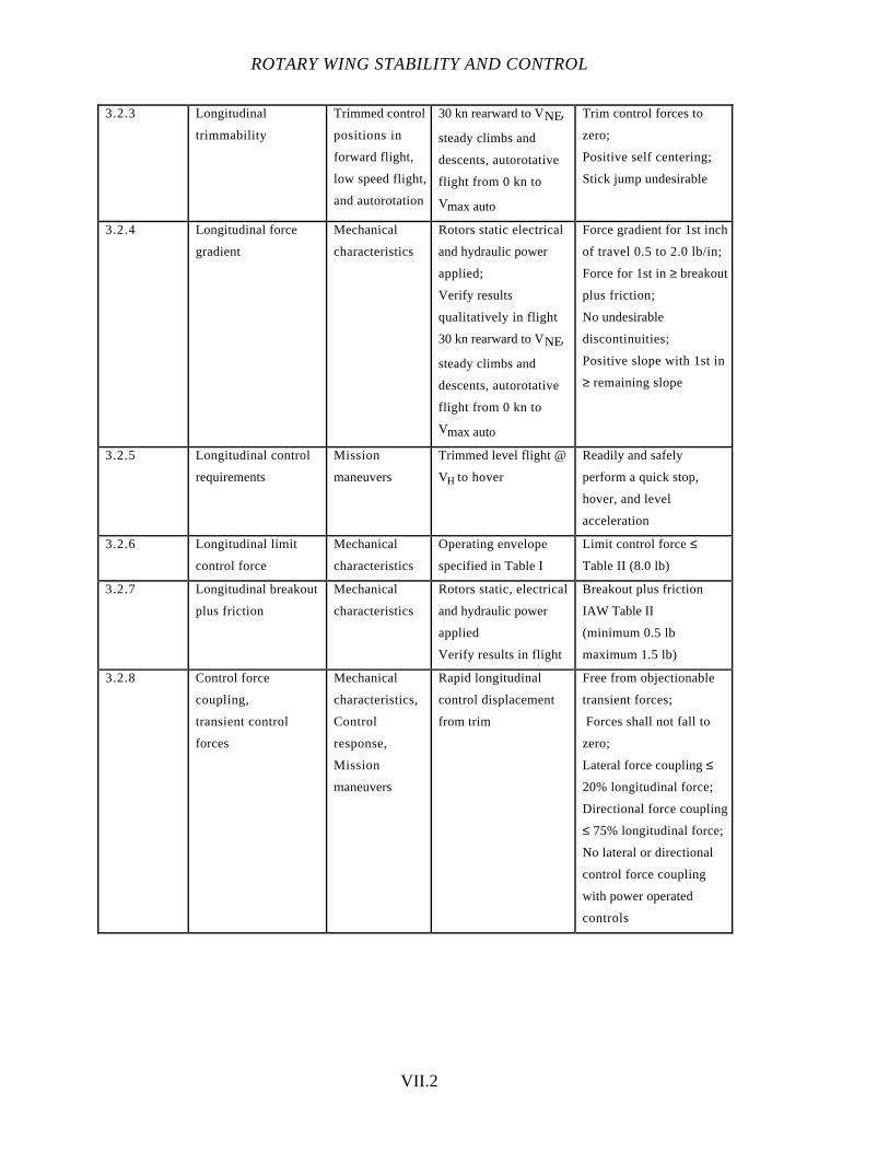
ROTARY WING STABILITY AND CONTROL
VII.2
3.2.3 Longitudinal
trimmability
Trimmed control
positions in
forward flight,
low speed flight,
and autorotation
30 kn rearward to VNE,
steady climbs and
descents, autorotative
flight from 0 kn to
Vmax auto
Trim control forces to
zero;
Positive self centering;
Stick jump undesirable
3.2.4 Longitudinal force
gradient
Mechanical
characteristics
Rotors static electrical
and hydraulic power
applied;
Verify results
qualitatively in flight
30 kn rearward to VNE,
steady climbs and
descents, autorotative
flight from 0 kn to
Vmax auto
Force gradient for 1st inch
of travel 0.5 to 2.0 lb/in;
Force for 1st in ≥ breakout
plus friction;
No undesirable
discontinuities;
Positive slope with 1st in
≥ remaining slope
3.2.5 Longitudinal control
requirements
Mission
maneuvers
Trimmed level flight @
VH to hover
Readily and safely
perform a quick stop,
hover, and level
acceleration
3.2.6 Longitudinal limit
control force
Mechanical
characteristics
Operating envelope
specified in Table I
Limit control force ≤
Table II (8.0 lb)
3.2.7 Longitudinal breakout
plus friction
Mechanical
characteristics
Rotors static, electrical
and hydraulic power
applied
Verify results in flight
Breakout plus friction
IAW Table II
(minimum 0.5 lb
maximum 1.5 lb)
3.2.8 Control force
coupling,
transient control
forces
Mechanical
characteristics,
Control
response,
Mission
maneuvers
Rapid longitudinal
control displacement
from trim
Free from objectionable
transient forces;
Forces shall not fall to
zero;
Lateral force coupling ≤
20% longitudinal force;
Directional force coupling
≤ 75% longitudinal force;
No lateral or directional
control force coupling
with power operated
controls
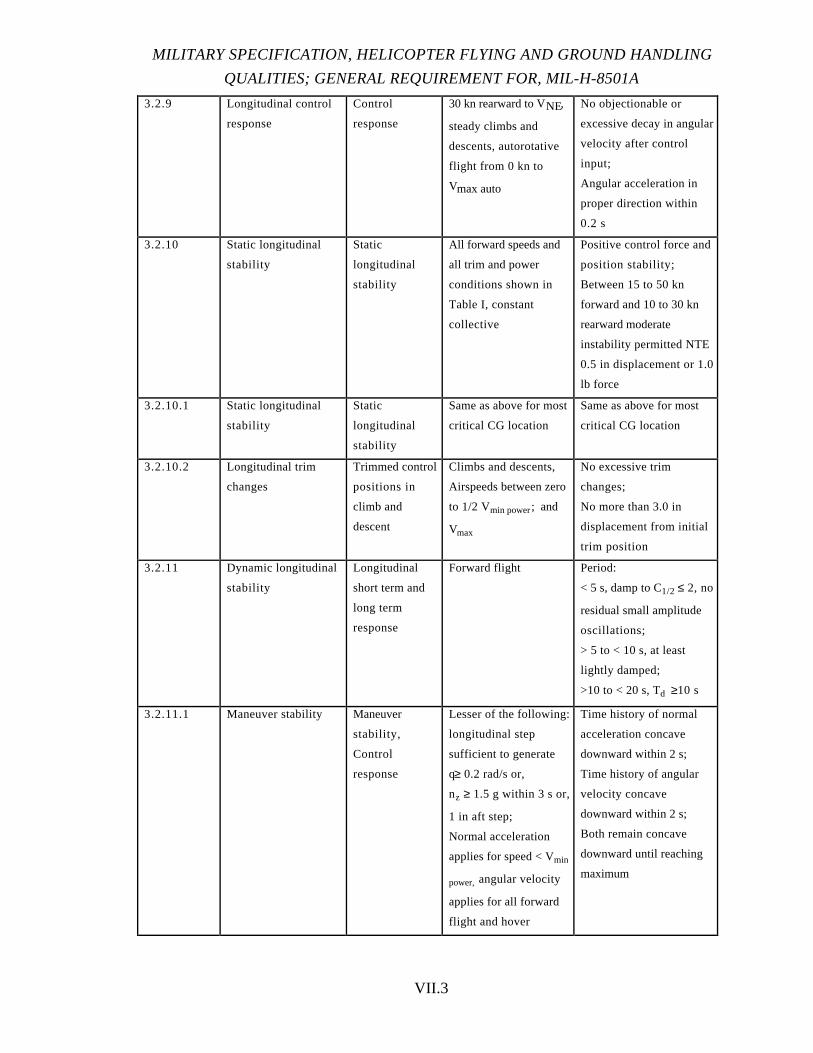
MILITARY SPECIFICATION, HELICOPTER FLYING AND GROUND HANDLING
QUALITIES; GENERAL REQUIREMENT FOR, MIL-H-8501A
VII.3
3.2.9 Longitudinal control
response
Control
response
30 kn rearward to VNE,
steady climbs and
descents, autorotative
flight from 0 kn to
Vmax auto
No objectionable or
excessive decay in angular
velocity after control
input;
Angular acceleration in
proper direction within
0.2 s
3.2.10 Static longitudinal
stability
Static
longitudinal
stability
All forward speeds and
all trim and power
conditions shown in
Table I, constant
collective
Positive control force and
position stability;
Between 15 to 50 kn
forward and 10 to 30 kn
rearward moderate
instability permitted NTE
0.5 in displacement or 1.0
lb force
3.2.10.1 Static longitudinal
stability
Static
longitudinal
stability
Same as above for most
critical CG location
Same as above for most
critical CG location
3.2.10.2 Longitudinal trim
changes
Trimmed control
positions in
climb and
descent
Climbs and descents,
Airspeeds between zero
to 1/2 Vmin power; and
Vmax
No excessive trim
changes;
No more than 3.0 in
displacement from initial
trim position
3.2.11 Dynamic longitudinal
stability
Longitudinal
short term and
long term
response
Forward flight Period:
< 5 s, damp to C1/2 ≤ 2, no
residual small amplitude
oscillations;
> 5 to < 10 s, at least
lightly damped;
>10 to < 20 s, Td ≥10 s
3.2.11.1 Maneuver stability Maneuver
stability,
Control
response
Lesser of the following:
longitudinal step
sufficient to generate
q≥ 0.2 rad/s or,
nz ≥ 1.5 g within 3 s or,
1 in aft step;
Normal acceleration
applies for speed < Vmin
power, angular velocity
applies for all forward
flight and hover
Time history of normal
acceleration concave
downward within 2 s;
Time history of angular
velocity concave
downward within 2 s;
Both remain concave
downward until reaching
maximum

ROTARY WING STABILITY AND CONTROL
VII.4
3.2.11.2 Gust response Cyclic pulse Hover and forward
flight;
Control displacement
IAW 3.2.11.1 for 0.5 s
pulse
Normal acceleration shall
not exceed ± 0.25 g
within 10 s after aft
longitudinal pulse
3.2.12 Maneuver stability Maneuver
stability,
Control
response
Hover and forward
flight control
displacement IAW
3.2.11.1
Normal acceleration
increase with time
following rapid rearward
displacement of
longitudinal control until
maximum acceleration is
reached
3.2.13 Longitudinal control
power
Control
response
Hover at maximum GW One in step input produce
angular displacement after
1.0 s ≥
45
W + 10003deg;
Maximum step input
produce angular
displacement after 1.0 s ≥
180
W + 10003deg
3.2.14 Pitch rate damping Control
response
Hover Pitch rate damping ≥
8(Iy)0.7 ft-lb/rad/s
3.3 Directional and Lateral
Characteristics
3.3.1 Directional control
power
Ground handling Ground taxi (wheel
gear);
Water taxi (float gear);
Wind 35 kn
Straight path without use
of brakes;
360 turn pivoting on one
wheel
3.3.2 Sideward flight Low speed flight Hover to 35 kn left and
right
Steady flight;
Controls and helicopter
free from objectionable
shake, vibration, or
roughness
3.3.3 Lateral-directional
control movement
during hover
Low speed flight Hover (wind ≤ 3 kn) Maintain hover over spot
up to OGE altitude;
Minimum cyclic
movement < ± 1 in lateral
cyclic;
Pedal movement < ± 1.0
in
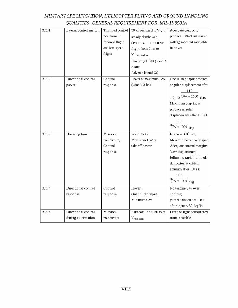
MILITARY SPECIFICATION, HELICOPTER FLYING AND GROUND HANDLING
QUALITIES; GENERAL REQUIREMENT FOR, MIL-H-8501A
VII.5
3.3.4 Lateral control margin Trimmed control
positions in
forward flight
and low speed
flight
30 kn rearward to VNE,
steady climbs and
descents, autorotative
flight from 0 kn to
Vmax auto;
Hovering flight (wind ≤
3 kn);
Adverse lateral CG
Adequate control to
produce 10% of maximum
rolling moment available
in hover
3.3.5 Directional control
power
Control
response
Hover at maximum GW
(wind ≤ 3 kn)
One in step input produce
angular displacement after
1.0 s ≥
110
W + 10003deg;
Maximum step input
produce angular
displacement after 1.0 s ≥
330
W + 10003deg
3.3.6 Hovering turn Mission
maneuvers,
Control
response
Wind 35 kn;
Maximum GW or
takeoff power
Execute 360 turn;
Maintain hover over spot;
Adequate control margin;
Yaw displacement
following rapid, full pedal
deflection at critical
azimuth after 1.0 s ≥
110
W + 10003 deg
3.3.7 Directional control
response
Control
response
Hover,
One in step input,
Minimum GW
No tendency to over
control;
yaw displacement 1.0 s
after input ≤ 50 deg/in
3.3.8 Directional control
during autorotation
Mission
maneuvers
Autorotation 0 kn to to
Vmax auto
Left and right coordinated
turns possible

ROTARY WING STABILITY AND CONTROL
VII.6
3.3.9 Static lateral-
directional stability
Steady heading
sideslips
50 kn to VNE,
up to full pedal
displacement
Positive control fixed
directional stability and
effective dihedral;
Stable gradient of control
displacement versus
sideslip;
Linear gradient between
sideslip angles of ± 15˚;
10% longitudinal and
lateral control
effectiveness remaining
3.3.9.1 Cyclic only turns Cyclic only
turns
50 kn to VNE;
Lateral control input
resulting in a bank of
30˚ in 6 s
Cyclic turns possible;
No reversal of rolling
velocity after small step
displacement
3.3.9.2 Adverse yaw Cyclic only
turns
50 kn to VNE No objectionable adverse
yaw
3.3.10 Lateral-directional
trimmability
Trimmed control
positions in
forward flight,
low speed flight,
and autorotation
30 kn rearward to VNE,
steady climbs and
descents, autorotative
flight from 0 kn to
Vmax auto;
Hovering flight (wind ≤
3 kn)
Trim control forces to
zero;
Positive self-centering;
Stick jump undesirable
3.3.11 Lateral-directional
force gradient
Mechanical
characteristics
Rotors static, electrical
and hydraulic power
applied;
Verify results in flight
30 kn rearward to VNE,
steady climbs and
descents, autorotative
flight from 0 kn to
Vmax auto;
Hovering flight (wind ≤
3 kn)
Lateral force gradient 1st
in of travel 0.5 to 2.0
lb/in;
Force for 1st in ≥ breakout
plus friction;
Positive slope with 1st in
≥ remaining slope;
Directional limit control
force 15 lb;
Linear directional force
gradient;
No undesirable lateral or
directional gradient
discontinuities
3.3.12 Lateral-directional
limit control force
Mechanical
characteristics
Operating envelope
specified in Table I
Lateral cyclic limit force ≤
Table II (7.0 lb);
Directional limit force ≤
Table II (15.0 lb)
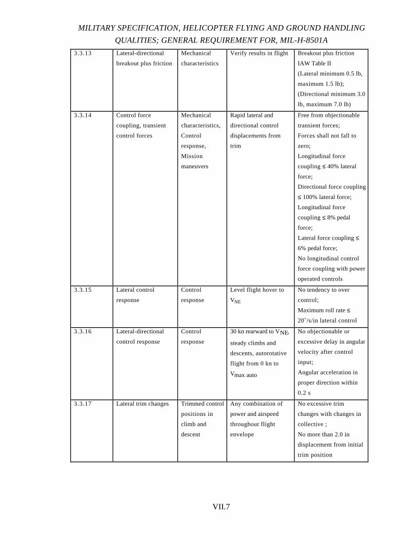
MILITARY SPECIFICATION, HELICOPTER FLYING AND GROUND HANDLING
QUALITIES; GENERAL REQUIREMENT FOR, MIL-H-8501A
VII.7
3.3.13 Lateral-directional
breakout plus friction
Mechanical
characteristics
Verify results in flight Breakout plus friction
IAW Table II
(Lateral minimum 0.5 lb,
maximum 1.5 lb);
(Directional minimum 3.0
lb, maximum 7.0 lb)
3.3.14 Control force
coupling, transient
control forces
Mechanical
characteristics,
Control
response,
Mission
maneuvers
Rapid lateral and
directional control
displacements from
trim
Free from objectionable
transient forces;
Forces shall not fall to
zero;
Longitudinal force
coupling≤ 40% lateral
force;
Directional force coupling
≤ 100% lateral force;
Longitudinal force
coupling≤ 8% pedal
force;
Lateral force coupling ≤
6% pedal force;
No longitudinal control
force coupling with power
operated controls
3.3.15 Lateral control
response
Control
response
Level flight hover to
VNE
No tendency to over
control;
Maximum roll rate ≤
20˚/s/in lateral control
3.3.16 Lateral-directional
control response
Control
response
30 kn rearward to VNE,
steady climbs and
descents, autorotative
flight from 0 kn to
Vmax auto
No objectionable or
excessive delay in angular
velocity after control
input;
Angular acceleration in
proper direction within
0.2 s
3.3.17 Lateral trim changes Trimmed control
positions in
climb and
descent
Any combination of
power and airspeed
throughout flight
envelope
No excessive trim
changes with changes in
collective ;
No more than 2.0 in
displacement from initial
trim position
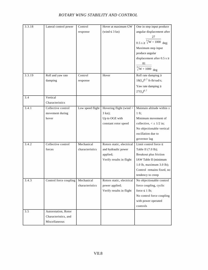
ROTARY WING STABILITY AND CONTROL
VII.8
3.3.18 Lateral control power Control
response
Hover at maximum GW
(wind ≤ 3 kn)
One in step input produce
angular displacement after
0.5 s ≥
27
W + 10003deg;
Maximum step input
produce angular
displacement after 0.5 s ≥
81
W + 10003
deg
3.3.19 Roll and yaw rate
damping
Control
response
Hover Roll rate damping ≥
18(Ix)0.7 ft-lb/rad/s;
Yaw rate damping ≥
27(Iz)0.7
3.4 Vertical
Characteristics
3.4.1 Collective control
movement during
hover
Low speed flight Hovering flight (wind <
3 kn);
Up to OGE with
constant rotor speed
Maintain altitude within ±
1 ft;
Minimum movement of
collective, < ± 1/2 in;
No objectionable vertical
oscillation due to
governor lag
3.4.2 Collective control
forces
Mechanical
characteristics
Rotors static, electrical
and hydraulic power
applied;
Verify results in flight
Limit control force ≤
Table II (7.0 lb);
Breakout plus friction
IAW Table II (minimum
1.0 lb, maximum 3.0 lb);
Control remains fixed, no
tendency to creep
3.4.3 Control force coupling Mechanical
characteristics
Rotors static, electrical
power applied;
Verify results in flight
No objectionable control
force coupling, cyclic
force≤ 1 lb;
No control force coupling
with power operated
controls
3.5 Autorotation, Rotor
Characteristics, and
Miscellaneous
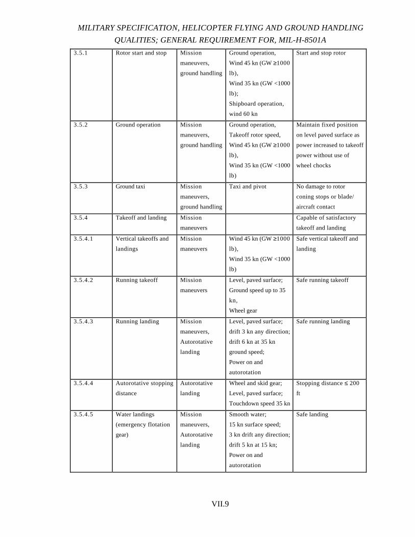
MILITARY SPECIFICATION, HELICOPTER FLYING AND GROUND HANDLING
QUALITIES; GENERAL REQUIREMENT FOR, MIL-H-8501A
VII.9
3.5.1 Rotor start and stop Mission
maneuvers,
ground handling
Ground operation,
Wind 45 kn (GW ≥1000
lb),
Wind 35 kn (GW <1000
lb);
Shipboard operation,
wind 60 kn
Start and stop rotor
3.5.2 Ground operation Mission
maneuvers,
ground handling
Ground operation,
Takeoff rotor speed,
Wind 45 kn (GW ≥1000
lb),
Wind 35 kn (GW <1000
lb)
Maintain fixed position
on level paved surface as
power increased to takeoff
power without use of
wheel chocks
3.5.3 Ground taxi Mission
maneuvers,
ground handling
Taxi and pivot No damage to rotor
coning stops or blade/
aircraft contact
3.5.4 Takeoff and landing Mission
maneuvers
Capable of satisfactory
takeoff and landing
3.5.4.1 Vertical takeoffs and
landings
Mission
maneuvers
Wind 45 kn (GW ≥1000
lb),
Wind 35 kn (GW <1000
lb)
Safe vertical takeoff and
landing
3.5.4.2 Running takeoff Mission
maneuvers
Level, paved surface;
Ground speed up to 35
kn,
Wheel gear
Safe running takeoff
3.5.4.3 Running landing Mission
maneuvers,
Autorotative
landing
Level, paved surface;
drift 3 kn any direction;
drift 6 kn at 35 kn
ground speed;
Power on and
autorotation
Safe running landing
3.5.4.4 Autorotative stopping
distance
Autorotative
landing
Wheel and skid gear;
Level, paved surface;
Touchdown speed 35 kn
Stopping distance ≤ 200
ft
3.5.4.5 Water landings
(emergency flotation
gear)
Mission
maneuvers,
Autorotative
landing
Smooth water;
15 kn surface speed;
3 kn drift any direction;
drift 5 kn at 15 kn;
Power on and
autorotation
Safe landing
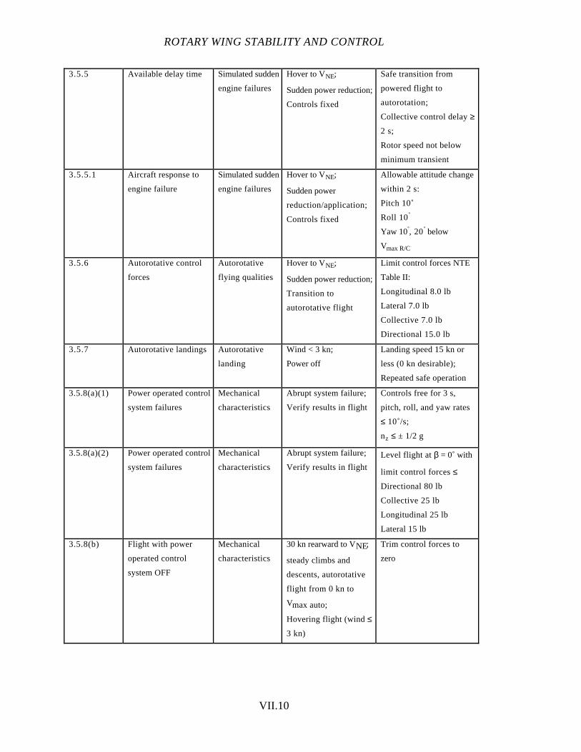
ROTARY WING STABILITY AND CONTROL
VII.10
3.5.5 Available delay time Simulated sudden
engine failures
Hover to VNE;
Sudden power reduction;
Controls fixed
Safe transition from
powered flight to
autorotation;
Collective control delay ≥
2 s;
Rotor speed not below
minimum transient
3.5.5.1 Aircraft response to
engine failure
Simulated sudden
engine failures
Hover to VNE;
Sudden power
reduction/application;
Controls fixed
Allowable attitude change
within 2 s:
Pitch 10˚
Roll 10
Yaw 10, 20 below
Vmax R/C
3.5.6 Autorotative control
forces
Autorotative
flying qualities
Hover to VNE;
Sudden power reduction;
Transition to
autorotative flight
Limit control forces NTE
Table II:
Longitudinal 8.0 lb
Lateral 7.0 lb
Collective 7.0 lb
Directional 15.0 lb
3.5.7 Autorotative landings Autorotative
landing
Wind < 3 kn;
Power off
Landing speed 15 kn or
less (0 kn desirable);
Repeated safe operation
3.5.8(a)(1) Power operated control
system failures
Mechanical
characteristics
Abrupt system failure;
Verify results in flight
Controls free for 3 s,
pitch, roll, and yaw rates
≤ 10˚/s;
nz ≤ ± 1/2 g
3.5.8(a)(2) Power operated control
system failures
Mechanical
characteristics
Abrupt system failure;
Verify results in flight
Level flight at β = 0˚ with
limit control forces ≤
Directional 80 lb
Collective 25 lb
Longitudinal 25 lb
Lateral 15 lb
3.5.8(b) Flight with power
operated control
system OFF
Mechanical
characteristics
30 kn rearward to VNE;
steady climbs and
descents, autorotative
flight from 0 kn to
Vmax auto;
Hovering flight (wind ≤
3 kn)
Trim control forces to
zero
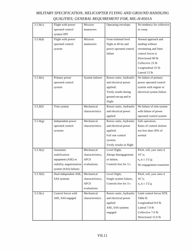
MILITARY SPECIFICATION, HELICOPTER FLYING AND GROUND HANDLING
QUALITIES; GENERAL REQUIREMENT FOR, MIL-H-8501A
VII.11
3.5.8(c) Flight with power
operated control
system OFF
Mission
maneuvers
Operating envelope No tendency for collective
to creep
3.5.8(d) Flight with power
operated control
system
Mission
maneuvers
From trimmed level
flight at 40 kn and
power operated control
failure
Normal approach and
landing without
retrimming and limit
control forces ≤
Directional 80 lb
Collective 25 lb
Longitudinal 25 lb
Lateral 15 lb
3.5.8(e) Primary power
operated control
system
System failures Rotors static, hydraulic
and electrical power
applied;
Verify results during
ground run-up and in
flight
No failure of primary
power operated control
system with engine or
electrical system failure
3.5.8(f) Trim system Mechanical
characteristics
Rotors static, hydraulic
and electrical power
applied
No failure of trim system
with failure of power
operated control system
3.5.8(g) Independent power
operated control
systems
Mechanical
characteristics
Rotors static, hydraulic
and electrical power
applied;
Fail one control
system;
Verify results in flight
Safe operation;
Rates of control motion
not less than 50% of
normal
3.5.9(a) Automatic
stabilization
equipment (ASE) or
stability augmentation
system (SAS) failures
Mechanical
characteristics,
AFCS
evaluations
Level flight,
Abrupt disengagement
or failure,
Controls free for 3 s
Pitch, roll, yaw rates ≤
10˚/s;
nz ≤ ± 1/2 g;
No engagement transients
3.5.9(b) Dual-independent ASE,
SAS systems
Mechanical
characteristics,
AFCS
evaluations
Level flight,
Single system failure,
Controls free for 3 s
Pitch, roll, yaw rates ≤
10˚/s;
nz ≤ ± 1/2 g
3.5.9(c) Control forces with
ASE, SAS engaged
Mechanical
characteristics
Rotors static, hydraulic
and electrical power
applied
ASE, SAS systems
engaged
Limit control forces NTE
Table II:
Longitudinal 8.0 lb
Lateral 7.0 lb
Collective 7.0 lb
Directional 15.0 lb
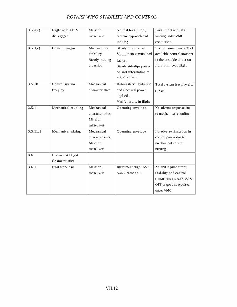
ROTARY WING STABILITY AND CONTROL
VII.12
3.5.9(d) Flight with AFCS
disengaged
Mission
maneuvers
Normal level flight,
Normal approach and
landing
Level flight and safe
landing under VMC
conditions
3.5.9(e) Control margin Maneuvering
stability,
Steady heading
sideslips
Steady level turn at
Vcruiseto maximum load
factor,
Steady sideslips power
on and autorotation to
sideslip limit
Use not more than 50% of
available control moment
in the unstable direction
from trim level flight
3.5.10 Control system
freeplay
Mechanical
characteristics
Rotors static, hydraulic
and electrical power
applied,
Verify results in flight
Total system freeplay ≤ ±
0.2 in
3.5.11 Mechanical coupling Mechanical
characteristics,
Mission
maneuvers
Operating envelope No adverse response due
to mechanical coupling
3.5.11.1 Mechanical mixing Mechanical
characteristics,
Mission
maneuvers
Operating envelope No adverse limitation in
control power due to
mechanical control
mixing
3.6 Instrument Flight
Characteristics
3.6.1 Pilot workload Mission
maneuvers
Instrument flight ASE,
SAS ON and OFF
No undue pilot effort;
Stability and control
characteristics ASE, SAS
OFF as good as required
under VMC

MILITARY SPECIFICATION, HELICOPTER FLYING AND GROUND HANDLING
QUALITIES; GENERAL REQUIREMENT FOR, MIL-H-8501A
VII.13
3.6.1.1 Control power and
damping
Control
response
Hovering flight 1 in
step control input
Angular displacement
after 1 s:
Longitudinal:
73
W + 10003 deg
Directional:
110
W + 10003deg
After 1/2 s:
Lateral:
32
W + 10003deg;
Rate damping:
Longitudinal 15(Iy)0.7
Directional 27(Iz)0.7
Lateral 25(Ix)0.7;
Maximum control
displacement shall
produce 4 times the above
angular displacement for
longitudinal axis and 3
time for the lateral and
directional axis
3.6.1.2 Longitudinal and
lateral-directional
dynamic stability
Longitudinal
long and short
term
oscillations;
Lateral-
directional
oscillations
Hover and level flight;
controls fixed
Period:
<5 s, C1/2 ≤ 1;
<10 s, C1/2 ≤ 2;
>10 s < 20 s, lightly
damped;
> 20 s Td ≥ 20 s;
No undamped residual
oscillations
3.6.2 Static lateral-
directional stability
Steady heading
sideslips
50 kn to VNE;
Up to full pedal
displacement
Stable control force and
position gradients;
Linear gradient between
sideslip of ±15˚;
10% longitudinal and
lateral control
effectiveness remaining;
Cyclic only turns
possible (pedals free)

ROTARY WING STABILITY AND CONTROL
VII.14
3.6.3 Static longitudinal
stability
Static
longitudinal
stability
Steady level flight,
Trim and power
conditions IAW Table I
Positive control force and
position stability
3.7 Vibration
Characteristics
3.7.1 (a) Control vibration Mission
maneuvers,
observe during
all flight tests
Design flight envelope No objectionable shake,
vibration, or roughness;
Maximum vibration
acceleration at controls <
0.4 g for frequencies ≤ 32
cps;
Ad of 0.008 in for
frequencies >32 cps
3.7.1 (b) Vibrations at crew and
cabin stations
Mission
maneuvers,
observe during
all flight tests
Design flight envelope 30 kn rearward to Vcruise:
≤ 0.15 g for frequencies ≤
32 cps;
Ad ≤ 0.003 in for
frequencies > 32 cps;
Vcruise to Vmax:
≤ 0.2 g for frequencies ≤
36 cps;
Ad ≤ 0.003 in for
frequencies > 36 cps;
vibration velocity ≤
0.039 fps for frequencies
> 50 cps
3.7.2 Longitudinal vibratory
control force
Control
response,
Mission
maneuvers
Rapid longitudinal or
lateral stick deflection
Control force vibration <
2 lb following rapid
displacement
3.7.3 Mechanical instability Mission
maneuvers,
observe during
all flight tests
Design flight to include
ground operations
No mechanical
instabilities to include
ground resonance
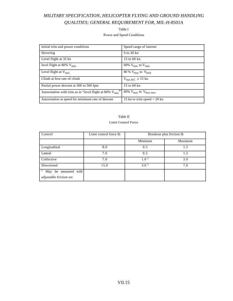
MILITARY SPECIFICATION, HELICOPTER FLYING AND GROUND HANDLING
QUALITIES; GENERAL REQUIREMENT FOR, MIL-H-8501A
VII.15
Table I
Power and Speed Conditions
Initial trim and power conditions Speed range of interest
Hovering 0 to 30 kn
Level flight at 35 kn 15 to 60 kn
level flight at 80% Vmax 60% Vmax to Vmax
Level flight at Vmax 80 % Vmax to Vlimit
Climb at best rate of climb Vmax R/C ± 15 kn
Partial power descent at 300 to 500 fpm 15 to 60 kn
Autorotation with trim as in “level flight at 80% Vmax” 60% Vmax to Vmax auto
Autorotation at speed for minimum rate of descent 15 kn to trim speed + 20 kn
Table II
Limit Control Force
Control Limit control force lb Breakout plus friction lb
Minimum Maximum
Longitudinal 8.0 0.5 1.5
Lateral 7.0 0.5 1.5
Collective 7.0 1.01 3.0
Directional 15.0 3.01 7.0
1 May be measured with
adjustable friction set

VIII
APPENDIX VIII
AUTOMATIC FLIGHT CONTROLSYSTEM ASSESSMENT
VIII.1
APPENDIX VIII
AUTOMATIC FLIGHT CONTROL SYSTEM ASSESSMENT
References: A ETPS Ground School Notes Chapter E11
B MOD Defense Standard 00-970 Volume 2 Issue 1
C Military Specifications MIL-H-8501B and MIL-C-18244
D BCAR G1-2 Para 7 and BCAR 29
ACKNOWLEDGMENT
The following information has been extracted substantially intact from the Empire
Test Pilot’s School Rotary Wing Flight Test Manual. Where appropriate, minor content
and stylistic changes have been made to improve readability for students at USNTPS.
INTRODUCTION
1. The term “Automatic Flight Control System” (AFCS) covers a multitude of
devices which may be used in various ways to alter or improve the stability and handling
qualities of a helicopter, or to permit certain mission maneuvers to be flown automatically.
For the purposes of this Appendix, the term “AFCS” will be taken to apply to all types of
system unless specifically defined. There are three different levels of augmentation,
although all three may well be considered in one aircraft system. These three levels are:
a. Stability Augmentation System (SAS). This system uses rate gyros to provide
rate damping and possibly integration of the signal to provide short term attitude
hold. This type of system alone may be fitted to light helicopters (e.g. Gazelle, Jet
Ranger).
b. Automatic Stabilization Equipment (ASE). This uses vertical gyro or VRS
information to provide a long term attitude hold. Rate damping may also be
incorporated when the pilot is making a control input. Heading hold using compass
information, although a Òhigher order functionÓ is normally a basic function of an
ASE.
ROTARY WING STABILITY AND CONTROL
VIII.2
c. Autopilot. The term ÒautopilotÓ covers all those piloting functions additional to
basic stability augmentation. Internal or external sensors may be used. Autopilot
functions include altitude and airspeed holds and operational modes such as
automatic transition and hover, capture and tracking of a navigation course (e.g.
VOR) and coupled approach (e.g. ILS).
Other definitions may also be encountered. [Annex A gives a glossary of AFCS
terminology.]
2. The type of testing required of an AFCS will depend on such aspects as the
capabilities and complexities of the system, the stability characteristics of the basic aircraft,
the missions of the aircraft, and the manner in which the aircraft will be operated to carry
out these missions. It is therefore essential to understand not only the system, but also the
operating requirements, before embarking on a test program. For example, many flight test
hours could be wasted evaluating the automatic approach to a hover from entry conditions
that are not mission relatable, although they are within the capability of the system. On the
other hand, the AFCS of a helicopter that is to be certified for single pilot IFR must
undergo considerable testing in all flight conditions.
AIMS OF THE TESTS
3. The aims of a full AFCS assessment are essentially the following:
a. To establish and analyze the correct operation of the system and of its
individual components.
b. To assess the operating characteristics and ease of use of the system,
the cockpit layout and all the controls, including engagement and
disengagement, both independently and against the mission requirement.
c. To assess the aircraft handling characteristics when using the system.
d. To determine whether the equipment meets operational requirements.
e. To measure the performance of the system in all its modes, and assess
the performance against the specification.
MILITARY SPECIFICATION, HELICOPTER FLYING AND GROUND HANDLINGQUALITIES; GENERAL REQUIREMENT FOR, MIL-H-8501A
VIII.3
f. To assess the reliability and maintainability of the system, and to
diagnose potential failures and evaluate their likely effect by carrying out a
Failure Modes and Effects Analysis (FMEA).
g. To determine the effects of failures revealed by the FMEA, and
particularly system runways, initially by simulation but then by flight
testing.
GENERAL TEST METHOD
4. A full AFCS assessment will usually begin with an engineering evaluation
and a cockpit assessment as the AFCS is developed. Increasing use is being made of
simulators for even these early phases, particularly as digital systems become more
common. In some cases, development hardware and software may be evaluated in the
simulator, with the same boxes then being flight tested to verify the simulation. Flight
testing will progress through engagement and disengagement of the various functions to
performance measurement of the basic autostabilizer and autopilot modes; on a new type of
helicopter, these tests may well be combined with stability and control tests of the basic
aircraft. Subsequently, any specialized functions or maneuvers (such as transitions) will be
assessed. Concurrently with the flight testing, the engineering evaluation will progress to
an assessment of the effect of production component tolerances, both on performance and
as part of the FMEA, so that finally, ground and flight testingof system failures and
malfunctions can be carried out. Environmental and EMI testing will also be required.
5. Flying techniques adopted for longitudinal, lateral/directional and low
airspeed stability and control tests are used for the basic data gathering sorties. From these
results an assessment of the AFCS performance in stability augmentation and datum
holding can be made. Mission relatable tests require a thorough knowledge and recent
experience of the mission combined with a systematic and methodical approach. A cockpit
assessment of the layout of the controls and indicators is important. During flight tests
detailed observation of the behavior of the aircraft and the AFCS actuators is required.
Hunting of actuators, oscillations in pitch and roll, tendency to overshoot required
conditions, height variations, extremes of aircraft attitude, rate of power demand and
indications to the pilot of loss of authority of the AFCS are a few of the characteristics
ROTARY WING STABILITY AND CONTROL
VIII.4
which should be assessed. Programmable control surfaces (such as horizontal stabilators)
should be evaluated in exactly the same way, either as part of an overall AFCS assessment
or separately.
ENGAGEMENT AND DISENGAGEMENT FACILITIES
6. General. It should be possible to engage and disengage the AFCS at any
time in flight and on the ground. On engagement the AFCS should come into operation
smoothly and complete disengagement of the AFCS should be possible quickly, safely and
positively at any time independently of all other primary services unless it can be shown
that the consequences of the AFCS remaining engaged in all circumstances are more
desirable (see also Reference D - 29.672: Stability Augmentation Systems). The
“emergency disengagement” facility should normally be on the cyclic control. The overall
system engagement/disengagement facilities may not be the only method of disconnecting
all or part of the AFCS. The pilot “flythrough” features should be verified as should the
operation of any airspeed and/or weight-on-wheels (WOW) switches which affect AFCS
operation. Ensure that the disengagement of attitude hold when the cyclic is moved (for
example) is smooth and does not introduce any discontinuities into the apparent control
response. Check that the heading hold is disengaged whenever the compass (or any other
sensor) is aligned or slewed. Verify the operation of any airspeed switches (e.g. UH-60A
FPS yaws, to hover-at 60 KIAS) at various combinations of sideslip and angle of attack to
determine the effects of airspeed sensor pressure errors or sudden operation of an actuator.
The consequences of an airspeed sensor malfunction will also have to be examined
especially when it controls a high-authority device such as a movable stabilator. WOW
switches are often used to override certain AFCS functions or to change their gain (e.g.
CH-47D/HC Mk 1 pitch channel). Make sure that they do not introduce any undesirable
characteristics such as hunting or transients especially during running landings or landings
on sloping ground when the switches may not operate “cleanly” or simultaneously.
Evaluate the effects of an airspeed switch malfunction.
7. Test Methods. Within the general requirements for engagement and
disengagement, flight testing involves the operation of the various engagement and
disengagement facilities both on the ground and throughout the flight envelope. Airborne
testing is carried out by approaching incrementally the extremes of maneuver and speed,

MILITARY SPECIFICATION, HELICOPTER FLYING AND GROUND HANDLINGQUALITIES; GENERAL REQUIREMENT FOR, MIL-H-8501A
VIII.5
starting from minimum power speed in level flight. The transient and steady state aircraft
responses following the engagement or disengagement of the AFCS and any dangerous
tendencies are recorded.
AFCS PERFORMANCE TESTING
8. Performance testing can be broken down into short term and long term
performance of the basic augmentation functions and the evaluation of operational modes.
The purpose of these tests is to measure the dynamic qualities of damping, datum holding,
and residual oscillations. AFCS performance evaluation is conducted incrementally. Initial
tests are done at a mid CG, light gross weight and at minimum power speed in level flight.
All initial testing will be done in day visual meteorological conditions.
9. Basic Augmentation Function. This paragraph deals with the basic
augmentation functions of an AFCS such as rate damping, heading hold and attitude hold.
Testing in this category can be considered as short-term wherein the aircraft’s augmented
response to deliberate control inputs and gusts is evaluated. Generally the system should
be subjected to the full range of stability and control testing methods in order to discover
the effect of the AFCS on the aircraft’s static and dynamic stability and control response in
all axes. Several examples of AFCS modes of operation are mentioned below but it is
emphasized that the list is by no means complete and that a thorough understanding of the
operation of the system must be achieved before testing can begin.
a. Static Stability Tests. The primary method by which an AFCS affects static
stability is through an attitude hold since rate damping is, by definition, a
“dynamic” stability mode and generally operates through series actuators.
Consider each axis in turn:
(1) Pitch. The performance of the AFCS in this respect will be strongly
influenced by the variation of pitch attitude with speed. If q varies little over
the speed range then an attitude hold system will contribute little to (and may
actually detract from) static stability. In such a case an artificial airspeed
hold augmentation (SH-60) or even a means of producing positive “cockpit”
static stability by altering the length of control runs (CH-47 DASH) may be
incorporated. Remember that both stick force and stick position cues are
ROTARY WING STABILITY AND CONTROL
VIII.6
important in determining static stability and that the operation of parallel
actuators can affect these characteristics in different ways. Artificial pitch
rate damping will increase maneuver stability but should not lead to an
excessive stick force-per-g which may detract from agility. The effects of
an attitude hold function on maneuver stability, especially during wind-up
turns, should be carefully evaluated.
(2) Roll. Most ASE incorporates an angle of bank (AOB) hold which may
operate over a limited range of roll attitude (Lynx) or over the full range
(Chinook). Some systems confer positive spiral stability on the aircraft by
requiring an into-turn cyclic deflection or force to hold an off-trim angle of
bank while others are more like a rate demand system and will hold attitude
(i.e. zero rate) when the cyclic is neutralized thus they produce perfect
neutral spiral stability. The effect of an AFCS on static lateral stability (Lv)
will depend upon the influence of yaw pedal movement on bank angle hold.
The effects of attitude hold on sideways flight should be examined to see if
it introduces discontinuities in the lateral cyclic/sideways speed relationship,
especially close to the AOB at which the system may revert to rate damping
only.
(3) Yaw. In many ways the artificial augmentation of the directional
stability of a helicopter is the most complex function for an AFCS because
the mode of operation of the system must change between hover and
forward flight. Generally speaking, the AFCS will provide a “feet-off”
heading hold (HH) in the low speed regime and a turn-coordination/heading
hold (TC/HH) facility above a certain airspeed. Some systems retain the
use of the yaw channel to provide simple HH in forward flight while others
use TC in yaw and hold heading by adjusting AOB. In forward flight the
disengagement of HH or the changeover from HH to TC can be a function
of AOB, lateral cyclic displacement, yaw pedal displacement or the
operation of a yaw force link or microswitch. The user friendliness of the
chosen system should be carefully evaluated and mission related since it
may force the pilot to employ a flying technique which is not ideal for the
mission. The hover/forward flight mode change is normally a function of
airspeed and should be evaluated in a variety of off-trim conditions with
various degrees of sideslip, during turns, etc. The initiation of a turn in
MILITARY SPECIFICATION, HELICOPTER FLYING AND GROUND HANDLINGQUALITIES; GENERAL REQUIREMENT FOR, MIL-H-8501A
VIII.7
forward flight can be problematic, especially for systems which achieve TC
via sideslip transducers. Some aircraft (e.g. CH-47C) use a feed forward
of the rate of lateral cyclic input into the yaw channel to initiate a yaw rate
during turn entry. The extra yaw input is then washed out as the
steady-state TC takes over again. The operation of such a system must be
evaluated during slow and rapid entries into turns at various bank angles
since imperfect operation can lead to adverse or proverse yaw. Any delay
in the disengagement of HH during a turn may cause the aircraft to
“hang-up” on its original heading as if directional stability was weak.
Remember that any system which uses a lateral accelerometer in the yaw
channel will be subject to the same sensations as the pilot in terms of
sideforce cues and inherent sideslip.
b. Dynamic Stability. The fundamental requirement for an AFCS in terms of
dynamic stability is to automatically suppress the nuisance modes of the natural
aircraft response such as the long term (phugoid) or lateral/directional oscillation
(dutch roll). Again the test techniques are similar to the dynamic stability tests
which are applied to the unaugmented aircraft and comprise displacement of the
aircraft from a trim condition, using either natural or artificial excitation, and
observation of its response. The parameters which should be noted are as follows:
(1) Rate and precision of return to trim.
(2) Damping/number of overshoots.
(3) Cross-coupling.
The trim condition may be defined in terms of attitude, heading, airspeed, altitude
or any other parameter which may be relevant to the particular AFCS function under
scrutiny. The displacement method should also be tailored to the particular function
and the following techniques may be employed:

ROTARY WING STABILITY AND CONTROL
VIII.8
(4) A rapid input with an immediate release to trim (RTT) which may
expose problems with lack of damping or the excitation of undesirable
response modes. This method may also “beat” switching functions thus
revealing problems which could occur during rapid maneuvering.
(5) A slow input followed by a smooth RTT as soon as the required
displacement is achieved.
(6) A slow input, holding the displacement for a number of seconds prior
to RTT. The pilot should be aware of any build-up of control forces during
this type of input since this may be indicative of the unrestricted operation of
a parallel actuator which may result in a violent return to trim (and probable
overshoot) when the controls are released.
(7) Very small, long period inputs which may be insufficient to disengage
an attitude hold and could result in a force build-up as in (6).
(8) Steps, pulses, doublets and frequency sweeps of various magnitudes
designed to expose any undesirable AFCS excitation.
(9) Open loop operation of trimmers to displace the AFCS datum without
compensatory control movement.
The amount of attitude change from trim will depend upon the particular axis and
the axis and flight envelope limits. Changes of ± 3°, ± 5°, and ± 10° are normally
sufficient to evaluate short term performance in the pitch axis. Care should be taken
at high airspeeds not to exceed VNE during the nosedown inputs. In the roll axis
the same inputs should be used, followed by the angle of bank required for a
standard rate turn (e.g. ± 15°), ± 30°, and the bank angle limit. In the yaw axis, the
displacements will depend upon the sideslip envelope. Changes in heading should
be made in increments up to the sideslip limit.
c. Control Response. The control response of the aircraft will be affected by
AFCS rate damping and control shaping (e.g. control quickening). Control
response should be evaluated in the normal way (i.e. using incremental step inputs)
with particular emphasis on the smooth operation of any augmentation and a
VIII.9
mission appropriate, predictable response. The disengagement of an attitude hold
during maneuvering must not lead to jerkiness or unpredictability. Any rate
damping will reduce the ultimate agility of the aircraft but this potential disadvantage
may be more than outweighed by a qualitative improvement in handling qualities.
Ideally the AFCS should completely suppress control cross-coupling, so check for
off-axis response. Varying the size of the inputs will enable any limits of
augmentation to be determined.
d. Long Term Test Methods. Long term performance testing involves the
assessment of the AFCS during extended flights. Attitude, altitude, and airspeed
holds are evaluated for their long term holding ability. These extended flights
should be made in both smooth and gusty air. AFCS gains, which produce
acceptable performance in smooth air, may cause a rough ride in gusty conditions.
There may well be other features in the AFCS designed to solve this problem or to
compensate for particular aircraft deficiencies (although they may not work as
advertised). An example is the "Turbulence" mode in the SFIM 155D AFCS fitted
to the SA365N; the helicopter suffers from a tendency to lateral/directional
oscillation which is increased by turbulence. To try to damp this out, a yaw-roll
precontrol signal, which is a function of yaw velocity and roll angle modulated for
forward speed, is fed into the AFCS roll channel when this mode is selected.
Ideally, AFCS gains should be optimized to provide a smooth, stable ride in calm
air, but not be so tight that they cause the system to overwork in turbulence. An
example might be a very tight heading hold. With a jump take-off, the heading may
not vary more than ± 1°, which is exceptionally tight. But in turbulence, the high
gains may cause the nose to return to trim too fast with the resultant high angular
accelerations, causing the helicopter to snake through the air. An important point to
check for during the extended flights is that the short term performance at the
beginning and at the end of the flight is unchanged.
10. Autopilot Modes. There are a wide variety of “high-order” autopilot
modes, the ultimate example of which is the full-authority digital FCS of the type which
will be found in the RAH-66 Comanche. We shall confine ourselves to less esoteric modes
which may be found in current generation helicopters. Autopilot modes usually operate
through parallel actuators and thus move the cockpit controls so that the pilot can verify
VIII.10
correct response. Ideally such a mode should operate in conjunction with a flight director,
not only so that the pilot can monitor the correct operation of the AFCS, but also to permit
him to fly the mode manually (e.g. manual TF) should he desire or should there be an
actuator failure.
a. Altitude Hold. Altitude hold should be evaluated in conditions which require
power changes in order to exercise the system. The system's response may be
optimized for a particular flight condition and so should be checked throughout the
permitted speed and altitude range. Specific points for evaluation are:
(1) Engagements in transient conditions. The maximum allowable rate of
climb or descent for engagement which results in an acceptable overshoot
should be checked.
(2) Evaluate any measures for the protection of the engine/drivetrain from
overtemp or overtorque. The absence of such devices may force a limit on
gross weight, AOB, speed or turbulence level. Check that the collective
actuator speed is matched to the characteristics of the engine control system
such that, for example, an excessively rapid collective movement, which
may cause a surge, is impossible.
(3) Ensure that it is impossible to excite an unstable mode of operation by
making a series of rapid cyclic inputs. It may be necessary to instrument the
drivetrain for this test.
(4) For systems which rely on the use of cyclic to hold altitude (e.g. Puma,
SA 365N) it should be impossible to engage the system below minimum
power speed. The pilot's choice of power setting will place considerable
constraints on the available system performance and these should be
investigated. Make sure that control margins are adequate especially at
extreme CG positions.
(5) Check that the system can be temporarily disengaged, via a maneuver
button, or permanently disengaged without removing the hand from the
collective.

VIII.11
(6) Verify the effect of sideslip and other sources of pressure errors on a
barometric altitude hold. Generally speaking there should be none since
most devices use a sealed aneroid which measures only changes in pressure
from the datum of the engagement altitude.
(7) Verify the effects of various surfaces on a radar altitude hold. If the
system is unsmoothed it may only be appropriate to use it in the hover
regime. Evaluate the effects of an underslung load if appropriate. Make
sure there are no engagement errors which could endanger the aircraft when
hovering close to the ground. The EMC/EMI characteristics of the sensor
should be thoroughly investigated.
b. Airspeed Hold. The precise criteria for the engagement (either manual or
automatic) of an airspeed hold must be thoroughly understood prior to testing. For
example, the UH-60 incorporates a time delay, during which no cyclic inputs may
occur, before it switches from pitch attitude hold to airspeed hold. Evaluate the
system during climbs, descents, turns and power changes. There is normally a
minimum speed for the engagement of an airspeed hold and so engagements at
various pitch attitudes and rates of acceleration around this speed should be
assessed. Evaluate the ease with which the airspeed datum can be altered and how
rapidly the system captures the new value. Pressure errors should be assessed,
especially during sideslips and if the system does not tap into the normal aircraft
pilot-static circuit.
c. Navigation Beacon Tracking. There are many different systems for tracking
courses defined by VORs or TACANs and so generalization is difficult. Some of
the points which may be considered are:
(1) How accurately does the equipment track the course? An independent
navaid (e.g. a map!) will be required to determine this. Does it track
smoothly or continuously oscillate about the desired position? How does it
cope with crosswind conditions? Is it accurate enough to allow an
approach to be flown? Is the performance consistent irrespective of range
ROTARY WING STABILITY AND CONTROL
VIII.12
from the navaid?
(2) How does it behave when navigation signals become weak in the short
term and in the long term? What happens during beacon passage in the cone
of silence? Does the system gracefully return to heading hold for instance?
(3) Does the course intercept mode function sensibly? What is the
maximum intercept angle? Does the system compute and execute the turn
on to course properly without overshoots and/or excessive bank angles?
What happens at beacon passage when a new outbound course is selected?
d. ILS/MLS Tracking. The evaluation of the automatic tracking of a landing aid is
similar to that of a VOR/TACAN coupler except with an added dimension! There
are some extra points to consider:
(1) How well does the system switch from altitude hold during the initial
approach to glideslope capture? What happens if the glideslope signal
fails?
(2) What happens at decision height? Is there a facility for leveling off at,
say, a pilot-selected or default radar altitude?
(3) What happens if the pilot changes speed during the approach?
(4) What happens if you attempt to intercept the glideslope from above or
below?
(5) Is there adequate indication of satisfactory system performance,
especially during the critical stages of the approach?

VIII.13
e. Automatic Transition and/or Hover Modes. These modes are normally
associated with maritime helicopters although they may have applications to future
battlefield aircraft with the introduction of accurate area navaids such as GPS. The
following items should be assessed in addition to appropriate elements of the
altitude hold tests described above:
(1) System performance from a range of operationally relevant entry gates
(i.e. speed/height combinations).
(2) The effects of wind strength, direction and shear.
(3) The accuracy of automatic flyover modes - how close to the marked
flyover position is the final hover?
(4) The effects of the use of trim during coupled flight. The effectiveness
of any automatic hover trim feature.
(5) The ease of pilot intervention and the cues to system malfunction.
(6) The ease with which the pilot can fly part of the transition manually
(e.g. the performance of a manual turn while maintaining the automatic
height/speed profile) and the subsequent re-engagement of the full automatic
system.
(7) The accuracy of the automatic hover and the nature of the changeover
from/to cable/doppler hover. The associated switching and advisory
elements should be evaluated as should any drift introduced during the
mode change.
f. Movable Control Surfaces. Programmable aerodynamic control surfaces are an
integral part of the AFCS in many modern helicopters such as the H-60 series and
the AH-64. Horizontal stabilators fulfill a variety of functions and contribute to
attitude hold, rate damping, reduction of trim changes with power and even control
augmentation. The yaw SAS of the MDH 520N operates a movable vertical surface

ROTARY WING STABILITY AND CONTROL
VIII.14
to improve directional stability. Generally, for the purposes of testing,
programmable surfaces may be regarded in the same way as any other
high-authority AFCS element although the following specific aspects should be
assessed:
(1) The stabilator will program with airspeed at a maximum rate which is
limited by actuator response. Generally this is fairly slow (about 10
deg/sec) as dictated by the runaway case. Evaluate the system during rapid
transitions to and from the hover to assess the impact of stabilator lag.
Undesirable nose-down pitch moments may occur, especially at forward
CG.
(2) If manual programming is normally permitted, evaluate the complete
airspeed/stabilator angle envelope concentrating on FOV and control
margins. Ensure that there are no undesirable transients when passing
from manual to automatic mode, especially during dynamic maneuvers.
The slew switches should be mounted on the normal flight controls.
(3) If manual programming is permitted in an emergency ensure that this
does not impose an excessive workload and that the degradation in handling
qualities is acceptable throughout the permitted flight envelope.
g. Actuator Authority. Most ASE incorporates parallel actuators which perform a
trim follow-up function and keep the series actuators close to their null positions
automatically by adjusting the positions of the flight controls at an appropriate, slow
rate. The presence or absence of such a facility will dictate which of the following
sets of testing should be performed:
(1) Observe whether the trim follow-up facility works correctly and permits
the low-authority, high-speed series actuators to perform rate damping and
control augmentation during maneuvering flight. Displace the aircraft from
the trim condition and then make an additional control input to check for
damping.
MILITARY SPECIFICATION, HELICOPTER FLYING AND GROUND HANDLINGQUALITIES; GENERAL REQUIREMENT FOR, MIL-H-8501A
VIII.15
(2) Assess whether the control activity produced by parallel actuator action
is acceptable or whether it produces unusual control forces during
maneuvering flight.
(3) Make an instantaneous CG change by picking up or releasing an
underslung load, releasing stores or winching to see how the system reacts.
(4) Assess the ease with which the pilot can accomplish nulling of the
actuators using the manual trim facility (if fitted). Does the system readily
go out of authority during normal flying necessitating constant attention to
maintain effective stabilization?
MISSION TESTING
11. The results of the performance testing should lead to the recommendation of
operating envelopes within which the ASE and autopilot modes may be used safety and
effectively. The testing should now be directed towards an evaluation of the AFCS during
typical mission tasks under realistic mission environments. If an AFCS is designed for a
night over water mission, it should be tested at night and over water. Mission testing will
be predominantly qualitative. The pilot must make the decision whether or not the AFCS is
an aid toward mission completion. Important keys for this decision are:
a. Does the system do the job it was designed to do?
b. Pilot workload - does the system ease pilot workload or does it create an
increased workload, even though it might well do the job?
c. Does the pilot have confidence that the system will aid him in completing his
mission or would he be better off without it?
d. Does the system display consistent performance?

ROTARY WING STABILITY AND CONTROL
VIII.16
Quantitative data can be used to determine specification compliance point to possible
reasons for problems. However only qualitative evaluation can decide whether or not the
AFCS satisfies its primary requirement - that of easing pilot workload and improving
operational effectiveness.
FAILURE MODE TESTING
12. The testing of malfunctions in an AFCS is an important step towards a
helicopter release to service. Faults may be "passive" (i.e. no disturbance) or oscillatory
(e.g. a position feedback failure) or a full hardover of an actuator. The use of rapid rate
(but limited authority) series actuators in autostabilizers increases the likelihood of a
malfunction causing a rapid divergence from a selected flight path. Reducing the rate of
operation of actuators reduces the likelihood of runaways causing severe handling
problems but slow acting actuators alone may be incapable of applying the stability
augmentation required by helicopters. The height channel can use slow acting parallel
actuators (e.g. Sea King), but in pitch, roll and yaw the AFCS will have rapid rate
actuators and therefore any malfunctions causing runaways must be anticipated unless
redundancy and self-monitoring are features of a particular system. This aspect is
becoming more and more important as digital AFCS and Active Control Technology (ACT)
start to become more common in the helicopter world, as indeed is true for the fixed wing
community. The helicopter's ability to tolerate runaways of the AFCS is affected by its
limited flight envelope in terms of “g”, IAS, stress, and the operational requirement that
most helicopter mission flying takes place at low level. Furthermore helicopter handling
characteristics make the task of a rapid recovery from a runaway difficult.
13. Pre-Test Study. Preparation for AFCS failure testing should cover the
following 3 aspects:
a. Specification. The specification must be interpreted in practical terms against a
background knowledge of how the aircraft is likely to be used in service. This is
particularly important when describing which criteria of pilot attentiveness to apply
for a particular flight condition. Single pilot/2 pilot operation should be considered
at this stage.

MILITARY SPECIFICATION, HELICOPTER FLYING AND GROUND HANDLINGQUALITIES; GENERAL REQUIREMENT FOR, MIL-H-8501A
VIII.17
b. Failure Analysis. A detailed study of the AFCS is required to establish the
effect of specific failures (e.g. gyro malfunctions, electronic faults etc.). The result
of such failures may vary from automatic compensation by a duplex or triplex
AFCS to a 3 axes simultaneous runaway as in the case of a failure of the No. 6
transistor in the Lynx ASE. The use of simulators to verify theoretical predictions
of the effects of component failures is advantageous but time consuming; it is likely
that the manufacturer will use simulation to develop safe characteristics on complex
AFCSs. Methods of inducing failures (and the failures themselves) can be various
and unexpected, especially if induced by electrical power supply interruptions or
fluctuations. Electro-Magnetic Compatibility (EMC) testing is also vital, and may
produce some unexpected results.
c. Aircraft Limits. A clear definition of the relevant aircraft limits is required.
Normally the failure testing will be aimed at establishing that AFCS runaways do
not cause a catastrophic failure. Thus it is likely that the sideslip, stress, g and IAS
limits applicable for the trial will be beyond those pertaining for normal operations.
Detailed structural analysis may be required to verify stress limitations. The
ultimate g or stress limit may either occur during the runaway or during the
subsequent recovery.
TEST METHODOLOGY
14. Definitions. The following definitions of AFCS failure testing
terminology are adapted from those outlined in Reference B:
a. Pilot Involvement. This is the degree of pilot involvement in, or attentiveness
to the flying task. Various levels may be distinguished:
(1) Active Flight. The pilot is continuously flying the aircraft via the
flying controls.
(2) Attentive Flight. The pilot has to pay particular attention to flight
control for short periods.
ROTARY WING STABILITY AND CONTROL
VIII.18
(3) PassiveFlight. Minimum pilot attention is required.
The attentive and passive phases of flight can be further divided into “hands-on”
and “hands-off” according to whether the pilot can release the flying controls for
substantial periods. It may be the responsibility of the test team to judge which
flight phase criteria are appropriate to the aircraft mission and the maneuvers which
this encompasses.
b. Times and Periods. The times and periods pertinent to AFCS testing can be
defined as follows:
(1) RotorcraftResponseTime. The period between failure occurrence and
its recognition by the pilot by means of a suitable cue.
(2) Pilot ResponseTime. The time which elapses between recognition of
the failure and the start of recovery action. Pilot response time comprises 2
elements:
(a) Decision Time. Decision time increases as the pilot relaxes his
involvement level.
(b) Reaction Time. Not surprisingly reaction time is longer during
“hands-off” flight phases.
(3) InterventionTime. Intervention time is the sum of rotorcraft response
time and pilot response time.
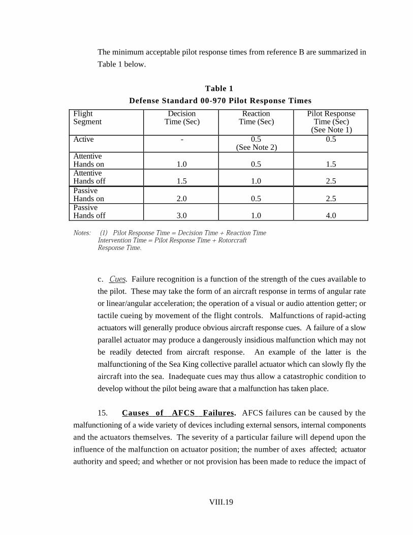
VIII.19
The minimum acceptable pilot response times from reference B are summarized in
Table 1 below.
Table 1
Defense Standard 00-970 Pilot Response Times
FlightSegment
DecisionTime (Sec)
ReactionTime (Sec)
Pilot ResponseTime (Sec)
(See Note 1)
PassiveHands on 2.0 0.5 2.5PassiveHands off 3.0 1.0 4.0
Notes: (1) Pilot Response Time = Decision Time + Reaction TimeIntervention Time = Pilot Response Time + RotorcraftResponse Time.
c. Cues. Failure recognition is a function of the strength of the cues available to
the pilot. These may take the form of an aircraft response in terms of angular rate
or linear/angular acceleration; the operation of a visual or audio attention getter; or
tactile cueing by movement of the flight controls. Malfunctions of rapid-acting
actuators will generally produce obvious aircraft response cues. A failure of a slow
parallel actuator may produce a dangerously insidious malfunction which may not
be readily detected from aircraft response. An example of the latter is the
malfunctioning of the Sea King collective parallel actuator which can slowly fly the
aircraft into the sea. Inadequate cues may thus allow a catastrophic condition to
develop without the pilot being aware that a malfunction has taken place.
15. Causes of AFCS Failures. AFCS failures can be caused by the
malfunctioning of a wide variety of devices including external sensors, internal components
and the actuators themselves. The severity of a particular failure will depend upon the
influence of the malfunction on actuator position; the number of axes affected; actuator
authority and speed; and whether or not provision has been made to reduce the impact of
Active - 0.5(See Note 2)
0.5
AttentiveHands on 1.0 0.5 1.5AttentiveHands off 1.5 1.0 2.5

ROTARY WING STABILITY AND CONTROL
VIII.20
the problem by monitors, comparitors, cut-outs or the “backing-off” of other lane(s) of a
multiplex system. Simplex components which could cause full-authority, multi-axis
hardovers should obviously have a very low probability of failure while the malfunctioning
of a component which produces a benign single-axis response could be more easily
tolerated. A detailed FMEA will reveal the likely outcomes and their chances of
occurrence. Reference B gives guidance in this respect.
16. Effects of AFCS Failures. The effects of AFCS failures may be
divided into 3 categories:
a. Soft Failures. The system in question merely ceases to function without causing
any intrinsic aircraft response. There may not be any noticeable effect in the short
term.
b. Runaways. An actuator is actively driven to an unwanted position. The
extreme case is a full-scale, maximum-rate deflection known as a hardover.
Runaways may occur in more than one axis simultaneously.
c. Oscillatory Failures. Oscillatory failures generally result from the failure of a
component in a feedback loop and may be so severe that the pilot is only able to
disengage the system using flight control-mounted devices.
17. Test Equipment. It is highly desirable that the test aircraft be specially
fitted with actuator position indicators if these are not standard equipment. The most
important piece of equipment is a runaway or hardover box which can be used to inject
artificial failures into the AFCS and cause actuator movement and consequent aircraft
response. The box should be capable of driving each actuator to any position at rates
varying from relatively slow (10 sec for full travel) to the maximum and holding the
actuator in any position. The simulation of failures which could cause multi-axis runaways
may also be necessary. Make sure that the simulated failure can be instantly removed in the
event of an emergency.
MILITARY SPECIFICATION, HELICOPTER FLYING AND GROUND HANDLINGQUALITIES; GENERAL REQUIREMENT FOR, MIL-H-8501A
VIII.21
18. Test Technique. The basic test technique comprises the injection of a
simulated failure, pilot intervention after an appropriate intervention time and recovery to
safe, controlled flight. This discussion will concentrate on the nose-down pitch case
(which may well be the most critical, especially at high speed) and Figure 1 shows a
simplified time history of such a condition.
It is essential to conduct an incremental build up to the critical failure cases and this takes
place in several stages for each flight condition:
a. Recovery from Unusual Attitudes. The aircraft is deliberately placed in an
unusual attitude representative of that likely at the intervention point and a recovery
is executed. An incremental approach to this maneuver is required and real-time
stress analysis is highly desirable since, at the most critical flight conditions, the
aircraft is likely to exceed its normal flight envelope. Stress levels may have to be
extrapolated to permit a limited number of demonstrations of AFCS failures out to
the design limit of the aircraft.
b. Simulated Failures. A series of ramp and then step control inputs are made to
demonstrate likely aircraft behavior after an AFCS failure. The maximum
magnitude of the input can be related to the authority of the actuator in question and
the ramp speed related to the actuator rate. A recovery is executed after a
representative intervention time. A provisional profile for the demonstration
runaway(s) can thus be established.
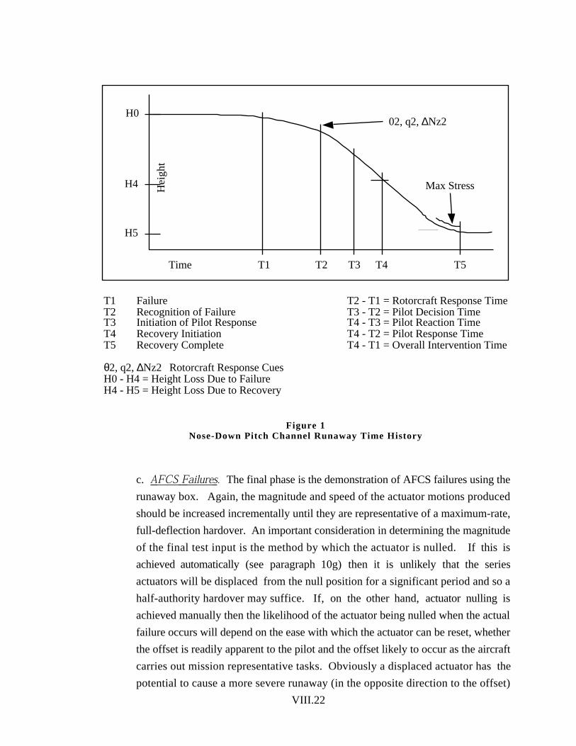
VIII.22
Nose-Down Pitch Channel Runaway Time History
c. AFCS Failures. The final phase is the demonstration of AFCS failures using the
runaway box. Again, the magnitude and speed of the actuator motions produced
should be increased incrementally until they are representative of a maximum-rate,
full-deflection hardover. An important consideration in determining the magnitude
of the final test input is the method by which the actuator is nulled. If this is
achieved automatically (see paragraph 10g) then it is unlikely that the series
actuators will be displaced from the null position for a significant period and so a
half-authority hardover may suffice. If, on the other hand, actuatornulling is
achieved manually then the likelihood of the actuator being nulled when the actual
failure occurs will depend on the ease with which the actuator can be reset, whether
the offset is readily apparent to the pilot and the offset likely to occur as the aircraft
carries out mission representative tasks. Obviously a displaced actuator has the
potential to cause a more severe runaway (in the opposite direction to the offset)
Time T1 T2 T3 T4 T5
H0
H4
H5
02, q2, ∆Nz2
Max Stress
T1 FailureT2 Recognition of FailureT3 Initiation of Pilot ResponseT4 Recovery InitiationT5 Recovery Complete
T2 - T1 = Rotorcraft Response TimeT3 - T2 = Pilot Decision TimeT4 - T3 = Pilot Reaction TimeT4 - T2 = Pilot Response TimeT4 - T1 = Overall Intervention Time
θ2, q2, ∆Nz2 Rotorcraft Response CuesH0 - H4 = Height Loss Due to FailureH4 - H5 = Height Loss Due to Recovery
Hei
ght
Figure 1
ROTARY WING STABILITY AND CONTROL
VIII.23
than one which is nulled. The final decision may well evolve from discussion
about probabilities between the user and the manufacturer. Recommendations
concerning aircrew training to minimize actuator offset may also be necessary.
d. Flight Conditions. Testing should begin in the most benign flight conditions,
probably level flight at medium altitude and Vmin pwr, and progress incrementally
to the most demanding such as high power climbs or flight at Vne. Any
post-failure height loss should be carefully noted as this may have an impact on the
operational effectiveness of the aircraft. For example the Chinook HC Mk 1 retains
a recommended minimum height of 300 ft due to poor cueing of a nose-down
DASH runaway. Testing should also build up to the most critical combinations of
CG and loading. Remember that CG position may have an effect on actuator offset
and thus runaway severity.
e. Test Personnel. Care should be taken to achieve realistic intervention times by
avoiding the use of pre-warned pilots who have already experienced several
malfunctions similar to the test condition. Ultimately the pilot should be required to
perform routine mission tasks appropriate to the flight phase being investigated and
then be subjected to unannounced AFCS failures. The use of several pilots will
also provide a greater pool of opinion about the suitability of the AFCS for the role.
19. AssessmentCriteria . There are several factors which may define the
end point of AFCS failure testing:
a. The desired intervention time is reached for the most critical failure in a particular
flight condition and flight phase.
b. The aircraft is unable to support the stress levels projected to occur at the test
point.
c. A handling problem is encountered which would cause problems for the average
operational pilot.

MILITARY SPECIFICATION, HELICOPTER FLYING AND GROUND HANDLINGQUALITIES; GENERAL REQUIREMENT FOR, MIL-H-8501A
VIII.24
d. The minimum control margin is encroached, possibly as a result of the
deflection of a series actuator.
e. The height loss encountered is sufficient to prevent useful exploitation of the
aircraft in its intended mission while fulfilling the necessary intervention criteria.
20. Test Results. Possible outcomes of AFCS failure mode testing are:
a. A flight envelope restriction. This may be quite severe in the case of a single
failure of a duplex system since the second failure would be unopposed.
b. AFCS modifications which could include the provision of better failure cueing
devices, cut-outs, limiters or comparitors (e.g. barometric altimeter monitoring the
gross errors of a radar altitude hold).
c. Operator advice concerning, for example, the nulling of actuators or the flight
conditions wherein the AFCS may be engaged. The Chinook HC Mk 1 AFCS
must be re-engaged in the same flight conditions as disengagement to avoid
engagement transients due to the operation of the DASH.
21. Training Facility . The recovery from a runaway may be possible for a
test pilot but too difficult for a newly trained squadron pilot. A requirement for training
using runaway boxes in flight or in simulators may be specified in the final release.
However the use of simulators should be treated with caution, because training is unlikely
to be fully representative of an actual runaway inflight; for example, the sudden onset of
harsh vibration in the real recovery may deter the pilot from pulling the stick back hard
enough.
CONCLUSION
22. AFCS testing is a most challenging blend of the evaluations of aircraft
systems and flying qualities. The test pilot must be completely open-minded and use an
unbiased analytical approach to ensure accurate results. He should not prejudge system
innovations; just because a system is new or it has a fancy display does not automatically
make it good or bad. These strong initial subjective impressions can cause the pilot to
overlook a bad feature or be overly critical in his assessment. Nevertheless all qualitative
ROTARY WING STABILITY AND CONTROL
VIII.25
opinion should be recorded as the trial develops, and the use of several pilots will
frequently aid in producing the correct analysis of the system. The aircraft will be in
service for many years and will invariably return for further evaluation of system
modifications or the testing of previously unforeseen failure modes. An accurate and
detailed report of the initial AFCS evaluation will ensure that these future trials can be
conducted expeditiously.
MILITARY SPECIFICATION, HELICOPTER FLYING AND GROUND HANDLINGQUALITIES; GENERAL REQUIREMENT FOR, MIL-H-8501A
VIII.26
ANNEX A
GLOSSARY OF HELICOPTER AFCS TERMINOLOGY
Note: These are generic terms only, and are constantly misquoted and misused. Be
absolutely accurate in defining your terms and letting your reader know what you are
saying.
Actuator - The means of mechanizing the desired output.
Actuator Trim - The means to adjust the actuator position, normally to either preposition
it prior to a specific maneuver or to maintain it near the center of travel. May be done
automatically or manually.
AFCS - Automatic Flight Control System. The portion of the flight controls that are
moved automatically by a device other than the pilot.
Automatic Actuator Trim - The automatic retrimming of an actuator. Generally done to
minimize the effects of a runaway in a simplex system.
ASE - Automatic Stabilization Equipment - generally an attitude hold system, it may
incorporate rate damping when the flight controls are commanding an input.
Authority - The amount of the control movement that the AFCS can influence. Normally
given as percentage of total control movement in each axis, it may also be useful to quote it
as an equivalent control deflection.
Autopilot - Will hold an external condition such as altitude, radial or track.
Attitude Hold System - Will hold the commanded attitude in the relevant axes. Note
that yaw is an axis, and heading hold is an attitude hold. Normally requires control
position information to disable the attitude hold function to permit maneuvering. Some
attitude holds may revert to rate damping during maneuvers commanded by the pilot.
VIII.27
Channel - The individual axis of the AFCS, i.e., pitch, roll or yaw, including all the
elements of that part of the AFCS, i.e. airspeed hold channel through the cyclic.
Closed Loop - Pilot in the loop of aircraft control - actively involved in flying or
maneuvering.
Comparator - The system of comparing signals, either between 2 computers, actuators
or other devices to see if they are the same. Generally used as a failure protection device,
i.e. to disconnect a channel when the output is in the same direction as the attitude change.
Control Augmentation - The movement of a flight control is sensed and fed forward
into the AFCS in such a manner to cause an initial movement of the actuator in the desired
direction. This is done to offset the sensation of a reduction in control response that would
occur due to the AFCS damping the motion when it senses a disturbance.
Coupled - The ability of the system to perform a specific function using various sensors:
i.e. a coupled ILS approach will require certain normal AFCS functions, as well as the use
of ILS signals.
Cross-coupled Feedback - Feeding the position of one actuator into both its own
computer and the other computers of a multiplexed system. This enables faster fault
detection as well as failure protection.
Degraded Modes - The modes of operation other than fully operational. For example,
with the pitch channel failed, it may be still possible to have a coupled turn, but not a
coupled ILS approach.
Duplex - The duplication of capabilities: i.e. a duplex pitch channel system will have 2
independent pitch systems for redundancy. Note that this is a different definition than you
may see elsewhere for duplex.
Failure Modes and Effects Analysis - The analysis of the complete AFCS and
related mechanical, electrical and hydraulic systems to assess the effects that failure of the
individual parts will have on the system. Generally will concentrate on the internal parts of
the computer and go heavily into the effect of failure of certain components (diodes,
ROTARY WING STABILITY AND CONTROL
VIII.28
transistors, etc.). The test pilot must review this to ensure that other items such as airspeed
signals and the like are adequately considered.
Feed Forward - The insertion of a signal in the system somewhere downstream of any
other signal, so as to ensure that the command has an effect (see Control Augmentation).
Fly-through - Enables the pilot to enter the loop and make a change without having to
disengage and then re-engage the AFCS either as a segment or completely.
FMEA - Failure Modes and Effects Analysis (see above).
Gain - The ratio of output to input, which normally translates to the rate of movement of
the actuator. The gain of a single channel of a duplex system may double if the other
channel should fail, resulting in no perceivable difference to the pilot.
Hardover - The rapid movement of an actuator to the end of its travel, which would not
have been commanded by the system given the conditions. Generally refers to a failure
case, and is used as the worst condition due to the rapid rate of control surface movement.
Hover - Any time the relative speed is zero. Note that this can mean a zero ground speed
hover, a zero airspeed hover, a hover alongside a moving ship, or a zero surface water
speed hover. It is extremely important to define the exact terms in this case.
Inner Loop - The inner loop is used to make small adjustments to remove external
disturbances. Typically, it does not move the cockpit controls. Series actuators are
normally used.
Intervention Time - The time between the insertion of a failure in the system and the
pilot taking control. It is comprised of:
a. Time for the failure to generate a response.
b. The time for the pilot to recognize the response.
c. The time to react to the response.
VIII.29
The intervention criteria used must be defined by the agency doing the testing, and as well,
it must specify the criteria used to alert the pilot that something is wrong. (“G” onset, pitch
or roll acceleration, airspeed change, etc.) and the time that it is expected to take for the
pilot to react (i.e. hands on the controls, actively watching the controls/aircraft or busy with
other tasks and not monitoring the aircraft/controls at all).
Lane - A British term, #1 lane could mean the #l pitch, roll and yaw channels if there was
a second lane. Note that it can mean the same as channel if there is no redundancy.
Linear Variable Displacement Transducer (LVDT) - A transducer for
determining control displacement or position, as well as the position of an actuator. A
better solution than the conventional potentiometer.
Long Term - The motion or response of the helicopter over a long time period, generally
longer than 5 seconds or so.
LVDT - Linear Variable Displacement Transducer. Sometimes also known as Linear
Variable Differential Transformer. (see above).
Model Following - The use of a synthetic model of the aircraft/response in the memory
of the computer and shaping the output to make the response follow this model.
Multiplex Systems - The use of more than one lane or channel. Simplex is the use of
only one lane/channel, duplex uses 2, triplex 3, quadruplex uses 4, etc.
Open Loop - The pilot is not in the loop of flying or maneuvering the aircraft.
Operational Autopilot -An autopilot which will carry out a particular operational
maneuver such as transition to a hover, or a coupled ILS. Generally built on top of an
autopilot which is built on to of an attitude hold system and incorporates the use of the
outer loop/parallel actuators.
Outer Loop - The outer loop of the system is used to make adjustments to ensure that a
particular condition is maintained. It is typically done by moving the pilot's controls.
Parallel actuators are often used.
ROTARY WING STABILITY AND CONTROL
VIII.30
Parallel Actuator - An actuator that is placed in parallel with the normal flight controls.
Generally slow moving (low gain) and with high authority.
Quickening - The term typically used for control augmentation. Generally done by
inserting a commanded input directly to the actuator before the computation has a chance to
neutralize the response.
Response Command - To command a specific feature, i.e. rate, attitude, linear
velocity and so on, regardless or with consideration of the aircraft/ environmental state.
For example, in a rate command system, a 1" lateral cyclic displacement may always give
a 10 degree/second roll rate, regardless of airspeed, or another system could give a constant
stick force/G at speeds above 40 KIAS and give a constant attitude change per unit
deflection below that speed.
Runaway - The movement of an actuator to an undesired position.
SAS - Stability Augmentation System.
Saturated - The inability of the system to work normally due to the relevant actuator being
at full travel.
SCAS - Stability and Control Augmentation System. A system that incorporates control
augmentation with another form of stability modification. One of the more widely misused
terms, as it implies that there is a feed forward (control augmentation) when very often
there is not.
Series Actuator - An actuator that moves in series with the normal flight controls.
Normally of limited authority and with a high gain (rate of actuator movement).
Short Term - The aircraft response in the very short term following a control input or
disturbance - usually within the time frame of 0 to 3 seconds.
MILITARY SPECIFICATION, HELICOPTER FLYING AND GROUND HANDLINGQUALITIES; GENERAL REQUIREMENT FOR, MIL-H-8501A
VIII.31
Simplex - A system with at least part of the system relying on only one component. Note
that if any part of a duplex system eventually relies upon a single component, anything
from a gyro to an actuator, then it becomes a simplex system. For purposes of most
discussions, this does not include “simple mechanical components” such as flight control
tubes or swash plates.
Stability Augmentation System (SAS) - Generally used to describe a system which
only dampens rates without regard to the pilot demand for maneuvering. Used to improve
the basic flying qualities. Should not affect statics, nor should it move the flight controls.
Normally an inner loop system. May incorporate rate integration for pseudo attitude hold.
Transparent - The quality of making the effects of the AFCS invisible to the pilot when
he wishes to maneuver. Also known as "Fly-through.”
Voting - In a triplex (or higher) system, or one that has a model following system,
“voting” will compare outputs from the various systems and (hopefully) eliminate the odd
man output, thus protecting against failures.