Ecological Applications, 20(1), 2010, pp. 60–79� 2010 by the Ecological Society of America

Use of dynamic soil–vegetation models to assess impactsof nitrogen deposition on plant species composition: an overview

W. DE VRIES,1,7 G. W. W. WAMELINK,1 H. VAN DOBBEN,1 J. KROS,1 G. J. REINDS,1 J. P. MOL-DIJKSTRA,1

S. M. SMART,2 C. D. EVANS,2 E. C. ROWE,2 S. BELYAZID,3 H. U. SVERDRUP,3 A. VAN HINSBERG,4 M. POSCH,4

J.-P. HETTELINGH,4 T. SPRANGER,5 AND R. BOBBINK6

1Alterra, Wageningen University and Research Centre, P.O. Box 47, 6700 AA Wageningen, The Netherlands2Centre for Ecology and Hydrology, Orton Building, Deiniol Road, Bangor LL57 2UP United Kingdom

3Lund University, Department of Chemical Engineering, Box 124, S-22100, Lund, Sweden4Coordination Centre for Effects (CCE), PBL, P.O. Box 303, 3720 BA Bilthoven, The Netherlands

5German Federal Environment Agency (UBA), Worlitzer Platz 1, 06844 Dessau, Germany6Research Centre B-WARE, Radboud University Nijmegen, P.O. Box 9010, 6500 GL Nijmegen, The Netherlands

Abstract. Field observations and experimental data of effects of nitrogen (N) depositionon plant species diversity have been used to derive empirical critical N loads for variousecosystems. The great advantage of such an approach is the inclusion of field evidence, butthere are also restrictions, such as the absence of explicit criteria regarding significant effectson the vegetation, and the impossibility to predict future impacts when N deposition changes.Model approaches can account for this. In this paper, we review the possibilities of static anddynamic multispecies models in combination with dynamic soil–vegetation models to (1)predict plant species composition as a function of atmospheric N deposition and (2) calculatecritical N loads in relation to a prescribed protection level of the species composition. Thesimilarities between the models are presented, but also several important differences, includingthe use of different indicators for N and acidity and the prediction of individual plant speciesvs. plant communities. A summary of the strengths and weaknesses of the various models,including their validation status, is given. Furthermore, examples are given of critical loadcalculations with the model chains and their comparison with empirical critical N loads. Weshow that linked biogeochemistry–biodiversity models for N have potential for applications tosupport European policy to reduce N input, but the definition of damage thresholds forterrestrial biodiversity represents a major challenge. There is also a clear need for furthertesting and validation of the models against long-term monitoring or long-term experimentaldata sets and against large-scale survey data. This requires a focused data collection in Europe,combing vegetation descriptions with variables affecting the species diversity, such as soilacidity, nutrient status and water availability. Finally, there is a need for adaptation andupscaling of the models beyond the regions for which dose–response relationships have beenparameterized, to make them generally applicable.

Key words: biodiversity; critical loads; model validation; nitrogen deposition; plant communities; plantspecies composition; soil–vegetation models; terrestrial ecosystems.

INTRODUCTION

Impacts of nitrogen deposition

on plant species composition

During the past two decades the reduction of sulfur

(S) emissions and the persistence of a high N pressure on

terrestrial and aquatic ecosystems shifted attention from

effects of S deposition and acidification toward effects of

N deposition and eutrophication. In Europe, N is the

most important air pollutant affecting plant species

diversity. Evidence suggests that increasing N avail-

ability often causes an overall decline in plant species

diversity (Tilman 1987, Bobbink et al. 1998) even at

long-term low-N inputs (Clark and Tilman 2008). In

some cases, especially under very nutrient-poor con-

ditions, however, an increase in plant species diversity

has been observed due to the expansion of nitrophilic

species (Emmett 2007). Effects of N deposition, either in

the form of ammonia (NH3), ammonium (NH4), nitro-

gen oxide (NOx), or nitrate (NO3), are now recognized in

nearly all oligotrophic and mesotrophic (semi-)natural

ecosystems. An overview of effects on plant species

diversity, including impacts on mosses, lichens, and

mycorrhizae, in forests, grasslands, heathlands, oligo-

Manuscript received 30 May 2008; revised 30 January 2009;accepted 11 March 2009; final version received 20 April 2009.Corresponding Editor: N. B. Grimm. For reprints of thisInvited Feature, see footnote 1, p. 3.

7 E-mail: wim.devries@wur.nl

60

INVITED FEATUREEcological Applications

Vol. 20, No. 1

trophic wetlands (mire, bog, and fen), and coastal

habitats, mainly in Europe, with related empirical critical

N loads, is presented in Achermann and Bobbink (2003).

More recently, an overview of effects of N deposition on

a global scale, distinguishing Arctic and Alpine ecosys-

tems, boreal forests, temperate forests and tropical

forests, heathlands and grasslands, Mediterranean vege-

tation, tropical savannas, and arid vegetation (desert and

semidesert) is presented in Bobbink et al. (2010).

Critical loads and their use in policy making

In order to set standards and targets for emission-

reduction policy, the concept of critical load has been

developed. The general definition of a critical load is ‘‘a

quantitative estimate of an exposure to one or more

pollutants below which significant harmful effects on

specified sensitive elements of the environment do not

occur according to present knowledge’’ (Nilsson and

Grennfelt 1988). Critical loads are defined for specific

combinations of pollutants, effects, and receptors. They

reflect spatially variable sensitivities, thus leading to

regionally defined emission-reduction needs. The con-

cept is most commonly used in connection with the

atmospheric deposition of S and N (acidification and

eutrophication) and in these cases the critical load is the

maximum flux (in kg N�ha�1�yr�1 or keq H�ha�1�yr�1)that an ecosystem is able to sustain. Since 1994, critical

loads for N and acidity have played an important role in

European air pollution abatement (Hettelingh et al.

2001, Spranger et al. 2008). European critical load

exceedances, calculated and mapped using the latest

methods and data sets for critical loads, deposition, and

emission scenarios, are presented in Hettelingh et al.

(2007) and Slootweg et al. (2007). Results show that the

area where critical loads of acidity are exceeded will

continue to decrease, even if no new legislation is

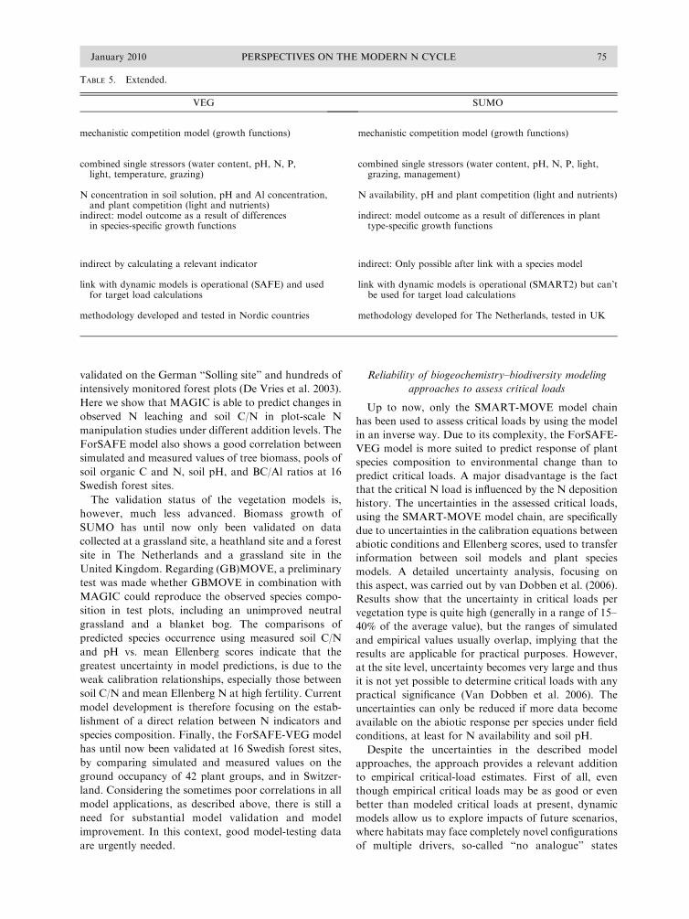
implemented, while high (.10 kg N�ha�1�yr�1) exceed-ances for critical N loads remain widespread especially

in northwestern European areas dominated by ammonia

emissions.

Exceedances of the critical load of acidity and N have

been used in European pollution abatement policy for

defining emission-reduction targets, i.e., in the UNECE

Convention on Long-range Transboundary Air Pollu-

tion (LRTAP Convention) and the European Union

(National Emission Ceilings Directive 2001, European

Commission 2005). Integrated assessment models (e.g.,

the RAINS model; Amann et al. 1999) use these data

and methods in scenario analyses. The exceedance of

critical loads of N is also used as an indicator for risk to

biodiversity by the European Environment Agency

(European Environment Agency 2007). The general

organization of effects-based European air pollution

policies is described in the LRTAP Convention (in-

formation available online).8

Critical load approaches for nitrogen used

in policy making

Critical loads for N, as used in European environ-

mental policy, are estimated empirically or by simula-tion. The empirical approach uses experimental fields or

‘‘mesocosms’’ where various levels of N fertilizer havebeen added. In that case, the critical load is determined

as the level of deposition at which a decrease inbiodiversity just starts to occur (Achermann and

Bobbink 2003). The great advantage of the use ofempirical critical N loads, based on N-addition experi-

ments, is that there is field and/or experimental evidencefor a relationship between N deposition and effects.

There are, however, several requirements for empiricalcritical N loads to be reliable, including (1) long-term

experiments (preferably .4 years) to show long-termeffects and (2) studies in low background N deposition

areas to ensure that major effects have not alreadyoccurred. In high background N deposition, high-Nadditions may be needed before (additional) effects

show up and N removal experiments should be usedinstead (Emmett 2007). The empirical critical N loads

are thus mainly based on long-term field-additionexperiments and mesocosm studies in low-N deposition

areas with realistic N loads (,100 kg N�ha�1�yr�1).However, since such experiments are time and labor

intensive, results are only available for a rather limitedgroup of broadly defined ecosystems. The reliability

(range) in empirical critical loads, being the level of thelowest N addition where effects occur, is mainly

influenced by the chosen interval in N additions andby an uncertain background N deposition that has to be

added to this level (Sutton et al. 2003). An aspect thatalso limits a strict comparability is the lack of fixed

criteria regarding significant effects for which a criticalload is derived (as, e.g., in critical limits for toxicsubstances), and it is also impossible to predict future

impacts when N deposition and other environmentalconditions change simultaneously.

The model-based critical load approach, used inEuropean environmental policy making, is based on an

ecosystem mass balance, which balances the depositionload to an ecosystem with its long-term capacity to

buffer this input or to remove it from the system withoutharmful effects inside or beyond the system (Hettelingh

et al. 2001, Spranger et al. 2008). The harmful effects aredefined in terms of critical limits above which a negative

effect is assumed to occur. An overview of those limits isgiven in De Vries et al. (2007). The model calculates a

critical load as the deposition level leading to soilconditions that are just tolerated by a given ecosystem.

The model-based critical load approach as used up tonow, however, is by definition based on the sustainable

state of a given ecosystem that is invariable in time(steady state) and excludes non-permanent bufferingprocesses such as temporary N release and retention and

cation exchange. This long-term critical load maytherefore differ from the atmospheric deposition level8 hwww.unece.org/env/lrtapi

January 2010 61PERSPECTIVES ON THE MODERN N CYCLE

actually affecting the ecosystem, since ecosystems differ

in sensitivity to perturbation depending on their current

state and recent history. Nitrogen deposition thresholds

may vary during forest stand development, as for

example shown also with dynamic-model approaches

(Tietema et al. 2002). These differences form the core of

resilience and sustainability theories. This aspect has not

been included in model based critical loads until now,

and their steady state concept implies that the exceed-

ance of such critical loads does not allow a prognosis of

ecosystem status at any point in time.

Need for dynamic model approaches and aim of this paper

Both empirical critical loads and steady-state models

do not allow prediction of the temporal response of

ecosystems to deposition scenarios, for example, in

terms of impacts on plant species diversity. This requires

the use of the dynamic integrated soil–vegetation

models. Such models can also be used to assess critical

loads, while accounting for differences in sensitivity to

perturbation depending on their current state and recent

history. In the context of ecological theory, N deposition

is a form of disturbance; i.e., an external influence that

moves the system away from its stable state (Gunderson

2000). If such a disturbance is not too large, the

ecosystem has the ability to return to its former state

(‘‘resilience’’; see, e.g., Gunderson 2000); in the case of N

deposition, this might happen by incorporation of N in

refractory soil organic material or N leaching. However,

if the disturbance is larger or extends over a prolonged

period, the system may move towards an alternative

stable state, from which it will not be able to return to its

former state without a new external influence (Ludwig et

al. 1997). N deposition will ultimately stimulate the

growth of more productive species, which usually

produce more easily degradable litter and reach a

greater height, thus increasing both the deposition itself,

and the amount of N cycling in the system. In these

terms, the critical load is the highest deposition that will

not cause an ecosystem to shift to an alternative (more

productive, usually species-poorer) state. In this alter-

native state the quantity of N cycling through the system

will be much larger than in its original state and, because

of the tight cycling of N, a return to the former, N-poor

state will only be possible by physically removing the

excess N even if deposition decreases (Wamelink et al.

2009). Critical-load assessments including such aspects

can be only be included in dynamic model approaches,

simulating delays in damage due to buffering processes

and delays in recovery to restore soils to their original

state.

In this overview, we describe the possibilities of

multispecies models in combination with dynamic soil–

vegetation models to (1) predict plant species composi-

tion or diversity as a function of atmospheric N

deposition and (2) calculate critical N loads in relation

to an acceptable plant species diversity change. First, we

present the two main model approaches that are

presently employed in Europe: (1) a simple soil acid-

ification and nutrient-cycling model (SMART2 or

MAGIC) combined with field-based empirical relation-

ships with plant species responses (MOVE, GBMOVE,

or NTM) and (2) a detailed, mechanistic, soil-acid-

ification and nutrient-cycling model (ForSAFE) with a

process-based description of plant species responses

(VEG). The model acronyms stand for Simulation

Model for Acidification’s Regional Trends (SMART),

Model for Acidification of Groundwater In Catchments

(MAGIC), Model of Vegetation (MOVE) with

GBMOVE being the Great Britain version of MOVE,

Nature Technical Model (NTM), Soil Acidification in

Forest Ecosystems (SAFE) and VEGetation model

(VEG). The overview includes a description of each

modeling approach, followed by application examples

illustrating the model validation status and the use of the

models in critical-load assessments. In a final section, we

discuss the potential of linked biogeochemistry–biodi-

versity models to support European pollution abatement

policy, including (1) strengths and weaknesses of the two

major model approaches, (2) the use of different

indicators for N availability, (3) the validation status

of each model, (4) the potential of the models to assess

critical loads, (5) the need for additional field surveys,

and (6) relevant extensions to the modeling approaches.

MODELING APPROACH

Integrated soil–vegetation models are used at present

in Europe to predict plant species composition as a

function of atmospheric deposition of N and acidity, as

illustrated in Fig. 1. The principle of such model-based

approaches is that a dynamic soil model (SMART2,

MAGIC, (For)SAFE) predicts the changes in water and

nutrient status (e.g., as N availability or C/N ratio) and

soil acidity (e.g., as soil pH or base saturation) in

response to atmospheric deposition, whereas a statistical

model (NTM, MOVE) or a process-based model

(SUMO, VEG) predicts vegetation succession or

changes in plant species composition in response to the

changes in water, nutrient, and acidity status, using

plant species-specific information on habitat preferen-

ces. Such coupled models can be used in an inverse way

to determine critical loads. In that case, critical values

for abiotic factors (e.g., N availability or soil pH ) have

to be empirically determined per vegetation type, either

directly or from information per species (step 1) and

subsequently used in the coupled soil model (step 2) to

back-calculate the critical N and acid loads.

Simulation of critical loads according to the above

principle was carried out in The Netherlands (Van

Dobben et al. 2006), where (1) the critical pH and N

availability per vegetation type (association) were deter-

mined on the basis of a large set of vegetation releves

(vegetation description of a small plot, cf. MOVE model;

Latour and Reiling 1993) and (2) the dynamic soil model

SMART2 (Kros et al. 1995) was used to calculate the

critical loads at which the above critical limits were not

INVITED FEATURE62Ecological Applications

Vol. 20, No. 1

exceeded in the long term. Other models use critical limits

for other abiotic variables, such as the C/N ratio in the

GBMOVE model (Smart et al. 2003) and the BERN

model (Schlutow and Hubener 2004). or the soil N, P,

base cation (BC) availability, soil moisture, pH, light,

and grazing pressure in the ForSAFE-VEG model

(Belyazid et al. 2006, Sverdrup et al. 2007).

Below, we discuss the two major model approaches

used at present, i.e., (1) dynamic soil models linked with

empirical static-vegetation models (the SMART2

(-SUMO)-MOVE/NTM and MAGIC(-SUMO)-

GBMOVE model chains) and (2) a deterministic,

dynamic ecosystem model integrating hydrology,

growth, biogeochemical cycles, and vegetation dynam-

ics. (ForSAFE-VEG).

Linked dynamic soil models with empirical

static vegetation models

Two major comparable model chains of dynamic soil

models linked with static vegetation models are

SMART2(-SUMO)-MOVE/NTM and MAGIC

(-SUMO)-GBMOVE, which are developed and used in

the Netherlands (NL) and the United Kingdom (UK),

respectively. The model chains consist of (1) the soil

models SMART2 (NL) or MAGIC (UK) that simulate

the cycling of nutrients in the soil and predict soil acidity

and N availability, (2) the succession model SUMO that

simulates the cycling of nutrients (N, P, K, Ca, Mg) in

the plant–soil system, including biomass growth through

photosynthesis and biomass removal through manage-

ment, and (3) multiple regression equations between

species presence and abiotic factors that define the

realized niches of a substantial proportion of the

vascular flora of each country (and in the UK also

bryophytes) (MOVE in NL and GBMOVE in UK), or

of plant communities (NTM in NL). In the Dutch

MOVE and NTM models, abiotic factors are ground-

water table, soil pH, and soil N availability, derived via

Ellenberg indicator values, whereas a version of the UK

GBMOVE model also includes three climatic variables,

i.e., the minimum January temperature, maximum July

temperature, and precipitation. Ellenberg’s indicator

values are classes of plants species with similar

ecological niches, which are derived for about 2720

central-European vascular plants (Ellenberg et al. 1992).

Ellenberg derived values for the following ecological

factors: light (EL), temperature (ET), continentality

(EK), moisture (EF), soil pH (ER), nutrients/nitrogen

(EN), and others (salinity, heavy metal resistance)

(Esonst). SMART2 can be used both in its original,

dynamic form, allowing the calculation of target loads,

and as a steady-state version, allowing the calculation of

steady state critical loads, as used in policy making. The

use of SUMO is optional in both model chains. Changes

in species composition are modeled by first simulating

the effects of N and S deposition on soil conditions,

followed by simulating the impacts of changed soil

conditions on species composition.

Modeling the relation between atmospheric deposition

and soil conditions

SMART2 and MAGIC are dynamic, process-oriented

models that predict changes in soil chemistry at a given

level of N and S deposition. Changes of N and S

deposition on soil variables such as pH, C/N ratio, or N

availability by SMART2 (Kros et al. 1995, Kros 2002)

or MAGIC (Cosby et al. 2001). Both SMART2 and

MAGIC include the major hydrological and biogeo-

chemical processes in the soil compartment, to calculate

the long-term effects of atmospheric deposition of NOx,

NHy, SOx, and base cations (BC2þ) on soil-solution

chemistry, and in case of MAGIC also the surface-water

FIG. 1. (A) Method to predict plant species composition as a function of atmospheric deposition and (B) to calculate criticalloads for nitrogen and acid deposition. The model abbreviations are explained in Tables 4 and 5. BS is base saturation and BC/Al isthe molar ratio of base cations (calcium, magnesium and potassium) to aluminum in soil solution.

January 2010 63PERSPECTIVES ON THE MODERN N CYCLE

chemistry. The models have a high degree of process

aggregation to minimize their data requirements, which

allows application on a regional scale. They consist of a

set of mass-balance equations, describing the soil input–

output relationships, and a set of equations describing

the rate-limited and equilibrium soil processes. Apart

from pH, the models predict changes in aluminum, base

cation, ammonium, nitrate, and sulfate concentrations

in the soil solution and solid phase. Key parameters

include the input and output fluxes of base cations and

strong acid anions, the soil cation exchange capacity,

and the fraction of this capacity that is occupied by Ca,

Mg, Na, and K ions. Nitrogen dynamics in MAGIC are

based on empirical relationships between net N reten-

tion and the current C/N ratio in the soil, whereas in

SMART2 litterfall, mineralization, root uptake and

immobilization are modeled explicitly. Both SMART2

and MAGIC have an internal simplified growth module

which enable the models to calculate nutrient cycling

detached from SUMO. The detached version of

SMART2 has been used for the calculation of critical

loads and target loads. For the computation of target

loads, a procedure was developed to iteratively run

SMART2 until the N and S deposition used, lead to the

critical pH or N availability for a given vegetation type.

Furthermore, a steady-state version of SMART2 has

been developed that computes the critical N and acid

load that in steady state leads to a given combination of

N availability and pH. A complete overview of these

models, and the differences between SMART2 model

and MAGIC can be found in the various references

mentioned and in De Vries et al. (2007).

SUMO is a process-based model that simulates

biomass growth under given soil, climate and manage-

ment conditions (Wamelink 2007). The basis of the model

is a maximum growth that is being reduced by a series of

linear and non-linear reduction factors to constrain

growth. These reduction factors convey the effect of

changes in the availability of light, N, phosphorous,

water, and temperature. SUMO distinguishes five func-

tional plant types (climax trees, pioneer trees, shrubs,

dwarf shrubs, and herbs) that compete for light and

nutrients. Their competitive balance is governed by

vegetation structure, i.e., canopy height and biomass of

roots and leaves per functional type. Management is

simulated as biomass removal by mowing, grazing,

cutting, or turf stripping. The accumulation of biomass

in the five functional types determines the succession

stage (e.g., pioneer, grassland, heathland, forest). SUMO

can be coupled to niche models, e.g., NTM or MOVE,

through vegetation structure and soil chemical conditions

(pH and nutrient availability) simulated by SMART2 or

MAGIC. For these soil models litterfall is a crucial input

term that is generated by SUMO. In each time step there

is feedback between SMART2 or MAGIC and SUMO;

the models exchange information about N and P,

litterfall, and vegetation structure.

Relationships between plant species occurrence

and soil conditions

MOVE and NTM.—The models MOVE (Latour and

Reiling 1993, Latour et al. 1994) and NTM (Schouwen-

berg et al. 2000, Wamelink et al. 2003a) are based on

response curves in which the probability of plant species

(MOVE) or plant community (NTM) occurrence is

determined by vegetation structure and the abiotic site

conditions of groundwater table, soil pH, and N

availability. The probability of occurrence is a simple

bell-shaped curve derived for 914 species by second-

order logistic regression based on presence/absence,

representing species occurrence along an environmental

gradient. These relationships are based on the realized

niche, i.e., they account for competitive exclusion, rather

than responses of the species in isolation. Since MOVE

and NTM focus on more than one abiotic factor, the

curves are multidimensional. The probabilities of

occurrence are determined per vegetation type relative

to soil pH and N availability, estimated on the basis of

Ellenberg’s (1992) indicator values for N (EN) and

acidity (ER). In the critical-load approach of Van

Dobben et al. (2006), the 20th and 80th percentiles of

these frequency distributions were used as the critical

limits, i.e., the range between these percentiles was

considered as the optimal range for each vegetation

type.

The above frequency distributions were determined in

a database of 160 000 vegetation releves that were

labeled in terms of vegetation type (Schaminee et al.

1989), originally developed for a revision of the Dutch

classification of plant communities. In a separate

procedure, the Ellenberg values (which are on an

arbitrary scale) were translated into physical units that

can be used as input to dynamic models. This translation

requires a training set where vegetation and soil

conditions (at least pH and N availability) have been

recorded simultaneously. In the past few years, much

effort has been put into the collection of such data

(Wamelink et al. 2007; see data set available online).9

Various translation functions between Ellenberg values

and physical units have been derived (e.g., Alkemade et

al. 1996, Ertsen et al. 1998, Wamelink et al. 2002, Van

Dobben et al. 2006). Those of Van Dobben et al. (2006),

for example, run

pH ¼ 3:1þ 0:53ER ðR2 ¼ 0:43; n ¼ 3630Þ ð1ÞpNav ¼ 6:19þ 0:64EN þ c 3 vegtype

ðR2 ¼ 0:24; n ¼ 6911Þ ð2Þ

where Nav ¼ N availability (kmol�ha�1�yr�1) and the

constants c per vegetation type are �1.182 for grass,

�1.898 for heath, �0.274 for coniferous forests, and 0

for deciduous forest.

9 hwww.abiotic.wur.nli

INVITED FEATURE64Ecological Applications

Vol. 20, No. 1

GBMOVE.—As with MOVE, multiple logistic re-

gression was used to construct empirical equations that

predict habitat suitability for higher and lower plants

representative of British plant communities, based on

their abundance along key environmental gradients as

recorded by extensive releve data (e.g., Roy et al. 2000).Each equation consists of regression coefficients that

apply to either four or seven explanatory variables,

depending on whether climate variables (minimum

January temperature, maximum July temperature, and

precipitation) are included or not. Important interaction

terms are also included. These quantify the extent to

which a species’ response on one gradient is conditionedby another gradient (e.g., Pakeman et al. 2008). The

data used to derive each equation were assembled from a

variety of sources as described in De Vries et al. (2007)

and covered more than 40 000 vegetation releves. The

regression was based on presence/absence data for each

plant species in each plot paired with values of climatic

variables (derived from the plot’s geographical position)

and plot-averaged Ellenberg indicator values. The finalnumber of species having GBMOVE regression models

is 327 for bryophytes and 803 for vascular plants in non-

coastal habitats (74 in coastal habitats).

As with MOVE, soil pH and soil C/N ratio are

translated instantaneously into mean Ellenberg ER and

EN values, respectively, using paired soil measurements

and mean Ellenberg values from the Countryside Survey

1998 database (Smart et al. 2003). The limitations of the

assumption that species presence immediately changes in

response to soil conditions are discussed in detail inComparison and evaluation of the model chains. Relation-

ships thus obtained are

lnðC=NÞ ¼ 3:61� 0:63 3 ln EN

ðR2 ¼ 0:62; n ¼ 256Þ ð3ÞpH ¼ 2:5þ 0:61ER

ðR2 ¼ 0:61; n ¼ 256Þ: ð4ÞThe mean Ellenberg ER and EN values per releve are

terms in the GBMOVE regression equations. At each

time step the simulated values of soil C/N, soil pH, soil

moisture percentage, and cover-weighted canopy height

are translated into Ellenberg units and put in the

regression equation, resulting in predicted probability

of species occurrence over time. Changes in soil pH and

C/N ratio are predicted with the dynamic soil model

MAGIC. Canopy height can be changed arbitrarilyusing preexisting knowledge of the pace of succession in

a particular location, or on a more process-linked basis

by the SUMO succession model. Climate variables can

be changed to mimic expectations under different

climate change scenarios. Likewise, soil moisture can

also be changed to mimic drainage or drought.

The integrated dynamic ForSAFE-VEG model

The only fully integrated dynamic soil and plant

species diversity (vegetation) model that is presently

available in Europe is the ForSAFE-VEG model chain.

This model chain, developed in Sweden, consists of (1)

the ForSAFE model, aimed at the dynamic simulation

of changes in soil chemistry, soil organic matter,

hydrology, and tree biomass growth in relation to

changes in environmental factors (Wallman et al. 2005),

and (2) the VEG submodel, which simulates changes in

the composition of the ground vegetation in response to

changes in biotic and abiotic factors such as light

intensity at the forest floor, temperature, grazing

pressure, soil moisture, soil pH, and alkalinity in

addition to competition between species based on height

and root depth (Belyazid et al. 2006, Sverdrup et al.

2007). For each time step, defined by the resolution of

the input data, ForSAFE simulates the changes in state

variables in response to environmental changes (temper-

ature and precipitation, atmospheric deposition, forest

management). These state variables are read by the VEG

module, where the occupancy strength is calculated for

each plant group. The plant groups are defined by the

user. The single occupancy strengths are then used to

calculate the relative occupancy of each plant group.

If a stress factor would eliminate a certain species, the

disappearance of this species will not be instantaneous,

but will happen with a delay, which depends on the

lifespan of the species. Unlike the model chains with

MOVE and GBMOVE, this aspect is included in

ForSAFE-VEG. The change in occupancy of a specific

plant group, dX/dt, depends on the actual occupancy of

the plant group (X ), the target occupancy (referred to as

equilibrium occupancy Xeq), and the specific regener-

ation time of the plant group (s) according to

dX

dt¼ 1

sðXeq � XÞ: ð5Þ

The regeneration time s is related to the life span of a

specific plant group. The life span depends on site

factors, such as drought. The equilibrium occupancy of

a plant group i, Xeq,i, is the ratio between the strength of

the species under the specific environmental conditions

and the sum of the strengths of all present species

according to

Xeq;i ¼Si

Xj¼plantgroup

j¼1

Sj

ð6Þ

where Si is the individual strength of the plant group i.

The sum of plant group strengths is also used as an

indicator of the density of the ground cover, referred to

as the mass index (MI). The strength of each plant group

is the product of the following drivers: (1) soil solution N

concentration (mol/L), (2) soil solution phosphorus

concentration (mol/L), (3) soil acidity ([Hþ], [BC2þ],

[Al3þ] (eq/L), (4) soil water content (m3 water/m3 soil),

(5) soil temperature (8C), (6) light reaching the ground

(lmol photons�m�2�s�1), (7) grazing (moose units/km2),

(8) wind tatter and wind chill damage, (9) plant

January 2010 65PERSPECTIVES ON THE MODERN N CYCLE

competition based on aboveground competition for light

and belowground competition for water and nutrients,

and (10) air CO2 concentration. ForSAFE-VEG thus

simulates the ground vegetation occupancy based on the

individual response of plant groups to these controlling

factors. The effects are multiplicative and have the same

weights in affecting the plant strength. Each plant group

represents various individual plant species, varying from

less than ten up to several hundreds.

For each plant group that has been selected, response

functions were parameterized for Sweden from published

laboratory and field data, by approximations from

empirical data, or by scaling the response with respect

to other plant groups for which the response is known.

Scaling of plant groups towards known responses was

based on generic knowledge and expert opinions from

Swedish plant ecologists. However, the basic shape of

each response function does not vary between the plant

groups. For example, all plant groups will respond

positively to an increase in water availability in the soil

up until a certain level where anaerobic conditions in the

saturating soil may hinder the plant’s growth. The

distinction between the plant groups is the minimal water

content required for survival, optimal water content for

growth, and the point at which water becomes damaging.

The individual response functions are described in detail

in Belyazid (2006) and De Vries et al. (2007).

MODEL VALIDATION ON CHANGES IN SOIL

AND VEGETATION DATA

Results of both types of model chains were compared

with measurements on changes in soil and vegetation

data. The performance of the models was calculated by

two measures that are often applied for this purpose; the

normalized root mean square error (NRMSE; Eq. 7),

and the normalized mean error (NME; Eq. 8) (Janssen

and Heuberger 1995):

NRMSE ¼

ffiffiffiffiffiffiffiffiffiffiffiffiffiffiffiffiffiffiffiffiffiffiffiffiffiffiffiffiffiffiffiffiffi1

N

XN

j¼1

ðPi � OiÞ2vuut

Oð7Þ

NME ¼ P� O

Nð8Þ

where Pi is the predicted value (model output), Oi is the

observed value (field value), P is the average for the

predicted values, O is the average for the observed

values, and N is the number of observations.

NRMSE describes the deviations between the meas-

urements and the predictions in a quadratic way and is

thus rather sensitive to extreme values. Optimally, it

should be 0. The NME compares predictions and

observations over the entire time span, on an average

basis. It expresses the bias in average values of model

predictions and observations, and gives a rough

indication of overestimation (NME . 0) or under-

estimation (NME , 0).

Linked dynamic soil models with static vegetation models

Here, examples are given of the validation of the

SMART2/MAGIC-GBMOVE/NTM model chains with

respect to soil chemical data (focus on MAGIC),

aboveground biomass data (SUMO) and time series of

observed species composition and species richness (focus

on GBMOVE in combination with MAGIC).

Validation of MAGIC on time series for soil chemical

data.—Data from plot-scale N-manipulation studies in

the United Kingdom have been used to test the ability of

MAGIC to predict changes in soil C/N under different

addition levels (Evans et al. 2006). For two sites with

high-quality soil C and N data (Fig. 2), the model

successfully reproduced observed decreases in C/N

under three treatments. These simulations incorporated

an (observed) increase in C storage as a consequence of

N deposition, which slowed down the rate of C/N

change. The NME’s derived were 0.0388 for the Ruabon

site and 0.0813 for the Budworth site, indicating a slight

overestimation of the predictions. The calculated

NRMSEs were very low, i.e., 0.0065 and 0.014,

respectively.

FIG. 2. Simulated and observed organic soil C/N ratiounder ambient N deposition (control) and long-term NH4NO3

addition at low, medium, and high levels at two heathlandexperimental sites. The vertical line indicates the start of theexperiment (after Evans et al. [2006]).

INVITED FEATURE66Ecological Applications

Vol. 20, No. 1

MAGIC was also validated on data on C/N ratios for

the Parkgrass experimental site at Rothamsted, which

are available for a 100-year period. N removal was

calculated by multiplying hay removal, for which

accurate measurements are available, by the proportion

of N in hay biomass. The uncertainty in N concentration

in hay has a large effect on the net addition (deposition

minus removal) and thus on the historic C/N trajectory

(Table 1). Note that raising N deposition would have the

same effect as reducing N removal.

Validation of SUMO on time series of aboveground

biomass.—Biomass growth predicted by SUMO was

validated using data collected at two unfertilized grass-

land sites, using site-specific historical deposition data.

The first grassland site is the Osse Kampen, situated

near Wageningen in The Netherlands and is part of a

long-term field experiment started in 1958 on former

agricultural land (Elberse et al. 1983). The second

grassland site is the Parkgrass experimental site at

Rothamstead in the United Kingdom mentioned before.

The Parkgrass site was mown twice a year and the

harvested biomass was weighed and averaged over 10-

year periods. The experiment started in 1856 and still

continues today. The trends in herbage yields are

extensively described by Jenkinson et al. (1994). At the

Dutch site, the measured biomass varies greatly between

years due to yearly differences in rainfall and temper-

ature. The simulated biomass does not vary much and

remains within the range of the measured biomass (Fig.

3). The high measured biomass in the first year is

probably caused by the former agricultural use of the

field. Both the measured and the simulated biomass

show a decrease over the years, due to the yearly

biomass removal. The results for Rothamstead show

that the harvested biomass is fairly well simulated by

SUMO. The reduction in biomass harvest between 1850

and 1900, due to exhaustion of the soil, the stabilization

of the harvest when the effect of N deposition

compensated for the exhaustion between 1900 and

1950, and the increase of the harvest later on due to

the further increase in deposition since 1950 are

simulated quite well. The effect of N deposition since

approximately 1960 is underestimated, however (Fig.

3B). Overall, the NME of the Ossekampen was �0.012and�0.0033 for Rothamsted, implying that on average,

the predictions are almost equal to the observations. The

values for the NMRSE are 0.290 and 0.195, respectively

indicating a considerable deviation for defined years.

SUMO was also validated on a heathland and a forest

site in The Netherlands, as described in De Vries et al.

(2007).

Validation of MAGIC-GBMOVE on time series of

observed species composition and species richness.—A

number of tests have been carried out to determine how

successfully MAGIC-GBMOVE could reproduce the

observed species composition in sampled plots. Obser-

vations were compared with predictions generated

initially by populating a simulated set of plots with (1)

species conditioned on probability of occurrence values

generated by GBMOVE and (2) a Poisson distribution

of mean species-richness values with proportional

variance, predicted by a separate general linear mixed

model using the same explanatory variables as

GBMOVE. This statistical model is fully described in

Smart et al. (2005). To assess the influence of uncertainty

in the calibration equations relating soil properties to

mean Ellenberg scores, predictions of species composi-

TABLE 1. Comparison of MAGIC-simulated and measuredC/N ratios at the Park Grass experimental site at Roth-amsted, UK, using 100% and 50% of the approximateestimate for nitrogen offtake in hay.

Year

MeasuredC/N ratio(g C/g N)

Simulated C/N ratio (g C/g N)

100% N offtake 50% N offtake

1876 12.8 9.7 12.31959 12.3 11.2 12.42000 12.4 12.2 12.0

Note: MAGIC is the model for acidification of ground waterin catchments.

FIG. 3. Measured and simulated biomass harvest for (A) a mown grassland site near Wageningen in The Netherlands and (B)an experimental grassland site at Rothamstead in the United Kingdom.

January 2010 67PERSPECTIVES ON THE MODERN N CYCLE

tion based on soil C/N and pH generated by MAGIC

were compared with predictions based on observed

mean Ellenberg scores. These comparisons were carried

out for control plots at the long-term continuous Park

Grass hay experiment at Rothamsted (unimproved

neutral grassland) and the Hard Hills grazing and

burning experiment at Moorhouse National Nature

Reserve (ombrogenous bog), described in Smart et al.

(2005). The results for Rothamsted indicated that when

mean Ellenberg scores based on observed species

composition were used as input to GBMOVE, on

average 67% of species observed were actually predicted.

However, when predictions were based on MAGIC

simulations of soil C/N and pH as input to GBMOVE,

the percentage of all species correctly predicted de-

creased substantially (Fig. 4A). The main reason for the

poor performance at Rothamsted appears to be that

observed soil changes were inconsistent with observed

vegetation changes. This is most likely due to sampling

practices in the experimental plots, avoiding a thin mat

of persistent litter that had developed in the O horizon

over the course of the experiment. This resulted in C/N

measurements indicating a higher fertility in the rooting

zone than that encountered by at least some of the more

shallow rooting species present. Also at Moorhouse,

both the predictions from MAGIC linked to GBMOVE

and the predictions based solely on observed mean

Ellenberg values did not compare well with the species

actually observed in the control plots, although the key

dominants in the vegetation were predicted to be present

by both models (Fig. 4B). When predicted species lists

for both GBMOVE and MAGICþGBMOVE were

examined, key absences included a range of bryophytes.

Possibly, bryophytes are more responsive to direct

deposition effects, and less so to changes in soil

chemistry, making the approach less useful for lower

plants.

From this model comparison it was concluded that it

is unlikely that both generally applicable yet highly

accurate models can be developed, because of the

dependence of current species composition on site-

specific aspects of patch and wider landscape history.

Because of this, probabilities of occurrence from

GBMOVE are no longer used as expectations of species

presence, but rather interpreted as indices of habitat

suitability where target species ought to be able to

persist and increase in population size in the absence of

constraints to dispersal and establishment. The further

validation work therefore focuses on comparing pre-

dicted trends through time with observed changes, based

on species present on-site and in the local species pool,

rather than attempting to predict the entire species

assemblage on a specific site.

Validation of MAGIC-GBMOVE on temporal changes

among plant species.—At Moorhouse, observed vs.

predicted species changes over time were summarized

as slope coefficients for each species in a linear

regression line relating (1) observed abundance over

the years and (2) predicted habitat suitability from

MAGIC and GBMOVE across the same time period.

Despite considerable scatter there was a positive

correlation between observed change in species fre-

quency and predicted change in habitat suitability (Fig.

5). A chi-square test of observed vs. predicted directions

of change was significant (P ¼ 0.016). While the

correlation between observed and predicted slopes was

also significant, predicted rates of change covered a

narrower range than observed species changes, which

may be due to weather fluctuations or sampling errors.

The integrated dynamic ForSAFE-VEG model

The ForSAFE-VEG model was validated on changes

in soil chemistry (Belyazid et al. 2006), standing wood

biomass (Belyazid 2006) and in ground vegetation cover

(Sverdrup et al. 2007) at 16 Swedish forest sites that are

part of the ICP Forest level II monitoring network

(International Co-operative Program on Assessment

and Monitoring of Air Pollution Effects on Forests).

At the sites, 42 plant groups and nine tree seedling types

have been identified. These plant groups were assumed

to be potentially present throughout Sweden, but are

only expected to manifest where environmental con-

FIG. 4. (A) Percentage of species correctly predicted in the three Park Grass control plots and (B) Moorhouse-based speciespredictions by MAGICþGBMOVE vs. predictions based on observed mean Ellenberg scores only, as input to GBMOVE. Modelabbreviations are explained in Tables 4 and 5.

INVITED FEATURE68Ecological Applications

Vol. 20, No. 1

ditions are favorable. The sites cover a wide range of

climatic conditions, soils, fire regimes, atmospheric

deposition gradients, and management histories. For-

SAFE-VEG was used to simulate the changes in soil

chemistry, hydrology, and tree biomass according to

these conditions, and the composition of the ground

vegetation was subsequently derived. Atmospheric

deposition data for NO3þ þ NH4

þ and SO4� were

derived on the basis of EMEP model estimates accord-

ing to the 1999 LRTAP Gothenburg protocol (Schopp

et al. 2003). The sites were subject to different histories

of fire regimes, alterations between open fields and forest

cover as well as different harvesting regimes depending

on the location of each site.

Validation on soil chemical data.—Simulated soil

organic matter contents showed a reasonable correlation

between the measured and modeled values of soil

organic carbon (C) and N at the 16 study sites. The

NME’s derived were�79 g/m2 for organic C and�3.04g/m2 for organic N, indicating a slight underestimation

of the predictions. The calculated NRMSE’s were quite

high, i.e., 0.58 for both organic C and N.

The model reconstructs the pH profiles at the 16 study

sites quite well (Fig. 6). The NME for the 16 sites varied

from �0.056 to þ0.097 while the NMRSE varied from

0.016 to 0.210, indicating an appropriate prediction of

the average pH and a limited deviation with measure-

ments at various depth. The model, however under-

estimates the acidity at the deeper soil layers (Fig. 6).

This inconsistency is probably due to the fact that the

model considers only a limited amount of roots at the

deep layers, thus underestimating uptake and the

presence of organic matter and its decomposition. Also

important for the ground-vegetation community is the

soil base cation to aluminum ratio (BC/Al ratio). The

variation in both the measured and modeled BC/Al

ratios was large for most of the sites, but the

correspondence between the model and the measure-

ments was reasonably good. More information on the

validation of soil organic C and N and of soil pH is given

in Belyazid (2006) and Belyazid et al. (2006), respectively.

Validation of standing tree biomass and ground

vegetation composition.—Predicted values for the ground

occupancy of the 42 identified plant groups calculated

with ForSAFE-VEG for the year 1995 were plotted

against measurements from the same year to establish

the validity of the model outputs at the 16 sites

(Sverdrup et al. 2007). Results are presented for two

representative sites, i.e., Brattfors (Fig. 7A) and

Svartberget (Fig. 7B). The model predicts fairly well

the occupancy of the present vegetation groups. The

NMRSE varied from 0.167 for Brattfors to 0.197 for

Svartberget, while the NME is close to 0. Recently, the

model has also been validated on two Swiss forest plots

(Aeschau and Bachtel). A comparison of the model

output for these test sites to ground vegetation assess-

ment showed that only 40–55% of the species present at

these two sites were also modeled. The presence of major

species, i.e., Vaccinium myrtillus, Blechnum spicant,

Dryopteris dilatata, Polytrichum formosum, Rubus fruti-

cosus, and Oxalis acetosella were, however, forecasted

correctly in both sites, for the latter two species even

predicted with a correct estimate of the cover degree.

The observed sensitive reaction of Rubus fructicosus

cover to N deposition, was also predicted well by

ForSAFE-VEG. Finally, tree biomass was predicted

well for the two Swiss test sites.

MODEL APPLICATION: ASSESSMENT

OF CRITICAL NITROGEN LOADS

Application of the SMART2-MOVE model

for Dutch vegetation types

To date, the MAGIC-GBMOVE model has not been

applied in ‘‘inverse mode’’ to estimate critical loads

based on biodiversity targets. The SMART2-MOVE

FIG. 5. Observed vs. predicted change in individual species in the Moorhouse Hard Hills control plots. Predicted change is theslope coefficient of a linear regression on occurrence probabilities predicted by MAGICþGBMOVE for each year between 1973and 2001. Observed change is the slope coefficient of a linear regression on frequency (measured as percentage) in sample plots ineach survey year. Pearson correlation coefficient: r ¼ 0.568, P¼ 0.002.

January 2010 69PERSPECTIVES ON THE MODERN N CYCLE

model, however, has been used in an inverse way to

assess critical loads and target loads for major vegeta-

tion types in The Netherlands and to compare results

with empirical critical N loads (Van Dobben et al. 2006).

The empirical critical loads and the calculated critical

loads correspond reasonably well (Table 2), i.e., their

ranges usually overlap, although there is no significant

correlation between the range midpoints of the two

methods. The comparison of methods is slightly

hampered by the fact that simulated values are

determined for a very detailed typology (associations

or sub-associations in the sense of Braun-Blanquet

[1964], Schaminee et al. [1995]) while the empirical

values were determined for so-called ‘‘EUNIS’’ classes,

where EUNIS stands for European Nature Information

System (Davies and Moss 2002). On average the

midpoints of the empirical ranges are 3.4 kg N�ha�1�yr�1below the simulated range midpoints, and this difference

is nearly significant (P ’ 0.07). There are various

reasons for the lower empirical values compared to the

simulated ones, the most important probably being that

the empirical critical loads tend to be based on the most

sensitive components of an ecosystem, often under

abiotic conditions that enhance sensitivity still further

(cf. Achermann and Bobbink 2003). In contrast, in the

simulation approach all environmental conditions are

usually set to ‘‘mean’’ or ‘‘most probable’’ values.

In The Netherlands, recent attempts to integrate the

empirical and the simulation method have made use of

the virtues of both: the broad scientific acceptance (at

least in Europe) of the empirical values, and the

ecological detail of the simulated ones (Van Dobben

and van Hinsberg 2008). To this end, both the EUNIS

typology and Schaminee et al.’s (1995) typology were

translated into the European habitat typology (Com-

mission of the European Communities 2003), and

critical load ranges were determined according to both

methods. For each habitat type, a unique critical load

FIG. 6. Modeled and measured pH values through the soil profile at 16 Swedish study sites (after Belyazid et al. 2006). The y-axis of each figure represents soil depth (cm), and the x-axis is the modeled pH (solid line) and measured pH (dots).

INVITED FEATURE70Ecological Applications

Vol. 20, No. 1

value was determined as the midpoint of the simulated

range when this midpoint was within the empirical

range; otherwise either the upper or the lower extreme of

the empirical range was used. This method was

developed in response to the policymaker’s need for

unique critical load values per habitat type, to be used

for the assessment of human activities in European

‘‘Natura 2000’’ areas.

Application of the ForSAFE-VEG model

at 16 Swedish forest sites

ForSAFE-VEG does not run in an inverse mode to

derive critical loads. Actually, this is impossible, as the

model is too complex to be used in an inverse way.

Instead the ‘‘critical load’’ is determined to be passed at

the time one can observe unwanted significant shifts in

vegetation composition or abundance. This time is used

for estimating the critical load, which is defined in this

case as the deposition of N at the point in time of

significant unwanted vegetation change. Actually, this

value is dependent on the site history. To estimate the

critical loads of N, a preliminary definition was adopted

by which 95% of the natural ground vegetation

composition is preserved. This definition excludes the

effect of other factors than N on the ground vegetation

composition.

Critical-load estimates for 16 forested sites in Sweden

thus derived are given in Table 3. The table presents the

year when the acceptable change in ground vegetation

composition occurred, and the value of the deposition at

that year. A reduction from today’s deposition values

can then be deduced to lower the deposition to the

historic value that preceded the undesired change in the

ground vegetation composition (Table 3). The estimates

set the critical load as the deposition at the time the

change occurs, probably leading to a slight overestimate

of the critical load. Results show that all sites have

significant exceedance, and in order to protect 95% of

the area, a 90% reduction of present deposition is

required, implying an average atmospheric deposition in

FIG. 7. Measured vs. modeled (ForSAFE-VEG) groundvegetation occupancy of different plant groups at two Swedishstudy sites: (A) Brattfors and (B) Svartberget. The included lineis the 1:1 relation. Note the log–log scale.

TABLE 2. Empirical (Achermann and Bobbink 2003) and average modeled (using SMART2) critical N loads and target N loadsfor 2030 and 2100 for European Nature Information System (EUNIS) classes.

EUNIS class

Critical load (kg N�ha�1�yr�1) Modeled target load (kg N�ha�1�yr�1)

Empirical Modeled 2030 2100

Forest (G) 10–20 16.8 (12.9–18.2) 8.4 (7.4–16.8) 14.0 (13.0–16.8)Raised bogs (D1) 5–10 6.1 (6.1–6.1) 4.5 (3.8–6.1) 5.7 (5.0–6.1)Salt marsh (A2.64/65)� 30–40 30.0 (30.0–34.1) 33.7 (29.9–33.9) 34.1 (34.0–34.1)Dry and neutral grasslands (E1.7)� 10–20 8.0 (8.0–8.0) 1.4 (0.2–3.1) 7.9 (4.4–10.9)Semi-dry calcareous grasslands (E1.26)� 15–25 12.4 (12.4–12.4) § §Moist and wet oligotrophic grasslands (E3.5) 10–20 12.6 (12.6–12.6) 1.4 (0.5–6.7) 1.2 (0.4–12.6)Coastal dune heaths (B1.5)} 10–20 15.5 (14.4–15.5) 3.3 (3.1–5.0) 12.9 (12.6–12.9)Dry heaths (F4.2) 10–20 11.2 (9.4–17.1) 19.8 (17.0–21.7) 19.8 (18.5–21.7)

Note: Values in parentheses refer to the 5th and 95th percentiles.� Consists of a few habitat types only with similar requirements regarding N status, leading to very similar values for the various

percentiles.� Consists of one habitat type only, so all critical nutrient N load computations yield equal results.§ Target load could not be calculated.} Consists of a few receptors only, leading to strongly skewed distribution.

January 2010 71PERSPECTIVES ON THE MODERN N CYCLE

southern Sweden of 1.1 kg N�ha�1�yr�1. Using a

protective level to 50%, still 55% reduction in present

deposition will be required, implying an average

deposition in southern Sweden of 2.8 kg N�ha�1�yr�1.

COMPARISON AND EVALUATION OF THE MODEL CHAINS

Comparison of model approaches and evaluation

of the model chains

The modeling approaches described in this article

consist of a combination of a biogeochemical model of

nutrient (including N) behavior in the soil, connected

with a vegetation model predicting water, N, and acidity

impacts on biodiversity. The biogeochemical models

discussed are SMART2 (either or not in connection with

SUMO), MAGIC, and ForSAFE. These models differ

with respect to the included processes and management

options (Table 4). Models of vegetation succession are

included in ForSAFE, and in the model chain

SMART2-SUMO-MOVE/NTM, with SUMO being

the model for vegetation succession. Vegetation-succes-

sion models are intermediates between biogeochemical

models and species-composition models since they

simulate changes in elemental budgets and biomass

distribution. Both SUMO and ForSAFE thus simulate

the development of vegetation biomass and stocks of

nutrient elements in relation to events such as fire,

grazing, mowing or turf stripping. For example, grazing

increases light availability and thus favors the growth of

short-growing plants.

A comparison of the characteristics of the vegetation

models and succession models predicting N impacts on

biodiversity (MOVE/NTM, VEG and SUMO) is given

in Table 5. The major strength of the SMART2/

MAGIC-GBMOVE/NTM approach is the empirical

determination of the relation between plant species

composition and soil moisture, nutrient availability, and

soil acidity. Furthermore, the relationships are based on

species-response curves of a large number of higher and

lower plant species (e.g., in MOVE about 900 plant

species are covered [Wiertz et al. 1992]). By using

vegetation releves identified on the level of vegetation

types, it was possible to estimate critical limits for these

vegetation types based on percentile values of the

Ellenberg indicators for nutrients and pH. Thus the

strength of the resulting empirical niche models is that

the weight of data reduces noise relative to species–

environment relationships, at least in the Ellenberg

domain. GBMOVE also includes climate and manage-

ment besides N and acidity, again based on survey data,

and thus incorporates the impacts of climate and

management on plant species diversity and its modifying

effect on critical loads.

The major weakness of the SMART2/MAGIC-

GBMOVE/NTM approach is that a relationship is

needed between Ellenberg indicators for N, moisture

availability, and acidity and measured values for these

abiotic variables. Such calibration equations increase

uncertainty because soil pH, soil C/N, and soil moisture

do not explain the total variation in mean Ellenberg

scores. The greater the scatter about each regression line

the more likely it is that predictions of mean Ellenberg

values from soil measurements will differ from actual

observations. The relationship with N indicators, such

as N availability used in MOVE and soil C/N ratio used

in GBMOVE, is rather weak, especially in high-fertility

ecosystems. The uncertainty in the Ellenberg indicator

for nutrient availability is thus large and can be the main

source of uncertainty in the end result (Schouwenberg et

al. 2000, Wamelink et al. 2002). Ideally the use of

Ellenberg indicator values should thus be avoided and

response curves should be estimated from actual

measurements of soil pH and N availability (Wamelink

et al. 2005). Furthermore, it is not likely that the

relations between Ellenberg indicator values and actual

conditions derived for The Netherlands or the United

Kingdom are valid for other countries. Therefore, to use

TABLE 3. Preliminary critical loads for N based on preservation of the ground vegetationbiodiversity according to the set conditions for non-effect for 16 Swedish study sites.

SiteYear of

vegetation response

Deposition (kg N�ha�1�yr�1)Required deposition

reduction (%)Critical load Present Excess

Hogbranna 1910 1.1 1.5 0.4 27Brattfors 1890 0.9 2.0 1.1 55Storulvsjon 1925 2.0 3.5 1.5 43Hogskogen 1928 4.8 7.9 3.2 40Orlingen 1910 3.6 8.5 3.9 52Edeby 1918 3.9 7.8 3.9 50Blabarskullen 1880 1.6 8.5 6.9 81Hoka 1920 4.0 8.9 4.9 55Hensbacka 1922 7.4 18.0 10.6 59Sostared 1868 2.1 20.0 17.9 89Gynge 1870 2.8 8.3 5.5 66Fagerhult 1915 3.7 7.5 3.8 51Bullsang 1870 2.1 15.0 12.9 86Timrilt 1889 3.6 23.0 19.4 84Vang 1910 7.8 17.0 9.2 54Vastra Torup 1866 2.4 27.0 24.6 91

INVITED FEATURE72Ecological Applications

Vol. 20, No. 1

these models in other countries it is necessary to analyze

local vegetation releves in order to assign critical site

factors to ecosystems. Finally, the output of the model

chains is the potential vegetation on a site, whereas the

observed vegetation may differ due to time lag effects.

The MOVE and GBMOVE models are based on

empirical observations recorded at different times in

the past 30–70 years across Dutch and British ecosys-

tems while the resulting regression models assume

equilibrium between species and environment and the

niche of each species is thus static. Another weakness is

the lack of feedback between vegetation change and the

soil model, at least when SUMO is not included.

The major strength of ForSAFE-VEG is the mecha-

nistic approach relating (many) abiotic parameters to

plant species diversity including (1) ground vegetation

community competition, feedbacks from climate and

from grazing animals and forest management and (2) the

mechanistic integration of the N cycle with process

kinetics and feedbacks to the chemistry, organic matter

decomposition, and growth cycles. Furthermore, the

model is field tested in Sweden. The major weakness of

the ForSAFE-VEG approach is the high data demand.

This holds specifically for the driving variables that

consist mainly of descriptions of events, in particular the

timing and intensity of grazing and other management

events, which is also a limitation of SUMO. Further-

more, the complexity of the model makes interpretation

of the results difficult, especially how different factors

like acidity, nitrogen, management and climate change

are all linked to biodiversity.

Use of nitrogen indicators in view of impacts

on plant species occurrence

To connect theory on N dynamics in soils with models

of plant species occurrence, a measure of N exposure,

i.e., of plant-available N, is required. There are different

measures to integrate N exposure into a single indicator.

Some of these indicators give direct information on an N

flux to the ecosystem, whereas other indicators only give

indirect information based on correlations with fluxes.

Most effects of N are due to an excess of N, either in the

form of NH4 or NO3. In the soil models, a differ-

entiation is made between NH4 and NO3 but not in the

vegetation response models, even though there are

indications that plants are more sensitive for NH4 than

for NO3 (see, e.g., Bobbink et al. 2003). The knowledge

is, however, considered too limited to include in the

vegetation effect models.

Major direct indicators of N availability are (1) gross

mineralization and nitrification rates, reflecting the

internal N cycling and thus potentially the maximum

inorganic-N pool available to plants in competition with

microbial uptake and (2) N deposition. The N deposi-

tion flux accurately reflects the exposure of species with

limited root systems, particularly bryophytes and

lichens. In other systems, however, the transformation

of N by soil microorganisms modifies plant exposure

and N deposition flux is thus not a good measure of

TABLE 4. Key processes represented in the biogeochemical models used in model chains forassessing impacts of nitrogen on biodiversity.

Process SMART2�SMART2/SUMO� MAGIC� ForSAFE-VEG

Photosynthesis/tree growth k d ��� dCompetition/succession ��� d ��� dPlant N uptake d d i dSymbiotic nitrogen fixation k d ��� kLitterfall d d i dDecomposition d d i dN mineralization d d i dNitrification d d i dDenitrification d d i iInorganic N leaching d d d dOrganic N leaching ��� ��� i iN immobilization d d d dSoil carbon dynamics d d i dSOM pools with different reactivity d d ��� dMajor ion chemistry/acidity d d d dBase cation weathering i d k iGrazing ��� d i dFire ��� d i dSod cutting ��� d i ���Tree felling ��� d i d

Notes: SMART stands for simulation model for acidification’s regional trends, SUMO forsuccession model, MAGIC for model for acidification of ground water in catchments, and SAFEfor soil acidification in forest ecosystems. Processes in each model are designated as follows: d,modeled dynamically; i, modeled indirectly or in a simplified way; k, included as constant or fittedterm; ���, not modeled.

� The combination of the vegetation model (GB)MOVE or NTM with either SMART2 orMAGIC does not include any additional process compared to the use of the individual models.

January 2010 73PERSPECTIVES ON THE MODERN N CYCLE

exposure for plants rooting in soil. A better indicator is

the sum of N deposition and N mineralization, as used

in the SMART2-SUMO-MOVE approach, although the

link to biodiversity is only expert-based, namely through

the Ellenberg N indicator.

Indirect indicators, which are correlated with N

availability, include (Rowe et al. 2005) (1) soil solution

N concentration, (2) plant tissue N concentration, (3)

soil C/N ratio, and (4) indicators based on the plant

species assemblage. Apart from various other factors,

use of a soil solution N concentration forms the basis of

the ForSAFE-VEG model approach. The advantage of

using this indicator is that the soluble N pool is

immediately available to plants. However, soil solution

only reflects the N in excess of uptake and leaching

losses and thus may underestimate total N availability to

plants. Concentrations are also very dynamic, both

spatially and temporally, and single measurements of

soil-solution N concentrations are thus of limited use.

Measures integrated over time are thus more reliable

indicators of N status. Furthermore, species differ in

their ability to use different forms of soluble N; i.e.,

NO3, NH4, and DON and the ratio of ammonium to

nitrate in solution may provide information relevant to

species occurrence and also the potential for microbial

uptake of nitrate. Measures of plant chemistry are not

yet used in any of the models. A disadvantage of the use

of tissue concentrations is that they vary considerably in

time (seasonally), among species, plant parts, tissue

age/phenological stage and with nutrient supply, grazing

or other management (Rowe et al. 2005). Nevertheless,

if these factors can be controlled (e.g., by sampling a

standard part, from a single species or group, at a

standard time of year), tissue concentrations of N and

amino acids may be good indicators of N exposure and

in principle could be outputs from biogeochemical

models. The soil C/N ratio, as used in the GBMOVE

approach, is not directly influencing plant response but

represents a readily measurable proxy for important

processes (e.g. mineralization or nitrification). In gen-

eral, the relationship is weak, since total soil N is largely

inactive, and it is not a good indicator of N availability

(Tamm 1991). Finally, Ellenberg indicators (Ellenberg et

al. 1992) are used in GBMOVE, MOVE, and NTM to

describe assemblages of European vascular plants and

bryophytes. Mean Ellenberg fertility scores have been

shown to be reasonable indicators of soil N availability

(Van Dobben 1993), although the relationship usually

shows large variation (Wamelink et al. 2002) and

appears to correlate best with annual aboveground

biomass production rather than soil nutrient status (Hill

and Carey 1997). However, in systems which are limited

by other nutrients, e.g., phosphorous or potassium, this

may not be the case.

In summary, plants do not respond to a single abiotic

variable, and there are problems with all variables that

could potentially be used as input to the vegetation

models. Those considered most useful are direct

indicators of N availability, such as N deposition plus

N mineralization, followed by indirect indicators, such

as soil solution N concentrations in the rooting zone,

foliar N concentration or soil C/N ratio.

Model validation status

The validation status of the various models differs,

specifically with respect to the comparisons between

measured and modeled changes in plant species compo-

sition. In general, the biogeochemical models used

(SMART2, MAGIC, and ForSAFE) have a good

validation status. For example, SMART2 has been

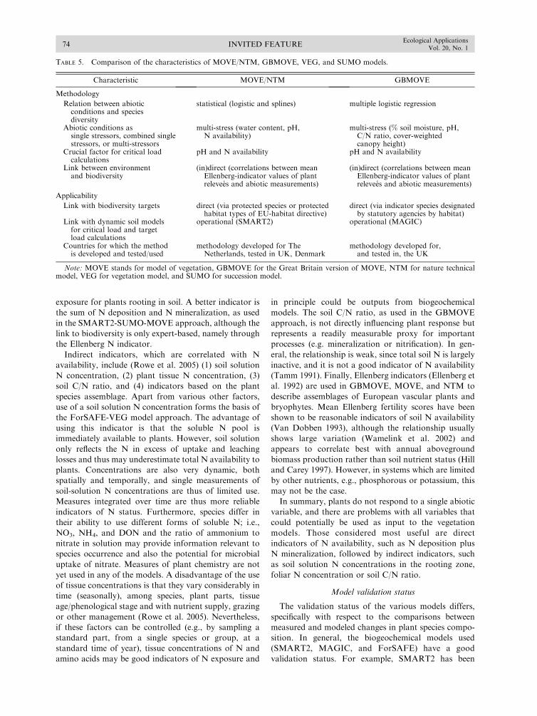
TABLE 5. Comparison of the characteristics of MOVE/NTM, GBMOVE, VEG, and SUMO models.

Characteristic MOVE/NTM GBMOVE

Methodology

Relation between abioticconditions and speciesdiversity

statistical (logistic and splines) multiple logistic regression

Abiotic conditions assingle stressors, combined singlestressors, or multi-stressors

multi-stress (water content, pH,N availability)

multi-stress (% soil moisture, pH,C/N ratio, cover-weightedcanopy height)

Crucial factor for critical loadcalculations

pH and N availability pH and N availability

Link between environmentand biodiversity

(in)direct (correlations between meanEllenberg-indicator values of plantrelevees and abiotic measurements)

(in)direct (correlations between meanEllenberg-indicator values of plantrelevees and abiotic measurements)

Applicability

Link with biodiversity targets direct (via protected species or protectedhabitat types of EU-habitat directive)

direct (via indicator species designatedby statutory agencies by habitat)

Link with dynamic soil modelsfor critical load and targetload calculations

operational (SMART2) operational (MAGIC)

Countries for which the methodis developed and tested/used

methodology developed for TheNetherlands, tested in UK, Denmark

methodology developed for,and tested in, the UK

Note: MOVE stands for model of vegetation, GBMOVE for the Great Britain version of MOVE, NTM for nature technicalmodel, VEG for vegetation model, and SUMO for succession model.

INVITED FEATURE74Ecological Applications

Vol. 20, No. 1

validated on the German ‘‘Solling site’’ and hundreds of

intensively monitored forest plots (De Vries et al. 2003).

Here we show that MAGIC is able to predict changes in

observed N leaching and soil C/N in plot-scale N

manipulation studies under different addition levels. The

ForSAFE model also shows a good correlation between

simulated and measured values of tree biomass, pools of

soil organic C and N, soil pH, and BC/Al ratios at 16

Swedish forest sites.

The validation status of the vegetation models is,

however, much less advanced. Biomass growth of

SUMO has until now only been validated on data

collected at a grassland site, a heathland site and a forest

site in The Netherlands and a grassland site in the

United Kingdom. Regarding (GB)MOVE, a preliminary

test was made whether GBMOVE in combination with

MAGIC could reproduce the observed species compo-

sition in test plots, including an unimproved neutral

grassland and a blanket bog. The comparisons of

predicted species occurrence using measured soil C/N

and pH vs. mean Ellenberg scores indicate that the

greatest uncertainty in model predictions, is due to the

weak calibration relationships, especially those between

soil C/N and mean Ellenberg N at high fertility. Current

model development is therefore focusing on the estab-

lishment of a direct relation between N indicators and

species composition. Finally, the ForSAFE-VEG model

has until now been validated at 16 Swedish forest sites,

by comparing simulated and measured values on the

ground occupancy of 42 plant groups, and in Switzer-

land. Considering the sometimes poor correlations in all

model applications, as described above, there is still a

need for substantial model validation and model

improvement. In this context, good model-testing data

are urgently needed.

Reliability of biogeochemistry–biodiversity modeling

approaches to assess critical loads

Up to now, only the SMART-MOVE model chain

has been used to assess critical loads by using the model

in an inverse way. Due to its complexity, the ForSAFE-

VEG model is more suited to predict response of plant

species composition to environmental change than to

predict critical loads. A major disadvantage is the fact

that the critical N load is influenced by the N deposition

history. The uncertainties in the assessed critical loads,

using the SMART-MOVE model chain, are specifically

due to uncertainties in the calibration equations between

abiotic conditions and Ellenberg scores, used to transfer

information between soil models and plant species

models. A detailed uncertainty analysis, focusing on

this aspect, was carried out by van Dobben et al. (2006).

Results show that the uncertainty in critical loads per

vegetation type is quite high (generally in a range of 15–

40% of the average value), but the ranges of simulated

and empirical values usually overlap, implying that the

results are applicable for practical purposes. However,

at the site level, uncertainty becomes very large and thus

it is not yet possible to determine critical loads with any

practical significance (Van Dobben et al. 2006). The

uncertainties can only be reduced if more data become

available on the abiotic response per species under field

conditions, at least for N availability and soil pH.

Despite the uncertainties in the described model

approaches, the approach provides a relevant addition

to empirical critical-load estimates. First of all, even

though empirical critical loads may be as good or even

better than modeled critical loads at present, dynamic

models allow us to explore impacts of future scenarios,

where habitats may face completely novel configurations

of multiple drivers, so-called ‘‘no analogue’’ states

TABLE 5. Extended.

VEG SUMO

mechanistic competition model (growth functions) mechanistic competition model (growth functions)

combined single stressors (water content, pH, N, P,light, temperature, grazing)

combined single stressors (water content, pH, N, P, light,grazing, management)

N concentration in soil solution, pH and Al concentration,and plant competition (light and nutrients)

N availability, pH and plant competition (light and nutrients)

indirect: model outcome as a result of differencesin species-specific growth functions

indirect: model outcome as a result of differences in planttype-specific growth functions

indirect by calculating a relevant indicator indirect: Only possible after link with a species model

link with dynamic models is operational (SAFE) and usedfor target load calculations

link with dynamic models is operational (SMART2) but can’tbe used for target load calculations

methodology developed and tested in Nordic countries methodology developed for The Netherlands, tested in UK

January 2010 75PERSPECTIVES ON THE MODERN N CYCLE

(Steffen et al. 2004). In these situations, empirical critical

loads that are based on reviews of contemporary and

historical data become may be increasingly inappropri-

ate and process based, detailed models are necessary.

Critical loads can be interpreted as a means of

identifying thresholds of ecosystem resilience (Gunder-

son 2000). Estimating resilience thresholds using linked

soil–vegetation models is therefore particularly appro-

priate, because of several key aspects associated with

ecosystem responses to perturbation. Threshold changes

and nonlinear responses to disturbance, species invasion

and changes in nutrient availability can result from the

dynamic interplay between above- and belowground

biota and differences in the extent to which soil and

vegetation store or more rapidly process and release

excess nutrients or buffer pH changes (Evans et al. 2001,

Craine et al. 2002). Hence resilience is a property related

to the ability of soil and vegetation to buffer or to

amplify the response to changing conditions. Quantify-

ing resilience and proximity to thresholds of change then

requires quantification of the dynamic relationships

between ecosystem compartments (e.g., Suding et al.

2008). Policy interest also focuses on timescales for

recovery; hence dynamic modeling is required to model

the persistence of alternative stable states that can result

when perturbations drive ecosystems into new domains

of stability (Gunderson 2000, Suding et al. 2004). While

it may be possible to identify critical ecosystem state

variables that are closely correlated with damage and

loss of adaptive capacity, these may be above or below

ground (e.g., Strengbom et al. 2001) once more

emphasizing the importance of jointly modeling soil

and vegetation. Lastly, the critical-load approach

increasingly recognizes that resilience is not realistically

thought of as a threshold situated along single or

multiple, yet independent, abiotic axes. Multiple drivers

and their interactions are important. For example, land

use around a nature reserve can change the composition

of the local species pool, increasing availability of

species that could capitalize on changes in soil con-

ditions driven by atmospheric pollutant deposition or

conversely, reducing the availability of desirable species

for recolonization following recovery and remediation

(Lindborg and Eriksson 2004). Dynamic model develop-

ment offers a way of incorporating other drivers as

modifiers of the critical-load range and allowing multi-

ple drivers to dynamically interact. The fully integrated,

mechanistic ForSAFE-VEG model is most appropriate

to investigate such interactions.

Measurements of plant species response

to environmental variables

Expert-based estimates of plant species responses to

environmental variables form the basis of all models.

Although the Ellenberg indicator system (Ellenberg et

al. 1992) or its derivates (Diekmann 2003) are the most

frequently used systems for this, their uncertainty is

quite large, it is sometimes unclear what the indicator

values represent, and they may be biased (Ertsen et al.

1998, Schaffers and Sykora 2000, Wamelink et al. 2002,

2003b, 2004, Witte and von Asmuth 2003, Smart and

Scott 2004). Furthermore, it requires a translation from

indicator values into soil chemical variables.

The most logical solution to avoid this highly

uncertain step is to replace the Ellenberg indicator

system by a system based on measurements (Wamelink

et al. 2002). On a small scale this was carried out for

France (Gegout et al. 2003) and The Netherlands

(Wamelink et al. 2005). Results are promising, but

Europe-wide and international data are needed, instead

of only national data to ensure a wide application. Such

data should consist of a vegetation description (releves)

and at least the following measured variables: geo-

graphical coordinates, soil acidity, nutrient status, and

water availability. Based on this, plant species response

per abiotic variable can be estimated, reviewed and

tested on independent datasets. The hypothesis that

plant species have different responses in different regions

can be tested on the basis of such data.

Relevant extensions to the modeling approaches

As mentioned above, in the SMART2/MAGIC-

(GB)MOVE/NTM model chain, model output is the

potential vegetation on a site, not accounting for time-

lag effects. Priorities for future work on modeling N

impacts on biodiversity in this model chain thus include

(1) inclusion of species-response curves based on

combined field measurements of vegetation releves and

abiotic data and (2) representation of lag times (e.g., due

to species persistence, dispersal).

The present linked-model approaches further centre

upon the impact of N deposition on existing species

assemblages. However, changes in resource availability

are also predicted to increase susceptibility to invasion

by immigrants, some of which could possess traits

associated with suppression of resident species and

changes in nutrient cycling (Evans et al. 2001, Davis et

al. 2005). If information about the composition of the

regional species pool is available, then model application

could be extended to estimate changes in habitat

suitability for potential immigrants. This would amount

to a risk assessment of the establishment of potential

invaders. Incorporating the dynamic impact of invasive

species on above and below-ground ecosystem compart-

ments is possible in the presented model approaches but

would require modification of the biomass growth

models in SUMO and ForSAFE/VEG.

Conclusions on the potential of linked biogeochemistry–

biodiversity modeling approaches

The following conclusions can be drawn regarding the

modeling approaches presented here:

1) Vegetation models, based on either large-scale

vegetation surveys (MOVE/GBMOVE, NTM) or

mainly experimental data (VEG), have been developed

and integrated with biogeochemical models, such as

INVITED FEATURE76Ecological Applications

Vol. 20, No. 1

SMART2 (either or not in connection with SUMO),

MAGIC, and ForSAFE.

2) There are large similarities between the models,

particularly those based on survey data, but there are

also several important differences, including (1) use of

different abiotic variables for N, such as N availability

and Ellenberg N indicators in SMART2-MOVE/NTM,

soil C/N ratio in GBMOVE, and soil-solution N in

ForSAFE, (2) prediction of individual plant species

(e.g., MOVE/GBMOVE) vs. plant communities (NTM),

and (3) calibration based on different (national) soil and

vegetation data sets.

3) At their current level of development, most

integrated models focus primarily on predicting the

biodiversity impacts of different scenarios in terms of

air-quality change and climate change.

4) The model chains can also predict biodiversity-

based critical loads or target loads. In doing this, the

definition of reference conditions and damage thresholds

for terrestrial biodiversity represents a major challenge.

Although the definition of biodiversity targets is an issue

for policy-makers, dynamic models can provide valuable

information on realistic reference conditions and achiev-

able recovery targets.

5) The reliance on Ellenberg indicator values, used as

a proxy for abiotic conditions in survey-based models

such as SMART2-MOVE and MAGIC-GBMOVE,

adds uncertainty to model predictions. However, Ellen-

berg values are likely to remain necessary in many areas

due to the insufficient European coverage of combined

vegetation and soil survey data.

6) Models based on survey data have largest potential

for country-wide mapping of critical loads in view of

their limited data demands. This holds not only for

Europe but also for other areas coping with elevated N

deposition, such as North America and China. How-

ever, testing and adaptation of the linkage between

vegetation and soil, using, e.g., Ellenberg indicators is

needed for other countries or ecosystems before large-

scale applications can be made. Furthermore, results are

quite reliable for vegetation types but at site level, the

uncertainty in critical loads becomes too large to be of

practical significance.

7) In combination, both empirical and model-based

critical loads, are powerful tools to assess a reliable

value for defined ecosystems. An example of such a

combination approach is presented by Van Dobben and

van Hinsberg (2008).

Despite the various limitations mentioned, this over-

view shows that linked biogeochemistry–biodiversity

models for N have great potential for applications to

support policies to reduce N inputs. Apart from further

model development, there is a need for further testing

and validation of the models against long-term mon-

itoring or long-term experimental data sets and against

large-scale survey data. In this context, the continuation

of existing programs, where possible with improved

integration of biotic and abiotic measurements, is

essential to the future development of this work. Finally,

there is a need for adaptation and upscaling of the

models beyond the regions for which dose-response

relationships have been parameterized, such as Medi-

terranean and Alpine regions, and Eastern Europe,

based on a focused data collection combing vegetation

descriptions with variables affecting the species diver-

sity. A similar approach outside Europe would also

allow the use of these models, both for predicting

impacts of scenarios and assessing critical loads.

ACKNOWLEDGMENTS

The publication of this paper has been partially supported bythe European Commission LIFE program within the frame-work of the European Consortium for Modelling Air Pollutionand Climate Strategies (EC4MACS), the trust fund for thepartial funding of effect-oriented activities under the Con-vention on Long-range Transboundary Air Pollution, and theU.S. Environmental Protection Agency. We also thank the twoanonymous reviewers for their detailed and helpful commentswhich largely improved the paper.

LITERATURE CITED

Achermann, B., and R. Bobbink, editors. 2003. Empiricalcritical loads for nitrogen: expert workshop, Berne, 11–13November 2002. Environmental Documentation 164. SwissAgency for Environment, Forest and Landscape, Berne,Switzerland.

Alkemade, J. R. M., J. Wiertz, and J. B. Latour. 1996.Kalibratie van Ellenbergs milieu-indicatiegetallen aan werke-lijk gemeten bodemfactoren. Rapport nr. 711901 016.Rijksinstituut voor volksgezondheid en milieu, Bilthoven,The Netherlands.

Amann, M., J. Cofala, C. Heyes, Z. Klimont, and W. Schopp.1999. The RAINS model: a tool for assessing regionalemission control strategies in Europe. Pollution Atmospher-ique 20:41–64.

Belyazid, S. 2006. Dynamic modelling of biogeochemicalprocesses in forest ecosystems. Dissertation. Reports inEcology and Environmental Engineering 2006:1. Departmentof Chemical Engineering, Lund University, Lund, Sweden.

Belyazid, S., O. Westling, and H. Sverdrup. 2006. Modellingchanges in forest soil chemistry at 16 Swedish coniferousforest sites following deposition reduction. EnvironmentalPollution 144:596–609.

Bobbink, R., M. Ashmore, S. Braun, W. Fluckiger, and I. J. J.van den Wyngaert. 2003. Empirical nitrogen critical loads fornatural and semi-natural ecosystems: 2002 update. Pages 43–170 in B. Achermann and R. Bobbink, editors. Empiricalcritical loads for nitrogen. Swiss Agency for Environment,Forest and Landscape, Berne, Switzerland.

Bobbink, R., et al. 2010. Global assessment of nitrogendeposition effects on terrestrial plant diversity: a synthesis.Ecological Applications 20:30–59.

Bobbink, R., M. Hornung, and J. G. M. Roelofs. 1998. Theeffects of air-borne nitrogen pollutants on species diversity innatural and semi-natural European vegetation. Journal ofEcology 86:717–738.

Braun-Blanquet, W. 1964. Pflanzensoziologie. Grundzuge derVegetationskunde. 3. Aufl. Springer, New York, New York,USA.

Clark, C. M., and D. Tilman. 2008. Loss of plant species afterchronic low-level nitrogen deposition to prairie grasslands.Nature 451:712–715.

Commission of the European Communities. 2003. Interpreta-tion manual of European Union habitats: EUR 25. DGEnvironment—Nature and Biodiversity. Commission of theEuropean Communities, Brussels, Belgium.

January 2010 77PERSPECTIVES ON THE MODERN N CYCLE

Cosby, B. J., R. C. Ferrier, A. Jenkins, and R. F. Wright. 2001.Modelling the effects of acid deposition: refinements, adjust-ments and inclusion of nitrogen dynamics in the MAGICmodel. Hydrology and Earth System Sciences 5:499–517.

Craine, J. M., D. Tilman, D. Wedin, P. Reich, M. Tjoelker, andJ. Knops. 2002. Functional traits, productivity and effects onnitrogen cycling of 33 grassland species. Functional Ecology16:563–574.

Davies, C. E., and D. Moss. 2002. EUNIS habitat classification.Centre for Ecology and Hydrology. 2001 Work Programme,Final report. European Environment Agency EuropeanTopic Centre on Nature Protection and Biodiversity, Paris,France.

Davis, M. A., K. Thompson, and J. P. Grime. 2005.Invasibility: the local mechanism driving community assem-bly and species diversity. Ecography 28:696–704.

De Vries, W., et al. 2007. Developments in modelling criticalnitrogen loads for terrestrial ecosystems in Europe. Report1382. Alterra Wageningen UR, Wageningen, The Nether-lands.

De Vries, W., G. J. Reinds, M. Posch, M. J. Sanz, G. H. M.Krause, V. Calatayud, J. P. Renaud, J. L. Dupouey, H.Sterba, P. Gundersen, J. C. H. Voogd, and E. M. Vel. 2003.Intensive monitoring of forest ecosystems in Europe.Technical Report 2003. UN/ECE and EC, Forest IntensiveMonitoring Coordinating Institute, Geneva, Switzerland.

Diekmann, M. 2003. Species indicator values as an importanttool in applied plant ecology: a review. Basic and AppliedEcology 4:493–506.

Elberse, W. T., J. P. van den Bergh, and J. P. G. Dirven. 1983.Effects of use and mineral supply on the botanicalcomposition and yield of old grassland on heavy-clay soil.Netherlands Journal of Agricultural Science 31:63–88.

Ellenberg, H., H. E. Weber, R. Dull, V. Wirth, W. Werner, andD. Paulißen. 1992. Zeigerwerte von Pflanzen in Mitteleuropa.Scripta Geobotanica 18:1–248.

Emmett, B. A. 2007. Nitrogen saturation of terrestrialecosystems: some recent findings and their implications forour conceptual framework. Water, Air, and Soil Pollution:Focus 7:99–109.

Ertsen, A. C. D., J. R. M. Alkemade, and M. J. Wassen. 1998.Calibrating Ellenberg indicator values for moisture, acidity,nutrient availability and salinity in The Netherlands. PlantEcology 135:113–124.

European Commission. 2005. Thematic strategy on air pollu-tion. Communication from the Commission to the Counciland the European Parliament. COM(2005) 446 final. Euro-pean Commission, Brussels, Belgium.

European Environment Agency. 2007. Halting the loss ofbiodiversity by 2010: proposal for a first set of indicators tomonitor progress in Europe. EEA Technical report 11/2007.Office for Official Publications of the European Commun-ities, Luxembourg.

Evans, C. D., S. J. M. Caporn, J. A. Carroll, M. G. Pilkington,D. B. Wilson, N. Ray, and N. Cresswell. 2006. Modellingnitrogen saturation and carbon accumulation in heathlandsoils under elevated nitrogen deposition. EnvironmentalPollution 143:468–478.

Evans, R. D., R. Rimer, L. Sperry, and J. Belnap. 2001. Exoticplant invasion alters nitrogen dynamics in an arid grassland.Ecological Applications 11:1301–1310.

Gegout, J. C., J. C. Herve, F. Houllier, and J. C. Pierrat. 2003.Prediction of forest soil nutrient status using vegetation.Journal of Vegetation Science 14:55–62.

Gunderson, L. H. 2000. Ecological resilience: in theory andapplication. Annual Review of Ecology and Systematics 31:425–439.

Hettelingh, J.-P., M. Posch, and P. A. M. de Smet. 2001. Multi-effect critical loads used in multi-pollutant reduction agree-ments in Europe. Water, Air, and Soil Pollution 130:1133–1138.

Hettelingh, J.-P., M. Posch, J. Slootweg, G. J. Reinds, T.Spranger, and L. Tarrason. 2007. Critical loads and dynamicmodelling to assess European areas at risk of acidificationand eutrophication. Water, Air, and Soil Pollution: Focus 7:379–384.

Hill, M. O., and P. D. Carey. 1997. Prediction of yield in theRothamsted Park Grass Experiment by Ellenberg indicatorvalues. Journal of Vegetation Science 8:579–586.

Janssen, P. H. M., and P. S. C. Heuberger. 1995. Calibration ofprocess-oriented models. Ecological Modelling 83:55–66.

Jenkinson, D. S., J. M. Potts, J. N. Perry, V. Barnett, K.Coleman, and A. E. Johnston. 1994. Trends in herbage yieldsover the last century on the Rothamsted long-term contin-uous hay experiment. Journal of Agricultural Science 122:365–374.

Kros, J. 2002. Evaluation of biogeochemical models at localand regional scale. Alterra 2002, Alterra scientific contribu-tions, Wageningen, The Netherlands.

Kros, J., G. J. Reinds, W. De Vries, J. B. Latour, and M. J. S.Bollen. 1995. Modelling abiotic site factors in response toatmospheric deposition and upward seepage. Pages 445–448in J. F. T. Schoute, P. A. Finke, F. R. Veeneklaas, and H. P.Wolfert, editors. Scenario studies for the rural environment.Kluwer, Dordrecht, The Netherlands.

Latour, J. B., and R. Reiling. 1993. A multiple stress model forvegetation (‘‘move’’): a tool for scenario studies and stand-ard-setting. Science of the Total Environment 134:1513–1526.

Latour, J. B., R. Reiling, and W. Slooff. 1994. Ecologicalstandards for eutrophication and dessication: perspectives fora risk assessment. Water, Air, and Soil Pollution 78:265–277.

Lindborg, R., and O. Eriksson. 2004. Historical landscapeconnectivity affects present plant species diversity. Ecology85:1840–1845.

Ludwig, D., B. Walker, and C. S. Holling. 1997. Sustainability,stability, and resilience. Conservation Ecology 1:7.

National Emission Ceilings Directive. 2001. Directive2001/81/EC of the European Parliament and of the Councilof 23 October 2001 on national emission ceilings for certainatmospheric pollutants. European Commission, Brussels,Belgium.

Nilsson, J., and P. Grennfelt. 1988. Critical loads for sulphurand nitrogen. Report from a Workshop held at SkoklosterSweden March 19–24 1988. Miljø rapport 1988: 15. NordicCouncil of Ministers, Copenhagen, Denmark.

Pakeman, R. J., C. L. Reid, J. J. Lennon, and M. Kent. 2008.Possible interactions between environmental factors indetermining species optima. Journal of Vegetation Science19:201–208.

Rowe, E. C., F. Moldan, B. A. Emmett, C. D. Evans, and S.Hellsten. 2005. Model chains for assessing impacts ofnitrogen on soils, waters and biodiversity: a review. Centrefor Ecology and Hydrology. Contract report project noC02887 for DEFRA (UK) project no. Cpea 19. Centre forEcology and Hydrology, Bangor, UK.

Roy, D. B., M. O. Hill, P. Rothery, and R. G. H. Bunce. 2000.Ecological indicator values of British species: an applicationof Gaussian logistic regression. Annales Botanici Fennici 37:219–226.

Schaffers, A. P., and K. V. Sykora. 2000. Reliability ofEllenberg indicator values for moisture, nitrogen and soilreaction: a comparison with field measurements. Journal ofVegetation Science 11:225–244.

Schaminee, J. H. J., A. H. F. Stortelder, and V. Westhoff. 1995.De vegetatie van Nederland 1. inleiding tot de plantenso-ciologie: grondslagen, methoden en toepassingen. OpulusPress, Uppsala, Sweden.

Schaminee, J. H. J., V. Westhoff, and G. van Wirdum. 1989.Naar een nieuw overzicht van de plantengemeenschappenvan Nederland. De Levende Natuur 90:204–209.

INVITED FEATURE78Ecological Applications

Vol. 20, No. 1

Schlutow, A., and P. Hubener. 2004. The BERN model:bioindication for ecosystem regeneration towards naturalconditions. Umwelt bundesamt. Research report 20085221.Umweltbundesamt, Berlin, Germany.

Schopp, W., M. Posch, S. Mylona, and M. Johansson. 2003.Long-term development of acid deposition (1880–2030) insensitive freshwater regions in Europe. Hydrology and EarthSystem Sciences 7:436–446.

Schouwenberg, E. P. A. G., H. Houweling, M. J. W. Jansen, J.Kros, and J. P. Mol-Dijkstra. 2000. Uncertainty propagationin model chains: a case study in nature conservancy. Alterra,Green World Research, Wageningen. Alterra rapport 1.Alterra, Wageningen, The Netherlands.

Slootweg, J., M. Posch, and J.-P. Hettelingh, editors. 2007.Critical loads of nitrogen and dynamic modelling: CCEProgress Report 2007. MNP Report 500090001. Coordina-tion Centre for Effects, Bilthoven, The Netherlands.

Smart, S. M., et al. 2005. Atmospheric nitrogen pollutionimpacts on biodiversity: phase 1. Model development andtesting. Final report to Department of the Environment,Food and Rural Affairs, Joint Nature Conservation Com-mittee and English Nature. Centre for Ecology andHydrology, Lancaster, UK

Smart, S. M., and W. A. Scott. 2004. Bias in Ellenberg indicatorvalues: problems with detection of the effect of vegetationtype. Journal of Vegetation Science 15:843–846.

Smart, S. M., W. A. Scott, J. Whittaker, C. Evans, and B.Emmett. 2003. Development and testing of linked soil–plantmodel systems. Pollution Umbrella Progress Report. May2003. Centre for Ecology and Hydrology, Bnagor, UK.

Spranger, T., J.-P. Hettelingh, J. Slootweg, and M. Posch. 2008.Modelling and mapping long-term risks due to reactivenitrogen effects: an overview of LRTAP convention activ-ities. Environmental Pollution 154:482–487.

Steffen, W., A. Sanderson, P. D. Tyson, J. Jager, P. A. Matson,B. Moore III, F. Oldfield, K. Richardson, H. J. Schellnhuber,B. L. Turner, and R. J. Wasson. 2004. Global change and theearth system: a planet under pressure. Springer-Verlag,Berlin, Germany.

Strengbom, J., A. Nordin, T. Nasholm, and L. Ericson. 2001.Slow recovery of boreal forest ecosystem following decreasednitrogen input. Functional Ecology 15:451–457.

Suding, K. N., I. W. Ashton, H. Bechtold, W. D. Bowman,M. L. Mobley, and R. Winkleman. 2008. Plant and microbecontribution to community resilience in a directionallychanging environment. Ecological Monographs 78:313–329.

Suding, K. N., K. L. Gross, and G. R. Houseman. 2004.Alternative states and positive feedbacks in restorationecology. Trends in Ecology and Evolution 19:46–53.

Sutton, M. A., J. N. Cape, B. Rihm, L. J. Sheppard, R. I.Smith, T. Spranger, and D. Fowler. 2003. The importance ofaccurate background atmospheric deposition estimates insetting critical loads for nitrogen. Pages 231–257 in B.Achermann and R. Bobbink, editors. Empirical critical loadsfor nitrogen. Proceedings of an Expert Workshop in Berne,Switzerland, November 11–13. Environmental Documenta-tion 164. Swiss Agency for the Environment, Forests andLandscape (SAEFL), Bern, Switzerland.

Sverdrup, H., S. Belyazid, B. Nihlgard, and L. Ericson. 2007.Modelling change in ground vegetation response to acid andnitrogen pollution, climate change and forest management atin Sweden 1500–2100 A.D. Water, Air, and Soil Pollution:Focus 7:163–179.

Tamm, C. O. 1991. Nitrogen in terrestrial ecosystems.Questions of productivity, vegetational changes and ecosys-tem stability. Springer-Verlag, Berlin, Germany.

Tietema, A., J. P. Mol Dijkstra, J. Kros, and W. De Vries. 2002.Dynamic nitrogen deposition thresholds during forest standdevelopments in a Douglas-fir forest analysed with twonitrogen models SMART2 and MERLIN. Hydrology andEarth System Sciences 6:375–382.

Tilman, D. 1987. Secondary succession and the pattern of plantdominance along experimental nitrogen gradients. EcologicalMonographs 57:189–214.

Van Dobben, H. F. 1993. Vegetation as a monitor fordeposition of nitrogen and acidity. Dissertation. Universityof Utrecht, Utrecht, The Netherlands.

Van Dobben, H. F., and A. van Hinsberg. 2008. Overzicht vankritische depositiewaarden voor stikstof, toegepast ophabitattypen en Natura 2000 gebieden. Alterra rapport1654. Alterra, Wageningen, The Netherlands.

Van Dobben, H. F., A. van Hinsberg, E. P. A. G. Schouwen-berg, M. J. W. Jansen, J. P. Mol-Dijkstra, H. J. J. Wieggers,J. Kros, and W. De Vries. 2006. Simulation of critical loadsfor nitrogen for terrestrial plant communities in TheNetherlands. Ecosystems 9:32–45.

Wallman, P., M. Svenssson, H. Sverdrup, and S. Belyazid.2005. ForSAFE: an integrated process-oriented forest modelfor long-term sustainability assessments. Forest Ecology andManagement 207:19–36.

Wamelink, G. W. W. 2007. Simulation of vegetation dynamicsas affected by nitrogen deposition. Pons and Looijen,Wageningen, The Netherlands.

Wamelink, G. W. W., P. W. Goedhart, J. Y. Frissel, R. M. A.Wegman, P. A. Slim, and H. F. van Dobben. 2007. Responsecurves for plant species and phytosociological classes. Alterrareport 1489. Alterra, Wageningen, The Netherlands.

Wamelink, G. W. W., P. W. Goedhart, and H. F. van Dobben.2004. Measurement errors and regression to the mean cannotexplain bias in average Ellenberg indicator values. Journal ofVegetation Science 15:847–851.

Wamelink, G. W. W., P. W. Goedhart, H. F. van Dobben, andF. Berendse. 2005. Plant species as predictors of soil pH:replacing expert judgement with measurements. Journal ofVegetation Science 16:461–470.

Wamelink, G. W. W., V. Joosten, H. F. van Dobben, and F.Berendse. 2002. Validity of Ellenberg indicator values judgedfrom physico-chemical field measurements. Journal ofVegetation Science 13:269–278.

Wamelink, G. W. W., C. J. F. ter Braak, and H. F. vanDobben. 2003a. Changes in large-scale patterns of plantbiodiversity predicted from environmental economic scenar-ios. Landscape Ecology 18:513–527.

Wamelink, G. W. W., H. F. van Dobben, and F. Berendse.2003b. Apparently we do need phytosociological classes tocalibrate Ellenberg indicator values! Journal of VegetationScience 14:619–620.

Wamelink, G. W. W., H. F. van Dobben, and F. Berendse.2009. Vegetation succession as affected by decreasing nitro-gen deposition, soil characteristics and site management: amodelling approach. Forest Ecology and Management 258:1762–1773.

Wiertz, J., J. van Dijk, and J. B. Latour. 1992. De MOVE-vegetatie module: De kans op voorkomen van 700 plante-soorten als functie van vocht, pH, nutrienten en zout. RIVMreport 711901006/IBN-DLO report no. IBN 92/24. RIVM,Wageningen, The Netherlands and IBN-DLO, Bilthoven,The Netherlands.

Witte, J. P. M., and J. R. von Asmuth. 2003. Do we really needphytosociological classes to calibrate Ellenberg indicatorvalues? Journal of Vegetation Science 14:615–618.

January 2010 79PERSPECTIVES ON THE MODERN N CYCLE