Use of image analysis in the measurement of finite strain by the normalized Fry method:

geological implications for the 'Zone Houill6re'

(Briangonnais zone, French Alps)

L. AILLERES, M. CHAMPENOIS, J. MACAUDIERE* AND J.M. BERTRAND

C.R.P.G.-C.N.R.S., 15 rue N-D des Pauvres, B.P. 20, 54501 Vandoeuvre les Nancy, France.

Abstract

Image analysis techniques are used to quantify finite strain in microconglomerates from the 'Zone Houill~re' (Brianqonnais Zone, French Alps) using the normalized Fry method. Two different techniques have been developed to extract the necessary parameters from quartz grains: the first uses an interactive videographic image analyser linked to a digitizer, and the second uses a semi-automatic image analyser algorithm working on numeric images. Comparison between these two techniques allows the data provided by the latter to be validated. Semi-automated image analysis is then employed to compute the characteristics of the finite strain ellipse as defined by the normalized Fry method. This has been tested on natural and simulated fabrics and gives accurate results. Finally, these techniques have been applied to samples from the French Alps, in an attempt to correlate the regional pattern of finite strain with deep seismic reflectors. This paper presents the preliminary results using finite strain data determined by image analysis processing.

KEYWORDS: image analysis, finite strain, normalized Fry method, French Alps.

Introduction

FINITE strain data can provide important information about the structure of a deformed terrane, such as strain intensity gradients close to a shear zone, or distribution of strain within a nappe complex. Many methods of finite strain determination exist, and are based either on grain-location analysis (Fry, 1979; Erslev, 1988) or on grain-shape analysis [Rf/qb method of Ramsay (1967) and Dunnet (1969); Panozzo methods (Panozzo, 1983, 1984); Feret diameters method of Lapique et al. (1988)]. These methods require different parameters to characterize the shape or location of the quartz grains or other strain markers (coordinates of the centres of mass,

* Alternative address: E.N.S.G., 94 ave De Lattre De Tassigny, BP 452, 54501 Nancy, France.

lengths of major and minor axes and their orientations, or location of whole boundaries of grains). In fact, all of these parameters can be computed from the whole boundary of a grain, if it is assumed to be an ellipse.

This paper deals with image analysis processes which allow (1) the extraction of grain boundary measurements from thin sections of microconglome- rates of the 'Zone Houi11~re' (Brianqonnais zone, French Alps) and (2) the computation of the finite strain ellipse using the normalized Fry method (Fry, 1979; Erslev, 1988). A third part presents preliminary geological implications concerning relationships between finite strain and deep seismic data.

Grain-boundary determination

Hardware equipment. Extraction of grain bound- ary information can be made using either a

Mineralogical Magazine, June 1995, Vol. 59, pp. 179-187 �9 Copyright the Mineralogical Society

180 L. AILLERES E T A L .

5

i /li~i~i~i~i~i~i~i~i~i~i~i~i~i~i~i~i~i~i,. ~ ~i~iiiiliiiiiiiiiiiiiiiiiiii!iii/i!iiiiii!i

a Configuration of the Videographic Analyser

3

4

b Configuration with Optimas

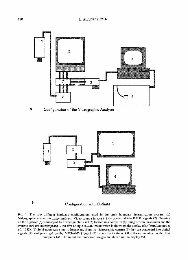
FIG. 1. The two different hardware configurations used in the grain boundary determination process. (a) Videographic interactive image analyser: Video camera images (1) are converted into R.G.B. signals (2). Drawing on the digitizer (6) is managed by a videographic card (3) located in a computer (4). Images from the camera and the graphic card are superimposed (7) to give a single R.G.B. image which is shown on the display (5). (From Lapique et al., 1988). (b) Semi-automatic system: Images are from the videographic camera (1) they are converted into digital signals (2) and processed by the MFG-AMVS board (3) driven by Optimas 4.0 software running on the host

computer (4). The initial and processed images are shown on the display (5).

MEASUREMENT OF FINITE STRAIN 181

Videographic Interactive Image Analyser (Lapique et al., 1988) or a Semi-Automatic Image Analyser.

The first configuration (Fig. la), using a videographic image analyser, has been developed by Lapique (1987) and Champenois (1989) at the CRPG (Nancy, France). By using a digitizing tablet, it allows the drawing of superimposed figures, such as grain boundaries or anything else, onto a videographic image. Thus, only the characteristics chosen by the operator are digitized and registered by the monitoring computer.

The second configuration (Fig. lb) uses image processing software called Optimas 4.0, distributed by Imasys Inc. This drives a graphic card (Modular Frame Grabber (MFG) from Imaging Tech. Inc.) linked to a variable-scan acquisition module (AMVS). This hardware is installed on a personal computer and allows the acquisition of images from a video camera. The signal provided by the camera is digitized by the frame grabber and the resulting image is displayed on a second screen. All subsequent image processes are carried out by Optimas 4.0 using the MFG-AMVS board on this numeric image.

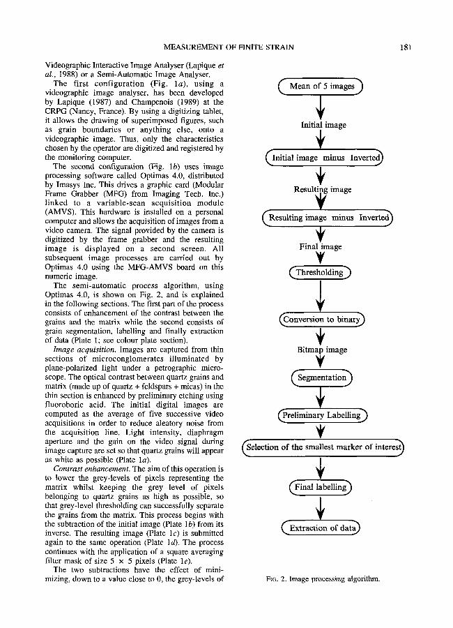
The semi-automatic process algorithm, using Optimas 4.0, is shown on Fig. 2, and is explained in the following sections. The first part of the process consists of enhancement of the contrast between the grains and the matrix while the second consists of grain segmentation, labelling and finally extraction of data (Plate 1; see colour plate section).

Image acquisition. Images are captured from thin sections of microconglomerates illuminated by plane-polarized light under a petrographic micro- scope. The optical contrast between quartz grains and matrix (made up of quartz + feldspars + micas) in the thin section is enhanced by preliminary etching using fluoroboric acid. The initial digital images are computed as the average of five successive video acquisitions in order to reduce aleatory noise from the acquisition line. Light intensity, diaphragm aperture and the gain on the video signal during image capture are set so that quartz grains will appear as white as possible (Plate la).

Contrast enhancement. The aim of this operation is to lower the grey-levels of pixels representing the matrix whilst keeping the grey level of pixels belonging to quartz grains as high as possible, so that grey-level thresholding can successfully separate the grains from the matrix. This process begins with the subtraction of the initial image (Plate lb) from its inverse. The resulting image (Plate lc) is submitted again to the same operation (Plate ld). The process continues with the application of a square averaging filter mask of size 5 x 5 pixels (Plate le).

The two subtractions have the effect of mini- mizing, down to a value close to 0, the grey-levels of

Mean of 5 images 3

Initial image

i,ial imago m nus Iovort

Resulting image V (Resulting image minus Inverted~

Final image

V (Thre sho ld ing )

~onvers ion to bina O

Bitmap image

V (So montation)

@reliminary Labelling~

~ election of the smallest marker of interest~

~ i n a l labelling 3

(Ext rac t ion of data~

F~G. 2. Image processing algorithm.

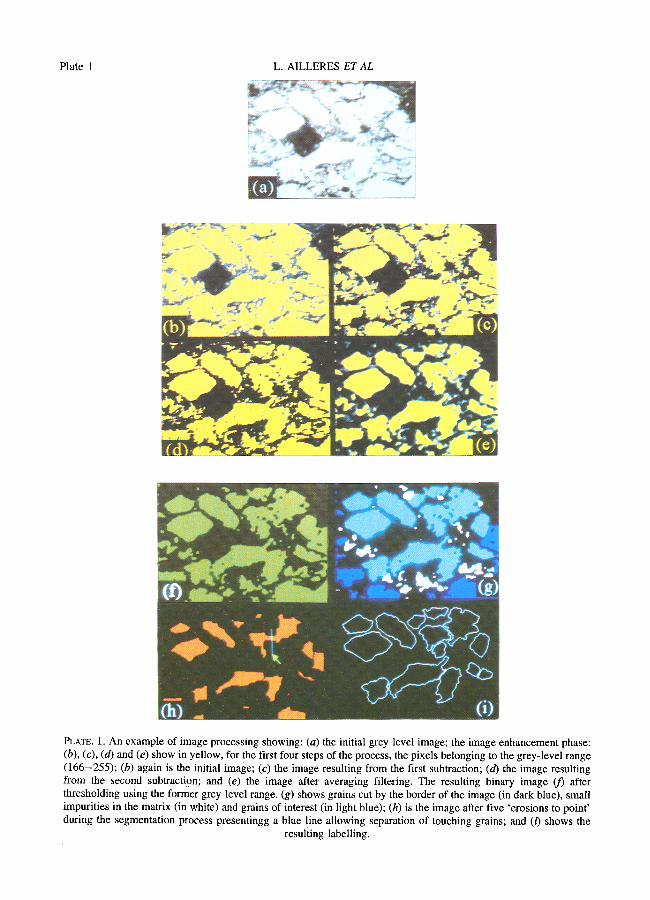
Plate 1 L. AILLERES ET AL

PLATE. 1. An example of image processing showing: (a) the initial grey-level image; the image enhancement phase: (b), (c), (d) and (e) show in yellow, for the first four steps of the process, the pixels belonging to the grey-level range (166-255); (b) again is the initial image; (c) the image resulting from the first subtraction; (d) the image resulting from the second subtraction; and (e) the image after averaging filtering. The resulting binary image (f) after thresholding using the former grey-level range. (g) shows grains cut by the border of the image (in dark blue), small impurities in the matrix (in white) and grains of interest (in light blue); (h) is the image after five 'erosions to point' during the segmentation process presentingg a blue line allowing separation of touching grains; and (0 shows the

resulting labelling.

182 L. AILLERES ETAL.

100000 - Init ia l I m a g e

Mean: 201 10000 -' / St. Dev." 66

1000 : [Var. : 4346 100j 10

1

[ ~ ] 0 64 128 192

I Finn image after ]

100000 - averaging mask I ,0000 i ]

1 /St.Dev.:102 | |

100 ~ 1

V ~ 0 64 128 192

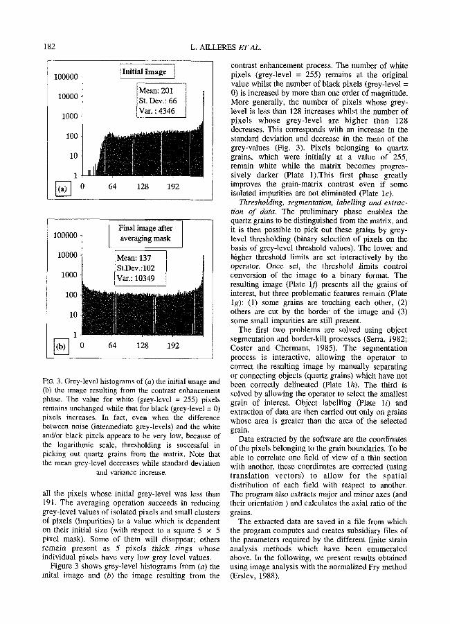
FIG. 3. Grey-level histograms of (a) the initial image and (b) the image resulting from the contrast enhancement phase. The value for white (grey-level = 255) pixels remains unchanged while that for black (grey-level = 0) pixels increases. In fact, even when the difference between noise (intermediate grey-levels) and the white and/or black pixels appears to be very low, because of the logarithmic scale, thresholding is successful in picking out quartz grains from the matrix. Note that the mean grey-level decreases while standard deviation

and variance increase.

all the pixels whose initial grey-level was less than 191. The averaging operation succeeds in reducing grey-level values of isolated pixels and small clusters of pixels (impurities) to a value which is dependent on their initial size (with respect to a square 5 x 5 pixel mask). Some of them will disappear; others remain present as 5 pixels thick rings whose individual pixels have very low grey level values.

Figure 3 shows grey-level histograms from (a) the inital image and (b) the image resulting from the

contrast enhancement process. The number of white pixels (grey-level = 255) remains at the original value whilst the number of black pixels (grey-level = 0) is increased by more than one order of magnitude. More generally, the number of pixels whose grey- level is less than 128 increases whilst the number of pixels whose grey-level are higher than 128 decreases. This corresponds with an increase in the standard deviation and decrease in the mean of the grey-values (Fig. 3). Pixels belonging to quartz grains, which were initially at a value of 255, remain white while the matrix becomes progres- sively darker (Plate 1).This first phase greatly improves the grain-matrix contrast even if some isolated impurities are not eliminated (Plate le).

Thresholding, segmentation, labelling and extrac- tion of data. The preliminary phase enables the quartz grains to be distinguished from the matrix, and it is then possible to pick out these grains by grey- level thresholding (binary selection of pixels on the basis of grey-level threshold values). The lower and higher threshold limits are set interactively by the operator. Once set, the threshold limits control conversion of the image to a binary format. The resulting image (Plate l f) presents all the grains of interest, but three problematic features remain (Plate lg): (1) some grains are touching each other, (2) others are cut by the border of the image and (3) some small impurities are still present.

The first two problems are solved using object segmentation and border-kill processes (Serra, 1982; Coster and Chermant, 1985). The segmentation process is interactive, allowing the operator to correct the resulting image by manually separating or connecting objects (quartz grains) which have not been correctly delineated (Plate l h). The third is solved by allowing the operator to select the smallest grain of interest. Object labelling (Plate 1i) and extraction of data are then carried out only on grains whose area is greater than the area of the selected grain.

Data extracted by the software are the coordinates of the pixels belonging to the grain boundaries. To be able to correlate one field of view of a thin section with another, these coordinates are corrected (using translat ion vectors) to allow for the spatial distribution of each field with respect to another. The program also extracts major and minor axes (and their orientation ) and calculates the axial ratio of the grains.

The extracted data are saved in a file from which the program computes and creates subsidiary files of the parameters required by the different finite strain analysis methods which have been enumerated above. In the following, we present results obtained using image analysis with the normalized Fry method (Erslev, 1988).

MEASUREMENT OF HNITE STRAIN 183

._ ..-.--__ 1+ ~., :_' .~-% - ,

~ . - d-:_T+ ,I ~~w,,-~ ;,+_.T_11

" - H - . . . . . - - - - - , ! ' ' - - ' ' - ~ + 7 - . ~ . ' . ' _ - H ~ - 7 - - M I

~ - . + . ~ - ~ 72:1' I I I - 1 ' - + q - l - I + - ~ + 7 . . . . .

J r l T _ ,` I,'.1 I 1 . . , I - I 'L--L ..: .--,--7~ a--. 7 ) . _ i -+'- ",' -~ : - - ' :-'-,--% +. -- '--h' U:-.- ,+ ~-. ---- +.7_--...,.--': .:7-~-~ -~

- ' - - - f , - - + I-- . -~ P- _]w'_~:~ ta:44.-,.?. ~_,. ~

j i i _1-.- - - r .IF' =Nk" ,- ; - . - .

_..._.! -~_'_.,.-~ .j-:.-..-,_-- #_-~~_-4::--+ ~-_-&+:, .._...-.+'_-.-~?~q- .-~ - _ > _ ~ - . - p . . . j . - : , ::.:-._:+.-~% _.- -:->-_ '_-:-t:::-' -LT_-t.+ :4:_-T~ ~' m m . ' s - c : ~ , ~ - b ! : - _ , : "-- ~ldJ7 +'- ,-: -~-,. -! ~ , -7,

b-_ 2 ~-;~ ;!~X ~,.,+

i4L~ %+ ~-+-Y

I

I . . . . - -+_~-++- .4 ---r q+l -I1"-1" -" ' "~ ' ~ - -- - �9 ~ . . . . i " , - i - + . , . , - . , I . + ~ - 7 ~ . - I~-~+. ---+-_ .-7~.,_ , . , - b - ] ,+t ~ :-q-;,:; . -:.-: -+-..-...+...,#:~,

I;+ ..... I-T fi-- , -'_ '. +-., -. -I. -T + . ---.AZ I

t::-~:+':+,4/+ -'%;'.t---:--:?,+l Iq 7:-:-:+ �9 ,.:-,._,:..:--_i

I . a . - t - - t , - _ . + 1 ' i - ' , ~ - " - + _ ~ " , |

+,I -~-:~-;" >+.. 4--7 . . . . ;7.-~ ,, "-%1 -~--+.~-: ":4---. -i i--:L.:-,-.-z.- ,' z_ ~:-_-7- !~- - - - , ' - - - - -+- -~v- t .~ ~_ .-, --e_:--. + ~ . - ~ , i : - & ~ - . , ~ ~+,~.~-b'-,,iP" "~' .-._--!:+..I -Z ' - - - . 1 ' - - [ - , ' _q - -~

-.--• S]--L~ .;~1 :~ '-- .~/ :~ --4..-;.-~+ ~.,-4'-[~1 4+_~u ,.L. ~-~44q1

e o j ~+ --4g+----:-+.4~--~ ~-31

|c-~;-:~ ~.-.r + -7-~-+-7e+ :T ,+1 .-._': +-.+_..-_ ~-Tu~.-.- ~_~.~4-:,~11 p I . - ] -~-""" - ' - - - - ) - i "' " - - . ' " ~-,<:-~ >:--~-'.-:+4~-4 .-+47,t

17;:! 'g:-:&-:~'-:q---7-+4:G::~+41 I - t - ~ . - - ! " . m + ~ @ = ~ q L �9 ' . , . - _ L . - - H I

I~---'------"-~I l---"-:,--::,:~-,q . - . . ~ .. -~ + . , _++ _ *

I-: -=7', '- ' , . , . ~ . ~ . ,..-• :-.+-~ I+--:7.~))<+-.-:~:'-,.:-;.%?+.-;I I . - . - - : : : + <--.. +---:--i--L-b7--.-,h)-!-I | . - + 7-~.+.+","- ~-: -'~'-#-, ~+1 l r - - u ~ - - ' , - - - t - : Lh - ' " - - - [ -+ : n L 3 , " - - ' - ' + - I

Lc3T-:4 +.,---, -- -~ ".~-~44 ,-+1

"4--' " ~!-t_ "1 1 " - " , - - 4 4 - ~ - T .- -. ,i.ff--i-i , - -_ 'q+ ' i , , ~ ' +" j - it~...-:,,. ,~_: :~--_-,--4_?_~_.7<~ �9 ~---- ~--4b/-:-?- ' -+' ,-:.---? -

2 5 ~ % ' : ?

I : I ' - " _ - t - ~ ' - 7 - . , ~ - S 4 - ~ - - b - q '

IH . ' 7 [ - ' -L~+" - - - - - - - ] i - ; - 1 -. _ . - ~ . 7 - - ] - - !.'

| ~ I+ -~q~--?+• 4' ' -"~~' i :4 ,tL.e -.-• " 7-; ' ~ "-"--+ -"~:-, -

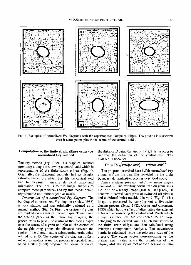
Fro. 4. Examples of normalized Fry diagrams with the superimposed computed ellipse. The process is successful even if some points plot in the centre of the central 'void'.

C o m p u t a t i o n of the f inite s train ell ipse us ing the n o r m a l i z e d Fry me tho d

The Fry method (Fry, 1979) is a graphical method providing a diagram showing a central void which is representative of the finite strain ellipse (Fig. 4). Originally, the structural geologist had to visually estimate the ellipse which best fits the central void and to measure manually its axial ratio and orientation. The idea is to use image analysis to compute these parameters and by this means obtain reproducible and more objective results.

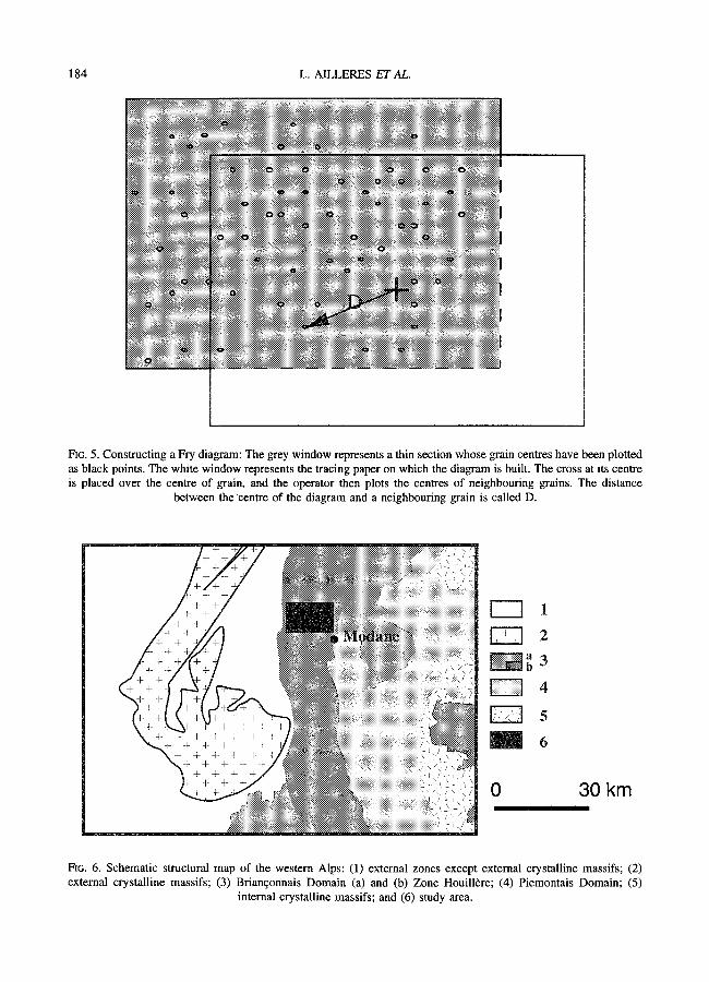
Construction of a normalized Fry diagram. The building of a normalized Fry diagram (Erslev, 1988) is very simple, and was originally designed as a manual method (Fig. 5). First, the centres of grains are marked on a sheet of tracing paper. Then, using the tracing paper as the future Fry diagram, the procedure is to place the centre of the tracing paper over the centre of a grain and plot all the centres of the neighbouring grains, the distance between the centre of the diagram and a neighbouring grain being refered to as D. The centre of the diagram is then moved to another grain, the process is repeated, and so on. Erslev (1988) proposed the normalization of

the distance D using the size of the grains, in order to improve the definition of the central void. The distance D becomes:

Dn = D / v / ( m a j o r axis) 2 + (minor a x i s ) 2

The program described here builds normalized Fry diagrams from the data file provided by the grain boundary determination process described above.

Image analysis process and finite strain ellipse computation. The resulting normalized diagram takes the form of a binary image (100 x 100 pixels). It contains a central void (area of switched off pixels) and additional holes outside this void (Fig. 4). This image is processed by carrying out a five-order closing process (Serra, 1982; Coster and Chermant, 1985) which has the effect of eliminating the external holes while conserving the central void. Pixels which remain switched off are considered to be those belonging to the central void. The characteristics of the finite strain ellipse are then calculated using Principal Components Analysis. The covariance matrix is calculated using the reference axes of the display. The eigen vector corresponding to the greater eigen value gives the orientation of the ellipse, while the square root of the eigen values ratio

184 L. AILLERES ET AL.

FI~. 5. Constructing a Fry diagram: The grey window represents a thin section whose grain centres have been plotted as black points. The white window represents the tracing paper on which the diagram is built. The cross at its centre is placed over the centre of grain, and the operator then plots the centres of neighbouring grains. The distance

between the centre of the diagram and a neighbouring grain is called D.

I I 1 ES~]2

4

~ 5 6

0 30 km

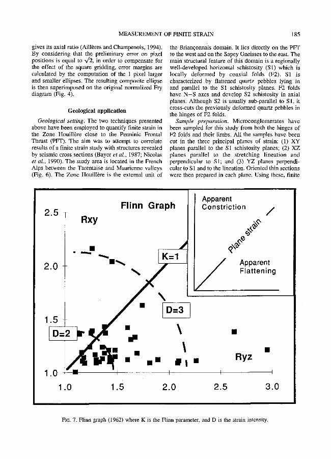
FIG. 6. Schematic structural map of the western Alps: (1) external zones except external crystalline massifs; (2) external crystalline massifs; (3) Brianqonnais Domain (a) and (b) Zone Houill~re; (4) Piemontais Domain; (5)

internal crystalline massifs; and (6) study area.

MEASUREMENT OF FINITE STRAIN 185

gives its axial ratio (Aill~res and Champenois, 1994). By considering that the preliminary error on pixel positions is equal to x/~, in order to compensate for the effect of the square gridding, error margins are calculated by the computation of the 1 pixel larger and smaller ellipses. The resulting composite ellipse is then superimposed on the original normalized Fry diagram (Fig. 4).

Geological application

Geological setting. The two techniques presented above have been employed to quantify finite strain in the Zone Houill~re close to the Penninic Frontal Thrust (PFT). The aim was to attempt to correlate results of a finite strain study with structures revealed by seismic cross sections (Bayer et aL, 1987; Nicolas et al., 1990). The study area is located in the French Alps between the Tarentaise and Maurienne valleys (Fig. 6). The Zone Houill~re is the external unit of

the Brianqonnais domain. It lies directly on the PFT to the west and on the Sapey Gneisses to the east. The main structural feature of this domain is a regionally well-developed horizontal schistosity ($1) which is locally deformed by coaxial folds (F2). S1 is characterized by flattened quartz pebbles lying in and parallel to the S1 schistosity planes. F2 folds have N - S axes and develop $2 schistosity in axial planes. Although $2 is usually sub-parallel to S 1, it cross-cuts the previously deformed quartz pebbles in the hinges of F2 folds.

Sample preparation. Microconglomerates have been sampled for this study from both the hinges of F2 folds and their limbs. All the samples have been cut in the three principal planes of strain: (1) XY planes parallel to the $1 schistosity planes; (2) XZ planes parallel to the stretching lineation and perpendicular to S1; and (3) YZ planes perpendi- cular to S 1 and to the lineation. Oriented thin sections were then prepared in each plane. Using these, finite

2.5 T

I 2.o[ Rxy

Flinn Graph

K=I

\ [] D=3

�9 m um nlPl ,,,m ~

1.0

1.0

Apparent Constrict ion

/

/

J Apparent Flattening

[]

�9 Ryz

I I

1.5 2.0 2.5 3.0

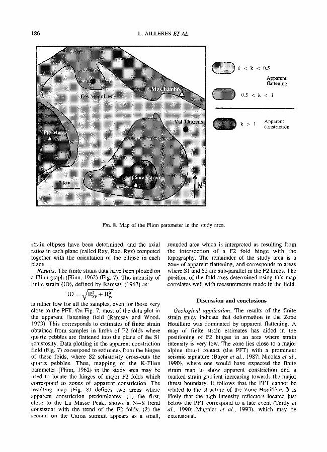
FIG. 7. Flinn graph (1962) where K is the Flinn parameter, and D is the strain intensity.

186 L. AILLERES ET AL.

0 < k < 0 . 5

App~ent flattenmg

~ 0 . 5 < k < l

O Apparent k > l constriction

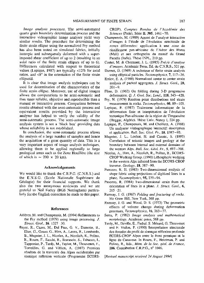
FIG. 8. Map of the Flinn parameter in the study area.

strain ellipses have been determined, and the axial ratios in each plane (called Rxy, Rxz, Ryz) computed together with the orientation of the ellipse in each plane.

Results . The finite strain data have been plotted on a Flinn graph (Flinn, 1962) (Fig. 7). The intensity of finite strain (ID), defined by Ramsay (1967) as:

is rather low for all the samples, even for those very close to the PFT. On Fig. 7, most of the data plot in the apparent flattening field (Ramsay and Wood, 1973). This corresponds to estimates of finite strain obtained from samples in limbs of F2 folds where quartz pebbles are flattened into the plane of the S 1 schistosity. Data plotting in the apparent constriction field (Fig. 7) correspond to estimates from the hinges of these folds, where $2 schistosity cross-cuts the quartz pebbles. Thus, mapping of the K-Flinn parameter (Flinn, 1962) in the study area may be used to locate the hinges of major F2 folds which correspond to zones of apparent constriction. The resulting map (Fig. 8) defines two areas where apparent constriction predominates: (1) the first, close to the La Masse Peak, shows a N - S trend consistent with the trend of the F2 folds; (2) the second on the Caron summit appears as a small,

rounded area which is interpreted as resulting from the intersection of a F2 fold hinge with the topography. The remainder of the study area is a zone of apparent flattening, and corresponds to areas where SI and $2 are sub-parallel in the F2 limbs. The position of the fold axes determined using this map correlates well with measurements made in the field.

Discussion and conclusions

Geological application. The results of the finite strain study indicate that deformation in the Zone Houill~re was dominated by apparent flattening. A map of finite strain estimates has aided in the positioning of F2 hinges in an area where strain intensity is very low. The zone lies close to a major alpine thrust contact (the PFT) with a prominent seismic signature (Bayer et al., 1987; Nicolas et al., 1990), where one would have expected the finite strain map to show apparent constriction and a marked strain gradient increasing towards the major thrust boundary. It follows that the PVI" cannot be related to the structure of the Zone Houill~re. It is likely that the high intensity reflectors located just below the PFr correspond to a late event (Tardy et al., 1990; Mugnier et al., 1993), which may be extensional.

MEASUREMENT OF FINITE STRAIN 187

Image analysis processes. The semi-automated quartz grain boundary determination process and the interactive videographic image analyser yield very similar results. The procedure for determining the finite strain ellipse using the normalized Fry method has also been tested on simulated fabrics, initially isotropic and subsequently deformed with a super- imposed shear coefficient of up to 2 (resulting in an axial ratio of the finite strain ellipses of up to 6). Differences calculated with respect to theoretical values (Lapique, 1987) are typically <12% for axial ratios, and <8 ~ in the orientation of the finite strain ellipsoid.

It is clear that image analysis techniques can be used for determination of the characteristics of the finite strain ellipse. Moreover, use of digital images allows the computations to be semi-automatic and thus more reliable, objective and reproducible than a manual or interactive process. Comparison between results obtained with the semi-automatic process and equivalent results provided by the interactive analyser has helped to verify the validity of the semi-automatic process. The semi-automatic image analysis system is not a 'black box' providing data whose reliability is not established.

In conclusion, the semi-automatic process allows the analysis of a large number of samples and hence the acquisition of a great quantity of data. This is a very important aspect of image analysis techniques, allowing them to be applied regionally to large geological areas such as the Zone Houill6re (the size of which is ~ 200 x 20 km).

Acknowledgements

We would like to thank the C.R.P.G. (C.N.R.S.) and the E.N.S.G. (Ecole Nationale Sup6rieure de G6ologie) for their financial supports. We thank also the two anonymous reviewers and we are grateful to Neil Fortey (BGS Nottingham) particu- larly for the English correction he made to this paper.

References

Aill~res, M. and Champenois, M. (1994) Refinements to the Fry method (1979) using image processing. 3". Struct. Geol., 16, 1327-30.

Bayer, R., Cazes, M., Dal Piaz, G. V., Damotte, B., Elter, G., Gosso, G., Hirn, A., Lanza, R., Lombardo, B., Mugnier, J. L., Nicolas, A., Nicolich, R., Polino, R., Roure, F., Sacchi, R., Scarascia, S,, Tabacco, I., Tapponier, P., Tardy, M., Taylor, M., Thouvenot, F., Torreilles, G. and Villien, A. (1987) Premiers r6sultats de la travers6e des Alpes occidentales par sismique reflexion verticale (Programme ECORS-

CROP). Comptes Rendus de l'Acaddmie des Sciences (Paris), S6rie II, 305, 1461-70.

Champenois, M. (1989) Apport de l'analyse interactive d'images ~ l'6tude de l'6volution structurale de zones d6form6es: application ~ une zone de cisaillement pan-africaine de l'Adrar des Iforas (Mali) et aux orthogneiss du massif du Grand Paradis (Italie). Th~se INPL, 210 pp.

Coster, M. & Chermant, J. L. (1985) Prdcis d'analyse d'images. Academic Press, Ed. du C.N.R.S., 521 pp.

Dunnet, D. (1969) A technique of finite strain analysis using elliptical particles. Tectonophysics, 7, 117-36.

Erslev, E. A. (1988) Normalized center to center strain analysis of packed aggregates. J. Struct. Geol., I0, 201-9.

Flinn, D. (1962) On folding during 3-D progressive deformation. Q. J. Geol. Soc. Lond., 118, 345-428.

Fry, N. (1979) Random point distributions and strain measurement in rocks. Tectonophysics, 60, 89--105.

Lapique, F. (1987) Traitement informatique de la d6formation finie et interpt6tation de l'6volution tectonique Pan-africaine de la r6gion de Timgaouine (Hoggar, Alg6rie). Thbse Univ. Nancy I, 224 pp.

Lapique, F., Champenois, M. and Cheilletz, A. (1988) Un analyseur vid6ographique interactif: description et application. Bull. Soc. Gdol. Fr., 18, 1387-93.

Mugnier, J. L., Loubat, H. and Cannic, S. (1993) Correlation of seismic images and geology at the boundary between internal and external domains of the western Alps. Bull, Soc. Gdol. Fr., 5, 697--708.

Nicolas, A., Hirn, A., Nicolich, R., Polino, R., ECORS- CROP Working Group. (1990) Lithospheric wedging in the western Alps inferred from the ECORS-CROP traverse. Geology, 18, 587-90.

Panozzo, R. H. (1983) Two-dimensionnal analysis of shape fabric using projections of digitized lines in a plane. Tectonophysics, 95, 279-94.

Panozzo, R. (1984) Two-dimensional strain from the orientation of lines in a plane. J. Struct. Geol., 6, 215-21.

Ramsay, J. G. (1967) Folding and fracturing of rocks. Mc Graw Hill, New York, 568 pp.

Ramsay, J. G. and Wood, D. S. (1973) The geometric effects of volume change during deformation processes, Tectonophysics, 16, 263-77.

Serra, P. (1982) Image analysis and mathematical morphology. Academic press, 568 pp.

Tardy, M., Deville, E., Fudral, S. M6nard, G. Thouvenot and F. Vialon, P. (1990) Interpr6tation structurale des donn6es du profil de sismique r6flexion profonde ECORS-CROP Alpes entre le front pennique et la ligne du Canavese. In Roure, F., Heiztman, P. and Polino, R., Eds., Mdm. de la Soc. g~ol. de France, 186. Contribution C.R.P.G., n ~ 1046.

[Revised manuscript received 24 August 1994]