Use of Range and Reflectance Data to Find Planar Surface Regions

IEEE TRANSACTIONS ON PATTERN ANALYSIS AND MACHINE INTELLIGENCE, VOL. PAMI-1, NO. 3, JULY 1979

cating the likelihoods of each of the possible descriptions. Theappropriate entries of the GCM are not simply incremented byone. Instead, the product of the corresponding descriptorprobabilities is added to the current entry value.

REFERENCES

[1] A. Hanson, E. Riseman, and P. Nagin, "Region growing in texturedoutdoor scenes," Computer and Information Sciences, TR-75C-3,1975.

[21 R. Haralick, K. Shanmugam, and I. Dinstein, "Texture features forimage classification," IEEE Trans. Syst., Man, Cybern., vol. SMC-3,pp. 610-622, 1973.

[3] A. Rosenfeld and A. Kak, Digital Picture Processing. New York:Academic, 1976.

[4] J. Maleson, C. Brown, and J. Feldman, "Understanding naturaltexture," in Proc. DARPA Image Understanding Workshop, PaloAlto, CA, 1977, pp. 19-27.

[5] D. Marr, "Early processing of visual information," Phil. Trans.Roy. Soc. B, to be published.

[61 S. Zucker, A. Rosenfeld, and L. Davis, "Picture segmentation bytexture discrimination," IEEE Trans. Comput., vol. C-24, pp.1228-1 233, 1975.

[71 P. Chen and T. Pavlidis, "Segmentation by texture using a split-and-merge algorithm," presented at the IEEE Workshop PatternRecognition and Artificial Intelligence, Princeton, NJ, 1978.

[81 R. Kirsch, "Computer determination of the constituent structureof biological images," Comput. Biomed. Res., vol. 4, 1971.

Larry S. Davis, for a photograph and biography, see p. 72 of the January1979 issue of this TRANSACTIONS.

Steven A. Johns was born in Lamarque, TX, onJuly 12, 1955. He received the B.S. degree incomputer science from the University of Hous-ton, Houston, TX, in 1976, and the M.A. de-gree in computer science from the University ofTexas at Austin in 1978.During the summers of 1975-1977 he worked

as an Engineer's Assistant at Aamoco TexasRefining Company in Texas City, TX. He iscurrently a Biostatistical Systems Analyst atAbbott Laboratories, Dallas, TX.

J. K. Aggarwal (S'62-M'65-SM'74-F'76), for a photograph and biog-raphy, see p. 135 of the April 1979 issue of this TRANSACTIONS.

Use of Range and Reflectance Data to Find PlanarSurface Regions

RICHARD 0. DUDA, SENIOR MEMBER, IEEE, DAVID NITZAN, SENIOR MEMBER, IEEE, AND PHYLLIS BARRETT

Abstract-This paper describes a sequential procedure for processingregistered range and intensity data to detect and extract regions thatcorrespond to planar surfaces in a scene.

Index Tenns-Hough transform, laser rangefinder, planar surfaces,planarity test, range data, region analysis, scene analysis, segmentation.

I. INTRODUCTIONIN [1] we described a scanning laser sensor that can provide

precisely registered arrays of intensity and range data.Using these data, we developed simple procedures for findingoutlines of occluding objects, obtaining normal views of planarsurfaces of known orientations, and finding regions corre-sponding to horizontal surfaces of known heights [1I, [2]. In

Manuscript received June 2, 1978; revised October 23, 1978. Thiswork was supported by the National Science Foundation under GrantENG 76-84623.The authors are with the Artificial Intelligence Center, SRI Inter-

national, Menlo Park, CA 94025.

this paper we describe automatic procedures for using suchdata to partition the scene into regions corresponding to arbi-trarily oriented planar surfaces with no a priori knowledgeabout them. As before, our primary concern is with the ex-traction of low-level representations of surfaces for subsequentthree-dimensional scene analysis.Several problems conspire to make scene analysis a difficult

task:1) Resolution and noise limitations of the sensors.2) Quantization errors due to constraints of memory size

and processing time.3) Variability in illumination-shading, shadows, highlights,

reflections, and secondary illumination.4) Variability in surface reflectance-markings, dirt and

smudges, and microstructures loosely referred to as "texture."5) Variability in the shapes and sizes of objects of the same

type.6) Variability in the image of a given object due to transla-

tion, rotation, and projection.

0162-8828/79/0700-0259$00.75 i 1979 IEEE

259


7) Occlusion of some objects in the scene by other objects,or by other parts of the same objects.No existing scene analysis programs can cope with all of

these problems simultaneously. The performance of any sceneanalysis program is ultimately limited by the nature and thequality of the input data. Traditional scene analysis programs(which are surveyed in [3] -[6]) use only intensity data re-ceived by visual sensors, such as television cameras. Theimages are typically monochromatic, although some sceneanalysis work has exploited color [7]-[14]. Similarly, mostof the programs treat single images, although multiple imageshave been analyzed for change detection [15] -[17], motion(surveyed in [18] ), and stereo [19] -[31 ] .Stereo augments intensity data with valuable range data.

Most of the work on the analysis of stereo images has focusedon the problem of finding effective and efficient methods formatching pairs of image points, each pair corresponding to thesame physical point in the scene. This difficult correspon-dence problem can be eliminated by using an active rangesensor.The two most popular active range measuring methods are

based on light-sheet triangulation and time-of-flight of light(optical radar). Using light-sheet triangulation methods, Willand Pennington [32] used Fourier spectra to find planar sur-faces in a scene; Shirai and Suwa [33] demonstrated recogni-tion of simple polyhedra; Agin and Binford [34] and Nevatiaand Binford [35] described curved objects with generalizedcylinders; Shirai [36] described objects by polyhedra; Rocker[37] and Rocker and Kiessling [38] extracted planes and usedtheir features in a sequential model matching procedure; Pop-plestone et al. [39] used a hypothesis-driven procedure tobuild models out of planar and cylindrical faces; Ishii andNagata [40] followed boundaries to recognize objects foracquisition by a robot hand; Kiesling [41] extracted objectboundaries by detecting breaks in intersecting lines computedfrom data points seen by the TV camera; and Sugihara andShirai [42] showed that a dictionary of Huffman/Clowes-type edge labels can be used to find missing edges and to seg-ment range data.The performance of light-sheet triangulation methods is lim-

ited primarily by the inherent drawbacks of triangulationrange finding: inaccurate range values for distant targets, andmissing data for close targets seen by the light source but notby the TV camera, or vice versa. These drawbacks are elim-inated by using range finding based on time of flight of light.This can be done either by pulse techniques [43], [44] or bymodulation techniques. Our work using modulation tech-niques, described in [1], [2], is summarized below.By scanning the scene with a modulated laser beam and mea-

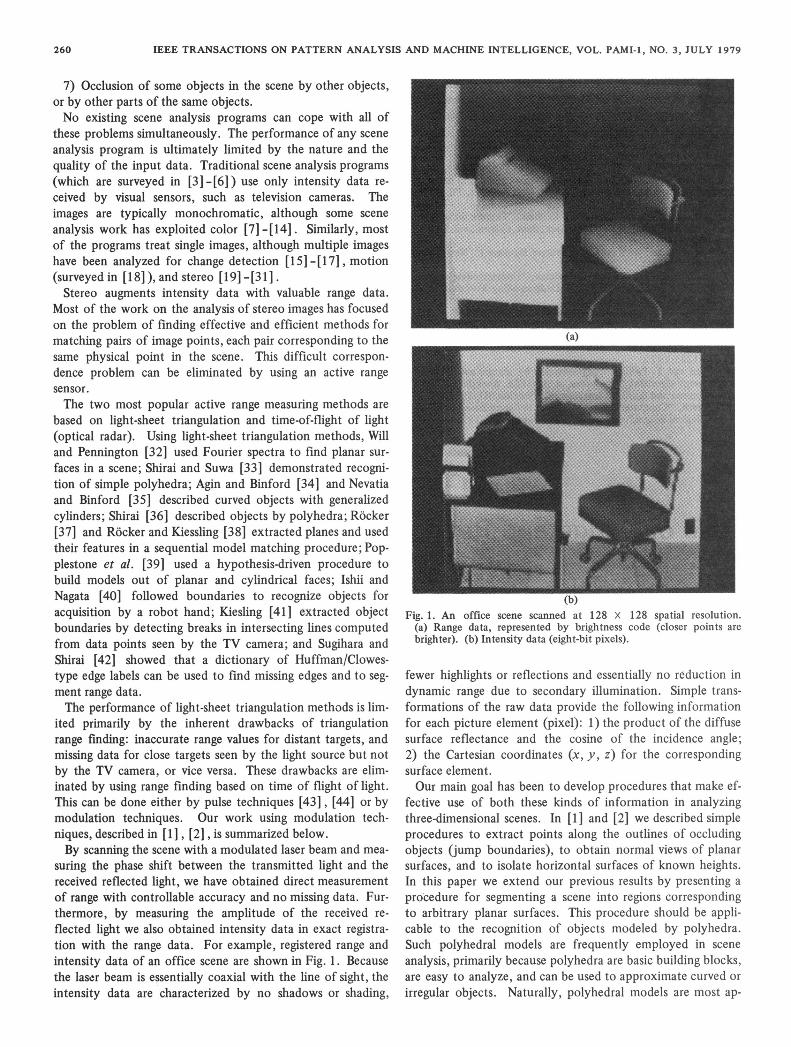
suring the phase shift between the transmitted light and thereceived reflected light, we have obtained direct measurementof range with controllable accuracy and no missing data. Fur-thermore, by measuring the amplitude of the received re-flected light we also obtained intensity data in exact registra-tion with the range data. For example, registered range andintensity data of an office scene are shown in Fig. 1. Becausethe laser beam is essentially coaxial with the line of sight, theintensity data are characterized by no shadows or shading,

Fig. 1. An office scene scanned at 128 X 128 spatial resolution.(a) Range data, represented by brightness code (closer points arebrighter). (b) Intensity data (eight-bit pixels).

fewer highlights or reflections and essentially no reduction indynamic range due to secondary illumination. Simple trans-formations of the raw data provide the following informationfor each picture element (pixel): 1) the product of the diffusesurface reflectance and the cosine of the incidence angle;2) the Cartesian coordinates (x, y, z) for the correspondingsurface element.Our main goal has been to develop procedures that make ef-

fective use of both these kinds of information in analyzingthree-dimensional scenes. In [ 1 ] and [2] we described simpleprocedures to extract points along the outlines of occludingobjects (jump boundaries), to obtain normal views of planarsurfaces, and to isolate horizontal surfaces of known heights.In this paper we extend our previous results by presenting aprocedure for segmenting a scene into regions correspondingto arbitrary planar surfaces. This procedure should be appli-cable to the recognition of objects modeled by polyhedra.Such polyhedral models are frequently employed in sceneanalysis, primarily because polyhedra are basic building blocks,are easy to analyze, and can be used to approximate curved orirregular objects. Naturally, polyhedral models are most ap-

260

DUDA et al.: USE OF RANGE AND REFLECTANCE DATA

propriate when the objects are basically polyhedral, as is oftenthe case in man-made environments. Our approach to findingplanar surface regions in a scene is a simple one of sequentialextraction. In general, it closely resembles the methods de-veloped by Tomita et al. [45] for partitioning textured im-ages, and by Ohlander [10] and Price [17] for partitioningcolor pictures. For each significant planar surface region inthe scene, we first use an appropriate histogram technique tofind a starting plane that describes the surface approximately,and then refine the fitting of that plane to the data by aniterative procedure. We segment the scene by sequentially re-moving regions of good fit. Our strategy requires that reliableregions be extracted before any questionable regions areanalyzed.The remainder of this paper is organized as follows. In Sec-

tion II we describe the basic iterative procedure that we use torefine the plane for each planar surface region. We use thisrefinement procedure in Section III to partition a scene intoregions that correspond to horizontal, vertical, and slantedplanar surfaces. Finally, in Section IV we summarize the re-sults reported in this paper and suggest directions for futurework.

II. A PROCEDURE FOR REFINING STARTING PLANESIn this section we give a detailed description of our iterative

procedure for refining the starting plane for every significantregion in the scene. We defer the question of how to obtainthe starting plane to the next section because different histo-grams and different techniques are employed for horizontal,vertical, and slanted surfaces. We shall use the scene shown inFig. 1 throughout this section to illustrate the steps of theprocedure.Let RT, called the retina, denote the complete array of

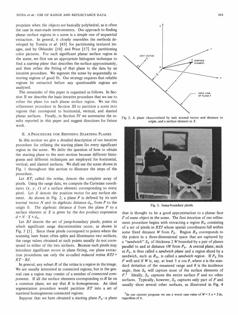
pixels. Using the range data, we compute the Cartesian coordi-nates (x, y, z) of a surface element corresponding to everypixel. Let X denote the position vector for any surface ele-ment. As shown in Fig. 2, a plane P is defined by its unitnormal vector N and its algebraic distance do, from P to theorigin 0. The algebraic distance d from the plane P to asurface element at X is given by the dot product expressiond=N*X+do.Let RJ denote the set of jump-boundary pixels, points at

which significant range discontinuities occur, as shown inFig. 3 [1]. Since these pixels correspond to points where thescanning laser beam often splits and illuminates two surfaces,the range values obtained at such points usually do not corre-spond to either of the two surfaces. Because such pixels mayintroduce significant errors in plane fitting, our plane extrac-tion procedures use only the so-called reduced retina RTJ=RT- RJ.

In general, any subset R of the retina is a region in the image.We are usually interested in connected regions, but in the gen-eral case a region may consist of a number of connected com-ponents. If all the surface elements corresponding to R lie ona common plane, we say that R is homogeneous. An idealsegmentation procedure would partition RT into a set ofmaximal homogeneous connected regions.Suppose that we have obtained a starting plane PO-a plane

z

EDGE VIEWOF PLANE P

Fig. 2. A plane characterized by unit normal vector and distance toorigin, and a surface element at X.

Fig. 3. Jump-boundary pixels.

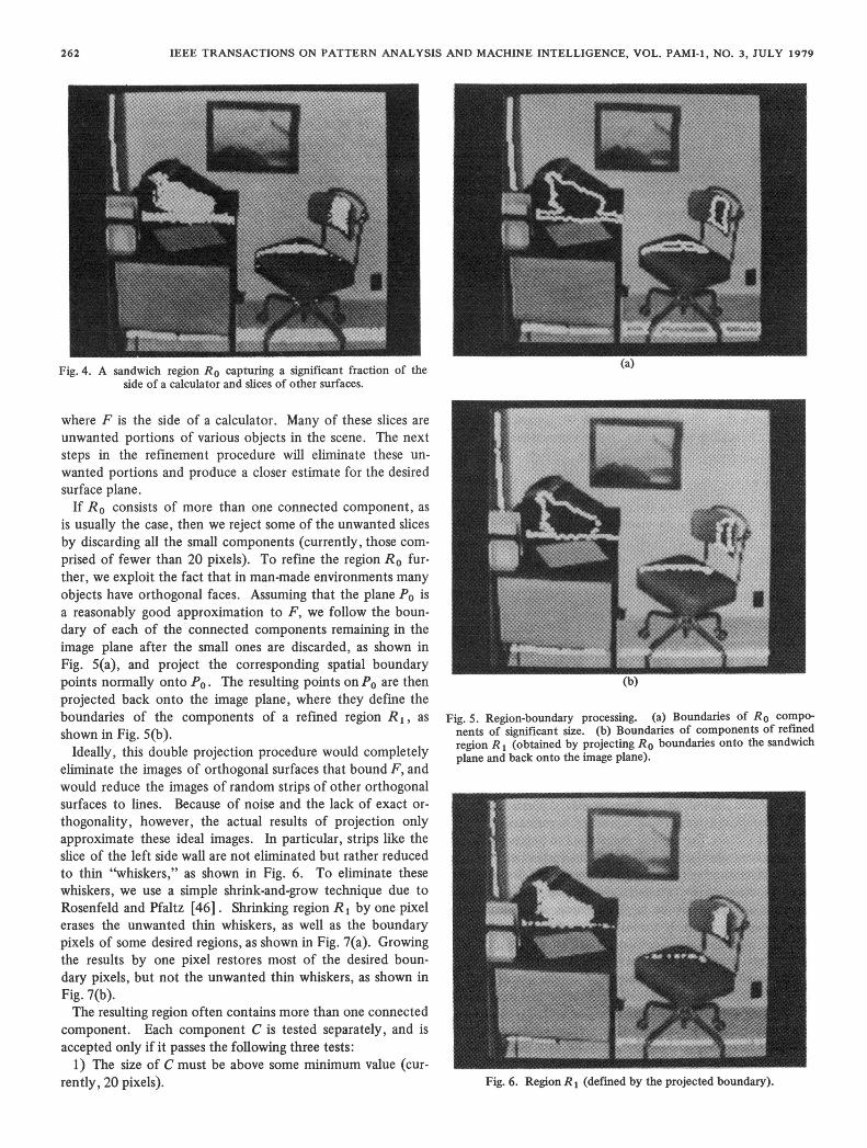
that is thought to be a good approximation to a planar faceF of some object in the scene. The first iteration of our refine-ment procedure begins with extracting a region Ro consistingof a set of pixels in RTJ whose spatial coordinates fall withinsome fixed distance W from P0. Region Ro corresponds tothe points in a three-dimensional space that are captured bya "sandwich" SO of thickness 2 W bounded by a pair of planesparallel to and at distance ±W from PO. A central plane, suchas P0, is thus called a sandwich plane and a region sliced by asandwich, such as Ro, is called a sandwich region. If P0 fitsF well and if W is, say, at least 5 a cos 0, where a is the stan-dard deviation of the measured range and 0 is the incidenceangle, then So will capture most of the surface elements ofF.1 Ideally, SO captures the entire surface F and no othersurfaces. Typically, however, SO captures only part of F andusually slices several other surfaces, as illustrated in Fig. 4

1In our current program we use a worst case value of W = 5 a = 2 in,regardless of 0.

261


Fig. 4. A sandwich region Ro capturing a significant fraction of theside of a calculator and slices of other surfaces.

where F is the side of a calculator. Many of these slices areunwanted portions of various objects in the scene. The nextsteps in the refinement procedure will eliminate these un-wanted portions and produce a closer estimate for the desiredsurface plane.

If Ro consists of more than one connected component, asis usually the case, then we reject some of the unwanted slicesby discarding all the small components (currently, those com-prised of fewer than 20 pixels). To refine the region Ro fur-ther, we exploit the fact that in man-made environments manyobjects have orthogonal faces. Assuming that the plane P0 isa reasonably good approximation to F, we follow the boun-dary of each of the connected components remaining in theimage plane after the small ones are discarded, as shown inFig. 5(a), and project the corresponding spatial boundarypoints normally onto P0. The resulting points on P0 are thenprojected back onto the image plane, where they define theboundaries of the components of a refined region R1, asshown in Fig. 5(b).

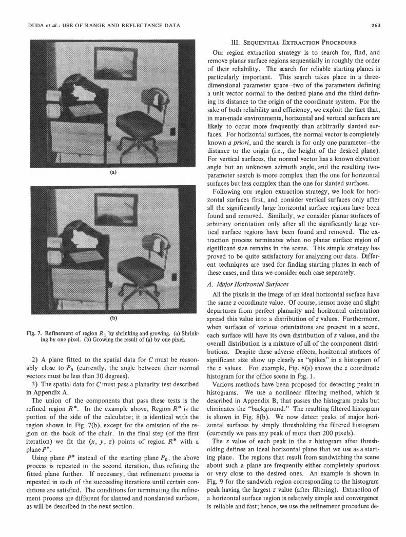
Ideally, this double projection procedure would completelyeliminate the images of orthogonal surfaces that bound F, andwould reduce the images of random strips of other orthogonalsurfaces to lines. Because of noise and the lack of exact or-thogonality, however, the actual results of projection onlyapproximate these ideal images. In particular, strips like theslice of the left side wall are not eliminated but rather reducedto thin "whiskers," as shown in Fig. 6. To eliminate thesewhiskers, we use a simple shrink-and-grow technique due toRosenfeld and Pfaltz [46]. Shrinking region R 1 by one pixelerases the unwanted thin whiskers, as well as the boundarypixels of some desired regions, as shown in Fig. 7(a). Growingthe results by one pixel restores most of the desired boun-dary pixels, but not the unwanted thin whiskers, as shown inFig. 7(b).The resulting region often contains more than one connected

component. Each component C is tested separately, and isaccepted only if it passes the following three tests:

1) The size of C must be above some minimum value (cur-rently, 20 pixels).

Fig. 5. Region-boundary processing. (a) Boundaries of Ro compo-nents of significant size. (b) Boundaries of components of refinedregion R1 (obtained by projecting Ro boundaries onto the sandwichplane and back onto the image plane).

Fig. 6. Region R 1 (defined by the projected boundary).

262


ta,

(b)

Fig. 7. Refinement of region R 1 by shrinking and growing. (a) Shrink-ing by one pixel. (b) Growing the result of (a) by one pixel.

2) A plane fitted to the spatial data for C must be reason-

ably close to PO (currently, the angle between their normalvectors must be less than 30 degrees).3) The spatial data for C must pass a planarity test described

in Appendix A.The union of the components that pass these tests is the

refined region R*. In the example above, Region R* is theportion of the side of the calculator; it is identical with theregion shown in Fig. 7(b), except for the omission of the re-

gion on the back of the chair. In the final step (of the firstiteration) we fit the (x, y, z) points of region R* with a

plane P*.Using plane P* instead of the starting plane P0, the above

process is repeated in the second iteration, thus refining thefitted plane further. If necessary, that refinement process isrepeated in each of the succeeding iterations until certain con-

ditions are satisfied. The conditions for terminating the refine-ment process are different for slanted and nonslanted surfaces,as will be described in the next section.

III. SEQUENTIAL EXTRACTION PROCEDUREOur region extraction strategy is to search for, find, and

remove planar surface regions sequentially in roughly the orderof their reliability. The search for reliable starting planes isparticularly important. This search takes place in a three-dimensional parameter space-two of the parameters defininga unit vector normal to the desired plane and the third defin-ing its distance to the origin of the coordinate system. For thesake of both reliability and efficiency, we exploit the fact that,in man-made environments, horizontal and vertical surfaces arelikely to occur more frequently than arbitrarily slanted sur-faces. For horizontal surfaces, the normal vector is completelyknown a priori, and the search is for only one parameter-thedistance to the origin (i.e., the height of the desired plane).For vertical surfaces, the normal vector has a known elevationangle but an unknown azimuth angle, and the resulting two-parameter search is more complex than the one for horizontalsurfaces but less complex than the one for slanted surfaces.Following our region extraction strategy, we look for hori-

zontal surfaces first, and consider vertical surfaces only afterall the significantly large horizontal surface regions have beenfound and removed. Similarly, we consider planar surfaces ofarbitrary orientation only after all the significantly large ver-tical surface regions have been found and removed. The ex-traction process terminates when no planar surface region ofsignificant size remains in the scene. This simple strategy hasproved to be quite satisfactory for analyzing our data. Differ-ent techniques are used for finding starting planes in each ofthese cases, and thus we consider each case separately.

A. Major Horizontal SurfacesAll the pixels in the image of an ideal horizontal surface have

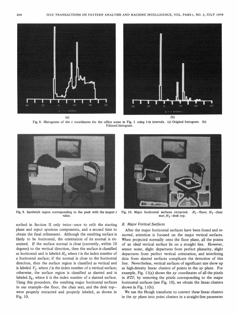
the same z coordinate value. Of course, sensor noise and slightdepartures from perfect planarity and horizontal orientationspread this value into a distribution of z values. Furthermore,when surfaces of various orientations are present in a scene,each surface will have its own distribution of z values, and theoverall distribution is a mixture of all of the component distri-butions. Despite these adverse effects, horizontal surfaces ofsignificant size show up clearly as "spikes" in a histogram ofthe z values. For example, Fig. 8(a) shows the z coordinatehistogram for the office scene in Fig. 1.Various methods have been proposed for detecting peaks in

histograms. We use a nonlinear filtering method, which isdescribed in Appendix B, that passes the histogram peaks buteliminates the "background." The resulting filtered histogramis shown in Fig. 8(b). We now detect peaks of major hori-zontal surfaces by simply thresholding the filtered histogram(currently we pass any peak of more than 200 pixels).The z value of each peak in the z histogram after thresh-

olding defines an ideal horizontal plane that we use as a start-ing plane. The regions that result from sandwiching the sceneabout such a plane are frequently either completely spuriousor very close to the desired ones. An example is shown inFig. 9 for the sandwich region corresponding to the histogrampeak having the largest z value (after filtering). Extraction ofa horizontal surface region is relatively simple and convergenceis reliable and fast; hence, we use the refinement procedure de-

263


(a)Fig. 8. Histograms of the z coordinates for the office scene in Fig. 1 using 1-in intervals. (a) Original histogram. (b)

Filtered histogram.

Fig. 9. Sandwich region corresponding to the peak with the largest zvalue.

scribed in Section II only twice-once to refit the startingplane and reject spurious components, and a second time toobtain the final refinement. Although the resulting surface islikely to be horizontal, the orientation of its normal is ex-

amined. If the surface normal is close (currently, within 10degrees) to the vertical direction, then the surface is classifiedas horizontal and is labeled Hi, where i is the index number ofa horizontal surface; if the normal is close to the horizontaldirection, then the surface region is classified as vertical andis labeled Vi, where is the index number of a vertical surface;otherwise, the surface region is classified as slanted and islabeled Sk' where k is the index number of a slanted surface.Using this procedure, the resulting major horizontal surfacesin our example-the floor, the chair seat, and the desk top-were properly extracted and properly labeled, as shown inFig. 10.

Fig. 10. Major horizontal surfaces extracted. H1 -floor; H2 -chairseat; H3 -desk top.

B. Major Vertical SurfacesAfter the major horizontal surfaces have been found and re-

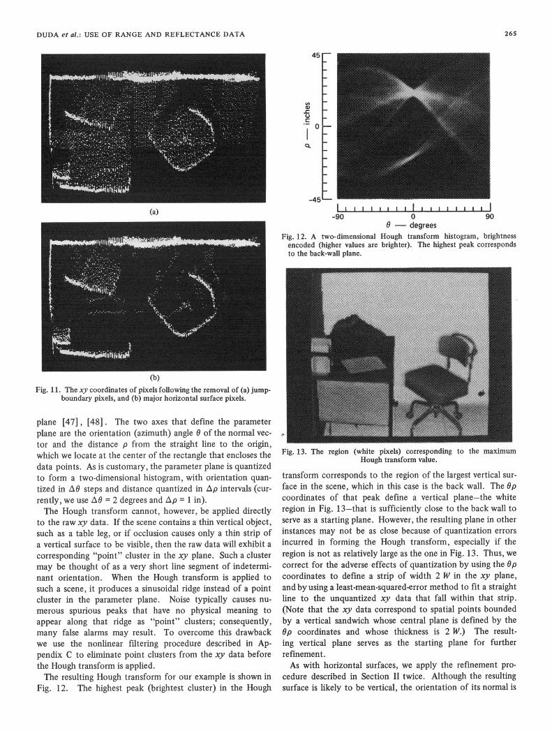
moved, attention is focused on the major vertical surfaces.When projected normally onto the floor plane, all the pointsof an ideal vertical surface lie on a straight line. However,sensor noise, slight departures from perfect planarity, slightdepartures from perfect vertical orientation, and interferingdata from slanted surfaces complicate the detection of thisline. Nevertheless, vertical surfaces of significant size show upas high-density linear clusters of points in the xy plane. Forexample, Fig. 11(a) shows the xy coordinates of all the pixelsin RTJ; by removing the pixels corresponding to the majorhorizontal surfaces (see Fig. 10), we obtain the linear clustersshown in Fig. 11(b).We use the Hough transform to convert these linear clusters

in the xy plane into point clusters in a straight-line parameter

264


45

.C

0

-45

Ii IIIIIIIIIIIi Ii I lIIi II-90 0 90

0- degreesFig. 12. A two-dimensional Hough transform histogram, brightnessencoded (higher values are brighter). The highest peak correspondsto the back-wall plane.

plane [47], [48]. The two axes that define the parameterplane are the orientation (azimuth) angle 0 of the normal vec-

tor and the distance p from the straight line to the origin,which we locate at the center of the rectangle that encloses thedata points. As is customary, the parameter plane is quantizedto form a two-dimensional histogram, with orientation quan-

tized in AO steps and distance quantized in Ap intervals (cur-rently, we use AO = 2 degrees and Ap = 1 in).The Hough transform cannot, however, be applied directly

to the raw xy data. If the scene contains a thin vertical object,such as a table leg, or if occlusion causes only a thin strip ofa vertical surface to be visible, then the raw data will exhibit a

corresponding "point" cluster in the xy plane. Such a clustermay be thought of as a very short line segment of indetermi-nant orientation. When the Hough transform is applied tosuch a scene, it produces a sinusoidal ridge instead of a pointcluster in the parameter plane. Noise typically causes nu-

merous spurious peaks that have no physical meaning toappear along that ridge as "point" clusters; consequently,many false alarms may result. To overcome this drawbackwe use the nonlinear filtering procedure described in Ap-pendix C to eliminate point clusters from the xy data beforethe Hough transform is applied.The resulting Hough transform for our example is shown in

Fig. 12. The highest peak (brightest cluster) in the Hough

Fig. 13. The region (white pixels) corresponding to the maximumHough transform value.

transform corresponds to the region of the largest vertical sur-

face in the scene, which in this case is the back wall. The Op

coordinates of that peak define a vertical plane-the whiteregion in Fig. 13-that is sufficiently close to the back wall toserve as a starting plane. However, the resulting plane in otherinstances may not be as close because of quantization errors

incurred in forming the Hough transform, especially if theregion is not as relatively large as the one in Fig. 13. Thus, wecorrect for the adverse effects of quantization by using the Opcoordinates to define a strip of width 2 W in the xy plane,and by using a least-mean-squared-error method to fit a straightline to the unquantized xy data that fall within that strip.(Note that the xy data correspond to spatial points boundedby a vertical sandwich whose central plane is defined by theOp coordinates and whose thickness is 2 W.) The result-ing vertical plane serves as the starting plane for furtherrefinement.As with horizontal surfaces, we apply the refinement pro-

cedure described in Section II twice. Although the resultingsurface is likely to be vertical, the orientation of its normal is

(a)

(b)Fig. 11. The xy coordinates of pixels following the removal of (a) jump-

boundary pixels, and (b) major horizontal surface pixels.

265


Fig. 14. Major vertical surfaces extracted. V1 -back wall; V2 -side ofdesk; V3 -side wall.

examined. As in the case of extraction of major horizontalsurfaces (see Section A), the surface is classified as the ithhorizontal surface, the jth vertical surface, or the kth slantedsurface and is labeled Hi, V1, or Sk, respectively, according tothe actual orientation of its normal. The resulting region isthen removed from the scene, and the entire process of pro-

jecting, filtering, transforming, and refining is repeated tofind the next vertical surface. This process is continued untileither the highest peak in the Hough transform is too low(currently, below 400 pixels), or one of the three tests in therefinement procedure (see Section Il) fails. In the formercase, the search for vertical surfaces is terminated. In thelatter case, to avoid finding this region again, we temporarilyremove it and continue the search for other vertical regions.However, when all vertical surfaces have been found, alltemporarily removed regions are restored. To shorten theprocessing time for scenes containing mostly slanted sur!faces, we also terminate the search for vertical surfaces if weencounter three successive failures. The final major verticalsurfaces in our example-the back wall, the side of the desk,and the side wall-are shown in Fig. 14.

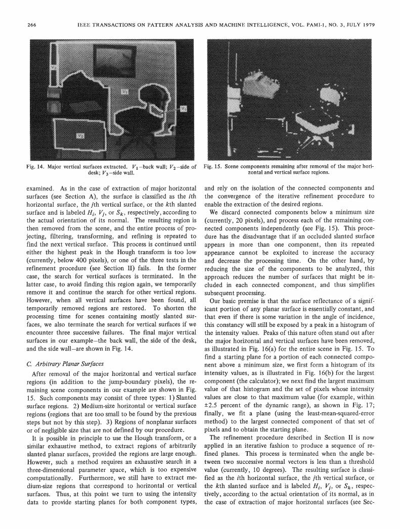
C Arbitrary Planar SurfacesAfter removal of the major horizontal and vertical surface

regions (in addition to the jump-boundary pixels), the re-

maining scene components in our example are shown in Fig.15. Such components may consist of three types: 1) Slantedsurface regions. 2) Medium-size horizontal or vertical surfaceregions (regions that are too small to be found by the previoussteps but not by this step). 3) Regions of nonplanar surfacesor of negligible size that are not defined by our procedure.

It is possible in principle to use the Hough transform, or a

similar exhaustive method, to extract regions of arbitrarilyslanted planar surfaces, provided the regions are large enough.However, such a method requires an exhaustive search in a

three-dimensional parameter space, which is too expensivecomputationally. Furthermore, we still have to extract me-

dium-size regions that correspond to horizontal or verticalsurfaces. Thus, at this point we turn to using the intensitydata to provide starting planes for both component types,

Fig. 15. Scene components remaining after removal of the major hori-zontal and vertical surface regions.

and rely on the isolation of the connected components andthe convergence of the iterative refinement procedure toenable the extraction of the desired regions.We discard connected components below a minimum size

(currently, 20 pixels), and process each of the remaining con-nected components independently (see Fig. 15). This proce-dure has the disadvantage that if an occluded slanted surfaceappears in more than one component, then its repeatedappearance cannot be exploited to increase the accuracyand decrease the processing time. On the other hand, byreducing the size of the components to be analyzed, thisapproach reduces the number of surfaces that might be in-cluded in each connected component, and thus simplifiessubsequent processing.Our basic premise is that the surface reflectance of a signif-

icant portion of any planar surface is essentially constant, andthat even if there is some variation in the angle of incidence,this constancy will still be exposed by a peak in a histogram ofthe intensity values. Peaks of this nature often stand out afterthe major horizontal and vertical surfaces have been removed,as illustrated in Fig. 16(a) for the entire scene in Fig. 15. Tofind a starting plane for a portion of each connected compo-nent above a minimum size, we first form a histogram of itsintensity values, as is illustrated in Fig. 16(b) for the largestcomponent (the calculator); we next find the largest maximumvalue of that histogram and the set of pixels whose intensityvalues are close to that maximum value (for example, within±2.5 percent of the dynamic range), as shown in Fig. 17;finally, we fit a plane (using the least-mean-squared-errormethod) to the largest connected component of that set ofpixels and to obtain the starting plane.The refinement procedure described in Section II is now

applied in an iterative fashion to produce a sequence of re-fined planes. This process is terminated when the angle be-tween two successive normal vectors is less than a thresholdvalue (currently, 10 degrees). The resulting surface is classi-fied as the ith horizontal surface, the jth vertical surface, orthe kth slanted surface and is labeled Hi, V", or Sk, respec-tively, according to the actual orientation of its normal, as inthe case of extraction of major horizontal surfaces (see Sec-

266


Fig. 18. The first planar surface region extracted from Fig. 15.

(a)

(b)

Fig. 16. Histograms for the intensity values of the remaining scene inFig. 15. (a) For the entire scene. (b) For the largest connected com-

ponent (the calculator).

Fig. 17. The set of pixels with intensity values near the highest peakof the intensity histogram in Fig. 16(b).

Fig. 19. Planar surface regions extracted by the procedure using in-tensity data to find starting regions.

tion A). The resulting region in our example-the side of thecalculator-is shown in Fig. 18. Based on the orientation ofits normal vector, the extracted surface in this example isproperly classified as vertical. The extracted region is nowremoved from its parental component (the calculator), theintensity histogram in Fig. 16(b) is modified accordingly, andthe same procedure is repeated for what remains of the cal-culator region.The above process is applied to each significant connected

component in the scene. This process terminates in failure ifeither one of the three tests in the refinement procedure (seeSection II) fails or if the number of iterations has exceeded itsmaximum value (currently, 9). In case of failure, we makeone more attempt by using a plane fitted to the entire com-ponent as a starting plane. While there is a variety of possibleways to choose other starting planes, in our experience therewere rarely any significant planar regions left when such fail-ures occurred. Thus, upon a second failure we classify thatimage component as undefined and proceed to process theremaining components. A set of seven regions, which wereproperly found and properly labeled by this procedure, isshown in Fig. 19.

267


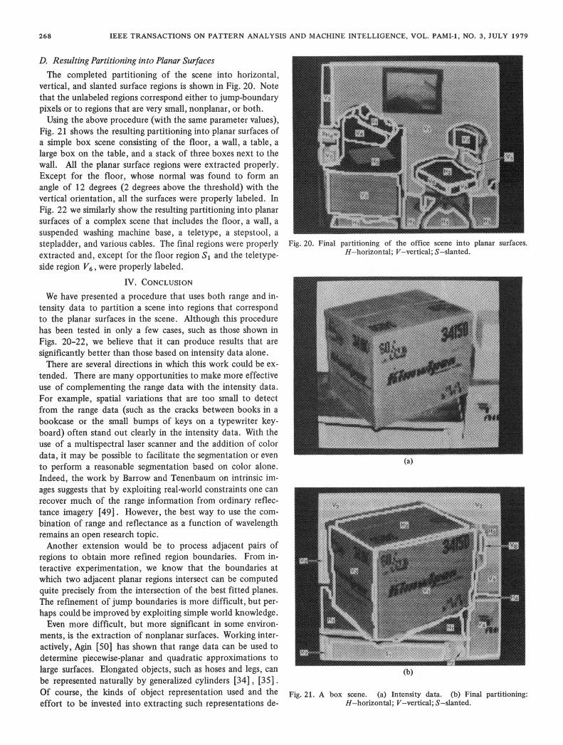
D. Resulting Partitioning into Planar SurfacesThe completed partitioning of the scene into horizontal,

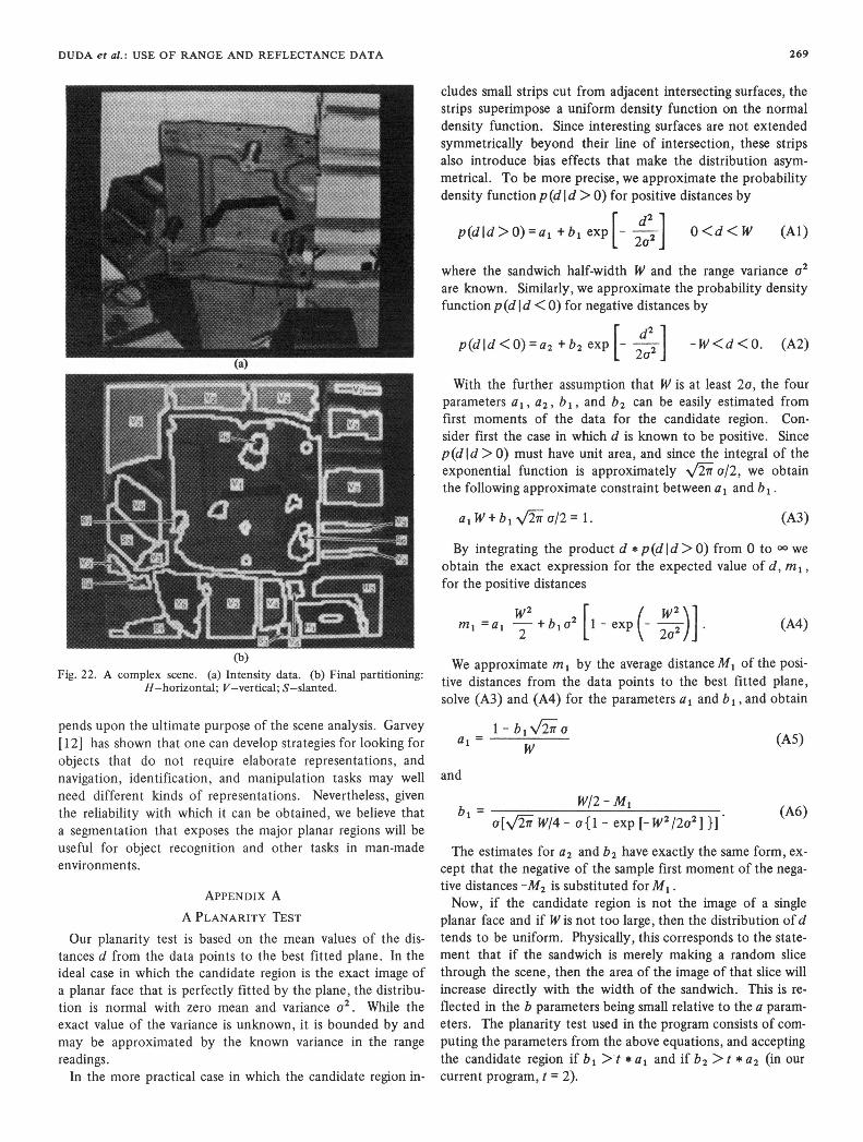
vertical, and slanted surface regions is shown in Fig. 20. Notethat the unlabeled regions correspond either to jump-boundarypixels or to regions that are very small, nonplanar, or both.Using the above procedure (with the same parameter values),

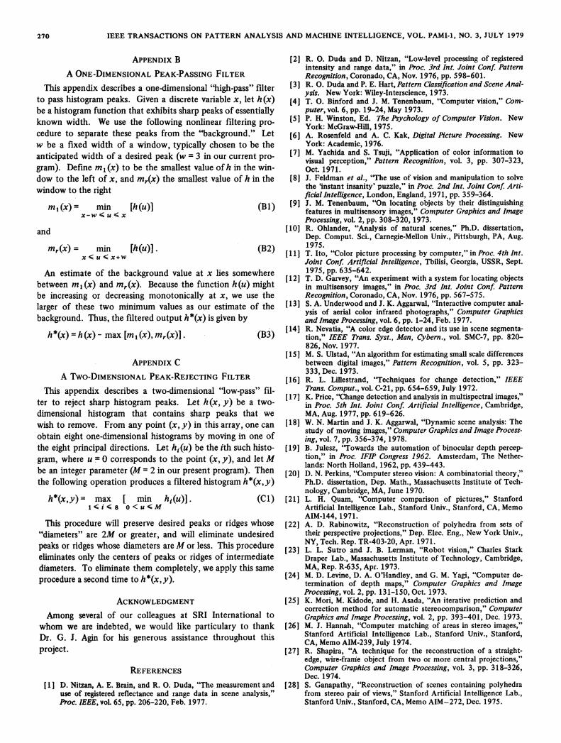
Fig. 21 shows the resulting partitioning into planar surfaces ofa simple box scene consisting of the floor, a wall, a table, alarge box on the table, and a stack of three boxes next to thewall. All the planar surface regions were extracted properly.Except for the floor, whose normal was found to form anangle of 12 degrees (2 degrees above the threshold) with thevertical orientation, all the surfaces were properly labeled. InFig. 22 we similarly show the resulting partitioning into planarsurfaces of a complex scene that includes the floor, a wall, asuspended washing machine base, a teletype, a stepstool, astepladder, and various cables. The final regions were properlyextracted and, except for the floor region SI and the teletype-side region V6, were properly labeled.

IV. CONCLUSIONWe have presented a procedure that uses both range and in-

tensity data to partition a scene into regions that correspondto the planar surfaces in the scene. Although this procedurehas been tested in only a few cases, such as those shown inFigs. 20-22, we believe that it can produce results that aresignificantly better than those based on intensity data alone.There are several directions in which this work could be ex-

tended. There are many opportunities to make more effectiveuse of complementing the range data with the intensity data.For example, spatial variations that are too small to detectfrom the range data (such as the cracks between books in abookcase or the small bumps of keys on a typewriter key-board) often stand out clearly in the intensity data. With theuse of a multispectral laser scanner and the addition of colordata, it may be possible to facilitate the segmentation or evento perform a reasonable segmentation based on color alone.Indeed, the work by Barrow and Tenenbaum on intrinsic im-ages suggests that by exploiting real-world constraints one canrecover much of the range information from ordinary reflec-tance imagery [49]. However, the best way to use the com-bination of range and reflectance as a function of wavelengthremains an open research topic.Another extension would be to process adjacent pairs of

regions to obtain more refined region boundaries. From in-teractive experimentation, we know that the boundaries atwhich two adjacent planar regions intersect can be computedquite precisely from the intersection of the best fitted planes.The refinement of jump boundaries is more difficult, but per-haps could be improved by exploiting simple world knowledge.Even more difficult, but more significant in some environ-

ments, is the extraction of nonplanar surfaces. Working inter-actively, Agin [50] has shown that range data can be used todetermine piecewise-planar and quadratic approximations tolarge surfaces. Elongated objects, such as hoses and legs, canbe represented naturally by generalized cylinders [34], [35].Of course, the kinds of object representation used and theeffort to be invested into extracting such representations de-

Fig. 20. Final partitioning of the office scene into planar surfaces.H-horizontal; V-vertical; S-slanted.

(a)

(b)

Fig. 21. A box scene. (a) Intensity data. (b) Final partitioning:H-horizontal; V-vertical; S-slanted.

268


cludes small strips cut from adjacent intersecting surfaces, thestrips superimpose a uniform density function on the normaldensity function. Since interesting surfaces are not extendedsymmetrically beyond their line of intersection, these stripsalso introduce bias effects that make the distribution asym-metrical. To be more precise, we approximate the probabilitydensity function p (d Id > 0) for positive distances by

d2P(dld>0)=ai+b,exp[ 2a2 0<d<W (Al)

where the sandwich half-width W and the range variance c2are known. Similarly, we approximate the probability densityfunction p(d Id <0) for negative distances by

d2p(dId<O)=a2 +b2 exp - 2]2 -W<d<0. (A2)

With the further assumption that W is at least 2a, the fourparameters a,, a2, bl, and b2 can be easily estimated fromfirst moments of the data for the candidate region. Con-sider first the case in which d is known to be positive. Sincep(d Id > 0) must have unit area, and since the integral of theexponential function is approximately v/2'ia2, we obtainthe following approximate constraint between al and b1.

a,W+blV2-Wr /2= 1. (A3)

By integrating the product d * p(d Id > 0) from 0 to oo weobtain the exact expression for the expected value of d, mlI,for the positive distances

ml-a, 2I2 w2-ml a= b lcr2I1-exp(-

2(A4)

Fig. 22. A complex scene. (a) Intensity data. (b) Final partitioning:H-horizontal; V-vertical; S-slanted.

pends upon the ultimate purpose of the scene analysis. Garvey[12] has shown that one can develop strategies for looking forobjects that do not require elaborate representations, andnavigation, identiflcation, and manipulation tasks may wellneed different kinds of representations. Nevertheless, giventhe reliability with which it can be obtained, we believe thata segmentation that exposes the major planar regions will beuseful for object recognition and other tasks in man-madeenvironments.

APPENDIX AA PLANARITY TEST

Our planarity test is based on the mean values of the dis-tances d from the data points to the best fitted plane. In theideal case in which the candidate region is the exact image ofa planar face that is perfectly fitted by the plane, the distribu-tion is normal with zero mean and variance a2. While theexact value of the variance is unknown, it is bounded by andmay be approximated by the known variance in the rangereadings.

In the more practical case in which the candidate region in-

We approximate m1 by the average distance M1 of the posi-tive distances from the data points to the best fitted plane,solve (A3) and (A4) for the parameters a1 and b1 , and obtain

=1 -b=aal=,

and

bi = W/2 - Mla[V7W/4 - ar{l - exp [- W2/2r2] }]

(A5)

(A6)

The estimates for a2 and b2 have exactly the same form, ex-cept that the negative of the sample first moment of the nega-tive distances -M2 is substituted for M1.Now, if the candidate region is not the image of a single

planar face and if W is not too large, then the distribution ofdtends to be uniform. Physically, this corresponds to the state-ment that if the sandwich is merely making a random slicethrough the scene, then the area of the image of that slice willincrease directly with the width of the sandwich. This is re-

flected in the b parameters being small relative to the a param-eters. The planarity test used in the program consists of com-puting the parameters from the above equations, and acceptingthe candidate region if bI >-t * a1 and if b2 > t * a2 (in ourcurrent program, t = 2).

(a)

269


APPENDIX BA ONE-DIMENSIONAL PEAK-PASSING FILTER

This appendix describes a one-dimensional "high-pass" filterto pass histogram peaks. Given a discrete variable x, let h(x)be a histogram function that exhibits sharp peaks of essentiallyknown width. We use the following nonlinear filtering pro-

cedure to separate these peaks from the "background." Letw be a fixed width of a window, typically chosen to be theanticipated width of a desired peak (w = 3 in our current pro-

gram). Define ml (x) to be the smallest value of h in the win-dow to the left of x, and mr(x) the smallest value of h in thewindow to the right

ml(x)= min [h(u)] (Bi)x-w 6 u < x

and

mr(x) = min [h(u)]. (B2)x s u< x+w

An estimate of the background value at x lies somewherebetween m1 (x) and mr (x). Because the function h (u) mightbe increasing or decreasing monotonically at x, we use thelarger of these two minimum values as our estimate of thebackground. Thus, the filtered output h*(x) is given by

h*(x) = h (x) - max [m 1 (x), Mr().WI (B3)

APPENDIX C

A Two-DIMENSIONAL PEAK-REJECTING FILTERThis appendix describes a two-dimensional "low-pass" fil-

ter to reject sharp histogram peaks. Let h (x, y) be a two-dimensional histogram that contains sharp peaks that we

wish to remove. From any point (x, y) in this array, one can

obtain eight one-dimensional histograms by moving in one ofthe eight principal directions. Let hi(u) be the ith such histo-gram, where u = 0 corresponds to the point (x, y), and let Mbe an integer parameter (M = 2 in our present program). Thenthe following operation produces a filtered histogram h*(x,y)

h*(x, y) = max [ min hi(u)]. (C 1)1 ti<i8 0 < u<M

This procedure will preserve desired peaks or ridges whose"diameters" are 2M or greater, and will eliminate undesiredpeaks or ridges whose diameters areM or less. This procedureeliminates only the centers of peaks or ridges of intermediatediameters. To eliminate them completely, we apply this sameprocedure a second time to h*(x,y).

ACKNOWLEDGMENTAmong several of our colleagues at SRI International to

whom we are indebted, we would like particulary to thankDr. G. J. Agin for his generous assistance throughout thisproject.

REFERENCES1] D. Nitzan, A. E. Brain, and R. 0. Duda, "The measurement and

use of registered reflectance and range data in scene analysis,"Proc. IEEE, vol. 65, pp. 206-220, Feb. 1977.

[2] R. 0. Duda and D. Nitzan, "Low-level processing of registeredintensity and range data," in Proc. 3rd Int. Joint Conf. PatternRecognition, Coronado, CA, Nov. 1976, pp. 598-601.

[31 R. 0. Duda and P. E. Hart, Pattern Classification and Scene Anal-ysis. New York: Wiley-Interscience, 1973.

[41 T. 0. Binford and J. M. Tenenbaum, "Computer vision," Com-puter, vol. 6, pp. 19-24, May 1973.

[5] P. H. Winston, Ed. The Psychology of Computer Vision. NewYork: McGraw-Hill, 1975.

[6] A. Rosenfeld and A. C. Kak, Digital Picture Processing. NewYork: Academic, 1976.

[7] M. Yachida and S. Tsuji, "Application of color information tovisual perception," Pattern Recognition, vol. 3, pp. 307-323,Oct. 1971.

[81 J. Feldman et al., "The use of vision and manipulation to solvethe 'instant insanity' puzzle," in Proc. 2nd Int. Joint Conf. Arti-ficial Intelligence, London, England, 1971, pp. 359-364.

[9] J. M. Tenenbaum, "On locating objects by their distinguishingfeatures in multisensory images," Computer Graphics and ImageProcessing, vol. 2, pp. 308-320, 1973.

[101 R. Ohlander, "Analysis of natural scenes," Ph.D. dissertation,Dep. Comput. Sci., Carnegie-Mellon Univ., Pittsburgh, PA, Aug.1975.

[11] T. Ito, "Color picture processing by computer," in Proc. 4th Int.Joint Confi Artificial Intelligence, Tbilisi, Georgia, USSR, Sept.1975, pp. 635-642.

[12] T. D. Garvey, "An experiment with a system for locating objectsin multisensory images," in Proc. 3rd Int. Joint Conf. PatternRecognition, Coronado, CA, Nov. 1976, pp. 567-575.

[13] S. A. Underwood and J. K. Aggarwal, "Interactive computer anal-ysis of aerial color infrared photographs," Computer Graphicsand Image Processing, vol. 6, pp. 1-24, Feb. 1977.

[14] R. Nevatia, "A color edge detector and its use in scene segmenta-tion," IEEE Trans. Syst., Man, Cybern., vol. SMC-7, pp. 820-826, Nov. 1977.

[15] M. S. Ulstad, "An algorithm for estimating small scale differencesbetween digital images," Pattern Recognition, vol. 5, pp. 323-333, Dec. 1973.

[16] R. L. Lillestrand, "Techniques for change detection," IEEETrans. Comput., vol. C-21, pp. 654-659, July 1972.

[17] K. Price, "Change detection and analysis in multispectral images,"in Proc. 5th Int. Joint Conf Artificial Intelligence, Cambridge,MA, Aug. 1977, pp. 619-626.

[18] W. N. Martin and J. K. Aggarwal, "Dynamic scene analysis: Thestudy of moving images," Computer Graphics and Image Process-ing, vol. 7, pp. 356-374, 1978.

[19] B. Julesz, "Towards the automation of binocular depth percep-tion," in Proc. IFIP Congress 1962. Amsterdam, The Nether-lands: North Holland, 1962, pp. 439-443.

[20] D. N. Perkins, "Computer stereo vision: A combinatorial theory,"Ph.D. dissertation, Dep. Math., Massachusetts Institute of Tech-nology, Cambridge, MA, June 1970.

[21] L. H. Quam, "Computer comparison of pictures," StanfordArtificial Intelligence Lab., Stanford Univ., Stanford, CA, MemoAIM-144, 1971.

[22] A. D. Rabinowitz, "Reconstruction of polyhedra from sets oftheir perspective projections," Dep. Elec. Eng., New York Univ.,NY, Tech. Rep. TR-403-20, Apr. 1971.

[23] L. L. Sutro and J. B. Lerman, "Robot vision," Charles StarkDraper Lab., Massachusetts Institute of Technology, Cambridge,MA, Rep. R-635, Apr. 1973.

[24] M. D. Levine, D. A. O'Handley, and G. M. Yagi, "Computer de-termination of depth maps," Computer Graphics and ImageProcessing, vol. 2, pp. 131-150, Oct. 1973.

[25] K. Mori, M. Kidode, and H. Asada, "An iterative prediction andcorrection method for automatic stereocomparison," ComputerGraphics and Image Processing, vol. 2, pp. 393-401, Dec. 1973.

[26] M. J. Hannah, "Computer matching of areas in stereo images,"Stanford Artificial Intelligence Lab., Stanford Univ., Stanford,CA, Memo AIM-239, July 1974.

[271 R. Shapira, "A technique for the reconstruction of a straight-edge, wire-frame object from two or more central projections,"Computer Graphics and Image Processing, vol. 3, pp. 318-326,Dec. 1974.

[28] 5. Ganapathy, "Reconstruction of scenes containing polyhedrafrom stereo pair of views," Stanford Artificial Intelligence Lab.,Stanford Univ., Stanford, CA, Memo AIM-272, Dec. 1975.

270


[29] R. Nevatia, "Depth measurement by motion stereo," ComputerGraphics and Image Processing, vol. 5, pp. 203-214, June 1976.

[30] D. B. Gennery, "A stereo vision system for an autonomous ve-hicle," in Proc. 5th Int. Joint Conf. Artificial Intelligence, Cam-bridge, MA, Aug. 1977, pp. 576-582.

[311 D. J. Burr and R. T. Chien, "A system for stereo computer visionwith geometric models," in Proc. 5th Int. Joint Conf. ArtificialIntelligence, Cambridge, MA, Aug. 1977, p. 583.

[32] P. M. Will and K. S. Pennington, "Grid coding: A preprocessingtechnique for robot and machine vision," Artificial Intelligence,vol. 2, pp. 319-329, Winter 1971.

[33] Y. Shirai and M. Suwa, "Recognition of polyhedrons with arangefinder," in Proc. 2nd Int. Joint Conf Artificial Intelligence,London, England, Sept. 1971, pp. 80-87.

[34] G. J. Agin and T. 0. Binford, "Computer description of curvedobjects," in Proc. 3rd Int. Joint Conf Artificial Intelligence,Stanford, CA, Aug. 1973, pp. 629-640.

[351 R. Nevatia and T. 0. Binford, "Structured descriptions of com-plex objects," in Proc. 3rd Int. Joint Conf. Artificial Intelligence,Stanford, CA, Aug. 1973, pp. 641-647.

[36] Y. Shirai, "A step toward context-sensitive recognition of ir-regular objects," Computer Graphics and Image Processing,pp. 298-307, Dec. 1973.

[37] F. Rocker, "Localization and classification of three-dimensionalobjects," in Proc. 2nd Int. Joint Conf Pattern Recognition,Copenhagen, Denmark, Aug. 1974, pp. 527-528.

[38] F. Rocker and A. Kiessling, "Methods for analyzing three-dimensional scenes," in Proc. 4th Int. Joint Conf. Artificial In-telligence, Tblishi, Georgia, USSR, Sept. 1975, pp. 669-673.

[391 R. J. Popplestone et al., "Forming models of plane-and-cylinderfaceted bodies from light stripes," in Proc. 4th Int. Joint Conf.Artificial Intelligence, Tblishi, Georgia, USSR, 1975, pp. 664-668.

[40] M. Ishii and T. Nagata, "Feature extraction of three-dimensionalobjects and visual processing in a hand-eye system using lasertracking," Pattern Recognition, vol. 8, pp. 229-237, Oct. 1976.

[41] A. Kiessling, "A fast scanning method for 3-dimensional scenes,"in Proc. 3rd Int. Joint Conf. Pattern Recognition, Coronado, CA,Nov. 1976, pp. 586-589.

[42] K. Sugihara and Y. Shirai, "Range data understanding guided bya junction dictionary," in Proc. 5th Int. Joint Conf. Artificial In-telligence, Cambridge, MA, 1977, p. 706.

[431 R. A. Lewis and A. R. Johnston, "A scanning laser rangefinderfor a robotic vehicle," in Proc. 5th Int. Joint Conf Artificial In-telligence, Cambridge, MA, Aug. 1977, pp. 762-768.

[441 H. J. Caulfield et al., "Laser stereometry," Proc. IEEE, vol. 65,pp. 84-88, Jan. 1977.

[45] F. Tomita, M. Yachida, and S. Tsuji, "Detection of homogeneousregions by structural analysis," in Proc. 3rd Int. Joint Conf.Artificial Intelligence, Stanford, CA, Aug. 1973, pp. 564-571.

[46] A. Rosenfeld and J. L. Pfaltz, "Distance functions on digital pic-tures," Pattern Recognition, vol. 1, pp. 33-6 1, July 1968.

[471 P. V. C. Hough, "Method and means for recognizing complexpatterns," U.S. Patent 3069654, Dec. 18, 1962.

[48] R. 0. Duda and P. E. Hart, "Use of the Hough transformation todetect lines and curves in pictures," Commun. Ass. Comput.Mach., vol. ACM-15, pp. 11-15, Jan. 1972.

[49] H. G. Barrow and J. M. Tenenbaum, "Recovering intrinsic scenecharacteristics from images," in Computer Vision Systems, A. R.Hanson and E. Riseman, Eds. New York: Academic, 1978,pp. 3-26.

[50] G. J. Agin, "Hierarchical representation of three-dimensionalobjects," Stanford Research Institute, Menlo Park, CA, FinalRep. SRI Project 1187, Mar. 1977.

Richard 0. Duda (S'57-M'58-SM'77) received>.<s.. the B.S. and the M.S. degrees in engineering

from the University of California at Los Ange-les, and the Ph.D. degree in electrical engi-neering from the Massachusetts Institute ofTechnology, Cambridge, MA.Currently, he is a Staff Scientist with the

Artificial Intelligence Center at SRI Interna-tional, Menlo Park, CA. Since joining SRI in1962, he has participated in research on charac-ter recognition, statistical pattern classification,

adaptive and learning systems, visual scene analysis, and knowledge-based Al systems. During the 1973-1974 academic year, he taughtelectrical engineering and computer science at the University of Texasat Austin. He has authored or coauthored over twenty technicalpapers, and is coauthor with P. E. Hart of the book Pattern Classifica-tion and Scene Analysis (New York: Wiley-Interscience, 1973).Dr. Duda was a past Associate Editor for the IEEE TRANSACTIONS

ON COMPUTERS.

David Nitzan (M'60-SM'63) received the B.S.degree from the Technion-Israel Institute ofTechnology, Haifa, Israel, and the M.S. andPh.D. degrees from the University of Californiaat Berkeley, all in electrical engineering.Prior to 1959 his experience included field

engineering for the Bechtel Corporation, andthe designing of electrical installations for theSollel Boneh Company of Haifa, Israel. From1959-1970 he developed models for magneticflux switching in toroidal and multipath cores,

and computer programs for analyzing electronic circuits, including mag-netic cores. During the academic year 1970-1971 he taught electricalengineering at the Technion in Haifa. He is currently a Senior ResearchEngineer with the Artificial Intelligence Center at SRI International,Menlo Park, CA, where he has been working on programmable indus-trial automation and machine perception using a laser range/reflectancesensor.Dr. Nitzan is a member of the Research Society of America.

Phyllis Barrett received the B.A. degree inpsychology from the University of Californiaat Davis, and a teaching credential in mathe-matics from San Jose State University, San

0 Jose, CA. She is currently working towardthe M.S. degree in computer science at StanfordUniversity, Stanford, CA.

- Since 1972 she has been a Scientific Program-mer with the Artificial Intelligence Center atSRI International, Menlo Park, CA, where shehas designed several interactive segmentation

and graphics systems for application in glaucoma and hypertensionstudies, segmentation of range data, the use of digitized geological mapsin mineral exploration, and character analysis of checks. She is thecoauthor of a paper entitled "Use of Digitized Retinal Photographs inthe Study of Glaucoma."

271

Documents

Use of Range and Reflectance Data to Find Planar Surface Regions