Use of satellite data for Environmental Monitoring

Slide 1

Use of satellite data for Environmental Monitoring

Angela Benedetti

Based on a lecture by: Antje Inness

Contributions from: Richard Engelen, Johannes Flemming, Sebastien Massart

Environmental Monitoring Slide 1

Slide 2


Outline

1. Introduction 2. Challenges for atmospheric composition DA 3. Observations of atmospheric composition 4. Atmospheric composition assimilation 5. Concluding remarks

Slide 3

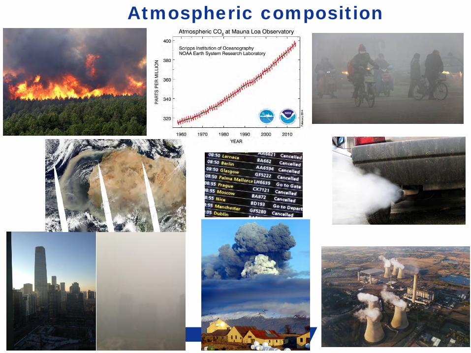
Atmospheric composition

Slide 3 Environmental Monitoring (II)

Slide 4


Scientific Motivation

Environmental and health concern (29,000 premature deaths due to pollution in UK per year)

Important to provide air quality forecasts Expertise in data assimilation and atmospheric modelling Not fundamentally different from meteorological DA but

several new challenges Interaction of atmospheric composition (AC) and NWP

- Feedback on dynamics via radiation scheme - Precipitation and clouds - Satellite data observations influenced by aerosols (and trace gases) - Hydrocarbon (Methane) oxidation is water vapour source - Assimilation of AC data can have impact on wind field

Slide 5


Over the last decade IFS has been extended with modules for atmospheric composition (aerosols, reactive gases, greenhouse gases)

GEMS -> MACC -> CAMS (Copernicus Atmosphere Monitoring Service) projects

At first a “Coupled System”, now composition fully integrated into IFS

Data assimilation of AC data to provide best possible IC for subsequent forecasts

AC benefits from online integration and high temporal availability of meteorological fields

C-IFS provides daily analyses and 5-day forecasts of atmospheric composition in NRT

Composition-IFS (C-IFS)

Slide 6 Air quality

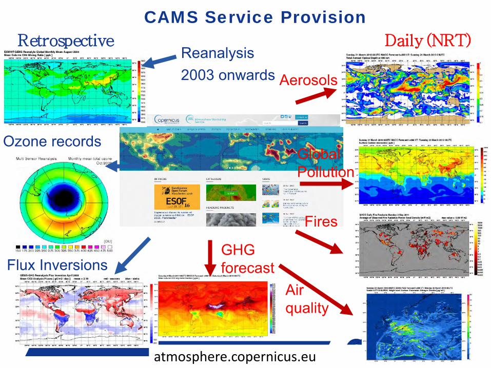
CAMS Service Provision

Global Pollution

Aerosols

Fires

Daily (NRT)

Flux Inversions

Reanalysis 2003 onwards

Ozone records

Retrospective

atmosphere.copernicus.eu

GHG forecast

Slide 7

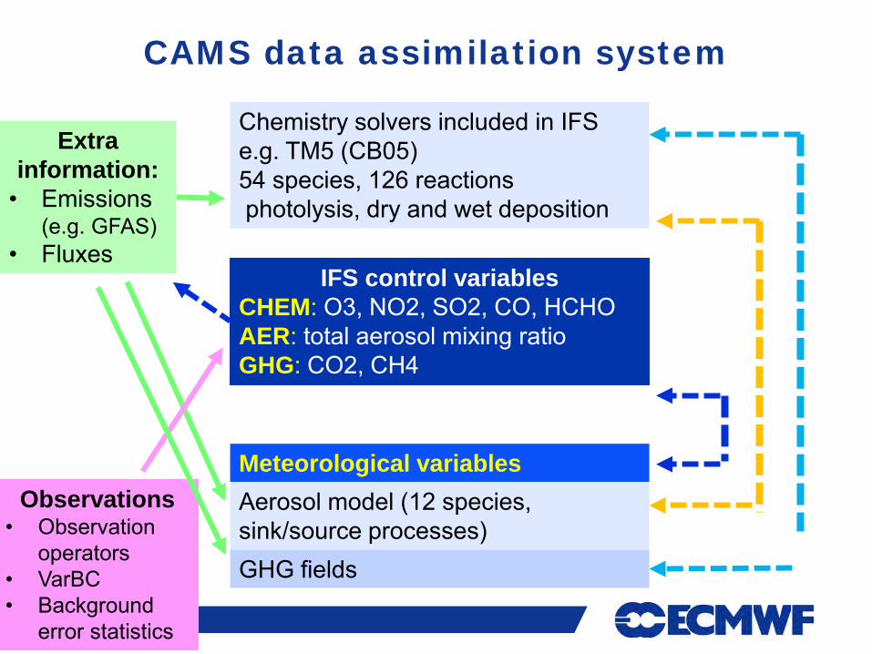
CAMS data assimilation system

IFS control variables CHEM: O3, NO2, SO2, CO, HCHO AER: total aerosol mixing ratio GHG: CO2, CH4

Chemistry solvers included in IFS e.g. TM5 (CB05) 54 species, 126 reactions photolysis, dry and wet deposition

Aerosol model (12 species, sink/source processes)

Extra information:

• Emissions (e.g. GFAS)

• Fluxes

Observations • Observation

operators • VarBC • Background

error statistics

GHG fields

Meteorological variables

Slide 8

ECMWF CAMS 4D-VAR Data Assimilation Scheme: Assimilation of AC

transport + chemistry + aerosol model

advection only (no chemistry or

aerosols)

transport + chemistry +

aerosol model

Slide 9

CHALLENGES IN ATMOSPHERIC

COMPOSITION DATA ASSIMILATION


Slide 10

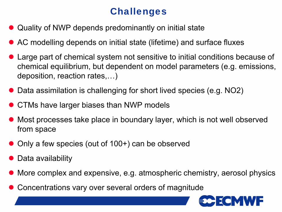
Challenges Quality of NWP depends predominantly on initial state

AC modelling depends on initial state (lifetime) and surface fluxes

Large part of chemical system not sensitive to initial conditions because of chemical equilibrium, but dependent on model parameters (e.g. emissions, deposition, reaction rates,…)

Data assimilation is challenging for short lived species (e.g. NO2)

CTMs have larger biases than NWP models

Most processes take place in boundary layer, which is not well observed from space

Only a few species (out of 100+) can be observed

Data availability

More complex and expensive, e.g. atmospheric chemistry, aerosol physics

Concentrations vary over several orders of magnitude

Slide 11

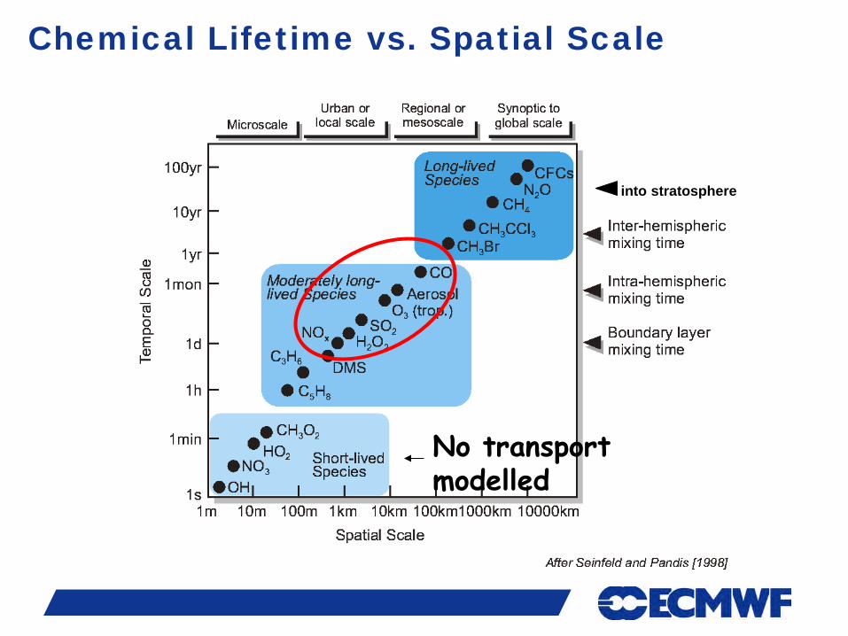
◄ into stratosphere

No transport modelled

Chemical Lifetime vs. Spatial Scale

Slide 12

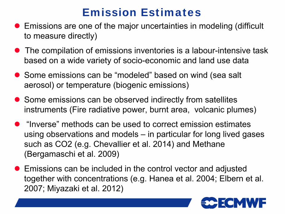
Emission Estimates Emissions are one of the major uncertainties in modeling (difficult

to measure directly)

The compilation of emissions inventories is a labour-intensive task based on a wide variety of socio-economic and land use data

Some emissions can be “modeled” based on wind (sea salt aerosol) or temperature (biogenic emissions)

Some emissions can be observed indirectly from satellites instruments (Fire radiative power, burnt area, volcanic plumes)

“Inverse” methods can be used to correct emission estimates using observations and models – in particular for long lived gases such as CO2 (e.g. Chevallier et al. 2014) and Methane (Bergamaschi et al. 2009)

Emissions can be included in the control vector and adjusted together with concentrations (e.g. Hanea et al. 2004; Elbern et al. 2007; Miyazaki et al. 2012)

Slide 13

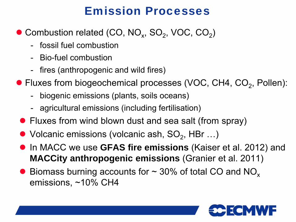
Combustion related (CO, NOx, SO2, VOC, CO2) - fossil fuel combustion - Bio-fuel combustion - fires (anthropogenic and wild fires)

Fluxes from biogeochemical processes (VOC, CH4, CO2, Pollen): - biogenic emissions (plants, soils oceans) - agricultural emissions (including fertilisation)

Fluxes from wind blown dust and sea salt (from spray) Volcanic emissions (volcanic ash, SO2, HBr …) In MACC we use GFAS fire emissions (Kaiser et al. 2012) and

MACCity anthropogenic emissions (Granier et al. 2011) Biomass burning accounts for ~ 30% of total CO and NOx

emissions, ~10% CH4

Emission Processes

Slide 14

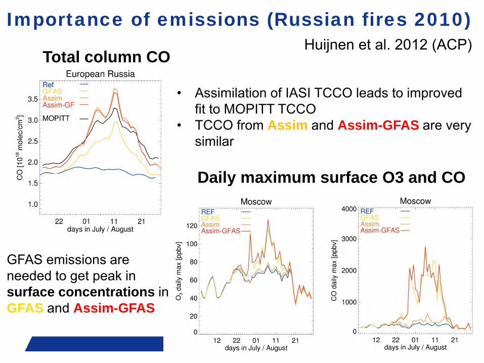
Importance of emissions (Russian fires 2010)

• Assimilation of IASI TCCO leads to improved fit to MOPITT TCCO

• TCCO from Assim and Assim-GFAS are very similar

Huijnen et al. 2012 (ACP)

GFAS emissions are needed to get peak in surface concentrations in GFAS and Assim-GFAS

Total column CO

Daily maximum surface O3 and CO

Slide 15

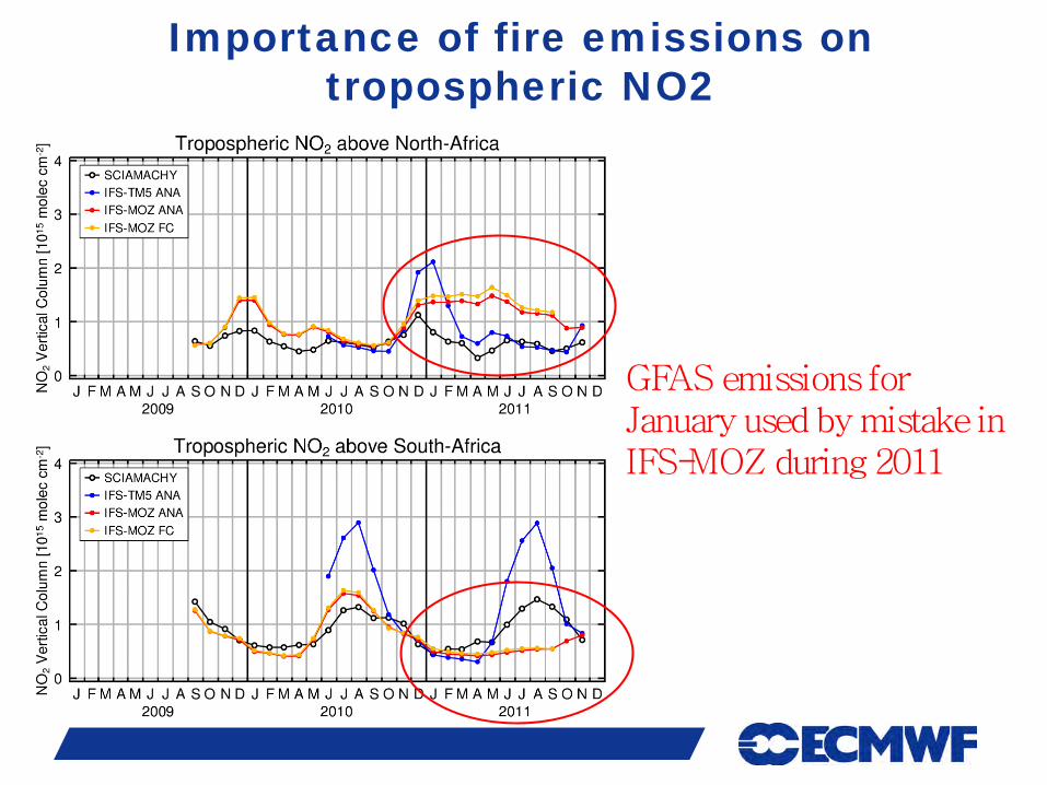
Importance of fire emissions on tropospheric NO2

GFAS emissions for January used by mistake in IFS-MOZ during 2011

Slide 16

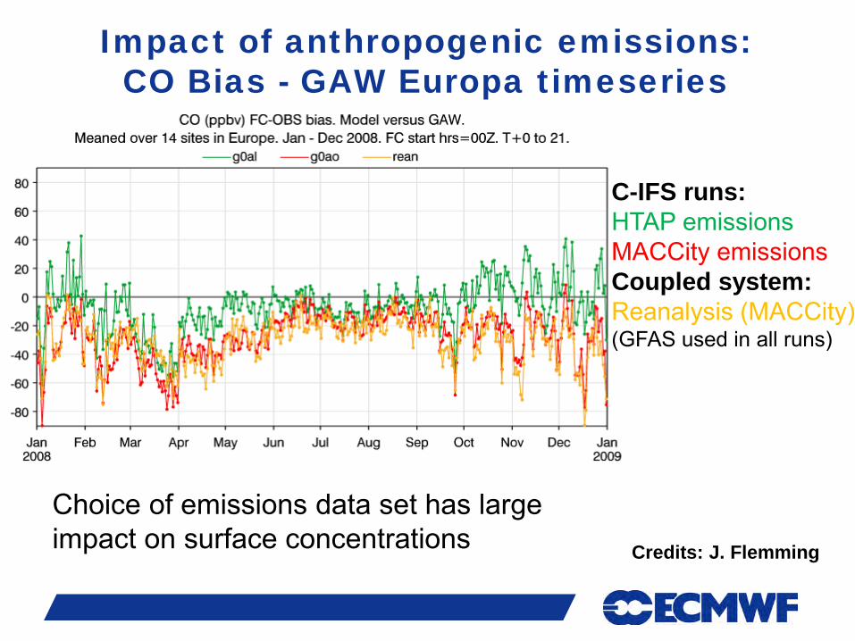
Impact of anthropogenic emissions: CO Bias - GAW Europa timeseries

C-IFS runs: HTAP emissions MACCity emissions Coupled system: Reanalysis (MACCity) (GFAS used in all runs)

Credits: J. Flemming

Choice of emissions data set has large impact on surface concentrations

Slide 17

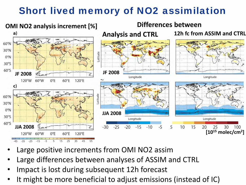
Short lived memory of NO2 assimilation OMI NO2 analysis increment [%] Differences between

[1015 molec/cm2]

JF 2008

JJA 2008

JF 2008

JJA 2008

• Large positive increments from OMI NO2 assim • Large differences between analyses of ASSIM and CTRL • Impact is lost during subsequent 12h forecast • It might be more beneficial to adjust emissions (instead of IC)

12h fc from ASSIM and CTRL Analysis and CTRL

Slide 18

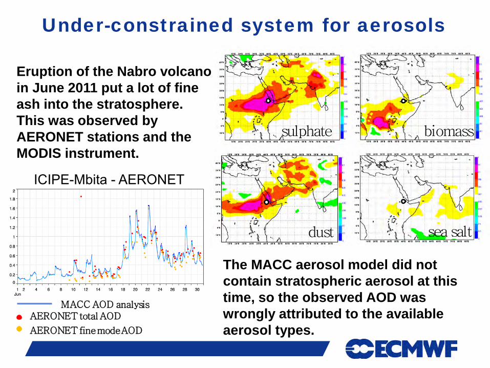
Under-constrained system for aerosols

sulphate biomass

dust sea salt

The MACC aerosol model did not contain stratospheric aerosol at this time, so the observed AOD was wrongly attributed to the available aerosol types.

MACC AOD analysis

Eruption of the Nabro volcano in June 2011 put a lot of fine ash into the stratosphere. This was observed by AERONET stations and the MODIS instrument.

AERONET fine mode AOD

ICIPE-Mbita - AERONET

AERONET total AOD

Slide 19

Graphics by Luke Jones

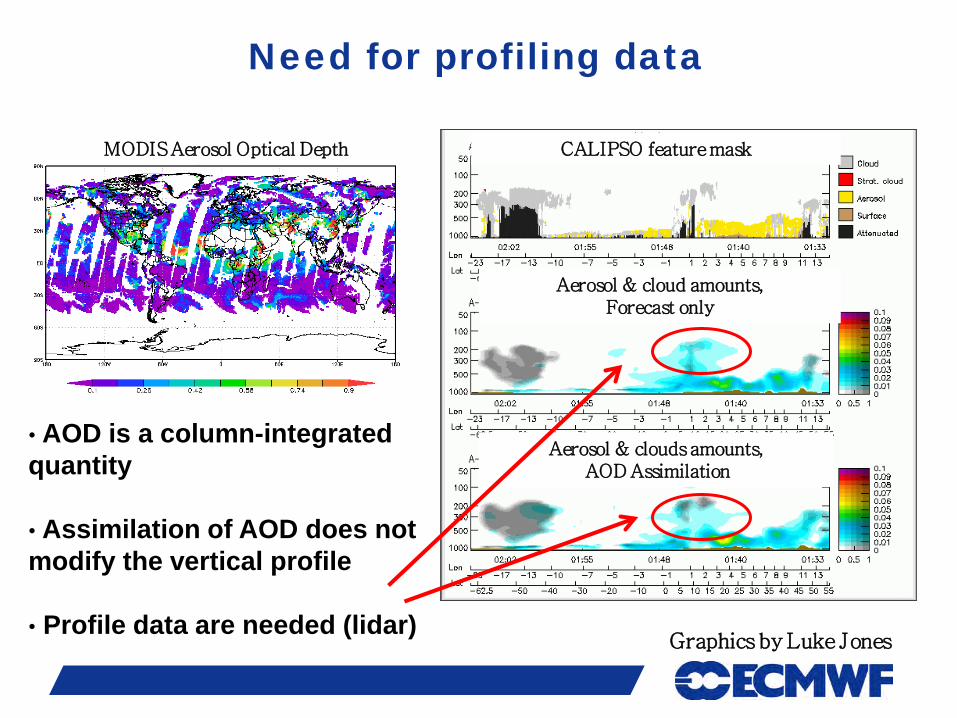
Aerosol & cloud amounts, Forecast only

Aerosol & clouds amounts, AOD Assimilation

CALIPSO feature mask

• AOD is a column-integrated quantity

• Assimilation of AOD does not modify the vertical profile

• Profile data are needed (lidar)

MODIS Aerosol Optical Depth

Need for profiling data

Slide 20

OBSERVATIONS OF ATMOSPHERIC COMPOSITION


Slide 21

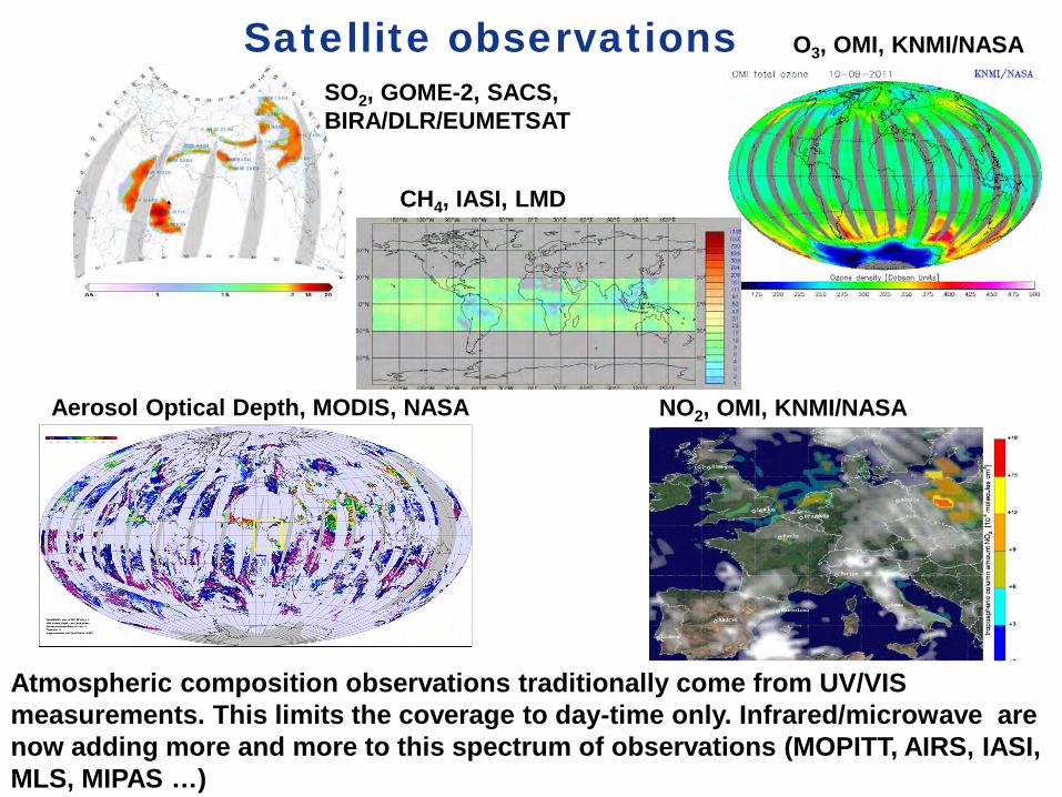
SO2, GOME-2, SACS, BIRA/DLR/EUMETSAT

NO2, OMI, KNMI/NASA Aerosol Optical Depth, MODIS, NASA

Satellite observations O3, OMI, KNMI/NASA

Atmospheric composition observations traditionally come from UV/VIS measurements. This limits the coverage to day-time only. Infrared/microwave are now adding more and more to this spectrum of observations (MOPITT, AIRS, IASI, MLS, MIPAS …)

CH4, IASI, LMD

Slide 22

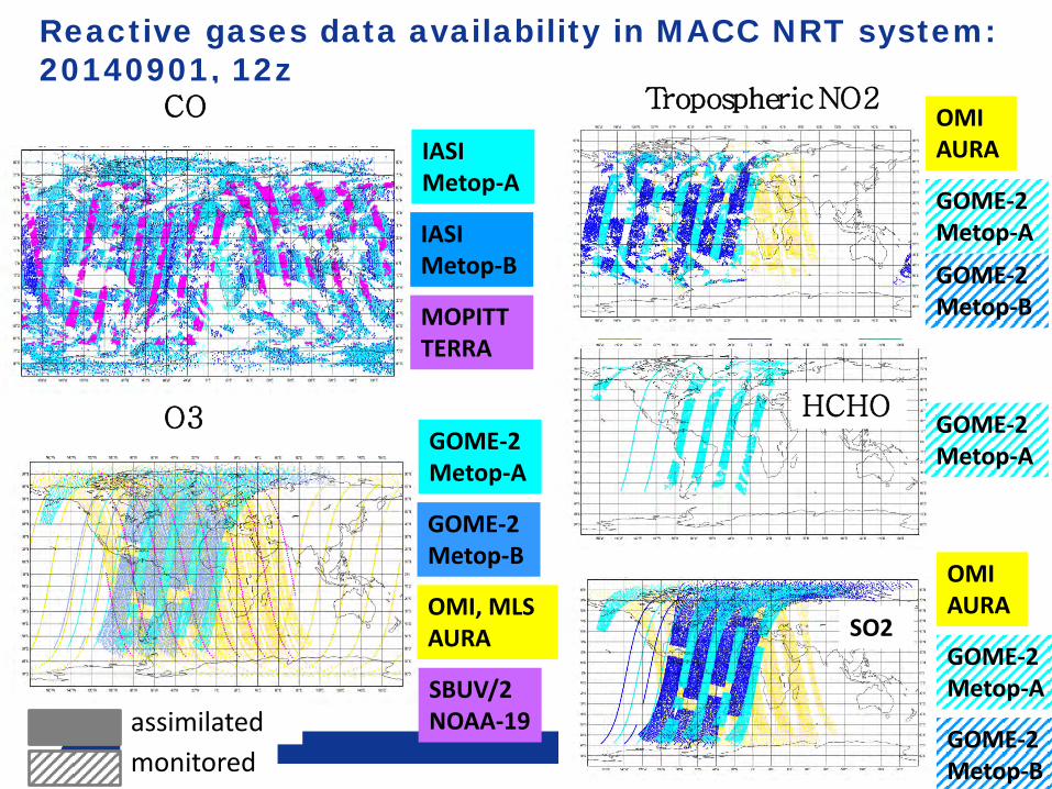
HCHO GOME-2 Metop-A

OMI AURA

SO2

GOME-2 Metop-B

GOME-2 Metop-A

OMI AURA

GOME-2 Metop-A

GOME-2 Metop-B

Tropospheric NO2

Reactive gases data availability in MACC NRT system: 20140901, 12z

IASI Metop-A

IASI Metop-B

MOPITT TERRA

CO

O3 GOME-2 Metop-A

OMI, MLS AURA

SBUV/2 NOAA-19

monitored assimilated

GOME-2 Metop-B

Slide 23

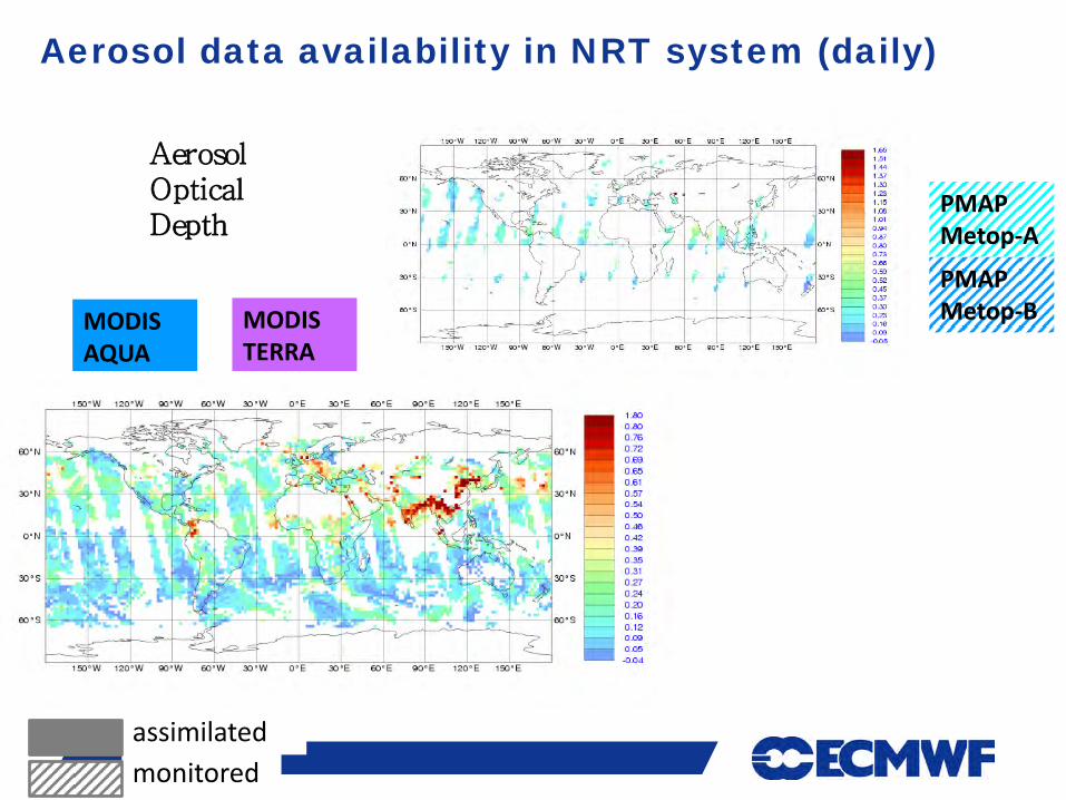
PMAP Metop-A

PMAP Metop-B

Aerosol data availability in NRT system (daily)

MODIS AQUA

MODIS TERRA

Aerosol Optical Depth

monitored assimilated

Slide 24

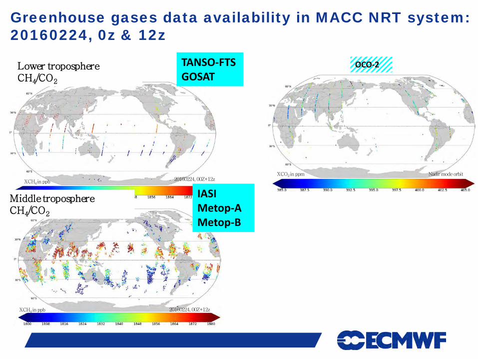
Greenhouse gases data availability in MACC NRT system: 20160224, 0z & 12z

TANSO-FTS GOSAT

Lower troposphere CH4/CO2

Middle troposphere CH4/CO2

IASI Metop-A Metop-B

XCH4 in ppb

XCH4 in ppb

OCO-2

20160224, 00Z+12z

20160224, 00Z+12z

XCO2 in ppm Nadir mode orbit

Slide 25

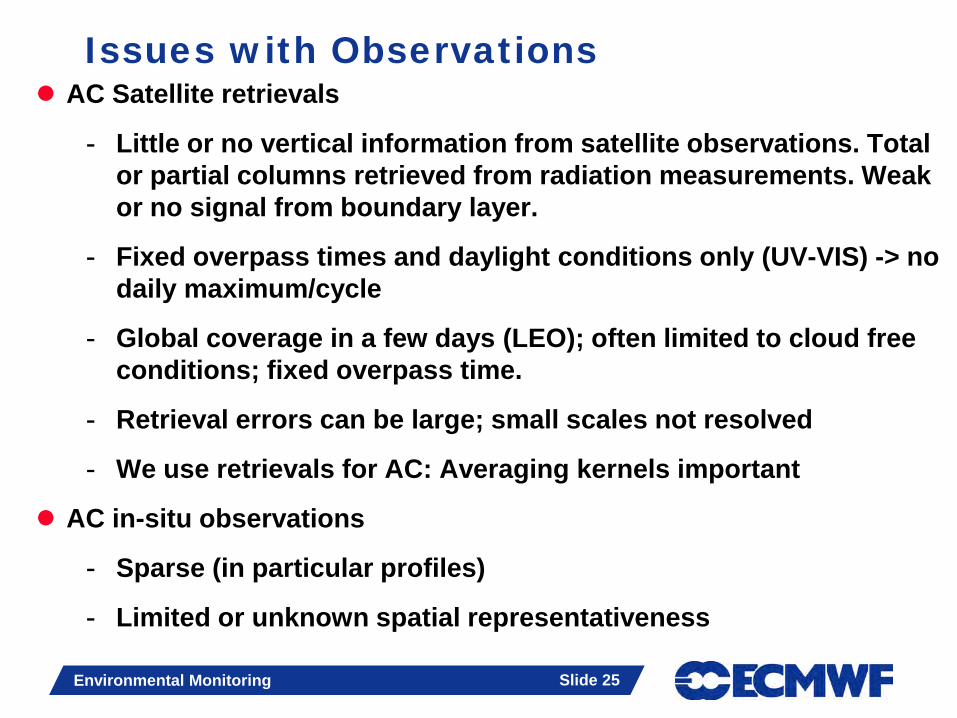
Issues with Observations AC Satellite retrievals

- Little or no vertical information from satellite observations. Total or partial columns retrieved from radiation measurements. Weak or no signal from boundary layer.

- Fixed overpass times and daylight conditions only (UV-VIS) -> no daily maximum/cycle

- Global coverage in a few days (LEO); often limited to cloud free conditions; fixed overpass time.

- Retrieval errors can be large; small scales not resolved

- We use retrievals for AC: Averaging kernels important

AC in-situ observations

- Sparse (in particular profiles)

- Limited or unknown spatial representativeness


Slide 26

ATMOSPHERIC COMPOSITION DATA

ASSIMILATION


Slide 27

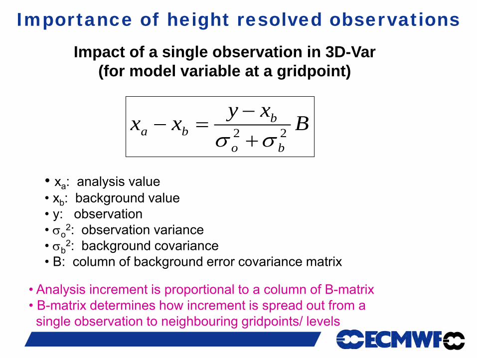
Impact of a single observation in 3D-Var (for model variable at a gridpoint)

Bxyxxbo

bba 22 σσ +

−=−

• xa: analysis value • xb: background value • y: observation • σo

2: observation variance • σb

2: background covariance • B: column of background error covariance matrix

• Analysis increment is proportional to a column of B-matrix • B-matrix determines how increment is spread out from a single observation to neighbouring gridpoints/ levels

Importance of height resolved observations

Slide 28

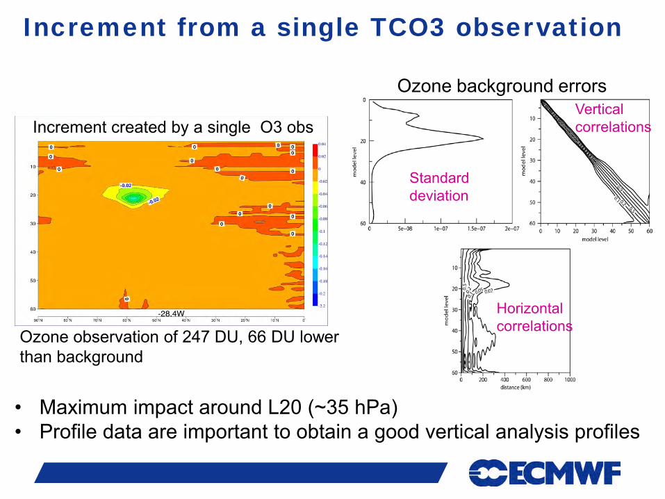
Increment created by a single O3 obs

Increment from a single TCO3 observation

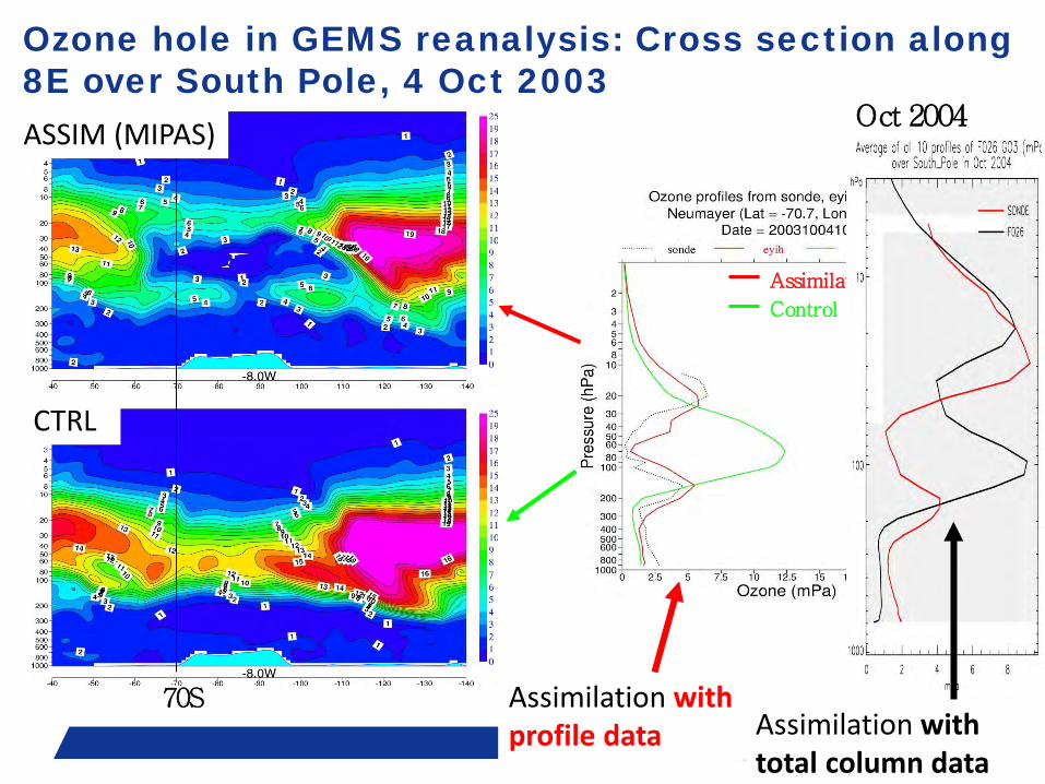
• Maximum impact around L20 (~35 hPa) • Profile data are important to obtain a good vertical analysis profiles

Horizontal correlations

Standard deviation

Vertical correlations

Ozone background errors

Ozone observation of 247 DU, 66 DU lower than background

Slide 29

Assimilation (MIPAS)

Control

70S

Ozone hole in GEMS reanalysis: Cross section along 8E over South Pole, 4 Oct 2003

Oct 2004 ASSIM (MIPAS)

CTRL

Assimilation with profile data Assimilation with

total column data

Slide 30

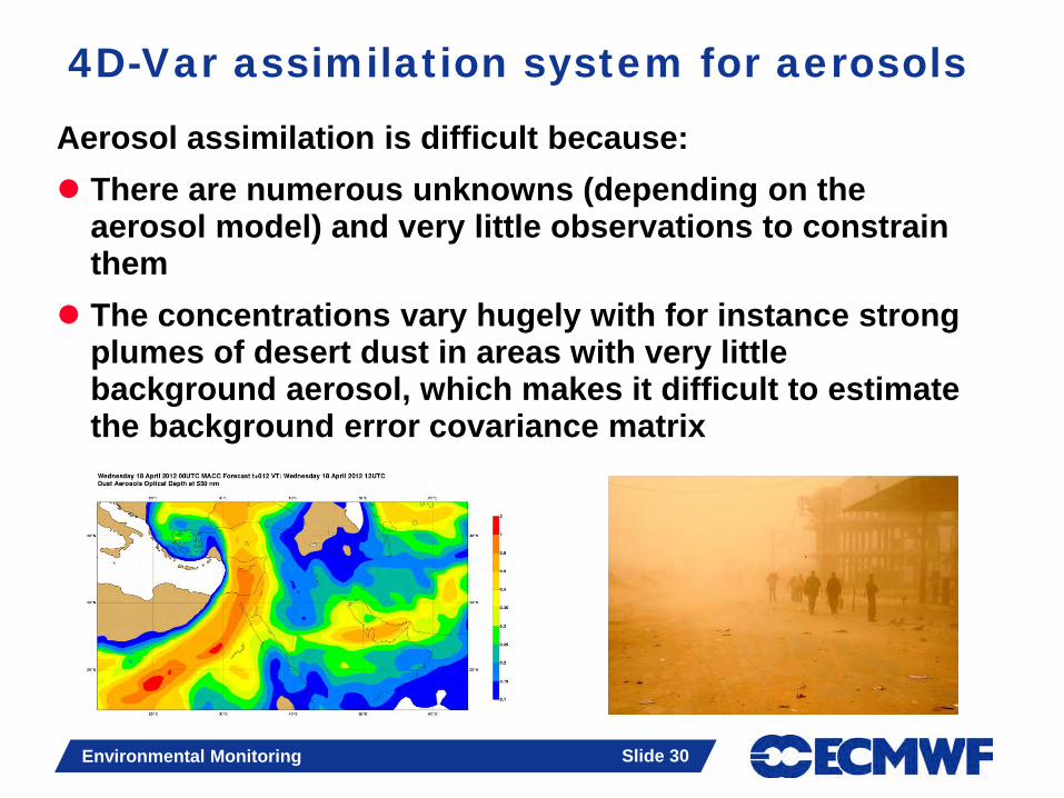
Aerosol assimilation is difficult because: There are numerous unknowns (depending on the

aerosol model) and very little observations to constrain them

The concentrations vary hugely with for instance strong plumes of desert dust in areas with very little background aerosol, which makes it difficult to estimate the background error covariance matrix

Slide 30 Environmental Monitoring

4D-Var assimilation system for aerosols

Slide 31

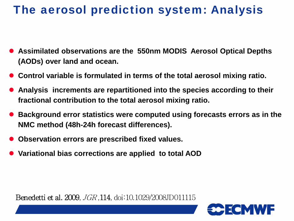
The aerosol prediction system: Analysis

Assimilated observations are the 550nm MODIS Aerosol Optical Depths (AODs) over land and ocean.

Control variable is formulated in terms of the total aerosol mixing ratio.

Analysis increments are repartitioned into the species according to their fractional contribution to the total aerosol mixing ratio.

Background error statistics were computed using forecasts errors as in the NMC method (48h-24h forecast differences).

Observation errors are prescribed fixed values.

Variational bias corrections are applied to total AOD

Benedetti et al. 2009, JGR ,114, doi:10.1029/2008JD011115

Slide 33

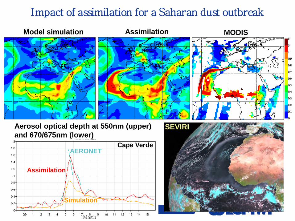
Impact of assimilation for a Saharan dust outbreak

Model simulation Assimilation MODIS

SEVIRI

AERONET

Assimilation

Simulation

March

Cape Verde

Aerosol optical depth at 550nm (upper) and 670/675nm (lower)

Slide 34

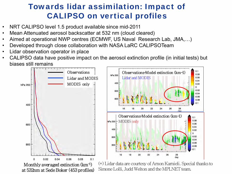
• NRT CALIPSO level 1.5 product available since mid-2011 • Mean Attenuated aerosol backscatter at 532 nm (cloud cleared) • Aimed at operational NWP centres (ECMWF, US Naval Research Lab, JMA,…) • Developed through close collaboration with NASA LaRC CALIPSOTeam • Lidar observation operator in place • CALIPSO data have positive impact on the aerosol extinction profile (in initial tests) but

biases still remains

(*) Lidar data are courtesy of Arnon Karnieli. Special thanks to Simone Lolli, Judd Welton and the MPLNET team.

Observations-Model extinction (km-1)

MODIS only

Lidar and MODIS

Observations

Towards lidar assimilation: Impact of CALIPSO on vertical profiles

Monthly averaged extinction (km-1) at 532nm at Sede Boker (453 profiles)

Lidar and MODIS

Observations-Model extinction (km-1)

MODIS only

Slide 35

6. Concluding remarks The ECMWF’s Integrated Forecast System has been extended to

include fields of atmospheric composition: Reactive gases, greenhouse gases, aerosols => Composition-IFS (C-IFS)

Modelling of AC needs to include many species with concentrations varying over several orders of magnitude

AC forecasts benefit from realistic initial conditions (data assimilation) but likewise from improved emissions

Extra challenges for DA of atmospheric composition compared to NWP - but also potential benefits through chemical coupling and impact on NWP

CAMS system produces useful AC forecast and analyses, freely available from atmosphere.copernicus.eu

Slide 36

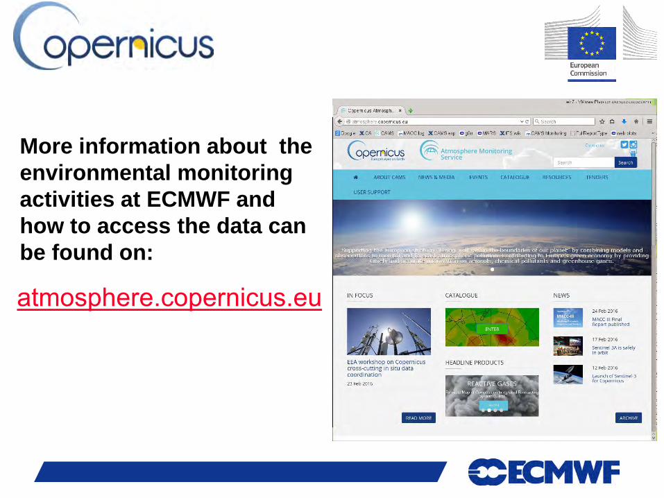
atmosphere.copernicus.eu

More information about the environmental monitoring activities at ECMWF and how to access the data can be found on:

http://www.copernicus-atmosphere.eu/

Slide 37


References: Reactive Gases N. Elguindi, H. Clark, C. Ordóñez, V. Thouret, J. Flemming, O. Stein, V. Huijnen, P. Moinat, A. Inness, V.-H. Peuch, A. Stohl, S. Turquety, G. Athier, J.-P. Cammas, and M. Schultz (2010): Current status of the ability of the GEMS/MACC models to reproduce the tropospheric CO vertical distribution as measured by MOZAIC. Geosci. Model Dev., 3, 501-518, 2010 Flemming, J., Huijnen, V., Arteta, J., Bechtold, P., Beljaars, A., Blechschmidt, A.-M., Josse, B., Diamantakis, M., Engelen, R. J., Gaudel, A., Inness, A., Jones, L., Katragkou, E., Marecal, V., Peuch, V.-H., Richter, A., Schultz, M. G., Stein, O., and Tsikerdekis, A.: Tropospheric chemistry in the integrated forecasting system of ECMWF, Geosci. Model Dev. Discuss., 7, 7733-7803, doi:10.5194/gmdd-7-7733-2014, 2014. Flemming, J., and A. Inness (2013), Volcanic sulfur dioxide plume forecasts based on UV satellite retrievals for the 2011 Grímsvötn and the 2010 Eyjafjallajökull eruption, J. Geophys. Res. Atmos., 118, doi:10.1002/jgrd.50753. Flemming, J., Inness, A., Jones, L., Eskes, H. J., Huijnen, V., Schultz, M. G., Stein, O., Cariolle, D., Kinnison, D., and Brasseur, G. (2011): Forecasts and assimilation experiments of the Antarctic ozone hole 2008, Atmos. Chem. Phys., 11, 1961-1977, doi:10.5194/acp-11-1961-2011 J. Flemming, Inness, A., Flentje, H., Huijen, V., Moinat, P., Schultz, M.G. and Stein O. (2009): Coupling global chemistry transport models to ECMWF's integrated forecast system. Geosci. Model Dev., 2, 253-265, 2009. www.geosci-model-dev.net/2/253/2009/ Huijnen, V., Flemming, J., Kaiser, J. W., Inness, A., Leitao, J., Heil, A., Eskes, H. J., Schultz, M. G., Benedetti, A., Hadji-Lazaro, J., Dufour, G., and Eremenko, M. (2012). Hindcast experiments of tropospheric composition during the summer 2010 fires over western Russia. Atmos. Chem. Phys., 12:4341–4364.

Slide 38


References: Reactive Gases Inness, A., Blechschmidt, A.-M., Bouarar, I., Chabrillat, S., Crepulja, M., Engelen, R. J., Eskes, H., Flemming, J., Gaudel, A., Hendrick, F., Huijnen, V., Jones, L., Kapsomenakis, J., Katragkou, E., Keppens, A., Langerock, B., de Mazière, M., Melas, D., Parrington, M., Peuch, V. H., Razinger, M., Richter, A., Schultz, M. G., Suttie, M., Thouret, V., Vrekoussis, M., Wagner, A., and Zerefos, C.: Data assimilation of satellite retrieved ozone, carbon monoxide and nitrogen dioxide with ECMWF's Composition-IFS, Atmos. Chem. Phys., 15, 5275-5303, doi:10.5194/acp-15-5275-2015, 2015. Inness, A., Baier, F., Benedetti, A., Bouarar, I., Chabrillat, S., Clark, H., Clerbaux, C., Coheur, P., Engelen, R. J., Errera, Q., Flemming, J., George, M., Granier, C., Hadji-Lazaro, J., Huijnen, V., Hurtmans, D., Jones, L., Kaiser, J. W., Kapsomenakis, J., Lefever, K., Leita ̃o, J., Razinger,M., Richter, A., Schultz, M. G., Simmons, A. J., Suttie, M., Stein, O., Th ́epaut, J.-N., Thouret, V., Vrekoussis, M., Zerefos, C., and the MACC team (2013). The MACC reanalysis: an 8 yr data set of atmospheric composition. Atmos. Chem. Phys., 13(8):4073–4109. Inness, A., Benedetti, A., Flemming, J., Huijnen, V., Kaiser, J. W., Parrington, M., and Remy, S.: The ENSO signal in atmospheric composition fields: emission-driven versus dynamically induced changes, Atmos. Chem. Phys., 15, 9083-9097, doi:10.5194/acp-15-9083-2015, 2015. Inness, A., Flemming, J., Suttie, M. and Jones, L., 2009: GEMS data assimilation system for chemically reactive gases. ECMWF RD Tech Memo 587. Available from http://www.ecmwf.int. C. Ordonez, N. Elguindi, O. Stein, V. Huijnen, J. Flemming, A. Inness, H. Flentje, E. Katragkou, P. Moinat, V-H. Peuch, A. Segers, V. Thouret, G. Athier, M. van Weele, C. S. Zerefos, J-P. Cammas, and M. G. Schultz (2009): Global model simulations of air pollution during the 2003 European heat wave. Atmos. Chem. Phys., 10, 789-815, 2010. www.atmos-chem-phys.net/10/789/2010/ Stein, O., Flemming, J., Inness, A., Kaiser, J. W., and Schultz, M. G. (2012). Global reactive gases forecasts and reanalysis in the MACC project. Journal of Integrative Environmental Sciences, 1:1–14

Slide 39


References: Areosols Bellouin, N., J. Quaas, J.-J. Morcrette, and O. Boucher, 2013: Estimates of radiative forcing from the MACC re-analysis. Atmos. Chem. Phys., 13, 2045-2062. Benedetti, A. et al, 2014: Operational dust prediction. Chapter 10 in: Knippertz, P.; Stuut, J.-B. (eds.), Mineral Dust – A Key Player in the Earth System, Springer Netherlands, 223–265, ISBN 978-94-017-8977-6. doi:10.1007/978-94-017-8978-3_10 Benedetti, A., Morcrette, J.-J., Boucher, O., Dethof, A., Engelen, R. J., Fisher, M., Flentje, H., Huneeus, N., Jones, L., Kaiser, J. W., Kinne, S., Manglold, A., Razinger, M., Simmons, A. J., and Suttie, M. (2009). Aerosol analysis and forecast in the European Centre for Medium-Range Weather Forecasts Integrated Forecast System: 2. Data assimilation. J. Geophys. Res., 114(D13):D13205 Benedetti, A., Kaiser, J. W., and Morcrette, J.-J. (2012). Global aerosols [in “State of the climate in 2011”]. Bull. Amer. Meteor. Soc., 93(7):S44–S46. (Also for subsequent years) Huneeus, N., M. Schulz, Y. Balkanski, J. Griesfeller, S. Kinne, J. Prospero, S. Bauer, O. Boucher, M. Chin, F. Dentener, T. Diehl, R. Easter, D. Fillmore, S. Ghan, P. Ginoux, A. Grini, L. Horowitz, D. Koch, M.C. Krol, W. Landing, X. Liu, N. Mahowald, R. Miller, J.-J. Morcrette, G. Myhre, J. Penner, J. Perlwitz, P. Stier, T. Takemura, and C. Zender, 2011: Global dust model intercomparison in AEROCOM phase I. Atmos. Chem. Phys., 11, 7781-7816, doi:10.5194/acp-11-7781-2011. Mangold, A., H. De Backer, B. De Paepe, S. Dewitte, I. Chiapello, Y. Derimian, M. Kacenelenbogen, J.-F. Léon, N. Huneeus, M. Schulz, D. Ceburnis, C. O'Dowd, H. Flentje, S. Kinne, A. Benedetti, J.-J. Morcrette, and O. Boucher, 2011: Aerosol analysis and forecast in the European Centre for Medium-Range Weather Forecasts Integrated Forecast System: 3. Evaluation by means of case studies, J. Geophys. Res.,116, D03302, doi: 10.1029 /2010JD014864.

Slide 40


References: Areosols Morcrette, J.-J., Boucher, O., Jones, L., Salmond, D., Bechtold, P., Beljaars, A., Benedetti, A., Bonet, A., Kaiser, J. W., Razinger, M., Schulz, M., Serrar, S., Simmons, A. J., Sofiev, M., Suttie, M., Tompkins, A. M., and Untch, A. (2009). Aerosol analysis and forecast in the European Centre for Medium-Range Weather Forecasts Integrated Forecast System: Forward modeling. J. Geophys. Res., 114(D6):D06206. Morcrette, J.-J., O. Boucher, L. Jones, D. Salmond, P. Bechtold, A. Beljaars, A. Benedetti, A. Bonet, J.W. Kaiser, M. Razinger, M. Schulz, S. Serrar, A.J. Simmons, M. Sofiev, M. Suttie, A.M. Tompkins, A. Untch, and the GEMS-AER team, 2009: Aerosol analysis and forecast in the ECMWF Integrated Forecast System: Forward modelling. J. Geophys. Res., 114, D06206, doi: 10.1029 /2008JD011235. Morcrette, J.-J., A. Beljaars, A. Benedetti, L. Jones, and O. Boucher, 2008: Sea-salt and dust aerosols in the ECMWF IFS. Geophys. Res. Lett., 35, L24813, doi:10.1029/2008GL036041. Morcrette, J.-J., A. Benedetti, L. Jones, J.W. Kaiser, M. Razinger, and M. Suttie, 2011: Prognostic aerosols in the ECMWF IFS: MACC vs. GEMS aerosols. ECMWF Technical Memorandum, 659, 32 pp. Morcrette, J.-J., A. Benedetti, A. Ghelli, J.W. Kaiser, and A.P. Tompkins, 2011: Aerosol-cloud-radiation interactions and their impact on ECMWF/MACC forecasts. ECMWF Technical Memorandum, 660, 35 pp. Nabat, P., S. Somot, M. Mallet, I. Chiapello, J.-J. Morcrette, F. Solmon, S. Szopa, and F. Dulac, 2013: A 4-D climatology (1979-2009) of the monthly aerosol optical depth distribution over the Mediterranean and surrounding regions from a comparative evaluation and blending of remote sensing and model products. Atmos. Meas. Tech., 6, 1287-1314, doi:10.5194/amt-6-1287-2013. Peubey, C., A. Benedetti, L. Jones, and J.-J. Morcrette, 2009: GEMS-Aerosol: Comparison and analysis with GlobAEROSOL data. In GlobAEROSOL User Report, October 2009, 11-20.

Slide 41


References: Greenhouse Gases

A. Agusti-Panareda; S. Massart; F. Chevallier; G. Balsamo; S. Boussetta; E. Dutra; A. Beljaars A biogenic C02 flux adjustment scheme for the mitigation of large-scale biases in global atmospheric CO2 analyses and forecasts. ECMWF Technical Memorandum, no 773, 2015 http://www.ecmwf.int/en/elibrary/technical-memoranda Agusti-Panareda, A., S.Massart, F.Chevallier,S.Boussetta, G.Balsamo, A.Beljaars, P.Ciais, N.M.Deutscher, R.Engelen, L.Jones and R.Kivi, J.-D.~Paris, V.-H. Peuch, V.Sherlock, A.T.Vermeulen, P.O.Wennberg, D.Wunch, 2014: Forecasting global atmospheric CO2, Atmospheric Chemistry and Physics ,14, 11959-11983 doi:10.5194/acp-14-11959-2014 Chevallier, F., R. J. Engelen, C. Carouge, T. J. Conway, P. Peylin, C. Pickett-Heaps, M. Ramonet, P. J. Rayne and I. Xueref-Remy, 2009. AIRS-based vs. flask-based estimation of carbon surface fluxes. J. Geophys. Res. 114, D20303, doi:10.1029/2009JD012311. Chevallier, F., R. J. Engelen, and P. Peylin, 2005. The contribution of AIRS data to the estimation of CO2 sources and sinks. Geophys. Res. Lett., 32, L23801, doi:10.1029/2005GL024229.

Slide 42


References: Greenhouse Gases Engelen, R.J., S. Serrar, and F. Chevallier, 2009. Four-dimensional data assimilation of atmospheric CO2 using AIRS observations. J. Geophys. Res., 114, D03303, doi:10.1029/2008JD010739. Engelen, R.J. and A. P. McNally, 2005. Estimating atmospheric CO2 from advanced infrared satellite radiances within an operational four-dimensional variational (4D-Var) data assimilation system: Results and validation. J. Geophys. Res., 110, D18305, doi:10.1029/2005JD005982 Massart et al. (2016) Ability of the 4-D-Var analysis of the GOSAT BESD XCO2 retrievals to characterize atmospheric CO2 at large and synoptic scales. Atmos. Chem. Phys., 16, 1653–1671, www.atmos-chem-phys.net/16/1653/2016/ doi:10.5194/acp-16-1653-2016. http://www.atmos-chem-phys.net/16/1653/2016/acp-16-1653-2016.pdf Massart, S. and Agusti-Panareda, A. and Aben, I. and Butz, A. and Chevallier, F. and Crevoisier, C. and Engelen, R. and Frankenberg, C. and Hasekamp, O., 2014: Assimilation of atmospheric methane products in the MACC-II system: from SCIAMACHY to TANSO and IASI0, Atmospheric Chemistry and Physics, 14, 6139–6158,10.5194/acp-14-6139-2014.

Slide 43


References: General Granier, C., Bessagnet, B., Bond, T., D’Angiola, A., Dernier van der Gon, H., Frost, G., Heil, A., Kaiser, J., Kinne, S., Klimont, G., Kloster, S., Lamarque, J.-F., Liousse, C., Masui, T., Meleux, F., Mieville, A., Ohara, T., Raut, J.-C., Riahi, K., Schultz, M., Smith, S., Thompson, A., van Aardenne, J., van der Werf, G., and van Vuuren, D. (2011). Evolution of anthropogenic and biomass burning emissions of air pollutants at global and regional scales during the 1980–2010 period. Climatic Change, 109(1-2):163–190. Hollingsworth, A., Engelen, R. J., Textor, C., Benedetti, A., Boucher, O., Chevallier, F., Dethof, A., Elbern, H., Eskes, H., Flemming, J., Granier, C., Kaiser, J. W., Morcrette, J.-J., Rayner, P., Peuch, V.-H., Rouil, L., Schultz, M. G., and Simmons, A. J. (2008). Toward a monitoring and forecasting system for atmospheric composition: The GEMS project. Bull. Amer. Meteor. Soc., 89(8):1147–1164.

References: Fires Kaiser, J. W., Heil, A., Andreae, M. O., Benedetti, A., Chubarova, N., Jones, L., Morcrette, J.-J., Razinger, M., Schultz, M. G., Suttie, M., and van der Werf, G. R. (2012). Biomass burning emissions estimated with a global fire assimilation system based on observed fire radiative power. Biogeosciences, 9:527–554. Kaiser, J. W. and van der Werf, G. R. (2012). Global Biomass Burning [in ”State of the Climate in 2011”]. Bull. Amer. Meteor. Soc., 93(7):S54–S55. (also for other years) Kaiser, J.W., M. Suttie, J. Flemming, J.-J. Morcrette, O. Boucher, and M.G. Schultz, 2009: Global real-time fire emission estimates based on space-borne fire radiative power observations. AIP Conf. Proc., 1100, 645-648.

Documents

Use of satellite data for Environmental Monitoring