Use of satellite data in monitoring and prediction of

USE OF SATELLITE DATA IN MONITORING AND PREDICTION OF RAINFALL OVER KENYA

By

Gilbert Ong’isa Ouma

Department of Meteorology

Faculty of Science

University of Nairobi

A thesis submitted in partial fulfillment of the requirements for the degree o f Doctor of

Philosophy in Meteorology, University o f Nairobi, Kenya

AUGUST, 2000

D E C L A R A T IO N

This thesis is my original work and has not been presented for a degree in any other University

Signature [o<? OO

Gilbert O. Ouma

This thesis has been submitted for examination with our approval as University Superv isors

Signature ____

Professor Laban A. Ogallo



Signature



TABLE OF CONTENTS

TITLE.......................................................................................................Error! Bookmark not defined.DECLARATION..............................................................................................................................................IITABLE OF CONTENTS.................................................................................................................................HIAbstract........................................................................................................................................................ vTABLE OF FIGURES...................................................................................................................................vmLIST OF TABLES........................................................................................................................................... XLIST OF ACRONYMS AND SPECIAL TERMS........................................................................................... XI

CHAPTER ONE.................................................................................................................................................. I

INTRODUCTION............................................................................................................................................. 11.0 Introduction...................................................................................................................................... //. 1 The Objectives o f the Study...............................................................................................................71.2 Justification for the Study................................................................................................................ 81.3 The Study Region............................................................................................................................101.3. / Location o f the Study Region...................................................................................................... 101.3.2 Rainfall Climatology o f the Study Region....................................................................................101.4 Literature Review............................................................................................................................141.4.1 Cloud indexing methods.............................................................................................................. 151.4.2 Life-History methods...................................................................................................................191.4.3 Bi-spectral and cloud model methods.........................................................................................211.4.4 Passive microwave methods........................................................................................................231.4.4.1 Emission-Based Methods............................................................................................................241.4.4.2 Scattering Based Methods........................................................................................................... 281.4.4.3 Emission and Scattering-based Methods.................................................................................... 29

CHAPTER TWO..............................................................................................................................................32

DATA AND DATA QUALITY CONTROL...................................................................................................322.0 Introduction....................................................................................................................................322.1 Rainfall Data..................................................................................................................................322.2 Satellite Data...................................................................................................................................352.2.1 Cold Cloud Duration (CCD) Data ..............................................................................................352.2.2 NASA Water Vapor Project (NVAP) Total Precipitable Water..................................................362.2.2.1 Radiosonde Data......................................................................................................................... 372.2.2.2 Special Sensor Microwave Imager (SSM/1) Data...................................................................... 382.2.2.3 TIROS Operational Vertical Sounder (TOVS) Data:..................................................................392.2.2.4 Blended TPW Data......................................................................................................................412.2.3 European Center fo r Medium-range Weather Forecasts (ECMWF) Data se t............................42

CHAPTER THREE..........................................................................................................................................44

METHODS OF ANALYSES........................................................................................................................ 443.0 Methodology...................................................................................................................................443.1 Regionalization...............................................................................................................................443.1.1 Principal Component Analysis (PCA)........................................................................................473.1.1.1 Number o f Significant Principal Components........................................................................... 483.1.1.1.1 Kaiser’s Criterion........................................................................................................................ 493.1.1.1.2 The Scree's Method..................................................................................................................... 493.1.1.1.3 The Logarithm o f Eigenvalue (LEV) Method............................................................................. 493.1.1.1.4 Sampling Errors o f Eigenvalues..................................................................................................493.1.2 Rotation o f the Principal Components........................................................................................503.2 Choice o f Representative Records fo r the Homogeneous Regions.................................................513.2.1 Unweighted Arithmetic Mean M ethod ............................................................................................. 523.2.2 Use o f PC A Weighted Averages........................................................................................................ 523.2.3 The use o f the Principle o f PC A Communality.................................................................................533.3 Correlation Analysis...................................................................................................................... 543.3.1 Testing Statistical Significance o f the Computed Correlation Coefficient........................................563.4 Regression Analysis........................................................................................................................ 563.4.1 Linear Regression Analysis............................................................................................................... 563.4.2 Multiple Regression Analysis........................................................................................................5 7

3.4.3 Canonical Correlation Analysis....................................................................................................... 583.4.4 Estimation of Parameters............................................................................................................623.4.4.1 Graphical Method.........................................................................................................................623.4.4.2 Least Squares Method..................................................................................................................623.4.4.3 Method o f Moments.................................................................................................................... 633.4.4.4 Maximum Likelihood M ethod .....................................................................................................643.5 Test o f the Skill o f the Fitted Models.............................................................................................. 663.5. / Analysis o f Variance Techniques (ANOVA)............................................................................... 663.5.1.1 Mean Square Error......................................................................................................................663.5.1.2 The Chi-Square (% ) Test.............................................................................................................673.5.1.3 The F- Test.....................................................................................................................................683.5.2 Kolmogorov-Smirnov Test...........................................................................................................693.5.3 Hits and Alarms.......................................................................................................................... 693.5.4 Akaike’s Information Criterion..................................................................................................693.5.5 Cross-Validation........................................................................................................ 72.?. 6 Rainfall Evolution Patterns during the Normal, Dry and Wet Seasons......................................... 733.6.1 Identification o f Anomalous Rainfall Seasons.............................................................................733.6.2 Onset, Withdrawal and Duration o f Rainfall Seasons................................................................753.6.3 Composite Analysis......................................................................................................................76

CHAPTER FOUR ■■••■•••••••••••••■■•■••••••••••••■•••••••••••••■••••••••■•••••••■•••••••••••••(•■•I 78

RESULTS AND DISCUSSION.................................................................................................................... 784.0 Introduction.................................................................................................................................... 784. 1 Skill o f the Estimated Data and Data Quality...............................................................................784.2 Results from Regionalization analyses...........................................................................................814.2.1 Regionalization from Rainfall Data............................................................................................814.2.1. / March - May (MAM) Season....................................................................................................814.2.1.2 September - November (SON) Season ........................................................................................894.2.1.3 June - August (JJA) Season..................................................................................................... 974.2.1.4 December- February (DJF) Season.......................................................................................... 104

A bstrac t

Skillful monitoring, prediction and early warning of the extreme weather events is

crucial in the planning and management of all rain dependent socio-economic activities. They

are also vital for the development o f effective disaster preparedness strategies. Prediction

methods depend on availability of long period, high quality data with good spatial coverage.

Real and near real time data are also useful as initial conditions for the integration of

prediction models. Thus, high quality data with good spatial and temporal coverage is

fundamental for any research and applications. Unfortunately, limitation of rainfall data is a

serious problem in many parts of the world, especially in the developing countries.

This study investigated the viability of satellite derived data in providing alternative

rainfall information and hence enhancing rainfall monitoring, prediction and disaster

preparedness in Kenya. The data sets used in the study included observed daily rainfall,

dekadal Cold Cloud Duration (CCD) and pentad Total Precipitable Water (TPW) data

together with the rearialysis data from ECMWF.

The various methods that were used to achieve the objectives of the study included

data quality analyses. S-mode Principal Component Analysis (PCA) together with correlation

and regression analyses. The regression models used included simple linear, stepwise and

canonical regression approaches. The skills of the developed models were further investigated

during anomalous wet and dry periods. Meteorological conditions that could be associated

w ith the decreased or increased skill o f the regression models during the anomalous periods

were also investigated.

The results obtained from the quality control tests indicated that all data used in the

study were of good quality. The S-mode PCA solutions delineated eleven regions for March-

April-May (MAM), June-July-August (JJA) and December-January-February (DJF) seasons,

while only nine were delineated for the September-October-November (SON) season from the

VI

rainfall data. The number of significant PCA modes was higher for the dry seasons of JJA and

DJF as compared to those from the wet seasons of MAM and SON. However, these

components extracted relatively low percentage of total variance in the observed rainfall and

hence the development of regression models concentrated on the wet seasons of MAM and

SON. Although the duration of the satellite-derived data available was shorter, the regions

derived from this data set were generally consistent with those obtained using the rainfall

data.

The results from correlation analyses showed significant linear relationships between

rain gauge rainfall and only CCD data. The results of ANOVA tests on the linear regression

models indicated that the developed models had reasonable skill in estimating rainfall from

CCD data. Results from stepwise regression analyses o f rain gauge rainfall, CCD and the

three layers of TPW data indicated that the additional variance explained by the inclusion of

TPW data were generally low. It was, however, evident that, in some regions, the inclusion of

TPW in the estimation models was o f added value. The examinations of the skill of the

models during anomalous dry and wet periods revealed better performance during the

anomalous seasons. The composites o f the meteorological conditions showed that for the

anomalous dry seasons, a westerly component exists in the equatorial winds (surface to 800

mb layer) that interferes with the supply of moisture from the Indian Ocean and lead to a

reduction in the amount of moisture available inland. During anomalous wet seasons, the

southeasterly flow inland is very strong enhancing the moisture influx from the Indian Ocean.

The last part of the study examined the more complex Canonical Correlation Analysis

(CCA) in the development of estimation and forecasting models. The results from the CCA

indicated significant year to year variations in the skills for the estimated areal observed

rainfall from satellite-derived data. A comparison of the CCA models results to those of the

stepwise regression revealed that the CCA models performed considerably better during the

VII

SON season in estimating the areal observed rainfall. The results from the forecasting models

revealed that the canonical correlation coefficients based on CCD data were all not

statistically significant in all locations and seasons. Results obtained from analyses of TPW

data, however, indicated some skill in forecasting of rainfall with SON season registering

higher canonical correlation coefficients.

This study has. for the first time, regionalized Kenya into seasonal climatological

homogeneous zones using satellite-derived data. It has also developed statistical models based

on satellite-derived data that can be used to estimate areal rainfall for the derived

climatological zones. The study further highlights the vital need to use distinct CCD

temperature thresholds for rainfall estimation for individual climatological zones and seasons.

Finally, it is the first time that a study has used CCA technique for the estimation of areal

rainfall from satellite-derived data in Kenya. CCA predictors were also derived for areal

rainfall forecasting. The complex CCA approach improved skills in the rainfall estimates

during some seasons that had relatively poor skills with the other methods.

In conclusion, the study has for the first time provided some useful information

regarding the enormous potential use o f satellite-derived data in the estimation o f 10-day areal

rainfall for specific regions in Kenya. The results from the PCA regionalization show that the

satellite-derived data can be used to delineate large-scale spatial anomalies in the rainfall over

the study region. Accurate delineation o f these anomalies is vital in drought monitoring, flash

Hood forecasting and general preparedness against extreme weather events.

VIII

TABLE OF FIGURES

Figure 1.1: Relief map of Kenya..................................................................................................... 4Figure 1.2: The location of the study area with respect to the continent of Africa....................11Figure 1.3: Mean annual rainfall map o f the study area................................................................12Figure 2.1: Map of the study area showing the distribution o f the rainfall stations................. 34Figure 4.1(a): Mass Curve for Lokichogio Station.......................................................................79Figure 4.1(b): Mass Curve for Mandera Station........................................................................... 79Figure 4.1(c): Mass Curve for Kisumu Station............................................................................. 80Figure 4.1(d): Mass Curve for Dagoretti Station.........................................................................80Figure 4.2: Scree's test selection of the dominant principal components for MAM season.... 82 Figure 4.3(a): Spatial patterns of the first rotated principal component during MAM season. 85 Figure 4.3(b): Spatial patterns of the second rotated principal component during MAM

season........................................................................................................................................ 86Figure 4.3(c): Spatial patterns of the third rotated principal component during MAM season.

...................................................................................................................................................87Figure 4.4: Homogenous divisions of the 60 stations derived from the MAM seasonal RPCA

patterns....................................................................................................................................... 88Figure 4.5: Scree's test selection of the dominant principal components for SON season.......90Figure 4.4.6(a): Spatial patterns of the first rotated principal component during SON season.

.................................................................................................................................................... 93Figure 4.6(b): Spatial patterns of the second rotated principal component during SON season.

.................................................................................................................................................... 94Figure 4.6(c): Spatial patterns of the third rotated principal component during SON season. 95 Figure 4.7: Homogenous divisions o f the 60 stations derived from the SON seasonal RPCA

patterns...................................................................................................................................... 96Figure 4.8: Scree’s test selection of the dominant principal components for JJA season....... 97Figure 4.9(a): Spatial patterns of the first rotated principal component during JJA season.. 100 Figure 4.9(b): Spatial patterns of the second rotated principal component during JJA season.

.......................................................................................................................... 101

Figure 4.9(c): Spatial patterns of the third rotated principal component during JJA season. 102 Figure 4.10: Homogenous divisions of the 60 stations derived from the JJA seasonal RPCA

patterns....................................................................................................................................103Figure 4.11: Scree’s test selection of the dominant principal components for DJF season... 104 Figure 4.12(a): Spatial patterns of the first rotated principal component during DJF season.

.................................................................................................................................................107Figure 4.12(b): Spatial patterns of the second rotated principal component during DJF season.

.................................................................................................................................................108Figure 4 .12(c): Spatial patterns of the third rotated principal component during DJF season.

.................................................................................................................................................109Figure 4.13: Homogenous divisions of the 60 stations derived from the DJF seasonal RPCA

patterns..................................................................................................................................... 110Figure 4.14(a): Spatial patterns of the first rotated principal component for decadal TPW

during MAM season............................................................................................................... 117Figure 4.14(b): Spatial patterns of the first rotated principal component for decadal TPW

during SON season................................................................................................................. 119Figure 4.14(c): Spatial patterns of the first rotated principal component for decadal TPW

during JJA season....................................................................................................................120Figure 4.14(d): Spatial patterns of the first rotated principal component for decadal TPW

during DJF season............................................................................................................... 121

IX

Figure 4.15(a): Homogenous divisions of study region derived from the MAM surface-700mbdecadal TPW seasonal RPC A patterns................................................................................ 122

Figure 4.15(b): Homogenous divisions of study region derived from the SON surface-700mbdecadal TPW seasonal RPC A patterns..................................................................................123

Figure 4.15(c): Homogenous divisions of study region derived from the JJA surface-700mbdecadal TPW seasonal RPCA patterns..................................................................................124

Figure 4.15(d): Homogenous divisions of study region derived from the DJF surface-700mbdecadal TPW seasonal RPCA patterns..................................................................................125

Figure 4.16: Scatter diagrams showing the relationship between rainfall and CCD with thesimple regression line included.............................................................................................. 136

Figure 4.17(a): Plot of the Observed and Estimated Rainfall Anomalies for MAM Season(1994/1995)........................................................................................................................... 142

Figure 4.17(b): Plot of the Observed and Estimated Rainfall Anomalies for SON Season(1994/1995)........................................................................................................................... 143

Figure 4.18: Examples of the cumulative curves used to determine the seasonal rainfall onset.withdrawal and duration..........................................................................................................146

Figure 4.19: Spatial distribution of 850mb wind during the wet SON season of 1982........ 151Figure 4.20: Spatial distribution of 850mb wind during the dry MAM season o f 1992....... 152Figure 4.21: Relationship between the observed rainfall and the CCA estimates for MAM

season........................................................................................................................................156Figure4.22: Relationship between the observed rainfall and the CCA estimates for SON

season........................................................................................................................................156

LIST OF TABLES

Table 2.1: List o f Stations used in the study................................................................................ 33Table 3.1: Classification of the dry, normal and wet seasons scenarios....................................75Table 4.1: Statistical characteristics o f 1982 -1995 dekadal rainfall from PCA o f MAM

season.......................................................................................................................................83Table 4.2: The possible physical reasons underlying the derived regions for M A M ..............89Table 4.3: Statistical characteristics o f 1982 -1995 dekadal rainfall from PCA o f SON season

....................................................................................................................................................92Table 4.4: Statistical characteristics o f 1982 -1995 dekadal rainfall from PCA o f JJA season

....................................................................................................................................................98Table 4.5: Statistical characteristics o f 1982 -1995 dekadal rainfall from PCA o f DJF season

.................................................................................................................................................. 105Table 4.6: Eigenvalue statistics from the PCA of TPW for all the seasons............................116Table 4.7: Representative stations for each homogenous region for MAM and SON seasons.

.................................................................................................................................................. 127Table 4.8: Correlation statistics of rainfall against CCD from the areal records derived using

arithmetic mean, PCA weights and the principle of communality....................................129Table 4.9: Correlation coefficients for the relationship between rainfall and TPW data...... 131Table 4.10: The simple regression analyses statistics of rainfall against CCD......................... 133Table 4.11: The multivariate regression analyses statistics from the representative records of

rainfall against CCD and the three layers of TPW data....................................................... 138Table 4.12: The ANOVA for the Estimation Period...................................................................140Table 4.13: Categorization of the years into dry, wet, or normal seasons..............................144Table 4.14: Onset, withdrawal and duration for MAM and SON during the study period.... 146 Table 4.15: ANOVA results and the correlation coefficient, r, for the anomalous dry years. 147 Table 4.17(a): Correlation between the observed rainfall and the satellite-derived estimates for

MAM season.......................................................................................................................... 154Table 4.17(b): Correlation between the observed rainfall and the satellite-derived estimates

for SON season........................................................................................................................154Table 4.18: The ANOVA for the CCA rainfall estimates.........................................................158Table 4.19: Canonical correlation coefficients between rainfall patterns and TPW patterns 158 Table 4.20: Contingency table grouping observed standard anomaly rainfall and CCA

estimates from TPW data for region nine during SON season 159

XI

LIST OF ACRONYMS AND SPECIAL TERMS

1D-VAR One Dimensional Variation

ADMIT Agricultural Drought Monitoring Integrated Technique

AIC Akaike’s Information Criterion

ANOVA Analysis of Variance

ASALS Arid and Semi-Arid Lands

BIAS Bristol/NOAA Interactive Scheme

CCA Canonical Correlation Analysis

CCD Cold Cloud Duration

CCR Cloud Cleared Radiance

CFA Common Factor Analysis

CL Confidence Level

CST Convective Stratiform Technique

CWV Column Water Vapor

DJF December-January-February

DMSP Defense Meteorological Satellite Project

EBBT Equivalent Black Body Temperature

ECMWF European Centre for Medium-range Weather Forecasts

EOF Empirical Orthogonal Functions

EPI ESOC Precipitation Index

ERA ECMWF Re-Analysis

ESA European Space Agency

ESMR Electrically Scanning Microwave Radiometer

ESOC European Space Operation Centre

GARP Global Atmospheric Research Program

XII

GATE GARP Atlantic Tropical Experiment

GMS Geostationary (Geosynchronous) Meteorological Satellite

GOES Geostationary Operational Environmental Satellites

GOES-E GOES East

GPI GOES Precipitation Index

GSCAT2 Goddard Scattering Algorithm version 2

GTS Global Telecommunications System

HIRS High Resolution Infrared Radiation Sounder

INSAT Indian Satellite

IR Infrared

ISCCP International Satellite Cloud Climatology Project

ITCZ Inter Tropical Convergence Zone

JJA June-July-August

JKIA Jomo Kenyatta International Airport

K-L Kullback-Liebler

MAM March-April-May

METEOSAT Meteorological Satellite

MSE Mean Square Error

MSG METEOSAT Second Generation

MSU Microwave Sounding Unit

NASA National Aeronautics and Space Administration

NCAR National Center for Atmospheric Research

NESDIS National Environmental Satellite Data and Information Service

NESS National Environmental Satellite Service

NO A A National Oceanic and Atmospheric Administration

XIII

NOAA-SRL NOAA Satellite Research Laboratories

NVAP NASA Water Vapor Project

NWP Numerical Weather Prediction

OF-HPP Owen Falls Hydroelectric Power Plant

PCA Principal Component Analysis

PCs Principal Components

PCT Polarization-Corrected Temperature

PM Passive Microwave

POT Percent-Of-Total

RCSSMRS Regional Centre for Services in Surveying, Mapping and Remote Sensing

SHARP Short Term Automated Radar Prediction

SMMR Scanning Multi-channel Microwave Radiometer

SSM/I Special Sensor Microwave/lmager

SON September-October-November

SST Sea Surface Temperature

SSU Stratospheric Sounding Unit

TIROS Television Infrared Observation Satellite

TOVS TIROS Operational Vertical Sounder

TPW Total Precipitable Water

UTH Upper Tropospheric Humidity

VIS Visible

1

CHAPTER ONE

INTRODUCTION

1.0 Introduction

One of the major forcing mechanisms of the general circulation is the tropical convection

with its attendant release of latent heat. Good knowledge of its space-time variability, and

detailed monitoring of its day to day evolutions are crucial for the proper understanding of the

dynamics of the global climate system and improvement of prediction skills.

In equatorial Africa, as in all other tropical regions, one of the most important climatic

elements is rainfall due to its large spatial and temporal variability. This high variability' has a major

impact on the socio-economic activities of the countries within this region since their economies

depend mainly on the rain-fed agriculture. Agriculture and the associated industries are also the

major employment sectors in the region. Extreme rainfall anomalies like droughts and floods often

have far reaching socio-economic impacts in the region including a decrease in food production and

agricultural exports, famine, mass migration of people and animals, environmental refugees, loss of

life and property among many other socio-economic miseries. Skillful prediction of the onset,

duration, amount, intensity, and cessation of rainfall expected during any season is crucial in the

planning and management of agricultural activities and, by extension, economies of these countries.

Skillful prediction of rainfall would also be useful in early warning of any impending extreme

rainfall events, and enable proper disaster preparedness policies to be adopted in time, in order to

avoid the post disaster relief policies that are common in the region.

2

A good example of the need for emergency mitigation policies was witnessed in Kenya

during the extreme floods that were associated with the 1997/98 El-Nino phenomenon. Over 80%

of Kenya may be classified as arid and semi arid lands (ASALs) that have very' high year to year

rainfall variability. During the period 1996 - 1997, for instance, the region experienced a prolonged

drought that forced the government of Kenya to declare a National Famine Disaster Emergency.

Extreme floods, associated with El-Nino phenomena, soon follow'ed in 1997 - 1998 and these

caused heavy damage to the country’s infrastructure, and loss of human and animal life. This was

followed by another drought that started in 1999 and persisted into the year 2000 in many parts of

Kenya. The 1999-2000 drought was considered as one of the worst in the century. During the times

o f such national disasters, resources meant for other development projects are diverted to the

management and mitigation of the effects of these rainfall-related problems. Such extreme events arc

capable of seriously depressing the economy of many developing nations.

For proper planning and management, disaster management policies are required if the

impacts of meteorological disasters that are very common in Kenya are to be minimized. The

disaster preparedness component requires, among others, effective early warning system, which can

provide good lead-time warning of any potential disasters. Such early warning systems are derived

from various prediction models, which are integrated using initial condition data. Data for defining

the initial conditions and the development of the prediction models must be of good quality, and

must have good spatial and temporal coverage. The study of the processes and the development of

the predictive models also require long periods of such data. Data insufficiency is a serious problem

in many parts of the world and. especially, in the developing countries.

Accurate measurement and monitoring of precipitation is therefore important in the planning

and management of all water-use activities. Long period, high quality data with good spatial density

are also required in order to study the past rainfall evolutions and help to improve prediction models

3

for rainfall. All prediction models attempt to use various ways to extrapolate the future from the

available information about the past and the present.

Standard rain gauges are the most accurate means of measuring rainfall at a point since they

give a reading of the actual rain collected at that point. However, they give accurate information

only at single point locations since, by their nature, they measure what is trapped in the container.

Tropical air masses are generally unstable with strong components of micro and meso scale

circulations that are closely teleconnected with the global general circulation. Regional features, like

topography and the existence of large water bodies, also have significant modification on the space-

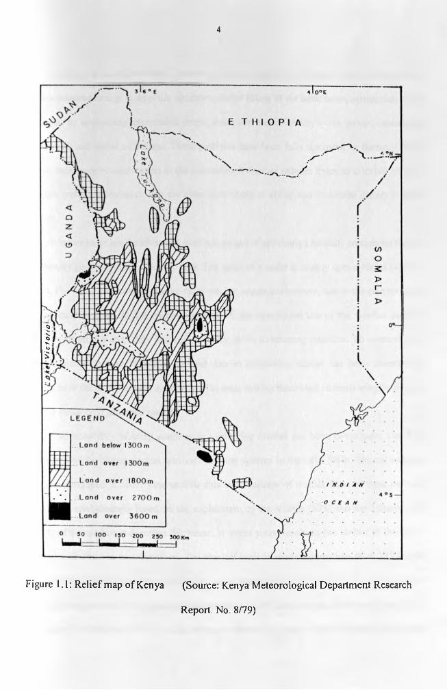
time patterns on rainfall over Kenya. The topography of the study region, Kenya, as is shown in

Figure 1.1, is very complex and this enhances the spatial variability of rainfall whose measurement

may only, therefore, be adequately done using a very dense network of rain gauges. However, the

rain gauge network available in this region is relatively sparse especially over remote areas.

Furthermore, the cost of development and maintenance of a dense rain gauge network would be

extremely expensive for a developing country like Kenya. Using rain gauges is further compounded

by the interrelated factors of wind, siting and gauge design.

Many efforts have therefore been made to find alternative methods of rainfall monitoring

both in space and time. These problems have led to the exploration of the potential use of

ground-based weather radar and satellite-based techniques as alternative methods of estimating

rainfall. For example, attempts have been made to estimate rainfall using the weather radar based

on the transmitted microwave radiation into space and then monitoring the backscattercd

microwave energy. The strength of the backscattered radiation depends on the raindrops in the

path of the transmitted radiation. An empirical relationship is developed that is then used to

convert the backscattered radiance into a measure of rainfall.

Vie

fo

r to

4

Figure 1.1: Relief map of Kenya (Source: Kenya Meteorological Department Research

Report. No. 8/79)

5

However, the weather radar has some problems relating to the proper relationship between

the back-scattered energy to drop size spectrum, partial filling of the radar beam, attenuation of the

radar beam by intervening precipitation drops, absorption and reflection by the ground (anomalous

propagation), and signal calibration. These problems have been fully discussed in Battan (1973).

Doppler radar may be used instead of the conventional weather radar in try ing to alleviate some of

the above problems. However, they are even more costly to set up and contribute greatly to noise

pollution.

Weather radar has the advantage over rain gauges of providing a spatially continuous field of

view thereby giving continuos flow of data. The range of a radar is usually upto a radius of about

200 km. For wider area coverage, more radar sets are required. However, due to the cost and need

for sophisticated technical and engineering support, the operational use of the weather radar in

rainfall monitoring is extremely limited, especially in the developing countries. To overcome the

above problems, the use of satellite-derived data in monitoring rainfall has been investigated.

Satellites have the ability to view extremely wide areas making them ideal in monitoring both large-

scale and meso-scale generated rainfall.

The probability of using satellites in monitoring rainfall has been investigated since the

inauguration of the meteorological satellite observing systems in the early 1960s. Several methods

have been developed to convert the satellite data into measures of rainfall. Most o f these methods

have been overwhelmingly based on the exploitation of the Visible (VIS) and the Infrared (IR)

channels of the satellite radiometers. However, in recent years, emphasis has shifted to the use of

microwave windows in the estimations. The physical basis of rainfall estimations from VIS and 1R

imagery depend on the supposition that inference of rain falling out of the base of a cloud may be

made from the analysis of the cloud-top characteristics which are monitored by the satellites. In the

VIS imagery, the brightest clouds, which are more reflective because of their thickness, may be the

6

most likely to precipitate while in the IR imageries the clouds with the coldest tops, and therefore

those with the highest tops, are the most likely to precipitate. The disadvantage of using techniques

dependent on VIS and IR images is the physical indirectness of the relationship between the

characteristics at the top of the clouds and the processes that are taking place at their bases. The

characteristics considered are just proxies of the temperature and liquid content of the clouds (Kidd

and Barrett, 1990).

Imagery from selected passive microwave (PM) windows can be used to provide

information of alternative or additional value for rainfall monitoring purposes. It was demonstrated,

using data from the pioneering instrument ESMR (the Electrically Scanning Microwave

Radiometer) on Nimbus-5 as early as in mid-1970s, that naturally emitted PM radiation in particular

frequencies, from the earth's lower atmosphere and surface can be measured and analyzed to give

pictures of instantaneous rainfall intensities. This was found to be true at least over sea surfaces. It

has now been shown that PM radiation is valuable for rainfall monitoring purposes over both land

and sea areas (Kidd and Barrett. 1990). The physical basis of monitoring rainfall through PM

radiation windows is dependent on the fact that PM radiation at certain frequencies are attenuated

mainly by rain drops in the atmosphere. Techniques using PM therefore depend on a physical

relationship between the liquid water in the clouds and the final precipitation rather than proxy

information in their estimation procedures.

However, the applications of the satellite-derived methods in the monitoring of rainfall also

have problems that create errors in the estimates. The VIS channels can only be used during daytime

while the IR channels are likely to give erroneous measurements during periods of large-scale

subsidence due to the inherent problems in the IR radiative transfer equation. The microwave

channels are. at the moment, only useful over large water bodies since the emissivity of land and

clouds are comparable. Additionally, all satellite procedures are hampered by the surface resolutions

7

of the satellites. The footprints of most satellites are at least 5 km (as in the case o f METEOSAT).

The next generation satellites, like METEOSAT Second Generation (MSG) set to be launched in the

year 2002. are going to solve this problem with better resolutions.

Inspite of the above mentioned problems, satellite-derived methods of estimation of rainfall

give very useful additional precipitation information, especially in areas with sparse rain gauge

observation network. They also provide near-real time precipitation data. However, they have to be

calibrated using other available rainfall observations ("ground truth"). Measurements of rainfall

from rain gauges and/or weather radar are usually used as "ground truth" in these cases. This study

looks at the possibilities of using satellite derived data in rainfall monitoring and forecasting over

Kenya. The details o f the objectives of the study are in the next section.

1.1 The Objectives of the Study

The overall objective of the study is to investigate the viability of using satellite derived data

as a means of enhancing rainfall monitoring and forecasting over Kenya. This objective will be

achieved by addressing the following specific objectives:

(i) Regionalization of the study region into homogeneous climatic zones based on 10-

day rain gauge and satellite-derived records. The delineated zones from the different

sets of data will be compared.

(ii) The development of empirical functions for the relationships between various types

of satellite data and rain gauge rainfall for each of the homogenous rainfall zones

based on (i).

(iii) Investigation of the skill of the derived models during anomalous wet/dry seasons.

(iv) The study of the evolution of 10-day/seasonal rainfall and general circulation

patterns, in order to identify the systems that could be associated with the low or

high skills of the satellite derived estimates during anomalous wet/dry years.

8

(v) Determination of the relationships between the rain gauge and satellite-derived

records in attempts to derive potential predictors of rain gauge rainfall records from

satellite-based data.

1.2 Justification for the Study

Extreme rainfall anomalies like floods and droughts, in Kenya usually result in untold

suffering of the people leading to loss o f life and massive damage to property and infrastructure.

It is. therefore, imperative that timely and accurate weather forecasts and climate prediction be

made for the study region in order to reduce the vulnerability of the society to climate related

disasters. Accurate weather forecasts and climate prediction require adequate and accurate

observations as inputs in either the conventional forecasting procedures or the numerical

forecasting techniques. One of the problems encountered in the region is lack of an adequate set

of observations for use in forecasting.

Furthermore, the economy of the study region. Kenya, is highly dependent on agriculture

and hence rainfall dependent. The existing station network used in rainfall measurements is

highly concentrated in the densely populated and most accessible areas, but sparse in the remote

areas, which unfortunately cover over 80% of the country. Rainfall data are also required in the

planning and management of all rainfall dependent activities such as water resources,

hydropower resources, building and construction, agricultural activities, among many others. The

study attempts to augment the existing station network to give timely and spatially representative

coverage for better forecasts, and hence enhance the use of rainfall information in sustainable

national development efforts.

The study region includes the world's second largest fresh water lake, Victoria. The lake

is of great economic importance in the region. It provides a livelihood to a large percentage of the

region's populace through fishing activities. It is also used for transportation in the transfer of

9

«>ds between the three East African states (Kenya, Uganda and Tanzania) and beyond. Most

importantly, the lake is the source of river Nile on which the Owen Falls HydroElectric Power

!’l.int (OF-HPP) is built. The OF-HPP plant supplies electricity to all three East African States.

I«> sustain the current industrial development in the region, a considerable extra amount of

energy is required. Fortunately, there exists the potential for expanding the OF-FIPP and,

currently, an extension is under construction to generate an extra 200MW.

The planning for hydroelectric power stations require an accurate estimation of the

volume of water that will be used. In the case of the OF-HPP, an accurate estimation of the

volume of water in the lake is important. The volume of water in the lake depends on the amount

of rainfall received around its catchment (about 20%) and the actual amount received over the

ike (about 80%) (Yin and Nicholson, 2000). The amount received in the catchment is usually

estimated from the rain gauges installed in the area. However, the amounts over the lake are

usually more difficult to quantify since the conventional methods of measuring rainfall are not

readily available. Accurate estimates from satellite records would, therefore, be o f immense value

for the planning o f the power generating stations over the region and help in the Kenya

covemment’s policy o f industrialization.

The national water development plan lays strategies for the provision o f tap water to

every Kenyan. Such a dream cannot be achieved without good network of historical rainfall

databases, w hich may also be used to compute the risk of some hydrological decisions.

With most o f the high potential areas being highly populated, many people are currently

being forced to move to the ASALs that cover over 80% of the country. Others are being forced

• > migrate to the urban centers. The national long-term development plan has addressed long term

development of the ASALs and large cities as some of the key challenges to Kenya in the future.

Data is the key limitation in assessing the vulnerability of such development plans. The data and

10

other information from this study can be used to fill some of this gap, and also in enhancing

national early warning efforts in Kenya for extreme rainfall anomalies.

1.3 The Study Region

This section defines the physical location of the study region and gives an overview of the

climatology of its rainfall.

1.3.1 Location of the Study Region

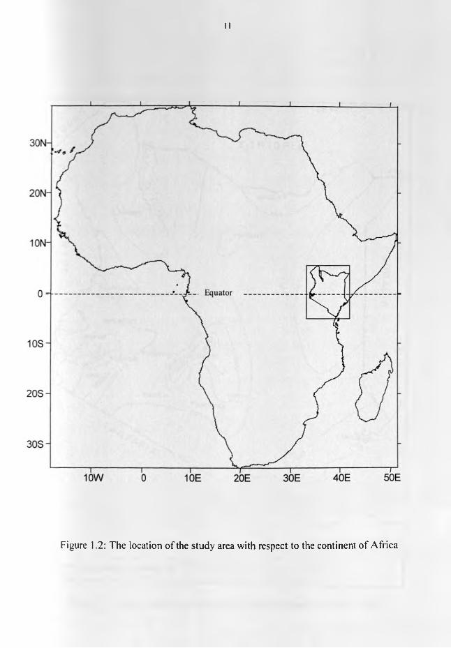
The study region is located within latitudes 5°N to 5° S, and longitudes 34° E to 42° E, and

covers the whole of Kenya. It is situated within the Eastern African States, and is bounded by

Uganda to the west. Tanzania to the southwest and south. Indian Ocean to the south and southeast.

Somalia to the east, and Sudan and Ethiopia to the north. A map showing the location of the study

region in Africa is given in Figure 1.2 while the list of stations is provided in Table 2.1.

1.3.2 Rainfall Climatology of the Study Region

Being in an equatorial region, the rainfall of the area is expected to be associated with

synoptic scale circulation patterns like the convergent low-level winds in the Inter Tropical

Convergence Zone (ITCZ) surface locations. However, superimposed on the synoptic-scale

circulation patterns are meso-scale systems induced by regional factors such as complex

topographical patterns, the existence of many large inland lakes and the proximity of the Indian

Ocean (Ogailo, 1983; Basalirwa et ai, 1999).

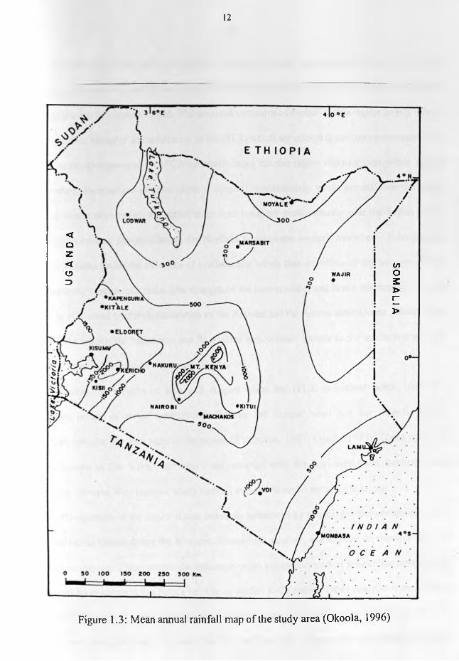
Studies have shown that a higher percentage of annual rainfall over most of the study area is

experienced during the MAM season (Okoola, 1996). However Camberlin and Wairoto (1997) show

that the southeasterly lowlands receive most of its rainfall during the SON season. The mean annual

rainfall map of the study region is shown in Figure 1.3.

II

Figure 1.2: The location of the study area with respect to the continent of Africa

UG

AN

DA

12

Figure 1.3 : Mean annual rainfall map of the study area (Okoola, 1996)

SO

MA

LIA

13

Several large-scale and synoptic-scale features influence precipitation in the study region.

The most important of these features is the ITCZ that is a broad low-pressure belt in which the trade

winds of the two hemispheres meet. The seasonal variations o f rainfall in this region largely depend

on the position, intensity and orientation o f the ITCZ, which are related to the sun's movements. The

north - south movements of the ITCZ seasonally bring into the region two monsoon winds. During

the Northern Hemisphere summer (June - August), southeasterly winds prevail over the region

bringing some moisture into the region since their tracts are predominantly over the Indian Ocean.

These winds reverse direction during the Northern Hemisphere winter (December - February ) and

the region comes under the influence of northeasterly winds that are relatively dry because of their

predominantly continental tracks. The strength of the convergence, and hence the strength of these

winds, is influenced by the characteristics of the Arabian and the Azores anticyclones located to the

north of the region; the Mascarene and St. Helena anticyclones located to the south; and a trough

located within and around the Mozambique Channel.

During the months of July and August when the ITCZ is furthest north, there is a

maximum influx of moist westerly winds from the Congo basin and the Atlantic Ocean,

especially into the Western parts of the region (Thompson. 1957; Ogallo, 1989). These winds are

locally known as the "Congo air mass” and. coupled with the semi-permanent thermal trough

over Lake Victoria, they produce heavy rainfall over the Western parts of the region.

Precipitation in the region is also indirectly influenced by tropical cyclones originating from

southern Indian Ocean during the Southern Hemisphere summer, and tropical depressions from the

Arabian Sea region. These storms also influence ocean parameters such as sea-surface temperatures

(SST) and ocean currents that have a bearing on rainfall in the region. Other synoptic systems which

control rainfall of the region include the Easterly waves, the Sub-Tropical Jetstreams, the East

African low level jetstream. Tropical Easterly Jetstream and remnants of extra-tropical weather

14

systems (e.g. fronts) that are forced further south or north into the region. A discussion on the

characteristics of some of the extra-tropical systems and their effects on the region's rainfall maybe

found in Fremming (1970) and Njau (1982).

There are large spatial and temporal variations in climate over the study region caused by

several regional features. These features include large inland lakes, like lakes Victoria, Nakuru and

Turkana. and topographic features including several mountain ranges (Kenya, Abadares, and Elgon)

and the Great Rift Valley that runs north to south through the study region. These physical features

induce significant modifications in the general wind patterns over the region creating variations in

the rainfall (Ogallo, 1989).

The following section reviews some of the literature that is relevant to the study.

1.4 Literature Review

Since the inauguration of the meteorological satellite observing systems in the early 1960s.

several authors have investigated the possibility of monitoring rainfall from satellite altitudes. This

section takes a look at the work that has already been done in line with this study. The review covers

even areas different from the study region since not a lot of this line of research has been undertaken

over this region.

Many methods have been developed in trying to convert the satellite data into estimates of

rainfall. Martin and Scherer (1973) have reviewed some of the methods developed earlier. Barrett

and Martin (1981) give an update of these methods in their review of those in use upto the end of

1970s. The earlier techniques of estimating rainfall from satellite data were mainly based on data

from Visible (VIS) and Infrared (IR) channels. However in recent years, more emphasis has been

laid on the use of Passive Microwave (PM) channels since these give data that have a more direct

relationship with rainfall than does VIS- or IR-derived data. The satellite rainfall estimating methods

15

can be broadly classified as cloud indexing, life history, bispectral and cloud model, and passive

microwave methods. In the next sections, these individual classes of methods are reviewed.

1.4.1 Cloud indexing methods

The cloud indexing methods use cloud indices, for example the fractional area covered by

raining clouds, derived from VIS and/or IR images to estimate rainfall. The algorithms developed

for these methods are generally simple and can be run on most of the available desktop personal

computer systems. The requirements, in terms of computer software and hardware are minimal.

Therefore, they have been applied to a wide range of climatic conditions as defined by latitudinal

zones and/or continental or maritime characteristics.

Two of the most applied families of cloud indexing methods have their origins in the

Applications Group of the National Environmental Satellite Services (NESS) o f the National

Oceanic and Atmospheric Administration (NOAA), and the Applied Climatology Laboratory of the

Department of Geography, University of Bristol, United Kingdom. The NESS technique basically

uses the convective cloud area as the index for the estimation o f rainfall (Follansbee. 1973). The

method maybe expressed as:

R _ ( KlAl + K 2A2+ K 3A3) ())

Where R is the estimated rainfall, Ao the area under observation. A|, A:, A3 are areas of A() covered

by the three most important types of rain producing clouds (cumulonimbus, cumilocongestus and

nimbostratus), and k|, k2 , k3 are empirical coefficients to be determined. The Bristol method

16

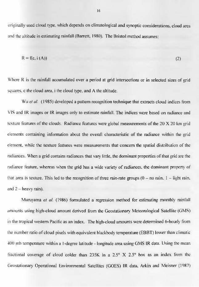
originally used cloud type, which depends on climatological and synoptic considerations, cloud area

and the altitude in estimating rainfall (Barrett. 1980). The Bristol method assumes:

R = tfc, i (A)) (2)

Where R is the rainfall accumulated over a period at grid intersections or in selected sizes of grid

squares, c the cloud area, i the cloud type, and A the altitude.

Wu et al. (1985) developed a pattern recognition technique that extracts cloud indices from

VIS and IR images or IR images only to estimate rainfall. The indices were based on radiance and

texture features of the clouds. Radiance features were global measurements of the 20 X 20 km grid

elements containing information about the overall characteristic of the radiance within the grid

element, while the texture features were measurements that concern the spatial distribution of the

radiances. When a grid contains radiances that vary little, the dominant properties of that grid are the

radiance feature, whereas when the grid has a wide variety of radiances, the dominant property of

that area is texture. This led to the recognition of three rain-rate groups (0 - no rain. 1 - light rain,

and 2 - heavy rain).

Muruyama et al. (1986) formulated a regression method for estimating monthly rainfall

amounts using high-cloud amount derived from the Geostationary Meteorological Satellite (GMS)

in the tropical western Pacific as an index. The high-cloud amounts were determined 6-hourly from

the number ratio of cloud pixels with equivalent blackbody temperature (EBBT) lower than climatic

400 mb temperature within a I-degree latitude - longitude area using GMS IR data. Using the mean

fractional coverage of cloud colder than 235K in a 2.5° X 2.5° box as an index from the

Geostationary Operational Environmental Satellites (GOES) IR data, Arkin and Meisner (1987)

17

derived estimates of large space- and long time-scale convective precipitation. These estimates are

known as the GOES Precipitation Index (GPI) and were developed for the Western Hemisphere.

They calculated this index as a product o f the mean fractional coverage of cloud colder than the

threshold temperature, the length of the averaging period in hours and a constant o f 3 mm h 1. That

is.

GPI=3FC/ (3)

WTiere GPI is in millimeters. Fc is the fractional cloudiness (a dimensionless number between 0 and

1). and t is the length of the period (hours) for which Fc was the mean fractional cloudiness.

Callis and LeComte (1987) similarly used the percentage of convective cloud cover,

considered to be producing rainfall, deduced from four images each day to produce daily estimates

of rainfall for the Sahel region of Africa. Chiu (1988) showed that fractional rain area o f clouds as an

index in estimating rainfall accounted for a large part of the area rainfall variance in the Global

Atmospheric Research Program (GARP) Atlantic Tropical Experiment region (GATE). His work

was improved upon by incorporating data from a network of rain gauges alongside the initially used

radar data as "ground truth” by Short et al. (1989). Mitchel and Smith (1987) developed a model for

estimating rainfall by applying statistical discriminant analysis on indices derived from cloud-top

parameters to determine the best combinations of the cloud indices that best classify rain versus

no-rain occurrences within the Cooperative Convective Precipitation Experiment (CCOPE) Mesonet

region. Some of the parameters used included the coldest cloud-top temperatures (to represent the

convectively active cloud region), largest absolute temperature gradients (found in the vicinity of

cloud updrafts), largest temperature laplacian (gives cloud towers within the area o f convection)

18

among many others. Similarly Negri and Adler (1987a,b) derived several indices from cloud

parameters using both VIS and 1R images to estimate rainfall over the Florida Peninsular.

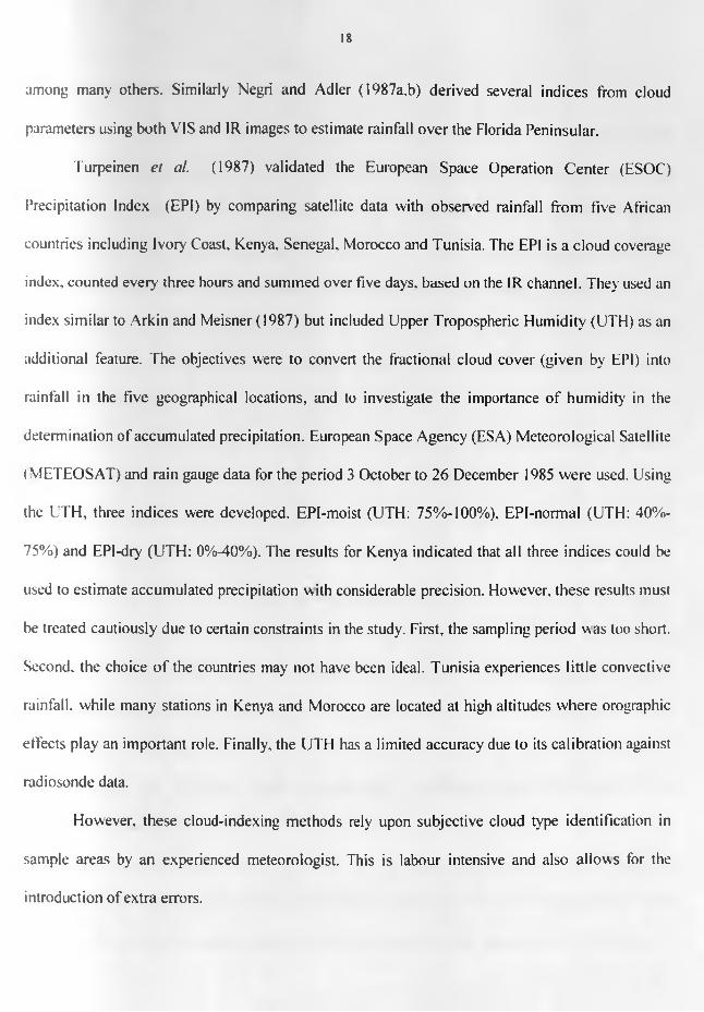
Turpeinen el al. (1987) validated the European Space Operation Center (ESOC)

Precipitation Index (EPI) by comparing satellite data with observed rainfall from five African

countries including Ivory Coast, Kenya, Senegal. Morocco and Tunisia. The EPI is a cloud coverage

index, counted every' three hours and summed over five days, based on the IR channel. They used an

index similar to Arkin and Meisner (1987) but included Upper Tropospheric Humidity (UTH) as an

additional feature. The objectives were to convert the fractional cloud cover (given by EPI) into

rainfall in the five geographical locations, and to investigate the importance of humidity in the

determination of accumulated precipitation. European Space Agency (ESA) Meteorological Satellite

(V1ETEOSAT) and rain gauge data for the period 3 October to 26 December 1985 were used. Using

the UTH, three indices were developed. EPI-moist (UTH: 75%-100%), EPl-normal (UTH: 40%-

75%) and EPI-dry (UTH: 0%-40%). The results for Kenya indicated that all three indices could be

used to estimate accumulated precipitation with considerable precision. However, these results must

be treated cautiously due to certain constraints in the study. First, the sampling period was too short.

Second, the choice of the countries may not have been ideal. Tunisia experiences little convective

rainfall, while many stations in Kenya and Morocco are located at high altitudes where orographic

effects play an important role. Finally, the UTH has a limited accuracy due to its calibration against

radiosonde data.

However, these cloud-indexing methods rely upon subjective cloud type identification in

sample areas by an experienced meteorologist. This is labour intensive and also allows for the

introduction of extra errors.

19

1.4.2 Life-History methods

Life-History methods depend on the premise that significant precipitation comes mostly

from convective clouds and these convective clouds can be distinguished in the satellite images from

the other clouds. These clouds can be recognized and the amount of rainfall from them can be

estimated largely from the changes that occur within them. These changes, therefore, need to be

closely monitored and hence it is important to use sequences of images from geostationary satellites

(short intervals between consecutive images) in order to follow the growth and decay of the

convective clouds. An example of these changes is the convective cloud area during the various

stages of development.

Purdom (1981) proposed the study of the development of mesoscale systems as an aid to

very short-range weather forecasting. The mesoscale developments were studied through the

information on cloud developments and patterns received from geostationary satellite data combined

with radar, surface and upper-air conventional observations. The clouds and cloud patterns observed

represent the integrated effect of ongoing dynamic and thermodynamic processes in the atmosphere.

W ith this information, he was able to make short-range weather forecasts. Martin and Howland

(1986) also developed a method that similarly produces forecasts by using measurements on cloud

developments from satellite information. The cloud measurements were taken at grid points at fixed

time intervals within a day using both VIS and IR imagery' to estimate daily rainfall in the tropics.

Doneaud et al. (1987) made a preliminary investigation into the usage of the

Area-Time-Integral (ATI) technique on satellite data. They applied the technique on the GOES rapid

scan satellite data alongside radar information over Bowman (Southwestern North Dakota) to

estimate the total rain volumes over fixed and floating target areas. The basis of the approach is the

existence of a strong correlation between the radar echo area coverage integrated over the lifetime of

20

a storm and the radar estimated rain volume. The lifetime of a storm is ascertained by using GOES

data to track convective clouds.

Dugdale el al. (1987) used the total duration taken by raining clouds derived from IR images

in estimating 10-day total rainfall amounts for the Sahel region. This technique involves the

identification of raining clouds by use of a temperature threshold and keeping track on how long that

particular cloud stays over a certain area. These durations are then totaled-up to give the 10-day

period that the raining cloud stayed over the region. This is what is used as a proxy of rainfall. Ouma

el al. (1995) used a similar approach to estimate 10-day rainfall amounts for southern Tanzania.

They found that using the Cold Cloud Durations (CCD) as a proxy gave reasonable estimates of that

region’s rainfall. They derived regression equations for retrieval of rainfall using optimum threshold

temperature of -50°C.

Scofield (1987) developed the National Environmental Satellite Data and Information

Service (NESDIS) operational convective precipitation estimation technique for estimating

half-hourly convective rainfall amounts by analyzing changes in two consecutive (half-hourly)

satellite images. This technique estimates rainfall following three steps. The first step involves

location of the active portion of the thunderstorm system. The active portion of a convective system

is the area of strong updrafts that coincides with heavy sector of the thunderstorm cluster under the

spreading anvil. The second step involves the computation of half-hourly rainfall estimate from

cloud-top temperature and cloud growth or divergence aloft, the overshooting tops, thunderstorm

cluster or convective cloud-line merger, and the saturated environment. Finally, these half-hourly

convective rainfall estimates from the second step are summed up and multiplied by a moisture

correction factor for the actual estimate. This technique was initially designed for deep convective

systems that occur in tropical air masses with high tropopauses. It is affected by cloud base level, the

height of the tropopause. and orography.

21

Mishra el al. (1988) used 3-hourly Indian geostationary multi-function Satellite

(INSAT-1B) data in a scheme to estimate heavy convective rainfall over India during the monsoon

season. They adopted the Scofield (1987) scheme and tailored it for the Indian subcontinent during

the monsoon season. The scheme takes into account the convective cloud structure, cloud growth in

space and time, and the prevailing environmental conditions.

However, these life-history methods rely on the successful tracking of convective clouds

through their life spans. Some convective systems have relatively short life spans that may be missed

out between consecutive images from the satellites, leading to an underestimation of rainfall.

1.4.3 Bi-spectral and cloud model methods

The other group of methods is the bi-spectral and cloud model methods. Bi-spectral methods

use VIS and IR images simultaneously to map the extent and distribution of precipitation. IR

images give information about the temperature and. indirectly, the heights of the tops of the clouds,

w hereas the VIS images provide information on the thickness, geometry and the composition of the

clouds. The bi-spectral methods use dual thresholds on both the VIS and IR data simultaneously to

identify the raining clouds. Some cloud indexing and life history methods also belong to this group

of techniques. These methods are based on bivariate frequency distributions.

Several bi-spectral satellite rainfall estimation methods have been developed. Austin (1981)

used VIS and IR images from Geosynchronous Meteorological Satellite (GMS) and GOES-E

archived at 30-minute intervals, and the corresponding radar data from McGill Radar Weather

Observatory in an attempt at short-range forecasting of precipitation. The radar information,

converted to rain rates using Short tenn Automated Radar Prediction (SHARP) procedure, were

used as the "ground truth" in defining raining and non-raining clouds. The fundamental algorithm

consisted of obtaining two bivariate frequency distributions from the VIS and IR images, collocated

22

with simultaneous radar data inorder to discriminate between raining and non-raining clouds. The

"ground truth" helped in defining the dual thresholds for both VIS and IR data.

Chema el al. (1985) used bivariate frequency distribution on VIS and IR images collocated

with simultaneous radar data to discriminate between thunderstorm and non-thunderstorm areas or

between rain and non-rain areas. Tsonis and Isaac (1985) while delineating instantaneous rain areas

in the mid-latitudes while using GOES data employed a similar approach. They also tried to

distinguish between four classes of rain-rates namely no rain, light rain, moderate rain and heavy

rain classes. Barrett and D'Souza (1986) integrated three time daily pairs of METEOSAT VIS and

IR images, and three night-time IR only images using the Agricultural Drought Monitoring

Integrated Technique (ADMIT) to detennine rain/no rain boundaries across the whole continent of

Africa. They plotted VIS and IR digital counts in the VIS/IR two-dimensional space and used

double thresholding technique to determine the rain/no rain boundaries.

The bivariate models have the advantage of effectively isolating the cirrus and stratus

components of the IR and VIS imageries. The information from VIS channels discards the cirrus

component while IR information removes the stratus component to reduce the over-estimation that

normally arises from these non-raining clouds when IR or VIS channels are used individually.

The convective cloud model methods incorporate models of convective processes in their

development. Satellite data is used to estimate the convective parameters of the convective clouds.

Gruber (1973) applied Kuo's (1965) parameterization scheme over a grided area in estimating

rainfall in the regions of active precipitation. The parameters were estimated using satellite data.

Wylie (1979) used the Simpson and Wiggert (1969) one-dimensional cloud model to estimate rain

in the Global Atmospheric Research Program (GARP) Atlantic Tropical Experiment (GATE) and

Montreal regions by calculating the stability factors. The incorporation of the cloud model was

found to substantially improve the satellite estimates of rain in the region. Adler and Negri (1988)

23

developed the Convective-Stratiform Technique (CST) to estimate both tropical convective and

stratiform precipitation (produced under anvils of mature and decaying convective systems) using

IR images. The method defines convective cores, and assigns rain-rate and rain-area to the features

based on the IR brightness temperature and the cloud model approach of Adler and Mack (1984).

The one-dimensional cloud model accounts for ambient temperature, moisture and shear conditions.

All the methods discussed above use the VIS and IR channels in acquiring information. The

VIS channels are only useful during daylight hours and also misclassify stratus clouds as rain clouds

due to their high reflectivity, while the IR channels usually wrongly classify the cirrus clouds due to

their low temperatures. Further, these channels give information that lead to indirect schemes of

rainfall retrieval because they provide cloud information that can only be used as proxy to rainfall.

Due to these problems, research into alternative channels to retrieve information started and hence

the use of PM channels was introduced. The next sections review the research that has been done

using the PM channels.

1.4.4 Passive microwave methods

The final group of satellite rainfall estimations are those that use PM windows in obtaining

satellite data for rainfall estimations. These estimation techniques are called direct since they are

based on observations of the radiative effects of precipitation-sized hydrometcors (Arkin and

Meisner, 1987). They use observations o f radiation at frequencies that are not affected by cloud

droplets or by the gaseous contents of the atmosphere. At microwave frequencies, the major source

of attenuation is due to precipitation-sized particles (Grody, 1984). Within the microwave spectrum,

raindrops may absorb, emit or scatter radiation, producing changes in the brightness temperature

relative to clear or cloudy conditions. The dominant attenuation process seems to be detemiined by

the nature and the quantity of both liquid droplets and ice particles. Together, these are a reflection

24

of the rainfall processes at work within a cloud (Kidd and Barrett, 1990). Monitoring the brightness

temperature would, therefore, give a good approximation of the rainfall received from such a cloud.

However, microwave emissions from the underlying surface usually affects this brightness

temperature. The radiation from the underlying surface depends on the temperature and emissivity

of the surface. Over the oceans, the emissivity is relatively low and constant providing a predictable

background signal. Over land, however, both the temperature and emissivity are highly variable due

to nature of the of land surface. This makes the microwave background signal over land highly

variable. It is. therefore, easier to monitor rainfall using microwave data over the oceans than over

land surface backgrounds (Arkin and Ardanuy. 1989).

Passive microwave rain-rate retrieval methods are based on one of three approaches,

emission-, scattering- and combination o f emission and scattering-based methods (Hong et al.,

1997). In the next sections, PM-based methods that fall under the various rainfall retrieval

approaches are reviewed.

1.4.4.1 Emission-Based Methods

The emission-based methods use the fact that absorption and emission by liquid cloud

drops and raindrops cause rapid increases of brightness temperatures over a radiometrically cold

background, such as the ocean. Most emission-based approaches rely on integration of the

equation of radiative transfer for hypothetical models of raining atmosphere to predict the

brightness temperature for a given rainfall rate. These methods are normally successful against a

surface background of low emissivity, such as the oceans, with rainfall standing out as a “warm”

area against a cold background. The principal drawbacks of these emission-based methods are

that they saturate at relatively low rainfall rates and also show substantial sensitivity to the

assumed freezing level. Lower frequency channels are used for these approaches.

25

(Wilheit et al., 1973) demonstrated that the data from the Electrically Scanning Microwave

Radiometer (ESV1R) system carried on Nimbus 5 could be qualitatively interpreted as indicating the

presence or absence of rain above an unspecified threshold intensity. Allison et al. (1974) found that

rain rate could at least be crudely estimated from this data. Wilheit et al. (1977) managed to develop

a theoretical model for calculating microwave radiative transfer in raining atmospheres and used this

to estimate rainfall from PM data.

Barrett et al. (1987) investigated the possibility of using PM data in support of their

Bristol/NOAA Interactive Scheme (BIAS) for improved satellite rainfall monitoring. BIAS is an

interactive scheme that uses VIS and IR imagery from polar orbiting or geostationary satellites,

synoptic weather reports from conventional stations, and vertical motion and precipitable water

charts to estimate rainfall. In this study, they overlaid the BIAS results with PM information

obtained using all three approaches of PM methods. The usefulness of PM data in rainfall

monitoring was clearly demonstrated by this study.

Barrett et al. (1989a) investigated the effect of combining the conventional rain gauge

observations, passive microwave satellite data, and radar observations in rainfall monitoring.

Their areas of interest included Kenya and the British Isles. There were three objectives for the

project over Kenya. The first objective was the examination of the performance of scanning

multi-channel microwave radiometer (SMMR) rainfall algorithms over a tropical area. Kenya

was chosen as representative of tropical regions. The second objective was the determination of

VIS and IR thresholds, through a more physically direct method by using hourly rain gauge and

weather radar data collected simultaneously with METEOSAT VIS and IR data. The final

objective was to examine the performance of the convective stratiform technique (CST)

developed by Adler and Negri (1988) over this tropical region. The CST has been briefly

discussed in earlier sections. They used METEOSAT data, hourly recorded rainfall data from

26

nine automatic rainfall stations, analog weather radar observations from ground based radar

located at Jomo Kenyatta International Airport (JKIA). and SMMR data for the period 20lh April

to 3rd May 1987.

The results from SMMR studies proved inconclusive, mainly due to lack o f sufficient data

to test a variety o f rain conditions. However, the background signals from the lakes were

detected and established. The examination of VIS/IR data in conjunction with ground based

weather radar imagery provided new insights into the pattern of rainfall in the area. Most of the

rain in the region fell from small rapidly moving convective cells seen on sequences of radar

imagery, but were often sub-pixel sized and were not therefore resolved as individual elements by

the infrared radiometers. Because of higher spatial resolutions of the textual features, and

shadows, the VIS imagery were found useful in distinguishing the convective cores. However,

this imagery is only available during the day light hours.

The CST results were very encouraging. Most major convective elements and their

associated stratiform rainfall were correctly located and identified. However, the rain area

assigned was, in some cases, smaller than the areas indicated by the radar echoes and VIS

imagery. Many smaller convective elements were also missed and Barrett et al. (1989a).

therefore, concluded that the CST can be tuned more finely to produce more accurate results in

this environment. Unfortunately, the technique requires weather radar observations or hourly

recording rain gauges. These are not readily available over all of Kenya and hence studies in this

direction have been hampered. A similar study was done over the British Isles and the

surrounding areas with better results mainly due to the availability of weather radar observations

(Barrett et al., 1989b)

A review of other methods developed using passive microwave data in rainfall monitoring

during the period upto 1989 has been given by Arkin and Ardanuy (1989). Using observations of

27

a three-month period beginning September 1987 from Special Sensor Microwave/lmager

(SSM/I) at 19.30 GHZ. Tjemkes et al. (1991) developed an algorithm to retrieve precipitable

water content over global oceans. They utilized measurements of the polarization state or the

radiation felt at the top of the atmosphere given the polarization state at the sea surface. The

results were compared with rawinsonde observations, which occurred within a kilometer radius

and within the same day of SSM/I observations. The correlation between the two independent

values of precipitable water was found to be very good. However, this scheme does not

distinguish between liquid and precipitable water and this may lead to large errors in

instantaneously retrieved precipitable water due to liquid water content contamination.

Greenwald et al. (1993) modified the method of Tjemkes et al. (1991) by taking into

account the temperature and moisture profile effects on the estimate of the emission temperature

of the atmosphere. Their primary goal was to develop and validate a simple physical scheme that

can be used to retrieve cloud liquid water from SSM/I observations on a global basis over the ice-

free oceans. This method was however found to be disappointing for tropical regions. While

comparing the column water vapour (CWV) information derived from both television infrared

observation satellite (TIROS) operational vertical sounder (TOVS) and SSM/I. Stephens et al.

(1994) applied the scheme of Greenwald et al. (1993). The results of the comparison show that

both sets of data give comparable estimates. Hong et al. (1997) developed a physical-statistical

approach that uses an emission-based method to retrieve instantaneous rain rates and computes

monthly rainfall. The method employs a maximum likelihood estimate method on a limited rain-

rate dynamic range. The beam filling error is corrected by multiplying by a factor of 1.8

generated from simulation studies of GATE data. The results indicated that the method performs

well in the tropics.

28

1.4.4.2 Scattering Based Methods

The scattering-based methods use the fact that scattering by ice hydrometers in the upper

parts of clouds causes brightness temperature decreases over land or ocean. The assumption is

that a larger amount of ice at cloud top is associated with heavier rainfall. The scattering-based

approaches are generally empirically based statistical relationships between satellite-measured

brightness temperatures and surface rain obtained from coincident ground-based radar

measurements or automatic recording rain gauges. Higher frequencies (typically higher than

37GHZ) are used inorder to get as much scattering information as possible. Difficulties in using

scattering-based techniques arise primarily in situations devoid of deep convective precipitation.

Grody (1991) developed a simple algorithm to classify precipitation and snow cover using

the SSM/I observations. He introduced a scattering index, based on 19, 22 and 85 GHz channels,

that is used to identify precipitation or snow cover using their scattering characteristics. Weng el

al (1994) evaluated two sources of error in the monthly rainfall estimates from the SSM/I

observations. These errors were due to poor temporal sampling of the instrument and due to

different averaging methods for converting instantaneous small-scale rain rates to climate scale

products. They used the SSM/I algorithm that was used by the NOAA satellite based on the

classification procedure developed by Grody (1991). This procedure uses a scattering index to

identity- the scattering signal at 85 GHz. from precipitation over land and ocean. It has been

briefly reviewed in earlier parts of this section.

The estimates of monthly global precipitation, from a single technique, are not very

reliable. Huffman el al. (1995) combined satellite-based estimates, rain gauge analysis, and

numerical weather prediction (NWP) model precipitation information in a bid to get more reliable

global monthly precipitation estimates. For the microwave estimates they used the Goddard

29

Scattering Algorithm, version 2, (GSCAT2) (Adler et al., 1994) in which a simple regression

relation is applied to the 86 GHz. horizontal polarization channel to infer precipitation rate.

Results show that this method compares favorably with the other state of the art microwave

techniques in retrieving rainfall.

1.4.4.3 Emission and Scattering-based Methods

The emission/scattering-methods use a multi-channel, statistical-physical rain-rate

retrieval approach. They establish the statistical relationships between multi-channel brightness

temperatures and rain rates based upon data generated by a cloud radiative model for a wide

range of conditions. The model simulates various atmospheric parameters, cloud structures and

microphysics, and surface characteristics, and then computes their associated brightness

temperatures in each of the available channels. This requires the solution of the radiative transfer

equation for every observed datum and assumptions about the structure of the rain clouds, which

arc usually unknown.

Mugnai and Smith (1988) investigated the impact of time-dependent microphysical

structure of clouds on the transfer to space of PM radiation at several frequencies. This was in

order to explore the feasibility of using multi-channel PM retrieval technique for the estimation

of precipitation from space-based platforms. They concluded that due to the considerable

variability and inhomogeneity of the microphysical and structural characteristics o f precipitation

clouds, it is necessary to use multi-channel PM precipitation retrieval techniques. In this way. the

various characteristics of a precipitating cloud will be taken care of leading to a more accurate

retrieval.

In an attempt to improve satellite rainfall retrievals using the SSM/I observations. Liu and

Curry (1992) used a radiative transfer model that combines emission and scattering. In the model.

30

three types of rain clouds were included, two of the types having both liquid and ice

hydrometeors. The results showed that combining SSM/I data at 19.35 and 85.5 GHz could

retrieve wider rainfall range than either emission- or scatter-based algorithms alone. Besides this

advantage, using these two wavelengths also results in the relationship between a linear function

of 19.35 and 85.5 GHz. brightness temperature, and rainfall rate being closer to linearity than the

relationship between brightness temperature of a single channel and the rainfall rate. Ferriday and

Avery (1994) used a vertically structured, plane-parallel and horizontally infinite cloud model

similar to that of Liu and Curry (1992) in PM remote sensing of rainfall from SSM/I

observations. They developed an inversion scheme for converting brightness temperatures to rain

rate that is relatively simple to apply, globally applicable and easily calibrated.

Weng and Grody (1994) developed a method combining several retrieval algorithms to

measure different ranges of liquid water in the atmosphere. This composite algorithm uses all

SSM/I frequencies to measure the liquid water for low stratus clouds as well as for highly

convective systems, and is based on data sets simulated from the radiative transfer model. The

calibration was done using ground-based radar observations. They realized that brightness

temperatures at 19.35 and 22.235 GHz are capable of retrieving high amounts of liquid in

convective clouds, whereas brightness temperatures at 85.5 and 22.235 GHz can be used to

retrieve low amount of liquid in the stratus or stratocumulus clouds.

Although there are several techniques available to identify areas of rain from PM

measurement observations, the conversion to an instantaneous rain rate is difficult because of the

inhomogeneity of rain field in the relatively large microwave footprints. This problem is

compounded by scarcity of validation data, especially over the oceans. Ferraro and Marks (1995)

empirically derived the rain rate retrieval coefficients for SSM/I rain algorithms developed at

NOAA-Satellite Research Laboratories (NOAA-SRL). They used both scattering- and emission-

31

based algorithms for rain retrieval and used ground-based radars for ground truth. Employing an

algorithm that uses an 85 GHz approach over land and a blended scattering/emission component

over oceans, Ferraro (1997) generated an 8-year monthly global data set from SSM/I

measurements.

Extracting rainfall from over both land surfaces and water bodies at the same time is

difficult due to the effects of background emissivities at microwave frequencies. To enhance the

precipitation signal by minimizing the effects of surface emissivity, Kidd (1998) used a

Polarization-Corrected Temperature (PCT) algorithm. The algorithm has a constant value, theta,

which is determined according to the prevailing meteorological conditions. Theta also controls

the threshold chosen to delineate rain from no-rain. As theta increases, the rain/no-rain threshold

also increases. The PCT algorithm has the advantage of being able to retrieve rainfall over land,

sea. and most importantly, coastal areas. Furthermore, using PCT at 85, 37 and 18 GHz provides

information about height distribution of hvdrometeors within the cloud system. Although the

PCT at 85 GHz is strongly affected by thick cirrus clouds, it is very sensitive to light precipitation

and is, therefore, ideal for rain/no-rain delineation.

From the literature review above, it can be noted that not a lot of work has been done over

the East African region as regards estimating rainfall from satellite information. It can also be

noted that the more direct method of estimating rainfall is based on PM channels. The validation

for the methods based on PM channels require ground-based radars or automatic recording rain

gauges. Both of these are not very available in the East African region. It is the aim of this study

to use appropriate satellite-derived data to estimate rainfall over some parts of the East African

region, bearing in mind the limitations mentioned above.

32

CHAPTER TWO

DATA AND DATA QUALITY CONTROL

2.0 Introduction

A discussion of the data used in the study is undertaken in this chapter. The data include

rain gauge recorded rainfall information, Cold Cloud Duration derived from METEOSAT

satellites, and Total Precipitable Water derived from a combination of data from radiosonde.

Special Sensor Microwave/Imager (SSM/I) and TIROS Operational Vertical Sounder (TOVS)

data, and wind derived from ECMWF reanalysis data.

2.1 Rainfall Data

Daily rainfall data from sixty stations distributed over the study region were used in the

study. Table 2.1 gives the list of names, locations in latitudes and longitudes, and altitudes of the

stations used in the study while Figure 2.1 show their spatial distribution. The data period

covered January 1st 1982 to December 31s1 1995. The sixty stations were chosen from about two

thousand Kenyan rainfall stations. A criterion for the selection of stations was less than 10%

missing data during the period considered for the study. Some synoptic stations were not

considered in the study because the rainfall cards, from where the daily records were extracted,

were missing. The data were obtained from The Kenya Meteorological Department, Nairobi.

Simple data quality control procedures were performed on the data to ascertain their

internal, temporal and spatial consistency. Single mass curves (Ogallo, 1982, 1987) were used to

test for the homogeneity of the data. The missing data were estimated using the correlation and

regression techniques. This was done using the station most highly correlated to the station with

missing data.

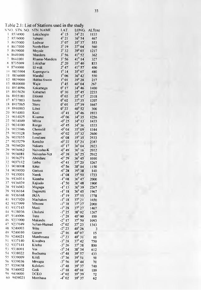
33

Table 2 .1: List of Stations used in the studyS N O . STN . NO. STN. N A M E LAT. LONG . ALT(m)

1 8534000 Lokichogio 4° 15 34° 21 11332 8536000 Sabarei 4° 21 36° 54 4673 8635000 Lodw ar 3° 07 35° 3 7 ' 5534 8637000 N orth-H orr 3° 19 37° 04 5605 8639000 M oyale 3° 32' 39° 03 12176 8641000 M andera 3° 56 41° 52 ' 362' 8641001 R ham u-M andera 3" 56 41° 14 327s 8735009 L okichar 2° 20 35° 40 ' 8339 8740000 E l w ak 2° 47 ' 41° 57 ' 400in 8835004 R apcnguria 1° 14 35° 07 ' 480II 8836000 M aralal 1° 06 36° 42 55012 8839000 H abba-Sw ein 1° 01 39° 28 21713 8840000 W ajir 1° 45 40° 04 26714 8 934096 K akam ega 0° 17' 34° 4 6 ' 140015 8935020 K abam et 0° 30 35° 4 5 ' 223316 8935181 Eldoret 0 ° 0 3 35° 17' 231817 8737003 Isiolo 0° 02 37° 35 ' 120718 8937065 M eru 0° 05 37° 39 ' 166719 8940003 Liboi 0° 22 40° 52 ' 30020 9034001 Kisii -0° 41 34° 4 6 193321 9034025 Kisum u -0° 06 34° 35 ' 125622 903 4 0 4 9 M bita -0° 25' 34° 13' 143323 903 4 1 0 0 Rongo -0° 4 5 ' 34° 36 153324 9 035046 C hem elil -0° 04 35° 09 134425 9 035128 Sorget -0° 02 35° 32 ' 260026 9 035155 Londiani -0° 08 35° 35 ' 253327 90 3 5 2 7 9 K ericho -0° 22 ' 53° 21 238728 90 3 6 0 2 0 N akuru -0° 17 36° 04 202329 90 3 6 0 6 2 N aivasha-K -0° 49 ' 36° 16 201230 9036081 N aivasha-V et -0° 39 36° 2 5 ' 201231 9036271 A bcrdare -0° 29 ' 36° 4 5 ' 101032 9 037112 Embu -0° 41 37° 2 0 ' 126733 9 038008 Kitui -0° 56' 38° 04 115034 90 3 9 0 0 0 G arissa -0° 28 39° 38 14035 9135001 Narok - I 11 08 35° 50 ' 173336 9136014 Kiam bu -1° 08 36° 47 200037 913 6 0 3 9 K ajiado -1° 50 36° 48 190038 9136043 M uguga -1° 13 36° 39 226739 9136164 Dagorctti •1° 18 36° 45 196740 913 6 1 6 8 JKIA -1° 19 37° 55 ' 177841 9 1 3 7 0 2 0 M achakos -1° 18 37° 2 1 165042 913 7 0 9 9 M booni -1° 38 37° 27 ' 200043 9137143 Masii -1° 28 37° 27 ' 146744 913 8 0 3 6 C huluni -1° 25 38° 02 126745 914 0 0 0 6 Tana -1° 28 40° 0 0 10046 9 2 3 7 0 0 0 M akindu -2° 17 37° 50 109347 9 2 3 7 0 4 9 Sultan-H am ud -2° 02' 37° 2 3 ' 134348 9 240003 W itu -2° 23 40° 26 349 924 0 0 1 0 G arsen -2° 16 40° 07 1550 9240021 M am bosasa -2° 23 40° 31 ' 1051 933 7 1 4 0 K iw alw a -3° 28 37° 4 2 ' 75052 9337141 Kitobo -3° 26 ' 37° 38 80053 9338001 Voi -3° 24 38° 34 61254 9338022 B uchum a -3° 48 39° 57 43355 933 9 0 0 9 Kilifi -3° 36 39° 51 5056 933 9 0 3 6 M uvapa -3° 56 39° 44 7057 9 339038 K alolcni -3° 48 39° 37 74058 9340002 Gedi -3° 18 40° 01 10059 9439000 D C EO -4° 02 39° 3 9 ' 7260 9439021 M om basa -4° 02 39° 37 ' 62

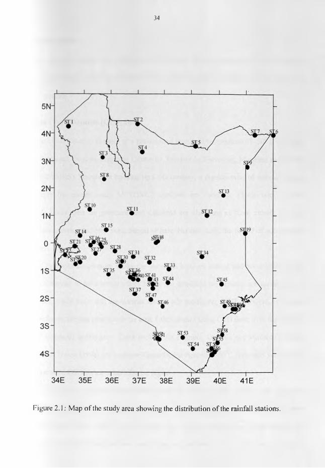
34

Figure 2.1: Map of the study area showing the distribution of the rainfall stations.

35

2.2 Satellite Data

Two types of satellite data were used in the study. These include Cold Cloud Duration

(CCD) and Total Precipitable Water (TPW). A discussion of these two satellite data types follows

in the next sections.

2.2.1 Cold Cloud Duration (CCD) Data

Cold cloud duration imager)' at a pre-selected threshold temperature of -50° C (Dugdale.

1990) was obtained from the Regional Center for Services in Surveying. Mapping and Remote

Sensing (RCSSMRS). Nairobi. In building up CCD imagery, a regular series of thermal infrared

imagery from the geostationary METOSAT satellites are received. Pixels with apparent

temperatures lower than the predetermined threshold are classified as “cold cloud" and their

characteristics accumulated over some period of time. For the study, the period o f accumulation

was ten days.

The threshold temperature marks the transition between raining and non-raining clouds.

All clouds observed to have temperatures below the threshold temperature are assumed to be

raining clouds, while those that are warmer are not rain producing. CCD, therefore, is the time

taken by particular raining clouds over an area. Other studies using CCD done over the area also

used -50°C threshold temperature. These include, for example, Dugdale and Milford (1987) for

Zimbabwe, and Ouma (1988) for southern Tanzania. Furthermore, -50°C threshold was the only

long-term archived CCD data available for the region

METEOSAT is in geostationary orbit around the earth at about 36,000 kms. above the

surface. This gives a continuos coverage of the same location on the surface of the earth hence

availing 24 hours o f data every day from that location. The radiometers carried aboard the

METEOSAT have narrow fields of view covering an area of about 5 kms. in the thermal infrared

36

and water vapor channels, and about 2.5 kms. in the visible channels at the satellite subpoint.

This gives the resolution of the scanners and is known as the footprint (Dugdale. 1990). The

coordinates of any point on the earth’s surface in relation to the satellites are derived from the

northward and eastward angular displacement from the satellite subpoint of the line of sight of

the satellite radiometer. Hence, any point above the surface of the earth, such as a cloud, will be

attributed coordinates not corresponding to the position vertically below the cloud, but to the

point on the earth's surface the radiometer would have viewed in the absence of the cloud

(Dugdale, 1990). The surface position o f the stations are corrected for the above parallax error

using the following equations:

. . . . , . /?tan(1.10) ...A( Latitude) = ------------- (3)110

. . . . , . /7tan(l.I0cos(0)) ...A (Longitude) = -------— - ---- (4)llOcos(0)

VVTiere 0 is the latitude, <f> the longitude, h the height of the cloud in kilometers and A is the

correction in degrees. The height of cumulonimbus clouds is taken as 12 km for tropical regions.

The CCD data used in the study was for the period 1989 to 1995 with a few months

missing. The missing months were ignored in the analysis. 10-day data for the period 1989 to

1993 were used for algorithm development while the period 1994 to 1995 was used in validation.

2.2.2 NASA Water Vapor Project (NVAP) Total Precipitable Water

This is the second set of Satellite-derived data used in the study. Currently, atmospheric

water vapour measurements are made from a variety of sources including radiosondes, aircraft

37

and surface observations, and in more recent years, by various satellite instruments. However,

these individual sources of data have certain limitations. Radiosonde measurements are made

primarily over land with limited, spatial and temporal coverage, infrared satellite techniques are

only applicable in the absence o f significant cloud cover, and microwave retrievals are presently

feasible only over oceans. A more accurate global moisture dataset should be derived from a

combination of the above measurement systems while working within the limitations of these

observing systems and using advantages o f each (Schurbert et al., 1993). To accomplish this, the

National Aeronautics and Space Administration (NASA) Water Vapour Project (NVAP) was set

up and produced a 8-year (1988 - 1995) total and layered global dataset (Randel et al., 1996).

This dataset comprises a combination of radiosonde observations, Television and Infrared

Operational Satellite (TIROS) Operational Vertical Sounder (TOVS), and Special Sensor

Microwave/Imager (SSM/1) data sets. There are three primary NVAP products including total

column precipitable water content (TPW). liquid water path and layered TPW. In this study, the

layered TPW dataset was used.

In the following sub-sections, a brief discussion of the individual datasets used in

compiling the NVAP water vapour data is given.

2.2.2.1 Radiosonde Data

The water vapour statistics used throughout scientific literature have historically been

based on upper-air balloon soundings (Oort A.H. 1983). These data are still the only global

ground truth available for atmospheric water vapour.

Radiosonde data from stations all over the world transmitted through the Global

lelecommunications System (GTS) were decoded at the National Center for Atmospheric

Research (NCAR) and supplied to NOAA. Among some 1800 stations that have reported since

38

1973. approximately 900 were used. This was done because the main objective was to create a

useful climatological data set thus limiting the chosen stations to those having long historical

records.

Using 00Z and I2Z soundings for each station, temperature, dewpoint depression, surface

pressure and geopotential heights were extracted for the mandatory levels (surface, 850, 700, 500,

400 and 300 mb). Past 300 mb level, the humidity measurements are not reliable and hence the

termination of the soundings at this level. From this information, dewpoint, relative humidity and

specific humidity were calculated at each level with precipitable water, temperature and dew

point lapse rate within each layer.

2.2.2.2 Special Sensor Microwave Imager (SSM/I) Data

The other source used to create the merged TPW data set is the SSM/I instruments flown

aboard the F8. FI0. FI 1 and F13 Defense Meteorological Satellite Project (DMSP) satellites.

The SSM/1 is a passive dual - polarization instrument (channels at 19.33, 22.235, 37.0. and 85.5

GHz) designed to provide measurements of rainfall, water vapour, liquid water, and near-surface

wind speed over ocean surfaces and the surface characteristics of sea-ice and land. The DSMP

Satellites are polar orbiters (Randel et al., 1996).

A retrieval scheme based on the physical method employed by Greenwald et al. (1993)

was used to simultaneously retrieve both total column water and integrated cloud liquid over the

oceans. This scheme was an extension of the method of Tjemkes et al. (1991) and is based on

measurements at 19.35 and 37.0 GHz. This retrieval model requires several input parameters, the

first of which is sea surface temperature (SST). NVAP used monthly mean SSTs produced by

NCtP on a 2 lat. x 2" long, global grid (Reynolds. 1988).

39

The near surface wind speed is the next input parameter using the Goodberlet el al. (1989)

algorithm. However, this algorithm is less reliable in regions of high water vapour and hence

Hates (1991) method was used instead for SSTs greater than 300K. A final input parameter is

cloud top temperatures that were taken from the International Satellite Cloud Climatology Project

(ISCCP) dataset.

There are three main sources of error in using the SSM/I retrievals (Randel el al., 1996).

The first is land contamination, which usually results in over-estimation in the retrieved

quantities. NVAP used a (0.5° lat. X 0.5° long.) land-mask to prevent retrievals over land

regions. Certain small islands that were not included in the land-mask were manually searched

for and removed by eliminating the gridded data from these specific areas.

The second problem is due to sea ice. This is prevalent around polar coastal regions but

does migrate north and south in accordance with the seasons. NVAP employed a sea ice

detection routine that allowed for the removal of these bad points. This was done using sea ice

detection routines o f Cavalieri (1991) and Grody (1991).

The final source of error is due to precipitation contamination. For precipitating clouds,

microwave retrievals of water vapour are likely to be overestimated. NVAP implemented quality

control measures to detect and eliminate precipitation-contaminated retrievals.

2.2.2.3 TIROS Operational Vertical Sounder (TOVS) Data:

The NOAA/National Environmental Satellite Data and information service (NESDIS)

have been making operational Satellite-based water vapour retrievals since 1978 using raw data

collected from the NOAA series of operational polar orbiting satellites (Werbowtzki. 1981).

Data from NOAA - 9. -10, -11 and -12 Satellites were used in compiling the NVAP data set.

I hese satellites have a near polar sun-synchronous orbit with 102-minute period and carry aboard

40

the TOVS instrument package made up of the second generation High Resolution Infrared

Radiation Sounder (HIRS/2), the Microwave Sounding Unit (MSU), and the Stratosphere

Sounding Unit (SSU). The TOVS instrument package is used for the retrieval o f atmospheric

temperature, ozone and humidity (Kidder and Vonder Haar. 1995).

Measurements from all three instruments were used for the retrieval of vertical

temperature and moisture profiles. The retrieval scheme was based on the radiance variance

approach proposed by Smith and Woolf (1984). Radiance data from HIRS/2 and MSU channels,

primarily centered on the CO2 and O2 absorption bands, were used simultaneously to generate

temperature soundings and layered moisture in a single solution matrix (Reale el a l., 1989).

NVAP project used quality controled operational TOVS sounding products produced by

\ESD1S. These data included total and three layered TPW for approximately 25000 retrievals

per day with geographical spacing of about 2° lat./long. NVAP processing consisted of gridding

this data into l" x l" lat./long. boxes and applying only minimal quality control during the merge

process when all three data sets including radiosonde and SSM/I were compared (Randel et al..

1996).

There are two problems inherent in all infrared moisture retrievals that tend to limit the

dynamic range of the TOVS data. First, the inability to perform retrievals in areas o f thick clouds

can cause a "dry bias", and. secondly, the limitations in infrared radiative transfer theory can

cause significant over-estimation of TPW in regions of large-scale subsidence (Randel et al..

1996).

The noted limitations of each of the three datasets led to the NV AP project in which the

three were merged to create a single dataset with better accuracy than any of the three

individually. The next section looks at the merging of the three data sets into one.

41

2.2.2.4 Blended TPW Data

The NVAP project created the TPW blended product by first gridding the three input data

sets individually into separate daily l" x l" lat./long. global grid maps. The SSM/I gridded

analysis were then checked for missing data over the oceans and spatially filled using linear

interpolation. The total column TPW blended products were created by using a weighing scheme

that considered the radiosonde retrievals to be most accurate and the SSM/I retrievals more

accurate than those from TOVS.

The blending process started by assuming the radiosonde points to be the truth and

weighing these values at 100%. This is because the radiosondes give actual values rather than

proxy values to be converted into measures of TPW. Next, the SSM/I and TOVS grids were

combined together using a selected weighting of 10% TOVS and 90% SSM/1 for coincident

points. These weightings arose from the limitations and the possible successful elimination of the

limitations for both SSM/I and TOVS datasets. Finally the blended TPW product was checked

for missing data and missing regions upto 10° lat. x 10° long, were spatially interpolated. The

remaining areas of missing data were filled using a temporal 3-day running average.

However, layered TPW dataset was used in this study. Two of the three input data sets,

radiosonde and TOVS, contained layered information and were used to create the layered TPW

dataset. The TOVS data were ordered in three layers namely surface-700. 700-500. and 500-300

mb. These were placed into 1° lat. x 1° long, grids for every layer. The radiosonde retrievals

were processed into identical matching layers. This layered information was then used to "slice"

the blended total column TPW product.

NVAP made two basic assumptions with respect to global water vapour distribution to

"slice" the total column TPW into layers. The first assumption was that although the TOVS

42

column TPW is not as accurate as the SSM/I value, the fraction of total column TPW in each

layer is relatively correct. The second assumption was that while the total column TPW may

vary rapidly in space and time, the fraction of the total TPW in each layer changes more slowly

and is a strong function of latitude and season.

The layered TPW from a combination of radiosonde and TOVS datasets were divided by

the total column TPW to derive the global distribution of the percent-of-total (POT) TPW in each

layer. POT is the same as the fraction of the total TPW in each layer. The POT grids were then

spatially interpolated to fill in small areas of missing data and temporally interpolated using a 5-

day running average to fill in larger gaps. 5-day average was used due to the slower time

variability of POT. To create the layered products, the blended total TPW grids produced earlier

were multiplied by the POT grids. This gave the layered products the advantage of including

SSM/I information along with TOVS and radiosonde data. Details of the process of producing

NVAP data set can be found in Randel et al. (1996).

This data was received through file transfer protocol (ftp) from the NVAP Internet

website at no cost.

2.2.3 European Center for Medium-range Weather Forecasts (ECMWF) Data set

To describe the general circulation associated with the various anomalous rainfall

scenarios in the study, the ECMWF Re-Analysis (ERA) project datasets and products were used.

This data set was chosen because it has been used by several researchers over the study area

including Mukabana (1992) to simulate the large-scale systems over Kenya, and Okoola (1996)

in describing the general circulation patterns associated with various Inter-Tropical Convergence

Zone (ITCZ) and rainfall anomalies. ECMWF has provided global atmospheric analyses from its

archive for many years. The data assimilation system used to produce the analyses uses a

43

multivariate optimum interpolation analysis, a non-linear normal mode initialization and a high-

resolution forecast that produces a first estimate for the subsequent analysis (Bengtsson, et al.

1082). The ERA data assimilation system is a special version of the ECMWF operational data

assimilation system which includes an intermittent statistical (optimum interpolation) analysis

with 6-hour cycling, one dimensional variational (1D-VAR) physical retrieval of TOVS cloud

cleared radiance (CCR) data, and diabatic, non-linear normal mode initialization (five vertical

modes). The system also includes a spectral T106 forecast model with 31 hybrid vertical levels,

and a fully three dimensional semi-lagrangean advection scheme. Finally, it has a physical

parameterization package that includes mean orography with a compatible parameterization of

sub-grid scale orography; a four layer prognostic soil scheme with no external forcing; an

interactive cloud/radiation scheme with full mode representation of cloud water content and

cloud cover; and a planetary boundary layer parameterization based on similarity.

The data had a spatial resolution of 2.5° lat. x 2.5° long. The general circulation

parameters derived from these records used in the study include wind fields with the associated

wind derived parameters at 850, 700 and 200 mb levels. This data was obtained from ECMWF

through the Department of Marine, Earth and Atmospheric Sciences at North Carolina State

University.

The next chapter discusses the methods used in the analyses of the data in the study.

44

CHAPTER THREE

METHODS OF ANALYSES

3.0 Methodology

In this chapter, the various methods that were employed to address the overall and

specific objectives of the study are discussed. The various objectives of the study were

highlighted in section 1.3. These include regionalization of the study area into homogeneous

climatic zones using rainfall and satellite data; the development of empirical functions for the

relationships between various types of satellite data and rain gauge rainfall; identification of the

systems that could be associated with the low/high skills of the satellite-derived estimates during

anomalous wet and dry periods; and the development of an early warning tool based on satellite-

derived products.

3.1 Regionalization

Due to the complexities of the study region, as highlighted in section 1.3.2, the mesoscale

systems have significant influence on the overall climate of the region. The major meso-scale

systems include complex topographical patterns and the existence of many large inland lakes that

have their own strong local and regional scale circulation patterns. Their interactions with the

large-scale systems are important and must be considered when looking at the distribution of

rainfall, both in time and space (Mukabana and Pielke, 1996). It is. therefore, important to zone

locations with similar rainfall mechanisms independently of the others with different rain forming

processes. In this section, the methods, which were used to develop homogenous climate zones

using daily rainfall and satellite records independently, are presented. The homogenous zones

derived from the two data sets namely rain gauge and satellite-derived estimates will be

45

compared. The rainfall records, which are considered as ground truth for the satellite-derived

estimates, were presented in section 2.1 while the models for the extraction and conversion of the

various satellite-derived data are discussed in section 3.2.

Several statistical methods based on eigenvalues have been used in delineating regions

into climatic zones. Among these techniques include the use o f empirical orthogonal functions

(EOFs) whose solutions are normally described through Common Factor Analysis (CFA) and

Principal Components Analysis (PCA). A review on these methods may be found in Ehrendorfer

(1987). The advantages of methods based on eigenvectors include:

(a) Their ability in the reduction of the dimension of a given data matrix by searching for a

new set of uncorrelated variables accounting for most o f the variance in the original data.

(b) The detection of homogenous groups of variables as in some kind of climate

classification.

(c) The simplification of investigation of spatial or temporal behavior of meteorological

variables, for example, periodicity, cycles, trends and prediction models through the use

of relatively few representative stations for each homogenous zone.

Theory and application of eigenvalue methods is adequately covered in standard statistical

textbooks, including Harman (1967), Morrison (1976) and Jolliffe (1986) among others. These

techniques have been widely applied in meteorology by many authors including Lorenz (1956),

Kutzbach (1967), Barring (1987, 1988) and Ogallo (1989). However, of the two techniques,

common factor analysis (CFA) has rarely been used in meteorological applications.

46

The basic principles of EOF analysis are derived from the concept of variance. It can be

shown through the calculus of variation that maximum variance in a field may be accounted for

b\ choosing, in order, the eigenvectors associated with the largest eigenvalues of the appropriate

covariance matrix. CFA assumes that the observed variable is influenced by various

determinants, some of which are shared by other variables in the set. while others are not shared

and are unique to the variable only. That part of a variable that is influenced by shared

determinants is called common, and the remaining part is called unique. This unique part results

in a variable not having a perfect correlation with itself and hence emphasis is placed on

covariance between variables within the input matrix, rather than the variances. The basic factor

model may be put in the form given by Harman (1967) as:

Z / = f j aikFk +UiBj (j = l,2...n) (5)*01

Where Zj is the variable j in standardized form. Fk the hypothetical factor k, ajk the standardized

multi-regression coefficient, Uj the standardized regression coefficient of variable j on unique

factor j. and B, the unique factor for j variable. The value that is inserted into the principle

diagonal o f the input matrix in CFA, Uj. is known as the communality estimate. Using

communality values usually separates the common variance (large scale map typing) from the

unique and error variance (local scale systems that may affect only one station, observational and

instrumental errors) in CFA (Richman, 1981). Maps from CFA would, therefore, bring out the

interplay between the large-scale systems and the mesoscale systems and also include small

complex regions that are results of the unique part. Such maps would be very difficult to

physically explain.

47

However, the major problem with CFA is the determination of the unique component.

This requires rigorous mathematical treatment, and hence superior computer facilities. Many

studies have neglected the unique component of the variance, and that reduces the CFA to PCA.

The model for PCA may then be expressed as:

Z i = l L ajkFk (6)i - l

In this case the uniqueness is ignored and the correlation of a variable with itself is considered to

be perfect (unity). That is, no account is taken of observational or instruments errors. Due to the

disadvantages of CFA mentioned above, PCA was preferred in this study.

3.1.1 Principal Component Analysis (PCA)

PCA can be performed in a number of different ways depending on the manner in which

the input matrix of observations is arranged (Richman, 1986). If the parameter under study (e.g.

rainfall anomalies) is fixed, then it is possible to generate the correlation data matrix between

locations over a set of periods (S-mode), or between periods over a set of locations (T-mode).

The S-mode yields a grouping of locations in terms of the change in time while the T-mode

yields a grouping of periods with similar spatial patterns (Ogallo, 1989).

The S-mode PCA was performed on the standardized dekadal anomaly rainfall data in this

study to delineate the different climatic zones within the study region. In an S-mode analysis, the

variables are the stations and the observations are the values at each time. The principal

component loading matrix contains the correlation of each station with each component. These

can be plotted on a map to depict the spatial pattern of each component that results in the

climatological zoning.

48

Mathematically, there are as many principal components as there are stations in the data

matrix. However it is typical of atmospheric data that substantial correlation exist among the

original variables. This implies that there is redundant information in the data matrix, and that the

first few components of the dispersion matrix will locate directions in which the joint variability

of the data is greatest. Similarly, the last few components will point to directions where the data

jointly exhibit very little variation. It is, therefore, possible to represent most of the information

content of the data by using only the significant principal components. The next sections looks at

the problem of determining the significant principal components.

3.1.1.1 Number of Significant Principal Components

PCA strives to reduce the dimensionality of a given data set by describing it completely

using new variables (principal components) that have two fundamental properties namely:

(a) any two different components are uncorrelated, and

(b) each component is derived from an empirical orthogonal variable accounting for a

maximum in residual total variance of the original data set (Ehrendorfer. 1987).

Each of the new variables explains a certain percentage of the variance in the original data and

they all. accumulatively, explain the total variance. The number of factors considered would

normally affect the configuration of the map types achieved. It is, therefore, crucial to identify

only those modes that produce patterns that maybe physically interpretable as opposed to those

that emerge only due to random process (noise). Several tests exist for the determination of the

appropriate number of components to retain. However, after surveys by several researchers none

of the methods have proved superior to the others (Richman, 1981).

In the next subsections, a brief discussion of the methods commonly used in determining

the number of components to retain is presented.

49

3.1.1.1.1 Kaiser's Criterion

This method, developed by Kaiser (1959), is one of the simplest methods o f determining

the significant principal components (PCs). This method assumes that all PCs whose

corresponding eigenvalues are greater than or equal to one are significant. It retains only those

PCs that extract variance at least as much as the equivalent of one original variable.

3.1.1.1.2 The Scree's Method

This method plots each raw eigenvalue against the mode number producing an

exponential curve that decreases as the number of modes increase. The point where the curve of

the graph breaks and becomes nearly linear is the determining number of significant principal

components. The principal components after this point, which have nearly equal eigenvalues,

theoretically represent random noise and maybe discarded (Cattell, 1966). Cohen (1983) gives a

variation of this test where the data is rotated before graphing. This gives a more distinct break in

the curve.

3.1.1.1.3 The Logarithm of Eigenvalue (LEV) Method

This is a method developed by Craddock and Flood (1969) and it is a variation of the

Scree test. It plots the natural logarithm of eigenvalues against the mode number. The point

where the graph becomes linear is where no further PCs are retained, since the linear tail with

nearly equal natural logarithms of the eigenvalues theoretically represent random noise.

3.1.1.1.4 Sampling Errors of Eigenvalues

North el al. (1982) uses the sampling errors of the associated eigenvalues in determining

significant principal components. The aim of the method is to determine whether a sample

component faithfully represents a real eigenvalue. The method assumes that the sampling errors

50

are of the order (2/N)1 * , where N is the total number of observations. Dealing with first order,

the shift in the eigenvectors can be shown to depend strongly on the spacing of the eigenvalues,

whereas the shift o f the eigenvalues does not.

If the sampling error of a particular eigenvalue, A a, given by dAa » A a (2/N)12 , is

comparable to or larger than the spacing between A a and A b, a neighbouring eigenvalue, then the

component associated with A a will be comparable to the size of the neighbouring component

associated with A t, The above results in the rule of thumb that tests for degeneracy by

examining if A a - At, > (2/N)1' and retains only the principal components that satisfy the

condition.

The Kaiser’s criterion. Scree test and North et al. sampling errors test were used in this

study to determine the number of principal components to retain. Using the unrotated principal

components has advantages and disadvantages. The next section looks at these.

3.1.2 Rotation of the Principal Components

Unrotated solutions offer a number of potential advantages, such as their economy, ability

to extract maximal variance from a data set, spatial and temporal orthogonality and pattern

insensitivity to the number of principal components retained. These characteristics make

unrotated solutions good candidates for situations where pure reduction of data, without the need

to interpret each mode, is the objective (Richman, 1986). However, the unrotated solutions

exhibit four characteristics that hamper their utility to isolate individual modes of variation.

These characteristics are domain-shape dependence, sub-domain instability, sampling problems

and inaccurate portrayal of the physical relationships embedded within the input data. A detailed

discussion of these characteristics may be found in Richman (1986).

51

There are two basic classes of mode rotation, orthogonal and oblique. The orthogonal

rotations rigidly rotate a predetermined number of principal components a number of degrees, to

better explain the data, while retaining the orthogonality of the vectors to each other. Oblique

rotations do not constrain orthogonality, thereby allowing the rotated vectors to more precisely

identify the data clusters. Examples o f orthogonal rotations include Quartimax, Varimax,

Transvarimax, Parsimax and Equamax while oblique rotations include Quartimin. Covarimin.

Oblimax and Direct Oblimin among others (Richman. 1986).

In this study, the orthogonal class of rotation, through Varimax rotation, was used in

rotating the principal components. Mapping the significant rotated components then delineated

the climatic zones.

3.2 Choice of Representative Records for the Homogeneous Regions

The point rain gauge records and gridded satellite data, which were used in this study,

were described in chapter 2. In section 3.1 PCA method was used to group the point rainfall and

gridded satellite data independently into homogenous climatological zones. Due to the high

degree of space-time variability of rainfall, it is necessary to use arealy averaged rainfall records

that may be taken as representative over all the climatic regions with similar rainfall

characteristics. Several methods are available for areal averaging whose details may be found

from many standard statistical references (Harman. 1967; WMO, 1974; Child. 1990; Basalirwa.

1991).

This section highlights the methods which were used to pick representative rainfall and

satellite data for each homogenous zone. The representative data will be used in all further

analyses. Three methods used in this study to pick representative records for each homogenous

52

group include the unweighted arithmetic mean, the principle of communality as derived from

rotated PC A. and the use of PC A weighted averages.

3.2.1 Unweighted Arithmetic Mean Method

In the unweighted arithmetic mean method, the average of all the stations in a climatic

zone is taken as representative of the areal rainfall for that region. Under this method arithmetic

averages are computed for all homogenous regions using all stations that were clustered into the

region by PCA. Time series of the generated areal averages for each region were used for

searching for relations between rain gauge and satellite-derived rainfall records. One of the major

problems w ith this method is that not all the homogenous regions have same number of stations.

Even w here the number of stations was the same, their spatial distributions were quite different.

The regional rainfall patterns are also variable owing to the complex topography and other

regional features as highlighted in section 1.3.2. The use of simple areal average method may

therefore not be realistic. This method may be expressed mathematically as:

r = '- X ,x « (7>

Where R is the areal average rainfall, n the number of stations, and X,j the observations from

each of the stations, /. and for particular years, /.

3.2.2 Use of PCA Weighted Averages

Arithmetic mean method shown in equation 7 gives equal weight of l/n to all locations

within the homogenous region. Many attempts have been made to derive a realistic weighting

function for each location which may be representative of the spatial differences in the mean

53

rainfall patterns. Such weighting functions have included the use of Thiessen polygons and the

isohyetal methods. Details of these and other areal averaging methods have been given in

Basalirwa (1979). In this study PCA eigenvalues were used as the weights. Under this method the

eigenvalue corresponding to each location was used as a weight in equation 7. which then takes

the form:

R = (8)n m

W here or, are the eigenvalues corresponding to station / in each predetermined climatic zone.

The eigenvalues provide the variances explained by each corresponding station in the

PCA. A summation of the eigenvalues divided by the total number of stations is equal to one. It

is. therefore, logical to use the eigenvalues as a fraction o f the total number of stations in

weighting the corresponding stations in the averaging function. The use of PCA-derivcd weights

in the weighting functions has been used in many recent studies due to its unique advantages over

many methods. Ogallo (1980), Basalirwa el al. (1999) and Indeje el al. (2000) have used

variations of this method in their studies.

3.2.3 The use of the Principle of PCA Communality

Communality, C(j), for any given location j in a homogenous zone may be expressed as:

k = \

(9)

54

where m is the number o f significant principal components.

It has been shown by Child (1990), that C(j) gives a measure of the degree of

interrelations amongst the various variables. The location with the highest value of C(j) in any

homogenous region may be reflective o f the location that is highly correlated with all other

stations within the homogenous zone. This communality principle has been widely used to pick

representative locations within each homogenous zone (Ogallo, 1980; Opere, 1998)

However, the problem with this method, as well as the method using PCA-weighted

averages discussed in 3.2.2 above, is that PCA assumes orthogonality. Measures derived from

PCA may therefore not be able to realistically represent the complex linkages, which are common

between various locations in Kenya due to the influence of local and regional factors

The results from these three areal averaging techniques will be compared in this study.

Similar methods were adopted for the homogenous zones, which were obtained from the gridded

satellite-derived data.

3.3 Correlation Analysis

In the previous section we have presented the methods that will be used to delineate

regions o f homogenous climate. We have also presented the methods for identifying

representative satellite-derived and rain gauge records for each delineated homogenous zone.

This section will examine the relationships between various types of satellite data and rain gauge

rainfall records for each of the homogenous zones. Correlation method will be adopted and results

will form the foundation for the development of empirical relationships between the various

satellite-derived information and rain gauge observations.

55

The satellite-derived data that were independently correlated with rain gauge rainfall records

in this study are the Cold Cloud Duration and the Total Precipitable Water. The details of these

records were presented in sections 2.2.1 and 2.2.2 respectively.

Correlation analysis examines the relationship between pairs of variables namely the

dependent variable (Y) and the independent variable (X). The degree of relationship between the

pair of variables Y and X are often quantified using correlation coefficient. The simple

correlation coefficient r may be expressed as:

t(x,-x\y,-r)r = i=i

±{x,-xl ife-Ff[ L/=! /=!

(10)

Where r is the correlation coefficient and X t and Yi are ilh observations of variables X and Y

respectively, while X and Y are the means of the variables with sample sizes N. In this study. X

represents the satellite-derived data while Y represents the rain gauge recorded rainfall

observations. The value of r lies between -I and 1. The value of r equals 1 when X and Y are

perfectly related, while it is zero when there is no relationship between the variables. Negative

and positive values of r reflect negative (one increases as the other decreases) and positive (both

increase and decrease simultaneously) relationships between X and Y. One of the major

challenges of correlation analysis is the determination whether the computed value of r for any

pair of variables is significantly different from zero. The following sections look at this problem.

56

3.3.1 Testing Statistical Significance of the Computed Correlation Coefficient

Several methods are available in most standard statistical textbooks that test the

significance of correlation coefficients. Examples maybe found in Cochran (1967), Hogg and

Craig (1970). Yevjevich (1972). and Clarke and Cooke (1992) among others. In this study, the

student t-test. which has been widely used in studies in the region, was used to test significance of

the correlation coefficient. This test may be expressed mathematically as:

r j N - 2

s / T v( i i )

where r is the correlation coefficient and N the sample size. The result of equation (11) is

compared to a value from a standard t-distribution table at N-2 degrees of freedom to confirm the

significance.

3.4 Regression Analysis

In section 3.3 we determined pairs of satellite-derived data and rain gauge records which

were significantly correlated. Such pairs of records had statistically significant values of r.

Regression analysis attempts to develop the best empirical equations that can be used to describe

relationships between pairs of significantly correlated variables X and Y. Simple, multiple and

canonical regression methods were used in this study.

3.4.1 Linear Regression Analysis

Simple or linear regression analysis assumes that all relationships between the dependent

and the independent variables X and Y are linear. The equation that can be used to quantify the

57

linear relationship between X and Y is simple or linear regression equation. Under this method,

the relationship between two significantly correlated variables X and Y may be represented as:

Y = a + fiX ( 12)

where a and P are constant parameters to be estimated.

3.4.2 Multiple Regression Analysis

Relationships between rain gauge and satellite-derived data may not be strictly linear as

presented in the section 3.4.1 since some of the satellite-derived data are based on various

characteristics of the clouds, while rain gauges measure rainfall falling into the gauge from the

clouds. Some time lead or lag may be expected between the two variables X and Y. and other

variables may also significantly play a role. Under multiple regression, attempts are made to

include some non-linear and. sometimes, time lead or lag relationships between Y and X. A

relationship between Y and several other variables is also considered. Equation 13 gives an

example of these.

In this study Y represents rain gauge recorded rainfall observations, while Xi, X2...XP

are the best p set o f correlated satellite variables. A linear additive model relating a dependent Y

variable to a set of p best-correlated independent variables X|, X2 , ...Xp may be expressed as:

Y = a + 0 iX i + /l2X 1+... + PPX P+ e (13)

where a . Pi, p2... Pp are constant parameters to be estimated and e is the residual term.

58

3.4.3 Canonical Correlation Analysis

Canonical Correlation Analysis (CCA) is at the top of the hierarchy of regression

modelling approaches. The simple regression approach regresses one variable against another.

Multiple regression attempts to relate a matrix of predictor data to a single predictand variable. In

this case the predictor is made up of more than one variable. The stepwise multiple regression

attempts to select, from a large set of variables, the most predictively important variables to

explain a single predictand. In all the above cases, the predictand is composed o f one variable.

CCA is a generalization of all these approaches. It finds the optimum linear combination of the

predictor data matrix that will explain the most variance in the predictand data matrix. In this

case, both the predictor and the predictand are full multidimensional vectors of information.

CCA is a multivariate statistical technique that examines the strength of the linear

association between two sets of random variables or geophysical fields (Cherry. 1996). It defines

co-ordinate systems that optimally describe the cross covariance between two different data sets.

The eigenstructure obtained is from the product of the cross covariance matrix between two data

sets and its transpose. Since this product matrix describes the hindcast skill (regression

coefficients squared), its eigenstructure maximizes this skill. The resulting eigenvalues are called

canonical correlation coefficients and represent the levels o f correlation between patterns of

predictor variables and patterns of predictand variables. The sum of all the coefficients is the

hindcast skill of the model.

The advantages of this method are its ability to operate on full fields of information and to

objectively define the most highly related patterns of predictors and predictands. By including

both space and time lag information in the predictor field, it is possible to define both space and

59

time evolution of the predictor data that best predicts an associated pattern of the predictand

\ ariability (Barnett and Preisendorfer, 1987).

However, the method also has several disadvantages. In highly intercorrelated data fields,

the estimation of the inverse matrices needed in CCA may be impossible since the matrices may

be degenerate. Further, the large number of spatial points can cause difficulties in inverting the

matrices and in the eigenvalue problem. These problems may be solved by first orthogonolizing

the predictor and predictand data, through a PCA analysis, and then using the orthogonal variates

as input to the CCA. This would also lead to the pre-filtering of the data to eliminate noise

(Barnett and Preisendorfer, 1987; Yu et al., 1997). The procedure of determining the number of

PCA modes to retain has been discussed in section 3.1.2. However, because the main purpose of

doing the PCA is data compaction and filtering, rotation of the significant PCA modes is not

necessary (Bamston and Smith. 1996).

The limitation of the number o f predictors is vital to CCA. Given enough predictors,

CCA, like any other regression scheme, will build a model capable of accounting for large

amounts o f variance in the predictand, but this apparent skill would be largely artificial.

Unfortunately, limiting the number of predictors and predictands in the analyses can exclude

information that is potentially useful. Therefore the choice o f the number of predictors is very

important. In this study, Kaiser’s, Scree’s test and sampling of error methods were used to

identify the number of modes to retain.

Following Yu e/ al. (1997), the CCA forecast model may be derived as given in the

following part. Assuming that X st denotes the predictor anomaly matrix and Yrl denotes the

predictand anomaly matrix, where the subscripts s and r represent space, and subscript t represent

time, such that

60

s = 1,2...m

r = 1,2. ..n

t= 1.2.. .k

PC A on X ,, and Yr , results in:

(14)

(15)

where £, t and Err represent the PC A spatial modes of the predictor and predictand matrices

respectively, and T , and Tr , are their attendant time coefficients.

If the first i PCA modes of the predictor time series ( Tu ,i < m) and the first / PCA modes

of the predictand time series (TJt, j < n ) are retained and used as input into CCA, canonical

vectors (m,v) and linear combinations Z = u'Tn and W = v'Tj , can be determined. The following

matrices are defined:

U '= [u\,u2,...,uil] (16)

( 17)

61

a,

An 0°2 0

(18)

where at, 0 2 ...aq are canonical correlation coefficients between Y and W, and a, > a, > ... > aq.

and </ is equal to / or j , whichever is smaller.

Prediction equation at time t for lead-time / for the first / modes of predictand variable can

he constructed as:

Tu . , = ( v y \ J U 'T u (19)

Using the orthogonal characteristics of PCA modes, truncated equations of equations (14) and

(15) can be written as:

t ,, = k J X , (20)

K , = [ £ „ F „ (21)

Using equations (20) and (21), T/ l+l can thus be transformed back to rainfall as:

KM - B ,A r r A „ v ( E j x „ (22)

62

Details of the mathematical derivation of CCA method may be found in several statistical

references, including Barnett and Preisendorfer (1978) and Wilks (1995). The next section deals

with the estimation of the parameters in the forecast models.

3.4.4 Estimation of Parameters

Major problems in applying equations 12 and 13 are encountered when trying to obtain

realistic values of the unknown parameters a,p,Pi,P 2 ...pp.E. A brief review of parameter

estimation methods is given in the following sections. These include the graphical method, least

squares method, method of moments and maximum likelihood method.

3.4.4.1 Graphical Method

The graphical method consists of fitting a function:

Y = f{X ,a , (},...)

v isually through the set of co-ordinate pairs. To estimate m parameters, m points on the curve are

selected giving m equations to solve. This process may be simplified by trying various types of

graph paper using transformed co-ordinates until a straight-line fit is possible. However, the

accuracy of this method is highly subjective, limited, and depends on the experience of the

researcher.

3.4.4.2 Least Squares Method

The least squares method consists of fitting a theoretical function to an empirical

distribution. The sum of all the squares of the deviations of the observed points from the fitted

function is then minimized. Thus to fit a function:

63

Y = f(X ,a ,p ,...)

the sum to be minimized is:

S = L tf - t v = - A X ,;a ,p ,...)Y/* I /-I

(23)

where X, and Y, are co-ordinates of observed points, a . p, ... are parameters and N the sample

size. To obtain the minimum sum of squares, equation (23) is partially differentiated with respect

to the parameters as follows:

l = \da

= 0;. (24)

The partial derivatives, equation (24), give equations equal in number to parameters to be

estimated.

3.4.-I.3 Method of Moments

The method of moments utilizes either the general equation for calculation of the rlh

moment about the origin of a distribution, P(X), given by:

f.ir = j xr P(X)dx (25)

64

or the corresponding equation for central moments of the distribution given as:

Hr = j O - / q )rP(X)dx-0 0

(26)

where fj\ is the first moment about the origin. The method o f moments then relates the derived

moments to the parameters of distribution.

3.4.-I.4 Maximum Likelihood Method

If f(X; a , p ...) is a probability density function of X, with a, p ... the parameters to be

estimated then the product

L = f[ f ( X - a , / } , . . . ) (27)

is called the likelihood function of a sample of N values from a population o f the continuos

\ariable. X. The estimation of a , P , ... consists of determining their values from sample data such

that the resultant value of L is as great as possible. Since the natural logarithm of L attains

maximum values at a given a . p, ... as L does, the likelihood equation (27) may also be

represented as:

In L = f j f ( X r,a,/3,...) = f > f ( X - a ,/*! /»!

(28)

65

while its partial derivatives in a , p... equated to zero and called maximum likelihood equations

are:

dlnZ. Sin L da ; dfi

(29)

These equations, same in number as the number of parameters, allow for the computation of

estimates of the parameters a, p ...

In terms of efficiency, the maximum likelihood method is the best method followed by

the method of moments and the least squares method. The graphical method is the least efficient.

Under the regularity conditions due to Birch (1964). the parameter estimates obtained by

minimizing all distance functions, as in the maximum likelihood method, the method of moments

and the least squares method, are best asymptotically normal. These estimators have the

following three important properties:

(a) They are consistent. That is, the estimator converges to the true value o f the estimated

parameter for sufficiently large sample size.

(b) They are asymptotically normally distributed.

(c) They are asymptotically efficient, in that no other estimator can have a smaller variance for

sufficiently large sample size.

Due to these three properties, for a sufficiently large sample size, these three methods produce

similar parameter estimates. However, the maximum likelihood method and the method of

moments are more mathematically complicated and require more computer capability and time.

In this study, the maximum likelihood method was used in the estimation of the parameters.

66

3.5 Test of the Skill of the Fitted Models

In section 3.4 we developed methods for estimating rainfall given the corresponding

satellite-derived data. In this section, the ability of these methods to accurately estimate rainfall is

investigated. This involves the estimation of rainfall (Y) using data for the period that is not used

in the model development. These results in sets of Y values made up of the estimates and the

observed. The difference between these values gives a measure of the skill o f the estimation

model. Several methods can be used to test for goodness of fit of the estimating model. Some of

these tests include the analysis of variance (ANOVA) techniques, the Smimov-Kolmogorov test

and the Akaike's Information Criterion (AIC). These methods are highlighted in the next sections.

However, details o f these and other relevant methods may be found in standard statistical

textbooks (e.g. Child, 1990).

3.5.1 Analysis of Variance Techniques (ANOVA)

These methods require a measuring parameter for fitting the discrete and continuous

distribution function to empirical distributions. They are based on the fact that the estimators

should be as close as possible to the population parameters. The differences between the observed

and the estimated values give the measures of the goodness-of-fit. Three such parameters are

discussed below including the mean square error, the chi-square and the F-test parameters.

3.5.1.1 Mean Square Error

T he difference between the model estimated value and the actual observation could give a

measure of the model skill. However, the square of this difference gives a more sensitive result

and is the more often used option. The mean square error (MSE) is defined as:

67

(36)

where Y, is the observed rainfall, Y, the estimated rainfall and N the sample size.

3.5.1.2 The Chi-Square (%2) Test

Let a discrete variable have k mutually exclusive random events, or a continuous variable

be divided into k class intervals, also of mutually exclusive events. If f, = 1,2...k are the relative

frequencies of the random events or class intervals for a sample of size N, and if the discrete or

continuous distribution functions have the probability mass of random events or the probability of

class intervals as pj = l,2...k. then the chi-square (x2) parameter may be expressed as:

where N, = Nf, are the observed sample absolute frequencies, and Npj are the expected values of

so that for <Zo> the null hypothesis of a good fit is accepted, otherwise it is rejected.

(37)

absolute frequencies. This parameter will have a x2-distribution with (k-1) degrees of freedom for

a sufficiently large N. The y'-test prescribes a critical value x l for a given level of significance.

However, sometimes there is loss of information due to the grouping done by chi-square test and

other goodness of fit methods may then be used.

68

3.5.13 The F-Test

The F-statistic used for testing the adequacy of estimation models makes use of the

coefficient of determination. R". The coefficient of determination may be expressed as

l a M ) 2 / = 1________ (39)

where Tis the observed dependent variable, Y is the value o f the dependent variable estimated

by the developed model, and Y is the mean of the observed values.

F-test used to test for model adequacy may then be calculated as:

F =

[« -(/? + !)]

(40)

Where p is the number of parameters (one for simple linear regression), and n is the sample

size.

The above calculated statistic is compared with the standard F-table values with p degrees

of freedom in the numerator and [n—(p-t-1)] degrees of freedom in the denominator at the desired

level of significance. Details of this test can be found in many standard statistical textbooks

including Wilks (1995).

69

3.5.2 Kolmogorov-Smirnov Test

The Kolmogorov-Smirnov statistic, D, is based on the deviations o f the sample

distribution function F(X) from the completely specified continuos hypothetical distribution

function P(X) such that

Dn = max imum\F(X) - P (X )| (38)

where D„ is the maximum difference between the two distributions and n the sample size. For a

sufficiently large sample size, the value o f D„ tends to be small if the actual distribution function

is close to the estimating function. Tables for this test, for various values of sample size n. have

been developed and are presented in many published collections of statistical tables (Yevjevich,

1972; Kite, 1978; DeGroot, 1986).

3.5.3 Hits and Alarms

Hit and Alarm rates can also be used to address the skill and reality of the fitted models.

In this case the observations and the estimates are ranked and grouped into below normal, normal

and above normal rainfall categories. Alarm signals correspond to all cases where the models

have predicted below or above normal category while the observed is normal. Hit rate, on the

other hand, refers to all correct forecasts. The percentage o f hit rates can be used to reflect the

skill of the model (Degene. 1999).

3.5.4 Akaike’s Information Criterion

Akaike (1973) proposed the use of the Kullback-Liebler (K-L) distance (Kullback and

I iebler. 1951) in the procedure for the identification of an optimal model from a class of the

70

estimation models. This distance may be conceptualized as a directed “distance” between two

models and is a measure of the discrepancy between them. The K-L distance between the models

FfX) and G(X) is defined, forcontinuos functions, as:

/I(F,G) = jFfJQ ln

\

F(X)G(X\0)

(30)

\<F.G) is a measure of the information “lost” when G is used to approximate F. Using the

approximating model that “loses” as little information as possible is equivalent to minimizing

ltF.G) over G. A relative expected K-L distance may be defined as:

= cons tan t — E- [/(f.G)] (31)

where 0(y ) are the estimated parameters from the data and I(F,G) the K-L distance estimated

given the estimated parameter, 9.

The expression on the left-hand side of equation (31) involves what looks like the natural

logarithm of the probability model for the data. That is. the conceptual ln(G(jf|^(k ))) bears a

strong resemblance to actual natural logarithm of the likelihood of the function. In other words.

in (i(5 (y]|r))- in (c(r|« (y)| (32)

71

where Y refers to the sample data and L(.) is the likelihood of the estimating function. Therefore,

we may estimate Et £ [iii(g (a'!^(T)))J by the maximized ln(z.(#(y|y))) for each model. However,

Akaike (1973) showed that the maximum natural logarithm-likelihood is biased upwards as an

estimator of the model selection target criterion, and that this bias is approximately equal to K,

the number of estimable parameters in the approximating model. Thus, an approximating

unbiased estimator may be given as:

f = ln(z.(#|y))- K (33)

where the notation 9 = 0(Y). This result is equivalent to:

relalive(K - L)dis\ance = -ln(z,(#|y))+ K (34)

The Akaike’s Information Criterion (AIC) is then defined by multiplying equation (34) by two to

get:

AIC = -21n(/.((?)y))+2/f (35)

The model with minimal AIC is the best fitting model. Further details of this method may be

found in Burnham and Anderson (1998).

72

3.5.5 Cross-Validation

After development of a prediction model, it is normally important to validate its

efficiency in giving an accurate forecast. This section looks at the method used in the validation

of the CCA models.

Forecasting models from CCA are developed in such a way as to give the best possible

relation between the predictor and the predictand variables. Significance tests on these models are

very- important in the interpretation of the results. A procedure that is usually used to test the skill

of the CCA models is often called cross validation (Barnett and Preisendorfer 1987; Yu et al„

1997).

Cross validation is a generalization of the common technique of repeatedly omitting a few

observations from the data, reconstructing the model, and then making forecasts for the omitted

cases (Stone. 1974). This is a non-parametric method that provides an unbiased estimate of the

forecast skill (Yu et al., 1997).

Assuming that the predictor and predictand data o f N-time points are divided into L

segments, a model is developed using the data of L-l segments. This developed model is then

used to predict the variable in the omitted segment. This process is successively repeated by

changing the segment that is excluded from the model development. By doing this, N predictions

are finally obtained. These predicted values are then correlated with the original N observations

and the overall skill ascertained using the usual statistical tests for correlation coefficients, which

were discussed in section 3.3.1.

In this study, ANOVA, the hits and alarms and the cross-validation techniques were used

to determine the goodness of fit of the developed models. In the next section, the methods used to

study the evolution patterns during anomalous seasons are discussed.

73

3.6 Rainfall Evolution Patterns during the Normal, Dry and Wet Seasons.

In sections 3.3 to 3.5 we dealt with the estimation o f rainfall using satellite-derived data

and assessing the skill of the satellite-derived information in estimating rain gauge recorded

rainfall information. This section discusses the various methods that may be used to study the

evolution of 10-day/seasonal rainfall and general circulation patterns, in order to identify the systems

that could be associated with the low/high skills of the satellite-derived estimates during wet/dry

seasons.

3.6.1 Identification of Anomalous Rainfall Seasons

In order to study the space-time evolution patterns of rainfall during the anomalous wet

and dry seasons, it was important to first identify the major wet and dry seasons within the study

period. Several methods are available for identification of years with wet. dry' and normal seasons

including rainfall indices and PCA T-mode.

The rainfall anomaly index involves the separation o f the standardized rainfall anomalies

into three categories representing excessive rainfall (wet case), deficit rainfall (dry case) and

normal rainfall (normal case). To delineate the three-rainfall anomaly categories, rainfall

standardized anomaly time series for the individual seasons and locations are computed in order

to generate the regional rainfall anomaly indices. These indices (Xt) may be expressed as follows:

(**“ */)cr

(41)

74

where ftl is the total number of rainfall stations within a particular climatological region, and Xt/

is the rainfall observation for a particular dekad for station j. The dekadal mean rainfall for

station j is represented by X , and CT; is the standard deviation for the rainfall in station j.

However this is a stringent index that may pick out only the very extreme cases.

Another rainfall index (/?,) that may be used to categorize the seasons utilises the observed

rainfall as a fraction of the mean and maybe expressed as follows:

z to o * , (42)

The rainfall indices are then ranked and appropriate values chosen to identify the dry, normal and

wet scenarios.

In order to select the anomalous rainfall years, seasonal rainfall data may also be

subjected to PCA in T-mode. The PCA solutions cluster together years with similar seasonal

rainfall patterns. Details of PCA methodology have been discussed in section 3.1.

Percentile and quartile methods can also be used in categorizing the seasons. These

involve ranking o f the data and dividing it into percentiles or quartiles, depending on the data

length. These methods directly compare one season with all the others under study and also take

into account the skewness of historical rainfall records (Ambenje et al., 1993). The season

scenarios are given in table 3.1. This is the method that is used by the Nairobi based Drought

Monitoring Centre for the Greater Horn of Africa region to quantify rainfall deficits and

surpluses. It was the method used in this study. After identifying the years with anomalous

seasons, the onset, duration and withdrawal of these seasons were determined.

75

Tabic 3.1: Classification of the dry. normal and wet seasons scenarios

Scenario Type RangeDry R < Q1

Normal Q1 < R < Q3

Wet R > Q3

Note: R represents observed rainfall. Q1 and Q3 the fist and third quartiles respectively.

The next section highlights the method used in the determination of these periods.

3.6.2 Onset, Withdrawal and Duration of Rainfall Seasons

Mass curves were used to determine the onset, withdrawal and hence the duration of

rainfall seasons at specific locations. Under this method, cumulative ten-day (dekad) average

rainfall values were plotted against the dekad numbers giving the mass curves. The dekad of

onset is the time when there is a sudden increase in rainfall values while the dekad of withdrawal

is the time when there is a sudden decrease (Ogallo el a i, 1994). The duration o f the season is

derived from the onset and withdrawal dates.

Several investigations have used this method in identifying the onset, withdrawal and

duration of rainfall seasons. These include Asnani (1993) for Indian Sub-continent, Alusa and

Mushi (1974) and Ogallo el al. (1994) for East African regions, and Jollife and Sarria-Dodd

(1994) for tropical rainfall.

After identifying the wet. dry and normal seasons, composites of the circulation patterns

were derived. Details of the compositing method are given in the next section.

76

3.6 J Composite Analysis

One of the major problems with correlation and regression methods is that they assume

that variables must be related in both positive and negative phases. For example if floods occur

during El Nino, droughts must occur during La Nina. This is sometimes not true in the case of

some physical processes. Composite method could provide some alternative way of simplifying

complex linkages. Composite analysis involves the identification and averaging o f one or more

categories of fields of a variable selected according to their association with “key” conditions

(Folland, 1983). The “key” conditions for this study include anomaly scenarios (wet. dry and

normal seasons), onset, withdrawal and duration for the respective anomaly scenarios.

Another major advantage of using composite analysis is the presentation of results in

meteorological units. This makes it easier to physically interpret composite fields, especially

their gradients, compared to the other statistical measures of association, which have been used in

meteorology. For example, a map of non-dimensional correlation coefficient is difficult to

physically interpret due to the low biasing of the correlation by random error on observation

(Kendall and Stuart. 1961). The composite method is also capable of displaying some features

that would otherwise be smoothed out by correlation analyses and many other basic

climatological/statisticai methods (Okoola, 1996).

Flowever, studies have indicated that the results obtained from composite analysis usually

agree closely with results from correlation methods (Ward, 1992). Several authors within and

around the study area have used the composite analysis method. Matarira and Jury (1992) studied

the meteorological structure of inter-seasonal wet and dry spells in Zimbabwe while Okoola

(1998) investigated the spatial evolutions of the active convective patterns in the equatorial East

77

African region using outgoing long-wave radiation. Okoola (1999) also did a diagnostic study on

the East African monsoon circulation using the same approach.

In this study the quartile method and the season anomaly scenarios given in table 3.1

were used to delineate wet. dry and normal years within the period of study. This was due to the

relatively short length of the study period. The averages o f the anomalous dry/vvet categories

were used as the composites for the specific variables at specific locations.

Composites were derived for winds (850 mb and 200 mb) for the seasons that were

identified for each category. These would provide evolutions of circulation patterns that may be

associated with the various season categories.

The next chapter presents and discusses the results obtained from the study.

CHAPTER FOUR

RESULTS AND DISCUSSION

4.0 Introduction

This chapter presents and discusses the results obtained from the various methods used

in this study. These methods include PCA for regionalization and identification of

representative station(s), correlation analysis for investigating the degree o f relationship

between the rain gauge recorded rainfall and the satellite-derived data and regression analyses

for the development of models for rainfall estimation. The rest of the methods are anomaly

index for the identification of anomalous wet or dry years, mass curves to identify the onset

and withdrawal o f the seasons, and composite analysis for the study of the evolution of the

circulation parameters.

4.1 Skill of the Estimated Data and Data Quality

The methods used to estimate the missing rainfall data and to test for the quality of the

data were discussed in section 2.1. These included the correlation and regression methods to

estimate the data and the mass curves to test for the homogeneity of the data. Results from the

mass curves of the data including the estimated missing indicated that in general only straight

single lines could be fitted to rainfall records from most of the stations. Examples of the

derived mass curves are shown in Figure 4.1. The results were indicative o f the acceptable

quality o f rainfall records that were subjected to various analyses in the rest of the study.

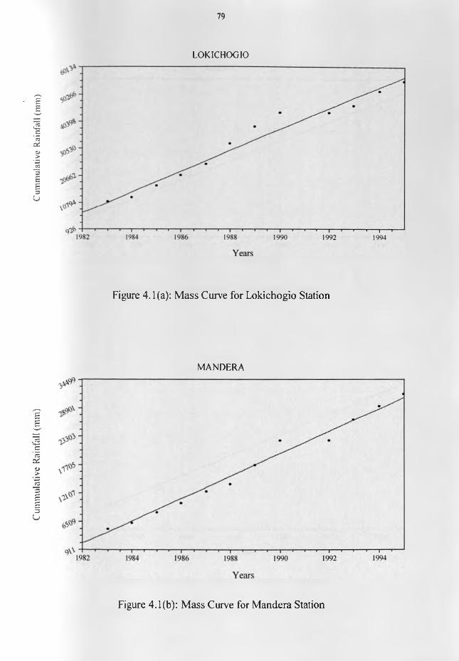
Cum

mul

ativ

e Ra

infa

ll (m

m)

Cum

mul

ative

Rain

fall

(mm

)

79

LOKICHOGIO

Figure 4.1(a): Mass Curve for Lokichogio Station

MANDERA

Figure 4.1(b): Mass Curve for Mandera Station

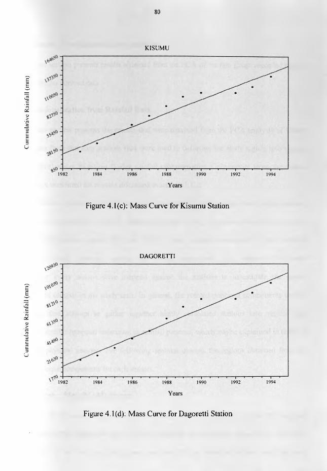
Cu

mm

ula

tiv

e R

ainf

all

(mm

) C

um

mu

lati

ve

Rai

nfal

l (m

m)

80

KISUMU

Figure 4.1(c): Mass Curve for Kisumu Station

DAGORETTI

Figure 4.1(d): Mass Curve for Dagoretti Station

81

4.2 Results from Regionalization analyses

This section presents results obtained from the PCA of the rain gauge recorded rainfall

and the satellite derived data.

4.2.1 Regionalization from Rainfall Data

This section presents the results that were obtained from the PCA analysis of 10-day

rainfall data from the sixty stations that were used to delineate the study region into various

climatological zones based on 10-day rainfall characteristics. Only results from the rotated

solutions are presented for reasons discussed in section 3.1.2.

PCA was independently performed on the dekadal data from the four typical seasons,

namely March-Apri 1-May (MAM), June-July-August (JJA). September-October-November

(SON) and December-January-February (DJF). These seasons correspond to the Northern

Hemisphere spring, summer, autumn and winter respectively. The rotated PCA factor

loadings for every' season were mapped against the stations to investigate the spatial

variability of rainfall in the study area. In general, the rotated principal components usually

give maps that attempt to gather together highly correlated stations into regions that

experience similar temporal anomalies in rainfall patterns, which maybe explained in terms of

underlying physical reasons. The following sections discuss the regions obtained from the

rotated principal components for each season.

4.2.1.1 March - May (MAM) Season

This is the main rainy season for the study area. It is normally called the long rain

season. During this season, the sun is directly overhead the equatorial region on its way from

the Southern to the Northern Hemisphere and the ITCZ is therefore located over the study

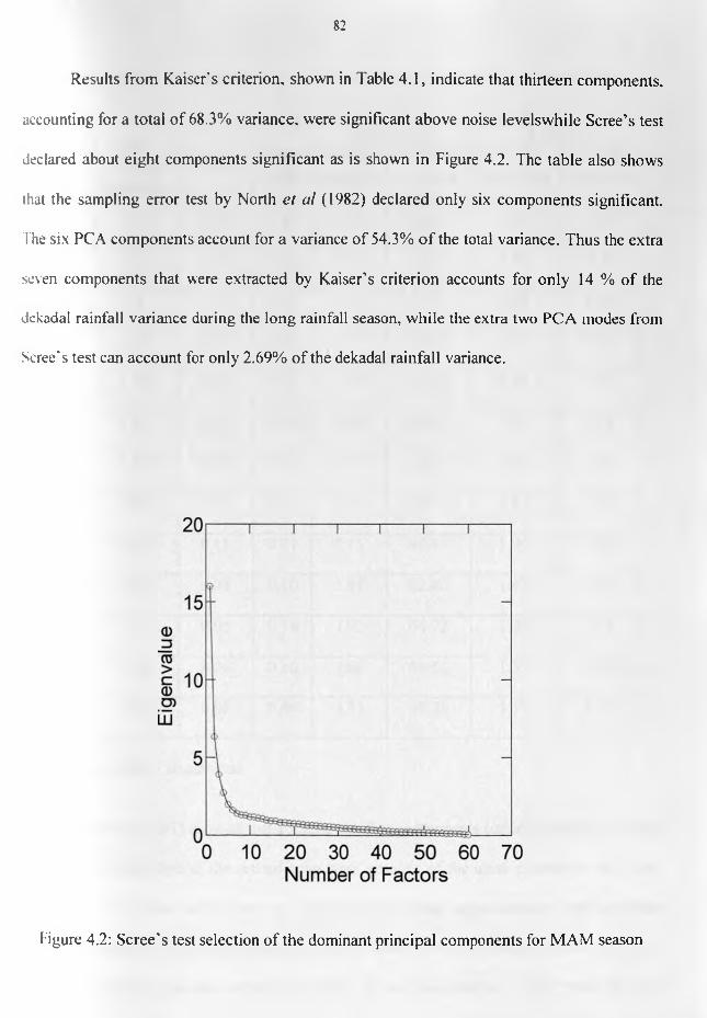
82

Results from Kaiser's criterion, shown in Table 4.1, indicate that thirteen components,

accounting for a total of 68.3% variance, were significant above noise levelswhile Scree's test

declared about eight components significant as is shown in Figure 4.2. The table also shows

that the sampling error test by North et al (1982) declared only six components significant.

The six PCA components account for a variance of 54.3% o f the total variance. Thus the extra

seven components that were extracted by Kaiser’s criterion accounts for only 14 % of the

dekadal rainfall variance during the long rainfall season, while the extra two PCA modes from

Scree's test can account for only 2.69% of the dekadal rainfall variance.

Figure 4.2: Scree's test selection of the dominant principal components for MAM season

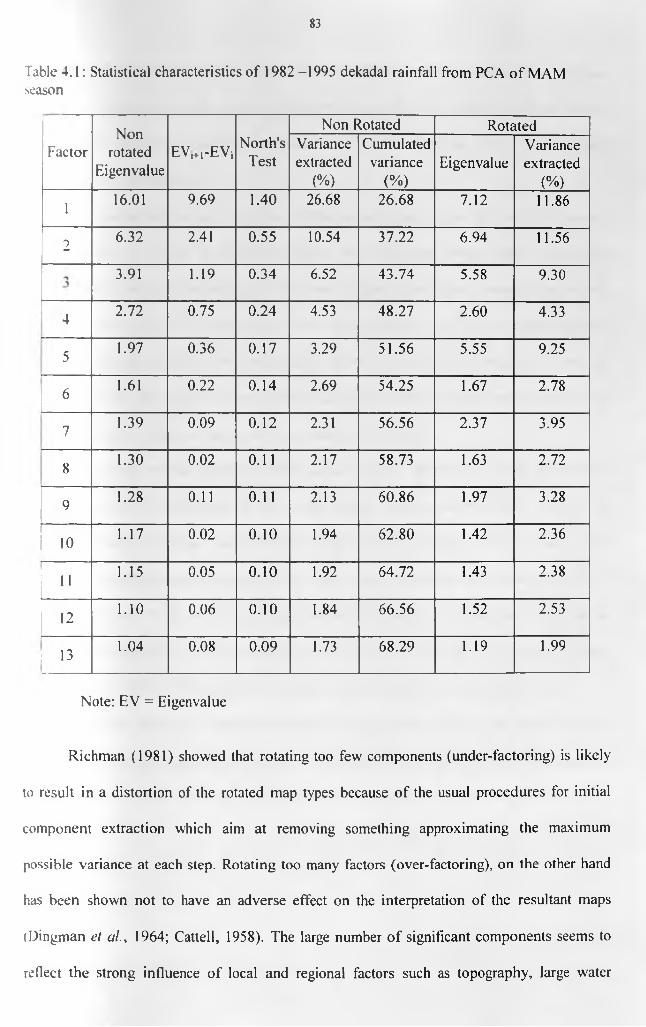
83

Table 4.1: Statistical characteristics of 1982 -1995 dekadal rainfall from PCA o f MAMseason

FactorNon

rotatedEigenvalue

EV,+1-EVj North'sTest

Non Rotated RotatedVarianceextracted

(%)

Cumulatedvariance

(%)Eigenvalue

Varianceextracted

(%)

1 16.01 9.69 1.40 26.68 26.68 7.12 11.86

2 6.32 2.41 0.55 10.54 37.22 6.94 11.56

3.91 1.19 0.34 6.52 43.74 5.58 9.30

4______

2.72 0.75 0.24 4.53 48.27 2.60 4.33

5 1.97 0.36 0.17 3.29 51.56 5.55 9.25

6 1.61 0.22 0.14 2.69 54.25 1.67 2.78

7 1.39 0.09 0.12 2.31 56.56 2.37 3.95

8 1.30 0.02 0.11 2.17 58.73 1.63 2.72

9 1.28 0.11 0.11 2.13 60.86 1.97 3.28

10 1.17 0.02 0.10 1.94 62.80 1.42 2.36

11 1.15 0.05 0.10 1.92 64.72 1.43 2.38

12 1.10 0.06 0.10 1.84 66.56 1.52 2.53

! 131.04 0.08 0.09 1.73 68.29 1.19 1.99

Note: EV = Eigenvalue

Richman (1981) showed that rotating too few components (under-factoring) is likely

to result in a distortion of the rotated map types because o f the usual procedures for initial

component extraction which aim at removing something approximating the maximum

possible variance at each step. Rotating too many factors (over-factoring), on the other hand

has been shown not to have an adverse effect on the interpretation of the resultant maps

(Dingman et al., 1964; Cattell, 1958). The large number o f significant components seems to

reflect the strong influence of local and regional factors such as topography, large water

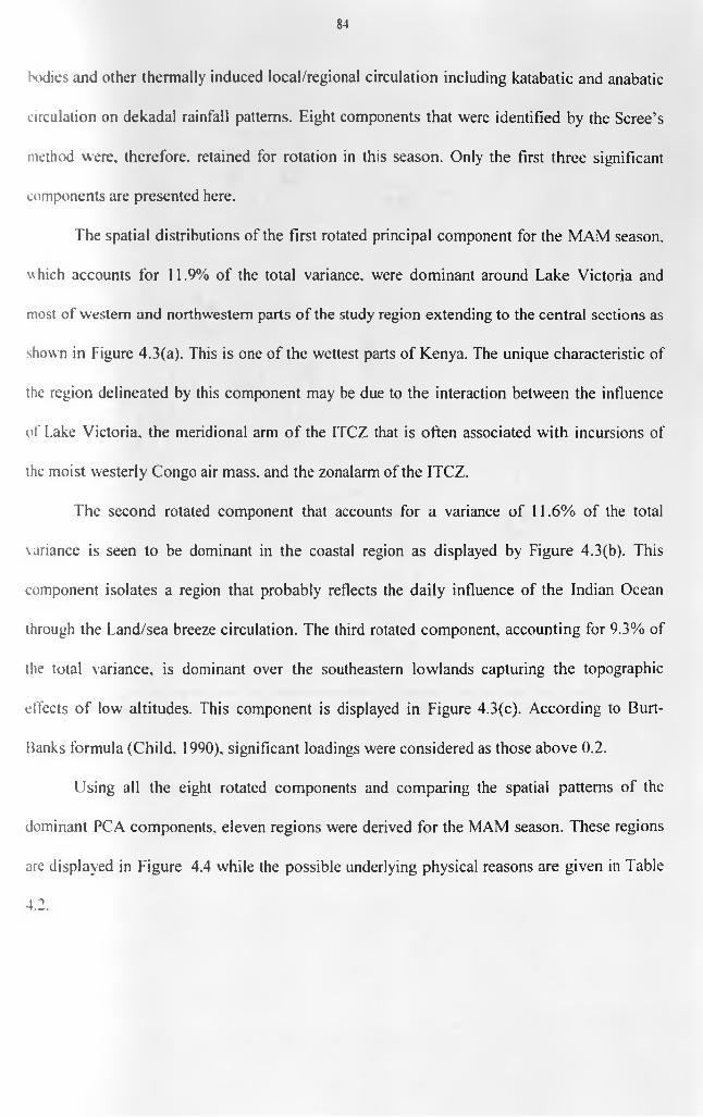
84

bodies and other thermally induced local/regional circulation including katabatic and anabatic

circulation on dekadal rainfall patterns. Eight components that were identified by the Scree’s

method were, therefore, retained for rotation in this season. Only the first three significant

components are presented here.

The spatial distributions of the first rotated principal component for the MAM season,

which accounts for 11.9% of the total variance, were dominant around Lake Victoria and

most of western and northwestern parts of the study region extending to the central sections as

shown in Figure 4.3(a). This is one of the wettest parts of Kenya. The unique characteristic of

the region delineated by this component may be due to the interaction between the influence

of L.ake Victoria, the meridional arm of the ITCZ that is often associated with incursions of

the moist westerly Congo air mass, and the zonalarm of the ITCZ.

The second rotated component that accounts for a variance of 11.6% of the total

variance is seen to be dominant in the coastal region as displayed by Figure 4.3(b). This

component isolates a region that probably reflects the daily influence of the Indian Ocean

through the Land/sea breeze circulation. The third rotated component, accounting for 9.3% of

the total variance, is dominant over the southeastern lowlands capturing the topographic

effects o f low altitudes. This component is displayed in Figure 4.3(c). According to Burt-

Banks formula (Child. 1990), significant loadings were considered as those above 0.2.

Using all the eight rotated components and comparing the spatial patterns of the

dominant PC A components, eleven regions were derived for the MAM season. These regions

are displayed in Figure 4.4 while the possible underlying physical reasons are given in Table

4.2.

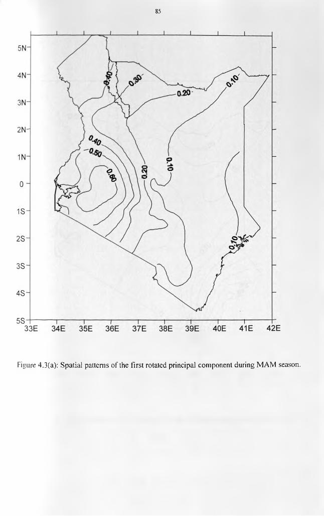
85

Figure 4.3(a): Spatial patterns of the first rotated principal component during MAM season.

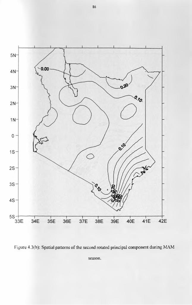
86

Figure 4.3(b): Spatial patterns of the second rotated principal component during MAM

season.

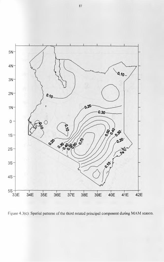
87

Figure 4.3(c): Spatial patterns of the third rotated principal component during MAM season.

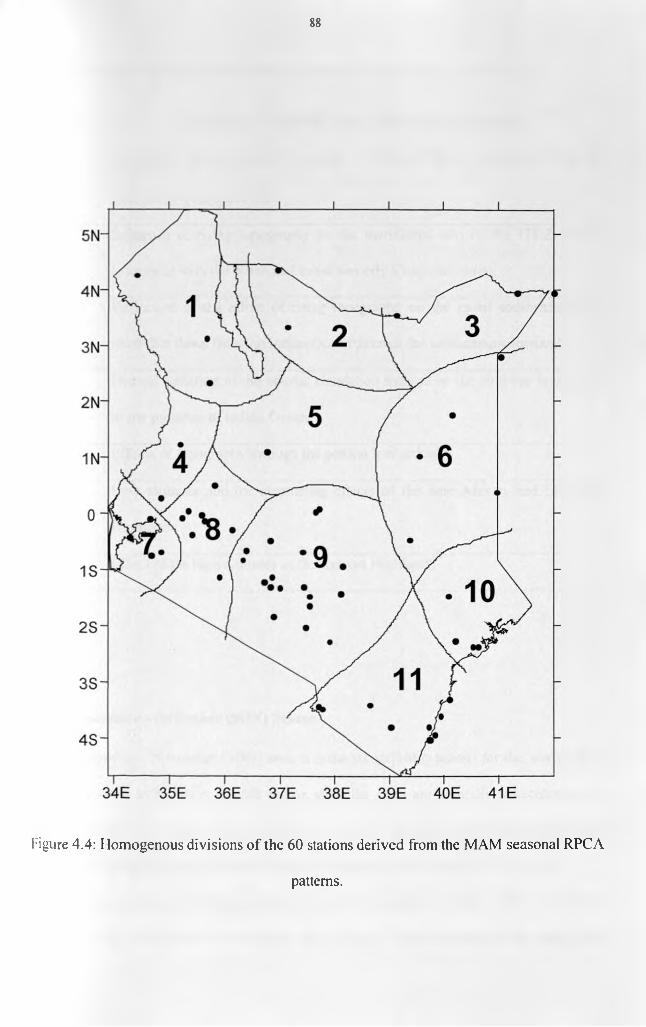
88

Figure 4.4: Homogenous divisions of the 60 stations derived from the MAM seasonal RPCA

patterns.

89

Table 4.2: The possible physical reasons underlying the derived regions for MAM

REGION POSSIBLE UNDERLYING PHYSICAL REASONS

7Reflection of the diurnal variation of Lake Victoria circulation and its

interaction with the ITCZ

4Influence of rising topography on the meridional arm of the ITCZ usually

associated with the warm and moist westerly Congo air mass

9Reflection of the effect of rising topography on the moist southeasterly air

mass that flows from the Indian Ocean through the southeastern lowlands

10& 11Diurnal variation of the coastal circulation marked by the land/sea breeze due

to the presence of Indian Ocean

3 & 6 Effects of topography through the general low altitudes

1.2 & 5Low altitudes and the channeling effects o f the East African and Ethiopian

Highlands

8 Effect of the high altitudes of the Kenyan Highlands

4.2.1.2 September - November (SON) Season

September - November (SON) season is the second rainy season for the study area. It

is locally known as the short rainfall season since the rains are normally concentrated only

over the months o f October and November. The ITCZ is located over the study area for the

second time w ithin the year as it moves from the Northern to the Southern Hemisphere.

The Scree's plot of the eigenvalues is given in Figure 4.5, while Table 4.3 gives the

summary of the results that were obtained when dekadal rainfall records for the season were

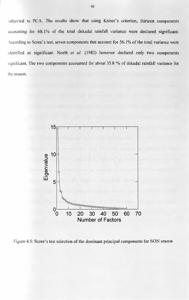
90

subjected to PCA. The results show that using Kaiser’s criterion, thirteen components

accounting for 68.1% of the total dekadal rainfall variance were declared significant.

According to Scree's test, seven components that account for 56.1% of the total variance were

identified as significant. North el al. (1982) however declared only two components

significant. The two components accounted for about 35.8 % of dekadal rainfall variance for

the season.

Figure 4.5: Scree’s test selection o f the dominant principal components for SON season

91

The spatial patterns o f the first three dominant rotated principal components for this

reason are displayed in Figure 4.6. The first rotated principal component, which explains

about 16% of the total variance, is shown to be relatively significant in most parts of the study

region except over the Lake Victoria region. However it is highly dominant around the

highlands to the southeast o f the Rift Valley. This is depicted in Figure 4.6(a). This

component may be capturing the homogeneity o f spatial rainfall characteristic during the

season that could be associated with the influence of the ITCZ. Such observations have been

made in previous studies (Ogallo, 1989; Ininda. 1994; Indeje el al., 2000). The spatial

distribution of the second rotated component that accounts for 11% of the total variance is

given in Figure 4.6(b). This component is dominant mainly to the west and northwest parts of

the study region and delineates an area that may be reflecting the interactions between the

ITCZ. the Lake Victoria circulation and the westerly moist air mass from the Congo Basin.

The third component, which accounts for about 7% of the variance, is displayed in Figure

4.6(c) and is dominant along the coastal region. Figure 4.7 gives the homogenous zones for

the season based on the spatial patterns of the loadings o f the significant components. The

number o f homogenous regions in this season is less than for the major rainfall season. This

may be due to the relative low total amounts of rainfall received and the widespread dryness

experienced during this season. It may also be due to the dominance of large-scale features

and teleconnections as can be seen in the better predictability of this season (Ininda. 1994;

Indeje et cil., 2000).

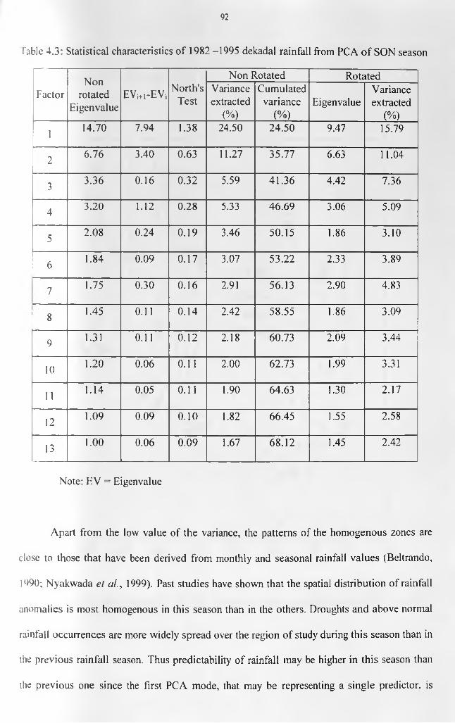
92

Table 4.3: Statistical characteristics of 1982 -1995 dekadal rainfall from PCA o f SON season

FactorNon

rotatedEigenvalue

E V i+1-EViNorth's

Test


(%)

Cumulatedvariance

(%)Eigenvalue

Varianceextracted

(%)

I 14.70 7.94 1.38 24.50 24.50 9.47 15.79

2 6.76 3.40 0.63 11.27 35.77 6.63 11.04

3 3.36 0.16 0.32 5.59 41.36 4.42 7.36

4 3.20 1.12 0.28 5.33 46.69 3.06 5.09

5 2.08 0.24 0.19 3.46 50.15 1.86 3.10

6 1.84 0.09 0.17 3.07 53.22 2.33 3.89

71.75 0.30 0.16 2.91 56.13 2.90 4.83

8 1.45 0.11 0.14 2.42 58.55 1.86 3.09

9 1.31 0.11 0.12 2.18 60.73 2.09 3.44

10 1.20 0.06 0.11 2.00 62.73 1.99 3.31

11 1.14 0.05 0.11 1.90 64.63 1.30 2.17

12 1.09 0.09 0.10 1.82 66.45 1.55 2.58

13 1.00 0.06 0.09 1.67 68.12 1.45 2.42


Apart from the low value of the variance, the patterns of the homogenous zones are

close to those that have been derived from monthly and seasonal rainfall values (Beltrando,

1990; Nyakwada et al., 1999). Past studies have shown that the spatial distribution of rainfall

anomalies is most homogenous in this season than in the others. Droughts and above normal

rainfall occurrences are more widely spread over the region of study during this season than in

the previous rainfall season. Thus predictability of rainfall may be higher in this season than

the previous one since the first PCA mode, that may be representing a single predictor, is

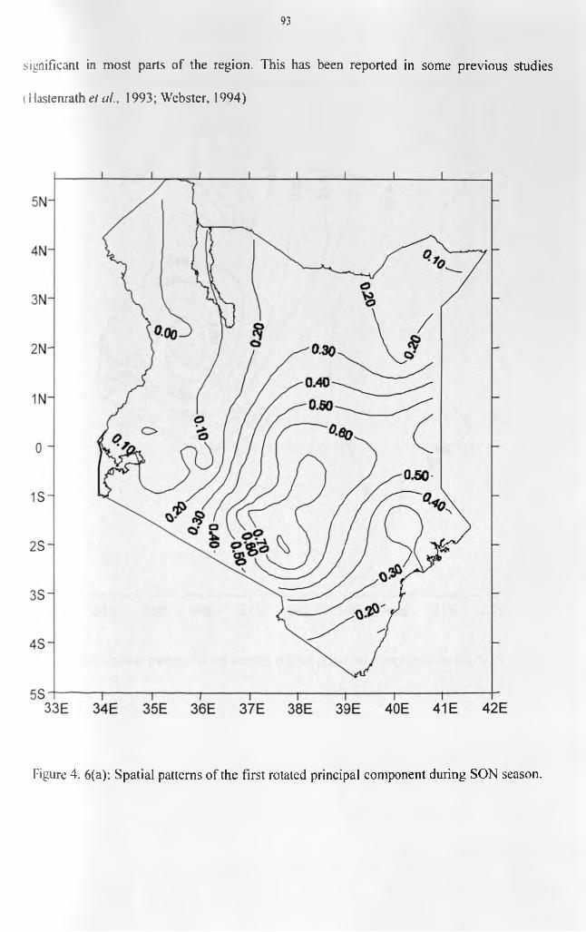
93

significant in most parts of the region. This has been reported in some previous studies

( I lastenrath el al., 1993; Webster, 1994)

Figure 4. 6(a): Spatial patterns of the first rotated principal component during SON season.

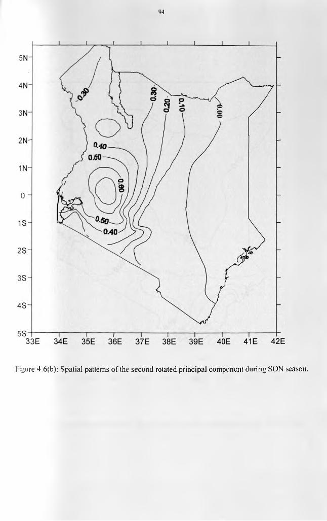
94

f igure 4.6(b): Spatial patterns of the second rotated principal component during SON season.

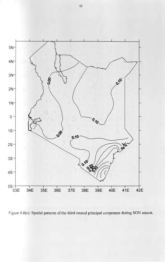
95

Figure 4.6(c): Spatial patterns of the third rotated principal component during SON season.

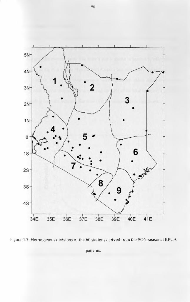
96

Figure 4.7: Homogenous divisions o f the 60 stations derived from the SON seasonal RPC A

patterns.

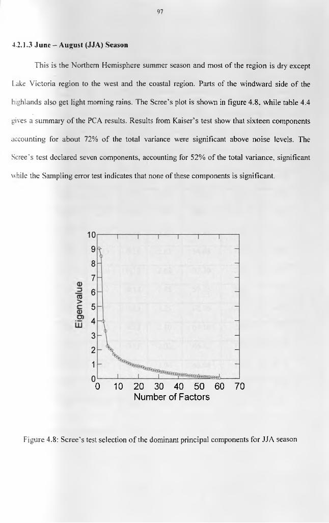
97

4.2.1.3 June - August (JJA) Season

This is the Northern Hemisphere summer season and most of the region is dry except

l ake Victoria region to the west and the coastal region. Parts of the windward side of the

highlands also get light morning rains. The Scree’s plot is shown in figure 4.8. while table 4.4

gives a summary of the PCA results. Results from Kaiser’s test show that sixteen components

accounting for about 72% of the total variance were significant above noise levels. The

Scree's test declared seven components, accounting for 52% of the total variance, significant

while the Sampling error test indicates that none of these components is significant.

11_____I______ 1______ I ______

0 10 20 30 40 50 60 70Number of Factors

Figure 4.8: Scree’s test selection o f the dominant principal components for JJA season

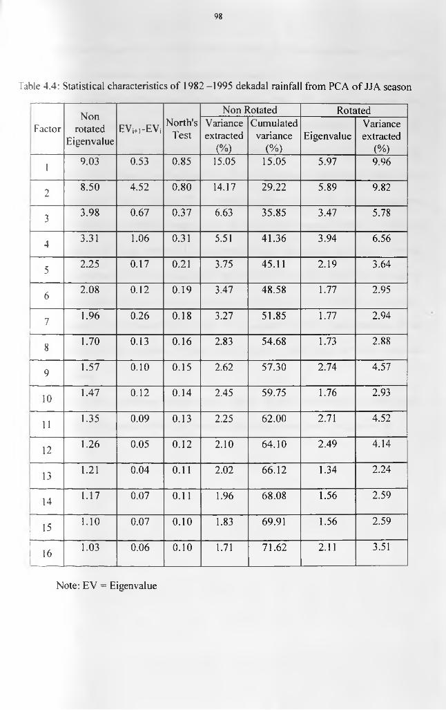
98

Table 4.4: Statistical characteristics of 1982 -1995 dekadal rainfall from PC A o f JJA season

■

FactorNon

rotatedEigenvalue

EVj+i-EVj North’sTest


(%)

Cumulatedvariance

(%)Eigenvalue

Varianceextracted

(%)

1 9.03 0.53 0.85 15.05 15.05 5.97 9.96

2 8.50 4.52 0.80 14.17 29.22 5.89 9.82

■3 3.98 0.67 0.37 6.63 35.85 3.47 5.78

4 3.31 1.06 0.31 5.51 41.36 3.94 6.56

5 2.25 0.17 0.21 3.75 45.11 2.19 3.64

6 2.08 0.12 0.19 3.47 48.58 1.77 2.95

7 1.96 0.26 0.18 3.27 51.85 1.77 2.94

8 1.70 0.13 0.16 2.83 54.68 1.73 2.88

9 1.57 0.10 0.15 2.62 57.30 2.74 4.57

10 1.47 0.12 0.14 2.45 59.75 1.76 2.93

11 1.35 0.09 0.13 2.25 62.00 2.71 4.52

12 1.26 0.05 0.12 2.10 64.10 2.49 4.14

13 1.21 0.04 0.11 2.02 66.12 1.34 2.24

14 1.17 0.07 0.11 1.96 68.08 1.56 2.59

15 1.10 0.07 0.10 1.83 69.91 1.56 2.59

161.03 0.06 0.10 1.71 71.62 2.11 3.51


99

Figure 4.9 display the spatial distributions of the First three significant components.

The first rotated component, which accounts for a variance of 9.96% of the total variance, is

shown to be dominant over the coastal regions in figure 4.9(a). The second component that

accounts for 9.82% of the total variance is dominant around the highlands east of the Rift

Valley extending south to the area around Mount Kilimanjaro as shown in figure 4.9(b). The

third component, accounting for a variance of 6.56%, is dominant in the western parts of the

stud) area but north of Lake Victoria. This is shown in figure 4.9(c). This region is known to

have a third rainfall peak within the year during this season (Davies et al., 1985). It should be

noted that, despite the large number o f components declared significant by Kaiser’s method,

even the first non-rotated PCA mode accounts for only 15% of rainfall variance in this season.

This may be a reflection of the highly localized nature o f rainfall variation in this season.

Seven components were retained for rotation. The complexity of the spatial patterns of the

PCA may be due to the existence of many zero dekadal rainfall values at many locations

during this season.

Using all the significant rotated components, eleven climatological regions were

derived from the PCA results o f the JJA season. These regions are shown in figure 4.10.

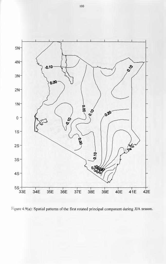
100

Figure 4.9(a): Spatial patterns of the first rotated principal component during JJA season.

101

Figure 4.9(b): Spatial patterns of the second rotated principal component during JJA season.

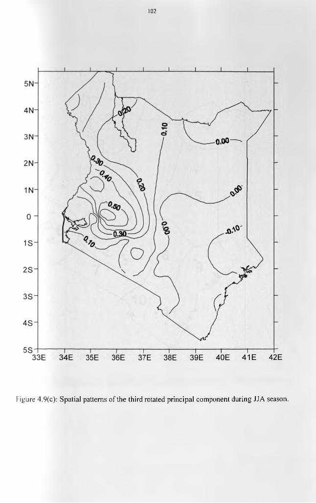
102

Figure 4.9(c): Spatial patterns of the third rotated principal component during JJA season.

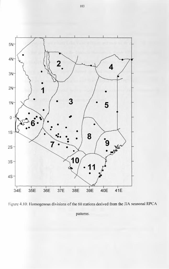
103

Figure 4.10: Homogenous divisions o f the 60 stations derived from the JJA seasonal RPCA

patterns.

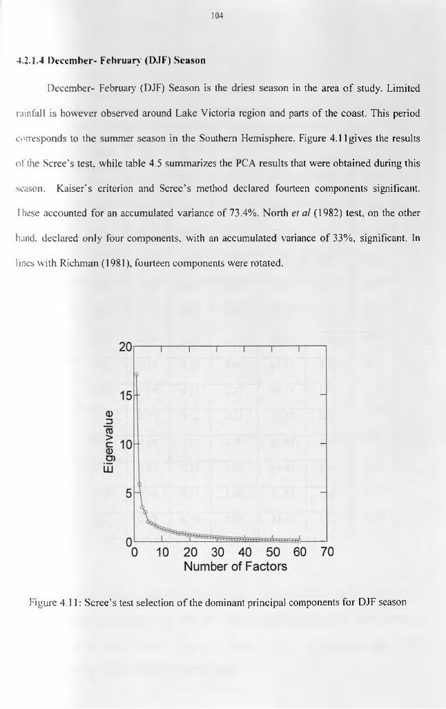
104

4.2.1.4 December- February (DJF) Season

December- February (DJF) Season is the driest season in the area o f study. Limited

rainfall is however observed around Lake Victoria region and parts of the coast. This period

corresponds to the summer season in the Southern Hemisphere. Figure 4.11 gives the results

o! the Scree’s test, while table 4.5 summarizes the PCA results that were obtained during this

season. Kaiser’s criterion and Scree’s method declared fourteen components significant.

These accounted for an accumulated variance of 73.4%. North el al (1982) test, on the other

hand, declared only four components, with an accumulated variance of 33%, significant. In

lines with Richman (1981), fourteen components were rotated.

Figure 4.11: Scree’s test selection o f the dominant principal components for DJF season

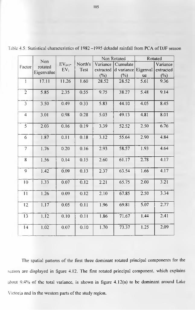
105

Table 4.5: Statistical characteristics o f 1982 -1995 dekadal rainfall from PCA o f DJF season

FactorNon

rotatedEigenvalue

EVi+i-EVj

North'sTest


(%)

Cumulate d variance

(%)Eigenval

ue

Varianceextracted

(%)1 17.11 11.26 1.60 28.52 28.52 5.61 9.36

2 5.85 2.35 0.55 9.75 38.27 5.48 9.14

3 3.50 0.49 0.33 5.83 44.10 4.05 8.45

4 3.01 0.98 0.28 5.03 49.13 4.81 8.01

5 2.03 0.16 0.19 3.39 52.52 2.50 6.76

6 1.87 0.11 0.18 3.12 55.64 2.90 4.84

7 1.76 0.20 0.16 2.93 58.57 1.93 4.64

8 1.56 0.14 0.15 2.60 61.17 2.78 4.17

9 1.42 0.09 0.13 2.37 63.54 1.66 4.17

10 1.33 0.07 0.12 2.21 65.75 2.00 3.21

11.

1.26 0.09 0.12 2.10 67.85 2.50 3.34

12 1.17 0.05 0.11 1.96 69.81 5.07 2.77

13 1.12 0.10 0.11 1.86 71.67 1.44 2.41

14 1.02 0.07 0.10 1.70 73.37 1.25 2.09

The spatial patterns of the first three dominant rotated principal components for the

season are displayed in figure 4.12. The first rotated principal component, which explains

about 9.4% of the total variance, is shown in figure 4.12(a) to be dominant around Lake

Victoria and in the western parts of the study region.

106

The second rotated principal component, which accounts for 9.1% of the total

\ariance, is dominant in the dry eastern regions of the study area and is shown in figure

4 12(b). The third rotated component, accounting for 8.5% of the total variance, is seen in

figure 4.12(c) to be dominant in the region to the east of the central highlands covering the

southeastern lowlands. The spatial distributions of the other components were used to get

further smaller zones from the ones discussed above. For example the sixth rotated principal

component, which accounts for 4.8% o f the total variance, is dominant over the area around

mount Kilimanjaro and helps in delineating this region.

The existence of many zero values and the localized nature of dekadal rainfall

\ariations in this season were reflected in the complexity of the PCA solutions. It should

however be noted that in some years the September - November rains extend to January-

February as was witnessed in 1998. Such rains extend over the whole region. This could

explain the relatively high variance that is accounted for by the first non-rotated component. It

should be noted that the year to year rainfall variability of dekadal rainfall is very high in this

dry season. Further it should be noted that PCA used normalized rainfall data to avoid

including zero values in the input matrix. Figure 4.13 illustrates the eleven climatic zones

derived from PCA of the DJF season.

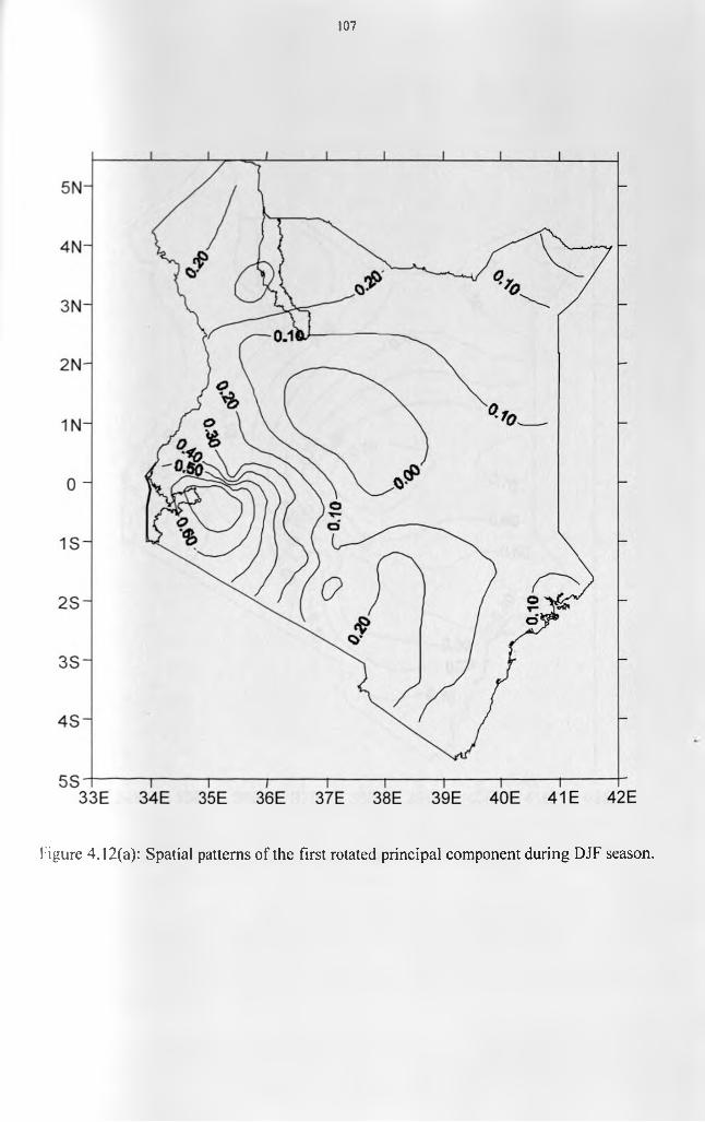
107

Figure 4.12(a): Spatial patterns of the first rotated principal component during DJF season.

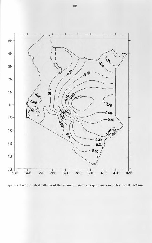
108

Figure 4.12(b): Spatial patterns of the second rotated principal component during DJF season.

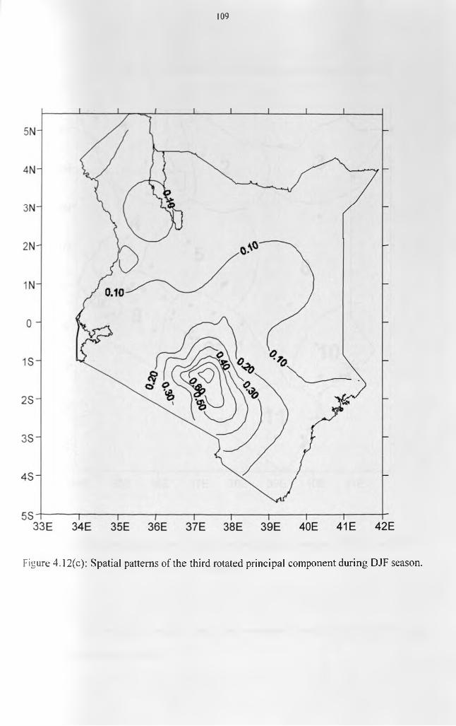
109

Figure 4.12(c): Spatial patterns of the third rotated principal component during DJF season.

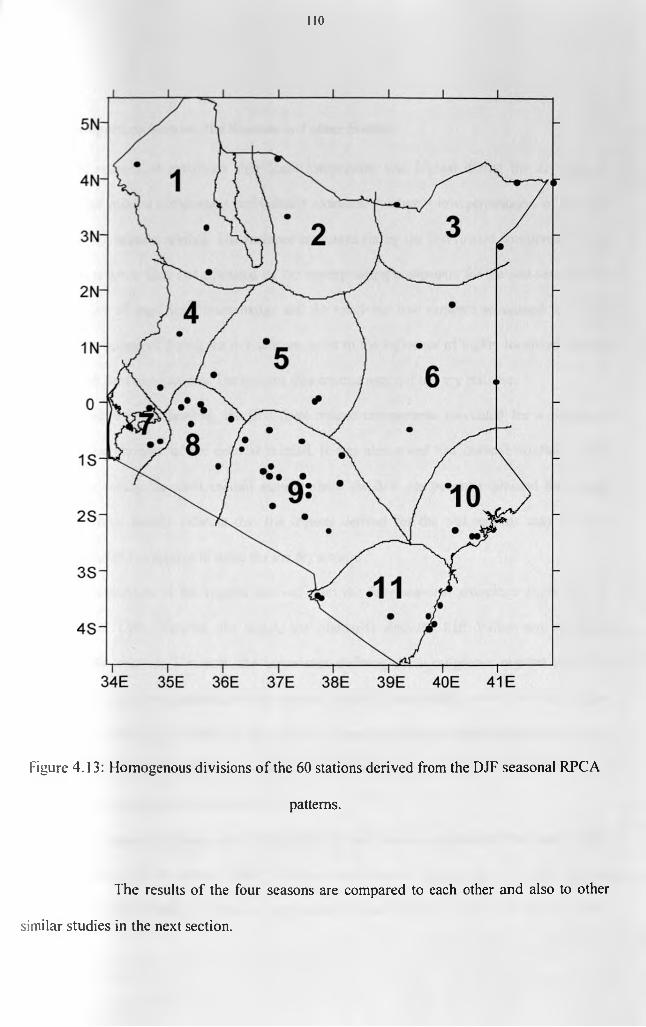
110

Figure 4.13: Homogenous divisions o f the 60 stations derived from the DJF seasonal RPCA

patterns.

The results of the four seasons are compared to each other and also to other

similar studies in the next section.

I l l

4.2.1.5 Comparison between the Seasons and other Studies

The number of maximum significant components was highest during the dry seasons.

I lowever, the rotated components individually extracted relatively low percentages of the total

\ariance o f the dekadal rainfall. The variance accounted for by the first rotated component for the

dry seasons is lower than that extracted by the corresponding component for the wet seasons. The

higher number of significant components and the relatively low variance accounted for by the

individual components during the dry seasons point to the influence of highly localized systems

in the rainfall for these seasons. The regions thus created may not be very realistic.

During the wet seasons, the first three rotated components accounted for a significant

amount o f the variance of the dekadal rainfall. It was also noted that dekadal rainfall is more

homogenous during the short rainfall season where the first component explained the highest

variance. These results indicate that the regions derived for the wet seasons may be more

physically realistic compared to those for the dry seasons.

A comparison of the regions derived from the four seasonal groupings show that the

region around Lake Victoria, the coast, the highlands and the Rift Valley are consistent

throughout the seasons. However, the boundaries defining the homogenous regions shift with

seasons reflecting the complexity of the seasonal rainfall characteristics over the study region.

T hese could arise from the interplay between the large- and synoptic-scale systems and the local

factors like topography. Detailed characteristics of the various systems that control rainfall over

the region has been outlined in section 1.3.2.

Other researchers have also, using different time scales, regionalized the study region.

The complexities of the spatial rainfall have also been noted in these previous studies. Barring

(1988) used daily rainfall to derive eleven annual regions over the study area. Most of these

112

regions are comparable to the regions derived in this study except for the areal extents. For

example, this study divides the northern part into three regions while Barring (1988) has two.

Ogallo (1989) used monthly data to group seasonal and annual climatic regions for East

\frica. His seasonal map combines the northern section into one region and has several smaller

regions in the central areas. The annual map, however, has only five regions demarcated over

Kenya. In this case the area around Lake Victoria is the only one which is similarly demarcated

in both studies. Indeje et al. (2000), using monthly data for East Africa, demarcated five annual

climatic regions over the study region. The region around Lake Victoria is delineated in both

studies while the coastal zone is lumped into one region by Indeje et al. (2000). It is evident from

these studies that the spatial patterns o f rainfall are more homogenous at monthly and seasonal

time scales than in the lower time scales. While the monthly and seasonal time scales give

cumulative rainfall totals for the specific periods, the daily and 10-day time scales include the

impacts of spatial migrations of the rainfall producing systems including the ITCZ.

The next section presents results of regionalization of the study area using satellite-

derived records.

4.2.2 Results from Regionalization using Satellite-Derived Data

This section presents and discusses results from the regionalization of the study area using

PC A of mean dekadal Total Precipitable Water (TPW) derived from satellite information. As in

the case of the dekadal rainfall, only rotated solutions are presented. TPW maybe defined as the

total amount of moisture present in a given column of air expressed as the depth of water that

\xould accumulate at the base of the column if all the water vapor could be condensed into water

(Zeng, 1999).

113

PCA was performed on the three available layers o f TPW (surface - 700 mb. 700 - 500

mb. 500 - 200 mb). Only one component was significant for the highest layer in all the seasons.

For the middle layer two components were significant for the first three seasons while the DJF

season had three significant components. In the surface-700 mb layer, more than three

components were declared significant in all seasons indicating the influence of several factors in

ihis layer. Due to the need of incorporating as many influencing factors as possible, for example

local, regional as well as synoptic factors, in the regionalization, the study therefore concentrated

only on the lowest layer.

Results from Kaiser's criterion. Scree’s and North el al. sampling error tests all declared

four components significant above noise levels for MAM, SON and JJA seasons accounting for

94.9, 92.1 and 92.5% of the total variance in the dekadal surface - 700 mb layer of TPW,

respectively. The tests identified six components, accounting for 90.4% of the total variance, for

the DJF season. Four components were retained for rotation for MAM, SON and JJA seasons

while six were rotated for DJF season. A summary of these results is presented in Table 4.6.

Figure 4.14 displays the spatial distribution of the first rotated component, w hich accounts

for 85.1% for MAM, 83.6% for SON, 84.4% for JJA and 74.5% for DJF seasons. The

distribution of this component may be as a result of the prevailing mean synoptic patterns over

the region during the various seasons.

Figures 4.14 (a) and (b) show the spatial distribution of the TPW content of the wet

seasons of MAM and SON respectively. There is a striking similarity in the TPW content of these

two seasons with the components being generally dominant over most of the study area with a

small area with low factor loadings. This general dominance maybe due to the presence of the

ITCZ in the area at these times, accompanied by widespread predominantly convective rainfall.

According to an earlier study by Tuller (1968), areas of low TPW over the continents are

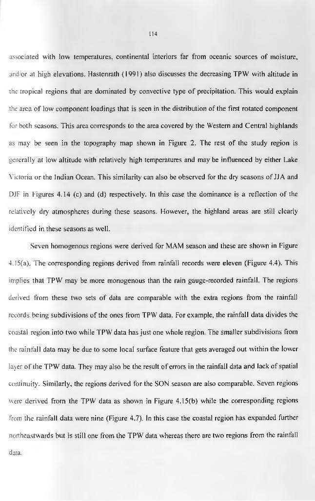
114

associated with low temperatures, continental interiors far from oceanic sources of moisture,

and or at high elevations. Hastenrath (1991) also discusses the decreasing TPW with altitude in

the tropical regions that are dominated by convective type o f precipitation. This would explain

the area of low component loadings that is seen in the distribution of the first rotated component

for both seasons. This area corresponds to the area covered by the Western and Central highlands

as may be seen in the topography map shown in Figure 2. The rest of the study region is

generally at low altitude with relatively high temperatures and may be influenced by either Lake

Victoria or the Indian Ocean. This similarity can also be observed for the dry seasons of JJA and

DJF in Figures 4.14 (c) and (d) respectively. In this case the dominance is a reflection of the

relatively dry atmospheres during these seasons. However, the highland areas are still clearly

identified in these seasons as well.

Seven homogenous regions were derived for MAM season and these are shown in Figure

4.15(a). The corresponding regions derived from rainfall records were eleven (Figure 4.4). This

implies that TPW may be more monogenous than the rain gauge-recorded rainfall. The regions

derived from these two sets of data are comparable with the extra regions from the rainfall

records being subdivisions of the ones from TPW data. For example, the rainfall data divides the

coastal region into two while TPW data has just one whole region. The smaller subdivisions from

the rainfall data may be due to some local surface feature that gets averaged out within the lower

layer of the TPW data. They may also be the result of errors in the rainfall data and lack of spatial

continuity. Similarly, the regions derived for the SON season are also comparable. Seven regions

were derived from the TPW data as shown in Figure 4.15(b) while the corresponding regions

from the rainfall data were nine (Figure 4.7). In this case the coastal region has expanded further

northeastwards but is still one from the TPW data whereas there are two regions from the rainfall

data.

115

The regions derived for the dry seasons of JJA and DJF are shown in Figures 4.15 (c) and

(d) respectively. Six regions were derived for the JJA season and eight for DJF season with the

corresponding regions from rainfall data being eleven in both cases. The extra regions from the

rainfall data are still subdivisions of the regions derived from TPW data. During these seasons,

the influence of local topographical features dominates the weather of the study region leading to

the several zones demarcated from the rainfall data. The presence of a small raised ground may

trigger off rainfall in a small area from the same amount of TPW for a larger area. These

influences maybe evened out within the TPW layer resulting in only a few homogenous regions

delineated. Flowever, due to the strong influence of local features leading to complex rainfall

distribution during these dry seasons, the rest of the study is concentrated on the two wet seasons.

The derived zones (based on both rainfall and TPW records) were compared to the agro-

ecological zones o f Kenya (Sombroek, el al., 1982). However, the time-scales were different,

annual for agro-ecological and seasonal for rainfall/TPW zoning. The zones based on rainfall

records were relatively smaller and hence more in number compared to the agro-ecological

zones. The TPW zones were closest to the agro-ecological zones in terms of size and numbers,

even though the time-scales were different. This indicates that the TPW is more closely linked to

crop requirements than simply rainfall amounts. Further work should be done in this line to

understand better this relationship.

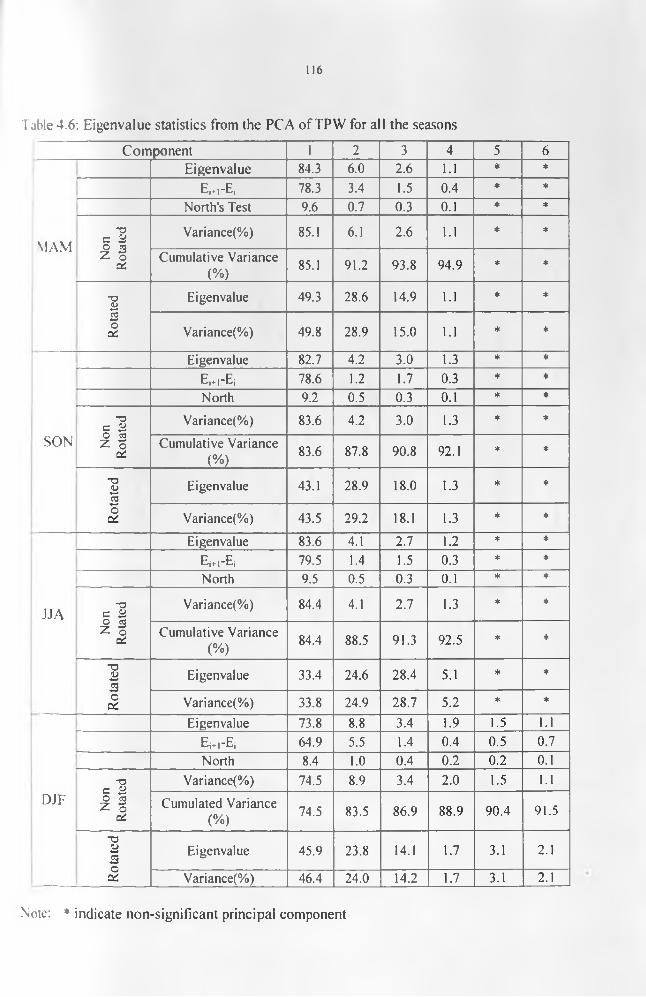
116

Table 4.6: Eigenvalue statistics from the PCA of TPW for all the seasons

Component 1 2 3 4 5 6

MAM

Eigenvalue 84.3 6 . 0 2 . 6 1 . 1 * *

Ej+i-Ej 78.3 3.4 1.5 0.4 * *North's Test 9.6 0.7 0.3 0 . 1 * ♦

Non

Rota

ted Variance(%) 85.1 6 . 1 2 . 6 1 . 1 * *

Cumulative Variance (%)

85.1 91.2 93.8 94.9 * *

Rota

ted Eigenvalue 49.3 28.6 14.9 1 . 1 * *

Variance(%) 49.8 28.9 15.0 1 . 1 * *

SON

Eigenvalue 82.7 4.2 3.0 1.3 * *

Ej+i-Ej 78.6 1 . 2 1.7 0.3 * *North 9.2 0.5 0.3 0 . 1 * *

Non

Rota

ted Variance(%) 83.6 4.2 3.0 1.3 * *


83.6 87.8 90.8 92.1 * *

Rot

ated Eigenvalue 43.1 28.9 18.0 1.3 * *

Variance(%) 43.5 29.2 18.1 1.3 * *

JJA

Eigenvalue 83.6 4.1 2.7 1 . 2 * *

Ej+i-Ei 79.5 1.4 1.5 0.3 * *North 9.5 0.5 0.3 0.1 * *

Non

Rota

ted Variance(%) 84.4 4.1 2.7 1.3 * *


84.4 88.5 91.3 92.5 * *

[ Rot

ated

i____

__ Eigenvalue 33.4 24.6 28.4 5.1 * *

Variance(%) 33.8 24.9 28.7 5.2 * *

DJF

Eigenvalue 73.8 8 . 8 3.4 1.9 1.5 l.lEi+i-Ei 64.9 5.5 1.4 0.4 0.5 0.7North 8.4 1.0 0.4 0 . 2 0 . 2 0 . 1

Non

Rota

ted Variance(%) 74.5 8.9 3.4 2 . 0 1.5 1.1

Cumulated Variance (%) 74.5 83.5 86.9 88.9 90.4 91.5

Rot

ated Eigenvalue 45.9 23.8 14.1 1.7 3.1 2 . 1

Variance(%) 46.4 24.0 14.2 1.7 3.1 2 . 1

Note: * indicate non-significant principal component

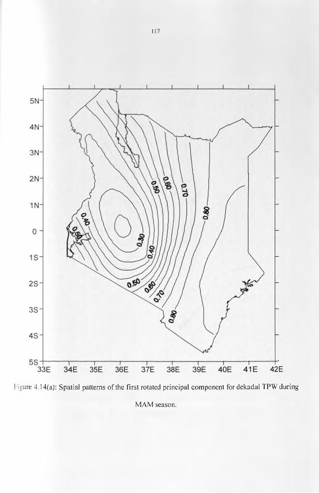
117

Figure 4.14(a): Spatial patterns of the first rotated principal component for dekadal TPW during

MAM season.

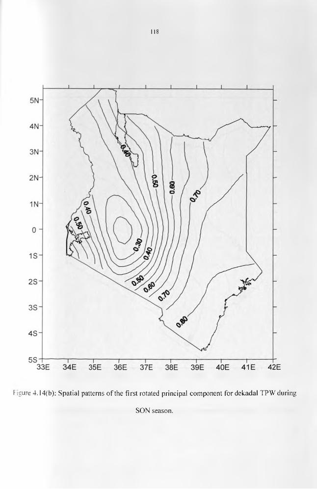
118

F igure 4 .14(b): Spatial patterns of the first rotated principal component for dekadal TPW during

SON season.

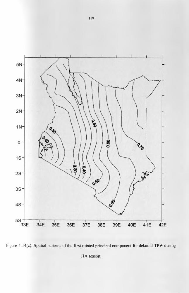
119

Figure 4 .14(c): Spatial patterns of the First rotated principal component for dekadal TPW during

JJA season.

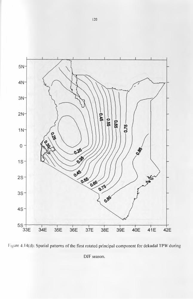
120

Figure 4.14(d): Spatial patterns of the first rotated principal component for dekadal TPW during

DJF season.

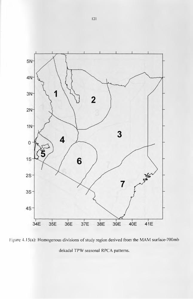
121

Figure 4.15(a): Homogenous divisions of study region derived from the MAM surface-700mb

dekadal TPW seasonal RPCA patterns.

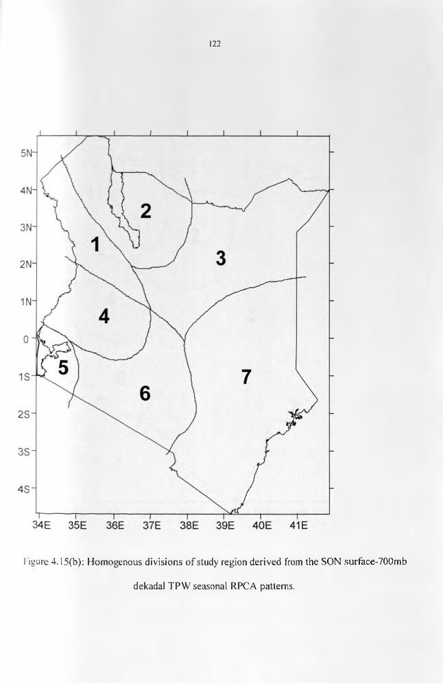
122

Figure 4.15(b): Homogenous divisions of study region derived from the SON surface-700mb


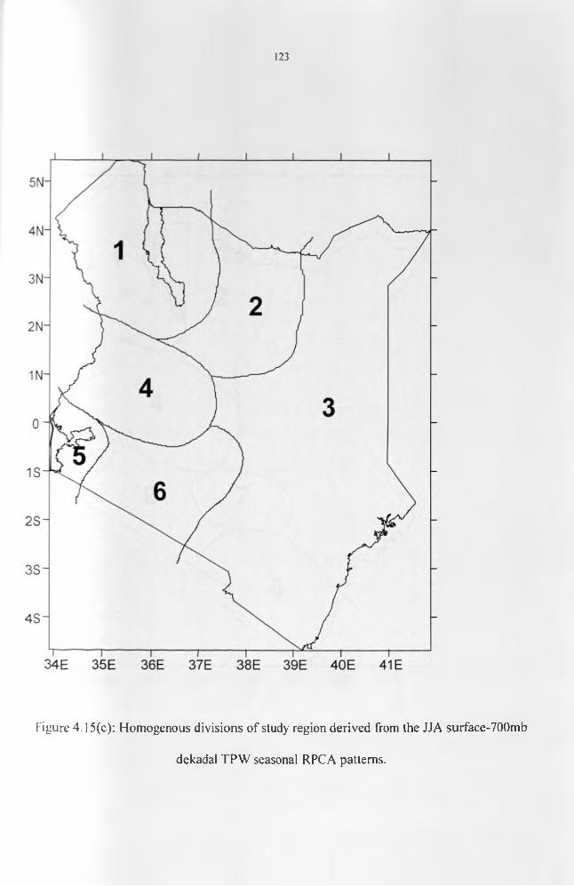
123

Figure 4 .15(c): Homogenous divisions of study region derived from the JJA surface-700mb


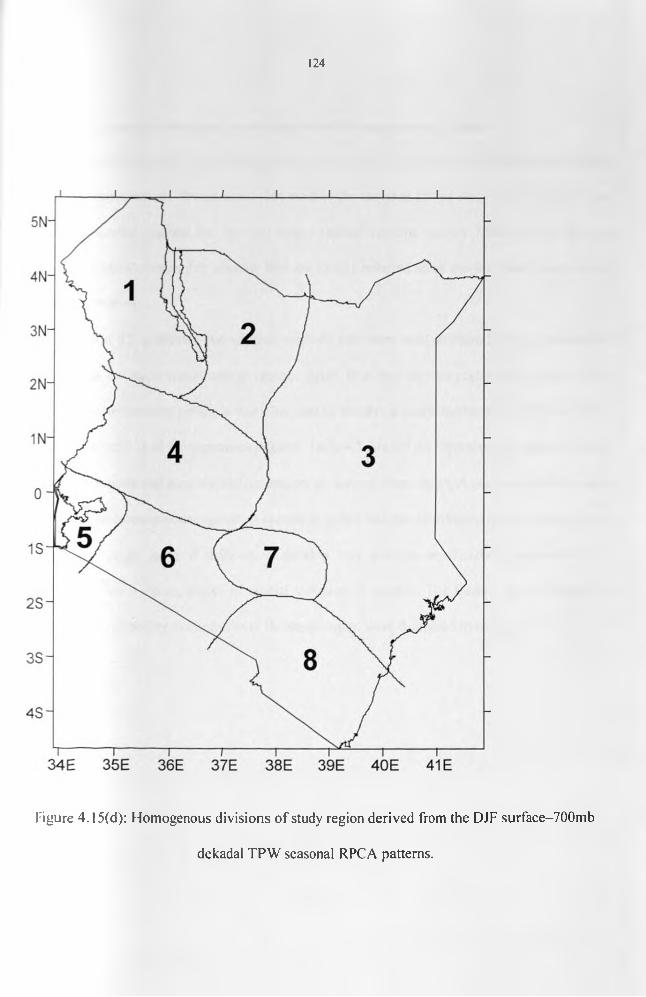
124

Figure 4.15(d): Homogenous divisions of study region derived from the DJF surface-700mb


125

4.3 Representative Records for the Individual Homogeneous Regions

In the previous section we have grouped the area of study into some homogeneous regions

for the different seasons. It was noted that most of the analyses in this study concentrated on the

specific delineated regions for the two major rainfall seasons namely March-Apri 1-May and

September-October-November seasons that are locally referred to as the long and short rainfall

seasons respectively.

Section 3.2 presented the various methods that were used to identify the representative

areal records for each homogeneous region. Apart from the various regionally averaged data.

PC A based communality principle was also used to identify a single station that could be used to

represent the individual homogeneous regions. Table 4.7 shows the representative stations for the

averaging methods and a representative station, as derived from the PCA communality principle,

for each of the homogenous regions. It should be noted that the distribution of the stations in the

study region might make if difficult to develop very accurate areal indices especially for a

variable that has a strong degree of spatial variation as rainfall. The factors that introduce this

strong spatial variability in rainfall over the study region were discussed in section 1.3.2.

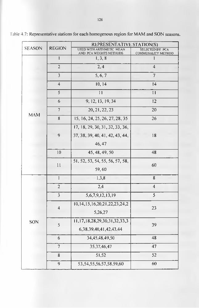
126

Table 4.7: Representative stations for each homogenous region for MAM and SON seasons.

SEASON REGIONREPRESENTATIVE STATION(S)

USED WITH ARITHMETIC MEAN AN D PC A WEIGHTS METHODS

SELECTED BY PCA COMMUNALITY METHOD

MAM

1 1,3,8 1

2 2,4 4

3 5 ,6 ,7 7

4 10, 14 14

5 1 1 1 1

6 9, 12,13, 19,34 1 2

7 20,21,22,23 2 0

8 15, 16, 24,25,26,27, 28, 35 26

9

17, 18.29,30,31,32,33, 36,

37,38,39, 40,41,42, 43, 44,

46,47

18

1 0 45,48.49, 50 48

1 1

51,52, 53, 54, 55,56,57, 58,

59, 6060

SON

1 1,3,8 8

2 2,4 4

3 5,6,7,9,12,13,19 5

410,14,15,16,20,21,22,23,24,2

5,26,2723

511,17,18,28,29,30,31,32,33,3

6,38.39.40,41,42.43,4439

6 34,45.48.49,50 48

7 35,37,46,47 47

8 51,52 52

9 53,54,55,56,57,58,59,60 60

127

4.4 Results from the Correlation Analyses

This is devoted to the results that were obtained from correlation analyses for the specific

regions using all the three areally averaged records namely those derived from simple arithmetic,

PC A weighting and PCA communality methods. As indicated in section 3.3 the correlation

methods examined if there were any significant relationships between rain gauge and satellite-

derived data within any specific homogeneous region. The correlation results from CCD and

TPW data are discussed independently in the next sections.

4.4.1 Results of Correlation with CCD Data

The correlation coefficient values (r) that were obtained for rain gauge and satellite-

derived CCD records at specific regions and seasons are given in table 4.8. Results of the

correlation analyses show that the correlation coefficients were all significant at 95% level except

for region eleven during the MAM season when using areal averages derived from the PCA

weights. Using the representative station derived from the communality method, the coefficients

were not significant at 95% level in regions ten and eleven during MAM and in regions one, two

and five during SON season. The coefficients for regions ten and eleven were not significant

during MAM season when using the arithmetic mean areal averages. The maximum value of

significant r was 0.9 for regions five and seven during MAM and SON seasons respectively. The

minimum was 0.1 in region five during SON season. Thus the variance of rain gauge rainfall that

can be derived from CCD records ranged from 1-81% when considering all the areal averaging

techniques. This variation was from location to location and season to season with the correlation

coefficients being generally lower for the SON season as compared to MAM season.

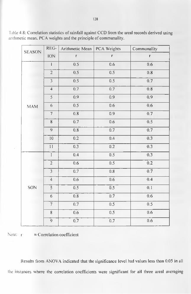
128

Table 4.8: Correlation statistics of rainfall against CCD from the areal records derived using arithmetic mean. PCA weights and the principle of communality.

SEASONREG- Arithmetic Mean PCA Weights Communality

ION r r r

1 0.5 0 . 6 0 . 6

2 0.5 0.5 0 . 8

3 0.5 0.5 0.7

4 0.7 0.7 0 . 8

5 0.9 0.9 0.9

MAM 6 0.5 0 . 6 0 . 6

7 0 . 8 0.9 0.7

8 0.7 0 . 6 0.5

9 0 . 8 0.7 0.7

1 0 0 . 2 0.4 0.3

1 1 0.3 0 . 2 0.3

1 0.4 0.5 0.3

2 0 . 6 0.5 0 . 2

3 0.7 0 . 8 0.7

4 0 . 6 0 . 6 0.4

SON 5 0.5 0.5 0 . 1

6 0 . 8 0.7 0 . 6

7 0.7 0.5 0.5

8 0 . 6 0.5 0 . 6

9 0.7 0.7 0 . 6

Note: r = Correlation coefficient

Results from ANOVA indicated that the significance level had values less than 0.05 in all

the instances where the correlation coefficients were significant for all three areal averaging

129

methods. However, the F-ratio was consistently highest for the PCA-weighting average method

compared to the other two methods indicating that the PCA-weighted averages were better

representatives of the areal rainfall estimate when compared with the other two methods. Based

on this comparison, the rest of the analyses were done using only the PCA-weighted averages.

4.4.2 Results of Correlation with TPW Data

Results that were obtained with TPW data against PCA-weighted average rainfall data are

given in table 4.9. The results show that region one during MAM season, and regions one. two.

eight and nine during SON season had no significant relationships at 95% level between areal

rainfall and TPW data. The maximum significant value of r was 0.7 for region five during SON

season, while a minimum of 0.1 was attained in region nine during SON season. Thus the

variance in the rain gauge rainfall that may be explained by the TPW records ranged from 1-49%.

This also varied from location to location and from season to season.

In general the results showed that r-values were higher for the relationship between

rainfall and CCD than that with TWP. This may be due to the fact that CCD attempts to identify

the actual convective clouds, and hence it may have a more direct relationship with the recorded

rainfall. TPW. on the other hand, records the total moisture available in the atmosphere regardless

of whether there is rainfall or not. The relationship may. therefore, not be as direct as in the case

of the CCD.

130

Table 4.9: Correlation coefficients for the relationship between rainfall and TPW data.

SEASON REGION r

MAM

1 0 . 2

2 0.33 0.54 0.45 0.46 0.47 0 . 6

8 0 . 6

9 0 . 6

1 0 0.41 1 0.5

SON

1 0 . 2

2 0 . 2

3 0.44 0.35 0.76 0.57 0.4

8 0 . 2

9 0 . 1

Due to the evident variation in the variance of the rainfall estimates derived from the

satellite-derived data, care must be taken while using regression equations that are presented

below for some regions and seasons.

4.5 Results from Regression Analyses

In this section, the attempt to develop functional relationship between areal rainfall and

the two types of satellite-derived data is discussed. Linear regression models were developed

between areal rainfall and CCD data while multivariate regression models were developed for the

relationship between the areal rainfall, CCD and the three layers of TPW data.

131

4.5.1 Results of the Simple Regression Analysis

This section deals with the functional relationship between areal rainfall and CCD data.

Linear regression models were developed only in cases where there were significant correlation

coefficients. From the results of the correlation analysis, discussed in section 4.3, it can be noted

that only region eleven during MAM season had no significant relationships between areal

rainfall and the corresponding CCD data. Thus regression models can be developed for estimation

of areal rain gauge records from the CCD data in all regions and rainfall seasons except for region

eleven during the MAM season. Table 4.10 shows the regression statistics for all homogeneous

regions that had significant correlation coefficients during both seasons, while Figure 4.16 gives

some examples o f scatter plots of the observed relationships.

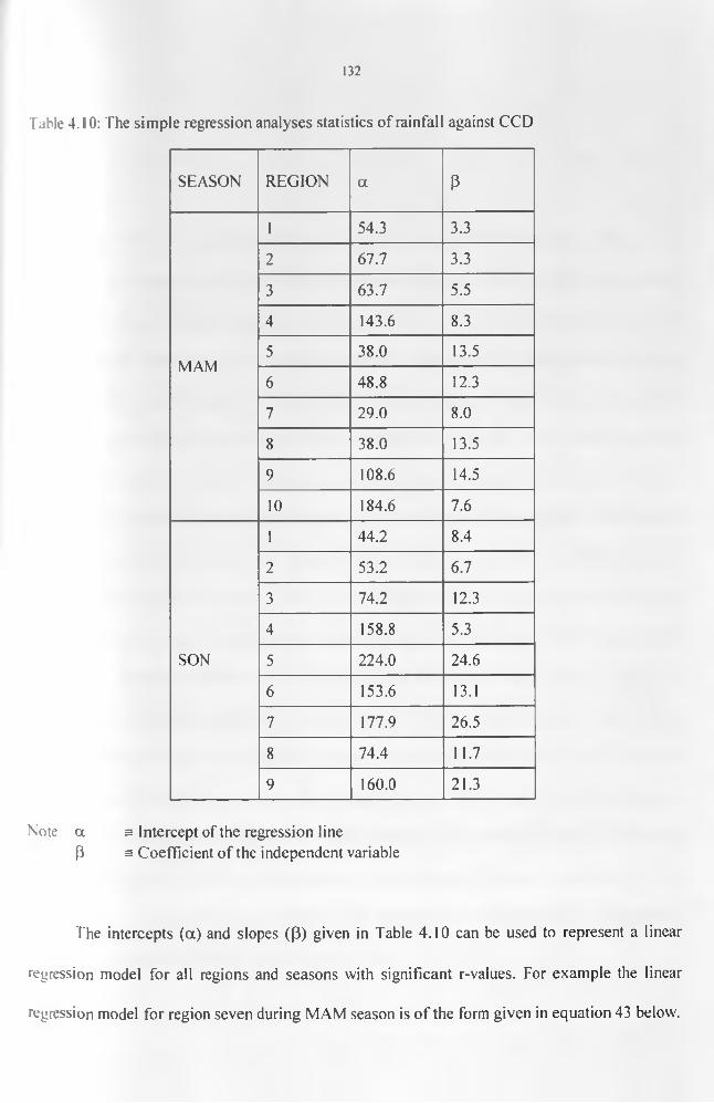
132

Table 4.10: The simple regression analyses statistics of rainfall against CCD

SEASON REGION a P

1 54.3 3.3

2 67.7 3.3

3 63.7 5.5

4 143.6 8.3

MAM5 38.0 13.5

6 48.8 12.3

7 29.0 8 . 0

8 38.0 13.5

9 108.6 14.5

1 0 184.6 7.6

1 44.2 8.4

2 53.2 6.7

3 74.2 12.3

4 158.8 5.3

SON 5 224.0 24.6

6 153.6 13.1

7 177.9 26.5

8 74.4 11.7

9 160.0 21.3

Note a s Intercept of the regression line3 s Coefficient of the independent variable

The intercepts (a) and slopes ((3) given in Table 4.10 can be used to represent a linear

regression model for all regions and seasons with significant r-values. For example the linear

regression model for region seven during MAM season is of the form given in equation 43 below.

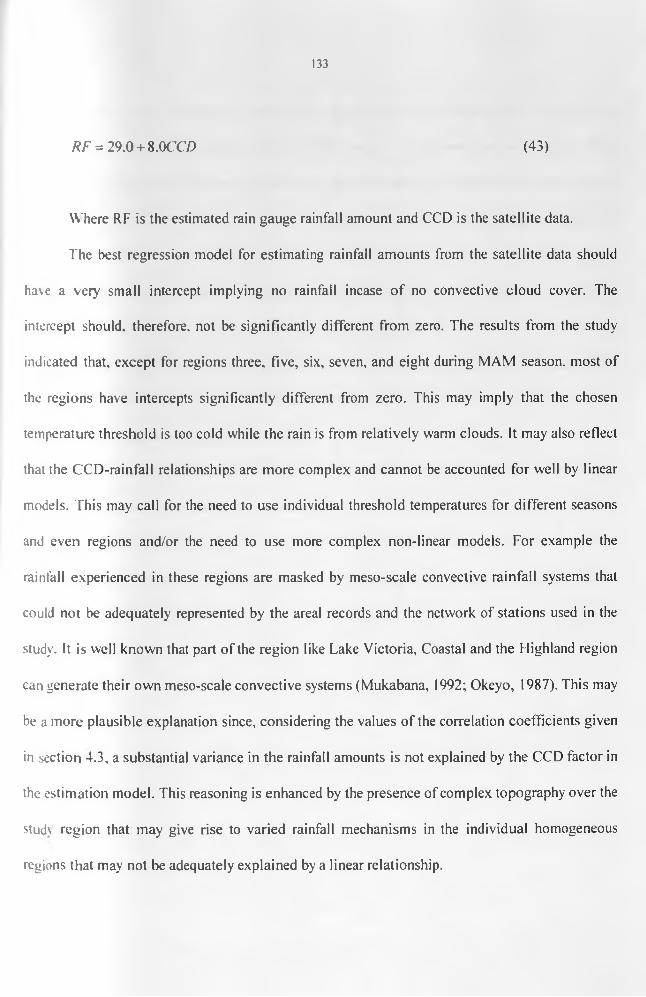
133

RF = 29.0 + 8.0CCZ) (43)

Where RF is the estimated rain gauge rainfall amount and CCD is the satellite data.

The best regression model for estimating rainfall amounts from the satellite data should

ha\e a very small intercept implying no rainfall incase o f no convective cloud cover. The

intercept should, therefore, not be significantly different from zero. The results from the study

indicated that, except for regions three, five, six, seven, and eight during MAM season, most of

the regions have intercepts significantly different from zero. This may imply that the chosen

temperature threshold is too cold while the rain is from relatively warm clouds. It may also reflect

that the CCD-rainfall relationships are more complex and cannot be accounted for well by linear

models. This may call for the need to use individual threshold temperatures for different seasons

and even regions and/or the need to use more complex non-linear models. For example the

rainfall experienced in these regions are masked by meso-scale convective rainfall systems that

could not be adequately represented by the areal records and the network of stations used in the

study. It is well known that part of the region like Lake Victoria, Coastal and the Highland region

can generate their own meso-scale convective systems (Mukabana, 1992; Okeyo, 1987). This may

be a more plausible explanation since, considering the values of the correlation coefficients given

in section 4.3, a substantial variance in the rainfall amounts is not explained by the CCD factor in

the estimation model. This reasoning is enhanced by the presence of complex topography over the

studv region that may give rise to varied rainfall mechanisms in the individual homogeneous

regions that may not be adequately explained by a linear relationship.

134

ANOVA tests show that, in comparison, the results for the SON season had relatively

lower levels of statistical significance than the MAM season. Furthermore, the intercepts for SON

season are all significantly different from zero. It should however be noted that previous studies

have shown that SON season has more homogeneous rainfall with a higher degree of

predictability with El Nino-Southern Oscillation (ENSO) and Sea Surface Temperature signals

(SST) (Ropelewski and Halpart. 1987; Ogallo, 1988; Semazzi et al., 1996; Indeje et al., 2000).

This may be indicative of strong influence of larger scale systems in the rainfall mechanism

during this season. The rainfall during the MAM season are however more reliable and extend

ov er a longer period compared to SON season where most o f the rains are only centered around

October and November months (Ogallo. 1988).

It may be concluded from simple regression analyses results that estimation of rain gauge

rainfall records using simple regression models of the -50°C threshold CCD records is limited to

a few regions during the major rainfall seasons of MAM and SON. This highlights the space-time

complexity of the convective rainfall systems over the region and the strong modulations by the

meso- and local- scale systems.

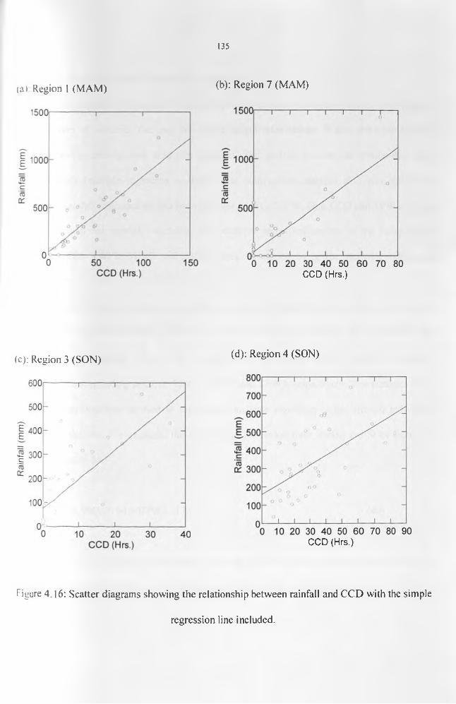
135

(a) Region 1 (MAM) (b): Region 7 (MAM)

CCD (Hrs.)

(c): Region 3 (SON) (d): Region 4 (SON)

CCD (Hrs.)

Figure 4 . 1 6 : Scatter diagrams showing the relationship between rainfall and CCD with the simple

regression line included.

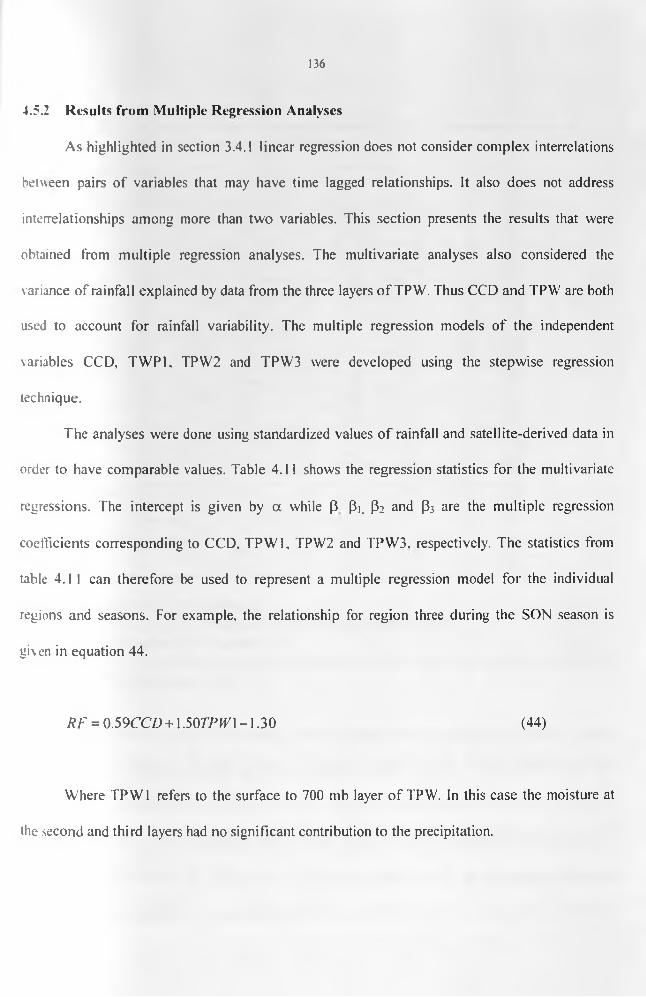
136

4.5.2 Results from Multiple Regression Analyses

As highlighted in section 3.4.1 linear regression does not consider complex interrelations

between pairs of variables that may have time lagged relationships. It also does not address

interrelationships among more than two variables. This section presents the results that were

obtained from multiple regression analyses. The multivariate analyses also considered the

variance of rainfall explained by data from the three layers o f TPW. Thus CCD and TPW are both

used to account for rainfall variability. The multiple regression models of the independent

variables CCD, TWP1. TPW2 and TPW3 were developed using the stepwise regression

technique.

The analyses were done using standardized values o f rainfall and satellite-derived data in

order to have comparable values. Table 4.11 shows the regression statistics for the multivariate

regressions. The intercept is given by a while p Pi. P2 and P3 are the multiple regression

coefficients corresponding to CCD. TPW1, TPW2 and TPW3. respectively. The statistics from

table 4.1 I can therefore be used to represent a multiple regression model for the individual

regions and seasons. For example, the relationship for region three during the SON season is

given in equation 44.

RF = 0.59CCD +1,50TPW\ -1.30 (44)

Where TPW1 refers to the surface to 700 mb layer of TPW. In this case the moisture at

the second and third layers had no significant contribution to the precipitation.

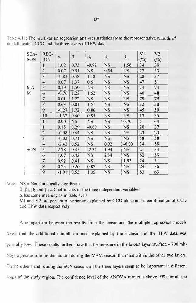
137

Table 4.11: The multivariate regression analyses statistics from the representative records of rainfall against CCD and the three layers of TPW data.

SEASON

REGION a P Pi P2 p3

VI(%)

V2(%)

MAM

1 1 . 0 2 0.75 -0.92 NS 1.56 34 392 0.07 0.51 NS 0.54 NS 27 333 -0.83 0.48 1.18 NS NS 28 374 0.07 1.37 0.61 NS NS 47 515 0.19 1.50 NS NS NS 74 746 -0.76 1.28 1.62 NS NS 40 487 0 . 0 1 1 . 2 2 NS NS NS 79 798 0.63 0.81 1.51 NS NS 32 389 -0.27 1.72 0 . 8 6 NS NS 45 501 0 -1.32 0.40 0.85 NS NS 13 351 1 0 . 0 0 NS NS NS 6.70 5 44

SON

I 0.15 0.29 -0.69 NS NS 2 0 372 -0.08 0.44 NS NS NS 23 233 -0 . 0 2 0.71 NS NS NS 58 584 -2.42 0.52 NS 0.92 -6 . 0 0 34 585 2.78 0.45 -2.34 1.94 NS 2 1 346 1.07 0.42 NS 2.34 NS 52 597 0.92 0.41 NS NS 1.93 24 318 0.25 0 . 2 0 0.87 NS NS 24 369 - 1 . 0 1 0.55 1.05 NS NS 53 63

Note: NS = Not statistically significantP. pi, P; and P3 s Coefficients o f the three independent variables a has same meaning as in table 4.10VI and V2 are percent of variance explained by CCD alone and a combination of CCD and TPW data respectively

A comparison between the results from the linear and the multiple regression models

reveal that the additional rainfall variance explained by the inclusion of the TPW data was

generally low. These results further show that the moisture in the lowest layer (surface - 700 mb)

plays a greater role on the rainfall during the MAM season than that within the other two layers.

On the other hand, during the SON season, all the three layers seem to be important in different

zones of the study region. The confidence level of the ANOVA results is above 95% for all the

138

de\eloped models. However, the complexity of rainfall systems as discussed in section 1.3.2 is

again confirmed here by the low percentages of variance explained by the multiple regression

models in most o f the homogeneous regions.

The results from multiple regression analyses further show that the constant terms in the

equations were negative and significant in several cases. This is expected since the atmosphere is

hardly ever dry. A negative intercept indicates that even when rainfall is zero, there still exists

some moisture in the atmosphere. This may be indicative for a need to also have a threshold for

TPW data. A comparison of the variances in rainfall explained by the two sets of satellite data

indicates that CCD is superior to TWP in estimation of areal rainfall over our region.

4.5.2.1 Tests of Goodness of Fit of the Regression Models

In the previous section, multiple regression models were developed for estimating rainfall

from a combination of CCD and TPW records for the individual homogeneous regions and

seasons. The model parameters were computed using dekadal data for the period 1989 to 1993.

Dekadal data for the period 1994 and 1995, which were not used during the model training period

were used to test the skill of the fitted regression models. Table 4.12 shows the summary of some

of the ANOVA statistics that were used to evaluate the skill of the fitted models while some

graphical examples of the goodness of fit of the models are shown in Figures 4 .17(a) and (b).

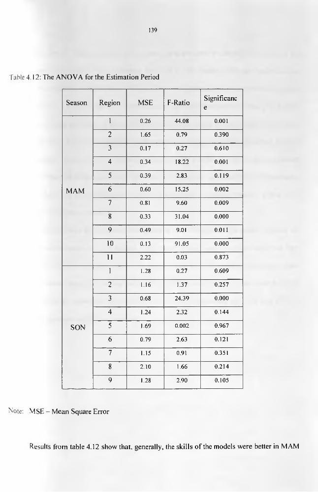
139

Table 4.12: The ANOVA for the Estimation Period

Season Region MSE F-Ratio Significance

1 0.26 44.08 0 . 0 0 1

2 1.65 0.79 0.390

3 0.17 0.27 0.610

4 0.34 18.22 0 . 0 0 1

5 0.39 2.83 0.119

MAM 6 0.60 15.25 0.002

7 0.81 9.60 0.009

8 0.33 31.04 0 . 0 0 0

9 0.49 9.01 0 . 0 1 1

1 0 0.13 91.05 0 . 0 0 0

1 1 2.22 0.03 0.873

1 1.28 0.27 0.609

2 1.16 1.37 0.257

3 0.68 24.39 0 . 0 0 0

4 1.24 2.32 0.144

SON 5 1.69 0.002 0.967

6 0.79 2.63 0.121

7 1.15 0.91 0.351

8 2.10 1.66 0.214

9 1.28 2.90 0.105

Note: MSE - Mean Square Error

Results from table 4.12 show that, generally, the skills of the models were better in MAM

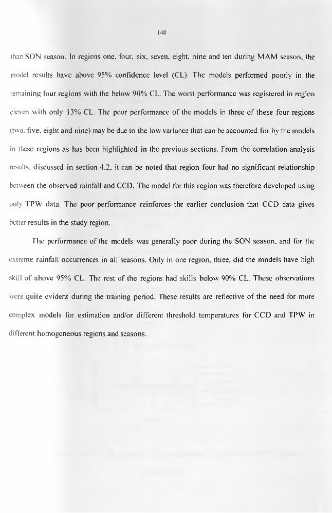
140

than SON season. In regions one. four, six, seven, eight, nine and ten during MAM season, the

model results have above 95% confidence level (CL). The models performed poorly in the

remaining four regions with the below 90% CL. The worst performance was registered in region

ele\en with only 13% CL. The poor performance of the models in three of these four regions

(two. five, eight and nine) may be due to the low variance that can be accounted for by the models

in these regions as has been highlighted in the previous sections. From the correlation analysis

results, discussed in section 4.2. it can be noted that region four had no significant relationship

between the observed rainfall and CCD. The model for this region was therefore developed using

only TPW data. The poor performance reinforces the earlier conclusion that CCD data gives

better results in the study region.

The performance of the models was generally poor during the SON season, and for the

extreme rainfall occurrences in all seasons. Only in one region, three, did the models have high

skill of above 95% CL. The rest of the regions had skills below 90% CL. These observations

were quite evident during the training period. These results are reflective of the need for more

complex models for estimation and/or different threshold temperatures for CCD and TPW in

different homogeneous regions and seasons.

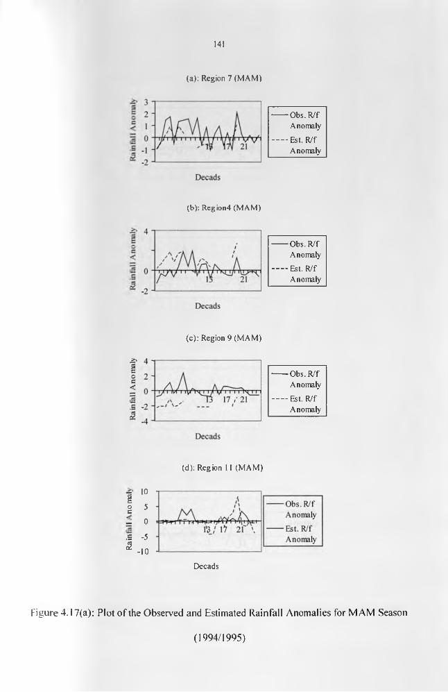
141

( a ) : R eg ion 7 ( M A M )

--------O b s . R / f

A n o m a ly

------- Est . R / f

A n o m a ly

(b ) : R e g io n 4 ( M A M )

( c ) : R eg io n 9 ( M A M )

--------O b s . R / f

A n o m a ly

------- Est . R / f

A n o m a ly

------- O b s . R / f

A n o m a ly

------- Est . R / f

A n o m a ly

(d ) : R e g io n 11 ( M A M )

| 10 I 5 - 0

,S -5

5 -10

D e c a d s

Figure 4.17(a): Plot of the Observed and Estimated Rainfall Anomalies for MAM Season

( 1994/ 1995)

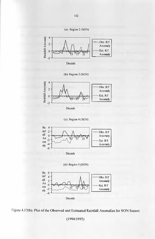
142

( a ) : R eg ion 2 ( S O N )

----- Obs.R/fA n o m a ly

-----Est. R/fA n o m a ly

(b ) : R e g io n 3 ( S O N )



( c ) : R eg io n 4 ( S O N )



(d ) : R e g io n 9 ( S O N )



Figure 4.17(b): Plot of the Observed and Estimated Rainfall Anomalies for SON Season

(1994/1995)

143

4.5.2 Results of the Performance of the Regressions during Anomalous Years

In the previous section, attempts were made to derive rainfall estimates from satellite data

through regression models. This section investigates the performance of these models during

anomalous seasons. The rainfall anomalies were investigated by delineating the anomalous

seasons, identifying anomalous onset/withdrawal dates and duration of the seasons. The physical

and climate patterns that may be associated with the observed poor or good estimation of rainfall

from satellite derived methods during the anomalous seasons are also presented.

4.5.2.1 Observed Anomalous Rainfall Seasons

Table 4.13 presents the categorization of the seasons within the period of study into

normal, dry or wet. It is evident from this table that the anomalous wet/dry seasons were recurrent

through the study period. The seasonal patterns of these anomalies also varied from year to year.

For example, rainfall anomalies during any SON season were not necessarily predetermined by

rainfall characteristics during the preceding MAM season.

Table 4.13: Categorization of the years into dry, wet, or normal seasons

Season Categorization Years

MAM

Dry 1984 1992 1993

Normal 1983 1985 1987 1989 1990 1994 1995

Wet 1982 1986 1988

SON

Dry 1983 1985 1987

Normal 1984 1986 1988 1989 1990 1992

Wet 1982 1995 1994

144

4.5J.2 Observed Rainfall Onset, Duration and Withdrawal

This section presents the patterns of the onset, withdrawal and duration o f the two rainfall

seasons as observed from the study. Details of the cumulative curve method used to delineate

these events were discussed in section 3.6. The delineated onset, withdrawal and duration for

MAM and SON seasons are given in table 4.14 while examples of the cumulative curves that

were used to determine the onset and withdrawal dates are shown in Figure 4.18

It is evident from table 4.14 that the onset and withdrawal dates varied significantly from

year to year and from season to season. On average the duration for MAM is generally longer, but

there were some years in which the SON season duration was equal to or even much longer. For

example The SON season of 1989 started on the 26lh dekad and persisted for ten dekads while

during MAM season of 1985 the duration was only six dekads. It can also be noted from these

results that, during the study period, late/early onset and withdrawal dates w'ere not always

indicative of poor/good performance of the season. For example some late onsets were sometimes

followed by late withdrawals leading to an extension of the rainfall seasons.

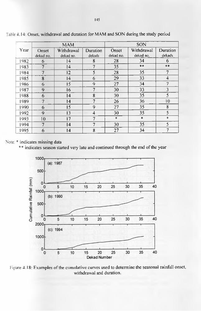
145

Table 4.14: Onset, withdrawal and duration for MAM and SON during the study period

YearMAM S O N

O n s e t d ek a d no.

Withdrawal d ek ad no.

Durationdekads

Onset dekad no.

Withdrawal dekad no.

Durationd ek ad s

1982 6 14 8 28 34 61983 7 14 7 35 ** **

1984 7 12 5 28 35 71985 8 14 6 29 33 41986 6 15 9 27 34 71987 9 16 7 30 33 31988 6 14 8 30 35 51989 7 14 7 26 36 101990 6 15 9 27 35 81992 9 13 4 30 35 51993 10 17 7 * * *1994 7 14 7 30 35 51995 6 14 8 27 34 7

Note: * indicates missing data** indicates season started very late and continued through the end of the year

Figure 4 .18: Examples of the cumulative curves used to determine the seasonal rainfall onset,withdrawal and duration.

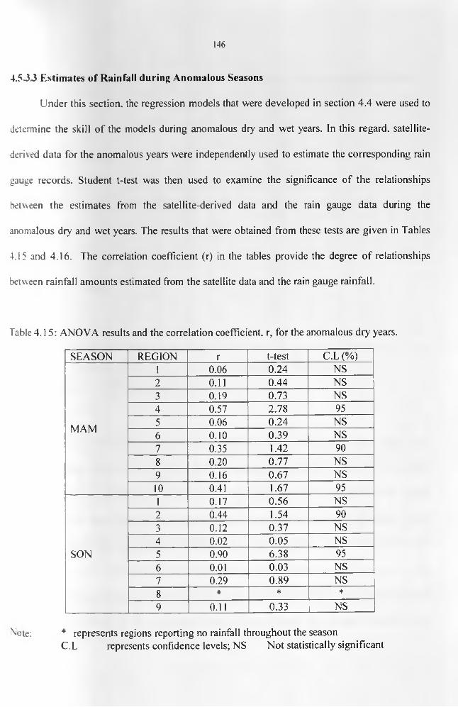
146

4.5JJ Estimates of Rainfall during Anomalous Seasons

Under this section, the regression models that were developed in section 4.4 were used to

determine the skill of the models during anomalous dry and wet years. In this regard, satellite-

derived data for the anomalous years were independently used to estimate the corresponding rain

gauge records. Student t-test was then used to examine the significance of the relationships

between the estimates from the satellite-derived data and the rain gauge data during the

anomalous dry and wet years. The results that were obtained from these tests are given in Tables

4.15 and 4.16. The correlation coefficient (r) in the tables provide the degree of relationships

between rainfall amounts estimated from the satellite data and the rain gauge rainfall.

Table 4.15: ANOVA results and the correlation coefficient, r, for the anomalous dry years.

SEASON REGION r t-test C.L (%)

MAM

1 0.06 0.24 NS2 0.11 0.44 NS3 0.19 0.73 NS4 0.57 2.78 955 0.06 0.24 NS6 0.10 0.39 NS7 0.35 1.42 908 0.20 0.77 NS9 0.16 0.67 NS10 0.41 1.67 95

SON

1 0.17 0.56 NS2 0.44 1.54 903 0.12 0.37 NS4 0.02 0.05 NS5 0.90 6.38 956 0.01 0.03 NS7 0.29 0.89 NS8 * * *

9 0.11 0.33 NS

^ote: * represents regions reporting no rainfall throughout the seasonC.L represents confidence levels; NS Not statistically significant

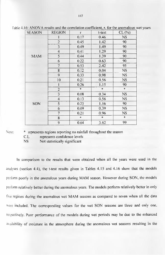
147

Table 4.16: ANOVA results and the correlation coefficient, r, for the anomalous wet yearsSEASON REGION r t-test CL (%)

MAM

1 0.17 0.46 NS2 0.45 1.42 903 0.49 1.49 904 0.41 1.29 905 0.44 1.39 906 0.22 0.63 907 0.53 2.42 958 0.12 0.04 NS9 0.33 0.98 NS10 0.21 0.56 NS

SON

1 0.26 1.15 902 * * *

3 0.08 0.34 NS4 0.13 0.56 NS5 0.23 1.16 906 0.09 0.39 NS7 0.21 0.96 NS8 * * *

9 0.64 3.62 99

Note: * represents regions reporting no rainfall throughout the seasonC.L represents confidence levelsNS Not statistically significant

In comparison to the results that were obtained when all the years were used in the

analyses (section 4.4), the t-test results given in Tables 4.15 and 4.16 show that the models

perform poorly in the anomalous years during MAM season. However during SON, the models

perform relatively better during the anomalous years. The models perform relatively better in only

five regions during the anomalous wet MAM seasons as compared to seven when all the data

were included. The corresponding values for the wet SON seasons are three and only one.

respectively. Poor performance of the models during wet periods may be due to the enhanced

availability of moisture in the atmosphere during the anomalous wet seasons resulting in the

148

release of rainfall even at warmer cloud temperatures leading to underestimation of the rainfall

from the chosen satellite threshold temperature.

A comparison between the results from anomalous dry seasons and the cases when all the

data were included reveal that the models perform well in only three as opposed to seven regions

during MAM seasons. The corresponding values for the SON seasons are two and only one,

respectively. It is evident that the models also have poor performance during the anomalous dry

MAM seasons, but with slightly better performance for the anomalous dry SON seasons. This

may be due to the localized nature of rainfall during the dry seasons that may lead to the

formation of localized thunderstorm clouds, which are in turn easily identified by the satellite

data. The regions with good model performance during the dry seasons include those around and

to the north of Lake Victoria, and a region along the coast o f Indian Ocean. These regions have

moisture sources in Lake Victoria, Congo Basin and the Indian Ocean. However, another region

with good model performance is located in the semi-arid northern parts of the study area. The

good performance o f the models in this region could be due to the existence of many zero or low

rainfall and satellite-estimated records that may also induce high correlation values.

■L5.3.4 Circulation Patterns during Anomalous Wet/Dry Seasons

This section presents some composites of the average circulation patterns during the

seasons based on the observed anomalous years within the study period. These could be used in

explaining the good or bad performance of the satellite data conversion models during the

anomalous seasons. Details of the method used in deriving the composites may be found in

section 3.6.

Examples o f the wind pattern composites are shown in Figures 4.19 and 4.20. One of the

major sources of moisture for the study region is the Indian Ocean. It is evident that from Figure

149

4 19 that during the anomalous wet years the whole region o f study is under the influence of the

moist southeasterly monsoonal circulation. These strong southeasterly winds carry a lot of

moisture from the Indian Ocean into the study region. This may result in the availability of excess

moisture that may trigger rainfall from relatively warm clouds that may not be identifiable by the

chosen CCD threshold temperature.

During the anomalous dry seasons, a strong southeasterly component is developed in the

equatorial flow as shown in Figure 4.20. This diffluent southeasterly flow diverts moisture from

the Indian Ocean away from the study region causing a reduction in the amount of moisture

reaching most of the study area with the resultant lessening of formation of widespread cumulus

clouds. However, the relative good performance of the satellite models during this season in some

regions may be due to presence of localized cumulonimbus clouds or low rain gauge/satellite-

estimate values as has been explained in section 4.4.3.3.

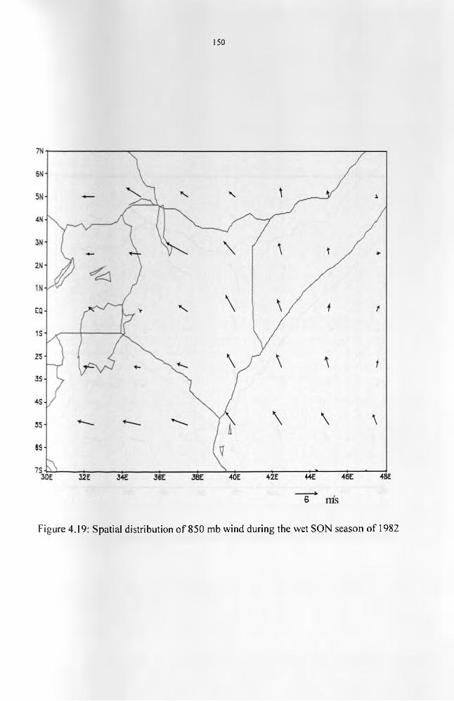
150

Figure 4.19: Spatial distribution of 850 mb wind during the wet SON season of 1982

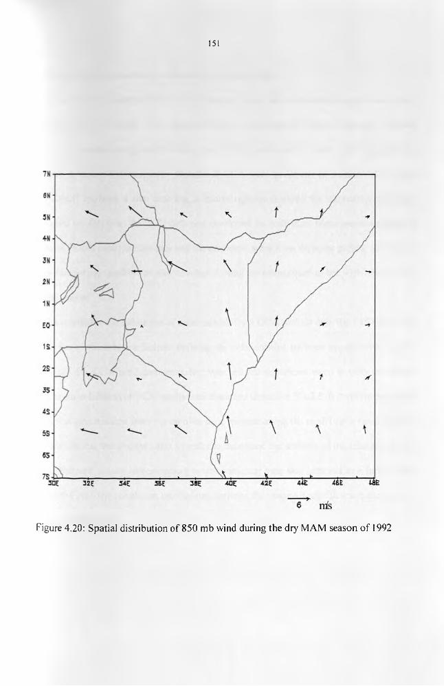
151

Figure 4.20: Spatial distribution of 850 mb wind during the dr)' MAM season of 1992

152

4.5J Results from Canonical Correlation Analysis (CCA)

In the previous sections the results of simple linear and multivariate regression models

were presented. These models were based on simple and stepwise relations between observed

rainfall and the corresponding satellite data. This section presents the results that were obtained

by the more complex CCA models. Details of CCA were presented in section 3.4.3. Using

equation 22 and applying a zero time lag, a matrix regression model for estimating rain gauge

recorded areal rainfall from the CCD data was developed for individual homogeneous regions in

both seasons. In this case the estimates and the predictors were from the same period. Similarly, a

model for forecasting rainfall was also developed using the same equation but with a built-in lag

time of one season.

The results for the estimation of areal rainfall from CCA include only the CCD data. This

is because the correlation coefficients defining the relationships between the observed rainfall

anomalies and the CCA predicted anomalies were all not significant even at 90% confidence

level. The cross-validation of CCA results was discussed in section 3.5.2.5. It involves repeatedly

omitting a few observations from the training data, reconstructing the model each time, and then

making forecasts for the omitted cases in order to determine the stability of the relations. In this

study, data for each season corresponding to one particular year was removed at a time. Tables

4.17(a) and (b) give the correlation coefficients between the observed rainfall anomalies and the

resultant predicted values.

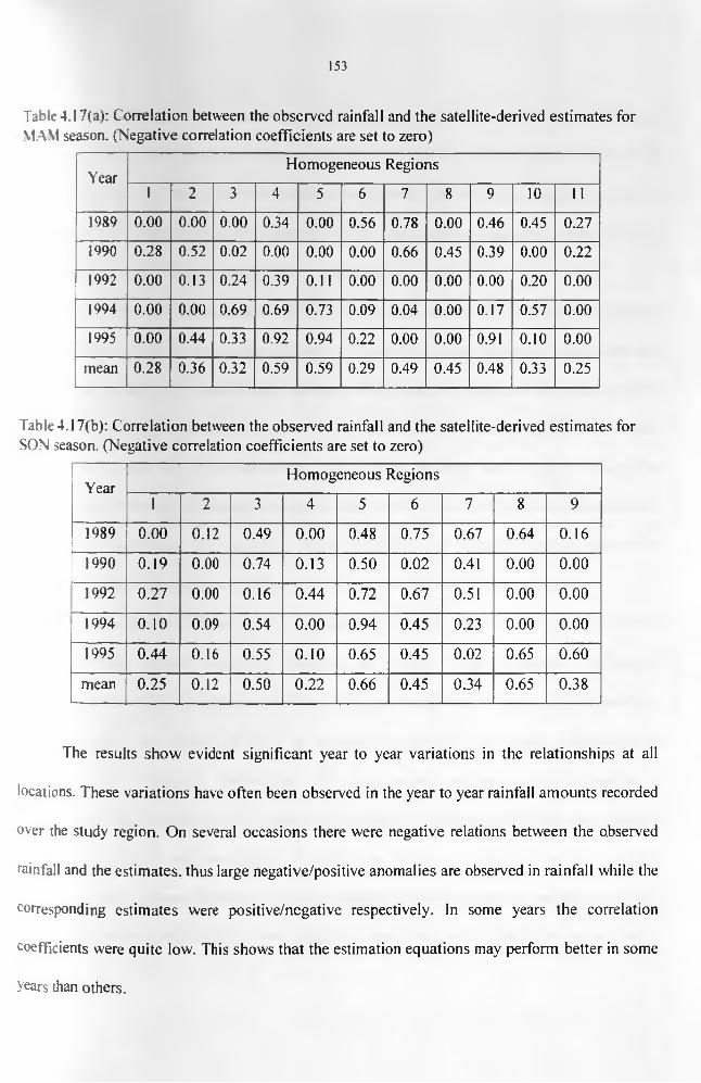
153

Table 4.17(a): Correlation between the observed rainfall and the satellite-derived estimates for MAM season. (Negative correlation coefficients are set to zero)

YearHomogeneous Regions

1 2 3 4 5 6 7 8 9 10 11

1989 0.00 0.00 0.00 0.34 0.00 0.56 0.78 0.00 0.46 0.45 0.27

1990 0.28 0.52 0.02 0.00 0.00 0.00 0.66 0.45 0.39 0.00 0.22

1992 0.00 0.13 0.24 0.39 0.11 0.00 0.00 0.00 0.00 0.20 0.00

1994 0.00 0.00 0.69 0.69 0.73 0.09 0.04 0.00 0.17 0.57 0.00

1995 0.00 0.44 0.33 0.92 0.94 0.22 0.00 0.00 0.91 0.10 0.00

mean 0.28 0.36 0.32 0.59 0.59 0.29 0.49 0.45 0.48 0.33 0.25

Table 4.17(b): Correlation between the observed rainfall and the satellite-derived estimates for SON season. (Negative correlation coefficients are set to zero)

YearHomogeneous Regions

1 2 3 4 5 6 7 8 9

1989 0.00 0.12 0.49 0.00 0.48 0.75 0.67 0.64 0.16

1990 0.19 0.00 0.74 0.13 0.50 0.02 0.41 0.00 0.00

1992 0.27 0.00 0.16 0.44 0.72 0.67 0.51 0.00 0.00

1994 0.10 0.09 0.54 0.00 0.94 0.45 0.23 0.00 0.00

1995 0.44 0.16 0.55 0.10 0.65 0.45 0.02 0.65 0.60

mean 0.25 0.12 0.50 0.22 0.66 0.45 0.34 0.65 0.38

The results show evident significant year to year variations in the relationships at all

locations. These variations have often been observed in the year to year rainfall amounts recorded

over the study region. On several occasions there were negative relations between the observed

rainfall and the estimates, thus large negative/positive anomalies are observed in rainfall while the

corresponding estimates were positive/negative respectively. In some years the correlation

coefficients were quite low. This shows that the estimation equations may perform better in some

years than others.

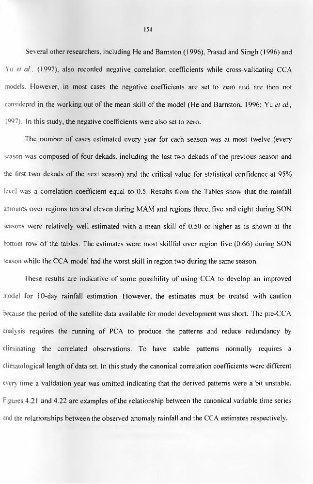
154

Several other researchers, including He and Bamston (1996), Prasad and Singh (1996) and

Yu el al.. (1997), also recorded negative correlation coefficients while cross-validating CCA

models. However, in most cases the negative coefficients are set to zero and are then not

considered in the working out of the mean skill of the model (He and Bamston, 1996; Yu et al.,

1997). In this study, the negative coefficients were also set to zero.

The number o f cases estimated every year for each season was at most twelve (every

season was composed of four dekads, including the last two dekads of the previous season and

the first two dekads o f the next season) and the critical value for statistical confidence at 95%

level was a correlation coefficient equal to 0.5. Results from the Tables show that the rainfall

amounts over regions ten and eleven during MAM and regions three, five and eight during SON

seasons were relatively well estimated with a mean skill of 0.50 or higher as is showm at the

bottom row o f the tables. The estimates were most skillful over region five (0.66) during SON

season while the CCA model had the worst skill in region two during the same season.

These results are indicative of some possibility of using CCA to develop an improved

model for 10-day rainfall estimation. However, the estimates must be treated with caution

because the period of the satellite data available for model development was short. The pre-CCA

analysis requires the running of PCA to produce the patterns and reduce redundancy by

eliminating the correlated observations. To have stable patterns normally requires a

climatological length of data set. In this study the canonical correlation coefficients were different

everx time a validation year was omitted indicating that the derived patterns were a bit unstable.

Figures 4.21 and 4.22 are examples of the relationship between the canonical variable time series

and the relationships between the observed anomaly rainfall and the CCA estimates respectively.

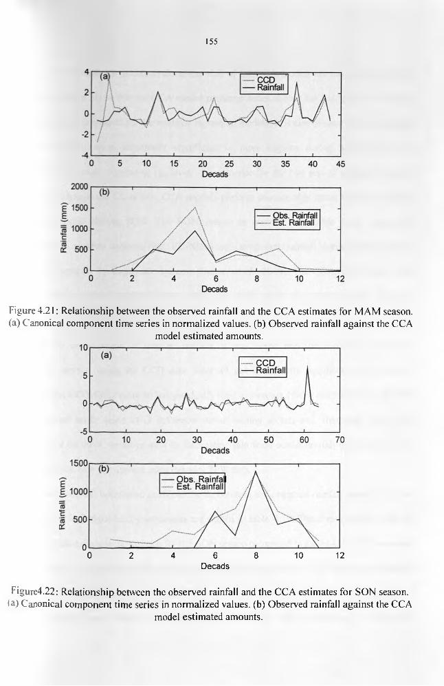
155

Figure 4.21: Relationship between the observed rainfall and the CCA estimates for MAM season, (a) Canonical component time series in normalized values, (b) Observed rainfall against the CCA

model estimated amounts.

I 1 1_____ L____ I___________I___________ I____ 2>_____0 2 4 6 8 10 12

Decads

Figure4.22: Relationship between the observed rainfall and the CCA estimates for SON season. <a) Canonical component time series in normalized values, (b) Observed rainfall against the CCA

model estimated amounts.

156

ANOVA statistics used to evaluate the skill of the CCA models are summarized in table

- i8. These results show that the CCA model performs better during the MAM than during the

SON season as was evident for the multiple regression models. It is also evident that the multiple

regression models were statistically significant in more regions during MAM season in

c 'mparison. However, comparing the level of confidence for the two sets of models, it can be

noted that, although the CL is low, CCA models perform considerably better than the multiple

regression models during SON. The SON season is usually predictable from large-scale,

teleconnection weather systems (e.g. EL-Nino) indicating that rainfall during this season is

influenced markedly by large-scale systems (Indeje, et a l, 2000). The CCA, which deals with

patterns, would therefore perform better during the SON season than the multiple regression

models.

In the development of forecast models, it was noted that the canonical correlation

coefficients derived using the CCD data were all not statistically significant. This may be

indicative that CCD data cannot be independently used to forecast 10-day rainfall o f an area. This

is an expected result since CCD delineates actual raining clouds and, therefore, forecasting

rainfall based on them would be akin to forecasting rain from actual rainfall observations. The

results presented here are derived using dekadal TPW data.

The canonical correlation coefficients, Sj, between the observed rainfall patterns and the

TPW patterns for i significant components are shown in table 4.19. These results show that the

canonical relationships were stronger for the SON season compared to the MAM. This is a result

consistent with the other studies that have found the short rain season of SON more predictable in

the study region (e.g. Indeje et al. (2000). The number of data cases used in the development of

the CCA matrices were at least one hundred and twenty. The critical correlation coefficient for

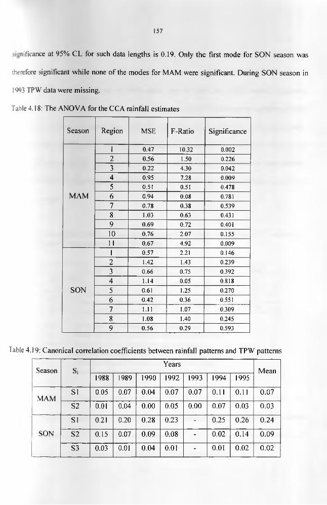
157

- .nificance at 95% CL for such data lengths is 0.19. Only the first mode for SON season was

therefore significant while none of the modes for MAM were significant. During SON season in

1993 TPW data were missing.

Table 4.18: The ANOVA for the CCA rainfall estimates

Season Region MSE F-Ratio Significance

MAM

1 0.47 10.32 0.0022 0.56 1.50 0.2263 0.22 4.30 0.0424 0.95 7.28 0.0095 0.51 0.51 0.4786 0.94 0.08 0.7817 0.78 0.38 0.5398 1.03 0.63 0.4319 0.69 0.72 0.40110 0.76 2.07 0.15511 0.67 4.92 0.009

SON

1 0.57 2.21 0.1462 1.42 1.43 0.2393 0.66 0.75 0.3924 1.14 0.05 0.8185 0.61 1.25 0.2706 0.42 0.36 0.5517 1.11 1.07 0.3098 1.08 1.40 0.2459 0.56 0.29 0.593

Table 4.19: Canonical correlation coefficients between rainfall patterns and TPW patterns

Season SiYears

Mean1988 1989 1990 1992 1993 1994 1995

MAMSI 0.05 0.07 0.04 0.07 0.07 0.11 0.11 0.07

S2 0.01 0.04 0.00 0.05 0.00 0.07 0.03 0.03

SON

SI 0.21 0.20 0.28 0.23 - 0.25 0.26 0.24

S2 0.15 0.07 0.09 0.08 - 0.02 0.14 0.09

S3 0.03 0.01 0.04 0.01 - 0.01 0.02 0.02

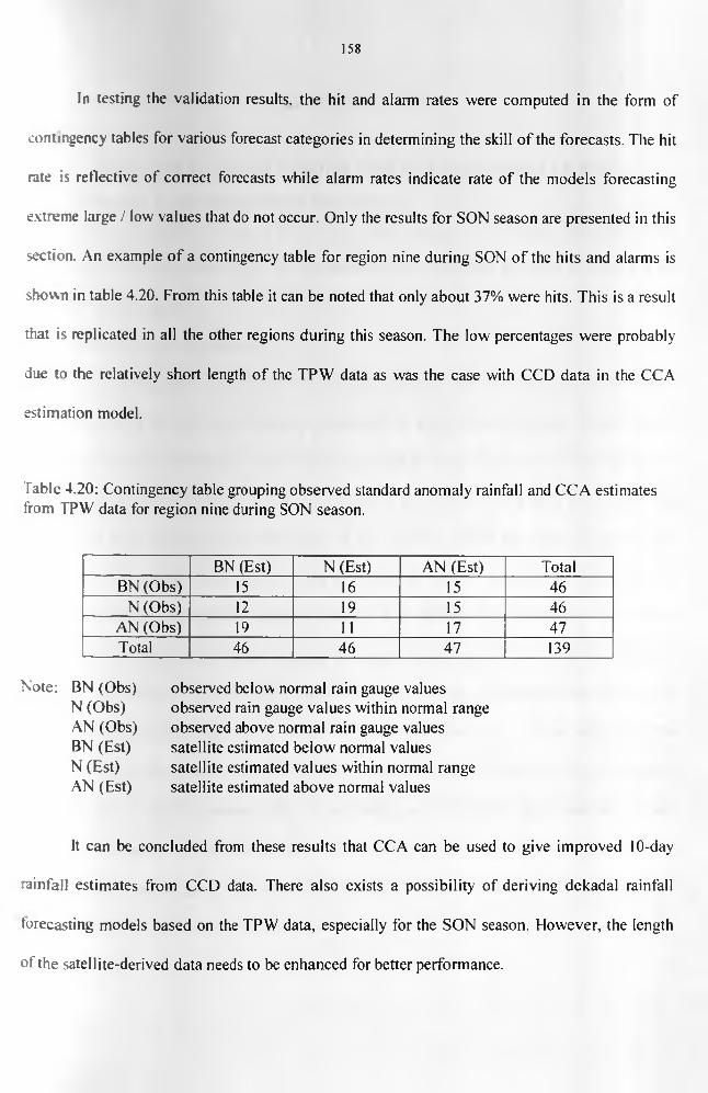
158

In testing the validation results, the hit and alarm rates were computed in the form of

contingency tables for various forecast categories in determining the skill o f the forecasts. The hit

rate is reflective of correct forecasts while alarm rates indicate rate of the models forecasting

extreme large / low values that do not occur. Only the results for SON season are presented in this

section. An example o f a contingency table for region nine during SON of the hits and alarms is

shown in table 4.20. From this table it can be noted that only about 37% were hits. This is a result

that is replicated in all the other regions during this season. The low percentages were probably

due to the relatively short length of the TPW data as was the case with CCD data in the CCA

estimation model.

Table 4.20: Contingency table grouping observed standard anomaly rainfall and CCA estimates from TPW data for region nine during SON season.

BN (Est) N (Est) AN (Est) TotalBN (Obs) 15 16 15 46

N (Obs) 12 19 15 46AN (Obs) 19 11 17 47Total 46 46 47 139

Note: BN (Obs) N (Obs) AN (Obs) BN (Est) N (Est) AN (Est)

observed below normal rain gauge values observed rain gauge values within normal range observed above normal rain gauge values satellite estimated below normal values satellite estimated values within normal range satellite estimated above normal values

It can be concluded from these results that CCA can be used to give improved 10-day

rainfall estimates from CCD data. There also exists a possibility of deriving dekadal rainfall

torecasting models based on the TPW data, especially for the SON season. However, the length

of the satellite-derived data needs to be enhanced for better performance.

159

CHAPTER FIVE

SUMMARY, CONCLUSIONS AND RECOMMENDATIONS5.0 Summary, Conclusions and Recommendations

This last chapter attempts to provide an overall summary of the thesis. The conclusions

drawn from the results of the study, recommendations and suggestions for future extension of the

stud> are also presented.

5.1 Summary and Conclusions

The presentation of this thesis is organized into five chapters. Chapter one provides a

general review of the climate of the study region and the major extreme climate events together

with the associated impacts. Key issues that are highlighted in this chapter include the spatial and

temporal variability o f rainfall, with special reference to extreme events such as droughts and

floods, and their impacts on the economies of the countries within the region. The problems

associated with rainfall monitoring through the existing “in situ" methods and the need for

alternative methods o f rainfall monitoring are also highlighted. The potential use of satellite-

derived data to estimate areal rainfall formed the foundation of this study. The specific objectives

that were addressed to meet the overall objective of the study are also presented in chapter one.

These include regionalization, using rainfall and satellite-derived data, of the study area into

homogeneous climatological zones and the development of empirical functions to investigate the

potential use of satellite-derived data in estimating and forecasting areal rainfall at each

homogeneous region. The skills of the developed empirical models were also examined. The final

part of the study investigated the meteorological factors that may be associated with the good or

poor performance of the empirical models during the anomalous dry and wet seasons.

160

Chapter two presents the data used in the study together with the various methods that

sere used to examine the quality of the rainfall data. The data used in the study include rain

gauge rainfall, satellite-derived and general circulation data. The rain gauge rainfall data

consisted of daily records for the period 1982 to 1995 obtained from the Kenya Meteorological

Department data archives. The satellite data included Cold Cloud Duration (CCD) information

and Total Precipitable Water (TPW) in the atmosphere. The CCD data were obtained from the

Regional Center for Services in Surveying, Mapping and Remote Sensing archives in Nairobi.

Kenya, while TPW data were obtained from NASA Water Vapor Project data archives. The

general circulation data used in the study were the reanalysis data from ECMWF. The last two

>ets of data were obtained through the Department of Marine, Earth and Atmospheric Sciences,

North Carolina State University. Few missing records were estimated using correlation method,

while the homogeneity o f the data was tested using single mass curves.

The various methods used in attempting to achieve the objectives of the study are

presented in chapter three. The first method involved the regionalization of the study region into

homogeneous climatological zones that could be used in the development of empirical models for

the specific zones. The regionalization was carried out using the S-mode Principal Component

Analysis (PCA) method. Both unrotated and rotated solutions were adopted in attempts to

delineate the region into zones with similar spatial climatic characteristics. Both the observed

rainfall and satellite-derived data were subjected to PCA. The methods that were used to

determine the number of significant PCA modes to be retained for rotation included Kaiser’s

criterion. Scree's test and the sampling of error method.

While the satellite data were in a grid format covering the whole of the study area, the

rain gauge records represented point information scattered unevenly across the study region. For

a more realistic frameu'ork for comparison of the two data sets, areally averaging o f each data set

161

on each homogenous region was required. Three methods were used to derive and compare

areal estimates in the study. These included arithmetic mean, PCA-weighted mean and the

principle of communal ity methods.

The development of relationships between the observed rainfall and the satellite-derived

data involved the use of correlation and regression methods. While correlation methods present

the degree of relationship between the variables, the functional relationships were provided by

regression analyses. The three types of regression methods that were used in the study include

simple, stepwise and canonical regression analyses. The canonical regression method was also

used in forecasting of rainfall from the satellite-derived data. The skill of the fitted models was

tested using various methods that ranged from simple mean square error method, x~ * ar|d F-test

to Kolmogorov-Smirnov test.

Finally, the anomalous wet and dry years were delineated using simple ranking statistics

while cumulative curves were used to identify the anomalous onset, cessation and hence duration

of the rainfall seasons. Composite maps of the corresponding general circulation patterns were

also derived in order to determine the major circulation patterns that were dominant during the

specific anomalous periods.

The results that were obtained from the various analyses are presented and discussed in

chapter four. It was evident from the data quality control tests that the data used in the study were

of good quality. The derived residual mass curves indicated that most of the data, including the

few estimated, were not heterogeneous. It should be noted that data were estimated only in cases

where less than 10% was missing. This was to minimize errors that may be associated with data

estimation. The quality-controlled data formed the fundamental basis of the various analyses

carried out in the study.

162

The regionalization techniques based on PCA of decadal data indicated that the S-mode

solutions delineated eleven regions for MAM, JJA and DJF seasons, while only nine were

delineated for the SON season from the rainfall data. The derived regions were generally

comparable to those delineated by other researchers using daily, monthly and annual data

(Barring, 1988: Ogallo, 1989; Indeje et al„ 2000). The results from the PCA indicated that the

number of significant PCA modes was higher for the dry seasons of JJA and DJF as compared to

those from the wet seasons of MAM and SON. However, these components extracted relatively

low percentage of total variance in the decadal rainfall. This may reflect the influence of highly

localized systems in the rainfall during these dry seasons. The development of regression models

for rainfall estimation from satellite data, therefore, concentrated on the wet seasons of MAM and

SON. It was further evident that the patterns of the PCA modes highlighted the significant roles

of Lake Victoria, Indian Ocean, the Highlands and the Rift Valley in the spatial distribution of

rainfall over the study region. The roles of these physical features were consistent throughout all

seasons as witnessed from the dominance of unique PCA modes at the specific locations.

When the satellite-derived surface to 700 mb layer of TPW data were subjected to PCA

analyses, only seven regions were delineated for MAM and SON seasons while six and eight

were delineated for JJA and DJF seasons, respectively. It was evident that fewer regions were

demarcated while using these satellite-derived data. This could be probably due to the

smoothening of some o f the regional features when TPW layer data were used. This was the first

time that attempts were being made to derive regional climatic zones based on satellite-derived

data. A comparison of the results from the regionalization based on rainfall data to the regions

delineated from the satellite-derived TPW data indicate significant large scale similarity in the

patterns of the PCA modes. The availability of more satellite-derived data in the coming years

163

would, however, require similar analyses to be repeated in order to confirm the stability of the

satellite-based data derived homogeneous regions.

Results from the comparison of the areal estimates derived from the three different

methods indicated that PCA-weighted method provided more realistic areal averaged rainfall at

the specific homogeneous regions than the other two methods. PCA-weighted areal estimates

were therefore used to develop the areal rainfall indices that were utilized in correlation and

regression analyses.

Results from the correlation analyses indicated higher correlation values between rainfall

and CCD data as compared to rainfall and TPW data. This was probably due to the fact that CCD

identifies the raining clouds and hence having a more direct relationship with the observed

rainfall as compared to TPW, which provides the total moisture in the atmosphere regardless of

the presence of rain. The results highlighted the potential use of satellite-derived CCD data in

providing realistic estimates of areal rainfall. Regression equations were therefore developed for

all regions that had significant correlation coefficients.

Linear regression models were developed between rainfall and CCD data, while multiple

regression models were developed between rainfall, CCD and the three layers o f TPW data.

Based on the results of testing the significance of the computed correlation coefficients, linear

models were developed for all homogeneous regions during both rainy seasons except for region

four in MAM. The developed linear regression models indicated that in general the intercepts of

the derived graphs were significantly different from zero. This could be indicative of complex

relationships between rainfall and CCD that may not be adequately described by a simple linear

model. It could also be due to the use of unrealistic CCD temperature threshold. This calls for

future efforts to identify unique individual threshold temperatures for different homogeneous

regions and seasons to enable identification of more realistic CCD values. The results of the

164

stikh are consistent with results obtained for tropical southern and western Africa (Dugdale and

Vfiltord, 1985: 1987; Ouma. 1995). This is the first time that such analyses were carried out for

the different homogenous regions of Kenya.

The results obtained from multiple regression analyses indicated that the additional

variance explained by the inclusion of TPW data were generally low. However, it was evident

that the inclusion of TPW in the estimation models added some skill to the estimated values at

some regions. For example, skillful regression for region four during MAM could be derived

only after the inclusion o f TPW data. The results also showed that, as in the case with the linear

■nodels, the constant term in the model equations were even more significantly different from

zero. Apart from the reasons already advanced for the linear models, the relatively large constant

terms may be indicative of a need to also have a threshold value for TPW data to better

discriminate atmospheric moisture amounts that result in rainfall. This is the first time that TPW

data have been used in the study region in attempts to improve the accuracy of satellite-derived

rainfall estimates. It was hoped that TPW data could capture some of the complex rainfall

processes inherent in the study region that could not be adequately represented by the CCD

estimates. The linear regression equations used in this study assumed that the CCD and TPW data

were independent. Future studies should, however, examine the linkages between these two sets

of data. Such information is vital for the improvement of the skill of the developed regression

models.

The results presented in section 4.5 of chapter four indicated that the years 1984. 1992

and 1993 could be categorized as dry while 1982, 1986 and 1988 were wet for the MAM season.

For the SON season the years 1983,1985 and 1987 were categorized as dry, while 1982.1994 and

1995 as wet. Further, the results from the study indicated that the onset and cessation dates had

no significant influence on the outcome o f a season within the study period. Thus, although

165

rairr'all started late in some years, such rains extended beyond the normal withdrawal dates.

There were also cases o f early onsets and withdrawal leading to poor rainfall seasons.

Finally, the study examined the skill of the regression models for areal rainfall estimation

usire satellite data during anomalous dry/wet periods. The results from the regression models

showed that the skills of such models were generally lower during the anomalous wet seasons,

but slightly better during the anomalous dry seasons. The prevailing circulation patterns for the

anomalous periods showed that during the dry seasons, a strong westerly component was

dominant in the equatorial winds. This would minimize the supply of moisture from the Indian

Ocean and lead to reduction in the amount of moisture available inland, especially east of the

highlands. It may therefore be assumed that the good performance of the regression models

during these dry seasons may be due to the dominance of the isolated localized heavy rainfall

during the dry season. The better perfonnance could also be due to the existence o f many zero

rainfall events with corresponding low satellite-derived values that could force some of the

observed high correlation values.

Circulation patterns for the anomalous wet seasons showed enhancement of the

southwesterly flows inland, which would increase the inland moisture influx from the Indian

Ocean. The resultant enhancement of moisture availability in the atmosphere could trigger

precipitation even from relatively warm clouds. This may lead to underestimation from the

chosen satellite threshold temperature and hence the poor skills of the models during these

periods.

The last part o f the study examined the skill of more complex relationship regression

models in estimating and forecasting rainfall based on satellite-derived data. In this regard the

Canonical Correlation Analysis (CCA) that is based on regional pattern recognition was adopted.

A comparison of the CCA models results to those of the multiple regression revealed that the

166

CCA models performed considerably better during the SON season. This could be due to the

strong response of the SON seasonal rainfall patterns to large-scale teleconnection systems

(Indeje et al., 2000; Ogallo, 1988). These results, however, showed that better areal rainfall

forecasts were derived from TPW data. It may, therefore, be concluded from the study that TPW

data provided enhanced rainfall prediction signals, especially for SON season. Such a conclusion

should, however, be taken cautiously since the satellite data used in the development of the

models were of relatively short duration. With the availability of more satellite records, more

studies will be required to determine the stability of these predictors.

Inadequacy of data has been a major problem during the weather forecasting procedures

leading to major portions of the study region, especially the remote regions, receiving inadequate

information. Hydrologists have also had problems in quantifying the rainfall component of their

models due to the inadequate rainfall station network. This study has shown the possibility of

using satellite-derived information in the estimation and forecasting of areal rainfall. This

information may be used to augment the existing observation station network.

In conclusion, the study has for the first time provided some useful information regarding

the enormous potential use of satellite-derived data in the estimation of 10-day areal rainfall for

specific regions in Kenya. The results from the PCA regionalization show that the satellite-

derived data can be used to delineate large-scale spatial anomalies in the rainfall over the study

region. Accurate delineation of these anomalies is vital in drought monitoring, flash flood

forecasting and general preparedness against extreme weather events.

The recommendations arising from the results o f the study are presented in the next

section.

167

5.2 Recommendations and Suggestions for Further Work

The recommendations of this study are targeted towards scientists, policy makers and

\arious professionals in all sectors that are affected by rainfall anomalies leading to too little or

tiK) much water. Such sectors include meteorology, hydrology, agriculture, industries, energy,

and researchers among many others.

5.2.1 Recommendations to Policy Makers

The source of water for all basic use, including agriculture, domestic and other water

resource activities, is rainfall. The planning and management of all rainfall-dependent socio

economic activities rely on accurate projections of rainfall patterns of a given region. The effect

of extreme rainfall anomalies can be devastating as is illustrated by the impacts of the 1997/98 El

Nino floods and 1998 - 2000 La Nina droughts in Kenya. The results of the study could be used

to enhance policies for monitoring o f the past and present rainfall patterns together with the

projection of future expectations that are vital in early warning and disaster preparedness.

With the launch of new generation of satellites, for example the METEOSAT Second

Generation (MSG), a large volume of very useful high-resolution data will become available that

would further enhance the skill of the rainfall diagnostic and prognostic models. There is a need

for the country to develop the capacity to fully utilize this data and those that are currently

a\ailabie. The capacity development involves the setting up of institutions, the relevant computer

hardware and the training of personnel to develop the required software.

Due to the expected varied applications of the satellite-derived data, the government

should set up a National Coordinating Office charged with the task of coordinating all efforts in

application of the satellite-derived data. The functions of this office would include:

• Receiving and releasing, to the relevant sectors, all the early warning information

emanating from the various institutions dealing with satellite applications.

168

• Running campaigns to sensitize the policy makers and the public about the benefits of

satellite-derived information by emphasizing the role of these information in the

monitoring of the environmental degradation, climate variability and change, and

applications to socio-economic activities among others.

• Coordinate capacity building programs and technological achievements in the use of

satellite-derived data.

• Get into alliances with neighboring countries to form a regional organization with the

objective of launching a meteorological/environmental satellite for the region.

5.2.2 Recommendations to Meteorology and Hydrology Sectors

The existing rainfall observation station network is not optimally adequate to give a

complete coverage of the study area. Some remote and inaccessible areas do not have any

representative stations. The weather forecasts have, therefore, been made for large representative

homogenous regions. The rainfall component in the hydrological models has also been difficult

to quantify for the same reason as above. The results of the study indicate the viability of utilizing

satellite-derived data to give a measure of the rainfall. It is recommended that in developing

models for meteorological and hydrological applications, including the monitoring of droughts

and catchment floods, meteorologists and hydrologists should incorporate the satellite derived

information for improved accuracy.

5.2.3 Recommendations to Agriculture Sector

Currently the most commonly utilized satellite-derived data by the agricultural sector are

the Normalized Vegetation Indices (NDVI). This research indicates that CCD data could also be

used to monitor cumulative rainfall deficits that could provide vital indices for the monitoring of

agricultural droughts.

169

5.2.4 Recommendations to Researchers

One of the major problems in this study stemmed from the relatively short duration of

satellite data. For a more complete study, a longer duration of data is desirable. Using a longer

duration of satellite data, regionalization should be comprehensively done so as to have better

homogeneous zones derived and the development of more stable regression models.

From the results of the skill o f the models it can be noted that the variance in rainfall

explained by the models are relatively low. These low variances could be related to the poor

knowledge of the linkages between rain gauge rainfall, CCD and TPW data. They could also be

due to the use o f a single threshold temperature for CCD data for the whole study region and

period. This study used a climatological approach in discussing the results. However there are

certain cloud characteristics that control the precipitation processes. These include cloud time

scales, cloud vertical velocities, cloud liquid-water content, cloud temperature, and cloud

turbulence (Cotton and Anthes, 1989). A future study, that incorporates the physical and

dxnamical aspects of clouds, should incorporate all these characteristics in a bid to improve the

model skills.

Finally, with the advent of the second generation of satellites, more infonnation with

better spatial and temporal resolutions will become available. More studies, especially with

reference to TPW, should be taken regarding the potential applications of satellite-based

methods. This may lead to higher skills in the derived indices that could improve the monitoring

of positive and negative stress that may be associated with too much and/or too little water and

other extreme climatic events that often have some socio-economic impacts in Kenya.

170

6.0 ACKNOWLEDGEMENT

My sincere appreciation goes to my supervisors. Prof. L. A. Ogallo and Dr. N. J.

Muthama. for their advice, corporation and valuable guidance during the duration of this

research. Further gratitude is extended for their constant reading of the manuscripts and offering

of very valuable suggestions.

I am most grateful to DAAD (German Academic Exchange Service) and the University of

Nairobi for providing the scholarship that made the pursuance of this study possible. I am also

indebted to the World Meteorological Organization (WMO) for providing a fellowship that

enabled me to travel and stay in North Carolina State University (NCSU) while accessing and

extracting the remote sensing data used in the study. My appreciation is also extended to Prof. F.

Semazzi of Department of Marine, Earth and Atmospheric Sciences, NCSU, for arranging for

computer time and office space during this visit. I would also like to thank Mr. E. Mukolwe, the

permanent representative to WMO of Kenya, for arranging for this fellowship.

My appreciation is also extended to the Kenya Meteorological Department, for providing

the rainfall data, and the Regional Center for Services in Surveying, Mapping and Remote

Sensing for the provision of the Cold Cloud Duration data.

I would also like to thank my colleagues and all members of staff in the Department of

Meteorology, University of Nairobi for the many useful discussions and support during the

period of this study.

Last, but not least, I wish to convey special gratitude to my wife, Victoria, and our

daughter. Ginger, for their encouragement, patience and support during the entire duration of this

study.

171

-.0 REFERENCES

\dler. R. F.. Huffman, G. J. and Keehn. P. R. (1994): Global rain estimates from microwave

adjusted geosynchronous IR data. Remote Sensing Rev., 11, 125-152.

\dler. R.F and Mack. R.A. (1984): Thunderstorm cloud height- rainfall rate relations for use with

rainfall estimation techniques. J. Clim. Appl. Meteor., 23. 280 - 296.

\dler. R.F and Negri. A.J. (1988): A satellite infrared technique to estimate tropical convective and

stratiform rainfall. J. Appl. Meteor. 27, 30 - 51.

Akaike. H. (1973): Information theory as an extension of the maximum likelihood principle.

Proc. 2ncJ Int. Symp. On Information Theory. Akademiai Kindo, Budapest.

Allison. L., Rodgers, E., Wilheit. T. and Fett. R. (1974): tropical cyclone rainfall as measured by

the Nimbus 5 ESMR. Bull Amer. Met. Soc. 55, 1074 - 1089.

Musa. A. L. and Mushi, M. T. (1974): A study of the onset, duration and cessation of the rains in

East Africa. Int. Trop. Meteorol. Meeting. Amer. Meteorol. Soc., 3-14.

Ambenje, P. G., Atheru. Z. K. and Degefu, W. (1993): An overview of the rainfall patterns in

Eastern and Southern Africa during the period March 1991 to September 1992. Proc. 1st

Int. Conf. O f African Meteorol. Soc., 482-492.

Arkin. P. A. and Ardanuy, P. E. (1989): Estimating climatic-scale precipitation from space: A

review../. Climate. 2. 1229-1238.

Arkin. P.A and Meisner. B.N. (1987): The relationship between large-scale convective rainfall and

cold cloud cover over the Western Hemisphere during 1982-84. Mon. Wea. Rev., 115. 52 -

74.

Asnani, G. C. (1993): Tropical meteorology. Noble Printers Pvt. Ltd., Pune-411002 {India).

1202pp.

172

Austin. G.L (1981): Combining satellite and radar data for the short range forecasting of

precipitation. Proc. IAMAP Symp. on Satellite Hydrology, Hamburg, 25 - 28 Aug.

1981.(ESA SP-I65), June 1981.

Barnett. T. P. and Preisendorfer P. (1987): Origins and levels of monthly and seasonal forecast

skill for United States surface air temperatures determined by canonical correlation

analysis. Mon. Wea. Rev., 115. 1825-1850.

Bamston, A. G. and Smith, T. M. (1996): Specification and prediction of global surface

temperature and precipitation from global SST using CCA. J. Climate 9, 2660-2697.

Barrett E.C. (1980): Satellite improved rainfall monitoring by cloud indexing methods: operational

experience in support of locust survey and control. Proc. AWRA Symposium on Satellite

Hydrology, Sioux Falls, S.D, June, 1979.

Barrett. E.C. and D'Souza. G. (1986): An objective monitoring method for African rainfall based

on METEOSAT visible and infrared images. Proc. ISLSCP Conf, Rome, Italy, 2 - 6 Dec.

1985. (ESA .S’P-248, May 1985/

Barrett. E.C., D'Souza. G.. Kidd, C. and Palmer, H. (1989a): Rainfall monitoring by passive

microwave satellite, radar and rain gauge: results from Kenya and the British Isles. Annual

Rept to the U.S Dept o f Commerce under Co-operative Agreement Ao._NA86AA-H-RA00l

(Amendment No. 4).

Barrett E.C., Kidd. C. and Bailey, J. O. (1987): The use of SMMR data in support of the

Bristol/NOAA Interactive Scheme (BIAS) for satellite-improved rainfall monitoring.

Annual Rept. to the U.S. Dept, o f Commerce under Co-operative Agreement No.

NA86AA-H-RA001.

Barrett E.C.. Kidd, C. and Palmer. H. (1989b): A passive microwave satellite technique for rainfall

monitoring over the British Isles and Surrounding Seas. Satellite Remote Sensing in

173

Hydrology and Water Management, Stage III. Part 2: Rept. To the US dept, o f

Environment.

Barrett. E.C. and Martin. D.W. (1981): The use of satellite data in rainfall monitoring. Academic-

Press, London (1981). 340 pp.

Barring. L. (1988): Regionalization of daily rainfall in Kenya by means of common factor

analysis. J. Climatol. 8. 371-389.

Barring. L. (1987): Spatial patterns o f daily rainfall in central Kenya: Application of principal

component analysis, common factor analysis and spatial correlation. J. Climatol., 7, 267-

289.

Basalirwa, C. P. K. (1991): Rain gauge network designs for Uganda. Ph.D. Thesis, Dept.

Meteorol., University o f Nairobi, Kenya.

Basalirwa, C. P. K. (1990): Estimation of areal rainfall in some catchments of Upper Tana River.

MSc. Thesis, University o f Nairobi, Kenya.

Basalirwa, C. P. K., Odiyo, J. O., Mngodo, R. J. and Mpeta, E. J. (1999): The climatological

regions of Tanzania based on the rainfall characteristics. Inti. J. Climatol. 19. 69-80.

Bates. J. J. (1991): High-frequency variability of SSM/I derived wind speed and moisture during

intraseasonal oscillation. J. Geophys. Res., 96, 3411-3423.

Battan, A.J. (1973): Radar observation of the atmosphere. The University o f Chicago Press,

Chicago and London. 324pp.

Beltrando, G. (1990): Space-time variability of rainfall in April and October-November over East

Africa during the period 1932-1983. Inti. J.Climatol, 10,691-702.

Bengtsson, L., Kanamitsu M., Kallberg P. and Uppala S. (1982): FGGE 4-dimensional data

assimilation at ECMWF. Bull. Amer. Meteorol. Soc., 63. 29-43.

Birch. M. W. (1964): A new proof of the Pearson-Fischer theorem. Ann. Math. Stat., 35, 818-824.

174

Oumham. K. P. and Anderson D. R. (1998): Model selection and inference.: A practical

information-theoretic approach. Springer- Verlag, New York Inc. 353pp.

Callis. L. S. and LeComte. M..D. (1987): Operational use of satellite imagery to estimate rainfall in

the Sahelian Countries of Africa. Proc. 5th. Joint Meeting Incorporating the 18//?.

Conference on Agricultural and Forest Meteorology and the 8th. Conference on

Biometeorology and Aerobiology. Dept. 15 -18, 1987, West Lafayette.

Cattell, R.B. (1966): The Scree test for the number of factors. Multivar. Behav. Res.. 1, 245-259.

Cattell. R.B. (1958): Extracting the correct number of factors in factor analysis. Edu. Psychol.

Meas. 18, 791-837.

Cavalieri. D. J., Crawford, J. P„ Drinkwater, M. R., Eppler, D. T., Farmer, L. D. and Jentz, R. R.

(1991): Aircraft, active and passive microwave validation of sea ice concentration from

Defense Meteorological Satellite Program (SSM/I). J. Geophys. Res., 96. C12, 21989-

22008.

C'hema. E., Bellon, A., Austin, G.L and Kilambi, A. (1985): An objective technique for the

delineation and extrapolation of thunderstorms from GOES satellite data. J. Geophysical

Res.. 90. 6203-6210.

Cherry . S. (1996): Singular value decomposition analysis and canonical correlation analysis. J.

Climate. 9. 2003-2009.

Child. D. (1990): The essentials of factor analysis. Cassell Educational Ltd., Second Edition.

120pp.

Chiu. L. S. (1988): Rain estimation from satellites: Areal rainfall - rain area relations. Proc. 3rd.

Conference on Satellite Meteorology and Oceanography, Feb 1 - 5, 1988, Anaheim, Ca.

Clarke. G. M. and Cooke. D. (1992): A basic course in statistics. Educational Low Priced Books

Scheme. 3 rd Edit ion .451 pp.

175

C ochran. W. G. (1967): Statistical methods. Oxford and IBH Publishing Co. 593pp.

Cohen S.J. (1983): Classification of 500-mb height anomalies using obliquely rotated principal

components. / dim . Appl. Meteorol., 22. 1975.

Cotton. W. R. and Anthes, R. A. (1989): Storm and cloud dynamics. Academic press, Inc.,

International Geophysics Series. 883pp.

C raddock. J.M. and Flood. C.R. (1969): Eigenvectors for representing the 500-mb geopotential

surface over the Northern Hemisphere. Quart. ,1. Roy. Meteorol. Soc., 95. 576.

Davies, T. D., Vincent, C. E. and Beresford, A. K. C. (1985): July-August rainfall in west-central

Kenya../. Climalol. 5, 17-33.

Degene. T. (1999): Seasonal rainfall prediction over Ethiopia for March-May 1999 using

empirical statistical methods. DMCN: Proc. Is1. Capacity Building and Training

Workshop for the Greater Horn o f Africa. 11 January - 5 February. 1999, Nairobi. Kenya.

DeGroot, M. (1986): Probability and statistics. 2nd Edition. Addision-Wesley Publishing

Company, Reading, Massachusetts. 723pp.

Dingman, FI. F.. Miller. C. R. and Eyman. R. K. (1964): A comparison between two analytic

rotational solutions where the number of factors in indeterminate. Behav. Sci. 9. 76 - 80.

Doneaud. A. A., Miller. R. J., Vonder-Haar. T.H. and Laybe, P. (1987): The Area-Time-Integral

technique to estimate convective rain volumes over areas applied to satellite data - a

preliminary investigation. J. Clint. Appl. Meteor., 26. 156 - 169.

Dugdale. G. (1990): METEOSAT pixel geometry. FAQ training workshop on estimating rainfall

over IGADD region using remote sensing techniques. February, 1990, Nairobi, Kenya.

Dugdale. G., Flitcroft, I.D. and McDougall, V. D. (1987): The calibration and interpretation of

METEOSAT based estimates of the Sahelian rainfall. EUMETSAT; Proc. 6th.

METEOSAT User's Meeting, Amsterdam, Nov., 1986.

176

Dugdale. (i and Milford. J. R. (1985): Rainfall estimation over the Sahel using METEOSAT

thermal infrared data. Proc. Conference on Parameterization o f Land Surface

Characteristics, ISLSCP, Rome, Dec., 1985.

Dugdale. G. and Milford. J. R. (1987): Rainfall mapping over Southern Africa in 1987. Rept. to

F.A.O o f the United Nation. Remote Sensing Center, AGR Division Project

GCP/FNT/432/NET.

1 hrendorfer. M. ( 1987): A regionalization of Austria's precipitation climate using principal

component analysis. / Climat., 7. 71-89.

Ferraro, R. R. (1997): Special Sensor Microwave Imager derived global rainfall estimates for

climatological applications../. Geophys. Res., 102. D14, 16715-16735.

Ferraro. R. R. and Marks, G. F. (1995): The development of SSM/I rain-rate retrieval algorithms

using ground-based radar measurements. J. Atmos. And Oceanic Techn., 12, 755-770.

Ferriday, J. G. and Avery, S. K. (1994): Passive microwave remote sensing of rainfall with

SSM/I: Algorithm development and implementation. J. Appl. Meteorol., 33, 1587-1596.

Holland. C. K. (1983): Regional scale inter-annual variability of climate: A northwest European

perspective. Meteorol Mag., 112. 163-187.

Follansbee. W. A. (1973): Estimation of daily precipitation from satellite cloud photographs.

NOAA Tech. Memo., NESS 44, Washington D.C, 39pp.

Fremming. D. (1970): Notes on Easterly disturbances affecting East Africa. E.A. Met. Dept. Tech.

Memo.,No. 13.

Goodberlet. M. A., Swift, C. T. and Wilkeson, J. C. (1989): Remote sensing of ocean surface

winds with the SSM/I. J. Geophys. Res.. 94. 14547-14555.

177

tireenwald, T. J., Stephens, G. L., Vonder-Haar, T. H. and Jackson, D. L. (1993): A physical

retrieval o f cloud liquid water over the global oceans using SSM/I observations. J.

Geophys. Res., 98. 18471-18488.

(irody. N. C. (1991): Classification o f snow cover and precipitation using the Special Sensor

Microwave/Imager (SSM/I)../. Geophys. Res., 96, D4. 7423-7435.

(irody. N.C. (1984): Precipitation monitoring over land from satellites by microwave radiometry.

Proc. International Geoscience and Remote Sensing Symposium (AGERSS, 1984),

Strasbourg, ESA SP - 215,417 -423.

Gruber. A. (1973): Estimating rainfall in areas of active convection. J. Appl. Meteor., 12, 110-

118.

Harman. H. H. (1967): Modem factor analysis. University o f Chicago Press, Chicago and

London, 474pp.

Hastenrath. S. (1991): Climate dynamics of the tropics. Atmospheric Sciences Library. Kluwer

Academic Publishers. 488pp.

Hastenrath. S., Nicklis, A. and Greischar. L. (1993): Atmospheric-hydrospheric mechanisms of

climate anomalies in the Western equatorial Indian Ocean. J. Geophys. Res., 98. 20219-

20236.

He. Y. and Bamston. A. G. (1996): Long-lead forecasts o f seasonal precipitation in the tropical

Pacific Islands using CCA. J. Climate. 9. 2020-2035.

Hogg. R. V. and Craig. A. T. (1970): Introduction to mathematical statistics. 4lh Edition.

Macmillan Publishing Co., New York. 438pp.

Hong. Y.. Wilheit, T. T. and Russell. W. R. (1997): Estimation of monthly rainfall over oceans

from truncated rain-rate samples: Application to SSM/I data. J. Atmos. And Oceanic

Techn. 14. 1012-1022.

178

Huffman, G. R.. Adler. R. F.. Rudolf. B., Schneider. U. and Keehn. P. R. (1995): Global

precipitation estimates based on a technique for combining satellite-based estimates, rain

gauge analysis and NWP model precipitation information../. Climate, 8. 1284-1295.

Indeje. M.. Semazzi. F.H.M., and Ogallo, L.J (2000): ENSO signals in East African seasons. Inti

J. Climatoi, 20. 19-46.

Ininda. J. M. (1994): Numerical simulation of the influence of the sea surface temperature

anomalies on the East African seasonal rainfall. PhD. Thesis, Dept. O f Meteoroi,

University o f Nairobi, Kenya.

Jolliffe. I.T. (1986): Principal component analysis. Springer-Verlag, New York.

Jolliffe. I. T. and Sarria-Dodd. D. E. (1994): Early detection of the start of the wet season in

tropical climates. J. Climatoi, !4, 71-76.

Kaiser. H.F. (1959): Computer program for Varimax rotation in factor analysis. Educ. Psych.

Meas., 19.413-426.

Kendall. M. G. and Stuart, A. (1961): The advanced theory of statistics, Vol.2: Inference

relationship. Charles Griffin (Ed), 676pp. London.

Kidd. C. (1998): On rainfall retrieval using polarization-corrected temperatures. Int. J. Remote

Sensing, 19. 981-996.

Kidd. C. and Barrett, E.C. (1990): The use of passive microwave imagery in rainfall monitoring.

Remote Sensing Reviews. 4,415 - 450.

Kidder. S. Q. and Vonder-Haar, T. H. (1995): Satellite meteorology: An introduction. Academic-

Press, 456pp.

Kullback. S. and R. A. Liebler (1951): On information and sufficiency. Annals o f Mathematical

Statisitics, 22, 79-86.

179

kite. G. W. (1978): Frequency and risk analyses in hydrology. Water Resources Publications,

Fort Collins, Colorado, USA, 2nd Printing. 224pp.

kuo. H. L (1965): On formation and intensification of tropical cyclones through latent heat by

cumulus convection. J. Atmos. Sci.. 22.40 - 63.

kutzbach. J. E (1967): Empirical eigenvectors of sea-level pressure, surface temperature and

precipitation complexes over North America. J. Appl. Meteorol. 6. 791-802.

Liu. G. and Curry. J. A. (1992): Retrieval of precipitation from satellite microwave measurement

using both emission and scattering. J. Geophys. Res., 97, D9, 9959-9974.

Lorenz. E.N. (1956): Empirical orthogonal functions and statistical weather prediction. Sci. Rep.

No. 1. Statist. Forecasting Proj., Dept. Meteorol., MIT. 49pp.

Martin. D.W. and Howland. M.R. (1986): A geostationary satellite technique for estimating daily

rainfall in the tropics. ./. Clim. Appl. Meteor., 25, 184 -195.

Martin. D.W. and Scherer. W. D. (1973): Review of satellite rainfall estimation methods. Bull.

Amer. Met. Soc.. 54. 661 - 674.

Matarira. C. H. and M. R. Jury (1992): Contrasting meteorological structure of intra-seasonal wet

and dry spells in Zimbabwe. Int. J. Climat., 12, 165-176.

Mitchel. W. and Smith, E. A. (1987): Precipitation discrimination from satellite infrared

temperatures over the CCOPE Mesonet region. J. Clim. Appl. Meteor.. 26. 687 -697.

Mishra. D. K., Kalsi, S. R. and Jain, R. K. (1988): The estimation of heavy rainfall using

INSAT-1B satellite data. Mausam, 39, 383 - 392.

Morrison, D. F. (1976): Multivariate statistical methods. McGrow Hill, 4 15pp.

Mugnai. A. and Smith, E. A. (1988): Radiative transfer to space through a precipitating cloud at

multiple microwave frequencies, Part I: Model definition. J. Appl. Meteor., 27, 1055 -

1073.

180

Mukabana. J. R. (1992): Numerical simulation of the influence of the large-scale monsoon flow

on the weather patterns over Kenya using a three-dimensional limited area model. PhD.

Thesis, Dept. O f Meteorol„ University o f Nairobi, Kenya.

Mukabana. J. R. and Pielke. R. A. (1996): Investigating the influence of synoptic-scale mosoonal

winds and mesoscale circulation on diurnal weather patterns over Kenya using a

Mesoscale Numerical Model. Mon. Wea. Rev. 124, 224-243.

Muruvama. T., Nitta. T. and Tsuneoka. Y. (1986): Estimation of monthly rainfall from satellite

observed cloud amount in tropical Western Pacific. J. Met. Soc. o f Japan. 64. 147 - 153.

Negri, A.J and Adler. R.F (1987a): Infrared and visible satellite rain estimation. Part I: A grid cell

approach../, d im . Appl. Meteor., 26, 1553 - 1564.

Negri, A.J and Adler, R.F (1987b): Infrared and visible satellite rain estimation. Part II: Cloud

model approach. J. Clim. Appl. Meteor., 26. 1565 - 1576.

\jau.L.N (1982): Tropospheric wave disturbances in East Africa. M.SC. Thesis, Dept, o f Met.,

University o f Nairobi.

North. G.R.. Bell, T. L„ Cahalan, R. F. and Moeng, F.J (1982): Sampling errors in estimation of

empirical orthogonal functions. Mon. Wea. Rev., 110. 699-706.

Nyakwada. W., Gathura. J. G. and Kariuki, J. M. (1999): Seasonal rainfall forecast for March-

May 1999 over Kenya using empirical statistical models. DMCN: Proc. I s'. Capacity

Building Training Workshop fo r the Greater Horn o f Africa. 55-77.

Ogallo. L. J. (1989): The spatial and temporal patterns of East African seasonal rainfall derived

from principal component analysis. Int. J. Climatol., 9. 145-167.

Ogallo. L. J. (1988): Relationship between seasonal rainfall in East Africa and the Southern

Oscillation. J. Climate, 8, 31-43.

181

()callo L. J. (1987): Climate data processing. Paper presented during Regional Training Seminar

fo r National Instructors o f RA IV, 26 October - 6 November 1987, Niamey, Niger).

Ogallo. L. J. (1983): Temporal fluctuations of seasonal rainfall patterns in East Africa. Mausam.

35. 175 - 180.

Ogallo L. J. (1982): Homogeneity o f the rainfall records over East Africa Kenya Met. Dept.

Research Rep. No. 4/1981,

Ogallo L. J. (1980): Regional classification of East African rainfall stations into homogeneous

groups using the method of Principal Component Analysis. Stat. Climatology. Devel. In

Atmos. Sci. 13, 255-266.

Ogallo, L. J., Okoola. R. E. A. and Wanjohi, D. N. (1994): Characteristics of quasi-biennial

oscillation over Kenya and their predictability potential for seasonal rainfall. Mausam, 45,

57-62.

Okeyo. A. E. (1987): The influence of Lake Victoria on the convective activities over the Kenya

highlands. J. Meteorol. Soc. Japan, special volume, 689-695.

Okoola. R. A. E. (1999): A diagnostic study of the Eastern Africa monsoon circulation during the

Northern Hemisphere spring season. Inti. J. Climatology, 19. 143-168.

Okoola. R. A. E. (1998): Spatial evolutions of the active convective patterns across the equatorial

Eastern Africa region during the northern hemisphere spring season using outgoing long

wave radiation records. Meteorol. and Aims. Phys., 66. 51-63.

Okoola. R. E. A. (1996): Space-time characteristics of the ITCZ over equatorial eastern Africa

during anomalous rainfall years. PhD. Thesis, Dept, o f Meteorol., University o f Nairobi,

Kenya.

Opere. A. O. (1998): Space-time characteristics of streamflow in Kenya. Ph D. Thesis, University

o f Nairobi, Kenya.

182

Oort, A. H. (1983): Global atmospheric circulation statistics, 1958-1973. NOAA Professional

Paper No. 14, 180pp.

Ouma. G.O. (1988): Estimation of areal rainfall from satellite data. M.SC. Thesis. Dept, o f Met.,

University o f Nairobi.

Ouma, G. O., Kumar. O. S. R. U. B. and Ogallo, L. J. (1995): Satellite remote sensing estimates

of point and areal rainfall over some parts of East Africa. J. Afri. Meteorol. Soc.. 2. 80-92.

Prasad. K. D. and Sing, S. V. (1996): Forecasting the spatial variability of the Indian monsoon

rainfall using canonical correlation. Int. J. Climat., 16. 1379-1390.

Purdom. J.F.W (1981): Combining satellite and conventional data for very short range forecasting

purposes. Proc. LAMAP Symposium. Hamburg. 25-28 June (ESA SP-\65, June. 1981/

Randel, D. L., Vonder-Haar. T. H., Ringemd. M. A., Stephens, G. L., Greenvvald, T. J. and

Combs. C. L. (1996): A new global water vapor data set. Bull. Amer. Meteorol. Soc.. 77,

1233-1246.

Reale. A. L., Goldberg, M. D. and Daniels, J. M. (1989): Operational TOVS soundings using a

physical approach. Proc. 1GARRS 1989 12th Canadian Symp. On Remote Sensing,

Vancouver. B. C„ Canada. IGARRS. 2653-2657.

Reynolds. R. W. (1988): A real-time global sea surface temperature analysis. J. Climate. 1, 75-

86.Richman. M. B. (1986): Rotation of principal components. A review article. J. Climatol., 6. 293-

335.

Richman, M. B. (1981): Obliquely rotated principal components: An improved meteorological

map typing technique? / Appl. Meteorol.. 20, 1145-1159.

Ropelewski, C. F. and Halpert, M. S. (1987): Global and regional scale precipitation patterns

associated with EI-Nino/Southern Oscillation. Mon. Wea. Rev., 115. 1606-1626.

183

Schubert, S. D.. Rood. R. B. and Pfaendner, J. (1993): An assimilated data set for earth science

applications. Bull. Amer. Meteorol. Soc., 74, 2331-2342.

Scofield. A. R. (1987): The NESDIS operational convective precipitation estimation technique.

Mon. Wea. Rev., 115, 1773- 1792.

Semazzi. F. H„ Burns, B., Lin, N. H. and Schemm, J. K. (1996): A GCM study of the

teleconnection between the continental climate of Africa and global sea surface

temperature anomalies.,/. Climate, 9. 2480-2497.

Short. D. A.. Wolf. D. B.. Rosenfeld. D. and Atlas. D. (1989): A rain gauge, radar and satellite

simulation study of the estimation of convective rainfall by Area-Time- Integrals. Proc.

4th. Conference on Satellite Meteorology, May 1989, San Diego, Ca.

Simpson, J. and Wiggert, V. (1969): Models of precipitating cumulus towers. Mon. Wea. Rev., 97.

471 -489.

Smith. W. L. and Woolf, H. M. (1984): Improved vertical sounding from amalgamation of polar

and geostationary radiance observations. Proc. Conf. On Satellite Meteorology/Remote

sensing/Applications. Clearwater Beach, FL., Amer. Meteorol. Soc., 45-48.

Sombroek, W.G., Braun H.M.H. and Van der Pouw, B.J.A (1982): Exploratory soil and agro-

ecological zone map o f Kenya. Exploratory soil survey report £1, Kenya Soil Survey,

Nairobi.

Stephens. G. L., Jackson, D. L. and Bates, J. J. (1994): A comparison of SSM/I and TOVS

column water vapor data over the global oceans. Meteorol. Atms. Phys. 54. 183-201.

Stone, M. (1974): Cross-validatory choice and assessment o f statistical predictors. J. Roy. Slat.

Soc., B36. I l l -147.

Thompson. B.W. (1957): Some reflections of equations and tropical forecasting. E.A Met. Dept.

Tech. Memo., No. 7

184

Tjemkes, S. A., Stephens, G. L. and Jackson, D. L. (1991): Spaceborne observation of columnar

water vapor: SSM/I observations and algorithm. J. Geophys. Res., 96, 10941-10954.

Isonis. A. A. and Isaac. G. A. (1987): On a new approach for instantaneous rain area delineation

in the mid-latitudes using GOES data. J. Clim. Appl. Meteor.. 24, 1208 - 1218.

Tuller, S. E. (1968): World distribution of the mean monthly and annual precipitable water. Mon.

Wea. Rev., 96, 785-797.

I urpenein, O. M.. Abedi. A. and Belhouane, W. (1987): Determination of rainfall with ESOC

Precipitation Index. Mon. Wea. Rev., 115, 52 - 74.

Ward, M. N. (1992): Provisionally corrected surface wind data, worldwide ocean-atmosphere

surface fields, and Sahelian rainfall variability. J. Climate, 5, 454-475.

Webster. P. J. (1994): The annual cycle and the predictability of the tropical coupled ocean-

atmosphere system. Meteorol. a n d Atmos. Phys. 56. 33-35.

Weng, F. and Grody, N. C. (1994): Retrieval of cloud liquid water using the Special Sensor

Microwave Imager (SSM/I). J. Geophys. Res., 99, D 12, 25535-25551.

Weng, F„ Ferraro. R. R. and Grody, N. C. (1994): Global precipitation estimates using Defense

Meteorological Satellite Program F10 and FI 1 Special Sensor Microwave Imager data. J.

Geophys. Res.. 99. D7, 14493-14502.

Werbowtzki. A. (1981): Atmospheric sounding user’s guide. NOAA Tech. Rep. NESS 83, US

Dept. O f Commerce, Washington, D.C., 82pp.

Wilheit, T. T„ Chang, A.T.C., Rao, M. S. V., Rodgers. E. B and Stone, J. S. (1977): A satellite

technique for quantitatively mapping rainfall rates over the oceans. J. Appl. Meteor., 16,

551-560.

Wilheit. T. T., Theon, J., Shenk, W., Allison, L. and Rodgers, E. (1973): Meteorological

interpretation of the images from Nimbus 5 ESMR. J. Appl. Meteor., 15, 168 - 172.

185

Wilks. D. S. (1995): Statistical methods in the Atmospheric Sciences: An introduction. Academic

Press, N ew York, 453pp.

WMO (1974): Guide to hydrological practices. Third Edition, WMO 168. Secretariat o fW M O ,

Geneva, Switzerland.

Wu, R.. Weinman. J. A. and Chin. R. T. (1985): Determination of rainfall rates from GOES

satellite images by a pattern recognition technique. J. Atmos, and Oceanic Technology, 2,

314-330.

Wylie. D. P. (1979): An application o f a geostationary satellite rain estimation technique to an

extratropical area. J. Appl. Meteor., 18. 1640- 1648.

Xubin. Z. (1999): The relationship among precipitation, cloud-top temperature and precipitable

water over the tropics. J. Climate, 12, 2503-2514.

Yevjevich, V. (1972): Probability and statistics in hydrology. Water Resources Publications, Fort

Collins, Colorado, USA. 303pp.

Yin X. and Nicholson, S. E (2000): On the feasibility of using a lake water balance model to infer

rainfall: an example of Lake Victoria. Hydrol. Sci. J., 45, 75-96.

Yu. Z. P., Chu, P. S. and Schroeder, T. (1997): Predictive skills of seasonal to annual rainfall

variations in the US affiliated Pacific Islands: Canonical correlation analysis and

multivariate principal component regression approaches../. Climate, 10, 2586-2599.

Zeng. X. (1999): The relationship among precipitation, cloud-top temperature, and precipitable

water over the tropics. J. Climate, 12,2503-2514.

Documents

Use of satellite data in monitoring and prediction of