Use of the package fitdistrplus to specify a …civil.colorado.edu/~balajir/CVEN5454/R-sessions/sess2/...Use of the package fitdistrplus to specify a distribution from non-censored

Use of the package fitdistrplus to specify a distribution from

non-censored or censored data

Marie Laure Delignette-Muller, Regis Pouillot , Jean-Baptiste Denis and Christophe Dutang

December 17, 2009

Here you will find some easy examples of use of the functions of the package fitdistrplus. The aim is to show youby examples how to use these functions to help you to specify a parametric distribution from data corresponding to arandom sample drawn from a theoretical distribution that you want to describe. For details, see the documentationof each function, using the R help command (ex.: ?fitdist). Do not forget to load the package using the functionlibrary or require before testing following examples.

> library(fitdistrplus)

Contents

1 Specification of a distribution from non-censored continuous data 21.1 Graphical display of the observed distribution . . . . . . . . . . . . . . . . . . . . . . . . . . . . . . . . 21.2 Characterization of the observed distribution . . . . . . . . . . . . . . . . . . . . . . . . . . . . . . . . 21.3 Fitting of a distribution . . . . . . . . . . . . . . . . . . . . . . . . . . . . . . . . . . . . . . . . . . . . 41.4 Simulation of the uncertainty by boostrap . . . . . . . . . . . . . . . . . . . . . . . . . . . . . . . . . . 11

2 Specification of a distribution from non-censored discrete data 12

3 Specification of a distribution from censored data 163.1 Graphical display of the observed distribution . . . . . . . . . . . . . . . . . . . . . . . . . . . . . . . . 163.2 Fitting of a distribution . . . . . . . . . . . . . . . . . . . . . . . . . . . . . . . . . . . . . . . . . . . . 18

4 Changing the optimization algorithm used to maximize the likelihood 214.1 Changing the arguments passed to optim . . . . . . . . . . . . . . . . . . . . . . . . . . . . . . . . . . 214.2 Supplying another optimization function . . . . . . . . . . . . . . . . . . . . . . . . . . . . . . . . . . . 22

1

1 Specification of a distribution from non-censored continuous data

1.1 Graphical display of the observed distribution

First of all, the observed distribution may be plotted using the function plotdist.

> x1 <- c(6.4, 13.3, 4.1, 1.3, 14.1, 10.6, 9.9, 9.6, 15.3, 22.1,

+ 13.4, 13.2, 8.4, 6.3, 8.9, 5.2, 10.9, 14.4)

> plotdist(x1)

Histogram

data

Den

sity

0 5 10 15 20 25

0.00

0.04

0.08

0 5 10 15 20 25

0.2

0.6

1.0

Cumulative distribution

data

CD

F

1.2 Characterization of the observed distribution

Descriptive parameters of the empirical distribution may be computed using the function descdist. This functionwill also provide by default a skewness-kurtosis plot which may help you to select which distribution(s) to fit amongthe potential candidates.

> descdist(x1)

summary statistics

------

min: 1.3 max: 22.1

median: 10.2

mean: 10.4

sample sd: 4.75

sample skewness: 0.314

sample kurtosis: 3.25

2

●

0 1 2 3 4

Cullen and Frey graph

square of skewness

kurt

osis

109

87

65

43

21 ● Observation Theoretical distributions

normaluniformexponentiallogistic

betalognormalgamma

(Weibull is close to gamma and lognormal)

●

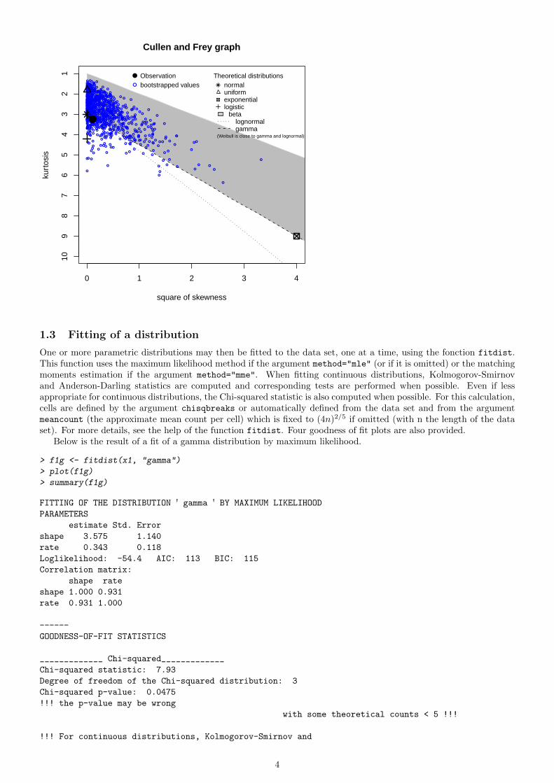
In order to take into account the uncertainty of the estimated values of kurtosis and skewness, the data set may beboostrapped by fixing the argument boot to an integer above 10 in descdist. boot values of skewness and kurtosiscorresponding to the boot nonparametric bootstrap samples are then computed and reported in blue color on theskewness-kurtosis plot.

> descdist(x1, boot = 1000)

summary statistics

------

min: 1.3 max: 22.1

median: 10.2

mean: 10.4

sample sd: 4.75



3

●

0 1 2 3 4


square of skewness

kurt

osis

109

87

65

43

21 ● Observation

● bootstrapped valuesTheoretical distributions

normaluniformexponentiallogistic

betalognormalgamma

(Weibull is close to gamma and lognormal)●

●

●

●

●

●

●

●

●

●

●

●

●

●

●

●

●

● ●

●●

●

●

●

●

●

●

●

●

●

●

●

●

●●

●● ●

●

●

●●●

●

●

●

●

●

●

●

●

●

●

●●

●

●

●

●

●

●

●

● ●

●

●

●

●

●

●

●

●

●

●

●

●

●

●

●

●

●

●

●

●

●

●

●

●

●

●

●

●

●

●

●

●

●

●

●

●

●

●

●

●

●

●

●

●

●

●

●

●

●

●

●

●

●

●

●

●

●

●●

●

●

●

●

●

●

●●

●

●●

●

●●

●

●

●

●

●

●

●

●

●

●

●

●

●

●

●

●

●

●

●

●

●

●

●

●

●

●

●

●

●

●●

●

●●

●●

●

●

●

●

●●

●

●

●

●

●

●

●

●

●

●

●●

●

● ●

●

●●

●

●

●

●

●

●

●

●

●

●

●

●

●

●

●

●

●

●

●

●

●

●

●

●

●

●

●

●

●

●

●

●

●

●

●

●●

●

●

●

●

●

●

●

●

●

●●

●

●

●

●

●●

●●

●

●●

●

●

●

●

●

●

●

● ●

●

●

●

●

●

●

●

●

●●

●

●

●

●

●

●

● ●

●

●

●

●

●

●

●

●

●

●

●

●

●

●

●●●

●

●

●

●

●

●

●

●

●

●

●

●

● ●

●

●

●

●

●

●

●

●

●

●

●

●

●

●

●●

●●

●

●●

●

●

●

●●

●

●

●

●

●

●

●

●

●

●

●

●

●

●

●

●

●

●

●

● ●

●

●

●

●

●

●

●

●

●

●

●

●

●

●

●

●

●

●

●

●

●

●

●

●

●

●

●

●●

●

●

●

●

●

●

●

●

●

●

●

●

●

●

●

●

●

●

● ●

●

●

●●

●●

●

●

●

●

●

●

●

●

●

●

●

●

●●

●

●

●

●

●

●

●

●

●

●

●

●

●

●

●

●

●

●

●

●

●●

●

●

●

●

●

●

●

●

●

●

●

●

●

●

●

●

●

●

●

●

●

●

●

●●

●

●

●

●

●

●

●

●

●

●

●

●

●

●

●

●

●

●

●

●

●●

●

●

● ●

●

●

●

●

●

●

●

●

●

●

●

●

●

●

●

●

●

●

●

●

●

●

●

●

●

● ●

●

●

●

●

●

●

●

●

●

●●●

●

●

●

●

●

●

●

●

●

●

●

●

●

●

●

●

●

●

●

●

●

●

●●

●

●

●

●

●

●

●

●

●

●

●

●

●

●

●

●

●

●

●

●

●

●

●

●

●

●

●

●

●

●●

●

●

●

●

●

●

●

●●

●

● ●

●

●

●

●

●

●

●

●

●

●

●

●

●

●

●

●

●●

●

●

●

●

●

●

●

●

● ●

●

● ●

●

●

●●

●

●

●

●

● ●

●

●

●●

●

●●

●

●

●

●

●

●

●

●●

●

●

●

●

●

●

●

●●

●

●

●

●

●

●

●

●●

●

●

●

●●

●

●●

●

●

●

●

●

●

●

●

●

●

●

●

●

●

●

●

●

●

●

●●

●

● ●

●

●●

●●

●●

●

●

●

●

●

●

●

●

●●

●

●

●

●

●

●

●

●

●

●

●

●

●

●

●

●

●

●

●●●

● ●● ●

●

●

●

●

●

●●

●

●

●

●

●●

●

●

●

●

●

●

●

●

●

●

●

●

●

●

●

●

●

●

●

●

●

●

●

●

●

●

●

●

●

●

●

●

●●

●

●

●

●

●

●

●●

●

●

●

●

●

●

●

●●

●

●

●

●

●

●

●

●

●

●

●

●●

●

●

●

●

●

●●

●

●

●

●

●

●

●

● ●

●

●

●

●●

●

●●

●

●

●

●

●

●

●

●

●

●

●

●

●

●

●

●

●

●

●

●

●

●

●

●●

●

●

●

●

●

●

●

●

●

●

●

●

●

●

●

●

●

●

●

●

●

●

●

●

●

●

●

●

●

●● ●

●

●

●

●

●

●

●

● ●

●

●

●

●

●

●

●

●

●

●

●

●

●

●

●

●

●

●

●

●

●

●

●

●

●

●

●

●

●

●

●

●

●

●

●

●

●

●

● ●

●

●

●

●●

●

●

●

●

●

●

●

●

●

●

●

●

●

●

●●

●

●

●

●

●

●

●

●

●

●

●

●

●●

●

1.3 Fitting of a distribution

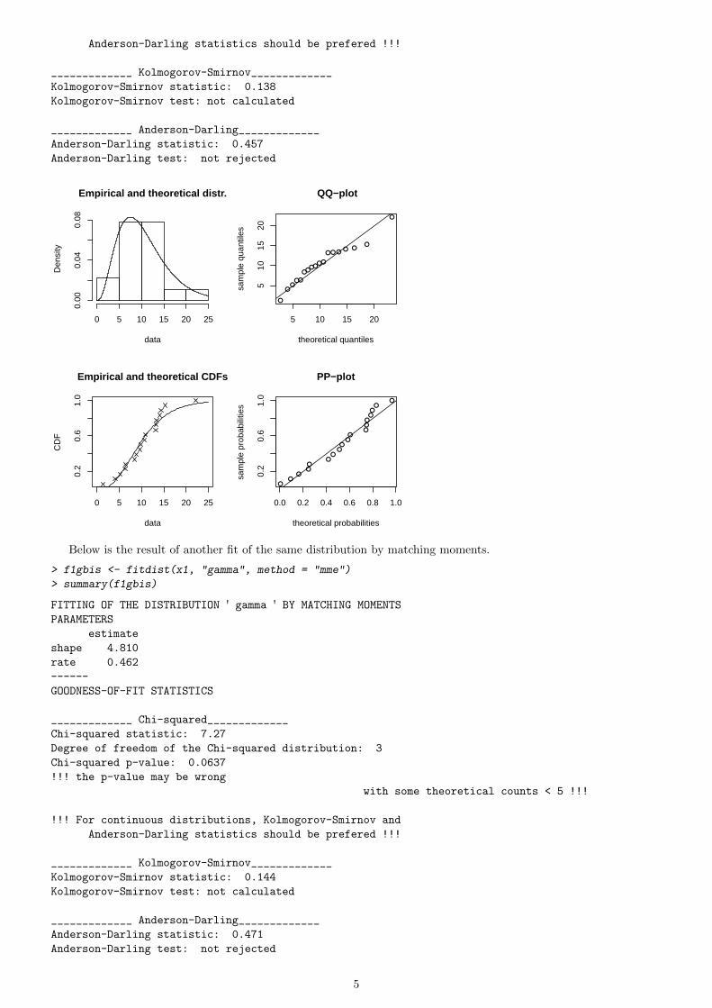
One or more parametric distributions may then be fitted to the data set, one at a time, using the fonction fitdist.This function uses the maximum likelihood method if the argument method="mle" (or if it is omitted) or the matchingmoments estimation if the argument method="mme". When fitting continuous distributions, Kolmogorov-Smirnovand Anderson-Darling statistics are computed and corresponding tests are performed when possible. Even if lessappropriate for continuous distributions, the Chi-squared statistic is also computed when possible. For this calculation,cells are defined by the argument chisqbreaks or automatically defined from the data set and from the argumentmeancount (the approximate mean count per cell) which is fixed to (4n)2/5 if omitted (with n the length of the dataset). For more details, see the help of the function fitdist. Four goodness of fit plots are also provided.

Below is the result of a fit of a gamma distribution by maximum likelihood.

> f1g <- fitdist(x1, "gamma")

> plot(f1g)

> summary(f1g)

FITTING OF THE DISTRIBUTION ' gamma ' BY MAXIMUM LIKELIHOOD

PARAMETERS

estimate Std. Error

shape 3.575 1.140

rate 0.343 0.118

Loglikelihood: -54.4 AIC: 113 BIC: 115

Correlation matrix:

shape rate

shape 1.000 0.931

rate 0.931 1.000

------

GOODNESS-OF-FIT STATISTICS

_____________ Chi-squared_____________

Chi-squared statistic: 7.93

Degree of freedom of the Chi-squared distribution: 3

Chi-squared p-value: 0.0475

!!! the p-value may be wrong

with some theoretical counts < 5 !!!

!!! For continuous distributions, Kolmogorov-Smirnov and

4

Anderson-Darling statistics should be prefered !!!

_____________ Kolmogorov-Smirnov_____________

Kolmogorov-Smirnov statistic: 0.138

Kolmogorov-Smirnov test: not calculated

_____________ Anderson-Darling_____________

Anderson-Darling statistic: 0.457

Anderson-Darling test: not rejected

Empirical and theoretical distr.

data

Den

sity

0 5 10 15 20 25

0.00

0.04

0.08

●

●●

●●

●●●●

●●

● ● ●● ●

●

●

5 10 15 20

510

1520

QQ−plot

theoretical quantiles

sam

ple

quan

tiles

0 5 10 15 20 25

0.2

0.6

1.0

Empirical and theoretical CDFs

data

CD

F

●●

●●●

●●

●●

●●

●●●

●●

●●

0.0 0.2 0.4 0.6 0.8 1.0

0.2

0.6

1.0

PP−plot

theoretical probabilities

sam

ple

prob

abili

ties

Below is the result of another fit of the same distribution by matching moments.

> f1gbis <- fitdist(x1, "gamma", method = "mme")

> summary(f1gbis)

FITTING OF THE DISTRIBUTION ' gamma ' BY MATCHING MOMENTS

PARAMETERS

estimate

shape 4.810

rate 0.462

------


_____________ Chi-squared_____________














5

As can be seen in this returned summary, the automatic definition of the cells required to calculate the Chi-squaredstatistic does not give theoretical counts large enough to validate the use of the test in this example. It is often thecase for small data sets. The observed and theoretical counts may be printed as below :

> f1g$chisqtable

obscounts theocounts

<= 5.2 3.000 2.895

<= 8.4 3.000 4.596

<= 9.9 3.000 2.108

<= 13.2 3.000 3.706

<= 14.1 3.000 0.758

> 14.1 3.000 3.936

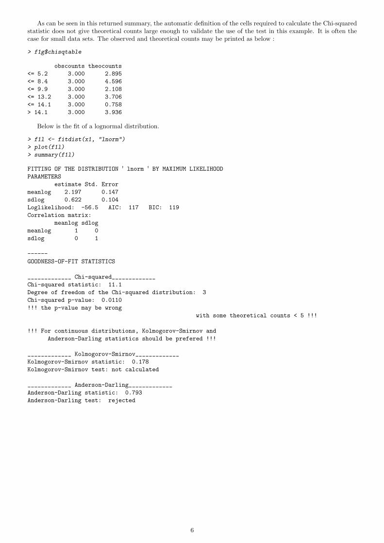
Below is the fit of a lognormal distribution.

> f1l <- fitdist(x1, "lnorm")

> plot(f1l)

> summary(f1l)

FITTING OF THE DISTRIBUTION ' lnorm ' BY MAXIMUM LIKELIHOOD

PARAMETERS

estimate Std. Error

meanlog 2.197 0.147

sdlog 0.622 0.104


Correlation matrix:

meanlog sdlog

meanlog 1 0

sdlog 0 1

------


_____________ Chi-squared_____________













Anderson-Darling test: rejected

6


data

Den

sity

0 5 10 15 20 25

0.00

0.04

0.08

●

●●●●

●●●●

●●

●● ●● ●

●

●

5 10 15 20 25 30

510

1520

QQ−plot


sam

ple

quan

tiles

0 5 10 15 20 25

0.2

0.6

1.0


data

CD

F

●●

●●●

●●

●●

●●

●●●

●●

●●

0.0 0.2 0.4 0.6 0.8

0.2

0.6

1.0

PP−plot


sam

ple

prob

abili

ties

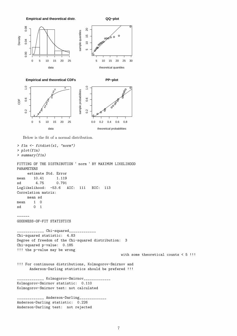
Below is the fit of a normal distribution.

> f1n <- fitdist(x1, "norm")

> plot(f1n)

> summary(f1n)

FITTING OF THE DISTRIBUTION ' norm ' BY MAXIMUM LIKELIHOOD

PARAMETERS

estimate Std. Error

mean 10.41 1.119

sd 4.75 0.791


Correlation matrix:

mean sd

mean 1 0

sd 0 1

------


_____________ Chi-squared_____________














7


data

Den

sity

0 5 10 15 20 25

0.00

0.04

0.08

●

●●

● ●

●●●●

●●

●●●● ●

●

●

5 10 15 20

510

1520

QQ−plot


sam

ple

quan

tiles

0 5 10 15 20 25

0.2

0.6

1.0


data

CD

F

●●

●●●

●●

●●

●●

●●●

●●

●●

0.0 0.2 0.4 0.6 0.8 1.0

0.2

0.6

1.0

PP−plot


sam

ple

prob

abili

ties

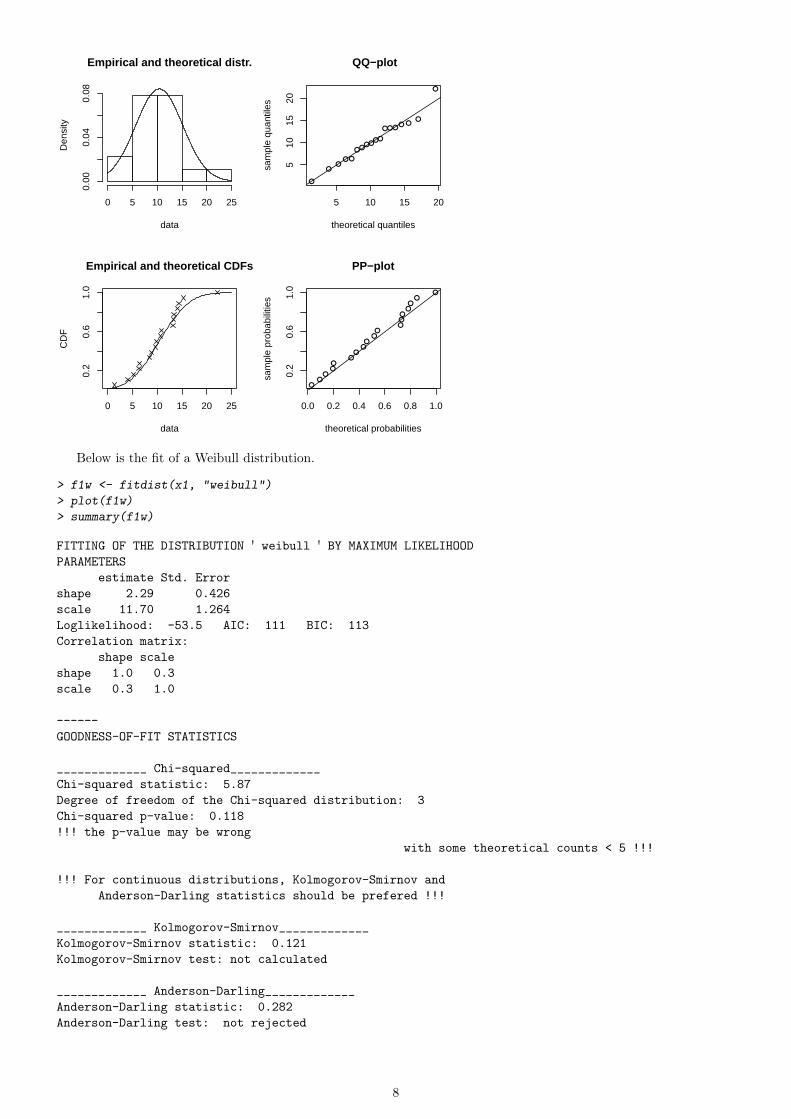
Below is the fit of a Weibull distribution.

> f1w <- fitdist(x1, "weibull")

> plot(f1w)

> summary(f1w)

FITTING OF THE DISTRIBUTION ' weibull ' BY MAXIMUM LIKELIHOOD

PARAMETERS

estimate Std. Error

shape 2.29 0.426

scale 11.70 1.264


Correlation matrix:

shape scale

shape 1.0 0.3

scale 0.3 1.0

------


_____________ Chi-squared_____________














8


data

Den

sity

0 5 10 15 20 25

0.00

0.04

0.08

●

●●

● ●

●●●●

●●

● ● ●● ●

●

●

5 10 15 20

510

1520

QQ−plot


sam

ple

quan

tiles

0 5 10 15 20 25

0.2

0.6

1.0


data

CD

F

●●

●●●

●●

●●

●●

●●●

●●

●●

0.0 0.2 0.4 0.6 0.8 1.0

0.2

0.6

1.0

PP−plot


sam

ple

prob

abili

ties

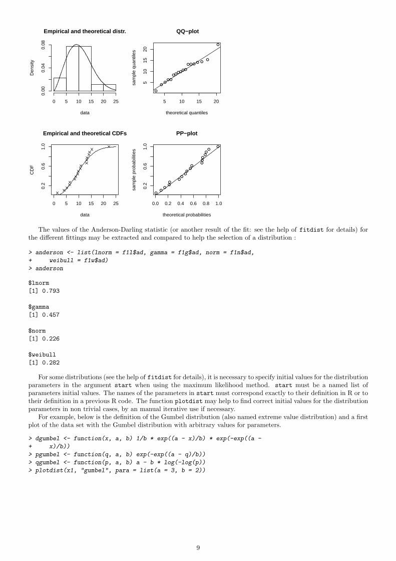
The values of the Anderson-Darling statistic (or another result of the fit: see the help of fitdist for details) forthe different fittings may be extracted and compared to help the selection of a distribution :

> anderson <- list(lnorm = f1l$ad, gamma = f1g$ad, norm = f1n$ad,

+ weibull = f1w$ad)

> anderson

$lnorm

[1] 0.793

$gamma

[1] 0.457

$norm

[1] 0.226

$weibull

[1] 0.282

For some distributions (see the help of fitdist for details), it is necessary to specify initial values for the distributionparameters in the argument start when using the maximum likelihood method. start must be a named list ofparameters initial values. The names of the parameters in start must correspond exactly to their definition in R or totheir definition in a previous R code. The function plotdist may help to find correct initial values for the distributionparameters in non trivial cases, by an manual iterative use if necessary.

For example, below is the definition of the Gumbel distribution (also named extreme value distribution) and a firstplot of the data set with the Gumbel distribution with arbitrary values for parameters.

> dgumbel <- function(x, a, b) 1/b * exp((a - x)/b) * exp(-exp((a -

+ x)/b))

> pgumbel <- function(q, a, b) exp(-exp((a - q)/b))

> qgumbel <- function(p, a, b) a - b * log(-log(p))

> plotdist(x1, "gumbel", para = list(a = 3, b = 2))

9


data

Den

sity

0 5 10 15 20 25

0.00

0.10

●

●●

●●

●●●●

●●

●● ●● ●

●

●

2 4 6 8 10

510

1520

QQ−plot


sam

ple

quan

tiles

0 5 10 15 20 25

0.2

0.6

1.0


data

CD

F

●●

●●●

●●●●●●●●●●●●●

0.2 0.4 0.6 0.8 1.0

0.2

0.6

1.0

PP−plot


sam

ple

prob

abili

ties

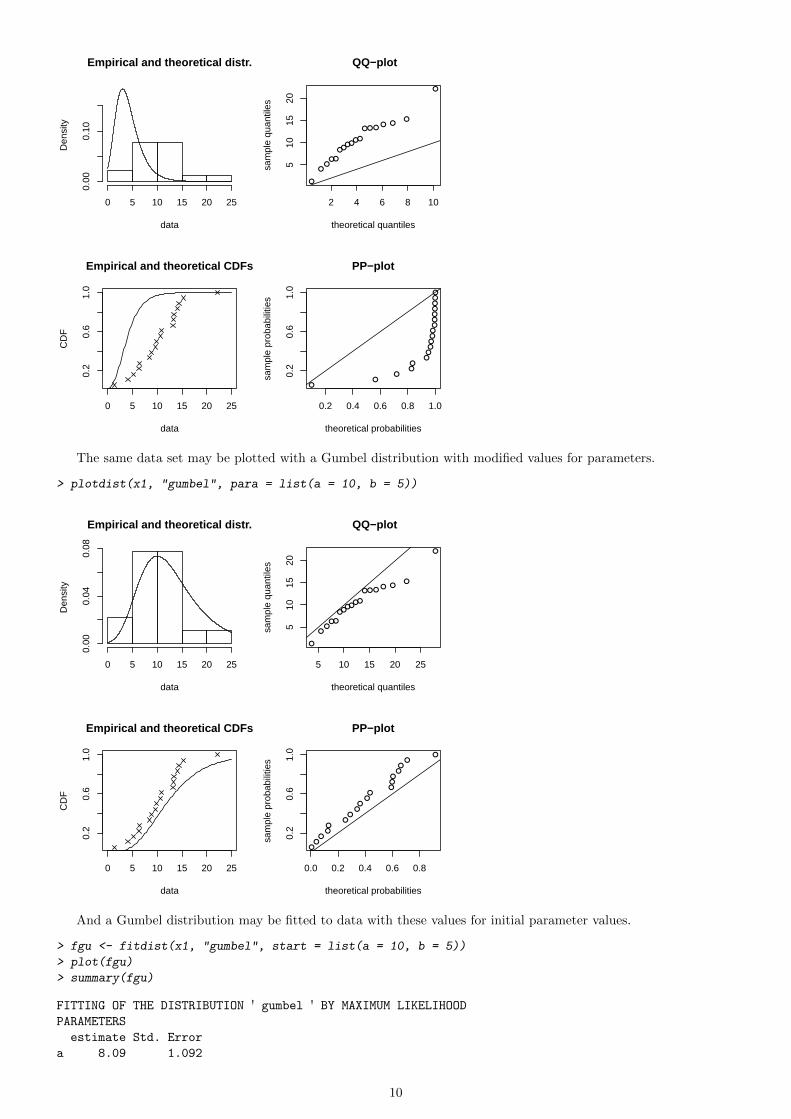
The same data set may be plotted with a Gumbel distribution with modified values for parameters.

> plotdist(x1, "gumbel", para = list(a = 10, b = 5))


data

Den

sity

0 5 10 15 20 25

0.00

0.04

0.08

●

●●

●●

●●●●

●●

●● ●● ●

●

●

5 10 15 20 25

510

1520

QQ−plot


sam

ple

quan

tiles

0 5 10 15 20 25

0.2

0.6

1.0


data

CD

F

●●

●●●

●●

●●

●●

●●●

●●

●●

0.0 0.2 0.4 0.6 0.8

0.2

0.6

1.0

PP−plot


sam

ple

prob

abili

ties

And a Gumbel distribution may be fitted to data with these values for initial parameter values.

> fgu <- fitdist(x1, "gumbel", start = list(a = 10, b = 5))

> plot(fgu)

> summary(fgu)

FITTING OF THE DISTRIBUTION ' gumbel ' BY MAXIMUM LIKELIHOOD

PARAMETERS

estimate Std. Error

a 8.09 1.092

10

b 4.38 0.766


Correlation matrix:

a b

a 1.000 0.330

b 0.330 1.000

------


_____________ Chi-squared_____________













Anderson-Darling test: not calculated


data

Den

sity

0 5 10 15 20 25

0.00

0.04

0.08

●

●●

●●

●●●●

●●

●● ●● ●

●

●

5 10 15 20

510

1520

QQ−plot


sam

ple

quan

tiles

0 5 10 15 20 25

0.2

0.6

1.0


data

CD

F

●●

●●●

●●

●●

●●

●●●

●●

●●

0.0 0.2 0.4 0.6 0.8

0.2

0.6

1.0

PP−plot


sam

ple

prob

abili

ties

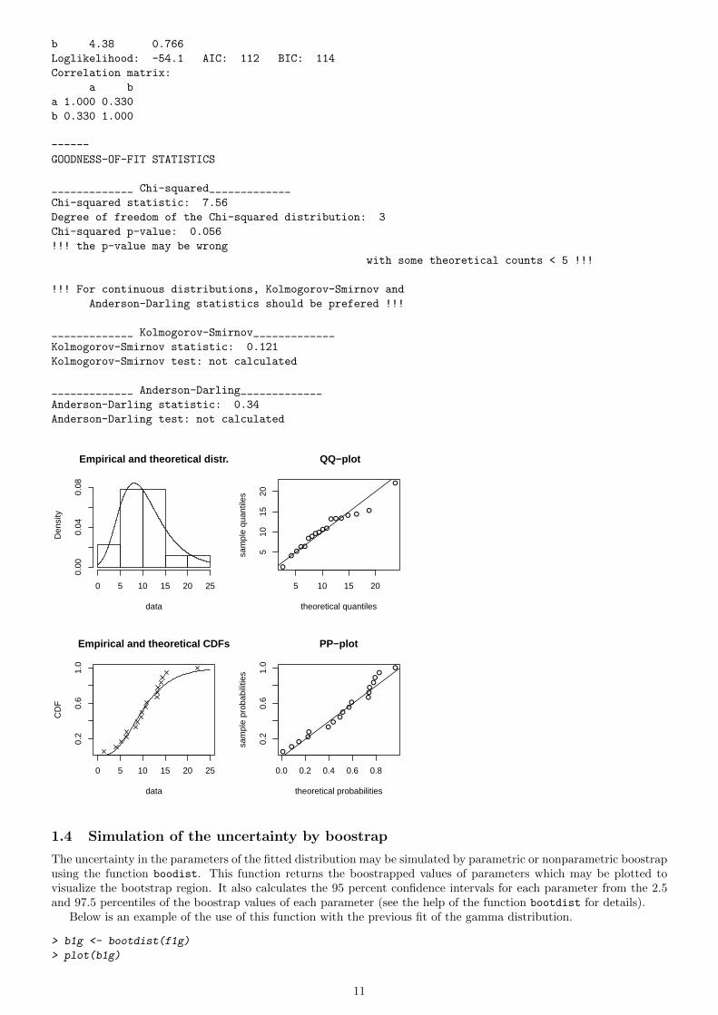
1.4 Simulation of the uncertainty by boostrap

The uncertainty in the parameters of the fitted distribution may be simulated by parametric or nonparametric boostrapusing the function boodist. This function returns the boostrapped values of parameters which may be plotted tovisualize the bootstrap region. It also calculates the 95 percent confidence intervals for each parameter from the 2.5and 97.5 percentiles of the boostrap values of each parameter (see the help of the function bootdist for details).

Below is an example of the use of this function with the previous fit of the gamma distribution.

> b1g <- bootdist(f1g)

> plot(b1g)

11

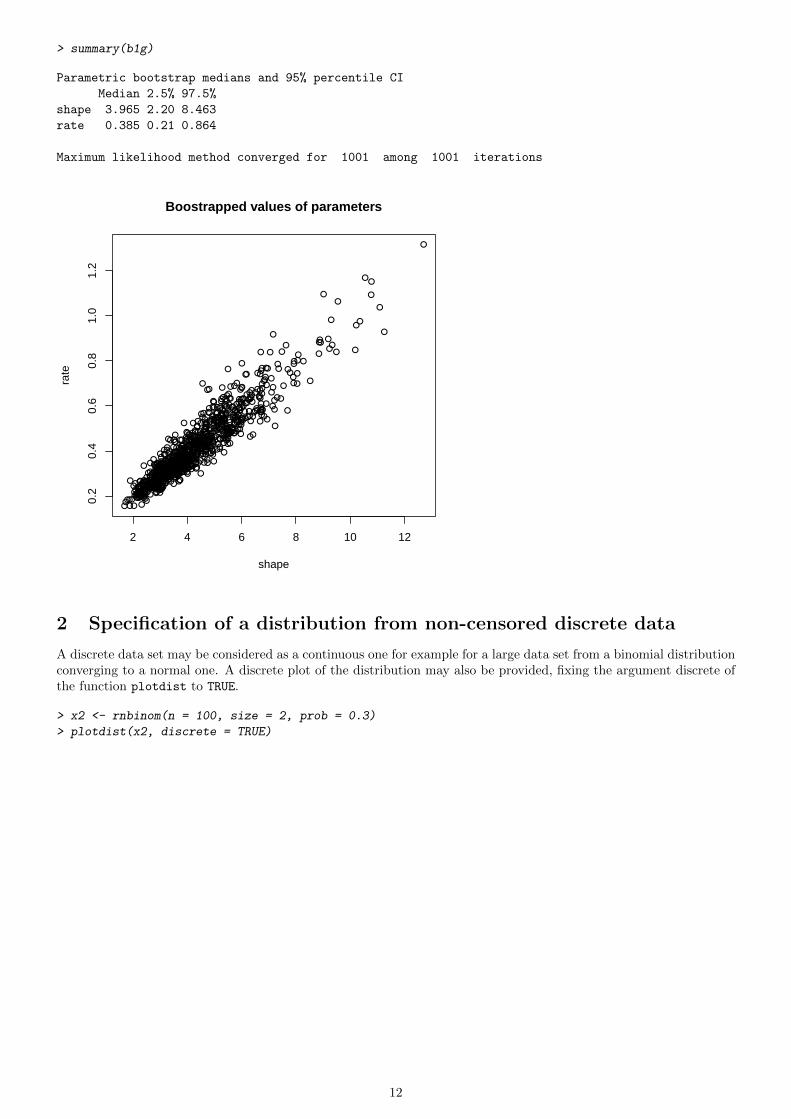
> summary(b1g)

Parametric bootstrap medians and 95% percentile CI

Median 2.5% 97.5%

shape 3.965 2.20 8.463

rate 0.385 0.21 0.864

Maximum likelihood method converged for 1001 among 1001 iterations

●

●

●

● ●

●

●

●

●●

●

●

●●

●

● ●

●

●

●

●

●

●

●

●●

●

●

●

●

●●

●

●

●

●

●

●

● ●

●

●

●

●

●

●●

●

●

●

●

●●

●

●

●●

● ●

●●

●

●

●

●

●

●

●

●

●

●

●

●

●

●

●

●

●

●

●

●

●

●

●

●

●

●

●

●

●●

●

●

●●

●

●●

●

●

●

●

●

●

●

●●●

●

●

●

●●

●

●

●

●

●

●●

●

●●

●●

●

●

● ●

●

●

●

●

●

●

●

●

●●

●

●

●

●

●

●

●

●

●●

●

●●

●

●

●

●

●

●

●●

●

●●●

●

●

●

●

●

●●●

●

●●

●

●

●

●

●

●

●●

●

●

●

●

●

●

●

●

●

●

●●

●

●

●

●

●

●

●

●

●●

●

●

● ●

●

●

●

●

●●

●

●

●

● ●

●

●●

●

●

●

●

●●

●

●

●

●

●

●

●

●

●

●

●●

●

●

●

●

●

●

● ●

●

●

●

●

●

● ●● ●

●●

●

●

●

●

●

●●

●

●

●

●

●

●

●

●

●●

●

●

●

●

●●

●

●

●

●

●

●●

●

●

●

●

●

●

●

●

●

●

●

●

●

●

●

●

●

●

●

●

●

●●

●

●

●

●

●

●

●

●

●

●

●

●

●

●

●

●

●

●

●

●

●

●

●

●●

●●

●

●

●

●

●

●

●●

●

●

●

●●

●

●

●

●

●

●

●

●

●

●

●

●

●

●

●●

●

●

●

●

●●

●●

●●

●

● ●●

●

●

●●

●

●

●

●

●

●●

●

●

●

●

●

●

●

●

●

●

●●

●

●●

●

●

●

●

●

●●

●

●

●

●●

●

●

●

●

●

●

●●

●

●●

●

●

●

●

●

●

●

●

●

●

●

●

●

●

●

●

● ●●●

●●

●

●●

●●

●

●

●

●

●

●

●●

●

●

●

●

●●

●

●

●

●

●

●

●

●

●

●

●

●

●

●

●

●

●

●●

●

●

●

●

●

● ●●

●

●

●

●

●

●

●●

●

●

●

●

●

●

●

●

●

●

●

●

●

●

●

●

●

●

●

●

●

●

●

●

●

●

●

●

●

●

●●

●

●

●

●

●

●

●

●

●●

●

●

●●

●

●

●

●

●

●●

●

●

●

●

●

● ●

●

●

●

●

●

●

●

●

●●●

●

●

●

●

●

●●

●

●

●

●

●●

●

●

●

●

●

●

●

●

●●

●

●

●

●●

●

●

●

●●

●

●●

●

●

●

●●

●

●

●

●

●

●

●

●

●

●

●

●

●

●

●

●●

●

●

●

●●

●●●

●

●●

●

●

●

●

●

●

●●

●●

●

●

●

●

●

●

●

●

●●

●

●

●

●

●●●

●

●

●

●

●

●

●●

●

●

●

●

●

●

●●●●

●●

●

●●

●

●

●

●

●

●●

●

●

●

●

●

●

●

●

●

●

●

●

●

●

●

●

●

●

●●

●

●

●

●

●

●

●●●

●

●●

●

●

●

●

●

●

●●

●●

●

●●

●

●

●

●

●

●●

●

●

●

●

●

● ● ●

●

●

●●

●

●

●

●●

●

●

●

●●

●

●

●

●

●

●

●

●

●

●●

●

●

●

●●

●

●

●

●

● ●

●

●

●

●

●● ●

●●

●

●●

●

●

●●

●

●

●

●

●

●●

●

●

●

●

●

●

●

●

●

●●

●

●●

●

●

●

● ●●●

●

●

●

●

●●

●

●

●

●●

●

●

●

●

●

●●

●

●●

●

●

●

●

●

●●

●

●

●

●

●

●

●

●

●

●

●

●

●

●

●

●

●

●●

●

●

●

●

●

●

●

●

●

●

●

●

●

●

●

●●●

●

●

●

●

●●

●

●●

●

●

●

●

●●

●

● ●

●

●

●

●

●

●

●

●

●

●

●

●

●

●

●

●

●

●

●

●

●

●

●

●

●

●

●

●

●●

●

●

●●

●

●

●

●

●

●

●

●

●

●

●●

●●

●●

●

●

●

●

●

●

●

●

●

●●

●

●

●●

●

●

●

●●

●

●

●

2 4 6 8 10 12

0.2

0.4

0.6

0.8

1.0

1.2

Boostrapped values of parameters

shape

rate

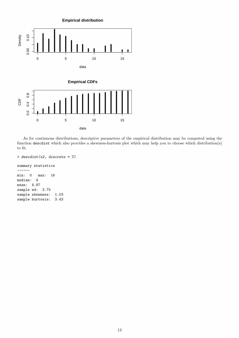
2 Specification of a distribution from non-censored discrete data

A discrete data set may be considered as a continuous one for example for a large data set from a binomial distributionconverging to a normal one. A discrete plot of the distribution may also be provided, fixing the argument discrete ofthe function plotdist to TRUE.

> x2 <- rnbinom(n = 100, size = 2, prob = 0.3)

> plotdist(x2, discrete = TRUE)

12

0 5 10 15

0.00

0.10

Empirical distribution

data

Den

sity

0 5 10 15

0.0

0.4

0.8

Empirical CDFs

data

CD

F

As for continuous distributions, descriptive parameters of the empirical distribution may be computed using thefunction descdist which also provides a skewness-kurtosis plot which may help you to choose which distribution(s)to fit.

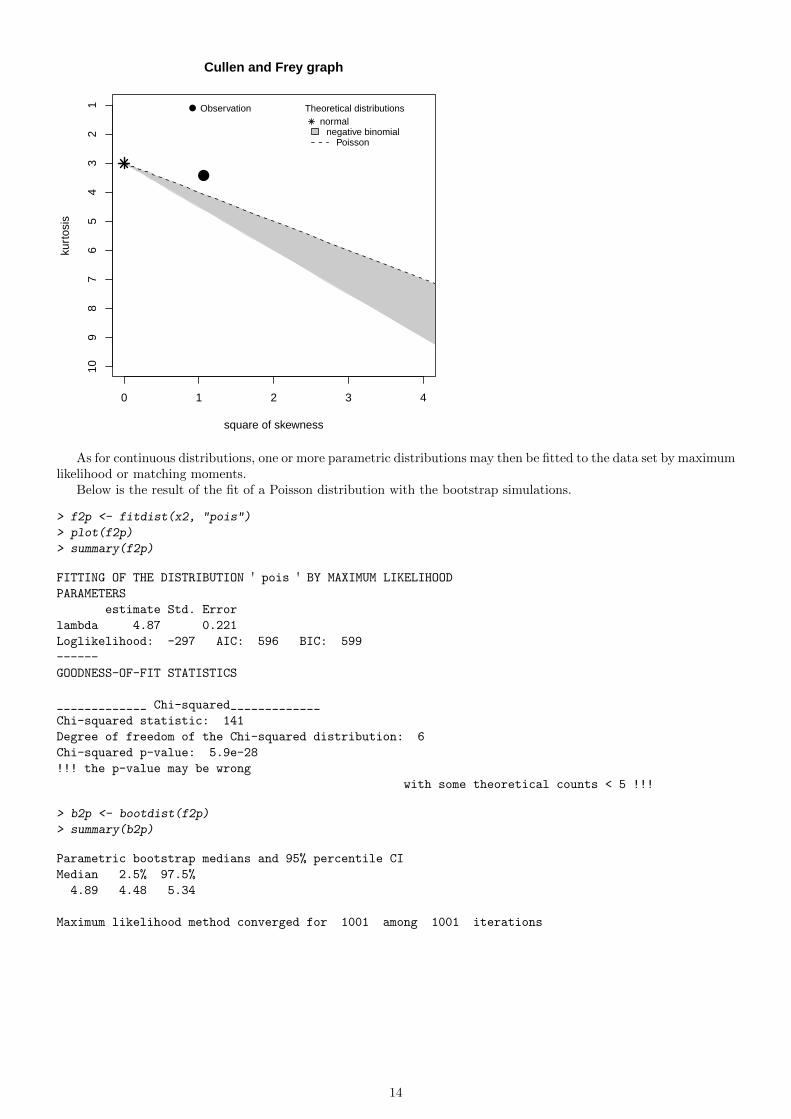
> descdist(x2, discrete = T)

summary statistics

------

min: 0 max: 16

median: 4

mean: 4.87

sample sd: 3.75



13

●

0 1 2 3 4


square of skewness

kurt

osis

109

87

65

43

21 ● Observation Theoretical distributions

normalnegative binomial

Poisson

●

As for continuous distributions, one or more parametric distributions may then be fitted to the data set by maximumlikelihood or matching moments.

Below is the result of the fit of a Poisson distribution with the bootstrap simulations.

> f2p <- fitdist(x2, "pois")

> plot(f2p)

> summary(f2p)

FITTING OF THE DISTRIBUTION ' pois ' BY MAXIMUM LIKELIHOOD

PARAMETERS

estimate Std. Error

lambda 4.87 0.221

Loglikelihood: -297 AIC: 596 BIC: 599

------


_____________ Chi-squared_____________

Chi-squared statistic: 141


Chi-squared p-value: 5.9e-28



> b2p <- bootdist(f2p)

> summary(b2p)


Median 2.5% 97.5%

4.89 4.48 5.34


14

0 5 10 15

0.00

0.10

Empirical (black) and theoretical (red) distr.

data

Den

sity

0 5 10 15

0.0

0.4

0.8

Empirical (black) and theoretical (red) CDFs

data

CD

F

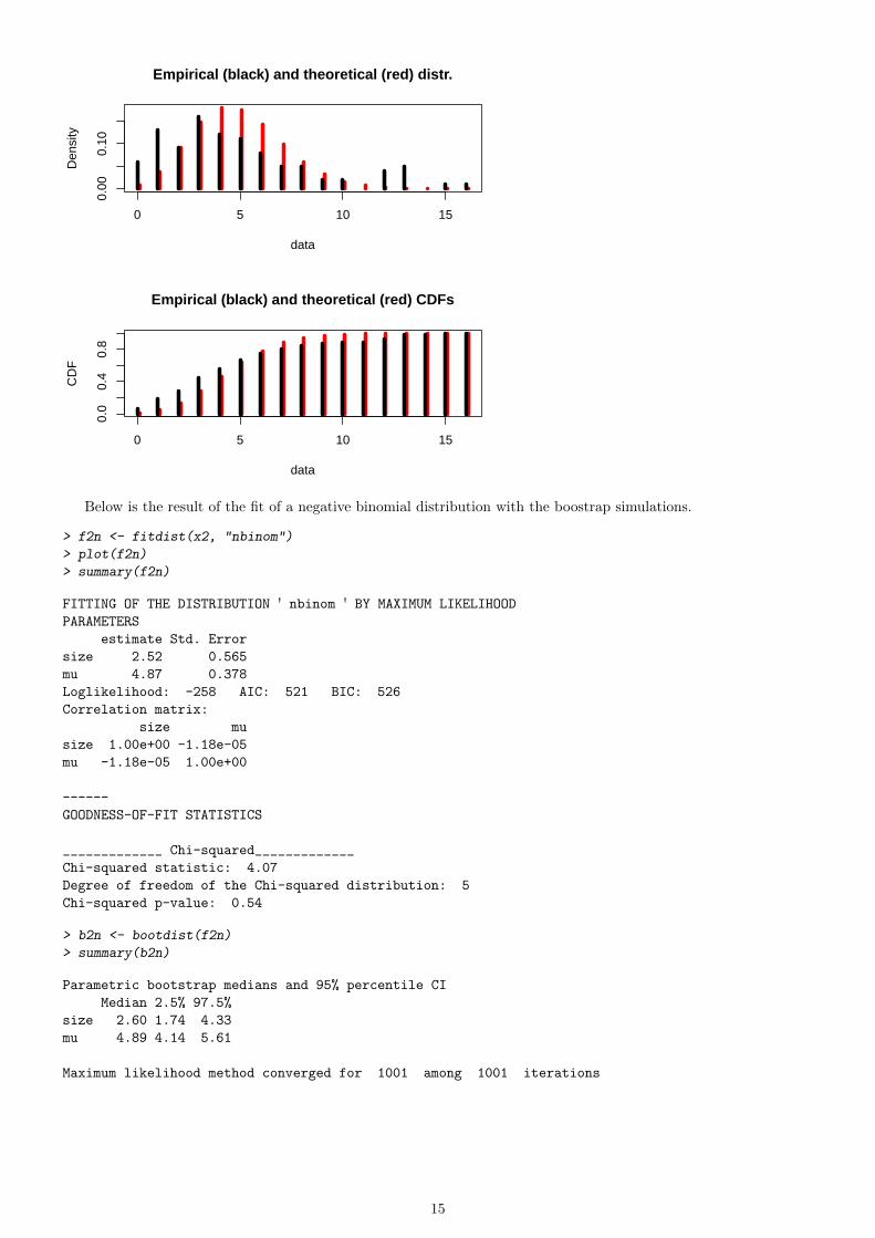
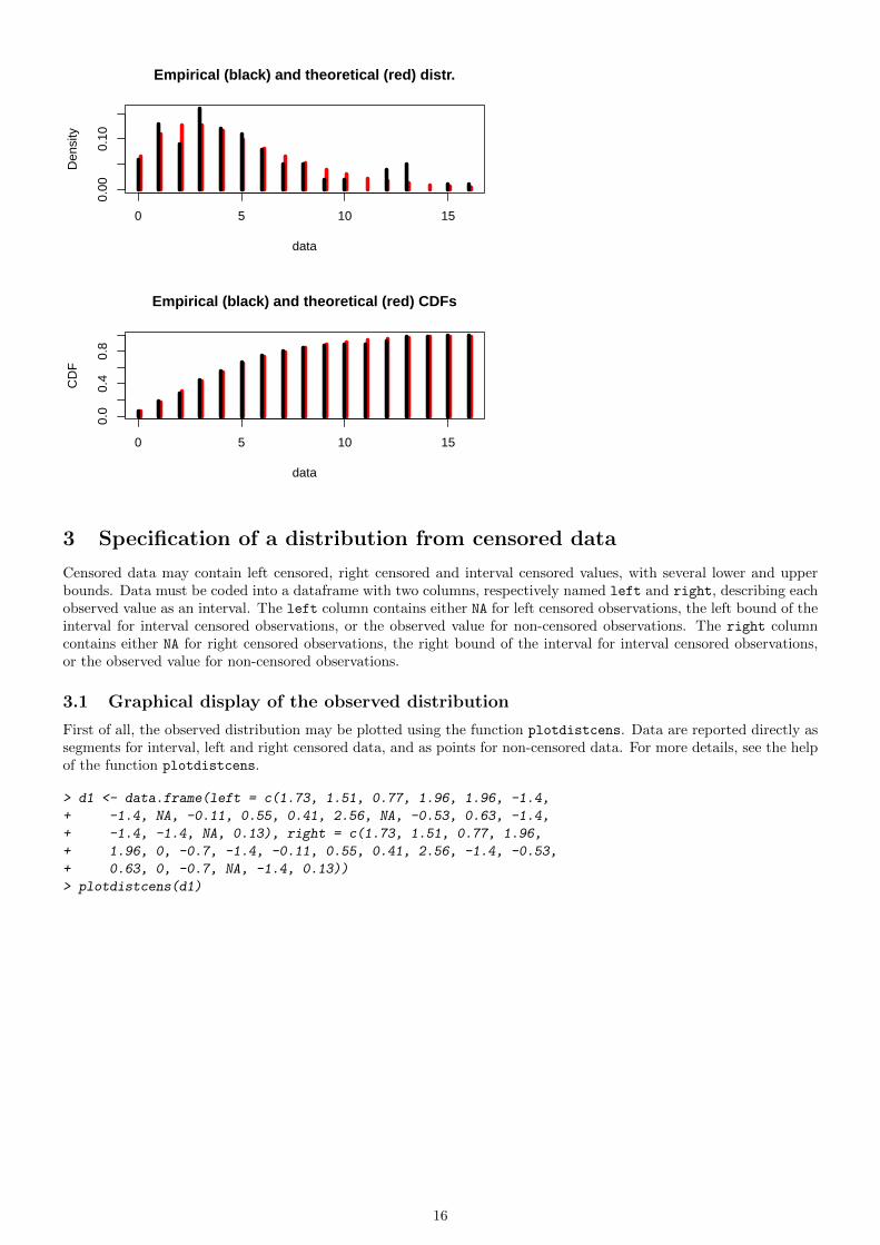
Below is the result of the fit of a negative binomial distribution with the boostrap simulations.

> f2n <- fitdist(x2, "nbinom")

> plot(f2n)

> summary(f2n)

FITTING OF THE DISTRIBUTION ' nbinom ' BY MAXIMUM LIKELIHOOD

PARAMETERS

estimate Std. Error

size 2.52 0.565

mu 4.87 0.378

Loglikelihood: -258 AIC: 521 BIC: 526

Correlation matrix:

size mu

size 1.00e+00 -1.18e-05

mu -1.18e-05 1.00e+00

------


_____________ Chi-squared_____________




> b2n <- bootdist(f2n)

> summary(b2n)


Median 2.5% 97.5%

size 2.60 1.74 4.33

mu 4.89 4.14 5.61


15

0 5 10 15

0.00

0.10

Empirical (black) and theoretical (red) distr.

data

Den

sity

0 5 10 15

0.0

0.4

0.8

Empirical (black) and theoretical (red) CDFs

data

CD

F

3 Specification of a distribution from censored data

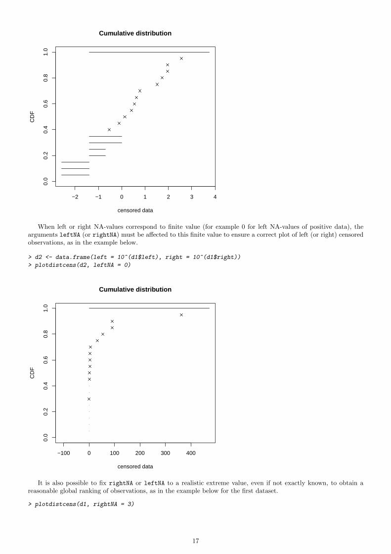
Censored data may contain left censored, right censored and interval censored values, with several lower and upperbounds. Data must be coded into a dataframe with two columns, respectively named left and right, describing eachobserved value as an interval. The left column contains either NA for left censored observations, the left bound of theinterval for interval censored observations, or the observed value for non-censored observations. The right columncontains either NA for right censored observations, the right bound of the interval for interval censored observations,or the observed value for non-censored observations.

3.1 Graphical display of the observed distribution

First of all, the observed distribution may be plotted using the function plotdistcens. Data are reported directly assegments for interval, left and right censored data, and as points for non-censored data. For more details, see the helpof the function plotdistcens.

> d1 <- data.frame(left = c(1.73, 1.51, 0.77, 1.96, 1.96, -1.4,

+ -1.4, NA, -0.11, 0.55, 0.41, 2.56, NA, -0.53, 0.63, -1.4,

+ -1.4, -1.4, NA, 0.13), right = c(1.73, 1.51, 0.77, 1.96,

+ 1.96, 0, -0.7, -1.4, -0.11, 0.55, 0.41, 2.56, -1.4, -0.53,

+ 0.63, 0, -0.7, NA, -1.4, 0.13))

> plotdistcens(d1)

16

−2 −1 0 1 2 3 4

0.0

0.2

0.4

0.6

0.8

1.0


censored data

CD

F

When left or right NA-values correspond to finite value (for example 0 for left NA-values of positive data), thearguments leftNA (or rightNA) must be affected to this finite value to ensure a correct plot of left (or right) censoredobservations, as in the example below.

> d2 <- data.frame(left = 10^(d1$left), right = 10^(d1$right))

> plotdistcens(d2, leftNA = 0)

−100 0 100 200 300 400

0.0

0.2

0.4

0.6

0.8

1.0


censored data

CD

F

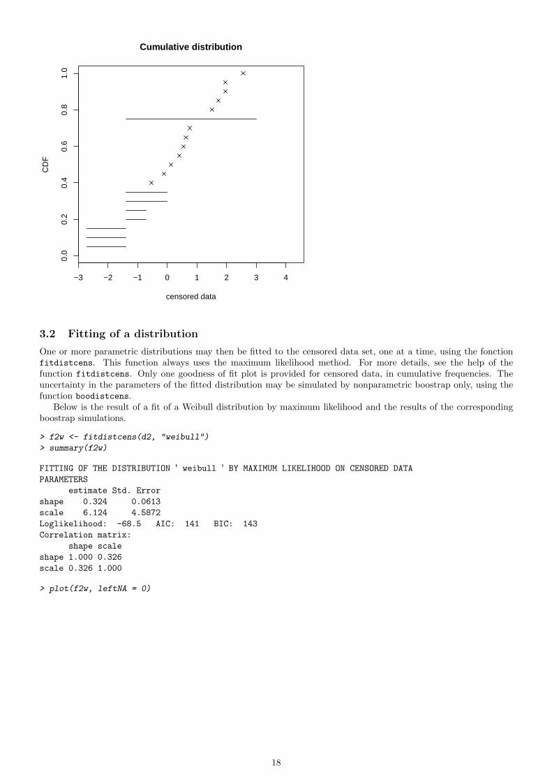
It is also possible to fix rightNA or leftNA to a realistic extreme value, even if not exactly known, to obtain areasonable global ranking of observations, as in the example below for the first dataset.

> plotdistcens(d1, rightNA = 3)

17

−3 −2 −1 0 1 2 3 4

0.0

0.2

0.4

0.6

0.8

1.0


censored data

CD

F

3.2 Fitting of a distribution

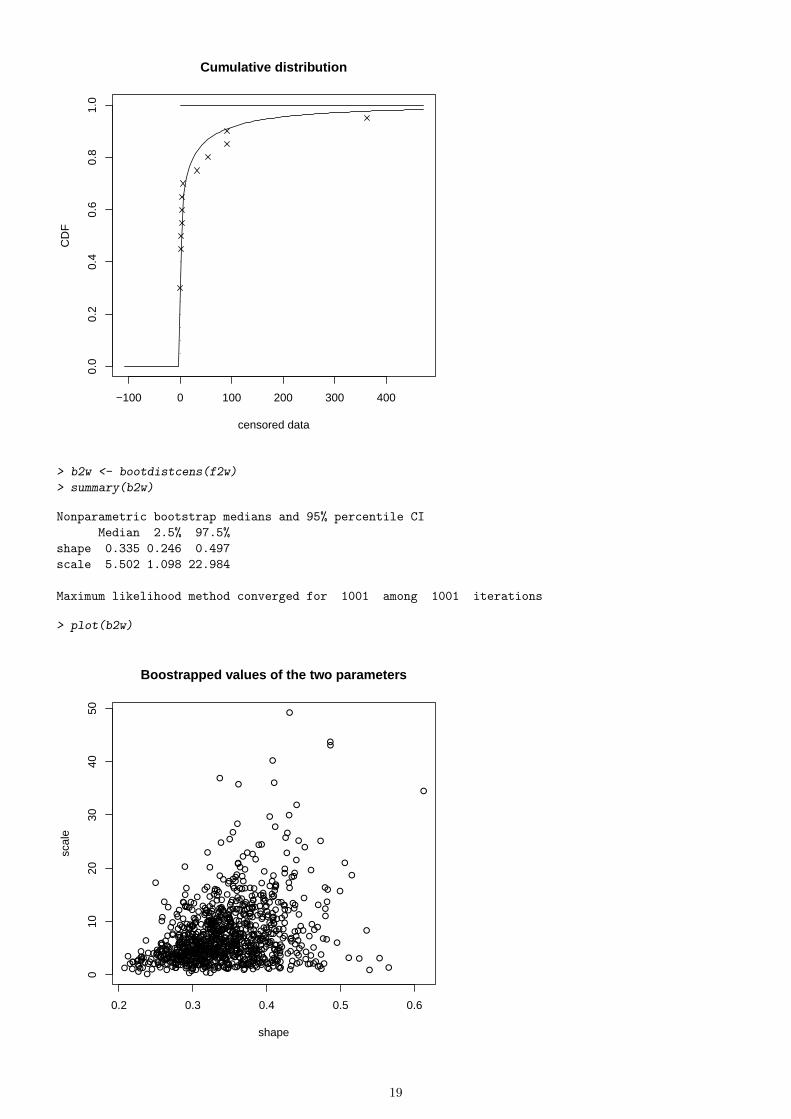
One or more parametric distributions may then be fitted to the censored data set, one at a time, using the fonctionfitdistcens. This function always uses the maximum likelihood method. For more details, see the help of thefunction fitdistcens. Only one goodness of fit plot is provided for censored data, in cumulative frequencies. Theuncertainty in the parameters of the fitted distribution may be simulated by nonparametric boostrap only, using thefunction boodistcens.

Below is the result of a fit of a Weibull distribution by maximum likelihood and the results of the correspondingboostrap simulations.

> f2w <- fitdistcens(d2, "weibull")

> summary(f2w)

FITTING OF THE DISTRIBUTION ' weibull ' BY MAXIMUM LIKELIHOOD ON CENSORED DATA

PARAMETERS

estimate Std. Error

shape 0.324 0.0613

scale 6.124 4.5872


Correlation matrix:

shape scale

shape 1.000 0.326

scale 0.326 1.000

> plot(f2w, leftNA = 0)

18

−100 0 100 200 300 400

0.0

0.2

0.4

0.6

0.8

1.0


censored data

CD

F

> b2w <- bootdistcens(f2w)

> summary(b2w)

Nonparametric bootstrap medians and 95% percentile CI

Median 2.5% 97.5%

shape 0.335 0.246 0.497

scale 5.502 1.098 22.984


> plot(b2w)

●●

●

●

●●

●

●

●

●●●

●

●

●

●

●

●

●

●

●

●

●

●

●●

●

●

●

●

●●●

●

●

●

● ●

●

●●

●

●

●●

●

●●

●

● ●

●

●

●

●

●

●

●●

●

●

● ●

●

●

●

●

●

●

●

●

●

●

●

●

●

● ●

●

●

●

●

●

●

●

●

●●

●

●

●

●

●

●●●

●

●

●

●

●

●

●●

●

●

●

●

●

●

●

●

●

●

●●

●

●

●

●

●

●●

●

●●

●

●

●

●●

●

●

●

●●

●

●

●

●●

●

●

●●

●●●

●

● ●

●

●

●

●

●●

●

●

●

●

●

●

●

●●

●

●●

● ●

●

●

●

●

●

●

●

●

●

●

●

●●●

●

●

●

●● ●

●●

●

●

●●

●

●

●●

●

●

●

●

●

●

●

●●

●

●

●

●

●

●●

●

●

●

●

●

●●

●

●

●

●

●

●●

●

●

●

●

●

●●

●

●

●●

●

●

●

● ●

●

●

●

●

●

●

●

●

●

●

●

●

●

●

●

●

●

●

●●

●

●●

●

●

●

●

●●●

●●●

●

●

●●

●

●

●

●●

●

●●

●

●

●

●

●

●

●

●●

●

● ●

● ●

●

●

●●●

●

●

●

●

●

●

● ●

●

●

●

●

●

●●

●●

●

●●●

●

●

●

●● ●

●

●

●●

●●

●

●●

●

●

●●

●

●

●

●●

●

●

●

●

●

●

●

●●

●

● ●

●●

●

●

●

●

●

●

●

●●

●

●

●●

●

●

●

●

●

●

●

●

●

●●

● ●

●

●

●

●

●

●

●

●

●

●

●

●

●

●

●

●

●

●

●

●

●

●

●

●

●

●

●

●

●●●

●

●

●●

●

●●

●●

●

●●

●●●

●

●●

●

●

●

●●

●

●

●

●

●

●

● ●

●●●

●

●●

●

●

●

●

●

●

●

●

●

●

●

●

●

●

●

●

● ●●

●

●

●●

●

●

●

●

●●

●●

●

●

●

●

●

●

●

●

●

●

●

●

●

●

●

●

●

●

●●

●

●

●

●

●

●

●

●

●

●

●

●

●●

●

● ●

●

●

●

●

●

●

●

●

●

●

●

●

●

●

●●

●●

●●

●

●

●

●

●

●

●●

●

●

●

●

●●

●●

● ●

●

●

●

●

●

●

●

●

●●

●

●

●

●

●

●

● ●●

●

●●

●

●

●

●

●●

●

●

●

●

●

●

●

●

●

●

●

● ●

●

●

●

●

●

●

●

●●

●

●

●

●

●

●

●

●

●

●

●

●

●

●

●

●

● ●

●

●

●

●●

●●

●

●

●

●

●

●

●

●

●

●

●

●

● ●

●●

●

●

●●●

●

●

●

●

●

●

●

●●

●

●

●

●

●

●

●

●

●

●

●

●

●

●

●

●

●

●

●●●

●

●

●

●

●

●●●

●

●

●

●

●

●

●

●

●

●

●

●●

●

●●

●

●

●●

●

●

●

●●

●

●●

●

●

●

●

●

●

●●

●●

●

●

●

●

●●

●

●●

● ●

●

●

●

●

●

●

●

●

●

●

●

●

●●

●

●●

●

● ●

●

●

●

●

●

●

●

●

●

●●

●

●

●

●

●

●

●

●●

●●

●

● ●

●

●

●●

●

●

●

●

●●

●

●

●

●

●

●

●

●

●

●

●

●

●

● ●

●

●

●

●

●

●

●

●

● ●

●●

●

●

●●

●●

●

●

●

●●

●

●

●

●●

●●

●

●●

●

●

●

●

●

●●

●●

●

●

●

●●

●

●

●

●●

●

●

●

●

●

●

●●

●

●

●

●

●

●● ●

●

●●

●

●

●

● ●

●

●

● ●

●

● ●

●●

●

●

●

●

●

●

●

●

● ●●

●

●

● ●

●

●

● ●

●

●

●

●●

●

●

● ●

●●

●

●

●●

●

●

●

●●

●

●

● ●

●

●

●

●

●

●

●

●

●

●

●

●

●

●●

●

●●

●●

●● ●

●

●●

●●

●

●●

●

● ●●

●●

●

●

●●

●

●

●

●

●

●

●

●

●

0.2 0.3 0.4 0.5 0.6

010

2030

4050

Boostrapped values of the two parameters

shape

scal

e

19

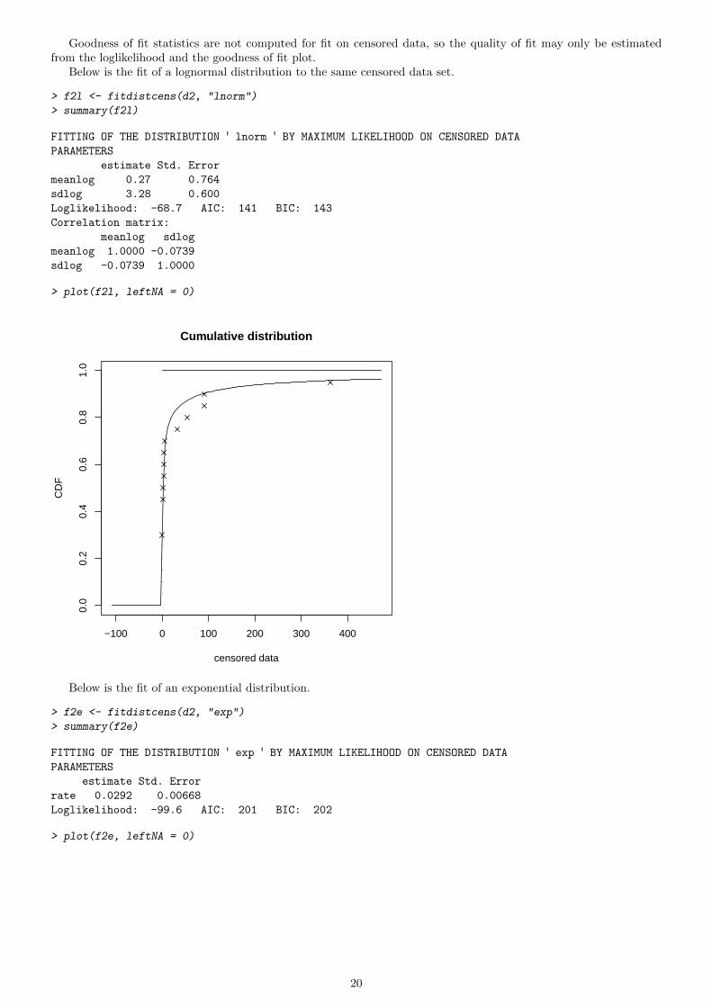
Goodness of fit statistics are not computed for fit on censored data, so the quality of fit may only be estimatedfrom the loglikelihood and the goodness of fit plot.

Below is the fit of a lognormal distribution to the same censored data set.

> f2l <- fitdistcens(d2, "lnorm")

> summary(f2l)

FITTING OF THE DISTRIBUTION ' lnorm ' BY MAXIMUM LIKELIHOOD ON CENSORED DATA

PARAMETERS

estimate Std. Error

meanlog 0.27 0.764

sdlog 3.28 0.600


Correlation matrix:

meanlog sdlog

meanlog 1.0000 -0.0739

sdlog -0.0739 1.0000

> plot(f2l, leftNA = 0)

−100 0 100 200 300 400

0.0

0.2

0.4

0.6

0.8

1.0


censored data

CD

F

Below is the fit of an exponential distribution.

> f2e <- fitdistcens(d2, "exp")

> summary(f2e)

FITTING OF THE DISTRIBUTION ' exp ' BY MAXIMUM LIKELIHOOD ON CENSORED DATA

PARAMETERS

estimate Std. Error

rate 0.0292 0.00668


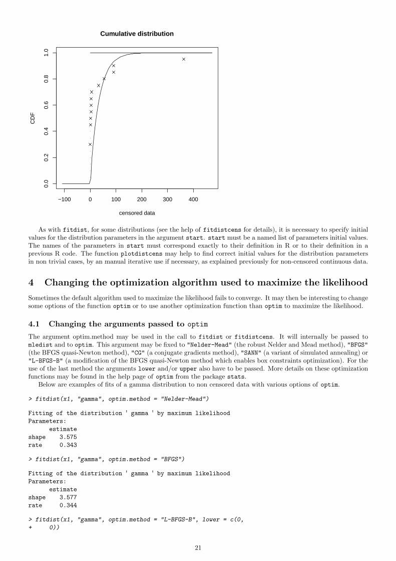
> plot(f2e, leftNA = 0)

20

−100 0 100 200 300 400

0.0

0.2

0.4

0.6

0.8

1.0


censored data

CD

F

As with fitdist, for some distributions (see the help of fitdistcens for details), it is necessary to specify initialvalues for the distribution parameters in the argument start. start must be a named list of parameters initial values.The names of the parameters in start must correspond exactly to their definition in R or to their definition in aprevious R code. The function plotdistcens may help to find correct initial values for the distribution parametersin non trivial cases, by an manual iterative use if necessary, as explained previously for non-censored continuous data.

4 Changing the optimization algorithm used to maximize the likelihood

Sometimes the default algorithm used to maximize the likelihood fails to converge. It may then be interesting to changesome options of the function optim or to use another optimization function than optim to maximize the likelihood.

4.1 Changing the arguments passed to optim

The argument optim.method may be used in the call to fitdist or fitdistcens. It will internally be passed tomledist and to optim. This argument may be fixed to "Nelder-Mead" (the robust Nelder and Mead method), "BFGS"(the BFGS quasi-Newton method), "CG" (a conjugate gradients method), "SANN" (a variant of simulated annealing) or"L-BFGS-B" (a modification of the BFGS quasi-Newton method which enables box constraints optimization). For theuse of the last method the arguments lower and/or upper also have to be passed. More details on these optimizationfunctions may be found in the help page of optim from the package stats.

Below are examples of fits of a gamma distribution to non censored data with various options of optim.

> fitdist(x1, "gamma", optim.method = "Nelder-Mead")

Fitting of the distribution ' gamma ' by maximum likelihood

Parameters:

estimate

shape 3.575

rate 0.343

> fitdist(x1, "gamma", optim.method = "BFGS")


Parameters:

estimate

shape 3.577

rate 0.344

> fitdist(x1, "gamma", optim.method = "L-BFGS-B", lower = c(0,

+ 0))

21


Parameters:

estimate

shape 3.574

rate 0.343

> fitdist(x1, "gamma", optim.method = "SANN")


Parameters:

estimate

shape 3.588

rate 0.345

4.2 Supplying another optimization function

You may also want to use another function than optim to maximize the likelihood. This optimization function has tobe specified by the argument custom.optim in the call to fitdist or fitdistcens. But before that, it is necessaryto customize this optimization function : custom.optim function must have (at least) the following arguments, fn forthe function to be optimized, par for the initialized parameters. It is assumed that custom.optim should carry out aMINIMIZATION. Finally, it should return at least the following components: par for the estimate, convergence forthe convergence code, value for fn(par) and hessian.

Below is an example of code written to customize genoud function from rgenoud package.

mygenoud <- function(fn, par, ...)

{

require(rgenoud)

res <- genoud(fn, starting.values=par, ...)

standardres <- c(res, convergence=0)

return(standardres)

}

The customized optimization function may then be passed as the argument custom.optim in the call to fitdist

or fitdistcens. The following code may for example be used to fit a gamma distribution to the non censoreddata x1. Note that in this example various arguments are also passed from fitdist to genoud : nvars, Domains,boundary.enforcement, print.level and hessian.

fitdist(x1, "gamma", custom.optim=mygenoud, nvars=2,

Domains=cbind(c(0,0), c(10, 10)), boundary.enforcement=1,

print.level=1, hessian=TRUE)

22

Documents

Use of the package fitdistrplus to specify a …civil.colorado.edu/~balajir/CVEN5454/R-sessions/sess2/...Use of the package fitdistrplus to specify a distribution from non-censored