Use of Variable Incidence Angle for Glide Slope Controlof Autonomous Parafoils

Nathan Slegers∗

University of Alabama in Huntsville, Huntsville, Alabama 35899

and

Eric Beyer† and Mark Costello‡

Georgia Institute of Technology, Atlanta, Georgia 30332

DOI: 10.2514/1.32099

Strictly speaking, most autonomous parafoil and payload systems possess only lateral control, achieved by right

and left parafoil brake deflection. An innovative technique to achieve direct longitudinal control through incidence

angle changes is reported. Addition of this extra control channel requires simple rigging changes and an additional

servoactuator. The ability of incidence angle to alter the glide slope of a parafoil and payload aircraft is demonstrated

through a flight-test program with a microparafoil system. Results from the flight-test program are synthesized and

integrated into a six degree-of-freedom simulation. The simulation model is subsequently used to assess the utility of

glide slope control to improve autonomous flight control system performance. Through Monte Carlo simulation,

impact point statistics with and without glide slope control indicate that dramatic improvements in impact point

statistics are possible using direct glide slope control.

Nomenclature

A, B, C = discrete linear model state-spacematrices

A, B, C, P, Q, R, H = Lamb’s coefficients for apparent mass,inertia, and spanwise camber

b = canopy spanCDS = payload drag coefficient�c = canopy main chord�d = brake characteristic lengthFW = weight vector in a body reference frameFS = payload drag vector in a body reference

frameFA,MA = aerodynamic force and moment vectors

in a body reference frameFAM,MAM = apparent mass force and moment vectors

in a body reference frameHp = discrete model predictive controller

prediction horizonIT = inertia matrix of total systemIAM, IAI, IH = apparent mass, inertia, and spanwise

camber matricesKp, Ki = glide slope controller proportional and

integral gainsKCA, KCAB = model predictive control state

propagation matricesK = model predictive control gain matrixm = mass of the combined system including

payload and canopy

p, q, r = angular velocity components in a bodyreference frame

~p, ~q, ~r = angular velocity of the system in thecanopy frame

rLOS = line-of-site vector from parafoil to target

SB!, SC! = cross-product matrix of the angular

velocity expressed in a body and canopyreference frame

SBCG;P = cross-product matrix of the vector fromthe mass center to aerodynamic center

SBCG;M = cross-product matrix of the vector fromthe mass center to apparent mass center

SBCG;C = cross-product matrix of the vector fromthe mass center to canopy rotation point

SCVA = cross-product matrix of the parafoilaerodynamic velcoity

SP, SS = reference area of the parafoil canopy andpayload

TAC = transformation from aerodynamic tocanopy frames

TBC = transformation from body to canopyframes

u, v, w = velocity components of mass center inthe body reference frame

~u, ~v, ~w = velocity components of the aerodynamiccenter in the canopy reference frame

uSA, vSA, wSA = aerodynamic velocities of the payload inthe body frame

VA=I = velocity vector of the wind in an inertialreference frame

VA, VS = total aerodynamic speed of the parafoilcanopy and payload

x, y, z = inertial positions of the system masscenter

� = canopy incidence angle�T = glide slope control sampling interval�xc, �yc, �zc = distance vector components from mass

center to the canopy rotation point in abody reference frame

�xp, �yp, �zp = distance vector components from thecanopy rotation point to the aerodynamiccenter in a canopy reference frame

�LOS = angle of the line-of-sight vector

Presented as Paper 2526 at the Aerodynamic Decelerator Conference,Williamsburg, VA, 21–24 May 2007; received 11 May 2007; revisionreceived 14 August 2007; accepted for publication 16 August 2007.Copyright ©2007 by theAmerican Institute ofAeronautics andAstronautics,Inc. All rights reserved. Copies of this paper may be made for personal orinternal use, on condition that the copier pay the $10.00 per-copy fee to theCopyright Clearance Center, Inc., 222 Rosewood Drive, Danvers, MA01923; include the code 0731-5090/08 $10.00 in correspondence with theCCC.

∗Assistant Professor, Department of Mechanical and AerospaceEngineering. Member AIAA.

†Graduate Research Assistant, School of Aerospace Engineering.MemberAIAA.

‡Sikorsky Associate Professor, School of Aerospace Engineering.Associate Fellow AIAA.

JOURNAL OF GUIDANCE, CONTROL, AND DYNAMICS

Vol. 31, No. 3, May–June 2008

585

�, �, = Euler roll, pitch, and yaw angles!LOS = angular velocity of the line-of-sight vector

I. Introduction

P ARAFOIL and payload systems are unique flight vehicles wellsuited to perform autonomous airdrop missions. These air

vehicles are compact before parafoil deployment, lightweight, fly atlow speed, and impact the ground with low velocity. Thepredominant control mechanism for parafoils is left and right brakedeflection. When a right brake control input is executed, the rightback corner of the parafoil canopy is pulled down by changing thelength of the appropriate suspension lines. Canopy changes createdby brake deflection subsequently cause predictable changes inaerodynamic loads which is leveraged for control of the vehicle. Formost parafoils, deployment of the right brake causes a significantdrag rise and a small lift increase on the right side of the parafoilcanopy combined with slight right tilt of the canopy. The overalleffect causes the parafoil to skid turn to the right when a right parafoilbrake is activated [1]. Longitudinal control is more difficult toachieve.Ware and Hassell showed symmetric deflection of brakes toan angle of 45 deg as pitch control did not effectively change the trimangle of attack; it did cause an increase in the lift and drag values attrim conditions, but the lift–drag ratio remained effectivelyunchanged [2]. Symmetric brake deflection to an angle of 90 degcaused large changes in trim angle of attack with the canopy stalling,reducing the lift–drag ratio to a value of about 0.5. Human skydiversuse weight shift for both longitudinal and lateral control. By shiftingweight fore and aft, glide slope can be actively controlled and itpermits accurate trajectory tracking, to include very accurate groundimpact point control in the presence of relatively high atmosphericwinds.

The bulk of current autonomous parafoil and payload aircraftemploy right and left brake deflection for control, which, strictlyspeaking, permits only lateral control. These aircraft typically do nothave a direct means of longitudinal control. Hence, autonomouscontrollers for these air vehicles are greatly challenged to track three-dimensional trajectories and impact a specific ground target point.The usual means to create some semblance of altitude control isthrough a weaving maneuver back and forth across a desiredtrajectory path to “dump” altitude as progress is made along thedesired path [3–10]. Near the intended ground impact location,current autonomous systems either spiral over the target or S-turn tothe target. A key to the success for these algorithms is accuratedescent rate estimation which is difficult to accomplish and prone toerror.

The work reported here creates a glide slope control mechanismintended for use on autonomous parafoil and payload aircraft. Ratherthan using weight shift or symmetric brake deflection, glide slopecontrol is physically achieved by changing the longitudinal riggingof the parafoil and payload combination dynamically in flight. Theextra degree of freedom of control requires simple rigging changesand the addition of one additional servoactuator to the system. Adetailed description of the basic mechanical design of the glide slopecontrol mechanism is provided next. Traditional parafoil dynamicmodels treat the canopy orientation fixed with respect to the payload[11–14]. These traditional models allow effects such as apparentmass to be easily incorporated. A new six degree-of-freedom modelis created that includes changing canopy orientation with respect tothe payload and model apparent mass effects in a complete manner.

When combined with traditional right and left brake control, glideslope control is an attractive feature for autonomous parafoil andpayload aircraft because it allows the flight control laws to directlycorrect descent rate, thus eliminating the need for descent rateestimation and the resulting error induced into the final deliveryerror. The ability of this system to change glide slope in flight isdemonstrated with flight-test results for an exemplar microparafoiland payload system. The microparafoil and payload system is fittedwith a data logger equipped with a sensor suite that contains a globalpositioning system (GPS), accelerometers, gyroscopes, barometricaltimeter, magnetometers, and servoposition, so that the complete

state of the payload along with all control inputs can be recorded.These flight-test results are subsequently synthesized andincorporated into a six degree-of-freedom (DOF) parafoilsimulation, and autonomous performance with and without glideslope control is reported. Monte Carlo simulations are performed topredict impact point statistics using only lateral control, and lateral/longitudinal control. Results indicate that a dramatic improvement inimpact point statistics is realized with the addition of glide slopecontrol.

II. Parafoil Dynamic Model

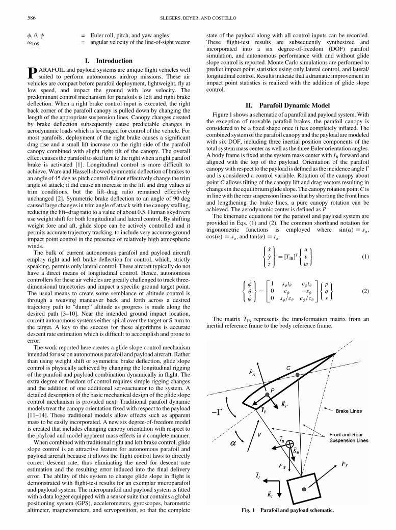
Figure 1 shows a schematic of a parafoil and payload system.Withthe exception of movable parafoil brakes, the parafoil canopy isconsidered to be a fixed shape once it has completely inflated. Thecombined system of the parafoil canopy and the payload aremodeledwith six DOF, including three inertial position components of thetotal systemmass center as well as the three Euler orientation angles.A body frame is fixed at the system mass center with IB forward andaligned with the top of the payload. Orientation of the parafoilcanopywith respect to the payload is defined as the incidence angle�and is considered a control variable. Rotation of the canopy aboutpoint C allows tilting of the canopy lift and drag vectors resulting inchanges in the equilibriumglide slope. The canopy rotation pointC isin linewith the rear suspension lines so that by shorting the front linesand lengthening the brake lines, a pure canopy rotation can beachieved. The aerodynamic center is defined as P.

The kinematic equations for the parafoil and payload system areprovided in Eqs. (1) and (2). The common shorthand notation fortrigonometric functions is employed where sin��� � s�,cos��� � s�, and tan��� � t�.8<

:_x_y_z

9=;� �TIB�T

(uvw

)(1)

8<:

_�_�_

9=;�

1 s�t� c�t�0 c� �s�0 s�=c� c�=c�

24

35(pq

r

)(2)

The matrix TIB represents the transformation matrix from aninertial reference frame to the body reference frame.

Fig. 1 Parafoil and payload schematic.

586 SLEGERS, BEYER, AND COSTELLO

TIB �c�c c�s �s�

s�s�c � c�s s�s�s � c�c s�c�c�s�c � s�s c�s�s � s�c c�c�

24

35 (3)

The dynamic equations are formed by summing forces andmoments about the system mass center both in the body referenceframe and equating to the time derivative of linear and angularmomentum, respectively.

8<:

_u_v_w

9=;� 1

m�FW � FA � FS � FAM� � SB!

(uvw

)(4)

8>><>>:

_p

_q

_r

9>>=>>;� �IT �

�1

0BBB@MA �MAM � SBCG;PFA � SBCG;SFS

� SBCG;MFAM � SB!�IT �

8>><>>:p

q

r

9>>=>>;

1CCCA (5)

The convention is used where the vector cross product of twovectors r� f rx ry rz gT and F� fFx Fy Fz gT both ex-pressed in the A reference frame can be written as

SArF�0 �rz ryrz 0 �rx�ry rx 0

24

358<:FxFyFz

9=; (6)

Forces appearing in Eq. (4) have contributions from weight,aerodynamic loads on the canopy and payload, and apparent mass.Weights contribution is given in Eq. (7).

FW �mg

8<:�s�s�c�c�c�

9=; (7)

Aerodynamic forces on the canopy appearing in Eq. (4) areexpressed in the body reference frame; however, they are a functionof the aerodynamics velocities in the canopy frame. Defining TBC asthe single axis transformation from the body to canopy referenceframe by the incidence angle �, the aerodynamic velocity of theparafoil in the canopy frame is given in Eq. (8).

8<:

~u~v~w

9=;� �TBC�

2664(uvw

)� SB!

0BB@8<:�xc�yc�zc

9=;� �TBC�T

8<:�xp�yp�zp

9=;1CCA

� �TIB�VA=I

3775 (8)

The aerodynamic angles then become �� a tan� ~w= ~u� and�� a sin� ~v=VA�. Equation (9) defines the canopy aerodynamicforces in the body reference frame using TAC as the transformationfrom aerodynamic to canopy frames by the angle �. Payload drag isdefined in a similar manner in Eq. (10), in which uSA, vSA, and wSA

are payload aerodynamic velocities in the body frame.

F A �1

2�V2

ASP�TBC�T �TAC�

8<:

CD0 � CD�2�2CY��

CL0 � CL��� CL�3�3

9=; (9)

F S ��1

2�VSSSCDS

8<:uSAvSAwSA

9=; (10)

Moments appearing in Eq. (5) have contributions fromaerodynamic moments and apparent inertia, and from forces on thecanopy and payload. Aerodynamic moments expressed in the bodyframe are given in Eq. (11).

M A �1

2�V2

ASP�TBC�T

8>><>>:b�Cl��� �b=2VA�Clp ~p� �b=2VA�Clr ~r� � Cl�a��a � �d�

�c�Cm0 � � �c=2VA�Cmq ~q�b�Cn��� �b=2VA�Cnp ~p� �b=2VA�Cnr ~r� � Cn�a��a � �d�

9>>=>>; (11)

A body moving in a fluid places the fluid in motion. The resultfrom accelerating the fluid is a rate of change in both its linear andangular momentum. Typical aircraft having large mass-to-volumeratios have negligible effects from the mass of the accelerating fluid.Parafoils with small mass-to-volume ratios can experience largeforces and moments from accelerating fluid called “apparent mass”and “apparent inertia” because they appear as additional mass andinertia values in the final equations of motion, provided that theireffects are not already covered by the aerodynamic coefficients.Kinetic energy of the fluid can be written as

2T � A ~u2 � B ~v2 � C ~w2 � P ~p2 �Q ~q2 � R ~r2 � 2H� ~u ~q� ~v ~p�(12)

where it is assumed that the canopy has two planes of symmetry, x–zand y–z. Asymmetry about the x–y plane is allowed to account forspanwise camber and the seven constants are defined by Lamb [15].A canopy of general shape may have has many as 21 constantsdefining the kinetic energy, however. Typical parafoil canopies willhave approximately two planes of symmetry reducing to only sevenconstants. If spanwise camber is neglected, the canopy can beapproximated by an ellipsoid so thatH becomes zero. The constantsin Eq. (12) can be calculated numerically for a known shape or can be

SLEGERS, BEYER, AND COSTELLO 587

approximated as discussed in [15–17]. Forces and moments fromapparentmass and inertia are found by relating thefluid’smomentumto its kinetic energy in a similar way as Lissman and Brown [16], andare summarized in Eqs. (13–17). In the apparent mass contributions,it is assumed that the incidence angle is slowly varying so that itsderivative is negligible compared with the body angular rates.

FAM ���TBC�T

0BB@�IAM�

8>><>>:

_~u

_~v

_~w

9>>=>>;� �IH �

8>><>>:

_~p

_~q

_~r

9>>=>>;� S

C! �IAM�

8>><>>:

~u

~v

~w

9>>=>>;

� SC! �IH�

8>><>>:

~p

~q

~r

9>>=>>;

1CCA (13)

MAM ���TBC�T

0BBB@�IH �

8>><>>:

_~u

_~v

_~w

9>>=>>;� �IAI�

8>><>>:

_~p

_~q

_~r

9>>=>>;� S

C! �IH �

8>><>>:

~u

~v

~w

9>>=>>;

� SC! �IAI� � SCVA �IH �

8>><>>:

~p

~q

~r

9>>=>>;

1CCCA (14)

�IAM� �A 0 0

0 B 0

0 0 C

24

35 (15)

�IAI� �P 0 0

0 Q 0

0 0 R

24

35 (16)

�IH � �0 H 0

H 0 0

0 0 0

24

35 (17)

Notice the forces and moments from apparent mass are a function ofthe canopy incidence angle. Equations (13) and (14) couple the linearand rotational dynamic in Eqs. (4) and (5). Final dynamic equationsof motion are found by substituting all forces and moments intoEqs. (4) and (5), resulting in the matrix solution shown in Eqs. (18)and (20). The common convention is used for tensors of second ranksuch that �I0X � � �TBC�T �IX��TBC� for the quantities in Eqs. (15–17).

mI� �I0AM� �I0H � � �I0AM�SBCG;MSBCG;M �I0AM� � �I0H � IT � �I0AI� � �I0H�SBCG;M � SBCG;M��I0H � � �I0AM��SBCG;M

� �8>>>>>>>>><>>>>>>>>>:

_u_v_w. . .

_p_q_r

9>>>>>>>>>=>>>>>>>>>;�

8<:

�

. . .

M

9=; (18)

��FA�Fs�FW �mSB!

8>><>>:u

v

w

9>>=>>;

� �TBC�TSC!

0BBB@�IAM�

8>><>>:

~u

~v

~w

9>>=>>;��IH �

8>><>>:

~p

~q

~r

9>>=>>;

1CCCA� �I0AM�SB!�TIB�VA=I (19)

M�MA � SBCG;PFA � SBCG;SFS � SB!�IT �

8>><>>:p

q

r

9>>=>>;

� SBCG;M �TBC�TSC!

0BBB@�IAM�

8>><>>:

~u

~v

~w

9>>=>>;� �IH �

8>><>>:

~p

~q

~r

9>>=>>;

1CCCA

� �TBC�TSC! �IH �

8>><>>:

~u

~v

~w

9>>=>>;� �TBC�

T�SC! �IAI� � SCVA=I �IH �

�8>><>>:

~p

~q

~r

9>>=>>;

��SBCG;M �I0AM� � �I0H �

�SB!�TIB�VA=I (20)

The matrix in Eq. (18) appears as an inertia matrix and satisfiesmany properties of a typical inertia matrix such as symmetry. In thecase where all apparent mass and inertia effects are negligible,Eq. (18) reduces to a block diagonal system where linear androtational dynamic equations decouple. The effective apparent massand inertia matrices I0AM, I

0H , and I

0AI are functions of the canopy

incidence angle, so that changing the incidence angle for glide slopecontrol results in varying apparent mass and inertia matrices. This isin contrast to conventional models in which apparent mass andinertia coefficients are assumed constant.

III. Test System

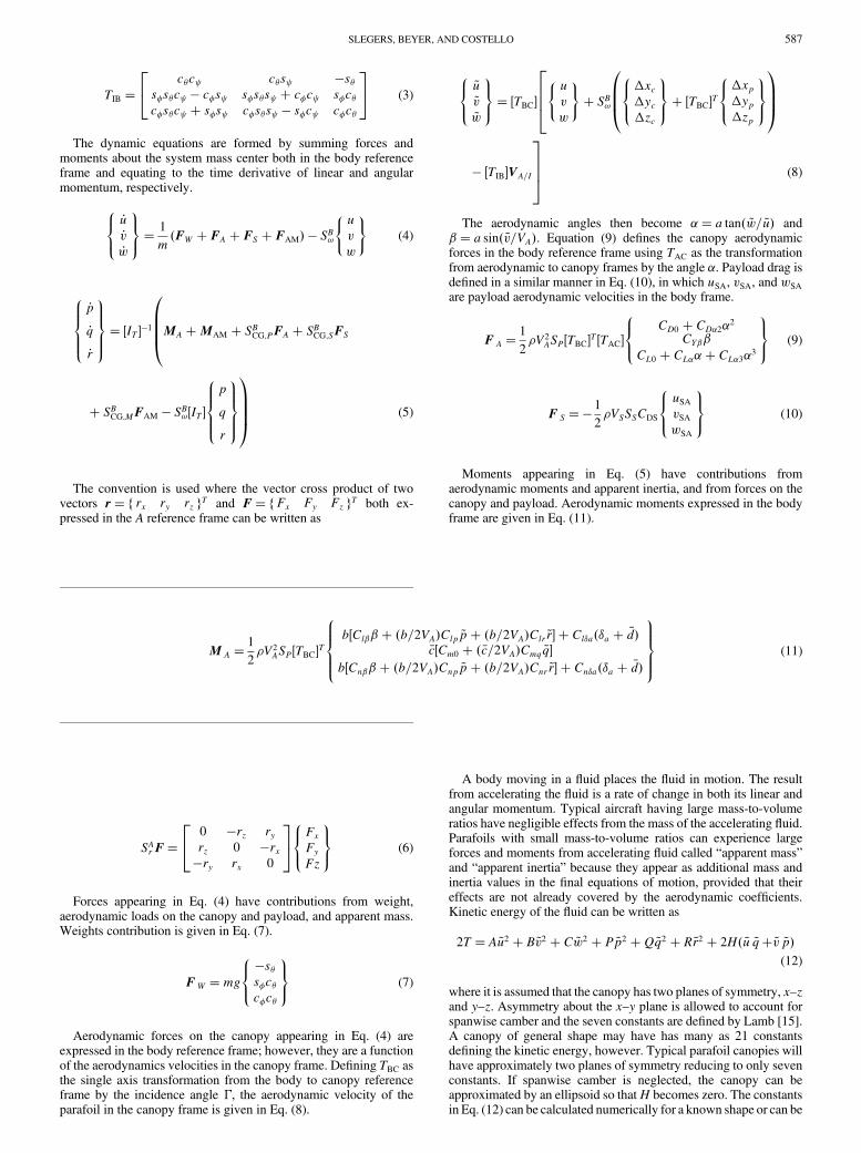
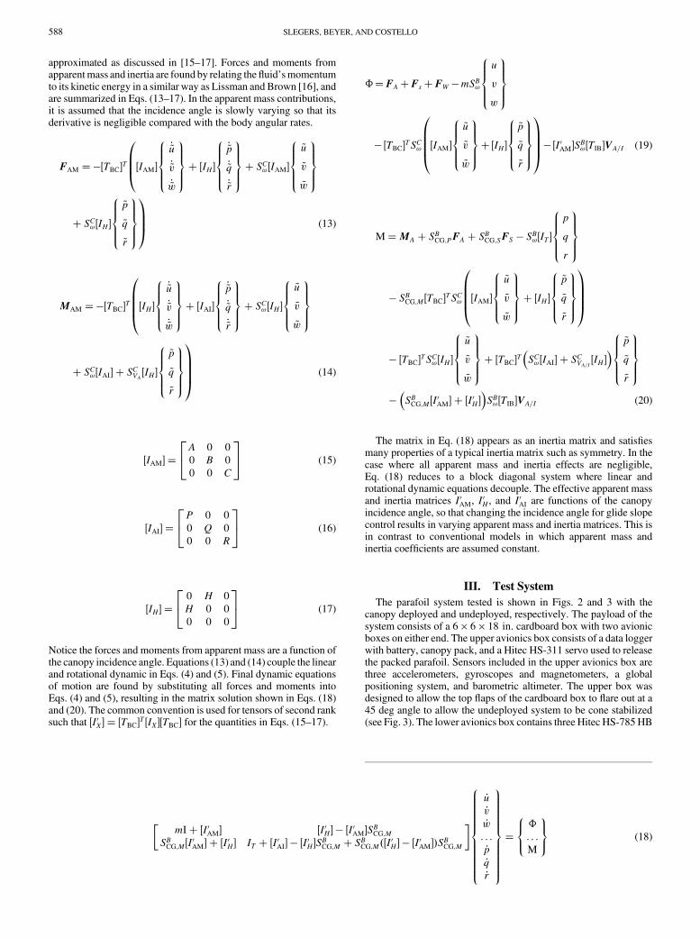
The parafoil system tested is shown in Figs. 2 and 3 with thecanopy deployed and undeployed, respectively. The payload of thesystem consists of a 6 6 18 in: cardboard box with two avionicboxes on either end. The upper avionics box consists of a data loggerwith battery, canopy pack, and a Hitec HS-311 servo used to releasethe packed parafoil. Sensors included in the upper avionics box arethree accelerometers, gyroscopes and magnetometers, a globalpositioning system, and barometric altimeter. The upper box wasdesigned to allow the top flaps of the cardboard box to flare out at a45 deg angle to allow the undeployed system to be cone stabilized(see Fig. 3). The lower avionics box contains three Hitec HS-785HB

588 SLEGERS, BEYER, AND COSTELLO

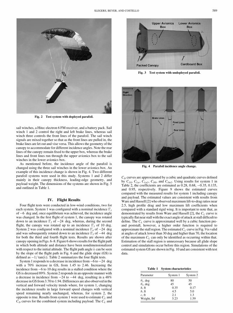
sail winches, a Hitec electron 6 FM receiver, and a battery pack. Sailwinch 1 and 2 control the right and left brake lines, whereas sailwinch three controls the front lines of the parafoil. The sail winchsignals are mixed together so that as the front lines are pulled in, thebrake lines are let out and vise versa. This allows the geometry of thecanopy to accommodate for different incidence angles. Note the rearlines of the canopy remain fixed to the upper box, whereas the brakelines and front lines run through the upper avionics box to the sailwinches in the lower avionics box.

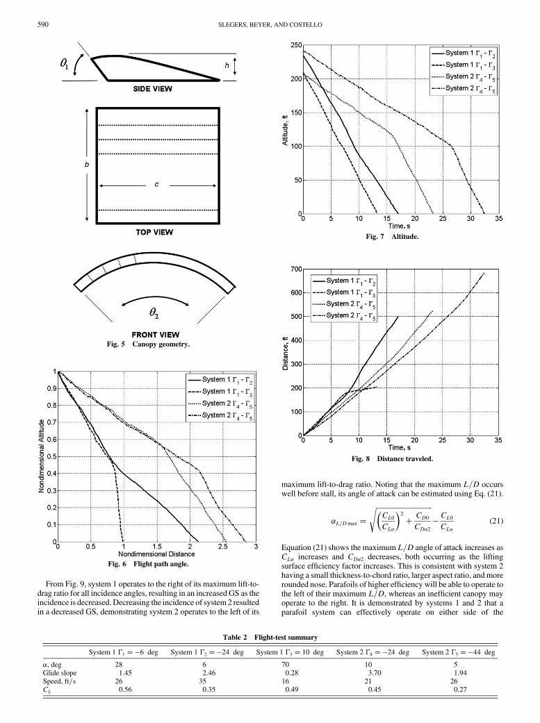
As mentioned before, the incidence angle of the parafoil ischanged using the three sail winches in the lower avionics box. Anexample of this incidence change is shown in Fig. 4. Two differentparafoil systems were used in this study. Systems 1 and 2 differmainly in their canopy thickness, leading-edge geometry, andpayload weight. The dimensions of the systems are shown in Fig. 5and outlined in Table 1.

IV. Flight Results

Four flight tests were conducted in low-wind conditions, two foreach system. System 1 was configured with a nominal incidence �1

of �6 deg and, once equilibrium was achieved, the incidence anglewas changed. In the first flight of system 1, the canopy was rotateddown to an incidence �2 of �24 deg, whereas, during the secondflight, the canopy was rotated up to an incidence �3 of 10 deg.System 2 was configured with a nominal incidence �4 of �24 degand was subsequently rotated down to an incidence �5 of �44 degfor both the third and fourth flight tests. Results are shown aftercanopy opening in Figs. 6–8. Figure 6 shows results for theflight pathin which both altitude and distance have been nondimensionalizedwith respect to the initial altitude. The flight path angle � can be seenby the slope of the flight path in Fig. 6 and the glide slope (GS) isdefined as �1= tan���. Table 2 summarizes the four flight tests.

System 1 responds to a decrease in incidence from�6 to�24 degwith a 70% increase in GS, from 1.45 to 2.46. Increasing theincidence from �6 to 10 deg results in a stalled condition where theGS is decreased 89%. System 2 responds in an opposite manner witha decrease in incidence from �24 to �44 deg, resulting in a 48%decrease inGS from3.70 to 1.94.Differences are also observed in thevertical and forward velocity trends where, for system 1, changingthe incidence results in large forward speed changes with verticalspeed remaining nearly unchanged, whereas, for system 2, theopposite is true. Results from system 1 were used to estimateCL andCD curves for the combined system including payload. The CL and

CD curves are approximated by a cubic and quadratic curves definedby CL0, CL�, CL�3, CD0, and CD�2. Using results for system 1 inTable 2, the coefficients are estimated as 0.28, 0.68, �0:35, 0.135,and 0.95, respectively. Figure 9 shows the estimated curvescompared with the measured results for system 1 including canopyand payload. The estimated values are consistent with results fromWare andHassell [2] who observedmaximum lift-to-drag ratios near2.5, high profile drag and low maximum lift coefficients whencompared with a standard rigid wing. It is important to note that, asdemonstrated by results from Ware and Hassell [2], the CL curve istypicallyflat near stall with the exact angle of attack at stall difficult todefine. The CL curve is approximated well by a cubic function pre-and poststall, however, a higher order function is required toapproximate the stall region. The estimatedCL curve in Fig. 9 is validat angles of attack lower than 30 deg and higher than 70, the locationof the maximum CL can only be identified as occurring within that.Estimation of the stall region is unnecessary because all glide slopecontrol and simulations occur before this region. Simulations of theestimated systemGS are shown in Fig. 10 and are consistent with testdata.

Fig. 2 Test system with deployed parafoil.

Fig. 3 Test system with undeployed parafoil.

Fig. 4 Parafoil incidence angle change.

Table 1 System characteristics

Parameter System 1 System 2

�1, deg 80 50�2, deg 45 45h, ft 0.35 0.17b, ft 4.5 5.0c, ft 2.1 1.3Weight, lbf 5.23 1.59

SLEGERS, BEYER, AND COSTELLO 589

From Fig. 9, system 1 operates to the right of its maximum lift-to-drag ratio for all incidence angles, resulting in an increased GS as theincidence is decreased.Decreasing the incidence of system 2 resultedin a decreased GS, demonstrating system 2 operates to the left of its

maximum lift-to-drag ratio. Noting that the maximum L=D occurswell before stall, its angle of attack can be estimated using Eq. (21).

�L=Dmax �

�����������������������������������CL0CL�

�2

� CD0CD�2

s� CL0CL�

(21)

Equation (21) shows the maximum L=D angle of attack increases asCL� increases and CD�2 decreases, both occurring as the liftingsurface efficiency factor increases. This is consistent with system 2having a small thickness-to-chord ratio, larger aspect ratio, and morerounded nose. Parafoils of higher efficiency will be able to operate tothe left of their maximum L=D, whereas an inefficient canopy mayoperate to the right. It is demonstrated by systems 1 and 2 that aparafoil system can effectively operate on either side of the

Fig. 5 Canopy geometry.

Fig. 6 Flight path angle.

Fig. 7 Altitude.

Fig. 8 Distance traveled.

Table 2 Flight-test summary

System 1 �1 ��6 deg System 1 �2 ��24 deg System 1 �3 � 10 deg System 2 �4 ��24 deg System 2 �5 ��44 deg

�, deg 28 6 70 10 5Glide slope 1.45 2.46 0.28 3.70 1.94Speed, ft=s 26 35 16 21 26CL 0.56 0.35 0.49 0.45 0.27

590 SLEGERS, BEYER, AND COSTELLO

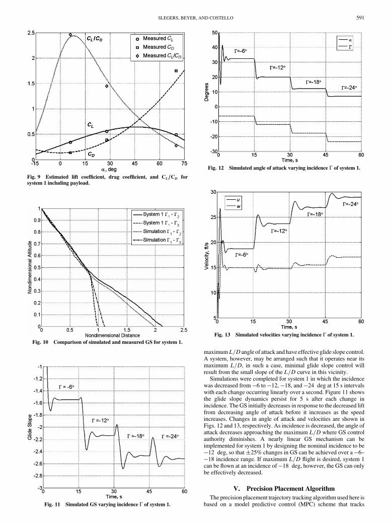
maximumL=D angle of attack and have effective glide slope control.A system, however, may be arranged such that it operates near itsmaximum L=D, in such a case, minimal glide slope control willresult from the small slope of the L=D curve in this vicinity.

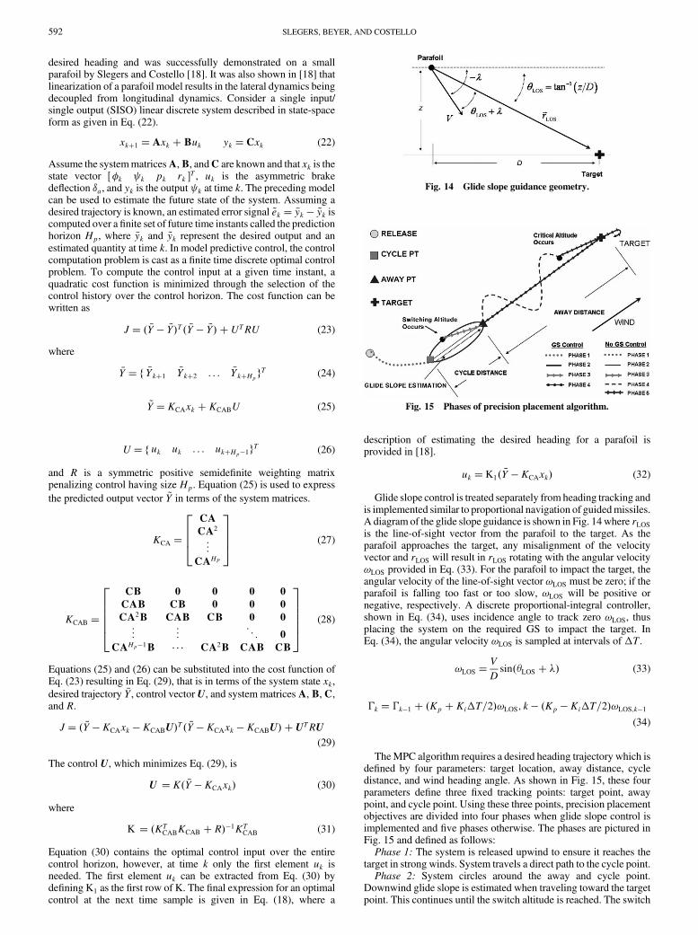
Simulations were completed for system 1 in which the incidencewas decreased from �6 to �12, �18, and �24 deg at 15 s intervalswith each change occurring linearly over a second. Figure 11 showsthe glide slope dynamics persist for 5 s after each change inincidence. TheGS initially decreases in response to the decreased liftfrom decreasing angle of attack before it increases as the speedincreases. Changes in angle of attack and velocities are shown inFigs. 12 and 13, respectively. As incidence is decreased, the angle ofattack decreases approaching the maximum L=D where GS controlauthority diminishes. A nearly linear GS mechanism can beimplemented for system 1 by designing the nominal incidence to be�12 deg, so that25% changes in GS can be achieved over a �6–�18 incidence range. If maximum L=D flight is desired, system 1can be flown at an incidence of�18 deg, however, the GS can onlybe effectively decreased.

V. Precision Placement Algorithm

The precision placement trajectory tracking algorithm used here isbased on a model predictive control (MPC) scheme that tracks

Fig. 9 Estimated lift coefficient, drag coefficient, and CL=CD for

system 1 including payload.

Fig. 10 Comparison of simulated and measured GS for system 1.

Fig. 11 Simulated GS varying incidence � of system 1.

Fig. 12 Simulated angle of attack varying incidence � of system 1.

Fig. 13 Simulated velocities varying incidence � of system 1.

SLEGERS, BEYER, AND COSTELLO 591

desired heading and was successfully demonstrated on a smallparafoil by Slegers and Costello [18]. It was also shown in [18] thatlinearization of a parafoil model results in the lateral dynamics beingdecoupled from longitudinal dynamics. Consider a single input/single output (SISO) linear discrete system described in state-spaceform as given in Eq. (22).

xk�1 �Axk �Buk yk �Cxk (22)

Assume the systemmatricesA,B, andC are known and that xk is thestate vector ��k k pk rk �T , uk is the asymmetric brakedeflection �a, and yk is the output k at time k. The preceding modelcan be used to estimate the future state of the system. Assuming adesired trajectory is known, an estimated error signal ~ek � �yk � ~yk iscomputed over a finite set of future time instants called the predictionhorizon Hp, where �yk and ~yk represent the desired output and anestimated quantity at time k. In model predictive control, the controlcomputation problem is cast as a finite time discrete optimal controlproblem. To compute the control input at a given time instant, aquadratic cost function is minimized through the selection of thecontrol history over the control horizon. The cost function can bewritten as

J� � �Y � ~Y�T� �Y � ~Y� �UTRU (23)

where

�Y � f �Yk�1 �Yk�2 . . . �Yk�HpgT (24)

~Y � KCAxk � KCABU (25)

U� f uk uk . . . uk�Hp�1gT (26)

and R is a symmetric positive semidefinite weighting matrixpenalizing control having size Hp. Equation (25) is used to express

the predicted output vector ~Y in terms of the system matrices.

KCA �

CACA2

..

.

CAHP

2664

3775 (27)

KCAB �

CB 0 0 0 0CAB CB 0 0 0CA2B CAB CB 0 0

..

. ... . .

.0

CAHp�1B � � � CA2B CAB CB

266664

377775 (28)

Equations (25) and (26) can be substituted into the cost function ofEq. (23) resulting in Eq. (29), that is in terms of the system state xk,desired trajectory �Y, control vector U, and system matricesA,B,C,and R.

J� � �Y � KCAxk � KCABU�T� �Y � KCAxk � KCABU� � UTRU(29)

The control U, which minimizes Eq. (29), is

U � K� �Y � KCAxk� (30)

where

K � �KTCABKCAB � R��1KTCAB (31)

Equation (30) contains the optimal control input over the entirecontrol horizon, however, at time k only the first element uk isneeded. The first element uk can be extracted from Eq. (30) bydefiningK1 as the first row ofK. The final expression for an optimalcontrol at the next time sample is given in Eq. (18), where a

description of estimating the desired heading for a parafoil isprovided in [18].

uk � K1� �Y � KCAxk� (32)

Glide slope control is treated separately from heading tracking andis implemented similar to proportional navigation of guidedmissiles.A diagram of the glide slope guidance is shown in Fig. 14where rLOSis the line-of-sight vector from the parafoil to the target. As theparafoil approaches the target, any misalignment of the velocityvector and rLOS will result in rLOS rotating with the angular velocity!LOS provided in Eq. (33). For the parafoil to impact the target, theangular velocity of the line-of-sight vector !LOS must be zero; if theparafoil is falling too fast or too slow, !LOS will be positive ornegative, respectively. A discrete proportional-integral controller,shown in Eq. (34), uses incidence angle to track zero !LOS, thusplacing the system on the required GS to impact the target. InEq. (34), the angular velocity !LOS is sampled at intervals of �T.

!LOS �V

Dsin��LOS � �� (33)

�k � �k�1 � �Kp � Ki�T=2�!LOS; k � �Kp � Ki�T=2�!LOS;k�1

(34)

TheMPC algorithm requires a desired heading trajectory which isdefined by four parameters: target location, away distance, cycledistance, and wind heading angle. As shown in Fig. 15, these fourparameters define three fixed tracking points: target point, awaypoint, and cycle point. Using these three points, precision placementobjectives are divided into four phases when glide slope control isimplemented and five phases otherwise. The phases are pictured inFig. 15 and defined as follows:

Phase 1: The system is released upwind to ensure it reaches thetarget in strong winds. System travels a direct path to the cycle point.

Phase 2: System circles around the away and cycle point.Downwind glide slope is estimated when traveling toward the targetpoint. This continues until the switch altitude is reached. The switch

Fig. 14 Glide slope guidance geometry.

Fig. 15 Phases of precision placement algorithm.

592 SLEGERS, BEYER, AND COSTELLO

altitude is defined as the distance to the target divided by theestimated glide slope plus an excess altitude. Excess altitude is onlyrequired when glide slope control is absent. Excess altitude allowsthe system to turn to the target early, because when GS control isabsent, the effective GS cannot be increased, only reduced, byswerving.

Phase 3: System travels directly to the away point. Glide slopeestimation is terminated.

Phase 4: With no GS control, system continues glide slopeestimation. At each update time, the distance to the target and adistance towaste are calculated.MPC turns left and right, tracking an“S” trajectory generated by waypoints to waste an appropriatedistance to impact the target. With GS control, at each update time,the angular velocity of the line-of-sight vector!LOS is calculated anda proportional-integral controller regulates it to zero. MPC tracks apath directly to the target.

Phase 5: The system flies directly to the target once a criticalaltitude is achieved.

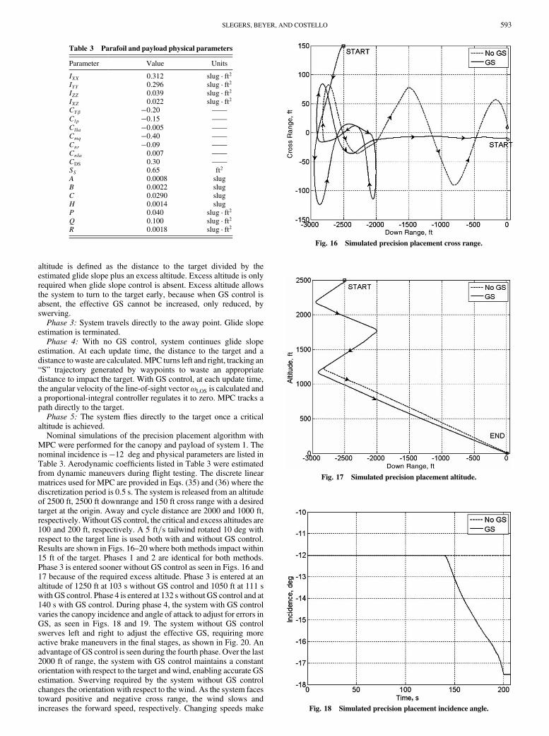
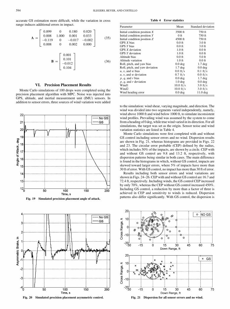
Nominal simulations of the precision placement algorithm withMPC were performed for the canopy and payload of system 1. Thenominal incidence is �12 deg and physical parameters are listed inTable 3. Aerodynamic coefficients listed in Table 3 were estimatedfrom dynamic maneuvers during flight testing. The discrete linearmatrices used for MPC are provided in Eqs. (35) and (36) where thediscretization period is 0.5 s. The system is released from an altitudeof 2500 ft, 2500 ft downrange and 150 ft cross range with a desiredtarget at the origin. Away and cycle distance are 2000 and 1000 ft,respectively.Without GS control, the critical and excess altitudes are100 and 200 ft, respectively. A 5 ft=s tailwind rotated 10 deg withrespect to the target line is used both with and without GS control.Results are shown in Figs. 16–20 where both methods impact within15 ft of the target. Phases 1 and 2 are identical for both methods.Phase 3 is entered sooner without GS control as seen in Figs. 16 and17 because of the required excess altitude. Phase 3 is entered at analtitude of 1250 ft at 103 s without GS control and 1050 ft at 111 swith GS control. Phase 4 is entered at 132 swithout GS control and at140 s with GS control. During phase 4, the system with GS controlvaries the canopy incidence and angle of attack to adjust for errors inGS, as seen in Figs. 18 and 19. The system without GS controlswerves left and right to adjust the effective GS, requiring moreactive brake maneuvers in the final stages, as shown in Fig. 20. Anadvantage of GS control is seen during the fourth phase. Over the last2000 ft of range, the system with GS control maintains a constantorientation with respect to the target and wind, enabling accurate GSestimation. Swerving required by the system without GS controlchanges the orientation with respect to the wind. As the system facestoward positive and negative cross range, the wind slows andincreases the forward speed, respectively. Changing speeds make

Table 3 Parafoil and payload physical parameters

Parameter Value Units

IXX 0.312 slug � ft2IYY 0.296 slug � ft2IZZ 0.039 slug � ft2IXZ 0.022 slug � ft2CY� �0:20 ——

Clp �0:15 ——

Cl�a �0:005 ——

Cmq �0:40 ——

Cnr �0:09 ——

Cn�a 0.007 ——

CDS 0.30 ——

SS 0.65 ft2

A 0.0008 slugB 0.0022 slugC 0.0290 slugH 0.0014 slugP 0.040 slug � ft2Q 0.100 slug � ft2R 0.0018 slug � ft2

Fig. 16 Simulated precision placement cross range.

Fig. 17 Simulated precision placement altitude.

Fig. 18 Simulated precision placement incidence angle.

SLEGERS, BEYER, AND COSTELLO 593

accurate GS estimation more difficult, while the variation in crossrange induces additional errors in impact.

A �

0:899 0 0:180 0:0200:008 1:000 0:001 0:033�0:119 0 �0:017 �0:0020:008 0 0:002 0:000

2664

3775 (35)

B �

0:0010:101�0:0120:104

2664

3775 (36)

VI. Precision Placement Results

Monte Carlo simulations of 100 drops were completed using theprecision placement algorithm with MPC. Noise was injected intoGPS, altitude, and inertial measurement unit (IMU) sensors. Inaddition to sensor errors, three sources of wind variation were added

to the simulation: wind shear, varying magnitude, and direction. Thewind was divided into two segments varied independently, namely,wind above 1000 ft and wind below 1000 ft, to simulate inconsistentwind profiles. Prevailing wind was assumed by the system to comefrom a heading of 0 deg,while truewind varied in its direction. For allsimulations, the target was set as the origin. Sensor noise and windvariation statistics are listed in Table 4.

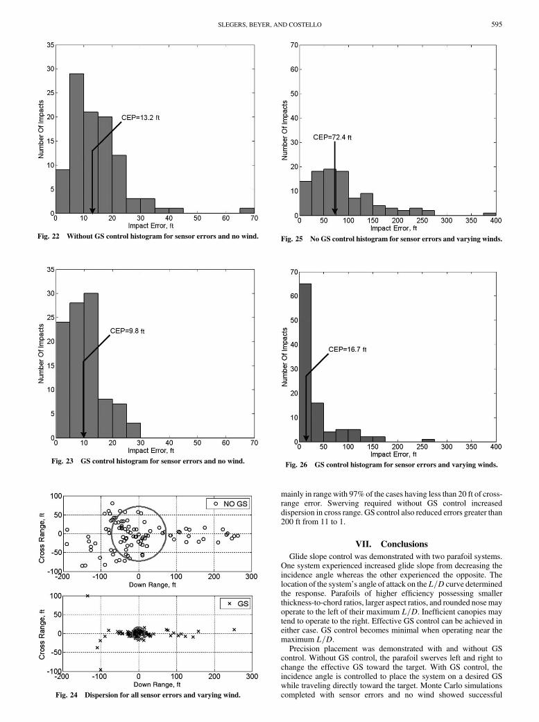
Monte Carlo simulations were first completed with and withoutGS control including sensor errors and no wind. Dispersion resultsare shown in Fig. 21, whereas histograms are provided in Figs. 22and 23. The circular error probable (CEP) defined by the radius,which includes 50% of the impacts, are shown by a circle. CEP withand without GS control are 9.8 and 13.2 ft, respectively, withdispersion patterns being similar in both cases. The main differenceis found in the histograms in which, without GS control, impacts areskewed toward larger errors, where 5% of impacts have more than30 ft of error.WithGS control, no impact hasmore than 30 ft of error.

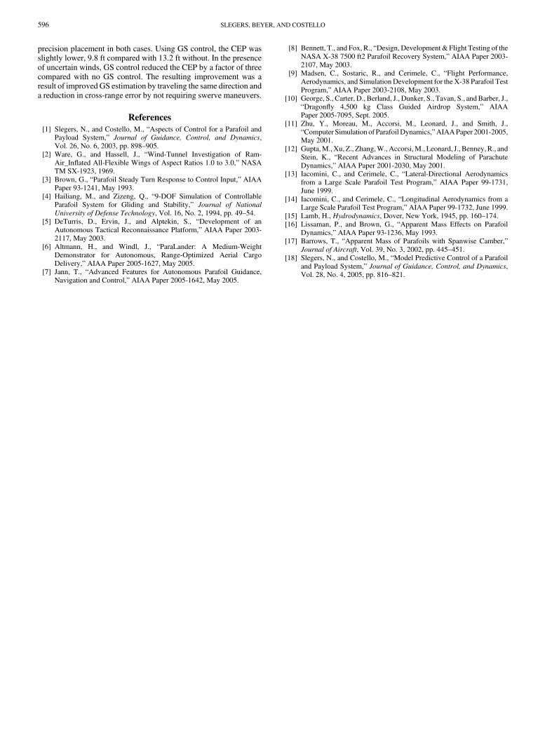
Results including both sensor errors and wind variations areshown in Figs. 24–26. CEPwith andwithout GS control are 16.7 and72.4 ft, respectively. Including winds, the GS control CEP increasedby only 70%, whereas the CEP without GS control increased 450%.Including GS control, a reduction by more than a factor of three isachieved in CEP and sensitivity to winds is reduced. Dispersionpatterns also differ significantly. With GS control, the dispersion is

Fig. 19 Simulated precision placement angle of attack.

Fig. 20 Simulated precision placement asymmetric control.

Table 4 Error statistics

Parameter Mean Standard deviation

Initial condition position X 3500 ft 750 ftInitial condition position Y 0 ft 750 ftInitial condition position Z 4500 ft 750 ftGPS X bias 0.0 ft 3.0 ftGPS Y bias 0.0 ft 3.0 ftGPS X deviation 1.0 ft 0.0 ftGPS Y deviation 1.0 ft 0.0 ftAltitude bias 0.0 ft 5.0 ftAltitude variation 1.0 ft 0.0 ftRoll, pitch, and yaw bias 0.0 deg 1.7 degRoll, pitch, and yaw deviation 1.7 deg 0.0 degu, v, and w bias 0:0 ft=s 0:1 ft=su, v, and w deviation 0:7 ft=s 0:0 ft=sp, q, and r bias 0.0 deg 1.7 degp, q, and r deviation 1.0 deg 0.0 degWind1 10:0 ft=s 3:0 ft=sWind2 10:0 ft=s 3:0 ft=sWind heading error 0.0 deg 11.0 deg

Fig. 21 Dispersion for all sensor errors and no wind.

594 SLEGERS, BEYER, AND COSTELLO

mainly in range with 97% of the cases having less than 20 ft of cross-range error. Swerving required without GS control increaseddispersion in cross range. GS control also reduced errors greater than200 ft from 11 to 1.

VII. Conclusions

Glide slope control was demonstrated with two parafoil systems.One system experienced increased glide slope from decreasing theincidence angle whereas the other experienced the opposite. Thelocation of the system’s angle of attack on theL=D curve determinedthe response. Parafoils of higher efficiency possessing smallerthickness-to-chord ratios, larger aspect ratios, and rounded nosemayoperate to the left of their maximum L=D. Inefficient canopies maytend to operate to the right. Effective GS control can be achieved ineither case. GS control becomes minimal when operating near themaximum L=D.

Precision placement was demonstrated with and without GScontrol. Without GS control, the parafoil swerves left and right tochange the effective GS toward the target. With GS control, theincidence angle is controlled to place the system on a desired GSwhile traveling directly toward the target. Monte Carlo simulationscompleted with sensor errors and no wind showed successful

Fig. 22 Without GS control histogram for sensor errors and no wind.

Fig. 23 GS control histogram for sensor errors and no wind.

Fig. 24 Dispersion for all sensor errors and varying wind.

Fig. 25 No GS control histogram for sensor errors and varying winds.

Fig. 26 GS control histogram for sensor errors and varying winds.

SLEGERS, BEYER, AND COSTELLO 595

precision placement in both cases. Using GS control, the CEP wasslightly lower, 9.8 ft compared with 13.2 ft without. In the presenceof uncertain winds, GS control reduced the CEP by a factor of threecompared with no GS control. The resulting improvement was aresult of improvedGS estimation by traveling the same direction anda reduction in cross-range error by not requiring swerve maneuvers.

References

[1] Slegers, N., and Costello, M., “Aspects of Control for a Parafoil andPayload System,” Journal of Guidance, Control, and Dynamics,Vol. 26, No. 6, 2003, pp. 898–905.

[2] Ware, G., and Hassell, J., “Wind-Tunnel Investigation of Ram-Air_Inflated All-Flexible Wings of Aspect Ratios 1.0 to 3.0,” NASATM SX-1923, 1969.

[3] Brown, G., “Parafoil Steady Turn Response to Control Input,” AIAAPaper 93-1241, May 1993.

[4] Hailiang, M., and Zizeng, Q., “9-DOF Simulation of ControllableParafoil System for Gliding and Stability,” Journal of National

University of Defense Technology, Vol. 16, No. 2, 1994, pp. 49–54.[5] DeTurris, D., Ervin, J., and Alptekin, S., “Development of an

Autonomous Tactical Reconnaissance Platform,” AIAA Paper 2003-2117, May 2003.

[6] Altmann, H., and Windl, J., “ParaLander: A Medium-WeightDemonstrator for Autonomous, Range-Optimized Aerial CargoDelivery,” AIAA Paper 2005-1627, May 2005.

[7] Jann, T., “Advanced Features for Autonomous Parafoil Guidance,Navigation and Control,” AIAA Paper 2005-1642, May 2005.

[8] Bennett, T., and Fox, R., “Design, Development & Flight Testing of theNASA X-38 7500 ft2 Parafoil Recovery System,” AIAA Paper 2003-2107, May 2003.

[9] Madsen, C., Sostaric, R., and Cerimele, C., “Flight Performance,Aerodynamics, and Simulation Development for the X-38 Parafoil TestProgram,” AIAA Paper 2003-2108, May 2003.

[10] George, S., Carter, D., Berland, J., Dunker, S., Tavan, S., andBarber, J.,“Dragonfly 4,500 kg Class Guided Airdrop System,” AIAAPaper 2005-7095, Sept. 2005.

[11] Zhu, Y., Moreau, M., Accorsi, M., Leonard, J., and Smith, J.,“Computer Simulation of Parafoil Dynamics,”AIAAPaper 2001-2005,May 2001.

[12] Gupta,M.,Xu, Z., Zhang,W.,Accorsi,M., Leonard, J., Benney,R., andStein, K., “Recent Advances in Structural Modeling of ParachuteDynamics,” AIAA Paper 2001-2030, May 2001.

[13] Iacomini, C., and Cerimele, C., “Lateral-Directional Aerodynamicsfrom a Large Scale Parafoil Test Program,” AIAA Paper 99-1731,June 1999.

[14] Iacomini, C., and Cerimele, C., “Longitudinal Aerodynamics from aLarge Scale Parafoil Test Program,” AIAA Paper 99-1732, June 1999.

[15] Lamb, H., Hydrodynamics, Dover, New York, 1945, pp. 160–174.[16] Lissaman, P., and Brown, G., “Apparent Mass Effects on Parafoil

Dynamics,” AIAA Paper 93-1236, May 1993.[17] Barrows, T., “Apparent Mass of Parafoils with Spanwise Camber,”

Journal of Aircraft, Vol. 39, No. 3, 2002, pp. 445–451.[18] Slegers, N., and Costello, M., “Model Predictive Control of a Parafoil

and Payload System,” Journal of Guidance, Control, and Dynamics,Vol. 28, No. 4, 2005, pp. 816–821.

596 SLEGERS, BEYER, AND COSTELLO