Useful Notes for the Lorentz Group

O. Preliminary Comments about linear transformations of vector spaces

We study vectorial quantities, such as velocity, momentum, force, etc. We need to be able

to combine different velocities, and also other systems of vectors of the same type; therefore, we

visualize them as being elements of vector spaces. We can describe these vectors, for instance,

via sets of numbers, which we think of as the components of these vectors relative to some

choice of basis vectors. One can then suppose that it is desirable to make a change in this

choice of basis vectors, which would then create a transformation of the components of the

vectors. Such a change does not, of course, change the underlying physics of the situation.

It is then important to understand sets of such transformations, which we can visualize

in terms of (sets of) matrices acting on the vector spaces. In these notes we will consider a

very important such set of transformations, namely the entire Lorentz group, which describe

changes of basis corresponding to different, allowed inertial observers. This set contains pure

rotations, pure Lorentz boosts, i.e., changes of observers, moving with distinct velocities, and

also products of such transformations. Physically, the insistence on products is just a way of

saying we may want to make more than one of these transformations at a time, in order to

create a desirable set of basis vectors.

We will begin by simply describing the rotations as they are easily perceived in 3-dimensional

space, before we proceed onward to the entire (4-dimensional) spacetime, embedding the ro-

tations into spacetime rather easily, and then looking at other transformations in that 4-

dimensional situation. Each of these sets of transformations is described by a set of parameters

that are allowed to vary continuously—and smoothly, remembering that smoothly means arbi-

trarily often differentiable—from one value to another of the parameters, in some appropriate

parameter space. Such an entire set of transformations can be viewed in two quite different

ways, which must be required to be consistent.

a. Since there are many of these transformations it is important that products of them also

be transformations. Since one could surely always not bother to perform a transformation

at all, an “identity” transformation must be included in the set, which does nothing to

the vectors in question. Lastly, since there is an identity there must be a way to move

backward toward doing nothing, after having done something; this is the same as saying

that there must be an inverse transformation to each and every transformation we consider.

A set of objects which satisfies the above notions, and which also has a product which is

associative, is called a group. That our transformations are associative follows from the

fact that they are transformations of elements of a vector space, of course preserving that

structure, and therefore linear, which makes them associative.

b. However, since the parameters are required to vary in a continuous manner, one can

conceive of the complete parameter space as a manifold with the parameters as (local)

coordinates on it. Therefore we have a manifold which is also a group. Such groups are

referred to as Lie groups, named for Sophus Lie who first studied them extensively.

Because some of the parameters may not vary continuously, an example being the deter-

minant of a matrix, then it is often the case that the manifold in question comes in more

than one connected part.

Although it could be that one is studying such transformations acting in a single vector

space, it is usually the case that there is an underlying physical manifold, i.e., the place where

“we live,” and there are several distinct vector spaces at each and every point on that manifold,

which in these notes we will refer to as spacetime, which has a local set of Cartesian coordinates,

{x, y, z, t} ≡ {r, t} defined on it, among other possible choices for coordinates there. There

are different sorts of vector spaces at each point, to accommodate different sorts of tensors

that one wants to study and/or measure at each coordinate point in spacetime, such as one

for 4-vectors, one for type [0,2] tensors, etc. For any particular sort of vector space the set of

all of them together, over different spacetime points in some neighborhood is referred to as a

vector bundle.

Since these transformations are linear transformations in the vector spaces defined at each

point of the spacetime manifold, just as we traditionally describe vectors, and other tensors, in

2

terms of their components, relative to a given, well-understood, fixed choice of a (complete) set

of basis vectors, we will also want to describe these transformations in terms of the components

of more complicated tensors which act on those components. The traditional way to do that

is via presentations of those components in terms of matrices which then act on the matrices

containing the components of the vectors, all of course still relative to a given, fixed choice

of basis set for the vector space(s) in question. Before we will be able to do that, we must

distinguish between two rather different ways to present transformations of vectors in a vector

space, and make a choice as to which mode we will use here: the so-called “passive” and

“active” modes of thinking about them. To describe these two modes, we begin with the

picture of a vector space along with a set of basis vectors, and some particular vector, A.

a. In the “passive” approach we hold the vector fixed, and rotate the set of axes. This

makes sense from the point of view that the vectors are actually not changed simply

because someone has chosen to pick some different set of basis vectors, i.e., ones that have

been rotated relative to the original ones.

This is the most commonly-used approach in classical physics, especially mechanics.

b. In the “active” approach, on the other hand, the vector is considered the physical

quantity of interest, and therefore it is the object that should be rotated. The basis set is

actually not physical, after all, and we shouldn’t waste our time rotating them.

This is the most common approach in quantum mechanics, where it is the “state vectors”

on which attention is concentrated. It could also be used to describe measurements of a

single vector made by two distinct allowed observers.

Either approach describes the rotations, in a very generic sense, in the same way. However, it

should be clear that any particular rotation in one mode is the inverse of that rotation viewed

in the other mode. To make that even more clear, suppose we rotate the vector and also rotate

the basis vectors, then nothing will have really changed in the sense that the components are

still the same as before. In any event, when making explicit analytic calculations, a decision

must be made as to which approach is to be used, and, of course, only that choice must then be

3

followed. In these notes I intend to follow the passive approach, leaving the vectors unchanged,

but allowing one to choose many different allowed sets of basis vectors, related to each other

in various ways, and then considering the resulting changes of the components of vectors,

when they are presented in the form, usually, of column vectors, i.e., matrices with only one

column. This will arrange it so that the group elements, i.e., the transformation operators will

be presented as square matrices.

I. The Rotation Group, in 3-dimensional space

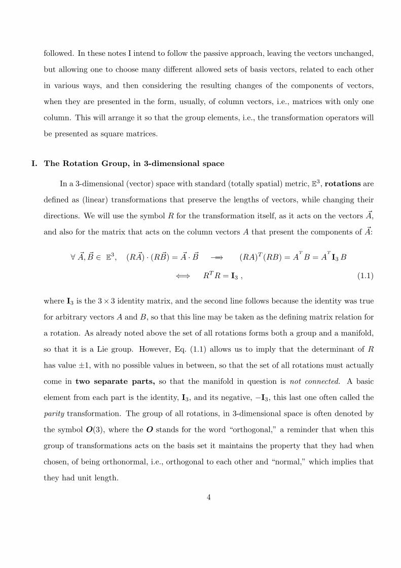
In a 3-dimensional (vector) space with standard (totally spatial) metric, E3, rotations are

defined as (linear) transformations that preserve the lengths of vectors, while changing their

directions. We will use the symbol R for the transformation itself, as it acts on the vectors A,

and also for the matrix that acts on the column vectors A that present the components of A:

∀ A, B ∈ E3, (RA) · (RB) = A · B =−→ (RA)T (RB) = AT

B = AT

I3 B

⇐⇒ RTR = I3 , (1.1)

where I3 is the 3× 3 identity matrix, and the second line follows because the identity was true

for arbitrary vectors A and B, so that this line may be taken as the defining matrix relation for

a rotation. As already noted above the set of all rotations forms both a group and a manifold,

so that it is a Lie group. However, Eq. (1.1) allows us to imply that the determinant of R

has value ±1, with no possible values in between, so that the set of all rotations must actually

come in two separate parts, so that the manifold in question is not connected. A basic

element from each part is the identity, I3, and its negative, −I3, this last one often called the

parity transformation. The group of all rotations, in 3-dimensional space is often denoted by

the symbol O(3), where the O stands for the word “orthogonal,” a reminder that when this

group of transformations acts on the basis set it maintains the property that they had when

chosen, of being orthonormal, i.e., orthogonal to each other and “normal,” which implies that

they had unit length.

4

The subset with determinant +1 is, separately, a group, since the product of two +1’s is also

+1; therefore, it constitutes a subgroup of all rotations, called SO(3), where the S stands for

the word “special.” It is also usual to refer to the elements of this subgroup as proper rotations;

this language means that one excludes those with negative determinant. Of course the set with

determinant −1 is not a subgroup, i.e., a group all by itself, since the product of two of them

lies in the other part.

A common choice of parameters to specify a rotation can be found by saying that we

“rotate through some angle θ, about some axis, n,” giving rise to the notation R(θ, n), where

we use the (standard) “right-hand rule” to define the sign of the angle in question. That is,

when the thumb of the right hand points in the direction of n, then as the fingers curl closed

they are moving in the direction of positive values of θ. Notice then that the rotation in

question is invariant when one both reverses the direction of n and switches the sign of θ. The

axis in question is of course only a direction, and so has only two degrees of freedom, which we

could specify, for instance, by giving its spherical coordinates, say (ϑ, φ), so that we see that

three degrees of freedom are necessary to specify a rotation. (Since the direction is most easily

specified by a unit vector, some people also use the notation θ ≡ θ n to specify a particular

direction.

One might normally have thought of the angle of rotation as some positive value between 0

and 2π. However, there is an approach that creates a better “visualization” of the manifold of

all possible rotations, with positive determinant, in other words the manifold already named as

SO(3). We surely can agree that it is an equivalent description of such an angle by subtracting

off π, so that the range for θ varies, instead, from −π to +π. Then, for those values that are

positive, with n taking on all possible directions, we may treat the value of θ as the length of a

vector pointing in the direction n away from the origin, the set of all of these rotations will fill

an entire ball of radius π. [Note that the word “ball” is intended to mean a “solid sphere,” i.e., a

sphere along with its interior.] This would appear to be troublesome since we have now ignored

all those angles which are negative. However if one changes both the sign of the angle and

5

the sign of the axis of rotation, this amounts to no change at all, i.e., R(θ, n) = R(−n;−θ).

This is a “counting problem” with this parametrization where one actually counts all the

rotations twice; therefore, if θ is negative, this correspondence gives us a different rotation

with a positive angle, in the opposite direction. By only including angles from 0 to π and

allowing all possible directions for n we are in fact only counting each rotation once, except

for a separate duplication problem when one rotates half way around, i.e., when the value for

the angle is θ = π. It is clear that we have an additional double counting problem in this

instance because R(n;π) = R(n;−π), i.e., both rotations bring us to the same place, so that

they are in fact completely equivalent. These two rotations of course occur on the boundary of

our ball; in fact they are best seen as at the opposite ends of any arbitrary diameter of our ball,

i.e., any straight line through the center. (I note that the pair of points at opposite ends of a

diameter are usually referred to as antipodal points.) Therefore our manifold for the rotation

group, which seemed fairly normal so far, is in fact a “little bit strange, since the apparently

two points at opposite ends of any diameter, in fact constitute only one point, so that the

manifold is in fact a curved space.

Because of this particular problem with the manifold it is sufficiently curved that it is not

possible to view it in its entirety in a straightforward way in the 3-dimensional space in which

we live, unless one simply says that every pair of antipodal points must be “identified” as the

same point. Such a manifold is referred to as “doubly connected,” which has the following

meaning. There are two distinct closed paths from any point, and back again, that cannot be

deformed into each other. As examples, consider a circular path that goes from the origin (of

the group, or of the ball, since those are the same point on the manifold) around on a circle

of diameter less than π, say, perhaps, π/2. By slowly changing the diameter from this value

to zero, in a continuous way, we deform that circular path into one which did not move at all.

On the other hand, now consider a path that goes, up along the z-axis, say, all the way to the

boundary of the ball, at the North pole. However, the North pole is exactly the same point

as the South pole, because of our identification of antipodal points. Therefore, now the path

6

proceeds from the South pole back along the z-axis to the origin again. This is obviously a

closed path; however, if we try to change the radius to become smaller we no longer have this

identification of points so that such a change cannot be made. This is the second closed path,

not deformable to the first one.

Having created a “visualization” of the manifold SO(3), our next step is to define explicit

presentations, using 3 × 3 matrices, for the action of these rotations, R(θ, n), in our vector

space. We remember that it has been agreed that we will use the passive approach to this,

where it is actually the basis set that is being rotated, and we ask what changes this creates

in the components of the vector, which has remained fixed during the rotation. Pretending

that we have inserted here a figure, suppose we have a 2-dimensional plane, with the usual

{x, y}-axes, and a vector A drawn in the plane, in the first quadrant, making some positive

angle α with the x-axis which is less than π/2. If I now rotate—about the z-axis—the axes

shown in this figure by some positive angle, since the vector is in the first quadrant, the angle

α will decrease, as the x-axis approaches the location of A. At the same time, the complement

of that angle, which is the angle with respect to the y-axis, originally π/2 − α, will increase.

Choosing the vector A to have unit length, for simplicity, this allows us to see that the correct

matrix presentation for such a transformation would be the following:

A =−→ A =

cosαsinα0

, R(θ, z) =−→

cos θ +sin θ 0− sin θ cos θ 0

0 0 1

,

=⇒ RA =

cos θ +sin θ 0− sin θ cos θ 0

0 0 1

cosαsinα0

=

cosα cos θ + sinα sin θ− cosα sin θ + sinα cos θ

0

=

cos(α− θ)sin(α− θ)

0

.

(1.2)

The expression above was very straightforward, except possibly for where the minus sign goes

in the matrix. It was by way of determining that sign that this discussion was given in such

detail, as well as the discussion relative to passive and active modes of presentation for the

transformations.

7

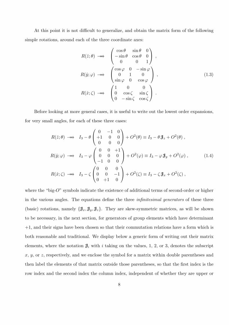
At this point it is not difficult to generalize, and obtain the matrix form of the following

simple rotations, around each of the three coordinate axes:

R(z; θ) =−→

cos θ sin θ 0− sin θ cos θ 0

0 0 1

,

R(y;φ) =−→

cosφ 0 − sinφ0 1 0

sinφ 0 cosφ

,

R(x; ζ) =−→

1 0 00 cos ζ sin ζ0 − sin ζ cos ζ

.

(1.3)

Before looking at more general cases, it is useful to write out the lowest order expansions,

for very small angles, for each of these three cases:

R(z; θ) =−→ I3 − θ

0 −1 0+1 0 00 0 0

+O2(θ) ≡ I3 − θ Jz +O2(θ) ,

R(y;φ) =−→ I3 − φ

0 0 +10 0 0−1 0 0

+O2(φ) ≡ I3 − φJy +O2(φ) ,

R(x; ζ) =−→ I3 − ζ

0 0 00 0 −10 +1 0

+O2(ζ) ≡ I3 − ζ Jx +O2(ζ) ,

(1.4)

where the “big-O” symbols indicate the existence of additional terms of second-order or higher

in the various angles. The equations define the three infinitesimal generators of these three

(basic) rotations, namely {Jx,Jy,Jz}. They are skew-symmetric matrices, as will be shown

to be necessary, in the next section, for generators of group elements which have determinant

+1, and their signs have been chosen so that their commutation relations have a form which is

both reasonable and traditional. We display below a generic form of writing out their matrix

elements, where the notation Ji with i taking on the values, 1, 2, or 3, denotes the subscript

x, y, or z, respectively, and we enclose the symbol for a matrix within double parentheses and

then label the elements of that matrix outside those parentheses, so that the first index is the

row index and the second index the column index, independent of whether they are upper or

8

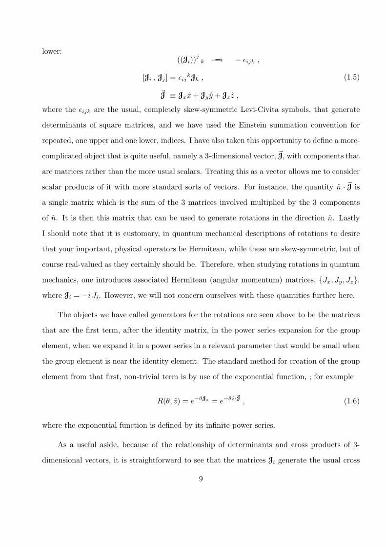
lower:((Ji))

jk =−→ − ϵijk ,

[Ji , Jj ] = ϵijkJk ,

J ≡ Jxx+ Jy y + Jz z ,

(1.5)

where the ϵijk are the usual, completely skew-symmetric Levi-Civita symbols, that generate

determinants of square matrices, and we have used the Einstein summation convention for

repeated, one upper and one lower, indices. I have also taken this opportunity to define a more-

complicated object that is quite useful, namely a 3-dimensional vector, J, with components that

are matrices rather than the more usual scalars. Treating this as a vector allows me to consider

scalar products of it with more standard sorts of vectors. For instance, the quantity n · J is

a single matrix which is the sum of the 3 matrices involved multiplied by the 3 components

of n. It is then this matrix that can be used to generate rotations in the direction n. Lastly

I should note that it is customary, in quantum mechanical descriptions of rotations to desire

that your important, physical operators be Hermitean, while these are skew-symmetric, but of

course real-valued as they certainly should be. Therefore, when studying rotations in quantum

mechanics, one introduces associated Hermitean (angular momentum) matrices, {Jx, Jy, Jz},

where Ji = −i Ji. However, we will not concern ourselves with these quantities further here.

The objects we have called generators for the rotations are seen above to be the matrices

that are the first term, after the identity matrix, in the power series expansion for the group

element, when we expand it in a power series in a relevant parameter that would be small when

the group element is near the identity element. The standard method for creation of the group

element from that first, non-trivial term is by use of the exponential function, ; for example

R(θ, z) = e−θJz = e−θz·J , (1.6)

where the exponential function is defined by its infinite power series.

As a useful aside, because of the relationship of determinants and cross products of 3-

dimensional vectors, it is straightforward to see that the matrices Ji generate the usual cross

9

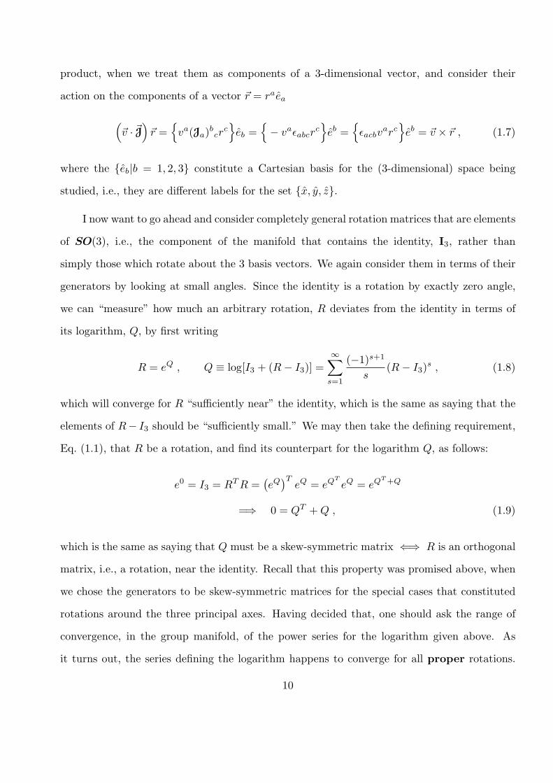
product, when we treat them as components of a 3-dimensional vector, and consider their

action on the components of a vector r = raea

(v · J

)r =

{va(Ja)

bcr

c}eb =

{− vaϵabcr

c}eb =

{ϵacbv

arc}eb = v × r , (1.7)

where the {eb|b = 1, 2, 3} constitute a Cartesian basis for the (3-dimensional) space being

studied, i.e., they are different labels for the set {x, y, z}.

I now want to go ahead and consider completely general rotation matrices that are elements

of SO(3), i.e., the component of the manifold that contains the identity, I3, rather than

simply those which rotate about the 3 basis vectors. We again consider them in terms of their

generators by looking at small angles. Since the identity is a rotation by exactly zero angle,

we can “measure” how much an arbitrary rotation, R deviates from the identity in terms of

its logarithm, Q, by first writing

R = eQ , Q ≡ log[I3 + (R− I3)] =∞∑s=1

(−1)s+1

s(R− I3)

s , (1.8)

which will converge for R “sufficiently near” the identity, which is the same as saying that the

elements of R− I3 should be “sufficiently small.” We may then take the defining requirement,

Eq. (1.1), that R be a rotation, and find its counterpart for the logarithm Q, as follows:

e0 = I3 = RTR =(eQ

)TeQ = eQ

T

eQ = eQT+Q

=⇒ 0 = QT +Q , (1.9)

which is the same as saying that Q must be a skew-symmetric matrix ⇐⇒ R is an orthogonal

matrix, i.e., a rotation, near the identity. Recall that this property was promised above, when

we chose the generators to be skew-symmetric matrices for the special cases that constituted

rotations around the three principal axes. Having decided that, one should ask the range of

convergence, in the group manifold, of the power series for the logarithm given above. As

it turns out, the series defining the logarithm happens to converge for all proper rotations.

10

However, this is certainly not true for general Lie groups where the range of convergence

is usually smaller than the entire, connected group, and simply requires fairly sophisticated

calculations to determine the range of convergence.

In general, in n dimensional space, a skew-symmetric matrix has 12n(n − 1) degrees of

freedom. In our 3-dimensional space, this tells us that there are exactly 3 independent degrees

of freedom to skew-symmetric matrices, so that it is also true that

a. again, we have shown that the group of all (3-dimensional) proper rotations has exactly 3

degrees of freedom.

b. The 3 skew-symmetric matrices, Ji, already presented in Eq. (1.3), constitute a choice

of basis for the vector space of all Q’s; i.e. any skew-symmetric 3 × 3 matrix is a linear

combination of those 3 matrices, say aJx + bJy + cJz ≡ θ · J. The 3 scalars {a, b, c} may

then be thought of as the components of a vector θ, which is a choice of parametrization

for all proper rotations, as we already briefly mentioned. However, it seemed simpler to

us, above, and more convenient to separate out the direction and magnitude of θ ≡ θn, so

that Q = θn · J.

c. The vector space which is the set of all possible skew-symmetric matrices Q is referred

to as the Lie algebra for the rotation group. One may think of it as the derivatives,

with respect to the set of parameters, of group elements which are then evaluated at the

identity element. From that point of view the Lie algebra is the tangent vector space, i.e.,

the set of all directional derivatives, at the identity of the group manifold. In general, for

any Lie group, this tangent vector space at the identity is its associated Lie algebra.

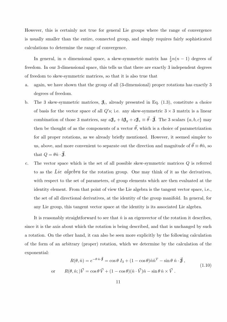
It is reasonably straightforward to see that n is an eigenvector of the rotation it describes,

since it is the axis about which the rotation is being described, and that is unchanged by such

a rotation. On the other hand, it can also be seen more explicitly by the following calculation

of the form of an arbitrary (proper) rotation, which we determine by the calculation of the

exponential:

R(θ, n) = e−θ n·J = cos θ I3 + (1− cos θ)nnT − sin θ n · J ,

or R(θ, n; )V = cos θ V + (1− cos θ)(n · V )n− sin θ n× V .

(1.10)

11

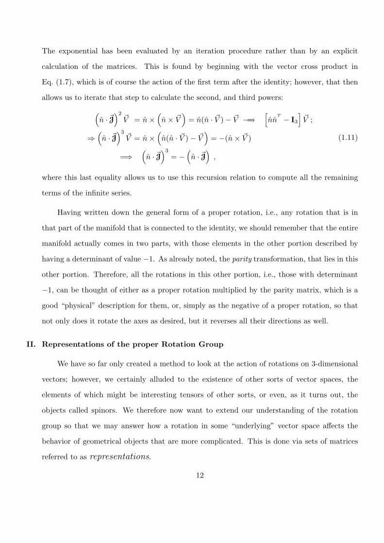
The exponential has been evaluated by an iteration procedure rather than by an explicit

calculation of the matrices. This is found by beginning with the vector cross product in

Eq. (1.7), which is of course the action of the first term after the identity; however, that then

allows us to iterate that step to calculate the second, and third powers:(n · J

)2

V = n×(n× V

)= n(n · V )− V =−→

[nn

T

− I3

]V ;

⇒(n · J

)3

V = n×(n(n · V )− V

)= −(n× V )

=⇒(n · J

)3

= −(n · J

),

(1.11)

where this last equality allows us to use this recursion relation to compute all the remaining

terms of the infinite series.

Having written down the general form of a proper rotation, i.e., any rotation that is in

that part of the manifold that is connected to the identity, we should remember that the entire

manifold actually comes in two parts, with those elements in the other portion described by

having a determinant of value −1. As already noted, the parity transformation, that lies in this

other portion. Therefore, all the rotations in this other portion, i.e., those with determinant

−1, can be thought of either as a proper rotation multiplied by the parity matrix, which is a

good “physical” description for them, or, simply as the negative of a proper rotation, so that

not only does it rotate the axes as desired, but it reverses all their directions as well.

II. Representations of the proper Rotation Group

We have so far only created a method to look at the action of rotations on 3-dimensional

vectors; however, we certainly alluded to the existence of other sorts of vector spaces, the

elements of which might be interesting tensors of other sorts, or even, as it turns out, the

objects called spinors. We therefore now want to extend our understanding of the rotation

group so that we may answer how a rotation in some “underlying” vector space affects the

behavior of geometrical objects that are more complicated. This is done via sets of matrices

referred to as representations.

12

A representation of a group is a (continuous) mapping that sends each element of the

group into a continuous linear operator that acts on some vector space, and which preserves

the group product. An irreducible representation is one which does not leave invariant any

proper subspace of the vector space on which it acts. One may also have representations

of the Lie algebra of a Lie group. The requirement that this be a representation is similar,

namely that the mapping preserve the commutation relations of the algebra elements. As

it is a vector space it is of course sufficient to simply preserve the commutation relations of

the basis vectors. Given a representation of the Lie group, the view of the Lie algebra as its

tangent vector space at the identity allows one to easily calculate the representation of the Lie

algebra that is associated with that representation of the group, just by taking appropriate

derivatives in the parameter space. On the other hand, given a representation of the Lie

algebra the exponential series acting on that representation may not give a representation of

the Lie group; instead, depending on the representation, the result of exponentiation may be a

representation of a larger group, instead. That larger group is the so-called universal covering

group of the original group. In general the universal covering group has an n to 1 mapping

down to the original group, where n is the number of non-equivalent closed paths one can draw

in the group manifold, which is often referred to by saying that the group is n-ly connected.

The rotation group, as an example of a compact group, has some nice properties for its

irreducible representations, which we do not prove here but simply quote, from well-established

sources, since we actually only need to make use of the results rather than the proofs.

a. We first recall that the rotation group is doubly connected. Therefore it has a universal

covering group which is larger than itself; that group is SU(2), the group of all 2 × 2,

unitary, complex-valued matrices that have determinant +1. See more discussion of this

group and its 2 → 1 mapping onto the rotation group below, after the description of the

j = 12 representation.

b. All the irreducible representations are in terms of finite-dimensional matrices.

c. The matrices in question are all unitary, which is of course the same as orthogonal when the

matrix elements are all real-valued. There is exactly one irreducible representation

13

for each finite dimension, n. It is customary to label these representations not by n,

however, but by the value of j, where n ≡ 2j + 1; the value of j is often called the “spin”

of the representation. In the case that j is an integer then there is a choice of basis for the

matrices such that they have only real-valued elements. When j is, instead, a half-integer,

so that the matrices are even-dimensional the matrices are not true representations, but,

instead representations of SU(2), so that there is a 2 to 1 mapping back to the rotation

group itself.

c. There are also infinite-dimensional representations, created from infinite sums or integrals

of irreducible ones, which are best visualized as unitary operators on some appropriate

space of functions, which is best thought of as infinite-dimensional vector space.

We will denote an arbitrary (unitary) representation of the rotation group, by U , so that the

linear operators which are its values can be denoted by U(R), or U [R(θ, n)], or, perhaps, as a

sometimes-shorthand, just by U(n; θ). As already noted, a representation of the group can be

used to determine, uniquely, a representation of the Lie algebra of that group, since the Lie

algebra are just the generators of the group near the identity. Denoting the generators by Ji

we can write, for any choice of axis, n,

U [R(θ, n)] = e−θn·J . (2.1)

n · J = − limθ→0

1

θ

{U [R(θ, n)]− I

}= − d

dθU [R(n; θ)]

∣∣∣∣θ=0

. (2.2)

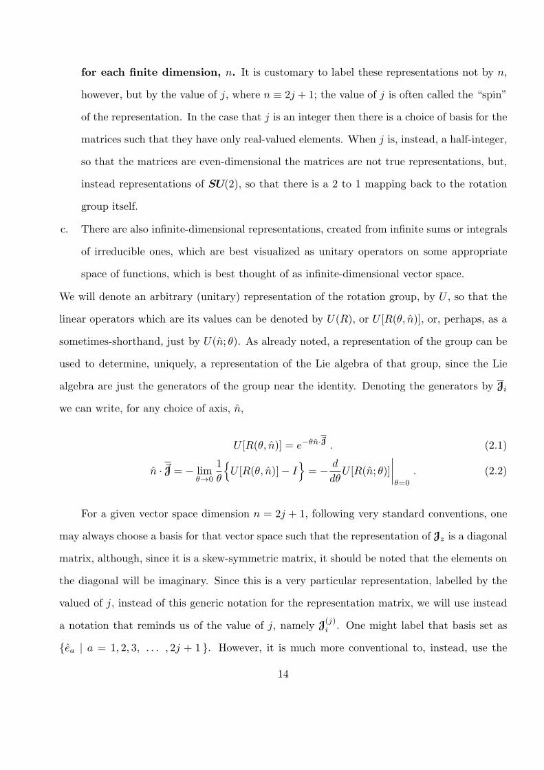
For a given vector space dimension n = 2j + 1, following very standard conventions, one

may always choose a basis for that vector space such that the representation of Jz is a diagonal

matrix, although, since it is a skew-symmetric matrix, it should be noted that the elements on

the diagonal will be imaginary. Since this is a very particular representation, labelled by the

valued of j, instead of this generic notation for the representation matrix, we will use instead

a notation that reminds us of the value of j, namely J(j)i . One might label that basis set as

{ea | a = 1, 2, 3, . . . , 2j + 1 }. However, it is much more conventional to, instead, use the

14

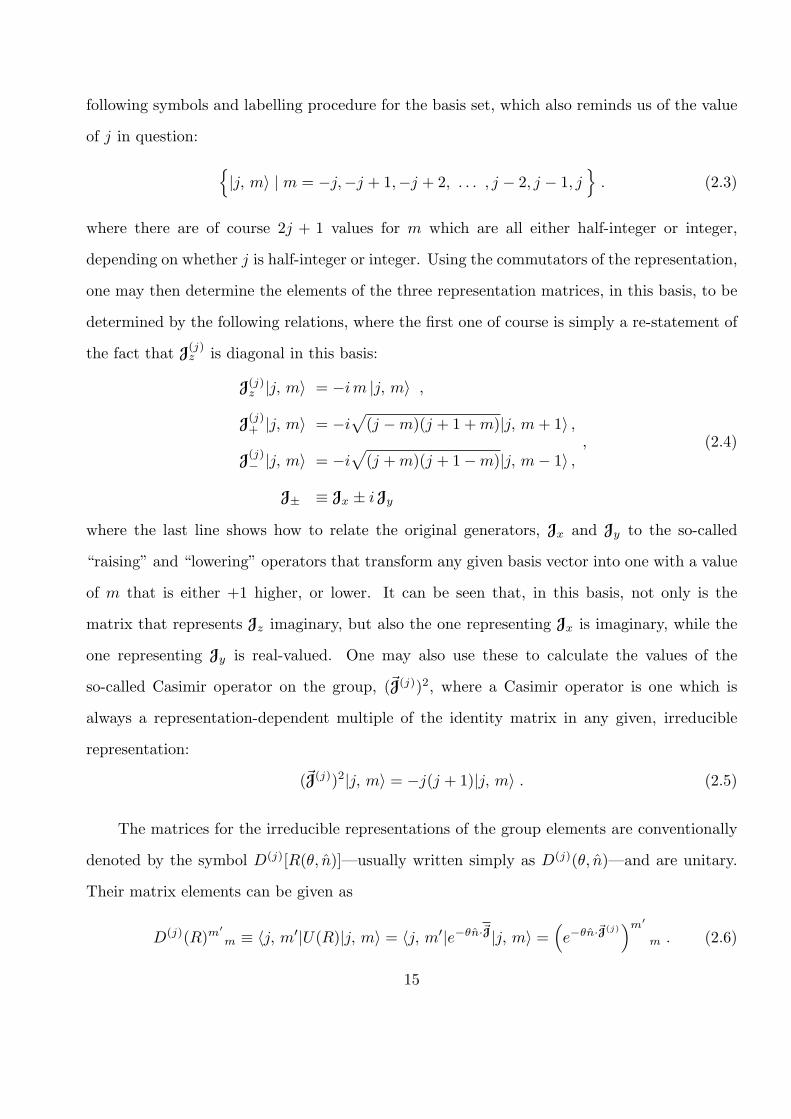
following symbols and labelling procedure for the basis set, which also reminds us of the value

of j in question: {|j, m⟩ | m = −j,−j + 1,−j + 2, . . . , j − 2, j − 1, j

}. (2.3)

where there are of course 2j + 1 values for m which are all either half-integer or integer,

depending on whether j is half-integer or integer. Using the commutators of the representation,

one may then determine the elements of the three representation matrices, in this basis, to be

determined by the following relations, where the first one of course is simply a re-statement of

the fact that J(j)z is diagonal in this basis:

J(j)z |j, m⟩ = −im |j, m⟩ ,

J(j)+ |j, m⟩ = −i

√(j −m)(j + 1 +m)|j, m+ 1⟩ ,

J(j)− |j, m⟩ = −i

√(j +m)(j + 1−m)|j, m− 1⟩ ,

J± ≡ Jx ± iJy

, (2.4)

where the last line shows how to relate the original generators, Jx and Jy to the so-called

“raising” and “lowering” operators that transform any given basis vector into one with a value

of m that is either +1 higher, or lower. It can be seen that, in this basis, not only is the

matrix that represents Jz imaginary, but also the one representing Jx is imaginary, while the

one representing Jy is real-valued. One may also use these to calculate the values of the

so-called Casimir operator on the group, (J(j))2, where a Casimir operator is one which is

always a representation-dependent multiple of the identity matrix in any given, irreducible

representation:

(J(j))2|j, m⟩ = −j(j + 1)|j, m⟩ . (2.5)

The matrices for the irreducible representations of the group elements are conventionally

denoted by the symbol D(j)[R(θ, n)]—usually written simply as D(j)(θ, n)—and are unitary.

Their matrix elements can be given as

D(j)(R)m′

m ≡ ⟨j, m′|U(R)|j, m⟩ = ⟨j, m′|e−θn·J|j, m⟩ =(e−θn·J(j)

)m′

m . (2.6)

15

1. The case j = 1.

Using the formulae above, we easily find that

J(1)z =−→ − i

1 0 00 0 00 0 −1

, J(1)x =−→ −i√

2

0 1 01 0 10 1 0

, J(1)y =−→ 1√

2

0 −1 01 0 −10 1 0

.

(2.7)

Since these are 3 × 3 matrices, and there is only one irreducible representation for each di-

mension, one might wonder why these matrices are distinct from the 3 × 3 matrices given in

Eqs. (1.4). The answer is that they are equivalent, via a similarity transformation, to those

others; more precisely, the matrices in Eqs. (1.4) are relative to a Cartesian basis set, while

these are relative to a basis in which Jz is diagonal. Finding the eigenvectors for the Cartesian

presentation of Jz, and making the standard choices about signs and normalizations, one finds

the following relationships between the two basis sets:

|1, 0⟩ = z , |1, 1⟩ = −1√2(x+ iy) , |1, −1⟩ = +1√

2(x− iy) . (2.8)

2. The case j = 12 .

In this case, the vector space is only 2-dimensional, and the representations of the gener-

ators are

J( 12 )

z = − i2

(+1 00 −1

), J

( 12 )

x = − i2

(0 +1

+1 0

), J

( 12 )

y = − i2

(0 −i+i 0

), (2.9)

where these three matrices are just a factor of −i/2 times the standard three Pauli matrices,

usually called σi. By explicit calculation of the exponential of these, one finds that

D( 12 )[R(θ, n)] = cos(θ/2) I2 − n · J( 1

2 ) sin(θ/2) . (2.10)

It is therefore immediately clear that

D( 12)(n; 2π) = −I2 , ∀n , (2.11)

which makes it clear that this is not a faithful representation of SO(3).

16

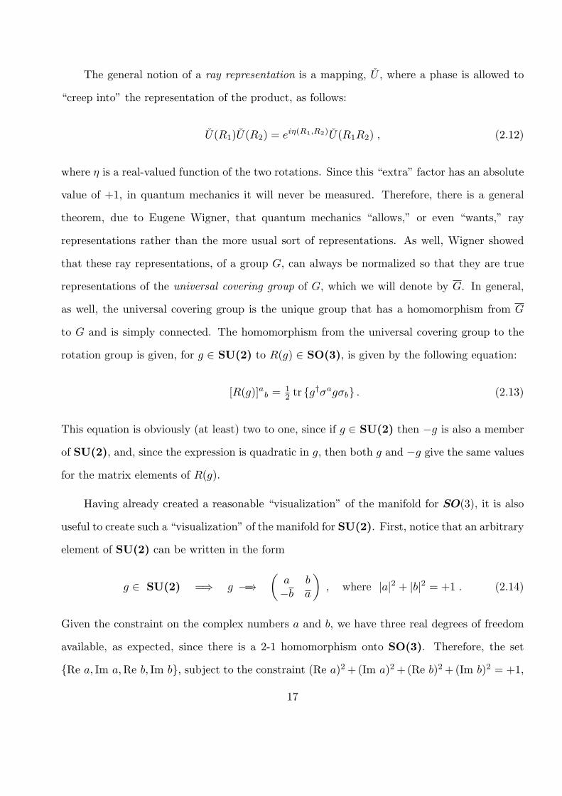
The general notion of a ray representation is a mapping, U , where a phase is allowed to

“creep into” the representation of the product, as follows:

U(R1)U(R2) = eiη(R1,R2)U(R1R2) , (2.12)

where η is a real-valued function of the two rotations. Since this “extra” factor has an absolute

value of +1, in quantum mechanics it will never be measured. Therefore, there is a general

theorem, due to Eugene Wigner, that quantum mechanics “allows,” or even “wants,” ray

representations rather than the more usual sort of representations. As well, Wigner showed

that these ray representations, of a group G, can always be normalized so that they are true

representations of the universal covering group of G, which we will denote by G. In general,

as well, the universal covering group is the unique group that has a homomorphism from G

to G and is simply connected. The homomorphism from the universal covering group to the

rotation group is given, for g ∈ SU(2) to R(g) ∈ SO(3), is given by the following equation:

[R(g)]ab =12 tr {g

†σagσb} . (2.13)

This equation is obviously (at least) two to one, since if g ∈ SU(2) then −g is also a member

of SU(2), and, since the expression is quadratic in g, then both g and −g give the same values

for the matrix elements of R(g).

Having already created a reasonable “visualization” of the manifold for SO(3), it is also

useful to create such a “visualization” of the manifold for SU(2). First, notice that an arbitrary

element of SU(2) can be written in the form

g ∈ SU(2) =⇒ g =−→(

a b−b a

), where |a|2 + |b|2 = +1 . (2.14)

Given the constraint on the complex numbers a and b, we have three real degrees of freedom

available, as expected, since there is a 2-1 homomorphism onto SO(3). Therefore, the set

{Re a, Im a,Re b, Im b}, subject to the constraint (Re a)2+(Im a)2+(Re b)2+(Im b)2 = +1,

17

constitutes a set of three real parameters to describe the group. However, the constraint equa-

tion is clearly just the equation for the (surface of the) sphere S3, i.e., the 3-dimensional sphere

in 4-dimensional flat space. Looking back at Eq. (2.11) which says that the ray-representation

of the rotation by 2π is the same no matter what is the direction of the associated axis. There-

fore, a reasonable way to think about this sphere is that the origin is the North pole, and the

rotation by 2π is the South pole. This also makes sense because of the fact that a rotation by

4π is represented by the identity matrix, again. Notice as well that the surface of a sphere,

in whatever number of dimensions, is simply connected, so that this group would be its own

universal covering group.

3. The case j = 0.

In that case the matrices that represent the rotations are just 1-dimensional, i.e., just

numbers, and the matrices that represent the generators are skew-symmetric numbers, i.e.,

numbers that equal their own negatives. There is only one such number, namely 0, and the

exponential of zero is just +1. Therefore, as might should have been expected, this is the

completely trivial representation where every group element is simply represented by +1. Yes,

it’s a representation, but not at all interesting.

III. Description of the Lorentz Group

One could just say that the Lorentz group is the set of all “orthogonal” transformations

of vectors defined over spacetime, where here the fact that “orthogonal” means preserving

lengths is “translated” to mean that it preserves the metric value of the length of a vector in

spacetime. This approach would give us the name O(3, 1) for the Lorentz group, where the

two integers after the orthogonality statement give us the number of spacelike directions and

the number of timelike directions. A more explicit approach to this generic statement would

be to remind ourselves about the metric in spacetime and the explicit matrix presentation of

it and the transformations, in a manner very similar to the procedure used in Eq. (1.1) above,

except that now the metric is not just the Cartesian one, but the Minkowski one, where we

18

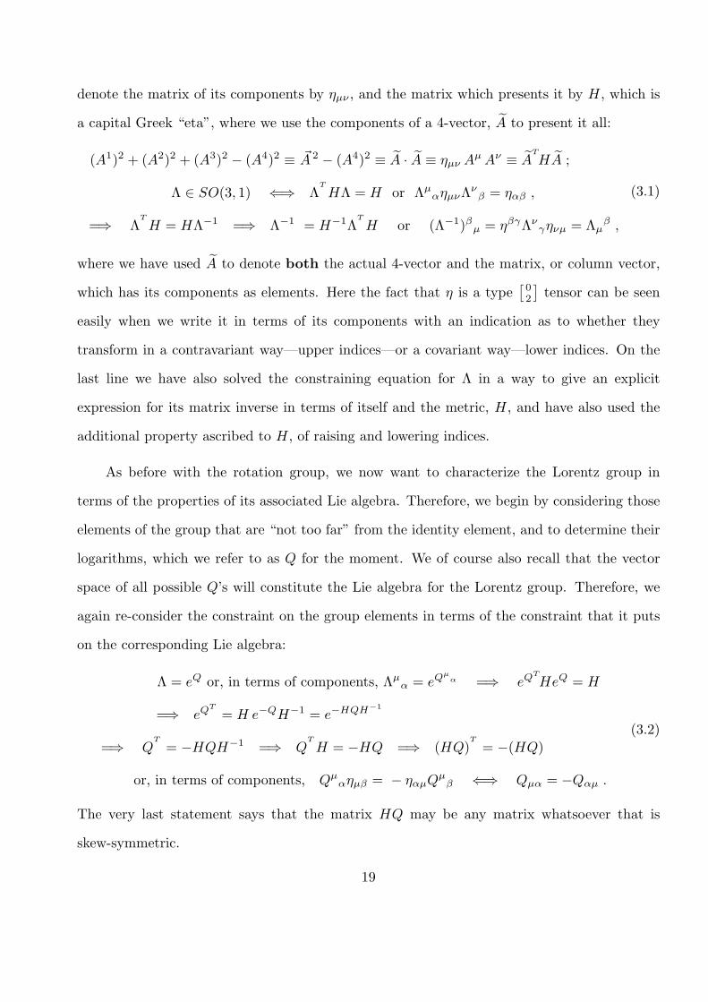
denote the matrix of its components by ηµν , and the matrix which presents it by H, which is

a capital Greek “eta”, where we use the components of a 4-vector, A to present it all:

(A1)2 + (A2)2 + (A3)2 − (A4)2 ≡ A 2 − (A4)2 ≡ A · A ≡ ηµν Aµ Aν ≡ A

T

HA ;

Λ ∈ SO(3, 1) ⇐⇒ ΛT

HΛ = H or ΛµαηµνΛ

νβ = ηαβ ,

=⇒ ΛT

H = HΛ−1 =⇒ Λ−1 = H−1ΛT

H or (Λ−1)βµ = ηβγΛνγηνµ = Λµ

β ,

(3.1)

where we have used A to denote both the actual 4-vector and the matrix, or column vector,

which has its components as elements. Here the fact that η is a type[02

]tensor can be seen

easily when we write it in terms of its components with an indication as to whether they

transform in a contravariant way—upper indices—or a covariant way—lower indices. On the

last line we have also solved the constraining equation for Λ in a way to give an explicit

expression for its matrix inverse in terms of itself and the metric, H, and have also used the

additional property ascribed to H, of raising and lowering indices.

As before with the rotation group, we now want to characterize the Lorentz group in

terms of the properties of its associated Lie algebra. Therefore, we begin by considering those

elements of the group that are “not too far” from the identity element, and to determine their

logarithms, which we refer to as Q for the moment. We of course also recall that the vector

space of all possible Q’s will constitute the Lie algebra for the Lorentz group. Therefore, we

again re-consider the constraint on the group elements in terms of the constraint that it puts

on the corresponding Lie algebra:

Λ = eQ or, in terms of components, Λµα = eQ

µα =⇒ eQ

T

HeQ = H

=⇒ eQT

= H e−QH−1 = e−HQH−1

=⇒ QT

= −HQH−1 =⇒ QT

H = −HQ =⇒ (HQ)T

= −(HQ)

or, in terms of components, Qµαηµβ = − ηαµQ

µβ ⇐⇒ Qµα = −Qαµ .

(3.2)

The very last statement says that the matrix HQ may be any matrix whatsoever that is

skew-symmetric.

19

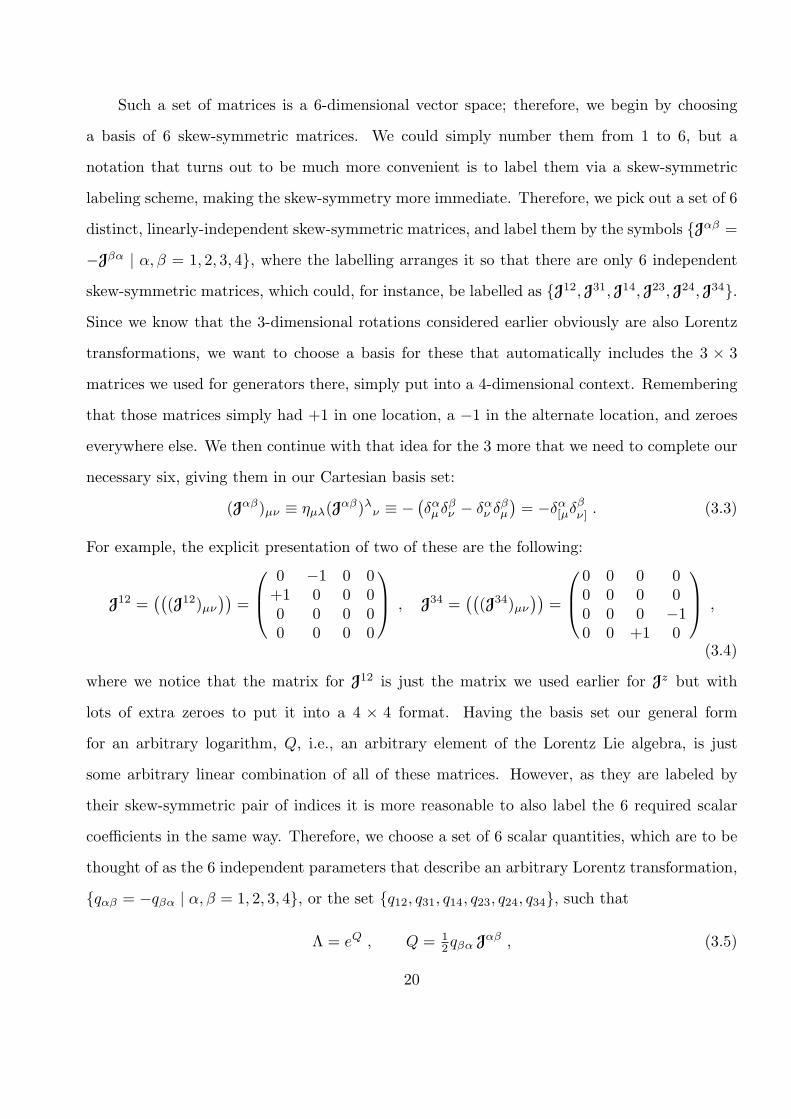
Such a set of matrices is a 6-dimensional vector space; therefore, we begin by choosing

a basis of 6 skew-symmetric matrices. We could simply number them from 1 to 6, but a

notation that turns out to be much more convenient is to label them via a skew-symmetric

labeling scheme, making the skew-symmetry more immediate. Therefore, we pick out a set of 6

distinct, linearly-independent skew-symmetric matrices, and label them by the symbols {Jαβ =

−Jβα | α, β = 1, 2, 3, 4}, where the labelling arranges it so that there are only 6 independent

skew-symmetric matrices, which could, for instance, be labelled as {J12,J31,J14,J23,J24,J34}.

Since we know that the 3-dimensional rotations considered earlier obviously are also Lorentz

transformations, we want to choose a basis for these that automatically includes the 3 × 3

matrices we used for generators there, simply put into a 4-dimensional context. Remembering

that those matrices simply had +1 in one location, a −1 in the alternate location, and zeroes

everywhere else. We then continue with that idea for the 3 more that we need to complete our

necessary six, giving them in our Cartesian basis set:

(Jαβ)µν ≡ ηµλ(Jαβ)λν ≡ −

(δαµδ

βν − δαν δ

βµ

)= −δα[µδ

βν] . (3.3)

For example, the explicit presentation of two of these are the following:

J12 =(((J12)µν

))=

0 −1 0 0+1 0 0 00 0 0 00 0 0 0

, J34 =(((J34)µν

))=

0 0 0 00 0 0 00 0 0 −10 0 +1 0

,

(3.4)

where we notice that the matrix for J12 is just the matrix we used earlier for Jz but with

lots of extra zeroes to put it into a 4 × 4 format. Having the basis set our general form

for an arbitrary logarithm, Q, i.e., an arbitrary element of the Lorentz Lie algebra, is just

some arbitrary linear combination of all of these matrices. However, as they are labeled by

their skew-symmetric pair of indices it is more reasonable to also label the 6 required scalar

coefficients in the same way. Therefore, we choose a set of 6 scalar quantities, which are to be

thought of as the 6 independent parameters that describe an arbitrary Lorentz transformation,

{qαβ = −qβα | α, β = 1, 2, 3, 4}, or the set {q12, q31, q14, q23, q24, q34}, such that

Λ = eQ , Q = 12qβα Jαβ , (3.5)

20

where the index order on the two entries has been chosen in the way that is most appropriate

for matrix multiplication, while the factor 1/2 is simply because the double sum counts things

twice because both sets of quantities are skew-symmetric in their indices.

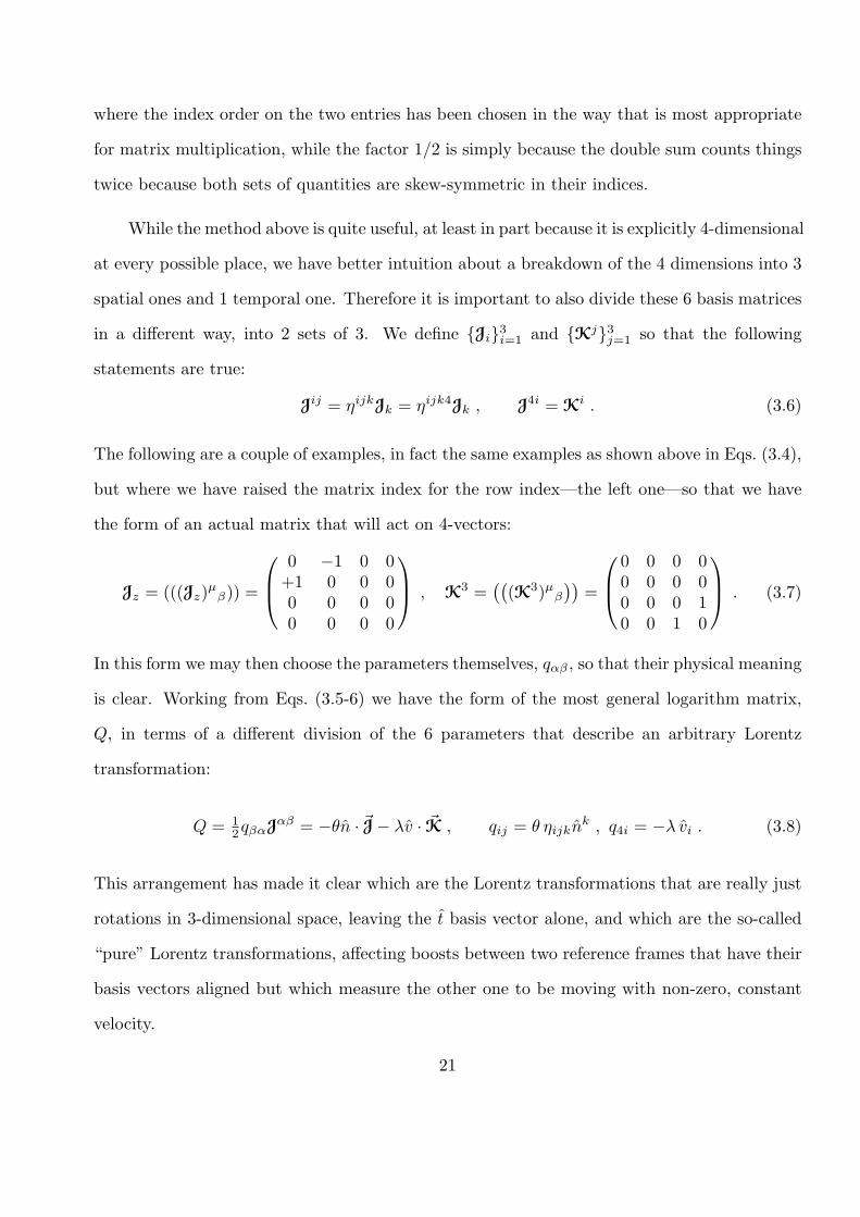
While the method above is quite useful, at least in part because it is explicitly 4-dimensional

at every possible place, we have better intuition about a breakdown of the 4 dimensions into 3

spatial ones and 1 temporal one. Therefore it is important to also divide these 6 basis matrices

in a different way, into 2 sets of 3. We define {Ji}3i=1 and {Kj}3j=1 so that the following

statements are true:

Jij = ηijkJk = ηijk4Jk , J4i = Ki . (3.6)

The following are a couple of examples, in fact the same examples as shown above in Eqs. (3.4),

but where we have raised the matrix index for the row index—the left one—so that we have

the form of an actual matrix that will act on 4-vectors:

Jz = (((Jz)µβ)) =

0 −1 0 0+1 0 0 00 0 0 00 0 0 0

, K3 =(((K3)µβ

))=

0 0 0 00 0 0 00 0 0 10 0 1 0

. (3.7)

In this form we may then choose the parameters themselves, qαβ , so that their physical meaning

is clear. Working from Eqs. (3.5-6) we have the form of the most general logarithm matrix,

Q, in terms of a different division of the 6 parameters that describe an arbitrary Lorentz

transformation:

Q = 12qβαJ

αβ = −θn · J− λv · K , qij = θ ηijknk , q4i = −λ vi . (3.8)

This arrangement has made it clear which are the Lorentz transformations that are really just

rotations in 3-dimensional space, leaving the t basis vector alone, and which are the so-called

“pure” Lorentz transformations, affecting boosts between two reference frames that have their

basis vectors aligned but which measure the other one to be moving with non-zero, constant

velocity.

21

Before going ahead to determine irreducible representations of these transformations it is

necessary to first determine the commutators of these 6 generators, where it is useful to have the

commutators available to us in both forms of their labelling. There are various “sophisticated”

ways to calculate their commutators; however, as we have explicit 4×4 matrices one can quite

easily calculate the commutators directly. The results are the following:

[Jαβ ,Jγδ] = ηαγJβδ − ηβγJαδ + ηβδJαγ − ηαδJβγ = ηα[γJβδ] − ηβ[γJαδ] , (3.9)

where a way of seeing why there are 4 distinct terms in the commutator is by noting that the

result must be skew-symmetric in α and β, and also skew-symmetric in γ and δ, and lastly

must be skew-symmetric in switching those two pairs. However, we also need the commutators

when they are divided into pure rotations and pure boosts:

[Jm,Jn] = + ϵmnc Jc ,

[Js,Kt] = + ϵstbKb ,

[Kb,Kd] = − ϵbdfJf .

(3.10)

The exponentials of the Lie algebra elements that are sums only of the three Ji are of

course just a 3×3 rotation matrix put into a 4×4 form with a +1 in the 4, 4-position and 0’s in

the 4, i- and i, 4-positions, showing that it performs a spatial rotation and neither changes the

temporal values nor mixes them with the spatial ones. We already understand their structure.

On the other hand the set of linear combinations of the other three generators, the Km, are the

usual Lorentz boosts that move the basis vectors from one reference frame to another reference

frame that is moving with respect to the first one. It is these boosts that one needs to describe

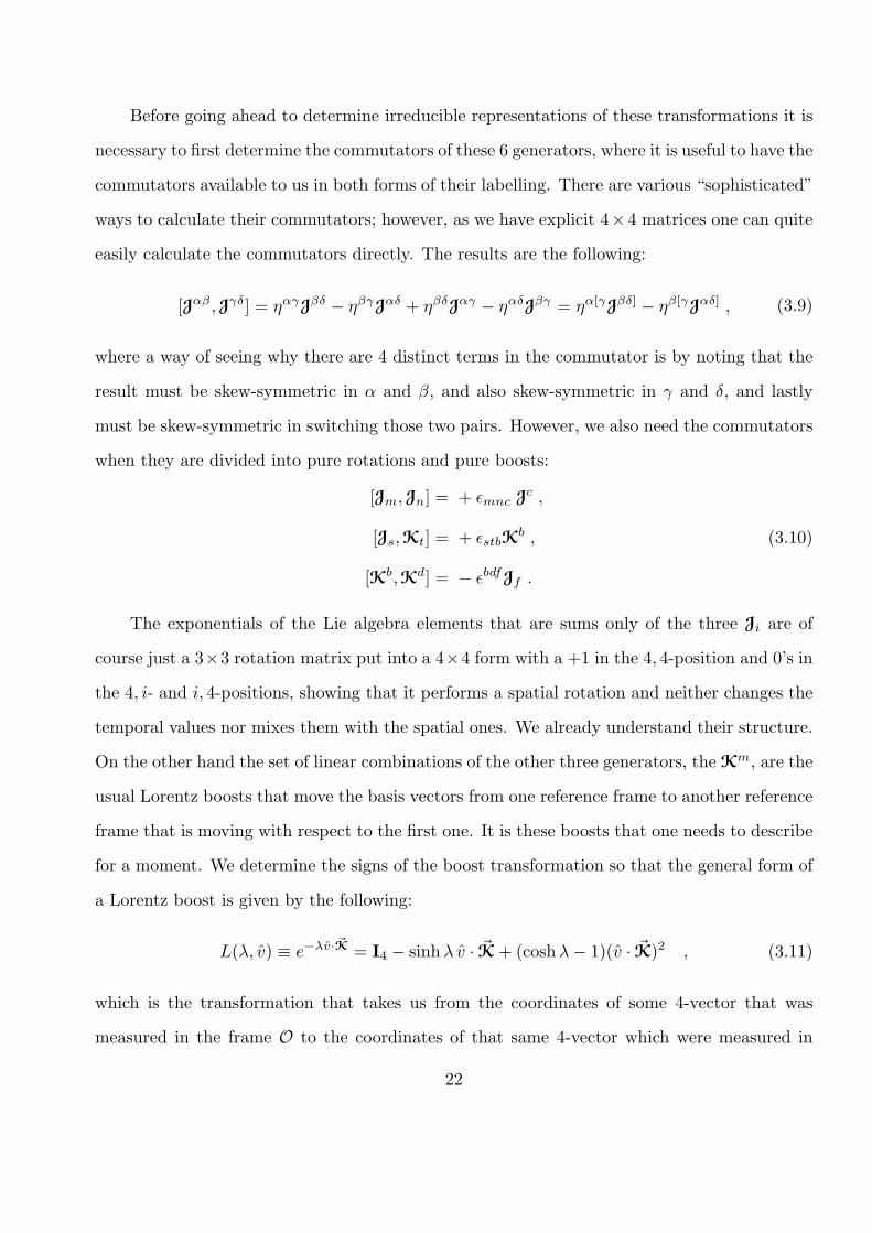
for a moment. We determine the signs of the boost transformation so that the general form of

a Lorentz boost is given by the following:

L(λ, v) ≡ e−λv·K = I4 − sinhλ v · K+ (coshλ− 1)(v · K)2 , (3.11)

which is the transformation that takes us from the coordinates of some 4-vector that was

measured in the frame O to the coordinates of that same 4-vector which were measured in

22

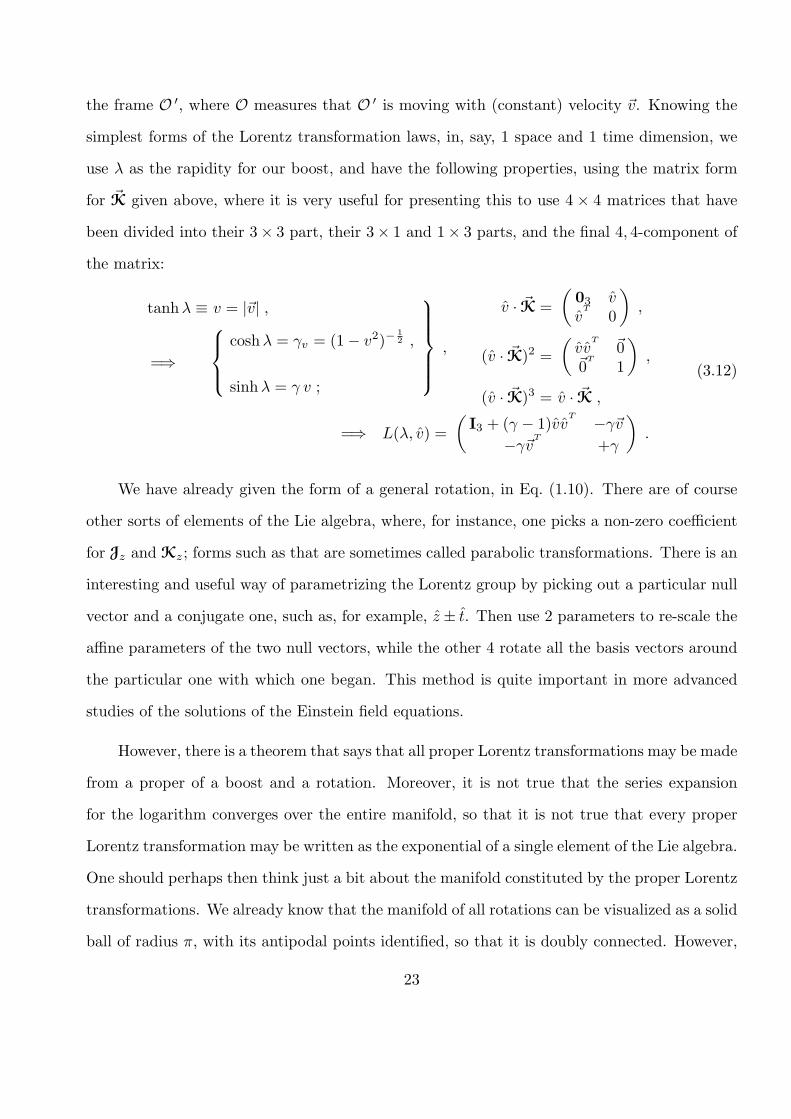
the frame O ′, where O measures that O ′ is moving with (constant) velocity v. Knowing the

simplest forms of the Lorentz transformation laws, in, say, 1 space and 1 time dimension, we

use λ as the rapidity for our boost, and have the following properties, using the matrix form

for K given above, where it is very useful for presenting this to use 4 × 4 matrices that have

been divided into their 3× 3 part, their 3× 1 and 1× 3 parts, and the final 4, 4-component of

the matrix:

tanhλ ≡ v = |v| ,

=⇒

coshλ = γv = (1− v2)−

12 ,

sinhλ = γ v ;

,

v · K =

(03 vv

T

0

),

(v · K)2 =

(vv

T

00T

1

),

(v · K)3 = v · K ,

=⇒ L(λ, v) =

(I3 + (γ − 1)vv

T −γv

−γvT

+γ

).

(3.12)

We have already given the form of a general rotation, in Eq. (1.10). There are of course

other sorts of elements of the Lie algebra, where, for instance, one picks a non-zero coefficient

for Jz and Kz; forms such as that are sometimes called parabolic transformations. There is an

interesting and useful way of parametrizing the Lorentz group by picking out a particular null

vector and a conjugate one, such as, for example, z ± t. Then use 2 parameters to re-scale the

affine parameters of the two null vectors, while the other 4 rotate all the basis vectors around

the particular one with which one began. This method is quite important in more advanced

studies of the solutions of the Einstein field equations.

However, there is a theorem that says that all proper Lorentz transformations may be made

from a proper of a boost and a rotation. Moreover, it is not true that the series expansion

for the logarithm converges over the entire manifold, so that it is not true that every proper

Lorentz transformation may be written as the exponential of a single element of the Lie algebra.

One should perhaps then think just a bit about the manifold constituted by the proper Lorentz

transformations. We already know that the manifold of all rotations can be visualized as a solid

ball of radius π, with its antipodal points identified, so that it is doubly connected. However,

23

the boosts are described by any possible direction, but their parameter λ should be considered

as varying between 0 and +∞, so that this is basically just the usual, complete 3-dimensional

space, E3. One should note that in principle one could have λ negative; however, one can

simply take a positive λ and reverse the direction associated with the negative one, so that

we do not do this, to avoid double counting. The entire manifold is then the direct product

of these two 3-dimensional manifolds, which is clearly not compact, i.e., closed and bounded

(inside some sufficiently large sphere, say).

We also know that the product of two boosts in different directions is not just a boost,

since the commutator of two non-parallel Ki is a Jk, so that the product of two different boosts

is in general equal to the product of a third boost, which takes one directly to the frame which

has the correct magnitude of velocity for the two separate boosts, but then one also needs a

rotation to align the axes properly.

Lastly one should say some things about those parts of the entire group that are not in

the connected part of the manifold containing the identity. From the fact that the rotations

have a disconnected part, we may see that it is obvious that the Lorentz group must also have

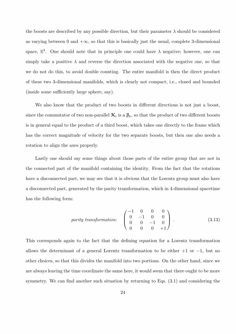
a disconnected part, generated by the parity transformation, which in 4-dimensional spacetime

has the following form:

parity transformation:

−1 0 0 00 −1 0 00 0 −1 00 0 0 +1

. (3.13)

This corresponds again to the fact that the defining equation for a Lorentz transformation

allows the determinant of a general Lorentz transformation to be either +1 or −1, but no

other choices, so that this divides the manifold into two portions. On the other hand, since we

are always leaving the time coordinate the same here, it would seem that there ought to be more

symmetry. We can find another such situation by returning to Eqs. (3.1) and considering the

24

4, 4-component of the equation that requires a Lorentz transformation to preserve the metric:

−1 = η44 = (ΛT

HΛ)44 = Λµ4ηµνΛ

ν4 =

3∑i=1

(Λi4)

2 − (Λ44)

2

=⇒ (Λ44)

2 = +1 +

3∑i=1

(Λi4)

2

=⇒ Λ44 ≥ +1 or Λ4

4 ≤ −1 .

(3.14)

this is again a separation of the entire group into two separate pieces: those which do something

or other but do not change the direction of time, and those which do; therefore they are referred

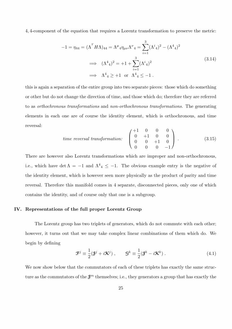
to as orthochronous transformations and non-orthochronous transformations. The generating

elements in each one are of course the identity element, which is orthochronous, and time

reversal:

time reversal transformation:

+1 0 0 00 +1 0 00 0 +1 00 0 0 −1

. (3.15)

There are however also Lorentz transformations which are improper and non-orthochronous,

i.e., which have detΛ = −1 and Λ44 ≤ −1. The obvious example entry is the negative of

the identity element, which is however seen more physically as the product of parity and time

reversal. Therefore this manifold comes in 4 separate, disconnected pieces, only one of which

contains the identity, and of course only that one is a subgroup.

IV. Representations of the full proper Lorentz Group

The Lorentz group has two triplets of generators, which do not commute with each other;

however, it turns out that we may take complex linear combinations of them which do. We

begin by defining

Fj ≡ 1

2(Jj + iKj) , Gk ≡ 1

2(Jk − iKk) . (4.1)

We now show below that the commutators of each of these triplets has exactly the same struc-

ture as the commutators of the Jm themselves; i.e., they generators a group that has exactly the

25

same group-theoretical structure as the rotation group, albeit of course with complex-valued

generators:

[Fj ,Fk] = 14 [J

j + iKj ,Jk + iKk] = 14ϵjkm{Jm + iKm − (−iKm) + Jm} = ϵjkmFm ,

[Gj ,Gk] = 14 [J

j − iKj ,Jk − iKk] = 14ϵjkm{Jm − iKm − (+iKm) + Jm} = ϵjkmGm ,

[Fj ,Gk] = 14 [J

j + iKj ,Jk − iKk] = 14ϵjkm{Jm − iKm − (−iKm)− Jm} = 0 ,

(4.2)

where the last line shows, additionally, that the two triplets commute between themselves,

so that the two “copies” of the rotation group that are involved do not interact with each

other, so that we could treat each one of them separately. Therefore we may now consider,

independently, representations of each of these “rotation groups,” labeling them by f and g,

where each of 2f and 2g are allowed to take on all non-zero integer values. Since we may

resolve the original equations backwards, for Ji and Kj , as follows:

Jm = Fm + Gm , Km = i(Gm −Fm) , (4.3)

the desired representations of the Lorentz group are simply direct sums of the two represen-

tations of the rotation group, so that it is reasonable to label an irreducible representation of

the Lorentz group by the two half-integers, f and g: D(f,g)[Λ(λ; v)], for example, or we could

refer to just the representation itself by the simpler notation, D(f, g).

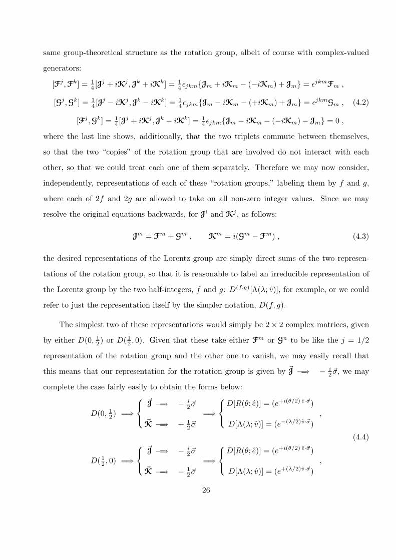
The simplest two of these representations would simply be 2× 2 complex matrices, given

by either D(0, 12 ) or D( 12 , 0). Given that these take either Fm or Gn to be like the j = 1/2

representation of the rotation group and the other one to vanish, we may easily recall that

this means that our representation for the rotation group is given by J =−→ − i2 σ, we may

complete the case fairly easily to obtain the forms below:

D(0, 12 ) =⇒

J =−→ − i

2 σ

K =−→ + 12 σ

=⇒

D[R(θ; e)] = (e+i(θ/2) e·σ)

D[Λ(λ; v)] = (e−(λ/2)v·σ)

,

D( 12 , 0) =⇒

J =−→ − i

2 σ

K =−→ − 12 σ

=⇒

D[R(θ; e)] = (e+i(θ/2) e·σ)

D[Λ(λ; v)] = (e+(λ/2)v·σ)

,

(4.4)

26

To study more complicated forms than these, such as, for instance, D( 12 ,12 ) = D(0, 1

2 ) ⊗

D( 12 , 0), we will need to understand how to create the generators when considering a product

representation. We understand that the matrices representing the group elements of a product

representation correspond to direct products of the individual representations of that group

element. However, one must be somewhat more careful with respect to the generators. The

following is the right approach for the generators, for any Lie group, G, with Lie algebra, G.

Let us suppose that we have been an element g ∈ G such that there exists Q ∈ G such that

g = eQ. Further let us have two distinct representations of G, which we label by D1(g) and

D2(g). Therefore, we also can find, and label, the representations of the generator Q, simply

by Q(1) and Q(2), so that

g = eQ =−→

D1(g) = eQ(1)

,

D2(g) = eQ(2)

.

(4.5)

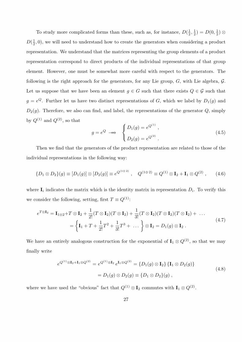
Then we find that the generators of the product representation are related to those of the

individual representations in the following way:

{D1 ⊗D2}(g) ≡ [D1(g)]⊗ [D2(g)] ≡ eQ(1⊕ 2)

, Q(1⊕ 2) ≡ Q(1) ⊗ I2 + I1 ⊗Q(2) , (4.6)

where Ii indicates the matrix which is the identity matrix in representation Di. To verify this

we consider the following, setting, first T ≡ Q(1):

eT⊗I2 = I1⊗2+T ⊗ I2 +1

2!(T ⊗ I2)(T ⊗ I2) +

1

3!(T ⊗ I2)(T ⊗ I2)(T ⊗ I2) + . . .

=

{I1 + T +

1

2!T 2 +

1

3!T 3 + . . .

}⊗ I2 = D1(g)⊗ I2 .

(4.7)

We have an entirely analogous construction for the exponential of I1 ⊗ Q(2), so that we may

finally write

eQ(1)⊗I2+I1⊗Q(2)

= eQ(1)⊗I2 eI1⊗Q(2)

= {D1(g)⊗ I2} {I1 ⊗D2(g)}

= D1(g)⊗D2(g) ≡ {D1 ⊗D2}(g) ,(4.8)

where we have used the “obvious” fact that Q(1) ⊗ I2 commutes with I1 ⊗Q(2).

27

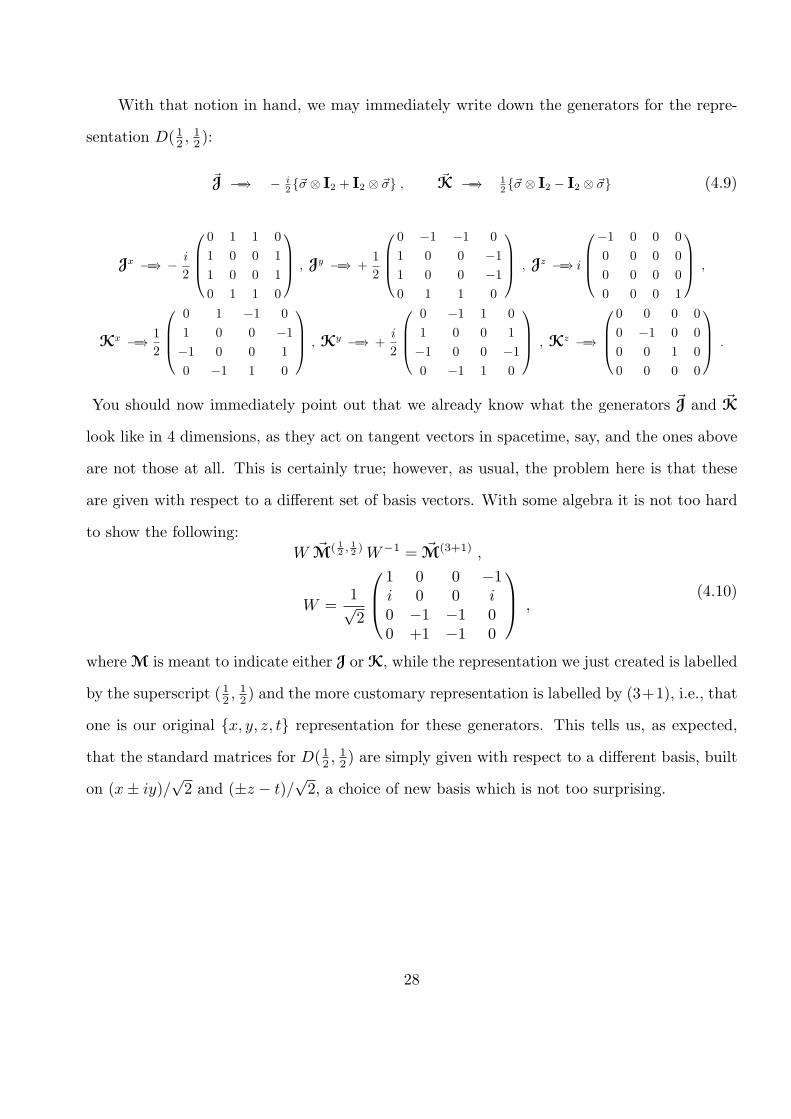
With that notion in hand, we may immediately write down the generators for the repre-

sentation D( 12 ,12 ):

J =−→ − i2{σ ⊗ I2 + I2 ⊗ σ} , K =−→ 1

2{σ ⊗ I2 − I2 ⊗ σ} (4.9)

Jx =−→ − i

2

0 1 1 0

1 0 0 1

1 0 0 1

0 1 1 0

, Jy =−→ +1

2

0 −1 −1 0

1 0 0 −1

1 0 0 −1

0 1 1 0

, Jz =−→ i

−1 0 0 0

0 0 0 0

0 0 0 0

0 0 0 1

,

Kx =−→ 1

2

0 1 −1 0

1 0 0 −1

−1 0 0 1

0 −1 1 0

, Ky =−→ +i

2

0 −1 1 0

1 0 0 1

−1 0 0 −1

0 −1 1 0

, Kz =−→

0 0 0 0

0 −1 0 0

0 0 1 0

0 0 0 0

.

You should now immediately point out that we already know what the generators J and K

look like in 4 dimensions, as they act on tangent vectors in spacetime, say, and the ones above

are not those at all. This is certainly true; however, as usual, the problem here is that these

are given with respect to a different set of basis vectors. With some algebra it is not too hard

to show the following:

W M( 12 ,

12 ) W−1 = M(3+1) ,

W =1√2

1 0 0 −1i 0 0 i0 −1 −1 00 +1 −1 0

,(4.10)

where M is meant to indicate either J or K, while the representation we just created is labelled

by the superscript ( 12 ,12 ) and the more customary representation is labelled by (3+1), i.e., that

one is our original {x, y, z, t} representation for these generators. This tells us, as expected,

that the standard matrices for D( 12 ,12 ) are simply given with respect to a different basis, built

on (x± iy)/√2 and (±z − t)/

√2, a choice of new basis which is not too surprising.

28