USER 4: User-Specified Estimation Routine

James M. Lady, John R. Skalski

Columbia Basin ResearchSchool of Aquatic and Fishery Sciences

University of Washington1325 4th Avenue, Suite 1820

Seattle, WA 98101-2509

Prepared forU.S. Department of Energy

Bonneville Power AdministrationDivision of Fish and Wildlife

P.O. Box 3621Portland, OR 98208-3621Project No. 1989-107-00

Contract No. 39987

May 2009

USER 4 ii

Contents

1 Overview 1

2 Interface Description 3

2.1 Navigation Panel . . . . . . . . . . . . . . . . . . . . . . . . . . . . . 3

2.2 Toolbar . . . . . . . . . . . . . . . . . . . . . . . . . . . . . . . . . . 3

3 Integrated Help System 5

4 Examples 7

4.1 One Likelihood . . . . . . . . . . . . . . . . . . . . . . . . . . . . . . 7

4.1.1 Model Definition . . . . . . . . . . . . . . . . . . . . . . . . . 7

4.1.2 Estimation . . . . . . . . . . . . . . . . . . . . . . . . . . . . . 11

4.1.3 Estimates . . . . . . . . . . . . . . . . . . . . . . . . . . . . . 14

4.2 Joint Likelihood Example . . . . . . . . . . . . . . . . . . . . . . . . 17

4.2.1 Define the Model . . . . . . . . . . . . . . . . . . . . . . . . . 18

4.2.2 Verify the Model . . . . . . . . . . . . . . . . . . . . . . . . . 22

4.2.3 Model Definition File and Category Counts File . . . . . . . . 22

4.2.4 Estimate . . . . . . . . . . . . . . . . . . . . . . . . . . . . . . 23

4.3 Estimating Abundance . . . . . . . . . . . . . . . . . . . . . . . . . . 25

4.3.1 Define the Model . . . . . . . . . . . . . . . . . . . . . . . . . 25

4.3.2 Estimate the Parameters . . . . . . . . . . . . . . . . . . . . . 27

4.4 Hypothesis Testing Example . . . . . . . . . . . . . . . . . . . . . . . 32

4.4.1 Full Model Definition . . . . . . . . . . . . . . . . . . . . . . . 33

4.4.2 Reduced Model Definition . . . . . . . . . . . . . . . . . . . . 35

4.4.3 Test the Hypothesis . . . . . . . . . . . . . . . . . . . . . . . . 37

4.4.4 Model Selection Using an Information-Theoretic Approach . . 38

i USER 4

USER 4 ii

List of Figures

2.1 USER 4 startup dialog . . . . . . . . . . . . . . . . . . . . . . . . . . 4

2.2 USER 4 toolbar . . . . . . . . . . . . . . . . . . . . . . . . . . . . . . 4

3.1 USER 4 help viewer . . . . . . . . . . . . . . . . . . . . . . . . . . . 6

4.1 The “Parameters” page for the one likelihood example . . . . . . . . 8

4.2 Using a workspace file . . . . . . . . . . . . . . . . . . . . . . . . . . 8

4.3 Convenience functions for the one likelihood example . . . . . . . . . 9

4.4 Likelihood definition for the one likelihood example . . . . . . . . . . 10

4.5 Verify the Model for the one likelihood example . . . . . . . . . . . . 11

4.6 Parameter seed for the one likelihood example . . . . . . . . . . . . . 12

4.7 Optimizer settings for the one likelihood example . . . . . . . . . . . 13

4.8 “Estimate the Model Parameters” page after the successful estimationof the model parameters for the one likelihood example . . . . . . . . 14

4.9 “Estimate the Model Parameters” page after estimation failure for theone likelihood example . . . . . . . . . . . . . . . . . . . . . . . . . . 15

4.10 “Estimation Summary” page for the one likelihood example . . . . . 16

4.11 Joint likelihood example: Diagram of the study design . . . . . . . . 17

4.12 Joint likelihood example: Diagram of the modified study design withtwo independent detection sites . . . . . . . . . . . . . . . . . . . . . 18

4.13 Parameters for the joint likelihood example . . . . . . . . . . . . . . . 19

4.14 Convenience Function for the joint likelihood example . . . . . . . . . 19

4.15 Button for renaming the current likelihood . . . . . . . . . . . . . . . 20

4.16 “main” likelihood in the joint likelihood example . . . . . . . . . . . . 21

4.17 Begin the auxiliary likelihood definition for the joint likelihood example 21

4.18 Completed auxiliary likelihood definition for the joint likelihood example 22

4.19 Category counts file for the joint likelihood example . . . . . . . . . . 23

4.20 Estimation Summary report for the joint likelihood example . . . . . 24

iii USER 4

4.21 Parameters for the abundance estimation example . . . . . . . . . . . 26

4.22 Convenience function for the abundance estimation example . . . . . 26

4.23 Partial likelihood definition for the abundance estimation example . . 27

4.24 Likelihood definition for the abundance estimation example . . . . . . 28

4.25 Category counts file for the abundance estimation example . . . . . . 28

4.26 Estimation Summary for the abundance estimation example . . . . . 30

4.27 Observed vs Expected Plot for the abundance estimation example . . 31

4.28 Residuals Plot for the abundance estimation example . . . . . . . . . 31

4.29 Parameter definitions for the hypothesis testing example . . . . . . . 33

4.30 Convenience function definition for the hypothesis testing example . . 34

4.31 Likelihood definition for the hypothesis testing example . . . . . . . . 34

4.32 Profile likelihood confidence interval requests for the hypothesis testingexample . . . . . . . . . . . . . . . . . . . . . . . . . . . . . . . . . . 35

4.33 Estimation Summary Report for the hypothesis testing example, fullmodel . . . . . . . . . . . . . . . . . . . . . . . . . . . . . . . . . . . 36

4.34 Delete the parameter S2 for the hypothesis testing example . . . . . . 37

4.35 Define the convenience function S2 for the hypothesis testing example 38

4.36 Estimation Summary Report for the hypothesis testing example, re-duced model . . . . . . . . . . . . . . . . . . . . . . . . . . . . . . . . 39

USER 4 iv

1.0 Overview

Program USER 4 is a tool that allows investigators to estimate parametersof a study with the following characteristics:

• All possible outcomes of the study can be characterized in terms of a finitenumber of discrete categories.

• The categories are mutually exclusive and exhaustive; i.e., an individual in thestudy can be classified into one and only one category.

• The data from the study consist of the number of individuals in the study thatfall into each category.

A model within the USER framework consists of a likelihood with zero ormore auxiliary likelihoods. Each likelihood consists of two or more categories, andeach category consists of:

• A unique label for identifying the category.

• The probability for the category, defined as a function of the modelparameters.

• A count indicating the number of observations for the category.

Since the categories are mutually exclusive and exhaustive, the probabilities mustsum to 1.0.

Program USER includes an integrated, context-sensitive help system thatguides the user on how to interact with the program. Therefore, this documentconcentrates on describing some applications, setting them up in USER, andestimating the parameters of interest.

The outline of this manual is as follows.

1. A brief description of the USER interface (Chapter 2).

2. A description of the integrated help system (Chapter 3).

3. The analysis of four hypothetical studies

(a) A study with one likelihood (Section 4.1).

(b) A study requiring an auxiliary likelihood (Section 4.2).

1 USER 4

(c) A study for estimating abundance, requiring the use of an unobservedcategory (Section 4.3).

(d) An example of performing hypothesis testing (Section 4.4).

This document describes version 4.4 of Program USER.

USER 4 2

2.0 Interface Description

The user interface for Program USER upon startup is illustrated inFigure 2.1. The left-hand side consists of the navigation panel, and the right-handside consists of the content page. The active content page at startup is the“Parameters” page.

Along the top of the USER dialog is a toolbar with buttons that provideshortcuts to corresponding actions in the “File” menu.

2.1 Navigation Panel

By default, the navigation panel is always displayed on the left-hand side ofthe USER dialog. Its visibility can be toggled on and off via the “View” menu.

The navigation panel is organized to show the usual progression of steps onewould normally take in defining a model, estimating the parameters, and viewingthe results. Each content page has a “Next” and “Previous” button (see Figure 2.1)in the lower right side of the screen to allow the user to progress through thesesteps. However, the user can also double-click on the title of any content page to godirectly to that page (unless it is grayed out and thus unavailable).

Headers used strictly for organizational purposes are distinguished fromcontent pages by the use of blue text for actual content pages. The title of thecurrently active page is displayed in bold text.

2.2 Toolbar

The USER toolbar (Figure 2.2) provides shortcut buttons for commands inthe “File” menu. The buttons with “W” on them pertain to a workspace file, thosewith “M” pertain to the model definition file, and those with “C” pertain to thecategory counts file. The toolbar also contains a context-sensitive help button. Thevisibility of the toolbar can be toggled off and on similarly to the Navigation Panel.

3 USER 4

Figure 2.1: The USER 4 dialog as it appears at startup.

Figure 2.2: The USER 4 toolbar provides shortcut buttons for commands in the“File” menu. “W” pertains to the workspace file, “M” to the model definition file,and “C” to the category counts file.

USER 4 4

3.0 Integrated Help System

Program USER 4 includes an integrated, context-sensitive help system. The“Contents” action under the “About” menu will bring up a separate help viewer asshown in Figure 3.1. The navigation panel on the left side shows the list of availabletopics. Under the “Content Pages,” the structure parallels the structure of thecontent pages of Program USER 4.

To obtain context-sensitive help on a specific item, the user clicks on the helpbutton on the toolbar (see Figure 2.2), and then clicks on the item of interest; if theuser clicks on the currently active content page, the help for that particular contentpage will be displayed on the help viewer.

5 USER 4

Figure 3.1: The integrated help viewer for USER 4.4.

USER 4 6

4.0 Examples

4.1 One Likelihood

A simple method for estimating the number of animals in a closedpopulation using a single mark-release of individuals is the Petersen Method. Asample of n1 individuals is taken from the population and marked for futureidentification and returned to the population. After some interval, a second sampleof n2 individuals is taken and it is found that m of them are marked. We areinterested in estimating the parameter N , the number of animals in the population.

For this example we will use the following expository data:

n1: 220n2: 235m: 40

If we let P represent the proportion marked after initial tagging, then P = n1

N.

Assuming that the proportion of marked individuals in the second sample isa reasonable estimate of the proportion marked in the population, then theprobability that an animal in n2 is marked is P .

The categories and their corresponding probabilities of occurrence are as follows:

Category Probabilitym P

n2 −m 1− P

The resulting likelihood is

L =

(n2

m

)(n1

N

)m (1− n1

N

)n2−m

(4.1)

4.1.1 Model Definition

Define the Parameters

On startup, the “Parameters” content page is active on the USER dialog. Inthis example, we have one parameter to estimate: N , so we place the cursor in thefirst cell of the parameter definitions table and type “N” and press “Tab” to moveto next cell (Figure 4.1).

7 USER 4

Figure 4.1: The “Parameters” page for the one likelihood example

Figure 4.2: Using a workspace file

Notice in Figure 4.1 that after entering the parameter N , two asterisksappear in the window title after the version number. This indicates that there areunsaved changes to the workspace. Use the “Save Workspace” or “Save Workspaceas” commands to save your work to a workspace file. If you then exit USER andstart it up again, you can use the “Load Workspace” command to pick up whereyou left off. (see Figure 4.2).

Define the Convenience Functions

From the “Parameters” content page, press the “Next” button (ordouble-click on “Convenience Functions” on the navigation panel). This will makethe “Convenience Functions” content page active.

USER 4 8

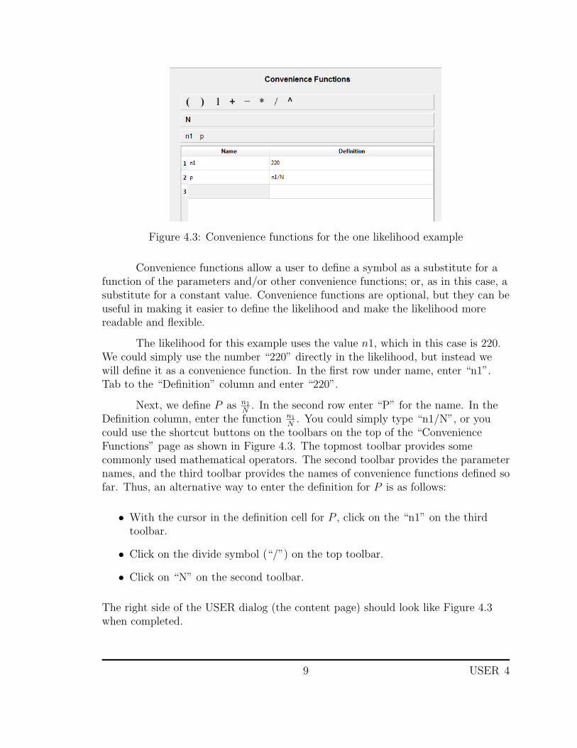
Figure 4.3: Convenience functions for the one likelihood example

Convenience functions allow a user to define a symbol as a substitute for afunction of the parameters and/or other convenience functions; or, as in this case, asubstitute for a constant value. Convenience functions are optional, but they can beuseful in making it easier to define the likelihood and make the likelihood morereadable and flexible.

The likelihood for this example uses the value n1, which in this case is 220.We could simply use the number “220” directly in the likelihood, but instead wewill define it as a convenience function. In the first row under name, enter “n1”.Tab to the “Definition” column and enter “220”.

Next, we define P as n1

N. In the second row enter “P” for the name. In the

Definition column, enter the function n1

N. You could simply type “n1/N”, or you

could use the shortcut buttons on the toolbars on the top of the “ConvenienceFunctions” page as shown in Figure 4.3. The topmost toolbar provides somecommonly used mathematical operators. The second toolbar provides the parameternames, and the third toolbar provides the names of convenience functions defined sofar. Thus, an alternative way to enter the definition for P is as follows:

• With the cursor in the definition cell for P , click on the “n1” on the thirdtoolbar.

• Click on the divide symbol (“/”) on the top toolbar.

• Click on “N” on the second toolbar.

The right side of the USER dialog (the content page) should look like Figure 4.3when completed.

9 USER 4

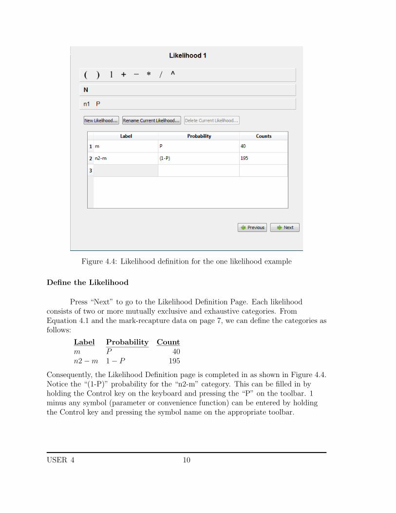
Figure 4.4: Likelihood definition for the one likelihood example

Define the Likelihood

Press “Next” to go to the Likelihood Definition Page. Each likelihoodconsists of two or more mutually exclusive and exhaustive categories. FromEquation 4.1 and the mark-recapture data on page 7, we can define the categories asfollows:

Label Probability Countm P 40n2−m 1− P 195

Consequently, the Likelihood Definition page is completed in as shown in Figure 4.4.Notice the “(1-P)” probability for the “n2-m” category. This can be filled in byholding the Control key on the keyboard and pressing the “P” on the toolbar. 1minus any symbol (parameter or convenience function) can be entered by holdingthe Control key and pressing the symbol name on the appropriate toolbar.

USER 4 10

Figure 4.5: Verify the Model for the one likelihood example

Verify the Model

Pressing the “Next” key from the Likelihood Definition page makes theVerify the Model page active, verifying that

1. There are no undefined symbols used in the likelihood definition, and

2. The probabilities of occurrence sum to 1.0.

The Verify the Model page also dispays the number of parameters and thedimension of the Minimum Sufficient Statistic. If the dimension is less than thenumber of parameters for a model with one likelihood, the parameters may not beestimable. If everything has been done correctly, the USER dialog should nowappear as on Figure 4.5. If there are any undefined symbols, or if the probabilitiesdo not sum to 1.0, you will not be able to estimate the model parameters.

We have now finished the model definition phase. The parameters andlikelihoods are defined, and we move to the estimation phase.

4.1.2 Estimation

Specify the Parameter Seeds

The “Next” button takes the investigator to the “Parameter Seeds” contentpage. Parameter estimation in USER is performed by maximizing the likelihoodfunction using numerical optimization. All numerical optimization proceduresrequire initial seeds, or starting points for the parameters. USER uses a defaultvalue of 0.5 for all parameter seeds. This is usually a good seed for estimating

11 USER 4

Figure 4.6: Parameter seed for the one likelihood example

probabilities that are between 0.0 and 1.0. In this case, however, the parameter tobe estimated is animal abundance, so we need to change the seed to a morereasonable number, say, 500 (Figure 4.6).

The next content page is the “Profile Likelihood Confidence Intervals” page.No profile likelihood confidence intervals will be requested for this example, soproceed to the “Optimizer” content page.

Optimizer

The next content page is titled “Optimizer,” and allows the user to specifythe numerical optimization settings. The default optimizer is called “Fletch” whichuses the “quasi Newton-Rhapson method” to numerically solve for the parameterestimates (Figure 4.7).

Refer to the context-sensitive help in the integrated help system (Chapter 3)for more information on the settings on the “Optimizer” content page. In mostcases, it is sufficient to use the default settings.

Estimate the Model Parameters

The next content page is the “Estimate the Model Parameters” page. This iswhere, after defining the model, specifying the counts, and setting up the optimizer,the parameters are actually estimated. Press the “Estimate” button on the upperleft, and the output of the optimizer will appear in the text area of this contentpage (Figure 4.8).

USER 4 12

Figure 4.7: Optimizer settings for the one likelihood example

13 USER 4

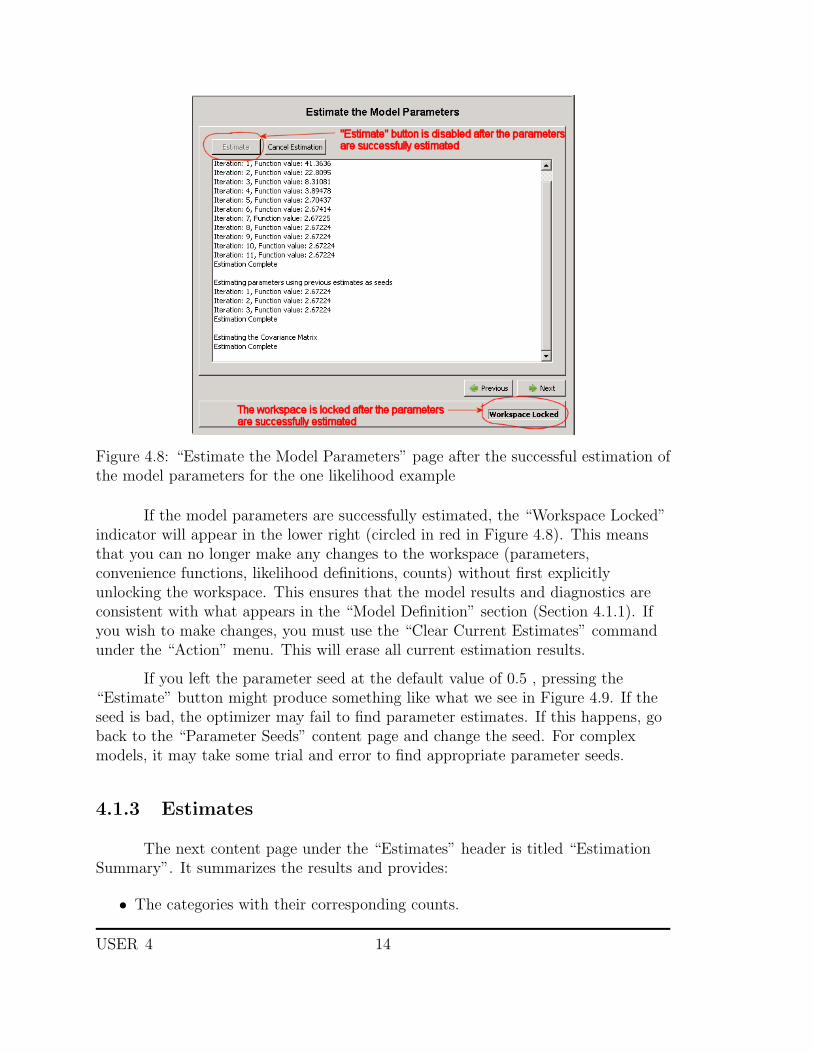
Figure 4.8: “Estimate the Model Parameters” page after the successful estimation ofthe model parameters for the one likelihood example

If the model parameters are successfully estimated, the “Workspace Locked”indicator will appear in the lower right (circled in red in Figure 4.8). This meansthat you can no longer make any changes to the workspace (parameters,convenience functions, likelihood definitions, counts) without first explicitlyunlocking the workspace. This ensures that the model results and diagnostics areconsistent with what appears in the “Model Definition” section (Section 4.1.1). Ifyou wish to make changes, you must use the “Clear Current Estimates” commandunder the “Action” menu. This will erase all current estimation results.

If you left the parameter seed at the default value of 0.5 , pressing the“Estimate” button might produce something like what we see in Figure 4.9. If theseed is bad, the optimizer may fail to find parameter estimates. If this happens, goback to the “Parameter Seeds” content page and change the seed. For complexmodels, it may take some trial and error to find appropriate parameter seeds.

4.1.3 Estimates

The next content page under the “Estimates” header is titled “EstimationSummary”. It summarizes the results and provides:

• The categories with their corresponding counts.

USER 4 14

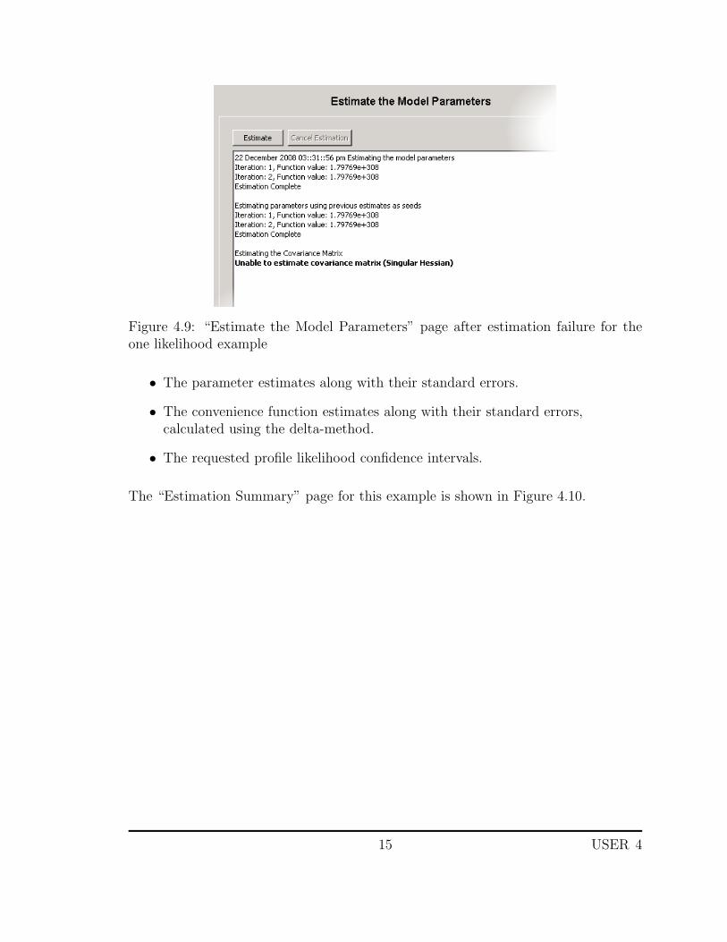
Figure 4.9: “Estimate the Model Parameters” page after estimation failure for theone likelihood example

• The parameter estimates along with their standard errors.

• The convenience function estimates along with their standard errors,calculated using the delta-method.

• The requested profile likelihood confidence intervals.

The “Estimation Summary” page for this example is shown in Figure 4.10.

15 USER 4

Figure 4.10: “Estimation Summary” page for the one likelihood example

USER 4 16

4.2 Joint Likelihood Example

We now look at an example in which not all the parameters are estimable ina single likelihood; an auxiliary likelihood is required to estimate the modelparameters.

In a simplified, hypothetical study to estimate the survival of downstreammigrating juvenile salmon in a given river reach, acoustic-tagged salmon are releasedand detected at a downstream detection site as show in Figure 4.11. The parameterof interest is the survival probability S. Not all fish are detected at the downstreamdetection site, so the model must include a detection probability P .

-

Release

S

P

Figure 4.11: Joint likelihood example: Diagram of the study design

The categories and corresponding probabilities of occurrence are as follows:

Category Description Probabilityn1 Detected SPn2 Not detected 1− SP

The resulting likelihood is as follows:

L1 ∝ (SP )n1(1− SP )n2 (4.2)

Notice that the parameters S and P always occur together in the likelihoodmodel, and therefore are not separately estimable; there is no way of distinguishingbetween mortality and non-detection. A solution is to modify the study so thatthere are two independent detection sites, as show in Figure 4.12.

This modified design makes is possible to estimate the detection probabilityseparately from the survival probability by using an auxiliary likelihood. Instead ofone detection probability, we now have two detection probabilities, P1 and P2,associated with each of the two detection arrays.

We now define the categories for the detection process. All probabilities inthe auxiliary likelihood are conditional on detection somewhere at the downstream

17 USER 4

-S

Release P1P2

Figure 4.12: Joint likelihood example: Diagram of the modified study design withtwo independent detection sites

detection site. The overall detection probability at the two arrays is now defined asP = 1− (1− P1)(1− P2).

Category Description Probabilityna Detected at site #1 only P1(1− P2)/Pnb Detected at site #2 only (1− P1)P2/Pnab Detected at both site #1 and site #2 P1P2/P

The auxiliary likelihood is defined as:

L2 ∝ (P1(1− P2)/P )na ((1− P1)P2/P )nb (P1P2/P )nab

The joint likelihood is defined as

L = L1 × L2

We can now define the joint model in USER 4.2.

4.2.1 Define the Model

Parameters

The first step is to define the parameters S, P1, and P2 as shown inFigure 4.13.

Convenience Functions

Move to the next content page in the “Define the Model” section, labeled“Convenience Functions.” The two likelihoods make use of the overall detection

USER 4 18

Figure 4.13: Parameters for the joint likelihood example

Figure 4.14: Convenience Function for the joint likelihood example

19 USER 4

Figure 4.15: Button for renaming the current likelihood

probability P = 1− (1− P1)(1− P2), a function of the two model parameters P1

and P2. Define the convenience function as shown in Figure 4.14.

Now may be good time to make use of the “Save Workspace” function tosave your work to a workspace file, say “Example2.txt”.

Likelihood Functions

The next content page is labeled “Likelihood 1”. In this example, there aretwo likelihoods: The main likelihood (L1) and the auxiliary likelihood (L2). Pressthe “Rename Current Likelihood” button (Figure 4.15) and rename the currentlikelihood “main”. Notice that the title on the current content page and thenavigation panel are updated to reflect the change. Enter the likelihood definitionfor the main likelihood as shown in Figure 4.16.

In order to define the auxiliary likelihood, press the “New Likelihood” button(to the left of the “Rename Current Likelihood” button), and give the newlikelihood the name “auxiliary”. This will add a new content page under“Likelihood Functions” labeled “auxiliary” (Figure 4.17).

Fill in the auxiliary likelihood definition as shown in Figure 4.18.

USER 4 20

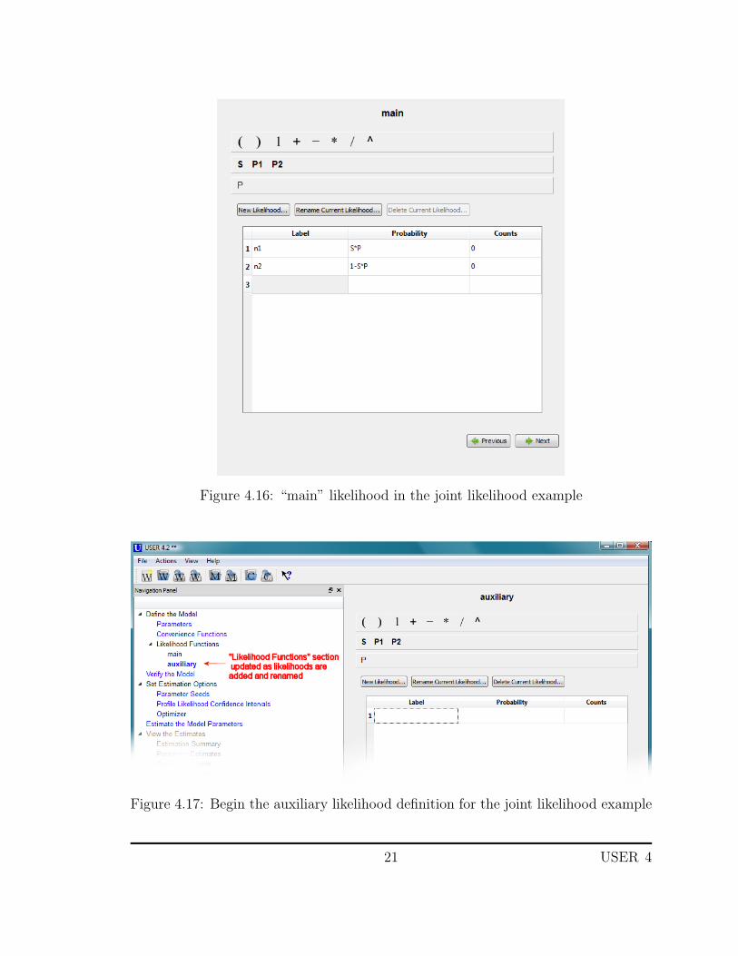
Figure 4.16: “main” likelihood in the joint likelihood example

Figure 4.17: Begin the auxiliary likelihood definition for the joint likelihood example

21 USER 4

Figure 4.18: Completed auxiliary likelihood definition for the joint likelihood example

4.2.2 Verify the Model

Once the auxiliary likelihood is complete, press the “Next” button and, ifeverything was entered correctly, you should see a message indicating that themodel definition is valid. If not, use the navigation panel to return to the pageswhere corrections need to be made, and then return to the “Verify Model” page.

4.2.3 Model Definition File and Category Counts File

You may have noticed that we have not entered any category counts for thelikelihoods, but have used the default value of zero. USER allows you to keep themodel definition separate from the actual data so that more than one dataset maybe used with the same model, or, conversely, a single dataset may be fitted withmultiple models.

From the “File” menu, select “Save Model Definition”, and enter a filename.Start a text editor, and enter the category counts as show in Figure 4.19. Each lineincludes a category label and a colon (“:”), separated by white space, followed bythe corresponding counts. The category labels must match what was entered in thelikelihood definitions; otherwise you will get an error when loading the counts into

USER 4 22

Figure 4.19: Category counts file for the joint likelihood example

USER. If the colon and the counts are omitted, the counts are assumed to be one; ifa category label is listed more than once, the counts are added together.

Save the category counts file and return to the USER program. If you exitedUSER previously, Use the “Load Model Definition” action under the “File” menu,and load the model definition file you created earlier. Now use the “Load CategoryCounts” action, also under the “File” menu to load the category counts text file youcreated.

After the counts have been loaded successfully, you may go back to thelikelihood definition pages and see that the “Counts” column has been updated.

4.2.4 Estimate

Next, go to the “Estimate the Model Parameters” page and press the“Estimate” button. If all was done correctly and the estimation is successful, youmay now proceed to the pages under the headings “View the Estimates” and “ViewModel Diagnostics” to examine the estimates and the suitability of the model forthe data. Figure 4.20 shows the Estimation Summary report.

23 USER 4

Figure 4.20: Estimation Summary report for the joint likelihood example

USER 4 24

4.3 Estimating Abundance

In this example, we look at a situation where we are interested in estimatingthe total abundance of a population, and we must take into account individualsnever observed.

This example uses a constant effort removal technique, where the populationof interest is a pest species, and it is advantageous to decimate the population. Aconstant effort P is used at each sampling occasion. Let N represent the totalnumber of individuals at the beginning of the study.

For the initial sampling event, the number of individuals removed will beNP , the number of individuals times the sampling effort. For the second event, thenumber of individuals still remaining is N(1− P ), so the expected number ofanimals removed will be N(1− P )P . For a study with four removal events, we candefine the categories and probabilities of occurrence as follows.

Category Probabilityn1 Pn2 (1− P )Pn3 (1− P )2Pn4 (1− P )3P

But this table is incomplete. Remember that the categories for a likelihood must bemutually exclusive and exhaustive, and we haven’t taken into account the animalsnever recaptured. The complete table is as follows:

Category Probabilityn1 Pn2 (1− P )Pn3 (1− P )2Pn4 (1− P )3Pn0 (1− P )4

4.3.1 Define the Model

In USER, define the parameters as shown in Figure 4.21. In order to makethe likelihood definition cleaner, we will define the convenience function q = 1− Pas show in Figure 4.22.

For the likelihood definition, enter the first four categories as shown inFigure 4.23. The final category represents individuals never observed - an“unobserved category.” We have no counts to enter for this category. In order toindicate that this is an unobserved category, in the Label column enter the

25 USER 4

Figure 4.21: Parameters for the abundance estimation example

Figure 4.22: Convenience function for the abundance estimation example

USER 4 26

Figure 4.23: Partial likelihood definition for the abundance estimation example

abundance parameter in parentheses - “(N)”, and press <Tab> to move to theProbability column. USER will put the text “N - ...” in the Counts column toindicate that the counts are assumed to be N minus the sum of all the othercategories in this likelihood. USER also italicizes the text to distinguish it from theobserved categories. Enter the probability as you would for any other category(Figure 4.24).

4.3.2 Estimate the Parameters

Load the Category Counts

Create category counts file as shown in Figure 4.25, and load them using the“Load Category Counts” action under the “File” menu.

27 USER 4

Figure 4.24: Likelihood definition for the abundance estimation example

Figure 4.25: Category counts file for the abundance estimation example

USER 4 28

Entering the Parameter Seed for an Abundance Parameter

At the “Parameter Seeds” content page, it is clear that the seed for theparameter N needs to be changed to be at least as large as the counts for “n1” - thenumber captured at the initial event. For this type of model, it may take severalattempts to find a seed which will allow the optimizer to converge to find theparameter estimates. It may be helpful to go to the “Optimizer” content page anduse the “Downhill Simplex” method instead of the default optimizer. Some sourcessuggest that this method may be more robust but less precise. Once an estimate isfound using the Downhill Simplex method, the resulting estimates could be used asseeds for the default “Fletch Quasi-Newton” method.

For this example, enter 20000 as the seed for N . This should lead tosuccessful estimation of the model parameters. Figure 4.26 shows the EstimationSummary report.

Model Diagnostics

We can now look at the model diagnostics to see how well the model fits thedata. Proceed to the “Observed vs Expected Plot” under “View ModelDiagnostics.” Note that this plot, as with all plots in USER, can be made largersimply by enlarging the USER dialog window, or by using the zoom slider at thetop (Figure 4.27).

If you go to the “Residuals Plot” content page (Figure 4.28), you will observethat two of the four observations fall well outside the ±1.96 range. If the data fitthe model well, the residuals will follow a standard normal distribution, and 95% ofthe observations should fall within the ±1.96 range. Note that by holding the cursorover a data point, USER will display the category label for that point, the observedcounts, and the expected counts. Perhaps, in this case, the assumption of constanteffort removal was violated.

29 USER 4

Figure 4.26: Estimation Summary for the abundance estimation example

USER 4 30

Figure 4.27: Observed vs Expected Plot for the abundance estimation example

Figure 4.28: Residuals Plot for the abundance estimation example

31 USER 4

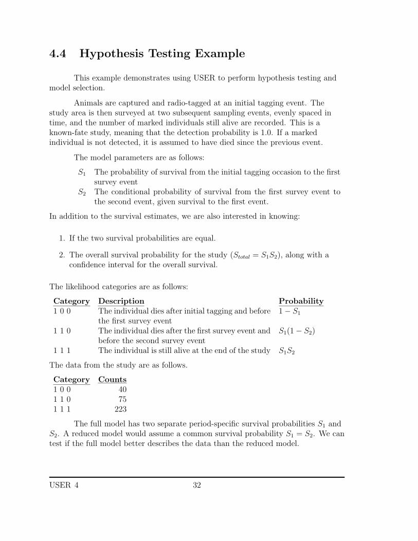
4.4 Hypothesis Testing Example

This example demonstrates using USER to perform hypothesis testing andmodel selection.

Animals are captured and radio-tagged at an initial tagging event. Thestudy area is then surveyed at two subsequent sampling events, evenly spaced intime, and the number of marked individuals still alive are recorded. This is aknown-fate study, meaning that the detection probability is 1.0. If a markedindividual is not detected, it is assumed to have died since the previous event.

The model parameters are as follows:

S1 The probability of survival from the initial tagging occasion to the firstsurvey event

S2 The conditional probability of survival from the first survey event tothe second event, given survival to the first event.

In addition to the survival estimates, we are also interested in knowing:

1. If the two survival probabilities are equal.

2. The overall survival probability for the study (Stotal = S1S2), along with aconfidence interval for the overall survival.

The likelihood categories are as follows:

Category Description Probability1 0 0 The individual dies after initial tagging and before

the first survey event1− S1

1 1 0 The individual dies after the first survey event andbefore the second survey event

S1(1− S2)

1 1 1 The individual is still alive at the end of the study S1S2

The data from the study are as follows.

Category Counts1 0 0 401 1 0 751 1 1 223

The full model has two separate period-specific survival probabilities S1 andS2. A reduced model would assume a common survival probability S1 = S2. We cantest if the full model better describes the data than the reduced model.

USER 4 32

Figure 4.29: Parameter definitions for the hypothesis testing example

4.4.1 Full Model Definition

We define the parameters as shown in Figure 4.29. In addition, we areinterested in the overall survival Stotal = S1S2. Therefore we need to define Stotal asa convenience function as shown in Figure 4.30. The likelihood definition is shownin Figure 4.31.

After defining the likelihood, go to the “Verify the Model” page. Onceeverything has been entered correctly, go to the “Parameter Seeds” page. Since weare estimating probabilities, the default seeds of 0.5 should suffice.

Profile Likelihood Confidence Intervals

We defined the convenience function Stotal = S1S2 because we were interestedin a confidence interval for the overall survival. Figure 4.32 shows that we arerequesting profile likelihood confidence intervals (alpha-level = 0.05) for theindividual survival probabilities as well as the overall survival.

Estimate the Parameters

Advance to the “Estimate the Model Parameters” page, and press the“Estimate” button. Figure 4.33 shows the estimation summary report for the full

33 USER 4

Figure 4.30: Convenience function definition for the hypothesis testing example

Figure 4.31: Likelihood definition for the hypothesis testing example

USER 4 34

Figure 4.32: Profile likelihood confidence interval requests for the hypothesis testingexample

model. In order to perform the the the hypothesis test, we need to record thelog-likelihood (-5.63645).

4.4.2 Reduced Model Definition

We are interested in comparing the full and reduced models. In the contextof hypothesis testing, the null hypothesis is: H0 : S1 = S2 (reduced model), vsHA : S1 6= S2 (full model). To define the reduced model, we can use the full modeldefinition from the previous section as starting point, as follows:

1. Unlock the workspace so that the model may be changed. Go to the “Actions”menu and select “Clear Current Estimates.” Press “OK” when asked forconfirmation. This will clear all estimates from the null model.

2. Double-click on “Parameters” on the navigation panel to return to the“Parameters” page. Right-click on the “S2” cell and select “Delete” as shownin Figure 4.34. We now have only one parameter: S1.

35 USER 4

Figure 4.33: Estimation Summary Report for the hypothesis testing example, fullmodel

USER 4 36

Figure 4.34: Delete the parameter S2 for the hypothesis testing example

3. Go to the “Convenience Functions” page, and add the convenience function“S2” as shown in Figure 4.35. Note that the actual likelihood definition doesnot need to be changed. The difference is that S2 is no longer a modelparameter to be estimated, but is simply another name for the one modelparameter S1.

4. Go to the “Estimate the Model Parameters” page and press “Estimate”.Figure 4.36 shows the resulting estimation summary report.

As with the full model, we must note the log-likelihood (-15.2063).

4.4.3 Test the Hypothesis

We can now test the hypothesis using a Likelihood Ratio Test:

• Null hypothesis: S1 = S2

• Alternative hypothesis: S1 6= S2

The likelihood ratio test statistic isχ2 = 2(−5.63645− (−15.2063)) = 19.1397. χ2 has an asymptotic chi-squaredistribution with one degree of freedom, giving a p-value of 0.00001, rejecting thenull hypothesis in favor of the alternative hypothesis S1 6= S2.

37 USER 4

Figure 4.35: Define the convenience function S2 for the hypothesis testing example

4.4.4 Model Selection Using an Information-TheoreticApproach

An alternative approach to hypothesis testing is model selection based on aninformation-theoretic approach(Model Selection and Multinomial Inference. APractical Information-Theoretic Approach. 2nd Ed, Burnham, Kenneth P. andDavid R. Anderson. 2002). With this approach, model selection is based onAkaike’s Information Criterion (AIC). The model with the smaller AIC is thepreferred model. In this example, the full model has an AIC of 15.2729, and thereduced model has an AIC of 32.4127. Based on the AIC, the full model is thepreferred model.

USER 4 38

Figure 4.36: Estimation Summary Report for the hypothesis testing example, reducedmodel

39 USER 4