Embed Size (px)
Citation preview
User Guide
ISOMAP & ROTOMAP 3D Surface Modelling &
Rockfall Analysis
Geo Soft di ing. G. Scioldo

ISOMAP & ROTOMAP - User Guide Summary · i
SummaryChapter 1 - Introduction to the ISOMAP family 1
Introduction to the ISOMAP family..........................................................................................................1
Chapter 2 - System requirements and program installation 2System requirements.............................................................................................................................. 2Program installation................................................................................................................................ 2
Chapter 3 - The program protection 7Program registration............................................................................................................................... 7
Chapter 4 - How to update the program 8Procedure for updating the program.......................................................................................................8Autoupdating requirements and troubleshooting....................................................................................9
Chapter 5 - User Interface 10Usage Notations................................................................................................................................... 10User Interface and Data Entering.........................................................................................................10
User Interface: Menu Bar and Menus..............................................................................................10The Input Dialogue Windows...........................................................................................................11Data Input With Tables.................................................................................................................... 12Message Windows.......................................................................................................................... 13Help On Line.................................................................................................................................... 13
Chapter 6 - Creation of a new project 14Project Menu........................................................................................................................................ 14
New Project Command.................................................................................................................... 14Open Project Command.................................................................................................................. 15Delete Project Command................................................................................................................. 16Printer Setup Command.................................................................................................................. 16
Chapter 7 - ISOMAP - Grid Generation 17Operation Grid Generation................................................................................................................... 17
Weighted Average........................................................................................................................... 17Kriging............................................................................................................................................. 17Method of the Weighted Average of Polynomial Surfaces...............................................................18Procedure........................................................................................................................................ 18
Edit Menu - Grid Generation................................................................................................................. 18Data Points Command..................................................................................................................... 19
The “Data Points” Dialogue box..................................................................................................19Gridding Parameters Command......................................................................................................19
The “Gridding Parameters” Dialogue Box...................................................................................20Example..................................................................................................................................... 21
Hidden Mesh Selection Command..................................................................................................21Calculate Menu - Grid Generation........................................................................................................22
Execute Calculation Command.......................................................................................................23Z(X,Y) Calculation Command..........................................................................................................23Volume Calculation Command........................................................................................................23
Print Menu............................................................................................................................................ 23Parameters Command..................................................................................................................... 23
The “Graphical Parameters” Dialogue Box.................................................................................23
ISOMAP & ROTOMAP - User Guide Summary · ii
The <Manual Colour Setting> Button.........................................................................................26Print Grid Command........................................................................................................................ 27
The Graphical Output Preview Window......................................................................................27Print Vertical Section Command......................................................................................................28
The “Vertical Section Configuration” Dialogue box.....................................................................28Export in SLK Format Command.....................................................................................................29Configure Command........................................................................................................................ 29
Exit Menu.............................................................................................................................................. 29
Chapter 8 - ISOMAP - Slope Map 30Slope Map (ISOMAP module)..............................................................................................................30
Procedure........................................................................................................................................ 30Edit menu - Slope Map......................................................................................................................... 30
Hidden Mesh Selection Command..................................................................................................30Calculate Menu - Slope Map................................................................................................................31
Execute Calculations Command......................................................................................................31Z(X,Y) Calculation Command..........................................................................................................31Volume Calculation Command........................................................................................................31
Print Menu - Slope Map........................................................................................................................ 31
Chapter 9 - ISOMAP - Exposure Map 32Exposure Map (ISOMAP module).........................................................................................................32
Procedure........................................................................................................................................ 32Edit menu - Exposure Map................................................................................................................... 32
Hidden Mesh Selection Command..................................................................................................32Calculate Menu - Exposure Map...........................................................................................................33
Execute Calculations Command......................................................................................................33Z(X,Y) Calculation Command..........................................................................................................33Volume Calculation Command........................................................................................................33
Print Menu - Exposure Map.................................................................................................................. 33
Chapter 10 - ISOMAP - Grid Difference 34Grid Difference (ISOMAP module)........................................................................................................34
Procedure........................................................................................................................................ 34Edit menu - Grid Difference.................................................................................................................. 34
Hidden Mesh Selection Command..................................................................................................34Select Subtrahend Grid Command..................................................................................................35
The “Select Subtrahend Grid” Dialogue Box...............................................................................35Calculate Menu - Grid Difference..........................................................................................................35
Execute Calculations Command......................................................................................................35Z(X,Y) Calculation Command..........................................................................................................35Volume Calculation Command........................................................................................................35
Print Menu - Grid Difference................................................................................................................. 35
Chapter 11 - ISOMAP - Linear Transformation 36Linear Transformation (ISOMAP module).............................................................................................36
Procedure........................................................................................................................................ 36Edit Menu - Linear Transformations......................................................................................................36
Hidden Mesh Selection Command..................................................................................................37Linear Transformation Parameters Command.................................................................................37
The “Linear Transformation Parameters” Dialogue box..............................................................37Calculate Menu - Linear Transformation...............................................................................................37
Execute Calculations Command......................................................................................................37Z(X,Y) Calculation Command..........................................................................................................37Volume Calculation Command........................................................................................................38
Print Menu - Linear Transformation......................................................................................................38
Chapter 12 - ISOMAP - Filtering 39Filtering (ISOMAP module)................................................................................................................... 39
Procedure........................................................................................................................................ 39
ISOMAP & ROTOMAP - User Guide Summary · iii
Edit Menu - Filtering.............................................................................................................................. 39Hidden Mesh Selection Command..................................................................................................40Select Filter Command.................................................................................................................... 40
The “Select Filter” Dialogue box.................................................................................................40Edit Filter Command........................................................................................................................ 40
Calculate Menu - Filtering..................................................................................................................... 40Execute Calculations Command......................................................................................................40Z(X,Y) Calculation Command..........................................................................................................40Volume Calculation Command........................................................................................................41
Print Menu - Filtering............................................................................................................................ 41
Chapter 13 - ISOMAP Menus - Grid Duplication 42Grid Duplication (ISOMAP module)......................................................................................................42
Procedure........................................................................................................................................ 42
Chapter 14 - ISOMAP Menus - DTM Import 43DTM Import (ISOMAP module).............................................................................................................43
Procedure........................................................................................................................................ 43
Chapter 15 - ISOMAP Menus - VID Import 44Import VID File (ISOMAP module)........................................................................................................44
Procedure........................................................................................................................................ 44
Chapter 16 - ISOMAP Menus - XYZ Import 45Import XYZ file (ISOMAP module).......................................................................................................45
Procedure........................................................................................................................................ 45
Chapter 17 - ISOMAP menus - DXF Import 46Import DXF file (ISOMAP module)........................................................................................................46
Procedure........................................................................................................................................ 47
Chapter 18 - ISOMAP menus - ASC Import 49Import ASC file (ISOMAP module)........................................................................................................49
Procedure........................................................................................................................................ 49
Chapter 19 - Introduction to the ROTOMAP module 50Introduction to the ROTOMAP module.................................................................................................50
Rockfall Analysis (ROTOMAP module)...........................................................................................50Procedure................................................................................................................................... 52
Edit Menu - Rockfall Analysis...............................................................................................................53Hidden Mesh Selection Command..................................................................................................53Rockfall Parameters Command.......................................................................................................53
The “Rockfall Parameters” Dialogue box....................................................................................53Geomechanical Parameters Command...........................................................................................55Placing Starting Lines Command....................................................................................................56
The “Placing Starting Lines” Dialogue Box................................................................................56Placing Protection Systems Command............................................................................................56
The “Placing Protection Systems” dialogue box.........................................................................56Calculate Menu - Rockfall Analysis.......................................................................................................57
Rockfall Calculation Command........................................................................................................58Stop Point Calculation Command....................................................................................................58Average Energy Calculation Command...........................................................................................58Maximum Energy Calculation Command.........................................................................................58Minimum Travel Time Calculation Command..................................................................................58Maximum Heights Calculation Command........................................................................................58Z(X,Y) Calculation Command..........................................................................................................58Volume Calculation Command........................................................................................................59
Print Menu - Rockfall Analysis..............................................................................................................59Parameters Command..................................................................................................................... 59
ISOMAP & ROTOMAP - User Guide Summary · iv
Physical Quantities Selection Command.........................................................................................59The “Physical Quantities Selection” dialogue window................................................................59
Print Grid Command........................................................................................................................ 60Print Vertical Section Command......................................................................................................60Print Rockfall Sections Command...................................................................................................60
The "Section Print Parameters" dialogue box.............................................................................60Export in SLK Format Command.....................................................................................................60Configure Command........................................................................................................................ 61
Chapter 20 - Miscellanea 62Reported values for coefficients of restitution.......................................................................................62References........................................................................................................................................... 64
ISOMAP & ROTOMAP - User Guide Chapter 1 - Introduction to the ISOMAP family · 1
Chapter 1 - Introduction to the ISOMAP family
Introduction to the ISOMAP familyThe ISOMAP family is an integrated software package that allows one to create a digital terrain model (DTM) that can be used for further elaborations, such as rockfall analysis and groundwater modelling.
The ISOMAP module allows one to create a grid from a set of spot points, and to produce maps, wireframe views, or solid views. It allows different calculations, such as slope mapping, exposure mapping, or filtering.
The ROTOMAP module is dedicated to 3D rockfall analysis, and allows the complete design of rockfall protective systems. It features true 3D modelling and many other options for model calibration and barrier design.
The INQIMAP module is dedicated to groundwater modelling. It leads to calculations from those based on simple analytical solutions to those that incorporate advanced and complex numerical techniques.The "Introduction to the INQUIMAP module" and the subsequent chapters are not included in the present version of the manual.
The ISOMAP family is a comprehensive package: it can directly produce high-quality graphic outputs, or export them to DXF or EMF formats, which preserve the vectorial quality of the printouts, even when the files are imported into external editors such as Microsoft Word or Corel Draw.
ISOMAP & ROTOMAP - User Guide Chapter 2 - System requirements and program installation · 2
Chapter 2 - System requirements and program installation
System requirements· Pentium® class processor
· Microsoft® Windows® 95 OSR 2.0, Windows 98, Windows Me, Windows NT®* 4.0 with Service Pack 5 or 6, Windows 2000, or Windows XP
· 64 MB of RAM (128 MB recommended)
· 100 MB of available hard-disk space
· CD-ROM drive
· A printer driver must be installed, even if the printer itself is not connected to the PC.
Program installationTo install the ROTOMAP program, run ROTOMAP32SETUP.EXE from the CD-ROM or from the folder where you downloaded and saved the setup program.
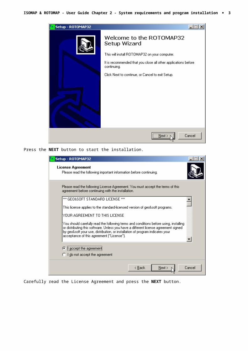
Press the NEXT button to start the installation.

ISOMAP & ROTOMAP - User Guide Chapter 2 - System requirements and program installation · 3
Carefully read the License Agreement and press the NEXT button.
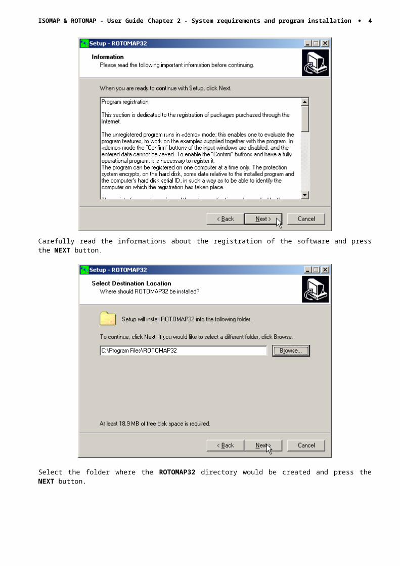
Carefully read the informations about the registration of the software and press the NEXT button.
ISOMAP & ROTOMAP - User Guide Chapter 2 - System requirements and program installation · 4
Select the folder where the ROTOMAP32 directory would be created and press the NEXT button.
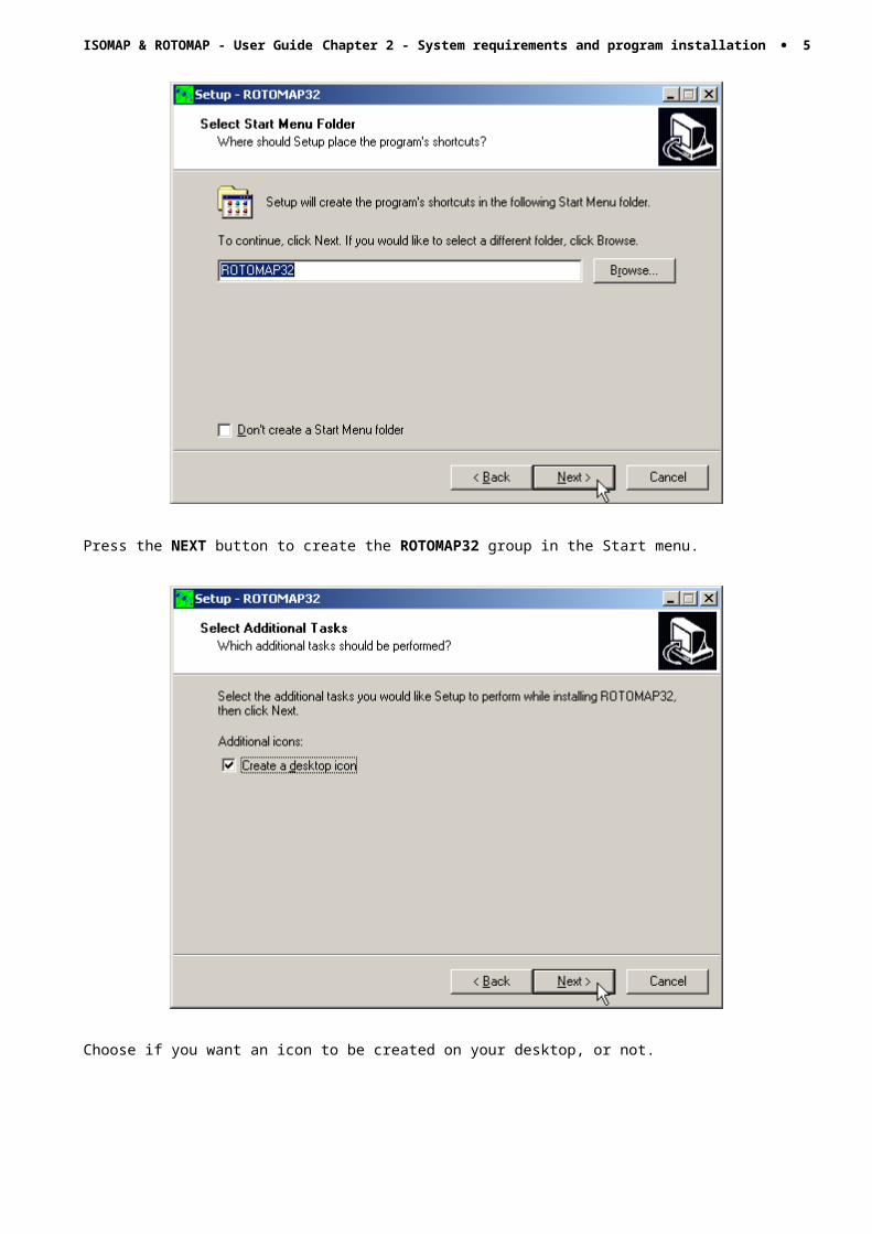
Press the NEXT button to create the ROTOMAP32 group in the Start menu.
ISOMAP & ROTOMAP - User Guide Chapter 2 - System requirements and program installation · 5
Choose if you want an icon to be created on your desktop, or not.
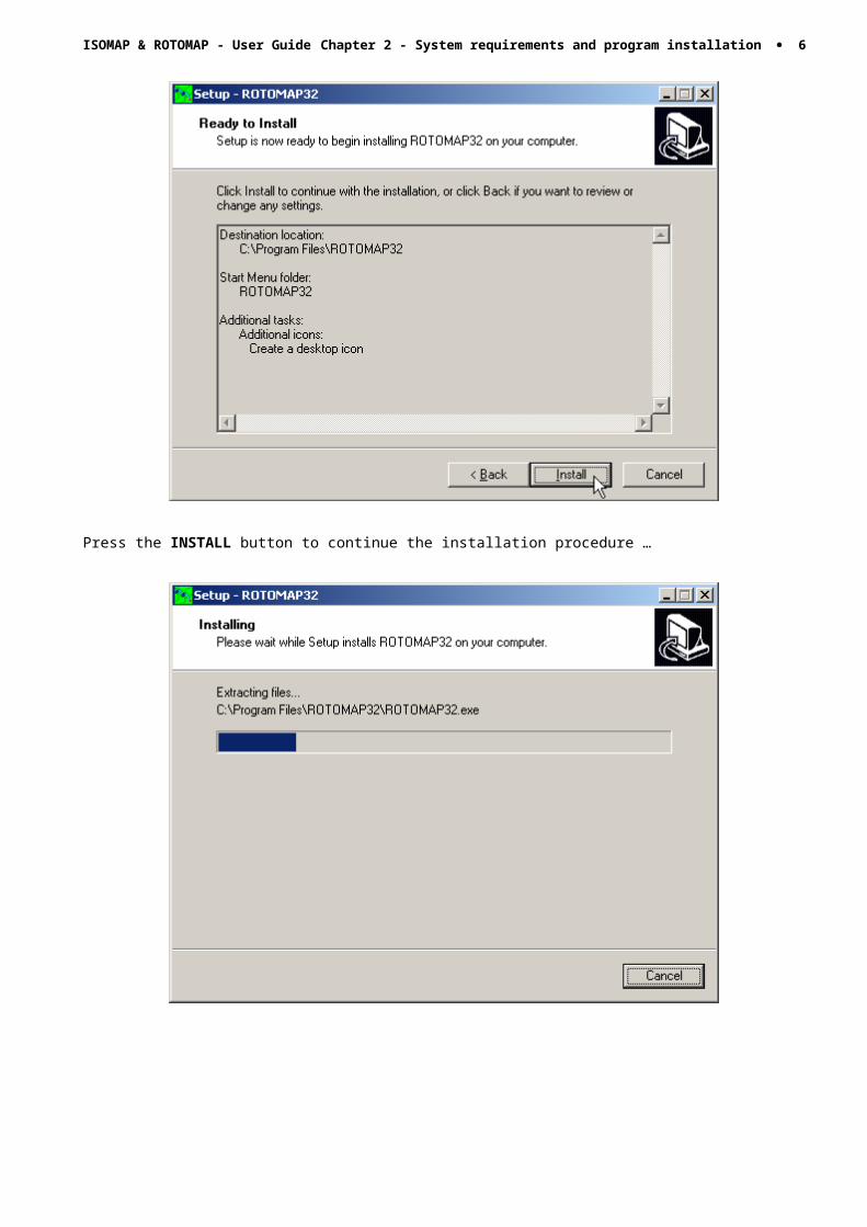
Press the INSTALL button to continue the installation procedure …
ISOMAP & ROTOMAP - User Guide Chapter 2 - System requirements and program installation · 6
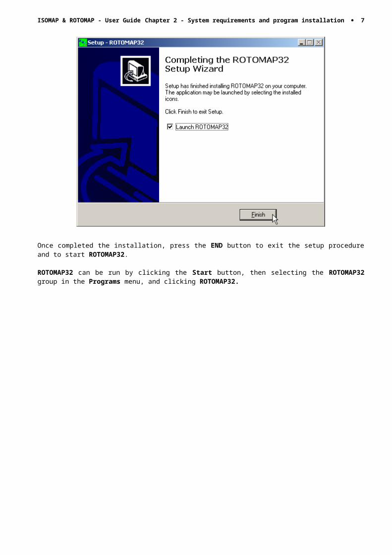
Once completed the installation, press the END button to exit the setup procedure and to start ROTOMAP32.
ROTOMAP32 can be run by clicking the Start button, then selecting the ROTOMAP32 group in the Programs menu, and clicking ROTOMAP32.
ISOMAP & ROTOMAP - User Guide Chapter 3 - The program protection · 7
Chapter 3 - The program protection
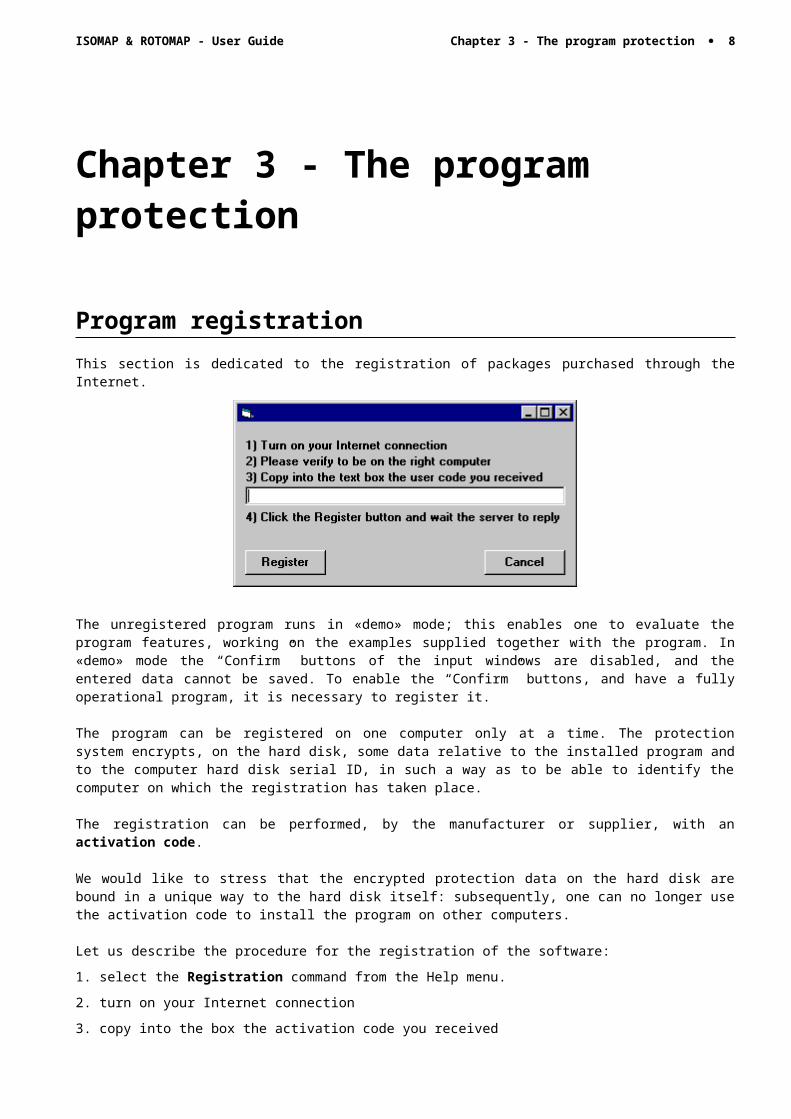
Program registrationThis section is dedicated to the registration of packages purchased through the Internet.
The unregistered program runs in «demo» mode; this enables one to evaluate the program features, working on the examples supplied together with the program. In «demo» mode the “Confirm” buttons of the input windows are disabled, and the entered data cannot be saved. To enable the “Confirm” buttons, and have a fully operational program, it is necessary to register it.
The program can be registered on one computer only at a time. The protection system encrypts, on the hard disk, some data relative to the installed program and to the computer hard disk serial ID, in such a way as to be able to identify the computer on which the registration has taken place.
The registration can be performed, by the manufacturer or supplier, with an activation code.
We would like to stress that the encrypted protection data on the hard disk are bound in a unique way to the hard disk itself: subsequently, one can no longer use the activation code to install the program on other computers.
Let us describe the procedure for the registration of the software:
1. select the Registration command from the Help menu.
2. turn on your Internet connection
3. copy into the box the activation code you received
4. click the <Registration> button and wait the server to replay
ISOMAP & ROTOMAP - User Guide Chapter 4 - How to update the program · 8
Chapter 4 - How to update the program
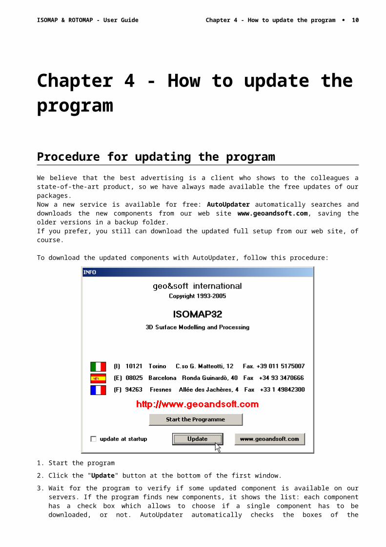
Procedure for updating the programWe believe that the best advertising is a client who shows to the colleagues a state-of-the-art product, so we have always made available the free updates of our packages.Now a new service is available for free: AutoUpdater automatically searches and downloads the new components from our web site www.geoandsoft.com, saving the older versions in a backup folder.If you prefer, you still can download the updated full setup from our web site, of course.
To download the updated components with AutoUpdater, follow this procedure:
1. Start the program
2. Click the "Update" button at the bottom of the first window.
3. Wait for the program to verify if some updated component is available on our servers. If the program finds new components, it shows the list: each component has a check box which allows to choose if a single component has to be downloaded, or not. AutoUpdater automatically checks the boxes of the components whose download is suggested, and leaves unchecked the files which could have been modified by the user, like the colour configuration files.
4. Select the files you want to download and click the "Update" button.
5. Once the files have been installed, AutoUpdater runs the updated program.
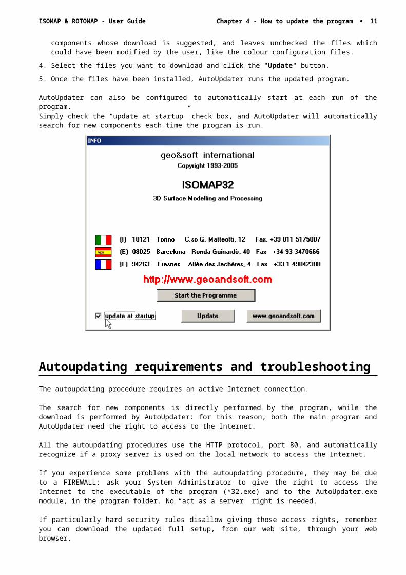
AutoUpdater can also be configured to automatically start at each run of the program.
ISOMAP & ROTOMAP - User Guide Chapter 4 - How to update the program · 9
Simply check the “update at startup” check box, and AutoUpdater will automatically search for new components each time the program is run.
Autoupdating requirements and troubleshootingThe autoupdating procedure requires an active Internet connection.
The search for new components is directly performed by the program, while the download is performed by AutoUpdater: for this reason, both the main program and AutoUpdater need the right to access to the Internet.
All the autoupdating procedures use the HTTP protocol, port 80, and automatically recognize if a proxy server is used on the local network to access the Internet.
If you experience some problems with the autoupdating procedure, they may be due to a FIREWALL: ask your System Administrator to give the right to access the Internet to the executable of the program (*32.exe) and to the AutoUpdater.exe module, in the program folder. No “act as a server” right is needed.
If particularly hard security rules disallow giving those access rights, remember you can download the updated full setup, from our web site, through your web browser.

ISOMAP & ROTOMAP - User Guide Chapter 5 - User Interface · 10
Chapter 5 - User Interface
Usage NotationsSome typographical notations and keyboard formats are used in this manual to help locate and interpret information more easily.
Bold print is used to indicate command names and related options. Characters appearing in bold print should be typed exactly as printed, including spaces.
Words written in italics indicate a request for information.
CAPITAL letters are used to indicate computer, printer, directory, and file names.
User Interface and Data EnteringThe user interface is designed to be easy to use and powerful and is supported by complete on-line help. This help contains practical hints and the theoretical background, where applicable. It should reduce the requirement of frequently consulting the printed manuals.All the commands are located inside a menu bar. Each menu contains a list of commands that one can select with the mouse or the keyboard. The arrangement of the menus, designed with ergonomic criteria, follows the logical order of the operations, inhibiting the access to further operations until all the necessary data have been entered.The interface layout is maintained in all of our programs, to simplify, as much as possible, the transition from one program to another to avoid having to learn different commands and procedures for similar functions (such as entering data or managing files).Let us examine the general components that are available in the user interface of geo&soft programs.
User Interface: Menu Bar and MenusThe Menu Bar manages the access to all the program commands. The goal of the menu design is to offer an ergonomic, simple, and understandable arrangement of the commands.The menus used to perform a complete operation are normally ordered left to right and top to bottom. When possible, the following scheme is used: definition of the name of the project, entering the required data, performing the calculation, and generating the output as a preview or final print.
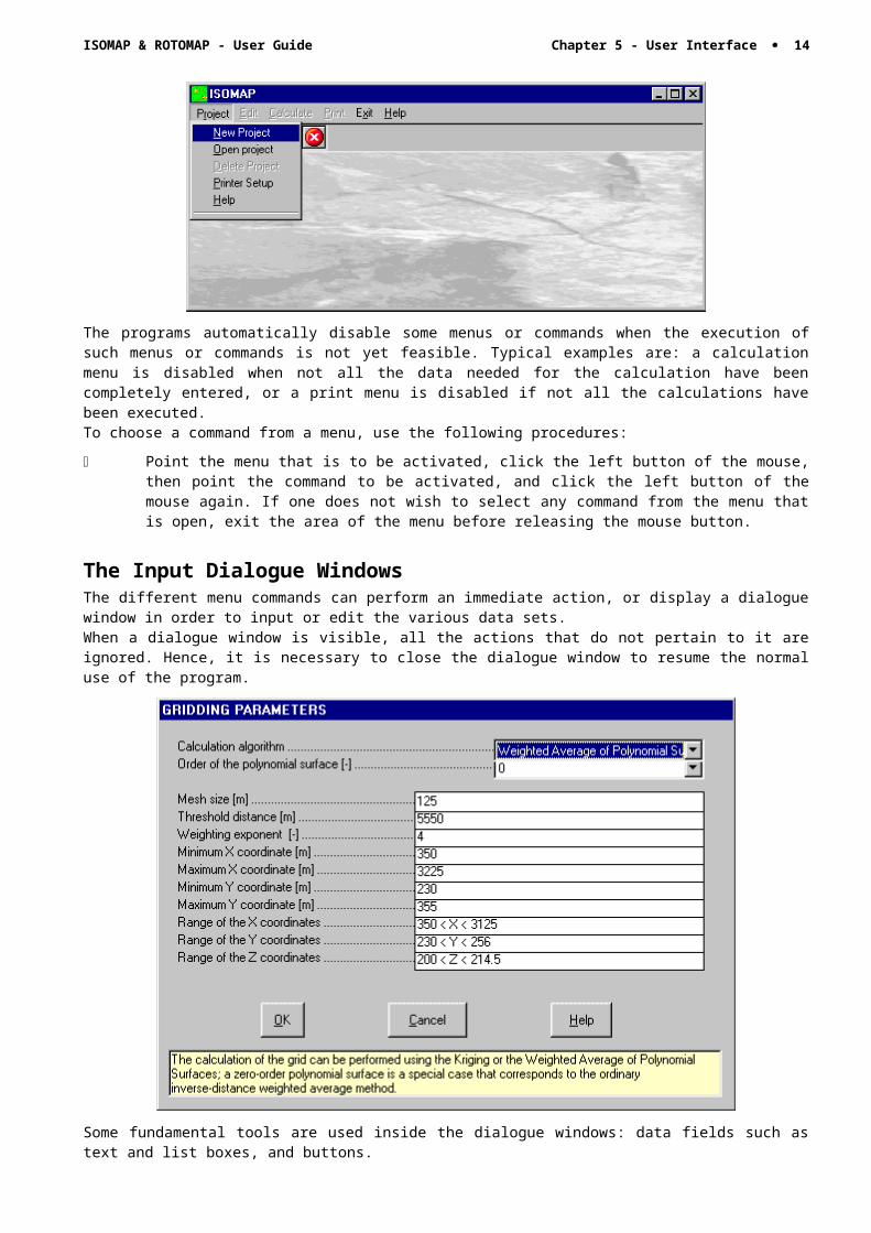
The programs automatically disable some menus or commands when the execution of such menus or commands is not yet feasible. Typical examples are: a calculation menu is disabled when not all the data
ISOMAP & ROTOMAP - User Guide Chapter 5 - User Interface · 11
needed for the calculation have been completely entered, or a print menu is disabled if not all the calculations have been executed.To choose a command from a menu, use the following procedures:
Point the menu that is to be activated, click the left button of the mouse, then point the command to be activated, and click the left button of the mouse again. If one does not wish to select any command from the menu that is open, exit the area of the menu before releasing the mouse button.
The Input Dialogue WindowsThe different menu commands can perform an immediate action, or display a dialogue window in order to input or edit the various data sets.When a dialogue window is visible, all the actions that do not pertain to it are ignored. Hence, it is necessary to close the dialogue window to resume the normal use of the program.
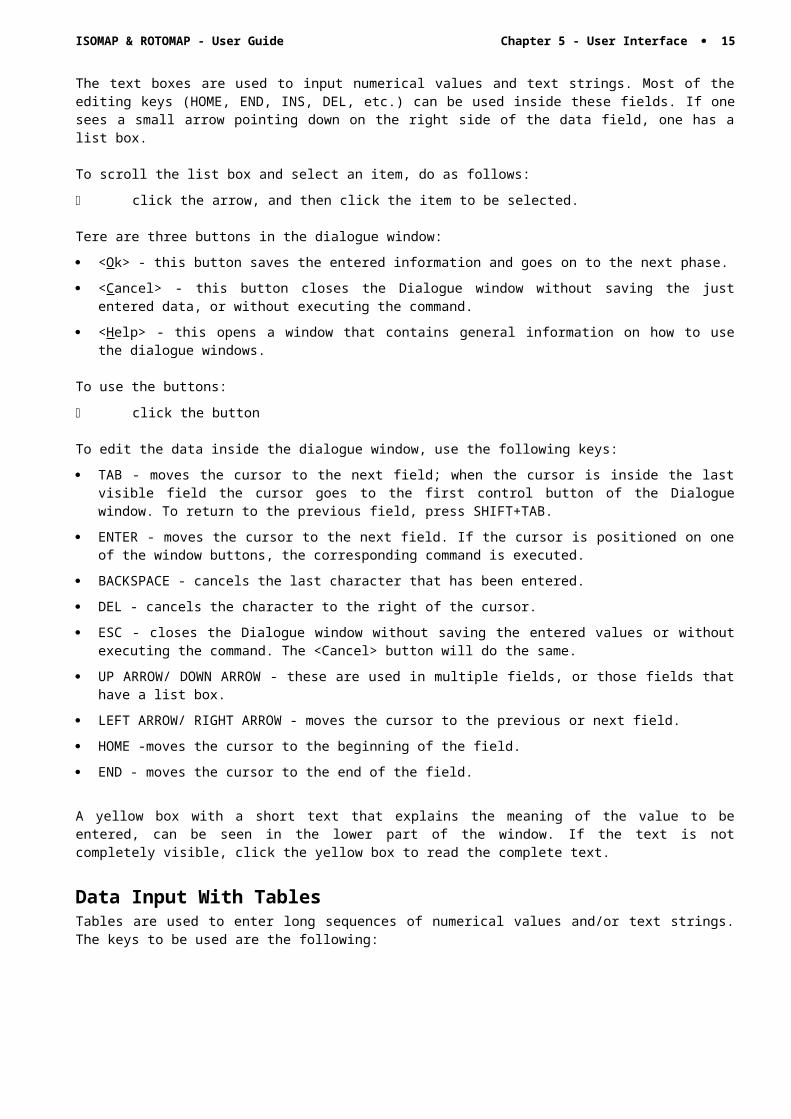
Some fundamental tools are used inside the dialogue windows: data fields such as text and list boxes, and buttons.The text boxes are used to input numerical values and text strings. Most of the editing keys (HOME, END, INS, DEL, etc.) can be used inside these fields. If one sees a small arrow pointing down on the right side of the data field, one has a list box.
To scroll the list box and select an item, do as follows:
click the arrow, and then click the item to be selected.
Tere are three buttons in the dialogue window:
· <Ok> - this button saves the entered information and goes on to the next phase.
· <Cancel> - this button closes the Dialogue window without saving the just entered data, or without executing the command.
· <Help> - this opens a window that contains general information on how to use the dialogue windows.
To use the buttons:
click the button
To edit the data inside the dialogue window, use the following keys:
· TAB - moves the cursor to the next field; when the cursor is inside the last visible field the cursor goes to the first control button of the Dialogue window. To return to the previous field, press SHIFT+TAB.
ISOMAP & ROTOMAP - User Guide Chapter 5 - User Interface · 12
· ENTER - moves the cursor to the next field. If the cursor is positioned on one of the window buttons, the corresponding command is executed.
· BACKSPACE - cancels the last character that has been entered.
· DEL - cancels the character to the right of the cursor.
· ESC - closes the Dialogue window without saving the entered values or without executing the command. The <Cancel> button will do the same.
· UP ARROW/ DOWN ARROW - these are used in multiple fields, or those fields that have a list box.
· LEFT ARROW/ RIGHT ARROW - moves the cursor to the previous or next field.
· HOME -moves the cursor to the beginning of the field.
· END - moves the cursor to the end of the field.
A yellow box with a short text that explains the meaning of the value to be entered, can be seen in the lower part of the window. If the text is not completely visible, click the yellow box to read the complete text.
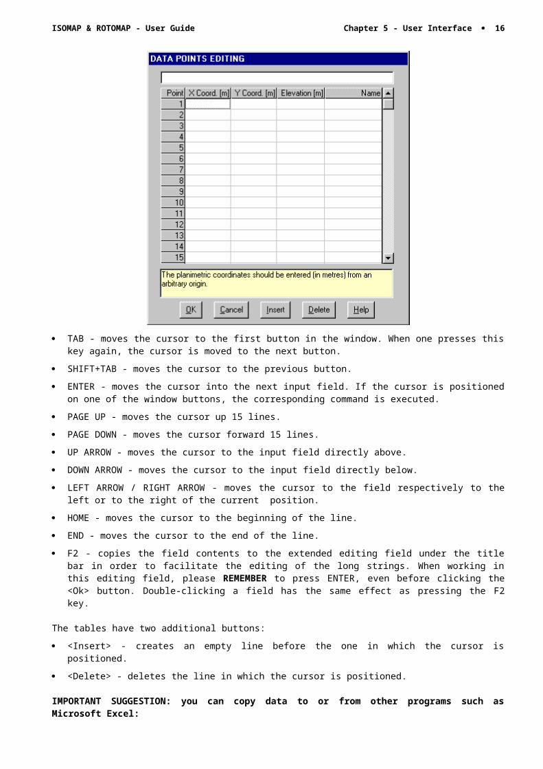
Data Input With TablesTables are used to enter long sequences of numerical values and/or text strings. The keys to be used are the following:
· TAB - moves the cursor to the first button in the window. When one presses this key again, the cursor is moved to the next button.
· SHIFT+TAB - moves the cursor to the previous button.
· ENTER - moves the cursor into the next input field. If the cursor is positioned on one of the window buttons, the corresponding command is executed.
· PAGE UP - moves the cursor up 15 lines.
· PAGE DOWN - moves the cursor forward 15 lines.
· UP ARROW - moves the cursor to the input field directly above.
· DOWN ARROW - moves the cursor to the input field directly below.
· LEFT ARROW / RIGHT ARROW - moves the cursor to the field respectively to the left or to the right of the current position.

ISOMAP & ROTOMAP - User Guide Chapter 5 - User Interface · 13
· HOME - moves the cursor to the beginning of the line.
· END - moves the cursor to the end of the line.
· F2 - copies the field contents to the extended editing field under the title bar in order to facilitate the editing of the long strings. When working in this editing field, please REMEMBER to press ENTER, even before clicking the <Ok> button. Double-clicking a field has the same effect as pressing the F2 key.
The tables have two additional buttons:
· <Insert> - creates an empty line before the one in which the cursor is positioned.
· <Delete> - deletes the line in which the cursor is positioned.
IMPORTANT SUGGESTION: you can copy data to or from other programs such as Microsoft Excel:
The data entered in the table can be copied in order to be pasted into another table.To copy the table’s contents:
press the key combination CTRL+C. The contents will be copied into the Clipboard of Windows.
To paste the Clipboard contents into the table:
press the key combination SHIFT+INS, or CTRL+V.
A yellow box with a short text that explains the meaning of the value to be entered, can be seen in the lower part of the window. If the text is not completely visible, click the yellow box to read the complete text.
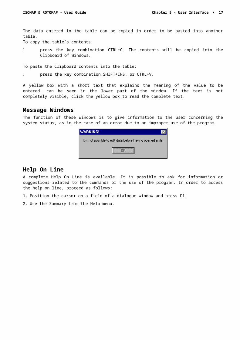
Message WindowsThe function of these windows is to give information to the user concerning the system status, as in the case of an error due to an improper use of the program.
Help On Line A complete Help On Line is available. It is possible to ask for information or suggestions related to the commands or the use of the program. In order to access the help on line, proceed as follows:
1. Position the cursor on a field of a dialogue window and press F1.
2. Use the Summary from the Help menu.
ISOMAP & ROTOMAP - User Guide Chapter 6 - Creation of a new project · 14
Chapter 6 - Creation of a new project
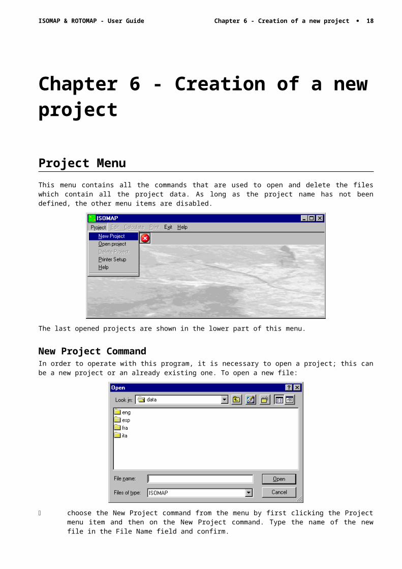
Project MenuThis menu contains all the commands that are used to open and delete the files which contain all the project data. As long as the project name has not been defined, the other menu items are disabled.
The last opened projects are shown in the lower part of this menu.
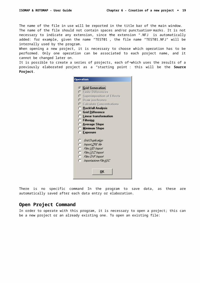
New Project CommandIn order to operate with this program, it is necessary to open a project; this can be a new project or an already existing one. To open a new file:
choose the New Project command from the menu by first clicking the Project menu item and then on the New Project command. Type the name of the new file in the File Name field and confirm.
The name of the file in use will be reported in the title bar of the main window.The name of the file should not contain spaces and/or punctuation marks. It is not necessary to indicate any extension, since the extension “.NFJ” is automatically added: for example, given the name “TEST01”, the file name “TEST01.NFJ" will be internally used by the program.When opening a new project, it is necessary to choose which operation has to be performed. Only one operation can be associated to each project name, and it cannot be changed later on.
ISOMAP & ROTOMAP - User Guide Chapter 6 - Creation of a new project · 15
It is possible to create a series of projects, each of which uses the results of a previously elaborated project as a “starting point”: this will be the Source Project.
There is no specific command In the program to save data, as these are automatically saved after each data entry or elaboration.
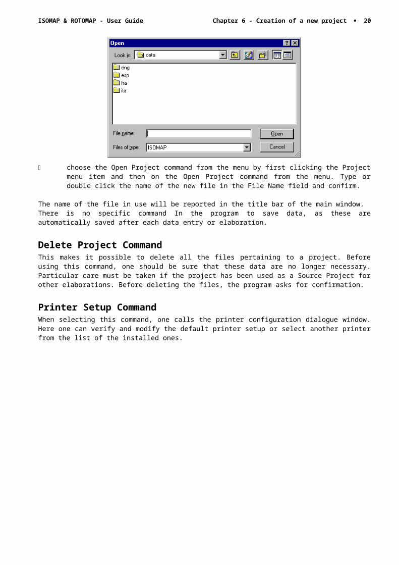
Open Project Command In order to operate with this program, it is necessary to open a project; this can be a new project or an already existing one. To open an existing file:
choose the Open Project command from the menu by first clicking the Project menu item and then on the Open Project command from the menu. Type or double click the name of the new file in the File Name field and confirm.
The name of the file in use will be reported in the title bar of the main window.There is no specific command In the program to save data, as these are automatically saved after each data entry or elaboration.
ISOMAP & ROTOMAP - User Guide Chapter 6 - Creation of a new project · 16
Delete Project CommandThis makes it possible to delete all the files pertaining to a project. Before using this command, one should be sure that these data are no longer necessary. Particular care must be taken if the project has been used as a Source Project for other elaborations. Before deleting the files, the program asks for confirmation.
Printer Setup CommandWhen selecting this command, one calls the printer configuration dialogue window. Here one can verify and modify the default printer setup or select another printer from the list of the installed ones.
ISOMAP & ROTOMAP - User Guide Chapter 7 - ISOMAP - Grid Generation · 17
Chapter 7 - ISOMAP - Grid Generation
Operation Grid GenerationThe basis of any project is the generation of a regular grid. The square grid is generated using one of the available methods, starting from a set of arbitrarily positioned points sampled on the surface under examination. The more regular the disposition and density of the input points are, the more reliable the final result will be, regardless of which calculation method is used. Let us consider the calculation methods that can be used.
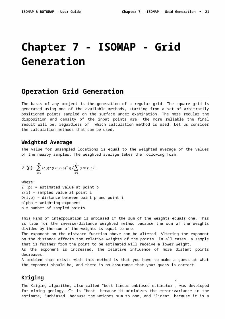
Weighted AverageThe value for unsampled locations is equal to the weighted average of the values of the nearby samples. The weighted average takes the following form:
Z'(p) = /(Z(i) * (1 / D(i, p) )) (1 / D(i, p) )i=1
n
i=1
n
where:Z'(p) = estimated value at point pZ(i) = sampled value at point iD(i,p) = distance between point p and point ialpha = weighting exponentn = number of sampled points
This kind of interpolation is unbiased if the sum of the weights equals one. This is true for the inverse-distance weighted method because the sum of the weights divided by the sum of the weights is equal to one.The exponent on the distance function above can be altered. Altering the exponent on the distance affects the relative weights of the points. In all cases, a sample that is further from the point to be estimated will receive a lower weight.As the exponent is increased, the relative influence of more distant points decreases.A problem that exists with this method is that you have to make a guess at what the exponent should be, and there is no assurance that your guess is correct.
KrigingThe Kriging algorithm, also called “best linear unbiased estimator”, was developed for mining geology. It is “best” because it minimizes the error variance in the estimate, “unbiased” because the weights sum to one, and “linear” because it is a simple weighted average. It also uses a weighted average method to calculate the value at unsampled locations, but rather than guessing at the relationship between similarity of values and distance (like we do when we guess at the exponent in inverse-distance methods), the relationship is calculated from the data using the semivariogram.
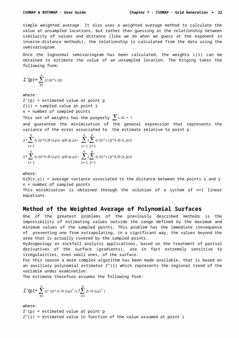
Once the lognormal semivariogram has been calculated, the weights L(i) can be obtained to estimate the value of an unsampled location. The Kriging takes the following form:
Z'(p) = (Z(i) * L(i))i=1
n
where:Z'(p) = estimated value at point p
ISOMAP & ROTOMAP - User Guide Chapter 7 - ISOMAP - Grid Generation · 18
Z(i) = sampled value at point in = number of sampled pointsThis set of weights has the property L(i) = 1and guarantee the minimisation of the general expression that represents the variance of the error associated to the estimate relative to point p.
2 * (L(i) * G(D(i, p)) - g(D(p, p))
i = 1
n- ( ( L(i) * L( j) * G(D(i, j))))
j = 1
n
i = 1
n
2 * (L(i) * G(D(i, p)) - g(D(p, p))
i = 1
n- ( ( L(i) * L( j) * G(D(i, j))))
j = 1
n
i = 1
n
where:G(D(x,y)) = average variance associated to the distance between the points x and yn = number of sampled pointsThis minimisation is obtained through the solution of a system of n+1 linear equations.
Method of the Weighted Average of Polynomial SurfacesOne of the greatest problems of the previously described methods is the impossibility of estimating values outside the range defined by the maximum and minimum values of the sampled points. This problem has the immediate consequence of preventing one from extrapolating, in a significant way, the values beyond the area that is actually covered by the sampled points.Hydrogeology or rockfall analysis applications, based on the treatment of partial derivatives of the surface (gradients), are in fact extremely sensitive to irregularities, even small ones, of the surface.For this reason a more complex algorithm has been made available, that is based on an auxiliary polynomial estimator Z"(i) which represents the regional trend of the variable under examination.The estimate therefore assumes the following form:
Z'(p) = / ( Z" (i) * (1 / D(i, p) )) (1 / D(i, p) )i=1
n
i=1
n
where:Z'(p) = estimated value at point pZ"(i) = estimated value in function of the value assumed at point iD(i,p) = distance between point p and point ialpha = weight exponentn = number of sampled points
Procedure· Select the “New Project” command from the “Project” menu
· Choose a new name for the project
· Select “Grid Generation” in the “Operation” window
· Use the “Edit Points” in the “Edit” menu to input the spot sampled points
· Use the “Grid Parameters” in the “Edit” menu to choose how the grid will be calculated
· Select “Calculation” on the menu bar
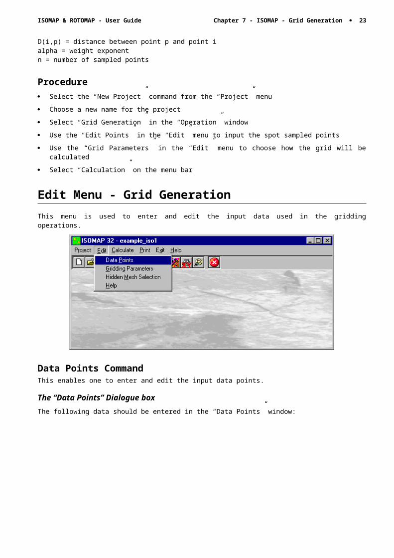
Edit Menu - Grid GenerationThis menu is used to enter and edit the input data used in the gridding operations.
ISOMAP & ROTOMAP - User Guide Chapter 7 - ISOMAP - Grid Generation · 19
Data Points CommandThis enables one to enter and edit the input data points.
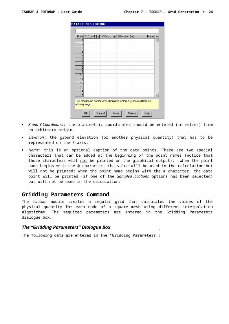
The “Data Points” Dialogue boxThe following data should be entered in the “Data Points” window:
· X and Y Coordinates: the planimetric coordinates should be entered (in metres) from an arbitrary origin.
· Elevation: the ground elevation (or another physical quantity) that has to be represented on the Z-axis.
· Name: this is an optional caption of the data points. There are two special characters that can be added at the beginning of the point names (notice that those characters will not be printed on the graphical output): when the point name begins with the @ character, the value will be used in the calculation but will not be printed; when the point name begins with the # character, the data point will be printed (if one of the Sampled locations options has been selected) but will not be used in the calculation.
Gridding Parameters CommandThe Isomap module creates a regular grid that calculates the values of the physical quantity for each node of a square mesh using different interpolation algorithms. The required parameters are entered in the Gridding Parameters dialogue box.
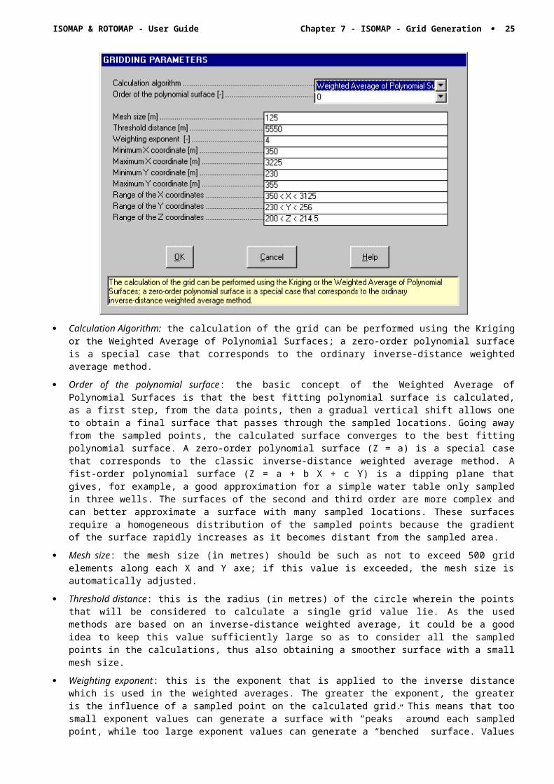
The “Gridding Parameters” Dialogue BoxThe following data are entered in the “Gridding Parameters”:
ISOMAP & ROTOMAP - User Guide Chapter 7 - ISOMAP - Grid Generation · 20
· Calculation Algorithm: the calculation of the grid can be performed using the Kriging or the Weighted Average of Polynomial Surfaces; a zero-order polynomial surface is a special case that corresponds to the ordinary inverse-distance weighted average method.
· Order of the polynomial surface: the basic concept of the Weighted Average of Polynomial Surfaces is that the best fitting polynomial surface is calculated, as a first step, from the data points, then a gradual vertical shift allows one to obtain a final surface that passes through the sampled locations. Going away from the sampled points, the calculated surface converges to the best fitting polynomial surface. A zero-order polynomial surface (Z = a) is a special case that corresponds to the classic inverse-distance weighted average method. A fist-order polynomial surface (Z = a + b X + c Y) is a dipping plane that gives, for example, a good approximation for a simple water table only sampled in three wells. The surfaces of the second and third order are more complex and can better approximate a surface with many sampled locations. These surfaces require a homogeneous distribution of the sampled points because the gradient of the surface rapidly increases as it becomes distant from the sampled area.
· Mesh size: the mesh size (in metres) should be such as not to exceed 500 grid elements along each X and Y axe; if this value is exceeded, the mesh size is automatically adjusted.
· Threshold distance: this is the radius (in metres) of the circle wherein the points that will be considered to calculate a single grid value lie. As the used methods are based on an inverse-distance weighted average, it could be a good idea to keep this value sufficiently large so as to consider all the sampled points in the calculations, thus also obtaining a smoother surface with a small mesh size.
· Weighting exponent: this is the exponent that is applied to the inverse distance which is used in the weighted averages. The greater the exponent, the greater is the influence of a sampled point on the calculated grid. This means that too small exponent values can generate a surface with “peaks” around each sampled point, while too large exponent values can generate a “benched” surface. Values between 4 and 6 can normally yield good results.
· Minimum X coordinate: together with the ordinate of the lower side, this defines the lower left corner of the grid.
· Maximum X coordinate: together with the ordinate of the upper side, this defines the upper right corner of the grid.
· Minimum Y coordinate: together with the abscissa of the left side, this defines the lower left corner of the grid.
· Maximum Y coordinate: together with the abscissa of the right side, this defines the upper right corner of the grid
ISOMAP & ROTOMAP - User Guide Chapter 7 - ISOMAP - Grid Generation · 21
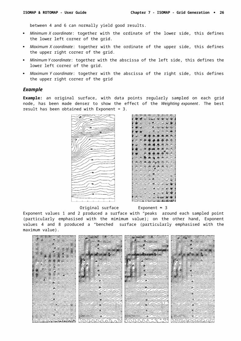
ExampleExample: an original surface, with data points regularly sampled on each grid node, has been made denser to show the effect of the Weighting exponent. The best result has been obtained with Exponent = 3.
Original surface Exponent = 3Exponent values 1 and 2 produced a surface with “peaks” around each sampled point (particularly emphasised with the minimum value); on the other hand, Exponent values 4 and 8 produced a “benched” surface (particularly emphasised with the maximum value).
Exponent = 1 Exponent = 2 Exponent = 4 Exponent = 8
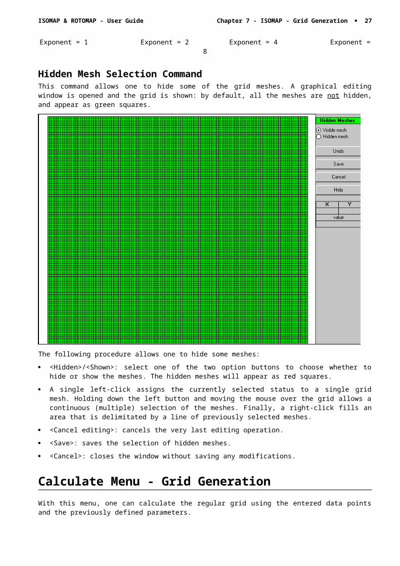
Hidden Mesh Selection CommandThis command allows one to hide some of the grid meshes. A graphical editing window is opened and the grid is shown: by default, all the meshes are not hidden, and appear as green squares.
ISOMAP & ROTOMAP - User Guide Chapter 7 - ISOMAP - Grid Generation · 22
The following procedure allows one to hide some meshes:
· <Hidden>/<Shown>: select one of the two option buttons to choose whether to hide or show the meshes. The hidden meshes will appear as red squares.
· A single left-click assigns the currently selected status to a single grid mesh. Holding down the left button and moving the mouse over the grid allows a continuous (multiple) selection of the meshes. Finally, a right-click fills an area that is delimitated by a line of previously selected meshes.
· <Cancel editing>: cancels the very last editing operation.
· <Save>: saves the selection of hidden meshes.
· <Cancel>: closes the window without saving any modifications.
Calculate Menu - Grid GenerationWith this menu, one can calculate the regular grid using the entered data points and the previously defined parameters.
ISOMAP & ROTOMAP - User Guide Chapter 7 - ISOMAP - Grid Generation · 23
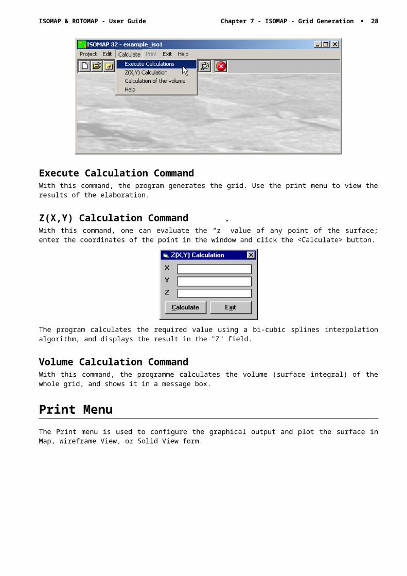
Execute Calculation Command With this command, the program generates the grid. Use the print menu to view the results of the elaboration.
Z(X,Y) Calculation Command With this command, one can evaluate the “z” value of any point of the surface; enter the coordinates of the point in the window and click the <Calculate> button.
The program calculates the required value using a bi-cubic splines interpolation algorithm, and displays the result in the "Z" field.
Volume Calculation CommandWith this command, the programme calculates the volume (surface integral) of the whole grid, and shows it in a message box.
Print MenuThe Print menu is used to configure the graphical output and plot the surface in Map, Wireframe View, or Solid View form.
Parameters CommandWith this command, the “Graphical Parameters” dialogue window is shown.
The “Graphical Parameters” Dialogue BoxThe " Graphical Parameters" dialogue window allows the configuration of most of the graphical parameters (see also the “Configure” item of the Print menu).
· Map, Wireframe View, Solid View: one can here choose the representation type.
The three buttons on this dialogue window allow one to select different parameter sets.
ISOMAP & ROTOMAP - User Guide Chapter 7 - ISOMAP - Grid Generation · 24
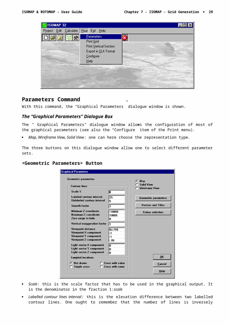
<Geometric Parameters> Button
· Scale: this is the scale factor that has to be used in the graphical output. It is the denominator in the fraction 1:scale
· Labelled contour lines interval: this is the elevation difference between two labelled contour lines. One ought to remember that the number of lines is inversely proportional to the given interval. A too small interval will slow down the drawing speed.
· Unlabeled contour lines interval: this is the elevation difference between adjacent unlabeled contour lines. One ought to remember that the number of lines is inversely proportional to the given interval. A too small interval will slow down the drawing speed.
· Smooth factor: this is the number of elements into which each grid element is divided, in order to represent more detailed contour lines; the larger this number the more accurate and attractive the drawing will be. If a high value is used there will consequently be a longer computing time and a larger file size, which increase proportionally with the square of the Smooth factor. If the Smooth factor is equal to one, a special faster algorithm is used. The Smooth factor value can vary between one and nine.
· Minimum Z coordinate: this defines the minimum threshold value of the contour lines that have to be represented. This parameter can be useful, for example, when plotting concentration contour lines where it would be erroneus to represent negative values. The range between minimum and maximum is an open interval.
· Maximum Z coordinate this defines the maximum threshold value of the contour lines that have to be represented. This parameter can be useful when one wants to eliminate values that are too high, such as the borders of polynomial extrapolations.
· Zero range to hide: this parameter allows one to hide the contour lines close to zero. This option is useful, for example, for the representation of magnetometric data.
· Vertical exaggeration factor: this factor enables one to stress the drawing, thus enhancing the anomalies of the plotted quantity.
· Viewpoint distance: this is only used in the Solid View. It is the absolute distance (in meters) between the viewpoint and the centre of the grid. This parameter is not used in the Wireframe View, because, in this case, the viewpoint distance is considered to be infinite.
· Viewpoint Vector X , Y, Z components: these define the direction of the viewpoint from the centre of the grid. The program disregards the vector magnitude, and automatically considers only the direction. It is used both in the Solid View and in the Wireframe View.
· Light Vector X , Y, Z components: these define the direction of the light point from the centre of the grid. If the three coordinates are equal to zero, no light effect is added. These parameters are used in the Map and
ISOMAP & ROTOMAP - User Guide Chapter 7 - ISOMAP - Grid Generation · 25
in the Solid View.
· Sampled locations: one can decide if and how the sampled locations will be drawn. The available options are: a simple cross, a cross labelled with the value of the sample, a cross labelled with the name of the location, or no representation at all.
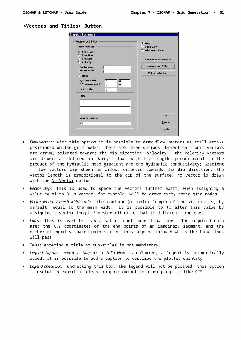
<Vectors and Titles> Button
· Flow vectors: with this option it is possible to draw flow vectors as small arrows positioned on the grid nodes. There are three options: Direction - unit vectors are drawn, oriented towards the dip direction; Velocity - the velocity vectors are drawn, as defined in Darcy’s law, with the lengths proportional to the product of the hydraulic head gradient and the hydraulic conductivity; Gradient - flow vectors are shown as arrows oriented towards the dip direction: the vector length is proportional to the dip of the surface. No vector is drawn with the No Vector option.
· Vector step: this is used to space the vectors further apart; when assigning a value equal to 3, a vector, for example, will be drawn every three grid nodes.
· Vector length / mesh width ratio: the maximum (or unit) length of the vectors is, by default, equal to the mesh width. It is possible to to alter this value by assigning a vector length / mesh width ratio that is different from one.
· Lines: this is used to draw a set of continuous flow lines. The required data are: the X,Y coordinates of the end points of an imaginary segment, and the number of equally spaced points along this segment through which the flow lines will pass.
· Titles: entering a title or sub-titles is not mandatory.
· Legend Caption: when a Map or a Solid View is coloured, a legend is automatically added. It is possible to add a caption to describe the plotted quantity.
· Legend check box: unchecking this box, the legend will not be plotted; this option is useful to export a “clean” graphic output to other programs like GIS.
ISOMAP & ROTOMAP - User Guide Chapter 7 - ISOMAP - Grid Generation · 26
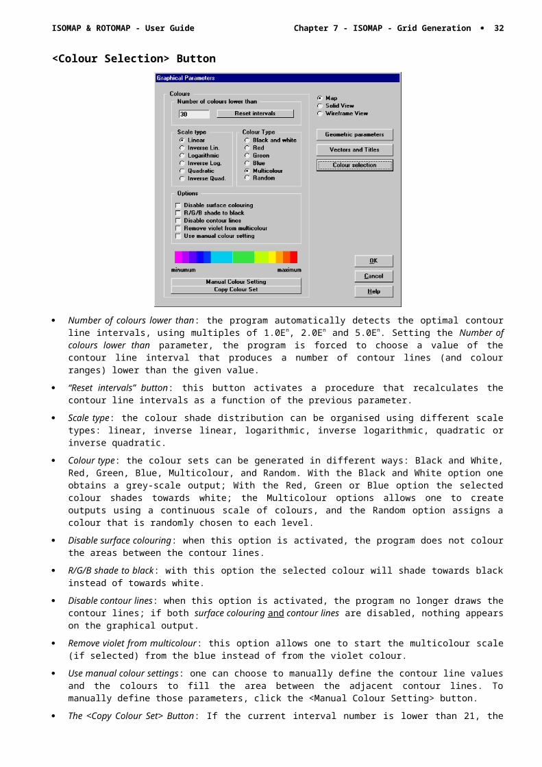
<Colour Selection> Button
· Number of colours lower than: the program automatically detects the optimal contour line intervals, using multiples of 1.0En, 2.0En and 5.0En. Setting the Number of colours lower than parameter, the program is forced to choose a value of the contour line interval that produces a number of contour lines (and colour ranges) lower than the given value.
· “Reset intervals” button: this button activates a procedure that recalculates the contour line intervals as a function of the previous parameter.
· Scale type: the colour shade distribution can be organised using different scale types: linear, inverse linear, logarithmic, inverse logarithmic, quadratic or inverse quadratic.
· Colour type: the colour sets can be generated in different ways: Black and White, Red, Green, Blue, Multicolour, and Random. With the Black and White option one obtains a grey-scale output; With the Red, Green or Blue option the selected colour shades towards white; the Multicolour options allows one to create outputs using a continuous scale of colours, and the Random option assigns a colour that is randomly chosen to each level.
· Disable surface colouring: when this option is activated, the program does not colour the areas between the contour lines.
· R/G/B shade to black: with this option the selected colour will shade towards black instead of towards white.
· Disable contour lines: when this option is activated, the program no longer draws the contour lines; if both surface colouring and contour lines are disabled, nothing appears on the graphical output.
· Remove violet from multicolour: this option allows one to start the multicolour scale (if selected) from the blue instead of from the violet colour.
· Use manual colour settings: one can choose to manually define the contour line values and the colours to fill the area between the adjacent contour lines. To manually define those parameters, click the <Manual Colour Setting> button.
· The <Copy Colour Set> Button: If the current interval number is lower than 21, the "Manual Colour Setting" dialogue box is opened, and the current settings are copied and can then be modified, otherwise the button is disabled.
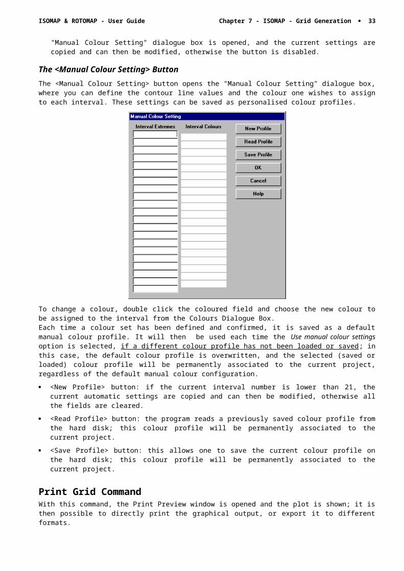
The <Manual Colour Setting> ButtonThe <Manual Colour Setting> button opens the "Manual Colour Setting" dialogue box, where you can define the contour line values and the colour one wishes to assign to each interval. These settings can be saved as personalised colour profiles.
ISOMAP & ROTOMAP - User Guide Chapter 7 - ISOMAP - Grid Generation · 27
To change a colour, double click the coloured field and choose the new colour to be assigned to the interval from the Colours Dialogue Box.Each time a colour set has been defined and confirmed, it is saved as a default manual colour profile. It will then be used each time the Use manual colour settings option is selected, if a different colour profile has not been loaded or saved; in this case, the default colour profile is overwritten, and the selected (saved or loaded) colour profile will be permanently associated to the current project, regardless of the default manual colour configuration.
· <New Profile> button: if the current interval number is lower than 21, the current automatic settings are copied and can then be modified, otherwise all the fields are cleared.
· <Read Profile> button: the program reads a previously saved colour profile from the hard disk; this colour profile will be permanently associated to the current project.
· <Save Profile> button: this allows one to save the current colour profile on the hard disk; this colour profile will be permanently associated to the current project.
Print Grid Command With this command, the Print Preview window is opened and the plot is shown; it is then possible to directly print the graphical output, or export it to different formats.
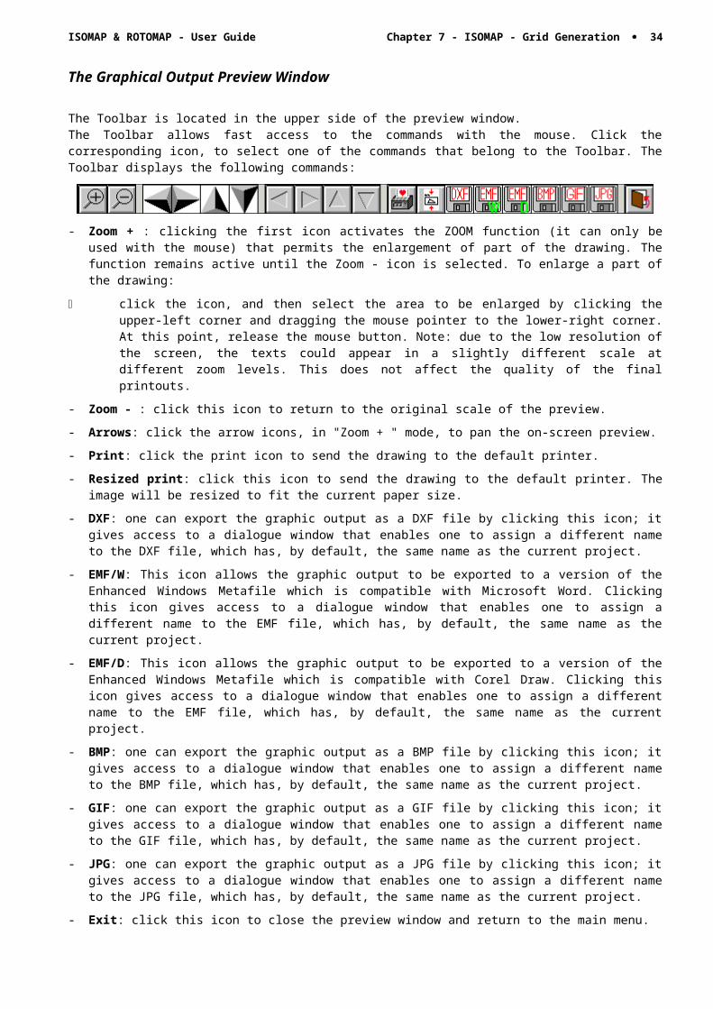
The Graphical Output Preview Window
The Toolbar is located in the upper side of the preview window.The Toolbar allows fast access to the commands with the mouse. Click the corresponding icon, to select one of the commands that belong to the Toolbar. The Toolbar displays the following commands:
- Zoom + : clicking the first icon activates the ZOOM function (it can only be used with the mouse) that permits the enlargement of part of the drawing. The function remains active until the Zoom - icon is selected. To enlarge a part of the drawing:
click the icon, and then select the area to be enlarged by clicking the upper-left corner and dragging the mouse pointer to the lower-right corner. At this point, release the mouse button. Note: due to the low resolution of the screen, the texts could appear in a slightly different scale at different zoom levels. This does not affect the quality of the final printouts.
- Zoom - : click this icon to return to the original scale of the preview.
ISOMAP & ROTOMAP - User Guide Chapter 7 - ISOMAP - Grid Generation · 28
- Arrows: click the arrow icons, in "Zoom + " mode, to pan the on-screen preview.
- Print: click the print icon to send the drawing to the default printer.
- Resized print: click this icon to send the drawing to the default printer. The image will be resized to fit the current paper size.
- DXF: one can export the graphic output as a DXF file by clicking this icon; it gives access to a dialogue window that enables one to assign a different name to the DXF file, which has, by default, the same name as the current project.
- EMF/W: This icon allows the graphic output to be exported to a version of the Enhanced Windows Metafile which is compatible with Microsoft Word. Clicking this icon gives access to a dialogue window that enables one to assign a different name to the EMF file, which has, by default, the same name as the current project.
- EMF/D: This icon allows the graphic output to be exported to a version of the Enhanced Windows Metafile which is compatible with Corel Draw. Clicking this icon gives access to a dialogue window that enables one to assign a different name to the EMF file, which has, by default, the same name as the current project.
- BMP: one can export the graphic output as a BMP file by clicking this icon; it gives access to a dialogue window that enables one to assign a different name to the BMP file, which has, by default, the same name as the current project.
- GIF: one can export the graphic output as a GIF file by clicking this icon; it gives access to a dialogue window that enables one to assign a different name to the GIF file, which has, by default, the same name as the current project.
- JPG: one can export the graphic output as a JPG file by clicking this icon; it gives access to a dialogue window that enables one to assign a different name to the JPG file, which has, by default, the same name as the current project.
- Exit: click this icon to close the preview window and return to the main menu.
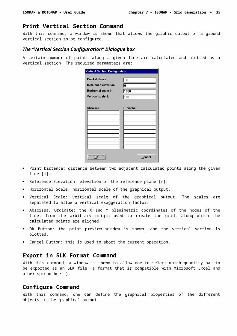
Print Vertical Section CommandWith this command, a window is shown that allows the graphic output of a ground vertical section to be configured.
The “Vertical Section Configuration” Dialogue boxA certain number of points along a given line are calculated and plotted as a vertical section. The required parameters are:
· Point Distance: distance between two adjacent calculated points along the given line [m].
· Reference Elevation: elevation of the reference plane [m].
· Horizontal Scale: horizontal scale of the graphical output.
· Vertical Scale: vertical scale of the graphical output. The scales are separated to allow a vertical
ISOMAP & ROTOMAP - User Guide Chapter 7 - ISOMAP - Grid Generation · 29
exaggeration factor.
· Abscissa, Ordinate: the X and Y planimetric coordinates of the nodes of the line, from the arbitrary origin used to create the grid, along which the calculated points are aligned.
· Ok Button: the print preview window is shown, and the vertical section is plotted.
· Cancel Button: this is used to abort the current operation.
Export in SLK Format Command With this command, a window is shown to allow one to select which quantity has to be exported as an SLK file (a format that is compatible with Microsoft Excel and other spreadsheets).
Configure CommandWith this command, one can define the graphical properties of the different objects in the graphical output.
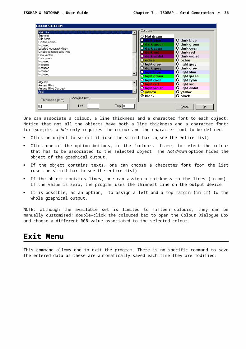
One can associate a colour, a line thickness and a character font to each object. Notice that not all the objects have both a line thickness and a character font: for example, a title only requires the colour and the character font to be defined.
· Click an object to select it (use the scroll bar to see the entire list)
· Click one of the option buttons, in the “colours” frame, to select the colour that has to be associated to the selected object. The Not drawn option hides the object of the graphical output.
· If the object contains texts, one can choose a character font from the list (use the scroll bar to see the entire list)
· If the object contains lines, one can assign a thickness to the lines (in mm). If the value is zero, the program uses the thinnest line on the output device.
· It is possible, as an option, to assign a left and a top margin (in cm) to the whole graphical output.
NOTE: although the available set is limited to fifteen colours, they can be manually customised; double-click the coloured bar to open the Colour Dialogue Box and choose a different RGB value associated to the selected colour.
Exit MenuThis command allows one to exit the program. There is no specific command to save the entered data as these are automatically saved each time they are modified.
ISOMAP & ROTOMAP - User Guide Chapter 8 - ISOMAP - Slope Map · 30
Chapter 8 - ISOMAP - Slope Map
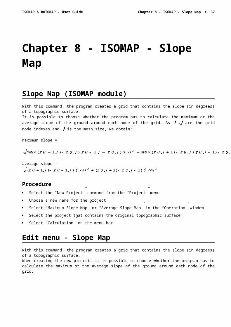
Slope Map (ISOMAP module)With this command, the program creates a grid that contains the slope (in degrees) of a topographic surface.It is possible to choose whether the program has to calculate the maximum or the average slope of the ground around each node of the grid. As are the grid node indexes and is the mesh size, we obtain:
maximum slope =
average slope =
Procedure· Select the “New Project” command from the “Project” menu
· Choose a new name for the project
· Select “Maximum Slope Map” or “Average Slope Map” in the “Operation” window
· Select the project that contains the original topographic surface
· Select “Calculation” on the menu bar
Edit menu - Slope MapWith this command, the program creates a grid that contains the slope (in degrees) of a topographic surface.When creating the new project, it is possible to choose whether the program has to calculate the maximum or the average slope of the ground around each node of the grid.
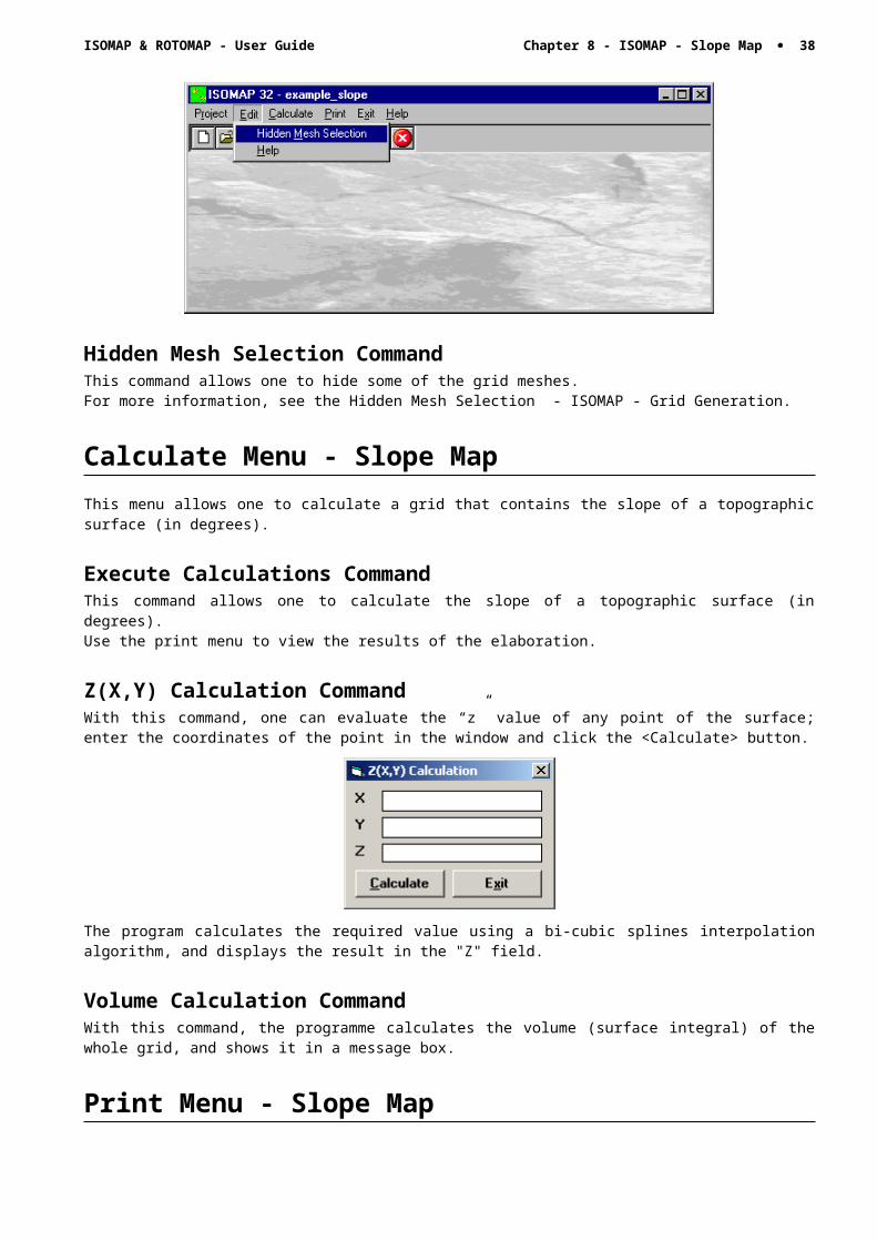
Hidden Mesh Selection CommandThis command allows one to hide some of the grid meshes.For more information, see the Hidden Mesh Selection - ISOMAP - Grid Generation.
ISOMAP & ROTOMAP - User Guide Chapter 8 - ISOMAP - Slope Map · 31
Calculate Menu - Slope MapThis menu allows one to calculate a grid that contains the slope of a topographic surface (in degrees).
Execute Calculations Command This command allows one to calculate the slope of a topographic surface (in degrees).Use the print menu to view the results of the elaboration.
Z(X,Y) Calculation CommandWith this command, one can evaluate the “z” value of any point of the surface; enter the coordinates of the point in the window and click the <Calculate> button.
The program calculates the required value using a bi-cubic splines interpolation algorithm, and displays the result in the "Z" field.
Volume Calculation CommandWith this command, the programme calculates the volume (surface integral) of the whole grid, and shows it in a message box.
Print Menu - Slope MapThe Print menu is used to configure the graphical output and to plot the surface in Map, Wireframe View or Solid View form.For more information, see the Print Menu - ISOMAP - Grid Generation.
ISOMAP & ROTOMAP - User Guide Chapter 9 - ISOMAP - Exposure Map · 32
Chapter 9 - ISOMAP - Exposure Map
Exposure Map (ISOMAP module)With this command, the program creates a grid that contains the angle from the North of the dip direction of the ground. The Y-axis must be oriented to the North. The South direction will result to be equal to 180°; both the East and West directions will be equal to 90°.
Procedure· Select the “New Project” command from the “Project” menu
· Choose a new name for the project
· Select “Exposure Map” in the “Operation” window
· Select the project that contains the original topographic surface
· Select “Calculation” on the menu bar
Note: as an alternative, it is possible to obtain interesting results working on the original topographic surface using a horizontal Light Vector.
Edit menu - Exposure MapWith this command, the program creates a grid that contains the angle from the North of the dip direction of the ground. The Y-axis must be oriented to the North. The South direction will result to be equal to 180°; both East and West directions will be equal to 90°.
Hidden Mesh Selection CommandThis command allows one to hide some of the grid meshes.For more information, see the Hidden Mesh Selection - ISOMAP - Grid Generation.
Calculate Menu - Exposure Map
ISOMAP & ROTOMAP - User Guide Chapter 9 - ISOMAP - Exposure Map · 33
This menu allows one to calculate the angle from the North of the ground dip direction.
Execute Calculations CommandThis command allows one to calculate the angle from the North of the ground dip direction.Use the print menu to view the results of the elaboration.
Z(X,Y) Calculation CommandWith this command, one can evaluate the “z” value of any point of the surface; enter the coordinates of the point in the window and click the <Calculate> button.
The program calculates the required value using a bi-cubic splines interpolation algorithm, and displays the result in the "Z" field.
Volume Calculation CommandWith this command, the programme calculates the volume (surface integral) of the whole grid, and shows it in a message box.
Print Menu - Exposure MapThe Print menu is used to configure the graphical output and plot the surface in Map, Wireframe View, or Solid View form.For more information, see the Print Menu - ISOMAP Menus - Grid Generation.
ISOMAP & ROTOMAP - User Guide Chapter 10 - ISOMAP - Grid Difference · 34
Chapter 10 - ISOMAP - Grid Difference
Grid Difference (ISOMAP module)With this command, the program creates a new grid that is calculated as the node-by-node subtraction of two given grids. A typical application could be the evaluation of the removed ground, which is obtained by subtracting two grids that represent the topographic surface before and after an excavation.It is mandatory that the two grids have the same number of rows and columns.
Procedure· Select the “New Project” command from the “Project” menu
· Choose a new name for the project
· Select “Grid Difference” in the “Operation” window
· Select the project to extract from the “minuend” grid
· Select the “Select Subtrahend Grid” command from the “Edit” menu
· Choose an existing project (of the same grid size) to extract from the “subtrahend” grid
· Select “Calculation” on the menu bar
Edit menu - Grid DifferenceWith this command, the program creates a new grid that is calculated as the node-by-node subtraction of two given grids. A typical application could be the evaluation of the removed ground, which is obtained by subtracting two grids that represent the topographic surface before and after an excavation.It is mandatory that the two grids have the same number of rows and columns.
Hidden Mesh Selection CommandThis command allows one to hide some of the grid meshes.For more information, see the Hidden Mesh Selection - ISOMAP Menus - Grid Generation.
ISOMAP & ROTOMAP - User Guide Chapter 10 - ISOMAP - Grid Difference · 35
Select Subtrahend Grid CommandThis command allows one to choose an existing project (of the same grid size) to extract from the “subtrahend” grid
The “Select Subtrahend Grid” Dialogue BoxTo select a file, type the name of the project to extract from the “subtrahend” grid in the File Name field, or browse the hard disk and double-click the project file name.
Calculate Menu - Grid DifferenceOnce selected the Subtrahend Grid, this menu allows one to calculate the grid difference as the node-by-node subtraction of the two given grids.
Execute Calculations CommandOnce selected the Subtrahend Grid, this command calculated the grid difference as the node-by-node subtraction of the two given grids. Use the print menu to view the results of the elaboration.
Z(X,Y) Calculation Command With this command, one can evaluate the “z” value of any point of the surface; enter the coordinates of the point in the window and click the <Calculate> button.
The program calculates the required value using a bi-cubic splines interpolation algorithm, and displays the result in the "Z" field.
Volume Calculation CommandWith this command, the programme calculates the volume (surface integral) of the whole grid, and shows it in a message box.
Print Menu - Grid DifferenceThe Print menu is used to configure the graphical output and plot the surface in Map, Wireframe View, or Solid View form.For more information, see the Print Menu - ISOMAP - Grid Generation.
ISOMAP & ROTOMAP - User Guide Chapter 11 - ISOMAP - Linear Transformation · 36
Chapter 11 - ISOMAP - Linear Transformation
Linear Transformation (ISOMAP module)The linear transformation operator makes it possible to perform a linear transformation of the surface, performing the following three sequential operations for each node:
1. sums a first translation factor (a);
2. multiplicates by a scale factor (b);
3. sums a second translation factor (c).
The general formula z'=(z+a)*b+c makes it possible to perform any linear transformation such as the Celsius-Fahrenheit conversion, with a=0, b=9/5 and c=32.
Procedure· Select the “New Project” command from the “Project” menu
· Choose a new name for the project
· Select “Linear Transformation” in the “Operation” window
· Select the project to be transformed
· Select the “Linear Transformation Parameters” command from the “Edit” menu
· Select “Calculation” on the menu bar
Edit Menu - Linear TransformationsThe linear transformation operator makes it possible to perform a linear transformation of the surface, performing the following three sequential operations for each node:
1. sums a first translation factor (a);2. multiplicates by a scale factor (b);
ISOMAP & ROTOMAP - User Guide Chapter 11 - ISOMAP - Linear Transformation · 37
3. sums a second translation factor (c).
The general formula z'=(z+a)*b+c makes it possible to perform any linear transformation such as the Celsius-Fahrenheit conversion, with a=0, b=9/5 and c=32.
Hidden Mesh Selection CommandThis command allows one to hide some of the grid meshes.For more information, see the Hidden Mesh Selection - ISOMAP - Grid Generation.
Linear Transformation Parameters CommandThis command enables one to define the parameters for the linear transformation.
The “Linear Transformation Parameters” Dialogue boxIn the “Linear Transformation Parameters” dialogue window the following data are required:
· First translation factor: it is the constant a in the linear transformation z'=(z+a)*b+c formula.
· Scale factor: it is the scale factor ‘b’ in the linear transformation formula.
· Second translation factor: it is the constant 'c' in the linear transformation formula.
Calculate Menu - Linear TransformationWith this menu, a linear transformation is performed on each node of the source grid.
Execute Calculations CommandWith this command, the linear transformation is performed on each node of the source grid, using the given parameters. Use the print menu to view the results of the elaboration.
Z(X,Y) Calculation CommandWith this command, one can evaluate the “z” value of any point of the surface; enter the coordinates of the point in the window and click the <Calculate> button.
ISOMAP & ROTOMAP - User Guide Chapter 11 - ISOMAP - Linear Transformation · 38
The program calculates the required value using a bi-cubic splines interpolation algorithm, and displays the result in the "Z" field.
Volume Calculation CommandWith this command, the programme calculates the volume (surface integral) of the whole grid, and shows it in a message box.
Print Menu - Linear TransformationThe Print menu is used to configure the graphical output and plot the surface in Map, Wireframe View, or Solid View form.For more information, see the Print Menu - ISOMAP – Grid Generation.
ISOMAP & ROTOMAP - User Guide Chapter 12 - ISOMAP - Filtering · 39
Chapter 12 - ISOMAP - Filtering
Filtering (ISOMAP module)This operator performs a numerical filtering in the space domain, that is to say, the convolution of a matrix operator of order 2n+1 with the grid itself.The filters should always be symmetrical to the axis that passes through its centre, and to the two diagonals.By using a unit matrix one will obtain a grid that is the moving average of the original grid. By using this command in conjunction with the Grid Difference operation, one can, for example, separate the local gravity anomalies from the regional ones.
Procedure· Select the “New Project” command from the “Project” menu
· Choose a new name for the project
· Select “Filtering” in the “Operation” window
· Select the project to be filtered
· Select the “Select Filter” command from the “Edit” menu
· Choose a filter (you can create a new one with a text editor)
· Select “Calculation” on the menu bar
Edit Menu - FilteringThis operator performs a numerical filtering in the space domain, that is to say, the convolution of a matrix operator of order 2n+1 with the grid itself.The filters should always be symmetrical to the axis that passes through its centre, and to the two diagonals.By using a unit matrix one will obtain a grid that is the moving average of the original grid. By using this command in conjunction with the Grid Difference operation, one can, for example, separate the local gravity anomalies from the regional ones.
Hidden Mesh Selection Command This command allows one to hide some of the grid meshes.

ISOMAP & ROTOMAP - User Guide Chapter 12 - ISOMAP - Filtering · 40
For more information, see the Hidden Mesh Selection - ISOMAP - Grid Generation.
Select Filter CommandWith this command, the program shows the “Select Filter” dialogue box.
The “Select Filter” Dialogue boxTo select a file, type the name of the file containing the digital filter to be used for the current operation in the File Name field, or browse the hard disk and double-click the filter file name.To create a new digital filter, type a new name and confirm, and then select the command Edit Filter from the Edit menu.
Edit Filter CommandWith this command Notepad is started, and one can create or edit a custom filter.The structure of the filters is quite simple: the order of the matrix operator is written in the first line. This should always be an odd number. The coefficients are written in the following lines, separated by spaces.
This is an example of a filter that performs the average of the values along a circle centred on a grid node:
11 .00000 .00000 .00000 .03571 .03571 .03571 .03571 .03571 .00000 .00000 .00000 .00000 .00000 .03571 .00000 .00000 .00000 .00000 .00000 .03571 .00000 .00000 .00000 .03571 .00000 .00000 .00000 .00000 .00000 .00000 .00000 .03571 .00000 .03571 .00000 .00000 .00000 .00000 .00000 .00000 .00000 .00000 .00000 .03571 .03571 .00000 .00000 .00000 .00000 .00000 .00000 .00000 .00000 .00000 .03571 .03571 .00000 .00000 .00000 .00000 .00000 .00000 .00000 .00000 .00000 .03571 .03571 .00000 .00000 .00000 .00000 .00000 .00000 .00000 .00000 .00000 .03571 .03571 .00000 .00000 .00000 .00000 .00000 .00000 .00000 .00000 .00000 .03571 .00000 .03571 .00000 .00000 .00000 .00000 .00000 .00000 .00000 .03571 .00000 .00000 .00000 .03571 .00000 .00000 .00000 .00000 .00000 .03571 .00000 .00000 .00000 .00000 .00000 .03571 .03571 .03571 .03571 .03571 .00000 .00000 .00000
The filters can be created with any external word-processor, shoud have the “.FIL” extension and shoud be saved as plain text.
Calculate Menu - FilteringWith this menu, the grid filtering is performed.
Execute Calculations CommandWith this command, the grid filtering is performed using the chosen filter.Use the print menu to view the results of the elaboration.
Z(X,Y) Calculation Command With this command, one can evaluate the “z” value of any point of the surface; enter the coordinates of the point in the window and click the <Calculate> button.
The program calculates the required value using a bi-cubic splines interpolation algorithm, and displays the result in the "Z" field.
ISOMAP & ROTOMAP - User Guide Chapter 12 - ISOMAP - Filtering · 41
Volume Calculation CommandWith this command, the programme calculates the volume (surface integral) of the whole grid, and shows it in a message box.
Print Menu - FilteringThe Print menu is used to configure the graphical output and plot the surface in Map, Wireframe View, or Solid View form.For more information, see the Print Menu - ISOMAP – Grid Generation.
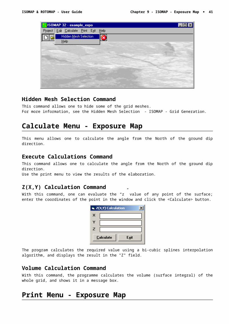
ISOMAP & ROTOMAP - User Guide Chapter 13 - ISOMAP Menus - Grid Duplication · 42
Chapter 13 - ISOMAP Menus - Grid Duplication
Grid Duplication (ISOMAP module)This command enables one to duplicate a project, for example to allow parametric analyses.It can also be used to create a new grid from an existing one, changing the extension of the grid and the size of the mesh.
Procedure· Select the “New Project” command from the “Project” menu
· Choose a new name for the project
· Select “Grid Duplication” in the “Operation” window
· Select the project to be duplicated
· Assign the new values of Xmin, Xmax, Ymin, Ymax and of the Mesh Size
· Select “Calculation” on the menu bar
Note: the X,Y values must be inside the ranges of the original grid.

ISOMAP & ROTOMAP - User Guide Chapter 14 - ISOMAP Menus - DTM Import · 43
Chapter 14 - ISOMAP Menus - DTM Import
DTM Import (ISOMAP module)With this command, it is possible to import regular grid data from other programs and convert these into the ISOMAP format. A default ISOMAP format can be used, or a custom made filter can be developed on request. The data files must previously have been created, with a text editor such as Notepad, and have the “.ZRE” extension.The structure of the ZRE files is quite simple: on the first line write the number of nodes on the X-axis, on the second line write the number of nodes on the Y-axis, on the third line write the mesh size (in metres) between two nodes, in the two next lines write the abscissa and ordinate of the first grid node in the bottom left corner.The file can now be completed with the Z-values, column by column (left to right), each column in a bottom-up order. Each column of Z-values must be preceded by a line that contains the text “Column #”, where # is the column number. Once the file is saved, the import procedure can be started.
Procedure· Select the “New Project” command from the “Project” menu
· Choose a new name for the project
· Select “Import ZRE file” in the “Operation” window
· Choose the ZRE file you want to import the grid from
Once confirmed the file name, the programme executes the conversion, then it directly activates the Print menu, because no further calculation must be performed.
ISOMAP & ROTOMAP - User Guide Chapter 15 - ISOMAP Menus - VID Import · 44
Chapter 15 - ISOMAP Menus - VID Import
Import VID File (ISOMAP module)This command enables one to import a file in VID format.
Procedure· Select the “New Project” command from the “Project” menu
· Choose a new name for the project
· Select “Import VID file” in the “Operation” window
· Choose the VID file you want to import the grid from
Once confirmed the file name, the programme executes the conversion, then it directly activates the Print menu, because no further calculation must be performed.
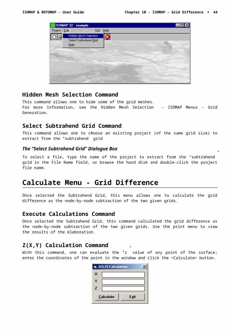
ISOMAP & ROTOMAP - User Guide Chapter 16 - ISOMAP Menus - XYZ Import · 45
Chapter 16 - ISOMAP Menus - XYZ Import
Import XYZ file (ISOMAP module)This command enables one to manage XYZ files. It is possible to join two or more files and, eventually, extract from them a partial area. This feature can be particularly useful when the area of interest (the green rectangle in the picture) crosses different, individual surveys (the black rectangles).
Procedure· Select the “New Project” command from the “Project” menu
· Choose a new name for the project
· Select “Import XYZ file” in the “Operation” window
· Type the coordinates of the lower-left and upper-right corners of the new grid
· Type XYZ file names you want to import the points from
Once confirmed the file names, the programme executes the conversion, then it activates the Calculation menu.
ISOMAP & ROTOMAP - User Guide Chapter 17 - ISOMAP menus - DXF Import · 46
Chapter 17 - ISOMAP menus - DXF Import
Import DXF file (ISOMAP module)This command enables one to import a file in DXF format.To correctly import a DXF file, it must have been saved as Autocad release 12 file, the contour lines must be POLYLINES (LINES are not imported), and the elevation value of each polyline must have been embedded in the file.
The programme extracts polylines only from the declared layers (“Contour lines layers” fields), so those layers must contain all and only the polylines representing contour lines (so roads, buildings and any other object in form of polyline must be removed from the declared layers before processing the file).Once obtained a clean DXF file, the names of the layers (1 to 7 max) can be typed in the (“Contour lines layers” fields. Some of the other fields in the window are mandatory:
· Mesh size: width (and height), in meters, of the square meshes of the grid which will be created. Remember the maximum grid size is 500x500 meshes;
· X,Y coordinates of the lower-left (Xmin, Ymin) and of the upper-right (Xmax, Ymax) corners of the new grid. Those four values must be exact multiples of the mesh size.
ISOMAP & ROTOMAP - User Guide Chapter 17 - ISOMAP menus - DXF Import · 47
The “Point Distance” field is optional, but strongly suggested for speed and quality reasons. This value allows the programme to pick few points out of the polylines, which are often very densely populated, obtaining a more isotropic point distribution which brings to a faster and more robust elaboration.A good value for this parameter is the average planimetric distance between the contour lines.
FREE WATER TABLESTo get a more agreeable output in presence of lakes or sea, it is possible to use a simple trick to assign a constant value to the water surfaces.Before importing the file, it is enough to add to the DXF file one or more coastal lines (see figure below), taking care that the closed lines are really closed (i.e. the first and the last points have the same coordinates) and the crossing lines surely exceed the rectangle defined by the lower-left and upper-right points previously typed.Those lines must be placed on a dedicated layer.Now we can compile the “Z water” field, typing the water table elevation; for graphical reasons, we suggest to choose a value slightly lower then the real value if this is an exact multiple of the contour line distance: for example, for the sea, use –0.1 instead of 0, to avoid generating random horizontal lines.For each separated water table, a couple of coordinates “X water” and “Y water” must be typed, to tell the programme which side of the coastal lines the water is; for example, you could give the coordinates of the big black points in the figure below.
Procedure· Select the “New Project” command from the “Project” menu
· Choose a new name for the project
· Select “Import DXF file” in the “Operation” window
· Choose the DXF file you want to import the grid from, and compile the required fields
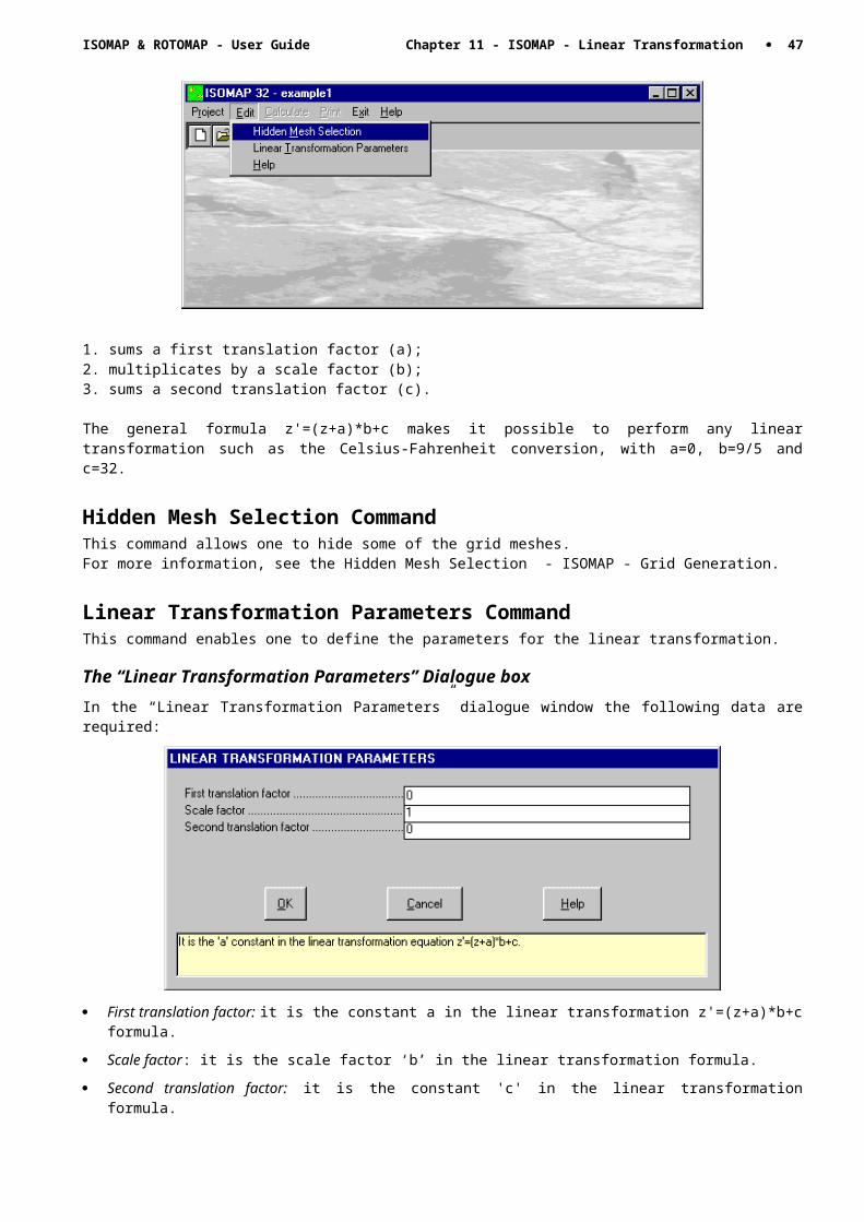
ISOMAP & ROTOMAP - User Guide Chapter 17 - ISOMAP menus - DXF Import · 48
Once confirmed, the programme executes the conversion, then it activates the Calculation menu.
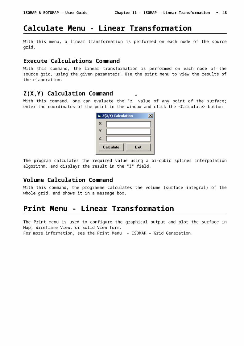
ISOMAP & ROTOMAP - User Guide Chapter 18 - ISOMAP menus - ASC Import · 49
Chapter 18 - ISOMAP menus - ASC Import
Import ASC file (ISOMAP module)This command enables one to import a file in ASC format.
Procedure· Select the “New Project” command from the “Project” menu
· Choose a new name for the project
· Select “Import ASC file” in the “Operation” window
· Choose the ASC file you want to import the grid from
Once confirmed the file name, the programme executes the conversion, then it directly activates the Print menu, because no further calculation must be performed.
ISOMAP & ROTOMAP - User Guide Chapter 19 - Introduction to the ROTOMAP module · 50
Chapter 19 - Introduction to the ROTOMAP module
Introduction to the ROTOMAP moduleROTOMAP is a three-dimensional model that is used for rockfall analysis and the design of rockfall protective systems. This module belongs to the Isomap family: a complete description of the main module features can be found in the ISOMAP chapters. ROTOMAP uses a statistical approach; it simulates a large number of rockfalls and, through the analysis of the distribution of the average and maximum kinetic energies, identifies the optimal areas for the installation of the protective systems. The program requires a detailed topographic map and a geomorphologic data collection to identify the areas where a rockfall can initiate, and to distinguish the different surface types, such as clean faces of hard unweathered rock or surfaces covered in talus, scree or gravel material.A digital terrain model can be obtained from an arbitrary distribution of points (X,Y,Z), that the program can convert into a regular grid, or by directly assigning the elevation values to the nodal points of the square mesh that is used in the model. It is also possible to import the elevation values from an external digital terrain model. A new, fast model calibration method is now available, thus avoiding carrying out expensive tests with high-speed cameras. ROTOMAP draws the contour lines of the minimum travel times of the blocks; with a simple chronometer and a standard video camera it is possible to compare the real and simulated times, in correspondence to pre-determined check-points. This allows a detailed and reliable calibration of the model. If in-field tests are not possible, a preliminary back-analysis stage can be used to determine the restitution and friction coefficients. These coefficients can be obtained through a comparison of the points where the rock blocks stop in the simulation with the rockfall history stop points. The kinetic energy distribution is thus calculated and this permits both the optimal positioning and the accurate design of barrier fences or catch benches.The maximum bouncing height over the slope can also be drawn. This allows the selection of the correct size of the barrier fences. In this way, the effectiveness of the whole rockfall protective system can be verified. The program can generate printouts of the topographic map, rockfall trajectories, kinetic energies, distribution of stop points and the vertical sections of each simulated fall.
Rockfall Analysis (ROTOMAP module)The rockfall problem is quite complex because the real behaviour of boulders, when rolling down a slope, depends on apparently insignificant geometric and mechanical details. The interaction between the morphology and the path taken by the boulders is not “linear”, but “chaotic”. There is, in fact, no proportionality between the variation of the initial conditions and the variation of the fall trajectory. Very small variations in the initial conditions normally cause large (and thus unforeseen) variations of the final conditions. This does not mean that the problem cannot be solved: it is simply not possible to calibrate the model with only a few simulations, therefore one cannot forecast the path and the stop point of a single real boulder. The only reasonable solution is a statistical approach. In this way the stop points are not considered individually, but as a probability distribution. The geomechanical parameters used in the model are defined as normal and tangential energy coefficients of restitution, friction coefficients of the rolling boulders and limit angle. These parameter sets should be calibrated for a small range of block sizes, as the same material can have an elastic or plastic behaviour as a function of the rock boulder size.Of all the geomechanical parameters, the limit angle is perhaps the most difficult to evaluate. This parameter is used to determine when the boulders start to bounce over the slope or return to the rolling conditions. A boulder
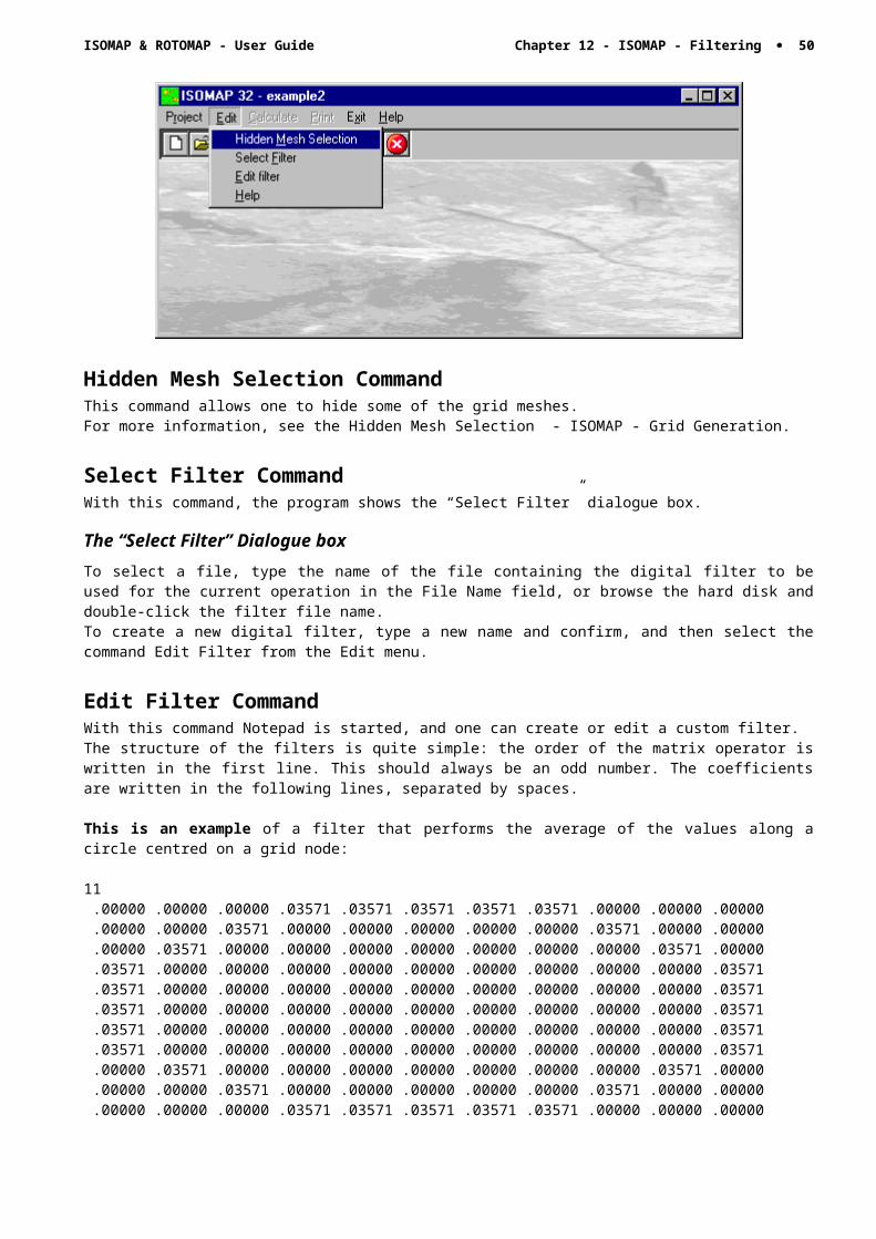
ISOMAP & ROTOMAP - User Guide Chapter 19 - Introduction to the ROTOMAP module · 51
starts to bounce if the increase of the slope dip, or the angle of the trajectory with the ground after impact, is greater than the limit angle. In all other cases, the fall proceeds in rolling conditions.In order to use the Rotomap module, one should first collect data to construct the numerical model of the slope with as much precision as possible.It is possible to determine the parameters from scratch through a back-analysis (which is however necessary to calibrate the final model), but an accurate initial data collection makes it possible to considerably narrow the range of variability, within which to perform the back-analysis, and enables one to set up a truly reliable model.The first phase of the work would be the geometrical reconstruction of the slope. For this purpose, one should use a detailed and up-to-date map. It would be even better to use a topographical survey specifically made for this purpose.The data entering shoud consist of a collection of sparse but uniformly distributed data set (X,Y,Z) that will be transformed by the program into a regular grid, but it would be better to use points directly sampled on the nodes of the square grid to be used in the model. It is also possible to use a pre-existing digital terrain model. In the case of manual input of the sampled points, the grid can be oriented at the optimal angle to minimize the data entry work.During the choice of the size of the mesh, one should keep in mind that the choice of an excessively large mesh will result in a reduced precision of the numerical model; on the other hand, a too small mesh size can either simulate unexpected peaks that interact with the boulder paths, or an excessive smoothing of the slope, which cause a drastic change in the boulder behaviour.The mesh should be “large” compared to the size of the boulders, but “small” compared to the examined area (the usual mesh size is generally between 5 and 15 metres). Once the topographic surface is defined, it is necessary to make an accurate geological and geomorphologic data collection.
Starting points: as detachments can occur at points that are not individually identifiable, the program does not require individual points to be entered, but rather detachment lines that can be arbitrarily placed below the top of the slope. The simulation lets the path of the boulders start from points aligned along these lines, with velocities that vary from a minimum to a maximum, depending on the geometry of the unstable slopes.The local behaviour along the detachment areas is ignored, and the values of the initial velocity of the blocks, when their trajectories cross the detachment lines, can be evaluated as Cs gh* ( )2 where g is the gravity acceleration, h is the vertical distance (h1 < h < h2) between the real detachment points and the assumed detachment lines, and Cs is a “first bounce” coefficient 1, this being necessary to take the local impacts along the detachment area into account.The minimum and maximum estimated vertical distances are h1 and h2, from which the minimum and maximum initial velocities are calculated.
Geomechanical parameters: it is therefore necessary to use the geological and geomorphologic data collection to identify the zones where homogeneous sets of restitution and friction coefficients can be assigned. It is important to remember that the best way to assign these parameters is to perform some field tests. As an alternative, such values can be found in literature.
Stop points: the planimetric points where, in the rockfall history, the boulders have stopped should also be identified.A comparison of the historical series of the stopping points with the frequency distribution calculated by the program, can confirm whether the model has been properly calibrated.
Main features of the mathematical modelThe main mathematical features of the Rotomap module are here discussed.
Three-dimensional modelThe choice of using a three-dimensional model for the representation of the surface is due to the fact that the paths followed by the boulders are not in a vertical plane, and that one cannot define a unique vertical cylindrical surface that contains all the rockfall paths. For this reason it is strongly advised to use a surface instead of a vertical section, and even though the two-dimensional calculations would be simpler, the three-dimensional approach constitutes an unacceptable simplification in most cases. This concept can be clarified through an example: a small increase of velocity can cause a boulder to pass a ridge and thus take a completely different path.
Statistical approachAs previously mentioned, rockfall is a “chaotic” phenomenon, whose behaviour in not compatible with deterministic forecasts. For this reason, rockfalls should be analysed from a statistical point of view. A great number of events (hundreds or even thousands of paths) should therefore be simulated, assigning several starting points with different initial velocities and directions along the detachment lines.
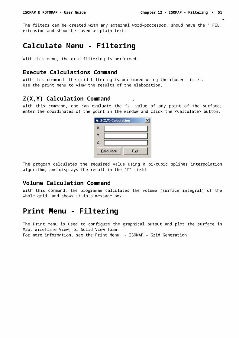
ISOMAP & ROTOMAP - User Guide Chapter 19 - Introduction to the ROTOMAP module · 52
The program saves each rockfall trajectory point, recording the position of the boulder and the velocity components for each time-step. In this way, it is possible to obtain a map of the frequency distribution of the stop points and of the travel-time (to check the calibration of the model) and a map of the distribution of the average or maximum kinetic energy (to design the protection systems).
Kinematical behaviourThe decision to only consider the kinematical behaviour of the centre of gravity of the boulders, thus disregarding the angular momentum of an ellipsoidal solid, was taken after a careful evaluation of the advantages and disadvantages of the two methods, that are here summarised:
a) degrees of freedom
An ellipsoidal solid enables one to consider the effects of the angular momentum; this makes it possible to accumulate a part of the energy as rotation energy that is later released as kinetic energy during the impacts. The boulder thus assumes a behaviour that is characterised by short and long leaps, with sudden decelerations and accelerations after each collision. It can be questioned whether this is realistic behaviour, especially for large boulders that roll off weathered rock and scree slopes. A boulder does not really have an ellipsoidal form, and thus it is impossible to obtain more precise “individual” simulations with this method. Furthermore, small variations in the mass, the initial rotation speed and the ratio between the axes will lead to completely different paths. All this simply adds redundant information to the model. The path of the gravity centre, disregarding the angular moment, can be considered as the most probable of all the paths that can be generated from infinite combinations of boulder shapes and initial conditions. It is possible to implicitly take into account the angular momentum effects by correcting the ratio between the normal and tangential restitution coefficient.
b) stopping criteria
A typical problem encountered in rockfall models is how to determine a valid criterion to stop the blocks. An ellipsoidal boulder usually stops when bouncing back, or when it slows down under a given limit. This is a rather gross simplification, especially because the concept of “back” is meaningless in a three-dimensional model. Considering the centre of gravity alone, an exact stopping criterion based on energy balances can be followed.
c) calculation time and memory usage
The calculation time and the memory usage would be onerous, as, for each time-step of the trajectory, six more values would have to be saved on the hard disk. In this way, the number of possible simulations would be halved. Fundamental importance has been given to the high number of simulations; as the variability of the initial conditions assure the simulation of thousands of trajectories, the introduction of a random factor such as the effect of the angular momentum would not introduce any improvement of the statistical analysis.
Interaction with protective systems
Barrier fences - barrier fences and catch fences are the most commonly used rockfall protective systems. The “local” calculation of the interaction between boulders and fences is beyond the scope of this program. The Rotomap module simulates fences with the three following parameters:
a) Capacity: this is the maximum energy that the nets can absorb. The units of measurement should be congruent with those of the boulders: the energy absorption capacity and the block mass multiplied by the unit energy V²/2 are, in fact, compared.
b) Mass of the rock blocks: this is the default mass of the boulder considered in the project. A detailed analysis of the rock mass is required to correctly define this value.
c) Height of the nets: one should verify that the boulders, when bouncing, do not exceed the height of the net. As the energy of the boulders is proportional to the mass, while the rockfall paths are mass-independent, a series of calculations obtained with constant unit mass boulders and variable energy absorption capacity would allow one to evaluate any boulder-fence interaction through the capacity/mass ratio.
Earth or rock fill – if the slope of the earth fill is vertical, it is sufficent to add a fictitious catch fence with a very high value of energy absorption capacity to the model. Otherwise, one can model catch benches by modifying the terrain geometry, and assigning proper geomechanical parameters to the earth fill.
Procedure- Select the command “New Project” from the “Project” menu
- Choose a new name for the project
ISOMAP & ROTOMAP - User Guide Chapter 19 - Introduction to the ROTOMAP module · 53
- Select “Rockfall” in the “Operation” window
- Select the project to extract the topographic surface from, then:
- input the position of the detachment lines from the “Edit” menu
- input the geomechanical parameters from the “Edit” menu
- input the calculation parameters from the “Edit” menu
- optionally input the position of the barrier fences from the “Edit” menu
- Select “Calculation” on the menu bar
Edit Menu - Rockfall AnalysisThis menu is used to enter and edit the input data used in rockfall analysis operations.
Hidden Mesh Selection Command This command allows one to hide some of the grid meshes.For more information, see the Hidden Mesh Selection - ISOMAP - Grid Generation.
Rockfall Parameters CommandThis command allows defining the parameters for the rockfalls analysis.
The “Rockfall Parameters” Dialogue boxIn the dialogue window “Rockfall Parameters”, the following data have to be entered:
ISOMAP & ROTOMAP - User Guide Chapter 19 - Introduction to the ROTOMAP module · 54
· Flying limit angle: This parameter is used to determine when the boulders start to fly over the slope after a bounce. A boulder starts to fly if the the angle of the trajectory with the ground after an impact is greater than the limit angle.
· Colliding limit angle: This parameter is used to determine when the boulders start to fly over the slope. A boulder starts to fly if the increase of the slope dip is greater than the limit angle.
· Bouncing limit angle: This parameter is used to determine when the boulders impact with the ground and bounce. A boulder bounces if the decrease of the slope dip is greater than the limit angle.
· Number of starting points: this is the total number of starting points aligned along one or more starting lines. As detachments happen at points that are not individually identifiable, the program does not require individual points to be entered, but rather lines of detachment that can be arbitrarily placed below the top of the slope. The simulation lets boulders start from points aligned along those lines, with velocities that vary from a minimum to a maximum, depending on the geometry of the unstable slopes.
· Number of initial velocities: this is the number of starting velocities for each starting point. The simulation lets boulders start from points aligned along those lines, with velocities that vary from a minimum to a maximum, depending on the geometry of the unstable slopes. The local behaviour along the detachment areas is ignored, and the values of the velocity of the blocks, when their trajectories cross the detachment lines, can be evaluated as Cs (2 g h) where g is the gravity acceleration, h is the vertical distance between the real detachment points and the assumed detachment lines, and Cs is a “first bounce” coefficient 1, which is necessary to take local impacts along the detachment area into account, h can be either the minimum or maximum estimated vertical distances that give the minimum and maximum initial velocities.
· Number of initial directions: this is the number of initial directions chosen in a given interval around the dip direction. To obtain a good statistical analysis, a large number of events (hundreds or even thousands of paths) should be simulated, assigning a large number of starting points along the detachment lines, with different initial velocities and directions. The total number of rock falls is calculated as follows: Number of initial directions * Number of initial velocities * Number of starting points.
· Minimum and maximum initial velocities: these values define the range of initial velocities of the rock blocks (see above for suggestions about how to calculate those values). The velocities are expressed in m/s.
· Maximum angular deviation: this value defines the range (+/- the maximum angular deviation) of the interval around the dip direction, in which the starting directions are chosen. It is expressed in degrees.
The next three values refer to the interaction between boulders and protection systems. Note that the rockfall paths are mass-independent, and a series of calculations obtained with constant unit mass boulders and variable energy absorption capacity would allow one to evaluate any boulder-fence interaction through the capacity/mass ratio.
· Capacity (kJ): this is the maximum energy absorption capacity of the protection system.
ISOMAP & ROTOMAP - User Guide Chapter 19 - Introduction to the ROTOMAP module · 55
· Boulders mass (t): this is the mass value of the boulders which, multiplied by the v2/2 value and compared to the barriers capacity, allows one to evaluate whether the protection system has been properly designed.
· Height of the nets (m): the program is able to simulate both flying and rolling paths; it can thus verify whether the blocks are bouncing over the protection systems or not.
The last two values are again related to the start conditions: they allow to simulate blocks which start from points placed over the ground level.
· Starting angle [°]: this value must be greater then 0° and less equal to 90° (free fall); if it is placed equal to 90° the next parameter would be greater then 0 m. If the starting angle is 0, the parameter is ignored and the blocks start in a direction parallel to the ground.
· Free fall height [m]: this parameter is used only if the starting angle is greater then 0, and allows to simulate a block which start from a point placed over the ground level at the given height.
Geomechanical Parameters CommandThis command allows one to assign the geomechanical parameters to each grid mesh.
The geomechanical parameters used in the model are defined as coefficients of restitution of normal and tangential energy, and friction coefficients of the rolling boulders.
A graphical editing window is opened, and the grid is shown, with the contour lines of the ground elevation.The following procedure allows one to assign the parameters:
· <Geomech. Param.>: in the text boxes beside the option button, one has to write the three parameters, separated by commas:
- coefficient of restitution of normal energy,
- coefficient of restitution of tangential energy,
- friction coefficient of the rolling boulders
Once the parameters have been written, select one of the parameter sets by clicking the option button.
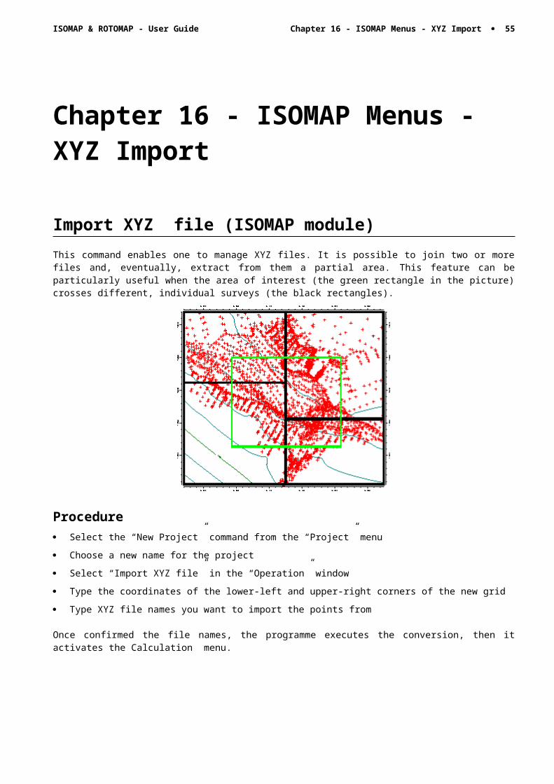
ISOMAP & ROTOMAP - User Guide Chapter 19 - Introduction to the ROTOMAP module · 56
A single left-click assigns the currently selected parameter set to a grid mesh. Holding down the left button and moving the mouse over the grid allows a continuous (multiple) selection of the meshes. Finally, a right-click fills an area delimitated by a line of the previously selected meshes.
· <Cancel editing>: cancels the very last editing operation.
· <Save>: saves the assigned geomechanical parameter sets.
· <Cancel>: closes the window without saving any modifications.
Placing Starting Lines CommandThis command enables one to define planimetric coordinates of the starting lines. As detachments happen at points that are not individually identifiable, the program does not require individual points to be entered but rather starting lines that can be arbitrarily placed below the top of the slope. The simulation lets boulders start from points aligned along those lines. The detachment lines cannot be placed on the grid border.
The “Placing Starting Lines” Dialogue BoxIn the “Placing Starting Lines” window, the following data are entered:
· X Coordinate: the X and Y planimetric coordinates of the starting lines should be defined in metres, from the arbitrary origin used to create the grid.
· Y Coordinate: the X and Y planimetric coordinates of the starting lines should be defined in metres, from the arbitrary origin used to create the grid.
· Code: it is possible to define one or more starting lines. For this reason it is necessary to assign a code to each point of the starting lines: every point must have code=1, except the initial point which should have code=0. For example to define two separated lines, with 4 and 3 points respectively, the sequence of codes must be: 0, 1, 1, 1, 0, 1, 1.
Placing Protection Systems CommandThis command allows one to define the lines along which the barrier fences are positioned.
The “Placing Protection Systems” dialogue boxIn the “Placing Protection Systems” dialogue window, the following data are entered:
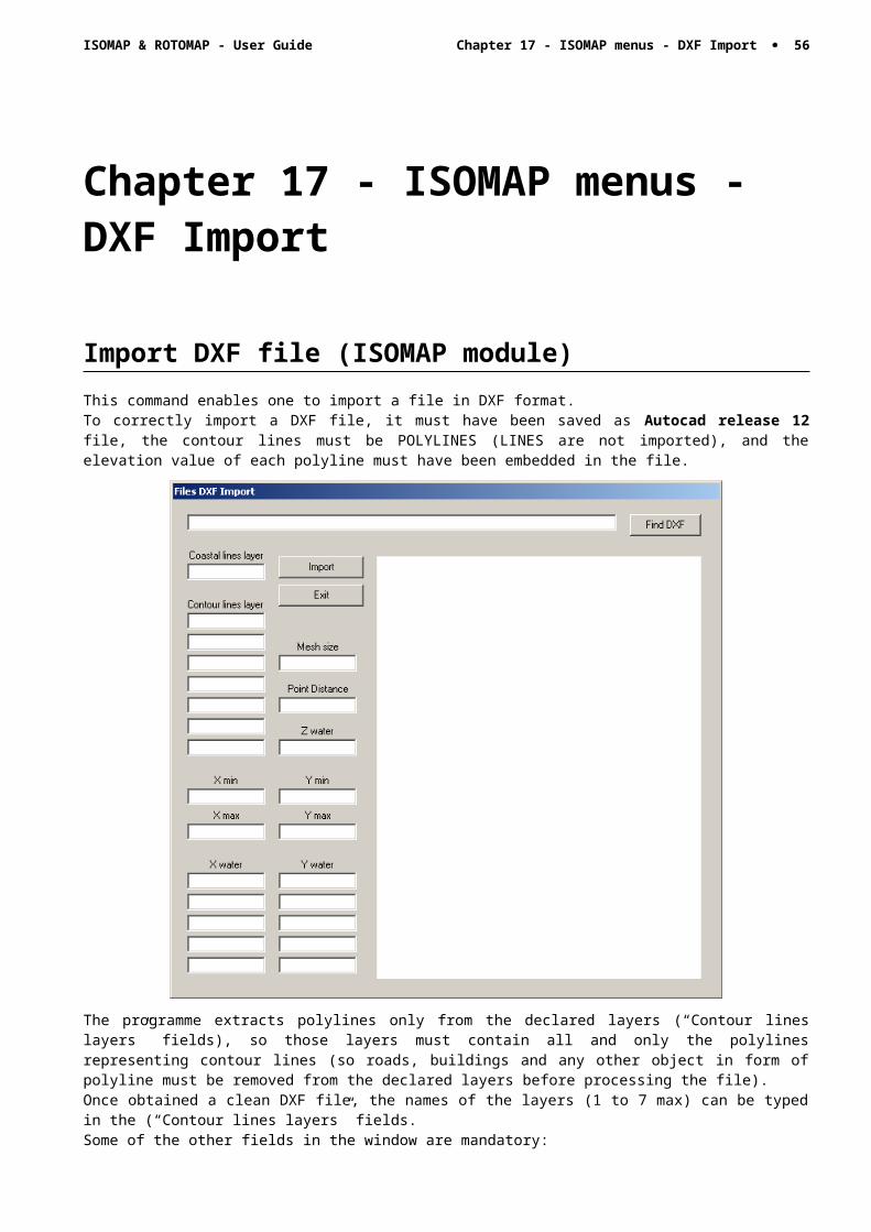
ISOMAP & ROTOMAP - User Guide Chapter 19 - Introduction to the ROTOMAP module · 57
· X Coordinate: the X and Y planimetric coordinates of the protection systems should be defined in metres, from the arbitrary origin used to create the grid.
· Y Coordinate: the X and Y planimetric coordinates of the protection systems should be defined in metres, from the arbitrary origin used to create the grid.
· Code: it is possible to define one or more starting lines. For this reason it is necessary to assign a code to each point of the starting lines: every point must have code=1, except the initial point which should have code=0. For example to define two separated lines, with 4 and 3 points respectively, the sequence of codes must be: 0, 1, 1, 1, 0, 1, 1.
· Capacity (kJ): this is the maximum energy absorption capacity of the protection system, individually asigned to each section of the net.
· Height of the nets (m): height of the nets, individually asigned to each section of the net. The program is able to simulate both flying and rolling paths; it can thus verify whether the blocks are bouncing over the protection systems or not.
Calculate Menu - Rockfall AnalysisWith this menu, one can choose the calculation which has to be performed.
ISOMAP & ROTOMAP - User Guide Chapter 19 - Introduction to the ROTOMAP module · 58
Rockfall Calculation CommandThe rockfalls are calculated with this command. Notice that each path is identified by a progressive number; this allows one to choose a single rockfall and printing it as a vertical section. A preview window is shown, and the first path is calculated, then the program pauses: clicking the “>“ button, the next path is calculated; clicking the “>>“ button, all the paths are calculated. At each moment it is possible, clicking the “>“ button, to interrupt the automatic sequence and return to the one-by-one mode.
Three other buttons are available in the rockfall calculation preview window:
· <Interrupt Single>: clicking on this button interrupts the current path calculation.
· <Interrupt All>: clicking on this button definitively interrupts the calculation of the paths.
· <Confirm>: closes the rockfall calculation windows.
Stop Point Calculation CommandThrough this command, one can calculate the frequency distribution of the stop points. This distribution is expressed in stop points per square metre per million of paths. If in-situ tests are not possible, a preliminary back-analysis stage can be used to determine the restitution and friction coefficients. These coefficients can be obtained by comparing the points where the rock blocks stop in the simulation with the real stop points in the rockfall history. If one compares the historical series of stop points with the frequency distribution calculated by the program, it is possible to confirm whether the model has been properly calibrated.Please note that this form of representation is dedicated to back analysis, and only takes into account the final position of the blocks. Thus, it cannot be considered a hazard map.
Average Energy Calculation CommandThrough this command one can calculate, for unit mass rock blocks, the average energy distribution (v2/2). The average kinetic energy distribution permits an optimal positioning of barrier fences or catch benches.
Maximum Energy Calculation CommandThrough this command one can calculate, for unit mass rock blocks, the maximum energy distribution (v2/2). The maximum kinetic energy distribution permits an optimal design of the capacity of the protection systems.
Minimum Travel Time Calculation CommandThrough this command, one can calculate the minimum travel times of the blocks.A new, fast calibration method of the model is now available, instead of expensive tests with high-speed cameras. ROTOMAP draws the contour lines of the minimum travel times of the blocks; with a simple chronometer and a standard video camera, it is possible to compare, in correspondence to pre-determined check-points, the real and simulated times. This allows a detailed and reliable calibration of the model.
Maximum Heights Calculation CommandThrough this command, one can calculate the maximum bouncing height of the rock blocks over the slope.This allows one to select the safe size of the barrier fences.
Z(X,Y) Calculation CommandWith this command, one can evaluate the “z” value of any point of the surface; enter the coordinates of the point in the window and click the <Calculate> button.
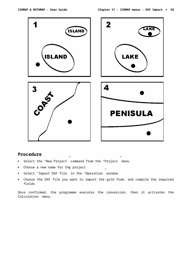
ISOMAP & ROTOMAP - User Guide Chapter 19 - Introduction to the ROTOMAP module · 59
The program calculates the required value using a bi-cubic splines interpolation algorithm, and displays the result in the "Z" field.
Volume Calculation CommandWith this command, the programme calculates the volume (surface integral) of the whole grid, and shows it in a message box.
Print Menu - Rockfall AnalysisThe Print menu is used to configure the graphical output, and to plot the surface in Map, Wireframe View, or Solid View form.
Parameters CommandWith this command, the “Graphical Parameters” dialogue window is shown.For more information, see the Print Menu – ISOMAP – Grid Generation.
Physical Quantities Selection Command With this command one can select which physical quantities should be superimposed in the final graphical output.
The “Physical Quantities Selection” dialogue window.Clicking the check boxes of this window it is possible to superimpose two or more different physical quantities in the same graphical output. The available quantities are:
· Topography: contour lines of the ground elevation.
· Stop Points: contour lines of the frequency distribution of the stop points. This distribution is expressed as number of stop points per square metre per million of paths.
· Minimum Travel Time: contour lines of the minimum travel time of the blocks. This allows a detailed and reliable calibration of the model.
· Maximum Heights: contour lines of the maximum bouncing height over the slope of the rock blocks. This allows one to select the safe size of the barrier fences.
· Average Energy: contour lines of the average energy distribution (v2/2). The average kinetic energy distribution permits an optimal positioning of barrier fences or catch benches.
· Maximum Energy: contour lines of the maximum energy distribution (v2/2). The average kinetic energy distribution permits an optimal design of the capacity of the protection systems.
· Rockfall paths: the path taken by the rock blocks while rolling down the slope.
· Rockfall path selection: during the rockfall simulation the path numbers are shown; to print anly a selection of the paths, type in the list the choosen path numbers. If no path is selected, all the paths will be printed.
ISOMAP & ROTOMAP - User Guide Chapter 19 - Introduction to the ROTOMAP module · 60
Print Grid CommandWith this command the Print Preview window is opened and the plot is shown; it is then possible to directly print the graphical output, or to export it into different formats. For more information, see the Print Menu – ISOMAP – Grid Generation.
Print Vertical Section CommandWith this command, a window is shown that allows one to configure the graphical output of a ground vertical section.For more information, see the Print Menu – ISOMAP – Grid Generation.
Print Rockfall Sections CommandThrough this command the window “Rockfall Sections preview” is invoked, and this enables one to visualise and print the rockfalls one-by-one. Enter the rockfall number from which to start, then click on the “Preview button”: the boulder path is shown on the screen as a cylindrical section of the topographic surface that passes through the selected path. The qualitative distribution of the kinetic energy is also shown. Clicking on the “>“ and “<“ buttons one can go forward or back in the sequence of the rockfalls.Clicking the <Print> button the selected rockfall is plotted in the Print Preview window.For more information, see the Print Menu – ISOMAP – Grid Generation.
The "Section Print Parameters" dialogue boxBy clicking on the <Parameters> button one can enter a main title and some subtitles, the drawing scale factor and the reference elevation for each rockfall. The lowest value of Z is normally assumed as the reference elevation; the possibility of defining another value enables one to normalise the reference plane for more drawings thus making their comparison easier.
Export in SLK Format CommandWith this command the “Export in SLK Format” window is opened, and it is then possible to export a grid as a SLK file, that is compatible with Excel and other common spreadsheets.Clicking the option buttons, it is possible to select one of the physical quantities that should be exported into the SLK format. The available quantities are:
· Topography: table of the ground elevation.
· Stop Points: table of the frequency distribution of the stop points. This distribution is expressed in number of stop points per square metre per million of paths.
· Minimum Travel Time: table of the minimum travel times of the blocks. This allows a detailed and reliable calibration of the model.
· Maximum Heights: table of the maximum bouncing height of the rock blocks over the slope. This allows one to select the safe size of the barrier fences.
ISOMAP & ROTOMAP - User Guide Chapter 19 - Introduction to the ROTOMAP module · 61
· Average Energy: table of the average energy distribution (v2/2). The average kinetic energy distribution permits an optimal positioning of barrier fences or catch benches.
· Maximum Energy: table of the maximum energy distribution (v2/2). The average kinetic energy distribution permits an optimal design of the capacity of the protection systems.
· Geomechanical Parameters: table of the coefficients of restitution of normal and tangential energy, and friction coefficients of the rolling boulders.
· Net crossing statistics: table where are collected informations about the paths which have reached or crossed the nets.
Configure Command With this command, one can define the properties of the different objects in the graphical output.For more information, see the Configure Command - Common Command.
ISOMAP & ROTOMAP - User Guide Chapter 20 - Miscellanea · 62
Chapter 20 - Miscellanea
Reported values for coefficients of restitutionReference Value for r Value for rn Value for rt Remarks
Habib (1977) 0.75 - 0.80 Based on experience in Italy0.50 - 0.60 Based on experience in Norway
Descoeudres et 0.40 Vineyard slopesZimmermann (1987) 0.80 Rock slopes
Broili (from 0.75 - 0.80 Rock to rock impactPasquero (1987)) 0.20 - 0.35 Rock to soil / scree impact
Type of material on slope surface
Piteau and Clayton 0.65 - 0.75 0.8 - 0.9 Solid rock(from Pasquero (1987)) 0.45 – 0.65 0.5 - 0.8 Detrital material mixed with large
rock boulders0.35 - 0.45 0.4 - 0.5 Compact detrital material mixed with
small boulders0.2 - 0.3 0.2 - 0.4 Grass covered slopes
Hoek (1987) 0.53 0.9 Clean hard bedrock(based on unpublished 0.40 0.90 Asphalt roadwayinformation from 0.35 0.85 Bedrock outcrops with hard surface,Departments of large bouldersTransportation in USA) 0.32 0.82 Talus cover
0.32 0.80 Talus cover with vegetation0.30 0.80 Soft soil, some vegetation
Pfeiffer, T.J., Bowen, 0,37 - 0,42 0,87 - 0,92 Hard surface pavingT.D. (1989) 0,33 - 0,37 0,83 - 0,87 Bedrock or boulders with little soil or
vegetation0,3 - 0,33 0,83 - 0,87 Talus with little vegetation0,3 - 0,33 0,8 - 0,83 Talus with some vegetation0,28 - 0,32 0,8 - 0,83 Soft soil slope with little vegetation0,28 - 0,32 0,78 - 0,82 Vegetated soil slope
Robotham, M.E., Wang, 0,315 0,712 Limestone faceH., Walton, G. (1995) 0,303 0,615 Partially vegetated limestone scree
0,315 0,712 Uncovered limestone blast pile0,251 0,489 Vegetated covered limestone pile
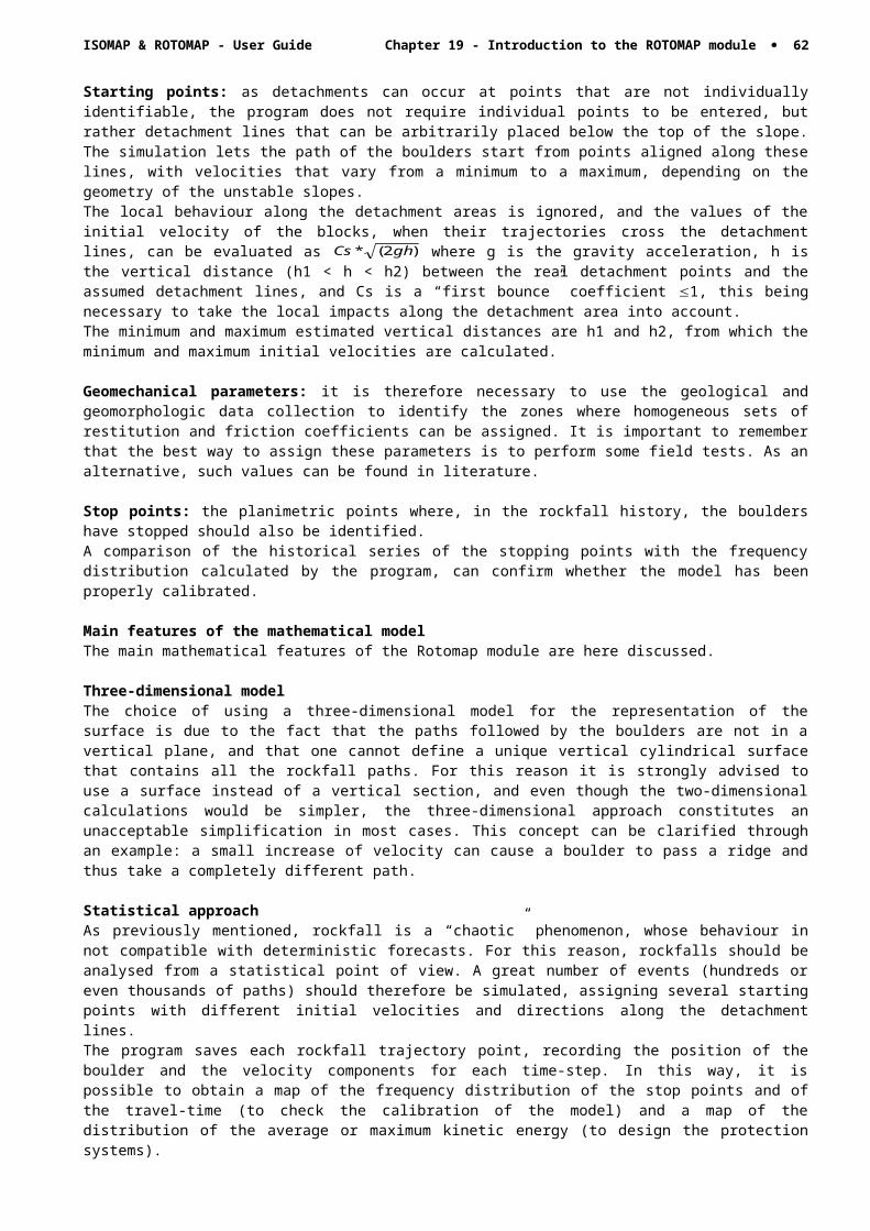
ISOMAP & ROTOMAP - User Guide Chapter 20 - Miscellanea · 63
0,276 0,835 Chalk face0,271 0,596 Vegetated chalk scree
Budetta, P., Santo, A. 0,2 0,53 Dolomitic limestone boulders on rockysurfaces and on talus desposits
0,1 0,2 Remolded pyroclastic from the terracessituated at the base of the cliff
0 0,24 Impacts on detritus of the fans presentat the foot of a rock cliff
Chau, K.T., Wong, R.H. 0,393 SoilC., Lee, C.F. (1996) 0,453 Shotcrete
0,487 Rock slope
Giani, G.P. (1992) 0,5 Bedrock0,35 Bedrock covered by large blocks0,3 Debris formed by uniform distributed
elements0,25 Soil covered by vegetation
Pfeiffer, T.J., Higgens, 0,37 - 0,42 Smooth hard surfaces and pavingJ.D. (1990) 0,33 - 0,37 Most bedrock and boulder fields
0,3 - 0,33 Talus and firm soil slopes0,28 - 0,3 Soft soil slopes
0,87 - 0,92 Smooth hard surfaces such as pavementor smooth bedrock surfaces
0,83 - 0,87 Most bedrock surfaces and talus with novegetation
0,82 - 0,85 Most talus slopes with some lowvegetation
0,8 - 0,83 Vegetated talus slopes and soil slopeswith spares vegetation
0,78 - 0,82 Brush covered soil slope
Hungr, O. Evans, S.G. 0,5 0,8 Sparsley forested slope is covered by a (1988) veneer of very fine weathered talus
derived from weak shistose units underlying the limestone cap.
0,5 0,8 Limestone on bare uniform talus slopeformed of basalt fragments with a modalsize of 5 cm.
0,7 0,9 Rectangular bolder of metamorphosedtuff on bare rock and a steep snow covered shelf.
References
ISOMAP & ROTOMAP - User Guide Chapter 20 - Miscellanea · 64
· Azimi C., Desvarreux P., Giraud A., Martin-Cocher J. (1982). Methodes de calcul de la dynamique des chutes des blocs. Application a l'etude du versant de la montagne de La Pale (Vercors). Bull Liason P.C., n. 122, pp. 93-102
· Bertozzi E., Broili L. (1978). Considerazioni sui criteri di progettazione delle opere di difesa nei processi di scendimento massi. Mem. Soc. Geol. It. n. 18, pp. 187-195
· Bozzolo D., Pamii R., Hutter K., (1989). Rockfall analysis - A mathematical model and its test with field data. pp. 555-560.
· Descoeudres F., Zimmermann T. (1987). Three dimensional dynamic calculations of rockfalls. 6 th ISMR, vol. 1, pp. 337-342
· Falcetta J.L. (1985). Un noveau modele de calcul de trajectories des blocs rocheux. Revue Francaise de Geotechnique, n. 30, pp. 11-17.
· Focardi P. (1982). Considerazioni cinematiche sul percorso di massi provenienti da frane di crollo. Geologia Tecnica, n. 4 pp. 13-23.
· Giani G.P. (1997). Caduta massi. Analisi del moto ed opere di protezione. Hevelius ISBN 88-86977-05-0
· Hampel F.R. (1968). Contributions to the theory of robust estimation. Ph.D. thesis. Berkeley
· Hogg R.V. (1977). An introduction to robust procedures. Commun. Statist. A 6, pp. 789-794
· Tukey J.W. (1960). A survey of sampling from contaminated distribuctions. In Contributions to Probability and Statistics, pp. 448-485