Département PERSYST UR Systèmes de Culture Annuels

PROBE-w (Water Balance PROgram): A software application for water balance modeling in a cultivated soil.

Presentation and User Manual.

JL Chopart1, L Le Mézo, M Mézino.

February 2009 1 CIRAD-CA station Ligne Paradis, 7, chemin de l’IRAT, 97410, St Pierre La Réunion. chopart@cirad.fr

2

Introduction and Antecedents

This software application enables fast, simple modeling of water balance in cultivated soils thanks to a simulation model of the same name (PROBE) proposed by Chopart and Siband (1988) and validated by Chopart and Vauclin (1990), Chopart et al. (2007). The hypotheses and choices of modeling, algorithms and equations are set out in detail in the founding technical document (Chopart and Siband, 1988) and in the scientific article that followed (Chopart and Vauclin, 1990). These scientific elements will not be repeated in this user guide to the PROBE-w application; only a few elements will be quoted. It is a capacity-based simulation model with a daily time step. The main information required concerns: (i) the maximum available water reserve in the soil that can be explored by the roots; (ii) the climate (rainfall, daily potential evapotranspiration); (iii) the crop’s water requirements (crop coefficient); (iv) simple information on the root system, considered here as what captures the water (growth of the root front); (v) simplified information on the processes of direct evaporation in the days subsequent to a rainfall event. The model calculates the two main terms of water balance: evapotranspiration from the soil-crop system; and water excess (drainage and runoff) together with various other resulting parameters (water deficit, satisfaction rate of crop water requirements). The published articles (Chopart and Siband, 1988, Chopart and Vauclin, 1990) can be consulted for further information on the model’s equations and the modeling choices. Cf. bibliography An initial software application was developed shortly after the model was created. However, it was written in Basic by the researchers themselves using the information technology of the 1980s, and was no longer functional. The PROBE model was used again more recently as a water balance model in an irrigation advice tool for farmers (OSIRI, Chopart et al., 2007), and in an irrigation decision support tool for managers (FIVE-Core, Chopart et al., 2007). But both of these cases were decision support tools whose function focused on irrigation. They can seem somewhat cumbersome to use for an agronomist who is not a specialist in irrigation and agricultural water management and wishes to carry out a fast, simple water balance calculation. PROBE-w, a new version of the PROBE application, was developed for use by agronomists, biologists, selectors, etc. who are not necessarily specialists in irrigation, nor even in the water functioning of soil and crops. Water balance in cultivated soil is of course an important element for understanding the spatio-temporal variability of yield according to the climate and soil (Chopart et al., 1991), and is thus, together with other factors, one of the elements for understanding genotype/environment interactions and, in the case of a number of crops, the product’s quality. This is why PROBE-w has been developed with current computing tools, in Windows. This version has a completely fresh presentation, whilst maintaining the functionalities and validity field of the initially published model.

3

SUMMARY 1. Basic Principles and Directions for Use.............................................................................. 4

Basic principles and validity field............................................................................................. 4 Concise presentation of the successive stages ....................................................................... 4

2. Climate Data and Irrigations ................................................................................................. 5 2.1. Creating and selecting a file.......................................................................................... 5

1. Keying data directly into PROBE-w or in a spreadsheet ........................................ 6 2. Save files .......................................................................................................................... 7 3. Selecting climate file for calculating............................................................................ 7

2.2. Analysis of missing data................................................................................................ 7 2.3. Modeling soil evaporation ............................................................................................ 8

3. Parametering Soil Reservoir, Crop and Roots.................................................................... 8 3.1. Soil reservoir parameters .............................................................................................. 9 3.2. The crop and its roots................................................................................................. 10

Crop factor (Kc) :.................................................................................................................. 10 3.3. Management of the plots............................................................................................ 12 3.4. Sensitivity analysis........................................................................................................ 13

4. Calculating and Exporting Water Balance ........................................................................ 14 4.1. Water balance calculation and display of results..................................................... 14 4.2. Exporting the results ................................................................................................... 15

5. IT Management ..................................................................................................................... 16 Annex 1: Limits of the Application .......................................................................................... 17 Bibliography ................................................................................................................................. 18

4

1. Basic Principles and Directions for Use

Basic principles and validity field PROBE-w is a software application for calculating soil water balance based on the PROBE capacity-based model. The application is in three parts:

- water balance entry parameters for one or several field plots; - calculation of the water balance and display of the results; - exporting of the data (entry parameters and results in text file format).

Contextual help and a user guide are available. The conceptual and practical limits, together with the information technology choices, are set out in detail in Annex 1.

When PROBE-w is closed, the above data is not saved in the tool’s memory. Similarly, there is no mapping of the results. These limits correspond to the choice of proposing a simple tool that is restricted to its main function, that of water balance modeling. Consequently graphics editing and statistical calculations are externalized.

Concise presentation of the successive stages The PROBE-w application displays a single screen made up of three tabs corresponding to the three stages of using the software. 1) The first stage consists of supplying, to PROBE-w, the daily climate data:

rainfall events and/or irrigations (compulsory); climate’s water requirements or potential evapotranspiration (compulsory); average air temperature (optional).

For each folder, the file containing these data can be keyed or preferably created before in a spreadsheet and saved in a format CSV.

2) In the second stage, the parameters relating to soil reservoir (available water reserve, drainage level, initial water reserves, etc.) and roots (initial root front depth, growth rate) must be filled in.

3) In the third stage, after the model’s entries in stages 1 and 2 have been parametered, PROBE-w calculates the soil’s water balance daily. The user then selects his output variables for exporting as a text file. Calculated values may be synthesized by different time periods or exported in full.

5

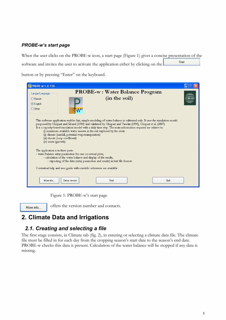
PROBE-w’s start page

When the user clicks on the PROBE-w icon, a start page (Figure 1) gives a concise presentation of the

software and invites the user to activate the application either by clicking on the

button or by pressing “Enter” on the keyboard.

Figure 1: PROBE-w’s start page

offers the version number and contacts.

2. Climate Data and Irrigations

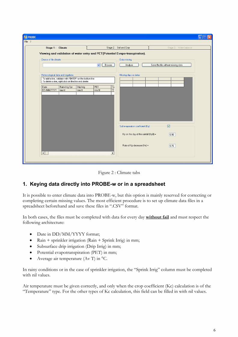
2.1. Creating and selecting a file The first stage consists, in Climate tab (fig. 2), in entering or selecting a climate data file. The climate file must be filled in for each day from the cropping season’s start date to the season’s end date. PROBE-w checks this data is present. Calculation of the water balance will be stopped if any data is missing.

6

Figure 2 : Climate tabs

1. Keying data directly into PROBE-w or in a spreadsheet

It is possible to enter climate data into PROBE-w, but this option is mainly reserved for correcting or completing certain missing values. The most efficient procedure is to set up climate data files in a spreadsheet beforehand and save these files in “.CSV” format.

In both cases, the files must be completed with data for every day without fail and must respect the following architecture:

• Date in DD/MM/YYYY format; • Rain + sprinkler irrigation (Rain + Sprink Irrig) in mm; • Subsurface drip irrigation (Drip Irrig) in mm; • Potential evapotranspiration (PET) in mm; • Average air temperature (Av T) in °C.

In rainy conditions or in the case of sprinkler irrigation, the “Sprink Irrig” column must be completed with nil values.

Air temperature must be given correctly, and only when the crop coefficient (Kc) calculation is of the “Temperature” type. For the other types of Kc calculation, this field can be filled in with nil values.

7

For fast completion of a dataset on a parameter, the user can select the whole column or several cells in the same column and enter the same value. The entry is then validated simultaneously for all selected cells.

It is possible and better to put in several years one after the other.

2. Save files

If data were enter directly in PROBE-w, they are saved with the “register” button. The user chooses the name of the file witch is automatically saved in .CSV format

If data were enter in a spreadsheet, it is necessary, before saving to verify that the first line (date etc.) is in the fist line of the first column of the page. It is necessary to erase all other information. The user has to save this file in « .CSV »format. Files saved in a different format cannot be read by PROBE-w. It is necessary to memorize where this file is.

A PROBE-w specific tree structure make easier researches Cf. IT Management

It is possible to correct or complete pre-existing climate files, in a spreadsheet.

In order to do this, open the “.CSV” file, select the “Text File” type or “All Files”, then select the separator “ ; ” in the second stage of the import assistant for Excel.

The user carries out the requisite modifications and then saves the file in “.CSV” format.

3. Selecting climate file for calculating After creating the climate data files, the user selects, in the tree structure, the appropriate file and views it in the selection window. After this choice, the file content is displayed in the left-hand window.

2.2. Analysis of missing data

As has already been indicated, it is indispensable to check that climate data has been entered for each of the days selected for modeling.

The command checks the file’s compliance with this and displays the missing days and/or the missing data in the right-hand window.

In this case, the user enters the missing data in the left-hand section and then clicks on the button in order to ensure data continuity.

Missing data in the climate file does not stop the user from moving on to stage 3 (calculations). However, calculations must then be carried out on a period without missing data.

8

2.3. Modeling soil evaporation

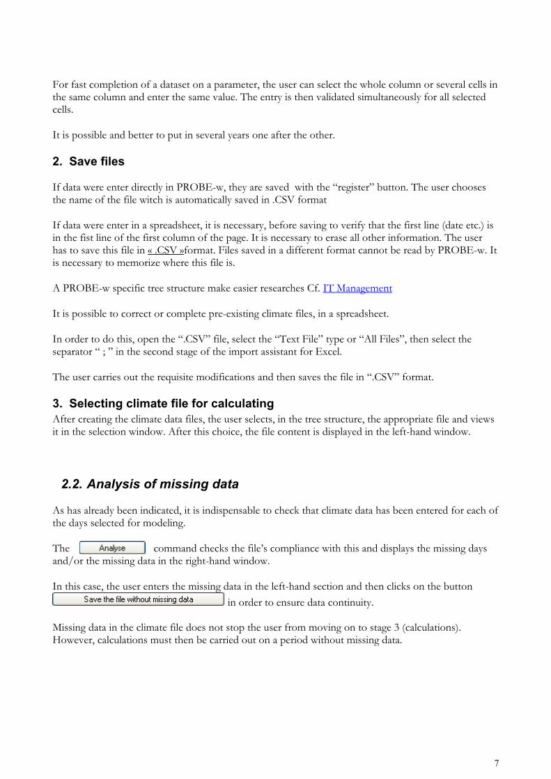
The software manages the evaporation part of evapotranspiration. For this, after rainfall or sprinkler irrigation, direct evaporation of this rain via the soil (and the direct drying of the leaves) represents a fraction of the Potential Evapotranspiration (PET) which decreases exponentially over time after rainfall according to the model:

KPd = KP0 exp (-VE DAR)

where:

- KP0 = evaporation of the first day (day 0); KP0 is between 1 (PET) and 0; - VE = rate of evaporation decrease of KP according to the number of days after rainfall (between 1

and 0); - DAR = number of days after a rain.

The application thus displays two windows: KP0 and VE. They already contain the values of KP0 and VE considered empirically as functional in tropical climates and soils.

The user can modify these values. If no modification is made, the values proposed by the model are retained.

In the case of subsurface drip irrigation, soil evaporation is considered as nil and the water balance calculation model does not use this algorithm.

3. Parametering Soil Reservoir, Crop and Roots The second stage enables configuration, in Soil and Crop tab (fig. 3), of the plots for which water balances are to be calculated. When the application is used for the first time, no plot is displayed. The user goes on to the first line and starts keying in information with the plot’s name, followed by the cropping season and calculation start dates. Nota bene: During the cropping period (the difference between the season’s start and end dates), the climate data must be known. (Cf. Climate data and irrigations) All the parameters are compulsory.

9

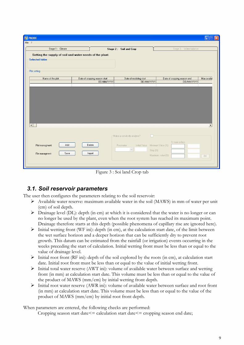
Figure 3 : Soi land Crop tab

3.1. Soil reservoir parameters The user then configures the parameters relating to the soil reservoir:

Available water reserve: maximum available water in the soil (MAWS) in mm of water per unit (cm) of soil depth.

Drainage level (DL): depth (in cm) at which it is considered that the water is no longer or can no longer be used by the plant, even when the root system has reached its maximum point. Drainage therefore starts at this depth (possible phenomena of capillary rise are ignored here).

Initial wetting front (WF ini): depth (in cm), at the calculation start date, of the limit between the wet surface horizon and a deeper horizon that can be sufficiently dry to prevent root growth. This datum can be estimated from the rainfall (or irrigation) events occurring in the weeks preceding the start of calculation. Initial wetting front must be less than or equal to the value of drainage level.

Initial root front (RF ini): depth of the soil explored by the roots (in cm), at calculation start date. Initial root front must be less than or equal to the value of initial wetting front.

Initial total water reserve (AWT ini): volume of available water between surface and wetting front (in mm) at calculation start date. This volume must be less than or equal to the value of the product of MAWS (mm/cm) by initial wetting front depth.

Initial root water reserve (AWR ini): volume of available water between surface and root front (in mm) at calculation start date. This volume must be less than or equal to the value of the product of MAWS (mm/cm) by initial root front depth.

When parameters are entered, the following checks are performed: Cropping season start date<= calculation start date<= cropping season end date;

10

AWR ini=< AWT ini RF ini + DRG* Age of root growth end=< DL WF ini =< DL AWT ini =MAWS* WF ini Age of root growth end =< cycle duration AWR ini <= RF ini x MAWS; Sum of the durations of Kc time-steps = duration of cropping season ± 5 days.

3.2. The crop and its roots The final data to be entered is relative to the crop and its roots. The user must validate:

A type of crop coefficient, and complete it. Root growth: daily root growth rate (cm d-1). Age of root growth end: age expressed in the number of days after the season start date from

which root growth ceases definitively. This age must be less than or equal to the value of: (drainage level / root growth rate) – initial root front.

Crop factor (Kc) : PROBE-w offers 3different means of evaluating crop factors:

FAO model (Kc FAO) Free style (Kc steps) In relation to temperature (Kc Temperature)

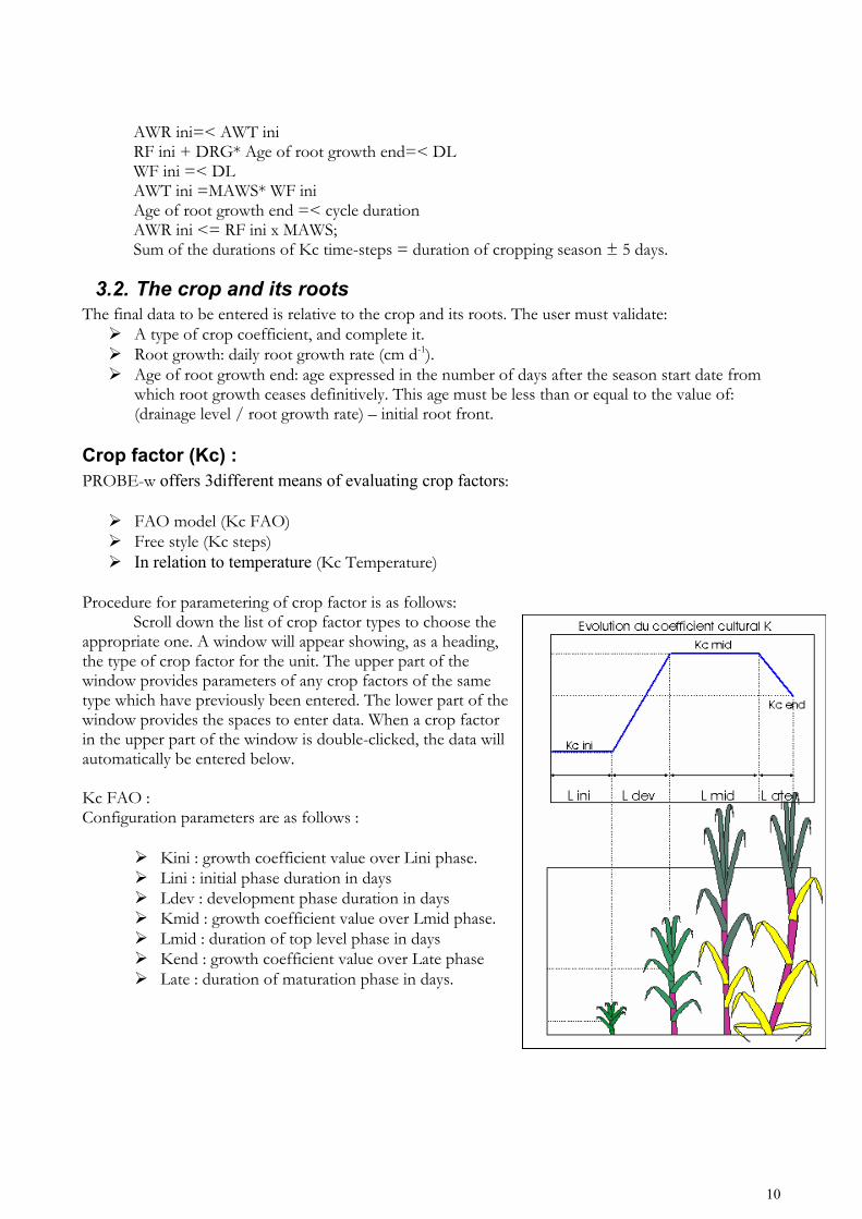
Procedure for parametering of crop factor is as follows: Scroll down the list of crop factor types to choose the appropriate one. A window will appear showing, as a heading, the type of crop factor for the unit. The upper part of the window provides parameters of any crop factors of the same type which have previously been entered. The lower part of the window provides the spaces to enter data. When a crop factor in the upper part of the window is double-clicked, the data will automatically be entered below. Kc FAO : Configuration parameters are as follows :

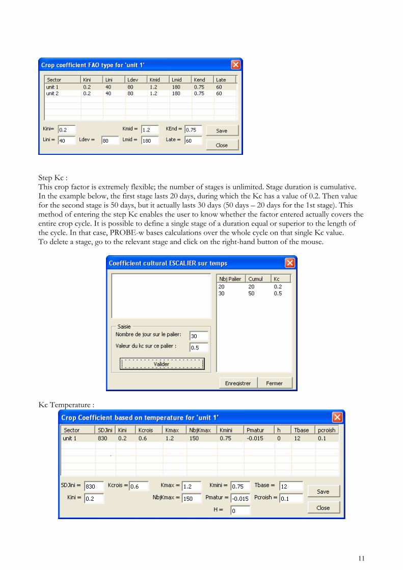
Kini : growth coefficient value over Lini phase. Lini : initial phase duration in days Ldev : development phase duration in days Kmid : growth coefficient value over Lmid phase. Lmid : duration of top level phase in days Kend : growth coefficient value over Late phase Late : duration of maturation phase in days.

11

Step Kc : This crop factor is extremely flexible; the number of stages is unlimited. Stage duration is cumulative. In the example below, the first stage lasts 20 days, during which the Kc has a value of 0.2. Then value for the second stage is 50 days, but it actually lasts 30 days (50 days – 20 days for the 1st stage). This method of entering the step Kc enables the user to know whether the factor entered actually covers the entire crop cycle. It is possible to define a single stage of a duration equal or superior to the length of the cycle. In that case, PROBE-w bases calculations over the whole cycle on that single Kc value. To delete a stage, go to the relevant stage and click on the right-hand button of the mouse.

Kc Temperature :

12

Configuration parameters are as follows:

SDJini : Sum of day degrees in °C to reach Kcrois from K ini Kini : growth coefficient value at cycle start date Kcrois : growth coefficient value at major growth start K max : maximum value of growth coefficient NbjKmax : Number of days at Kmax Kmini : growth coefficient value at cycle end date Pmatur : Kmax period end slope to reach Kmin at cycle end. H : initial height in m Tbase : Temperature in °C; day degrees will be cumulated from this reference temperature. Pcroish : growth speed in m j-1.

NB: for KC choices, cumulated duration of each sequence must be equal to cropping season as defined previously in “Soil and crop” stage

In the case of FAO or step models, a procedure that is internal to the application checks for consistency. In contrast, in the case of the more complex temperature model with phase durations that are dependent on the temperature and other factors, the user himself must check for consistency. If the minimum Kc is reached before actual cropping season end, it will stay at this minimum Kc until the end of the season.

3.3. Management of the plots

After entering the data for all of a plot’s parameters, the user may duplicate this plot by clicking on the button.

This command replicates all the information relating to the existing or selected plot, excepting the name and type of crop coefficient, which will require filling in.

Should it be required, the command erases the selected plot.

Once the user has filled in all the parameters for one or several plots, it is advisable to save the configuration. PROBE-w does not store the settings in its memory.

opens a dialog box enabling the user to specify the name and the storage directory of the file. The plots displayed onscreen are grouped together in a folder. These files are in a text format.

A tree structure specific to PROBE-w was created when the application was installed, and contains a directory named “Plots” which will be the default suggestion for saving.

When PROBE-w is used again, the user can pick up on a configuration that has already been made by clicking on the button.

Advanced use of files containing plots is possible in a spreadsheet application such as Excel. To open the file, select the “Text File” type or “All Files”, and then select the “ ; ” separator in the second stage of the import assistant for Excel.

13

The user makes the requisite changes and then saves the file in “.TXT” or “.CSV” format. Files saved in a different format cannot be read by PROBE-w.

Another advanced use of PROBE-w enables a parameter to be changed for several plots simultaneously. This simply requires selecting the same column for several plots and then validating the modification.

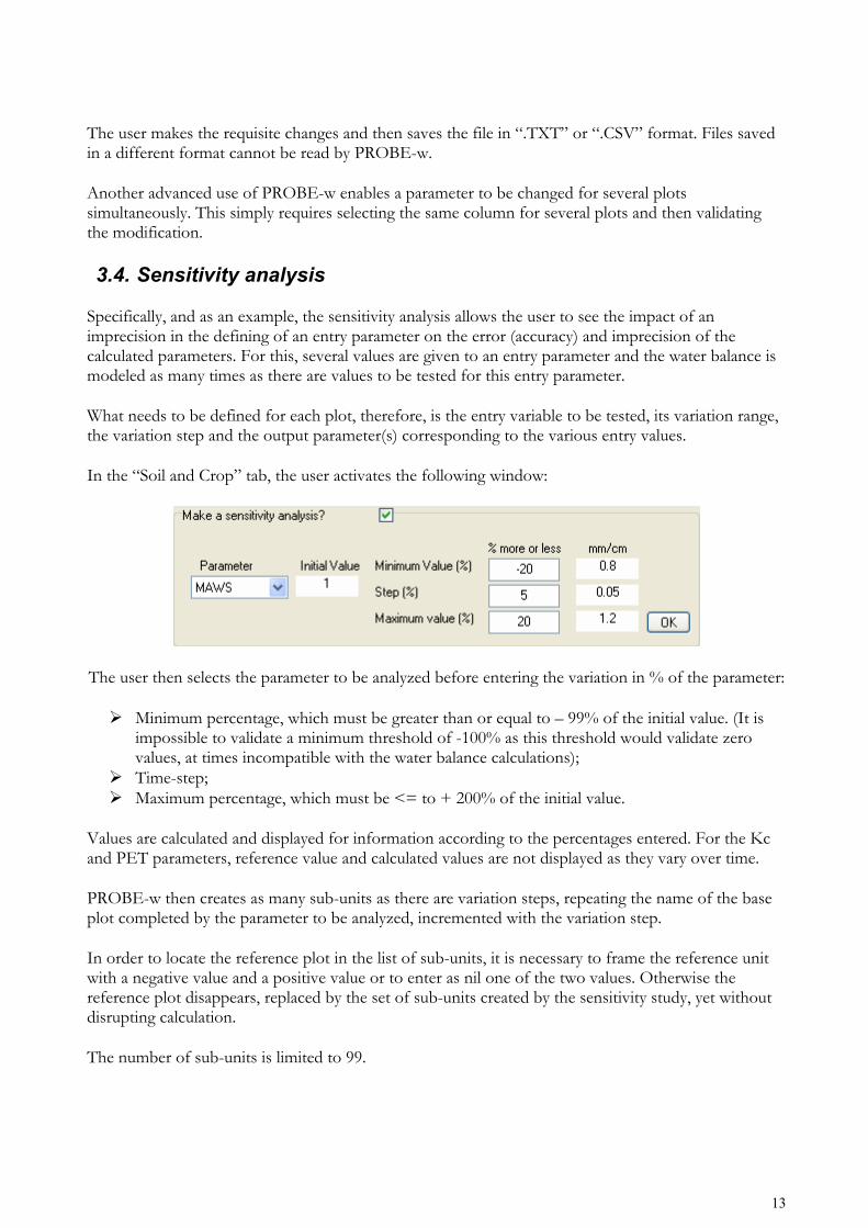
3.4. Sensitivity analysis

Specifically, and as an example, the sensitivity analysis allows the user to see the impact of an imprecision in the defining of an entry parameter on the error (accuracy) and imprecision of the calculated parameters. For this, several values are given to an entry parameter and the water balance is modeled as many times as there are values to be tested for this entry parameter.

What needs to be defined for each plot, therefore, is the entry variable to be tested, its variation range, the variation step and the output parameter(s) corresponding to the various entry values.

In the “Soil and Crop” tab, the user activates the following window:

The user then selects the parameter to be analyzed before entering the variation in % of the parameter:

Minimum percentage, which must be greater than or equal to – 99% of the initial value. (It is impossible to validate a minimum threshold of -100% as this threshold would validate zero values, at times incompatible with the water balance calculations);

Time-step; Maximum percentage, which must be <= to + 200% of the initial value.

Values are calculated and displayed for information according to the percentages entered. For the Kc and PET parameters, reference value and calculated values are not displayed as they vary over time.

PROBE-w then creates as many sub-units as there are variation steps, repeating the name of the base plot completed by the parameter to be analyzed, incremented with the variation step.

In order to locate the reference plot in the list of sub-units, it is necessary to frame the reference unit with a negative value and a positive value or to enter as nil one of the two values. Otherwise the reference plot disappears, replaced by the set of sub-units created by the sensitivity study, yet without disrupting calculation.

The number of sub-units is limited to 99.

14

Nota bene: A large number of sub-units over a long cropping season period may result in a lengthy calculation time of the water balance.

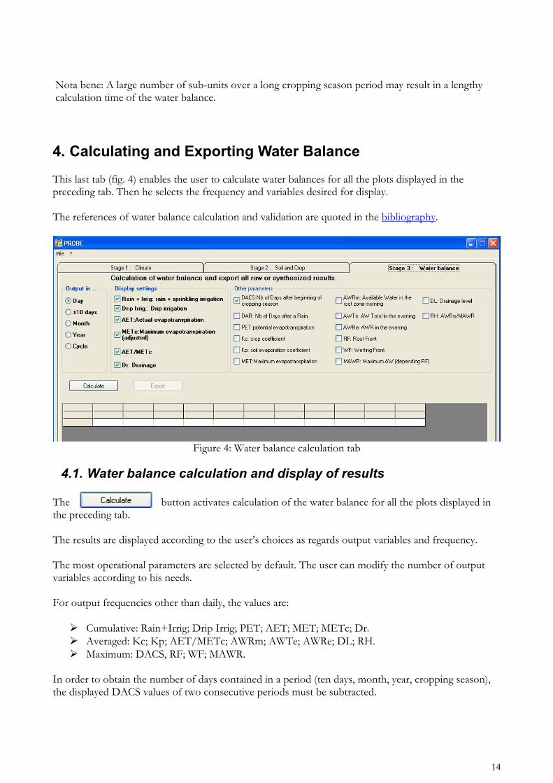
4. Calculating and Exporting Water Balance This last tab (fig. 4) enables the user to calculate water balances for all the plots displayed in the preceding tab. Then he selects the frequency and variables desired for display. The references of water balance calculation and validation are quoted in the bibliography.

Figure 4: Water balance calculation tab

4.1. Water balance calculation and display of results The button activates calculation of the water balance for all the plots displayed in the preceding tab. The results are displayed according to the user’s choices as regards output variables and frequency. The most operational parameters are selected by default. The user can modify the number of output variables according to his needs. For output frequencies other than daily, the values are:

Cumulative: Rain+Irrig; Drip Irrig; PET; AET; MET; METc; Dr. Averaged: Kc; Kp; AET/METc; AWRm; AWTe; AWRe; DL; RH. Maximum: DACS, RF; WF; MAWR.

In order to obtain the number of days contained in a period (ten days, month, year, cropping season), the displayed DACS values of two consecutive periods must be subtracted.

15

An advanced use of PROBE-w enables the user to copy all or part of the displayed values and then to paste them into a spreadsheet without going through the export method (see below). However, the export method is faster for a large number of lines and in particular carries over the configuration of the plots.

4.2. Exporting the results opens a dialog box where the user specifies the file name and the storage directory.

The file exported to text format is made up of 3 parts:

Presentation of the configuration of the plots; Display of the column’s abbreviations and literal title; Viewing of the calculated values.

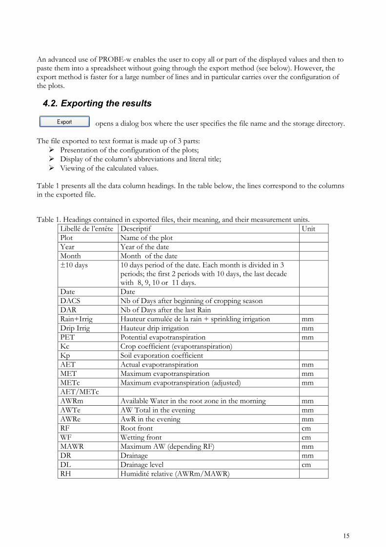
Table 1 presents all the data column headings. In the table below, the lines correspond to the columns in the exported file. Table 1. Headings contained in exported files, their meaning, and their measurement units.

Libellé de l’entête Descriptif Unit Plot Name of the plot Year Year of the date Month Month of the date ±10 days 10 days period of the date. Each month is divided in 3

periods; the first 2 periods with 10 days, the last decade with 8, 9, 10 or 11 days.

Date Date DACS Nb of Days after beginning of cropping season DAR Nb of Days after the last Rain Rain+Irrig Hauteur cumulée de la rain + sprinkling irrigation mm Drip Irrig Hauteur drip irrigation mm PET Potential evapotranspiration mm Kc Crop coefficient (evapotranspiration) Kp Soil evaporation coefficient AET Actual evapotranspiration mm MET Maximum evapotranspiration mm METc Maximum evapotranspiration (adjusted) mm AET/METc AWRm Available Water in the root zone in the morning mm AWTe AW Total in the evening mm AWRe AwR in the evening mm RF Root front cm WF Wetting front cm MAWR Maximum AW (depending RF) mm DR Drainage mm DL Drainage level cm RH Humidité relative (AWRm/MAWR)

16

5. IT Management PROBE-w makes no automatic internal back-up of the data: neither data entered (plot, entry variable, etc.), nor calculated values. All values that are calculated must be saved in external files by the user, in order to be backed up. Four directories are created in the PROBE-w folder when the application is installed:

Entités-Plot: contains the plot groups in the form of a folder name; BHY-WB: contains the files exported in text format; KC: the storage folder for each plot’s crop coefficients; Climat(e): contains the climate files.

Nota bene: It is strongly advised not to modify these file names. If they are modified, PROBE-w will

create these folders again the next time the software is used. These files are selected by default for importing, saving and backing up files. They are deleted via the browser, since PROBE-w does not offer this functionality. The application “unins000” uninstalls the application part of the PROBE-W software in the computer. The files created by the user and stored in the tree structure must be deleted by the user after the application has been uninstalled. The application “unins000” deletes the files that were created when the software was installed, but does not delete those created as the software was used.

Apart from the contextual help to be found on-screen or on part of a screen, some buttons offer specific help. The symbol can be seen when the mouse pointer is passed over these buttons

17

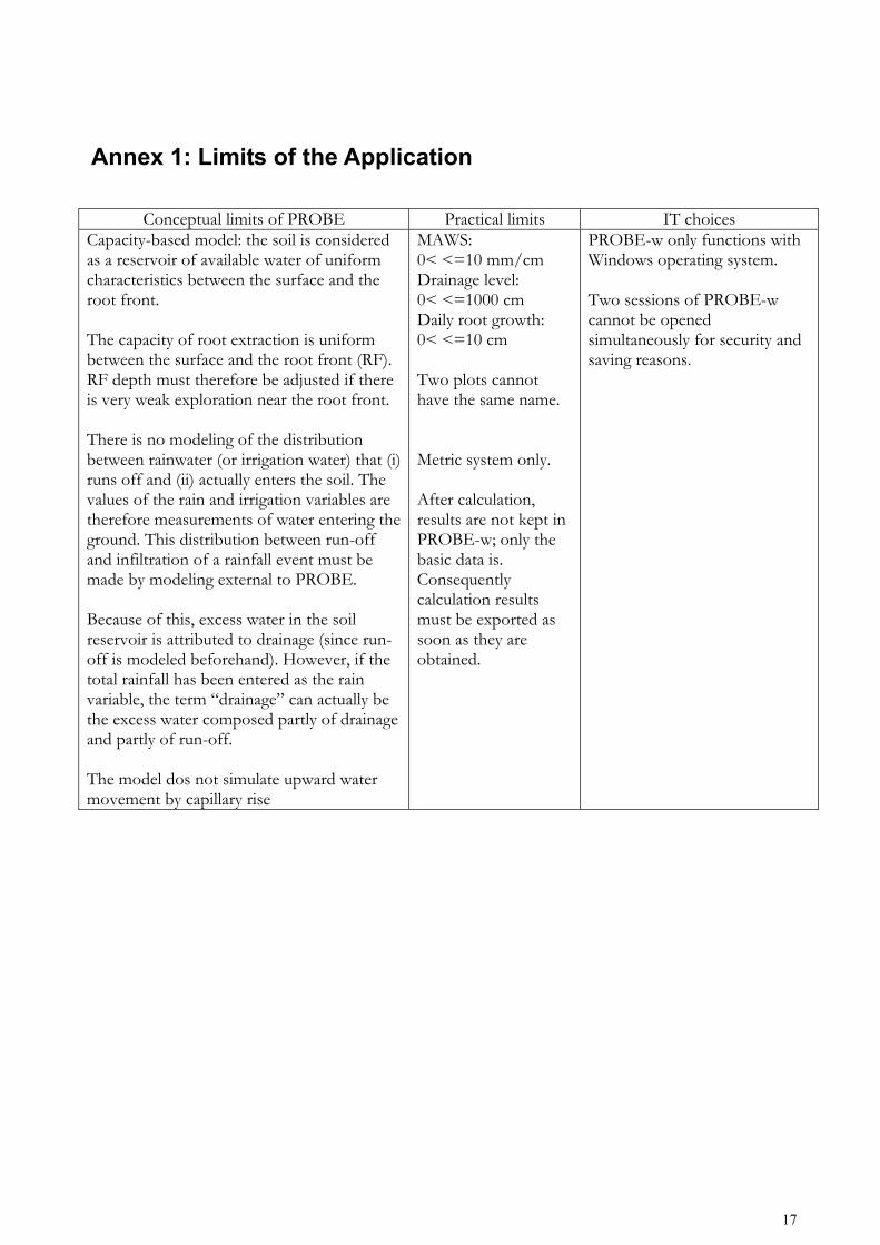
Annex 1: Limits of the Application

Conceptual limits of PROBE Practical limits IT choices Capacity-based model: the soil is considered as a reservoir of available water of uniform characteristics between the surface and the root front. The capacity of root extraction is uniform between the surface and the root front (RF). RF depth must therefore be adjusted if there is very weak exploration near the root front. There is no modeling of the distribution between rainwater (or irrigation water) that (i) runs off and (ii) actually enters the soil. The values of the rain and irrigation variables are therefore measurements of water entering the ground. This distribution between run-off and infiltration of a rainfall event must be made by modeling external to PROBE. Because of this, excess water in the soil reservoir is attributed to drainage (since run-off is modeled beforehand). However, if the total rainfall has been entered as the rain variable, the term “drainage” can actually be the excess water composed partly of drainage and partly of run-off. The model dos not simulate upward water movement by capillary rise

MAWS: 0< <=10 mm/cm Drainage level: 0< <=1000 cm Daily root growth: 0< <=10 cm Two plots cannot have the same name. Metric system only. After calculation, results are not kept in PROBE-w; only the basic data is. Consequently calculation results must be exported as soon as they are obtained.

PROBE-w only functions with Windows operating system. Two sessions of PROBE-w cannot be opened simultaneously for security and saving reasons.

18

Bibliography Chopart J.L., Siband P., 1988. PROBE, PROgramme de Bilan de l’Eau. Mémoires et travaux de l’IRAT, n° 17, CIRAD- IRAT édit. France, 76 p. Chopart J.L., Vauclin M., 1990. Water balance estimation model : Field test and sensitivity analysis. Soil Science Society of America Journal, 54, 1377-1384. Chopart J.L., Vauclin M., Nicou R., 1991. Le bilan hydrique : Dilettantisme ou nécessité pour comprendre les relations milieu physique-culture en zone tropicale sèche? In : “Soil Water Balance in the Sudano-Sahelian Zone, IAHS edit Wallingford, Royaume-Uni , n. 199, p. 345-357. Chopart J.L., Mézino M., Aure F., Le Mézo L., Mété M., Vauclin M., 2007. OSIRI: A simple decision-making tool for monitoring irrigation of small farms in heterogeneous environments. Agric. Water Manage. vol. 87, n°2, 128-138.

Chopart J.L., Mézino M., Le Mézo L., Fusillier J.L., 2007. FIVE-CoRe: A simple model for farm irrigation volume estimates according to constraints and requirements. Application to sugar cane in Reunion (France). In : ”Proceedings Int. Society of sugar cane technologists vol. 26, XXXVI ISSCT Congress, Durban, South Africa 29-07, 02-08 2007, Abstracts book pp. 98-99 and poster paper in ISSCT Congress proceedings CD, pp. 490, 493.

Chopart J.L., Aure F., Le Mézo L., Mézino M., Antoir J., Vauclin M., 2007. Field tests of OSIRI, a decision making tool for irrigation of sugarcane farms in Réunion. In: “Proceedings of fourth USCID Int. Conf. on Irrigation and Drainage 2-5 oct. 2007, Sacramento: The role of Irrigation and Drainage in a Sustainable Future”, USCID Edit., USA, pp. 423, 435.