User Manual

2018

Version 3

By

Karen Lindsay, Michael Popp, Muthukumar Bagavathiannan, Jason Norsworthy

 

 

Table of Contents

I. Introduction ......................................................................................................................................... 5 Study Species: Palmer Amaranth ..................................................................................................... 5 Use Caveats ...................................................................................................................................... 5

II. Purpose ................................................................................................................................................ 6 Core Components ............................................................................................................................ 6

Population Dynamics ................................................................................................................... 6 Management ................................................................................................................................. 7 Economics..................................................................................................................................... 7

Model Implementation ..................................................................................................................... 7 Saving User Modifications for Comparison .................................................................................... 8

III. Installation and General Use Instructions ........................................................................................... 9 Installation ....................................................................................................................................... 9 Saving and Exiting Files ................................................................................................................ 11 Navigating Worksheets .................................................................................................................. 11 Tutorials ......................................................................................................................................... 12 Controls .......................................................................................................................................... 12

Command Buttons ...................................................................................................................... 12 Drop-down Lists ......................................................................................................................... 12 Comment Boxes .......................................................................................................................... 12 Conditional Formatting .............................................................................................................. 12 Copy and Paste Restriction ........................................................................................................ 13 Userforms ................................................................................................................................... 13 Text Boxes ................................................................................................................................... 13

IV. Title ....................................................................................................................................................... 13 V. ‘Systems’ Worksheet ............................................................................................................................. 15

Calculate Total Specified Expenses Userforms .......................................................................... 16 Specify Fall Options Userform ................................................................................................... 17

VI. ‘Strategy’ Worksheet ........................................................................................................................ 20 VII. ‘Output’ Worksheet ........................................................................................................................... 27 VIII. Conclusion ........................................................................................................................................ 28

Assumptions and Limitations ...................................................................................................... 28 References ................................................................................................................................................... 29

 

 

List of Figures

Figure 1. Model Flow Chart .......................................................................................................... 8 Figure 2. Save and Load Flow Chart ............................................................................................ 9 Figure 3. Initial File Installation Message for Excel 2016 and 2010 – 2013 .............................. 10 Figure 4. Welcome Banner ......................................................................................................... 10 Figure 5. Exiting PAM ................................................................................................................ 11 Figure 6. ‘Title’ Worksheet ......................................................................................................... 14 Figure 7. ‘Systems’ Worksheet ................................................................................................... 15 Figure 8. ‘Calculate Total Specified Expenses’ Userform ......................................................... 16 Figure 9. ‘Specify Fall Options’ Userform ................................................................................. 17 Figure 10. Saving Systems .......................................................................................................... 18 Figure 11. Loading Saved Systems ............................................................................................. 19 Figure 12. ‘Strategy’ Worksheet ................................................................................................. 21 Figure 13. Example User Selections in ‘Strategy’ Worksheet .................................................... 22 Figure 14. Example Conditional Formatting in ‘Strategy’ Worksheet ....................................... 23 Figure 15. Risk Assessment Definition ...................................................................................... 24 Figure 16. Year and Within Year Timing of Palmer Amaranth Escapes .................................. 24 Figure 17. Saving Strategies ...................................................................................................... 25 Figure 18. Loading Saved Strategies .......................................................................................... 26 Figure 19. Clearing Saved Strategies .......................................................................................... 26 Figure 20. ‘Output’ Worksheet ................................................................................................... 27

4

 

Disclaimer This software is provided ‘as is’ and without warranties as to performance or merchantability. Further, statements may have been made to you about this software. Any such statements do not constitute warranties and shall not be relied on by the user in deciding whether to use the program or act on its results. This program is provided without any expressed or implied warranties whatsoever. Because the diversity of conditions and hardware under which this program may be used, no warranty of merchantability or warranty of fitness for a particular purpose is offered. The user is advised to test the program thoroughly before relying on it. The user assumes the entire risk of using the program. The University of Arkansas will not be liable for any claim or damage brought against the user by any third party, nor will the University of Arkansas be liable for any consequential, indirect, or special damages suffered by the user as a result of the software.

5

 

I. Introduction

The Palmer Amaranth Integrated Management Model (PAM) was developed using the Microsoft Excel® software platform to assist cotton, corn, and/or soybean producers, consultants, distributors, and extension personnel, in adopting integrated management tactics for the management of Palmer amaranth and promoting long-term economic viability of crop production through the minimization of adverse economic, human health, and environmental impacts associated with herbicide resistance.

The PAM software serves as a valuable decision-support tool for guiding integrated management of Palmer amaranth by utilizing existing research knowledge and providing a greater understanding of the long-term biological (seedbank size and persistence) and economic (improved cost-benefit analysis) implications of various management choices. Decision support will allow improved crop production and profitability through adoption of IPM tactics that preserve the long-term utility of available herbicide options, and minimize the human health risks and environmental impacts associated with herbicide resistance.

Study Species: Palmer Amaranth

Palmer amaranth is a pigweed native to the southern United States and considered to be both aggressive and invasive with a growing resistance to glyphosate and ALS-inhibitor herbicides (Legleiter and Johnson, 2013; Sprague, 2013). Palmer amaranth is one of the most problematic herbicide-resistant weeds causing great losses to cotton, corn, and soybean production in the Southern US (Riar et al., 2013; Webster and Nichols, 2012). In addition to being a predominant weed in the Southern region, Palmer amaranth is also a growing concern in other agriculturally important regions in the country, particularly the Southwestern (Rios et al., 2014), Midwestern (Jhala et al. 2014), and Northcentral (Sprague, 2012) states. In places such as Texas, the spread of resistant Palmer amaranth has been very rapid within the past few years from the Pan Handle to the Gulf Coast regions (Smith, 2012). Palmer amaranth is currently infesting crop lands in at least 30 US states (Heap, 2016).

Palmer amaranth is regarded as the most troublesome weed in crop production in the United States (Van Wychen, 2016). This species is widely considered invasive and threatens the profitability and sustainability of U.S. agriculture. The ability for rapid growth, high seed production, high genetic diversity, tolerance to adverse conditions, and high tendency for evolving herbicide resistance have further enabled the dominance of Palmer amaranth in agricultural systems (Ward et al., 2013).

Use Caveats

This model uses default values that are based on a review of published scientific literature and expert opinions as well as user-specifications based on existing operations. Estimates using these parameters lead to results that are function of a set of complex calculations performed in this model.

Input values pertaining to commodity prices, various production costs, and weed management options based on default values may be customized to suit operation specific parameters. Input

6

 

values for some of the difficult-to-assess variables are extrapolated based on simple indicators. For instance, initial Palmer amaranth seedbank densities are derived based on the plant population densities observed in the previous (existing) cropping seasons.

Changes in parameter values and its implications on economic returns are only estimates and the user should use their own reasonable judgment to reflect whether the direction of change in returns is appropriate before changing their operation on the basis of the results. As such, the outputs are only intended to provide trends in likely changes to Palmer amaranth seedbank and economic returns.

II. Purpose

PAM was designed to provide producers and researchers with a planning tool to allow for the evaluation of the effectiveness of various Palmer amaranth management options on long-term Palmer amaranth seedbank dynamics and economic returns. PAM integrates agronomic, biological, and economic information to help the user understand the long-term implications of adopting a given management strategy, or a lack thereof, and thereby make informed management decisions.

The PAM model is intended for use as an educational tool by extension agents, crop consultants, growers, and any personnel interested in understanding the benefits of integrated weed management. PAM is not an herbicide resistance simulation model; however, it adequately accounts for any pre-existing resistance and the likelihood for developing resistance under any chosen strategy.

Core Components

PAM has three integral components: 1) population dynamics of Palmer amaranth, 2) management, and 3) economics. These components interact with each other in delivering output for comparison of alternative strategies.

Population Dynamics

The population dynamics sub-model simulates the life cycle of Palmer amaranth from seeds in the soil seedbank to seedbank replenishment at the end of the growing season, described in its simplest form as:

N (t+1) = Nt * Σ a * Σ (1-b)

where N (t+1) is the future population size in the next time step, Nt is the current population size, a represents additive factors to population abundance, and b indicates subtractive factors.

PAM tracks the size of soil seedbank and aboveground Palmer amaranth density at different stages in a growing season. The model accounts for seed production as influenced by factors such as seedling emergence pattern, crop competition, and density-dependence. Palmer amaranth typically shows a prolonged seedling emergence pattern (Jha, 2008), with emergence commencing in April and continuing up to September in the Southern US. As a result, the aboveground population is structured into various cohorts to represent differences

7

 

in competitive ability and fecundity. Additionally, the effects of density-dependence (both intra- and inter-specific) on survival, growth, and fecundity are captured in the population dynamics sub-model.

Management

The management component of the model represents various crop and weed management options considered in the model. The crop management choices may have a direct or indirect influence on weed population dynamics. For example, different tillage patterns (no-till or shallow tillage) will have different outcomes on the seedbank distribution and subsequent emergence and dynamics. Efficacies are assigned for each crop/management option based on its effects on overall weed control. Ultimately, the crop and weed management choices affect and interact with long-term weed population dynamics as well as economic returns.

Economics

The economic considerations of PAM are designed to reflect Southern US crop production practices. One of the key considerations of PAM is to allow the user to recognize the extent of long-term benefits through short-term compromises in profit. In particular, the economic value of proactive resistance management strategies is demonstrated, highlighting the savings that would otherwise be spent on additional weed control options if resistance was allowed to evolve. PAM employs partial and capital budgeting techniques to evaluate various proactive strategies surrounding Palmer amaranth management.

Cash net returns or profitability is calculated each year and is based on proceeds from commodity sales less operating expenses incurred. Ownership charges for equipment and land are treated as sunk costs that would not change with weed management practices and hence profitability estimates are returns to management, equipment and land. PAM uses ‘Net Present Value’ (NPV) analysis as a dollar received or spent today is different from a dollar received or spent in the future given potential interest earnings forgone (Robinson and Barry, 1996). The goal is to maximize the sum of all cash net returns over a 10-year period in today’s dollars and choose the strategy with the highest amortized 10-year net cashflows or NPV. Specifying different interest rates to reflect differences in risk and/or different crop yield improvement over time (apart from yield effects due to weed control) demonstrates the sensitivity of outcomes to interest rate and yield growth expectations. Similar sensitivity analyses may also be performed using different input cost and output price trend expectations.

Model Implementation

PAM follows three progressive steps: 1) define the current user system to capture crop rotation, initial weed density and resistance as well as setting price, yield and cost expectations and crop traits; 2) analyze strategic options by modifying a range of crop production and weed management options from a default strategy that is automatically generated from system choices; 3) comparing results of strategies developed. As such, the user may customize various parameters to represent individual production circumstances and build a number of integrated (chemical and non-chemical) strategies for making comparisons using this tool.

8

 

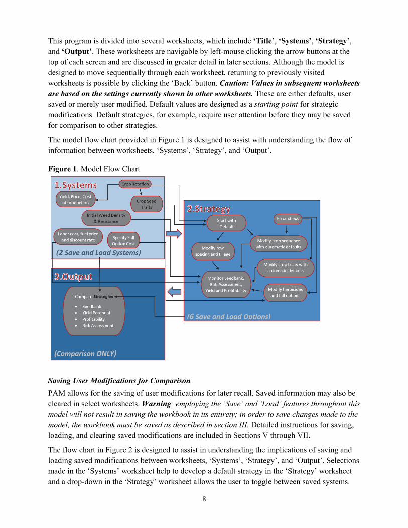
This program is divided into several worksheets, which include ‘Title’, ‘Systems’, ‘Strategy’, and ‘Output’. These worksheets are navigable by left-mouse clicking the arrow buttons at the top of each screen and are discussed in greater detail in later sections. Although the model is designed to move sequentially through each worksheet, returning to previously visited worksheets is possible by clicking the ‘Back’ button. Caution: Values in subsequent worksheets are based on the settings currently shown in other worksheets. These are either defaults, user saved or merely user modified. Default values are designed as a starting point for strategic modifications. Default strategies, for example, require user attention before they may be saved for comparison to other strategies.

The model flow chart provided in Figure 1 is designed to assist with understanding the flow of information between worksheets, ‘Systems’, ‘Strategy’, and ‘Output’.

Figure 1. Model Flow Chart 

 

Saving User Modifications for Comparison

PAM allows for the saving of user modifications for later recall. Saved information may also be cleared in select worksheets. Warning: employing the ‘Save’ and ‘Load’ features throughout this model will not result in saving the workbook in its entirety; in order to save changes made to the model, the workbook must be saved as described in section III. Detailed instructions for saving, loading, and clearing saved modifications are included in Sections V through VII.

The flow chart in Figure 2 is designed to assist in understanding the implications of saving and loading saved modifications between worksheets, ‘Systems’, ‘Strategy’, and ‘Output’. Selections made in the ‘Systems’ worksheet help to develop a default strategy in the ‘Strategy’ worksheet and a drop-down in the ‘Strategy’ worksheet allows the user to toggle between saved systems.

9

 

Note: System changes that are saved after strategies have been saved are automatically applied to those saved strategies.

Figure 2. Save and Load Flow Chart  

 

III. Installation and General Use Instructions

Installation

This software was developed as a macro-enabled workbook in a 2010 – 2016 compatible file format of Excel® using a Windows 7 working environment. Its file extension is ‘.xlsm’ and the name of the file is ‘PAM.xlsm’.

The file may be saved to any directory or file folder by right-clicking the file name and using the ‘Save As’ option; however, a flash drive should not be used for this directory. This practice may lead to many problems, including slow read/write speeds as well as loss of data if the flash drive becomes damaged, corrupted, or fails to integrate when files are backed-up to the computer’s hard drive. In addition, if this file is received via email, please first save the file to the computer instead of opening the file directly from the email. This will ensure ease of access to the file at a later time. The user is strongly encouraged to close other Excel® files before using PAM as Excel® defaults are modified and will be restored when PAM is closed properly.

Several warning messages may appear when opening the file (Figure 3). These messages will differ depending on the version of Excel®, operating system, and the user’s security settings. Please complete the following screen instructions in Excel® to set the appropriate security settings to enable macros:

10

 

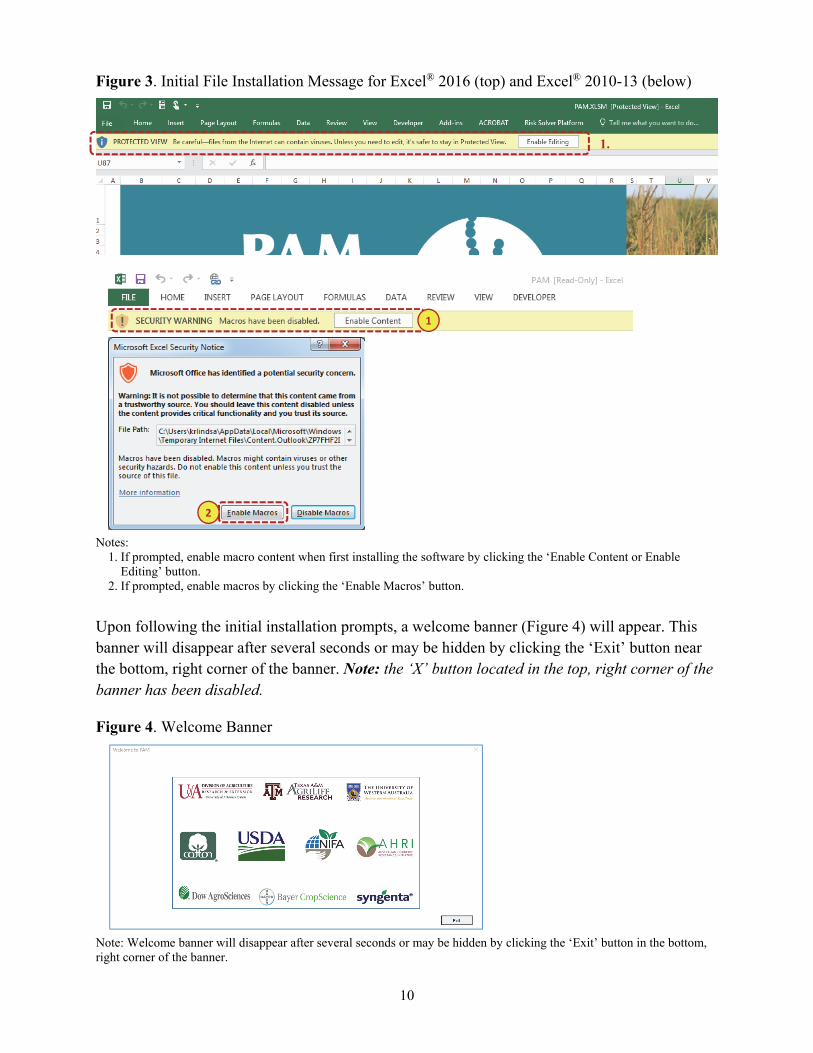
Figure 3. Initial File Installation Message for Excel® 2016 (top) and Excel® 2010-13 (below)

 

Notes:

1. If prompted, enable macro content when first installing the software by clicking the ‘Enable Content or Enable Editing’ button.

2. If prompted, enable macros by clicking the ‘Enable Macros’ button.

Upon following the initial installation prompts, a welcome banner (Figure 4) will appear. This banner will disappear after several seconds or may be hidden by clicking the ‘Exit’ button near the bottom, right corner of the banner. Note: the ‘X’ button located in the top, right corner of the banner has been disabled.

Figure 4. Welcome Banner

  Note: Welcome banner will disappear after several seconds or may be hidden by clicking the ‘Exit’ button in the bottom, right corner of the banner.

1.

1

2 

11

 

Saving and Exiting Files

PAM is an Excel® program compatible with Excel® 2010 – 2016 with a ‘.xlsm’ file extension. PAM works in full screen mode, therefore, the user will be prompted to either save the file and exit, exit the file without changes, or cancel exiting to return to PAM. This process is initiated by clicking on the ‘X’ near the top right to exit the program and save. The flow chart provided in Figure 5 is designed to assist in understanding the implications of selecting ‘Yes’ to exit PAM and save changes, ‘No’ to exit PAM without saving changes, or ‘Cancel’ if the user has changed their mind and does not wish to exit PAM.

Figure 5. PAM Exit Flow Chart

This process also restores Excel® default features that were disabled to allow the full screen mode to work properly. Again, it is advisable to run PAM without other spreadsheets open in Excel® at the same time for that reason. Note further that, if PAM should close improperly, reloading and exiting PAM normally will restore Excel® default program features.

Several versions of PAM may be maintained on the user’s computer or device by renaming alternate versions of the file after having closed Excel®. Please use only one version at a time. The user may always revert to the original file by downloading it online, if needed.

Navigating Worksheets

To simplify the use of the software, PAM is divided into different worksheets that may be accessed by clicking the blue ‘Back’ or ‘Next’ arrow buttons located at the top of each screen. Note: this user manual and its accompanying spreadsheet use the terms ‘screen’, ‘worksheet, and ‘sheet’ interchangeably.

12

 

Tutorials

The user may access tutorial userforms at any time by clicking the help button, , located in the top, right corner of each worksheet. Where applicable, the user may click the ‘Next’ button to view additional tutorials relevant to the currently opened worksheet. Note: the ‘X’ button, located in the top, right corner of the userform has been disabled. The user may exit the tutorial at any time by clicking the ‘Exit’ button located in the bottom, right corner of each tutorial userform.

Controls

PAM contains many different working parts on each worksheet known as ‘controls’. These controls include command buttons, drop-down lists, check boxes, comment boxes, conditional formatting, and userforms that are briefly discussed below:

Command Buttons

Command buttons, also referred to as ‘buttons’, contain macros that allow the user to access userforms, navigate across worksheets, load default values, compare strategies, or save and load saved information across worksheets. These buttons provide easy access to different screens and an easy way to revert to program defaults. Warning: macro commands cannot be reversed using the ‘Undo’ feature in Excel that may be activated by pressing the <CTRL> and <Z> buttons simultaneously to return to a condition before the command button was clicked. For this reason, the user may be prompted to continue when clicking on a command button. Clicking the ‘Cancel’ button allows the user to stop and consider implications of moving forward before permanently altering the spreadsheet.

Drop-down Lists

Drop-down lists are located throughout the program and may be accessed by clicking on the cell. After clicking the cell, a downward pointing arrow will appear to the right of the cell. Clicking on this arrow will display the options contained in the drop-down list. Select a desired option by scrolling up or down the list using the mouse cursor and clicking on the desired option. Once the desired option is selected, the selection will appear in the cell.

Comment Boxes

Comment boxes may be accessed by moving the cursor over the small red triangles located in the top, right corner of a cell containing a comment. These comment boxes contain information to better explain contents of a cell, or range of cells, and aids in the selection of data entered by the user. They do not affect the operation of the spreadsheet, but add information for the user.

Conditional Formatting

Conditional formatting (error checking) has been applied to various cells throughout this program to indicate when a change has occurred that may lead to potential errors in the way the program operates. This conditional formatting will change the appearance of those formatted cells when a potential error is made and will return to its original state when the

13

 

necessary corrections are made. In some cases, the color or font a cell changes to show a deviation from default values (e.g. modifications in the ‘Systems’ worksheet). While formatting within the ‘Systems’ worksheet highlights the changes to default values, it does not affect the performance of the software. Highlights in the ‘Strategy’ worksheets, however, typically require corrective action.

Copy and Paste Restriction

The copy and paste feature has been disabled in the program and will be restored when the user properly exits the program. Should the user have been able to bypass the disabling of the copy and paste feature, the program’s integrity cannot be ensured and the user is therefore advised to revert to a previously saved copy of the program.

Userforms

Userforms may be accessed by clicking on command buttons throughout the spreadsheet program. These userforms allow the user to make specifications based on user-specifiable production parameters. Figure 6 is an example of the ‘Calculate Total Specified Expenses’ userform in the ‘Systems’ worksheet. Section V provides greater detail on properly entering data in userforms in the ‘Systems’ worksheet.

Note: after selecting the desired options within each userform, the user must click the ‘Save’ button in the lower right corner of the userform to save the desired changes to the workbook. Note: the ‘X’ button, located in the top, right corner of the userform has been disabled. Exit the userform at any time by clicking either the ‘Exit’ or ‘Cancel’ button located in the bottom, right corner of each userform. Warning: clicking ‘Save’ in the userform will not result in saving the workbook in its entirety; in order to save changes made to the model, the workbook must be saved as described in section III. Warning: changes made in a userform, like command button macros, cannot be reversed using the ‘Undo’ feature in Excel® that may be activated by pressing the <CTRL> and <Z> buttons simultaneously.

Text Boxes

Userforms contain text boxes to allow users to specify various inputs using textboxes. Text Boxes allow the user to input customized data into the userform by typing the data directly into the text box provided. This data may be entered in alphanumeric format, similar to entering data into an active cell within a worksheet.

IV. Title

The first worksheet that appears upon initial install of PAM is the ‘Title’ worksheet shown in Figure 6. This sheet provides a brief introduction to PAM as well as credits and additional information, which may be accessed by clicking the blue ‘Credits’ or ‘Info’ buttons located in the green column to the right of the ‘Title’ worksheet. Additionally, a series of introductory tutorials are available by clicking the ‘?’ button (Figure 6 (3)). Navigate to the next worksheet by clicking on the blue ‘START’ button (Figure 6 (4)).

14

 

Figure 6. ‘Title’ Worksheet

 

Notes: 1. Click the ‘Info’ button to view information on what PAM is, contact and copyright information and a disclaimer. 2. Click the ‘Credits’ button to view PAM’s credits and acknowledgements banner. 3. Click the ‘?’ button for help. 4. Click the ‘START’ button to begin making modifications to the ‘Systems’ worksheet. 5. Click the green envelope to send questions or feedback to developers. 6. Click the ‘Back’ arrow button to return to the ‘Title’ worksheet.

1

2

3

4

5

6

15

 

V. ‘Systems’ Worksheet

The ‘Systems’ worksheet in Figure 7, allows for the customization of the model’s default parameters based on current production practices.

Figure 7. ‘Systems’ Worksheet

Notes: 1. The current ‘System’ actively displayed is shown in blue text on the top, right corner of the worksheet. Conditional

formatting indicates the system displayed is NOT a saved system when the font changes from blue to red, italicized font. Once the changes are saved as one of the two saved systems or a previously saved system is loaded, the font will return to blue. See Figures 12 and 13 for further information.

2. Enter the name of the operation or operator. 3. Select the typical duration of crops in rotation using the drop-down list provided. Choosing a 1-year rotation will

remove the year 2- and year 3-options. This may be reversed by choosing a 2- or 3-year rotation then re-entering crop choices and recalculating total specified expenses.

4. a. Select a typical crop for each year in rotation. b. Enter the expected yield for each crop in the rotation or use the default provided. c. Enter the expected price received for each crop in the rotation or use the default provided. d. Calculate the total specified expenses for each crop using the userforms provided by clicking the gray buttons

located below each respective year titled ‘Calculate Total Specified Expenses’ (See Figure 10). 5. Select up to four crop traits for each crop in the rotation. This information is used to create default parameters in the

‘Strategy’ worksheet that is accessed by pressing the ‘Next’ button (See note 11). Each row represents a year for the crop in the rotation.

6. Specify prices and rates for fall options using the userform provided by clicking on the gray button titled ‘Specify Fall Options’ (See Figure 11).

7. Enter other expenses associated with herbicide applications such as labor, fuel, and the amortization rate. 8. Select weed density per 250 square feet. 9. Enter expected resistance levels for Roundup, ALS Chemistry, and PPO applications. 10. Save and load up to two systems by clicking the blue ‘Save’ or ‘Load’ buttons. See Figures 12 and 13 for

instructions on saving and loading systems. 11. Navigate back to the ‘Title’ sheet by clicking the ‘Back’ arrow or navigate forward to the ‘Strategy’ worksheet by

clicking the ‘Next’ arrow. 12. Click the ‘Print’ button to print the area currently displayed on the screen or the ‘?’ button for help.

 

12

3

4 

5  6

7  8 9

10

11 

12

16

 

Calculate Total Specified Expenses Userforms

The ‘Calculate Total Specified Expenses’ (TSE) userforms (Figure 8) allow for the specification of acre-based input and yield-specific harvest expenses as well as operating interest for each crop. Default values are based on recommendations provided by University of Arkansas Cooperative Extension Service publications (Watkins et al., 2017). Note: the calculated TSE calculated do not include weed control and seed costs at expected yield. Note that weed control costs include cost of fall options and extra charges for narrow row planting and shallow tillage. If a crop or the expected yield is changed, the TSE amount will be automatically updated with default values.

Figure 8. ‘Calculate Total Specified Expenses’ Userform

Notes: 1. Enter expected costs for production inputs in dollar ($) per acre or click the ‘Use Default Values’ button to

restore default values. Returns to wheat or other double crop are only available to enter for double cropped soybean (Soybean_Double).

2. Enter the operating interest rate for 50% of the operating expenses listed above. The interest rate entered should be the annual interest rate as the program adjusts interest costs for the period needed. Fifty percent (50%) of operating expenses are used because timing of expenses are not all at the start of using an operating credit line.

3. Enter expected yield-specific harvest costs incurred at time of harvest. For cotton crops, harvest expenses are covered by cottonseed revenue and hence not shown.

4. Click the ‘Calculate Costs’ button to calculate the total specified production expenses given user-specifications provided within the userform. The TSE shown will be automatically updated as any subsequent changes are made within the userform.

5. Click ‘Save’ to exit the userform and apply the changes or ‘Cancel’ to exit the userform without applying changes to the model.

 

 

 

  

1

2

3 

4 

5

17

 

Specify Fall Options Userform

The ‘Specify Fall Options’ userform (Figure 9) allows for the specification of cost and quantity for fall field practices such as moldboard plough, cereal rye and cover crop mix, and windrow burn. Broadcast or drill seed planting methods for fall cover crops may also be specified. Default values are based on recommendations provided by expert opinion.

Figure 9. ‘Specify Fall Options’ Userform

Notes: 1. Select the default custom rate for the moldboard plough fall option or customize the cost of moldboard

plough. Enter the user-specified cost in dollars ($) per acre in the textbox provided. Because the custom rate for moldboard plough includes fixed equipment costs, a good estimate for fuel, labor, repair and maintenance only would be roughly $7/acre in case the farm has their own moldboard plough.

2. Select the default quantity and cost for the ‘Cereal Rye Cover Crop’ fall option or customize the quantity and cost. Enter the user-specified seed quantity in pounds (lbs) per acre and cost in dollars ($) per pound of seed in the textboxes provided.

3. Select planting method, ‘Broadcast’ or ‘Drill Seed’, for the ‘Cereal Rye Cover Crop’ fall option. 4. Select the default quantity and cost for the ‘Cover Crop Mix’ fall option or customize the quantity and cost.

Enter the user-specified seed quantity in pounds (lbs) per acre and cost in dollars ($) per pound of seed. 5. Select planting method, ‘Broadcast’ or ‘Drill Seed’, for the ‘Cover Crop Mix’ fall option. 6. Select the default cost of fall windrow burn or customize the cost of windrow burn in dollars ($) per acre. 7. Click ‘Save’ to exit the userform and apply the changes made within the userform or click ‘Cancel’ to exit the

userform without applying changes. 8. Click the ‘Use Default Values’ button to restore program defaults.

Up to two default systems may be saved by clicking the blue ‘Save’ or ‘Load’ buttons located to the right of each saved system name. Be aware that default values are designed to be a starting point for strategic modifications and do not limit selections in subsequent worksheets. In addition to serving as default parameters from which to build strategies for comparison, information from saved systems will be associated with saved strategies (See also section VI). Note: Once a strategy has been saved, any subsequent changes made to the saved system associated with that

1 

2 

3 

4 

5 

6 

7

8

18

 

strategy will be automatically updated to that strategy. Use caution when returning to and/or editing previously saved systems after saving strategies.

Follow the steps provided in the notes for Figures 10 and 11 to save or load systems.

Figure 10. Saving Systems

   

 

 

 

 

   Notes: 1. Click the blue ‘Save’ button to the right of a saved system name to save the system that is currently displayed in the

‘Systems’ worksheet. 2. Upon clicking the ‘Save’ button, a message box will appear asking if it is okay to overwrite any previously saved

data. Follow steps 3 through 5 if ‘Yes’ or skip to step 6 if ‘No’. 3. If ‘Yes’ was selected in step 2, enter a name for the saved system by typing the desired alpha-numeric name into

the text box provided, or do nothing to keep the previously saved system name (highlighted in blue). Click the ‘OK’ button to continue.

4. Upon clicking the ‘OK’ button, another message box will appear stating the current system information has been saved and may be reloaded using the ‘Load’ button. Click the ‘OK’ button to continue.

5. The name of the saved system is now displayed next to the ‘Save’ and ‘Load’ buttons. 6. If ‘No’ was selected in step 2, a message box will appear stating the previously saved system has not been changed.

Click ‘OK’ to continue.

1 

2 

3 

4 

5 

6 

19

 

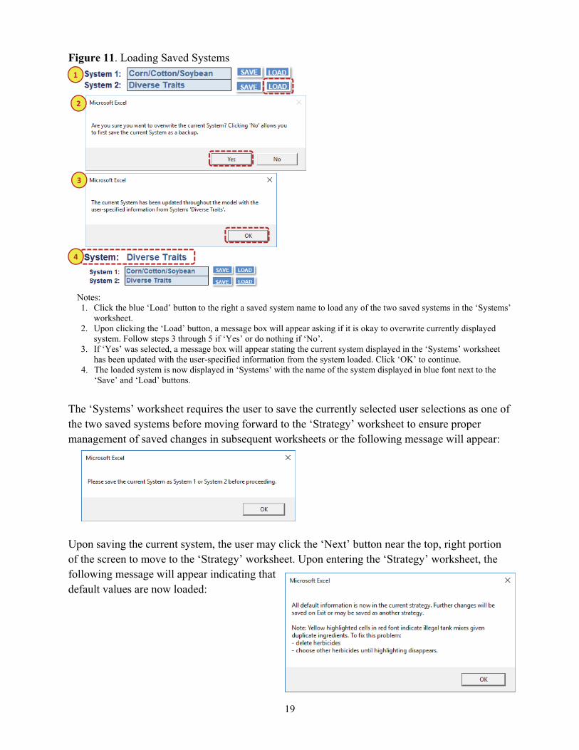
Figure 11. Loading Saved Systems

   

 

 Notes: 1. Click the blue ‘Load’ button to the right a saved system name to load any of the two saved systems in the ‘Systems’

worksheet. 2. Upon clicking the ‘Load’ button, a message box will appear asking if it is okay to overwrite currently displayed

system. Follow steps 3 through 5 if ‘Yes’ or do nothing if ‘No’. 3. If ‘Yes’ was selected, a message box will appear stating the current system displayed in the ‘Systems’ worksheet

has been updated with the user-specified information from the system loaded. Click ‘OK’ to continue. 4. The loaded system is now displayed in ‘Systems’ with the name of the system displayed in blue font next to the

‘Save’ and ‘Load’ buttons.

The ‘Systems’ worksheet requires the user to save the currently selected user selections as one of the two saved systems before moving forward to the ‘Strategy’ worksheet to ensure proper management of saved changes in subsequent worksheets or the following message will appear:

Upon saving the current system, the user may click the ‘Next’ button near the top, right portion of the screen to move to the ‘Strategy’ worksheet. Upon entering the ‘Strategy’ worksheet, the following message will appear indicating that default values are now loaded:

1 

2 

3 

4 

20

 

VI. ‘Strategy’ Worksheet

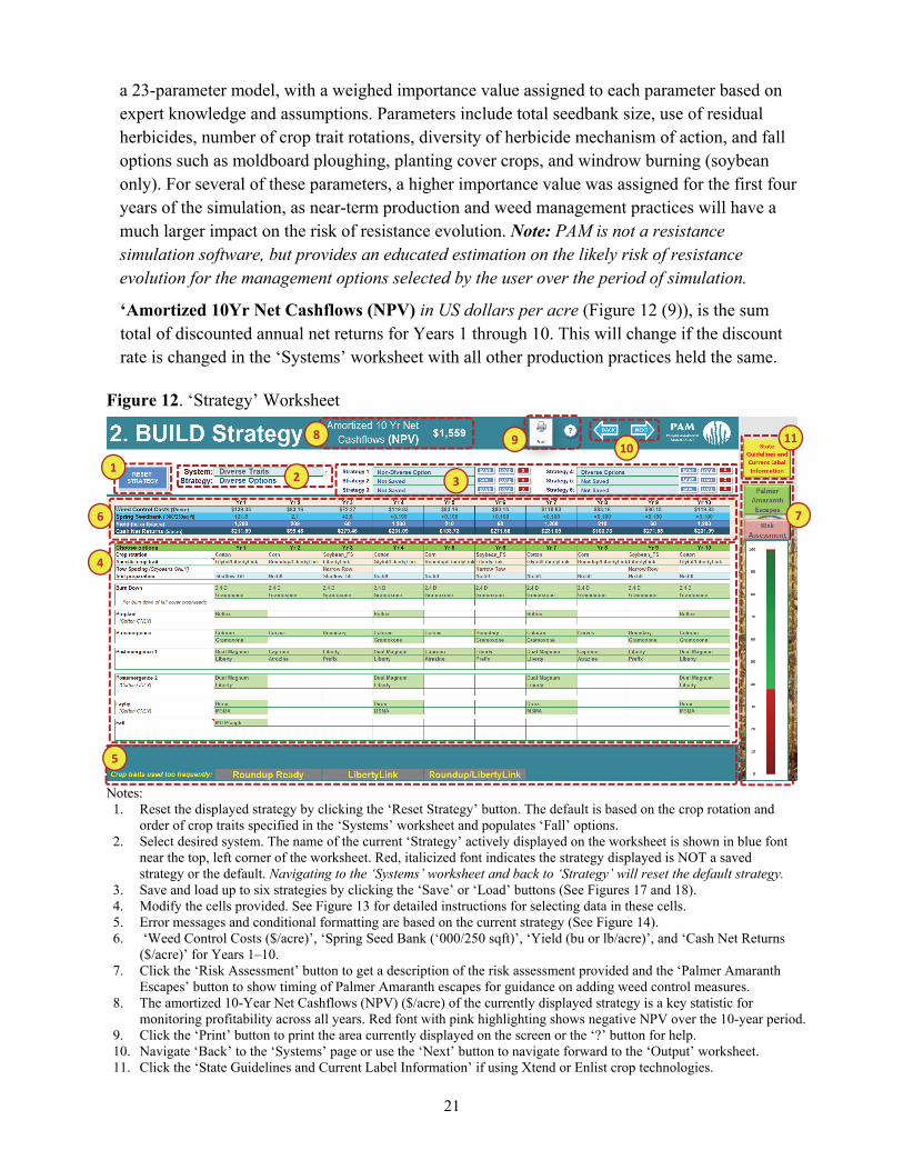
The ‘Strategy’ worksheet, shown in Figure 12, allows the user to load the default strategy based on the user specifications entered in the ‘Systems’ worksheets or customize and save up to six strategies for comparison in the ‘Output’ worksheet discussed in section VII. A key point to remember is that the ‘Reset Strategy’ button will not necessarily result in a good strategy recommendation that requires no attention from the user. Below is a list of values to observe when modifying strategies.

‘Weed Control Costs’ in US dollars per acre (Figure 12 (6)), are estimated as the sum of costs incurred towards herbicides as well as fall weed management options. Weed control costs are based on prices provided by University of Arkansas Cooperative Extension Service publications (Scott et al., 2018). Equipment costs needed for application cover labor, fuel, repair and maintenance, and chemical applied. These costs do not reflect ownership charges for equipment and hence are lower than custom applied costs.

‘Spring Seedbank’ in 000’ per 250 square feet (Figure 12 (6)), is the amount of total Palmer amaranth seed present in the soil seedbank in spring immediately prior to the beginning of seedling emergence. The ‘Spring Seedbank’ is estimated based on the number of Palmer amaranth escapes observed in a 250 square feet area during previous year, after accounting for potential seed losses between fall and spring. Values ‘<0.100’ indicates that seedbank levels are depleted to <100 seed/250 square feet. Parameter values for seedbank dynamics and seedling emergence were obtained from published literature shown in the References section. Note: Values reported for ‘Spring Seedbank’ DO NOT equate to the number of emerged seedlings that spring. This is because seedling emergence is only a fraction of the amount of seed present in the soil. PAM accounts for the fact that Palmer amaranth seedlings emerge in a number of flushes (i.e. cohorts) over a prolonged period.

‘Yield’ per acre (Figure 12 (6)) is a product of expected yield specified by the user in the ‘Systems’ worksheet and the % yield reduction calculated as a function of Palmer amaranth density. Additional functions were included to calculate the impact of the timing of weed emergence relative to the crop and intra-specific weed density on crop yield. Expected yields are based on yields provided by University of Arkansas Cooperative Extension Service publications (Watkins et al., 2018).

‘Net Returns’ in US dollars per acre (Figure 12 (6)) are estimated as the yield times the expected price, less total specified operating expenses as well as weed control costs that vary with changes to options in the ‘Strategy’ worksheet. Note that ownership charges for equipment are not included as the user would consider those as sunk costs and not changing as a result of weed management practices. Cash rent for land use can be modified in the total specified expenses, however. Hence returns are to management, equipment, and owned land resources as operator and hired labor are accounted for.

The ‘Resistance Risk’ calculator (Figure 12 (8)) illustrates the overall risk of resistance for the combination of management options selected. However, it does not predict resistance for any specific herbicide chemistry. The risk of resistance evolution is estimated as a percentage using

21

 

a 23-parameter model, with a weighed importance value assigned to each parameter based on expert knowledge and assumptions. Parameters include total seedbank size, use of residual herbicides, number of crop trait rotations, diversity of herbicide mechanism of action, and fall options such as moldboard ploughing, planting cover crops, and windrow burning (soybean only). For several of these parameters, a higher importance value was assigned for the first four years of the simulation, as near-term production and weed management practices will have a much larger impact on the risk of resistance evolution. Note: PAM is not a resistance simulation software, but provides an educated estimation on the likely risk of resistance evolution for the management options selected by the user over the period of simulation.

‘Amortized 10Yr Net Cashflows (NPV) in US dollars per acre (Figure 12 (9)), is the sum total of discounted annual net returns for Years 1 through 10. This will change if the discount rate is changed in the ‘Systems’ worksheet with all other production practices held the same.

Figure 12. ‘Strategy’ Worksheet

Notes: 1. Reset the displayed strategy by clicking the ‘Reset Strategy’ button. The default is based on the crop rotation and

order of crop traits specified in the ‘Systems’ worksheet and populates ‘Fall’ options. 2. Select desired system. The name of the current ‘Strategy’ actively displayed on the worksheet is shown in blue font

near the top, left corner of the worksheet. Red, italicized font indicates the strategy displayed is NOT a saved strategy or the default. Navigating to the ‘Systems’ worksheet and back to ‘Strategy’ will reset the default strategy.

3. Save and load up to six strategies by clicking the ‘Save’ or ‘Load’ buttons (See Figures 17 and 18). 4. Modify the cells provided. See Figure 13 for detailed instructions for selecting data in these cells. 5. Error messages and conditional formatting are based on the current strategy (See Figure 14). 6. ‘Weed Control Costs ($/acre)’, ‘Spring Seed Bank (‘000/250 sqft)’, ‘Yield (bu or lb/acre)’, and ‘Cash Net Returns

($/acre)’ for Years 1–10. 7. Click the ‘Risk Assessment’ button to get a description of the risk assessment provided and the ‘Palmer Amaranth

Escapes’ button to show timing of Palmer Amaranth escapes for guidance on adding weed control measures. 8. The amortized 10-Year Net Cashflows (NPV) ($/acre) of the currently displayed strategy is a key statistic for

monitoring profitability across all years. Red font with pink highlighting shows negative NPV over the 10-year period. 9. Click the ‘Print’ button to print the area currently displayed on the screen or the ‘?’ button for help. 10. Navigate ‘Back’ to the ‘Systems’ page or use the ‘Next’ button to navigate forward to the ‘Output’ worksheet. 11. Click the ‘State Guidelines and Current Label Information’ if using Xtend or Enlist crop technologies.

1 2  3

4 

6 

5 

7

8  910

11

22

 

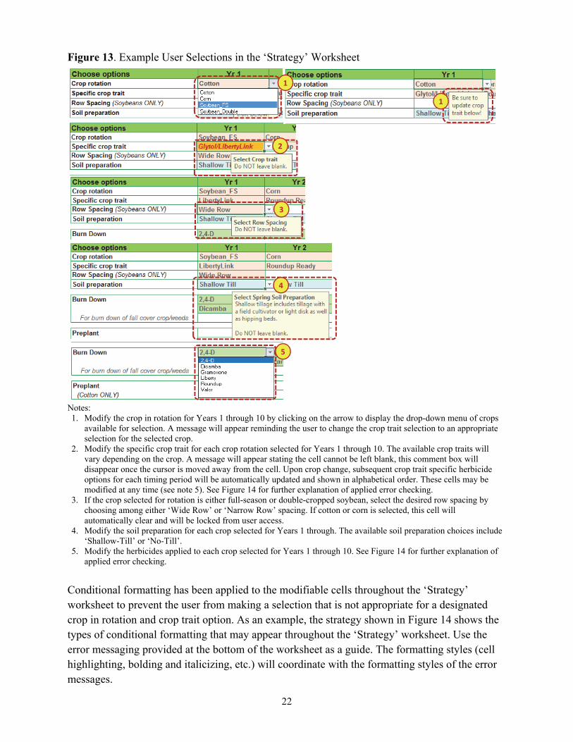
Figure 13. Example User Selections in the ‘Strategy’ Worksheet

Notes: 1. Modify the crop in rotation for Years 1 through 10 by clicking on the arrow to display the drop-down menu of crops

available for selection. A message will appear reminding the user to change the crop trait selection to an appropriate selection for the selected crop.

2. Modify the specific crop trait for each crop rotation selected for Years 1 through 10. The available crop traits will vary depending on the crop. A message will appear stating the cell cannot be left blank, this comment box will disappear once the cursor is moved away from the cell. Upon crop change, subsequent crop trait specific herbicide options for each timing period will be automatically updated and shown in alphabetical order. These cells may be modified at any time (see note 5). See Figure 14 for further explanation of applied error checking.

3. If the crop selected for rotation is either full-season or double-cropped soybean, select the desired row spacing by choosing among either ‘Wide Row’ or ‘Narrow Row’ spacing. If cotton or corn is selected, this cell will automatically clear and will be locked from user access.

4. Modify the soil preparation for each crop selected for Years 1 through. The available soil preparation choices include ‘Shallow-Till’ or ‘No-Till’.

5. Modify the herbicides applied to each crop selected for Years 1 through 10. See Figure 14 for further explanation of applied error checking.

Conditional formatting has been applied to the modifiable cells throughout the ‘Strategy’ worksheet to prevent the user from making a selection that is not appropriate for a designated crop in rotation and crop trait option. As an example, the strategy shown in Figure 14 shows the types of conditional formatting that may appear throughout the ‘Strategy’ worksheet. Use the error messaging provided at the bottom of the worksheet as a guide. The formatting styles (cell highlighting, bolding and italicizing, etc.) will coordinate with the formatting styles of the error messages.

1 

1

2

3

4

5

23

 

Figure 14. Example Conditional Formatting in ‘Strategy’ Worksheet

 

Notes: 1. The messages provided near the bottom of the worksheet coordinate with conditional formatting in the cells above

to indicate potential errors or otherwise flag strategy decisions that may lead to increased risk of resistance or lowered profitability.

2. Italicized, red, bold font with orange highlighting indicates when the crop trait selected is not appropriate for the crop in rotation.

3. Italicized, yellow, bold font with red highlighting indicates the herbicide option is a mismatch with the selected crop trait, which may happen when the user changes crops and does not update the crop trait.

4. Italicized, bold font with light yellow highlighting indicates when two of the herbicide options selected result in improper tank mixes at their full-labeled rates.

5. Italicized, red, bold font with pink highlighting) indicates when the herbicide option selected is duplicated within an application time.

6. If either a crop or a crop trait variety is planted too frequently, the name of the crop or crop trait in question will appear in bright yellow, italicized, bold font with gray highlighting. The Roundup/LibertyLink and LibertyLink warnings appear to show reliance on too few herbicide options. A crop rotation (corn in years four through eight) with too much emphasis on a particular single crop is also flagged here.

1 

2 

3 4

5

6 

2 34 

5

24

 

The user may wish to either maximize economic returns by maximizing NPV or lower the risk of evolution resistance. This risk is graphically represented using red/green meter to the right of the ‘Strategy’ worksheet (Figure 12 (8)) and can be defined by clicking the pink ‘Risk Assessment’ button near the top, right of the worksheet. The ‘Risk Assessment’ shown in Figure 15 is based on the default strategy using the ‘Diverse Traits’ system.

Figure 15. Risk Assessment Definition 

Further, clicking the green ‘Palmer Amaranth Escapes’ button near the top, right of the screen allows the user to see information about timing of critical attention to weed control by year. The ‘Palmer Amaranth Escapes’ screen shown in Figure 16 is also based on the default system using the ‘Diverse Traits’ system.

Figure 16. Year and Within Year Timing of Palmer Amaranth Escapes

25

 

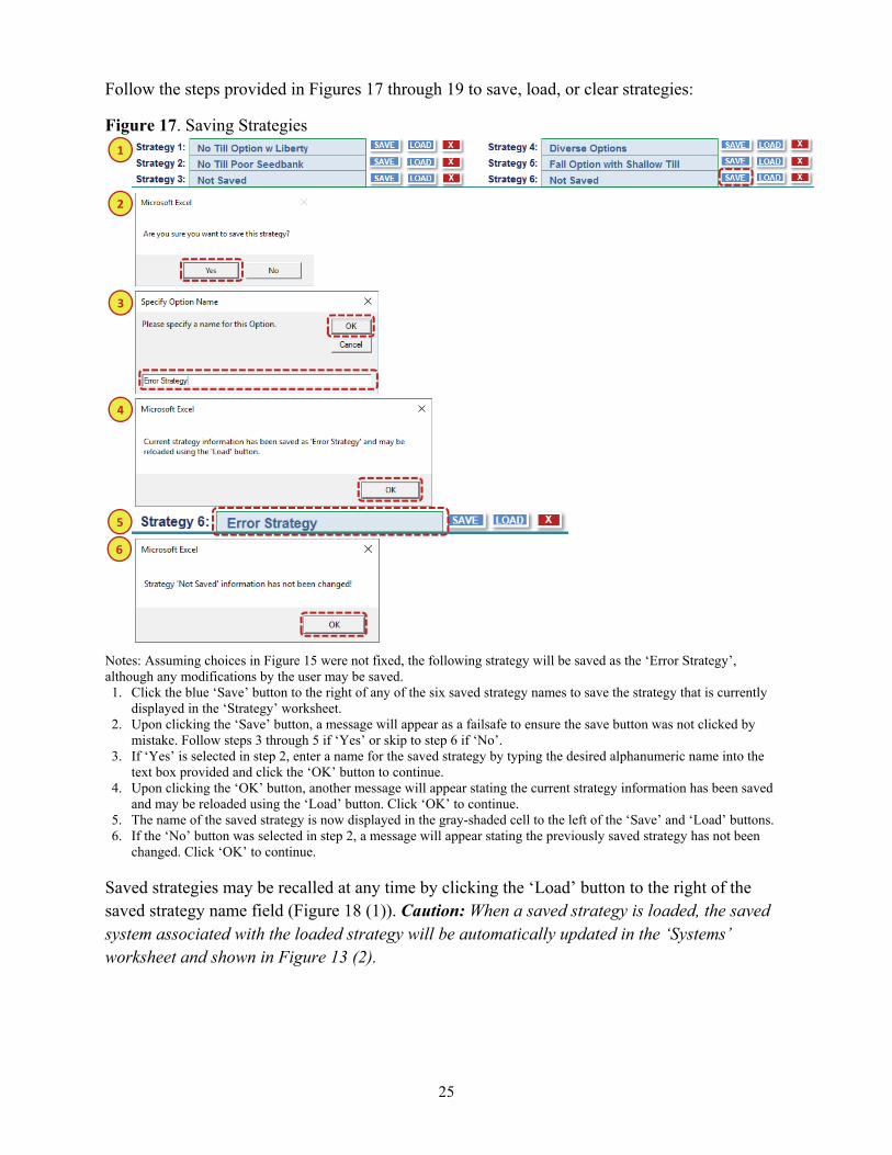
Follow the steps provided in Figures 17 through 19 to save, load, or clear strategies:

Figure 17. Saving Strategies

 

   

   

   

 

   

Notes: Assuming choices in Figure 15 were not fixed, the following strategy will be saved as the ‘Error Strategy’, although any modifications by the user may be saved. 1. Click the blue ‘Save’ button to the right of any of the six saved strategy names to save the strategy that is currently

displayed in the ‘Strategy’ worksheet. 2. Upon clicking the ‘Save’ button, a message will appear as a failsafe to ensure the save button was not clicked by

mistake. Follow steps 3 through 5 if ‘Yes’ or skip to step 6 if ‘No’. 3. If ‘Yes’ is selected in step 2, enter a name for the saved strategy by typing the desired alphanumeric name into the

text box provided and click the ‘OK’ button to continue. 4. Upon clicking the ‘OK’ button, another message will appear stating the current strategy information has been saved

and may be reloaded using the ‘Load’ button. Click ‘OK’ to continue. 5. The name of the saved strategy is now displayed in the gray-shaded cell to the left of the ‘Save’ and ‘Load’ buttons. 6. If the ‘No’ button was selected in step 2, a message will appear stating the previously saved strategy has not been

changed. Click ‘OK’ to continue.

Saved strategies may be recalled at any time by clicking the ‘Load’ button to the right of the saved strategy name field (Figure 18 (1)). Caution: When a saved strategy is loaded, the saved system associated with the loaded strategy will be automatically updated in the ‘Systems’ worksheet and shown in Figure 13 (2).

1 

2 

3 

4 

5 

6 

26

 

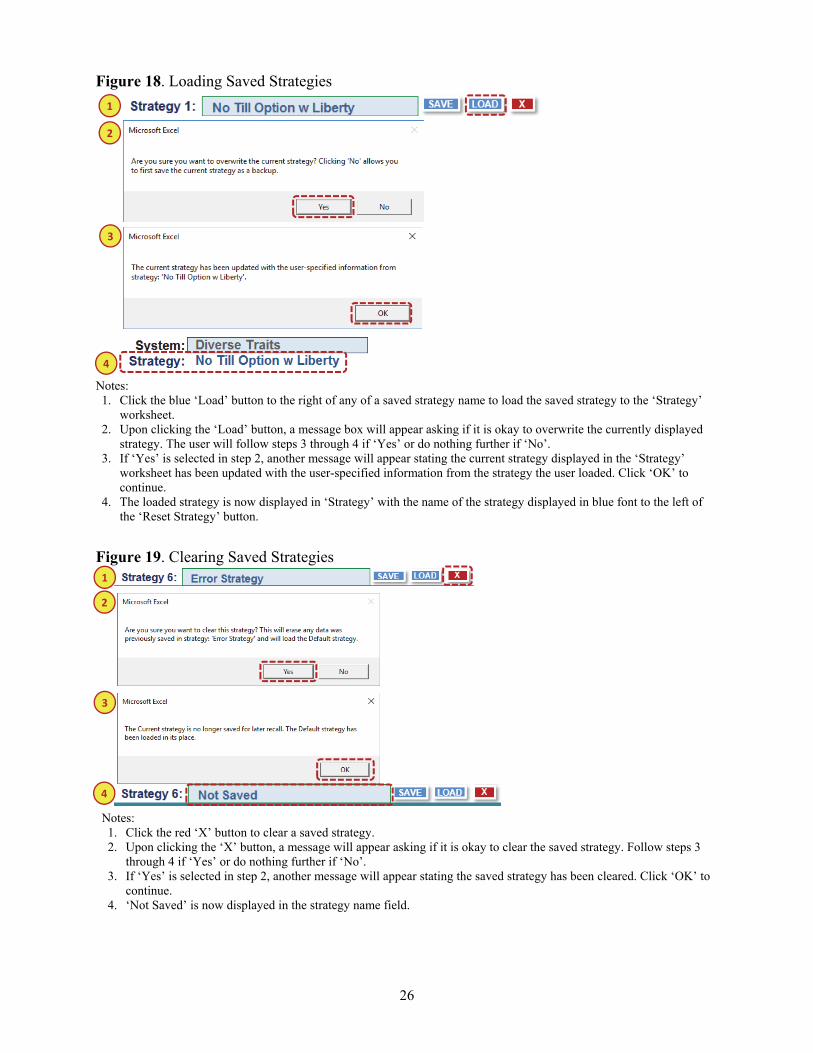
Figure 18. Loading Saved Strategies

 

   

   

 

Notes: 1. Click the blue ‘Load’ button to the right of any of a saved strategy name to load the saved strategy to the ‘Strategy’

worksheet. 2. Upon clicking the ‘Load’ button, a message box will appear asking if it is okay to overwrite the currently displayed

strategy. The user will follow steps 3 through 4 if ‘Yes’ or do nothing further if ‘No’. 3. If ‘Yes’ is selected in step 2, another message will appear stating the current strategy displayed in the ‘Strategy’

worksheet has been updated with the user-specified information from the strategy the user loaded. Click ‘OK’ to continue.

4. The loaded strategy is now displayed in ‘Strategy’ with the name of the strategy displayed in blue font to the left of the ‘Reset Strategy’ button.

Figure 19. Clearing Saved Strategies

 

 

Notes: 1. Click the red ‘X’ button to clear a saved strategy. 2. Upon clicking the ‘X’ button, a message will appear asking if it is okay to clear the saved strategy. Follow steps 3

through 4 if ‘Yes’ or do nothing further if ‘No’. 3. If ‘Yes’ is selected in step 2, another message will appear stating the saved strategy has been cleared. Click ‘OK’ to

continue. 4. ‘Not Saved’ is now displayed in the strategy name field.

 

1 

2 

3 

4 

1 

2 

3 

4 

27

 

The ‘Strategy’ worksheet does not require the user to save the currently selected user options as one of six strategies before moving forward to the ‘Output’ worksheet. This is to allow comparisons in the ‘Output’ page of the current settings in the ‘Strategy’ page even if it has not been saved. The message box to the right appears when clicking on ‘Next’ near the top, right of the ‘Strategy’ page. Clicking ‘Cancel’ returns the user to the ‘Strategy’ page so changes may be saved.

VII. ‘Output’ Worksheet

The ‘Output’ worksheet, shown in Figure 20, allows the user to compare two of the six strategies saved in the ‘Strategy’ worksheet. Specifically, the ‘Output’ worksheet allows for a 10 year comparison of ‘Seedbank’ (in 000’s of palmer amaranth seeds per 250 square feet), annual yield potential, and annual ‘Net Returns’ (in dollars ($) per acre) as well as the net present value (NPV) and the risk of developing herbicide resistance for each of the two strategies selected for comparison.

Figure 20. ‘Output’ Worksheet

Notes: 1. Select two strategies for comparison. Conditional formatting highlights strategies using different ‘Systems’. Pink

highlighting with red, italicized font (not shown) appears when the same strategy is compared. 2. A 10-year comparison of the seedbank (000’s seeds/250 sqft) is shown for each of the two strategies selection. 3. A 10-year comparison of the yield potential as a percent of the default yield is shown for each of the two strategies

selected. 4. A 10-year comparison of the cash net returns (dollars $/acre) is shown for each of the two strategies selected. Returns

are to equipment, owned land resources, and management as equipment ownership charges and land charges are not included.

5. The resistance risk is shown for each of the two strategies selected. Click the ‘Risk Assessment’ button for more information.

6. The amortized 10-year net cashflows (NPV) ($/acre) is shown for each of the two strategies selected to provide a comparison of relative profitability across strategies.

7. Click the ‘Print’ button to print the area currently displayed on the screen. 8. Click the ‘?’ button for help. 9. Navigate back to the ‘Strategy’ worksheet by clicking the ‘Back’ arrow.

1 

2 4

5 

6

7 8 9 

3 

28

 

VIII. Conclusion

The PAM model is intended for use as an educational tool by extension agents, crop consultants, producers, and any personnel interested in understanding the benefits of integrated weed management. Various parameters may be customized to represent individual production circumstances and build a number of integrated (chemical and non-chemical) strategies for making comparisons.

Assumptions and Limitations

The PAM software is not a forecast model and is only intended to illustrate long-term biological and economic trends associated with certain management choices. Further, PAM is not an herbicide resistance simulation model, but it adequately accounts for any pre-existing resistance and the likelihood for developing resistance under any chosen strategy. PAM is a deterministic model and any year-to-year and field to-field variations in parameter values are not accounted for. The model is only expected to provide an average response for a given strategy. The model assumes a single farm that is already equipped with basic equipment; therefore, fixed costs, including capital costs are not included in the calculations.

The PAM software does not automatically recommend a management program, but the goal of this tool is to facilitate the users understanding of the benefits of IPM approach based on trial and error. The PAM model is expected to be a powerful educational tool for teaching the value of sound IPM strategies in managing Palmer amaranth, by illustrating generalized long-term trends in biology and economics. The software is only intended to be a demonstration-based, decision-support tool that highlights general trends.

29

 

References

Ferrell, J. and R. Leon. 2013. “Control of Palmer Amaranth in Agronomic Crops”. University of Florida, Institute of Food and Agricultural Services Extension. Accessed January 2016. http://edis.ifas.ufl.edu/pdffiles/AG/AG34800.pdf.

Heap I. 2016. “The International Survey of Herbicide Resistant Weeds”. Accessed September 2016. http://www.weedscience.org.

Jha, P. 2008. “Biology and ecology of Palmer amaranth (Amaranthus palmeri) and tall morningglory (Ipomoea purpurea)”. PhD Thesis, Clemson University, USA.

Jhala, A. J., L. D. Sandell, N. Rana, G. R. Kruger, and S. Z. Knezevic. 2014. “Confirmation and Control of Triazine and 4-Hydroxyphenylpyruvate Dioxygenase-Inhibiting Herbicide Resistant Palmer Amaranth (Amaranthus palmeri) in Nebraska”. Weed Technology, 28(1):28-38. DOI: http://dx.doi.org/10.1614/WT-D-13-00090.1.

Legleiter, T., and B. Johnson, 2013. “Palmer Amaranth Biology, Identification, and Management”. Purdue University, Purdue Extension. Accessed January 2016. https://www.extension.purdue.edu/extmedia/WS/WS-51-W.pdf.

Riar, D. S., J. K. Norsworthy, L. E. Steckel, D. O. Stephenson, and J. A. Bond. 2013. “Consultant Perspectives on Weed Management Needs in Midsouthern United States Cotton: a Follow-Up Survey”. Weed Technology, 27(4):778-787. DOI: http://dx.doi.org/10.1614/WT-D-13-00070.1.

Rios, S.I., S.D. Wright, A. Shrestha. 2014. “Evaluating for Palmer amaranth (Amaranthus palmeri) resistance in herbicide tolerant cropping systems in the San Joaquin Valley. In proceedings of the Beltwide Cotton Conference, New Orleans, LA.

Robinson, L.J. and P.J. Barry. 1996. “Present Value Models and Investment Analysis: the Academic Page”. Northport, AL.

Scott, R. C., L. T. Barber, J. W. Boyd, G. Selden, J. K. Norsworthy, and N. Burgos. 2018. “Recommended Chemicals for Weed and Brush Control.” Vers. MP-44. University of Arkansas Cooperative Extension Service, Division of Agriculture. Accessed February 2018. https://www.uaex.edu/publications/pdf/mp44/mp44.pdf.

Smith, J.T. 2012. “Pigweed resistance spreading in Texas”. Accessed December 2016. http://magissues.farmprogress.com/TFS/FS04Apr12/tfs008.pdf.

Sprague, C. 2012. “Glyphosate-resistant Palmer amaranth in Michigan: confirmation and management options”. Accessed December 2016. http://www.msuweeds.com/assest/ExtensionPubs/Palmer-Clyphosate-Confirmation-Feb12.pdf.

30

 

Sprague, C. 2013. “Palmer Amaranth Management in Soybeans”. United Soybean Board. Accessed January 2016. http://takeactiononweeds.com/wp-content/uploads/2014/01/palmer-amaranth-management-in-soybeans.pdf.

Van Wychen, L. 2016. “2015 Survey of the Most Common and Troublesome Weeds in the United States and Canada”. Weed Science Society of America National Weed Survey Dataset. Accessed September 2016. http://wssa.net/wp-content/uploads/2015-Weed-Survey_FINAL1.xlsx.

Watkins, B., R. Baker, T. Barber, C. Elkins, T. Faske, M. Hamilton, J. Hardke, K. Lawson, G. Lorenz, R. Mazzanti, C. Norton, B. Robertson, N. Seiter, and G. Studebaker. 2017. “2018 Crop.” University of Arkansas Cooperative Extension Service, Division of Agriculture. Accessed February 2018. https://www.uaex.edu/farm-ranch/economics-marketing/farm-planning/budgets/crop-budgets.aspx.

Ward, S.M., T.M. Webster, and L.E. Steekel. 2013. “Palmer amaranth (Amaranthus palmeri): A review”. Weed Technology 27(1):12-27.

Webster, T.M. and R.L. Nichols. 2012. “”Changes in the prevalence of weed species in the major agronomic crops of the Southern United States: 1994/1995 to 2008/2009. Weed Science 60(2):145-157.