User Manual for Stochastic Sumulation Capability in GREET

User Manual for Stochastic Simulation Capability in GREET

Prepared for

Center for Transportation Research

Argonne National Laboratory Argonne, Illinois, USA

Prepared by

Karthik Subramanyan and Urmila M. Diwekar Vishwamitra Research Institute

Westmont, Illinois, USA

December, 2005

2

Table of Contents

1. Introduction................................................................................................................................. 3

2. Loading the Stochastic Simulation Tool into GREET................................................................ 5

3. Overview of Probability Distribution Functions......................................................................... 7

3.1 Beta Distribution................................................................................................................... 7 3.2 Normal Distribution .............................................................................................................. 7 3.3 Lognormal Distribution ........................................................................................................ 8 3.4 Uniform Distribution ............................................................................................................ 8 3.5 Triangular Distribution ......................................................................................................... 8 3.6 Weibull Distribution ............................................................................................................. 9 3.7 Gamma Distribution.............................................................................................................. 9 3.8 Extreme Value Distribution ................................................................................................ 10 3.9 Exponential Distribution..................................................................................................... 10 3.10 Pareto Distribution ............................................................................................................ 11 3.11 Logistic Distribution ......................................................................................................... 11

4. Overview of Sampling Techniques........................................................................................... 12

4.1 Monte Carlo Sampling (MCS)............................................................................................ 12 4.2 Median Latin Hypercube Sampling (MLHS) ..................................................................... 12 4.3 Hammersley Sequence Sampling (HSS) ............................................................................ 13 4.4 Latin Hypercube Hammersley Sampling (LHHS).............................................................. 14

5. Stepwise Description of the Stochastic Simulation Process ..................................................... 15

5.1 Cell Input ............................................................................................................................ 15 5.1.1 Normal Distribution ..................................................................................................... 16 5.1.2 Lognormal Distribution ............................................................................................... 19 5.1.3 Beta Distribution.......................................................................................................... 21 5.1.4 Weibull Distribution .................................................................................................... 22 5.1.5 Triangular Distribution ................................................................................................ 25 5.1.6 Extreme Value Distribution ......................................................................................... 27 5.1.7 Pareto Distribution ....................................................................................................... 28 5.1.8 Gamma Distribution..................................................................................................... 29 5.1.9 Logistic Distribution .................................................................................................... 30 5.1.10 Exponential Distribution............................................................................................ 32 5.1.11 Uniform Distribution ................................................................................................. 33

5.2 Sampling ............................................................................................................................. 34 5.3 Forecast Cells...................................................................................................................... 35 5.4 Delete Distributions ............................................................................................................ 40 5.5 Run Simulation ................................................................................................................... 40

Acknowledgments......................................................................................................................... 43

References..................................................................................................................................... 43

3

User Manual for Stochastic Simulation Capability in GREET

1. Introduction This tool incorporates stochastic simulation capability into the GREET model. GREET is a

complex model for estimating the full fuel-cycle energy and emission impacts of various

transportation fuels and vehicle technologies. The GREET model incorporates large number of

input parameters and a wide variety of output results. Many of the input parameter assumptions

involve uncertainties, which require probability distributions to represent the trend of occurrence

of the parameter over a specific range that define the uncertainty. Since the parameters in

GREET are uncertain, the resulting output variables consequently have to be represented by

distributions.

To address these uncertainties, a stochastic simulation tool has been developed to incorporate

various sampling techniques. The tool has been built as a Microsoft® Excel add-in file, to assign

probability distributions and perform sampling on the input parameters. The add-in file can be

loaded whenever you need to perform a stochastic simulation within the GREET model. Broadly

speaking, the software add-in tool allows you to:

1) Assign probability distribution functions to the input variables;

2) Specify the number of samples required and the sampling technique to be used;

3) Define the forecast variables (the tool provides you with various options to narrow down

your preferences for forecast variables from approximately 3,000 choices);

4) Propagate the uncertainties; and

5) Statistically analyze the outputs.

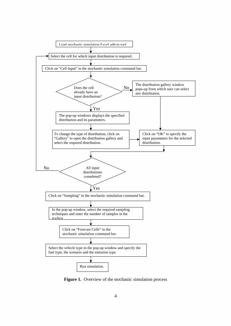
Figure 1 shows a more detailed overview of the stochastic simulation process using the Excel

add-in tool.

4

Figure 1. Overview of the stochastic simulation process

Load stochastic simulation Excel add-in tool.

Select the cell for which input distribution is required.

Click on “Cell Input” in the stochastic simulation command bar.

Does the cell already have an input distribution?

The pop-up windows displays the specified distribution and its parameters.

The distribution gallery window pops-up from which user can select any distribution.

Click on “OK” to specify the input parameters for the selected distribution.

To change the type of distribution, click on “Gallery” to open the distribution gallery and select the required distribution.

All input distributions completed?

Click on “Sampling” in the stochastic simulation command bar.

In the pop-up window, select the required sampling techniques and enter the number of samples in the textbox.

Click on “Forecast Cells” in the stochastic simulation command bar.

Select the vehicle type in the pop-up window and specify the fuel type, the scenario and the emission type.

Run simulation.

Yes

Yes

No

No

5

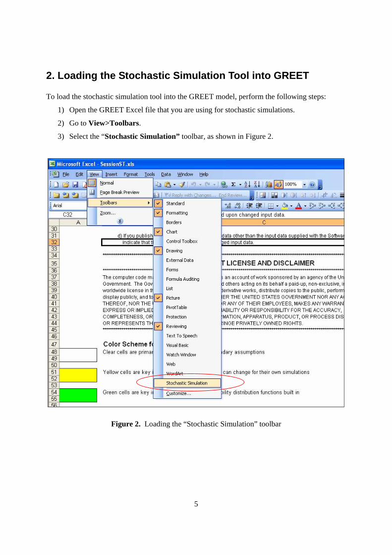
2. Loading the Stochastic Simulation Tool into GREET To load the stochastic simulation tool into the GREET model, perform the following steps:

1) Open the GREET Excel file that you are using for stochastic simulations.

2) Go to View>Toolbars.

3) Select the “Stochastic Simulation” toolbar, as shown in Figure 2.

Figure 2. Loading the “Stochastic Simulation” toolbar

6

4) A command bar with all the command buttons required for the stochastic simulation

process appears as shown in Figure 3. The stochastic capability of the GREET model has

been interfaced as a command bar containing five buttons for the five main steps of the

uncertainty analysis process. Section 5 provides a detailed explanation of the

functionality of each button in the stochastic simulation command bar.

Figure 3. Stochastic simulation command bar

7

3. Overview of Probability Distribution Functions The tool contains eleven built-in probability distributions. The following paragraphs provide a

brief description of each probability distribution.

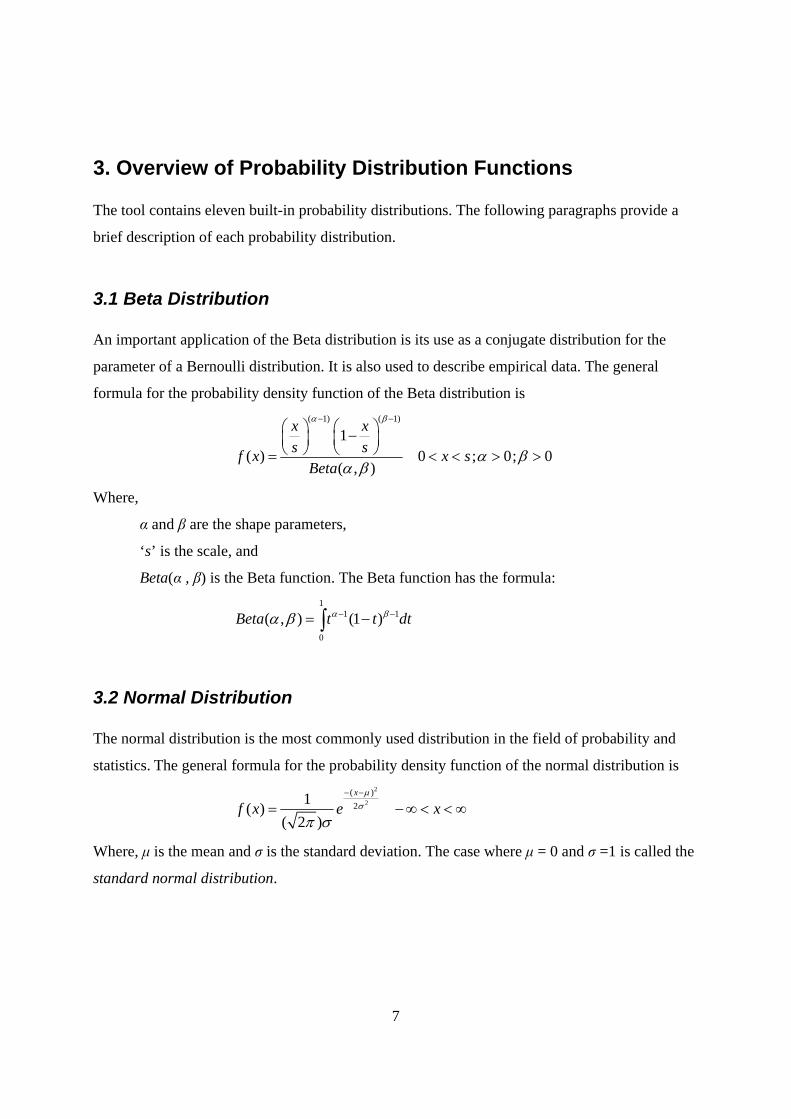
3.1 Beta Distribution An important application of the Beta distribution is its use as a conjugate distribution for the

parameter of a Bernoulli distribution. It is also used to describe empirical data. The general

formula for the probability density function of the Beta distribution is ( 1) ( 1)

1( ) 0 ; 0; 0

( , )

x xs sf x x s

Beta

α β

α βα β

− −⎛ ⎞ ⎛ ⎞−⎜ ⎟ ⎜ ⎟⎝ ⎠ ⎝ ⎠= < < > >

Where,

α and β are the shape parameters,

‘s’ is the scale, and

Beta(α , β) is the Beta function. The Beta function has the formula: 1

1 1

0

( , ) (1 )Beta t t dtα βα β − −= −∫

3.2 Normal Distribution The normal distribution is the most commonly used distribution in the field of probability and

statistics. The general formula for the probability density function of the normal distribution is 2

2( )21( )

( 2 )

x

f x e xμ

σ

π σ

− −

= −∞ < < ∞

Where, μ is the mean and σ is the standard deviation. The case where μ = 0 and σ =1 is called the

standard normal distribution.

8

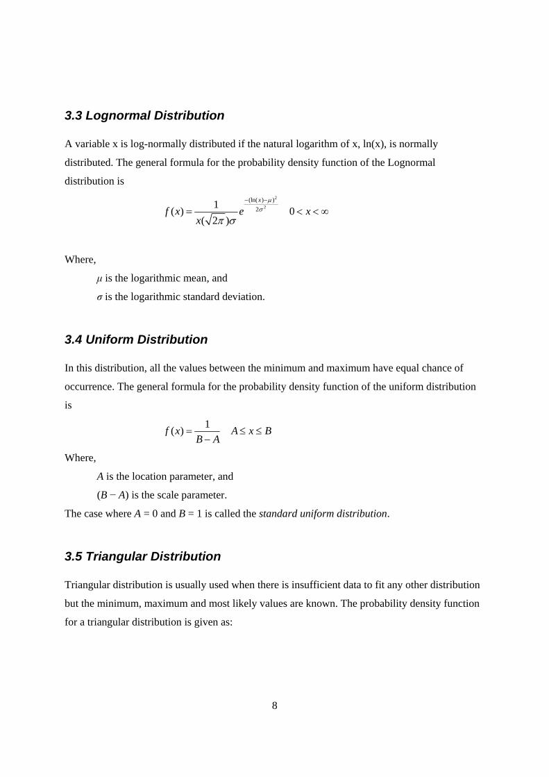
3.3 Lognormal Distribution A variable x is log-normally distributed if the natural logarithm of x, ln(x), is normally

distributed. The general formula for the probability density function of the Lognormal

distribution is 2

2(ln( ) )

21( ) 0( 2 )

x

f x e xx

μσ

π σ

− −

= < < ∞

Where,

μ is the logarithmic mean, and

σ is the logarithmic standard deviation.

3.4 Uniform Distribution In this distribution, all the values between the minimum and maximum have equal chance of

occurrence. The general formula for the probability density function of the uniform distribution

is

1( )f x A x BB A

= ≤ ≤−

Where,

A is the location parameter, and

(B − A) is the scale parameter.

The case where A = 0 and B = 1 is called the standard uniform distribution.

3.5 Triangular Distribution Triangular distribution is usually used when there is insufficient data to fit any other distribution

but the minimum, maximum and most likely values are known. The probability density function

for a triangular distribution is given as:

9

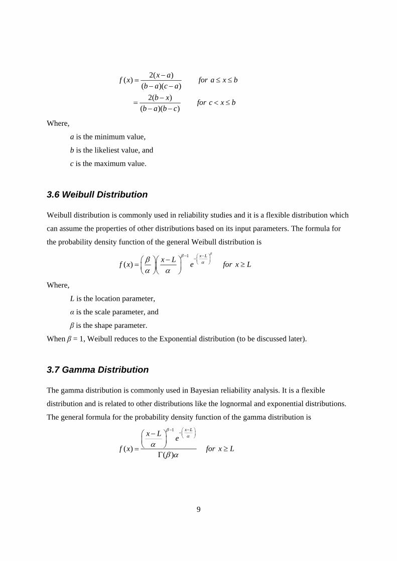
2( )( )( )( )

2( )( )( )

x af x for a x bb a c a

b x for c x bb a b c

−= ≤ ≤

− −−

= < ≤− −

Where,

a is the minimum value,

b is the likeliest value, and

c is the maximum value.

3.6 Weibull Distribution Weibull distribution is commonly used in reliability studies and it is a flexible distribution which

can assume the properties of other distributions based on its input parameters. The formula for

the probability density function of the general Weibull distribution is

1

( )x Lx Lf x e for x L

ββαβ

α α

− −⎛ ⎞−⎜ ⎟⎝ ⎠−⎛ ⎞⎛ ⎞= ≥⎜ ⎟⎜ ⎟

⎝ ⎠⎝ ⎠

Where,

L is the location parameter,

α is the scale parameter, and

β is the shape parameter.

When β = 1, Weibull reduces to the Exponential distribution (to be discussed later).

3.7 Gamma Distribution The gamma distribution is commonly used in Bayesian reliability analysis. It is a flexible

distribution and is related to other distributions like the lognormal and exponential distributions.

The general formula for the probability density function of the gamma distribution is 1

( )( )

x Lx L ef x for x L

βα

αβ α

−− ⎛ ⎞−⎜ ⎟⎝ ⎠−⎛ ⎞

⎜ ⎟⎝ ⎠= ≥

Γ

10

Where,

L is the location parameter,

α is the scale parameter,

β is the shape parameter, and

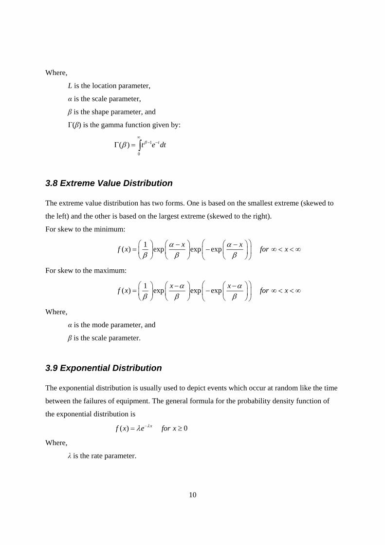
Г(β) is the gamma function given by:

1

0

( ) tt e dtββ∞

− −Γ = ∫

3.8 Extreme Value Distribution The extreme value distribution has two forms. One is based on the smallest extreme (skewed to

the left) and the other is based on the largest extreme (skewed to the right).

For skew to the minimum:

1( ) exp exp expx xf x for xα αβ β β

⎛ ⎞⎛ ⎞ ⎛ ⎞ ⎛ ⎞− −= − ∞ < < ∞⎜ ⎟⎜ ⎟ ⎜ ⎟ ⎜ ⎟⎝ ⎠ ⎝ ⎠ ⎝ ⎠⎝ ⎠

For skew to the maximum:

1( ) exp exp expx xf x for xα αβ β β

⎛ ⎞⎛ ⎞ ⎛ ⎞ ⎛ ⎞− −= − ∞ < < ∞⎜ ⎟⎜ ⎟ ⎜ ⎟ ⎜ ⎟⎝ ⎠ ⎝ ⎠ ⎝ ⎠⎝ ⎠

Where,

α is the mode parameter, and

β is the scale parameter.

3.9 Exponential Distribution The exponential distribution is usually used to depict events which occur at random like the time

between the failures of equipment. The general formula for the probability density function of

the exponential distribution is

( ) 0xf x e for xλλ −= ≥

Where,

λ is the rate parameter.

11

3.10 Pareto Distribution The Pareto distribution is generally used to describe empirical phenomena like birth rate, income

growth rate, etc. The general formula for the probability density function of the Pareto

distribution is:

( 1)( ) Lf x for x Lx

β

β

β+= >

Where,

L is the location parameter, and

β is the shape parameter.

3.11 Logistic Distribution The logistic distribution is used to model binary responses (e.g., Gender) and is commonly used

in logistic regression. The logistic distribution is defined as:

2( )

1

x

x

ef x for x

e

μα

μαα

−⎛ ⎞−⎜ ⎟⎝ ⎠

−⎛ ⎞−⎜ ⎟⎝ ⎠

= −∞ < < ∞⎛ ⎞+⎜ ⎟⎜ ⎟

⎝ ⎠

Where,

μ is the mean parameter, and

α is the scale parameter.

12

4. Overview of Sampling Techniques The stochastic simulation tool has four sampling techniques incorporated into it [1]: 1) Monte

Carlo Sampling; 2) Latin Hypercube Sampling; 3) Hammersley Sequence Sampling; and 4)

Latin Hypercube Hammersley Sampling. The following paragraphs explain each sampling

technique in more detail.

4.1 Monte Carlo Sampling (MCS) One of the most widely used techniques for sampling from a probability distribution is the Monte

Carlo sampling technique, which is based on a pseudo-random generator used to approximate a

uniform distribution (i.e., having equal probability in the range from 0 to 1). The specific values

for each input variable are selected by inverse transformation over the cumulative probability

distribution. A Monte Carlo sampling technique also has the important property that the

successive points in the sample are independent.

4.2 Median Latin Hypercube Sampling (MLHS) Latin Hypercube sampling is one form of stratified sampling that can yield more precise

estimates of the distribution function. In Latin Hypercube sampling, the range of each uncertain

parameter Xi is sub-divided into non-overlapping intervals of equal probability. In LHS, one

value from each interval is selected at random with respect to the probability distribution in the

interval. In MLHS, this value is the mid-point of the interval. The ‘n’ values thus obtained for X1

are paired in a random manner (i.e., equally likely combinations) with ‘n’ values of X2. These n

values are then combined with n values of X3 to form n-triplets, and so on, until ‘n’ k-tuplets are

formed. The MLHS technique is used in the stochastic modeling tool that we developed.

13

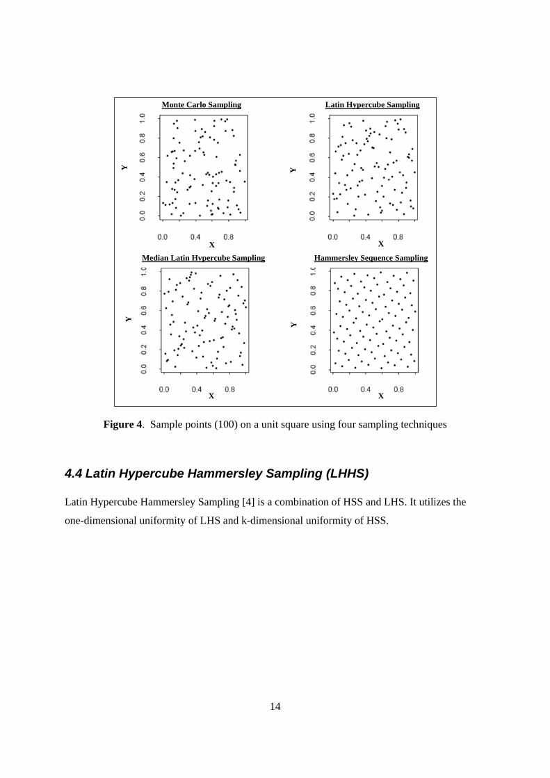
4.3 Hammersley Sequence Sampling (HSS) In the late 1990s, an efficient sampling technique, Hammersley Sequence Sampling, based on

Hammersley points, was developed [2], which uses an optimal design scheme for placing the ‘n’

points on a k-dimensional hypercube. Unlike Monte Carlo Sampling, the Latin Hypercube and

its variant (the Median Latin Hypercube), the HSS sampling technique ensures that the sample

set is more representative of the population, showing uniformity properties in multi-dimensions.

Figure 4 graphs the samples generated by different techniques on a unit square. This provides a

qualitative picture of the uniformity properties of the different techniques. It is clear from Figure

4 that the Hammersley points have better uniformity properties compared to other techniques.

The main reason for this is that the Hammersley points are an optimal design for placing n points

on a k-dimensional hypercube. In contrast, other stratified techniques such as the Latin

Hypercube are designed for uniformity along a single dimension and then randomly paired for

placement on a k-dimensional cube.

One of the main advantages of the Monte Carlo method is that the number of samples required to

obtain a given accuracy of estimates does not scale exponentially with the number of uncertain

variables. HSS preserves this property of Monte Carlo. Hammersley Sequence Sampling is

estimated to be 3 to 100 times faster than the LHS and MCS and hence, is a preferred technique

for uncertainty analysis as well as optimization under uncertainty [2, 3]. Recent findings show

that the uniformity property of HSS for higher dimensions (more than 30 uncertain variables)

gets distorted. HSS (and LHSS given below) is generated based on prime numbers as bases. In

order to break this distortion, we introduced leaps in prime numbers for higher dimensions. This

‘leaped’ HSS and LHHS technique showed better uniformity than the basic HSS and LHHS

techniques. For simplicity, we have leaped HSS and LHHS as a part of the HSS and LHHS

techniques in the stochastic modeling capability. When the number uncertain variables exceeds

30, the switch occurs automatically. GREET applies this sampling method as the default

sampling technique.

14

Y

Y Y

Y

X

X X

X

Latin Hypercube Sampling Monte Carlo Sampling

Median Latin Hypercube Sampling Hammersley Sequence Sampling

Figure 4. Sample points (100) on a unit square using four sampling techniques

4.4 Latin Hypercube Hammersley Sampling (LHHS) Latin Hypercube Hammersley Sampling [4] is a combination of HSS and LHS. It utilizes the

one-dimensional uniformity of LHS and k-dimensional uniformity of HSS.

15

5. Stepwise Description of the Stochastic Simulation Process The stochastic simulation command bar contains five buttons as shown in Figure 3, one for each

step in the stochastic simulation process. The following paragraphs explain the functionality of

each button in detail.

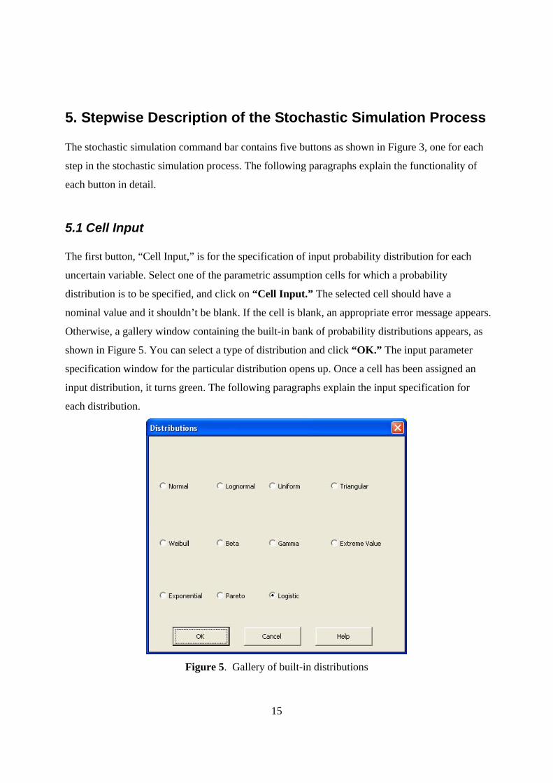
5.1 Cell Input The first button, “Cell Input,” is for the specification of input probability distribution for each

uncertain variable. Select one of the parametric assumption cells for which a probability

distribution is to be specified, and click on “Cell Input.” The selected cell should have a

nominal value and it shouldn’t be blank. If the cell is blank, an appropriate error message appears.

Otherwise, a gallery window containing the built-in bank of probability distributions appears, as

shown in Figure 5. You can select a type of distribution and click “OK.” The input parameter

specification window for the particular distribution opens up. Once a cell has been assigned an

input distribution, it turns green. The following paragraphs explain the input specification for

each distribution.

Figure 5. Gallery of built-in distributions

16

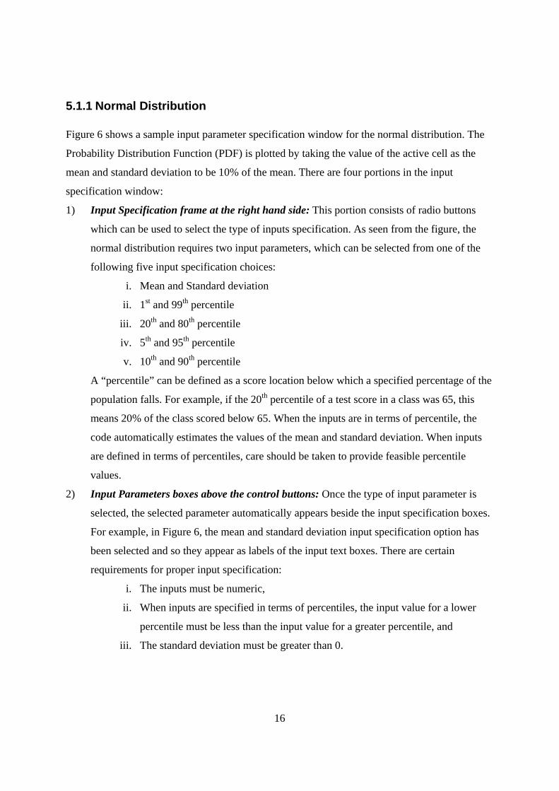
5.1.1 Normal Distribution Figure 6 shows a sample input parameter specification window for the normal distribution. The

Probability Distribution Function (PDF) is plotted by taking the value of the active cell as the

mean and standard deviation to be 10% of the mean. There are four portions in the input

specification window:

1) Input Specification frame at the right hand side: This portion consists of radio buttons

which can be used to select the type of inputs specification. As seen from the figure, the

normal distribution requires two input parameters, which can be selected from one of the

following five input specification choices:

i. Mean and Standard deviation

ii. 1st and 99th percentile

iii. 20th and 80th percentile

iv. 5th and 95th percentile

v. 10th and 90th percentile

A “percentile” can be defined as a score location below which a specified percentage of the

population falls. For example, if the 20th percentile of a test score in a class was 65, this

means 20% of the class scored below 65. When the inputs are in terms of percentile, the

code automatically estimates the values of the mean and standard deviation. When inputs

are defined in terms of percentiles, care should be taken to provide feasible percentile

values.

2) Input Parameters boxes above the control buttons: Once the type of input parameter is

selected, the selected parameter automatically appears beside the input specification boxes.

For example, in Figure 6, the mean and standard deviation input specification option has

been selected and so they appear as labels of the input text boxes. There are certain

requirements for proper input specification:

i. The inputs must be numeric,

ii. When inputs are specified in terms of percentiles, the input value for a lower

percentile must be less than the input value for a greater percentile, and

iii. The standard deviation must be greater than 0.

17

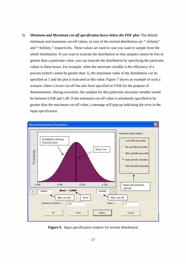
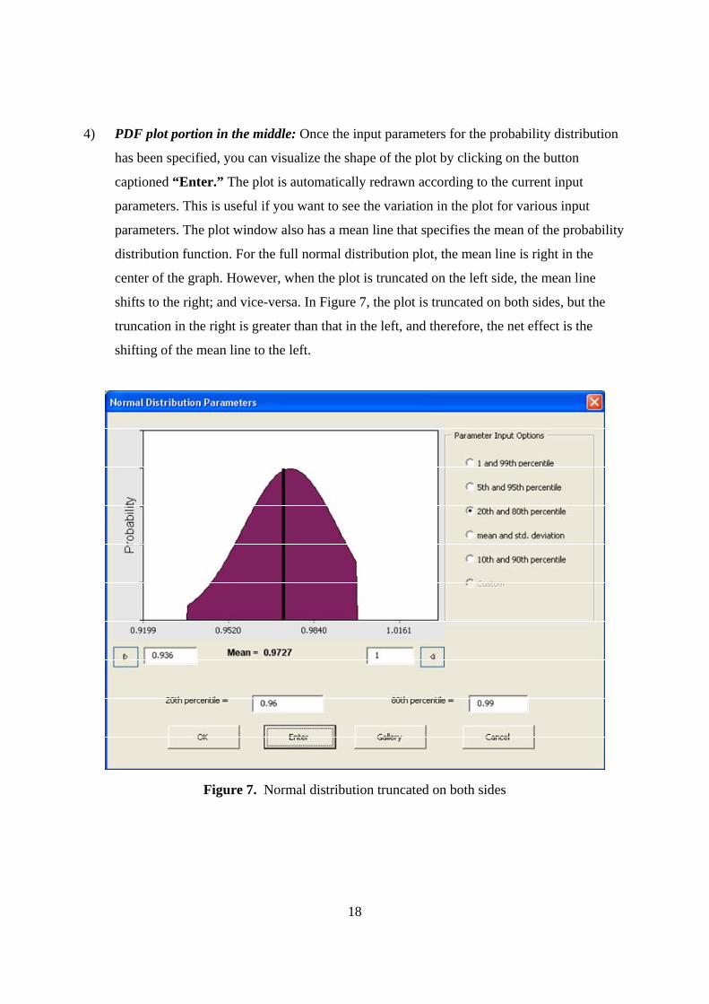
3) Minimum and Maximum cut-off specification boxes below the PDF plot: The default

minimum and maximum cut-off values, in case of the normal distribution are “–Infinity”

and “+Infinity,” respectively. These values are used in case you want to sample from the

whole distribution. If you want to truncate the distribution so that samples cannot be less or

greater than a particular value, you can truncate the distribution by specifying the particular

values in these boxes. For example, when the uncertain variable is the efficiency of a

process (which cannot be greater than 1), the maximum value of the distribution can be

specified as 1 and the plot is truncated at this value. Figure 7 shows an example of such a

scenario where a lower cut-off has also been specified at 0.936 for the purpose of

demonstration. During execution, the samples for this particular uncertain variable would

be between 0.936 and 1.00. If the minimum cut-off value is mistakenly specified to be

greater than the maximum cut-off value, a message will pop-up indicating the error in the

input specification.

Probability Density Function plot

Input specification options

Min cut-off Max cut-offMean

Mean Line

Figure 6. Input specification window for normal distribution

18

4) PDF plot portion in the middle: Once the input parameters for the probability distribution

has been specified, you can visualize the shape of the plot by clicking on the button

captioned “Enter.” The plot is automatically redrawn according to the current input

parameters. This is useful if you want to see the variation in the plot for various input

parameters. The plot window also has a mean line that specifies the mean of the probability

distribution function. For the full normal distribution plot, the mean line is right in the

center of the graph. However, when the plot is truncated on the left side, the mean line

shifts to the right; and vice-versa. In Figure 7, the plot is truncated on both sides, but the

truncation in the right is greater than that in the left, and therefore, the net effect is the

shifting of the mean line to the left.

Figure 7. Normal distribution truncated on both sides

19

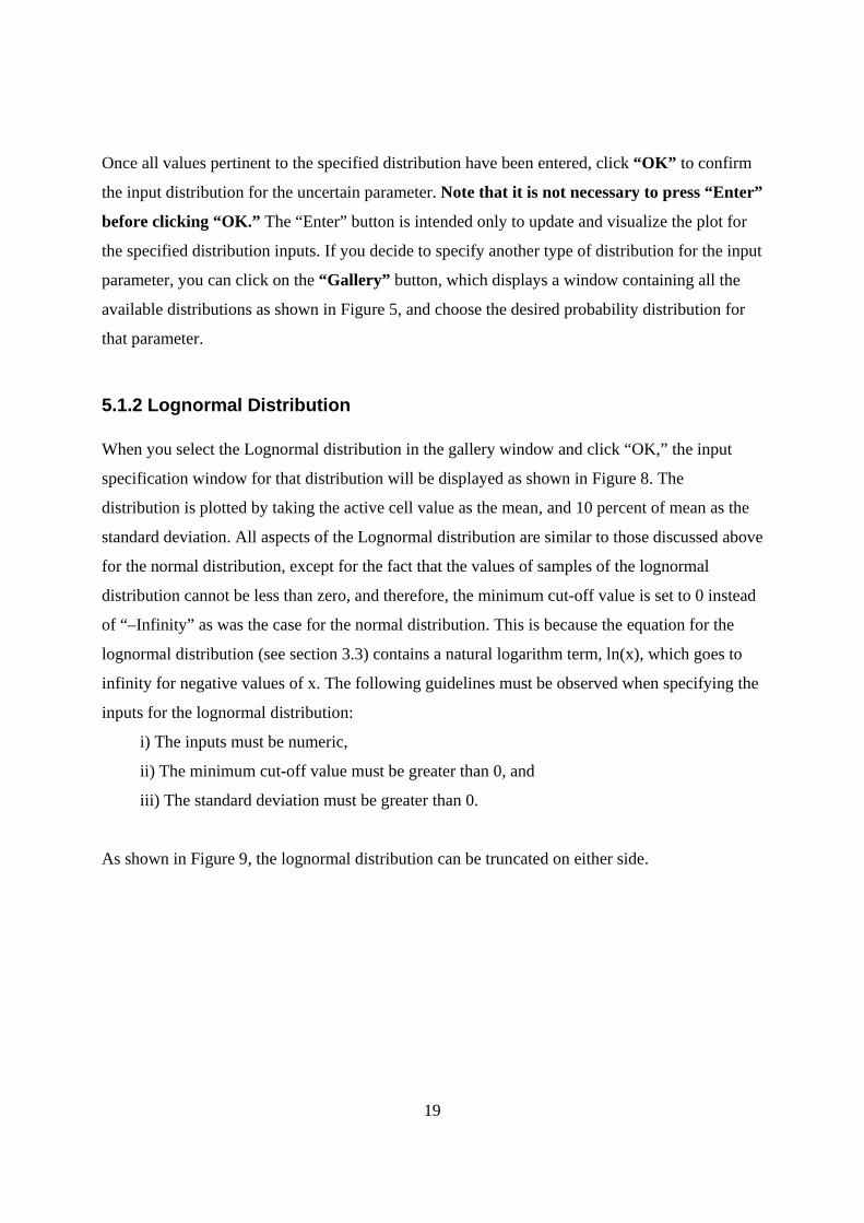
Once all values pertinent to the specified distribution have been entered, click “OK” to confirm

the input distribution for the uncertain parameter. Note that it is not necessary to press “Enter”

before clicking “OK.” The “Enter” button is intended only to update and visualize the plot for

the specified distribution inputs. If you decide to specify another type of distribution for the input

parameter, you can click on the “Gallery” button, which displays a window containing all the

available distributions as shown in Figure 5, and choose the desired probability distribution for

that parameter.

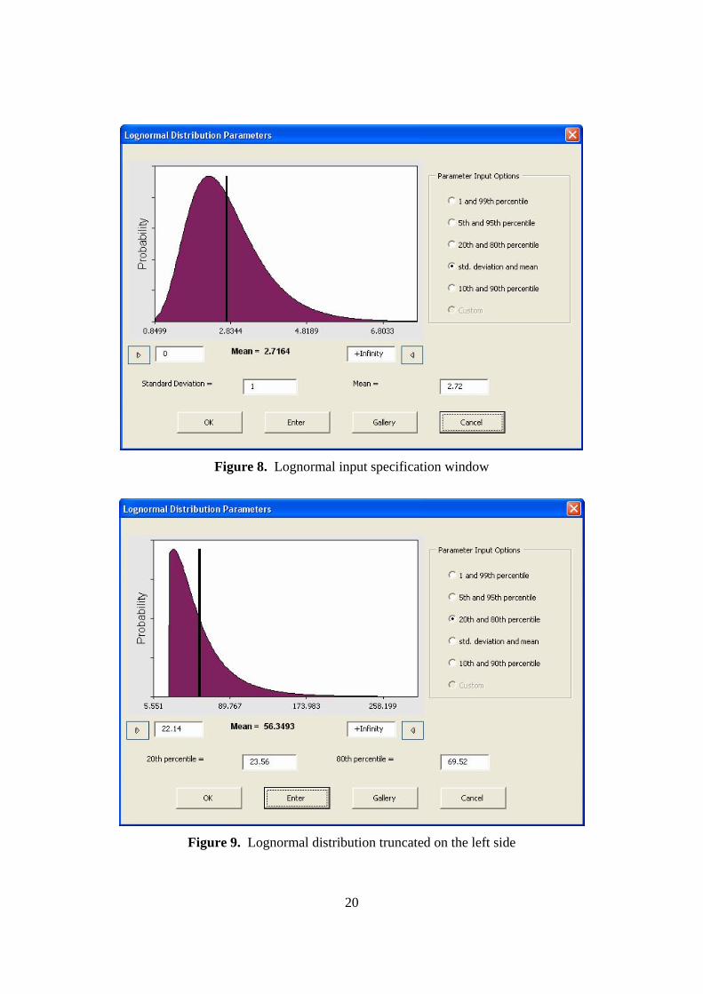
5.1.2 Lognormal Distribution When you select the Lognormal distribution in the gallery window and click “OK,” the input

specification window for that distribution will be displayed as shown in Figure 8. The

distribution is plotted by taking the active cell value as the mean, and 10 percent of mean as the

standard deviation. All aspects of the Lognormal distribution are similar to those discussed above

for the normal distribution, except for the fact that the values of samples of the lognormal

distribution cannot be less than zero, and therefore, the minimum cut-off value is set to 0 instead

of “–Infinity” as was the case for the normal distribution. This is because the equation for the

lognormal distribution (see section 3.3) contains a natural logarithm term, ln(x), which goes to

infinity for negative values of x. The following guidelines must be observed when specifying the

inputs for the lognormal distribution:

i) The inputs must be numeric,

ii) The minimum cut-off value must be greater than 0, and

iii) The standard deviation must be greater than 0.

As shown in Figure 9, the lognormal distribution can be truncated on either side.

20

Figure 8. Lognormal input specification window

Figure 9. Lognormal distribution truncated on the left side

21

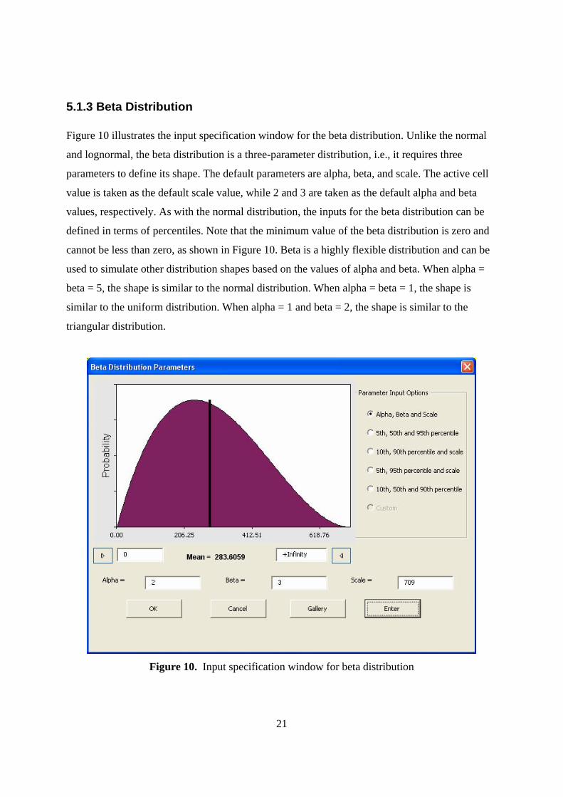
5.1.3 Beta Distribution Figure 10 illustrates the input specification window for the beta distribution. Unlike the normal

and lognormal, the beta distribution is a three-parameter distribution, i.e., it requires three

parameters to define its shape. The default parameters are alpha, beta, and scale. The active cell

value is taken as the default scale value, while 2 and 3 are taken as the default alpha and beta

values, respectively. As with the normal distribution, the inputs for the beta distribution can be

defined in terms of percentiles. Note that the minimum value of the beta distribution is zero and

cannot be less than zero, as shown in Figure 10. Beta is a highly flexible distribution and can be

used to simulate other distribution shapes based on the values of alpha and beta. When alpha =

beta = 5, the shape is similar to the normal distribution. When alpha = beta = 1, the shape is

similar to the uniform distribution. When alpha = 1 and beta = 2, the shape is similar to the

triangular distribution.

Figure 10. Input specification window for beta distribution

22

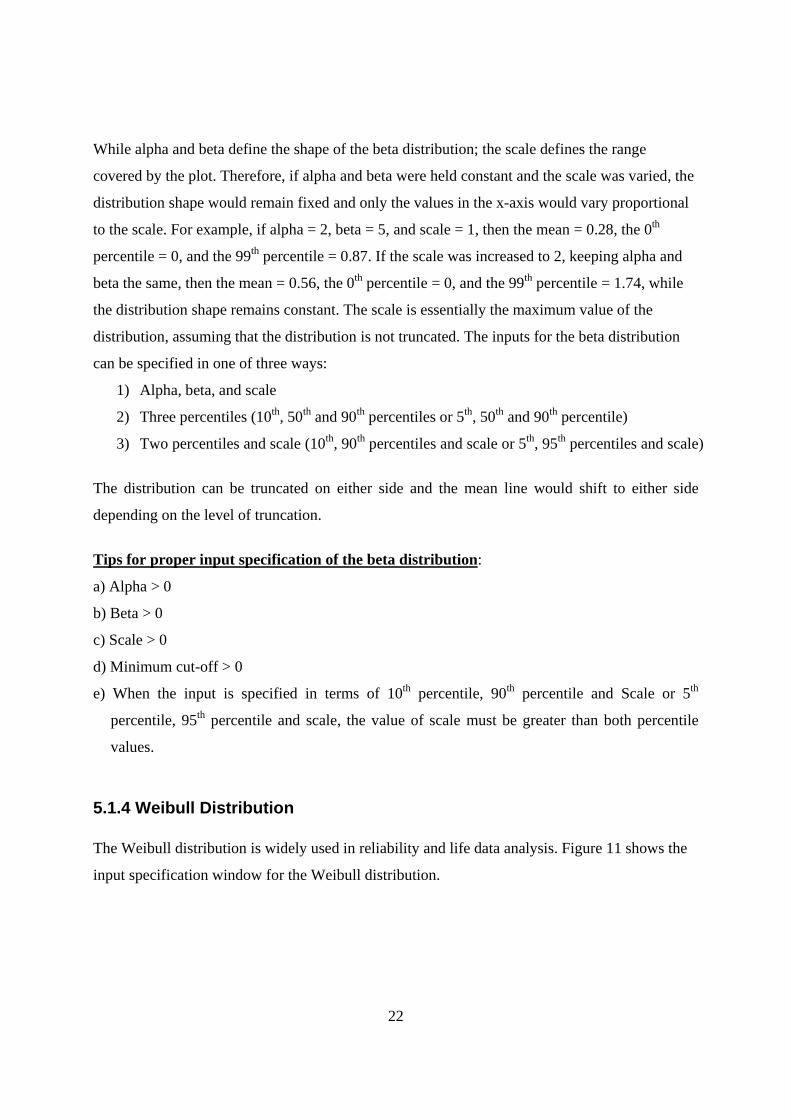
While alpha and beta define the shape of the beta distribution; the scale defines the range

covered by the plot. Therefore, if alpha and beta were held constant and the scale was varied, the

distribution shape would remain fixed and only the values in the x-axis would vary proportional

to the scale. For example, if alpha = 2, beta = 5, and scale = 1, then the mean = 0.28, the 0th

percentile = 0, and the 99th percentile = 0.87. If the scale was increased to 2, keeping alpha and

beta the same, then the mean = 0.56, the 0th percentile = 0, and the 99th percentile = 1.74, while

the distribution shape remains constant. The scale is essentially the maximum value of the

distribution, assuming that the distribution is not truncated. The inputs for the beta distribution

can be specified in one of three ways:

1) Alpha, beta, and scale

2) Three percentiles (10th, 50th and 90th percentiles or 5th, 50th and 90th percentile)

3) Two percentiles and scale (10th, 90th percentiles and scale or 5th, 95th percentiles and scale)

The distribution can be truncated on either side and the mean line would shift to either side

depending on the level of truncation.

Tips for proper input specification of the beta distribution:

a) Alpha > 0

b) Beta > 0

c) Scale > 0

d) Minimum cut-off > 0

e) When the input is specified in terms of 10th percentile, 90th percentile and Scale or 5th

percentile, 95th percentile and scale, the value of scale must be greater than both percentile

values.

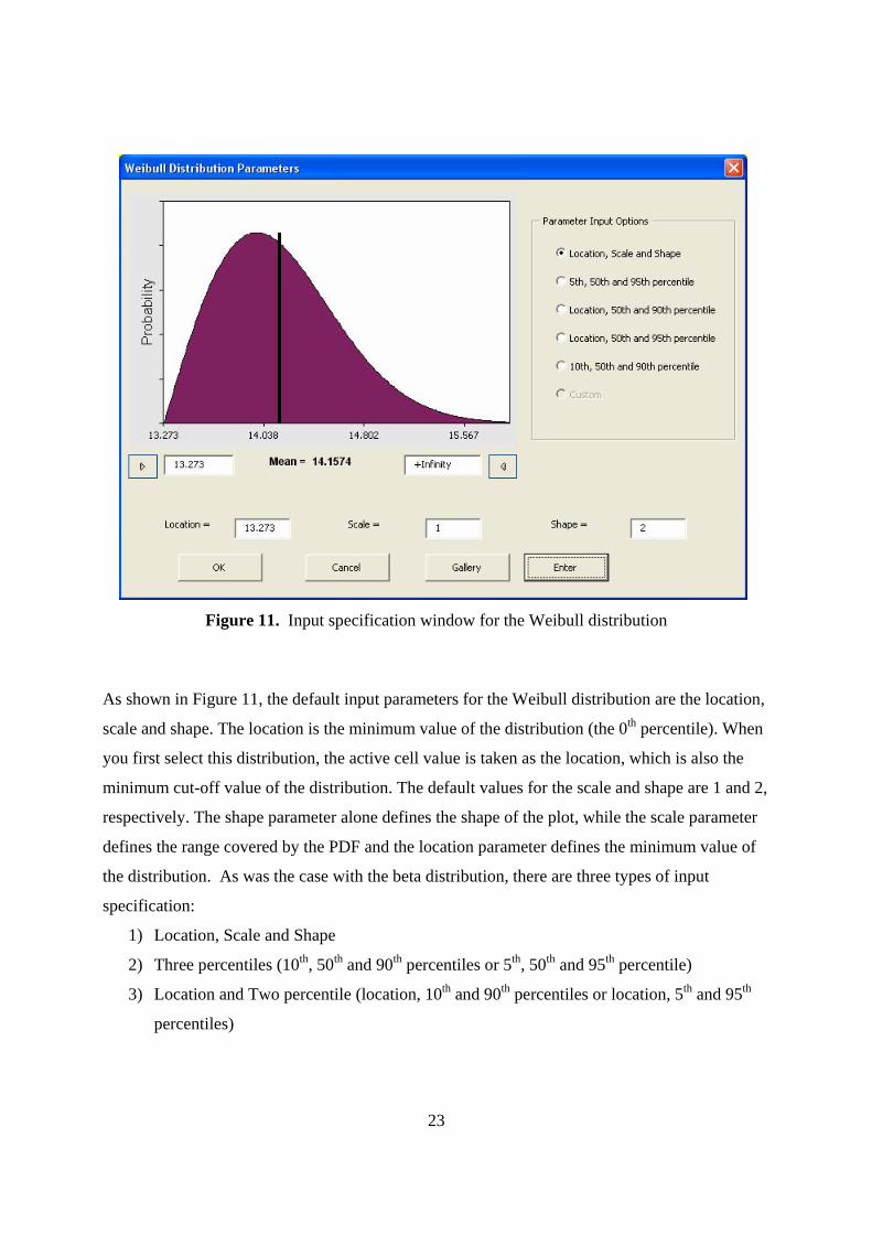
5.1.4 Weibull Distribution The Weibull distribution is widely used in reliability and life data analysis. Figure 11 shows the

input specification window for the Weibull distribution.

23

Figure 11. Input specification window for the Weibull distribution

As shown in Figure 11, the default input parameters for the Weibull distribution are the location,

scale and shape. The location is the minimum value of the distribution (the 0th percentile). When

you first select this distribution, the active cell value is taken as the location, which is also the

minimum cut-off value of the distribution. The default values for the scale and shape are 1 and 2,

respectively. The shape parameter alone defines the shape of the plot, while the scale parameter

defines the range covered by the PDF and the location parameter defines the minimum value of

the distribution. As was the case with the beta distribution, there are three types of input

specification:

1) Location, Scale and Shape

2) Three percentiles (10th, 50th and 90th percentiles or 5th, 50th and 95th percentile)

3) Location and Two percentile (location, 10th and 90th percentiles or location, 5th and 95th

percentiles)

24

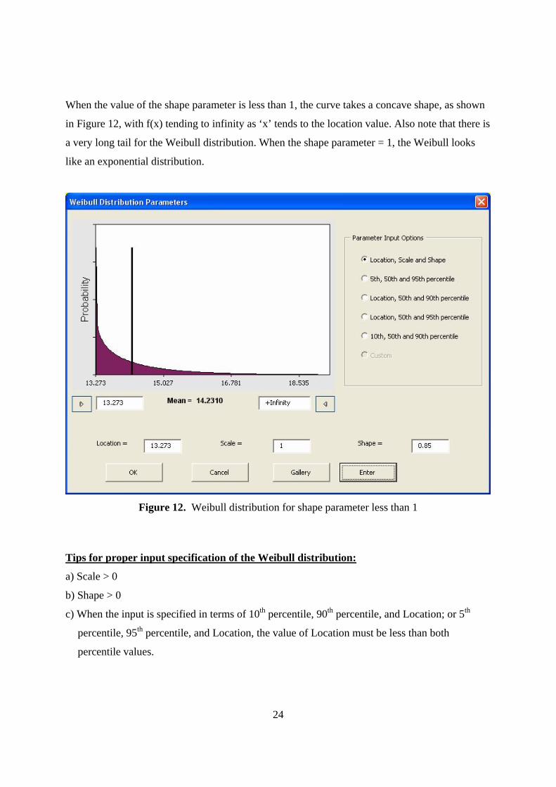
When the value of the shape parameter is less than 1, the curve takes a concave shape, as shown

in Figure 12, with f(x) tending to infinity as ‘x’ tends to the location value. Also note that there is

a very long tail for the Weibull distribution. When the shape parameter = 1, the Weibull looks

like an exponential distribution.

Figure 12. Weibull distribution for shape parameter less than 1

Tips for proper input specification of the Weibull distribution:

a) Scale > 0

b) Shape > 0

c) When the input is specified in terms of 10th percentile, 90th percentile, and Location; or 5th

percentile, 95th percentile, and Location, the value of Location must be less than both

percentile values.

25

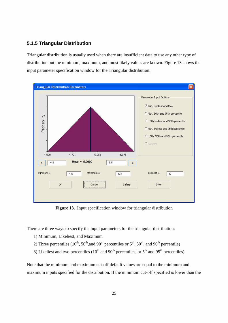
5.1.5 Triangular Distribution Triangular distribution is usually used when there are insufficient data to use any other type of

distribution but the minimum, maximum, and most likely values are known. Figure 13 shows the

input parameter specification window for the Triangular distribution.

Figure 13. Input specification window for triangular distribution

There are three ways to specify the input parameters for the triangular distribution:

1) Minimum, Likeliest, and Maximum

2) Three percentiles (10th, 50th,and 90th percentiles or 5th, 50th, and 90th percentile)

3) Likeliest and two percentiles (10th and 90th percentiles, or 5th and 95th percentiles)

Note that the minimum and maximum cut-off default values are equal to the minimum and

maximum inputs specified for the distribution. If the minimum cut-off specified is lower than the

26

minimum input, then it will be ignored. If the minimum cut-off value specified is greater than the

minimum input or the maximum cut-off value specified is lower than the maximum input, the

distribution will be truncated at these values.

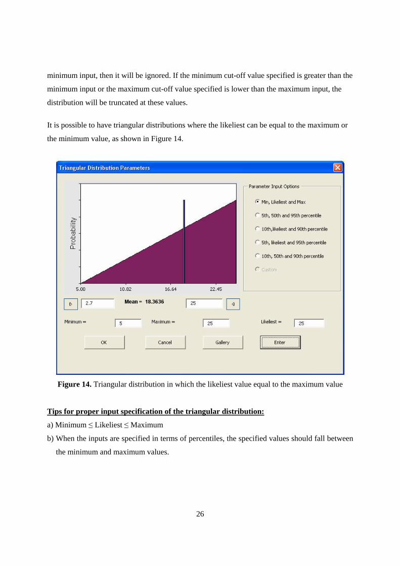
It is possible to have triangular distributions where the likeliest can be equal to the maximum or

the minimum value, as shown in Figure 14.

Figure 14. Triangular distribution in which the likeliest value equal to the maximum value

Tips for proper input specification of the triangular distribution:

a) Minimum ≤ Likeliest ≤ Maximum

b) When the inputs are specified in terms of percentiles, the specified values should fall between

the minimum and maximum values.

27

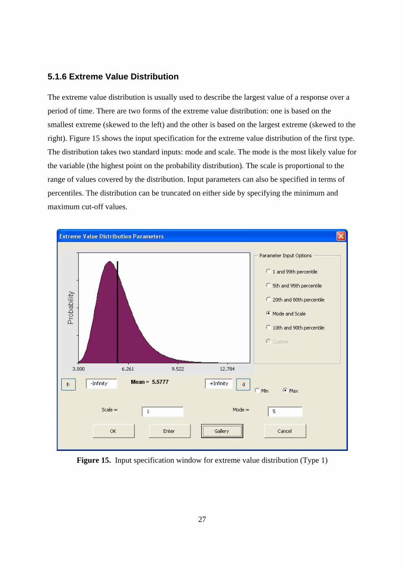
5.1.6 Extreme Value Distribution The extreme value distribution is usually used to describe the largest value of a response over a

period of time. There are two forms of the extreme value distribution: one is based on the

smallest extreme (skewed to the left) and the other is based on the largest extreme (skewed to the

right). Figure 15 shows the input specification for the extreme value distribution of the first type.

The distribution takes two standard inputs: mode and scale. The mode is the most likely value for

the variable (the highest point on the probability distribution). The scale is proportional to the

range of values covered by the distribution. Input parameters can also be specified in terms of

percentiles. The distribution can be truncated on either side by specifying the minimum and

maximum cut-off values.

Figure 15. Input specification window for extreme value distribution (Type 1)

28

Tips for proper input specification of the extreme value distribution:

a) Scale > 0

b) When the input is specified in terms of mode and 90th or mode and 95th percentile, the value of

mode must be lesser than the percentile value.

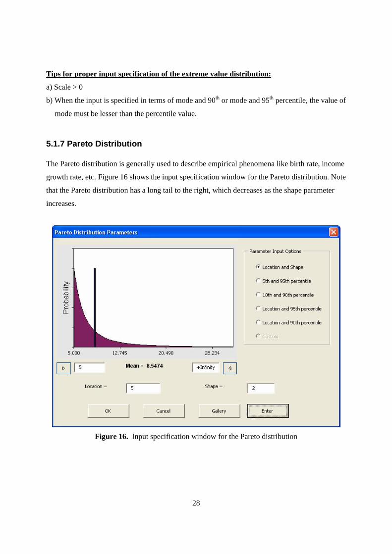
5.1.7 Pareto Distribution The Pareto distribution is generally used to describe empirical phenomena like birth rate, income

growth rate, etc. Figure 16 shows the input specification window for the Pareto distribution. Note

that the Pareto distribution has a long tail to the right, which decreases as the shape parameter

increases.

Figure 16. Input specification window for the Pareto distribution

29

The Pareto distribution features two standard parameters: location and shape. The location

parameter is the lower bound for the distribution, while the shape parameter defines the

distribution shape. As the shape parameter decreases, the concavity of the distribution increases,

i.e., the curve becomes inwardly steeper. Inputs can also be specified in terms of:

1) Percentiles (5th and 95th percentiles or 10th and 95th percentiles)

2) Location and a percentile

Tips for proper input specification of the Pareto distribution:

a) Location > 0

b) Shape > 0

c) Minimum cut-off value > 0

d) When the input is specified in terms of location and 90th or location and 95th percentile, the

value of location must be less than the percentile value.

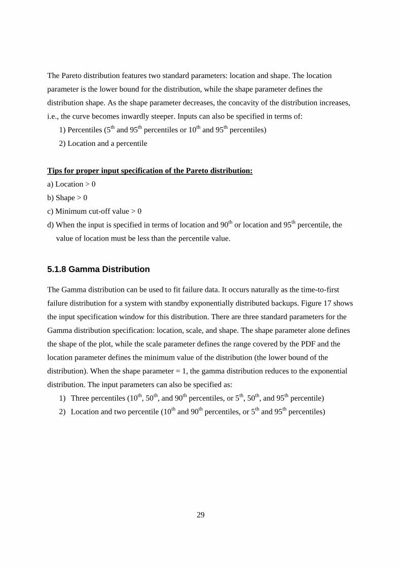
5.1.8 Gamma Distribution The Gamma distribution can be used to fit failure data. It occurs naturally as the time-to-first

failure distribution for a system with standby exponentially distributed backups. Figure 17 shows

the input specification window for this distribution. There are three standard parameters for the

Gamma distribution specification: location, scale, and shape. The shape parameter alone defines

the shape of the plot, while the scale parameter defines the range covered by the PDF and the

location parameter defines the minimum value of the distribution (the lower bound of the

distribution). When the shape parameter = 1, the gamma distribution reduces to the exponential

distribution. The input parameters can also be specified as:

1) Three percentiles (10th, 50th, and 90th percentiles, or 5th, 50th, and 95th percentile)

2) Location and two percentile (10th and 90th percentiles, or 5th and 95th percentiles)

30

Tips for proper input specification for the Gamma distribution:

a) Scale > 0

b) Shape > 0

c) When the input is specified in terms of 10th percentile, 90th percentile and Location or 5th

percentile, 95th percentile and Location, the value of Location must be less than both

percentile values.

Figure 17. Input specification window for the Gamma distribution

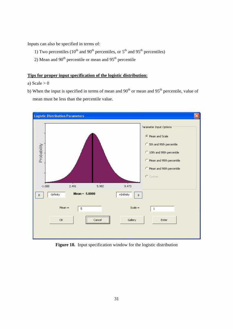
5.1.9 Logistic Distribution The logistic distribution is used to describe growth of population. Figure 18 shows the input

specification window for the logistic distribution. The logistic distribution is specified by two

standard parameters: mean and scale. The distribution is a symmetric distribution and hence

mode = median = mean. Scale denotes the range of values covered by the distribution.

31

Inputs can also be specified in terms of:

1) Two percentiles (10th and 90th percentiles, or 5th and 95th percentiles)

2) Mean and 90th percentile or mean and 95th percentile

Tips for proper input specification of the logistic distribution:

a) Scale > 0

b) When the input is specified in terms of mean and 90th or mean and 95th percentile, value of

mean must be less than the percentile value.

Figure 18. Input specification window for the logistic distribution

32

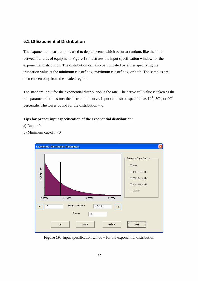
5.1.10 Exponential Distribution The exponential distribution is used to depict events which occur at random, like the time

between failures of equipment. Figure 19 illustrates the input specification window for the

exponential distribution. The distribution can also be truncated by either specifying the

truncation value at the minimum cut-off box, maximum cut-off box, or both. The samples are

then chosen only from the shaded region.

The standard input for the exponential distribution is the rate. The active cell value is taken as the

rate parameter to construct the distribution curve. Input can also be specified as 10th, 50th, or 90th

percentile. The lower bound for the distribution = 0.

Tips for proper input specification of the exponential distribution:

a) Rate > 0

b) Minimum cut-off > 0

Figure 19. Input specification window for the exponential distribution

33

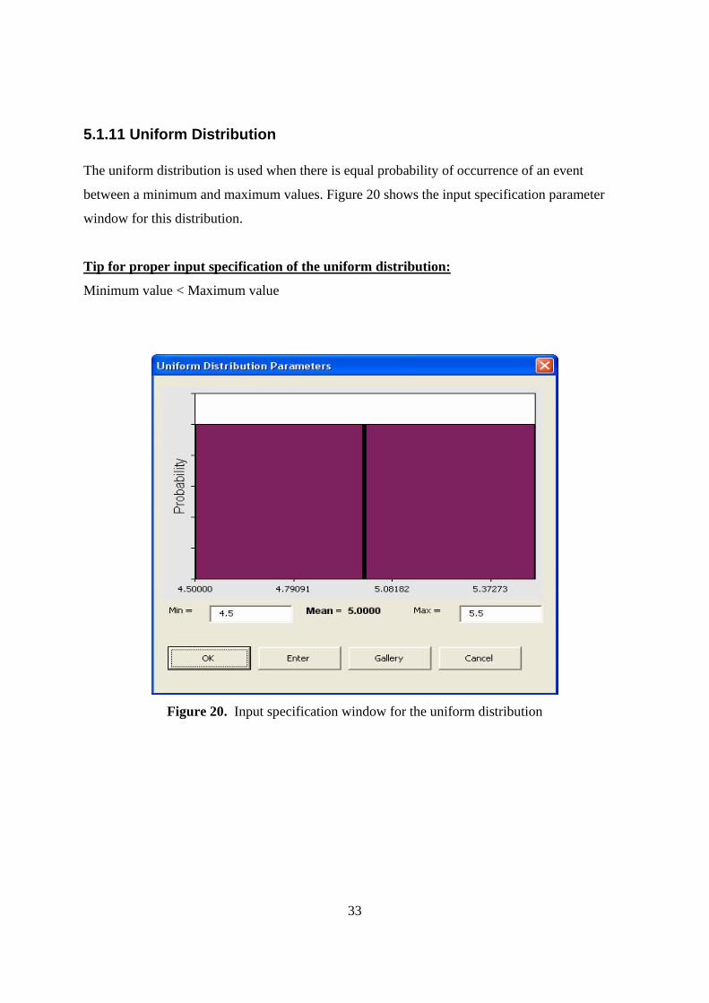
5.1.11 Uniform Distribution The uniform distribution is used when there is equal probability of occurrence of an event

between a minimum and maximum values. Figure 20 shows the input specification parameter

window for this distribution.

Tip for proper input specification of the uniform distribution:

Minimum value < Maximum value

Figure 20. Input specification window for the uniform distribution

34

General guidelines to be followed during any distribution input specification

Improper input values are met with appropriate error messages. Proper input requirements

common to all distribution include the following:

a) Inputs must be numeric.

b) When inputs are specified in terms of percentiles, input value for a less percentile must be less

than input value for a greater percentile.

c) Minimum cut-off value must be less than maximum cut-off value.

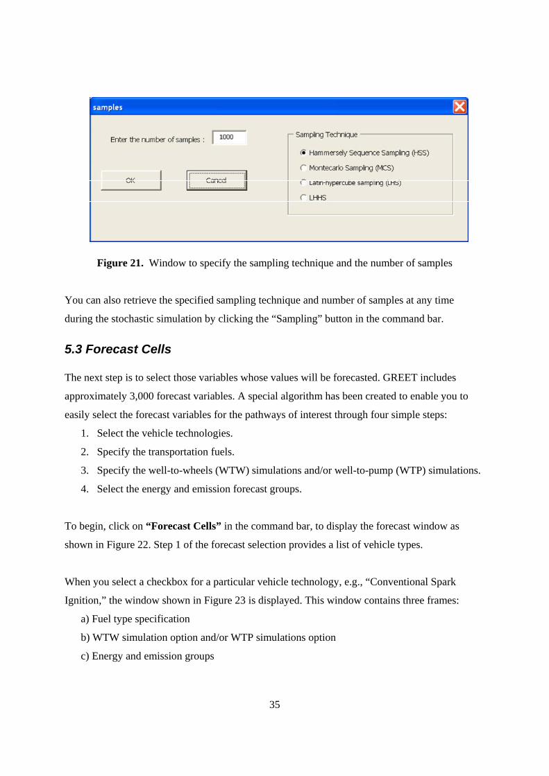
5.2 Sampling Once the distributions for all the uncertain parameters have been specified, the next step is to

specify the sampling technique to be used and the number of samples required. When you click

on “Sampling” in the stochastic simulation command bar, the window shown in Figure 21

appears. You can select from one of four sampling techniques:

a) Hammersley Sequence Sampling [Default number of samples = 1000]

b) Monte Carlo Sampling [Default number of samples = 4000]

c) Latin Hypercube Sampling [Default number of samples = 2000]

d) Latin Hypercube Hammersley Sampling [Default number of samples = 1000]

The sampling techniques have been explained in detail in section 4. MCS is the conventional

sampling technique in many stochastic simulations. The new and efficient HSS sampling

technique typically requires 1/4th the number of samples required by the MCS technique. Latin-

hypercube sampling performs better than MCS but is not as efficient as HSS. Most of the time,

LHHS performs better than HSS. However, unlike MCS or HSS, the performance measure for

LHHS is not independent of number of variables or type of functionality used to compute the

output distributions. When you select a sampling technique, the default number of samples

(based on the assumption that number of uncertain variables are more than 100 and less than 500)

required automatically appears in the corresponding textbox. You can change the number of

samples according to your preference.

35

Figure 21. Window to specify the sampling technique and the number of samples

You can also retrieve the specified sampling technique and number of samples at any time

during the stochastic simulation by clicking the “Sampling” button in the command bar.

5.3 Forecast Cells The next step is to select those variables whose values will be forecasted. GREET includes

approximately 3,000 forecast variables. A special algorithm has been created to enable you to

easily select the forecast variables for the pathways of interest through four simple steps:

1. Select the vehicle technologies.

2. Specify the transportation fuels.

3. Specify the well-to-wheels (WTW) simulations and/or well-to-pump (WTP) simulations.

4. Select the energy and emission forecast groups.

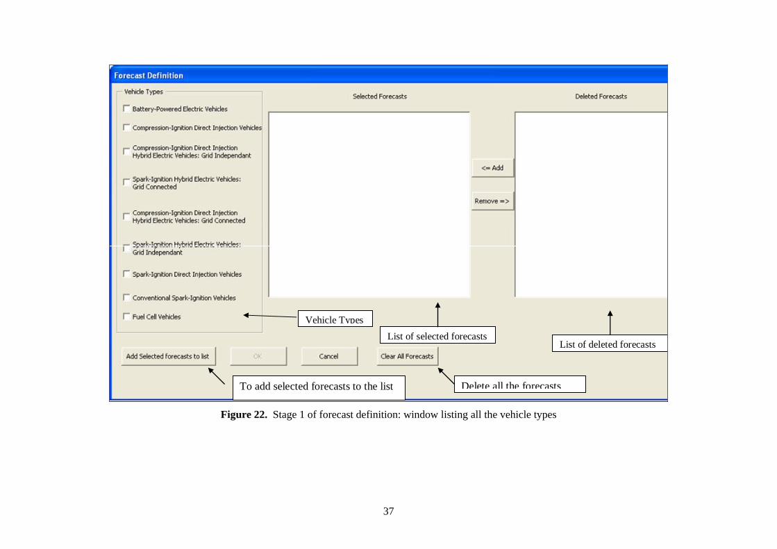
To begin, click on “Forecast Cells” in the command bar, to display the forecast window as

shown in Figure 22. Step 1 of the forecast selection provides a list of vehicle types.

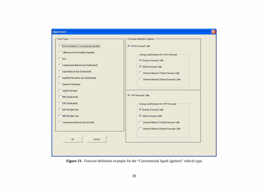
When you select a checkbox for a particular vehicle technology, e.g., “Conventional Spark

Ignition,” the window shown in Figure 23 is displayed. This window contains three frames:

a) Fuel type specification

b) WTW simulation option and/or WTP simulations option

c) Energy and emission groups

36

For any fuel type, the WTW and WTP boxes, and the energy and GHG forecasts are selected by

default. If you do not select any fuel type before clicking “OK,” these default selections will be

ignored when the stochastic simulation is executed.

After making the necessary selections in this window, click “OK” and repeat the process for

other vehicle technologies as needed.

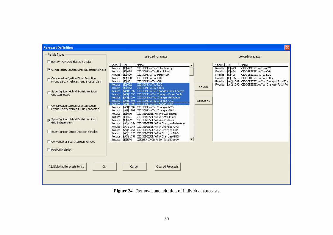
Once you finish defining the forecasts, click on the button captioned “add forecasts to list” in

the "Forecast Definition" window to add the defined forecasts to the “Selected” listbox (see

Figure 22). This adds the selected forecasts to the “selected” listbox, enabling you to remove/add

individual forecasts as needed using the “Remove =>” and “<= Add” buttons in that window.

This process is shown in Figure 24.

Once the forecasts are added to the “Selected” listbox, individual forecasts can be moved back

and forth to and from the “Deleted” listbox. When a vehicle technology is unchecked, the

corresponding forecasts are automatically deleted from the list.

The naming convention for the forecasts is “Vehicle Technology – Transportation Fuel – WTW

and/or WTP – Energy and Emission Forecast.” For example, “CIDI-DME-WTW-N2O” can be

interpreted as the well-to-wheels N2O emission results for the CIDI vehicle fueled with DME.

The forecasts listed in the list box titled “Selected” are the forecasts which would be predicted at

the end of the stochastic simulation.

After completing the forecast selection process, click the “OK” button to confirm the list of

selected forecasts.

37

Vehicle TypesList of selected forecasts

List of deleted forecasts

To add selected forecasts to the list Delete all the forecasts

Figure 22. Stage 1 of forecast definition: window listing all the vehicle types

38

Figure 23. Forecast definition example for the “Conventional Spark Ignition” vehicle type

39

Figure 24. Removal and addition of individual forecasts

40

5.4 Delete Distributions For any parametric assumption cell with a probability distribution, if you decide to just assign a

point value to that cell, the probability distribution can be deleted by selecting the cell and

clicking on the “Deleted Distribution” button. The input distribution is automatically deleted and

the cell color turns from green to white.

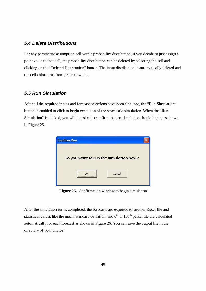
5.5 Run Simulation After all the required inputs and forecast selections have been finalized, the “Run Simulation”

button is enabled to click to begin execution of the stochastic simulation. When the “Run

Simulation” is clicked, you will be asked to confirm that the simulation should begin, as shown

in Figure 25.

Figure 25. Confirmation window to begin simulation

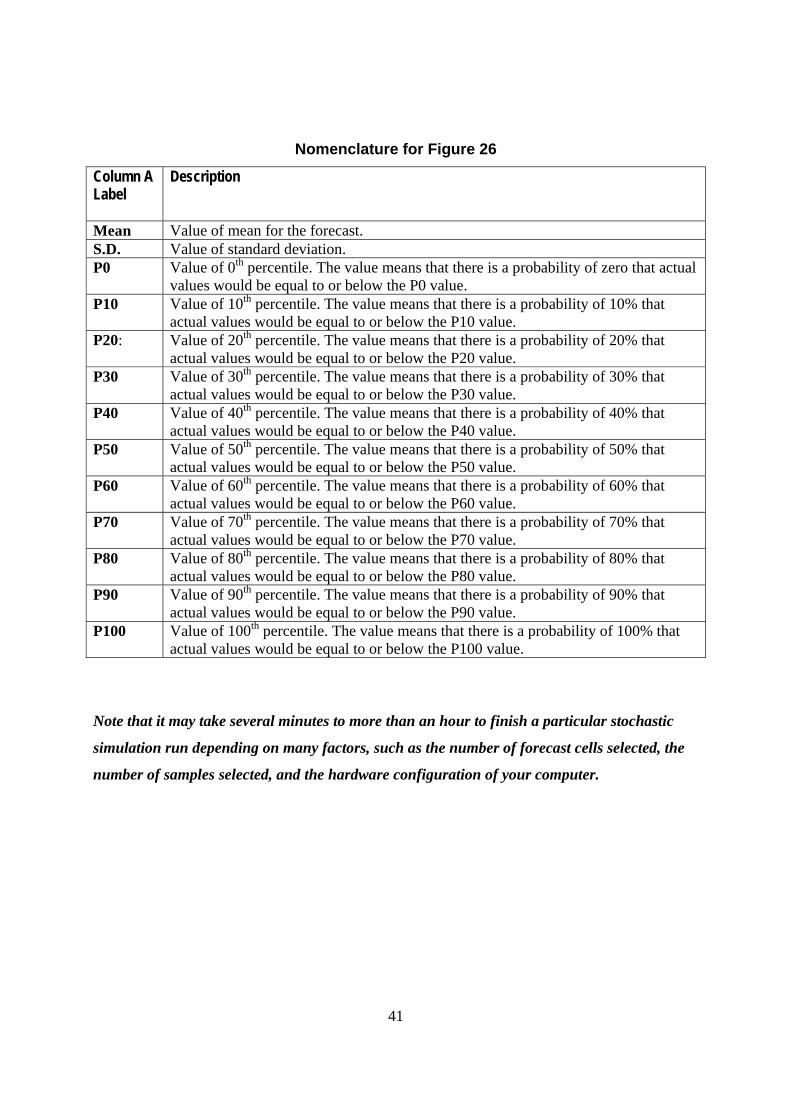
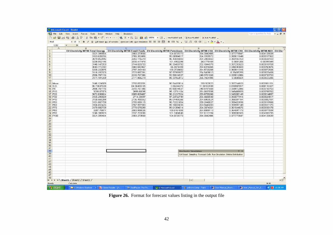
After the simulation run is completed, the forecasts are exported to another Excel file and

statistical values like the mean, standard deviation, and 0th to 100th percentile are calculated

automatically for each forecast as shown in Figure 26. You can save the output file in the

directory of your choice.

41

Nomenclature for Figure 26

Column A Label

Description

Mean Value of mean for the forecast. S.D. Value of standard deviation. P0 Value of 0th percentile. The value means that there is a probability of zero that actual

values would be equal to or below the P0 value. P10 Value of 10th percentile. The value means that there is a probability of 10% that

actual values would be equal to or below the P10 value. P20: Value of 20th percentile. The value means that there is a probability of 20% that

actual values would be equal to or below the P20 value. P30 Value of 30th percentile. The value means that there is a probability of 30% that








actual values would be equal to or below the P100 value.

Note that it may take several minutes to more than an hour to finish a particular stochastic

simulation run depending on many factors, such as the number of forecast cells selected, the

number of samples selected, and the hardware configuration of your computer.

42

Figure 26. Format for forecast values listing in the output file

43

Acknowledgments This effort was funded by Argonne National Laboratory. The authors thank Drs. Amgad

Elgowainy, Michael Wang, and Ye Wu of Argonne National Laboratory for their inputs during

the course of developing the stochastic simulation tool for Argonne’s GREET model.

References 1. Diwekar, U.M., Introduction to Applied Optimization, Kluwer Academic Publishers,

Dordrecht, 2003.

2. Kalagnanam J.R. and U.M. Diwekar, “An Efficient Sampling Technique for Off-line Quality

Control,” Technometrics 39(3), 308, 1997.

3. Diwekar, U., & J. Kalagnanam, “An efficient sampling technique for optimization under

uncertainty,” AIChE Journal 43, 440–459, 1997.

4. Wang, R., U.M. Diwekar, and C. Gregoire-Padro, “Latin Hypercube Hammersley Sampling

for risk and uncertainty analysis,” Environmental Progress 23(2):141, 2004.

44

This page intentionally left blank.

Documents

User Manual for Stochastic Sumulation Capability in GREET