User's Guide for the Rapid Assessmentof the Functional Condition of Stream-

Riparian Ecosystems in the American Southwest

Peter B. Stacey, Allison L. Jones, Jim C. Catlin, Don A. Duff

Lawrence E. Stevens, and Chad Gourley

Authors:

Peter B. Stacey is a Research Professor in the Department of Biology, University of New Mexico, Albuquerque,NM 87131. His teaching and research interests include restoration and conservation biology. He has conductednumerous studies on the ecology and population dynamics of birds that utilize riparian habitats, including theendangered southwestern willow flycatcher and the Mexican spotted owl.

Allison Jones is the conservation biologist at the Wild Utah Project, 68 South Main Street, Salt Lake City, UT84101. She previously has worked as an ecological consultant, where she conducted wetland delineations and habi-tat assessments, surveys for riparian-obligate threatened and endangered species, and helped design and carry-outwetland and riparian mitigation projects. Her current research interests include the analysis of livestock grazingmanagement and impacts.

James C. Catlin is also with the Wild Utah Project. He is the project coordinator of the Wild Utah Project, and spe-cializes in habitat analysis for a variety of species at risk. His current research efforts focus on how livestock graz-ing affects wildlife habitat and forage availability in both riparian zones and uplands.

Don A. Duff is an aquatic ecologist retired from the U.S. Forest Service. He is currently a technical consultant forTrout Unlimited at 421 E. 10th Ave., Salt Lake City, UT 84103. He also held positions in fisheries with the Bureauof Land Management and the U.S. Fish and Wildlife Service. His career experience has been in aquatic and ripari-an habitat management and native fishes recovery, and he has directed many stream-riparian restoration projects.

Lawrence E. Stevens is the principle author for an assessment protocol that determines the health and function ofsouthwest springs. He is an entomologist and riparian ecologist with the Grand Canyon Wildlands Council, P.O.Box 1315, Flagstaff, AZ 86002.

Chad Gourley is a fluvial geomorphologist who has directed a number of riparian restoration projects in the west-ern United States. He is with Otis Bay Consultants, 9225 Cordoba Blvd., Sparks, NV 89436.

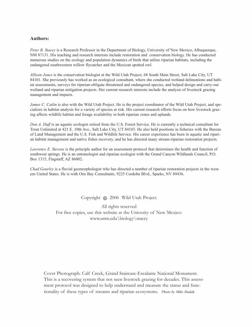
Cover Photograph: Calf Creek, Grand Staircase-Escalante National Monument.This is a recovering system that not seen livestock grazing for decades. This assess-ment protocol was designed to help understand and measure the status and func-tionality of these types of streams and riparian ecosystems. Photo by Mike Hudak.

Copyright 8 2006 Wild Utah Project

All rights reservedFor free copies, use this website at the Univesity of New Mexico:

www.unm.edu\biology\stacey

Table of Contents

Summary . . . . . . . . . . . . . . . . . . . . . . . . . . . . . . . . . . . . . . . . . . . . . . . . . . . . . . . . .2

1. Introduction to the Rapid Stream-Riparian Assessment Method . . . . . . . . . . . .3Table 1: RSRA indicator variables and justification . . . . . . . . . . . . . . . . . . . . .4

2. Conducting the Rapid Stream-Riparian Assessment . . . . . . . . . . . . . . . . . . . . .8A. Identify study reach of interest . . . . . . . . . . . . . . . . . . . . . . . . . . . . . . . . . . .8B. Identify one or more reference reaches . . . . . . . . . . . . . . . . . . . . . . . . . . . . .8C. Collect background information on the reference reach and study reach . .9

Box 1: Background information to help interpret site visit . . . . . . . . . . . . .9D. Conduct the RSRA field assessment . . . . . . . . . . . . . . . . . . . . . . . . . . . . . . .11

1. Field Gear . . . . . . . . . . . . . . . . . . . . . . . . . . . . . . . . . . . . . . . . . . . . . . . . . .112. Timing . . . . . . . . . . . . . . . . . . . . . . . . . . . . . . . . . . . . . . . . . . . . . . . . . . . . .113. Establishment of Transects . . . . . . . . . . . . . . . . . . . . . . . . . . . . . . . . . . . . .114. Scoring - General Considerations . . . . . . . . . . . . . . . . . . . . . . . . . . . . . . . .125. Tallying the Scores and Interpretation . . . . . . . . . . . . . . . . . . . . . . . . . . . .13

3. Specific Directions for Scoring Each Indicator . . . . . . . . . . . . . . . . . . . . . . . . .14A. Water Quality . . . . . . . . . . . . . . . . . . . . . . . . . . . . . . . . . . . . . . . . . . . . . . . . .15B. Hydro-geomorphology . . . . . . . . . . . . . . . . . . . . . . . . . . . . . . . . . . . . . . . . .16C. Fish/Aquatic Habitat . . . . . . . . . . . . . . . . . . . . . . . . . . . . . . . . . . . . . . . . . . .21D. Riparian Vegetation . . . . . . . . . . . . . . . . . . . . . . . . . . . . . . . . . . . . . . . . . . . .25E. Terrestrial Wildlife Habitat . . . . . . . . . . . . . . . . . . . . . . . . . . . . . . . . . . . . . .32

Definitions . . . . . . . . . . . . . . . . . . . . . . . . . . . . . . . . . . . . . . . . . . . . . . . . . . . . . . .34

Appendix 1. Drawings of Aquatic Insect Orders Typically Found in the Southwestern United States. . . . . . . . . . . . . . . . . . . . .37

Appendix 2. The RSRA Score Sheet . . . . . . . . . . . . . . . . . . . . . . . . . . . . . . . . . . .39Appendix 3. The RSRA Field Worksheet . . . . . . . . . . . . . . . . . . . . . . . . . . . . . . .45Appendix 4. Human Impacts Worksheet . . . . . . . . . . . . . . . . . . . . . . . . . . . . . . . .53

1

Summary

Stream-riparian ecosystems are among the most productive, biologically diverse and threatenedhabitats in arid regions, including the American Southwest. Standardized assessment protocolsare needed in order to effectively measure the current health and functional condition of theseecosystems, as well as to serve as a guide for future restoration and monitoring programs.However, most existing survey methods either focus on only a limited subset of the differentcomponents of the ecosystem, base their evaluations upon some hypothesized future state ratherthan upon the current conditions of the reach, and/or rely heavily upon subjective judgments ofecosystem health. We describe an integrated, multi-dimensional method for rapid assessment ofthe functional condition of riparian and associated aquatic habitats called Rapid Stream-Riparian Assessment (RSRA). This method evaluates the extent to which natural processes pre-dominate in the stream-riparian ecosystem and whether there is sufficient terrestrial and aquatichabitat complexity to allow for the development of diverse native plant and animal communi-ties.

The Rapid Stream-Riparian Assessment involves a quantitative evaluation of between two toseven indicator variables in five different ecological categories: water quality, fluvial geomor-phology, aquatic and fish habitat, vegetation composition and structure, and terrestrial wildlifehabitat. Each variable is rated on a scale that ranges from "1", representing highly impacted andnon-functional conditions, to "5", representing a healthy and completely functional system.Whenever possible, scores are scaled against what would be observed in control or referencesites that have similar ecological and geophysical characteristics, but which have not been heav-ily impacted by human activities. The protocol was designed to be used both by specialists andby non-specialists after suitable training. It is particularly appropriate for small to medium sizedstreams and rivers in the American Southwest, but with slight modification it also should beapplicable to reaches in other temperate regions and geomorphic settings.

2

1. Introduction to the User’s Guide for the Rapid Assessment of theFunctional Condition of Stream-Riparian Ecosytems in the AmericanSouthwest.

Stream-riparian zones are some of the most productive and important natural resources foundon public and private lands. These ecosystems are highly valued as habitats for fish andwildlife, as a water source for human communities, for recreation, and for many different eco-nomic uses. This is particularly true in arid and semi-arid regions like the American Southwest,where riparian areas support a biotic community whose richness far exceeds the relative totalland area that these systems occupy.

Because of both the ecological importance of riparian areas and their heavy utilization byhumans, there is a need for assessment methods that can be used to objectively evaluate theexisting conditions of the stream-riparian ecosystem, detect at-risk components, prioritize man-agement strategies and/or possible restoration activities if problems are discovered, and then beused to objectively monitor any future changes within the system. An effective assessment pro-tocol must include consideration of the interactions among stream, fluvial wetland, and riparianhabitats (here referred to as the stream-riparian ecosystem), as well as the potential impacts ofupstream and adjacent upland areas.

The Rapid Stream-Riparian Assessment (RSRA) utilizes a primarily qualitative assessmentbased on quantitative measurements. It focuses upon five functional components of the stream-riparian ecosystem that provide important benefits to humans and wildlife, and which, on publiclands, are often the subject of government regulation and standards. These components are: 1)water quality and pollution, 2) stream channel and flood plain morphology and the ability of thesystem to limit erosion and withstand flooding without damage, 3) the presence of habitat fornative fish and other aquatic species, 4) vegetation structure and composition, including theoccurrence and relative dominance of exotic or non-native species, and 5) suitability as habitatfor terrestrial wildlife, including threatened or endangered species.

Within each of these areas, the RSRA evaluates between two and seven variables which reflectthe overall function and health of the stream-riparian ecosystem. The basis for the inclusion ofthe individual indicators is briefly summarized in Table 1. A more complete discussion of thevariables, including selected references, can be found in Stevens et al. (2005)1. Definitions ofkey terms used in Table 1 are provided at the end of the User's Guide; illustrations of selectedvariables accompany the directions for scoring those indicator variables that are included inSection 3.

3

1 Stevens, L.E., Stacey, P.B., Jones, A. L., Duff, D., Gourley, C., and J.C. Catlin. 2005. A protocol for rapidassessment of southwestern stream-riparian ecosystems. Proceedings of the Seventh Biennial Conference ofResearch on the Colorado Plateau titled The Colorado Plateau II, Biophysical, Socioeconomic, and CulturalResearch. Charles van Riper III and David J. Mattsen, Ed.s pp 397-420. Tuscon, AZ: University of Arizona Press.

Table 1: RSRA indicator variables and the reasons for including them in the protocol.

4

CATEGORY AND VARIABLE JUSTIFICATION FOR INCLUSION IN RSRA ASSESSMENT

Water Quality: Algal growth

Dense algal growth may indicate nutrient enrichment and other types of pollution which may result in decreased dissolved oxygen in the water column and affect invertebrates and the ability of fish to spawn.

Water Quality: Channel shading and solar exposure

Solar exposure affects stream temperature and productivity. Decreased streambank vegetation cover, increased channel width, and reduced stream depth increases exposure, raises water temperatures and impacts aquatic life. Native trout usually require cool stream temperatures.

Hydrogeomorphology: Floodplain connection and inundation frequency

Channels that are deeply downcut or incised result in a reduced frequency of overbank flooding into the adjacent flood plain during peak runoff or stream flows. The absence of flooding lowers water tables, reduces nutrient availability in the floodplain, decreases plant germination, growth and survivorship, and may lead to the loss of riparian vegetation and the invasion of upland species.

Hydrogeomorphology: Vertical bank stability

Steep and unstable vertical banks dominate many southwestern streams, limiting the physical dynamics of aquatic ecosystems and increasing erosion and sediment loads through sloughing off of soils during high flow events. Steep banks may limit wildlife access to water.

Hydrogeomorphology: Hydraulic habitat diversity

Fish and aquatic invertebrate diversity and population health is related to habitat diversity. Features such as oxbows, side channels, sand bars, gravel/cobble bars, riffles, and pools can provide habitat for different species or for the different life stages of a single species.

Hydrogeomorphology: Riparian area soil integrity

Riparian soils reflect existing stream flow dynamics (e.g., flooding), management practices, and vegetation. It affects potential vegetation dynamics and species composition, as well as wildlife habitat distribution and quality.

Hydrogeomorphology: Beaver activity

Beavers are keystone species in riparian systems because they modify geomorphology and vegetation, and reduce variance in water flows and the frequency of floods. Beaver dams and adjacent wet meadows provide important fish and plant nursery habitat.

Fish/Aquatic Habitat Qualifier: Loss of perennial flows

Fish and most aquatic invertebrates require perennial or constant flows to survive. Streams that were originally perennial but are now ephemeral no longer provide habitat for these species unless there are refuges that never dry out (e.g., permanent pools).

Fish/Aquatic Habitat: Pool distribution

Fish use pools, with reduced current velocity and deep water, to rest, feed and hide from predators. Many species use gravel-bottomed riffles to lay their eggs. The number, size, distribution, and quality of pools, and pool to riffle ratios indicate the quality of fish habitat. 1:1 pools to riffle ratios are generally considered to be optimum.

Fish/Aquatic Habitat: Underbank cover

Underbank cover is an important component of good fish habitat, used for resting and protection from predators. A number of aquatic invertebrates also use these areas. Underbank cover usually occurs with vigorous vegetative riparian growth, dense root masses, and stable soil conditions.

Fish/Aquatic Habitat: Cobble embeddedness

Low levels of gravel and boulder embeddedness on the channel bottom increase benthic productivity and fish production. The filling of interstitial spaces between rocks with silt, sand, and organic material reduces habitat suitability for feeding, nursery cover, and spawning (egg to fry survival) by limiting space and macroinvertebrate production. Increased embeddedness often reflects increased sediment loads and altered water flow patterns.

Fish/Aquatic Habitat: Diversity of aquatic invertebrates

The density and composition of aquatic invertebrates are strong indicators of stream health, including temperature stresses, oxygen levels, nutrients, pollutants, and sediment loads. Larvae and adult macroinvertebrates provide critical food for fish and other invertebrate and vertebrate species in stream-riparian ecosystems.

5

CATEGORY AND VARIABLE JUSTIFICATION FOR INCLUSION IN RSRA ASSESSMENT

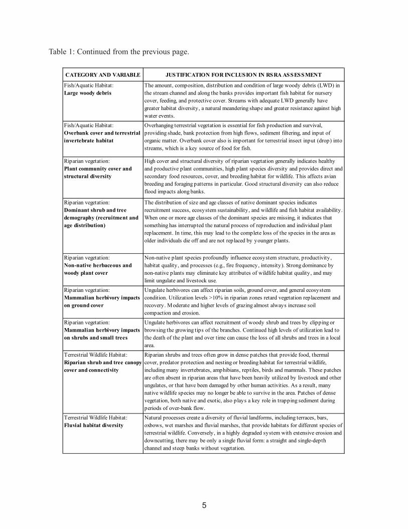
Fish/Aquatic Habitat: Large woody debris

The amount, composition, distribution and condition of large woody debris (LWD) in the stream channel and along the banks provides important fish habitat for nursery cover, feeding, and protective cover. Streams with adequate LWD generally have greater habitat diversity, a natural meandering shape and greater resistance against high water events.

Fish/Aquatic Habitat: Overbank cover and terrestrial invertebrate habitat

Overhanging terrestrial vegetation is essential for fish production and survival, providing shade, bank protection from high flows, sediment filtering, and input of organic matter. Overbank cover also is important for terrestrial insect input (drop) into streams, which is a key source of food for fish.

Riparian vegetation: Plant community cover and structural diversity

High cover and structural diversity of riparian vegetation generally indicates healthy and productive plant communities, high plant species diversity and provides direct and secondary food resources, cover, and breeding habitat for wildlife. This affects avian breeding and foraging patterns in particular. Good structural diversity can also reduce flood impacts along banks.

Riparian vegetation: Dominant shrub and tree demography (recruitment and age distribution)

The distribution of size and age classes of native dominant species indicates recruitment success, ecosystem sustainability, and wildlife and fish habitat availability. When one or more age classes of the dominant species are missing, it indicates that something has interrupted the natural process of reproduction and individual plant replacement. In time, this may lead to the complete loss of the species in the area as older individuals die off and are not replaced by younger plants.

Riparian vegetation: Non-native herbaceous and woody plant cover

Non-native plant species profoundly influence ecosystem structure, productivity, habitat quality, and processes (e.g., fire frequency, intensity). Strong dominance by non-native plants may eliminate key attributes of wildlife habitat quality, and may limit ungulate and livestock use.

Riparian vegetation: Mammalian herbivory impacts on ground cover

Ungulate herbivores can affect riparian soils, ground cover, and general ecosystem condition. Utilization levels >10% in riparian zones retard vegetation replacement and recovery. Moderate and higher levels of grazing almost always increase soil compaction and erosion.

Riparian vegetation: Mammalian herbivory impacts on shrubs and small trees

Ungulate herbivores can affect recruitment of woody shrub and trees by clipping or browsing the growing tips of the branches. Continued high levels of utilization lead to the death of the plant and over time can cause the loss of all shrubs and trees in a local area.

Terrestrial Wildlife Habitat: Riparian shrub and tree canopy cover and connectivity

Riparian shrubs and trees often grow in dense patches that provide food, thermal cover, predator protection and nesting or breeding habitat for terrestrial wildlife, including many invertebrates, amphibians, reptiles, birds and mammals. These patches are often absent in riparian areas that have been heavily utilized by livestock and other ungulates, or that have been damaged by other human activities. As a result, many native wildlife species may no longer be able to survive in the area. Patches of dense vegetation, both native and exotic, also plays a key role in trapping sediment during periods of over-bank flow.

Terrestrial Wildlife Habitat: Fluvial habitat diversity

Natural processes create a diversity of fluvial landforms, including terraces, bars, oxbows, wet marshes and fluvial marshes, that provide habitats for different species of terrestrial wildlife. Conversely, in a highly degraded system with extensive erosion and downcutting, there may be only a single fluvial form: a straight and single-depth channel and steep banks without vegetation.

Table 1: Continued from the previous page.

Indicator Selection

Four principles guided our selection of the specific variables that are included in the RSRA.First, we focused upon indicators that not only measured the ability of the system to providespecific functions, but that at the same time would reflect other important ecological processeswithin the stream-riparian system. For example, in the fish habitat section we consider the rela-tive amount of undercut banks along the reach. Undercut banks not only provide importanthabitat and cover for fish and other aquatic species, but their presence indicates that the bankitself is well vegetated, and that there is sufficient root mass to allow the development of thehour-glass shape channel cross-section typical of most healthy stream systems. This in turnwould suggest that the fluvial processes of erosion and deposition along that stretch of the reachare in relative equilibrium.

Second, we focused upon variables that could be measured rapidly in the field and that wouldnot require specialized equipment or training. As a result, the protocol can be conducted notonly by specialists, but also by conservationists, agency personnel, ranchers, and interested lay-people that have received some initial training. More detailed methods have been developed formany of the individual indicators included in this protocol. However, because they often requireconsiderable time and expensive equipment, the use of such protocols will often limit the otherkinds of information that can be reasonably collected from the reach. Our goal was to obtain anoverall picture of the functioning of the system under assessment within a two to three hourperiod. Should any of the individual components of the reach be found to be particularly prob-lematic or non-functional, the more specialized methods can then be used during later visits tocollect additional quantitative information on that variable.

Third, we measure only the current condition of the ecosystem, rather than creating scores thatare based upon some hypothesized future state or successional trend. That is, we are concernedwith the ability of the ecosystem to provide some important function at the present time, andnot whether it would be likely to do so at some point in the future, if current trends or manage-ment practices continue. We used this approach because stream-riparian systems are highlydynamic and they are often subject to disturbances (e.g., large flooding) that will alter succes-sional trends and make predictions of future conditions highly problematic.

In addition, by evaluating only current conditions, this protocol can be used as a powerful toolfor monitoring and measuring future changes in the functional status of the system. For exam-ple, if a reach is rated as in poor condition with respect to a particular set of parameters, reeval-uating the system using the identical protocol in subsequent years gives one the ability to meas-ure the effectiveness of any management change or active restoration program and to undertakecorrections if the restoration actions are found to be not producing the desired changes. Thistype of adaptive management approach can be extremely difficult if the evaluation and monitor-ing measures are based primarily upon the expectations of some future, rather than current, con-dition.

Fourth, and for similar reasons, we use a quantitative approach to score variables and measure ecosystem health. Many current assessment systems that are based upon dichotomous

6

categories, such as "functional/non-functional", or "yes/no", can be subjective and difficult torepeat in the same way from one year to the next, or when conducted by different observers. Inaddition, dichotomous scoring systems often are not able to provide sufficient insight into theecological processes that may be affecting the ability of the system to provide (or not provide)desired functions that would indicate whether active restoration efforts might be necessary. Weused a review of existing assessment and monitoring protocols, extensive external peer-review,and our own individual research experiences to create a five point scale for each variable. Themaximum score (5 points) is given when that component of the system is fully functional andhealthy, and is what would be found in a similar reach that has not been heavily impacted byhumans. The minimum score (1 point) is given when the component is completely non-func-tional, and when it is not capable of providing the desired ecosystem value of that variable.2

Reference Reaches

Every stream will have its own geologic and watershed characteristics that will necessarily limitboth its potential geomorphic form and its ultimate ecological function. For example, streams innarrow bed-rock canyons will never develop the same number of meanders and flood plainwidth as will similarly sized streams that run through broad alluvial fans. For this reason, wesuggest that whenever possible, the stream reach under evaluation should be compared to a ref-erence reach, and the scores given be scaled with respect to that reach. Reference areas shouldhave similar geomorphic, fluvial and biological characteristics to the study reach, and should beas free as possible of current and past human impacts. When this type of reference reach is notavailable, ratings should be based upon what the observer would expect to see if all physicaland ecological processes were occurring without human impact, while allowing for natural dis-turbance processes that may be characteristic of the system.

Geographic Application

The RSRA protocol presented here was developed specifically in reference to small and medi-um sized stream reaches in the Colorado Plateau and in the adjacent areas of the AmericanSouthwest. It applies most directly to low and mid-gradient watercourses, and therefore will bemost useful in the lower and middle elevation watersheds of this region. Large streams andrivers, as well as those at high elevations in mountainous regions that have high gradients, areoften subject to forces and conditions that are not fully considered here and therefore may notbe adequately described by this protocol. However, with only slight modification, the RSRAshould be applicable to many other parts of the American West, as well as to other arid andsemi-arid regions of the world.

7

2 The range of scores used in the RSRA method from 1 to 5 is similar to the functional condition judgments usedby the US Bureau of Land Management and other agencies in their “Proper Functioning Condition” (PFC) assess-ment protocol (USDI 1998). In that system, streams are rated as ranging from either “not in proper functioningcondition,” which would be equivalent to mean scores of 1-2 in the RSRA, to “in proper functioning condition,”which would be equivalent to means scores of 4-5 in the RSRA. Intermediate scores in the RSRA protocol (>2 -<4) can be considered to be equivalent to the “functional at risk” rating in the PFC protocol. Additional discussionof the similarities and differences between the RSRA and PFC survey protocols is given in Stevens et al. (2005).

2. Conducting the Rapid Stream-Riparian Assessment

The overall approach for assessing stream-riparian health with the RSRA protocol is to:

A. Identify the specific reach of interest within a watershedB. Identify, if possible, a reference area for that reach with similar geomorphology and biotic

structureC. Collect as much background information on the reach as is available and appropriateD. Conduct the protocol in the field

We recommend that the protocol be conducted by a team of at least two or three people, andthat each team member read this User's Guide and become familiar with the RSRA FieldWorksheet and Score Sheet (Appendices 2 and 3) before beginning the field surveys.

A. Identify the Study Reach of Interest

The segment of a stream or river that is to be examined should be representative of the area ofinterest, and it should generally be relatively uniform in character, landform, geology and vege-tation. The study reach should be approximately 1 km in length, and, when possible, include atleast 3-4 stream meanders. Different reaches within a watershed may have different characteris-tics due to varying geology, hydrology, elevation, and past histories of land use. In such cases,it is appropriate to conduct separate evaluations in several different reaches. The location of thestudy stream reach should be representative of the range of conditions found in the watershedand should not be chosen to illustrate particularly good (or bad) conditions that would bias thescores given to the entire stream.

B. Identify One or More Reference Reaches

Because of the long history of occupation and use by Native Americans and Hispanic andAnglo settlers, it can often be difficult to visualize the natural or unaltered condition of manywestern streams and rivers. Therefore, whenever possible, reference sites should be identifiedand visited prior to conducting the protocol on the study reach itself. These sites can also be agood location to train new individuals about general ecological and fluvial processes, as well asin the use of the protocol itself.

In choosing a reference reach, the team should look for systems with the following characteris-tics: 1) similar geology, elevation, and flow patterns (both in the amount and timing of peak andaverage water flows) to the study reach; and 2) nearly natural or close to natural conditions andas free as possible from recent and historic human caused disturbances, especially water diver-sions, roads, livestock grazing, mining, and ground water pumping. Streams that have been sub-ject to recent catastrophic disturbances such as fires or heavy flooding will not usually serve asgood reference reaches since they may still be in the process of recovering or reaching a newequilibrium after the disturbance.

8

In some situations, a good reference site may not be available in the immediate area. In thesecases, streams in other watersheds or regions that have similar geomorphic and ecological fea-tures can be used to gain a basic understanding of the general fluvial and ecological processesthat would be expected in the study reach under unaltered conditions, and can thus offer a rea-sonable "surrogate" reference site.

C. Collect Background Information on the Reference Reach and Study Reach

Prior to using RSRA in the field, it is recommended that the user collect some basic, back-ground information on the study reach (see Box 1 for specific suggestions). In a few cases,information gathered ahead of time will be needed to complete a score sheet item; those cate-gories marked optional will be helpful to interpreting the field scores, but are not needed toassign the actual scores themselves.

9

BOX 1: BACKGROUND INFORMATION TO HELP INTERPRET SITE VISIT

The information listed below gives a range of data that could be useful in understanding presentand past conditions on the study reach. Three kinds of background information are needed to answer spe-cific items in the Score Sheet: whether beavers were historically present in the watershed, whether thestream was historically perennial, and the various species of non-native or exotic plant species that havebeen reported or are likely to be encountered at the study reach. The other information listed here is notrequired, but may help to explain why the reach scores the way it does for individual indicators. Not all ofthe data will be available for any particular reach. Possible sources of information include local land man-agement agencies, state and federal soil and conservation services, local residents, distribution maps offish and wildlife from past surveys, etc.

Water Quality 1. (optional) Are there known sources of pollution that should be considered in the evaluation (e.g.,

upstream mine tailings, water treatment facilities, or livestock feedlots and holding pens)?

Hydro/Geomorphology1. (optional) Determine origin(s) of stream flow for the study reach (size of watersheds, springs, etc.).

Is it likely to be subject to large flows or flooding events? 2. (optional) Determine human alterations of flow (dams, diversions or augmentations).3. (optional) Determine whether there have been alterations in the upland portions of the watershed that

might impact the stream (e.g., timber harvests that might lead to increased sediment loads).4. (optional) Determine the current sinuosity of study reach. This can be defined as the ratio of the actual

distance or length of a channel to the straight line distance between the beginning and end of the study reach, and is best measured using aerial photographs. Such photographs may also show geomorphic evidence of past meanders, which can then make it possible to determine changes in sinuosity over time. Sinuosity information can also be used to place the study reach within various classification schemes, such as the categories developed by Rosgen (D.L. Rosgen, A Classification of Natural Rivers, Catena 22(1994), pages 169-199).

5. (required) Indicator 7 considers historic use of the study reach by beavers. Use existing records or recollections by local residents to determine if beavers were ever present on the reach.

10

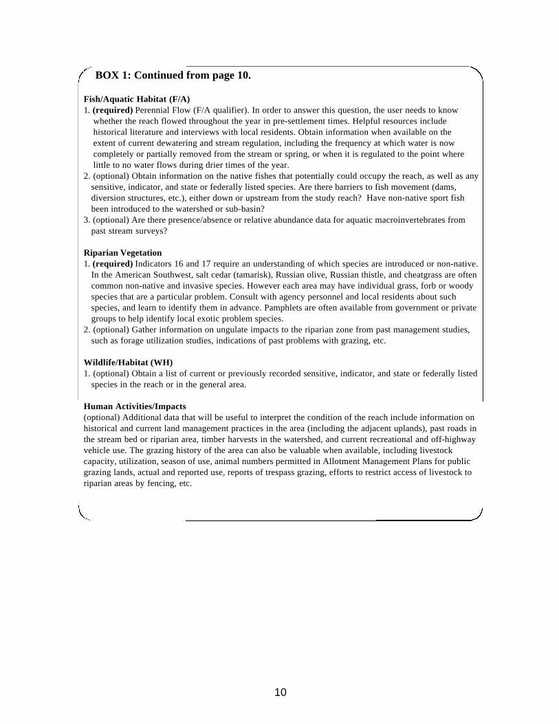
BOX 1: Continued from page 10.

Fish/Aquatic Habitat (F/A)1. (required) Perennial Flow (F/A qualifier). In order to answer this question, the user needs to know

whether the reach flowed throughout the year in pre-settlement times. Helpful resources include historical literature and interviews with local residents. Obtain information when available on the extent of current dewatering and stream regulation, including the frequency at which water is now completely or partially removed from the stream or spring, or when it is regulated to the point wherelittle to no water flows during drier times of the year.

2. (optional) Obtain information on the native fishes that potentially could occupy the reach, as well as anysensitive, indicator, and state or federally listed species. Are there barriers to fish movement (dams, diversion structures, etc.), either down or upstream from the study reach? Have non-native sport fish been introduced to the watershed or sub-basin?

3. (optional) Are there presence/absence or relative abundance data for aquatic macroinvertebrates from past stream surveys?

Riparian Vegetation 1. (required) Indicators 16 and 17 require an understanding of which species are introduced or non-native.

In the American Southwest, salt cedar (tamarisk), Russian olive, Russian thistle, and cheatgrass are often common non-native and invasive species. However each area may have individual grass, forb or woody species that are a particular problem. Consult with agency personnel and local residents about such species, and learn to identify them in advance. Pamphlets are often available from government or privategroups to help identify local exotic problem species.

2. (optional) Gather information on ungulate impacts to the riparian zone from past management studies, such as forage utilization studies, indications of past problems with grazing, etc.

Wildlife/Habitat (WH)1. (optional) Obtain a list of current or previously recorded sensitive, indicator, and state or federally listed

species in the reach or in the general area.

Human Activities/Impacts (optional) Additional data that will be useful to interpret the condition of the reach include information onhistorical and current land management practices in the area (including the adjacent uplands), past roads inthe stream bed or riparian area, timber harvests in the watershed, and current recreational and off-highwayvehicle use. The grazing history of the area can also be valuable when available, including livestockcapacity, utilization, season of use, animal numbers permitted in Allotment Management Plans for publicgrazing lands, actual and reported use, reports of trespass grazing, efforts to restrict access of livestock toriparian areas by fencing, etc.

D. Conduct the RSRA field assessment

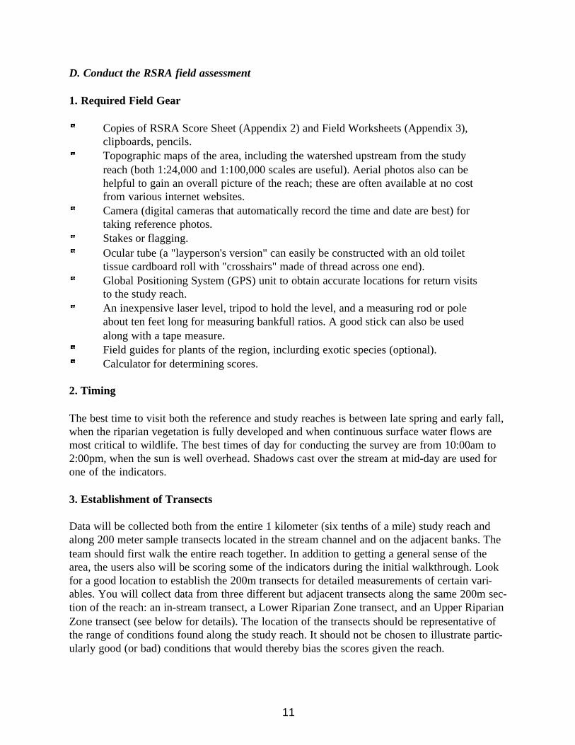
1. Required Field Gear

Copies of RSRA Score Sheet (Appendix 2) and Field Worksheets (Appendix 3),clipboards, pencils.Topographic maps of the area, including the watershed upstream from the study reach (both 1:24,000 and 1:100,000 scales are useful). Aerial photos also can be helpful to gain an overall picture of the reach; these are often available at no cost from various internet websites.Camera (digital cameras that automatically record the time and date are best) for taking reference photos.Stakes or flagging.Ocular tube (a "layperson's version" can easily be constructed with an old toilet tissue cardboard roll with "crosshairs" made of thread across one end).Global Positioning System (GPS) unit to obtain accurate locations for return visits to the study reach.An inexpensive laser level, tripod to hold the level, and a measuring rod or pole about ten feet long for measuring bankfull ratios. A good stick can also be used along with a tape measure.Field guides for plants of the region, inclurding exotic species (optional).Calculator for determining scores.

2. Timing

The best time to visit both the reference and study reaches is between late spring and early fall,when the riparian vegetation is fully developed and when continuous surface water flows aremost critical to wildlife. The best times of day for conducting the survey are from 10:00am to2:00pm, when the sun is well overhead. Shadows cast over the stream at mid-day are used forone of the indicators.

3. Establishment of Transects

Data will be collected both from the entire 1 kilometer (six tenths of a mile) study reach andalong 200 meter sample transects located in the stream channel and on the adjacent banks. Theteam should first walk the entire reach together. In addition to getting a general sense of thearea, the users also will be scoring some of the indicators during the initial walkthrough. Lookfor a good location to establish the 200m transects for detailed measurements of certain vari-ables. You will collect data from three different but adjacent transects along the same 200m sec-tion of the reach: an in-stream transect, a Lower Riparian Zone transect, and an Upper RiparianZone transect (see below for details). The location of the transects should be representative ofthe range of conditions found along the study reach. It should not be chosen to illustrate partic-ularly good (or bad) conditions that would thereby bias the scores given the reach.

11

To set up the transects, first mark the beginning of the in-stream or channel transect with a flag,measure 200 meters either upstream or downstream, and follow the center of the channel whenmaking measurements. Flag the end of the transect (make sure that all flagging and other mate-rials are removed at the end of the survey). Then, using the same starting point, measure 200malong the edge of the channel that marks the beginning of the Lower Riparian Zone. This tran-sect will usually be along the edge of the water or the edge of the channel if the stream is dry.Finally, and again using the same starting point, measure 200m just outside (in the directionaway from the stream) of the terrace that marks the boundary between the Lower Riparian Zone(the bankfull location, or area that is flooded during peak flows in most years) and the UpperRiparian Zone (the part of the flood plain that is flooded only irregularly and during exception-ally high flow events; see Figure 1). Because the channel and the terraces may follow differentpaths, the ending point of all three transects may not be located at the same precise place.

All locations (including the start and end points of the study reach, the starting point and direc-tion [upstream or downstream] of the 200m sample transects, and photo reference points)should be located with a GPS unit and recorded on the Score Sheet. Photographs to illustratethe current conditions at the site should be taken at least at the upstream and downstream endsof the stream reach, at each end of the 200m stream transect looking downstream and upstream,as well as any other location that would be valuable for future comparisons. Photographsshould include geologic features and the horizon to make relocation of the photo site easier inthe future.

4. Scoring - General Considerations

The 1-5 point range of scoring values assigned to each indicator on the RSRA Score Sheeteither involve specific values for that indicator, or it may use terms such as "few," "slight,""limited," "moderate," "substantial," or "abundant." In both situations, the evaluation team'sexperience in the reference riparian area(s) is very important to establish a standard of geomor-phic consistency and expected values for measurement. A score of "N/A" (Not Applicable) isassigned to variables that are not applicable to the particular reach being assessed. The FieldWorksheet in Appendix 3 organizes tasks by the initial whole reach walkthrough and the in-stream and vegetation sample transects. This worksheet will help simplify the observation anddata collection process but may not be necessary for highly experienced observers.

Each indicator is measured and the data recorded in the field, along with any additional com-ments that would assist in future interpretation of results. The most efficient method of scoringinvolves partitioning tasks among the team. For example, one individual who is well-versed inriparian plants may walk the 200m Upper and Lower Riparian transects, while another teammember who is more familiar with fluvial morphology and aquatic habitats can take measure-ments along the 200m in-stream transect.

After the initial data are collected on the worksheets, all members of the team should meet todiscuss their evaluations and scoring assignment for the Assessment Score Sheet, as well as anyrecommendations the team may make for the possible future restoration of the reach. It isimportant to emphasize that variables are scored entirely on the basis of existing conditions

12

within the reach and not on any potential or hypothesized future condition.

An additional worksheet on Human Impacts is included as Appendix 4. This worksheet shouldbe used to take note of various types of human activities and impacts that are occurring on thestudy reach or adjacent areas. This information is not used in the scoring because the RSRAmethod is specifically designed to measure the current ecological functioning and condition(health) of the reach, regardless of how those conditions came about. However, it can be usefulto take note of human-related impacts in the stream channel and floodplain, as these mayexplain why certain indicators may receive low functional scores. This information may alsoprovide suggestions for future restoration projects if needed.

5. Tallying the Scores and Interpretation

After completing all the field surveys, the observation team should rate each indicator from 1 to5, using the scoring definitions on the Score Sheet. Then, for each category, calculate andrecord the mean score for that set of indicators in that section and on the last page. The overallscore for the surveyed stream reach is then obtained by calculating the overall mean of the fivecategory mean scores.

An overall mean score of 1-2 indicates that most or all components of the stream are not func-tioning and that the reach probably cannot provide many of the values of healthy stream-ripari-an ecosystems. Scores of 2-4 indicate that some components may be in healthy condition whileothers are not, and/or that the entire system in general has been impacted by human activities ornatural disturbances in the past, but it is now in a transitional state. The direction of the change,and whether the system is improving or getting worse, can only be determined by subsequentvisits and monitoring programs. Scores of 4-5 indicate that the ecosystem is healthy and that itmatches what would be expected in a geomorphically similar reference reach or in an unim-pacted "presettlement" condition. Because of the dynamic nature of stream-riparian ecosystems,it is very unlikely that any reach, even one in pristine condition, would obtain a mean score of 5for any category or overall, and this should not be expected.

While a single composite site score is desirable for judging site health and developing regionalrestoration priorities as appropriate, such scores should not constitute the final interpretation ofsite status. While the overall score may indicate that a stream reach is functioning well, one ormore individual indicators may be extremely off balance. Very low individual or clusteredscores in an otherwise high scoring system often indicate that there are specific impacts on thestream or riparian area that should be addressed, and which, if not reversed, may eventuallylead to an overall decline in the health of the system. For example, a reach may be functioningwell physically, but be biologically degraded, in which case the need for restoration actiondepends on the management goals for that reach, and whether biological functions are impor-tant. Alternatively, a reach's hydrology and streamflow patterns may be highly altered but thesystem might appear otherwise healthy. Thus the interpretation of reach conditions shouldinvolve an analysis of the overall scores against the mean category scores and reference condi-tions to improve understanding of ecological function and management goals for the reach.

13

3. Specific Directions for Scoring Each Indicator

This section provides detailed instructions for collecting the information needed to score eachvariable. The instructions are given in the order the variables appear on the Score Sheet. TheField Worksheet organizes the variables according to the physical areas of observations, result-ing in a different order.

14

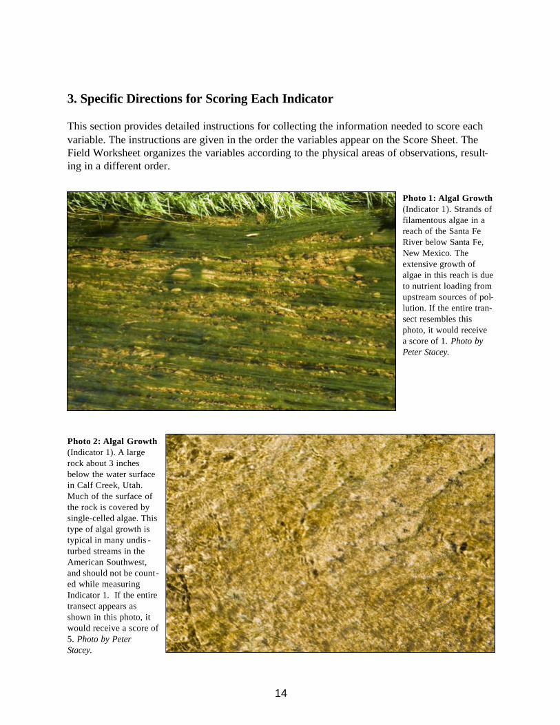
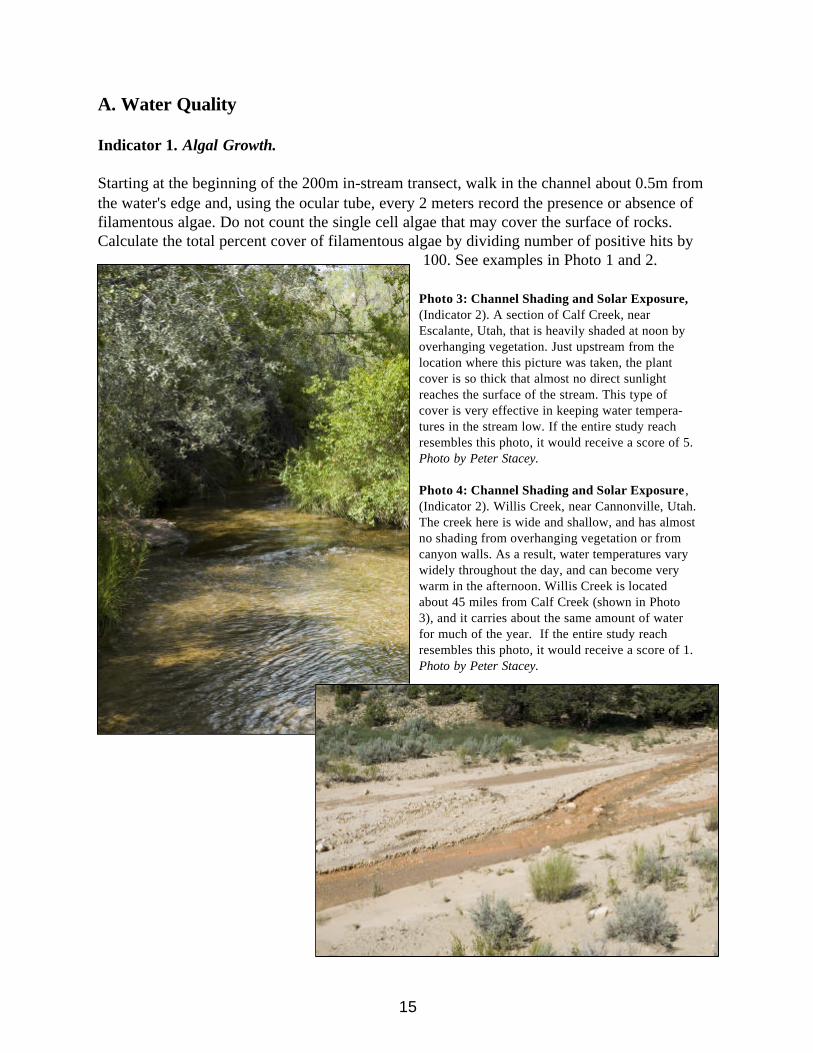
Photo 1: Algal Growth(Indicator 1). Strands offilamentous algae in areach of the Santa FeRiver below Santa Fe,New Mexico. Theextensive growth ofalgae in this reach is dueto nutrient loading fromupstream sources of pol-lution. If the entire tran-sect resembles thisphoto, it would receivea score of 1. Photo byPeter Stacey.

Photo 2: Algal Growth(Indicator 1). A largerock about 3 inchesbelow the water surfacein Calf Creek, Utah.Much of the surface ofthe rock is covered bysingle-celled algae. Thistype of algal growth istypical in many undis -turbed streams in theAmerican Southwest,and should not be count-ed while measuringIndicator 1. If the entiretransect appears asshown in this photo, itwould receive a score of5. Photo by PeterStacey.

A. Water Quality

Indicator 1. Algal Growth.

Starting at the beginning of the 200m in-stream transect, walk in the channel about 0.5m fromthe water's edge and, using the ocular tube, every 2 meters record the presence or absence offilamentous algae. Do not count the single cell algae that may cover the surface of rocks.Calculate the total percent cover of filamentous algae by dividing number of positive hits by

100. See examples in Photo 1 and 2.

15

Photo 3: Channel Shading and Solar Exposure,(Indicator 2). A section of Calf Creek, nearEscalante, Utah, that is heavily shaded at noon byoverhanging vegetation. Just upstream from thelocation where this picture was taken, the plantcover is so thick that almost no direct sunlightreaches the surface of the stream. This type ofcover is very effective in keeping water tempera-tures in the stream low. If the entire study reachresembles this photo, it would receive a score of 5.Photo by Peter Stacey.

Photo 4: Channel Shading and Solar Exposure ,(Indicator 2). Willis Creek, near Cannonville, Utah.The creek here is wide and shallow, and has almostno shading from overhanging vegetation or fromcanyon walls. As a result, water temperatures varywidely throughout the day, and can become verywarm in the afternoon. Willis Creek is locatedabout 45 miles from Calf Creek (shown in Photo3), and it carries about the same amount of waterfor much of the year. If the entire study reachresembles this photo, it would receive a score of 1.Photo by Peter Stacey.

16

B. Hydrogeomorphology

Indicator 3. Floodplain Connection and Inundation.

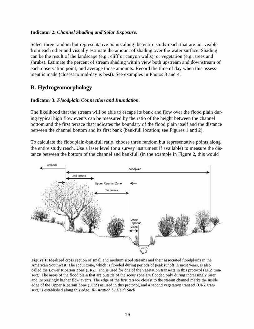
The likelihood that the stream will be able to escape its bank and flow over the flood plain dur-ing typical high flow events can be measured by the ratio of the height between the channelbottom and the first terrace that indicates the boundary of the flood plain itself and the distancebetween the channel bottom and its first bank (bankfull location; see Figures 1 and 2).

To calculate the floodplain-bankfull ratio, choose three random but representative points alongthe entire study reach. Use a laser level (or a survey instrument if available) to measure the dis-tance between the bottom of the channel and bankfull (in the example in Figure 2, this would

Figure 1: Idealized cross section of small and medium sized streams and their associated floodplains in theAmerican Southwest. The scour zone, which is flooded during periods of peak runoff in most years, is alsocalled the Lower Riparian Zone (LRZ), and is used for one of the vegetation transects in this protocol (LRZ tran-sect). The areas of the flood plain that are outside of the scour zone are flooded only during increasingly rarerand increasingly higher flow events. The edge of the first terrace closest to the stream channel marks the insideedge of the Upper Riparian Zone (URZ) as used in this protocol, and a second vegetation transect (URZ tran-sect) is established along this edge. Illustration by Heidi Snell

Indicator 2. Channel Shading and Solar Exposure.

Select three random but representative points along the entire study reach that are not visiblefrom each other and visually estimate the amount of shading over the water surface. Shadingcan be the result of the landscape (e.g., cliff or canyon walls), or vegetation (e.g., trees andshrubs). Estimate the percent of stream shading within view both upstream and downstream ofeach observation point, and average those amounts. Record the time of day when this assess-ment is made (closest to mid-day is best). See examples in Photos 3 and 4.

be 1.2 feet). Then measure the distance or height of the beginning or closest part of the flood-plain to the channel, and the channel bottom (1.8 feet in this example). Next, divide the flood-plain depth by bankfull depth. For Figure 2, 1.8 divided by 1.2 gives 1.5. Use the scoring scalein Figure 3 to determine the score to put on the Score Sheet for this location. In this example,the observed ratio of 1.5 leads to a score of 2. Repeat the measurements at two additional repre-sentative locations along the reach, and then take the mean of the three values for the finalscore for this indicator. The final score indicates the level of connectivity between the streamand its floodplain; a high ratio (and low indicator score) shows less potential for overbankflooding.

17

Figure 2: Method used to measure the ratio between the height above the bottom of thechannel to the first terrace on the floodplain and the height of bankfull. This is used forIndicator 3- Flood plain connection and inundation. Illustration by Heidi Snell

Figure 3: Floodplain/bankfull scoringscale. This scale translates the ratio ofthe floodplain height above the streambottom divided by the height of thebankfull into an indicator score.

18

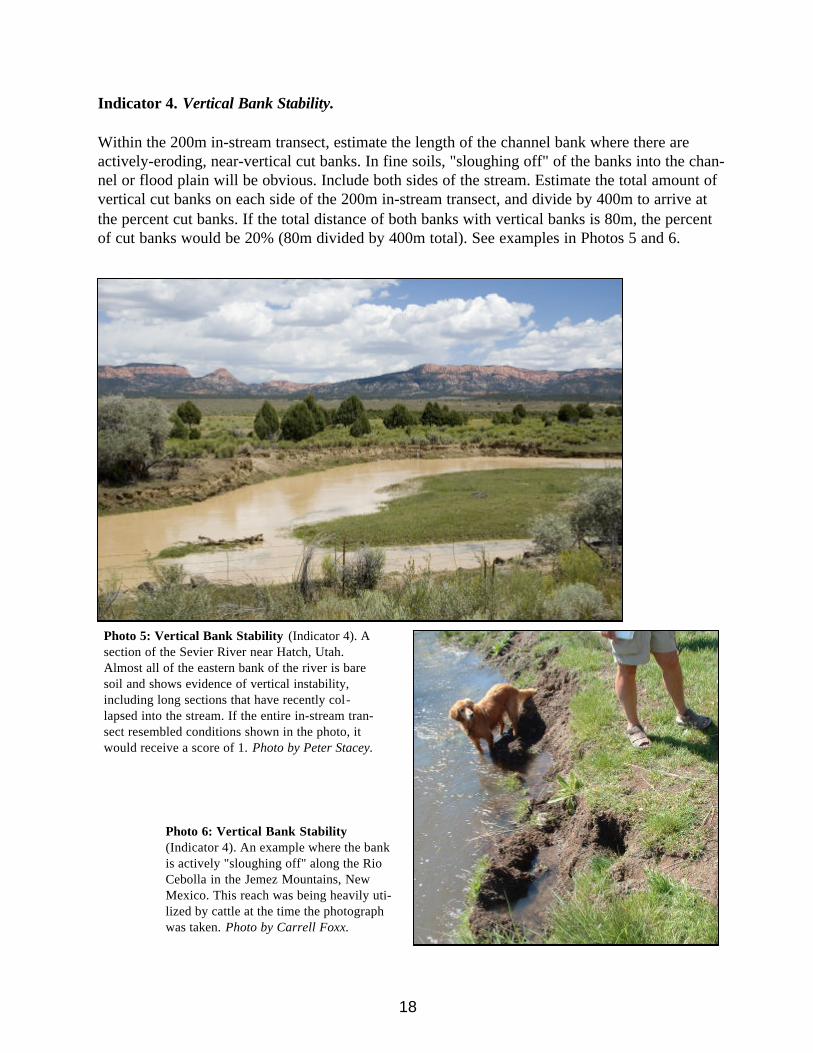
Indicator 4. Vertical Bank Stability.

Within the 200m in-stream transect, estimate the length of the channel bank where there areactively-eroding, near-vertical cut banks. In fine soils, "sloughing off" of the banks into the chan-nel or flood plain will be obvious. Include both sides of the stream. Estimate the total amount ofvertical cut banks on each side of the 200m in-stream transect, and divide by 400m to arrive atthe percent cut banks. If the total distance of both banks with vertical banks is 80m, the percentof cut banks would be 20% (80m divided by 400m total). See examples in Photos 5 and 6.

Photo 5: Vertical Bank Stability (Indicator 4). Asection of the Sevier River near Hatch, Utah.Almost all of the eastern bank of the river is baresoil and shows evidence of vertical instability,including long sections that have recently col-lapsed into the stream. If the entire in-stream tran-sect resembled conditions shown in the photo, itwould receive a score of 1. Photo by Peter Stacey.

Photo 6: Vertical Bank Stability(Indicator 4). An example where the bankis actively "sloughing off" along the RioCebolla in the Jemez Mountains, NewMexico. This reach was being heavily uti-lized by cattle at the time the photographwas taken. Photo by Carrell Foxx.

19

Figure 4: Examples of reaches with different levels of hydraulic habitat diversity (Indicator 5). Note that thenumber of different hydraulic habitats tends to increase with the number of meanders. Illustration by ChadGourley.ew = edge water lvr = low velocity rifflehvr = high velocity riffle lp = lateral poollgr = low gradient riffle hgr = high gradient riffle sp = scour pool

Indicator 5. Hydraulic Habitat Diversity.

Count the number of distinctive hydraulic and geomorphic channel features observed in theoverall reach walk-through. Look for runs, cobble or boulder debris fans, oxbows or other sidechannels, backwaters, sand-floored runs, or other features that can provide different habitats for fish and other aquatic organisms. Figure 4 gives an example of reaches with different levels of hydraulic feature diversity.

20

Indicator 6. Riparian Area Soil Integrity.

During the overall reach walkthrough estimate the extent of soil disturbance in both the lowerand upper riparian zones throughout the entire reach. Include both geomorphically inconsistenterosion from human activities (e.g., roads, trails) as well as damage from livestock and fromnative ungulates such as deer and elk. See examples in Photos 7 and 8.

Photo 7: Riparian AreaSoil Integrity (Indicator6). Photo of riparian areasoil disturbed by off-roadvehicles. Photo by LizThomas.

Photo 8: Riparian Area Soil Integrity(Indicator 6). A section of the riparianarea of the Rio Cebolla in the JemezMountains, New Mexico, where the soilhas been extensively disturbed by ungu-late activity. Note the "cow pie" at thebottom center of the photograph.Whenever possible, the source of any soildisturbance found in the reach should benoted. Photo by Carrell Fox.

21

Indicator 7. Beaver Activity.

Determine during the overall reach walkthrough the extent in the reach of recent beaver activitywithin the last year, as indicated by tracks, drags, digging marks, cut stems, burrows, dams, andcaches.

C. Fish/Aquatic Habitat

When assessing the Fish/Aquatic habitat components of the reach, the observer should walk theentire study reach, and then examine the channel and both banks of the in-stream 200m tran-sect.

Qualifier: If there is no flow currently, but this reach historically supported a fishery, then theentire Fish/Aquatic habitat section receives a score of 1. Continue on to the next section.

Indicator 8. Pool Number and Distribution.

In a stream that is in dynamic equilibrium, stretches of fast moving and relatively shallow water(riffles) will usually alternate with sections that are deeper and slower moving (pools; seeFigure 4). Note and record the number of pools and riffles within the 200m stream transect.Look for geomorphic consistency. For example, a larger number of pools and riffles will occurper unit distance in medium gradient streams, while fewer will be typical of high and low gradi-ent streams.

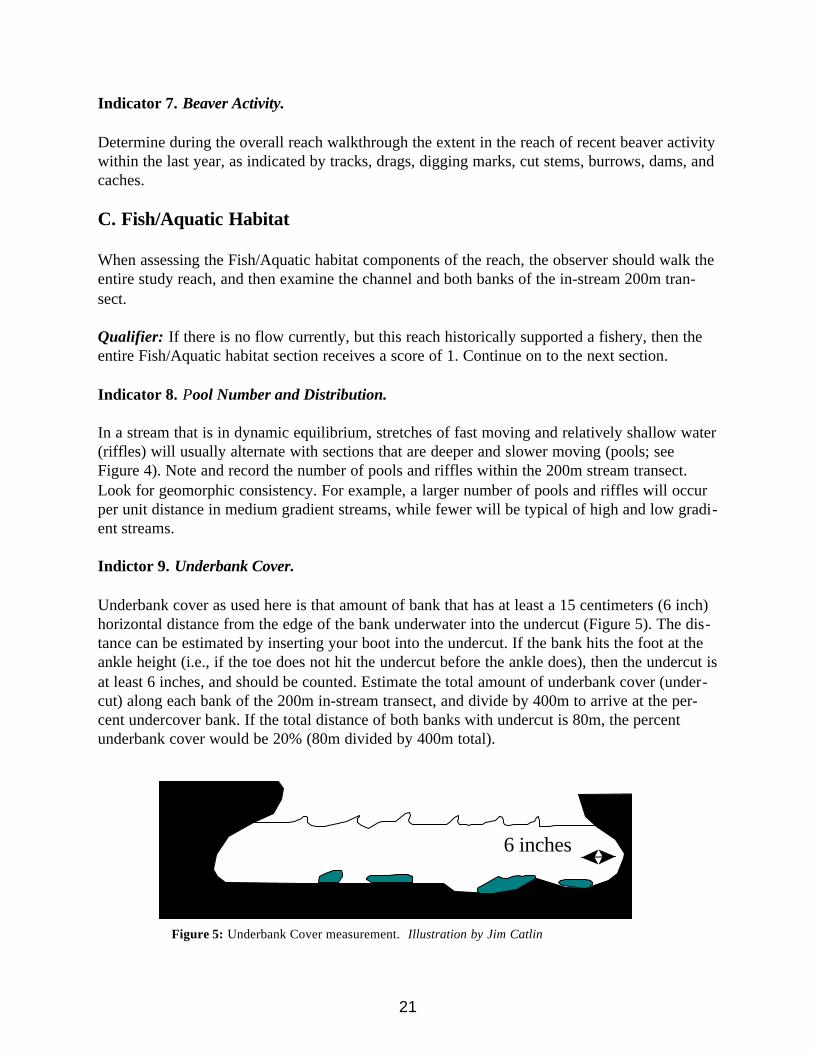
Indictor 9. Underbank Cover.

Underbank cover as used here is that amount of bank that has at least a 15 centimeters (6 inch)horizontal distance from the edge of the bank underwater into the undercut (Figure 5). The dis-tance can be estimated by inserting your boot into the undercut. If the bank hits the foot at theankle height (i.e., if the toe does not hit the undercut before the ankle does), then the undercut isat least 6 inches, and should be counted. Estimate the total amount of underbank cover (under-cut) along each bank of the 200m in-stream transect, and divide by 400m to arrive at the per-cent undercover bank. If the total distance of both banks with undercut is 80m, the percentunderbank cover would be 20% (80m divided by 400m total).

6 inches

Figure 5: Underbank Cover measurement. Illustration by Jim Catlin

22

Indicator 10. Cobble Embeddedness.

This measure is defined as the percent surface area of larger particles on the channel bottom(cobbles, larger pebbles and gravel) that is surrounded or covered by sand or silt. To determineembeddedness, randomly select three riffle areas along the reach. Within each area, stand in themiddle of the channel and randomly pick up from the bottom six rocks that are 3-8 inches indiameter and note the degree to which each rock was embedded within the substrate. A "sedi-ment line" should be readily visible on the rock, separating that portion of the rock which wasresting below the streambed and that above the bed in the flowing water zone (Figure 6). If thesediment line separates the rock halfway between top and bottom, the rating is 50% embedded;25% of the rock below the line would be 25% embedded, etc. Take the average of all rocksmeasured to determine the final score.

Indicator 11. Aquatic Macroinvertebrate Diversity.

Sampling for aquatic invertebrates should be done at the same locations in riffle areas whereembeddedness is recorded. Pick up and observe the organisms on at least five rocks greater than6 inches in diameter in each of the three riffle areas. Identify (to the Order only: e.g., stoneflylarvae, mayfly larvae, caddisfly larvae, Diptera larvae, beetles, etc.) using the illustrations inAppendix 1 or a suitable field guide. List the Orders found on the worksheet, and note the rela-tive numbers of each.

Indicator 12. Large Woody Debris.

This is defined as wood that is at least partially in the water or located in the active streamchannel and that is at least 15cm (approximately 6 inches) in diameter and 1m (approximately 3feet) in length. Record the number of large woody debris pieces observed within the 200m in-stream transects.

Figure 6: Determining the embeddedness of rocks or cobbles in the stream bed. Illustration by Jim Catlin

23

Figure 7: Overhanging vegetation allows insectsto drop into the stream. Illustration by Jim Catlin.

Photo 9: Overbank Cover and Terrestrial Invertebrate Habitat (Indicator 13). Section of CalfCreek, near Escalante, Utah, with dense vegetation overhanging almost all of the sides of the streamchannel. This vegetation provides habitat for insects and other invertebrates, which may then drop intothe water column and provide a key input of food for fish and other aquatic life. If the entire in-streamtransect resembles this photo, it would receive a score of 5. Photo by Peter Stacey.

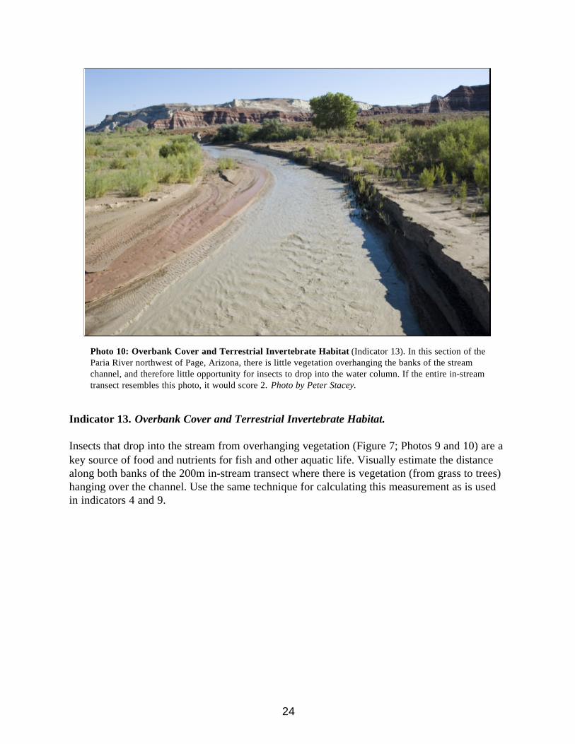
Indicator 13. Overbank Cover and Terrestrial Invertebrate Habitat.

Insects that drop into the stream from overhanging vegetation (Figure 7; Photos 9 and 10) are akey source of food and nutrients for fish and other aquatic life. Visually estimate the distancealong both banks of the 200m in-stream transect where there is vegetation (from grass to trees)hanging over the channel. Use the same technique for calculating this measurement as is usedin indicators 4 and 9.

24

Photo 10: Overbank Cover and Terrestrial Invertebrate Habitat (Indicator 13). In this section of theParia River northwest of Page, Arizona, there is little vegetation overhanging the banks of the streamchannel, and therefore little opportunity for insects to drop into the water column. If the entire in-streamtransect resembles this photo, it would score 2. Photo by Peter Stacey.

25

D. Riparian Vegetation

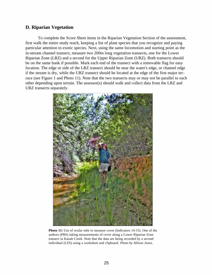
To complete the Score Sheet items in the Riparian Vegetation Section of the assessment,first walk the entire study reach, keeping a list of plant species that you recognize and payingparticular attention to exotic species. Next, using the same locomotion and starting point as thein-stream channel transect, measure two 200m long vegetation transects, one for the LowerRiparian Zone (LRZ) and a second for the Upper Riparian Zone (URZ). Both transects shouldbe on the same bank if possible. Mark each end of the transect with a removable flag for easylocation. The edge or side of the LRZ transect should be near the water's edge, or channel edgeif the stream is dry, while the URZ transect should be located at the edge of the first major ter-race (see Figure 1 and Photo 11). Note that the two transects may or may not be parallel to eachother depending upon terrain. The assessor(s) should walk and collect data from the LRZ andURZ transects separately.

Photo 11: Use of ocular tube to measure cover (Indicators 14-15). One of theauthors (PBS) taking measurements of cover along a Lower Riparian Zonetransect in Kanab Creek. Note that the data are being recorded by a secondindividual (LES) using a worksheet and clipboard . Photo by Allison Jones.

26

Indicators 14 and 15. Lower and Upper Riparian Zone Plant Community Structure andCover.

The presence or absence of vegetation cover observed in each of the four structural layers(ground, shrub, middle canopy, and tall canopy; see Figure 8) should be recorded for both theLRZ and URZ transects. Ground cover is both living grass and herbaceous vegetation, and deadvegetative matter up to 1 meter above the ground. Shrub cover is woody perennial vegetationoccurring up to 4 meters above the ground. Middle canopy vegetation is large shrub and smalltree cover 4-10 meters above the ground. Tall canopy vegetation is tree cover greater than 10meters above the ground. The same species (e.g., cottonwoods) may have individuals in differ-

ent structural layers,depending on the particularage of the plant.

Using an ocular cross-hairtube and the FieldWorksheet, walk along thetransect and every 2 meterslook directly up and downthrough the tube, andrecord the presence orabsence of plant material(dead or alive) intersectingthe vertical sight line of thecross-hairs in each structur-al layer - ground cover,shrub layer, mid-canopylayer and upper canopylayer (Figure 8 and Photo11). The line-of-sightthrough the ocular tubeshould mimic whether ornot a ray of light originat-ing directly overhead willstrike any vegetation as itpasses through each layer.Use the number of "hits"through the ocular tube forcover in each layer (out of100 samples along the200m transect) to determine

percent cover for that layer. Average the scores for the four layers to achieve an overall score.Because local geomorphology can influence the degree of vegetation cover, the scores from the

Figure 8: Method of using ocular tube to measure cover in each of the fourstructural layers used in Indicators 14-15. The four hits in the midcanopy layer are scored as a single “yes” on the worksheet. In this illustra-tion, there is one hit for upper canopy, four for mid canopy and one hiteach in the shrub and ground layers. Illustration by Heidi Snell.

study reach can be compared with the average values obtained from an appropriate nearby ref-erence site to help guide interpretation.

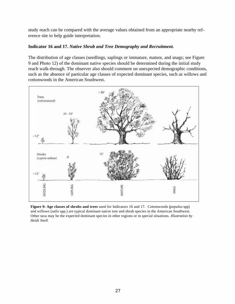
Indicator 16 and 17. Native Shrub and Tree Demography and Recruitment.

The distribution of age classes (seedlings, saplings or immature, mature, and snags; see Figure9 and Photo 12) of the dominant native species should be determined during the initial studyreach walk-through. The observer also should comment on unexpected demographic conditions,such as the absence of particular age classes of expected dominant species, such as willows andcottonwoods in the American Southwest.

27

Figure 9: Age classes of shrubs and trees used for Indicators 16 and 17. Cottonwoods (populus spp)and willows (salix spp.) are typical dominant native tree and shrub species in the American Southwest.Other taxa may be the expected dominant species in other regions or in special situations. Illustration byHeidi Snell.

28

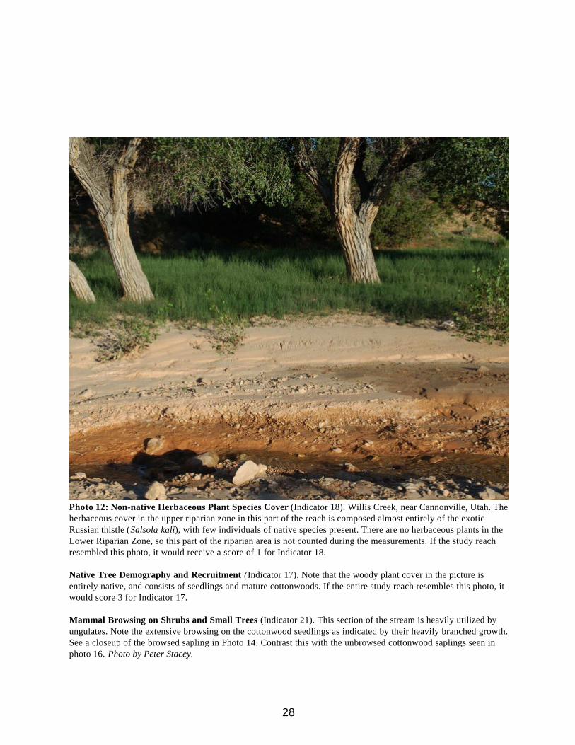
Photo 12: Non-native Herbaceous Plant Species Cover (Indicator 18). Willis Creek, near Cannonville, Utah. Theherbaceous cover in the upper riparian zone in this part of the reach is composed almost entirely of the exoticRussian thistle (Salsola kali), with few individuals of native species present. There are no herbaceous plants in theLower Riparian Zone, so this part of the riparian area is not counted during the measurements. If the study reachresembled this photo, it would receive a score of 1 for Indicator 18.

Native Tree Demography and Recruitment (Indicator 17). Note that the woody plant cover in the picture isentirely native, and consists of seedlings and mature cottonwoods. If the entire study reach resembles this photo, itwould score 3 for Indicator 17.

Mammal Browsing on Shrubs and Small Trees (Indicator 21). This section of the stream is heavily utilized byungulates. Note the extensive browsing on the cottonwood seedlings as indicated by their heavily branched growth.See a closeup of the browsed sapling in Photo 14. Contrast this with the unbrowsed cottonwood saplings seen inphoto 16. Photo by Peter Stacey.

29

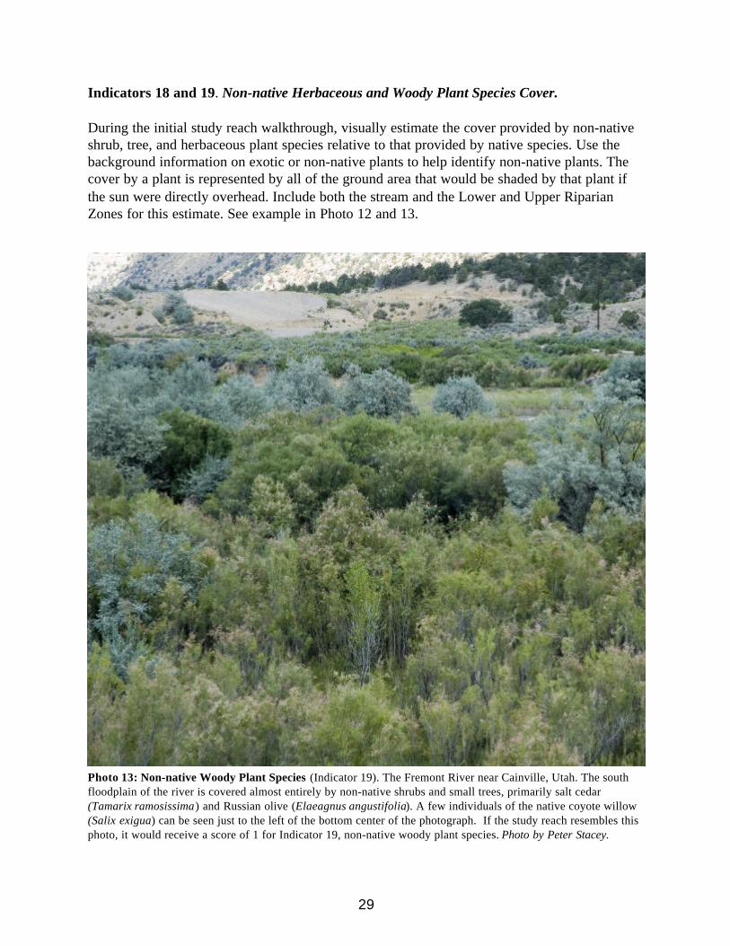
Indicators 18 and 19. Non-native Herbaceous and Woody Plant Species Cover.

During the initial study reach walkthrough, visually estimate the cover provided by non-nativeshrub, tree, and herbaceous plant species relative to that provided by native species. Use thebackground information on exotic or non-native plants to help identify non-native plants. Thecover by a plant is represented by all of the ground area that would be shaded by that plant ifthe sun were directly overhead. Include both the stream and the Lower and Upper RiparianZones for this estimate. See example in Photo 12 and 13.

Photo 13: Non-native Woody Plant Species (Indicator 19). The Fremont River near Cainville, Utah. The southfloodplain of the river is covered almost entirely by non-native shrubs and small trees, primarily salt cedar(Tamarix ramosissima) and Russian olive (Elaeagnus angustifolia). A few individuals of the native coyote willow(Salix exigua) can be seen just to the left of the bottom center of the photograph. If the study reach resembles thisphoto, it would receive a score of 1 for Indicator 19, non-native woody plant species. Photo by Peter Stacey.

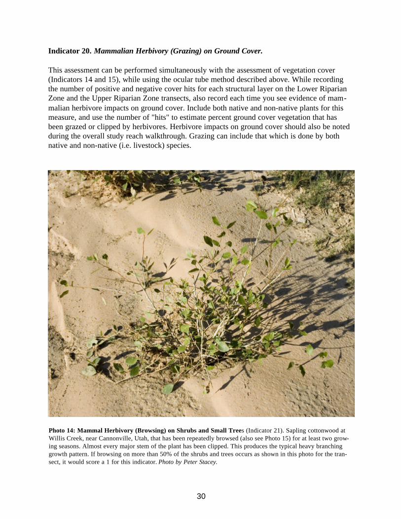
Indicator 20. Mammalian Herbivory (Grazing) on Ground Cover.

This assessment can be performed simultaneously with the assessment of vegetation cover(Indicators 14 and 15), while using the ocular tube method described above. While recordingthe number of positive and negative cover hits for each structural layer on the Lower RiparianZone and the Upper Riparian Zone transects, also record each time you see evidence of mam-malian herbivore impacts on ground cover. Include both native and non-native plants for thismeasure, and use the number of "hits" to estimate percent ground cover vegetation that hasbeen grazed or clipped by herbivores. Herbivore impacts on ground cover should also be notedduring the overall study reach walkthrough. Grazing can include that which is done by bothnative and non-native (i.e. livestock) species.

30

Photo 14: Mammal Herbivory (Browsing) on Shrubs and Small Trees (Indicator 21). Sapling cottonwood atWillis Creek, near Cannonville, Utah, that has been repeatedly browsed (also see Photo 15) for at least two grow-ing seasons. Almost every major stem of the plant has been clipped. This produces the typical heavy branchinggrowth pattern. If browsing on more than 50% of the shrubs and trees occurs as shown in this photo for the tran-sect, it would score a 1 for this indicator. Photo by Peter Stacey.

Indicator 21. Mammalian Herbivory (Browsing) on Shrubs and Small Trees.

Walk again along both the Lower and Upper Riparian Zone transects and estimate the numberof shrubs and trees along those transects whose branches or trunks show signs of browsing(clipped ends, etc.; see Photos 14 and 15 for examples). Compare this to those plants that donot show signs of browsing (Photo 16). Herbivore impacts on shrubs and small trees shouldalso be noted during the overall study reach walk through. Browsing can include that done byboth native and non-native (livestock) species.

31

Photo 15: Mammal Herbivory (Browsing) onShrubs and Small Trees (Indicator 21). Closeupof a coyote willow stem that has recently beenclipped by ungulates on the Rio Cebolla in theJemez Mountains, New Mexico. Photo by CarrellFoxx.

Photo 16: Mammal Herbivory on Shrubs and Small Trees (Indicator 21). Cottonwoods inan area of North Wash near Lake Powell in southeast Utah show no evidence of livestockbrowsing for decades. Note the erect growth form of the sapling cottonwoods, with a singlemain stem (compare with Photos 12 and 14). If the entire transect resembles this photo, itwould score 5. Photo by Peter Stacey.

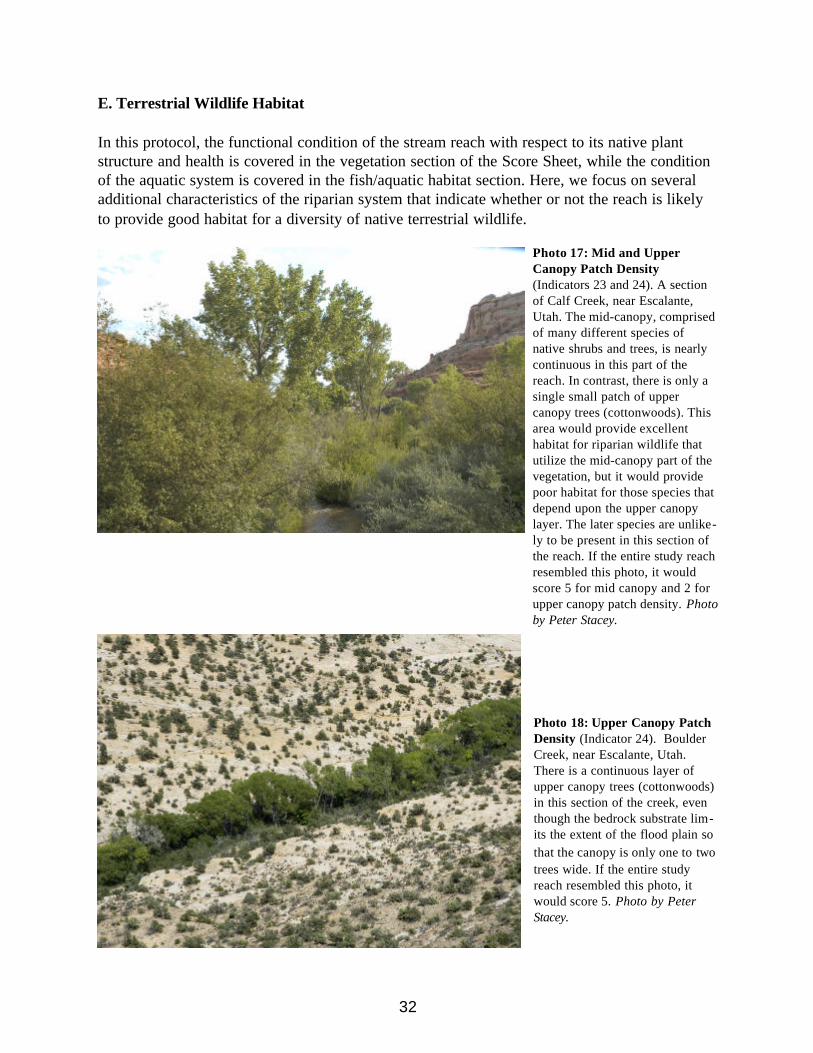
E. Terrestrial Wildlife Habitat

In this protocol, the functional condition of the stream reach with respect to its native plantstructure and health is covered in the vegetation section of the Score Sheet, while the conditionof the aquatic system is covered in the fish/aquatic habitat section. Here, we focus on severaladditional characteristics of the riparian system that indicate whether or not the reach is likelyto provide good habitat for a diversity of native terrestrial wildlife.

32

Photo 17: Mid and UpperCanopy Patch Density(Indicators 23 and 24). A sectionof Calf Creek, near Escalante,Utah. The mid-canopy, comprisedof many different species ofnative shrubs and trees, is nearlycontinuous in this part of thereach. In contrast, there is only asingle small patch of uppercanopy trees (cottonwoods). Thisarea would provide excellenthabitat for riparian wildlife thatutilize the mid-canopy part of thevegetation, but it would providepoor habitat for those species thatdepend upon the upper canopylayer. The later species are unlike-ly to be present in this section ofthe reach. If the entire study reachresembled this photo, it wouldscore 5 for mid canopy and 2 forupper canopy patch density. Photoby Peter Stacey.

Photo 18: Upper Canopy PatchDensity (Indicator 24). BoulderCreek, near Escalante, Utah.There is a continuous layer ofupper canopy trees (cottonwoods)in this section of the creek, eventhough the bedrock substrate lim-its the extent of the flood plain sothat the canopy is only one to twotrees wide. If the entire studyreach resembled this photo, itwould score 5. Photo by PeterStacey.

Indicators 22 and 23. Shrub and Mid-Canopy Patch Densities.

While in a few situations, such as narrow canyons with rock sides, continuous bands of willowsand other plants may not be geomorphically possible, most reaches commonly support manysuch patches, particularly right along the channel. Shrubs are considered here to be woodyperennial vegetation occurring up to 4m above the ground. Middle canopy vegetation is largeshrub and small tree cover 4-10m above the ground. The frequency and connectedness of patch-es of both shrubs and mid-canopy trees should be estimated during the overall study reachwalkthrough. Include both native and non-native species for these scores. See the example inphoto 17.

Indicator 24. Upper Canopy Tree Patch Connectivity.

Depending on the geomorphic setting, riparian zones often support many areas where there is acontinuously connected tree canopy, made up of cottonwoods, tree willows, and/or other treespecies. The canopy can be of different height classes depending on the age of the trees, buthere is considered to be at least 10m tall. Note the connectivity of upper canopy patches overthe full study reach during the overall walkthrough. Include both native and non-native speciesfor this score. See examples in Photo 17 and 18.

Indicator 25. Fluvial Habitat Diversity.

The different types of riparian landforms that can provide unique habitats for wildlife should berecorded during the overall study reach walkthrough. These include adjacent springs, wet mead-ows, ox-bows, marshes, cut banks, sand bars, islands in the channel, etc. (see Figure 10). Thegeomorphic setting can limit the potential number of fluvial landforms present on the reach.Streams and rivers in canyons and very flat meadows generally exhibit a lower diversity oflandforms than those with an intermediate gradient and a well-defined flood plain; scores forthis indicator should be scaled to what would be geomorphically possible within the specificstudy reach.

33

Figure 10: Fluvial habitatdiversity (Indicator 25) . Typesof fluvial habitats. Drawing byLarry Stevens.

Definitions

Bankfull level. This is the level that a stream reaches during average peak run-offs or flowsfor an average year. There are a few indicators that will help the surveyor find the bankfulllevel. Look for evidence of water flow that has bent vegetation or deposited silt or litter. Oftenthere is an abrupt break between the upper and lower flood plain that marks bankfull levels.The lower areas are often bare soil or contain aquatic and annual vegetation, while the areasabove bankfull often contain perennial forbs, shrubs and trees. In the American Southwest, peakannual stream flows often occur at the end of spring runoff (March and April).

Benthic Invertebrates. Primarily stream bottom insects that spend all or a portion of their lifestages in a stream, but may include other groups (e.g., worms and snails).

Ephemeral. A stream that does not flow continuously throughout the year, but only in directresponse to precipitation or during seasonal runoffs such as snow melt in the spring. There maybe subsurface water flow year round in ephemeral streams. Other streams may flow year roundbut dry up during the afternoon on the hottest days. Flow resumes at night when temperaturesand surface evaporation declines. These streams are considered ephemeral for the purposes ofthis protocol since most (but not all) aquatic species cannot tolerate even brief periods of expo-sure to air. See also Perennial.

Flood Plain Level. The flood plain is usually a series of terraces above the bankfull level. Thefirst terrace, or active flood plain, is inundated by high flow events that occur on average onceor twice every three years. Look for piles of debris to help age the more recent flood events.Additional terraces are usually found on the flood plain that are the result of increasingly rarebut larger flow events (see Lower and Upper Riparian Zones, below).

Fluvial. Features and characteristics that are the result of the interaction between water and theunderlying substrate (rock, soil, etc.).

Geomorphically inconsistent and consistent. The term "geomorphic" refers to the shape,structural characteristics, and geology of a stream channel and its adjacent banks and floodplain. Even in a single region, geomorphic characteristics can vary dramatically among differentreaches and watersheds. These, in turn, will affect the expected structure and composition of theaquatic and terrestrial plant and animal communities found in that reach. For example, a streamthat runs through a narrow and deep rock canyon would not be expected to develop the samenumber and type of fluvial habitat types (e.g., ox bows, sand bars, side channels) as would thesame sized stream that runs through an open area consisting of alluvial deposits and erodablesoils. Therefore, scoring of field indicators must include consideration of the geomorphic con-text. This guide uses the phrase "geomorphically consistent" and "geomorphically inconsistent"to help the user identify unusual situations that may affect checklist indicator scoring, and is amajor reason why reference reaches can be so useful.

34

35

Gradient. Measured by the distance that a stream drops per unit length of its channel. Highgradient streams drop quickly over short distances; as a result water velocities in the stream arehigh and the water column can move larger particles and more rapidly erode the substrate thancan lower gradient, slow moving streams. As a result of these differences, high gradient streamsalso tend to have fewer meanders than low gradient streams.

Herbaceous plants. These are non-woody plants (not trees or shrubs). Herbaceous plants arealso known as grasses and forbs.

Hydrogeomorphology. Features that pertain to the hydrology and/or geomorphology of thestream and its associated flood plain.

Lower and Upper Riparian Zones. There are a number of ways to define the riparian zone.As used here, it consists of the flood plain immediately adjacent to the stream or stream chan-nel, and is where plant growth is affected by surface or underground water flows from thestream system. Plants in the riparian zone are usually able to grow with their roots into thewater table. Many also require surface water flows in order to germinate from seeds. Outside ofthe riparian zone, plants may not be able reach the water table, and they do not require under-ground or surface waters to grow or germinate. This later area is called, in reference to theriparian zone, the uplands (see Figure 1). The riparian zone itself is further divided for the pur-poses of this protocol into two sections. The Lower Riparian Zone (LRZ) is the area that isimmediately adjacent to the stream channel. It is flooded during peak flows every year, and, asa result, soils are almost always saturated. This zone is occupied by wetland and water-lovingspecies of grasses and sedges, as well as various herbs, shrubs and occasionally trees (see Photo11). The yearly water flows often create small banks or edges at the outside of the LowerRiparian Zone. Above this, and further away from the channel, is the Upper Riparian Zone(URZ), which consists of the upper terrace(s) of the flood plain. The first terrace of the URZwhich is closest to the channel is overtopped by floods only every 1-2 years under normal orunaltered conditions. As one moves further away from the channel, the frequency of floodingbecomes progressively less, because the amount of water flow required to reach the higher ele-vations becomes progressively greater. The URZ extends up to the top of fluvial deposits suchas water-borne sand and gravels. While riparian water-loving plants and trees occur in the URZ,it is generally characterized by increasing abundance of upland species that have very deep rootsystems and do not always need to have water near the surface to germinate or flourish.

Mammalian herbivory. This term is used to refer primarily to the consumption of vegetation(i.e. grasses and forbs and shrubs) by mammals. Browse is the grazing of woody shrubs andtrees, and can also be used as a noun.

Macroinvertebrates. Animals without backbones and that are large enough in size to be seenwithout the aid of a magnifying glass or other tool.

Perennial. In perennial streams, there is surface flow of water year-round. Ephemeral streamsdry up during some times of the year (although there may still be subsurface flows). In somesystems, all but a few pools in a reach may dry up during the hottest part of the year. Fish may

find refuge in the remnant pools, and spread out once continuous flows resume. These streamsare considered perennial for the purposes of this assessment protocol.

Sinuosity. A measure of how much the stream channel meanders within the flood plain or val-ley bottom. A common measure of sinuosity is the length of a line along the middle of thestream channel (thalweg) divided by the straight line distance between the top and bottom ofthe sample reach. The greater the resulting value is, the more sinuous the stream. Sinuosityvaries greatly depending upon gradient, type of substrate, shape of the natural hydrograph orannual patterns of stream flow, etc., as well as being highly impacted by human alterations ofthe channel and the stream's hydrograph.

Succession. The tendency of plant communities to move through a regular series of speciescompositions and structures (called seral stages) over time on a specific site, and in the absenceof disturbance. Thus, a riparian zone that has been "wiped clean" by a large flood may first becolonized by forbs, then later by grasses and sedges, next by shrubs, and finally by trees. Thelast stage in succession is called the climax community, or the potential vegetation state. Theextent to which succession is an important process in riparian communities is controversial.Some researchers believe stream riparian systems in the absence of disturbances are in dynamicequilibrium and constantly changing at any one location.

Woody plants. Shrubs and trees that have woody stems and trunks, and that are generally longlived. New growth is added each year at the tip of the stem, rather than at the base as withgrasses.

36

18 April 2006

37

Appendix 1: Benthic MacroinvertebrateSpecies Orders, Used for Indicator 11Page 1 of 2.

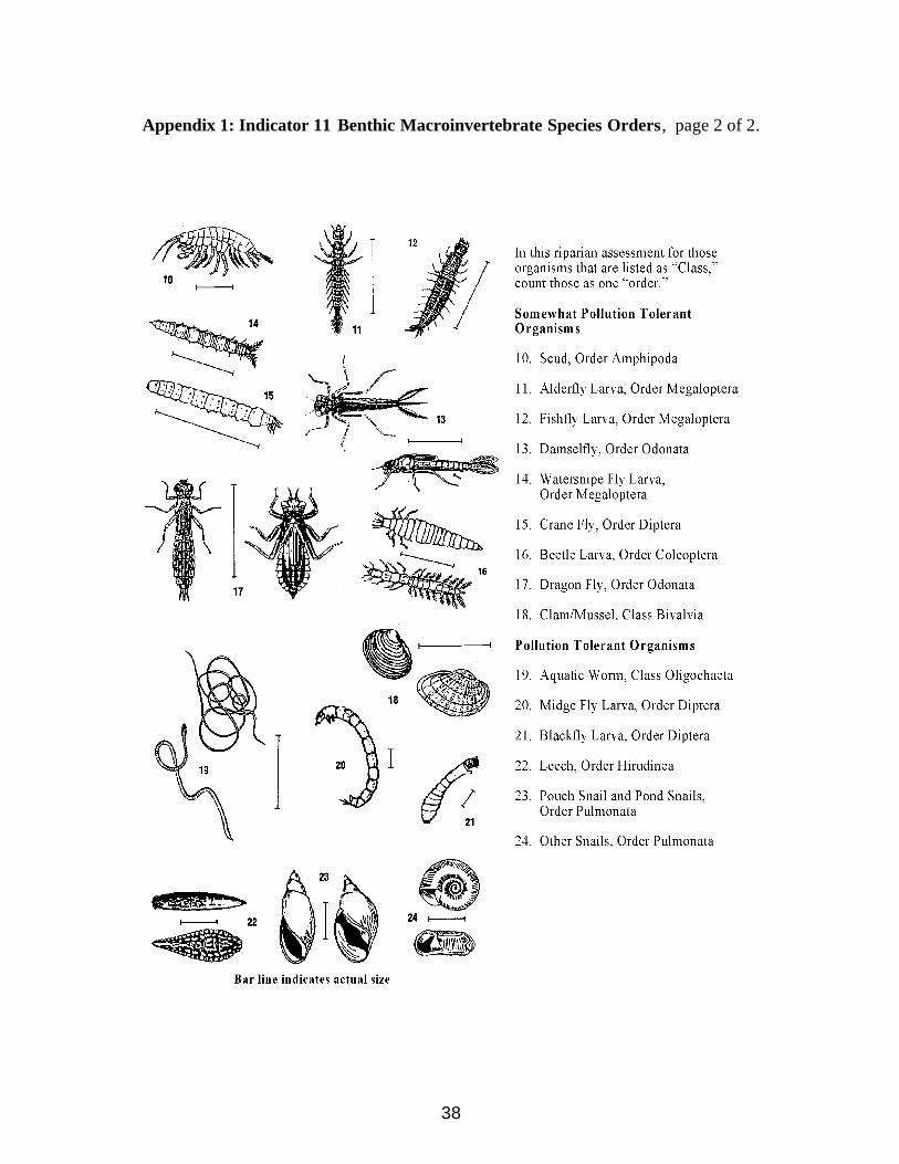
38

Appendix 1: Indicator 11 Benthic Macroinvertebrate Species Orders, page 2 of 2.

Appendix 2: Rapid Stream-Riparian Assessment Score Sheet rev March 2006

Stream _____________________ Watershed ________________________ Reach _____________________

Survey Date _________________ Time ____________ Weather ___________________________________

Background information available? ____ Observers _____________________________________________

Contact Info: Address _________________________________ Phone ___________ Email ______________

Reach (UTM) Start ________________ N _______________________ E Length Suveyed ________Stop ________________ N _______________________ E

UTM zone __________Stream Transect Start ________________ N _______________________ E

Upstream or Down? ____ USGS Quad Map Name:Veg. Transect Upstream or Down? ____ ____________________Reference Photos #1 _________________ N _______________________ E

#2 _________________ N _______________________ E Reach Elevation _________

OVERALL RATING: _____________________ CONDITION ____________________________________

Previous Ratings: DATE ________ Overall Score __________ Current Trend ___________

Individual Previous Scores WQ ____ HG ____ F/AH ____ RV ______ TWH _______

39

Score (1-5 orN/A)

IndicatorNumber Indicator

Scoring Definitions and DirectionsScores of 5 indicate that the indicator is close to the potentialof the geologically and biologically similar reference reach,and/or what would be expected to be found in a healthyecosystem, a reference reach without anthropogenic distur-bance. Scores of 1 indicate riparian or stream componentsthat are not functioning properly. Use N/A if the indicator isnot relevant or appropriate for this particular reach.

Notes onmeasurement

methods

1 AlgalGrowth

1 = >50% of stream bottom covered by filamentousalgae

2 = 26-50% of bottom covered by filamentous algae3 = 11-25% of bottom covered by filamentous algae4 = 1-10% of bottom covered by filamentous algae5 = no filamentous algae on stream bottom

Use ocular tube and fieldworksheet to score 0.5mfrom bank every 2m in200m in-stream transect.Do not count the singlecell algae on the surfaceof rocks.

2ChannelShading,

SolarExposure

1 = stream channel completely unshaded2 = slight shading3 = moderate shading4 = substantial shading5 = shading is geomorphically consistent

Look up and downstream in three differentrepresentative points inthe overall stream reach.Look for geomorphicconsistency.

WATER QUALITY

Water qualitymean score:

Notes:

40

HYDROGEOMORPHOLOGY (STREAM FORM)

3FloodplainConnection

andInundation

1 = >1.7 bankfull / depth ratio2 = >1.5 -1.7 bankfull / depth ratio3 = >1.4 - 1.5 bankfull / depth ratio4 = >1.3 - 1.4 bankfull / depth ratio5 = 1.0 - 1.3 bankfull / depth ratio

Use field worksheet andmeasure ratios at threerepresentative locationsin the overall streamreach.

4 VerticalBank

Stability

1 = >90% of channel banks are vertically unstable2 = 61 - 90% of banks are unstable3 = 31 - 60% of banks are unstable4 = 5 - 30% of banks are unstable5 = <5% of banks are unstable

Estimate along bothbanks of 200m in-streamtransect. Do not includerock or cliff faces.

5Hydraulic

HabitatDiversity

1 = no diversity (variability) of stream form features2 = low diversity3 = moderate diversity4 = moderately high diversity5 = high diversity, geomorphically consistent

Check in overall walkthrough. Examplesinclude runs, pools, cob-ble or boulder debrisfans, off-river side chan-nels, backwaters, sand-floored runs, etc.

6RiparianArea SoilIntegrity

1 = >25% of surface riparian soil surface disturbed2 = 16 - 25% disturbed3 = 6 - 15% disturbed4 = 1 - 5% disturbed5 = <1% disturbed

Check in overall walkthrough. Look for unnat-ural surface disturbancesin the flood plain fromsuch things as vehicles,foot travel, and ungulateactivity.

7 BeaverActivity

1 = beavers not now present but were historically2 = no beaver dams, few signs of activity

in last year3 = conspicuous recent activity but no dams4 = beaver dams on some of the stream5 = beaver activity and dams dominate stream

Check in overall walkthrough. Beaver signincludes tracks, drags,digging marks, cutstems, burrows, dams,and caches active withinpast season.

Hydrogeomorphologymean score:

Notes:

41

FISH/AQUATIC HABITATQualifier: If the stream is no longer perennial, but used to be a fishery, the mean score enteredfor this section is a score of “1.” (It is no longer functioning as fish/aquatic habitat>)

8 PoolDistribution

1 = no pool habitat in 200m stream transect2 = one to several pools3 = limited to moderate pool and riffle

distribution in reach4 = moderate to abundant pool and riffle

distribution5 = pools abundant (>50% of transect has pools

connected by riffles)

Check along 200m in-stream transect. Look forgeomorphic consistency(e.g. high gradient streamswill have more pools thanlow gradient streams).

9 UnderbankCover

1 = no underbank cover in 200m stream transect

2 = <10% transect has underbank cover3 = 10 - 25% of transect has underbank cover4 = 26 - 50% of transect has underbank cover5 = >50% of transect has underbank cover

Check along both banks of200m in-stream transect.Undercut must be at least15cm (6 in) into thestreambank.

10Cobble

Embedded-ness

1 = average of >50% of rock volume is imbedded in fine silt

2 = 41 - 50% of rock imbedded3 = 26 - 40% of rock imbedded4 = 20 - 25% of rock imbedded5 = <20% of rock imbedded

Determine the precentembeddedness of a sampleof 6 rocks 3-8” in diameterfrom riffles in each ofthree different randompoints along the overallstream reach.

11Aquatic Macro-

invertebrateDiversity

1 = no aquatic (benthic) macroinvertebratesfound

2 = 1 macroinvertebrate order present3 = 2 macroinvertebrate orders present4 = 3 macroinvertebrate orders present5 = 4 or more orders present

Examine 5 rocks 15cm(6”) or larger at the samesites used for Indicator 10.Use Appendix 2 or otherguide to identify macroin-vertebrate orders.

12 Large WoodyDebris

1 = no large woody debris (LWD) in transect2 = <3 LWD pieces in transect3 = 3 - 5 LWD pieces in transect4 = 6 - 10 LWD pieces in transect5 = >10 LWD pieces in transect

Count woody debris pieceslarger than 15cm (6”) indiameter and 1m (3 ft)long or longer in the chan-nel in the 200m in-streamtransect

13OverbankCover andTerrestrial

InvertebrateHabitat

1 = no grass, shrubs, trees overhang water2 = <10% of bank has grass, trees, shrubs that

overhang the water3 = 10 - 25% of bank has overhanging veg.4 = 26 - 50% of bank has overhanging veg.5 = >50% of bank has overhanging veg.

Check along both banks of200m in-stream transect.Look for geomorphic con-sistency. Do not includerocks or cliff faces.

Fish/Aquatic Habitatmean score:

Notes:

42

RIPARIAN VEGETATION

14

LowerRiparian

Zone PlantCommunity

Structureand Cover

1 = <5% average plant cover in lower riparian zone (LRZ)

2 = 5 - 25% average plant cover in LRZ3 = 26 - 50% average plant cover in LRZ4 = 51 - 80% average plant cover in LRZ5 = >80% average plant cover in LRZ

Use the field worksheet andocular tube to determine thecover for the ground, shrub,midcanopy and tall canopylayers along 200m transect inthe lower riparian zone.Look for geomorphic consis-tency.

15

UpperRiparian

Zone PlantCommunity

Structureand Cover

1 = <5% average plant cover in upper riparian zone (URZ)

2 = 5 - 25% average plant cover in URZ3 = 26 - 50% average plant cover in URZ4 = 51 - 80% average plant cover in URZ5 = >80% average plant cover in URZ

Use the field worksheet andocular tube to determine thecover for ground, shrub, mid-canopy and tall canopy layersalong the 200m transect inthe upper riparian zone. Lookfor geomorphic consistency.

16Shrub

Demographyand

Recruitment

1 = no native shrubs present in study reach2 = one age class present3 = two classes present, one class with

seedlings or young shrubs4 = three age classes present5 = all age classes present

Determine during the overallwalk through the number ofage classes (seedlings,saplings, mature, standingdead) for the dominant (mostcommon) native shrubspecies.

17Tree

Demographyand

Recruitment

1 = no native tree present in study reach2 = one age class present3 = two classes present, one class with

seedlings or saplings4 = three age classes present5 = all age classes present

Determine during the overallwalk through the number ofage classes (seedlings,saplings, mature, standingdead) for the dominant (mostcommon) deciduous nativetree species.

18Non-nativeHerbaceous

Plant Species

1 = >50% of herbaceous plant cover are not native species

2 = 26 - 50% herbaceous not native3 = 11 - 25% herbaceous not native4 = 5 - 10% herbaceous not native5 = <5% of herbaceous cover not native

Estimate on the overall walkthrough.

19Non-native

Woody PlantSpecies

1 = >50% of woody plant cover are not native species

2 = 26 - 50% of woody cover not native3 = 11 - 25% of woody cover not native4 = 5 - 10% of woody cover not native5 = <5% of woody cover not native

Estimate on the overall walkthrough.

20

MammalHerbivory(Grazing)

Impacts onGround Cover

1 = >50% of plants impacted by grazing,signs of ungulates common (scat, trampling and trails)

2 = 26 - 50% of plants impacted, ungulate use signs are common

3 = 11 - 25% of plants impacted4 = 5 - 10% of plants impacted5 = <5% of plants impacted

Use the field worksheet andocular tube to determine thenumber of “hits” showingherbivory on the ground cov-ering plants (grasses andforbs) on the LRZ and URZ200m transect. Use averageof the two transects to score.

43

21

MammalHerbivory(Browsing)Impacts onShrubs andSmall Trees

1 = >50% of plants (shrubs and trees) impacted2 = 26 - 50% of plants impacted3 = 11 - 25% of plants impacted4 = 5 - 10% of plants impacted5 = <5% of plants impacted

Using the same transectsas for Indicator 20, esti-mate the percentage ofshrubs and small trees thathave branch tips that havebeen clipped or eaten bylarge mammals.

RIPARIAN VEGETATION, CONTINUED

Riparian Vegetation,mean score:

Notes:

TERRESTRIAL WILDLIFE HABITAT

22Shrub Patch

Density

1 = no shrub patches in stream reach2 = few, isolated shrub patches3 = isolated patches4 = few large open areas between large patches5 = almost continuous dense shrub cover

In overall walk through,examine patches and clustersof shrubs (<4m tall) andopenings between those clus-ters. Look for geomorphicconsistency.

23 Mid-CanopyPatch Density

1 = no mid-canopy shrub or tree patches in reach2 = few isolated small patches in mid canopy3 = isolated patches4 = few large open areas between large patches5 = almost continuous dense mid-canopy cover

In overall walkthrough,examine clusters of mid-canopy large shrubs and trees(4-10m tall) and openingsbetween those clusters. Lookfor geomorphic consistency.

24Upper

CanopyPatch

Density andConnectivity

1 = no large trees present in reach2 = 1 - 25% of upper canopy patches connected3 = 26-50% of upper canopy patches connected4 = 51-75% of upper canopy patches connected5 = >75% of upper canopy patches connected

In overall walk through,examine clusters of uppercanopy trees (>10m tall) andopenings between those clus-ters. Look for geomorphicconsistency.

25FluvialHabitat

Diversity

1 = no other fluvial habitat besides thestream channel

2 = one other type of fluvial habitat present3 = two other types present4 = three other types present5 = four or more other types present

Examine during overall walkthrough. Fluvial habitat typesinclude flood-plain ponds,oxbows, side channels, sandbars, wet meadows, beaverponds, and stable cutbanks.

Terrestrial WildlifeHabitat, mean score:

Notes:

Final Score - Rapid Stream Raparian Assessment

44

Mean Scores:

Water Quality:

Hydro-geomorphology:

Fish/Aquatic Habitat:

Riparian Vegetation:

Wildlife Habitat:

Overall Score:

Overall Comments:

Attach field worksheets (including the human impact worksheet) to this score sheet

Appendix 3: Rapid Stream Riparian Assessment Field Worksheet

The worksheet that follows is used in the field to collect the data that are then used to calculatethe scores for the indicators in the Rapid Stream Riparian Assessment. This completed work-sheet should be attached to the RSRA Score Sheet and kept as part of the permanent record.

The worksheet is organized into physical areas of observation (study reach or individual tran-sects). A GPS unit should be used to record the ends of the stream reach, individual transects,and other sample locations. This will allow other observers to return to the exact same locationin future years and collect the same data. This will allow anyone to determine whether therehave been any changes in the indicators over the intervening period (positive or negative).

The record for photographs also should include information that will allow others in the futureto revisit the same site and take a similar photograph. This information includes the GPS loca-tion and the direction that the photograph was taken. Try to frame your picture to show both theground and surrounding topography.

In some cases, the indicator assessment method calls for the User to count the number of obser-vations that, for example, show the presence of filamentous algae. An efficient way to tally thedata for these indicators is the “five strike” method where each count gets a vertical mark andthe fifth then crosses through the other four to make five. This is continued in groups of five,and makes totaling the count easier. Updated 7 April 2006

45

Rapid Stream Riparian Assessment Field Worksheet revised 7 April 2006

Stream reach identification: ____________________ Date: _____________

Whole Study Reach TransectBegin by recording the GPS locations of the ends of the study reach on the Score Sheet, andtake reference photos at both ends of the study stream reach transect. Data for the followingindicators are gathered on the whole reach transect:

Indicator 5 (Hydraulic Habitat diversity), Indicator 6 (Riparian Area Soil Integrity)Indicator 7 (Beaver, Signs of activity), Indicator 16 (Native Shrub Demography),Indicator 17 (Native Tree Demography), Indicator 18 (Non-Native Herbaceous species),Indicator 19 (Non-Native Woody Plant Species), Indicator 22 (Shrub Patch Density), Indicator 23 (Mid-Canopy Patch Density), Indicator 24 (Upper Canopy Patch Density), and Indicator 25 (Fluvial Habitat Diversity).

Indicator 5: Hydraulic Habitat Diversity (number of different stream features).Check each type of hydraulic (stream) features providing aquatic habitat.o edge watero low velocity riffleo high velocity riffleo lateral poolo high gradient riffleo low gradient riffleo scour poolo cobble/boulder debris fanso side channelso backwaterso sand-floored runso other (type ______________________________________________)

Total number of different feature types: _______

Indicator 6: Riparian Area Soil Integrity.Notes ________________________________________ Percent soil area disturbed _____

Indicator 7: Beaver Activity. (Signs of beaver activity include tracks, drags, digging marks, cut stems, burrows, dams, and caches).Signs observed ___________________________________________________________

Indicator 16: Native Shrub Demography and recruitment.Circle age classes present: seedling, immature, mature, old dead clumps.Notes ___________________________________________________________________

46

Rapid Stream Riparian Assessment Field Worksheet, continued

Indicator 17: Native Tree Demography and Recruitment.Circle age classes present: seedling, immature, mature, snags. Notes ___________________________________________________________________

Indicator 18: Non-Native Herbaceous Plant Species Cover. (grasses and forbs, as percentage of total grass and forb cover).Percent of non-native herbaceous plants ________Notes __________________________________________________________________

Indicator 19: Non-Native Woody Plant Cover. (shrubs and trees, as percentage of total shrub and tree cover).Percent of non-native woody plant cover _______Notes __________________________________________________________________

Indicator 22: Shrub Patch Density.Notes ___________________________________________________________________

Indicator 23: Mid-canopy Patch Density.Notes ___________________________________________________________________

Indicator 24: Upper Canopy Patch Density.Notes ___________________________________________________________________

Indicator 25: Fluvial Habitat Diversity.Check each type of geophysical feature providing riparian habitat:o flood-plain pondso oxbowso side channelso sandbarso wet meadowso marsho stable cutbankso beaver pondo others (name __________________________________________________)

Total number of fluvial habitat types ________

47

Rapid Stream Riparian Assessment Field Worksheet, continued

Three Representitve Reach SitesData for the following indicators are collected at three different and representative sitesalong the study reach. The locations used for each indicator may be the same or differentas appropriate.

Indicator 2: Channel Shading and Solar Exposure.(percent of stream surface shaded at mid-day).

Observation Site 1: Percent stream shaded ______ % (Optional GPS) UTM N __________________ E ____________________

Observation Site 2: Percent stream shaded ______ %(Optional GPS) UTM N __________________ E ____________________

Observation site 3: Percent stream shaded: ______ %(Optional GPS) UTM N __________________ E _____________________

Average of three observation sites _________% Time recorded ______________

Indicator 3: Floodplain Connection and Inundation.(data are taken at three representative sites).

Site 1: Value for channel bottom ________ Bankfull ________ 1st Terrace ________Bankfull depth ______ Floodplain height ______Ratio of floodplain/bankfull ____________ Score from Figure 3 ________(Optional Site GPS) UTM N ________________ E __________________(Optional) Photo ID ___________Direction ________

Site 2: Value for channel bottom ________ Bankfull ________ 1st Terrace ________Bankfull depth ______ Floodplain height ______Ratio of floodplain/bankfull ____________ Score from Figure 3 ________(Optional Site GPS) UTM N ________________ E __________________(Optional) Photo ID __________ Direction _______

Site 3: Value for channel bottom ________ Bankfull ________ 1st Terrace ________Bankfull depth ______ Floodplain height ______Ratio of floodplain/bankfull ____________ Score from Figure 3 _________(Optional Site GPS) UTM N _________________ E __________________(Optional) Photo ID ___________________________ Direction _________

Indicator 3, average score for three sites _______

48

Rapid Stream Riparian Assessment Field Worksheet, continued

Three Representative Instream Sites

Collect the data for Indicators 10 and 11 at the same representative stream riffle locations(these sites may be different than those used for the other indicators)

Indicator 10: Cobble Embeddedness (three representative riffles, observe six samples per site).

Riffle site 1: Rock embedded ____ _____ ____ ____ ____ _____ Average ______

(Optional GPS) UTM N. ______________ E ________________

Riffle site 2: Rock embedded ____ _____ ____ ____ ____ _____ Average ______

(Optional GPS) UTM N. ______________ E ________________

Riffle site 3: Rock embedded ____ _____ ____ ____ ____ _____ Average ______

(Optional GPS) UTM N. ______________ E ________________

Overall average embeddedness: ___________

Indicator 11: Aquatic Invertebrates (Examine at least 5 rocks at least six inches in diameter at each of the sites used tomeasure embeddedness. Use key for identification and the invertebrate orders found below).

__________________________________________________________________________

__________________________________________________________________________

__________________________________________________________________________

49

Rapid Stream Riparian Assessment Field Worksheet, continued

In-stream 200 meter transect Data for the following assessment indicators are collected on this transect:Indicator 1 (Algal Growth), Indicator 4 (Vertical Bank Stability), Indicator 8 (Pool Distribution), Indicator 9 (Underbank Cover), Indicator 12 (Large Woody Debris), and Indicator 13 (Terrestrial Invertebrate Habitat,Overbank cover).

(Optional Photo) Identification _________________ Photo direction ________(Optional Photo) Location: UTM N __________________ E ______________________

Indicator 1: Algal Growth. (Count the number of samples with filamentous algae taken every 2 meterslooking straight down with the ocular tube).Count ____________________________________________________________________Percent of total stops on transect that are “hits” for algae _______

Indicator 4: Vertical Stability of Stream Banks.Meters unstable bank (both sides) ______________________________________________Total __________ Percent of transect ___________

Indicator 8: Pool Distribution.Number of pools __________ Number of riffles _______________________Approximate percent of total transect with riffle/pool habitat __________________

Indicator 9: Underbank Cover.Meters of underbank cover (both sides) _________________________________________Total ______ Percent of transect _________

Indicator 12: Large Wood Debris.( > 6 inches in diameter and three feet long).Pieces of large woody debris _________________________ Total __________________

Indicator 13: Overbank Cover and Terrestrial Invertebrate Habitat.Meters of vegetation hanging over bank (both sides) _______________________________ Total _________ Percent of stream transect _________________

50

Rapid Stream Riparian Assessment Field Worksheet, continued

Lower Riparian Zone 200 meter transect

Data for the following indicators are collected on this transect: Indicator 14 (Lower Riparian Zone Plant Community Structure and Cover), Indicator 20 (Mammalian Herbivory, Grazing of Ground Cover), andIndicator 21 (Mammalian Browse of Shrubs).

Indicator 14: Lower Riparian Zone Plant Community Structure.(every two meters observe directly up and down ground, shrub, and middle and tall canopy).

Groundcover count ________________________________________________________Total positive hits _____ Percentage positive hits _________

Shrub count ______________________________________________________________Total positive hits _____ Percentage positive hits _________

Middle canopy ____________________________________________________________Total positive hits _____ Percentage positive hits _________

Upper canopy ____________________________________________________________Total positive hits _____ Percentage positive hits _________

Average percent cover (all four layers) _____

Indicator 20 (part): Ungulate Grazing in Lower Riparian Zone.(Count grass and forb cover that show signs of grazing when performing observations for Indicator 14, LRZ Plant Community Structure and Cover).Groundcover that has been grazed ____________________________________________Total positive hits _____ Percentage positive hits _________

Indicator 21 (part): Mammalian Browsing of Shrubs and small Trees in LRZ.Percent of trees and shrubs showing clipped branches ____________

Notes ___________________________________________________________________

51

Rapid Stream Riparian Assessment Field Worksheet, continued

Upper Riparian Zone 200 meter transect

Data for the following indicators are collected on this transect: Indicator 15 (Upper Riparian Zone Plant Community Structure),Indicator 20 (Mammalian (wild and domestic livestock) Grazing of Ground Cover), andIndicator 21 (Mammal Browse of Shrubs).

Indicator 15: Upper Riparian Zone Plant Community Structure.(every two meters observe directly up and down for groundcover, shrub, middle and tall canopy).

Groundcover count ________________________________________________________ Total positive hits _____ Percentage positive hits _________

Shrub count ______________________________________________________________Total positive hits _____ Percentage positive hits _________

Middle canopy ___________________________________________________________Total positive hits _____ Percentage positive hits _________

Upper canopy _____________________________________________________________Total positive hits _____ Percentage positive hits _________

Average percent cover (all four layers) _____

Indicator 20 (part): Ungulate Grazing in Upper Riparian Zone.(Count grass and forb cover that show signs of grazing when performing observations forIndicator 15, URZ Plant Community Structure and Cover).

Groundcover that has been grazed ____________________________________________Total positive hits ____ Percentage positive hits _______ Average of LRZ, URZ ______

Indicator 21 (part): Ungulate Browsing of Shrubs and Small Trees in URZ.

Percent of trees and shrubs showing clipped branches ____________ Average of LRZ, URZ __________________

Notes ___________________________________________________________________

52

53

Appendix 4: Human Impacts Worksheet

(Note: This information can be used to help interpret the scores recorded from a survey in thestudy reach during the assessment and suggest possible areas for future restoration, if necessary.This information does not influence the assessment score. If this optional worksheet is complet-ed, attach it to the other worksheets for this stream reach.

To what extent does the current hydrograph of the stream match the likely historic and undis-turbed hydrograph?

To what extent has the upland areas of the watershed been altered by human activity in a waythat would impact the functioning of this reach (e.g. timber harvests, loss of plant cover, etc.)?

If the reach is grazed by livestock, is grazing use consistent with the current management plan(Allotment Management Plan) and appropriate for the watershed?

To what extent is the stream and adjacent areas free of road impacts, including bridges? Howfar from the channel are the impacts from the road?

To what extent has the channel geomorphology been affected by human activities (e.g., chan-nelization, check dams, irrigation canals, etc.)?

Revised 22 February 2006

Acknowledgements:

This User's Guide is based on a slightly longer version of the RSRA protocol describedin Stevens, Stacey, Jones, Duff, Gourley and Catlin (2005)1. The original protocol was devel-oped with the cooperation and financial support of the Wild Utah Project, with additional finan-cial contributions by the Judy & Leon Jones, and Henry Wallace Foundations. Twenty-threeindividuals from various government agencies and academic institutions peer reviewed the pro-tocol and we greatly appreciate their numerous helpful suggestions for improvement. Fieldworkshops conducted with members of the Great Old Broads for Wilderness, the Sierra Club,Red Rock Forests, Western Watershed Project, and the Forest Guardians provided valuablefeedback that helped shape the current protocol. Technical assistance in fisheries was providedby Trout Unlimited’s Partnership Program. Veronica Egan and Rose Chilcoat provided impor-tant help in many areas. Production of this document was made possible by contributions fromthe Wild Utah Project and the Utah Chapter of the Sierra Club.

1 Stevens, L.E., Stacey, P.B., Jones, A. L., Duff, D., Gourley, C., and J.C. Catlin. 2005. A protocol for rapidassessment of southwestern stream-riparian ecosystems. Proceedings of the Seventh Biennial Conference ofResearch on the Colorado Plateau titled The Colorado Plateau II, Biophysical, Socioeconomic, and CulturalResearch. Charles van Riper III and David J. Mattsen Ed. pp 397-420. Tuscon, AZ: University of Arizona Press.