Embed Size (px)
Citation preview

USimInDepthRelease 3.0.1
Tech-X Corporation
May 03, 2018

2
CONTENTS
1 Basic Concepts 11.1 Pre File Syntax . . . . . . . . . . . . . . . . . . . . . . . . . . . . . . . . . . . . . . . . . . . . . . 11.2 Key Parameters . . . . . . . . . . . . . . . . . . . . . . . . . . . . . . . . . . . . . . . . . . . . . . 7
2 Macros 112.1 Introduction . . . . . . . . . . . . . . . . . . . . . . . . . . . . . . . . . . . . . . . . . . . . . . . 112.2 Overview . . . . . . . . . . . . . . . . . . . . . . . . . . . . . . . . . . . . . . . . . . . . . . . . . 11
3 Basic USim Simulations 193.1 Using USim to solve the Euler Equations . . . . . . . . . . . . . . . . . . . . . . . . . . . . . . . . 193.2 Using USim to solve the Magnetohydrodynamic Equations . . . . . . . . . . . . . . . . . . . . . . . 323.3 Solving Multi-Dimensional Problems in USim . . . . . . . . . . . . . . . . . . . . . . . . . . . . . 503.4 Solving Problems on Advanced Structured Meshes in USim . . . . . . . . . . . . . . . . . . . . . . 613.5 Solving Problems on Unstructured Meshes in USim . . . . . . . . . . . . . . . . . . . . . . . . . . 69
4 Advanced USim Simulations 854.1 Advanced USim Simulation Concepts . . . . . . . . . . . . . . . . . . . . . . . . . . . . . . . . . . 854.2 Advanced Methods for Solving the Euler Equations with USim . . . . . . . . . . . . . . . . . . . . 914.3 Advanced Methods for Solving the Magnetohydrodynamics Equations with USim . . . . . . . . . . 1004.4 Advanced Methods for Solving for Solving Problems in Multi-Dimensions with Usim . . . . . . . . 1124.5 Advanced Methods for Solving Problems on Advanced Meshes with USim . . . . . . . . . . . . . . 132
5 Using USim to Solve Advanced Physics Problems 1475.1 Using USim to Solve a Diffusion Problem . . . . . . . . . . . . . . . . . . . . . . . . . . . . . . . 1475.2 Using USim to Solve the Two-Fluid Plasma Model . . . . . . . . . . . . . . . . . . . . . . . . . . . 1495.3 Using USim to Solve MHD with General Equation of State . . . . . . . . . . . . . . . . . . . . . . 1595.4 Using USim to Solve MHD with General Equation of State . . . . . . . . . . . . . . . . . . . . . . 1665.5 Using USim to Solve a Magnetic Nozzle Problem . . . . . . . . . . . . . . . . . . . . . . . . . . . 1715.6 Using USim to Solve an Anisotropic Diffusion Problem . . . . . . . . . . . . . . . . . . . . . . . . 1785.7 Using USim to Solve Multi-Fluid Problems with Collisions . . . . . . . . . . . . . . . . . . . . . . 1805.8 Using USim to solve 10 moment ions with 5 moment electrons . . . . . . . . . . . . . . . . . . . . 1845.9 Using USim to Solve Navier-Stokes Equations . . . . . . . . . . . . . . . . . . . . . . . . . . . . . 1875.10 Using USim to Solve Multi-Species Reactive Flows . . . . . . . . . . . . . . . . . . . . . . . . . . 1915.11 Advanced Time-Stepping Methods in USim . . . . . . . . . . . . . . . . . . . . . . . . . . . . . . . 1975.12 Running USim from the Command Line . . . . . . . . . . . . . . . . . . . . . . . . . . . . . . . . 1995.13 Restarting a USim Simulation . . . . . . . . . . . . . . . . . . . . . . . . . . . . . . . . . . . . . . 2035.14 Running on a Remote Host . . . . . . . . . . . . . . . . . . . . . . . . . . . . . . . . . . . . . . . . 206
i

ii
CHAPTER
ONE
BASIC CONCEPTS
1.1 Pre File Syntax
The most basic elements of the USim simulation process, which are discussed in USimcomposer-intro and consideredprerequisites for this section, are creating, running, and visualizing a run space. Here we will examine the basicconcepts within a USim input file, which contains more detailed information than the Key Input Parameters view inthe USimComposer Setup tab, and is by default not exposed to the user.
This section discusses the syntax used in pre files.
A pre file consists of:
• Comments
• Variables
• Top-level simulation parameters
• Parameters and vectors of parameters organized into input blocks
• Macros
1.1.1 Accessing the Input File
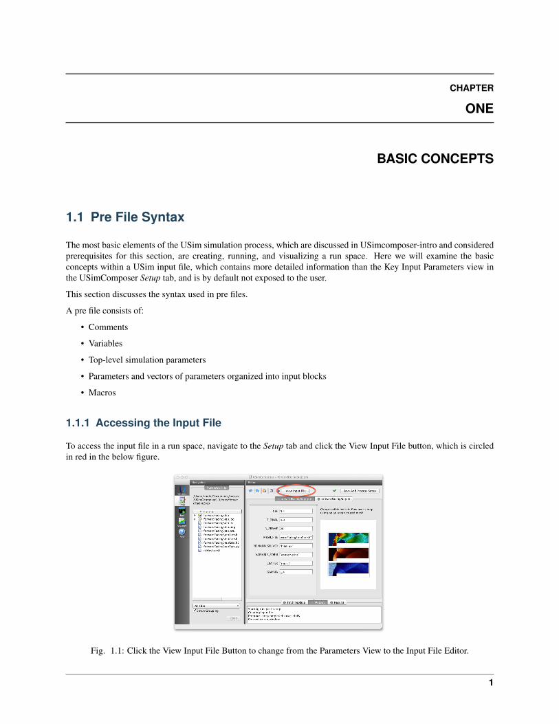
To access the input file in a run space, navigate to the Setup tab and click the View Input File button, which is circledin red in the below figure.
Fig. 1.1: Click the View Input File Button to change from the Parameters View to the Input File Editor.
1
USimInDepth, Release 3.0.1
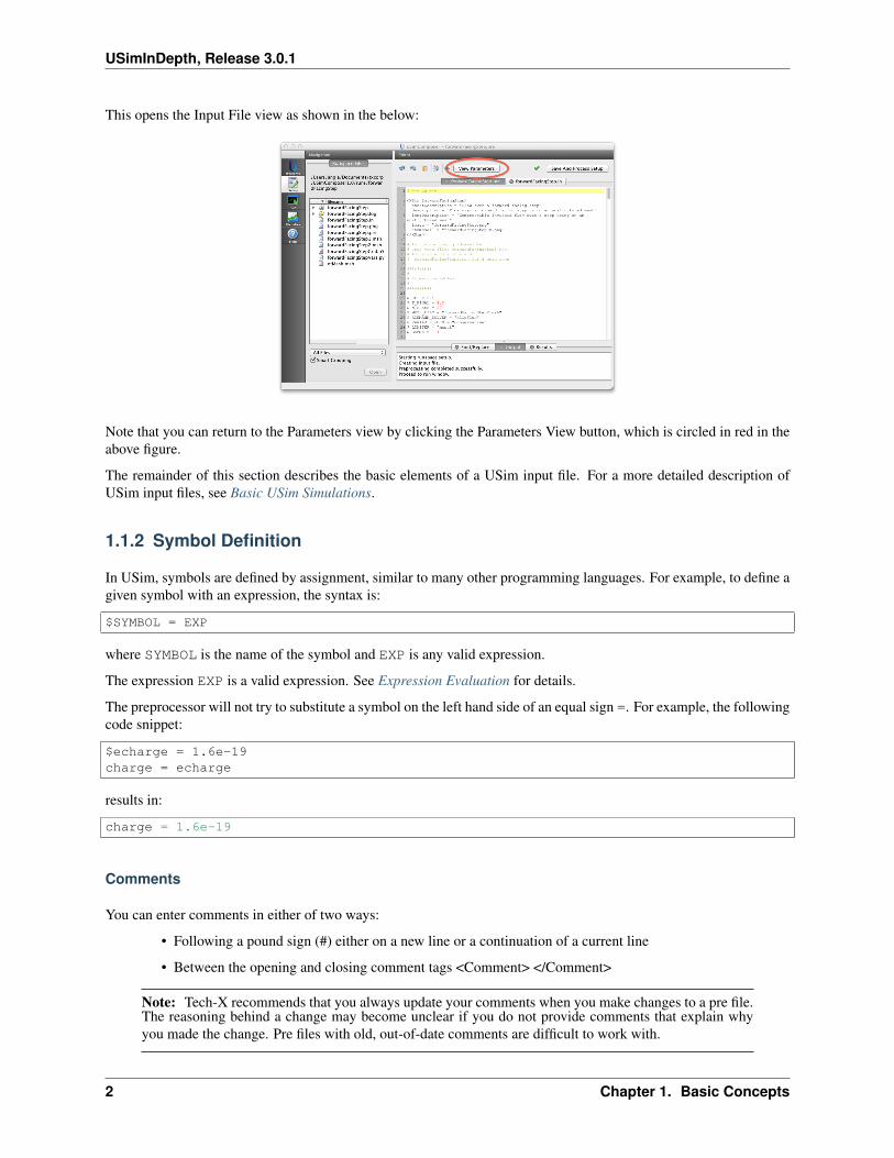
This opens the Input File view as shown in the below:
Note that you can return to the Parameters view by clicking the Parameters View button, which is circled in red in theabove figure.
The remainder of this section describes the basic elements of a USim input file. For a more detailed description ofUSim input files, see Basic USim Simulations.
1.1.2 Symbol Definition
In USim, symbols are defined by assignment, similar to many other programming languages. For example, to define agiven symbol with an expression, the syntax is:
$SYMBOL = EXP
where SYMBOL is the name of the symbol and EXP is any valid expression.
The expression EXP is a valid expression. See Expression Evaluation for details.
The preprocessor will not try to substitute a symbol on the left hand side of an equal sign =. For example, the followingcode snippet:
$echarge = 1.6e-19charge = echarge
results in:
charge = 1.6e-19
Comments
You can enter comments in either of two ways:
• Following a pound sign (#) either on a new line or a continuation of a current line
• Between the opening and closing comment tags <Comment> </Comment>
Note: Tech-X recommends that you always update your comments when you make changes to a pre file.The reasoning behind a change may become unclear if you do not provide comments that explain whyyou made the change. Pre files with old, out-of-date comments are difficult to work with.
2 Chapter 1. Basic Concepts
USimInDepth, Release 3.0.1
Variables
Each line defining a variable begins with a dollar sign ($).
Parameters
Parameters can be integers, floating-point numbers, or text strings.
The format of the parameter value determines the type of parameter. For example:
• x = 10 indicates an integer
• x = 10.0 indicates a floating-point number
• x = ten indicates a text string
Some parameters accept any text string (within reason). Other parameters accept only a choice of text strings.
If USim can parse a value, such as 42, as an integer, it will do so. If USim cannot parse the value as an integer, it willattempt to parse it as a floating-point number – for example, any of the following:
42.3.141591.60217646e-19
If USim cannot parse the value as either an integer or a floating-point number, it will parse the value as a string of text,for example, either of the following:
4o. (4 and lowercase O) or4O (4 and uppercase O).
Given these rules, use a decimal point to specify a floating point number. Any number without of decimal point willotherwise be interpreted as an integer.
If a parameter is specified twice, USim will use the second occurrence of the parameter in the input file produced fromthe pre file. The style recommendations in this user guide will help avoid multiple specifications of parameters.
Vectors of Parameters
Vectors of parameters are enclosed by brackets [ ] with white space used as separators. For example:
• x = [10 10 10] indicates a vector of integers
• x = [10. 10. 10.] indicates a vector of floats
1.1.3 Input Blocks
Input blocks are used to create simulation objects. The block is enclosed by opening and closing tags such as:
<Grid globalGrid>...
</Grid>
The tag determines:
• object type: indicated by an initial capital letter, for example, Grid
• object name: indicated by an initial lowercase letter, for example, globalGrid
1.1. Pre File Syntax 3
USimInDepth, Release 3.0.1
You use the object name to refer to the object in other input blocks. For example, in the input block for a particleobject, you may refer to the name of the electromagnetic field object.
Input blocks can be nested. For example, input blocks for boundary conditions are nested within the input block foran electromagnetic field.
1.1.4 Macros
Macros simplify input file construction through providing a mechanism for encapsulating commonly used input filesnippets. A user can then put into the input file only the macro, and then it will be expanded into the full input file atthe time of pre-processing the prefile.
Macros can have multiple uses including importing a group of parameters from a separate file, or simplifying an inputblock such as follows:
<macro myFluid>
equations = [euler]
<Equation euler>kind = eulerEqngasGamma = GAMMA
</Equation></macro>
You could then call your myFluid macro within the input file like this:
<Updater hyper>kind = classicMuscl1donGrid = domain...
myFluid
</Updater>
For more information about macros, see Overview
1.1.5 Scoping and Evaluation
Symbols in USim are scoped. This means that the effect of a symbol’s definition is confined to the macro or block inwhich that symbol is defined. Whenever USim enters a macro or a new input file block, it enters a new scope.
In the case in which SYMBOL is defined in multiple scopes, USim ignores the previously defined SYMBOL for theduration of the current scope. In the case in which SYMBOL is defined more than once in the current scope, the newvalue overrides the previous value defined in the current scope.
This scope is closed once USim leaves the block or macro. That is, the symbol’s definition no longer has an effectonce USim has used the symbol’s value in the macro or block where it was defined and then proceeded to a differentblock or macro. Scoping allows the next block or macro to be free to redefine the value of the symbol for its ownpurposes.
4 Chapter 1. Basic Concepts
USimInDepth, Release 3.0.1
Global Variables
It is possible to declare a global variable in USim. This is done by first defining the variable, then declaring it global.For example:
<Block>$ X = 4$ global X
</Block>
Will cause the variable X to be equal to 4 outside of the Block. It is important to note that the variable must be defined,and declared global on seperate lines. For example $ global X = 4 will not define X as a global variable with value 4.
Expression Evaluation
USim evaluates expressions by interpreting them as Python expressions. Python expressions are composed of tokens.A token is a single element of an expression, such as a constant, identifier, or operation. The preprocessor breaks theexpression string into individual tokens then performs recursive substitution on each token. Once a token is no longerfound to be substitutable, the preprocessor tries to evaluate it as a Python expression. The result of this evaluation willthen be used as the value of this token. All the token values are then concatenated and again evaluated as a Pythonexpression. This result will then be assigned to the symbol.
Tokenizing, the act of breaking a string into tokens, is performed following the lexical rules of Python. This meansthat white spaces are used to delimit tokens, but are otherwise entirely ignored.
Note: A string within matched quotes is treated as a single token with the matching quotes removed.
The input files generated by USim are sensitive to white spaces; as a result, USim has to re-introduce white spaces inthe translation process. By default, tokens are joined without any white spaces. However, if both tokens are of typestring, then a white space is introduced. Also, tokens inside an array (delineated by [ and ]) are delimited by a whitespace.
See the Python documentation on the official Python website at http://www.python.org for more information aboutPython expressions.
Python Token Evaluator (txpp.py)
The Python preprocessor has the following features:
• It accepts a file, conventionally with suffix .pre, for processing.
• Lines in that file that start with the character $ are processed by the preprocessor.
• Those lines are sent through the python interpreter to for evaluation
• The resulting values are replaced and written to a new file with suffix, .in
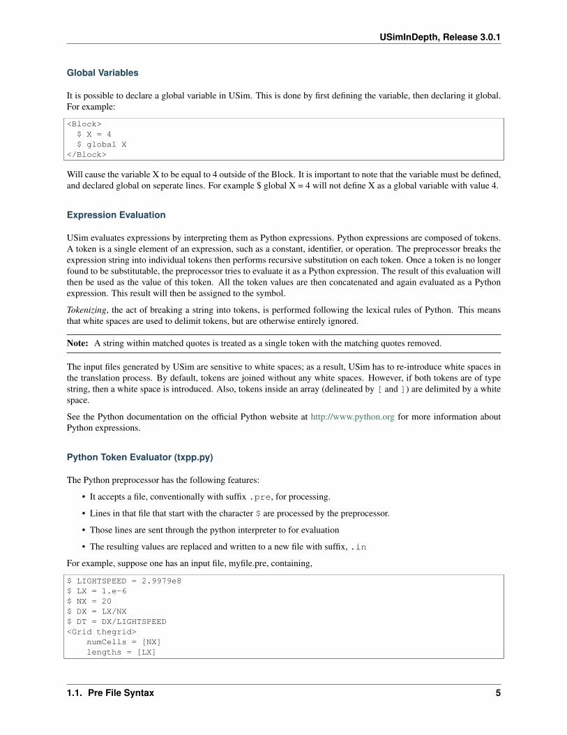
For example, suppose one has an input file, myfile.pre, containing,
$ LIGHTSPEED = 2.9979e8$ LX = 1.e-6$ NX = 20$ DX = LX/NX$ DT = DX/LIGHTSPEED<Grid thegrid>
numCells = [NX]lengths = [LX]
1.1. Pre File Syntax 5
USimInDepth, Release 3.0.1
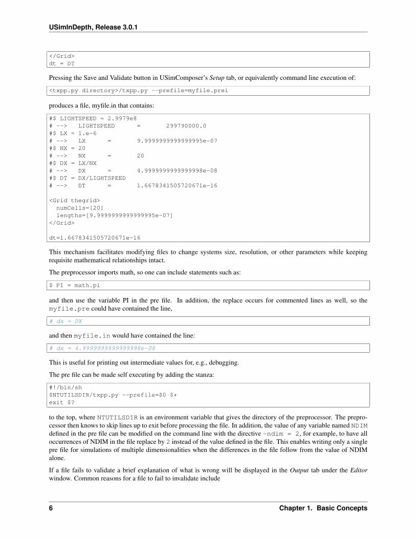
</Grid>dt = DT
Pressing the Save and Validate button in USimComposer’s Setup tab, or equivalently command line execution of:
<txpp.py directory>/txpp.py --prefile=myfile.prei
produces a file, myfile.in that contains:
#$ LIGHTSPEED = 2.9979e8# --> LIGHTSPEED = 299790000.0#$ LX = 1.e-6# --> LX = 9.9999999999999995e-07#$ NX = 20# --> NX = 20#$ DX = LX/NX# --> DX = 4.9999999999999998e-08#$ DT = DX/LIGHTSPEED# --> DT = 1.6678341505720671e-16
<Grid thegrid>numCells=[20]lengths=[9.9999999999999995e-07]
</Grid>
dt=1.6678341505720671e-16
This mechanism facilitates modifying files to change systems size, resolution, or other parameters while keepingrequisite mathematical relationships intact.
The preprocessor imports math, so one can include statements such as:
$ PI = math.pi
and then use the variable PI in the pre file. In addition, the replace occurs for commented lines as well, so themyfile.pre could have contained the line,
# dx = DX
and then myfile.in would have contained the line:
# dx = 4.9999999999999998e-08
This is useful for printing out intermediate values for, e.g., debugging.
The pre file can be made self executing by adding the stanza:
#!/bin/sh$NTUTILSDIR/txpp.py --prefile=$0 $*exit $?
to the top, where NTUTILSDIR is an environment variable that gives the directory of the preprocessor. The prepro-cessor then knows to skip lines up to exit before processing the file. In addition, the value of any variable named NDIMdefined in the pre file can be modified on the command line with the directive -ndim = 2, for example, to have alloccurrences of NDIM in the file replace by 2 instead of the value defined in the file. This enables writing only a singlepre file for simulations of multiple dimensionalities when the differences in the file follow from the value of NDIMalone.
If a file fails to validate a brief explanation of what is wrong will be displayed in the Output tab under the Editorwindow. Common reasons for a file to fail to invalidate include
6 Chapter 1. Basic Concepts
USimInDepth, Release 3.0.1
1. Using features not available to your USim module. i.e. an example under the USimHS templates will notvalidate if you are using a USimHEDP license.
2. A variable being declared as an integer instead of a float or vice versa. i.e. $ VAR = 6 instead of $ VAR = 6.0
3. A macro being called without it’s parent first being imported.
4. A macro has been called with the wrong number of parameters.
Now that we have examined USim pre file syntax, we are ready to discuss the creation of key parameters in the Setuptab of USimComposer in Key Parameters.
1.2 Key Parameters
USim has the ability to create key parameters. These variables are visible in the Editor pane of the Setup tab inUSimComposer, and they can be modified without the user having to sift through the input file (also called the prefile). They are useful when creating a base simulation that can be easily modified to simulate different phenomenawithin the same base simulation. This tutorial is for power users who wish to use key parameters within their ownsimulations and who are familiar with the USimcomposer-intro. As preparation for a discussion of key parameters,the user must be comfortable with accessing the input file, as discussed in Pre File Syntax.
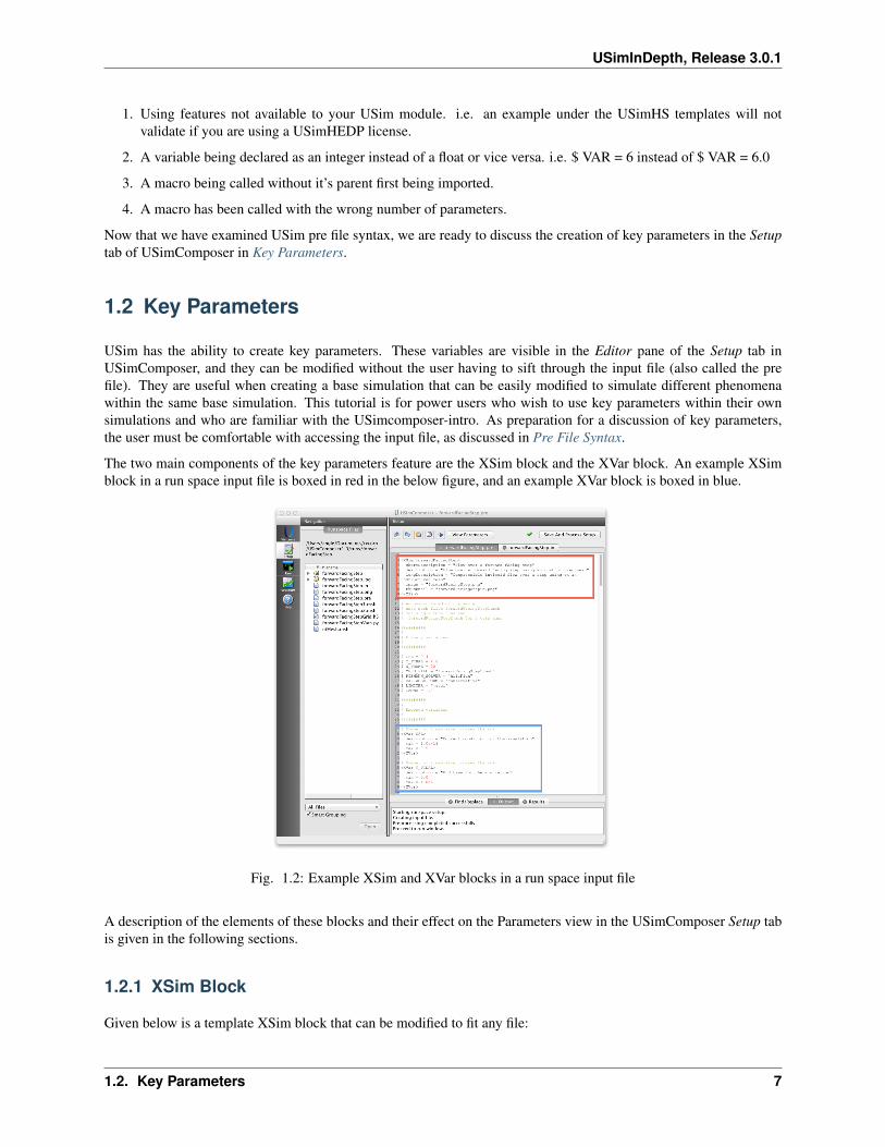
The two main components of the key parameters feature are the XSim block and the XVar block. An example XSimblock in a run space input file is boxed in red in the below figure, and an example XVar block is boxed in blue.
Fig. 1.2: Example XSim and XVar blocks in a run space input file
A description of the elements of these blocks and their effect on the Parameters view in the USimComposer Setup tabis given in the following sections.
1.2.1 XSim Block
Given below is a template XSim block that can be modified to fit any file:
1.2. Key Parameters 7
USimInDepth, Release 3.0.1
<XSim simulationName>shortDescription = "Simulation Name"description = "Description of the simulation."longDescription = "Longer description of the simulation."image = "simulationName.png"thumbnail = "simulationNameTn.png"
</XSim>
Each line in this block is explained below:
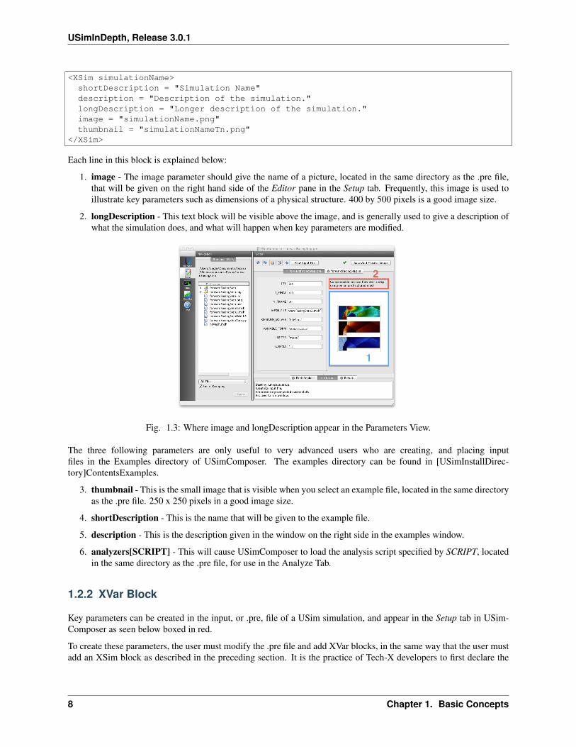
1. image - The image parameter should give the name of a picture, located in the same directory as the .pre file,that will be given on the right hand side of the Editor pane in the Setup tab. Frequently, this image is used toillustrate key parameters such as dimensions of a physical structure. 400 by 500 pixels is a good image size.
2. longDescription - This text block will be visible above the image, and is generally used to give a description ofwhat the simulation does, and what will happen when key parameters are modified.
Fig. 1.3: Where image and longDescription appear in the Parameters View.
The three following parameters are only useful to very advanced users who are creating, and placing inputfiles in the Examples directory of USimComposer. The examples directory can be found in [USimInstallDirec-tory]ContentsExamples.
3. thumbnail - This is the small image that is visible when you select an example file, located in the same directoryas the .pre file. 250 x 250 pixels in a good image size.
4. shortDescription - This is the name that will be given to the example file.
5. description - This is the description given in the window on the right side in the examples window.
6. analyzers[SCRIPT] - This will cause USimComposer to load the analysis script specified by SCRIPT, locatedin the same directory as the .pre file, for use in the Analyze Tab.
1.2.2 XVar Block
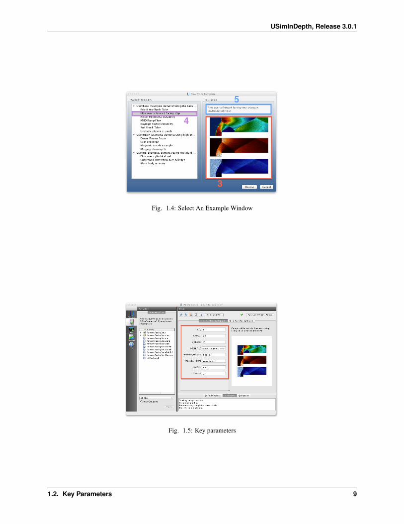
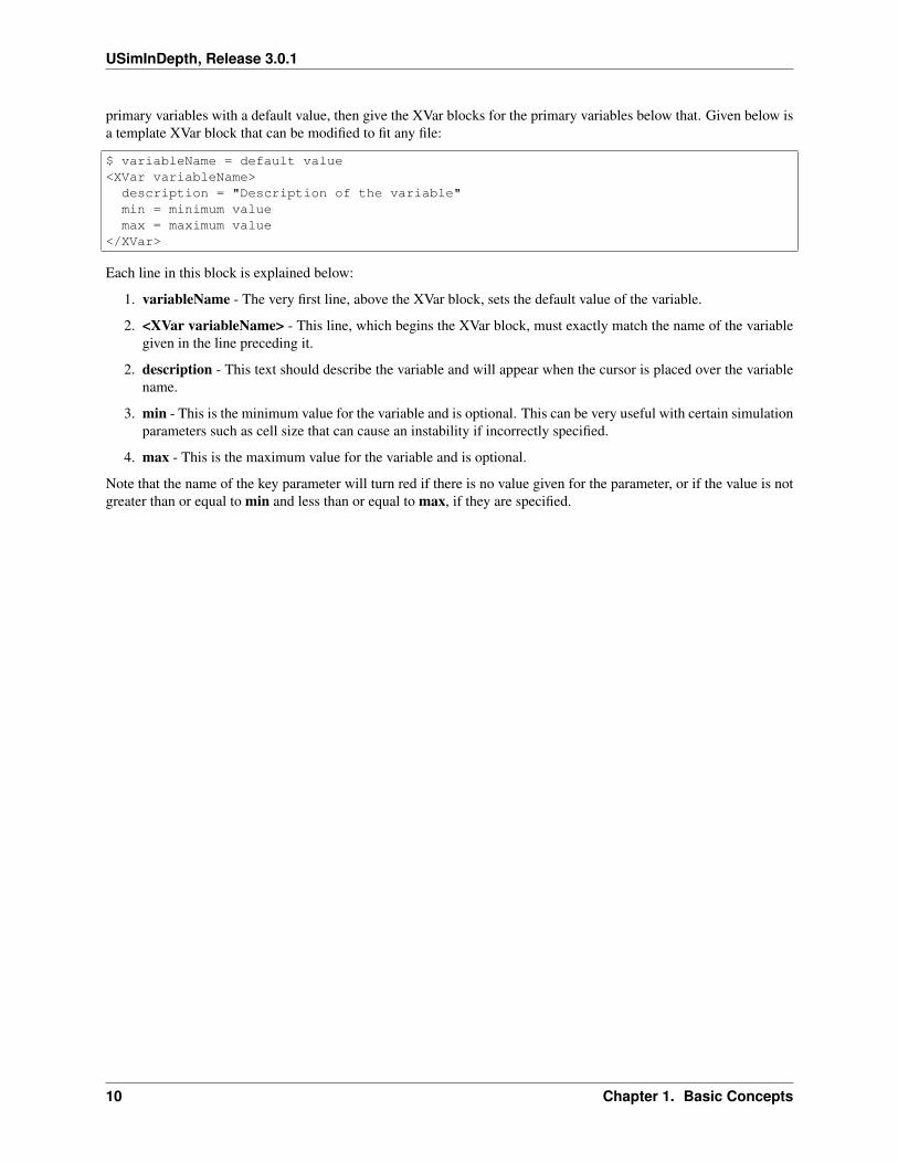
Key parameters can be created in the input, or .pre, file of a USim simulation, and appear in the Setup tab in USim-Composer as seen below boxed in red.
To create these parameters, the user must modify the .pre file and add XVar blocks, in the same way that the user mustadd an XSim block as described in the preceding section. It is the practice of Tech-X developers to first declare the
8 Chapter 1. Basic Concepts
USimInDepth, Release 3.0.1
Fig. 1.4: Select An Example Window
Fig. 1.5: Key parameters
1.2. Key Parameters 9
USimInDepth, Release 3.0.1
primary variables with a default value, then give the XVar blocks for the primary variables below that. Given below isa template XVar block that can be modified to fit any file:
$ variableName = default value<XVar variableName>
description = "Description of the variable"min = minimum valuemax = maximum value
</XVar>
Each line in this block is explained below:
1. variableName - The very first line, above the XVar block, sets the default value of the variable.
2. <XVar variableName> - This line, which begins the XVar block, must exactly match the name of the variablegiven in the line preceding it.
2. description - This text should describe the variable and will appear when the cursor is placed over the variablename.
3. min - This is the minimum value for the variable and is optional. This can be very useful with certain simulationparameters such as cell size that can cause an instability if incorrectly specified.
4. max - This is the maximum value for the variable and is optional.
Note that the name of the key parameter will turn red if there is no value given for the parameter, or if the value is notgreater than or equal to min and less than or equal to max, if they are specified.
10 Chapter 1. Basic Concepts
CHAPTER
TWO
MACROS
2.1 Introduction
USim contains a number of pre-defined macros that are used throughout the example input files available through theUSimComposer interface. The macros are used to help automate the process of setting up certain types of simulations.Input files can also be generated by external tools, one that we’ve found especially useful is Mako
2.2 Overview
2.2.1 Using Macros in Input Files
A macro is a mechanism to abstract complex input file sequences into (parameterized) tokens. In its simplest form, amacro provides a way to substitute a code snippet from an input file:
<macro snippet>line1line2line3
</macro>
In this example, every occurrence of the code named snippet in the input file will now be replaced by the three linesdefined between the <macro> and </macro> tags.
For example, you could define a macro to set up a laser pulse like this:
<macro myFluid>
equations = [euler]
<Equation euler>kind = eulerEqngasGamma = GAMMA
</Equation></macro>
You could then call your myLaser macro within the input file like this:
<Updater hyper>kind = classicMuscl1donGrid = domain...
myFluid
11
USimInDepth, Release 3.0.1
</Updater>
The USim engine (USim) will expand the input file use of your macro into:
<Updater hyper>kind = classicMuscl1donGrid = domain...
equations = [euler]
<Equation euler>kind = eulerEqngasGamma = GAMMA
</Equation>
</Updater>
Importing Local Macros
It is also possible to define a macro file, and provided that it is in the same directory as your input file, import it. Thisis useful when writing one custom macro that will be used over multiple simulations. The macro must have a .macextension on it to be imported as a local macro. To extend the example above, say the macro myLaser is in the fileLasers.mac, the input file would look like this:
$ import fluidModels.mac
<Updater hyper>kind = classicMuscl1donGrid = domain...
myFluid
</Updater>
USim will expand the input file use of your macro into:
<Updater hyper>kind = classicMuscl1donGrid = domain...
equations = [euler]
<Equation euler>kind = eulerEqngasGamma = GAMMA
</Equation>
</Updater>
The macro definition would remain the exact same. As long as the macro file is imported properly, it is just like havingit defined explicitly in the input file.
12 Chapter 2. Macros
USimInDepth, Release 3.0.1
2.2.2 Macro Parameters
Macros can take parameters, allowing variables to be passed into and used by the macro. Parameters are listed inparentheses after the macro name in the macro declaration, as in this example:
<macro finiteVolumeData(name, grid, components, write)><DataStruct name>kind = nodalArrayonGrid = gridnumComponents = componentsnumNodes = 1writeOut = write
</DataStruct></macro>
Once a macro is defined, it can be used by calling it and providing values or symbols for the parameters. The macrowill substitute the parameter values into the body provided. Calling the example above with parameters defined likethis:
finiteVolumeData(density, domain, 1, true)
will create the following code fragment in the processed input file:
<DataStruct name>kind = nodalArrayonGrid = gridnumComponents = componentsnumNodes = 1writeOut = write
</DataStruct>
Note: The parameter substitution happened in the scope of the caller. Parameters do not have scope outside of themacro in which they are defined.
2.2.3 Macro Overloading
As with symbols, macros can be overloaded within a scope. The particular instance of a macro that is used is deter-mined by the number of parameters provided at the time of instantiation. This enables the user to write macros withdifferent levels of parameterization:
<macro circle(x0, y0, r)>r^2 - ((x-x0)^2 + (y-y0)^2)
</macro><macro circle(r)>
circle(0, 0, r)</macro>
Looking in the example above, whenever the macro circle is used with a single parameter, it creates a circle aroundthe origin; if you use the macro with 3 parameters, you can specify the center of the circle.
The macro substitution does not occur until the macro instantiation is actually made. This means that you do not haveto define the 3-parameter circle prior to defining the 1-parameter circle, even though the 1-parameter circle refers tothe 3-parameter circle. It is only necessary that the first time the 1-parameter circle is instantiated, that 3-parametercircle has already been defined, otherwise you will receive an error.
2.2. Overview 13
USimInDepth, Release 3.0.1
2.2.4 Defining Functions Using Macros
Macros can be particularly useful for defining complex mathematical expressions, such as defining functions in exprlists.
Consider a macro that should simplify the setup of a Gaussian. One could define the following macro:
<macro badGauss(A, x, sigma)>A * exp(-x^2/sigma)
</macro>
While this is a legitimate macro, an instantiation of the macro via:
badGauss(A0+5, x-3, 2*sigma)
will result in:
A0+5*exp(-x+3^3/2*sigma)
which is probably not the expected result. One alternative is to put parentheses around the parameters whenever theyare used in the macro.
<macro betterGauss(A, x, sigma)>((A) * exp(-(x)^2/(sigma)))
</macro>
This will ensure that the expressions in parameters will not cause any unexpected side effects. The downside of thisapproach, however, is that the macro text is hard to read due to all the parentheses. To overcome this issue, txppprovides a mechanism to automatically introduce the parentheses around arguments by using a function block
<function goodGauss(A, x, sigma)>A * exp(-x^2/sigma)
</function>
The previous example will produce the same output as the badGauss macro, but without requiring the additionalparentheses in the macro text.
2.2.5 Importing Files
USim allows input files to be split into individual files, thus enabling macros to be encapsulated into separate libraries.For example, physical constant definitions or commonly-used geometry setups can be stored in files that can then beused by many USim simulations. Input files can be nested to arbitrary depth.
Files are imported via the import keyword:
$ import FILENAME
where FILENAME represents the name of the file to be included. txpp applies the standard rules for token substitutionto any tokens after the import token. Quotes around the filename are optional and computed filenames are possible.
2.2.6 Conditionals
The USim preprocessor includes both flow control and conditional statements, similar to other scripting languages.These features allow the user a great deal of flexibility when creating input files.
A conditional takes either the form:
14 Chapter 2. Macros
USimInDepth, Release 3.0.1
$ if COND...
$ endif
or
$ if COND...
$ else...
$ endif
Conditionals can be arbitrarily nested. All the tokens following the if token are interpreted following the expressionevaluation procedure (see above) and if they evaluate to true, the text following the if statement is inserted into theoutput. If the conditional statement evaluates to false, the text after the else is inserted (if present). Note that trueand false in preprocessor macros are evaluated by Python – in addition to evaluating conditional statements suchas x == 1, other tokens can be evaluated. The most common use of this is using 0 for false and 1 for true. Emptystrings are also evaluated to false. For more detailed information, consult the Python documentation.
Example Conditional Statements
$ if TYPE == "MHD"$ numComponents = 9$ else$ numComponents = 5$ endif
A conditional statement can also use Boolean operators:
$ A = 0$ B = 0$ C = 1## Below, D1 is 1 if A, B, or C are non-zero. Otherwise D1=0:$ D1 = (A) or (B) or (C)## Below, D2 is 1 if A is non-zero or if both B and C are non-zero. Otherwise D2=0:$ D2 = (A) or ( (B) and (C) )## This can be also be written as an if statement:$ if (A) or ( (B) and (C) )$ D3 = 1$ else $$ D3 = 0$ endif
2.2.7 Repetition
For repeated execution, USim provides while loops; these take the form:
$ while COND...
$ endwhile
2.2. Overview 15
USimInDepth, Release 3.0.1
which repeatedly inserts the loop body into the output. For example, to create 10 stacked circles using the circle macrofrom above, you could use:
$ n = 10$ while n > 0 circle(n)$ n = n - 1$ endwhile
2.2.8 Recursion
Macros can be called recursively. E.g. the following computes the Fibonacci numbers:
<macro fib(a)>$ if a < 2
a$ else
fib(a-1)+fib(a-2)$ endif
</macro>fib(7)
Note: There is nothing preventing you from creating infinitely recursive macros; if terminal conditions are not givenfor the recursion, infinite loops can occur.
2.2.9 Symbol Definition on the Command Line
txpp allows symbols to be defined on the command line. These definitions override any symbol definitions in theouter-most (global) scope. This allows you to set a default value inside an input file that can then be overridden on thecommand line if needed.
For example, if the following is in the outermost scope of the input file (outside of any blocks or macros):
$ X = 3X
Then this will result in a line containing 3 in the output. However, if you were to invoke txpp via:
txpp.py -DX=4
then this will result in a line 4.
However, if you were to define X inside a block (not in the global scope), such as:
<block foo>$ X = 3X
</block>
then X will always be 3, no matter what value for X is specified on the command line.
2.2.10 Requires
When writing reusable macros, best practices compel macro authors to help ensure that the user can be prevented frommaking obvious mistakes. One such mechanism is the requires directive, which terminates translation if one or moresymbols are not defined at the time. This allows users to write macros that depend on symbols that are not passed as
16 Chapter 2. Macros
USimInDepth, Release 3.0.1
parameters. For example, the following code snippet will not be processed if the symbol NDIM has not been previouslydefined:
<macro circle(r)>$requires NDIM$if NDIM == 2 r^2 - x^2 - y^2$endif$if NDIM == 3 r^2 - x^2 - y^2 - z^2$endif
</macro>
2.2.11 String Concatenation
One task that is encountered often during the simulation process is naming groups of similar blocks, e.g. similarspecies. Macros can allow us to concatenate strings to make this process more clean and simple. However, based onthe white-spacing rules, strings will always be concatenated with a space between them. For example,
$a = hello$b = worlda bwill result inhello world
However, we can get around this rule to get the desired output with the following:
<macro concat(a, b)>$ tmp = 'a tmp b'
</macro>
Now when calling
concat(hello, world)
the result will be:
helloworld
The first line appends a single quote to a and stores the result in tmp. The next line then puts the token a together withthe token b. As they are now no longer two strings, they will be concatenated without a space. The final evaluation ofthe resulting string then removes the quotes around it, resulting in the desired output.
Now that we have examined macros in an overview, we are ready for Introduction.
2.2. Overview 17

USimInDepth, Release 3.0.1
18 Chapter 2. Macros
CHAPTER
THREE
BASIC USIM SIMULATIONS
The following tutorials can be worked through with a USimBase license and utilize Macros to perform simulationsusing USim.
3.1 Using USim to solve the Euler Equations
In this tutorial, we demonstrate the basic methods used by USim to solve the Euler equations. This will serve as afoundation for understanding how to run any simulation in USim.
Contents
• Using USim to solve the Euler Equations– The Euler Equations– Initializing a Simulation– Adding a Simulation Grid– Creating a Fluid Simulation– Evolving the Fluid– Putting it all Together– An Example Simulation
3.1.1 The Euler Equations
This tutorial is based on the quickstart-shocktube example. The Shock Tube simulation is designed to set up a varietyof tube simulations including those by Einfeldt, Sod, Liska & Wendroff, Brio & Wu, and Ryu & Jones. In this tutorial,we will look at the Sod Shock Tube based on the classic paper:
Sod, Gary A. "A survey of several finite difference methods forsystems of nonlinear hyperbolic conservation laws.";Journal of Computational Physics 27.1 (1978): 1-31.
Note: It is important to note that while we will be following the quickstart-shocktube example, we will not reproducethe example file in its entirety. The shockTube example is designed to set up a variety of simulations, and by using“Flags” (if statements) in the shockTube.pre file, only certain parts of the file are used when simulating the Sod ShockTube. Therefore, at the end of this tutorial, our input will not be an exact copy of the shockTube.pre file but willdirectly represent only the Sod Shock portion of it.
In this example we will look at the use of equations for inviscid compressible hydrodynamics (the Euler equations).It is appropriate to use these equations for transonic, supersonic and hypersonic flows (Mach numbers of 0.1 and
19
USimInDepth, Release 3.0.1
above) where compressibility effects are important and at high Reynolds numbers where the effects of viscosity andconductivity are relatively unimportant.
The Euler equations for an adiabatic gas can be written as a hyperbolic conservation law, which has the form:
𝜕q
𝜕𝑡+ ∇ · [ℱ (w)] = 0
where q is a vector of conserved variables (e.g. density, momentum, total energy), ℱ (w) is a non-linear flux tensorcomputed from a vector of primitive variables, (e.g. density, velocity, pressure), and w = w(q). Assuming anadiabatic equations of state, the Euler equations can be written in this form such that:
𝜕𝜌
𝜕𝑡+ ∇ · [𝜌u] = 0
𝜕𝜌u
𝜕𝑡+ ∇ ·
[𝜌uu𝑇 + I𝑃
]= 0
𝜕𝐸
𝜕𝑡+ ∇ · [(𝐸 + 𝑃 )u] = 0
Here, I is the identity matrix, 𝑃 = 𝜌𝜖(𝛾 − 1) is the pressure of an ideal gas, 𝜖 is the specific internal energy and 𝛾 isthe adiabatic index (ratio of specific heats).
The Euler equations are represented in USim by refmanual-eulerEqn. USim solves these equations by calculating anupwind approximation of the flux tensor, ℱ(w) (see refmanual-classicMUSCL) and then using this approximation toadvance the conserved state from time 𝑡 to 𝑡+ ∆𝑡 (see refmanual-multiUpdater).
In this tutorial, we introduce the structure of a USim simulation, using quickstart-shocktube as an example. At the endof this tutorial, you will understand how to setup simple USim simulations on structured meshes.
3.1.2 Initializing a Simulation
The first step in any USim simulation is to import the macros that are needed to define the simulation. For theShockTube example, there are two macros that are needed:
$ import fluidsBase.mac$ import euler.mac
These macros provide basic capabilities for setting up a USim simulation of the Euler Equations. We can now de-fine global parameters that tell USim basic information about the simulation. This is done through the use of theinitializeFluidSimulation macro:
initializeFluidSimulation(NDIM,0.0,END_TIME,NUMDUMPS,CFL,GAS_GAMMA,WRITE_RESTART,DEBUG)
The parameters for the version of the macro used for the refmanual-eulerEqn are documented at euler-macro. Forcompleteness, we include them here, showing how the parameters specified here map onto the parameters used in theinitializeFluidSimulation macro:
NDIM (dimensionality): 1,2,3. Number of dimensions for the simulation
0.0 (tStart): Start time for simulation
END_TIME (tEnd): End time for simulation
NUMDUMPS (numFrames): Number of data outputs
CFL (cflNum): Cfl limit, typically ∆𝑡 = 𝑐𝑓𝑙𝑁𝑢𝑚 * ∆𝑥/𝑉𝑚𝑎𝑥
GAS_GAMMA (gammaIn): Adiabatic index for ideal gas eqn. of state. Pressure = (gammaIn - 1.0) *density * internal energy
WRITE_RESTART (writeRestartIn): Output data required for simulation restart
20 Chapter 3. Basic USim Simulations
USimInDepth, Release 3.0.1
DEBUG (debugIn): Run simulation in debug mode
USim includes the ability to perform in place substitution of variables within the input file, as described in SymbolDefinition. This means that we can define the options given above earlier in the input file and USim will replace themin the initializeFluidSimulation macro:
# X-extent of domain$PAR_LENGTH = 1.0# Y-extent of domain$PERP_LENGTH = 1.0# Zones parallel to shock normal direction$PAR_ZONES = 256# Zones perpendicular to shock normal direction$PERP_ZONES = 256# Shock tube to solve$SHOCK_TUBE = "SOD"# adiabatic index$GAS_GAMMA = 5.0/3.0# Atmospheric Pressure$REFERENCE_PRESSURE = 1.0 # [Pa]# density of air$REFERENCE_DENSITY = 1.0 # [kg/m^3]# end time for simulation (units of # of sound wave crossings)$TEND = 0.125# number of frames$NUMDUMPS = 10# Whether to use a diffusive (but robust) integration scheme$DIFFUSIVE = False# Order in time$TIME_ORDER = "second"# Write data for restarting the simulation$WRITE_RESTART = False# Output info for debugging purposes$DEBUG = False# Default dimensionality$NDIM = 1
Note that we have included a range of other variables that are defined in the quickstart-shocktube example. We willrefer to these later in this tutorial as needed. In the above, the variable TEND is given in units of the the number oftimes a sound wave crosses the grid. In order to use this to specify the end time for the simulation (END_TIME), weconvert this to have units of time through:
# nominal speed of sound$ c0 = math.sqrt(GAS_GAMMA*REFERENCE_PRESSURE/REFERENCE_DENSITY) # [m/s]
# Set end time according to (user specified)# number of times a wave crosses the box.$END_TIME = $PERP_LENGTH*TEND/c0$
The specification of the CFL parameter is described in the next section. Our simulation starts off as:
# Import macros to setup simulation$ import fluidsBase.mac$ import euler.mac
# X-extent of domain$PAR_LENGTH = 1.0# Y-extent of domain$PERP_LENGTH = 1.0
3.1. Using USim to solve the Euler Equations 21
USimInDepth, Release 3.0.1
# Zones parallel to shock normal direction$PAR_ZONES = 256# Zones perpendicular to shock normal direction$PERP_ZONES = 256# Shock tube to solve$SHOCK_TUBE = "SOD"# adiabatic index$GAS_GAMMA = 5.0/3.0# Atmospheric Pressure$REFERENCE_PRESSURE = 1.0 # [Pa]# density of air$REFERENCE_DENSITY = 1.0 # [kg/m^3]# end time for simulation (units of # of sound wave crossings)$TEND = 0.125# number of frames$NUMDUMPS = 10# Whether to use a diffusive (but robust) integration scheme$DIFFUSIVE = False# Order in time$TIME_ORDER = "second"# Write data for restarting the simulation$WRITE_RESTART = False# Output info for debugging purposes$DEBUG = False# Default dimensionality$NDIM = 1
# nominal speed of sound$ c0 = math.sqrt(GAS_GAMMA*REFERENCE_PRESSURE/REFERENCE_DENSITY) # [m/s]
# Set end time according to (user specified)# number of times a wave crosses the box.$END_TIME = $PERP_LENGTH*TEND/c0$
# Initialize a USim simulationinitializeFluidSimulation(NDIM,0.0,END_TIME,NUMDUMPS,CFL,GAS_GAMMA,WRITE_RESTART,DEBUG)
3.1.3 Adding a Simulation Grid
The next step in setting up a USim simulation is to specify a simulation grid. The quickstart-shocktube uses arefmanual-ntcart grid, which is added to the simulation through the addGrid macro:
addGrid(lowerBounds, upperBounds, numCells, periodicDirections)
The options for this macro are documented in grid-macro. For completeness, we include them here:
lowerBounds: Vector of coordinates for lower edge of grid, lowerBounds = [ XMIN YMIN ZMIN ]
upperBounds: Vector of coordinates for upper edge of grid, upperBounds = [ XMAX YMAX ZMAX]
numCells: Vector of number of cells in grid, numCells = [ NX NY NZ ]
periodicDirections: List of directions that are periodic
periodicDirections = [ 0 ] (x-direction periodic)periodicDirections = [ 0 1 ] (x,y-directions periodic)periodicDirections = [ 0 1 2 ] (x,y,z-directions periodic)
22 Chapter 3. Basic USim Simulations
USimInDepth, Release 3.0.1
The options are setup in the ShockTube example according to the dimensionality of the simulation, as specified by thevariable NDIM above:
$XMIN = -0.5*PERP_LENGTH$XMAX = 0.5*PERP_LENGTH$YMIN = -0.5*PAR_LENGTH$YMAX = 0.5*PAR_LENGTH$ZMIN = -0.5*PAR_LENGTH$ZMAX = 0.5*PAR_LENGTH
$if NDIM==1$ CFL = 0.5$ numCells = [PERP_ZONES]$ periodicDirections = []$ lowerBounds = [XMIN]$ upperBounds = [XMAX]$ else$if NDIM==2$ CFL = 0.4$ numCells = [PERP_ZONES, PAR_ZONES]# Make the direction perpendicular to the shock# normal periodic.$ periodicDirections = [1]$ lowerBounds = [XMIN, YMIN]$ upperBounds = [XMAX, YMAX]$ else$ CFL = 0.32$ numCells = [PERP_ZONES, PAR_ZONES, PAR_ZONES]# Make the directions perpendicular to the shock# normal periodic.$ periodicDirections = [1,2]$ lowerBounds = [XMIN, YMIN, ZMIN]$ upperBounds = [XMAX, YMAX, ZMAX]$ endif$ endif
Note as well that the CFL condition that is used for the simulation changes according to the dimension of the simula-tion. This is because the scheme for solving the hyperbolic equations has different stability requirements in differentdimensions:
CFL <=1
NDIM
So, our simulation now looks like:
# Import macros to setup simulation$ import fluidsBase.mac$ import euler.mac
# X-extent of domain$PAR_LENGTH = 1.0# Y-extent of domain$PERP_LENGTH = 1.0# Zones parallel to shock normal direction$PAR_ZONES = 256# Zones perpendicular to shock normal direction$PERP_ZONES = 256# Shock tube to solve$SHOCK_TUBE = "SOD"# adiabatic index
3.1. Using USim to solve the Euler Equations 23
USimInDepth, Release 3.0.1
$GAS_GAMMA = 5.0/3.0# Atmospheric Pressure$REFERENCE_PRESSURE = 1.0 # [Pa]# density of air$REFERENCE_DENSITY = 1.0 # [kg/m^3]# end time for simulation (units of # of sound wave crossings)$TEND = 0.125# number of frames$NUMDUMPS = 10# Whether to use a diffusive (but robust) integration scheme$DIFFUSIVE = False# Order in time$TIME_ORDER = "second"# Write data for restarting the simulation$WRITE_RESTART = False# Output info for debugging purposes$DEBUG = False# Default dimensionality$NDIM = 1
# nominal speed of sound$ c0 = math.sqrt(GAS_GAMMA*REFERENCE_PRESSURE/REFERENCE_DENSITY) # [m/s]
# Set end time according to (user specified)# number of times a wave crosses the box.$END_TIME = $PERP_LENGTH*TEND/c0$
$XMIN = -0.5*PERP_LENGTH$XMAX = 0.5*PERP_LENGTH$YMIN = -0.5*PAR_LENGTH$YMAX = 0.5*PAR_LENGTH$ZMIN = -0.5*PAR_LENGTH$ZMAX = 0.5*PAR_LENGTH
$if NDIM==1$ CFL = 0.5$ numCells = [PERP_ZONES]$ periodicDirections = []$ lowerBounds = [XMIN]$ upperBounds = [XMAX]$ else$if NDIM==2$ CFL = 0.4$ numCells = [PERP_ZONES, PAR_ZONES]# Make the direction perpendicular to the shock# normal periodic.$ periodicDirections = [1]$ lowerBounds = [XMIN, YMIN]$ upperBounds = [XMAX, YMAX]$ else$ CFL = 0.32$ numCells = [PERP_ZONES, PAR_ZONES, PAR_ZONES]# Make the directions perpendicular to the shock# normal periodic.$ periodicDirections = [1,2]$ lowerBounds = [XMIN, YMIN, ZMIN]$ upperBounds = [XMAX, YMAX, ZMAX]$ endif
24 Chapter 3. Basic USim Simulations
USimInDepth, Release 3.0.1
$ endif
# Initialize a USim simulationinitializeFluidSimulation(NDIM,0.0,END_TIME,NUMDUMPS,CFL,GAS_GAMMA,WRITE_RESTART,DEBUG)
# Setup the gridaddGrid(lowerBounds, upperBounds, numCells, periodicDirections)
3.1.4 Creating a Fluid Simulation
The next step in setting up a USim simulation is to create the basic set of variables needed to simulate the fluid. Thisis accomplished through the createFluidSimulation macro, documented at euler-macro:
createFluidSimulation()
Now that these variables have been automatically created via the macro, it is possible to specify the distribution offluid on the grid. This is a three-step process:
1. Use addVariable to add variables that are independent of grid position.
2. Use addPreExpression to add quantities that are functions of grid position, variables and any previously definedPreExpression in this block. Evaluated before expressions and the result is not accessible outside of this block.Any number of PreExpressions can be added.
3. Use addExpression to define each initial condition for the fluid. There is one expression for density, eachcomponent of momentum and the total energy. The order of the exprssions correspond to the order in the statevector and there can only be one expression per entry in the state vector.
For the ShockTube example, the variables added in Step 1 in the above process are:
addVariable(pi_value,math.pi)addVariable(gas_gamma,GAS_GAMMA)addVariable(densityL,DENSITY_L)addVariable(densityR,DENSITY_R)addVariable(pressureL,PRESSURE_L)addVariable(pressureR,PRESSURE_R)addVariable(normalVelocityL,NORMAL_VELOCITY_L)addVariable(normalVelocityR,NORMAL_VELOCITY_R)addVariable(perpendicularVelocityL,PERPENDICULAR_VELOCITY_L)addVariable(perpendicularVelocityR,PERPENDICULAR_VELOCITY_R)addVariable(tangentialVelocityL,TANGENTIAL_VELOCITY_L)addVariable(tangentialVelocityR,TANGENTIAL_VELOCITY_R)
The variables are then used in the PreExpressions that are defined in Step 2:
addPreExpression(rho = if (x>0.0, densityR, densityL))addPreExpression(pr = if (x>0.0, pressureR, pressureL))addPreExpression(vx = if (x>0.0, normalVelocityR, normalVelocityL))addPreExpression(vy = if (x>0.0, perpendicularVelocityR, perpendicularVelocityL))addPreExpression(vz = if (x>0.0, tangentialVelocityR, tangentialVelocityL))
Finally, these PreExpressions are used to specify the initial conditions define in Step 3:
addExpression(rho)addExpression(rho*vx)addExpression(rho*vy)addExpression(rho*vz)addExpression((pr/(gas_gamma-1))+0.5*rho*(vx*vx+vy*vy+vz*vz))
3.1. Using USim to solve the Euler Equations 25
USimInDepth, Release 3.0.1
The ShockTube example includes many different initial conditions that are based on a range of cases proposed inthe literature. The simples case is the SOD shock tube, specified through $SHOCK_TUBE = “SOD” above. Thiscorresponds to the following variable definitions:
$ DENSITY_L = $3.0*REFERENCE_DENSITY$$ DENSITY_R = $0.125*REFERENCE_DENSITY$$ PRESSURE_L = $1.0*REFERENCE_PRESSURE$$ PRESSURE_R = $0.1*REFERENCE_PRESSURE$$ NORMAL_VELOCITY_L = 0.0$ NORMAL_VELOCITY_R = 0.0$ PERPENDICULAR_VELOCITY_L = 0.0$ PERPENDICULAR_VELOCITY_R = 0.0$ TANGENTIAL_VELOCITY_L = 0.0$ TANGENTIAL_VELOCITY_R = 0.0
Our simulation now looks like:
# Import macros to setup simulation$ import fluidsBase.mac$ import euler.mac
# X-extent of domain$PAR_LENGTH = 1.0# Y-extent of domain$PERP_LENGTH = 1.0# Zones parallel to shock normal direction$PAR_ZONES = 256# Zones perpendicular to shock normal direction$PERP_ZONES = 256# Shock tube to solve$SHOCK_TUBE = "SOD"# adiabatic index$GAS_GAMMA = 5.0/3.0# Atmospheric Pressure$REFERENCE_PRESSURE = 1.0 # [Pa]# density of air$REFERENCE_DENSITY = 1.0 # [kg/m^3]# end time for simulation (units of # of sound wave crossings)$TEND = 0.125# number of frames$NUMDUMPS = 10# Whether to use a diffusive (but robust) integration scheme$DIFFUSIVE = False# Order in time$TIME_ORDER = "second"# Write data for restarting the simulation$WRITE_RESTART = False# Output info for debugging purposes$DEBUG = False# Default dimensionality$NDIM = 1
# nominal speed of sound$ c0 = math.sqrt(GAS_GAMMA*REFERENCE_PRESSURE/REFERENCE_DENSITY) # [m/s]
# Set end time according to (user specified)# number of times a wave crosses the box.$END_TIME = $PERP_LENGTH*TEND/c0$
26 Chapter 3. Basic USim Simulations
USimInDepth, Release 3.0.1
$XMIN = -0.5*PERP_LENGTH$XMAX = 0.5*PERP_LENGTH$YMIN = -0.5*PAR_LENGTH$YMAX = 0.5*PAR_LENGTH$ZMIN = -0.5*PAR_LENGTH$ZMAX = 0.5*PAR_LENGTH
$if NDIM==1$ CFL = 0.5$ numCells = [PERP_ZONES]$ periodicDirections = []$ lowerBounds = [XMIN]$ upperBounds = [XMAX]$ else$if NDIM==2$ CFL = 0.4$ numCells = [PERP_ZONES, PAR_ZONES]# Make the direction perpendicular to the shock# normal periodic.$ periodicDirections = [1]$ lowerBounds = [XMIN, YMIN]$ upperBounds = [XMAX, YMAX]$ else$ CFL = 0.32$ numCells = [PERP_ZONES, PAR_ZONES, PAR_ZONES]# Make the directions perpendicular to the shock# normal periodic.$ periodicDirections = [1,2]$ lowerBounds = [XMIN, YMIN, ZMIN]$ upperBounds = [XMAX, YMAX, ZMAX]$ endif$ endif
# Parameters to specify the fluid state at t=0.0$ DENSITY_L = $3.0*REFERENCE_DENSITY$$ DENSITY_R = $0.125*REFERENCE_DENSITY$$ PRESSURE_L = $1.0*REFERENCE_PRESSURE$$ PRESSURE_R = $0.1*REFERENCE_PRESSURE$$ NORMAL_VELOCITY_L = 0.0$ NORMAL_VELOCITY_R = 0.0$ PERPENDICULAR_VELOCITY_L = 0.0$ PERPENDICULAR_VELOCITY_R = 0.0$ TANGENTIAL_VELOCITY_L = 0.0$ TANGENTIAL_VELOCITY_R = 0.0
# Initialize a USim simulationinitializeFluidSimulation(NDIM,0.0,END_TIME,NUMDUMPS,CFL,GAS_GAMMA,WRITE_RESTART,DEBUG)
# Setup the gridaddGrid(lowerBounds, upperBounds, numCells, periodicDirections)
# Create data structures needed for the simulationcreateFluidSimulation()
# Step 1: Add VariablesaddVariable(pi_value,math.pi)addVariable(gas_gamma,GAS_GAMMA)addVariable(densityL,DENSITY_L)
3.1. Using USim to solve the Euler Equations 27
USimInDepth, Release 3.0.1
addVariable(densityR,DENSITY_R)addVariable(pressureL,PRESSURE_L)addVariable(pressureR,PRESSURE_R)addVariable(normalVelocityL,NORMAL_VELOCITY_L)addVariable(normalVelocityR,NORMAL_VELOCITY_R)addVariable(perpendicularVelocityL,PERPENDICULAR_VELOCITY_L)addVariable(perpendicularVelocityR,PERPENDICULAR_VELOCITY_R)addVariable(tangentialVelocityL,TANGENTIAL_VELOCITY_L)addVariable(tangentialVelocityR,TANGENTIAL_VELOCITY_R)
# Step 2: Add Pre-ExpressionsaddPreExpression(rho = if (x>0.0, densityR, densityL))addPreExpression(pr = if (x>0.0, pressureR, pressureL))addPreExpression(vx = if (x>0.0, normalVelocityR, normalVelocityL))addPreExpression(vy = if (x>0.0, perpendicularVelocityR, perpendicularVelocityL))addPreExpression(vz = if (x>0.0, tangentialVelocityR, tangentialVelocityL))
# Step 3: Add expressions specifying initial condition on density,# momentum, total energyaddExpression(rho)addExpression(rho*vx)addExpression(rho*vy)addExpression(rho*vz)addExpression((pr/(gas_gamma-1))+0.5*rho*(vx*vx+vy*vy+vz*vz))
3.1.5 Evolving the Fluid
USim implements the well-known MUSCL scheme to advance the conserved variables in time. There is a simplemacro that can be called to implement this scheme as shown below:
finiteVolumeScheme(DIFFUSIVE)
This macro is documented at euler-macro. It’s purpose is to compute the numerical flux for the hyperbolic system:
∇ · [ℱ (w)] − 𝒮 (w)
The next part of evolving the fluid is to apply boundary conditions at the left and right of the domain to ensure thatat the next time step, physically-valid data is used to update the conserved state. Without this, the simulation willfail. It is possible to specify arbitrary boundary conditions in USim. For the Sod shock tube example considered here,appropriate boundary conditions are outflow (“open”) boundary conditions at both ends of the domain
boundaryCondition(copy,left)boundaryCondition(copy,right)
The copy boundary condition block is described in refmanual-copy. This boundary condition updater copies the valueson the layer next to the ghost cells into the ghost cells - this is equivalent to a zero derivative boundary condition. If weare evolving in more than one-dimension, we have to specify boundary conditions on the rest of the domain boundaries.For this example, this is done using periodic boundary conditions (refmanual-periodicCartBc):
boundaryCondition(periodic)
The final element of advancing the conserved quantities from time 𝑡 to 𝑡 + ∆𝑡 is to apply a time integration scheme,specified through:
timeAdvance(TIME_ORDER)
28 Chapter 3. Basic USim Simulations
USimInDepth, Release 3.0.1
This applies an explicit Runge-Kutta time-integration scheme with the order of accuracy determined by theTIME_ORDER parameter. TIME_ORDER can be one of first, second, third or fourth according to the desired or-der of accuracy.
3.1.6 Putting it all Together
The final step in the USim simulation is to add:
runFluidSimulation()
This tells USim that we’re done specifying the simulation and that it can be run. So, our simulation now looks like:
# Import macros to setup simulation$ import fluidsBase.mac$ import euler.mac
# X-extent of domain$PAR_LENGTH = 1.0# Y-extent of domain$PERP_LENGTH = 1.0# Zones parallel to shock normal direction$PAR_ZONES = 256# Zones perpendicular to shock normal direction$PERP_ZONES = 256# Shock tube to solve$SHOCK_TUBE = "SOD"# adiabatic index$GAS_GAMMA = 5.0/3.0# Atmospheric Pressure$REFERENCE_PRESSURE = 1.0 # [Pa]# density of air$REFERENCE_DENSITY = 1.0 # [kg/m^3]# end time for simulation (units of # of sound wave crossings)$TEND = 0.125# number of frames$NUMDUMPS = 10# Whether to use a diffusive (but robust) integration scheme$DIFFUSIVE = False# Order in time$TIME_ORDER = "second"# Write data for restarting the simulation$WRITE_RESTART = False# Output info for debugging purposes$DEBUG = False# Default dimensionality$NDIM = 1
# nominal speed of sound$ c0 = math.sqrt(GAS_GAMMA*REFERENCE_PRESSURE/REFERENCE_DENSITY) # [m/s]
# Set end time according to (user specified)# number of times a wave crosses the box.$END_TIME = $PERP_LENGTH*TEND/c0$
$XMIN = -0.5*PERP_LENGTH$XMAX = 0.5*PERP_LENGTH$YMIN = -0.5*PAR_LENGTH$YMAX = 0.5*PAR_LENGTH
3.1. Using USim to solve the Euler Equations 29
USimInDepth, Release 3.0.1
$ZMIN = -0.5*PAR_LENGTH$ZMAX = 0.5*PAR_LENGTH
$if NDIM==1$ CFL = 0.5$ numCells = [PERP_ZONES]$ periodicDirections = []$ lowerBounds = [XMIN]$ upperBounds = [XMAX]$ else$if NDIM==2$ CFL = 0.4$ numCells = [PERP_ZONES, PAR_ZONES]# Make the direction perpendicular to the shock# normal periodic.$ periodicDirections = [1]$ lowerBounds = [XMIN, YMIN]$ upperBounds = [XMAX, YMAX]$ else$ CFL = 0.32$ numCells = [PERP_ZONES, PAR_ZONES, PAR_ZONES]# Make the directions perpendicular to the shock# normal periodic.$ periodicDirections = [1,2]$ lowerBounds = [XMIN, YMIN, ZMIN]$ upperBounds = [XMAX, YMAX, ZMAX]$ endif$ endif
# Parameters to specify the fluid state at t=0.0$ DENSITY_L = $3.0*REFERENCE_DENSITY$$ DENSITY_R = $0.125*REFERENCE_DENSITY$$ PRESSURE_L = $1.0*REFERENCE_PRESSURE$$ PRESSURE_R = $0.1*REFERENCE_PRESSURE$$ NORMAL_VELOCITY_L = 0.0$ NORMAL_VELOCITY_R = 0.0$ PERPENDICULAR_VELOCITY_L = 0.0$ PERPENDICULAR_VELOCITY_R = 0.0$ TANGENTIAL_VELOCITY_L = 0.0$ TANGENTIAL_VELOCITY_R = 0.0
# Initialize a USim simulationinitializeFluidSimulation(NDIM,0.0,END_TIME,NUMDUMPS,CFL,GAS_GAMMA,WRITE_RESTART,DEBUG)
# Setup the gridaddGrid(lowerBounds, upperBounds, numCells, periodicDirections)
# Create data structures needed for the simulationcreateFluidSimulation()
# Step 1: Add VariablesaddVariable(pi_value,math.pi)addVariable(gas_gamma,GAS_GAMMA)addVariable(densityL,DENSITY_L)addVariable(densityR,DENSITY_R)addVariable(pressureL,PRESSURE_L)addVariable(pressureR,PRESSURE_R)addVariable(normalVelocityL,NORMAL_VELOCITY_L)
30 Chapter 3. Basic USim Simulations
USimInDepth, Release 3.0.1
addVariable(normalVelocityR,NORMAL_VELOCITY_R)addVariable(perpendicularVelocityL,PERPENDICULAR_VELOCITY_L)addVariable(perpendicularVelocityR,PERPENDICULAR_VELOCITY_R)addVariable(tangentialVelocityL,TANGENTIAL_VELOCITY_L)addVariable(tangentialVelocityR,TANGENTIAL_VELOCITY_R)
# Step 2: Add Pre-ExpressionsaddPreExpression(rho = if (x>0.0, densityR, densityL))addPreExpression(pr = if (x>0.0, pressureR, pressureL))addPreExpression(vx = if (x>0.0, normalVelocityR, normalVelocityL))addPreExpression(vy = if (x>0.0, perpendicularVelocityR, perpendicularVelocityL))addPreExpression(vz = if (x>0.0, tangentialVelocityR, tangentialVelocityL))
# Step 3: Add expressions specifying initial condition on density,# momentum, total energyaddExpression(rho)addExpression(rho*vx)addExpression(rho*vy)addExpression(rho*vz)addExpression((pr/(gas_gamma-1))+0.5*rho*(vx*vx+vy*vy+vz*vz))
# Add the spatial discretization of the fluxesfiniteVolumeScheme(DIFFUSIVE)
# Boundary conditionsboundaryCondition(copy,left)boundaryCondition(copy,right)boundaryCondition(periodic)
# Time integrationtimeAdvance(TIME_ORDER)
# Run the simulation!runFluidSimulation()
Note: For more depth, you can view the actual input blocks to Ulixes in the Setup window by choosing Save AndProcess Setup and then clicking on the shockTube.in file. In the .in file all macros are expanded to produce inputblocks.
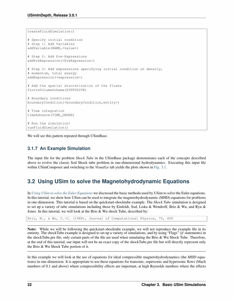
Most USimBase simulations have a underlying pattern, that can be represented as:
# Import macros to setup simulation$ import fluidsBase.mac$ import euler.mac
# Specify parameters for the specific physics problem$ PARAM_1 = <value>$ PARAM_2 = <value>$ PARAM_N = <value>
# Initialize a USim simulationinitializeFluidSimulation(NDIM,0.0,END_TIME,NUMDUMPS,CFL,GAS_GAMMA,WRITE_RESTART,DEBUG)
# Setup the gridaddGrid(lowerBounds, upperBounds, numCells, periodicDirections)
# Create data structures needed for the simulation
3.1. Using USim to solve the Euler Equations 31
USimInDepth, Release 3.0.1
createFluidSimulation()
# Specify initial condition# Step 1: Add VariablesaddVariable(NAME,<value>)
# Step 2: Add Pre-ExpressionsaddPreExpression(<PreExpression>)
# Step 3: Add expressions specifying initial condition on density,# momentum, total energyaddExpression(<expression>)
# Add the spatial discretization of the fluxesfiniteVolumeScheme(DIFFUSIVE)
# Boundary conditionsboundaryCondition(<boundaryCondition,entity>)
# Time integrationtimeAdvance(TIME_ORDER)
# Run the simulation!runFluidSimulation()
We will see this pattern repeated through USimBase.
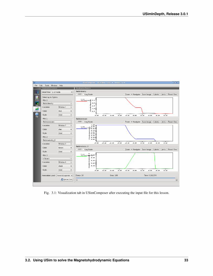
3.1.7 An Example Simulation
The input file for the problem Shock Tube in the USimBase package demonstrates each of the concepts describedabove to evolve the classic Sod Shock tube problem in one-dimensional hydrodynamics. Executing this input filewithin USimComposer and switching to the Visualize tab yields the plots shown in Fig. 3.1.
3.2 Using USim to solve the Magnetohydrodynamic Equations
In Using USim to solve the Euler Equations we discussed the basic methods used by USim to solve the Euler equations.In this tutorial, we show how USim can be used to integrate the magnetohydrodynamic (MHD) equations for problemsin one-dimension. This tutorial is based on the quickstart-shocktube example. The Shock Tube simulation is designedto set up a variety of tube simulations including those by Einfeldt, Sod, Liska & Wendroff, Brio & Wu, and Ryu &Jones. In this tutorial, we will look at the Brio & Wu shock Tube, described by:
Brio, M., & Wu, C.~C. (1988), Journal of Computational Physics, 75, 400
Note: While we will be following the quickstart-shocktube example, we will not reproduce the example file in itsentirety. The shockTube example is designed to set up a variety of simulations, and by using “Flags” (if statements) inthe shockTube.pre file, only certain parts of the file are used when simulating the Brio & Wu Shock Tube. Therefore,at the end of this tutorial, our input will not be an exact copy of the shockTube.pre file but will directly represent onlythe Brio & Wu Shock Tube portion of it.
In this example we will look at the use of equations for ideal compressible magnetohydrodynamics (the MHD equa-tions) in one-dimension. It is appropriate to use these equations for transonic, supersonic and hypersonic flows (Machnumbers of 0.1 and above) where compressibility effects are important, at high Reynolds numbers where the effects
32 Chapter 3. Basic USim Simulations
USimInDepth, Release 3.0.1
Fig. 3.1: Visualization tab in USimComposer after executing the input file for this lesson.
3.2. Using USim to solve the Magnetohydrodynamic Equations 33
USimInDepth, Release 3.0.1
of viscosity and thermal conductivity are relatively unimportant and at high magnetic Reynolds number where Ohmicresistivity is relatively unimportant.
We will follow the pattern established in Using USim to solve the Euler Equations in order that the user can see thedifferences between solving the MHD equations and the Euler equations. These are summarized in Notes at the endof each section of the tutorial.
Contents
• Using USim to solve the Magnetohydrodynamic Equations– The Magnetohydrodynamic Equations– Solving the MHD Equations in One Dimension– Adding a Simulation Grid– Creating a Fluid Simulation– Evolving the Fluid– Putting it all Together– An Example Simulation– Combining Euler and MHD Equations in the Same Input File
3.2.1 The Magnetohydrodynamic Equations
The MHD equations for an adiabatic gas can be written as a hyperbolic conservation law, which has the form:
𝜕q
𝜕𝑡+ ∇ · [ℱ (w)] = 0
where q is a vector of conserved variables (e.g. density, momentum, total energy), ℱ (w) is a non-linear flux tensorcomputed from a vector of primitive variables, (e.g. density, velocity, pressure), and w = w(q). Assuming anadiabatic equations of state, the MHD equations can be written in this form such that:
𝜕𝜌
𝜕𝑡+ ∇ · [𝜌u] = 0
𝜕𝜌u
𝜕𝑡+ ∇ ·
[𝜌uu𝑇 − bb𝑇 + I
(𝑃 + 1
2 |b|2)]
= 0
𝜕𝐸
𝜕𝑡+ ∇ · [(𝐸 + 𝑃 )u + e× b] = 0
𝜕bplasma
𝜕𝑡+ ∇× e + ∇𝜓 = 0
𝜕𝜓
𝜕𝑡+ ∇ ·
[𝑐2fastb
]= 0
Here, I is the identity matrix, 𝑃 = 𝜌𝜖(𝛾 − 1) is the pressure of an ideal gas, 𝜖 is the specific internal energy and 𝛾 isthe adiabatic index (ratio of specific heats). The quantity 𝑐fast corresponds to the fastest wave speed over the entiresimulation domain; divergence errors are advected out of the domain with this speed.
The MHD equations are represented in USim by refmanual-mhdDednerEqn. USim solves these equations by calcu-lating an upwind approximation of the flux tensor, ℱ(w) (see refmanual-classicMUSCL) and then using this approxi-mation to advance the conserved state from time 𝑡 to 𝑡+ ∆𝑡 (see refmanual-multiUpdater).
3.2.2 Solving the MHD Equations in One Dimension
The first step in any USim simulation is to import the macros that are needed to define the simulation. For theShockTube example, there are two macros that are needed:
34 Chapter 3. Basic USim Simulations
USimInDepth, Release 3.0.1
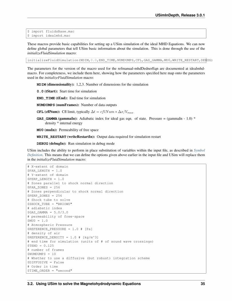
$ import fluidsBase.mac$ import idealmhd.mac
These macros provide basic capabilities for setting up a USim simulation of the ideal MHD Equations. We can nowdefine global parameters that tell USim basic information about the simulation. This is done through the use of theinitializeFluidSimulation macro:
initializeFluidSimulation(NDIM,0.0,END_TIME,NUMDUMPS,CFL,GAS_GAMMA,MU0,WRITE_RESTART,DEBUG)
The parameters for the version of the macro used for the refmanual-mhdDednerEqn are documented at idealmhd-macro. For completeness, we include them here, showing how the parameters specified here map onto the parametersused in the initializeFluidSimulation macro:
NDIM (dimensionality): 1,2,3. Number of dimensions for the simulation
0.0 (tStart): Start time for simulation
END_TIME (tEnd): End time for simulation
NUMDUMPS (numFrames): Number of data outputs
CFL (cflNum): Cfl limit, typically ∆𝑡 = 𝑐𝑓𝑙𝑁𝑢𝑚 * ∆𝑥/𝑉𝑚𝑎𝑥
GAS_GAMMA (gammaIn): Adiabatic index for ideal gas eqn. of state. Pressure = (gammaIn - 1.0) *density * internal energy
MU0 (muIn): Permeability of free space
WRITE_RESTART (writeRestartIn): Output data required for simulation restart
DEBUG (debugIn): Run simulation in debug mode
USim includes the ability to perform in place substitution of variables within the input file, as described in SymbolDefinition. This means that we can define the options given above earlier in the input file and USim will replace themin the initializeFluidSimulation macro:
# X-extent of domain$PAR_LENGTH = 1.0# Y-extent of domain$PERP_LENGTH = 1.0# Zones parallel to shock normal direction$PAR_ZONES = 256# Zones perpendicular to shock normal direction$PERP_ZONES = 256# Shock tube to solve$SHOCK_TUBE = "BRIOWU"# adiabatic index$GAS_GAMMA = 5.0/3.0# permeability of free-space$MU0 = 1.0# Atmospheric Pressure$REFERENCE_PRESSURE = 1.0 # [Pa]# density of air$REFERENCE_DENSITY = 1.0 # [kg/m^3]# end time for simulation (units of # of sound wave crossings)$TEND = 0.125# number of frames$NUMDUMPS = 10# Whether to use a diffusive (but robust) integration scheme$DIFFUSIVE = False# Order in time$TIME_ORDER = "second"
3.2. Using USim to solve the Magnetohydrodynamic Equations 35
USimInDepth, Release 3.0.1
# Write data for restarting the simulation$WRITE_RESTART = False# Output info for debugging purposes$DEBUG = False# Default dimensionality$NDIM = 1
Note that we have included a range of other variables that are defined in the quickstart-shocktube example. We willrefer to these later in this tutorial as needed. In the above, the variable TEND is given in units of the the number oftimes a sound wave crosses the grid. In order to use this to specify the end time for the simulation (END_TIME), weconvert this to have units of time through:
# nominal speed of sound$ c0 = math.sqrt(GAS_GAMMA*REFERENCE_PRESSURE/REFERENCE_DENSITY) # [m/s]
# Set end time according to (user specified)# number of times a wave crosses the box.$END_TIME = $PERP_LENGTH*TEND/c0$
The specification of the CFL parameter is described in the next section. Our simulation starts off as:
# Import macros to setup simulation$ import fluidsBase.mac$ import idealmhd.mac
# X-extent of domain$PAR_LENGTH = 1.0# Y-extent of domain$PERP_LENGTH = 1.0# Zones parallel to shock normal direction$PAR_ZONES = 256# Zones perpendicular to shock normal direction$PERP_ZONES = 256# Shock tube to solve$SHOCK_TUBE = "BRIOWU"# adiabatic index$GAS_GAMMA = 5.0/3.0# permeability of free-space$MU0 = 1.0# Atmospheric Pressure$REFERENCE_PRESSURE = 1.0 # [Pa]# density of air$REFERENCE_DENSITY = 1.0 # [kg/m^3]# end time for simulation (units of # of sound wave crossings)$TEND = 0.125# number of frames$NUMDUMPS = 10# Whether to use a diffusive (but robust) integration scheme$DIFFUSIVE = False# Order in time$TIME_ORDER = "second"# Write data for restarting the simulation$WRITE_RESTART = False# Output info for debugging purposes$DEBUG = False# Default dimensionality$NDIM = 1
# nominal speed of sound
36 Chapter 3. Basic USim Simulations
USimInDepth, Release 3.0.1
$ c0 = math.sqrt(GAS_GAMMA*REFERENCE_PRESSURE/REFERENCE_DENSITY) # [m/s]
# Set end time according to (user specified)# number of times a wave crosses the box.$END_TIME = $PERP_LENGTH*TEND/c0$
# Initialize a USim simulationinitializeFluidSimulation(NDIM,0.0,END_TIME,NUMDUMPS,CFL,GAS_GAMMA,MU0,WRITE_RESTART,DEBUG)
Note: Compared to the Euler equations discussed in Using USim to solve the Euler Equations, there are threedifferences:
1. We have replaced $ import euler.mac with $ import idealmhd.mac to change the system of equations from theEuler equations to the ideal MHD equations.
2. We have defined the permeability of free-space, 𝜇0 through the parameter MU0 (here MU0 = 1.0).
3. We have added 𝜇0 to the parameters used to initialized the simulation, replacing:
initializeFluidSimulation(NDIM,0.0,END_TIME,NUMDUMPS,CFL,GAS_GAMMA,WRITE_RESTART,DEBUG)
with:
initializeFluidSimulation(NDIM,0.0,END_TIME,NUMDUMPS,CFL,GAS_GAMMA,MU0,WRITE_RESTART,DEBUG)
3.2.3 Adding a Simulation Grid
The next step in setting up a USim simulation is to specify a simulation grid. The quickstart-shocktube uses arefmanual-ntcart grid, which is added to the simulation through the addGrid macro:
addGrid(lowerBounds, upperBounds, numCells, periodicDirections)
This options for this macro are documented in grid-macro. For completeness, we include them here:
lowerBounds: Vector of coordinates for lower edge of grid, lowerBounds = [ XMIN YMIN ZMIN ]
upperBounds: Vector of coordinates for upper edge of grid, upperBounds = [ XMAX YMAX ZMAX]
numCells: Vector of number of cells in grid, numCells = [ NX NY NZ ]
periodicDirections: List of directions that are periodic
periodicDirections = [ 0 ] (x-direction periodic)periodicDirections = [ 0 1 ] (x,y-directions periodic)periodicDirections = [ 0 1 2 ] (x,y,z-directions periodic)
The options are setup in the ShockTube example according to the dimensionality of the simulation, as specified by thevariable NDIM above:
$XMIN = -0.5*PERP_LENGTH$XMAX = 0.5*PERP_LENGTH$YMIN = -0.5*PAR_LENGTH$YMAX = 0.5*PAR_LENGTH$ZMIN = -0.5*PAR_LENGTH$ZMAX = 0.5*PAR_LENGTH
$if NDIM==1$ CFL = 0.5
3.2. Using USim to solve the Magnetohydrodynamic Equations 37
USimInDepth, Release 3.0.1
$ numCells = [PERP_ZONES]$ periodicDirections = []$ lowerBounds = [XMIN]$ upperBounds = [XMAX]$ else$if NDIM==2$ CFL = 0.4$ numCells = [PERP_ZONES, PAR_ZONES]# Make the direction perpendicular to the shock# normal periodic.$ periodicDirections = [1]$ lowerBounds = [XMIN, YMIN]$ upperBounds = [XMAX, YMAX]$ else$ CFL = 0.32$ numCells = [PERP_ZONES, PAR_ZONES, PAR_ZONES]# Make the directions perpendicular to the shock# normal periodic.$ periodicDirections = [1,2]$ lowerBounds = [XMIN, YMIN, ZMIN]$ upperBounds = [XMAX, YMAX, ZMAX]$ endif$ endif
Note as well that the CFL condition that is used for the simulation changes according to the dimension of the simula-tion. This is because the scheme for solving the hyperbolic equations has different stability requirements in differentdimensions:
CFL <=1
NDIM
So, our simulation now looks like:
# Import macros to setup simulation$ import fluidsBase.mac$ import idealmhd.mac
# X-extent of domain$PAR_LENGTH = 1.0# Y-extent of domain$PERP_LENGTH = 1.0# Zones parallel to shock normal direction$PAR_ZONES = 256# Zones perpendicular to shock normal direction$PERP_ZONES = 256# Shock tube to solve$SHOCK_TUBE = "BRIOWU"# adiabatic index$GAS_GAMMA = 5.0/3.0# permeability of free-space$MU0 = 1.0# Atmospheric Pressure$REFERENCE_PRESSURE = 1.0 # [Pa]# density of air$REFERENCE_DENSITY = 1.0 # [kg/m^3]# end time for simulation (units of # of sound wave crossings)$TEND = 0.125# number of frames$NUMDUMPS = 10
38 Chapter 3. Basic USim Simulations
USimInDepth, Release 3.0.1
# Whether to use a diffusive (but robust) integration scheme$DIFFUSIVE = False# Order in time$TIME_ORDER = "second"# Write data for restarting the simulation$WRITE_RESTART = False# Output info for debugging purposes$DEBUG = False# Default dimensionality$NDIM = 1
# nominal speed of sound$ c0 = math.sqrt(GAS_GAMMA*REFERENCE_PRESSURE/REFERENCE_DENSITY) # [m/s]
# Set end time according to (user specified)# number of times a wave crosses the box.$END_TIME = $PERP_LENGTH*TEND/c0$
$XMIN = -0.5*PERP_LENGTH$XMAX = 0.5*PERP_LENGTH$YMIN = -0.5*PAR_LENGTH$YMAX = 0.5*PAR_LENGTH$ZMIN = -0.5*PAR_LENGTH$ZMAX = 0.5*PAR_LENGTH
$if NDIM==1$ CFL = 0.5$ numCells = [PERP_ZONES]$ periodicDirections = []$ lowerBounds = [XMIN]$ upperBounds = [XMAX]$ else$if NDIM==2$ CFL = 0.4$ numCells = [PERP_ZONES, PAR_ZONES]# Make the direction perpendicular to the shock# normal periodic.$ periodicDirections = [1]$ lowerBounds = [XMIN, YMIN]$ upperBounds = [XMAX, YMAX]$ else$ CFL = 0.32$ numCells = [PERP_ZONES, PAR_ZONES, PAR_ZONES]# Make the directions perpendicular to the shock# normal periodic.$ periodicDirections = [1,2]$ lowerBounds = [XMIN, YMIN, ZMIN]$ upperBounds = [XMAX, YMAX, ZMAX]$ endif$ endif
# Initialize a USim simulationinitializeFluidSimulation(NDIM,0.0,END_TIME,NUMDUMPS,CFL,GAS_GAMMA,MU0,WRITE_RESTART,DEBUG)
# Setup the gridaddGrid(lowerBounds, upperBounds, numCells, periodicDirections)
Note: The process of adding the simulation grid is identical for both the Euler equations and the MHD equations.
3.2. Using USim to solve the Magnetohydrodynamic Equations 39
USimInDepth, Release 3.0.1
This is true for all USim simulations.
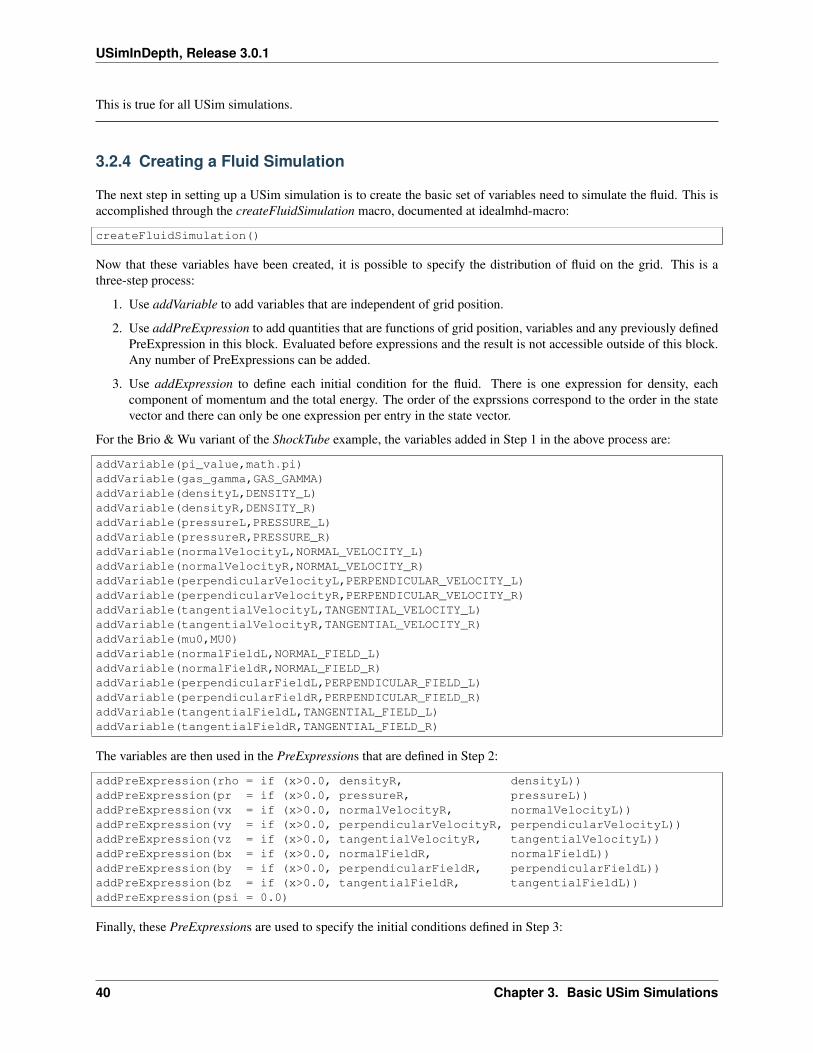
3.2.4 Creating a Fluid Simulation
The next step in setting up a USim simulation is to create the basic set of variables need to simulate the fluid. This isaccomplished through the createFluidSimulation macro, documented at idealmhd-macro:
createFluidSimulation()
Now that these variables have been created, it is possible to specify the distribution of fluid on the grid. This is athree-step process:
1. Use addVariable to add variables that are independent of grid position.
2. Use addPreExpression to add quantities that are functions of grid position, variables and any previously definedPreExpression in this block. Evaluated before expressions and the result is not accessible outside of this block.Any number of PreExpressions can be added.
3. Use addExpression to define each initial condition for the fluid. There is one expression for density, eachcomponent of momentum and the total energy. The order of the exprssions correspond to the order in the statevector and there can only be one expression per entry in the state vector.
For the Brio & Wu variant of the ShockTube example, the variables added in Step 1 in the above process are:
addVariable(pi_value,math.pi)addVariable(gas_gamma,GAS_GAMMA)addVariable(densityL,DENSITY_L)addVariable(densityR,DENSITY_R)addVariable(pressureL,PRESSURE_L)addVariable(pressureR,PRESSURE_R)addVariable(normalVelocityL,NORMAL_VELOCITY_L)addVariable(normalVelocityR,NORMAL_VELOCITY_R)addVariable(perpendicularVelocityL,PERPENDICULAR_VELOCITY_L)addVariable(perpendicularVelocityR,PERPENDICULAR_VELOCITY_R)addVariable(tangentialVelocityL,TANGENTIAL_VELOCITY_L)addVariable(tangentialVelocityR,TANGENTIAL_VELOCITY_R)addVariable(mu0,MU0)addVariable(normalFieldL,NORMAL_FIELD_L)addVariable(normalFieldR,NORMAL_FIELD_R)addVariable(perpendicularFieldL,PERPENDICULAR_FIELD_L)addVariable(perpendicularFieldR,PERPENDICULAR_FIELD_R)addVariable(tangentialFieldL,TANGENTIAL_FIELD_L)addVariable(tangentialFieldR,TANGENTIAL_FIELD_R)
The variables are then used in the PreExpressions that are defined in Step 2:
addPreExpression(rho = if (x>0.0, densityR, densityL))addPreExpression(pr = if (x>0.0, pressureR, pressureL))addPreExpression(vx = if (x>0.0, normalVelocityR, normalVelocityL))addPreExpression(vy = if (x>0.0, perpendicularVelocityR, perpendicularVelocityL))addPreExpression(vz = if (x>0.0, tangentialVelocityR, tangentialVelocityL))addPreExpression(bx = if (x>0.0, normalFieldR, normalFieldL))addPreExpression(by = if (x>0.0, perpendicularFieldR, perpendicularFieldL))addPreExpression(bz = if (x>0.0, tangentialFieldR, tangentialFieldL))addPreExpression(psi = 0.0)
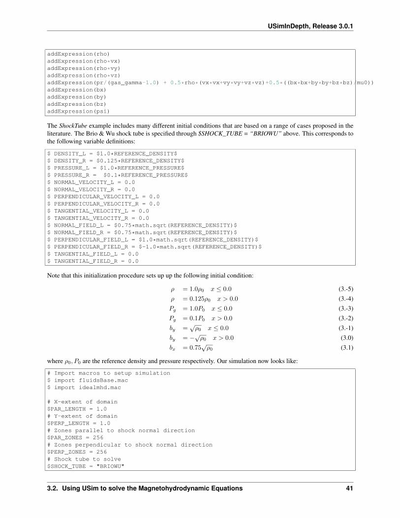
Finally, these PreExpressions are used to specify the initial conditions defined in Step 3:
40 Chapter 3. Basic USim Simulations
USimInDepth, Release 3.0.1
addExpression(rho)addExpression(rho*vx)addExpression(rho*vy)addExpression(rho*vz)addExpression(pr/(gas_gamma-1.0) + 0.5*rho*(vx*vx+vy*vy+vz*vz)+0.5*((bx*bx+by*by+bz*bz)/mu0))addExpression(bx)addExpression(by)addExpression(bz)addExpression(psi)
The ShockTube example includes many different initial conditions that are based on a range of cases proposed in theliterature. The Brio & Wu shock tube is specified through $SHOCK_TUBE = “BRIOWU” above. This corresponds tothe following variable definitions:
$ DENSITY_L = $1.0*REFERENCE_DENSITY$$ DENSITY_R = $0.125*REFERENCE_DENSITY$$ PRESSURE_L = $1.0*REFERENCE_PRESSURE$$ PRESSURE_R = $0.1*REFERENCE_PRESSURE$$ NORMAL_VELOCITY_L = 0.0$ NORMAL_VELOCITY_R = 0.0$ PERPENDICULAR_VELOCITY_L = 0.0$ PERPENDICULAR_VELOCITY_R = 0.0$ TANGENTIAL_VELOCITY_L = 0.0$ TANGENTIAL_VELOCITY_R = 0.0$ NORMAL_FIELD_L = $0.75*math.sqrt(REFERENCE_DENSITY)$$ NORMAL_FIELD_R = $0.75*math.sqrt(REFERENCE_DENSITY)$$ PERPENDICULAR_FIELD_L = $1.0*math.sqrt(REFERENCE_DENSITY)$$ PERPENDICULAR_FIELD_R = $-1.0*math.sqrt(REFERENCE_DENSITY)$$ TANGENTIAL_FIELD_L = 0.0$ TANGENTIAL_FIELD_R = 0.0
Note that this initialization procedure sets up up the following initial condition:
𝜌 = 1.0𝜌0 𝑥 ≤ 0.0 (3.-5)𝜌 = 0.125𝜌0 𝑥 > 0.0 (3.-4)𝑃𝑔 = 1.0𝑃0 𝑥 ≤ 0.0 (3.-3)𝑃𝑔 = 0.1𝑃0 𝑥 > 0.0 (3.-2)𝑏𝑦 =
√𝜌0 𝑥 ≤ 0.0 (3.-1)
𝑏𝑦 = −√𝜌0 𝑥 > 0.0 (3.0)
𝑏𝑥 = 0.75√𝜌0 (3.1)
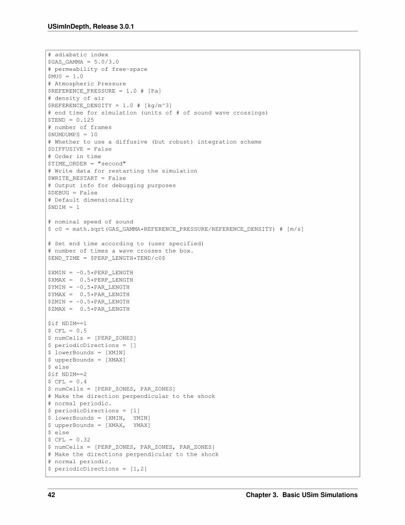
where 𝜌0, 𝑃0 are the reference density and pressure respectively. Our simulation now looks like:
# Import macros to setup simulation$ import fluidsBase.mac$ import idealmhd.mac
# X-extent of domain$PAR_LENGTH = 1.0# Y-extent of domain$PERP_LENGTH = 1.0# Zones parallel to shock normal direction$PAR_ZONES = 256# Zones perpendicular to shock normal direction$PERP_ZONES = 256# Shock tube to solve$SHOCK_TUBE = "BRIOWU"
3.2. Using USim to solve the Magnetohydrodynamic Equations 41
USimInDepth, Release 3.0.1
# adiabatic index$GAS_GAMMA = 5.0/3.0# permeability of free-space$MU0 = 1.0# Atmospheric Pressure$REFERENCE_PRESSURE = 1.0 # [Pa]# density of air$REFERENCE_DENSITY = 1.0 # [kg/m^3]# end time for simulation (units of # of sound wave crossings)$TEND = 0.125# number of frames$NUMDUMPS = 10# Whether to use a diffusive (but robust) integration scheme$DIFFUSIVE = False# Order in time$TIME_ORDER = "second"# Write data for restarting the simulation$WRITE_RESTART = False# Output info for debugging purposes$DEBUG = False# Default dimensionality$NDIM = 1
# nominal speed of sound$ c0 = math.sqrt(GAS_GAMMA*REFERENCE_PRESSURE/REFERENCE_DENSITY) # [m/s]
# Set end time according to (user specified)# number of times a wave crosses the box.$END_TIME = $PERP_LENGTH*TEND/c0$
$XMIN = -0.5*PERP_LENGTH$XMAX = 0.5*PERP_LENGTH$YMIN = -0.5*PAR_LENGTH$YMAX = 0.5*PAR_LENGTH$ZMIN = -0.5*PAR_LENGTH$ZMAX = 0.5*PAR_LENGTH
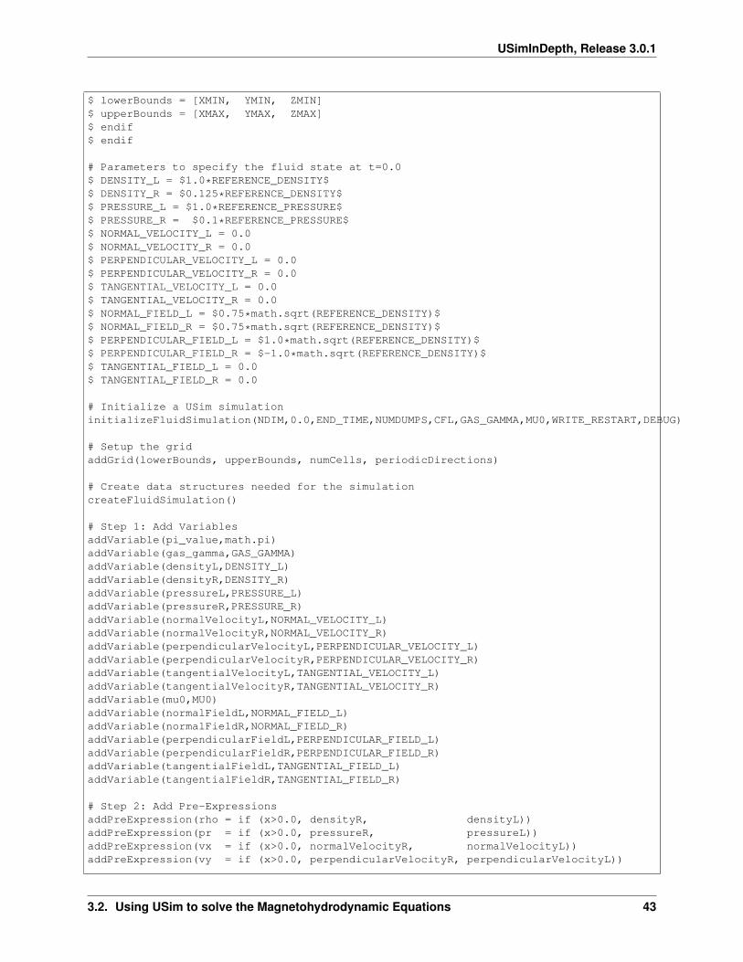
$if NDIM==1$ CFL = 0.5$ numCells = [PERP_ZONES]$ periodicDirections = []$ lowerBounds = [XMIN]$ upperBounds = [XMAX]$ else$if NDIM==2$ CFL = 0.4$ numCells = [PERP_ZONES, PAR_ZONES]# Make the direction perpendicular to the shock# normal periodic.$ periodicDirections = [1]$ lowerBounds = [XMIN, YMIN]$ upperBounds = [XMAX, YMAX]$ else$ CFL = 0.32$ numCells = [PERP_ZONES, PAR_ZONES, PAR_ZONES]# Make the directions perpendicular to the shock# normal periodic.$ periodicDirections = [1,2]
42 Chapter 3. Basic USim Simulations
USimInDepth, Release 3.0.1
$ lowerBounds = [XMIN, YMIN, ZMIN]$ upperBounds = [XMAX, YMAX, ZMAX]$ endif$ endif
# Parameters to specify the fluid state at t=0.0$ DENSITY_L = $1.0*REFERENCE_DENSITY$$ DENSITY_R = $0.125*REFERENCE_DENSITY$$ PRESSURE_L = $1.0*REFERENCE_PRESSURE$$ PRESSURE_R = $0.1*REFERENCE_PRESSURE$$ NORMAL_VELOCITY_L = 0.0$ NORMAL_VELOCITY_R = 0.0$ PERPENDICULAR_VELOCITY_L = 0.0$ PERPENDICULAR_VELOCITY_R = 0.0$ TANGENTIAL_VELOCITY_L = 0.0$ TANGENTIAL_VELOCITY_R = 0.0$ NORMAL_FIELD_L = $0.75*math.sqrt(REFERENCE_DENSITY)$$ NORMAL_FIELD_R = $0.75*math.sqrt(REFERENCE_DENSITY)$$ PERPENDICULAR_FIELD_L = $1.0*math.sqrt(REFERENCE_DENSITY)$$ PERPENDICULAR_FIELD_R = $-1.0*math.sqrt(REFERENCE_DENSITY)$$ TANGENTIAL_FIELD_L = 0.0$ TANGENTIAL_FIELD_R = 0.0
# Initialize a USim simulationinitializeFluidSimulation(NDIM,0.0,END_TIME,NUMDUMPS,CFL,GAS_GAMMA,MU0,WRITE_RESTART,DEBUG)
# Setup the gridaddGrid(lowerBounds, upperBounds, numCells, periodicDirections)
# Create data structures needed for the simulationcreateFluidSimulation()
# Step 1: Add VariablesaddVariable(pi_value,math.pi)addVariable(gas_gamma,GAS_GAMMA)addVariable(densityL,DENSITY_L)addVariable(densityR,DENSITY_R)addVariable(pressureL,PRESSURE_L)addVariable(pressureR,PRESSURE_R)addVariable(normalVelocityL,NORMAL_VELOCITY_L)addVariable(normalVelocityR,NORMAL_VELOCITY_R)addVariable(perpendicularVelocityL,PERPENDICULAR_VELOCITY_L)addVariable(perpendicularVelocityR,PERPENDICULAR_VELOCITY_R)addVariable(tangentialVelocityL,TANGENTIAL_VELOCITY_L)addVariable(tangentialVelocityR,TANGENTIAL_VELOCITY_R)addVariable(mu0,MU0)addVariable(normalFieldL,NORMAL_FIELD_L)addVariable(normalFieldR,NORMAL_FIELD_R)addVariable(perpendicularFieldL,PERPENDICULAR_FIELD_L)addVariable(perpendicularFieldR,PERPENDICULAR_FIELD_R)addVariable(tangentialFieldL,TANGENTIAL_FIELD_L)addVariable(tangentialFieldR,TANGENTIAL_FIELD_R)
# Step 2: Add Pre-ExpressionsaddPreExpression(rho = if (x>0.0, densityR, densityL))addPreExpression(pr = if (x>0.0, pressureR, pressureL))addPreExpression(vx = if (x>0.0, normalVelocityR, normalVelocityL))addPreExpression(vy = if (x>0.0, perpendicularVelocityR, perpendicularVelocityL))
3.2. Using USim to solve the Magnetohydrodynamic Equations 43
USimInDepth, Release 3.0.1
addPreExpression(vz = if (x>0.0, tangentialVelocityR, tangentialVelocityL))addPreExpression(bx = if (x>0.0, normalFieldR, normalFieldL))addPreExpression(by = if (x>0.0, perpendicularFieldR, perpendicularFieldL))addPreExpression(bz = if (x>0.0, tangentialFieldR, tangentialFieldL))addPreExpression(psi = 0.0)
# Step 3: Add expressions specifying initial condition on density,# momentum, total energy, magnetic field and correction potentialaddExpression(rho)addExpression(rho*vx)addExpression(rho*vy)addExpression(rho*vz)addExpression(pr/(gas_gamma-1.0) + 0.5*rho*(vx*vx+vy*vy+vz*vz)+0.5*((bx*bx+by*by+bz*bz)/mu0))addExpression(bx)addExpression(by)addExpression(bz)addExpression(psi)
Note: Compared to the Euler equations discussed in Using USim to solve the Euler Equations, there are threeimportant differences in specifying the initial conditions:
1. We have to specify the three components of the magnetic field, here these are denoted 𝑏{𝑥,𝑦,𝑧}.
2. We have to specify the correction potential, here denoted, psi. Typically, 𝜓 = 0 at 𝑡 = 0.
3. We have to change the definition of the total energy from 𝐸 = 𝑃Γ−1 + 𝜌|u|2
2 to 𝐸 = 𝑃Γ−1 + 𝜌|u|2
2 + |b|22 ; that is
we include the contribution of the magnetic field to the total energy
3.2.5 Evolving the Fluid
USim implements the well-known MUSCL scheme to advance the conserved variables in time. There is a simplemacro that can be called to implement this scheme as shown below:
finiteVolumeScheme(DIFFUSIVE)
This macro is documented at idealmhd-macro. It’s purpose is to compute the numerical flux for the hyperbolic system:
∇ · [ℱ (w)] − 𝒮 (w)
The next part of evolving the fluid is to apply boundary conditions at the left and right of the domain to ensure that atthe next time step, physically-valid data is used to update the conserved state. Without this, the simulation will fail. Itis possible to specify arbitrary boundary conditions in USim. For the Brio & Wu shock tube example considered here,appropriate boundary conditions are outflow (“open”) boundary conditions at both ends of the domain
boundaryCondition(copy,left)boundaryCondition(copy,right)
The copy boundary condition block is described in refmanual-copy. This boundary condition updater copies the valueson the layer next to the ghost cells into the ghost cells - this is equivalent to a zero derivative boundary condition. If weare evolving in more than one-dimension, we have to specify boundary conditions on the rest of the domain boundaries.For this example, this is done using periodic boundary conditions (refmanual-periodicCartBc):
boundaryCondition(periodic)
The final element of advancing the conserved quantities from time 𝑡 to 𝑡 + ∆𝑡 is to apply a time integration scheme,specified through:
44 Chapter 3. Basic USim Simulations
USimInDepth, Release 3.0.1
timeAdvance(TIME_ORDER)
This applies an explicit Runge-Kutta time-integration scheme with the order of accuracy determined by theTIME_ORDER parameter. TIME_ORDER can be one of first, second, third or fourth according to the desired or-der of accuracy.
Note: The method for evolving the fluid is identical for the Euler equations and the MHD equations in one-dimension.
3.2.6 Putting it all Together
The final step in the USim simulation is to add:
runFluidSimulation()
This tells USim that we’re done specifying the simulation and that it can be run. So, our simulation now looks like:
# Import macros to setup simulation$ import fluidsBase.mac$ import idealmhd.mac
# X-extent of domain$PAR_LENGTH = 1.0# Y-extent of domain$PERP_LENGTH = 1.0# Zones parallel to shock normal direction$PAR_ZONES = 256# Zones perpendicular to shock normal direction$PERP_ZONES = 256# Shock tube to solve$SHOCK_TUBE = "BRIOWU"# adiabatic index$GAS_GAMMA = 5.0/3.0# permeability of free-space$MU0 = 1.0# Atmospheric Pressure$REFERENCE_PRESSURE = 1.0 # [Pa]# density of air$REFERENCE_DENSITY = 1.0 # [kg/m^3]# end time for simulation (units of # of sound wave crossings)$TEND = 0.125# number of frames$NUMDUMPS = 10# Whether to use a diffusive (but robust) integration scheme$DIFFUSIVE = False# Order in time$TIME_ORDER = "second"# Write data for restarting the simulation$WRITE_RESTART = False# Output info for debugging purposes$DEBUG = False# Default dimensionality$NDIM = 1
# nominal speed of sound$ c0 = math.sqrt(GAS_GAMMA*REFERENCE_PRESSURE/REFERENCE_DENSITY) # [m/s]
# Set end time according to (user specified)
3.2. Using USim to solve the Magnetohydrodynamic Equations 45
USimInDepth, Release 3.0.1
# number of times a wave crosses the box.$END_TIME = $PERP_LENGTH*TEND/c0$
$XMIN = -0.5*PERP_LENGTH$XMAX = 0.5*PERP_LENGTH$YMIN = -0.5*PAR_LENGTH$YMAX = 0.5*PAR_LENGTH$ZMIN = -0.5*PAR_LENGTH$ZMAX = 0.5*PAR_LENGTH
$if NDIM==1$ CFL = 0.5$ numCells = [PERP_ZONES]$ periodicDirections = []$ lowerBounds = [XMIN]$ upperBounds = [XMAX]$ else$if NDIM==2$ CFL = 0.4$ numCells = [PERP_ZONES, PAR_ZONES]# Make the direction perpendicular to the shock# normal periodic.$ periodicDirections = [1]$ lowerBounds = [XMIN, YMIN]$ upperBounds = [XMAX, YMAX]$ else$ CFL = 0.32$ numCells = [PERP_ZONES, PAR_ZONES, PAR_ZONES]# Make the directions perpendicular to the shock# normal periodic.$ periodicDirections = [1,2]$ lowerBounds = [XMIN, YMIN, ZMIN]$ upperBounds = [XMAX, YMAX, ZMAX]$ endif$ endif
# Parameters to specify the fluid state at t=0.0$ DENSITY_L = $1.0*REFERENCE_DENSITY$$ DENSITY_R = $0.125*REFERENCE_DENSITY$$ PRESSURE_L = $1.0*REFERENCE_PRESSURE$$ PRESSURE_R = $0.1*REFERENCE_PRESSURE$$ NORMAL_VELOCITY_L = 0.0$ NORMAL_VELOCITY_R = 0.0$ PERPENDICULAR_VELOCITY_L = 0.0$ PERPENDICULAR_VELOCITY_R = 0.0$ TANGENTIAL_VELOCITY_L = 0.0$ TANGENTIAL_VELOCITY_R = 0.0$ NORMAL_FIELD_L = $0.75*math.sqrt(REFERENCE_DENSITY)$$ NORMAL_FIELD_R = $0.75*math.sqrt(REFERENCE_DENSITY)$$ PERPENDICULAR_FIELD_L = $1.0*math.sqrt(REFERENCE_DENSITY)$$ PERPENDICULAR_FIELD_R = $-1.0*math.sqrt(REFERENCE_DENSITY)$$ TANGENTIAL_FIELD_L = 0.0$ TANGENTIAL_FIELD_R = 0.0
# Initialize a USim simulationinitializeFluidSimulation(NDIM,0.0,END_TIME,NUMDUMPS,CFL,GAS_GAMMA,MU0,WRITE_RESTART,DEBUG)
# Setup the grid
46 Chapter 3. Basic USim Simulations
USimInDepth, Release 3.0.1
addGrid(lowerBounds, upperBounds, numCells, periodicDirections)
# Create data structures needed for the simulationcreateFluidSimulation()
# Step 1: Add VariablesaddVariable(pi_value,math.pi)addVariable(gas_gamma,GAS_GAMMA)addVariable(densityL,DENSITY_L)addVariable(densityR,DENSITY_R)addVariable(pressureL,PRESSURE_L)addVariable(pressureR,PRESSURE_R)addVariable(normalVelocityL,NORMAL_VELOCITY_L)addVariable(normalVelocityR,NORMAL_VELOCITY_R)addVariable(perpendicularVelocityL,PERPENDICULAR_VELOCITY_L)addVariable(perpendicularVelocityR,PERPENDICULAR_VELOCITY_R)addVariable(tangentialVelocityL,TANGENTIAL_VELOCITY_L)addVariable(tangentialVelocityR,TANGENTIAL_VELOCITY_R)addVariable(mu0,MU0)addVariable(normalFieldL,NORMAL_FIELD_L)addVariable(normalFieldR,NORMAL_FIELD_R)addVariable(perpendicularFieldL,PERPENDICULAR_FIELD_L)addVariable(perpendicularFieldR,PERPENDICULAR_FIELD_R)addVariable(tangentialFieldL,TANGENTIAL_FIELD_L)addVariable(tangentialFieldR,TANGENTIAL_FIELD_R)
# Step 2: Add Pre-ExpressionsaddPreExpression(rho = if (x>0.0, densityR, densityL))
addPreExpression(pr = if (x>0.0, pressureR, pressureL))addPreExpression(vx = if (x>0.0, normalVelocityR, normalVelocityL))addPreExpression(vy = if (x>0.0, perpendicularVelocityR, perpendicularVelocityL))addPreExpression(vz = if (x>0.0, tangentialVelocityR, tangentialVelocityL))addPreExpression(bx = if (x>0.0, normalFieldR, normalFieldL))addPreExpression(by = if (x>0.0, perpendicularFieldR, perpendicularFieldL))addPreExpression(bz = if (x>0.0, tangentialFieldR, tangentialFieldL))addPreExpression(psi = 0.0)
# Step 3: Add expressions specifying initial condition on density,# momentum, total energy, magnetic field and correction potentialaddExpression(rho)addExpression(rho*vx)addExpression(rho*vy)addExpression(rho*vz)addExpression(pr/(gas_gamma-1.0) + 0.5*rho*(vx*vx+vy*vy+vz*vz)+0.5*((bx*bx+by*by+bz*bz)/mu0))addExpression(bx)addExpression(by)addExpression(bz)addExpression(psi)
# Add the spatial discretization of the fluxesfiniteVolumeScheme(DIFFUSIVE)
# Boundary conditionsboundaryCondition(copy,left)boundaryCondition(copy,right)boundaryCondition(periodic)
# Time integration
3.2. Using USim to solve the Magnetohydrodynamic Equations 47
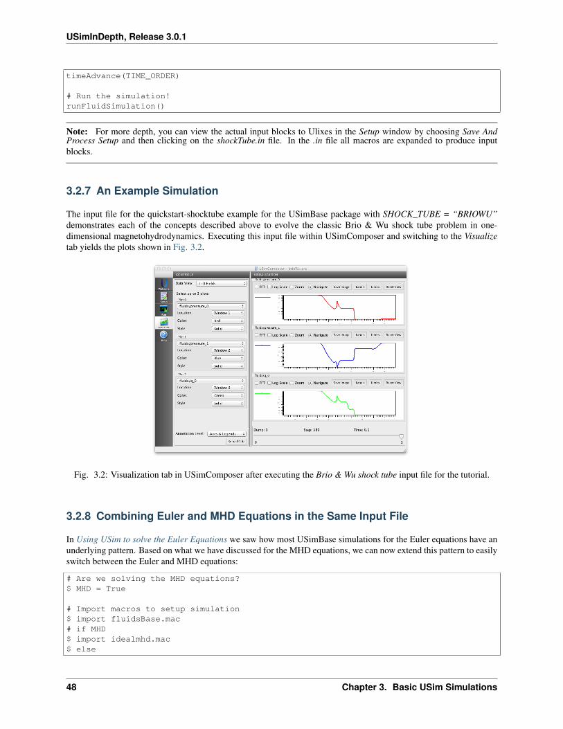
USimInDepth, Release 3.0.1
timeAdvance(TIME_ORDER)
# Run the simulation!runFluidSimulation()
Note: For more depth, you can view the actual input blocks to Ulixes in the Setup window by choosing Save AndProcess Setup and then clicking on the shockTube.in file. In the .in file all macros are expanded to produce inputblocks.
3.2.7 An Example Simulation
The input file for the quickstart-shocktube example for the USimBase package with SHOCK_TUBE = “BRIOWU”demonstrates each of the concepts described above to evolve the classic Brio & Wu shock tube problem in one-dimensional magnetohydrodynamics. Executing this input file within USimComposer and switching to the Visualizetab yields the plots shown in Fig. 3.2.
Fig. 3.2: Visualization tab in USimComposer after executing the Brio & Wu shock tube input file for the tutorial.
3.2.8 Combining Euler and MHD Equations in the Same Input File
In Using USim to solve the Euler Equations we saw how most USimBase simulations for the Euler equations have anunderlying pattern. Based on what we have discussed for the MHD equations, we can now extend this pattern to easilyswitch between the Euler and MHD equations:
# Are we solving the MHD equations?$ MHD = True
# Import macros to setup simulation$ import fluidsBase.mac# if MHD$ import idealmhd.mac$ else
48 Chapter 3. Basic USim Simulations
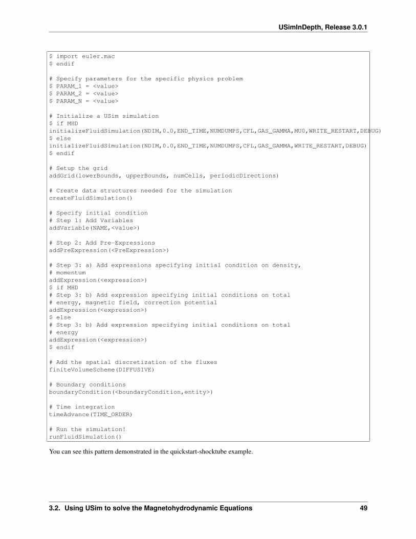
USimInDepth, Release 3.0.1
$ import euler.mac$ endif
# Specify parameters for the specific physics problem$ PARAM_1 = <value>$ PARAM_2 = <value>$ PARAM_N = <value>
# Initialize a USim simulation$ if MHDinitializeFluidSimulation(NDIM,0.0,END_TIME,NUMDUMPS,CFL,GAS_GAMMA,MU0,WRITE_RESTART,DEBUG)$ elseinitializeFluidSimulation(NDIM,0.0,END_TIME,NUMDUMPS,CFL,GAS_GAMMA,WRITE_RESTART,DEBUG)$ endif
# Setup the gridaddGrid(lowerBounds, upperBounds, numCells, periodicDirections)
# Create data structures needed for the simulationcreateFluidSimulation()
# Specify initial condition# Step 1: Add VariablesaddVariable(NAME,<value>)
# Step 2: Add Pre-ExpressionsaddPreExpression(<PreExpression>)
# Step 3: a) Add expressions specifying initial condition on density,# momentumaddExpression(<expression>)$ if MHD# Step 3: b) Add expression specifying initial conditions on total# energy, magnetic field, correction potentialaddExpression(<expression>)$ else# Step 3: b) Add expression specifying initial conditions on total# energyaddExpression(<expression>)$ endif
# Add the spatial discretization of the fluxesfiniteVolumeScheme(DIFFUSIVE)
# Boundary conditionsboundaryCondition(<boundaryCondition,entity>)
# Time integrationtimeAdvance(TIME_ORDER)
# Run the simulation!runFluidSimulation()
You can see this pattern demonstrated in the quickstart-shocktube example.
3.2. Using USim to solve the Magnetohydrodynamic Equations 49
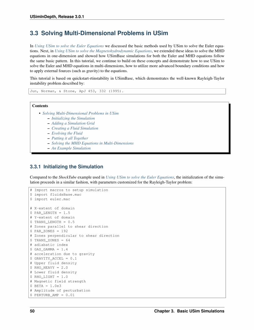
USimInDepth, Release 3.0.1
3.3 Solving Multi-Dimensional Problems in USim
In Using USim to solve the Euler Equations we discussed the basic methods used by USim to solve the Euler equa-tions. Next, in Using USim to solve the Magnetohydrodynamic Equations, we extended these ideas to solve the MHDequations in one-dimension and showed how USimBase simulations for both the Euler and MHD equations followthe same basic pattern. In this tutorial, we continue to build on these concepts and demonstrate how to use USim tosolve the Euler and MHD equations in multi-dimensions, how to utilize more advanced boundary conditions and howto apply external fources (such as gravity) to the equations.
This tutorial is based on quickstart-rtinstability in USimBase, which demonstrates the well-known Rayleigh-Taylorinstability problem described by:
Jun, Norman, & Stone, ApJ 453, 332 (1995).
Contents
• Solving Multi-Dimensional Problems in USim– Initializing the Simulation– Adding a Simulation Grid– Creating a Fluid Simulation– Evolving the Fluid– Putting it all Together– Solving the MHD Equations in Multi-Dimensions– An Example Simulation
3.3.1 Initializing the Simulation
Compared to the ShockTube example used in Using USim to solve the Euler Equations, the initialization of the simu-lation proceeds in a similar fashion, with parameters customized for the Rayleigh-Taylor problem:
# Import macros to setup simulation$ import fluidsBase.mac$ import euler.mac
# X-extent of domain$ PAR_LENGTH = 1.5# Y-extent of domain$ TRANS_LENGTH = 0.5# Zones parallel to shear direction$ PAR_ZONES = 192# Zones perpendicular to shear direction$ TRANS_ZONES = 64# adiabatic index$ GAS_GAMMA = 1.4# acceleration due to gravity$ GRAVITY_ACCEL = 0.1# Upper fluid density$ RHO_HEAVY = 2.0# Lower fluid density$ RHO_LIGHT = 1.0# Magnetic field strength$ BETA = 1.0e3# Amplitude of perturbation$ PERTURB_AMP = 0.01
50 Chapter 3. Basic USim Simulations
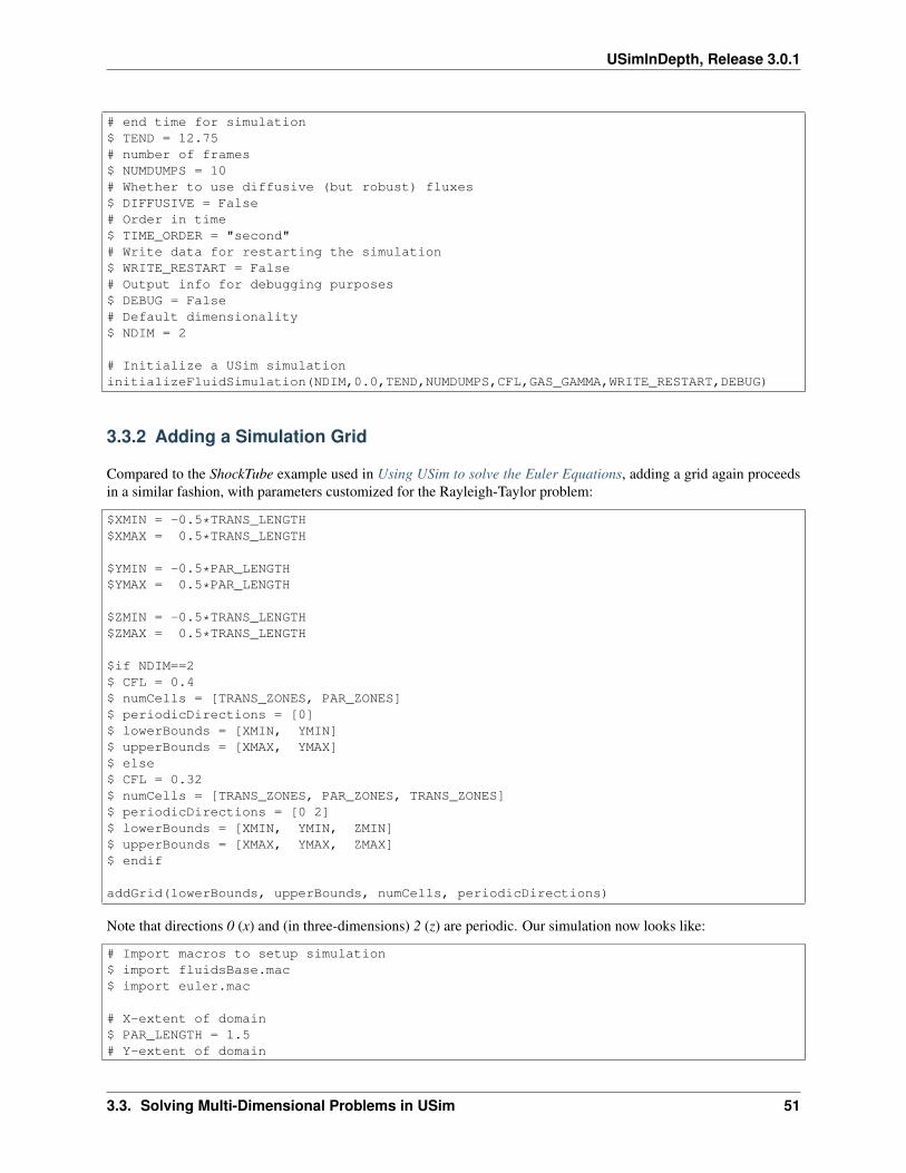
USimInDepth, Release 3.0.1
# end time for simulation$ TEND = 12.75# number of frames$ NUMDUMPS = 10# Whether to use diffusive (but robust) fluxes$ DIFFUSIVE = False# Order in time$ TIME_ORDER = "second"# Write data for restarting the simulation$ WRITE_RESTART = False# Output info for debugging purposes$ DEBUG = False# Default dimensionality$ NDIM = 2
# Initialize a USim simulationinitializeFluidSimulation(NDIM,0.0,TEND,NUMDUMPS,CFL,GAS_GAMMA,WRITE_RESTART,DEBUG)
3.3.2 Adding a Simulation Grid
Compared to the ShockTube example used in Using USim to solve the Euler Equations, adding a grid again proceedsin a similar fashion, with parameters customized for the Rayleigh-Taylor problem:
$XMIN = -0.5*TRANS_LENGTH$XMAX = 0.5*TRANS_LENGTH
$YMIN = -0.5*PAR_LENGTH$YMAX = 0.5*PAR_LENGTH
$ZMIN = -0.5*TRANS_LENGTH$ZMAX = 0.5*TRANS_LENGTH
$if NDIM==2$ CFL = 0.4$ numCells = [TRANS_ZONES, PAR_ZONES]$ periodicDirections = [0]$ lowerBounds = [XMIN, YMIN]$ upperBounds = [XMAX, YMAX]$ else$ CFL = 0.32$ numCells = [TRANS_ZONES, PAR_ZONES, TRANS_ZONES]$ periodicDirections = [0 2]$ lowerBounds = [XMIN, YMIN, ZMIN]$ upperBounds = [XMAX, YMAX, ZMAX]$ endif
addGrid(lowerBounds, upperBounds, numCells, periodicDirections)
Note that directions 0 (x) and (in three-dimensions) 2 (z) are periodic. Our simulation now looks like:
# Import macros to setup simulation$ import fluidsBase.mac$ import euler.mac
# X-extent of domain$ PAR_LENGTH = 1.5# Y-extent of domain
3.3. Solving Multi-Dimensional Problems in USim 51
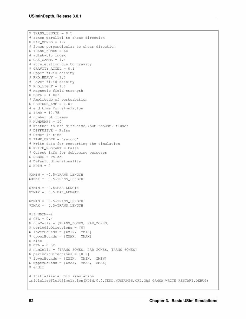
USimInDepth, Release 3.0.1
$ TRANS_LENGTH = 0.5# Zones parallel to shear direction$ PAR_ZONES = 192# Zones perpendicular to shear direction$ TRANS_ZONES = 64# adiabatic index$ GAS_GAMMA = 1.4# acceleration due to gravity$ GRAVITY_ACCEL = 0.1# Upper fluid density$ RHO_HEAVY = 2.0# Lower fluid density$ RHO_LIGHT = 1.0# Magnetic field strength$ BETA = 1.0e3# Amplitude of perturbation$ PERTURB_AMP = 0.01# end time for simulation$ TEND = 12.75# number of frames$ NUMDUMPS = 10# Whether to use diffusive (but robust) fluxes$ DIFFUSIVE = False# Order in time$ TIME_ORDER = "second"# Write data for restarting the simulation$ WRITE_RESTART = False# Output info for debugging purposes$ DEBUG = False# Default dimensionality$ NDIM = 2
$XMIN = -0.5*TRANS_LENGTH$XMAX = 0.5*TRANS_LENGTH
$YMIN = -0.5*PAR_LENGTH$YMAX = 0.5*PAR_LENGTH
$ZMIN = -0.5*TRANS_LENGTH$ZMAX = 0.5*TRANS_LENGTH
$if NDIM==2$ CFL = 0.4$ numCells = [TRANS_ZONES, PAR_ZONES]$ periodicDirections = [0]$ lowerBounds = [XMIN, YMIN]$ upperBounds = [XMAX, YMAX]$ else$ CFL = 0.32$ numCells = [TRANS_ZONES, PAR_ZONES, TRANS_ZONES]$ periodicDirections = [0 2]$ lowerBounds = [XMIN, YMIN, ZMIN]$ upperBounds = [XMAX, YMAX, ZMAX]$ endif
# Initialize a USim simulationinitializeFluidSimulation(NDIM,0.0,TEND,NUMDUMPS,CFL,GAS_GAMMA,WRITE_RESTART,DEBUG)
52 Chapter 3. Basic USim Simulations
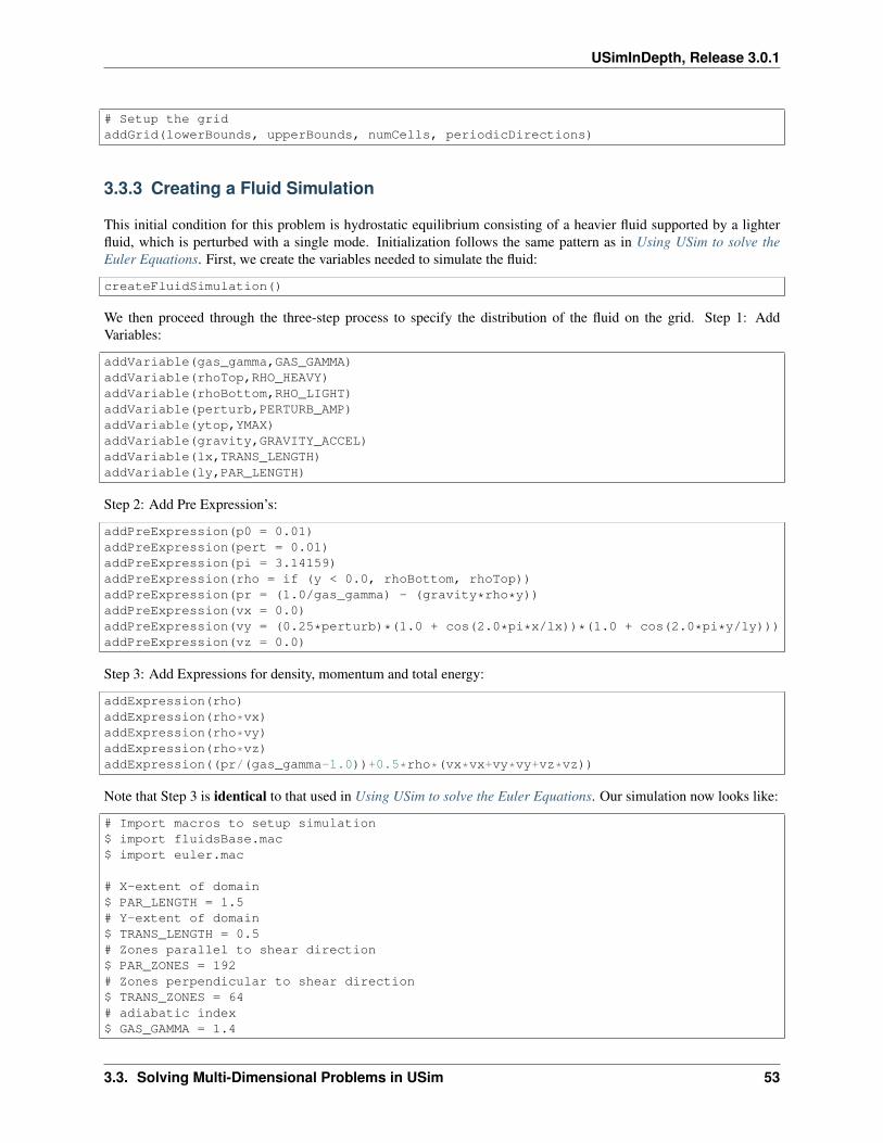
USimInDepth, Release 3.0.1
# Setup the gridaddGrid(lowerBounds, upperBounds, numCells, periodicDirections)
3.3.3 Creating a Fluid Simulation
This initial condition for this problem is hydrostatic equilibrium consisting of a heavier fluid supported by a lighterfluid, which is perturbed with a single mode. Initialization follows the same pattern as in Using USim to solve theEuler Equations. First, we create the variables needed to simulate the fluid:
createFluidSimulation()
We then proceed through the three-step process to specify the distribution of the fluid on the grid. Step 1: AddVariables:
addVariable(gas_gamma,GAS_GAMMA)addVariable(rhoTop,RHO_HEAVY)addVariable(rhoBottom,RHO_LIGHT)addVariable(perturb,PERTURB_AMP)addVariable(ytop,YMAX)addVariable(gravity,GRAVITY_ACCEL)addVariable(lx,TRANS_LENGTH)addVariable(ly,PAR_LENGTH)
Step 2: Add Pre Expression’s:
addPreExpression(p0 = 0.01)addPreExpression(pert = 0.01)addPreExpression(pi = 3.14159)addPreExpression(rho = if (y < 0.0, rhoBottom, rhoTop))addPreExpression(pr = (1.0/gas_gamma) - (gravity*rho*y))addPreExpression(vx = 0.0)addPreExpression(vy = (0.25*perturb)*(1.0 + cos(2.0*pi*x/lx))*(1.0 + cos(2.0*pi*y/ly)))addPreExpression(vz = 0.0)
Step 3: Add Expressions for density, momentum and total energy:
addExpression(rho)addExpression(rho*vx)addExpression(rho*vy)addExpression(rho*vz)addExpression((pr/(gas_gamma-1.0))+0.5*rho*(vx*vx+vy*vy+vz*vz))
Note that Step 3 is identical to that used in Using USim to solve the Euler Equations. Our simulation now looks like:
# Import macros to setup simulation$ import fluidsBase.mac$ import euler.mac
# X-extent of domain$ PAR_LENGTH = 1.5# Y-extent of domain$ TRANS_LENGTH = 0.5# Zones parallel to shear direction$ PAR_ZONES = 192# Zones perpendicular to shear direction$ TRANS_ZONES = 64# adiabatic index$ GAS_GAMMA = 1.4
3.3. Solving Multi-Dimensional Problems in USim 53
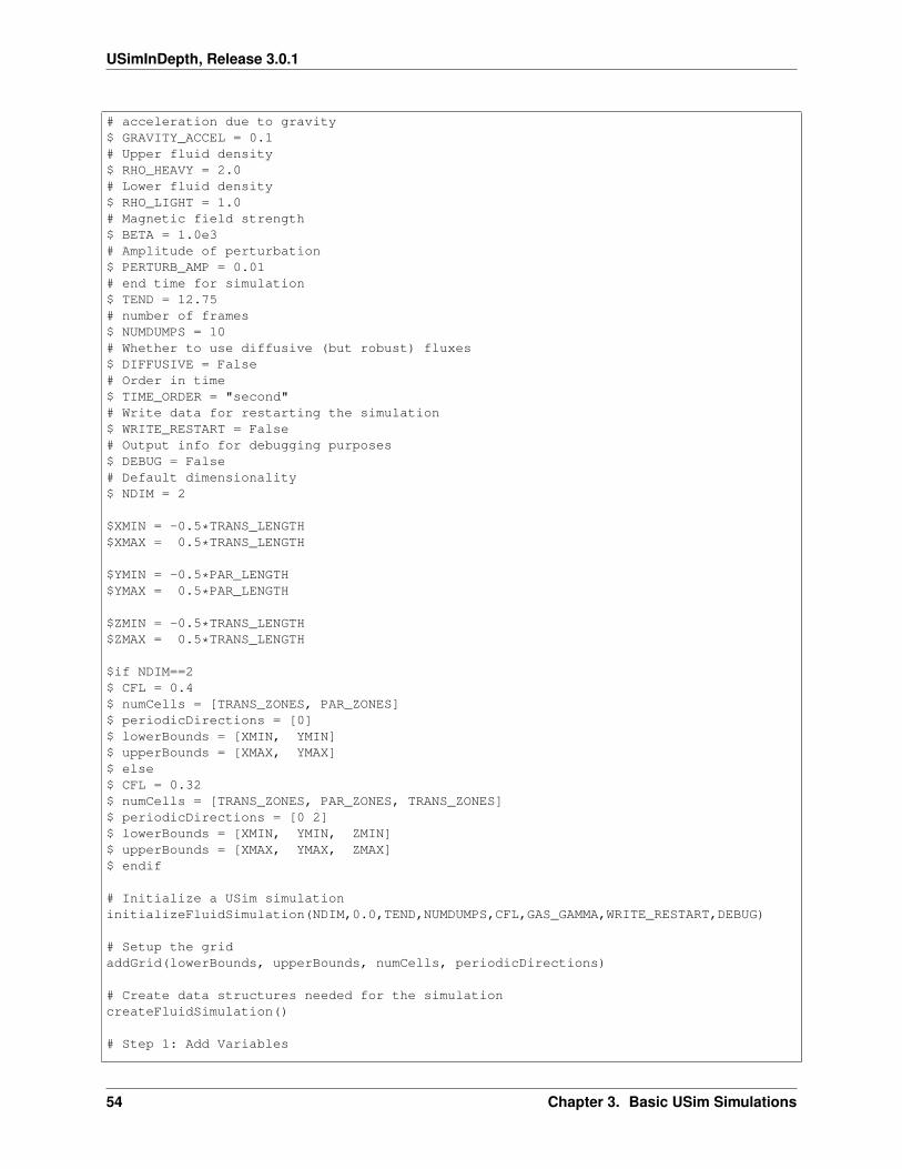
USimInDepth, Release 3.0.1
# acceleration due to gravity$ GRAVITY_ACCEL = 0.1# Upper fluid density$ RHO_HEAVY = 2.0# Lower fluid density$ RHO_LIGHT = 1.0# Magnetic field strength$ BETA = 1.0e3# Amplitude of perturbation$ PERTURB_AMP = 0.01# end time for simulation$ TEND = 12.75# number of frames$ NUMDUMPS = 10# Whether to use diffusive (but robust) fluxes$ DIFFUSIVE = False# Order in time$ TIME_ORDER = "second"# Write data for restarting the simulation$ WRITE_RESTART = False# Output info for debugging purposes$ DEBUG = False# Default dimensionality$ NDIM = 2
$XMIN = -0.5*TRANS_LENGTH$XMAX = 0.5*TRANS_LENGTH
$YMIN = -0.5*PAR_LENGTH$YMAX = 0.5*PAR_LENGTH
$ZMIN = -0.5*TRANS_LENGTH$ZMAX = 0.5*TRANS_LENGTH
$if NDIM==2$ CFL = 0.4$ numCells = [TRANS_ZONES, PAR_ZONES]$ periodicDirections = [0]$ lowerBounds = [XMIN, YMIN]$ upperBounds = [XMAX, YMAX]$ else$ CFL = 0.32$ numCells = [TRANS_ZONES, PAR_ZONES, TRANS_ZONES]$ periodicDirections = [0 2]$ lowerBounds = [XMIN, YMIN, ZMIN]$ upperBounds = [XMAX, YMAX, ZMAX]$ endif
# Initialize a USim simulationinitializeFluidSimulation(NDIM,0.0,TEND,NUMDUMPS,CFL,GAS_GAMMA,WRITE_RESTART,DEBUG)
# Setup the gridaddGrid(lowerBounds, upperBounds, numCells, periodicDirections)
# Create data structures needed for the simulationcreateFluidSimulation()
# Step 1: Add Variables
54 Chapter 3. Basic USim Simulations
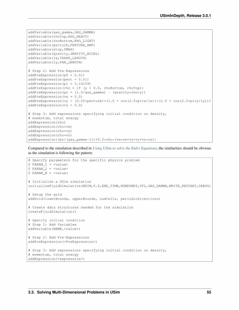
USimInDepth, Release 3.0.1
addVariable(gas_gamma,GAS_GAMMA)addVariable(rhoTop,RHO_HEAVY)addVariable(rhoBottom,RHO_LIGHT)addVariable(perturb,PERTURB_AMP)addVariable(ytop,YMAX)addVariable(gravity,GRAVITY_ACCEL)addVariable(lx,TRANS_LENGTH)addVariable(ly,PAR_LENGTH)
# Step 2: Add Pre-ExpressionsaddPreExpression(p0 = 0.01)addPreExpression(pert = 0.01)addPreExpression(pi = 3.14159)addPreExpression(rho = if (y < 0.0, rhoBottom, rhoTop))addPreExpression(pr = (1.0/gas_gamma) - (gravity*rho*y))addPreExpression(vx = 0.0)addPreExpression(vy = (0.25*perturb)*(1.0 + cos(2.0*pi*x/lx))*(1.0 + cos(2.0*pi*y/ly)))addPreExpression(vz = 0.0)
# Step 3: Add expressions specifying initial condition on density,# momentum, total energyaddExpression(rho)addExpression(rho*vx)addExpression(rho*vy)addExpression(rho*vz)addExpression((pr/(gas_gamma-1))+0.5*rho*(vx*vx+vy*vy+vz*vz))
Compared to the simulation described in Using USim to solve the Euler Equations, the similarities should be obviousas the simulation is following the pattern:
# Specify parameters for the specific physics problem$ PARAM_1 = <value>$ PARAM_2 = <value>$ PARAM_N = <value>
# Initialize a USim simulationinitializeFluidSimulation(NDIM,0.0,END_TIME,NUMDUMPS,CFL,GAS_GAMMA,WRITE_RESTART,DEBUG)
# Setup the gridaddGrid(lowerBounds, upperBounds, numCells, periodicDirections)
# Create data structures needed for the simulationcreateFluidSimulation()
# Specify initial condition# Step 1: Add VariablesaddVariable(NAME,<value>)
# Step 2: Add Pre-ExpressionsaddPreExpression(<PreExpression>)
# Step 3: Add expressions specifying initial condition on density,# momentum, total energyaddExpression(<expression>)
3.3. Solving Multi-Dimensional Problems in USim 55
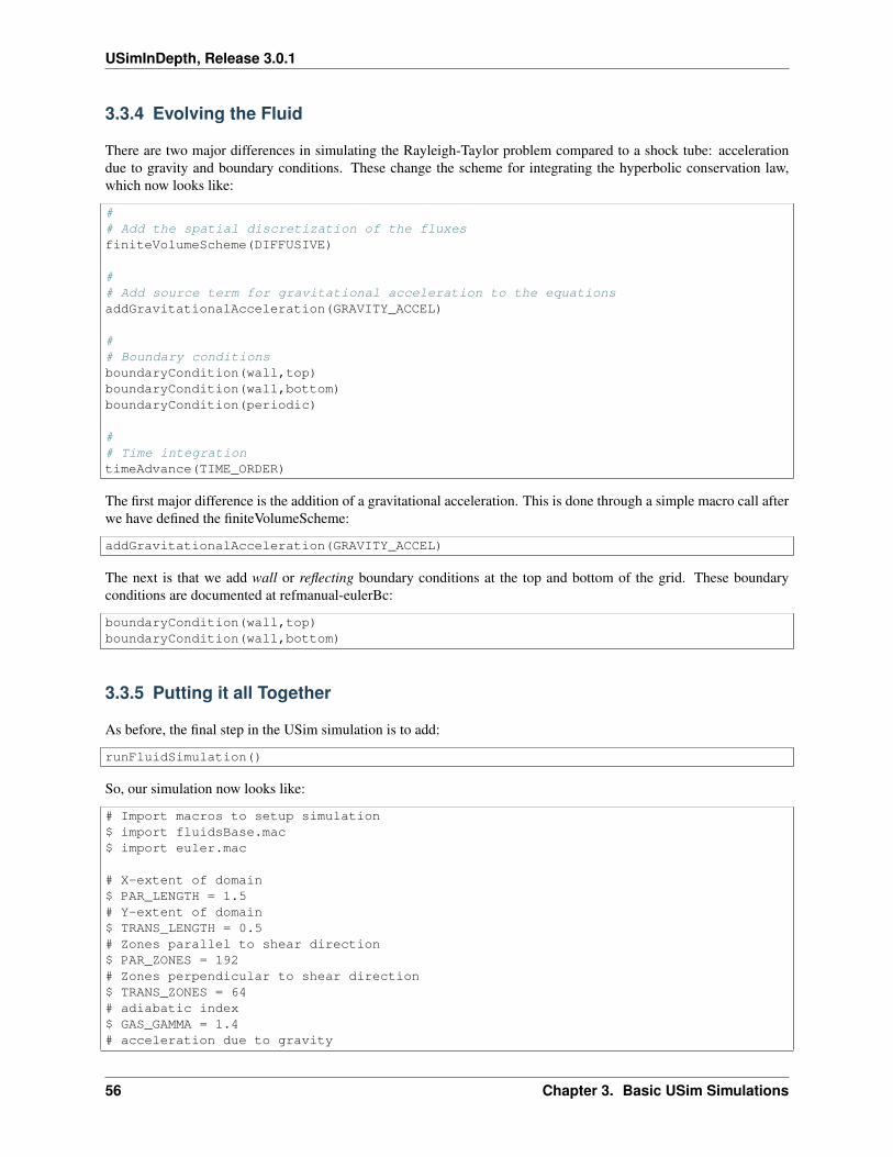
USimInDepth, Release 3.0.1
3.3.4 Evolving the Fluid
There are two major differences in simulating the Rayleigh-Taylor problem compared to a shock tube: accelerationdue to gravity and boundary conditions. These change the scheme for integrating the hyperbolic conservation law,which now looks like:
## Add the spatial discretization of the fluxesfiniteVolumeScheme(DIFFUSIVE)
## Add source term for gravitational acceleration to the equationsaddGravitationalAcceleration(GRAVITY_ACCEL)
## Boundary conditionsboundaryCondition(wall,top)boundaryCondition(wall,bottom)boundaryCondition(periodic)
## Time integrationtimeAdvance(TIME_ORDER)
The first major difference is the addition of a gravitational acceleration. This is done through a simple macro call afterwe have defined the finiteVolumeScheme:
addGravitationalAcceleration(GRAVITY_ACCEL)
The next is that we add wall or reflecting boundary conditions at the top and bottom of the grid. These boundaryconditions are documented at refmanual-eulerBc:
boundaryCondition(wall,top)boundaryCondition(wall,bottom)
3.3.5 Putting it all Together
As before, the final step in the USim simulation is to add:
runFluidSimulation()
So, our simulation now looks like:
# Import macros to setup simulation$ import fluidsBase.mac$ import euler.mac
# X-extent of domain$ PAR_LENGTH = 1.5# Y-extent of domain$ TRANS_LENGTH = 0.5# Zones parallel to shear direction$ PAR_ZONES = 192# Zones perpendicular to shear direction$ TRANS_ZONES = 64# adiabatic index$ GAS_GAMMA = 1.4# acceleration due to gravity
56 Chapter 3. Basic USim Simulations
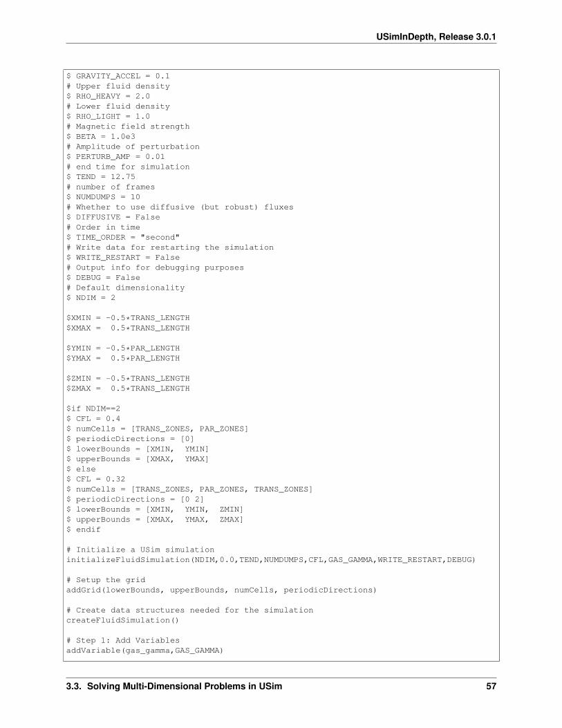
USimInDepth, Release 3.0.1
$ GRAVITY_ACCEL = 0.1# Upper fluid density$ RHO_HEAVY = 2.0# Lower fluid density$ RHO_LIGHT = 1.0# Magnetic field strength$ BETA = 1.0e3# Amplitude of perturbation$ PERTURB_AMP = 0.01# end time for simulation$ TEND = 12.75# number of frames$ NUMDUMPS = 10# Whether to use diffusive (but robust) fluxes$ DIFFUSIVE = False# Order in time$ TIME_ORDER = "second"# Write data for restarting the simulation$ WRITE_RESTART = False# Output info for debugging purposes$ DEBUG = False# Default dimensionality$ NDIM = 2
$XMIN = -0.5*TRANS_LENGTH$XMAX = 0.5*TRANS_LENGTH
$YMIN = -0.5*PAR_LENGTH$YMAX = 0.5*PAR_LENGTH
$ZMIN = -0.5*TRANS_LENGTH$ZMAX = 0.5*TRANS_LENGTH
$if NDIM==2$ CFL = 0.4$ numCells = [TRANS_ZONES, PAR_ZONES]$ periodicDirections = [0]$ lowerBounds = [XMIN, YMIN]$ upperBounds = [XMAX, YMAX]$ else$ CFL = 0.32$ numCells = [TRANS_ZONES, PAR_ZONES, TRANS_ZONES]$ periodicDirections = [0 2]$ lowerBounds = [XMIN, YMIN, ZMIN]$ upperBounds = [XMAX, YMAX, ZMAX]$ endif
# Initialize a USim simulationinitializeFluidSimulation(NDIM,0.0,TEND,NUMDUMPS,CFL,GAS_GAMMA,WRITE_RESTART,DEBUG)
# Setup the gridaddGrid(lowerBounds, upperBounds, numCells, periodicDirections)
# Create data structures needed for the simulationcreateFluidSimulation()
# Step 1: Add VariablesaddVariable(gas_gamma,GAS_GAMMA)
3.3. Solving Multi-Dimensional Problems in USim 57
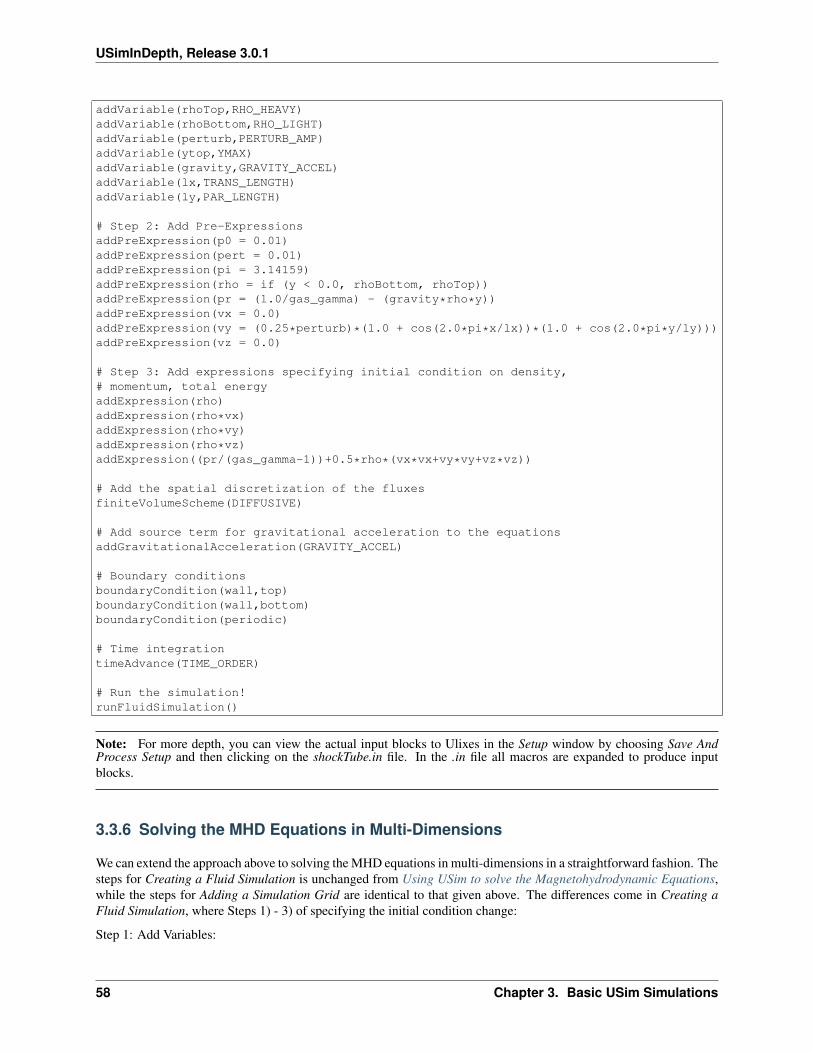
USimInDepth, Release 3.0.1
addVariable(rhoTop,RHO_HEAVY)addVariable(rhoBottom,RHO_LIGHT)addVariable(perturb,PERTURB_AMP)addVariable(ytop,YMAX)addVariable(gravity,GRAVITY_ACCEL)addVariable(lx,TRANS_LENGTH)addVariable(ly,PAR_LENGTH)
# Step 2: Add Pre-ExpressionsaddPreExpression(p0 = 0.01)addPreExpression(pert = 0.01)addPreExpression(pi = 3.14159)addPreExpression(rho = if (y < 0.0, rhoBottom, rhoTop))addPreExpression(pr = (1.0/gas_gamma) - (gravity*rho*y))addPreExpression(vx = 0.0)addPreExpression(vy = (0.25*perturb)*(1.0 + cos(2.0*pi*x/lx))*(1.0 + cos(2.0*pi*y/ly)))addPreExpression(vz = 0.0)
# Step 3: Add expressions specifying initial condition on density,# momentum, total energyaddExpression(rho)addExpression(rho*vx)addExpression(rho*vy)addExpression(rho*vz)addExpression((pr/(gas_gamma-1))+0.5*rho*(vx*vx+vy*vy+vz*vz))
# Add the spatial discretization of the fluxesfiniteVolumeScheme(DIFFUSIVE)
# Add source term for gravitational acceleration to the equationsaddGravitationalAcceleration(GRAVITY_ACCEL)
# Boundary conditionsboundaryCondition(wall,top)boundaryCondition(wall,bottom)boundaryCondition(periodic)
# Time integrationtimeAdvance(TIME_ORDER)
# Run the simulation!runFluidSimulation()
Note: For more depth, you can view the actual input blocks to Ulixes in the Setup window by choosing Save AndProcess Setup and then clicking on the shockTube.in file. In the .in file all macros are expanded to produce inputblocks.
3.3.6 Solving the MHD Equations in Multi-Dimensions
We can extend the approach above to solving the MHD equations in multi-dimensions in a straightforward fashion. Thesteps for Creating a Fluid Simulation is unchanged from Using USim to solve the Magnetohydrodynamic Equations,while the steps for Adding a Simulation Grid are identical to that given above. The differences come in Creating aFluid Simulation, where Steps 1) - 3) of specifying the initial condition change:
Step 1: Add Variables:
58 Chapter 3. Basic USim Simulations
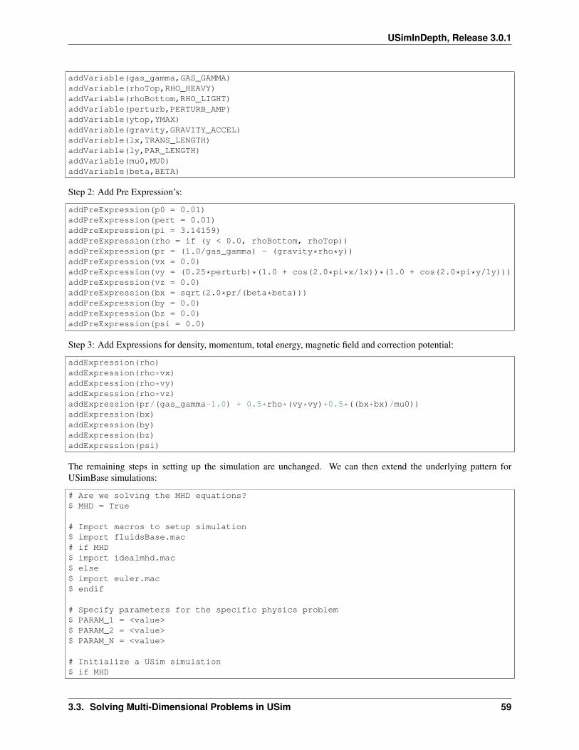
USimInDepth, Release 3.0.1
addVariable(gas_gamma,GAS_GAMMA)addVariable(rhoTop,RHO_HEAVY)addVariable(rhoBottom,RHO_LIGHT)addVariable(perturb,PERTURB_AMP)addVariable(ytop,YMAX)addVariable(gravity,GRAVITY_ACCEL)addVariable(lx,TRANS_LENGTH)addVariable(ly,PAR_LENGTH)addVariable(mu0,MU0)addVariable(beta,BETA)
Step 2: Add Pre Expression’s:
addPreExpression(p0 = 0.01)addPreExpression(pert = 0.01)addPreExpression(pi = 3.14159)addPreExpression(rho = if (y < 0.0, rhoBottom, rhoTop))addPreExpression(pr = (1.0/gas_gamma) - (gravity*rho*y))addPreExpression(vx = 0.0)addPreExpression(vy = (0.25*perturb)*(1.0 + cos(2.0*pi*x/lx))*(1.0 + cos(2.0*pi*y/ly)))addPreExpression(vz = 0.0)addPreExpression(bx = sqrt(2.0*pr/(beta*beta)))addPreExpression(by = 0.0)addPreExpression(bz = 0.0)addPreExpression(psi = 0.0)
Step 3: Add Expressions for density, momentum, total energy, magnetic field and correction potential:
addExpression(rho)addExpression(rho*vx)addExpression(rho*vy)addExpression(rho*vz)addExpression(pr/(gas_gamma-1.0) + 0.5*rho*(vy*vy)+0.5*((bx*bx)/mu0))addExpression(bx)addExpression(by)addExpression(bz)addExpression(psi)
The remaining steps in setting up the simulation are unchanged. We can then extend the underlying pattern forUSimBase simulations:
# Are we solving the MHD equations?$ MHD = True
# Import macros to setup simulation$ import fluidsBase.mac# if MHD$ import idealmhd.mac$ else$ import euler.mac$ endif
# Specify parameters for the specific physics problem$ PARAM_1 = <value>$ PARAM_2 = <value>$ PARAM_N = <value>
# Initialize a USim simulation$ if MHD
3.3. Solving Multi-Dimensional Problems in USim 59
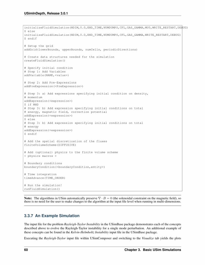
USimInDepth, Release 3.0.1
initializeFluidSimulation(NDIM,0.0,END_TIME,NUMDUMPS,CFL,GAS_GAMMA,MU0,WRITE_RESTART,DEBUG)$ elseinitializeFluidSimulation(NDIM,0.0,END_TIME,NUMDUMPS,CFL,GAS_GAMMA,WRITE_RESTART,DEBUG)$ endif
# Setup the gridaddGrid(lowerBounds, upperBounds, numCells, periodicDirections)
# Create data structures needed for the simulationcreateFluidSimulation()
# Specify initial condition# Step 1: Add VariablesaddVariable(NAME,<value>)
# Step 2: Add Pre-ExpressionsaddPreExpression(<PreExpression>)
# Step 3: a) Add expressions specifying initial condition on density,# momentumaddExpression(<expression>)$ if MHD# Step 3: b) Add expression specifying initial conditions on total# energy, magnetic field, correction potentialaddExpression(<expression>)$ else# Step 3: b) Add expression specifying initial conditions on total# energyaddExpression(<expression>)$ endif
# Add the spatial discretization of the fluxesfiniteVolumeScheme(DIFFUSIVE)
# Add (optional) physics to the finite volume scheme< physics macros >
# Boundary conditionsboundaryCondition(<boundaryCondition,entity>)
# Time integrationtimeAdvance(TIME_ORDER)
# Run the simulation!runFluidSimulation()
Note: The algorithms in USim automatically preserve ∇ ·𝐵 = 0 (the solenoidal constraint on the magnetic field), sothere is no need for the user to make changes to the algorithm at the input file level when running in multi-dimensions.
3.3.7 An Example Simulation
The input file for the problem Rayleigh-Taylor Instability in the USimBase package demonstrates each of the conceptsdescribed above to evolve the Rayleigh-Taylor instability for a single mode perturbation. An additional example ofthese concepts can be found in the Kelvin-Helmholtz Instability input file in the USimBase package.
Executing the Rayleigh-Taylor input file within USimComposer and switching to the Visualize tab yields the plots
60 Chapter 3. Basic USim Simulations
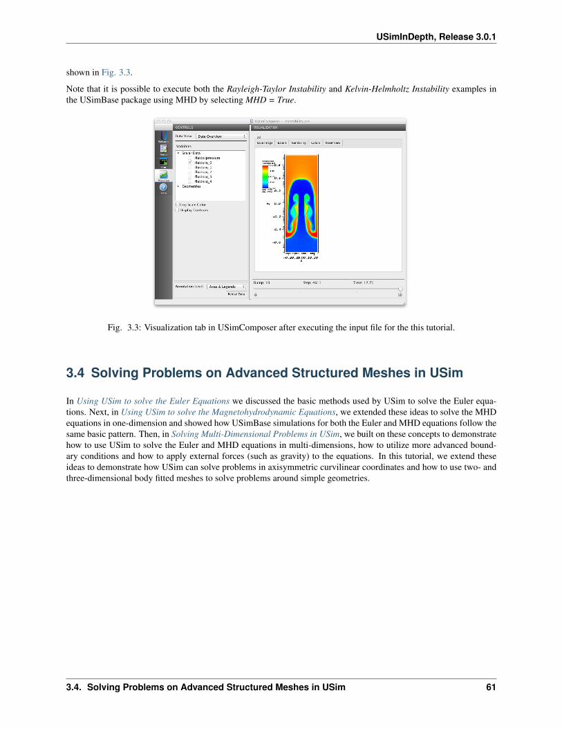
USimInDepth, Release 3.0.1
shown in Fig. 3.3.
Note that it is possible to execute both the Rayleigh-Taylor Instability and Kelvin-Helmholtz Instability examples inthe USimBase package using MHD by selecting MHD = True.
Fig. 3.3: Visualization tab in USimComposer after executing the input file for the this tutorial.
3.4 Solving Problems on Advanced Structured Meshes in USim
In Using USim to solve the Euler Equations we discussed the basic methods used by USim to solve the Euler equa-tions. Next, in Using USim to solve the Magnetohydrodynamic Equations, we extended these ideas to solve the MHDequations in one-dimension and showed how USimBase simulations for both the Euler and MHD equations follow thesame basic pattern. Then, in Solving Multi-Dimensional Problems in USim, we built on these concepts to demonstratehow to use USim to solve the Euler and MHD equations in multi-dimensions, how to utilize more advanced bound-ary conditions and how to apply external forces (such as gravity) to the equations. In this tutorial, we extend theseideas to demonstrate how USim can solve problems in axisymmetric curvilinear coordinates and how to use two- andthree-dimensional body fitted meshes to solve problems around simple geometries.
3.4. Solving Problems on Advanced Structured Meshes in USim 61
USimInDepth, Release 3.0.1
Contents
• Solving Problems on Advanced Structured Meshes in USim– Solving Problems in Axi-Symmetric Curvilinear Coordinates
* Adding a Simulation Grid* Creating a Fluid Simulation* Putting it all Together* An Example Simulation
– Solving Problems on Two-Dimensional Body-Fitted Meshes in USim* Adding a Simulation Grid* An Example Simulation
– Solving Problems on Three-Dimensional Body-Fitted Meshes in USim* Adding a Simulation Grid* Creating a Fluid Simulation* An Example Simulation
3.4.1 Solving Problems in Axi-Symmetric Curvilinear Coordinates
An example of using USim to solve the MHD equations in axi-symmetric curvilinear coordinates is found in quickstart-zpinch.
Adding a Simulation Grid
The use of axisymmetric cylindrical coordinates in this problem is specified through the use of the grid:
addCylindricalGrid(lowerBounds, upperBounds, numCells, periodicDirections)
This macro is documented at grid-macro and follows the same pattern that we have seen previously for logicallystructured Cartesian grids:
lowerBounds: Vector of coordinates for lower edge of grid, lowerBounds = [ RMIN ZMIN PHIMIN ]
upperBounds: Vector of coordinates for upper edge of grid, upperBounds = [ RMAX ZMAX PHI-MAX ]
numCells: Vector of number of cells in grid, numCells = [ NR NZ NPHI ]
periodicDirections: List of directions that are periodic
periodicDirections = [ 0 ] (R-direction periodic)periodicDirections = [ 0 1 ] (R,Z-directions periodic)periodicDirections = [ 0 1 2 ] (R,Z,PHI-directions periodic)
Using the addCylindricalGrid macro automatically tells the rest of the USim solvers to use the cylindrical form of theoperator. If a cylindrical form of an operator is not available, USim will stop with an error message.
Note: Cylindrical grids in USim are designed with axisymmetric coordinates in mind, so a one-dimensional meshsimulates the 𝑅 coordinate, a two-dimensional mesh simulates the (𝑅,𝑍) coordinates and a three-dimensional meshsimulates the (𝑅,𝑍, 𝜑) coordinates.
Creating a Fluid Simulation
The initial conditions for the quickstart-zpinch in axisymmetric cylindrical coordinates are given by:
62 Chapter 3. Basic USim Simulations
USimInDepth, Release 3.0.1
Step 1:
addVariable(gas_gamma,GAS_GAMMA)addVariable(mu0,MU0)addVariable(invSqrtMu0,INV_SQRT_MU0)addVariable(Rp,RP)addVariable(n_0,N0)addVariable(j_0,J0)addVariable(p_0,P0)addVariable(mi,MI)addVariable(k,WAVENUMBER)addVariable(alpha,BASE_PRESSURE_RATIO)addVariable(perturb,PERTURBATION_AMPLITUDE)
Step2:
addPreExpression(r = x)addPreExpression(Z = y)addPreExpression(phi = z)addPreExpression(rho = if(r<Rp, mi*n_0*(alpha+(1.0-(r*r)/(Rp*Rp))), mi*n_0*alpha))addPreExpression(vr = 0.0)addPreExpression(vphi = 0.0)addPreExpression(vz = 0.0)addPreExpression(pr = if(r < Rp, p_0-0.25*mu0*j_0*j_0*r*r, alpha*0.25*mu0*j_0*j_0*Rp*Rp))addPreExpression(br = 0.0)addPreExpression(bphi = if(r < Rp, -0.5*r*mu0*j_0*(1.0+perturb*sin(k*Z)), -0.5*(Rp*Rp/r)*mu0*j_0*(1.0+perturb*sin(k*Z))))addPreExpression(bz = 0.0)addPreExpression(psi = 0.0)
Step 3:
addExpression(rho)addExpression(rho*vr)addExpression(rho*vphi)addExpression(rho*vz)addExpression(pr/(gas_gamma-1.0) + 0.5*rho*(vr*vr+vphi*vphi+vz*vz)+0.5*((br*br+bphi*bphi+bz*bz)/mu0))addExpression(br*invSqrtMu0)addExpression(bphi*invSqrtMu0)addExpression(bz*invSqrtMu0)addExpression(psi)
Note: While the ordering of coordinates on cylindrical grids in USim is (𝑅,𝑍, 𝜑), the components of vectors (suchas the momentum and magnetic field defined in step 3 above) take the order (R, 𝜑, Z). Many issues in simulationsinvolving cylindrical coordinates originate in an incorrect ordering of vector components.
Putting it all Together
We can then extend the underlying pattern for USimBase simulations to incorporate curvilinear coordinates:
# Are we solving the MHD equations?$ MHD = True
# Are we using cylindrical coordinates?$ CYLINDRICAL = True
# Import macros to setup simulation$ import fluidsBase.mac
3.4. Solving Problems on Advanced Structured Meshes in USim 63
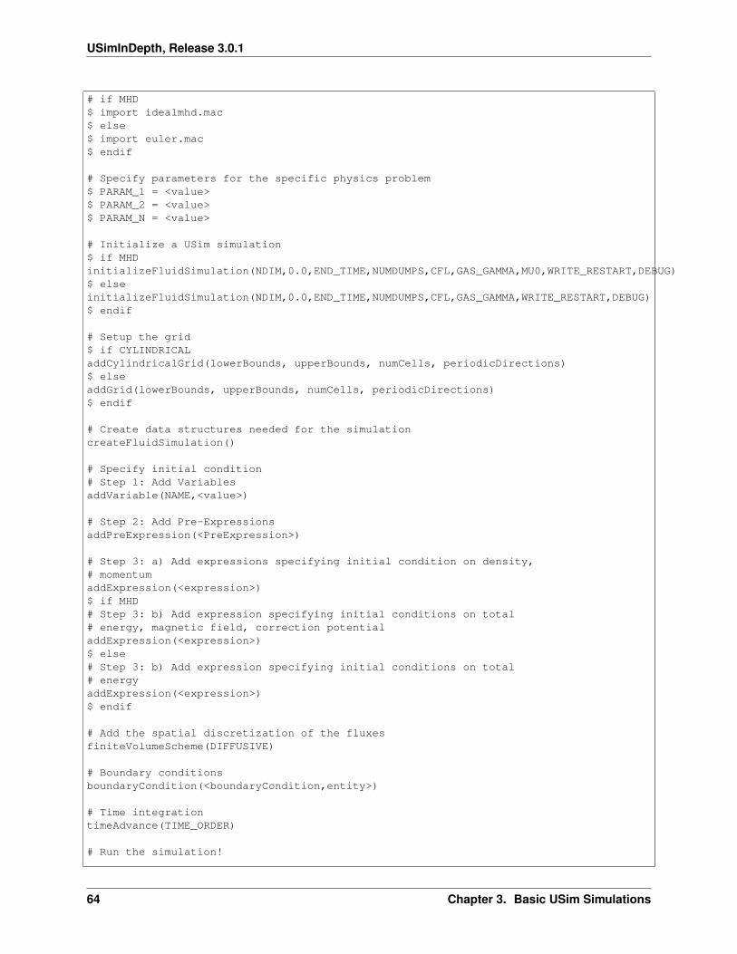
USimInDepth, Release 3.0.1
# if MHD$ import idealmhd.mac$ else$ import euler.mac$ endif
# Specify parameters for the specific physics problem$ PARAM_1 = <value>$ PARAM_2 = <value>$ PARAM_N = <value>
# Initialize a USim simulation$ if MHDinitializeFluidSimulation(NDIM,0.0,END_TIME,NUMDUMPS,CFL,GAS_GAMMA,MU0,WRITE_RESTART,DEBUG)$ elseinitializeFluidSimulation(NDIM,0.0,END_TIME,NUMDUMPS,CFL,GAS_GAMMA,WRITE_RESTART,DEBUG)$ endif
# Setup the grid$ if CYLINDRICALaddCylindricalGrid(lowerBounds, upperBounds, numCells, periodicDirections)$ elseaddGrid(lowerBounds, upperBounds, numCells, periodicDirections)$ endif
# Create data structures needed for the simulationcreateFluidSimulation()
# Specify initial condition# Step 1: Add VariablesaddVariable(NAME,<value>)
# Step 2: Add Pre-ExpressionsaddPreExpression(<PreExpression>)
# Step 3: a) Add expressions specifying initial condition on density,# momentumaddExpression(<expression>)$ if MHD# Step 3: b) Add expression specifying initial conditions on total# energy, magnetic field, correction potentialaddExpression(<expression>)$ else# Step 3: b) Add expression specifying initial conditions on total# energyaddExpression(<expression>)$ endif
# Add the spatial discretization of the fluxesfiniteVolumeScheme(DIFFUSIVE)
# Boundary conditionsboundaryCondition(<boundaryCondition,entity>)
# Time integrationtimeAdvance(TIME_ORDER)
# Run the simulation!
64 Chapter 3. Basic USim Simulations
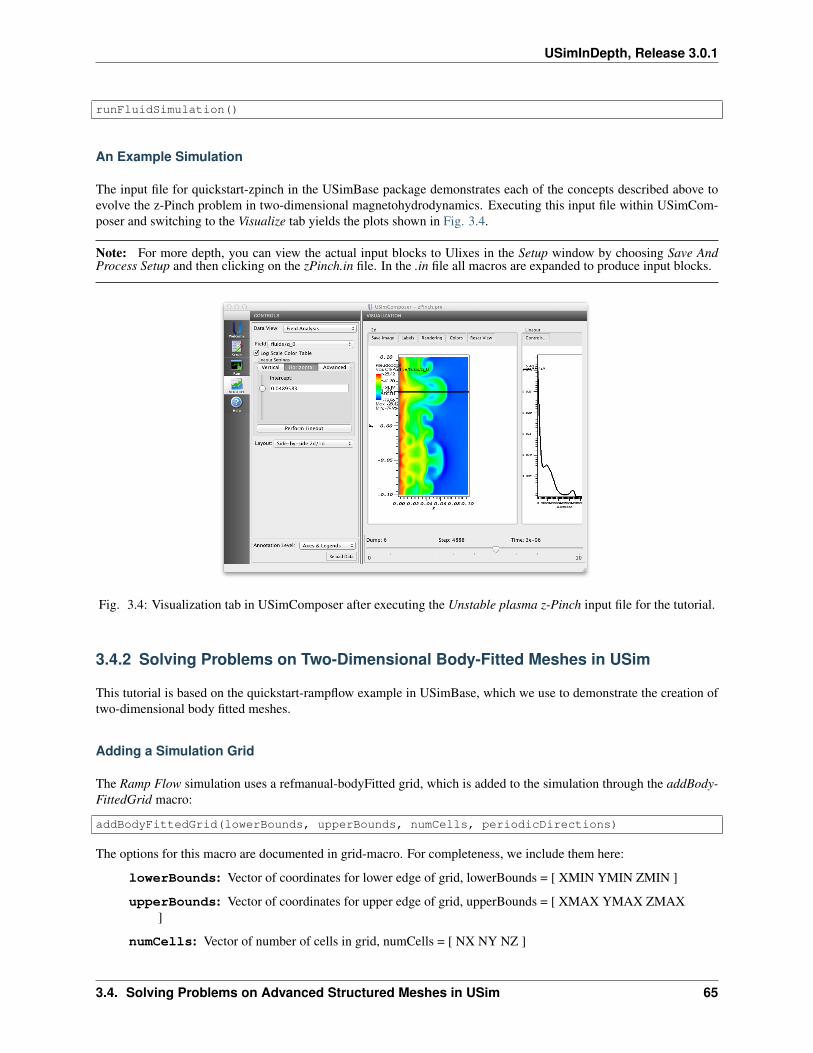
USimInDepth, Release 3.0.1
runFluidSimulation()
An Example Simulation
The input file for quickstart-zpinch in the USimBase package demonstrates each of the concepts described above toevolve the z-Pinch problem in two-dimensional magnetohydrodynamics. Executing this input file within USimCom-poser and switching to the Visualize tab yields the plots shown in Fig. 3.4.
Note: For more depth, you can view the actual input blocks to Ulixes in the Setup window by choosing Save AndProcess Setup and then clicking on the zPinch.in file. In the .in file all macros are expanded to produce input blocks.
Fig. 3.4: Visualization tab in USimComposer after executing the Unstable plasma z-Pinch input file for the tutorial.
3.4.2 Solving Problems on Two-Dimensional Body-Fitted Meshes in USim
This tutorial is based on the quickstart-rampflow example in USimBase, which we use to demonstrate the creation oftwo-dimensional body fitted meshes.
Adding a Simulation Grid
The Ramp Flow simulation uses a refmanual-bodyFitted grid, which is added to the simulation through the addBody-FittedGrid macro:
addBodyFittedGrid(lowerBounds, upperBounds, numCells, periodicDirections)
The options for this macro are documented in grid-macro. For completeness, we include them here:
lowerBounds: Vector of coordinates for lower edge of grid, lowerBounds = [ XMIN YMIN ZMIN ]
upperBounds: Vector of coordinates for upper edge of grid, upperBounds = [ XMAX YMAX ZMAX]
numCells: Vector of number of cells in grid, numCells = [ NX NY NZ ]
3.4. Solving Problems on Advanced Structured Meshes in USim 65
USimInDepth, Release 3.0.1
periodicDirections: List of directions that are periodic
periodicDirections = [ 0 ] (x-direction periodic)periodicDirections = [ 0 1 ] (x,y-directions periodic)periodicDirections = [ 0 1 2 ] (x,y,z-directions periodic)
Now that the body-fitted grid has been created, it is possible to transform the coordinates of the grid into the desiredshaped. This is a three-step process, much like specifying an initial condition:
1. Use addGridVariable to add variables that are independent of grid position.
2. Use addGridPreExpression to add quantities that are functions of grid position, variables and any previouslydefined PreExpression in this block. Evaluated before expressions and the result is not accessible outside of thisblock. Any number of PreExpressions can be added.
3. Use addGridExpression to define the new coordinates in the grid. The order of the expressions correspond tothe order of the coordinates in the grid and there must be the same number of expressions as dimensions in thegrid.
For the RampFlow example, the GridVariables added in Step 1 in the above process are:
# Grid propertiesaddGridVariable(xmin,XIN)addGridVariable(xmax,XUP)addGridVariable(ymax,YUP)addGridVariable(slope,$math.tan(math.pi*THETA/180)$)
# Numbers of cellsaddGridVariable(inletCells,1.0*NXI)addGridVariable(rampCells,1.0*NXR)addGridVariable(yCells,$1.0*NY$)
# x direction cell spacing in computational spaceaddGridVariable(dxc,$1.0/(NXI+NXR)$)# y direction cell spacing in computational spaceaddGridVariable(dyc,$1.0/NY$)# z direction cell spacing in computational space
Next, the GridPreExpressions added in Step 2 in the above process are:
# Grid preExpressionsaddGridPreExpression(ix=rint(x/dxc))addGridPreExpression(iy=rint(y/dyc))addGridPreExpression(dxi=xmin/inletCells)addGridPreExpression(dxr=(xmax-xmin)/rampCells)addGridPreExpression(xp=if(inletCells>=ix,dxi*ix,xmin+dxr*(ix-inletCells)))addGridPreExpression(dyi = ymax/yCells)addGridPreExpression(b = -slope*xmin)addGridPreExpression(y0 = slope*xp + b)addGridPreExpression(dyr = (ymax-y0)/yCells)addGridPreExpression(yp=if(inletCells>=ix,dyi*iy,y0+dyr*iy))
Finally, the GridExpressions added in Step 3 in the above process are:
addGridExpression(xp)addGridExpression(yp)
The bodyFitted Grid in USim is an extension of the cart grid. The cart Grid lays out the grid in a uniform mannerand provides an x-y coordinate for each of the vertices of the cells. The bodyFitted grid allows the user to modify thelocations of these x-y vertices. The lowerBounds upperBounds and numCells parameters set up the uniform cartesian
66 Chapter 3. Basic USim Simulations
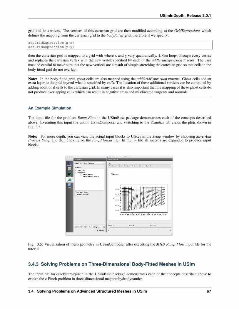
USimInDepth, Release 3.0.1
grid and its vertices. The vertices of this cartesian grid are then modified according to the GridExpressions whichdefines the mapping from the cartesian grid to the bodyFitted grid, therefore if we specify:
addGridExpression(x*x)addGridExpression(y*y)
then the cartesian grid is mapped to a grid with where x and y vary quadratically. USim loops through every vertexand replaces the cartesian vertex with the new vertex specified by each of the addGridExpression macros. The usermust be careful to make sure that the new vertices are a result of simple stretching the cartesian grid so that cells in thebody fitted grid do not overlap.
Note: In the body fitted grid, ghost cells are also mapped using the addGridExpression macros. Ghost cells add anextra layer to the grid beyond what is specified by cells. The location of these additional vertices can be computed byadding additional cells to the cartesian grid. In many cases it is also important that the mapping of these ghost cells donot produce overlapping cells which can result in negative areas and misdirected tangents and normals.
An Example Simulation
The input file for the problem Ramp Flow in the USimBase package demonstrates each of the concepts describedabove. Executing this input file within USimComposer and switching to the Visualize tab yields the plots shown inFig. 3.5.
Note: For more depth, you can view the actual input blocks to Ulixes in the Setup window by choosing Save AndProcess Setup and then clicking on the rampFlow.in file. In the .in file all macros are expanded to produce inputblocks.
Fig. 3.5: Visualization of mesh geometry in USimComposer after executing the MHD Ramp Flow input file for thetutorial.
3.4.3 Solving Problems on Three-Dimensional Body-Fitted Meshes in USim
The input file for quickstart-zpinch in the USimBase package demonstrates each of the concepts described above toevolve the z-Pinch problem in three-dimensional magnetohydrodynamics
3.4. Solving Problems on Advanced Structured Meshes in USim 67
USimInDepth, Release 3.0.1
Adding a Simulation Grid
The three-dimensional version of the zPinch simulation uses a refmanual-bodyFitted grid, which is added to thesimulation through the addBodyFittedGrid macro:
addBodyFittedGrid(lowerBounds, upperBounds, numCells, periodicDirections)
The options for this macro are documented in grid-macro. For completeness, we include them here:
lowerBounds: Vector of coordinates for lower edge of grid, lowerBounds = [ XMIN YMIN ZMIN ]
upperBounds: Vector of coordinates for upper edge of grid, upperBounds = [ XMAX YMAX ZMAX]
numCells: Vector of number of cells in grid, numCells = [ NX NY NZ ]
periodicDirections: List of directions that are periodic
periodicDirections = [ 0 ] (x-direction periodic)periodicDirections = [ 0 1 ] (x,y-directions periodic)periodicDirections = [ 0 1 2 ] (x,y,z-directions periodic)
In this example, we use the body-fitted grid to transform a three-dimensional cylindrical mesh into a three-dimensional(𝑋,𝑌, 𝑍) mesh that utilizes a cylindrical distribution. To accomplish this, we only have to perform the third step ofthe three-step process above:
addGridExpression(x*cos(y))addGridExpression(x*sin(y))addGridExpression(z)
Creating a Fluid Simulation
In order to specify the initial condition on a three-dimensional Cartesian mesh when we start from a cylindrical initialcondition, we need to transform components of vectors from cylindrical to cartesian coordinates. We can do thisduring the specification of the initial condition:
Step 1
addVariable(gas_gamma,GAS_GAMMA)addVariable(mu0,MU0)addVariable(invSqrtMu0,INV_SQRT_MU0)addVariable(Rp,RP)addVariable(n_0,N0)addVariable(j_0,J0)addVariable(p_0,P0)addVariable(mi,MI)addVariable(k,WAVENUMBER)addVariable(alpha,BASE_PRESSURE_RATIO)addVariable(perturb,PERTURBATION_AMPLITUDE)
Step 2
# Compute cylindrical coordinatees based on our x,y,z coordinates in# the gridaddPreExpression(r = sqrt(x^2+y^2))addPreExpression(phi = atan2(y,x))addPreExpression(Z = z)
# Setup our plasma parameters in cylindrical coordinatesaddPreExpression(rho = if(r<Rp, mi*n_0*(alpha+(1.0-(r*r)/(Rp*Rp))), mi*n_0*alpha))
68 Chapter 3. Basic USim Simulations
USimInDepth, Release 3.0.1
addPreExpression(vr = 0.0)addPreExpression(vphi = 0.0)addPreExpression(vz = 0.0)addPreExpression(pr = if(r < Rp, p_0-0.25*mu0*j_0*j_0*r*r, alpha*0.25*mu0*j_0*j_0*Rp*Rp))addPreExpression(br = 0.0)addPreExpression(bphi = if(r < Rp, -0.5*r*mu0*j_0*(1.0+perturb*sin(k*Z)), -0.5*(Rp*Rp/r)*mu0*j_0*(1.0+perturb*sin(k*Z))))addPreExpression(bz = 0.0)addPreExpression(psi = 0.0)
# Transform from cylindrical coordinates into Cartesian.addPreExpression(vx = vr*cos(phi)+vphi*sin(phi))addPreExpression(vy = vr*sin(phi)-vphi*cos(phi))addPreExpression(bx = br*cos(phi)+bphi*sin(phi))addPreExpression(by = br*sin(phi)-bphi*cos(phi))
Step 3
# Specify initial condition according to cartesian vector componentsaddExpression(rho)addExpression(rho*vx)addExpression(rho*vy)addExpression(rho*vz)addExpression(pr/(gas_gamma-1.0) + 0.5*rho*(vx*vx+vy*vy+vz*vz)+0.5*((bx*bx+by*by+bz*bz)/mu0))addExpression(bx*invSqrtMu0)addExpression(by*invSqrtMu0)addExpression(bz*invSqrtMu0)addExpression(psi)
An Example Simulation
The input file for quickstart-zpinch in the USimBase package with NDIM=3 demonstrates each of the concepts de-scribed above to evolve the z-Pinch problem in three-dimensional magnetohydrodynamics.
Note: For more depth, you can view the actual input blocks to Ulixes in the Setup window by choosing Save AndProcess Setup and then clicking on the zPinch.in file. In the .in file all macros are expanded to produce input blocks.
3.5 Solving Problems on Unstructured Meshes in USim
In Using USim to solve the Euler Equations we discussed the basic methods used by USim to solve the Euler equa-tions. Next, in Using USim to solve the Magnetohydrodynamic Equations, we extended these ideas to solve the MHDequations in one-dimension and showed how USimBase simulations for both the Euler and MHD equations follow thesame basic pattern. Then, in Solving Multi-Dimensional Problems in USim, we built on these concepts to demonstratehow to use USim to solve the Euler and MHD equations in multi-dimensions, how to utilize more advanced boundaryconditions and how to apply external fources (such as gravity) to the equations. Following on from this in SolvingProblems on Advanced Structured Meshes in USim, we demonstrated how USim can solve problems in axisymmet-ric curvilinear coordinates and how to use two- and three-dimensional body fitted meshes to solve problems aroundsimple geometries. In this tutorial, we introduce unstructured meshes in USim, show how to create boundary condi-tions for simple geometries, apply custom boundary conditions based on user specified parameters, and compute flowdiagnostics.
The quickstart-forwardfacingstep example in USimBase illustrates how to solve problems on unstructured meshes.
Note: In USim Version 3.0 unstructured meshes should be quadrilateral or hexahedral. If unstructured grids are
3.5. Solving Problems on Unstructured Meshes in USim 69
USimInDepth, Release 3.0.1
used in parallel then the user needs to define the partitioning of the grid prior to import; USim does not partitionunstructured meshes itself.
Contents
• Solving Problems on Unstructured Meshes in USim– Creating Unstructured Meshes in CUBIT for USim– Creating Unstructured Meshes in Trelis for USim– Creating Unstructured Meshes in Gmsh for USim– Running Unstructured Meshes in Parallel
* CUBIT/Trelis* Gmsh
– Initializing a Simulation– Adding a Simulation Grid– Creating a Fluid Simulation– Evolving the Fluid– Boundary Conditions on Unstructured Meshes– Adding Output Diagnostics– Putting it all Together– An Example Simulation
3.5.1 Creating Unstructured Meshes in CUBIT for USim
USim currently accepts Exodus II files created in a number of programs including CUBIT and Trelis. Exodus II filesgenerally have the extension .exo, however we frequently use the genesis format (.g) which contains only the meshdata of the Exodus II file.
USim 3.0 currently accepts only quad or hex elements.
• First, create a mesh in CUBIT following the CUBIT tutorials.
• After the mesh has been created, sidesets (used for boundaries) can also be created and then used in defining thelocations of boundary conditions.
– In CUBIT, select ‘Materials and Bcs’ then select ‘Entities - Blocks’. From the drop down menu select‘Add’ and set the ‘Block ID’ to 1. If the mesh is 2d pick ‘Surface’ and hit ‘Apply’. If the mesh is 3D,instead select ‘Volume’ and hit ‘Apply’.
– Next, in ‘Entities - Blocks’ switch the drop down menu to ‘Element Type’. If the mesh is 2D select‘Surfaces’ and then ‘Quad4’, if the mesh is 3D select ‘Volumes’ and ‘Hex8’, hit ‘Apply’.
– Next switch from ‘Entity - Blocks’ to ‘Entity - Sidesets’. In 2D select ‘Curve’ then click on the mesh orthe boundary you wish to choose for your sideset. In 3D select ‘Surface’ then select the boundary you areinterested in. You will now have a boundary defined as sideset 1 (for example).
• Once the grid is read into USim an entity is defined over the side with the name sideSetHalosId1. This entitycan then be used USim boundary conditions.
• Add any other side sets you wish to use as boundaries at this point. The mesh is now ready to export.
• In the main CUBIT window select ‘File->Export’. Choose the directory to export the file and from the dropdownmenu select ‘Genesis’ to export a Genesis file. Type in the file name and select ‘Save’. You should now have agrid that can be read into USim.
70 Chapter 3. Basic USim Simulations
USimInDepth, Release 3.0.1
3.5.2 Creating Unstructured Meshes in Trelis for USim
USim currently accepts Exodus II files created in a number of programs including CUBIT and Trelis. Exodus II filesgenerally have the extension .exo, however we frequently use the genesis format (.g) which contains only the meshdata of the Exodus II file.
USim 3.0 currently accepts only quad or hex elements.
• First, create a mesh in Trelis using tutorials and documentation.
• After the mesh has been created, sidesets (used for boundaries) can also be created and then used in defining thelocations of boundary conditions.
– In Trelis, select the ‘Analysis Groups and Materials’ mode, then select ‘Entity-Sidesets’.
– Set the ‘Action’ to ‘Create sideset’ and set the ‘Sideset ID’ to 1
– Select ‘Curve’ if the mesh is 2D and ‘Surface’ if the mesh is 3D and type in the curve/surface ID or selectit with your mouse and hit ‘Apply’
• Once the grid is read into USim an entity is defined over the side with the name sideSetHalosId1. This entitycan then be used USim boundary conditions.
• Add any other side sets you wish to use as boundaries at this point. The mesh is now ready to export.
• In the main Trelis window select ‘File->Export’. Choose the directory to export the file and from the dropdownmenu select ‘Exodus’ to export an Exodus file. Type in the file name and select ‘Save’. You should now have agrid that can be read into USim.
3.5.3 Creating Unstructured Meshes in Gmsh for USim
USim also accepts Gmsh meshes with extension .msh.
• First, create a geometry in Gmsh following any Gmsh tutorials.
• Gmsh will mesh using triangles/tets unless instructed otherwise. Open the ‘Tools -> Options’ menu, and un-der the ‘General’ tab for ‘Mesh’, check the box “Recombine all triangular meshes”. Also set the subdivisionalgorithm to “All Quads” or “All Hexes” for 2D or 3D meshes.
• Save the mesh. You should now have a grid that can be read into USim.
Gmsh does not have a facility for setting sideSets used for USim boundary conditions. Instead, an entity can be createdin USim by masking off ghost cells to isolate those you would like to create a boundary condition on.
An example of masking off a region of the ghost cells is as follows:
<Updater generateOpenBc>kind = entityGenerator2donGrid = domainnewEntityName = openBconEntity = ghost<Function mask>kind = exprFuncexprs = ["if(x>0 && y>0.03,1.0,-1.0)"]
</Function></Updater>
This block creates a new entity of name “openBC” which can be called in an Updater and used for setting a boundarycondition.
3.5. Solving Problems on Unstructured Meshes in USim 71
USimInDepth, Release 3.0.1
3.5.4 Running Unstructured Meshes in Parallel
CUBIT/Trelis
If you wish to run your simulation in parallel, the mesh will need to be decomposed prior to use in USim. CUBIT andTrelis do not have a facility to do this, so an external program must be used. We recommend using SEACAS, which isa suite of applications for supporting finite element analysis software using Exodus file format. SEACAS Specifically,nem_slice and nem_spread.
In the Linux distribution of USim 3.0, an Exodus II mesh file can be decomposed using the provided partitioner script,decomp.
For example, if you plan to use 8 processors, from the command line run:
<ULIXES_BIN_DIR>/decomp -p 8 --root ./ meshfile.g
or
<ULIXES_BIN_DIR>/decomp -p 8 --root ./ meshfile.exo
For more information about the decomp script, run the script with the help option:
<ULIXES_BIN_DIR>/decomp -h
A number of files will be output corresponding to the number of processors you plan to run on. In the case above, 8files, namely:
meshfile.g.8.0 meshfile.g.8.1 meshfile.g.8.2 meshfile.g.8.3 meshfile.g.8.4 meshfile.g.8.5 meshfile.g.8.6 meshfile.g.8.7
USim will automatically detect these files upon running with 8 cores. In your <Creator> block, you simply need to setthe file to ‘meshfile.g’:
<Creator ctor>kind = exodusndim = 3file = meshfile.g
</Creator>
Gmsh
Gmsh, on the other hand, can partition your grid prior to saving. In Gmsh, select ‘Mesh->Partition’ and set the‘Number of Partitions’ to however many cores you would like to run on. Then hit ‘Partition’. The colors in your meshshould change to show the decomposition of the mesh onto your chosen number of partitions.
Saving this mesh will result in 1 file being written. We recommend you save the file with the number of partitions inthe file name.:
meshfile16.msh
USim will NOT automatically detect which file to use when running in parallel. In your <Creator> block, be sure toset the correct meshfile.:
<Creator ctor>kind = gmshndim = 3file = meshfile16.msh
</Creator>
72 Chapter 3. Basic USim Simulations
USimInDepth, Release 3.0.1
3.5.5 Initializing a Simulation
One of the great strengths of USim is that the underlying algorithms are able to work on both structured and unstruc-tured meshes. This means that the worflow to setup a simulation on a unstructured mesh is very similar to that seenpreviously:
# Are we solving the MHD equations?$ MHD = False
# Import macros to setup simulation$ import fluidsBase.mac$ if MHD$ import idealmhd.mac$ else$ import euler.mac$ endif
# Specify parameters for the specific physics problem$ PARAM_1 = <value>$ PARAM_2 = <value>$ PARAM_N = <value>
# Initialize a USim simulation$ if MHDinitializeFluidSimulation(NDIM,0.0,TEND,NUMDUMPS,CFL,GAS_GAMMA,MU0,WRITE_RESTART,DEBUG)$ elseinitializeFluidSimulation(NDIM,0.0,TEND,NUMDUMPS,CFL,GAS_GAMMA,WRITE_RESTART,DEBUG)$ endif
For the Forward Facing Step example with the Euler equations, the parameters that we specify for the physics problemare as follows:
# grid for simulation$ GRIDFILE = "forwardFacingStep"# format of grid$ GRIDTYPE = "gmsh"# adiabatic index$ GAS_GAMMA = 1.4# Magnetic field strength$ BETA = 1.0e3# end time for simulation$ TEND = 4.0# number of frames$ NUMDUMPS = 20# Riemann solver$ DIFFUSIVE = True# Order in time$ TIME_ORDER = "second"# Write data for restarting the simulation$ WRITE_RESTART = False# Output info for debugging purposes$ DEBUG = False# Dimensionality$ NDIM = 2# Permeability of free space$ MU0 = 1.0# CFL condition$ CFL = 0.4
3.5. Solving Problems on Unstructured Meshes in USim 73
USimInDepth, Release 3.0.1
3.5.6 Adding a Simulation Grid
The use of an unstructured mesh in USim is specified through the use of one of the two grids:
addExodusGrid(GRIDFILE)
or:
addGmshGrid(GRIDFILE)
The choice of which block to use corresponds to the format of the mesh; either GMSH or ExodusII format. TheGRIDFILE is the name of the file containing the mesh without the file extension.
Our simulation input file now looks like:
# Are we solving the MHD equations?$ MHD = False
# Import macros to setup simulation$ import fluidsBase.mac$ if MHD$ import idealmhd.mac$ else$ import euler.mac$ endif
# Specify parameters for the specific physics problem# grid for simulation$ GRIDFILE = "forwardFacingStep"# format of grid$ GRIDTYPE = "gmsh"# adiabatic index$ GAS_GAMMA = 1.4# Magnetic field strength$ BETA = 1.0e3# end time for simulation$ TEND = 4.0# number of frames$ NUMDUMPS = 20# Riemann solver$ DIFFUSIVE = True# Order in time$ TIME_ORDER = "second"# Write data for restarting the simulation$ WRITE_RESTART = False# Output info for debugging purposes$ DEBUG = False# Dimensionality$ NDIM = 2# Permeability of free space$ MU0 = 1.0# CFL condition$ CFL = 0.4
# Initialize a USim simulation$ if MHDinitializeFluidSimulation(NDIM,0.0,TEND,NUMDUMPS,CFL,GAS_GAMMA,MU0,WRITE_RESTART,DEBUG)$ elseinitializeFluidSimulation(NDIM,0.0,TEND,NUMDUMPS,CFL,GAS_GAMMA,WRITE_RESTART,DEBUG)$ endif
74 Chapter 3. Basic USim Simulations
USimInDepth, Release 3.0.1
$ if isEqualString(GRIDTYPE,ExodusII)addExodusGrid(GRIDFILE)$ elseaddGmshGrid(GRIDFILE)$ endif
3.5.7 Creating a Fluid Simulation
As in the Initializing a Simulation step, the procedure for setting up a fluid simulation on an unstructured mesh isidentical to that on a structured mesh. For the Flow Over a Forward Facing Step example, this proceeds as follows.First, we create the variables needed to simulate the fluid:
createFluidSimulation()
We then proceed through the three-step process to specify the distribution of the fluid on the grid. Step 1: AddVariables:
addVariable(gasGamma,GAS_GAMMA)
Step 2: Add Pre Expression’s:
addPreExpression(rho = gasGamma)addPreExpression(vx = 3.0)addPreExpression(vy = 0.0)addPreExpression(vz = 0.0)addPreExpression(pr = 1.0)
Step 3: Add Expressions for density, momentum and total energy:
addExpression(rho)addExpression(rho*vx)addExpression(rho*vy)addExpression(rho*vz)addExpression((pr/(gas_gamma-1.0))+0.5*rho*(vx*vx+vy*vy+vz*vz))
Note that Step 3 is identical to that used in Using USim to solve the Euler Equations. Our simulation input file nowlooks like:
# Are we solving the MHD equations?$ MHD = False
# Import macros to setup simulation$ import fluidsBase.mac$ if MHD$ import idealmhd.mac$ else$ import euler.mac$ endif
# Specify parameters for the specific physics problem# grid for simulation$ GRIDFILE = "forwardFacingStep"# format of grid$ GRIDTYPE = "gmsh"# adiabatic index$ GAS_GAMMA = 1.4# Magnetic field strength
3.5. Solving Problems on Unstructured Meshes in USim 75
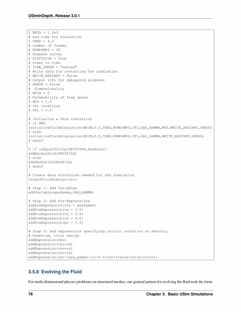
USimInDepth, Release 3.0.1
$ BETA = 1.0e3# end time for simulation$ TEND = 4.0# number of frames$ NUMDUMPS = 20# Riemann solver$ DIFFUSIVE = True# Order in time$ TIME_ORDER = "second"# Write data for restarting the simulation$ WRITE_RESTART = False# Output info for debugging purposes$ DEBUG = False# Dimensionality$ NDIM = 2# Permeability of free space$ MU0 = 1.0# CFL condition$ CFL = 0.4
# Initialize a USim simulation$ if MHDinitializeFluidSimulation(NDIM,0.0,TEND,NUMDUMPS,CFL,GAS_GAMMA,MU0,WRITE_RESTART,DEBUG)$ elseinitializeFluidSimulation(NDIM,0.0,TEND,NUMDUMPS,CFL,GAS_GAMMA,WRITE_RESTART,DEBUG)$ endif
$ if isEqualString(GRIDTYPE,ExodusII)addExodusGrid(GRIDFILE)$ elseaddGmshGrid(GRIDFILE)$ endif
# Create data structures needed for the simulationcreateFluidSimulation()
# Step 1: Add VariablesaddVariable(gasGamma,GAS_GAMMA)
# Step 2: Add Pre-ExpressionsaddPreExpression(rho = gasGamma)addPreExpression(vx = 3.0)addPreExpression(vy = 0.0)addPreExpression(vz = 0.0)addPreExpression(pr = 1.0)
# Step 3: Add expressions specifying initial condition on density,# momentum, total energyaddExpression(rho)addExpression(rho*vx)addExpression(rho*vy)addExpression(rho*vz)addExpression((pr/(gas_gamma-1))+0.5*rho*(vx*vx+vy*vy+vz*vz))
3.5.8 Evolving the Fluid
For multi-dimensional physics problems on structured meshes, our general pattern for evolving the fluid took the form:
76 Chapter 3. Basic USim Simulations
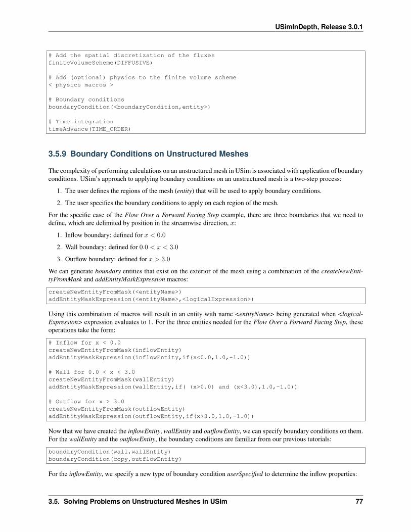
USimInDepth, Release 3.0.1
# Add the spatial discretization of the fluxesfiniteVolumeScheme(DIFFUSIVE)
# Add (optional) physics to the finite volume scheme< physics macros >
# Boundary conditionsboundaryCondition(<boundaryCondition,entity>)
# Time integrationtimeAdvance(TIME_ORDER)
3.5.9 Boundary Conditions on Unstructured Meshes
The complexity of performing calculations on an unstructured mesh in USim is associated with application of boundaryconditions. USim’s approach to applying boundary conditions on an unstructured mesh is a two-step process:
1. The user defines the regions of the mesh (entity) that will be used to apply boundary conditions.
2. The user specifies the boundary conditions to apply on each region of the mesh.
For the specific case of the Flow Over a Forward Facing Step example, there are three boundaries that we need todefine, which are delimited by position in the streamwise direction, 𝑥:
1. Inflow boundary: defined for 𝑥 < 0.0
2. Wall boundary: defined for 0.0 < 𝑥 < 3.0
3. Outflow boundary: defined for 𝑥 > 3.0
We can generate boundary entities that exist on the exterior of the mesh using a combination of the createNewEnti-tyFromMask and addEntityMaskExpression macros:
createNewEntityFromMask(<entityName>)addEntityMaskExpression(<entityName>,<logicalExpression>)
Using this combination of macros will result in an entity with name <entityName> being generated when <logical-Expression> expression evaluates to 1. For the three entities needed for the Flow Over a Forward Facing Step, theseoperations take the form:
# Inflow for x < 0.0createNewEntityFromMask(inflowEntity)addEntityMaskExpression(inflowEntity,if(x<0.0,1.0,-1.0))
# Wall for 0.0 < x < 3.0createNewEntityFromMask(wallEntity)addEntityMaskExpression(wallEntity,if( (x>0.0) and (x<3.0),1.0,-1.0))
# Outflow for x > 3.0createNewEntityFromMask(outflowEntity)addEntityMaskExpression(outflowEntity,if(x>3.0,1.0,-1.0))
Now that we have created the inflowEntity, wallEntity and outflowEntity, we can specify boundary conditions on them.For the wallEntity and the outflowEntity, the boundary conditions are familiar from our previous tutorials:
boundaryCondition(wall,wallEntity)boundaryCondition(copy,outflowEntity)
For the inflowEntity, we specify a new type of boundary condition userSpecified to determine the inflow properties:
3.5. Solving Problems on Unstructured Meshes in USim 77
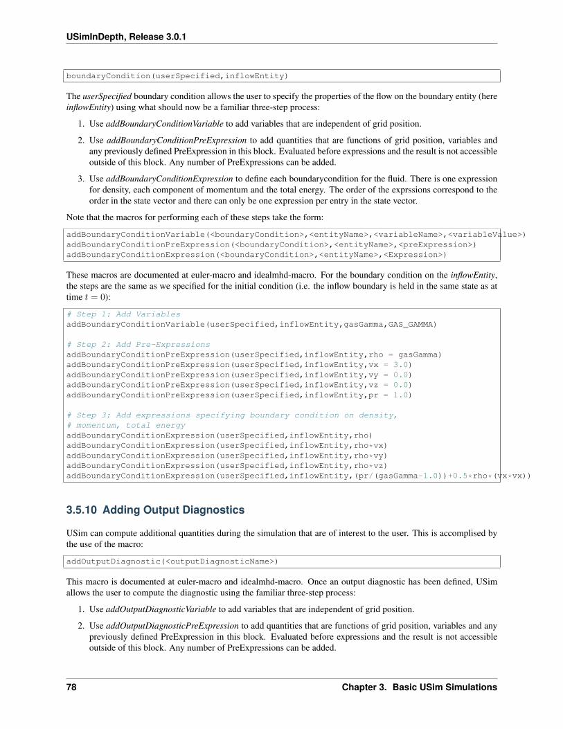
USimInDepth, Release 3.0.1
boundaryCondition(userSpecified,inflowEntity)
The userSpecified boundary condition allows the user to specify the properties of the flow on the boundary entity (hereinflowEntity) using what should now be a familiar three-step process:
1. Use addBoundaryConditionVariable to add variables that are independent of grid position.
2. Use addBoundaryConditionPreExpression to add quantities that are functions of grid position, variables andany previously defined PreExpression in this block. Evaluated before expressions and the result is not accessibleoutside of this block. Any number of PreExpressions can be added.
3. Use addBoundaryConditionExpression to define each boundarycondition for the fluid. There is one expressionfor density, each component of momentum and the total energy. The order of the exprssions correspond to theorder in the state vector and there can only be one expression per entry in the state vector.
Note that the macros for performing each of these steps take the form:
addBoundaryConditionVariable(<boundaryCondition>,<entityName>,<variableName>,<variableValue>)addBoundaryConditionPreExpression(<boundaryCondition>,<entityName>,<preExpression>)addBoundaryConditionExpression(<boundaryCondition>,<entityName>,<Expression>)
These macros are documented at euler-macro and idealmhd-macro. For the boundary condition on the inflowEntity,the steps are the same as we specified for the initial condition (i.e. the inflow boundary is held in the same state as attime 𝑡 = 0):
# Step 1: Add VariablesaddBoundaryConditionVariable(userSpecified,inflowEntity,gasGamma,GAS_GAMMA)
# Step 2: Add Pre-ExpressionsaddBoundaryConditionPreExpression(userSpecified,inflowEntity,rho = gasGamma)addBoundaryConditionPreExpression(userSpecified,inflowEntity,vx = 3.0)addBoundaryConditionPreExpression(userSpecified,inflowEntity,vy = 0.0)addBoundaryConditionPreExpression(userSpecified,inflowEntity,vz = 0.0)addBoundaryConditionPreExpression(userSpecified,inflowEntity,pr = 1.0)
# Step 3: Add expressions specifying boundary condition on density,# momentum, total energyaddBoundaryConditionExpression(userSpecified,inflowEntity,rho)addBoundaryConditionExpression(userSpecified,inflowEntity,rho*vx)addBoundaryConditionExpression(userSpecified,inflowEntity,rho*vy)addBoundaryConditionExpression(userSpecified,inflowEntity,rho*vz)addBoundaryConditionExpression(userSpecified,inflowEntity,(pr/(gasGamma-1.0))+0.5*rho*(vx*vx))
3.5.10 Adding Output Diagnostics
USim can compute additional quantities during the simulation that are of interest to the user. This is accomplised bythe use of the macro:
addOutputDiagnostic(<outputDiagnosticName>)
This macro is documented at euler-macro and idealmhd-macro. Once an output diagnostic has been defined, USimallows the user to compute the diagnostic using the familiar three-step process:
1. Use addOutputDiagnosticVariable to add variables that are independent of grid position.
2. Use addOutputDiagnosticPreExpression to add quantities that are functions of grid position, variables and anypreviously defined PreExpression in this block. Evaluated before expressions and the result is not accessibleoutside of this block. Any number of PreExpressions can be added.
78 Chapter 3. Basic USim Simulations
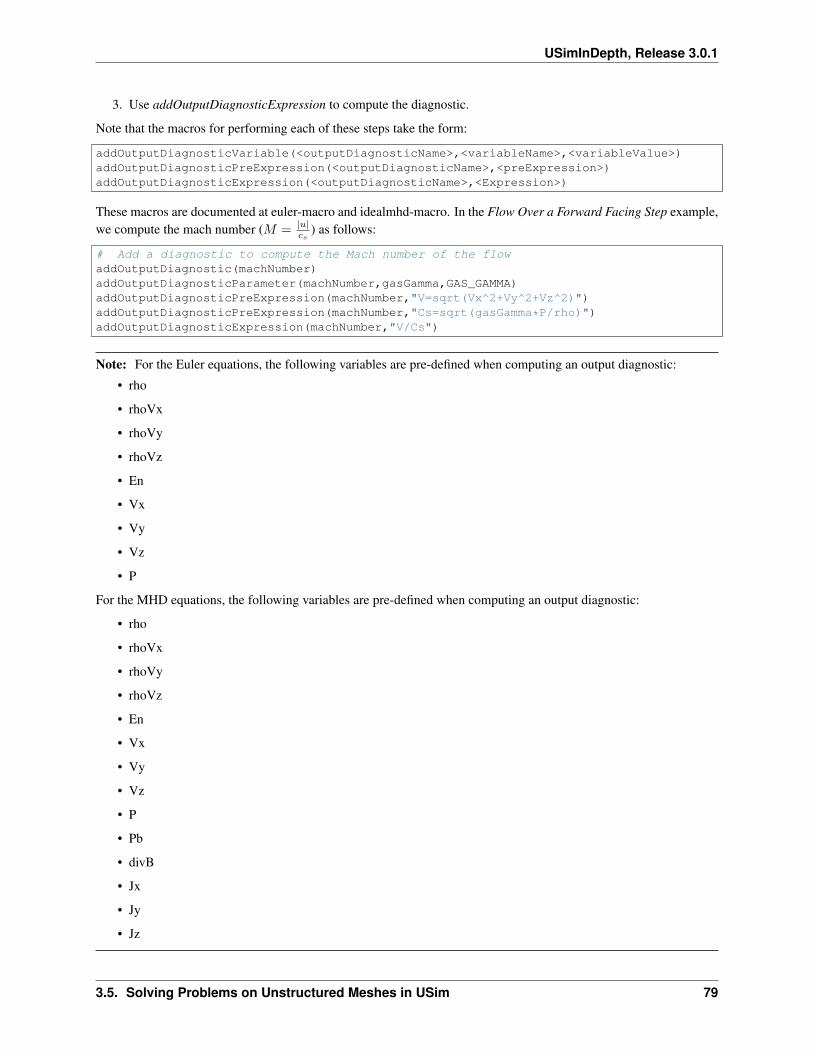
USimInDepth, Release 3.0.1
3. Use addOutputDiagnosticExpression to compute the diagnostic.
Note that the macros for performing each of these steps take the form:
addOutputDiagnosticVariable(<outputDiagnosticName>,<variableName>,<variableValue>)addOutputDiagnosticPreExpression(<outputDiagnosticName>,<preExpression>)addOutputDiagnosticExpression(<outputDiagnosticName>,<Expression>)
These macros are documented at euler-macro and idealmhd-macro. In the Flow Over a Forward Facing Step example,we compute the mach number (𝑀 = |𝑢|
𝑐𝑠) as follows:
# Add a diagnostic to compute the Mach number of the flowaddOutputDiagnostic(machNumber)addOutputDiagnosticParameter(machNumber,gasGamma,GAS_GAMMA)addOutputDiagnosticPreExpression(machNumber,"V=sqrt(Vx^2+Vy^2+Vz^2)")addOutputDiagnosticPreExpression(machNumber,"Cs=sqrt(gasGamma*P/rho)")addOutputDiagnosticExpression(machNumber,"V/Cs")
Note: For the Euler equations, the following variables are pre-defined when computing an output diagnostic:
• rho
• rhoVx
• rhoVy
• rhoVz
• En
• Vx
• Vy
• Vz
• P
For the MHD equations, the following variables are pre-defined when computing an output diagnostic:
• rho
• rhoVx
• rhoVy
• rhoVz
• En
• Vx
• Vy
• Vz
• P
• Pb
• divB
• Jx
• Jy
• Jz
3.5. Solving Problems on Unstructured Meshes in USim 79
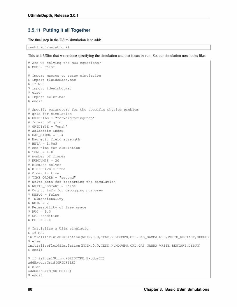
USimInDepth, Release 3.0.1
3.5.11 Putting it all Together
The final step in the USim simulation is to add:
runFluidSimulation()
This tells USim that we’re done specifying the simulation and that it can be run. So, our simulation now looks like:
# Are we solving the MHD equations?$ MHD = False
# Import macros to setup simulation$ import fluidsBase.mac$ if MHD$ import idealmhd.mac$ else$ import euler.mac$ endif
# Specify parameters for the specific physics problem# grid for simulation$ GRIDFILE = "forwardFacingStep"# format of grid$ GRIDTYPE = "gmsh"# adiabatic index$ GAS_GAMMA = 1.4# Magnetic field strength$ BETA = 1.0e3# end time for simulation$ TEND = 4.0# number of frames$ NUMDUMPS = 20# Riemann solver$ DIFFUSIVE = True# Order in time$ TIME_ORDER = "second"# Write data for restarting the simulation$ WRITE_RESTART = False# Output info for debugging purposes$ DEBUG = False# Dimensionality$ NDIM = 2# Permeability of free space$ MU0 = 1.0# CFL condition$ CFL = 0.4
# Initialize a USim simulation$ if MHDinitializeFluidSimulation(NDIM,0.0,TEND,NUMDUMPS,CFL,GAS_GAMMA,MU0,WRITE_RESTART,DEBUG)$ elseinitializeFluidSimulation(NDIM,0.0,TEND,NUMDUMPS,CFL,GAS_GAMMA,WRITE_RESTART,DEBUG)$ endif
$ if isEqualString(GRIDTYPE,ExodusII)addExodusGrid(GRIDFILE)$ elseaddGmshGrid(GRIDFILE)$ endif
80 Chapter 3. Basic USim Simulations
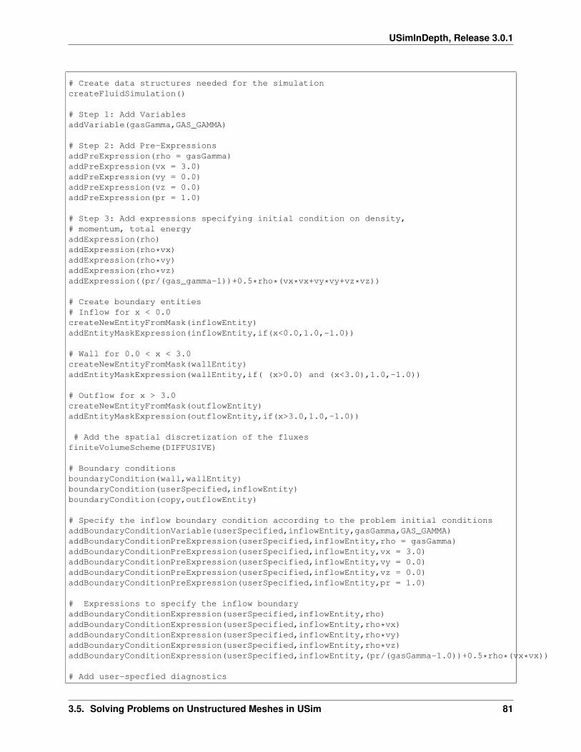
USimInDepth, Release 3.0.1
# Create data structures needed for the simulationcreateFluidSimulation()
# Step 1: Add VariablesaddVariable(gasGamma,GAS_GAMMA)
# Step 2: Add Pre-ExpressionsaddPreExpression(rho = gasGamma)addPreExpression(vx = 3.0)addPreExpression(vy = 0.0)addPreExpression(vz = 0.0)addPreExpression(pr = 1.0)
# Step 3: Add expressions specifying initial condition on density,# momentum, total energyaddExpression(rho)addExpression(rho*vx)addExpression(rho*vy)addExpression(rho*vz)addExpression((pr/(gas_gamma-1))+0.5*rho*(vx*vx+vy*vy+vz*vz))
# Create boundary entities# Inflow for x < 0.0createNewEntityFromMask(inflowEntity)addEntityMaskExpression(inflowEntity,if(x<0.0,1.0,-1.0))
# Wall for 0.0 < x < 3.0createNewEntityFromMask(wallEntity)addEntityMaskExpression(wallEntity,if( (x>0.0) and (x<3.0),1.0,-1.0))
# Outflow for x > 3.0createNewEntityFromMask(outflowEntity)addEntityMaskExpression(outflowEntity,if(x>3.0,1.0,-1.0))
# Add the spatial discretization of the fluxesfiniteVolumeScheme(DIFFUSIVE)
# Boundary conditionsboundaryCondition(wall,wallEntity)boundaryCondition(userSpecified,inflowEntity)boundaryCondition(copy,outflowEntity)
# Specify the inflow boundary condition according to the problem initial conditionsaddBoundaryConditionVariable(userSpecified,inflowEntity,gasGamma,GAS_GAMMA)addBoundaryConditionPreExpression(userSpecified,inflowEntity,rho = gasGamma)addBoundaryConditionPreExpression(userSpecified,inflowEntity,vx = 3.0)addBoundaryConditionPreExpression(userSpecified,inflowEntity,vy = 0.0)addBoundaryConditionPreExpression(userSpecified,inflowEntity,vz = 0.0)addBoundaryConditionPreExpression(userSpecified,inflowEntity,pr = 1.0)
# Expressions to specify the inflow boundaryaddBoundaryConditionExpression(userSpecified,inflowEntity,rho)addBoundaryConditionExpression(userSpecified,inflowEntity,rho*vx)addBoundaryConditionExpression(userSpecified,inflowEntity,rho*vy)addBoundaryConditionExpression(userSpecified,inflowEntity,rho*vz)addBoundaryConditionExpression(userSpecified,inflowEntity,(pr/(gasGamma-1.0))+0.5*rho*(vx*vx))
# Add user-specfied diagnostics
3.5. Solving Problems on Unstructured Meshes in USim 81
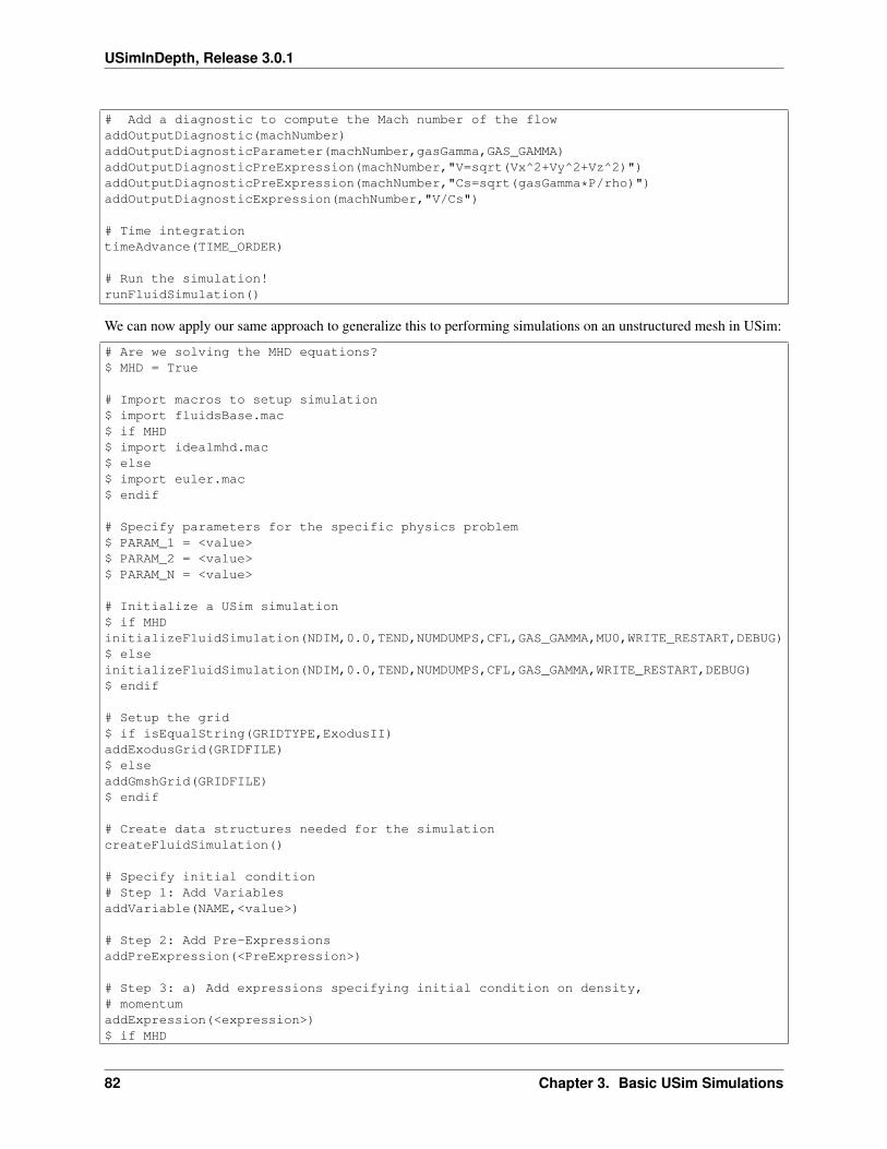
USimInDepth, Release 3.0.1
# Add a diagnostic to compute the Mach number of the flowaddOutputDiagnostic(machNumber)addOutputDiagnosticParameter(machNumber,gasGamma,GAS_GAMMA)addOutputDiagnosticPreExpression(machNumber,"V=sqrt(Vx^2+Vy^2+Vz^2)")addOutputDiagnosticPreExpression(machNumber,"Cs=sqrt(gasGamma*P/rho)")addOutputDiagnosticExpression(machNumber,"V/Cs")
# Time integrationtimeAdvance(TIME_ORDER)
# Run the simulation!runFluidSimulation()
We can now apply our same approach to generalize this to performing simulations on an unstructured mesh in USim:
# Are we solving the MHD equations?$ MHD = True
# Import macros to setup simulation$ import fluidsBase.mac$ if MHD$ import idealmhd.mac$ else$ import euler.mac$ endif
# Specify parameters for the specific physics problem$ PARAM_1 = <value>$ PARAM_2 = <value>$ PARAM_N = <value>
# Initialize a USim simulation$ if MHDinitializeFluidSimulation(NDIM,0.0,TEND,NUMDUMPS,CFL,GAS_GAMMA,MU0,WRITE_RESTART,DEBUG)$ elseinitializeFluidSimulation(NDIM,0.0,TEND,NUMDUMPS,CFL,GAS_GAMMA,WRITE_RESTART,DEBUG)$ endif
# Setup the grid$ if isEqualString(GRIDTYPE,ExodusII)addExodusGrid(GRIDFILE)$ elseaddGmshGrid(GRIDFILE)$ endif
# Create data structures needed for the simulationcreateFluidSimulation()
# Specify initial condition# Step 1: Add VariablesaddVariable(NAME,<value>)
# Step 2: Add Pre-ExpressionsaddPreExpression(<PreExpression>)
# Step 3: a) Add expressions specifying initial condition on density,# momentumaddExpression(<expression>)$ if MHD
82 Chapter 3. Basic USim Simulations
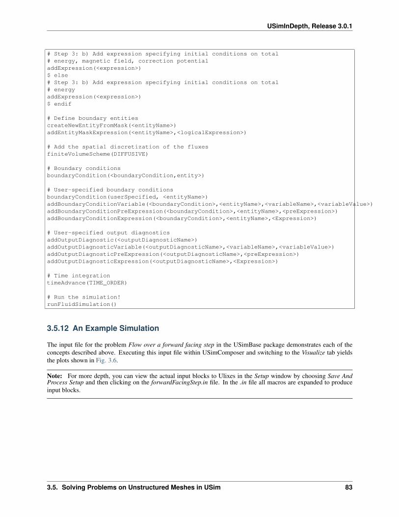
USimInDepth, Release 3.0.1
# Step 3: b) Add expression specifying initial conditions on total# energy, magnetic field, correction potentialaddExpression(<expression>)$ else# Step 3: b) Add expression specifying initial conditions on total# energyaddExpression(<expression>)$ endif
# Define boundary entitiescreateNewEntityFromMask(<entityName>)addEntityMaskExpression(<entityName>,<logicalExpression>)
# Add the spatial discretization of the fluxesfiniteVolumeScheme(DIFFUSIVE)
# Boundary conditionsboundaryCondition(<boundaryCondition,entity>)
# User-specified boundary conditionsboundaryCondition(userSpecified, <entityName>)addBoundaryConditionVariable(<boundaryCondition>,<entityName>,<variableName>,<variableValue>)addBoundaryConditionPreExpression(<boundaryCondition>,<entityName>,<preExpression>)addBoundaryConditionExpression(<boundaryCondition>,<entityName>,<Expression>)
# User-specified output diagnosticsaddOutputDiagnostic(<outputDiagnosticName>)addOutputDiagnosticVariable(<outputDiagnosticName>,<variableName>,<variableValue>)addOutputDiagnosticPreExpression(<outputDiagnosticName>,<preExpression>)addOutputDiagnosticExpression(<outputDiagnosticName>,<Expression>)
# Time integrationtimeAdvance(TIME_ORDER)
# Run the simulation!runFluidSimulation()
3.5.12 An Example Simulation
The input file for the problem Flow over a forward facing step in the USimBase package demonstrates each of theconcepts described above. Executing this input file within USimComposer and switching to the Visualize tab yieldsthe plots shown in Fig. 3.6.
Note: For more depth, you can view the actual input blocks to Ulixes in the Setup window by choosing Save AndProcess Setup and then clicking on the forwardFacingStep.in file. In the .in file all macros are expanded to produceinput blocks.
3.5. Solving Problems on Unstructured Meshes in USim 83
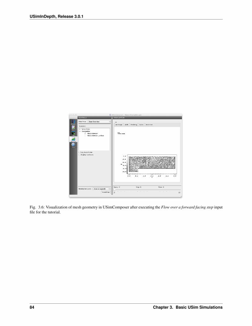
USimInDepth, Release 3.0.1
Fig. 3.6: Visualization of mesh geometry in USimComposer after executing the Flow over a forward facing step inputfile for the tutorial.
84 Chapter 3. Basic USim Simulations
CHAPTER
FOUR
ADVANCED USIM SIMULATIONS
The following tutorials can be worked through with a USimBase license and described how to perform simulationsusing USim by working directly with the input file.
4.1 Advanced USim Simulation Concepts
In Using USim to solve the Euler Equations, Solving Problems on Unstructured Meshes in USim, we saw how tosolve the Euler and MHD equations for a range of problems using USim. The algorithms that we used to do this werecreated using a range of macros. USim simulations can also be created without the use of these macros, allowing theuser much greater control over the simulation design process and enabling simulations with greater complexity. Thenext set of tutorials describes how to create USim simulations without the use of macros. It does so by making use ofthe examples in USimBase again, but this time we examine the actual input blocks generated from the macros. This isdone in the Setup window by choosing Save And Process Setup and then clicking on the <exampleName>.in tab. Inthe .in tab all macros are expanded to produce input blocks.
We start this set of tutorials by presenting advanced concepts about USim that you should understand before creatingand running USim simulations without using the macros described in earlier tutorials. Taking the time to examinethese concepts before reading about the simulation process will make the simulation procedures simple to understandand tutorial lessons straightforward to follow.
Contents
• Advanced USim Simulation Concepts– The Fluids Component– Defining the Simulation Grid– Allocating Memory– Setting Initial Conditions– Writing Out Data
* Writing out Additional Data– An Example Simulation File
4.1.1 The Fluids Component
USim input files without macros look like XML files. Input files can contain nested blocks, each block can containdouble, integer and string values and vectors (arrays) of these types. Remember: if you want to specify a double inthe input file you must not omit the decimal point. Otherwise, the number will be interpreted as an integer. Similarly,if you want an array of doubles, the first element must have a decimal point. Hence, what follows are examples of adouble scalar and a double vector:
85
USimInDepth, Release 3.0.1
value = 1.0listOfNumbers = [1.0, 2.0, 3.0]
The simplest example of an input file given below. It basically does nothing but starts USim and quits:
# start and end timestStart = 0.0tEnd = 0.2# number of frames to writenumFrames = 2# initial time-step to useinitDt = 0.01verbosity = debugdefaultParallelSync = false
# top level component<Component fluids>
kind = updaterComponent</Component>
All input files need a start and end time for the simulation, specified as tStart and tEnd. The numFrames variabletells USim how many frames of data to write. USim will always write the initial frame and then will write additionalnumFrames frames. Each frame is an HDF5 file named same as the input file with numbers appended to indicateframe number. For example, euler_0.h5, euler_1.h5 and euler_2.h5 will be created by the above simulation. Moreinformation on USim data output is given in Writing Out Data.
The initial time-step is specified in initDt. This can be set to whatever you want as USim will simply adjust thisdepending on the physics included in the simulation.
The option defaultParallelSync=false tells USim that the user will specify the parallel synchronization of the data inthe simulation. defaultParallelSync is optional, but defaults to false. If defaultParallelSync=true then parallel datasynchronization is done automatically. Automatic synchronization is less efficient than user defined synchronization,but avoids many of the pitfalls. If you are having problems with a parallel simulations, a simple check of yoursynchronization is to set defaultParallelSync=true.
In each simulation there must be exactly one top-level Component block. This block is called fluids. You can name itanything you want and this name will be reflected in the output HDF5 files. Many blocks take a special field calledthe kind field. This field tells USim what kind of Component (in this case) to create. For now, we will use the standardupdaterComponent component kind.
4.1.2 Defining the Simulation Grid
Every object in a USim simulation interacts with a grid in one, two or three dimensions, in either Cartesian or axisym-metric Cylindrical coordinates. Grids in USim can either be rectangular, body-fitted or unstructured. The simplestexample is a one-dimensional rectangular grid, which here we name domain:
<Grid domain>kind = cart1dghostLayers = 2lower = [0.0]upper = [1.0]cells = [512]
</Grid>
This will create a 512 zone, 1D Cartesian grid spanning the physical space (0.0, 1.0). Instructions for creating multi-dimensional Cartesian grids, body-fitted grids and unstructured meshes can be found in other sections of this manual.
86 Chapter 4. Advanced USim Simulations
USimInDepth, Release 3.0.1
4.1.3 Allocating Memory
Data can be allocated on the grid defined in Defining the Simulation Grid through the code block such as:
<DataStruct q>kind = nodalArrayonGrid = domainnumComponents = 5
</DataStruct>
This block will create a nodalArray array called “q”. A nodal array is one that interacts with rectangular, body-fittedand unstructured meshes and is decomposed using MPI when run in parallel. Note we have to specify the name of thegrid the data lives on using the onGrid field. The field numComponents tells USim that we wish to store 5 componentsin this array.
Now our input file should look like:
# start and end timestStart = 0.0tEnd = 0.2
# number of frames to writenumFrames = 2
# initial time-step to useinitDt = 0.01verbosity = debug
# top level component<Component fluids>kind = updaterComponent
<Grid domain>kind = cart1dghostLayers = 2lower = [0.0]upper = [1.0]cells = [512]
</Grid>
<DataStruct q>kind = nodalArrayonGrid = domainnumComponents = 5
</DataStruct>
</Component>
This input file can be executed within USimComposer.
4.1.4 Setting Initial Conditions
Now that we have allocated an array we will initialize it. USim provides a block called Updater to perform actionon data. There are many Updaters and we will use them extensively in constructing a simulation. Updaters are verypowerful and can be used to create very complex simulations by combining them carefully. Think of an updater as ageneralization of a subroutine or function.
Let’s create an updater, named “init” to initialize the “q” array. This updater will use a expressions to initialize allthe components of “q”. As a simple example, we will use the initial condition for a one-dimensional Sod Shock tube,which consists of a left-state and a right-state separated by a discontinuity:
4.1. Advanced USim Simulation Concepts 87
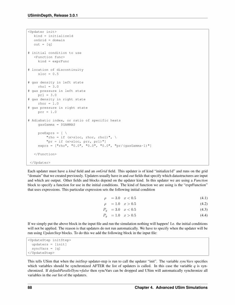
USimInDepth, Release 3.0.1
<Updater init>kind = initialize1donGrid = domainout = [q]
# initial condition to use<Function func>
kind = exprFunc
# location of discontinuitysloc = 0.5
# gas density in left staterhol = 3.0
# gas pressure in left stateprl = 3.0
# gas density in right staterhor = 1.0
# gas pressure in right stateprr = 1.0
# Adiabatic index, or ratio of specific heatsgasGamma = $GAMMA$
preExprs = [ \"rho = if (x>sloc, rhor, rhol)", \"pr = if (x>sloc, prr, prl)"]
exprs = ["rho", "0.0", "0.0", "0.0", "pr/(gasGamma-1)"]
</Function>
</Updater>
Each updater must have a kind field and an onGrid field. This updater is of kind “initialize1d” and runs on the grid“domain” that we created previously. Updaters usually have in and out fields that specify which datastructures are inputand which are output. Other fields and blocks depend on the updater kind. In this updater we are using a Functionblock to specify a function for use in the initial conditions. The kind of function we are using is the “exprFunction”that uses expressions. This particular expression sets the following initial condition
𝜌 = 3.0 𝑥 < 0.5 (4.1)𝜌 = 1.0 𝑥 > 0.5 (4.2)𝑃𝑔 = 3.0 𝑥 < 0.5 (4.3)𝑃𝑔 = 1.0 𝑥 > 0.5 (4.4)
If we simply put the above block in the input file and run the simulation nothing will happen! I.e. the initial conditionswill not be applied. The reason is that updaters do not run automatically. We have to specify when the updater will berun using UpdateStep blocks. To do this we add the following block in the input file:
<UpdateStep initStep>updaters = [init]syncVars = [q]
</UpdateStep>
This tells USim that when the initStep updater-step is run to call the updater “init”. The variable syncVars specifieswhich variables should be synchronized AFTER the list of updaters is called. In this case the variable q is syn-chronized. If defaultParallelSync=false then syncVars can be dropped and USim will automatically synchronize allvariables in the out list of the updaters.
88 Chapter 4. Advanced USim Simulations
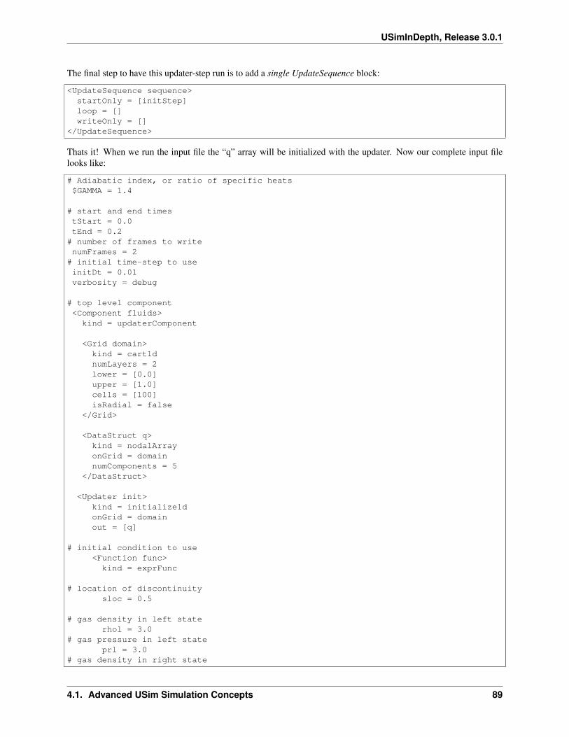
USimInDepth, Release 3.0.1
The final step to have this updater-step run is to add a single UpdateSequence block:
<UpdateSequence sequence>startOnly = [initStep]loop = []writeOnly = []
</UpdateSequence>
Thats it! When we run the input file the “q” array will be initialized with the updater. Now our complete input filelooks like:
# Adiabatic index, or ratio of specific heats$GAMMA = 1.4
# start and end timestStart = 0.0tEnd = 0.2
# number of frames to writenumFrames = 2
# initial time-step to useinitDt = 0.01verbosity = debug
# top level component<Component fluids>kind = updaterComponent
<Grid domain>kind = cart1dnumLayers = 2lower = [0.0]upper = [1.0]cells = [100]isRadial = false
</Grid>
<DataStruct q>kind = nodalArrayonGrid = domainnumComponents = 5
</DataStruct>
<Updater init>kind = initialize1donGrid = domainout = [q]
# initial condition to use<Function func>
kind = exprFunc
# location of discontinuitysloc = 0.5
# gas density in left staterhol = 3.0
# gas pressure in left stateprl = 3.0
# gas density in right state
4.1. Advanced USim Simulation Concepts 89
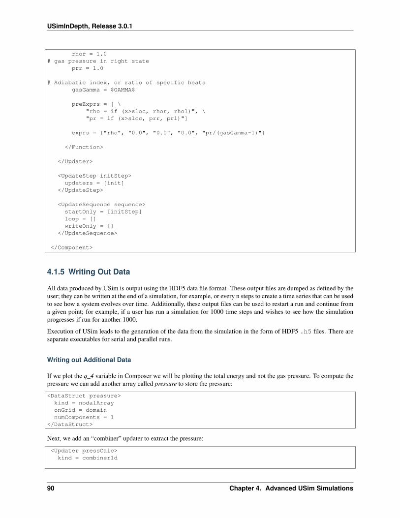
USimInDepth, Release 3.0.1
rhor = 1.0# gas pressure in right state
prr = 1.0
# Adiabatic index, or ratio of specific heatsgasGamma = $GAMMA$
preExprs = [ \"rho = if (x>sloc, rhor, rhol)", \"pr = if (x>sloc, prr, prl)"]
exprs = ["rho", "0.0", "0.0", "0.0", "pr/(gasGamma-1)"]
</Function>
</Updater>
<UpdateStep initStep>updaters = [init]
</UpdateStep>
<UpdateSequence sequence>startOnly = [initStep]loop = []writeOnly = []
</UpdateSequence>
</Component>
4.1.5 Writing Out Data
All data produced by USim is output using the HDF5 data file format. These output files are dumped as defined by theuser; they can be written at the end of a simulation, for example, or every n steps to create a time series that can be usedto see how a system evolves over time. Additionally, these output files can be used to restart a run and continue froma given point; for example, if a user has run a simulation for 1000 time steps and wishes to see how the simulationprogresses if run for another 1000.
Execution of USim leads to the generation of the data from the simulation in the form of HDF5 .h5 files. There areseparate executables for serial and parallel runs.
Writing out Additional Data
If we plot the q_4 variable in Composer we will be plotting the total energy and not the gas pressure. To compute thepressure we can add another array called pressure to store the pressure:
<DataStruct pressure>kind = nodalArrayonGrid = domainnumComponents = 1
</DataStruct>
Next, we add an “combiner” updater to extract the pressure:
<Updater pressCalc>kind = combiner1d
90 Chapter 4. Advanced USim Simulations
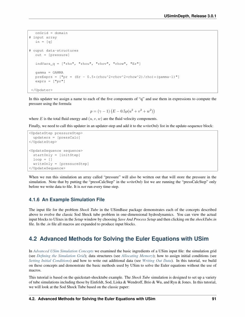
USimInDepth, Release 3.0.1
onGrid = domain# input array
in = [q]
# ouput data-structuresout = [pressure]
indVars_q = ["rho", "rhou", "rhov", "rhow", "Er"]
gamma = GAMMApreExprs = ["pr = (Er - 0.5*(rhou^2+rhov^2+rhow^2)/rho)*(gamma-1)"]exprs = ["pr"]
</Updater>
In this updater we assign a name to each of the five components of “q” and use them in expressions to compute thepressure using the formula
𝑝 = (𝛾 − 1)(𝐸 − 0.5𝜌(𝑢2 + 𝑣2 + 𝑤2)
)where 𝐸 is the total fluid energy and (𝑢, 𝑣, 𝑤) are the fluid velocity components.
Finally, we need to call this updater in an updater-step and add it to the writeOnly list in the update-sequence block:
<UpdateStep pressureStep>updaters = [pressCalc]
</UpdateStep>
<UpdateSequence sequence>startOnly = [initStep]loop = []writeOnly = [pressureStep]
</UpdateSequence>
When we run this simulation an array called “pressure” will also be written out that will store the pressure in thesimulation. Note that by putting the “pressCalcStep” in the writeOnly list we are running the “pressCalcStep” onlybefore we write data to file. It is not run every time-step.
4.1.6 An Example Simulation File
The input file for the problem Shock Tube in the USimBase package demonstrates each of the concepts describedabove to evolve the classic Sod Shock tube problem in one-dimensional hydrodynamics. You can view the actualinput blocks to Ulixes in the Setup window by choosing Save And Process Setup and then clicking on the shockTube.infile. In the .in file all macros are expanded to produce input blocks.
4.2 Advanced Methods for Solving the Euler Equations with USim
In Advanced USim Simulation Concepts we examined the basic ingredients of a USim input file: the simulation grid(see Defining the Simulation Grid); data structures (see Allocating Memory); how to assign initial conditions (seeSetting Initial Conditions) and how to write out additional data (see Writing Out Data). In this tutorial, we buildon these concepts and demonstrate the basic methods used by USim to solve the Euler equations without the use ofmacros.
This tutorial is based on the quickstart-shocktube example. The Shock Tube simulation is designed to set up a varietyof tube simulations including those by Einfeldt, Sod, Liska & Wendroff, Brio & Wu, and Ryu & Jones. In this tutorial,we will look at the Sod Shock Tube based on the classic paper:
4.2. Advanced Methods for Solving the Euler Equations with USim 91
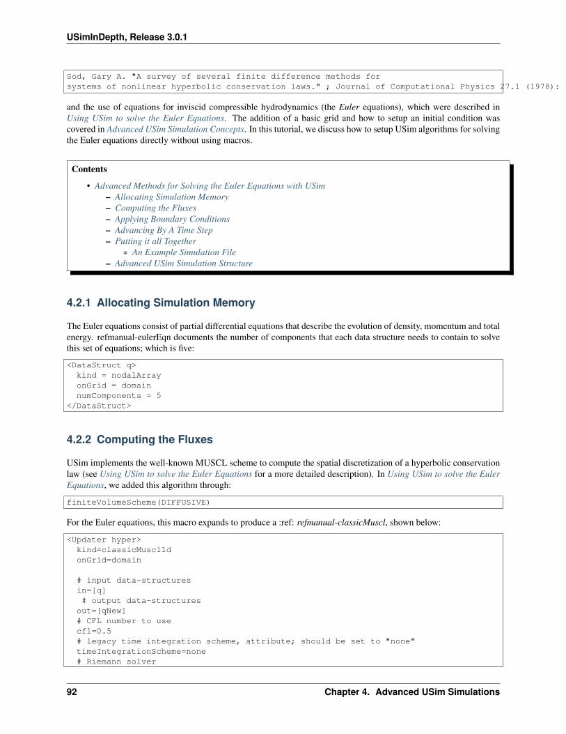
USimInDepth, Release 3.0.1
Sod, Gary A. "A survey of several finite difference methods forsystems of nonlinear hyperbolic conservation laws." ; Journal of Computational Physics 27.1 (1978): 1-31.
and the use of equations for inviscid compressible hydrodynamics (the Euler equations), which were described inUsing USim to solve the Euler Equations. The addition of a basic grid and how to setup an initial condition wascovered in Advanced USim Simulation Concepts. In this tutorial, we discuss how to setup USim algorithms for solvingthe Euler equations directly without using macros.
Contents
• Advanced Methods for Solving the Euler Equations with USim– Allocating Simulation Memory– Computing the Fluxes– Applying Boundary Conditions– Advancing By A Time Step– Putting it all Together
* An Example Simulation File– Advanced USim Simulation Structure
4.2.1 Allocating Simulation Memory
The Euler equations consist of partial differential equations that describe the evolution of density, momentum and totalenergy. refmanual-eulerEqn documents the number of components that each data structure needs to contain to solvethis set of equations; which is five:
<DataStruct q>kind = nodalArrayonGrid = domainnumComponents = 5
</DataStruct>
4.2.2 Computing the Fluxes
USim implements the well-known MUSCL scheme to compute the spatial discretization of a hyperbolic conservationlaw (see Using USim to solve the Euler Equations for a more detailed description). In Using USim to solve the EulerEquations, we added this algorithm through:
finiteVolumeScheme(DIFFUSIVE)
For the Euler equations, this macro expands to produce a :ref: refmanual-classicMuscl, shown below:
<Updater hyper>kind=classicMuscl1donGrid=domain
# input data-structuresin=[q]# output data-structuresout=[qNew]# CFL number to usecfl=0.5# legacy time integration scheme, attribute; should be set to "none"timeIntegrationScheme=none# Riemann solver
92 Chapter 4. Advanced USim Simulations
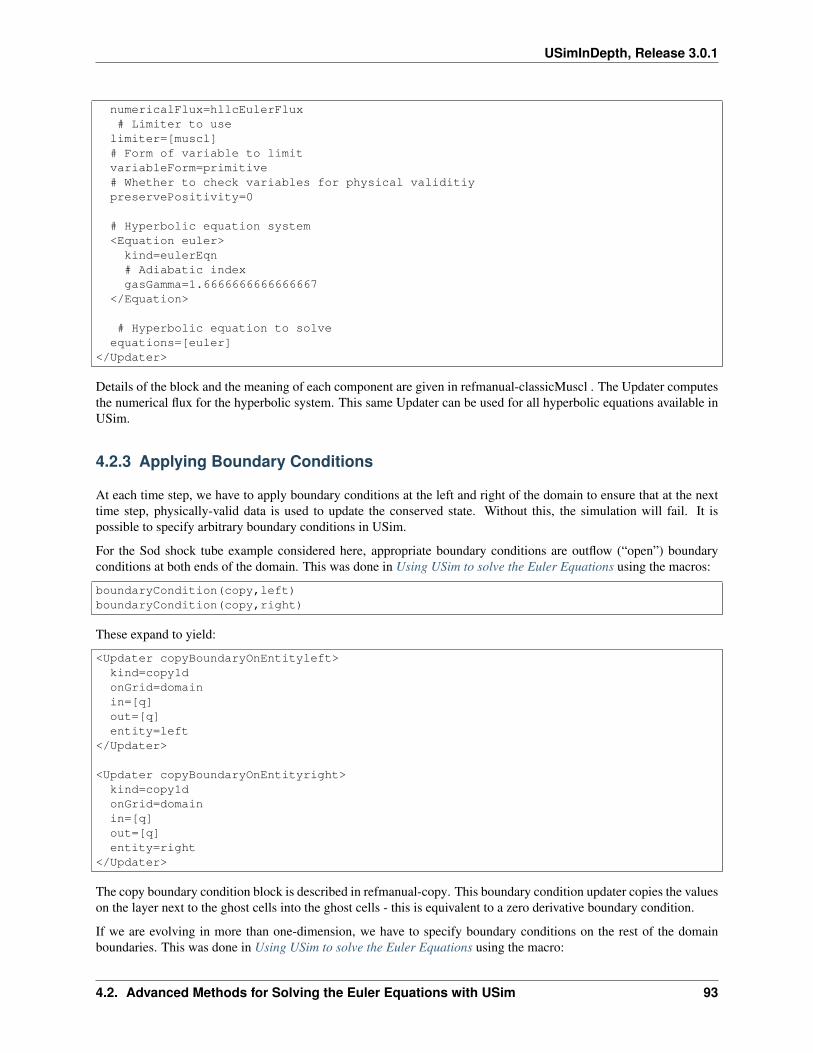
USimInDepth, Release 3.0.1
numericalFlux=hllcEulerFlux# Limiter to uselimiter=[muscl]# Form of variable to limitvariableForm=primitive# Whether to check variables for physical validitiypreservePositivity=0
# Hyperbolic equation system<Equation euler>kind=eulerEqn# Adiabatic indexgasGamma=1.6666666666666667
</Equation>
# Hyperbolic equation to solveequations=[euler]
</Updater>
Details of the block and the meaning of each component are given in refmanual-classicMuscl . The Updater computesthe numerical flux for the hyperbolic system. This same Updater can be used for all hyperbolic equations available inUSim.
4.2.3 Applying Boundary Conditions
At each time step, we have to apply boundary conditions at the left and right of the domain to ensure that at the nexttime step, physically-valid data is used to update the conserved state. Without this, the simulation will fail. It ispossible to specify arbitrary boundary conditions in USim.
For the Sod shock tube example considered here, appropriate boundary conditions are outflow (“open”) boundaryconditions at both ends of the domain. This was done in Using USim to solve the Euler Equations using the macros:
boundaryCondition(copy,left)boundaryCondition(copy,right)
These expand to yield:
<Updater copyBoundaryOnEntityleft>kind=copy1donGrid=domainin=[q]out=[q]entity=left
</Updater>
<Updater copyBoundaryOnEntityright>kind=copy1donGrid=domainin=[q]out=[q]entity=right
</Updater>
The copy boundary condition block is described in refmanual-copy. This boundary condition updater copies the valueson the layer next to the ghost cells into the ghost cells - this is equivalent to a zero derivative boundary condition.
If we are evolving in more than one-dimension, we have to specify boundary conditions on the rest of the domainboundaries. This was done in Using USim to solve the Euler Equations using the macro:
4.2. Advanced Methods for Solving the Euler Equations with USim 93
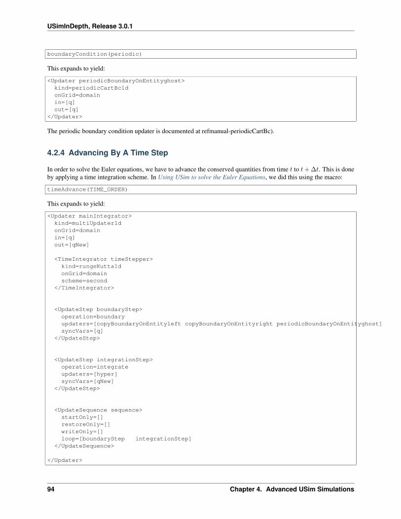
USimInDepth, Release 3.0.1
boundaryCondition(periodic)
This expands to yield:
<Updater periodicBoundaryOnEntityghost>kind=periodicCartBc1donGrid=domainin=[q]out=[q]
</Updater>
The periodic boundary condition updater is documented at refmanual-periodicCartBc).
4.2.4 Advancing By A Time Step
In order to solve the Euler equations, we have to advance the conserved quantities from time 𝑡 to 𝑡+ ∆𝑡. This is doneby applying a time integration scheme. In Using USim to solve the Euler Equations, we did this using the macro:
timeAdvance(TIME_ORDER)
This expands to yield:
<Updater mainIntegrator>kind=multiUpdater1donGrid=domainin=[q]out=[qNew]
<TimeIntegrator timeStepper>kind=rungeKutta1donGrid=domainscheme=second
</TimeIntegrator>
<UpdateStep boundaryStep>operation=boundaryupdaters=[copyBoundaryOnEntityleft copyBoundaryOnEntityright periodicBoundaryOnEntityghost]syncVars=[q]
</UpdateStep>
<UpdateStep integrationStep>operation=integrateupdaters=[hyper]syncVars=[qNew]
</UpdateStep>
<UpdateSequence sequence>startOnly=[]restoreOnly=[]writeOnly=[]loop=[boundaryStep integrationStep]
</UpdateSequence>
</Updater>
94 Chapter 4. Advanced USim Simulations
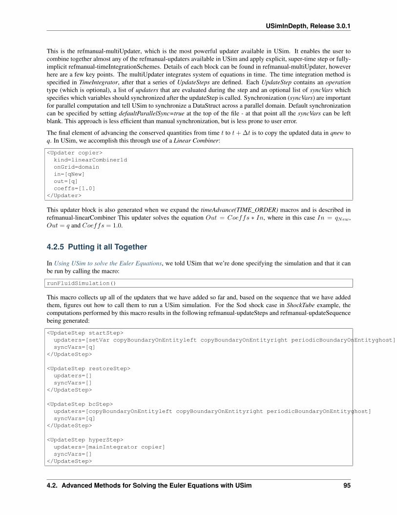
USimInDepth, Release 3.0.1
This is the refmanual-multiUpdater, which is the most powerful updater available in USim. It enables the user tocombine together almost any of the refmanual-updaters available in USim and apply explicit, super-time step or fully-implicit refmanual-timeIntegrationSchemes. Details of each block can be found in refmanual-multiUpdater, howeverhere are a few key points. The multiUpdater integrates system of equations in time. The time integration method isspecified in TimeIntegrator, after that a series of UpdateSteps are defined. Each UpdateStep contains an operationtype (which is optional), a list of updaters that are evaluated during the step and an optional list of syncVars whichspecifies which variables should synchronized after the updateStep is called. Synchronization (syncVars) are importantfor parallel computation and tell USim to synchronize a DataStruct across a parallel domain. Default synchronizationcan be specified by setting defaultParallelSync=true at the top of the file - at that point all the syncVars can be leftblank. This approach is less efficient than manual synchronization, but is less prone to user error.
The final element of advancing the conserved quantities from time 𝑡 to 𝑡 + ∆𝑡 is to copy the updated data in qnew toq. In USim, we accomplish this through use of a Linear Combiner:
<Updater copier>kind=linearCombiner1donGrid=domainin=[qNew]out=[q]coeffs=[1.0]
</Updater>
This updater block is also generated when we expand the timeAdvance(TIME_ORDER) macros and is described inrefmanual-linearCombiner This updater solves the equation 𝑂𝑢𝑡 = 𝐶𝑜𝑒𝑓𝑓𝑠 * 𝐼𝑛, where in this case 𝐼𝑛 = 𝑞𝑁𝑒𝑤,𝑂𝑢𝑡 = 𝑞 and 𝐶𝑜𝑒𝑓𝑓𝑠 = 1.0.
4.2.5 Putting it all Together
In Using USim to solve the Euler Equations, we told USim that we’re done specifying the simulation and that it canbe run by calling the macro:
runFluidSimulation()
This macro collects up all of the updaters that we have added so far and, based on the sequence that we have addedthem, figures out how to call them to run a USim simulation. For the Sod shock case in ShockTube example, thecomputations performed by this macro results in the following refmanual-updateSteps and refmanual-updateSequencebeing generated:
<UpdateStep startStep>updaters=[setVar copyBoundaryOnEntityleft copyBoundaryOnEntityright periodicBoundaryOnEntityghost]syncVars=[q]
</UpdateStep>
<UpdateStep restoreStep>updaters=[]syncVars=[]
</UpdateStep>
<UpdateStep bcStep>updaters=[copyBoundaryOnEntityleft copyBoundaryOnEntityright periodicBoundaryOnEntityghost]syncVars=[q]
</UpdateStep>
<UpdateStep hyperStep>updaters=[mainIntegrator copier]syncVars=[]
</UpdateStep>
4.2. Advanced Methods for Solving the Euler Equations with USim 95
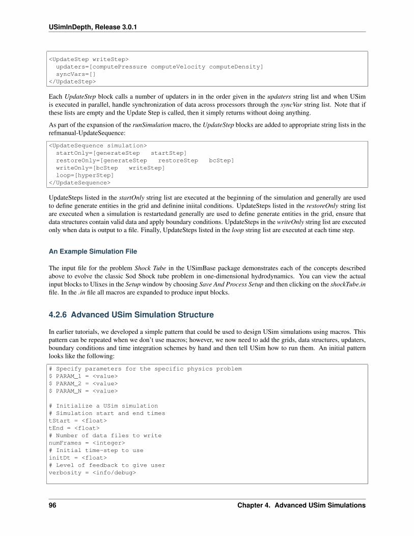
USimInDepth, Release 3.0.1
<UpdateStep writeStep>updaters=[computePressure computeVelocity computeDensity]syncVars=[]
</UpdateStep>
Each UpdateStep block calls a number of updaters in in the order given in the updaters string list and when USimis executed in parallel, handle synchronization of data across processors through the syncVar string list. Note that ifthese lists are empty and the Update Step is called, then it simply returns without doing anything.
As part of the expansion of the runSimulation macro, the UpdateStep blocks are added to appropriate string lists in therefmanual-UpdateSequence:
<UpdateSequence simulation>startOnly=[generateStep startStep]restoreOnly=[generateStep restoreStep bcStep]writeOnly=[bcStep writeStep]loop=[hyperStep]
</UpdateSequence>
UpdateSteps listed in the startOnly string list are executed at the beginning of the simulation and generally are usedto define generate entities in the grid and definine iniital conditions. UpdateSteps listed in the restoreOnly string listare executed when a simulation is restartedand generally are used to define generate entities in the grid, ensure thatdata structures contain valid data and apply boundary conditions. UpdateSteps in the writeOnly string list are executedonly when data is output to a file. Finally, UpdateSteps listed in the loop string list are executed at each time step.
An Example Simulation File
The input file for the problem Shock Tube in the USimBase package demonstrates each of the concepts describedabove to evolve the classic Sod Shock tube problem in one-dimensional hydrodynamics. You can view the actualinput blocks to Ulixes in the Setup window by choosing Save And Process Setup and then clicking on the shockTube.infile. In the .in file all macros are expanded to produce input blocks.
4.2.6 Advanced USim Simulation Structure
In earlier tutorials, we developed a simple pattern that could be used to design USim simulations using macros. Thispattern can be repeated when we don’t use macros; however, we now need to add the grids, data structures, updaters,boundary conditions and time integration schemes by hand and then tell USim how to run them. An initial patternlooks like the following:
# Specify parameters for the specific physics problem$ PARAM_1 = <value>$ PARAM_2 = <value>$ PARAM_N = <value>
# Initialize a USim simulation# Simulation start and end timestStart = <float>tEnd = <float># Number of data files to writenumFrames = <integer># Initial time-step to useinitDt = <float># Level of feedback to give userverbosity = <info/debug>
96 Chapter 4. Advanced USim Simulations
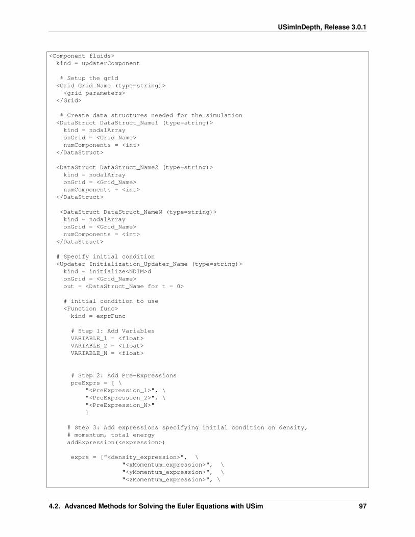
USimInDepth, Release 3.0.1
<Component fluids>kind = updaterComponent
# Setup the grid<Grid Grid_Name (type=string)><grid parameters>
</Grid>
# Create data structures needed for the simulation<DataStruct DataStruct_Name1 (type=string)>kind = nodalArrayonGrid = <Grid_Name>numComponents = <int>
</DataStruct>
<DataStruct DataStruct_Name2 (type=string)>kind = nodalArrayonGrid = <Grid_Name>numComponents = <int>
</DataStruct>
<DataStruct DataStruct_NameN (type=string)>kind = nodalArrayonGrid = <Grid_Name>numComponents = <int>
</DataStruct>
# Specify initial condition<Updater Initialization_Updater_Name (type=string)>kind = initialize<NDIM>donGrid = <Grid_Name>out = <DataStruct_Name for t = 0>
# initial condition to use<Function func>
kind = exprFunc
# Step 1: Add VariablesVARIABLE_1 = <float>VARIABLE_2 = <float>VARIABLE_N = <float>
# Step 2: Add Pre-ExpressionspreExprs = [ \
"<PreExpression_1>", \"<PreExpression_2>", \"<PreExpression_N>"]
# Step 3: Add expressions specifying initial condition on density,# momentum, total energyaddExpression(<expression>)
exprs = ["<density_expression>", \"<xMomentum_expression>", \"<yMomentum_expression>", \"<zMomentum_expression>", \
4.2. Advanced Methods for Solving the Euler Equations with USim 97
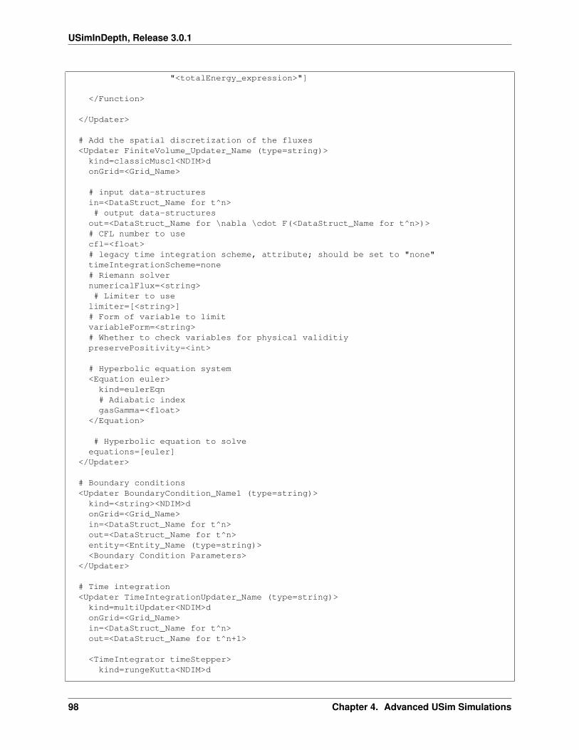
USimInDepth, Release 3.0.1
"<totalEnergy_expression>"]
</Function>
</Updater>
# Add the spatial discretization of the fluxes<Updater FiniteVolume_Updater_Name (type=string)>kind=classicMuscl<NDIM>donGrid=<Grid_Name>
# input data-structuresin=<DataStruct_Name for t^n># output data-structures
out=<DataStruct_Name for \nabla \cdot F(<DataStruct_Name for t^n>)># CFL number to usecfl=<float># legacy time integration scheme, attribute; should be set to "none"timeIntegrationScheme=none# Riemann solvernumericalFlux=<string># Limiter to use
limiter=[<string>]# Form of variable to limitvariableForm=<string># Whether to check variables for physical validitiypreservePositivity=<int>
# Hyperbolic equation system<Equation euler>
kind=eulerEqn# Adiabatic indexgasGamma=<float>
</Equation>
# Hyperbolic equation to solveequations=[euler]
</Updater>
# Boundary conditions<Updater BoundaryCondition_Name1 (type=string)>kind=<string><NDIM>donGrid=<Grid_Name>in=<DataStruct_Name for t^n>out=<DataStruct_Name for t^n>entity=<Entity_Name (type=string)><Boundary Condition Parameters>
</Updater>
# Time integration<Updater TimeIntegrationUpdater_Name (type=string)>kind=multiUpdater<NDIM>donGrid=<Grid_Name>in=<DataStruct_Name for t^n>out=<DataStruct_Name for t^n+1>
<TimeIntegrator timeStepper>kind=rungeKutta<NDIM>d
98 Chapter 4. Advanced USim Simulations
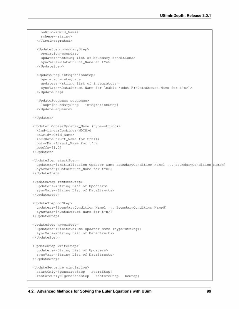
USimInDepth, Release 3.0.1
onGrid=<Grid_Name>scheme=<string>
</TimeIntegrator>
<UpdateStep boundaryStep>operation=boundaryupdaters=<string list of boundary conditions>syncVars=<DataStruct_Name at t^n>
</UpdateStep>
<UpdateStep integrationStep>operation=integrateupdaters=<string list of integrators>syncVars=<DataStruct_Name for \nabla \cdot F(<DataStruct_Name for t^n>)>
</UpdateStep>
<UpdateSequence sequence>loop=[boundaryStep integrationStep]
</UpdateSequence>
</Updater>
<Updater CopierUpdater_Name (type=string)>kind=linearCombiner<NDIM>donGrid=<Grid_Name>in=<DataStruct_Name for t^n+1>out=<DataStruct_Name for t^n>coeffs=[1.0]
</Updater>
<UpdateStep startStep>updaters=[Initialization_Updater_Name BoundaryCondition_Name1 ... BoundaryCondition_NameN]syncVars=[<DataStruct_Name for t^n>]
</UpdateStep>
<UpdateStep restoreStep>updaters=<String List of Updaters>syncVars=<String List of DataStructs>
</UpdateStep>
<UpdateStep bcStep>updaters=[BoundaryCondition_Name1 ... BoundaryCondition_NameN]syncVars=[<DataStruct_Name for t^n>]
</UpdateStep>
<UpdateStep hyperStep>updaters=[FiniteVolume_Updater_Name (type=string)]syncVars=<String List of DataStructs>
</UpdateStep>
<UpdateStep writeStep>updaters=<String List of Updaters>syncVars=<String List of DataStructs>
</UpdateStep>
<UpdateSequence simulation>startOnly=[generateStep startStep]restoreOnly=[generateStep restoreStep bcStep]
4.2. Advanced Methods for Solving the Euler Equations with USim 99
USimInDepth, Release 3.0.1
writeOnly=[bcStep writeStep]loop=[hyperStep]
</UpdateSequence>
</Component>
Note that we have not filled in some of the entries in the UpdateSteps above. How to use these UpdateSteps is discussedin later tutorials.
4.3 Advanced Methods for Solving the MagnetohydrodynamicsEquations with USim
In Advanced USim Simulation Concepts we examined the basic ingredients of a USim input file: the simulation grid(see Defining the Simulation Grid); data structures (see Allocating Memory); how to assign initial conditions (seeSetting Initial Conditions) and how to write out additional data (see Writing Out Data). In Advanced Methods forSolving the Euler Equations with USim, we built on these concepts and demonstrated the basic methods used by USimto solve the Euler equations without the use of macros.
This tutorial is based on the quickstart-shocktube example. The Shock Tube simulation is designed to set up a varietyof tube simulations including those by Einfeldt, Sod, Liska & Wendroff, Brio & Wu, and Ryu & Jones. In this tutorial,we will look at the Brio & Wu shock Tube, described by:
Brio, M., & Wu, C.~C. (1988), Journal of Computational Physics, 75, 400
and the use of equations for ideal compressible magnetohydrodynamics (the MHD equations) in one-dimension, whichwere described in Using USim to solve the Magnetohydrodynamic Equations. In this tutorial, we discuss how to setupUSim algorithms for solving the MHD equations directly without using macros.
Contents
• Advanced Methods for Solving the Magnetohydrodynamics Equations with USim– Allocating Simulation Memory– Initializing the Fluid– Evolving the Fluid– Applying Boundary Conditions– Advancing By A Time Step– Simulation Diagnostics– Putting it all Together
* An Example Simulation File– Advanced USim Simulation Structure
4.3.1 Allocating Simulation Memory
The MHD equations consist of partial differential equations that describe the evolution of density, momentum. to-tal energy and the magnetic field. refmanual-mhdDednerEqn documents the number of components that each datastructure needs to contain to solve this set of equations. In addition to the quantities defined by the MHD equations,the refmanual-mhdDednerEqn evolves an additional partial differential equation that controls the divergence of themagnetic field (the correction potential). As a result, our data structures need nine components:
<DataStruct q>kind = nodalArrayonGrid = domain
100 Chapter 4. Advanced USim Simulations
USimInDepth, Release 3.0.1
numComponents = 9</DataStruct>
i.e. modifying the numComponents input block to contain 9 entries. This must be applied to all data structures thatcontain the conserved state, fluxes or the primitive variables in the input file.
4.3.2 Initializing the Fluid
The initial condition for a MHD simulation follows the same basic three-step pattern outlined previously, but with theneed to specify the additional componets associated with the magnetic field and the correction potential:
<Updater init>kind = initialize1donGrid = domainout = [q,qnew]
<Function initFunc>kind=exprFunc
# Step 1: Add Variablespi_value=3.141592653589793gas_gamma=1.6666666666666667densityL=1.0densityR=0.125pressureL=1.0pressureR=0.1normalVelocityL=0.0normalVelocityR=0.0perpendicularVelocityL=0.0perpendicularVelocityR=0.0tangentialVelocityL=0.0tangentialVelocityR=0.0mu0=1.0normalFieldL=0.75normalFieldR=0.75perpendicularFieldL=1.0perpendicularFieldR=-1.0tangentialFieldL=0.0tangentialFieldR=0.0
# Step 2: Add Pre-ExpressionspreExprs=[ rho=if(x>0.0,densityR,densityL) pr=if(x>0.0,pressureR,pressureL) vx=if(x>0.0,normalVelocityR,normalVelocityL) vy=if(x>0.0,perpendicularVelocityR,perpendicularVelocityL) vz=if(x>0.0,tangentialVelocityR,tangentialVelocityL) bx=if(x>0.0,normalFieldR,normalFieldL) by=if(x>0.0,perpendicularFieldR,perpendicularFieldL) bz=if(x>0.0,tangentialFieldR,tangentialFieldL) psi=0.0 ]
# Step 3: Add Expressionsexprs=[ rho rho*vx rho*vy rho*vz pr/(gas_gamma-1.0)+0.5*rho*(vx*vx+vy*vy+vz*vz)+0.5*((bx*bx+by*by+bz*bz)/mu0) bx by bz psi ]
</Function>
</Updater>
Notice how each of the three steps are added to the function block that defines the initial condition:
1. Step 1 creates a list of <variablesName> = <value> pairs; one per line.
2. Step 2 creates a string vector called preExprs (short for preExpressions). Each of the addPreExpression callsdescribed in Using USim to solve the Magnetohydrodynamic Equations adds one entry to this vector, whichcontains the function specified in the addPreExpression call.
3. Step 3 creates a string vector called exprs (short for expressions). As with Step 2, each of the addExpression
4.3. Advanced Methods for Solving the Magnetohydrodynamics Equations with USim 101
USimInDepth, Release 3.0.1
call described in Using USim to solve the Magnetohydrodynamic Equations adds one entry to this vector, whichcontains the function specified in the addExpression call. Note that the order of the addExpression calls is pre-served in the string vector; this is critical as these entries specify each component of the refmanual-nodalArrayspecified in the [out] attribute.
We will see this pattern repeated whenever we used this three step process in the simple input files.
4.3.3 Evolving the Fluid
USim implements the well-known MUSCL scheme to compute the spatial discretization of a hyperbolic conservationlaw (see Using USim to solve the Euler Equations for a more detailed description). In Using USim to solve theMagnetohydrodynamic Equations, we added this algorithm through:
finiteVolumeScheme(DIFFUSIVE)
For the MHD equations, this macro expands to produce a :ref: refmanual-classicMuscl, shown below:
<Updater hyper>kind=classicMuscl1donGrid=domain# input data-structuresin=[q]# output data-structuresout=[qNew]# CFL number to usecfl=0.5# legacy time integration scheme attribute; should be set to "none"timeIntegrationScheme=none# Riemann solvernumericalFlux=hlldFlux# Limiter to uselimiter=[muscl]# Form of variable to limitvariableForm=primitive# Whether to check variables for physical validitiypreservePositivity=0# Maximum wave speed in the grid at this time stepwaveSpeeds=[maxWaveSpeed]
# Hyperbolic equation system<Equation idealMhd>kind=mhdDednerEqn# Adiabatic indexgasGamma=1.6666666666666667# Permeability of free space; should always be set to unitymu0=1.0
</Equation>
# Hyperbolic equation to solveequations=[idealMhd]
</Updater>
Compare to the case for the Euler equations described in Advanced Methods for Solving the Euler Equations withUSim, this example of the refmanual-classicMuscl updater has two key differences:
1. The use of the refmanual-mhdDednerEqn to describe the hyperbolic equation system.
2. The use of the waveSpeeds = <string vector> to specify a list of refmanual-dynVectors to provide the fastestwave speed in the grid at the current time step.
102 Chapter 4. Advanced USim Simulations
USimInDepth, Release 3.0.1
The waveSpeeds = <string vector> attribute is required for the refmanual-mhdDednerEqn in order to control thedivergence of the magnetic field. These wave speeds are computed dynamically by USim using a refmanual-timeStepRestrictionUpdater, which in the shock tube example looks like:
<Updater getMaxWaveSpeed>kind=timeStepRestrictionUpdater1donGrid=domain# input data-structuresin=[q]# no output data-structuresout=[]# CFL number to usecourantCondition=0.5# DynVector to hold the maximum wave speedwaveSpeeds=[maxWaveSpeed]
# Time step restriction to compute<TimeStepRestriction idealMhdRestriction># Compute a time step restriction for a hyperbolic equationkind=hyperbolic1d# Adiabatic indexgasGamma=1.6666666666666667# Permeability of free-space, should always be 1.0mu0=1.0# Hyperbolic equation to usemodel=mhdDednerEqn
</TimeStepRestriction>
# List of time step restrictions to computerestrictions=[idealMhdRestriction]
</Updater>
This updater computes the global maximum wave speed over the entire simulation based on the refmanual-nodalArrayspecified in the in string vector. The wave speed is stored in the refmanual-dynVector specified in the waveSpeedsstring vector.
4.3.4 Applying Boundary Conditions
At each time step, we have to apply boundary conditions at the left and right of the domain to ensure that at the nexttime step, physically-valid data is used to update the conserved state. Without this, the simulation will fail. It ispossible to specify arbitrary boundary conditions in USim.
The boundary conditions used for the Brio & Wu shock tube are the same as those used in Using USim to solve theEuler Equations, Using USim to solve the Magnetohydrodynamic Equations and Advanced Methods for Solving theEuler Equations with USim: outflow (“open”) boundary conditions at both ends of the domain. This was done inUsing USim to solve the Magnetohydrodynamic Equations using the macros:
boundaryCondition(copy,left)boundaryCondition(copy,right)
These expand to yield:
<Updater copyBoundaryOnEntityleft>kind=copy1donGrid=domainin=[q]out=[q]entity=left
4.3. Advanced Methods for Solving the Magnetohydrodynamics Equations with USim 103
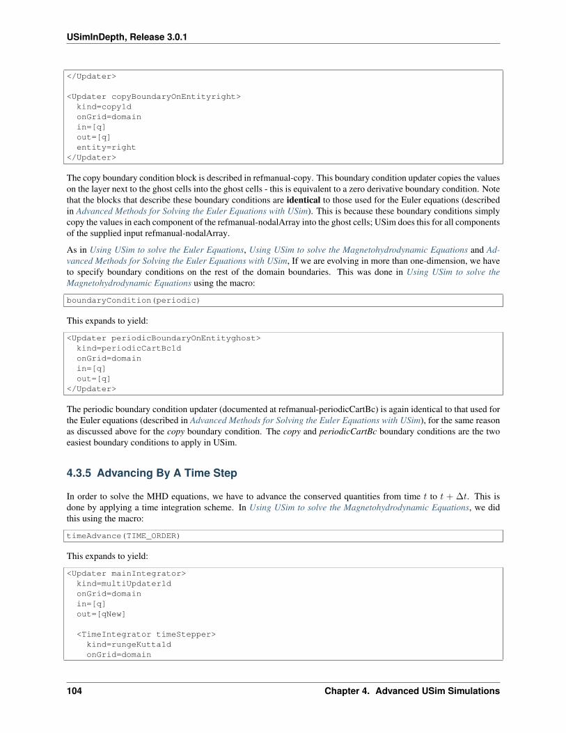
USimInDepth, Release 3.0.1
</Updater>
<Updater copyBoundaryOnEntityright>kind=copy1donGrid=domainin=[q]out=[q]entity=right
</Updater>
The copy boundary condition block is described in refmanual-copy. This boundary condition updater copies the valueson the layer next to the ghost cells into the ghost cells - this is equivalent to a zero derivative boundary condition. Notethat the blocks that describe these boundary conditions are identical to those used for the Euler equations (describedin Advanced Methods for Solving the Euler Equations with USim). This is because these boundary conditions simplycopy the values in each component of the refmanual-nodalArray into the ghost cells; USim does this for all componentsof the supplied input refmanual-nodalArray.
As in Using USim to solve the Euler Equations, Using USim to solve the Magnetohydrodynamic Equations and Ad-vanced Methods for Solving the Euler Equations with USim, If we are evolving in more than one-dimension, we haveto specify boundary conditions on the rest of the domain boundaries. This was done in Using USim to solve theMagnetohydrodynamic Equations using the macro:
boundaryCondition(periodic)
This expands to yield:
<Updater periodicBoundaryOnEntityghost>kind=periodicCartBc1donGrid=domainin=[q]out=[q]
</Updater>
The periodic boundary condition updater (documented at refmanual-periodicCartBc) is again identical to that used forthe Euler equations (described in Advanced Methods for Solving the Euler Equations with USim), for the same reasonas discussed above for the copy boundary condition. The copy and periodicCartBc boundary conditions are the twoeasiest boundary conditions to apply in USim.
4.3.5 Advancing By A Time Step
In order to solve the MHD equations, we have to advance the conserved quantities from time 𝑡 to 𝑡 + ∆𝑡. This isdone by applying a time integration scheme. In Using USim to solve the Magnetohydrodynamic Equations, we didthis using the macro:
timeAdvance(TIME_ORDER)
This expands to yield:
<Updater mainIntegrator>kind=multiUpdater1donGrid=domainin=[q]out=[qNew]
<TimeIntegrator timeStepper>kind=rungeKutta1donGrid=domain
104 Chapter 4. Advanced USim Simulations
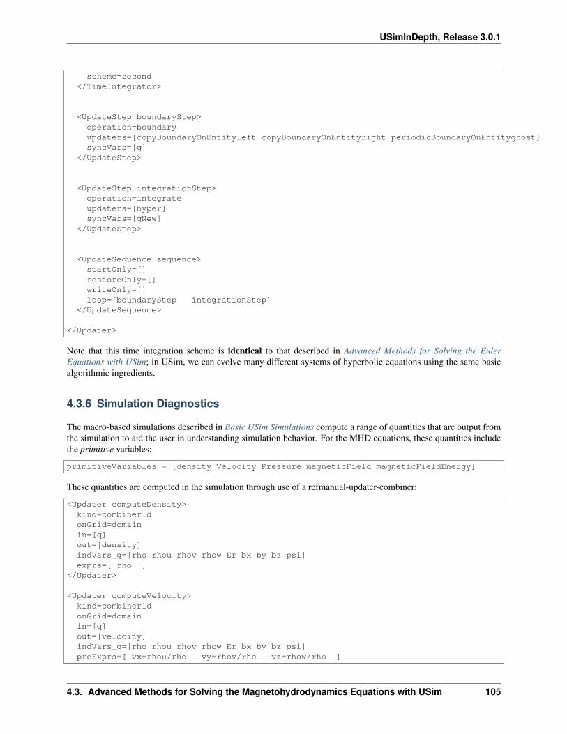
USimInDepth, Release 3.0.1
scheme=second</TimeIntegrator>
<UpdateStep boundaryStep>operation=boundaryupdaters=[copyBoundaryOnEntityleft copyBoundaryOnEntityright periodicBoundaryOnEntityghost]syncVars=[q]
</UpdateStep>
<UpdateStep integrationStep>operation=integrateupdaters=[hyper]syncVars=[qNew]
</UpdateStep>
<UpdateSequence sequence>startOnly=[]restoreOnly=[]writeOnly=[]loop=[boundaryStep integrationStep]
</UpdateSequence>
</Updater>
Note that this time integration scheme is identical to that described in Advanced Methods for Solving the EulerEquations with USim; in USim, we can evolve many different systems of hyperbolic equations using the same basicalgorithmic ingredients.
4.3.6 Simulation Diagnostics
The macro-based simulations described in Basic USim Simulations compute a range of quantities that are output fromthe simulation to aid the user in understanding simulation behavior. For the MHD equations, these quantities includethe primitive variables:
primitiveVariables = [density Velocity Pressure magneticField magneticFieldEnergy]
These quantities are computed in the simulation through use of a refmanual-updater-combiner:
<Updater computeDensity>kind=combiner1donGrid=domainin=[q]out=[density]indVars_q=[rho rhou rhov rhow Er bx by bz psi]exprs=[ rho ]
</Updater>
<Updater computeVelocity>kind=combiner1donGrid=domainin=[q]out=[velocity]indVars_q=[rho rhou rhov rhow Er bx by bz psi]preExprs=[ vx=rhou/rho vy=rhov/rho vz=rhow/rho ]
4.3. Advanced Methods for Solving the Magnetohydrodynamics Equations with USim 105
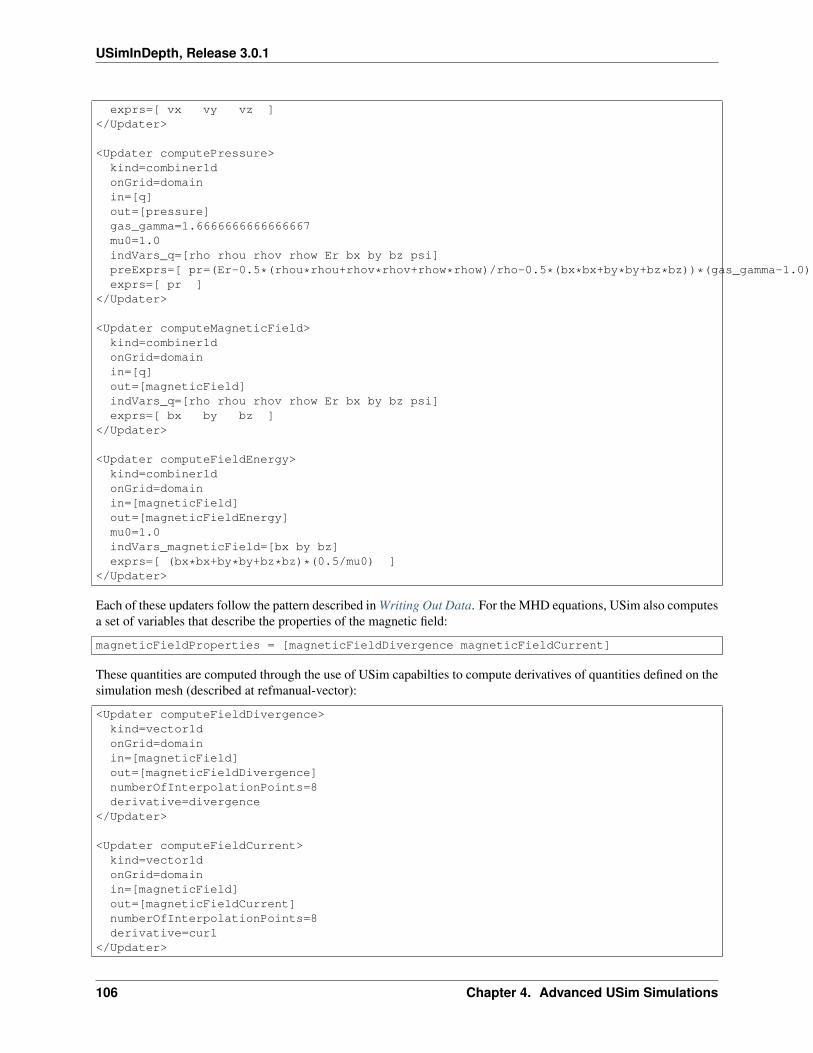
USimInDepth, Release 3.0.1
exprs=[ vx vy vz ]</Updater>
<Updater computePressure>kind=combiner1donGrid=domainin=[q]out=[pressure]gas_gamma=1.6666666666666667mu0=1.0indVars_q=[rho rhou rhov rhow Er bx by bz psi]preExprs=[ pr=(Er-0.5*(rhou*rhou+rhov*rhov+rhow*rhow)/rho-0.5*(bx*bx+by*by+bz*bz))*(gas_gamma-1.0) ]exprs=[ pr ]
</Updater>
<Updater computeMagneticField>kind=combiner1donGrid=domainin=[q]out=[magneticField]indVars_q=[rho rhou rhov rhow Er bx by bz psi]exprs=[ bx by bz ]
</Updater>
<Updater computeFieldEnergy>kind=combiner1donGrid=domainin=[magneticField]out=[magneticFieldEnergy]mu0=1.0indVars_magneticField=[bx by bz]exprs=[ (bx*bx+by*by+bz*bz)*(0.5/mu0) ]
</Updater>
Each of these updaters follow the pattern described in Writing Out Data. For the MHD equations, USim also computesa set of variables that describe the properties of the magnetic field:
magneticFieldProperties = [magneticFieldDivergence magneticFieldCurrent]
These quantities are computed through the use of USim capabilties to compute derivatives of quantities defined on thesimulation mesh (described at refmanual-vector):
<Updater computeFieldDivergence>kind=vector1donGrid=domainin=[magneticField]out=[magneticFieldDivergence]numberOfInterpolationPoints=8derivative=divergence
</Updater>
<Updater computeFieldCurrent>kind=vector1donGrid=domainin=[magneticField]out=[magneticFieldCurrent]numberOfInterpolationPoints=8derivative=curl
</Updater>
106 Chapter 4. Advanced USim Simulations
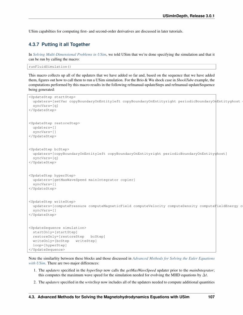
USimInDepth, Release 3.0.1
USim capabilties for computing first- and second-order derivatives are discussed in later tutorials.
4.3.7 Putting it all Together
In Solving Multi-Dimensional Problems in USim, we told USim that we’re done specifying the simulation and that itcan be run by calling the macro:
runFluidSimulation()
This macro collects up all of the updaters that we have added so far and, based on the sequence that we have addedthem, figures out how to call them to run a USim simulation. For the Brio & Wu shock case in ShockTube example, thecomputations performed by this macro results in the following refmanual-updateSteps and refmanual-updateSequencebeing generated:
<UpdateStep startStep>updaters=[setVar copyBoundaryOnEntityleft copyBoundaryOnEntityright periodicBoundaryOnEntityghost getMaxWaveSpeed]syncVars=[q]
</UpdateStep>
<UpdateStep restoreStep>updaters=[]syncVars=[]
</UpdateStep>
<UpdateStep bcStep>updaters=[copyBoundaryOnEntityleft copyBoundaryOnEntityright periodicBoundaryOnEntityghost]syncVars=[q]
</UpdateStep>
<UpdateStep hyperStep>updaters=[getMaxWaveSpeed mainIntegrator copier]syncVars=[]
</UpdateStep>
<UpdateStep writeStep>updaters=[computePressure computeMagneticField computeVelocity computeDensity computeFieldEnergy computeFieldDivergence computeFieldCurrent]syncVars=[]
</UpdateStep>
<UpdateSequence simulation>startOnly=[startStep]restoreOnly=[restoreStep bcStep]writeOnly=[bcStep writeStep]loop=[hyperStep]
</UpdateSequence>
Note the similarlity between these blocks and those discussed in Advanced Methods for Solving the Euler Equationswith USim. There are two major differences:
1. The updaters specified in the hyperStep now calls the getMaxWaveSpeed updater prior to the mainIntegrator;this computes the maximum wave speed for the simulation needed for evolving the MHD equations by ∆𝑡.
2. The updaters specified in the writeStep now includes all of the updaters needed to compute additional quantities
4.3. Advanced Methods for Solving the Magnetohydrodynamics Equations with USim 107
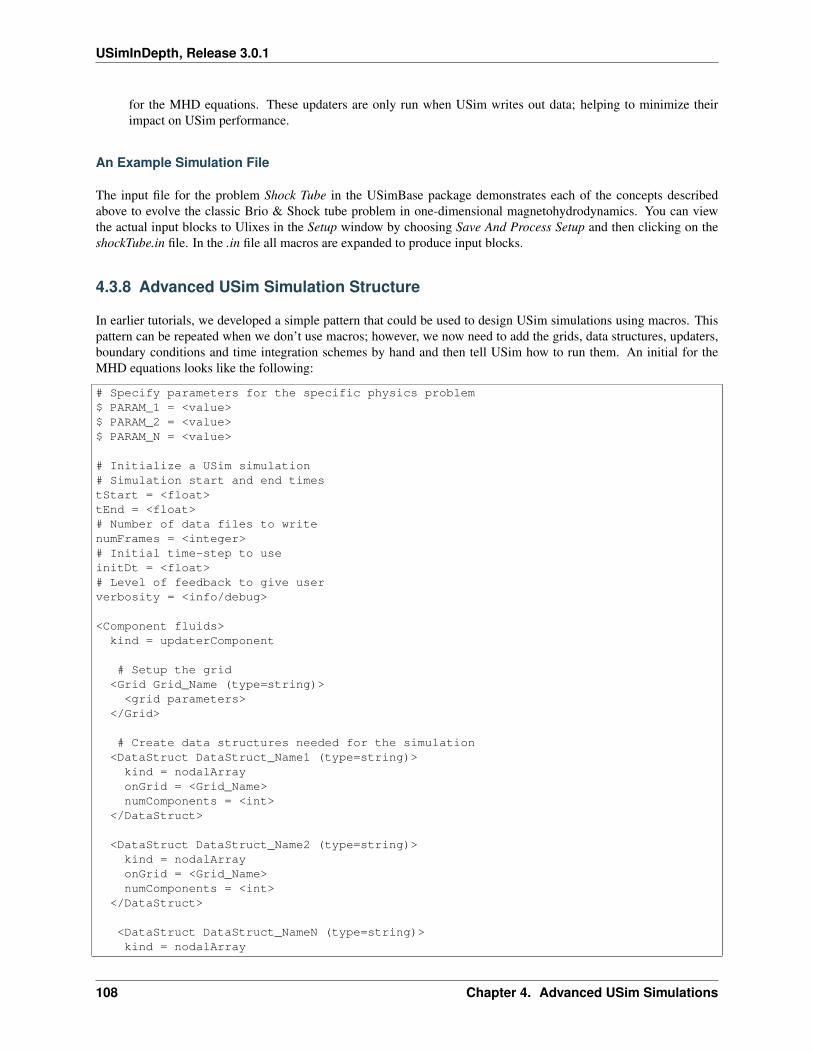
USimInDepth, Release 3.0.1
for the MHD equations. These updaters are only run when USim writes out data; helping to minimize theirimpact on USim performance.
An Example Simulation File
The input file for the problem Shock Tube in the USimBase package demonstrates each of the concepts describedabove to evolve the classic Brio & Shock tube problem in one-dimensional magnetohydrodynamics. You can viewthe actual input blocks to Ulixes in the Setup window by choosing Save And Process Setup and then clicking on theshockTube.in file. In the .in file all macros are expanded to produce input blocks.
4.3.8 Advanced USim Simulation Structure
In earlier tutorials, we developed a simple pattern that could be used to design USim simulations using macros. Thispattern can be repeated when we don’t use macros; however, we now need to add the grids, data structures, updaters,boundary conditions and time integration schemes by hand and then tell USim how to run them. An initial for theMHD equations looks like the following:
# Specify parameters for the specific physics problem$ PARAM_1 = <value>$ PARAM_2 = <value>$ PARAM_N = <value>
# Initialize a USim simulation# Simulation start and end timestStart = <float>tEnd = <float># Number of data files to writenumFrames = <integer># Initial time-step to useinitDt = <float># Level of feedback to give userverbosity = <info/debug>
<Component fluids>kind = updaterComponent
# Setup the grid<Grid Grid_Name (type=string)><grid parameters>
</Grid>
# Create data structures needed for the simulation<DataStruct DataStruct_Name1 (type=string)>kind = nodalArrayonGrid = <Grid_Name>numComponents = <int>
</DataStruct>
<DataStruct DataStruct_Name2 (type=string)>kind = nodalArrayonGrid = <Grid_Name>numComponents = <int>
</DataStruct>
<DataStruct DataStruct_NameN (type=string)>kind = nodalArray
108 Chapter 4. Advanced USim Simulations
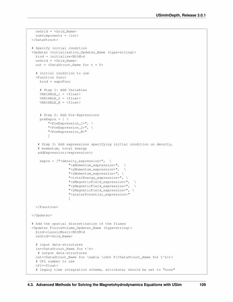
USimInDepth, Release 3.0.1
onGrid = <Grid_Name>numComponents = <int>
</DataStruct>
# Specify initial condition<Updater Initialization_Updater_Name (type=string)>kind = initialize<NDIM>donGrid = <Grid_Name>out = <DataStruct_Name for t = 0>
# initial condition to use<Function func>
kind = exprFunc
# Step 1: Add VariablesVARIABLE_1 = <float>VARIABLE_2 = <float>VARIABLE_N = <float>
# Step 2: Add Pre-ExpressionspreExprs = [ \
"<PreExpression_1>", \"<PreExpression_2>", \"<PreExpression_N>"]
# Step 3: Add expressions specifying initial condition on density,# momentum, total energyaddExpression(<expression>)
exprs = ["<density_expression>", \"<xMomentum_expression>", \"<yMomentum_expression>", \"<zMomentum_expression>", \"<totalEnergy_expression>", \"<xMagneticField_expression>", \"<yMagneticField_expression>", \"<zMagneticField_expression>", \"<scalarPotential_expression>"]
</Function>
</Updater>
# Add the spatial discretization of the fluxes<Updater FiniteVolume_Updater_Name (type=string)>kind=classicMuscl<NDIM>donGrid=<Grid_Name>
# input data-structuresin=<DataStruct_Name for t^n># output data-structures
out=<DataStruct_Name for \nabla \cdot F(<DataStruct_Name for t^n>)># CFL number to usecfl=<float># legacy time integration scheme, attribute; should be set to "none"
4.3. Advanced Methods for Solving the Magnetohydrodynamics Equations with USim 109
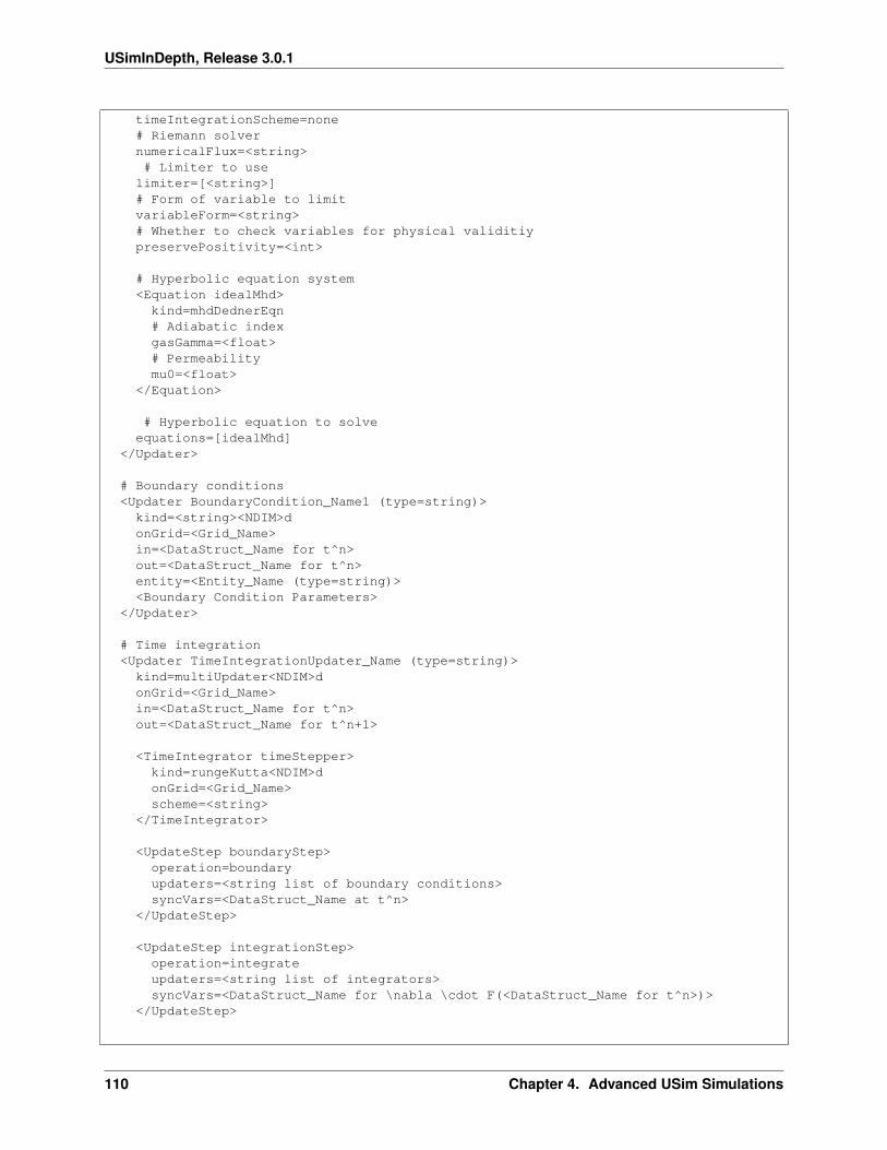
USimInDepth, Release 3.0.1
timeIntegrationScheme=none# Riemann solvernumericalFlux=<string># Limiter to use
limiter=[<string>]# Form of variable to limitvariableForm=<string># Whether to check variables for physical validitiypreservePositivity=<int>
# Hyperbolic equation system<Equation idealMhd>
kind=mhdDednerEqn# Adiabatic indexgasGamma=<float># Permeabilitymu0=<float>
</Equation>
# Hyperbolic equation to solveequations=[idealMhd]
</Updater>
# Boundary conditions<Updater BoundaryCondition_Name1 (type=string)>kind=<string><NDIM>donGrid=<Grid_Name>in=<DataStruct_Name for t^n>out=<DataStruct_Name for t^n>entity=<Entity_Name (type=string)><Boundary Condition Parameters>
</Updater>
# Time integration<Updater TimeIntegrationUpdater_Name (type=string)>kind=multiUpdater<NDIM>donGrid=<Grid_Name>in=<DataStruct_Name for t^n>out=<DataStruct_Name for t^n+1>
<TimeIntegrator timeStepper>kind=rungeKutta<NDIM>donGrid=<Grid_Name>scheme=<string>
</TimeIntegrator>
<UpdateStep boundaryStep>operation=boundaryupdaters=<string list of boundary conditions>syncVars=<DataStruct_Name at t^n>
</UpdateStep>
<UpdateStep integrationStep>operation=integrateupdaters=<string list of integrators>syncVars=<DataStruct_Name for \nabla \cdot F(<DataStruct_Name for t^n>)>
</UpdateStep>
110 Chapter 4. Advanced USim Simulations
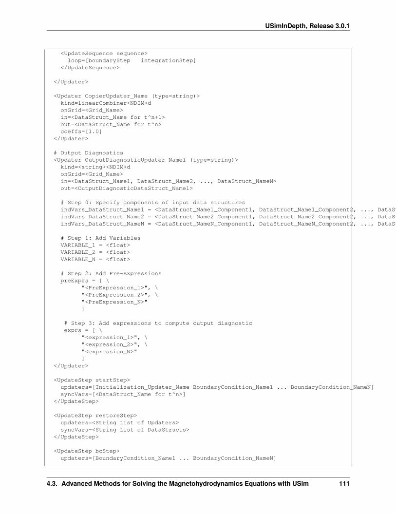
USimInDepth, Release 3.0.1
<UpdateSequence sequence>loop=[boundaryStep integrationStep]
</UpdateSequence>
</Updater>
<Updater CopierUpdater_Name (type=string)>kind=linearCombiner<NDIM>donGrid=<Grid_Name>in=<DataStruct_Name for t^n+1>out=<DataStruct_Name for t^n>coeffs=[1.0]
</Updater>
# Output Diagnostics<Updater OutputDiagnosticUpdater_Name1 (type=string)>kind=<string><NDIM>donGrid=<Grid_Name>in=<DataStruct_Name1, DataStruct_Name2, ..., DataStruct_NameN>out=<OutputDiagnosticDataStruct_Name1>
# Step 0: Specify components of input data structuresindVars_DataStruct_Name1 = <DataStruct_Name1_Component1, DataStruct_Name1_Component2, ..., DataStruct_Name1_ComponentN>indVars_DataStruct_Name2 = <DataStruct_Name2_Component1, DataStruct_Name2_Component2, ..., DataStruct_Name2_ComponentN>indVars_DataStruct_NameN = <DataStruct_NameN_Component1, DataStruct_NameN_Component2, ..., DataStruct_NameN_ComponentN>
# Step 1: Add VariablesVARIABLE_1 = <float>VARIABLE_2 = <float>VARIABLE_N = <float>
# Step 2: Add Pre-ExpressionspreExprs = [ \
"<PreExpression_1>", \"<PreExpression_2>", \"<PreExpression_N>"]
# Step 3: Add expressions to compute output diagnosticexprs = [ \
"<expression_1>", \"<expression_2>", \"<expression_N>"]
</Updater>
<UpdateStep startStep>updaters=[Initialization_Updater_Name BoundaryCondition_Name1 ... BoundaryCondition_NameN]syncVars=[<DataStruct_Name for t^n>]
</UpdateStep>
<UpdateStep restoreStep>updaters=<String List of Updaters>syncVars=<String List of DataStructs>
</UpdateStep>
<UpdateStep bcStep>updaters=[BoundaryCondition_Name1 ... BoundaryCondition_NameN]
4.3. Advanced Methods for Solving the Magnetohydrodynamics Equations with USim 111
USimInDepth, Release 3.0.1
syncVars=[<DataStruct_Name for t^n>]</UpdateStep>
<UpdateStep hyperStep>updaters=[FiniteVolume_Updater_Name (type=string)]syncVars=<String List of DataStructs>
</UpdateStep>
<UpdateStep writeStep>updaters=< OutputDiagnosticUpdater_Name1, OutputDiagnosticUpdater_Name2, OutputDiagnosticUpdater_NameN>syncVars=<OutputDiagnosticDataStruct_Name1, OutputDiagnosticDataStruct_Name2, ..., OutputDiagnosticDataStruct_NameN>
</UpdateStep>
<UpdateSequence simulation>startOnly=[generateStep startStep]restoreOnly=[generateStep restoreStep bcStep]writeOnly=[bcStep writeStep]loop=[hyperStep]
</UpdateSequence>
</Component>
Note that we have not filled in some of the entries in the UpdateSteps above. How to use these UpdateSteps is discussedin later tutorials.
4.4 Advanced Methods for Solving for Solving Problems in Multi-Dimensions with Usim
In Advanced USim Simulation Concepts we examined the basic ingredients of a USim input file: the simulation grid(see Defining the Simulation Grid); data structures (see Allocating Memory); how to assign initial conditions (seeSetting Initial Conditions) and how to write out additional data (see Writing Out Data). In Advanced Methods forSolving the Euler Equations with USim, we built on these concepts and demonstrated the basic methods used by USimto solve the Euler equations without the use of macros. Next, in Advanced Methods for Solving the Magnetohydro-dynamics Equations with USim, we extended these ideas to demonstrate how to solve the MHD equations in USim,again without the use of macros.
This tutorial is based on the quickstart-rtInstability example in USimBase, which demonstrates the well-knownRayleigh-Taylor instability problem described by:
Jun, Norman, & Stone, ApJ 453, 332 (1995).
Using this example, we will examine how to solve the equations of inviscid compressible hydrodynamics and idealcompressible magnetohydrodynamics directly without the use of macros.
112 Chapter 4. Advanced USim Simulations
USimInDepth, Release 3.0.1
Contents
• Advanced Methods for Solving for Solving Problems in Multi-Dimensions with Usim– Defining the Simulation Grid– Allocating Simulation Memory– Initializing the Fluid– Evolving the Fluid– Applying Boundary Conditions
* Periodic Boundary Conditions* Reflecting Wall Boundary Conditions
– Advancing By A Time Step– Putting it all Together– Advanced USim Simulation Structure– Advanced Methods for Solving the MHD Equations in Multi-Dimensions
* Advanced USim Simulation Structure for MHD in Multi-Dimensions
4.4.1 Defining the Simulation Grid
In order to execute the two-dimensional Rayleigh-Taylor, we must define a two-dimensional grid simulation grid. InUSim, this is done by replacing the Grid input block defined in Defining the Simulation Grid with:
<Grid domain>kind=cart2dlower=[-0.25 -0.75]upper=[0.25 0.75]cells=[64 192]periodicDirs=[0]ghostLayers=2isRadial=0writeGeom=0writeConn=0writeHalos=0
</Grid>
Notice that the lower, upper and cells input blocks now take two entries, one for each dimension. A three-dimensionalCartesian grid would therefore be defined by:
<Grid domain>kind=cart3dlower=[-0.25 -0.75 -0.25]upper=[0.25 0.75 0.25]cells=[64 192 64]periodicDirs=[0 2]ghostLayers=2isRadial=0writeGeom=0writeConn=0writeHalos=0
</Grid>
Note the usage of the periodicDirs attribute in these blocks. This attribute species the directions in the computationalmesh that are periodic. For this example in two-dimensions, the 0 (or x) direction is periodic; similarly, in three-dimensions, both the 0 and 2 (z) directions are periodic. Note that this attribute is necessary to setup informationwithin the simulation grid regarding periodicity; however, periodic boundary conditions must still be applied in thesimulation. This is discussed below.
4.4. Advanced Methods for Solving for Solving Problems in Multi-Dimensions with Usim 113
USimInDepth, Release 3.0.1
4.4.2 Allocating Simulation Memory
USim data structures automatically account for the chosen dimensionality of the simulation. As a result, there is noneed to change how data structures are added for the Euler equations compared to the discussion in Advanced Methodsfor Solving the Euler Equations with USim or the MHD equations compared to the discussion in Advanced Methodsfor Solving the Magnetohydrodynamics Equations with USim.
4.4.3 Initializing the Fluid
The initial condition for a multi-dimensional simulation follows the same basic three-step pattern outlined previously;however, the kind attribute for the initialization updater has to match the dimension of the mesh:
<Updater setVar>kind=initialize2donGrid=domainin=noneout=[q qNew]
<Function initFunc>kind=exprFunc# adiabatic indexgas_gamma=1.4# Upper fluid densityrhoTop=2.0# Lower fluid densityrhoBottom=1.0# Perturbation amplitudeperturb=0.01# Location of upper y boundaryytop=0.75# acceleration due to gravitygravity=0.1# X-extent of domainlx=0.5# Y-extent of domainly=1.5preExprs=[ p0=0.01 pert=0.01 pi=3.14159 rho=if(y<0.0,rhoBottom,rhoTop) pr=(1.0/gas_gamma)-(gravity*rho*y) vx=0.0 vy=(0.25*perturb)*(1.0+cos(2.0*pi*x/lx))*(1.0+cos(2.0*pi*y/ly)) vz=0.0 ]exprs=[ rho rho*vx rho*vy rho*vz (pr/(gas_gamma-1.0))+0.5*rho*vy*vy ]
</Function>
</Updater>
As in Solving Multi-Dimensional Problems in USim, this initialization block creates a hydrostatic equilibrium consist-ing of a heavier fluid supported by a lighter fluid, which is perturbed with a single mode. Compared to the initializationblock for the Sod shock tube problem discussed in Advanced Methods for Solving the Euler Equations with USim, thekey difference as far as problem dimensionality is concerned is that the kind block is specified as initialize2d for thisproblem. This pattern is repeated for all updaters within a USim input file, e.g. for the generic updater update:
<Updater Updater_Name (type=string)>kind = updateKind<NDIM>donGrid = <Grid_Name>
</Updater>
Here, updateKind is the kind of the USim updater that is being utilized (e.g. for the initialization input block, this isinitialize) and <NDIM> is the dimensionality of the problem, e.g. 1,2,3 for one-, two- and three-dimensions.
114 Chapter 4. Advanced USim Simulations
USimInDepth, Release 3.0.1
4.4.4 Evolving the Fluid
USim implements the well-known MUSCL scheme to compute the spatial discretization of a hyperbolic conservationlaw (see Using USim to solve the Euler Equations for a more detailed description). In Solving Multi-DimensionalProblems in USim, we added this algorithm through:
## Add the spatial discretization of the fluxesfiniteVolumeScheme(DIFFUSIVE)
## Add source term for gravitational acceleration to the equationsaddGravitationalAcceleration(GRAVITY_ACCEL)
For the quickstart-rtinstability example in two-dimensions, this macro expands to give:
<Updater hyper>kind=classicMuscl2donGrid=domainin=[q]out=[qNew]cfl=0.4timeIntegrationScheme=nonenumericalFlux=hllcEulerFluxlimiter=[muscl]variableForm=primitivepreservePositivity=0
<Equation euler>kind=eulerEqngasGamma=1.4
</Equation>
equations=[euler]
<Source gravity>kind=exprHyperSrcgravity=0.1rhoSrc=0.0mxSrc=0.0mzSrc=0.0inpRange=[0 1 2 3 4]outRange=[0 1 2 3 4]indVars=[rho rhou rhov rhow Er]exprs=[ rhoSrc mxSrc -rho*gravity mzSrc -gravity*rhov ]
</Source>
sources=[gravity]</Updater>
Compared to the quickstart-shocktube example discussed in Advanced Methods for Solving the Euler Equations withUSim, we see that this is following the pattern discussed above, i.e. kind = classicMuscl1d has been replaced by kind= classicMuscl2d. We also have added an additional Source block to this updater, corresponding to the use of themacro:
# Add source term for gravitational acceleration to the equationsaddGravitationalAcceleration(GRAVITY_ACCEL)
The use of this macro resulted in the addition of refmanual-exprHyperSrc to the refmanual-classicMuscl updater:
4.4. Advanced Methods for Solving for Solving Problems in Multi-Dimensions with Usim 115
USimInDepth, Release 3.0.1
<Source gravity>kind=exprHyperSrcgravity=0.1rhoSrc=0.0mxSrc=0.0mzSrc=0.0inpRange=[0 1 2 3 4]outRange=[0 1 2 3 4]indVars=[rho rhou rhov rhow Er]exprs=[ rhoSrc mxSrc -rho*gravity mzSrc -gravity*rhov ]
</Source>
Note that this block is following the classic three step pattern that used throughout USim (in this case, no preExpres-sions have been defined). The additional attributes inpRange and outRange tell USim which components of the inputand output variables for the refmanual-classicMuscl updater to work with.
4.4.5 Applying Boundary Conditions
The Rayleigh-Taylor instability problem requires more advanced boundary conditions that were used for the SodShock tube in the previous example. In two-dimensions, appropriate boundary conditions for the Rayleigh-Taylorinstability are periodic boundaries in the direction transverse to the gravitational field and reflecting boundaries in theparallel direction, which are the x and y directions respectively.
In the quickstart-rtinstability example, we applied these boundary conditions through the use of the macros:
## Boundary conditionsboundaryCondition(wall,top)boundaryCondition(wall,bottom)boundaryCondition(periodic)
The first two of these macros expand to yield the blocks:
<Updater wallBoundaryOnEntitytop>kind=eulerBc2donGrid=domainin=[q]out=[q]model=eulerEqnbcType=wallentity=topgasGamma=1.4
</Updater>
<Updater wallBoundaryOnEntitybottom>kind=eulerBc2donGrid=domainin=[q]out=[q]model=eulerEqnbcType=wallentity=bottomgasGamma=1.4
</Updater>
These reflecting wall boundary conditions are described below. The third macro expands to yield a periodic boundarycondition:
116 Chapter 4. Advanced USim Simulations
USimInDepth, Release 3.0.1
<Updater periodicBoundaryOnEntityghost>kind=periodicCartBc2donGrid=domainin=[q]out=[q]
</Updater>
We discuss this in the next section.
Periodic Boundary Conditions
Periodic boundary conditions in USim are specified in two ways, both of which must be used simultaneously. First, aninput block peroidicDirs is added to the Grid block:
<Grid domain>kind = cart2dghostLayers = 2lower = [-0.25, -0.75]upper = [ 0.25, 0.75]cells = [64, 192]periodicDirs = [0]
</Grid>
The dimensions in which periodic boundary conditions are applied are specified by a vector. In this case, we applyperiodic boundary conditions in the x direction, so we set:
periodicDirs = [0]
If we wished (for example) to extend the Rayleigh-Taylor instability problem to three-dimensions, then it might beappropriate to apply periodic boundary conditions to the x and z directions. In this case, we would set:
periodicDirs = [0,2]
In addition to the periodicDirs input block that is added to Grid, we must also add an updater block to apply theperiodic boundary conditions within the simulation loop. This is done through the updater:
<Updater periodicBoundaryOnEntityghost>kind=periodicCartBc2donGrid=domainin=[q]out=[q]
</Updater>
where the meanings of the various input blocks are described as in Evolving the Fluid. Note that if we wished to applyperiodic boundary conditions in a three-dimensional problem, then we would set:
kind = periodicCartBc3d
This follows the pattern for changing the dimension of a USim simulation discussed previously.
Reflecting Wall Boundary Conditions
In the transverse direction to the flow (here the y direction), we specify reflecting wall boundary conditions. In USim,this is done using the updater:
4.4. Advanced Methods for Solving for Solving Problems in Multi-Dimensions with Usim 117
USimInDepth, Release 3.0.1
<Updater wallBoundaryOnEntitytop>kind=eulerBc2donGrid=domainin=[q]out=[q]model=eulerEqnbcType=wallentity=topgasGamma=1.4
</Updater>
<Updater wallBoundaryOnEntitybottom>kind=eulerBc2donGrid=domainin=[q]out=[q]model=eulerEqnbcType=wallentity=bottomgasGamma=1.4
</Updater>
The refmanual-eulerBc applies boundary condition appropriate for systems of equations that follow the pattern ofthe Euler equations, i.e. a conserved state vector similar to that described at refmanual-eulerEqn. The specific typeof hydrodynamic equation that the boundary condition is applied to is specified by the attribute modelEqn. Validoptions for this attribute include refmanual-eulerEqn, refmanual-realGasEqn and refmanual-realGasEosEqn. Notethat attributes required by these equations should be specified in the block associated with the boundary condition. Inthe examples above, this includes the gasGamma parameter required for refmanual-eulerEqn.
A range of boundary conditions can be applied by refmanual-eulerBc; the specific choice is specified by the attributebcType. Valid options for this attribute include wall, noInflow and noSlip.
Finally, we must specify the boundary that the boundary condition is to be applied on. For a structured mesh such asused in the quickstart-rtinstability example, a range of boundaries are predefined:
left The lower x-boundary.
right The upper x-boundary.
bottom The lower y-boundary.
top The upper y-boundary.
back The lower z-boundary.
front The upper z-boundary.
We specify the boundary to apply the boundary through the use of the entityType attribute, e.g. to apply the wallboundary condition on the upper y-boundary, we set:
entity=top
4.4.6 Advancing By A Time Step
In order to solve the MHD equations, we have to advance the conserved quantities from time 𝑡 to 𝑡+ ∆𝑡. This is doneby applying a time integration scheme. In Solving Multi-Dimensional Problems in USim, we did this using the macro:
timeAdvance(TIME_ORDER)
118 Chapter 4. Advanced USim Simulations
USimInDepth, Release 3.0.1
This expands to yield:
<Updater mainIntegrator>kind=multiUpdater2donGrid=domainin=[q]out=[qNew]
<TimeIntegrator timeStepper>kind=rungeKutta2donGrid=domainscheme=second
</TimeIntegrator>
<UpdateStep boundaryStep>operation=boundaryupdaters=[wallBoundaryOnEntitytop wallBoundaryOnEntitybottom periodicBoundaryOnEntityghost]syncVars=[q]
</UpdateStep>
<UpdateStep integrationStep>operation=integrateupdaters=[hyper]syncVars=[qNew]
</UpdateStep>
<UpdateSequence sequence>startOnly=[]restoreOnly=[]writeOnly=[]loop=[boundaryStep integrationStep]
</UpdateSequence>
</Updater>
This time integration scheme is very similar to that described in Advanced Methods for Solving the Euler Equationswith USim; we follow the pattern described above to switch the dimension of the mainIntegrator and the timeStepperblocks. To handle the changes to the boundary conditions compared to Advanced Methods for Solving the EulerEquations with USim, we change the boundaryStep block from:
<UpdateStep boundaryStep>operation=boundaryupdaters=[copyBoundaryOnEntityleft copyBoundaryOnEntityright periodicBoundaryOnEntityghost]syncVars=[q]
</UpdateStep>
to:
<UpdateStep boundaryStep>operation=boundaryupdaters=[wallBoundaryOnEntitytop wallBoundaryOnEntitybottom periodicBoundaryOnEntityghost]syncVars=[q]
</UpdateStep>
4.4. Advanced Methods for Solving for Solving Problems in Multi-Dimensions with Usim 119
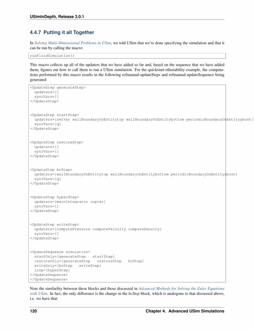
USimInDepth, Release 3.0.1
4.4.7 Putting it all Together
In Solving Multi-Dimensional Problems in USim, we told USim that we’re done specifying the simulation and that itcan be run by calling the macro:
runFluidSimulation()
This macro collects up all of the updaters that we have added so far and, based on the sequence that we have addedthem, figures out how to call them to run a USim simulation. For the quickstart-rtInstability example, the computa-tions performed by this macro results in the following refmanual-updateSteps and refmanual-updateSequence beinggenerated:
<UpdateStep generateStep>updaters=[]syncVars=[]
</UpdateStep>
<UpdateStep startStep>updaters=[setVar wallBoundaryOnEntitytop wallBoundaryOnEntitybottom periodicBoundaryOnEntityghost]syncVars=[q]
</UpdateStep>
<UpdateStep restoreStep>updaters=[]syncVars=[]
</UpdateStep>
<UpdateStep bcStep>updaters=[wallBoundaryOnEntitytop wallBoundaryOnEntitybottom periodicBoundaryOnEntityghost]syncVars=[q]
</UpdateStep>
<UpdateStep hyperStep>updaters=[mainIntegrator copier]syncVars=[]
</UpdateStep>
<UpdateStep writeStep>updaters=[computePressure computeVelocity computeDensity]syncVars=[]
</UpdateStep>
<UpdateSequence simulation>startOnly=[generateStep startStep]restoreOnly=[generateStep restoreStep bcStep]writeOnly=[bcStep writeStep]loop=[hyperStep]
</UpdateSequence></UpdateSequence>
Note the similarlity between these blocks and those discussed in Advanced Methods for Solving the Euler Equationswith USim. In fact, the only difference is the change in the bcStep block, which is analogous to that discussed above,i.e. we have that:
120 Chapter 4. Advanced USim Simulations
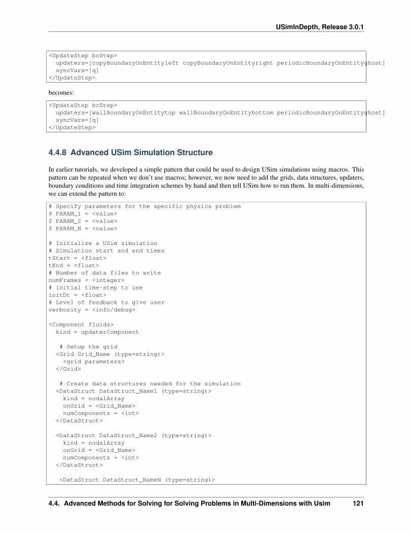
USimInDepth, Release 3.0.1
<UpdateStep bcStep>updaters=[copyBoundaryOnEntityleft copyBoundaryOnEntityright periodicBoundaryOnEntityghost]syncVars=[q]
</UpdateStep>
becomes:
<UpdateStep bcStep>updaters=[wallBoundaryOnEntitytop wallBoundaryOnEntitybottom periodicBoundaryOnEntityghost]syncVars=[q]
</UpdateStep>
4.4.8 Advanced USim Simulation Structure
In earlier tutorials, we developed a simple pattern that could be used to design USim simulations using macros. Thispattern can be repeated when we don’t use macros; however, we now need to add the grids, data structures, updaters,boundary conditions and time integration schemes by hand and then tell USim how to run them. In multi-dimensions,we can extend the pattern to:
# Specify parameters for the specific physics problem$ PARAM_1 = <value>$ PARAM_2 = <value>$ PARAM_N = <value>
# Initialize a USim simulation# Simulation start and end timestStart = <float>tEnd = <float># Number of data files to writenumFrames = <integer># Initial time-step to useinitDt = <float># Level of feedback to give userverbosity = <info/debug>
<Component fluids>kind = updaterComponent
# Setup the grid<Grid Grid_Name (type=string)><grid parameters>
</Grid>
# Create data structures needed for the simulation<DataStruct DataStruct_Name1 (type=string)>kind = nodalArrayonGrid = <Grid_Name>numComponents = <int>
</DataStruct>
<DataStruct DataStruct_Name2 (type=string)>kind = nodalArrayonGrid = <Grid_Name>numComponents = <int>
</DataStruct>
<DataStruct DataStruct_NameN (type=string)>
4.4. Advanced Methods for Solving for Solving Problems in Multi-Dimensions with Usim 121
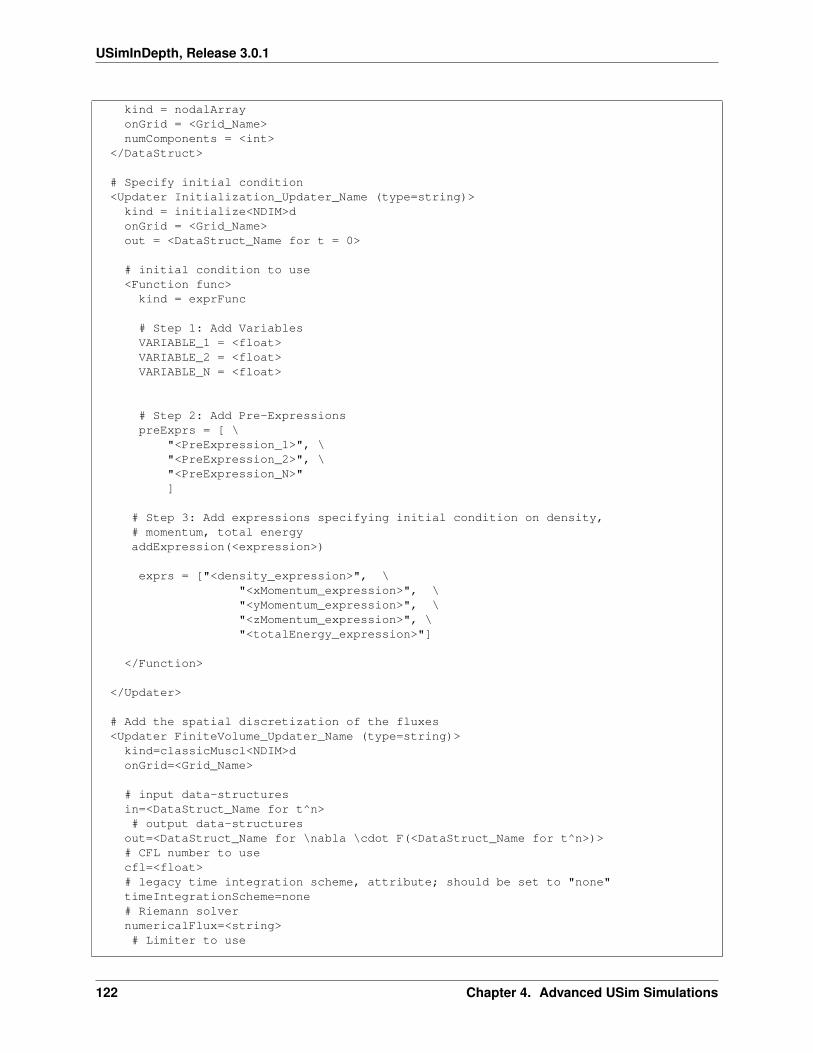
USimInDepth, Release 3.0.1
kind = nodalArrayonGrid = <Grid_Name>numComponents = <int>
</DataStruct>
# Specify initial condition<Updater Initialization_Updater_Name (type=string)>kind = initialize<NDIM>donGrid = <Grid_Name>out = <DataStruct_Name for t = 0>
# initial condition to use<Function func>
kind = exprFunc
# Step 1: Add VariablesVARIABLE_1 = <float>VARIABLE_2 = <float>VARIABLE_N = <float>
# Step 2: Add Pre-ExpressionspreExprs = [ \
"<PreExpression_1>", \"<PreExpression_2>", \"<PreExpression_N>"]
# Step 3: Add expressions specifying initial condition on density,# momentum, total energyaddExpression(<expression>)
exprs = ["<density_expression>", \"<xMomentum_expression>", \"<yMomentum_expression>", \"<zMomentum_expression>", \"<totalEnergy_expression>"]
</Function>
</Updater>
# Add the spatial discretization of the fluxes<Updater FiniteVolume_Updater_Name (type=string)>kind=classicMuscl<NDIM>donGrid=<Grid_Name>
# input data-structuresin=<DataStruct_Name for t^n># output data-structures
out=<DataStruct_Name for \nabla \cdot F(<DataStruct_Name for t^n>)># CFL number to usecfl=<float># legacy time integration scheme, attribute; should be set to "none"timeIntegrationScheme=none# Riemann solvernumericalFlux=<string># Limiter to use
122 Chapter 4. Advanced USim Simulations
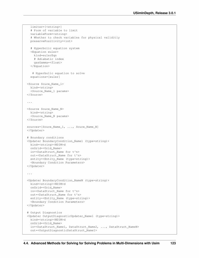
USimInDepth, Release 3.0.1
limiter=[<string>]# Form of variable to limitvariableForm=<string># Whether to check variables for physical validitiypreservePositivity=<int>
# Hyperbolic equation system<Equation euler>
kind=eulerEqn# Adiabatic indexgasGamma=<float>
</Equation>
# Hyperbolic equation to solveequations=[euler]
<Source Souce_Name_1>kind=<string><Source_Name_1 params>
</Source>
...
<Source Souce_Name_N>kind=<string><Source_Name_N params>
</Source>
sources=[Souce_Name_1, ..., Souce_Name_N]</Updater>
# Boundary conditions<Updater BoundaryCondition_Name1 (type=string)>kind=<string><NDIM>donGrid=<Grid_Name>in=<DataStruct_Name for t^n>out=<DataStruct_Name for t^n>entity=<Entity_Name (type=string)><Boundary Condition Parameters>
</Updater>
...
<Updater BoundaryCondition_NameN (type=string)>kind=<string><NDIM>donGrid=<Grid_Name>in=<DataStruct_Name for t^n>out=<DataStruct_Name for t^n>entity=<Entity_Name (type=string)><Boundary Condition Parameters>
</Updater>
# Output Diagnostics<Updater OutputDiagnosticUpdater_Name1 (type=string)>kind=<string><NDIM>donGrid=<Grid_Name>in=<DataStruct_Name1, DataStruct_Name2, ..., DataStruct_NameN>out=<OutputDiagnosticDataStruct_Name1>
4.4. Advanced Methods for Solving for Solving Problems in Multi-Dimensions with Usim 123
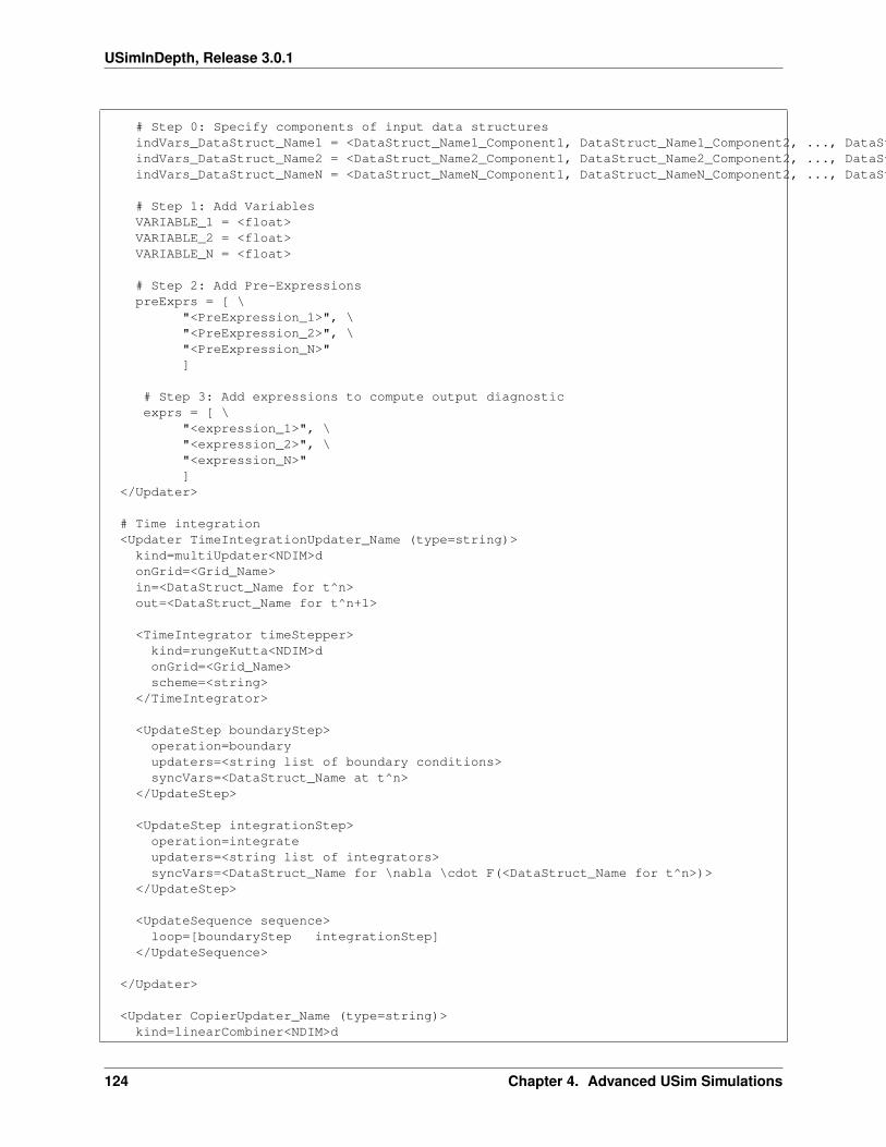
USimInDepth, Release 3.0.1
# Step 0: Specify components of input data structuresindVars_DataStruct_Name1 = <DataStruct_Name1_Component1, DataStruct_Name1_Component2, ..., DataStruct_Name1_ComponentN>indVars_DataStruct_Name2 = <DataStruct_Name2_Component1, DataStruct_Name2_Component2, ..., DataStruct_Name2_ComponentN>indVars_DataStruct_NameN = <DataStruct_NameN_Component1, DataStruct_NameN_Component2, ..., DataStruct_NameN_ComponentN>
# Step 1: Add VariablesVARIABLE_1 = <float>VARIABLE_2 = <float>VARIABLE_N = <float>
# Step 2: Add Pre-ExpressionspreExprs = [ \
"<PreExpression_1>", \"<PreExpression_2>", \"<PreExpression_N>"]
# Step 3: Add expressions to compute output diagnosticexprs = [ \
"<expression_1>", \"<expression_2>", \"<expression_N>"]
</Updater>
# Time integration<Updater TimeIntegrationUpdater_Name (type=string)>kind=multiUpdater<NDIM>donGrid=<Grid_Name>in=<DataStruct_Name for t^n>out=<DataStruct_Name for t^n+1>
<TimeIntegrator timeStepper>kind=rungeKutta<NDIM>donGrid=<Grid_Name>scheme=<string>
</TimeIntegrator>
<UpdateStep boundaryStep>operation=boundaryupdaters=<string list of boundary conditions>syncVars=<DataStruct_Name at t^n>
</UpdateStep>
<UpdateStep integrationStep>operation=integrateupdaters=<string list of integrators>syncVars=<DataStruct_Name for \nabla \cdot F(<DataStruct_Name for t^n>)>
</UpdateStep>
<UpdateSequence sequence>loop=[boundaryStep integrationStep]
</UpdateSequence>
</Updater>
<Updater CopierUpdater_Name (type=string)>kind=linearCombiner<NDIM>d
124 Chapter 4. Advanced USim Simulations
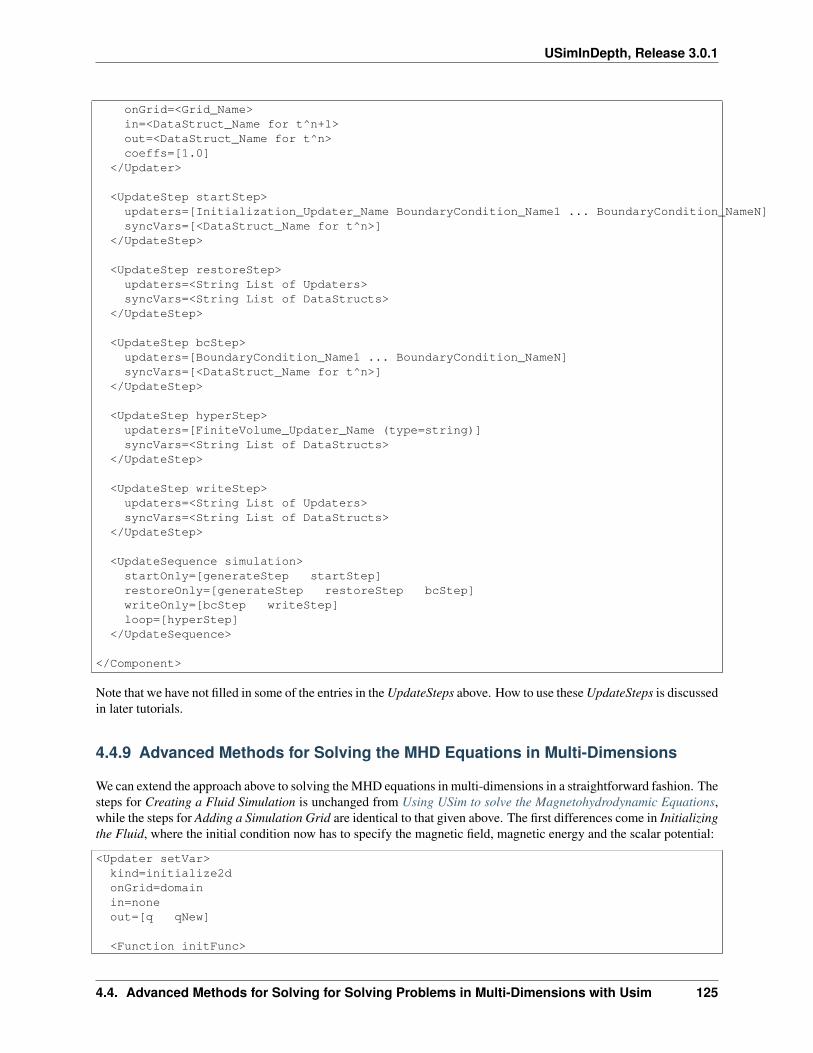
USimInDepth, Release 3.0.1
onGrid=<Grid_Name>in=<DataStruct_Name for t^n+1>out=<DataStruct_Name for t^n>coeffs=[1.0]
</Updater>
<UpdateStep startStep>updaters=[Initialization_Updater_Name BoundaryCondition_Name1 ... BoundaryCondition_NameN]syncVars=[<DataStruct_Name for t^n>]
</UpdateStep>
<UpdateStep restoreStep>updaters=<String List of Updaters>syncVars=<String List of DataStructs>
</UpdateStep>
<UpdateStep bcStep>updaters=[BoundaryCondition_Name1 ... BoundaryCondition_NameN]syncVars=[<DataStruct_Name for t^n>]
</UpdateStep>
<UpdateStep hyperStep>updaters=[FiniteVolume_Updater_Name (type=string)]syncVars=<String List of DataStructs>
</UpdateStep>
<UpdateStep writeStep>updaters=<String List of Updaters>syncVars=<String List of DataStructs>
</UpdateStep>
<UpdateSequence simulation>startOnly=[generateStep startStep]restoreOnly=[generateStep restoreStep bcStep]writeOnly=[bcStep writeStep]loop=[hyperStep]
</UpdateSequence>
</Component>
Note that we have not filled in some of the entries in the UpdateSteps above. How to use these UpdateSteps is discussedin later tutorials.
4.4.9 Advanced Methods for Solving the MHD Equations in Multi-Dimensions
We can extend the approach above to solving the MHD equations in multi-dimensions in a straightforward fashion. Thesteps for Creating a Fluid Simulation is unchanged from Using USim to solve the Magnetohydrodynamic Equations,while the steps for Adding a Simulation Grid are identical to that given above. The first differences come in Initializingthe Fluid, where the initial condition now has to specify the magnetic field, magnetic energy and the scalar potential:
<Updater setVar>kind=initialize2donGrid=domainin=noneout=[q qNew]
<Function initFunc>
4.4. Advanced Methods for Solving for Solving Problems in Multi-Dimensions with Usim 125
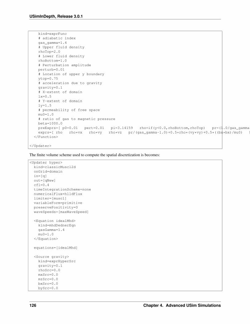
USimInDepth, Release 3.0.1
kind=exprFunc# adiabatic indexgas_gamma=1.4# Upper fluid densityrhoTop=2.0# Lower fluid densityrhoBottom=1.0# Perturbation amplitudeperturb=0.01# Location of upper y boundaryytop=0.75# acceleration due to gravitygravity=0.1# X-extent of domainlx=0.5# Y-extent of domainly=1.5# permeability of free spacemu0=1.0# ratio of gas to magnetic pressurebeta=1000.0preExprs=[ p0=0.01 pert=0.01 pi=3.14159 rho=if(y<0.0,rhoBottom,rhoTop) pr=(1.0/gas_gamma)-(gravity*rho*y) vx=0.0 vy=(0.25*perturb)*(1.0+cos(2.0*pi*x/lx))*(1.0+cos(2.0*pi*y/ly)) vz=0.0 bx=sqrt(2.0*pr/(beta*beta)) by=0.0 bz=0.0 psi=0.0 ]exprs=[ rho rho*vx rho*vy rho*vz pr/(gas_gamma-1.0)+0.5*rho*(vy*vy)+0.5*((bx*bx)/mu0) bx by bz psi ]
</Function>
</Updater>
The finite volume scheme used to compute the spatial discretization is becomes:
<Updater hyper>kind=classicMuscl2donGrid=domainin=[q]out=[qNew]cfl=0.4timeIntegrationScheme=nonenumericalFlux=hlldFluxlimiter=[muscl]variableForm=primitivepreservePositivity=0waveSpeeds=[maxWaveSpeed]
<Equation idealMhd>kind=mhdDednerEqngasGamma=1.4mu0=1.0
</Equation>
equations=[idealMhd]
<Source gravity>kind=exprHyperSrcgravity=0.1rhoSrc=0.0mxSrc=0.0mzSrc=0.0bxSrc=0.0bySrc=0.0
126 Chapter 4. Advanced USim Simulations
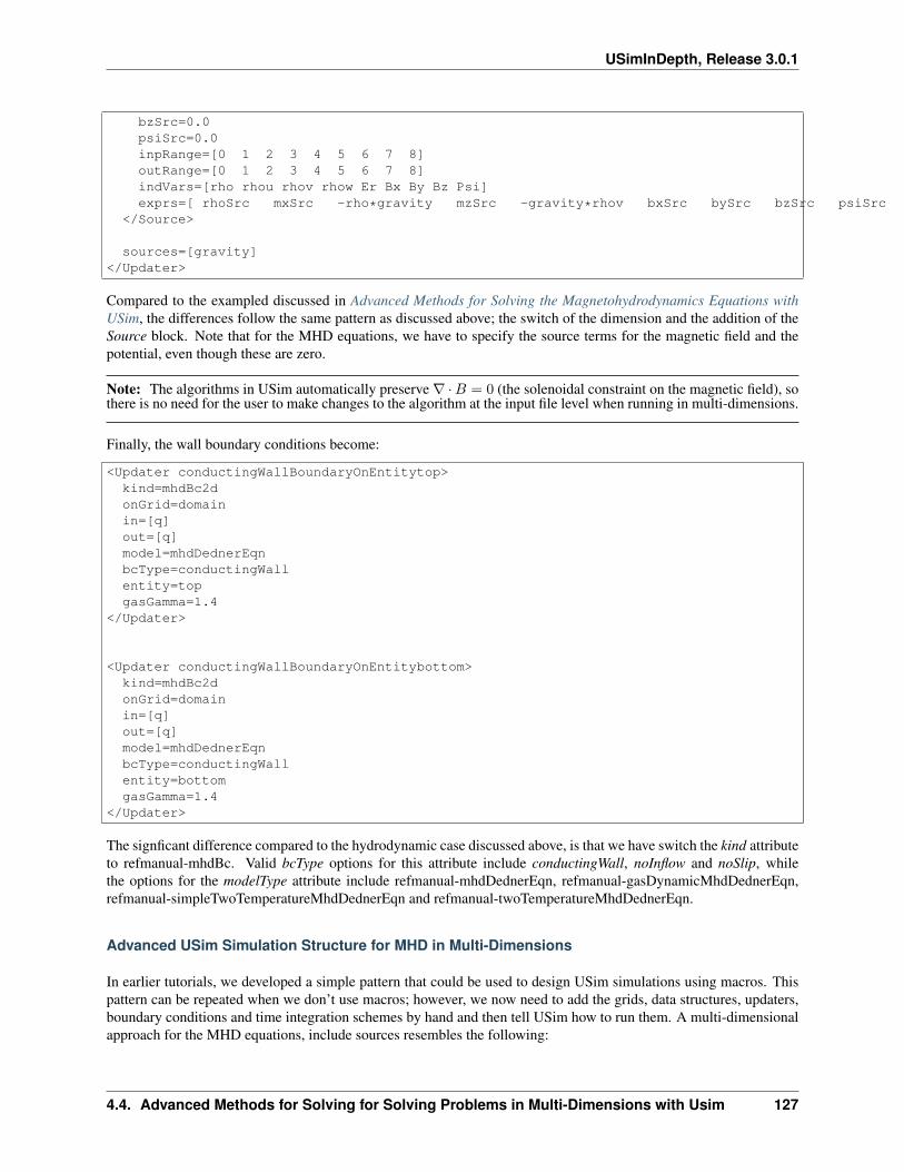
USimInDepth, Release 3.0.1
bzSrc=0.0psiSrc=0.0inpRange=[0 1 2 3 4 5 6 7 8]outRange=[0 1 2 3 4 5 6 7 8]indVars=[rho rhou rhov rhow Er Bx By Bz Psi]exprs=[ rhoSrc mxSrc -rho*gravity mzSrc -gravity*rhov bxSrc bySrc bzSrc psiSrc ]
</Source>
sources=[gravity]</Updater>
Compared to the exampled discussed in Advanced Methods for Solving the Magnetohydrodynamics Equations withUSim, the differences follow the same pattern as discussed above; the switch of the dimension and the addition of theSource block. Note that for the MHD equations, we have to specify the source terms for the magnetic field and thepotential, even though these are zero.
Note: The algorithms in USim automatically preserve ∇ ·𝐵 = 0 (the solenoidal constraint on the magnetic field), sothere is no need for the user to make changes to the algorithm at the input file level when running in multi-dimensions.
Finally, the wall boundary conditions become:
<Updater conductingWallBoundaryOnEntitytop>kind=mhdBc2donGrid=domainin=[q]out=[q]model=mhdDednerEqnbcType=conductingWallentity=topgasGamma=1.4
</Updater>
<Updater conductingWallBoundaryOnEntitybottom>kind=mhdBc2donGrid=domainin=[q]out=[q]model=mhdDednerEqnbcType=conductingWallentity=bottomgasGamma=1.4
</Updater>
The signficant difference compared to the hydrodynamic case discussed above, is that we have switch the kind attributeto refmanual-mhdBc. Valid bcType options for this attribute include conductingWall, noInflow and noSlip, whilethe options for the modelType attribute include refmanual-mhdDednerEqn, refmanual-gasDynamicMhdDednerEqn,refmanual-simpleTwoTemperatureMhdDednerEqn and refmanual-twoTemperatureMhdDednerEqn.
Advanced USim Simulation Structure for MHD in Multi-Dimensions
In earlier tutorials, we developed a simple pattern that could be used to design USim simulations using macros. Thispattern can be repeated when we don’t use macros; however, we now need to add the grids, data structures, updaters,boundary conditions and time integration schemes by hand and then tell USim how to run them. A multi-dimensionalapproach for the MHD equations, include sources resembles the following:
4.4. Advanced Methods for Solving for Solving Problems in Multi-Dimensions with Usim 127
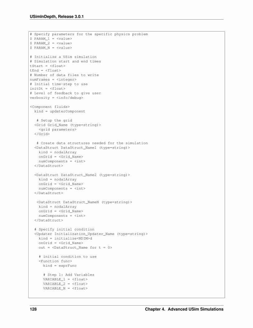
USimInDepth, Release 3.0.1
# Specify parameters for the specific physics problem$ PARAM_1 = <value>$ PARAM_2 = <value>$ PARAM_N = <value>
# Initialize a USim simulation# Simulation start and end timestStart = <float>tEnd = <float># Number of data files to writenumFrames = <integer># Initial time-step to useinitDt = <float># Level of feedback to give userverbosity = <info/debug>
<Component fluids>kind = updaterComponent
# Setup the grid<Grid Grid_Name (type=string)><grid parameters>
</Grid>
# Create data structures needed for the simulation<DataStruct DataStruct_Name1 (type=string)>kind = nodalArrayonGrid = <Grid_Name>numComponents = <int>
</DataStruct>
<DataStruct DataStruct_Name2 (type=string)>kind = nodalArrayonGrid = <Grid_Name>numComponents = <int>
</DataStruct>
<DataStruct DataStruct_NameN (type=string)>kind = nodalArrayonGrid = <Grid_Name>numComponents = <int>
</DataStruct>
# Specify initial condition<Updater Initialization_Updater_Name (type=string)>kind = initialize<NDIM>donGrid = <Grid_Name>out = <DataStruct_Name for t = 0>
# initial condition to use<Function func>
kind = exprFunc
# Step 1: Add VariablesVARIABLE_1 = <float>VARIABLE_2 = <float>VARIABLE_N = <float>
128 Chapter 4. Advanced USim Simulations
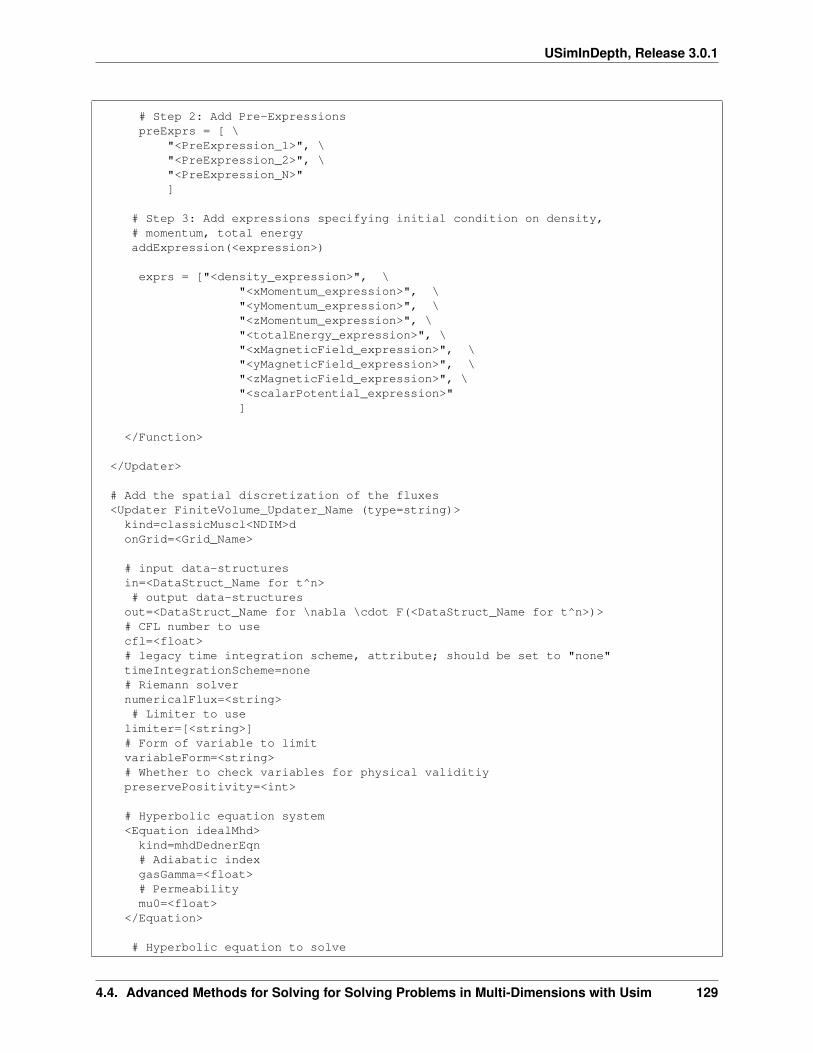
USimInDepth, Release 3.0.1
# Step 2: Add Pre-ExpressionspreExprs = [ \
"<PreExpression_1>", \"<PreExpression_2>", \"<PreExpression_N>"]
# Step 3: Add expressions specifying initial condition on density,# momentum, total energyaddExpression(<expression>)
exprs = ["<density_expression>", \"<xMomentum_expression>", \"<yMomentum_expression>", \"<zMomentum_expression>", \"<totalEnergy_expression>", \"<xMagneticField_expression>", \"<yMagneticField_expression>", \"<zMagneticField_expression>", \"<scalarPotential_expression>"]
</Function>
</Updater>
# Add the spatial discretization of the fluxes<Updater FiniteVolume_Updater_Name (type=string)>kind=classicMuscl<NDIM>donGrid=<Grid_Name>
# input data-structuresin=<DataStruct_Name for t^n># output data-structures
out=<DataStruct_Name for \nabla \cdot F(<DataStruct_Name for t^n>)># CFL number to usecfl=<float># legacy time integration scheme, attribute; should be set to "none"timeIntegrationScheme=none# Riemann solvernumericalFlux=<string># Limiter to use
limiter=[<string>]# Form of variable to limitvariableForm=<string># Whether to check variables for physical validitiypreservePositivity=<int>
# Hyperbolic equation system<Equation idealMhd>
kind=mhdDednerEqn# Adiabatic indexgasGamma=<float># Permeabilitymu0=<float>
</Equation>
# Hyperbolic equation to solve
4.4. Advanced Methods for Solving for Solving Problems in Multi-Dimensions with Usim 129
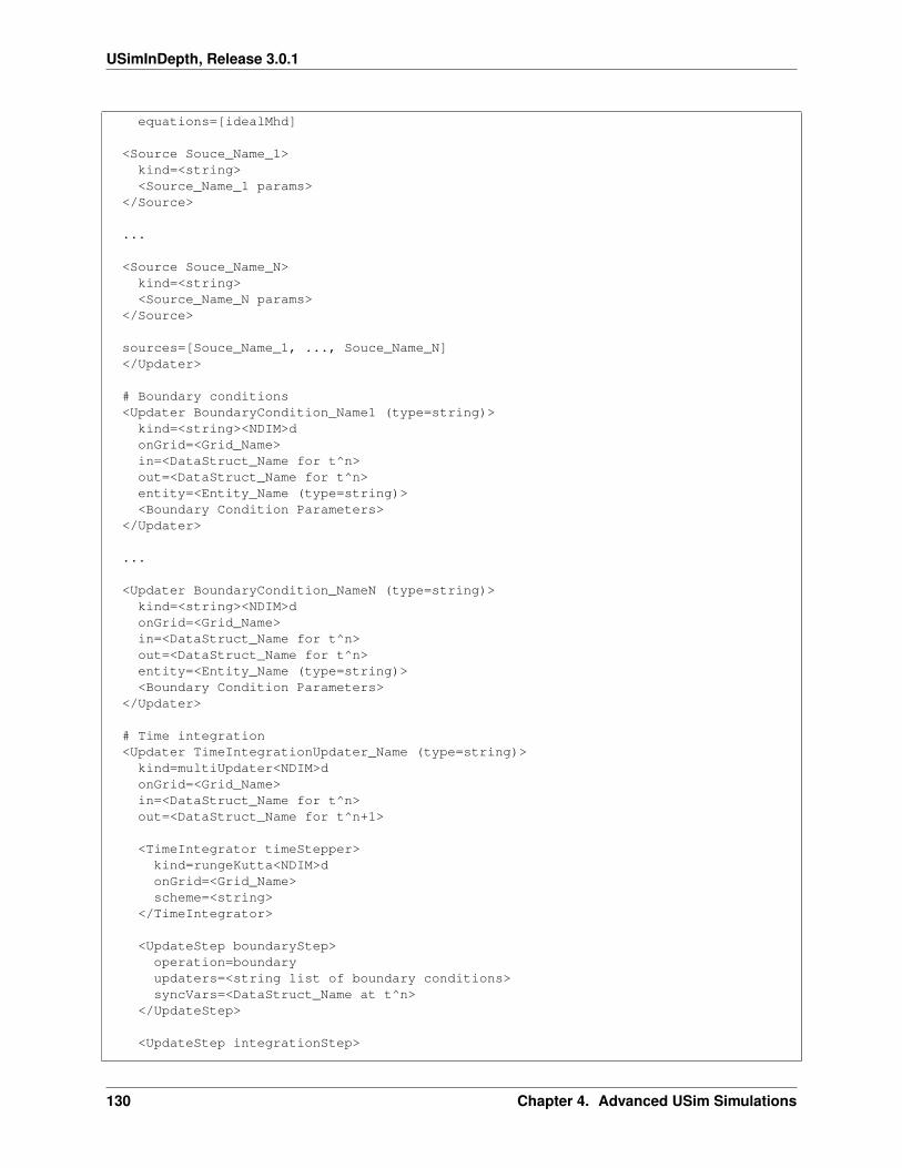
USimInDepth, Release 3.0.1
equations=[idealMhd]
<Source Souce_Name_1>kind=<string><Source_Name_1 params>
</Source>
...
<Source Souce_Name_N>kind=<string><Source_Name_N params>
</Source>
sources=[Souce_Name_1, ..., Souce_Name_N]</Updater>
# Boundary conditions<Updater BoundaryCondition_Name1 (type=string)>kind=<string><NDIM>donGrid=<Grid_Name>in=<DataStruct_Name for t^n>out=<DataStruct_Name for t^n>entity=<Entity_Name (type=string)><Boundary Condition Parameters>
</Updater>
...
<Updater BoundaryCondition_NameN (type=string)>kind=<string><NDIM>donGrid=<Grid_Name>in=<DataStruct_Name for t^n>out=<DataStruct_Name for t^n>entity=<Entity_Name (type=string)><Boundary Condition Parameters>
</Updater>
# Time integration<Updater TimeIntegrationUpdater_Name (type=string)>kind=multiUpdater<NDIM>donGrid=<Grid_Name>in=<DataStruct_Name for t^n>out=<DataStruct_Name for t^n+1>
<TimeIntegrator timeStepper>kind=rungeKutta<NDIM>donGrid=<Grid_Name>scheme=<string>
</TimeIntegrator>
<UpdateStep boundaryStep>operation=boundaryupdaters=<string list of boundary conditions>syncVars=<DataStruct_Name at t^n>
</UpdateStep>
<UpdateStep integrationStep>
130 Chapter 4. Advanced USim Simulations
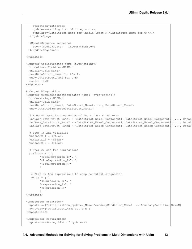
USimInDepth, Release 3.0.1
operation=integrateupdaters=<string list of integrators>syncVars=<DataStruct_Name for \nabla \cdot F(<DataStruct_Name for t^n>)>
</UpdateStep>
<UpdateSequence sequence>loop=[boundaryStep integrationStep]
</UpdateSequence>
</Updater>
<Updater CopierUpdater_Name (type=string)>kind=linearCombiner<NDIM>donGrid=<Grid_Name>in=<DataStruct_Name for t^n+1>out=<DataStruct_Name for t^n>coeffs=[1.0]
</Updater>
# Output Diagnostics<Updater OutputDiagnosticUpdater_Name1 (type=string)>kind=<string><NDIM>donGrid=<Grid_Name>in=<DataStruct_Name1, DataStruct_Name2, ..., DataStruct_NameN>out=<OutputDiagnosticDataStruct_Name1>
# Step 0: Specify components of input data structuresindVars_DataStruct_Name1 = <DataStruct_Name1_Component1, DataStruct_Name1_Component2, ..., DataStruct_Name1_ComponentN>indVars_DataStruct_Name2 = <DataStruct_Name2_Component1, DataStruct_Name2_Component2, ..., DataStruct_Name2_ComponentN>indVars_DataStruct_NameN = <DataStruct_NameN_Component1, DataStruct_NameN_Component2, ..., DataStruct_NameN_ComponentN>
# Step 1: Add VariablesVARIABLE_1 = <float>VARIABLE_2 = <float>VARIABLE_N = <float>
# Step 2: Add Pre-ExpressionspreExprs = [ \
"<PreExpression_1>", \"<PreExpression_2>", \"<PreExpression_N>"]
# Step 3: Add expressions to compute output diagnosticexprs = [ \
"<expression_1>", \"<expression_2>", \"<expression_N>"]
</Updater>
<UpdateStep startStep>updaters=[Initialization_Updater_Name BoundaryCondition_Name1 ... BoundaryCondition_NameN]syncVars=[<DataStruct_Name for t^n>]
</UpdateStep>
<UpdateStep restoreStep>updaters=<String List of Updaters>
4.4. Advanced Methods for Solving for Solving Problems in Multi-Dimensions with Usim 131
USimInDepth, Release 3.0.1
syncVars=<String List of DataStructs></UpdateStep>
<UpdateStep bcStep>updaters=[BoundaryCondition_Name1 ... BoundaryCondition_NameN]syncVars=[<DataStruct_Name for t^n>]
</UpdateStep>
<UpdateStep hyperStep>updaters=[FiniteVolume_Updater_Name (type=string)]syncVars=<String List of DataStructs>
</UpdateStep>
<UpdateStep writeStep>updaters=< OutputDiagnosticUpdater_Name1, OutputDiagnosticUpdater_Name2, OutputDiagnosticUpdater_NameN>syncVars=<OutputDiagnosticDataStruct_Name1, OutputDiagnosticDataStruct_Name2, ..., OutputDiagnosticDataStruct_NameN>
</UpdateStep>
<UpdateSequence simulation>startOnly=[generateStep startStep]restoreOnly=[generateStep restoreStep bcStep]writeOnly=[bcStep writeStep]loop=[hyperStep]
</UpdateSequence>
</Component>
Note that we have not filled in some of the entries in the UpdateSteps above. How to use these UpdateSteps is discussedin later tutorials.
4.5 Advanced Methods for Solving Problems on Advanced Mesheswith USim
In Advanced USim Simulation Concepts we examined the basic ingredients of a USim input file: the simulation grid(see Defining the Simulation Grid); data structures (see Allocating Memory); how to assign initial conditions (see Set-ting Initial Conditions) and how to write out additional data (see Writing Out Data). In Advanced Methods for Solvingthe Euler Equations with USim, we built on these concepts and demonstrated the basic methods used by USim to solvethe Euler equations without the use of macros. Next, in Advanced Methods for Solving the MagnetohydrodynamicsEquations with USim, we extended these ideas to demonstrate how to solve the MHD equations in USim, again with-out the use of macros. Then, in Advanced Methods for Solving for Solving Problems in Multi-Dimensions with Usim,we demonstrated how to extend these concepts to multi-dimensions for both the Euler and MHD without the use ofmacros.
In this tutorial, we show how USim can be used to solve problems on more advanced meshes, building on the conceptspresented in Solving Problems on Advanced Structured Meshes in USim and Solving Problems on Unstructured Meshesin USim to demonstrate how to solve problems in USim on a range of advanced mesh types.
132 Chapter 4. Advanced USim Simulations
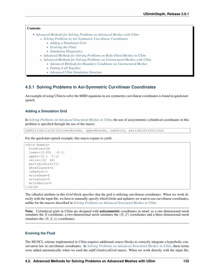
USimInDepth, Release 3.0.1
Contents
• Advanced Methods for Solving Problems on Advanced Meshes with USim– Solving Problems in Axi-Symmetric Curvilinear Coordinates
* Adding a Simulation Grid* Evolving the Fluid* Simulation Diagnostics
– Advanced Methods for Solving Problems on Body-Fitted Meshes in USim– Advanced Methods for Solving Problems on Unstructured Meshes with USim
* Advanced Methods for Boundary Conditions on Unstructured Meshes* Putting it all Together* Advanced USim Simulation Structure
4.5.1 Solving Problems in Axi-Symmetric Curvilinear Coordinates
An example of using USim to solve the MHD equations in axi-symmetric curvilinear coordinates is found in quickstart-zpinch.
Adding a Simulation Grid
In Solving Problems on Advanced Structured Meshes in USim, the use of axisymmetric cylindrical coordinates in thisproblem is specified through the use of the macro:
addCylindricalGrid(lowerBounds, upperBounds, numCells, periodicDirections)
For the quickstart-zpinch example, this macro expans to yield:
<Grid domain>kind=cart2dlower=[0.001 -0.1]upper=[0.1 0.1]cells=[32 64]periodicDirs=[1]ghostLayers=2isRadial=1writeGeom=0writeConn=0writeHalos=0
</Grid>
The isRadial attribute in this Grid block specifies that the grid is utilizing curvilinear coordinates. When we work di-rectly with the input file, we have to manually specify which Grids and updaters we want to use curvilinear coordinates,unlike for the macros described in Solving Problems on Advanced Structured Meshes in USim.
Note: Cylindrical grids in USim are designed with axisymmetric coordinates in mind, so a one-dimensional meshsimulates the 𝑅 coordinate, a two-dimensional mesh simulates the (𝑅,𝑍) coordinates and a three-dimensional meshsimulates the (𝑅,𝑍, 𝜑) coordinates.
Evolving the Fluid
The MUSCL scheme implemented in USim requires additional source blocks to correctly integrate a hyperbolic con-servation law in curvilinear coordinates. In Solving Problems on Advanced Structured Meshes in USim, these termswere added automatically when we used the addCylindricalGrid macro. When we work directly with the input file,
4.5. Advanced Methods for Solving Problems on Advanced Meshes with USim 133
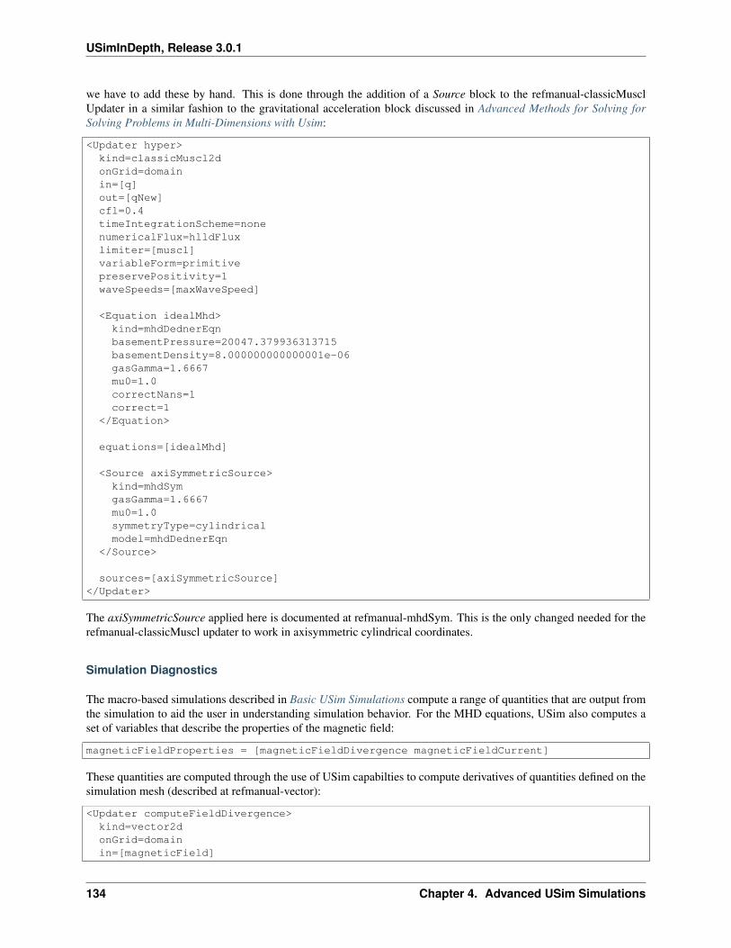
USimInDepth, Release 3.0.1
we have to add these by hand. This is done through the addition of a Source block to the refmanual-classicMusclUpdater in a similar fashion to the gravitational acceleration block discussed in Advanced Methods for Solving forSolving Problems in Multi-Dimensions with Usim:
<Updater hyper>kind=classicMuscl2donGrid=domainin=[q]out=[qNew]cfl=0.4timeIntegrationScheme=nonenumericalFlux=hlldFluxlimiter=[muscl]variableForm=primitivepreservePositivity=1waveSpeeds=[maxWaveSpeed]
<Equation idealMhd>kind=mhdDednerEqnbasementPressure=20047.379936313715basementDensity=8.000000000000001e-06gasGamma=1.6667mu0=1.0correctNans=1correct=1
</Equation>
equations=[idealMhd]
<Source axiSymmetricSource>kind=mhdSymgasGamma=1.6667mu0=1.0symmetryType=cylindricalmodel=mhdDednerEqn
</Source>
sources=[axiSymmetricSource]</Updater>
The axiSymmetricSource applied here is documented at refmanual-mhdSym. This is the only changed needed for therefmanual-classicMuscl updater to work in axisymmetric cylindrical coordinates.
Simulation Diagnostics
The macro-based simulations described in Basic USim Simulations compute a range of quantities that are output fromthe simulation to aid the user in understanding simulation behavior. For the MHD equations, USim also computes aset of variables that describe the properties of the magnetic field:
magneticFieldProperties = [magneticFieldDivergence magneticFieldCurrent]
These quantities are computed through the use of USim capabilties to compute derivatives of quantities defined on thesimulation mesh (described at refmanual-vector):
<Updater computeFieldDivergence>kind=vector2donGrid=domainin=[magneticField]
134 Chapter 4. Advanced USim Simulations
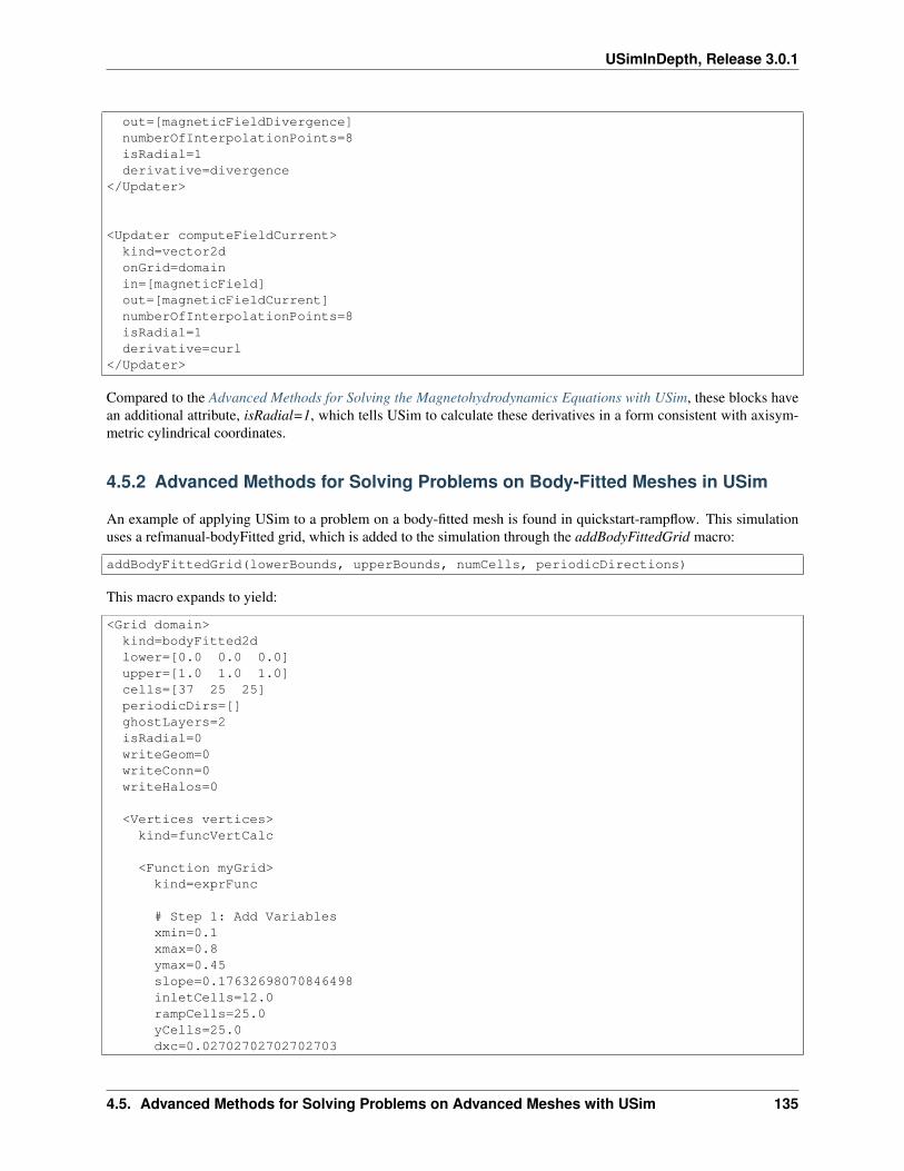
USimInDepth, Release 3.0.1
out=[magneticFieldDivergence]numberOfInterpolationPoints=8isRadial=1derivative=divergence
</Updater>
<Updater computeFieldCurrent>kind=vector2donGrid=domainin=[magneticField]out=[magneticFieldCurrent]numberOfInterpolationPoints=8isRadial=1derivative=curl
</Updater>
Compared to the Advanced Methods for Solving the Magnetohydrodynamics Equations with USim, these blocks havean additional attribute, isRadial=1, which tells USim to calculate these derivatives in a form consistent with axisym-metric cylindrical coordinates.
4.5.2 Advanced Methods for Solving Problems on Body-Fitted Meshes in USim
An example of applying USim to a problem on a body-fitted mesh is found in quickstart-rampflow. This simulationuses a refmanual-bodyFitted grid, which is added to the simulation through the addBodyFittedGrid macro:
addBodyFittedGrid(lowerBounds, upperBounds, numCells, periodicDirections)
This macro expands to yield:
<Grid domain>kind=bodyFitted2dlower=[0.0 0.0 0.0]upper=[1.0 1.0 1.0]cells=[37 25 25]periodicDirs=[]ghostLayers=2isRadial=0writeGeom=0writeConn=0writeHalos=0
<Vertices vertices>kind=funcVertCalc
<Function myGrid>kind=exprFunc
# Step 1: Add Variablesxmin=0.1xmax=0.8ymax=0.45slope=0.17632698070846498inletCells=12.0rampCells=25.0yCells=25.0dxc=0.02702702702702703
4.5. Advanced Methods for Solving Problems on Advanced Meshes with USim 135
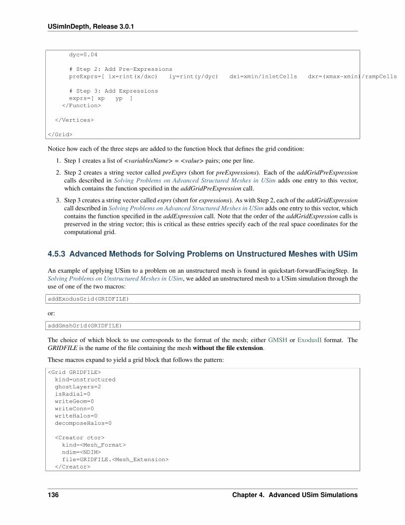
USimInDepth, Release 3.0.1
dyc=0.04
# Step 2: Add Pre-ExpressionspreExprs=[ ix=rint(x/dxc) iy=rint(y/dyc) dxi=xmin/inletCells dxr=(xmax-xmin)/rampCells xp=if(inletCells>=ix,dxi*ix,xmin+dxr*(ix-inletCells)) dyi=ymax/yCells b=-slope*xmin y0=slope*xp+b dyr=(ymax-y0)/yCells yp=if(inletCells>=ix,dyi*iy,y0+dyr*iy) ]
# Step 3: Add Expressionsexprs=[ xp yp ]
</Function>
</Vertices>
</Grid>
Notice how each of the three steps are added to the function block that defines the grid condition:
1. Step 1 creates a list of <variablesName> = <value> pairs; one per line.
2. Step 2 creates a string vector called preExprs (short for preExpressions). Each of the addGridPreExpressioncalls described in Solving Problems on Advanced Structured Meshes in USim adds one entry to this vector,which contains the function specified in the addGridPreExpression call.
3. Step 3 creates a string vector called exprs (short for expressions). As with Step 2, each of the addGridExpressioncall described in Solving Problems on Advanced Structured Meshes in USim adds one entry to this vector, whichcontains the function specified in the addExpression call. Note that the order of the addGridExpression calls ispreserved in the string vector; this is critical as these entries specify each of the real space coordinates for thecomputational grid.
4.5.3 Advanced Methods for Solving Problems on Unstructured Meshes with USim
An example of applying USim to a problem on an unstructured mesh is found in quickstart-forwardFacingStep. InSolving Problems on Unstructured Meshes in USim, we added an unstructured mesh to a USim simulation through theuse of one of the two macros:
addExodusGrid(GRIDFILE)
or:
addGmshGrid(GRIDFILE)
The choice of which block to use corresponds to the format of the mesh; either GMSH or ExodusII format. TheGRIDFILE is the name of the file containing the mesh without the file extension.
These macros expand to yield a grid block that follows the pattern:
<Grid GRIDFILE>kind=unstructuredghostLayers=2isRadial=0writeGeom=0writeConn=0writeHalos=0decomposeHalos=0
<Creator ctor>kind=<Mesh_Format>ndim=<NDIM>file=GRIDFILE.<Mesh_Extension>
</Creator>
136 Chapter 4. Advanced USim Simulations
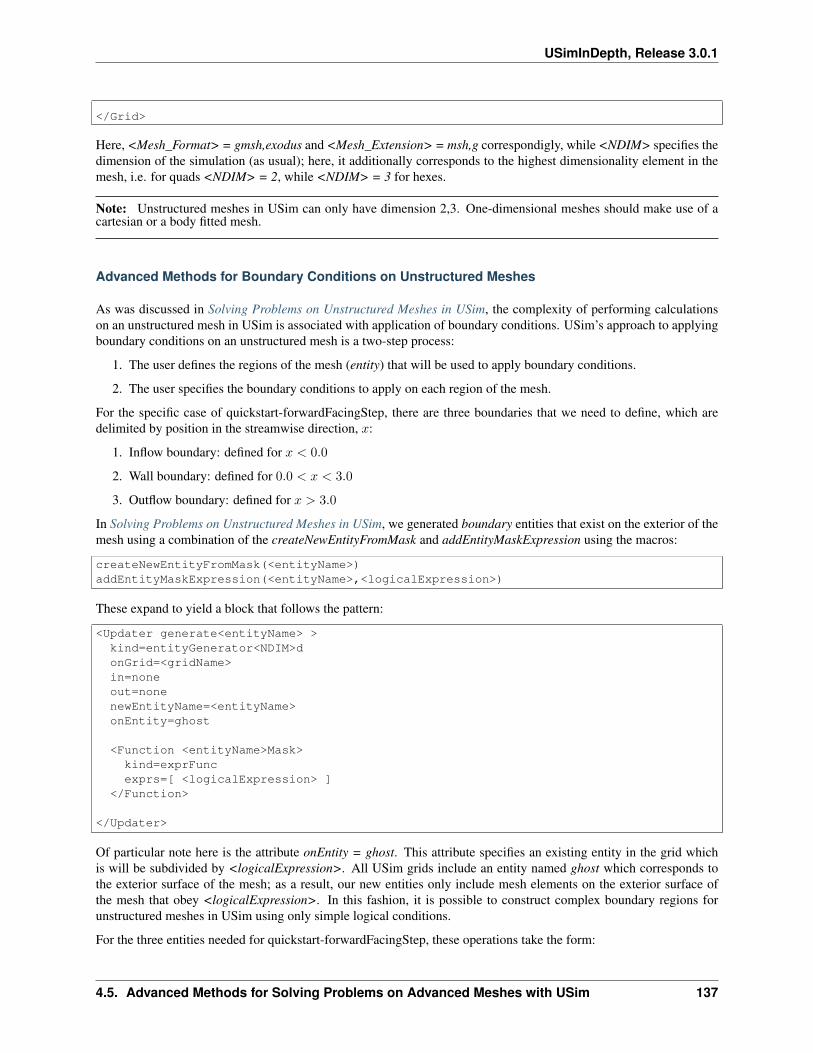
USimInDepth, Release 3.0.1
</Grid>
Here, <Mesh_Format> = gmsh,exodus and <Mesh_Extension> = msh,g correspondigly, while <NDIM> specifies thedimension of the simulation (as usual); here, it additionally corresponds to the highest dimensionality element in themesh, i.e. for quads <NDIM> = 2, while <NDIM> = 3 for hexes.
Note: Unstructured meshes in USim can only have dimension 2,3. One-dimensional meshes should make use of acartesian or a body fitted mesh.
Advanced Methods for Boundary Conditions on Unstructured Meshes
As was discussed in Solving Problems on Unstructured Meshes in USim, the complexity of performing calculationson an unstructured mesh in USim is associated with application of boundary conditions. USim’s approach to applyingboundary conditions on an unstructured mesh is a two-step process:
1. The user defines the regions of the mesh (entity) that will be used to apply boundary conditions.
2. The user specifies the boundary conditions to apply on each region of the mesh.
For the specific case of quickstart-forwardFacingStep, there are three boundaries that we need to define, which aredelimited by position in the streamwise direction, 𝑥:
1. Inflow boundary: defined for 𝑥 < 0.0
2. Wall boundary: defined for 0.0 < 𝑥 < 3.0
3. Outflow boundary: defined for 𝑥 > 3.0
In Solving Problems on Unstructured Meshes in USim, we generated boundary entities that exist on the exterior of themesh using a combination of the createNewEntityFromMask and addEntityMaskExpression using the macros:
createNewEntityFromMask(<entityName>)addEntityMaskExpression(<entityName>,<logicalExpression>)
These expand to yield a block that follows the pattern:
<Updater generate<entityName> >kind=entityGenerator<NDIM>donGrid=<gridName>in=noneout=nonenewEntityName=<entityName>onEntity=ghost
<Function <entityName>Mask>kind=exprFuncexprs=[ <logicalExpression> ]
</Function>
</Updater>
Of particular note here is the attribute onEntity = ghost. This attribute specifies an existing entity in the grid whichis will be subdivided by <logicalExpression>. All USim grids include an entity named ghost which corresponds tothe exterior surface of the mesh; as a result, our new entities only include mesh elements on the exterior surface ofthe mesh that obey <logicalExpression>. In this fashion, it is possible to construct complex boundary regions forunstructured meshes in USim using only simple logical conditions.
For the three entities needed for quickstart-forwardFacingStep, these operations take the form:
4.5. Advanced Methods for Solving Problems on Advanced Meshes with USim 137
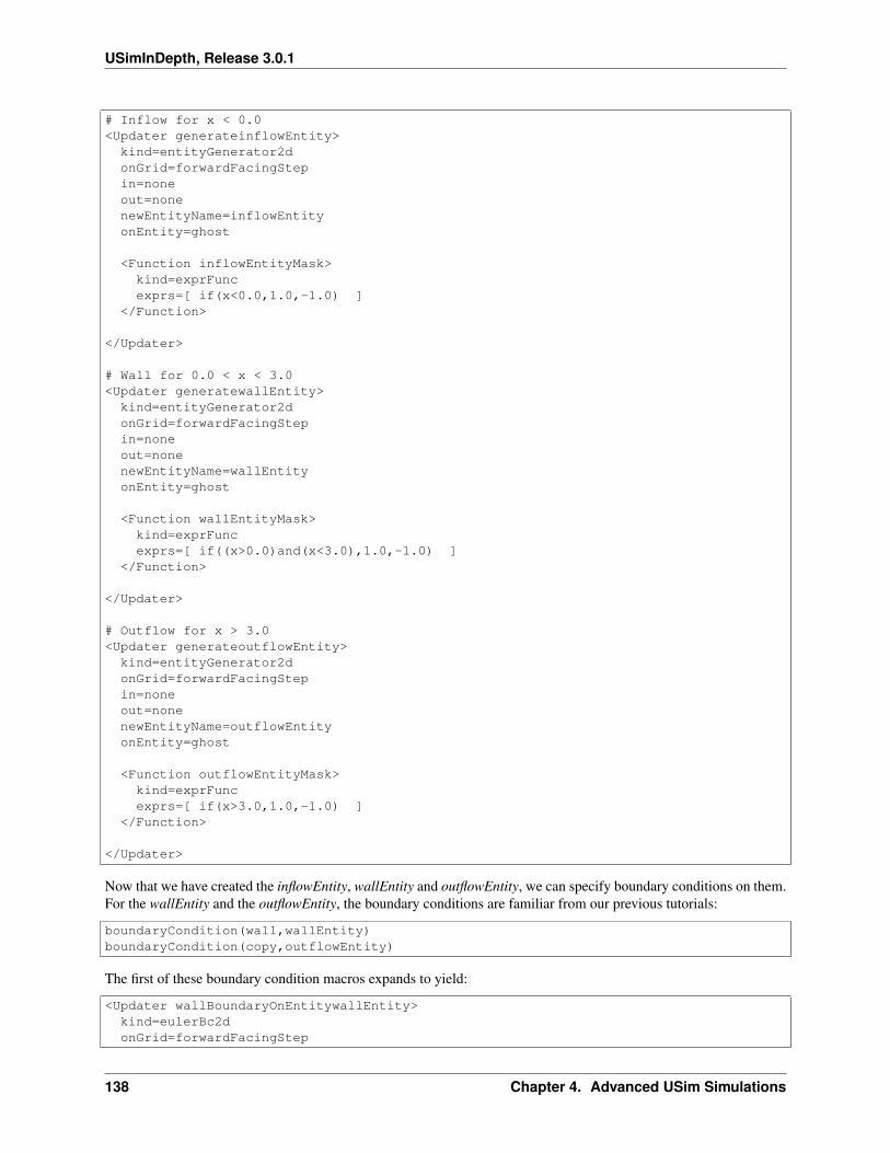
USimInDepth, Release 3.0.1
# Inflow for x < 0.0<Updater generateinflowEntity>
kind=entityGenerator2donGrid=forwardFacingStepin=noneout=nonenewEntityName=inflowEntityonEntity=ghost
<Function inflowEntityMask>kind=exprFuncexprs=[ if(x<0.0,1.0,-1.0) ]
</Function>
</Updater>
# Wall for 0.0 < x < 3.0<Updater generatewallEntity>
kind=entityGenerator2donGrid=forwardFacingStepin=noneout=nonenewEntityName=wallEntityonEntity=ghost
<Function wallEntityMask>kind=exprFuncexprs=[ if((x>0.0)and(x<3.0),1.0,-1.0) ]
</Function>
</Updater>
# Outflow for x > 3.0<Updater generateoutflowEntity>
kind=entityGenerator2donGrid=forwardFacingStepin=noneout=nonenewEntityName=outflowEntityonEntity=ghost
<Function outflowEntityMask>kind=exprFuncexprs=[ if(x>3.0,1.0,-1.0) ]
</Function>
</Updater>
Now that we have created the inflowEntity, wallEntity and outflowEntity, we can specify boundary conditions on them.For the wallEntity and the outflowEntity, the boundary conditions are familiar from our previous tutorials:
boundaryCondition(wall,wallEntity)boundaryCondition(copy,outflowEntity)
The first of these boundary condition macros expands to yield:
<Updater wallBoundaryOnEntitywallEntity>kind=eulerBc2donGrid=forwardFacingStep
138 Chapter 4. Advanced USim Simulations
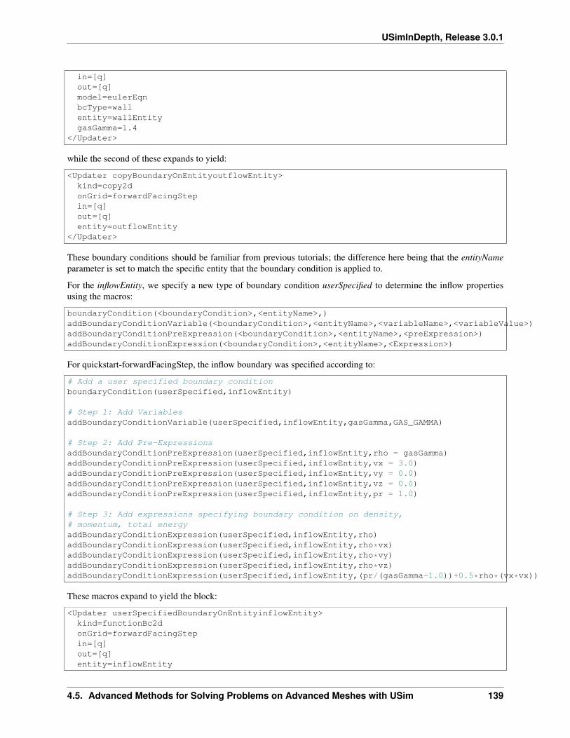
USimInDepth, Release 3.0.1
in=[q]out=[q]model=eulerEqnbcType=wallentity=wallEntitygasGamma=1.4
</Updater>
while the second of these expands to yield:
<Updater copyBoundaryOnEntityoutflowEntity>kind=copy2donGrid=forwardFacingStepin=[q]out=[q]entity=outflowEntity
</Updater>
These boundary conditions should be familiar from previous tutorials; the difference here being that the entityNameparameter is set to match the specific entity that the boundary condition is applied to.
For the inflowEntity, we specify a new type of boundary condition userSpecified to determine the inflow propertiesusing the macros:
boundaryCondition(<boundaryCondition>,<entityName>,)addBoundaryConditionVariable(<boundaryCondition>,<entityName>,<variableName>,<variableValue>)addBoundaryConditionPreExpression(<boundaryCondition>,<entityName>,<preExpression>)addBoundaryConditionExpression(<boundaryCondition>,<entityName>,<Expression>)
For quickstart-forwardFacingStep, the inflow boundary was specified according to:
# Add a user specified boundary conditionboundaryCondition(userSpecified,inflowEntity)
# Step 1: Add VariablesaddBoundaryConditionVariable(userSpecified,inflowEntity,gasGamma,GAS_GAMMA)
# Step 2: Add Pre-ExpressionsaddBoundaryConditionPreExpression(userSpecified,inflowEntity,rho = gasGamma)addBoundaryConditionPreExpression(userSpecified,inflowEntity,vx = 3.0)addBoundaryConditionPreExpression(userSpecified,inflowEntity,vy = 0.0)addBoundaryConditionPreExpression(userSpecified,inflowEntity,vz = 0.0)addBoundaryConditionPreExpression(userSpecified,inflowEntity,pr = 1.0)
# Step 3: Add expressions specifying boundary condition on density,# momentum, total energyaddBoundaryConditionExpression(userSpecified,inflowEntity,rho)addBoundaryConditionExpression(userSpecified,inflowEntity,rho*vx)addBoundaryConditionExpression(userSpecified,inflowEntity,rho*vy)addBoundaryConditionExpression(userSpecified,inflowEntity,rho*vz)addBoundaryConditionExpression(userSpecified,inflowEntity,(pr/(gasGamma-1.0))+0.5*rho*(vx*vx))
These macros expand to yield the block:
<Updater userSpecifiedBoundaryOnEntityinflowEntity>kind=functionBc2donGrid=forwardFacingStepin=[q]out=[q]entity=inflowEntity
4.5. Advanced Methods for Solving Problems on Advanced Meshes with USim 139
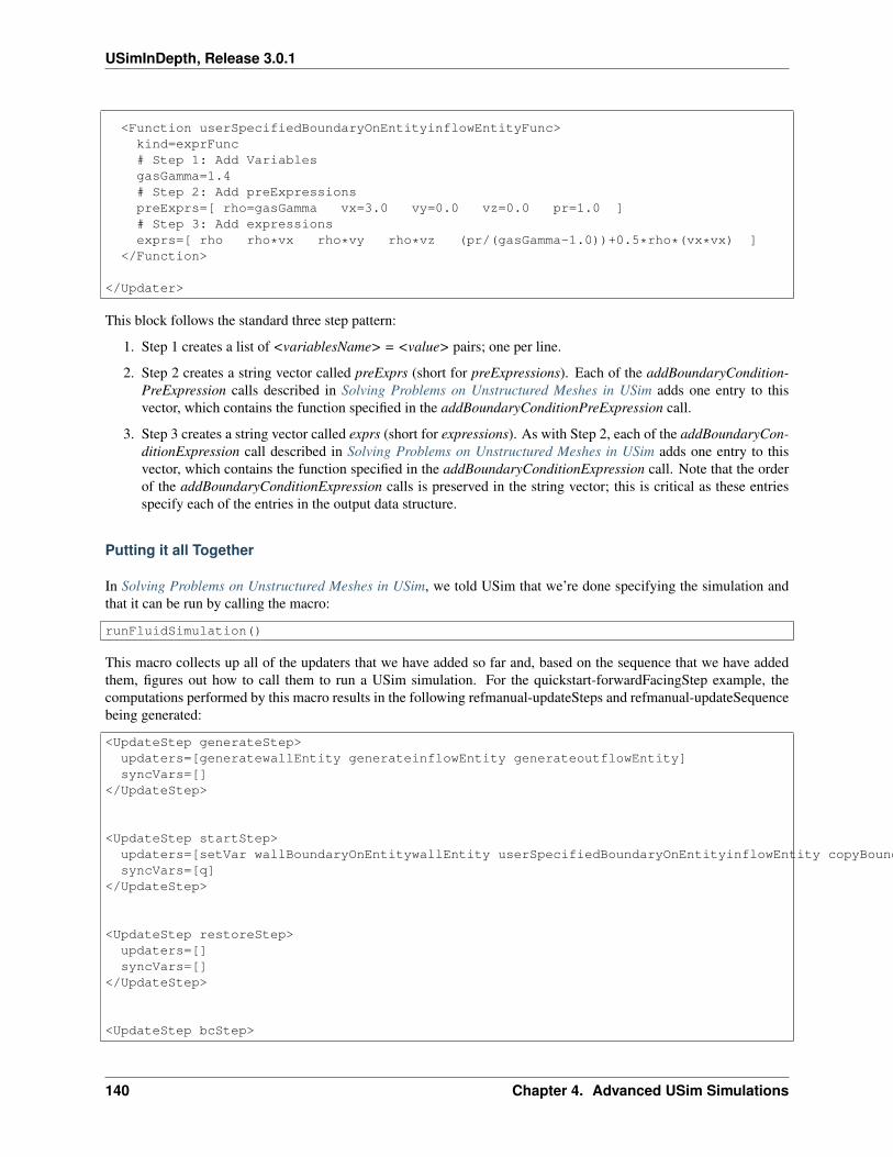
USimInDepth, Release 3.0.1
<Function userSpecifiedBoundaryOnEntityinflowEntityFunc>kind=exprFunc# Step 1: Add VariablesgasGamma=1.4# Step 2: Add preExpressionspreExprs=[ rho=gasGamma vx=3.0 vy=0.0 vz=0.0 pr=1.0 ]# Step 3: Add expressionsexprs=[ rho rho*vx rho*vy rho*vz (pr/(gasGamma-1.0))+0.5*rho*(vx*vx) ]
</Function>
</Updater>
This block follows the standard three step pattern:
1. Step 1 creates a list of <variablesName> = <value> pairs; one per line.
2. Step 2 creates a string vector called preExprs (short for preExpressions). Each of the addBoundaryCondition-PreExpression calls described in Solving Problems on Unstructured Meshes in USim adds one entry to thisvector, which contains the function specified in the addBoundaryConditionPreExpression call.
3. Step 3 creates a string vector called exprs (short for expressions). As with Step 2, each of the addBoundaryCon-ditionExpression call described in Solving Problems on Unstructured Meshes in USim adds one entry to thisvector, which contains the function specified in the addBoundaryConditionExpression call. Note that the orderof the addBoundaryConditionExpression calls is preserved in the string vector; this is critical as these entriesspecify each of the entries in the output data structure.
Putting it all Together
In Solving Problems on Unstructured Meshes in USim, we told USim that we’re done specifying the simulation andthat it can be run by calling the macro:
runFluidSimulation()
This macro collects up all of the updaters that we have added so far and, based on the sequence that we have addedthem, figures out how to call them to run a USim simulation. For the quickstart-forwardFacingStep example, thecomputations performed by this macro results in the following refmanual-updateSteps and refmanual-updateSequencebeing generated:
<UpdateStep generateStep>updaters=[generatewallEntity generateinflowEntity generateoutflowEntity]syncVars=[]
</UpdateStep>
<UpdateStep startStep>updaters=[setVar wallBoundaryOnEntitywallEntity userSpecifiedBoundaryOnEntityinflowEntity copyBoundaryOnEntityoutflowEntity]syncVars=[q]
</UpdateStep>
<UpdateStep restoreStep>updaters=[]syncVars=[]
</UpdateStep>
<UpdateStep bcStep>
140 Chapter 4. Advanced USim Simulations
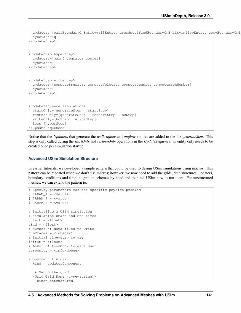
USimInDepth, Release 3.0.1
updaters=[wallBoundaryOnEntitywallEntity userSpecifiedBoundaryOnEntityinflowEntity copyBoundaryOnEntityoutflowEntity]syncVars=[q]
</UpdateStep>
<UpdateStep hyperStep>updaters=[mainIntegrator copier]syncVars=[]
</UpdateStep>
<UpdateStep writeStep>updaters=[computePressure computeVelocity computeDensity computemachNumber]syncVars=[]
</UpdateStep>
<UpdateSequence simulation>startOnly=[generateStep startStep]restoreOnly=[generateStep restoreStep bcStep]writeOnly=[bcStep writeStep]loop=[hyperStep]
</UpdateSequence>
Notice that the Updaters that generate the wall, inflow and outflow entities are added to the the generateStep. Thisstep is only called during the startOnly and restoreOnly operations in the UpdateSequence: an entity only needs to becreated once per simulation startup.
Advanced USim Simulation Structure
In earlier tutorials, we developed a simple pattern that could be used to design USim simulations using macros. Thispattern can be repeated when we don’t use macros; however, we now need to add the grids, data structures, updaters,boundary conditions and time integration schemes by hand and then tell USim how to run them. For unstructuredmeshes, we can extend the pattern to:
# Specify parameters for the specific physics problem$ PARAM_1 = <value>$ PARAM_2 = <value>$ PARAM_N = <value>
# Initialize a USim simulation# Simulation start and end timestStart = <float>tEnd = <float># Number of data files to writenumFrames = <integer># Initial time-step to useinitDt = <float># Level of feedback to give userverbosity = <info/debug>
<Component fluids>kind = updaterComponent
# Setup the grid<Grid Grid_Name (type=string)>kind=unstructured
4.5. Advanced Methods for Solving Problems on Advanced Meshes with USim 141
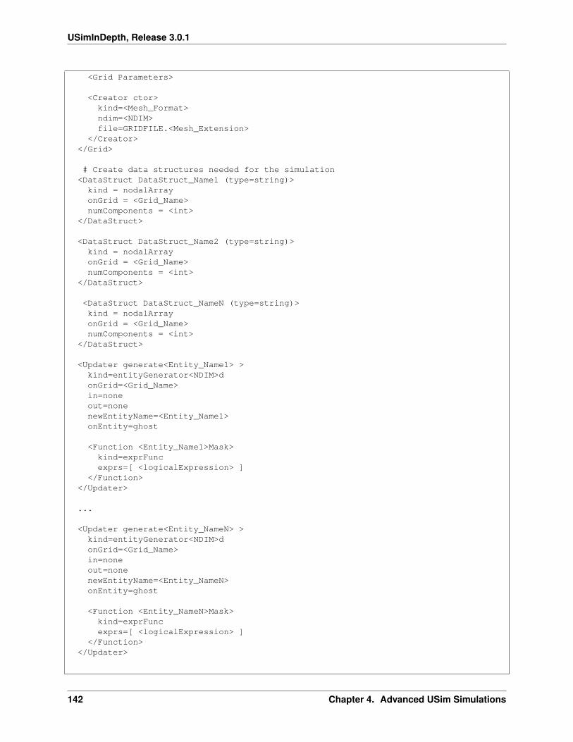
USimInDepth, Release 3.0.1
<Grid Parameters>
<Creator ctor>kind=<Mesh_Format>ndim=<NDIM>file=GRIDFILE.<Mesh_Extension>
</Creator></Grid>
# Create data structures needed for the simulation<DataStruct DataStruct_Name1 (type=string)>kind = nodalArrayonGrid = <Grid_Name>numComponents = <int>
</DataStruct>
<DataStruct DataStruct_Name2 (type=string)>kind = nodalArrayonGrid = <Grid_Name>numComponents = <int>
</DataStruct>
<DataStruct DataStruct_NameN (type=string)>kind = nodalArrayonGrid = <Grid_Name>numComponents = <int>
</DataStruct>
<Updater generate<Entity_Name1> >kind=entityGenerator<NDIM>donGrid=<Grid_Name>in=noneout=nonenewEntityName=<Entity_Name1>onEntity=ghost
<Function <Entity_Name1>Mask>kind=exprFuncexprs=[ <logicalExpression> ]
</Function></Updater>
...
<Updater generate<Entity_NameN> >kind=entityGenerator<NDIM>donGrid=<Grid_Name>in=noneout=nonenewEntityName=<Entity_NameN>onEntity=ghost
<Function <Entity_NameN>Mask>kind=exprFuncexprs=[ <logicalExpression> ]
</Function></Updater>
142 Chapter 4. Advanced USim Simulations
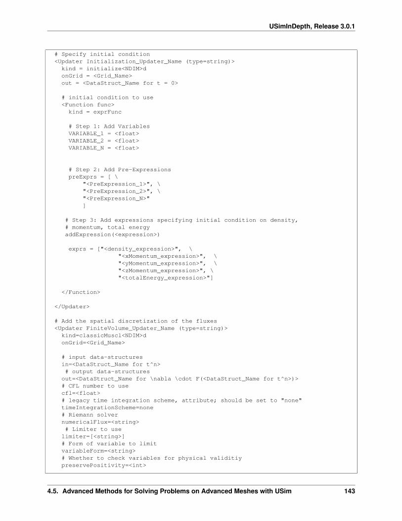
USimInDepth, Release 3.0.1
# Specify initial condition<Updater Initialization_Updater_Name (type=string)>kind = initialize<NDIM>donGrid = <Grid_Name>out = <DataStruct_Name for t = 0>
# initial condition to use<Function func>
kind = exprFunc
# Step 1: Add VariablesVARIABLE_1 = <float>VARIABLE_2 = <float>VARIABLE_N = <float>
# Step 2: Add Pre-ExpressionspreExprs = [ \
"<PreExpression_1>", \"<PreExpression_2>", \"<PreExpression_N>"]
# Step 3: Add expressions specifying initial condition on density,# momentum, total energyaddExpression(<expression>)
exprs = ["<density_expression>", \"<xMomentum_expression>", \"<yMomentum_expression>", \"<zMomentum_expression>", \"<totalEnergy_expression>"]
</Function>
</Updater>
# Add the spatial discretization of the fluxes<Updater FiniteVolume_Updater_Name (type=string)>kind=classicMuscl<NDIM>donGrid=<Grid_Name>
# input data-structuresin=<DataStruct_Name for t^n># output data-structures
out=<DataStruct_Name for \nabla \cdot F(<DataStruct_Name for t^n>)># CFL number to usecfl=<float># legacy time integration scheme, attribute; should be set to "none"timeIntegrationScheme=none# Riemann solvernumericalFlux=<string># Limiter to use
limiter=[<string>]# Form of variable to limitvariableForm=<string># Whether to check variables for physical validitiypreservePositivity=<int>
4.5. Advanced Methods for Solving Problems on Advanced Meshes with USim 143
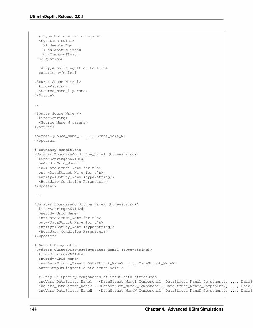
USimInDepth, Release 3.0.1
# Hyperbolic equation system<Equation euler>
kind=eulerEqn# Adiabatic indexgasGamma=<float>
</Equation>
# Hyperbolic equation to solveequations=[euler]
<Source Souce_Name_1>kind=<string><Source_Name_1 params>
</Source>
...
<Source Souce_Name_N>kind=<string><Source_Name_N params>
</Source>
sources=[Souce_Name_1, ..., Souce_Name_N]</Updater>
# Boundary conditions<Updater BoundaryCondition_Name1 (type=string)>kind=<string><NDIM>donGrid=<Grid_Name>in=<DataStruct_Name for t^n>out=<DataStruct_Name for t^n>entity=<Entity_Name (type=string)><Boundary Condition Parameters>
</Updater>
...
<Updater BoundaryCondition_NameN (type=string)>kind=<string><NDIM>donGrid=<Grid_Name>in=<DataStruct_Name for t^n>out=<DataStruct_Name for t^n>entity=<Entity_Name (type=string)><Boundary Condition Parameters>
</Updater>
# Output Diagnostics<Updater OutputDiagnosticUpdater_Name1 (type=string)>kind=<string><NDIM>donGrid=<Grid_Name>in=<DataStruct_Name1, DataStruct_Name2, ..., DataStruct_NameN>out=<OutputDiagnosticDataStruct_Name1>
# Step 0: Specify components of input data structuresindVars_DataStruct_Name1 = <DataStruct_Name1_Component1, DataStruct_Name1_Component2, ..., DataStruct_Name1_ComponentN>indVars_DataStruct_Name2 = <DataStruct_Name2_Component1, DataStruct_Name2_Component2, ..., DataStruct_Name2_ComponentN>indVars_DataStruct_NameN = <DataStruct_NameN_Component1, DataStruct_NameN_Component2, ..., DataStruct_NameN_ComponentN>
144 Chapter 4. Advanced USim Simulations
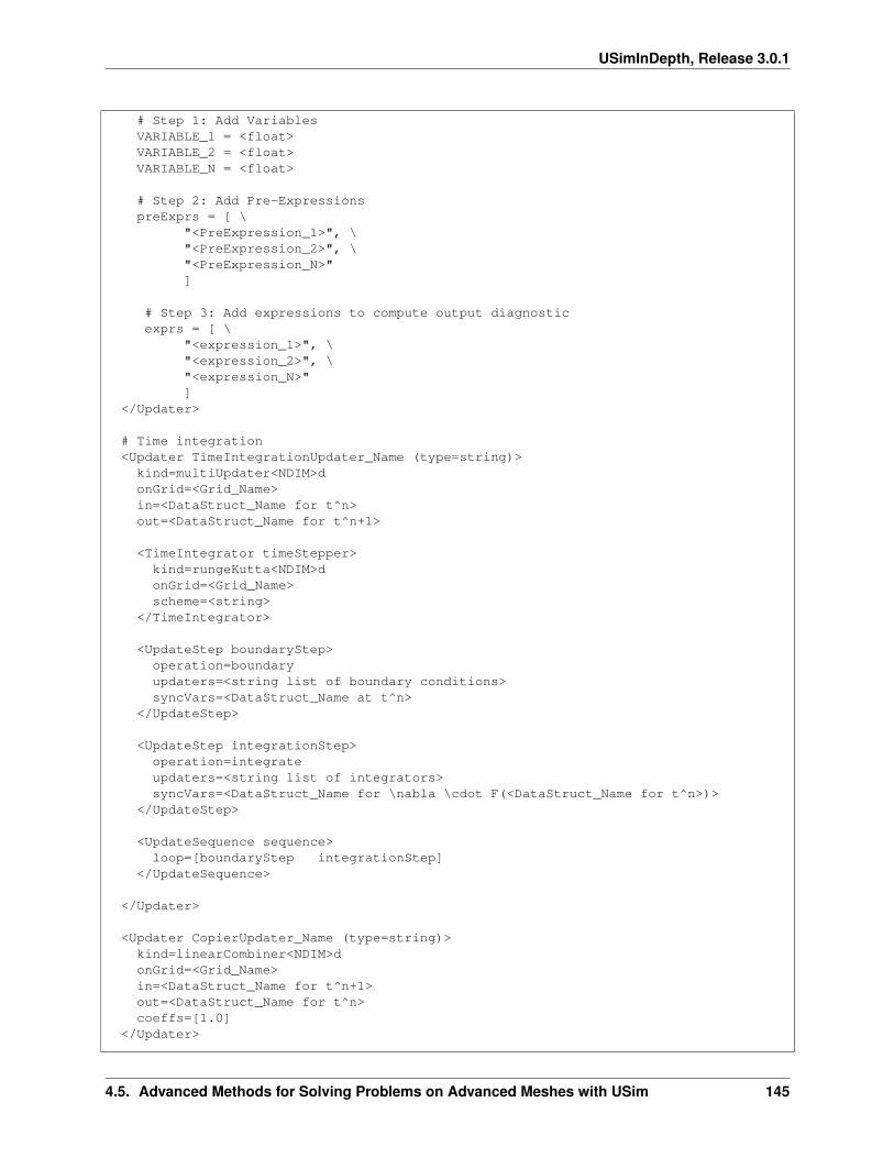
USimInDepth, Release 3.0.1
# Step 1: Add VariablesVARIABLE_1 = <float>VARIABLE_2 = <float>VARIABLE_N = <float>
# Step 2: Add Pre-ExpressionspreExprs = [ \
"<PreExpression_1>", \"<PreExpression_2>", \"<PreExpression_N>"]
# Step 3: Add expressions to compute output diagnosticexprs = [ \
"<expression_1>", \"<expression_2>", \"<expression_N>"]
</Updater>
# Time integration<Updater TimeIntegrationUpdater_Name (type=string)>kind=multiUpdater<NDIM>donGrid=<Grid_Name>in=<DataStruct_Name for t^n>out=<DataStruct_Name for t^n+1>
<TimeIntegrator timeStepper>kind=rungeKutta<NDIM>donGrid=<Grid_Name>scheme=<string>
</TimeIntegrator>
<UpdateStep boundaryStep>operation=boundaryupdaters=<string list of boundary conditions>syncVars=<DataStruct_Name at t^n>
</UpdateStep>
<UpdateStep integrationStep>operation=integrateupdaters=<string list of integrators>syncVars=<DataStruct_Name for \nabla \cdot F(<DataStruct_Name for t^n>)>
</UpdateStep>
<UpdateSequence sequence>loop=[boundaryStep integrationStep]
</UpdateSequence>
</Updater>
<Updater CopierUpdater_Name (type=string)>kind=linearCombiner<NDIM>donGrid=<Grid_Name>in=<DataStruct_Name for t^n+1>out=<DataStruct_Name for t^n>coeffs=[1.0]
</Updater>
4.5. Advanced Methods for Solving Problems on Advanced Meshes with USim 145
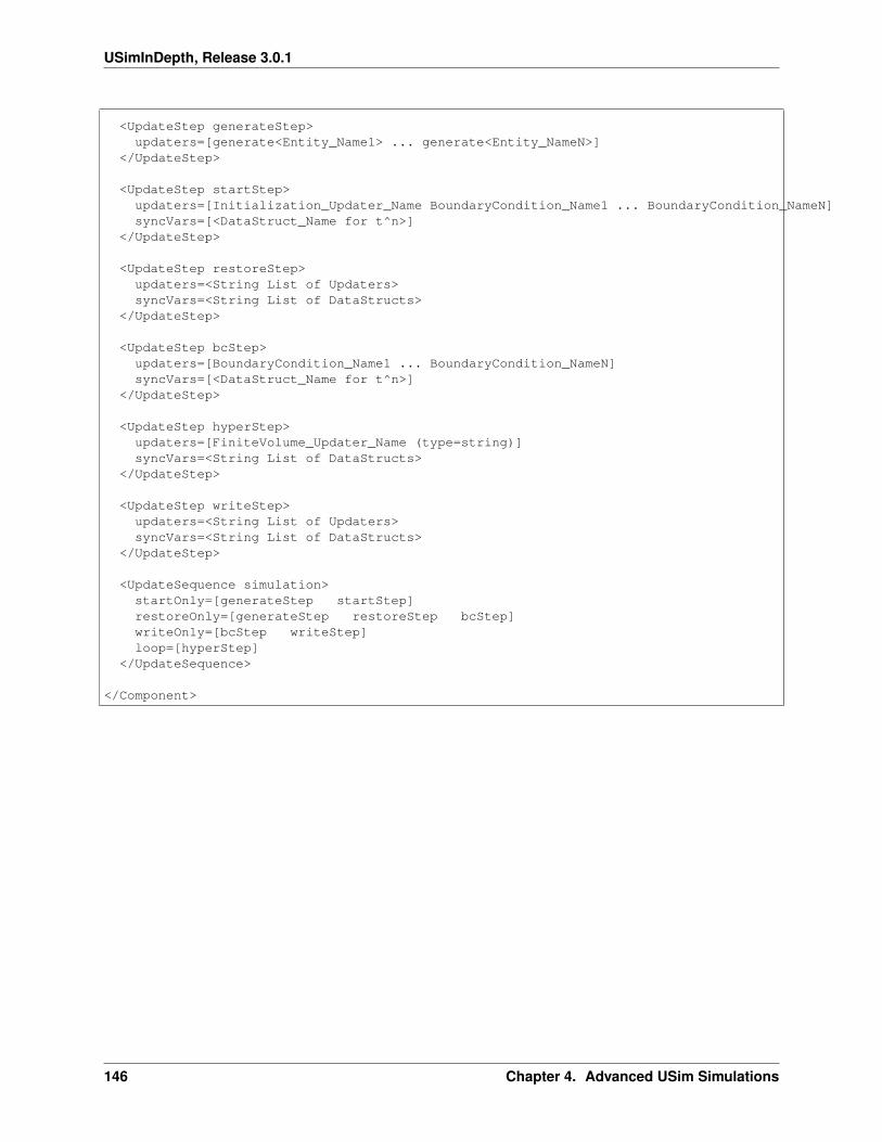
USimInDepth, Release 3.0.1
<UpdateStep generateStep>updaters=[generate<Entity_Name1> ... generate<Entity_NameN>]
</UpdateStep>
<UpdateStep startStep>updaters=[Initialization_Updater_Name BoundaryCondition_Name1 ... BoundaryCondition_NameN]syncVars=[<DataStruct_Name for t^n>]
</UpdateStep>
<UpdateStep restoreStep>updaters=<String List of Updaters>syncVars=<String List of DataStructs>
</UpdateStep>
<UpdateStep bcStep>updaters=[BoundaryCondition_Name1 ... BoundaryCondition_NameN]syncVars=[<DataStruct_Name for t^n>]
</UpdateStep>
<UpdateStep hyperStep>updaters=[FiniteVolume_Updater_Name (type=string)]syncVars=<String List of DataStructs>
</UpdateStep>
<UpdateStep writeStep>updaters=<String List of Updaters>syncVars=<String List of DataStructs>
</UpdateStep>
<UpdateSequence simulation>startOnly=[generateStep startStep]restoreOnly=[generateStep restoreStep bcStep]writeOnly=[bcStep writeStep]loop=[hyperStep]
</UpdateSequence>
</Component>
146 Chapter 4. Advanced USim Simulations
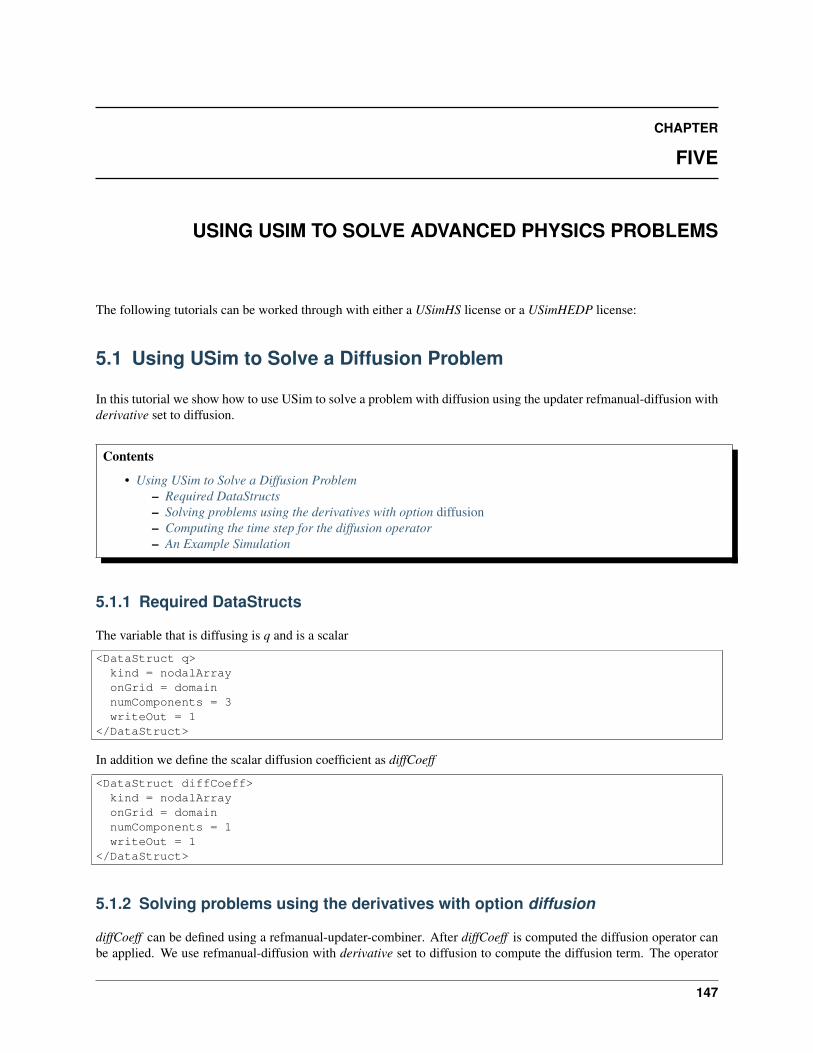
CHAPTER
FIVE
USING USIM TO SOLVE ADVANCED PHYSICS PROBLEMS
The following tutorials can be worked through with either a USimHS license or a USimHEDP license:
5.1 Using USim to Solve a Diffusion Problem
In this tutorial we show how to use USim to solve a problem with diffusion using the updater refmanual-diffusion withderivative set to diffusion.
Contents
• Using USim to Solve a Diffusion Problem– Required DataStructs– Solving problems using the derivatives with option diffusion– Computing the time step for the diffusion operator– An Example Simulation
5.1.1 Required DataStructs
The variable that is diffusing is q and is a scalar
<DataStruct q>kind = nodalArrayonGrid = domainnumComponents = 3writeOut = 1
</DataStruct>
In addition we define the scalar diffusion coefficient as diffCoeff
<DataStruct diffCoeff>kind = nodalArrayonGrid = domainnumComponents = 1writeOut = 1
</DataStruct>
5.1.2 Solving problems using the derivatives with option diffusion
diffCoeff can be defined using a refmanual-updater-combiner. After diffCoeff is computed the diffusion operator canbe applied. We use refmanual-diffusion with derivative set to diffusion to compute the diffusion term. The operator
147
USimInDepth, Release 3.0.1
take in q and diffCoeff and the result (in this case) is stored in qnew
<Updater computeDiffusion>kind = diffusion2donGrid = domainderivative = diffusionnumScalars = 1coefficient = 1.0numberOfInterpolationPoints = 8
in = [q,diffCoeff]out = [qnew]
</Updater>
Note that the complete list of options available in refmanual-diffusion are diffusion, anisotropicDiffusion and gradi-entOfDivergence.
5.1.3 Computing the time step for the diffusion operator
Time integration is performed using super time stepping. Super time stepping is a variable stage Runge-Kutta ap-proach that is much faster (by the number of stages) than standard Runge-Kutta methods for solving diffusionproblems. The approach requires two time steps. The desired (actual) time step is computed using a refmanual-timeStepRestrictionUpdater. The key here is that STS_CFL=40.0 so it is much higher than the explicitly stable timestep for a diffusive system
<Updater timeStepRestriction>
kind = timeStepRestrictionUpdater2din = [diffCoeff]
onGrid = domainrestrictions = [quadratic]
<TimeStepRestriction quadratic>kind = quadraticcfl = STS_CFL
</TimeStepRestriction>
</Updater>
Next the time step for the super time stepping method is computed where an explicitly stable CFL=0.25 is used. Thetime step is stored in stsDt
<Updater getSTSdt>kind = getTimeStepUpdater2din = [diffCoeff]out = [stsDt]onGrid = domainrestrictions = [quadratic]
<TimeStepRestriction quadratic>kind = quadraticcfl = EXPLICIT_CFL
</TimeStepRestriction></Updater>
The Super Time Stepping integrator then knows to take the ratio of the desired time step and the explicitly stable timestep to compute the number of stages used in the STS Updater.
148 Chapter 5. Using USim to Solve Advanced Physics Problems
USimInDepth, Release 3.0.1
5.1.4 An Example Simulation
The input file for the problem Diffusion in the USimHS package demonstrates each of the concepts described above.
5.2 Using USim to Solve the Two-Fluid Plasma Model
In the USimBase tutorials the basic concepts of USim were described. In this first HEDP tutorial we describe howto solve the fully electromagnetic two-fluid plasma equations using a semi-implicit operator to step over the plasmafrequency and cyclotron frequency and electric field diffusion to minimize errors in in the electric field divergencerelation.
Contents
• Using USim to Solve the Two-Fluid Plasma Model– Semi-Implicit Solution for the Lorentz Forces and Current Sources– Electric and Magnetic Field Divergence Cleaning– Computing the Reconnected Magnetic Flux– An Example Simulation
5.2.1 Semi-Implicit Solution for the Lorentz Forces and Current Sources
To demonstrate how to use USim to solve a problem using the two-fluid plasma system, we will use the well knownGEM (geomagnetic environmental modeling) reconnection challenge setup to solve fast reconnection of a currentlayer. The GEM challenge was originally described in
Birn, J., et al. "Geospace Environmental Modeling (GEM) magnetic reconnection challenge."Journal of Geophysical Research: Space Physics (1978-2012) 106.A3 (2001): 3715-3719.
This tutorial is based on the GEM Challenge template.
The first thing we need to model two-fluids, is data structures for the electrons, ions and the electromagnetic field. Inthis case the electrons will be represented by a 5-moment compressible fluid:
<DataStruct electrons>kind = nodalArrayonGrid = domainnumComponents = 5
</DataStruct>
The ions are also represented by a 5-moment compressible fluid:
<DataStruct ions>kind = nodalArrayonGrid = domainnumComponents = 5
</DataStruct>
The electromagnetic field variable contains the full Field vector [Ex,Ey,Ez,Bx,By,Bz,Ep,Bp] with the variables Ep andBp the error correction potentials. As such the electromagnetic field data structure is defined as:
<DataStruct em>kind = nodalArrayonGrid = domain
5.2. Using USim to Solve the Two-Fluid Plasma Model 149
USimInDepth, Release 3.0.1
numComponents = 8</DataStruct>
Separate initialization using an refmanual-initialize updater is performed for each variable, electrons, ions and em:
<Updater initElectrons>kind = initialize2donGrid = domainout = [electrons]
<Function func>kind = exprFunc
.
.
.
preExprs = [ \"rhoe = n0*me*(1.0/(cosh(y/lambda)*cosh(y/lambda))+0.2)", \
"mze = -(me/qe)*b0*(1.0/lambda)*1.0/(cosh(y/lambda)*cosh(y/lambda))", \"ee = (1.0/12.0)*(1./(gamma-1.0))*b0*b0*(rhoe/me)+0.5*(mze*mze/rhoe)"]
exprs = [ \"rhoe", "0.0", "0.0", "mze", "ee"]
</Function>
</Updater>
<Updater initIons>kind = initialize2donGrid = domainout = [ions]
<Function func>kind = exprFunc
.
.
.
preExprs = [ \"rhoi = n0*mi*(1.0/(cosh(y/lambda)*cosh(y/lambda))+0.2)", \
"ei = (5.0/12.0)*(1.0/(gamma-1.0))*b0*b0*(rhoi/mi)"]
exprs = ["rhoi", "0.0", "0.0", "0.0", "ei"]
</Function>
</Updater>
<Updater initEm>kind = initialize2donGrid = domainout = [em]
<Function func>kind = exprFunc
150 Chapter 5. Using USim to Solve Advanced Physics Problems
USimInDepth, Release 3.0.1
.
.
.
preExprs = ["bx = b0*tanh(y/lambda)-psi*(pi/Ly)*cos(2.0*pi*x/Lx)*sin(pi*y/Ly)", \"by = psi*(2.0*pi/Lx)*sin(2.0*pi*x/Lx)*cos(pi*y/Ly)"]
exprs = ["0.0", "0.0", "0.0", "bx", "by", "0.0", "0.0", "0.0"]
</Function>
</Updater>
In the above initialization some variables have been eliminated for conciseness. In addition, every variable, electrons,ions, em, must have their own refmanual-classicMuscl
<Updater hyperElectrons>kind = classicMuscl2donGrid = domaintimeIntegrationScheme = none
numericalFlux = FLUID_NUMERICAL_FLUXpreservePositivity = truelimiter = [LIMITER, none]limiterType = characteristicvariableForm = conservative
in = [electrons]out = [electronsNew]
cfl = CFLequations = [euler]
<Equation euler>kind = eulerEqngasGamma = GAS_GAMMAbasementDensity = BASEMENT_DENSITYbasementPressure = BASEMENT_PRESSURE
</Equation></Updater>
<Updater hyperIons>kind = classicMuscl2donGrid = domaintimeIntegrationScheme = nonenumericalFlux = FLUID_NUMERICAL_FLUXpreservePositivity = truelimiter = [LIMITER]limiterType = characteristicvariableForm = conservative
in = [ions]out = [ionsNew]
cfl = CFLequations = [euler]
<Equation euler>kind = eulerEqn
5.2. Using USim to Solve the Two-Fluid Plasma Model 151
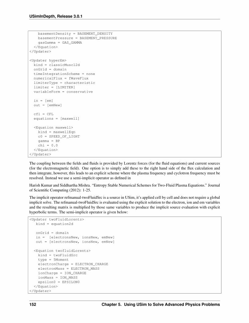
USimInDepth, Release 3.0.1
basementDensity = BASEMENT_DENSITYbasementPressure = BASEMENT_PRESSUREgasGamma = GAS_GAMMA
</Equation></Updater>
<Updater hyperEm>kind = classicMuscl2donGrid = domaintimeIntegrationScheme = nonenumericalFlux = fWaveFluxlimiterType = characteristiclimiter = [LIMITER]variableForm = conservative
in = [em]out = [emNew]
cfl = CFLequations = [maxwell]
<Equation maxwell>kind = maxwellEqnc0 = SPEED_OF_LIGHTgamma = BPchi = 0.0
</Equation></Updater>
The coupling between the fields and fluids is provided by Lorentz forces (for the fluid equations) and current sources(for the electromagnetic field). One option is to simply add these to the right hand side of the flux calculation andthen integrate, however, this leads to an explicit scheme where the plasma frequency and cyclotron frequency must beresolved. Instead we use a semi-implicit operator as defined in
Harish Kumar and Siddhartha Mishra. “Entropy Stable Numerical Schemes for Two-Fluid Plasma Equations.” Journalof Scientific Computing (2012): 1-25.
The implicit operator refmanual-twoFluidSrc is a source in USim, it’s applied cell by cell and does not require a globalimplicit solve. The refmanual-twoFluidSrc is evaluated using the explicit solution to the electron, ion and em variablesand the resulting matrix is multiplied by those same variables to produce the implicit source evaluation with explicithyperbolic terms. The semi-implicit operator is given below:
<Updater twoFluidLorentz>kind = equation2d
onGrid = domainin = [electronsNew, ionsNew, emNew]out = [electronsNew, ionsNew, emNew]
<Equation twofluidLorentz>kind = twoFluidSrctype = 5MomentelectronCharge = ELECTRON_CHARGEelectronMass = ELECTRON_MASSionCharge = ION_CHARGEionMass = ION_MASSepsilon0 = EPSILON0
</Equation></Updater>
152 Chapter 5. Using USim to Solve Advanced Physics Problems
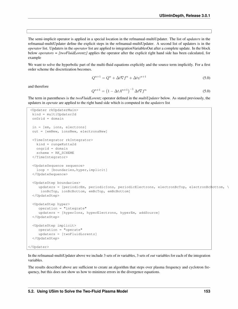
USimInDepth, Release 3.0.1
The semi-implicit operator is applied in a special location in the refmanual-multiUpdater. The list of updaters in therefmanual-multiUpdater define the explicit steps in the refmanual-multiUpdater. A second list of updaters is in theoperator list. Updaters in the operator list are applied to integrationVariablesOut after a complete update. In the blockbelow operators = [twoFluidLorentz] applies the operator after the explicit right hand side has been calculated, forexample
We want to solve the hyperbolic part of the multi-fluid equations explicitly and the source term implicitly. For a firstorder scheme the discretization becomes.
𝑄𝑛+1 = 𝑄𝑛 + ∆𝑡∇𝑓𝑛 + ∆𝑡𝜓𝑛+1 (5.0)
and therefore𝑄𝑛+1 =
(1 − ∆𝑡𝐴𝑛+1
)−1∆𝑡∇𝑓𝑛 (5.0)
The term in parentheses is the twoFluidLorentz operator defined in the multiUpdater below. As stated previously, theupdaters in operate are applied to the right hand side which is computed in the updaters list
<Updater rkUpdaterMain>kind = multiUpdater2donGrid = domain
in = [em, ions, electrons]out = [emNew, ionsNew, electronsNew]
<TimeIntegrator rkIntegrator>kind = rungeKutta2dongrid = domainscheme = RK_SCHEME
</TimeIntegrator>
<UpdateSequence sequence>loop = [boundaries,hyper,implicit]
</UpdateSequence>
<UpdateStep boundaries>updaters = [periodicEm, periodicIons, periodicElectrons, electronBcTop, electronBcBottom, \ionBcTop, ionBcBottom, emBcTop, emBcBottom]
</UpdateStep>
<UpdateStep hyper>operation = "integrate"updaters = [hyperIons, hyperElectrons, hyperEm, addSource]
</UpdateStep>
<UpdateStep implicit>operation = "operate"updaters = [twoFluidLorentz]
</UpdateStep>
</Updater>
In the refmanual-multiUpdater above we include 3 sets of in variables, 3 sets of out variables for each of the integrationvariables.
The results described above are sufficient to create an algorithm that steps over plasma frequency and cyclotron fre-quency, but this does not show us how to minimze errors in the divergence equations.
5.2. Using USim to Solve the Two-Fluid Plasma Model 153
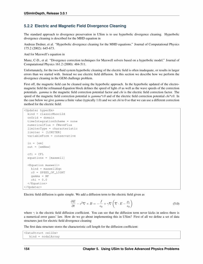
USimInDepth, Release 3.0.1
5.2.2 Electric and Magnetic Field Divergence Cleaning
The standard approach to divergence preservation in USim is to use hyperbolic divergence cleaning. Hyperbolicdivergence cleaning is described for the MHD equation in
Andreas Dedner, et al. “Hyperbolic divergence cleaning for the MHD equations.” Journal of Computational Physics175.2 (2002): 645-673.
And for Maxwell’s equation in
Munz, C-D., et al. “Divergence correction techniques for Maxwell solvers based on a hyperbolic model.” Journal ofComputational Physics 161.2 (2000): 484-511.
Unfortunately, for the two-fluid system hyperbolic cleaning of the electric field is often inadequate, or results in largererrors than we started with. Instead we use electric field diffusion. In this section we describe how we perform thedivergence cleaning in the GEM challenge problem.
First off, the magnetic field can be cleaned using the hyperbolic approach. In the hyperbolic updated of the electro-magnetic field the refmanual-Equation block defines the speed of light c0 as well as the wave speeds of the correctionpotentials. gamma is the magnetic field correction potential factor and chi is the electric field correction factor. Thespeed of the magnetic field correction potential is gamma*c0 and of the electric field correction potential chi*c0. Inthe case below we give gamma a finite value (typically 1.0) and we set chi to 0 so that we can use a different correctionmethod for the electric field:
<Updater hyperEm>kind = classicMuscl2donGrid = domaintimeIntegrationScheme = nonenumericalFlux = fWaveFluxlimiterType = characteristiclimiter = [LIMITER]variableForm = conservative
in = [em]out = [emNew]
cfl = CFLequations = [maxwell]
<Equation maxwell>kind = maxwellEqnc0 = SPEED_OF_LIGHTgamma = BPchi = 0.0
</Equation></Updater>
Electric field diffusion is quite simple. We add a diffusion term to the electric field given as
𝜕𝐸
𝜕𝑡− 𝑐2∇×𝐵 = − 𝐽
𝜖0+ 𝛾∇
(∇ · 𝐸 − 𝜌𝑐
𝜖0
)(5.0)
where 𝛾 is the electric field diffusion coefficient. You can see that the diffusion term never kicks in unless there isa numerical error gauss’ law. How do we go about implementing this in USim? First of all we define a set of datastructures just for electric field divergence cleaning
The first data structure stores the characteristic cell length for the diffusion coefficient:
<DataStruct cellDx>kind = nodalArray
154 Chapter 5. Using USim to Solve Advanced Physics Problems
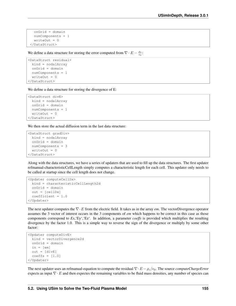
USimInDepth, Release 3.0.1
onGrid = domainnumComponents = 1writeOut = 0
</DataStruct>
We define a data structure for storing the error computed from ∇ · 𝐸 − 𝜌𝑐
𝜖0:
<DataStruct residual>kind = nodalArrayonGrid = domainnumComponents = 1writeOut = 0
</DataStruct>
We define a data structure for storing the divergence of E:
<DataStruct divE>kind = nodalArrayonGrid = domainnumComponents = 1writeOut = 0
</DataStruct>
We then store the actual diffusion term in the last data structure:
<DataStruct gradDiv>kind = nodalArrayonGrid = domainnumComponents = 3writeOut = 0
</DataStruct>
Along with the data structures, we have a series of updaters that are used to fill up the data structures. The first updaterrefmanual-characteristicCellLength simply computes a characteristic length for each cell. This updater only needs tobe called at startup since the cell length does not change.
<Updater computeCellDx>kind = characteristicCellLength2donGrid = domainout = [cellDx]coefficient = 1.0
</Updater>
The next updater computes the ∇·𝐸 from the electric field. It takes as in the array em. The vectorDivergence operatorassumes the 3 vector of interest occurs in the 3 components of em which happens to be correct in this case as thosecomponents correspond to Ex,‘Ey‘,‘Ez‘. In addition, a parameter coeffs is provided which multiplies the resultingdivergence by the factor 1.0. This is a simple way to reverse the sign of the divergence or multiply by some otherfactor:
<Updater computeDivE>kind = vectorDivergence2donGrid = domainin = [em]out = [divE]coeffs = [1.0]
</Updater>
The next updater uses an refmanual-equation to compute the residual ∇·𝐸−𝜌𝑐/𝜖0. The source computeChargeErrorexpects as input ∇ ·𝐸 and then expectes the remaining variables to be fluid mass densities, any number of species can
5.2. Using USim to Solve the Two-Fluid Plasma Model 155
USimInDepth, Release 3.0.1
be added. Along with the species mass densities we provide a list indicating the species mass and species charge foreach of these species densities. We also specify the permittivity epsilon0 so that the residual can be calculated.
<Updater computeResidual>kind = equation2donGrid = domain
in = [divE, electrons, ions]out = [residual]
<Equation>kind = computeChargeErrorspeciesCharge = [ELECTRON_CHARGE, ION_CHARGE]speciesMass = [ELECTRON_MASS, ION_MASS]epsilon0 = EPSILON0
</Equation>
</Updater>
The final diffusion term including gamma factor is computed using a scalar gradient calculator. The scalar gradienttakes 2 inputs. It takes the gradient of the first input (residual in this case) and multiplies that gradient by the secondinput cellDx. The result is the multiplied by coefficient which is constant for all space. This particular form of diffusionis such that the diffusion is stable to explicit time stepping. If super time stepping is used or subcycling, the diffusioncoefficient can be increased to do a better job of error cleaning.
<Updater gradient>kind = scalarGradient2dgradientType = leastSquaresonGrid = domainin = [residual, cellDx]out = [gradDiv]coefficient = 0.5
</Updater>
Once the diffusion term is computed it needs to be added to the right hand side of the update equation. The term isadded after the hyperbolic explicit terms are computed. We use a combiner2d to add the diffusion term to the equation.In this example the updater takes two input data structures, emNew and gradDiv and dumps the output into emNew.Every input variable requires an indVars_inputName block which provides a way to access each component of theinput variable. These names can then be used in the output expression exprs. In the refmanual-multiUpdater, theaddSource block is called after the hyperbolic terms so that it is not overwritten by updaters that are called earlier.
<Updater addSource>kind = combiner2donGrid = domain
in = [emNew, gradDiv]out = [emNew]
indVars_emNew = ["ex","ey","ez","bx","by","bz","phiE","phiB"]indVars_gradDiv = ["dx","dy","dz"]c = SPEED_OF_LIGHTexprs = ["ex+c*dx","ey+c*dy","ez+c*dz","bx","by","bz","phiE","phiB"]
</Updater>
Finally, boundary conditions must be provided to the residual. In this problem the residual on the boundary should be0 so we use a refmanual-functionBc to explicitly set the residual on the boundary to zero. The variable out specifiesthe data that the boundary condition will be applied to, while entity tells the boundary condition which boundary itshould be applied to. In this case entity=ghost means that the boundary is applied to all boundary cells.
156 Chapter 5. Using USim to Solve Advanced Physics Problems
USimInDepth, Release 3.0.1
<Updater residualBc>kind = functionBc2d
onGrid = domain
<Function func>kind = exprFuncexprs = ["0.0"]
</Function>
out = [residual]entity = ghost
</Updater>
This simulation has periodic boundaries in the x direction so we also apply a periodic boundary condition to theresidual. This boundary condition is called after residualBc so it overwrites the boundry conditions in the X directionset by residualBc
<Updater periodicResidual>kind = periodicCartBc2donGrid = domainin = [residual]out = [residual]
</Updater>
Now that we’ve added a bunch of new updaters we need to modify the multiUpdater to include the changes thathave been made. The new updater added to the updater list include computeDivE, computeResidual, residu-alBc,‘periodicResidual‘,‘gradient‘ in the UpdateStep‘s compute and clean. These updaters are evaluated after theboundary conditions for electrons,‘ions‘ and em are applied, but before the hyperbolic updaters are called hyperI-ons, hyperElectrons and hyperEm. Once again, for parallel simulations it’s very important to get the synchronizationcorrect. We’ve added one synchronizations. The new synchronization occurs directly after periodicResidual. peri-odicResidual is the last updater that is applied before a derivative gradient is computed on residual so we need tosynchronize residual at this point.
<Updater rkUpdaterMain>kind = multiUpdater2donGrid = domain
in = [em, ions, electrons]out = [emNew, ionsNew, electronsNew]
<TimeIntegrator rkIntegrator>kind = rungeKutta2dongrid = domainscheme = RK_SCHEME
</TimeIntegrator>
<UpdateSequence sequence>loop = [boundaries,compute,clean,hyper,implicit]
</UpdateSequence>
<UpdateStep boundaries>updaters = [periodicEm, periodicIons, periodicElectrons, electronBcTop, electronBcBottom, \ionBcTop, ionBcBottom, emBcTop, emBcBottom]
</UpdateStep>
<UpdateStep compute>updaters = [ computeDivE, computeResidual, residualBc, periodicResidual]
5.2. Using USim to Solve the Two-Fluid Plasma Model 157
USimInDepth, Release 3.0.1
</UpdateStep>
<UpdateStep clean>updaters = [ gradient]
</UpdateStep>
<UpdateStep hyper>operation = "integrate"updaters = [hyperIons, hyperElectrons, hyperEm, addSource]
</UpdateStep>
<UpdateStep implicit>operation = "operate"updaters = [twoFluidLorentz]
</UpdateStep>
</Updater>
Finally, recall that the characteristic cell lengths only need to be calculated once. As a result we calculate them duringthe initialization step.
<UpdateStep initStep>updaters = [initElectrons, initIons, initEm, computeCellDx]syncVars = [electrons, ions, em]
</UpdateStep>
5.2.3 Computing the Reconnected Magnetic Flux
In the GEM Challenge simulation we’ve added passive diagnostic to compute the line integral across the domain. Inorder to compute the line integral we add two data structures. The first data structure is called a refmanual-bin. Thebin is a uniform grid that overlays the exiting grid. The extents of the bin match the extents of the grid, but a binis rectangular regardless of the shape of the grid. The bin has two important parameters, the first is onGrid whichspecifies which grid the bin will use to define itself, the second is the scale. scale tells roughly how many bins thereare per grid cell in domain. The bin is used for fast lookup so that USim can quickly tell which cell a particular pointin space is in. The bin is given as
<DataStruct cellBin>kind = binonGrid = domainscale = 2.0
</DataStruct>
In addition we need to fill the bin with data. In this particular case we want to fill each bin with a a list of indexescorresponding to the cells that fall inside each cell of the bin. The refmanual-binCells updater does exactly that. Thisupdater only needs to be called at startup since the grid does not change with time.
<Updater fillBin>kind = binCells2donGrid = domainout = [cellBin]
</Updater>
The second variable is a refmanual-dynVector. A dynVector is a dataStructure which is a vector and has the same valueon all domains in parallel simulations. dynVectors store a time series of data, so the value of the dynVector is dumpedat every time step so it can be used to store integrated quantities. The dynVector had numComponents to specify howlong the vector is. In this case it stores only 1 value. writeOut=true is set so the dynVector is written.
158 Chapter 5. Using USim to Solve Advanced Physics Problems
USimInDepth, Release 3.0.1
<DataStruct integratedFlux>kind = dynVectornumComponents = 1writeOut = 1
</DataStruct>
These two data structures are then used to compute the line integral with the refmanual-lineIntegral updater. Therefmanual-lineIntegral behaves like a refmanual-updater-combiner except that it takes in refmanual-nodalArray‘s andfills up a refmanual-dynVector.
<Updater computeLineIntegral>kind = lineIntegral2donGrid = domainstartPosition = [XMIN, 0.0]endPosition = [XMAX, 0.0]numberOfSamples = 1000
layout = [cellBin]in = [em]indVars_em = ["ex","ey","ez","bx","by","bz","phiE","phiB"]exprs = ["0.5*abs(by)"]out = [integratedFlux]
</Updater>
This updater should not be called within an rkUpdater otherwise it will store multiple values per time step. Instead wecall this updater in its own refmanual-UpdateStep
<UpdateStep diagnosticStep>updaters = [computeLineIntegral]
</UpdateStep>
5.2.4 An Example Simulation
The input file for the problem GEM Challenge in the USim USimHEDP package demonstrates each of the conceptsdescribed above to solve fast magnetic reconnection.
5.3 Using USim to Solve MHD with General Equation of State
In the USimBase tutorials the basic concepts of USim were described. In this HEDP tutorial we show how to use theideal MHD equations with general equation of state and a simple radiation model.
Contents
• Using USim to Solve MHD with General Equation of State– Solving Problems using the idealMhdEosEqn– Adding an Analytic Energy Loss Term– Divergence Cleaning the Magnetic Field as A Separate Step– Using the vertexJetUpdater– An Example Simulation
5.3. Using USim to Solve MHD with General Equation of State 159
USimInDepth, Release 3.0.1
5.3.1 Solving Problems using the idealMhdEosEqn
The plasma jets problem uses an ideal MHD model with general equation of state refmanual-idealMhdEosEqn anda simple radiation loss model refmanual-bremsPowerSrc. More sophisticated radiation loss can be included withpurchase of the PROPACEOS tables from prism computational sciences or use of the SESAME tables from LosAlamos National Laboratory. The key to this whole development is the use of the refmanual-idealMhdEosEqn in thehyperbolic updater given below:
<Updater hyper>kind = classicMuscl$DIM$donGrid = domainnumericalFlux = NUMERICAL_FLUXtimeIntegrationScheme = none
variableForm = conservativepreservePositivity = truelimiter = [LIMITER, LIMITER, none]
in = [q, pressure, soundSpeed]out = [qnew]
cfl = CFL
equations = [mhd]
<Equation mhd>kind = idealMhdEosEqnbasementDensity = $0.1*BASEMENT_DENSITY$basementPressure = $0.1*BASEMENT_PRESSURE$mu0 = MU0correctionSpeed = 0.0
</Equation>
</Updater>
A few key differences for this refmanual-classicMuscl updater are that it takes in multiple input variables. In this casethe conserved variables q, the fluid pressure pressure and an estimate of the speed of sound soundSpeed. Since thepressure and sound speed are inputs the user can define these however they wish, with the caveat that the sound speedshould be a good estimate in order to produce accurate (and stable) results.
For every variable input into the refmanual-classicMuscl updater a limiter must be provided limiter=[LIMITER, LIM-ITER, none]. In this case we limit the conserved variable and the pressure, but don’t limit the sound speed since it’sonly used to add diffusion to the system and compute a time step. In this case the ‘correctionSpeed is being set to 0.0as we will use a separate updater to evolve the correction potential.
The key issue then becomes how to compute the pressure and sound speed outside the hyperbolic update? As anexample we use an ideal equation of state and use a refmanual-updater-combiner to compute the pressure from theenergy:
<Updater computePressure>kind = combiner$DIM$donGrid = domain
in = [q]out = [pressure]mu0 = MU0gamma = GAMMAbp = BASEMENT_PRESSUREindVars_q = ["rho","mx","my","mz","en","bx","by","bz","phi"]
160 Chapter 5. Using USim to Solve Advanced Physics Problems
USimInDepth, Release 3.0.1
exprs = ["max(1.1*bp,(gamma-1)*(en-(0.5/mu0)*(bx*bx+by*by+bz*bz)-0.5*(mx*mx+my*my+mz*mz)/rho))"]</Updater>
In this case a basement pressure is used so the maximum of the basement pressure and the computed pressure is taken.Alternatively, the refmanual-propaceosVariables or refmanual-sesameVariables updaters may be used to compute anequation of state for the pressure as a function of the temperature and density. Similarly, we use a combiner to computethe sound speed based on the pressure and the density:
<Updater computeSoundSpeed>kind = combiner$DIM$donGrid = domain
in = [q, pressure]out = [soundSpeed]gamma = GAMMAindVars_q = ["rho","mx","my","mz","en","bx","by","bz","phi"]indVars_pressure = ["pressure"]
exprs = ["sqrt(gamma*pressure/rho)"]</Updater>
These results can be easily applied in a multiUpdater to produce an MHD model with a user specified equation ofstate. The refmanual-multiUpdater for this system follows where the pressure and density are computed before hyperupdater is called:
<Updater rkUpdater>kind = multiUpdater$DIM$donGrid = domaintimeIntegrationScheme = RKSCHEME
updaters = [bc, computePressure, computeSoundSpeed, hyper]
syncVars_bcBack =[q]syncVars_hyper = [qnew]
integrationVariablesIn = [q]integrationVariablesOut = [qnew]dummyVariables_q = [dummy1, dummy2]
syncAfterSubStep = [qnew]</Updater>
5.3.2 Adding an Analytic Energy Loss Term
Adding an energy loss term is quite simple, except the user needs to make sure that the energy loss does not leadnegative energies in the MHD model. In this case we use radiated power as estimated by analytical estimates ofBremsstrahlung radiation. The refmanual-bremsPowerSrc computes radiated power density (𝑊/𝑚3) given plasmadensity, temperature and the effective Z. The block below shows how to use the refmanual-bremsPowerSrc:
<Updater computeRadPower>kind = equation$DIM$donGrid = domainin = [density, temperature, zEffective]out = [radiationPower]
<Equation Bremsstrahlung>kind = bremsPowerSrc
5.3. Using USim to Solve MHD with General Equation of State 161
USimInDepth, Release 3.0.1
</Equation></Updater>
The dataStruct radiationPower has a single component and this value must then be subtracted from the fluid energyequation as shown below using a refmanual-updater-combiner:
<Updater addRadiation>kind = combiner$DIM$donGrid = domain
in = [qnew, radiationPower]out = [qnew]
indVars_qnew = ["rho","mx","my","mz","en","bx","by","bz","phi"]indVars_radiationPower = ["radiation"]
exprs = ["rho","mx","my","mz","en-radiation","bx","by","bz","phi"]</Updater>
In certain cases the radiated power an be huge, so much so that if the time step is not reduced all the energy in thesystem will dissappear. To get around this problem we use a positiveValue time step restriction inside a refmanual-timeStepRestrictionUpdater. A refmanual-timeStepRestrictionUpdater takes a list of input variables, and a list ofrestriction‘s. The restriction in this case is the refmanual-positiveValue restriction. The variable positiveIndex refersto the index of the first input variable (in this case pressure). The variable sourceIndex refers to the index of the secondvariable sourceIndex. In this case the maximum time step is computed using
∆𝑡 = alpha*(pressure[positiveValue]-basementValue)/(-coefficient*radiationPower[sourceIndex]) (5.0)
And what the refmanual-positiveValue restriction does is it choses a time step so that you only subtract off the fractionalpha of the remaining energy in the input pressure. This time step is then compared with the other time steps computedby other restrictions and updaters and the smallest time allowable time step is used for the update:
<Updater timeStepRestriction>kind = timeStepRestrictionUpdater$DIM$din = [pressure, radiationPower]onGrid = domainrestrictions = [radiation]
<TimeStepRestriction radiation>kind = positiveValuepositiveIndex = 0sourceIndex = 0basementValue = BASEMENT_PRESSUREalpha = 0.25coefficient = -1.0
</TimeStepRestriction></Updater>
In this case radiatedPower is always positive. Since radiatedPower is actually subtracted from pressure (not added)we set coefficient=-1.0. If radiatedPower was defined to be negative then coefficient=1.0 would be the correct value.With radiation added the refmanual-multiUpdater looks like this:
<Updater rkUpdater>kind = multiUpdater$DIM$donGrid = domaintimeIntegrationScheme = RKSCHEME
updaters = [correctMore, bc, computeDensity, computeTemperature, computePressure, \
162 Chapter 5. Using USim to Solve Advanced Physics Problems
USimInDepth, Release 3.0.1
computeSoundSpeed, computeRadPower, timeStepRestriction, \hyper, addRadiation]
syncVars_bcBack =[q]syncVars_hyper = [qnew]
integrationVariablesIn = [q]integrationVariablesOut = [qnew]dummyVariables_q = [dummy1, dummy2]
syncAfterSubStep = [qnew]</Updater>
The timeStepRestriction is included in the refmanual-multiUpdater, but could also be included in a separate Updat-eStep depending on how rapidly the power loss is changing.
5.3.3 Divergence Cleaning the Magnetic Field as A Separate Step
In this problem divergence cleaning is computed as a separate step using refmanual-hyperbolicCleanEqn. This ap-proach has benefits because a less diffusive method can be used for the cleaning update and for certain choices ofnumerical flux, it can reduce overall diffusion of the solution. We use a separate refmanual-classicMuscl updater asdefined below:
<Updater hyperClean>kind = classicMuscl2dtimeIntegrationScheme = nonevariableForm = conservative
cfl = CFL
numericalFlux = hlleFlux
limiter = [muscl]
onGrid = domainin = [qClean]out = [qCleanNew]
equations = [clean]
<Equation clean>kind = hyperbolicCleanEqnwaveSpeed = CORRECTIONSPEED
</Equation></Updater>
Which uses the refmanual-hyperbolicCleanEqn. The refmanual-hyperbolicCleanEqn takes one parameter waveSpeedwhich is the speed that the correction wave propagates at. As with the refmanual-multiUpdater for evolving the rest ofthe MHD model, we must also include boundary conditions for the cleaning update:
<Updater rkClean>kind = multiUpdater2donGrid = domaintimeIntegrationScheme = rk2updaters = [cleanCopyBc, hyperClean]
integrationVariablesIn = [qClean]
5.3. Using USim to Solve MHD with General Equation of State 163
USimInDepth, Release 3.0.1
integrationVariablesOut = [qCleanNew]dummyVariables_qClean = [dummyClean1,dummyClean2]
syncAfterSubStep = [qCleanNew]</Updater>
<Updater cleanCopyBc>kind = copy2donGrid = domainout = [qClean]entity = ghost
</Updater>
<Updater copyClean>kind = linearCombiner2donGrid = domainin = [qCleanNew]out = [qClean]coeffs = [1.0]
</Updater>
In the above example we used the DataStructAlias which is a pointer to a DataStruct:
<DataStructAlias qClean>kind = nodalArraytarget = qcomponentRange = [5,9]
</DataStructAlias>
<DataStructAlias qCleanNew>kind = nodalArraytarget = qNewcomponentRange = [5,9]
</DataStructAlias>
In the DataStructAlias we only need to define target which is the DataStruct that the alias is pointing to, the compo-nentRange which defines which components of DataStruct to use. In the case above componentRange=[5,9] meansthat qClean points to elements [5,6,7,8] of q.
Finally, we put all of this into its own update step:
<UpdateStep cleanStep>updaters = [rkClean, copyClean]
</UpdateStep>
Which can then be called before the main refmanual-multiUpdater.
5.3.4 Using the vertexJetUpdater
The refmanual-vertexJetUpdater was an updater specifically designed for modeling the Los Alamos Plasma LinerExperiment. It allows one to easily generate a series of directed jets with uniform initial conditions each alignedabout their own axis. The refmanual-vertexJetUpdater works in both 2 and 3 dimensions. The variety of optionsprovided by the updater are described in the reference manual, however we can point out a few key things here. Anarbitrary number of jets can be defined by adding additional vertices, but they must be labeled in sequential ordervertex0,1,2,3,.... The vertex represents the tip of the jet and that jet will be directed towards the location specified byorigin. The width of the jet defines the width about each jet will be evaluated perpendicular to the line from the vertexto the origin. The length specifies the distance from the vertex along the line from the vertex to the origin that the
164 Chapter 5. Using USim to Solve Advanced Physics Problems
USimInDepth, Release 3.0.1
jet will be evaluated. The normalizedDensityFunction is used to define jets with non-uniform density profiles. Thedensity profile is rotated into the coordinate system where X is parallel to the vector from the origin to the vertex andY and Z are perpendicular. An example block is given below where it is used to update q:
<Updater jetSet>kind = vertexJetUpdater$DIM$d
origin = [0.0, 0.0, 0.0]width = JET_INIT_WIDTHlength = JET_INIT_LENGTH
radialVelocity = $-U$
numberDensity = $RHO_JET/MI$speciesMass = MItemperature = TKELVIN
<normalizedDensityFunction>kind = exprFuncpreExprs = JET_DENSITY_PRE_FUNCTIONexprs = JET_DENSITY_FUNCTION
</normalizedDensityFunction>
vertex0 = [RAD, 0.0, 0.0]vertex1 = [0.0, RAD, 0.0]vertex2 = [-RAD, 0.0, 0.0]vertex3 = [0.0, -RAD, 0.0]
vertex4 = [$(1.0/sqrt(2.0))*RAD$, $(1.0/sqrt(2.0))*RAD$, 0.0]vertex5 = [$-(1.0/sqrt(2.0))*RAD$, $(1.0/sqrt(2.0))*RAD$, 0.0]vertex6 = [$-(1.0/sqrt(2.0))*RAD$, $-(1.0/sqrt(2.0))*RAD$, 0.0]vertex7 = [$(1.0/sqrt(2.0))*RAD$, $-(1.0/sqrt(2.0))*RAD$, 0.0]
includeElectronTemperature = false
correctionSpeed = CORRECTIONSPEED
gasGamma = GAMMA
#We use the mhdMunzEqn to initialize energy based on a temperaturemodel = mhdMunzEqnmu0 = MU0onGrid = domain
out = [q]</Updater>
5.3.5 An Example Simulation
The input file for the problem Plasma Jet Merging in the USim USimHEDP package demonstrates each of the conceptsdescribed above to solve the plasma jet merging problem.
5.3. Using USim to Solve MHD with General Equation of State 165
USimInDepth, Release 3.0.1
5.4 Using USim to Solve MHD with General Equation of State
In the USimBase tutorials the basic concepts of USim were described. In this HEDP tutorial we show how to use thetwo-temperature mhd equations with general equation of state on an unstructured grid.
Contents
• Using USim to Solve MHD with General Equation of State– Solving Problems Using The twoTemperatureMhdEosEqn– Computing the Electric Field– Computing J through ∇×𝐵– Computing Pressure– Current Boundary Condition– An Example Simulation
5.4.1 Solving Problems Using The twoTemperatureMhdEosEqn
This problem is performed on an unstructured grid in axisymmetric geometry. The standard grid block is used makingsure to set isRadial=true and using the unstructured gmsh grid file called dpf1.msh:
<Grid domain>kind = unstructured
ghostLayers = 2isRadial = truedecomposeHalos = false
<Creator ctor>kind = gmshndim = 2file = dpf1.msh
</Creator></Grid>
The refmanual-twoTemperatureMhdEosEqn is considerably more complex than any of the ideal MHD models sincethe electric field is computed externally. The hyperbolic updater is given below using the refmanual-classicMusclmethod:
<Updater hyper>kind = classicMuscl2donGrid = domainvariableForm = conservativegradientType = leastSquares
timeIntegrationScheme = nonepreservePositivity = truenumericalFlux = NUMERICALFLUXlimiterType = component
in = [q, pressure, electronPressure, soundSpeed, J, E, Z]out = [qnew]
cfl = CFLlimiter = [LIMITER, LIMITER, LIMITER, none, LIMITER, LIMITER, none]equations = [mhd]
166 Chapter 5. Using USim to Solve Advanced Physics Problems
USimInDepth, Release 3.0.1
sources = [axisymmetricSource, mhdSrc]
<Equation mhd>kind = twoTemperatureMhdEosEqnmu0 = MU0ionMass = MIgasGamma = GAMMAfundamentalCharge = CHARGEbasementDensity = BASEMENTDENSITYbasementPressure = BASEMENTPRESSURE
</Equation>
<Source axisymmetricSource>kind = mhdSymsymmetryType = cylindricalmodel = twoTemperatureMhdEosEqninputVariables = [q, pressure, electronPressure, J, E, Z]fundamentalCharge = CHARGEmu0 = MU0ionMass = MI
</Source>
<Source mhdSrc>kind = mhdSrcmodel = twoTemperatureMhdEosEqninputVariables = [q, J, E, Z]fundamentalCharge = CHARGEmu0 = MU0ionMass = MI
</Source>
</Updater>
The updater differs from previous MHD type schemes in that we have 7 input variables which are described in thereference manual for refmanual-twoTemperatureMhdEosEqn. The 7 variables are the conserved variable vector q, thepressure p the electron pressure electronPressure an estimate of the local sound speed soundSpeed the current density(computed from the curl of the magnetic field) J, the electric field E and the local charge state Z which can varyspatially
Limiters must be defined for each input variable, in this case we have
limiter = [LIMITER, LIMITER, LIMITER, none, LIMITER, LIMITER, none]
where each limiter corresponds to the corresponding input variable. Limiters need to be applied to q, p, electronPres-sure, E and J since derivatives of each of these terms are compute. No limiters are applied to the remaining variable.Limiters could also be applied to soundSpeed and Z however the stability of the scheme does not depend on limitingthis terms so we reduce the work load by not limiting these variables.
The Equation block is kind=twoTemperatureMhdEosEqn and is given by
<Equation mhd>kind = twoTemperatureMhdEosEqnmu0 = MU0ionMass = MIgasGamma = GAMMAfundamentalCharge = CHARGEbasementDensity = BASEMENTDENSITYbasementPressure = BASEMENTPRESSURE
</Equation>
5.4. Using USim to Solve MHD with General Equation of State 167
USimInDepth, Release 3.0.1
Where the variables are described in the reference manual. In addition to the Equation block we require two Sourceblocks. The following line indicates which sources will be called by the updater
sources = [axisymmetricSource, mhdSrc]
The first source adds the axisymmetric terms of the hyperbolic flux so that the derivative is correct in axisymmetricgeometry. This block is defined in refmanual-mhdSym and some specifics outlined here
<Source axisymmetricSource>kind = mhdSymsymmetryType = cylindricalmodel = twoTemperatureMhdEosEqninputVariables = [q, pressure, electronPressure, J, E, Z]fundamentalCharge = CHARGEmu0 = MU0ionMass = MI
</Source>
We are interested in cylindrical symmetry so symmetryType=cylindrical is specified. The model being used is model= twoTemperatureMhdEosEqn. The key parameter in the axisymmetricSource block is the inputVariable block. Incomputing sources, if USim does not include inputVariable block it will assume that the inputVariables will be pro-vided for the updaters in list in the order they are provided. In this case this is not what is desired so we must specifya inputVariable list so that USim uses the correct variables in evaluating the source.
First note that in the classicaMuscl2d updater the in list is given as
in = [q, pressure, electronPressure, soundSpeed, J, E, Z]
The axisymmetric source does not need the variable soundSpeed, so, if no inputVariables list is specified in the ax-isymmetric source then USim will try and use the first 6 variables q,‘pressure‘,‘electronPressure‘ soundSpeed,‘J‘ andE in evaluating the source. Fortunately the size of soundSpeed is wrong (size 1 instead of the expected size 3) soUSim will throw an exception and won’t run. In order to get around this problem, and to get the correct computedsource we specify the inputVariables list. The inputVariables can only contain variables specified in the in list of theclassicMusclUpdater2d. In this example the correct inputVariables is
inputVariables = [q, pressure, electronPressure, J, E, Z]
note that there is no soundSpeed variable in this list.
The next Source is the mhdSrc. This source is needed to add the 𝐸 · 𝐽𝑒 term to the electron energy equation since thetwo-temperature mhd system cannot be written entirely in flux form. The source is desribed in refmanual-mhdSrc andsome details are given here
<Source mhdSrc>kind = mhdSrcmodel = twoTemperatureMhdEosEqninputVariables = [q, J, E, Z]fundamentalCharge = CHARGEmu0 = MU0ionMass = MI
</Source>
The kind=mhdSrc is specified and the model is twoTemperatureMhdEosEqn. As with the axisymmetric source theuser must specify inputVariables to override the default input variables that would be used based on the in list fromthe classicaMuscl2d updater. In this case the list is given as
inputVariables = [q, J, E, Z]
168 Chapter 5. Using USim to Solve Advanced Physics Problems
USimInDepth, Release 3.0.1
5.4.2 Computing the Electric Field
The electric field could be computed using a combiner, but USim also has a refmanual-generalizedOhmsLaw updaterwhich can simplify things. The generalizedOhmsLaw updater is discussed in the reference manual. It allows the userto add electron pressure gradient, resistive hall and ideal terms to the electric field. All derivatives (such as the electronpressure gradient) are computed outside of the generalizedOhmsLaw updater. The generalizedOhmsLaw used in thiscase is specified below
<Updater computeE>kind = generalizedOhmsLaw2donGrid = domain
in = [q, J, Z]out = [E]
hallTerm = false
fundamentalCharge = CHARGEionMass = MIelectronMass = MEboltzmannConstant = KB
</Updater>
The updater takes in parameters conserved variable vector q, current density J and the charge state Z. These terms aresufficient to compute the ideal and hall terms. In order to add in resistivity and the electron pressure gradient refer tothe manual. In this case hallTerm is set to false as it severly constrains the time step in many explicit simulations. Theoutput is stored in the electric field E which has 3 components regardless of whether a refmanual-generalizedOhmsLaw1d, 2d or 3d is used.
5.4.3 Computing J through ∇×𝐵
Derivatives such as gradient, divergence and curl can be computed using two different types of algorithms in USim.The first approach is a finite difference approach which is fast, but becomes inaccurate on triangular and sufficientlyskewed quadrilateral meshes. This approach currently works consistently in 1, 2 and 3 dimension. The followingexample shows how to compute the curl using a finite difference approach
<Updater computeJ>kind = curl2donGrid = domaininIndex = [5, 6, 7]outIndex = [0, 1, 2]in = [q]out = [J]coefficient = $1.0/MU0$
</Updater>
The updater is described in the reference manual. In this case we want the curl of the magnetic field to compute thecurrent density J. The input variable is the conserved variable vector q and the output is the current density J. Themagnetic field component stored in the conserved variable vector q occur in components [5,6,7] of the vector q so wemust specify inIndex=[5,6,7] so that USim takes the correct components when computing J.
The second approach produces better results on unstructured grids and uses a least squares approach to computingthe curl. This method is more accurate than the finite difference approach and is robust in 1 and 2 dimensions, but isslower than the previous method. An example block using the least squares refmanual-vector, with the option curl isgiven below
5.4. Using USim to Solve MHD with General Equation of State 169
USimInDepth, Release 3.0.1
<Updater computeJ>kind = vector2donGrid = domainderivative = curlnumScalars = 1orderAccuracy = 1coefficient = $1.0/MU0$numberOfInterpolationPoints = 5
in = [BPhi]out = [J]
</Updater>
This updater expects an input vector of size 3 and produces and output vector of size 3. In this case, a second datastruct BPhi was created and the magnetic field form q was copied into that variable. In addition, the parameternumberOfInterpolationPoints must be specified. The value chosen here is variable depending on the grid, but shouldgenerally be 5 or greater in 2d. Note that the complete list of options available in refmanual-vector are gradient, curland divergence.
5.4.4 Computing Pressure
Discussion of the pressure calculation for this system is included for clarity using a refmanual-updater-combiner.Pressure in this case is total pressure or electron pressure + ion pressure. If we are using the ideal gas law (as is donein this case) the pressure must be broken into ion pressure and electron pressure separately. The combiner below doesjust that
<Updater computePressure>kind = combiner2donGrid = domain
in = [q, electronPressure]out = [pressure]mi = MImu0 = MU0gamma = GAMMAk=KBindVars_q = ["rho","mx","my","mz","en","bx","by","bz","ene"]indVars_electronPressure = ["ene"]exprs = ["(gamma-1)*(en-ene-(0.5/mu0)*(bx*bx+by*by+bz*bz)-0.5*(mx*mx+my*my+mz*mz)/rho)+(gamma-1.0)*ene"]
</Updater>
5.4.5 Current Boundary Condition
The boundary at the inlet is specified using a refmanual-functionBc. The functionBc allows you to specify the boundarycondition as a function of time t and spatial variables x,‘y‘,‘z‘. This is to be contrasted with the refmanual-generalBcwhich also allows boundaries to be specified as functions of other DataStructs. The functionBc used in this exampleis specified below
<Updater bcSource>kind = functionBc2donGrid = domainout = [q]
entity = source
170 Chapter 5. Using USim to Solve Advanced Physics Problems
USimInDepth, Release 3.0.1
<Function func>kind = exprFunc
#insulator endiEnd = $0.027-0.81e-2$iRad = $1.5*0.27e-2$b0 = B0riseTime = 2.0e-6mu0 = MU0gamma = GAMMAp=$BETA*P0$rho0 = $2.0*BASEMENTDENSITY$
preExprs = ["uz=1.0e3","by = (b0*iRad/x)*sin(6.28*t/riseTime)","en=(p/(gamma-1))+0.5*rho0*uz*uz+0.5*by*by/mu0"]
exprs = ["rho0","0.0","0.0","rho0*uz","en","0.0","by","0.0","0.5*p/(gamma-1.0)"]</Function>
</Updater>
As with all USim boundary conditions an entity must be defined to tell USim where to apply the boundary condition. Inaddition a Function block must be specified to define the initial conditions. The kind of this block is always exprFunc.Inside this block we specify a preExprs list to provide some work space for performing computations before the valuesof q are set in the boundary with exprs. The preExprs list is given below
preExprs = ["uz=1.0e3","by = (b0*iRad/x)*sin(6.28*t/riseTime)","en=(p/(gamma-1))+0.5*rho0*uz*uz+0.5*by*by/mu0"]
We’ve specified by as a sin function to mimic current rise and fall. The values defined in the preExprs can then be usedin exprs
exprs = ["rho0","0.0","0.0","rho0*uz","en","0.0","by","0.0","0.5*p/(gamma-1.0)"]
In this examples magnetic field is fed into the domain using a small velocity uz and low density rho0. Using thistechnique we can make sure the magnetic field gets into the domain without defining a “resistive” layer near the wall.Since the model is an MHD model a finite plasma density must exist so that the Alfven wave speed does not becomeinfinite.
5.4.6 An Example Simulation
The input file for the problem Dense Plasma Focus in the USimHEDP package demonstrates each of the conceptsdescribed above to evolve the dense plasma focus problem in 2D axisymmetric geometry using two temperature MHDwith a general equation of state.
5.5 Using USim to Solve a Magnetic Nozzle Problem
In this tutorial we show how to use USim to solve a problem with both an induced and imposed magnetic field usingthe gas dynamic form of the mhd equations.
5.5. Using USim to Solve a Magnetic Nozzle Problem 171
USimInDepth, Release 3.0.1
Contents
• Using USim to Solve a Magnetic Nozzle Problem– Solving Problems Using The Gas Dynamic Form of the MHD Equations– Computing the ∆𝑡 restriction for explicit resistive term– Divergence Cleaning with an Imposed Field– An Example Simulation
5.5.1 Solving Problems Using The Gas Dynamic Form of the MHD Equations
This tutorial follows many of the same concepts as the previous tutorial Using USim to Solve MHD with GeneralEquation of State. In this case we are solving the MHD system written in gas dynamic form. This form is significantsince it is not conservative, but simplifies some considerations when there are both imposed and induces magneticfields.
First of all we want to split the field into an imposed field generated by external coils and and induced field generatedby the plasma motion. To do this we have 3 data structures, the first, backgroundB stores the field generated by amagnetic field coil
<DataStruct backgroundB>kind = nodalArrayonGrid = domainnumComponents = 3
</DataStruct>
The second variable stores the conserved variables along with the total magnetic field, i.e., the induced field + thebackground field
<DataStruct qModified>kind = nodalArrayonGrid = domainnumComponents = NUMCOMP
</DataStruct>
The 3rd variable stores the conserved variables and only the induced magnetic field
<DataStruct q>kind = nodalArrayonGrid = domainnumComponents = NUMCOMP
</DataStruct>
The imposed magnetic field is generated at startup using a wire source refmanual-wireFieldEqn and a refmanual-equation updater. The refmanual-equation updater works with all USim refmanual-Source blocks. Since the problemis not axisymmetric we use a wire, but could use a refmanual-coilFieldEqn to model a current carrying loop. Therefmanual-wireFieldEqn initialization of the background magnetic field is given below
<Updater initMagField>kind = equation2donGrid = domainin = []out = [backgroundB]
<Equation coil>kind = wireFieldEqn
outRange = [0, 1, 2]
172 Chapter 5. Using USim to Solve Advanced Physics Problems
USimInDepth, Release 3.0.1
point = [$COILRAD$, -0.001, 0.0]mu0 = MU0normal = [0.0, 0.0, 1.0]current = $COILCURRENT$
</Equation></Updater>
Now the fields are split into induces q and imposed fields backgroundB. The imposed field backgroundB does notevolve in time, but does affect the flow of fluid through the 𝐽 × 𝐵 force which is treated as a source in this example.Taking this into account we apply the hyperbolic update to q (which ignores the imposed field) not qModified whichincludes the imposed field. The refmanual-classicMuscl updater is used with the input file seen below
<Updater hyper>kind = classicMuscl2dtimeIntegrationScheme = nonegradientType = leastSquares
numericalFlux = hlleFluxvariableForm = conservativepreservePositivity = true
limiter = [muscl, none, muscl, none]
onGrid = domainin = [q, J, E, Z]out = [qnew]
cfl = CFL
equations = [mhd]
<Equation mhd>kind = gasDynamicMhdEqngasGamma = ION_GAMMAmu0 = MU0correctionSpeed = 0.0ionMass = ION_MASSchargeState = ZRATIOfundamentalCharge = FUNDAMENTAL_CHARGE
</Equation></Updater>
Since this equation system does not use the general equation of state the inputs are somewhat simpler than in thecase of the refmanual-twoTemperatureMhdEosEqn. The inputs are the conserved variables q, the total current J, theelectric field E and the charge state Z. Also, note that we have not included the refmanual-mhdSrc which was includedin the case of refmanual-twoTemperatureMhdEosEqn. Instead we add the refmanual-mhdSrc in a separate step. Firstwe compute qModified which includes the conserved variables and both the induced and imposed field (we use arefmanual-updater-combiner)
<Updater computeQMod>kind = combiner2donGrid = domain
in = [q, backgroundB]out = [qModified]
indVars_q = ["rho", "mx", "my", "mz", "en", "bx", "by", "bz", "phi", "ee"]indVars_backgroundB = ["B0x","B0y","B0z"]
5.5. Using USim to Solve a Magnetic Nozzle Problem 173
USimInDepth, Release 3.0.1
exprs = ["rho", "mx", "my", "mz", "en", "bx+B0x", "by+B0y", "bz+B0z", "phi", "ee"]</Updater>
The current density is computed from the perturbed magnetic field only 𝐽 = 1𝜇0∇× 𝐵 since it is already known that
that the curl of the imposed field is zero everywhere inside the domain
<Updater computeJ>kind = vector2d
onGrid = domainderivative = curlnumScalars = 1orderAccuracy = 2coefficient = 1.0numberOfInterpolationPoints = 8
in = [B]out = [J]
</Updater>
Now that we’ve computed qModified we use this to compute the refmanual-mhdSrc through the use of a refmanual-equation so that both the induced and imposed fields provide a force to the fluids. The source term is stored in src.
<Updater computeSource>kind = equation2din = [qModified, J, E, Z]out = [src]onGrid = domain
<Equation gdSrc>kind = mhdSrcmodel = gasDynamicMhdEqngasGamma = ION_GAMMAelectronGasGamma = ELECTRON_GAMMAionMass = ION_MASSchargeState = ZRATIOfundamentalCharge = FUNDAMENTAL_CHARGEcorrectionSpeed = 0.0mu0 = MU0
</Equation></Updater>
The source term is then added to the update q, qnew through the use of a refmanual-uniformCombiner. The refmanual-uniformCombiner acts just like a refmanual-updater-combiner except that it assumes all input variables and outputvariables are of the same size and that the same operation is being applied to all components. In the block below wehave added src generated by the computeSource Updater above
<Updater updateQ>kind = uniformCombiner2donGrid = domain
in = [qnew, src]out = [qnew]
indVars_qnew = ["qn"]indVars_src = ["s"]exprs = ["qn+s"]
</Updater>
As in the previous tutorial the electric field is computed using a refmanual-generalizedOhmsLaw updater. Notice
174 Chapter 5. Using USim to Solve Advanced Physics Problems
USimInDepth, Release 3.0.1
that the conserved variables including the total magnetic field qModified is used in computing the electric field. Inaddition, we’ve included a resistivity term by defining resistivity=eta. eta is a refmanual-nodalArray defined using arefmanual-updater-combiner
<Updater computeE>kind = generalizedOhmsLaw2donGrid = domain
in = [qModified, J, Z]out = [E]resistivity = eta
hallTerm = false
fundamentalCharge = FUNDAMENTAL_CHARGEionMass = ION_MASSelectronMass = MEboltzmannConstant = KB
mu0 = MU0</Updater>
5.5.2 Computing the Δ𝑡 restriction for explicit resistive term
USim has a refmanual-TimeStepRestriction for explicit diffusion type terms. The restriction can be applied to viscous,thermal diffusion and resistive terms. In order to compute the restriction properly the diffusion coefficient needs to becomputed properly. In the case of resistivity we want to compute the diffusion coefficient 𝛾 in the proper form
𝜕𝐵
𝜕𝑡= 𝛾∇2𝐵
It turns out gamma=eta/mu_{0} in the case of magnetic field diffusion. In this simulation we first compute the resis-tivity
<Updater initEta>kind = initialize2donGrid = domainout = [eta]
<Function func>kind = exprFunceta0 = RESISTIVITYexprs = ["eta0"]
</Function></Updater>
and then compute etaBymu0 = eta0/mu0 so that we can compute the explicit time step constraint
<Updater initEtaBymu0>kind = combiner2donGrid = domainin = [eta]out = [etaBymu0]indVars_eta = ["eta0"]mu0 = $MU0$exprs = ["eta0/mu0"]
</Updater>
5.5. Using USim to Solve a Magnetic Nozzle Problem 175
USimInDepth, Release 3.0.1
etaByMu0 can then be used in the refmanual-quadratic time step restriction updater
<Updater timeStepRestriction>kind = timeStepRestrictionUpdater2din = [etaBymu0]onGrid = domainrestrictions = [quadratic]
<TimeStepRestriction quadratic>kind = quadraticcfl = 0.5
</TimeStepRestriction></Updater>
Note that diffusion terms have explicit time step restriction given by ∆𝑡 ≈ ∆𝑥2 so that the time step reduces qua-datically as the grid is refined. Currently we can get around this problem in USim by using super time stepping (seeAdvanced Time-Stepping Methods in USim).
5.5.3 Divergence Cleaning with an Imposed Field
Divergence cleaning with imposed fields is accomplished by cleaning the induced field only. It is already known thatthe imposed field is divergence free so that part can be ignored. Hyperbolic divergence cleaning in this case, but onlyapplied to the perturbed field. A refmanual-DataStructAlias is used to point just to the magnetic field and correctionpotential components in the conserved variable vector
<DataStructAlias qClean>kind = nodalArraytarget = qcomponentRange = [5,9]writeOut = 0
</DataStructAlias>
This refmanual-DataStructAlias is used in the hyperbolic cleaning step which consists of a refmanual-classicMusclupdater, a refmanual-multiUpdater and associated boundary conditions.
<Updater hyperClean>kind = classicMuscl2dtimeIntegrationScheme = nonegradientType = leastSquaresvariableForm = conservative
cfl = CFL
numericalFlux = hlleFlux
limiter = [muscl]
onGrid = domainin = [qClean]out = [qCleanNew]
equations = [clean]
syncAfterSubStep = [qCleanNew]<Equation clean>kind = hyperbolicCleanEqnwaveSpeed = CORRECTION_SPEED
</Equation>
176 Chapter 5. Using USim to Solve Advanced Physics Problems
USimInDepth, Release 3.0.1
</Updater>
<Updater hyperClean2>kind = multiUpdater2donGrid = domaintimeIntegrationScheme = rk2updaters = [cleanCopyBc, cleanInflow, hyperClean]
integrationVariablesIn = [qClean]integrationVariablesOut = [qCleanNew]dummyVariables_qClean = [dummyClean1,dummyClean2]
syncAfterSubStep = [qCleanNew]</Updater>
In this case the boundary conditions consist of copying out the magnetic field and reversing the sign of the correctionpotential. In can be the case that field build up can occur at the boundary and in these cases simply setting the perturbedmagnetic field to zero resolves the issue. Boundary conditions used for the hyperbolic cleaning step with the perturbedmagnetic field are shown below using a refmanual-generalBc
<Updater cleanCopyBc>kind = generalBc2donGrid = domain
in = [qClean]dynVectors = []
indVars_qClean = ["Bx","By","Bz","Phi"]
exprs = ["Bx","By","Bz","-Phi"]out = [qClean]
entity = ghost</Updater>
<Updater cleanInflow>kind = generalBc2donGrid = domain
in = [qClean]dynVectors = []
indVars_qClean = ["Bx","By","Bz","Phi"]
exprs = ["Bx","By","Bz","-Phi"]out = [qClean]
entity = ghost</Updater>
5.5.4 An Example Simulation
The input file for the problem Magnetic Nozzle in the USimHEDP package demonstrates each of the concepts de-scribed above.
5.5. Using USim to Solve a Magnetic Nozzle Problem 177
USimInDepth, Release 3.0.1
5.6 Using USim to Solve an Anisotropic Diffusion Problem
In this tutorial we show how to use USim to solve a problem with anisotropic diffusion using the updater refmanual-diffusion with option anisotropicDiffusion. The problem used an example is based off of the problem described in
Parrish, Ian J., and James M. Stone. "Nonlinear evolution of the magnetothermal instability in two dimensions." The Astrophysical Journal 633.1 (2005): 334.
but solved on an unstructured grid.
Contents
• Using USim to Solve an Anisotropic Diffusion Problem– Required DataStructs– Computing a Conductivity Tensor– Solving problems using Derivatives with option anisotropicDiffusion– Computing the time step for the diffusion operator– An Example Simulation
5.6.1 Required DataStructs
This tutorial follows many of the same concepts as prior tutorials
First of all we initialize a vector (in this case B) that defines the field that is used to construct the conductivity tensor
<DataStruct B>kind = nodalArrayonGrid = domainnumComponents = 3writeOut = 1
</DataStruct>
In addition we define the parallel conductivity (parallel to the vector field) kParallel
<DataStruct kParallel>kind = nodalArrayonGrid = domainnumComponents = 1writeOut = 1
</DataStruct>
And the conductivity perpendicular to the vector field kPerpendicular
<DataStruct kPerpendicular>kind = nodalArrayonGrid = domainnumComponents = 1writeOut = 1
</DataStruct>
Finally we define the conductivity tensor conductivityTensor. The conductivity tensor always has 9 components evenif the simulation is 2 dimensional
<DataStruct conductivityTensor>kind = nodalArrayonGrid = domainnumComponents = 9
178 Chapter 5. Using USim to Solve Advanced Physics Problems
USimInDepth, Release 3.0.1
writeOut = 1</DataStruct>
5.6.2 Computing a Conductivity Tensor
In general the conductivityTensor could be filled up manually using a refmanual-updater-combiner, but thermal dif-fusion in a magnetic field is best split into parallel and perpendicular conductivities. A built in source computes thisautomatically given the parallel and perpendicular conductivities. The conductivityTensor takes a vector field B a paral-lel conductivity kParallel (scalar) and a perpendicular conductivity kPerpendicular (scalar). The use of a ConductivityTensor is given below
<Updater initConductivityTensor>kind = equation2donGrid = domain
in = [B, kParallel, kPerpendicular]
out = [conductivityTensor]
<Equation a>kind = conductivityTensor
</Equation>
</Updater>
5.6.3 Solving problems using Derivatives with option anisotropicDiffusion
Now that conductivityTensor is defined we can compute the diffusion. We use the refmanual-diffusion which suppliessecond order derivatives. In this case the we use anisotropicDiffusion which expects a scalar input (in this casetemperature) and a 9 component conductivity tensor (in this case conductivityTensor)
<Updater computeDiffusion>kind = diffusion2dderivative = anisotropicDiffusiononGrid = domainnumScalars = 3coefficient = 1.0
orderAccuracy = 1numberOfInterpolationPoints = 8
in = [temperature, conductivityTensor]out = [temperatureNew]
</Updater>
Note that the complete list of options available in refmanual-diffusion are diffusion, anisotropicDiffusion and gradi-entOfDivergence.
5.6.4 Computing the time step for the diffusion operator
Time integration is performed using super time stepping. Super time stepping is a variable stage Runge-Kutta ap-proach that is much faster (by the number of stages) than standard Runge-Kutta methods for solving diffusion
5.6. Using USim to Solve an Anisotropic Diffusion Problem 179
USimInDepth, Release 3.0.1
problems. The approach requires two time steps. The desired (actual) time step is computed using a refmanual-timeStepRestrictionUpdater. The key here is that CFLSTEP=100.0 so it is much higher than the explicitly stable timestep for a diffisive system
<Updater timeStepRestriction>
kind = timeStepRestrictionUpdater2din = [maxConductivity]
onGrid = domainrestrictions = [quadratic]
<TimeStepRestriction quadratic>kind = quadraticcfl = CFLSTEP
</TimeStepRestriction>
</Updater>
Next the time step for the super time stepping method is computed where an explicitly stable CFL=0.1 is used. Thetime step is stored in diffDT1
<Updater getDiffDT1>kind = getTimeStepUpdater2din = [maxConductivity]out = [diffDT1]onGrid = domainrestrictions = [quadratic]
<TimeStepRestriction quadratic>kind = quadraticcfl = CFL
</TimeStepRestriction></Updater>
The Super Time Stepping integrator then knows to take the ratio of the desired time step and the explicitly stable timestep to compute the number of stages used in the STS Updater.
5.6.5 An Example Simulation
The input file for the problem Anisotropic Diffusion in the USimHEDP package demonstrates each of the conceptsdescribed above.
5.7 Using USim to Solve Multi-Fluid Problems with Collisions
In this tutorial we show how to use USim to solve a problem with collisions in a multi-fluid simulation. This tutorialuses refmanual-collisionFrequency, refmanual-momentumEnergyExchange, refmanual-temperatureRelaxation.
180 Chapter 5. Using USim to Solve Advanced Physics Problems
USimInDepth, Release 3.0.1
Contents
• Using USim to Solve Multi-Fluid Problems with Collisions– Required DataStructs– Computing the collision tensor using Collision Frequency– Computing the momentum and energy exchange terms using Momentum Energy Exchange– Computing the temperature relaxation terms using Temperature Relaxation– Adding the momentum/energy sources to the fluid equations– Computing the time step for collisions using Frequency– An Example Simulation
5.7.1 Required DataStructs
In this example we have 3 different fluids. The first thing we need to define is a variable to contain the collision matrix.Since there are 3 fluids the collision matrix will have 3X3=9 components
<DataStruct collisionMatrix>kind = nodalArrayonGrid = domainnumComponents = 9writeOut = 1
</DataStruct>
So that we can look at the total density, energy and momentum of the system we define qTotal for convenience (thisvariable is not necessary for this simulation)
<DataStruct qTotal>kind = nodalArrayonGrid = domainnumComponents = 5
</DataStruct>
For each of the 3 fluids we define a vector to contain the mass density, momentum density and energy density. Thefirst fluid DataStruct is defined as q1 along with its updated value qnew1
<DataStruct q1>kind = nodalArrayonGrid = domainnumComponents = 5
</DataStruct>
<DataStruct qnew1>kind = nodalArrayonGrid = domainnumComponents = 5writeOut = false
</DataStruct>
Also, we need a variable to hold the momentum and energy collisional source terms for each of the fluids. The lengthof the vector is 5 to match the number of conserved variables even though the collisional source for the first variable(density) is 0
<DataStruct q1Mom>kind = nodalArrayonGrid = domainnumComponents = 5
5.7. Using USim to Solve Multi-Fluid Problems with Collisions 181
USimInDepth, Release 3.0.1
writeOut = false</DataStruct>
In addition data for storing collisions due to thermal energy exchange for each species are also created. The length ofthis DataStruct is 1
<DataStruct tempRelax1>kind = nodalArrayonGrid = domainnumComponents = 1writeOut = false
</DataStruct>
Data for the species number density is required for each species
<DataStruct N1>kind = nodalArrayonGrid = domainnumComponents = 1writeOut = 1
</DataStruct>
Data for the temperature of each species is also required
<DataStruct T1>kind = nodalArrayonGrid = domainnumComponents = 1
</DataStruct>
Data is also required for the velocity of each species
<DataStruct V1>kind = nodalArrayonGrid = domainnumComponents = 3
</DataStruct>
5.7.2 Computing the collision tensor using Collision Frequency
In general the collisionFrequency could be filled up manually using a refmanual-updater-combiner, but it is mucheasier to use collisionFrequency. The in variable takes temperature number density and velocity for each species(repeated as below for any number of species). In the case where plasma collision are modeled type=ionized chargestates Z are also required. In the example below type=neutrals is used so collision cross sections are computed fromspecies diameters given by speciesDia. Notice that inverse=false which means collision frequencies are returned incollisionMatrix. If inverse=true then collision times are returned
<Updater collisionFrequency>kind = equation1donGrid = domain
in = [T1, N1, V1, T2, N2, V2, T3, N3, V3]
out = [collisionMatrix]
<Equation momentum>kind = collisionFrequencyinverse = false
182 Chapter 5. Using USim to Solve Advanced Physics Problems
USimInDepth, Release 3.0.1
type = neutralsspeciesMass = [MI1, MI2, MI3]speciesDia = [DI1, DI2, DI3]
</Equation></Updater>
5.7.3 Computing the momentum and energy exchange terms using Momentum En-ergy Exchange
Once collisionMatrix is computed it can be used to compute the momentum and energy exchange term can be com-puted. Note that this term ignores thermal collisions which are computed using a different operator. refmanual-momentumEnergyExchange takes in the conserved variables for each of the fluids along with the collisionMatrix andproduces momentum and energy exchange terms that can then be added to the fluid equations
<Updater momentumSource>kind = equation1donGrid = domainin = [q1, q2, q3, collisionMatrix]out = [q1Mom, q2Mom, q3Mom]
<Equation momentum>kind = momentumEnergyExchangespeciesMass = [MI1, MI2, MI3]
</Equation></Updater>
5.7.4 Computing the temperature relaxation terms using Temperature Relaxation
collisionMatrix is also used to compute the temperature relaxation between fluids. temperatureRelaxation takes massdensities or number densities (depending on whether isNumberDensity=1 (takes number densities) or isNumberDen-sity=0 (takes mass densities). q1,‘q2‘ and q3 are conserved variable vectors where the first component is mass density,the remaining 4 components of the vector are ignored by temperatureRelaxation. The resulting relaxation terms arestored in the output variables and then are added to energy term of the respective fluid equations to compute the effectof temperature relaxation
<Updater energySource>kind = equation1donGrid = domainin = [q1, q2, q3, T1, T2, T3, collisionMatrix]out = [tempRelax1, tempRelax2, tempRelax3]
<Equation momentum>kind = temperatureRelaxationisNumberDensity = 0speciesMass = [MI1, MI2, MI3]
</Equation></Updater>
5.7.5 Adding the momentum/energy sources to the fluid equations
Now that the momentum and energy exchange terms have been computed along with the temperature relaxation termhave been computed these are added to the solution after the hyperbolic part is computed. The source terms are addedusing a combiner. Notice that the energy term contains contributions from both the momentum exchange and the
5.7. Using USim to Solve Multi-Fluid Problems with Collisions 183
USimInDepth, Release 3.0.1
thermal relaxation term. The updater for the first fluid is given below, the updaters for the remaining fluids will besimilar
<Updater addThermalRelaxation1>kind = combiner1donGrid = domain
in = [qnew1, tempRelax1, q1Mom]out = [qnew1]
indVars_qnew1 = ["rho","mx","my","mz","en"]indVars_q1Mom = ["dRho","dMx","dMy","dMz","dEn"]indVars_tempRelax1 = ["dT"]
exprs = ["rho","mx+dMx","my+dMy", "mz+dMz","en+dT+dEn"]
</Updater>
5.7.6 Computing the time step for collisions using Frequency
Collisions add new time scales that need to be applied when an explicit approach is used. A special updater is usedto compute the smallest time scale introduced by collisionMatrix. We use refmanual-timestepRestriction which takesin collisionMatrix and then used the restriction kind given by kind=frequency. The frequency restriction takes compo-nents which tells USim how many of the components in collisionMatrix should be used. In this case all componentsare used. This restriction will ensure that the explicit solution is stable to the collisions
<Updater timestepRestriction>kind = timeStepRestrictionUpdater1din = [collisionMatrix]onGrid = domainrestrictions = [inverseTime]
<TimeStepRestriction inverseTime>kind = frequencycomponents = 9cfl = 0.5
</TimeStepRestriction></Updater>
5.7.7 An Example Simulation
The input file for the problem Multi-Fluids with collisions in the USimHEDP package demonstrates each of theconcepts described above.
5.8 Using USim to solve 10 moment ions with 5 moment electrons
In this tutorial we show how to solve the two-fluid system where the ions use the 10-moment model and the electronsuse the 5 moment model. The simulation is based off of the result published in
Hakim, Ammar H. "Extended MHD modelling with the ten-moment equations." Journal of Fusion Energy 27.1-2 (2008): 36-43.
Readers should refer to Using USim to Solve the Two-Fluid Plasma Model since the setup is virtually identical. Thedifference in this case lays in the use of refmanual-tenMomentEqn as well as the options type = 10MomentIonsStep1and type = 10MomentIonsStep2 in refmanual-twoFluidSrc.
184 Chapter 5. Using USim to Solve Advanced Physics Problems
USimInDepth, Release 3.0.1
Contents
• Using USim to solve 10 moment ions with 5 moment electrons– DataStructs– Computing the semi-implicit operators– Integrating the 10 moment ion 5 moment electron system– An Example Simulation
5.8.1 DataStructs
The electrons use the 5 moment model so the electron conserved variables have 5 components refmanual-eulerEqn
<DataStruct electrons>kind = nodalArrayonGrid = domainnumComponents = 5
</DataStruct>
The ions use the 10 moment model so the ion conserved variables have 10 components refmanual-tenMomentEqn
<DataStruct ions>kind = nodalArrayonGrid = domainnumComponents = 10
</DataStruct>
5.8.2 Computing the semi-implicit operators
The first part of the semi-implicit operator is computed as shown below. The type must be set to 10MomentIonsStepas this operator is applied first
<Updater twoFluidSrc1>kind = equation1d
onGrid = domainin = [electronsNew, ionsNew, emNew]out = [electronsNew, ionsNew, emNew]
<Equation twofluidLorentz>kind = twoFluidSrctype = 10MomentIonsStep1useImposedField = falseelectronCharge = ELECTRON_CHARGEelectronMass = ELECTRON_MASSionCharge = ION_CHARGEionMass = ION_MASSepsilon0 = EPSILON0
</Equation></Updater>
The second operator can be applied after the conserved variables have been updated from the first operator. In thiscase the type is 10MomentIonsStep2 as shown below. Notice that the result is only applied to the updated ion valuesionsNew
5.8. Using USim to solve 10 moment ions with 5 moment electrons 185
USimInDepth, Release 3.0.1
<Updater twoFluidSrc2>kind = equation1d
onGrid = domainin = [ionsNew, emNew]out = [ionsNew]
<Equation twofluidLorentz>kind = twoFluidSrctype = 10MomentIonsStep2ionCharge = ION_CHARGEionMass = ION_MASS
</Equation></Updater>
5.8.3 Integrating the 10 moment ion 5 moment electron system
Time integration is performed in the standard way, but now two operators must be applied. Notice the block
<UpdateStep operators>updaters = [twoFluidSrc1, twoFluidSrc2]syncVars = [emNew, ionsNew, electronsNew]
</UpdateStep>
where both twoFluidSrc1 and then twoFluidScr2 are applied
<Updater rkUpdaterMain>kind = multiUpdater1donGrid = domain
in = [em, ions, electrons]out = [emNew, ionsNew, electronsNew]
<TimeIntegrator rkIntegrator>kind = rungeKutta1dongrid = domainscheme = secondNonTVD
</TimeIntegrator>
<UpdateSequence sequence>fluxStep = [hyper]boundaryStep = [boundaries]operatorStep = [operators]
</UpdateSequence>
<UpdateStep boundaries>updaters = [bcIons, bcElectrons, bcEm]syncVars = [em, ions, electrons]
</UpdateStep>
<UpdateStep hyper>updaters = [hyperIons, hyperElectrons, hyperEm]syncVars = [emNew, ionsNew, electronsNew]
</UpdateStep>
<UpdateStep operators>updaters = [twoFluidSrc1, twoFluidSrc2]
186 Chapter 5. Using USim to Solve Advanced Physics Problems
USimInDepth, Release 3.0.1
syncVars = [emNew, ionsNew, electronsNew]</UpdateStep>
</Updater>
5.8.4 An Example Simulation
The input file for the problem Ten-Moment Two-Fluid Shock in the USimHEDP package demonstrates each of theconcepts described above.
5.9 Using USim to Solve Navier-Stokes Equations
Conservative form of Navier-Stokes equations are solved in USim. Convective and diffusion terms are de-coupled.Hence the diffusion terms are added as source in the Euler equations (see Using USim to solve the Euler Equations).
Contents
• Using USim to Solve Navier-Stokes Equations– Viscous and Thermal Terms in Navier-Stokes Equations– Evaluation and Addition of the Diffusion Terms– Time Step Restriction– An Example Simulation
5.9.1 Viscous and Thermal Terms in Navier-Stokes Equations
Navier-Stokes equations are solved in Supersonic cross flow over cylinder example of the USimHS by adding thediffusion terms to regular Euler equations. The diffusion terms considered for the evaluation are found in refmanual-navierStokesViscousOperator. An example updater block that evaluates the diffusion terms in momentum and energyequations is shown below:
<Updater computeViscousFluxes>kind = navierStokesViscousOperator2disRadial = falsenumberOfInterpolationPoints = 8onGrid = domaincoefficient = 1.0enableThermal = trueenableViscous = truetemperatureIndex = 0in = [velocity, dynamicViscosity, temperature, thermalCoefficient]out = [source]
</Updater>
The meanings for the input blocks in this updater are as follows:
kind (string)
Specifies the navierStokesViscousOperator2d updater, which tells USim to evaluate the diffusion termson two-dimensional grid. Similarly navierStokesViscousOperator1d and navierStokesViscousOperator3dcan be used for one and three dimensional space domains.
isRadial (boolean)
5.9. Using USim to Solve Navier-Stokes Equations 187
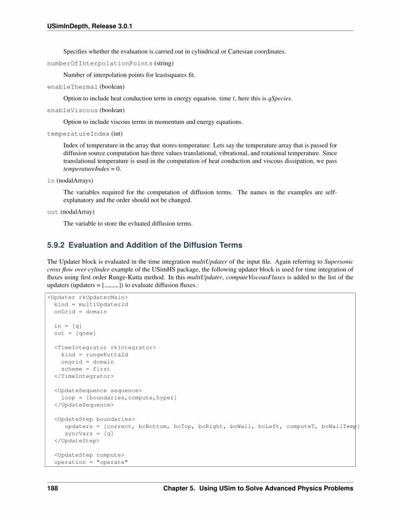
USimInDepth, Release 3.0.1
Specifies whether the evaluation is carried out in cylindrical or Cartesian coordinates.
numberOfInterpolationPoints (string)
Number of interpolation points for leastsquares fit.
enableThermal (boolean)
Option to include heat conduction term in energy equation. time 𝑡, here this is qSpecies.
enableViscous (boolean)
Option to include viscous terms in momentum and energy equations.
temperatureIndex (int)
Index of temperature in the array that stores temperature. Lets say the temperature array that is passed fordiffusion source computation has three values translational, vibrational, and rotational temperature. Sincetranslational temperature is used in the computation of heat conduction and viscous dissipation, we passtemperatureIndex = 0.
in (nodalArrays)
The variables required for the computation of diffusion terms. The names in the examples are self-explanatory and the order should not be changed.
out (nodalArray)
The variable to store the evluated diffusion terms.
5.9.2 Evaluation and Addition of the Diffusion Terms
The Updater block is evaluated in the time integration multiUpdater of the input file. Again referring to Supersoniccross flow over cylinder example of the USimHS package, the following updater block is used for time integration offluxes using first order Runge-Kutta method. In this multiUpdater, computeViscousFluxes is added to the list of theupdaters (updaters = [.,.,.,.,.]) to evaluate diffusion fluxes.:
<Updater rkUpdaterMain>kind = multiUpdater2donGrid = domain
in = [q]out = [qnew]
<TimeIntegrator rkIntegrator>kind = rungeKutta2dongrid = domainscheme = first
</TimeIntegrator>
<UpdateSequence sequence>loop = [boundaries,compute,hyper]
</UpdateSequence>
<UpdateStep boundaries>updaters = [correct, bcBottom, bcTop, bcRight, bcWall, bcLeft, computeT, bcWallTemp]syncVars = [q]
</UpdateStep>
<UpdateStep compute>operation = "operate"
188 Chapter 5. Using USim to Solve Advanced Physics Problems
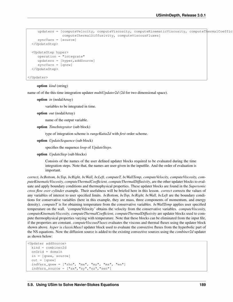
USimInDepth, Release 3.0.1
updaters = [computeVelocity, computeViscosity, computeKinematicViscosity, computeThermalCoefficient, \computeThermalDiffusivity, computeViscousFluxes]
syncVars = [source]</UpdateStep>
<UpdateStep hyper>operation = "integrate"updaters = [hyper,addSource]syncVars = [qnew]
</UpdateStep>
</Updater>
option kind (string)
name of of the this time integration updater multiUpdater2d (2d for two dimensional space).
option in (nodalArray)
variables to be integrated in time.
option out (nodalArray)
name of the output variable.
option TimeIntegrator (sub block)
type of integration scheme is rungeKutta2d with first order scheme.
option UpdateSequence (sub block)
specifies the suquence loop of UpdateSteps.
option UpdateStep (sub blocks)
Consists of the names of the user defined updater blocks required to be evaluated during the timeintegration steps. Note that, the names are user-given in the inputfile. And the order of evaluation isimportant.
correct, bcBottom, bcTop, bcRight, bcWall, bcLeft, computeT, bcWallTemp, computeVelocity, computeViscosity, com-puteKinematicViscosity, computeThermalCoefficient, computeThermalDiffusivity, are the other updater blocks to eval-uate and apply boundary conditions and thermophysical properties. These updater blocks are found in the Supersoniccross flow over cylinder example. Their usefulness will be briefed here in this lesson. correct corrects the values ofany variables of interest to user specified limits. bcBottom, bcTop, bcRight, bcWall, bcLeft are the boundary condi-tions for conservative variables (here in this example, they are mass, three components of momentum, and energydensity). computeT is for obtaining temperature from the conservative variables. bcWallTemp applies user specifiedtemperature on the wall. ‘computeVelocity’ obtains the velocity from the conservative variables. computeViscosity,computeKinematicViscosity, computeThermalCoefficient, computeThermalDiffusivity are updater blocks used to com-pute thermophysical properties varying with temperature. Note that these blocks can be eliminated from the input file,if the properties are constant. computeViscousFluxes evaluates the viscous and thermal fluxes using the updater blockshown above. hyper is classicMuscl updater block used to evaluate the convective fluxes from the hyperbolic part ofthe NS equations. Now the diffusion source is added to the existing convective sources using the combiner2d updateras shown below:
<Updater addSource>kind = combiner2donGrid = domainin = [qnew, source]out = [qnew]indVars_qnew = ["rho", "mx", "my", "mz", "en"]indVars_source = ["sx","sy","sz","sen"]
5.9. Using USim to Solve Navier-Stokes Equations 189
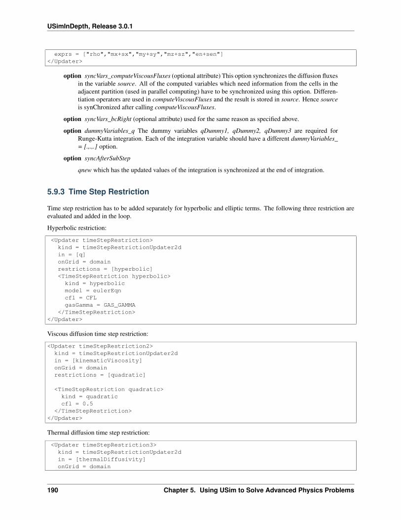
USimInDepth, Release 3.0.1
exprs = ["rho","mx+sx","my+sy","mz+sz","en+sen"]</Updater>
option syncVars_computeViscousFluxes (optional attribute) This option synchronizes the diffusion fluxesin the variable source. All of the computed variables which need information from the cells in theadjacent partition (used in parallel computing) have to be synchronized using this option. Differen-tiation operators are used in computeViscousFluxes and the result is stored in source. Hence sourceis synChronized after calling computeViscousFluxes.
option syncVars_bcRight (optional attribute) used for the same reason as specified above.
option dummyVariables_q The dummy variables qDummy1, qDummy2, qDummy3 are required forRunge-Kutta integration. Each of the integration variable should have a different dummyVariables_= [.,.,.] option.
option syncAfterSubStep
qnew which has the updated values of the integration is synchronized at the end of integration.
5.9.3 Time Step Restriction
Time step restriction has to be added separately for hyperbolic and elliptic terms. The following three restriction areevaluated and added in the loop.
Hyperbolic restriction:
<Updater timeStepRestriction>kind = timeStepRestrictionUpdater2din = [q]onGrid = domainrestrictions = [hyperbolic]<TimeStepRestriction hyperbolic>
kind = hyperbolicmodel = eulerEqncfl = CFLgasGamma = GAS_GAMMA
</TimeStepRestriction></Updater>
Viscous diffusion time step restriction:
<Updater timeStepRestriction2>kind = timeStepRestrictionUpdater2din = [kinematicViscosity]onGrid = domainrestrictions = [quadratic]
<TimeStepRestriction quadratic>kind = quadraticcfl = 0.5
</TimeStepRestriction></Updater>
Thermal diffusion time step restriction:
<Updater timeStepRestriction3>kind = timeStepRestrictionUpdater2din = [thermalDiffusivity]onGrid = domain
190 Chapter 5. Using USim to Solve Advanced Physics Problems
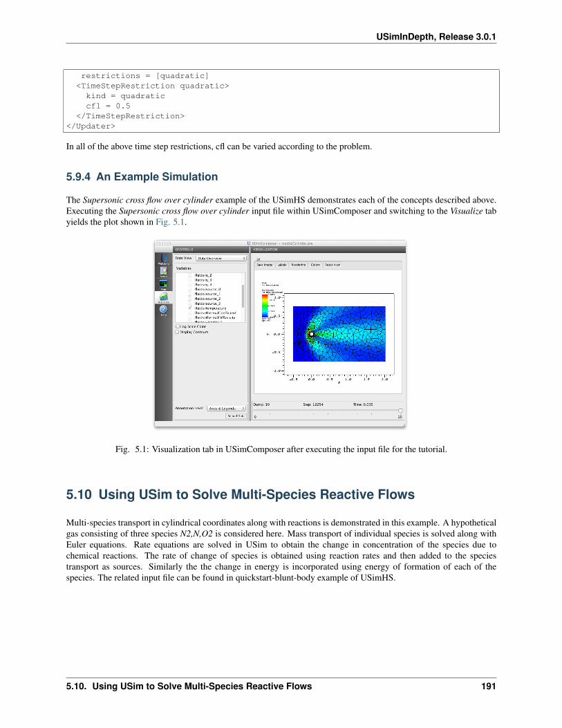
USimInDepth, Release 3.0.1
restrictions = [quadratic]<TimeStepRestriction quadratic>kind = quadraticcfl = 0.5
</TimeStepRestriction></Updater>
In all of the above time step restrictions, cfl can be varied according to the problem.
5.9.4 An Example Simulation
The Supersonic cross flow over cylinder example of the USimHS demonstrates each of the concepts described above.Executing the Supersonic cross flow over cylinder input file within USimComposer and switching to the Visualize tabyields the plot shown in Fig. 5.1.
Fig. 5.1: Visualization tab in USimComposer after executing the input file for the tutorial.
5.10 Using USim to Solve Multi-Species Reactive Flows
Multi-species transport in cylindrical coordinates along with reactions is demonstrated in this example. A hypotheticalgas consisting of three species N2,N,O2 is considered here. Mass transport of individual species is solved along withEuler equations. Rate equations are solved in USim to obtain the change in concentration of the species due tochemical reactions. The rate of change of species is obtained using reaction rates and then added to the speciestransport as sources. Similarly the the change in energy is incorporated using energy of formation of each of thespecies. The related input file can be found in quickstart-blunt-body example of USimHS.
5.10. Using USim to Solve Multi-Species Reactive Flows 191
USimInDepth, Release 3.0.1
Contents
• Using USim to Solve Multi-Species Reactive Flows– Multi-Species Mass Transport– Mass Diffusion– Rate of Change of Density– Chemical Energy– Addition of sources in time integrator– An Example Simulation
5.10.1 Multi-Species Mass Transport
Species mass transport fluxes are evaluated using the classicMuscl updater and Eigenvalues values of the Euler equa-tion (see Using USim to solve the Euler Equations). The updater block is as given below.
<Updater hyperSpecies>kind = classicMuscl2dtimeIntegrationScheme = nonenumericalFlux = localLaxFluxlimiter = [minmod, minmod, minmod, none]
variableForm = conservativecfl = CFLonGrid = domainin = [speciesDens, q, p, a]out = [speciesDensNew]equations = [speciesContinuity]sources = [multiSpeciesAxiSrc]
<Equation speciesContinuity>useParentEigenvalues = trueinputVariables = [speciesDens, q]kind = multiSpeciesSingleVelocityEqnnumberOfSpecies = NSPECIES
<Equation euler>kind = realGasEosEqninputVariables = [q, p, a]numSpecies = NSPECIES
</Equation>
</Equation>
<Source multiSpeciesAxiSrc>kind = multiSpeciesSymsymmetryType = cylindricalnumberOfSpecies = NSPECIES
</Source></Updater>
This block uses Equation sub-block and a Source block. The mass fluxes are computed in the Equation block usingthe Eigenvalues of conservative variables q. Here q contains the conservative variables of realGasEosEqn equation.The equation of state is user specified, hence it requires pressure p and speed of sound a as inputs. The Source blockcomputes the sources due to additional terms in cylindrical coordinates. The fluxes evaluated in both of the sub-blocksare added to the out variable speciesDensNew.
192 Chapter 5. Using USim to Solve Advanced Physics Problems
USimInDepth, Release 3.0.1
5.10.2 Mass Diffusion
Mass diffusion source for the multi-species can computed using the following block. This block uses refmanual-diffusion operator to compute the diffusion source, with the derivative specified as diffusion, numScalars is the num-ber of species, isRadial is true for cylindrical coordinates, and the input variables are species density and diffusioncoefficient D. out variable diffSrc contains the output.
<Updater computeDiffSrc>kind = diffusion2donGrid = domainderivative = diffusionnumScalars = NSPECIEScoefficient = 1.0numberOfInterpolationPoints = 8isRadial = truein = [speciesDens,D]out = [diffSrc]
</Updater>
5.10.3 Rate of Change of Density
The following equation block shows the computation of rate of change of density three species due to two reactions.In order to use this block, a nodalArray variable consisting of the species densities speciesDens has to be initialized,another array to add the density change rates speciesDensNew should be declared, and an nodalArray with averagetemperature of the species. The two reactions are N2 + N2 -> N + N + N2 and N2 + O2 -> N + N + O2. The equationblock follow.
<Updater sourceUpdater>kind = equation2donGrid = domain
in = [speciesDens, temperature]out = [speciesDensNew]
equations = [reactionSrc]
<Equation reactionSrc>kind = reactionTableRhsoutputEnergyRate = 0maxRate = 1.0e28species = [N2, N, O2]fileName = airReaction.txt
</Equation></Updater>
The attributes used in the above block are
option kind (string)
Specifies the type of updater. Here it is equation2d
option in (nodalArray)
Names of the required nodalArray inputs. In this example, those are speciesDens, temperature
option out
Name of the output variable.
5.10. Using USim to Solve Multi-Species Reactive Flows 193
USimInDepth, Release 3.0.1
option equations (string)
Name of the equation. Here the name is reactionSrc
Attributes within the Equation sub blocks
option kind (string)
Type of equation. In this example, it is refmanual-reactionTableRhs
option outputEnergyRate (boolean)
option to compute reaction energy. it is chosen to be false in this demo.
option maxRate (real number)
An option to introduce artificial limit on the maximum value of reaction rate. It is useful in stabilizingthe solution at reasonably small time steps.
option species (list of strings)
Names of the species considered.
option fileName (string)
Name of the refmanual-MultiSpeciesDataFiles.
Within the Equation Any number of reactions can be included by simply adding those to refmanual-MultiSpeciesDataFiles.
5.10.4 Chemical Energy
The energy of formation is computed using the following Updater block. The total energy of formation of all thespecies is added to get the mixture’s energy. This energyOfFormation is added to internal energy in the energy equation.Hence during the initialization, the initial value of energyOfFormation should be computed using the initial densitiesof species and added to the energy density variable.
<Updater computeChemEn>kind = equation2donGrid = domain
in = [speciesDens,cpR,temperature]out = [chemEn]
<Equation cp>kind = transportCoeffSrccoeff = chemicalEnergynumSpecies = NSPECIESfileName = airReaction.txt
</Equation></Updater>
The attributes used in the above block are
option kind (string)
Specifies the type of updater. Here it is equation2d
option in (nodalArray)
Names of the required nodalArray inputs. In this example, those are speciesDens, cpR, temperature.specisDens is the number densities of all species, cpR is specific heats. temperature is averagetemperature of species. speciesDens and cpR are arrays with size equal to the number of species.
194 Chapter 5. Using USim to Solve Advanced Physics Problems
USimInDepth, Release 3.0.1
option out
Name of the output variable. contains the energy of formation. This variable will have only onecomponent.
5.10.5 Addition of sources in time integrator
Two updaters are here, one for integrating the conservative variables q and species density speciesDens. The other isto integrate time rate of change of species due to reactions in using detailed explanation of the attributes is found inrefmanual-multiUpdater.
<Updater rkUpdaterFluid>kind = multiUpdater2donGrid = domain
in = [q,speciesDens]out = [qnew,speciesDensNew]
<TimeIntegrator rkIntegrator>kind = TIMEINTEGRATION_METHODongrid = domainscheme = TIMEINTEGRATION_SCHEME
</TimeIntegrator>
<UpdateSequence sequence>loop = [boundaries,hyper]
</UpdateSequence>
<UpdateStep boundaries>updaters = [bcOutflowSpecies, bcInflowSpecies, bcAbWallSpecies1, bcAbWallSpecies2, bcAbWallSpecies3, computeChemEn, computeTemperature, temperatureCorrector, bcFluidTempAxis, bcFluidTempWall, bcFluidTempInflow, bcFluidTempCopy, bcSurfTemp, bcOutflow, bcInflow, bcAxis, bcAbWall1, bcAbWall2, bcAbWall3]syncVars = [speciesDens,chemEn, temperature, surfTemp, q]
</UpdateStep>
<UpdateStep hyper>operation = "integrate"updaters = [computeChemEn, computeTemperature, temperatureCorrector, computeCpAvg, computeMwAvg, computeGammaAvg, computeViscosity, computeThermalCoefficient, computeGasPressure, computeElectronPressure, computeHvpPressure, bcPressureWall1, bcPressureWall2, bcPressureWall3, computeSoundSpeed, computeKinematicViscosity, computeThermalDiffusivityFluid, computeVelocity,computeViscousSource,hyper, hyperSpecies, addViscousSource]syncVars = [temperature, p,a,velocity,viscousSource,qnew,speciesDensNew]
</UpdateStep>
Boundary conditions are applied on species using bcOutflowSpecies, bcInflowSpecies, bcAbWallSpecies1, bcAbWall-Species2, bcAbWallSpecies3. Energy of formation and temperature are computed using computeChemEn, com-puteTemperature. Remember that, energy of formation is required to compute temperature. Boundary conditionson temperature are then applied using bcFluidTempAxis, bcFluidTempWall, bcFluidTempInflow, bcFluidTempCopy,bcSurfTemp updaters. Finally boundary conditions are applied to bcOutflow, bcInflow, bcAxis, bcAbWall1, bcAbWall2,bcAbWall3 conservative variables.
Energy of formation, computeChemEn is evaluated and then temperature is computed using the updater computeTem-perature. The properties are evaluated using computeCpAvg for average value of constant pressure specific heat ofspecies, computeMwAvg for the average molecular weight, and computeGammaAvg for average gamma of the mix-ture. Viscosity an thermal conductivity are evaluated using computeViscosity, computeThermalCoefficient. The totalpressure of the gas, electron pressure and heavy particle pressure are computed using computeGasPressure, com-puteElectronPressure, computeHvpPressure updaters respectively. The pressure is copied into the ghost layers usingthe boundary condition updaters bcPressureWall1, bcPressureWall2, bcPressureWall3. Pressure boundary conditionis applied for refmanual-realGasEosEqn. Then computeSoundSpeed is evaluated. computeKinematicViscosity, com-puteThermalDiffusivityFluid are evaluated to obtain kinematic viscosity and thermal diffusivity. These are requiredfor time step restriction based on diffusion. Velocity of fluid is evaluated using computeVelocity and then viscoussource is computed computeViscousSource. Convective fluxes of conservative variable are computed in ‘hyper’ and
5.10. Using USim to Solve Multi-Species Reactive Flows 195
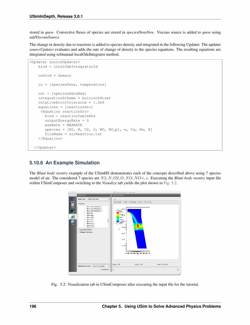
USimInDepth, Release 3.0.1
stored in qnew. Convective fluxes of species are stored in speciesDensNew. Viscous source is added to qnew usingaddViscousSource.
The change in density due to reactions is added to species density and integrated in the following Updater. The updatersourceUpdater evaluates and adds the rate of change of density to the species equations. The resulting equations areintegrated using refmanual-localOdeIntegrator method.
<Updater sourceUpdater>kind = localOdeIntegrator2d
onGrid = domain
in = [speciesDens, temperature]
out = [speciesDensNew]integrationScheme = bulirschStoerrelativeErrorTolerance = 1.0e9equations = [reactionSrc]<Equation reactionSrc>
kind = reactionTableRhsoutputEnergyRate = 0maxRate = MAXRATEspecies = [N2, N, O2, O, NO, NO_p1, e, Ca, Na, K]fileName = airReaction.txt
</Equation>
</Updater>
5.10.6 An Example Simulation
The Blunt body reentry example of the USimHS demonstrates each of the concepts described above using 7 speciesmodel of air. The considered 7 species are 𝑁2, 𝑁,𝑂2, 𝑂,𝑁𝑂,𝑁𝑂+, 𝑒. Executing the Blunt body reentry input filewithin USimComposer and switching to the Visualize tab yields the plot shown in Fig. 5.2.
Fig. 5.2: Visualization tab in USimComposer after executing the input file for the tutorial.
196 Chapter 5. Using USim to Solve Advanced Physics Problems
USimInDepth, Release 3.0.1
5.11 Advanced Time-Stepping Methods in USim
USim implements methods that allows a simulation to be advanced on the timestep associated with the inviscid equa-tions (e.g. the Euler equations), rather than that associated with (for example) the Navier-Stokes equations or complexreaction chemistry. These methods typically allow a speed up ∼
√𝑁 where 𝑁 is the ratio of the inviscid to the (for
example) viscous timesteps.
Contents
• Advanced Time-Stepping Methods in USim– Subcycling for Complex Chemsitry– Super Time Stepping for Viscous Operators– An Example Simulation
5.11.1 Subcycling for Complex Chemsitry
The Flow over cylindrical rod example of the USimHS package of USim implements methods for accelerating chem-ical reaction rates through sub-cycling. An example updater block that implements these methods is shown below:
<Updater chemistryUpdater>kind = stsUpdater2donGrid = domaintimeIntegrationScheme = zerothOrderupdaters = [sourceUpdater]
integrationVariablesIn = [qSpecies]integrationVariablesOut = [qSpeciesNew]timeStepRestrictions = [reactionrateDT]dummyVariables_qSpecies = [dummySpecies1, dummySpecies2, dummySpecies3, dummySpecies4, dummySpecies5]
</Updater>
The meanings for the input blocks in this updater are as follows:
kind (string)
Specifies the stsUpdater2d updater, which tells USim to advance the solution vector super time steppingmethods in 2d.
timeIntegratioScheme (string)
The order of accuracy of the time-integration scheme that to be used. Here we have specified a sub-cyclingscheme using zerothOrder.
updaters (string)
The list of updaters that are used to perform the time integration. This is equivalent to the loop field ofthe update-sequence that was discussed in USimBase Tutorial on Euler Equations, input file, with theexception that updater are called directly, rather than through an update-step. In this case, we call oneupdater sourceUpdater, which calculates chemical reaction rates.
integrationVariablesIn (string)
Specifies the data structure that contains the conserved state at time 𝑡, here this is qSpecies.
integrationVariablesOut (string)
Specifies the data structure that contains the conserved state updated to time 𝑡+ ∆𝑡, here this is qSpecies-New
5.11. Advanced Time-Stepping Methods in USim 197
USimInDepth, Release 3.0.1
timeStepRestrictions (string)
Specifies the dynVector data structure that holds the timestep associated with the chemical reaction. Here,this is reactionrateDT, which is defined through:
<DataStruct reactionrateDT>kind = dynVectornumComponents = 1writeOut = false
</DataStruct>
The timestep restriction is calculated using the dynVectorOperator updater:
<Updater fixDt># to fix dt to specified valuekind = dynVectorOperatorin = [ ]out = [reactionrateDT]onGrid = [domain]
maxDt = MAX_DT
exprs = ["maxDt"]</Updater>
This updater sets the dynVector called reactionrateDT to hold the value specified by MAX_DT.
dummyVariables_q (string)
A list of dummy variables that are used by the multiUpdater to perform the integration. These are subsi-tituted for the qSpecies vector and should have the same number of components. The stsUpdater requiresfive dummy vectors, irrespective of the choice of timeIntegrationScheme.
5.11.2 Super Time Stepping for Viscous Operators
The Flow over cylindrical rod example of the USimHS package of USim implements methods for accelerating chem-ical reaction rates through sub-cycling. An example updater block that implements these methods is shown below:
<Updater stsUpdater>kind = stsUpdater2donGrid = domaintimeIntegrationScheme = secondOrder
updaters = [bcAxis, bcInflow, bcWall, bcOutflow,bcFreeflow, \computeViscousSource,setViscSource]
integrationVariablesIn = [q]integrationVariablesOut = [qnew]timeStepRestrictions = [diffDT1,diffDT2]dummyVariables_q = [dummy1, dummy2, dummy3, dummy4, dummy5]
</Updater>
The meanings for the input blocks in this updater are as follows:
timeIntegratioScheme (string)
The order of accuracy of the time-integration scheme that to be used. Here we have specified a secondorder super time stepping scheme using secondOrder.
timeStepRestrictions (string)
198 Chapter 5. Using USim to Solve Advanced Physics Problems
USimInDepth, Release 3.0.1
Specifies the dynVector data structure that holds the timestep associated with the chemical reaction. Here,this is [diffDT1,diffDT2], which are defined through:
<DataStruct diffDT1>kind = dynVectornumComponents = 1writeOut = false
</DataStruct>
<DataStruct diffDT2>kind = dynVectornumComponents = 1writeOut = false
</DataStruct>
These timestep restriction are calculated using the getTimeStepRestriction updater:
<Updater getDiffDT1>kind = getTimeStepUpdater2din = [kinematicViscosity]out = [diffDT1]onGrid = domainrestrictions = [quadratic]
<TimeStepRestriction quadratic>kind = quadraticcfl = CFL
</TimeStepRestriction></Updater>
<Updater getDiffDT2>kind = getTimeStepUpdater2din = [kinematicConductivity]out = [diffDT2]onGrid = domainrestrictions = [quadratic]
<TimeStepRestriction quadratic>kind = quadraticcfl = CFL
</TimeStepRestriction></Updater>
These updaters set the dynVector called diffDT1 and diffDT2 to hold the timesteps associated with theviscous and conductivity operators in the Navier-Stokes equations respectively.
5.11.3 An Example Simulation
The Flow over cylindrical rod example of the USimHS package demonstrates each of the concepts described above.Executing the Flow over cylindrical rod input file within USimComposer and switching to the Visualize tab yields theplot shown in Fig. 5.3.
5.12 Running USim from the Command Line
The following sections describe how to run USim from the command line.
5.12. Running USim from the Command Line 199
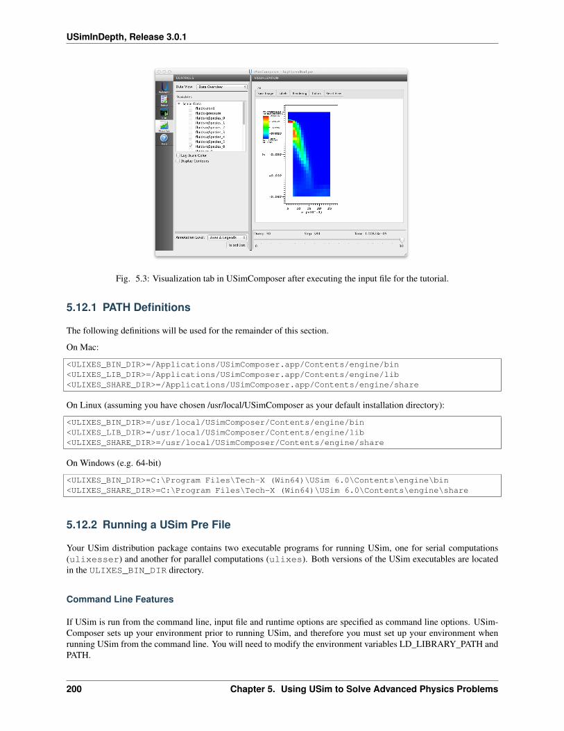
USimInDepth, Release 3.0.1
Fig. 5.3: Visualization tab in USimComposer after executing the input file for the tutorial.
5.12.1 PATH Definitions
The following definitions will be used for the remainder of this section.
On Mac:
<ULIXES_BIN_DIR>=/Applications/USimComposer.app/Contents/engine/bin<ULIXES_LIB_DIR>=/Applications/USimComposer.app/Contents/engine/lib<ULIXES_SHARE_DIR>=/Applications/USimComposer.app/Contents/engine/share
On Linux (assuming you have chosen /usr/local/USimComposer as your default installation directory):
<ULIXES_BIN_DIR>=/usr/local/USimComposer/Contents/engine/bin<ULIXES_LIB_DIR>=/usr/local/USimComposer/Contents/engine/lib<ULIXES_SHARE_DIR>=/usr/local/USimComposer/Contents/engine/share
On Windows (e.g. 64-bit)
<ULIXES_BIN_DIR>=C:\Program Files\Tech-X (Win64)\USim 6.0\Contents\engine\bin<ULIXES_SHARE_DIR>=C:\Program Files\Tech-X (Win64)\USim 6.0\Contents\engine\share
5.12.2 Running a USim Pre File
Your USim distribution package contains two executable programs for running USim, one for serial computations(ulixesser) and another for parallel computations (ulixes). Both versions of the USim executables are locatedin the ULIXES_BIN_DIR directory.
Command Line Features
If USim is run from the command line, input file and runtime options are specified as command line options. USim-Composer sets up your environment prior to running USim, and therefore you must set up your environment whenrunning USim from the command line. You will need to modify the environment variables LD_LIBRARY_PATH andPATH.
200 Chapter 5. Using USim to Solve Advanced Physics Problems
USimInDepth, Release 3.0.1
If you are using the bash shell, you will need to modify LD_LIBRARY_PATH by adding the following line to your.bashrc:
export LD_LIBRARY_PATH=<ULIXES_LIB_PATH>:$LD_LIBRARY_PATH
Instead, if you are using the csh shell (or one of its variants such as tcsh), you will need to add the following line toyour .cshrc:
setenv LD_LIBRARY_PATH <ULIXES_LIB_DIR>:$LD_LIBRARY_PATH
Similarily, to set your PATH in the bash shell, you will need to add the following line to your .bashrc:
export PATH=<ULIXES_BIN_DIR>:$PATH
whereas in csh/tcsh, you will need to add the following line to your .cshrc:
setenv PATH <ULIXES_BIN_DIR>:$PATH
Note that any changes you make to your .bashrc/.cshrc do not take effect until the next time you log in, so aftermodifying your startup file, you must execute the following command in your current shell, but will not need to do itin the future:
source ~/.bashrc (for bash)
or
source ~/.cshrc (for csh/tcsh)
Order of Parameter Precedence
If a parameter is both set within the input file and specified on the command line, the command line parameter valuetakes precedence. The command line override enables you to configure an input file with default values while exploringalternative parameter settings from the command line. From the command line, you can quickly change simulationrun lengths, dimensionality, output timing, etc.
Examples of Running USim from the Command Line
In these examples, it is assumed that you are either in the directory in which the ulixesser is installed or you haveadded the appropriate directory to your shell path.
Command Line Options
The first step in running USim on the command line is to preprocess the input file. Run the preprocessor (txpp.py) onthe .pre file as follows
./txpp.py filaname.pre
The output will be a file called filename.in. The .in file is then used with the ulixes executable as follows To usemultiple options, the command line syntax is:
./ulixesser -i filename.in [-o prefix_name] [-r num]
in which ./ulixesser is used to run a serial computation. See Serial Computation for details about serial compu-tation. See the Parallel Computation for details of command line invocation with parallel computation scripts.
Commonly used options that you can specify on the command line include:
5.12. Running USim from the Command Line 201
USimInDepth, Release 3.0.1
-i filename.in Read input from file named filename.
For example:
./ulixesser -i sodShock.in
-o prefix_name Base names of output files on the text string prefix_name.
For example, if you want output files named newforwardFacingStep rather thanforwardFacingStep, use:
./ulixesser -i forwardFacingStep.in -o newforwardFacingStep
-r num Restart USim from dump num.
For example, if you want to restartforwardFacingStep using the output dumped at time step 50, use:
./ulixesser -i sodShock.in -r 50
More details on how to restart USim are given in Restarting a USim Simulation
5.12.3 Serial Computation
The USim executable for use in serial computation is named ulixesser. Except as noted, the explanations andtutorials within the USim In Depth and USim-Quick-Start demonstrate USim usage for serial computations. Hereis an example of USim command line invocation using a pre file named myfile.pre with corresponding .in filemyfile.in. By default, the output files for this example would be named using the format myfile.out.
ulixesser -i myfile.in
Note: The above invocation line assumes you added <ULIXES_BIN_DIR> to your PATH, as noted in the CommandLine Features section.
Note: When running USim via USimComposer, command line options are not directly available, however -i and -ocommand line options described in this document are implicit; that is, these options are automatically invoked whenrunning USimComposer.
5.12.4 Parallel Computation
The USim executable for use in parallel computation is named ulixes. This section explains use of the USimexecutable program for parallel computations.
USim for parallel computations requires the Message Passing Interface (MPI). For information about mpi for use withUSim, see Running USim with mpiexec.
Parallel Computation Scripts
Running USim with MPI or Parallel Queuing Systems requires use of different shell scripts to enable invocation ofthe USim executable as discussed in the following sections.
Running USim with mpiexec
USim comes bundled with a distribution of Open MPI, which must be used to run USim in parallel (in other words,even if you have an installation of Open MPI on your machine, you should use the one included with USim).
202 Chapter 5. Using USim to Solve Advanced Physics Problems
USimInDepth, Release 3.0.1
In order to run USim in parallel via the command line, you must first add the <ULIXES_BIN_DIR> to your PATH, asnoted in the Command Line Features section.
To run USim in parallel, execute the following command:
mpiexec -np <#> ulixes -i filename.in
in which <#> is the number of processors, ulixes is the executable program for parallel computations, andfilename.in is the name of the USim .in file (which must be in the current directory, or must be specified bya full path).
Following mpiexec, but before <ULIXES_BIN_DIR>, you can specify a variety of mpiexec options. For moreinformation about mpiexec, including the complete list of options, see a man page or other documentation formpiexec.
Following ulixes, you can specify a variety of USim options. For a list of commonly used options, see CommandLine Features.
USim automatically adjusts its decomposition to match the number of processors it is given.
Running USim with Parallel Queuing Systems
Parallel queuing systems, such as LoadLeveler and PBS, require the submission of a shell script with embeddedcomments that the systems interpret. Here is an example of a basic shell script for a PBS-based system:
#PBS -N NDS_ulixes#PBS -l nodes=2:ppn=2cd /directory/containing/your/input/filempiexec -np 4 ulixes -i your_input_file.in
Running USim in Parallel under Windows
To run USim in parallel on a Windows system, bring up a DOS window. From the command prompt,
<ULIXES_BIN_DIR>\mpiexec.exe -np 2 <ULIXES_BIN_DIR>\ulixes.exe -i your_input_file.in
Running SEACAS partitioner on Linux
To decompose a meshfile for a number of processors use the provided SEACAS partitioner script (decomp). Forexample, if you plan to use 8 processors, from the command line run:
<ULIXES_BIN_DIR>/decomp -p 8 meshfile.g
For more information about the decomp script, run the script with the help option:
<ULIXES_BIN_DIR>/decomp -h
5.13 Restarting a USim Simulation
Restart in USim is performed on the command line with the -r option. To restart from dump 5 in parallel enter:
mpiexec -np 4 ulixes -i sodshock.in -r 5
5.13. Restarting a USim Simulation 203
USimInDepth, Release 3.0.1
Restart in USim can be tricky so for large problems it’s best to first test restart to make sure that you’ve dumped outall the required data and furthermore that you’ve included the correct updater in the restoreOnly loop and entered theproper synchronization during the restoreOnly loop. The restore loop should include all the entities that are generatedalong with anything in the initialization loop that does not overwrite the data you are reading in. An example of therestoreOnly loop and the associated UpdateStep is:
<UpdateStep generateStep>updaters = [generateOpen, generateWall, generateInflow, generateNoInflow]syncVars = [q]
</UpdateStep>
restoreOnly=[generateStep]
Geometry is regenerated at the beginning of every simulation regardless of whether it is restarted or no. Secondly,all DataStruct write their data out to file by default unless writeOut=false (or 0). All the DataStructs that have beenwritten out will be written in. It is best not to modify the writeOut option before a simulation is restarted since USimonly reads in values whose writeOut value is true (the default). The example below is a fairly typical input file using anunstructured grid. The input file uses the entityGenerator which is typically called only once during the initializationstep. Restore will work properly in this case only if the entity generators are also called with the restoreOnly option.The startOnly loop is not called on restart so restoreOnly acts as it’s substitute for restart. The reason for this is simple,during restart we do not want to initialize our DataStruct since they are being read in, however we do want to initializegeometric quantities. One final important point to make, in addition to reading in the proper data synchronization mustbe performed across the DataStructs that are read in. In the example below our step generateStep initialized entitiesand synchronizes the DataStruct q.
An example of a USim input file that illustrates the concepts described above is given below:
<Component fluids>kind = updaterComponent
<Grid domain>kind = unstructured
writeGeom = truewriteConn = trueghostLayers = 2decomposeHalos = false
<Creator ctor>kind = gmshndim = 2file = rampgeom4.msh
</Creator></Grid>
<DataStruct q>kind = nodalArraynumComponents = 5onGrid = domain
</DataStruct>
<DataStruct dummy1>kind = nodalArraynumComponents = 5onGrid = domainwriteOut = false
</DataStruct>
204 Chapter 5. Using USim to Solve Advanced Physics Problems
USimInDepth, Release 3.0.1
<DataStruct qnew>kind = nodalArraynumComponents = 5onGrid = domainwriteOut = false
</DataStruct>
.
.
.
<Updater generateOpen>kind = entityGenerator2donGrid = domainnewEntityName = openBoundaryonEntity = ghost<Function mask>
kind = exprFuncexprs = ["if( (x>0.001) and (y>0.34),1.0,-1.0)"]
</Function></Updater>
<Updater generateWall>kind = entityGenerator2donGrid = domainnewEntityName = wallBoundaryonEntity = ghost<Function mask>
kind = exprFuncexprs = ["if( (x>0.01) and (y<0.35),1.0,-1.0)"]
</Function></Updater>
<Updater generateInflow>kind = entityGenerator2donGrid = domainnewEntityName = inflowBoundaryonEntity = ghost<Function mask>
kind = exprFuncexprs = ["if(x<0.01,1.0,-1.0)"]
</Function></Updater>
<Updater generateNoInflow>kind = entityGenerator2donGrid = domainnewEntityName = noInFlowBoundaryonEntity = ghost<Function mask>
kind = exprFuncexprs = ["if(y<0.0,1.0,-1.0)"]
</Function></Updater>
.
.
.
5.13. Restarting a USim Simulation 205
USimInDepth, Release 3.0.1
<UpdateStep initStep>updaters = [initdn]
</UpdateStep>
<UpdateStep generateStep>updaters = [generateOpen, generateWall, generateInflow, generateNoInflow]syncVars = [q]
</UpdateStep>
.
.
.
<UpdateSequence seq>startOnly = [initStep, generateStep]restoreOnly = [generateStep]loop = [boundaryStep, hyperStep, copyStep]
</UpdateSequence>
</Component>
5.14 Running on a Remote Host
USim allows the user to run on a remote host if desired. This is potentially beneficial for several reasons, includingruns with large data sets, running on a large cluster, or shared resources.
5.14.1 Setting up a Remote Host
To use the remote capability, one must install USim on both the local and remote hosts. Only 64-bit Linux platformsare supported for the remote host, so follow the Linux installation instructions. The local host can be any of thesupported operating systems and with the proper license a user can switch back and forth between local and remoteoperations from the same local USim installation.
Once a Linux version of USim is installed on the remote host, note the location of the installation (e.g./path/to/usim/installation). On the local machine:
• Open USimComposer.
• Open the Settings Dialog (choose Tools -> Settings on Windows/Linux or Preferences under the USimComposermenu in Mac OS).
• Click on the Host Settings tab on the left.
• Click on the Add button under the Profiles pane.
• Under General :
– Choose the host profile name, enter your user name, and host address.
– Optionally Enter your password if you want to test the connection. You will be prompted for your pass-word later as well, when needed. Note that your password will not be saved. Dynamic (key-fob-based)passwords are also supported.
– Click Apply and switch to Paths.
206 Chapter 5. Using USim to Solve Advanced Physics Problems
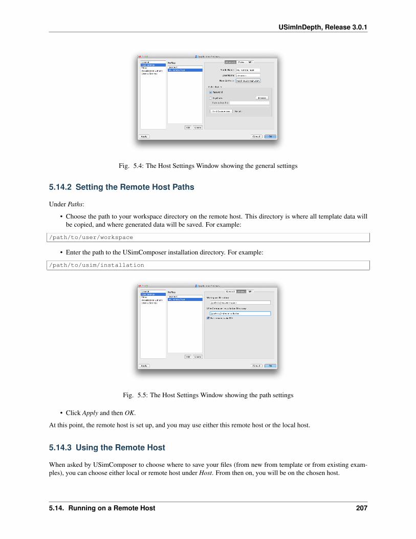
USimInDepth, Release 3.0.1
Fig. 5.4: The Host Settings Window showing the general settings
5.14.2 Setting the Remote Host Paths
Under Paths:
• Choose the path to your workspace directory on the remote host. This directory is where all template data willbe copied, and where generated data will be saved. For example:
/path/to/user/workspace
• Enter the path to the USimComposer installation directory. For example:
/path/to/usim/installation
Fig. 5.5: The Host Settings Window showing the path settings
• Click Apply and then OK.
At this point, the remote host is set up, and you may use either this remote host or the local host.
5.14.3 Using the Remote Host
When asked by USimComposer to choose where to save your files (from new from template or from existing exam-ples), you can choose either local or remote host under Host. From then on, you will be on the chosen host.
5.14. Running on a Remote Host 207
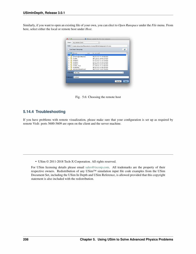
USimInDepth, Release 3.0.1
Similarly, if you want to open an existing file of your own, you can elect to Open Runspace under the File menu. Fromhere, select either the local or remote host under Host.
Fig. 5.6: Choosing the remote host
5.14.4 Troubleshooting
If you have problems with remote visualization, please make sure that your configuration is set up as required byremote VisIt: ports 5600-5609 are open on the client and the server machine.
• USim © 2011-2018 Tech-X Corporation. All rights reserved.
For USim licensing details please email [email protected]. All trademarks are the property of theirrespective owners. Redistribution of any USim™ simulation input file code examples from the USimDocument Set, including the USim In Depth and USim Reference, is allowed provided that this copyrightstatement is also included with the redistribution.
208 Chapter 5. Using USim to Solve Advanced Physics Problems