Using a Personalized Machine Learning Approach to Detect Stolen Phones

by

Huizhong Hu

A thesis submitted to the Graduate School of

Florida Institute of Technology

in partial fulfillment of the requirements

for the degree of

Master of Science

in

Computer Science

Melbourne, Florida

December, 2015

We the undersigned committee hereby approve the attached thesis, “Using a

Personalized Machine Learning Approach to Detect Stolen Phones” by Huizhong

Hu.

_________________________________________________

Philip Chan, Ph.D.

Associate Professor and Major Advisor

Computer Sciences and Cybersecurity

_________________________________________________

Shengzhi Zhang, Ph.D.

Assistant Professor

Computer Sciences and Cybersecurity

_________________________________________________

Georgios Anagnostopoulos, Ph.D.

Associate Professor

Electrical and Computer Engineering

_________________________________________________

Richard Newman, Ph.D.

Professor and Department Head

Computer Sciences and Cybersecurity

iii

Abstract

Title: Using a Personalized Machine Learning Approach to Detect Stolen Phones

Author: Huizhong Hu

Advisor: Philip K. Chan, Ph. D.

With the increasing number of smartphone penetration, mining smartphone data that make

smartphone smarter became a top research area, there are a lot of event data which we

can use to predict behavior or detect anomalies. The privacy disclosure caused by stolen

or lost phones becomes an increasingly difficult problem that cannot be ignored. So we

design an anomaly detection system by mining patterns to detect stolen phones. We use a

pattern mining algorithm to abstract patterns from user past behavior, then construct a

personalized model and use a scoring function and threshold setting strategy to detect

stolen events. Moreover, we apply our system to a data set from MIT Real Mining Project.

Experimental results show that our system can detect 87% stolen events with 0.009 false

positive rate on the average.

iv

Table of Contents

Table of Contents ................................................................................................... iv

List of Figures ......................................................................................................... vi

List of Tables ......................................................................................................... vii

Acknowledgement ................................................................................................ viii

Chapter 1 Introduction ............................................................................................ 1

Chapter 2 Related Works ........................................................................................ 3 2.1 Data mining based on location data ......................................................................... 3 2.1 Data mining based on application data ................................................................... 4 2.2 Data mining for other goal ....................................................................................... 6 2.3 Contributions of this work ........................................................................................ 7

Chapter 3 Approach ................................................................................................ 8 3.1 Data Preprocessing .................................................................................................... 9 3.2 Sequential Pattern Mining ...................................................................................... 10 3.3 Modeling Patterns ................................................................................................... 14 3.4 Scoring Function...................................................................................................... 15 3.4.1 Scoring Similarity ................................................................................................. 15 3.4.2 Scoring Difference ................................................................................................ 16 3.4.3 Scoring by Machine Learning Algorithm .......................................................... 18 3.5 Selecting Threshold ................................................................................................. 19 3.5.1 Anomaly detection (User data only) ................................................................... 19 3.5.2 Using an external database of other users to help determine thresholds ........ 20 3.5 Naïve anomaly Detection System by Using Hidden Markov Model ................... 21

Chapter 4 Empirical Evaluation ........................................................................... 23 4.1 Data Description ...................................................................................................... 23 4.2 Evaluation Criteria.................................................................................................. 26 4.3 Experimental Procedures ....................................................................................... 28 4.4 Experimental Results .............................................................................................. 28 4.4.1 Anomaly detection ................................................................................................ 28 4.4.2 Using an external dataset of other users to help determine thresholds ........... 29 4.4.3 Scoring Function................................................................................................... 30 4.4.3.1 Train with User Data Only ............................................................................... 31 4.4.3.2 Train with User and Other Data ...................................................................... 31 4.4.4 Relationship between valid data rate and performance ................................... 32

Chapter 5 Conclusion ............................................................................................ 35 5.1 Contributions ........................................................................................................... 35 5.2 Future works ............................................................................................................ 35

v

References ............................................................................................................... 36

vi

List of Figures

Figure 1 —Overview of the whole system. It contains two main parts: human

behavior learning and anomalous behavior detection. ....................................... 8

Figure 2 —24 hourly data separation. ...................................................................... 10

Figure 3 —Example of deep-first tree search on sequence of DID 2. The gray

squares mean when the support number is below MS, it then will be

pruned. .............................................................................................................. 12

Figure 4 —S-Step process without gap. ................................................................... 13

Figure 5 —The whole structure of the Personalized Model. ................................... 14

Figure 6 —Example of scoring 3 cases by calculate similarity. .............................. 16

Figure 7 —Example of scoring 3 cases by calculate difference. ............................. 17

Figure 8 —Example of four value of user input for learnt algorithm ...................... 18

Figure 9 —K-fold Cross Validation. ........................................................................ 19

Figure 10 —Use external dataset to set threshold. ................................................... 21

Figure 11 —Discretion of Data. ............................................................................... 23

Figure 12 —Ranked User Data. Data size over red line (120 days) will be used in

this thesis. ......................................................................................................... 24

Figure 13 —Visualization of #23 user’s data. ......................................................... 25

Figure 14 —Valid data rate for 42 users. ................................................................. 25

Figure 15 —Classifications table ............................................................................. 26

Figure 16 —Classifications table with unknown prediction .................................... 27

Figure 17 —TPR and FPR for Strategy 1 and Strategy 2 ........................................ 29

Figure 18 —Correlation between Vailed Data Rate with FPR ................................ 33

Figure 19 —Correlation between Vailed Data Rate with TPR ................................ 33

Figure 20 —Example of data visualization .............................................................. 34

vii

List of Tables

Table 1 —Example of time movement database sorted by DID and TID ............... 11

Table 2 —Sequence for each data base ................................................................... 11

Table 3 —Bitmap format transformed by Table 1. .................................................. 13

Table 4 —Input for learnt algorithm. ....................................................................... 18

Table 5 —Overview of Strategies on setting and adjust threshold. ......................... 21

Table 6 —Average TPR and FPR for anomaly detection ........................................ 29

Table 7 —Average TPR, FPR, Unknown rate for other and user............................ 30

Table 8 —Performance Table of using 𝑻𝒎𝒊𝒏𝒊 ....................................................... 30

Table 9 —AUC for SF1, SF2 and HMM (FPR under 1%) ...................................... 31

Table 10 —Performance of all scoring functions (average) .................................... 32

viii

Acknowledgement

Firstly, I would like to sincerely thank my thesis advisor Dr. Philip Chan for his kindness

and scrupulous advice on my oversea study life, patience and professional guidance on my

study and research. He is just like my family, led me to the right way on study computer

science and machine learning area.

I also would like to thank the other members of my thesis committee, Dr. Shengzhi Zhang

and Dr. Georgios Anagnostopoulos. They gve me the comments and helped me to finish

this thesis.

I would also like to thank my friends and classmates, Kai Wang, Xunhu Sun, Lingfeng

Zhang and Makoto Mori, they give me a lot of idea and suggestion on my thesis.

1

Chapter 1

Introduction

Nowadays, with the developing Internet, smartphones have become more and more

functional. It can be used to make videos, take pictures, contact with friends and so on.

Moreover, online payment cannot be feasible without smartphones. If your phone is lost or

stolen, nightmare will soon begin. You will worry about your property damage and

personal privacy disclosure. With global increasing presence of smartphones, crimes of

stealing phones has also been a huge problem. In the United States there are 113 phone

being lost or stolen every minute. According to the U.S. Federal Communications

Commission, there are nearly one third of robbery with smartphones involved. In 2012, 1.6

million Americans lost about 30 billion dollars because of smartphone crime. Shockingly,

3 million Americans became victims because of it in 2013. The figure almost doubled in

2012 [21].

“How to detect phone stolen?” has become a difficult issue. To solve this problem, the U.S.

Government and the Government of Mexico have developed some countermeasures. In

2012, a number of communication companies including AT&T joined it and built a central

database of stolen smartphones. Thereafter, once a mobile phone is reported to be missing

and registered in the database, it will get a unique serial number correlated to its hardware.

Then the Mobile Operator can block any connection about that number. Moreover, Apple

and Samsun use a different way to handle this issue. They provide a remote permission

about sending the phone’s location or restoring factory setting to erase all data in that

phone.

2

However, all those solutions are not intelligent. They all need phone’s owner to react when

they find their phone to be stolen. It will generally take a long time until they realize it.

We propose a machine learning solution which make phone itself to detect stolen status.

First of all, we estimate users’ behavior by using the data collected by mobile phone

sensors. After using the pattern mining approach to abstract users’ movement behavior,

construct a personalized model to detect anomalies. Once we have the model, we also

abstract patterns from test data and give scores for these patterns, normally within one

hour. Consequently, compare the scores to detect anomalies.

More specifically, we implement a modified pattern mining algorithm to abstract human

movement patterns and construct them into a personalized model. Moreover, we design a

scoring function that can separate 86% suspicious behavior from user activity which means

86 TPR with 0% FPR. Then we frame a threshold setting strategy to detect 87% anomalous

behavior with only 0.9% FPR.

The remaining part introduces this paper’s organization. We discuss some previous works

on mobile phone data mining for different tasks in Chapter 2. Chapter 3 discusses the

structure and function of the entire anomaly detection system. The details of experiment

and procedures will be presented in Chapter 4. In Chapter 5, we summarize the findings

and discuss

3

Chapter 2

Related Works

We will discuss some previous works on mobile phone data mining for different tasks in

this chapter. Moreover, we will review some literature based on three separate problems,

which are location-related mining, application-related mining and other data mining based

on mobile phones. The first section will introduce some existing approaches on the basis of

mining location data. Subsequently, how present tectonics can predict applications is

briefly explored. Other approaches achieved by using data from mobile phones will be

introduced in the third section.

2.1 Data mining based on location data

To detect suspicious behavior in private WLAN connections, an algorithm for temporal

location anomaly detection [1] is proposed to learn the distributions of location probability

by using a combination of sequence of time and location data. In order to approach

anomaly detection, a modified Markov is employed to calculate anomalous scores that

represent differences and similarities of summarized location probability distributions.

In order to track lost phones, the author uses one hour record of Cell Tower ID as location

data and generates Cell ID Entropy which represents how fast or how far the cell phone

moves within this period of time [2]. Moreover, the author uses deviations of entropy for

the past 3 hours to estimate the cellphone’s movement and classify data as normal use or

loss (static loss and dynamic loss), and then input hourly call counts to FeedForward

Neural Networks to predict whether the phone is statically lost, dynamically lost or

normally used.

In [3], the author presents an approach for large-scale unsupervised learning and predicts

people’s routines through the joint modeling of human locations and proximity interactions

by using Latent Dirichlet Allocation probabilistic topic model. Firstly, the author builds a

4

multimodal framework and joints representations for location and proximity to represent a

day as a multimodal bag of words. Then they label an individual’s locations into 4 words:

work (W), home (H), out (O), and no reception (N) and quantize the number of proximate

people into four prototypical groups: user alone, dyad (one person in proximity), a small

group (two–four people in proximity) and a large group (five or more people in proximity).

Further, they divide each day into eight timeslots: 0-7, 7-9, 9-11, 11-14, 14-17, 17-19 and

19-24. After mining the topic by using LDA, they take the most probable combination of

location and proximity interactions in the model from previous data.

2.1 Data mining based on application data

Normally, Most Recently Used (MRU) and Most Frequently Used (MFU) are two most

common ways to predict next applications. However, in [4], the author uses GPS data and

application data to predict what application will be used next. In addition, GPS data are

added and data mining is used to achieve this goal. Firstly, he preprocess data to detect the

location and transforms GPS geographic locations into semantic locations. Then a density-

based clustering algorithm is utilized to find out where the user stays. And frequent app

uses are found and a threshold is given. Moreover, he finds the path the user stays, and

then builds a Mobile App Sequential Pattern Tree to represent the correlations between

locations and applications with path data. Then current data are compared with the path

model to find the best match for prediction. Similar approach present by [16] which replace

GPS data with WLAN connection information.

Similarly, in order to advise several applications for users to choose from, in [5] the author

combines the lunch time and previous application data to predict and advise applications.

Firstly the author uses three separate components, which are Usage Logger, Temporal

Profile Constructor and App Usage Predictor, to achieve this goal. The Usage Logger

component collects users’ app usage history and contains launch time and App ID. The

Temporal Profile Constructor component first detects the periodicities of App. Then for an

app with periodicity set {P1, P2…}, separate and group them into different groups

according to their behavior. Then for each group, count accumulated usage in 24 hours,

5

and then calculate the mean and variance. Give a time and rate such as :( 09:23, 0.95). The

App Usage Predictor component is based on Chebyshev’s inequality from the probability

theory, and gives a probability-based scoring function to calculate the probability of each

application. And the max one serves as prediction.

The same as [5], in [6] the author uses the same data in different ways to achieve this goal.

First of all, the author abstracts three features from the data and calculates the usage

probability for each app. Global Usage Feature gives a probability about the app which is

calculated by the total number of times that the app is used during the whole time. Similar

to Global Usage Feature, Temporal Usage Feature gives a probability of the app usage

within a period of time. Similarly, Periodical Usage Feature has a usage habit. So it means

that the user uses that app frequently. Then the author gives this feature to count the

probability of that app used temporally. Then an algorithm is presented called Min Entropy

Selection which counts the entropy about each feature, and selects the best one for

prediction.

In [7], the author uses more data from smart phones’ sensors to perform a comprehensive

analysis of the context related to mobile app use, and builds prediction models to calculate

the probability of an app in different contexts. Firstly they build a context model for

application prediction, including sampling data, extracting features, and discretizing data.

Afterwards, a sample is create to describe the user’s situation as a vector of discrete states.

Then in the modeling context, he builds an inference to calculate the probability of apps

being associated with a given context using naïve Bayes (NB) classifiers. Moreover, he

constructs an app model (appNB) for each app, which calculates only the probability of

that app for a single user. In the end, two functions are constructed for dynamic screen

applications to show users which app will be recommended: 1) present app shortcuts with

the n highest probabilities, and 2) highlight app shortcuts whose probability has increased

the most from its previous inference.

6

2.2 Data mining for other goal

In order to recognize humans’ daily activities, in [8], the author collects Accelerometer and

Gyroscope’s data and using several classification algorithms to achieve this goal. Similar

with [14], firstly, they capture 3-axial linear acceleration and 3-axial angular velocity at a

constant rate of 50Hz. After noise filtration, they sample the data into fixed-width sliding

windows of 2.56 sec and 50% overlapped to segment the data. Moreover, after extracting

five features (mean, energy, standard deviation, correlation and entropy), six human

activities (walking, siting, standing, downstairs, upstairs and laying) are recognized by the

classification algorithms (J48 decision tree, the logistic regression, and the SVM). More

specifically, the improvement of past research is that they use gyroscope signals to solve

difficulties about classifier downstairs and upstairs activities.

Generally speaking, current methods to detect different kinds of events require domain

knowledge to determine the duration of an event and devise features. However, in [9] and

[15], the author proposes that Genetic Programming based on the event detection

methodology can abstract and detect events from raw data and get great results from

experiments. Firstly, he defines a function set of GP, and then applies sliding windows to

operate the data with several functions: 1) different temporal functions: count value

differences between two time points; 2) window function: use 8 size data sets and

randomly [1,2S -1] pick them to get one result for average, standard deviation, and sum of

differences skew value of the selected points under the window; 3) multivariable time

series function: handle an event occurring in multiple variables, use the same way to

randomly pick variables and get one result: middle value, average, standard derivation or

values range; 4) spatially related multivariable function: deal with an event happening

depending on a region of spatial related variables. Similarly, it randomly picks a region of

values based on sliding windows, and give one of the values similar to multivariable time

series function; 5) perturbed periodical function: the author samples every 2π/7 second, and

summarizes all time differences in 8 time points. Moreover, if the point goes as

uncompleted circles, it will be reported as negative.

7

2.3 Contributions of this work

Basically, the goal of this thesis is different from previous works. We use the pattern

mining approach to detect anomalies in order to alarm stolen phone events. Unlikely, in

[2], they use location data to generate one attribute that helps to detect lost phone events,

rather than analyzing it deeply to mine behavioral patterns from it. Moreover, the lost event

is simpler than theft events. Instead of reacting to events three hours after, our system

reacts event three times faster. We use a sequential mining algorithm and a frame work to

build personalized model to predict stolen with in hour.

8

Chapter 3

Approach

Our goal is to use machine learning algorithms to personalize user behavior in order to help

users automatically detect stolen phones and protect users’ property and privacy. In this

chapter, we will describe the algorithm that we have explored and how we achieve the

main goal.

The learning and detecting architecture is shown in Fig. 1. It contains two procedures

which are behavior learning procedure and anomalous detecting procedure. In the first part,

we use a pattern mining algorithm [11] to abstract behavior patterns set by using raw data,

and then merge and process them into a personalized model set. Different with [20] which

use unsupervised learning to clustering user’s past behavior.

Similarly, the second part is to input new data which is current behavior in this case, and

after abstracting behavior patterns, insert them into a correlation detecting model to get

anomaly scores over a threshold, which means an anomalous behavior and identify the

phone as stolen status. The detecting model generated by multiple behavioral pattern

models from the model set learned from raw data.

Figure 1 —Overview of the whole system. It contains two main parts: human behavior

learning and anomalous behavior detection.

9

3.1 Data Preprocessing

Because the data contains location and recording time, the location contains area id and the

cell tower id which connect the phone. Then we remove the data which are identified as

non-compliant (such as no signal, only time record or location only has area id without

tower id). We will explain the data more specifically in Chapter 4. Then we separate data

into the date ordered format in order to build seven daily models, which is the Monday

through Sunday model. The reason why we separate the original dataset into seven sub-

datasets to build seven daily models is that most of human schedules is one weak,

signifying that the similar schedule will be repeated every seven days as last week. The

main reason we didn’t separate data as weekday and weekend model is that for some

people, such as students, the activity cycle is around one week. Moreover, we still can

apply the seven models into the weekday and weekend model.

Furthermore, we use a modified version of sliding-window to separate one-day dataset into

24 hourly subsets as shown in Figure 2. The 24 hourly subsets are used to build 24 hourly

models to abstract human daily behavior into 24 models. Moreover, this window will cover

a two-hour time space, including one current hour and two half hours shift from forward

and backward. More specifically, each hourly subset has three subsets. It not only contains

one hour data from correlated hour subsets which are cut on the hour (for example 1:00 am

to 2:00 am), but also has two shift hour subsets. Similarly, it shifts border of time on half

hour to get shift subsets (for example 1:30 am to 2:30 am, 2:30 am to 3:30 am).

Additionally, the main reason we set one hour as the basic unit is that we want to detect

stolen phone within one hour after the phone is stolen. Obviously, the earlier you detect

stolen phone, the less property you will lose. Otherwise the detection will be meaningless.

Secondly, we use two half-hour shifted datasets because one cyclical activity may not

always occur within exactly that hour, so we want to relax the data range. However, three

of the total sub-datasets still have one hour data overlapped on that hour, thus making that

hour data still have the main effect on the hourly subset.

10

Figure 2 —24 hourly data separation.

Each small square area represents one hour sub-dataset. Each big square area represents

one hourly sub-dataset. Every three of small squares in the middle construct one hourly

sub-dataset on the side. So use a modified sliding window to build 24 hourly subsets. For

example, the three small green square datasets are the first widow, which constructs a big

green square hourly dataset. Likewise, the window slides to three small deep blue squares

to construct another hourly dataset and so on so forth.

3.2 Sequential Pattern Mining

In order to extract human behavioral patterns, we use the well-known Sequential Pattern

Mining (SPAM) algorithm [12] and using bitmap representation [11] and applying

Constraints to SPAM [13]. The data that can be used in this algorithm are sequence data

with time ordered. Table 1 shows an example of location database with three datasets; each

contains time and location record. The different Data set ID (DID) represents different

datasets, and “a”, “b” and “c” represent three different locations. Table 2 shows its

sequence database order by DID. Once the sequence database S contains subsequence s

over a Minimum Support threshold (MS) times with a given Gap Size (GS), then the

11

subsequence s will be considered as an efficient pattern in sequence S and it will be the

result.

For example, s ={c a}, when MS = 1 and GS = 1, the subsequence s is efficient at all

datasets. But with MS = 1 and GS = 0, then s is efficient at datasets 1 and 2. Moreover,

when MS = 2 and GS = 0, it is just efficient in dataset 2.

Table 1 —Example of time movement database sorted by DID and TID

Table 2 —Sequence for each data base

For the purpose of searching all possible combinations of efficient subsequence, SPAM

uses the deep-first search strategy to traverse the whole search tree. Figure 3 is an example

of the deep-first tree search with MS = 2 and GS = 1 on dataset 2. Each node represents

one sequence search on S and counts how many times it occurs in the main sequence S as

Data set ID

(DID)Time ID (TID) Location

1 1 a

1 2 a

1 3 b

1 4 c

1 5 a

2 1 c

2 2 a

2 3 c

2 4 a

2 5 b

3 1 c

3 2 b

3 3 a

3 4 c

3 5 c

DID Location sequence

1 {a, a, b, c, a}

2 {c, a, c, a, b}

3 {c, b, a, c, c}

12

the support number. As is shown in Figure 3, SPAM first finds all locations as the

candidate set and begins with empty subsequence. Furthermore, SPAM keeps adding each

location from candidate set into the current subsequence. When the support number is not

small, then MS will be considered as an efficient subsequence and will keep searching on

that branch. Otherwise the whole branch will be pruned because if that subsequence is not

efficient, the longer subsequence will not be efficient either. Finally, the result pattern set

will be all subsequence with its support number over MS as the frequency.

Figure 3 —Example of deep-first tree search on sequence of DID 2. The gray squares mean

when the support number is below MS, it then will be pruned.

More specifically, to calculate the support number for each subsequence, the SPAM

algorithm transforms databases into the vertical bitmap format. Furthermore, two basic

steps are used to merge bitmaps to find support number. Firstly it begins with the bitmap of

first element in subsequence to apply S-Step to process that bitmap into what they call

transformed bitmap, it sets the positions with number 1 into 0 and sets the GS+1 numbers

of bits after into “1”. If the gap size is infinite, then set all bits after into “1”. Secondly, use

this transformed vertical bitmap to do AND operations with next vertical bitmap to

generate a new bitmap, and replace the first two bitmaps with this new bitmap. Keep doing

these two operations until all bitmaps become one. Then the support number of this

13

subsequence will be easily calculated by summing up all bits together. As is shown in

Figure 4, in order to seek the support number of subsequence {a, b}, we first take bitmap

of {a} and by using the S-Step process, transform it to S-{a} with no gap. Then after

performing AND operation, get the result bitmap. Then by summing up all bits together,

we can know that sequence DID 1 and 2 contain subsequence {a, b}, and the support

number is one.

Table 3 —Bitmap format transformed by Table 1.

Figure 4 —S-Step process without gap.

DID TID {a} {b} {c}

1 1 1 0 01 2 1 0 01 3 0 1 01 4 0 0 11 5 1 0 0

2 1 0 0 12 2 1 0 02 3 0 0 12 4 1 0 02 5 0 1 0

3 1 0 0 13 2 0 1 03 3 1 0 03 4 0 0 13 5 0 0 1

14

3.3 Modeling Patterns

After we apply the sequential pattern mining algorithm into each one of the one-hour

datasets, we can begin to build our personalized Model. The whole structure is shown in

Figure 5. We will explain each level from the bottom up. The first level is the pattern level

which contains a bunch of patterns and each pattern contains sequence and its frequency.

The second level is the pattern set level which we construct by patterns, and it is generated

by applying the SPAM algorithm as explained in 3.2 to three one-hour datasets. Hourly

Model sets are level 3, which has 24 hourly model sets and each model set is constructed

by three pattern sets form level 2. Furthermore, level 4 is daily models generated by

multiple sets of daily data. The last level is Daily model sets which contain 7 model sets

through the whole week form Monday to Sunday. Each model set contains multiple daily

models through the whole data interval. For scoring purpose, we will merge all daily

models in to one daily model and we will discuss it specifically in the next section (the

reason why we do not merge them in the first place is that we will apply K-Fold Cross

Validation approach in all daily models to set thresholds). Our Personalized Model is

constructed by all of these 7 models. The data separation operation that supports this

structure is introduced in 4.2.

Figure 5 —The whole structure of the Personalized Model.

15

3.4 Scoring Function

3.4.1 Scoring Similarity

One idea of scoring a new behavior is to find the similarity between new and previous

behavior. More specifically, compare two pattern sets and calculate score similarity

between test pattern sets with correlated hourly model in the personalized model.

Firstly, we have to merge all correlation model sets from the personalized model into one

model set as the merged personalized model is used to calculate the score. To take Monday

model set (level 5) as an example, we merge all Monday daily models (level 4) into one

Monday model. Additionally, we merge hourly model sets (level 3) correspondingly, and

the three pattern sets (level 2) will be merged into one model. At level 1, if two patterns are

the same, we will sum up all frequencies together; otherwise we simply copy the pattern

and frequency into the merged pattern set and all the frequencies will be divided by the

number of days in the end.

In order to score new data in the one-hour time period, firstly, we abstract a pattern set by

applying the pattern mining algorithm in the new data. Then compare this pattern set with

the merged personalized model. Here we define 3 cases to analyze the similarity. The

example is displayed in Figure 6. As we can see, the first case means these two pattern sets

have the same pattern and the similarity for this pattern is the number of overlaps. Also, the

second case represents that the pattern only occurs in the training pattern set but the

similarity in this case is zero. Similarly, the third case means the pattern in the test pattern

set is never seen in training before. So we define a way to calculate the similarity score we

call it SF1; all formulas are shown below:

𝑂𝑖 = 𝑚𝑖𝑛(𝐹𝑝, 𝐹𝑡) (1)

𝑆𝑜 = ∑ 𝑂𝑖𝑛𝑢𝑚𝑏𝑒𝑟 𝑜𝑓 𝑃𝑎𝑡𝑡𝑒𝑟 𝑖𝑛 𝐶𝑎𝑠𝑒1

𝑖=1 (2)

16

𝑆𝑐𝑜𝑟𝑒 =

𝑆𝑜𝑆𝑝

+ 𝑆𝑜𝑆𝑡

2 (3)

Where 𝐹𝑝 is frequency of pattern i in the personalized model, is frequency of pattern i in

the test pattern set, so 𝑂𝑖 means overlapped frequency value. 𝑆𝑜 is the superposition of all

overlapped pattern frequency values. The reason why cases 2 and 3 are not considered is

because the overlapped pattern frequency is always zero. 𝑆𝑝 is the total number of

frequency in the personalized model; similarly, 𝑆𝑡 is the total frequency value in the test

pattern set. Consequently, the score formula represents the percentage of overlapped

pattern frequency amount in training and test set, and then normalizes the value. More

specifically, if there are large numbers of frequency either in training or test set, it will

reduce the score value.

Figure 6 —Example of scoring 3 cases by calculate similarity.

3.4.2 Scoring Difference

Similarly, another way to scoring a new behavior is to find the difference between new and

previous behavior, it is kind of opposite of similarity but calculating in different angle, and

we call it SF2. More specifically, this time we compare two pattern sets and calculate

17

difference between test pattern sets with correlated hourly model in the personalized

model. All formula are shown below:

𝐷𝑖 = |𝐹𝑝 − 𝐹𝑡| (4)

𝑆𝐷 = ∑ 𝐷𝑖𝑛𝑢𝑚𝑏𝑒𝑟 𝑜𝑓 𝑃𝑎𝑡𝑡𝑒𝑟 𝑖𝑛 𝐶𝑎𝑠𝑒1,2 and 3

𝑖=1 (5)

𝑆𝑐𝑜𝑟𝑒 =𝑆𝐷

𝑆𝑝+ 𝑆𝑡 (6)

Where 𝐷𝑖 means the difference of the pattern frequency, we subtract test pattern frequency

from training pattern frequency which the pattern are same, then take absolutely value.

Moreover, the difference of pattern frequency for case 2 and 3 is its frequency subtract by

zero which equals to itself. The example of calculate difference is showing in Figure 7.

Figure 7 —Example of scoring 3 cases by calculate difference.

18

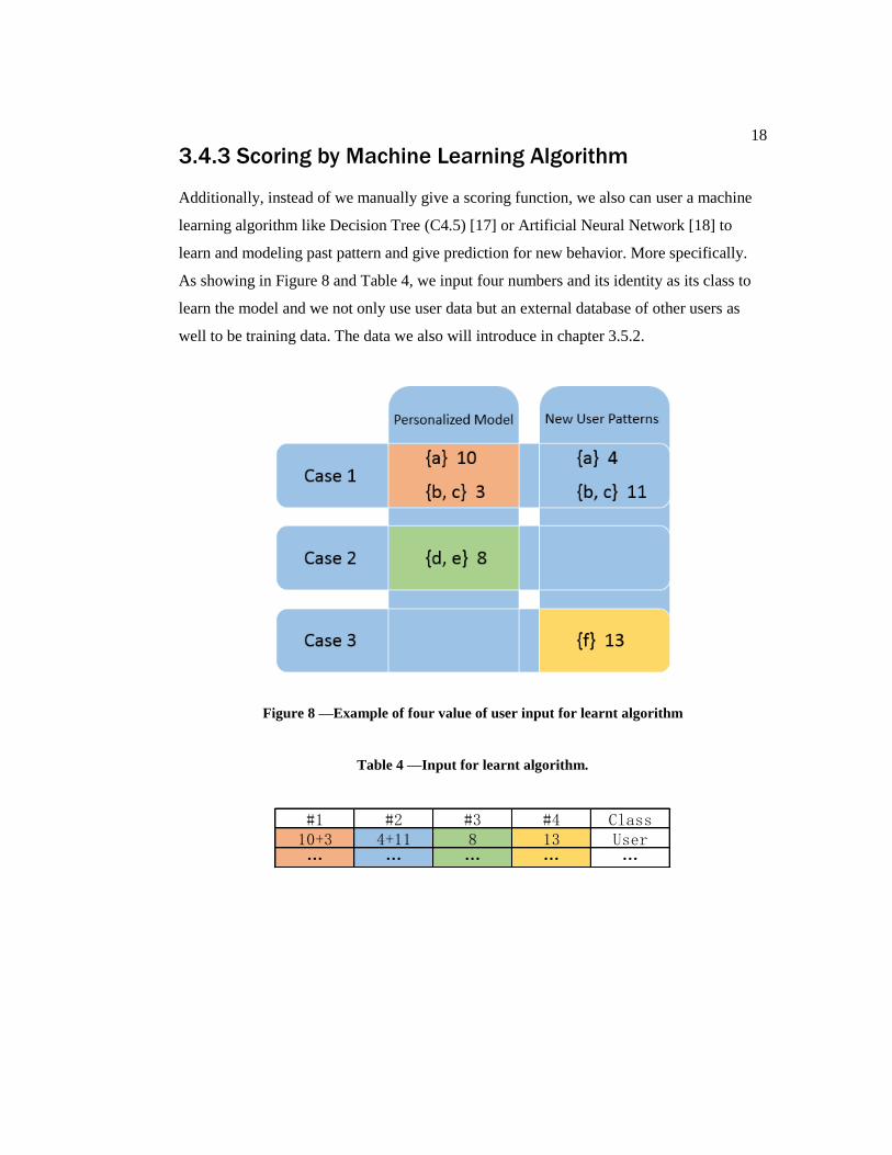
3.4.3 Scoring by Machine Learning Algorithm

Additionally, instead of we manually give a scoring function, we also can user a machine

learning algorithm like Decision Tree (C4.5) [17] or Artificial Neural Network [18] to

learn and modeling past pattern and give prediction for new behavior. More specifically.

As showing in Figure 8 and Table 4, we input four numbers and its identity as its class to

learn the model and we not only use user data but an external database of other users as

well to be training data. The data we also will introduce in chapter 3.5.2.

Figure 8 —Example of four value of user input for learnt algorithm

Table 4 —Input for learnt algorithm.

#1 #2 #3 #4 Class10+3 4+11 8 13 User… … … … …

19

3.5 Selecting Threshold

3.5.1 Anomaly detection (User data only)

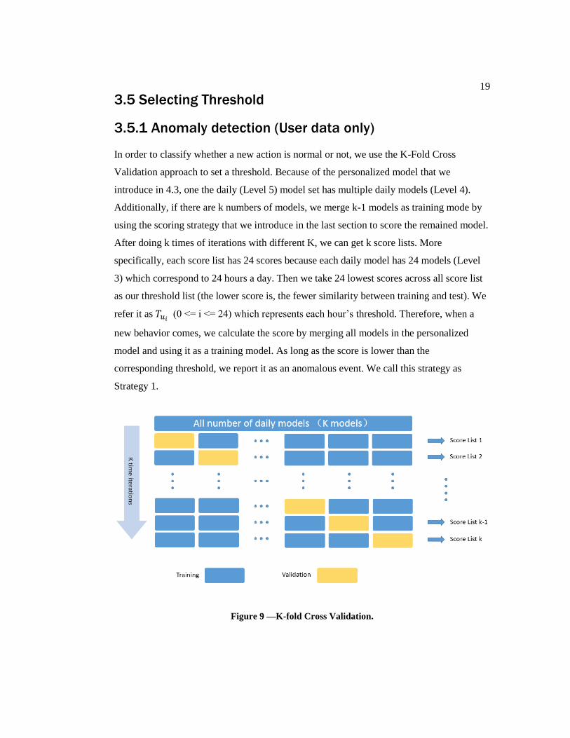
In order to classify whether a new action is normal or not, we use the K-Fold Cross

Validation approach to set a threshold. Because of the personalized model that we

introduce in 4.3, one the daily (Level 5) model set has multiple daily models (Level 4).

Additionally, if there are k numbers of models, we merge k-1 models as training mode by

using the scoring strategy that we introduce in the last section to score the remained model.

After doing k times of iterations with different K, we can get k score lists. More

specifically, each score list has 24 scores because each daily model has 24 models (Level

3) which correspond to 24 hours a day. Then we take 24 lowest scores across all score list

as our threshold list (the lower score is, the fewer similarity between training and test). We

refer it as 𝑇𝑢𝑖 (0 <= i <= 24) which represents each hour’s threshold. Therefore, when a

new behavior comes, we calculate the score by merging all models in the personalized

model and using it as a training model. As long as the score is lower than the

corresponding threshold, we report it as an anomalous event. We call this strategy as

Strategy 1.

Figure 9 —K-fold Cross Validation.

20

Furthermore, we define a strategy that adjusts the threshold to reduce false positive rate,

and we call it as Strategy 2. Instead of using the fixed threshold, we reduce threshold from

𝑇𝑢𝑖 (0 <= i <= 24) to 𝑇𝑚𝑖𝑛𝑖

(0 <= i <= 24) every time when it detects a new normal

activity as stolen because the score for the new activity is lower than the threshold.

Therefore, when next activity is close to the last misclassified activity, it will not be

considered as stolen. The main reason of that this adjustable threshold is because we

cannot guarantee that our system have not false alarm, therefor we want to adjust threshold

that avoid false alarm cause by some similar normal behavior.

3.5.2 Using an external database of other users to help

determine thresholds

Moreover, compared to setting only one threshold to classify whether new behavior is

normal, we invent another threshold 𝑇𝑜𝑖 (0 <= i <= 24) which has to use external datasets

of other users. More specifically, the external dataset must have enough user data and then

use a similar way as 4.5.1 to set 𝑇𝑜𝑖. Firstly, we find the highest score for other user form

database (the other user’s behavior is considered as anomalous behavior) and then set a

threshold between this and the closest higher user score. Moreover, as is shown in Figure

10, we set 𝑇𝑢𝑖′ which is not on the lowest user score, but between this user score and the

closet lower validation score. Then we predict events whose score is over 𝑇𝑜𝑖 as a normal

activity, behavior’s score between 𝑇𝑜𝑖 and 𝑇𝑢𝑖

′ as unknown behavior and below will be

reported as stolen. We call this strategy as Strategy 3

Moreover, we also use the false alarm data to decrease 𝑇𝑢𝑖‘ (0 <= i <= 24) to 𝑇𝑚𝑖𝑛𝑖

’ (0

<= i <= 24) in order to enhance its performance and called as Strategy 4.

21

Figure 10 —Use external dataset to set threshold.

Furthermore, we use Table 5 to summarize strategy 1 to strategy 4. They all use user data

only during training process, but Strategy 1 and Strategy 2 only use user data to set

threshold, Strategy 3 and Strategy 4 use both user and other data to set threshold.

Moreover, Strategy 1 and Strategy 3 do not adjust the threshold during testing. But

Strategy 2 and Strategy 4 adjust its threshold during testing.

Table 5 —Overview of Strategies on setting and adjust threshold.

3.5 Naïve anomaly Detection System by Using Hidden

Markov Model

Instead of using the approach we introduced above, we apply Hidden Markov Model to

detect stolen phones on our data set.

No adjustment during test Adjust during testSetting with user data only Strategy 1 Strategy 2

Setting with user and other data Strategy 3 Strategy 4

22

Firstly, we separate one day data into 24 sub data sets represent 24 hours through the data.

Then find all locations appeared in that hour and take top 10 as observation states.

Moreover, use an additional observation state represents all other locations. We replace all

locations with these 11 observation states.

Secondly, after we put all past sequential data into HMM algorithm to learn a personalized

model, we use this model to estimate a probability for each sequence in the validation data

to set a threshold using Strategy 1. And when a new incoming sequence’s probability is

lower than this threshold, it will be predicted as stolen.

23

Chapter 4

Empirical Evaluation

In this chapter, we first describe what kind of data we have used in this thesis, followed by

the way to evaluate the algorithm in Section 3.2. Moreover, the procedures will be

explored in the last section.

4.1 Data Description

In this thesis, the data we use are from previous work [10]. The project named Reality

Mining was conducted at MIT Media Laboratory. The data collected from smartphones of

94 individuals working or studying at a university from September 2004 to June 2005. It

contains Call logs, Bluetooth devices’ connection data, cell tower IDs, application usage,

and status of mobile phones. Of these 94 subjects, 68 were working or studying in the same

place on main campus which contains ninety percent of graduate students and ten percent

of staff, and the other 26 subjects were new students from the business school in the

university.

Figure 11 —Discretion of Data.

24

For each user, after preprocessing data, we got three separate parts of data: cell tower

transition time and cell tower Id pair (26-Jan-2005 16:42:35, 24127.0011) which represent

location information, log time and application name pair (26-Jan-2005 16:39:51 Menu)

and time and activity pair (26-Jan-2005 16:57:30 1) which use 1 and 0 to represent whether

the phone is being used or not. Moreover, for efficiency purpose, we eliminate the data in

less than 120 days of sampling period. Therefore, 42 remained after elimination and data

size of each user is shown in Figure 12.

However, the 42 datasets [10] were still not as good as we expect: there are lots of blank

intervals in the data. For example, one data visualization is shown in Figure 13. Each pixel

with color represents one location record and different colors mean different locations.

Likewise, black pixels mean no data. More specifically, X-axis represents hour of day from

00:00 to 23:59, and the Y-axis means day axis sorted out by its date. As we can see that

most of the space are covered by black pixels which means this user’s data just cover less

than half of his daily life. Moreover, we define valid data rate as percentages of pixels with

color in this data set represent percentages of time the user data has his location record.

Figure 12 —Ranked User Data. Data size over red line (120 days) will be used in this thesis.

25

Figure 13 —Visualization of #23 user’s data.

Figure 14 —Valid data rate for 42 users.

26

Additionally, the valid data rate for 42 users over 120 days are shown in Figure 14. As we

can see, more than 50% of the data are blank or invalid, and worst still, the valid data rate

is only 15%.

4.2 Evaluation Criteria

To measure our system, we will use several criteria below to evaluate the algorithms:

1. True Positive Rate (TPR)

𝑇𝑃𝑅 =𝑇𝑃

𝑇𝑃+𝐹𝑁 (7)

2. False Positive Rate (TPR)

𝐹𝑃𝑅 =𝐹𝑃

𝐹𝑃+𝑇𝑁 (8)

3. Area Under the ROC Curve (AUC)

The results of classifications are shown in Figure 15:

Figure 15 —Classifications table

TP is denoted as True Positive, and will be counted only when the phone is defined as

stolen and the algorithm predicts correctly. FN means False Negative and will be counted

when the algorithm cannot detect stolen status. Similarly, FP represents False Positive and

will be counted when user still holds the phone but the algorithm gives an alarm, and TN

means True Negative, and will be counted when the algorithm recognizes owner’s identity.

27

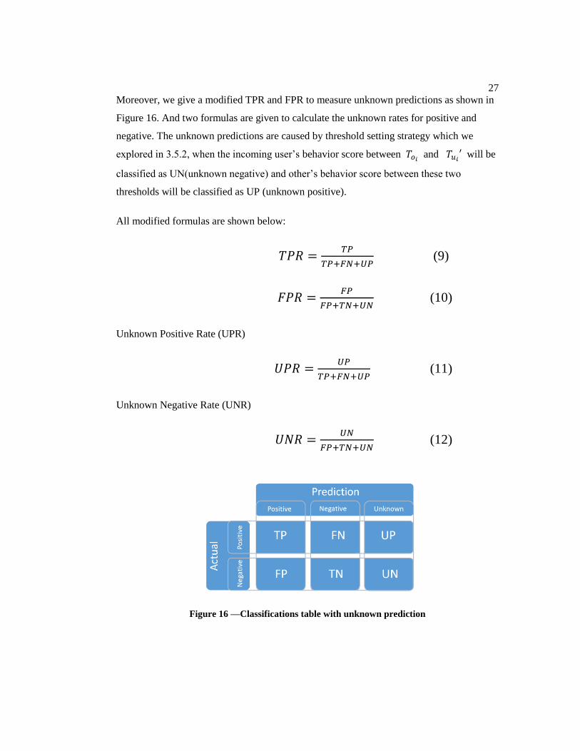
Moreover, we give a modified TPR and FPR to measure unknown predictions as shown in

Figure 16. And two formulas are given to calculate the unknown rates for positive and

negative. The unknown predictions are caused by threshold setting strategy which we

explored in 3.5.2, when the incoming user’s behavior score between 𝑇𝑜𝑖 and 𝑇𝑢𝑖

′ will be

classified as UN(unknown negative) and other’s behavior score between these two

thresholds will be classified as UP (unknown positive).

All modified formulas are shown below:

𝑇𝑃𝑅 =𝑇𝑃

𝑇𝑃+𝐹𝑁+𝑈𝑃 (9)

𝐹𝑃𝑅 =𝐹𝑃

𝐹𝑃+𝑇𝑁+𝑈𝑁 (10)

Unknown Positive Rate (UPR)

𝑈𝑃𝑅 =𝑈𝑃

𝑇𝑃+𝐹𝑁+𝑈𝑃 (11)

Unknown Negative Rate (UNR)

𝑈𝑁𝑅 =𝑈𝑁

𝐹𝑃+𝑇𝑁+𝑈𝑁 (12)

Figure 16 —Classifications table with unknown prediction

28

For AUC, it is area under Receiver Operating Characteristic (ROC) Curves, X axis of ROC

represents FPR, and Y axis represents TPR. So we will use different thresholds that are set

to detect stolen phone to draw the ROC and calculate the ACU for that curve. Those are

measurements of scouring the function’s performance.

4.3 Experimental Procedures

Experiments will be presented by learning users past behavior and detecting stolen

behavior after. We take one of the user as the phone owner, and our experiment will take

one data set from 42 datasets [10] which represent the owner of the mobile phone, while

the rest of datasets represents thief. Moreover, we take 60 present data from original sets as

training data, and combine reset with a data set group one day data from each user as test

data. Also, we group another one-day data from each user as validation data to apply 3.5.2.

Furthermore, after building a personalized model for that typical user, we use the four-

threshold selecting strategy (3.5) to construct four different detecting models, and then use

TPR and FPR to measure their performance, and use ROC and AUC to evaluate the

scoring function. Furthermore, after doing 42 experiments with different data from datasets

as phone holder, we take the average performance for comparisons and discussions.

4.4 Experimental Results

4.4.1 Anomaly detection

In this and next subsection, we will experiment all threshold setting strategy by using

scoring function SF1 in section 3.4.1 for evaluating their performance.

Firstly, we use user data only to set a threshold, which means there is an absence of

validation set but k fold is used cross validation to set a threshold. As we introduce in

3.5.1, we call the fixed threshold setting method as Strategy 1 and call an adjustable

threshold setting method as Strategy 2. As shown in Figure 17 and Table 6, we can see that

TRP are quite same but FPR for Strategy 2 is lower than Strategy 1 and shows our

adjustable threshold setting method decreases FPR a lot.

29

Table 6 —Average TPR and FPR for anomaly detection

Figure 17 —TPR and FPR for Strategy 1 and Strategy 2

4.4.2 Using an external dataset of other users to help

determine thresholds

In this section, we evaluate two methods to set thresholds with an external dataset of other

users as discussed in 3.5.2. We call the fixed threshold setting method as Strategy 3, and

the adjustable threshold setting method as Strategy 4. Both of them will output unknown

prediction when the behavior’s score is between those two thresholds. As shown in Table

7, these two strategies have much lower FPR compared to Strategies 1 and 2. Moreover,

they also very low UPR compare to TPR and the reducing TPR is because there are lower

than 1% TP be classified as UP.

TPR FPRStrategy 1 88% 7%Strategy 2 87% 5%

30

Table 7 —Average TPR, FPR, Unknown rate for other and user

Science adjustment threshold reduces the FPR with slightly decreasing TPR, so we give

the performance table of 𝑇𝑚𝑖𝑛𝑖 in order to show how well the Best-case scenario can do.

𝑇𝑚𝑖𝑛𝑖 is the lowest threshold. By using that all the time we can yield no false positives in

the test set. Comparing Table 8 to Table 6 and Table 7 we can see that even with zero FPR,

our algorithm still maintains a high positive detection rate. Moreover, because the 𝑇𝑚𝑖𝑛 is

the best classifier threshold we can do on FPR, so we can basically compare 𝑇𝑚𝑖𝑛𝑖 with 𝑇𝑢𝑖

and 𝑇𝑢𝑖′ to see how close they are to the best of circumstances. As we can see in Table 8,

𝑇𝑢𝑖′ / 𝑇𝑚𝑖𝑛𝑖

is greater than 𝑇𝑢𝑖′ / 𝑇𝑚𝑖𝑛𝑖

, it means 𝑇𝑢𝑖′ is better classifier threshold than 𝑇𝑢𝑖

because it closer to 𝑇𝑚𝑖𝑛𝑖 compare with 𝑇𝑢𝑖

′ , however, they both are very close to best

threshold.

Table 8 —Performance Table of using 𝑻𝒎𝒊𝒏𝒊

4.4.3 Scoring Function

In this section, we will compare performance of 2 manually designed scoring functions,

HMM and several learned scoring functions.

TPR FPR UPR UNRStrategy 3 87.5% 1.0% 9.8% 46.1%Strategy 4 87.3% 0.9% 9.4% 46.3%

Tu / Tmin 1.016Tu' / Tmin 1.041

TPR of Tmin 86.1%

FPR of Tmin 0%

31

4.4.3.1 Train with User Data Only

The first compare is SF1, SF2 and HMM, SF1 is a manually designed Scoring Function

(SF1) as we discuss in 3.4, and we measure similarities between two patterns as we

introduced in 3.4.1. For second Scoring Function (SF2), we calculate difference between

two pattern sets as we discussed in 3.4.2. The last is HMM, as we proposed in 3.4.3 is use a

HMM to learn past behavior by preprocessing data into our modified version. Moreover,

AUC values showing in Table 9, we calculate AUC for SF1, SF2 and HMM with FPR

below to 1%, we can see SF1 is slightly higher than SF2 it means with same FPR, it

classifier anomalous behavior better than SF2. However, they both higher than naïve

HMM because they can classifier much better than HMM.

Table 9 —AUC for SF1, SF2 and HMM (FPR under 1%)

4.4.3.2 Train with User and Other Data

Moreover, we modified the Decision Tree (C4.5), Decision Tree with Pruning approach

(C4.5-P), Random Forest (RF) and Artificial Neural Networks (ANN) as learning

algorithms and training set for all those machine learning algorithm includes not only user

data but an external database of other users as well. As we introduced in chapter 3.4, for

our algorithm it is one class problem, those method that we proposed before does not use

data from other users in the training set, but the external database of other user for setting

threshold. So all machine learning algorithm has potential advantage on this experiment.

After training, we predict whether a new behavior is User or not. The performance is

shown in Table 10. Scoring functions and HMM are above red line means they train with

user data only and below machine learning algorithm train with both user and other data.

SF1 SF2 HMMAUC 0.008005 0.008007 0.003015

32

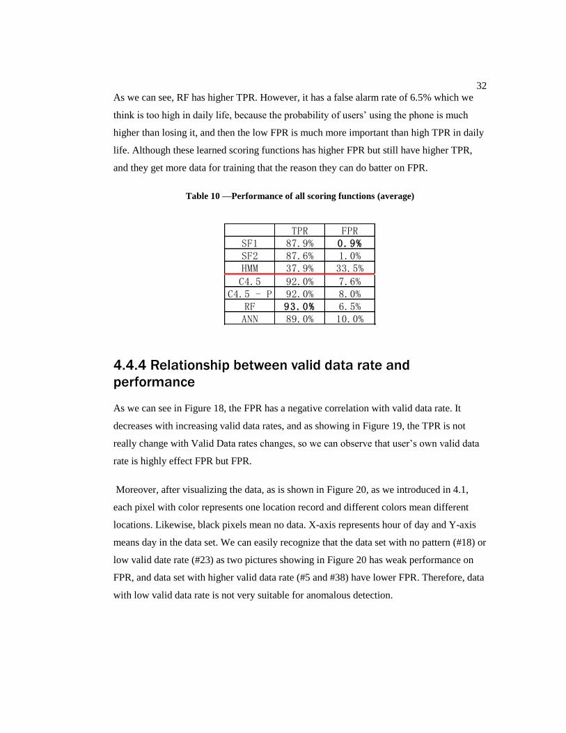
As we can see, RF has higher TPR. However, it has a false alarm rate of 6.5% which we

think is too high in daily life, because the probability of users’ using the phone is much

higher than losing it, and then the low FPR is much more important than high TPR in daily

life. Although these learned scoring functions has higher FPR but still have higher TPR,

and they get more data for training that the reason they can do batter on FPR.

Table 10 —Performance of all scoring functions (average)

4.4.4 Relationship between valid data rate and

performance

As we can see in Figure 18, the FPR has a negative correlation with valid data rate. It

decreases with increasing valid data rates, and as showing in Figure 19, the TPR is not

really change with Valid Data rates changes, so we can observe that user’s own valid data

rate is highly effect FPR but FPR.

Moreover, after visualizing the data, as is shown in Figure 20, as we introduced in 4.1,

each pixel with color represents one location record and different colors mean different

locations. Likewise, black pixels mean no data. X-axis represents hour of day and Y-axis

means day in the data set. We can easily recognize that the data set with no pattern (#18) or

low valid date rate (#23) as two pictures showing in Figure 20 has weak performance on

FPR, and data set with higher valid data rate (#5 and #38) have lower FPR. Therefore, data

with low valid data rate is not very suitable for anomalous detection.

TPR FPRSF1 87.9% 0.9%SF2 87.6% 1.0%HMM 37.9% 33.5%

C4.5 92.0% 7.6%C4.5 - P 92.0% 8.0%

RF 93.0% 6.5%ANN 89.0% 10.0%

33

Figure 18 —Correlation between Vailed Data Rate with FPR

Figure 19 —Correlation between Vailed Data Rate with TPR

34

Figure 20 —Example of data visualization

35

Chapter 5

Conclusion

5.1 Contributions

In this thesis, we propose a system to detect stolen phones. Firstly, we preprocess data into

a well formed framework, which contains 24 datasets across a day. Secondly, we apply a

modified sequential pattern mining algorithm to extract sequential behavioral patterns from

user data. Moreover, we construct those patterns generated by 24 previous datasets into a

personalized model which contains 5 levels. Furthermore, for analyzing the similarities

between two patterns, we identify comparable cases. Then, we create a scoring formula to

calculate how close a new behavior is to the past behavior. We use a K-Fold cross

validation approach to set a threshold. We only use user data to find the threshold and

adjust it when alerts are confirmed to the false during testing. Alternatively, we can add

external data from other users to find the threshold and similarity adjust it when alerts are

confirmed to be false. Finally, after we do the experiment, we find that this system has

87.9% TPR with 0.9% FPR on detect stolen phones.

However, the performance is restricted by the dataset quality. And the similarity

quantization function still has some space to improve. Moreover, we can try other models

to personalize user data such as users’ previous hours to help the current model detect

anomalous behavior.

5.2 Future works

Moreover, we could use more than one model as our prediction model such like combine

our sequential pattern mining model and HMM together to give prediction. Secondly, we

could attach previous predictions to give a comprehensive prediction. Thirdly, we could

use some algorithms to generate fake data to handle low vailed data rate problem.

36

References

[1] Gaurav Tandon and Philip K Chan. Tracking User Mobility to Detect Suspicious

Behavior. Society for Industrial and Applied Mathematics. Year: 01/2009, page:

871.

[2] Chi Zhang, Robert W.H. Fisher, Joel Wei. I Want to Go Home: Empowering the

Lost Mobile Device. 2010 IEEE 6th International Conference on Wireless and

Mobile Computing, Networking and Communications. Year: Oct. 2010, pages 64 -

70.

[3] Katayoun Farrahi, Gatica-Perez, Daniel. Probabilistic Mining of Socio-Geographic

Routines from Mobile Phone Data. IEEE Journal of Selected Topics in Signal

Processing. Year: May. 2010, Pages 745 – 755.

[4] Eric Hsueh-Chan Lu, Yi-Wei Lin and Jing-Bin Ciou. Mining mobile application

sequential patterns for usage prediction. 2014 IEEE International Conference on

Granular Computing. Year: Oct. 2014, Pages: 185 – 190.

[5] ZhungXun Liao, PoRuey Lei, TsuJou Shen, ShouChung Li, WenChih Peng,

AppNow: Predicting Usages of Mobile Applications on Smart Phones. 2012

Conference on Technologies and Applications of Artificial Intelligence. Year:

Nov. 2012, pages: 300 – 303.

[6] Liao Zhuang-Xun, Pan Yi-Chin, Peng Wen-Chih, Lei Po-Ruey. On Mining Mobile

Apps Usage Behavior for Predicting Apps Usage in Smartphones. Proceedings of

the 22nd ACM international conference on conference on information &

knowledge managementYear: Oct. 2013, Pages: 609 – 618.

[7] Shin Choonsung, Hong Jin-Hyuk, Dey Anind. Understanding and Prediction of

Mobile Application Usage for Smart Phones. Proceedings of the 2012 ACM

Conference on ubiquitous computing. Year: Sep. 2012, Pages: 173 – 182.

[8] Weichaih Hung, Fan Shen, Yileh Wu. Activity Recognition with Sensors on

Mobile Devices. 2014 International Conference on Machine Learning and

Cybernetics (ICMLC). Year: July 2014, Pages: 449 – 454.

[9] Feng Xie; Song, Andy; Ciesielski, Vic. Genetic programming based activity

recognition on a smartphone sensory data benchmark. 2014 IEEE Congress on

Evolutionary Computation (CEC). Year: Feb 2014, Pages: 2917 - 2924

37

[10] B Nathan Eagle, Alex Pentland, and David Lazer. Inferring Social Network

Structure using Mobile Phone Data. Proceedings of the National Academy of

Sciences (PNAS). Year: 2009, Pages: 15274-15278.

[11] Ayres Jay, Flannick Jason, Gehrke Johannes, Yiu Tomi. Sequential pattern mining

using a bitmap representation. Proceedings of the eighth ACM SIGKDD

international conference on knowledge discovery and data mining. Year: 2002,

Pages: 429-435.

[12] Agrawal, R, Srikant R. Mining Sequential Patterns. In Proceedings of the Eleventh

IEEE International Conference on Data Engineering. Year: 1995, Pages: 3-14.

[13] Ho, J., Lukov, L., and Chawla, S. Sequential pattern mining with constraints on

large protein databases. Proceedings of the 12th International Conference on

Management of Data (COMAD). Year: 2005, Pages: 89–100.

[14] Bridle, Robert and McCreath, Eric. Context-Aware Mobile Computing: Learning

Context-Dependent Personal Preferences from a Wearable Sensor Array. IEEE

Transactions on Mobile Computing. Year: Feb 2006, Pages: 113 – 127.

[15] Feng Xie; Song, Andy; Ciesielski, Vic. Event detection in time series by genetic

programming. 2012 IEEE Congress on Evolutionary Computation. Year: 2012,

Pages: 1 – 8.

[16] Huang, Ke; Zhang, Chunhui; Ma, Xiaoxiao; Chen, Guanling. Predicting mobile

application usage using contextual information. Proceedings of the 2012 ACM

Conference on ubiquitous computing. Year: 2012, Pages: 1059 – 1065.

[17] Quinlan, J. Ross. C4.5: Programs for Machine Learning. The Morgan Kaufmann

series in machine learning. Year: 2014.

[18] Russell, Stuart J and Norvig, Peter. Artificial intelligence: a modern approach.

2003, 2nd ed., Prentice Hall series in artificial intelligence. Year: 2003.

[19] Breiman, Leo. Random Forests. Machine Learning, ISSN 0885-6125. Year: 2001

Pages: 5-32.

[20] Farrahi, Katayoun and Gatica-Perez, Daniel. Probabilistic Mining of Socio-

Geographic Routines From Mobile Phone Data. IEEE Journal of Selected Topics

in Signal Processing. Year: 2010 Pages: 746 - 755.

[21] U.S. Federal Communications Commission.

https://www.fcc.gov/search/#q=smartphone%20crime