Using Adaptive Sparse Grids to Solve

High-Dimensional Dynamic Models∗

Johannes BrummDBF, University of Zurichjohannes.brumm@uzh.ch

Simon ScheideggerDBF, University of Zurichsimon.scheidegger@uzh.ch

October 31, 2013

Abstract

We present a flexible and scalable method to compute global solu-tions of high-dimensional non-smooth dynamic models. Within a time-iteration setup, we interpolate policy functions using an adaptive sparsegrid algorithm with piecewise multi-linear (hierarchical) basis functions.As the dimensionality increases, sparse grids grow considerably slowerthan standard tensor product grids. In addition, the grid scheme we useis automatically refined locally and can thus capture steep gradients oreven non-differentiabilities. To further increase the maximal problem sizewe can handle, our implementation is fully hybrid parallel, i.e. using acombination of MPI and OpenMP. This parallelization enables us to effi-ciently use modern high-performance computing architectures. Our timeiteration algorithm scales up nicely to more than one thousand parallelprocesses. To demonstrate the performance of our method, we apply itto high-dimensional international real business cycle models with capitaladjustment costs and irreversible investment.

∗We are grateful to Felix Kubler for very helpful discussions and support. We thank seminarparticipants at the University of Zurich, Stanford University and the CEF 2013 in Vancouver.Moreover, we thank Xiang Ma for very instructive email discussions regarding the workings ofadaptive sparse grids. We are grateful for the support of Olaf Schenk, Antonio Messina andRiccardo Murri concerning HPC related issues. We acknowledge CPU time granted on theUniversity of Zurich’s ‘Schrodinger’ HPC cluster. Johannes Brumm gratefully acknowledgesfinancial support from the ERC.

1

1 Introduction

Model-based macroeconomics has for decades relied on the representative agentassumption and on local solution methods. This approach allows for a sim-ple and transparent analysis, yet it has severe limitations. Therefore, from thenineties onward more and more economists included various kinds of hetero-geneity in their models and also started to use global solution techniques (see,e.g. [38] or [24]). Eventually, the recent financial crisis with its large price move-ments and spillover effects has made it obvious that important aspects of theeconomy can be captured only if its global equilibrium dynamics as well as theinteractions between different firms, sectors or countries are taken into account.However, solving for the global solution of a model that includes substantialheterogeneity is very costly: Using conventional solution methods, the compu-tation time and storage requirements increase exponentially with the amount ofheterogeneity, i.e. the dimensionality of the problem.

This paper makes an effort to shift the limits of how much heterogeneitywe can assume in an economic model and still be able to compute an accurateglobal solution in a reasonable amount of time. We achieve this by employing ahighly parallel implementation of a so-called adaptive sparse grid method [25]within a time iteration framework. This method can handle high-dimensionalproblems even if they exhibit non-smooth behavior like non-differentiable policyfunctions.

Standard algorithms that are used to compute global solutions of economicmodels rely on a grid-based numerical representation of a multivariate policyfunction (see, [19]). However, starting with a one-dimensional discretizationscheme that employs N grid points, a straightforward extension to d dimen-sions leads to Nd grid points. Sparse grids are able to alleviate this so-called‘curse of dimensionality’ by reducing the number of grid points from O

(Nd)

to O(N · (logN)d−1

)with only slightly deteriorated accuracy if the underlying

function is sufficiently smooth (see, e.g. [5], with references therein).The sparse grid construction we are using was introduced by Zenger [40] for

the solution of partial differential equations (PDEs). However, the underlyingprinciple, a sparse tensor product decomposition, goes back to the seminal workof Smolyak [37]. Sparse grids have been applied to a whole range of differentresearch fields such as physics, visualization, and finance (see, e.g. [10, 5, 14,27]). Using the original formulation of Smolyak [37], Kruger and Kubler [23]were the first to solve dynamic economic models using sparse grids. Recently,Judd et al. [18] propose an implementation that is more efficient and also allowsfor grids that are ex ante chosen to be finer in some dimensions than in others.However, these two papers rely on global polynomials as basis functions, whichfail to capture the local behavior of policy functions that are not sufficientlysmooth. In contrast, we use piecewise multi-linear (hierarchical) basis functionswith local support in order to successfully resolve non-smooth behaviour. On topof this, we employ an automatic, adaptive grid refinement strategy that scaleslinearly with increasing dimensionality (see, e.g. [25, 31, 29]). This framework –an adaptive sparse grid combined with local basis functions – offers the promiseof an efficient and accurate solution of economic problems that are both high-dimensional and non-smooth.

However, the latter class of problems requires substantial computation timeeven if an efficient solution method is applied. Therefore, our implementation

2

aims to access high-performance computing (HPC) facilities. Their mainstreamhardware design nowadays consists of shared memory nodes with several multi-core CPUs that are connected via a network structure. Hence, efficient parallelprogramming must make use of multiple computational units by combining dis-tributed memory parallelization on the node interconnect with shared memoryparallelization inside each node (see, e.g. [32]). We address this challenge byan implementation that is ‘hybrid’ parallel, i.e. using MPI (‘Message PassingInterface’; cf. [36]) between nodes and OpenMP (shared memory parallelism; cf.[17]) within the nodes. In the hybrid MPI/OpenMP mode, we are able to useefficiently at least 1,200 cores.

To show that our algorithm can solve standard high-dimensional economicproblems, we solve the international real business cycle (IRBC) model withadjustment costs. For this application the performance of alternative algorithmsis well documented in a study comparing various solution methods (see, [22]).Like many of these established methods, we use a time iteration procedure(see, e.g. [19]) to solve for an equilibrium that is Markov in the capital stockand the productivity levels of all countries. The innovation of our approachlies within each time iteration step, where we use an (adaptive) sparse grid tointerpolate the policy functions. As the policy functions in this model are verysmooth, our linear interpolation scheme has a disadvantage compared to smoothinterpolation schemes. Nevertheless, we can compute quite accurate solutionsfor models that are of higher dimension than any that have been reported inthe comparison study by [22]. However, the purpose and comparative advantageof our algorithm lies in solving models that exhibit non-smooth behavior. Todemonstrate its performance with respect to such models, we augment the IRBCmodel with irreversible investment. In spite of the non-differentiabilities (alsocalled ‘kinks’) induced by this assumption we are still able to compute accuratesolutions for high-dimensional examples. The adaptivity of the grid now ensuresthat we can capture the kinks fairly well without increasing the number ofgridpoints too much.

The main contribution of this paper is as follows: We apply for the firsttime an adaptive sparse grid algorithm to solve large-scale economic models.Using modern high-performance computing facilities, we are able to computeaccurate global solutions for models with more than 20 dimensions, and also tohigh-dimensional models with kinks.

In addition to the above discussed literature on sparse grids, both in math-ematics and economics, our paper is also closely related to two other standsof the literature. First, to papers that develop methods for solving dynamiceconomic models with occasionally binding constraints, e.g. [15, 2, 9]. Whilethese methods are able to match the non-differentiabilities induced by such con-straints very precisely, they are not as flexible and scalable as our method, whichis therefore superior when it comes to problems with more than three or fourcontinuous state variables. Second, our paper is part of the emergent literatureon parallel computing applications in economics (see, e.g. [6]). To the bestof our knowledge, we are the first to efficiently use current high-performancecomputing technology to solve dynamic economic models. We are able to do soas our implementation is fully hybrid parallel.

The remainder of the paper is organized as follows. In Sec. 2, we explain theconstruction of adaptive sparse grids and also provide simple test cases for theiruse in interpolation. In Sec. 3, we embed adaptive sparse grid interpolation

3

in a time iteration algorithm to solve high-dimensional IRBC models, also withirreversible investment. We discuss the performance of this algorithm and reporthow hybrid parallelization can speed up the computations. Sec. 4 concludes.

2 From Full Grids to Adaptive Sparse Grids

In this section, we first provide a brief introduction to ‘classical’, i.e. non-adaptive, sparse grid interpolation. In contrast to the sparse grid interpolationschemes used so far in economics (see, e.g. [23, 18]), we follow a different ap-proach and use hierarchical basis functions (see [5, 10], with references therein).We then proceed to adaptive sparse grids (see, e.g. [29, 30]). The latter usethe hierarchical structure of the grid and of the associated basis functions torefine the sparse grid such that it can capture the local behavior of the inter-polant. Based on examples, we show why adaptive sparse grids are superior ininterpolating functions that exhibit steep gradients or kinks.

2.1 Notation

We first introduce some notation and definitions that we will require later on[5, 10]. For all our considerations, we will focus on the domain Ω = [0, 1]d,where d is the dimensionality of the problem. This situation can be achievedfor other domains by a proper rescaling. Furthermore, let ~l = (l1, ..., ld) ∈ Ndand ~i = (i1, ..., id) ∈ Nd denote multi-indices representing the grid refinementlevel as well as the spatial position of a d−dimensional grid point ~x~l,~i. We then

define the anisotropic, full grid Ω~l on Ω with mesh size h~l := (hl1 , ..., hld) =

2−~l :=

(2−l1 , ..., 2−ld

). Ω~l has different but equidistant mesh sizes hlt in each

coordinate direction t = 1, ..., d. In this way, the grid Ω~l consists of the points

~x~l,~i := (xl1,i1 , ..., xld,id) , (1)

where xlt,it := it · hlt = it · 2−lt , and it ∈ 0, 1, ..., 2lt. In addition, when

dealing with d−dimensional multi-indices such as ~l, we use relational operatorscomponent-wise,

~l ≤ ~k ⇔ lt ≤ kt, 1 ≤ t ≤ d. (2)

We use the l1-norm |~l|1,

|~l|1 :=

d∑t=1

lt (3)

and the maximum norm |~l|∞,

|~l|∞ := max1≤t≤d

lt. (4)

Finally, we define for d−dimensional functions f : Ω→ R the L2−norm

‖f‖L2:=

(∫Ω

|f(~x)|2d~x)1/2

. (5)

4

2.2 Hierarchical Basis Functions in One Dimension

As sparse grid methods are based on a hierarchical decomposition of the un-derlying approximation spaces that are constructed by tensor products, we nowfirst go one step back, starting with one dimension, i.e. Ω = [0, 1]. Afterwards,we will extend the principles to the multivariate case.

The first ingredient of a sparse grid interpolation method is a one-dimensionalmultilevel basis. Let us assume that a function f : Ω → R of interest is suffi-ciently smooth [5]. For the time being we also assume for simplicity that thefunction f vanishes at the boundary, i.e. f |∂Ω = 0. We delegate the treatmentof non-zero boundaries to the Appendix A. An interpolation formula is thengiven by

f (x) ≈ u (x) :=∑i

αiφi (x) (6)

with coefficients αi and a set of appropriate piecewise linear basis functionsφi (~x). In the ‘classical’ sparse grid approach, a hierarchical basis based onstandard hat functions,

φ(x) =

1− |x| if x ∈ [−1, 1]

0 else(7)

is used. The standard hat function is then taken to generate a family of basisfunctions φl,i having support [xl,i − hl, xl,i + hl] by dilation and translation, i.e.

φl,i(x) := φ

(x− i · hl

hl

). (8)

This basis is usually termed nodal basis [5]. The basis functions defined in Eq. 8are used to define the function spaces Vl consisting of piecewise linear functions

Vl := spanφl,i : 1 ≤ i ≤ 2l − 1. (9)

The hierarchical increment spaces Wl are defined by

Wl := spanφl,i : i ∈ Il, (10)

using the index set

Il = i ∈ N, 1 ≤ i ≤ 2l − 1, i odd. (11)

In this way, the hierarchical increment spaces Wl are related to the nodalspaces Vl by the direct sum

Vl =⊕k≤l

Wk. (12)

Fig. 1 shows the first three levels of these hierarchical, piecewise linear basisfunctions. Going now back to Eq. 6, we can see that any function f ∈ Vl canbe uniquely represented as

f (x) ≈ u (x) =

l∑k=1

∑i∈Ik

αk,iφk,i (x) , (13)

with the coefficients αk,i ∈ R. Note that the supports of all basis functions φk,ispanning Wk are mutually disjoint, as can be seen in Fig. 1.

5

Figure 1: Hierarchical basis functions of level 1 (solid blue), 2 (dashed red) and3 (dotted black) for V3.

Figure 2: Basis functions on the subspace W2,1.

2.3 Hierarchical Basis Functions in d−Dimensions

This one dimensional hierarchical basis can now be extended to a d−dimensionalone on the unit cube Ω = [0, 1]d by a tensor construction. In line with theabove argumentation related to the one-dimensional case, all notations can betransferred to the arbitrary-dimensional case as well.

For each grid point ~x~l,~i, an associated piecewise d−linear basis function

φ~l,~i (~x) is defined as the product of the one-dimensional basis functions (see,

Eq. 7)

φ~l,~i (~x) :=

d∏t=1

φlt,it (xt) . (14)

Note that each of the multidimensional (nodal) basis functions φ~l,~i (~x) hassupport of size 2 · h~l. The latter basis functions are again used to define func-tion spaces V~l consisting of piecewise d−linear functions that are zero on the

6

boundary of Ω:

V~l := spanφ~l,~i : ~1 ≤~i ≤ 2~l −~1. (15)

Again, the index set I~l is given by

I~l := ~i : 1 ≤ it ≤ 2lt − 1, it odd, 1 ≤ t ≤ d. (16)

Note that the hierarchical increments, formally defined as

W~l := spanφ~l,~i :~i ∈ I~l, (17)

can alternatively be written as

W~l := V~l \d⊕t=1

V~l−~et , (18)

where ~et is the t−th unit vector.In other words, W~l consist of all φ~l,~i ∈ V~l (using the hierarchical basis func-

tions) which are not included in any of the spaces V~k smaller than V~l1. An

example of such a function space is given if Fig. 2. These hierarchical differencespaces now allow us the definition of a multilevel space decomposition. In linewith the sparse grid literature (see, e.g. [29, 10, 5]), we define Vn := V~n as adirect sum of spaces. Consequently, the hierarchical increment spaces W~l arerelated to the nodal spaces V~l of piecewise d−linear functions with mesh widthhl in each dimension by

Vn :=

n⊕l1=1

· · ·n⊕

ld=1

W~l =⊕|l|∞≤n

W~l, (19)

leading to a full grid with (2n − 1)d

grid points. The interpolant of f , namelyu(~x) ∈ Vn can uniquely be represented by

f(~x) ≈ u(~x) =∑|l|∞≤n

∑~i∈I~l

α~l,~i · φ~l,~i(~x) =∑|l|∞≤n

f~l(~x), (20)

with fl ∈W~l and α~l,~i ∈ R.

For sufficiently smooth f and its interpolant u ∈ Vn [5], we obtain an asymp-totic error decay of

‖f (~x)− u (~x) ‖L2∈ O

(h2n

), (21)

but at the cost ofO(h−dn

)= O

(2nd)

(22)

function evaluations, encountering the so-called curse of dimensionality. Thelatter, i.e. the exponential dependence of the overall computational effort onthe number of dimensions is a prohibitive obstacle for the numerical treatmentof high-dimensional problems. The number of dimensions typically does notallow to handle more than four to five dimensional problems with reasonableaccuracy. For example a resolution of 15 points in each dimension, i.e. n = 4, fora ten-dimensional problem therefore needs 0.58 · 1012 coefficients, which bringsus already to the capacity limits of today’s most advanced computer systems[8].

1Note that a function space V~k is called ‘smaller’ than a space V~l if ∀kt ≤ lt and ∃t : kt < lt.Similarly, a grid Ω~k

is smaller than Ω~l[5, 10].

7

2.4 Classical Sparse Grids

As a consequence of Sec. 2.3, the question that needs to be answered is howwe can construct discrete approximation spaces that are better than Vn in thesense that the same number of invested grid points leads to a higher orderof accuracy [40, 5]. The ’classical’ sparse grid construction arises from a costto benefit analysis (see, e.g., [40, 10, 5], with references therein) in functionapproximation. Thereby, functions f (~x) : Ω → R which have bounded mixedderivatives,

D~lf :=

∂~|l|1

∂xl11 · · · ∂xldd

f (23)

for |l|∞ ≤ 2 are considered. These functions belong to a so-called Sobolev space

Hmix2 (Ω) with

Hmix2 (Ω) := f : Ω→ R : D

~lf ∈ L2 (Ω) , |~l|∞ ≤ 2, f |∂Ω = 0. (24)

Under this prerequisite, the hierarchical coefficients α~l,~i (see, Eq. 20 and [5])

rapidly decay for functions f ∈ Hmix2 , namely as

|α~l,~i| = O(

2−2|~l|1). (25)

The strategy of constructing a sparse grid is now to leave out those subspacesfrom the full grid space Vn that only contribute little to the overall interpolant[5]. An optimization with respect to the number of degrees of freedom, i.e.the grid points, and the resulting approximation accuracy directly leads to thesparse grid space V S0,n of level n, defined by

V S0,n :=⊕

|~l|1≤n+d−1

W~l, (26)

where the index 0 in V S0,n implies f |∂Ω = 0. Note that the concrete choiceof subspaces depends on the norm in which we measure the error. The resultobtained in Eq. 26 is optimal for the L2−norm and the L∞−norm [5].

The dimension of the space V S0,n, i.e. the number of grid points required isnow given by [5, 10]

|V S0,n| = 2n ·(

nd−1

(d− 1)!+O

(nd−2

))= O

(h−1n ·

(log(h−1

n ))d−1

). (27)

This shows the order O(2n · nd−1

), which is a significant reduction of the num-

ber of grid points and, in consequence, of the computational and storage re-quirements compared to O

(2nd)

given in Eq. 22 of the full grid space |Vn| (see,Tabs. 1 and 7). In analogy to Eq. 20, a function f ∈ V S0,n ⊂ Vn can now beexpanded by

fS0,n(~x) ≈ u(~x) =∑

|l|1≤n+d−1

∑~i∈I~l

α~l,~i · φ~l,~i(~x) =∑

|l|1≤n+d−1

f~l(~x), (28)

where fl ∈ W~l. Note that α~l,~i ∈ R are commonly termed the hierarchical

surpluses [40, 5]. They are simply the difference between the function values

8

d |Vn| |V S0,n|1 15 152 225 493 3375 1114 50’625 2095 759’375 351

10 5.77 · 1011 2’00115 4.37 · 1017 5’95120 3.33 · 1023 13’20130 1.92 · 1035 41’60140 1.11 · 1047 95’20150 6.38 · 1058 182’001

100 >Googol 1’394’001

Table 1: Number of grid points for several different types of grids of level 4.Left column: dimension; middle column: full grid; right column: classical, L2

optimal sparse grid with no points at the boundaries.

at the current and the previous interpolation levels (see, Fig. 3). The elegantpoint about Eq. 28 is that it allows to utilize the previous results generatedto improve the interpolation. As we have chosen our set of grid points to benested, i.e. in a way the set of points X l−1 at level l−1 with support nodes ~x~l,~iis contained in X l, namely X l−1 ⊂ X l, the extension of the interpolation levelfrom level l − 1 to l only requires to evaluate the function at grid points thatare unique to X l, that is, at X l

∆ = X l\X l−1.The asymptotic accuracy of the interpolant deteriorates only slightly from

O(h2n

)in case of the full grid (cf. Eq. 21) down to

O(h2n · log(h−1

n )d−1)), (29)

as shown e.g. in [5, 10]. Eqs. 27 and 29 condense the essence why sparsegrids are especially well-suited for high-dimensional problems. Note that Eq.29 also holds for sparse grids with non-vanishing boundaries, i.e. f |∂Ω 6= 0 [5].For sparse grid constructions with non-zero boundaries, we point the reader toAppendix A.

The coefficients α~l,~i in the interpolant of the function f (see, Eq. 28) canquite easily be determined due a nice property of the hierarchical grid, namelyits nested structure, in which the set of points X l−1 at level l− 1 with supportnodes ~x~l,~i is contained in X l, i.e. X l−1 ⊂ X l.

In one dimension, the following relation for the hierarchical coefficients αl,i,l ≥ 1, i odd holds [5, 10]:

αl,i = f (xl,i)−f (xl,i − hl) + f (xl,i + hl)

2

= f (xl,i)−f (xl,i−1) + f (xl,i+1)

2

= f (xl,i)−f(xl−1,(i−1)/2

)+ f

(xl−1,(i+1)/2

)2

. (30)

Note that the coefficients for the basis functions associated to a non-zero bound-ary in case of the ‘Clenshaw-Curtis’ grid (see, Sec. A) are simply given by

9

Figure 3: Construction of u (x) interpolating f (x) = x2 · sin(π · x) with hier-archical linear basis functions of levels 1 and 2. The hierarchical surpluses αl,ithat belong to the respective basis functions are indicated by arrows (cf, Eq.30). They are simply the difference between the function values at the currentand the previous interpolation levels.

α2,i = f (x2,i) , i = 0, 1.In operator form, Eq. 30 can conveniently be rewritten as [10, 5]

αl,i =

[−1

21− 1

2

]l,i

f, (31)

with a generalization to the d−dimensional case

α~l,~i =

(d∏t=1

[−1

21− 1

2

]lt,it

)f. (32)

Note that coefficients are called hierarchical surpluses [5] since a coefficient α~l,~icorrects the interpolant of level l − 1 at the points ~xl,i to the actual value off (~xl,i), as displayed in Fig. 3.

2.5 Adaptive Sparse Grids

The sparse grid structure introduced in the previous sections defines an a prioriselection of grid points that is optimal if certain smoothness conditions are met,i.e. if the function has bounded mixed derivatives (cf., Sec. 2.4 and Eq. 24).However, in many applications (see, e.g. [30], with references therein) includ-ing economic models with occasionally binding constraints, these prerequisitesare not met: the functions of interest often show kinks or finite discontinuities.

10

Thus, the sparse grid methods outlined so far may fail to provide good approx-imations, as they can capture the local behaviour only to some limited extend.Therefore, the next task is to find a way of efficiently approximating functionswhich do not fulfill the necessary smoothness conditions given in Eq. 24.

A very effective strategy to achieve this is to adaptively refine the sparse gridat points around the discontinuity region and spend less points in the region ofsmooth variation (see, e.g. [30, 31, 29, 13, 4, 16, 25]). By doing so, resources areonly invested where needed. While there are various ways to refine a sparse grid(see, e.g. [29], with references therein), we outline only briefly the basic ideasbehind the algorithms that we are using in the course of solving our economicmodels below and omit the technical details. For these, we refer the reader tothe original articles, namely the ones by [25] and [29].

When approximating a function as a sum of piecewise linear basis functions,we can hope that the main contributions to the interpolant stem from compar-atively few terms with big surpluses (cf., Eq. 28 and Fig. 3). The key pointof the refinement strategies of [25, 29] therefore is to monitor the size of thehierarchical surpluses. Recall from Sec. 2.3 and Sec. 2.4 that the interpolatedfunction is represented by a linear combination of hierarchical, piecewise linearhat functions. The piecewise linear hat function has local support in contrastto approaches such as Chebyshev polynomials [26], so it can in principle beused to resolve discontinuities. The coefficients of the hat functions - the hier-archical surpluses - are just the hierarchical increments between two successiveinterpolation levels. The magnitude of the hierarchical surplus reflects the localregularity of the function. For smooth functions, its value tends to zero as thelevel l tends to infinity (cf., Eq. 25). On the other hand, for a non-smoothfunction, a singularity/discontinuity is indicated by the magnitude of the hi-erarchical surplus. The larger the magnitude is, the stronger the singularity.Therefore, the hierarchical surplus serves as a natural error indicator for thesparse grid interpolation.

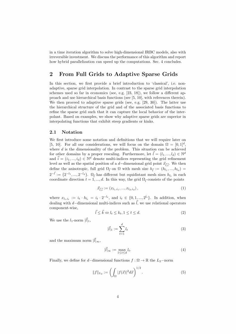
Technically, the adaptive grid refinement can be built on top of the hier-archical grid structure. Let us first consider the one dimensional case. Theequidistant grid points form a tree-like data structure [25], as displayed in Fig.4. Going from one level to the next, we see that for each grid point there aretwo sons. For example, the point 0.5 from level l = 1 is the father of the points0.25 and 0.75 from level l = 2. In the d−dimensional case, there are then con-sequently two sons in each dimension for each grid point, i.e. 2d sons, whengoing from one to the next hierarchical grid level. Moreover, note that the sonsare also the neighbor points of the father. Recall now from Sec. 2.4 and Eq.16 that the neighboring points are the support nodes of the hierarchical basisin the next interpolation level. Therefore, by adding neighboring points, wesimply add the support nodes from the next interpolation level, i.e. we refinean interpolation from level l − 1 to l. In order to adaptively refine the grid,we use the hierarchical surpluses as an error indicator in order to detect thesmoothness of the solution and refine the hierarchical basis functions φ~l,~i whose

magnitude of the hierarchical surplus satisfies:2

|α~l,~i| ≥ ε (33)

Whenever this criterion is satisfied, 2d neighbor points of the current point are

2Note that there exist also alternative refinement strategies, as described e.g. in [30].

11

Figure 4: One-dimensional tree-like structure of a ‘classical’ sparse grid (cf.,Sec. 2.4) for the hierarchical levels l = 1, 2, 3.

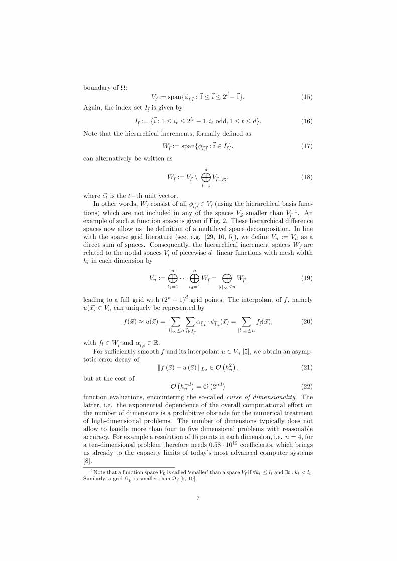
Figure 5: A schematic example of nodes (denoted either by Father or Son) andsupports (size of the respective boxes) of a locally refined sparse grid in twodimensions according to [25, 4].

added to the sparse grid, as shown in Fig. 5. Note that this refinement methodis linear in its scaling and thus does not suffer from the curse of dimensionality.For more technical information regarding the implementation of adaptive sparsegrid methods, we refer to [25, 29].Note that in our application in Sec. 3, we interpolate several policies on onegrid, i.e. we interpolate a function

f : Ω→ Rm.

Therefore, we get m surpluses at each gridpoint and we thus have to replace therefinement criterion in Eq. 33 by

g(α1~l,~i, . . . , αm~l,~i

)≥ ε, (34)

where the refinement choice is governed by a function g : Rm → R. A naturalchoice for g is the maximum function. However, the optimal choice of g dependson the application at hand, as we will discuss in Sec. 3.5.

12

Analytical Examples

We now demonstrate the ability of adaptive sparse grid algorithms to efficientlyinterpolate functions that exhibit steep gradients and kinks. This part containsanalytical tests in one and two dimensions in order to foster the understandingof the adaptive sparse grid algorithms in use, namely the ones by [29] and [25].Their behaviour will be investigated with respect to different settings of grid-and basis functions. Note, however, that these algorithms were extensively andcarefully tested before, e.g. via the test problems by [11]. Therefore, we restrictourselves below to a few examples.

For the testing, we proceed as follows [25, 21]: We pick a (non-smooth)analytical function f (~x), construct the interpolant u (~x) of f (~x) (cf, Eq. 28),

then randomly generate 1000 test points from a uniform distribution in [0, 1]d,

and finally compute the maximum error as follows:

e = maxi=1,...,1000

|f (~xi)− u (~xi) |. (35)

Moreover, we also assess which choice of the sparse grid and its respective basisfunctions suits our purposes best, either the ones by [29] or the ones by [25].More precisely, we compare the following two settings:

• setting A (algorithm by [25]):

– grid: Curtis-Clenshaw grid (cf., Eq. 65)

– basis functions: modified linear basis functions (cf., Eq. 66)

• setting B (algorithm by [29]):

– grid: ‘standard’ sparse grid (cf., Eq. 11)

– basis functions: modified linear basis functions (cf, Eq. 64)

As a first educational example, we apply ‘setting B’ to the one dimensional testfunction

f (x) =1

|0.5− x4|+ 0.01. (36)

The refinement criterion for the adaptive sparse grid algorithm (cf., Eq. 33) ischosen to be ε = 10−2. With this setting, the maximum interpolation errorreaches O

(10−2

)(cf., Eq. 35), while 109 grid points have to be spent. In

contrast, to attain the same level of convergence, 1023 equidistant grid pointshave to be spent,3 as shown in Fig. 6. From Fig. 6, it is obvious that theadaptive sparse grid places points in regions where high resolution is needed,while putting only few points in areas where the function varies little. Thisfact makes adaptive sparse grid algorithms favourable over all other (sparse)grid interpolation methods if kinks or discontinuities have to be handled. Asnon-adaptive methods can only provide one resolution over the whole domain,they waste resources where not needed.

As a second example, we apply both ‘setting A’ and ‘setting B’ with athreshold of ε = 10−2 to the two dimensional test function

1

|0.5− x4 − y4|+ 0.1, (37)

3Note that in the one dimensional case, an ordinary sparse grid of level l corresponds tothe full grid with the same level of refinement.

13

Figure 6: Evaluation of the function given by Eq. 36 at the adaptive sparsegrid points (red diamond) and the ‘full grid’ (blue dots). Both grids attain anmaximum error e = O

(10−2

). The adaptive sparse grid reaches this level of

convergence with 109 points, whereas the full grid needs 1023 points.

Figure 7: Evaluation of Eq. 37 at the grid points obtained by the adaptive sparsegrid algorithm ‘setting B’ after 15 refinement steps.

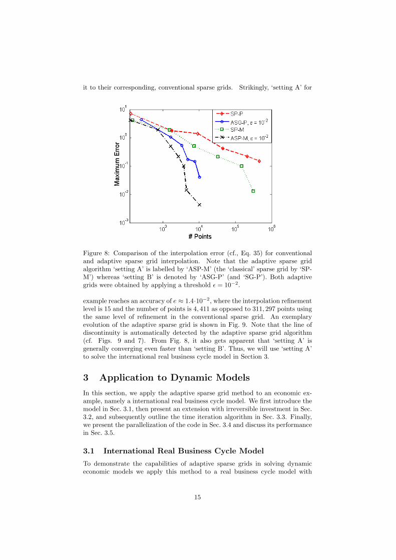
a line-singularity, as shown in Fig. 7. In Fig. 8, we show the convergence rate of‘setting A’ and ‘setting B’ with respect to the required grid points, and compare

14

it to their corresponding, conventional sparse grids. Strikingly, ‘setting A’ for

Figure 8: Comparison of the interpolation error (cf., Eq. 35) for conventionaland adaptive sparse grid interpolation. Note that the adaptive sparse gridalgorithm ‘setting A’ is labelled by ‘ASP-M’ (the ‘classical’ sparse grid by ‘SP-M’) whereas ‘setting B’ is denoted by ‘ASG-P’ (and ‘SG-P’). Both adaptivegrids were obtained by applying a threshold ε = 10−2.

example reaches an accuracy of e ≈ 1.4·10−2, where the interpolation refinementlevel is 15 and the number of points is 4, 411 as opposed to 311, 297 points usingthe same level of refinement in the conventional sparse grid. An exemplaryevolution of the adaptive sparse grid is shown in Fig. 9. Note that the line ofdiscontinuity is automatically detected by the adaptive sparse grid algorithm(cf. Figs. 9 and 7). From Fig. 8, it also gets apparent that ‘setting A’ isgenerally converging even faster than ‘setting B’. Thus, we will use ‘setting A’to solve the international real business cycle model in Section 3.

3 Application to Dynamic Models

In this section, we apply the adaptive sparse grid method to an economic ex-ample, namely a international real business cycle model. We first introduce themodel in Sec. 3.1, then present an extension with irreversible investment in Sec.3.2, and subsequently outline the time iteration algorithm in Sec. 3.3. Finally,we present the parallelization of the code in Sec. 3.4 and discuss its performancein Sec. 3.5.

3.1 International Real Business Cycle Model

To demonstrate the capabilities of adaptive sparse grids in solving dynamiceconomic models we apply this method to a real business cycle model with

15

Figure 9: The evolution of an adaptive sparse grid on [0, 1]2 with a thresholdε = 10−2. The refinement levels 1, 5, 10 and 15 are shown.

multiple countries, i.e. an international real business cycle model. This modelhas become a standard for testing computational methods for solving high-dimensional dynamic models (see, [7], with references therein).

Model Description

There are N countries that differ with respect to their exogenous productivity(and possibly preferences) as well as their endogenous capital stock. They allproduce, trade and consume a single homogeneous good. Production of countryj at time t is given by

yjt = ajt · f j(kjt ) (38)

where ajt , fj , and kjt are productivity, a neoclassical production function, and

the capital stock of country j respectively. The law of motion of productivity isgiven by

ln ajt = ln ajt−1 + σ(ejt + et

), (39)

where the shock ejt is specific to country j, while et is a global shock. Theseshocks are all i.i.d. standard normal.

The law of motion of capital is given by

kjt+1 = kjt · (1− δ) + ijt , (40)

where δ is the rate of capital depreciation, and ijt is investment. There is aconvex adjustment cost on capital, given by

Γjt (kjt , k

jt+1) =

φ

2· kjt ·

(kjt+1

kjt− 1

)2

. (41)

16

The aggregate (i.e. global) resource constraint is thus given by

N∑j=1

yjt ≥N∑j=1

(ijt + Γjt (k

jt , k

jt+1) + cjt

), (42)

where cjt denotes consumption of country j at time t. Substituting and rear-ranging, we get

N∑j=1

(ajt · f j(k

jt ) + kjt · (1− δ)− k

jt+1 − Γjt (k

jt , k

jt+1)− cjt

)≥ 0. (43)

We assume that the preferences of each country are represented by a time sepa-rable utility function with discount factor β and per-period utility function uj .By further assuming complete markets, the decentralized competitive equilib-rium allocation can be obtained as the solution to a social planner’s problem,where the welfare weights, τ j , of the various countries depend on their initialendowments. More precisely, the social planner solves

maxcjt ,k

jtE0

N∑j=1

τ j ·

( ∞∑t=1

βt · uj(cjt )

), (44)

subject to the aggregate resource constraint (43).

First Order Conditions

To get the first order conditions (FOCs) of problem (44), we differentiate theLagrangian with respect to cjt :

τ j · ujc(cjt )− λt = 0, (45)

and with respect to kjt+1:

λt

[−1−

∂Γjt (kjt , k

jt+1)

∂kjt+1

]+

β · Et

λt+1 ·

[ajt+1 · f

jk(kjt+1) + (1− δ)−

∂Γjt+1(kjt+1, kjt+2)

∂kjt+1

]= 0, (46)

where λt denotes the multiplier on the time t resource constraint. Differentiatingthe adjustment cost function (41), simplifying, and defining the growth rate ofcapital by gjt = kjt /k

jt−1 − 1, Eq. 46 reads:

− λt ·[1 + φ · gjt+1

]+

β · Etλt+1 ·

[ajt+1 · f

jk(kjt+1) + 1− δ +

φ

2· gjt+2 ·

(gjt+2 + 2

)]= 0. (47)

Concerning the production function f j(kjt ) and the marginal utility functionujc(c

jt ), we assume the following standard functional forms:

f j(kjt ) = A · (kjt )α (48)

17

andujc(c

jt ) = (cjt )

− 1γj , (49)

which imply

f jk(kjt ) = A · α · (kjt )α−1, (50)

cjt =

(λtτj

)−γj(51)

Using these expressions, we finally get the system of N+1 equilibrium conditionsthat we solve in our computations, namely for all countries j ∈ 1, ..., N :

λt ·[1 + φ · gjt+1

]−

β · Etλt+1

[ajt+1 ·A · α · (k

jt+1)α−1 + (1− δ) +

φ

2· gjt+2 ·

(gjt+2 + 2

)]= 0,

(52)

and the aggregate resource constraint

N∑j=1

(ajt ·A · (k

jt )α + kjt ·

((1− δ)− φ

2· (gjt+1)2

)− kjt+1 −

(λtτj

)−γj)= 0.

(53)We solve the IRBC model by iterating on Eqs. 52 and 53. The implementationdetails are provided in Sec. 3.3.

Parameterization

With respect to the parameter choices, we follow Juillard and Villemot (2011)[20], who provide the model specifications for the comparison study that usesthe IRBC model to compare several solution methods (see, [7]). We choose anasymmetric specification where preferences are heterogeneous across countries.In particular, the intertemporal elasticity of substitution (IES) of the N coun-tries is evenly spread over the interval [0.25, 1]. This corresponds to model A5 inJuillard and Villemot (2011) [20]. The only difference between our parameteri-zation and theirs is that we use a (quarterly) depreciation rate of δ = 1%, whilethey write down the model such that they have effectively no depreciation. Theparameters we use are reported in Tab. 2. The Negishi weights τ j need not tobe specified as they do not matter for the capital allocation, but only for theconsumption allocation which we do not consider. The parameter A is chosensuch that the steady state capital of each country is equal to 1.

3.2 IRBC Model With Irreversible Investment

To demonstrate that our algorithm can handle non-smooth behavior, we includeirreversible investment in the IRBC model of Sec. 3.1. More precisely, weassume that investment cannot be negative, thus for each country j ∈ 1, ..., Nthe following constraint has to be satisfied:

kjt+1 ≥ kjt · (1− δ) (54)

18

Parameter Symbol Valuediscount factor β 0.99IES of country j γj a+(j-1)(b-a)/(N-1)

with a=0.25, b=1capital share α 0.36depreciation δ 0.01std. of log-productivity shocks σ 0.01autocorrelation of log-productivity ρ 0.95intensity of capital adjustment costs φ 0.50number of countries N 4, 6, 8, 10, or 11

Table 2: Choice of parameters for the IRBC model

As a consequence, we have to solve a system of 2N + 1 equilibrium conditions.Namely, for all countries j ∈ 1, ..., N the Euler equations and the irreversibilityconstraints:

λt ·[1 + φ · gjt+1

]− µjt

− β · Etλt+1

[ajt+1 ·A · α · (k

jt+1)α−1 + (1− δ) +

φ

2· gjt+2 ·

(gjt+2 + 2

)]= 0,

kjt+1 − kjt (1− δ) ≥ 0, µjt ≥ 0,

(kjt+1 − k

jt (1− δ)

)· µjt = 0

(55)

and also the aggregate resource constraint:

N∑j=1

(ajt ·A · (k

jt )α + kjt ·

((1− δ)− φ

2· (gjt+1)2

)− kjt+1 −

(λtτj

)−γj)= 0.

(56)In Eq. 55 the variable µjt denotes the Kuhn-Tucker multiplier for the irreversibil-ity constraint kjt+1 − k

jt · (1− δ) ≥ 0.

The parameters we use for the IRBC model with irreversible investment are thesame as the ones we use for the IRBC model, except that we set φ = 0. Thus,the convex adjustment costs on capital are now replaced by the irreversibilityconstraint.

3.3 Time Iteration Algorithm

To compute an equilibrium of the IRBC model, we embed adaptive sparse gridinterpolation in a time iteration algorithm 4 (see, e.g. [19]). We solve for anequilibrium that is Markov in the the physical state of the economy, which isgiven by the capital stock and the productivity levels of all N countries:(

a1t , . . . , a

Nt , k

1t , . . . , k

Nt

). (57)

Denoting the state space by S ⊂ R2N+ , we thus solve for policies

p =(k1t+1, . . . , k

Nt+1, λt

): S → RN+1

+ . (58)

4Note that the focus in this section lies on the description of the time iteration algorithmfor the smooth IRBC model – however, the time-iteration procedure for the non-smooth IRBCworks analogously.

19

Such policies represent an equilibrium of the IRBC model, only if they satisfyEqs. 52 and 53 at all points in the state space. To compute policies that ap-proximately satisfy this condition, we use time iteration and employ adaptivesparse grid interpolation in each of its iteration steps.

The structure of the time iteration algorithm is as follows:

1. Make an initial guess for next period’s policy function:

pinit =(k1t+2, . . . , k

Nt+2, λt+1

).

Set pnext = pinit.

2. Make one time iteration step:

(a) Using an adaptive sparse grid procedure, construct a set G of gridpoints

g =(a1t , . . . , a

Nt , k

1t , . . . , k

Nt

)∈ G ⊂ S

and optimal policies at these points

p(g) =(k1t+1(g), . . . , kNt+1(g), λt(g)

)by solving at each grid point g the system of equilibrium conditions(cf. Eqs. 52 and 53, or 55 and 56) given next period’s policy

pnext =(k1t+2, . . . , k

Nt+2, λt+1

).

(b) Define the policy function p by interpolating between p(g)g∈G.

(c) Calculate (an approximation for) the error, e.g.

η = ‖p− pnext‖∞.

If η > ε, set pnext = p and go to step 2, else go to step 3.

3. The (approximate) equilibrium policy function is given by p.

The essential step in this algorithm is 2(a). To understand the details of thisstep, it is crucial to know which variables in Eqs. 52 and 53 (or 55 and 56) aregrid points, known policy functions, or unknown policies respectively.

3.4 Parallelization and Scaling

In order to enable the solution of ‘large’ problems in a reasonable amount oftime, we aim to access modern high-performance computing architectures. Thetime iteration algorithm used to solve the IRBC model is therefore parallelizedby a hybrid parallelization scheme, i.e. with MPI [36] (distributed memory par-allelization) between the compute nodes and OpenMP [17] within the nodes.We achieve this as follows. We construct adaptive sparse grids according to thealgorithm of [25] (cf. ‘setting A’, Sec. 2.5), which allows for an MPI parallelevaluation of the hierarchical surpluses, i.e. it distributes the newly generatedpoints within a refinement step among different multicores (see, Fig. 10). Ontop of this, we add an additional level of parallelism. Locally, we solve the non-linear system of equations (see, Sec. 3.1 and Eqs. 52 and 53 or Eqs. 55 and 56,

20

respectively) in a shared memory fashion (OpenMP) in order to evaluate thehierarchical surpluses at these particular gridpoints. A schematic illustration ofan arbitrary time step is displayed in in Fig. 10. Note that in our implementa-tion, we solve the set of nonlinear equations with IPOPT [39] in combinationwith PARDISO [35, 34].

Figure 10: Schematic representation of the hybrid parallelization of a time iter-ation step (see, Sec. 3.3). The total number of cores used is given by the numberof MPI processes times the numbers OpenMP threads.

The advantage of this parallelization scheme is that it drastically reduces theamount of MPI communication required between different multicores. This factis important, as the MPI communication overhead between different processescan turn out to be a roadblock for the efficiency of the code when going to ‘large’process numbers [36].

Indicative performance numbers are shown in Fig. 11, where we display thespeedup Sp and the efficiency Ep of the code. These two quantities are definedby [33]

Sp =T0

Tp, Ep =

Spp

=T0

pTp, (59)

where T0 is the execution time of the test benchmark, Tp is the execution time ofthe algorithm running with a multiple of p−times the processes of the baseline.We see that the code scales nicely to at least about 1, 200 parallel processes, asshown in Fig. 11.

21

In Fig. 12, we show how the number of gridpoints grows with the number ofcontinuous state variables in models that are solved with an adaptive sparse grid.As expected, the number of points grows only moderately with the dimension,i.e. ∼ O (d). The running times on the other hand grow faster, because thenumber of gridpoints is not the only thing that is increasing with the dimensionof the problem. The size of the equation systems (cf., Eqs. 52 and 53, or Eqs.55 and 56, respectively) that have to be solved at each gridpoint also growslinearly in the dimension, implying that the size of the Jacobians that have tobe computed grows quadratically. Therefore, the time spent solving the set ofnonlinear equations represents the true roadblock of the time iteration schemepresented here. However, we can - at least to some limited extend - control theincreasing running times by simply using a larger number of CPUs. Thus, while14 to 16 dimensional models are still comfortably tractable on a single desktopor workstation with acceptable accuracy, models with 20 or more dimensionsneed to be run on a high performance computer in order to get results in areasonable amount of time.

Figure 11: The figure shows ‘strong scaling’ of the code under a hybrid paral-lelization with MPI between nodes and Open MP within nodes. The test wasperformed on the Schrodinger system (nodes with 8 core Intel Xeon X5560 2.8GHz processors) at the University of Zurich and consisted of one representativetime step. The test problem was a 10-dimensional classical sparse grid of re-finement level 3 on which we solve Eqs. 52 and 53. The speedup, normalizedto 8 processes, is shown on the left hand side and refers to how much the par-allel algorithm is faster compared to its baseline (see, Eq. 59). The efficiency isdisplayed on the right hand side.

3.5 Performance and Accuracy

So far, we have described the models we solve, the algorithm we use to solvethem, and the way in which we parallelize this algorithm. In this section, weshow how this algorithm performs in solving the IRBC model. Yet first of all,some implementation details and the measures we use to assess accuracy haveto be described.

22

Figure 12: The figure shows how the number of gridpoints grows with increasingdimensionality of the problem, normalized to 4 dimensions. The test problemwas the IRBC model that was run with an adaptive sparse grid and the refine-ment criterion set to |α~l,~i| ≥ ε = 2.5 · 10−3 (cf., Eq. 33). Note that this choiceof ε leads to model accuracies comparable to the ones reported in Tab. 4.

Implementation Details

One important detail is the integration procedure used to evaluate the expec-tations operator, e.g. in Eq. 52. As we want to focus on the grid structure, wechose an integration rule that is simple and fast, yet not very accurate 5. Inparticular, we use a simple monomial rule that uses just two evaluation pointsper shock, i.e. 2(N+1) points in total (see, [19], with references therein). As weapply the same rule along the time-iteration algorithm as well as for the errorevaluation, this choice factors out the question of finding integration proceduresthat are both accurate and efficient. In principle integration could also be car-ried out using an (adaptive) sparse grid (see Appendix B), yet not over thesame space that the policy functions are interpolated on. Therefore, we viewintegration as a problem that is orthogonal to the choice of the grid structure,and thus do not focus on it.Another implementation detail concerns the possibility of accelerating the timeiteration procedure by starting with coarse grids and later changing to finergrids. For instance, using classical sparse grids, the overall computation timecan be reduced by one order of magnitude when using a level one grid for 200iterations, followed by 80 iterations on a level 2 grid, before finally using a levelthree grid for 20 periods instead of running all 300 iterations with a grid oflevel 3. Our tests indicate that this approach yields the same accuracy of re-

5For the IRBC, however, the integration rule we use delivers the same accuracy as MonteCarlo integration with 1000 random evaluation points.

23

sults as if the entire simulation would have been carried out at level 3. As withintegration, it is not the focus of this paper to discuss the most efficient acceler-ation strategy. Of course, if results are compared below, they are achieved withcomparable acceleration strategies.

Error Measure

To evaluate the accuracy of our solutions we compute (unit-free) errors in theN +1 first-order equilibrium conditions. Namely, for all countries j ∈ 1, ..., Nwe get one Euler equation error:[

β · Etλt+1 ·

[ajt+1 ·A · α · (k

jt+1)α−1 + (1− δ) +

φ

2· gjt+2 ·

(gjt+2 + 2

)]]·[λt ·

(1 + φ · gjt+1

)]−1

− 1, (60)

and we get one additional error from the aggregate resource constraint:

N∑j=1

(ajt ·A · (k

jt )α + kjt ·

((1− δ)− φ

2· (gjt+1)2

)− kjt+1 −

(λtτj

)−γj)

·

N∑j=1

(ajt ·A · (k

jt )α + kjt ·

(−φ

2· (gjt+1)2

))−1

. (61)

These expressions are evaluated by using the computed equilibrium policy func-tion to calculate both today’s policy and next period’s policy. We compute theseerrors for all points in the state space that are visited along a (ten thousandperiod) long simulation path. For each of these points we get N + 1 errors. Wethen take the maximum over the absolute value of these errors, which results inone error for each point. Over all these errors, we compute both the maximum(Max. Error) and the average (Avg. Error), which we all report in log10-scale.In case of the IRBC model with irreversible investment there is one additionalcomplication. Denoting the error defined in Eq. 60 by EEj and defining thepercentage violation of the irreversibility constraint by

ICj ≡ −kjt+1

kjt · (1− δ)(62)

the error is now given by

max(EEj , ICj ,min

(−EEj ,−ICj

))(63)

The first term within the max operator, EEj , is positive when the marginal costof investing in country j today is lower then the discounted marginal benefitof this investment tomorrow. Thus, investment in country j is sub-optimallylow. Independent of irreversibility, this is always an error, as the irreversibilityconstraint does not prohibit investing more. The second term, ICj , is positiveif the irreversibility constraint is violated; in this case, it measures the relativesize of the violation. Finally, if −EEj is positive, then the marginal cost ofinvesting in country j today is higher then the discounted marginal benefit

24

Dimension Level Points Max. Error Avg. Error

4 3 137 -2.82 -3.684 4 401 -2.98 -4.194 5 1105 -3.19 -4.244 6 2929 -3.28 -4.55

Table 3: Errors for a ‘classical’ sparse grid solution of the smooth IRBC modelwith fixed dimension and increasing approximation level.

Dimension Level Points Max. Error Avg. Error

4 3 137 -2.97 -3.558 3 849 -3.04 -3.8312 3 2649 -2.71 -3.7816 3 6049 -2.72 -3.80

20* 2 841 -2.58 -3.2922* 2 1013 -2.60 -3.29

Table 4: Errors for a ‘classical’ sparse grid solution of the smooth IRBC modelwith increasing dimension and fixed approximation level 3, except for dimensions20 and 22 where we use only level 2.

of this investment tomorrow. Thus, investment in country j is sub-optimallyhigh. Thus, lower investment would be optimal. Yet, if the constraint is almostbinding investment can only be lowered slightly. In this case, the error made isgiven by the slack in the irreversibility constraint, which is −ICj . Therefore, inthe case that −EEj is positive, the error is not simply given by −EEj but bymin

(−EEj ,−ICj

).

Results for the smooth IRBC model

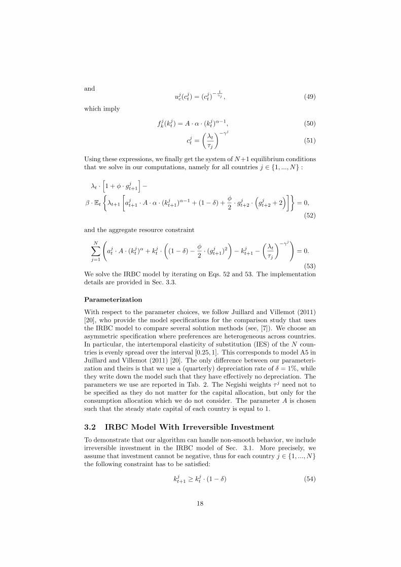
We first consider sparse grids that are not adaptive. Tab. 3 shows how theapproximation errors decrease as we increase the resolution level of the gridkeeping the dimensionality of the problem fixed at 2N = 4. We can see that themaximal and average errors fall as the level of the grid and thereby the num-ber of gridpoints increases. This is exactly what is to be expected. Note thatthe errors are reasonably low even for a relatively small number of gridpoints.This is simply because the policy functions of the IRBC model are very smooth.Therefore, an adaptive grid cannot improve much on classical sparse grids. Forthe same reason, the accuracy of our solutions falls short of the accuracy ob-tained by some smooth approximation methods used in the comparison studysummarized by [22].Let us now turn to higher dimensions. In Tab. 4, we vary the dimensionality of

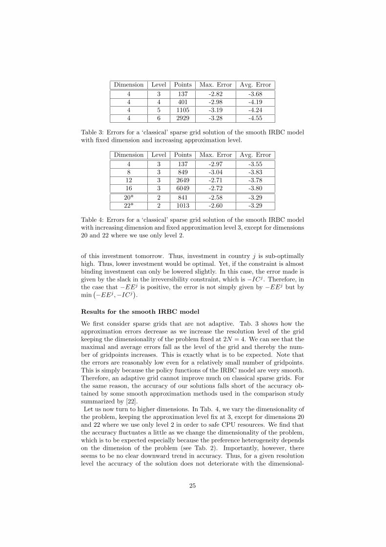
the problem, keeping the approximation level fix at 3, except for dimensions 20and 22 where we use only level 2 in order to safe CPU resources. We find thatthe accuracy fluctuates a little as we change the dimensionality of the problem,which is to be expected especially because the preference heterogeneity dependson the dimension of the problem (see Tab. 2). Importantly, however, thereseems to be no clear downward trend in accuracy. Thus, for a given resolutionlevel the accuracy of the solution does not deteriorate with the dimensional-

25

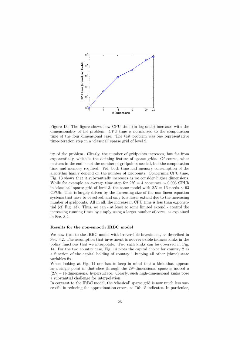
Figure 13: The figure shows how CPU time (in log-scale) increases with thedimensionality of the problem. CPU time is normalized to the computationtime of the four dimensional case. The test problem was one representativetime-iteration step in a ‘classical’ sparse grid of level 2.

ity of the problem. Clearly, the number of gridpoints increases, but far fromexponentially, which is the defining feature of sparse grids. Of course, whatmatters in the end is not the number of gridpoints needed, but the computationtime and memory required. Yet, both time and memory consumption of thealgorithm highly depend on the number of gridpoints. Concerning CPU time,Fig. 13 shows that it substantially increases as we consider higher dimensions.While for example an average time step for 2N = 4 consumes ∼ 0.003 CPUhin ‘classical’ sparse grid of level 3, the same model with 2N = 16 needs ∼ 93CPUh. This is largely driven by the increasing size of the non-linear equationsystems that have to be solved, and only to a lesser extend due to the increasingnumber of gridpoints. All in all, the increase in CPU time is less than exponen-tial (cf, Fig. 13). Thus, we can - at least to some limited extend - control theincreasing running times by simply using a larger number of cores, as explainedin Sec. 3.4.

Results for the non-smooth IRBC model

We now turn to the IRBC model with irreversible investment, as described inSec. 3.2. The assumption that investment is not reversible induces kinks in thepolicy functions that we interpolate. Two such kinks can be observed in Fig.14. For the two country case, Fig. 14 plots the capital choice for country 2 asa function of the capital holding of country 1 keeping all other (three) statevariables fix.When looking at Fig. 14 one has to keep in mind that a kink that appearsas a single point in that slice through the 2N -dimensional space is indeed a(2N − 1)-dimensional hypersurface. Clearly, such high-dimensional kinks posea substantial challenge for interpolation.In contrast to the IRBC model, the ‘classical’ sparse grid is now much less suc-cessful in reducing the approximation errors, as Tab. 5 indicates. In particular,

26

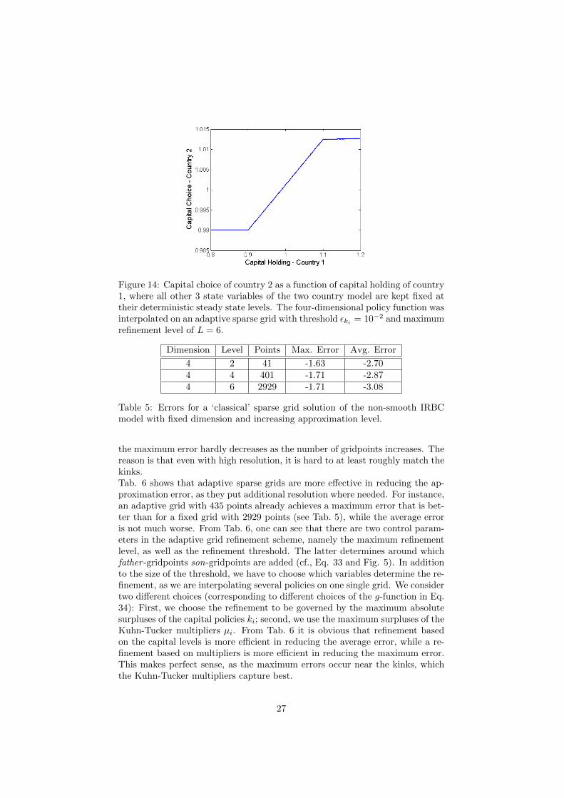
Figure 14: Capital choice of country 2 as a function of capital holding of country1, where all other 3 state variables of the two country model are kept fixed attheir deterministic steady state levels. The four-dimensional policy function wasinterpolated on an adaptive sparse grid with threshold εki = 10−2 and maximumrefinement level of L = 6.

Dimension Level Points Max. Error Avg. Error

4 2 41 -1.63 -2.704 4 401 -1.71 -2.874 6 2929 -1.71 -3.08

Table 5: Errors for a ‘classical’ sparse grid solution of the non-smooth IRBCmodel with fixed dimension and increasing approximation level.

the maximum error hardly decreases as the number of gridpoints increases. Thereason is that even with high resolution, it is hard to at least roughly match thekinks.Tab. 6 shows that adaptive sparse grids are more effective in reducing the ap-proximation error, as they put additional resolution where needed. For instance,an adaptive grid with 435 points already achieves a maximum error that is bet-ter than for a fixed grid with 2929 points (see Tab. 5), while the average erroris not much worse. From Tab. 6, one can see that there are two control param-eters in the adaptive grid refinement scheme, namely the maximum refinementlevel, as well as the refinement threshold. The latter determines around whichfather -gridpoints son-gridpoints are added (cf., Eq. 33 and Fig. 5). In additionto the size of the threshold, we have to choose which variables determine the re-finement, as we are interpolating several policies on one single grid. We considertwo different choices (corresponding to different choices of the g-function in Eq.34): First, we choose the refinement to be governed by the maximum absolutesurpluses of the capital policies ki; second, we use the maximum surpluses of theKuhn-Tucker multipliers µi. From Tab. 6 it is obvious that refinement basedon the capital levels is more efficient in reducing the average error, while a re-finement based on multipliers is more efficient in reducing the maximum error.This makes perfect sense, as the maximum errors occur near the kinks, whichthe Kuhn-Tucker multipliers capture best.

27

Level StatisticsRefinement Threshold

εki = 0.015 εki = 0.010 εµi = 0.015 εµi = 0.010

6Points 200 677 213 435

Max. Error -1.60 -1.95 -1.99 -2.41Avg. Error -2.70 -2.92 -2.41 -2.75

10Points 384 2558 334 1996

Max. Error -1.60 -2.43 -1.99 -2.46Avg. Error -2.70 -2.91 -2.70 -2.80

Table 6: Errors for an adaptive sparse grid solution of the non-smooth IRBCmodel with fixed dimension, for different refinement thresholds, and for variousmaximal approximation levels (first row). The columns with εki and εµi repre-sent models in which we refined the grid either with respect to capital (ki) orthe Kuhn-Tucker multipliers (µi).

By cleverly choosing the maximal refinement level, the refinement rule, as wellas the refinement threshold, we can (already in low dimensions) speed-up thecomputations by at least one order of magnitude since considerably fewer pointshave to be computed. Note that choosing |ε| → 0 leads to a ‘classical’ sparse gridof the corresponding refinement level, which is not desirable. On the other hand,setting |ε| too big may lead to the case that the regions of interest will not bedetected, as the automatic refinement stops already after only a few refinementlevels (see results for εk = 0.015 in Tab. 6). Reducing |ε| can therefore be seenas the major control parameter for reducing the average errors. The maximumrefinement level on the other hand gives control over how much the adaptivesparse grid can be refined at a local instance. This allows for a very high localresolution in areas of the computation where the function values vary consider-ably, while regions of smooth behavior obtain less grid points. We display thisbehaviour in Fig. 15, where a two dimensional projection of two adaptive gridsis shown which only differ in their maximum refinement level. The maximumrefinement level therefore can be considered as the major control parameter forreducing the maximum error, as the case εk = 0.01 shows best. However, if thethreshold is to high, then higher refinement levels cannot help much in reducingthe maximum error, as the examples εk = 0.015 and εµ = 0.015 in Tab. 6show. In any case, one has to experiment with the maximum refinement levelas well as with the refinement rule and threshold in order to find an efficientupdate scheme for a particular problem at hand. In the case of the non-smoothIRBC model for example, we find εµ = 0.015 with maximal refinement level 6provides the best balance between a low number of gridpoints and a relativelyhigh accuracy.

4 Conclusion

We are the first to use an adaptive sparse grid algorithm to solve dynamic eco-nomic models. We achieve this by embedding this algorithm in a time-iterationprocedure. In addition, we provide a fully hybrid parallel implementation of theresulting time-iteration adaptive sparse grid algorithm. With this implementa-tion, we can efficiently use current high-performance computing technology and

28

Figure 15: A 2 dimensional slice of an adaptive sparse grid that was generatedin the course of running a 2N = 4 dimensional simulation. The x-axis showscapital holding of country 1, the y-axis shows capital holding of country 2, whilethe productivities of the two countries are kept fixed at their mean levels. The‘blue-dotted’ grid was generated by the refinement threshold ε = 0.01 and themaximum refinement level fixed at L = 6. The ‘red-crossed’ grid was createdby the same ε = 0.01, but with the maximum refinement level set to L = 8.

are, to the best of our knowledge, the first paper on dynamic economic modelsto do so. We thus provide an important contribution to the emergent literatureon parallel computing applications in economics.The time-iteration adaptive sparse grid algorithm we use is highly flexible andscalable. First, by choosing the resolution level we can tightly control accuracy,thus being able to strike the right balance between running times and the de-sired accuracy of the solution. Second, keeping the resolution level fixed, we canincrease the dimensionality of the problem without worsening accuracy. Third,due to the highly parallelized implementation, we can speed up the computa-tions tremendously by simply using a larger number of CPUs. This allows us tosolve hard problems in a relatively short amount of time, and to tackle problemsthat were so-far non-tractable.We apply this algorithm to an IRBC model with adjustment costs and up morethan 20 continuous state variables. We are also able to solve a high-dimensionalIRBC model with irreversible investment. In that application the comparativeadvantage of the adaptive sparse grid comes into full play, as it can efficientlycapture the kinks induced by irreversibility without wasting additional grid-points in regions of the state space where they are not needed.

29

Note that to solve the IRBC model we embed the adaptive sparse grid in atime iteration procedure that operates in the space of policy function. However,adaptive sparse grids are also very promising for interpolating value functionsin classical dynamic programming applications. For such applications, one onlyneeds to approximate a one-dimensional value function on the adaptive sparsegrid, whereas we have to approximate several policy functions on a single grid.We hope that our paper inspires many economic applications of adaptive sparsegrids. Being scalable and flexible, adaptive sparse grids can make use of mod-ern high-performance computing infrastructure, and they can be applied to abroad variety of setups where high dimensional functions have to be interpo-lated efficiently. This tool thus offers the promise to economic modellers of beingable to solve models that include much more heterogeneity than was previouslypossible.

A Sparse Grids with Non-Zero Boundaries

In Sec. 2, we have assumed that the functions under consideration vanish at theboundary of the domain, i.e. f |∂Ω = 0. To allow for non-zero values on theboundaries, the procedure one usually follows is to add additional gridpointsthat are directly located on ∂Ω, and additional, overlapping basis functions areadded [3, 29, 21]. However, this method is not suited for higher-dimensionalproblems, since at least 3d support nodes are needed [21], with almost all grid-points located on the boundary and only a few in the inner part.

A natural way to mitigate this effect while still being able to handle f |∂Ω 6= 0is, among others, to omit gridpoints on the boundary and modify the interiorbasis functions instead to extrapolate towards the boundary of the domain. Thisapproach is especially well suited in settings where for example high accuracyclose to the boundary is not required and where the underlying function doesnot change too much towards the boundary [29].

An appropriate choice for the modified one-dimensional basis functions reads[29]:

φlt,it(xt) =

1 if l = 1 ∧ i = 12− 2l · xt if xt ∈

[0, 1

2l−1

]0 else

if l > 1 ∧ i = 1

2l · xt + 1− i if xt ∈[1− 1

2l−1 , 1]

0 else

if l > 1 ∧ i = 2l − 1

φ(xt · 2l − i

)else.

(64)where the support nodes have the same coordinates as in the ordinary sparsegrid (cf., Eq. 26). The d−dimensional basis functions are obtained in analogyto Eq. 14 by a tensor product construction of the one-dimensional ones. Wedenote this function space V Sn , as it also handles boundary points.

Another popular choice to handle non-zero boundaries is the so-called ‘Clenshaw-Curtis’ sparse grid V S,CCn with equidistant support nodes [25, 21, 1, 28]. Theonly difference compared to the sparse grid V Sn,0 is that the index set of the

30

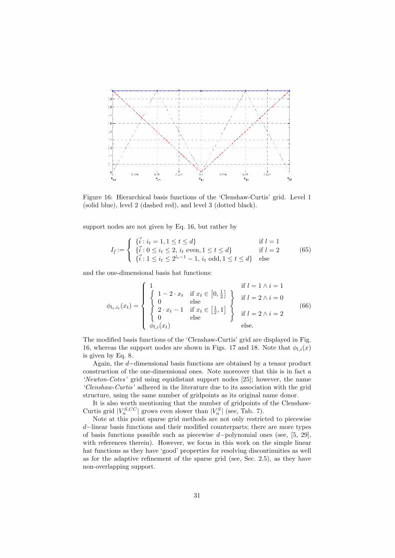
Figure 16: Hierarchical basis functions of the ‘Clenshaw-Curtis’ grid. Level 1(solid blue), level 2 (dashed red), and level 3 (dotted black).

support nodes are not given by Eq. 16, but rather by

I~l :=

~i : it = 1, 1 ≤ t ≤ d if l = 1

~i : 0 ≤ it ≤ 2, it even, 1 ≤ t ≤ d if l = 2

~i : 1 ≤ it ≤ 2lt−1 − 1, it odd, 1 ≤ t ≤ d else

(65)

and the one-dimensional basis hat functions:

φlt,it(xt) =

1 if l = 1 ∧ i = 11− 2 · xt if xt ∈

[0, 1

2

]0 else

if l = 2 ∧ i = 0

2 · xt − 1 if xt ∈[

12 , 1]

0 else

if l = 2 ∧ i = 2

φl,i(xt) else.

(66)

The modified basis functions of the ‘Clenshaw-Curtis’ grid are displayed in Fig.16, whereas the support nodes are shown in Figs. 17 and 18. Note that φl,i(x)is given by Eq. 8.

Again, the d−dimensional basis functions are obtained by a tensor productconstruction of the one-dimensional ones. Note moreover that this is in fact a‘Newton-Cotes’ grid using equidistant support nodes [25]; however, the name‘Clenshaw-Curtis’ adhered in the literature due to its association with the gridstructure, using the same number of gridpoints as its original name donor.

It is also worth mentioning that the number of gridpoints of the Clenshaw-Curtis grid |V S,CCn | grows even slower than |V Sn | (see, Tab. 7).

Note at this point sparse grid methods are not only restricted to piecewised−linear basis functions and their modified counterparts; there are more typesof basis functions possible such as piecewise d−polynomial ones (see, [5, 29],with references therein). However, we focus in this work on the simple linearhat functions as they have ‘good’ properties for resolving discontinuities as wellas for the adaptive refinement of the sparse grid (see, Sec. 2.5), as they havenon-overlapping support.

31

Figure 17: Schematic construction of a ‘Clenshaw-Curtis’ sparse grid in twodimensions (cf., Eq. 65), i.e. d = 2. Hierarchical increment spaces Wl1,l2 for1 ≤ l1, l2 ≤ n = 4. The area enclosed by the red bold lines marks the regionwhere |~l| ≤ n+d−1, fulfilling Eq. 26. The blue dots represent the gridpoints ofthe respective subspaces. Finally, the dashed black lines indicate the hierarchicalincrement spaces for constant |~l|.

Figure 18: Sparse grid space V S,CC4 in 2 dimensions, constructed according toEq. 26 from the increments displayed in Fig. 17. Note that it contains only 29support nodes, whereas a full grid would consist of 225 points.

B Hierarchical Integration

The sparse grid approach can also be used for high-dimensional numerical inte-gration, e.g. for the computation of expectations [12, 25, 28].

Starting from Eq. 28, the mean from the interpolant can be evaluated as

32

d |Vn| |V S0,n| |V S,CCn |1 15 15 92 225 49 293 3375 111 694 50’625 209 1375 759’375 351 241

10 5.77 · 1011 2’001 1’58115 4.37 · 1017 5’951 5’02120 3.33 · 1023 13’201 11’56130 1.92 · 1035 41’601 37’94140 1.11 · 1047 95’201 88’72150 6.38 · 1058 182’001 171’901

100 >Googol 1’394’001 1’353’801

Table 7: Number of gridpoints for several different types of grids of level 4.First column: dimension; second column: full grid; third column: ‘classical’ L2

optimal sparse grid with no points at the boundaries; last column: ‘Clenshaw-Curtis’ sparse grid.

follows:

E [u(~x)] =∑

|l|1≤n+d−1

∑~i∈I~l

α~l,~i

∫Ω

φ~l,~i(~x)d~x, (67)

where we assume for simplicity that the probability density is 1 on Ω = [0, 1]d.Using in the example here the basis functions described in Eqs. 65 and 66, theone dimensional integral can now be computed analytically [25]:

∫ 1

0

φl,i (x) dx =

1, if l = 114 if l = 2

21−l else

(68)

The multi-dimensional integrals are therefore again the product of one dimen-sional integrals. Following [25], we denote

∫Ωφl,i (~x) d~x = J~l,~i. Now, we can

rewrite Eq. 67 by

E [u(~x)] =∑

|l|1≤n+d−1

∑~i∈I~l

α~l,~i · J~l,~i. (69)

Expression 69 states that the mean is an arithmetic sum of the product of thehierarchical surpluses and the integral weights at each point of the interpolant[25]. All other sorts of integrals can be computed in a similar fashion.

References

[1] Volker Barthelmann, Erich Novak, and Klaus Ritter. High dimensionalpolynomial interpolation on sparse grids. Advances in Computational Math-ematics, 12:273–288, 2000.

[2] J. Brumm and M. Grill. Computing equilibria in dynamic models withoccasionally binding constraints. Journal of Economic Dynamics and Con-trol, accepted for publication.

33

[3] H.-J. Bungartz. Dunne Gitter und deren Anwendung bei der adaptivenLosung der dreidimensionalen Poisson-Gleichung. PhD thesis, Munchen,1992.

[4] H.-J. Bungartz and S. Dirnstorfer. Multivariate quadrature on adaptivesparse grids. Computing, 71:89–114, 2003.

[5] Hans-Joachim Bungartz and Michael Griebel. Sparse grids. Acta Numerica,13:1–123, 2004.

[6] Yongyang Cai, Kenneth L. Judd, Greg Thain, and Stephen J. Wright.Solving dynamic programming problems on a computational grid. NBERWorking Papers 18714, National Bureau of Economic Research, Inc, Jan-uary 2013.

[7] Wouter J. Den Haan, Kenneth L. Judd, and Michel Juillard. Computationalsuite of models with heterogeneous agents ii: Multi-country real businesscycle models. Journal of Economic Dynamics and Control, 35(2):175–177,February 2011.

[8] J. J. Dongarra and A. J. van der Steen. High-performance computingsystems: Status and outlook. Acta Numerica, 21:379–474, 4 2012.

[9] Giulio Fella. A generalized endogenous grid method for non-smooth andnon-concave problems. Review of Economic Dynamics, In Press, 2013.

[10] J. Garcke and M. Griebel. Sparse Grids and Applications. Lecture Notesin Computational Science and Engineering Series. Springer-Verlag GmbH,2012.

[11] Alan Genz. Testing multidimensional integration routines. In Proc. ofinternational conference on Tools, methods and languages for scientific andengineering computation, pages 81–94, New York, NY, USA, 1984. ElsevierNorth-Holland, Inc.

[12] Thomas Gerstner and Michael Griebel. Numerical integration using sparsegrids. Numerical Algorithms, 18:209–232, 1998.

[13] M. Griebel. Adaptive sparse grid multilevel methods for elliptic PDEsbased on finite differences. Computing, 61(2):151–179, 1998. also as Pro-ceedings Large-Scale Scientific Computations of Engineering and Environ-mental Problems, 7. June - 11. June, 1997, Varna, Bulgaria, Notes onNumerical Fluid Mechanics 62, Vieweg-Verlag, Braunschweig, M. Griebel,O. Iliev, S. Margenov and P. Vassilevski (editors).

[14] C. Hager, S. Hueber, and B. Wohlmuth. Numerical techniques for thevaluation of basket options and its greeks. J. Comput. Fin., 13(4):1–31,2010.

[15] Thomas Hintermaier and Winfried Koeniger. The method of endogenousgridpoints with occasionally binding constraints among endogenous vari-ables. Journal of Economic Dynamics and Control, 34(10):2074–2088, Oc-tober 2010.

34

[16] John D Jakeman and Stephen G Roberts. Local and dimension adaptivesparse grid interpolation and quadrature. arXiv preprint arXiv:1110.0010,2011.

[17] Gabriele Jost, Barbara Chapman, and Ruud van der Pas. Using OpenMP- Portable Shared Memory Parallel Programming. MIT Press, 2007.

[18] Kenneth Judd, Lilia Maliar, Rafael Valero, and Serguei Maliar. Smolyakmethod for solving dynamic economic models: Lagrange interpolation,anisotropic grid and adaptive domain. Working Papers. Serie AD 2013-06,Instituto Valenciano de Investigaciones Economicas, S.A. (Ivie), September2013.

[19] Kenneth L Judd. Numerical methods in economics. The MIT press, 1998.

[20] Michel Juillard and Sebastien Villemot. Multi-country real business cyclemodels: Accuracy tests and test bench. Journal of Economic Dynamicsand Control, 35(2):178–185, February 2011.

[21] Andreas Klimke and Barbara Wohlmuth. Algorithm 847: Spinterp: piece-wise multilinear hierarchical sparse grid interpolation in matlab. ACMTrans. Math. Softw., 31(4):561–579, December 2005.

[22] Robert Kollmann, Serguei Maliar, Benjamin A. Malin, and Paul Pichler.Comparison of solutions to the multi-country real business cycle model.Journal of Economic Dynamics and Control, 35(2):186 – 202, 2011. Com-putational Suite of Models with Heterogeneous Agents II: Multi-CountryReal Business Cycle Models.

[23] Dirk Krueger and Felix Kubler. Computing equilibrium in OLG modelswith stochastic production. Journal of Economic Dynamics and Control,28(7):1411 – 1436, 2004.

[24] Deborah J. Lucas. Asset pricing with undiversifiable income risk and shortsales constraints: Deepening the equity premium puzzle. Journal of Mon-etary Economics, 34(3):325 – 341, 1994.

[25] Xiang Ma and Nicholas Zabaras. An adaptive hierarchical sparse grid col-location algorithm for the solution of stochastic differential equations. J.Comput. Phys., 228(8):3084–3113, May 2009.

[26] Benjamin A Malin, Dirk Kruger, and Felix Kubler. Solving the multi-country real business cycle model using a smolyak-collocation method.Journal of Economic Dynamics and Control, 35(2):229–239, October 2010.

[27] Alin Murarasu, Josef Weidendorfer, Gerrit Buse, Daniel Butnaru, and DirkPflueger. Compact data structure and parallel alogrithms for the sparsegrid technique. In 16th ACM SIGPLAN Symposium on Principles andPractice of Parallel Programming, 2011.

[28] Erich Novak and Klaus Ritter. High dimensional integration of smoothfunctions over cubes. Numerische Mathematik, 75:79–97, 1996.

[29] Dirk Pfluger. Spatially Adaptive Sparse Grids for High-Dimensional Prob-lems. PhD thesis, Munchen, August 2010.

35

[30] Dirk Pfluger. Spatially adaptive refinement. In Jochen Garcke and MichaelGriebel, editors, Sparse Grids and Applications, Lecture Notes in Computa-tional Science and Engineering, pages 243–262, Berlin Heidelberg, October2012. Springer.

[31] Dirk Pfluger, Benjamin Peherstorfer, and Hans-Joachim Bungartz. Spa-tially adaptive sparse grids for high-dimensional data-driven problems.Journal of Complexity, 26(5):508—-522, October 2010. published onlineApril 2010.

[32] Rolf Rabenseifner, Georg Hager, and Gabriele Jost. Hybrid mpi/openmpparallel programming on clusters of multi-core smp nodes. In Proceedings ofthe 2009 17th Euromicro International Conference on Parallel, Distributedand Network-based Processing, PDP ’09, pages 427–436, Washington, DC,USA, 2009. IEEE Computer Society.

[33] Thomas Rauber and Gudula Runger. Parallel Programming: for Multicoreand Cluster Systems. Springer, 2010 edition, March 2010.

[34] Olaf Schenk, Matthias Bollhofer, and Rudolf A. Romer. On large-scalediagonalization techniques for the anderson model of localization. SIAMRev., 50(1):91–112, February 2008.

[35] Olaf Schenk, Andreas Wachter, and Michael Hagemann. Matching-basedpreprocessing algorithms to the solution of saddle-point problems in large-scale nonconvex interior-point optimization. Comput. Optim. Appl., 36(2-3):321–341, April 2007.

[36] Anthony Skjellum, William Gropp, and Ewing Lusk. Using MPI. MITPress, 1999.

[37] S.A. Smolyak. Quadrature and interpolation formulas for tensor productsof certain classes of functions. Soviet Math. Dokl., 4:240–243, 1963.

[38] Chris I. Telmer. Asset-pricing puzzles and incomplete markets. The Journalof Finance, 48(5):1803–1832, 1993.

[39] Andreas Waechter and Lorenz T. Biegler. On the implementation of aninterior-point filter line-search algorithm for large-scale nonlinear program-ming. Math. Program., 106(1):25–57, May 2006.

[40] Christoph Zenger. Sparse grids. In Wolfgang Hackbusch, editor, Paral-lel Algorithms for Partial Differential Equations, volume 31 of Notes onNumerical Fluid Mechanics, pages 241–251. Vieweg, 1991.

36