Using Artificial Neural Networks for Estimation of Thermal Conductivity ofBinary Gaseous Mixtures

Reza Eslamloueyan* and Mohammad Hasan Khademi

Chemical, Oil and Gas Engineering Department, Shiraz University, Zand Avenue, Shiraz, Iran

Prediction of gas thermal conductivity is crucial in the heat transfer process. In this article, we develop anovel method to estimate conductivities of binary gaseous mixtures at atmospheric pressure. The method isa neural network scheme consisting of two consecutive multilayer perceptrons (MLPs). The first MLPestimates pure component conductivities as a function of critical temperature, critical pressure, molecularweight, and temperature. The conductivities calculated in the first MLP as well as molecular weights ofboth compounds and mole fraction of the light components are fed to the second MLP to predict the thermalconductivity of the mixture. The proposed model was trained and tested through a large set of experimentaldata over wide ranges of temperatures, compositions, and substances. Comparing the test and training resultsindicates that the accuracy of the neural model is remarkably better than other alternative methods proposedin the literature. Conventional conductivity correlations require more input parameters which are not availablefor many gases. Also, correlations recommended for pure gas conductivity are usually valid for a particularrange of temperature and substances. However, the MLP scheme is able to cover a wide range of temperaturesand substances with a few numbers of parameters which are abundant for most gases.

Introduction

Thermal conductivity of gases is one of the most importantthermal properties since it is needed in the analysis of heattransfer equipment. Data on thermal conductivity are requiredfor mathematical modeling and computer simulation of heattransfer processes. Over the years, the thermal conductivity hasbeen measured and compiled for many gases. Generally, theestimation methods of thermal conductivity of pure gases canbe classified into two wide categories. In one category, thermalconductivity is estimated through using relations based on thetheory of gases. For example, Pidduck extended theChapman-Enskog method of an infinitely dilute gas of sphericalmolecules to the case of rigid spherical molecules havingrotational energy convertible to translational energy.1 Eucken2

investigated the influence of internal degree of freedom onconductivity of a dilute gas of a polyatomic molecule andproposed a correlation based on the ratio of heat capacities atconstant pressure and constant volume. Ubbelohde assumed thatthe molecules of a dilute gas at different energy states could beconsidered as chemical species, and the flux of energy wasconnected to the diffusion of these species.3 The first work oncalculation of dense gas conductivity based on the hard spheremodel was done by Enskog.4 Longuet-Higgins and Popledeveloped a correlation for conductivity of a dense gas assumingthe existence of a collision mechanism.5 Some other studies inthis category are given in the references.6-13

The second category consists of correlations relating thermalconductivity to other measurable properties such as criticaltemperature, critical pressure, and molecular weight. Forinstance, Misic and Thodos developed two different correlationsfor thermal conductivity of low-pressure pure hydrocarbongases.14,15 One of their correlations was suggested for methane

and cyclic compounds below reduced temperatures of 1.0, andthe other correlation was recommended for higher reducedtemperatures as well as the rest of the hydrocarbons at anytemperature. Bromley and Wilke suggested correlations for purenonhydrocarbon monatomic and linear molecules at low pressure(less than 1 atm).16,17 Plinski estimated the thermal conductivityof CO2, N2, He, Xe, CO, O2, and Ar as a function oftemperature.18 Also, Stiel and Thodos proposed an equation topredict the thermal conductivity of nonlinear molecules ofnonhydrocarbon gases at low pressure.19

Heating or cooling of gaseous mixtures has many applicationsin process industries. Estimation of thermal conductivity of agaseous mixture plays an important role in the design of heatexchangers involving gaseous mixtures. The determination ofthe thermal conductivity of gaseous mixtures is more complexthan pure gases, from both the theoretical and experimentalpoints of view. The thermal conductivity of a gas mixture cannotbe simply predicted through linear combination of conductivitiesof the individual component gases. A number of methods havebeen developed for estimating the thermal conductivity ofgaseous mixtures. The choice of a particular method dependsmainly upon available parameters and the desired accuracy ofestimation. Muckenfuss and Curtiss20 proposed a formula forthe thermal conductivity of an n-component gas mixture. Masonand Saxena showed that the formula of Muckenfuss and Curtisshas two disadvantages from a practical viewpoint.21 First, theformula is quite complicated and involves laborious computa-tion. Second, it requires a reliable knowledge of force laws forthe various molecular interactions, which are rarely availa-ble. To overcome these difficulties, Mason and Saxena21

suggested the following approximate formula

λmix )∑i)1

n

λi[1+ ∑k)1,

n

k*i

Gik

xk

xi ]-1

(1)

where* Corresponding author. Fax: 98-711-6287294. E-mail: eslamlo@shirazu.ac.ir.

J. Chem. Eng. Data 2009, 54, 922–932922

10.1021/je800706e CCC: $40.75 2009 American Chemical SocietyPublished on Web 01/13/2009

Gik )1.065

2√2 (1+Mi

Mk)-

1

2[1+ (λi0

λk0)

1

2(Mi

Mk)

1

4]2

(2)

where M is molecular weight; x is component mole fraction inthe mixture; λ is thermal conductivity of the pure component;and λmix is gas mixture thermal conductivity. Gki is obtainedfrom Gik by interchanging the subscripts, and λi

0 is the frozenthermal conductivity of a pure gas from the following relation

λi0 ) λi[0.115+ 0.354γ ⁄ (γ- 1)]-1 (3)

where γ is the ratio of specific heat of a gas at constant pressureto that at constant volume. Lindsay and Bromley22 suggestedthat Gik in eq 1 be determined from the relation

Gik )14[1+ { ηi

ηk(Mk

Mi)3⁄4 1+ Si ⁄ T

1+ Sk ⁄ T} 1⁄2]21+ Sik ⁄ T

1+ Sk ⁄ T(4)

where ηi and Si are the viscosity and Sutherland constant of acomponent, respectively. Sik is the geometric mean of Si andSk. The Sutherland constant for all pure gases (with the exceptionof hydrogen, deuterium, and helium) was taken from theexpression S ) 1.5Tb, where Tb is the absolute boilingtemperature at atmospheric pressure. For hydrogen, deuterium,and helium, the Sutherland constant was assumed to be equalto 79. It was shown that Lindsay and Bromley correlation doesnot yield accurate values for gas mixture thermal conductivity.23,24

Srivastava and Saxena modified eq 1 through introducing anadditional unknown constant being determined from the valueof mixture conductivity (λmix) at a given composition.23 Ulybinet al.25 used an empirical procedure for computing the thermalconductivity of a binary mixture at a higher temperature fromthe known thermal conductivity of the mixture at some lowertemperature

λmix(T2)) λmix(T1)[x1

λ1(T2)

λ1(T1)+ x2

λ2(T2)

λ2(T1)] (5)

Hirschfelder26 derived the expression for the thermal conductiv-ity of a binary mixture involving polyatomic gases

λmix ) λmix0 +

λ1 - λ10

1+D11

D12

x2

x1

+λ2 - λ2

0

1+D22

D12

x1

x2

(6)

λmix0 )

4(x12L22 - 2x1x2L12 + x2

2L11)

(L122 - L11L22)

(7)

L11 )-4x1

2

λ10-

16Tx1x2

25PD12(M1 +M2)2[(15 ⁄ 2)M1

2 + (25 ⁄ 4)M22 -

3M22B12

* + 4M1M2A12* ] (8)

L12 )16Tx1x2M1M2

25PD12(M1 +M2)2[(55 ⁄ 4)- 3B12

* - 4A12* ] (9)

L22 is obtained from L11 by interchanging the subscripts. HereP is the pressure; D12 is the accurate value of the binary diffusioncoefficient for components 1 and 2; D11 and D22 are self-diffusion coefficients for gases 1 and 2, respectively; and A12*and B12* are dimensionless ratios of certain collision integralscharacterizing molecules of gases 1 and 2. The A12* and B12*are weakly affected by temperature change and the forcesbetween molecules 1 and 2, so they are usually considered tobe unity.

Neural networks have been used extensively in various fieldsof chemical engineering over the last two decades. Turias et al.studied the application of pattern recognition and artificialintelligence techniques in the characterization of a multiphaserealistic disordered composite and in the design of a multipleregression model to estimate effective thermal conductivity.27

Sablani and Rahman presented an artificial neural network

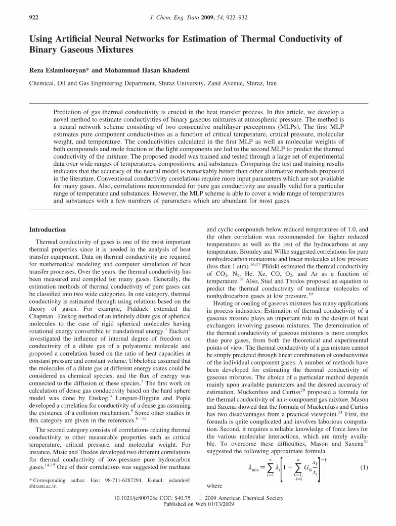
Figure 1. MSE versus iteration number (n) for MLP predicting pure gasconductivity. Solid line: goal; dashed line, training.

Figure 2. MSE versus iteration number (n) for MLP predicting conductivityof a binary gaseous mixture. Solid line, goal; dash line, training.

Figure 3. Correlation of training experimental data versus the predictedconductivities of the pure gases.

Journal of Chemical & Engineering Data, Vol. 54, No. 3, 2009 923

model for the prediction of the thermal conductivity of food atdifferent temperatures, moisture contents, and apparent porosi-ties.28 The model was able to predict thermal conductivity witha mean relative error of 12.6 %. Sablani et al. used artificialneural networks to estimate thermal conductivity of bakery.29

Their model was able to predict thermal conductivity with amean relative error of 10 %. Zhou et al. focused on modelingthe electrical conductivity of recombined milk by artificial neural

networks.30 Jalali-Heravi et al. developed a neural network topredict the response factor of a thermal conductivity detector.31

Eslamloueyan and Khademi designed a multilayer perceptronfor estimation of pure gas thermal conductivity.32 They used aset of 236 experimental data points for hydrocarbon andnonhydrocarbon compounds to develop their neuromorphicmodel. They showed that the proposed neural network outper-forms other alternative methods, with respect to accuracy aswell as extrapolation capabilities.

The objective of this work is to formulate a neural networkscheme for prediction of thermal conductivities of binarygaseous mixtures at atmospheric pressure over a wide range oftemperatures and compositions. The proposed scheme consistsof two consecutive neural networks: the first one is used forpure gas conductivity and the second one for gaseous mixtureconductivity.

Method

Artificial neural networks have the inherent characteristic oflearning and recognizing nonlinear complex relationships, sothey can be used to predict thermal conductivity of gas. Theproposed method is based on multilayer perceptron (MLP)networks.

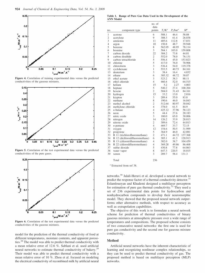
Figure 4. Correlation of training experimental data versus the predictedconductivities of the gaseous mixtures.

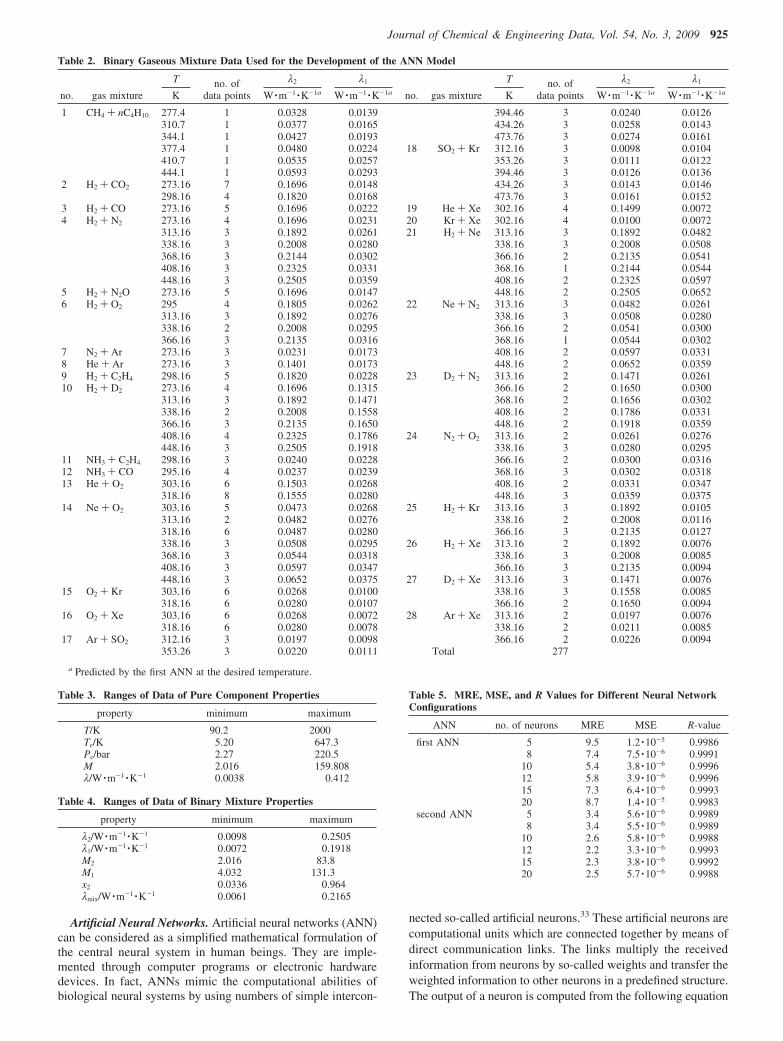
Figure 5. Correlation of the test experimental data versus the predictedconductivities of the pure gases.

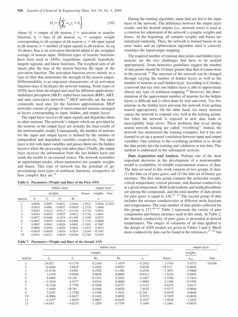
Figure 6. Correlation of the test experimental data versus the predictedconductivities of the gaseous mixtures.

Table 1. Range of Pure Gas Data Used in the Development of theANN Model

no. component type

no. ofdata

points Tc/Ka Pc/bara Ma

1 acetone 6 508.1 46.4 58.082 acetylene 9 308.3 61.4 26.0383 ammonia 11 405.6 112.8 17.0314 argon 10 150.8 48.7 39.9485 benzene 8 562.05 48.95 78.1146 bromine 3 584.1 103.0 159.8087 carbon dioxide 22 304.2 73.8 44.018 carbon disulfide 2 552.0 78.0 76.1319 carbon tetrachloride 5 556.4 45.0 153.82310 chlorine 5 417.0 76.0 70.90611 chloroform 3 536.4 54.0 119.37812 cyclohexane 1 553.5 40.73 84.16113 deuterium 3 38.4 16.4 4.03214 ethane 6 305.32 48.72 30.0715 ethyl acetate 3 523.2 38.3 88.1116 ethyl chloride 4 460.4 52.0 64.51517 helium 15 5.2 2.27 4.00318 heptane 5 540.2 27.4 100.20419 hexene 2 504.0 31.43 84.16120 hydrogen 15 33.2 13.0 2.01621 krypton 3 209.4 55.0 83.822 methane 8 190.6 46.0 16.04323 methyl alcohol 2 512.64 80.97 30.04224 methylene chloride 4 378.0 61.5 84.925 n-butane 4 425.12 37.96 58.12326 neon 5 44.4 27.6 20.18327 nitric oxide 3 180.0 65.0 30.00628 nitrogen 14 126.2 33.9 28.01329 nitrous oxide 2 309.6 72.4 44.01330 n-pentane 4 469.7 33.7 72.1531 oxygen 12 154.6 50.5 31.99932 propylene 5 364.9 46.0 42.08133 R 11 (trichlorofluoromethane) 2 471.1 44.72 137.36834 R 12 (dichlorodifluoromethane) 6 385.1 41.3 120.91335 R 13 (chlorotrifluoromethane) 4 302.0 38.7 104.45936 R 22 (chlorodifluoromethane) 4 369.28 49.86 86.46837 sulfur dioxide 5 430.8 77.8 64.06338 water vapor 8 647.3 220.5 18.01539 xenon 3 289.7 58.4 131.3

Total 236

a Extracted from ref 38.

924 Journal of Chemical & Engineering Data, Vol. 54, No. 3, 2009

Artificial Neural Networks. Artificial neural networks (ANN)can be considered as a simplified mathematical formulation ofthe central neural system in human beings. They are imple-mented through computer programs or electronic hardwaredevices. In fact, ANNs mimic the computational abilities ofbiological neural systems by using numbers of simple intercon-

nected so-called artificial neurons.33 These artificial neurons arecomputational units which are connected together by means ofdirect communication links. The links multiply the receivedinformation from neurons by so-called weights and transfer theweighted information to other neurons in a predefined structure.The output of a neuron is computed from the following equation

Table 2. Binary Gaseous Mixture Data Used for the Development of the ANN Model

T λ2 λ1 T λ2 λ1

no. gas mixture Kno. of

data points W ·m-1 ·K-1a W ·m-1 ·K-1a no. gas mixture Kno. of

data points W ·m-1 ·K-1a W ·m-1 ·K-1a

1 CH4 + nC4H10 277.4 1 0.0328 0.0139 394.46 3 0.0240 0.0126310.7 1 0.0377 0.0165 434.26 3 0.0258 0.0143344.1 1 0.0427 0.0193 473.76 3 0.0274 0.0161377.4 1 0.0480 0.0224 18 SO2 + Kr 312.16 3 0.0098 0.0104410.7 1 0.0535 0.0257 353.26 3 0.0111 0.0122444.1 1 0.0593 0.0293 394.46 3 0.0126 0.0136

2 H2 + CO2 273.16 7 0.1696 0.0148 434.26 3 0.0143 0.0146298.16 4 0.1820 0.0168 473.76 3 0.0161 0.0152

3 H2 + CO 273.16 5 0.1696 0.0222 19 He + Xe 302.16 4 0.1499 0.00724 H2 + N2 273.16 4 0.1696 0.0231 20 Kr + Xe 302.16 4 0.0100 0.0072

313.16 3 0.1892 0.0261 21 H2 + Ne 313.16 3 0.1892 0.0482338.16 3 0.2008 0.0280 338.16 3 0.2008 0.0508368.16 3 0.2144 0.0302 366.16 2 0.2135 0.0541408.16 3 0.2325 0.0331 368.16 1 0.2144 0.0544448.16 3 0.2505 0.0359 408.16 2 0.2325 0.0597

5 H2 + N2O 273.16 5 0.1696 0.0147 448.16 2 0.2505 0.06526 H2 + O2 295 4 0.1805 0.0262 22 Ne + N2 313.16 3 0.0482 0.0261

313.16 3 0.1892 0.0276 338.16 3 0.0508 0.0280338.16 2 0.2008 0.0295 366.16 2 0.0541 0.0300366.16 3 0.2135 0.0316 368.16 1 0.0544 0.0302

7 N2 + Ar 273.16 3 0.0231 0.0173 408.16 2 0.0597 0.03318 He + Ar 273.16 3 0.1401 0.0173 448.16 2 0.0652 0.03599 H2 + C2H4 298.16 5 0.1820 0.0228 23 D2 + N2 313.16 2 0.1471 0.026110 H2 + D2 273.16 4 0.1696 0.1315 366.16 2 0.1650 0.0300

313.16 3 0.1892 0.1471 368.16 2 0.1656 0.0302338.16 2 0.2008 0.1558 408.16 2 0.1786 0.0331366.16 3 0.2135 0.1650 448.16 2 0.1918 0.0359408.16 4 0.2325 0.1786 24 N2 + O2 313.16 2 0.0261 0.0276448.16 3 0.2505 0.1918 338.16 3 0.0280 0.0295

11 NH3 + C2H4 298.16 3 0.0240 0.0228 366.16 2 0.0300 0.031612 NH3 + CO 295.16 4 0.0237 0.0239 368.16 3 0.0302 0.031813 He + O2 303.16 6 0.1503 0.0268 408.16 2 0.0331 0.0347

318.16 8 0.1555 0.0280 448.16 3 0.0359 0.037514 Ne + O2 303.16 5 0.0473 0.0268 25 H2 + Kr 313.16 3 0.1892 0.0105

313.16 2 0.0482 0.0276 338.16 2 0.2008 0.0116318.16 6 0.0487 0.0280 366.16 3 0.2135 0.0127338.16 3 0.0508 0.0295 26 H2 + Xe 313.16 2 0.1892 0.0076368.16 3 0.0544 0.0318 338.16 3 0.2008 0.0085408.16 3 0.0597 0.0347 366.16 3 0.2135 0.0094448.16 3 0.0652 0.0375 27 D2 + Xe 313.16 3 0.1471 0.0076

15 O2 + Kr 303.16 6 0.0268 0.0100 338.16 3 0.1558 0.0085318.16 6 0.0280 0.0107 366.16 2 0.1650 0.0094

16 O2 + Xe 303.16 6 0.0268 0.0072 28 Ar + Xe 313.16 2 0.0197 0.0076318.16 6 0.0280 0.0078 338.16 2 0.0211 0.0085

17 Ar + SO2 312.16 3 0.0197 0.0098 366.16 2 0.0226 0.0094353.26 3 0.0220 0.0111 Total 277

a Predicted by the first ANN at the desired temperature.

Table 3. Ranges of Data of Pure Component Properties

property minimum maximum

T/K 90.2 2000Tc/K 5.20 647.3Pc/bar 2.27 220.5M 2.016 159.808λ/W ·m-1 ·K-1 0.0038 0.412

Table 4. Ranges of Data of Binary Mixture Properties

property minimum maximum

λ2/W ·m-1 ·K-1 0.0098 0.2505λ1/W ·m-1 ·K-1 0.0072 0.1918M2 2.016 83.8M1 4.032 131.3x2 0.0336 0.964λmix/W ·m-1 ·K-1 0.0061 0.2165

Table 5. MRE, MSE, and R Values for Different Neural NetworkConfigurations

ANN no. of neurons MRE MSE R-value

first ANN 5 9.5 1.2 ·10-5 0.99868 7.4 7.5 ·10-6 0.9991

10 5.4 3.8 ·10-6 0.999612 5.8 3.9 ·10-6 0.999615 7.3 6.4 ·10-6 0.999320 8.7 1.4 ·10-5 0.9983

second ANN 5 3.4 5.6 ·10-6 0.99898 3.4 5.5 ·10-6 0.9989

10 2.6 5.8 ·10-6 0.998812 2.2 3.3 ·10-6 0.999315 2.3 3.8 ·10-6 0.999220 2.5 5.7 ·10-6 0.9988

Journal of Chemical & Engineering Data, Vol. 54, No. 3, 2009 925

Oj ) f(∑i)1

n

wjiyi + bj) (10)

where Oj ) output of jth neuron; f ) activation or transferfunction; bj ) bias of jth neuron; wji ) synaptic weightcorresponding to ith synapse of jth neuron; yi ) ith input signalto jth neuron; n ) number of input signals to jth neuron. As eq10 shows, bias is an activation threshold added to the weightedaverage of neuron input. Different types of transfer functionshave been used in ANNs: logarithmic sigmoid, hyperbolictangent sigmoid, and linear functions. The weighted sum of allinputs plus the bias of the neuron become the input of theactivation function. The activation function serves mainly as atype of filter that determines the strength of the neuron output.Differentiability is an important characteristic of an activationfunction since it facilitates the network training. Some types ofANNs have been developed and used for different applications:multilayer perceptron (MLP), radial basis function (RBF), ART,and auto associative networks.34 MLP networks are the mostcommonly used ones for the function approximation. MLPnetworks consist of groups of interconnected neurons arrangedin layers corresponding to input, hidden, and output layers.

The input layer receives all input signals and dispatches themto other neurons. The network’s outputs which are provided bythe neurons in the output layer are actually the final results ofthe neuromorphic model. Consequently, the number of neuronsfor the input and output layers is defined by the number ofindependent and dependent variables, respectively. The inputlayer is fed with input variables and passes them into the hiddenlayer(s) where the processing task takes place. Finally, the outputlayer receives the information from the last hidden layer andsends the results to an external source. The network resemblesan input/output model, whose parameters are synaptic weightsand biases. This type of network has the potential of ap-proximating most types of nonlinear functions, irrespective ofhow complex they are.34

During the training algorithm, input data are fed to the inputlayer of the network. The difference between the output layerresults, and the desired outputs (i.e., network error) is used asa criterion for adjustment of the network’s synaptic weights andbiases. At the beginning, all synaptic weights and biases areinitialized randomly. Then, the network is trained based on anerror index and an optimization algorithm until it correctlysimulates the input/output mapping.

The required number of training data points and hidden layerneurons are the two challenges that have to be tackledappropriately. Some heuristics guidelines suggest the numberof data points should be 10 times greater than that of connectionsin the network.35 The structure of the network can be changedthrough varying the number of hidden layers as well as thenumber of neurons in each hidden layer. According to Cybenko,a network that has only one hidden layer is able to approximatealmost any type of nonlinear mapping.36 However, the deter-mination of the approximate number of neurons for the hiddenlayers is difficult and is often done by trial and error. Too fewneurons in the hidden layer prevents the network from gettingtrained appropriately. On the other hand, too many neuronscauses the network to respond very well at the training points,but when the network is exposed to new data leads tounacceptably large errors. These problems that occur duringneural network training are called “overfitting”. Indeed, thenetwork has memorized the training examples, but it has notlearned to set up a general correlation between input and outputvariables. One solution to the overfitting problem is to dividethe data points into the training and validation or test data. Thismethod is elaborated in the subsequent sections.

Data Acquisition and Analysis. Perhaps one of the mostimportant decisions in the development of a neuromorphicmodel is availability of reliable experimental sources of data.The data set used in this work consists of two groups of data:(1) the data set of pure gases, and (2) the data set of binary gasmixtures. The first data group contains the molecular weight,critical temperature, critical pressure, and thermal conductivityat a given temperature. Both hydrocarbons and nonhydrocarbonsare among the compounds, and the total number of data pointsfor pure gases is equal to 236.37-47 The second group of dataincludes the mixture conductivities at different mole fractionsand temperatures. The total number of data points collected forthis group is 277.48-63 Table 1 represents the variety of purecomponents and binary mixtures used in this study. In Table 2,the thermal conductivity of pure gases is presented at desiredtemperatures. The ranges of variations of all data applied tothe design of ANN models are given in Tables 3 and 4. Muchmore conductivity data can be found in the references,37-63 but

Table 6. Parameters (Weight and Bias) of the First ANN

hidden layer output layer

weights biases weights bias

neuron T Tc Pc M λ

1 0.0056 0.0087 -0.0851 0.5484 -1.9631 0.0266 0.25932 0.0014 0.0001 -0.0037 -0.0029 -2.2370 1.66063 0.0025 0.0125 -0.0317 -0.2144 0.1724 0.08324 0.0014 -0.0025 0.0027 0.0012 -2.1738 -1.60615 -0.0077 -0.0468 0.1674 -0.1409 2.1109 0.02726 -0.0007 0.0070 -0.0016 -0.0000 -1.3710 -0.08097 0.0007 0.0041 0.0020 0.0002 -2.1501 -0.78878 0.0006 0.0036 0.0020 0.0004 -1.8533 0.90339 -0.0019 -0.8016 1.8916 0.5834 2.6549 -0.149710 0.0013 -0.0311 0.0659 -0.0306 0.1766 0.2493

Table 7. Parameters (Weight and Bias) of the Second ANN

hidden layer output layer

weights weights

neuron λ2 λ1 M2 M1 x2 biases λmix bias

1 -24.027 -9.1178 0.2160 1.1079 -0.2562 2.5745 5.9372 0.02902 -6.8484 3.8835 -2.4926 0.9023 9.4038 -20.517 -0.00463 23.4736 9.6501 0.2502 -0.1586 0.2556 -7.3071 5.98804 1.6359 -8.0949 0.0020 -0.0000 -0.0412 -1.5214 -0.99455 8.6869 19.165 -0.1552 0.2854 0.1467 -2.3386 -1.78146 -2.3418 4.5377 0.0316 0.0000 -1.0985 2.1296 -0.57047 -9.7146 4.7798 -0.7689 0.0727 4.3115 0.8415 0.01178 -1.8480 20.783 0.4488 0.0029 7.4425 -5.9777 -0.00469 7.6187 -2.2780 -3.5288 3.3652 -12.264 0.4530 0.004910 -8.0066 -4.8437 -0.1403 0.0020 0.5253 0.7829 -0.065811 -4.3437 1.8629 0.0067 -0.0105 0.1457 -1.9038 -1.443512 -14.843 -9.8215 -1.3295 0.7795 5.1496 -2.1681 -0.0074

926 Journal of Chemical & Engineering Data, Vol. 54, No. 3, 2009

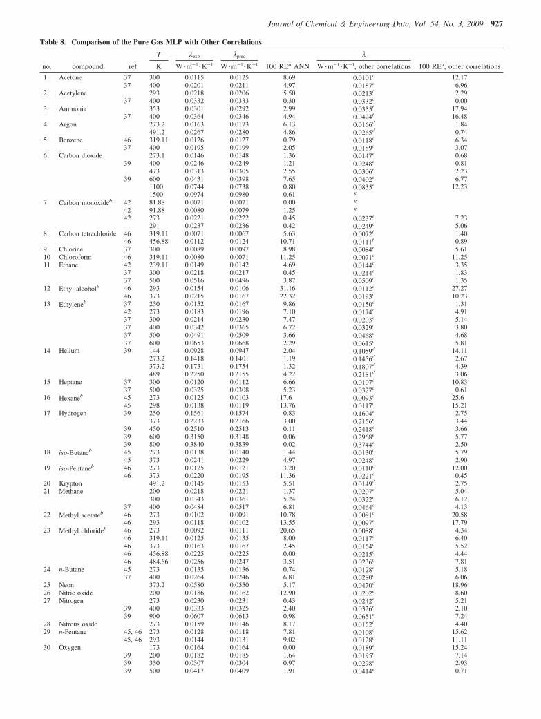
Table 8. Comparison of the Pure Gas MLP with Other Correlations

T λexp λpred λ

no. compound ref K W ·m-1 ·K-1 W ·m-1 ·K-1 100 REa ANN W ·m-1 ·K-1, other correlations 100 REa, other correlations

1 Acetone 37 300 0.0115 0.0125 8.69 0.0101c 12.1737 400 0.0201 0.0211 4.97 0.0187c 6.96

2 Acetylene 293 0.0218 0.0206 5.50 0.0213c 2.2937 400 0.0332 0.0333 0.30 0.0332c 0.00

3 Ammonia 353 0.0301 0.0292 2.99 0.0355f 17.9437 400 0.0364 0.0346 4.94 0.0424f 16.48

4 Argon 273.2 0.0163 0.0173 6.13 0.0166d 1.84491.2 0.0267 0.0280 4.86 0.0265d 0.74

5 Benzene 46 319.11 0.0126 0.0127 0.79 0.0118c 6.3437 400 0.0195 0.0199 2.05 0.0189c 3.07

6 Carbon dioxide 273.1 0.0146 0.0148 1.36 0.0147e 0.6839 400 0.0246 0.0249 1.21 0.0248e 0.81

473 0.0313 0.0305 2.55 0.0306e 2.2339 600 0.0431 0.0398 7.65 0.0402e 6.77

1100 0.0744 0.0738 0.80 0.0835e 12.231500 0.0974 0.0980 0.61 g

7 Carbon monoxideb 42 81.88 0.0071 0.0071 0.00 g

42 91.88 0.0080 0.0079 1.25 g

42 273 0.0221 0.0222 0.45 0.0237e 7.23291 0.0237 0.0236 0.42 0.0249e 5.06

8 Carbon tetrachloride 46 319.11 0.0071 0.0067 5.63 0.0072f 1.4046 456.88 0.0112 0.0124 10.71 0.0111f 0.89

9 Chlorine 37 300 0.0089 0.0097 8.98 0.0084e 5.6110 Chloroform 46 319.11 0.0080 0.0071 11.25 0.0071c 11.2511 Ethane 42 239.11 0.0149 0.0142 4.69 0.0144c 3.35

37 300 0.0218 0.0217 0.45 0.0214c 1.8337 500 0.0516 0.0496 3.87 0.0509c 1.35

12 Ethyl alcoholb 46 293 0.0154 0.0106 31.16 0.0112c 27.2746 373 0.0215 0.0167 22.32 0.0193c 10.23

13 Ethyleneb 37 250 0.0152 0.0167 9.86 0.0150c 1.3142 273 0.0183 0.0196 7.10 0.0174c 4.9137 300 0.0214 0.0230 7.47 0.0203c 5.1437 400 0.0342 0.0365 6.72 0.0329c 3.8037 500 0.0491 0.0509 3.66 0.0468c 4.6837 600 0.0653 0.0668 2.29 0.0615c 5.81

14 Helium 39 144 0.0928 0.0947 2.04 0.1059d 14.11273.2 0.1418 0.1401 1.19 0.1456d 2.67373.2 0.1731 0.1754 1.32 0.1807d 4.39489 0.2250 0.2155 4.22 0.2181d 3.06

15 Heptane 37 300 0.0120 0.0112 6.66 0.0107c 10.8337 500 0.0325 0.0308 5.23 0.0327c 0.61

16 Hexaneb 45 273 0.0125 0.0103 17.6 0.0093c 25.645 298 0.0138 0.0119 13.76 0.0117c 15.21

17 Hydrogen 39 250 0.1561 0.1574 0.83 0.1604e 2.75373 0.2233 0.2166 3.00 0.2156e 3.44

39 450 0.2510 0.2513 0.11 0.2418e 3.6639 600 0.3150 0.3148 0.06 0.2968e 5.7739 800 0.3840 0.3839 0.02 0.3744e 2.50

18 iso-Butaneb 45 273 0.0138 0.0140 1.44 0.0130c 5.7945 373 0.0241 0.0229 4.97 0.0248c 2.90

19 iso-Pentaneb 46 273 0.0125 0.0121 3.20 0.0110c 12.0046 373 0.0220 0.0195 11.36 0.0221c 0.45

20 Krypton 491.2 0.0145 0.0153 5.51 0.0149d 2.7521 Methane 200 0.0218 0.0221 1.37 0.0207c 5.04

300 0.0343 0.0361 5.24 0.0322c 6.1237 400 0.0484 0.0517 6.81 0.0464c 4.13

22 Methyl acetateb 46 273 0.0102 0.0091 10.78 0.0081c 20.5846 293 0.0118 0.0102 13.55 0.0097c 17.79

23 Methyl chlorideb 46 273 0.0092 0.0111 20.65 0.0088c 4.3446 319.11 0.0125 0.0135 8.00 0.0117c 6.4046 373 0.0163 0.0167 2.45 0.0154c 5.5246 456.88 0.0225 0.0225 0.00 0.0215c 4.4446 484.66 0.0256 0.0247 3.51 0.0236c 7.81

24 n-Butane 45 273 0.0135 0.0136 0.74 0.0128c 5.1837 400 0.0264 0.0246 6.81 0.0280c 6.06

25 Neon 373.2 0.0580 0.0550 5.17 0.0470d 18.9626 Nitric oxide 200 0.0186 0.0162 12.90 0.0202e 8.6027 Nitrogen 273 0.0230 0.0231 0.43 0.0242e 5.21

39 400 0.0333 0.0325 2.40 0.0326e 2.1039 900 0.0607 0.0613 0.98 0.0651e 7.24

28 Nitrous oxide 273 0.0159 0.0146 8.17 0.0152f 4.4029 n-Pentane 45, 46 273 0.0128 0.0118 7.81 0.0108c 15.62

45, 46 293 0.0144 0.0131 9.02 0.0128c 11.1130 Oxygen 173 0.0164 0.0164 0.00 0.0189e 15.24

39 200 0.0182 0.0185 1.64 0.0195e 7.1439 350 0.0307 0.0304 0.97 0.0298e 2.9339 500 0.0417 0.0409 1.91 0.0414e 0.71

Journal of Chemical & Engineering Data, Vol. 54, No. 3, 2009 927

all of them are not experimental. In this research, onlyexperimental data points have been utilized.

After identifying and collecting the data set, the next step isthe selection of input variables, which are the model’s inde-pendent variables. The available correlations for prediction ofconductivity at constant pressure are essentially based on theassumption that conductivity (λ) can be described as a functionof temperature (T), critical temperature (Tc), critical pressure(Pc), and molecular weight (M):

λ) f(T, Tc, Pc, M) (11)

Following this approach, temperature, critical temperature,critical pressure, and molecular weight were used as the inputsof the first ANN model for the prediction of conductivity ofpure gases.

The conductivity of gaseous binary mixtures is usually estimatedthrough using semiempirical correlations. These correlations areessentially a function of thermal conductivity, molecular weight,and composition of each component as follows

λmix ) f(λ1, λ2, M1, M2, x2) (12)

According to eq 12, the inputs of the second ANN model arethermal conductivity of light (λ2) and heavy (λ1) component(which can be predicted in the first ANN at the desiredtemperature), molecular weight of light (M2) and heavy (M1)component, and the molar composition of the lighter component(x2).

Neural Network Training. The multilayer perceptron (MLP)network is used here to develop the predictive models ofconductivity for both pure gas and binary gas mixtures. Bothproposed MLPs have one hidden layer with a different numberof neurons, determined through the constructive approach.64 Onthe basis of the constructive approach, a small number ofneurons are used in the hidden layer, and if the error of thetrained network does not meet the desired tolerance the numberof neurons in the hidden layer is increased one by one. Theprocedure is continued until the trained network performssatisfactorily (i.e., its training, validation and testing error arelower than the target goals). The Levenberg-Marquardt algo-rithm was used in the training procedure.65-67 Different neuralnetwork topologies were compared using their mean relative

errors (MRE) and mean square errors (MSE). The MRE andMSE are defined with the following equations

MRE) 1N∑

i)1

N |λexp - λpred|

λexp(13)

MSE) 1N∑

i)1

N

(λexp - λpred)2 (14)

N is the number of data points, and λexp and λpred are theexperimental and predicted values of thermal conductivity,respectively. Also, the coefficient of determination, R2, was usedas a measure to evaluate how the trained network estimation iscorrelated to the experimental data.

The structure of the trained MLP for prediction of pure gasconductivity consists of four neurons in the input layer, tenneurons in the hidden layer, and one neuron at the output layer.The MLP for the estimation of thermal conductivity of a binarymixture of gases has five neurons in the input layer, twelveneurons in the hidden layer, and one neuron at the output layer.

Results and Discussion

Table 5 shows the MRE, MSE, and R values calculated forvarious neural network configurations, differing with respectto their number of hidden layer neurons. The configuration withminimum error measures (i.e., MRE and MSE) and appropriateR-value was selected as the best network architecture. Accordingto Table 5, the best neural network configuration for predictionof thermal conductivity of pure gases has one hidden layer withten neurons. Also, an MLP with one hidden layer with twelveneurons is needed for prediction of thermal conductivity ofbinary gas mixtures. Figure 1 and Figure 2 represent thevariation of training errors for the selected MLPs. The param-eters (weight and bias values) of the first and the second ANNare shown in Tables 6 and 7, respectively.

Figures 3 and 4 illustrate the correlation between thepredictions of the trained MLPs and the corresponding experi-mental data. The perfect fit is indicated by the solid line. Theclose proximity of the best linear fit to the perfect fit shows agood correlation among network predictions and experimentaldata.

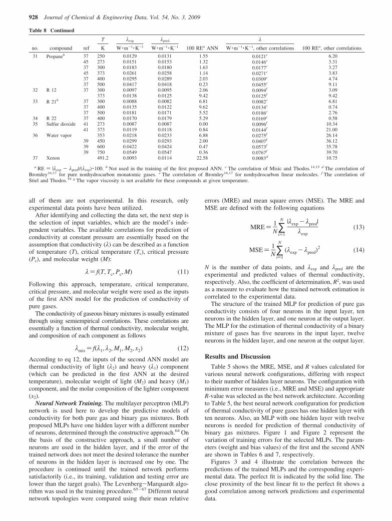
Table 8 Continued

T λexp λpred λ

no. compound ref K W ·m-1 ·K-1 W ·m-1 ·K-1 100 REa ANN W ·m-1 ·K-1, other correlations 100 REa, other correlations

31 Propaneb 37 250 0.0129 0.0131 1.55 0.0121c 6.2045 273 0.0151 0.0153 1.32 0.0146c 3.3137 300 0.0183 0.0180 1.63 0.0177c 3.2745 373 0.0261 0.0258 1.14 0.0271c 3.8337 400 0.0295 0.0289 2.03 0.0309c 4.7437 500 0.0417 0.0418 0.23 0.0455c 9.11

32 R 12 37 300 0.0097 0.0095 2.06 0.0094f 3.09373 0.0138 0.0125 9.42 0.0125f 9.42

33 R 21b 37 300 0.0088 0.0082 6.81 0.0082c 6.8137 400 0.0135 0.0122 9.62 0.0134c 0.7437 500 0.0181 0.0171 5.52 0.0186c 2.76

34 R 22 37 400 0.0170 0.0179 5.29 0.0169c 0.5835 Sulfur dioxide 41 273 0.0087 0.0087 0.00 0.0096f 10.34

41 373 0.0119 0.0118 0.84 0.0144f 21.0036 Water vapor 353 0.0218 0.0233 6.88 0.0275f 26.14

39 450 0.0299 0.0293 2.00 0.0407f 36.1239 600 0.0422 0.0424 0.47 0.0573f 35.7839 750 0.0549 0.0547 0.36 0.0767f 39.70

37 Xenon 491.2 0.0093 0.0114 22.58 0.0083d 10.75

a RE ) |λexp - λpred|/(λexp) ·100. b Not used in the training of the first proposed ANN. c The correlation of Misic and Thodos.14,15 d The correlation ofBromley16,17 for pure nonhydrocarbon monatomic gases. e The correlation of Bromley16,17 for nonhydrocarbon linear molecules. f The correlation ofStiel and Thodos.19 g The vapor viscosity is not available for these compounds at given temperature.

928 Journal of Chemical & Engineering Data, Vol. 54, No. 3, 2009

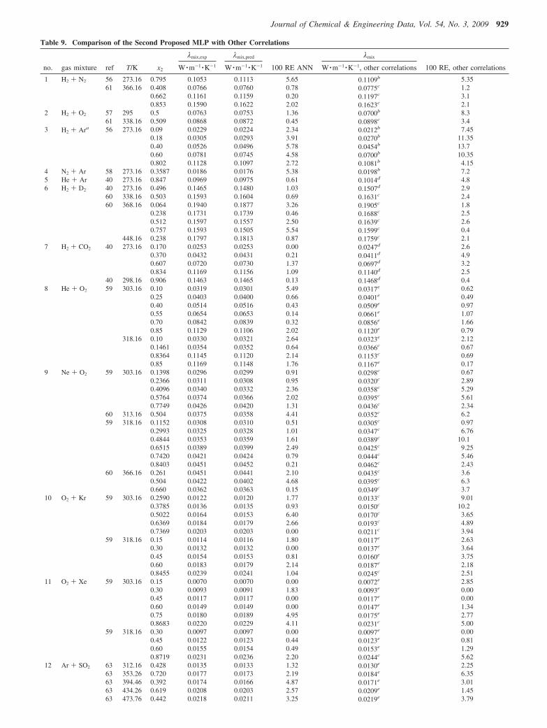
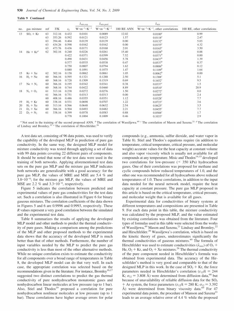
Table 9. Comparison of the Second Proposed MLP with Other Correlations

λmix,exp λmix,pred λmix

no. gas mixture ref T/K x2 W ·m-1 ·K-1 W ·m-1 ·K-1 100 RE ANN W ·m-1 ·K-1, other correlations 100 RE, other correlations

1 H2 + N2 56 273.16 0.795 0.1053 0.1113 5.65 0.1109b 5.3561 366.16 0.408 0.0766 0.0760 0.78 0.0775c 1.2

0.662 0.1161 0.1159 0.20 0.1197c 3.10.853 0.1590 0.1622 2.02 0.1623c 2.1

2 H2 + O2 57 295 0.5 0.0763 0.0753 1.36 0.0700b 8.361 338.16 0.509 0.0868 0.0872 0.45 0.0898c 3.4

3 H2 + Ara 56 273.16 0.09 0.0229 0.0224 2.34 0.0212b 7.450.18 0.0305 0.0293 3.91 0.0270b 11.350.40 0.0526 0.0496 5.78 0.0454b 13.70.60 0.0781 0.0745 4.58 0.0700b 10.350.802 0.1128 0.1097 2.72 0.1081b 4.15

4 N2 + Ar 58 273.16 0.3587 0.0186 0.0176 5.38 0.0198b 7.25 He + Ar 40 273.16 0.847 0.0969 0.0975 0.61 0.1014d 4.86 H2 + D2 40 273.16 0.496 0.1465 0.1480 1.03 0.1507d 2.9

60 338.16 0.503 0.1593 0.1604 0.69 0.1631c 2.460 368.16 0.064 0.1940 0.1877 3.26 0.1905c 1.8

0.238 0.1731 0.1739 0.46 0.1688c 2.50.512 0.1597 0.1557 2.50 0.1639c 2.60.757 0.1593 0.1505 5.54 0.1599c 0.4

448.16 0.238 0.1797 0.1813 0.87 0.1759c 2.17 H2 + CO2 40 273.16 0.170 0.0253 0.0253 0.00 0.0247d 2.6

0.370 0.0432 0.0431 0.21 0.0411d 4.90.607 0.0720 0.0730 1.37 0.0697d 3.20.834 0.1169 0.1156 1.09 0.1140d 2.5

40 298.16 0.906 0.1463 0.1465 0.13 0.1468d 0.48 He + O2 59 303.16 0.10 0.0319 0.0301 5.49 0.0317e 0.62

0.25 0.0403 0.0400 0.66 0.0401e 0.490.40 0.0514 0.0516 0.43 0.0509e 0.970.55 0.0654 0.0653 0.14 0.0661e 1.070.70 0.0842 0.0839 0.32 0.0856e 1.660.85 0.1129 0.1106 2.02 0.1120e 0.79

318.16 0.10 0.0330 0.0321 2.64 0.0323e 2.120.1461 0.0354 0.0352 0.64 0.0366c 0.670.8364 0.1145 0.1120 2.14 0.1153c 0.690.85 0.1169 0.1148 1.76 0.1167e 0.17

9 Ne + O2 59 303.16 0.1398 0.0296 0.0299 0.91 0.0298c 0.670.2366 0.0311 0.0308 0.95 0.0320c 2.890.4096 0.0340 0.0332 2.36 0.0358c 5.290.5764 0.0374 0.0366 2.02 0.0395c 5.610.7749 0.0426 0.0420 1.31 0.0436c 2.34

60 313.16 0.504 0.0375 0.0358 4.41 0.0352c 6.259 318.16 0.1152 0.0308 0.0310 0.51 0.0305c 0.97

0.2993 0.0325 0.0328 1.01 0.0347c 6.760.4844 0.0353 0.0359 1.61 0.0389c 10.10.6515 0.0389 0.0399 2.49 0.0425c 9.250.7420 0.0421 0.0424 0.79 0.0444c 5.460.8403 0.0451 0.0452 0.21 0.0462c 2.43

60 366.16 0.261 0.0451 0.0441 2.10 0.0435c 3.60.504 0.0422 0.0402 4.68 0.0395c 6.30.660 0.0362 0.0363 0.15 0.0349c 3.7

10 O2 + Kr 59 303.16 0.2590 0.0122 0.0120 1.77 0.0133c 9.010.3785 0.0136 0.0135 0.93 0.0150c 10.20.5022 0.0164 0.0153 6.40 0.0170c 3.650.6369 0.0184 0.0179 2.66 0.0193c 4.890.7369 0.0203 0.0203 0.00 0.0211c 3.94

59 318.16 0.15 0.0114 0.0116 1.80 0.0117e 2.630.30 0.0132 0.0132 0.00 0.0137e 3.640.45 0.0154 0.0153 0.81 0.0160e 3.750.60 0.0183 0.0179 2.14 0.0187e 2.180.8455 0.0239 0.0241 1.04 0.0245c 2.51

11 O2 + Xe 59 303.16 0.15 0.0070 0.0070 0.00 0.0072e 2.850.30 0.0093 0.0091 1.83 0.0093e 0.000.45 0.0117 0.0117 0.00 0.0117e 0.000.60 0.0149 0.0149 0.00 0.0147e 1.340.75 0.0180 0.0189 4.95 0.0175e 2.770.8683 0.0220 0.0229 4.11 0.0231c 5.00

59 318.16 0.30 0.0097 0.0097 0.00 0.0097e 0.000.45 0.0122 0.0123 0.44 0.0123e 0.810.60 0.0155 0.0154 0.49 0.0153e 1.290.8719 0.0231 0.0236 2.20 0.0244c 5.62

12 Ar + SO2 63 312.16 0.428 0.0135 0.0133 1.32 0.0130e 2.2563 353.26 0.720 0.0177 0.0173 2.19 0.0184e 6.3563 394.46 0.392 0.0174 0.0166 4.87 0.0171e 3.0163 434.26 0.619 0.0208 0.0203 2.57 0.0209e 1.4563 473.76 0.442 0.0218 0.0211 3.25 0.0219e 3.79

Journal of Chemical & Engineering Data, Vol. 54, No. 3, 2009 929

A test data set, consisting of 96 data points, was used to verifythe capability of the developed MLP in prediction of pure gasconductivity. In the same way, the designed MLP model formixture conductivity was tested through applying a set of datawith 99 data points covering 22 different pairs of components.It should be noted that none of the test data were used in thetraining of both networks. Applying aforementioned test datasets on the pure gas MLP and the mixture gas MLP indicatesboth networks are generalizable with a good accuracy: for thepure gas MLP, the values of MRE and MSE are 5.4 % and3.8 ·10-6; for the mixture gas MLP, the values of MRE andMSE are 2.2 % and 3.3 ·10-6, respectively.

Figure 5 indicates the correlation between predicted andexperimental values of pure gas conductivities for the test dataset. Such a correlation is also illustrated in Figure 6 for binarygaseous mixtures. The correlation coefficients of the data shownin Figures 5 and 6 are 0.9996 and 0.9993, respectively. TheseR values represent a very good correlation between the simulatedand the experimental test data.

Table 8 summarizes the results of applying the developedMLP model and other methods to predict the thermal conductiv-ity of pure gases. Making a comparison among the predictionsof the MLP and other proposed methods to the experimentaldata shows that the accuracy of the developed MLP is muchbetter than that of other methods. Furthermore, the number ofinput variables needed by the MLP to predict the pure gasconductivity is less than most of the other alternative methods.While no unique correlation exists to estimate the conductivityfor all components over a broad range of temperatures in Table8, the developed MLP model can do that very well. In eachcase, the appropriate correlation was selected based on therecommendations given in the literature. For instance, Bromley16,17

suggested two distinct correlations to predict the gas thermalconductivity of pure nonhydrocarbon monatomic gases andnonhydrocarbon linear molecules at low pressure (up to 1 bar).Also, Stiel and Thodos19 proposed a correlation for purenonhydrocarbon nonlinear molecules at low pressure (up to 1bar). These correlations have higher average errors for polar

compounds (e.g., ammonia, sulfur dioxide, and water vapor inTable 8). Stiel and Thodos’s equations require (in addition totemperature, critical temperature, critical pressure, and molecularweight) accurate values for the heat capacity at constant volumeand also vapor viscosity which is usually not available for allcompounds at any temperature. Misic and Thodos14,15 developedtwo correlations for low-pressure (< 350 kPa) hydrocarbongases. One of their correlations was proposed for methane andcyclic compounds below reduced temperatures of 1.0, and theother one was recommended for all hydrocarbons above reducedtemperatures of 1.0. These correlations, in addition to the inputdata needed for the neural network model, require the heatcapacity at constant pressure. The pure gas MLP proposed inthis article is based on the critical temperature, critical pressure,and molecular weight that is available for all gases.

Experimental data for conductivities of binary systems atdifferent temperatures and compositions are presented in Table9. For each data point in this table, the mixture conductivitywas calculated by the proposed MLP, and the value estimatedby existing correlations was obtained from the literature. Fourtypes of formulas used in this table were selected from the worksof Wassiljewa,49 Mason and Saxena,21 Lindsay and Bromley,22

and Hirschfelder.26 Wassiljewa’s correlation, which is based onthe kinetic theory of gases, underestimates significantly thethermal conductivities of gaseous mixtures.49 The formula ofHirschfelder was used to estimate conductivities (λmix) of O2 +He, O2 + Kr, and O2 + Xe mixtures.26 The thermal conductivityof the pure component needed in Hirschfelder’s formula wasobtained from experimental data. The accuracy of the Hir-schfelder’s method is very good and comparable to that of thedesigned MLP in this work. In the case of SO2 + Kr, the forceparameters needed in Hirschfelder’s correlation (ε12/k ) 244K; σ12 ) 3.808 Å) were determined from diffusion data,68 butbecause of unavailability of reliable diffusion data for the SO2

+ Ar system, the force parameters (ε12/k ) 280 K; σ12 ) 3.392Å) were determined from binary viscosity data.69 For 47experimental data points, the procedure of Manson and Saxena21

leads to an average relative error of 4.4 % while the proposed

Table 9 Continued

λmix,exp λmix,pred λmix

no. gas mixture ref T/K x2 W ·m-1 ·K-1 W ·m-1 ·K-1 100 RE ANN W ·m-1 ·K-1, other correlations 100 RE, other correlations

13 SO2 + Kr 63 312.16 0.432 0.0101 0.0089 12.02 0.0100e 0.9963 353.26 0.592 0.0121 0.0123 1.57 0.0118e 2.4763 394.46 0.404 0.0139 0.0139 0.00 0.0132e 5.0363 434.26 0.598 0.0162 0.0162 0.00 0.0155e 4.3263 473.76 0.436 0.0171 0.0168 2.01 0.0165e 3.50

14 He + Kra 62 302.16 0.240 0.0226 0.0261 15.40 0.0228b 0.880.422 0.0371 0.0399 7.52 0.0371b 0.000.490 0.0431 0.0456 5.78 0.0437b 1.390.577 0.0535 0.0538 0.47 0.0537b 0.370.750 0.0807 0.0794 1.62 0.0806b 0.120.880 0.1091 0.1075 1.47 0.1109b 1.64

15 Kr + Xe 62 302.16 0.158 0.0062 0.0061 1.05 0.0062b 0.0016 H2 + Ne 60 366.16 0.595 0.1321 0.1288 2.50 0.1388c 5.1

60 368.16 0.728 0.1509 0.1519 0.69 0.1652c 9.517 Ne + N2 60 366.16 0.195 0.0342 0.0341 0.38 0.0337c 1.5

60 368.16 0.744 0.0422 0.0460 8.89 0.0510c 20.918 N2 + O2 61 313.16 0.238 0.0272 0.0276 1.50 0.0272c 0.0

61 366.16 0.751 0.0313 0.0313 0.00 0.0305c 2.460 408.16 0.486 0.0355 0.0351 1.12 0.0328c 7.7

19 H2 + Kr 60 338.16 0.531 0.0698 0.0707 1.22 0.0723c 3.620 H2 + Xe 60 313.16 0.566 0.0648 0.0632 2.54 0.0625c 3.521 D2 + Xe 60 366.16 0.504 0.0493 0.0482 2.21 0.0455c 7.722 D2 + N2 61 338.16 0.399 0.0578 0.0583 0.88 0.0588c 1.7

0.778 0.1004 0.1009 0.46 0.1033c 2.9

a Not used in the training of the second proposed ANN. b The correlation of Wassiljewa.49 c The correlation of Mason and Saxena.21 d The correlationof Lindsay and Bromley.22 e The correlation of Hirschfelder.26

930 Journal of Chemical & Engineering Data, Vol. 54, No. 3, 2009

MLP has an average relative error of 1.8 %. Also, comparingthe results of the Lindsay and Bromley correlation to that ofthe MLP method shows that the relative error of the MLP ismuch better. For instance, the average relative error of theLindsay and Bromley method for H2 + CO2 is 2.7 %, while forthe proposed neural network it is 0.56 %.

Comparing the relative errors of the methods in Table 9reveals that the overall accuracy of the designed MLP is morethan that of other suggested correlations. Furthermore, thenumber of input variables required for the proposed MLP modelis less than that of most other alternative methods. Thedeveloped mixture gas MLP predicts the mixture conductivitybased on the pure component conductivity (which can beestimated from the pure gas MLP at desired temperatures),molecular weight of pure component, and composition of thelight component. While some of the binary mixtures of gasesshown in the table were not used in the training of the MLPmodel, we applied intentionally them to the network to assessits extrapolation capability. It should be notified that predictionof thermal conductivity of the binary mixture of gases by otherproposed correlations is really tedious and boring, while thedeveloped network scheme is easy to use and requires fewerinput properties which are usually available for most gases.

Conclusions

In this research, an artificial network scheme was developedto approximate the thermal conductivities of binary gaseousmixtures. The proposed scheme consists of two consecutivemultilayer perceptrons (MLPs). Critical temperature, criticalpressure, molecular weight, and the gas temperature are fed tothe first MLP by which the pure gas conductivity is ap-proximated for use in the next MLP. The second MLP estimatesthe binary mixture conductivity from the conductivities andmolecular weights of both components as well as the molefraction of the lighter component. Both networks were trainedand verified by using a large experimental data set of pure andmixture gas conductivities over wide ranges of temperaturesand molecular structures. Also, we applied four differentcorrelations, recommended in the literature, to the experimentaldata points. Comparing the errors of the developed networkscheme and other suggested correlations reveals that the neuralnetwork model can predict the thermal conductivities of the pureand binary gaseous mixture remarkably better than othersuggested methods. Some advantages can be mentioned for theneural network model over other alternative correlations: (1)compressing a vast range of experimental thermal conductivitiesof pure and mixed gases in an easy to use and accurate neuralmodel, (2) predicting pure gas conductivity through a singleMLP model over wide ranges of temperatures and molecularstructures, rather than using alternative correlations validatedacross limited ranges of temperatures and substances, (3)requiring fewer physical input parameters which are commonlyavailable for all components.

The results of applying the trained MLP model to the testdata indicate that this method has very good interpolation andextrapolation capabilities with respect to not only change intemperature range but also molecular structure.

Literature Cited(1) Chapman, S.; Cowling, T. G. The Mathematical Theory of Non-

Uniform Gases; Cambridge University Press: London, 1953.(2) Hirschfelder, J. O.; Bird, R. B. The Molecular Theory of Gases and

Liquids; Wiley: New York, 1954.(3) Ubbelohde, A. R. The Thermal Conductivity of Polyatomic Gases.

J. Chem. Phys. 1935, 3, 219.

(4) Tye, R. P. Thermal ConductiVity; Academic Press: London and NewYork, 1969; Vol. 2.

(5) Longuet-Higgins, H. C.; Pople, J. A. Transport Properties of a DenseFluid of Hard Spheres. J. Chem. Phys. 1956, 25, 884.

(6) Horrocks, J. K.; McLaughlin, E. Non-Steady-State Measurements ofthe Thermal Conductivities of Liquid Polyphenyls. Proc. R. Soc. 1963,273, 259.

(7) Horrocks, J. K.; McLaughlin, E. Temperature Dependence of theThermal Conductivity of Liquids. Trans. Faraday Soc. 1963, 59, 1709.

(8) Longuet-Higgins, H. C.; Valleau, J. P. Transport coefficients of densefluids of molecules interacting according to a square well potential.Mol. Phys. 1958, 1, 284.

(9) Davis, H. T.; Rice, S. A.; Sengers, J. V. On the Kinetic Theory ofDense Fluids. IX. The Fluid of Rigid Spheres with a Square-WellAttraction. J. Chem. Phys. 1961, 35, 2210–2233.

(10) Sengers, J. V. Divergence in the Density Expansion of the TransportCoefficients of a Two-Dimensional Gas. Phys. Fluids 1966, 9, 1685–1696.

(11) Choh, S. T.; Uhlenbeck, G. E. The Kinetic Theory of Phenomena inDense Gases; University of Michigan Report: 1958.

(12) Cohen, E. G. D. Statistical Mechanics of Equilibrium and Non-equilibrium Processes; Meixne, J., Ed.;North-Holland: Amesterdam,1965.

(13) Bogolubov, G. N. N. Studies in statistical Mechanics; de Boer, J.,Uhlenbeck, G. E., Eds.; North-Holland, Amsterdam, 1962; Vol. 7.

(14) Misic, D.; Thodos, G. Thermal Conductivity of Hydrocarbon Gasesat Normal Pressures. AIChE J. 1961, 7, 264.

(15) Misic, D.; Thodos, G. Atmospheric Thermal Conductivity for Gasesof Simple Molecular Structure. J. Chem. Eng. Data 1963, 9, 540.

(16) Bromley, L. A. Thermal ConductiVity of Gases at Moderate Pressures;University of California Radiation Laboratory, Report No. UCRL-1852, Berkeley, CA 1952.

(17) Bromley, L. A.; Wilke, C. R. Viscosity Behavior of Gases. Ind. Eng.Chem. 1951, 43, 1641–1648.

(18) Plinski Edward, F.; Witkowski Jerzy, S. Prediction of the thermalproperties of CO2, CO, and Xe laser media. Opt. Laser Technol. 2001,32, 61–66.

(19) Stiel, L. I.; Thodos, G. The thermal conductivity of nonpolar substancesin the dense gaseous and liquid regions. AIChE J. 1964, 10, 26–32.

(20) Muckenfuss, C.; Curtiss, C. F. Thermal Conductivity of Multicom-ponent Gas Mixtures. J. Chem. Phys. 1958, 29, 1273.

(21) Mason, E. A.; Saxena, S. C. Thermal Conductivity of MulticomponentGas Mixtures. II. J. Chem. Phys. 1959, 31, 511–518.

(22) Lindsay, A. L.; Bromley, L. A. Thermal Conductivity of Gas Mixtures.Ind. Eng. Chem. 1950, 43, 1508–1511.

(23) Srivastava, B. N.; Saxena, S. C. Thermal Conductivity of Binary andTernary Rare Gas Mixtures. Proc. Phys. Soc. (London) 1957, B70,583.

(24) Saxena, S. C. Thermal Conductivity of Binary and Ternary Mixturesof Helium, Argon and Xenon. Indian J. Phys. 1957, 31, 597–606.

(25) Ulybin, S. A.; Bugrov, V. P.; Vulyin, A. V. Temperature Dependenceof Thermal Conductivity of Nonreacting Low Density Gas Mixtures.Teplofizika Vysokikh Temperatur 1966, 4, 210.

(26) Hirschfelder, J. O. Sixth International Combustion Symposium; P 351,Reinhold: New York, N. Y., 1957.

(27) Ignacio, J.; Turias, J.; Gutierrez, M.; Galindo, P. L. Modeling theeffective thermal conductivity of a unidirectional composite by theuse of artificial neural networks. Compos. Sci. Technol. 2005, 65, 609–619.

(28) Sablani, S. S.; Shafiur, R. M. Using neural networks to predict thermalconductivity of food as a function of moisture content, temperature,and apparent porosity. Food Res. Int. 2003, 36, 617–623.

(29) Sablani, S. S.; Oon-Doo, B.; Marcotte, M. Neural networks forpredicting thermal conductivity of bakery products. J. Food Eng. 2002,52, 299–304.

(30) Therdthai, N.; Weibiao, Z. Artificial neural network modeling of theelectrical conductivity property of recombined milk. J. Food Eng.2001, 50, 107-111.

(31) Jalali-Heravi, M.; Fatemi, M. H. Prediction of thermal conductivitydetection response factor using an artificial neural networks. J. Chro-matogr. 2000, 897, 227–235.

(32) Eslamloueyan R.; Khademi M. H. Estimation of Thermal Conductivityof Pure Gases by Using Artificial Neural Networks. Int. J. ThermalSci. 2008, in press.

(33) Hagan, M. T.; Demuth, H. B.; Beale, M. H. Neural Network Design;PWS Publishing: Boston, MA, 1996.

(34) Boozarjomehri, R.; Abdolahi, F.; Moosavian, M. A. Characterizationof basic properties for pure substances and petroleum fractions byneural network. Fluid Phase Equilib. 2005, 231, 188–196.

(35) Statistical Neural Networks, User’s Manual, Release 4.0 F, Statsoft:Tulsa, OK, 2000.

(36) Cybenco, G. V. Mathematics of control. Signals Syst. 1989, 2, 303–314.

Journal of Chemical & Engineering Data, Vol. 54, No. 3, 2009 931

(37) Perry, R. H.; Green, D. W. Perry’s chemical engineers handbook,7th ed.; McGraw Hill: New York, 1997.

(38) Reid, R. C.; Prausnitz, J. M.; Poling, B. E. The Properties of Gasesand Liquids, 4th ed., McGraw-Hill: New York, 1987.

(39) Holman J. P. Heat Transfer, 8th ed.; McGraw-Hill: United States ofAmerica, 1997.

(40) Tsederberg, N. V. Thermal ConductiVity of Gases and Liquids; Robert,D., Ed.; M.I.T. Press: Cambridge, Mass, 1965.

(41) Dickens, B. G. The Effect of Accommodation on Heat ConductionThrough Gases. Proc. R. Soc. A (London) 1934, 850, 517.

(42) Eucken, A. On the temperature dependence of the thermal conductivityof some gases (in German). Physik. Z. 1911, 12, 1101–1107.

(43) Gregory, H.; Marshall, S. Thermal Conductivities of Oxygen andNitrogen. Proc. R. Soc. A (London) 1928, 118, 594–607.

(44) Washburn, E. W., Ed. International Critical Tables; McGraw-Hill:New York, 1929.

(45) Mann, W. B.; Dickens, B. G. The Thermal Conductivities of theSaturated Hydrocarbons in the Gaseous. Proc. R. Soc. A (London)1931, (823), 77.

(46) Moser, E. Dissertation, Berlin, 1913.(47) Sherratt, G. G.; Griffiths, E. A hot-wire method for the thermal

conductivity of gases. Phil. Mag. 1939, 27, 68.(48) Carmichal, L. T.; Jackobs, J.; Sage, B. H. Thermal Conductivity of

fluids, A mixture of methane and n-Butane. J. Chem. Eng. Data 1968,3 (4), 489.

(49) Wassiljewa, A. Heat-Conduction in gaseous mixtures. Phys. Z. 1904,5 (22), 737–742.

(50) Gruss, H.; Schmick, H. Siemens Konzern 1928, VII (1), 202.(51) Ibbs, T. L.; Hirst, A. A. The Thermal Conductivity of Gas Mixtures.

Proc. R. Soc. Ser. A 1929, 123 (791), 134–142.(52) Waschmuth, J. Phys. Z., Leipzig 1908, No. 7 (The original data of

Waschmuth is reproduced in ref 40).(53) Kornfield, G.; Hilferding, K. Z. Phys. Chem., Ergänzungsband

Bodenstein Festband, 1931, 792 (The original data of Kornfield andHilferding is reproduced in ref 40).

(54) Weber, S. Theoretical and Experimental Study of Thermal Conductivityof Gas Mixtures. Ann. Phys. 1917, 359 (23), 481.

(55) Archer, C. T. Thermal Conduction in Hydrogen-Deuterium Mixtures.Proc. R. Soc. Ser. A 1938, 165, 474.

(56) Kihara, T. Determination of Intermolecular Forces from the Equationof State of Gases. II. J. Phys. Soc. Jpn. 1951, 6 (3), 184.

(57) Bird, R. B. Dissertation, University of Wisconsin, 1950.(58) Bird, R. B.; Spotz, E. L.; Hirschfelder, J. O. The Third Virial

Coefficient for Non-Polar Gases. J. Chem. Phys. 1950, 18, 1359.(59) Srivastava, B. N.; Barua, A. K. Thermal Conductivity of Binary

Mixtures of Diatomic and Monatomic Gases. J. Chem. Phys. 1960,32 (2), 427–435.

(60) Saxena, S. C.; Tondon, P. K. Experimental Data and Procedures forPredicting Thermal Conductivity of Binary Mixtures of NonpolarGases. J. Chem. Eng. Data 1971, 16 (2), 212–220.

(61) Saxena, S. C.; Gupta, G. P. Experimental Data and Procedures forPredicting Thermal Conductivity of Multicomponent Mixtures ofNonpolar Gases. J. Chem. Eng. Data 1970, 15 (1), 98–107.

(62) Brokaw, R. S. Approximate Formulas for Viscosity and ThermalConductiVity of Gas Mixtures; Lewis Research Center Cleveland: OH,1964.

(63) Das Gupta, A. Thermal Conductivity of Binary Mixtures of SulphurDioxide and Inert Gases. Int. J. Heat Mass Transfer 1967, 10, 921–929.

(64) Haykin S. Neural Networks: A ComprehensiVe Foundation, 2nd ed.;Prentice-Hall: Englewood Cliffs, NJ, 1999.

(65) Levenberg, K. A method for the solution of certain problems in leastsquares. SIAM J. Numer. Anal. 1944, 16, 588–604.

(66) Marquardt, D. An algorithm for least-squares estimation of nonlinearparameters. SIAM J. Appl. Math. 1963, 11, 431–441.

(67) Hagan, M. T.; Menhaj, M. Training Feedforward Networks with theMarquardt Algorithm. IEEE Trans. Neural Netw. 1994, 5, 989–993.

(68) Srivastava, B. N.; Saran, A. Mutual diffusion in polar-nonpolar gases:krypton-sulphur dioxide and krypton-diethyl ether. Can. J. Phys.(Paris) 1966, 44, 2595.

(69) Chakraborti, P. K.; Gray, P. Viscosities of gaseous mixtures containingpolar gases; mixtures with one polar constituent. Trans. Faraday Soc.1965, 61, 2422.

Received for review September 22, 2008. Accepted November 15, 2008.

JE800706E

932 Journal of Chemical & Engineering Data, Vol. 54, No. 3, 2009