Using Biological Criteria to Validate Applications of ...epa.ohio.gov/portals/35/documents/gli_bio.pdfUsing Biological Criteria to Validate Applications of Water ... Dissolved and

State of Ohio Ecological AssessmentEnvironmental Protection Agency Division of Surface Water

P.O. Box 1049, 1800 WaterMark Dr., Columbus, Ohio 43266-1049

February 3, 1997

Using Biological Criteria to ValidateApplications of Water Quality Criteria:Dissolved and Total Recoverable Metals

Using Biological Criteria to ValidateApplications of Water Quality Criteria:Dissolved and Total Recoverable Metals

Februrary 3, 1997

OEPA Technical Bulletin 1997-12-4

prepared by

State of Ohio Environmental Protection AgencyDivision of Surface Water

Monitoring and Assessment Section1685 Westbelt Drive

Columbus, Ohio 43228

Agency Web Site:www.epa.ohio.gov

Left Cover Photo: White amur or Grass Carp (Ctenopharyngodon idella).Bottom Cover Photo: Golden redhorse (Moxostoma erythrurum) with spinal deformity.

1

Ohio EPA GLWQG Fact SheetFeb 3, 1996

Using Biological Criteria to Validate Applications of WaterQuality Criteria: Dissolved and Total Recoverable Metals

What Are Biological Criteria?Biological criteria (biocriteria) are narrative or numeric expressions of the health and well-being ofaquatic life and are based on the numbers and kinds of aquatic organisms which inhabit a particularstream or river sampling site. Biocriteria are derived from a complex process using data whichreflects the reference condition within a particular geographic region of the state (Ohio EPA 1987a,b;Ohio EPA 1989a,b). As such biocriteria represent a direct measure of the attainment or non-attainment of aquatic life use designations for Ohio’s streams. Ohio EPA incorporated biocriteriainto the Ohio Water Quality Standards (WQS; Ohio Administrative Code 3745-1) regulations inFebruary 1990 (effective May 1990). These criteria consist of numeric values for the Index of BioticIntegrity (IBI) and the Modified Index of well-being (MIwb), both of which are based on informationabout stream fish assemblages, and the Invertebrate Community Index (ICI), which is based oninformation about stream macroinvertebrate assemblages. Criteria for each biological index arespecified for each of Ohio's five ecoregions (as described by Omernik 1987) and are furtherorganized by organism group, index, site type, and aquatic life use designation. Biocriteria, alongwith the existing chemical and whole effluent toxicity evaluation methods and criteria, figureprominently in the monitoring and assessment of Ohio’s surface water resources.

How Are Biocriteria Used By Ohio EPA?Biocriteria are implemented primarily as an ambient assessment tool. The basic data necessary touse biocriteria are obtained from biological surveys. A biological and water quality survey, or“biosurvey”, is an interdisciplinary monitoring effort coordinated on a waterbody specific or watershedscale. This effort may involve a relatively simple setting focusing on one or two small streams, oneor two principal stressors, and a handful of sampling sites or a much more complex effort includingentire drainage basins, multiple and overlapping stressors, and tens of sites. Each year Ohio EPAconducts biosurveys in 10-15 different study areas with an aggregate total of at least 250-300sampling sites. Ohio EPA employs biological, chemical, and physical monitoring and assessmenttechniques in biosurveys in order to meet three major objectives:

1) determine the extent to which use designations assigned in the Ohio WQS are eitherattained or not attained;

2) determine if use designations assigned to a given water body are appropriate andattainable; and,

3) determine if any changes in key ambient biological, chemical, or physical indicators havetaken place over time, particularly before and after the implementation of point sourcepollution controls or best management practices.

The data gathered by a biosurvey is processed, evaluated, and synthesized in a biological and waterquality report. Each biological and water quality report contains a summary of the major findingsincluding progress towards meeting designated uses and recommendations for revisions to usedesignations, future monitoring needs, or other actions which may be needed to resolve existing

2

impairments of designated uses. While the principal focus of a biosurvey is on the status of aquaticlife uses, the status of other uses such as recreation and water supply, as well as human healthconcerns, are also addressed.

The Role of Biocriteria in the Ohio Water Quality Standards: Designated Aquatic Life UsesThe Ohio Water Quality Standards (WQS; Ohio Administrative Code 3745-1) consist of designateduses and chemical, physical, and biological criteria designed to represent measurable properties ofthe environment that are consistent with the narrative goals specified by each use designation. Usedesignations consist of two broad groups, aquatic life and non-aquatic life uses. In applications ofthe Ohio WQS to the management of surface water resource issues, the aquatic life use criteriafrequently control the protection and restoration requirements, hence their emphasis in biological andwater quality reports. Also, an emphasis on protecting aquatic life generally results in water qualitysuitable for all uses. The five different aquatic life uses currently defined in the Ohio WQS with thebiological intent of each are described as follows:

1) Warmwater Habitat (WWH) - this use designation defines the “typical” warmwaterassemblage of aquatic organisms for Ohio streams; this use represents the principalrestoration target for the majority of water resource management efforts in Ohio.Biological criteria are stratified across five ecoregions for the WWH use designation.

2) Exceptional Warmwater Habitat (EWH) - this use designation is reserved for waterswhich support “unusual and exceptional” assemblages of aquatic organisms which arecharacterized by a high diversity of species, particularly those which are highly intolerantand/or rare, threatened, endangered, or special status (i.e., declining species); thisdesignation represents a protection goal for water resource management efforts dealingwith Ohio’s best water resources. Biological criteria for EWH apply uniformly across thestate.

3) Coldwater Habitat (CWH) - this use is intended for waters which support assemblagesof cold water organisms and/or those which are stocked with salmonids with the intentof providing a put-and-take fishery on a year round basis which is further sanctioned bythe Ohio DNR, Division of Wildlife; this use should not be confused with the SeasonalSalmonid Habitat (SSH) use which applies to the Lake Erie tributaries that supportperiodic “runs” of salmonids during the spring, summer, and/or fall. No specific biologicalcriteria have been developed for the CWH use although the WWH biocriteria are viewedas attainable for CWH designated streams.

4) Modified Warmwater Habitat (MWH) - this use applies to streams which have beensubjected to extensive, maintained, and essentially permanent hydromodifications suchthat the biocriteria for the WWH use are not attainable and where the activities havebeen sanctioned and permitted by state or federal law; the representative aquaticassemblages are generally composed of species which are tolerant to low dissolvedoxygen, silt, nutrient enrichment, and poor quality habitat. Biological criteria for MWHwere derived from a separate set of habitat modified reference sites and are stratifiedacross five ecoregions and three major modification types: channelization, run-of-riverimpoundments, and extensive sedimentation due to non-acidic mine drainage.

5) Limited Resource Water (LRW) - this use applies to small streams (usually <3 mi.2

drainage area) and other water courses which have been irretrievably altered to theextent that no appreciable assemblage of aquatic life can be supported; such waterways

3

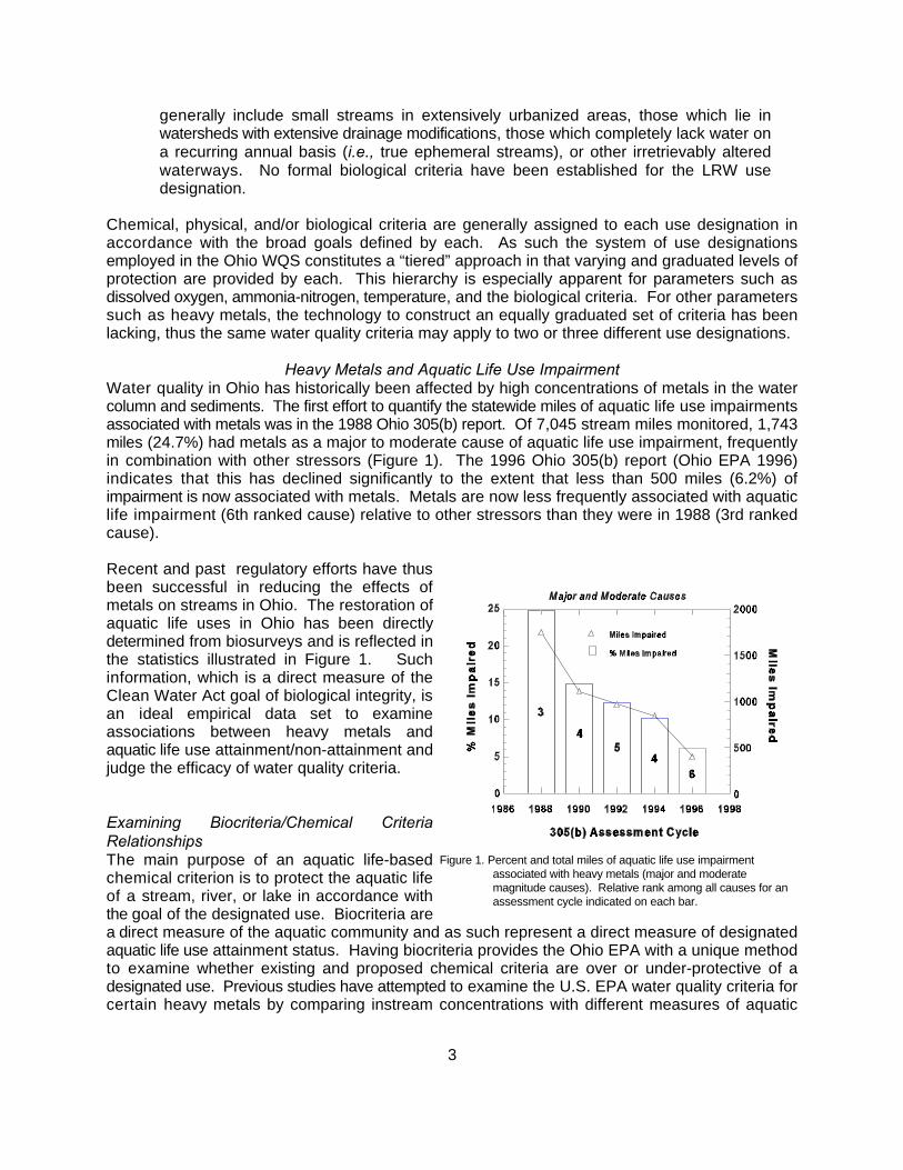
Figure 1. Percent and total miles of aquatic life use impairmentassociated with heavy metals (major and moderatemagnitude causes). Relative rank among all causes for anassessment cycle indicated on each bar.

generally include small streams in extensively urbanized areas, those which lie inwatersheds with extensive drainage modifications, those which completely lack water ona recurring annual basis (i.e., true ephemeral streams), or other irretrievably alteredwaterways. No formal biological criteria have been established for the LRW usedesignation.

Chemical, physical, and/or biological criteria are generally assigned to each use designation inaccordance with the broad goals defined by each. As such the system of use designationsemployed in the Ohio WQS constitutes a “tiered” approach in that varying and graduated levels ofprotection are provided by each. This hierarchy is especially apparent for parameters such asdissolved oxygen, ammonia-nitrogen, temperature, and the biological criteria. For other parameterssuch as heavy metals, the technology to construct an equally graduated set of criteria has beenlacking, thus the same water quality criteria may apply to two or three different use designations.

Heavy Metals and Aquatic Life Use ImpairmentWater quality in Ohio has historically been affected by high concentrations of metals in the watercolumn and sediments. The first effort to quantify the statewide miles of aquatic life use impairmentsassociated with metals was in the 1988 Ohio 305(b) report. Of 7,045 stream miles monitored, 1,743miles (24.7%) had metals as a major to moderate cause of aquatic life use impairment, frequentlyin combination with other stressors (Figure 1). The 1996 Ohio 305(b) report (Ohio EPA 1996)indicates that this has declined significantly to the extent that less than 500 miles (6.2%) ofimpairment is now associated with metals. Metals are now less frequently associated with aquaticlife impairment (6th ranked cause) relative to other stressors than they were in 1988 (3rd rankedcause).

Recent and past regulatory efforts have thusbeen successful in reducing the effects ofmetals on streams in Ohio. The restoration ofaquatic life uses in Ohio has been directlydetermined from biosurveys and is reflected inthe statistics illustrated in Figure 1. Suchinformation, which is a direct measure of theClean Water Act goal of biological integrity, isan ideal empirical data set to examineassociations between heavy metals andaquatic life use attainment/non-attainment andjudge the efficacy of water quality criteria.

Examining Biocriteria/Chemical CriteriaRelationshipsThe main purpose of an aquatic life-basedchemical criterion is to protect the aquatic lifeof a stream, river, or lake in accordance withthe goal of the designated use. Biocriteria area direct measure of the aquatic community and as such represent a direct measure of designatedaquatic life use attainment status. Having biocriteria provides the Ohio EPA with a unique methodto examine whether existing and proposed chemical criteria are over or under-protective of adesignated use. Previous studies have attempted to examine the U.S. EPA water quality criteria forcertain heavy metals by comparing instream concentrations with different measures of aquatic

4

community health and well-being. However, no study yet has utilized a fully calibrated andstandardized system of biocriteria and a statewide chemical water quality and biological databasefor this purpose.

Many studies have shown the toxic effects of heavy metals on aquatic macroinvertebrates(summarized by Johnson et al. 1993) and fish (summarized in Sorenson 1991). In many instancesin Ohio, adverse effects on ambient aquatic life have been strongly associated with exceedencesof Ohio water quality criteria for various total recoverable metals as well as high concentrations ofmetals in sediments (e.g., study of Rocky Fork Mohican River, Ohio EPA 1994). Reductions in metalconcentrations are strongly related to recovery of previously impaired aquatic life uses across Ohioand this recovery is reflected in the aggregate in Figure 1.

The most toxic Cu species is the Cu ion, although CuOH , CuCO3, and Cu(OH) have also been+2 + +2

reported as being toxic (Sorenson 1991). The fraction of total copper as each form varies from siteto site and from one time period to another (summarized in Sorenson 1991) in the same water.Toxicity of metals to fish also varies with fish size and stage, acclimation, and pattern ofaccumulation (Sorenson 1991). The mode of effect (e.g., effects on various tissues, blood, immunesystem, behavior) can also vary with species, size, and concentration of metals (Sorenson 1991).Metals can affect all life stages, but are usually most limiting during reproductive and embryonicstages (Sorenson 1991). Mixtures of metals (e.g., Cu and Zn) have been shown to have synergisticeffects on toxicity to fish (Lewis 1978) and changes in fish behavior (James 1990).

Because of the complexity of the toxicity of metals to organisms the U. S. EPA has encouraged theuse of biological data in decision making. Much of the initial use of biological data by the Ohio EPAwas to help interpret water chemistry data collected during surveys. In fact, the U. S. EPA TechnicalGuidance Manual for Performing Wastelaod Allocations (U.S. EPA 1984) specifically states that itis preferable to coordinate chemical sampling with a biological survey:

“As the numerical criteria of water quality standards are mostly derived from singlespecies laboratory tests, an observation that a criterion is violated for a certain timeperiod may provide no indication of how the integrity of the ecosystem is beingaffected. In addition to demonstrating the impairment of a use, a biological survey,coordinated with a chemical survey, can help in identifying culprint pollutants andin substantiating the criteria values.”

Thus, U. S. EPA identified substantiation of chemical criteria values as one intended use ofbiological data.

5

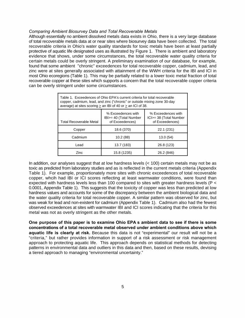
Comparing Ambient Biosurvey Data and Total Recoverable MetalsAlthough essentially no ambient dissolved metals data exists in Ohio, there is a very large databaseof total recoverable metals data at or near sites where biosurvey data have been collected. The totalrecoverable criteria in Ohio's water quality standards for toxic metals have been at least partiallyprotective of aquatic life designated uses as illustrated by Figure 1. There is ambient and laboratoryevidence that shows, under some circumstances, the total recoverable water quality criteria forcertain metals could be overly stringent. A preliminary examination of our database, for example,found that some ambient "chronic" exceedences for total recoverable copper, cadmium, lead, andzinc were at sites generally associated with attainment of the WWH criteria for the IBI and ICI inmost Ohio ecoregions (Table 1). This may be partially related to a lower toxic metal fraction of totalrecoverable copper at these sites which supports a concern that the total recoverable copper criteriacan be overly stringent under some circumstances.

Table 1. Exceedences of Ohio EPA’s current criteria for total recoverablecopper, cadmium, lead, and zinc (“chronic” or outside mixing zone 30-dayaverage) at sites scoring > an IBI of 40 or > an ICI of 38.

Total Recoverable Metal of Exceedences) of Exceedences)

% Exceedences with % Exceedences withIBI>= 40 (Total Number ICI>= 38 (Total Number

Copper 18.6 (370) 22.1 (231)

Cadmium 10.2 (88) 13.0 (54)

Lead 13.7 (183) 26.8 (123)

Zinc 15.8 (1235) 26.2 (846)

In addition, our analyses suggest that at low hardness levels (< 100) certain metals may not be astoxic as predicted from laboratory studies and as is reflected in the current metals criteria (AppendixTable 1). For example, proportionately more sites with chronic exceedences of total recoverablecopper, whcih had IBI or ICI scores reflecting at least warmwater conditions, were found thanexpected with hardness levels less than 100 compared to sites with greater hardness levels (P <0.0001, Appendix Table 1). This suggests that the toxicity of copper was less than predicted at lowhardness values and accounts for some of the discrepancy between the ambient biological data andthe water quality criteria for total recoverable copper. A similar pattern was observed for zinc, butwas weak for lead and non-existent for cadmium (Appendix Table 1). Cadmium also had the fewestobserved exceedences at sites with warmwater IBI and ICI scores indicating that the criteria for thismetal was not as overly stringent as the other metals.

One purpose of this paper is to examine Ohio EPA’s ambient data to see if there is someconcentrations of a total recoverable metal observed under ambient conditions above whichaquatic life is clearly at risk. Because this data is not “experimental” our result will not be a“criteria,” but rather provides information in support of a risk assessment or risk managementapproach to protecting aquatic life. This approach depends on statistical methods for detectingpatterns in environmental data and outliers in this data and then, based on these results, devisinga tiered approach to managing “environmental uncertainty.”

IBIorICI

Heavy Metal Concentration (µg/l)Li

ne A

In creasingRisk of Impairment

"Safe"Area

Water QualityCr ite ria

6

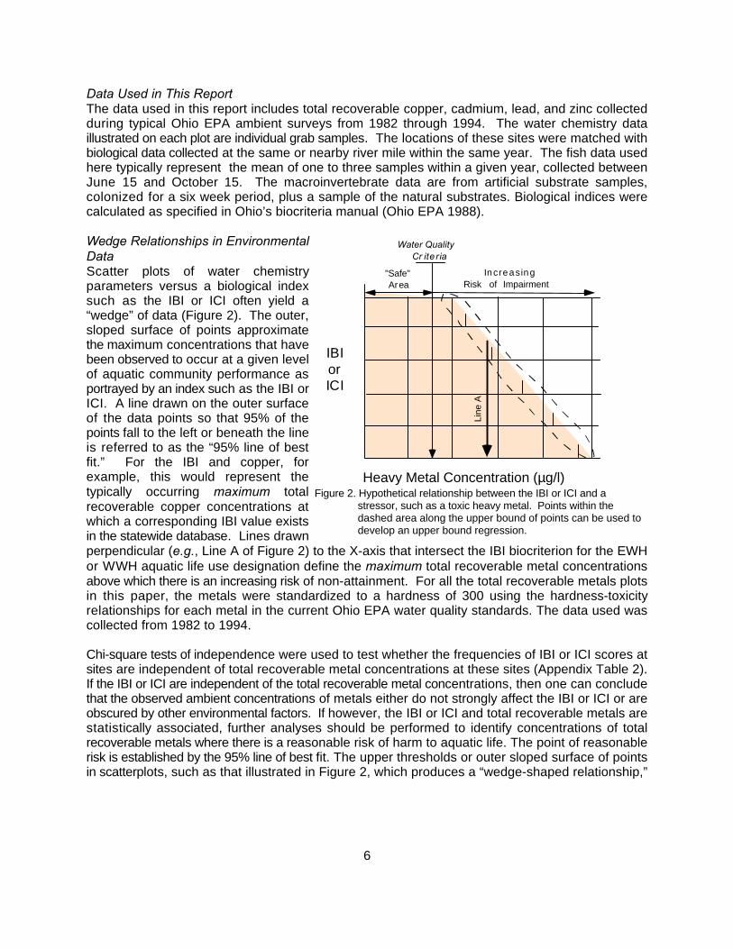
Figure 2. Hypothetical relationship between the IBI or ICI and astressor, such as a toxic heavy metal. Points within thedashed area along the upper bound of points can be used todevelop an upper bound regression.

Data Used in This ReportThe data used in this report includes total recoverable copper, cadmium, lead, and zinc collectedduring typical Ohio EPA ambient surveys from 1982 through 1994. The water chemistry dataillustrated on each plot are individual grab samples. The locations of these sites were matched withbiological data collected at the same or nearby river mile within the same year. The fish data usedhere typically represent the mean of one to three samples within a given year, collected betweenJune 15 and October 15. The macroinvertebrate data are from artificial substrate samples,colonized for a six week period, plus a sample of the natural substrates. Biological indices werecalculated as specified in Ohio’s biocriteria manual (Ohio EPA 1988).

Wedge Relationships in EnvironmentalDataScatter plots of water chemistryparameters versus a biological indexsuch as the IBI or ICI often yield a“wedge” of data (Figure 2). The outer,sloped surface of points approximatethe maximum concentrations that havebeen observed to occur at a given levelof aquatic community performance asportrayed by an index such as the IBI orICI. A line drawn on the outer surfaceof the data points so that 95% of thepoints fall to the left or beneath the lineis referred to as the “95% line of bestfit.” For the IBI and copper, forexample, this would represent thetypically occurring maximum totalrecoverable copper concentrations atwhich a corresponding IBI value existsin the statewide database. Lines drawnperpendicular (e.g., Line A of Figure 2) to the X-axis that intersect the IBI biocriterion for the EWHor WWH aquatic life use designation define the maximum total recoverable metal concentrationsabove which there is an increasing risk of non-attainment. For all the total recoverable metals plotsin this paper, the metals were standardized to a hardness of 300 using the hardness-toxicityrelationships for each metal in the current Ohio EPA water quality standards. The data used wascollected from 1982 to 1994.

Chi-square tests of independence were used to test whether the frequencies of IBI or ICI scores atsites are independent of total recoverable metal concentrations at these sites (Appendix Table 2).If the IBI or ICI are independent of the total recoverable metal concentrations, then one can concludethat the observed ambient concentrations of metals either do not strongly affect the IBI or ICI or areobscured by other environmental factors. If however, the IBI or ICI and total recoverable metals arestatistically associated, further analyses should be performed to identify concentrations of totalrecoverable metals where there is a reasonable risk of harm to aquatic life. The point of reasonablerisk is established by the 95% line of best fit. The upper thresholds or outer sloped surface of pointsin scatterplots, such as that illustrated in Figure 2, which produces a “wedge-shaped relationship,”

0

5

10

15

20

25

30

35

40

1 10 100 1000Nu

mb

er o

f F

ish

Sp

ecie

s

Drainage Area (sq mi)

StatisticallyDerived

Drawn By EyeReference Sites

EWH

WWH

WWH-2

MWH

LRW

Existing Criteria

Never/Rarely Observed BiologicalIndex Value For These Range ofMetals Concentrations

IBIorICI

Total Metal Concentration (µg/l)

90th

10th

75th

25th50th

Min

Max

Outlier

7

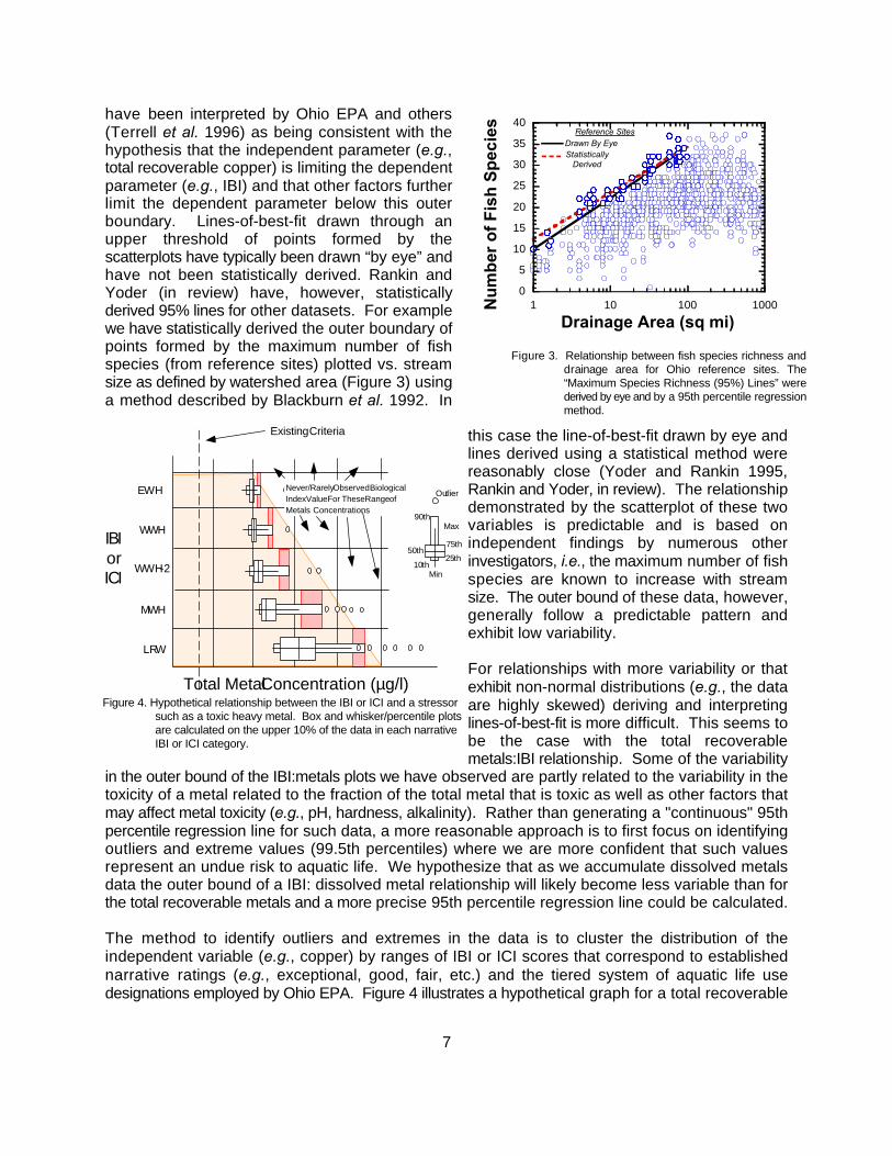
Figure 3. Relationship between fish species richness anddrainage area for Ohio reference sites. The“Maximum Species Richness (95%) Lines” werederived by eye and by a 95th percentile regressionmethod.

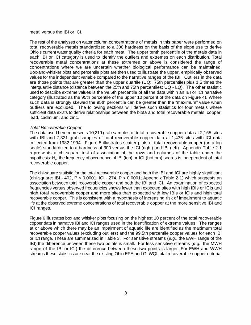
Figure 4. Hypothetical relationship between the IBI or ICI and a stressorsuch as a toxic heavy metal. Box and whisker/percentile plotsare calculated on the upper 10% of the data in each narrativeIBI or ICI category.

have been interpreted by Ohio EPA and others(Terrell et al. 1996) as being consistent with thehypothesis that the independent parameter (e.g.,total recoverable copper) is limiting the dependentparameter (e.g., IBI) and that other factors furtherlimit the dependent parameter below this outerboundary. Lines-of-best-fit drawn through anupper threshold of points formed by thescatterplots have typically been drawn “by eye” andhave not been statistically derived. Rankin andYoder (in review) have, however, statisticallyderived 95% lines for other datasets. For examplewe have statistically derived the outer boundary ofpoints formed by the maximum number of fishspecies (from reference sites) plotted vs. streamsize as defined by watershed area (Figure 3) usinga method described by Blackburn et al. 1992. In

this case the line-of-best-fit drawn by eye andlines derived using a statistical method werereasonably close (Yoder and Rankin 1995,Rankin and Yoder, in review). The relationshipdemonstrated by the scatterplot of these twovariables is predictable and is based onindependent findings by numerous otherinvestigators, i.e., the maximum number of fishspecies are known to increase with streamsize. The outer bound of these data, however,generally follow a predictable pattern andexhibit low variability.

For relationships with more variability or thatexhibit non-normal distributions (e.g., the dataare highly skewed) deriving and interpretinglines-of-best-fit is more difficult. This seems tobe the case with the total recoverablemetals:IBI relationship. Some of the variability

in the outer bound of the IBI:metals plots we have observed are partly related to the variability in thetoxicity of a metal related to the fraction of the total metal that is toxic as well as other factors thatmay affect metal toxicity (e.g., pH, hardness, alkalinity). Rather than generating a "continuous" 95thpercentile regression line for such data, a more reasonable approach is to first focus on identifyingoutliers and extreme values (99.5th percentiles) where we are more confident that such valuesrepresent an undue risk to aquatic life. We hypothesize that as we accumulate dissolved metalsdata the outer bound of a IBI: dissolved metal relationship will likely become less variable than forthe total recoverable metals and a more precise 95th percentile regression line could be calculated.

The method to identify outliers and extremes in the data is to cluster the distribution of theindependent variable (e.g., copper) by ranges of IBI or ICI scores that correspond to establishednarrative ratings (e.g., exceptional, good, fair, etc.) and the tiered system of aquatic life usedesignations employed by Ohio EPA. Figure 4 illustrates a hypothetical graph for a total recoverable

8

metal versus the IBI or ICI.

The rest of the analyses on water column concentrations of metals in this paper were performed ontotal recoverable metals standardized to a 300 hardness on the basis of the slope use to deriveOhio’s current water quality criteria for each metal. The upper tenth percentile of the metals data ineach IBI or ICI category is used to identify the outliers and extremes on each distribution. Totalrecoverable metal concentrations at these extremes or above is considered the range ofconcentrations where we are uncertain whether biological performance can be maintained.Box-and-whisker plots and percentile plots are then used to illustrate the upper, empirically observedvalues for the independent variable compared to the narrative ranges of the IBI. Outliers in the dataare those points that are greater than the upper quartile (UQ: 75th percentile) plus 1.5 times theinterquartile distance (distance between the 25th and 75th percentiles: UQ - LQ). The other statisticused to describe extreme values is the 99.5th percentile of all the data within an IBI or ICI narrativecategory (illustrated as the 95th percentile of the upper 10 percent of the data on Figure 4). Wheresuch data is strongly skewed the 95th percentile can be greater than the “maximum” value whenoutliers are excluded. The following sections will derive such statistics for four metals wheresufficient data exists to derive relationships between the biota and total recoverable metals: copper,lead, cadmium, and zinc.

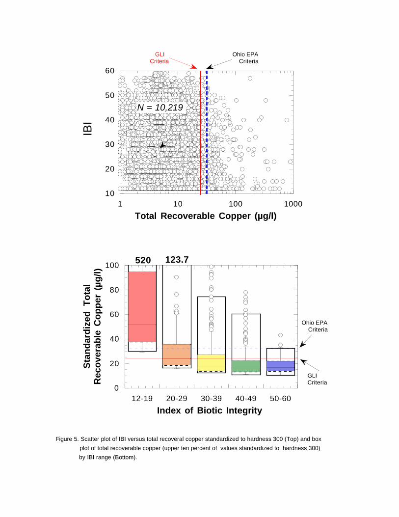
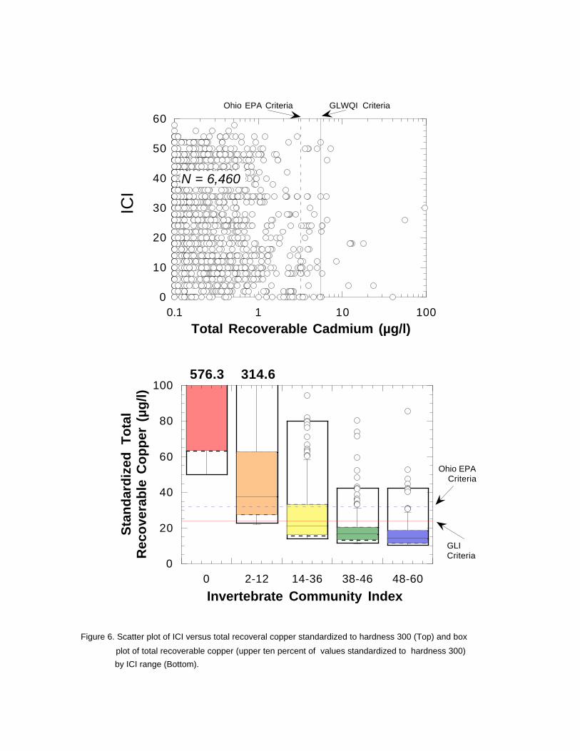
Total Recoverable CopperThe data used here represents 10,219 grab samples of total recoverable copper data at 2,165 siteswith IBI and 7,321 grab samples of total recoverable copper data at 1,436 sites with ICI datacollected from 1982-1994. Figure 5 illustrates scatter plots of total recoverable copper (on a logscale) standardized to a hardness of 300 versus the ICI (right) and IBI (left). Appendix Table 2-1represents a chi-square test of association of the rows and columns of the table under thehypothesis: H : the frequency of occurrence of IBI (top) or ICI (bottom) scores is independent of totalo

recoverable copper.

The chi-square statistic for the total recoverable copper and both the IBI and ICI are highly significant(chi-square: IBI - 402, P < 0.0001; ICI - 274, P < 0.0001; Appendix Table 2-1) which suggests anassociation between total recoverable copper and both the IBI and ICI. An examination of expectedfrequencies versus observed frequencies shows fewer than expected sites with high IBIs or ICIs andhigh total recoverable copper and more sites than expected with low IBIs or ICIs and high totalrecoverable copper. This is consistent with a hypothesis of increasing risk of impairment to aquaticlife at the observed extreme concentrations of total recoverable copper at the more sensitive IBI andICI ranges.

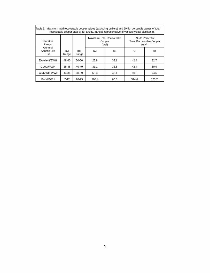
Figure 6 illustrates box and whisker plots focusing on the highest 10 percent of the total recoverablecopper data in narrative IBI and ICI ranges used in the identification of extreme values. The rangesat or above which there may be an impairment of aquatic life are identified as the maximum totalrecoverable copper values (excluding outliers) and the 99.5th percentile copper values for each IBIor ICI range. These are summarized in Table 3. For sensitive streams (e.g., the EWH range of theIBI) the difference between these two points is small. For less sensitive streams (e.g., the MWHrange of the IBI or ICI) the difference between these two points is larger. For EWH and WWHstreams these statistics are near the existing Ohio EPA and GLWQI total recoverable copper criteria.

9

Table 3. Maximum total recoverable copper values (excluding outliers) and 99.5th percentile values of totalrecoverable copper data by IBI and ICI ranges representative of various typical biocriteria).

NarrativeRange/General

Aquatic Life ICI IBI Use Range Range

Maximum Total Recoverable 99.5th PercentileCopper Total Recoverable Copper(ug/l) (ug/l)

ICI IBI ICI IBI

Excellent/EWH 48-60 50-60 28.8 33.1 42.4 32.7

Good/WWH 38-46 40-49 31.1 33.6 42.4 60.9

Fair/MWH-WWH 14-36 30-39 58.3 46.4 80.2 74.5

Poor/MWH 2-12 20-29 108.4 60.8 314.6 123.7

0

20

40

60

80

100

50-6040-4930-3920-2912-19

Sta

nd

ard

ized

T

ota

lR

eco

vera

ble

Co

pp

er (

µg

/l)

Index of Biotic Integrity

GLICriteria

Ohio EPACriteria

520 123.7

10

20

30

40

50

60

1 10 100 1000

IBI

Total Recoverable Copper (µg/l)

N = 10,219

GLI Criteria

Ohio EPACriteria

Figure 5. Scatter plot of IBI versus total recoveral copper standardized to hardness 300 (Top) and box

plot of total recoverable copper (upper ten percent of values standardized to hardness 300)

by IBI range (Bottom).

0

20

40

60

80

100

0 2-12 14-36 38-46 48-60

Sta

nd

ard

ized

T

ota

lR

eco

vera

ble

Co

pp

er (

µg

/l)

Invertebrate Community Index

GLICriteria

Ohio EPACriteria

576.3 314.6

0

10

20

30

40

50

60

0.1 1 10 100

ICI

Total Recoverable Cadmium (µg/l)

GLWQI CriteriaOhio EPA Criteria

N = 6,460

Figure 6. Scatter plot of ICI versus total recoveral copper standardized to hardness 300 (Top) and box

plot of total recoverable copper (upper ten percent of values standardized to hardness 300)

by ICI range (Bottom).

12

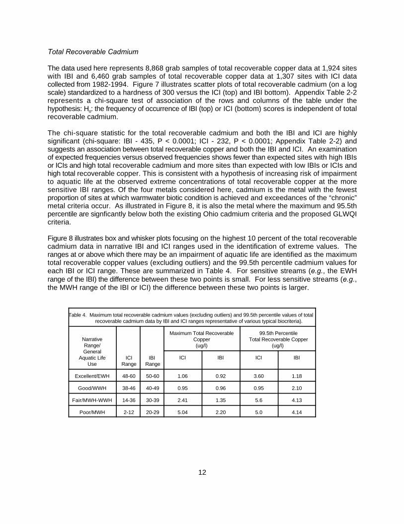
Total Recoverable Cadmium

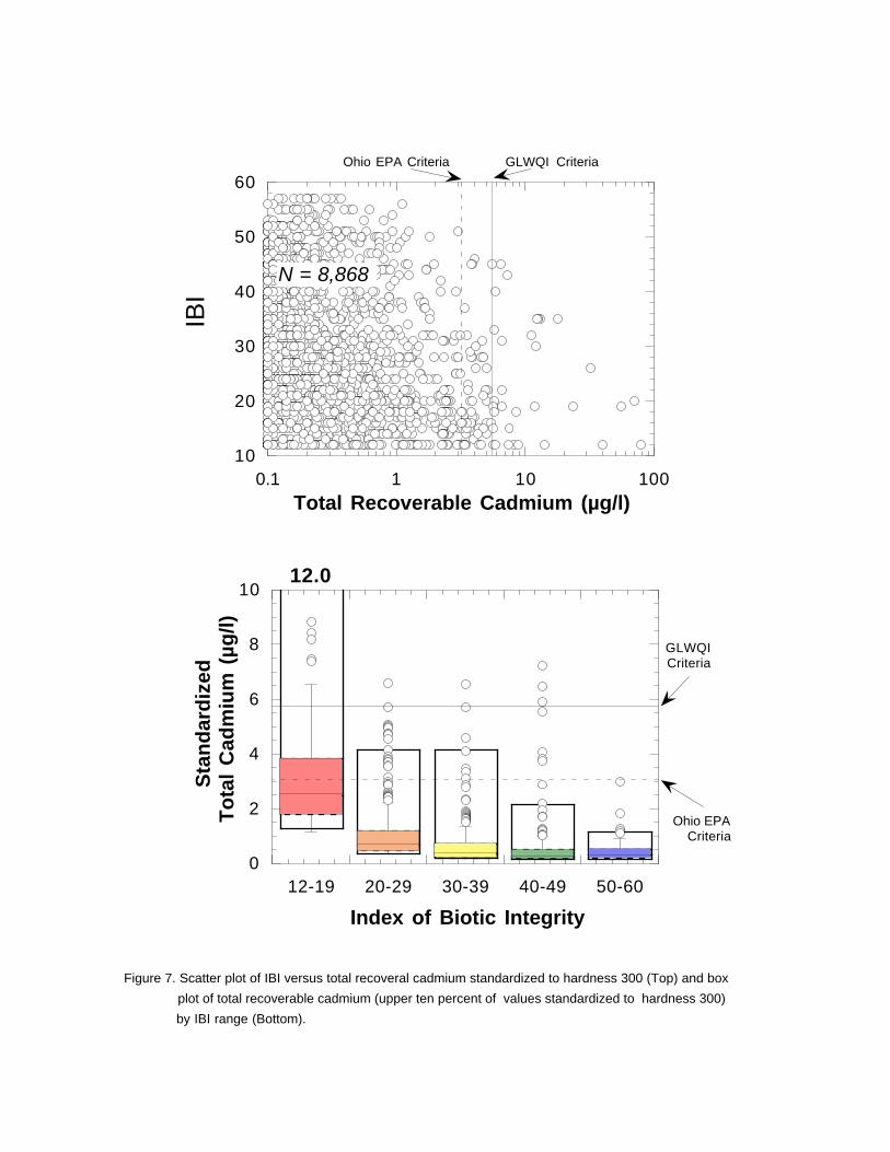
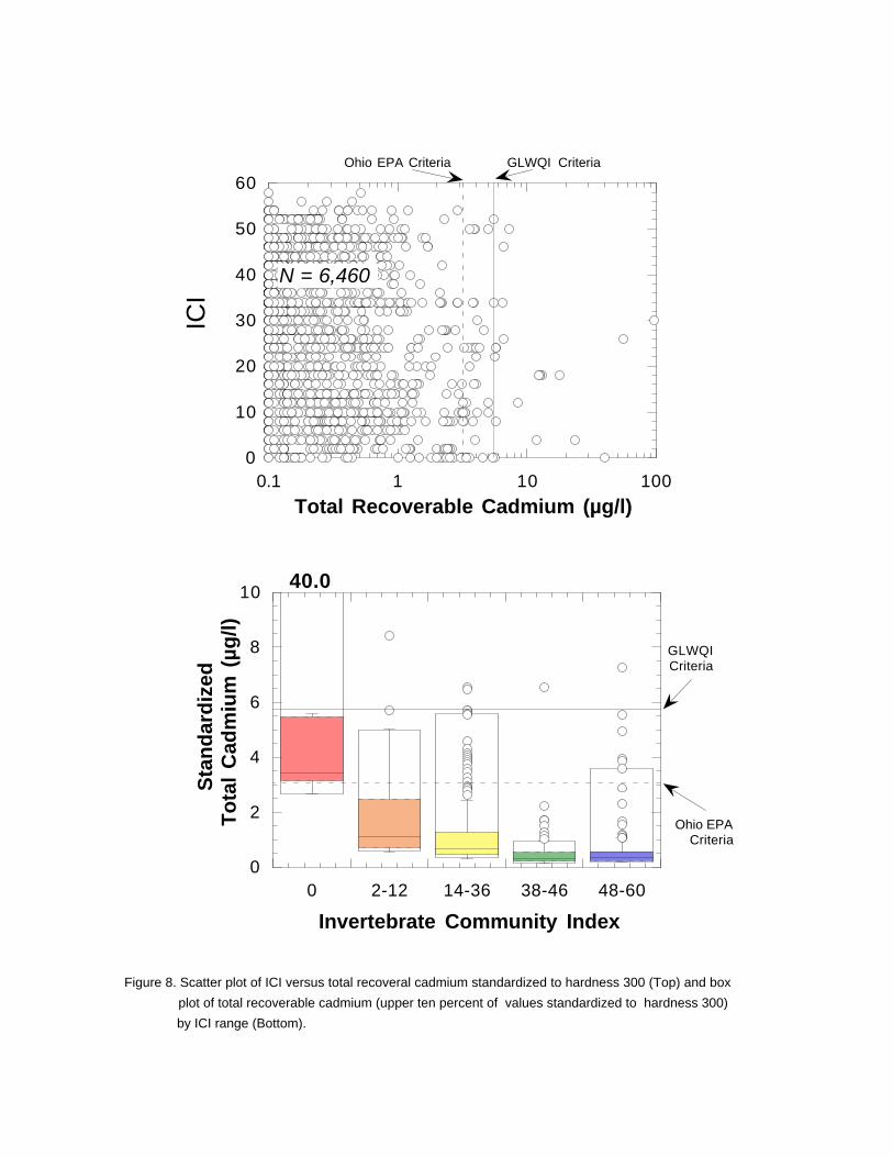
The data used here represents 8,868 grab samples of total recoverable copper data at 1,924 siteswith IBI and 6,460 grab samples of total recoverable copper data at 1,307 sites with ICI datacollected from 1982-1994. Figure 7 illustrates scatter plots of total recoverable cadmium (on a logscale) standardized to a hardness of 300 versus the ICI (top) and IBI bottom). Appendix Table 2-2represents a chi-square test of association of the rows and columns of the table under thehypothesis: H : the frequency of occurrence of IBI (top) or ICI (bottom) scores is independent of totalo

recoverable cadmium.

The chi-square statistic for the total recoverable cadmium and both the IBI and ICI are highlysignificant (chi-square: IBI - 435, P < 0.0001; ICI - 232, P < 0.0001; Appendix Table 2-2) andsuggests an association between total recoverable copper and both the IBI and ICI. An examinationof expected frequencies versus observed frequencies shows fewer than expected sites with high IBIsor ICIs and high total recoverable cadmium and more sites than expected with low IBIs or ICIs andhigh total recoverable copper. This is consistent with a hypothesis of increasing risk of impairmentto aquatic life at the observed extreme concentrations of total recoverable copper at the moresensitive IBI ranges. Of the four metals considered here, cadmium is the metal with the fewestproportion of sites at which warmwater biotic condition is achieved and exceedances of the “chronic”metal criteria occur. As illustrated in Figure 8, it is also the metal where the maximum and 95.5thpercentile are signficantly below both the existing Ohio cadmium criteria and the proposed GLWQIcriteria.

Figure 8 illustrates box and whisker plots focusing on the highest 10 percent of the total recoverablecadmium data in narrative IBI and ICI ranges used in the identification of extreme values. Theranges at or above which there may be an impairment of aquatic life are identified as the maximumtotal recoverable copper values (excluding outliers) and the 99.5th percentile cadmium values foreach IBI or ICI range. These are summarized in Table 4. For sensitive streams (e.g., the EWHrange of the IBI) the difference between these two points is small. For less sensitive streams (e.g.,the MWH range of the IBI or ICI) the difference between these two points is larger.

Table 4. Maximum total recoverable cadmium values (excluding outliers) and 99.5th percentile values of totalrecoverable cadmium data by IBI and ICI ranges representative of various typical biocriteria).




ICI IBI ICI IBI

Excellent/EWH 48-60 50-60 1.06 0.92 3.60 1.18

Good/WWH 38-46 40-49 0.95 0.96 0.95 2.10

Fair/MWH-WWH 14-36 30-39 2.41 1.35 5.6 4.13

Poor/MWH 2-12 20-29 5.04 2.20 5.0 4.14

0

2

4

6

8

10

50-6040-4930-3920-2912-19

Sta

nd

ard

ized

T

ota

l C

adm

ium

(µ

g/l)


GLWQICriteria

Ohio EPACriteria

12.0

10

20

30

40

50

60

0.1 1 10 100

IBI



N = 8,868

Figure 7. Scatter plot of IBI versus total recoveral cadmium standardized to hardness 300 (Top) and box

plot of total recoverable cadmium (upper ten percent of values standardized to hardness 300)


0

2

4

6

8

10

48-6038-4614-362-120

Sta

nd

ard

ized

T

ota

l C

adm

ium

(µ

g/l)


GLWQICriteria

Ohio EPACriteria

40.0

0

10

20

30

40

50

60

0.1 1 10 100

ICI



N = 6,460

Figure 8. Scatter plot of ICI versus total recoveral cadmium standardized to hardness 300 (Top) and box

plot of total recoverable cadmium (upper ten percent of values standardized to hardness 300)


15

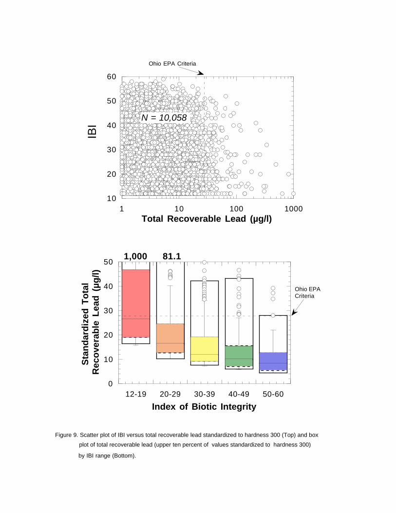
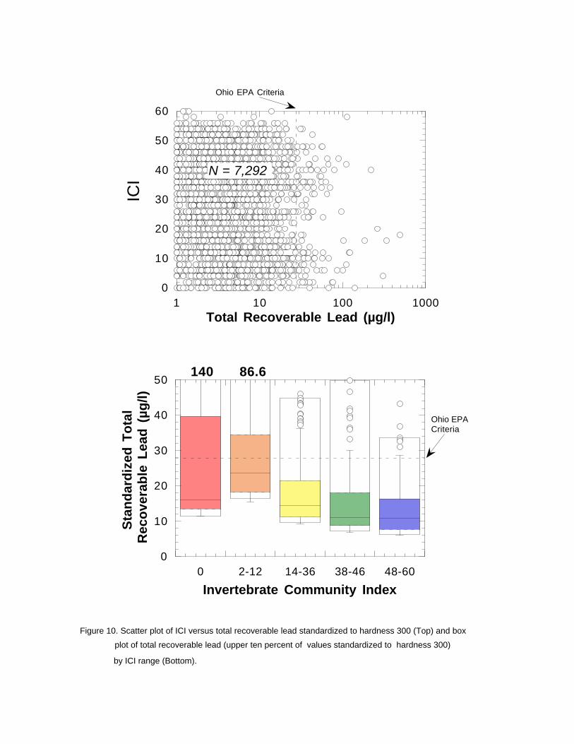
Total Recoverable LeadThe data used here represents 10,058 grab samples of total recoverable lead data at 2,132 siteswith IBI and 7.292 grab samples of total recoverable lead data at 1,426 sites with ICI data collectedfrom 1982-1994. Figure 9 illustrates scatter plots of total recoverable lead (on a log scale)standardized to a hardness of 300 versus the ICI (top) and IBI bottom). Appendix Table 2-3represents a chi-square test of association of the rows and columns of the table under thehypothesis: H : the frequency of occurrence of IBI (top) or ICI (bottom) scores is independent of totalo

recoverable lead.

The chi-square statistic for the total recoverable lead and both the IBI and ICI are highly significant(chi-square: IBI - 435, P < 0.0001; ICI - 232, P < 0.0001; Appendix Table 2-3) and suggests anassociation between total recoverable lead and both the IBI and ICI. An examination of expectedfrequencies versus observed frequencies shows fewer than expected sites with high IBIs or ICIs andhigh total recoverable lead and more sites than expected with low IBIs or ICIs and high totalrecoverable lead. This is consistent with a hypothesis of increasing risk of impairment to aquatic lifeat the observed extreme concentrations of total recoverable lead at the more sensitive IBI ranges.

Figure 9 illustrates box and whisker plots focusing on the highest 10 percent of the total recoverablelead data in narrative IBI and ICI ranges used in the identification of extreme values. The ranges ator above which there may be an impairment of aquatic life are identified as the maximum totalrecoverable lead values (excluding outliers) and the 99.5th percentile lead values for each IBI or ICIrange. These are summarized in Table 5. For sensitive streams (e.g., the EWH range of the IBI) thedifference between these two points is small. For less sensitive streams (e.g., the MWH range ofthe IBI or ICI) the difference between these two points is larger.

Table 5. Maximum total recoverable lead values (excluding outliers) and 99.5th percentile values of totalrecoverable lead data by IBI and ICI ranges representative of various typical biocriteria).




ICI IBI ICI IBI

Excellent/EWH 48-60 50-60 28.6 22.0 33.7 28.1

Good/WWH 38-46 40-49 30 27.1 49.8 43.6

Fair/MWH-WWH 14-36 30-39 36.2 34.2 44.8 42.2

Poor/MWH 2-12 20-29 58.4 40.4 86.6 81.1

0

10

20

30

40

50

50-6040-4930-3920-2912-19

Sta

nd

ard

ized

To

tal

Rec

ove

rab

le L

ead

(µ

g/l)


Ohio EPACriteria

1,000 81.1

10

20

30

40

50

60

1 10 100 1000

IBI

Total Recoverable Lead (µg/l)

Ohio EPA Criteria

N = 10,058

Figure 9. Scatter plot of IBI versus total recoverable lead standardized to hardness 300 (Top) and box

plot of total recoverable lead (upper ten percent of values standardized to hardness 300)


0

10

20

30

40

50

48-6038-4614-362-120

Sta

nd

ard

ized

To

tal

Rec

ove

rab

le L

ead

(µ

g/l)


Ohio EPACriteria

140 86.6

0

10

20

30

40

50

60

1 10 100 1000

ICI

Total Recoverable Lead (µg/l)

Ohio EPA Criteria

N = 7,292

Figure 10. Scatter plot of ICI versus total recoverable lead standardized to hardness 300 (Top) and box

plot of total recoverable lead (upper ten percent of values standardized to hardness 300)


18

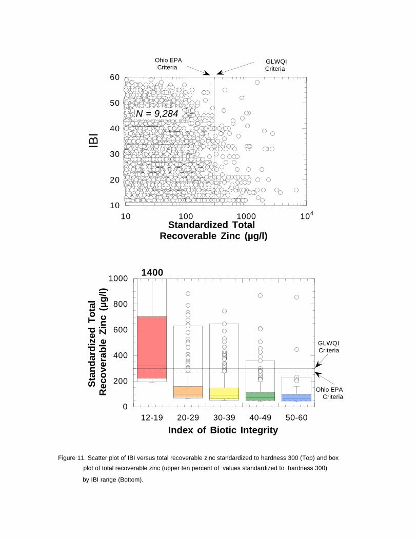
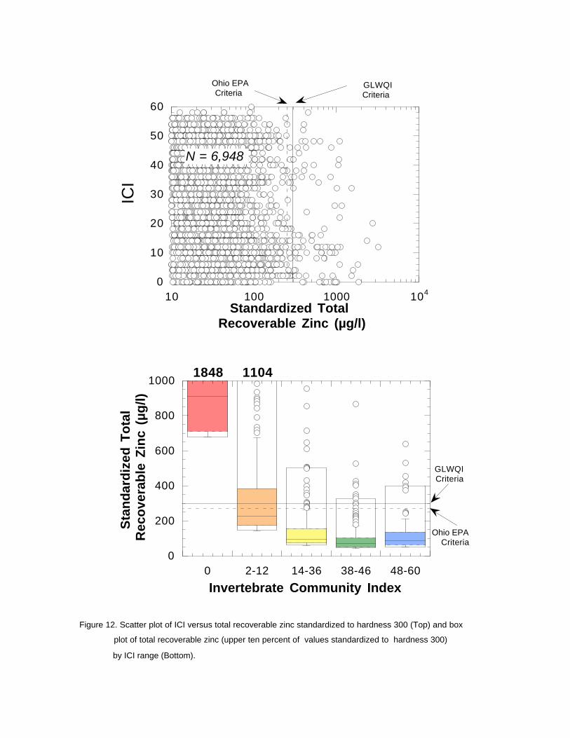
Total Recoverable ZincThe data used here represents 9,824 grab samples of total recoverable zinc data at 2,101 sites withIBI and 6,948 grab samples of total recoverable zinc data at 1,385 sites with ICI data collected from1982-1994. Figure 9 illustrates scatter plots of total recoverable zinc (on a log scale) standardizedto a hardness of 300 versus the ICI (top) and IBI bottom). Appendix Table 2-4 represents achi-square test of association of the rows and columns of the table under the hypothesis: H : theo

frequency of occurrence of IBI (top) or ICI (bottom) scores is independent of total recoverable zinc.

The chi-square statistic for the total recoverable zinc and both the IBI and ICI are highly significant(chi-square: IBI - 745, P < 0.0001; ICI - 470, P < 0.0001; Appendix Table 2-4) and suggests anassociation between total recoverable zinc and both the IBI and ICI. An examination of expectedfrequencies versus observed frequencies shows fewer than expected sites with high IBIs or ICIs andhigh total recoverable zinc and more sites than expected with low IBIs or ICIs and high totalrecoverable zinc. This is consistent with a hypothesis of increasing risk of impairment to aquatic lifeat the observed extreme concentrations of total recoverable zinc at the more sensitive IBI ranges.

Figure 10 illustrates box and whisker plots focusing on the highest 10 percent of the total recoverablezinc data in narrative IBI and ICI ranges used in the identification of extreme values. The ranges ator above which there may be an impairment of aquatic life are identified as the maximum totalrecoverable zinc values (excluding outliers) and the 99.5th percentile zinc values for each IBI or ICIrange. These are summarized in Table 6. For sensitive streams (e.g., the EWH range of the IBI) thedifference between these two points is small. For less sensitive streams (e.g., the MWH range ofthe IBI or ICI) the difference between these two points is larger.

Table 6. Maximum total recoverable zinc (standardized to 300 hardness) values (excluding outliers) and99.5th percentile values of total recoverable zinc data by IBI and ICI ranges representative ofvarious typical biocriteria).




ICI IBI ICI IBI

Excellent/EWH 48-60 50-60 209.2 158.2 399.2 230.0

Good/WWH 38-46 40-49 169.6 200.0 326.8 360.5

Fair/MWH-WWH 14-36 30-39 262.2 266.1 501.7 645.7

Poor/MWH 2-12 20-29 690 267.8 1104.4 632.1

0

200

400

600

800

1000

50-6040-4930-3920-2912-19

Sta

nd

ard

ized

To

tal

Rec

ove

rab

le Z

inc

(µg

/l)


GLWQICriteria

Ohio EPACriteria

1400

10

20

30

40

50

60

10 100 1000 104

IBI

Standardized Total Recoverable Zinc (µg/l)

GLWQICriteria

Ohio EPACriteria

N = 9,284

Figure 11. Scatter plot of IBI versus total recoverable zinc standardized to hardness 300 (Top) and box

plot of total recoverable zinc (upper ten percent of values standardized to hardness 300)


0

200

400

600

800

1000

48-6038-4614-362-120

Sta

nd

ard

ized

To

tal

Rec

ove

rab

le Z

inc

(µg

/l)


GLWQICriteria

Ohio EPACriteria

1848 1104

0

10

20

30

40

50

60

10 100 1000 104

ICI

Standardized Total Recoverable Zinc (µg/l)

GLWQICriteria

Ohio EPACriteria

N = 6,948

Figure 12. Scatter plot of ICI versus total recoverable zinc standardized to hardness 300 (Top) and box

plot of total recoverable zinc (upper ten percent of values standardized to hardness 300)


21

Inferring Cause and Effect Relationships in IBI: Metals AssociationsThe upper thresholds or outer bounds of points in wedge shaped relationships have been interpretedby Ohio EPA and others (Terrell et al. 1996) as being consistent with the hypothesis that theindependent parameter (e.g., total recoverable copper) is likely limiting the dependent parameter(e.g., IBI) and that other factors further limit the dependent parameter below this outer bound. Usingonly the upper 10% (and upper 2%) of total copper values in various IBI ranges, we tested thepossibility that some other parameter may actually be limiting the biota and may simply be correlatedwith metal in question. We calculated correlation coefficients between the IBI, total recoverablecopper, and a suite of other chemical parameters typically collected during our intensive surveys,plus the QHEI, a measure of physical habitat quality important to aquatic life. Total recoverablecopper was the only measure, when paired with the IBI that explained more than 40% of the variationin the relationship (Table 4). The only other parameter that explained more than 30% of the variationin the IBI was habitat (the QHEI) and this parameter was not strongly related to total recoverablecopper (Table 4).

The concern of the agency is related to the potential occurrence of situations where concentrationsof total metals are beyond where we have typically observed biological communities attaining theiraquatic life use, i.e., where uncertainty is high. Where the frequency of high total recoverable metalsvalues are higher there are signficantly fewer high IBI scores (see chi-square test). In other words,we ask the question “Why haven’t we seen many, if any, attaining biological scores above a totalrecoverable metal concentration of X?” This uncertainty is sufficient justification to require moreinformation (through increased monitoring) on the status of the ambient conditions. This increaseddata should result in an increased knowledge of the relation between total metals, dissolved metals,and the biological condition of streams. Nevertheless, the correlation analyses illustrated in Table4 can provide insight into the likelihood whether a particular metal has a strong or weak affect onaquatic life under ambient conditions.

Advantages of Including Biocriteria in Chemical Criteria DerviationUsing the relationships portrayed in the preceding examples in combination with the traditionaltoxicity-based chemical criteria (Stephan et al. 1985) provides an effective way to evaluate and/orestablish chemical water quality criteria. Toxicity derived criteria, because of uncertaintiesassociated with comparatively limited data, may well be under or over-protective. A biological datacan function as an effective "reality check" on toxicity derived criteria. Some further advantages ofusing biocriteria to evaluate toxicity-based chemical criteria include the following:

1) Biological criteria can be used to adjust chemical criteria to account for the differingsensitivities between aquatic life use designations and ecoregions. The toxicity-basedprocedure is less able to produce such stratified water quality criteria because offrequently limited databases and the inability of the technique to discriminate thedifferences between the different uses that are accounted for by the biological criteria.

2) The biological criteria method incorporates the effects of other overlying stressors thatare present to varying degrees in the ambient environment, thus additive effects fromother substances and impacts are automatically incorporated; and,

0

20

40

60

80

100

120

VE

RY

PO

OR

PO

OR

FA

IR

MA

RG

. GO

OD

GO

OD

VE

RY

GO

OD

EX

CE

PT

ION

AL

COPPER (75th %ILE)C

OP

PE

R (

MG

/KG

)

IBI RANGES OFPERFORMANCE>>>

0

20

40

60

80

100

VE

RY

PO

OR

PO

OR

FA

IR

MA

RG

. GO

OD

GO

OD

VE

RY

GO

OD

EX

CE

PT

ION

AL

COPPER (75th %ILE)

CO

PP

ER

(M

G/K

G)

ICI RANGES OFPERFORMANCE>>>

22

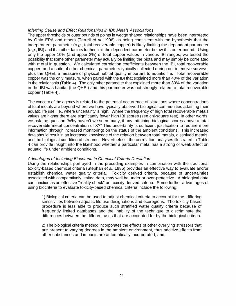
Figure 13. Total copper (mg/kg) in sediment from the statewide OhioEPA database compared to the gradient of aquatic communityperformance defined by the IBI (upper) and ICI (lower).

3) Instream data can be used toexamine the response of biologicalcommunities to a given parameter,thus uncertainties associated withapplying different forms of thechemical (e.g., total vs. dissolved) orwith other parameters that affect ametal’s toxicity (e.g., hardness,alkalinity) can be “ground-truthed”with empirical data.

Using Biocriteria To Evaluate SedimentContaminationOhio EPA has collected sedimentchemistry data as a part of the biosurveyprocess which has resulted in a robuststatewide database. Recently it hasbecome evident that sediment chemistrydata reveals more about the history ofchemical contamination than do watercolumn analyses alone. Presently, thereare no readily available sediment criteriathat are directly linked to adverse effectson aquatic life. Kelly and Hite (1984) inIllinois developed thresholds for aquaticlife for selected heavy metals, and theOntario guidelines (Persuad et al. 1991)have also been developed for the effectsof sediment on aquatic life. Neithermethod alone is viewed as sufficient forevaluating the potential of contaminatedsediments to contribute to aquatic lifeuse impairment in Ohio streams.

In order to address this deficiency,comparisons between biologicalsampling and sediment chemistry results

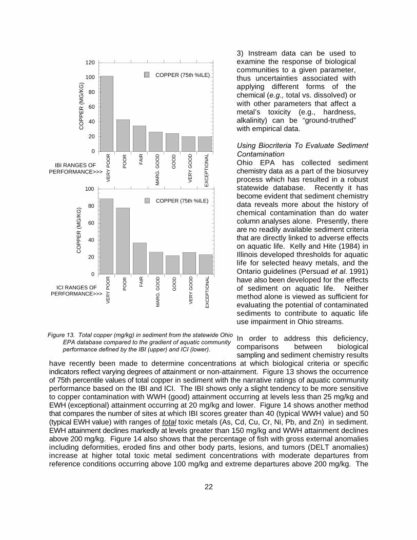
have recently been made to determine concentrations at which biological criteria or specificindicators reflect varying degrees of attainment or non-attainment. Figure 13 shows the occurrenceof 75th percentile values of total copper in sediment with the narrative ratings of aquatic communityperformance based on the IBI and ICI. The IBI shows only a slight tendency to be more sensitiveto copper contamination with WWH (good) attainment occurring at levels less than 25 mg/kg andEWH (exceptional) attainment occurring at 20 mg/kg and lower. Figure 14 shows another methodthat compares the number of sites at which IBI scores greater than 40 (typical WWH value) and 50(typical EWH value) with ranges of total toxic metals (As, Cd, Cu, Cr, Ni, Pb, and Zn) in sediment.EWH attainment declines markedly at levels greater than 150 mg/kg and WWH attainment declinesabove 200 mg/kg. Figure 14 also shows that the percentage of fish with gross external anomaliesincluding deformities, eroded fins and other body parts, lesions, and tumors (DELT anomalies)increase at higher total toxic metal sediment concentrations with moderate departures fromreference conditions occurring above 100 mg/kg and extreme departures above 200 mg/kg. The

0

5

10

15

20

0-50

51-1

00

101-

150

151-

200

201-

250

251-

300

301-

350

351-

400

401-

450

451-

500

>50

0

%DELT (5Oth %ile)%DELT (75th %ile)

%D

ELT

AN

OM

ALI

ES

TOTAL TOXIC METALS (MG/KG)

ExtremeDeparture

ModerateDeparture

0

10

20

30

40

50

60

70

80

0-50

51-1

00

101-

150

151-

200

201-

250

251-

300

301-

350

351-

400

401-

450

451-

500

>50

0

IBI >40 (Meets WWH)IBI >50 (Meets EWH)

NU

MB

ER

OF

SIT

ES

TOTAL TOXIC METALS (MG/KG)

23

Figure 14. The number of sites with IBI values meeting theEWH and WWH biocriteria by ranges of total toxic heavymetals in sediment (upper) and the median and 75thpercentiles of %DELT anomalies on fish by ranges oftotal toxic heavy metals in sediment (lower).

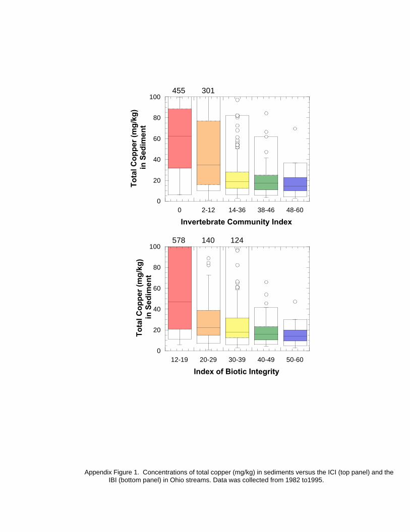
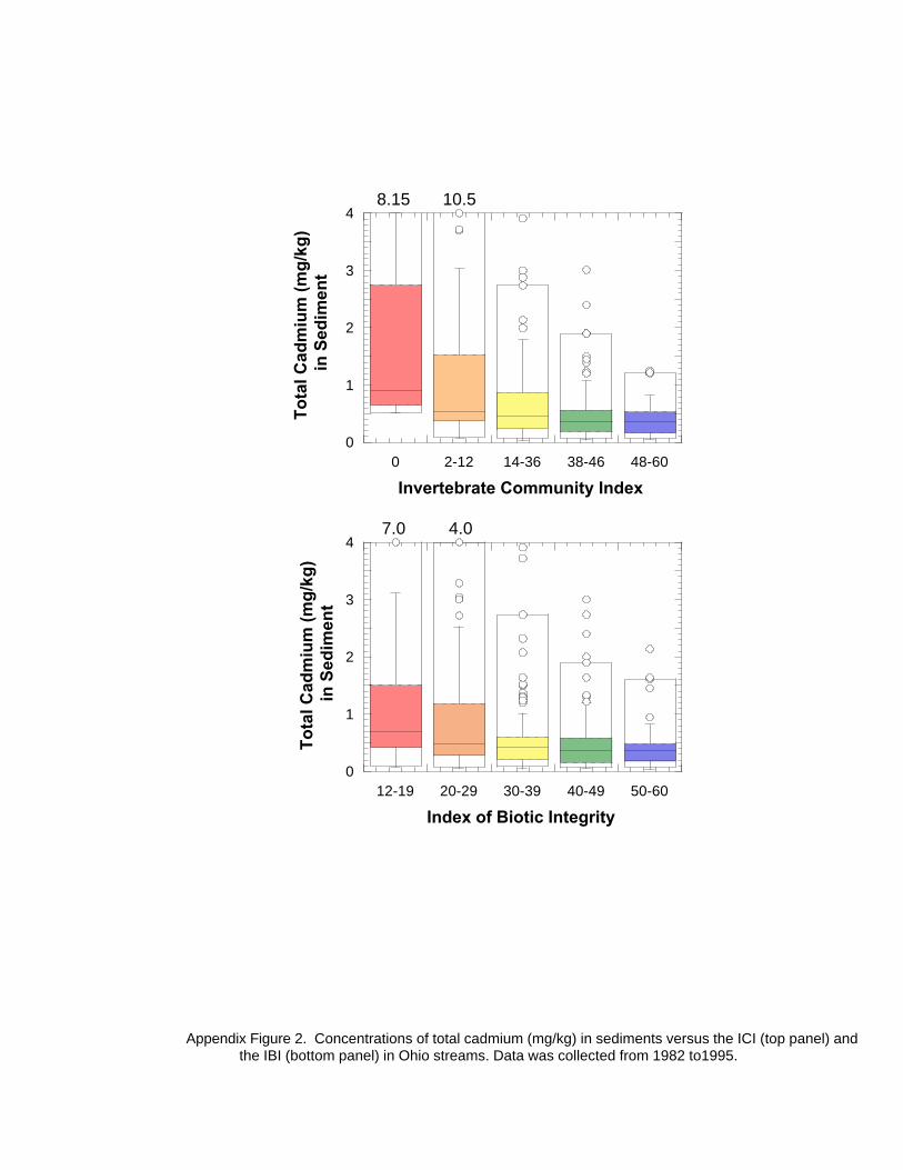
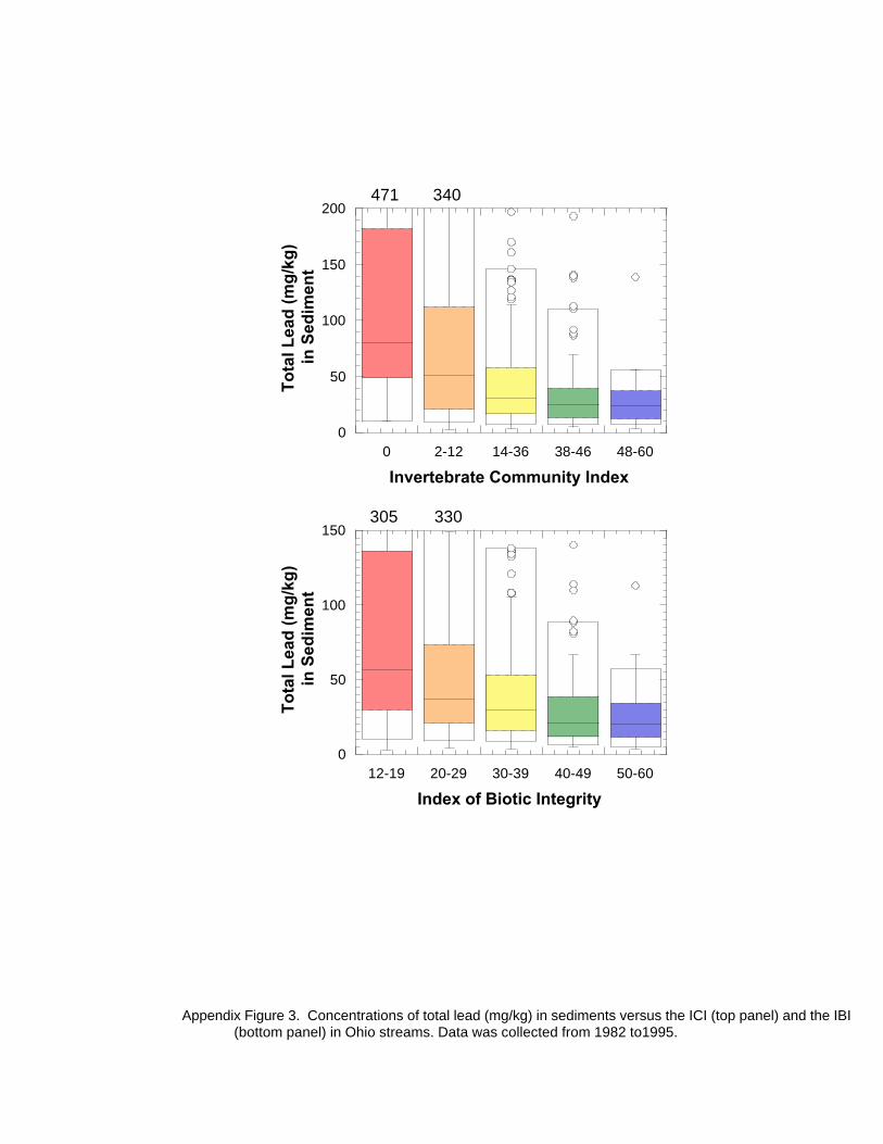
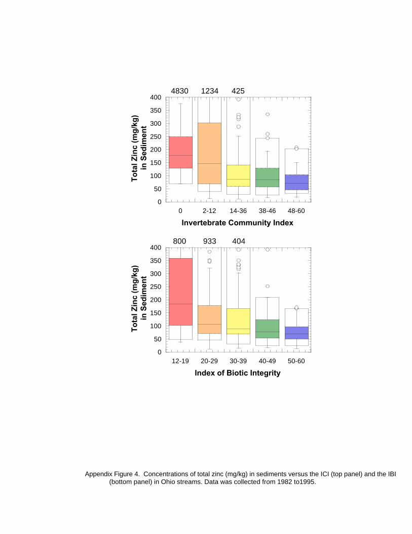
good relationships between the biologicalindicators and the degree of sedimentcontamination by heavy metals are areflection of the history of metals loadings.These loadings and their effects can easilyescape accurate quantification bychemical sampling alone. Box andwhisker plots of sediment concentrationsfor copper, cadmium, lead, and zinc byranges of the IBI abd ICI are illustrated inAppendix Figures 1 through 4. The 95thpercentiles by ranges of the IBI and ICI arelisted in Appendix Table ??.

Application To the GLWQG

The application of these methodologies tothe GLWQG seems to be useful in threegeneral areas: 1) ground truthing and/orfine tuning GLWQG and/or existing OhioEPA water quality criteria as describedpreviously; 2) providing insight into theeffects of total metals that result from apermit based on dissolved rather than totalrecoverable form; and, 3) in monitoring theeffectiveness of the GLWQG approach tosetting and applying water quality criteriafor the protection of aquatic life in general.

The analyses portrayed in Figures 5through 12 and Tables 3 through 6 couldbe used to evaluate the risk of anyincreases in total recoverable metalsconcentration that result from usingvarious translators (i.e., factors used totranslate from dissolved to totalrecoverable) to determine an effectivewater quality criterion. Concentrationthresholds based on the same type ofa n a l y s i s w h i c hresulted in Tables 3 - 6 could representtriggers above which an effective totalrecoverable criterion could not be raisedwithout: 1) biosurvey monitoring to ensure the aquatic life use is protected at relatively highdischarges of total metals (“maximum” value trigger) or 2) a demonstration that the use is currentlymet plus additional monitoring during the life of a permit (99.5th percentile trigger) where theconcentrations will be extreme compared to past observations or where sediment contamination isa concern. Sediment thresholds resulting from analyses like those portrayed in Figures 7 and 8 andAppendix Figures 1-4 could be used to evaluate the existing setting (i.e., what is the extent of anysediment contamination?) and whether any increases in heavy metals loadings resulting from the

24

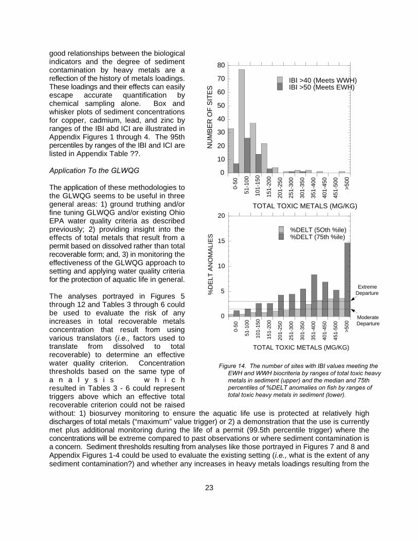
Figure 15. Flow chart illustrating the methodology for identifying outliers of total recoverablemetals where aquatic life may be at risk (top) and application of “monitoringtriggers” where additional monitoring may be required when environmentaluncertainly is high.

use of translators would pose anunreasonable risk to aquatic life useattainment.

One important limitation is thatthese methods are useable only if asufficiently large ambient databaseis available which is true in Ohioonly for the common heavy metalssuch as copper, cadmium, zinc, andlead. The ambient database forother heavy metals such aschromium and nickel is insufficientdue to the few detections that havebeen observed in the ambientenvironment. For other metals suchas selenium and arsenic thedatabase is insufficient becausethey are only infrequently monitored.Where sufficient data exists themethod promises to offer the abilityto stratify chemical water qualitycriteria according to the tieredaquatic life use designations andecoregions. This has already beenaccomplished for dissolved oxygenand ammonia-N. However, theseanalyses should be used tosupplement, not replace, theestabl ished toxicity-basedapproaches to deriving chemicalwater quality criteria for theGLWQG.

The identification of outliersdescribed in the methodologyillustrated by Figure 4 can be usedin applications of water qualitycriteria within the previouslymentioned risk management contextas summarized in Figure 15. Thereare three possible outcomes thatcould result from deriving loads of atotal recoveable metal after theapplication of site-specific, regional,or statwide translators. The firstcase (A) is where the projected loads result in an ambient total recoverable metal concentrationsbelow the maximum values (excluding outliers) consistent with the applicable biocriteria for the IBIand ICI. In this scenario no further considerations are necessary since the total recoverableconcentration does not appear to pose an undue risk to aquatic life use attainment (see Figure 15,

25

bottom). The second and third cases are where the maximum total recoverable concentration willbe exceeded for the IBI or ICI:

B) In cases where the ambient total recoverable metals concentrations are above the maximumvalue (excluding outliers) consistent with the applicable biocriteria, but below the 99.5thpercentile value for the IBI and ICI, Ohio EPA is considering ambient biosurvey monitoring of theappropriate organism group(s) at risk and dissolved metal monitoring during the third or fourthyear of the permit cycle, unless it is an existing discharge, there is no increase in load and thebiocriteria are currently attained

C) In cases where the ambient total recoverable metals concentrations are above the 99.5thpercentile value for the IBI and ICI, Ohio EPA will require a demonstration that the applicablebiological criteria are currently met, sediment samples with concentrations associated withunimpaired biological assemblages (see Figure 14) and will require annual monitoring of theaquatic assemblage(s) at risk using Ohio EPA standard methods (Ohio EPA 1987b, 1989b). Ifthe biocriteria are not currently met or the sediment concentrations of total toxic metals aregreater than levels associated with unimpaired biological assemblages then the permitted loadwill be reduced to a level that will result in a concentration below the 99.5th percentiles (for bothassemblages).

This represents a tiered application of the biocriteria derived total recoverable metals criteriaindependent of the dissolved/total recoverable translator process. The biocriteria derived totalrecoverable thresholds represent an increasing risk of aquatic life use non-attainment based on adatabase spanning the entire state, multiple types and severities of stress, and over a 15 yearperiod. Any process which results in total recoverable metals concentrations above thesethresholds, either predicted or observed, must be carefully evaluated within the risk managementprocess just described. Otherwise, without this type of ground truthing process Ohio risks potentialreversals in the recent trend of recovering 1-2% of previously impaired waters each year (Ohio EPA1994).

Is This Approach Overly Stringent?Because the analyses described here are an associative or “correlative” effort and are not an“absolute” cause and effect analysis there are concerns that this approach could be overly-stringent.Earlier sections of this paper discussed the specific strengths and advantages of using biosurveydata to gain real-world insight into water chemistry - aquatic life relationships. There are otherfactors in the biosurvey-based risk management approach delineated here that suggest that thisapproach is not overly-stringent or an over-regulation of a discharge:

1.) The concentrations that are used to potentially limit dischargeconcentrations are extreme percentiles (99.5th percentiles); i.e.,those we are likely to see 5 out of 1,000 times for a given range ofbiological condition.

2.) Individual grab samples of metals were used to deriveconcentrations that could act to affect discharge limits that areexpressed as 30-day averages.

3.) The “trigger” values that are derived will be a limit to dischargelevels only when the assemblages are currently impaired or whensediment concentrations of metals would exceed an extreme value

26

(95th percentile) based on multiple samples collected downstreamof a discharge point.

4.) Ohio has a tiered system of aquatic life uses that allows agraduated approach to risk management. Thus, the number ofacceptable risks in high quality waters (EWH or SHQW waterstreams) will be fewer than in lower quality waterbodies (MWH orLRW streams).

5.) The tier of streams that meet our EWH aquatic life criteria havethe most stringent “trigger” total metal concentrations that are oftennear or below the current aquatic life criteria for total metals. Theoverall affect of these lower triggers will be minimal because thesestreams generally have the fewer dischargers than other watersand the antidegradation rule will require EWH streams that fall intothe SHQW tier to have a reserve in the assimilative capcaity ofthese waters.

Thus, there are a series of factors that support Ohio EPA’s approach of deriving trigger levels of totalmetals to protect aquatic life that are ecologically meaningful and are not unnecisarily stringent.

References

Blackburn, T. M., J. H. Lawton, and J. N. Perry. 1992. A method of estimating the slope of upperbounds of plots of body size and abundance in natural animal assemblages. OIKOS 65:107-112.

James, R. 1990. Individual and combined effects of heavy metals on behaviour and respiratoryresponses of Oreochromis mossambicus. Indian Journal of Fisheries 37: 139-143.

Johnson, R. K., Wiederholm, T., and D. M. Rosenberg. 1993, Freshwater biomonitoring usingindividual organisms, populations, and species assemblages of benthicmacroinvertebrates. Pp 40 158, In: Freshwater biomonitoring and benthicmacroinvertebrates, D.M. Rosenberg and V. H. Resh, editors. Chapmans and Hall, NewYork, NY.

Kelly, M. H., R. L. Hite. 1984. Evaluation of Illinois stream sediment data: 1974-1980. IllinoisEnvironmental Protection Agency, Division of Water Pollution Control. Springfield, Illinois.

Lewis, M. 1978. Acute toxicity of copper, zinc, and manganese in single and mixed salt solutionsto juvenile longnose dace, Agosia chrysogaster. Journal of Fish Biology 13: 695-700.[Abstract Only]

Ohio Environmental Protection Agency. 1987a. Biological criteria for the protection of aquaticlife: Volume I. The role of biological data in water quality assessment. Division of WaterQual. Monitoring and Assess., Surface Water Section, Columbus, Ohio.

Ohio Environmental Protection Agency. 1987b. Biological criteria for the protection of aquatic

27

life: Volume II. Users manual for biological field assessment of Ohio surface waters. Division of Water Qual. Monitoring and Assess., Surface Water Section, Columbus, Ohio.

Ohio Environmental Protection Agency. 1988. Ohio 1988 305(b) report, Volume I. Division ofWater Qual. Monitoring and Assess., Surface Water Section, Columbus, Ohio.

Ohio Environmental Protection Agency. 1989a. Addendum to biological criteria for theprotection of aquatic life: Users manual for biological field assessment of Ohio surfacewaters. Division of Water Qual. Plan. and Assess., Surface Water Section, Columbus,Ohio.

Ohio Environmental Protection Agency. 1989b. Biological criteria for the protection of aquaticlife: Volume III. Standardized biological field sampling and laboratory methods forassessing fish and macroinvertebrate communities. Division of Water Qual. Plan. andAssess., Columbus, Ohio.

Ohio Environmental Protection Agency. 1994. Biological and water quality study of the RockyFork Mohican River, Richland County, Ohio. Ohio EPA, Division of Surface Water,Ecological Assessment Section. OEPA Technical Report EAS/1994-6-5.

Ohio Environmental Protection Agency. 1996. Draft Ohio 1996 Water resource inventory:Summary, status, and trends. Volume I. Ohio EPA, Division of Surface Water,Ecological Assessment Section, Columbus, Ohio.

Omernik, J. M. 1987. Ecoregions of the conterminous United States. Ann. Assoc. Amer. Geogr. 77(1): 118-125.

Persaud D., J. Jaagumagi, and A. Hayton. 1993. Guidelines for the protection and management of aquatic sediment quality in Ontario. Ontario Ministry of Environment. Toronto. 24 pp.

Rankin, E. T. And C. O. Yoder. In preparation. Methods for deriving maximum species richnesslines and other threshhold relationships in biological field data. In: T. Simon, editor

Sorenson, E. M. 1991. Metal poisoning in fish. CRC Press, Boca Raton, Florida.

Terrell, J. W., Cade, B. S., Carpenter, J. and J. M. Thompson. 1996. Modeling stream fishhabitat limitations from wedge-shaped patterns of variation in standing stock. Transactions of the American Fisheries Society 125: 104-117.

Stephan, C. E.and others. 1985. Guidelines for deriving numerical national water quality criteriafor the protection of aquatic organisms and their uses. National Technical InformationService, Springfield, VA.

U.S. EPA. 1985. Ambient water quality criteria for copper - 1984. Offc. Of Research andDevelopment, Environmental Research Laboratory, Duluth, MN and Narragansett, RI. 142 pp.

Yoder, C.O. and E.T. Rankin. 1995. Biological criteria program development andimplementation in Ohio, pp. 109-144. in W. Davis and T. Simon (eds.). BiologicalAssessment and Criteria: Tools for Water Resource Planning and Decision Making.

28

Lewis Publishers, Boca Raton, FL.

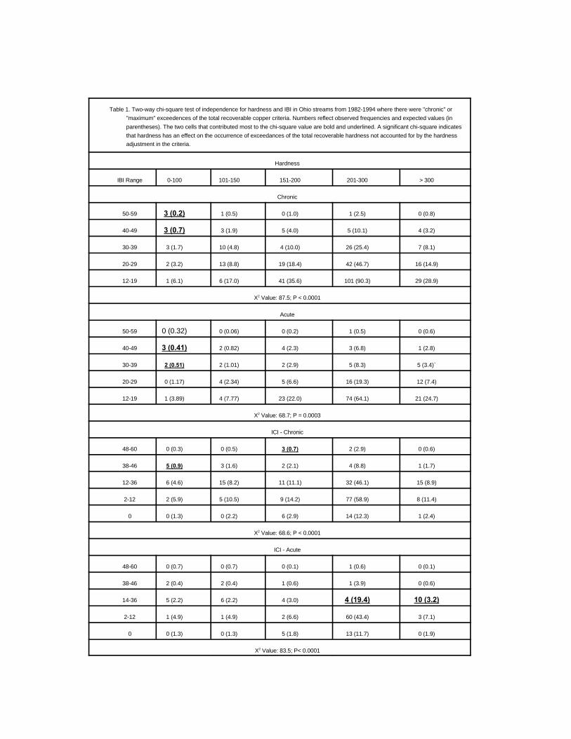
Table 1. Two-way chi-square test of independence for hardness and IBI in Ohio streams from 1982-1994 where there were "chronic" or

"maximum" exceedences of the total recoverable copper criteria. Numbers reflect observed frequencies and expected values (in

parentheses). The two cells that contributed most to the chi-square value are bold and underlined. A significant chi-square indicates

that hardness has an effect on the occurrence of exceedances of the total recoverable hardness not accounted for by the hardness

adjustment in the criteria.

Hardness

IBI Range 0-100 101-150 151-200 201-300 > 300

Chronic

50-59 3 (0.2) 1 (0.5) 0 (1.0) 1 (2.5) 0 (0.8)

40-49 3 (0.7) 3 (1.9) 5 (4.0) 5 (10.1) 4 (3.2)

30-39 3 (1.7) 10 (4.8) 4 (10.0) 26 (25.4) 7 (8.1)

20-29 2 (3.2) 13 (8.8) 19 (18.4) 42 (46.7) 16 (14.9)

12-19 1 (6.1) 6 (17.0) 41 (35.6) 101 (90.3) 29 (28.9)

X Value: 87.5; P < 0.00012

Acute

50-59 0 (0.32) 0 (0.06) 0 (0.2) 1 (0.5) 0 (0.6)

40-49 3 (0.41) 2 (0.82) 4 (2.3) 3 (6.8) 1 (2.8)

30-39 2 (0.51) 2 (1.01) 2 (2.9) 5 (8.3) 5 (3.4)`

20-29 0 (1.17) 4 (2.34) 5 (6.6) 16 (19.3) 12 (7.4)

12-19 1 (3.89) 4 (7.77) 23 (22.0) 74 (64.1) 21 (24.7)

X Value: 68.7; P = 0.00032

ICI - Chronic

48-60 0 (0.3) 0 (0.5) 3 (0.7) 2 (2.9) 0 (0.6)

38-46 5 (0.9) 3 (1.6) 2 (2.1) 4 (8.8) 1 (1.7)

12-36 6 (4.6) 15 (8.2) 11 (11.1) 32 (46.1) 15 (8.9)

2-12 2 (5.9) 5 (10.5) 9 (14.2) 77 (58.9) 8 (11.4)

0 0 (1.3) 0 (2.2) 6 (2.9) 14 (12.3) 1 (2.4)

X Value: 68.6; P < 0.00012

ICI - Acute

48-60 0 (0.7) 0 (0.7) 0 (0.1) 1 (0.6) 0 (0.1)

38-46 2 (0.4) 2 (0.4) 1 (0.6) 1 (3.9) 0 (0.6)

14-36 5 (2.2) 6 (2.2) 4 (3.0) 4 (19.4) 10 (3.2)

2-12 1 (4.9) 1 (4.9) 2 (6.6) 60 (43.4) 3 (7.1)

0 0 (1.3) 0 (1.3) 5 (1.8) 13 (11.7) 0 (1.9)

X Value: 83.5; P< 0.00012

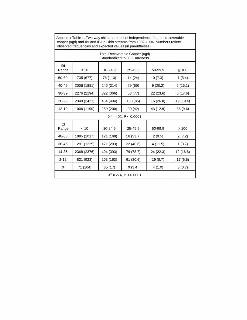
Appendix Table 1. Two-way chi-square test of independence for total recoverablecopper (ug/l) and IBI and ICI in Ohio streams from 1982-1994. Numbers reflectobserved frequencies and expected values (in parentheses).

Total Recoverable Copper (ug/l)Standardized to 300 Hardness

IBIRange < 10 10-24.9 25-49.9 50-99.9 > 100

50-60 735 (677) 76 (113) 14 (24) 0 (7.3) 1 (5.4)

40-49 2006 (1881) 246 (314) 29 (66) 9 (20.2) 6 (15.1)

30-39 2276 (2194) 322 (366) 53 (77) 22 (23.6) 5 (17.6)

20-29 2348 (2421) 464 (404) 108 (85) 16 (26.0) 19 (19.4)

12-19 1006 (1199) 289 (200) 90 (42) 43 (12.9) 36 (9.6)

X = 402, P < 0.00012

ICIRange < 10 10-24.9 25-49.9 50-99.9 > 100

48-60 1095 (1017) 121 (168) 16 (33.7) 2 (9.5) 2 (7.2)

38-46 1291 (1225) 171 (203) 22 (40.6) 4 (11.5) 1 (8.7)

14-36 2368 (2376) 404 (393) 79 (78.7) 24 (22.3) 12 (16.8)

2-12 821 (923) 203 (153) 61 (30.6) 19 (8.7) 17 (6.5)

0 71 (104) 35 (17) 9 (3.4) 4 (1.0) 8 (0.7)

X = 274, P < 0.00012

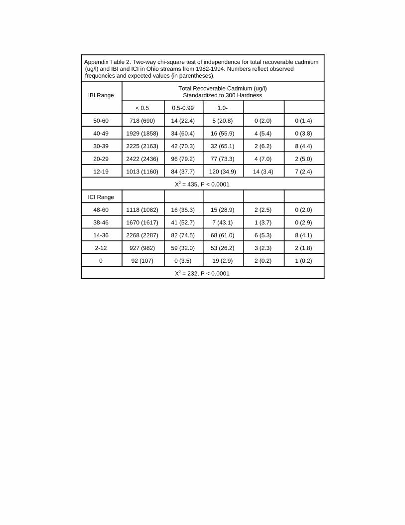
Appendix Table 2. Two-way chi-square test of independence for total recoverable cadmium(ug/l) and IBI and ICI in Ohio streams from 1982-1994. Numbers reflect observedfrequencies and expected values (in parentheses).

IBI Range Standardized to 300 HardnessTotal Recoverable Cadmium (ug/l)

< 0.5 0.5-0.99 1.0-

50-60 718 (690) 14 (22.4) 5 (20.8) 0 (2.0) 0 (1.4)

40-49 1929 (1858) 34 (60.4) 16 (55.9) 4 (5.4) 0 (3.8)

30-39 2225 (2163) 42 (70.3) 32 (65.1) 2 (6.2) 8 (4.4)

20-29 2422 (2436) 96 (79.2) 77 (73.3) 4 (7.0) 2 (5.0)

12-19 1013 (1160) 84 (37.7) 120 (34.9) 14 (3.4) 7 (2.4)

X = 435, P < 0.00012

ICI Range

48-60 1118 (1082) 16 (35.3) 15 (28.9) 2 (2.5) 0 (2.0)

38-46 1670 (1617) 41 (52.7) 7 (43.1) 1 (3.7) 0 (2.9)

14-36 2268 (2287) 82 (74.5) 68 (61.0) 6 (5.3) 8 (4.1)

2-12 927 (982) 59 (32.0) 53 (26.2) 3 (2.3) 2 (1.8)

0 92 (107) 0 (3.5) 19 (2.9) 2 (0.2) 1 (0.2)

X = 232, P < 0.00012

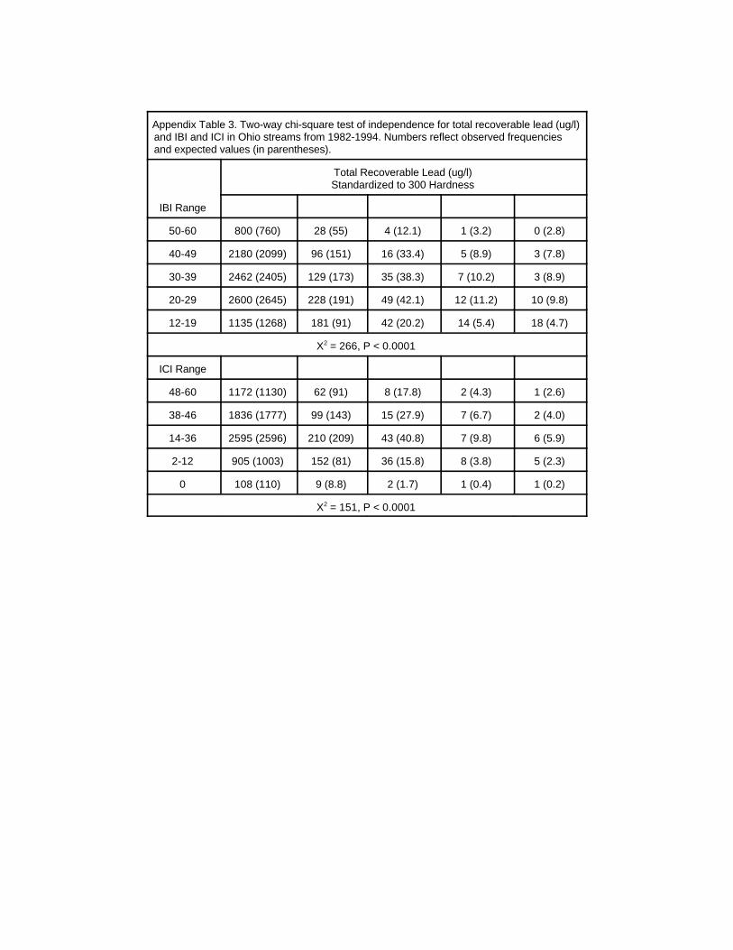
Appendix Table 3. Two-way chi-square test of independence for total recoverable lead (ug/l)and IBI and ICI in Ohio streams from 1982-1994. Numbers reflect observed frequenciesand expected values (in parentheses).

IBI Range

Total Recoverable Lead (ug/l)Standardized to 300 Hardness

50-60 800 (760) 28 (55) 4 (12.1) 1 (3.2) 0 (2.8)

40-49 2180 (2099) 96 (151) 16 (33.4) 5 (8.9) 3 (7.8)

30-39 2462 (2405) 129 (173) 35 (38.3) 7 (10.2) 3 (8.9)

20-29 2600 (2645) 228 (191) 49 (42.1) 12 (11.2) 10 (9.8)

12-19 1135 (1268) 181 (91) 42 (20.2) 14 (5.4) 18 (4.7)

X = 266, P < 0.00012

ICI Range

48-60 1172 (1130) 62 (91) 8 (17.8) 2 (4.3) 1 (2.6)

38-46 1836 (1777) 99 (143) 15 (27.9) 7 (6.7) 2 (4.0)

14-36 2595 (2596) 210 (209) 43 (40.8) 7 (9.8) 6 (5.9)

2-12 905 (1003) 152 (81) 36 (15.8) 8 (3.8) 5 (2.3)

0 108 (110) 9 (8.8) 2 (1.7) 1 (0.4) 1 (0.2)

X = 151, P < 0.00012

Appendix Table 4. Two-way chi-square test of independence for total recoverable zinc (ug/l)and IBI and ICI in Ohio streams from 1982-1994. Numbers reflect observed frequenciesand expected values (in parentheses).

IBI Range

Total Recoverable Zinc (ug/l)Standardized to 300 Hardness

50-60 730 (675) 41 (64) 15 (41.6) 1 (4.7) 1 (3.0)

40-49 1931 (1803) 109 (171) 58 (111) 4 (12.6) 3 (7.9)

30-39 2315 (2209) 154 (209) 95 (136) 5 (15.5) 11 (9.7)

20-29 2508 (2497) 265 (236) 125 (154) 11 (17.5) 7 (11.0)

12-19 929 (1229) 227 (116) 226 (75.8) 38 (8.6) 15 (5.4)

X = 745, P < 0.00012

ICI Range

48-60 1077 (1032) 77 (100) 45 (60) 2 (7.3) 1 (3.3)

38-46 1678 (1566) 98 (151) 44 (90) 2 (11.0) 2 (5.0)

14-36 2323 (2290) 219 (221) 111 (132) 8 (16.1) 6 (7.3)

2-12 801 (967) 164 (93) 135 (56) 19 (6.8) 7 (3.1)

0 88 (111) 18 (11) 9 (6.4) 11 (0.8) 3 (0.4)

X = 470, P < 0.00012

6

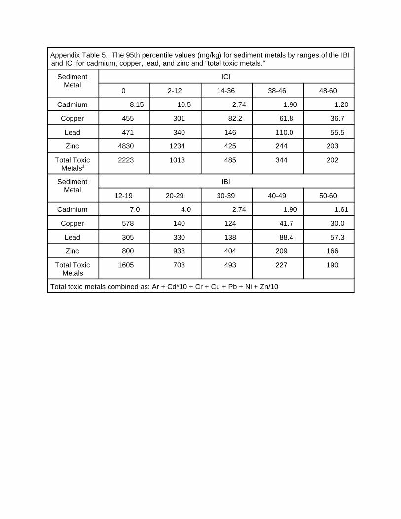
Appendix Table 5. The 95th percentile values (mg/kg) for sediment metals by ranges of the IBIand ICI for cadmium, copper, lead, and zinc and “total toxic metals.”

Sediment ICIMetal

0 2-12 14-36 38-46 48-60

Cadmium 8.15 10.5 2.74 1.90 1.20

Copper 455 301 82.2 61.8 36.7

Lead 471 340 146 110.0 55.5

Zinc 4830 1234 425 244 203

Total Toxic 2223 1013 485 344 202Metals1

Sediment IBIMetal

12-19 20-29 30-39 40-49 50-60

Cadmium 7.0 4.0 2.74 1.90 1.61

Copper 578 140 124 41.7 30.0

Lead 305 330 138 88.4 57.3

Zinc 800 933 404 209 166

Total Toxic 1605 703 493 227 190Metals

Total toxic metals combined as: Ar + Cd*10 + Cr + Cu + Pb + Ni + Zn/10

0

20

40

60

80

100

0 2-12 14-36 38-46 48-60

To

tal C

op

per

(m

g/k

g)

in S

edim

ent


455 301

0

20

40

60

80

100

12-19 20-29 30-39 40-49 50-60

To

tal C

op

per

(m

g/k

g)

in S

edim

ent


578 140 124

Appendix Figure 1. Concentrations of total copper (mg/kg) in sediments versus the ICI (top panel) and theIBI (bottom panel) in Ohio streams. Data was collected from 1982 to1995.

0

1

2

3

4

0 2-12 14-36 38-46 48-60

To

tal C

adm

ium

(m

g/k

g)

in S

edim

ent


8.15 10.5

0

1

2

3

4

50-6040-4930-3920-2912-19

To

tal C

adm

ium

(m

g/k

g)

in S

edim

ent


7.0 4.0

Appendix Figure 2. Concentrations of total cadmium (mg/kg) in sediments versus the ICI (top panel) andthe IBI (bottom panel) in Ohio streams. Data was collected from 1982 to1995.

0

50

100

150

200

0 2-12 14-36 38-46 48-60

To

tal L

ead

(m

g/k

g)

in S

edim

ent


471 340

0

50

100

150

12-19 20-29 30-39 40-49 50-60

To

tal L

ead

(m

g/k

g)

in S

edim

ent


305 330

Appendix Figure 3. Concentrations of total lead (mg/kg) in sediments versus the ICI (top panel) and the IBI(bottom panel) in Ohio streams. Data was collected from 1982 to1995.

0

50

100

150

200

250

300

350

400

0 2-12 14-36 38-46 48-60

To

tal Z

inc

(mg

/kg

)in

Sed

imen

t


4830 1234 425

0

50

100

150

200

250

300

350

400

12-19 20-29 30-39 40-49 50-60

To

tal Z

inc

(mg

/kg

)in

Sed

imen

t


800 933 404

Appendix Figure 4. Concentrations of total zinc (mg/kg) in sediments versus the ICI (top panel) and the IBI(bottom panel) in Ohio streams. Data was collected from 1982 to1995.

Documents

Using Biological Criteria to Validate Applications of ...epa.ohio.gov/portals/35/documents/gli_bio.pdfUsing Biological Criteria to Validate Applications of Water ... Dissolved and