Norman G. Loeb, NASA Langley Research Center, Hampton, VACo-Authors: R. Allan, T. Andrews, K. Armour, J.-L. Dufresne, P. Forster, A. Gettelman, T. Mauritsen, Y. Ming, D. Paynter, C. Proistosescu,

M. F. Stuecker, H. Wang

CERES Science Team Meeting, October 31, 2019, Berkeley, CA

Using CERES Observations to Assess CMIP6 Climate Model Simulations of

Changes in Earth’s Radiation Budget During and After the Global Warming “Hiatus”

Background/Motivation• Global radiative feedback under transient warming is time dependent.

- Changes in surface warming patterns induce changes in global TOA radiation that are distinct from those associated with global mean surface warming (“Pattern Effect”).

• Recent decades have seen cooling over the eastern tropical Pacific and Southern Oceans while temperatures have risen globally.

• GCMs driven with historical patterns of SST and sea-ice concentrations produce radiative feedbacks that trend toward more stabilizing, implying low climate sensitivity.

• The pattern of future warming is expected to produce radiative feedbacks that are less stabilizing, implying increasing climate sensitivity in the future.

Can we use ERB observations to test model response to SST pattern changes?

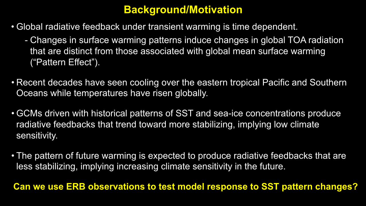
Global Mean All-Sky TOA Flux Anomalies & Multivariate ENSO Index(CERES EBAF Ed4.1; 03/2000 – 06/2019)

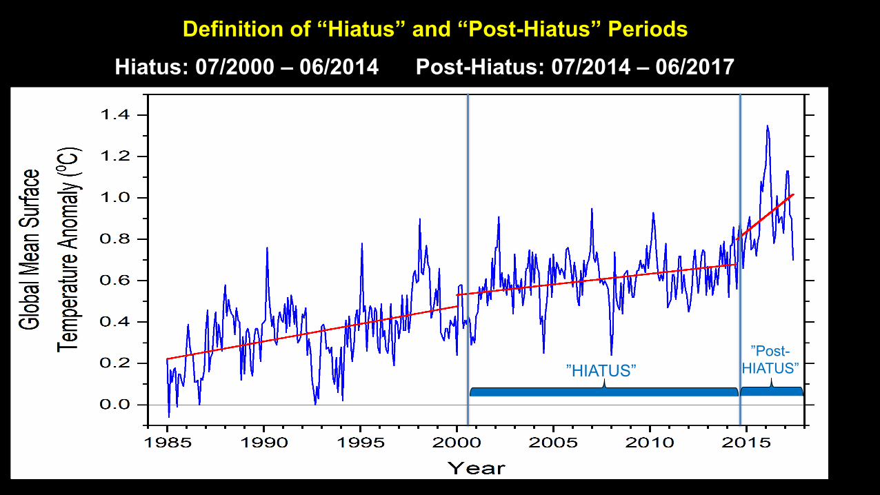
Definition of “Hiatus” and “Post-Hiatus” PeriodsHiatus: 07/2000 – 06/2014 Post-Hiatus: 07/2014 – 06/2017

”HIATUS””Post-

HIATUS”

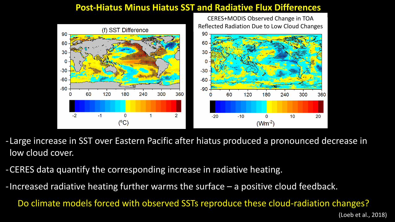
-Large increase in SST over Eastern Pacific after hiatus produced a pronounced decrease in low cloud cover.

-CERES data quantify the corresponding increase in radiative heating.

- Increased radiative heating further warms the surface – a positive cloud feedback.

Do climate models forced with observed SSTs reproduce these cloud-radiation changes?

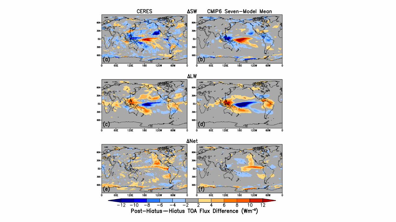
Post-Hiatus Minus Hiatus SST and Radiative Flux Differences

(Loeb et al., 2018)

CERES+MODIS Observed Change in TOA Reflected Radiation Due to Low Cloud Changes

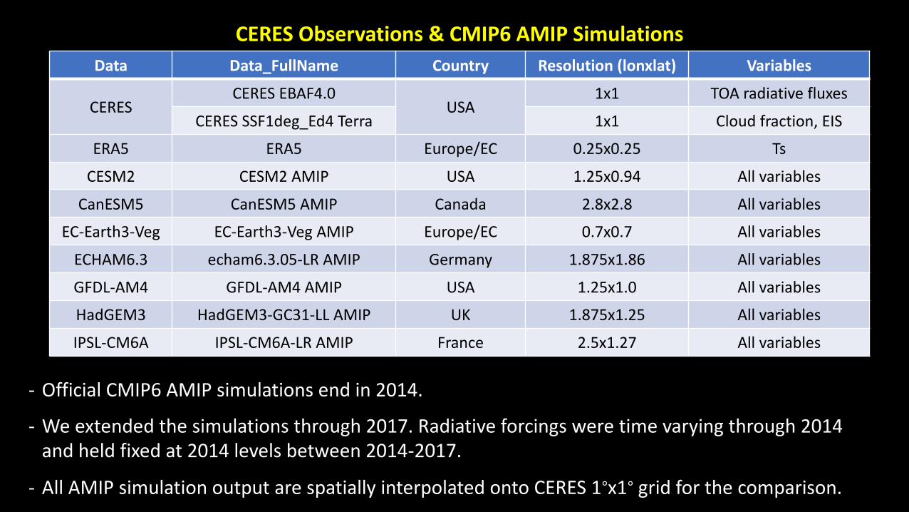
- Official CMIP6 AMIP simulations end in 2014.

- We extended the simulations through 2017. Radiative forcings were time varying through 2014 and held fixed at 2014 levels between 2014-2017.

- All AMIP simulation output are spatially interpolated onto CERES 1∘x1∘ grid for the comparison.

CERES Observations & CMIP6 AMIP Simulations

NEED TO EDIT MODEL NAMES TO BE CONSISTENT WITH FIGURES

Data Data_FullName Country Resolution (lonxlat) Variables

CERESCERES EBAF4.0

USA1x1 TOA radiative fluxes

CERES SSF1deg_Ed4 Terra 1x1 Cloud fraction, EIS

ERA5 ERA5 Europe/EC 0.25x0.25 Ts

CESM2 CESM2 AMIP USA 1.25x0.94 All variables

CanESM5 CanESM5 AMIP Canada 2.8x2.8 All variables

EC-Earth3-Veg EC-Earth3-Veg AMIP Europe/EC 0.7x0.7 All variables

ECHAM6.3 echam6.3.05-LR AMIP Germany 1.875x1.86 All variables

GFDL-AM4 GFDL-AM4 AMIP USA 1.25x1.0 All variables

HadGEM3 HadGEM3-GC31-LL AMIP UK 1.875x1.25 All variables

IPSL-CM6A IPSL-CM6A-LR AMIP France 2.5x1.27 All variables

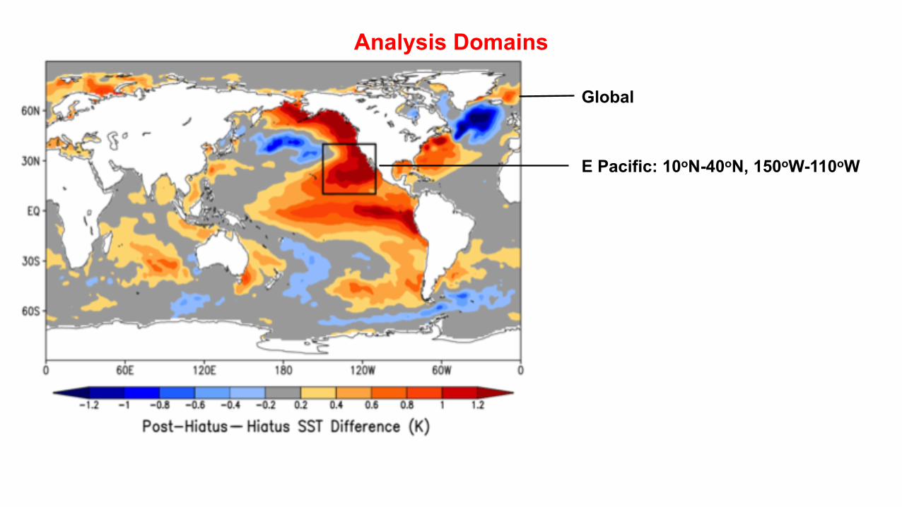
E Pacific: 10oN-40oN, 150oW-110oW

Analysis Domains

Global

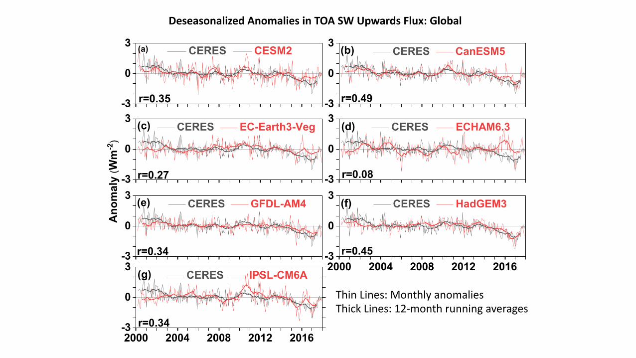
Deseasonalized Anomalies in TOA SW Upwards Flux: Global

Thin Lines: Monthly anomaliesThick Lines: 12-month running averages

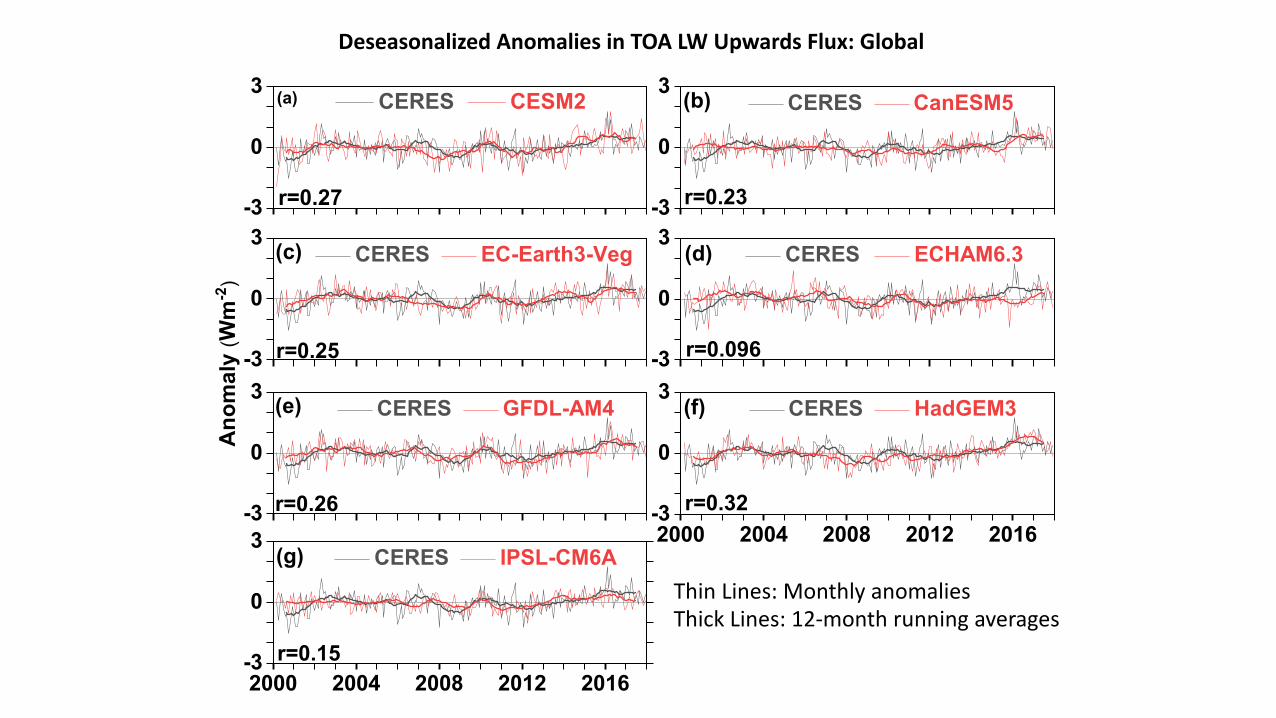
Deseasonalized Anomalies in TOA LW Upwards Flux: Global

Thin Lines: Monthly anomaliesThick Lines: 12-month running averages

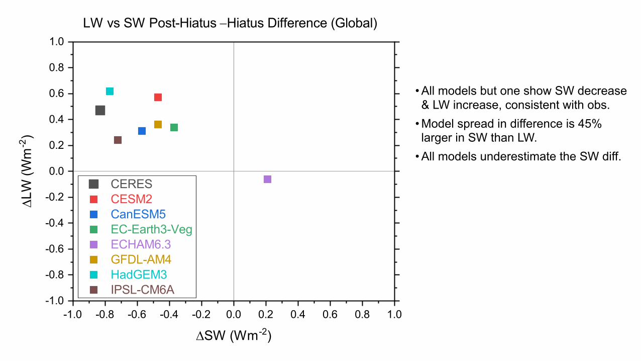
• All models but one show SW decrease & LW increase, consistent with obs.

• Model spread in difference is 45% larger in SW than LW.

• All models underestimate the SW diff.

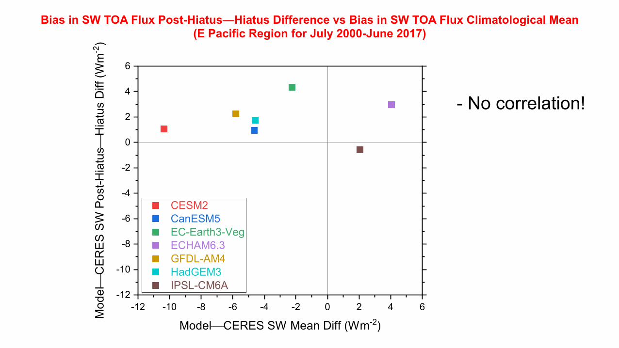
Bias in SW TOA Flux Post-Hiatus—Hiatus Difference vs Bias in SW TOA Flux Climatological Mean(E Pacific Region for July 2000-June 2017)

- No correlation!

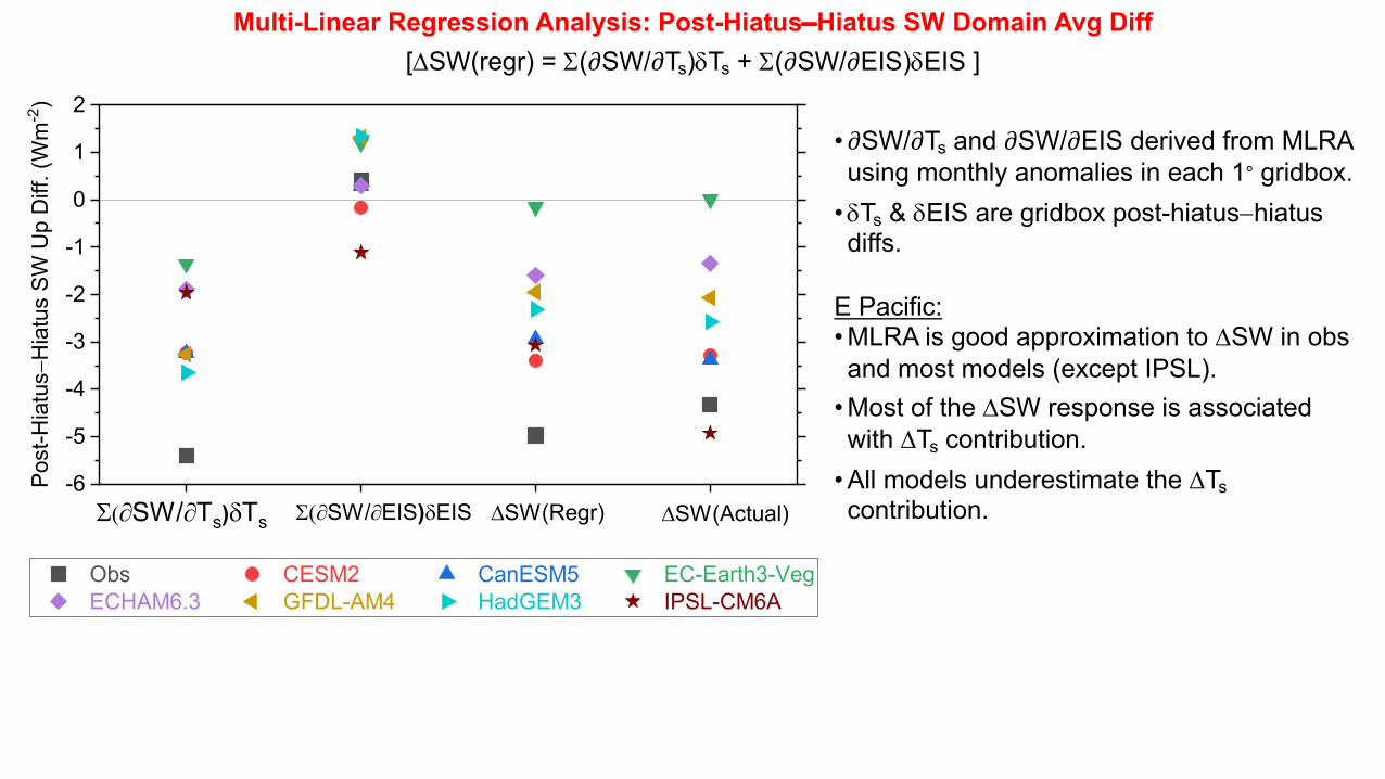
Multi-Linear Regression Analysis: Post-Hiatus-Hiatus SW Domain Avg Diff[DSW(regr) = S(∂SW/∂Ts)dTs + S(∂SW/∂EIS)dEIS ]

•∂SW/∂Ts and ∂SW/∂EIS derived from MLRA using monthly anomalies in each 1∘ gridbox.

• dTs & dEIS are gridbox post-hiatus-hiatus diffs.

E Pacific:• MLRA is good approximation to DSW in obsand most models (except IPSL).

• Most of the DSW response is associated with DTs contribution.

• All models underestimate the DTscontribution.

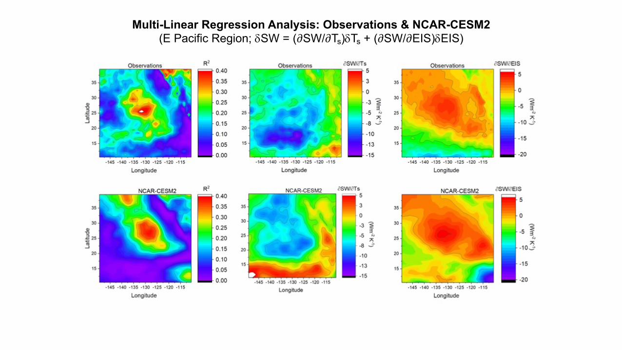
Multi-Linear Regression Analysis: Observations & NCAR-CESM2(E Pacific Region; dSW = (∂SW/∂Ts)dTs + (∂SW/∂EIS)dEIS)

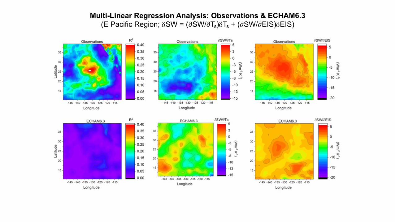
Multi-Linear Regression Analysis: Observations & ECHAM6.3(E Pacific Region; dSW = (∂SW/∂Ts)dTs + (∂SW/∂EIS)dEIS)

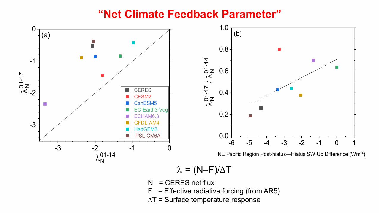
l = (N-F)/DTN = CERES net fluxF = Effective radiative forcing (from AR5)DT = Surface temperature response

“Net Climate Feedback Parameter”

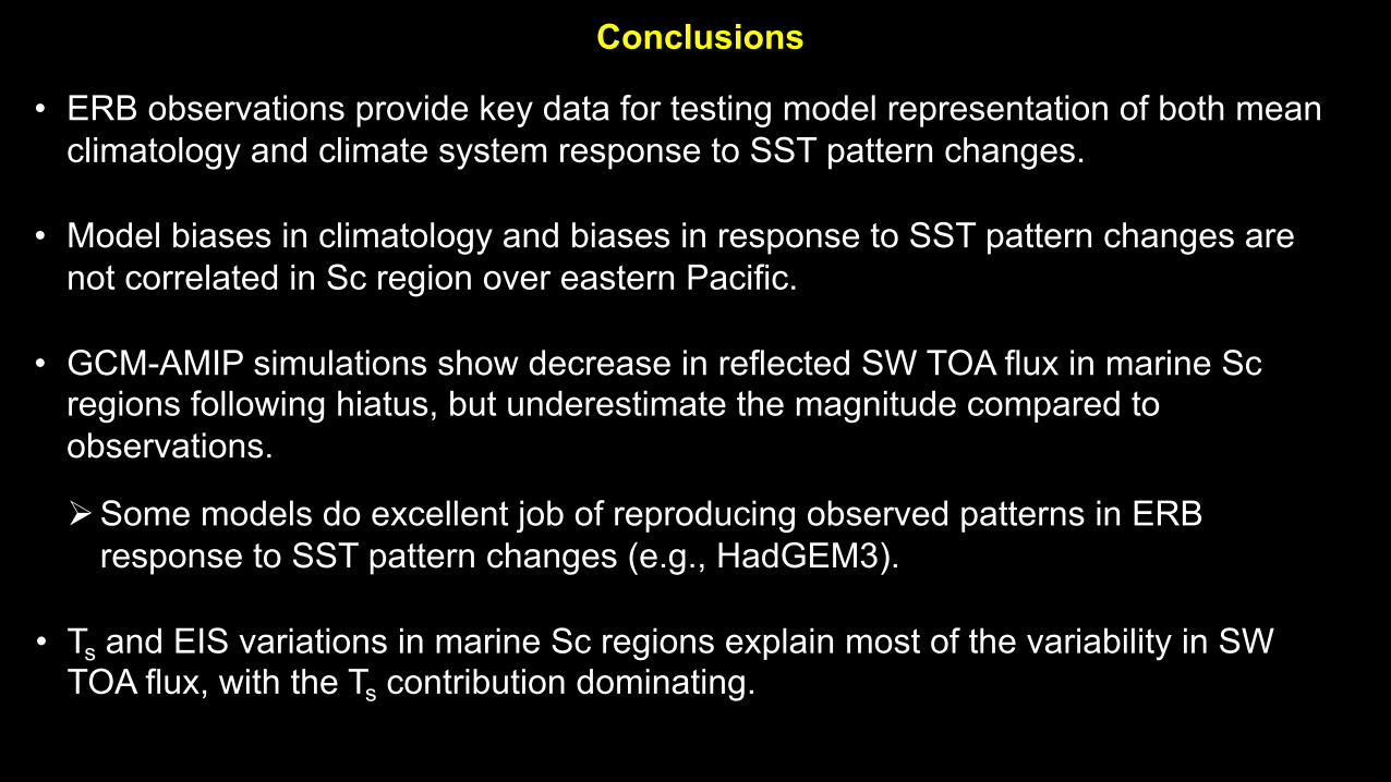
Conclusions

• ERB observations provide key data for testing model representation of both mean climatology and climate system response to SST pattern changes.

• Model biases in climatology and biases in response to SST pattern changes are not correlated in Sc region over eastern Pacific.

• GCM-AMIP simulations show decrease in reflected SW TOA flux in marine Sc regions following hiatus, but underestimate the magnitude compared to observations.

ØSome models do excellent job of reproducing observed patterns in ERB response to SST pattern changes (e.g., HadGEM3).

• Ts and EIS variations in marine Sc regions explain most of the variability in SW TOA flux, with the Ts contribution dominating.