Using exact equations in PSF calculations. Jean­Claude Perrin

Consultant

ABSTRACT

We are interested in calculating precisely the Point Spread Function (PSF) far from its maximum, where the irradiance is falling to 1E­06, or less. The first and most used method consist in calculating the Fourier transform of the wavefront using the Fast Fourier Transform algorithm (FFT). Another method is using the Beam Superposition Technique (BST) to decompose the wavefront in Gaussian beams, propagate those beams, and recompose to obtain the result. The third method is to apply the exact equations derived at the end of last century and described in reference books like Born and Wolf or Maréchal and Françon. We shall compare the results obtained with the three methods, FFT (CODE V), BST (ASAP) and exact calculation (MATLAB) in the case of a F/3 system working at 4000 nm, in focus and in presence of small defocusing.

1. INTRODUCTION

A renewing interest is appearing to calculate precisely the diffraction pattern in regions where the irradiance is falling to 1E­06, or less, from its maximum.

This is for example the case when the optical system is illuminated by disturbing sources, like lasers or others, which may blind the surrounding area in the focal plane. Is it also the case in the 3 to 5 µm band of infrared radiation because of the high contrast of the scenes in this band and numbers of possible natural blinding sources.

Computer programs commercially available today are using very different methods to do this calculation. The most popular and conventional method, used for example by CODE V, is using the Fast Fourier Transform (FFT), which has been abundantly described in the literature. This technique has some limitations, which may lead to erroneous results when looking far from the central region of the PSF.

Another method, apparently solely implemented in ASAP, is the Beam Superposition Technique (BST). BST permit to calculate the field and the irradiance everywhere in the optical system, taking into account the apertures. The method is nevertheless difficult to use, and this may give little confidence concerning the exactness of the result.

The last method is rarely used. It consist in applying the exact equations derived at the end of last century and described in reference books like Born and Wolf or Maréchal and Françon (Ref. 1,2). Those equations are using complicated development of Bessel functions, which can be applied exactly in the region surrounding the focus, even in the case of small aberrations, not exceeding a few lambda. These equations are not used in present days computer programs commercially available. Using advanced programming language available today, like MATLAB, make it possible to apply those equations exactly.

In the past, the Author presented an interface made between CODE V and MATLAB and some possibilities offered in using MATLAB for special calculations in optics. (Ref. 5).

This paper will present further results obtained with MATLAB by applying exact equations in image forming system, and compare with the result obtained using the FFT technique in CODE V and the Beam Superposition Technique in ASAP.

As a simple test case, we choose a F/3 parabola, and a monochromatic wavelength of 4000 nm. The system is free of aberration, which eases the comparisons done. Also, lack of isoplanetism is not a problem here, because we are considering only the parabola on axis.

The PSF in that case is the classical function 2

1 ) ( 2

=

Z Z J I , with 2 2 ' 2 y x u Z + =

λ π

(x and y are the coordinates

in the focal plane. In our test case, we have u’=1/6 and lambda = 4000 nm.

The corresponding Airy pattern in logarithmic scale is given on the figure I below:

­1 ­0 .75 ­0 .5 ­0 .2 0 0 .2 0 .5 0 .75 1 10

­14

10 ­12

10 ­10

10 ­8

10 ­6

10 ­4

10 ­2

10 0

Fig. I : Airy pattern of the test case chosen

The irradiance in the airy pattern falls below 1E­06 at about 0.5 mm of the centre.

­ 0 . 2 ­ 0 . 1 0 0 . 1 0 . 2 1 0

­ 1 0

1 0 ­ 8

1 0 ­ 6

1 0 ­ 4

1 0 ­ 2

1 0 0

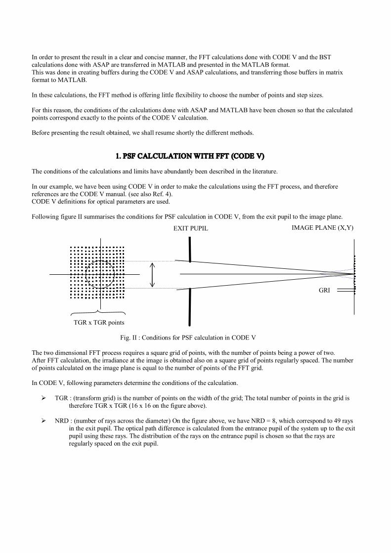
In order to present the result in a clear and concise manner, the FFT calculations done with CODE V and the BST calculations done with ASAP are transferred in MATLAB and presented in the MATLAB format. This was done in creating buffers during the CODE V and ASAP calculations, and transferring those buffers in matrix format to MATLAB.

In these calculations, the FFT method is offering little flexibility to choose the number of points and step sizes.

For this reason, the conditions of the calculations done with ASAP and MATLAB have been chosen so that the calculated points correspond exactly to the points of the CODE V calculation.

Before presenting the result obtained, we shall resume shortly the different methods.

1. PSF CALCULATION WITH FFT (CODE V)

The conditions of the calculations and limits have abundantly been described in the literature.

In our example, we have been using CODE V in order to make the calculations using the FFT process, and therefore references are the CODE V manual. (see also Ref. 4). CODE V definitions for optical parameters are used.

Following figure II summarises the conditions for PSF calculation in CODE V, from the exit pupil to the image plane.

TGR x TGR points

Fig. II : Conditions for PSF calculation in CODE V

The two dimensional FFT process requires a square grid of points, with the number of points being a power of two. After FFT calculation, the irradiance at the image is obtained also on a square grid of points regularly spaced. The number of points calculated on the image plane is equal to the number of points of the FFT grid.

In CODE V, following parameters determine the conditions of the calculation.

Ø TGR : (transform grid) is the number of points on the width of the grid; The total number of points in the grid is therefore TGR x TGR (16 x 16 on the figure above).

Ø NRD : (number of rays across the diameter) On the figure above, we have NRD = 8, which correspond to 49 rays in the exit pupil. The optical path difference is calculated from the entrance pupil of the system up to the exit pupil using these rays. The distribution of the rays on the entrance pupil is chosen so that the rays are regularly spaced on the exit pupil.

EXIT PUPIL IMAGE PLANE (X,Y)

GRI

When TGR and NRD are chosen, the image grid spacing GRI (the sample spacing of the points in the image) is given by GRI = λN(NRD/TGR), where N is the f/number. The result of the calculation can be bufferized in a square matrix format. In that case, the point of the matrix which correspond to the position of the intersection of the chief ray with the image plane is the point (TGR/2+1, TGR/2+1) in the matrix, i.e. (9,9) on figure II.

The figure III summarises the positions of the points being calculated in the Airy pattern, corresponding to the figure II.

Fig. III : Positions and GRID interval of the calculated points.

On this figure, dotted vertical lines correspond to the positions of the points calculated on the axis Y (16 points here). Note that only five points are calculated in the first ring of the Airy pattern. The chief ray (x = y = 0) correspond to point TGR/2 + 1 = 9.

Proper choice of TGR and NRD is not an easy task. NRD must be chosen depending on the level of residual aberration of the optical system. CODE V manual recommend that the optical path difference between adjacent points on the pupil do not exceed a half wave, preferably less.

Also, and in a related way, NRD must be chosen to reduce the aliasing due to the sampling of the pupil, inherent to the FFT algorithm. CODE V only print a message, if the level of the irradiance at the edge of the calculated image grid exceed 0.5 percent of the peak irradiance, in what case aliasing could lead to incorrect results.

Once NRD is fixed, the value of TGR determines the width of the grid on the image plane, equal to TGR x GRI = λNxNRD, which depend only on NRD.

There is no evident rule as to determine the correct value of TGR, once NRD value is fixed. CODE V manual indicates that the default value for NRD is TGR/2, and recommend to keep NRD in­between TGR/4 and TGR. Choosing NRD values outside from this range introduce increasingly large errors, without any possibility to be sure about the validity of the result.

For this reason, most user are using default value of NRD, NRD = TGR/2, and adjust the value of TGR to have no error message in CODE V listing. We therefore did the same in the case of our F/3 parabola. The corresponding value of GRI calculated by CODE V (according to its definition of focal length) is equals to 0.00604 mm.

According to figure I, we need an image width more than 1 mm to have the irradiance dropping below 1E­06.

With TGR = 256, the width of the image is equal to 1.546 mm, which is far sufficient for our comparison.

These values also fix the parameters for following, i.e. 256 points on the image with an interval of 0.00604 mm.

GRI

16 15 14 13 12 11 10 9 8 7 6 5 4 3 2 1

3. PSF calculation with Beam Superposition Technique (ASAP)

The Beam Superposition Technique is a another method to do PSF calculation in a completely different manner.

The background of the method is described in references (6,7). Its principle can be discussed with respect to the figure below, derived from ASAP literature.

Fig. IV : Principle of the Beam Superposition Technique.

The method consist in decomposing the incoming field in individual Gaussian beams, one per ray, propagate those beams independently (ray trace), and recompose the field everywhere in the optical system. The irradiance is obtained as the square of the modulus of the field.

There are as many individual beams as rays defined in the system, the number of which being limited only by the capacity of the computer.

In order to model properly the individual beams as Gaussian beams, several auxiliary rays, or parabasals rays, are created for each ray. They are used to model waist and divergence of each Gaussian beam, and are propagated (ray traced) together with the main set of ray.

Decomposing the incoming field into individual Gaussian beams and propagating those beams in the optical system permit to recompose the field everywhere along the path, and calculate the optical field, and irradiance.

With reference to ASAP terminology, following parameters determine the condition of the calculation:

Ø The number of the base rays (GRID POLAR)

Ø The number of parabasals rays (PARABASALS)

Ø The scale factor to be applied to the width (waist) of each individual Gaussian beam (WIDTH)

Ø The size of the window where the calculation is done (WIN) (in our case, near the focal plane )

Ø The number of pixels in this window (PIXEL)

The most difficult and arbitrary choice concerns the number of parabasals rays and their width. There is no evident rule to choose those parameters, the best being to make successive test to check how the result is affected. Also, violation of the paraxial wave equation may occur, leading to inaccurate result.

ENTRANCE PUPIL Beam decomposition in this plane

PLANE OF ANALYSIS Recomposition of the beam

ASAP manual indicates some rules and recommendations for choosing PARABASAL and WIDTH. Following these, and making some trials on our simple test case, led us to PARABASAL = 4 and WIDTH = 1.414.

In order to test if the number of rays is sufficient, the best method is to recalculate the energy at the entrance pupil (FIELD ENERGY), and compare with the theoretical circular aperture. Doing this, it appeared that the sharpness of the edge is difficult to model accurately, the best result being obtained with the maximum number of rays permitted by the program itself (also depending on the number of pixels).

Determining WIN and PIXEL is more straightforward, and completely fixed by the conditions of the CODE V FFT calculation. In these calculation, the number of points is 256, with the interval equal to 0.00604 mm. These correspond in ASAP to 256 pixels (in one direction) in a window of length equal to 2 x 0.773 mm.

To reduce the computer time (and the total number of pixels), we choose WIN Y ­0.773 0.773 X ­0.001 0.001.

The result can be stored in a buffer in ascii format, readable by any other program (MATLAB in our case).

4. PSF CALCULATION USING EXACT EQUATIONS

The mathematics involved in exact calculation of the PSF where derived last century by Lommel, and summarised in detail in reference 1.

Mathematical developments are described for the case of an optical system without aberration, or with the presence of a small residue of aberration, not exceeding a few lambda.

Here, we are interested in the case of no aberration, near the focus.

The figure V summarises the hypotheses:

Fig. V : Notations (Born and Wolf).

We are considering a converging spherical wave, focusing in F, and limited by the circular aperture of diameter 2a. The Gaussian extreme rays define the boundary of the geometrical shadow.

The following parameters u and v are used :

z f a u 2 ) ( 2

λ π

= ) ( ) ( 2 2 2 y x f a v + =

λ π

F

z

x, y

2a

Limit of the geometrical shadow

f

The limit of the geometrical shadow correspond to u=±v.

The irradiance in the x,y plane is given in function of the two developments of the functions Un , Vn as follows :

∑ ∞

= + + − =

0 2 2 ) ( ) ( ) 1 ( ) , (

s s n s n s

n v J v u v u U

∑ ∞

= + + − =

0 2 2 ) ( ) ( ) 1 ( ) , (

s s n s n s

n v J u v v u V

In these equations, Jn is the Bessel function of order n.

Using these expressions, two different equations determine the irradiance, in the illuminated region, and in the region of the geometrical shadow.

In the illuminated region (u<=v) :

[ ] 0 2 2

2 1

2 ) , ( ) , ( ) 2( ) , ( I v u U v u U u

v u I + =

In the shadow (u>v) :

0

2

1

2

0 21

2 0

2 ) (2 1 sin ) , ( 2 ) (

2 1 cos ) , ( 2 ) , ( ) , ( 1 ) 2( ) , ( I

u v u v u V

u v u v u V v u V v u V

u v u I

+ −

+ − + + =

These equations have been programmed in MATLAB language under following conditions:

Ø In our case, we have a/f = 1/6, and lambda = 4 microns

Ø Several test have been made to determine the maximum numbers of s in the serial development of U and V. In practice, s=5 proved to be sufficient.

Ø As before, the conditions of the calculations are fixed by CODE V FFT calculation. The number of points in Y direction is 256, with the interval equal to 0.00604 mm.

In case of a system with a residue of aberration, other mathematical equations can be applied also, but with more complexity. In that case, the wavefront must be calculated first by ray tracing, and Zernike polynomial determined.

5 – RESULT OBTAINED

The buffer created both by CODE V and ASAP have been used to draw the curves on the same figure, in MATLAB format, superimposed on the result obtained with exact equations. Normalisation was achieved on each case, so that the maximum value correspond to unity.

To limit our presentation, we have selected two focus planes only : the best focus, and a defocus in z of 0.864 mm, which correspond to 3 lambda of wavefront curvature. Serial of figures VIa to VIc show the result obtained in the best focus. In that case, they are directly comparable to the result shown on figure I.

Fig VIa is from y=­0.8 mm to 0.8 mm, in logarithmic scale. The MATLAB result is in solid line, ASAP in dotted line and CODE V in dashed line.

­0 .8 ­0 .5 ­0 .2 0 0 .2 0 .5 0 .8 10

­12

10 ­10

10 ­8

10 ­6

10 ­4

10 ­2

10 0

Fig. VIa : Defocus = 0 ­ Comparison of the result obtained with : FFT (CODE V) : BST (ASAP) : Exact equations (MATLAB) :

In that figure, result obtained with MATLAB and the exact equations above correspond exactly to the function 2

1 ) ( 2

=

Z Z J I of figure I.

The difference between the figure VIa and figure I is the fact that on figure VIa, the calculated points are uniformly spaced with an interval of 0.00604 mm, which is rather coarse to reproduce precisely the numerous lobes present in the Airy pattern. Of course, there is no limitation in MATLAB to reduce this step interval. Because we want to make a comparison between the three methods, the interval is fixed by the CODE V FFT value, with little flexibility to reduce it to smaller value.

To have a better view to the results, figures VIb and VIc show in more detail the regions from –0.2 mm to 0.2 mm, and from –0.05 mm to 0.05 mm.

­ 0 . 2 ­ 0 . 1 0 0 . 1 0 . 2 1 0 ­ 6

1 0 ­ 5

1 0 ­ 4

1 0 ­ 3

1 0 ­ 2

1 0 ­ 1

1 0 0

Fig. VIb : Logarithmic scale from –0.2 mm to 0.2 mm.

­ 0 . 0 5 ­ 0 . 0 2 5 0 0 . 0 2 5 0 . 0 5 1 0

­ 4

1 0 ­ 3

1 0 ­ 2

1 0 ­ 1

1 0 0

Fig. VIc : Logarithmic scale from –0.05 mm to 0.05 mm.

The differences in the result obtained with the three methods appear clearly on these figures.

Looking near the centre, (figure VIc), it appears that the three methods are giving quite similar result.

Some disagreement are appearing when looking farther from the centre (figure VIb). The FFT tends to give higher values, and BST lower values. Moreover, the result obtained with FFT and BST seems to introduce a phase offset in the position of the zeros, as the result obtained with FFT and BST are maximum when those obtained with exact equations are minimum.

The tendency is becoming quite obvious when looking farther again (figure VIa). In region where the irradiance drops below 1E­04 from its maximum. FFT result are more and more noisy, but the mean value is following approximately the exact value. In comparison, the BST is quite pessimistic. For values below 1E­06 (at 0.5 mm from the centre), values are failing down quite abruptly.

The second series of figures VIIa to VIIc below correspond to 3 lambda of defocusing.

­0 .8 ­0 .5 ­0 .2 0 0 .2 0 .5 0 .8 10 ­7

10 ­6

10 ­5

10 ­4

10 ­3

10 ­2

10 ­1

10 0

Fig. VIIa : Defocus = 3 lambda ­ Comparison of the result.

­ 0 . 2 ­ 0 . 1 0 0 . 1 0 . 2 1 0 ­ 3

1 0 ­ 2

1 0 ­ 1

1 0 0

Fig. VIIb : Logarithmic scale from –0.2 mm to 0.2 mm. FFT (CODE V) : BST (ASAP) : Exact equations (MATLAB) :

­ 0 . 0 5 0 0 . 0 5 0

0 . 2

0 . 4

0 . 6

0 . 8

1

Fig. VIIc : Linear scale from –0.05 mm to 0.05 mm.

For a defocus of 3 lambda, the irradiance at the center (x=y=0) drops down to zero exactly, theoretically.

Figure VIIc shows the differences obtained near the centre, in linear scale. In each case, the maximum value correspond to the second point being calculated after the center. Values obtained with FFT are very near exact values, with again an increasing difference when going farther. The centre value equals 3x10 ­3 .

With BST, difference is more pronounced. The value at the centre is about 5x10 ­2 .

Figure VIIa shows the same tendency as figure VIa, the BST value getting lower as distance from the centre increases.

5. DISCUSSION AND CONCLUSION

Although the details of the algorithms used in both programs CODE V and ASAP are not known, it is nevertheless possible to draw some useful remarks and conclusions, with respect to each method.

1. FFT calculation (CODE V) :

A disadvantage to the FFT method is the necessity to sample the wavefront and the image, with little flexibility to adjust the sampling interval in the image. In standard use, only about 5 points are calculated in the diameter of central Airy disk.

Aliasing is the second major limitation, especially when looking far from the centre, as in our example. The method to reduce aliasing is to increase the number of point in the pupil (TGR) but it is difficult to make sure that the result is correct, when looking so far from the centre of the Airy pattern. In the example here, we have been using TGR = 256. Some test not described in this paper have been made also with larger value, the limit being the computer time, or the memory of the computer itself. These test have shown that the result are much more accurate by this way, probably because aliasing is reduced.

Other sources of error could also be the accuracy of OPD calculation, and of the accuracy of the FFT algorithm itself.

2. BST calculation (ASAP) :

In case of the Beam Superposition Technique, there is no limit (or the memory) concerning the sampling of the image.

More serious seems to be the limitation of the number of rays which can be used to model the pupil in a set of individual Gaussian beams. This makes it difficult to model precisely the abrupt transition of the circular diaphragm of the pupil., which is the main source of diffraction of the energy far from the centre. This effect seems to be the principal reason of inaccuracy.

Beside this point, the method as many advantages compared to the others, by offering more flexibility to calculate the energy everywhere in the optical path, as the FFT technique is limited to Fraunhoffer diffraction. (Some possibilities also exist in CODE V to calculate the energy in the pupil, using a special technique).

3. Exact equations (MATLAB) :

Calculating OPD by ray tracing in MATLAB language, determine the Zernike polynomials, and applying the Born and Wolf exact equations for PSF calculations is greatly simplified due to the high level of the language and library of MATLAB.

When applying this to our simple test case, a possible source of error is the truncature in the calculation of the series of the Bessel functions.

Other sources of error are the limit of validity of the equations itself.

6. REFERENCES

1. Born and Wolf (Sixth corrected edition. Cambridge University Press) 2. Maréchal et Françon – Diffraction et structure des images ­ Masson 3. CODE V manual (Optical Research Associates) 4. ORA news (Vol 8, N°4) 5. ASAP manual (Breault Research Organization) 6. J. Arnaud : Representation of Gaussian beams by complex rays. A.O. Vol. 24, N°.4, Feb. 1985 7. A.W.Greynolds : Propagation of generally astigmatic Gaussians beams along skew ray paths.

SPIE, Vol. 560. 1985 8. JC Perrin : La conception optique des systèmes optroniques

(Conférence Optronique et Défense, Paris, Décembre 1996 ­ AAAF)