Using generalized additive models to reduce residual confounding

STATISTICS IN MEDICINEStatist. Med. 2004; 23:3781–3801Published online in Wiley InterScience (www.interscience.wiley.com). DOI: 10.1002/sim.2073

Using generalized additive models to reduceresidual confounding

Andrea Benedetti1; 2 and Michal Abrahamowicz1;2;∗;†

1McGill University; Department of Epidemiology and Biostatistics; Canada2Division of Clinical Epidemiology; Montreal General Hospital; Canada

SUMMARY

Traditionally, confounding by continuous variables is controlled by including a linear or categoricalterm in a regression model. Residual confounding occurs when the e�ect of the confounder on theoutcome is mis-modelled. A continuous representation of a covariate was previously shown to result ina less biased estimate of the adjusted exposure e�ect than categorization provided the functional formof the covariate–outcome relationship is correctly speci�ed. However, this is rarely known. In contrastto parametric regression, generalized additive models (GAM) �t a smooth dose–response curve to thedata, without requiring a priori knowledge of the functional form.We used simulations to compare parametric multiple logistic regression vs its non-parametric GAM

extension in their ability to control for a continuous confounder. We also investigated several issuesrelated to the implementation of GAM in this context, including: (i) selecting the degrees of freedom;and (ii) alternative criteria for inclusion=exclusion of the potential confounder and for choosing betweenparametric and non-parametric representation of its e�ect. The impact of the shape and strength of theconfounder–disease association, sample size, and the correlation between the confounder and exposurewere investigated.Simulations showed that when the confounder has a non-linear association with the outcome, com-

pared to a parametric representation, GAM modelling (i) reduced the mean squared error for theadjusted exposure e�ect; (ii) avoided in�ation of the type I error for testing the exposure e�ect. Whenthe true confounder–outcome relationship was linear, GAM performed as well as the parametric logisticregression.When modelling a continuous exposure non-parametrically, in the presence of a continuous con-

founder, our results suggest that assuming a linear e�ect of the confounder and focussing on thenon-linearity of the exposure–outcome relationship leads to spurious �ndings of non-linearity: jointnon-linear modelling is necessary.Overall, our results suggest that the use of GAM to reduce residual confounding o�ers several

improvements over conventional parametric modelling. Copyright ? 2004 John Wiley & Sons, Ltd.

KEY WORDS: simulations; residual confounding; GAM; logistic regression; AIC; BIC

∗Correspondence to: M. Abrahamowicz, Division of Clinical Epidemiology, Montreal General Hospital, 1650Cedar Ave., Room L10-520, Montreal, Quebec, Canada H3G 1A4.

†E-mail: [email protected]

Contract=grant sponsors: NSERC, CIHR; contract=grant number: 6391

Received October 2003Copyright ? 2004 John Wiley & Sons, Ltd. Accepted September 2004

3782 A. BENEDETTI AND M. ABRAHAMOWICZ

1. INTRODUCTION

Controlling confounding remains a primary concern in non-experimental epidemiologic re-search. Although other methods to control confounding exist, regression modelling is oftenused [1]. However, even if the confounder is included in the multivariable regression model,residual confounding of the exposure e�ect may occur due to incorrect modelling of theconfounder e�ect [2].For a continuous confounder, conventional approaches involve either categorization into two

or more categories, or an a priori selected, simple parametric representation (usually linear orlog-linear). The parametric speci�cation of the continuous confounder has been shown to bepreferable to categorization, in terms of bias and e�ciency of the estimation of the exposuree�ect, provided the correct functional form is speci�ed, and even under some mis-speci�cation[2, 3].However, the correct functional form is rarely known, and incorrect speci�cation may lead to

residual confounding. Depending on the degree of mis-speci�cation, categorization may evenbe preferable to a parametric model that relies on incorrect assumptions such as linearity [2].This calls for an approach that avoids the downfalls of both categorization and of a priorispeci�ed parametric models.Flexible parametric or non-parametric regression techniques which avoid the need to spec-

ify a priori the analytical form of the dose–response relationship and estimate the shapeof the association directly from the data, have been proposed to enhance the accuracy ofmodelling continuous predictors [4–7]. Brenner and Blettner investigated the advantages ofnon-parametric regression in comparison to several parametric and categorical representationsfor controlling confounding in very large data sets [3]. The results suggested that a relativelysimple non-parametric representation, based on linear spline regression, was generally satis-factory [3]. Although interesting, Brenner and Blettner’s results apply only to the largest ofdata sets, as their analyses used sample sizes of one million observations [8].The performance of non-parametric modelling of continuous covariates in controlling con-

founding in smaller data sets remains mostly unknown. Moreover, linear spline regressionrequires an arbitrary partition of the range of the independent variable and �ts a broken line,imposing clinically implausible breakpoints [3]. More �exible approaches are necessary toobtain smoother, more realistic estimates.Generalized additive models (GAM) are a �exible, non-parametric regression technique

[6]. Contrary to parametric regression, GAM �ts a smooth curve to the data whose shape isestimated directly from the data. Typically, the estimated function ensures the continuity ofthe �rst and second derivatives, avoiding implausible breakpoints. Recently, use of GAM tomodel epidemiologic data has yielded several insightful results [4, 9–12].Whereas it seems likely that �exible non-parametric models, such as GAM, may help

to reduce the risk of residual confounding by continuous confounders, several practical andconceptual issues related to the implementation of such a strategy remain to be systemati-cally investigated. For example, should the decision regarding (i) whether to adjust for theconfounder and (ii) whether to model the continuous e�ect non-parametrically rather thanparametrically, be made a priori or be data dependent? In the latter case, what criteria shouldbe employed? Furthermore, if a confounder is modelled non-parametrically, how should thedegree of smoothing be determined? Deciding how to represent potential confounders variesdepending on the type of study. In the context of clinical trials, there is a clear preference

Copyright ? 2004 John Wiley & Sons, Ltd. Statist. Med. 2004; 23:3781–3801

RESIDUAL CONFOUNDING AND GAM 3783

for specifying the functional form, typically linear, of the confounder–outcome associationa priori [13, 14]. In contrast, in epidemiological cohort studies, investigators are often moreinclined to decide a posteriori how to model a continuous covariate, based on goodness-of-�tcriteria [4, 15, 16]. In addition, it is unclear to what extent the sample size and=or the strengthand form of the relationship between the confounder and the outcome, as well as betweenthe confounder and the exposure may a�ect the responses to the above questions.To systematically study these issues we carry out a series of simulations. We evaluate

the potential advantages of GAM in the control of confounding by continuous covariates,and investigate the model selection issues in small to medium sized data sets. We focus onbinary outcomes and compare the GAM generalization of multiple logistic regression [6] toparametric logistic models.

2. METHODS

2.1. Data generation

We generated data sets with three variables: a dichotomous outcome (Y ), an exposure (X )and a continuous confounder (Z). Two general scenarios were investigated: a dichotomousexposure and a continuous exposure.

2.1.1. Dichotomous exposure. The exposure was generated from the binomial distributionwith P(X =1)=0:5. The confounder values were generated a lognormal distribution, the pa-rameters of which depended on the exposure. Two levels of point–biserial correlation betweenthe exposure and the confounder (rxz) were investigated: rxz ≈ 0:3 and rxz ≈ 0:6. The level ofcorrelation was achieved by manipulating the mean and variance of the confounder distribu-tions in the two groups, corresponding to the two values of a binary exposure. The exposurewas either generated to have no e�ect (�x=0; odds ratio (OR)=1:0) or to have an e�ect(�x=−0:693; OR=0.5) on the logit of the outcome.

2.1.2. Continuous exposure. To generate a continuous exposure, we �rst generated the con-founder from a lognormal distribution. The individual exposure values (xi; i=1; : : : ; n) werethen generated, conditional on the confounder, using Xi=0:5 ∗ Zi + �i, where the errors, �i,were generated from the normal distribution (N [0; ��]). To control the expected correlationbetween X and Z , we manipulated �� with �� ≈ 5 and 2.5 yielding, respectively, rxz ≈ 0:3and rxz ≈ 0:6. We investigated residual confounding both when the exposure had no e�ect(�x=0;OR=1:0 per standard deviation(SD)) on the outcome and when the exposure had alinear e�ect (�x=0:262 or OR= 1.3=SD) on the logit of the outcome.

2.1.3. Outcome. The dichotomous outcome was generated, conditional on X and Z , from amultiple logistic model logit(Y =1)=�0 +�xX +f(Z). The confounder–outcome association,f(Z), was assumed to take one of several shapes, shown in Figure 1 and referred to lateras, respectively: (a) linear, (b) quadratic, (c) linear-quadratic with a threshold at the 50thpercentile, (d) linear-quadratic with the threshold at the 80th percentile, (e) asymmetric J,(f) plateau, (g) hump, and (h) double asymmetric hump. The rationale was to include bothsimple (a)–(c) and more complex (d)–(h) shapes. Whereas cases (a) and (b) are the most



Figure 1. ZY associations generated: (a) linear; (b) quadratic; (c) linear quadratic thresholdat 50th; (d) linear quadratic threshold at 80th; (e) asymmetric J; (f) Plateau; (g) hump;

(h) double asymmetric hump.

frequent, the other curves presented in Figure 1 represent shapes that may occur in somespeci�c situations. Cases (c) and (d) represent the ‘no-e�ect threshold’, an issue of interest indi�erent areas of epidemiologic research, with respectively, low and high value of the threshold[17–19]. An asymmetric J-shape, (e), represents a risk factor for which the risks increase inboth tails of the distribution, but to a di�erent degree. For example, both very low and highblood pressure may be associated with an increased hazard of negative health outcomes, butthe impact of the latter is usually more serious, accounting for the asymmetry. The ‘hump’(g) represents a similar situation with the exception that (i) the outcome is ‘positive’, and(ii) the curve is symmetric; this corresponds to the association between consumption of a‘healthy’ food and an improvement in health—only those consuming ‘reasonable’ amountswill see the bene�ts. A double-hump scenario (h) extends (g) to the situation where there isa mixture of two subpopulations with di�erent responsiveness to the exposure. For example,subjects with a given genetic mutation will ‘respond’ only to a higher dose of exposure, asre�ected by the second bump, whereas those without the mutation will respond to a lowerdose. Finally, (f) represents a similar mixture as (h) but the relationship for each subgroup



is weakly monotonic, with the risks levelling o� after the subgroup speci�c saturation levelhas been reached.For each scenario, 3000 independent random samples were generated with samples sizes of

n=300 or 1000, corresponding to, respectively, approximately 100 or 300 events.

2.2. Analysis strategies

All generated samples were analysed by di�erent versions of conventional, parametric multiplelogistic regression and its non-parametric GAM extension using SPLUS [20].

2.2.1. Basics of generalized additive models. GAM generalizes the multiple logistic regres-sion model to: logit(Y )=�0 +

∑j∈A �jXj +

∑k∈B Sk(Xk), where A represents the set com-

posed of all binary independent variables, and those variables that are modelled parametrically(df= l) using linear functions, whereas subset B includes those quantitative variables that aremodelled using non-parametric smoothers (Sk(Xk), with df¿1). Using many df results in abumpy curve that closely approximates the data [6]. In our GAM analyses, cubic smoothingsplines were used as the smoother [21, 22].In GAM, inference about the e�ect of a given smoothed continuous predictor involves

comparing the deviance of the k-df smooth estimate to the deviance of (i) a 1-df linearmodel (linearity test) or (ii) a 0-df null model (test of association). The e�cacy and accuracyof these tests may depend on both the amount of smoothing chosen and how that choice wasmade. Contrary to generalized linear models, here the di�erence in deviance under H0 is onlyapproximately distributed as �2k−1 or �

2k , respectively [6]. Simulations show that these tests

are reasonably accurate for conventional 0.05 signi�cance levels with only slight in�ation oftype I error [6].

2.2.2. Df-selection strategies in GAM. In GAM, the data analyst must specify the df foreach variable that is to be modelled non-parametrically. The df, which control the amountof smoothing, are de�ned as the trace of the smoother matrix, which is analogous to thehat matrix in multiple linear regression [6]. We investigated three df-selection strategies.For the a priori method, the df were set to 4, considered the default in GAM [6]. Thetwo other approaches were a posteriori and the df were chosen from a pre-speci�ed set ofvalues to minimize, respectively, (i) Akaike’s information criterion (AIC) [23] or (ii) Bayesianinformation criterion (BIC) [24]. AIC measures the �t of the model, in terms of deviance,while penalizing for the df used. BIC is similar to AIC but is more conservative as it alsoaccounts for the sample size, and typically results in lower dfs than AIC [25].

2.2.3. Criteria for retaining the confounder and=or deciding how it should be modelled. Theanalysis strategies attempted to mimic how modelling decisions might be made in real lifein di�erent types of studies. As such, some strategies, which we will refer to as ‘a pri-ori strategies’, mimicked the clinical trials paradigm in that the potential confounder wasincluded in the model irrespective of the empirical results. In contrast, ‘data-dependent strate-gies’ resembled the approach of observational epidemiologic studies, in that the confounderwas excluded, or modelled in a di�erent form, depending on comparisons between alternativemodels. Two criteria were investigated for excluding or changing the representation of theconfounder. In the �rst, a more complex model for the confounder was selected only if it



Table I. Analysis strategies when dealing with a dichotomous exposure.

Criteria to decideModelling strategy between primary

Strategy for the confounder Primary model∗ Alternative model and alternative model

D1 Ignore X — a prioriD2 As a linear X + Z — a priori

variableD3a As a quadratic X + Z + Z2 — a priori

variableD3b ′′′′ X + Z + Z2 X + Z 1-df test of Z2

D4a Smoothed with X + s(Z; 4) — a prioria priorispeci�ed df (4)

D4b ′′′′ X + s(Z; 4) X 4-df test vs null H0D4c ′′′′ X + s(Z; 4) X + Z 3-df test vs linear H0D4d ′′′′ X + s(Z; 4) X + Z |ORx − ORxz|60:1 ∗ OR†

xzD4e ′′′′ X + s(Z; 4) X |ORx − ORxz|60:1 ∗ ORxzD5a Smoothed with X + s(Z; dfAIC) — a priori

df selected byAIC from 2–10

D5b ′′′′ X + s(Z; dfAIC) X + Z (k − 1)-df test vs linear H0D5c ′′′′ X + s(Z; dfAIC) X + Z |ORx − ORxz|60:1 ∗ ORxzD6a Smoothed with X + s(Z; dfAIC) — a priori

df selected byAIC from 1–10

D6b ′′′′ X + s(Z; dfAIC) X k-df test vs null H0D6c ′′′′ X + s(Z; dfAIC) X |ORx − ORxz|60:1 ∗ ORxzD7a Smoothed with X + s(Z; dfBIC) — a priori

df selected byBIC from 2–10

D7b ′′′′ X + s(Z; dfBIC) X + Z (k − 1)-df test vs linear H0D7c ′′′′ X + s(Z; dfBIC) X + Z |ORx − ORxz|60:1 ∗ ORxzD8a Smoothed with X + s(Z; dfBIC) — a priori

df selected byBIC from 1–10

D8b ′′′′ X + s(Z; dfBIC) X k-df test vs null H0D8c ′′′′ X + s(Z; dfBIC) X |ORx − ORxz|60:1 ∗ ORxz∗Y =outcome, X =exposure, Z =confounder.†where ORx = exp(�x), the crude estimate of the exposure e�ect; and ORxz = exp(�xz)= the estimate of the exposuree�ect adjusted for the confounder.

changed the adjusted exposure e�ect by more than 10 per cent [26]. When the confounderwas modelled non-parametrically, this criterion was applied in two ways: by excluding theconfounder or modelling it as a linear function if the exposure e�ect estimate, adjusted fora non-parametric e�ect of Z , was (i) close to the unadjusted estimate; or (ii) close to theexposure estimate adjusted for a linear e�ect of Z , respectively. In the second approach, sta-tistical signi�cance at the �=0:05 level of the appropriate test of the confounder e�ect wasused to decide (i) whether to retain the confounder in the model, (ii) use a quadratic ratherthan linear representation of its e�ect, or (iii) model it non-parametrically.



2.2.4. Analysis strategies for dichotomous exposure. Di�erent approaches to deal with theconfounder while estimating the adjusted e�ect of a dichotomous exposure, are summarizedin Table I. For each strategy, the ‘primary model’ represents the most complex model for theconfounder, while the ‘alternative model’ uses a simpler representation, except for strategiesin which the primary model is selected a priori, as indicated in the last column of Table I.For all other strategies, the last column speci�es the data-dependent criteria used to choosebetween the primary and alternative models. Five broad groups can be distinguished: (i)ignoring the confounder (D1); (ii) conventional parametric modelling of the confounder e�ectby either a linear or quadratic function (D2, D3); and using GAM with the confounder e�ectsmoothed with df chosen, respectively, (iii) a priori as 4 (D4a–e); (iv) to minimize AIC(D5a–c, D6a–c); and (v) to minimize BIC (D7a–c, D8a–c).Some strategies in Table I involve testing against a null H0 or a linear H0. When choosing

the df to minimize AIC or BIC, the df were selected from integer values between 2 and 10for linear H0 (strategies D5a–c, D7a–c) and for a null H0 the option of 1-df was added, asthe 1-df model is here consistent with the alternative hypothesis (strategies D6a–c, D8a–c).Using standard statistical inference if the dfs are selected a posteriori leads to an in�atedrate of type I error [27]. For this reason, we used the corrected critical values, derived froma previous simulation study in which we estimated the 95th percentiles of the test statisticconditional on the AIC- or BIC-optimal dfs [28].

2.2.5. Analysis strategies for continuous exposure. For continuous exposures, the possibil-ity of smoothing their e�ects was also investigated. The strategies, summarized in Table II,included: (i) ignoring the confounder and modelling the exposure e�ect as linear (C1a) ornon-parametrically (C1b); (ii) modelling the exposure as linear and the confounder e�ectsas linear or quadratic (C2, C3); (iii) smoothing only the confounder e�ect (with df chosena priori (C4a–c) or a posteriori (C7a–b, C10a–b)) and modelling the exposure e�ect as linear;(iv) smoothing only the exposure e�ect, with alternative df-selection criteria (C5a–c, C8a–b,C11a–b), and modelling the confounder e�ect as linear; and lastly, (v) smoothing both theexposure and confounder e�ects with alternative df-selection criteria (C6a–e, C9a–c, C12a–c).In simulations involving a continuous exposure, the df were selected from a restricted set

of values: 1-2-4-8 or 2-4-8, depending on the hypothesis being tested, to reduce the numberof alternative models.We investigated several strategies that started by modelling both the confounder and expo-

sure non-parametrically, and then replaced one or both terms with linear terms, depending onthe corresponding tests. The decision tree for the strategy that starts with testing the non-lineare�ect of the exposure (X ) is shown in Figure 2. An alternative strategy followed a similarprocess that started with testing the non-linearity of the confounder (Z).

3. RESULTS

3.1. Dichotomous exposure

3.1.1. Mean square error of the adjusted exposure regression coe�cient. Figure 3 shows themean squared error (MSE) of the estimated regression coe�cient for a dichotomous exposure.The results were based on 3000 samples of 1000 observations (∼300 events) with exposure


3788 A. BENEDETTI AND M. ABRAHAMOWICZTableII.Analysisstrategieswhendealingwithacontinuousexposure.

Criteriatodecide

Modellingthe

Modellingthe

betweenprimaryand

Strategy

confounder

exposure

Primarymodel

∗Alternativemodels

alternativemodel

C1a

Ignore

Asalinearvariable

X—

apriori

C1b

Non-parametrically

s(X;4)

—apriori

(df=4apriori)

C2

Asalinearvariable

Asalinearvariable

X+Z

—apriori

C3

Asaquadraticvariable

Asalinearvariable

X+Z+Z2

—apriori

C4a

Non-parametrically

Asalinearvariable

X+s(Z;4)

—apriori

(df=4apriori)

C4b

X+s(Z;4)

X4-dftestvs

nullH0ofZ

C4c

X+s(Z;4)

X+Z

3-dftestvs

linearH0ofZ

C5a

Asalinearvariable

Non-parametrically

s(X;4)+Z

—apriori

(df=4apriori)

C5b

s(X;4)+Z

s(X;4)

1dftestofZ

C5c

s(X;4)+Z

X+Z

3-dftestvslinear

H0ofX

C6a

Non-parametrically

Non-parametrically

s(X;4)+s(Z;4)

—apriori

(df=4apriori)

(df=4apriori)

C6b

s(X;4)+s(Z;4)

s(X;4)+Z

3-dftestvslinear

H0ofZ

C6c

s(X;4)+Z

Testingstarted

s(X;4)+s(Z;4)

X+s(Z;4)

withZ

†

X+Z

C6d

s(X;4)+s(Z;4)

X+s(Z;4)

3-dftestvslinear

H0ofX

X+s(Z;4)

C6e

s(X;4)+s(Z;4)

s(X;4)+Z

Testingstarted

X+Z

withX

†

C7a

Non-parametrically(df

Asalinearvariable

X+s(Z;dfAIC)

—apriori

from

2-4-8byAIC)



TableII.Continued.

C7b

X+s(Z;dfAIC)

X+Z

(k−1)-dftestvs

linearH0ofZ

C8a

Asalinearvariable

Non-parametrically

s(X;df AIC)+Z

—apriori

(dffrom

2-4-8byAIC)

C8b

s(X;df AIC)+Z

X+Z

(k−1)-dftestvs

linearH0ofX

C9a



s(X;df AIC)+s(Z;dfAIC)

—apriori

from

2-4-8byAIC)

from

2-4-8byAIC)

C9b

X+s(Z;dfAIC)

Testingstarted


s(X;df AIC)+Z

withX

†

X+Z

C9c

s(X;df AIC)+Z

Testingstarted


X+s(Z;dfAIC)

withZ

†

X+Z

C10a

Non-parametrically

Asalinearvariable

X+s(Z;dfBIC)

—apriori

(dffrom

2-4-8byBIC)

C10b

X+s(Z;dfBIC)

X+Z

(k−1)-dftestvs

linearH0ofZ

C11a

Asalinearvariable

Non-parametrically

s(X;df BIC)+Z

—apriori

(dffrom

2-4-8byBIC)

C11b

s(X;df BIC)+Z

X+Z

(k−1)-dftestvs

linearH0ofX

C12a

Non-parametrically

Non-parametricaly

s(X;df BIC)+s(Z;dfBIC)

—apriori

(dffrom

2-4-8byBIC)

(dffrom

2-4-8byBIC)

C12b

X+s(Z;dfAIC)

Testingstarted


s(X;df AIC)+Z

withX

†

X+Z

C12c

s(X;df AIC)+Z

Testingstarted


X+s(Z;dfAIC)

withZ

†

X+Z

∗ Y=outcome,X=exposure,Z=confounder.

†i.e.testswereappliedsequentiallyasdescribedinFigure2.



Figure 2. Flow chart describing joint non-linear modelling and associated testing.

generated to have no e�ect on the outcome, and where the correlation between the confounderand exposure was about 0.6. In Figure 3, MSE is broken up into its two components: squaredbias (the upper, grey part of the bar) and variance (the lower, black part of the bar) of theestimated coe�cient.Figure 3 is divided into �ve parts, corresponding to �ve di�erent ‘true’ relationships between

the confounder and the logit of the outcome, listed along the top of the �gure, (i) linear, (ii)linear-quadratic with threshold at 50th percentile, (iii) weakly linear-quadratic with thresholdat 80th percentile, (iv) strongly linear-quadratic with threshold at 80th percentile, and (v) anasymmetric J shape (parts a, c, d and e of Figure 1). For each scenario, the �gure comparesMSE for 6 ‘a priori’ analysis strategies, listed along the bottom of the �gure, in whichlogit(Y ) is modelled, respectively, as: (i) D1: X (crude), (ii) D2: X + Z (linear), (iii) D3a:X + Z + Z2 (quadratic), (iv) D4a: X + s(Z; 4) (GAM, 4-df), (v) D5a: X + s(Z; dfAIC) (GAM,AIC-optimal df), and (vi) D7a: X+s(Z; dfBIC) (GAM, BIC-optimal df). See Table I for detailsof each strategy.When the true association between the confounder and outcome was linear, leftmost part

of Figure 3, using GAM to smooth the e�ect of the confounder yielded no bias and MSE aslow as with the ‘correct’ linear function. When the confounder was very weakly associatedwith the outcome (3rd part of Figure 3) MSE was similar as with using the linear function,though in this case excluding Z yielded the lowest MSE. This re�ected a decreased varianceof the exposure estimate and a virtual absence of bias, because the e�ect of Z on the outcome



Figure 3. Mean squared error broken into its two components (bias2 and variance) for the exposureregression coe�cient for six modelling strategies applied to data generated with XZ correlation ∼0:6and one of �ve confounder–outcome associations. Non-linearity of Z–Y association indicated by dfAIC,listed at top of �gure. Based on 3000 samples of 1000 observations. Crude: D1, logit(Y )=X . Lin: D2,logit(Y )=X + Z . Quad: D3a, logit(Y )=X + Z + Z2. GAM-4: D4a, logit(Y )=X + s(Z; 4). GAM-AIC:

D5a, logit(Y )=X + s(Z; dfAIC). GAM-BIC: D7a, logit(Y )=X + s(Z; dfBIC).

is too weak to make it a true confounder. In these scenarios, all models that did include theconfounder resulted in approximately equivalent MSE, as there was no bias and all varianceswere very similar. The only exception was the approach that ignored the confounder altogether,which in almost all scenarios led to a biased estimate, as expected, with the magnitude of thebias roughly proportional to the strength of the confounder e�ect (Figure 3).When the true association between the confounder and outcome was strong and non-linear

(parts 2, 4 and 5 of Figure 3), MSE for the adjusted estimate of the exposure e�ect decreased ifthe confounder e�ect was modelled non-parametrically, compared to representing it by a linearterm. Moreover, in all scenarios, the quadratic representation of its e�ect yielded MSE equalto or higher than non-parametric modelling (Figure 3). The higher MSE of both parametricmodels, for non-linear confounder e�ect, was due to increased bias; in fact, the variance of �̂xwas slightly lower in the linear and quadratic model than in GAM. The improvement in MSEdue to non-parametric modelling increased as the non-linearity of the confounder–outcomerelationship increased. Here, the non-linearity of an e�ect is approximately characterized bythe mean df which optimized AIC across the 3000 simulated samples (shown at the top of



Figure 3 for each scenario), with larger values representing more ‘non-linear’ associations.As expected, with highly non-linear or non-monotone confounder–outcome relationships, thebene�ts of using GAM increased further. For example, for the ‘hump’ the MSE for theexposure e�ect of the GAM models were 3–4 times smaller than using a linear model (datanot shown).Most GAM estimates were mainly unbiased, except for a small bias when the df were

chosen to optimize BIC (Figure 3). However, mean MSE for the BIC df-selection strat-egy was quite similar to the other GAM-based strategies as BIC seemed to slightly reducethe variance of the estimates. This is probably because optimizing BIC routinely resulted inlower df than optimizing AIC (data not shown), leading to over-smoothing more complexrelationships. Choosing a priori the df= 4 resulted in MSE comparable to using AIC, perhapsbecause the AIC-optimal df was often near 4. The same pattern of results was seen whenthe confounder–exposure correlation was near 0.3, though gains due to non-parametric mod-elling were somewhat smaller (data not shown). In the smaller data set, results were similar,however, the GAM estimates were more variable, though still less biased than using a linearrepresentation (data not shown).In addition to the a priori strategies assessed in Figure 3, a number of modelling strate-

gies were employed which included or excluded the confounder depending on its statisticalsigni�cance. No strategy was uniformly superior. The results depended on the underlying as-sumptions about the ‘true’ Z–Y association. Strategies based on statistical signi�cance of agiven e�ect improved MSE if the true e�ect was null, and increased it, especially for n=300,in the opposite case. Deciding a priori to include the confounder, whether or not statisticallysigni�cant, resulted in just slightly lower MSE for the estimated exposure coe�cient, as ex-pected, when the confounder had an e�ect.Using the alternative confounder inclusion criterion (D4d in Table I), based on the dif-

ference between the adjusted and unadjusted exposure estimate [26] gave similar results asusing the signi�cance-based criterion when deciding whether to model the confounder non-parametrically or not. However, with n=300, even when the true e�ect of the confounder wasnon-linear, the linear representation of its e�ect was selected more often in the signi�cance-based strategy (D4c), resulting in very slight increases in the MSE of the estimated exposureregression coe�cient and a more biased estimate. This can be explained by the low powerof the test, and by the fact that a 10 per cent di�erence is easy to achieve when �̂x is veryclose to 0 (here true �x=0). In the larger sample, there was little di�erence between the twocriteria (data not shown).

3.1.2. Type I error for testing the e�ect of exposure. For di�erent modelling strategies,Table III shows the empirical type I error rates (i.e. the proportion of samples where H0 wasrejected at �=0:05), for testing the e�ect of a dichotomous X with no e�ect (�x=0), in a dataset of size 1000. An asterisk speci�es when the corresponding 95 per cent exact con�denceinterval excludes the nominal type I error rate of 0.05, indicating a statistically signi�cantin�ation. For all scenarios, excluding the confounder resulted in an expected in�ation of typeI error (�fth column of Table III). As before, when the true association between the confounderand outcome is linear, all strategies perform comparably, with type I error near 0.05 (2 �rstrows of Table III). However, when the e�ect of the confounder is truly non-linear, there issigni�cant in�ation of type I error if the confounder is modelled parametrically (rows 3–15).


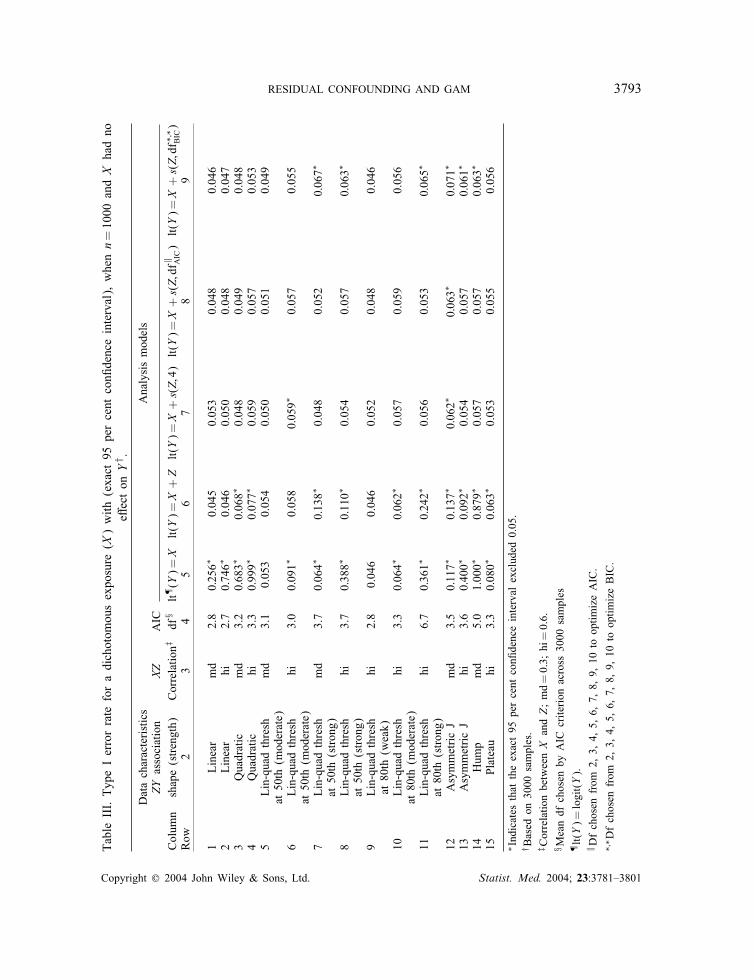
RESIDUAL CONFOUNDING AND GAM 3793TableIII.TypeIerrorrateforadichotomousexposure(X)with(exact95percentcon�denceinterval),whenn=1000andXhadno

e�ectonY

† .

Datacharacteristics

Analysismodels

ZYassociation

XZ

AIC

Column

shape(strength)

Correlation‡

df§lt

¶ (Y)=

Xlt(Y)=

X+Zlt(Y)=

X+s(Z;4)

lt(Y)=

X+s(Z;df

‖ AIC)lt(Y)=

X+s(Z;df

∗;∗ BIC)

Row

23

45

67

89

1Linear

md

2.8

0:256∗

0.045

0.053

0.048

0.046

2Linear

hi2.7

0:746∗

0.046

0.050

0.048

0.047

3Quadratic

md

3.2

0:683∗

0:068∗

0.048

0.049

0.048

4Quadratic

hi3.3

0:999∗

0:077∗

0.059

0.057

0.053

5Lin-quadthresh

md

3.1

0.053

0.054

0.050

0.051

0.049

at50th(moderate)

6Lin-quadthresh

hi3.0

0:091∗

0.058

0:059∗

0.057

0.055

at50th(moderate)

7Lin-quadthresh

md

3.7

0:064∗

0:138∗

0.048

0.052

0:067∗

at50th(strong)

8Lin-quadthresh

hi3.7

0:388∗

0:110∗

0.054

0.057

0:063∗

at50th(strong)

9Lin-quadthresh

hi2.8

0.046

0.046

0.052

0.048

0.046

at80th(weak)

10Lin-quadthresh

hi3.3

0:064∗

0:062∗

0.057

0.059

0.056

at80th(moderate)

11Lin-quadthresh

hi6.7

0:361∗

0:242∗

0.056

0.053

0:065∗

at80th(strong)

12AsymmetricJ

md

3.5

0:117∗

0:137∗

0:062∗

0:063∗

0:071∗

13AsymmetricJ

hi3.6

0:400∗

0:092∗

0.054

0.057

0:061∗

14Hump

md

5.0

1:000∗

0:879∗

0.057

0.057

0:063∗

15Plateau

hi3.3

0:080∗

0:063∗

0.053

0.055

0.056

∗ Indicatesthattheexact95percentcon�denceintervalexcluded0.05.

† Basedon3000samples.

‡ CorrelationbetweenXandZ;md=0.3;hi=0.6.

§ MeandfchosenbyAICcriterionacross3000samples

¶ lt(Y)=

logit(Y).

‖ Dfchosenfrom

2,3,4,5,6,7,8,9,10tooptimizeAIC.

∗;∗Dfchosenfrom

2,3,4,5,6,7,8,9,10tooptimizeBIC.



Figure 4. Investigating confounder inclusion criteria. D4a: Includes Z , smoothed with 4df, a priori.D4b: Excludes Z if test vs null model is not signi�cant. D4c: Models Z as a linear function if test ofnon-linearity is not signi�cant. D4d: Models Z as a linear function if the di�erence between exposureestimate adjusted for linear Z and exposure estimate adjusted for s(Z; 4) is small. D4e: Excludes Z if

di�erence between crude exposure estimate and exposure estimate adjusted for s(Z; 4) is small.

This in�ation increases with increasing (i) correlation between X and Z , (ii) non-linearity ofZ , and �nally (iii) strength of the Z–Y association (Table III, column 6). In our simulations,the empirical type I error from a model that uses an (incorrect) linear representation of theconfounder e�ect, was as high as 0.24 for a strongly non-linear but monotone e�ect and 0.87for a non-monotone e�ect (rows 11 and 14 in Table III). This in�ation is either completelyeliminated or reduced to not more than 0.07 when the confounder e�ect is modelled non-parametrically, no matter how the df are selected (last three columns of Table III).In Figure 4 we investigate di�erent data-dependent strategies that may be used to decide

whether or not to include the confounder, and how to model it. In all strategies evaluated inFigure 4, the GAM models use dfs a priori �xed at 4 (strategies D4a–d in Table II). Eachpart of Figure 4 corresponds to a di�erent combination of shape and strength of the Z–Yassociation, and sample size (listed along the bottom of the �gure). Each bar represents adi�erent strategy and depicts the type I error for testing the null hypothesis of no associationbetween the exposure and the outcome. When the true Z–Y association was linear (�rstfour parts of Figure 4), including Z a priori (D4a, black bars) yielded an acceptable type Ierror rate. As expected, excluding the confounder altogether when it was not signi�cant (D4b,striped bar) resulted in large in�ation of the type I error rates for the exposure e�ect, especially



in the smaller data set, and when the true Z–Y association was linear. For non-linear Z–Y ,modelling the confounder e�ect by a linear term (D4c, grey bars) when the non-parametrice�ect was not signi�cant resulted in slightly higher type I error for the estimated exposuree�ect than choosing the non-parametric representation a priori (D4a). Using the less than10 per cent change in exp(�̂x) criterion to select a linear representation (D4d, checked bar)resulted in greater in�ation of the type I error. The worst in�ation of type I error was seenwhen the confounder was �rst replaced by a linear term if it was not signi�cantly non-linearand then was excluded if this term was also not statistically signi�cant (data not shown).This suggests that inference about the exposure e�ect deteriorates as the number of data-dependent choices increases. When Z had a very weak e�ect on the outcome, all strategiesperformed similarly, with type I error for testing the X term ranging between 0.046–0.066and 0.051–0.066, when n=1000 and 300, respectively (data not shown).

3.2. Continuous exposure

When dealing with a continuous exposure, we focussed mainly on the MSE of the estimatedregression coe�cient for the exposure e�ect, generated to have a linear e�ect on the outcome.First, we investigated a simpler case, when the (correct) linear representation of the exposuree�ect was selected a priori. The pattern of results was generally similar to those seen with adichotomous exposure, though gains due to non-parametric modelling of the confounder e�ectwere smaller. The MSE of the estimated adjusted exposure e�ect was 5–10 per cent lowerwhen the confounder e�ect was modelled non-parametrically rather than by a linear function(data not shown). The reduction in MSE was driven by a decrease in bias, and, as expected,was larger when the Z–Y association was more non-linear, and when the X –Z correlationwas higher.

3.2.1. Modelling the e�ect of a continuous exposure non-parametrically. In the previoussection, we assumed that the exposure is known a priori to have a linear e�ect on the outcome.However, in real-life applications the true form of the relationship between a continuousexposure and the outcome is often unknown. In such a situation, a test of the linearity of theexposure e�ect, based on comparing the �t of a linear vs �exible exposure representation, isoften important in terms of both etiology and model parsimony [4–7, 29]. In this section, weinvestigate how the type I error rate of the test of the non-linear e�ect of a continuous exposuredepends on the strategy for modelling a continuous confounder, across a range of scenarios.To this aim, the exposure was generated to have a linear association with the outcome andthe confounder, while the confounder was generated to have a range of associations with theoutcome. Table IV shows the type I error for testing the non-linearity of the exposure–outcomeassociation in a data set with n=1000, for three modelling alternatives that all representthe exposure e�ect non-parametrically and respectively model the confounder e�ect: (i) byignoring it (4th column); (ii) as a linear function (5th column); and (iii) non-parametrically(6th column). The second column of Table IV describes the shape and strength of the Z–Y association. The third column shows the level of X –Z correlation and the fourth columndescribes the shape of the X –Z association. The df for exposure and, when appropriate,confounder were a priori �xed at 4.If both the confounder–outcome and the exposure-confounder associations were linear (�rst

two rows of Table IV) regardless of the correlation between the exposure and confounder, in



Table IV. Type I error for testing the non-linearity of X with N =1000, when X had a linear e�ect onY , by shape of XZ , correlation between XZ , and shape of ZY .

2 3 4 5 6Column ZY Association XZ lt(Y )= s(X; 4) lt(Y )= s(X; 4) + Z lt(Y )= s(X; 4) + s(Z; 4)Row (Strength) Correlation†

1 Linear md 0:075∗ 0:080∗ 0:079∗

2 Linear hi 0:087∗ 0:065∗ 0:068∗

3 Lin-quad thresh md 0:075∗ 0:074∗ 0:076∗

at 80th (weak)4 Lin-quad thresh hi 0:065∗ 0:066∗ 0:082∗

at 80th (weak)5 Quadratic md 0:088∗ 0:072∗ 0:076∗

6 Quadratic hi 0:203∗ 0:130∗ 0:088∗

7 Lin-quad thresh md 0:074∗ 0:072∗ 0:066∗

at 50th (moderate)8 Lin-quad thresh md 0:088∗ 0:080∗ 0:069∗

at 50th (strong)9 Lin-quad thresh hi 0:105∗ 0:097∗ 0:082∗

at 50th (moderate)10 Lin-quad thresh hi 0:297∗ 0:208∗ 0:070∗

at 50th (strong)11 Lin-quad thresh hi 0:289∗ 0:226∗ 0:081∗

at 80th (moderate)12 Lin-quad thresh hi 0:393∗ 0:287∗ 0:071∗

at 80th (strong)13 Plateau hi 0:093∗ 0:148∗ 0:076∗

14 Hump md 0:177∗ 0:314∗ 0.05715 Asymmetric J hi 0:861∗ 0:792∗ 0:068∗

(moderate)16 Asymmetric md 0:181∗ 0:156∗ 0:072∗

(moderate)17 Asymmetric md 0:425∗ 0:371∗ 0:060∗

(strong)18 Asym. double hi 0:462∗ 0:453∗ 0:066∗

hump19 Asym. double md 0:109∗ 0:106∗ 0:067∗

hump

∗Indicates that the exact 95 per cent con�dence interval excluded 0.05.†Correlation between X and Z ; md=0.3; hi= 0.6.

all modelling strategies the exposure was (incorrectly) found to be non-linear in around 8 percent of the samples. Similarly, a small systematic in�ation of type I error was observed, whenthe confounder was only weakly associated with the outcome (rows 3 and 4). However, ifthe confounder–outcome association was non-linear (rows 5–19), exclusion of the confounder(column 4) resulted in a higher in�ation of type I error for the non-linearity of exposure thanthe two other strategies (columns 5 and 6) and increased, as expected, with (i) the level ofcorrelation, and (ii) the strength and (iii) non-linearity of the confounder–outcome association.In the presence of a non-linear confounder e�ect, representing this e�ect by a linear term

did little to alleviate the problem with type I error rates for linearity of exposure ranging from



0.066 to as high as 0.792 (column 5 of Table IV). In contrast, modelling both the confounderand exposure non-parametrically reduced the probability of incorrectly �nding the exposuree�ect non-linear to less than 0.09 (0.057–0.088, depending on the scenario, last column ofTable IV). The type I error was always somewhat in�ated; however the in�ation was minor,in contrast to modelling the confounder parametrically or excluding it. Results were verysimilar for n=300, but the gains due to joint non-parametric modelling were more moderateand mainly con�ned to cases when the exposure was strongly associated with the confounderand=or the confounder e�ect was highly non-linear, and especially non-monotone (data notshown).As described in the Methods, we also investigated di�erent data-dependent strategies that

started by modelling both the confounder and exposure non-parametrically, and then replacedone or both smoothers with linear terms, depending on the results (see Figure 2). Fortunately,with respect to the type I error of the test of non-linearity for X , the order in which thetwo variables were tested had only a minor impact on the results. Type I error for the testof non-linearity of the exposure e�ect was very slightly higher when Z is investigated �rst,though still never higher than 0.077 (vs 0.068 for testing X �rst).

4. DISCUSSION

We investigated various approaches to controlling for a continuous confounder in the con-text of multiple logistic regression, including parametric modelling and generalized additivemodels (GAM) [6]. Using GAM improved the accuracy of the estimated adjusted e�ect ofa dichotomous exposure over conventional parametric methods when the true association be-tween the outcome and the confounder was non-linear. Depending on the strength and shapeof the non-linear confounder–outcome relationship GAM o�ered a 19–53 per cent reductionof the MSE for the exposure e�ect in comparison to modelling the confounder by a linearterm. The gains were due to eliminating the bias, whereas the variances of the GAM andparametric estimates were similar. Moreover, GAM largely reduced the in�ation of type Ierror for testing the exposure e�ect that occurred in parametric models of truly non-linearconfounder e�ects. Yet, when the association between the confounder and outcome was trulylinear, GAM performed as well as using a parametric representation of the confounder. Thus,using GAM is advisable in this situation.We also investigated non-parametric modelling of a continuous exposure, in the presence

of a continuous confounder, with possibly non-linear e�ect. The results show that failure toproperly account for non-linear e�ects of confounders can lead to spurious �ndings of non-linearity of the exposure e�ect. Thus, when investigating the non-linearity of the exposureof primary interest joint non-linear modelling of both the confounder and exposure e�ects isnecessary.Our results extend those of Brenner and Blettner’s [3] in several ways. Firstly, we have

demonstrated that non-parametric methods reduce residual confounding in data sets with mod-erate sample sizes, representative of those typically used in epidemiology. Moreover, we haveinvestigated a greater variability of the shape and strength of the relevant associations. Wealso investigated the impact of residual confounding on inference concerning the exposuree�ect and found that GAM avoids the in�ation of type I error that often occurs in parametricmodels. We have addressed the challenging issues related to non-parametric modelling of both



exposure and confounder e�ects. Lastly, we have investigated the technical details associatedwith using non-parametric methods, including how best to choose the amount of smoothing inthis context, and under what circumstances to replace non-parametric smoothing with standardparametric modelling. Although gains due to using GAM were larger with higher correlation(near 0.6) between the confounder and exposure, they were also evident when the correlationwas near 0.3.Whereas our results suggest the bene�ts of using GAM to control for continuous con-

founders, the data analyst will have to face some particular issues related to modelling inGAM. We have attempted to provide some insights regarding these issues. We recommendusing the df set a priori at the default value of 4. Among the a posteriori methods, AICperformed similarly to the a priori method in terms of bias and MSE. As the non-linearityincreases, presumably AIC would outperform the a priori 4-df model, but this was not evidentin our simulations even when the average AIC based df was as high as 6.7. On the otherhand, the a priori strategy avoids inferential problems due to a posteriori model selection[27].Although the bene�ts due to using GAM were greater in a larger dataset, they were also

evident when n=300. As n decreases, the bias-variance trade-o� becomes less favourable to�exible models. With small n, even a �exible model is unlikely to avoid bias as the riskof over�tting bias increases and the ability to determine the adequate degree of smoothingdeteriorates. On the other hand, the variance of the non-parametric estimates increases at asteep rate as the ratio of the observed outcomes to the model’s dfs decreases. More generally,as n decreases further, the ability to make the optimal data-dependent decision becomes moredi�cult. If the non-linearity of the confounder e�ect is statistically signi�cant in a smallsample the non-linear e�ect must be quite strong. In such cases, failure to account for itshould increase both bias and variance of the exposure estimate. If the non-linear e�ect is notsigni�cant, the choice is more di�cult as this could be due to insu�cient power. Yet, decidinga priori to represent continuous covariates by non-linear smoothers considerably increases themodel complexity and the risk of over�tting, especially in smaller samples.BIC [24] was routinely optimized by fewer df than AIC [23] leading to a more stable

but more biased estimate, especially as the non-linearity of the confounder–outcome asso-ciation increased. The AIC penalizes models on the basis of the number of df, and makesno adjustment for sample size. BIC, on the other hand, takes sample size into account. Ac-cordingly, both simulations and empirical studies have shown that, as n increases, BIC tendsto accept less complicated models than AIC [25, 30]. The AIC approximates the expectedKullback–Leibler distance, a measure of the di�erence between the true and estimated curves[23, 31]. However, as the df increase in relation to the sample size, the AIC underestimatesthe KL-distance which may lead to over�tting [30, 31]. Indeed, both theoretical argumentsand empirical results indicate that the AIC tends to perform better if the ‘true’ relationshipis complex while BIC will be expected to perform better if the underlying data structure issimpler [32, 33].Our results suggest that choosing a non-parametric representation of one continuous con-

founder a priori is bene�cial in terms of avoiding bias in the estimated exposure e�ect. Still,the decisions whether (i) to include a given variable in the model and (ii) to represent itse�ect by a �exible function are challenging whenever there is no su�cient a priori knowledgeabout the true e�ect of the confounder. On one hand, if the confounder has a truly non-lineare�ect, data-dependent choices may lead to choosing an (incorrect) linear representation or to



excluding the confounder altogether, thus introducing bias and in�ation of type I error of theadjusted exposure e�ect.On the other hand, if the true e�ect of the confounder is linear, then an a priori choice

of non-linear representation (i) leads to an needlessly complex and more di�cult to interpretmodel; and (ii) may lead to excessive dfs especially when n is small, or as the number ofcontinuous confounders increases. Further research is necessary to establish how the trade-o� between a priori and data-dependent modelling strategies depends on sample size, thenumber of potential covariates to be considered and previous knowledge about their e�ectson the outcome. Our preliminary results suggest that the decision to exclude the confounderaltogether should rely on the 10 per cent criterion, rather than on signi�cance testing, as theformer leads to smaller in�ation of type I error rate. On the other hand, the decision to modelthe confounder by a linear function rather than non-parametrically may rely on (i) the test ofnon-linearity in larger samples and (ii) either criterion in smaller samples. Overall, our resultssuggest minimizing the number of data-dependent decisions so that careful consideration ofmodelling choices should be made before modelling begins.In this article, we investigated the relatively simple scenario of estimating the e�ect of

one exposure in the presence of one continuous confounder. Given the number of decisionsnecessary to fully de�ne a modelling strategy, and their various e�ects on results, even insuch a simple case, at this stage such a restriction seems reasonable. Moreover, we have notinvestigated smoothers other than smoothing splines, such as loess [34] or �exible parametricmethods such as fractional polynomials [35]. However, since most �exible techniques yieldsimilar estimates [4, 35], we expect that our �ndings extend to these settings.Lastly, the slightly in�ated type I error obtained when smoothing two continuous variables

suggests that the GAM-based tests may become less accurate as more variables are includedin the model. Alternatively, the in�ation of type I error might be due to problems withthe way GAM handles concurvity. Concurvity, of two or more continuous variables, is thenon-parametric analog of multi-collinearity. It occurs when the function representing the e�ectof one of the variables can be approximated by a linear combination of the dose–responsefunctions of the other variables. Recently, it has been shown to result in an underestimationof standard errors due to ambiguity in separating the e�ects of two correlated variables ona third variable that is correlated with both [36]. However, the impact of concurvity on theestimated e�ect of correlated variables, and its dependence on the other parameters varied inour simulations, remain to be systematically investigated.Overall, our results suggest that the use of GAM to reduce residual confounding o�ers

several improvements over conventional parametric modelling. Moreover, we have providedguidance for several of the decisions that users of GAM would need to make. We hope thatour results will help researchers bene�t from the potential advantages of �exible assumption-free modelling.

ACKNOWLEDGEMENTS

This work was supported by grants from the Canadian Institutes for Health Research (CIHR No. 6391)and from the National Sciences and Engineering Research Council of Canada. Dr Michal Abrahamowiczis a James McGill Professor. We thank Drs Mark Goldberg, Igor Karp and Karen Le�ondr�e for helpfuldiscussions and insightful comments.



REFERENCES

1. Rothman KJ, Greenland S. Modern Epidemiology. Lippincott-Raven: Philadelphia, 1998.2. Becher H. The concept of residual confounding in regression models and some applications. Statistics inMedicine 1992; 11:1747–1758.

3. Brenner H, Blettner M. Controlling for continuous confounders in epidemiologic research. Epidemiology 1997;8:429–434.

4. Abrahamowicz M, du Berger R, Grover SA. Flexible modeling of the e�ects of serum cholesterol on coronaryheart disease mortality. American Journal of Epidemiology 1997; 145:714–729.

5. Ramsay JO. Monotone regression splines in action. Statistical Science 1988; 3:425–461.6. Hastie TJ, Tibshirani RJ. Generalized Additive Models. Chapman & Hall: New York, 1990.7. Royston P, Altman DG. Regression using fractional polynomials or continuous covariates: parsimoniousparametric modelling. Applied Statistics 1994; 43:429–467.

8. Brenner H, Loomis D. Varied forms of bias due to nondi�erential error in measuring exposure. Epidemiology1994; 5:510–517.

9. Axtell CD, Cox C, Myers GJ, Davidson PW, Choi AL, Cernichiari E, Sloane-Reeves J, Shamlaye CF, ClarksonTW. Association between methylmercury exposure from �sh consumption and child development at �ve anda half years of age in the Seychelles Child Development Study: an evaluation of nonlinear relationships.Environmental Research 2000; 84:71–80.

10. Schwartz, Joel. Nonparametric smoothing in the analysis of air pollution and respiratory illness. The CanadianJournal of Statistics 1994; 22:471–487.

11. Ha E, Cho SI, Park H, Chen D, Chen C, Wang L, Xu X, Christiani DC. Does standing at work during pregnancyresult in reduced infant birth weight? Journal of Occupational & Environmental Medicine 2002; 44:815–821.

12. Heinrich J, Bolte G, Holscher B, Douwes J, Lehmann I, Fahlbusch B, Bischof W, Weiss M, Borte M, WichmannHE, and LISA Study Group. Allergens and endotoxin on mothers’ mattresses and total immunoglobulin E incord blood of neonates. European Respiratory Journal 2002; 20:617–623.

13. Shain RN, Piper JM, Newton ER, Perdue ST, Ramos R, Dimmitt Champion J, Guerra FA. A randomized,controlled trial of a behavioral intervention to prevent sexually transmitted disease among minority women.New England Journal of Medicine 1999; 340:93–100.

14. Perondi MBM, Reis AG, Paiva EF, Nadkarni VM, Berg RA. A comparison of high-dose and standard-doseepinephrine in children with cardiac arrest. New England Journal of Medicine 2004; 350:1722–1730.

15. Iki M, Dohi Y, Nishino H, Kajita E, Kusaka Y, Tsuchida C, Ishii Y, Yamamoto K. Relative contributions ofage and menopause to the vertebral bone density of healthy Japanese women. Bone 1996; 18:671–620.

16. Royall DR, Palmer R, Chiodo LK, Polk MJ. Decline in learning ability best predicts future dementia type: thefreedom house study. Experimental Aging Research 2003; 29:385–406.

17. Kaufman JS, Asuzu MC, Mufunda J, Forrester T, Wilks R, Luke A, Long AE, Cooper RS. Relationship betweenblood pressure and body mass index in lean populations. Hypertension 1997; 30:1511–1516.

18. Bunker CH, Ukoli FA, Matthews KA, Kriska AM, Huston SL, Kuller LH. Weight threshold and blood pressurein a lean black population. Hypertension 1995; 26:616–623.

19. Cakmak S, Burnett RT, Krewski D. Methods for detecting and estimating population threshold concentrationsfor air pollution-related mortality with exposure measurement error. Risk Analysis 1999; 19:487–496.

20. Insightful Corp. SPLUS 6.0 Professional Release 1, 2001.21. Wahba G. Improper priors, spline smoothing and the problem of guarding against model errors in regression.

Journal of the Royal Statistical Society, Series B, Methodological 1978; 40:364–372.22. Green PJ, Silverman BW. Nonparametric Regression and Generalized Linear Models. Chapman & Hall:

New York, 1994.23. Akaike H. A new look at the statistical model identi�cation. IEEE Transactions on Automation Control 1974;

AC-19:716–723.24. Schwarz G. Estimating the dimension of a model. Annals of Statistics 1978; 6:461–464.25. Zucchini W. An introduction to model selection. Journal of Mathematical Psychology 2000; 44:41–61.26. Mickey RM, Greenland S. The impact of confounder selection criteria on e�ect estimation. American Journal

of Epidemiology 1989; 129:125–137.27. Abrahamowicz M, MacKenzie T, Esdaile J. Time-dependent hazard ratio: modeling and hypothesis testing with

application in Lupus Nephritis. Journal of the American Statistical Association 1996; 91:1432–1439.28. Benedetti A. Using generalized additive models in epidemiologic research. Doctoral Thesis, McGill University,

2004.29. Je�erys WH, Bergers JO. Ockham’s razor and bayesian analysis. American Scientist 1992; 80:64–72.30. Abrahamowicz M, Ciampi A. Information theoretic criteria in non-parametric density estimation: bias and

variance in the in�nite dimensional case. Computational Statistics & Data Analysis 1991; 12:239–247.31. Hurvich CM, Tsai CL. Regression and time series model selection in small samples. Biometrika 1989; 76:

297–307.



32. Wasserman L. Bayesian model selection and model averaging. Journal of Mathematical Psychology 2000;44:92–107.

33. Forster MR. Key concepts in model selection: performance and generalizability. Journal of MathematicalPsychology 2000; 44:205–231.

34. Cleveland, William S, Devlin Susan J. Locally weighted regression: an approach to regression analysis by local�tting. Journal of the American Statistical Association 1988; 83:596–610.

35. Royston P. A strategy for modelling the e�ect of a continuous covariate in medicine and epidemiology. Statisticsin Medicine 2000; 19:1831–1847.

36. Ramsay TO, Burnett RT, Krewski D. The e�ect of concurvity in generalized additive models linking mortalityto ambient particulate matter (comment). Epidemiology 2003; 14:18–23.


Documents

Using generalized additive models to reduce residual confounding