1

Using GIS to find affects of Mesoscale Thunderstorm systems with Boundary Layer formations from January 1950-July 2001

Charles T Schoeneberger Department of Resource Analysis, St. Mary’s University of Minnesota, Winona, MN 55987 Keywords thunderstorms, boundary layer, mesoscale systems, hail, thunderstorm winds, tornadoes, land features, air parcels Abstract: Thunderstorms are affected by many factors and there are ongoing efforts to understand them. One of the factors that influences storm intensity is the boundary layer or ground. If you make assumptions and simplifications, you can examine and relate the effects of landforms to thunderstorm damage. The intent of this paper is to look at the known geospatial historical data from the National Weather Service’s National Climatic Data Center (NCDC) from 1950 through 2001. In this effort, these data were plotted, contoured, and then compared to landforms too look for relationships. The results showed relationship with tornado density and intensity to river valleys and hills, as surface moisture plays an important role in storm processes. Hail reports show no outstanding conclusions, and due to data acquition limitations, no hard conclusions can be found with straight-line wind events. Introduction Background The National Weather Service (NWS) produces weather forecasts for regions year round. During the spring, summer and fall they focus on mesoscale systems. Mesoscale systems are systems that range in size from a few miles to a couple hundred miles. This size range encompasses summer thunderstorm events. A single cell system is smaller. While multiple cells, increase dramatically in size. The NWS offices have many tools at their disposal. Three of the most important ones are the WSR-88D NEXt generation weather RADar (NEXRAD), storm spotters from the NWS Skywarn, a network of amateur radio operators and law enforcement agencies, and Radiosonde instruments located on weather balloons. Here the balloons

record temperature and dewpoint and radio the information back to ground stations as balloons are released and rise through the atmosphere.

As a weather forecaster, you get estimates of thunderstorm intensity by looking at NEXRAD radar and by examining the information from weather balloons and spotters. Radar is limited because the radar beam travels in a straight line and does not follow the curvature of the earth and it gains altitude as it moves away from the radar source. As a consequence, radar is less reliable and less sensitive in locating weather systems as you move away from the radar site. Hence information from all possible sources is needed to understand and predict weather. The information recorded for each storm also varies by storm event. Straight-line wind data are easy to record, such as that collected by

2

calibrated anemometers located at airports. Other information easily recorded is hail size obtained by simply measuring hailstones with a ruler. Other information is difficult to obtain such as exact tornado intensity. It would be desirable to directly measure all storm events, but there are times where it is impossible to acquire the desired information due to the lack of nearby weather instruments, radar coverage, and/or spotters. One has to examine the damage left after a storm to assess its magnitude to arrive at estimates of the storm’s magnitude. Because of the varying and diverse locations of storm monitoring instruments, the latter is a critical element of storm assessment and prone to human error. Tornado and straight-line wind incidents that occur away from airport instruments are estimated using a damage scale by assessing damage visually. The scale is called the Beuford scale for winds and the Fujita scale for tornadoes. This system of assessing tornado intensity using the Fujita Scale is subject to human error and built in error, as it has never been calibrated (Doswell, 1999). For instance, the NWS’s policy is not to verify a tornado event on the ground if it is a weak event. Therefore most of the verified information found in the NWS database is for stronger events. Additionally, sometimes verification is not done at all even with large events, or if it is done, it is done poorly or incorrectly. The latter often results because the NWS operates on a tight budget with a lack of resources, experienced personnel, time, and policies (Doswell, 1999). A thorough damage assessment should use both aerial and ground

surveys but funds for the ground survey are not normally present in the NWS budget unless the storm is of unusual magnitude or exceptionally destructive. In most cases, tornado intensity is determined from information obtained from storm spotters and media reports in the area (Doswell, 1999). To determine tornado intensities before 1978, when the Fujita Scale was devised, the National Severe Storms Forecast Center (NSSFC), now the Storm Prediction Center (SPC), contracted with college students to cross-reference damage reports and make judgment calls on storm intensities. While using the Fujita Scale has errors, it is the best we have (Edwards, 2001). In weather and atmospheric sciences, the idea of Chaos Theory is important. A basic definition of the Chaos Theory is that processes in a system are random and not likely to happen in a repetitive fashion (Fairfield et al 1997). To the science of meteorology, this describes air molecules, either alone or in larger groups (air masses and parcels) and the flow around them. While some weather events may look similar, they have differences. This makes assumptions about future weather forecasts difficult at best. The further one forecasts into the future, the greater the impact of chaos (randomness) in influencing weather and the lower the ability to predict with accuracy actual upcoming weather phenomenon (AMS Council, 1998). There is much still unknown about thunderstorms and much more is learned every day. One way to help understand complicated events like thunderstorms is to analyze assumptions based on thermodynamic theory. One of

3

these is the ‘air parcel’ theory. The air parcel theory deals with the thermodynamic properties of an air parcel when it rises and sinks. The thermodynamic properties are temperature and dewpoint. On thermodynamic charts, there are lines of an ideal parcel movement called adiabats, one for dry, unsaturated parcels, and others for moist, saturated parcels. There is an average temperature rate of change of –3.6 deg(F)/1000 ft. In the atmosphere, the temperature gradients can vary much more depending on conditions. There are two ways to move air parcels, thermodymically and physically. Air parcels sink if the parcel is cooler than the surrounding air and rise if it is warmer than the surrounding air. Physical features, with elevation change can also force an air parcel up or down. The atmosphere contains large quantities of energy, existing in the form of temperature and moisture gradients. This is called the latent energy in the air. When an air parcel containing latent energy rises into a cooler environment, it releases energy. When this happens energy flows into the surrounding environment. How much energy is exchanged depends on the difference between the air parcel and the environment. If the parcel is lowered in elevation, it warms slightly and rises in dewpoint, and is able to absorb additional latent energy itself and less is released into the surrounding air. The most basic cause for most weather comes from temperature gradients, both horizontal and vertical. The atmosphere uses weather events to equalize itself and to move towards a uniform state. As a rule, the stronger the gradient, the stronger the storm as there

is a greater potential for massive energy release from the air parcels. There are at least two ways that an air parcel gains motion. One is when the temperature gradient is large enough with cooler air above warm air that the air parcel moves upward. Another is for an air mass to be physically pushed upwards by a passing cold front or land formation. Here the denser colder air moves downward, displacing the higher energy warmer air upwards. As a thunderstorm updraft grows, the air parcels give off its latent energy into the surrounding atmosphere. The reduced temperatures and dewpoints cause the moisture to attach to small particles, which fall as rain and create a downdraft. The downdraft not only releases energy as precipitation falls to the ground, but it displaces warmer and moister air near the ground upward. Straight-line winds are caused by an accumulation of cooler and moister air due to updraft conditions, it can move towards the ground in one burst. This displaces the air below and allows greater wind speeds to move towards the surface. Which causes a downburst of air parcels. These air parcels spread on the ground and cause strong winds. The magnitude of this is dependent on the strength of the downdraft. The stronger the updraft, the easier it is for a thunderstorm to keep precipitation aloft. This takes the water droplets above and below the freezing layer above the ground. Each time it passes below the vertical freezing level, it accumulates another layer of water, which will freeze again as it passes upward through the clouds. This is the hail formation process. It is more dependent on the vertical freezing level than storm intensity.

4

Another factor that is necessary for thunderstorm development is the change of direction of airflow with height called wind shear. This causes air parcels in thunderstorms to rotate and increase their vertical velocity. This motion increases the mixing of the two types of air and speeds the rate of energy release between the two. The term for this is vorticity. It should be noted that having too much wind shear could also blow a storm apart. Two different areas of wind maximums produce the wind shear associated with strong to severe storms. One is around 300 mb, or approximately 30,000 ft and the other is near the ground surface, or about 850 mb or approximately 5,000 ft (in the midlatitudes). The higher one is associated with the traditional jet stream and the low level jet stream is a seasonal phenomenon that is related to landforms on a scale of hundreds of miles. In general, the upper level jet stream blows from a westerly direction while the low level jet stream blows from a southerly direction. It is the upper level jet stream that exerts the greatest effect on the storm movement. In the northern plains states, this is generally in a east to northeasterly direction.

The basic reason for these formations comes from a strong gradient in temperature and moisture. The gradient creates a pressure difference, as cooler and dryer air is denser than warm moist air. These ingredients give rise to the most common type of thunderstorm that spans tornadoes, the supercell. It is in the storm rotation that encourages tornado formation. All types of thunderstorms have the potential to produce tornadoes, but they most often occur with supercell thunderstorms.

Once strong rotation of the thunderstorm begins, a rotating cloud forms called a mesocyclone can form. These range in size from 10 to 15 km. The size range of tornadoes is usually from 10 to 100 m in size, while extreme events can be more than a mile in size. The mesocyclone and other thunderstorm updrafts depend on a constant supply of warm, moist air to keep redeveloping. The inflow comes from near the ground in the boundary layer. The boundary layer effects the thunderstorm through friction with the ground, low level wind direction forcing, and warming and cooling due to elevation changes and surface features (Kessler 1992). If the air inflow into a thunderstorm comes from a low elevation, it will be slightly warmed, with the ability to hold more energy. If it rises in elevation, it cools and releases some of its energy on its way into the thunderstorm (Bluestien, 1993). Additional energy can also be gained by boundary layer air parcels coming from areas of higher surface moisture, like lakes and streams. This moisture will strengthen a storm to some level. Laboratory simulations have determined that the intensity of this thunderstorm updraft is the chief factor in determining tornado intensity (Nolan et al, 2000). Methods Data Acquisition The data for this project was obtained from the National Climatic Data Center (NCDC). It was in an online database that was accessed via the Internet. This database holds all storm events for the entire country from 1950 to within a month of the present day. It contains many types of storm events, from

5

summer type (hail, flooding, tornadoes, strong winds), winter type (blizzards, strong winds, heavy snow), to tropical (hurricanes). Since this study is related to summer convective thunderstorm events, the only events examined were hail, tornadoes, and strong winds. The extracted data output was in tabular format, with information about each event. These were printed in hard copy format. The data included each event’s date, time, deaths, injuries, property damage, crop damage, and magnitude. One of the most important elements missing in the table were the Latitude/Longitude data. This data was found by looking at each individual record separately. This was done and recorded for each record in the table. Other data came from the Minnesota Department of Natural Resources Data Deli (http://deli.state. mn.us). It is here that the 30 m Digital Elevation Model (DEM) for each county in the state of Minnesota were acquired. The polygon shapefile of different land regions across the state were also obtained at this site. The final data came from decoded Minnesota TIGER Line Files from the U.S. Census Bureau. The shapefiles used were hydrology, both line and polygon and urban areas polygons. The urban areas were unioned by county to form one shapefile for the state. The hydrology polygons were unioned in smaller groups of interest related to the data density and intensity contours. Data Input, Format and Standardization Since the data obtained by the Internet came in hard copy format, it had to be entered into the ArcView database

manually. The database combined the columns of all three-storm event types; straight-line winds, tornadoes, and hail. The final .dbf table had information on County name, Latitude, Longitude, Month, Day, Year, Time (in 24 hr format), Type of event, Death, Injuries, Property Damage, Crop Damage, Magnitude, Tornado End Latitude, Tornado End Longitude, and Tornado width. After the storm event database was created, it had to be checked for errors. There were a few errors, some from the data entry, and others from the database itself. First, the ESRI sample Avenue script DMS to DD was used to convert the degrees, minutes and seconds to decimal degrees. Then, the data was added as a point shapefile with ArcView’s Add Event Theme command. Finally, to find errors, it was then displayed, according to the county column in the database, and points that did not fit the color scheme for each county were rechecked for errors.

Some of the entries were errantly recorded, due to not checking where the Latitude/Longitude point was measured. One significant example were the storm reports for Apple Valley, Minnesota in Dakota County. The latitude and longitude of events for that city placed the reports in central St. Louis County in the Northeast part of the state, instead of in the south part of the Twin Cities metropolitan area. Some data degradation occurred because accurate location data was not available; degrees and minutes were used with no seconds’ data available. This affected the amount of accuracy and resolution.

Other errors came from the event being recorded as miles in a direction from a city. If this city was in a different county than the Lat/Lon of the event, it

6

would affect subsetting of the data by associating it with the wrong county. After all the data were checked for accuracy, they were added again as a new point event theme and projected from decimal degrees to NAD83, UTM Zone 15 for Minnesota. This was to decrease projection errors and because all the DEM data existed in the UTM projection. The shapefile was then subsetted into the three storm damage event types: tornadoes, hail, and strong thunderstorm winds. The thunderstorm winds were subset a second time because there were many events without a recorded speed or estimate. The tornado study only uses the recorded touch down location because not all events had the corresponding ending location and widths expected for a complete event record. Spatial and Statistical Methods In the analysis, there were several extensions that were key to the process. These were ESRI’s Spatial Analyst, GRID Mosaic, Projector, and third party extensions; Grid Analyst by Dr. Saraf of Indian Institute of Technology, Spatial Statistics by Daniel Monk, and TIGER reader by MapClick. The key extension used for this analysis was the Spatial Analyst extension. The Grid Analyst was used as a GRID masker using the extract GRID from Polygon feature. The Projector extension was used to transform and project shapefiles to UTM NAD83 Zone 15. The GRID Mosaic extension was used to combine the county DEM’s into larger areas, and the TIGER Reader was used to decode the urban area files from the US Census Bureau’s raw TIGER files.

The most important feature of Spatial Analyst was its ability to grid data. More specifically, the interpolation and density functions were particularly important. For this study the Inverse Distance Weighted (IDW) interpolation function and the simple density function were used. These were because the chances of being affect by the storm event decrease with distance away from an event and areas with repeat events will show up in a higher density grid. According to ESRI’s help menus, the IDW function weights each point from the distance of the point being analyzed and averages the values to get the final output. In other words, the grid cell value decrease as the distance increases from the point(s). In the simple density function, the algorithm takes the number of points per area and gives the grid a higher value the more points there are in that area. It uses a defined search radius to look for different density levels. As with all grids, you have to balance grid cell size and computer storage space, the smaller the grid cell, the bigger the grid size. You also have to decide if a smaller grid cell size will increase the overall accuracy of the study. It was determined that since the entire state was being looked at, and the data was only accurate to Degrees and Minutes, using a smaller grid did not add accuracy to the analysis. Results depended on the accuracy of the data being gridded. Two different assessments were undertaken to decide if there was meaningful loss of resolution.

The first was using the automatic grid cell size for Spatial Analyst. This created a grid cell of around 3 km. The other resolution examined was a cell size of 30 m. The value of 30 m was chosen

7

to try to match the 30 m DEMs for the state. This meant any grid data structure would be quite large, if used on a state level, so it was only computed on a county level. There were differences, between data sets, some contour lines did not line up exactly, because of smoothing the contour lines. This added some error to the contours, losing proximity to data points in neighboring counties, but most contours were close to the 3 km grid cell and were considered acceptable. The most dramatic difference noted was in the 30 m resolution dataset for the entire state. This was a big file and dramatically increased space used and processing time. Grid sizes were in the hundreds of Megabytes and not tens of Megabytes. So the 3 km cell size was used. In the statistical analysis, two programs were used, the Crimestat program from the US Department of Justice and the Spatial Statistics extension. The Spatial Statistics extension has many features, but the most useful was the Nearest Neighbor command. The Nearest Neighbor algorithm examines the distance between points and determines whether they are distributed in a random or clustered manner.

To do a 2-dimensional statistical analysis, the Department of Justice’s Crimestat program was adapted for this project. The Crimestat program was designed to do statistical analysis for mapping crime areas. In the Geographic Information Systems, data being analyzed is in the same format, an area of points with known location and intensity. The features used were the standard deviation ellipses and mean center functions. This was used to see if the numbers of reports in each part of the state were high enough to be statically

relevant, or if there were just a couple of points unfairly weighting the distribution. Generally, points outside the second deviation ellipse over a distribution of the state of Minnesota were not considered statically meaningful because of the low number of points in that area. Statistical Results and Comparisons The first part of the analysis was to see how biased the data was to the urban areas. Thunderstorm reports come from many sources, but mainly from people calling the NWS and/or trained storm spotters and law enforcement. I selected by polygon the points on the urban area polygon to see how many were in the urban and rural areas. The ratios had the smallest number of tornadoes in the urban areas, about one third of hail reports in urban areas and almost half of the straight-line wind reports come from urban areas, especially in the subset of straight-line winds. The percentage of reports in urban areas is shown in Table 1. Table 1: Breakdown of urban versus rural reports Damage Type

Number of reports in urban area

Total number of thunderstorm reports

Percent of reports in urban areas

Hail Urban=1408 Total=4023 35.0% Tornado Urban = 195 Total=1170 16.6% All straight-line winds

Urban=1754 Total=4099 42.8%

Subset of straight-line winds

Urban=1087 Total=2268 47.9%

The next analyses determined the randomness of the data types. The amount of randomness comes from procedures in obtaining the reports. The straight-line wind reports are usually recorded at airports, even though other estimating procedures have recently been added. The reports for hail and

8

tornadoes do not have this problem as they can be measured almost anywhere. To confirm this, the Nearest Neighbor Computation in the Spatial Statistics extension was used. It runs the Nearest Neighbor analysis with the Ho, null hypothesis; with the points to be randomly placed, or the Ha, alternate hypothesis; for the points to lean towards a clustered relationship. R is the average distance between points, n is the number of maximum bounding rectangle areas to do the distance calculation, and |z| is the observed distance R between points minus the expected distance of R (Chen, Getis, 1998). If |z| > R, you accept Ha, otherwise you assume the data to be randomly distributed. The extension displays a dialog box at the end to display if the dataset is clustered or random. The results showed that the tornado and hail data were both accepted as random. As is shown in Table 2, the thunderstorm straight-line wind data was random, but the subset with speeds greater than zero leaned towards a clustered relationship. Table 2: The Nearest Neighbor Test for Randomness Type of Report

Avg Distance R

Number of Bounding Rectangles

Observed-Expected R Or |z|

Ho or Ha Accepted

Hail R=1.05828 n=17 |z|=0.45966 Ho accepted

Tornado R=0.99569 n=3 |z|=0.01426 Ho accepted

All Straight-Line Winds

R=0.76116 n=17 |z|=1.8839 Ho accepted

Subset Straight-Line Winds

R=0.56326 n=6 |z|=2.04654 Ho rejected

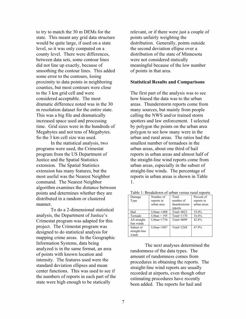
The next part of my analysis was to look for areas with enough points to make valid statistical conclusions. This is where I used the Crimestat program to create standard deviation ellipses as shown in Figure 1. If any area was

outside the second standard deviation polygon, the number of points in that area was not enough to make conclusions for the area. Areas that have only a couple of points could be outliers and any conclusions reached were treated with caution. Part of the effect is a result of the shape of the state; it does show that for straight-line winds and tornadoes, in far northeast Minnesota, it is hard to determine conclusions.

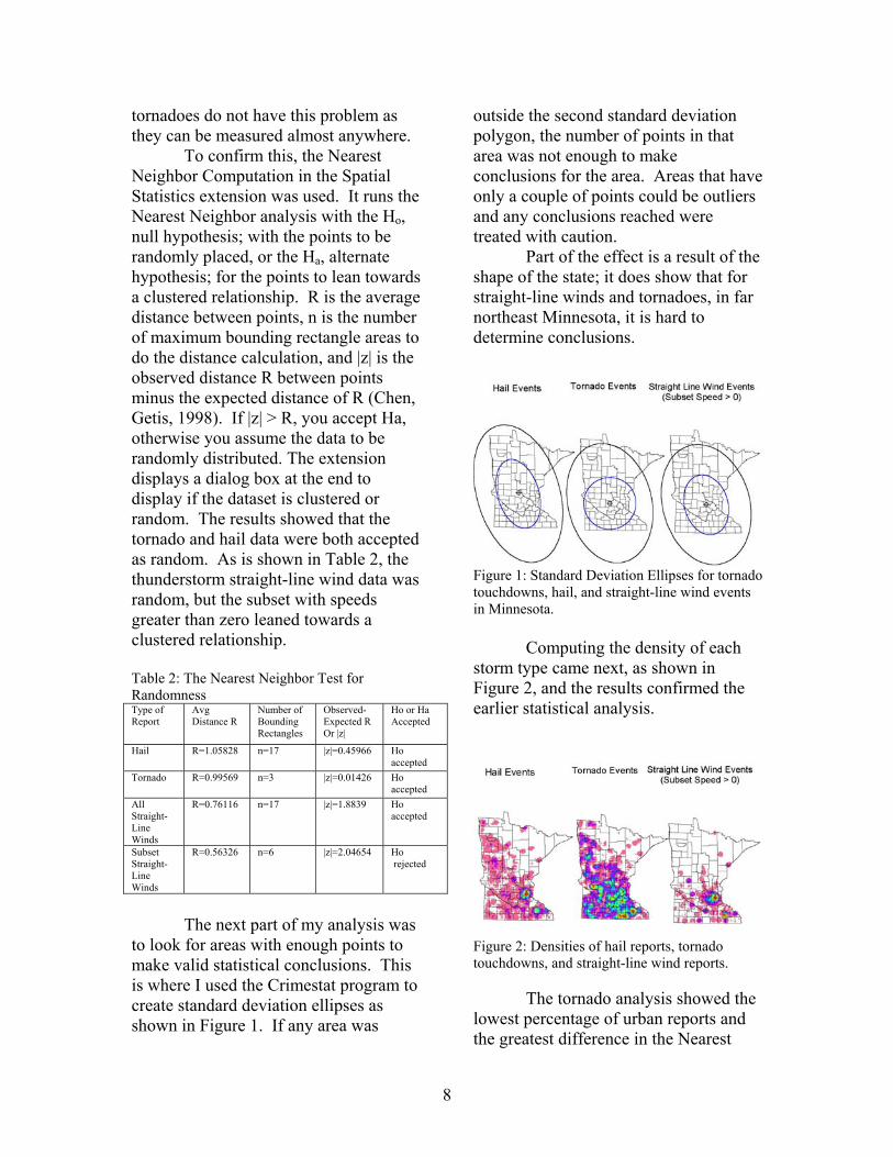
Figure 1: Standard Deviation Ellipses for tornado touchdowns, hail, and straight-line wind events in Minnesota. Computing the density of each storm type came next, as shown in Figure 2, and the results confirmed the earlier statistical analysis.

Figure 2: Densities of hail reports, tornado touchdowns, and straight-line wind reports. The tornado analysis showed the lowest percentage of urban reports and the greatest difference in the Nearest

9

Neighbor R and |z|. This means that the highest density areas can be assumed to be random. It does show that the highest density areas are around Rochester, Albert Lea, Mankato, Marshall, St. Cloud, Willmar, and the south part of the Minneapolis-St. Paul metropolitan area. With regard to hail density, the data show signs of being more clustered than the tornado data. The higher density areas are around the cities of Rochester and Minneapolis. This is also shown in the statistical results, in that a higher percentage of data are within urban areas and the difference between R and |z| in the Nearest Neighbor were not as great. With the thunderstorm straight-line wind data, the density grid shows that the data were mainly clustered. The main reason, as mentioned before, unless you estimate the wind speed based on the damage, like is done now, the only way to get the data is to measure it. Most anemometers are placed at airports, which is where the density search circles occur. This follows the Nearest Neighbor analysis, which shows higher percentage of the data being recorded in urban areas still and even though the data is clustered, more than half do not occur in urban areas. There are enough points outside the clustered areas that some understanding can be determined in the final analysis. Physical Trends Results To make the previous results easier to overlay, the densities and magnitudes were contoured into vector line files. I subdivided my analysis into different regions based on my knowledge and experience of thunderstorms, land regions, and the grouping of the data. The conclusions that follow are based on

the contours and no known specifics of the meteorological conditions that led up to each event. In the contours in the images that follow, the black contours are tornado intensity, color coded contours are density contours from the density grid shown in Figure 2 that go in increasing density from a low of purple to a high of red. The most important assumption is that almost all heavy to severe thunderstorm cell movement is from the W to S towards the E to N. Another is that warm moist thunderstorm low-level inflow comes in from the S to E and cooler, drier low-level inflow comes from the backside of the thunderstorm, N to W. As seen by the statistical analyses, the most random data is in the tornado touchdown data, followed by the hail and the straight-line winds. It is easiest to make conclusions about the tornadoes and the hardest for the straight-line winds. The clearest relationship seen with the tornado data were with terrain features and surface moisture sources (rivers and lakes). The contours of intense tornadoes and tornado density show a relationship with these features. Not every river is a factor, but the axis of some rivers appear to be a factor, and certain rivers have areas of interest. Generally, rivers with a W-E or SW-NE axis, but there are cases of a N-S river having the same affects. These rivers are usually 2nd, 3rd, or 4th order streams. The greater intensity comes from a combination of river valley shapes and moisture from the river. Increased surface moisture near the rivers is brought into the low level airflow of the thunderstorms. This air rises into the thunderstorm and gives off latent energy.

10

The shape of the river valleys also appears to influence the thunderstorms. One way is that the river valleys may ‘funnel’ low-level airflow. The other is that the slope of river valleys tends to be less than the surrounding land, and this weakens the disruption of low-level inflow and mesocyclones.

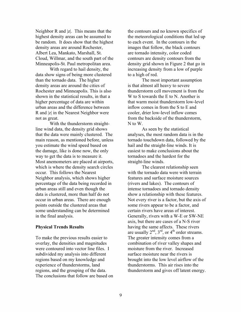
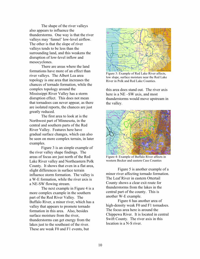
There are areas where the land formations have more of an effect than river valleys. The Albert Lea area topology is one area that increases the chances of tornado formation, while the complex topology around the Mississippi River Valley has a storm disruption effect. This does not mean that tornadoes can never appear, as there are isolated reports, the chances are just greatly reduced. The first area to look at is the Northwest part of Minnesota, in the central and southern parts of the Red River Valley. Features here have gradual surface changes, which can also be seen on more complex terrain, in later examples. Figure 3 is an simple example of the river valley shape findings. The areas of focus are just north of the Red Lake River valley and Northeastern Polk County. It shows that even in a flat area, slight differences in surface terrain influence storm formation. The valley is a W-E formation, while the river axis is a NE-SW flowing stream. The next example in Figure 4 is a more complex example in the southern part of the Red River Valley. The Buffalo River, a minor river, which has a valley that appears to promote tornado formation in this area. Also, besides surface moisture from the river, thunderstorms can get energy from the lakes just to the southeast of the river. These are weak F0 and F1 events, but

Figure 3: Example of Red Lake River affects, low slope, surface moisture near the Red Lake River in Polk and Red Lake Counties. this area does stand out. The river axis here is a NE –SW axis, and most thunderstorms would move upstream in the valley.

Figure 4: Example of Buffalo River affects in western Becker and eastern Cass Counties Figure 5 is another example of a minor river affecting tornado formation. The Leaf River in eastern Ottertail County shows a clear exit route for thunderstorms from the lakes in the central part of the county. This is another W-E example.

Figure 6 has another area of high-density weak F0 and F1 tornadoes. The focus area here is around the Chippewa River. It is located in central Swift County. The river axis in this location is a N-S river.

11

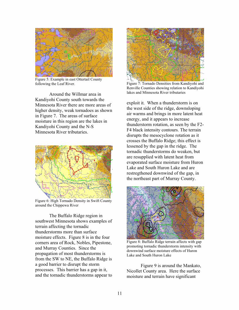
Figure 5: Example in east Ottertail County following the Leaf River. Around the Willmar area in Kandiyohi County south towards the Minnesota River there are more areas of higher density, weak tornadoes as shown in Figure 7. The areas of surface moisture in this region are the lakes in Kandiyohi County and the N-S Minnesota River tributaries.

Figure 6: High Tornado Density in Swift County around the Chippewa River The Buffalo Ridge region in southwest Minnesota shows examples of terrain affecting the tornadic thunderstorms more than surface moisture effects. Figure 8 is in the four corners area of Rock, Nobles, Pipestone, and Murray Counties. Since the propagation of most thunderstorms is from the SW to NE, the Buffalo Ridge is a good barrier to disrupt the storm processes. This barrier has a gap in it, and the tornadic thunderstorms appear to

Figure 7: Tornado Densities from Kandiyohi and Renville Counties showing relation to Kandiyohi lakes and Minnesota River tributaries exploit it. When a thunderstorm is on the west side of the ridge, downsloping air warms and brings in more latent heat energy, and it appears to increase thunderstorm rotation, as seen by the F2-F4 black intensity contours. The terrain disrupts the mesocyclone rotation as it crosses the Buffalo Ridge; this effect is lessened by the gap in the ridge. The tornadic thunderstorms do weaken, but are resupplied with latent heat from evaporated surface moisture from Huron Lake and South Huron Lake and are restregthened downwind of the gap, in the northeast part of Murray County.

Figure 8: Buffalo Ridge terrain affects with gap promoting tornadic thunderstorm intensity with downwind surface moisture effects of Huron Lake and South Huron Lake Figure 9 is around the Mankato, Nicollet County area. Here the surface moisture and terrain have significant

12

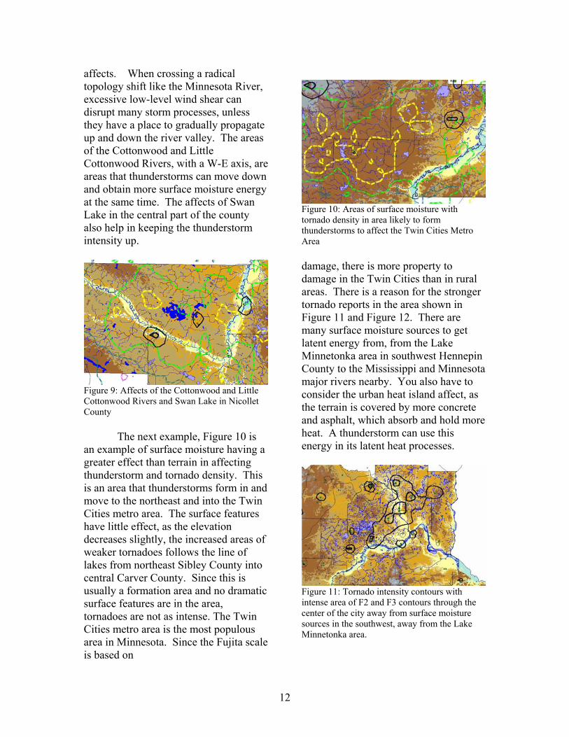
affects. When crossing a radical topology shift like the Minnesota River, excessive low-level wind shear can disrupt many storm processes, unless they have a place to gradually propagate up and down the river valley. The areas of the Cottonwood and Little Cottonwood Rivers, with a W-E axis, are areas that thunderstorms can move down and obtain more surface moisture energy at the same time. The affects of Swan Lake in the central part of the county also help in keeping the thunderstorm intensity up.

Figure 9: Affects of the Cottonwood and Little Cottonwood Rivers and Swan Lake in Nicollet County

The next example, Figure 10 is an example of surface moisture having a greater effect than terrain in affecting thunderstorm and tornado density. This is an area that thunderstorms form in and move to the northeast and into the Twin Cities metro area. The surface features have little effect, as the elevation decreases slightly, the increased areas of weaker tornadoes follows the line of lakes from northeast Sibley County into central Carver County. Since this is usually a formation area and no dramatic surface features are in the area, tornadoes are not as intense. The Twin Cities metro area is the most populous area in Minnesota. Since the Fujita scale is based on

Figure 10: Areas of surface moisture with tornado density in area likely to form thunderstorms to affect the Twin Cities Metro Area damage, there is more property to damage in the Twin Cities than in rural areas. There is a reason for the stronger tornado reports in the area shown in Figure 11 and Figure 12. There are many surface moisture sources to get latent energy from, from the Lake Minnetonka area in southwest Hennepin County to the Mississippi and Minnesota major rivers nearby. You also have to consider the urban heat island affect, as the terrain is covered by more concrete and asphalt, which absorb and hold more heat. A thunderstorm can use this energy in its latent heat processes.

Figure 11: Tornado intensity contours with intense area of F2 and F3 contours through the center of the city away from surface moisture sources in the southwest, away from the Lake Minnetonka area.

13

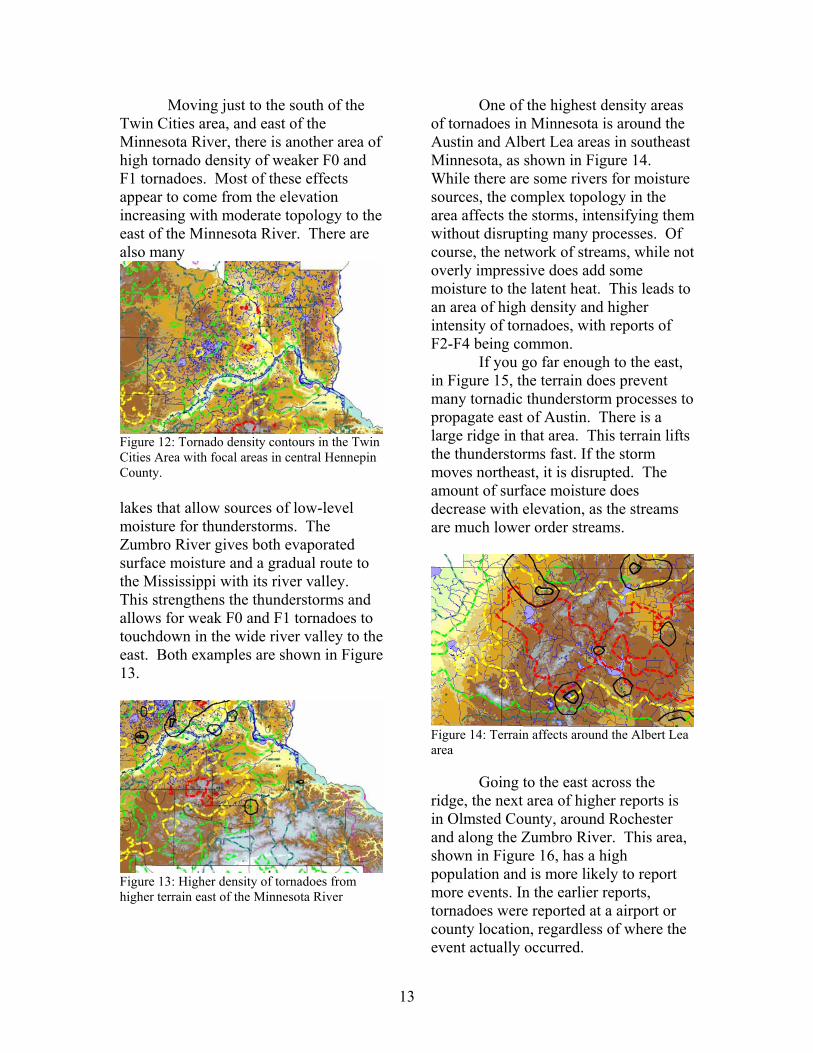
Moving just to the south of the Twin Cities area, and east of the Minnesota River, there is another area of high tornado density of weaker F0 and F1 tornadoes. Most of these effects appear to come from the elevation increasing with moderate topology to the east of the Minnesota River. There are also many

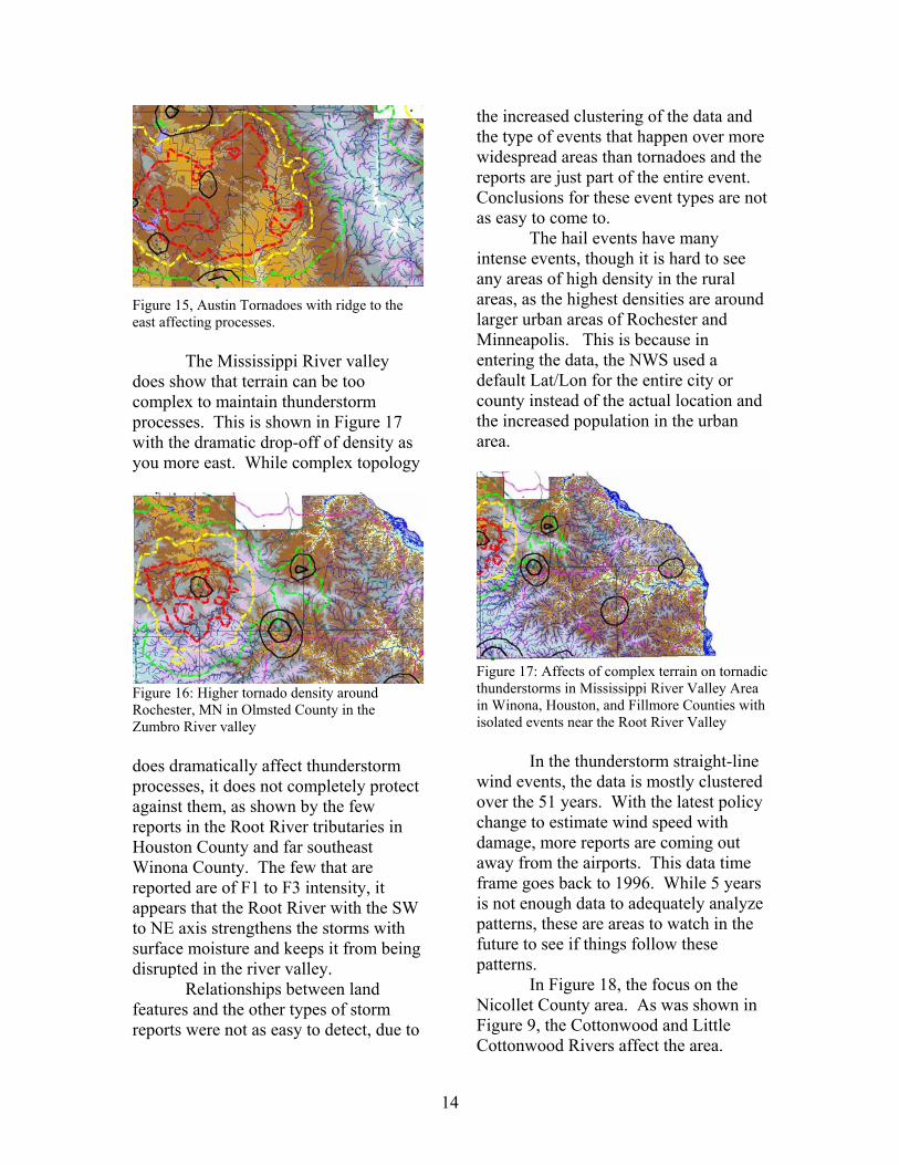
Figure 12: Tornado density contours in the Twin Cities Area with focal areas in central Hennepin County. lakes that allow sources of low-level moisture for thunderstorms. The Zumbro River gives both evaporated surface moisture and a gradual route to the Mississippi with its river valley. This strengthens the thunderstorms and allows for weak F0 and F1 tornadoes to touchdown in the wide river valley to the east. Both examples are shown in Figure 13.

Figure 13: Higher density of tornadoes from higher terrain east of the Minnesota River

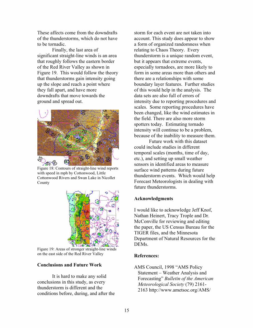
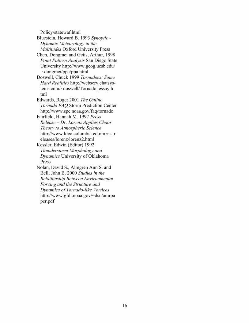
One of the highest density areas of tornadoes in Minnesota is around the Austin and Albert Lea areas in southeast Minnesota, as shown in Figure 14. While there are some rivers for moisture sources, the complex topology in the area affects the storms, intensifying them without disrupting many processes. Of course, the network of streams, while not overly impressive does add some moisture to the latent heat. This leads to an area of high density and higher intensity of tornadoes, with reports of F2-F4 being common. If you go far enough to the east, in Figure 15, the terrain does prevent many tornadic thunderstorm processes to propagate east of Austin. There is a large ridge in that area. This terrain lifts the thunderstorms fast. If the storm moves northeast, it is disrupted. The amount of surface moisture does decrease with elevation, as the streams are much lower order streams.

Figure 14: Terrain affects around the Albert Lea area Going to the east across the ridge, the next area of higher reports is in Olmsted County, around Rochester and along the Zumbro River. This area, shown in Figure 16, has a high population and is more likely to report more events. In the earlier reports, tornadoes were reported at a airport or county location, regardless of where the event actually occurred.

14

Figure 15, Austin Tornadoes with ridge to the east affecting processes. The Mississippi River valley does show that terrain can be too complex to maintain thunderstorm processes. This is shown in Figure 17 with the dramatic drop-off of density as you more east. While complex topology

Figure 16: Higher tornado density around Rochester, MN in Olmsted County in the Zumbro River valley does dramatically affect thunderstorm processes, it does not completely protect against them, as shown by the few reports in the Root River tributaries in Houston County and far southeast Winona County. The few that are reported are of F1 to F3 intensity, it appears that the Root River with the SW to NE axis strengthens the storms with surface moisture and keeps it from being disrupted in the river valley. Relationships between land features and the other types of storm reports were not as easy to detect, due to

the increased clustering of the data and the type of events that happen over more widespread areas than tornadoes and the reports are just part of the entire event. Conclusions for these event types are not as easy to come to.

The hail events have many intense events, though it is hard to see any areas of high density in the rural areas, as the highest densities are around larger urban areas of Rochester and Minneapolis. This is because in entering the data, the NWS used a default Lat/Lon for the entire city or county instead of the actual location and the increased population in the urban area.

Figure 17: Affects of complex terrain on tornadic thunderstorms in Mississippi River Valley Area in Winona, Houston, and Fillmore Counties with isolated events near the Root River Valley

In the thunderstorm straight-line wind events, the data is mostly clustered over the 51 years. With the latest policy change to estimate wind speed with damage, more reports are coming out away from the airports. This data time frame goes back to 1996. While 5 years is not enough data to adequately analyze patterns, these are areas to watch in the future to see if things follow these patterns.

In Figure 18, the focus on the Nicollet County area. As was shown in Figure 9, the Cottonwood and Little Cottonwood Rivers affect the area.

15

These affects come from the downdrafts of the thunderstorms, which do not have to be tornadic.

Finally, the last area of significant straight-line winds is an area that roughly follows the eastern border of the Red River Valley as shown in Figure 19. This would follow the theory that thunderstorms gain intensity going up the slope and reach a point where they fall apart, and have more downdrafts that move towards the ground and spread out.

Figure 18: Contours of straight-line wind reports with speed in mph by Cottonwood, Little Cottonwood Rivers and Swan Lake in Nicollet County

Figure 19: Areas of stronger straight-line winds on the east side of the Red River Valley Conclusions and Future Work It is hard to make any solid conclusions in this study, as every thunderstorm is different and the conditions before, during, and after the

storm for each event are not taken into account. This study does appear to show a form of organized randomness when relating to Chaos Theory. Every thunderstorm is a unique random event, but it appears that extreme events, especially tornadoes, are more likely to form in some areas more than others and there are a relationships with some boundary layer features. Further studies of this would help in the analysis. The data sets are also full of errors of intensity due to reporting procedures and scales. Some reporting procedures have been changed, like the wind estimates in the field. There are also more storm spotters today. Estimating tornado intensity will continue to be a problem, because of the inability to measure them. Future work with this dataset could include studies in different temporal scales (months, time of day, etc.), and setting up small weather sensors in identified areas to measure surface wind patterns during future thunderstorm events. Which would help Forecast Meteorologists in dealing with future thunderstorms. Acknowledgments I would like to acknowledge Jeff Knof, Nathan Heinert, Tracy Trople and Dr. McConville for reviewing and editing the paper, the US Census Bureau for the TIGER files, and the Minnesota Department of Natural Resources for the DEMs. References: AMS Council, 1998 “AMS Policy

Statement – Weather Analysis and Forecasting” Bulletin of the American Meteorological Society (79) 2161-2163 http://www.ametsoc.org/AMS/

16

Policy/statewaf.html Bluestein, Howard B. 1993 Synoptic -

Dynamic Meteorology in the Multitudes Oxford University Press

Chen, Dongmei and Getis, Arthur, 1998 Point Pattern Analysis San Diego State University http://www.geog.ucsb.edu/

~dongmei/ppa/ppa.html Doswell, Chuck 1999 Tornadoes: Some

Hard Realities http://webserv.chatsys-tems.com/~doswell/Tornado_essay.h-tml

Edwards, Roger 2001 The Online Tornado FAQ Storm Prediction Center http://www.spc.noaa.gov/faq/tornado

Fairfield, Hannah M. 1997 Press Release – Dr. Lorenz Applies Chaos Theory to Atmospheric Science http://www.ldeo.columbia.edu/press_releases/lorenz/lorenz2.html

Kessler, Edwin (Editor) 1992 Thunderstorm Morphology and Dynamics University of Oklahoma Press

Nolan, David S., Almgren Ann S. and Bell, John B. 2000 Studies in the Relationship Between Environmental Forcing and the Structure and Dynamics of Tornado-like Vortices http://www.gfdl.noaa.gov/~dsn/amrpaper.pdf