Using HDR Sky Luminance Maps to Improve Accuracy of ... · Proceedings of the 15th IBPSA Conference San Francisco, CA, USA, Aug. 7-9, 2017 1448 sensors are capable of considering

Proceedings of the 15th IBPSA ConferenceSan Francisco, CA, USA, Aug. 7-9, 2017

1447https://doi.org/10.26868/25222708.2017.368

Using HDR Sky Luminance Maps to Improve Accuracy of Virtual Work Plane Illuminance Sensors

Christian Humann, Andrew McNeil

Terrestrial Light, Berkeley, California, USA

Abstract Virtual sensors use simulation to predict conditions at predetermined locations. Such sensors can potentially replace physical sensors for controlling automated building systems, saving cost, labor, and permitting sensor locations that would not be feasible for physical devices. This study tests the accuracy of virtual work plane illuminance sensors against real world measurements in a physical, scale model illuminated under varying sky conditions. We consider three methods for modelling exterior daylight conditions as follows: 1. The Perez All-weather sky. 2. A horizontal HDR sky image. 3. A vertically oriented hemispherical HDR image of

the exterior environment.

Introduction Architects and lighting designers commonly strive to increase provisions for daylight and views in commercial buildings. While there is no physiological difference between daylight and electric light for visual acuity, there is evidence that daylight in commercial buildings reinforces circadian rhythms, and that strong circadian cycles improve worker health and productivity (Boyce et al. 2003). At times, daylight entering through windows will cause visual discomfort and glare. Providing static shading elements that effectively shade the window for all possible conditions without significantly hampering daylight or views is challenging and/or costly. Often, designers will opt for a dynamic solution that can be deployed when needed and retracted when not. When manually controlled by occupants, these devices are controlled in a sub-optimal manner (O’Brien et al. 2013). Additionally, evidence suggests that shades are often kept in compromised positions or completely closed for much of the time without being adjusted (Rubin et al. 1978). Providing automated, dynamic shading is an attractive option over manual operation for preventing shades from being left closed indefinitely, improving both daylight and views. However, a common outcome of automated shading control is dissatisfied occupants. When designing their new headquarters, the New York Times enlisted the help of Lawrence Berkeley National Lab’s

Windows and Daylighting group to provide assistance with designing and commissioning the shade controls. Years later in a post-occupancy report, Lee et al. found that “many occupants felt that shades were controlled in a meaningless or inappropriate manner” (Lee et al. 2013). Later, Genentech enlisted the help of LBNL to commission and test their automated shading controls (McNeil et al. 2013) and again, anecdotal evidence suggested that occupants were not satisfied with how the shades were controlled (Kohler, C. 2014. Personal communication August 24). The current state of the art in automated shade controls employs an array of exterior mounted radiometers and photometers to measure sky conditions and sky brightness’ from a building’s roof top as well as from specific façade orientations. Unfortunately these radiometers and photometers are only capable of taking very specific measurements (i.e. irradiation and illuminance) of the global component of the sky (i.e. the diffuse sky and solar contribution are measured together). Without the ability to sample the sky directionally and discreetly, clouds cannot be discerned from the clear sky component to determine such metrics as amount of cloud coverage, cloud size and brokenness of cloud coverage. Given the temporal and spatial dynamics of the sky, these measurements are necessary for approximating and predicting if, when, and for how long the sun is or may be occluded by clouds. Without the latter capabilities, controls systems tend to either not react in time, or to overreact when control is or is not needed. Additionally, building interiors often employ physical sensors at discrete zones for controlling automated systems. However, these sensors can be expensive to install, difficult to commission and often located too far away from the areas they are meant to control. Using simulation to estimate the physical condition at a location, virtual sensors offer a potential solution to the difficulties associated with physical sensors (Zach 2013 and Zain 2016). Furthermore, physical sensors typically provide a single integrated value without accounting for the size, intensity and direction of potential glare sources. For example, a small specular reflection off of a nearby building would likely cause only a small increase in the value reported by a typical, spatially integrated sensor while still causing a substantial risk of glare. Virtual


1448

sensors are capable of considering size, intensity and direction when determining glare risk, allowing them to identify the relatively low energy but high intensity specular reflection as a source of glare. This study investigates the potential use of roof mounted cameras for capturing HDR sky illuminance maps as input to a simulation based, automated building controls system. With the advent and increased use of building information modelling (BIM) in the building industry, the authors identify a strong potential for leveraging the accuracy of and the ease of updating these models as proxies for the actual building spaces for use in automated controls. In addition, the increased availability of 3D models of urban neighbourhoods allows these models to be situated within the context of their local site in order to minimize the effect that camera parallax and exterior-reflecting surfaces might have on accuracy. The ultimate goal of these studies will be to offer a way of making buildings more sentient and responsive to the temporal and spatial changes in their local environment. Being the first of several, this study tests the accuracy of virtual work plane illuminance sensors against real world measurements in a physical, scale model globally illuminated by different sky conditions. Additionally we compare three of the following sources for characterizing the sky condition used to simulate virtual sensor values: 1. The industry standard Perez All-weather sky model

(Perez et al. 1993) with measured values of diffuse horizontal and direct normal illuminance as inputs.

2. A camera system with a fisheye lens oriented horizontal to the ground plane for capturing diffuse sky luminance maps that are post processed to include the contribution of the measured, direct solar component.

3. The same camera system as 2, but with the camera lens oriented vertically.

Background It has been generally accepted amongst researchers and practitioners in the building simulation field that daylight simulation, using mathematical representations of the sky as input to physically based rendering (PBR) techniques, can produce errors up to 20% when calculating horizontal illuminance levels (Rea 2000). While recent research has focussed on evaluating the accuracy of using HDR luminance maps as input to image based lightning (IBL) simulation, these studies have primarily focussed on comparing the results against PBR techniques rather than against real, monitored spaces (Inanici et al. 2016). Additionally, these studies have focused on luminance comparisons relative to visual comfort, rather than task illuminance (jones et al. 2017). Furthermore, while recent studies have also compared results between using vertical and horizontal camera orientations for capturing HDR images as input to IBL simulations, these studies have also mostly

focused on resultant values of luminance relative to visual comfort (Inanici 2010). The daylight simulation requires information regarding the current luminance distribution of the sky. The Perez All-weather sky model (Perez 1993) is commonly employed to represent various sky conditions using direct normal and horizontal diffuse irradiance/illuminance values as input. However, the Perez All-weather sky model cannot reproduce luminance variations caused by cloud patterns. Using a camera system to capture an HDR image of the sky for use as a sky luminance map in the daylight simulation can provide substantial improvement in replicating current daylight conditions (Inanici 2010). A study similar to this one demonstrated a simulation based control system (Mahdavi 2008) using sky luminance maps derived from low dynamic range images and horizontal illuminance measurements. The study used 256 discrete sky patches to represent the sky luminance distribution in daylight simulations for controlling the adjustment of window shades at 15-minute intervals.

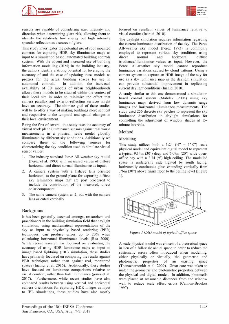
Method Modelling This study utilizes both a 1:24 (½” = 1’-0”) scale physical model and equivalent digital model to represent a typical 9.14m (30’) deep and 6.09m (20’) wide open-office bay with a 2.74 (9’) high ceiling. The modelled space is unilaterally side lighted by south facing, horizontally continuous glass extending vertically from .76m (30”) above finish floor to the ceiling level (Figure 1).

Figure 1 CAD model of typical office space

A scale physical model was chosen of a theoretical space in lieu of a full-scale actual space in order to reduce the systematic errors often introduced when modelling, either physically or virtually, the geometric and photometric properties of an existing space (Thanachareonkit et al. 2009). Great care was taken to match the geometric and photometric properties between the physical and digital model. In addition, photocells were placed at reasonable distances from the window wall to reduce scale effect errors (Cannon-Brookes 1997).


1449

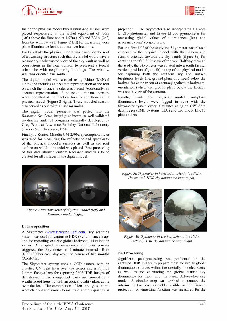
Inside the physical model two illuminance sensors were placed respectively at the scaled equivalent of .76m (30”) above the floor and at 4.57m (15’) and 7.31m (24’) from the window wall (Figure 2 left) for measuring work plane illuminance levels at these two locations. For this study the physical model was placed on the roof of an existing structure such that the model would have a reasonably unobstructed view of the sky vault as well as obstructions in the near horizon to represent a typical urban site with neighbouring buildings. The window wall was oriented true south. The digital model was created using Rhino (McNeel 1993) and includes an accurate representation of the roof on which the physical model was placed. Additonally, an accurate representation of the two illuminance sensors were modelled at the identical locations to those in the physical model (Figure 2 right). These modeled sensors also served as our ‘virtual’ sensor nodes. The digital model geometry was ported into the Radiance Synthetic Imaging software, a well-validated ray-tracing suite of programs originally developed by Greg Ward at Lawrence Berkeley National Laboratory (Larson & Shakespeare, 1998). Finally, a Konica Minolta CM-2500d spectrophotometer was used for measuring the reflectance and specularity of the physical model’s surfaces as well as the roof surface on which the model was placed. Post-processing of this data allowed custom Radiance materials to be created for all surfaces in the digital model.

Figure 2 Interior views of physical model (left) and

Radiance model (right)

Data Acquisition A Skyometer (www.terrestriallight.com) sky scanning system was used for capturing HDR sky luminance maps and for recording exterior global horizontal illumination values. A scripted, time-sequence computer process triggered the Skyometer at 3-minute intervals from 0700-1800hrs each day over the course of two months (April-May). The Skyometer system uses a CCD camera with an attached UV light filter over the sensor and a Fujinon 1.4mm fisheye lens for capturing 360° HDR images of the skyvault. The component parts are housed in a weatherproof housing with an optical quality glass dome over the lens. The combination of lens and glass dome were checked and shown to maintain a true, equiangular

projection. The Skyometer also incorporates a Li-cor LI-210 photometer and Li-cor LI-200 pyranometer for measuring global values of illuminance (lux) and irradiance (w/m2) respectively. For the first half of the study the Skyometer was placed adjacent to the physical model with the camera and sensors oriented towards the sky zenith (figure 3a) for capturing the full 360° view of the sky. Halfway through the study, the Skyometer was rotated into a south facing, vertical position (figure 3b) on top of the physical model for capturing both the southern sky and surface brightness levels (i.e. ground plane and trees) below the horizon for comparison of accuracy against its horizontal orientation (where the ground plane below the horizon was not in view of the camera). Finally, inside the physical model workplane illuminance levels were logged in sync with the Skyometer system every 3-minutes using an OWL3pro data logger (EME Systems, LLC) and two Li-cor LI-210 photometers.

Figure 3a Skyometer in horizontal orientation (left).

Horizontal, HDR sky luminance map (right)

Figure 3b Skyometer in vertical orientation (left).

Vertical, HDR sky luminance map (right)

Post Processing Significant post-processing was performed on the captured HDR images to prepare them for use as global illumination sources within the digitally modeled scene as well as for calculating the global diffuse sky illuminance for input into the Perez All-weather sky model. A circular crop was applied to remove the interior of the lens assembly visible in the fisheye projection. A vingetting function was measured for the


1450

combination of camera lens and glass dome and applied to the images as in Inanici (2010). Additionally, a precalculated intensity scale factor was applied to the image based on comparative readings from a Konica Minolta LS-110 luminance meter in order to put the HDR pixel values in calbrated units of luminance (cd/m2). Finally, a 5° solid angle (WMO 2010) disk was modelled and masked over the sun and its circumsolar region in all images (HDRsunmask) where the sun was not occluded by clouds, trees or other buildings. Due to the upper limit of the camera’s CCD sensor’s pixel well capacity (a pixel’s maximum charge saturation level from incoming light), the brightness of the solar disc, as well as a large portion of its circumsolar region, can not be fully captured using the HDR process. However, as some circumsolar brightness is captured using the HDR process, the superimposed disk removes the direct solar contribution allowing the postprocessed image to be used for both the calculation and representation of the diffuse sky component for input into the Perez All-weather sky model and the two HDR sky luminance map models respectively.

Daylight input Three methods for modelling exterior daylight environments were used for comparison in this study for measuring the accuracy of the virtual sensors: (1) the industry standard Perez All-weather sky with inputs of diffuse horizontal sky illuminance and direct normal solar illuminance values; (2) the horizontally oriented, post processed, HDR sky luminance map combined with a modeled description of the direct normal solar component; and (3) the vertically oriented version of the latter. For the three sky models, illuminance (lux) values for the direct and diffuse sky components were used rather than full spectrum irradiance (w/m2) values due to the inherent limitation of the camera sensor to capture outside the visible light specrtrum (400-700nm). The diffuse horizontal illuminance sky component (DHIllum) was calculated directly from the HDRsunmask using Radiance’s pcomb, pvalue and rcalc programs to first perform a solid angle correction of the image’s angular, fisheye projection and then to integrate over the image’s pixels for calculating their total contribution to diffuse sky illuminance. For the Perez sky model and the horizontal HDR model, the direct normal illuminance (DNIllum) was calclutated by inputing the DHIllum value (measured form the HDRsunmask) and the global horizontal illuminance (GHIllum) value (measured from the Skyometer’s photometer) into the equation:

DNIllum=(GHIllum-DHIllum)/sin𝜃. (1)

Where: DNIllum direct normal iilluminance GHIllum global horizontal illuminance DHIllum diffuse horizontal illuminance

𝜃 sun’s altitude angle above horizon The DNIllum for the vertically oriented HDR model was calclutated by inputing the diffuse vertical sky illuminance (DVIllum) value (measured from the vertical HDRsunmask using the same process as described for DHIllum) and the global vertical illuminance (GVIllum) value (measured from the Skyometer’s photometer) into the equation:

DNIllum=(GVIllum-DVIllum)/cos𝜃�𝑐𝑜𝑠Ψ. (2)

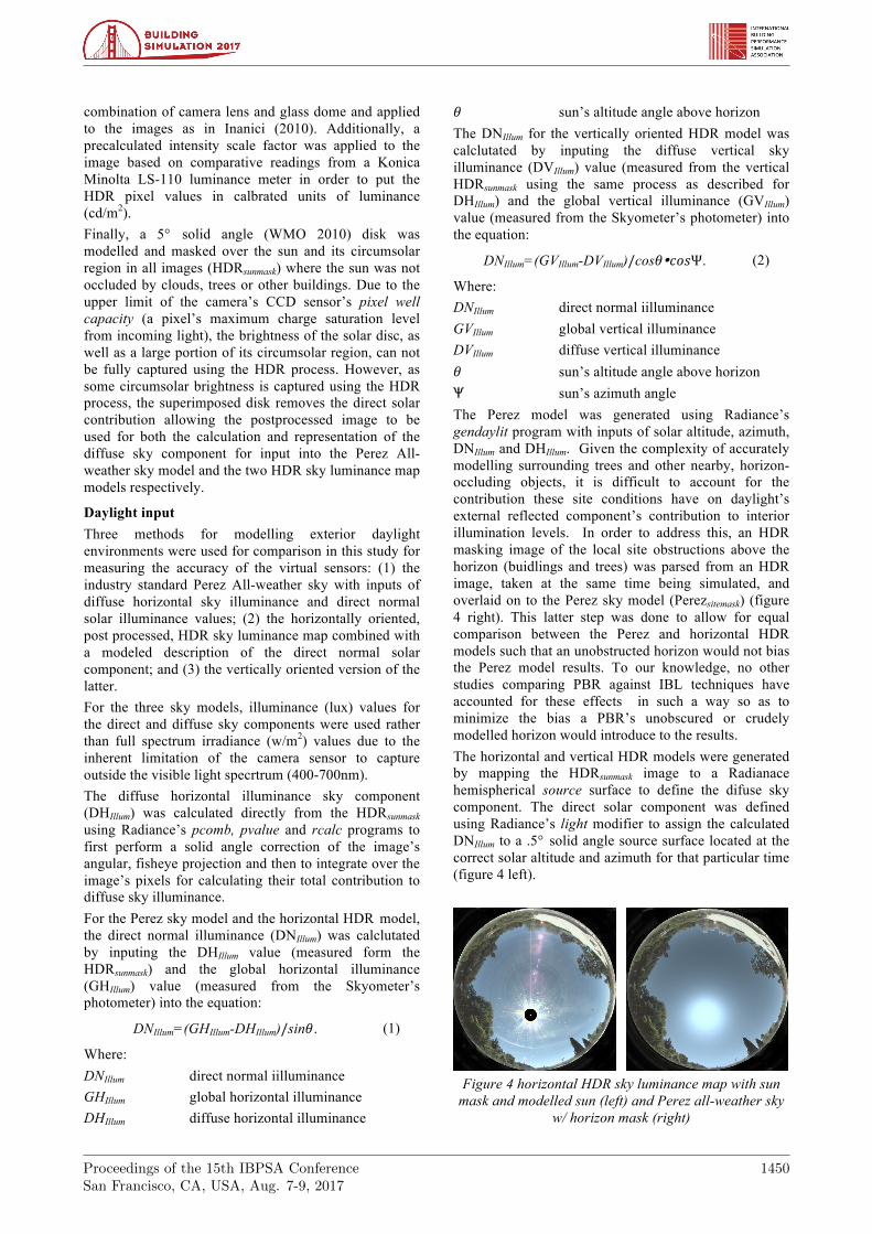
Where: DNIllum direct normal iilluminance GVIllum global vertical illuminance DVIllum diffuse vertical illuminance 𝜃 sun’s altitude angle above horizon Ψ sun’s azimuth angle The Perez model was generated using Radiance’s gendaylit program with inputs of solar altitude, azimuth, DNIllum and DHIllum. Given the complexity of accurately modelling surrounding trees and other nearby, horizon-occluding objects, it is difficult to account for the contribution these site conditions have on daylight’s external reflected component’s contribution to interior illumination levels. In order to address this, an HDR masking image of the local site obstructions above the horizon (buidlings and trees) was parsed from an HDR image, taken at the same time being simulated, and overlaid on to the Perez sky model (Perezsitemask) (figure 4 right). This latter step was done to allow for equal comparison between the Perez and horizontal HDR models such that an unobstructed horizon would not bias the Perez model results. To our knowledge, no other studies comparing PBR against IBL techniques have accounted for these effects in such a way so as to minimize the bias a PBR’s unobscured or crudely modelled horizon would introduce to the results. The horizontal and vertical HDR models were generated by mapping the HDRsunmask image to a Radianace hemispherical source surface to define the difuse sky component. The direct solar component was defined using Radiance’s light modifier to assign the calculated DNIllum to a .5° solid angle source surface located at the correct solar altitude and azimuth for that particular time (figure 4 left).

Figure 4 horizontal HDR sky luminance map with sun

mask and modelled sun (left) and Perez all-weather sky w/ horizon mask (right)


1451

Simulation The physical model was simulated at each 3-minute time step from 0700-1800hrs using Radiance’s rtrace program to measure horizontal illuminance at the two virtual sensor locations in the digital model. For the horizontal Skyometer orientation (figure 3a), two rtrace calculations were performed for each time step: once using the Perezsitemask model; and a second time using the horizontal HDRsunmask model with a modelled description of the sun. For days using the vertical Skyometer orientation (figure 3b), only one rtrace calculation was performed using the south facing, vertical HDRsunmask model and modelled sun description. For expediency, the simulations were run without ambient caching by setting the ambient accuracy parameter to zero (-aa 0). Prior to running the rtrace calculations a convergence test of three important Radiance parameters for simulation accuracy (-ab, -ad and –lw) determined optimal settings for our situation. Convergence testing consisted of parametric simulations of the same condition while varying the three simulation parameters considered. Increasing the number of ambient bounces (-ab) generally increases the simulated illuminance result. Convergence for ambient bounces was achieved when adding more bounces no longer affected the simulation result. For ambient divisions (-ad) and limit weight (–lw) the parameter settings affects the variability between illuminance simulated at multiple, identical sensor positions. As ambient divisions increases and limit weight decreases variability in simulated illuminance result is diminished. Convergence was achieved when variability in simulation was negligible. The Radiance rtrace parameters selected for the simulations were:

rtrace -n 8 -w -h -I+ -aa 0 -ab 16 -ad 64000 -lr -24 -lw 1e-10 -dc 1 -ds 0 -u+

(3)

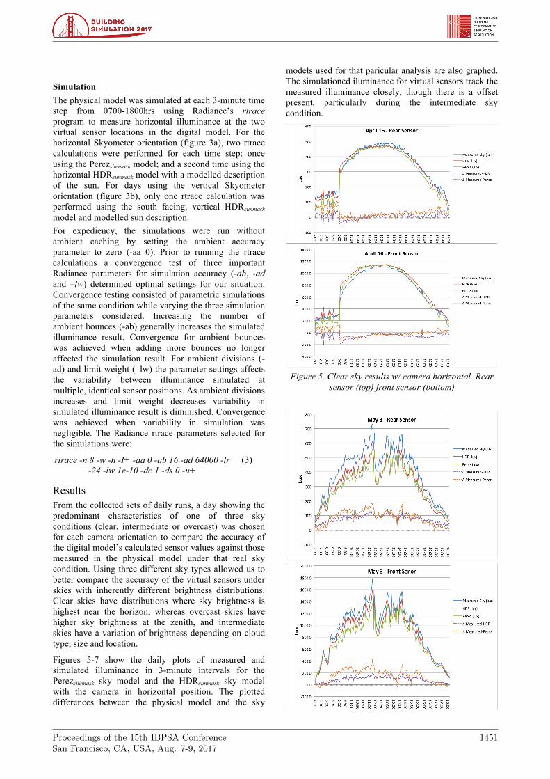
Results From the collected sets of daily runs, a day showing the predominant characteristics of one of three sky conditions (clear, intermediate or overcast) was chosen for each camera orientation to compare the accuracy of the digital model’s calculated sensor values against those measured in the physical model under that real sky condition. Using three different sky types allowed us to better compare the accuracy of the virtual sensors under skies with inherently different brightness distributions. Clear skies have distributions where sky brightness is highest near the horizon, whereas overcast skies have higher sky brightness at the zenith, and intermediate skies have a variation of brightness depending on cloud type, size and location.

Figures 5-7 show the daily plots of measured and simulated illuminance in 3-minute intervals for the Perezsitemask sky model and the HDRsunmask sky model with the camera in horizontal position. The plotted differences between the physical model and the sky

models used for that paricular analysis are also graphed. The simulationed iluminance for virtual sensors track the measured illuminance closely, though there is a offset present, particularly during the intermediate sky condition.

Figure 5. Clear sky results w/ camera horizontal. Rear

sensor (top) front sensor (bottom)


1452

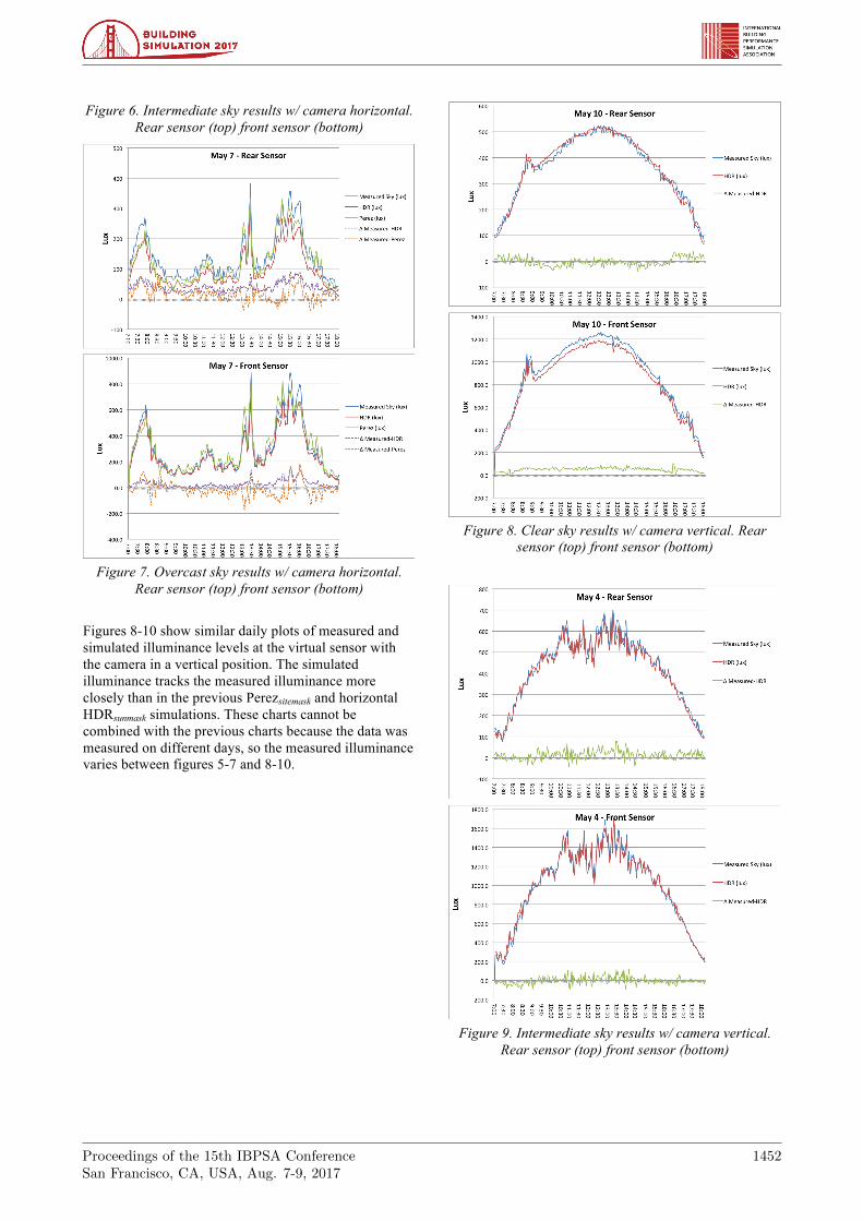
Figure 6. Intermediate sky results w/ camera horizontal. Rear sensor (top) front sensor (bottom)

Figure 7. Overcast sky results w/ camera horizontal.

Rear sensor (top) front sensor (bottom)

Figures 8-10 show similar daily plots of measured and simulated illuminance levels at the virtual sensor with the camera in a vertical position. The simulated illuminance tracks the measured illuminance more closely than in the previous Perezsitemask and horizontal HDRsunmask simulations. These charts cannot be combined with the previous charts because the data was measured on different days, so the measured illuminance varies between figures 5-7 and 8-10.

Figure 8. Clear sky results w/ camera vertical. Rear

sensor (top) front sensor (bottom)

Figure 9. Intermediate sky results w/ camera vertical.

Rear sensor (top) front sensor (bottom)


1453

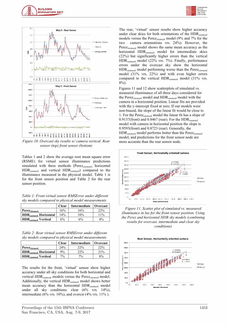
Figure 10. Overcast sky results w/ camera vertical. Rear

sensor (top) front sensor (bottom) Tables 1 and 2 show the average root mean square error (RSME) for virtual sensor illuminance predictions simulated with three methods (Perezsitemask, horizontal HDRsunmask and vertical HDRsunmask) compared to the illuminance measured in the physical model. Table 1 is for the front sensor position and Table 2 for the rear sensor position.

Table 1: Front virtual sensor RMSError under different sky models compared to physical model measurements

Clear Intermediate Overcast Perezsitemask 16% 16% 22% HDRsunmask Horizontal 14% 10% 11% HDRsunmask Vertical 6% 6% 4%

Table 2: Rear virtual sensor RMSError under different sky models compared to physical model measurements

Clear Intermediate Overcast Perezsitemask 24% 22% 22% HDRsunmask Horizontal 9% 22% 31% HDRsunmask Vertical 7% 7% 8%

The results for the front, ‘virtual’ sensor show higher accuracy under all sky conditions for both horizontal and vertical HDRsunmask models versus the Perezsitemask model. Additionally, the vertical HDRsunmask model shows better mean accuracy than the horizontal HDRsunmask model under all sky conditions: clear (6% vrs. 14%), intermediate (6% vrs. 10%), and overcst (4% vrs. 11% ).

The rear, ‘virtual’ sensor results show higher accuracy under clear skies for both orientations of the HDRsunmask models versus the Perezsitemask model (9% and 7% for the two camera orientations vrs. 24%). However, the Perezsitemask model shows the same mean accuracy as the horizontal HDRsunmask model for intermediate skies (22%) but significantly higher errors than the vertical HDRsunmask model (22% vrs. 7%). Finally, performance errors under the overcast sky show the horizontal HDRsunmask model performing worse than the Perezsitemask model (31% vrs, 22%) and with even higher errors compared to the vertical HDRsunmask model (31% vrs. 8%). Figures 11 and 12 show scatterplots of simulated vs. measured illuminance of all three days considered for the Perezsitemask model and HDRsunmask model with the camera in a horizontal position. Linear fits are provided with the y-intercept fixed at zero. If our models were non-biased, the slope of the linear fit would be close to 1. For the Perezsitemask model the linear fit has a slope of 0.9137(front) and 0.8467 (rear). For the HDRsunmask model with camera in horizontal position the slope is 0.9593(front) and 0.8723 (rear). Generally, the HDRsunmask model performs better than the Perezsitemask model, and predictions for the front sensor node are more accurate than the rear sensor node.

Figure 11. Scatter plot of simulated vs. measured

illuminance in lux for the front sensor position. Using the Perez and horizontal HDR sky models (combining

results for overcast, intermediate and clear sky conditions)


1454

Figure 12. Scatter plot of simulated vs. measured illuminance in lux for the rear sensor position. Using the

Perez and horizontal HDR sky models (combining results for overcast, intermediate and clear sky

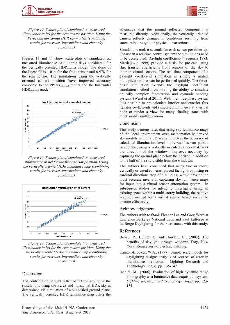
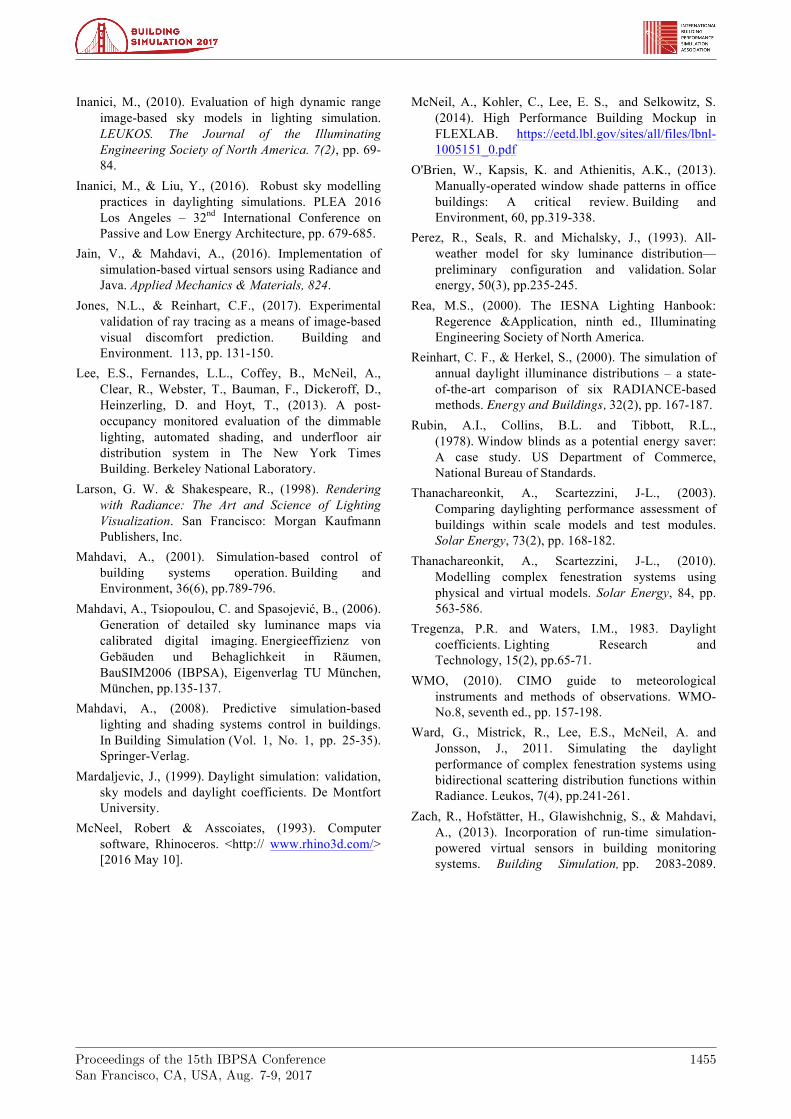
conditions) Figures 13 and 14 show scatterplots of simulated vs. measured illuminance of all three days considered for the vertically oriented HDRsunmask model. The slope of the linear fit is 1.014 for the front sensor and 0.978 for the rear sensor. The simulations using the vertically oriented camera position have improved accuracy compared to the PPerezsitemask model and the horizontal HDRsunmask model.


illuminance in lux for the front sensor position. Using the vertically oriented HDR luminance map (combining



illuminance in lux for the rear sensor position. Using the vertically oriented HDR luminance map (combining


Discussion The contribution of light reflected off the ground in the simulations using the Perez and horizontal HDR sky is determined via simulation of a simplified ground plane. The vertically oriented HDR luminance map offers the

advantage that the ground reflected component is measured directly. Additionally, the vertically oriented camera reflects changes in conditions resulting from snow, rain, drought, or physical obstructions.

Simulations took 6-seconds for each sensor per timestep. For use in a realtime control system the simulations need to be accelerated. Daylight coefficients (Tregenza 1983, Mardaljevic 1999) provide a basis for pre-calculating flux transfer coefficients from regions of the sky to interior virtual sensors. The real-time component of a daylight coefficient simulation is simply a matrix multiplication that can be performed quickly. The three-phase simulation extends the daylight coefficient simulation method incorporating the ability to simulate optically complex fenestration and dynamic shading systems (Ward et al 2011). With the three-phase system it is possible to pre-calculate interior and exterior flux transfer coefficients and simulate illuminance at a virtual node or render a view for many shading states with quick matrix multiplications.

Conclusion This study demonstrates that using sky luminance maps of the local environment over mathematically derived sky models within a 3D scene improves the accuracy of calculated illumination levels at ‘virtual’ sensor points. In addition, using a vertically oriented camera that faces the direction of the windows improves accuracy by capturing the ground plane below the horizon in addition to the half of the sky visible from the windows. The authors have concluded that using two or more, vertically oriented cameras, placed facing in opposing or cardinal directions atop of a building, would provide the most accurate means of capturing sky luminance maps for input into a virtual sensor automation system. In subsequent studies we intend to investigate, using an existing space within a multi-storey building, the relative accuracy needed for a virtual sensor based system to operate effectively.

Acknowledgement The authors wish to thank Eleanor Lee and Greg Ward at Lawrence Berkeley National Labs and Paul LaBerge at La Berge Daylighting for their assistance with this study.

References Boyce, P., Hunter, C. and Howlett, O., (2003). The

benefits of daylight through windows. Troy, New York: Rensselaer Polytechnic Institute.

Cannon-Brookes, W.A., (1997). Simple scale models for daylighting design: analysis of sources of error in illuminance prediction. Lighting Research and Technology. 29(3), pp. 135-142.

Inanici, M., (2006). Evaluation of high dynamic range photography as a luminance data acquisition system. Lighting Research and Technology. 38(2), pp. 123-134.


1455

Inanici, M., (2010). Evaluation of high dynamic range image-based sky models in lighting simulation. LEUKOS. The Journal of the Illuminating Engineering Society of North America. 7(2), pp. 69-84.

Inanici, M., & Liu, Y., (2016). Robust sky modelling practices in daylighting simulations. PLEA 2016 Los Angeles – 32nd International Conference on Passive and Low Energy Architecture, pp. 679-685.

Jain, V., & Mahdavi, A., (2016). Implementation of simulation-based virtual sensors using Radiance and Java. Applied Mechanics & Materials, 824.

Jones, N.L., & Reinhart, C.F., (2017). Experimental validation of ray tracing as a means of image-based visual discomfort prediction. Building and Environment. 113, pp. 131-150.

Lee, E.S., Fernandes, L.L., Coffey, B., McNeil, A., Clear, R., Webster, T., Bauman, F., Dickeroff, D., Heinzerling, D. and Hoyt, T., (2013). A post-occupancy monitored evaluation of the dimmable lighting, automated shading, and underfloor air distribution system in The New York Times Building. Berkeley National Laboratory.

Larson, G. W. & Shakespeare, R., (1998). Rendering with Radiance: The Art and Science of Lighting Visualization. San Francisco: Morgan Kaufmann Publishers, Inc.

Mahdavi, A., (2001). Simulation-based control of building systems operation. Building and Environment, 36(6), pp.789-796.

Mahdavi, A., Tsiopoulou, C. and Spasojević, B., (2006). Generation of detailed sky luminance maps via calibrated digital imaging. Energieeffizienz von Gebäuden und Behaglichkeit in Räumen, BauSIM2006 (IBPSA), Eigenverlag TU München, München, pp.135-137.

Mahdavi, A., (2008). Predictive simulation-based lighting and shading systems control in buildings. In Building Simulation (Vol. 1, No. 1, pp. 25-35). Springer-Verlag.

Mardaljevic, J., (1999). Daylight simulation: validation, sky models and daylight coefficients. De Montfort University.

McNeel, Robert & Asscoiates, (1993). Computer software, Rhinoceros. <http:// www.rhino3d.com/> [2016 May 10].

McNeil, A., Kohler, C., Lee, E. S., and Selkowitz, S. (2014). High Performance Building Mockup in FLEXLAB. https://eetd.lbl.gov/sites/all/files/lbnl-1005151_0.pdf

O'Brien, W., Kapsis, K. and Athienitis, A.K., (2013). Manually-operated window shade patterns in office buildings: A critical review. Building and Environment, 60, pp.319-338.

Perez, R., Seals, R. and Michalsky, J., (1993). All-weather model for sky luminance distribution—preliminary configuration and validation. Solar energy, 50(3), pp.235-245.

Rea, M.S., (2000). The IESNA Lighting Hanbook: Regerence &Application, ninth ed., Illuminating Engineering Society of North America.

Reinhart, C. F., & Herkel, S., (2000). The simulation of annual daylight illuminance distributions – a state-of-the-art comparison of six RADIANCE-based methods. Energy and Buildings, 32(2), pp. 167-187.

Rubin, A.I., Collins, B.L. and Tibbott, R.L., (1978). Window blinds as a potential energy saver: A case study. US Department of Commerce, National Bureau of Standards.

Thanachareonkit, A., Scartezzini, J-L., (2003). Comparing daylighting performance assessment of buildings within scale models and test modules. Solar Energy, 73(2), pp. 168-182.

Thanachareonkit, A., Scartezzini, J-L., (2010). Modelling complex fenestration systems using physical and virtual models. Solar Energy, 84, pp. 563-586.

Tregenza, P.R. and Waters, I.M., 1983. Daylight coefficients. Lighting Research and Technology, 15(2), pp.65-71.

WMO, (2010). CIMO guide to meteorological instruments and methods of observations. WMO-No.8, seventh ed., pp. 157-198.

Ward, G., Mistrick, R., Lee, E.S., McNeil, A. and Jonsson, J., 2011. Simulating the daylight performance of complex fenestration systems using bidirectional scattering distribution functions within Radiance. Leukos, 7(4), pp.241-261.

Zach, R., Hofstätter, H., Glawishchnig, S., & Mahdavi, A., (2013). Incorporation of run-time simulation-powered virtual sensors in building monitoring systems. Building Simulation, pp. 2083-2089.

Documents

Using HDR Sky Luminance Maps to Improve Accuracy of ... · Proceedings of the 15th IBPSA Conference San Francisco, CA, USA, Aug. 7-9, 2017 1448 sensors are capable of considering