Using Hilbert Curves to Organize, Sample, and Sonify Solar Data1

Abstract2

How many ways can we explore the Sun? We have images in many wavelengths and squiggly lines of3

many parameters that we can use to characterize the Sun. We know that while the Sun is blindingly bright4

to the naked eye it also has regions that are dark in some wavelengths of light and bright in others. All of5

those classifications are based on vision. Hearing is another sense that can be used to explore solar data.6

Some data, such as the sunspot number or the extreme ultraviolet spectral irradiance, can be readily sonified7

by converting the data values to musical pitches. Images are more difficult. Using a raster scan algorithm8

to convert a full-disk image of the Sun to a stream of pixel values is dominated by the pattern of moving on9

and off the limb of the Sun. A sonification of such a raster scan will contain discontinuities at the limbs that10

mask the information contained in the image. As an alternative, Hilbert curves are continuous space-filling11

curves that map a linear variable onto the two-dimensional coordinates of an image. We have investigated12

using Hilbert curves as a way to sample and analyze solar images. Reading the image along a Hilbert curve13

keeps most neighborhoods close together as the resolution (i.e., the order of the Hilbert curve) increases. It14

also removes most of the detector size periodicities and may reveal larger-scale features. We present several15

examples of sonified solar data, including the sunspot number, a selection of extreme ultraviolet (EUV)16

spectral irradiances, different ways to sonify an EUV image, and a series of EUV images during a filament17

eruption.18

1

2

I. INTRODUCTION19

Sonifying a data set has the basic purposes of making data accessible to the blind and allowing20

the data to serve as an adjunct to other senses. It can also help all to appreciate or understand a21

data set in a new way. Although a one-dimensional data set can be sonified by scaling the data22

to pitches, image data is a more ambitious target. The data has variations in two dimensions that23

should be represented by the sonification, and variations seen in a series of images are even more24

difficult to sonify. Solar data is often in the form of images and the changes in time and space are25

an integral part of understanding solar variations. We will describe sonifying several solar datasets,26

including an exploration of ways to sonify solar images in space and time.27

Composers have used many ways to create sounds and music that mimic the natural and me-28

chanical worlds. Camille Saint-Saëns used pianos and other instruments to imitate about 14 an-29

imals in The Carnival of the Animals.1 Old-time fiddle tunes use the flexibility of the combined30

performer and violin to imitate chickens and other natural sounds. Luigi Russolo built “intonaru-31

mori" to produce a broad spectrum of modulated, rhythmic sounds that imitated machines.2 He32

also developed a graphical form of musical score to compose pieces for these devices. Others33

have produced music from time sequences of the natural world. A well-known example is Concret34

PH,3 which was created by splicing together short, random segments of tape recordings of burning35

charcoal.36

Analog electronic synthesizers provided another path. In their early stages they were often37

used to produce sound effects. As analog synthesizers became more capable, such as the Moog38

modular synthesizer,4 some used them to reproduce well-known musical pieces in electronic form39

(e.g., Switched-On Bach by Wendy Carlos, 1968) while others invented new types of music (the40

improvisations of Keith Emerson in the works of Emerson, Lake, and Palmer.)41

Few, if any, of these techniques are examples of sonifying data. Sonification can be as simple42

as the shrieking of a smoke alarm or as complicated as converting multi-dimensional data to an43

audible signal. The incessant beeps and whistles of electronic vital sign monitors in hospitals are44

one example where the change in a sound signals a change in the health of a patient. These use45

the 1-D structure of sound to convey information that conditions are both normal and alarming.46

Whistlers are an example of how scientists sonified radio frequency data to study the ionosphere.547

3

The interactions of lightning with the electrons in the magnetosphere are heard as descending tones48

lasting a few seconds.49

Digital electronic synthesizers give us the ability to convert any type of information from a50

digital representation into music.6 One example is that a 1-D time series can be sonified by scaling51

the values to musical pitches, assuming a constant duration for each value, to produce a set of52

Musical Instrument Digital Interface (MIDI7) commands. A MIDI-enabled synthesizer is then used53

to create the musical instrument waveforms and play the commands in the MIDI file. Different54

time series can be combined into a sonification by using different pitch ranges or timbres (the55

distinctive set of tones in the selected instrument) to distinguish between them. We will use the56

International Sunspot Number (Version 2, S) and extreme ultraviolet (EUV) spectral irradiances57

from two satellites as examples of solar time series data.58

Sonifying an image is different. Sound is intrinsically a 1-D format that evolves in time. A 2-D59

image must be converted to a 1-D series of pixel values where the order of the pixels serves as the60

time variable. Once the 1-D sequence exists, the pixel values are scaled to pitches, the duration is61

again set to a constant, and the data run through the synthesizer.62

There are many ways to map a 2-D image (or higher-dimensional data) to a 1-D sequence. A63

raster scan is a linear reading of the image from the upper left to the lower right moving down to64

the next row when the current one is read, much like reading an English language document. This65

can be modified into a boustrophedonic algorithm where the first row is read left to right and the66

next right to left, continuing in this way to the end of the image. This resembles the way an ox67

(Greek bous) plows a field and hence the term. Another way is to use a space-filling curve, such68

as the Hilbert used here, to map the image pixels to a sequence. We will describe using Hilbert69

curves to convert 2-D images into 1-D sequences and converting those sequences to sound.70

The sonifications of these data sets will be described:71

1. International Sunspot Number (annual and monthly variations)72

2. Extreme ultraviolet (EUV) spectral irradiances as a time series and a spectrum73

3. A complete EUV image and seven subimages74

4. A montage of EUV images showing a filament liftoff75

4

All of the sound files are available as .MIDI and .MP3 files at https://sdo.gsfc.nasa.gov/sonify/76

table.html.77

We start by introducing some useful musical concepts. That will be followed by a discussion78

of the synthesizer used and the analysis of of the 1-D data sets. The image data will be introduced,79

and an example using a raster scan to convert the data to 1-D will be described. We will then80

describe the Hilbert curves used to address the image data and present several ways to sonify the81

images. We discuss what can be learned from these sonifications and end with several conclusions82

on the utility of this method. All of the science datasets are open-source and are available at the83

locations listed in the Acknowledgements.84

II. SONIFYING DATA85

The JythonMusic software described in Manaris and Brown 8 was used to convert a data series86

into MIDI commands and drive a synthesizer. The concepts and terms we use to convert data to87

music are:88

• Pitch: One of 128 frequencies (spanning 10.75 octaves of the 12-tone equal-tempered scale),89

from 8.18 Hz [C−1 ] – 12.54 kHz [G9]), with Middle C (C4, 261.63 Hz) roughly in the90

middle at position 60. Twenty one pitches are added below the lowest note on the piano91

and 19 pitches above the highest note. A range of only 128 values is small compared to the92

linear range of many solar and geophysical data sets. It is also small compared to the pitch93

discrimination of human ears. Untrained humans can discern pitch changes of ≈ 0.3%,994

so roughly 43000 pitches would be necessary to resolve that frequency range. However,95

the MIDI standard only allows limited microtones at that spacing. Images encoded with the96

Joint Photographic Experts Group (JPEG10) algorithm have pixel values ranging from 0–25597

(either in separate channels or through a color table), so we have only half of the range in98

pitches. Transforming data that varies by several orders of magnitude into logarithms can99

compress the range to small enough to sonify.100

• Duration and Tempo: The duration (or length) of pitches and rests (periods of time without101

any sound) are specified with a floating point number that can vary from 0 (no time) to 1102

(a quarter note) to 4 (corresponds to a whole note) and longer. The tempo of a piece is the103

5

speed at which the pitches and rests are heard. Tempo is specified by the number of beats per104

minute (bpm); where a quarter note (QN in JythonMusic) is one beat. Durations are relative105

to the tempo of the piece, increasing the tempo proportionally reduces the duration of all106

pitches and rests. We commonly use sixteenth notes in the image sonifications. A sixteenth107

note has a duration of 0.25 relative to a quarter note.108

• Loudness: The loudness (also called the dynamics or MIDI velocity) is set by an integer in109

the range 0 (silent) to 127 (very, very loud). As the range of sound pressure level varies from110

0 dB (threshold of hearing) to 120 dB (threshold of pain), the loudness maps to a change111

of roughly one per dB. The response of human ears to loudness variations strongly varies112

from one person to another and with frequency. The least noticeable change in loudness also113

varies with frequency, but a reasonable value is 0.4 dB.11 This corresponds to a 5% change114

in pressure and is easily accommodated by the 128 possible values. We only use loudness to115

weight the various datasets. It is also possible to encode information in the loudness, such116

as a longer duration being louder, but we do not present such cases here.117

• Timbre: There are 128 possible timbres in the MIDI standard, which are refered to as tracks.118

These timbres are not specified in the MIDI standard and a numbered timbre may sound119

different in different synthesizers. One track is devoted to percussion and uses the pitch120

designator to select a percussive timbre.121

• Pan: Position in space is limited in this study to left-right pan. A floating point number122

between 0 (left) and 1 (right) determines the position, with 0.5 (centered) the default. Placing123

one data set in the left side and another in the right is a good way to compare two data sets.124

Where they agree the sounds will appear to come from the middle and otherwise they will125

come from separate sides.126

JythonMusic is based on Java rather than C. Programs in JythonMusic are written in Python 2.7127

syntax but do not have access to many of the libraries used for numerical work. As a result, data128

access and extraction routines were written and executed in a C-based Python environment that129

provided access to the NumPy library for array manipulation. The computational sequence was to130

read the data, extract the appropriate part, write the extracted data to a comma-separated variable131

(CSV) file, read that file in the JythonMusic environment, convert the data into a MIDI file, and use132

6

the JythonMusic synthesizer to play that file. A permanent record was created by playing the MIDI133

commands in another synthesizer that could export the sounds to an MP3 file.134

III. SAMPLING AND SONIFYING SOLAR DATA135

Several types of solar data were sonified and reported here. A summary is presented in Table I,136

where the source, type, and name of the corresponding MP3 file are listed. The Sec. column is the137

part of the paper where the data is described. A version of this table, with links to the MP3 and138

MIDI files, is available at https://sdo.gsfc.nasa.gov/sonify/table.html.139

TABLE I. Files for each Sonified Data Set

Sec. Source Sonified Data mp3 Filename

III A SIDC Sunspot number TS_sunspot_annual_month.mid.mp3

III B EVE EUV spectral irradiances (spectrum) TS_EVE_sonified.mid.mp3

III B SEE EUV spectral irradiances (time series) TS_SEE_sonified.mid.mp3

III D AIA 193 Å Complete image (raster) AIA_193_full_image_sonified_raster.mp3

V AIA 193 Å Complete image (Hilbert) AIA_193_full_image_sonified.mid.mp3

V A AIA 193 Å Subimage 1 (Arcs) subimage_1_x_685_y_1755.mid.mp3

V A AIA 193 Å Subimage 2 (Fan) subimage_2_x_1060_y_1120.mid.mp3

V A AIA 193 Å Subimage 3 (Island) subimage_3_x_1290_y_1690.mid.mp3

V A AIA 193 Å Subimage 4 (Limb) subimage_4_x_1800_y_992.mid.mp3

V A AIA 193 Å Subimage 5 (Spot) subimage_5_x_890_y_1035.mid.mp3

V A AIA 193 Å Subimage 6 (Swirl) subimage_6_x_750_y_1125.mid.mp3

V A AIA 193 Å Subimage 7 (X) subimage_7_x_760_y_405.mid.mp3

V B AIA 193 Å Filament liftoff montage liftoff_complete.mid.mp3

140

141

142

A. International Sunspot Number143

The first example is the variation of the International Sunspot Number (S) with time. The144

sunspot number is a weighted count of dark regions on the Sun that is often used as a long-term145

7

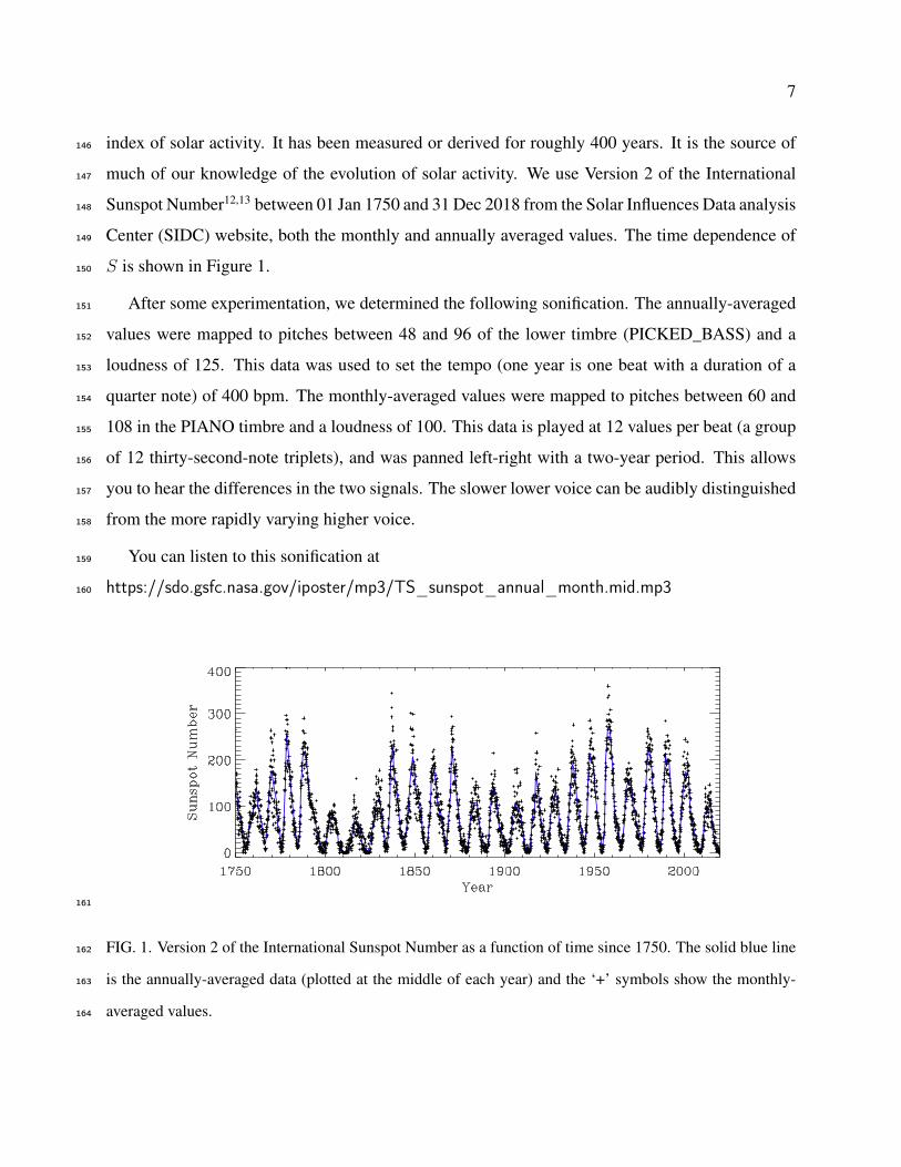
index of solar activity. It has been measured or derived for roughly 400 years. It is the source of146

much of our knowledge of the evolution of solar activity. We use Version 2 of the International147

Sunspot Number12,13 between 01 Jan 1750 and 31 Dec 2018 from the Solar Influences Data analysis148

Center (SIDC) website, both the monthly and annually averaged values. The time dependence of149

S is shown in Figure 1.150

After some experimentation, we determined the following sonification. The annually-averaged151

values were mapped to pitches between 48 and 96 of the lower timbre (PICKED_BASS) and a152

loudness of 125. This data was used to set the tempo (one year is one beat with a duration of a153

quarter note) of 400 bpm. The monthly-averaged values were mapped to pitches between 60 and154

108 in the PIANO timbre and a loudness of 100. This data is played at 12 values per beat (a group155

of 12 thirty-second-note triplets), and was panned left-right with a two-year period. This allows156

you to hear the differences in the two signals. The slower lower voice can be audibly distinguished157

from the more rapidly varying higher voice.158

You can listen to this sonification at159

https://sdo.gsfc.nasa.gov/iposter/mp3/TS_sunspot_annual_month.mid.mp3160

161

FIG. 1. Version 2 of the International Sunspot Number as a function of time since 1750. The solid blue line162

is the annually-averaged data (plotted at the middle of each year) and the ‘+’ symbols show the monthly-163

averaged values.164

8

B. Extreme Ultraviolet Spectral Irradiances165

The next example is to sonify extreme ultraviolet (EUV) spectral irradiances from two instru-166

ments in two ways. The solar EUV spectral irradiance spans wavelengths between X-rays and167

the ultraviolet (roughly 10–100 nm) but is often extended to include the H I 1216 emission line168

(Ly-α). (Emission lines are described by the element symbol, the ion state of the element [where169

H I is neutral hydrogen, H II is singly-ionized hydrogen, etc.], and the wavelength of the line170

in Å.) This radiation is easily absorbed as it ionizes the outer electrons of many elements. This171

also makes it the major source of the ionosphere in the terrestrial and planetary atmospheres. The172

EUV emissions are also a direct measure of the solar magnetic field. The Sun would have con-173

siderably smaller EUV emissions if it did not have a magnetic field. For a 5770 K blackbody,174

the spectral irradiance at an EUV wavelength of 30.4 nm is 10−26 times the peak value at175

the visible wavelength of 500 nm. This ratio is 10−4 in an observed solar spectrum. These two176

properties, sensitivity to the solar magnetic field and acting as the source of the ionosphere, make177

measurements of the solar EUV spectral irradiance a primary goal in solar physics.178

Solar EUV spectral irradiances are completely absorbed by the atmosphere and must be mea-179

sured by an instrument in space. These instruments record the spectral irradiances as a function180

of wavelength and time. We first sonify a single spectrum from the Extreme ultraviolet Variabil-181

ity Experiment (EVE)14 on NASA’s Solar Dynamics Observatory (SDO).15 EVE data is available182

from 5 to 105 nm from 1 May 2010 until 26 May 2014 and from 37–105 nm thereafter. Figure 2183

shows that the EUV spectral irradiance has many emission lines. Two of the strongest (He I 304184

and C III 977) are labeled, and several roughly triangular regions of continuum emission (such as185

the one highlighted between 70 nm and 91 nm.) The third label points to the emission line Fe XII186

193, which will be explored in later sections.187

We elected to sonify the day-averaged solar EUV spectrum from EVE on 27 Feb 2014, the day188

of maximum sunspot number for Solar Cycle 24 (Figure 2). The log of the spectral irradiances was189190

scaled to MIDI frequencies 36–96. That means every order of magnitude in the data spans about191

1.5 octaves. The PIANO timbre was used, each value occupies an 8th note, the tempo was set to192

600 bpm, and the loudness was set to 80.193

This example shows how the independent variable, in this case wavelength, does not have to194

9

FIG. 2. A day-averaged EUV spectral irradiance for 27 Feb 2014, as measured by EVE, plotted against the

wavelength in nm. Three wavelengths are identified with vertical dashed lines. The He II 304 Å line is the

brightest in this wavelength range, with the C III 977 Å line the next brightest. The 70–90 nm continuum

emission region is highlighted. The Fe XII 193 emission line will be analyzed in images below. Although the

total radiant energy in this spectrum is 4.7 mW m−2, about 10−5 times the total solar irradiance of 1361 W

m−2, it is responsible for much of the ionization in the thermospheres of the Earth, Venus, and Mars.

be time to sonify a data set. The independent variable must at least provide an ordering of the195

data set, in this case with a uniform spacing between the data points. This was judged to be the196

most musical example. Some of Bach’s Goldberg Variations (BWV 988) sound much like this197

sonification. Variation 24, at around the 33-minute mark as played by Glenn Gould in his 1981198

album of the same name, has several long chromatic runs that sound like the gradual rise of the199

EUV spectrum between 70–91 nm. The rapid increases in pitch of the strong spectral lines also200

add musical contrast to this piece.201

You can listen to this sonification at202

https://sdo.gsfc.nasa.gov/iposter/mp3/TS_EVE_sonified.mid.mp3203

Spectral irradiances at selected wavelengths can also be extracted from the measurements as204

a function of time. The source of another set of EUV spectral irradiances is the Solar Extreme205

10

ultraviolet Experiment (SEE)16 on NASA’s Thermosphere Ionosphere Mesosphere Energetics and206

Dynamics (TIMED) spacecraft, which provides daily values of the irradiances between 0.5 and207

195 nm. The spectral irradiances from 9 Feb 2002 to 11 May 2019 of several strong emission208

lines (He I 304, Ly-α, C IV 1548, and Fe XVI 335), along with the 0.1–7 nm soft X-ray radiometer209

channel, were sonified. The time dependence of these channels is shown in Figure 3. Pitches210

between 24 and 108 were interpolated from the log of the irradiances using the maximum and211

minimum of each channel as the limits. This forces the channels to have the same pitch range.212

The timbres were PIANO, PICKED_BASS, TROMBONE, FLUTE, and MARIMBA, respectively.213

Each value occupies an eighth note, the tempo was set to 640 bpm and the loudness was set to 100.214

You can listen to this sonification at215

https://sdo.gsfc.nasa.gov/iposter/mp3/TS_SEE_sonified.mid.mp3216

217

FIG. 3. The variation of selected EUV spectral irradiances from SEE with time. The selected wavelengths218

show different levels of solar cycle modulation. The Ly-α and 0.1–7 nm irradiances were divided by 10 and219

20, respectively, before plotting.220

11

C. Extreme Ultraviolet Images221

Although measuring the EUV spectral irradiance is important, understanding those emissions222

requires that you also have images at those wavelengths showing how the source regions of the223

emissions vary in both space and time. Extreme ultraviolet images from the Atmospheric Imaging224

Assembly (AIA)17 on SDO were sonified as complete images, subimages, and a time sequence225

of subimages. AIA provides 10 passbands: seven EUV, two ultraviolet, and one visible light.226

AIA 193 Å images were selected as they highlighted the desired coronal details. We will describe227

different ways to sonify an AIA 193 Å image from 23:55:53 UTC on 18 Mar 2018.228

Compared with time series data, we found that images are difficult to sonify because they are229

dense in information and have variations in two directions. As an example of density, a sonified230

512 × 512 image would take almost 15 hours to listen to at a moderate tempo of 300 bpm, and231

a full-resolution (4096×4096) AIA image would require 40 days. Many people have a hard time232

remembering tone sequences and whatever is happening near the end would be disconnected from233

the beginning. We overcome this by either binning the image to a smaller number of pixels or234

selecting subimages. Based on our experiences when playing our sonifications, where we found235

that a person can remember tone sequences for a few minutes, we aim to create sonifications that236

last three minutes by binning the image to 32 × 32 pixels or by using much higher tempos (up237

to 3000 bpm). Pieces such as John Cage’s Organ2/ASLSP (As Slow as Possible) may be written238

for performance times of hours to years, but the density of notes is far smaller in these pieces.239

Only 31 notes have been sounded since a 639 year version of the piece was begun in 2001 at the240

Burchardikirche in Halberstadt, Germany.18 One of our sonifications would sound 31 notes in the241

first 6.2 s at our standard tempo of 300 bpm.242

AIA science data is served as monochromatic, 4k×4k, 14-bit files using the Flexible Image243

Transport System (FITS).19 To make these sonifications more accessible to students, we elected244

to use the quicklook AIA images that are served as JPEG files created from the FITS data by245

binning to a lower resolution (typically 2048× 2048 pixels), then applying a log scaling and an246

arbitrary color table. Concentrating on converting JPEG images allowed us to test the algorithms247

using images with higher contrast or more distinct features. This allows the students to sonify248

their favorite images. When necessary the JPEG images were converted to greyscale using the249

12

luminosity form of relative luminance to weight the individual red (R), green (G), and blue (B)250

channels:251

IM(B&W) = 0.21R + 0.72G+ 0.07B. (1)

Although the solar images used have redundant information in the separate color channels, by252

applying the luminosity form to all JPEG images it is possible to analyze any image with a three-253

color format.254

D. Raster-scan Sampling255

The greyscale images must now be converted into a 1-D series for sonification. The first ex-256

ample is to sample them along a raster scan as described above. One initial image, binned from257

dimensions of 2048 × 2048 to 32 × 32, is shown in Figure 4, with the image overdrawn by the258

raster scan used to generate the sampling curve in the lower plot. This image is also shown in259

higher resolution and with fewer obscuring lines in Figure 7.260

Similar to the sunspot series in § III A, the image was sampled in two different resolutions. The261

higher register was scaled from the 32 × 32 binned image by mapping the pixel values between262

[0, 250] to pitches between [60, 120] (or C4 to C9, a span of 5 octaves). The duration was set to a263

sixteenth note, the loudness to 110, and the SOPRANO_SAX timbre was used. The lower register264

was added by mapping pixels from a 16× 16 binned image with values between [0,250] to pitches265

[48, 96] (or C3 to C7, a span of 4 octaves). The duration was set to a quarter note, the loudness266

to 90, and the ACOUSTIC_GRAND timbre was used. The dark regions of the lower register were267

omitted by being set to the special variable REST. The lower register is the average value of the268

four pitches in the higher register in the same region of the image. The relative timing of the voices269

is arbitrary, but we keep the two different sequences synchronized by using a ratio of four to one.270

You can listen to this sonification at271

https://sdo.gsfc.nasa.gov/iposter/mp3/AIA_193_full_image_sonified_raster.mp3272

The lower curve (b) in Figure 4 shows how the raster scan is dominated by the quasi-periodic273

variations caused by the scan moving onto and off of the disk of the Sun. We reduced some of the274

noisy variations at low pixel values by replacing the dark regions with a rest, but the sonification275

still does not reveal much about the image other than the broad shape of the Sun. As a result, we276

13

FIG. 4. A greyscale SDO/AIA 193 Å image from 18 Mar 2019 binned from 2048× 2048 to 32× 32. At the

top is an example of how a raster scan from the top left to the lower right samples the image. The dashed

lines are the return from right to left that is not used in the sampling. The resulting sampling curve for this

image is shown in the lower plot (b). The vertical lines show the four horizontal strips of the image.

explored using other methods to sample the image. The Hilbert curve was one of those methods.277

14

IV. HILBERT CURVES278

Hilbert curves are continuous space-filling curves that have been used in a surprisingly large279

number of disciplines. They were first described by Hilbert 20 as a simpler form of the space-filling280

curves of Peano 21 . A true Hilbert curve exists only as the limit of n→∞ of the nth approximation281

to a Hilbert curve (Hn). However, the approximations are useful to provide mappings of 2-D282

images onto a 1-D sequence. Figure 5 shows Hn for n = 1, 2, . . . , 6.283

A summary of the properties of Hn:284

1. There are 2n pixels along each side of the square containing the curve285

2. The Euclidean length of Hn grows exponentially with n, 2n − 2−n286

3. Hn covers a finite area as it is always bounded by the unit square287

4. Two points in the image, (x1, y2) and (x2, y2), that are close together in Hn are also, with a288

few exceptions, close together in Hn′ , n′ > n289

A Hilbert curve maps a linear variable onto the two-dimensional coordinates of an image. Its290

inverse is a mapping of the image coordinates onto a linear variable. This mapping property means291

we can use Hilbert curves to map solar images onto a linear sequence of pixel values that can then292

be sonified. Images tend to have dimensions that are powers of 2, so the Hilbert curves are a natural293

fit to addressing them.294

Reading the image along a Hilbert curve has the advantage of keeping neighborhoods close to-295

gether as the resolution (i.e., the length of the curve) increases. It also removes most of the detector296

size periodicities and actually shows the presence of larger-scale features. This locality property297

means that averages to produce a slower-varying voice are better defined when an image is298

sampled along a Hilbert curve. Let’s assume you produce a sampling curve by addressing299

an image with Hn and then reduce that curve by bin-averaging four points at a time. That300

new curve has the same values that are found by first binning the image by averaging 2 × 2301

subimages and then sampling the lower-resolution image with Hn−1. Sampling curves at all302

resolutions can be derived by recursively bin-averaging the next higher-resolution sampling303

curve four points at a time. Even though averaging is not a musical operation, this equiva-304

15

FIG. 5. The first six Hilbert curves, plotted from upper left to lower right, with arrows showing the direction

of the motion into each vertex. Each subplot is drawn with axes limits of [0,1] in both directions. Among

the most important properties of these curves is the single line connecting two quadrants. This can be seen

by examining the dotted lines drawn to separate the quadrants. Another property is that the sampling goes

around each quadrant in a similar motion (upper quadrants are sampled in a clockwise fashion and the lower

quadrants in a counter-clockwise fashion.)

lence is superior to using a raster scan where bin-averaging the sampling curve and sampling305

a binned image do not return the same value.306

The neighborhood property works with other space-filling curves. Bartholdi et al. 22 describe307

using a Sierpinski space-filling curve to design delivery routes for Meals on Wheels. The system308

was simple, cheap, and paper-based. It used a manual “Rolodex" method of entering or removing309

addresses.310

Vinoy et al. 23 and others have shown how to use Hilbert curves to construct microwave anten-311

nas. They describe models and measurements of the input impedance to show that a small square312

overlain with a conducting Hilbert curve produced an antenna whose resonance frequencies were313

consistent with a much longer wire antenna. They also showed how those frequencies shifted and314

16

how additional resonances were added as the order of the Hilbert curve was increased. This makes315

these antennas useful for mobile wireless devices.316

Seeger and Widmayer 24 describe using space-filling curves to access multi-dimensional datasets317

with a 1-D addressing scheme. The 1-D curve imposes an order on the data access that is difficult318

to implement using a multi-dimensional access polynomial. Morton 25 describes using the space-319

filling Z-order curves to access a file address database. Like the Hilbert curve, Z-order curves320

preserve the locality of most of the points being mapped.321

Multi-dimensional Fourier integrals (as well as others) can be reduced to a 1-D form by map-322

ping the coordinates onto a space-filling curve, essentially converting the integral into a Lebesque323

integral.26324

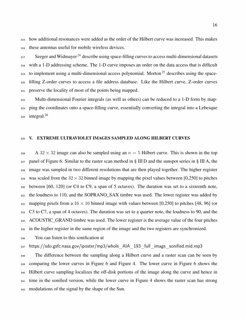
V. EXTREME ULTRAVIOLET IMAGES SAMPLED ALONG HILBERT CURVES325

A 32 × 32 image can also be sampled using an n = 5 Hilbert curve. This is shown in the top326

panel of Figure 6. Similar to the raster scan method in § III D and the sunspot series in § III A, the327

image was sampled in two different resolutions that are then played together. The higher register328

was scaled from the 32× 32 binned image by mapping the pixel values between [0,250] to pitches329

between [60, 120] (or C4 to C9, a span of 5 octaves). The duration was set to a sixteenth note,330

the loudness to 110, and the SOPRANO_SAX timbre was used. The lower register was added by331

mapping pixels from a 16 × 16 binned image with values between [0,250] to pitches [48, 96] (or332

C3 to C7, a span of 4 octaves). The duration was set to a quarter note, the loudness to 90, and the333

ACOUSTIC_GRAND timbre was used. The lower register is the average value of the four pitches334

in the higher register in the same region of the image and the two registers are synchronized.335

You can listen to this sonification at336

https://sdo.gsfc.nasa.gov/iposter/mp3/whole_AIA_193_full_image_sonified.mid.mp3337

The difference between the sampling along a Hilbert curve and a raster scan can be seen by338

comparing the lower curves in Figure 6 and Figure 4. The lower curve in Figure 6 shows the339

Hilbert curve sampling localizes the off-disk portions of the image along the curve and hence in340

time in the sonified version, while the lower curve in Figure 4 shows the raster scan has strong341

modulations of the signal by the shape of the Sun.342

17

FIG. 6. The top panel has an n = 5 Hilbert curve (H5) drawn over the greyscale SDO/AIA 193 Å image

from 18 Mar 2019 binned from 2048 × 2048 to 32 × 32. The lower plot (b) shows the resulting sampling

curve. Each pixel in the image is assigned to a point in the curve. The centers of square pixels are located

where the curve has a right angle bend, at the halfway mark of straight segments that are two units long, or

two centers proportionally spaced along the straight segments that are three units long. The vertical lines

show the four quadrants of the image.

18

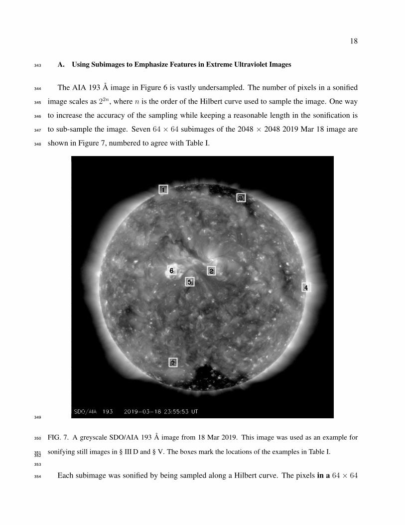
A. Using Subimages to Emphasize Features in Extreme Ultraviolet Images343

The AIA 193 Å image in Figure 6 is vastly undersampled. The number of pixels in a sonified344

image scales as 22n, where n is the order of the Hilbert curve used to sample the image. One way345

to increase the accuracy of the sampling while keeping a reasonable length in the sonification is346

to sub-sample the image. Seven 64 × 64 subimages of the 2048 × 2048 2019 Mar 18 image are347

shown in Figure 7, numbered to agree with Table I.348

349

FIG. 7. A greyscale SDO/AIA 193 Å image from 18 Mar 2019. This image was used as an example for350

sonifying still images in § III D and § V. The boxes mark the locations of the examples in Table I.351352

353

Each subimage was sonified by being sampled along a Hilbert curve. The pixels in a 64 × 64354

19

patch were first binned to 32 × 32 and then sampled with an n = 5 Hilbert curve. The tones355

were produced by mapping pixel values between [0, 255] to pitches between [60, 120] (or C4 to356

C9). The duration was set to a sixteenth note, the tempo to 300 bpm, the loudness to 110, and357

the SOPRANO_SAX timbre was used. A second voice was added by mapping the pixels from a358

16 × 16 binned image with values between [0,255] to pitches [48, 84] (or C3 to C6, a span of 3359

octaves). The duration was set to a quarter note, the loudness to 75, and the ACOUSTIC_GRAND360

timbre was used.361

You can listen to this sonifications by accessing the clickable image at362

https://sdo.gsfc.nasa.gov/iposter/.363

B. Filament Liftoff Sequence in Extreme Ultraviolet Images364

The final example is sonifying a series of images from AIA on SDO. The goal is to determine365

whether the time sequence in the images can be heard. We selected the filament liftoff of 10–12366

Mar 2010 as an example (Figure 8). Eight 128 × 128 subimages that included the filament liftoff367

were extracted, binned to 32 × 32, sampled along an n = 5 Hilbert curve and sonified. A short368

chorus and ending cadence were written. The piece was made by inserting the subimages in turn,369

separated by a chorus and ending with the cadence, thus creating a single time series of pitches.370

The early results for this sequence were not very successful. We then tried several ways to371

improve the sonification. First, the length of the individual frames was reduced by including only372

the lower-left and upper-left quadrants of those subimages. This corresponds to the first half of the373

sequence sampled by the Hilbert curve. When this did not produce a satisfactory result, we selected374

only those images with a noticeable difference. This produced seven images that emphasized the375

variation but were unevenly spaced in time. Finally, the pixels in this sequence were converted376

to tones by subtracting the average of each image from the sampled data, mapping the resulting377

values from [-60, 60] to pitches [36, 96] (or C2 to C7, a span of 5 octaves). The duration was set378

to a sixteenth note, the loudness to 110, and the PIANO timbre was used. Only the final attempt379

that includes all of these steps is presented here.380

You can listen to this sonification at381

https://sdo.gsfc.nasa.gov/iposter/mp3/liftoff_complete.mid.mp3382

20

FIG. 8. Montage of the final seven solar images showing a filament liftoff. Starting from the upper left,

the images were recorded at a) 2012-03-10 02:27:20, b) 2012-03-11 03:27:44, c) 2012-03-11 17:59:08, d)

2012-03-11 23:29:08, e) 2012-03-12 01:29:20, f) 2012-03-12 02:28:56, g) 2012-03-12 04:27:56, and h)

2012-03-12 06:29:56, respectively. (All times are UTC).

This was the least satisfying sonification because the changes in time were subtle and difficult383

to resolve. We have been investigating other ways to show the movement of material through384

both space and time. The subtraction of the mean was one example of one such a technique.385

By removing the average any overall brightening or darkening of the region did not dominate the386

change in time. Another possibility is to sonify the running difference images that AIA produces.387

We have sonified shapes moving through space to study this effect. Part of the issue is the large388

number of redundant pixels that do not significantly change value in time. Sonifying a sequence in389

time remains an area of active research.390

VI. DISCUSSION OF SONIFIED DATA391

Based on our experiments, percussive sounds, such as PIANO and PICKED_BASS, seem to392

work better for sonifying data. Percussive timbres securely place the sound on the beat and produce393

interesting changes as the tempo increases. A timbre with a noticeable rise or decay time tends to394

sound muddy as the tempo is increased.395

21

Our attempts to create a beat and melody by playing two versions of averaged data, such as the396

annual vs. the monthly values of S, were not a complete success. We continue to explore how to397

make the sonified data sound more like music and less mechanical.398

Although sonified data does not sound like most types of music, at least some pieces of classical399

music has similar qualities. Bach’s Goldberg Variations (BWV 988) sounds much like the image400

sonifications described above. As we note above, the chromatic runs in Variation 24, at around401

the 33-minute mark as played by Glenn Gould in his 1981 album of the same name, sound quite402

similar to the EVE spectrum.403

Sonifying data streams is a flexible area of study. To skip the image analysis step, you can load404

the MIDI files provided for each of the sonifications into any compatible synthesizer. This will405

immediately reveal that different synthesizers assign different timbres to each numbered track, so406

the files will sound different in each synthesizer. You can also change the timbre of a part in407

the synthesizer, providing another level of experimentation. Other sound font files can also be408

used with the synthesizers, including the JythonMusic synthesizer, again providing another area to409

explore.410

This also explains why the provided MP3 files do not always match what was heard when the411

JythonMusic synthesizer is used. You cannot create an MP3 file directly from the JythonMusic412

synthesizer. You can capture the sounds in either a recorder or software such as Audacity while413

the MIDI commands are executed. Or you can load the file containing the commands into another414

synthesizer that has export capability. The MP3 files provided here were created by opening the415

MIDI files in GarageBand, a proprietary program from Apple, and exporting the MP3 files.416

You can also use other programs to generate the MIDI file from a dataset. For example,417

Lilypond27 is a music engraving program that can also produce a MIDI file that is playable in a418

MIDI-capable synthesizer. You also get a beautiful score of the piece as a bonus. Similar to the419

JythonMusic workflow, the data file was opened in Python, the data was scaled to pitches and those420

pitches were written in Lilypond syntax to a Lilypond-readable text file. An example of a score is421

shown in Figure 9. Strong spectral lines can be seen in measures 31 and 35.422423

Mapping data to variations in pitch may not be the optimum solution for sonifying data. A large424

value of a dataset may be better represented by changes in the volume, emphasizing the strength of425

the larger value. We did some experiments on such variations and found that the limited ability of426

22

EUV on 27 Feb 2014 (Solar Maximum)Piano Old Sol

! !!! ! !" !" !# !!" !!" !# !"! !" " !" !! !" ! ! " !# !!" !$

# ! ! !! ! !" !!$ !! !% "# !! #&

!" !

! !!"!!!!# !" !! !"!" !# !"

! !!!"!" " !!#!!

# !" !!!!! !!"!!"!#%&

6

" !"!!"!# !!" !! "!# !!! !!

"!!! !" " ! # !! " ! !

!!! !! " !! ! !" !!

" !" ! !!# ! ! !! ! ! !" ! ! !" ! !"&%

12

!!!

!"" !" ! ! !! ! !"! !

!! !# !!" "!" !!" ! !"!!# !!!!# !"!!# ! !" !" !!!"!! "!!!"!! !!&%

18

! ! !!!!!!# ! !!"!

!"! " !

!!" !!"!

!"!" !"

!" !!" ! !!"!!

!!

!!# !" !!

!"!!!!"!" !!!

&%

24

! !!"!!!" !" !" !!" !

!!#!!" ! !

!! !""

!

" !

!

!!

"!!"!"

" !!!

"! !

! ! "!! !"! !

" ! ! !!"!!"

!" !" !#!!

&%

30

# !"!!!!

"!" !

!

!"! !!"! !"He II 304 Fe XVI 335

FIG. 9. The first page of a piano score of the EVE spectrum in Figure 2 created by Lilypond. The He II

304 Å line can be seen in measure 31 and the Fe XVI 335 Å line in measure 35. The scaling to pitch is

different than the sonified example to better fit on the staves.

humans to sense changes in loudness and to remember a baseline level of loudness over an entire427

piece made this less effective at sonifying data. Sonifying the data using a constant pitch with428

variable loudness also led to annoyance caused by the unchanging pitch.429

Following on the success of whistlers, numerous other datasets from solar physics and430

related fields of research were sonified, such as the variations of the solar wind.28,29 Solar431

sound waves propagating in the resonant chamber of the solar interior are observed as wave432

fields at the solar surface. The size of and run of temperature inside the Sun mean these waves433

have frequencies of several mHz, which can be inverted to probe the solar interior. The waves434

have been audified by frequency shifting them to audible ranges.30,31 Those examples are for435

1-D time series. In another the motion of a person is used to sample an image and create an436

interactive image-to-music experience.32 Others have produced a sonified solar system.33 The437

23

image sonifications described herein may be one of the few examples of such a project.438

VII. CONCLUSIONS439

We have sonified a sunspot time series, an EUV spectrum, a time series of EUV spectral440

irradiances, EUV images with various techniques, and a time sequence of EUV images. The EUV441

spectrum showed that the independent variable does not have to be time. We demonstrated that442

using a Hilbert curve to address a solar image gives a sonification that shows more of the image443

variations and less of the shape of the Sun. The locality property of the Hilbert curve ensures444

the method of using multi-resolution sampling curves to sonify the image in different voices445

is a well-defined operation.446

One shortcoming of the Hilbert curve sampling method is the separation of two regions near the447

limb. In these examples, images are sampled by a curve that crosses from the upper left quadrant448

to the upper right near the equator. This means the northern polar region is sampled in two distinct449

areas far from one another. The two lower quadrants do not have a direct connection, so the450

southern polar region is also divided into two distinct regions, one at the beginning of the series451

and the other at the end. This can be remedied by rotating the Hilbert curve (or the image) 90◦452

in either direction, which moves the connection between quadrants to the poles and keeps those453

regions in a smaller neighborhood while dividing the equatorial limb sectors into disparate parts of454

the sampling curve.455

Other techniques can be used to sonify solar images. Coincident images observed in different456

wavelengths of light can be sampled and placed in different timbres or pan positions. Once the next457

solar maximum passes, another EVE spectrum could be used to play against the solar maximum458

spectrum illustrated here. Higher-order Hilbert curves can be constructed to sample a series of459

images. This would keep points within a neighborhood in both space and time. Software that460

directly produces sounds rather than adhering to the MIDI standard might create sonifications that461

better represented the data. This could overcome the limited number of pitches available in the462

MIDI standard.463

Sonifying solar images is a way to explore the interface between tempo and pitch. Increasing464

the tempo to 3000 bpm (or 50 Hz) allows you to investigate whether an extremely rapid tempo465

24

results in an envelope with the individual pitches providing an amplitude modulation of that enve-466

lope. Frequencies of 15–30 Hz (900–1800 bpm) are near the limit of pitch discrimination.34 The467

difference between the buzz saw of the raster scan image (Sec. III D) and the smoother sound of468

Hilbert curve sampling of Sec. V is one example of how the envelope makes a big difference in the469

perception of the data.470

Listening to the Sun allows people to enjoy our closest star in a new direction. This does not471

apply only to the blind, most people can hear the variations of the Sun. With time these techniques472

will also allow people to more fully explore images.473

VIII. QUESTIONS AND OTHER PROJECTS474

Many projects can come from data-driven sonifications. There are also many ways to do those475

sonifications. We selected the JythonMusic synthesizer because we could load any data we wanted476

into the program. Once the MIDI exists it can be loaded into any compatible synthesizer for play-477

back or experimenting.478

Here are some suggestions that can motivate students to listen to their data:479

1. A simple way to sonify an image is to put the sampled pixels into a sound file, such as a WAV480

file and played at the CD sample rate of 44100 samples per second. This “audification” of481

an image does not require a synthesizer. The file can be opened in most media players and482

listened to. Compare the audified image with the sonified image and describe the differences,483

aside from the speed of the audified image.484

2. Can you find ways to vary the tempo of the music to represent variations in a data set?485

Scientific data tends to have even spacing and the simplest way to sonify the data is to486

maintain an even tempo. You can use the JythonMusic routine Mod.tiePitches to tie together487

identical notes to add some variety to the rhythmic spacing. Another routine, Mod.accent488

allows you to accent a beat, which also provides some rhythmic texture to the music.489

3. Can loudness be used to emphasize important features in a log-scaled variable? Comparing490

the score of the spectrum in Figure 9 with the physical data in Figure 2, we can see that a491

few emission lines outshine much of that spectral region but that dominance is not reflected492

25

in the sonification. Perhaps increasing the loudness of the strong emission lines would better493

illustrate this dominance.494

4. Three-color AIA images are created by putting coincident images in different wavelengths495

into individual color channels. These can be sonified by assigning a voice and pan position496

to each of the channels that will audibly emphasize the differences in the channels.497

5. A wavelet analysis of a time series can be used to isolate persistent from ephemeral frequen-498

cies. Can a wavelet spectrum be sonified to show the persistent frequencies as droning notes499

and ephemeral events as more rapid variations?500

6. Can other instruments be played against the synthesizer output? The sonified data has no501

explicit key, so improvised solos and rhythms can be played along with the sonified data.502

ACKNOWLEDGMENTS503

Version 4.6 of the JythonMusic software was downloaded from https://jythonmusic.me. All of504

the data used in this research is available as continually updated files from publicly-accessible sites.505

The monthly averaged (SN_m_tot_V2.0.csv) and the annually averaged (SN_y_tot_V2.0.csv)506

International Sunspot Number (Version 2) data were obtained from the Solar Influences Data507

Center (http://sidc.oma.be/silso/datafiles). Daily averaged SEE measurements were obtained508

as the SEE Level 3 Merged NetCDF file at http://lasp.colorado.edu/data/timed_see/level3/509

latest_see_L3_merged.ncdf. Daily averaged EVE measurements were obtained from the EVE510

Level 3 Merged NetCDF file at http://lasp.colorado.edu/eve/data_access/evewebdataproducts/511

merged/EVE_L3_merged_1a_2019135_006.ncdf. AIA images were obtained as JPEGs from512

the SDO website https://SDO.gsfc.nasa.gov.513

1 Sabina Teller Ratner. Camille Saint-Saëns, 1835-1921: A Thematic Catalogue of His Complete Works,514

volume 1. Oxford Univ. Press, New York, 2002. pp. 185–192.515

2 Dieter Daniels. Luigi russolo «intonarumori», 2020. URL http://www.medienkunstnetz.de/works/516

intonarumori/audio/1/.517

26

3 Iannis Xenakis. Electro-Acoustic Music. Vinyl LP, Nonesuch H-71246, 1970.518

4 Roger Luther. Moog Archives. URL http://moogarchives.com.519

5 Robert A. Helliwell. Whistlers and Related Ionospheric Phenomena. Dover Publications, Inc., 2006.520

Originally published by Stanford University Press, Stanford, California (1965).521

6 John H. Flowers. Thirteen years of reflection on auditory graphing: Promises, pitfalls, and potential new522

directions. In Proceedings of ICAD 05-Eleventh Meeting of the International Conference on Auditory523

Display, Limerick, Ireland, July 6-9, 2005, pages 406–409, 2005.524

7 The MIDI Association. Midi association, 2020. URL https://www.midi.org.525

8 Bill Manaris and Andrew R. Brown. Making Music with Computers: Creative Programming in Python.526

Taylor and Francis Group, LLC, Boca Raton, Florida, 2014.527

9 John Backus. The Acoustical Foundations of Music. W. W. Norton & Company, New York, 1969. p.528

113.529

10 Frederik Temmermans. JPEG, 2020. URL https://jpeg.org/index.html.530

11 John Backus. The Acoustical Foundations of Music. W. W. Norton & Company, New York, 1969. The531

Fletcher-Munson curves in this work have been revised and updated in ISO 226:2003 but the conclusions532

needed here remain valid.533

12 F. Clette, L. Svalgaard, J. M. Vaquero, and E. W. Cliver. Revisiting the Sunspot Number. A 400-Year534

Perspective on the Solar Cycle. Space Sci. Rev., 186:35–103, December 2014. doi:10.1007/s11214-014-535

0074-2.536

13 Frédéric Clette and Laure Lefèvre. The new sunspot number: Assembling all corrections. Solar Phys.,537

291:2629–2651, 2016. doi:10.1007/s11207-016-1014-y.538

14 T. N. Woods, F. G. Eparvier, R. Hock, A. R. Jones, D. Woodraska, D. Judge, L. Didkovsky, J. Lean,539

J. Mariska, H. Warren, D. McMullin, P. Chamberlin, G. Berthiaume, S. Bailey, T. Fuller-Rowell, J. Sojka,540

W. K. Tobiska, and R. Viereck. Extreme Ultraviolet Variability Experiment (EVE) on the Solar Dynamics541

Observatory (SDO): Overview of Science Objectives, Instrument Design, Data Products, and Model542

Developments. Solar Phys., 275:115–143, January 2012. doi:10.1007/s11207-009-9487-6.543

15 W. D. Pesnell, B. J. Thompson, and P. C. Chamberlin. The Solar Dynamics Observatory (SDO). Solar544

Phys., 275:3–15, January 2012. doi:10.1007/s11207-011-9841-3.545

27

16 T. Woods, S. Bailey, F. Eparvier, G. Lawrence, J. Lean, B. McClintock, R. Roble, G. Rottman,546

S. Solomon, and W. Tobiska. TIMED Solar EUV experiment. Physics and Chemistry of the Earth547

C, 25:393–396, 2000. doi:10.1016/S1464-1917(00)00040-4.548

17 J. R. Lemen, A. M. Title, D. J. Akin, P. F. Boerner, C. Chou, J. F. Drake, D. W. Duncan, C. G. Edwards,549

F. M. Friedlaender, G. F. Heyman, N. E. Hurlburt, N. L. Katz, G. D. Kushner, M. Levay, R. W. Lindgren,550

D. P. Mathur, E. L. McFeaters, S. Mitchell, R. A. Rehse, C. J. Schrijver, L. A. Springer, R. A. Stern,551

T. D. Tarbell, J.-P. Wuelser, C. J. Wolfson, C. Yanari, J. A. Bookbinder, P. N. Cheimets, D. Caldwell,552

E. E. Deluca, R. Gates, L. Golub, S. Park, W. A. Podgorski, R. I. Bush, P. H. Scherrer, M. A. Gummin,553

P. Smith, G. Auker, P. Jerram, P. Pool, R. Soufli, D. L. Windt, S. Beardsley, M. Clapp, J. Lang, and554

N. Waltham. The Atmospheric Imaging Assembly (AIA) on the Solar Dynamics Observatory (SDO).555

Solar Phys., 275:17–40, January 2012. doi:10.1007/s11207-011-9776-8.556

18 John-Cage-Orgel-Kunst-Projekt. Organ2/aslsp. URL https://www.aslsp.org/de/klangwechsel.html.557

19 W. D. Pence, L. Chiappetti, C. G. Page, R. A. Shaw, and E. Stobie. Definition of the Flexible Im-558

age Transport System (FITS), version 3.0. A. & Ap., 524:A42, December 2010. doi:10.1051/0004-559

6361/201015362.560

20 D. Hilbert. Über die stetige abbildung einer linie auf ein flächenstück. Mathematische Annalen, 38:561

459–460, 1891.562

21 G. Peano. Sur une courbe, qui remplit toute une aire plane. Mathematische Annalen, 36:157–160, 1890.563

22 John J. Bartholdi, Loren K. Platzman, R. Lee Collins, and William H. Warden. A minimal technology564

routing system for Meals on Wheels. Interfaces, 13(3):1–8, 1983.565

23 K. J. Vinoy, K. A. Jose, V. K. Varadan, and V. V. Varadan. Hilbert curve fractal antenna: A small resonant566

antenna for VHF/UHF applications. Microwave Opt Technol Lett, 29(4):215–219, 2001.567

24 Bernhard Seeger and Peter Widmayer. Geographic information systems. In Sartaj Sahni and Dinesh P.568

Mehta, editors, Handbook of Data Structures and Applications, chapter 56. CRC Press, Boca Raton,569

Florida, 2nd edition, 2018.570

25 G. M. Morton. A computer oriented geodetic data base; and a new technique in file sequencing. Technical571

report, IBM Ltd., Ottawa, Canada, 1966.572

26 Norbert Wiener. The Fourier Integral and Certain of its Applications. Dover, New York, 1933.573

27 Lilypond. Lilypond . . . music notation for everyone, 2020. URL http://lilypond.org.574

28

28 Robert L. Alexander. Solar wind sonification, 2011. URL http://www.srl.caltech.edu/ACE/ACENews/575

ACENews144.html.576

29 Andrea effe Rao. Sounds from the Sun - Data Sonification - Thesis, 2016. URL https://www.behance.577

net/gallery/35831845/Sounds-from-the-Sun-Data-Sonification-Thesis.578

30 Alexander G. Kosovichev. Solar Sounds, 1997. URL http://soi.stanford.edu/results/sounds.html.579

31 Tim Larson. SoSH Project: Sonification of Solar Harmonics, 2020. URL http://solar-center.stanford.580

edu/sosh/.581

32 Marty Quinn. “Walk on the Sun”: An interactive image sonification exhibit. AI & SOCIETY, 27(2):582

303–305, 2012. doi:10.1007/s00146-011-0355-1. URL https://doi.org/10.1007/s00146-011-0355-1.583

33 Michael Quinton, Iain McGregor, and David Benyon. Sonifying the solar system. In The 22nd Interna-584

tional Conference on Auditory Display (ICAD-2016), pages 28–35, 07 2016. doi:10.21785/icad2016.003.585

34 John Backus. The Acoustical Foundations of Music. W. W. Norton & Company, New York, 1969. Ch. 7.586