Using MMCAR to explore the structure of personality …personality-project.org/revelle/presentations/imps.17.pdfIntroduction SAPA theory SimulationsSAPA in practice FAConclusions AppendicesReferences

Introduction SAPA theory Simulations SAPA in practice FA Conclusions Appendices References

Using MMCAR to explore the structure ofpersonality and ability

Part of an invited symposium (chaired by Jingchen Liu):Big data analysis in cognitive assessment and

latent variable modelsInternational Meeting of Psychometric Society, Zurich,

William Revellea & David M. Condonb

aDepartment of Psychology, Northwestern University, Evanston, IllinoisbDepartment of Medical Social Sciences, Northwestern University Chicago Illinois

Partially supported by a grant from the National Science Foundation:SMA-1419324

Slides at http://personality-project.org/sapa.html

July, 2017

1 / 48

http://personality-project.org/sapa.html


OutlineIntroduction

Measuring individual differences: the tradeoff between breadthversus depthSynthetic Aperture Astronomy

SAPA theorySample items as well as people

Simulating SAPA dataStandard Errors and Effective Sample SizeComparing SAPA factors to complete data

The SAPA projectFactor analysis of sampled data

Stability of ICAR 16 solutions3 Dimensional Rotation Items

ConclusionsAppendices

Stability of ICAR 16 solutions3 Dimensional Rotation Items

2 / 48


Abstract

Personality and ability item pools can be very large (> 5, 000) butno one person likes to answer more than 50-150 items. Using webbased “Synthetic Aperture Personality Assessment” atsapa-project.org we collect data using a Massively MissingCompletely at Random (MMCAR) design.1,000 x 1,000 covariance matrices based upon 250,000 subjectsusing pairwise covariances have roughly 2 - 3,000observations/pair. Using conventional covariance algebra and Rfunctions in the psych package, we can examine the joint structureof personality, ability, and interests.The advantages of aSAPA/MMCAR design compared to the more conventional use ofshort forms will be discussed. In particular, by using large sampleswith many items, the structure of personality can be examined atmany levels of resolution, from the conventional 3-5 factors to ourpreferred 27 homogeneous scales, down to the unique (but stable)correlates of individual items.

3 / 48

sapa-project.org


The basic problem: Fidelity versus bandwidth

1. Many personality traits, interests and cognitive abilities aremultidimensional and have complex structure.

• To measure these, we need to have the precision that comeswith many participants.

• But we also need the bandwidth that comes with many items.• But participants are reluctant to answer very many items.

2. This has led to the quandary of should you give many peoplea few items or a few people, many items?

3. Our answer is to do both, but with a Massively MissingCompletely At Random (MMCAR) data structure.

4. We refer to this technique as Synthetic Aperture PersonalityAssessment (SAPA) to recognize the analogy to syntheticaperture radio astronomy (Revelle, Wilt & Rosenthal, 2010; Revelle, Condon, Wilt,

French, Brown & Elleman, 2016)

5. This is functionally what Frederic Lord (1955, 1977)suggested 62 years ago. It is time to take him seriously.

4 / 48


Breadth vs. depth of measurement

1. Factor structure of domains needs multiple constructs todefine structure.

2. Each construct needs multiple items to be measured reliably.

3. This leads to an explosion of potential items.

4. But, people are willing to only answer a limited number ofitems.

5. This leads to the use of short and shorter forms (theNEO-PI-R (Costa & McCrae, 1992) with 300, the IPIP (Goldberg, 1999) Big 5with 100, the BFI (John, Donahue & Kentle, 1991) with 44 items, the BFI2(Soto & John, 2017) with 60, the TIPI (Gosling, Rentfrow & Swann, 2003) with 10and 10 item BFI (Rammstedt & John, 2007) ) to include as part of othersurveys.

6. Unfortunately, with this reduction of items, breadth ofsubstantive content is lost.

5 / 48


Example studies with subject/item tradeoffs

1. The Potter-Gosling internet project (outofservice.com) hasgiven over 10,000,000 tests since 1997. Originally the 44items of the Big Five Inventory (BFI) (John et al., 1991) althoughthey are now giving the BFI2 (Soto & John, 2017)

2. The Stillwell-Kosinski (mypersonality.org) Facebookapplication (no longer in service) gave 7,765 people the IPIPversion of the NEO-PI-R with facets (300 items), 1,108,472the IPIP NEO-PI R domains (100 items), and 3,646,237 brief(20 item) surveys. Cross linked to likes and Facebook pages(Kosinski, Matz, Gosling, Popov & Stillwell, 2015; Youyou, Kosinski & Stillwell, 2015)

3. Smaller scale studies include the initial report on the BFI-2(Soto & John, 2017) with several thousand subjects with 60 item.

6 / 48

http://outofservice.com

http://mypersonality.org


Exceptions to the shorter and shorter inventory trend

1. Lew Goldberg and his colleagues at the University of Oregondeveloped the Eugene-Springfield sample (Goldberg & Saucier, 2016)

which has given several thousand items to ≈ 1, 000participants over 10 years. This sample has been the basis ofthe development and validation of the InternationalPersonality Item Pool (see ipip.ori.org). In fact, many of thesubsequent attempts at personality scale development haveused the Eugene-Springfield sample, e.g., the BFI (John et al., 1991),and the Big Five Aspect Scales (BFAS) of DeYoung, Quilty &Peterson (2007).

2. Our Personality Project (Revelle et al., 2010, 2016) (now atsapa.project.org) has taken the opposite direction and hasgiven more and more items including measures oftemperament, ability, and interests and we are now developingitem statistics on more than 4,000 items (Condon & Revelle, 2017) formore than 250,000 participants (but uses SAPA procedures).

7 / 48

http://ipip.ori.org

http://personality-project.org

http://sapa-project.org


Trading items for people: Studies, Items, People, Items x People

Table: Data sets vary in their sampling strategy and the Potter-Goslingand Stillwell/Kosinski data sets seem to have more data than the others

Study N Items Items/ Items*(k) Person People

Potter-Gosling 107 44 44 4.4 ∗ 108

Stillwell-Kosinski 4.5 ∗ 106 20-300 20-300 1.7 ∗ 108

SAPA 2.5 ∗ 105 1-4,000 100-150 2.5 ∗ 107

Eugene-Springfield 103 3,000 3,000 3 ∗ 106

But given basic statistical theory, is it worth while to increase thesample size so much? What is the effect of giving more items atthe cost of reducing the sample size?Consider the amount of information which varies by number ofcorrelations k∗(k−1)

2 and√N.

8 / 48


Trading items for people: Studies: Items, People, Items x Peopleand Information

Information varies by the number of correlations (k ∗ (k − 1)/2)weighted by their standard errors which vary by

√N

Table: Data sets vary in their sampling strategy and the seemingly smallersets, by giving many more items actually have more total information

Study N Items Items/ Items* InformationPerson People

SAPA* 2.5 ∗ 105 1-2,000 100-150 2.5 ∗ 107 2.5 ∗ 108

E-S 1,000 3,000? 3,000 3 ∗ 106 1.4 ∗ 108

S-Ki 4.5 ∗ 106 20-300 20-300 1.7 ∗ 108 9.5 ∗ 107

SAPA* 4.3 ∗ 103 953 100-150 2.5 ∗ 107 3 ∗ 107

P-G 107 44 44 4.4 ∗ 108 3.0 ∗ 106

*The average pairwise count of observations for the SAPA data reported today are

4,291 from 250,000 total participants for 953 items. 9 / 48


Many items versus many people

1. Not only do want many people, we also want many items.

2. Resolution (fidelity) goes up with sample size, N, (standarderrors are a function of

√N)

σx̄ =σx√N − 1

σr =1− r2

√N − 2

3. Also increases as number of items, k, measuring eachconstruct (reliability as well as signal/noise ratio varies asnumber of items and average correlation of the items)

λ3 = α =kr̄

1 + (k − 1)r̄s/n =

kr̄

(1− kr̄)

4. Breadth of constructs (band width) measured goes up bynumber of items (k).

5. Thus, we need to increase N as well as k. But how?

10 / 48


A short diversion: the history of optical telescopes

Resolution varies by aperture diameter (bigger is better)

11 / 48


A short diversion: history of radio telescopes

Resolution varies by aperture diameter (bigger is still better)

Aperture can be synthetically increased across multiple telescopesor even multiple observatories

12 / 48


Can we increase N and n at the same time?

1. Frederic Lord (1955) introduced the concept of samplingpeople as well as items.

2. Apply basic sampling theory to include not just people (wellknown) but also to sample items within a domain (less wellknown).

3. Basic principle of Item Response Theory and tailored tests.

4. Used by Educational Testing Service (ETS) to pilot items.

5. Used by Programme for International Student Assessment(PISA) in incomplete block design (Anderson, Lin, Treagust, Ross & Yore, 2007).

6. Discussed at this meeting by Rutkowski and Matta in themissing data symposium.

7. Can we use this procedure for the study of individualdifferences without being a large company?

8. Yes, apply the techniques of radio astronomy to combinemeasures synthetically and take advantage of the web.

13 / 48


Subjects are expensive, so are items

1. In a survey such as Amazon’s Mechanical Turk (MTURK), wewould need to pay by the person and by the item.

2. Volunteer subjects are not very willing to answer many items.

3. Why give each person the same items? Sample items, as wesample people.

4. Synthetically combine data across subjects and across items.This will imply a missing data structure which is

• Missing Completely At Random (MCAR), or even moredescriptively:

• Massively Missing Completely at Random (MMCAR) (wesometimes have 99% missing data although our median is only93% missing!)

5. This is the essence of Synthetic Aperture PersonalityAssessment (SAPA) (Condon & Revelle, 2014; Condon, 2014; Revelle et al., 2016, 2010).

6. This is a much higher rate of missingness than discussed inthe balanced incomplete block design of NAEPS or PISA.

14 / 48


3 Methods of collecting 256 subject * items dataa) 8 x 32 complete

4621363452114345344364533121241421243623166421516154432261516513516613511551654636222244356233441114134336233221561215213561452225353121264561433433232246526411613351545664241146126412253535162463434215153624242541351343511611554654453123111162423325516334

b) 32 x 8 complete4632311425443314433154232631414541435614422361536242134435234443345141666341515444441342135143216636566312264546314661353264551466151251144114416244363633316236633254251153112661155546332453615224165463212356244146636366141445555223143644332146141633232365

c) 32 x 32 MCAR p=.25..3..2..6.....4.55.......44................4..6..45..3.4..6....16..3.......6.1.....6.2.......5.6....3522......5.3...3......5........3.2.2.......3..2......65..5......51....324.........23......5....552............25...54.5.......44.4.5....3..6...6........3......61.523.2....2...........3...5.............42.4..6.5......61.....3....3.6..1.4...1..5......5.1....54..........2.4.33..6......4.....52..6.....44.3...........2..44...1........1..42....5..1.....1..3.......2..3.521.......6..........3.142.........22......12..4...2..........3..162...4.....4..4..6..3.4...1....5.33.........5..........243..5....41......1....5..3..4...4.4..5..1.........4......4.......3..5.2.....64.4..4....1.1.2...6....4......55....2.......3..2..53.....2..2.3.3............1...2..43...3.13........5....2.........4..54...2.3..62....22.......332..1.....5......6.......5..3.4.....3....5.241..............63.1.......6...5..4..2...5..2.4..5..........52.4.....44...2.55.....2.....6.....6.....55.....5..........4....6341.4..2.........55......5.......45....3..32.15 / 48


Synthetic Aperture Personality Assessment

1. Give each participant a random sample of pn items taken froma larger pool of n items. pi might be anywhere from .01 to 1.

2. Find covariances based upon “pairwise complete data”. Eachpair appears with probability pipj with a median of .01.

3. Find scales based upon basic covariance algebra.• Let the raw data be the matrix NXn with N observations

converted to deviation scores.• Then the item variance covariance matrix is nCn = X ′XN−1

• and scale scores, NSs are found by S = NXppKs .• nKs is a keying matrix, with kij = 1 if itemi is to be scored in

the positive direction for scale j, 0 if it is not to be scored, and-1 if it is to be scored in the negative direction.

• In this case, the covariance between scales,

sCs = sSN′NSsN

−1 =

sCs = (XK )′(XK )N−1 = K ′X ′XKN−1 = K ′nCnK . (1)

4. That is, we can find the correlations/covariances betweenscales from the item covariances, not the raw items.

16 / 48


Two sets of simulations

1. For both sets, we consider the effect of sample size (N) andsampling probability (p).

2. The effect on standard errors of intercorrelations of itemcomposites of composite length

3. Examining the standard errors of factor loadings

4. We consider effective sample size and compare it to thenominal sample size of pairwise correlations.

17 / 48


The basic tradeoff: standard errors and effective sample size

1. Standard error of correlations between any single pair of itemsis just

σr =1− r2

√N − 2

2. However, simulation (and some theory) shows that thestandard error of correlations of synthetic correlations ofscales of length k decreases as a joint function of the numberof items in the scale and the inverse of the probability of anytwo items being administered.

3. Effectively, this is because what ever causes error in anycorrelation does not aggregate across k independent pairs ofitems.

18 / 48


SAPA standard errors of correlations vary by scale length

1. When forming synthetic scales from MMCAR based items, thestandard error of correlations decreases as a function of theTotal number of subjects (N), the the inverse of thepercentage of items sampled (p), and the number of itemsforming the scale (k).

2. Ashley Brown has shown this quite clearly by simulation (Brown,

2014) and we discussed this last year at APS (Revelle & Condon, 2016)

and in a recent chapter (Revelle et al., 2016),

3. A good way to visualize this is to examine the standard errorof correlations as a function of N, p, and k.

4. An even more dramatic way is to plot the Effective SampleSize (Neff ) which because

σr =1− r2

√N − 2

is merely Neff =(1− r2)2

σ2r

+ 2

19 / 48


Effective sample size varies by the size of the composite scale.

Simulating N= 10,000 with probability of any item (Brown, 2014)

(p = .125, .25, .5, or 1) and items in the composite 1 , 2, 4, 8, 16.

Rw: 0.3

p=0.125

p=0.25

p=0.5

p=1

0

2500

5000

7500

1000010000

Rb: 0

1 2 4 8 16n (items per scale)

Effe

ctive

Sam

ple

Size

20 / 48


Comments on simulation values

1. These simulations are based upon N = 10,000

2. Although for k = 1, the effective sample size is, of course, justNp2 and thus for p = .25 = 10, 000 ∗ .252 = 625 this providesa relatively small standard error (σr = .04).

3. Had we not sampled, we would have a standard error of .01but for 1/4 the number of items and thus 1/16 the number ofcorrelations.

4. Is this extra precision worth the reduction in bandwidth?

5. More importantly, the standard error of 4 items scales with aneven more dramatic sampling (p = .125) would also beroughly .04 but with 8 times as many items and thus 64 timesas many correlations.

21 / 48


Standard deviations of factor loadings

1. 3 Simulation of SAPA procedures

2. Generate 200,000 simulated cases with a 1 factor model

3. Compare no sampling, 50% sample, and 25% sample

4. This leads to 100%, 25% or 6.25% pairwise correlations.

5. The question becomes what is the effective size? Is it thenumber of pairwise observations or something greater?

22 / 48


Factor loadings and standard errors for 50% sampling

0.0 0.2 0.4 0.6 0.8 1.0

200 pairwise, 50% sampling

0.0 0.2 0.4 0.6 0.8 1.0


0.0 0.2 0.4 0.6 0.8 1.0


0.0 0.2 0.4 0.6 0.8 1.0


23 / 48


Factor loadings and standard errors for 25% sampling

0.0 0.2 0.4 0.6 0.8 1.0


0.0 0.2 0.4 0.6 0.8 1.0


0.0 0.2 0.4 0.6 0.8 1.0


0.0 0.2 0.4 0.6 0.8 1.0


24 / 48


Standard deviations of factor loadings

0.95% confidence limits

Pairwise Complete Observations

Sta

ndar

d D

evia

tions

of L

oadi

ngs

p 200 p 400 p 800 p 1600

0.01

0.02

0.03

0.04

G1G2G3

1. “Normal ” =>pairwise = samplesize

2. 50% sample =>pairwise = .25 ofsample size

3. 25% sample =.0625% pairwise

25 / 48


Effective sample size based upon sampling variability of factorloadings

0.95% confidence limits

Pairwise Complete Observations

Effe

ctiv

e S

ampl

e S

ize

p 200 p 400 p 800 p 1600

01000

2000

3000

4000

5000

G1G2G3

1. 25% sample => totalsample = 16 timespairwise sample

2. 50% sample => totalsample = 4 timespairwise sample

3. “Normal ” =>pairwise = samplesize

26 / 48


Conclusions based upon simulations

1. Massively missing completely at random (MMCAR/SAPA)procedures increase bandwidth and fidelity.

2. For the same number items * people, sampling items increasesthe number of items that can be studied

3. Precision of scale x scale correlations and factor loadingswithin a scale is increased by sampling items

4. However, to achieve stable number of pairwise correlations,we need to increase overall number of subjects studied.

5. Nice in theory, does it work in practice? Yes, the SAPAproject.

27 / 48




Integrating measures of Temperament , Ability and Interests (TAI)

1. Temperament• 696 items taken from 200 International Personality Item Pool

(IPIP) (Goldberg, 1999) scales (representing 2,084 overlapping items)• 100% coverage of 200 IPIP scales, 57% to 85% of 235 other

scales. (Condon, 2014, 2017; Condon & Revelle, 2017)

2. Ability• 60 items from the original International Cognitive Ability

Resource (ICAR) data set (Condon & Revelle, 2014)

• The original 4 item types: Verbal Reasoning, MatrixReasoning, Number/Letter series, and 3 Dimensional rotation,

• Now supplemented with 12 more item types as part of theICAR project done in collaboration with Phillip Doebler, HeinzHollng and Ehsan Masoudi in Germany; John Rust, DavidStillwell, Luning Sun, Fiona Chan and Aiden Loe from the UK.

• See http://ICAR-project.com for more information3. Interest

• Items taken from the Oregon Vocational Interests (ORVIS)(Pozzebon, Visser, Ashton, Lee & Goldberg, 2010) and Occupational Interests(ORAIS) (Goldberg, 2010). See Elleman, Condon & Revelle (2017). 28 / 48

http://ICAR-project.com


How stable are factor analytic solutions of SAPA data?

1. Compare solutions for entire sample (255K) to subsamples

2. Examine the identification of structure of the ICAR16 sampletest for a 4 factor solution

3. Examine the stability of factor loadings for the 3 DimensionalRotation items (relevant for doing subsequent IRT scoring)

4. Show variation in loadings and in interfactor correlations for100 replications of 5, 10, 20, and 40 % samples.

5. Compare hierarchical (omega) factor solution for entiresample to 2 and 5% samples.

6. Examine the stability of factor solutions for simulated datavarying the probability of item selection.

29 / 48


Sample characteristics

Items presented are sample from subsets of items (e.g. there are24 3D rotation items and thus the probability of any pair beingpresented is less than the 16 sample test (ICAR 16) items.

Table: Sample sizes and number of times items were presented as well aspairwise counts

Fraction sample icar16 ic16 pairs 3DRot 3D pairs0.05 12,767 3,717 1,238 1,668 2000.10 25,535 7,435 2,479 3,335 3990.20 51,070 14,869 4,950 6,670 7980.40 102,139 29,738 9,907 13,340 1,5961.00 255,348 74,345 24,768 33,351 3,990

We want to examine the stability of solutions across samplingframes.

30 / 48


Stability of factor loadings for a 4 factor solution – Summary

0.0 0.2 0.4 0.6 0.8 1.0

ICAR 16 4 Factors pairwise = 1238

0.0 0.2 0.4 0.6 0.8 1.0


0.0 0.2 0.4 0.6 0.8 1.0


0.0 0.2 0.4 0.6 0.8 1.0

ICAR 16 4 Factors 4 pairwise = 9907

31 / 48



q_12007q_12033q_12034q_12058q_12045q_12046q_12047q_12055q_11003q_11004q_11006q_11008q_12004q_12016q_12017q_12019

0.0 0.2 0.4 0.6 0.8 1.0

ICAR 16 1 Factor 5%


0.0 0.2 0.4 0.6 0.8 1.0

ICAR 16 1Factor 10%


0.0 0.2 0.4 0.6 0.8 1.0

ICAR 16 1 Factor 20%


0.0 0.2 0.4 0.6 0.8 1.0

ICAR 16 1 Factor 40%

32 / 48


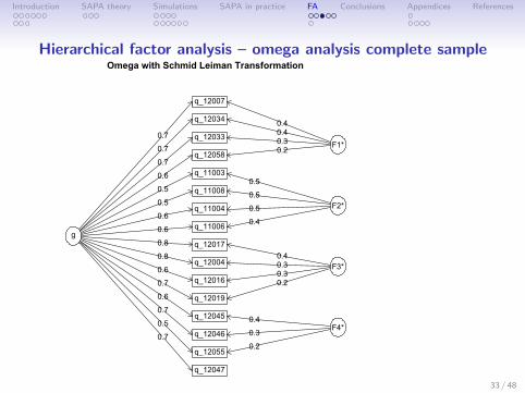
Hierarchical factor analysis – omega analysis complete sampleOmega with Schmid Leiman Transformation

q_12007

q_12034

q_12033

q_12058

q_11003

q_11008

q_11004

q_11006

q_12017

q_12004

q_12016

q_12019

q_12045

q_12046

q_12055

q_12047

F1*

0.40.40.30.2

F2*

0.5

0.5

0.5

0.4

F3*0.40.30.30.2

F4*0.4

0.3

0.2

g

0.7

0.7

0.7

0.6

0.5

0.5

0.6

0.6

0.8

0.8

0.6

0.7

0.6

0.7

0.5

0.7

33 / 48


Hierarchical factor analysis – omega analysis 5% sampleOmega with Schmid Leiman Transformation

q_12004

q_12017

q_12016

q_12019

q_11008

q_11003

q_11004

q_11006

q_12007

q_12034

q_12058

q_12033

q_12045

q_12055

q_12046

q_12047

F1*

0.30.30.30.3

F2*

0.6

0.6

0.4

0.4

F3*0.60.30.20.2

F4*0.5

0.3

0.2

g

0.8

0.7

0.6

0.7

0.5

0.5

0.5

0.6

0.7

0.7

0.6

0.6

0.6

0.5

0.6

0.7

34 / 48


Factor congruence of omega solutions: complete vs. 5% sample

Factor Congruence: total sample vs. 5% sample

h2

F4*

F3*

F2*

F1*

g

g F1* F2* F3* F4* h2

0.99 0.77 0.54 0.54 0.56 0.99

0.54 0.28 0.1 0.16 0.94 0.51

0.68 0.96 0.06 0.1 0.15 0.61

0.5 0.13 0.99 0.07 0.21 0.57

0.62 0.38 0.08 0.93 0.23 0.62

1 0.79 0.49 0.55 0.59 0.98

-1

-0.8

-0.6

-0.4

-0.2

0

0.2

0.4

0.6

0.8

1

35 / 48


Factor loadings for the 24 3D rotation items: summary

q_11001q_11002q_11003q_11004q_11005q_11006q_11007q_11008q_11009q_11010q_11011q_11012q_11013q_11014q_11015q_11016q_11017q_11018q_11019q_11020q_11021q_11022q_11023q_11024

0.0 0.2 0.4 0.6 0.8 1.0

3D rotation items pairwise = 200


0.0 0.2 0.4 0.6 0.8 1.0



0.0 0.2 0.4 0.6 0.8 1.0



0.0 0.2 0.4 0.6 0.8 1.0

3D rotation items pairwise=1596

36 / 48


SAPA or MMCAR procedures are very powerful

1. Able to estimate difficulty parameters and covariancestructures for 1,000s of items even though only 100 itemsanswered per subject

2. Structure of ability measures using the open source ability testfrom the International Cognitive Ability Resource (ICAR)http://icar-project.com

3. Join the ICAR and SAPA projects.

4. Data sharing: https://dataverse.harvard.edu/

dataverse/SAPA-ProjectCode/manuscript/

5. workbook: https://sapa-project.org/research/SPI/

SPIdevelopment.pdf

6. SPI scales, norms, IRT parameters:https://sapa-project.org/research/SPI

7. Today’s slides athttp://personality-project.org/sapa.html

37 / 48

http://icar-project.com

https://dataverse.harvard.edu/dataverse/SAPA-Project Code/manuscript/

https://dataverse.harvard.edu/dataverse/SAPA-Project Code/manuscript/

https://sapa-project.org/research/SPI/SPIdevelopment.pdf

https://sapa-project.org/research/SPI/SPIdevelopment.pdf

https://sapa-project.org/research/SPI

http://personality-project.org/sapa.html


R code

The next few slides show the R code used for these analysesR code

sapa <- read.file() #this searched for and loaded the master data fileicar.dictionary <- read.file() #this searches for and loads a dictionary file

sapa <- SAPAdata18aug2010thru7feb2017 #change the name to make the following analyses clearer#the raw sapa has alphanumeric codes for some fields. Convert to numericsapa <- char2numeric(sapa)icar <- sapa[rownames(icar.dictionary)] #Identify the ICAR itemsicar.keys <- ItemLists[417:421] #the keys are loaded as part of the sapa read.file lineicar #show the item numbers of ICAR

icar.16 <- c("q_12007","q_12033" ,"q_12034","q_12058","q_12045", "q_12046","q_12047","q_12055", "q_11003", "q_11004","q_11006" ,"q_11008","q_12004","q_12016","q_12017", "q_12019")

#now do random resamples, 100 times each of various fractions of the icar.16 dataicar.16.sapa.05 <-fa.sapa(sapa[icar.16],4,n.iter=100,frac=.05)icar.16.sapa.1 <-fa.sapa(sapa[icar.16],4,n.iter=100,frac=.1)

icar.16.sapa.2 <-fa.sapa(sapa[icar.16],4,n.iter=100,frac=.2)icar.16.sapa.4 <-fa.sapa(sapa[icar.16],4,n.iter=100,frac=.4)

38 / 48


More R

R code

error.dots(icar.16.sapa.05,head=40,tail=40,sort=FALSE,main="ICAR 16 4 Factors pairwise = 1238",xlim=c(0,1),labels=NULL)error.dots(icar.16.sapa.1,head=40,tail=40,sort=FALSE,main="ICAR 16 4 Factors pairwise = 2479" ,xlim=c(0,1),labels=NULL)error.dots(icar.16.sapa.2,head=40,tail=40,sort=FALSE,main="ICAR 16 4 Factors pairwise = 4950",xlim=c(0,1),labels=NULL)error.dots(icar.16.sapa.4,head=40,tail=40,sort=FALSE,main="ICAR 16 4 Factors 4 pairwise = 9907",xlim=c(0,1),labels=NULL)

#now show the factor intercorrelationsnames(icar.16.sapa.05$cis$means.rot) <- label.icar.rotnames(icar.16.sapa.1$cis$means.rot) <- label.icar.rotnames(icar.16.sapa.2$cis$means.rot) <- label.icar.rotnames(icar.16.sapa.4$cis$means.rot) <- label.icar.rot

error.dots(icar.16.sapa.05$cis$means.rot,se=icar.16.sapa.05$cis$sds.rot,sort=FALSE,xlim=c(0,1),main="Interfactor correlations ICAR 16 pairwise = 1238")error.dots(icar.16.sapa.1$cis$means.rot,se=icar.16.sapa.1$cis$sds.rot,sort=FALSE,xlim=c(0,1),main="Interfactor correlations ICAR 16 pairwise = 2479")error.dots(icar.16.sapa.2$cis$means.rot,se=icar.16.sapa.2$cis$sds.rot,sort=FALSE,xlim=c(0,1),main="Interfactor correlations ICAR 16 pairwise = 4950")error.dots(icar.16.sapa.4$cis$means.rot,se=icar.16.sapa.4$cis$sds.rot,sort=FALSE,xlim=c(0,1),main="Interfactor correlations ICAR 16 pairwise = 9907 ")

op <- par(mfrow=c(2,2))error.dots(icar.16.sapa.05$cis$means.rot,se=icar.16.sapa.05$cis$sds.rot,sort=FALSE,xlim=c(0,1),main="ICAR 16 pairwise = 1238")error.dots(icar.16.sapa.1$cis$means.rot,se=icar.16.sapa.1$cis$sds.rot,sort=FALSE,xlim=c(0,1),main="ICAR 16 pairwise = 2479")error.dots(icar.16.sapa.2$cis$means.rot,se=icar.16.sapa.2$cis$sds.rot,sort=FALSE,xlim=c(0,1),main="ICAR 16 pairwise = 4950")error.dots(icar.16.sapa.4$cis$means.rot,se=icar.16.sapa.4$cis$sds.rot,sort=FALSE,xlim=c(0,1),main="ICAR 16 pairwise = 9907 ")

39 / 48


More RR code

op <- par(mfrow=c(1,1)icar.16.sapa.05$cis$mean.pair #1238.375icar.16.sapa.1$cis$mean.pair # 2478.613icar.16.sapa.2$cis$mean.pair # 4950.1icar.16.sapa.4$cis$mean.pair # 9906.598

#now, just take out a general factoricar.16.sapa.1.05 <-fa.sapa(sapa[icar.16],n.iter=100,frac=.05)icar.16.sapa.1.1 <-fa.sapa(sapa[icar.16],n.iter=100,frac=.1)icar.16.sapa.1.2 <-fa.sapa(sapa[icar.16],n.iter=100,frac=.2)icar.16.sapa.1.4 <-fa.sapa(sapa[icar.16],n.iter=100,frac=.4)

error.dots(icar.16.sapa.1.05,head=40,tail=40,sort=FALSE,main="ICAR 16 1 Factor 5% sample",xlim=c(0,1))error.dots(icar.16.sapa.1.1,head=40,tail=40,sort=FALSE,main="ICAR 16 1Factor 10% sample" ,xlim=c(0,1))error.dots(icar.16.sapa.1.2,head=40,tail=40,sort=FALSE,main="ICAR 16 1 Factor 20% sample",xlim=c(0,1))error.dots(icar.16.sapa.1.4,head=40,tail=40,sort=FALSE,main="ICAR 16 1 Factor 40% sample",xlim=c(0,1))

error.dots(icar.16.sapa.1.05,head=40,tail=40,sort=FALSE,main="ICAR 16 1 Factor 5% ",xlim=c(0,1))error.dots(icar.16.sapa.1.1,head=40,tail=40,sort=FALSE,main="ICAR 16 1Factor 10% " ,xlim=c(0,1))error.dots(icar.16.sapa.1.2,head=40,tail=40,sort=FALSE,main="ICAR 16 1 Factor 20% ",xlim=c(0,1))error.dots(icar.16.sapa.1.4,head=40,tail=40,sort=FALSE,main="ICAR 16 1 Factor 40% ",xlim=c(0,1))

icar.keys <- keys.list[398:402]

R3Diq.sapa <-fa.sapa(sapa[icar.keys[[4]]],1,n.iter=100,frac=.05)R3Diq.sapa.1 <-fa.sapa(sapa[icar.keys[[4]]],1,n.iter=100,frac=.1)R3Diq.sapa.2 <-fa.sapa(sapa[icar.keys[[4]]],1,n.iter=100,frac=.2)R3Diq.sapa.4 <-fa.sapa(sapa[icar.keys[[4]]],1,n.iter=100,frac=.4)

R3Diq.sapa$cis$mean.pairR3Diq.sapa.1$cis$mean.pairR3Diq.sapa.2$cis$mean.pairR3Diq.sapa.4$cis$mean.pair

40 / 48


R code

#this next one fails#R3Diq.sapa.01 <-fa.sapa(sapa[icar.keys[[4]]],1,n.iter=100,frac=.01)# error.dots(R3Diq.sapa..01,head=40,tail=40,sort=FALSE,main="3D rotation items -- 1% sample",xlim=c(0,1))op <- par(mfrow=c(2,2))

error.dots(R3Diq.sapa,head=40,tail=40,sort=FALSE,main="3D rotation items pairwise = 200",xlim=c(0,1))error.dots(R3Diq.sapa.1,head=40,tail=40,sort=FALSE,main="3D rotation items pairwise = 399",xlim=c(0,1))error.dots(R3Diq.sapa.2,head=40,tail=40,sort=FALSE,main="3D rotation items pairwise = 798",xlim=c(0,1))error.dots(R3Diq.sapa.4,head=40,tail=40,sort=FALSE,main="3D rotation items pairwise=1596",xlim=c(0,1))

op <- par(mfrow=c(1,1)

samp.size <- data.frame(fraction=fraction,sample = fraction * 255348,icar16=fraction * 74345,icar16_pairwise=c(1238,2479,4950,9907,24768),DRRotation = fraction * 33351,DRotation_pairwise=c(200,399,798,1596,3990))

#now, some omega comparisonsom16 <- omega(sapa[icar.16],4) #the complete sampleomega.diagram(om16)

# a 5% samplesapa.5.samp <- sapa[sample(1:255348,12767,replace=TRUE),icar.16]om.samp.5 <- omega(sapa.5.samp,4)omega.diagram(om.samp.5)

mean(count.pairwise(sapa.5.samp,diagonal=FALSE),na.rm=TRUE)cp <- count.pairwise(sapa.5.samp)

> mean(diag(cp))[1] 3718.562

corPlot(factor.congruence(om16,om.samp.5),numbers=TRUE,gr=gr,main="Factor Congruence: total sample vs. 5% sample")

sapa.02.samp <- sapa[sample(1:255348,5000,replace=TRUE),icar.16]om.02 <- omega(sapa.02.samp,4)corPlot(factor.congruence(om16,om.02),numbers=TRUE,gr=gr,main="Factor Congruence: total sample vs. 2% sample")mean(count.pairwise(sapa.02.samp,diagonal=FALSE),na.rm=TRUE)[1] 468.8833>> mean(diag(count.pairwise(sapa.02.samp)))[1] 1446.125

#find the ipip by icar correlations just do the IPIP100, the SPI 135 and the ICARipip.items <- selectFromKeys(c(ItemLists[[ 384]], ItemLists[[417]] , ItemLists[[52]])

ipip.icar.keys <- keys.list[c(398:402,366:397,49:53)]ipip.icar.items <- selectFromKeys(ipip.icar.keys)

ipip.icar.R <- mixedCor(sapa[ipip.icar.items])ipip.icar.scores <- scoreOverlap (pip.icar.keys,ipip,icar.R$rho)

sim.1 <- sim.irt(24,250000,low=-1,high=1,a=3)f1.sapa.0064 <- fa.sapa(sim.1$items,frac=.0064,n.iter=100)

f1.sapa.0032 <- fa.sapa(sim.1$items,frac=.0032,n.iter=100)

f1.sapa.0016 <- fa.sapa(sim.1$items,frac=.0016,n.iter=100)f1.sapa.008 <- fa.sapa(sim.1$items,frac=.0008,n.iter=100)par(mfrow=c(2,2))

error.dots(f1.sapa.008,head=12,tail=24,sort=FALSE,main="Simulated items pairwise = 200",xlim=c(0,1))error.dots(f1.sapa.0016,head=12,tail=24,sort=FALSE,main="Simulated items pairwise = 400",xlim=c(0,1))

error.dots(f1.sapa.0032,head=12,tail=24,sort=FALSE,main="Simulated items pairwise = 800",xlim=c(0,1))error.dots(f1.sapa.0064,head=12,tail=24,sort=FALSE,main="Simulated items pairwise = 1600",xlim=c(0,1))

41 / 48


R code

#now some interesting simulations

sim.1 <- sim.irt(24,200000,low=-1,high=1,a=3)simp <- sim.1$itemsfilter <- matrix(NA,nrow=200000,ncol=24)filter <- sample(1:24,24*200000,replace=TRUE)

filter<- matrix(filter,ncol=24)simp[filter > 12 ] <- NA. #rhis is a 50% samplesimp <- matrix(simp,ncol=24)

sim.fa.008 <- fa.sapa(simp,frac=.008,n.iter=100)sim.fa.0016<- fa.sapa(simp,frac=.0016,n.iter=100)sim.fa.016<- fa.sapa(simp,frac=.016,n.iter=100)sim.fa.032<- fa.sapa(simp,frac=.032,n.iter=100).sim.fa.032$cis$mean.pair #[1] 1600.788

#Now, do this again for a 25% samplesimp.25 <- sim.1$itemssimp.25[filter > 6 ] <- NA. #rhis is a 50% samplesimp,25 <- matrix(simp.25,ncol=24)

sim.fa.25.016<- fa.sapa(simp.25,frac=.016,n.iter=100) #200sim.fa.25.032<- fa.sapa(simp.25,frac=.032,n.iter=100). #400sim.fa.25.064<- fa.sapa(simp.25,frac=.064,n.iter=100) #800sim.fa.25.128<- fa.sapa(simp.25,frac=.128,n.iter=100). #1600

tot.f1.004 <- fa.sapa(sim.1$items,frac=.004,n.iter=100)tot.f1.004$cis$mean.pair. #[1] 800

tot.f1.002 <- fa.sapa(sim.1$items,frac=.002,n.iter=100)tot.f1.001 <- fa.sapa(sim.1$items,frac=.001,n.iter=100)tot.f1.001$cis$mean.pair

total.df <- data.frame(group=rep(1,24),p200=tot.f1.001$cis$sds, p400=tot.f1.002$cis$sds, p800=tot.f1.004$cis$sds, p1600=tot.f1.008$cis$sds, p200=unclass(tot.f1.001$cis$means), p400= unclass(tot.f1.002$cis$means), p800=unclass(tot.f1.004$cis$means), p1600= unclass(tot.f1.008$cis$means))

sim.df <- data.frame(group=rep(2,24), p200=sim.fa.004$cis$sds,p400=sim.fa.008$cis$sds,p800=sim.fa.016$cis$sds,p1600=sim.fa.032$cis$sds,p200=unclass(sim.fa.004$cis$means), p400=unclass(sim.fa.008$cis$means), p800= unclass(sim.fa.016$cis$means), p1600= unclass(sim.fa.032$cis$means))

sim.25.df <- data.frame(group=rep(3,24),p200=sim.fa.25.016$cis$sds, p400=sim.fa.25.032$cis$sds, p800=sim.fa.25.064$cis$sds, p1600=sim.fa.25.128$cis$sds,p200= unclass(sim.fa.25.016$cis$means) ,p400=unclass(sim.fa.25.032$cis$means), p800=sim.fa.25.064$cis$sds, p1600= unclass(sim.fa.25.128$cis$means))

tot.sapa <- rbind(sim.df,sim.25.df,total.df)

tot.sapa[1:24,1] <- "sapa"tot.sapa[25:48,1] <- "complete"error.bars.by(tot.sapa[2:5],tot.sapa[1],xlab="Pairwise Complete Observations",ylab="Standard Deviations of Loadings",legend=7)

eff.size <- (1-.67ˆ2)ˆ2/tot.sapaˆ2error.bars.by(eff.size[,2:5],group=tot.sapa[,1]xlab="Pairwise Complete Observations",ylab="Effective Sample Size",legend=7))

42 / 48


Error dots for factor loadings

NOte that the error bars are smaller for the 25 versus 50 % samplesR code

op <- par(mfrow=c(2,2))error.dots(sim.fa.004,sort=FALSE,xlim=c(0,1),main="200 pairwise, 50% sampling")error.dots(sim.fa.008,sort=FALSE,xlim=c(0,1),main="400 pairwise, 50% sampling")error.dots(sim.fa.016,sort=FALSE,xlim=c(0,1),main="800 pairwise, 50% sampling")error.dots(sim.fa.032,sort=FALSE,xlim=c(0,1),main="1600 pairwise, 50% sampling")

error.dots(sim.fa.25.016,sort=FALSE,xlim=c(0,1),main="200 pairwise, 25% sampling")error.dots(sim.fa.25.032,sort=FALSE,xlim=c(0,1),main="400 pairwise, 25% sampling")error.dots(sim.fa.25.064,sort=FALSE,xlim=c(0,1),main="800 pairwise, 25% sampling")error.dots(sim.fa.25.128,sort=FALSE,xlim=c(0,1),main="1600 pairwise, 25% sampling")op <- par(mfrow=c(1,1))

43 / 48



0.0 0.2 0.4 0.6 0.8 1.0


0.0 0.2 0.4 0.6 0.8 1.0


0.0 0.2 0.4 0.6 0.8 1.0


0.0 0.2 0.4 0.6 0.8 1.0

ICAR 16 4 Factors 4 pairwise = 9907

44 / 48


Factor loadings for the 24 3D rotation items: 40 % sample


0.0 0.2 0.4 0.6 0.8 1.0

3D rotation items pairwise=1596

45 / 48




0.0 0.2 0.4 0.6 0.8 1.0


46 / 48




0.0 0.2 0.4 0.6 0.8 1.0


47 / 48




0.0 0.2 0.4 0.6 0.8 1.0


48 / 48


Anderson, J., Lin, H., Treagust, D., Ross, S., & Yore, L. (2007).Using large-scale assessment datasets for research in science andmathematics education: Programme for International StudentAssessment (PISA). International Journal of Science andMathematics Education, 5(4), 591–614.

Brown, A. D. (2014). Simulating the MMCAR method: Anexamination of precision and bias in synthetic correlations whendata are ‘massively missing completely at random’. Master’sthesis, Northwestern University, Evanston, Illinois.

Condon, D. . (2017). The sapa personality inventory: Anempirically-derived, hierarchically-organized self-reportpersonality assessment model.

Condon, D. M. (2014). An organizational framework for thepsychological individual differences: Integrating the affective,cognitive, and conative domains. PhD thesis, NorthwesternUniversity.

Condon, D. M. & Revelle, W. (2014). The International Cognitive48 / 48


Ability Resource: Development and initial validation of apublic-domain measure. Intelligence, 43, 52–64.

Condon, D. M. & Revelle, W. (2017). The times they area-changin’ (in personality assessment). In European Conferenceon Psychological Assessment.

Costa, P. T. & McCrae, R. R. (1992). NEO PI-R professionalmanual. Odessa, FL: Psychological Assessment Resources, Inc.

DeYoung, C. G., Quilty, L. C., & Peterson, J. B. (2007). Betweenfacets and domains: 10 aspects of the big five. Journal ofPersonality and Social Psychology, 93(5), 880–896.

Elleman, L., Condon, D., & Revelle, W. (2017). Exploring theORAIS: Unexpected patterns of habits and hobbies. InPresented as a poster, San Antonio, Texas. Society ofPersonality and Social Psychology.

Goldberg, L. R. (1999). A broad-bandwidth, public domain,personality inventory measuring the lower-level facets of severalfive-factor models. In I. Mervielde, I. Deary, F. De Fruyt, &

48 / 48


F. Ostendorf (Eds.), Personality psychology in Europe, volume 7(pp. 7–28). Tilburg, The Netherlands: Tilburg University Press.

Goldberg, L. R. (2010). Personality, demographics and selfreported acts: the development of avocational interest scalesfrom estimates of the mount time spent in interest relatedactivities. In C. Agnew, D. Carlston, W. Graziano, & J. Kelly(Eds.), Then a miracle occurs: Focusing on the behavior insocial psychological theory and research (pp. 205–226). NewYork, NY: Oxford University Press.

Goldberg, L. R. & Saucier, G. (2016). The Eugene-SpringfieldCommunity Sample:Information available from the research participants. TechnicalReport 56-1, Oregon Research Institute, Eugene, Oregon.

Gosling, S. D., Rentfrow, P. J., & Swann, W. B. (2003). A verybrief measure of the big-five personality domains. Journal ofResearch in Personality, 37(6), 504 – 528.

John, O. P., Donahue, E. M., & Kentle, R. L. (1991). The Big48 / 48


Five Inventory-Versions 4a and 54. Berkeley, CA: University ofCalifornia, Berkeley, Institue of Personality and Social Research.

Kosinski, M., Matz, S. C., Gosling, S. D., Popov, V., & Stillwell,D. (2015). Facebook as a research tool for the social sciences:Opportunities, challenges, ethical considerations, and practicalguidelines. American Psychologist, 70(6), 543.

Lord, F. M. (1955). Estimating test reliability. Educational andPsychological Measurement, 15, 325–336.

Lord, F. M. (1977). Some item analysis and test theory for asystem of computer-assisted test construction for individualizedinstruction. Applied Psychological Measurement, 1(3), 447–455.

Pozzebon, J. A., Visser, B. A., Ashton, M. C., Lee, K., &Goldberg, L. R. (2010). Psychometric characteristics of apublic-domain self-report measure of vocational interests: TheOregon Vocational Interest Scales. Journal of PersonalityAssessment, 92(2), 168–174.

48 / 48


Rammstedt, B. & John, O. P. (2007). Measuring personality inone minute or less: A 10-item short version of the big fiveinventory in english and german. Journal of Research inPersonality, 41(1), 203 – 212.

Revelle, W. & Condon, D. M. (2016). Embrace your missingness.In Part of symposium: approaching complex research designsfrom the perspective of missing data., Chicago, Il. Associationfor Psychological Science.

Revelle, W., Condon, D. M., Wilt, J., French, J. A., Brown, A., &Elleman, L. G. (2016). Web and phone based data collectionusing planned missing designs. In N. G. Fielding, R. M. Lee, &G. Blank (Eds.), SAGE Handbook of Online Research Methods(2nd ed.). chapter 37, (pp. 578–595). Sage Publications, Inc.

Revelle, W., Wilt, J., & Rosenthal, A. (2010). Individualdifferences in cognition: New methods for examining thepersonality-cognition link. In A. Gruszka, G. Matthews, &B. Szymura (Eds.), Handbook of Individual Differences in

48 / 48


Cognition: Attention, Memory and Executive Control chapter 2,(pp. 27–49). New York, N.Y.: Springer.

Soto, C. J. & John, O. P. (2017). The next big five inventory(bfi-2): Developing and assessing a hierarchical model with 15facets to enhance bandwidth, fidelity, and predictive power.Journal of personality and social psychology, 113(1), 117–143.

Youyou, W., Kosinski, M., & Stillwell, D. (2015). Computer-basedpersonality judgments are more accurate than those made byhumans. Proceedings of the National Academy of Sciences,112(4), 1036–1040.

48 / 48

Documents

Using MMCAR to explore the structure of personality …personality-project.org/revelle/presentations/imps.17.pdfIntroduction SAPA theory SimulationsSAPA in practice FAConclusions AppendicesReferences