Using Predictor Antennas for the Prediction of Small … · Small-scale Fading Provides an Order-of-Magnitude Improvement of Prediction Horizons ... Wireless Solutions Dresden, Germany

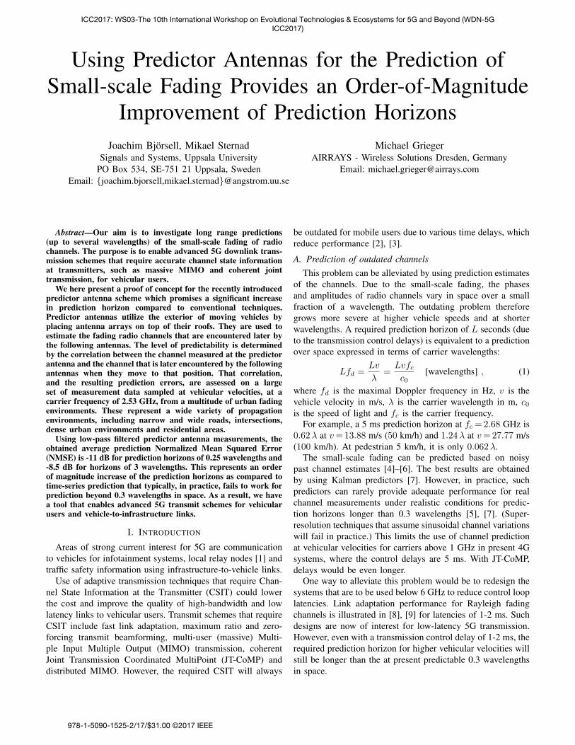
Using Predictor Antennas for the Prediction ofSmall-scale Fading Provides an Order-of-Magnitude

Improvement of Prediction HorizonsJoachim Bjorsell, Mikael Sternad

Signals and Systems, Uppsala UniversityPO Box 534, SE-751 21 Uppsala, Sweden

Email: {joachim.bjorsell,mikael.sternad}@angstrom.uu.se

Michael GriegerAIRRAYS - Wireless Solutions Dresden, Germany

Email: [email protected]

Abstract—Our aim is to investigate long range predictions(up to several wavelengths) of the small-scale fading of radiochannels. The purpose is to enable advanced 5G downlink trans-mission schemes that require accurate channel state informationat transmitters, such as massive MIMO and coherent jointtransmission, for vehicular users.

We here present a proof of concept for the recently introducedpredictor antenna scheme which promises a significant increasein prediction horizon compared to conventional techniques.Predictor antennas utilize the exterior of moving vehicles byplacing antenna arrays on top of their roofs. They are used toestimate the fading radio channels that are encountered later bythe following antennas. The level of predictability is determinedby the correlation between the channel measured at the predictorantenna and the channel that is later encountered by the followingantennas when they move to that position. That correlation,and the resulting prediction errors, are assessed on a largeset of measurement data sampled at vehicular velocities, at acarrier frequency of 2.53 GHz, from a multitude of urban fadingenvironments. These represent a wide variety of propagationenvironments, including narrow and wide roads, intersections,dense urban environments and residential areas.

Using low-pass filtered predictor antenna measurements, theobtained average prediction Normalized Mean Squared Error(NMSE) is -11 dB for prediction horizons of 0.25 wavelengths and-8.5 dB for horizons of 3 wavelengths. This represents an orderof magnitude increase of the prediction horizons as compared totime-series prediction that typically, in practice, fails to work forprediction beyond 0.3 wavelengths in space. As a result, we havea tool that enables advanced 5G transmit schemes for vehicularusers and vehicle-to-infrastructure links.

I. INTRODUCTION

Areas of strong current interest for 5G are communicationto vehicles for infotainment systems, local relay nodes [1] andtraffic safety information using infrastructure-to-vehicle links.

Use of adaptive transmission techniques that require Chan-nel State Information at the Transmitter (CSIT) could lowerthe cost and improve the quality of high-bandwidth and lowlatency links to vehicular users. Transmit schemes that requireCSIT include fast link adaptation, maximum ratio and zero-forcing transmit beamforming, multi-user (massive) Multi-ple Input Multiple Output (MIMO) transmission, coherentJoint Transmission Coordinated MultiPoint (JT-CoMP) anddistributed MIMO. However, the required CSIT will always

be outdated for mobile users due to various time delays, whichreduce performance [2], [3].

A. Prediction of outdated channelsThis problem can be alleviated by using prediction estimates

of the channels. Due to the small-scale fading, the phasesand amplitudes of radio channels vary in space over a smallfraction of a wavelength. The outdating problem thereforegrows more severe at higher vehicle speeds and at shorterwavelengths. A required prediction horizon of L seconds (dueto the transmission control delays) is equivalent to a predictionover space expressed in terms of carrier wavelengths:

Lfd =

Lv

�=

Lvfcc0

[wavelengths] , (1)

where fd is the maximal Doppler frequency in Hz, v is thevehicle velocity in m/s, � is the carrier wavelength in m, c0is the speed of light and fc is the carrier frequency.

For example, a 5 ms prediction horizon at fc =2.68 GHz is0.62� at v=13.88 m/s (50 km/h) and 1.24� at v=27.77 m/s(100 km/h). At pedestrian 5 km/h, it is only 0.062�.

The small-scale fading can be predicted based on noisypast channel estimates [4]–[6]. The best results are obtainedby using Kalman predictors [7]. However, in practice, suchpredictors can rarely provide adequate performance for realchannel measurements under realistic conditions for predic-tion horizons longer than 0.3 wavelengths [5], [7]. (Super-resolution techniques that assume sinusoidal channel variationswill fail in practice.) This limits the use of channel predictionat vehicular velocities for carriers above 1 GHz in present 4Gsystems, where the control delays are 5 ms. With JT-CoMP,delays would be even longer.

One way to alleviate this problem would be to redesign thesystems that are to be used below 6 GHz to reduce control looplatencies. Link adaptation performance for Rayleigh fadingchannels is illustrated in [8], [9] for latencies of 1-2 ms. Suchdesigns are now of interest for low-latency 5G transmission.However, even with a transmission control delay of 1-2 ms, therequired prediction horizon for higher vehicular velocities willstill be longer than the at present predictable 0.3 wavelengthsin space.

ICC2017: WS03-The 10th International Workshop on Evolutional Technologies & Ecosystems for 5G and Beyond (WDN-5GICC2017)

978-1-5090-1525-2/17/$31.00 ©2017 IEEE

B. Predictor antennas

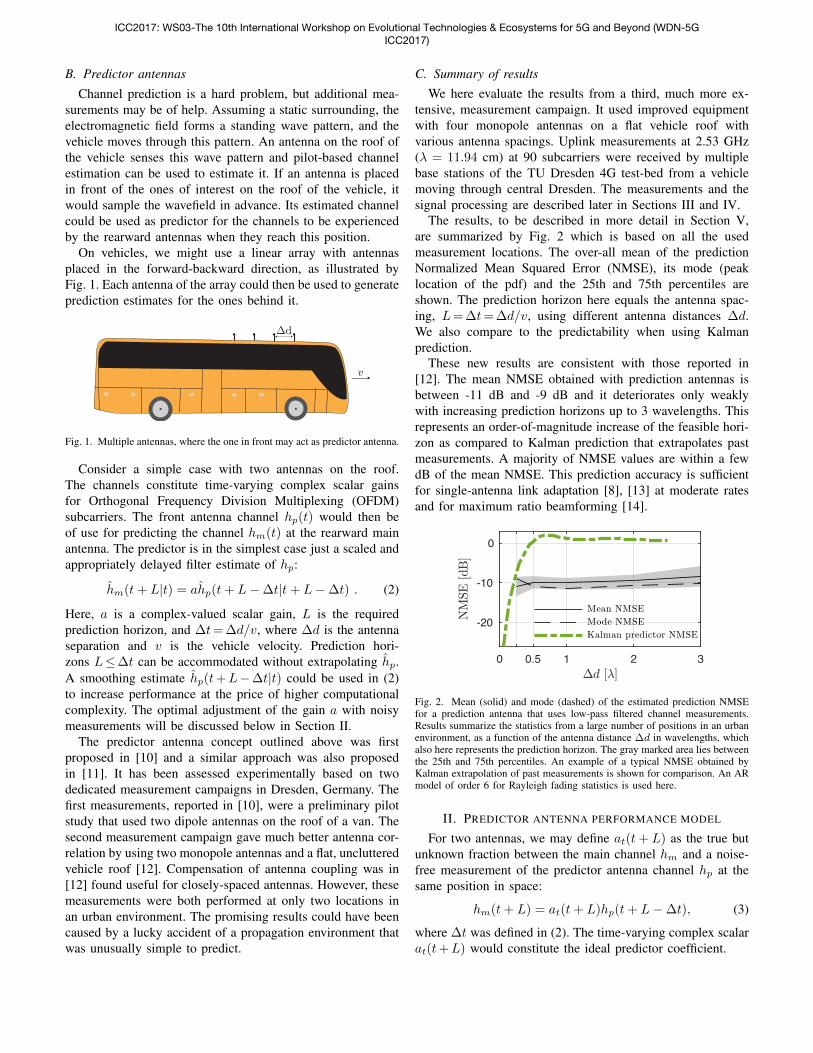
Channel prediction is a hard problem, but additional mea-surements may be of help. Assuming a static surrounding, theelectromagnetic field forms a standing wave pattern, and thevehicle moves through this pattern. An antenna on the roof ofthe vehicle senses this wave pattern and pilot-based channelestimation can be used to estimate it. If an antenna is placedin front of the ones of interest on the roof of the vehicle, itwould sample the wavefield in advance. Its estimated channelcould be used as predictor for the channels to be experiencedby the rearward antennas when they reach this position.

On vehicles, we might use a linear array with antennasplaced in the forward-backward direction, as illustrated byFig. 1. Each antenna of the array could then be used to generateprediction estimates for the ones behind it.

"d

v

Fig. 1. Multiple antennas, where the one in front may act as predictor antenna.

Consider a simple case with two antennas on the roof.The channels constitute time-varying complex scalar gainsfor Orthogonal Frequency Division Multiplexing (OFDM)subcarriers. The front antenna channel hp(t) would then beof use for predicting the channel hm(t) at the rearward mainantenna. The predictor is in the simplest case just a scaled andappropriately delayed filter estimate of hp:

ˆhm(t+ L|t) = aˆhp(t+ L��t|t+ L��t) . (2)

Here, a is a complex-valued scalar gain, L is the requiredprediction horizon, and �t=�d/v, where �d is the antennaseparation and v is the vehicle velocity. Prediction hori-zons L�t can be accommodated without extrapolating ˆhp.A smoothing estimate ˆhp(t+L��t|t) could be used in (2)to increase performance at the price of higher computationalcomplexity. The optimal adjustment of the gain a with noisymeasurements will be discussed below in Section II.

The predictor antenna concept outlined above was firstproposed in [10] and a similar approach was also proposedin [11]. It has been assessed experimentally based on twodedicated measurement campaigns in Dresden, Germany. Thefirst measurements, reported in [10], were a preliminary pilotstudy that used two dipole antennas on the roof of a van. Thesecond measurement campaign gave much better antenna cor-relation by using two monopole antennas and a flat, unclutteredvehicle roof [12]. Compensation of antenna coupling was in[12] found useful for closely-spaced antennas. However, thesemeasurements were both performed at only two locations inan urban environment. The promising results could have beencaused by a lucky accident of a propagation environment thatwas unusually simple to predict.

C. Summary of resultsWe here evaluate the results from a third, much more ex-

tensive, measurement campaign. It used improved equipmentwith four monopole antennas on a flat vehicle roof withvarious antenna spacings. Uplink measurements at 2.53 GHz(� = 11.94 cm) at 90 subcarriers were received by multiplebase stations of the TU Dresden 4G test-bed from a vehiclemoving through central Dresden. The measurements and thesignal processing are described later in Sections III and IV.

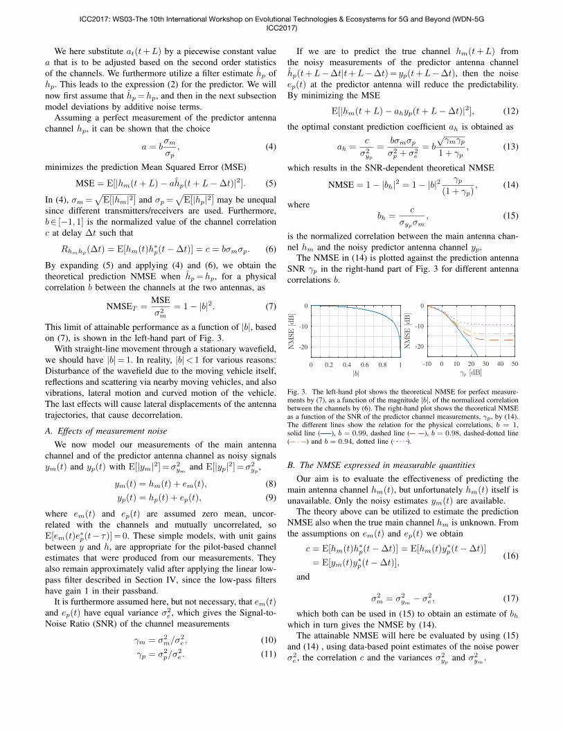
The results, to be described in more detail in Section V,are summarized by Fig. 2 which is based on all the usedmeasurement locations. The over-all mean of the predictionNormalized Mean Squared Error (NMSE), its mode (peaklocation of the pdf) and the 25th and 75th percentiles areshown. The prediction horizon here equals the antenna spac-ing, L=�t=�d/v, using different antenna distances �d.We also compare to the predictability when using Kalmanprediction.

These new results are consistent with those reported in[12]. The mean NMSE obtained with prediction antennas isbetween -11 dB and -9 dB and it deteriorates only weaklywith increasing prediction horizons up to 3 wavelengths. Thisrepresents an order-of-magnitude increase of the feasible hori-zon as compared to Kalman prediction that extrapolates pastmeasurements. A majority of NMSE values are within a fewdB of the mean NMSE. This prediction accuracy is sufficientfor single-antenna link adaptation [8], [13] at moderate ratesand for maximum ratio beamforming [14].

0 0.5 1 2 3"d [6]

-20

-10

0

NM

SE

[dB]

Mean NMSE

Mode NMSE

Kalman predictor NMSE

Fig. 2. Mean (solid) and mode (dashed) of the estimated prediction NMSEfor a prediction antenna that uses low-pass filtered channel measurements.Results summarize the statistics from a large number of positions in an urbanenvironment, as a function of the antenna distance �d in wavelengths, whichalso here represents the prediction horizon. The gray marked area lies betweenthe 25th and 75th percentiles. An example of a typical NMSE obtained byKalman extrapolation of past measurements is shown for comparison. An ARmodel of order 6 for Rayleigh fading statistics is used here.

II. PREDICTOR ANTENNA PERFORMANCE MODEL

For two antennas, we may define at(t+ L) as the true butunknown fraction between the main channel hm and a noise-free measurement of the predictor antenna channel hp at thesame position in space:

hm(t+ L) = at(t+ L)hp(t+ L��t), (3)

where �t was defined in (2). The time-varying complex scalarat(t+L) would constitute the ideal predictor coefficient.


We here substitute at(t+L) by a piecewise constant valuea that is to be adjusted based on the second order statisticsof the channels. We furthermore utilize a filter estimate ˆhp ofhp. This leads to the expression (2) for the predictor. We willnow first assume that ˆhp =hp, and then in the next subsectionmodel deviations by additive noise terms.

Assuming a perfect measurement of the predictor antennachannel hp, it can be shown that the choice

a = b�m

�p, (4)

minimizes the prediction Mean Squared Error (MSE)

MSE = E[|hm(t+ L)� aˆhp(t+ L��t)|2]. (5)

In (4), �m =

pE[|hm|2] and �p =

pE[|hp|2] may be unequal

since different transmitters/receivers are used. Furthermore,b2 [�1, 1] is the normalized value of the channel correlationc at delay �t such that

Rhmhp(�t) = E[hm(t)h⇤p(t��t)] = c = b�m�p. (6)

By expanding (5) and applying (4) and (6), we obtain thetheoretical prediction NMSE when ˆhp =hp, for a physicalcorrelation b between the channels at the two antennas, as

NMSET =

MSE�2m

= 1� |b|2. (7)

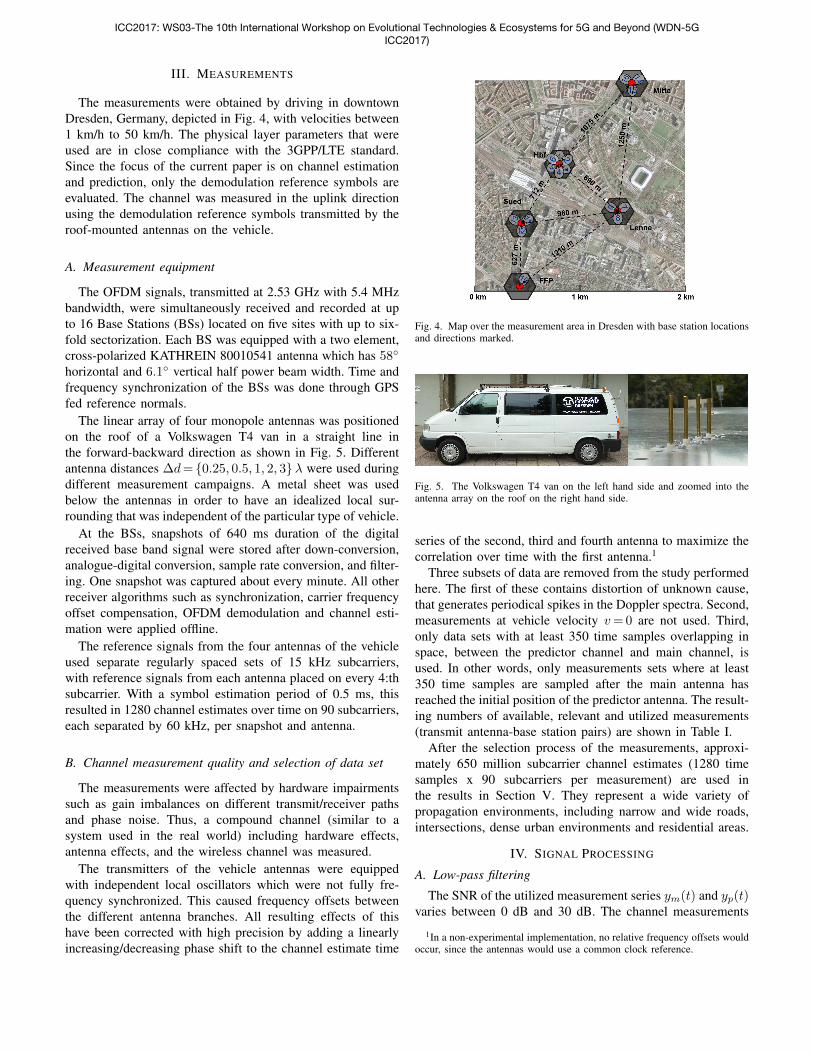
This limit of attainable performance as a function of |b|, basedon (7), is shown in the left-hand part of Fig. 3.

With straight-line movement through a stationary wavefield,we should have |b|=1. In reality, |b|< 1 for various reasons:Disturbance of the wavefield due to the moving vehicle itself,reflections and scattering via nearby moving vehicles, and alsovibrations, lateral motion and curved motion of the vehicle.The last effects will cause lateral displacements of the antennatrajectories, that cause decorrelation.

A. Effects of measurement noiseWe now model our measurements of the main antenna

channel and of the predictor antenna channel as noisy signalsym(t) and yp(t) with E[|ym|2] =�2

ymand E[|yp|2] =�2

yp,

ym(t) = hm(t) + em(t), (8)yp(t) = hp(t) + ep(t), (9)

where em(t) and ep(t) are assumed zero mean, uncor-related with the channels and mutually uncorrelated, soE[em(t)e⇤p(t� ⌧)] = 0. These simple models, with unit gainsbetween y and h, are appropriate for the pilot-based channelestimates that were produced from our measurements. Theyalso remain approximately valid after applying the linear low-pass filter described in Section IV, since the low-pass filtershave gain 1 in their passband.

It is furthermore assumed here, but not necessary, that em(t)and ep(t) have equal variance �2

e , which gives the Signal-to-Noise Ratio (SNR) of the channel measurements

�m = �2m/�2

e , (10)�p = �2

p/�2e . (11)

If we are to predict the true channel hm(t+L) fromthe noisy measurements of the predictor antenna channelˆhp(t+L��t|t+L��t)= yp(t+L��t), then the noiseep(t) at the predictor antenna will reduce the predictability.By minimizing the MSE

E[|hm(t+ L)� ahyp(t+ L��t)|2], (12)

the optimal constant prediction coefficient ah is obtained as

ah =

c

�2yp

=

b�m�p

�2p + �2

e

= b

p�m�p

1 + �p, (13)

which results in the SNR-dependent theoretical NMSE

NMSE = 1� |bh|2 = 1� |b|2 �p(1 + �p)

, (14)

wherebh =

c

�yp�m, (15)

is the normalized correlation between the main antenna chan-nel hm and the noisy predictor antenna channel yp.

The NMSE in (14) is plotted against the prediction antennaSNR �p in the right-hand part of Fig. 3 for different antennacorrelations b.

0 0.2 0.4 0.6 0.8 1

|b|

-20

-10

0

NMSE[dB]

-10 0 10 20 30 40 50

γp [dB]

-20

-10

0

NMSE[dB]

Fig. 3. The left-hand plot shows the theoretical NMSE for perfect measure-ments by (7), as a function of the magnitude |b|, of the normalized correlationbetween the channels by (6). The right-hand plot shows the theoretical NMSEas a function of the SNR of the predictor channel measurements, �p, by (14).The different lines show the relation for the physical correlations, b = 1,solid line ( ), b = 0.99, dashed line ( ), b = 0.98, dashed-dotted line( ) and b = 0.94, dotted line ( ).

B. The NMSE expressed in measurable quantitiesOur aim is to evaluate the effectiveness of predicting the

main antenna channel hm(t), but unfortunately hm(t) itself isunavailable. Only the noisy estimates ym(t) are available.

The theory above can be utilized to estimate the predictionNMSE also when the true main channel hm is unknown. Fromthe assumptions on em(t) and ep(t) we obtain

c = E[hm(t)h⇤p(t��t)] = E[hm(t)y⇤p(t��t)]

= E[ym(t)y⇤p(t��t)],(16)

and

�2m = �2

ym� �2

e , (17)

which both can be used in (15) to obtain an estimate of bhwhich in turn gives the NMSE by (14).

The attainable NMSE will here be evaluated by using (15)and (14) , using data-based point estimates of the noise power�2e , the correlation c and the variances �2

ypand �2

ym.


III. MEASUREMENTS

The measurements were obtained by driving in downtownDresden, Germany, depicted in Fig. 4, with velocities between1 km/h to 50 km/h. The physical layer parameters that wereused are in close compliance with the 3GPP/LTE standard.Since the focus of the current paper is on channel estimationand prediction, only the demodulation reference symbols areevaluated. The channel was measured in the uplink directionusing the demodulation reference symbols transmitted by theroof-mounted antennas on the vehicle.

A. Measurement equipment

The OFDM signals, transmitted at 2.53 GHz with 5.4 MHzbandwidth, were simultaneously received and recorded at upto 16 Base Stations (BSs) located on five sites with up to six-fold sectorization. Each BS was equipped with a two element,cross-polarized KATHREIN 80010541 antenna which has 58�horizontal and 6.1� vertical half power beam width. Time andfrequency synchronization of the BSs was done through GPSfed reference normals.

The linear array of four monopole antennas was positionedon the roof of a Volkswagen T4 van in a straight line inthe forward-backward direction as shown in Fig. 5. Differentantenna distances �d= {0.25, 0.5, 1, 2, 3}� were used duringdifferent measurement campaigns. A metal sheet was usedbelow the antennas in order to have an idealized local sur-rounding that was independent of the particular type of vehicle.

At the BSs, snapshots of 640 ms duration of the digitalreceived base band signal were stored after down-conversion,analogue-digital conversion, sample rate conversion, and filter-ing. One snapshot was captured about every minute. All otherreceiver algorithms such as synchronization, carrier frequencyoffset compensation, OFDM demodulation and channel esti-mation were applied offline.

The reference signals from the four antennas of the vehicleused separate regularly spaced sets of 15 kHz subcarriers,with reference signals from each antenna placed on every 4:thsubcarrier. With a symbol estimation period of 0.5 ms, thisresulted in 1280 channel estimates over time on 90 subcarriers,each separated by 60 kHz, per snapshot and antenna.

B. Channel measurement quality and selection of data set

The measurements were affected by hardware impairmentssuch as gain imbalances on different transmit/receiver pathsand phase noise. Thus, a compound channel (similar to asystem used in the real world) including hardware effects,antenna effects, and the wireless channel was measured.

The transmitters of the vehicle antennas were equippedwith independent local oscillators which were not fully fre-quency synchronized. This caused frequency offsets betweenthe different antenna branches. All resulting effects of thishave been corrected with high precision by adding a linearlyincreasing/decreasing phase shift to the channel estimate time

Fig. 4. Map over the measurement area in Dresden with base station locationsand directions marked.

Fig. 5. The Volkswagen T4 van on the left hand side and zoomed into theantenna array on the roof on the right hand side.

series of the second, third and fourth antenna to maximize thecorrelation over time with the first antenna.1

Three subsets of data are removed from the study performedhere. The first of these contains distortion of unknown cause,that generates periodical spikes in the Doppler spectra. Second,measurements at vehicle velocity v=0 are not used. Third,only data sets with at least 350 time samples overlapping inspace, between the predictor channel and main channel, isused. In other words, only measurements sets where at least350 time samples are sampled after the main antenna hasreached the initial position of the predictor antenna. The result-ing numbers of available, relevant and utilized measurements(transmit antenna-base station pairs) are shown in Table I.

After the selection process of the measurements, approxi-mately 650 million subcarrier channel estimates (1280 timesamples x 90 subcarriers per measurement) are used inthe results in Section V. They represent a wide variety ofpropagation environments, including narrow and wide roads,intersections, dense urban environments and residential areas.

IV. SIGNAL PROCESSING

A. Low-pass filtering

The SNR of the utilized measurement series ym(t) and yp(t)varies between 0 dB and 30 dB. The channel measurements

1In a non-experimental implementation, no relative frequency offsets wouldoccur, since the antennas would use a common clock reference.


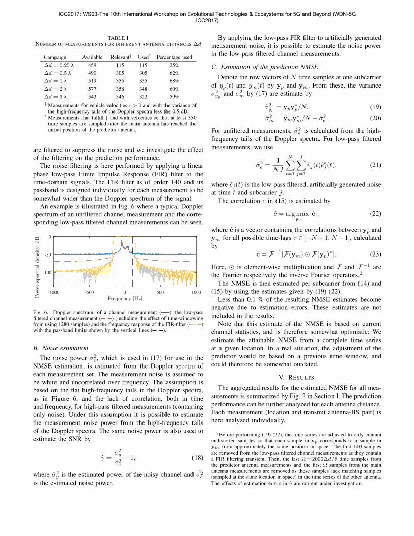
TABLE INUMBER OF MEASUREMENTS FOR DIFFERENT ANTENNA DISTANCES �d

Campaign Available Relevant† Used* Percentage used�d = 0.25� 459 115 115 25%�d = 0.5� 490 305 305 62%�d = 1� 519 355 355 68%�d = 2� 577 358 348 60%�d = 3� 543 346 322 59%† Measurements for vehicle velocities v > 0 and with the variance of

the high-frequency tails of the Doppler spectra less the 0.5 dB.* Measurements that fulfill † and with velocities so that at least 350

time samples are sampled after the main antenna has reached theinitial position of the predictor antenna.

are filtered to suppress the noise and we investigate the effectof the filtering on the prediction performance.

The noise filtering is here performed by applying a linearphase low-pass Finite Impulse Response (FIR) filter to thetime-domain signals. The FIR filter is of order 140 and itspassband is designed individually for each measurement to besomewhat wider than the Doppler spectrum of the signal.

An example is illustrated in Fig. 6 where a typical Dopplerspectrum of an unfiltered channel measurement and the corre-sponding low-pass filtered channel measurements can be seen.

-1000 -500 0 500 1000

Frequency [Hz]

-100

-50

0

Pow

erspectral

density

[dB]

Fig. 6. Doppler spectrum, of a channel measurement ( ), the low-passfiltered channel measurement ( ) (including the effect of time-windowingfrom using 1280 samples) and the frequency response of the FIR-filter ( )with the passband limits shown by the vertical lines ( ).

B. Noise estimation

The noise power �2e , which is used in (17) for use in the

NMSE estimation, is estimated from the Doppler spectra ofeach measurement set. The measurement noise is assumed tobe white and uncorrelated over frequency. The assumption isbased on the flat high-frequency tails in the Doppler spectra,as in Figure 6, and the lack of correlation, both in timeand frequency, for high-pass filtered measurements (containingonly noise). Under this assumption it is possible to estimatethe measurement noise power from the high-frequency tailsof the Doppler spectra. The same noise power is also used toestimate the SNR by

� =

�2y

�2e

� 1, (18)

where �2y is the estimated power of the noisy channel and ˆ�2

e

is the estimated noise power.

By applying the low-pass FIR filter to artificially generatedmeasurement noise, it is possible to estimate the noise powerin the low-pass filtered channel measurements.

C. Estimation of the prediction NMSE

Denote the row vectors of N time samples at one subcarrierof yp(t) and ym(t) by yp and ym. From these, the variance�2yp

and �2m by (17) are estimate by

�2yp

= ypy⇤p/N, (19)

�2m = ymy⇤

m/N � �2e . (20)

For unfiltered measurements, �2e is calculated from the high-

frequency tails of the Doppler spectra. For low-pass filteredmeasurements, we use

�2e =

1

NJ

NX

t=1

JX

j=1

ej(t)e⇤j (t), (21)

where ej(t) is the low-pass filtered, artificially generated noiseat time t and subcarrier j.

The correlation c in (15) is estimated by

c = argmax

c|ˆc|, (22)

where ˆc is a vector containing the correlations between yp andym for all possible time-lags ⌧ 2 [�N +1, N � 1], calculatedby

ˆc = F�1[F(ym)� F(yp)

⇤]. (23)

Here, � is element-wise multiplication and F and F�1 arethe Fourier respectively the inverse Fourier operators.2

The NMSE is then estimated per subcarrier from (14) and(15) by using the estimates given by (19)-(22).

Less than 0.1 % of the resulting NMSE estimates becomenegative due to estimation errors. These estimates are notincluded in the results.

Note that this estimate of the NMSE is based on currentchannel statistics, and is therefore somewhat optimistic: Weestimate the attainable NMSE from a complete time seriesat a given location. In a real situation, the adjustment of thepredictor would be based on a previous time window, andcould therefore be somewhat outdated.

V. RESULTS

The aggregated results for the estimated NMSE for all mea-surements is summarized by Fig. 2 in Section I. The predictionperformance can be further analyzed for each antenna distance.Each measurement (location and transmit antenna-BS pair) ishere analyzed individually.

2Before performing (19)-(22), the time series are adjusted to only containundistorted samples so that each sample in yp corresponds to a sample inym from approximately the same position in space. The first 140 samplesare removed from the low-pass filtered channel measurements as they containa FIR filtering transient. Then, the last ⌦=2000�d/v time samples fromthe predictor antenna measurements and the first ⌦ samples from the mainantenna measurements are removed as these samples lack matching samples(sampled at the same location in space) in the time series of the other antenna.The effects of estimation errors in v are current under investigation.


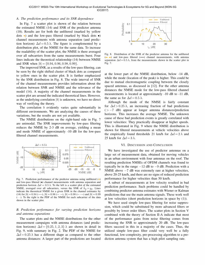
A. The prediction performance and its SNR dependence

In Fig. 7 a scatter plot is shown of the relation betweenthe estimated NMSE (14) and SNR of the predictor antenna(18). Results are for both the unfiltered (marked by yellowdots •) and the low-pass filtered (marked by black dots •)channel measurements with antenna separation (and predic-tion horizon) �d=0.5�. The figure is complemented by adistribution plot, of the NMSE for the same data. To increasethe readability of the scatter plot, the NMSE is there averagedover all subcarriers from the same measurements burst. Fourlines indicate the theoretical relationship (14) between NMSEand SNR when |b|= {0.94, 0.96, 0.98, 0.99}.

The improved SNR, as a results of the low-pass filtering, canbe seen by the right shifted cluster of black dots as comparedto yellow ones in the scatter plot. It is further emphasizedby the SNR distribution in Fig. 8. The wide interval of SNRof the channel measurements provides information about therelation between SNR and NMSE and the relevance of themodel (14). A majority of the channel measurements in thescatter plot are around the indicated theoretical lines. However,as the underlying correlation |b| is unknown, we have no directway of verifying the theory.

The correlation b evidently varies quite substantially indifferent environments. We are analyzing the causes of thesevariations, but the results are not yet available.

The NMSE distributions on the right-hand side in Fig. 7are unimodal. The SNR improvements by low-pass filteringreduces the NMSE by 2-3 dB on average, yielding a meanand mode NMSE of approximately -10 dB for the low-passfiltered channel measurements.

0 10 20 30

γp [dB]

-20

-10

0

NMSE

[dB]

∆d = 0.5λ

-25 -20 -15 -10 -5 0

NMSE [dB]

0

0.025

0.05

0.075

0.1

Probab

ility

UnfilteredFiltered

Fig. 7. Prediction performance of the predictor antenna using unfiltered (•)and low-pass filtered (•) channel measurements with antenna separation andprediction horizon �d = 0.5�. To the left is a scatter plot of the estimatedNMSE, averaged over all subcarriers, versus the SNR of hp = yp. Linesindicate the theoretical NMSE for a given SNR in the channel estimates by(14) for |b|=0.94 ( ), |b|=0.96 ( ), |b|=0.98 ( ) and |b|=0.99( ). To the right is the PDF of the NMSE for each subcarrier of the datashown in the scatter plot.

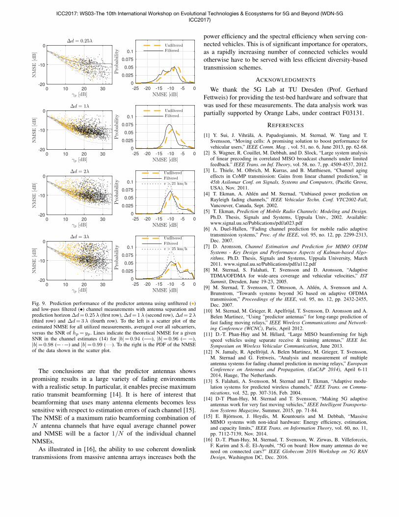
B. Prediction performance for varying prediction horizonsand antenna separations

The scatter plots and the NMSE distributions for the othermeasurement campaigns with antenna distances (and predic-tion horizons) �d= {0.25, 1, 2, 3}� are shown in detail inFig. 9, with summary in Fig. 2. The PDF of the NMSE for�d=0.25� has a different shape as compared to the otherantenna distances: A larger part of the predictions are located

0 10 20 30

γp [dB]

0

0.05

0.1

Probab

ility

UnfilteredFiltered

Fig. 8. Distribution of the SNR of the predictor antenna for the unfiltered( ) and low-pass filtered ( ) channel measurements, with antennaseparation �d=0.5�, from the measurements shown in the scatter plot inFig. 7.

at the lower part of the NMSE distribution, below -14 dB,while the mode (location of the peak) is higher. This could bedue to mutual electromagnetic coupling between the closelyspaced antennas, as discussed in [12]. For the other antennadistances the NMSE mode for the low-pass filtered channelmeasurements is located at approximately -10 dB to -11 dB,the same as for �d=0.5�.

Although the mode of the NMSE is fairly constantfor �d> 0.25�, an increasing fraction of bad predictions(>�7 dB) appear at longer antenna distances/predictionhorizons. This increases the average NMSE. The unknowncause of these bad prediction events is greatly correlated withlower velocities: They practically disappear at higher speeds.This is illustrated in Fig. 9 where the NMSE distribution isshown for filtered measurements at vehicle velocities abovethe empirically found thresholds 21 km/h for �d=2� and25 km/h for �d=3�.

VI. DISCUSSION AND CONCLUSION

We have investigated the use of predictor antennas on alarge set of measurement data, obtained for moving vehiclesin an urban environment with four antennas on the roof. Theresulting prediction NMSEs of OFDM channels was found totypically be in the range �12 dB to �9 dB. Prediction with aNMSE above �7 dB was extremely rare at higher velocities,above 20-25 km/h, and there are no signs of reduced predictionperformance for higher velocities than 50 km/h.

A subset of measurements at low velocity resulted in badprediction performance. Such problems could be handled bycombining predictor antenna estimates with Wiener or Kalmanpredictions that use the main antenna signals. These work wellat low velocities (short prediction horizons in space by (1)).

We have used simple low-pass filtering for noise suppres-sion, which could be substituted by more advanced filters orpossibly by lower order filters. The scatter plots in Section Vcombined with the theory of Section II-A indicate that mostof the performance gains from noise filtering comes fromincreasing the SNR to approximately 20 dB. The low-passfilters succeed in this in a majority of the cases. Thus, theutilized simple low-pass filter could very well be a fullyfunctional, low-complexity, pre-processing algorithm to a pre-diction antenna system that has a high pilot sampling rate.


0 10 20 30

γp [dB]

-20

-10

0

NMSE

[dB]

∆d = 0.25λ

-25 -20 -15 -10 -5 0

NMSE [dB]

0

0.025

0.05

0.075

0.1

Probab

ility

UnfilteredFiltered

0 10 20 30

γp [dB]

-20

-10

0

NMSE

[dB]

∆d = 1λ

-25 -20 -15 -10 -5 0

NMSE [dB]

0

0.025

0.05

0.075

0.1Probab

ility

UnfilteredFiltered

0 10 20 30

γp [dB]

-20

-10

0

NMSE

[dB]

∆d = 2λ

-25 -20 -15 -10 -5 0

0

0.025

0.05

0.075

0.1

0 10 20 30

γp [dB]

-20

-10

0

NMSE

[dB]

∆d = 3λ

-25 -20 -15 -10 -5 0

0

0.025

0.05

0.075

0.1

Fig. 9. Prediction performance of the predictor antenna using unfiltered (•)and low-pass filtered (•) channel measurements with antenna separation andprediction horizon �d=0.25� (first row), �d=1� (second row), �d=2�(third row) and �d=3� (fourth row). To the left is a scatter plot of theestimated NMSE for all utilized measurements, averaged over all subcarriers,versus the SNR of hp = yp. Lines indicate the theoretical NMSE for a givenSNR in the channel estimates (14) for |b|=0.94 ( ), |b|=0.96 ( ),|b|=0.98 ( ) and |b|=0.99 ( ). To the right is the PDF of the NMSEof the data shown in the scatter plot.

The conclusions are that the predictor antennas showspromising results in a large variety of fading environmentswith a realistic setup. In particular, it enables precise maximumratio transmit beamforming [14]. It is here of interest thatbeamforming that uses many antenna elements becomes lesssensitive with respect to estimation errors of each channel [15].The NMSE of a maximum ratio beamforming combination ofN antenna channels that have equal average channel powerand NMSE will be a factor 1/N of the individual channelNMSEs.

As illustrated in [16], the ability to use coherent downlinktransmissions from massive antenna arrays increases both the

power efficiency and the spectral efficiency when serving con-nected vehicles. This is of significant importance for operators,as a rapidly increasing number of connected vehicles wouldotherwise have to be served with less efficient diversity-basedtransmission schemes.

ACKNOWLEDGMENTS

We thank the 5G Lab at TU Dresden (Prof. GerhardFettweis) for providing the test-bed hardware and software thatwas used for these measurements. The data analysis work waspartially supported by Orange Labs, under contract F03131.

REFERENCES

[1] Y. Sui, J. Vihrala, A. Papadogiannis, M. Sternad, W. Yang and T.Svensson, “Moving cells: A promising solution to boost performance forvehicular users,” IEEE Comm. Mag. , vol. 51, no. 6, June 2013, pp. 62-68.

[2] S. Wagner, R. Couillet, M. Debbah, and D. Slock, “Large system analysisof linear precoding in correlated MISO broadcast channels under limitedfeedback.” IEEE Trans. on Inf. Theory, vol. 58, no. 7, pp. 4509-4537, 2012.

[3] L. Thiele, M. Olbrich, M. Kurras, and B. Matthiesen, “Channel agingeffects in CoMP transmission: Gains from linear channel prediction,” in45th Asilomar Conf. on Signals, Systems and Computers, (Pacific Grove,USA), Nov. 2011.

[4] T. Ekman, A. Ahlen and M. Sternad, “Unbiased power prediction onRayleigh fading channels,” IEEE Vehicular Techn. Conf. VTC2002-Fall,Vancouver, Canada, Sept. 2002.

[5] T. Ekman, Prediction of Mobile Radio Channels: Modeling and Design.Ph.D. Thesis, Signals and Systems, Uppsala Univ., 2002. Available:www.signal.uu.se/Publications/pdf/a023.pdf

[6] A. Duel-Hallen, “Fading channel prediction for mobile radio adaptivetransmission systems,” Proc. of the IEEE, vol. 95, no. 12, pp. 2299-2313,Dec. 2007.

[7] D. Aronsson, Channel Estimation and Prediction for MIMO OFDMSystems - Key Design and Performance Aspects of Kalman-based Algo-rithms. Ph.D. Thesis, Signals and Systems, Uppsala University, March2011. www.signal.uu.se/Publications/pdf/a112.pdf

[8] M. Sternad, S. Falahati, T. Svensson and D. Aronsson, “AdaptiveTDMA/OFDMA for wide-area coverage and vehicular velocities,” ISTSummit, Dresden, June 19-23, 2005.

[9] M. Sternad, T. Svensson, T. Ottosson, A. Ahlen, A. Svensson and A.Brunstrom, “Towards systems beyond 3G based on adaptive OFDMAtransmission,” Proceedings of the IEEE, vol. 95, no. 12, pp. 2432-2455,Dec. 2007.

[10] M. Sternad, M. Grieger, R. Apelfrojd, T. Svensson, D. Aronsson and A.Belen Martinez, “Using ”predictor antennas” for long-range prediction offast fading moving relays,” IEEE Wireless Communications and Network-ing Conference (WCNC), Paris, April 2012.

[11] D.-T. Phan-Huy and M. Helard, “Large MISO beamforming for highspeed vehicles using separate receive & training antennas,” IEEE Int.Symposium on Wireless Vehicular Communication, June 2013.

[12] N. Jamaly, R. Apelfrojd, A. Belen Martinez, M. Grieger, T. Svensson,M. Sternad and G. Fettweis, “Analysis and measurement of multipleantenna systems for fading channel prediction in moving relays,” EuropeanConference on Antennas and Propagation, (EuCAP 2014), April 6-112014, Hauge, The Netherlands.

[13] S. Falahati, A. Svensson, M. Sternad and T. Ekman, “Adaptive modu-lation systems for predicted wireless channels,” IEEE Trans. on Commu-nications, vol. 52, pp. 307-316, Feb. 2004.

[14] D-T Phan-Huy, M. Sternad and T. Svensson, “Making 5G adaptiveantennas work for very fast moving vehicles,” IEEE Intelligent Transporta-tion Systems Magazine, Summer, 2015, pp. 71-84.

[15] E. Bjornson, J. Hoydis, M. Kountouris and M. Debbah, “MassiveMIMO systems with non-ideal hardware: Energy efficiency, estimation,and capacity limits,” IEEE Trans. on Information Theory, vol. 60, no. 11,pp. 7112-7139, Nov. 2014.

[16] D.-T. Phan-Huy, M. Sternad, T. Svensson, W. Zirwas, B. Villeforceix,F. Karim and S.-E. El-Ayoubi, “5G on board: How many antennas do weneed on connected cars?” IEEE Globecom 2016 Workshop on 5G RANDesign, Washington DC, Dec. 2016.


Documents

Using Predictor Antennas for the Prediction of Small … · Small-scale Fading Provides an Order-of-Magnitude Improvement of Prediction Horizons ... Wireless Solutions Dresden, Germany