Embed Size (px)
DESCRIPTION
Using Profile Likelihood ratios at the LHC. Clement Helsens , CERN-PH Top LHC-France, CC IN2P3-Lyon, 22 March 2013. Outline. Introduction Reminder of statistic Hypothesis testing Profile Likelihood ratio Some example helping to build an analysis From real analyses From Toy MC - PowerPoint PPT Presentation
Citation preview
Using Profile Likelihood ratios at the LHCClement Helsens, CERN-PHTop LHC-France, CC IN2P3-Lyon, 22 March 2013
Hel
sens
Cle
men
t Top
LH
C-Fr
ance
Outline• Introduction• Reminder of statistic• Hypothesis testing
• Profile Likelihood ratio• Some example helping to build an analysis• From real analyses• From Toy MC
• Conclusion
22/0
3/13
2
Hel
sens
Cle
men
t Top
LH
C-Fr
ance
Introduction• Disclaimers • This talk is not a lecture in statistic!• I will not encourage you to use any particular tool or method
• Only talk about (hybrid) Frequentist methods and not about Bayesian marginalization
• This talk should be seen like a methodology to follow when one wants to use profiling in an analysis
• For the example I will only talk about searches (LHC is a discovery machine )
• I will rather try to give tips to perform an analysis using profiling rather than reviewing analysis using it• This might help you to have better results
22/0
3/13
3
Hel
sens
Cle
men
t Top
LH
C-Fr
ance
Hypothesis Testing 1/5• Deciding between two hypothesis• Null hypothesis H0 (background only, process already known)
• Test hypothesis H1 (background + alternative model)
• Why can’t we just decide by testing H0 hypothesis only? Why do we need an alternate hypothesis?• Data points are randomly distributed:
• If a discrepancy between the data and the H0 hypothesis is observed, we will be obliged to call it a random fluctuation
• H0 might look globally right but predictions slightly wrong• If we look at enough different distributions, we will find some that are mis-modeled • Having a second hypothesis provides guidance where to look
• Duhem–Quine thesis:• It is impossible to test a scientific hypothesis in isolation, because an empirical
test of the hypothesis requires one or more background assumptions (also called auxiliary/alternate hypotheses).
• http://en.wikipedia.org/wiki/Quine-Duhem_thesis
22/0
3/13
4

Hel
sens
Cle
men
t Top
LH
C-Fr
ance
Hypothesis Testing 2/5• Is square A darker
than square B? (there is only one correct answer) 22
/03/
13
5
Hel
sens
Cle
men
t Top
LH
C-Fr
ance
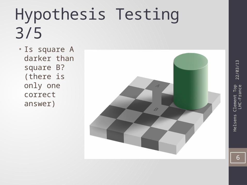
Hypothesis Testing 3/5• Is square A darker
than square B? (there is only one correct answer) 22
/03/
13
6
Hel
sens
Cle
men
t Top
LH
C-Fr
ance
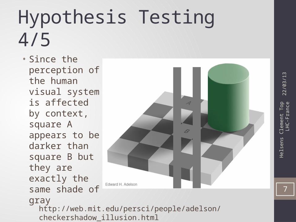
Hypothesis Testing 4/5• Since the
perception of the human visual system is affected by context, square A appears to be darker than square B but they are exactly the same shade of gray
http://web.mit.edu/persci/people/adelson/checkershadow_illusion.html
22/0
3/13
7
Hel
sens
Cle
men
t Top
LH
C-Fr
ance
Hypothesis Testing 5/5• So proving one hypothesis is wrong does not mean the
proposed alternative must right• For example, search for highly energetic processes (like heavy-
quarks)• Use inclusive distributions like HT (ΣpT)• If discrepancies observed in the tails of HT, does this necessarily
means we have new physics?
22/0
3/13
8
Hel
sens
Cle
men
t Top
LH
C-Fr
ance
Frequentist Hypothesis Testing 1/2• 1) Construct a quantity that ranks outcomes as being more
signal-like or more background-like. Called a test statistic:• Search for a new particle by counting events passing selection
cuts• Expect B events in H0 and S+B events in H1
• The number of observed events nObs is a good test statistic
• 2) Build a prediction of the test statistic separately assuming• H0 is true
• H1 is true
• 3) Run the experiment and get nObs (in our case run LHC + ATLAS/CMS)
• 4) Compute the p-value
22/0
3/13
9
Hel
sens
Cle
men
t Top
LH
C-Fr
ance
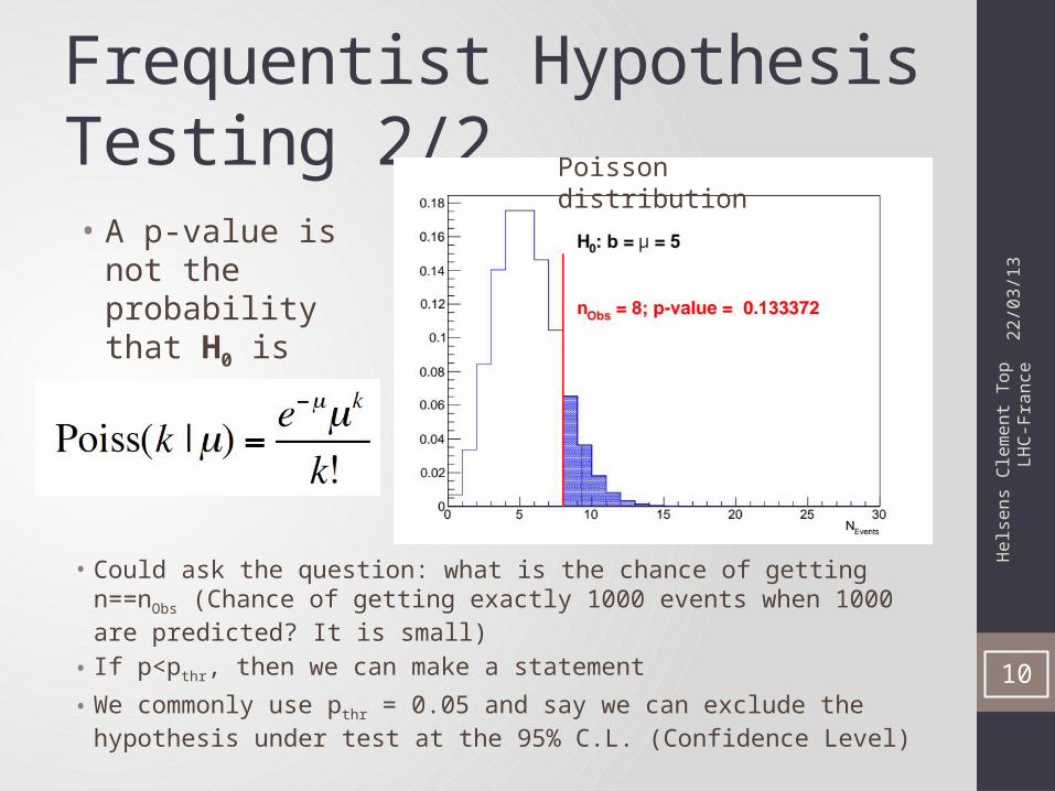
Frequentist Hypothesis Testing 2/2
• Could ask the question: what is the chance of getting n==nObs (Chance of getting exactly 1000 events when 1000 are predicted? It is small)
• If p<pthr, then we can make a statement
• We commonly use pthr = 0.05 and say we can exclude the hypothesis under test at the 95% C.L. (Confidence Level)
22/0
3/13
10
• A p-value is not the probability that H0 is true
Poisson distribution
Hel
sens
Cle
men
t Top
LH
C-Fr
ance
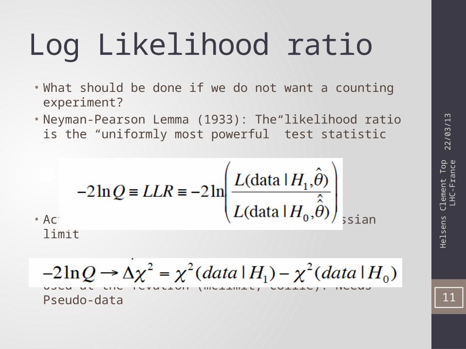
Log Likelihood ratio• What should be done if we do not want a counting
experiment?• Neyman-Pearson Lemma (1933): The likelihood ratio is the
“uniformly most powerful” test statistic
• Acts like the difference of χ2 in the Gaussian limit
• Used at the Tevatron (mclimit, collie). Needs Pseudo-data
22/0
3/13
11
Hel
sens
Cle
men
t Top
LH
C-Fr
ance
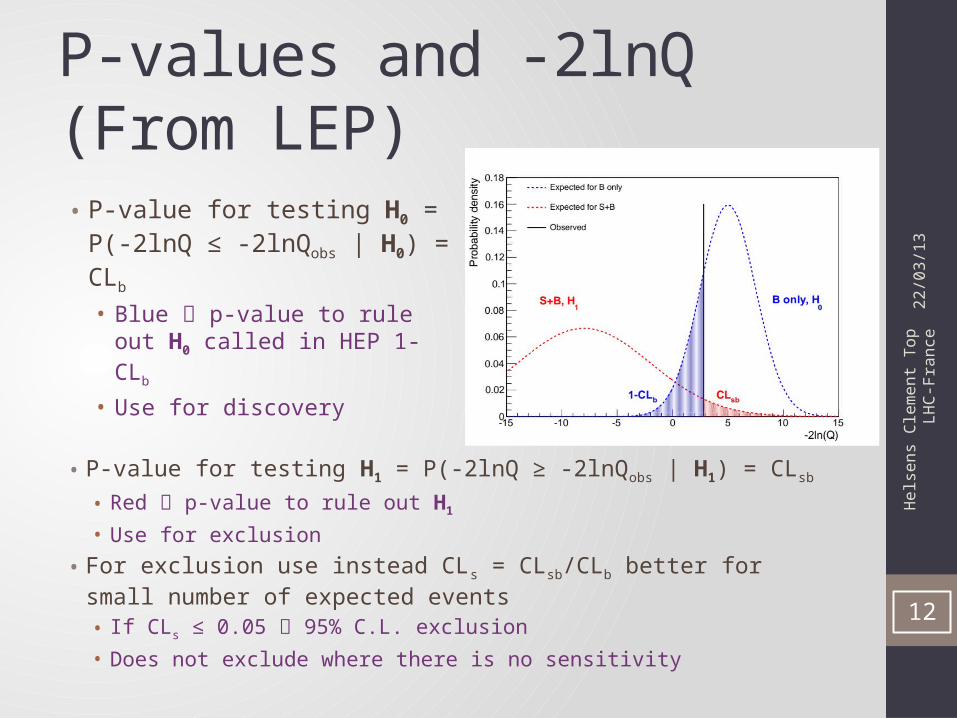
P-values and -2lnQ (From LEP)
• P-value for testing H0 = P(-2lnQ ≤ -2lnQobs | H0) = CLb
• Blue p-value to rule out H0 called in HEP 1-CLb
• Use for discovery
22/0
3/13
12
• P-value for testing H1 = P(-2lnQ ≥ -2lnQobs | H1) = CLsb
• Red p-value to rule out H1
• Use for exclusion
• For exclusion use instead CLs = CLsb/CLb better for small number of expected events• If CLs ≤ 0.05 95% C.L. exclusion• Does not exclude where there is no sensitivity
Hel
sens
Cle
men
t Top
LH
C-Fr
ance
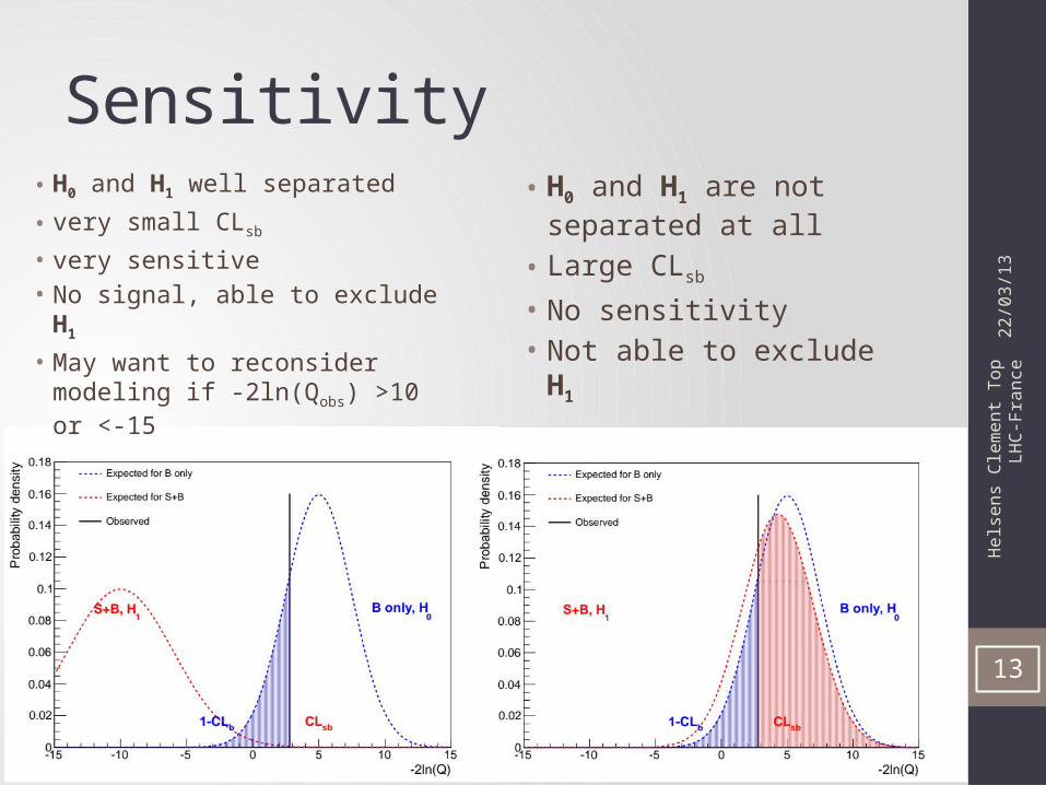
Sensitivity• H0 and H1 are not
separated at all• Large CLsb
• No sensitivity• Not able to exclude H1
22/0
3/13
13
• H0 and H1 well separated
• very small CLsb
• very sensitive• No signal, able to exclude H1
• May want to reconsider modeling if -2ln(Qobs) >10 or <-15
Hel
sens
Cle
men
t Top
LH
C-Fr
ance
Incorporating systematics
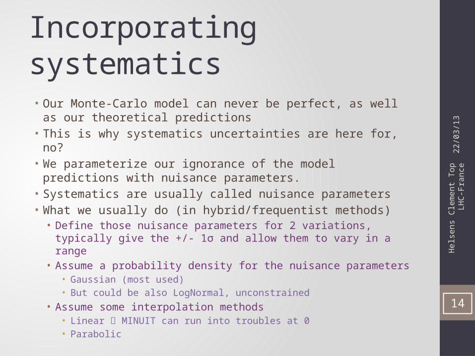
• Our Monte-Carlo model can never be perfect, as well as our theoretical predictions
• This is why systematics uncertainties are here for, no?• We parameterize our ignorance of the model predictions with
nuisance parameters.• Systematics are usually called nuisance parameters• What we usually do (in hybrid/frequentist methods)• Define those nuisance parameters for 2 variations, typically give the
+/- 1σ and allow them to vary in a range• Assume a probability density for the nuisance parameters
• Gaussian (most used)• But could be also LogNormal, unconstrained
• Assume some interpolation methods • Linear MINUIT can run into troubles at 0• Parabolic
22/0
3/13
14
Hel
sens
Cle
men
t Top
LH
C-Fr
ance
Fitting/Profiling
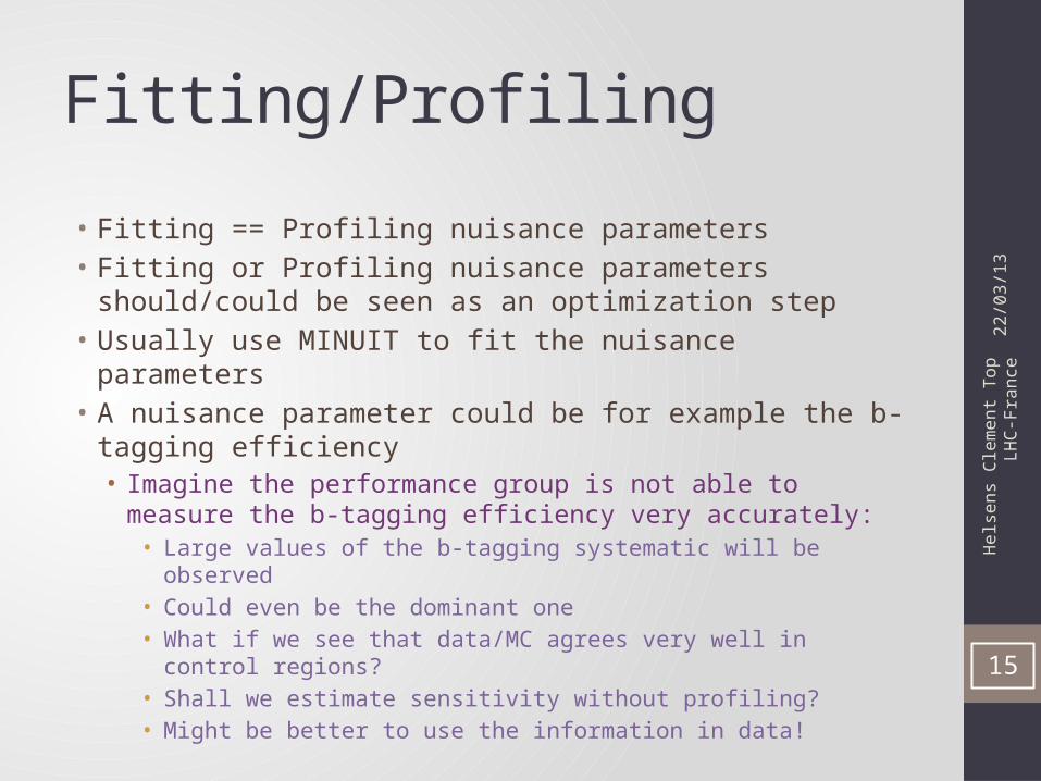
• Fitting == Profiling nuisance parameters• Fitting or Profiling nuisance parameters should/could be seen
as an optimization step• Usually use MINUIT to fit the nuisance parameters• A nuisance parameter could be for example the b-tagging
efficiency• Imagine the performance group is not able to measure the b-
tagging efficiency very accurately:• Large values of the b-tagging systematic will be observed• Could even be the dominant one• What if we see that data/MC agrees very well in control regions?• Shall we estimate sensitivity without profiling?• Might be better to use the information in data!
22/0
3/13
15
Hel
sens
Cle
men
t Top
LH
C-Fr
ance
Deeper in the Log Likelihood ratio
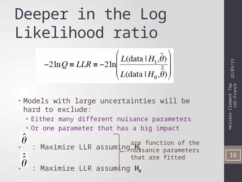
• Models with large uncertainties will be hard to exclude:• Either many different nuisance parameters• Or one parameter that has a big impact
• : Maximize LLR assuming H1
• : Maximize LLR assuming H0
22/0
3/13
16
are function of the nuisance parameters that are fitted
Hel
sens
Cle
men
t Top
LH
C-Fr
ance
What is done in practice• Fit twice:• Once assuming H0, once assuming H1
• Two sets of fitted parameters are extracted• When running Toy-MC should:• Assume H0
• Assume H1
• So at the end of the day, 4 fits are needed to have one 2 expected values to be used to compute the confidence level
22/0
3/13
17
Hel
sens
Cle
men
t Top
LH
C-Fr
ance
Building an analysis using profiling• If you are running a cut and count analysis, you can not use
profiling of nuisance parameters, all the systematics have the same impact for all the samples:• All normalization, no shape
• If you are using a shape analysis that is tight enough there is also maybe no need to use profiling
• But if you have sidebands (enough bins or channels to constrain the nuisance parameters), you might want to consider using profiling
• Number of things needs to be checked (not a complete list!!) :• If the fitted nuisance parameters are constrained in data• Pull distributions: (fit-injected)/(fitted error)• Fitted error
22/0
3/13
18
Hel
sens
Cle
men
t Top
LH
C-Fr
ance
Fitting or not fitting?
• See Favara and Pieri, hep-ex/9706016• Some channels or bins within channels might be better off
being neglected when estimating the sensitivity in order to gain discrimination power
• If the systematic uncertainty on the background B exceeds the expected signal S, then reduce sensitivity
• Fitting background helps to constraint them• Sidebands with little signal provide useful information, but
they need to be fitted
22/0
3/13
19
Hel
sens
Cle
men
t Top
LH
C-Fr
ance
Toy MC example: Binning
• All cases : • 500 GeV t’, 100% mixing to Wb• Only consider ttbar as a background• Systematic added (norm only)
• 50% in total for BG (same in all bins)
• Comparison made for• Statistical only nuisance parameters• Statistical + Systematics no profiling• Statistical + Systematics profiling
22/0
3/13
20
Hel
sens
Cle
men
t Top
LH
C-Fr
ance
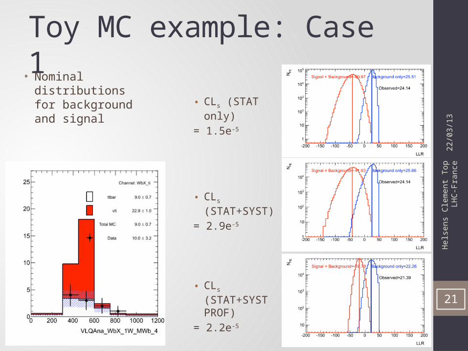
Toy MC example: Case 1
• CLs (STAT only)
= 1.5e-5
• CLs (STAT+SYST)
= 2.9e-5
• CLs (STAT+SYST PROF)
= 2.2e-5
22/0
3/13
21
• Nominal distributions for background and signal
Hel
sens
Cle
men
t Top
LH
C-Fr
ance
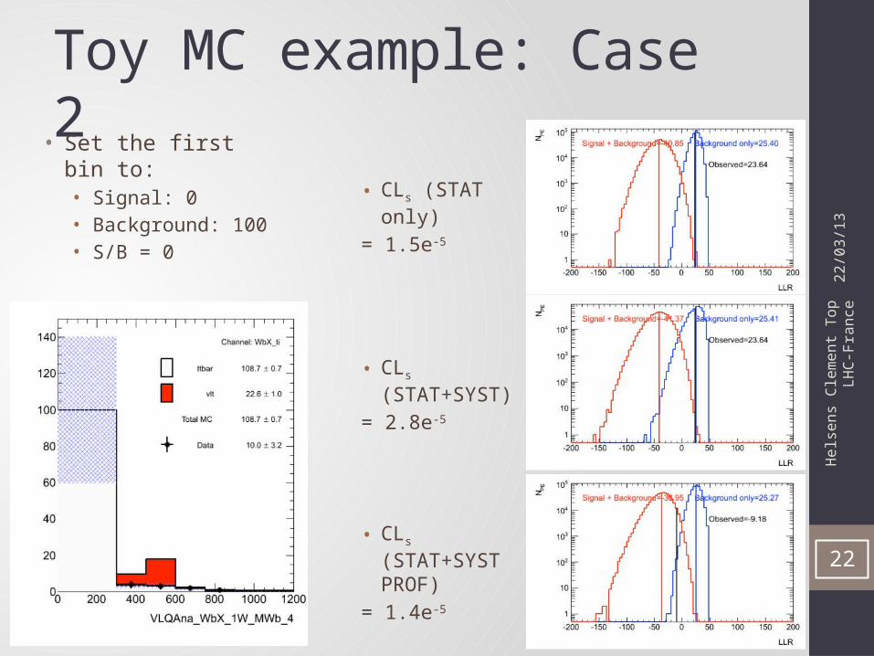
Toy MC example: Case 2
• CLs (STAT only)
= 1.5e-5
• CLs (STAT+SYST)
= 2.8e-5
• CLs (STAT+SYST PROF)
= 1.4e-5
22/0
3/13
22
• Set the first bin to:• Signal: 0• Background: 100• S/B = 0
Hel
sens
Cle
men
t Top
LH
C-Fr
ance
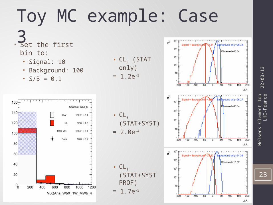
Toy MC example: Case 3
• CLs (STAT only)
= 1.2e-5
• CLs (STAT+SYST)
= 2.0e-4
• CLs (STAT+SYST PROF)
= 1.7e-5
22/0
3/13
23
• Set the first bin to:• Signal: 10• Background: 100• S/B = 0.1
Hel
sens
Cle
men
t Top
LH
C-Fr
ance
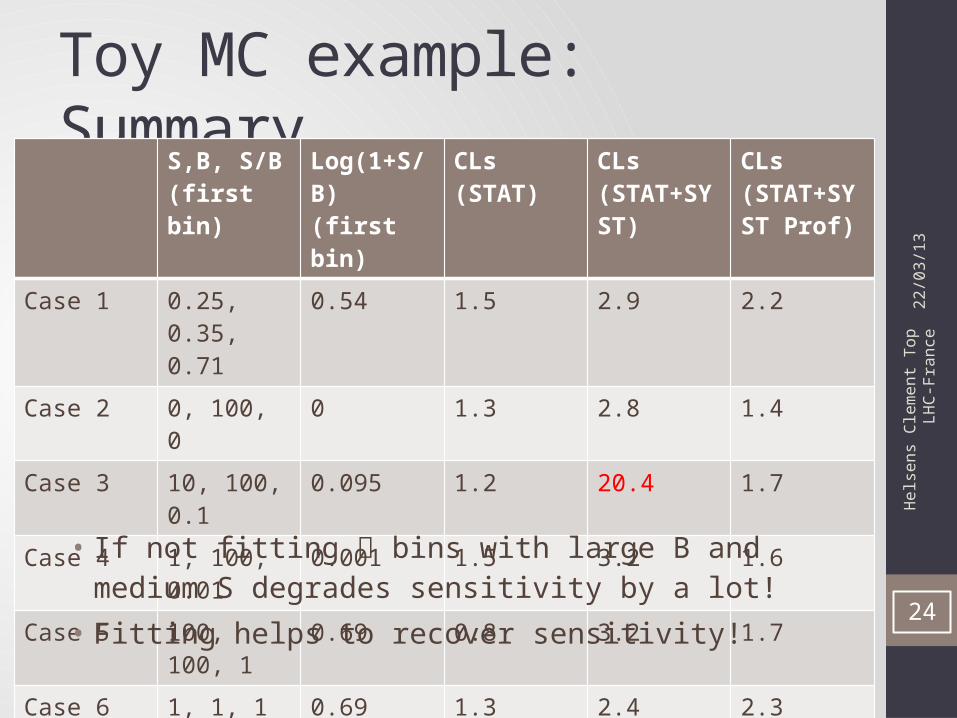
Toy MC example: Summary
22/0
3/13
24
S,B, S/B (first bin)
Log(1+S/B) (first bin)
CLs (STAT)
CLs (STAT+SYST)
CLs (STAT+SYST Prof)
Case 1 0.25, 0.35, 0.71
0.54 1.5 2.9 2.2
Case 2 0, 100, 0 0 1.3 2.8 1.4
Case 3 10, 100, 0.1 0.095 1.2 20.4 1.7
Case 4 1, 100, 0.01 0.001 1.5 3.2 1.6
Case 5 100, 100, 1 0.69 0.8 3.2 1.7
Case 6 1, 1, 1 0.69 1.3 2.4 2.3
• If not fitting bins with large B and medium S degrades sensitivity by a lot!
• Fitting helps to recover sensitivity!
Hel
sens
Cle
men
t Top
LH
C-Fr
ance
Toy MC example: Profiling
• In the next slides I will take an other toy-MC example • Signal: Gaussian signal• BG1: linearly falling background • BG2: flat background• Data are fluctuations around the expected Monte-Carlo
predictions• Systematics• Normalization only:
• Luminosity ± 5% for all the samples• BG1: ± 20%• BG2: ± 20%
• One shape systematic affecting BG1 and BG2
22/0
3/13
25
Hel
sens
Cle
men
t Top
LH
C-Fr
ance
Optimize the binning 1/4
• Two competing effects:• 1) Split events into classes with very different S/B improves the
sensitivity of a search or a measurement • Adding events in categories with low S/B to events in categories
with higher S/B dilutes information and reduces sensitivity• Pushes towards more bins
• 2) Insufficient Monte-Carlo can cause some bins to be empty, or nearly so.
• Need reliable predictions of signals and backgrounds in each bin• Pushes towards fewer bins
22/0
3/13
26
Hel
sens
Cle
men
t Top
LH
C-Fr
ance
Optimize the binning 2/4
• It doesn’t matter that there are bins with zero data events• in any case, most of the time a search analysis is build blinded• so you do not know a-priori if all your bins will be populated with data
events• there’s always a Poisson probability for observing zero events
• The problem is wrong prediction: • Zero background expectation and nonzero signal expectation is a
discovery!• Never have bins with empty background predictions
• Pay attention to Monte-Carlo error• keep in mind that the statistical error in each bin is an un-correlated
nuisance parameter• Do not hesitate to merge bins in order to reduce the statistical error
in each bin below a certain threshold• For example ΔB/B < 10%
22/0
3/13
27
Hel
sens
Cle
men
t Top
LH
C-Fr
ance
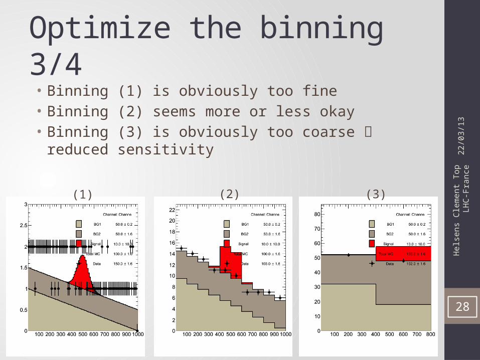
Optimize the binning 3/4• Binning (1) is obviously too fine• Binning (2) seems more or less okay• Binning (3) is obviously too coarse reduced sensitivity
22/0
3/13
28
(1) (2) (3)
Hel
sens
Cle
men
t Top
LH
C-Fr
ance
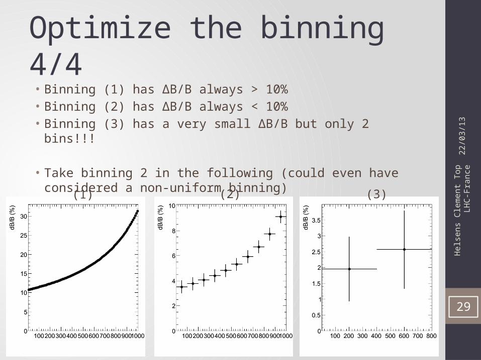
Optimize the binning 4/4• Binning (1) has ΔB/B always > 10%• Binning (2) has ΔB/B always < 10%• Binning (3) has a very small ΔB/B but only 2 bins!!!
• Take binning 2 in the following (could even have considered a non-uniform binning)
22/0
3/13
29
(1) (2) (3)
Hel
sens
Cle
men
t Top
LH
C-Fr
ance
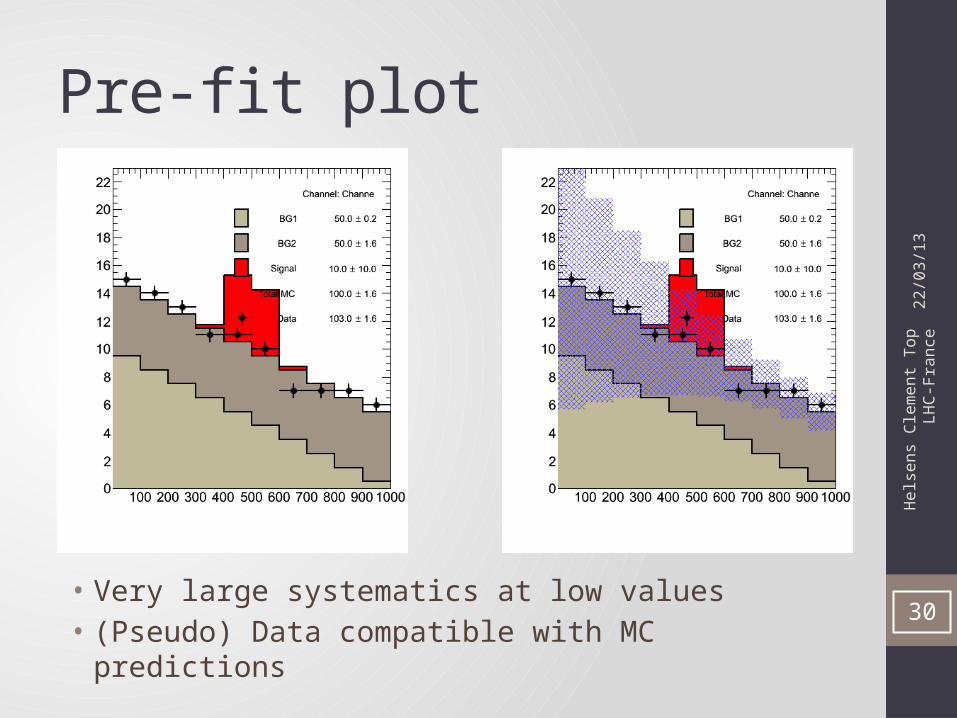
Pre-fit plot
• Very large systematics at low values• (Pseudo) Data compatible with MC predictions
22/0
3/13
30
Hel
sens
Cle
men
t Top
LH
C-Fr
ance
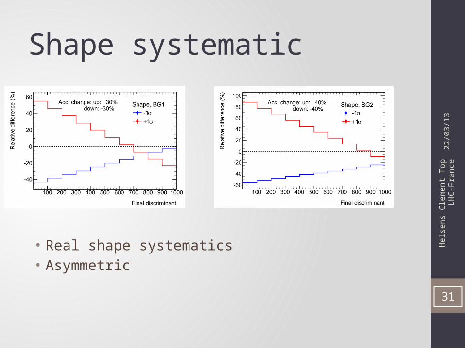
Shape systematic
• Real shape systematics• Asymmetric
22/0
3/13
31
Hel
sens
Cle
men
t Top
LH
C-Fr
ance
Context of the study• Will consider 3 cases in the following:• No fitting• Fitting the shape systematic only• Fitting all the systematics 22
/03/
13
32
Hel
sens
Cle
men
t Top
LH
C-Fr
ance
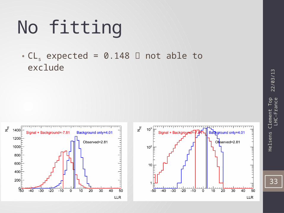
No fitting• CLs expected = 0.148 not able to exclude
22/0
3/13
33

Hel
sens
Cle
men
t Top
LH
C-Fr
ance
Fitting the shape systematic 1/2• CLs expected = 0.071 not able to exclude, but much better result• Reduce the uncertainty
22/0
3/13
34
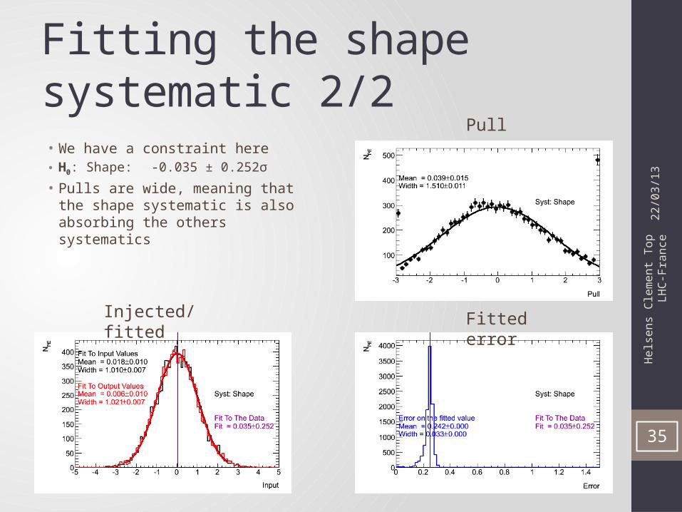
Post-Fit considering H0
Shape: 0.035 ± 0.252σPost-Fit considering H1
Shape: -0.105 ± 0.256σ
Hel
sens
Cle
men
t Top
LH
C-Fr
ance
Fitting the shape systematic 2/2• We have a constraint here• H0: Shape: -0.035 ± 0.252σ
• Pulls are wide, meaning that the shape systematic is also absorbing the others systematics
22/0
3/13
35
Pull
Injected/fitted Fitted error
Hel
sens
Cle
men
t Top
LH
C-Fr
ance
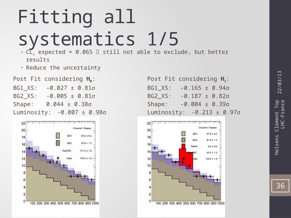
Fitting all systematics 1/5
Post Fit considering H0:
BG1_XS: -0.027 ± 0.81σBG2_XS: -0.005 ± 0.81σShape: 0.044 ± 0.38σLuminosity: -0.007 ± 0.98σ
22/0
3/13
36
• CLs expected = 0.065 still not able to exclude, but better results• Reduce the uncertainty
Post Fit considering H1:
BG1_XS: -0.165 ± 0.94σBG2_XS: -0.187 ± 0.82σShape: -0.004 ± 0.39σLuminosity: -0.213 ± 0.97σ
Hel
sens
Cle
men
t Top
LH
C-Fr
ance
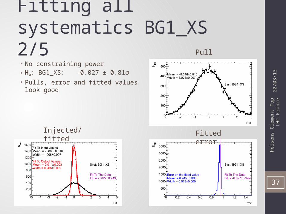
Fitting all systematics BG1_XS 2/5
22/0
3/13
37
• No constraining power• H0: BG1_XS: -0.027 ± 0.81σ• Pulls, error and fitted values look good
Pull
Injected/fitted Fitted error
Hel
sens
Cle
men
t Top
LH
C-Fr
ance
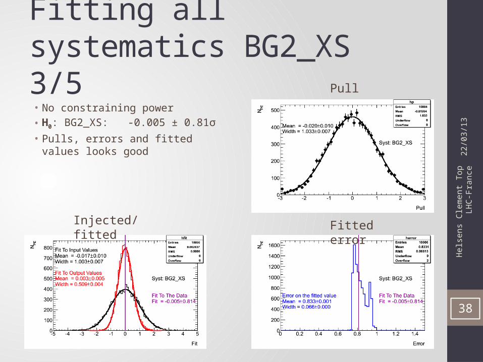
Fitting all systematics BG2_XS 3/5
22/0
3/13
38
• No constraining power• H0: BG2_XS: -0.005 ± 0.81σ• Pulls, errors and fitted values looks good
Pull
Injected/fitted Fitted error

Hel
sens
Cle
men
t Top
LH
C-Fr
ance
Fitting all systematics Luminosity 4/5
22/0
3/13
39
• No constraining power• H0: Luminosity: -0.007 ± 0.98σ• Pulls, errors and fitted values looks good
Pull
Injected/fitted Fitted error
Hel
sens
Cle
men
t Top
LH
C-Fr
ance
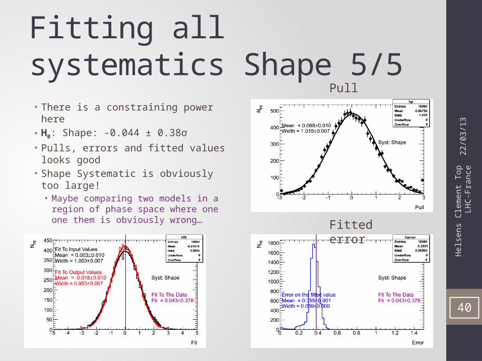
Fitting all systematics Shape 5/5
22/0
3/13
40
• There is a constraining power here• H0: Shape: -0.044 ± 0.38σ• Pulls, errors and fitted values looks
good• Shape Systematic is obviously too large!• Maybe comparing two models in a
region of phase space where one one them is obviously wrong…
Pull
Fitted error
Hel
sens
Cle
men
t Top
LH
C-Fr
ance
Constraining the nuisance parameters• One can argue (during internal review for example) that fitting
nuisance parameters in data is similar to a measurement• So if for example one fits in data the b-tagging efficiency to be
(in units of σ) 0.5 ± 0.2σ• Does this means we can derive a measurement of the b-tagging
efficiency with 0.2σ precision?• Or maybe like in the Toy Monte-Carlo, the error is over-estimated
and that in your signal region (that most of the case does not contain signal) you observe that your data/MC comparisons are within the systematics
22/0
3/13
41
Hel
sens
Cle
men
t Top
LH
C-Fr
ance
Fitting overall parameters
• An other solution than profiling could be to fit overall parameters or normalizations factors
• Those normalization factors should be seen as correction factors
• This can be used for example:• When you have a dominant background• When you have enough side-bands to constraint the parameter• When you have evidence that data/MC in control region is not
great and your systematics uncertainties are very large
22/0
3/13
42
Hel
sens
Cle
men
t Top
LH
C-Fr
ance
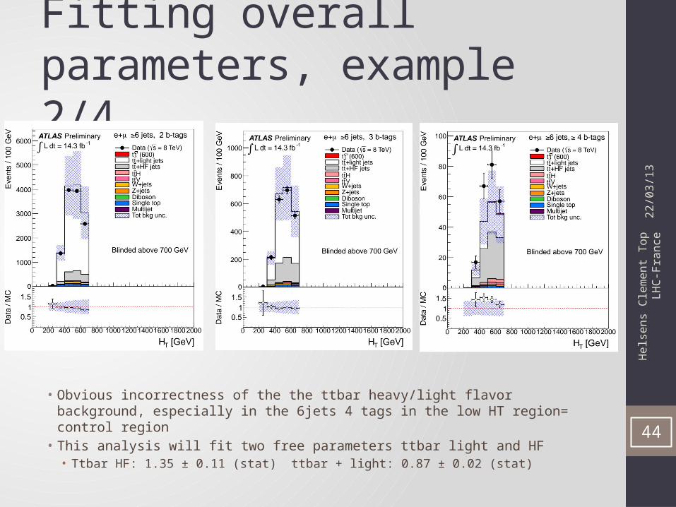
Fitting overall parameters, example 1/4• Example of Ht+X: ATL-CONF-2013-018• Using HT distribution as discriminant: scalar sum of all the
objects pT in the event• “Poor mans way” to discover new physics, and if something
unexpected appears in HT tails, either mis-modeling or signal• Can not use HT to identify the type of new particle…• This analysis is suffering from large systematics and obviously
what seems to be a mis-modeling of HT
22/0
3/13
43
Hel
sens
Cle
men
t Top
LH
C-Fr
ance
Fitting overall parameters, example 2/4
• Obvious incorrectness of the the ttbar heavy/light flavor background, especially in the 6jets 4 tags in the low HT region= control region
• This analysis will fit two free parameters ttbar light and HF• Ttbar HF: 1.35 ± 0.11 (stat) ttbar + light: 0.87 ± 0.02 (stat)
22/0
3/13
44
Hel
sens
Cle
men
t Top
LH
C-Fr
ance
Fitting overall parameters, example 3/4
22/0
3/13
45
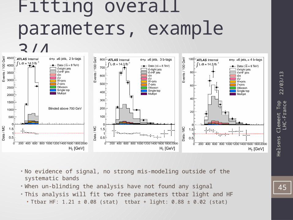
• No evidence of signal, no strong mis-modeling outside of the systematic bands• When un-blinding the analysis have not found any signal• This analysis will fit two free parameters ttbar light and HF
• Ttbar HF: 1.21 ± 0.08 (stat) ttbar + light: 0.88 ± 0.02 (stat)
Hel
sens
Cle
men
t Top
LH
C-Fr
ance
Fitting overall parameters, example 4/4
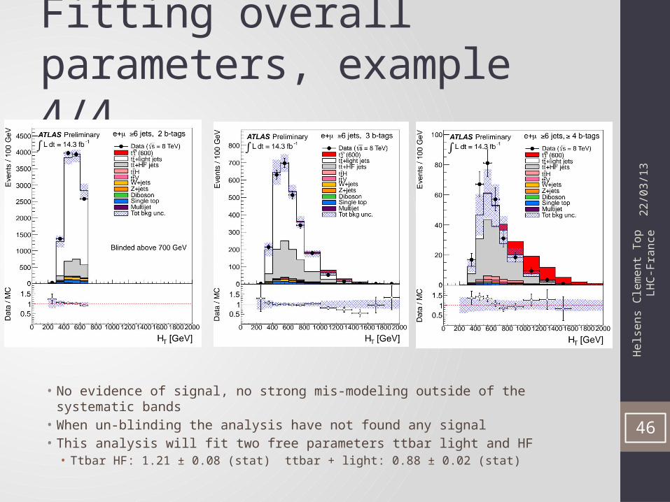
• No evidence of signal, no strong mis-modeling outside of the systematic bands• When un-blinding the analysis have not found any signal• This analysis will fit two free parameters ttbar light and HF
• Ttbar HF: 1.21 ± 0.08 (stat) ttbar + light: 0.88 ± 0.02 (stat)
22/0
3/13
46
Hel
sens
Cle
men
t Top
LH
C-Fr
ance
Other tips that could help performing a profiled analysis• Merging channels:• If you are performing an analysis using leptons (for example single
lepton analysis) you can merge electron and muon for example, if there is no reason the physics is different between the 2 lepton flavors this will help to gain statistics in the tails
• Merging Backgrounds:• If you are suffering from low Monte-Carlo statistic for small background
and if the shape of those small backgrounds looks similar, why not merging them in a single sample!
• Merging systematics:It is also possible to merge small systematics that have the basically the same effect. For example, if you have several lepton systematics (like trigger SF, Reco SF, ID SF) then might be better to merge them into a single systematic
• Note that when merging channels or background, the systematic treatment should remain consistent
22/0
3/13
47
Hel
sens
Cle
men
t Top
LH
C-Fr
ance
Other tips that could help performing a profiled analysis• You might also want to consider smoothing of histograms• Be also very cautious here, because if there is no shape to start
with, smoothing algorithm might invent a shape…• Keep in mind that profiling nuisance parameter is at the end of
the day a fit (using MIMUIT)• So if you give to MINUIT crapy/shaky templates, it can not do
miracles…• Number of parameters, their variations are the most important
thing when doing profiling
22/0
3/13
48
Hel
sens
Cle
men
t Top
LH
C-Fr
ance
Summary
• Hope you know everything about profiling now • Profiling should be really seen as an optimization step that
helps to recover the degradation due to systematics • Now time for discussion
• References:• Mclimit:
http://www-cdf.fnal.gov/~trj/mclimit/production/mclimit.html• Roostat:
https://twiki.cern.ch/twiki/bin/view/RooStats/WebHome• Wikipedia has a lot of interesting and detailed information about
statistics!!
22/0
3/13
49
Hel
sens
Cle
men
t Top
LH
C-Fr
ance
Bonus slides
22/0
3/13
50
Hel
sens
Cle
men
t Top
LH
C-Fr
ance
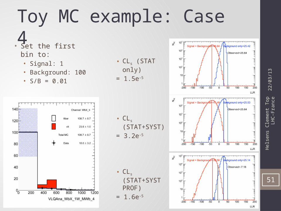
Toy MC example: Case 4
• CLs (STAT only)
= 1.5e-5
• CLs (STAT+SYST)
= 3.2e-5
• CLs (STAT+SYST PROF)
= 1.6e-5
22/0
3/13
51
• Set the first bin to:• Signal: 1• Background: 100• S/B = 0.01
Hel
sens
Cle
men
t Top
LH
C-Fr
ance
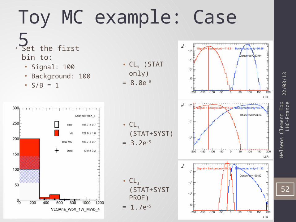
Toy MC example: Case 5
• CLs (STAT only)
= 8.0e-6
• CLs (STAT+SYST)
= 3.2e-5
• CLs (STAT+SYST PROF)
= 1.7e-5
22/0
3/13
52
• Set the first bin to:• Signal: 100• Background: 100• S/B = 1
Hel
sens
Cle
men
t Top
LH
C-Fr
ance
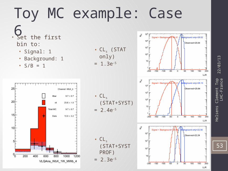
Toy MC example: Case 6
• CLs (STAT only)
= 1.3e-5
• CLs (STAT+SYST)
= 2.4e-5
• CLs (STAT+SYST PROF)
= 2.3e-5
22/0
3/13
53
• Set the first bin to:• Signal: 1• Background: 1• S/B = 1
Hel
sens
Cle
men
t Top
LH
C-Fr
ance
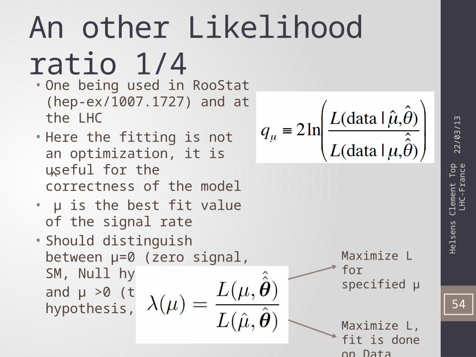
An other Likelihood ratio 1/4• One being used in RooStat (hep-
ex/1007.1727) and at the LHC• Here the fitting is not an
optimization, it is useful for the correctness of the model
• µ is the best fit value of the signal rate
• Should distinguish between µ=0 (zero signal, SM, Null hypothesis, H0) and µ >0 (test hypothesis, H1)
22/0
3/13
54
Maximize L for specified µ
Maximize L, fit is done on Data
^
Hel
sens
Cle
men
t Top
LH
C-Fr
ance
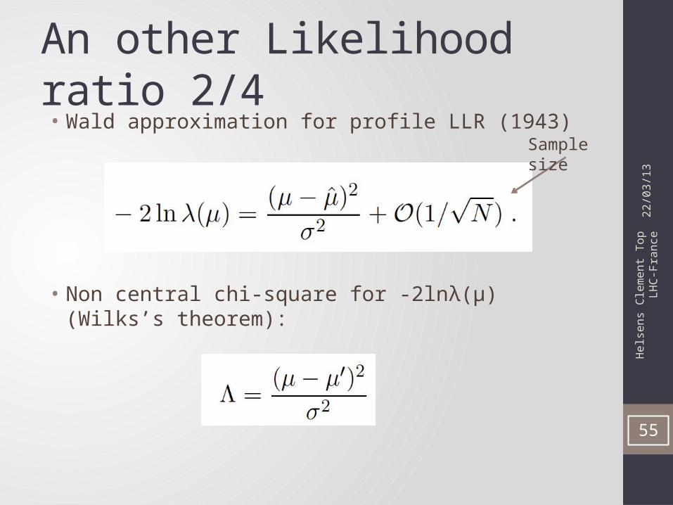
An other Likelihood ratio 2/4• Wald approximation for profile LLR (1943)
• Non central chi-square for -2lnλ(µ) (Wilks’s theorem):
22/0
3/13
55
Sample size
Hel
sens
Cle
men
t Top
LH
C-Fr
ance
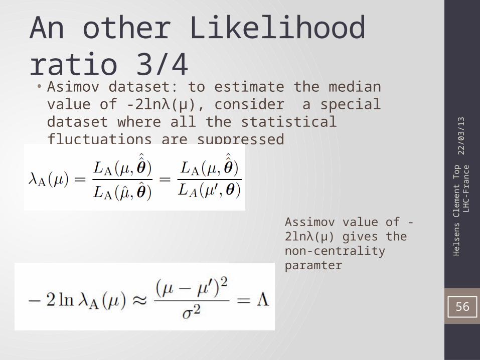
An other Likelihood ratio 3/4• Asimov dataset: to estimate the median value of -2lnλ(µ),
consider a special dataset where all the statistical fluctuations are suppressed
22/0
3/13
56
Assimov value of -2lnλ(µ) gives the non-centrality paramter
Hel
sens
Cle
men
t Top
LH
C-Fr
ance
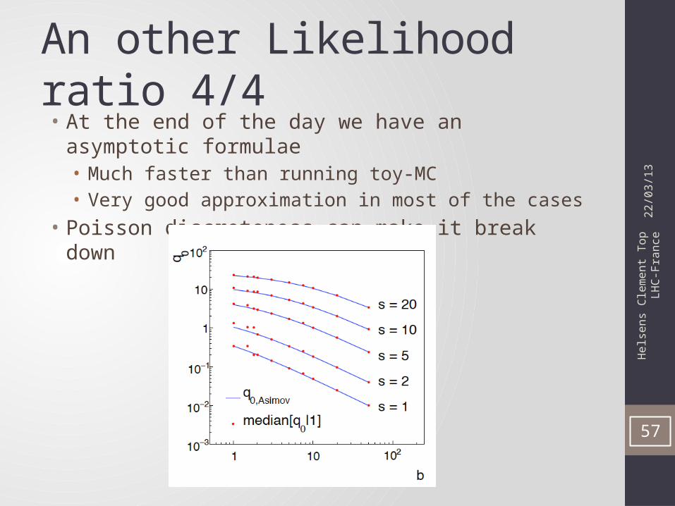
An other Likelihood ratio 4/4• At the end of the day we have an asymptotic formulae• Much faster than running toy-MC• Very good approximation in most of the cases
• Poisson discreteness can make it break down
22/0
3/13
57