Mach Learn (2014) 95:51–70DOI 10.1007/s10994-013-5346-7

Using random forests to diagnose aviation turbulence

John K. Williams

Received: 22 November 2012 / Accepted: 1 April 2013 / Published online: 23 April 2013© The Author(s) 2013. This article is published with open access at Springerlink.com

Abstract Atmospheric turbulence poses a significant hazard to aviation, with severe en-counters costing airlines millions of dollars per year in compensation, aircraft damage, anddelays due to required post-event inspections and repairs. Moreover, attempts to avoid tur-bulent airspace cause flight delays and en route deviations that increase air traffic controllerworkload, disrupt schedules of air crews and passengers and use extra fuel. For these rea-sons, the Federal Aviation Administration and the National Aeronautics and Space Adminis-tration have funded the development of automated turbulence detection, diagnosis and fore-casting products. This paper describes a methodology for fusing data from diverse sourcesand producing a real-time diagnosis of turbulence associated with thunderstorms, a signif-icant cause of weather delays and turbulence encounters that is not well-addressed by cur-rent turbulence forecasts. The data fusion algorithm is trained using a retrospective datasetthat includes objective turbulence reports from commercial aircraft and collocated predictordata. It is evaluated on an independent test set using several performance metrics includingreceiver operating characteristic curves, which are used for FAA turbulence product evalua-tions prior to their deployment. A prototype implementation fuses data from Doppler radar,geostationary satellites, a lightning detection network and a numerical weather predictionmodel to produce deterministic and probabilistic turbulence assessments suitable for use byair traffic managers, dispatchers and pilots. The algorithm is scheduled to be operationallyimplemented at the National Weather Service’s Aviation Weather Center in 2014.

Keywords Turbulence · Aviation · Weather · Air traffic · Thunderstorms · Random forest ·Data fusion

Editors: Kiri Wagstaff and Cynthia Rudin.

J.K. Williams (�)Research Applications Laboratory, National Center for Atmospheric Research, P.O. Box 3000,Boulder, CO, USAe-mail: jkwillia@ucar.edu

52 Mach Learn (2014) 95:51–70

1 Problem of interest

1.1 Aviation impact of en-route turbulence

Nearly everyone who has flown in an aircraft has experienced atmospheric turbulence—thatunnerving jolting up and down and side to side that feels like an amusement park ride gonebad. Although commercial airline crashes are now exceedingly rare, turbulence encounterscontinue to remind passengers that flying is not completely safe. Indeed, according to a studyof National Transportation Safety Board (NTSB) data from 1983–1997, turbulence was thepredominant cause of accidents and injuries in large commercial aircraft, accounting forabout 70 % of all weather-related incidents (Eichenbaum 2000). Including general aviation(GA) aircraft, turbulence contributed to 664 accidents leading to 609 fatalities (all but 3 GA),239 serious injuries and 584 minor injuries over that time period. A joint government andindustry study (CAST 2001) estimated that there were 15,000 minor injuries on commercialaircraft over the same period that were not reported to the NTSB. The CAST study alsofound that 13 % of NTSB cases included minor cabin damage, and 4 % were associatedwith severe aircraft damage. One study estimated the costs to U.S. airlines associated withthese incidents, including liability lawsuits, lost crew work time, inspections, and repairsat nearly $200 million per year (Eichenbaum 2003). Moreover, even turbulence that doesn’tcause injuries or accidents shapes the public’s impression of an airline’s safety, thus affectingits business. Sharman et al. (2006a) note that pilot reports (PIREPs) of moderate-or-greaterturbulence encounters average about 65,000 per year, and severe-or-greater reports average5,500 per year.

Airline dispatchers and pilots strive to avoid turbulence or quickly exit turbulent regionswhen they chance upon them. A severe or extreme turbulence report frequently causes theaviation weather forecaster responsible for that region to issue a turbulence Significant Me-teorological Information advisory (SIGMET), and the airspace nearby can be shut downto air traffic or have its capacity for flights reduced. Pilots’ requests for route changes tofind smoother air can significantly increase air traffic controller workload; a survey of FAAAir Route Traffic Control Centers, Traffic Management Units and Terminal Radar Control(Cook 2008) found that turbulence ranked behind only ceiling and visibility as the mostimportant weather factor affecting the National Air Space (NAS). Avoiding areas of sus-pected turbulence results in increased fuel expenditure and flight delays that can cascadeinto disruptions to other flights and quickly escalating costs (Cook et al. 2004).

Atmospheric turbulence is often generated by large-scale forcing mechanisms such as thejet stream, upper level fronts, wind flow over rough terrain, or thunderstorm updrafts, down-drafts, windshear and outflow. Avoiding turbulence associated with thunderstorms, known asconvectively-induced turbulence (CIT), is particularly difficult, and CIT has been estimatedto be responsible for 60 % of turbulence-related aircraft accidents (Cornman and Carmichael1993). 86 % of the 44 aviation accident cases analyzed by Kaplan et al. (2005) were foundto be within 100 km of convection. CIT can exist at small scales and short time periods,and the dynamic evolution of thunderstorms makes CIT notoriously difficult to accuratelydiagnose or forecast (Lane et al. 2012).

1.2 Limitations of thunderstorm avoidance guidelines

Thunderstorms are responsible for aviation hazards including lightning, hail, windshear,and airframe icing, but CIT is unique in that it can produce a threat well away from theactive storm. For this reason, FAA guidelines specify that aircraft should circumnavigate

Mach Learn (2014) 95:51–70 53

thunderstorms by wide margins, affecting large regions of airspace on days of widespreadconvection. They include the following (Federal Aviation Administration 2012):

1. Don’t land or takeoff in the face of an approaching thunderstorm. A sudden gust front oflow level turbulence could cause loss of control.

2. Don’t attempt to fly under a thunderstorm even if you can see through to the other side.Turbulence and wind shear under the storm could be disastrous.

3. Don’t fly without airborne radar into a cloud mass containing scattered embedded thun-derstorms . . .

4. Don’t trust the visual appearance to be a reliable indicator of the turbulence inside athunderstorm.

5. Do avoid by at least 20 miles any thunderstorm identified as severe or giving an intenseradar echo. This is especially true under the anvil of a large cumulonimbus.

6. Do clear the top of a known or suspected severe thunderstorm by at least 1,000 feetaltitude for each 10 knots of wind speed at the cloud top . . .

7. Do circumnavigate the entire area if the area has 6/10 thunderstorm coverage.8. Do remember that vivid and frequent lightning indicates the probability of a strong thun-

derstorm.9. Do regard as extremely hazardous any thunderstorm with tops 35,000 feet or higher . . .

Interpretation of these guidelines is subjective and limited by the information available toairline dispatchers and pilots. Moreover, recent studies have shown that significant CIT mayoccur outside these prescribed margins and may be dependent on environmental factors in-visible to a pilot (Lane et al. 2012), while the NEXRAD Turbulence Detection Algorithm(NTDA) has frequently identified in-cloud areas near storms with benign null or light tur-bulence (Williams et al. 2006, 2008b). For these reasons, an automated, real-time griddedproduct that explicitly identifies hazardous regions of CIT is desirable.

1.3 Limitations of operational turbulence forecasts

The study by Eichenbaum (2000) found that only 65 % of the NTSB turbulence-relatedaccidents had either a valid Airman’s Meteorological Information advisory (AIRMET) orSIGMET at the time and location of the accident, and thus 35 % would have been unex-pected by the flight crews. Moreover, AIRMET and SIGMET polygons are often relativelylarge compared to the actual hazard area. In order to improve the guidance available todispatchers and air traffic managers, the FAA Aviation Weather Research Program (AWRP)has sponsored the development of the Graphical Turbulence Guidance (GTG) product (Shar-man et al. 2006b). GTG uses operational rapid-update numerical weather prediction (NWP)model output to compute a number of derived turbulence “diagnostics” and combines themusing fuzzy logic to create 3-D, 0–12 hour turbulence forecasts over the conterminousU.S. (CONUS). GTG runs operationally at the National Weather Service (NWS) AviationWeather Center (AWC) and is available online via the Aviation Digital Data Service (ADDS)at aviationweather.gov/adds/turbulence/.

GTG development (Sharman et al. 2006a, 2006b) has followed an incremental approach,focusing first on upper-level clear-air turbulence (CAT) and then extending to mid-levels andaddressing mountain-wave turbulence (MWT). However, the currently operational version,GTG 2.5, does not explicitly address CIT. Both GTG 2.5 and the new GTG 3 currently underdevelopment use the Weather Research and Forecasting Rapid Refresh (WRF-RAP) NWPmodel (Benjamin et al. 2006), which produces hourly 13-km horizontal resolution forecaststhat are too coarse to fully resolve thunderstorms. Moreover, WRF-RAP forecasts are not

54 Mach Learn (2014) 95:51–70

available until an hour or more after they are initialized, and hence often do not providemeaningful information about new and rapidly evolving storms.

In recent years, analysis of en-route turbulence reports, case studies and fine-scale sim-ulations have facilitated better understanding of some sources of CIT. These include theproduction, upward propagation and breaking of gravity waves when a convective cell pen-etrates the tropopause (Lane et al. 2003; Trier et al. 2012); however, conditions for wavebreaking appear highly dependent on the storm environment (Lane and Sharman 2008).Fovell et al. (2007) showed that ducted gravity waves could propagate away from a stormand cause isolated, transient regions of turbulence. Trier and Sharman (2009) found that theoutflow from large storm systems could interact with the ambient flow to cause wind shearthat produced turbulence hundreds of km away and hours later. These studies suggest thatcombining information about the storm environment obtained from NWP models with muchhigher resolution remote observations of storm attributes will be necessary to best identifyregions of likely CIT. However, doing so requires a more flexible data fusion methodologythan that currently used by GTG.

1.4 Need for tactical turbulence diagnosis products

The real-time information about the current turbulent state of the atmosphere required bypilots and dispatchers for making tactical en-route decisions is not adequately provided viathe FAA’s thunderstorm avoidance guidelines or by currently operational turbulence fore-casts. To address this deficiency, the FAA Aviation Weather Research Program (AWRP) hassponsored the development of a GTG “Nowcast” (GTGN) component for GTG 3 that willcombine turbulence observations, inferences and forecasts to produce new turbulence as-sessments every 15 minutes. One component of the GTGN system is a Diagnosis of CIT(DCIT) module that focuses on identifying likely regions of existing near-storm turbulencebased on the latest observations and NWP model data (Williams et al. 2008b, 2012). TheDCIT and GTGN products will also address requirements for the Next Generation Air Trans-portation System (NextGen), which includes gridded deterministic and probabilistic now-casts and forecasts to support the increasing automation of air traffic management systems(JPDO 2008; Lindholm et al. 2010; Sharman and Williams 2009).

2 Data sources and preparation

The goal of DCIT is to fuse remote observations and NWP model data in a real-time algo-rithm to produce 3-D gridded diagnoses of CIT. The “truth” data used for DCIT trainingand evaluation must be objective and have sufficiently high temporal and spatial resolutionto capture even small-scale, transient patches of CIT. The predictor data must be operational(i.e., reliable), free or low-cost and readily available at the AWC via standard communica-tions channels with minimal latency.

2.1 Automated aircraft turbulence reports

The FAA sponsored the development and implementation on select commercial aircraft ofa system that provides high-resolution, automated, objective turbulence reports suitable foruse as “truth” in training DCIT (Cornman et al. 1995, 2004). The system reports eddy dis-sipation rate (EDR, ε1/3), an aircraft-independent atmospheric turbulence metric, includingboth the median and peak EDR over approximately one-minute intervals. DCIT’s prediction

Mach Learn (2014) 95:51–70 55

target is the peak EDR because it supplies a good indication of the turbulence hazard and isbetter distributed over the reporting bins than the median value.

NCAR maintains a database of these in situ EDR reports from approximately 95 UnitedAirlines (UAL) Boeing 757 (B757) aircraft and approximately 80 Delta Air Lines (DAL)Boeing 737 (B737) aircraft. UAL data are primarily from routes between the northeast andsouthwest U.S., while DAL also includes the southeast and thus provides somewhat morecomprehensive coverage. The UAL algorithm, developed in the mid-1990s, utilizes aircraftaccelerometer data along with an aircraft response model. EDR data are coarsely binnedwith just 8 bins centered at 0.05, 0.15, 0.25, 0.35, 0.45, 0.55, 0.65 and 0.75 m2/3 s−1, timeis reported to the nearest minute, time and position are given for every fourth report, andthe algorithm’s onboard quality control capabilities are limited. The DAL implementation,developed several years later, utilizes aircraft-measured vertical winds, obviating the needfor an aircraft response function, and includes a sophisticated on-board quality control al-gorithm. It bins the EDR data at 0.02 m2/3 s−1 and reports time to the nearest 10 s. How-ever, in order to save communications costs, it does not transmit every report. Rather, itproduces a routine report every 15 minutes and includes “triggered” reports when the mea-sured turbulence reaches certain intensity or longevity thresholds. It does report all peakEDR ≥ 0.20 m2/3 s−1.

In situ EDR report values may be roughly associated with atmospheric turbulence sever-ity, although actual aircraft experience of turbulence depends on factors such as its weight,structure (particularly wing area), airspeed, and altitude. For instance, light aircraft generallyexperience more severe turbulence because they are more easily moved by variable winds.The International Civil Aviation Organization (2001) recommended interpreting 0.0–0.1 asnull turbulence, 0.1–0.2 as light, 0.2–0.3 as light to moderate, 0.3–0.4 as moderate, 0.4–0.5as moderate to severe, 0.5–0.6 as severe, 0.6 to 0.7 as severe to extreme, and greater than0.7 m2/3 s−1 as extreme, and these thresholds were used in the official GTG 2.5 evaluation(Wandishin et al. 2011). Since commercial aircraft typically fly at airspeeds near 250 m s−1,a 1-minute flight segment may be 15 km in length, and the peak EDR locations may be inerror by as much as 8 km or so. Nevertheless, these uncertainties are significantly less thanthose of pilot reports (PIREPs), which have traditionally been used for turbulence forecasttraining and evaluation. PIREPs are subjective, non-representative and frequently involvesignificant errors in the reported event’s location and time (Schwartz 1996). The high tem-poral and spatial resolution and objective nature of the in situ EDR reports make them idealfor the present study.

2.2 Predictor data

2.2.1 Numerical weather prediction model and diagnostics

Despite their limitations, NWP model data and derived diagnostics provide valuable infor-mation about the storm environment as well as turbulence produced by large-scale, long-lasting forcing mechanisms. The DCIT training set includes 2-D and 3-D fields derivedfrom the 13-km WRF-RAP NWP model including winds, turbulent kinetic energy (TKE),convective available potential energy (CAPE), convective inhibition (CIN), potential tem-perature, humidity mixing ratio, and many others. It also makes use of derived quantitiesand diagnostics that have been developed for turbulence forecasting including Richardsonnumber (Ri), structure function eddy dissipation rate, horizontal and vertical shear, inversestability, tropopause height, tropopause strength and a large number of others (Sharman et al.2006b). In addition, based on studies like those described in Lane et al. (2012) and intuitionabout possibly relevant environmental factors, a number of new quantities were computed,e.g., distance above or below the tropopause.

56 Mach Learn (2014) 95:51–70

2.2.2 Ground-based Doppler radar

The nation’s network of Weather Surveillance Radar-1988 Doppler (WSR-88D) radars, alsoknown as NEXRADs, provides information about the location and intensity of clouds andstorms. The DCIT training set includes information about the radar echoes, known as radarreflectivity, provided by the National Severe Storms Laboratory (NSSL) National Mosaicsystem (Zhang et al. 2011). These include composite reflectivity (the maximum reflectivityin a column), echo tops (the highest altitude with reflectivity ≥18 dBZ), and vertically-integrated liquid (an estimate of the total liquid water in a column).

Additionally, the Doppler capabilities of the radars can be used to measure wind variabil-ity and thereby determine turbulence in clouds where the radar signal is sufficiently strongand free of contaminants. The NTDA (Williams et al. 2006, 2008b) computes EDR fromindividual radar sweeps and merges the results from 133 NEXRADs over the CONUS toproduce 3-D maps of in-cloud turbulence. Note that the NTDA is not able to detect turbu-lence outside the cloud boundary, which must be inferred by other means. In addition tothe 3-D EDR field, 2-D turbulence “tops” fields were created from the highest altitudes ofNTDA-detected light, moderate, and severe turbulence.

2.2.3 Geostationary satellite imagery

The National Oceanic and Atmospheric Administration maintains geostationary operationalenvironmental satellites (GOES) that make periodic radiometric measurements of the earthat several channels of the electromagnetic spectrum with a temporal frequency ranging from15 minutes over the CONUS to 3 hours for other parts of the hemisphere. These includevisible light, channel 2 (3.9 µm wavelength), channel 3 (6.7 µm), channel 4 (10.7 µm), andchannel 6 (13.3 µm) windows that provide information about clouds and storms. In additionto the raw imager data, several derived products were computed. For example, overshootingtops, identified using the longwave infrared 10.7 µm channel (Bedka et al. 2010), are satellitesignatures of convective cells that penetrate into the lower stratosphere and indicate thelikely generation of gravity waves. The presence of a tropopause fold, where the tropopausechanges rapidly in height, is often associated with turbulence and may be derived using thewater vapor (6.7 µm) channel (Wimmers and Moody 2004; Wimmers and Feltz 2012).

2.2.4 Lightning detection network

Lightning strike data from the National Lightning Detection Network (NLDN) owned byVaisala Oyj (Cummins and Murphy 2009) is also used. The number and frequency of light-ning strikes are often related to the intensity of the storm and the updraft inside it. In fact,Deierling et al. (2011) show evidence that lightning density may be related to the volume ofin-cloud convective turbulence as measured by the NTDA.

2.2.5 Derived fields and features

In order to investigate the predictive value of the observed and model quantities describedabove, a number of derived fields were computed via local neighborhood filters, arithmeticcombinations of fields, and distances to certain thresholds. For example, to capture infor-mation about spatial scales and proximities, statistics such as max, min, mean, standarddeviation and number of good measurement points were computed over 10, 20, 40, 80 and160-km radius discs for the radar composite reflectivity, composite reflectivity height and

Mach Learn (2014) 95:51–70 57

echo tops fields, the NTDA turbulence tops fields, the satellite imager fields and the 3-DNTDA EDR and reflectivity fields. Vertical distances were computed from the aircraft alti-tude to various reflectivity and EDR thresholds, to the tropopause, and to the surface. Dif-ferences were computed between the temperature at the aircraft altitude or the surface andvarious statistics of the GOES 10.7 µm brightness temperature, which represents the tem-perature of the cloud top or, when no cloud is present, the Earth’s surface. Differences werealso computed between the various GOES channels, and between values of their disc statis-tics. Such differences can often be powerful predictors; for instance, the difference betweenthe longwave infrared (10.7 µm) and water vapor (6.7 µm) channels was found so effectiveat determining thunderstorm intensity that it has been named the Global Convective Diag-nostic (GCD, Martin et al. 2008). Finally, distances were computed from the aircraft in situEDR report location to various features including reflectivity, NTDA, lightning density andecho top contours, overshooting tops, and tropopause folds. In order to determine whetherdirection was important, these distances were also computed within six 60◦ “wedges” ori-ented relative to the wind vector at the aircraft location. In all, 1030 candidate predictorswere computed for this investigation. However, the results presented here do not utilize theindividual wedge distances, leaving a total of 778 candidate predictors.

2.3 Dataset preparation

2.3.1 Preparing “truth” data

A ground-based quality control algorithm monitors the distribution of the in situ EDR re-ports from each aircraft and flags them as bad if it deviates from expected norms. Thishappens periodically, and may result from a software, communications or instrument mal-function. The archived turbulence data are sorted into flights, and omitted data positionsand times are estimated via interpolation. For DAL data, if routine reports are present every15 minutes, intermediate reports are assumed to be missing because the reporting thresholdof 0.2 m2/3 s−1 is not met; 14 reports of zero turbulence are inserted into these segments.(Note that the 0.0–0.2 m2/3 s−1 interval therefore has the correct total count, but not thecorrect distribution within that interval.) The time, distance and change in altitude of eachflight segment between reports is computed, and only reports associated with time intervalsbetween 45 and 75 seconds and altitude changes less than 3,000 ft are kept in the dataset.The position used for collocation with predictor variables is computed as the midpoint ofeach one-minute flight segment.

2.3.2 Handling missing predictor data

Predictor data can be missing for many reasons. For instance, an NWP model run or mea-surement may be missing from the archive maintained at NCAR or may be corrupted. Radardata are missing if the aircraft report is out of radar range or if there was no weather toreturn a signal. Data values that are missing for a known reason (e.g., no weather present)are replaced with an appropriate substitute value or flag. Instances for which one or moreof the predictor variables is missing for an unknown reason are omitted from the dataset.While imputation or random assignment can be used to deal with missing data, eliminatingcompromised instances ensures the integrity of the dataset and facilitates the comparisonof several statistical learning methods. For the present study, which utilizes data collectedbetween March 10 and November 4, 2010, this procedure reduced the DAL dataset from7,964,159 to 5,623,738 and the UAL dataset from 10,583,369 to 6,595,922 instances.

58 Mach Learn (2014) 95:51–70

3 Machine learning technique: random forest

The machine learning method used in this study is the random forest classifier (Breiman2001). Random forests (RFs) are collections of weak, weakly-correlated decision trees thatfunction as “ensembles of experts.” Each tree is trained using a bootstrap sample of thetraining data, and at each node the best split is selected from among a random subset ofthe predictor variables. This process ensures that each tree utilizes the training data andpredictor variables in a different way, reducing its statistical dependence on the other trees.RFs have seen numerous successful applications over the past decade, particularly in thebiomedical field (e.g., Díaz-Uriarte and de Andrés 2006). They have also been successfullyused in a number of environmental science applications. For example, Pal (2005) showedthat an RF could improve satellite radiometer-based land cover classification and argued thatit was simpler to use than alternatives such as support vector machines. RFs have also beenused by the author for thunderstorm prediction (e.g., Williams et al. 2008a) and for earlierwork on CIT diagnosis (e.g., Williams et al. 2008b).

RF appears to be a good candidate methodology for diagnosing CIT using the diverseset of predictors described above. Many, such as the GTG diagnostics, are monotonicallyrelated to turbulence likelihood or intensity, but others may have a more complicated pre-dictive relationship or are useful primarily in concert with other variables. The RF has thepotential to utilize the joint distribution of the predictor variables. Used for classification,the votes of the RF can be related to a probability of turbulence. And RFs are known to beless susceptible to overfitting a training dataset, making them more likely to generalize wellwithout the need for “optimal stopping” or similar techniques.

Moreover, because not all training instances are used to train each decision tree, those notused—the so-called out-of-bag instances—may be used to evaluate the performance of thattree, and this provides a way of quantifying the “importance” of each predictor variable. TheRF estimates the “permutation accuracy importance” for each predictor by computing thedegradation in classification performance over out-of-bag instances for each tree when thepredictor’s values are permuted over instances, then aggregating the results. These impor-tance assessments can be quite useful in selecting predictors from a large set of candidates,as described below.

4 Empirical results

4.1 Training and testing datasets

Because the main purpose of this study is to predict turbulence associated with convection,only in situ EDR reports within 80 km of rain regions (composite reflectivity ≥18 dBZ)were used. To help ensure independence between the training and testing datasets, train-ing data were sampled only from odd Julian days and testing data only from even Juliandays, or vice-versa. UAL and DAL datasets were analyzed separately because it wasn’tclear that their EDR values were identically calibrated. The data were also split into upperlevels (above 25,000 ft) and mid-levels (10,000–25,000 ft); turbulence mechanisms are of-ten different in these two levels, and the dataset includes many more in situ EDR reports atupper levels where aircraft cruise that would dominate a combined dataset. No UAL databelow 20,000 ft were used because they are deemed unreliable (Larry Cornman, personalcommunication). The resulting distribution of EDR values is shown in Table 1. The RF wastrained to use the collocated predictors described in Sect. 2, including the nearest observa-tions in time and space and NWP model data interpolated to the aircraft position, to predict

Mach Learn (2014) 95:51–70 59

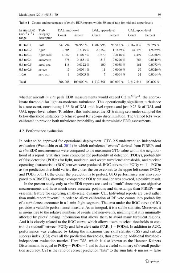
Table 1 Counts and percentages of in situ EDR reports within 80 km of rain for mid and upper levels

In situ EDR(m2/3 s−1)range

Turb.categorydescriptor

DAL, mid-level DAL, upper-level UAL, upper-level

Count Percent Count Percent Count Percent

0.0 to 0.1 null 347,794 94.956 % 1,707,998 98.583 % 2,167,839 97.759 %

0.1 to 0.2 light 13,605 3.7145 % 20,252 1.1689 % 44,193 1.9929 %

0.2 to 0.3 light-mod. 4,057 1.1077 % 3,670 0.2118 % 4,497 0.2028 %

0.3 to 0.4 moderate 678 0.1851 % 513 0.0296 % 766 0.0345 %

0.4 to 0.5 mod.-sev. 118 0.0322 % 100 0.0058 % 161 0.0073 %

0.5 to 0.6 severe 15 0.0041 % 11 0.0006 % 57 0.0026 %

≥0.6 sev.-extr. 1 0.0003 % 7 0.0004 % 31 0.0014 %

Total 366,268 100.000 % 1,732,551 100.000 % 2,217,544 100.000 %

whether aircraft in situ peak EDR measurements would exceed 0.2 m2/3 s−1, the approx-imate threshold for light-to-moderate turbulence. This operationally significant turbulenceis a rare event, constituting 1.33 % of DAL mid-level reports and just 0.25 % of DAL andUAL upper-level values. To address this imbalance, the RF training sets under-sampled thebelow-threshold instances to achieve good RF yes-no discrimination. The trained RFs werecalibrated to provide both turbulence probability and deterministic EDR assessments.

4.2 Performance evaluation

In order to be approved for operational deployment, GTG 2.5 underwent an independentevaluation (Wandishin et al. 2011) in which turbulence “events” derived from PIREPs andin situ EDR measurements were compared to the maximum GTG value within the neighbor-hood of a report. Statistics were computed for probability of detection (PODy), probabilityof false detection (PODn) for light, moderate, and severe turbulence thresholds, and receiveroperating characteristic (ROC) curves were produced. ROC curves plot PODy vs. 1−PODnas the prediction threshold varies; the closer the curve comes to the upper left corner (PODyand PODn both 1), the closer the prediction is to perfect. GTG performance was also com-pared to AIRMETs, showing a comparable PODy but smaller area covered, a positive result.

In the present study, only in situ EDR reports are used as “truth” since they are objectivemeasurements and have much more accurate positions and timestamps than PIREPs—anessential feature for capturing small-scale, dynamic CIT. Individual reports are used ratherthan multi-report “events” in order to allow calibration of RF vote counts into probabilityof a turbulence encounter in a 1-min flight segment. The area under the ROC curve (AUC)provides a valuable performance measure. As an integral, it is a stable statistic. Moreover, itis insensitive to the relative numbers of events and non-events, meaning that it is minimallyaffected by pilots’ having information that allows them to avoid many turbulent regions.And it is closely related to the ROC curve, which allows users to select thresholds to con-trol the tradeoff between PODy and false alert ratio (FAR, 1 − PODn). In addition to AUC,performance was evaluated by taking the maximum true skill statistic (TSS) and criticalsuccess index (CSI) over all the prediction thresholds, thus providing additional threshold-independent evaluation metrics. Here TSS, which is also known as the Hanssen-KuipersDiscriminant, is equal to PODy + PODn − 1 and is thus a useful summary of overall predic-tion accuracy. CSI is the ratio of correct prediction “hits” to the sum hits + misses + false

60 Mach Learn (2014) 95:51–70

alerts; since it ignores correct nulls, CSI is often used to evaluate forecasts of rare eventssuch as severe thunderstorms (e.g., Schaefer 1990), and so is ideal for evaluating turbulencepredictions.

The actual utility of improved turbulence predictions will vary based on the end-user(e.g., airline dispatcher, GA pilot, or air traffic controller), the scenario (e.g., air traffic con-gestion, time of day), the spatial and temporal structures of the turbulent regions, and otherfactors. Thus, while an aggregate metric that takes into account all the economic costs andbenefits over the U.S. air transportation system might be desirable, creating a comprehensivemetric would be difficult and it would be complicated to use in practice. However, perfor-mance evaluations like ROC curves could be used by users to set their own thresholds basedon the relative costs of false positives and false negatives in the context of their operationaldecisions. For example, Williams (2009) showed how to compute optimal routes given prob-abilistic aviation weather forecasts and a financial model for fuel use and the average costof a hazardous weather encounter.

4.3 Variable selection

The permutation accuracy importance estimates produced by an RF during training arebased on classification accuracy, not contributions to the final probabilistic or determinis-tic predictions, and it has been shown that they can be biased when the predictor fields havevarying scales of measurement (Strobl et al. 2007), as is true for this dataset. Nevertheless,predictors that have very low or zero RF importance seem unlikely to contribute much to afinal model; thus, RF importance may be used to whittle down the list of candidate predic-tors. Predictor importances were evaluated using separate RFs for UAL and DAL, upper andmid-levels, and even and odd Julian days. The lowest performing predictors were removed,particularly if they appeared to duplicate the kind of information contained in higher per-formers or if they were particularly expensive to compute. Through this process, the list ofcandidate predictors was reduced to 107.

A second stage of the variable selection process was performed via a set of forward andbackward selection experiments using AUC as the objective function. For each experiment,random subsets were drawn from the training and testing datasets. Two steps of forwardselection (a pass through the unselected candidates to find which would yield the best per-formance when added to the predictor list) were followed by one step of backward selection(a pass through the predictors to see which could be removed with the least impact on per-formance). This procedure was performed for DAL and UAL, upper and mid-levels, andwith even and odd Julian days used for the training dataset. A split of 70/30 non-turbulenceto turbulence cases was selected through sensitivity tests with only 50 RF trees. The exper-iments were also performed using logistic regression. With this small number of trees, RFsdid not perform statistically better than logistic regression on AUC or max TSS, but did ob-tain a slightly better max CSI. The cross-validation performance reaches a maximum after50 to 60 iterations, at which point 17–20 predictors have been selected.

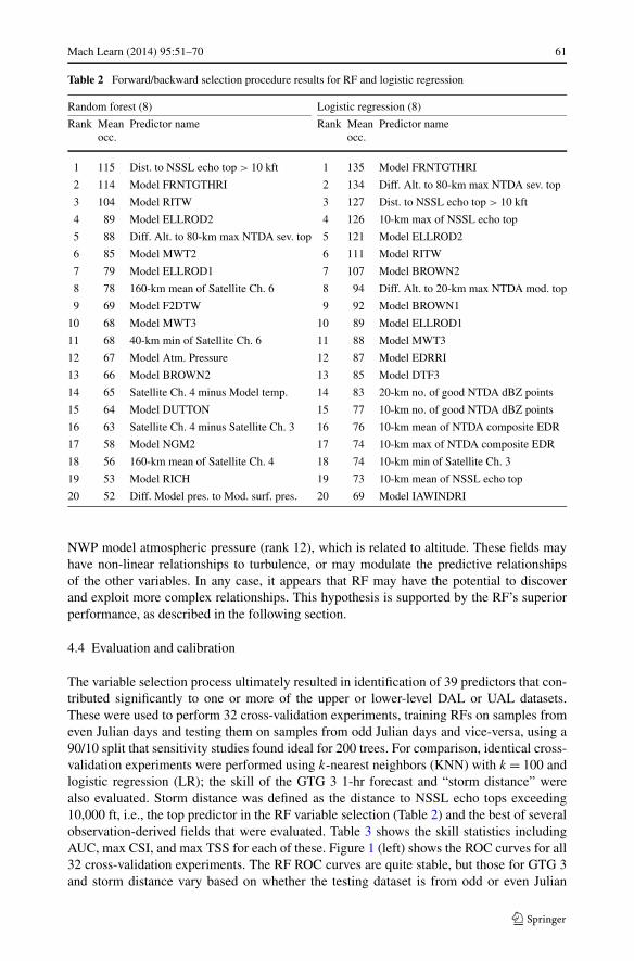
Table 2 shows the top 20 predictors for predicting DAL EDR ≥ 0.2 m2/3 s−1 at upperlevels using RF (left) and logistic regression (right) based on their average occurrences over8 forward/backward selection experiments of 150 iterations each. Both results show a mixof model, satellite, and radar-derived fields, suggesting that these sources provide comple-mentary information. The predictors selected by logistic regression are all monotonicallyrelated to the likelihood of turbulence. On the other hand, the RF results include a surprise,160-km mean of Satellite Channel 6 (rank 8), which hadn’t previously been known to berelated to CIT, plus plausible predictors not monotonically related to turbulence, including

Mach Learn (2014) 95:51–70 61

Table 2 Forward/backward selection procedure results for RF and logistic regression

Random forest (8) Logistic regression (8)

Rank Meanocc.

Predictor name Rank Meanocc.

Predictor name

1 115 Dist. to NSSL echo top > 10 kft 1 135 Model FRNTGTHRI

2 114 Model FRNTGTHRI 2 134 Diff. Alt. to 80-km max NTDA sev. top

3 104 Model RITW 3 127 Dist. to NSSL echo top > 10 kft

4 89 Model ELLROD2 4 126 10-km max of NSSL echo top

5 88 Diff. Alt. to 80-km max NTDA sev. top 5 121 Model ELLROD2

6 85 Model MWT2 6 111 Model RITW

7 79 Model ELLROD1 7 107 Model BROWN2

8 78 160-km mean of Satellite Ch. 6 8 94 Diff. Alt. to 20-km max NTDA mod. top

9 69 Model F2DTW 9 92 Model BROWN1

10 68 Model MWT3 10 89 Model ELLROD1

11 68 40-km min of Satellite Ch. 6 11 88 Model MWT3

12 67 Model Atm. Pressure 12 87 Model EDRRI

13 66 Model BROWN2 13 85 Model DTF3

14 65 Satellite Ch. 4 minus Model temp. 14 83 20-km no. of good NTDA dBZ points

15 64 Model DUTTON 15 77 10-km no. of good NTDA dBZ points

16 63 Satellite Ch. 4 minus Satellite Ch. 3 16 76 10-km mean of NTDA composite EDR

17 58 Model NGM2 17 74 10-km max of NTDA composite EDR

18 56 160-km mean of Satellite Ch. 4 18 74 10-km min of Satellite Ch. 3

19 53 Model RICH 19 73 10-km mean of NSSL echo top

20 52 Diff. Model pres. to Mod. surf. pres. 20 69 Model IAWINDRI

NWP model atmospheric pressure (rank 12), which is related to altitude. These fields mayhave non-linear relationships to turbulence, or may modulate the predictive relationshipsof the other variables. In any case, it appears that RF may have the potential to discoverand exploit more complex relationships. This hypothesis is supported by the RF’s superiorperformance, as described in the following section.

4.4 Evaluation and calibration

The variable selection process ultimately resulted in identification of 39 predictors that con-tributed significantly to one or more of the upper or lower-level DAL or UAL datasets.These were used to perform 32 cross-validation experiments, training RFs on samples fromeven Julian days and testing them on samples from odd Julian days and vice-versa, using a90/10 split that sensitivity studies found ideal for 200 trees. For comparison, identical cross-validation experiments were performed using k-nearest neighbors (KNN) with k = 100 andlogistic regression (LR); the skill of the GTG 3 1-hr forecast and “storm distance” werealso evaluated. Storm distance was defined as the distance to NSSL echo tops exceeding10,000 ft, i.e., the top predictor in the RF variable selection (Table 2) and the best of severalobservation-derived fields that were evaluated. Table 3 shows the skill statistics includingAUC, max CSI, and max TSS for each of these. Figure 1 (left) shows the ROC curves for all32 cross-validation experiments. The RF ROC curves are quite stable, but those for GTG 3and storm distance vary based on whether the testing dataset is from odd or even Julian

62 Mach Learn (2014) 95:51–70

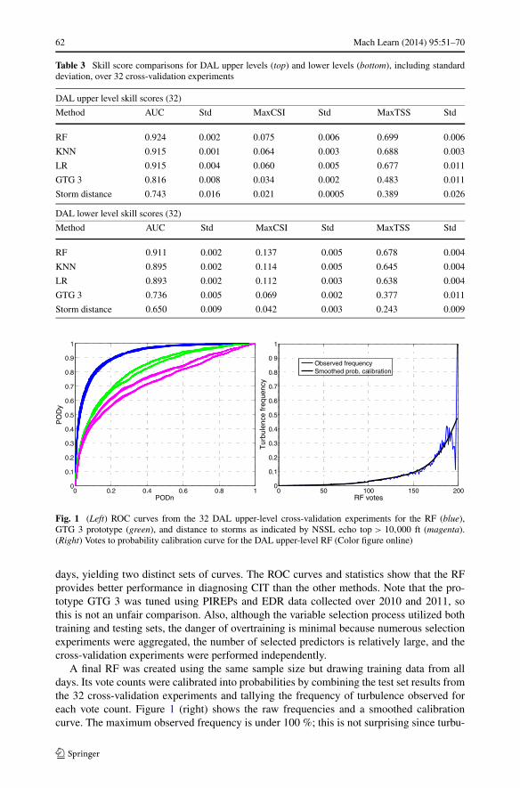
Table 3 Skill score comparisons for DAL upper levels (top) and lower levels (bottom), including standarddeviation, over 32 cross-validation experiments

DAL upper level skill scores (32)

Method AUC Std MaxCSI Std MaxTSS Std

RF 0.924 0.002 0.075 0.006 0.699 0.006

KNN 0.915 0.001 0.064 0.003 0.688 0.003

LR 0.915 0.004 0.060 0.005 0.677 0.011

GTG 3 0.816 0.008 0.034 0.002 0.483 0.011

Storm distance 0.743 0.016 0.021 0.0005 0.389 0.026

DAL lower level skill scores (32)

Method AUC Std MaxCSI Std MaxTSS Std

RF 0.911 0.002 0.137 0.005 0.678 0.004

KNN 0.895 0.002 0.114 0.005 0.645 0.004

LR 0.893 0.002 0.112 0.003 0.638 0.004

GTG 3 0.736 0.005 0.069 0.002 0.377 0.011

Storm distance 0.650 0.009 0.042 0.003 0.243 0.009

Fig. 1 (Left) ROC curves from the 32 DAL upper-level cross-validation experiments for the RF (blue),GTG 3 prototype (green), and distance to storms as indicated by NSSL echo top > 10,000 ft (magenta).(Right) Votes to probability calibration curve for the DAL upper-level RF (Color figure online)

days, yielding two distinct sets of curves. The ROC curves and statistics show that the RFprovides better performance in diagnosing CIT than the other methods. Note that the pro-totype GTG 3 was tuned using PIREPs and EDR data collected over 2010 and 2011, sothis is not an unfair comparison. Also, although the variable selection process utilized bothtraining and testing sets, the danger of overtraining is minimal because numerous selectionexperiments were aggregated, the number of selected predictors is relatively large, and thecross-validation experiments were performed independently.

A final RF was created using the same sample size but drawing training data from alldays. Its vote counts were calibrated into probabilities by combining the test set results fromthe 32 cross-validation experiments and tallying the frequency of turbulence observed foreach vote count. Figure 1 (right) shows the raw frequencies and a smoothed calibrationcurve. The maximum observed frequency is under 100 %; this is not surprising since turbu-

Mach Learn (2014) 95:51–70 63

lence is an essentially random process, and predicting turbulence encounters with certaintyat 1-min resolution is very difficult. Additionally, the training dataset includes turbulence re-ports only where aircraft fly, which rarely include places where turbulence is very likely. TheRF votes were also calibrated to EDR by mapping the votes to the lognormal distribution ofaircraft peak EDR measurements. Since the mappings are monotonic, the estimated AUC,max TSS and max CSI for both calibrated products are the same as those for the vote-basedcross-validation experiments.

The selection of training and testing sets from odd and even Julian days is intendedto produce representative yet independent sets (e.g., if instances were drawn completelyrandomly, adjacent turbulence reports might often end up in different sets), and the cross-validation estimates how well an RF will generalize. To test the accuracy of this approach,data from March 13–September 15 of both 2010 and 2011 were assembled, though NTDAfields weren’t available in 2011 and so were omitted. Using DAL upper-level data, 32×cross-validation with training and testing datasets drawn from odd and even Julian daysproduced the following skill scores and (standard deviations): mean AUC = 0.919(0.002),MaxCSI = 0.056(0.005), and MaxTSS = 0.695(0.006). An identical cross-validation ex-periment with training and testing dataset pairs drawn from 2010 and 2011 produced a meanAUC = 0.915(0.009), MaxCSI = 0.051(0.005), and MaxTSS = 0.688(0.019). Thus, theRF’s generalization between years was slightly poorer than suggested by cross-validationusing odd and even Julian days; however, this difference was small relative to the disparitywith the GTG 3 1-hr forecast scores: mean AUC = 0.795(0.004), MaxCSI = 0.027(0.001),and MaxTSS = 0.449(0.005). DCIT’s skill will also be affected in practice by the lag timebetween its creation and subsequent use over the next 15 minutes of evolving weather beforethe next diagnosis. However, there are also time differences between the predictor field validtimes and the in situ EDR reports used for the cross-validation study, and case study timeloops of the RF-based DCIT turbulence diagnoses generally show smooth transitions fromone frame to the next. Thus, while it will be fully considered in the official GTG 3/GTGNevaluation, the lag isn’t expected to significantly erode the superiority of DCIT over thevalid GTG forecast.

4.5 Case study

In the evening of May 25, 2011, a line of deep convective storms developed from easternTexas to western New York and significantly disrupted air traffic by blocking most east-westroutes. The FAA’s Air Traffic Control System Command Center database, available onlineat www.fly.faa.gov, indicates that at 00:24 UTC on May 26, 2011, an advisory was issuednoting constraints due to weather in the Air Route Traffic Control Center (ARTCC) areasfor KZOB (Cleveland), KZID (Indianapolis), and KZME (Memphis) until 04:30 UTC thatrequired re-routes and “metering” of flights. Constraints were already in effect for the KZKC(Kansas City) and KZAU (Chicago) ARTCCs, and air traffic involving nearly all major U.S.airports was affected. Ground delay programs were in effect at several airports includingDetroit beginning at 00:04 and Memphis at 01:07, and ground stops were ordered at ChicagoO’Hare at 01:48, Indianapolis at 2:01, and Louisville, KY at 02:45 UTC. Delays mountedrapidly. Despite the unusually disruptive weather, the NWP model-based GTG forecast didnot predict any significant turbulence near the line of storms, and pilots, dispatchers, andair traffic managers were left to use heuristics, SIGMET polygons, and the FAA’s stormavoidance guidelines to assess the hazard and make decisions about flight cancellations,delays, and re-routes.

64 Mach Learn (2014) 95:51–70

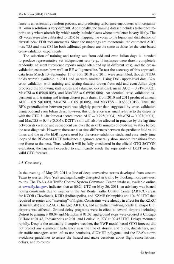
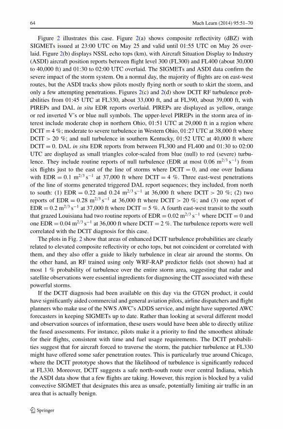
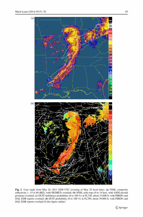
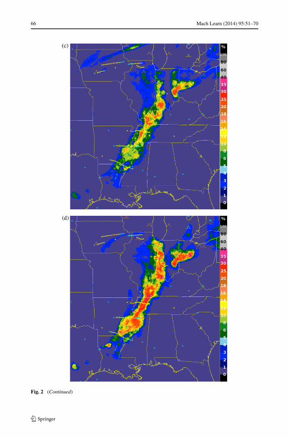
Figure 2 illustrates this case. Figure 2(a) shows composite reflectivity (dBZ) withSIGMETs issued at 23:00 UTC on May 25 and valid until 01:55 UTC on May 26 over-laid. Figure 2(b) displays NSSL echo tops (km), with Aircraft Situation Display to Industry(ASDI) aircraft position reports between flight level 300 (FL300) and FL400 (about 30,000to 40,000 ft) and 01:30 to 02:00 UTC overlaid. The SIGMETs and ASDI data confirm thesevere impact of the storm system. On a normal day, the majority of flights are on east-westroutes, but the ASDI tracks show pilots mostly flying north or south to skirt the storm, andonly a few attempting penetrations. Figures 2(c) and 2(d) show DCIT RF turbulence prob-abilities from 01:45 UTC at FL330, about 33,000 ft, and at FL390, about 39,000 ft, withPIREPs and DAL in situ EDR reports overlaid. PIREPs are displayed as yellow, orangeor red inverted V’s or blue null symbols. The upper-level PIREPs in the storm area of in-terest include moderate chop in northern Ohio, 01:51 UTC at 29,000 ft in a region whereDCIT = 4 %; moderate to severe turbulence in Western Ohio, 01:27 UTC at 38,000 ft whereDCIT > 20 %; and null turbulence in southern Kentucky, 01:52 UTC at 40,000 ft whereDCIT = 0. DAL in situ EDR reports from between FL300 and FL400 and 01:30 to 02:00UTC are displayed as small triangles color-scaled from blue (null) to red (severe) turbu-lence. They include routine reports of null turbulence (EDR at most 0.06 m2/3 s−1) fromsix flights just to the east of the line of storms where DCIT = 0, and one over Indianawith EDR = 0.1 m2/3 s−1 at 37,000 ft where DCIT = 4 %. Three east-west penetrationsof the line of storms generated triggered DAL report sequences; they included, from northto south: (1) EDR = 0.22 and 0.24 m2/3 s−1 at 36,000 ft where DCIT > 20 %; (2) tworeports of EDR = 0.28 m2/3 s−1 at 36,000 ft where DCIT > 20 %; and (3) one report ofEDR = 0.2 m2/3 s−1 at 37,000 ft where DCIT = 5 %. A fourth east-west transit to the souththat grazed Louisiana had two routine reports of EDR = 0.02 m2/3 s−1 where DCIT = 0 andone EDR = 0.04 m2/3 s−1 at 36,000 ft where DCIT = 2 %. The turbulence reports were wellcorrelated with the DCIT diagnosis for this case.

The plots in Fig. 2 show that areas of enhanced DCIT turbulence probabilities are clearlyrelated to elevated composite reflectivity or echo tops, but not coincident or correlated withthem, and they also offer a guide to likely turbulence in clear air around the storms. Onthe other hand, an RF trained using only WRF-RAP predictor fields (not shown) had atmost 1 % probability of turbulence over the entire storm area, suggesting that radar andsatellite observations were essential ingredients for diagnosing the CIT associated with thesepowerful storms.

If the DCIT diagnosis had been available on this day via the GTGN product, it couldhave significantly aided commercial and general aviation pilots, airline dispatchers and flightplanners who make use of the NWS AWC’s ADDS service, and might have supported AWCforecasters in keeping SIGMETs up to date. Rather than looking at several different modeland observation sources of information, these users would have been able to directly utilizethe fused assessments. For instance, pilots make it a priority to find the smoothest altitudefor their flights, consistent with time and fuel usage requirements. The DCIT probabili-ties suggest that for aircraft forced to traverse the storm, the patchier turbulence at FL330might have offered some safer penetration routes. This is particularly true around Chicago,where the DCIT prototype shows that the likelihood of turbulence is significantly reducedat FL330. Moreover, DCIT suggests a safe north-south route over central Indiana, whichthe ASDI data show that a few flights are taking. However, this region is blocked by a validconvective SIGMET that designates this area as unsafe, potentially limiting air traffic in anarea that is actually benign.

Mach Learn (2014) 95:51–70 65

Fig. 2 Case study from May 26, 2011 0200 UTC (evening of May 25 local time). (a) NSSL compositereflectivity (−15 to 60 dBZ), with SIGMETs overlaid; (b) NSSL echo tops (0 to 14 km), with ASDI aircraftpositions overlaid; (c) DCIT turbulence probability (0 to 100 %) at FL330, about 33,000 ft, with PIREPs andDAL EDR reports overlaid; (d) DCIT probability (0 to 100 %) at FL390, about 39,000 ft, with PIREPs andDAL EDR reports overlaid (Color figure online)

66 Mach Learn (2014) 95:51–70

Fig. 2 (Continued)

Mach Learn (2014) 95:51–70 67

5 Operational infusion and anticipated benefits

An RF-based DCIT prototype is running in real-time at NCAR, producing gridded outputat 6-km horizontal and 1,000 ft vertical resolution every 15 minutes for internal use in casestudies, statistical performance evaluation, and integration into GTGN. The multi-threadedC++ implementation uses a decision tree to determine which RF and calibration to runbased on altitude and on available predictor data; thus, it accommodates minor data outagesgracefully. Input data are processed asynchronously as they arrive, including by advectingsatellite, radar and lightning data forward to the next scheduled DCIT generation time toaccount for storm motion. This helps ensure that the data are temporally aligned and thatlatency will be minimal. Output is displayed graphically (as in Fig. 2) and analyzed to ensureits plausibility and spatial and temporal coherence. The DCIT EDR assessment is combinedwith the latest GTG 3 NWP-based turbulence forecast and “nudged” using recent PIREPsand in situ EDR reports to create the GTGN product. GTG 3, which includes GTGN as itsnowcast component, is scheduled to be evaluated by the FAA AWRP’s Quality AssessmentProduct Development Team beginning in late 2013, likely using an approach similar toWandishin et al. (2011). An FAA Technical Review Panel will review the evaluation, andif results are favorable, GTG 3 could be deployed for operational use at the NWS AWC asearly as 2014. Users including pilots, airline dispatchers, aviation weather forecasters andprivate weather service providers will then be able to retrieve the gridded nowcasts for use intheir own displays and automated systems or view them via the ADDS website introducedin Sect. 1.3.

DCIT’s deterministic EDR diagnoses will improve the operational aviation weather prod-uct, GTG, in the important domain of CIT assessment where it currently performs poorly, ashas been shown via some of the same metrics used in official GTG evaluations. DCIT’s prob-abilistic assessments, which will be extended in the future to include short-term forecasts,will make an important contribution to the U.S. NextGen air traffic modernization effort(JPDO 2008) by providing authoritative information required for automated decision mak-ing (e.g., Krozel et al. 2007; Lindholm et al. 2010). For instance, Williams (2009) showedthat dynamic programming could be used to choose optimal routes based on probabilisticforecasts. Quantifying DCIT’s impact on accidents, injuries, fuel costs, delays and cancel-lations will be difficult due to the complexity of the NAS and the diverse, decentralized,asynchronous decision-making processes involved at multiple timescales. However, it seemsclear that, when fully integrated into NextGen, this improved information on CIT locationand intensity will assist dispatchers and pilots in choosing efficient, safe routes near stormsand will decrease the number of unexpected turbulence encounters and re-routing requests,reducing controller workload.

6 Lessons learned

Using machine learning to diagnose turbulence requires dealing effectively with the rarenessof encounters captured in the available “truth” data. Initial approaches to DCIT develop-ment using multi-category predictions or regressions were difficult to calibrate. Reducingthe problem to binary classification facilitated rebalancing of the dataset and producing reli-able probabilistic diagnoses, simplifying DCIT interpretation and optimization. It was foundthat the output of an RF trained to identify light-to-moderate or greater turbulence could bescaled to EDR, and it also performed well on discriminating moderate and severe turbulence(Williams et al. 2012). The use of a calibrated random forest classifier also facilitated theuse of DAL data, whose use of “triggering” skews the distribution of small EDR values.

68 Mach Learn (2014) 95:51–70

Domain knowledge was useful in selecting appropriate data sources, deriving featuresand transformations that better exposed the relevant information, and selecting “truth” datathat adequately capture the temporal and spatial scales of the CIT phenomenon. RF im-portances provided a helpful guide to initial predictor selection but can be biased and donot expose correlations between variables. Using forward and backward selection appearedmore reliable in identifying a minimal set of skillful predictors.

The RF did show better skill than logistic regression for this problem, perhaps becauseit makes better use of predictors not monotonically related to the predictand, and also betterthan k-nearest neighbors. It may be that some of the predictor variables could be transformedor combined to make them more effective in a simpler model, which would be preferablefrom the standpoint of computational intensity in a real-time system. This possibility will befurther investigated. Other RF formulations (e.g., Menze et al. 2011) may also provide moreuseful variable importance information or improved performance. For instance, by utilizingobject-based relationships rather than relying on the numerous neighborhood statistics em-ployed in the present study, the Spatiotemporal Relational Random Forest (SRRF) approachdescribed in McGovern et al. (2013) may provide a simpler, more easily interpreted andmore flexible model.

In using a machine learning model in an operational system, it is important to mini-mize run-time while dealing gracefully with data latency and availability issues. The DCITsystem was designed to handle the asynchronous arrival of real-time input data by imme-diately deriving features and performing forward motion-adjustment to align with the nextproduct generation time. Predictor field alignment is critical; without it, RF output becomes“blurred” and less useful. Potential data outages are dealt with by utilizing similar or redun-dant sources of information and training different RFs for different data feed failure modes.An appropriate RF model is selected at run-time if sufficient input data are present to meetperformance requirements.

A significant problem in applying empirically-based techniques for weather prediction isthat the observation platforms and NWP models that supply predictor variables evolve overtime, and weather phenomena themselves may vary based on climate change and large-scale patterns like the El Niño/La Niña–Southern Oscillation. During DCIT development,the training database was re-created after NOAA switched from the RUC to the WRF-RAPNWP model, and there were also changes in the radar and satellite systems. To performoptimally, DCIT will likely require periodically re-calibration after it becomes operational.Eventually, on-line training and calibration could be incorporated so that the system willautomatically adjust to such changes.

In conclusion, as the amount of data from models and observations continues to growat an exponential rate, techniques like the one described in this paper hold the promise ofeffectively exploiting the available data to provide societally relevant information.

Acknowledgements This research is in response to requirements and funding by the Federal AviationAdministration (FAA). The views expressed are those of the authors and do not necessarily represent theofficial policy or position of the FAA. This material is also based upon work supported by the NationalAeronautics and Space Administration under CAN Grant No. NNS06AA61A and Grant No. NNX08AL89G,issued through the Science Mission Directorate. Bob Sharman, Gerry Wiener, Gary Blackburn, Wayne Feltz,Tony Wimmers, and Kris Bedka contributed data or software used in this study as well as helpful insights.Greg Meymaris designed and maintained the NCAR database, and Jason Craig assembled data, engineeredthe real-time DCIT prototype and configured the display. This work would not have been possible withouttheir many contributions. This manuscript also benefited greatly from the suggestions of three anonymousreviewers.

Open Access This article is distributed under the terms of the Creative Commons Attribution Licensewhich permits any use, distribution, and reproduction in any medium, provided the original author(s) and thesource are credited.

Mach Learn (2014) 95:51–70 69

References

Bedka, K. M., Brunner, J., Dworak, R., Feltz, W., Otkin, J., & Greenwald, T. (2010). Objective satellite-basedovershooting top detection using infrared window channel brightness temperature gradients. Journal ofApplied Meteorology and Climatology, 49, 181–202.

Benjamin, S. G., Devenyi, D., Smirnova, T., Weygandt, S. S., Brown, J. M., Peckham, S., Brundage, K. J.,Smith, T. L., Grell, G. A., & Schlatter, T. W. (2006). From the 13-km RUC to the rapid refresh. In AMS12th conference on aviation, range, and aerospace meteorology, Atlanta, GA (paper 9.1).

Breiman, L. (2001). Random forests. Machine Learning, 45, 5–32.Cornman, L. B., & Carmichael, B. (1993). Varied research efforts are under way to find means of avoiding

air turbulence. ICAO Journal, 48, 10–15.Commercial Aviation Safety Team (CAST) (2001). Turbulence Joint Safety Analysis Team (JSAT) Analysis

and Results (Report), 83 pp. www.cast-safety.org/pdf/jsat_turbulence.pdf.Cornman, L. B., Morse, C. S., & Cunning, G. (1995). Real-time estimation of atmospheric turbulence severity

from in-situ aircraft measurements. Journal of Aircraft, 32, 171–177.Cornman, L. B., Meymaris, G., & Limber, M. (2004). An update on the FAA Aviation Weather Research

Program’s in situ turbulence measurement and reporting system. In AMS 12th conference on aviation,range, and aerospace meteorology (paper 4.3).

Cook, A. J., Tanner, G., & Anderson, S. (2004). Evaluating the true cost to airlines of one minute of airborneor ground delay (Technical Report). Transport Studies Group, University of Westminster.

Cook, L. (2008). Translating weather information (convective and non-convective) into TFM constraints:report of parameters that affect TFM decisions (MOSAIC ATM/AvMet report under NASA NRA Con-tract No. NNA07BC57C).

Cummins, K. L., & Murphy, M. J. (2009). An overview of lightning locating systems: history, techniques,and data uses, with an in-depth look at the U.S. NLDN. IEEE Transactions on Electromagnetic Com-patibility, 51(3), 499–518.

Deierling, W., Williams, J. K., Kessinger, C. J., Sharman, R. D., & Steiner, M. (2011). The relationshipof in-cloud convective turbulence to total lightning. In AMS 15th conference on aviation, range, andaerospace meteorology, Los Angeles, CA (paper 2.3).

Díaz-Uriarte, R., & de Andrés, S. A. (2006). Gene selection and classification of microarray data usingrandom forest. BMC Bioinformatics, 7, 3.

Eichenbaum, H. (2000). Historical overview of turbulence accidents (MCR Federal Report TR-7100/023-1).Available from MCR Federal Inc., 175 Middlesex Turnpike, Bedford, MA 01730.

Eichenbaum, H. (2003). Historical overview of turbulence accidents and case study analysis (MCR FederalReport Br-M021/080-1), 82 pp. Available from MCR Federal Inc., 175 Middlesex Turnpike, Bedford,MA 01730.

Federal Aviation Administration (2012). FAA aeronautical information manual. Chap. 7. Available online atwww.faa.gov/air_traffic/publications/atpubs/aim/.

Fovell, R. G., Sharman, R. D., & Trier, S. B. (2007). A case study of convectively-induced clear-air turbu-lence. In AMS 12th conference on mesoscale processes, Waterville Valley, NH (paper 13.4).

International Civil Aviation Organization (ICAO) (2001). Meteorological service for international air navi-gation. Annex 3 to the convention on international civil aviation (14th ed.), 128 pp.

Joint Planning and Development Office (JPDO) (2008). Integrated work plan for the next generationair transportation system. Version 0.2, 432 pp. http://ebookbrowse.com/iwp-version-02-master-w-o-appendix-pdf-d90599595.

Kaplan, M. L., Huffman, A. W., Lux, K. M., Charney, J. J., Riordan, A. J., & Lin, Y.-L. (2005). Characterizingthe severe turbulence environments associated with commercial aviation accidents. Part 1: a 44-casestudy synoptic observational analysis. Meteorology and Atmospheric Physics, 88, 129–153.

Krozel, J., Mitchell, J. S. B., Polishchuk, V., & Prete, J. (2007). Maximum flow rates for capacity estimationin level flight with convective weather constraints. Air Traffic Control Quarterly, 15(3), 209–238.

Lane, T. P., Sharman, R. D., Clark, T. L., & Hsu, H.-M. (2003). An investigation of turbulence generationmechanisms above deep convection. J. Atmos. Sci., 60, 1297–1321.

Lane, T. P., & Sharman, R. D. (2008). Some influences of background flow conditions on the generation ofturbulence due to gravity wave breaking above deep convection. Journal of Applied Meteorology andClimatology, 47(11), 2777–2796.

Lane, T. P., Sharman, R. D., Trier, S. B., Fovell, R. G., & Williams, J. K. (2012). Recent advances in theunderstanding of near-cloud turbulence. Bulletin of the American Meteorological Society, 93, 499–515.

Lindholm, T., Sharman, R., Krozel, J., Klimenko, V., Krishna, S., Downs, N., & Mitchell, J. S. B. (2010).Translating weather into traffic flow management impacts for NextGen. In AMS 14th conference onaviation, range, and aerospace meteorology, Atlanta, GA (paper J12.4).

70 Mach Learn (2014) 95:51–70

Martin, D. W., Kohrs, R. A., Mosher, F. R., Medaglia, C. M., & Adamo, C. (2008). Over-ocean validation ofthe global convective diagnostic. Journal of Applied Meteorology and Climatology, 47(2), 525–543.

McGovern, A., Gagne, D. J. II, Williams, J. K., Brown, R. A., & Basara, J. B. (2013). Enhancing understand-ing and improving prediction of severe weather through spatiotemporal relational learning. MachineLearning. doi:10.1007/s10994-013-5343-x.

Menze, B., Kelm, B. M., Splitthoff, D., Koethe, U., & Hamprecht, F. (2011). On oblique random forests. InD. Gunopulos, T. Hofmann, D. Malerba, & M. Vazirgiannis (Eds.), Lecture notes in computer science:Machine learning and knowledge discovery in databases (pp. 453–469). Berlin: Springer.

Pal, M. (2005). Random forest classifier for remote sensing classification. International Journal of RemoteSensing, 26(1), 217–222.

Schaefer, J. T. (1990). The critical success index as an indicator of warning skill. Weather and Forecasting,5, 570–575.

Schwartz, B. (1996). The quantitative use of PIREPs in developing aviation weather guidance products.Weather and Forecasting, 11, 372–384.

Sharman, R. D., Cornman, L., Williams, J. K., Koch, S. E., & Moninger, W. R. (2006a). The AWRP turbu-lence PDT. In AMS 12th conference on aviation, range, and aerospace meteorology (paper 3.3).

Sharman, R., Tebaldi, C., Wiener, G., & Wolff, J. (2006b). An integrated approach to mid-and upper-levelturbulence forecasting. Weather and Forecasting, 21, 268–287.

Sharman, R., & Williams, J. K. (2009). The complexities of thunderstorm avoidance due to turbulence andimplications for traffic flow management. In AMS aviation, range and aerospace meteorology specialsymposium on weather-air traffic management integration, Phoenix, AZ (paper 2.4).

Strobl, C., Boulesteix, A.-L., Zeileis, A., & Hothorn, T. (2007). Bias in random forest variable importancemeasures: illustrations, sources and a solution. BMC Bioinformatics, 8, 25.

Trier, S. B., & Sharman, R. D. (2009). Convection-permitting simulations of the environment support-ing widespread turbulence within the upper-level outflow of a mesoscale convective system. MonthlyWeather Review, 137, 1972–1990.

Trier, S. B., Sharman, R. D., & Lane, T. P. (2012). Influences of moist convection on a cold-season outbreakof clear-air turbulence (CAT). Monthly Weather Review, 140, 2477–2496.

Wandishin, M. S., Pettegrew, B. P., Petty, M. A., & Mahoney, J. L. (2011). Quality assessment report forGraphical Turbulence Guidance, version 2.5. United States National Oceanic and Atmospheric Ad-ministration, Earth System Research Laboratory, Global Systems Division. http://purl.fdlp.gov/GPO/gpo15528.

Williams, J. K., Cornman, L. B., Yee, J., Carson, S. G., Blackburn, G., & Craig, J. (2006). NEXRAD detectionof hazardous turbulence. In Proceedings of 44th AIAA aerospace sciences meeting and exhibit (paperAIAA 2006-0076).

Williams, J. K., Ahijevych, D., Dettling, S., & Steiner, M. (2008a). Combining observations and model datafor short-term storm forecasting. In W. Feltz & J. Murray (Eds.), Proceedings of SPIE: Vol. 7088. Re-mote sensing applications for aviation weather hazard detection and decision support (paper 708805).

Williams, J. K., Sharman, R., Craig, J., & Blackburn, G. (2008b). Remote detection and diagnosis of thun-derstorm turbulence. In W. Feltz & J. Murray (Eds.), Proceedings of SPIE: Vol. 7088. Remote sensingapplications for aviation weather hazard detection and decision support (paper 708804).

Williams, J. K. (2009). Reinforcement learning of optimal controls. In S. E. Haupt, A. Pasini, & C. Marzban(Eds.), Artificial intelligence methods in the environmental sciences (pp. 297–327).

Williams, J. K., Blackburn, G., Craig, J. A., & Meymaris, G. (2012). A data mining approach to data fusionfor turbulence diagnosis. In K. Das, N. V. Chawla, & A. N. Srivastava (Eds.), Proc. 2012 conference onintelligent data understanding (pp. 168–169).

Wimmers, A. J., & Moody, J. L. (2004). Tropopause folding at satellite-observed spatial gradients: 2. devel-opment of an empirical model. Journal of Geophysical Research, 109, D19307.

Wimmers, A., & Feltz, W. (2012). The GOES-R tropopause folding turbulence product: finding clear-airturbulence in GOES water vapor imagery. In AMS 18th conference on satellite meteorology, oceanogra-phy and climatology and 1st joint AMS-Asia satellite meteorology conference, New Orleans, LA (paper471).

Zhang, J., Howard, K., Langston, C., Vasiloff, S., Kaney, B., Arthur, A., Cooten, S. V., Kellehe, K., Kitzmiller,D., Ding, F., Seo, D.-J., Wells, E., & Dempsey, C. (2011). National mosaic and multi-sensor QPE(NMQ) system: description, results, and future plans. Bulletin of the American Meteorological Soci-ety, 92, 1321–1338.