Using S-PLUS for Data Analysis & Graphics

J H Maindonald

Statistical Consulting Unit of the Graduate School

Australian National University.

Canberra

Hobart

AdelaideAlbury

Alice_Springs

Brisbane

BroomeCairns

Darwin

Melbourne

NewcastlePerthSydney

Townsville

© J. H. Maindonald 2001. A licence is granted for personal study and classroom use. Redistribution in any other form is prohibited.

25 June 2001

Languages shape the way we think, and determine what we can think about. (Benjamin Whorf)

2

oz.all

function()

{

oz()

points(.Oz.cities)

points(.Oz.cities$x[7], .Oz.cities$y[7], pch = 16)

justif <- c(1, 1, 1, 1, 1, 1, 0, 1, 0, 1, 1, 1, 1, 1)

here <- justif == 0

cities1 <- lapply(.Oz.cities, function(x, here)

x[here], here = here)

chw <- par()$cxy[1]

cities1$x <- cities1$x + chw/2

chh <- par()$cxy[2]

cities2 <- lapply(.Oz.cities, function(x, here)

x[!here], here = here)

cities2$y[9] <- cities2$y[9] + chh/3

cities2$x <- cities2$x - chw/2

text(cities1, cities1$name, adj = 0)

text(cities2, cities2$name, adj = 1)

}

Contents Introduction – Why S-PLUS?.............................................................................................................................1 1. Starting Up .....................................................................................................................................................3

1.1 Using the Command Window ..................................................................................................................4 1.2 A Short S-PLUS Session..........................................................................................................................4 1.3 Using the S-PLUS Data Menu .................................................................................................................6 1.4 Further Notational Details........................................................................................................................7 1.5 On-line Help.............................................................................................................................................8 1.6 Exercises ..................................................................................................................................................8

2. An Overview of S-PLUS ..............................................................................................................................11 2.1 The Uses of S-PLUS ..............................................................................................................................11 2.2 The Look and Feel of S..........................................................................................................................14 2.3 S-PLUS Objects .....................................................................................................................................14 *2.4 Looping ................................................................................................................................................14 2.5 S-PLUS Functions..................................................................................................................................15 2.6 Vectors ...................................................................................................................................................16 2.7 Data Frames ...........................................................................................................................................19 2.8 Common Useful Functions.....................................................................................................................20 2.9 Making Tables........................................................................................................................................21 2.10 The Use of attach()...............................................................................................................................22 2.11 More Detailed Information...................................................................................................................23 2.12 Exercises ..............................................................................................................................................23

3. Plotting .........................................................................................................................................................25 3.1 plot () and allied functions .....................................................................................................................25 3.2 Fine control – Parameter settings ...........................................................................................................25 3.3 Adding points, lines and text..................................................................................................................26 3.4 Identification and Location on the Figure Region..................................................................................28 3.5 Plots that show the distribution of data values .......................................................................................29 3.6 Other Useful Plotting Functions.............................................................................................................31 3.7 Guidelines for Graphs ............................................................................................................................33 3.8 Exercises ................................................................................................................................................33 3.9 References..............................................................................................................................................34

4. Trellis Graphics ............................................................................................................................................35 4.1 Fine control over the graphics window ..................................................................................................35 4.2 Examples that Present Panels of Scatterplots – Using xyplot()........................................................35 4.3 An Incomplete List of Trellis Functions.................................................................................................36 4.4 Trellis Functions – Further Examples ....................................................................................................37 4.5 The Panel Function ................................................................................................................................38 *4.6 Adding a Key .......................................................................................................................................39 *4.7 The Subscripts Argument .....................................................................................................................39 4.8 Exercises ................................................................................................................................................40

5. Regression Models and Analysis of Variance ..............................................................................................43 5.1 The Model Formula in Straight Line Regression ...................................................................................43

ii

5.2 Regression Objects.................................................................................................................................43 5.3 Model Formulae, and the X Matrix........................................................................................................45 5.4 Multiple Linear Regression Models .......................................................................................................47 5.5 Polynomial regression ............................................................................................................................50 5.6 Using Factors in S-PLUS Models ..........................................................................................................53 5.7 Multiple Lines – Different Regression Lines for Different Species .......................................................56 5.8 Explaining Fuel Consumption – 2 variables, plus the factor Type.........................................................58 *5.9 aov models (Analysis of Variance) ......................................................................................................59 5.10 Exercises ..............................................................................................................................................60 5.11 References............................................................................................................................................61

6. Multivariate and Tree-Based Methods .........................................................................................................63 6.1 Multivariate EDA, and Principal Components Analysis ........................................................................63 6.2 Cluster Analysis .....................................................................................................................................64 6.3 Discriminant Analysis ............................................................................................................................64 6.4 Decision Tree models (Tree-based models) ...........................................................................................65 6.5 Exercises ................................................................................................................................................66 6.6 References..............................................................................................................................................66

*7. S-PLUS Data Structures .............................................................................................................................67 7.1 Vectors ............................................................................................................................................67 7.2 Missing Values.......................................................................................................................................68 7.3 Data frames ............................................................................................................................................68 7.4 Data Entry ..............................................................................................................................................70 7.5 Factors....................................................................................................................................................71 7.6 Ordered Factors......................................................................................................................................73 7.7 Lists........................................................................................................................................................73 *7.8 Matrices and Arrays .............................................................................................................................74 7.9 Different Types of Attachments .............................................................................................................75 7.10 Exercises ..............................................................................................................................................77

8. Useful Functions...........................................................................................................................................79 8.1 Matching and Ordering ..........................................................................................................................79 8.2 String Functions .....................................................................................................................................79 8.3 Application of a Function to the Columns of an Array or Data Frame...................................................79 *8.4 tapply() .................................................................................................................................................80 8.5 Breaking Vectors and Data Frames Down into Lists – split() ................................................................81 *8.6 Merging Data Frames...........................................................................................................................81 8.7 Dates ......................................................................................................................................................82 8.8 Exercises ................................................................................................................................................83

9. Writing Functions and other Code................................................................................................................85 9.1 Syntax and Semantics.............................................................................................................................85 9.2 A Function that gives Data Frame Details..............................................................................................85 9.3 Coding that assists Data Management....................................................................................................86 9.4 Issues for the Writing and Use of Functions ..........................................................................................86 9.5 Calling Modelling Functions from User-Written Functions...................................................................87 9.6 A Simulation Example ...........................................................................................................................87

iii

9.7 Exercises ................................................................................................................................................88 10. GLM, GAM and General Non-linear Models.............................................................................................91

10.1 A Taxonomy of Extensions to the Linear Model .................................................................................91 10.2 Logistic Regression..............................................................................................................................92 10.3 glm models (Generalised Linear Regression Modelling) .....................................................................96 10.4 gam models (Generalised Additive Models) ........................................................................................97 10.5 Prediction with New Data ....................................................................................................................97 10.6 Non-linear Models ...............................................................................................................................98 10.7 Model Summaries ................................................................................................................................98 10.8 Further Elaborations.............................................................................................................................98 10.9 Exercises ..............................................................................................................................................98 10.10 References..........................................................................................................................................98

11. Multi-level Models, Time Series and Survival Analysis ............................................................................99 *11.1 Multi-Level Models, Including Repeated Measures Models..............................................................99 *11.2 Repeated Measures Models..............................................................................................................103 11.3 Time Series Models ...........................................................................................................................104 11.4 Survival Analysis ...............................................................................................................................105 11.5 Exercises ............................................................................................................................................105 11.6 References..........................................................................................................................................105

12. Advanced Programming Topics ...............................................................................................................107 12.1. Methods.............................................................................................................................................107 12.2 Extracting Arguments to Functions ....................................................................................................107 12.3 Parsing and Evaluation of Expressions ..............................................................................................108 12.4 Searching S-PLUS functions for a specified token. ...........................................................................110

13. Appendix 1 – S-PLUS Resources.............................................................................................................111 13.1 Official Documentation......................................................................................................................111 13.3 Libraries .............................................................................................................................................112 13.4 The s-news electronic mail discussion list..........................................................................................112 13.5 Competing Systems – R and XLISP-STAT .......................................................................................112

14. Appendix ..................................................................................................................................................113 14.1 Data Sets Used in this Course ............................................................................................................113 14.2 Answers to Selected Exercises ...........................................................................................................113

iv

Introduction – Why S-PLUS? S-PLUS is a commercial implementation and substantial enhancement of the S data analysis, graphics and programming environment1. The data analysis and graphics abilities are implemented in an environment that is attractive for more general interactive commercial and scientific computation. In the words of the citation for John Chambers’ 1998 Association for Computing Machinery Software Award, S has “forever altered how people analyse, visualize and manipulate data.” These notes hope to convey a sense of why it is reasonable to describe S in this way.

Insightful Corporation, who market S-PLUS, have made substantial enhancements to S. They have ported the system across to Microsoft Windows 95, 98 and NT. They developed the graphical user interface that is available for Microsoft Windows environments. The S-PLUS command line language retains some features that reflect S-PLUS’s origin in a Unix environment.

Leading statistical researchers have contributed substantial new statistical analysis abilities. Some of these enhancements are distributed as part of S-PLUS, and some are available separately. Section 13.3 gives useful web addresses for software libraries that are available separately.

Features which S-PLUS offers include:

1. There are extensive and powerful graphics abilities, which are tightly linked with its analytic abilities. Trellis graphics, not widely available elsewhere, are a distinguishing feature of S-PLUS graphics. Trellis graphics provide multi-panel graphical summaries that reflect data structure. These may be very helpful in highlighting major features of the data. Carefully chosen trellis plots often provide clues which may be followed up in subsequent analysis.

2. S-PLUS gives access to a style of interactive statistical analysis that statistical professionals increasingly take for granted.

3. S-PLUS offers a modern and up to date choice of statistical methods. There are ongoing projects that aim to fill perceived gaps.

4. S-PLUS gives access to a sophisticated and relatively state of the art programming language. Professionals who are familiar both with the S language and with the relevant statistical methodology can often rapidly develop any new routine that they need. Analyses need not be limited by the abilities that are immediately available.

5. S-PLUS finds extensive use for rapid prototyping and development of new statistical methods. S-PLUS is used in most major centres that develop new statistical methods for practical use.

6. Because computer-intensive components can be handled by a call to a C function, S-PLUS’s implementation as an interpreted language is not usually a serious handicap.

7. S-PLUS users have access to large libraries of S-PLUS functions that have been developed by Frank Harrell & others (Division of Biostatistics & Epidemiology, Virginia Medical Institute), Brian Ripley (Statistics Department, Oxford University) and Bill Venables (CMIS, CSIRO) and R. J. Tibshirani & others (Statistics Department, Stanford University).

1 The S system was developed by Richard A Becker, John M Chambers, Allan R Wilks, William S Cleveland, and colleagues, at AT&T Bell Laboratories. The S system is now a project of Lucent Technologies.

2

S-PLUS is the statistical computing environment of choice for many highly skilled statistical professionals. As a result, it has received higher levels of critical scrutiny than most other statistical software. Note however that many of the model fitting routines in S-PLUS are leading edge. Some features have not been tested and checked as adequately as one would like. Because the language is powerful it also, inevitably, has elements of subtlety. There are traps which call for special care from users. There are also annoying inconsistencies. Especially when you are doing anything at all complicated, check every step with care.

______________________________________________________________________________

Jeff Wood (CMIS, CSIRO), Andreas Rukhstuhl (Technikum Winterthur Ingenieurschule, Switzerland), and Ken Brewer (Department of Statistics & Econometrics, ANU) gave me exemplary help in getting this document somewhere near shipshape form. I am indebted to John Braun (University of Winnipeg) for a number of the exercises. I take full responsibility for the errors that remain.

S-PLUS is available from the CMIS division of CSIRO: Web address http://www.cmis.csiro.au Email address S+inquiries@cmis.csiro.au

This document has immediate relevance to the use of S-PLUS under Windows 95. Sections which might be omitted at a first reading are marked with an asterisk.

3

1. Starting Up S-PLUS must be installed on your system! If it is not, follow the instructions that came with the installation CD-ROM.

Following installation you should have one or more S-PLUS icons (or a folder containing one or more icons) on your screen. If you have closed the screen icons then click on the START menu, place the mouse cursor on Programs, and look for a program folder that holds the S-PLUS icon(s).

Click on the S-PLUS icon. If there is more than one icon, this will be because you have different icons for different projects or groups of projects. Click on the icon for the project on which you want to work. For this demonstration I will click on my S-course icon.

Here, we will work from the command line. If you do not have a command line window, click on Window (or type Alt/W) and then on Commands Window. On my system the following appears:

Fig. 1: An S-PLUS screen, at the start of a session. We have opened a Commands window, but closed the object browser. There is no script window.

In interactive use under Microsoft Windows there are several ways to input commands to S-PLUS. One can use any or all of the following three forms of input:

1. Open and work in a command window, typing commands at the command line prompt. For the moment, we will work in a commands window.

2. Open and work in a script window. In the screen snapshot above, there is no script window. To get a script window, go to the File menu.

4

Commands can be input to the script window from a file, and/or typed in directly. Any commands that are to be input to S-PLUS are highlighted in the script window. Clicking on the arrow in the script toolbar then sends these commands to S-PLUS.

3. Use the graphical user (gui) point and click command interface. In other words, use the icons such as are shown in the screen snapshot. In this course, we will make little use of the graphical user command interface.

Under Unix, the standard form of input is the command line interface. Under both Microsoft Windows and Unix, a further possibility is to run S-PLUS from within the emacs editor.

1.1 Using the Command Window Here is what appeared in the command window when it was first opened:

Working data will be in C:Working data will be in C:Working data will be in C:Working data will be in C:\\\\statsstatsstatsstats\\\\SSSS----coursecoursecoursecourse\\\\_Data _Data _Data _Data

>>>>

The command line prompt, i.e. the >, is an invitation to start typing in your commands. For example, type in 2+2 and press the Enter key. Here is what I now have on my screen:

Working data will be in C:Working data will be in C:Working data will be in C:Working data will be in C:\\\\statsstatsstatsstats\\\\SSSS----coursecoursecoursecourse\\\\____

Data Data Data Data

> 2+2> 2+2> 2+2> 2+2

[1] 4[1] 4[1] 4[1] 4

>>>>

Here the result is 4. I will explain the [1] later. The final > indicates that S-PLUS is ready for another command.

Just in case you want to quit from S-PLUS at this point, you should know that the exit or quit command is

> q()> q()> q()> q()

Alternatives are to click on the File menu and then on Exit, or to click on the ×××× in the top right hand corner of the S-PLUS window.

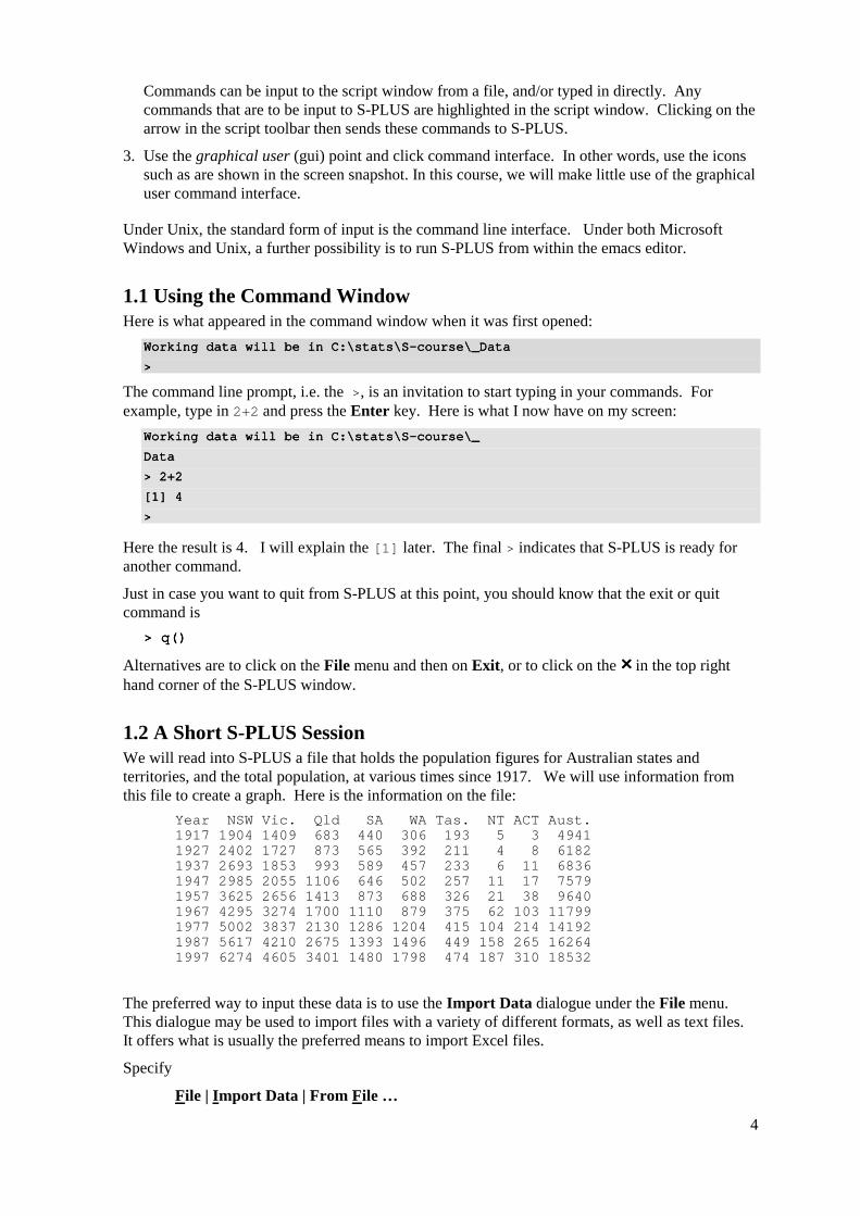
1.2 A Short S-PLUS Session We will read into S-PLUS a file that holds the population figures for Australian states and territories, and the total population, at various times since 1917. We will use information from this file to create a graph. Here is the information on the file:

Year NSW Vic. Qld SA WA Tas. NT ACT Aust. 1917 1904 1409 683 440 306 193 5 3 4941 1927 2402 1727 873 565 392 211 4 8 6182 1937 2693 1853 993 589 457 233 6 11 6836 1947 2985 2055 1106 646 502 257 11 17 7579 1957 3625 2656 1413 873 688 326 21 38 9640 1967 4295 3274 1700 1110 879 375 62 103 11799 1977 5002 3837 2130 1286 1204 415 104 214 14192 1987 5617 4210 2675 1393 1496 449 158 265 16264 1997 6274 4605 3401 1480 1798 474 187 310 18532

The preferred way to input these data is to use the Import Data dialogue under the File menu. This dialogue may be used to import files with a variety of different formats, as well as text files. It offers what is usually the preferred means to import Excel files.

Specify

File | Import Data | From File …

5

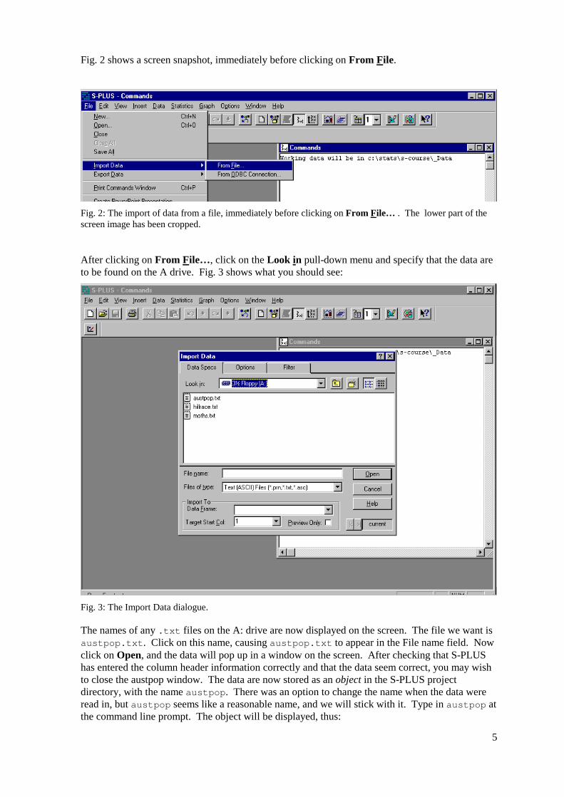
Fig. 2 shows a screen snapshot, immediately before clicking on From File.

Fig. 2: The import of data from a file, immediately before clicking on From File… . The lower part of the screen image has been cropped.

After clicking on From File…, click on the Look in pull-down menu and specify that the data are to be found on the A drive. Fig. 3 shows what you should see:

Fig. 3: The Import Data dialogue.

The names of any .txt files on the A: drive are now displayed on the screen. The file we want is austpop.txt. Click on this name, causing austpop.txt to appear in the File name field. Now click on Open, and the data will pop up in a window on the screen. After checking that S-PLUS has entered the column header information correctly and that the data seem correct, you may wish to close the austpop window. The data are now stored as an object in the S-PLUS project directory, with the name austpop. There was an option to change the name when the data were read in, but austpop seems like a reasonable name, and we will stick with it. Type in austpop at the command line prompt. The object will be displayed, thus:

6

> austpop> austpop> austpop> austpop

Year NSW Vic. Qld SA Year NSW Vic. Qld SA Year NSW Vic. Qld SA Year NSW Vic. Qld SA WA Tas. NT ACT Aust. WA Tas. NT ACT Aust. WA Tas. NT ACT Aust. WA Tas. NT ACT Aust.

1 1917 1904 1409 683 440 306 193 5 3 49411 1917 1904 1409 683 440 306 193 5 3 49411 1917 1904 1409 683 440 306 193 5 3 49411 1917 1904 1409 683 440 306 193 5 3 4941

2 1927 2402 1727 873 565 392 211 4 8 61822 1927 2402 1727 873 565 392 211 4 8 61822 1927 2402 1727 873 565 392 211 4 8 61822 1927 2402 1727 873 565 392 211 4 8 6182

3 1937 2693 1853 993 589 457 233 6 11 68363 1937 2693 1853 993 589 457 233 6 11 68363 1937 2693 1853 993 589 457 233 6 11 68363 1937 2693 1853 993 589 457 233 6 11 6836

4 1947 2985 2055 1106 646 502 257 11 17 75794 1947 2985 2055 1106 646 502 257 11 17 75794 1947 2985 2055 1106 646 502 257 11 17 75794 1947 2985 2055 1106 646 502 257 11 17 7579

5 1957 3625 2656 1413 873 5 1957 3625 2656 1413 873 5 1957 3625 2656 1413 873 5 1957 3625 2656 1413 873 688 326 21 38 9640688 326 21 38 9640688 326 21 38 9640688 326 21 38 9640

6 1967 4295 3274 1700 1110 879 375 62 103 117996 1967 4295 3274 1700 1110 879 375 62 103 117996 1967 4295 3274 1700 1110 879 375 62 103 117996 1967 4295 3274 1700 1110 879 375 62 103 11799

7 1977 5002 3837 2130 1286 1204 415 104 214 141927 1977 5002 3837 2130 1286 1204 415 104 214 141927 1977 5002 3837 2130 1286 1204 415 104 214 141927 1977 5002 3837 2130 1286 1204 415 104 214 14192

8 1987 5617 4210 2675 1393 1496 449 158 265 162648 1987 5617 4210 2675 1393 1496 449 158 265 162648 1987 5617 4210 2675 1393 1496 449 158 265 162648 1987 5617 4210 2675 1393 1496 449 158 265 16264

9 1997 6274 4605 3401 1480 1798 474 187 310 185329 1997 6274 4605 3401 1480 1798 474 187 310 185329 1997 6274 4605 3401 1480 1798 474 187 310 185329 1997 6274 4605 3401 1480 1798 474 187 310 18532

>>>>

We will learn later that austpop is a special form of S-PLUS object, known as a data frame. Data frames that consist entirely of numeric data are similar in structure to numeric matrices.

We will now do a plot of the ACT population between 1917 and 1997. We will first of all remind ourselves of the column names:

> names(austpop)

[1] "Year" "NSW" "Vic." "Qld"

[5] "SA" "WA" "Tas." "NT"

[9] "ACT" "Aust."

>

A simple way to get the plot is: > plot(ACT ~ Year, data=austpop, pch=16)> plot(ACT ~ Year, data=austpop, pch=16)> plot(ACT ~ Year, data=austpop, pch=16)> plot(ACT ~ Year, data=austpop, pch=16)

>>>>

The option pch=16 sets the plotting character to solid black dots. Fig. 4 shows the graph:

Year

ACT

1920 1940 1960 1980 2000

050

100

150

200

250

300

Fig. 4: ACT population versus year, over 1917 - 1997.

There is a great deal that we could do to improve this plot. We can specify more informative axis labels, change size of the text and of the plotting symbol, and so on.

If you wish to quit from the S-PLUS session at this point, type > q()> q()> q()> q()

1.3 Using the S-PLUS Data Menu

7

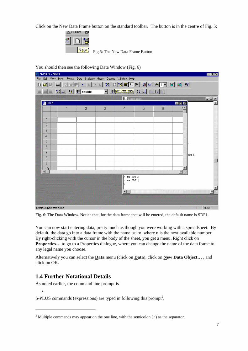
Click on the New Data Frame button on the standard toolbar. The button is in the centre of Fig. 5:

Fig.5: The New Data Frame Button

You should then see the following Data Window (Fig. 6)

Fig. 6: The Data Window. Notice that, for the data frame that will be entered, the default name is SDF1.

You can now start entering data, pretty much as though you were working with a spreadsheet. By default, the data go into a data frame with the name SDFn, where n is the next available number. By right-clicking with the cursor in the body of the sheet, you get a menu. Right click on Properties… to go to a Properties dialogue, where you can change the name of the data frame to any legal name you choose.

Alternatively you can select the Data menu (click on Data), click on New Data Object… , and click on OK.

1.4 Further Notational Details As noted earlier, the command line prompt is

>>>>

S-PLUS commands (expressions) are typed in following this prompt2.

2 Multiple commands may appear on the one line, with the semicolon (;) as the separator.

8

There is also a continuation prompt, used when, following a carriage return, the command is still not complete. By default, the continuation prompt is

++++

In these notes, we often continue commands over more than one line, but omit the + that will appear on the commands window if the command is typed in as we show it.

When typing the names of S-PLUS objects or commands, case is significant. Thus Austpop is different from austpop. For file names however, the Microsoft Windows conventions apply, and case does not distinguish file names. On Unix systems letters that have a different case are treated as different.

Anything which follows a # on the command line is taken as comment, and ignored by S-PLUS.

Note: Recall that we had to type q(), not q, in order to quit from the S-PLUS session. This is because q is a function. Typing q on its own, without the parentheses, displays the text of the function on the screen. Try it!

1.5 On-line Help To get a help window (under S-PLUS for Windows) with a list of help topics, type in

> help()> help()> help()> help()

In S-PLUS for Windows, you can alternatively click on the help menu item, and then use key words to do a search. To get help on a specific S-PLUS function, e. g. plot(), type in

> help(plot)

In addition, the official manuals noted in Appendix 1 are available on-line for searching.

In general the supplied documentation does a good job in providing broad-ranging accounts of the methodology, with extensive references to recent literature. It is often short on detail. Users may need to experiment to discover precisely what a specific S-PLUS function does. The documentation may be short on details of the specific formula that has been used.

1.6 Exercises 1. The following data give, for each amount by which an elastic band is stretched over the end of a ruler, the distance which the band moved when released:

Stretch (mm) Distance (cm) 46 148 54 182 48 173 50 166 44 109 42 141 52 166

Enter the data into a data frame elasticband (or into a name of your own choosing). Plot distance against stretch.

2. The following ten observations, taken during the years 1970-79, are on October snow cover for Eurasia. (Snow cover is in millions of square kilometers):

Year CoverYear CoverYear CoverYear Cover

1970 6.51970 6.51970 6.51970 6.5

1971 12.0 1971 12.0 1971 12.0 1971 12.0

1972 14.91972 14.91972 14.91972 14.9

1973 10.0 1973 10.0 1973 10.0 1973 10.0

9

1974 10.7 1974 10.7 1974 10.7 1974 10.7

1975 7.91975 7.91975 7.91975 7.9

1976 21.9 1976 21.9 1976 21.9 1976 21.9

1977 12.5 1977 12.5 1977 12.5 1977 12.5

1978 14.5 1978 14.5 1978 14.5 1978 14.5

i. Enter the data into S-PLUS. You might call the data set snow.cover.

ii. Plot snow cover versus time.

iii. Repeat, after taking logarithms of snow cover.

3. Input the following data, on damage that had occurred in space shuttle launches prior to the disastrous launch of Jan 28 1986. These are the data, for 6 launches out of 24, that were included in the pre-launch charts that were used in deciding whether to proceed with the launch. (Data for the 23 launches where the rocket casing could be recovered is in the data set orings that accompanies these notes.) Temperature Erosion Blowby Total (F) incidents incidents incidents 53 3 2 5 57 1 0 1

63 1 0 1

70 1 0 1

70 1 0 1

75 0 2 1

Enter these data into a data frame, with (for example) column names temperature, erosion, blowby and total. Plot total incidents against temperature.

10

11

2. An Overview of S-PLUS This chapter gives brief summary information that should be enough for getting started on the graphics and data analysis exercises in chapters 3-6. Chapters 7 and 8 give more detailed information.

2.1 The Uses of S-PLUS

2.1.1 S-PLUS may be used as a calculator. S-PLUS evaluates and prints out the result of any expression that one types in at the command line. Remember that S-PLUS expressions are typed following the prompt (>) on the screen. The result is printed on subsequent lines

> 2+2> 2+2> 2+2> 2+2

4444

> sqrt(10)> sqrt(10)> sqrt(10)> sqrt(10)

[1] 3.162278[1] 3.162278[1] 3.162278[1] 3.162278

> 2*3*4*5> 2*3*4*5> 2*3*4*5> 2*3*4*5

[1] 120[1] 120[1] 120[1] 120

> 1000*(1+0.075)^5 > 1000*(1+0.075)^5 > 1000*(1+0.075)^5 > 1000*(1+0.075)^5 ---- 1000 # Interest on $1000, 1000 # Interest on $1000, 1000 # Interest on $1000, 1000 # Interest on $1000, compounded annually compounded annually compounded annually compounded annually

# at 7.5% p.a. for five years # at 7.5% p.a. for five years # at 7.5% p.a. for five years # at 7.5% p.a. for five years

[1] 435.6293[1] 435.6293[1] 435.6293[1] 435.6293

> pi # S> pi # S> pi # S> pi # S----PLUS knows about piPLUS knows about piPLUS knows about piPLUS knows about pi

[1] 3.141593[1] 3.141593[1] 3.141593[1] 3.141593

> 2*pi*6378 #Circumference of Earth at Equator, in km; radius is 6378km> 2*pi*6378 #Circumference of Earth at Equator, in km; radius is 6378km> 2*pi*6378 #Circumference of Earth at Equator, in km; radius is 6378km> 2*pi*6378 #Circumference of Earth at Equator, in km; radius is 6378km

[1] 40074.16[1] 40074.16[1] 40074.16[1] 40074.16

> sin(c(30,60,90)*pi/180) # Convert a> sin(c(30,60,90)*pi/180) # Convert a> sin(c(30,60,90)*pi/180) # Convert a> sin(c(30,60,90)*pi/180) # Convert angles to radians, then take sin()ngles to radians, then take sin()ngles to radians, then take sin()ngles to radians, then take sin()

[1] 0.500 0.866 1.000[1] 0.500 0.866 1.000[1] 0.500 0.866 1.000[1] 0.500 0.866 1.000

2.1.2 S-PLUS will provide numerical or graphical summaries of data There is a special class of object called a data frame, used to store rectangular arrays in which the columns may be vectors of numbers or factors or text strings. Data frames are central to the way that all the more recent S-PLUS routines process data . For now, think of data frames as matrices, where the rows are observations and the columns are variables.

As a first example, consider the supplied data frame hills, available from Professor Brian Ripley’s MASS library. This has three columns (variables), with the names dist, climb, and time. Typing in summary(hills)gives summary information on these variables. There is one column for each variable,thus:

> summary(hills)> summary(hills)> summary(hills)> summary(hills)

distance climb time distance climb time distance climb time distance climb time

Min.: 2.000 Min.: 300 Min.: 15.95 Min.: 2.000 Min.: 300 Min.: 15.95 Min.: 2.000 Min.: 300 Min.: 15.95 Min.: 2.000 Min.: 300 Min.: 15.95

1st Qu.: 4.500 1st Qu.: 725 1st Qu.: 28.00 1st Qu.: 4.500 1st Qu.: 725 1st Qu.: 28.00 1st Qu.: 4.500 1st Qu.: 725 1st Qu.: 28.00 1st Qu.: 4.500 1st Qu.: 725 1st Qu.: 28.00

Median: 6.000 Median:1000 Media Median: 6.000 Median:1000 Media Median: 6.000 Median:1000 Media Median: 6.000 Median:1000 Median: 39.75 n: 39.75 n: 39.75 n: 39.75

Mean: 7.529 Mean:1815 Mean: 57.88 Mean: 7.529 Mean:1815 Mean: 57.88 Mean: 7.529 Mean:1815 Mean: 57.88 Mean: 7.529 Mean:1815 Mean: 57.88

3rd Qu.: 8.000 3rd Qu.:2200 3rd Qu.: 68.62 3rd Qu.: 8.000 3rd Qu.:2200 3rd Qu.: 68.62 3rd Qu.: 8.000 3rd Qu.:2200 3rd Qu.: 68.62 3rd Qu.: 8.000 3rd Qu.:2200 3rd Qu.: 68.62

Max.:28.000 Max.:7500 Max.:204.60 Max.:28.000 Max.:7500 Max.:204.60 Max.:28.000 Max.:7500 Max.:204.60 Max.:28.000 Max.:7500 Max.:204.60

Thus we can immediately see that the range of distances (first column) is from 2 miles to 28 miles, and that the range of times (third column) is from 15.95 (minutes) to 204.6 minutes

12

We will discuss graphical summaries in the next section.

2.1.3 S-PLUS has extensive abilities for graphical presentation S-PLUS has two styles of graphics – conventional graphics and trellis graphics. Conventional graphics using plot() and related commands requires you to attend to details which trellis graphics may handle fairly automatically. When trellis graphics does not have the immediate features that you need, adaptation to get exactly what you want can sometimes be complicated. In addition to plot() there are functions for adding points and lines to existing graphs, for placing text at specified positions, for specifying tick marks and tick labels, for labelling axes, and so on. For plotting Fig. 4, you could in fact replace

plot(ACT~Year, data=austpop, pch=16)plot(ACT~Year, data=austpop, pch=16)plot(ACT~Year, data=austpop, pch=16)plot(ACT~Year, data=austpop, pch=16)

by xyplot(ACT~Year, data=austpop, pch=16)xyplot(ACT~Year, data=austpop, pch=16)xyplot(ACT~Year, data=austpop, pch=16)xyplot(ACT~Year, data=austpop, pch=16)

The first of these is a conventional graphics command, while the second is a trellis graphics command. The general form of trellis display is a multi-panel display in which the trellis-like layout of the panels can be designed to reflect important features of the data.

Trellis graphics provide various alternative helpful forms of graphical summary. A helpful form of graphical summary for the hills data frame is the scatterplot matrix, shown in Fig. 7, that was obtained by typing

splom(~hills) # splom is an acronym for scatterplot matrix

5 10 15

15 20 25

15

20

25

5

10

15distance

2000 4000

4000 6000

4000

6000

2000

4000climb

50 100

150 200

150

200

50

100time

Figure 7: Scatterplot matrix for the Scottish hill race data. The diagonal panels give the x-axis variables and labels for all panels in the same column. They give the y-axis variables and labels for all panels in the same row.

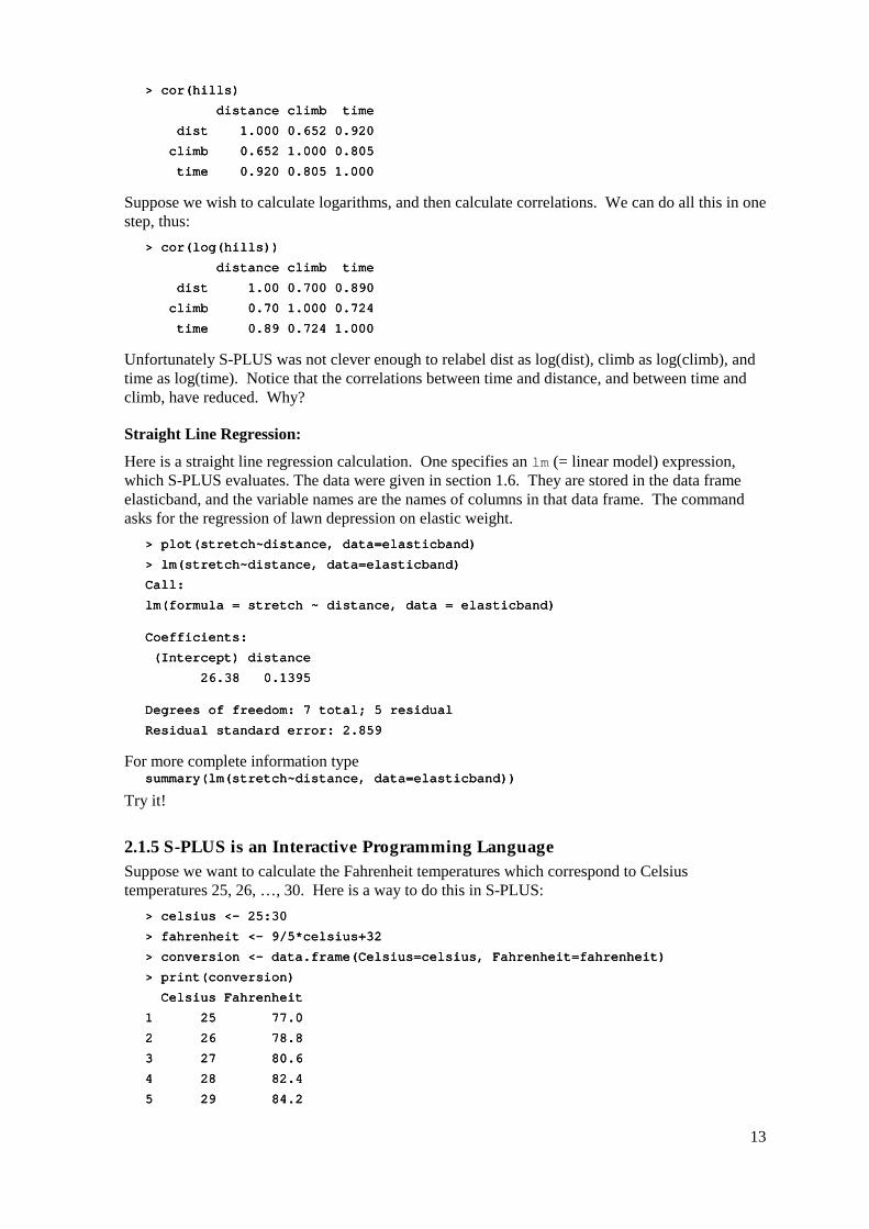
2.1.4 S-PLUS will handle a variety of specific analyses The examples that will be given are correlation and regression.

Correlation: > options(digits=3)> options(digits=3)> options(digits=3)> options(digits=3)

13

> cor(hills)> cor(hills)> cor(hills)> cor(hills)

distance climb time distance climb time distance climb time distance climb time

dist 1.000 0.652 0.920 dist 1.000 0.652 0.920 dist 1.000 0.652 0.920 dist 1.000 0.652 0.920

climb 0.652 1.000 0.805 climb 0.652 1.000 0.805 climb 0.652 1.000 0.805 climb 0.652 1.000 0.805

time 0.920 0 time 0.920 0 time 0.920 0 time 0.920 0.805 1.000.805 1.000.805 1.000.805 1.000

Suppose we wish to calculate logarithms, and then calculate correlations. We can do all this in one step, thus:

> cor(log(hills))> cor(log(hills))> cor(log(hills))> cor(log(hills))

distance climb time distance climb time distance climb time distance climb time

dist 1.00 0.700 0.890 dist 1.00 0.700 0.890 dist 1.00 0.700 0.890 dist 1.00 0.700 0.890

climb 0.70 1.000 0.724 climb 0.70 1.000 0.724 climb 0.70 1.000 0.724 climb 0.70 1.000 0.724

time 0.89 0.724 time 0.89 0.724 time 0.89 0.724 time 0.89 0.724 1.000 1.000 1.000 1.000

Unfortunately S-PLUS was not clever enough to relabel dist as log(dist), climb as log(climb), and time as log(time). Notice that the correlations between time and distance, and between time and climb, have reduced. Why?

Straight Line Regression:

Here is a straight line regression calculation. One specifies an lm (= linear model) expression, which S-PLUS evaluates. The data were given in section 1.6. They are stored in the data frame elasticband, and the variable names are the names of columns in that data frame. The command asks for the regression of lawn depression on elastic weight.

> plot(stretch~distance, data=elasticband)> plot(stretch~distance, data=elasticband)> plot(stretch~distance, data=elasticband)> plot(stretch~distance, data=elasticband)

> lm(stretch~distance, data=elasticband)> lm(stretch~distance, data=elasticband)> lm(stretch~distance, data=elasticband)> lm(stretch~distance, data=elasticband)

Call:Call:Call:Call:

lm(formula = stretch ~ distance, data = elasticband)lm(formula = stretch ~ distance, data = elasticband)lm(formula = stretch ~ distance, data = elasticband)lm(formula = stretch ~ distance, data = elasticband)

Coefficients:Coefficients:Coefficients:Coefficients:

(I (I (I (Intercept) distance ntercept) distance ntercept) distance ntercept) distance

26.38 0.1395 26.38 0.1395 26.38 0.1395 26.38 0.1395

Degrees of freedom: 7 total; 5 residualDegrees of freedom: 7 total; 5 residualDegrees of freedom: 7 total; 5 residualDegrees of freedom: 7 total; 5 residual

Residual standard error: 2.859Residual standard error: 2.859Residual standard error: 2.859Residual standard error: 2.859

For more complete information type summary(lm(stretch~distance, data=elasticband))summary(lm(stretch~distance, data=elasticband))summary(lm(stretch~distance, data=elasticband))summary(lm(stretch~distance, data=elasticband))

Try it!

2.1.5 S-PLUS is an Interactive Programming Language Suppose we want to calculate the Fahrenheit temperatures which correspond to Celsius temperatures 25, 26, …, 30. Here is a way to do this in S-PLUS:

> celsius <> celsius <> celsius <> celsius <---- 25:30 25:30 25:30 25:30

> fahrenheit <> fahrenheit <> fahrenheit <> fahrenheit <---- 9/5*celsius+32 9/5*celsius+32 9/5*celsius+32 9/5*celsius+32

> conversion <> conversion <> conversion <> conversion <---- data.frame(Celsius=celsius, Fahrenheit=f data.frame(Celsius=celsius, Fahrenheit=f data.frame(Celsius=celsius, Fahrenheit=f data.frame(Celsius=celsius, Fahrenheit=fahrenheit)ahrenheit)ahrenheit)ahrenheit)

> print(conversion)> print(conversion)> print(conversion)> print(conversion)

Celsius Fahrenheit Celsius Fahrenheit Celsius Fahrenheit Celsius Fahrenheit

1 25 77.01 25 77.01 25 77.01 25 77.0

2 26 78.82 26 78.82 26 78.82 26 78.8

3 27 80.63 27 80.63 27 80.63 27 80.6

4 28 82.44 28 82.44 28 82.44 28 82.4

5 29 84.25 29 84.25 29 84.25 29 84.2

14

6 30 86.06 30 86.06 30 86.06 30 86.0

We could also have used a loop. In general it is preferable to avoid loops whenever, as here, there is a good alternative. Loops may involve severe computational overheads.

2.2 The Look and Feel of S S-PLUS is a function language. There is a language core that uses standard forms of algebraic notation, allowing the calculations described in Section 2.1.1. Beyond this, most computation is handled using functions. Even the action of quitting from an S session uses, as we noted earlier, the function call q().

In most expressions you can treat every object – vectors, arrays, lists and so on – as a whole. Use of operators and functions that operate on objects as a whole largely avoids the need for explicit loops. For an example, look back to section 2.1.5 above.

The structure of an S-PLUS program looks very like the structure of the widely used general purpose language C and its successors C++ and Java3.

2.3 S-PLUS Objects All S-PLUS entities, including functions and data structures, exist as objects. They can all be operated on as data. Type in ls() to get a vector of text strings giving the names of all objects in your working directory. An alternative to ls() is objects(). In both cases you can restrict the names to those with a particular pattern, e. g. starting with the letter `p’. However different parameter settings are required depending on whether you use ls() or objects().

In S-PLUS 4.0 or later the object browser allows you to filter out what you list, i.e. you can restrict the list to data frames, or to matrices, or to vectors.

Typing the name of an object causes the contents of the object to be printed. Try typing in q, mean, etc.

Important: Objects that are created stay in place until removed. It pays to remove objects that will be no longer required at the end of each session, while the details are fresh in the mind. Care is needed to avoid removing anything that may be required later.

*42.4 Looping In S-PLUS there is often a better alternative to writing an explicit loop. Where possible, you should use one of the built-in functions to avoid explicit looping. A simple example of a for loop is5

for (i in 1:10) print(i)for (i in 1:10) print(i)for (i in 1:10) print(i)for (i in 1:10) print(i)

Here is another example of a for loop, to do in a complicated way what we did very simply in section 2.1.5:

> # Fahrenheit to Celsius> # Fahrenheit to Celsius> # Fahrenheit to Celsius> # Fahrenheit to Celsius

3 Note however that S-PLUS has no header files, most declarations are implicit, there are no pointers, and vectors of text strings can be defined and manipulated directly. The implementation of S-PLUS relies heavily on list processing ideas from the LISP language. Lists are a key part of S-PLUS syntax. 4 Asterisks (*) identify sections which are more technical and might be omitted at a first reading. 5 Other looping constructs are:

repeat <expression> ## You’ll need break somewhere insiderepeat <expression> ## You’ll need break somewhere insiderepeat <expression> ## You’ll need break somewhere insiderepeat <expression> ## You’ll need break somewhere inside

while (x>0) <expressionwhile (x>0) <expressionwhile (x>0) <expressionwhile (x>0) <expression>>>>

Here <expression><expression><expression><expression> is an S-PLUS statement, or a sequence of statements that are enclosed within braces.

15

> for (fahrenheit in 25:30)prin> for (fahrenheit in 25:30)prin> for (fahrenheit in 25:30)prin> for (fahrenheit in 25:30)print(c(fahrenheit, 9/5*fahrenheit + 32))t(c(fahrenheit, 9/5*fahrenheit + 32))t(c(fahrenheit, 9/5*fahrenheit + 32))t(c(fahrenheit, 9/5*fahrenheit + 32))

[1] 25 77[1] 25 77[1] 25 77[1] 25 77

[1] 26.0 78.8[1] 26.0 78.8[1] 26.0 78.8[1] 26.0 78.8

[1] 27.0 80.6[1] 27.0 80.6[1] 27.0 80.6[1] 27.0 80.6

[1] 28.0 82.4[1] 28.0 82.4[1] 28.0 82.4[1] 28.0 82.4

[1] 29.0 84.2[1] 29.0 84.2[1] 29.0 84.2[1] 29.0 84.2

[1] 30 86[1] 30 86[1] 30 86[1] 30 86

2.4.1 More on looping Here is a long-winded way to sum the three numbers 3, 5 and 9.

> answer <> answer <> answer <> answer <---- 0 0 0 0

> for (j in c(31,51,91){answer <> for (j in c(31,51,91){answer <> for (j in c(31,51,91){answer <> for (j in c(31,51,91){answer <---- j+answer} j+answer} j+answer} j+answer}

> answer> answer> answer> answer

[1] 173[1] 173[1] 173[1] 173

The calculation iteratively builds up the object answer, using the successive values of j listed in the vector (31,51,91). i.e. Initially, j=31, and answer is assigned the value 31 + 0 = 31. Then j=51, and answer is assigned the value 51 + 31 = 82. Finally, j=91, and answer is assigned the value 91 + 81 = 173. Then the procedure ends, and the contents of answer can be examined by typing in answer and pressing the Enter key.

There is a much easier way to do this calculation: > sum(c(31> sum(c(31> sum(c(31> sum(c(31,51,91)),51,91)),51,91)),51,91))

[1] 173[1] 173[1] 173[1] 173

Skilled S-PLUS users have limited recourse to loops. There are often, as in the example above, better alternatives.

2.5 S-PLUS Functions We give two simple examples of S-PLUS functions.

2.5.1 An Approximate Miles to Kilometers Conversion > miles.to.km <> miles.to.km <> miles.to.km <> miles.to.km <---- function(miles)miles*8/5 function(miles)miles*8/5 function(miles)miles*8/5 function(miles)miles*8/5

The return value is the value of the final (and in this instance only) expression which appears in the function body6.

Use the function thus > miles.to.km(175) # Approximate distance to Sydney,> miles.to.km(175) # Approximate distance to Sydney,> miles.to.km(175) # Approximate distance to Sydney,> miles.to.km(175) # Approximate distance to Sydney, in miles in miles in miles in miles

[1] 280[1] 280[1] 280[1] 280

You can do the conversion for several distances, all at the one time. To convert a vector of the three distances 100, 200 and 300 miles to distances in kilometers, specify:

> miles.to.km(c(100,200,300))> miles.to.km(c(100,200,300))> miles.to.km(c(100,200,300))> miles.to.km(c(100,200,300))

[1] 160 320 480[1] 160 320 480[1] 160 320 480[1] 160 320 480

2.5.2 A Plotting function The data set florida has the votes in the 2000 election for the various Presidential candidates, county by county in the state of Florida. The following plots the vote for Buchanan against the vote for Bush.

6 Alternatively a return value may be given using an explicit return() statement. This is however an uncommon construction.

16

attach(florida)attach(florida)attach(florida)attach(florida)

plot(BUSH, BUCHANAN, xlplot(BUSH, BUCHANAN, xlplot(BUSH, BUCHANAN, xlplot(BUSH, BUCHANAN, xlab=”Bush”, ylab=”Buchanan”)ab=”Bush”, ylab=”Buchanan”)ab=”Bush”, ylab=”Buchanan”)ab=”Bush”, ylab=”Buchanan”)

detach(“florida”)detach(“florida”)detach(“florida”)detach(“florida”)

Here is a function that makes it possible to plot the figures for any pair of candidates. plot.florida <plot.florida <plot.florida <plot.florida <---- function(xvar=”BUSH”, yvar=”BUCHANAN”){ function(xvar=”BUSH”, yvar=”BUCHANAN”){ function(xvar=”BUSH”, yvar=”BUCHANAN”){ function(xvar=”BUSH”, yvar=”BUCHANAN”){

x <x <x <x <---- florida[,xvar] florida[,xvar] florida[,xvar] florida[,xvar]

y<y<y<y<---- florida[,yvar] florida[,yvar] florida[,yvar] florida[,yvar]

plot(x, y, xlab=xvar,ylabplot(x, y, xlab=xvar,ylabplot(x, y, xlab=xvar,ylabplot(x, y, xlab=xvar,ylab=yvar)=yvar)=yvar)=yvar)

mtext(side=3, line=1, mtext(side=3, line=1, mtext(side=3, line=1, mtext(side=3, line=1,

“Votes in Florida, by county, in the 2000 US Presidential election”) “Votes in Florida, by county, in the 2000 US Presidential election”) “Votes in Florida, by county, in the 2000 US Presidential election”) “Votes in Florida, by county, in the 2000 US Presidential election”)

}}}}

Note that the function body is enclosed in braces ({ }).

Now try plot.florida()plot.florida()plot.florida()plot.florida()

plot.florida(yvar=”NADER”) # yvar=”NADER” overplot.florida(yvar=”NADER”) # yvar=”NADER” overplot.florida(yvar=”NADER”) # yvar=”NADER” overplot.florida(yvar=”NADER”) # yvar=”NADER” over----rides the defaultrides the defaultrides the defaultrides the default

plot.fplot.fplot.fplot.florida(xvar=”GORE”, yvar=”NADER”)lorida(xvar=”GORE”, yvar=”NADER”)lorida(xvar=”GORE”, yvar=”NADER”)lorida(xvar=”GORE”, yvar=”NADER”)

Fig. 8 shows the graph produced by plot.florida()

BUSH

BUC

HAN

AN

0 50000 100000 200000 300000

010

0020

0030

00

Votes in Florida, by county, in the 2000 US Presidential election

Figure 8: Votes in Florida, by county, in the election night returns in the 2000 US Presidential election.

2.6 Vectors Examples of vectors are

c(2,3,5,2,7,1)c(2,3,5,2,7,1)c(2,3,5,2,7,1)c(2,3,5,2,7,1)

3:10 # The numbers 3, 4, .., 103:10 # The numbers 3, 4, .., 103:10 # The numbers 3, 4, .., 103:10 # The numbers 3, 4, .., 10

c(T,F,F,F,T,T,F)c(T,F,F,F,T,T,F)c(T,F,F,F,T,T,F)c(T,F,F,F,T,T,F)

c(”Canberra”,”Sydney”,”Newcastle”,”Darwin”)c(”Canberra”,”Sydney”,”Newcastle”,”Darwin”)c(”Canberra”,”Sydney”,”Newcastle”,”Darwin”)c(”Canberra”,”Sydney”,”Newcastle”,”Darwin”)

17

Vectors may have mode logical, numeric or character7. The first two vectors above are numeric, the third is logical (i.e. a vector with elements of mode logical), and the fourth is a string vector (i.e. a vector with elements of mode character).

The missing value symbol, which is NA, can be included as an element of a vector.

2.6.1 Joining (concatenating) vectors The c in c(2, 3, 5, 7, 1) above was an acronym for “concatenate”, i.e. the meaning is: “Join these numbers together in to a vector. Existing vectors may be included among the elements that are to be concatenated. In the following we form vectors x and y, which we then concatenate to form a vector z:

> x <> x <> x <> x <---- c(2,3,5,2,7,1) c(2,3,5,2,7,1) c(2,3,5,2,7,1) c(2,3,5,2,7,1)

> x> x> x> x

[1] 2 3 5 2 7 1[1] 2 3 5 2 7 1[1] 2 3 5 2 7 1[1] 2 3 5 2 7 1

> y <> y <> y <> y <---- c(10,15,12) c(10,15,12) c(10,15,12) c(10,15,12)

> y> y> y> y

[1] 10 15 12[1] 10 15 12[1] 10 15 12[1] 10 15 12

> z <> z <> z <> z <---- c(x, y) c(x, y) c(x, y) c(x, y)

> z> z> z> z

[1] 2 3 5 2 7 1 10 15 12[1] 2 3 5 2 7 1 10 15 12[1] 2 3 5 2 7 1 10 15 12[1] 2 3 5 2 7 1 10 15 12

>>>>

We will later meet lists. The concatenate function c() may also be used to join lists.

2.6.2 Subsets of Vectors There are two common ways to extract subsets of vectors8.

1. Specify the numbers of the elements which are to be extracted, e.g. > x <> x <> x <> x <---- c(3,11,8,15,12) c(3,11,8,15,12) c(3,11,8,15,12) c(3,11,8,15,12) # Assign to x the values 3, 11, 8, 15, 12 # Assign to x the values 3, 11, 8, 15, 12 # Assign to x the values 3, 11, 8, 15, 12 # Assign to x the values 3, 11, 8, 15, 12

> x[c(2,4)] # Extract elements (rows) 2 and 4> x[c(2,4)] # Extract elements (rows) 2 and 4> x[c(2,4)] # Extract elements (rows) 2 and 4> x[c(2,4)] # Extract elements (rows) 2 and 4

[1] 11 15[1] 11 15[1] 11 15[1] 11 15

One can use negative numbers to omit elements: > x <> x <> x <> x <---- c(3,11,8,15,12) c(3,11,8,15,12) c(3,11,8,15,12) c(3,11,8,15,12)

> x[> x[> x[> x[----c(2,3)]c(2,3)]c(2,3)]c(2,3)]

[1] 3 15 12[1] 3 15 12[1] 3 15 12[1] 3 15 12

2. Specify a vector of logical values. The elements that are extracted are those for which the logical value is T. (Beware of NAs, as noted below.) Thus suppose we want to extract values of x which are greater than 10.

> x <> x <> x <> x <---- c(3,11,8,15,12) c(3,11,8,15,12) c(3,11,8,15,12) c(3,11,8,15,12)

7 Below, we will meet the notion of “class”, which is important for some of the more sophisticated language features of S-PLUS. The logical, numeric and character vectors just given have class NULL, i.e. they have no class. There are special types of numeric vector which do have a class attribute. Factors are the most important example. Although often used as a compact way to store character strings, factors are, technically, numeric vectors. The class attribute of a factor has, not surprisingly, the value “factor”. 8 A third more subtle method is available when vectors have named elements. One can then use a vector of names to extract the elements, thus:

> c(Andreas=178, John=185, Jeff=183)[c("John","Jeff")]> c(Andreas=178, John=185, Jeff=183)[c("John","Jeff")]> c(Andreas=178, John=185, Jeff=183)[c("John","Jeff")]> c(Andreas=178, John=185, Jeff=183)[c("John","Jeff")]

John Jeff John Jeff John Jeff John Jeff

185 183 185 183 185 183 185 183

18

> x>10 # This generates a vector of logical (T or F)> x>10 # This generates a vector of logical (T or F)> x>10 # This generates a vector of logical (T or F)> x>10 # This generates a vector of logical (T or F)

[1] F T F T T[1] F T F T T[1] F T F T T[1] F T F T T

>>>> x[x>10] x[x>10] x[x>10] x[x>10]

[1] 11 15 12[1] 11 15 12[1] 11 15 12[1] 11 15 12

Arithmetic relations that may be used in the extraction of subsets of vectors are <, <=, >, >=, ==, and !=. The first four compare magnitudes, == tests for equality, and != tests for inequality.

2.6.3 The Use of NA in Vector Subscripts Note that any arithmetic operation or relation that involves NA generates an NA.

Suppose that one has y <y <y <y <---- c(1, NA, 3, 0, NA) c(1, NA, 3, 0, NA) c(1, NA, 3, 0, NA) c(1, NA, 3, 0, NA)

Be warned that y[y==NA] <- 0 leaves y unchanged. The reason is that all elements of y==NA evaluate to NA. Also y[NA] evaluates to NA. Where an element on the left of an expression evaluates to NA, no assignment is made9.

To replace all NAs by 0, use y[is.na(y)] <y[is.na(y)] <y[is.na(y)] <y[is.na(y)] <---- 0 0 0 0

2.6.3 Factors A factor is a special type of vector, stored internally as a numeric vector with values 1, 2, 3, m. The value m is the number of levels.

Consider a survey that has data on 691 females and 692 males. If the first 691 are females and the next 692 males, we can create a vector of strings that that holds the values thus:

gender <gender <gender <gender <---- c(rep(“female”, c(rep(“female”, c(rep(“female”, c(rep(“female”,691), rep(“male”,692))691), rep(“male”,692))691), rep(“male”,692))691), rep(“male”,692))

(The usage is that rep(“female”, 691) creates 691 copies of the character string “female”, and similarly for the creation of 692 copies of “male”.)

We can change the vector to a factor, by entering: gender <gender <gender <gender <---- factor(gender) factor(gender) factor(gender) factor(gender)

Internally the factor gender is stored as 691 1’s, followed by 692 2’s. It has stored with it a table that looks like this:

1 female 2 male

One benefit is that once stored as a factor, the space required for storage is reduced.

In most (but not all) contexts that seem to demand a character string, the 1 is translated into “female” and the 2 into “male”. The values “female” and “male” are the levels of the factor. By default, the levels are chosen to be in alphanumeric order, so that “female” precedes “male”. Hence:

> levels(gender) # Assumes gender is a factor, created as above> levels(gender) # Assumes gender is a factor, created as above> levels(gender) # Assumes gender is a factor, created as above> levels(gender) # Assumes gender is a factor, created as above

[1] "female" "male" [1] "female" "male" [1] "female" "male" [1] "female" "male"

9 Where there are vectors on both sides of the equation (e.g. x <- 1:5; x[y>10] <- y[y>10]), this may have the effect of making the vector of places on the left that are available for assignment shorter than the vector of values that is to be assigned. The result may be nonsense.

19

The order of the levels in a factor determines the order in which the levels appear in graphs that use this information, and in tables. To cause “male” to come before “female”, use

gender <gender <gender <gender <---- factor(gender, levels=c(“male”, “female”)) factor(gender, levels=c(“male”, “female”)) factor(gender, levels=c(“male”, “female”)) factor(gender, levels=c(“male”, “female”))

levels(gender) # Check the order of the levelslevels(gender) # Check the order of the levelslevels(gender) # Check the order of the levelslevels(gender) # Check the order of the levels

This syntax is available both when the factor is first created, or later when one wishes to change the order in an existing factor. Incorrect spelling of the level names will generate an error message. Try

gender <gender <gender <gender <---- factor(c(rep(“female”,691), rep(“male”,692))) factor(c(rep(“female”,691), rep(“male”,692))) factor(c(rep(“female”,691), rep(“male”,692))) factor(c(rep(“female”,691), rep(“male”,692)))

table(gender)table(gender)table(gender)table(gender)

gender <gender <gender <gender <---- factor(gender, levels=c(“male”, “female”)) factor(gender, levels=c(“male”, “female”)) factor(gender, levels=c(“male”, “female”)) factor(gender, levels=c(“male”, “female”))

table(gender)table(gender)table(gender)table(gender)

gender <gender <gender <gender <---- factor(gender, levels=c(“Male”, “femal factor(gender, levels=c(“Male”, “femal factor(gender, levels=c(“Male”, “femal factor(gender, levels=c(“Male”, “female”)) # Generates an errore”)) # Generates an errore”)) # Generates an errore”)) # Generates an error

rm(gender) # Remove gender.rm(gender) # Remove gender.rm(gender) # Remove gender.rm(gender) # Remove gender.

2.7 Data Frames Data frames are fundamental to the use of the newer style S-PLUS modelling and graphics functions. A data frame is a generalisation of a matrix, in which different columns may have different modes. All elements of any column must however have the same mode, i.e. all numeric or all factor, or all character.

Among the data sets that are supplied to accompany these notes is one called vehicle.summary. Here is what one sees when it is printed out:

> vehicle.summary> vehicle.summary> vehicle.summary> vehicle.summary

abbrev Type Average.Price abbrev Type Average.Price abbrev Type Average.Price abbrev Type Average.Price

Small Sm Small 7737 Small Sm Small 7737 Small Sm Small 7737 Small Sm Small 7737

Medium Md Medium 21623 Medium Md Medium 21623 Medium Md Medium 21623 Medium Md Medium 21623

Compact Cm Compact 15202Compact Cm Compact 15202Compact Cm Compact 15202Compact Cm Compact 15202

Large Lr Large 21500Large Lr Large 21500Large Lr Large 21500Large Lr Large 21500

NK NK NK NK ---- NA NA NA NA

Van Vn Van 14014 Van Vn Van 14014 Van Vn Van 14014 Van Vn Van 14014

Sporty Sp Sporty 15308 Sporty Sp Sporty 15308 Sporty Sp Sporty 15308 Sporty Sp Sporty 15308

The rows of the data frame have names Small, Medium, . . . To print out the row names, type in row.names(vehicle.summary)row.names(vehicle.summary)row.names(vehicle.summary)row.names(vehicle.summary)

The column names are abbrev, Type, and Average.Price. To print out the column names, type in

names(vehicle.summary)names(vehicle.summary)names(vehicle.summary)names(vehicle.summary)

The first two columns are of mode character, and the third of mode numeric. Columns can be vectors of any mode. They can be factors. Note the missing value for Average.Price in the fifth row.

Any of the following10 will pick out the second column of the data frame type.df, then storing it in the vector type.

type <type <type <type <---- vehicle.summary$Type vehicle.summary$Type vehicle.summary$Type vehicle.summary$Type

type <type <type <type <---- vehicle.summary[,2] vehicle.summary[,2] vehicle.summary[,2] vehicle.summary[,2]

type <type <type <type <---- vehicle.summary[,”Type”] vehicle.summary[,”Type”] vehicle.summary[,”Type”] vehicle.summary[,”Type”]

type <type <type <type <---- vehicle.summary[[2]] vehicle.summary[[2]] vehicle.summary[[2]] vehicle.summary[[2]] # Tak# Tak# Tak# Take the object that is storede the object that is storede the object that is storede the object that is stored

# in the second list element. # in the second list element. # in the second list element. # in the second list element.

10 Also legal is vehicle.summary[2]. This gives a data frame with the single column Type.

20

2.7.1 Inclusion of character string vectors in data frames When data are imported using the Import Data dialogue, or when the data.frame() function is used to create data frames, vectors of character strings are by default turned into factors. Often this is convenient. If not, there is a setting on the options menu of the Import Data dialogue that will prevent this behaviour. The as.is=T parameter setting will prevent this behaviour when data.frame() is used to include one or more columns of factors in a data frame.

2.7.2 Built-in data sets We will often use one of S-PLUS’s built-in data sets, all stored as data frames. One such data frame is environmental11111111, giving measurements made on 111 successive days in New York. Here is summary information on this data frame

> summary(environmental)> summary(environmental)> summary(environmental)> summary(environmental)

ozone radiation temperature wind ozone radiation temperature wind ozone radiation temperature wind ozone radiation temperature wind

Min.: 1.0 Min.: 7 Min.:57.0 Min.: 2.30 Min.: 1.0 Min.: 7 Min.:57.0 Min.: 2.30 Min.: 1.0 Min.: 7 Min.:57.0 Min.: 2.30 Min.: 1.0 Min.: 7 Min.:57.0 Min.: 2.30

1st Qu. 1st Qu. 1st Qu. 1st Qu.: 18.0 1st Qu.:114 1st Qu.:71.0 1st Qu.: 7.40 : 18.0 1st Qu.:114 1st Qu.:71.0 1st Qu.: 7.40 : 18.0 1st Qu.:114 1st Qu.:71.0 1st Qu.: 7.40 : 18.0 1st Qu.:114 1st Qu.:71.0 1st Qu.: 7.40

Median: 31.0 Median:207 Median:79.0 Median: 9.70 Median: 31.0 Median:207 Median:79.0 Median: 9.70 Median: 31.0 Median:207 Median:79.0 Median: 9.70 Median: 31.0 Median:207 Median:79.0 Median: 9.70

Mean: 42.1 Mean:185 Mean:77.8 Mean: 9.94 Mean: 42.1 Mean:185 Mean:77.8 Mean: 9.94 Mean: 42.1 Mean:185 Mean:77.8 Mean: 9.94 Mean: 42.1 Mean:185 Mean:77.8 Mean: 9.94

3rd Qu.: 62.0 3rd Qu.:256 3rd Qu.:84.5 3rd Qu.:11.50 3rd Qu.: 62.0 3rd Qu.:256 3rd Qu.:84.5 3rd Qu.:11.50 3rd Qu.: 62.0 3rd Qu.:256 3rd Qu.:84.5 3rd Qu.:11.50 3rd Qu.: 62.0 3rd Qu.:256 3rd Qu.:84.5 3rd Qu.:11.50

Max.:168.0 Max.:168.0 Max.:168.0 Max.:168.0 Max.:334 Max.:97.0 Max.:20.70 Max.:334 Max.:97.0 Max.:20.70 Max.:334 Max.:97.0 Max.:20.70 Max.:334 Max.:97.0 Max.:20.70

See section 14.1 for a list of the built-in data sets to which we will refer in this course.

2.8 Common Useful Functions print() print() print() print() # Prints a single S# Prints a single S# Prints a single S# Prints a single S----PLUS objectPLUS objectPLUS objectPLUS object

cat() cat() cat() cat() # Prints multiple objects, one afte# Prints multiple objects, one afte# Prints multiple objects, one afte# Prints multiple objects, one after the otherr the otherr the otherr the other

length() length() length() length() # Number of elements in a vector or a list# Number of elements in a vector or a list# Number of elements in a vector or a list# Number of elements in a vector or a list

mean()mean()mean()mean()

median()median()median()median()

range()range()range()range()

unique() unique() unique() unique() # Vector of distinct values# Vector of distinct values# Vector of distinct values# Vector of distinct values

diff() diff() diff() diff() # Vector of first differences# Vector of first differences# Vector of first differences# Vector of first differences

# N. B. diff(x) has one less element than x# N. B. diff(x) has one less element than x# N. B. diff(x) has one less element than x# N. B. diff(x) has one less element than x

sort() sort() sort() sort() # Sort elements into o# Sort elements into o# Sort elements into o# Sort elements into order.rder.rder.rder.

order()order()order()order() # x[order(x)] orders elements of x, with NAs last# x[order(x)] orders elements of x, with NAs last# x[order(x)] orders elements of x, with NAs last# x[order(x)] orders elements of x, with NAs last

cumsum()cumsum()cumsum()cumsum()

cumprod()cumprod()cumprod()cumprod()

rev() rev() rev() rev() # reverse the order of vector elements# reverse the order of vector elements# reverse the order of vector elements# reverse the order of vector elements

The functions mean(), median(), range(), and a number of other functions, take the argument na.rm=T; i.e. remove NAs, then proceed with the calculation.

By default, sort() omits any NAs. The function order() places NAs last. Hence: > x <> x <> x <> x <---- c(1, 20, 2, NA, 22) c(1, 20, 2, NA, 22) c(1, 20, 2, NA, 22) c(1, 20, 2, NA, 22)

> order(x)> order(x)> order(x)> order(x)

[1] 1 3 2 5 4[1] 1 3 2 5 4[1] 1 3 2 5 4[1] 1 3 2 5 4

> x[order(x)]> x[order(x)]> x[order(x)]> x[order(x)]

[1] 1 2 20 22 NA[1] 1 2 20 22 NA[1] 1 2 20 22 NA[1] 1 2 20 22 NA

> sort(x)> sort(x)> sort(x)> sort(x)

[1] 1 2 20 22[1] 1 2 20 22[1] 1 2 20 22[1] 1 2 20 22

11 The data set air is identical, except that ozone has been replaced by the cube root of ozone level.

21

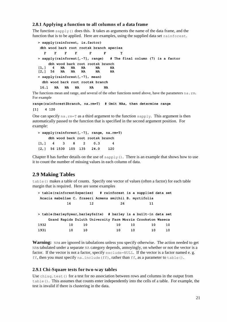
2.8.1 Applying a function to all columns of a data frame The function sapply() does this. It takes as arguments the name of the data frame, and the function that is to be applied. Here are examples, using the supplied data set rainforest.

> sapply(rainforest, is.factor)> sapply(rainforest, is.factor)> sapply(rainforest, is.factor)> sapply(rainforest, is.factor)

dbh wood bark r dbh wood bark r dbh wood bark r dbh wood bark root rootsk branch species oot rootsk branch species oot rootsk branch species oot rootsk branch species

F F F F F F T F F F F F F T F F F F F F T F F F F F F T

> sapply(rainforest[,> sapply(rainforest[,> sapply(rainforest[,> sapply(rainforest[,----7], range) # The final column (7) is a factor7], range) # The final column (7) is a factor7], range) # The final column (7) is a factor7], range) # The final column (7) is a factor

dbh wood bark root rootsk branch dbh wood bark root rootsk branch dbh wood bark root rootsk branch dbh wood bark root rootsk branch [1,] 4 NA NA NA NA NA[1,] 4 NA NA NA NA NA[1,] 4 NA NA NA NA NA[1,] 4 NA NA NA NA NA [2,] 56 NA NA NA NA NA[2,] 56 NA NA NA NA NA[2,] 56 NA NA NA NA NA[2,] 56 NA NA NA NA NA

> > > > sapply(rainforest[,sapply(rainforest[,sapply(rainforest[,sapply(rainforest[,----7], mean)7], mean)7], mean)7], mean)

dbh wood bark root rootsk branch dbh wood bark root rootsk branch dbh wood bark root rootsk branch dbh wood bark root rootsk branch

16.1 NA NA NA NA NA 16.1 NA NA NA NA NA 16.1 NA NA NA NA NA 16.1 NA NA NA NA NA

The functions mean and range, and several of the other functions noted above, have the parameters na.rm. For example range(rainforest$branch, na.rm=T) # range(rainforest$branch, na.rm=T) # range(rainforest$branch, na.rm=T) # range(rainforest$branch, na.rm=T) # Omit NAs, then determine rangeOmit NAs, then determine rangeOmit NAs, then determine rangeOmit NAs, then determine range

[1] 4 120[1] 4 120[1] 4 120[1] 4 120

One can specify na.rm=T as a third argument to the function sapply. This argument is then automatically passed to the function that is specified in the second argument position. For example:

> sapply(rainforest[> sapply(rainforest[> sapply(rainforest[> sapply(rainforest[,,,,----7], range, na.rm=T)7], range, na.rm=T)7], range, na.rm=T)7], range, na.rm=T)

dbh wood bark root rootsk branch dbh wood bark root rootsk branch dbh wood bark root rootsk branch dbh wood bark root rootsk branch

[1,] 4 3 8 2 0.3 4[1,] 4 3 8 2 0.3 4[1,] 4 3 8 2 0.3 4[1,] 4 3 8 2 0.3 4

[2,] 56 1530 105 135 24.0 120[2,] 56 1530 105 135 24.0 120[2,] 56 1530 105 135 24.0 120[2,] 56 1530 105 135 24.0 120

Chapter 8 has further details on the use of sapply(). There is an example that shows how to use it to count the number of missing values in each column of data.

2.9 Making Tables table() makes a table of counts. Specify one vector of values (often a factor) for each table margin that is required. Here are some examples

> table(rainforest$species) # rainf> table(rainforest$species) # rainf> table(rainforest$species) # rainf> table(rainforest$species) # rainforest is a supplied data setorest is a supplied data setorest is a supplied data setorest is a supplied data set

Acacia mabellae C. fraseri Acmena smithii B. myrtifolia Acacia mabellae C. fraseri Acmena smithii B. myrtifolia Acacia mabellae C. fraseri Acmena smithii B. myrtifolia Acacia mabellae C. fraseri Acmena smithii B. myrtifolia

16 12 26 11 16 12 26 11 16 12 26 11 16 12 26 11

> table(barley$year,barley$site) # barley is a built> table(barley$year,barley$site) # barley is a built> table(barley$year,barley$site) # barley is a built> table(barley$year,barley$site) # barley is a built----in data setin data setin data setin data set

Grand Rapids Duluth University Farm Morr Grand Rapids Duluth University Farm Morr Grand Rapids Duluth University Farm Morr Grand Rapids Duluth University Farm Morris Crookston Waseca is Crookston Waseca is Crookston Waseca is Crookston Waseca

1932 10 10 10 10 10 101932 10 10 10 10 10 101932 10 10 10 10 10 101932 10 10 10 10 10 10

1931 10 10 10 10 10 101931 10 10 10 10 10 101931 10 10 10 10 10 101931 10 10 10 10 10 10

Warning: NAs are ignored in tabulations unless you specify otherwise. The action needed to get NAs tabulated under a separate NA category depends, annoyingly, on whether or not the vector is a factor. If the vector is not a factor, specify exclude=NULL. If the vector is a factor named e. g. ff, then you must specify na.include(ff), rather than ff, as a parameter to table().

2.9.1 Chi-Square tests for two-way tables Use chisq.test() for a test for no association between rows and columns in the output from table(). This assumes that counts enter independently into the cells of a table. For example, the test is invalid if there is clustering in the data.

22

2.9.2 Number of NAs, broken down by subgroups of the data The following shows how to get information on the number of NAs in subgroups of the data:

> table(rainforest$species, !is.na(rainforest$branch))> table(rainforest$species, !is.na(rainforest$branch))> table(rainforest$species, !is.na(rainforest$branch))> table(rainforest$species, !is.na(rainforest$branch))

FALSE TRUE FALSE TRUE FALSE TRUE FALSE TRUE

Acacia mabellae 6 10Acacia mabellae 6 10Acacia mabellae 6 10Acacia mabellae 6 10

C. fraseri 0 12 C. fraseri 0 12 C. fraseri 0 12 C. fraseri 0 12

Acmena smithii 15 11 Acmena smithii 15 11 Acmena smithii 15 11 Acmena smithii 15 11

B. myrtifolia 1 10 B. myrtifolia 1 10 B. myrtifolia 1 10 B. myrtifolia 1 10

Thus for Acacia mabellae there are 6 NAs for the variable branch (i.e. number of branches over 2cm in diameter), out of a total of 16 data values.

2.10 The Use of attach() Users have, by default, access both to objects in their own working directory and to objects in a variety of system directories. There is a search list (type search() to see this list) that controls where S-PLUS looks first. The attach function extends this list.

Users can extend the search list in two ways. S-PLUS data frames can be added to the search list. Alternatively, or in addition, one can add new directories. Adding data frames to the search list is a convenience, so that explicit reference to the data frame from which vectors are taken is not necessary. The addition of new directories is needed so that the users will have access to objects in those directories.

The command library() gives access to libraries, which must be already installed, that are not otherwise available. Details of the attaching and detaching of other (non-library) directories will be given later, in chapter 5.

The S-PLUS documentation speaks of attaching databases, as a way of encompassing all these types of extension.

2.10.1 Attaching Data Frames A data frame is in fact a specialised list, with its columns as the objects. Once a data frame has been added to the search list, the user can refer to the columns by name, without the need to specify the data frame to which they belong. If there is any overlap of names, the order on the search list determines the name that will be taken.

Thus attach(vehicle.summary)attach(vehicle.summary)attach(vehicle.summary)attach(vehicle.summary)

then allows the user to refer to Type and Average.Price, where it would otherwise be necessary to type vehicle.summary$Type and vehicle.summary$Average.Price. This assumes that there are no other variables or columns of attached data frames that have either of these names.

> attach(vehicle.summary)> attach(vehicle.summary)> attach(vehicle.summary)> attach(vehicle.summary)

> Type> Type> Type> Type

Small Me Small Me Small Me Small Medium Compact Large NK Van Sporty dium Compact Large NK Van Sporty dium Compact Large NK Van Sporty dium Compact Large NK Van Sporty

"Small" "Medium" "Compact" "Large" "" "Van" "Sporty" "Small" "Medium" "Compact" "Large" "" "Van" "Sporty" "Small" "Medium" "Compact" "Large" "" "Van" "Sporty" "Small" "Medium" "Compact" "Large" "" "Van" "Sporty"

> Average.Price> Average.Price> Average.Price> Average.Price

Small Medium Compact Large NK Van Sporty Small Medium Compact Large NK Van Sporty Small Medium Compact Large NK Van Sporty Small Medium Compact Large NK Van Sporty

7737 21623 15202 21500 NA 14014 15308 7737 21623 15202 21500 NA 14014 15308 7737 21623 15202 21500 NA 14014 15308 7737 21623 15202 21500 NA 14014 15308

To detach this data frame, type > detach(“vehicle.summa> detach(“vehicle.summa> detach(“vehicle.summa> detach(“vehicle.summary”)ry”)ry”)ry”)

i.e. quotes are now used.

23

Note how the use of quotes changes. Specify the name (without quotes) when attaching, and enclose the name between quotes when detaching.

2.10.2 Libraries Third party libraries that are installed on the user’s system are likely to be attached and appear on the search list only if the user requests them. These are usually attached using the command library(). To attach the Venables and Ripley mass library that is included in the S-PLUS distribution, type in

library(mass)library(mass)library(mass)library(mass)

2.11 More Detailed Information This chapter has given the minimum detail that seems to me necessary for getting started. Look in chapters 7 and 8 for a more detailed coverage of the topics in this chapter. It may pay, at this point, to glance through chapter 7 to see what is there. Remember also to use the S-PLUS help.

Topics from chapter 7, additional to those covered above, that may be important for relatively elementary uses of S-PLUS include:

o The entry of patterned data (7.1.2)

o The handling of missing values in subscripts when vectors are assigned (7.2)

o Unexpected consequences (e.g. conversion of columns of numeric data into factors) from errors in data (7.3.1).

2.12 Exercises 1. For each of the following code sequences, sequences, predict the result. Then use S-PLUS to do the computation:

a) answer <answer <answer <answer <---- 0 0 0 0

for (j in 3:5){ answer <for (j in 3:5){ answer <for (j in 3:5){ answer <for (j in 3:5){ answer <---- j+answer } j+answer } j+answer } j+answer }

b) answer<answer<answer<answer<---- 10 10 10 10

for (j in 3:5){ answer <for (j in 3:5){ answer <for (j in 3:5){ answer <for (j in 3:5){ answer <---- j+answer } j+answer } j+answer } j+answer }

c) answer <answer <answer <answer <---- 10 10 10 10

for (j in 3:5){ answer <for (j in 3:5){ answer <for (j in 3:5){ answer <for (j in 3:5){ answer <---- j*answer } j*answer } j*answer } j*answer }

2. Look up the help for the function prod(), and use prod() to do the calculation in 1(c) above. Alternatively, how would you expect prod() to work? Try it!

3. Add up all the numbers from 1 to 100 in two different ways: using for and using sum.

4. Multiply all the numbers from 1 to 50 in two different ways: using for and using prod.

5. The volume of a sphere of radius r is given by 4πr3/3. For spheres having radii 3, 4, 5, …, 20 find the corresponding volumes and print the results out in a table. Construct a data frame with columns radius and volume.

6. Use sapply() to apply the function is.factor to each column of the built-in data frame market.survey. For each of the columns that are identified as factors, determine the levels. Which columns are ordered factors? [Use is.ordered()].

24

25

3. Plotting The complex of functions plot(), points(), lines(), text(), mtext(), axis() etc. belong to the earlier style of S-PLUS graphics, that preceded trellis graphics.

3.1 plot () and allied functions The following are equivalent:

plot(y ~ x)plot(y ~ x)plot(y ~ x)plot(y ~ x)

plot(x, y)plot(x, y)plot(x, y)plot(x, y)

where x and y must be the same length. This second form of command is the model that is followed for points(), lines(), text(), etc., which modify the current plot. The command is the model that is followed by points() etc.

Try plot((0:20)*pi/10, sin((0:20)*plot((0:20)*pi/10, sin((0:20)*plot((0:20)*pi/10, sin((0:20)*plot((0:20)*pi/10, sin((0:20)*pi/10))pi/10))pi/10))pi/10))

plot((1:30)*0.92, sin((1:30)*0.92))plot((1:30)*0.92, sin((1:30)*0.92))plot((1:30)*0.92, sin((1:30)*0.92))plot((1:30)*0.92, sin((1:30)*0.92))

Comment on the pattern of the points in these graphs. Is it obvious from these graphs that the points lie on a sine curve? One way to make it obvious is to reduce the height of the graphsheet, while keeping the same height. Here are further examples:

attach(elasticband) # Sattach(elasticband) # Sattach(elasticband) # Sattach(elasticband) # S----PLUS now knows where to find distance & stretchPLUS now knows where to find distance & stretchPLUS now knows where to find distance & stretchPLUS now knows where to find distance & stretch

plot(distance~stretch) plot(distance~stretch) plot(distance~stretch) plot(distance~stretch)

detach(“elasticband”) # Not strictly necessary, but it is well to tidy up.detach(“elasticband”) # Not strictly necessary, but it is well to tidy up.detach(“elasticband”) # Not strictly necessary, but it is well to tidy up.detach(“elasticband”) # Not strictly necessary, but it is well to tidy up.

plot(ACT ~ Year, data=austpop, type=”l”)plot(ACT ~ Year, data=austpop, type=”l”)plot(ACT ~ Year, data=austpop, type=”l”)plot(ACT ~ Year, data=austpop, type=”l”)

pppplot(ACT ~ Year, data=austpop, type=”b”)lot(ACT ~ Year, data=austpop, type=”b”)lot(ACT ~ Year, data=austpop, type=”b”)lot(ACT ~ Year, data=austpop, type=”b”)

The points() function adds points to a plot. The lines() function adds lines to a plot12. The text() function adds text to the plot. The mtext() function places text in one of the margins. The axis() function gives fine control over axis ticks and labels.

3.1.1 Newer plot methods Above, I described the default plot method. There are other ways to use plot(). In spite of its ancient ancestry, the plot function has been updated to become a generic function that has special methods for “plotting” different classes of object. For example, you can plot a data frame. Plotting a data frame gives, for each numeric variable, a normal probability plot. Or you can plot the lm object that is created by the use of the lm() modelling function. This is designed to give helpful diagnostic and other information that will aid in the interpretation of regression results.

Try plot(hills)plot(hills)plot(hills)plot(hills)

3.2 Fine control – Parameter settings Much of the time, the default settings of parameters, such as character size, are adequate. If however you do need to adjust parameters, the par() function will do this. For example,

12 Actually these functions are identical, differing only in the default setting for the parameter type. . . . The default setting for points() is type = "p", and for lines() is type = "l". Explicitly setting type = "p" causes either function to plot points, while type = "l" gives lines.

26

par(cex=1.25, mex=1.25)par(cex=1.25, mex=1.25)par(cex=1.25, mex=1.25)par(cex=1.25, mex=1.25)

increases the text size 25% above the default. The setting mex=1.25 may be needed to ensure that there is room in the margin for the increased text size.

On the first use of par() to make changes to the current device, it is a good idea to store the existing settings, for later restoration if this is required. In order to store the existing settings in oldpar, before making changes to parameters (here cex and mex), specify

oldpar <oldpar <oldpar <oldpar <---- par(cex=1.25, mex=1.25) par(cex=1.25, mex=1.25) par(cex=1.25, mex=1.25) par(cex=1.25, mex=1.25)

One can then restore the original parameter settings later, with par(oldpar).

For example attach(elastiattach(elastiattach(elastiattach(elasticband) cband) cband) cband)

oldpar <oldpar <oldpar <oldpar <---- par(cex=1.5, mex=1.5) par(cex=1.5, mex=1.5) par(cex=1.5, mex=1.5) par(cex=1.5, mex=1.5)

plot(distance~stretch) plot(distance~stretch) plot(distance~stretch) plot(distance~stretch)

par(oldpar) # Restores the earlier settingspar(oldpar) # Restores the earlier settingspar(oldpar) # Restores the earlier settingspar(oldpar) # Restores the earlier settings

detach(“elasticband”) detach(“elasticband”) detach(“elasticband”) detach(“elasticband”)

Inside a function it is a good idea to specify, e. g. oldpar <oldpar <oldpar <oldpar <---- par(cex=1.25, mex=1.25) par(cex=1.25, mex=1.25) par(cex=1.25, mex=1.25) par(cex=1.25, mex=1.25)

on.exit(par(oldpar)) # on.exit(par(oldpar)) # on.exit(par(oldpar)) # on.exit(par(oldpar)) # Restores the settings on exiting the functionRestores the settings on exiting the functionRestores the settings on exiting the functionRestores the settings on exiting the function

3.2.1 Multiple plots on the one page The parameter mfrow can be used to configure the graphics sheet so that subsequent plots appear row by row, one after the other in a rectangular layout, on the one page. If you want a column by column layout, then use mfcol. In the example below we look at four different transformations of the primates data.

par(mfrow=c(2,2), pch=16)par(mfrow=c(2,2), pch=16)par(mfrow=c(2,2), pch=16)par(mfrow=c(2,2), pch=16)

attach(primates) # Needed if primates is not already attached.attach(primates) # Needed if primates is not already attached.attach(primates) # Needed if primates is not already attached.attach(primates) # Needed if primates is not already attached.

plotplotplotplot(Bodywt,Brainwt)(Bodywt,Brainwt)(Bodywt,Brainwt)(Bodywt,Brainwt)

plot(sqrt(Bodywt),sqrt(Brainwt))plot(sqrt(Bodywt),sqrt(Brainwt))plot(sqrt(Bodywt),sqrt(Brainwt))plot(sqrt(Bodywt),sqrt(Brainwt))

plot((Bodywt)^0.1,(Brainwt)^0.1)plot((Bodywt)^0.1,(Brainwt)^0.1)plot((Bodywt)^0.1,(Brainwt)^0.1)plot((Bodywt)^0.1,(Brainwt)^0.1)

plot(log(Bodywt),log(Brainwt))plot(log(Bodywt),log(Brainwt))plot(log(Bodywt),log(Brainwt))plot(log(Bodywt),log(Brainwt))

detach(“primates”)detach(“primates”)detach(“primates”)detach(“primates”)

par(mfrow = c(1,1), pch=1)par(mfrow = c(1,1), pch=1)par(mfrow = c(1,1), pch=1)par(mfrow = c(1,1), pch=1)

3.2.2 The shape of the graph sheet Often it is desirable to exercise control over the shape of the graph page, e. g. so that the individual plots are approximately square. In S-PLUS for windows you can use graphsheet() to set up the graphics page. It takes the parameters width (in inches), height (in inches) and pointsize (in 1/72 of an inch). The setting of pointsize (default =12) determines character heights. It is the relative sizes of these parameters that matter for screen display or for incorporation into Word and similar programs. Graphs can be enlarged or shrunk by pointing at one corner, holding down the left mouse button, and pulling.

3.3 Adding points, lines and text Here is a simple example that shows how to use the function text() to add text labels to the points on a plot.

> prim> prim> prim> primatesatesatesates

Bodywt Brainwt Bodywt Brainwt Bodywt Brainwt Bodywt Brainwt

Potar monkey 10.0 115 Potar monkey 10.0 115 Potar monkey 10.0 115 Potar monkey 10.0 115

27

Gorilla 207.0 406 Gorilla 207.0 406 Gorilla 207.0 406 Gorilla 207.0 406

Human 62.0 1320 Human 62.0 1320 Human 62.0 1320 Human 62.0 1320

Rhesus monkey 6.8 179Rhesus monkey 6.8 179Rhesus monkey 6.8 179Rhesus monkey 6.8 179

Chimp 52.2 440 Chimp 52.2 440 Chimp 52.2 440 Chimp 52.2 440

attach(primates) # Needed if primates is not already attached.attach(primates) # Needed if primates is not already attached.attach(primates) # Needed if primates is not already attached.attach(primates) # Needed if primates is not already attached.

plot(Bplot(Bplot(Bplot(Bodywt, Brainwt, xlim=c(5, 240))odywt, Brainwt, xlim=c(5, 240))odywt, Brainwt, xlim=c(5, 240))odywt, Brainwt, xlim=c(5, 240))

# Specify xlim so that there is room for the labels # Specify xlim so that there is room for the labels # Specify xlim so that there is room for the labels # Specify xlim so that there is room for the labels

text(x=Bodywt, y=Brainwt, labels=row.names(primates), adj=0) text(x=Bodywt, y=Brainwt, labels=row.names(primates), adj=0) text(x=Bodywt, y=Brainwt, labels=row.names(primates), adj=0) text(x=Bodywt, y=Brainwt, labels=row.names(primates), adj=0) # adj=0 implies left adjusted text # adj=0 implies left adjusted text # adj=0 implies left adjusted text # adj=0 implies left adjusted text

Fig. 9 shows the result.

Bodywt

Brai

nwt

0 50 100 150 200

200

400

600

800

1000

1200

Potar monkey

Gorilla

Human

Rhesus monkey

Chimp

Fig. 9: Plot of the primate brain weight data, with row names as labels.

Fig. 9 would be adequate for identifying points, but is not a presentation quality graph.

Fig. 10 shows how to improve it.

Body weight (kg)

Brai

n w

eigh

t (g)

0 50 100 150 200

200

400

600

800

1000

1200

Potar monkey

Gorilla

Human

Rhesus monkey

Chimp

Figure 10: Improved version of Fig. 9.

28

We stop text from over-writing the point symbols, and we improve the labelling of the axes. We use the xlab (x-axis) and ylab (y-axis) parameters to specify meaningful axis titles. We move the labelling to one side of the points by the use of appropriate horizontal and vertical offsets. We use chw <- par()$cxy[1] to get a 1-character space horizontal offset. We use pch=16 to make the plot character a heavy black dot. This helps make the points stand out against the labelling.

Here is the S-PLUS code: plot(x=Bodywt, y=Brainwt, pch=16, plot(x=Bodywt, y=Brainwt, pch=16, plot(x=Bodywt, y=Brainwt, pch=16, plot(x=Bodywt, y=Brainwt, pch=16,

xlab="Body weight (kg)", ylab="Brain weight (g)", xlim=c(5,240)) xlab="Body weight (kg)", ylab="Brain weight (g)", xlim=c(5,240)) xlab="Body weight (kg)", ylab="Brain weight (g)", xlim=c(5,240)) xlab="Body weight (kg)", ylab="Brain weight (g)", xlim=c(5,240))

chw <chw <chw <chw <---- par()$cxy[1] # Character width par()$cxy[1] # Character width par()$cxy[1] # Character width par()$cxy[1] # Character width

text(x=Bodywt+0.75*chw, y=Brainwt, labels=row.names(primates), adj=0)text(x=Bodywt+0.75*chw, y=Brainwt, labels=row.names(primates), adj=0)text(x=Bodywt+0.75*chw, y=Brainwt, labels=row.names(primates), adj=0)text(x=Bodywt+0.75*chw, y=Brainwt, labels=row.names(primates), adj=0)

detach(“primates”)detach(“primates”)detach(“primates”)detach(“primates”)

3.3.1 Adding Text in the Margin mtext(side, line, text, ..) adds text in the margin of the current plot. The sides are numbered 1(x-axis), 2(y-axis), 3(top) and 4.

3.4 Identification and Location on the Figure Region Two functions are available for this purpose. They are for use once a graph has been drawn.

! identify() labels points. One positions the cursor near the point that is to be identified, and clicks the left mouse button.

! locator() prints out the co-ordinates of points. One positions the cursor at the location for which coordinates are required, and clicks the left mouse button.

A click with the right mouse button signifies that the identification or location task is complete, unless the setting of the parameter n is reached first. For identify() the default setting of n is the number of data points, while for locator() the default setting is n = 500.

3.4.1 identify() This function requires specification of a vector x, a vector y, and a vector of text strings that are available for use a labels. The data set florida has the votes in the 2000 election for the various Presidential candidates, county by county in the state of Florida. We plot the vote for Buchanan against the vote for Bush, then invoking identify() so that we can label selected points on the plot.

attach(florida)attach(florida)attach(florida)attach(florida)

plot(BUSH, BUCHANAN, xlab=”Bush”, ylab=”Buchanan”)plot(BUSH, BUCHANAN, xlab=”Bush”, ylab=”Buchanan”)plot(BUSH, BUCHANAN, xlab=”Bush”, ylab=”Buchanan”)plot(BUSH, BUCHANAN, xlab=”Bush”, ylab=”Buchanan”)

identify(BUSH, BUCHANAN, County)identify(BUSH, BUCHANAN, County)identify(BUSH, BUCHANAN, County)identify(BUSH, BUCHANAN, County)

Click to the left or right, and slightly above or below a point, depending on the preferred positioning of the label. When labelling is terminated (click with the right mouse button), the row numbers of the observations that have been labelled are printed on the screen, in order.

3.4.2 locator() Left click at the locations whose coordinates are required

attach(florida) # if not already attachedattach(florida) # if not already attachedattach(florida) # if not already attachedattach(florida) # if not already attached

plot(Bplot(Bplot(Bplot(BUSH, BUCHANAN, xlab=”Bush”, ylab=”Buchanan”)USH, BUCHANAN, xlab=”Bush”, ylab=”Buchanan”)USH, BUCHANAN, xlab=”Bush”, ylab=”Buchanan”)USH, BUCHANAN, xlab=”Bush”, ylab=”Buchanan”)

locator()locator()locator()locator()

29

The function can be used to mark new points (specify type=”p”) or lines (specify type=”l”) or both points and lines (specify type=”b”).

3.5 Plots that show the distribution of data values We discuss histograms, density plots, boxplots and normal probability plots.

3.5.1 Histograms The shapes of histograms depend on the placement of the breaks. Fig. 11 is an example:

75 80 85 90 95

05

1015

20

totlngth[here]

A: Breaks at 72.5, 77.5, ...

75 80 85 90 95 1000

510

1520

totlngth[here]

B: Breaks at 75, 80, ... Figure 11: The two graphs show the same data, but with a different choice of breakpoints.

Here is the code used to plot the histograms: par(mfrow = c(1, 2))par(mfrow = c(1, 2))par(mfrow = c(1, 2))par(mfrow = c(1, 2))

attach(possum)attach(possum)attach(possum)attach(possum)

here <here <here <here <---- sex == "f" sex == "f" sex == "f" sex == "f"

hist(totlngth[here], breaks = 72.5 + (0:5) * 5, ylim = c(0, 20))hist(totlngth[here], breaks = 72.5 + (0:5) * 5, ylim = c(0, 20))hist(totlngth[here], breaks = 72.5 + (0:5) * 5, ylim = c(0, 20))hist(totlngth[here], breaks = 72.5 + (0:5) * 5, ylim = c(0, 20))

hist(totlngth[here], breaks = 75 + (0:5) * 5, ylihist(totlngth[here], breaks = 75 + (0:5) * 5, ylihist(totlngth[here], breaks = 75 + (0:5) * 5, ylihist(totlngth[here], breaks = 75 + (0:5) * 5, ylim = c(0, 20))m = c(0, 20))m = c(0, 20))m = c(0, 20))

par(mfrow = c(1,1))par(mfrow = c(1,1))par(mfrow = c(1,1))par(mfrow = c(1,1))

3.5.2 Density Plots Density plots, now that they are available, are often a preferred alternative to a histogram. In Fig. 12 the histograms from Figure 11 are overlaid with a density plot.

70 75 80 85 90 95 100

0.0

0.04

0.08

totlngth[here]

A: Breaks at 72.5, 77.5, ...

70 75 80 85 90 95 100

0.0

0.04

0.08

totlngth[here]

B: Breaks at 75, 80, ...

30

Figure 12: On each of the histograms from Fig. 11 a density plot has been overlaid.

Density plots do not depend on the choice of breakpoints. The choice of width and type of window, controlling the nature and amount of smoothing, does affect the appearance of the plot. The main effect is to make it more or less smooth.

The density plot can be produced with plot(density(totlngth[here]),type="l")plot(density(totlngth[here]),type="l")plot(density(totlngth[here]),type="l")plot(density(totlngth[here]),type="l")

Note that in Fig. 12 the y-axis for the histogram is labelled so that the area of a rectangle is the frequency for that rectangle. To get the plot on the left, specify:

here <here <here <here <---- sex == "f" sex == "f" sex == "f" sex == "f"

dens <dens <dens <dens <---- density(totlngth[here]) density(totlngth[here]) density(totlngth[here]) density(totlngth[here])

xlim <xlim <xlim <xlim <---- range(dens$x) range(dens$x) range(dens$x) range(dens$x)

ylim <ylim <ylim <ylim <---- range(dens$y) range(dens$y) range(dens$y) range(dens$y)

hist(totlngth[here], breaks = 72.5 + (0:5) * 5, hist(totlngth[here], breaks = 72.5 + (0:5) * 5, hist(totlngth[here], breaks = 72.5 + (0:5) * 5, hist(totlngth[here], breaks = 72.5 + (0:5) * 5,

probability = T, xlim = xlim, ylim = ylim)probability = T, xlim = xlim, ylim = ylim)probability = T, xlim = xlim, ylim = ylim)probability = T, xlim = xlim, ylim = ylim)

linelinelinelines(dens)s(dens)s(dens)s(dens)

3.5.3 Boxplots Here is how to obtain a boxplot of the above data:

boxplot(totlngth[here])boxplot(totlngth[here])boxplot(totlngth[here])boxplot(totlngth[here])

detach(“possum”)detach(“possum”)detach(“possum”)detach(“possum”)

Fig. 13 adds information that should assist in the interpretation of boxplots.

7580

8590

95

Leng

th

Largest value (outliers excepted)

upper quartile

median

lower quartile

Smallest value (outliers excepted)

85

90.5

Inter-quartile range= 90.5 - 85 = 5.5

Compare 0.75 x Inter-Quartile Range = 4.12with standard deviation = 4.18

Figure 13: Boxplot of female possum lengths, with additional labelling information.

3.5.4 Normal probability plots qqnorm(y) gives a normal probability plot of the elements of y. The points of this plot will lie approximately on a straight line if the distribution is Normal. It is a good idea to calibrate your eye

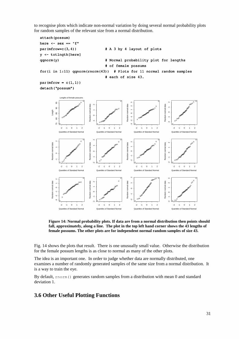
31

to recognise plots which indicate non-normal variation by doing several normal probability plots for random samples of the relevant size from a normal distribution.

attach(possum)attach(possum)attach(possum)attach(possum)

here <here <here <here <---- sex == "f" sex == "f" sex == "f" sex == "f"

par(mfrow=c(3,4)) par(mfrow=c(3,4)) par(mfrow=c(3,4)) par(mfrow=c(3,4)) # A 3 by 4 layout of plots # A 3 by 4 layout of plots # A 3 by 4 layout of plots # A 3 by 4 layout of plots

y <y <y <y <---- totlngth[here] totlngth[here] totlngth[here] totlngth[here]

qqnorm(y) # Normal probability plot for lengthsqqnorm(y) # Normal probability plot for lengthsqqnorm(y) # Normal probability plot for lengthsqqnorm(y) # Normal probability plot for lengths

# of female possums # of female possums # of female possums # of female possums

for(i in 1:11) qqnorm(rnorm(43)) # Plots for 11 normal random samplesfor(i in 1:11) qqnorm(rnorm(43)) # Plots for 11 normal random samplesfor(i in 1:11) qqnorm(rnorm(43)) # Plots for 11 normal random samplesfor(i in 1:11) qqnorm(rnorm(43)) # Plots for 11 normal random samples

# each of size 43. # each of size 43. # each of size 43. # each of size 43.

par(mfrow = c(1,1))par(mfrow = c(1,1))par(mfrow = c(1,1))par(mfrow = c(1,1))

detach(“possum”)detach(“possum”)detach(“possum”)detach(“possum”)

Quantiles of Standard Normal

Leng

th

-2 -1 0 1 2

7580

8590

95

Lengths of female possums

Quantiles of Standard Normal

Ran

dom

nor

mal

dat

a

-2 -1 0 1 2

-10

12

Quantiles of Standard Normal

Ran

dom

nor

mal

dat

a-2 -1 0 1 2

-3-2

-10

12

3Quantiles of Standard Normal

Ran

dom

nor

mal

dat

a

-2 -1 0 1 2

-2-1

01

2Quantiles of Standard Normal

Ran

dom

nor

mal

dat

a

-2 -1 0 1 2

-10

12

Quantiles of Standard Normal

Ran

dom

nor

mal

dat

a

-2 -1 0 1 2

-2-1

01

2

Quantiles of Standard Normal

Ran

dom

nor

mal

dat

a

-2 -1 0 1 2

-2-1

01

2

Quantiles of Standard Normal

Ran

dom

nor

mal

dat

a-2 -1 0 1 2

-2-1

01

2

Quantiles of Standard Normal

Ran

dom

nor

mal

dat

a

-2 -1 0 1 2

-3-2

-10

12

Quantiles of Standard Normal

Ran

dom

nor

mal

dat

a

-2 -1 0 1 2

-2-1

01

2

Quantiles of Standard Normal

Ran

dom

nor

mal

dat

a

-2 -1 0 1 2

-2-1

01

2

Quantiles of Standard Normal

Ran

dom

nor

mal

dat

a

-2 -1 0 1 2

-2-1

01

23

Figure 14: Normal probability plots. If data are from a normal distribution then points should fall, approximately, along a line. The plot in the top left hand corner shows the 43 lengths of female possums. The other plots are for independent normal random samples of size 43.

Fig. 14 shows the plots that result. There is one unusually small value. Otherwise the distribution for the female possum lengths is as close to normal as many of the other plots.

The idea is an important one. In order to judge whether data are normally distributed, one examines a number of randomly generated samples of the same size from a normal distribution. It is a way to train the eye.

By default, rnorm() generates random samples from a distribution with mean 0 and standard deviation 1.

3.6 Other Useful Plotting Functions

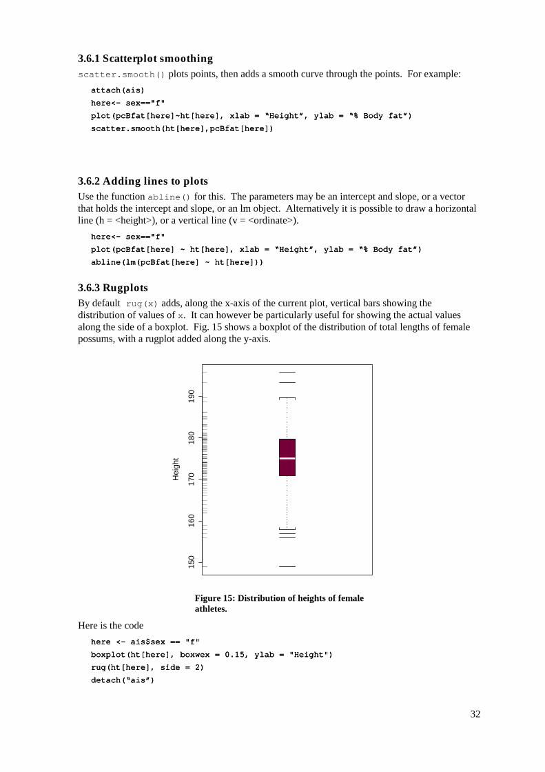
32

3.6.1 Scatterplot smoothing scatter.smooth() plots points, then adds a smooth curve through the points. For example:

attach(ais)attach(ais)attach(ais)attach(ais)

here<here<here<here<---- sex=="f" sex=="f" sex=="f" sex=="f"

plot(pcBfat[here]~ht[here], xlab = “Height”, ylab = “% Body fat”)plot(pcBfat[here]~ht[here], xlab = “Height”, ylab = “% Body fat”)plot(pcBfat[here]~ht[here], xlab = “Height”, ylab = “% Body fat”)plot(pcBfat[here]~ht[here], xlab = “Height”, ylab = “% Body fat”)

scatter.smooth(ht[here],pcBfat[here])scatter.smooth(ht[here],pcBfat[here])scatter.smooth(ht[here],pcBfat[here])scatter.smooth(ht[here],pcBfat[here])

3.6.2 Adding lines to plots Use the function abline() for this. The parameters may be an intercept and slope, or a vector that holds the intercept and slope, or an lm object. Alternatively it is possible to draw a horizontal line (h = <height>), or a vertical line (v = <ordinate>).

here<here<here<here<---- sex=="f" sex=="f" sex=="f" sex=="f"

plot(pcBfat[here] ~ ht[here], xlab = “Height”, ylab plot(pcBfat[here] ~ ht[here], xlab = “Height”, ylab plot(pcBfat[here] ~ ht[here], xlab = “Height”, ylab plot(pcBfat[here] ~ ht[here], xlab = “Height”, ylab = “% Body fat”)= “% Body fat”)= “% Body fat”)= “% Body fat”)

abline(lm(pcBfat[here] ~ ht[here]))abline(lm(pcBfat[here] ~ ht[here]))abline(lm(pcBfat[here] ~ ht[here]))abline(lm(pcBfat[here] ~ ht[here]))

3.6.3 Rugplots By default rug(x) adds, along the x-axis of the current plot, vertical bars showing the distribution of values of x. It can however be particularly useful for showing the actual values along the side of a boxplot. Fig. 15 shows a boxplot of the distribution of total lengths of female possums, with a rugplot added along the y-axis.

150

160

170

180

190

Hei

ght

Figure 15: Distribution of heights of female athletes.

Here is the code here <here <here <here <---- ais$sex == "f" ais$sex == "f" ais$sex == "f" ais$sex == "f"

boxplot(ht[here], boxwex = 0.15, ylab = "Height")boxplot(ht[here], boxwex = 0.15, ylab = "Height")boxplot(ht[here], boxwex = 0.15, ylab = "Height")boxplot(ht[here], boxwex = 0.15, ylab = "Height")

rug(ht[here], side = 2)rug(ht[here], side = 2)rug(ht[here], side = 2)rug(ht[here], side = 2)

detach(“ais”)detach(“ais”)detach(“ais”)detach(“ais”)

33

The parameter boxwex is used to control the width of the boxplot. Reduction from the default width often gives a more elegant result.

3.7 Guidelines for Graphs Design graphs to make their point tersely and clearly, with a minimum waste of ink. Label as necessary to identify important features. In scatterplots the graph should attract the eye’s attention to the points that are plotted, and to important grouping in the data. Use solid points when there is little or no overlap.

When there is extensive overlap, use open plotting symbols. Where points are dense, overlapping points will give a high ink density, which is exactly what one wants.

Use scatterplots in preference to bar or related graphs whenever the horizontal axis represents a quantitative effect.

Use graphs from which information can be read directly and easily in preference to those that rely on visual impression and perspective. Thus in scientific papers contour plots are much preferable to surface plots or two-dimensional bar graphs.

Draw graphs so that reduction and reproduction will not interfere with visual clarity.

Explain clearly how error bars should be interpreted — ± SE limits, ± 95% confidence interval, ± SD limits, or whatever. Explain what source of error is represented. It is pointless to present information on a source of error that is of little or no interest.

3.8 Exercises 1. Plot the graph of brain weight (brain) versus body weight (body) for the built-in data set brains. Label the axes appropriately.

2. Repeat the plot 1, but this time plotting log(brain weight) versus log(body weight). Use the row labels to label the points with the three largest body weight values. Label the axes in untransformed units.

3. Repeat the plots 1 and 2, but this time place the plots side by side on the one page.

4. The supplied data set huron has mean July average water surface elevations, in feet, IGLD (1955) for Harbor Beach, Michigan, on Lake Huron, Station 5014, for 1860-198613.

a) Plot mean.height against year.

b) Use the identify function to determine which years correspond to the lowest and highest mean levels. That is, type identify(huron$year,huron$mean.height,la identify(huron$year,huron$mean.height,la identify(huron$year,huron$mean.height,la identify(huron$year,huron$mean.height,labels=huron$year)bels=huron$year)bels=huron$year)bels=huron$year)

and use the left mouse button to click on the lowest point and highest point on the plot. To quit, press both mouse buttons simultaneously.

c) As in the case of many time series, the mean levels are correlated from year to year. To see how each year's mean level is related to the previous year's mean level, use lag.plot(huron$mean.height) lag.plot(huron$mean.height) lag.plot(huron$mean.height) lag.plot(huron$mean.height)

This plots the mean level at year i against the mean level at year i-1.

5. Write versions of plot.florida() that (a) plot the square roots of the numbers of votes on the respective axes; and (b) plot the logarithms of the numbers of votes on the respective axes.

13 Source: Great Lakes Water Levels, 1860-1986. U.S. Dept. of Commerce, National Oceanic and Atmospheric Administration, National Ocean Survey.

34

6. Try x <- rnorm(10). Print out the numbers that you get. Look up the help for rnorm. Now generate a sample of size 10 from a normal distribution with mean 170 and standard deviation 4.

7. Use mfrow() to set up the layout for a 3 by 4 array of plots. In the top 4 rows, show normal probability plots (section 3.4.2) for four separate `random’ samples of size 10, all from a normal distribution. In the middle 4 rows, display plots for samples of size 100. In the bottom four rows, display plots for samples of size 1000. Comment on how the appearance of the plots changes as the sample size changes.

8. The function runif() can be used to generate a sample from a uniform distribution, by default on the interval 0 to 1. Try x <- runif(10), and print out the numbers you get. Then repeat exercise 7 above, but taking samples from a uniform distribution rather than from a normal distribution. What shape do the points follow?

9. If you find exercise 8 interesting, you might like to try it for some further distributions. For example x <- rchisq(10,1) will generate 10 random values from a chi-squared distribution with degrees of freedom 1. The statement x <- rt(10,1) will generate 10 random values from a t distribution with degrees of freedom 1. Make normal probability plots for samples of various sizes from these distributions.

10. For the first two columns of the data frame hills, examine the distribution using:

(a) histograms

(b) density plots

(c) normal probability plots.

Repeat (a), (b) and (c), now working with the logarithms of the data values.

3.9 References Cleveland, W. S. 1993. Visualizing Data. Hobart Press, Summit, New Jersey.

Cleveland, W. S. 1985. The Elements of Graphing Data. Wadsworth, Monterey, California.

Maindonald J H 1992. Statistical design, analysis and presentation issues. New Zealand Journal of Agricultural Research 35: 121-141.

Tufte, E. R. 1983. The Visual Display of Quantitative Information. Graphics Press, Cheshire, Connecticut, U.S.A.

Tufte, E. R. 1990. Envisioning Information. Graphics Press, Cheshire, Connecticut, U.S.A.

Tufte, E. R. 1997. Visual Explanations. Graphics Press, Cheshire, Connecticut, U.S.A.

Wainer, H. 1997. Visual Revelations. Springer-Verlag, New York

35

4. Trellis Graphics Trellis plots allow the use of the layout on the page to reflect meaningful aspects of data structure. They offer other innovations also, that are described in S-PLUS documentation and in articles that you can get from the internet. Go to

http://achille.cs.bell-labs.com/cm/ms/departments/sia/project/trellis/index.html

S-PLUS 4.0 and later attaches the Trellis library automatically. In S-PLUS 3.4 for UNIX, use library(trellis, first=T) to attach the Trellis library.

4.1 Fine control over the graphics window Implementations of trellis under S-PLUS 4.0 and later for Windows have a unified approach to hard copy and screen display. It is often best to print or copy directly from the screen display. A variety of different display formats are available, most of which can be used either for the screen display or for the printer.

S-PLUS 4.0 and later for Windows open the graphics window automatically when it is needed. On occasions it is however desirable to open it explicitly, allowing you to make changes from the default height and width, pointsize, etc. If you want the default trellis settings, specify

trellis.device(graphsheet)trellis.device(graphsheet)trellis.device(graphsheet)trellis.device(graphsheet)

rather than the standard graphsheet()graphsheet()graphsheet()graphsheet()

In either case you can set width=, height=, pointsize=, color=, etc.. The parameters width and height are in inches, while pointsize is in units of 1

72 inch. If you do not want colour you can specify

trellis.device(graphsheet, color=F)trellis.device(graphsheet, color=F)trellis.device(graphsheet, color=F)trellis.device(graphsheet, color=F)

One side effect of setting color=F is that, if you use the groups= parameter when you call a trellis function, different symbols rather than different colours will by default be used to distinguish the different groups.

To close the current graphics window, specify dev.off() # closes current graphics devicedev.off() # closes current graphics devicedev.off() # closes current graphics devicedev.off() # closes current graphics device

4.2 Examples that Present Panels of Scatterplots – Using xyplot() The basic function for use in drawing panels of scatterplots is xyplot(). We will use the S-PLUS built-in data frame CO2 to demonstrate the use of xyplot(). In this data frame uptake and conc are variables, while Type (2 levels), Treatment (2 levels) and Plant (3 levels within each Type and Treatment combination) are factors.

xyplot(uptake~conc|Type+xyplot(uptake~conc|Type+xyplot(uptake~conc|Type+xyplot(uptake~conc|Type+Treatment, data=CO2) # Simple use of xyplot()Treatment, data=CO2) # Simple use of xyplot()Treatment, data=CO2) # Simple use of xyplot()Treatment, data=CO2) # Simple use of xyplot()

xyplot(uptake~conc|Type+Treatment, data=CO2, panel=panel.smooth)xyplot(uptake~conc|Type+Treatment, data=CO2, panel=panel.smooth)xyplot(uptake~conc|Type+Treatment, data=CO2, panel=panel.smooth)xyplot(uptake~conc|Type+Treatment, data=CO2, panel=panel.smooth)

xyplot(uptake~conc|Type+Treatment, data=CO2,xyplot(uptake~conc|Type+Treatment, data=CO2,xyplot(uptake~conc|Type+Treatment, data=CO2,xyplot(uptake~conc|Type+Treatment, data=CO2, panel=panel.superpose, groups=Plant) panel=panel.superpose, groups=Plant) panel=panel.superpose, groups=Plant) panel=panel.superpose, groups=Plant)

36

All three of the above commands plot uptake against conc for each combination of Type and Treatment. The second command adds a smooth. The third command uses different colours, or different symbols if the plot is black and white, for the different Echinochloa crus-galli plants14.

Fig. 16 shows the output from the third of these sets of commands:

10

20

30

40

Quebecnonchilled

200 400 600 800 1000

Mississippinonchilled

Quebecchilled

10

20

30

40

Mississippichilled

200 400 600 800 1000

conc

upta

ke

Fig. 16: Output from xyplot(uptake~conc|Type+Treatment, data=CO2, panel=panel.superpose, groups=Plant)

If you want to smooth separately for the separate groups, you will need to write your own panel function. We will come to that later.

4.2.1 Using Ranges of Continuous Variables to Define Panels The function equal.count() may be used to break a continuous variable down into (possibly overlapping) ranges. For example

hills$climbcat <hills$climbcat <hills$climbcat <hills$climbcat <---- equal.count(hills$climb, 3) equal.count(hills$climb, 3) equal.count(hills$climb, 3) equal.count(hills$climb, 3)

# climbcat specifies three overlapping ranges of “climb”# climbcat specifies three overlapping ranges of “climb”# climbcat specifies three overlapping ranges of “climb”# climbcat specifies three overlapping ranges of “climb”

xyplot(time ~ distance | climbcat, data=hills)xyplot(time ~ distance | climbcat, data=hills)xyplot(time ~ distance | climbcat, data=hills)xyplot(time ~ distance | climbcat, data=hills)

You can use the parameter overlap of equal.count() to control the fraction of overlap. By default overlap is 0.5, i.e. each successive pair of categories have around half their values in common.

4.3 An Incomplete List of Trellis Functions splom(~data.frame) # Scatterplot matrixsplom(~data.frame) # Scatterplot matrixsplom(~data.frame) # Scatterplot matrixsplom(~data.frame) # Scatterplot matrix

contourplot(numecontourplot(numecontourplot(numecontourplot(numeric1~numeric2*numeric3 , . .) # Contour plotric1~numeric2*numeric3 , . .) # Contour plotric1~numeric2*numeric3 , . .) # Contour plotric1~numeric2*numeric3 , . .) # Contour plot

levelplot(numeric1~numeric2*numeric3 , . .) # Glitzy contour displaylevelplot(numeric1~numeric2*numeric3 , . .) # Glitzy contour displaylevelplot(numeric1~numeric2*numeric3 , . .) # Glitzy contour displaylevelplot(numeric1~numeric2*numeric3 , . .) # Glitzy contour display

wireframe(numeric1~numeric2*numeric3 , . .)wireframe(numeric1~numeric2*numeric3 , . .)wireframe(numeric1~numeric2*numeric3 , . .)wireframe(numeric1~numeric2*numeric3 , . .)

bwplot(factor~numeric , . .) # Box and whisker plotbwplot(factor~numeric , . .) # Box and whisker plotbwplot(factor~numeric , . .) # Box and whisker plotbwplot(factor~numeric , . .) # Box and whisker plot

qq(factor~numeric , . .)qq(factor~numeric , . .)qq(factor~numeric , . .)qq(factor~numeric , . .)

dotplotdotplotdotplotdotplot(character~numeric , . .) # 1(character~numeric , . .) # 1(character~numeric , . .) # 1(character~numeric , . .) # 1----dim. Displaydim. Displaydim. Displaydim. Display

barchart(character~numeric , . .)barchart(character~numeric , . .)barchart(character~numeric , . .)barchart(character~numeric , . .)

piechart(character~numeric , . .)piechart(character~numeric , . .)piechart(character~numeric , . .)piechart(character~numeric , . .)

14 Data are from: Potvin, C. and Lechowicz, M.J. (1990), "The statistical analysis of ecophysiological response curves obtained from experiments involving repeated measures", Ecology, 71, 1389-1400.

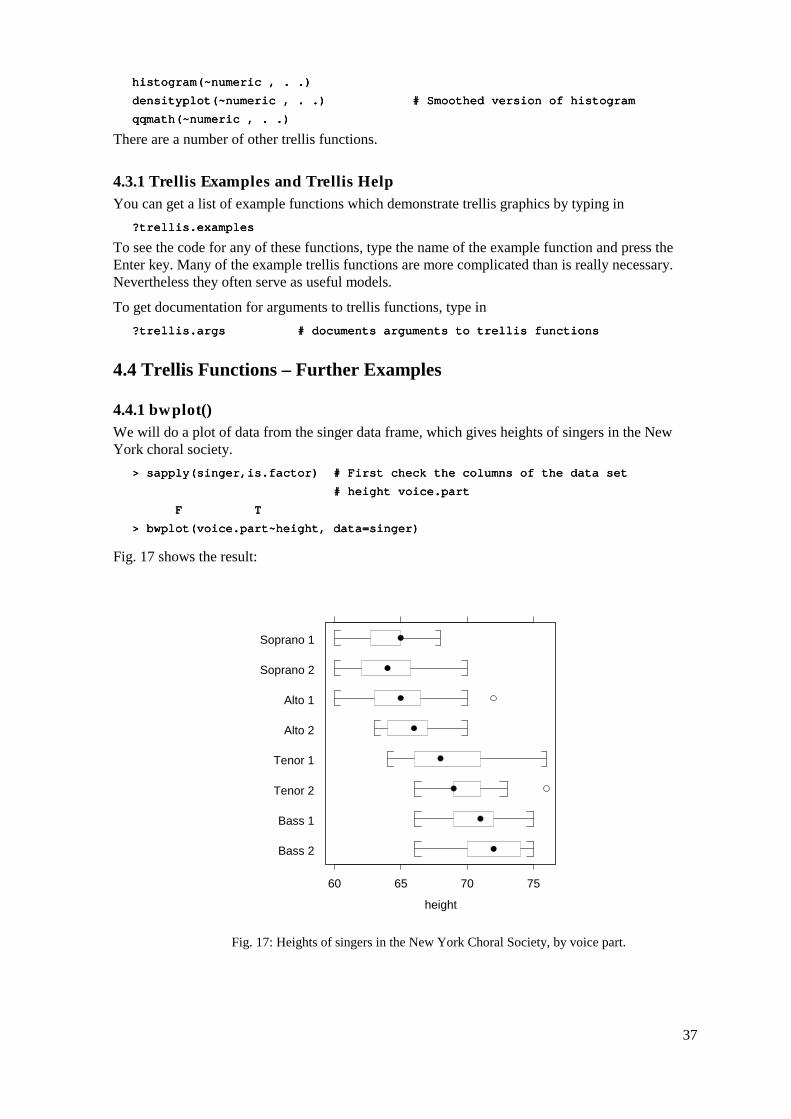
37

histogram(~numeric , . .)histogram(~numeric , . .)histogram(~numeric , . .)histogram(~numeric , . .)

densityplot(~numeric , . .) # Smoothed version of histogramdensityplot(~numeric , . .) # Smoothed version of histogramdensityplot(~numeric , . .) # Smoothed version of histogramdensityplot(~numeric , . .) # Smoothed version of histogram

qqmath(~numeric , . .) qqmath(~numeric , . .) qqmath(~numeric , . .) qqmath(~numeric , . .)

There are a number of other trellis functions.

4.3.1 Trellis Examples and Trellis Help You can get a list of example functions which demonstrate trellis graphics by typing in

?trellis.examples?trellis.examples?trellis.examples?trellis.examples

To see the code for any of these functions, type the name of the example function and press the Enter key. Many of the example trellis functions are more complicated than is really necessary. Nevertheless they often serve as useful models.

To get documentation for arguments to trellis functions, type in ?trellis.args # docu?trellis.args # docu?trellis.args # docu?trellis.args # documents arguments to trellis functionsments arguments to trellis functionsments arguments to trellis functionsments arguments to trellis functions

4.4 Trellis Functions – Further Examples

4.4.1 bwplot() We will do a plot of data from the singer data frame, which gives heights of singers in the New York choral society.

> sapply(singer,is.factor) # First check the> sapply(singer,is.factor) # First check the> sapply(singer,is.factor) # First check the> sapply(singer,is.factor) # First check the columns of the data set columns of the data set columns of the data set columns of the data set

# height voice.part # height voice.part # height voice.part # height voice.part

F T F T F T F T

> bwplot(voice.part~height, data=singer)> bwplot(voice.part~height, data=singer)> bwplot(voice.part~height, data=singer)> bwplot(voice.part~height, data=singer)

Fig. 17 shows the result:

Bass 2

Bass 1

Tenor 2

Tenor 1

Alto 2

Alto 1

Soprano 2

Soprano 1

60 65 70 75

height

Fig. 17: Heights of singers in the New York Choral Society, by voice part.

38

It assists interpretation to know how many points are represented in each boxplot. The table() command will give this information:

> table(singer$voice.part) Bass 2 Bass 1 Tenor 2 Tenor 1 Alto 2 Alto 1 Soprano 2 Soprano 1 26 39 21 21 27 35 30 36

4.4.2 Scatterplot matrix Examples – splom()splom()splom()splom() The function splom() plots out a scatterplot matrix, or perhaps a series of panels of scatterplot matrices. Just as before one can have multiple panels of scatterplot matrices, different symbols may be used for different groups, and so on. Here are some possibilities

splom(~hillraces)splom(~hillraces)splom(~hillraces)splom(~hillraces)

splom(~kyphosis[,splom(~kyphosis[,splom(~kyphosis[,splom(~kyphosis[,----1] | kyphosis[,1])1] | kyphosis[,1])1] | kyphosis[,1])1] | kyphosis[,1])

splom(~kyphosis[,splom(~kyphosis[,splom(~kyphosis[,splom(~kyphosis[,----1], panel=panel.superpose, groups=kyphosis[,1])1], panel=panel.superpose, groups=kyphosis[,1])1], panel=panel.superpose, groups=kyphosis[,1])1], panel=panel.superpose, groups=kyphosis[,1])

splom(~kyphosis[splom(~kyphosis[splom(~kyphosis[splom(~kyphosis[,,,,----1] | kyphosis[,1], panel=panel.smooth)1] | kyphosis[,1], panel=panel.smooth)1] | kyphosis[,1], panel=panel.smooth)1] | kyphosis[,1], panel=panel.smooth)

Compare the first two displays. The second uses the same panel, but different colours, for “absent” and “present”. Which display do you consider the more helpful?

4.5 The Panel Function The Trellis functions have a default panel function as argument. For xyplot() the default panel function is panel.xyplot(). Thus

xyplot(uptake~conc|Type+Treatment, data=CO2) xyplot(uptake~conc|Type+Treatment, data=CO2) xyplot(uptake~conc|Type+Treatment, data=CO2) xyplot(uptake~conc|Type+Treatment, data=CO2)

is equivalent to xyplot(uptake~conc|Type+Treatment, data=CO2, panel=panel.xyplot) xyplot(uptake~conc|Type+Treatment, data=CO2, panel=panel.xyplot) xyplot(uptake~conc|Type+Treatment, data=CO2, panel=panel.xyplot) xyplot(uptake~conc|Type+Treatment, data=CO2, panel=panel.xyplot)

A built-in alternative to panel.xyplot() is panel.smooth(). This fits a smooth curve to the data. A further possibility is to write your own panel function. This allows you to greatly enhance the capabilities of the Trellis library.

If you want different colours for different groups then, as demonstrated earlier, specify the groups argument when you call the trellis function, and set panel equal to panel.superpose. We can control the different colours used for the different groups. Also we can join the points for each plant. Thus we have

xyplot(uptake~conc|Treatment+Type,data=CO2, panel=panel.superpose, xyplot(uptake~conc|Treatment+Type,data=CO2, panel=panel.superpose, xyplot(uptake~conc|Treatment+Type,data=CO2, panel=panel.superpose, xyplot(uptake~conc|Treatment+Type,data=CO2, panel=panel.superpose,

groups=Plant, col=2:4, type=”b”) groups=Plant, col=2:4, type=”b”) groups=Plant, col=2:4, type=”b”) groups=Plant, col=2:4, type=”b”)

There are three plants in each panel. So we specified three colours, which are recycled each time we move to a new panel. The parameters type=”b” and col=2:4 both get passed to panel.superpose(). There are three possible settings for type. The default is type=”p” (points); other settings are type=”l” (lines), and type=”b” (both points & lines).

*4.5.1 A user-defined panel function Here is how you might, while using bwplot, use a rugplot along the x-direction to examine in more detail the distribution of data values in each panel.

bwplot(Type ~ uptake|Treatment, data=CO2, bwplot(Type ~ uptake|Treatment, data=CO2, bwplot(Type ~ uptake|Treatment, data=CO2, bwplot(Type ~ uptake|Treatment, data=CO2,

panel=function(x,y){ panel.bwp panel=function(x,y){ panel.bwp panel=function(x,y){ panel.bwp panel=function(x,y){ panel.bwplot(x,y); rug(x) } )lot(x,y); rug(x) } )lot(x,y); rug(x) } )lot(x,y); rug(x) } )

Of course it would be nice to make the colour of the rug bars different for the two different Types. Here is how to do it. We have to define our own panel function, which calls panel.bwplot() and does more besides.

panel.mybw <panel.mybw <panel.mybw <panel.mybw <---- func func func function(x,y)tion(x,y)tion(x,y)tion(x,y)

39

{ panel.bwplot(x,y) # x will be set to uptake, and y to Type { panel.bwplot(x,y) # x will be set to uptake, and y to Type { panel.bwplot(x,y) # x will be set to uptake, and y to Type { panel.bwplot(x,y) # x will be set to uptake, and y to Type

for(u in unique(y)){par(col=u+2); rug(x[y==u])} for(u in unique(y)){par(col=u+2); rug(x[y==u])} for(u in unique(y)){par(col=u+2); rug(x[y==u])} for(u in unique(y)){par(col=u+2); rug(x[y==u])}

par(col=1) } # End panel.mybw par(col=1) } # End panel.mybw par(col=1) } # End panel.mybw par(col=1) } # End panel.mybw

bwplot(Type~uptake|Treatment, data=CO2, panel=panel.mybw)bwplot(Type~uptake|Treatment, data=CO2, panel=panel.mybw)bwplot(Type~uptake|Treatment, data=CO2, panel=panel.mybw)bwplot(Type~uptake|Treatment, data=CO2, panel=panel.mybw)

Note that Type has values 1 and 2. When panel.bwplot is called to create each individual panel, uptake is the x argument, and Type is the y argument.

*4.6 Adding a Key Keys may be used to identify the plotting symbols, line styles and colours that have been used for different subsets of the data.

We illustrate with a modified and substantially simplified version of the commands in the built-in example.overplot() example trellis function. The part of the command that generates the key has been shaded. Notice its somewhat complicated structure. I have specified three list elements – a numeric value y, a list with the name points, and a list with the name text. The value of y sets the vertical positioning; the graphics region finishes at around y = 1. I have left x at its default value, i.e. 0.5:

dotplot(variety~yield | site, data=barley, groups=year,dotplot(variety~yield | site, data=barley, groups=year,dotplot(variety~yield | site, data=barley, groups=year,dotplot(variety~yield | site, data=barley, groups=year,

panel=panel.superpose, pch=16, col=3:4, panel=panel.superpose, pch=16, col=3:4, panel=panel.superpose, pch=16, col=3:4, panel=panel.superpose, pch=16, col=3:4,

key=list(y=1.08, key=list(y=1.08, key=list(y=1.08, key=list(y=1.08,

points=list(pch=16,col=3:4), points=list(pch=16,col=3:4), points=list(pch=16,col=3:4), points=list(pch=16,col=3:4),

text=list(text=levels(barley$year),col=3:4) text=list(text=levels(barley$year),col=3:4) text=list(text=levels(barley$year),col=3:4) text=list(text=levels(barley$year),col=3:4)

) ) ) )

) ) ) )

There are a wide variety of other settings that one can include in the list: columns to specify the number of columns into which to divide the key (in the above we might have set columns=2), the parameter between to specify the distance in character widths between the different key elements, and between.columns for use when columns>1 to specify the distance between columns. The syntax carries across from that for the function key(), which can be used to put a key on a graph after it has been drawn. The difference is that one has to make sure that there is space available before the function key() is called.

You might want to control the aspect ratio and layout. Try aspect=0.4 and layout=c(1,6) as parameters to dotplot().

*4.7 The Subscripts Argument All of the Trellis functions take a subscripts argument. If this argument is set to TRUE (T), then "subscripts" can be passed to the panel function. These subscripts can then be used in conditional statements so that the panel function's behaviour depends on the level of the conditioning variable.

The subscripts are useful when variables other than those passed as x or y or groups are to be used in the individual panels. If for example the variable is called z, then the values that are relevant to any specific panel can be passed as z[subscripts].

If you want to use panel.superpose inside your own function, you must either explicitly pass the groups argument, or else include the . . . argument as a parameter to your function, and call panel.superpose as panel.superpose(x, y, ...). The . . . argument must be specified just as it appears. It allows for the passing of additional arguments, at this point unspecified.

Here is how you might fit a separate smooth curve for each of the different plants. This is given here for completeness. First we define a new panel function:

40

my.panel <my.panel <my.panel <my.panel <---- function(x, y, subscripts, groups, ...) function(x, y, subscripts, groups, ...) function(x, y, subscripts, groups, ...) function(x, y, subscripts, groups, ...)

{{{{

gps <gps <gps <gps <---- groups[subscripts] groups[subscripts] groups[subscripts] groups[subscripts]

ugp <ugp <ugp <ugp <---- as.character(unique(gps)) as.character(unique(gps)) as.character(unique(gps)) as.character(unique(gps))

i <i <i <i <---- 1 1 1 1

for(u in ugp) {for(u in ugp) {for(u in ugp) {for(u in ugp) {

i <i <i <i <---- i + 1 i + 1 i + 1 i + 1

here <here <here <here <---- gps == u gps == u gps == u gps == u

panel.smooth(x[hpanel.smooth(x[hpanel.smooth(x[hpanel.smooth(x[here], y[here], col = i, pch = i, ...)ere], y[here], col = i, pch = i, ...)ere], y[here], col = i, pch = i, ...)ere], y[here], col = i, pch = i, ...)

}}}}

}}}}

To do the trellis graph, proceed as follows: xyplot(uptake ~ conc | Type + Treatment, data = CO2, panel = xyplot(uptake ~ conc | Type + Treatment, data = CO2, panel = xyplot(uptake ~ conc | Type + Treatment, data = CO2, panel = xyplot(uptake ~ conc | Type + Treatment, data = CO2, panel =

my.panel, groups = Plant, span=1)my.panel, groups = Plant, span=1)my.panel, groups = Plant, span=1)my.panel, groups = Plant, span=1)

The span=1span=1span=1span=1 parameter is passed as an unnamed parameter. Whenever a function has … in the list of arguments, this is allowed. It is passed through to my.panelmy.panelmy.panelmy.panel and thence to panel.smoothpanel.smoothpanel.smoothpanel.smooth, which knows how to extract the value of span from its … list.

4.8 Exercises 1. The following data gives milk volume (g/day) for smoking and nonsmoking mothers: Smoking Mothers: 621, 793, 593, 545, 753, 655, 895, 767, 714, 598, 693 Nonsmoking Mothers: 947, 945, 1086, 1202, 973, 981, 930, 745, 903, 899, 961 Present the data (i) in side by side boxplots; (ii) using a dotplot form of display. [The data were taken from the paper ``Smoking During Pregnancy and Lactation and Its Effects on Breast Milk Volume'' (Amer. J. of Clinical Nutrition).]

2. The built-in data frame environmental has columns ozone (a variable), radiation (a variable), temp (a variable), and wind (a variable). Plot ozone against radiation for each of three temperature ranges, and each of three wind ranges. [Use equal.count() to generate the ranges of temp and wind.

3. Repeat the plot as in example 1, but this time including a scatterplot smooth on each panel.

4. Taking the supplied data frame ships, plot incidents against service for each level of consyr (construction period) and for each level of period (period of service).

5. Repeat the plot from exercise 4, but now plot log(incidents+1) against log(service), and use a different colour or plot symbol for each different shiptype.

6. Use suitable trellis plots to explore the built-in kyphosis data set. [To get details of the variables, type in help(kyphosis).]

7. For the possum data set, generate the following plots for each separate population (Pop) and for each sex (sex) separately:

a) histograms of hdlngth – use histogram();

b) normal probability plots of hdlngth – use qqmath();

c) density plots of hdlngth – use densityplot().

The histogram function allows you to control the ration of the y to x scales (aspect) and the number of intervals (nint). Investigate the effect of varying these. The densityplot function allows you to vary parameters aspect and width. The parameter width controls the width of the smoothing window. Investigate the effect of varying these parameters.

8. Import the data frame called ACF, from the file acf.txt . The data were obtained from an experiment involving 66 rats which were injected with a carcinogen 1, 2 or 3 times. The rats were sacrificed at either TIME = 6, 12 or 24 weeks, and their colons were stained and examined. Each

41

colon was divided into 6 sections, and the numbers and sizes of aberrant crypt foci (ACF) were evaluated. The average size (AVERAGE) and total number (TOTAL) of ACF were recorded for each section.

(a) Using the xyplot function, explore the relation between the total number of ACF and TIME, taking into account the number of injections and the section.

(b) Repeat (a), using AVERAGE in place of TOTAL.

(c) Construct a contour plot of TOTAL versus TIME and SECTION.

(d) Repeat (c), using the wireframe plot instead of the contour plot.

(e) Repeat (c) and (d), using AVERAGE in place of TOTAL.

(f) Repeat (c),(d) and (e), using INJECTION in place of SECTION.

(g) Construct box and whisker plots for TOTAL, using TIME as a factor.

(h) Repeat (g), using AVERAGE in place of TOTAL.

(i) Construct normal probability plots for TOTAL, using TIME>12 as the factor. Is there evidence that the distribution of TOTAL for TIME>12 differs from the distribution of TOTAL for TIME <= 12?

(j) Repeat (i), using AVERAGE instead of TOTAL. What can you say about the distributions of AVERAGE for different times?

(k) Use the command bwplot(TIME~TOTAL|SECbwplot(TIME~TOTAL|SECbwplot(TIME~TOTAL|SECbwplot(TIME~TOTAL|SECTION,data=ACF,panel=function(x,y){ panel.bwplot(x,y);TION,data=ACF,panel=function(x,y){ panel.bwplot(x,y);TION,data=ACF,panel=function(x,y){ panel.bwplot(x,y);TION,data=ACF,panel=function(x,y){ panel.bwplot(x,y);

rug(x)} ) rug(x)} ) rug(x)} ) rug(x)} )

to create a rugplot.

(l) Repeat (k), replacing SECTION with SECTION+INJECTION.

(m) Construct a dotplot using dotplot(TIME~TOTAL|SECTION+INJECTION, data=ACF)dotplot(TIME~TOTAL|SECTION+INJECTION, data=ACF)dotplot(TIME~TOTAL|SECTION+INJECTION, data=ACF)dotplot(TIME~TOTAL|SECTION+INJECTION, data=ACF)

42

43

5. Regression Models and Analysis of Variance

5.1 The Model Formula in Straight Line Regression We begin with a straight line regression example:

plot(distance ~ stretch, data=elasticband, pch=16) # Plot the dataplot(distance ~ stretch, data=elasticband, pch=16) # Plot the dataplot(distance ~ stretch, data=elasticband, pch=16) # Plot the dataplot(distance ~ stretch, data=elasticband, pch=16) # Plot the data

The code for the regression calculation is: elaselaselaselastic.lm <tic.lm <tic.lm <tic.lm <---- lm(distance ~ stretch, data=elasticband) lm(distance ~ stretch, data=elasticband) lm(distance ~ stretch, data=elasticband) lm(distance ~ stretch, data=elasticband)

Here distance ~ stretch is a model formula. We will meet more general types of model formulae in the course of this chapter. The output from the regression is an lm object, which we have called elastic.lm .

Now examine a summary of the regression results. Notice that the documentation of the call gives details of the model formula.

> options(digits=4)> options(digits=4)> options(digits=4)> options(digits=4)

> summary(elastic.lm)> summary(elastic.lm)> summary(elastic.lm)> summary(elastic.lm)

Call: lm(formula = distance ~ stretch, data = elasticband)Call: lm(formula = distance ~ stretch, data = elasticband)Call: lm(formula = distance ~ stretch, data = elasticband)Call: lm(formula = distance ~ stretch, data = elasticband)

Residuals:Residuals:Residuals:Residuals:

1 1 1 1 2 3 4 5 6 7 2 3 4 5 6 7 2 3 4 5 6 7 2 3 4 5 6 7

2.11 2.11 2.11 2.11 ----0.321 18 1.89 0.321 18 1.89 0.321 18 1.89 0.321 18 1.89 ----27.8 13.3 27.8 13.3 27.8 13.3 27.8 13.3 ----7.217.217.217.21

Coefficients:Coefficients:Coefficients:Coefficients:

Value Std. Error t value Pr(>|t|) Value Std. Error t value Pr(>|t|) Value Std. Error t value Pr(>|t|) Value Std. Error t value Pr(>|t|)

(Intercept) (Intercept) (Intercept) (Intercept) ----63.571 74.332 63.571 74.332 63.571 74.332 63.571 74.332 ----0.855 0.431 0.855 0.431 0.855 0.431 0.855 0.431

stretch 4.554 1.543 2.951 0.032 stretch 4.554 1.543 2.951 0.032 stretch 4.554 1.543 2.951 0.032 stretch 4.554 1.543 2.951 0.032

Residual standard error: 16.Residual standard error: 16.Residual standard error: 16.Residual standard error: 16.3 on 5 degrees of freedom3 on 5 degrees of freedom3 on 5 degrees of freedom3 on 5 degrees of freedom

Multiple RMultiple RMultiple RMultiple R----Squared: 0.635 Squared: 0.635 Squared: 0.635 Squared: 0.635

FFFF----statistic: 8.71 on 1 and 5 degrees of freedom, the pstatistic: 8.71 on 1 and 5 degrees of freedom, the pstatistic: 8.71 on 1 and 5 degrees of freedom, the pstatistic: 8.71 on 1 and 5 degrees of freedom, the p----vvvv

alue is 0.0319 alue is 0.0319 alue is 0.0319 alue is 0.0319

Correlation of Coefficients:Correlation of Coefficients:Correlation of Coefficients:Correlation of Coefficients:

(Intercept) (Intercept) (Intercept) (Intercept)

stretch stretch stretch stretch ----0.9970.9970.9970.997

5.2 Regression Objects An lm object is a list of named elements. Above, we created the object elastic.lm . Let us look at the names of its elements:

> names(elastic.lm)> names(elastic.lm)> names(elastic.lm)> names(elastic.lm)

[1] "coefficients" "residuals" "fitted.values" "effects" [1] "coefficients" "residuals" "fitted.values" "effects" [1] "coefficients" "residuals" "fitted.values" "effects" [1] "coefficients" "residuals" "fitted.values" "effects"

[5] "R" "rank" "assign" "df.residual" [5] "R" "rank" "assign" "df.residual" [5] "R" "rank" "assign" "df.residual" [5] "R" "rank" "assign" "df.residual"

[9] "contr [9] "contr [9] "contr [9] "contrasts" "terms" "call" asts" "terms" "call" asts" "terms" "call" asts" "terms" "call"

Various functions are available for extracting information that you might want from the list. This is better than manipulating the list directly. Examples are:

> coef(elastic.lm)> coef(elastic.lm)> coef(elastic.lm)> coef(elastic.lm)

(Intercept) stretch (Intercept) stretch (Intercept) stretch (Intercept) stretch

----63.57 4.5563.57 4.5563.57 4.5563.57 4.554444

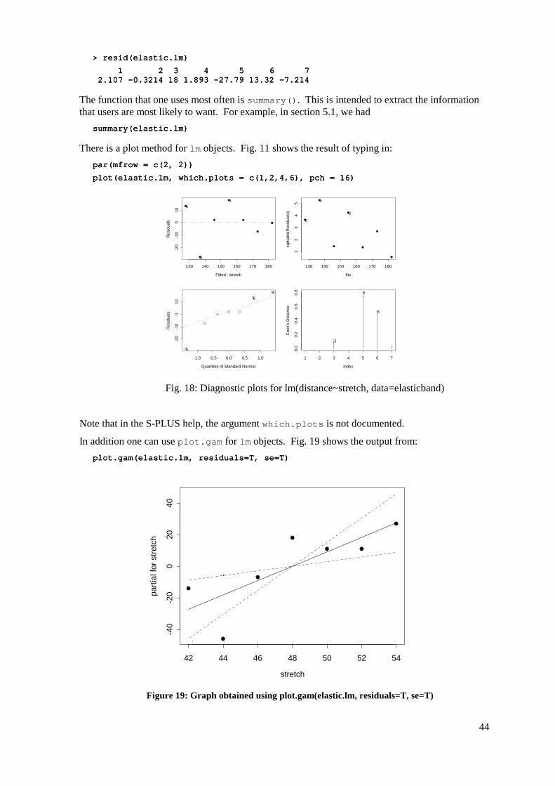
44

> resid(elastic.lm)> resid(elastic.lm)> resid(elastic.lm)> resid(elastic.lm)

1 2 3 4 5 6 7 1 2 3 4 5 6 7 1 2 3 4 5 6 7 1 2 3 4 5 6 7 2.107 2.107 2.107 2.107 ----0.3214 18 1.893 0.3214 18 1.893 0.3214 18 1.893 0.3214 18 1.893 ----27.79 13.32 27.79 13.32 27.79 13.32 27.79 13.32 ----7.214 7.214 7.214 7.214

The function that one uses most often is summary(). This is intended to extract the information that users are most likely to want. For example, in section 5.1, we had

summary(elastic.lm)summary(elastic.lm)summary(elastic.lm)summary(elastic.lm)

There is a plot method for lm objects. Fig. 11 shows the result of typing in: par(mfrow = c(2, 2))par(mfrow = c(2, 2))par(mfrow = c(2, 2))par(mfrow = c(2, 2))

plot(elastic.lm, which.plots = c(1,2,4,6), pch = 16)plot(elastic.lm, which.plots = c(1,2,4,6), pch = 16)plot(elastic.lm, which.plots = c(1,2,4,6), pch = 16)plot(elastic.lm, which.plots = c(1,2,4,6), pch = 16)

Fitted : stretch

Res

idua

ls

130 140 150 160 170 180

-20

-10

010

63

5

fits

sqrt(

abs(

Res

idua

ls))

130 140 150 160 170 180

12

34

5

6

3

5

Quantiles of Standard Normal

Res

idua

ls

-1.0 -0.5 0.0 0.5 1.0

-20

-10

010

63

5

Index

Coo

k's

Dis

tanc

e

1 2 3 4 5 6 7

0.0

0.2

0.4

0.6

0.8

3

6

5

Fig. 18: Diagnostic plots for lm(distance~stretch, data=elasticband)

Note that in the S-PLUS help, the argument which.plots is not documented.

In addition one can use plot.gam for lm objects. Fig. 19 shows the output from: plot.gam(elastic.lm, residuals=T, se=T)plot.gam(elastic.lm, residuals=T, se=T)plot.gam(elastic.lm, residuals=T, se=T)plot.gam(elastic.lm, residuals=T, se=T)

stretch

parti

al fo

r stre

tch

42 44 46 48 50 52 54

-40

-20

020

40

Figure 19: Graph obtained using plot.gam(elastic.lm, residuals=T, se=T)

45

The X-matrix has two columns, one for the constant term, and one for weight. What the graph shows is the contribution of weight in explaining depression, after taking out the effect that is due to the mean. The dotted lines show the bounds that are determined by 95% confidence intervals for the slope of the line.

5.2.1 Pointwise confidence bounds for fitted values To get 95% confidence bounds for fitted values one would need to incorporate uncertainty in the estimate of the fitted mean. One can get those as follows:

> elastic.hat <> elastic.hat <> elastic.hat <> elastic.hat <---- predict(elastic.lm, se=T) predict(elastic.lm, se=T) predict(elastic.lm, se=T) predict(elastic.lm, se=T)

> elastic.ci <> elastic.ci <> elastic.ci <> elastic.ci <---- pointwise(elastic.hat, coverage=0.95) pointwise(elastic.hat, coverage=0.95) pointwise(elastic.hat, coverage=0.95) pointwise(elastic.hat, coverage=0.95)

> elastic.ci> elastic.ci> elastic.ci> elastic.ci

$upper:$upper:$upper:$upper: 1 2 3 4 1 2 3 4 1 2 3 4 1 2 3 4 5 6 7 5 6 7 5 6 7 5 6 7 163.6 210.9 170.9 181.8 159.2 156.3 195.7 163.6 210.9 170.9 181.8 159.2 156.3 195.7 163.6 210.9 170.9 181.8 159.2 156.3 195.7 163.6 210.9 170.9 181.8 159.2 156.3 195.7 $fit:$fit:$fit:$fit: 1 2 3 4 5 6 7 1 2 3 4 5 6 7 1 2 3 4 5 6 7 1 2 3 4 5 6 7 145.9 182.3 155 164.1 136.8 127.7 173.2 145.9 182.3 155 164.1 136.8 127.7 173.2 145.9 182.3 155 164.1 136.8 127.7 173.2 145.9 182.3 155 164.1 136.8 127.7 173.2 $lower:$lower:$lower:$lower: 1 2 3 4 5 6 7 1 2 3 4 5 6 7 1 2 3 4 5 6 7 1 2 3 4 5 6 7 128.2 153.7 139.1 146.4 114.3 99.07 150.8 128.2 153.7 139.1 146.4 114.3 99.07 150.8 128.2 153.7 139.1 146.4 114.3 99.07 150.8 128.2 153.7 139.1 146.4 114.3 99.07 150.8

> plot(d> plot(d> plot(d> plot(distance~stretch, data=elasticband)istance~stretch, data=elasticband)istance~stretch, data=elasticband)istance~stretch, data=elasticband)

> ord<> ord<> ord<> ord<----order(elasticband$stretch)order(elasticband$stretch)order(elasticband$stretch)order(elasticband$stretch)

> lines(elasticband$stretch[ord],elastic.ci$fit[ord])> lines(elasticband$stretch[ord],elastic.ci$fit[ord])> lines(elasticband$stretch[ord],elastic.ci$fit[ord])> lines(elasticband$stretch[ord],elastic.ci$fit[ord])

> lines(elasticband$stretch[ord],elastic.ci$upper[ord], lty=3)> lines(elasticband$stretch[ord],elastic.ci$upper[ord], lty=3)> lines(elasticband$stretch[ord],elastic.ci$upper[ord], lty=3)> lines(elasticband$stretch[ord],elastic.ci$upper[ord], lty=3)

> lines(elasticband$stretch[ord],elastic.ci$lower[ord], lty=3)> lines(elasticband$stretch[ord],elastic.ci$lower[ord], lty=3)> lines(elasticband$stretch[ord],elastic.ci$lower[ord], lty=3)> lines(elasticband$stretch[ord],elastic.ci$lower[ord], lty=3)

Here is way to get smoother confidence bounds: lines(spline(elasticband$stretch,elastic.ci$lower), lty=3)lines(spline(elasticband$stretch,elastic.ci$lower), lty=3)lines(spline(elasticband$stretch,elastic.ci$lower), lty=3)lines(spline(elasticband$stretch,elastic.ci$lower), lty=3)

This has the advantage that you do not need to first order the points.

5.3 Model Formulae, and the X Matrix The model formula for the elastic band example was distance~stretch. The model formula is a recipe for setting up the calculations. It describes how to set up the model matrix or X matrix, and specifies the vector y of values of the dependent variable. For some of the examples we discuss later, it helps to know what the X matrix looks like. Details for the elastic band example follow.

For the elastic band example the X matrix, with the y-vector alongside, is:

X y

Stretch (mm) Distance (cm) 1 46 148 1 54 182 1 48 173 1 50 166 1 44 109 1 42 141 1 52 166

46

The function model.matrix() prints out the model matrix. Thus: > model.matrix(distance ~ stretch, data=elasticband)> model.matrix(distance ~ stretch, data=elasticband)> model.matrix(distance ~ stretch, data=elasticband)> model.matrix(distance ~ stretch, data=elasticband)

(Intercept) stretch (Intercept) stretch (Intercept) stretch (Intercept) stretch

1 1 1 1 1 46 1 46 1 46 1 46

2 1 542 1 542 1 542 1 54

3 1 483 1 483 1 483 1 48

4 1 504 1 504 1 504 1 50

5 1 445 1 445 1 445 1 44

6 1 426 1 426 1 426 1 42

7 1 527 1 527 1 527 1 52

Another possibility, with elastic.lm calculated as in section 5.1, is: model.matrix(elastic.lm)model.matrix(elastic.lm)model.matrix(elastic.lm)model.matrix(elastic.lm)

The model matrix corresponds directly to the equation for the model. The model is

y = a + b x + residual

which we write as

y = 1× a + x × b + residual

For each row, one takes a multiple a of the value in the first column of the model matrix, a multiple b of the value in the second column, and adds them, to give fitted values. Another name is predicted values. The aim is to reproduce, as closely as possible, the values in the y-column. The residuals are the differences between the values in the y-column and the fitted values. Least squares regression, which is the form of regression that we describe in this course, chooses a and b so that the sum of squares of the residuals is as small as possible.

The following are the fitted values and residuals that we get with the estimates of a (= -63.6) and b ( = 4.55) that a least squares regression program chooses for us:

X $y y y y− $

Stretch (mm) (Fitted) (Observed) (Residual)

× -63.6 × 4.55 1 × -63.6 + 4.55 × Stretch Distance (mm) Observed - Fitted

1 46 -63.6 + 4.55 × 46 = 145.7 148 148-145.7 = 2.3

1 54 -63.6 + 4.55 × 54 = 182.1 182 182-182.1 = -0.1

1 48 -63.6 + 4.55 × 48 = 154.8 173 173-154.8 = 18.2

1 50 -63.6 + 4.55 × 50 = 163.9 166 166-163.9 = 2.1

1 44 -63.6 + 4.55 × 44 = 136.6 109 109-136.6 = -27.6

1 42 -63.6 + 4.55 × 42 = 127.5 141 141-127.5 = 13.5

1 52 -63.6 + 4.55 × 52 = 173.0 166 166-173.0 = -7.0

Note that we use $y [pronounced y-hat] as the symbol for predicted values. They may also be called fitted values.

We might also fit the simpler (no intercept) model. For this we have

y = x × b +residual

The X matrix then consists of a single column, the x’s.

47

5.3.1 Model Formulae in General Here is what model formulae look like:

y~x+z : lm, glm,, etc.

y~x+fac+fac:x : lm, glm, aov, etc. (If fac is a factor and x is a variable, fac:x allows a different slope for each different level of fac.)

Model formulae are widely used to set up most of the model calculations in S-PLUS. However there are some older S-PLUS analysis commands that do not use model formulae. Examples are prcomp(), cancor(), mclust(), hclust(), ace(),,,, and avas().

The S-PLUS parser15 makes no distinction between model formulae and the sorts of formulae that are used for specifying trellis plots. The difference may matter once one tries to do something with the formula. By way of reminder, here is a graph formula for trellis plots.

y~x | fac1+fac2 : This gives a plot of y against x for each different combination of levels of fac1 (across the page) and fac2 (up the page).

*5.3.2 Manipulating Model Formulae Model formulae can be assigned, e. g.

formyxz <- formula(y~x+z)

or formyxz <- formula(“y~x+z”)

The argument to formula() can be a text string. This makes it straightforward to paste the argument together from components that are stored in text strings. For example

For example

> names(elasticb> names(elasticb> names(elasticb> names(elasticband)and)and)and)

[1] "stretch" "distance"[1] "stretch" "distance"[1] "stretch" "distance"[1] "stretch" "distance"

> nam <> nam <> nam <> nam <---- names(elasticband) names(elasticband) names(elasticband) names(elasticband)

> formds <> formds <> formds <> formds <---- paste(nam[1],"~",nam[2]) paste(nam[1],"~",nam[2]) paste(nam[1],"~",nam[2]) paste(nam[1],"~",nam[2])

> lm(formds,data=elasticband)> lm(formds,data=elasticband)> lm(formds,data=elasticband)> lm(formds,data=elasticband)

Call:Call:Call:Call:

lm(formula = formds, data = elasticband)lm(formula = formds, data = elasticband)lm(formula = formds, data = elasticband)lm(formula = formds, data = elasticband)

Coefficients:Coefficients:Coefficients:Coefficients:

(Intercept) distance (Intercept) distance (Intercept) distance (Intercept) distance

26.3780 0.1395 26.3780 0.1395 26.3780 0.1395 26.3780 0.1395

5.4 Multiple Linear Regression Models

5.4.1 The Data Frame Rubber > library(mass,first=T)> library(mass,first=T)> library(mass,first=T)> library(mass,first=T)

MASS library for Venables & Ripley (1999) version 5.1MASS library for Venables & Ripley (1999) version 5.1MASS library for Venables & Ripley (1999) version 5.1MASS library for Venables & Ripley (1999) version 5.1

This library is provided by Venables & Ripley <MASS@stats.ox.ac.uk>This library is provided by Venables & Ripley <MASS@stats.ox.ac.uk>This library is provided by Venables & Ripley <MASS@stats.ox.ac.uk>This library is provided by Venables & Ripley <MASS@stats.ox.ac.uk>

It is not supported by It is not supported by It is not supported by It is not supported by MathSoft. Use the command `library(MASS, help=T)' MathSoft. Use the command `library(MASS, help=T)' MathSoft. Use the command `library(MASS, help=T)' MathSoft. Use the command `library(MASS, help=T)'

to view the `readme.txt' file for this library.to view the `readme.txt' file for this library.to view the `readme.txt' file for this library.to view the `readme.txt' file for this library.

15 The parser is a part of the S-PLUS implementation code. It takes S-PLUS statements and turns them into code which can be more directly executed by the computer.

48

Use addMassMenus() to install the menus and dialogsUse addMassMenus() to install the menus and dialogsUse addMassMenus() to install the menus and dialogsUse addMassMenus() to install the menus and dialogs

removeMassMenus() to remove them removeMassMenus() to remove them removeMassMenus() to remove them removeMassMenus() to remove them

> splom(~Rubber)> splom(~Rubber)> splom(~Rubber)> splom(~Rubber)

> Rubber.lm <> Rubber.lm <> Rubber.lm <> Rubber.lm <---- lm(loss~hard+tens, data=Rubber) lm(loss~hard+tens, data=Rubber) lm(loss~hard+tens, data=Rubber) lm(loss~hard+tens, data=Rubber)

> > > > summary(Rubber.lm)summary(Rubber.lm)summary(Rubber.lm)summary(Rubber.lm)

Call: lm(formula = loss ~ hard + tens, data = Rubber)Call: lm(formula = loss ~ hard + tens, data = Rubber)Call: lm(formula = loss ~ hard + tens, data = Rubber)Call: lm(formula = loss ~ hard + tens, data = Rubber)

Residuals:Residuals:Residuals:Residuals:

Min 1Q Median 3Q Max Min 1Q Median 3Q Max Min 1Q Median 3Q Max Min 1Q Median 3Q Max

----79.4 79.4 79.4 79.4 ----14.6 3.82 19.8 6614.6 3.82 19.8 6614.6 3.82 19.8 6614.6 3.82 19.8 66

Coefficients:Coefficients:Coefficients:Coefficients:

Value Std. Error t value Pr(>|t|) Value Std. Error t value Pr(>|t|) Value Std. Error t value Pr(>|t|) Value Std. Error t value Pr(>|t|)

(Intercept) 885.161 61.752 14.334 0.0(Intercept) 885.161 61.752 14.334 0.0(Intercept) 885.161 61.752 14.334 0.0(Intercept) 885.161 61.752 14.334 0.000000000

hard hard hard hard ----6.571 0.583 6.571 0.583 6.571 0.583 6.571 0.583 ----11.267 0.00011.267 0.00011.267 0.00011.267 0.000

tens tens tens tens ----1.374 0.194 1.374 0.194 1.374 0.194 1.374 0.194 ----7.073 0.0007.073 0.0007.073 0.0007.073 0.000

Residual standard error: 36.5 on 27 degrees of freedomResidual standard error: 36.5 on 27 degrees of freedomResidual standard error: 36.5 on 27 degrees of freedomResidual standard error: 36.5 on 27 degrees of freedom

Multiple RMultiple RMultiple RMultiple R----Squared: 0.84 Squared: 0.84 Squared: 0.84 Squared: 0.84

FFFF----statistic: 71 on 2 and 27 degrees of freedom, the pstatistic: 71 on 2 and 27 degrees of freedom, the pstatistic: 71 on 2 and 27 degrees of freedom, the pstatistic: 71 on 2 and 27 degrees of freedom, the p----value is 1.77evalue is 1.77evalue is 1.77evalue is 1.77e----010101011 1 1 1

Correlation of Coefficients:Correlation of Coefficients:Correlation of Coefficients:Correlation of Coefficients:

(Intercept) hard (Intercept) hard (Intercept) hard (Intercept) hard

hard hard hard hard ----0.834 0.834 0.834 0.834

tens tens tens tens ----0.766 0.2990.766 0.2990.766 0.2990.766 0.299

Now examine diagnostic plots: par(mfrow=c(2,2))par(mfrow=c(2,2))par(mfrow=c(2,2))par(mfrow=c(2,2))

plot(Rubber.lm, which=c(1,2,4,6))plot(Rubber.lm, which=c(1,2,4,6))plot(Rubber.lm, which=c(1,2,4,6))plot(Rubber.lm, which=c(1,2,4,6))

par(mfrow=c(1,1))par(mfrow=c(1,1))par(mfrow=c(1,1))par(mfrow=c(1,1))

5.4.2 Weights of Books The books to which the data in the data set oddbooks (accompanying these notes) refer were chosen to cover a wide range of weight to height ratios. Here are the data:

> oddbooks> oddbooks> oddbooks> oddbooks

thick height width weight thick height width weight thick height width weight thick height width weight

1 44 13.5 9.2 2501 44 13.5 9.2 2501 44 13.5 9.2 2501 44 13.5 9.2 250

2 29 17.3 10.5 3002 29 17.3 10.5 3002 29 17.3 10.5 3002 29 17.3 10.5 300

3 28 19.8 12.6 3 28 19.8 12.6 3 28 19.8 12.6 3 28 19.8 12.6 350 350 350 350

4 25 23.5 15.5 6004 25 23.5 15.5 6004 25 23.5 15.5 6004 25 23.5 15.5 600

5 18 27.5 18.5 6255 18 27.5 18.5 6255 18 27.5 18.5 6255 18 27.5 18.5 625

6 15 29.1 20.5 9406 15 29.1 20.5 9406 15 29.1 20.5 9406 15 29.1 20.5 940

7 14 30.5 23.0 10757 14 30.5 23.0 10757 14 30.5 23.0 10757 14 30.5 23.0 1075

> logbooks <> logbooks <> logbooks <> logbooks <---- log(oddbooks) # We might expect weight to be log(oddbooks) # We might expect weight to be log(oddbooks) # We might expect weight to be log(oddbooks) # We might expect weight to be

> # proportional to thick * height * width> # proportional to thick * height * width> # proportional to thick * height * width> # proportional to thick * height * width

> logbook> logbook> logbook> logbooks.lm1<s.lm1<s.lm1<s.lm1<----lm(weight~thick,data=logbooks)lm(weight~thick,data=logbooks)lm(weight~thick,data=logbooks)lm(weight~thick,data=logbooks)

> summary(logbooks.lm1)$coef> summary(logbooks.lm1)$coef> summary(logbooks.lm1)$coef> summary(logbooks.lm1)$coef

Value Std. Error t value Pr(>|t|) Value Std. Error t value Pr(>|t|) Value Std. Error t value Pr(>|t|) Value Std. Error t value Pr(>|t|)

(Intercept) 10.370 0.6005 17.270 0.00001192(Intercept) 10.370 0.6005 17.270 0.00001192(Intercept) 10.370 0.6005 17.270 0.00001192(Intercept) 10.370 0.6005 17.270 0.00001192

thick thick thick thick ----1.315 0.1902 1.315 0.1902 1.315 0.1902 1.315 0.1902 ----6.913 0.000970876.913 0.000970876.913 0.000970876.913 0.00097087

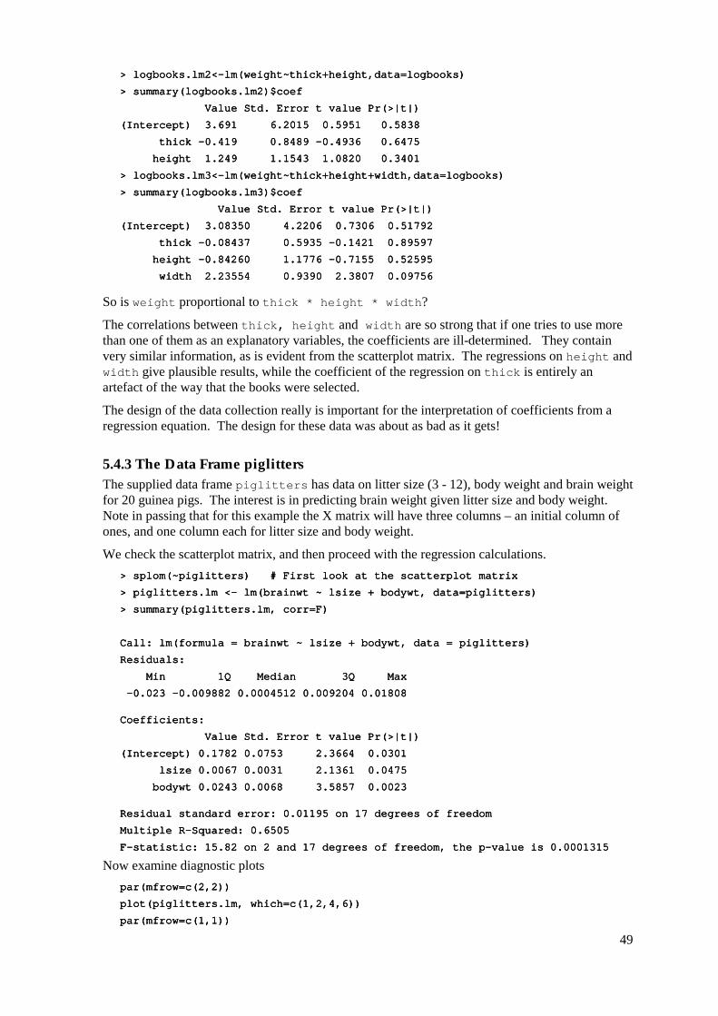
49

> logbooks.lm2<> logbooks.lm2<> logbooks.lm2<> logbooks.lm2<----lm(weight~thick+heightlm(weight~thick+heightlm(weight~thick+heightlm(weight~thick+height,data=logbooks),data=logbooks),data=logbooks),data=logbooks)

> summary(logbooks.lm2)$coef> summary(logbooks.lm2)$coef> summary(logbooks.lm2)$coef> summary(logbooks.lm2)$coef

Value Std. Error t value Pr(>|t|) Value Std. Error t value Pr(>|t|) Value Std. Error t value Pr(>|t|) Value Std. Error t value Pr(>|t|)

(Intercept) 3.691 6.2015 0.5951 0.5838(Intercept) 3.691 6.2015 0.5951 0.5838(Intercept) 3.691 6.2015 0.5951 0.5838(Intercept) 3.691 6.2015 0.5951 0.5838

thick thick thick thick ----0.419 0.8489 0.419 0.8489 0.419 0.8489 0.419 0.8489 ----0.4936 0.64750.4936 0.64750.4936 0.64750.4936 0.6475

height 1.249 1.1543 1.0820 0.3401 height 1.249 1.1543 1.0820 0.3401 height 1.249 1.1543 1.0820 0.3401 height 1.249 1.1543 1.0820 0.3401

> logbooks.lm3<> logbooks.lm3<> logbooks.lm3<> logbooks.lm3<----lm(weilm(weilm(weilm(weight~thick+height+width,data=logbooks)ght~thick+height+width,data=logbooks)ght~thick+height+width,data=logbooks)ght~thick+height+width,data=logbooks)

> summary(logbooks.lm3)$coef> summary(logbooks.lm3)$coef> summary(logbooks.lm3)$coef> summary(logbooks.lm3)$coef

Value Std. Error t value Pr(>|t|) Value Std. Error t value Pr(>|t|) Value Std. Error t value Pr(>|t|) Value Std. Error t value Pr(>|t|)

(Intercept) 3.08350 4.2206 0.7306 0.51792(Intercept) 3.08350 4.2206 0.7306 0.51792(Intercept) 3.08350 4.2206 0.7306 0.51792(Intercept) 3.08350 4.2206 0.7306 0.51792

thick thick thick thick ----0.08437 0.5935 0.08437 0.5935 0.08437 0.5935 0.08437 0.5935 ----0.1421 0.895970.1421 0.895970.1421 0.895970.1421 0.89597

height height height height ----0.84260 1.1776 0.84260 1.1776 0.84260 1.1776 0.84260 1.1776 ----0.7155 0.7155 0.7155 0.7155 0.525950.525950.525950.52595

width 2.23554 0.9390 2.3807 0.09756 width 2.23554 0.9390 2.3807 0.09756 width 2.23554 0.9390 2.3807 0.09756 width 2.23554 0.9390 2.3807 0.09756

So is weight proportional to thick * height * width?

The correlations between thick, , , , height and width are so strong that if one tries to use more than one of them as an explanatory variables, the coefficients are ill-determined. They contain very similar information, as is evident from the scatterplot matrix. The regressions on height and width give plausible results, while the coefficient of the regression on thick is entirely an artefact of the way that the books were selected.

The design of the data collection really is important for the interpretation of coefficients from a regression equation. The design for these data was about as bad as it gets!

5.4.3 The Data Frame piglitters The supplied data frame piglitters has data on litter size (3 - 12), body weight and brain weight for 20 guinea pigs. The interest is in predicting brain weight given litter size and body weight. Note in passing that for this example the X matrix will have three columns – an initial column of ones, and one column each for litter size and body weight.

We check the scatterplot matrix, and then proceed with the regression calculations. > splom(~piglitters) # First look at the scatterplot matrix> splom(~piglitters) # First look at the scatterplot matrix> splom(~piglitters) # First look at the scatterplot matrix> splom(~piglitters) # First look at the scatterplot matrix

> piglitters.lm <> piglitters.lm <> piglitters.lm <> piglitters.lm <---- lm lm lm lm(brainwt ~ lsize + bodywt, data=piglitters)(brainwt ~ lsize + bodywt, data=piglitters)(brainwt ~ lsize + bodywt, data=piglitters)(brainwt ~ lsize + bodywt, data=piglitters)

> summary(piglitters.lm, corr=F)> summary(piglitters.lm, corr=F)> summary(piglitters.lm, corr=F)> summary(piglitters.lm, corr=F)

Call: lm(formula = brainwt ~ lsize + bodywt, data = piglitters)Call: lm(formula = brainwt ~ lsize + bodywt, data = piglitters)Call: lm(formula = brainwt ~ lsize + bodywt, data = piglitters)Call: lm(formula = brainwt ~ lsize + bodywt, data = piglitters)

Residuals:Residuals:Residuals:Residuals:

Min 1Q Median 3Q Max Min 1Q Median 3Q Max Min 1Q Median 3Q Max Min 1Q Median 3Q Max

----0.023 0.023 0.023 0.023 ----0.009882 0.0004512 0.009204 0.018080.009882 0.0004512 0.009204 0.018080.009882 0.0004512 0.009204 0.018080.009882 0.0004512 0.009204 0.01808

CoefficientsCoefficientsCoefficientsCoefficients::::

Value Std. Error t value Pr(>|t|) Value Std. Error t value Pr(>|t|) Value Std. Error t value Pr(>|t|) Value Std. Error t value Pr(>|t|)

(Intercept) 0.1782 0.0753 2.3664 0.0301 (Intercept) 0.1782 0.0753 2.3664 0.0301 (Intercept) 0.1782 0.0753 2.3664 0.0301 (Intercept) 0.1782 0.0753 2.3664 0.0301

lsize 0.0067 0.0031 2.1361 0.0475 lsize 0.0067 0.0031 2.1361 0.0475 lsize 0.0067 0.0031 2.1361 0.0475 lsize 0.0067 0.0031 2.1361 0.0475

bodywt 0.0243 0.0068 3.5857 0.0023 bodywt 0.0243 0.0068 3.5857 0.0023 bodywt 0.0243 0.0068 3.5857 0.0023 bodywt 0.0243 0.0068 3.5857 0.0023

Residual standard error: 0.01195 on 17 degrees of freedomResidual standard error: 0.01195 on 17 degrees of freedomResidual standard error: 0.01195 on 17 degrees of freedomResidual standard error: 0.01195 on 17 degrees of freedom

MultiplMultiplMultiplMultiple Re Re Re R----Squared: 0.6505 Squared: 0.6505 Squared: 0.6505 Squared: 0.6505

FFFF----statistic: 15.82 on 2 and 17 degrees of freedom, the pstatistic: 15.82 on 2 and 17 degrees of freedom, the pstatistic: 15.82 on 2 and 17 degrees of freedom, the pstatistic: 15.82 on 2 and 17 degrees of freedom, the p----value is 0.0001315 value is 0.0001315 value is 0.0001315 value is 0.0001315

Now examine diagnostic plots par(mfrow=c(2,2))par(mfrow=c(2,2))par(mfrow=c(2,2))par(mfrow=c(2,2))

plot(piglitters.lm, which=c(1,2,4,6))plot(piglitters.lm, which=c(1,2,4,6))plot(piglitters.lm, which=c(1,2,4,6))plot(piglitters.lm, which=c(1,2,4,6))

par(mfrow=c(1,1))par(mfrow=c(1,1))par(mfrow=c(1,1))par(mfrow=c(1,1))

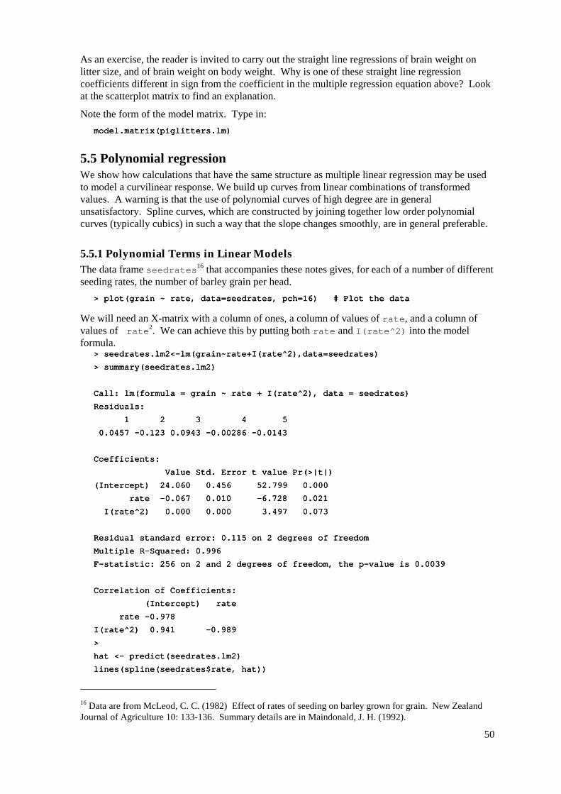
50

As an exercise, the reader is invited to carry out the straight line regressions of brain weight on litter size, and of brain weight on body weight. Why is one of these straight line regression coefficients different in sign from the coefficient in the multiple regression equation above? Look at the scatterplot matrix to find an explanation.

Note the form of the model matrix. Type in: model.matrix(piglitters.lm)model.matrix(piglitters.lm)model.matrix(piglitters.lm)model.matrix(piglitters.lm)

5.5 Polynomial regression We show how calculations that have the same structure as multiple linear regression may be used to model a curvilinear response. We build up curves from linear combinations of transformed values. A warning is that the use of polynomial curves of high degree are in general unsatisfactory. Spline curves, which are constructed by joining together low order polynomial curves (typically cubics) in such a way that the slope changes smoothly, are in general preferable.

5.5.1 Polynomial Terms in Linear Models The data frame seedrates16 that accompanies these notes gives, for each of a number of different seeding rates, the number of barley grain per head.

> plot(grain ~ rate, data=seedrates, pch=16) # Plot the data> plot(grain ~ rate, data=seedrates, pch=16) # Plot the data> plot(grain ~ rate, data=seedrates, pch=16) # Plot the data> plot(grain ~ rate, data=seedrates, pch=16) # Plot the data

We will need an X-matrix with a column of ones, a column of values of rate, and a column of values of rate2. We can achieve this by putting both rate and I(rate^2) into the model formula.

> seedrates.lm2<> seedrates.lm2<> seedrates.lm2<> seedrates.lm2<----lm(grain~rate+I(rate^2),data=seedrates)lm(grain~rate+I(rate^2),data=seedrates)lm(grain~rate+I(rate^2),data=seedrates)lm(grain~rate+I(rate^2),data=seedrates)

> summary(seedrates.lm2)> summary(seedrates.lm2)> summary(seedrates.lm2)> summary(seedrates.lm2)

Call: lm(formula = grain ~ rate + I(rate^2), data = seedrates)Call: lm(formula = grain ~ rate + I(rate^2), data = seedrates)Call: lm(formula = grain ~ rate + I(rate^2), data = seedrates)Call: lm(formula = grain ~ rate + I(rate^2), data = seedrates)

Residuals:Residuals:Residuals:Residuals:

1 2 3 4 5 1 2 3 4 5 1 2 3 4 5 1 2 3 4 5

0.0457 0.0457 0.0457 0.0457 ----0.123 0.0943 0.123 0.0943 0.123 0.0943 0.123 0.0943 ----0.00286 0.00286 0.00286 0.00286 ----0.01430.01430.01430.0143

Coefficients:Coefficients:Coefficients:Coefficients:

Value Std. Error t value Pr(>|t|) Value Std. Error t value Pr(>|t|) Value Std. Error t value Pr(>|t|) Value Std. Error t value Pr(>|t|)

(Intercept) 24.060 0.456 52.799 0.000 (Intercept) 24.060 0.456 52.799 0.000 (Intercept) 24.060 0.456 52.799 0.000 (Intercept) 24.060 0.456 52.799 0.000

rate rate rate rate ----0.067 0.010 0.067 0.010 0.067 0.010 0.067 0.010 ----6.728 0.021 6.728 0.021 6.728 0.021 6.728 0.021

I(rate^2) 0.000 0.000 3.497 0.073 I(rate^2) 0.000 0.000 3.497 0.073 I(rate^2) 0.000 0.000 3.497 0.073 I(rate^2) 0.000 0.000 3.497 0.073

Residual standard error: 0.115 on 2 degrees of Residual standard error: 0.115 on 2 degrees of Residual standard error: 0.115 on 2 degrees of Residual standard error: 0.115 on 2 degrees of freedomfreedomfreedomfreedom

Multiple RMultiple RMultiple RMultiple R----Squared: 0.996 Squared: 0.996 Squared: 0.996 Squared: 0.996

FFFF----statistic: 256 on 2 and 2 degrees of freedom, the pstatistic: 256 on 2 and 2 degrees of freedom, the pstatistic: 256 on 2 and 2 degrees of freedom, the pstatistic: 256 on 2 and 2 degrees of freedom, the p----value is 0.0039 value is 0.0039 value is 0.0039 value is 0.0039

Correlation of Coefficients:Correlation of Coefficients:Correlation of Coefficients:Correlation of Coefficients:

(Intercept) rate (Intercept) rate (Intercept) rate (Intercept) rate

rate rate rate rate ----0.978 0.978 0.978 0.978

I(rate^2) 0.941 I(rate^2) 0.941 I(rate^2) 0.941 I(rate^2) 0.941 ----0.9890.9890.9890.989

>>>>

hat <hat <hat <hat <---- predict(seedrates.lm2) predict(seedrates.lm2) predict(seedrates.lm2) predict(seedrates.lm2)

lines(spline(seedrates$rate, hat))lines(spline(seedrates$rate, hat))lines(spline(seedrates$rate, hat))lines(spline(seedrates$rate, hat))

16 Data are from McLeod, C. C. (1982) Effect of rates of seeding on barley grown for grain. New Zealand Journal of Agriculture 10: 133-136. Summary details are in Maindonald, J. H. (1992).

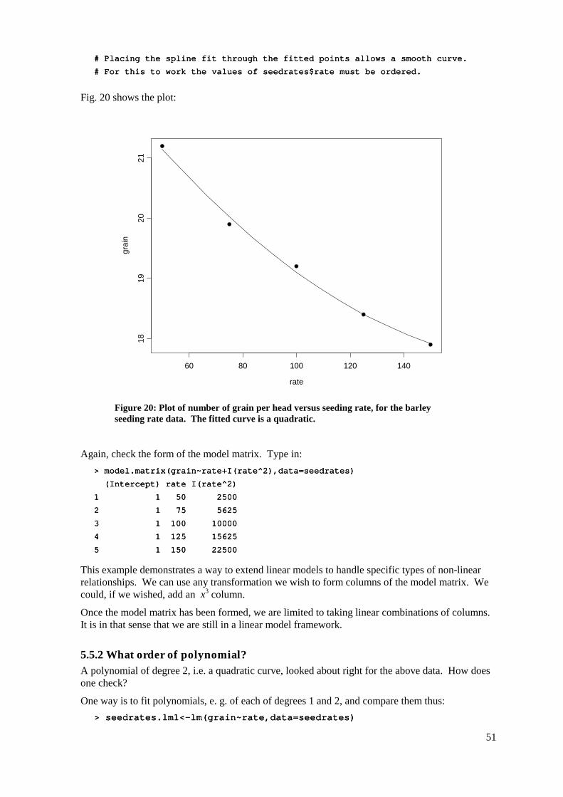
51

# Placing the spline fit through the fitted points allows a smooth curve.# Placing the spline fit through the fitted points allows a smooth curve.# Placing the spline fit through the fitted points allows a smooth curve.# Placing the spline fit through the fitted points allows a smooth curve.

# For this to work the values of seedrates$rate must be ordered.# For this to work the values of seedrates$rate must be ordered.# For this to work the values of seedrates$rate must be ordered.# For this to work the values of seedrates$rate must be ordered.

Fig. 20 shows the plot:

rate

grai

n

60 80 100 120 140

1819

2021

Figure 20: Plot of number of grain per head versus seeding rate, for the barley seeding rate data. The fitted curve is a quadratic.

Again, check the form of the model matrix. Type in: > model.matrix(grain~rate+I(rate^2),data=seedrates)> model.matrix(grain~rate+I(rate^2),data=seedrates)> model.matrix(grain~rate+I(rate^2),data=seedrates)> model.matrix(grain~rate+I(rate^2),data=seedrates)

(Intercept) rate I(rate^2) (Intercept) rate I(rate^2) (Intercept) rate I(rate^2) (Intercept) rate I(rate^2)

1 1 1 1 1 50 2500 1 50 2500 1 50 2500 1 50 2500

2 1 75 56252 1 75 56252 1 75 56252 1 75 5625

3 1 100 100003 1 100 100003 1 100 100003 1 100 10000

4 1 125 156254 1 125 156254 1 125 156254 1 125 15625

5 1 150 225005 1 150 225005 1 150 225005 1 150 22500

This example demonstrates a way to extend linear models to handle specific types of non-linear relationships. We can use any transformation we wish to form columns of the model matrix. We could, if we wished, add an x3 column.

Once the model matrix has been formed, we are limited to taking linear combinations of columns. It is in that sense that we are still in a linear model framework.

5.5.2 What order of polynomial? A polynomial of degree 2, i.e. a quadratic curve, looked about right for the above data. How does one check?

One way is to fit polynomials, e. g. of each of degrees 1 and 2, and compare them thus: > seed> seed> seed> seedrates.lm1<rates.lm1<rates.lm1<rates.lm1<----lm(grain~rate,data=seedrates)lm(grain~rate,data=seedrates)lm(grain~rate,data=seedrates)lm(grain~rate,data=seedrates)

52

> seedrates.lm2<> seedrates.lm2<> seedrates.lm2<> seedrates.lm2<----lm(grain~rate+I(rate^2),data=seedrates)lm(grain~rate+I(rate^2),data=seedrates)lm(grain~rate+I(rate^2),data=seedrates)lm(grain~rate+I(rate^2),data=seedrates)

> anova(seedrates.lm2,seedrates.lm1)> anova(seedrates.lm2,seedrates.lm1)> anova(seedrates.lm2,seedrates.lm1)> anova(seedrates.lm2,seedrates.lm1)

Analysis of Variance TableAnalysis of Variance TableAnalysis of Variance TableAnalysis of Variance Table

Response: grainResponse: grainResponse: grainResponse: grain

Terms Resid. Df RSS Test Df Sum of Sq Terms Resid. Df RSS Test Df Sum of Sq Terms Resid. Df RSS Test Df Sum of Sq Terms Resid. Df RSS Test Df Sum of Sq

1 rate + I(rate^21 rate + I(rate^21 rate + I(rate^21 rate + I(rate^2) 2 0.0263 ) 2 0.0263 ) 2 0.0263 ) 2 0.0263

2 rate 3 0.1870 2 rate 3 0.1870 2 rate 3 0.1870 2 rate 3 0.1870 ----I(rate^2) I(rate^2) I(rate^2) I(rate^2) ----1 1 1 1 ----0.16070.16070.16070.1607

F Value Pr(F) F Value Pr(F) F Value Pr(F) F Value Pr(F)

1 1 1 1

2 12.23 0.072942 12.23 0.072942 12.23 0.072942 12.23 0.07294

The F-value is large, but on this evidence there are too few degrees of freedom to make a totally convincing case for preferring a quadratic to a line. However the paper from which these data come gives an independent estimate of the error mean square (0.17 on 35 d.f.) based on 8 replicate results that were averaged to give each value for number of grains per head. If we compare the change in the sum of squares (0.1607, on 1 df) with a mean square of 0.172 (35 df), the F-value is now 5.4 on 1 and 35 degrees of freedom, and we have p=0.024 . The increase in the number of degrees of freedom more than compensates for the reduction in the F-statistic.

> # However we have an independent estimate of the error mean square> # However we have an independent estimate of the error mean square> # However we have an independent estimate of the error mean square> # However we have an independent estimate of the error mean square

> # The estimate is 0.17^2, on 35 df.> # The estimate is 0.17^2, on 35 df.> # The estimate is 0.17^2, on 35 df.> # The estimate is 0.17^2, on 35 df.

> 1> 1> 1> 1----pf(0.16/0.17^2, 1, 35)pf(0.16/0.17^2, 1, 35)pf(0.16/0.17^2, 1, 35)pf(0.16/0.17^2, 1, 35)

[1] 0.02437[1] 0.02437[1] 0.02437[1] 0.02437

Finally note that R2 was 0.972 for the straight line model. This may seem good, but given the accuracy of these data it was not good enough! The statistic is not an inadequate guide to whether a model is adequate. Even for any one context, R2 will in general increase as the range of the values of the dependent variable increases. (R2 is larger when there is more variation to be explained.) A predictive model is adequate when the standard errors of predicted values are acceptably small, not when R2 achieves some magic threshold.

R2 may be used for comparing results from different sets of data where the combinations of values of explanatory variables are broadly similar. Even for that purpose, it is a crude measure.

5.5.3 Pointwise confidence bounds for the fitted curve Here is code that will give pointwise 95% confidence bounds. Note that these do not combine to give a confidence region for the total curve! The construction of such a region is a much more complicated task!

plot(grain ~ rate, data = seedrates, pch = 16, xlim = c(50, 175), ylimplot(grain ~ rate, data = seedrates, pch = 16, xlim = c(50, 175), ylimplot(grain ~ rate, data = seedrates, pch = 16, xlim = c(50, 175), ylimplot(grain ~ rate, data = seedrates, pch = 16, xlim = c(50, 175), ylim

= = = = c(15.5, 22),xlab="Seeding rate",ylab="Grains per head")c(15.5, 22),xlab="Seeding rate",ylab="Grains per head")c(15.5, 22),xlab="Seeding rate",ylab="Grains per head")c(15.5, 22),xlab="Seeding rate",ylab="Grains per head")

new.df <new.df <new.df <new.df <---- data.frame(rate = c((4:14) * 12.5)) data.frame(rate = c((4:14) * 12.5)) data.frame(rate = c((4:14) * 12.5)) data.frame(rate = c((4:14) * 12.5))

seedrates.lm2 <seedrates.lm2 <seedrates.lm2 <seedrates.lm2 <---- lm(grain ~ rate + I(rate^2), data = seedrates) lm(grain ~ rate + I(rate^2), data = seedrates) lm(grain ~ rate + I(rate^2), data = seedrates) lm(grain ~ rate + I(rate^2), data = seedrates)

fitinfo <fitinfo <fitinfo <fitinfo <---- predict(seedrates.lm2, newdata=new.df, se=T) predict(seedrates.lm2, newdata=new.df, se=T) predict(seedrates.lm2, newdata=new.df, se=T) predict(seedrates.lm2, newdata=new.df, se=T)

ci <ci <ci <ci <---- pointwise(fitinfo, coverage= pointwise(fitinfo, coverage= pointwise(fitinfo, coverage= pointwise(fitinfo, coverage=0.95)0.95)0.95)0.95)

lines(new.df$rate, ci$fit)lines(new.df$rate, ci$fit)lines(new.df$rate, ci$fit)lines(new.df$rate, ci$fit)

lines(new.df$rate, ci$lower,lty=2)lines(new.df$rate, ci$lower,lty=2)lines(new.df$rate, ci$lower,lty=2)lines(new.df$rate, ci$lower,lty=2)

lines(new.df$rate, ci$upper,lty=2)lines(new.df$rate, ci$upper,lty=2)lines(new.df$rate, ci$upper,lty=2)lines(new.df$rate, ci$upper,lty=2)

The extrapolation has deliberately been taken beyond the range of the data, in order to show how the confidence bounds spread out. Confidence bounds for a fitted line will spread out much more slowly, but are even less believable!

53

*5.5.4 Spline Terms in Linear Models By now, readers of this document will be used to the idea that it is possible to use linear models to fit terms that may be highly nonlinear functions of one or more variables. The fitting of polynomial functions was a simple example of this. Spline functions variables extend this idea further. The splines that I demonstrate are constructed by joining together cubic curves, in such a way the joins are smooth. The places where the cubics join are known as `knots’. It turns out that, once the knots are fixed, and depending on the class of spline curves that are used, spline functions of a variable can be constructed as a linear combination of basis functions, where each basis function is a transformation of the variable.

The data frame cars accompanies these notes: > plot(dist~speed,data=cars)> plot(dist~speed,data=cars)> plot(dist~speed,data=cars)> plot(dist~speed,data=cars)

> cars.lm<> cars.lm<> cars.lm<> cars.lm<----lm(dist~bs(speed),data=cars) # By default, there are no knotslm(dist~bs(speed),data=cars) # By default, there are no knotslm(dist~bs(speed),data=cars) # By default, there are no knotslm(dist~bs(speed),data=cars) # By default, there are no knots

> hat<> hat<> hat<> hat<----predict(cars.lm, sepredict(cars.lm, sepredict(cars.lm, sepredict(cars.lm, se=T)=T)=T)=T)

> lines(cars$speed,hat,lty=3) # NB assumes values of speed are sorted> lines(cars$speed,hat,lty=3) # NB assumes values of speed are sorted> lines(cars$speed,hat,lty=3) # NB assumes values of speed are sorted> lines(cars$speed,hat,lty=3) # NB assumes values of speed are sorted

> cars5.lm<cars5.lm<cars5.lm<cars5.lm<----lm(dist~bs(speed,5), data=cars)lm(dist~bs(speed,5), data=cars)lm(dist~bs(speed,5), data=cars)lm(dist~bs(speed,5), data=cars)

# B # B # B # B----spline fit, 1 knotspline fit, 1 knotspline fit, 1 knotspline fit, 1 knot

> ci5 <> ci5 <> ci5 <> ci5 <---- pointwise(predict(cars5.lm, se.fit=T), coverage=0.95 pointwise(predict(cars5.lm, se.fit=T), coverage=0.95 pointwise(predict(cars5.lm, se.fit=T), coverage=0.95 pointwise(predict(cars5.lm, se.fit=T), coverage=0.95

> names(ci5)> names(ci5)> names(ci5)> names(ci5)

[1] "fit" "se.fit" [1] "fit" "se.fit" [1] "fit" "se.fit" [1] "fit" "se.fit" "df" "residual.scale" "df" "residual.scale" "df" "residual.scale" "df" "residual.scale"

> lines(cars$speed, ci5$fit)> lines(cars$speed, ci5$fit)> lines(cars$speed, ci5$fit)> lines(cars$speed, ci5$fit)

> lines(cars$speed, ci5$lower,lty=2)> lines(cars$speed, ci5$lower,lty=2)> lines(cars$speed, ci5$lower,lty=2)> lines(cars$speed, ci5$lower,lty=2)

> lines(cars$speed, ci5$upper,lty=2)> lines(cars$speed, ci5$upper,lty=2)> lines(cars$speed, ci5$upper,lty=2)> lines(cars$speed, ci5$upper,lty=2)

5.6 Using Factors in S-PLUS Models Factors are essential, when there are categorical or “factor” variables, for specifying S-PLUS models. Consider data from an experiment that compared houses with and without cavity insulation. While one would not usually handle these calculations using an lm model, it makes a simple example to illustrate the choice of a baseline level, and a set of contrasts. Different choices, although they fit equivalent models, give output in which some of the numbers are different and must be interpreted differently.

We begin by entering the data from the command line: insulation insulation insulation insulation <<<<---- factor(c(rep("without", 8), rep("with", 7))) factor(c(rep("without", 8), rep("with", 7))) factor(c(rep("without", 8), rep("with", 7))) factor(c(rep("without", 8), rep("with", 7)))

# 8 without, then 7 with# 8 without, then 7 with# 8 without, then 7 with# 8 without, then 7 with

kWh <kWh <kWh <kWh <---- c(10225, 10689, 14683, 6584, 8541, 12086, 12467, c(10225, 10689, 14683, 6584, 8541, 12086, 12467, c(10225, 10689, 14683, 6584, 8541, 12086, 12467, c(10225, 10689, 14683, 6584, 8541, 12086, 12467,

12669, 9708, 6700, 4307, 10315, 8017, 8162, 8022)12669, 9708, 6700, 4307, 10315, 8017, 8162, 8022)12669, 9708, 6700, 4307, 10315, 8017, 8162, 8022)12669, 9708, 6700, 4307, 10315, 8017, 8162, 8022)

To formulate this as a regression model, we take kWh as the dependent variable, and the factor insulation as the explanatory variable.

> options(contrasts = c("contr.treatment", "contr.poly"), digits = 2)> options(contrasts = c("contr.treatment", "contr.poly"), digits = 2)> options(contrasts = c("contr.treatment", "contr.poly"), digits = 2)> options(contrasts = c("contr.treatment", "contr.poly"), digits = 2)

> insulation.lm <> insulation.lm <> insulation.lm <> insulation.lm <---- lm(kWh ~ insulation) lm(kWh ~ insulation) lm(kWh ~ insulation) lm(kWh ~ insulation)

> summary(insulation.lm, corr=F)> summary(insulation.lm, corr=F)> summary(insulation.lm, corr=F)> summary(insulation.lm, corr=F)

Call: lm(formula = kWh ~ insulation)Call: lm(formula = kWh ~ insulation)Call: lm(formula = kWh ~ insulation)Call: lm(formula = kWh ~ insulation)

Residuals:Residuals:Residuals:Residuals:

M M M Min 1Q Median 3Q Max in 1Q Median 3Q Max in 1Q Median 3Q Max in 1Q Median 3Q Max

----4409 4409 4409 4409 ----979 132 1575 3690979 132 1575 3690979 132 1575 3690979 132 1575 3690

Coefficients:Coefficients:Coefficients:Coefficients:

Value Std. Error t value Pr(>|t|) Value Std. Error t value Pr(>|t|) Value Std. Error t value Pr(>|t|) Value Std. Error t value Pr(>|t|)

(Intercept) 7890.143 873.753 9.030 0.000(Intercept) 7890.143 873.753 9.030 0.000(Intercept) 7890.143 873.753 9.030 0.000(Intercept) 7890.143 873.753 9.030 0.000

insulation 3102.857 1196.436 2.593 0.022 insulation 3102.857 1196.436 2.593 0.022 insulation 3102.857 1196.436 2.593 0.022 insulation 3102.857 1196.436 2.593 0.022

54

Residual standard error: 2310 on 13Residual standard error: 2310 on 13Residual standard error: 2310 on 13Residual standard error: 2310 on 13 degrees of freedom degrees of freedom degrees of freedom degrees of freedom

Multiple RMultiple RMultiple RMultiple R----Squared: 0.34 Squared: 0.34 Squared: 0.34 Squared: 0.34

FFFF----statistic: 6.7 on 1 and 13 degrees of freedom, the pstatistic: 6.7 on 1 and 13 degrees of freedom, the pstatistic: 6.7 on 1 and 13 degrees of freedom, the pstatistic: 6.7 on 1 and 13 degrees of freedom, the p----value is 0.022 value is 0.022 value is 0.022 value is 0.022

The p-value is 0.022, which may be taken to indicate (p < 0.05) that we can distinguish between the two types of houses. But what does the “intercept” of 9441.57 mean, and what does the value for “insulation” of 1551.43 mean? To interpret this, we need to know that the factor levels are, by default, taken in alphabetical order, and that the initial level is taken as the baseline. So with comes before without, and with is the baseline. Hence:

Average for Insulated Houses = 7980.1

To get the estimate for uninsulated houses take 7980.1 + 3102.9 = 10993.0

The standard error of the difference is 1196.4

Warning: Unless you specifically want helmert contrasts (see section 5.6.2), make sure that before fitting any lm model that uses factors you give the command:

options(contrasts = c("contr.treatment", "contr.poly"), digits = 3)options(contrasts = c("contr.treatment", "contr.poly"), digits = 3)options(contrasts = c("contr.treatment", "contr.poly"), digits = 3)options(contrasts = c("contr.treatment", "contr.poly"), digits = 3)

[Setting the number of digits is optional; but three is often sensible.]

Another possibility is: options(contrasts = c("contr.sum", "contr.poly"), digits = 3)options(contrasts = c("contr.sum", "contr.poly"), digits = 3)options(contrasts = c("contr.sum", "contr.poly"), digits = 3)options(contrasts = c("contr.sum", "contr.poly"), digits = 3)

Section 5.6.2 will explain why.

5.6.1 The Model Matrix It often helps to think in terms of the model matrix or X matrix. Here are the X and the y that are used for the calculations. Note that the first eight data values were all withouts:

Contrast kWh

× 7980.1 × 3102.9 Add to get Compare with Residual

1 1 7980.1+3102.9=10993.0 10225 10225-10993.0 1 1 7980.1+3102.9=10993.0 10689 10689-10993.0 . . . . 1 0 7980.1+0 9708 9708-7980.1 1 0 7980.1+0 6700 6700-7980.1 . . . .

Type in model.matrix(kWh~insulation)model.matrix(kWh~insulation)model.matrix(kWh~insulation)model.matrix(kWh~insulation)

and check that one gets the above model matrix.

*5.6.2 Other Choices of Contrasts There are other ways to set up the X matrix. In technical jargon, there are other contrasts that one can choose. One obvious alternative is to make without the first factor level, so that it becomes the baseline. You can do this in the following way:

> insulation <> insulation <> insulation <> insulation <---- factor(insulation, labels=c(“without”, “with”) factor(insulation, labels=c(“without”, “with”) factor(insulation, labels=c(“without”, “with”) factor(insulation, labels=c(“without”, “with”)

55

Another possibility is to use what are called the “helmert” contrasts. Although this is the S-PLUS default, I recommend that you avoid them. That was the reason for the option setting:

> options(contrasts = c("contr.treatment", "contr.poly"), digits = 2)> options(contrasts = c("contr.treatment", "contr.poly"), digits = 2)> options(contrasts = c("contr.treatment", "contr.poly"), digits = 2)> options(contrasts = c("contr.treatment", "contr.poly"), digits = 2)

Here is the output you get if you use the Helmert contrasts: Coefficients:Coefficients:Coefficients:Coefficients:

Value Std. Error t value Pr(>|t|) Value Std. Error t value Pr(>|t|) Value Std. Error t value Pr(>|t|) Value Std. Error t value Pr(>|t|)

(Intercept) 9441.571 598.218 15.783 0.000(Intercept) 9441.571 598.218 15.783 0.000(Intercept) 9441.571 598.218 15.783 0.000(Intercept) 9441.571 598.218 15.783 0.000

insulation 1551.429 598.218 2.593 0.022 insulation 1551.429 598.218 2.593 0.022 insulation 1551.429 598.218 2.593 0.022 insulation 1551.429 598.218 2.593 0.022

Residual standard error: 2310 on 13 degrees of freedomResidual standard error: 2310 on 13 degrees of freedomResidual standard error: 2310 on 13 degrees of freedomResidual standard error: 2310 on 13 degrees of freedom

Multiple RMultiple RMultiple RMultiple R----Squared: 0.341 Squared: 0.341 Squared: 0.341 Squared: 0.341

FFFF----statistic: 6.73 on 1 and 13 degrees of freedom, the pstatistic: 6.73 on 1 and 13 degrees of freedom, the pstatistic: 6.73 on 1 and 13 degrees of freedom, the pstatistic: 6.73 on 1 and 13 degrees of freedom, the p----value is 0.0223 value is 0.0223 value is 0.0223 value is 0.0223

Here is the interpretation:

average of (mean for “without”, “mean for with”) = 9441.57

To get the estimate for insulated houses (the first level), take 9441.57 - 1551.43 = 7890.14

To get the estimate for insulated houses (the first level), take 9441.57 + 1551.43 = 10993.

The interpretation of the helmert contrasts is simple enough when there are just two levels. With >2 levels, the helmert contrasts give parameter estimates which in general do not make a lot of sense, basically because the baseline keeps changing, to the average for all previous factor levels. You do better to use either the treatment contrasts, or the sum contrasts. With the sum contrasts the baseline is the overall mean. The sum contrasts are sometimes called “analysis of variance” contrasts17.

You can set the choice of contrasts for each factor separately, with a statement such as: insulation <insulation <insulation <insulation <---- C(insulation, contr=treatment) C(insulation, contr=treatment) C(insulation, contr=treatment) C(insulation, contr=treatment)

The statement that we used earlier, i.e.18 options(contrasts=c("contr.treatment", "contr.poly"))

does this for all factors, except any that have perhaps been set individually.

*5.6.3 Factor Attributes Factors are relatively complex objects. Below, we form a factor and then examine its attributes:

> options(contrasts=c(“contr.treatment”,”contr.poly”))> options(contrasts=c(“contr.treatment”,”contr.poly”))> options(contrasts=c(“contr.treatment”,”contr.poly”))> options(contrasts=c(“contr.treatment”,”contr.poly”))

> fac<> fac<> fac<> fac<---- factor(1:5) factor(1:5) factor(1:5) factor(1:5)

> attributes(fac)> attributes(fac)> attributes(fac)> attributes(fac)

$levels:$levels:$levels:$levels:

[1] "1" "2" "[1] "1" "2" "[1] "1" "2" "[1] "1" "2" "3" "4" "5"3" "4" "5"3" "4" "5"3" "4" "5"

$class:$class:$class:$class:

[1] "factor"[1] "factor"[1] "factor"[1] "factor"

17 To make the sum contrasts the default for all factors, begin your work by specifying options(contrasts=c("contr.sum", "contr.poly"))

The Helmert contrasts, which are the default, contrast each level with the average of all earlier levels. The coefficients are half of this difference. 18 The second string element, i.e. "contr.poly", is the default setting for factors with ordered levels. [One uses the function ordered() to create ordered factors.]

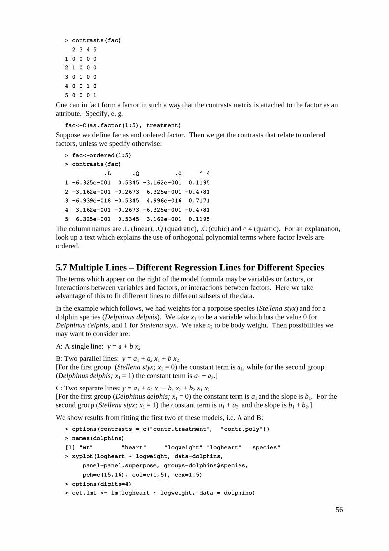
56

> contrasts(fac)> contrasts(fac)> contrasts(fac)> contrasts(fac)

2 3 4 5 2 3 4 5 2 3 4 5 2 3 4 5

1 0 0 0 01 0 0 0 01 0 0 0 01 0 0 0 0

2 1 0 0 02 1 0 0 02 1 0 0 02 1 0 0 0

3 0 1 0 03 0 1 0 03 0 1 0 03 0 1 0 0

4 0 0 1 04 0 0 1 04 0 0 1 04 0 0 1 0

5 0 0 0 15 0 0 0 15 0 0 0 15 0 0 0 1

One can in fact form a factor in such a way that the contrasts matrix is attached to the factor as an attribute. Specify, e. g.

fac<fac<fac<fac<----C(as.factorC(as.factorC(as.factorC(as.factor(1:5), treatment)(1:5), treatment)(1:5), treatment)(1:5), treatment)

Suppose we define fac as and ordered factor. Then we get the contrasts that relate to ordered factors, unless we specify otherwise:

> fac<> fac<> fac<> fac<----ordered(1:5)ordered(1:5)ordered(1:5)ordered(1:5)

> contrasts(fac)> contrasts(fac)> contrasts(fac)> contrasts(fac)

.L .Q .C ^ 4 .L .Q .C ^ 4 .L .Q .C ^ 4 .L .Q .C ^ 4

1 1 1 1 ----6.325e6.325e6.325e6.325e----001 0.5345 001 0.5345 001 0.5345 001 0.5345 ----3.3.3.3.162e162e162e162e----001 0.1195001 0.1195001 0.1195001 0.1195

2 2 2 2 ----3.162e3.162e3.162e3.162e----001 001 001 001 ----0.2673 6.325e0.2673 6.325e0.2673 6.325e0.2673 6.325e----001 001 001 001 ----0.47810.47810.47810.4781

3 3 3 3 ----6.939e6.939e6.939e6.939e----018 018 018 018 ----0.5345 4.996e0.5345 4.996e0.5345 4.996e0.5345 4.996e----016 0.7171016 0.7171016 0.7171016 0.7171

4 3.162e4 3.162e4 3.162e4 3.162e----001 001 001 001 ----0.2673 0.2673 0.2673 0.2673 ----6.325e6.325e6.325e6.325e----001 001 001 001 ----0.47810.47810.47810.4781

5 6.325e5 6.325e5 6.325e5 6.325e----001 0.5345 3.162e001 0.5345 3.162e001 0.5345 3.162e001 0.5345 3.162e----001 0.1195001 0.1195001 0.1195001 0.1195

The column names are .L (linear), .Q (quadratic), .C (cubic) and ^ 4 (quartic). For an explanation, look up a text which explains the use of orthogonal polynomial terms where factor levels are ordered.

5.7 Multiple Lines – Different Regression Lines for Different Species The terms which appear on the right of the model formula may be variables or factors, or interactions between variables and factors, or interactions between factors. Here we take advantage of this to fit different lines to different subsets of the data.

In the example which follows, we had weights for a porpoise species (Stellena styx) and for a dolphin species (Delphinus delphis). We take x1 to be a variable which has the value 0 for Delphinus delphis, and 1 for Stellena styx. We take x2 to be body weight. Then possibilities we may want to consider are:

A: A single line: y = a + b x2

B: Two parallel lines: y = a1 + a2 x1 + b x2 [For the first group (Stellena styx; x1 = 0) the constant term is a1, while for the second group (Delphinus delphis; x1 = 1) the constant term is a1 + a2.]

C: Two separate lines: y = a1 + a2 x1 + b1 x2 + b2 x1 x2 [For the first group (Delphinus delphis; x1 = 0) the constant term is a1 and the slope is b1. For the second group (Stellena styx; x1 = 1) the constant term is a1 + a2, and the slope is b1 + b2.]

We show results from fitting the first two of these models, i.e. A and B: > options(contrasts = c("contr.treatment", > options(contrasts = c("contr.treatment", > options(contrasts = c("contr.treatment", > options(contrasts = c("contr.treatment", "contr.poly"))"contr.poly"))"contr.poly"))"contr.poly"))

> names(dolphins)> names(dolphins)> names(dolphins)> names(dolphins)

[1] "wt" "heart" "logweight" "logheart" "species" [1] "wt" "heart" "logweight" "logheart" "species" [1] "wt" "heart" "logweight" "logheart" "species" [1] "wt" "heart" "logweight" "logheart" "species"

> xyplot(logheart ~ logweight, data=dolphins,> xyplot(logheart ~ logweight, data=dolphins,> xyplot(logheart ~ logweight, data=dolphins,> xyplot(logheart ~ logweight, data=dolphins,

panel=panel. panel=panel. panel=panel. panel=panel.superpose, groups=dolphins$species, superpose, groups=dolphins$species, superpose, groups=dolphins$species, superpose, groups=dolphins$species,

pch=c(15,16), col=c(1,5), cex=1.5) pch=c(15,16), col=c(1,5), cex=1.5) pch=c(15,16), col=c(1,5), cex=1.5) pch=c(15,16), col=c(1,5), cex=1.5)

> options(digits=4)> options(digits=4)> options(digits=4)> options(digits=4)

> cet.lm1 <> cet.lm1 <> cet.lm1 <> cet.lm1 <---- lm(logheart ~ logweight, data = dolphins) lm(logheart ~ logweight, data = dolphins) lm(logheart ~ logweight, data = dolphins) lm(logheart ~ logweight, data = dolphins)

57

> summary(cet.lm1, corr=F)> summary(cet.lm1, corr=F)> summary(cet.lm1, corr=F)> summary(cet.lm1, corr=F)

Call: lm(formula = logheart ~ logweight, data = dolphins)Call: lm(formula = logheart ~ logweight, data = dolphins)Call: lm(formula = logheart ~ logweight, data = dolphins)Call: lm(formula = logheart ~ logweight, data = dolphins)

Residuals:Residuals:Residuals:Residuals:

Min Min Min Min 1Q Median 3Q Max 1Q Median 3Q Max 1Q Median 3Q Max 1Q Median 3Q Max

----0.159 0.159 0.159 0.159 ----0.0825 0.00274 0.0498 0.2190.0825 0.00274 0.0498 0.2190.0825 0.00274 0.0498 0.2190.0825 0.00274 0.0498 0.219

Coefficients:Coefficients:Coefficients:Coefficients:

Value Std. Error t value Pr(>|t|) Value Std. Error t value Pr(>|t|) Value Std. Error t value Pr(>|t|) Value Std. Error t value Pr(>|t|)

(Intercept) 1.325 0.522 2.539 0.024 (Intercept) 1.325 0.522 2.539 0.024 (Intercept) 1.325 0.522 2.539 0.024 (Intercept) 1.325 0.522 2.539 0.024

logweight 1.133 0.133 8.523 0.000 logweight 1.133 0.133 8.523 0.000 logweight 1.133 0.133 8.523 0.000 logweight 1.133 0.133 8.523 0.000

Residual standard error: 0.111 onResidual standard error: 0.111 onResidual standard error: 0.111 onResidual standard error: 0.111 on 14 degrees of freedom 14 degrees of freedom 14 degrees of freedom 14 degrees of freedom

Multiple RMultiple RMultiple RMultiple R----Squared: 0.838 Squared: 0.838 Squared: 0.838 Squared: 0.838

FFFF----statistic: 72.6 on 1 and 14 degrees of freedom, the pstatistic: 72.6 on 1 and 14 degrees of freedom, the pstatistic: 72.6 on 1 and 14 degrees of freedom, the pstatistic: 72.6 on 1 and 14 degrees of freedom, the p----value is 6.51evalue is 6.51evalue is 6.51evalue is 6.51e----007 007 007 007

> cet.lm2 <> cet.lm2 <> cet.lm2 <> cet.lm2 <---- lm(logheart ~ species + logweight, data=dolphins) lm(logheart ~ species + logweight, data=dolphins) lm(logheart ~ species + logweight, data=dolphins) lm(logheart ~ species + logweight, data=dolphins)

Check what the model matrix looks like: > model.matrix(cet.lm2)> model.matrix(cet.lm2)> model.matrix(cet.lm2)> model.matrix(cet.lm2)

(Intercept) species logweight (Intercept) species logweight (Intercept) species logweight (Intercept) species logweight

1 1 1 3.56 1 1 1 3.56 1 1 1 3.56 1 1 1 3.56

. . . . . . . . . . . . . . . .

7 1 1 3.81 7 1 1 3.81 7 1 1 3.81 7 1 1 3.81

8 1 0 3.99 8 1 0 3.99 8 1 0 3.99 8 1 0 3.99

. . . . . . . . . . . . . . . .

16 1 0 3.9516 1 0 3.9516 1 0 3.9516 1 0 3.95

Now look at an output summary: > summary(cet.lm2, corr=F)> summary(cet.lm2, corr=F)> summary(cet.lm2, corr=F)> summary(cet.lm2, corr=F)

Call: lm(formulaCall: lm(formulaCall: lm(formulaCall: lm(formula = logheart ~ species + logweight, data = dolphins) = logheart ~ species + logweight, data = dolphins) = logheart ~ species + logweight, data = dolphins) = logheart ~ species + logweight, data = dolphins)

Residuals:Residuals:Residuals:Residuals:

Min 1Q Median 3Q Max Min 1Q Median 3Q Max Min 1Q Median 3Q Max Min 1Q Median 3Q Max

----0.116 0.116 0.116 0.116 ----0.0649 0.0649 0.0649 0.0649 ----0.0114 0.0606 0.1280.0114 0.0606 0.1280.0114 0.0606 0.1280.0114 0.0606 0.128

Coefficients:Coefficients:Coefficients:Coefficients:

Value Std. Error t value Pr(>|t|) Value Std. Error t value Pr(>|t|) Value Std. Error t value Pr(>|t|) Value Std. Error t value Pr(>|t|)

(Intercept) 1.605 0.414 3.878 0.002 (Intercept) 1.605 0.414 3.878 0.002 (Intercept) 1.605 0.414 3.878 0.002 (Intercept) 1.605 0.414 3.878 0.002

specie specie specie species 0.144 0.045 3.206 0.007 s 0.144 0.045 3.206 0.007 s 0.144 0.045 3.206 0.007 s 0.144 0.045 3.206 0.007

logweight 1.046 0.107 9.801 0.000 logweight 1.046 0.107 9.801 0.000 logweight 1.046 0.107 9.801 0.000 logweight 1.046 0.107 9.801 0.000

Residual standard error: 0.0859 on 13 degrees of freedomResidual standard error: 0.0859 on 13 degrees of freedomResidual standard error: 0.0859 on 13 degrees of freedomResidual standard error: 0.0859 on 13 degrees of freedom

Multiple RMultiple RMultiple RMultiple R----Squared: 0.91 Squared: 0.91 Squared: 0.91 Squared: 0.91

FFFF----statistic: 65.5 on 2 and 13 degrees of freedom, the pstatistic: 65.5 on 2 and 13 degrees of freedom, the pstatistic: 65.5 on 2 and 13 degrees of freedom, the pstatistic: 65.5 on 2 and 13 degrees of freedom, the p----value is 1.62evalue is 1.62evalue is 1.62evalue is 1.62e----007007007007

> plot> plot> plot> plot(cet.lm2) # Plot diagnostic information for the model just fitted.(cet.lm2) # Plot diagnostic information for the model just fitted.(cet.lm2) # Plot diagnostic information for the model just fitted.(cet.lm2) # Plot diagnostic information for the model just fitted.

> cet.lm3 <> cet.lm3 <> cet.lm3 <> cet.lm3 <---- lm(logheart ~ species + logweight + species:logweight, lm(logheart ~ species + logweight + species:logweight, lm(logheart ~ species + logweight + species:logweight, lm(logheart ~ species + logweight + species:logweight, + data=dolphins)+ data=dolphins)+ data=dolphins)+ data=dolphins)

Check what the model matrix looks like: > model.matrix(cet.lm3)> model.matrix(cet.lm3)> model.matrix(cet.lm3)> model.matrix(cet.lm3)

(Intercept) species logweight (Intercept) species logweight (Intercept) species logweight (Intercept) species logweight species:logweight species:logweight species:logweight species:logweight

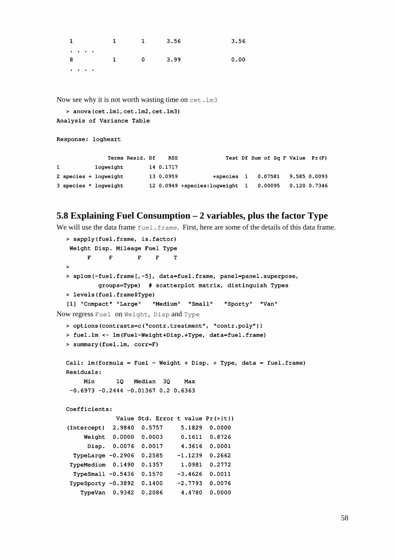
58

1 1 1 3.56 3.56 1 1 1 3.56 3.56 1 1 1 3.56 3.56 1 1 1 3.56 3.56

. . . . . . . . . . . . . . . .

8 1 0 3.99 0.00 8 1 0 3.99 0.00 8 1 0 3.99 0.00 8 1 0 3.99 0.00

. . . . . . . . . . . . . . . .

Now see why it is not worth wasting time on cet.lm3 > anova(cet.lm1,cet.lm2,cet.lm3) > anova(cet.lm1,cet.lm2,cet.lm3) > anova(cet.lm1,cet.lm2,cet.lm3) > anova(cet.lm1,cet.lm2,cet.lm3)

Analysis of Variance TableAnalysis of Variance TableAnalysis of Variance TableAnalysis of Variance Table

ReReReResponse: logheartsponse: logheartsponse: logheartsponse: logheart

Terms Resid. Df RSS Test Df Sum of Sq F Value Pr(F) Terms Resid. Df RSS Test Df Sum of Sq F Value Pr(F) Terms Resid. Df RSS Test Df Sum of Sq F Value Pr(F) Terms Resid. Df RSS Test Df Sum of Sq F Value Pr(F)

1 logweight 14 0.1717 1 logweight 14 0.1717 1 logweight 14 0.1717 1 logweight 14 0.1717

2 species + logweight 13 0.0959 +species 1 0.2 species + logweight 13 0.0959 +species 1 0.2 species + logweight 13 0.0959 +species 1 0.2 species + logweight 13 0.0959 +species 1 0.07581 9.585 0.009307581 9.585 0.009307581 9.585 0.009307581 9.585 0.0093

3 species * logweight 12 0.0949 +species:logweight 1 0.00095 0.120 0.73463 species * logweight 12 0.0949 +species:logweight 1 0.00095 0.120 0.73463 species * logweight 12 0.0949 +species:logweight 1 0.00095 0.120 0.73463 species * logweight 12 0.0949 +species:logweight 1 0.00095 0.120 0.7346

5.8 Explaining Fuel Consumption – 2 variables, plus the factor Type We will use the data frame fuel.frame. First, here are some of the details of this data frame.

> sapply(fuel.frame, is.factor)> sapply(fuel.frame, is.factor)> sapply(fuel.frame, is.factor)> sapply(fuel.frame, is.factor)

Weight Disp. Mileage Fuel Type Weight Disp. Mileage Fuel Type Weight Disp. Mileage Fuel Type Weight Disp. Mileage Fuel Type

F F F F T F F F F T F F F F T F F F F T

>>>>

> splom(~fuel.frame[,> splom(~fuel.frame[,> splom(~fuel.frame[,> splom(~fuel.frame[,----5], data=fuel.frame, panel=panel.superpose,5], data=fuel.frame, panel=panel.superpose,5], data=fuel.frame, panel=panel.superpose,5], data=fuel.frame, panel=panel.superpose,

groups=Type) # scatterplot matrix, distinguish Types groups=Type) # scatterplot matrix, distinguish Types groups=Type) # scatterplot matrix, distinguish Types groups=Type) # scatterplot matrix, distinguish Types

> levels(fue> levels(fue> levels(fue> levels(fuel.frame$Type)l.frame$Type)l.frame$Type)l.frame$Type)

[1] "Compact" "Large" "Medium" "Small" "Sporty" "Van" [1] "Compact" "Large" "Medium" "Small" "Sporty" "Van" [1] "Compact" "Large" "Medium" "Small" "Sporty" "Van" [1] "Compact" "Large" "Medium" "Small" "Sporty" "Van"

Now regress Fuel on Weight, Disp and Type > options(contrasts=c(“contr.treatment”, “contr.poly”))> options(contrasts=c(“contr.treatment”, “contr.poly”))> options(contrasts=c(“contr.treatment”, “contr.poly”))> options(contrasts=c(“contr.treatment”, “contr.poly”))

> fuel.lm <> fuel.lm <> fuel.lm <> fuel.lm <---- lm(Fuel~Weight+Disp.+Type, data=fuel.frame) lm(Fuel~Weight+Disp.+Type, data=fuel.frame) lm(Fuel~Weight+Disp.+Type, data=fuel.frame) lm(Fuel~Weight+Disp.+Type, data=fuel.frame)

> summary(fuel.lm, co> summary(fuel.lm, co> summary(fuel.lm, co> summary(fuel.lm, corr=F)rr=F)rr=F)rr=F)

Call: lm(formula = Fuel ~ Weight + Disp. + Type, data = fuel.frame)Call: lm(formula = Fuel ~ Weight + Disp. + Type, data = fuel.frame)Call: lm(formula = Fuel ~ Weight + Disp. + Type, data = fuel.frame)Call: lm(formula = Fuel ~ Weight + Disp. + Type, data = fuel.frame)

Residuals:Residuals:Residuals:Residuals:

Min 1Q Median 3Q Max Min 1Q Median 3Q Max Min 1Q Median 3Q Max Min 1Q Median 3Q Max

----0.6973 0.6973 0.6973 0.6973 ----0.2444 0.2444 0.2444 0.2444 ----0.01367 0.2 0.63630.01367 0.2 0.63630.01367 0.2 0.63630.01367 0.2 0.6363

Coefficients:Coefficients:Coefficients:Coefficients:

Value Std. Error t value Pr(>|t|) Value Std. Error t value Pr(>|t|) Value Std. Error t value Pr(>|t|) Value Std. Error t value Pr(>|t|)

(Intercept) 2.9840 0.5757 (Intercept) 2.9840 0.5757 (Intercept) 2.9840 0.5757 (Intercept) 2.9840 0.5757 5.1829 0.0000 5.1829 0.0000 5.1829 0.0000 5.1829 0.0000

Weight 0.0000 0.0003 0.1611 0.8726 Weight 0.0000 0.0003 0.1611 0.8726 Weight 0.0000 0.0003 0.1611 0.8726 Weight 0.0000 0.0003 0.1611 0.8726

Disp. 0.0076 0.0017 4.3616 0.0001 Disp. 0.0076 0.0017 4.3616 0.0001 Disp. 0.0076 0.0017 4.3616 0.0001 Disp. 0.0076 0.0017 4.3616 0.0001

TypeLarge TypeLarge TypeLarge TypeLarge ----0.2906 0.2585 0.2906 0.2585 0.2906 0.2585 0.2906 0.2585 ----1.1239 0.2662 1.1239 0.2662 1.1239 0.2662 1.1239 0.2662

TypeMedium 0.1490 0.1357 1.0981 0.2772 TypeMedium 0.1490 0.1357 1.0981 0.2772 TypeMedium 0.1490 0.1357 1.0981 0.2772 TypeMedium 0.1490 0.1357 1.0981 0.2772

TypeSmall TypeSmall TypeSmall TypeSmall ----0.5436 0.1570 0.5436 0.1570 0.5436 0.1570 0.5436 0.1570 ----3.4626 0.0011 3.4626 0.0011 3.4626 0.0011 3.4626 0.0011

TypeSporty TypeSporty TypeSporty TypeSporty ----0.3892 0.1400 0.3892 0.1400 0.3892 0.1400 0.3892 0.1400 ----2.7793 0.0076 2.7793 0.0076 2.7793 0.0076 2.7793 0.0076

TypeVan 0.9342 0.2086 4.4780 0.0000 TypeVan 0.9342 0.2086 4.4780 0.0000 TypeVan 0.9342 0.2086 4.4780 0.0000 TypeVan 0.9342 0.2086 4.4780 0.0000

59

Residual standard error: 0.3139 on 52 degrees of freedomResidual standard error: 0.3139 on 52 degrees of freedomResidual standard error: 0.3139 on 52 degrees of freedomResidual standard error: 0.3139 on 52 degrees of freedom

Multiple RMultiple RMultiple RMultiple R----Squared: 0.8486 Squared: 0.8486 Squared: 0.8486 Squared: 0.8486

FFFF----statistic: 41.65 on 7 and 52 degrees of freedom, the pstatistic: 41.65 on 7 and 52 degrees of freedom, the pstatistic: 41.65 on 7 and 52 degrees of freedom, the pstatistic: 41.65 on 7 and 52 degrees of freedom, the p----value is 0 value is 0 value is 0 value is 0

> r> r> r> res.fuel<es.fuel<es.fuel<es.fuel<----residuals(fuel.lm) # Store residuals for possible later useresiduals(fuel.lm) # Store residuals for possible later useresiduals(fuel.lm) # Store residuals for possible later useresiduals(fuel.lm) # Store residuals for possible later use

> par(mfrow=c(2,2))> par(mfrow=c(2,2))> par(mfrow=c(2,2))> par(mfrow=c(2,2))

> plot(fuel.lm) # Gives useful diagnostic plots> plot(fuel.lm) # Gives useful diagnostic plots> plot(fuel.lm) # Gives useful diagnostic plots> plot(fuel.lm) # Gives useful diagnostic plots

> par(mfrow=c(1,1))> par(mfrow=c(1,1))> par(mfrow=c(1,1))> par(mfrow=c(1,1))

> plot.gam(fuel.lm) # Gives a graphical view of the model> plot.gam(fuel.lm) # Gives a graphical view of the model> plot.gam(fuel.lm) # Gives a graphical view of the model> plot.gam(fuel.lm) # Gives a graphical view of the model

> anova(fuel.lm)> anova(fuel.lm)> anova(fuel.lm)> anova(fuel.lm)

It may be possible to improve on this model, either by transforming one or more of the explanatory variables, or by including interaction terms.

*5.9 aov models (Analysis of Variance) The class of models which can be directly fitted as aov models is quite limited. In essence, aov provides, for data where all combinations of factor levels have the same number of observations, another view of an lm model. It has an ability, not available in lm(), to specify the mean square that will be used to estimate the `error’ term.

> sapply(catalyst,is.factor)> sapply(catalyst,is.factor)> sapply(catalyst,is.factor)> sapply(catalyst,is.factor)

Temp Conc Cat Yield Temp Conc Cat Yield Temp Conc Cat Yield Temp Conc Cat Yield

T T T F T T T F T T T F T T T F

> sapply(catalyst[,> sapply(catalyst[,> sapply(catalyst[,> sapply(catalyst[,----4],levels)4],levels)4],levels)4],levels)

Temp Conc Cat Temp Conc Cat Temp Conc Cat Temp Conc Cat

[1,] "160" "20" "A"[1,] "160" "20" "A"[1,] "160" "20" "A"[1,] "160" "20" "A"

[2,] "180" "40" "B"[2,] "180" "40" "B"[2,] "180" "40" "B"[2,] "180" "40" "B"

# fit main effects and 2 factor interactions# fit main effects and 2 factor interactions# fit main effects and 2 factor interactions# fit main effects and 2 factor interactions

> options(cont> options(cont> options(cont> options(contrasts=c(“contr.treatment”, “contr.poly”))rasts=c(“contr.treatment”, “contr.poly”))rasts=c(“contr.treatment”, “contr.poly”))rasts=c(“contr.treatment”, “contr.poly”))

> cat.aov2 <> cat.aov2 <> cat.aov2 <> cat.aov2 <---- aov(Yield ~ (Temp+Conc+Cat)^2, data=catalyst) aov(Yield ~ (Temp+Conc+Cat)^2, data=catalyst) aov(Yield ~ (Temp+Conc+Cat)^2, data=catalyst) aov(Yield ~ (Temp+Conc+Cat)^2, data=catalyst)

> # All first order interactions> # All first order interactions> # All first order interactions> # All first order interactions

> summary(cat.aov2) # look at anova table> summary(cat.aov2) # look at anova table> summary(cat.aov2) # look at anova table> summary(cat.aov2) # look at anova table

> summary.lm(cat.aov2) # Examine effects> summary.lm(cat.aov2) # Examine effects> summary.lm(cat.aov2) # Examine effects> summary.lm(cat.aov2) # Examine effects

> # Effects are relative to th> # Effects are relative to th> # Effects are relative to th> # Effects are relative to the first level as baselinee first level as baselinee first level as baselinee first level as baseline

Above, we have fitted a model that has all first order interactions. We have one degree of freedom left for estimating error.

*5.9.1 Shading of Kiwifruit Vines These data (yields in kilograms) are in the data frame kiwishade which accompanies these notes. They are from an experiment19 where there were four treatments - no shading, shading from August to December, shading from December to February, and shading from February to May. Each treatment appeared once in each of the three blocks. The northernmost plots were grouped in one block because they were similarly affected by shading from the sun. For the remaining two blocks shelter effects, in one case from the east and in the other case from the west, were thought more important. Results are given for each of the four vines in each plot. In experimental design parlance, the four vines within a plot constitute subplots.

19 I am grateful to W. S. Snelgar for the use of these data. Further details, including a diagram showing the layout of plots and vines and details of shelter, are in Maindonald (1992).

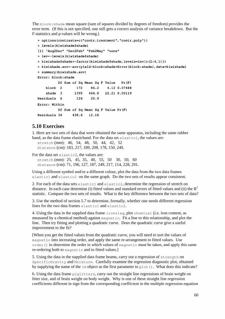
60

The block:shade mean square (sum of squares divided by degrees of freedom) provides the error term. (If this is not specified, one still gets a correct analysis of variance breakdown. But the F-statistics and p-values will be wrong.)

> options(contrasts=c("contr.treatment","contr.poly"))> options(contrasts=c("contr.treatment","contr.poly"))> options(contrasts=c("contr.treatment","contr.poly"))> options(contrasts=c("contr.treatment","contr.poly"))

> levels(kiwishade$shade)> levels(kiwishade$shade)> levels(kiwishade$shade)> levels(kiwishade$shade)

[1] "Aug2Dec" "Dec2Feb" "Feb2May" "none" [1] "Aug2Dec" "Dec2Feb" "Feb2May" "none" [1] "Aug2Dec" "Dec2Feb" "Feb2May" "none" [1] "Aug2Dec" "Dec2Feb" "Feb2May" "none"

> l> l> l> lev<ev<ev<ev<----levels(kiwishade$shade)levels(kiwishade$shade)levels(kiwishade$shade)levels(kiwishade$shade)

> kiwishade$shade<> kiwishade$shade<> kiwishade$shade<> kiwishade$shade<----factor(kiwishade$shade,levels=lev[c(2:4,1)])factor(kiwishade$shade,levels=lev[c(2:4,1)])factor(kiwishade$shade,levels=lev[c(2:4,1)])factor(kiwishade$shade,levels=lev[c(2:4,1)])

> kiwishade.aov<> kiwishade.aov<> kiwishade.aov<> kiwishade.aov<----aov(yield~block+shade+Error(block:shade),data=kiwishade)aov(yield~block+shade+Error(block:shade),data=kiwishade)aov(yield~block+shade+Error(block:shade),data=kiwishade)aov(yield~block+shade+Error(block:shade),data=kiwishade)

> summary(kiwishade.aov)> summary(kiwishade.aov)> summary(kiwishade.aov)> summary(kiwishade.aov)

Error: block:shade Error: block:shade Error: block:shade Error: block:shade

Df Sum of Sq Mean Sq F Value Pr(F Df Sum of Sq Mean Sq F Value Pr(F Df Sum of Sq Mean Sq F Value Pr(F Df Sum of Sq Mean Sq F Value Pr(F) ) ) )

block 2 172 86.2 4.12 0.07488 block 2 172 86.2 4.12 0.07488 block 2 172 86.2 4.12 0.07488 block 2 172 86.2 4.12 0.07488

shade 3 1395 464.8 22.21 0.00119 shade 3 1395 464.8 22.21 0.00119 shade 3 1395 464.8 22.21 0.00119 shade 3 1395 464.8 22.21 0.00119

Residuals 6 126 20.9 Residuals 6 126 20.9 Residuals 6 126 20.9 Residuals 6 126 20.9

Error: Within Error: Within Error: Within Error: Within

Df Sum of Sq Mean Sq F Value Pr(F) Df Sum of Sq Mean Sq F Value Pr(F) Df Sum of Sq Mean Sq F Value Pr(F) Df Sum of Sq Mean Sq F Value Pr(F)

Residuals 36 438.6 12.18 Residuals 36 438.6 12.18 Residuals 36 438.6 12.18 Residuals 36 438.6 12.18

5.10 Exercises 1. Here are two sets of data that were obtained the same apparatus, including the same rubber band, as the data frame elasticband. For the data set elastic1, the values are: stretch (mm): 46, 54, 48, 50, 44, 42, 52 distance (cm): 183, 217, 189, 208, 178, 150, 249.

For the data set elastic2, the values are: stretch (mm): 25, 45, 35, 40, 55, 50 30, 50, 60 distance (cm): 71, 196, 127, 187, 249, 217, 114, 228, 291.

Using a different symbol and/or a different colour, plot the data from the two data frames elastic1 and elastic2 on the same graph. Do the two sets of results appear consistent.

2. For each of the data sets elastic1 and elastic2, determine the regression of stretch on distance. In each case determine (i) fitted values and standard errors of fitted values and (ii) the R2 statistic. Compare the two sets of results. What is the key difference between the two sets of data?

3. Use the method of section 5.7 to determine, formally, whether one needs different regression lines for the two data frames elastic1 and elastic2.

4. Using the data in the supplied data frame ironslag, plot chemical (i.e. iron content, as measured by a chemical method) against magnetic. Fit a line to this relationship, and plot the line. Then try fitting and plotting a quadratic curve. Does the quadratic curve give a useful improvement to the fit?

[When you get the fitted values from the quadratic curve, you will need to sort the values of magnetic into increasing order, and apply the same re-arrangement to fitted values. Use order() to determine the order in which values of magnetic must be taken, and apply this same re-ordering both to magnetic and to fitted values.]

5. Using the data in the supplied data frame beams, carry out a regression of strength on SpecificGravity and Moisture. Carefully examine the regression diagnostic plot, obtained by supplying the name of the lm object as the first parameter to plot(). What does this indicate?

6. Using the data frame piglitters, carry out the straight line regressions of brain weight on litter size, and of brain weight on body weight. Why is one of these straight line regression coefficients different in sign from the corresponding coefficient in the multiple regression equation

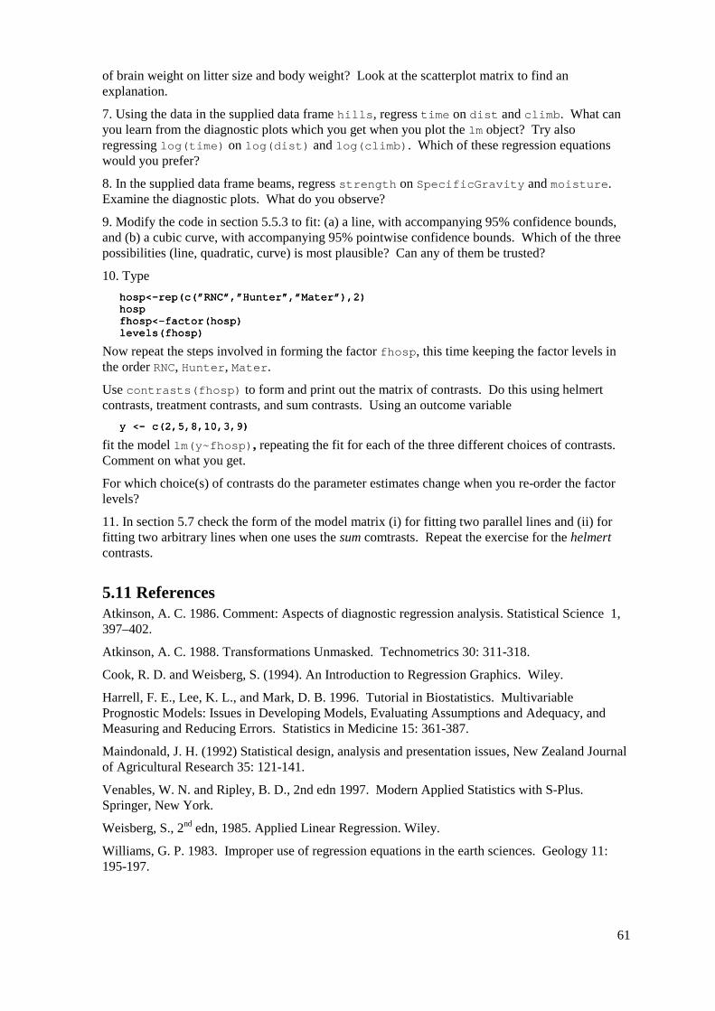
61

of brain weight on litter size and body weight? Look at the scatterplot matrix to find an explanation.

7. Using the data in the supplied data frame hills, regress time on dist and climb. What can you learn from the diagnostic plots which you get when you plot the lm object? Try also regressing log(time) on log(dist) and log(climb). Which of these regression equations would you prefer?

8. In the supplied data frame beams, regress strength on SpecificGravity and moisture. Examine the diagnostic plots. What do you observe?

9. Modify the code in section 5.5.3 to fit: (a) a line, with accompanying 95% confidence bounds, and (b) a cubic curve, with accompanying 95% pointwise confidence bounds. Which of the three possibilities (line, quadratic, curve) is most plausible? Can any of them be trusted?

10. Type hosp<hosp<hosp<hosp<----rep(c(”RNC”,”Hunter”,”Mater”),2)rep(c(”RNC”,”Hunter”,”Mater”),2)rep(c(”RNC”,”Hunter”,”Mater”),2)rep(c(”RNC”,”Hunter”,”Mater”),2) hosphosphosphosp fhosp<fhosp<fhosp<fhosp<----factor(hosp)factor(hosp)factor(hosp)factor(hosp) levels(fhosp)levels(fhosp)levels(fhosp)levels(fhosp)

Now repeat the steps involved in forming the factor fhosp, this time keeping the factor levels in the order RNC, Hunter, Mater.

Use contrasts(fhosp) to form and print out the matrix of contrasts. Do this using helmert contrasts, treatment contrasts, and sum contrasts. Using an outcome variable

y <y <y <y <---- c(2,5,8,10,3,9) c(2,5,8,10,3,9) c(2,5,8,10,3,9) c(2,5,8,10,3,9)

fit the model lm(y~fhosp), repeating the fit for each of the three different choices of contrasts. Comment on what you get.

For which choice(s) of contrasts do the parameter estimates change when you re-order the factor levels?

11. In section 5.7 check the form of the model matrix (i) for fitting two parallel lines and (ii) for fitting two arbitrary lines when one uses the sum comtrasts. Repeat the exercise for the helmert contrasts.

5.11 References Atkinson, A. C. 1986. Comment: Aspects of diagnostic regression analysis. Statistical Science 1, 397–402.

Atkinson, A. C. 1988. Transformations Unmasked. Technometrics 30: 311-318.

Cook, R. D. and Weisberg, S. (1994). An Introduction to Regression Graphics. Wiley.

Harrell, F. E., Lee, K. L., and Mark, D. B. 1996. Tutorial in Biostatistics. Multivariable Prognostic Models: Issues in Developing Models, Evaluating Assumptions and Adequacy, and Measuring and Reducing Errors. Statistics in Medicine 15: 361-387.

Maindonald, J. H. (1992) Statistical design, analysis and presentation issues, New Zealand Journal of Agricultural Research 35: 121-141.

Venables, W. N. and Ripley, B. D., 2nd edn 1997. Modern Applied Statistics with S-Plus. Springer, New York.

Weisberg, S., 2nd edn, 1985. Applied Linear Regression. Wiley.

Williams, G. P. 1983. Improper use of regression equations in the earth sciences. Geology 11: 195-197.

62

63

6. Multivariate and Tree-Based Methods

6.1 Multivariate EDA, and Principal Components Analysis Principal components analysis is often a useful exploratory tool for multivariate data. The supplied data set possum has nine morphometric measurements on each of 102 mountain brushtail possums, trapped at seven sites from southern Victoria to central Queensland. With such data it is sensible to begin by examining relevant scatterplot matrices. This may draw attention to gross errors in the data. A plot in which the sites and/or the sexes are identified will draw attention to any very strong structure in the data. For example one site may be quite different from the others, for some or all of the variables.

Here are some of the possibilities for examining these data: splom(~possum[,6:14], panel=panel.superpose, groups=possum$sex)splom(~possum[,6:14], panel=panel.superpose, groups=possum$sex)splom(~possum[,6:14], panel=panel.superpose, groups=possum$sex)splom(~possum[,6:14], panel=panel.superpose, groups=possum$sex)

splom(~possum[,6:14], panel=panel.superpose, groups=possum$sitsplom(~possum[,6:14], panel=panel.superpose, groups=possum$sitsplom(~possum[,6:14], panel=panel.superpose, groups=possum$sitsplom(~possum[,6:14], panel=panel.superpose, groups=possum$site)e)e)e)

here<here<here<here<----!is.na(possum$pes) # We need to exclude missing values!is.na(possum$pes) # We need to exclude missing values!is.na(possum$pes) # We need to exclude missing values!is.na(possum$pes) # We need to exclude missing values

print(sum(!here)) # Check how many values are missingprint(sum(!here)) # Check how many values are missingprint(sum(!here)) # Check how many values are missingprint(sum(!here)) # Check how many values are missing

possum.prc <possum.prc <possum.prc <possum.prc <---- princomp(possum[here,6:14]) # Principal components princomp(possum[here,6:14]) # Principal components princomp(possum[here,6:14]) # Principal components princomp(possum[here,6:14]) # Principal components

# Print scores on second pc versus scores on first pc# Print scores on second pc versus scores on first pc# Print scores on second pc versus scores on first pc# Print scores on second pc versus scores on first pc

xyploxyploxyploxyplot(possum.prc$scores[,2] ~ possum.prc$scores[,1]|possum$Pop[here],t(possum.prc$scores[,2] ~ possum.prc$scores[,1]|possum$Pop[here],t(possum.prc$scores[,2] ~ possum.prc$scores[,1]|possum$Pop[here],t(possum.prc$scores[,2] ~ possum.prc$scores[,1]|possum$Pop[here],

panel=panel.superpose, groups=possum$sex[here]) panel=panel.superpose, groups=possum$sex[here]) panel=panel.superpose, groups=possum$sex[here]) panel=panel.superpose, groups=possum$sex[here])

xyplot(possum.prc$scores[,2] ~ possum.prc$scores[,1]|possum$site[here],xyplot(possum.prc$scores[,2] ~ possum.prc$scores[,1]|possum$site[here],xyplot(possum.prc$scores[,2] ~ possum.prc$scores[,1]|possum$site[here],xyplot(possum.prc$scores[,2] ~ possum.prc$scores[,1]|possum$site[here],

panel=panel.superpose, groups=possum$sex[here]) panel=panel.superpose, groups=possum$sex[here]) panel=panel.superpose, groups=possum$sex[here]) panel=panel.superpose, groups=possum$sex[here])

Fig. 21 shows the second of these plots:

-10

-5

0

5

10 possum$site[here]

-15 -10 -5 0 5 10 15

possum$site[here] possum$site[here]

-15 -10 -5 0 5 10 15

possum$site[here]

possum$site[here] possum$site[here]

-15 -10 -5 0 5 10 15

-10

-5

0

5

10possum$site[here]

scores[, 1]

scor

es[,

2]

Females Males

Figure 21: Plot of second principal component versus first principal component, for the possum morphometric data.

See chapter 1 of the S-PLUS 2000 Guide to Statistics.

64

6.2 Cluster Analysis In the language of Ripley (1996)20, cluster analysis is a form of unsupervised classification. It is “unsupervised” because the clusters are not known in advance. There are two types of algorithms – algorithms based on hierachical agglomeration, and algorithms based on iterative relocation. Both types of algorithm are available in S-PLUS.

In hierarchical agglomeration each observation starts as a separate group. Groups that are “close” to one another are then successively merged. The output yields a hierarchical clustering tree which shows the relationships between observations and between the clusters into which they are successively merged. A judgement is then needed on the point at which further merging is unwarranted.

In iterative relocation, the algorithm starts with an initial classification, which it then tries to improve. How does one get the initial classification? Typically, by a prior use of a hierarchical agglomeration algorithm.

6.3 Discriminant Analysis We start with data which are classified into several groups, and want a rule which will allow us to predict the group to which a new data value will belong. In the language of Ripley (1996), our interest is in supervised classification. For example, we may wish to predict, based on prognostic measurements and outcome information for previous patients, which future patients will remain free of disease symptoms for twelve months or more. Here are calculations for the possum data frame, using the lda() function from the Venables & Ripley MASS library:

> library(MASS,first=T)> library(MASS,first=T)> library(MASS,first=T)> library(MASS,first=T)

> here<> here<> here<> here<---- !is.na(possum$pes) !is.na(possum$pes) !is.na(possum$pes) !is.na(possum$pes)

> possum.lda <> possum.lda <> possum.lda <> possum.lda <---- lda(site~hdlngth+skullw+totlngth+ lda(site~hdlngth+skullw+totlngth+ lda(site~hdlngth+skullw+totlngth+ lda(site~hdlngth+skullw+totlngth+

+ taill+pes+earconch+eye+chest+belly,data=possum, subset=here)+ taill+pes+earconch+eye+chest+belly,data=possum, subset=here)+ taill+pes+earconch+eye+chest+belly,data=possum, subset=here)+ taill+pes+earconch+eye+chest+belly,data=possum, subset=here)

> possum.lda$svd # Examine th> possum.lda$svd # Examine th> possum.lda$svd # Examine th> possum.lda$svd # Examine the singular valuese singular valuese singular valuese singular values

[1] 15.7577838 3.9372136 3.1859729[1] 15.7577838 3.9372136 3.1859729[1] 15.7577838 3.9372136 3.1859729[1] 15.7577838 3.9372136 3.1859729

[4] 1.5078461 1.1420103 0.7771947[4] 1.5078461 1.1420103 0.7771947[4] 1.5078461 1.1420103 0.7771947[4] 1.5078461 1.1420103 0.7771947

> plot(possum.lda, dimen=3) > plot(possum.lda, dimen=3) > plot(possum.lda, dimen=3) > plot(possum.lda, dimen=3)

> # Scatterplot matrix for scores on 1> # Scatterplot matrix for scores on 1> # Scatterplot matrix for scores on 1> # Scatterplot matrix for scores on 1stststst 3 canonical variates, as in Fig. 18 3 canonical variates, as in Fig. 18 3 canonical variates, as in Fig. 18 3 canonical variates, as in Fig. 18

The singular values are the ratio of between to within group sums of squares, for the canonical variates in turn. Clearly canonical variates after the third have little if any discriminatory power. One can use predict.lda() to get (among other information) scores on the first few canonical variates.

20 References are at the end of the chapter.

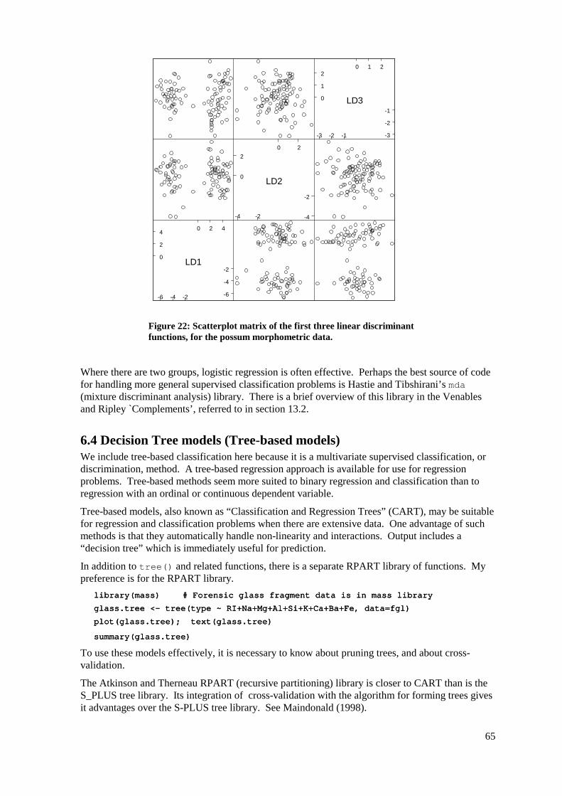
65

-6 -4 -2

0 2 4

0

2

4

-6

-4

-2LD1

-4 -2

0 2

0

2

-4

-2

LD2

-3 -2 -1

0 1 2

0

1

2

-3

-2

-1LD3

Figure 22: Scatterplot matrix of the first three linear discriminant functions, for the possum morphometric data.

Where there are two groups, logistic regression is often effective. Perhaps the best source of code for handling more general supervised classification problems is Hastie and Tibshirani’s mda (mixture discriminant analysis) library. There is a brief overview of this library in the Venables and Ripley `Complements’, referred to in section 13.2.

6.4 Decision Tree models (Tree-based models) We include tree-based classification here because it is a multivariate supervised classification, or discrimination, method. A tree-based regression approach is available for use for regression problems. Tree-based methods seem more suited to binary regression and classification than to regression with an ordinal or continuous dependent variable.

Tree-based models, also known as “Classification and Regression Trees” (CART), may be suitable for regression and classification problems when there are extensive data. One advantage of such methods is that they automatically handle non-linearity and interactions. Output includes a “decision tree” which is immediately useful for prediction.

In addition to tree() and related functions, there is a separate RPART library of functions. My preference is for the RPART library.

library(mass) library(mass) library(mass) library(mass) # Forensic glass fragment data is in mass library# Forensic glass fragment data is in mass library# Forensic glass fragment data is in mass library# Forensic glass fragment data is in mass library

glass.tree <glass.tree <glass.tree <glass.tree <---- tree(type ~ RI+Na+Mg+Al+Si+K+Ca+Ba+Fe, data=fgl) tree(type ~ RI+Na+Mg+Al+Si+K+Ca+Ba+Fe, data=fgl) tree(type ~ RI+Na+Mg+Al+Si+K+Ca+Ba+Fe, data=fgl) tree(type ~ RI+Na+Mg+Al+Si+K+Ca+Ba+Fe, data=fgl)

plot(glass.tplot(glass.tplot(glass.tplot(glass.tree); text(glass.tree)ree); text(glass.tree)ree); text(glass.tree)ree); text(glass.tree)

summary(glass.tree)summary(glass.tree)summary(glass.tree)summary(glass.tree)

To use these models effectively, it is necessary to know about pruning trees, and about cross-validation.

The Atkinson and Therneau RPART (recursive partitioning) library is closer to CART than is the S_PLUS tree library. Its integration of cross-validation with the algorithm for forming trees gives it advantages over the S-PLUS tree library. See Maindonald (1998).

66

6.5 Exercises 1. Using the data.frame function, convert the object testscores into an S-PLUS data frame. Apply principal components analysis to the scores for diffgeom, complex, algebra, and reals. Plot the scores for the first principal component against the statistics scores.

2. Apply principal components analysis to the four response variables pre.mean, post.mean, pre.dev and post.dev in the dataframe wafer. Use xyplot to plot the second principal component scores against the first principal component scores for each value of maskdim.

3. (a) Use predict(kyphosis.tree,data.frame(Kyphosis=NA,Age=1predict(kyphosis.tree,data.frame(Kyphosis=NA,Age=1predict(kyphosis.tree,data.frame(Kyphosis=NA,Age=1predict(kyphosis.tree,data.frame(Kyphosis=NA,Age=11,Number=3,Start=5))1,Number=3,Start=5))1,Number=3,Start=5))1,Number=3,Start=5))

to predict whether kyphosis will be present or absent for an 11-month-old whose operation involved 3 vertebrae starting at the 5th. What about a 36-month-old whose operation involved 6 vertebrae starting at the 7th.

(b) Use summary(ksummary(ksummary(ksummary(kyphosis.tree) yphosis.tree) yphosis.tree) yphosis.tree)

to obtain an estimate of the misclassification rate.

4. The mass library has the Aids2 data set, containing de-identified data on the survival status of patients diagnosed with AIDS before July 1 1991. Use tree-based classification (rpart()) to identify major influences on survival.

5. Investigate discrimination between plagiotropic and orthotropic species in the data set leafshape

21.

6.6 References Chambers, J. M. and Hastie, T. J. 1992. Statistical Models in S. Wadsworth and Brooks Cole Advanced Books and Software, Pacific Grove CA.

Everitt, B. S. and Dunn, G. 1992. Applied Multivariate Data Analysis. Arnold, London.

Friedman, J., Hastie, T. and Tibshirani, R. (1998). Additive logistic regression: A statistical view of boosting. Available from the internet.

Lindenmayer, D. B., Viggers, K. L., Cunningham, R. B., and Donnelly, C. F. 1995. Morphological variation among columns of the mountain brushtail possum, Trichosurus caninus Ogilby (Phalangeridae: Marsupiala). Australian Journal of Zoology 43: 449-458.

Magidson, Jay 1996. SPSS for Windows CHAID Release 6. SPSS Inc., Chicago.

Maindonald, J. H. 1998a. Classification and Regression Trees. Unpublished manuscript, 62pp.

Ripley, B. D. 1996. Pattern Recognition and Neural Networks. Cambridge University Press, Cambridge UK.

Therneau, T. M. and Atkinson, E. J. 1997. An Introduction to Recursive Partitioning Using the RPART Routines. This is one of two documents included in: http://www.stats.ox.ac.uk/pub/SWin/rpartdoc.zip

Venables, W. N. and Ripley, B. D., 2nd edn 1997. Modern Applied Statistics with S-Plus. Springer, New York.

21 These data are discussed in the paper King. D. A.; Maindonald, J. H. 1999. Tree architecture in relation to leaf dimensions and tree stature in temperate and tropical rain forests. Journal of Ecology 87: 1012-1024.

67

*7. S-PLUS Data Structures Chapter 2 included brief summaries of the S-PLUS data structures that beginning S-PLUS users will encounter. This chapter has more detailed information.

7.1 Vectors Recall that vectors may have mode logical, numeric or character22. Recall also the use of c() to join (concatenate) vectors.

7.1.1 Subsets of Vectors Recall (section 2.6.1) two common ways to extract subsets of vectors:

1. Specify the numbers of the elements which are to be extracted. One can use negative numbers to omit elements.

2. Specify a vector of logical values. The elements that are extracted are those for which the logical value is T. Thus suppose we want to extract values of x which are greater than 10.

The following demonstrates a third possibility, for vectors that have named elements: > c(Andreas=178, John=185, Jeff=1> c(Andreas=178, John=185, Jeff=1> c(Andreas=178, John=185, Jeff=1> c(Andreas=178, John=185, Jeff=183)[c("John","Jeff")]83)[c("John","Jeff")]83)[c("John","Jeff")]83)[c("John","Jeff")]

John Jeff John Jeff John Jeff John Jeff

185 183 185 183 185 183 185 183

A vector of names has been used to extract the elements.

7.1.2 Patterned Data Use 5:15 to generate the numbers 5, 6, …, 15. Entering 15:5 will generate the sequence in the reverse order.

To repeat the sequence (2, 3, 5) four times over, enter rep(c(2,3,5), 4) thus: > rep(c(2,3,5),4)> rep(c(2,3,5),4)> rep(c(2,3,5),4)> rep(c(2,3,5),4)

[1] 2 3 5 2 3 5 2 3 5 2 3 5 [1] 2 3 5 2 3 5 2 3 5 2 3 5 [1] 2 3 5 2 3 5 2 3 5 2 3 5 [1] 2 3 5 2 3 5 2 3 5 2 3 5

>>>>

If instead one wants four 2s, then four 3s, then four 5s, enter rep(c(2,3,5), c(4,4,4)). > rep(c(2,3,5),c(4,4,4)) # An alte> rep(c(2,3,5),c(4,4,4)) # An alte> rep(c(2,3,5),c(4,4,4)) # An alte> rep(c(2,3,5),c(4,4,4)) # An alternative is rep(c(2,3,5), each=4)rnative is rep(c(2,3,5), each=4)rnative is rep(c(2,3,5), each=4)rnative is rep(c(2,3,5), each=4)

[1] 2 2 2 2 3 3 3 3 5 5 5 5 [1] 2 2 2 2 3 3 3 3 5 5 5 5 [1] 2 2 2 2 3 3 3 3 5 5 5 5 [1] 2 2 2 2 3 3 3 3 5 5 5 5

Note further that, in place of c(4,4,4) we could write rep(4,3). So a further possibility is that in place of rep(c(2,3,5), c(4,4,4)) we could enter rep(c(2,3,5), rep(4,3)). Another way to achieve the same effect is rep(c(2,3,5), each=4).

In addition to the above, note that the function rep() has an argument length.out, meaning “keep on repeating the sequence until the length is length.out.”

22 Below, we will meet the notion of “class”, which is important for some of the more sophisticated language features of S-PLUS. The logical, numeric and character vectors just given have class NULL, i.e. they have no class. There are special types of numeric vector which do have a class attribute. Factors are the most important example. Although often used as a compact way to store character strings, factors are, technically, numeric vectors. The class attribute of a factor has, not surprisingly, the value “factor”.

68

7.2 Missing Values We noted in section 2.6.2 that any arithmetic operation or relation that involves NA generates an NA. This applies also to the relations <, <=, >, >=, ==, !=. This may have unintended consequences. Specifically, note that x==NA generates NA.

Be sure to use is.na(x) to test which values of x are NA. Note the following: > x <> x <> x <> x <---- c(1,6,2,NA) c(1,6,2,NA) c(1,6,2,NA) c(1,6,2,NA)

> is.na(x) # T for when NA appears, and otherwise false> is.na(x) # T for when NA appears, and otherwise false> is.na(x) # T for when NA appears, and otherwise false> is.na(x) # T for when NA appears, and otherwise false

[1] F F F T[1] F F F T[1] F F F T[1] F F F T

> x==NA # All elements of the result are NA> x==NA # All elements of the result are NA> x==NA # All elements of the result are NA> x==NA # All elements of the result are NA

[1] NA NA NA NA[1] NA NA NA NA[1] NA NA NA NA[1] NA NA NA NA

> x[x==NA]> x[x==NA]> x[x==NA]> x[x==NA]

[1] NA NA NA NA[1] NA NA NA NA[1] NA NA NA NA[1] NA NA NA NA

> x[x>2]> x[x>2]> x[x>2]> x[x>2]

[1] 6 N[1] 6 N[1] 6 N[1] 6 NAAAA

> NA==NA> NA==NA> NA==NA> NA==NA

[1] NA[1] NA[1] NA[1] NA

WARNING: If x and y have the same length and x has missing values, then y[x>2] <y[x>2] <y[x>2] <y[x>2] <---- x[x>2] x[x>2] x[x>2] x[x>2]

will not give the result that the naïve user might expect. Suppose for example we make the assignments

> x <> x <> x <> x <---- c(1,6,2,NA) c(1,6,2,NA) c(1,6,2,NA) c(1,6,2,NA)

> y <> y <> y <> y <---- c(1,10,2,3) c(1,10,2,3) c(1,10,2,3) c(1,10,2,3)

> y[> y[> y[> y[x>2] <x>2] <x>2] <x>2] <---- x[x>2] x[x>2] x[x>2] x[x>2]

Warning messages:Warning messages:Warning messages:Warning messages:

Replacement length not a multiple of number of elements Replacement length not a multiple of number of elements Replacement length not a multiple of number of elements Replacement length not a multiple of number of elements

to replace in: y[x > 2] < to replace in: y[x > 2] < to replace in: y[x > 2] < to replace in: y[x > 2] <---- x[x > 2] x[x > 2] x[x > 2] x[x > 2]

The warning messages indicate that something is wrong. As one might expect, y[NA] equals NA. On the left-hand side, any element whose subscript evaluates to NA is omitted. Thus in

> y[x>2]> y[x>2]> y[x>2]> y[x>2]

[1] 10 NA[1] 10 NA[1] 10 NA[1] 10 NA

there is only one position (that occupied by the 10) to which a value can be assigned. On the right we have

> x[x>2]> x[x>2]> x[x>2]> x[x>2]

[1] 6 NA[1] 6 NA[1] 6 NA[1] 6 NA

There are two elements, which are used in turn to replace the value 10 on the left. The value that is finally assigned is not 6, but NA.

One can use !is.na(x) to limit the selection, on both sides, to those elements of x that are not NAs. Specify

y[!is.na(x) & x>2] <y[!is.na(x) & x>2] <y[!is.na(x) & x>2] <y[!is.na(x) & x>2] <---- x[!is.na(x) & x>2] x[!is.na(x) & x>2] x[!is.na(x) & x>2] x[!is.na(x) & x>2]

We will have more to say on missing values in the section on data frames which now follows.

7.3 Data frames Recall (section 2.7) that a data frame is a generalisation of a matrix, in which different columns may have different modes. All elements of any column must however have the same mode, i.e. all numeric or all factor, or all character. For some purposes data frames behave like matrices. There

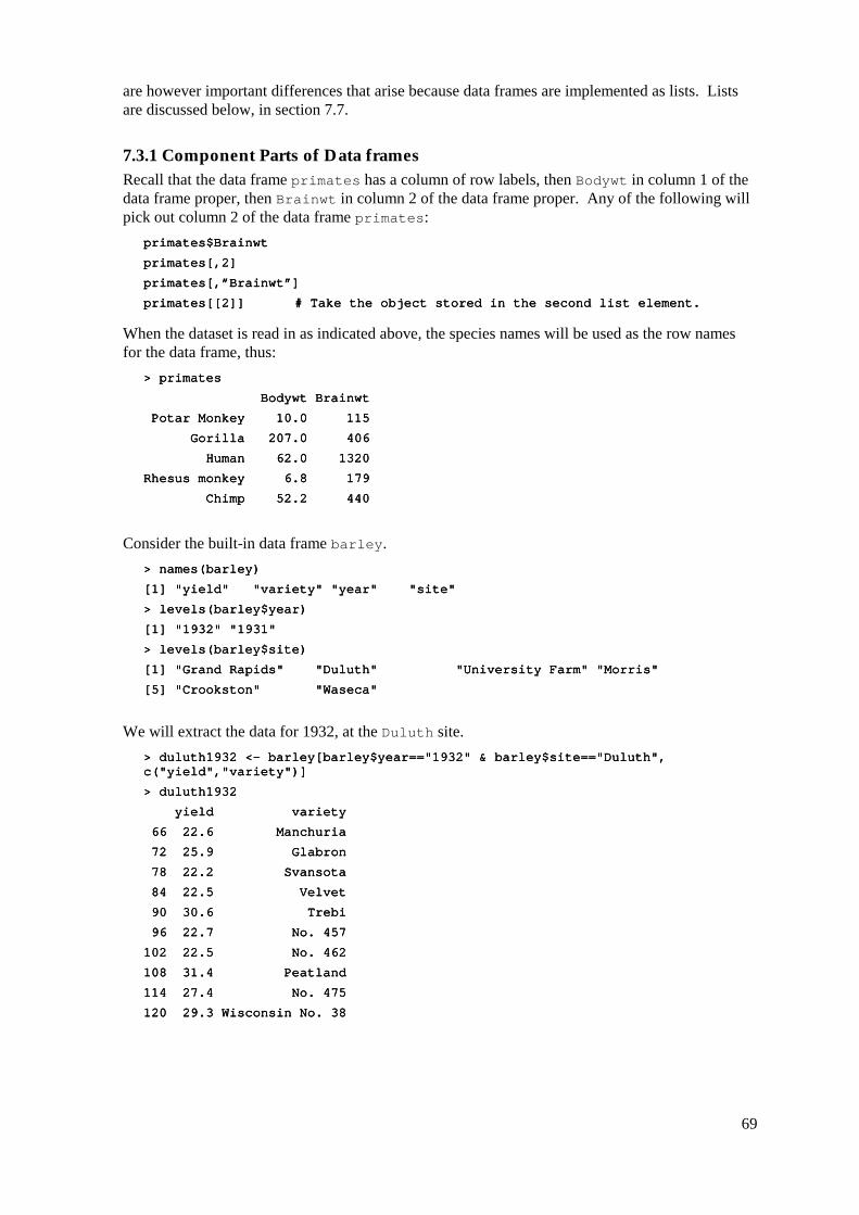
69

are however important differences that arise because data frames are implemented as lists. Lists are discussed below, in section 7.7.

7.3.1 Component Parts of Data frames Recall that the data frame primates has a column of row labels, then Bodywt in column 1 of the data frame proper, then Brainwt in column 2 of the data frame proper. Any of the following will pick out column 2 of the data frame primates:

primates$Brainwtprimates$Brainwtprimates$Brainwtprimates$Brainwt

primates[,2]primates[,2]primates[,2]primates[,2]

primates[,”Brainwt”]primates[,”Brainwt”]primates[,”Brainwt”]primates[,”Brainwt”]

primates[[2]] primates[[2]] primates[[2]] primates[[2]] # Take the object stored in the second list element. # Take the object stored in the second list element. # Take the object stored in the second list element. # Take the object stored in the second list element.

When the dataset is read in as indicated above, the species names will be used as the row names for the data frame, thus:

> primates> primates> primates> primates

Bodywt Brainwt Bodywt Brainwt Bodywt Brainwt Bodywt Brainwt

Potar Monkey 10.0 115 Potar Monkey 10.0 115 Potar Monkey 10.0 115 Potar Monkey 10.0 115

Gorilla 207.0 406 Gorilla 207.0 406 Gorilla 207.0 406 Gorilla 207.0 406

Human 62.0 1320 Human 62.0 1320 Human 62.0 1320 Human 62.0 1320

Rhesus monkey 6.8 179Rhesus monkey 6.8 179Rhesus monkey 6.8 179Rhesus monkey 6.8 179

Chimp 52.2 440 Chimp 52.2 440 Chimp 52.2 440 Chimp 52.2 440

Consider the built-in data frame barley. > names(barley)> names(barley)> names(barley)> names(barley)

[1] "yield" "variety" "year" "site" [1] "yield" "variety" "year" "site" [1] "yield" "variety" "year" "site" [1] "yield" "variety" "year" "site"

> levels(barley$year)> levels(barley$year)> levels(barley$year)> levels(barley$year)

[1] "1932" "1931"[1] "1932" "1931"[1] "1932" "1931"[1] "1932" "1931"

> levels(barley$site)> levels(barley$site)> levels(barley$site)> levels(barley$site)

[1] "Grand Rapids" "Duluth" "University Farm" "Morris" [1] "Grand Rapids" "Duluth" "University Farm" "Morris" [1] "Grand Rapids" "Duluth" "University Farm" "Morris" [1] "Grand Rapids" "Duluth" "University Farm" "Morris"

[5] "Crookston" "Waseca"[5] "Crookston" "Waseca"[5] "Crookston" "Waseca"[5] "Crookston" "Waseca"

We will extract the data for 1932, at the Duluth site. > duluth1932 <> duluth1932 <> duluth1932 <> duluth1932 <---- barley[barley$year=="1932" & barley$site=="Duluth", barley[barley$year=="1932" & barley$site=="Duluth", barley[barley$year=="1932" & barley$site=="Duluth", barley[barley$year=="1932" & barley$site=="Duluth", c("yield","variety")]c("yield","variety")]c("yield","variety")]c("yield","variety")]

> duluth1932> duluth1932> duluth1932> duluth1932

yield variety yield variety yield variety yield variety

66 22.6 Manchuria 66 22.6 Manchuria 66 22.6 Manchuria 66 22.6 Manchuria

72 25.9 Glabron 72 25.9 Glabron 72 25.9 Glabron 72 25.9 Glabron

78 78 78 78 22.2 Svansota22.2 Svansota22.2 Svansota22.2 Svansota

84 22.5 Velvet 84 22.5 Velvet 84 22.5 Velvet 84 22.5 Velvet

90 30.6 Trebi 90 30.6 Trebi 90 30.6 Trebi 90 30.6 Trebi

96 22.7 No. 457 96 22.7 No. 457 96 22.7 No. 457 96 22.7 No. 457

102 22.5 No. 462102 22.5 No. 462102 22.5 No. 462102 22.5 No. 462

108 31.4 Peatland108 31.4 Peatland108 31.4 Peatland108 31.4 Peatland

114 27.4 No. 475114 27.4 No. 475114 27.4 No. 475114 27.4 No. 475

120 29.3 Wisconsin No. 38120 29.3 Wisconsin No. 38120 29.3 Wisconsin No. 38120 29.3 Wisconsin No. 38

70

The first column holds the row labels, which in this case are the numbers of the rows that have been extracted. In place of c(“yield”,”variety”) we could have written, more simply, c(1,2), or even 1:2.

7.3.2 Built-in data frames Built-in data frames to which we may refer are:

barley (yield, variety barley (yield, variety barley (yield, variety barley (yield, variety 10, year 2, site 6)10, year 2, site 6)10, year 2, site 6)10, year 2, site 6)

car.all car.all car.all car.all –––– values of 36 variable for each of 111 cars values of 36 variable for each of 111 cars values of 36 variable for each of 111 cars values of 36 variable for each of 111 cars

claims (age 8, car.age 4, type 4, cost number)claims (age 8, car.age 4, type 4, cost number)claims (age 8, car.age 4, type 4, cost number)claims (age 8, car.age 4, type 4, cost number)

CO2 (Plant 12, Type 2, Treatment 2, conc, uptake) [SCO2 (Plant 12, Type 2, Treatment 2, conc, uptake) [SCO2 (Plant 12, Type 2, Treatment 2, conc, uptake) [SCO2 (Plant 12, Type 2, Treatment 2, conc, uptake) [S----PLUS 4.0]PLUS 4.0]PLUS 4.0]PLUS 4.0]

ethanol (NOx, C = compression ratio, E = richness)ethanol (NOx, C = compression ratio, E = richness)ethanol (NOx, C = compression ratio, E = richness)ethanol (NOx, C = compression ratio, E = richness)

environmental (ozonenvironmental (ozonenvironmental (ozonenvironmental (ozone, radiation, temperature, wind)e, radiation, temperature, wind)e, radiation, temperature, wind)e, radiation, temperature, wind)

fuel.frame (Weight Disp. Mileage Fuel Type 6) fuel.frame (Weight Disp. Mileage Fuel Type 6) fuel.frame (Weight Disp. Mileage Fuel Type 6) fuel.frame (Weight Disp. Mileage Fuel Type 6)

kyphosis (Kyphosis 2, Age, Number, Start)kyphosis (Kyphosis 2, Age, Number, Start)kyphosis (Kyphosis 2, Age, Number, Start)kyphosis (Kyphosis 2, Age, Number, Start)

market.survey (pick 2,income 7, moves 9, age 6, education 6,market.survey (pick 2,income 7, moves 9, age 6, education 6,market.survey (pick 2,income 7, moves 9, age 6, education 6,market.survey (pick 2,income 7, moves 9, age 6, education 6, employment 7, usage, nonpub 2, reach.out 3, card 2) employment 7, usage, nonpub 2, reach.out 3, card 2) employment 7, usage, nonpub 2, reach.out 3, card 2) employment 7, usage, nonpub 2, reach.out 3, card 2)

pigmenpigmenpigmenpigment (Batch 15, Sample 2, Test 2, Moisture)t (Batch 15, Sample 2, Test 2, Moisture)t (Batch 15, Sample 2, Test 2, Moisture)t (Batch 15, Sample 2, Test 2, Moisture)

Where a number is given, this is a factor, and the number is the number of levels.

7.4 Data Entry For entering a rectangular array into an S-PLUS data frame, the function read.table() is an alternative to the Import Data dialogue on the File menu. Suppose that the file primates.dat contains:

"Potar monkey" 10 115"Potar monkey" 10 115"Potar monkey" 10 115"Potar monkey" 10 115

Gorilla 207 406Gorilla 207 406Gorilla 207 406Gorilla 207 406

Human 62 1320Human 62 1320Human 62 1320Human 62 1320

"Rhesus monkey" 6.8 179"Rhesus monkey" 6.8 179"Rhesus monkey" 6.8 179"Rhesus monkey" 6.8 179

Chimp 52.2 440Chimp 52.2 440Chimp 52.2 440Chimp 52.2 440

Then primates <primates <primates <primates <---- read.table("a:/primates.dat") read.table("a:/primates.dat") read.table("a:/primates.dat") read.table("a:/primates.dat")

will create the data frame primates, from a file on the a: drive. The text strings in the first column will become row names23, which you can access as row.names(primates).

Suppose that primates is a data frame with two columns – body weight, and brain weight. You can give the columns names by typing in:

names(primates)<names(primates)<names(primates)<names(primates)<----c("Bodywt","Brainwt")c("Bodywt","Brainwt")c("Bodywt","Brainwt")c("Bodywt","Brainwt")

7.4.1 Idiosyncrasies The function read.table() is straightforward for reading in arrays that are entirely numeric. Problems arise when small mistakes cause S-PLUS to interpret a column of supposedly numeric data as character strings. For example there may be an O (oh) somewhere where there should be a 0 (zero), or an el (l) where there should be a one (1). The same problem arises if you use * or a dot (.) as the missing value (NA) symbol, but fail to warn S-PLUS of this. (The default is to use NA as the missing value symbol.)

23 Note that this is different from the default behaviour of the Import Data dialogue. A column of row labels is taken from the data that are to be imported only if the user specifically identifies, through the Options dialogue, one of the columns as a column of row labels.

71

Where the array contains character as well as numeric data, whether by design or accident, the behaviour of read.table() may seem idiosyncratic24. Users can avoid the use of the first available column of character strings to provide row names by specifying the parameter setting row.names = NULL. The parameter setting as.is = T25252525 will ensure that columns of character strings are not turned into factors.

7.4.2 Missing values when using read.table() The function read.table() expects missing values to be coded as NA, unless you set na.strings to recognise other characters as missing value indicators. For a text file that has been output from SAS, the setting na.strings=c(".") may be appropriate. There may be multiple missing value indicators, e. g. na.strings=c(".",""). The "" will ensure that empty cells are entered as NAs.

7.4.3 Separators when using read.table() It is sometimes necessary to specify tab (“\t”) or comma as the separator. The default separator is white space. To set tab as the separator, specify sep="\t". In order to ensure that empty cells are entered as NA, specify na.strings=c("").

7.5 Factors As noted in section 2.6.3, factors provide an economical way to store vectors of character strings in which there are many multiple occurrences of the same strings. Factors have a dual identity. They are stored as integer vectors, with each of the values interpreted according to the information that is in the table of levels26. Model formulae (e.g. in analysis of variance and regression models, as in chapter 6), and graphics formulae, provide another reason for the use of factor objects.

The data frame islandcities that accompanies these notes holds the populations of the 19 island nation cities with a 1995 urban centre population of 1.4 million or more. The row names are the city names, the first column (country) has the name of the country, and the second column (population) has the urban centre population, in millions. Here is a table that gives the number of times each country occurs Australia Cuba Indonesia Japan Philippines Taiwan United Kingdom 3 1 4 6 2 1 2

[There are 19 cities in all.]

Rather than store `Australia’ three times, `Indonesia’ four times, and so on, the factor representation stores different numerical codes for each of the different countries. It then uses a look-up table, stored in a list of levels that is associated with the factor, to associate the code with the name of a country.

> levels(islandcities$country)> levels(islandcities$country)> levels(islandcities$country)> levels(islandcities$country)

[1] "Australia" "Cuba" "Indonesia" [1] "Australia" "Cuba" "Indonesia" [1] "Australia" "Cuba" "Indonesia" [1] "Australia" "Cuba" "Indonesia"

[4] "Japan" [4] "Japan" [4] "Japan" [4] "Japan" "Philippines" "Taiwan" "Philippines" "Taiwan" "Philippines" "Taiwan" "Philippines" "Taiwan"

24 The first column of character strings that are distinct is, by default, used for row labels. Specify row.names = NULL to over-ride this. Any other column that has one or more character strings will, unless you specify otherwise, become a factor with as many levels as there are unique values in the column. Specify as.is=T to over-ride this. Storage of columns of character strings as factors is efficient when a small number of distinct strings are each repeated a large number of times. 25 Specifying as.is = T prevents columns of (intended or unintended) character strings from being converted into factors. Under the Import Data dialogue, an option setting is available that has the same effect. The default is, as with read.table(), to convert any columns of character strings into factors. 26 Factors are vectors that have mode numeric and class “factor”. They have an attribute levels that holds the level names.

72

[7] "United Kingdom"[7] "United Kingdom"[7] "United Kingdom"[7] "United Kingdom"

Thus “Australia”, because it is stored in the first position, has the code 1, “Cuba” has the code 2, “Indonesia” has the code 3, and so on. The country names are the factor levels.

Printing the contents of the column with the name country gives the names, not the codes. S-PLUS does the translation invisibly. In fact the codes are invisible in most operations with factors. There are though annoying exceptions that can make the use of factors tricky. To be sure of getting the country names, specify

as.character(islandcities$country)as.character(islandcities$country)as.character(islandcities$country)as.character(islandcities$country)

To get the codes, specify as.integer(islandcities$country)as.integer(islandcities$country)as.integer(islandcities$country)as.integer(islandcities$country)

By default, S-PLUS sorts the level names in alphabetical order. If we form a table that has the number of times that each country appears, this is the order that is used:

> table(islandcities$country)> table(islandcities$country)> table(islandcities$country)> table(islandcities$country)

Australia Cuba Indonesia Japan Philippines Taiwan United Kingdom Australia Cuba Indonesia Japan Philippines Taiwan United Kingdom Australia Cuba Indonesia Japan Philippines Taiwan United Kingdom Australia Cuba Indonesia Japan Philippines Taiwan United Kingdom

3 1 4 6 2 1 2 3 1 4 6 2 1 2 3 1 4 6 2 1 2 3 1 4 6 2 1 2

This order of the level names is purely a convenience. We might prefer countries to appear in order of latitude, from North to South. We can change the order of the level names to reflect this desired order:

> lev <> lev <> lev <> lev <---- levels(islandcities$country) levels(islandcities$country) levels(islandcities$country) levels(islandcities$country)

> lev[c(7,4,6,2,5,3,1)]> lev[c(7,4,6,2,5,3,1)]> lev[c(7,4,6,2,5,3,1)]> lev[c(7,4,6,2,5,3,1)]

[1] "United [1] "United [1] "United [1] "United Kingdom" "Japan" "Taiwan" "Cuba" Kingdom" "Japan" "Taiwan" "Cuba" Kingdom" "Japan" "Taiwan" "Cuba" Kingdom" "Japan" "Taiwan" "Cuba"

[5] "Philippines" "Indonesia" "Australia" [5] "Philippines" "Indonesia" "Australia" [5] "Philippines" "Indonesia" "Australia" [5] "Philippines" "Indonesia" "Australia"

> country <> country <> country <> country <---- factor(islandcities$country, levels=lev[c(7,4,6,2,5,3,1)]) factor(islandcities$country, levels=lev[c(7,4,6,2,5,3,1)]) factor(islandcities$country, levels=lev[c(7,4,6,2,5,3,1)]) factor(islandcities$country, levels=lev[c(7,4,6,2,5,3,1)])

> table(country)> table(country)> table(country)> table(country)

United Kingdom Japan Taiwan Cuba Philippines Indone United Kingdom Japan Taiwan Cuba Philippines Indone United Kingdom Japan Taiwan Cuba Philippines Indone United Kingdom Japan Taiwan Cuba Philippines Indonesia Australia sia Australia sia Australia sia Australia

2 6 1 1 2 4 3 2 6 1 1 2 4 3 2 6 1 1 2 4 3 2 6 1 1 2 4 3

Later we will meet ordered factors, i.e. factors with ordered levels, where the order is not arbitrary.

Note the dual identity of the factor country. It is at one and the same time a numeric vector and a vector of character strings. In truth it is neither of these, but rather a data structure that encompasses them both. The view which a factor presents depends on how you intend to use it.

Factors have the potential to cause a few surprises, so be careful! Points to note are:

1. When a vector of character strings becomes a column of a data frame, S-PLUS by default turns it into a factor. Enclose the vector of character strings in the wrapper function I() if you want it to remain character.

2. There are some contexts in which factors become numeric vectors. To be sure of getting the vector of text strings specify e.g. as.character(islandcities$country).

7.5.1 Changing level names The “labels” parameter of factor makes it possible to change level names. The label text string that is specified for each level becomes the new level name. Care is necessary to ensure that the label names are in the same order as the relevant level names vector.

> factor(c("UC","UC", "ANU","ANU"), label> factor(c("UC","UC", "ANU","ANU"), label> factor(c("UC","UC", "ANU","ANU"), label> factor(c("UC","UC", "ANU","ANU"), labels=c("Australian National s=c("Australian National s=c("Australian National s=c("Australian National University","University of Canberra"))University","University of Canberra"))University","University of Canberra"))University","University of Canberra"))

[1] University of Canberra University of Canberra [1] University of Canberra University of Canberra [1] University of Canberra University of Canberra [1] University of Canberra University of Canberra

[3] Australian National University Australian National University[3] Australian National University Australian National University[3] Australian National University Australian National University[3] Australian National University Australian National University

> factor(c("UC","UC", "ANU","ANU"),levels=c("UC","ANU"), lab> factor(c("UC","UC", "ANU","ANU"),levels=c("UC","ANU"), lab> factor(c("UC","UC", "ANU","ANU"),levels=c("UC","ANU"), lab> factor(c("UC","UC", "ANU","ANU"),levels=c("UC","ANU"), labels=c("University els=c("University els=c("University els=c("University of Canberra","Australian National University"))of Canberra","Australian National University"))of Canberra","Australian National University"))of Canberra","Australian National University"))

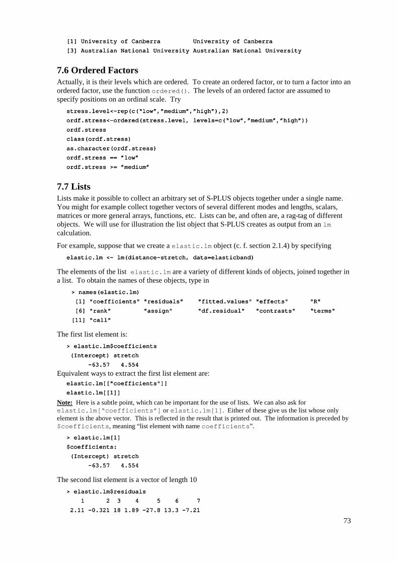
73

[1] University of Canberra University of Canberra [1] University of Canberra University of Canberra [1] University of Canberra University of Canberra [1] University of Canberra University of Canberra

[3] Australian National University Australian National University[3] Australian National University Australian National University[3] Australian National University Australian National University[3] Australian National University Australian National University

7.6 Ordered Factors Actually, it is their levels which are ordered. To create an ordered factor, or to turn a factor into an ordered factor, use the function ordered(). The levels of an ordered factor are assumed to specify positions on an ordinal scale. Try

stress.level<stress.level<stress.level<stress.level<----rep(c(“low”,”mrep(c(“low”,”mrep(c(“low”,”mrep(c(“low”,”medium”,”high”),2)edium”,”high”),2)edium”,”high”),2)edium”,”high”),2)

ordf.stress<ordf.stress<ordf.stress<ordf.stress<----ordered(stress.level, levels=c(“low”,”medium”,”high”))ordered(stress.level, levels=c(“low”,”medium”,”high”))ordered(stress.level, levels=c(“low”,”medium”,”high”))ordered(stress.level, levels=c(“low”,”medium”,”high”))

ordf.stressordf.stressordf.stressordf.stress

class(ordf.stress)class(ordf.stress)class(ordf.stress)class(ordf.stress)

as.character(ordf.stress)as.character(ordf.stress)as.character(ordf.stress)as.character(ordf.stress)

ordf.stress == ”low”ordf.stress == ”low”ordf.stress == ”low”ordf.stress == ”low”

ordf.stress >= ”medium”ordf.stress >= ”medium”ordf.stress >= ”medium”ordf.stress >= ”medium”

7.7 Lists Lists make it possible to collect an arbitrary set of S-PLUS objects together under a single name. You might for example collect together vectors of several different modes and lengths, scalars, matrices or more general arrays, functions, etc. Lists can be, and often are, a rag-tag of different objects. We will use for illustration the list object that S-PLUS creates as output from an lm calculation.

For example, suppose that we create a elastic.lm object (c. f. section 2.1.4) by specifying elastic.lm <elastic.lm <elastic.lm <elastic.lm <---- lm(distance~stretch, data=elasticband) lm(distance~stretch, data=elasticband) lm(distance~stretch, data=elasticband) lm(distance~stretch, data=elasticband)

The elements of the list elastic.lm are a variety of different kinds of objects, joined together in a list. To obtain the names of these objects, type in

> names(elastic.lm)> names(elastic.lm)> names(elastic.lm)> names(elastic.lm)

[1] "coefficients" "residuals" "fitted.values" "effects" "R" [1] "coefficients" "residuals" "fitted.values" "effects" "R" [1] "coefficients" "residuals" "fitted.values" "effects" "R" [1] "coefficients" "residuals" "fitted.values" "effects" "R"

[6 [6 [6 [6] "rank" "assign" "df.residual" "contrasts" “terms" ] "rank" "assign" "df.residual" "contrasts" “terms" ] "rank" "assign" "df.residual" "contrasts" “terms" ] "rank" "assign" "df.residual" "contrasts" “terms"

[11] "call" [11] "call" [11] "call" [11] "call"

The first list element is: > elastic.lm$coefficients> elastic.lm$coefficients> elastic.lm$coefficients> elastic.lm$coefficients

(Intercept) stretch (Intercept) stretch (Intercept) stretch (Intercept) stretch

----63.57 4.55463.57 4.55463.57 4.55463.57 4.554

Equivalent ways to extract the first list element are: elastelastelastelastic.lm[["coefficients"]]ic.lm[["coefficients"]]ic.lm[["coefficients"]]ic.lm[["coefficients"]]

elastic.lm[[1]]elastic.lm[[1]]elastic.lm[[1]]elastic.lm[[1]]

Note: Here is a subtle point, which can be important for the use of lists. We can also ask for elastic.lm[“coefficients”] or elastic.lm[1]. Either of these give us the list whose only element is the above vector. This is reflected in the result that is printed out. The information is preceded by $coefficients, meaning “list element with name coefficients”.

> elastic.lm[1]> elastic.lm[1]> elastic.lm[1]> elastic.lm[1]

$coefficients:$coefficients:$coefficients:$coefficients:

(Intercept) stretch (Intercept) stretch (Intercept) stretch (Intercept) stretch

----63.57 4.55463.57 4.55463.57 4.55463.57 4.554

The second list element is a vector of length 10 > elastic.lm$residuals> elastic.lm$residuals> elastic.lm$residuals> elastic.lm$residuals

1 2 3 4 5 6 7 1 2 3 4 5 6 7 1 2 3 4 5 6 7 1 2 3 4 5 6 7

2.11 2.11 2.11 2.11 ----0.321 18 1.89 0.321 18 1.89 0.321 18 1.89 0.321 18 1.89 ----27.8 13.3 27.8 13.3 27.8 13.3 27.8 13.3 ----7.217.217.217.21

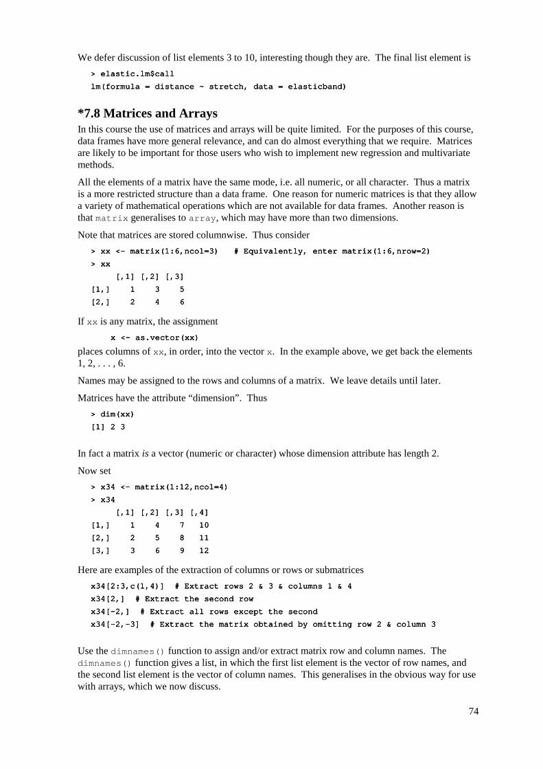
74

We defer discussion of list elements 3 to 10, interesting though they are. The final list element is > elastic.lm$call> elastic.lm$call> elastic.lm$call> elastic.lm$call

lm(formula = distancelm(formula = distancelm(formula = distancelm(formula = distance ~ stretch, data = elasticband) ~ stretch, data = elasticband) ~ stretch, data = elasticband) ~ stretch, data = elasticband)

*7.8 Matrices and Arrays In this course the use of matrices and arrays will be quite limited. For the purposes of this course, data frames have more general relevance, and can do almost everything that we require. Matrices are likely to be important for those users who wish to implement new regression and multivariate methods.

All the elements of a matrix have the same mode, i.e. all numeric, or all character. Thus a matrix is a more restricted structure than a data frame. One reason for numeric matrices is that they allow a variety of mathematical operations which are not available for data frames. Another reason is that matrix generalises to array, which may have more than two dimensions.

Note that matrices are stored columnwise. Thus consider > xx <> xx <> xx <> xx <---- matrix(1:6,ncol=3) # Equivalently, enter matrix(1:6,nrow=2) matrix(1:6,ncol=3) # Equivalently, enter matrix(1:6,nrow=2) matrix(1:6,ncol=3) # Equivalently, enter matrix(1:6,nrow=2) matrix(1:6,ncol=3) # Equivalently, enter matrix(1:6,nrow=2)

> xx> xx> xx> xx

[,1] [,2] [,3] [,1] [,2] [,3] [,1] [,2] [,3] [,1] [,2] [,3]

[1,] 1 3 5[1,] 1 3 5[1,] 1 3 5[1,] 1 3 5

[2,] 2 4 6[2,] 2 4 6[2,] 2 4 6[2,] 2 4 6

If xx is any matrix, the assignment x <x <x <x <---- as.vector(xx) as.vector(xx) as.vector(xx) as.vector(xx)

places columns of xx, in order, into the vector x. In the example above, we get back the elements 1, 2, . . . , 6.

Names may be assigned to the rows and columns of a matrix. We leave details until later.

Matrices have the attribute “dimension”. Thus > dim(xx)> dim(xx)> dim(xx)> dim(xx)

[1] 2 3[1] 2 3[1] 2 3[1] 2 3

In fact a matrix is a vector (numeric or character) whose dimension attribute has length 2.

Now set > x34 <> x34 <> x34 <> x34 <---- matrix(1:12,ncol=4) matrix(1:12,ncol=4) matrix(1:12,ncol=4) matrix(1:12,ncol=4)

> x34> x34> x34> x34

[,1] [,2] [,3] [,4] [,1] [,2] [,3] [,4] [,1] [,2] [,3] [,4] [,1] [,2] [,3] [,4]

[1,] 1 4 7 10[1,] 1 4 7 10[1,] 1 4 7 10[1,] 1 4 7 10

[2,] 2 5 8 11[2,] 2 5 8 11[2,] 2 5 8 11[2,] 2 5 8 11

[3,] 3 6 9 12[3,] 3 6 9 12[3,] 3 6 9 12[3,] 3 6 9 12

Here are examples of the extraction of columns or rows or submatrices x34[2:3,c(1,4)] # Extract rows 2 & 3 & columns 1 & 4x34[2:3,c(1,4)] # Extract rows 2 & 3 & columns 1 & 4x34[2:3,c(1,4)] # Extract rows 2 & 3 & columns 1 & 4x34[2:3,c(1,4)] # Extract rows 2 & 3 & columns 1 & 4

x34[2,] # Extract the second rowx34[2,] # Extract the second rowx34[2,] # Extract the second rowx34[2,] # Extract the second row

x34[x34[x34[x34[----2,] # Extract all rows except the second2,] # Extract all rows except the second2,] # Extract all rows except the second2,] # Extract all rows except the second

x34[x34[x34[x34[----2,2,2,2,----3] # Extract the matrix obtained by omittin3] # Extract the matrix obtained by omittin3] # Extract the matrix obtained by omittin3] # Extract the matrix obtained by omitting row 2 & column 3g row 2 & column 3g row 2 & column 3g row 2 & column 3

Use the dimnames() function to assign and/or extract matrix row and column names. The dimnames() function gives a list, in which the first list element is the vector of row names, and the second list element is the vector of column names. This generalises in the obvious way for use with arrays, which we now discuss.

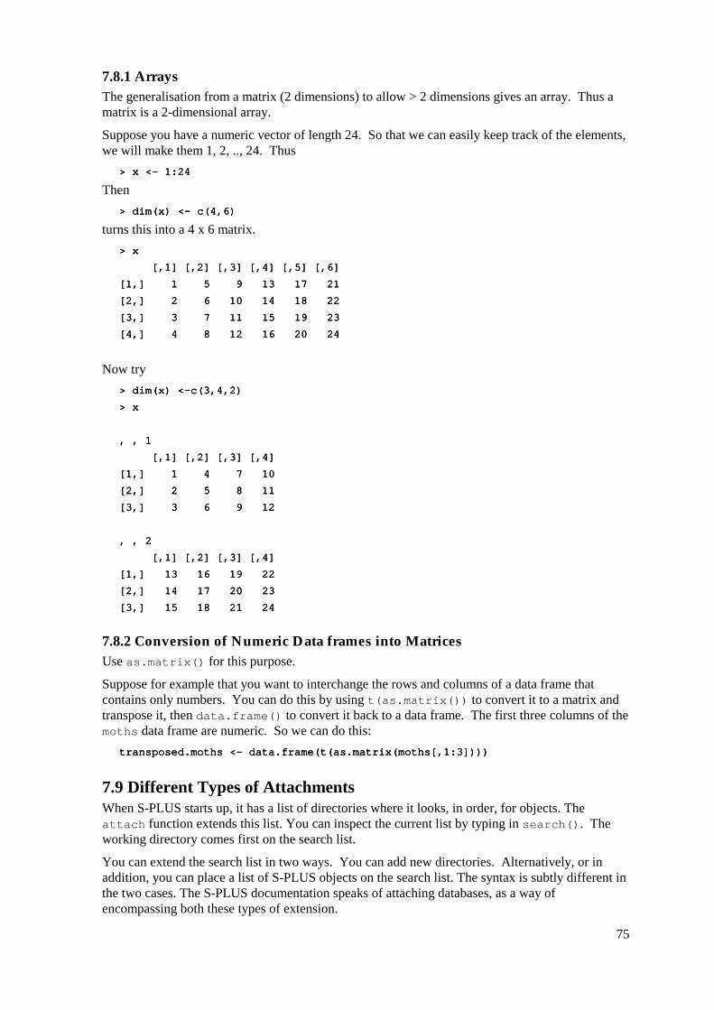
75

7.8.1 Arrays The generalisation from a matrix (2 dimensions) to allow > 2 dimensions gives an array. Thus a matrix is a 2-dimensional array.

Suppose you have a numeric vector of length 24. So that we can easily keep track of the elements, we will make them 1, 2, .., 24. Thus

> x <> x <> x <> x <---- 1:24 1:24 1:24 1:24

Then > dim(x) <> dim(x) <> dim(x) <> dim(x) <---- c(4,6) c(4,6) c(4,6) c(4,6)

turns this into a 4 x 6 matrix. > x> x> x> x

[,1] [,2] [,3] [,4] [,5] [,6] [,1] [,2] [,3] [,4] [,5] [,6] [,1] [,2] [,3] [,4] [,5] [,6] [,1] [,2] [,3] [,4] [,5] [,6]

[1,] [1,] [1,] [1,] 1 5 9 13 17 21 1 5 9 13 17 21 1 5 9 13 17 21 1 5 9 13 17 21

[2,] 2 6 10 14 18 22[2,] 2 6 10 14 18 22[2,] 2 6 10 14 18 22[2,] 2 6 10 14 18 22

[3,] 3 7 11 15 19 23[3,] 3 7 11 15 19 23[3,] 3 7 11 15 19 23[3,] 3 7 11 15 19 23

[4,] 4 8 12 16 20 24[4,] 4 8 12 16 20 24[4,] 4 8 12 16 20 24[4,] 4 8 12 16 20 24

Now try > dim(x) <> dim(x) <> dim(x) <> dim(x) <----c(3,4,2)c(3,4,2)c(3,4,2)c(3,4,2)

> x> x> x> x

, , 1, , 1, , 1, , 1

[,1] [,2] [,3] [,4] [,1] [,2] [,3] [,4] [,1] [,2] [,3] [,4] [,1] [,2] [,3] [,4]

[1,] 1 4 7 10[1,] 1 4 7 10[1,] 1 4 7 10[1,] 1 4 7 10

[2,] 2 5 8 11[2,] 2 5 8 11[2,] 2 5 8 11[2,] 2 5 8 11

[3,] [3,] [3,] [3,] 3 6 9 12 3 6 9 12 3 6 9 12 3 6 9 12

, , 2, , 2, , 2, , 2

[,1] [,2] [,3] [,4] [,1] [,2] [,3] [,4] [,1] [,2] [,3] [,4] [,1] [,2] [,3] [,4]

[1,] 13 16 19 22[1,] 13 16 19 22[1,] 13 16 19 22[1,] 13 16 19 22

[2,] 14 17 20 23[2,] 14 17 20 23[2,] 14 17 20 23[2,] 14 17 20 23

[3,] 15 18 21 24[3,] 15 18 21 24[3,] 15 18 21 24[3,] 15 18 21 24

7.8.2 Conversion of Numeric Data frames into Matrices Use as.matrix() for this purpose.

Suppose for example that you want to interchange the rows and columns of a data frame that contains only numbers. You can do this by using t(as.matrix()) to convert it to a matrix and transpose it, then data.frame() to convert it back to a data frame. The first three columns of the moths data frame are numeric. So we can do this:

transposed.moths <transposed.moths <transposed.moths <transposed.moths <---- data.frame(t(as.matrix(moths[,1:3]))) data.frame(t(as.matrix(moths[,1:3]))) data.frame(t(as.matrix(moths[,1:3]))) data.frame(t(as.matrix(moths[,1:3])))

7.9 Different Types of Attachments When S-PLUS starts up, it has a list of directories where it looks, in order, for objects. The attach function extends this list. You can inspect the current list by typing in search(). The working directory comes first on the search list.

You can extend the search list in two ways. You can add new directories. Alternatively, or in addition, you can place a list of S-PLUS objects on the search list. The syntax is subtly different in the two cases. The S-PLUS documentation speaks of attaching databases, as a way of encompassing both these types of extension.

76

A data frame is in fact a specialised list, with its columns as the objects. If you add a data frame to the search list, then you can refer to the columns by name, without the need to specify the data frame to which they belong. If there is any overlap of names, the order on the search list determines what name will be taken.

7.9.1 Attaching Data Frames Thus

> attach(primates)> attach(primates)> attach(primates)> attach(primates)

then allows you to refer to Brainwt and Bodywt, where you would otherwise have to type primates$Brainwt and primates$Bodywt. This assumes that you do not have any other variables or columns of attached data frames that have either of these names.

> Bodywt> Bodywt> Bodywt> Bodywt

Potar monkey Gorilla Human Rhesus monkey Chimp Potar monkey Gorilla Human Rhesus monkey Chimp Potar monkey Gorilla Human Rhesus monkey Chimp Potar monkey Gorilla Human Rhesus monkey Chimp

10 207 62 6.8 52.2 10 207 62 6.8 52.2 10 207 62 6.8 52.2 10 207 62 6.8 52.2

> Brainwt> Brainwt> Brainwt> Brainwt

Potar monkey Gorilla Human Rhesus monkey Chimp Potar monkey Gorilla Human Rhesus monkey Chimp Potar monkey Gorilla Human Rhesus monkey Chimp Potar monkey Gorilla Human Rhesus monkey Chimp

115 115 115 115 406 1320 179 440 406 1320 179 440 406 1320 179 440 406 1320 179 440

To detach this data frame, type > detach(“primates”)> detach(“primates”)> detach(“primates”)> detach(“primates”)

i.e. quotes are now used.

Note how the use of quotes changes. You specify the name (without quotes) when you attach, and enclose the name between quotes when you detach.

7.9.2 The S-PLUS Directory Structure S-PLUS has a search list, which can however be changed in the course of a session. This is the list of directories where S-PLUS will look for the objects that are needed as the session proceeds. To get a full list of these directories, type in

search()search()search()search()

The following are the different sorts of directories that will or (in the case of third party libraries) may appear on the search list:

• Working Directory: e.g. “C:/jhm/s“C:/jhm/s“C:/jhm/s“C:/jhm/s----course/_Data”course/_Data”course/_Data”course/_Data”

• System Directories: ““““C:/Program FilC:/Program FilC:/Program FilC:/Program Files/splus45/. . .”es/splus45/. . .”es/splus45/. . .”es/splus45/. . .”

• MathSoft Libraries: “C:/Program Files/splus45/library/. . .”“C:/Program Files/splus45/library/. . .”“C:/Program Files/splus45/library/. . .”“C:/Program Files/splus45/library/. . .”

• Third Party Libraries: “C:/Program Files/splus45/library/. . .”“C:/Program Files/splus45/library/. . .”“C:/Program Files/splus45/library/. . .”“C:/Program Files/splus45/library/. . .”

(Note that within S-PLUS you need to use //// or \\\\\\\\, not \\\\. This is a throwback to Unix.)

Objects that the user creates or changes are, unless specified otherwise, kept in the working directory.

7.9.3 Directories as databases The syntax for attaching and detaching a directory is a little different. For example I have a directory c:\stats\shape\_Data where I keep S-PLUS functions and other objects for size and shape calculations. Inside S-PLUS this will be referred to as c:/stats/shape/_Data, i.e. forward slashes replace backslashes.

I can attach this directory, and so gain use to its functions and other objects, by specifying attach(“c:/stats/shape/_Data”) # N. B. forward slashes

77

The default action is to attach it at position 2 in the search list. [You can check this by typing in search() . . . .] The directory automatically detaches at the end of your S-PLUS session. Otherwise, assuming that it is at position 2 on the search list, specify detach(2).

Observe that, here, the path was enclosed in quotes when you attached. To detach, specify the position on the search list. Thus if the directory was attached at position 2, specify

detach(2)

7.10 Exercises 1. Generate the numbers 101, 102, …, 112, and store the result in the vector x.

2. Generate four repeats of the sequence of numbers (4, 6, 3).

3. Generate the sequence consisting of eight 4s, then seven 6s, and finally nine 3s.

4. Create a vector consisting of one 1, then two 2’s, three 3’s, etc., and ending with nine 9’s.

5. In the built-in data frame environmental determine, for each of the columns, the median, mean, upper and lower quartiles, and range.

6. For each of the following calculations, decide what you would expect, and then check to see if you were right!

a) answer <answer <answer <answer <---- c(2, 7, 1, 5, 12, 3, 4) c(2, 7, 1, 5, 12, 3, 4) c(2, 7, 1, 5, 12, 3, 4) c(2, 7, 1, 5, 12, 3, 4)

for (j in 2:length(answer)){ answer[j] <for (j in 2:length(answer)){ answer[j] <for (j in 2:length(answer)){ answer[j] <for (j in 2:length(answer)){ answer[j] <---- max(answer[j],answer[j max(answer[j],answer[j max(answer[j],answer[j max(answer[j],answer[j----1])}1])}1])}1])}

b) answer <answer <answer <answer <---- c(2, 7, 1, 5, 12, 3, 4) c(2, 7, 1, 5, 12, 3, 4) c(2, 7, 1, 5, 12, 3, 4) c(2, 7, 1, 5, 12, 3, 4)

for (j in 2:lengtfor (j in 2:lengtfor (j in 2:lengtfor (j in 2:length(answer)){ answer[j] <h(answer)){ answer[j] <h(answer)){ answer[j] <h(answer)){ answer[j] <---- sum(answer[j],answer[j sum(answer[j],answer[j sum(answer[j],answer[j sum(answer[j],answer[j----1])}1])}1])}1])}

7. In the data frame environmental (a) extract the row or rows for which ozone has its maximum value; and (b) extract the vector of values of wind for values of ozone that are above the upper quartile.

8. Determine which columns of the built-in data frame claims are factors. For each of these factor columns, print out the levels vector. Which of these are ordered factors?

9. Determine which columns in the built-in data frame market.survey are variables, which are factors, and which are ordered factors.

10. Use summary() to get information about data in the data frames environmental, claims, and market.survey. Write brief notes, for each of these data sets, on what you have been able to learn.

11. From the data frame claims, extract a data frame claimsA which holds only the information for car type A.

12. From the data frame car.test.frame extract a data frame which holds only information for cars manufactured in Germany, France, Sweden, or England.

13. Store the numbers obtained in exercise 2, in order, in the columns of a 3 x 4 matrix.

Store the numbers obtained in exercise 3, in order, in the columns of a 6 by 4 matrix. Extract the matrix consisting of rows 3 to 6 and columns 3 and 4, of this matrix.

78

79

8. Useful Functions

8.1 Matching and Ordering match(<vec1>, <vec2>) ## For each element of <vec1>, returns the match(<vec1>, <vec2>) ## For each element of <vec1>, returns the match(<vec1>, <vec2>) ## For each element of <vec1>, returns the match(<vec1>, <vec2>) ## For each element of <vec1>, returns the

## position of the first occurrence in <vec2> ## position of the first occurrence in <vec2> ## position of the first occurrence in <vec2> ## position of the first occurrence in <vec2>

order(<vector>) ## Returns the vector of subscripts givingorder(<vector>) ## Returns the vector of subscripts givingorder(<vector>) ## Returns the vector of subscripts givingorder(<vector>) ## Returns the vector of subscripts giving ## the order in which elements must be taken ## the order in which elements must be taken ## the order in which elements must be taken ## the order in which elements must be taken

## so that <vector> will be sorted. ## so that <vector> will be sorted. ## so that <vector> will be sorted. ## so that <vector> will be sorted.

rank(<vector>) ## Returns the ranks of the successive elements.rank(<vector>) ## Returns the ranks of the successive elements.rank(<vector>) ## Returns the ranks of the successive elements.rank(<vector>) ## Returns the ranks of the successive elements.

Numeric vectors will be sorted in numerical order. Character vectors will be sorted in alphanumeric order.

The function match() can be used in all sorts of clever ways to pick out subsets of data. For example:

> x <> x <> x <> x <---- rep(1:5,rep(3,5)) rep(1:5,rep(3,5)) rep(1:5,rep(3,5)) rep(1:5,rep(3,5))

> x> x> x> x

[1] 1 1 1 2 2 2 3 3 3 4 4 4 5 5 5 [1] 1 1 1 2 2 2 3 3 3 4 4 4 5 5 5 [1] 1 1 1 2 2 2 3 3 3 4 4 4 5 5 5 [1] 1 1 1 2 2 2 3 3 3 4 4 4 5 5 5

> two4 <> two4 <> two4 <> two4 <---- match(x,c(2,4), nomatch=0) match(x,c(2,4), nomatch=0) match(x,c(2,4), nomatch=0) match(x,c(2,4), nomatch=0)

> > > > two4two4two4two4

[1] 0 0 0 1 1 1 0 0 0 2 2 2 0 0 0 [1] 0 0 0 1 1 1 0 0 0 2 2 2 0 0 0 [1] 0 0 0 1 1 1 0 0 0 2 2 2 0 0 0 [1] 0 0 0 1 1 1 0 0 0 2 2 2 0 0 0

> # We can use this to pick out the 2s and the 4s> # We can use this to pick out the 2s and the 4s> # We can use this to pick out the 2s and the 4s> # We can use this to pick out the 2s and the 4s

> as.logical(two4)> as.logical(two4)> as.logical(two4)> as.logical(two4)

[1] F F F T T T F F F T T T F F F [1] F F F T T T F F F T T T F F F [1] F F F T T T F F F T T T F F F [1] F F F T T T F F F T T T F F F

> x[as.logical(two4)]> x[as.logical(two4)]> x[as.logical(two4)]> x[as.logical(two4)]

[1] 2 2 2 4 4 4> x <[1] 2 2 2 4 4 4> x <[1] 2 2 2 4 4 4> x <[1] 2 2 2 4 4 4> x <---- rep(1:5,rep(3,5)) rep(1:5,rep(3,5)) rep(1:5,rep(3,5)) rep(1:5,rep(3,5))

> x> x> x> x

8.2 String Functions substring(<vector of text strings>, <first position>, <last position>)substring(<vector of text strings>, <first position>, <last position>)substring(<vector of text strings>, <first position>, <last position>)substring(<vector of text strings>, <first position>, <last position>)

nchar(<vector of text strings>) nchar(<vector of text strings>) nchar(<vector of text strings>) nchar(<vector of text strings>)

## Returns vector of number of characters in each element. ## Returns vector of number of characters in each element. ## Returns vector of number of characters in each element. ## Returns vector of number of characters in each element.

*8.2.1 Operations with Vectors of Text Strings – A Further Example The following stores, in nblank, the position of the first occurrence of a blank space in each of the row names of the built-in dataset fuel.frame.

nblank <nblank <nblank <nblank <---- sapply(row.names(fuel.frame),function(x){n < sapply(row.names(fuel.frame),function(x){n < sapply(row.names(fuel.frame),function(x){n < sapply(row.names(fuel.frame),function(x){n <---- nchar(x); nchar(x); nchar(x); nchar(x);

a < a < a < a <---- substring(x,1:n,1:n); m < substring(x,1:n,1:n); m < substring(x,1:n,1:n); m < substring(x,1:n,1:n); m <---- match(" " match(" " match(" " match(" ",a,nomatch=1); m}),a,nomatch=1); m}),a,nomatch=1); m}),a,nomatch=1); m})

To extract the first part of the name, up to the first space, specify car.names <car.names <car.names <car.names <---- substring(row.names(fuel.frame), 1, nblank substring(row.names(fuel.frame), 1, nblank substring(row.names(fuel.frame), 1, nblank substring(row.names(fuel.frame), 1, nblank----1)1)1)1)

8.3 Application of a Function to the Columns of an Array or Data Frame apply(<array>, <dimension>, <functioapply(<array>, <dimension>, <functioapply(<array>, <dimension>, <functioapply(<array>, <dimension>, <function>)n>)n>)n>)

lapply(<list>, <function>) lapply(<list>, <function>) lapply(<list>, <function>) lapply(<list>, <function>)

## N. B. A dataframe is a list. Output is a list. ## N. B. A dataframe is a list. Output is a list. ## N. B. A dataframe is a list. Output is a list. ## N. B. A dataframe is a list. Output is a list.

sapply(<list>, <function>) sapply(<list>, <function>) sapply(<list>, <function>) sapply(<list>, <function>) ## As lapply(), but simplify (e. g. to a vector ## As lapply(), but simplify (e. g. to a vector ## As lapply(), but simplify (e. g. to a vector ## As lapply(), but simplify (e. g. to a vector

## or matrix), if possible. ## or matrix), if possible. ## or matrix), if possible. ## or matrix), if possible.

80

8.3.1 apply() The function apply() can be used on data frames as well as matrices. Here is an example:

> apply(possum[,> apply(possum[,> apply(possum[,> apply(possum[,----(3:4)],2,mean)(3:4)],2,mean)(3:4)],2,mean)(3:4)],2,mean)

case site age hdlngth skullw totlngth taill pes case site age hdlngth skullw totlngth taill pes case site age hdlngth skullw totlngth taill pes case site age hdlngth skullw totlngth taill pes

52.5 3.62 NA 92.6 56.9 87.1 37 NA 52.5 3.62 NA 92.6 56.9 87.1 37 NA 52.5 3.62 NA 92.6 56.9 87.1 37 NA 52.5 3.62 NA 92.6 56.9 87.1 37 NA

earconch eye chest belly earconch eye chest belly earconch eye chest belly earconch eye chest belly

48.1 15 27 32.648.1 15 27 32.648.1 15 27 32.648.1 15 27 32.6

> apply(possum[,> apply(possum[,> apply(possum[,> apply(possum[,----(3:4)],2,mean,na.rm=T)(3:4)],2,mean,na.rm=T)(3:4)],2,mean,na.rm=T)(3:4)],2,mean,na.rm=T)

case site age hdlngth skullw totlngth taill pes case site age hdlngth skullw totlngth taill pes case site age hdlngth skullw totlngth taill pes case site age hdlngth skullw totlngth taill pes

52.5 3.62 3.83 92.6 56.9 87.1 37 68.5 52.5 3.62 3.83 92.6 56.9 87.1 37 68.5 52.5 3.62 3.83 92.6 56.9 87.1 37 68.5 52.5 3.62 3.83 92.6 56.9 87.1 37 68.5

earconch eye chest belly earconch eye chest belly earconch eye chest belly earconch eye chest belly

48.1 15 27 32.6 48.1 15 27 32.6 48.1 15 27 32.6 48.1 15 27 32.6

The use of apply(possum[,-(3:4)],1,mean) will give means for each row. These are not, for these data, useful information!

8.3.2 sapply() The function sapply() can be useful for getting information about the columns of a data frame. Here we use it to count that number of missing values in each column of the supplied data frame possum.

> sapply(possum[,> sapply(possum[,> sapply(possum[,> sapply(possum[,----(3:4)],function(x)sum(is.na(x)))(3:4)],function(x)sum(is.na(x)))(3:4)],function(x)sum(is.na(x)))(3:4)],function(x)sum(is.na(x)))

case site age hdlngth skullw totlngth taill pes case site age hdlngth skullw totlngth taill pes case site age hdlngth skullw totlngth taill pes case site age hdlngth skullw totlngth taill pes

0 0 2 0 0 0 0 1 0 0 2 0 0 0 0 1 0 0 2 0 0 0 0 1 0 0 2 0 0 0 0 1

earconch eye chest belly earconch eye chest belly earconch eye chest belly earconch eye chest belly

0 0 0 0 0 0 0 0 0 0 0 0 0 0 0 0

Here are several further examples that use the data frame moths that accompanies these notes: > sapply(moths,is.factor)> sapply(moths,is.factor)> sapply(moths,is.factor)> sapply(moths,is.factor) # Determine which columns are factors# Determine which columns are factors# Determine which columns are factors# Determine which columns are factors

meters A P habitat meters A P habitat meters A P habitat meters A P habitat

FALSE FALSE FALSE TRUE FALSE FALSE FALSE TRUE FALSE FALSE FALSE TRUE FALSE FALSE FALSE TRUE

> # How many levels does each factor have?> # How many levels does each factor have?> # How many levels does each factor have?> # How many levels does each factor have?

> sapply(moths, function(x)if(!is.factor(x))return(0) else length(levels(x)))> sapply(moths, function(x)if(!is.factor(x))return(0) else length(levels(x)))> sapply(moths, function(x)if(!is.factor(x))return(0) else length(levels(x)))> sapply(moths, function(x)if(!is.factor(x))return(0) else length(levels(x)))

meters A P habitat meters A P habitat meters A P habitat meters A P habitat

0 0 0 8 0 0 0 8 0 0 0 8 0 0 0 8

The function sapply() often works most conveniently if we can ensure that the function we use returns just one element for each column. In some circumstances, it may be helpful to use the paste() function to paste several different items together into a character string.

*8.4 tapply() The arguments are a variable, a list of factors, and a function that operates on a vector to return a single value. For each combination of factor levels, the function is applied to corresponding values of the variable. The output is an array with as many dimensions as there are factors. Where there are no data values for a particular combination of factor levels, NA is returned.

Often one wishes to get back, not an array, but a data frame with one row for each combination of factor levels. For example, we may have a data frame with two factors and a numeric variable, and want to create a new data frame with all possible combinations of the factors, and the cell means as the response. Here is an example of how to do it.

First, use tapply() to produce an array of cell means. The function dimnames(), applied to this array, returns a list whose first element holds the row names (i.e. for the level names for the first factor), and whose second element holds the column names. [Further dimensions are possible.]

81

We pass this list (row names, column names) to expand.grid(), which returns a data frame with all possible combinations of the factor levels. Finally, stretch the array of means out into a vector, and append this to the data frame. Here is an example using the S-PLUS data set 'catalyst'.

> names(catalyst)> names(catalyst)> names(catalyst)> names(catalyst)

[1] "Temp" "Conc" "Ca[1] "Temp" "Conc" "Ca[1] "Temp" "Conc" "Ca[1] "Temp" "Conc" "Cat" "Yield"t" "Yield"t" "Yield"t" "Yield"

> attach(catalyst)> attach(catalyst)> attach(catalyst)> attach(catalyst)

> cat.tab <> cat.tab <> cat.tab <> cat.tab <---- tapply(Yield,list(Temp,Cat),mean) tapply(Yield,list(Temp,Cat),mean) tapply(Yield,list(Temp,Cat),mean) tapply(Yield,list(Temp,Cat),mean)

> cat.tab ## Examine the two> cat.tab ## Examine the two> cat.tab ## Examine the two> cat.tab ## Examine the two----dimensional arraydimensional arraydimensional arraydimensional array

AAAA BBBB

160160160160 57575757 48.548.548.548.5

180180180180 70707070 81.581.581.581.5

> cat.names <> cat.names <> cat.names <> cat.names <---- dimnames (cat.tab) # The list cat.names holds the two dimnames (cat.tab) # The list cat.names holds the two dimnames (cat.tab) # The list cat.names holds the two dimnames (cat.tab) # The list cat.names holds the two

# vectors c(“160”,”180” # vectors c(“160”,”180” # vectors c(“160”,”180” # vectors c(“160”,”180”) and c(“A”,”B”)) and c(“A”,”B”)) and c(“A”,”B”)) and c(“A”,”B”)

> cat.df <> cat.df <> cat.df <> cat.df <---- expand.grid(Temp=factor (cat.names[[1]]), expand.grid(Temp=factor (cat.names[[1]]), expand.grid(Temp=factor (cat.names[[1]]), expand.grid(Temp=factor (cat.names[[1]]),

Cat=factor(cat.names[[2]])) Cat=factor(cat.names[[2]])) Cat=factor(cat.names[[2]])) Cat=factor(cat.names[[2]]))

> cat.df$Means <> cat.df$Means <> cat.df$Means <> cat.df$Means <---- as.vector(cat.tab) # Stretch the array of means out as.vector(cat.tab) # Stretch the array of means out as.vector(cat.tab) # Stretch the array of means out as.vector(cat.tab) # Stretch the array of means out

# into a vector, and create a new # into a vector, and create a new # into a vector, and create a new # into a vector, and create a new

# col # col # col # column of cat.df, named Means,umn of cat.df, named Means,umn of cat.df, named Means,umn of cat.df, named Means,

# to hold the array values. # to hold the array values. # to hold the array values. # to hold the array values.

> cat.df> cat.df> cat.df> cat.df

TempTempTempTemp CatCatCatCat MeansMeansMeansMeans

1111 160160160160 AAAA 57.057.057.057.0

2222 180180180180 AAAA 70.070.070.070.0

3333 160160160160 BBBB 48.548.548.548.5

4444 180180180180 BBBB 81.581.581.581.5

In a case where there are no data for some combinations of factor levels, one might want to omit the corresponding rows.

8.5 Breaking Vectors and Data Frames Down into Lists – split() As an example,

split(catalyst$Yield, catalyst$Cat)split(catalyst$Yield, catalyst$Cat)split(catalyst$Yield, catalyst$Cat)split(catalyst$Yield, catalyst$Cat)

returns a list with two elements, the first named “A” and containing values of Yield where Cat has the level A, and the second named “B” that has the values of Yield where Cat has the level B. You need to use split() in this way in order to do side by side boxplots. The function boxplot() takes as its first element a list in which the first list element is the vector of values for the first boxplot, the second list element is the vector of values for the second boxplot, and so on.

You can use split to split up a data frame into a list of data frames. For example split(catalyst[,split(catalyst[,split(catalyst[,split(catalyst[,----3], catalyst$Cat) # Split remaining col3], catalyst$Cat) # Split remaining col3], catalyst$Cat) # Split remaining col3], catalyst$Cat) # Split remaining columnsumnsumnsumns

# by levels of Cat # by levels of Cat # by levels of Cat # by levels of Cat

split(fuel.frame[,split(fuel.frame[,split(fuel.frame[,split(fuel.frame[,----5], fuel.frame$Type)5], fuel.frame$Type)5], fuel.frame$Type)5], fuel.frame$Type)

*8.6 Merging Data Frames The data frame car.all holds extensive information on 111 cars, derived from the April 1990 edition of the US publication “Consumer Reports”. One of the variables, stored as a factor, is

82

Type. I havc created a data frame type.df which holds two character abbreviations of each of the car types, suitable for use in plotting.

> type.df # Let’s look at type.df> type.df # Let’s look at type.df> type.df # Let’s look at type.df> type.df # Let’s look at type.df

Type abbrev Type abbrev Type abbrev Type abbrev

1 1 1 1 Small SmSmall SmSmall SmSmall Sm

2 Medium Md2 Medium Md2 Medium Md2 Medium Md

3 Compact Cm3 Compact Cm3 Compact Cm3 Compact Cm

4 Large Lr4 Large Lr4 Large Lr4 Large Lr

5 5 5 5 ----

6 Van Vn6 Van Vn6 Van Vn6 Van Vn

7 Sporty Sp7 Sporty Sp7 Sporty Sp7 Sporty Sp

Then > new.df <> new.df <> new.df <> new.df <---- merge(car.all, type.df, by=”Type”) merge(car.all, type.df, by=”Type”) merge(car.all, type.df, by=”Type”) merge(car.all, type.df, by=”Type”)

will create a data frame which has the abbreviations in the additional column with name “abbrev”. Note that rows with missing values will be omitted from the new data frame.

> dim(car.all) # car.all is a built> dim(car.all) # car.all is a built> dim(car.all) # car.all is a built> dim(car.all) # car.all is a built----in data framein data framein data framein data frame

[1] 111 36[1] 111 36[1] 111 36[1] 111 36

> dim(new.df)> dim(new.df)> dim(new.df)> dim(new.df)

[1] 105 37[1] 105 37[1] 105 37[1] 105 37

There are six missing values in car.all$Type, which explains the discrepancy. One way to get them included is to specify

> car.all$Type <> car.all$Type <> car.all$Type <> car.all$Type <---- as.character(car.all$Type) as.character(car.all$Type) as.character(car.all$Type) as.character(car.all$Type)

> type.df$Type <> type.df$Type <> type.df$Type <> type.df$Type <---- as.character(type.df$Type) as.character(type.df$Type) as.character(type.df$Type) as.character(type.df$Type)

> new.df <> new.df <> new.df <> new.df <---- merge(car.all, type.df, by=”Type”) merge(car.all, type.df, by=”Type”) merge(car.all, type.df, by=”Type”) merge(car.all, type.df, by=”Type”)

> dim(new.df)> dim(new.df)> dim(new.df)> dim(new.df)

[1] 111 37[1] 111 37[1] 111 37[1] 111 37

The function as.character() converts the missing values into empty strings (“”). So rows initially with NA in car.all$Type will have the empty string in new.df$Type. Moreover new.df$Type will be a vector of character strings.

Here is a longwinded way, using match(), to achieve the same effect. > unique(as.character(car.all$Type)) # Just checking> unique(as.character(car.all$Type)) # Just checking> unique(as.character(car.all$Type)) # Just checking> unique(as.character(car.all$Type)) # Just checking

[1] "Small" "Medium" "Compact" "Large" "" "Van" "Sporty" [1] "Small" "Medium" "Compact" "Large" "" "Van" "Sporty" [1] "Small" "Medium" "Compact" "Large" "" "Van" "Sporty" [1] "Small" "Medium" "Compact" "Large" "" "Van" "Sporty"

> entry <> entry <> entry <> entry <---- match(as.character(car.all$Type), as.character(type.df$Type)) match(as.character(car.all$Type), as.character(type.df$Type)) match(as.character(car.all$Type), as.character(type.df$Type)) match(as.character(car.all$Type), as.character(type.df$Type))

> sum(is.na(entry)) # Just check> sum(is.na(entry)) # Just check> sum(is.na(entry)) # Just check> sum(is.na(entry)) # Just checking that there are no NAsing that there are no NAsing that there are no NAsing that there are no NAs

[1] 0[1] 0[1] 0[1] 0

> car.all$abbrev <> car.all$abbrev <> car.all$abbrev <> car.all$abbrev <---- type.df$abbrev[entry] type.df$abbrev[entry] type.df$abbrev[entry] type.df$abbrev[entry]

> table(car.all$abbrev)> table(car.all$abbrev)> table(car.all$abbrev)> table(car.all$abbrev)

---- Cm Lr Md Sm Sp Vn Cm Lr Md Sm Sp Vn Cm Lr Md Sm Sp Vn Cm Lr Md Sm Sp Vn

6 19 7 26 22 21 10 6 19 7 26 22 21 10 6 19 7 26 22 21 10 6 19 7 26 22 21 10

8.7 Dates The function dates() will convert a character string into a dates object. By default, dates are stored using January 1 1960 as origin. This is important when you use as.integer to convert a date into an integer value.

> as.integer(dates("20/7/1999",format="d/m/year"))> as.integer(dates("20/7/1999",format="d/m/year"))> as.integer(dates("20/7/1999",format="d/m/year"))> as.integer(dates("20/7/1999",format="d/m/year"))

[1] 14445[1] 14445[1] 14445[1] 14445

> as.integer(dates("1/1/1960",format="d/m/year"))> as.integer(dates("1/1/1960",format="d/m/year"))> as.integer(dates("1/1/1960",format="d/m/year"))> as.integer(dates("1/1/1960",format="d/m/year"))

83

[1] 0[1] 0[1] 0[1] 0

> # Convert> # Convert> # Convert> # Convert from “no of days” to date from “no of days” to date from “no of days” to date from “no of days” to date

> tday<> tday<> tday<> tday<----dates(14445, format="d", out.format="day month year")dates(14445, format="d", out.format="day month year")dates(14445, format="d", out.format="day month year")dates(14445, format="d", out.format="day month year")

> tday> tday> tday> tday

[1] 20 July 1999[1] 20 July 1999[1] 20 July 1999[1] 20 July 1999

A wide variety of different formats are possible. You can specify the origin that is to be used for dates, if you prefer something different from the default.

One can subtract two dates and get the time between them in days. > dates("20/7/99",format="d/m/y")> dates("20/7/99",format="d/m/y")> dates("20/7/99",format="d/m/y")> dates("20/7/99",format="d/m/y")----dates("27/1/98",format="d/m/y")dates("27/1/98",format="d/m/y")dates("27/1/98",format="d/m/y")dates("27/1/98",format="d/m/y")

[1] 539[1] 539[1] 539[1] 539

attr(, "format"):attr(, "format"):attr(, "format"):attr(, "format"):

[1] "h:m:s"[1] "h:m:s"[1] "h:m:s"[1] "h:m:s"

attr(, "class"):attr(, "class"):attr(, "class"):attr(, "class"):

[1] "times"[1] "times"[1] "times"[1] "times"

> dates("20/7/1999",format="d/m/year") > dates("20/7/1999",format="d/m/year") > dates("20/7/1999",format="d/m/year") > dates("20/7/1999",format="d/m/year") ----

dates("27/1/1998",format="d/m/year") dates("27/1/1998",format="d/m/year") dates("27/1/1998",format="d/m/year") dates("27/1/1998",format="d/m/year")

[1] 539[1] 539[1] 539[1] 539

>>>>

8.8 Exercises 1) For the data frame fuel.frame, get the information provided by summary() for each level

of Type. (Use split().)

2) Determine the number of cars, in the built-in data frame car.all, for each Country and Type.

3) In the data frame claims: (a) determine the number of rows of information for each age category (age) and car type (type); (b) determine the total number of claims for each age category and car type; (c) determine, for each age category and car type, the number of rows for which data are missing; (d) determine, for each age category and car type, the total cost of claims.

4) Determine the number of days, according to S-PLUS, between the following dates:

a) January 1 in the year 1, and January 1 in the year 500 [Remember to specify the format as e. g. “d/m/year”]

b) January 1 in the year 500, and January 1 in the year 1000

c) January 1 in the year 1000, and January 1 in the year 1500

d) January 1 in the year 1500, and January 1 in the year 2000

5) Generate a dates object that holds dates for each day in the year 1999. Specify the format so that the first day is printed as `1 January 1999’.

84

85

9. Writing Functions and other Code We have already met several functions. Here is a function to convert Fahrenheit to Celsius:

> fahrenheit2celsius <> fahrenheit2celsius <> fahrenheit2celsius <> fahrenheit2celsius <---- function(fahrenheit=32:40)(fahrenheit function(fahrenheit=32:40)(fahrenheit function(fahrenheit=32:40)(fahrenheit function(fahrenheit=32:40)(fahrenheit----32)*5/932)*5/932)*5/932)*5/9

> # Now invoke the function> # Now invoke the function> # Now invoke the function> # Now invoke the function

> fahrenheit2celsius(c(40,50,60))> fahrenheit2celsius(c(40,50,60))> fahrenheit2celsius(c(40,50,60))> fahrenheit2celsius(c(40,50,60))

[1] 4.444444 10.000000 15.555556[1] 4.444444 10.000000 15.555556[1] 4.444444 10.000000 15.555556[1] 4.444444 10.000000 15.555556

The function returns the value (fahrenheit-32)*5/9. More generally, a function returns the value of the last statement of the function. Unless the result from the function is assigned to a name, the result is printed.

Here is a function that prints out the mean and standard deviation of a set of numbers: > mean.and.> mean.and.> mean.and.> mean.and.sd <sd <sd <sd <---- function(x=1:10){ function(x=1:10){ function(x=1:10){ function(x=1:10){

+ av <+ av <+ av <+ av <---- mean(x) mean(x) mean(x) mean(x)

+ sd <+ sd <+ sd <+ sd <---- sqrt(var(x)) sqrt(var(x)) sqrt(var(x)) sqrt(var(x))

+ c(mean=av, SD=sd)+ c(mean=av, SD=sd)+ c(mean=av, SD=sd)+ c(mean=av, SD=sd)

+ }+ }+ }+ }

>>>>

> # Now invoke the function> # Now invoke the function> # Now invoke the function> # Now invoke the function

> mean.and.sd()> mean.and.sd()> mean.and.sd()> mean.and.sd()

mean SD mean SD mean SD mean SD

5.5 3.02765 5.5 3.02765 5.5 3.02765 5.5 3.02765

> mean.and.sd(hills$climb)> mean.and.sd(hills$climb)> mean.and.sd(hills$climb)> mean.and.sd(hills$climb)

mean SD mean SD mean SD mean SD

1815.314 1619.151 1815.314 1619.151 1815.314 1619.151 1815.314 1619.151

9.1 Syntax and Semantics A function is created using an assignment. On the right hand side, the parameters appear within round brackets. You can if you wish give a default. In the example above the default was x = 1:10, so that users can run the function without specifying a parameter, just to see what it does.

Following the closing “)” the function body appears. Except where the function body consists of just one statement, this is enclosed between curly braces ({ }). The return value usually appears on the final line of the function body. In the example above, this was the vector consisting of the two named elements mean and sd.

9.2 A Function that gives Data Frame Details First we will define a function which accepts a vector x as its only argument. It will allow us to determine whether x is a factor, and if a factor, how many levels it has. The built-in function is.factor() will return T if x is a factor, and otherwise F. The following function faclev() uses is.factor() to test whether x is a factor. It prints out 0 if x is not a factor, and otherwise the number of levels of x.

faclev <faclev <faclev <faclev <---- function(x)if(!is.factor(x))return(0) else length(levels(x)) function(x)if(!is.factor(x))return(0) else length(levels(x)) function(x)if(!is.factor(x))return(0) else length(levels(x)) function(x)if(!is.factor(x))return(0) else length(levels(x))

The function sapply() can be used to repeat a calculation on all columns of a data frame. [More generally, the first argument of sapply() may be a list.] To apply faclev() to all columns of the data frame market.survey we can specify

sapply(market.survey, faclev) sapply(market.survey, faclev) sapply(market.survey, faclev) sapply(market.survey, faclev)

We can alternatively put the definition of faclev in directly as the second argument of sapply, thus

86

sapply(market.ssapply(market.ssapply(market.ssapply(market.survey, function(x)if(!is.factor(x))return(0) urvey, function(x)if(!is.factor(x))return(0) urvey, function(x)if(!is.factor(x))return(0) urvey, function(x)if(!is.factor(x))return(0)

else length(levels(x)))else length(levels(x)))else length(levels(x)))else length(levels(x)))

Finally, we may want to do similar calculations on a number of different data frames. So we create a function check.df() which encapsulates the calculations. Here is the definition of check.df().

check.df <check.df <check.df <check.df <---- function(df=market.survey) function(df=market.survey) function(df=market.survey) function(df=market.survey)

sapply(df, function(x)if(!is.factor(x))return(0) else sapply(df, function(x)if(!is.factor(x))return(0) else sapply(df, function(x)if(!is.factor(x))return(0) else sapply(df, function(x)if(!is.factor(x))return(0) else length(levels(x))) length(levels(x))) length(levels(x))) length(levels(x)))

9.3 Coding that assists Data Management Where data, labelling etc must be pulled together from a number of sources, and especially where you may want to retrace your steps some months later, take the same care over structuring data as over structuring code. Thus if there is a factorial structure to the data files, choose file names that reflect it. You can then generate the file names automatically, using paste() to glue the separate portions of the name together.

Lists are a useful mechanism for grouping together all data and labelling information that one may wish to bring together in a single set of computations. Use as the name of the list a unique and meaningful identification code. Consider whether you should include objects as list items, or whether identification by name is preferable. Bear in mind, also, the use of switch(), with the identification code used to determine what switch() should pick out, to pull out specific information and data that is required for a particular run.

Concentrate in one function the task of pulling together data and labelling information, perhaps with some subsequent manipulation, from a number of separate files. This structures the code, and makes the function a source of documentation for the data.

Use user-defined data frame attributes to document your data. For example, given a data frame “roller” containing roller weights and resulting lawn depressions, you might specify

attributes(elasticband)$title <attributes(elasticband)$title <attributes(elasticband)$title <attributes(elasticband)$title <----

“Extent of stretch of band, and Resulting Distance” “Extent of stretch of band, and Resulting Distance” “Extent of stretch of band, and Resulting Distance” “Extent of stretch of band, and Resulting Distance”

9.4 Issues for the Writing and Use of Functions There can be many functions. Choose the names for your own functions carefully, so that they are meaningful.

Choose meaningful names for arguments, even if this means that they are longer than you would like. Remember that they can be abbreviated in actual use.

Settings that you may need to change in later use of the function should appear as default settings for parameters. Use lists, where this seems appropriate, to group together parameters that belong together conceptually.

As far as possible, make code self-documenting. Use meaningful names for S-PLUS objects. Ensure that the names used reflect the hierarchies of files, data structures and code.

S-PLUS allows the use of names for elements of vectors and lists, and for rows and columns of arrays and dataframes. Consider the use of names rather than numbers when you pull out individual elements, columns etc. Thus dead.tot[,”dead”] is more meaningful and safer than dead.tot[,2].

Where appropriate, provide a demonstration mode for functions. Such a mode will print out summary information on the data and/or on the results of manipulations prior to analysis, with appropriate labelling. The code needed to implement this feature has the side-effect of showing by example what the function does, and may be useful for debugging.

Break your functions up into a small number of sub-functions or “primitives”. Re-use existing functions wherever possible. Write any new “primitives” so that they can be re-used. This helps

87

ensure that functions contain well-tested and well-understood components. Watch s-news (section 13.3) for useful functions for routine tasks.

If at all possible, give parameters sensible defaults. Often a good strategy is to use as defaults parameters that will serve for a demonstration run of the function.

NULL is a useful default where the parameter mostly is not required, but where the parameter if it appears may be any one of several types of data structure. The test if(!is.null()) then determines whether one needs to investigate that parameter further.

Structure code to avoid multiple entry of information.

Structure computations so that it is easy to retrace them. For this reason substantial chunks of code should be incorporated into functions sooner rather than later.

9.4.1 Graphs Use graphs freely to shed light both on computations and on data. One of S-PLUS’s big pluses is its tight integration of computation and graphics.

9.5 Calling Modelling Functions from User-Written Functions Objects that are in the working directory are global, i.e. any function can refer to them without passing them as parameters.

There are however occasions when commands work when invoked from the working directory, but not from within a function. All objects in the working directory are visible to functions that are called from that directory, to any functions that they call, and so on. Objects that are visible within a function are visible only to any function that is immediately called, unless specific action is taken to ensure otherwise. An assignments in frame 1 (use assign()) is sometimes necessary to deal with this problem. This is not a tidy solution to the problem, but it does work! The problem turns up in a number of different contexts.

9.6 A Simulation Example We would like to know how well such a student would do, by random guessing, on a multiple choice test consisting of 100 questions each with five alterantives. We can get an idea by using simulation. Each question corresponds to an independent Bernoulli trial with probability of success equal to 0.2. We can simulate the correctness of the student for each question by generating an independent uniform random number. If this number is less than .2, we say that the student guessed correctly; otherwise, we say that the student guessed incorrectly.

This will work, because the probability that a uniform random variable is less than .2 is exactly .2, while the probability that a uniform random variable exceeds .2 is exactly .8, which is the same as the probability that the student guesses incorrectly. Thus, the uniform random number generator is simulating the student. S-PLUS can do this as follows:

Guesses <Guesses <Guesses <Guesses <---- runif(100) runif(100) runif(100) runif(100)

correct.answers <correct.answers <correct.answers <correct.answers <---- 1*(guesses < .2) 1*(guesses < .2) 1*(guesses < .2) 1*(guesses < .2)

The multiplication by 1 causes (guesses<.2), which is calculated as T or F, to be coerced to 1 (T) or 0 (F). The vector correct.answers thus contains the results of the student's guesses. A 1 is recorded each time the student correctly guesses the answer, while a 0 is recorded each time the student is wrong.

One can thus write an S-PLUS function which simulates a student guessing at a True-False test consisting of some arbitrary number of questions. We leave this as an exercise.

88

9.6.1 Poisson Random Numbers You can think of the Poisson distribution as the distribution of the total for occurrences of rare events. For example, the occurrence of an accident at an intersection on any one day should be a rare event. The total number of accidents over the course of a year may well follow a distribution which is close to Poisson. [However the total number of people injured is unlikely to follow a Poisson distribution. Why?] We can generate Poisson random numbers using rpois(). It is similar to the rbinom function, but there is only one parameter – the mean. Suppose for example traffic accidents occur at an intersection with a Poisson distribution that has a mean rate or 3.7 per year. To simulate the annual number of accidents for a 10-year period, we can specify rpois(10,3.7).

We pursue the Poisson distribution in an exercise below.

9.7 Exercises 1. Use the round function together with runif() to generate 100 random integers between 0 and 99. Now look up the help for sample(), and use it for the same purpose.

2. Write a general function to carry out the calculations of section 8.6. More specifically, the function will take as its arguments a list of response variables, a list of factors, a data frame, and a function. It will return a data frame in which each value for each combination of factor levels is summarised in a single statistic, for example the mean or the median.

3. The supplied data frame angina has columns placebo and TNG. Here is a function that plots, for each patient, the TNG result against the placebo result, but insisting on the same range for the x and y axes27.

plot.angina <plot.angina <plot.angina <plot.angina <---- function() function() function() function()

{{{{

xyrange < xyrange < xyrange < xyrange <---- range(angina) # Calculates the range of all values range(angina) # Calculates the range of all values range(angina) # Calculates the range of all values range(angina) # Calculates the range of all values

# in the data frame # in the data frame # in the data frame # in the data frame

par(pin=c(6.75, 6.75)) # Set p par(pin=c(6.75, 6.75)) # Set p par(pin=c(6.75, 6.75)) # Set p par(pin=c(6.75, 6.75)) # Set plotting area = 6.75 in. by 6.75 in.lotting area = 6.75 in. by 6.75 in.lotting area = 6.75 in. by 6.75 in.lotting area = 6.75 in. by 6.75 in.

plot(TNG~placebo,data=angina, xlim=xyrange, ylim=xyrange, pch=16) plot(TNG~placebo,data=angina, xlim=xyrange, ylim=xyrange, pch=16) plot(TNG~placebo,data=angina, xlim=xyrange, ylim=xyrange, pch=16) plot(TNG~placebo,data=angina, xlim=xyrange, ylim=xyrange, pch=16)

abline(0,1) # Line where TNG value = placebo value abline(0,1) # Line where TNG value = placebo value abline(0,1) # Line where TNG value = placebo value abline(0,1) # Line where TNG value = placebo value

}}}}

Rewrite this function so that, given the name of a data frame and of any two of its columns, it will plot the second named column against the first named column, showing also the line y=x.

4. Write a function that prints, with their row and column labels, only those elements of a correlation matrix for which abs(correlation) >= 0.9.

5. Write your own wrapper function for one-way analysis of variance which provides a side by side boxplot of the distribution of values by groups. If no response variable is specified, the function will generate random normal data (no difference between groups) and provide the analysis of variance and boxplot information for that.

6. Write a function which adds a text string containing documentation information as an attribute to a dataframe.

7. Write a function that computes a moving average of order 2 of the values in a given vector. Apply the above function to the data (in the data set huron that accompanies these notes) for the levels of Lake Huron. Repeat for a moving average of order 3. 27 The acronym TNG stands for trinitroglycerine, taken to help ward off attacks of angina. Data are from a clinical trial that compared TNG with placebo. All patients were assessed on both treatments, with the order randomised. The TNG treatment was known to be short-lived in its effect, acting only for five to fifteen minutes. So there is unlikely to be any serious carry-over effect to the later result with a placebo.

89

8. Find a way of computing the moving averages in exercise 3 that does not involve the use of a for loop.

9. Create a function to compute the average, variance and standard deviation of 1000 randomly generated uniform random numbers, on [0,1]. (Compare your results with the theoretical results: the expected value of a uniform random variable on [0,1] is 0.5, and the variance of such a random variable is 0.0833.)

10. Write a function which generates 100 independent observations on a uniformly distributed random variable on the interval [3.7, 5.8]. Find the mean, variance and standard deviation of such a uniform random variable. Now modify the function so that you can specify an arbitrary interval.

11. Look up the help for the sample() function. Use it to generate 50 random integers between 0 and 99, sampled without replacement. (This means that we do not allow any number to be sampled a second time.) Now, generate 50 random integers between 0 and 9, with replacement.

12. Write an S-PLUS function which simulates a student guessing at a True-False test consisting of 40 questions. Find the mean and variance of the student's answers. Compare with the theoretical values of .5 and .25.

13. Write an S-PLUS function which simulates a student guessing at a multiple choice test consisting of 40 questions, where there is chance of 1 in 5 of getting the right answer to each question. Find the mean and variance of the student's answers. Compare with the theoretical values of .2 and .16.

14. Write an S-PLUS function which simulates the number of working light bulbs out of 500, where each bulb has a probability .99 of working. Using simulation, estimate the expected value and variance of the random variable X, which is 1 if the light bulb works and 0 if the light bulb does not work. What are the theoretical values?

15. Write a function that does an arbitrary number n of repeated simulations of the number of accidents in a year, plotting the result in a suitable way. Assume that the number of accidents in a year follows a Poisson distribution. Run the function assuming an average rate of 2.8 accidents per year.

16. Write a function which simulates the repeated calculation of the coefficient of variation (= the ratio of the mean to the standard deviation), for independent random samples from a normal distribution.

17. Write a function which, for any sample, calculates the median of the absolute values of the deviations from the sample median.

*18. Generate random samples from normal, exponential, t (2 d. f.), and t (1 d. f.), thus:

a) xn<-rnorm(100)

b) xe<-rexp(100)

c) xt2<-rt(100, df=2)

d) xt2<-rt(100, df=1)

Apply the function from exercise 17 to each sample. Compare with the standard deviation in each case.

*19. The vector x consists of the frequencies 5, 3, 1, 4, 6 The first element is the number of occurrences of level 1, the second is the number of occurrences of level 2, and so on. Write a function which takes any such vector x as its input, and outputs the vector of factor levels, here 1 1 1 1 1 2 2 2 3 . . . [You’ll need the information that is provided by cumsum(x). Form a vector in which 1’s appear whenever the factor level is incremented, and is otherwise zero. . . .]

90

*20. Write a function which calculates the minimum of a quadratic, and the value of the function at the minimum.

*21. A “between times” correlation matrix, has been calculated from data on heights of trees at times 1, 2, 3, 4, . . . Write a function that calculates the average of the correlations for any given lag.

*22. Given data on trees at times 1, 2, 3, 4, . . ., write a function that calculates the matrix of “average” relative growth rates over the several intervals. Apply your function to the data frame rats that accompanies these notes.

[The relative growth rate may be defined as dt

wddtdw

wlog1 = . Hence its is reasonable to

calculate the average over the interval from t1 to t2 as 12

12 loglogtt

ww−−

.]

91

10. GLM, GAM and General Non-linear Models GLM models are Generalized Linear Models. GAM models are Generalized Additive Models. GLM models extend the multiple regression model. The GAM model is a further extension.

10.1 A Taxonomy of Extensions to the Linear Model S-PLUS allows a variety of extensions to the multiple linear regression model. In this chapter we describe the alternative functional forms.

The basic model formulation28 is:

Observed value = Model Prediction + Statistical Error

Often it is assumed that the statistical error values (values of ε in the discussion below) are independently and identically distributed as Normal. Generalised Linear Models, and the other extensions we describe, allow a variety of non-normal distributions. In the discussion of this section, our focus is on the form of the model prediction, and we leave until later sections the discussion of different possibilities for the “error” distribution.

Multiple regression model

y = α + β1x1 + β2x2 + . . . +βpxp + ε

Use lm() to fit multiple regression models. The various other models we describe are, in essence, generalizations of this model.

Generalized Linear Model (e. g. logit model)

y = g(a + b1x1) + ε

Here g(.) is selected from one of a small number of options.

For logit models, επ +=y , where

11)1

log( xba +=−ππ

Here π is an expected proportion, and

log(odds). is )logit( )1

log( ππ

π =−

We can turn this model around, and write

εε +++

+=++=)exp(1

)exp()(11

1111 xba

xbaxbagy

Here g(.) undoes the logit transformation.

We can add more explanatory variables: a + b1x1 + . . . + bpxp.

28 This may be generalised in various ways. Models that have this form may be nested within other models which have this basic form. Thus there may be `predictions’ and `errors’ at different levels within the total model.

92

Use glm() to fit generalised linear models.

Additive Model

εφφφ ++++= )(....)()( 2211 pp xxxy

Additive models are a generalisation of lm models. In 1 dimension

εφ += )( 11 xy

Some of )(),...,(),( 222111 ppp xzxzxz φφφ === may be smoothing functions, while others may be the usual linear model terms. The constant term gets absorbed into one or more of the φ s.

Generalized Additive Model

εφφφ ++++= ))(....)()(( 2211 pp xxxgy

Generalised Additive Models are a generalisation of Generalised Linear Models. For example, g(.) may be the function that undoes the logit transformation, as in a logistic regression model.

Some of )(),...,(),( 222111 ppp xzxzxz φφφ === may be smoothing functions, while others may be the usual linear model terms.

We can transform to get the model

ε+++= )...( 21 pzzzgy

Notice that even if p = 1, we may still want to retain both 1φ (.) and g(.), i.e.

εφ += ))(( 11 xgy

The reason is that g(.) is a specific function, such as the inverse of the logit function. The function (.)1φ does any further necessary smoothing, in case g(.) is not quite the right transformation. One

wants g(.) to do as much of possible of the task of transformation, with (.)1φ giving the transformation any necessary additional flourishes.

Use gam() to fit generalised additive models.

We now give examples of fitting glm, gam, and other models besides.

10.2 Logistic Regression We will use a logistic regression model as a starting point for discussing Generalized Linear Models.

With proportions that range from less than 0.1 to 0.99, it is not reasonable to expect that the expected proportion will be a linear function of x. Some such transformation (`link’ function) as the logit is required. A good way to think about logit models is that they work on a log(odds) scale. If p is a probability (e. g. that horse A will win the race), then the corresponding odds are p/(1-p), and

log(odds) = log(p

p1−) = log(p) -log(1-p)

93

The linear model predicts, not p, but log(p

p1−). Fig. 23 shows the logit transformation

Proportion

0.0 0.2 0.4 0.6 0.8 1.0

-6-4

-20

24

6

logi

t(Pro

porti

on),

i. e.

log(

Odd

s)

0.001

0.01

0.10.250.50.750.9

0.99

0.999

Prop

ortio

n

-6 -4 -2 0 2 4 6

0.0

0.2

0.4

0.6

0.8

1.0

logit(Proportion), i. e. log(Odds)

0.001 0.1 0.5 0.9 0.99

Figure 23: The logit or log(odds) transformation. The left panel shows a plot of log(odds) versus proportion, while the right panel shows a plot of proportion versus log(odds). Notice how the range is stretched out at both ends.

The logit or log(odds) function turns expected proportions into values that may range from -∞ to +∞. It is not satisfactory to use a linear model to predict proportions. The values from the linear model may well lie outside the range from 0 to 1. It is however in order to use a linear model to predict logit(proportion). The logit function is an example of a link function.

There are various other link functions that we can use with proportions. One of the commonest is the complementary log-log function.

10.2.1 Anaesthetic Depth Example Thirty patients were given an anaesthetic agent which was maintained at a pre-determined [alveolar] concentration for 15 minutes before making an incision29. It was then noted whether the patient moved, i.e. jerked or twisted. The interest is in estimating how the probability of jerking or twisting varies with increasing concentration of the anaesthetic agent.

The response is best taken as nomove, for reasons that will emerge later. There is a small number of concentrations; so we begin by tabulating proportion that have the nomove outcome against concentration. Alveolar Concentration

nomove 0.8 1 1.2 1.4 1.6 2.5

0 6 4 2 2 0 0

1 1 1 4 4 4 2

Total 7 5 6 6 4 2

_____________________________________________

Table 1: Patients moving (0) and not moving (1), for each of six different alveolar concentrations.

29 I am grateful to John Erickson (Anesthesia and Critical Care, University of Chicago) and to Alan Welsh (Centre for Mathematics & its Applications, Australian National University) for use of these data.

94

Fig. 24 then displays a plot of these proportions.

Concentration

Prop

ortio

n

1.0 1.5 2.0 2.5

0.0

0.2

0.4

0.6

0.8

1.0

75

6 6

4 2

Figure 24: Plot, versus concentration, of proportion of patients not moving. The dotted horizontal line is the estimate of the proportion of moves one would expect if the concentration had no effect.

We fit two models, the logit model and the complementary log-log model. We can fit the models either directly to the 0/1 data, or to the proportions in Table 1. To understand the output, you need to know about “deviances”. A deviance has a role very similar to a sum of squares in regression. Thus we have:

Regression Logistic regression

degrees of freedom degrees of freedom

sum of squares deviance

mean sum of squares

(divide by d.f.)

mean deviance

divide by d.f.)

We prefer models with a small mean residual sum of squares.

We prefer models with a small mean deviance.

If individuals respond independently, with the same probability, then we have Bernoulli trials. While individuals will be different in their response the assumption is that, each time a new individual is taken, they are drawn at random from some larger population. Here is the S-PLUS code:

> anaes.logit <> anaes.logit <> anaes.logit <> anaes.logit <---- glm(nomove ~ conc, family = binomial(link = logit), glm(nomove ~ conc, family = binomial(link = logit), glm(nomove ~ conc, family = binomial(link = logit), glm(nomove ~ conc, family = binomial(link = logit),

+ data = anesthetic)+ data = anesthetic)+ data = anesthetic)+ data = anesthetic)

The output summary is:

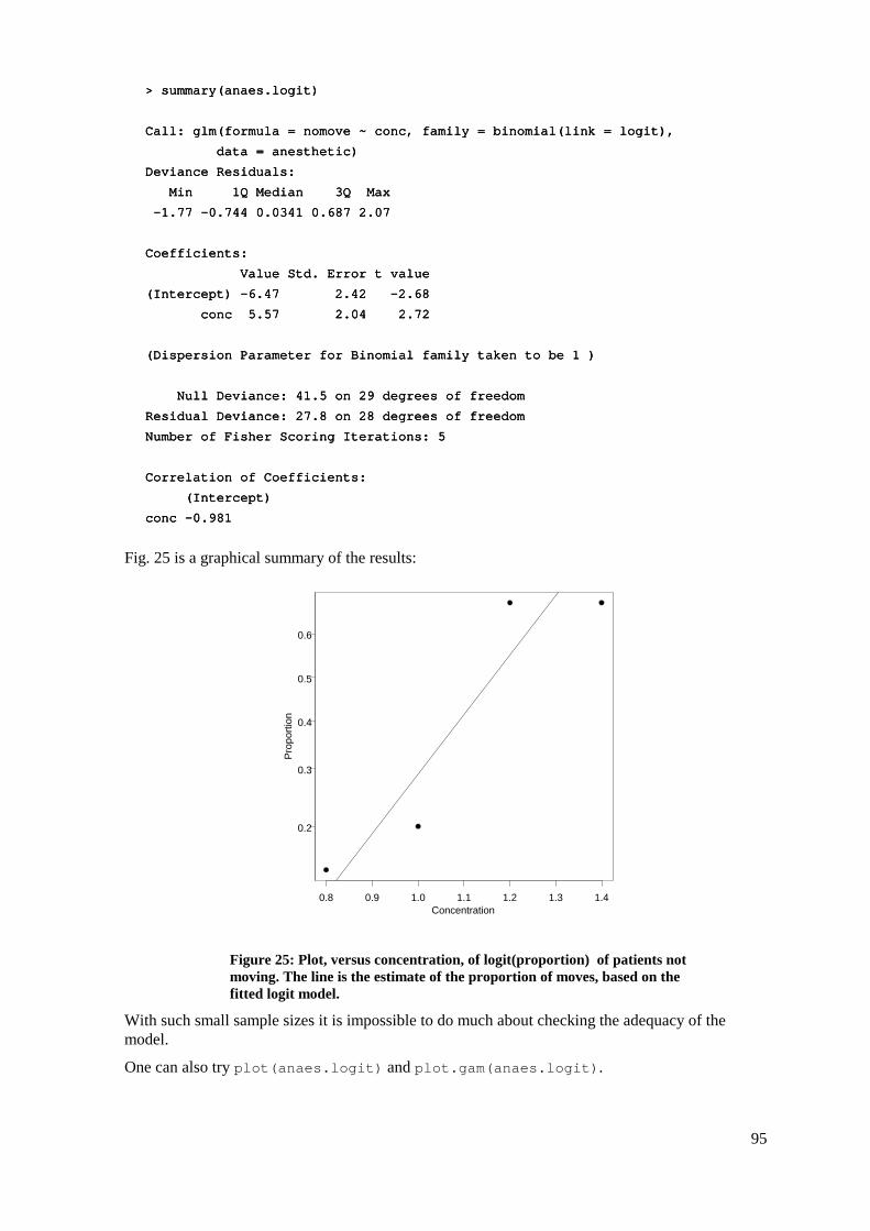
95

> summary(anaes.logit)> summary(anaes.logit)> summary(anaes.logit)> summary(anaes.logit)

Call: glm(formula = nomove ~ conc, family = binomial(linCall: glm(formula = nomove ~ conc, family = binomial(linCall: glm(formula = nomove ~ conc, family = binomial(linCall: glm(formula = nomove ~ conc, family = binomial(link = logit), k = logit), k = logit), k = logit),

data = anesthetic) data = anesthetic) data = anesthetic) data = anesthetic)

Deviance Residuals:Deviance Residuals:Deviance Residuals:Deviance Residuals:

Min 1Q Median 3Q Max Min 1Q Median 3Q Max Min 1Q Median 3Q Max Min 1Q Median 3Q Max

----1.77 1.77 1.77 1.77 ----0.744 0.0341 0.687 2.070.744 0.0341 0.687 2.070.744 0.0341 0.687 2.070.744 0.0341 0.687 2.07

Coefficients:Coefficients:Coefficients:Coefficients:

Value Std. Error t value Value Std. Error t value Value Std. Error t value Value Std. Error t value

(Intercept) (Intercept) (Intercept) (Intercept) ----6.47 2.42 6.47 2.42 6.47 2.42 6.47 2.42 ----2.682.682.682.68

conc 5.57 2.04 2.72 conc 5.57 2.04 2.72 conc 5.57 2.04 2.72 conc 5.57 2.04 2.72

(D(D(D(Dispersion Parameter for Binomial family taken to be 1 )ispersion Parameter for Binomial family taken to be 1 )ispersion Parameter for Binomial family taken to be 1 )ispersion Parameter for Binomial family taken to be 1 )

Null Deviance: 41.5 on 29 degrees of freedom Null Deviance: 41.5 on 29 degrees of freedom Null Deviance: 41.5 on 29 degrees of freedom Null Deviance: 41.5 on 29 degrees of freedom

Residual Deviance: 27.8 on 28 degrees of freedomResidual Deviance: 27.8 on 28 degrees of freedomResidual Deviance: 27.8 on 28 degrees of freedomResidual Deviance: 27.8 on 28 degrees of freedom

Number of Fisher Scoring Iterations: 5 Number of Fisher Scoring Iterations: 5 Number of Fisher Scoring Iterations: 5 Number of Fisher Scoring Iterations: 5

Correlation of Coefficients:Correlation of Coefficients:Correlation of Coefficients:Correlation of Coefficients:

(Intercept) (Intercept) (Intercept) (Intercept)

conc conc conc conc ----0.9810.9810.9810.981

Fig. 25 is a graphical summary of the results:

Concentration

Prop

ortio

n

0.8 0.9 1.0 1.1 1.2 1.3 1.4

0.2

0.3

0.4

0.5

0.6

Figure 25: Plot, versus concentration, of logit(proportion) of patients not moving. The line is the estimate of the proportion of moves, based on the fitted logit model.

With such small sample sizes it is impossible to do much about checking the adequacy of the model.

One can also try plot(anaes.logit) and plot.gam(anaes.logit).

96

10.3 glm models (Generalised Linear Regression Modelling) In the above we had

anaes.logit <anaes.logit <anaes.logit <anaes.logit <---- glm(nomove ~ conc, family = binomial(link = logit), glm(nomove ~ conc, family = binomial(link = logit), glm(nomove ~ conc, family = binomial(link = logit), glm(nomove ~ conc, family = binomial(link = logit), data=anesthetic)data=anesthetic)data=anesthetic)data=anesthetic)

The family parameter specifies the distribution for the dependent variable. There is an optional argument which allows us to specify the link function. Below we give further examples.

10.3.1 Further analyses of binomial data In the first example below the family is again binomial, with the default logit link. The dependent variable is Kyphosis, which may be either Present or Absent.

kyph.glm<kyph.glm<kyph.glm<kyph.glm<----glm(Kyphoglm(Kyphoglm(Kyphoglm(Kyphosis ~ poly(Age, 2) + (Number > 5)*Start,sis ~ poly(Age, 2) + (Number > 5)*Start,sis ~ poly(Age, 2) + (Number > 5)*Start,sis ~ poly(Age, 2) + (Number > 5)*Start,

family = binomial, data = kyphosis) # logit link family = binomial, data = kyphosis) # logit link family = binomial, data = kyphosis) # logit link family = binomial, data = kyphosis) # logit link

summary(kyph.glm)summary(kyph.glm)summary(kyph.glm)summary(kyph.glm)

res.kyph<res.kyph<res.kyph<res.kyph<----residuals(kyph.glm, type=”deviance”)residuals(kyph.glm, type=”deviance”)residuals(kyph.glm, type=”deviance”)residuals(kyph.glm, type=”deviance”)

# Other types of residuals are “pearson” and “working” # Other types of residuals are “pearson” and “working” # Other types of residuals are “pearson” and “working” # Other types of residuals are “pearson” and “working”

10.3.2 Data in the form of counts Data that are in the form of counts can often be analysed quite effectively assuming the poisson family. The link that is commonly used here is log. The log link transforms from positive numbers to numbers in the range -∞ to +∞ which a linear model may predict.

skips.glm<skips.glm<skips.glm<skips.glm<----glm(skips ~ ., family = poisson, data = solder.balance)glm(skips ~ ., family = poisson, data = solder.balance)glm(skips ~ ., family = poisson, data = solder.balance)glm(skips ~ ., family = poisson, data = solder.balance) # log link # log link # log link # log link

summary(skips.glm)summary(skips.glm)summary(skips.glm)summary(skips.glm)

10.3.3 The gaussian family If no family is specified, then the family is taken to be gaussian. The default link is then the identity, as for an lm model. This way of formulating an lm type model does however have the advantage that one is not restricted to the identity link.

air.glm<air.glm<air.glm<air.glm<----glm(ozone^(1/3) ~ bs(radiation, 5) + poly(wind, temperature,glm(ozone^(1/3) ~ bs(radiation, 5) + poly(wind, temperature,glm(ozone^(1/3) ~ bs(radiation, 5) + poly(wind, temperature,glm(ozone^(1/3) ~ bs(radiation, 5) + poly(wind, temperature, degree = 2), data = air) degree = 2), data = air) degree = 2), data = air) degree = 2), data = air) # Assumes gaussian famil # Assumes gaussian famil # Assumes gaussian famil # Assumes gaussian family, i.e. normal errors modely, i.e. normal errors modely, i.e. normal errors modely, i.e. normal errors model

# bs(radiation, 5) fits a spline curve which accounts for 5 d.f. # bs(radiation, 5) fits a spline curve which accounts for 5 d.f. # bs(radiation, 5) fits a spline curve which accounts for 5 d.f. # bs(radiation, 5) fits a spline curve which accounts for 5 d.f.

# B # B # B # B----spline models can in fact be fitted as linear models!spline models can in fact be fitted as linear models!spline models can in fact be fitted as linear models!spline models can in fact be fitted as linear models!

plot(air.glm)plot(air.glm)plot(air.glm)plot(air.glm)

plot.gam(air.glm)plot.gam(air.glm)plot.gam(air.glm)plot.gam(air.glm)

10.3.4 The robust(gaussian) family We investigate what a robust fit will make of the aberrant point in the hills data:

hills.glm<hills.glm<hills.glm<hills.glm<----glm(log(time)~log(distance)+log(climb), glm(log(time)~log(distance)+log(climb), glm(log(time)~log(distance)+log(climb), glm(log(time)~log(distance)+log(climb),

family=robust(gaussian), data=hills) family=robust(gaussian), data=hills) family=robust(gaussian), data=hills) family=robust(gaussian), data=hills)

> summary(hills.glm,corr=F)> summary(hills.glm,corr=F)> summary(hills.glm,corr=F)> summary(hills.glm,corr=F)

Call: glm(formula = log(time) ~ log(dist) + log(climb), Call: glm(formula = log(time) ~ log(dist) + log(climb), Call: glm(formula = log(time) ~ log(dist) + log(climb), Call: glm(formula = log(time) ~ log(dist) + log(climb),

family = robust(gaus family = robust(gaus family = robust(gaus family = robust(gaussian), data = hills)sian), data = hills)sian), data = hills)sian), data = hills)

Deviance Residuals:Deviance Residuals:Deviance Residuals:Deviance Residuals:

Min 1Q Median 3Q Max Min 1Q Median 3Q Max Min 1Q Median 3Q Max Min 1Q Median 3Q Max

----0.396 0.396 0.396 0.396 ----0.0581 0.00356 0.0618 0.7230.0581 0.00356 0.0618 0.7230.0581 0.00356 0.0618 0.7230.0581 0.00356 0.0618 0.723

Coefficients:Coefficients:Coefficients:Coefficients:

97

Value Std. Error t value Value Std. Error t value Value Std. Error t value Value Std. Error t value

(Intercept) 0.377 0.2862 1.32 (Intercept) 0.377 0.2862 1.32 (Intercept) 0.377 0.2862 1.32 (Intercept) 0.377 0.2862 1.32

log(dist) 0.903 0.0653 13.83 log(dist) 0.903 0.0653 13.83 log(dist) 0.903 0.0653 13.83 log(dist) 0.903 0.0653 13.83

log( log( log( log(climb) 0.240 0.0490 4.91climb) 0.240 0.0490 4.91climb) 0.240 0.0490 4.91climb) 0.240 0.0490 4.91

(Dispersion Parameter for Robust Gaussian family taken to be 0.024 )(Dispersion Parameter for Robust Gaussian family taken to be 0.024 )(Dispersion Parameter for Robust Gaussian family taken to be 0.024 )(Dispersion Parameter for Robust Gaussian family taken to be 0.024 )

Null Deviance: 16.9 on 34 degrees of freedom Null Deviance: 16.9 on 34 degrees of freedom Null Deviance: 16.9 on 34 degrees of freedom Null Deviance: 16.9 on 34 degrees of freedom

Residual Deviance: 1.15 on 32 degrees of freedomResidual Deviance: 1.15 on 32 degrees of freedomResidual Deviance: 1.15 on 32 degrees of freedomResidual Deviance: 1.15 on 32 degrees of freedom

Number of Fisher Scoring Iterations: 5Number of Fisher Scoring Iterations: 5Number of Fisher Scoring Iterations: 5Number of Fisher Scoring Iterations: 5

10.4 gam models (Generalised Additive Models) These make it possible to fit spline and other smooth transformations of explanatory variables.

kyph.gam<kyph.gam<kyph.gam<kyph.gam<----gam(Kyphosis ~ s(Age,4) + Number, family = binomial, data = gam(Kyphosis ~ s(Age,4) + Number, family = binomial, data = gam(Kyphosis ~ s(Age,4) + Number, family = binomial, data = gam(Kyphosis ~ s(Age,4) + Number, family = binomial, data = kyphosis)kyphosis)kyphosis)kyphosis)

Here s(Age, 4) is a spline smooth transformation of Age, with the smoothing chosen to account for around 4 degrees of freedom. Kyphosis is a factor that has two levels (present/absent); it is treated as a variable with values 0 or 1.

Ozone.gam<Ozone.gam<Ozone.gam<Ozone.gam<----gam(ozone^(1/3) ~ lo(radgam(ozone^(1/3) ~ lo(radgam(ozone^(1/3) ~ lo(radgam(ozone^(1/3) ~ lo(radiation) + lo(wind, temperature), iation) + lo(wind, temperature), iation) + lo(wind, temperature), iation) + lo(wind, temperature),

data = air) data = air) data = air) data = air)

kyphsub.gam<kyphsub.gam<kyphsub.gam<kyphsub.gam<----gam(Kyphosis ~ poly(Age, 2) + s(Start), data = kyphosis,gam(Kyphosis ~ poly(Age, 2) + s(Start), data = kyphosis,gam(Kyphosis ~ poly(Age, 2) + s(Start), data = kyphosis,gam(Kyphosis ~ poly(Age, 2) + s(Start), data = kyphosis,

subset = Number>5) subset = Number>5) subset = Number>5) subset = Number>5)

plot(kyph.gam)plot(kyph.gam)plot(kyph.gam)plot(kyph.gam)

print(kyph.gam)print(kyph.gam)print(kyph.gam)print(kyph.gam)

summary(kyph.gam)summary(kyph.gam)summary(kyph.gam)summary(kyph.gam)

summary.glm(kyph.gam) # Output is hard to interpret!summary.glm(kyph.gam) # Output is hard to interpret!summary.glm(kyph.gam) # Output is hard to interpret!summary.glm(kyph.gam) # Output is hard to interpret!

For a discussion of the Generalised Additive Model methodology, see Hastie & Tibshirani (1990).

10.5 Prediction with New Data The function predict() is a generic function that may be used to get model predictions. It does however have serious traps. If you have fitted a gam model, then the default is to use predict.gam (of course!), and all should be well. There is potential for trouble when you fit the inherently simpler lm or glm models. The problem arises with the computations which the more mathematically sophisticated novice is likely to undertake!

Warning: With models other than gam (lm, glm, etc.), you must explicitly use predict.gam() rather than predict() when you want predictions for new data under any of the following circumstances:

• the model uses poly() to include polynomial terms in one or more explanatory variables. [For example poly(x, 2) is mathematically equivalent to including terms in x and x2.]

• one or more factors has a levels vector which is a subset of the levels for the original data

• spline terms are included. [Usually one would then use a gam model.]

98

10.6 Non-linear Models You can use nls() (non-linear least squares) to obtain a least squares fit to a non-linear function. You can use nlmin() (minimum of a non-linear function) or ms() (another way to find a minimum of a non-linear function) to fit non-linear models using maximum likelihood or other such statistical criteria.

10.7 Model Summaries Type in

?methods(summary)?methods(summary)?methods(summary)?methods(summary)

to get a list of the summary methods that are available. You may want to mix and match, e.g. summary.lm() on an aov or gam object. The output may not be what you might expect. So be careful!

10.8 Further Elaborations Generalised Linear Models were developed in the 1970s. They unified a huge range of diverse methodology. They have now become a stock-in-trade of statistical analysts. Their practical implementation built on the powerful computational abilities which, by the 1970s, had been developed for handling linear model calculations.

Practical data analysis demands further elaborations. An important elaboration is to the incorporation of more than one term in the error structure. The S-PLUS nlme library implements such extensions, both for linear models and for a wide class of nonlinear models.

Each such new development builds on the theoretical and computational tools that have arisen from earlier developments. Exciting new analysis tools will continue to appear for a long time yet. This is fortunate. Most professional users of S-PLUS will regularly encounter data where the methodology that the data ideally demands is not yet available.

10.9 Exercises 1. Fit a Poisson regression model to the data in the data frame moths. Allow different intercepts for different habitats. Use log(meters) as covariate.

10.10 References Dobson, A. J. 1983. An Introduction to Statistical Modelling. Chapman and Hall, London.

Hastie, T. J. and Tibshirani, R. J. 1990. Generalised Additive Models. Chapman and Hall, London.

McCullagh, P. and Nelder, J. A., 2nd edn., 1989. Generalized Linear Models. Chapman and Hall.

Venables, W. N. and Ripley, B. D., 2nd edn 1997. Modern Applied Statistics with S-Plus. Springer, New York.

99

11. Multi-level Models, Time Series and Survival Analysis

*11.1 Multi-Level Models, Including Repeated Measures Models Variance component models and repeated measures models are special cases of multi-level models.

Models have both a fixed effects structure and an error structure. For example, in an inter-laboratory comparison there may be variation between laboratories, between observers within laboratories, and between multiple determinations made by the same observer on different samples. If we treat laboratories and observers as random, the only fixed effect is the mean.

The functions lme() and nlme(), from the Pinheiro and Bates library, handle models in which a repeated measures error structure is superimposed on a linear (lme) or non-linear (nlme) model. Version 3 of lme, which is currently in β-test, is broadly comparable in its abilities to Proc Mixed which is available in the widely used SAS statistical package. The function lme has associated with it highly useful abilities for diagnostic checking and for various insightful plots.

There is a strong link between a wide class of repeated measures models and time series models. In the time series context there is usually just one realisation of the series, which may however be observed at a large number of time points. In the repeated measures context there may be a large number of realisations of a series which is typically quite short.

11.1.1 The Kiwifruit Shading Data, Again Refer back to section 6.9.1 for details of these data. The fixed effects are block and treatment (shade). The random effects are block (though making block a random effect is optional), plot within block, and units within each block/plot combination. Here is the analysis:

> kiwishade.lme<> kiwishade.lme<> kiwishade.lme<> kiwishade.lme<----lme(yield~shade,random=~1|block/plot, data=kiwishade)lme(yield~shade,random=~1|block/plot, data=kiwishade)lme(yield~shade,random=~1|block/plot, data=kiwishade)lme(yield~shade,random=~1|block/plot, data=kiwishade)

> summary(kiwishade.lme)> summary(kiwishade.lme)> summary(kiwishade.lme)> summary(kiwishade.lme)

Linear mixedLinear mixedLinear mixedLinear mixed----effeeffeeffeeffects model fit by REMLcts model fit by REMLcts model fit by REMLcts model fit by REML

Data: kiwishade Data: kiwishade Data: kiwishade Data: kiwishade

AIC BIC logLik AIC BIC logLik AIC BIC logLik AIC BIC logLik

272.3 284.8 272.3 284.8 272.3 284.8 272.3 284.8 ----129.2129.2129.2129.2

Random effects:Random effects:Random effects:Random effects:

Formula: ~ 1 | block Formula: ~ 1 | block Formula: ~ 1 | block Formula: ~ 1 | block

(Intercept) (Intercept) (Intercept) (Intercept)

StdDev: 2.019StdDev: 2.019StdDev: 2.019StdDev: 2.019

Formula: ~ 1 | plot %in% block Formula: ~ 1 | plot %in% block Formula: ~ 1 | plot %in% block Formula: ~ 1 | plot %in% block

(Intercept) Residual (Intercept) Residual (Intercept) Residual (Intercept) Residual

StdDev: 1.479 3.49StdDev: 1.479 3.49StdDev: 1.479 3.49StdDev: 1.479 3.49

Fixed effects: yield ~ shade Fixed effects: yield ~ shade Fixed effects: yield ~ shade Fixed effects: yield ~ shade

Value Std.Error DF t Value Std.Error DF t Value Std.Error DF t Value Std.Error DF t----value pvalue pvalue pvalue p----value value value value

(Intercept) 96.53 1.340 36 72.05 <.0001(Intercept) 96.53 1.340 36 72.05 <.0001(Intercept) 96.53 1.340 36 72.05 <.0001(Intercept) 96.53 1.340 36 72.05 <.0001

shade1 1.43 0.934 6 1.53 0.1774 shade1 1.43 0.934 6 1.53 0.1774 shade1 1.43 0.934 6 1.53 0.1774 shade1 1.43 0.934 6 1.53 0.1774

shade2 2.95 0.539 6 5.47 0.0016 shade2 2.95 0.539 6 5.47 0.0016 shade2 2.95 0.539 6 5.47 0.0016 shade2 2.95 0.539 6 5.47 0.0016

shade3 2.23 0.381 6 5 shade3 2.23 0.381 6 5 shade3 2.23 0.381 6 5 shade3 2.23 0.381 6 5.86 0.0011.86 0.0011.86 0.0011.86 0.0011

Correlation: Correlation: Correlation: Correlation:

(Intr) shade1 shade2 (Intr) shade1 shade2 (Intr) shade1 shade2 (Intr) shade1 shade2

100

shade1 0 shade1 0 shade1 0 shade1 0

shade2 0 0 shade2 0 0 shade2 0 0 shade2 0 0

shade3 0 0 0 shade3 0 0 0 shade3 0 0 0 shade3 0 0 0

Standardized WithinStandardized WithinStandardized WithinStandardized Within----Group Residuals:Group Residuals:Group Residuals:Group Residuals:

Min Q1 Med Q3 Max Min Q1 Med Q3 Max Min Q1 Med Q3 Max Min Q1 Med Q3 Max

----2.415 2.415 2.415 2.415 ----0.5981 0.5981 0.5981 0.5981 ----0.069 0.7805 1.5890.069 0.7805 1.5890.069 0.7805 1.5890.069 0.7805 1.589

NumbNumbNumbNumber of Observations: 48er of Observations: 48er of Observations: 48er of Observations: 48

Number of Groups: Number of Groups: Number of Groups: Number of Groups:

block plot %in% block block plot %in% block block plot %in% block block plot %in% block

3 12 3 12 3 12 3 12

> anova(kiwishade.lme)> anova(kiwishade.lme)> anova(kiwishade.lme)> anova(kiwishade.lme)

numDF denDF F numDF denDF F numDF denDF F numDF denDF F----value pvalue pvalue pvalue p----value value value value

(Intercept) 1 36 5191 <.0001(Intercept) 1 36 5191 <.0001(Intercept) 1 36 5191 <.0001(Intercept) 1 36 5191 <.0001

shade 3 6 22 0.0012 shade 3 6 22 0.0012 shade 3 6 22 0.0012 shade 3 6 22 0.0012

This was a balanced design, which is why in section 6.8.2 we could use aov() for an analysis. We can get an output summary that is helpful for showing how the error mean squares match up with standard deviation information given above thus:

> intervals(kiwishade.lme)> intervals(kiwishade.lme)> intervals(kiwishade.lme)> intervals(kiwishade.lme)

ApproximaApproximaApproximaApproximate 95% confidence intervalste 95% confidence intervalste 95% confidence intervalste 95% confidence intervals

Fixed effects: Fixed effects: Fixed effects: Fixed effects:

lower est. upper lower est. upper lower est. upper lower est. upper

(Intercept) 93.8153 96.533 99.250(Intercept) 93.8153 96.533 99.250(Intercept) 93.8153 96.533 99.250(Intercept) 93.8153 96.533 99.250

shade1 shade1 shade1 shade1 ----0.8583 1.427 3.7120.8583 1.427 3.7120.8583 1.427 3.7120.8583 1.427 3.712

shade2 1.6324 2.952 4.271 shade2 1.6324 2.952 4.271 shade2 1.6324 2.952 4.271 shade2 1.6324 2.952 4.271

shade3 1.3007 2.234 3.166 shade3 1.3007 2.234 3.166 shade3 1.3007 2.234 3.166 shade3 1.3007 2.234 3.166

Random Effects: Random Effects: Random Effects: Random Effects:

Level: block Level: block Level: block Level: block

lower est. upper lower est. upper lower est. upper lower est. upper

sd((Intercept)) 0.5469 2.019 7.456sd((Intercept)) 0.5469 2.019 7.456sd((Intercept)) 0.5469 2.019 7.456sd((Intercept)) 0.5469 2.019 7.456

Level: plot Level: plot Level: plot Level: plot

lower est. upper lower est. upper lower est. upper lower est. upper

sd((Intercept)) 0.3676 1.479 5.947sd((Intercept)) 0.3676 1.479 5.947sd((Intercept)) 0.3676 1.479 5.947sd((Intercept)) 0.3676 1.479 5.947

Within Within Within Within----group standard error:group standard error:group standard error:group standard error:

lower est. upper lower est. upper lower est. upper lower est. upper

2.77 3.49 4.397 2.77 3.49 4.397 2.77 3.49 4.397 2.77 3.49 4.397

We are interested in the three estimates. By squaring the standard deviations and converting them to variances we get the information in the following table:

Variance component

Notes

block 2.0192 = 4.076 Three blocks

plot 1.4792= 2.186 4 plots per block

residual (within group)

3.4902=12.180 4 vines (subplots) per plot

101

The above allows us to put together the information for an analysis of variance table. We have:

Variance component

Mean square for anova table d.f.

block 4.076 12.180 + 4 × 2.186 + 16 × 4.076

= 86.14

2

(3-1)

plot 2.186 12.180 + 4 × 2.186

= 20.92

6

(3-1) ×(2-1)

residual (within group)

12.180 12.18 3×4×(4-1)

Now find see where these same pieces of information appeared in the analysis of variance table of section 6.9.1:

> kiwishade.aov<> kiwishade.aov<> kiwishade.aov<> kiwishade.aov<----aov(yield~block+shadeaov(yield~block+shadeaov(yield~block+shadeaov(yield~block+shade+Error(block:shade),data=kiwishade)+Error(block:shade),data=kiwishade)+Error(block:shade),data=kiwishade)+Error(block:shade),data=kiwishade)

> summary(kiwishade.aov)> summary(kiwishade.aov)> summary(kiwishade.aov)> summary(kiwishade.aov)

Error: block:shade Error: block:shade Error: block:shade Error: block:shade

Df Sum of Sq Mean Sq F Value Pr(F) Df Sum of Sq Mean Sq F Value Pr(F) Df Sum of Sq Mean Sq F Value Pr(F) Df Sum of Sq Mean Sq F Value Pr(F)

block 2 172 86.2 4.12 0.07488 block 2 172 86.2 4.12 0.07488 block 2 172 86.2 4.12 0.07488 block 2 172 86.2 4.12 0.07488

shade 3 1395 464.8 22.21 0.00119 shade 3 1395 464.8 22.21 0.00119 shade 3 1395 464.8 22.21 0.00119 shade 3 1395 464.8 22.21 0.00119

Residuals 6 126 20.9 Residuals 6 126 20.9 Residuals 6 126 20.9 Residuals 6 126 20.9

Error: Within Error: Within Error: Within Error: Within

Df Sum of Sq Mean Sq F Value Pr(F) Df Sum of Sq Mean Sq F Value Pr(F) Df Sum of Sq Mean Sq F Value Pr(F) Df Sum of Sq Mean Sq F Value Pr(F)

Residuals 36 438.6 12.18Residuals 36 438.6 12.18Residuals 36 438.6 12.18Residuals 36 438.6 12.18

11.1.2 The Pigment Data These are multi-level analysis of variance models. The varcomp() function offers one way to fit them. They are now better handled using the function lme() in the Pinheiro and Bates nlme library, which can handle a vastly wider class of problems. In this particular instance, the data are balanced over factor levels, and we can use analysis of variance.

We give scant explanation. This section may perhaps be useful for readers who already have some understanding of the methodology. Data are from the built-in data frame pigment.

First, we use analysis of variance: > pigment.aov <> pigment.aov <> pigment.aov <> pigment.aov <---- aov(Moisture ~ aov(Moisture ~ aov(Moisture ~ aov(Moisture ~ Batch/Sample, data=pigment) Batch/Sample, data=pigment) Batch/Sample, data=pigment) Batch/Sample, data=pigment)

> summary(pigment.aov) # Sum of squares (and mean squares) table> summary(pigment.aov) # Sum of squares (and mean squares) table> summary(pigment.aov) # Sum of squares (and mean squares) table> summary(pigment.aov) # Sum of squares (and mean squares) table

Df Sum of Sq Mean Sq F Value Pr(F) Df Sum of Sq Mean Sq F Value Pr(F) Df Sum of Sq Mean Sq F Value Pr(F) Df Sum of Sq Mean Sq F Value Pr(F)

Batch 14 1210.933 86.49524 94.35844 0 Batch 14 1210.933 86.49524 94.35844 0 Batch 14 1210.933 86.49524 94.35844 0 Batch 14 1210.933 86.49524 94.35844 0

Sample %in% Batch 15 869.750 57.98333 63.25Sample %in% Batch 15 869.750 57.98333 63.25Sample %in% Batch 15 869.750 57.98333 63.25Sample %in% Batch 15 869.750 57.98333 63.25455 0455 0455 0455 0

Residuals 30 27.500 0.91667 Residuals 30 27.500 0.91667 Residuals 30 27.500 0.91667 Residuals 30 27.500 0.91667

Here is what we get from the lme() function: > pigment.lme <> pigment.lme <> pigment.lme <> pigment.lme <---- lme(Moisture~1, random=~1|Batch/Sample, data=pigment) lme(Moisture~1, random=~1|Batch/Sample, data=pigment) lme(Moisture~1, random=~1|Batch/Sample, data=pigment) lme(Moisture~1, random=~1|Batch/Sample, data=pigment)

> intervals(pigment.lme)> intervals(pigment.lme)> intervals(pigment.lme)> intervals(pigment.lme)

Approximate 95% confidence intervalsApproximate 95% confidence intervalsApproximate 95% confidence intervalsApproximate 95% confidence intervals

102

Fixed effec Fixed effec Fixed effec Fixed effects:ts:ts:ts:

lower est. upper lower est. upper lower est. upper lower est. upper

(Intercept) 24.33 26.78 29.24(Intercept) 24.33 26.78 29.24(Intercept) 24.33 26.78 29.24(Intercept) 24.33 26.78 29.24

Random Effects: Random Effects: Random Effects: Random Effects:

Level: Batch Level: Batch Level: Batch Level: Batch

lower est. upper lower est. upper lower est. upper lower est. upper

sd((Intercept)) 0.6999 2.67 10.18sd((Intercept)) 0.6999 2.67 10.18sd((Intercept)) 0.6999 2.67 10.18sd((Intercept)) 0.6999 2.67 10.18

Level: Sample Level: Sample Level: Sample Level: Sample

lower est. upper lower est. upper lower est. upper lower est. upper

sd((Intercept)) 3.713 5.342 7.684sd((Intercept)) 3.713 5.342 7.684sd((Intercept)) 3.713 5.342 7.684sd((Intercept)) 3.713 5.342 7.684

WithinWithinWithinWithin----group standard error:group standard error:group standard error:group standard error:

lower est. upper lower est. upper lower est. upper lower est. upper

0.7427 0.9574 1.234 0.7427 0.9574 1.234 0.7427 0.9574 1.234 0.7427 0.9574 1.234

> c(26.78, 5.342, .9574)^2> c(26.78, 5.342, .9574)^2> c(26.78, 5.342, .9574)^2> c(26.78, 5.342, .9574)^2

[1] 717.1684 28.5370 0.9166[1] 717.1684 28.5370 0.9166[1] 717.1684 28.5370 0.9166[1] 717.1684 28.5370 0.9166

> c(2.67, 5.342, .9574)^2> c(2.67, 5.342, .9574)^2> c(2.67, 5.342, .9574)^2> c(2.67, 5.342, .9574)^2

[1] 7.1289 28.5370 0.9166[1] 7.1289 28.5370 0.9166[1] 7.1289 28.5370 0.9166[1] 7.1289 28.5370 0.9166

Thus the variance components are 7.12 (between batches), 28.54 (between samples within batches), and 0.92 (within samples).

Finally, for completeness, here is the output from varcomp(): > is.random(pigment) <> is.random(pigment) <> is.random(pigment) <> is.random(pigment) <---- T # make T # make T # make T # make all factors random > pigment.varcomp <> pigment.varcomp <> pigment.varcomp <> pigment.varcomp <---- varcomp(Moisture ~ Batch/Sample, pigment) varcomp(Moisture ~ Batch/Sample, pigment) varcomp(Moisture ~ Batch/Sample, pigment) varcomp(Moisture ~ Batch/Sample, pigment)

> # Explain variation in Mo> # Explain variation in Mo> # Explain variation in Mo> # Explain variation in Moisture in terms of variation between batches,isture in terms of variation between batches,isture in terms of variation between batches,isture in terms of variation between batches,

> # and variation of samples within batches> # and variation of samples within batches> # and variation of samples within batches> # and variation of samples within batches

> > > >

> summary(pigment.varcomp) # Components of variance breakdown> summary(pigment.varcomp) # Components of variance breakdown> summary(pigment.varcomp) # Components of variance breakdown> summary(pigment.varcomp) # Components of variance breakdown

Call:Call:Call:Call:

varcomp(formula = Moisture ~ Batch/Sample, data = pigment)varcomp(formula = Moisture ~ Batch/Sample, data = pigment)varcomp(formula = Moisture ~ Batch/Sample, data = pigment)varcomp(formula = Moisture ~ Batch/Sample, data = pigment)

Variance Estimates:Variance Estimates:Variance Estimates:Variance Estimates:

Variance Variance Variance Variance

Batch 7.1279762 Batch 7.1279762 Batch 7.1279762 Batch 7.1279762

Sample %in% Batch 28.5333333Sample %in% Batch 28.5333333Sample %in% Batch 28.5333333Sample %in% Batch 28.5333333

Residuals 0.9166667 Residuals 0.9166667 Residuals 0.9166667 Residuals 0.9166667

Method: minque0 Method: minque0 Method: minque0 Method: minque0

Coefficients:Coefficients:Coefficients:Coefficients:

(Intercept) (Intercept) (Intercept) (Intercept)

26.78333 26.78333 26.78333 26.78333

Approximate Covariance Matrix of Coefficients:Approximate Covariance Matrix of Coefficients:Approximate Covariance Matrix of Coefficients:Approximate Covariance Matrix of Coefficients:

[1] 1.441587[1] 1.441587[1] 1.441587[1] 1.441587

The first summary above is an analysis of variance (aov) summary. It gives the sum of squares table, and the corresponding mean squares. The variance components, given using lme() and varcomp(), provide a model for the generation of the mean squares. We now show how the mean square can be constructed from the variance components.

103

11.1.3 Analysis of Variance Versus Variance Components – The Pigment Data df AOV Mean

Square Estimate from Variance Components

Number of these units in next level

Batch 14 86.5 0.92+2×28.53+2×2×7.128 = 86.5 15

Sample in Batch

15 58.0 0.92+2×28.23 = 57.98 2

Residual 30 0.92 0.92 2

Here is another possibility: varcomp(Moisture ~ Batch/Sample, pigment, method=c("winsor", "r"))varcomp(Moisture ~ Batch/Sample, pigment, method=c("winsor", "r"))varcomp(Moisture ~ Batch/Sample, pigment, method=c("winsor", "r"))varcomp(Moisture ~ Batch/Sample, pigment, method=c("winsor", "r"))

*11.2 Repeated Measures Models The functions lme() and nlme() handle models in which a repeated measures error structure is superimposed on a linear (lme) or non-linear (nlme) model. Version 3 of lme, which is currently in β-test, is broadly comparable in its abilities to Proc Mixed which is available in the widely used SAS statistical package. The function lme has associated with it vastly superior abilities for diagnostic checking and for various insightful plots.

There is a strong link between a wide class of repeated measures models and time series models. In the time series context there is usually just one realisation of the series, which may however be observed at a large number of time points. In the repeated measures context there may be a large number of realisations of a series which is typically quite short.

Here is an example of the use of lme() for the Michelson speed of light data which are in the Venables and Ripley MASS library.

> michelson$Run <> michelson$Run <> michelson$Run <> michelson$Run <---- as.numeric(michelson$Run) # Ensure Run is a variable as.numeric(michelson$Run) # Ensure Run is a variable as.numeric(michelson$Run) # Ensure Run is a variable as.numeric(michelson$Run) # Ensure Run is a variable

> > > > mich.lme20 <mich.lme20 <mich.lme20 <mich.lme20 <---- lme(fixed = Speed ~ Run lme(fixed = Speed ~ Run lme(fixed = Speed ~ Run lme(fixed = Speed ~ Run, data = michelson, , data = michelson, , data = michelson, , data = michelson,

random = ~ Run| Expt, correlation = corARMA(value = c(0.25, 0.25), random = ~ Run| Expt, correlation = corARMA(value = c(0.25, 0.25), random = ~ Run| Expt, correlation = corARMA(value = c(0.25, 0.25), random = ~ Run| Expt, correlation = corARMA(value = c(0.25, 0.25),

form = ~ 1 | Expt, p = 2, q = 0), form = ~ 1 | Expt, p = 2, q = 0), form = ~ 1 | Expt, p = 2, q = 0), form = ~ 1 | Expt, p = 2, q = 0),

weights = varIdent(form = ~ 1 | Expt)) weights = varIdent(form = ~ 1 | Expt)) weights = varIdent(form = ~ 1 | Expt)) weights = varIdent(form = ~ 1 | Expt))

> summary(mich.lme20)> summary(mich.lme20)> summary(mich.lme20)> summary(mich.lme20)

Linear mixedLinear mixedLinear mixedLinear mixed----effects model fit by maximum likelihoodeffects model fit by maximum likelihoodeffects model fit by maximum likelihoodeffects model fit by maximum likelihood

Da Da Da Data: michelson ta: michelson ta: michelson ta: michelson

AIC BIC logLik AIC BIC logLik AIC BIC logLik AIC BIC logLik

1117 1148 1117 1148 1117 1148 1117 1148 ----546.4546.4546.4546.4

Random effects:Random effects:Random effects:Random effects:

Formula: ~ Run | Expt Formula: ~ Run | Expt Formula: ~ Run | Expt Formula: ~ Run | Expt

Structure: General positive Structure: General positive Structure: General positive Structure: General positive----definitedefinitedefinitedefinite

StdDev Corr StdDev Corr StdDev Corr StdDev Corr

(Intercept) 47.031 (Inter(Intercept) 47.031 (Inter(Intercept) 47.031 (Inter(Intercept) 47.031 (Inter

Run 3.628 Run 3.628 Run 3.628 Run 3.628 ----1 1 1 1

Residual 121.930 Residual 121.930 Residual 121.930 Residual 121.930

Correlation SCorrelation SCorrelation SCorrelation Structure: ARMA(2,0)tructure: ARMA(2,0)tructure: ARMA(2,0)tructure: ARMA(2,0)

Parameter estimate(s): Parameter estimate(s): Parameter estimate(s): Parameter estimate(s):

Phi1 Phi2 Phi1 Phi2 Phi1 Phi2 Phi1 Phi2

0.6321 0.6321 0.6321 0.6321 ----0.31060.31060.31060.3106

Variance function:Variance function:Variance function:Variance function:

Structure: Different standard deviations per stratum Structure: Different standard deviations per stratum Structure: Different standard deviations per stratum Structure: Different standard deviations per stratum

104

Formula: ~ 1 | Expt Formula: ~ 1 | Expt Formula: ~ 1 | Expt Formula: ~ 1 | Expt

Parameter estimates: Parameter estimates: Parameter estimates: Parameter estimates:

1 2 3 4 5 1 2 3 4 5 1 2 3 4 5 1 2 3 4 5

1 0.2993 0.6276 0.5678 0.4381 1 0.2993 0.6276 0.5678 0.4381 1 0.2993 0.6276 0.5678 0.4381 1 0.2993 0.6276 0.5678 0.4381

Fixed effects: Speed ~ Run Fixed effects: Speed ~ Run Fixed effects: Speed ~ Run Fixed effects: Speed ~ Run

Value Std.Error z Value Std.Error z Value Std.Error z Value Std.Error z----value pvalue pvalue pvalue p----value value value value

(Intercept) 860.9 27.2 31.6 0.0(Intercept) 860.9 27.2 31.6 0.0(Intercept) 860.9 27.2 31.6 0.0(Intercept) 860.9 27.2 31.6 0.0

Run Run Run Run ----1.6 2.1 1.6 2.1 1.6 2.1 1.6 2.1 ----0.7 0.50.7 0.50.7 0.50.7 0.5

Correlation: Correlation: Correlation: Correlation:

(Intr) (Intr) (Intr) (Intr)

Run Run Run Run ----0.9620.9620.9620.962

Standardized WithinStandardized WithinStandardized WithinStandardized Within----Group Residuals:Group Residuals:Group Residuals:Group Residuals:

Min Q1 Min Q1 Min Q1 Min Q1 Med Q3 Max Med Q3 Max Med Q3 Max Med Q3 Max

----2.905 2.905 2.905 2.905 ----0.6207 0.1222 0.7373 1.9550.6207 0.1222 0.7373 1.9550.6207 0.1222 0.7373 1.9550.6207 0.1222 0.7373 1.955

Number of Observations: 100Number of Observations: 100Number of Observations: 100Number of Observations: 100

Number of Groups: 5Number of Groups: 5Number of Groups: 5Number of Groups: 5

> # Now plot population residuals versus BLUP fitted values> # Now plot population residuals versus BLUP fitted values> # Now plot population residuals versus BLUP fitted values> # Now plot population residuals versus BLUP fitted values

> plot(mich.lme20, fitted(.) ~ Run | Expt, > plot(mich.lme20, fitted(.) ~ Run | Expt, > plot(mich.lme20, fitted(.) ~ Run | Expt, > plot(mich.lme20, fitted(.) ~ Run | Expt,

between = list(x = 0.25, y = 0.25), type =between = list(x = 0.25, y = 0.25), type =between = list(x = 0.25, y = 0.25), type =between = list(x = 0.25, y = 0.25), type = "b") "b") "b") "b")

> # NB S> # NB S> # NB S> # NB S----PLUS invokes plot.lme()PLUS invokes plot.lme()PLUS invokes plot.lme()PLUS invokes plot.lme()

> # Plot BLUP fitted effects versus Run, to help explain previous plot> # Plot BLUP fitted effects versus Run, to help explain previous plot> # Plot BLUP fitted effects versus Run, to help explain previous plot> # Plot BLUP fitted effects versus Run, to help explain previous plot

> plot(mich.lme20, resid(., type = "p") ~ > plot(mich.lme20, resid(., type = "p") ~ > plot(mich.lme20, resid(., type = "p") ~ > plot(mich.lme20, resid(., type = "p") ~

fitted(.) | Expt, between = list(x = 0.25, y = 0.25))

11.3 Time Series Models S-PLUS has a number of functions for manipulating and plotting time series, and for calculating the autocorrelation function.

There are two styles of analysis methods – time domain methods and frequency domain methods. In the time domain there are two classes of models – the conventional “short memory” models where the autocorrelation function decays quite rapidly to zero, and the relatively recently developed “long memory” time series models, where the autocorrelation function decays very slowly as observations move apart in time. A characteristic of “long memory” models is that there is variation at all temporal scales. Thus in a study of wind speeds it may be possible to characterise windy days, windy weeks, windy months, windy years, windy decades, and perhaps even windy centuries. S-PLUS has functions both for fitting conventional short memory models and for fitting the more recently developed long memory models.

The function stl() decomposes a times series into a trend and seasonal components, etc. (This is intended to replace the older sabl() function.) The functions ar() (for “autoregressive” models) and arima.mle() ( “autoregressive integrated moving average models”) fit standard types of time domain short memory models. Advanced users may want to be aware of the function arima.fracdiff() (“fractionally differenced ARIMA model”). This is designed for fitting “long memory” time domain models in which there is some residual correlation even at very long time lags.

There is in addition an extensive collection of functions for working with frequency domain or “spectral” analysis.

See the discussion of these models, including a brief survey of the statistical theory, in chapters 20-21 of the S-PLUS 4 Guide to Statistics (MathSoft, 1997).

105

11.4 Survival Analysis For example times at which subjects were either lost to the study or died (“failed”) may be recorded for individuals in each of several treatment groups. Engineering or business failures can be modelled using this same methodology. S-PLUS is strong in this area, with what may be the best abilities for survival analysis that are available in any statistical analysis package.

Chapters 22-26 of the S-PLUS4 Guide to Statistics (MathSoft, 1997) give an extended overview of the relevant theory, and details of S-PLUS abilities. There is a progression from the Kaplan-Meier non-parametric model, to models which assume specific parametric forms for the hazard ratio, and then through to fully parametric survival models.

11.5 Exercises 1. Use the function acf() to plot the autocorrelation function of lake levels in successive years in the data set huron that accompanies these notes. Do the plots both with type=”correlation” and with type=”partial”.

11.6 References Chambers, J. M. and Hastie, T. J. 1992. Statistical Models in S. Wadsworth and Brooks Cole Advanced Books and Software, Pacific Grove CA.

Diggle, Liang & Zeger (1996). Analysis of Longitudinal Data. Clarendon Press, Oxford.

Everitt, B. S. and Dunn, G. 1992. Applied Multivariate Data Analysis. Arnold, London.

Hand, D. J. & Crowder, M. J. (1996). Practical longitudinal data analysis. Chapman and Hall, London.

Little, R. C., Milliken, G. A., Stroup, W. W. and Wolfinger, R. D. (1996). SAS Systems for Mixed Models. SAS Institute Inc., Cary, New Carolina.

Maindonald, J. H. 1998. Repeated Measures. Unpublished manuscript, 25pp. Pinheiro, J. C. and Bates, D. M. 2000. Mixed effects models in S and S-PLUS. Springer, New York.

Venables, W. N. and Ripley, B. D., 2nd edn 1997. Modern Applied Statistics with S-Plus. Springer, New York.

106

107

12. Advanced Programming Topics

12.1. Methods S-PLUS is an object-oriented language. Objects may have a “class”. For functions such as print(), summary(), etc., the class of the object determines what action will be taken. Thus in response to print(x), S-PLUS determines the class attribute of x, if one exists. If for example the class attribute is “factor”, then the function which finally handles the printing is print.factor(). The function print.default() is used to print objects which have not been assigned a class.

More generally, the class attribute of an object may be a vector of strings. If there are “ancestor” classes – parent, grandparent, . . ., these are specified in order in subsequent elements of the class vector. For example, ordered factors have the class “ordered”, which inherits from the class “factor”. Thus:

> fac<> fac<> fac<> fac<----ordered(1:3)ordered(1:3)ordered(1:3)ordered(1:3)

> class(fac)> class(fac)> class(fac)> class(fac)

[1] "ordered" "factor" [1] "ordered" "factor" [1] "ordered" "factor" [1] "ordered" "factor"

> > > >

Here fac has the class “ordered”, which inherits from the parent class “factor”.

The function print.ordered(), which is the function that is called when you invoke print() with an ordered factor, makes use of the fact that “ordered” inherits from “factor”.

> print.ordered> print.ordered> print.ordered> print.ordered

function(x, ...)function(x, ...)function(x, ...)function(x, ...)

{{{{

NextMethod("print") ##NextMethod("print") ##NextMethod("print") ##NextMethod("print") ## Causes printing as for “factor” Causes printing as for “factor” Causes printing as for “factor” Causes printing as for “factor”

cat("cat("cat("cat("\\\\n", paste(levels(x), collapse = " < "), "n", paste(levels(x), collapse = " < "), "n", paste(levels(x), collapse = " < "), "n", paste(levels(x), collapse = " < "), "\\\\n") n") n") n")

## Adds extra information because factor is ordered## Adds extra information because factor is ordered## Adds extra information because factor is ordered## Adds extra information because factor is ordered

invisible(x)invisible(x)invisible(x)invisible(x)

}}}}

Note that it is purely a convenience for print.ordered() to operate in this way. The printing of a gam object generates a call to print.gam(), which does not call print.glm(). Nor does print.glm() call print.lm(). Here is an example:

> kyph.gam(formula = Kyphosis ~ lo(Age, 0.8) + Start + > kyph.gam(formula = Kyphosis ~ lo(Age, 0.8) + Start + > kyph.gam(formula = Kyphosis ~ lo(Age, 0.8) + Start + > kyph.gam(formula = Kyphosis ~ lo(Age, 0.8) + Start +

lo(Number, 0.8), family = binomial, data = kyphosis)lo(Number, 0.8), family = binomial, data = kyphosis)lo(Number, 0.8), family = binomial, data = kyphosis)lo(Number, 0.8), family = binomial, data = kyphosis)

> clas> clas> clas> class(kyph.gam)s(kyph.gam)s(kyph.gam)s(kyph.gam)

[1] "gam" "glm" "lm" [1] "gam" "glm" "lm" [1] "gam" "glm" "lm" [1] "gam" "glm" "lm"

12.2 Extracting Arguments to Functions How, inside a function, can one extract the value assigned to a parameter when the function was called? Below there is a function extract.arg(). When it is called as extract.arg(a=xx), we want it to return “xx”. When it is called as extract.arg(a=xy), we want it to return “xy”. Here is how it is done.

extract.arg <extract.arg <extract.arg <extract.arg <----

function (a)function (a)function (a)function (a)

{{{{

s <s <s <s <---- substitute(a) substitute(a) substitute(a) substitute(a)

108

as.character(s)as.character(s)as.character(s)as.character(s)

}}}}

> extract.arg(a=xy)> extract.arg(a=xy)> extract.arg(a=xy)> extract.arg(a=xy)

[1] [1] [1] [1] “xy”“xy”“xy”“xy”

If the argument is a function, we may want to get at the arguments to the function. Here is how one can do it

deparse.args <deparse.args <deparse.args <deparse.args <----

function (a)function (a)function (a)function (a)

{{{{

s <s <s <s <---- substitute (a) substitute (a) substitute (a) substitute (a)

if(mode(s) == "call"){if(mode(s) == "call"){if(mode(s) == "call"){if(mode(s) == "call"){

# the first element of a 'call' is the function called# the first element of a 'call' is the function called# the first element of a 'call' is the function called# the first element of a 'call' is the function called

# so# so# so# so we don't deparse that, just the arguments. we don't deparse that, just the arguments. we don't deparse that, just the arguments. we don't deparse that, just the arguments.

print(paste(“The function is: “, s[1],”()”, collapse=””)) print(paste(“The function is: “, s[1],”()”, collapse=””)) print(paste(“The function is: “, s[1],”()”, collapse=””)) print(paste(“The function is: “, s[1],”()”, collapse=””))

lapply (s[lapply (s[lapply (s[lapply (s[----1], function (x)1], function (x)1], function (x)1], function (x)

paste (deparse(x), collapse = "paste (deparse(x), collapse = "paste (deparse(x), collapse = "paste (deparse(x), collapse = "\\\\n"))n"))n"))n"))

} } } }

else stop ("argument is not a function call")else stop ("argument is not a function call")else stop ("argument is not a function call")else stop ("argument is not a function call")

}}}}

For example: > deparse.args(list(x+y, foo(bar)))> deparse.args(list(x+y, foo(bar)))> deparse.args(list(x+y, foo(bar)))> deparse.args(list(x+y, foo(bar)))

[1] “The function is: list()”[1] “The function is: list()”[1] “The function is: list()”[1] “The function is: list()”

[[1]]:[[1]]:[[1]]:[[1]]:

[1] "x + y"[1] "x + y"[1] "x + y"[1] "x + y"

[[2]]:[[2]]:[[2]]:[[2]]:

[1] "foo(bar)"[1] "foo(bar)"[1] "foo(bar)"[1] "foo(bar)"

12.3 Parsing and Evaluation of Expressions When you type in an expression such as mean(x+y) or cbind(x,y) for S-PLUS to evaluate, there are two steps:

1. The text string which you type in is parsed and turned into an expression, i.e. the syntax is checked and it is turned into code which the S-PLUS engine can more immediately evaluate.

2. The expression is evaluated.

If you type in expression(mean(x+y))expression(mean(x+y))expression(mean(x+y))expression(mean(x+y))

the output is the unevaluated expression expression(mean(x+y)). By setting my.exp <my.exp <my.exp <my.exp <---- expression(mean(x+y)) expression(mean(x+y)) expression(mean(x+y)) expression(mean(x+y))

you can store this unevaluated expression in my.exp . Actually what is actually stored in my.exp is a little different from what is printed out. S-PLUS gives you as much information as it judges is (most of the time) helpful for you to know.

Note that expression(mean(x+y)) is different from expression(“mean(x+y)”), as is obvious when the expression is evaluated. A text string is a text string is a text string, unless you explicitly change it into an expression or part of an expression.

Let’s see how this works in practice

109

> x <> x <> x <> x <---- 101:110 101:110 101:110 101:110

> y <> y <> y <> y <---- 21:30 21:30 21:30 21:30

> my.exp <> my.exp <> my.exp <> my.exp <---- expression(mean(x+y)) expression(mean(x+y)) expression(mean(x+y)) expression(mean(x+y))

> my.txt <> my.txt <> my.txt <> my.txt <---- expression("m expression("m expression("m expression("mean(x+y)")ean(x+y)")ean(x+y)")ean(x+y)")

> eval(my.exp)> eval(my.exp)> eval(my.exp)> eval(my.exp)

[1] 131[1] 131[1] 131[1] 131

> eval(my.txt)> eval(my.txt)> eval(my.txt)> eval(my.txt)

[1] "mean(x+y)"[1] "mean(x+y)"[1] "mean(x+y)"[1] "mean(x+y)"

What if we already have “mean(x+y)” stored in a text string, and we want to turn it into an expression? The answer is to use the function parse(), but you must tell it that you are supplying text rather than the name of a file. Thus

> parse(text="mean(x+y)")> parse(text="mean(x+y)")> parse(text="mean(x+y)")> parse(text="mean(x+y)")

expression(mean(x + y))expression(mean(x + y))expression(mean(x + y))expression(mean(x + y))

Let’s store the expression in my.exp2, and then evaluate it > my.exp2 <> my.exp2 <> my.exp2 <> my.exp2 <---- parse(text="mean(x+y)") parse(text="mean(x+y)") parse(text="mean(x+y)") parse(text="mean(x+y)")

> eval(my.exp2)> eval(my.exp2)> eval(my.exp2)> eval(my.exp2)

[1] 131[1] 131[1] 131[1] 131

Here is a function that creates a new data frame from an arbitrary set of columns of an existing data frame. Once in the function, we attach the data frame so that we can leave off the name of the data frame, and use only the column names

function(old.df = fuel.frame, colnames = c("Disp.", "Fuel"function(old.df = fuel.frame, colnames = c("Disp.", "Fuel"function(old.df = fuel.frame, colnames = c("Disp.", "Fuel"function(old.df = fuel.frame, colnames = c("Disp.", "Fuel"))))))))

{{{{

attach(old.df)attach(old.df)attach(old.df)attach(old.df)

on.exit(detach("old.df"))on.exit(detach("old.df"))on.exit(detach("old.df"))on.exit(detach("old.df"))

argtxt <argtxt <argtxt <argtxt <---- paste(colnames, collapse = ",") paste(colnames, collapse = ",") paste(colnames, collapse = ",") paste(colnames, collapse = ",")

exprtxt <exprtxt <exprtxt <exprtxt <---- paste("data.frame(", argtxt, ")", sep = "") paste("data.frame(", argtxt, ")", sep = "") paste("data.frame(", argtxt, ")", sep = "") paste("data.frame(", argtxt, ")", sep = "")

expr <expr <expr <expr <---- parse(text = exprtxt) parse(text = exprtxt) parse(text = exprtxt) parse(text = exprtxt)

df <df <df <df <---- eval(expr) eval(expr) eval(expr) eval(expr)

names(df) <names(df) <names(df) <names(df) <---- colnames colnames colnames colnames

dfdfdfdf

}}}}

To verify that the function does what it should, type in > z <> z <> z <> z <---- make.new.df() make.new.df() make.new.df() make.new.df()

> z[1:4,] # Display the first four rows of z> z[1:4,] # Display the first four rows of z> z[1:4,] # Display the first four rows of z> z[1:4,] # Display the first four rows of z

Disp. Fuel Disp. Fuel Disp. Fuel Disp. Fuel

Eagle Summit 4 97 3.030303 Eagle Summit 4 97 3.030303 Eagle Summit 4 97 3.030303 Eagle Summit 4 97 3.030303

Ford Escort 4 114 3.030303Ford Escort 4 114 3.030303Ford Escort 4 114 3.030303Ford Escort 4 114 3.030303

Ford Festiva 4 81 2.702703 Ford Festiva 4 81 2.702703 Ford Festiva 4 81 2.702703 Ford Festiva 4 81 2.702703

Honda Civic 4 91 3.125000 Honda Civic 4 91 3.125000 Honda Civic 4 91 3.125000 Honda Civic 4 91 3.125000

>>>>

The function do.call() may be convenient if you want to keep the function name and the argument list in separate text strings. When do.call is used it is only necessary to use parse() in generating the argument list.

For example make.new.df <make.new.df <make.new.df <make.new.df <----

function(old.df = fuel.frame, colnames = c("Disp.", "Fuel"))function(old.df = fuel.frame, colnames = c("Disp.", "Fuel"))function(old.df = fuel.frame, colnames = c("Disp.", "Fuel"))function(old.df = fuel.frame, colnames = c("Disp.", "Fuel"))

{{{{

attach(old.df)attach(old.df)attach(old.df)attach(old.df)

110

on.exit(detach("old.df"))on.exit(detach("old.df"))on.exit(detach("old.df"))on.exit(detach("old.df"))

argtxt <argtxt <argtxt <argtxt <---- paste(colnames, collapse = ",") paste(colnames, collapse = ",") paste(colnames, collapse = ",") paste(colnames, collapse = ",")

listexpr <listexpr <listexpr <listexpr <---- parse(paste("list(", argtxt, ")", sep = "")) parse(paste("list(", argtxt, ")", sep = "")) parse(paste("list(", argtxt, ")", sep = "")) parse(paste("list(", argtxt, ")", sep = ""))

df <df <df <df <---- do.call(“data.frame”, eval(listexpr)) do.call(“data.frame”, eval(listexpr)) do.call(“data.frame”, eval(listexpr)) do.call(“data.frame”, eval(listexpr))

nanananames(df) <mes(df) <mes(df) <mes(df) <---- colnames colnames colnames colnames

dfdfdfdf

}}}}

12.4 Searching S-PLUS functions for a specified token. A token is a syntactic entity; for example function names are tokens. For example, we search all functions in the working directory. The purpose of using unlist() in the code below is to change myfunc from a list into a simple vector of characters.

> mygrep> mygrep> mygrep> mygrep

function(str)function(str)function(str)function(str)

{ { { {

## Assign the names of all objects in current S## Assign the names of all objects in current S## Assign the names of all objects in current S## Assign the names of all objects in current S----PLUS PLUS PLUS PLUS

## working directory to tempobj## working directory to tempobj## working directory to tempobj## working directory to tempobj

########

tempobj < tempobj < tempobj < tempobj <---- objects() objects() objects() objects()

objstring < objstring < objstring < objstring <---- char char char character(0)acter(0)acter(0)acter(0)

for(i in tempobj) { for(i in tempobj) { for(i in tempobj) { for(i in tempobj) {

myfunc < myfunc < myfunc < myfunc <---- get(i) get(i) get(i) get(i)

if(is.function(myfunc)) if(is.function(myfunc)) if(is.function(myfunc)) if(is.function(myfunc))

if(length(grep(str, if(length(grep(str, if(length(grep(str, if(length(grep(str,

unlist(myfunc)))) unlist(myfunc)))) unlist(myfunc)))) unlist(myfunc))))

objstring < objstring < objstring < objstring <---- c(objstring, i) c(objstring, i) c(objstring, i) c(objstring, i)

}}}}

return(objstring)return(objstring)return(objstring)return(objstring)

}}}}

111

13. Appendix 1 – S-PLUS Resources

13.1 Official Documentation S-PLUS 2000 Guide to Statistics. Data Analysis Products Division, MathSoft, Seattle. The quality is variable. Some chapters are excellent summaries of the current state of the statistical methodology, and of the S-PLUS abilities.

S-PLUS 2000 Programmer’s Guide. Data Analysis Products Division, MathSoft, Seattle.

S-PLUS 2000 User’s Guide. Data Analysis Products Division, MathSoft, Seattle.

These documents are available at the web site: http://www.insightful.comhttp://www.insightful.comhttp://www.insightful.comhttp://www.insightful.com

13.2 Literature written by expert users Burns, P. J. 1998. S Poetry. This 439 page document is available from

http://www.seanet.com/~pburns/Spoetry/.http://www.seanet.com/~pburns/Spoetry/.http://www.seanet.com/~pburns/Spoetry/.http://www.seanet.com/~pburns/Spoetry/.

Although the style is leisurely, this assumes some prior knowledge of computing language terms. It may be a good book to work through once you have some initial knowledge of S-PLUS.

Chambers, J. M. 1998. Programming with Data. A Guide to the S Language. Springer-Verlag, New York. This is a book for specialists. It describes a version 4 (N. B. 4, not 5) of the S language, which is the basis for version 5 of S-PLUS. To date, version 5 of S-PLUS is available only for Unix. Chambers, J. M. and Hastie, T. J. 1992. Statistical Models in S. Wadsworth and Brooks Cole Advanced Books and Software, Pacific Grove CA. This is the basic reference on S-PLUS model formulae and models.

Everitt, B. S. 1994. A Handbook of Statistical Analyses using S-PLUS. Chapman and Hall, London. The choice of analysis methods may seem idiosyncratic. It has little on the more recently developed methods which are S-PLUS’s strength.

Harrell, F. An Introduction to S-PLUS and the Hmisc and Design Libraries. The latest version of this manual is available from

http://hesweb1.med.virginia.edu/biostat/http://hesweb1.med.virginia.edu/biostat/http://hesweb1.med.virginia.edu/biostat/http://hesweb1.med.virginia.edu/biostat/s/index.htmls/index.htmls/index.htmls/index.html

Chapters 1-4 and 9-10 are a good introduction to S-PLUS, likely to be particularly helpful to anyone who comes to S-PLUS from SAS. The examples in this manual are largely medical.

Krause, A. and Olsen, M. 1997. The Basics of S and S-PLUS. Springer 1997. This is an introductory book, at about the same level as Spector. Spector, P. 1994. An Introduction to S and S-PLUS. Duxbury Press. This is a readable and compact beginner’s guide to the S-PLUS language. Copies are available from the ANU Co-op bookshop.

Venables, W. N. and Ripley, B. D., 3rd edn 1999. Modern Applied Statistics with S-Plus. Springer, New York. This has become a text book for the use of S-PLUS for applied statistical analysis. It assumes a fair level of statistical sophistication. Explanation is careful, but often terse. Together with the ‘Complements’ it gives brief introductions to extensive libraries of functions that have been written or adapted by Ripley, Venables, and a number of other statisticians. Supplementary material (`Complements’) is available from

http://www.stats.ox.ac.uk/pub/MASS3/.http://www.stats.ox.ac.uk/pub/MASS3/.http://www.stats.ox.ac.uk/pub/MASS3/.http://www.stats.ox.ac.uk/pub/MASS3/.

112

The supplementary material is extensive, and is continually supplemented. The present version of the statistical `Complements’ has extensive information on new libraries that have come from third party sources. There is helpful information, additional to what is in the book, that is specific to the S-PLUS 4.0 and S-PLUS 4.5 releases for Microsoft Windows.

Venables, W.N. and Ripley, B.D. 2000. S Programming. Springer 2000.

13.3 Libraries Extensive libraries and/or collections of S-PLUS functions are available from the web sites:

http://hesweb1.med.virginia.edu/biostat/s/index.html http://hesweb1.med.virginia.edu/biostat/s/index.html http://hesweb1.med.virginia.edu/biostat/s/index.html http://hesweb1.med.virginia.edu/biostat/s/index.html (Hmisc and Design) http://www.stats.ox.ac.uk/pub/MASS3/ (MASS2, and other librahttp://www.stats.ox.ac.uk/pub/MASS3/ (MASS2, and other librahttp://www.stats.ox.ac.uk/pub/MASS3/ (MASS2, and other librahttp://www.stats.ox.ac.uk/pub/MASS3/ (MASS2, and other libraries)ries)ries)ries)

http://lib.stat.cmu.eduhttp://lib.stat.cmu.eduhttp://lib.stat.cmu.eduhttp://lib.stat.cmu.edu

13.4 The s-news electronic mail discussion list This is an email list which is devoted to discussion of S-PLUS. To subscribe, send the message

subscribe s-news

to s-news-request@wubios.wustl.edu

If your mailer inserts a signature, follow the above request with

end

on a separate line.

There is an archive of past discussion that you can access via the web page

http://lib.stat.cmu.edu

13.5 Competing Systems – R and XLISP-STAT The R language implementation is an S clone that is available at no cost. It has a less extensive range of analysis functions than S-PLUS. There is wide international co-operation in adding new function libraries, which . You can get it from (among other places):

http://mirror.aarnet.edu.auhttp://mirror.aarnet.edu.auhttp://mirror.aarnet.edu.auhttp://mirror.aarnet.edu.au/pub/CRAN/pub/CRAN/pub/CRAN/pub/CRAN

It is available for Unix, for the Macintosh and for Windows 95.

The Venables and Ripley collection of libraries is now also available for R.

XLISP-STAT is a lisp-based system that, like S-PLUS and R, allows a seamless extensibility. It is available from

ftp://ftp.stat.umn.edu/pub/xlispstat/current/ftp://ftp.stat.umn.edu/pub/xlispstat/current/ftp://ftp.stat.umn.edu/pub/xlispstat/current/ftp://ftp.stat.umn.edu/pub/xlispstat/current/

113

14. Appendix

14.1 Data Sets Used in this Course

Data Sets that Accompany these Notes ACF ais anaesthetic angina austpop

beams cars dolphins elasticband florida

huron ironslag islandcities kiwishade moths

oddbooks piglitters possum primates rainforest

roller seedrates snow.cover type.df vehicle.summary

Data Sets in Library MASS fgl hills michelson Rubber

Data Sets Supplied with S-PLUS CO2 air barley brains car.all

catalyst environmental fuel.frame hills kyphosis

market.survey pigment singer

14.2 Answers to Selected Exercises

Section 1.6 1. plot(distance~stretch,data=elasticband)

2. (ii), (iii) plot(snow.cover ~ year, data = snow)plot(snow.cover ~ year, data = snow)plot(snow.cover ~ year, data = snow)plot(snow.cover ~ year, data = snow)

hist(snow$snow.cover)hist(snow$snow.cover)hist(snow$snow.cover)hist(snow$snow.cover)

hist(log(snow$snow.cover))hist(log(snow$snow.cover))hist(log(snow$snow.cover))hist(log(snow$snow.cover))

Section 2.8 1. The value of answer is (a) 12, (b) 22, (c) 600.

2. prod(c(10,3:5))

3(i) bigsum <- 0; for (i in 1:100) {bigsum <- bigsum+i }; bigsum

3(ii) sum(1:100)

4(i) bigprod <- 1; for (i in 1:50) {bigprod <- bigprod*i }; bigprod

4(ii) prod(1:50)

5. radius <- 3:20; volume <- 4*pi*radius^3/3

114

sphere.data <- data.frame(radius=radius, volume=volume) 6. sapply(market.survey, is.factor) sapply(market.survey[,-7], levels) sapply(market.survey, is.ordered)

Section 3.8 1. plot(brain ~ body, data=brains, pch=1, xlab="Body weight (kg)",ylab="Brain weight (g)")

2. plot(log(brain) ~ log(body), data=brains, pch=1, xlab="Body weight (kg)", ylab="Brain weight (g)", axes=F)xlab="Body weight (kg)", ylab="Brain weight (g)", axes=F)xlab="Body weight (kg)", ylab="Brain weight (g)", axes=F)xlab="Body weight (kg)", ylab="Brain weight (g)", axes=F)

brainaxis <brainaxis <brainaxis <brainaxis <---- 10^seq( 10^seq( 10^seq( 10^seq(----1,4) 1,4) 1,4) 1,4)

bodyaxis <bodyaxis <bodyaxis <bodyaxis <----10^seq(10^seq(10^seq(10^seq(----2,4)2,4)2,4)2,4)

axis(1, at=log(bodyaxis), axis(1, at=log(bodyaxis), axis(1, at=log(bodyaxis), axis(1, at=log(bodyaxis), lab=bodyaxis)lab=bodyaxis)lab=bodyaxis)lab=bodyaxis)

axis(2, at=log(brainaxis), lab=brainaxis)axis(2, at=log(brainaxis), lab=brainaxis)axis(2, at=log(brainaxis), lab=brainaxis)axis(2, at=log(brainaxis), lab=brainaxis)

box()box()box()box()

identify(log(brains$body), log(brains$brain), labels=row.names(brains)) identify(log(brains$body), log(brains$brain), labels=row.names(brains)) identify(log(brains$body), log(brains$brain), labels=row.names(brains)) identify(log(brains$body), log(brains$brain), labels=row.names(brains))

(See problem 4.)

3. par(mfrow = c(1,2)), etc. 4. (a) plot(mean.height ~ year, data=huron) (b) identify(huron$year,huron$mean.height,labels=huron$year) (c) lag.plot(huron$mean.height) 5. The following is a simple version:

plot.florida <plot.florida <plot.florida <plot.florida <---- function(xvar=”BUSH”, yvar=”BUCHANAN”, fun = sqrt){ function(xvar=”BUSH”, yvar=”BUCHANAN”, fun = sqrt){ function(xvar=”BUSH”, yvar=”BUCHANAN”, fun = sqrt){ function(xvar=”BUSH”, yvar=”BUCHANAN”, fun = sqrt){

x <x <x <x <---- florida[,xvar] florida[,xvar] florida[,xvar] florida[,xvar]

y<y<y<y<---- florida[,yvar] florida[,yvar] florida[,yvar] florida[,yvar]

plot(fun(x), fun(y), xlab=xvar,ylabplot(fun(x), fun(y), xlab=xvar,ylabplot(fun(x), fun(y), xlab=xvar,ylabplot(fun(x), fun(y), xlab=xvar,ylab=yvar)=yvar)=yvar)=yvar)

mtext(side=3, line=1, mtext(side=3, line=1, mtext(side=3, line=1, mtext(side=3, line=1,

“Votes in Florida, by county, in the 2000 US Presidential election”) “Votes in Florida, by county, in the 2000 US Presidential election”) “Votes in Florida, by county, in the 2000 US Presidential election”) “Votes in Florida, by county, in the 2000 US Presidential election”)

}}}}

A better version, which labels the axes with the actual numbers of votes, is: plot.florida <plot.florida <plot.florida <plot.florida <---- function(xvar=”BUSH”, yvar=”BUCHANAN”, fun = sqrt){ function(xvar=”BUSH”, yvar=”BUCHANAN”, fun = sqrt){ function(xvar=”BUSH”, yvar=”BUCHANAN”, fun = sqrt){ function(xvar=”BUSH”, yvar=”BUCHANAN”, fun = sqrt){

x <x <x <x <---- flo flo flo florida[,xvar]rida[,xvar]rida[,xvar]rida[,xvar]

y<y<y<y<---- florida[,yvar] florida[,yvar] florida[,yvar] florida[,yvar]

xtik <xtik <xtik <xtik <---- pretty(x) pretty(x) pretty(x) pretty(x)

xtik <xtik <xtik <xtik <---- xtik[xtik>0] xtik[xtik>0] xtik[xtik>0] xtik[xtik>0]

ytik <ytik <ytik <ytik <---- pretty(y) pretty(y) pretty(y) pretty(y)

ytik <ytik <ytik <ytik <---- ytik[ytik>0] ytik[ytik>0] ytik[ytik>0] ytik[ytik>0]

plot(fun(x), fun(y), xlab=xvar,ylab=yvar, axes=F)plot(fun(x), fun(y), xlab=xvar,ylab=yvar, axes=F)plot(fun(x), fun(y), xlab=xvar,ylab=yvar, axes=F)plot(fun(x), fun(y), xlab=xvar,ylab=yvar, axes=F)

axis(1, at=fun(xtik), labels=xtik)axis(1, at=fun(xtik), labels=xtik)axis(1, at=fun(xtik), labels=xtik)axis(1, at=fun(xtik), labels=xtik)

axis(2, at=fun(ytik), labels=ytik)axis(2, at=fun(ytik), labels=ytik)axis(2, at=fun(ytik), labels=ytik)axis(2, at=fun(ytik), labels=ytik)

box()box()box()box()

mtext(side=3, line=1,mtext(side=3, line=1,mtext(side=3, line=1,mtext(side=3, line=1,

“Votes in Florida, by county, in the 2000 US Presidential election”) “Votes in Florida, by county, in the 2000 US Presidential election”) “Votes in Florida, by county, in the 2000 US Presidential election”) “Votes in Florida, by county, in the 2000 US Presidential election”)

}}}}

6. rnorm(10, 170, 4)

7. par(mfrow = c(3, 4))

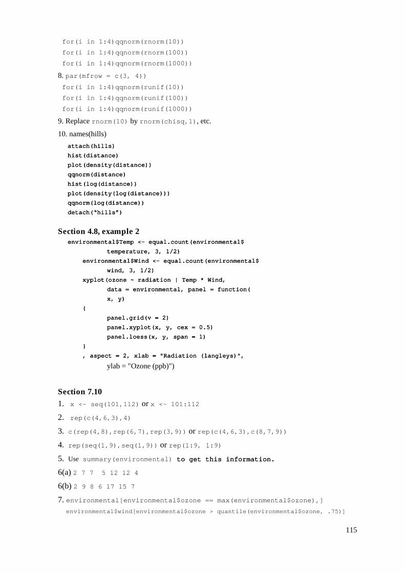
115

for(i in 1:4)qqnorm(rnorm(10))

for(i in 1:4)qqnorm(rnorm(100))

for(i in 1:4)qqnorm(rnorm(1000))

8. par(mfrow = c(3, 4)) for(i in 1:4)qqnorm(runif(10))

for(i in 1:4)qqnorm(runif(100))

for(i in 1:4)qqnorm(runif(1000))

9. Replace rnorm(10) by rnorm(chisq,1), etc.

10. names(hills) attach(hills) attach(hills) attach(hills) attach(hills)

hist(distance)hist(distance)hist(distance)hist(distance)

plot(density(distance))plot(density(distance))plot(density(distance))plot(density(distance))

qqnorm(distance)qqnorm(distance)qqnorm(distance)qqnorm(distance)

hist(log(distance))hist(log(distance))hist(log(distance))hist(log(distance))

plot(density(logplot(density(logplot(density(logplot(density(log(distance)))(distance)))(distance)))(distance)))

qqnorm(log(distance))qqnorm(log(distance))qqnorm(log(distance))qqnorm(log(distance))

detach(“hills”)detach(“hills”)detach(“hills”)detach(“hills”)

Section 4.8, example 2 environmental$Temp <environmental$Temp <environmental$Temp <environmental$Temp <---- equal.count(environmental$ equal.count(environmental$ equal.count(environmental$ equal.count(environmental$

temperature, 3, 1/2)temperature, 3, 1/2)temperature, 3, 1/2)temperature, 3, 1/2)

environmental$Wind <environmental$Wind <environmental$Wind <environmental$Wind <---- equal.count(environmental$ equal.count(environmental$ equal.count(environmental$ equal.count(environmental$

wind, 3, 1/2)wind, 3, 1/2)wind, 3, 1/2)wind, 3, 1/2)

xyplot(ozone ~ radiation | Temp * Wind, xyplot(ozone ~ radiation | Temp * Wind, xyplot(ozone ~ radiation | Temp * Wind, xyplot(ozone ~ radiation | Temp * Wind,

data = environmental, panel = function(data = environmental, panel = function(data = environmental, panel = function(data = environmental, panel = function(

x, y)x, y)x, y)x, y)

{{{{

panel.grid(v = 2)panel.grid(v = 2)panel.grid(v = 2)panel.grid(v = 2)

panel.xyplot(x, y, cex = 0.5)panel.xyplot(x, y, cex = 0.5)panel.xyplot(x, y, cex = 0.5)panel.xyplot(x, y, cex = 0.5)

panel.loess(x, y, span = 1)panel.loess(x, y, span = 1)panel.loess(x, y, span = 1)panel.loess(x, y, span = 1)

}}}}

, aspect = 2, xlab = "Radiation (langleys)", , aspect = 2, xlab = "Radiation (langleys)", , aspect = 2, xlab = "Radiation (langleys)", , aspect = 2, xlab = "Radiation (langleys)",

ylab = "Ozone (ppb)")

Section 7.10 1. x <- seq(101,112) or x <- 101:112

2. rep(c(4,6,3),4)

3. c(rep(4,8),rep(6,7),rep(3,9)) or rep(c(4,6,3),c(8,7,9))

4. rep(seq(1,9),seq(1,9)) or rep(1:9, 1:9)

5. Use summary(environmental) to get this information.to get this information.to get this information.to get this information.

6(a) 2 7 7 5 12 12 4

6(b) 2 9 8 6 17 15 7

7. environmental[environmental$ozone == max(environmental$ozone),] environmental$wind[environmental$ozone > quantile(environmental$ozone, .75)]

116

8. sapply(claims, function(x)if(is.factor(x))levels(x) else “”)

9. sapply(market.survey, is.factor); sapply(market.survey, is.ordered)

10. summary(environmental); summary(claims); summary(market.survey)

11. claimsA <- claims[claims$type==”A”,]

12. gfse <- as.logical(match(car.test.frame$Country, c("Germany","France","Sweden","England"),nomatch=0))

car.test.frame[gfse,]

13. mat34 <- matrix(rep(c(4,6,3),4), nrow=3, ncol=4)

14. mat64 <- matrix(c(rep(4,8),rep(6,7),rep(3,9)), nrow=6, ncol=4) mat64[3:6,3:4]

Additional solutions will be included in later versions of this document.