1

Using Simple Tools

(Alternatives to Mechanistic Models)

Introduction to Watershed Model Training

Wednesday, July 8, 2015 Larry Hauck

hauck@tiaer.tarleton.edu

2

Mechanistic Model: • A model that has a structure that explicitly

represents an understanding of biological, chemical, and/or physical processes.

• These models attempt to quantify phenomena by their underlying casual mechanisms.

Source: EPA website, glossary of frequently used modeling

terms and WPP Handbook

Key Definition

3

• Resource limitations Amount of monitoring data available Time or budget constraints

• Level of “sophistication” requirements bacteria impairments in Texas often

addressed with simpler approaches

Why Consider Alternatives to (Mechanistic) Models

4

• Load duration curves • GIS land-use based methods • Export coefficients • Empirical methods • Other methods

Alternative Approaches

5

• Less resource intensive Less time, money, and staff commitment Typically requires less monitoring data Less experience required to apply

• Often more easily communicated to stakeholders and interested parties

Advantages of Alternative Approaches (as compared to mechanistic modeling

approaches)

6

• Typically not predictive or not rigorously predictive, thus limited in abilities to evaluate control measures & BMPs

• Typically lacks quantitative link between sources of pollution and receiving water body quality

Disadvantages of Alternative Approaches (as compared to mechanistic modeling

approaches)

7

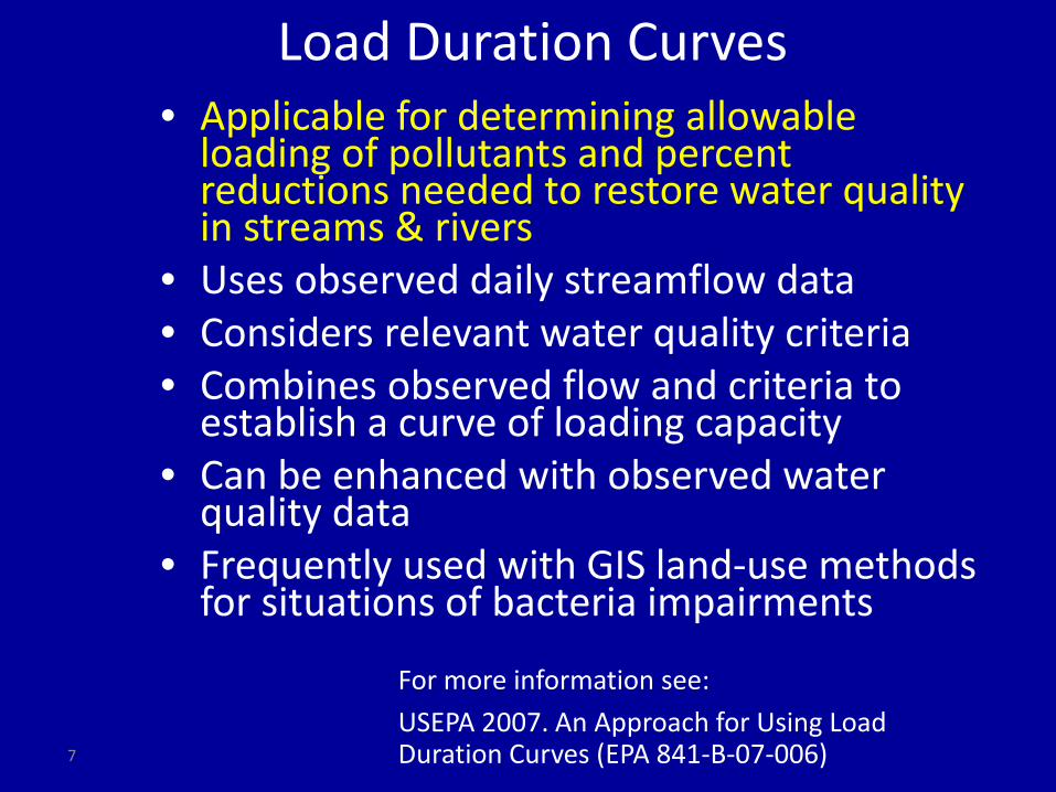
• Applicable for determining allowable loading of pollutants and percent reductions needed to restore water quality in streams & rivers

• Uses observed daily streamflow data • Considers relevant water quality criteria • Combines observed flow and criteria to

establish a curve of loading capacity • Can be enhanced with observed water

quality data • Frequently used with GIS land-use methods

for situations of bacteria impairments

Load Duration Curves

For more information see: USEPA 2007. An Approach for Using Load Duration Curves (EPA 841-B-07-006)

8

• Combines measured concentrations of a pollutant with flow at the same time to develop a load

• The LDC illustrates the load of a pollutant versus the time that a given load is exceeded

• Time is illustrated as percentage of time • Able to see if a stream is exceeding the

standard in terms of load (flow and measured concentrations)

• Able to calculate a percent reduction based on flow categories

Load Duration Curves (continued)

9

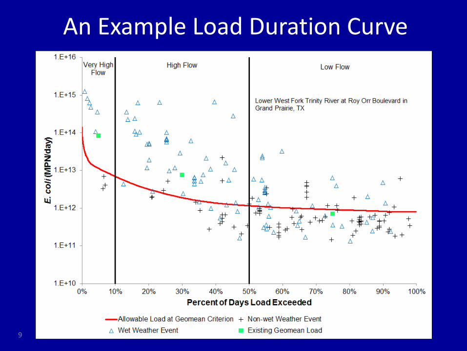
An Example Load Duration Curve

1.E+10

1.E+11

1.E+12

1.E+13

0 10 20 30 40 50 60 70 80 90 100

Percent of days loading exceeded (%)

E. C

oli (c

fu/d

)

TMDL WLA for WWTFs TMDL - MOS

EXAMPLE TMDL ALLOCATION

TMDL

WLA for WWTF & Future Capacity

TMDL - MOS

Regulated Stormwater (WLASW)+Unregulated Stormwater (LA)

TMDL = WLAWWTF + WLASW + LA + Future Growth + Margin of Safety

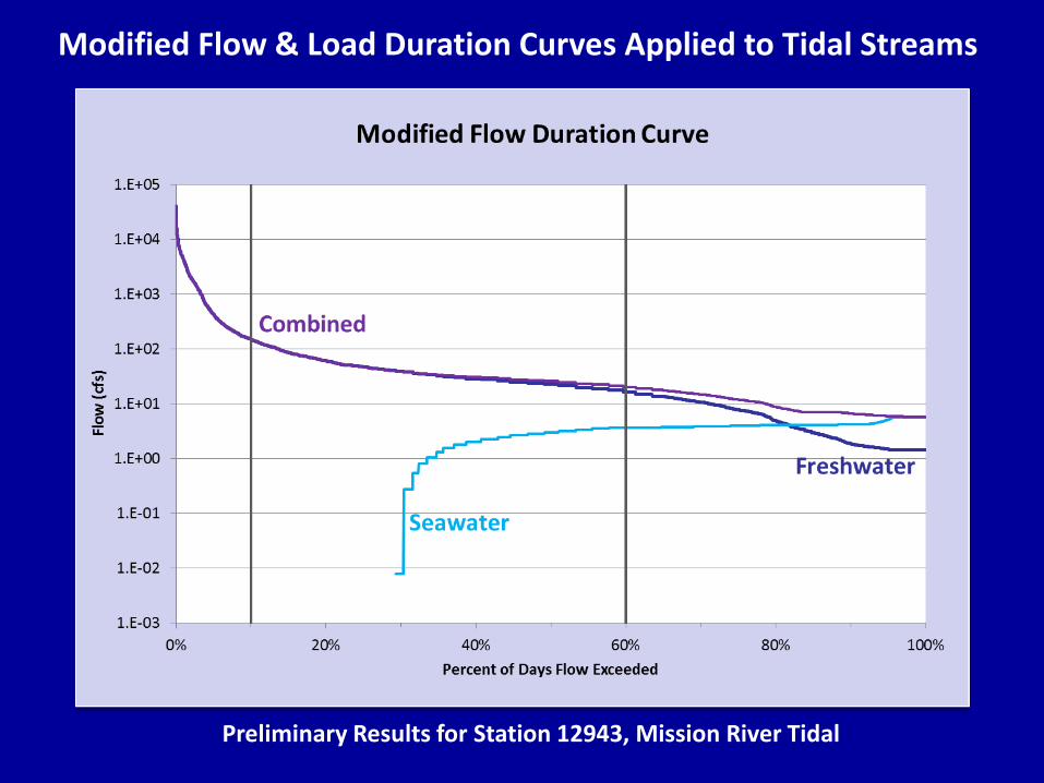
Preliminary Results for Station 12943, Mission River Tidal

Modified Flow & Load Duration Curves Applied to Tidal Streams

Preliminary Results for Station 12943, Mission River Tidal

13

• Widely accepted and used in Texas • Only moderate data requirements • Ease of application • Identifies allowable loading for all flow

conditions • When combined with monitoring data,

identifies existing loading for all flow conditions and can provide percent reduction required

• Readily communicated to stakeholders

Advantages of Load Duration Curves

14

• Only identifies broad categories of sources (i.e., nonpoint source and point source) – not a problem if sources already well understood

• Does not quantitatively link sources to receiving water body quality

• Generally applicable only to non-tidal streams (selectively applicable in transition zones of reservoirs & in weakly tidal streams)

• Not readily applied in predictive mode (e.g., to evaluate control measures & BMPs)

Disadvantages of Load Duration Curves

15

• Applicable for determining likely sources of loadings of pollutants and areas of highest loadings and facilitating stakeholder interactions

• Can use readily available GIS data layers Digital elevation models (DEMs) Land use/land cover (e.g., NLCD 2006) Soil layers (NRCS STATSGO & SSURGO) Stream networks (USGS NHD), etc.

• Can use other readily available data sources For example, USDA Agricultural Census Data

GIS Land-Use Based Methods

16

• Spatially Explicit Load Enrichment Calculation Tool (SELECT)

• GIS based tool • Newly developed Visual Basic frontend

for easier interface • Developed at Texas A&M University • Training (as well as for LDCs) through

AgriLife TWRI

One Land-Use Based Method SELECT

17

• Census Blocks (U.S. Census Bureau) • Soils (USDA-NRCS) • Digital Elevation Map (BASINS) • Urban Areas (TCEQ) • Sub-watersheds & stream network

• Livestock Stakeholder input Agricultural Statistics (USDA) Poultry Operations within the watershed (TSSWCB)

• Wildlife Stakeholder input Wildlife experts input, Resource Management Unit

data for Deer (TPWD)

Examples of Input Included in SELECT

18

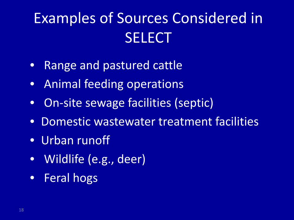
• Range and pastured cattle • Animal feeding operations • On-site sewage facilities (septic) • Domestic wastewater treatment facilities • Urban runoff • Wildlife (e.g., deer) • Feral hogs

Examples of Sources Considered in SELECT

19

Example Results from SELECT, Walnut Creek Watershed

Source: Biological and Agricultural Engineering Department, Texas A&M University

Cattle #s in Leona Uvalde 5,516 Zavala 10,566 Frio 6,418

Input Fecal Production Rate Cattle 10E10 cfu/animal/day

21

• One such tool has been developed in Texas (SELECT) and has been successfully applied in Texas watersheds

• Uses readily available data sources • Relative ease of application • Readily communicated to stakeholders • When properly used can facilitate

stakeholder input & interest (project buy-in)

• Can locate areas for control measure and BMP implementation

Advantages of GIS Land-Use Based Methods

22

• Can evaluate only potential loadings and not actual loadings of pollutants

• Does not quantitatively link sources to receiving water body quality

• Not readily applied in predictive mode (e.g., to evaluate control measures & BMPs), but could be based on best professional judgment

• SELECT – present applications limited to bacteria, but should be adaptable to other pollutants

Disadvantages of GIS Land-Use Based Methods

23

• An export coefficient is the loading of a specific pollutant per unit area for a specific land use and time period

• Examples: Kilograms/hectare/year of lead from industrial

land use Pounds/acre/month of phosphorus from

cultivated agricultural fields

Export Coefficients

24

• Applicable for determining pollutant loadings, likely sources of loadings of pollutants & areas of highest loadings

• Values can be obtained in literature from regional and national studies

• Requires GIS land use/land cover data layer (typically readily available from various sources)

• Approach amenable to including point sources or permitted discharges

Export Coefficients

25

An example application of export coefficients: Bosque River Watershed

Urban Woods Range Improved pasture Row crop Waste application fields Water

26

Soluble Reactive Phosphorus (PO4-P) Export Coefficients Estimated Using Multiple Regression Models

DATA: 1 November 1995 – 30 March 1998

Land Use Export Coefficient

Wood/Range 0.07 lb PO4-P / ac /yr

Pasture/Cropland 0.14 lb PO4-P / ac /yr

Urban 0.98 lb PO4-P / ac /yr

Dairy manure application fields 3.08 lb PO4-P / ac /yr

Source: McFarland and Hauck (1998), McFarland and Hauck (2000)

27

Bosque-Lake Waco Watershed

PO4-P Source Contribution

Land Uses

Row-Crop 11% Pasture

10%

Wood/Range 22%

WWTP 8%

Urban 11%

Non-Row Crop 1%

Dairy Waste Appl. 36%

Row-Crop 16%

Wood/Range 64%

Dairy Waste Appl. 2%

Urban 2%

Non-Row Crop 1%

Pasture 15%

01 Nov 95 - 30 Mar 98

28

• Limited watershed specific water quality data requirements, unless developing project specific export coefficients

• Uses readily available data sources • Ease of application • Readily communicated to stakeholders • Can locate land-use types for control

measure and BMP implementation

Advantages of Export Coefficients

29

• May not quantitatively link sources and loadings to receiving water body quality

• Not readily applied in predictive mode (e.g., to evaluate control measures & BMPs), but could be based on best professional judgment

Disadvantages of Export Coefficients

30

• Applicable for determining loadings of pollutants; sometimes even allowable loadings

• Various methods available Simple Method – for small urban catchments Vollenweider approach – allowable

phosphorus loadings to meet desired trophic level based on lake characteristics

Empirical Methods

31

• A model where the structure is determined by the observed relationship among experimental data.

• These models can be used to develop relationships for forecasting and describing trends.

• These relationships and trends are not necessarily mechanistically relevant.

Source: EPA website, glossary of frequently used

modeling terms.

Empirical Model or Method:

32

• Investigating the relationship of inflowing nutrients in a lake to algal biomass production (eutrophication).

• Most early (circa 1970) lake eutrophication models based on statistical relationships between mass loading of nutrients and average algal biomass (e.g., Vollenweider models with numerous adaptations by others)

• Applied to PL-566 reservoirs in North Bosque River Watershed

An Example of an Empirical Model:

33

Annual mean summer chlorophyll-a concentration as a function of predicted total-P for years 1993-1998 from PL-566 reservoirs. N=25

Example of an Empirical Approach Used in Data Analysis

34

• Limited watershed specific water quality data requirements, unless developing project specific empirical relationships

• Uses readily available data sources • Ease of application • If applicable to your situation, significant

savings in commitment of resources

Advantages of Empirical Methods

35

• Do not quantitatively link sources and loadings to receiving water body quality

• Depending upon data used in developing the empirical method, may not be applicable to your watershed or water body

Disadvantages of Empirical Methods

36

• Steady-State or Mass-Balance Analysis Typically applied to critical flow condition to

determine allowable loading Assumes conservation of mass Can accommodate multiple sources

• Percent Reduction Existing pollutant concentrations compared to

applicable criteria to get percent load reduction Assumes 1:1 relationship between water body

concentrations and pollutant loadings to determine an allowable loading

Source: USEPA. 2008. Draft Handbook for Developing Watershed TMDLs

Other Methods – An Overview

37

• Tidal Prism Method Used to determine allowable loading under

environmental conditions of concern Applicable to tidal water bodies (tidal streams

and bay & estuaries) Simplified approach compared to a

mechanistic model for tidal water bodies Has been applied on Texas coast to situation of

bacteria impairment Savings in resources compared to mechanistic

modeling approaches

Other Methods – An Overview (cont’d)

Dickinson Bayou TMDL – Tidal Prism

Model

39

• Simple alternative approaches often used together LDCs for allowable loadings and SELECT for

pollutant loadings, probable sources & generally locating BMPs Mass-Balance Analysis for allowable loading and

Export Coefficients for pollutant loadings, probable sources & generally locating BMPs Simple alternative approaches

• Viable alternative to mechanistic modeling in certain situations When data is limiting or other resources are

limiting Often used in Texas for bacteria impairments

Concluding Comments

40

Thank You

Questions?