Embed Size (px)
Citation preview

1 © Nokia Solutions and Networks 2014
Using space-filling curves for multi-dimensional indexing
Public
Dr. Bisztray Dénes
Senior Research Engineer

2 © Nokia Solutions and Networks 2014
Performance
problems with
RDBMS
In medias res
Public
Switch to
NoSQL store
(HBase)
Query is based
on multiple
properties
Multi-
dimensional
indexing
Space-filling
curves

3 © Nokia Solutions and Networks 2014
• Brief introduction to indexes and databases
• The „main topic”, i.e. problem statement and
ways to solve the problem
• Solution and Results
Table of Contents
Public

4 © Nokia Solutions and Networks 2014
Databases and Indexes
Introduction
Public

5 © Nokia Solutions and Networks 2014
Example of a Relation
attributes
(or columns)
tuples
(or rows)
Slide content ©Silberschatz, Korth. Sudarshan, 2010

6 © Nokia Solutions and Networks 2014
• A1, A2, …, An are attributes
• R = (A1, A2, …, An ) is a relation schema
Example:
instructor = (ID, name, dept_name, salary)
• Formally, given sets D1, D2, …. Dn a relation r is a subset of
D1 x D2 x … x Dn
Thus, a relation is a set of n-tuples (a1, a2, …, an) where each ai Di
• The current values (relation instance) of a relation are specified by a table
• An element t of r is a tuple, represented by a row in a table
Relation schema
Slide content ©Silberschatz, Korth. Sudarshan, 2010

7 © Nokia Solutions and Networks 2014
• Let K R
• K is a superkey of R if values for K are sufficient to identify a unique tuple of each possible relation r(R)
- Example: {ID} and {ID,name} are both superkeys of instructor.
• Superkey K is a candidate key if K is minimal
Example: {ID} is a candidate key for Instructor
• One of the candidate keys is selected to be the primary key.
- which one?
Keys
Slide content ©Silberschatz, Korth. Sudarshan, 2010

8 © Nokia Solutions and Networks 2014
• Indexing mechanisms used to speed up access to desired data.
- E.g., author catalog in library
• Search Key - attribute to set of attributes used to look up records in a file.
• An index file consists of records (called index entries) of the form
• Index files are typically much smaller than the original file
• Two basic kinds of indices:
- Ordered indices: search keys are stored in sorted order
- Hash indices: search keys are distributed uniformly across “buckets” using a “hash function”.
Indexing Basic Concepts
search key pointer
Slide content ©Silberschatz, Korth. Sudarshan, 2010
9 © Nokia Solutions and Networks 2014
• In an ordered index, index entries are stored sorted on the search key value. E.g., author catalog in library.
• Primary index: in a sequentially ordered file, the index whose search key specifies the sequential order of the file.
- Also called clustering index
- The search key of a primary index is usually but not necessarily the primary key.
• Secondary index: an index whose search key specifies an order different from the sequential order of the file. Also called non-clustering index.
• Index-sequential file: ordered sequential file with a primary index.
Ordered Indices
Slide content ©Silberschatz, Korth. Sudarshan, 2010

10 © Nokia Solutions and Networks 2014
• Dense index — Index record appears for every search-key value in the file.
• E.g. index on ID attribute of instructor relation
Dense Index Files
Slide content ©Silberschatz, Korth. Sudarshan, 2010

11 © Nokia Solutions and Networks 2014
• Sparse Index: contains index records for only some search-key values.
- Applicable when records are sequentially ordered on search-key
• To locate a record with search-key value K we:
- Find index record with largest search-key value < K
- Search file sequentially starting at the record to which the index record points
Sparse Index Files
Slide content ©Silberschatz, Korth. Sudarshan, 2010

12 © Nokia Solutions and Networks 2014
• Frequently, one wants to find all the records whose values in a certain
field (which is not the search-key of the primary index) satisfy some
condition.
- Example 1: In the instructor relation stored sequentially by ID, we
may want to find all instructors in a particular department
- Example 2: as above, but where we want to find all instructors with a
specified salary or with salary in a specified range of values
• We can have a secondary index with an index record for each search-
key value
Secondary Indices
Slide content ©Silberschatz, Korth. Sudarshan, 2010
13 © Nokia Solutions and Networks 2014
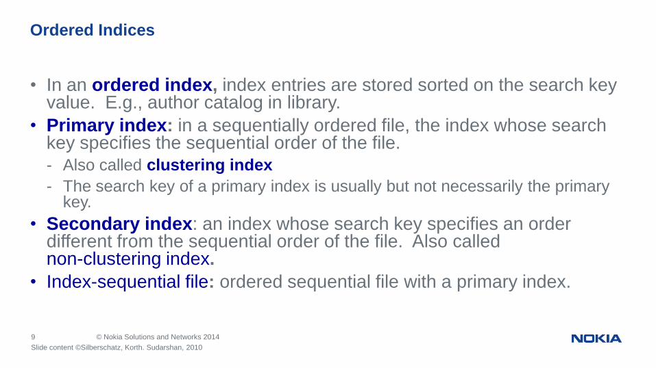
• Index record points to a bucket that contains pointers to all the actual records with that particular search-key value.
• Secondary indices have to be dense
Secondary Indices Example Secondary index on salary field of instructor
Slide content ©Silberschatz, Korth. Sudarshan, 2010

14 © Nokia Solutions and Networks 2014
Multi dimensional indexing and
the space filling curves
Public

15 © Nokia Solutions and Networks 2014
• Statistic analysis of massive CDR data to generate Business Reports: - On-demand report with URL and Time Range
- On-demand report with MSISDN and Time Range
• Data-intensive and performance-critical application: - Cut down the reporting response time from hours to
minutes
- Extremely high load to Disk I/O due to high throughput requirement
Application Characteristics
Public

16 © Nokia Solutions and Networks 2014
Technical Requirements for Storage
Public
Items Product 1 Product 2
Record Size 450Byte/record Multimedia Message (MM): 150KB - 10MB
Short Message (SMS): 160Byte
Data Retention time 3 months 6 months
Concurrency 20,000 per second MM 200 requests/second for writing
1000 requests/second for reading
SMS 800 requests/second for writing 1000 requests/second for reading
Total data size 70 TB 30 TB
Latency Write delay < 10ms
Reporting < 5 minutes MM reading delay < 0.2s, writing delay <0.4s
SMS reading delay < 0.1s, writing delay < 0.2s
Throughputs 72 Mbps for writing
584 Mbps for reading (1hour)
14.4 Gbps for reading (1day)
432 Gbps for reading (1month)
MM 1.228 Gbps for reading
246 Mbps for writing
SMS 1 Mbps for reading
1.28 Mbps for writing
17 © Nokia Solutions and Networks 2014
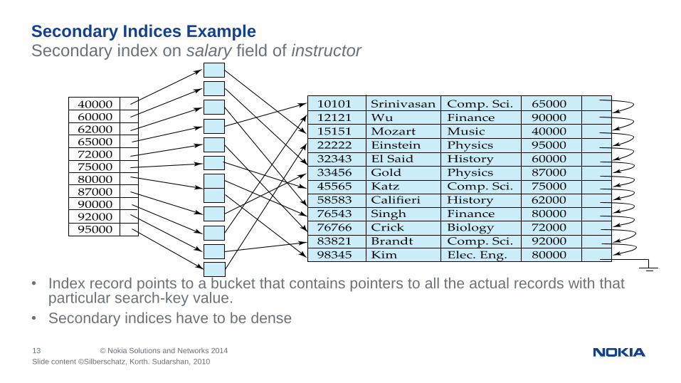
Existing Solution and Disadvantage
Public
•Traditional RDBMS became bottleneck for Big Data
storage and processing
•Low performance in Data Intensive application, e.g.
Generating business reports through big data analysis
•Incapable Scale-In/Out for ever-increasing data volume
Oracle database &
EMC disk array
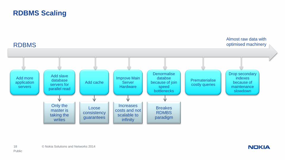
18 © Nokia Solutions and Networks 2014
RDBMS Scaling
RDBMS
Add more application
servers
Add slave database
servers for parallel read
Only the master is taking the
writes
Add cache
Loose consistency guarantees
Improve Main Server
Hardware
Increases costs and not
scalable to infinity
Denormalise databse
because of join speed
bottlenecks
Almost raw data with
optimised machinery
Prematerialise costly queries
Drop secondary indexes
because of maintenance
slowdown
Breakes RDMBS
paradigm
Public

19 © Nokia Solutions and Networks 2014
CAP Theorem
Availability
Consistency Partition
Tolerance
Pick Two
MySQL,
Postgres, etc
Cassandra,
SimpleDB, Riak,
Dynamo, etc
MongoDB, Hbase,
BigTable, Redis,
etc
all nodes see the same data at
the same time the system continues to operate
despite arbitrary message loss
or failure of part of the system
a guarantee that every request receives a
response about whether it was successful or failed
Public
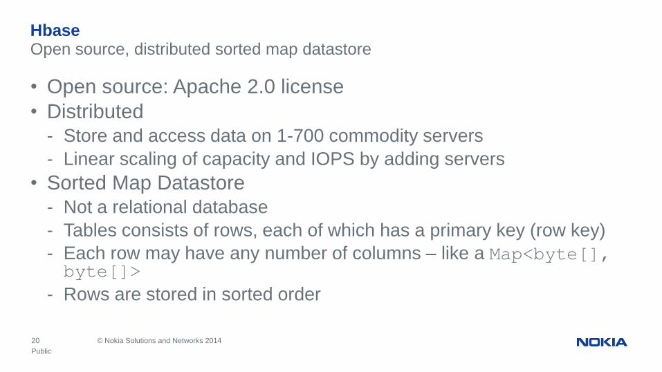
20 © Nokia Solutions and Networks 2014
• Open source: Apache 2.0 license
• Distributed - Store and access data on 1-700 commodity servers
- Linear scaling of capacity and IOPS by adding servers
• Sorted Map Datastore - Not a relational database
- Tables consists of rows, each of which has a primary key (row key)
- Each row may have any number of columns – like a Map<byte[], byte[]>
- Rows are stored in sorted order
Hbase Open source, distributed sorted map datastore
Public

21 © Nokia Solutions and Networks 2014
Sorted Map Datastore
Slide content © Cloudera Inc.
Row key Data
cutting info: {‘height’: ’274cm’, ‘state’: ‘CA’}
roles: {‘ASF’: ‘Director’, ‘Hadoop’:
‘Founder’}
tlipcon info: {‘height’: ‘170cm’, ‘state’: ‘CA’}
roles: {‘Hadoop’: ‘Committer’@ts=2010,
‘Hadoop’: ‘PMC’@ts=2011,
‘Hive’:’Contributor’}
A single cell might have different
values at different timestamps
Implicit PRIMARY KEY
in RDBMS terms
Data is all byte[] in HBase
Different types of
data separated into
different „column
families”
Different rows may have different sets
of columns (table is sparse)

22 © Nokia Solutions and Networks 2014
• Table contains sorted rows and dynamically splitted into regions
- Rows stored in byte-lexicographic order based on rowkey
- Somewhat similar to Relational DB Primary Index (always unique)
• Region is a continuous set of sorted rows
• Hbase ensures that all cells of the same rowkey are all on the same server
Scalability with Regions
Public

23 © Nokia Solutions and Networks 2014
Table and Regions
Slide content © Cloudera Inc.
Rows
A
.
.
.
H
.
.
.
.
Q
.
.
Z
Keys: [T-Z)
Keys: [I-M)
Keys: [F-I)
Keys: [A-C)
Keys: [M-T)
Keys: [C-F)
Region Server 1 Region Server 2 Region Server 3

24 © Nokia Solutions and Networks 2014
• Get - Retrieves a single row using a rowkey
• Scan - Scans the full table
• Range - Retrieves a range of rows between a given startRow
and stopRow
Hbase Query Methods
Public
25 © Nokia Solutions and Networks 2014
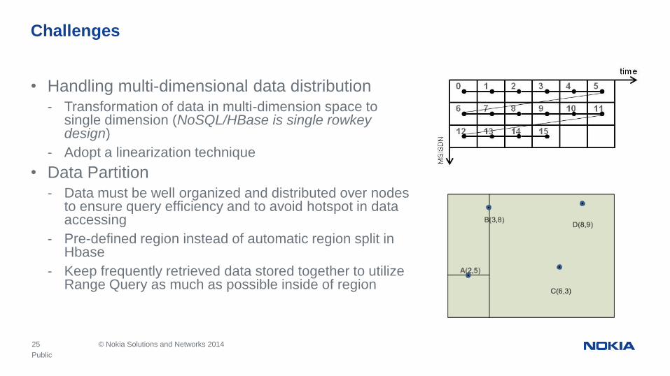
• Handling multi-dimensional data distribution
- Transformation of data in multi-dimension space to single dimension (NoSQL/HBase is single rowkey design)
- Adopt a linearization technique
• Data Partition
- Data must be well organized and distributed over nodes to ensure query efficiency and to avoid hotspot in data accessing
- Pre-defined region instead of automatic region split in Hbase
- Keep frequently retrieved data stored together to utilize Range Query as much as possible inside of region
Challenges
Public

26 © Nokia Solutions and Networks 2014
• Good extendibility in space size (recursion level and region placeholder)
• Spatial indexing is natively supported (while subdividing, prefix also fit to curve)
• Easy to build up additional indexing on top of it (Prefix Hash Tree, B Tree, KD-Tree etc.)
• Different granularity in sub-space size
Rowkey Design Rowkey algorithm by a space-filling curve
Public

27 © Nokia Solutions and Networks 2014
• It loosely preserves the locality of data-points in the multi-dimensional space
• Easy to implement.
- Binary Z-ordering space, bitwise interleaving .
- Using the Z-order value as rowkey.
Rowkey algorithm by Z-ordering
Public
00 01 10 11
11
10
01
00
00 01 10 11
11
10
01
00
Z-order encoding (2-D) multiple-dimensional
Z-order curve Z-order curve (2-D)

28 © Nokia Solutions and Networks 2014
- little complex compared to the Z-order curve
- better one-dimensional continuity
Rowkey algorithm by Hilbert Curve
Public
Hilbert encoding (2-D) Hilbert curve (2-D)
00 01 10 11
11
10
01
00
multiple-dimensional
Hilbert curve
11
10
01
00
00 01 10 11

29 © Nokia Solutions and Networks 2014
Hilbert Curve Generation
Public
first order second order third order fourth order
30 © Nokia Solutions and Networks 2014
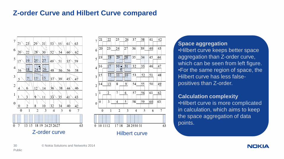
Z-order Curve and Hilbert Curve compared
Public
Z-order curve Hilbert curve
Space aggregation
•Hilbert curve keeps better space
aggregation than Z-order curve,
which can be seen from left figure.
•For the same region of space, the
Hilbert curve has less false-
positives than Z-order.
Calculation complexity
•Hilbert curve is more complicated
in calculation, which aims to keep
the space aggregation of data
points.

31 © Nokia Solutions and Networks 2014
• It can be achieved by pre-defined regions (bucket) in Hbase
- Automatic region split can’t be used in consideration of performance
• Region split solutions
- Trie-based space split (by the mid-point of dimension)
- Point-based space split (by the median of data points)
Data partitioning based on multi-dimension
Public

32 © Nokia Solutions and Networks 2014
Data Partitioning Two dimensional data distribution by time and MSISDN
Public
MSISDN dimension:
-users’ data will be evenly
distributed to different
regions
- avoids the Writing
Hotspot in case of high
concurrent data insert
(20,000 per second)
Time dimension
-Inside a region, one users’s
data will be written in a time
continuous way
-increases query efficiency

33 © Nokia Solutions and Networks 2014
Binary Tree for Hilbert curve
Public

34 © Nokia Solutions and Networks 2014
• splits the space at the mid-
point of all dimensions
- equal size splits in space-
filling curve
- each subspace uniquely
corresponds to a segment of
the curve.
Data Partition: Trie-based region split
Public

35 © Nokia Solutions and Networks 2014
• Splits the space by the median of data points
• Results in subspaces with equal number of data points
• Data point distribution must be known beforehand to select median
KD-Tree
Public

36 © Nokia Solutions and Networks 2014
Solution and Results
Public

37 © Nokia Solutions and Networks 2014
...
• The rowkey algorithm uses multiple data attributes to generate Hilbert curve.
• Each value in Hilbert curve represents the rowkey in HBase.
Rowkey algorithm based on Hilbert Curve
Public
Rowkey
Rowkey_1
...
...
Rowkey_2
Rowkey_3
Rowkey_n
Rowkey algorithm data
data
data
data
data
data
data
data
data

38 © Nokia Solutions and Networks 2014
• Selecting the middle-point of each dimension to make customized region pre-split
• Each segment represents a range Hilbert value and corresponds to a region.
Trie-based region split
Public
Hilbert curve
Value_ Range_1
...
Value_ Range_2
Value_ Range_3
Value_ Range_k
Value_ Range_n
HBase
Region_1
...
Region_2
Region_3
Region_k
Region_n
Rowkey algorithm
...
data
data
data
data
data
data
data
data
data
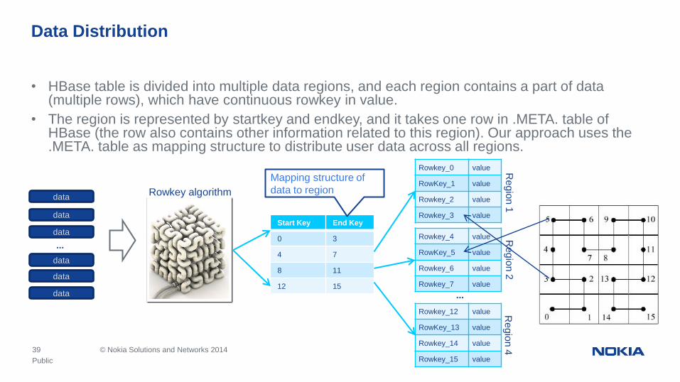
39 © Nokia Solutions and Networks 2014
...
• HBase table is divided into multiple data regions, and each region contains a part of data (multiple rows), which have continuous rowkey in value.
• The region is represented by startkey and endkey, and it takes one row in .META. table of HBase (the row also contains other information related to this region). Our approach uses the .META. table as mapping structure to distribute user data across all regions.
Data Distribution
Start Key End Key
0 3
4 7
8 11
12 15
Public
Rowkey algorithm
...
data
data
data
data
data
data
Rowkey_0 value
RowKey_1 value
Rowkey_2 value
Rowkey_3 value
Rowkey_4 value
RowKey_5 value
Rowkey_6 value
Rowkey_7 value
Rowkey_12 value
RowKey_13 value
Rowkey_14 value
Rowkey_15 value
Mapping structure of
data to region
Re
gio
n 1
R
eg
ion
2
Re
gio
n 4

40 © Nokia Solutions and Networks 2014
• Response time is decreased from hours to minutes (comparing to original Oracle solution)
• ~3x performance speedup after optimizations
• Experiment with 1 master + 8 data node
• Better performance after the extension of nodes and memory
Results – URL Query Performance
Public
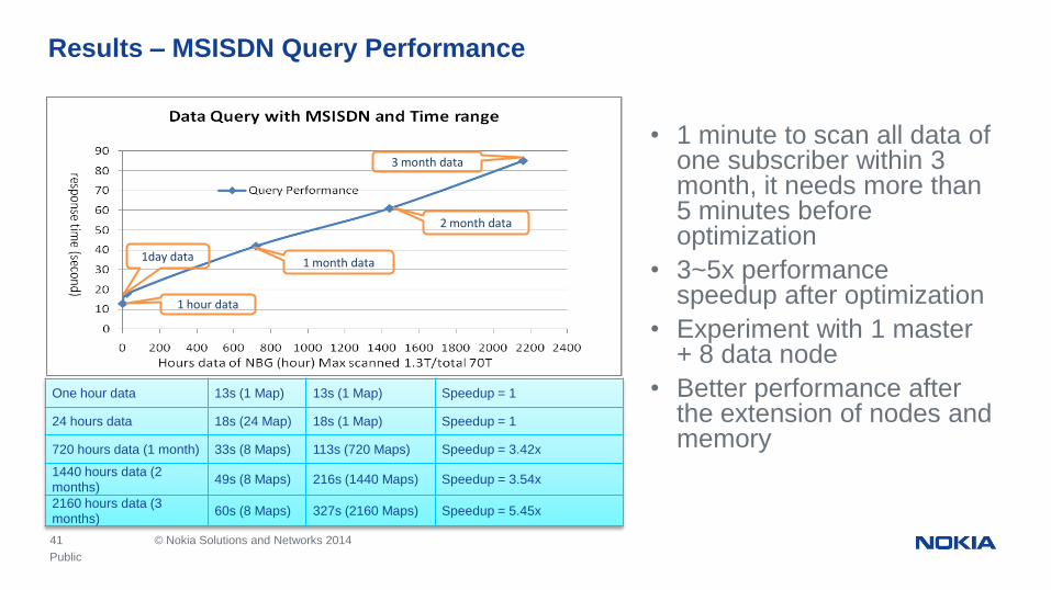
41 © Nokia Solutions and Networks 2014
• 1 minute to scan all data of one subscriber within 3 month, it needs more than 5 minutes before optimization
• 3~5x performance speedup after optimization
• Experiment with 1 master + 8 data node
• Better performance after the extension of nodes and memory
Results – MSISDN Query Performance
Public
1 hour data
1day data 1 month data
2 month data
3 month data
One hour data 13s (1 Map) 13s (1 Map) Speedup = 1
24 hours data 18s (24 Map) 18s (1 Map) Speedup = 1
720 hours data (1 month) 33s (8 Maps) 113s (720 Maps) Speedup = 3.42x
1440 hours data (2
months) 49s (8 Maps) 216s (1440 Maps) Speedup = 3.54x
2160 hours data (3
months) 60s (8 Maps) 327s (2160 Maps) Speedup = 5.45x

42 © Nokia Solutions and Networks 2014
• Data Writing latency is less than 0.05ms on average (requirement is <10ms)
• Before Optimization, region flush, split and compaction will affect writing latency badly, even cause service break
• Region split and compaction storm is avoided by scheduled region compaction, flush and advanced region split, performance curve of high concurrent writing become stable.
Results – Data Writing Performance
Public

43 © Nokia Solutions and Networks 2014
• Response time of reporting is decreased from hours to minutes comparing to the original Oracle solution
• 4 minutes to scan 2 hours data (144m records) in high concurrency (20,000tps), 3x performance speedup by Hadoop & Hbase optimization
• 1 minute to scan all data of one subscriber within 3 month, 3~5x performance speedup by further Hadoop & HBase optimization
• Writing latency is less than 0.05ms, much less than requirement (<10ms)
Achievement
Public