Embed Size (px)
Citation preview
University of Potsdam
Cumulative Dissertation
Using spaceborne radar platforms to enhance the
homogeneity of weather radar calibration
by
Irene Crisologo
Supervisors:
Maik Heistermann, Ph.D.
Prof. Dr. Axel Bronstert
for the degree of
doctor rerum naturalium (Dr. rer. nat.)
in Geoecology
Institute of Environmental Science and Geography
Faculty of Science
April 2019

This work is licensed under a Creative Commons License: Attribution 4.0 International. This does not apply to quoted content from other authors. To view a copy of this license visit https://creativecommons.org/licenses/by/4.0/ Published online at the Institutional Repository of the University of Potsdam: https://doi.org/10.25932/publishup-44570 https://nbn-resolving.org/urn:nbn:de:kobv:517-opus4-445704

iii
Using spaceborne radar platforms to enhance the homogeneity of weather
radar calibration
by Irene Crisologo
Supervisor:
Maik Heistermann, Ph.D. (Reviewer )
Affiliation:
University of Potsdam
Co-Supervisor:
Prof. Dr. Axel Bronstert (Reviewer ) University of Potsdam
Mentor:
Prof. Oliver Korup, Ph.D.University of Potsdam
Assessment Committee:
Prof. Oliver Korup, Ph.D. (Chair)
Prof. Dr. Bodo Bookhagen
Prof. Dr. Annegret Thieken
Prof. Dr. Remko Uijlenhoet (Reviewer )
University of Potsdam
University of Potsdam
University of Potsdam
Wageningen University and Research, Netherlands
Publication-based dissertation submitted in fulfilment of the requirements for the degree of Doctor of Philosophy under the
discipline of Geoecology in the Institute of Environmental Science and Geography Faculty of Science at the University of
Potsdam.


v
Declaration of Authorship
I, Irene Crisologo, declare that this thesis titled, “Using spaceborne radar platforms to enhance the homogeneity of
weather radar calibration ” and the work presented in it are my own. I confirm that:
• This work was done wholly or mainly while in candidature for a research degree at the University of Potsdam.
• Where any part of this dissertation has previously been submitted for a degree or any other qualification at
the University of Potsdam, or any other institution, this has been clearly stated.
• Where I have consulted the published work of others, this is always clearly attributed.
• Where I have quoted from the work of others, the source is always given. With the exception of such quota-
tions, this thesis is entirely my own work.
• I have acknowledged all main sources of help.
• Where the thesis is based on work done by myself jointly with others, I have made clear exactly what was
done by others and what I have contributed myself.
Signature:
Date:


vii
“Sometimes attaining the deepest familiarity with a question is our best substitute for actually having the answer.”
Brian Greene


ix
Abstract
Accurate weather observations are the keystone to many quantitative applications, such
as precipitation monitoring and nowcasting, hydrological modelling and forecasting, climate
studies, as well as understanding precipitation-driven natural hazards (i.e. floods, landslides,
debris flow). Weather radars have been an increasingly popular tool since the 1940s to pro-
vide high spatial and temporal resolution precipitation data at the mesoscale, bridging the gap
between synoptic and point scale observations. Yet, many institutions still struggle to tap the
potential of the large archives of reflectivity, as there is still much to understand about factors
that contribute to measurement errors, one of which is calibration. Calibration represents a
substantial source of uncertainty in quantitative precipitation estimation (QPE). A miscalibra-
tion of a few dBZ can easily deteriorate the accuracy of precipitation estimates by an order of
magnitude. Instances where rain cells carrying torrential rains are misidentified by the radar as
moderate rain could mean the difference between a timely warning and a devastating flood.
Since 2012, the Philippine Atmospheric, Geophysical, and Astronomical Services Admin-
istration (PAGASA) has been expanding the country’s ground radar network. We had a first
look into the dataset from one of the longest running radars (the Subic radar) after devastating
week-long torrential rains and thunderstorms in August 2012 caused by the annual southwest-
monsoon and enhanced by the north-passing Typhoon Haikui. The analysis of the rainfall spa-
tial distribution revealed the added value of radar-based QPE in comparison to interpolated
rain gauge observations. However, when compared with local gauge measurements, severe
miscalibration of the Subic radar was found. As a consequence, the radar-based QPE would
have underestimated the rainfall amount by up to 60% if they had not been adjusted by rain
gauge observations—a technique that is not only affected by other uncertainties, but which is
also not feasible in other regions of the country with very sparse rain gauge coverage.
Relative calibration techniques, or the assessment of bias from the reflectivity of two radars,
has been steadily gaining popularity. Previous studies have demonstrated that reflectivity ob-
servations from the Tropical Rainfall MeasuringMission (TRMM) and its successor, theGlobal
Precipitation Measurement (GPM), are accurate enough to serve as a calibration reference for
ground radars over low-to-mid-latitudes (± 35 deg for TRMM;± 65 deg for GPM). Compar-
ing spaceborne radars (SR) and ground radars (GR) requires cautious consideration of differ-
ences inmeasurement geometry and instrument specifications, as well as temporal coincidence.
For this purpose, we implement a 3-D volume matching method developed by Schwaller and
Morris (2011) and extended by Warren et al. (2018) to 5 years worth of observations from the
Subic radar. In this method, only the volumetric intersections of the SR and GR beams are
considered.
Calibration bias affects reflectivity observations homogeneously across the entire radar
domain. Yet, other sources of systematic measurement errors are highly heterogeneous in
space, and can either enhance or balance the bias introduced by miscalibration. In order to
account for such heterogeneous errors, and thus isolate the calibration bias, we assign a quality
index to each matching SR–GR volume, and thus compute the GR calibration bias as a quality-
weighted average of reflectivity differences in any sample of matching SR–GR volumes. We
exemplify the idea of quality-weighted averaging by using beam blockage fraction (BBF) as
a quality variable. Quality-weighted averaging is able to increase the consistency of SR and

x
GR observations by decreasing the standard deviation of the SR–GR differences, and thus
increasing the precision of the bias estimates.
To extend this framework further, the SR–GR quality-weighted bias estimation is applied
to the neighboring Tagaytay radar, but this time focusing on path-integrated attenuation (PIA)
as the source of uncertainty. Tagaytay is a C-band radar operating at a lower wavelength and is
therefore more affected by attenuation. Applying the same method used for the Subic radar,
a time series of calibration bias is also established for the Tagaytay radar.
Tagaytay radar sits at a higher altitude than the Subic radar and is surrounded by a gen-
tler terrain, so beam blockage is negligible, especially in the overlapping region. Conversely,
Subic radar is largely affected by beam blockage in the overlapping region, but being an S-
Band radar, attenuation is considered negligible. This coincidentally independent uncertainty
contributions of each radar in the region of overlap provides an ideal environment to exper-
iment with the different scenarios of quality filtering when comparing reflectivities from the
two ground radars. The standard deviation of the GR–GR differences already decreases if we
consider either BBF or PIA to compute the quality index and thus the weights. However, com-
bining them multiplicatively resulted in the largest decrease in standard deviation, suggesting
that taking both factors into account increases the consistency between the matched samples.
The overlap between the two radars and the instances of the SR passing over the two
radars at the same time allows for verification of the SR–GR quality-weighted bias estimation
method. In this regard, the consistency between the two ground radars is analyzed before
and after bias correction is applied. For cases when all three radars are coincident during
a significant rainfall event, the correction of GR reflectivities with calibration bias estimates
from SR overpasses dramatically improves the consistency between the two ground radars
which have shown incoherent observations before correction. We also show that for cases
where adequate SR coverage is unavailable, interpolating the calibration biases using a moving
average can be used to correct the GR observations for any point in time to some extent. By
using the interpolated biases to correct GR observations, we demonstrate that bias correction
reduces the absolute value of the mean difference in most cases, and therefore improves the
consistency between the two ground radars.
This thesis demonstrates that in general, taking into account systematic sources of un-
certainty that are heterogeneous in space (e.g. BBF) and time (e.g. PIA) allows for a more
consistent estimation of calibration bias, a homogeneous quantity. The bias still exhibits an
unexpected variability in time, which hints that there are still other sources of errors that remain
unexplored. Nevertheless, the increase in consistency between SR and GR as well as between
the two ground radars, suggests that considering BBF and PIA in a weighted-averaging ap-
proach is a step in the right direction.
Despite the ample room for improvement, the approach that combines volume matching
between radars (either SR–GR or GR–GR) and quality-weighted comparison is readily avail-
able for application or further scrutiny. As a step towards reproducibility and transparency in
atmospheric science, the 3D matching procedure and the analysis workflows as well as sam-
ple data are made available in public repositories. Open-source software such as Python and
wradlib are used for all radar data processing in this thesis. This approach towards open sci-
ence provides both research institutions and weather services with a valuable tool that can be
applied to radar calibration, from monitoring to a posteriori correction of archived data.

xi
Zusammenfassung
Die zuverlässige Messung des Niederschlags ist Grundlage für eine Vielzahl quantitativer An-
wendungen. Bei der Analyse und Vorhersage von Naturgefahren wie Sturzfluten oder Hangrut-
schungen ist dabei die räumliche Trennschärfe der Niederschlagsmessung besonders wichtig, da
hier oft kleinräumige Starkniederschläge auslösend sind. Seit dem 2. Weltkrieg gewinnen Nieder-
schlagsradare an Bedeutung für die flächenhafte Erfassung des Niederschlags in hoher raum-
zeitlicher Auflösung. Und seit Ende des 20. Jahrhunderts investieren Wetterdienste zunehmend
in die Archivierung dieser Beobachtungen. Die quantitative Auswertung solcher Archive gestaltet
sich jedoch aufgrund unterschiedlicher Fehlerquellen als schwierig. Eine Fehlerquelle ist die Kalib-
rierung der Radarsysteme, die entlang der sog. “receiver chain” eine Beziehung zwischen der primären
Beobachtungsvariable (der zurückgestreuten Strahlungsleistung) und der Zielvariable (des Radar-
reflektivitätsfaktors, kurz Reflektivität) herstellt. Die Reflektivität wiederum steht über mehrere
Größenordnungen hinweg in Beziehung zur Niederschlagsintensität, so dass bereits kleine relative
Fehler in der Kalibrierung große Fehler in der quantitativen Niederschlagsschätzung zur Folge
haben können. Doch wie kann eine mangelhafte Kalibrierung nachträglich korrigiert werden?
Diese Arbeit beantwortet diese Frage am Beispiel des kürzlich installierten Radarnetzwerks
der Philippinen. In einer initialen Fallstudie nutzen wir das S-Band-Radar nahe Subic, welches
die Metropolregion Manila abdeckt, zur Analyse eines außergewöhnlich ergiebigen Niederschlags-
ereignisses im Jahr 2012: Es zeigt sich, dass die radargestützte Niederschlagsschätzung um rund
60% unter den Messungen von Niederschlagsschreibern liegt. Kann die Hypothese einer mangel-
haften Kalibrierung bestätigt werden, indem die Beobachtungen des Subic-Radars mit den Mes-
sungen exzellent kalibrierter, satellitengestützter Radarsysteme verglichen werden? Kann die satel-
litengestützte Referenz ggf. sogar für eine nachträgliche Kalibrierung genutzt werden? Funktion-
iert eine solche Methode auch für das benachbarte C-Band-Radar nahe Tagaytay? Können wir
die Zuverlässigkeit einer nachträglichen Kalibrierung erhöhen, indem wir andere systematische
Fehlerquellen in den Radarmessungen identifizieren?
Zur Beantwortung dieser Fragen vergleicht diese Arbeit die Beobachtungen bodengestützter
Niederschlagsradare (GR) mit satellitengestützten Niederschlagsradaren (SR) der Tropical Rainfall
Measuring Mission (TRMM) und ihrem Nachfolger, der Global Precipitation Measurement (GPM) Mis-
sion. Dazu wird eine Methode weiterentwickelt, welche den dreidimensionalen Überlappungs-
bereich der Samplingvolumina des jeweiligen Instruments—GR und SR—berücksichtigt. Des-
weiteren wird jedem dieser Überlappungsbereiche ein Wert für die Datenqualität zugewiesen,
basierend auf zwei Unsicherheitsquellen: dem Anteil der Abschattung (engl. beam blockage frac-
tion, BBF) und der pfadintegrierten Dämpfung (engl. path-integrated attenuation, PIA). Die BBF
zeigt, welcher Anteil des Radarstrahls von der Geländeoberfläche blockiert wird (je höher, desto
niedriger dieQualität). PIA quantifiziert denEnergieverlust des Signals, wenn es intensivenNieder-
schlag passiert (je höher, desto niedriger die Qualität). Entsprechend wird der Bias (also der
Kalibrierungsfaktor) als das qualitätsgewichtete Mittel der Differenzen zwischen den GR- und
SR-Reflektivitäten (ausgedrückt auf der logarithmischen Dezibelskala) berechnet.
Diese Arbeit zeigt, dass beide Radare, Subic und Tagaytay, gerade in den frühen Jahren stark
von mangelhafter Kalibrierung betroffen waren. Der Vergleich mit satellitengestützten Messun-
gen erlaubt es uns, diesen Fehler nachträglich zu schätzen und zu korrigieren. Die Zuverlässigkeit
dieser Schätzung wird durch die Berücksichtigung anderer systematischer Fehler im Rahmen der
Qualitätsgewichtung deutlich erhöht. Dies konnte auch dadurch bestätigt werden, dass nach Ko-
rrektur der Kalibierung die Signale im Überlappungsbereich der beiden bodengestützten Radare
deutlich konsistenter wurden. Eine Interpolation des Fehlers in der Zeit war erfolgreich, so dass
die Radarbeobachtungen auch für solche Tage korrigiert werden können, an denen keine satel-
litengestützten Beobachtungen verfügbar sind.

xii

xiii
Acknowledgements
I would like to extend my sincere gratitude to the people who have been instrumental in this PhD journey.
To Maik, my main supervisor, for his unwavering trust and support, for sharing his sense of humor when I have lost
mine. It was through his guidance that I learned about radars and decided to pursue it further, six years and counting.
To Axel, for support in all forms, for believing in me from the start and for the encouragement throughout the PhD.
To the institutions that supported me—to RTG NatRiskChange for adopting me as an associate PhD student and
providing the environment for collaboration and learning; to DAAD for the financial support; and to the Geoecol-
ogy staff (namely Andi, Daniel, and Sabine) for all the help in the administrative and technical things, and for the
many thoughtful things in between.
To Mr. Jun Austria and PAGASA, for providing the data and technical support needed to carry out this research
study.
To my PhD colleagues, who I consider friends and family. The “old’’ ones—Sebastian, Dadi, Ugur, Jonas, Tobi,
Georg, Erwin, for the cordial camaraderie and constructive collaboration. The “new’’ ones as well—Ina, Melli,
Matthias, Joscha, Kata—for introducing our Monday evening activity that helps relieve the stress of the later part of
the PhD. To my working group—Arthur, Georgy, and Lisei—for the fruitful discussions about work and non-work
subjects.
To Arlena, for the life-enriching moments inside and outside the office.
To my Potsdam Filipino family, for being my home away from home.
To my family, who despite the distance, extended their support and believed in me.


xv
Contents
Declaration of Authorship v
Abstract ix
Zusammenfassung xi
Acknowledgements xiii
1 Introduction 1
2 Using the new Philippine radar network to reconstruct the Habagat of August 2012 monsoon event 9
2.1 Introduction . . . . . . . . . . . . . . . . . . . . . . . . . . . . . . . . . . . . . . . . . . . . . . 9
2.2 Radar data and data processing . . . . . . . . . . . . . . . . . . . . . . . . . . . . . . . . . . . . . 10
2.3 Event reconstruction . . . . . . . . . . . . . . . . . . . . . . . . . . . . . . . . . . . . . . . . . . 11
2.4 Conclusions . . . . . . . . . . . . . . . . . . . . . . . . . . . . . . . . . . . . . . . . . . . . . . . 14
3 Enhancing the Consistency of Spaceborne and Ground-Based Radar Comparisons 17
3.1 Introduction . . . . . . . . . . . . . . . . . . . . . . . . . . . . . . . . . . . . . . . . . . . . . . 17
3.2 Data . . . . . . . . . . . . . . . . . . . . . . . . . . . . . . . . . . . . . . . . . . . . . . . . . . . 18
3.2.1 Spaceborne precipitation radar . . . . . . . . . . . . . . . . . . . . . . . . . . . . . . . . 18
3.2.2 Ground radar . . . . . . . . . . . . . . . . . . . . . . . . . . . . . . . . . . . . . . . . . 19
3.3 Method . . . . . . . . . . . . . . . . . . . . . . . . . . . . . . . . . . . . . . . . . . . . . . . . . 19
3.3.1 Partial beam shielding and quality index based on beam blockage fraction . . . . . . . . . 19
3.3.2 SR–GR Volume Matching . . . . . . . . . . . . . . . . . . . . . . . . . . . . . . . . . . . 21
3.3.3 Assessment of the average reflectivity bias . . . . . . . . . . . . . . . . . . . . . . . . . . 22
3.3.4 Computational details . . . . . . . . . . . . . . . . . . . . . . . . . . . . . . . . . . . . . 22
3.4 Results and discussion . . . . . . . . . . . . . . . . . . . . . . . . . . . . . . . . . . . . . . . . . 23
3.4.1 Single event comparison . . . . . . . . . . . . . . . . . . . . . . . . . . . . . . . . . . . . 23
Case 1: 08 November 2013 . . . . . . . . . . . . . . . . . . . . . . . . . . . . . . . . . . 23
Case 2: 01 October 2015 . . . . . . . . . . . . . . . . . . . . . . . . . . . . . . . . . . . 24
3.4.2 Overall June–November comparison during the 5-year observation period . . . . . . . . . 24
3.5 Conclusions . . . . . . . . . . . . . . . . . . . . . . . . . . . . . . . . . . . . . . . . . . . . . . . 28
4 Using ground radar overlaps to verify the retrieval of calibration bias estimates from spaceborne
platforms 31
4.1 Introduction . . . . . . . . . . . . . . . . . . . . . . . . . . . . . . . . . . . . . . . . . . . . . . 31
4.2 Data and Study Area . . . . . . . . . . . . . . . . . . . . . . . . . . . . . . . . . . . . . . . . . . 33
4.2.1 Subic radar (SUB) . . . . . . . . . . . . . . . . . . . . . . . . . . . . . . . . . . . . . . . 33
4.2.2 Tagaytay radar (TAG) . . . . . . . . . . . . . . . . . . . . . . . . . . . . . . . . . . . . . 33
4.2.3 Spaceborne precipitation radar . . . . . . . . . . . . . . . . . . . . . . . . . . . . . . . . 33
4.3 Methods . . . . . . . . . . . . . . . . . . . . . . . . . . . . . . . . . . . . . . . . . . . . . . . . 33
4.3.1 Overview . . . . . . . . . . . . . . . . . . . . . . . . . . . . . . . . . . . . . . . . . . . 33
4.3.2 SR–GR matching . . . . . . . . . . . . . . . . . . . . . . . . . . . . . . . . . . . . . . . 35
4.3.3 GR–GR matching . . . . . . . . . . . . . . . . . . . . . . . . . . . . . . . . . . . . . . . 35
4.3.4 Estimation of path-integrated attenuation . . . . . . . . . . . . . . . . . . . . . . . . . . 36
4.3.5 Beam Blockage . . . . . . . . . . . . . . . . . . . . . . . . . . . . . . . . . . . . . . . . 36

xvi
4.3.6 Quality index and quality-weighted averaging . . . . . . . . . . . . . . . . . . . . . . . . . 37
4.3.7 Computational details . . . . . . . . . . . . . . . . . . . . . . . . . . . . . . . . . . . . . 37
4.4 Results and Discussion . . . . . . . . . . . . . . . . . . . . . . . . . . . . . . . . . . . . . . . . . 37
4.4.1 The effect of extended quality filtering: the case of December 9, 2014 . . . . . . . . . . . 38
4.4.2 Estimating the GR calibration bias from SR overpass events . . . . . . . . . . . . . . . . 39
4.4.3 The effect of bias correction on the GR consistency: case studies . . . . . . . . . . . . . . 39
4.4.4 Can we interpolate calibration bias estimates in time? . . . . . . . . . . . . . . . . . . . . 43
4.5 Conclusions . . . . . . . . . . . . . . . . . . . . . . . . . . . . . . . . . . . . . . . . . . . . . . . 44
5 Discussion, Limitations, Outlook 47
6 Summary and Conclusion 51
7 Additional Publications 53
Bibliography 55

xvii
List of Figures
1.1 Sources of uncertainty in weather radar measurements . . . . . . . . . . . . . . . . . . . . . . . . 2
1.2 Reflectivity vs rain-rate estimates for different calibration biases . . . . . . . . . . . . . . . . . . . 4
1.3 Radars and study area . . . . . . . . . . . . . . . . . . . . . . . . . . . . . . . . . . . . . . . . . 5
1.4 Schematic diagram of the research flow and structure . . . . . . . . . . . . . . . . . . . . . . . . 6
2.1 Geographical overview of the study area . . . . . . . . . . . . . . . . . . . . . . . . . . . . . . . 10
2.2 Cumulative rainfall from 6 to 9 August for three rain gauges in Metropolitan Manila . . . . . . . . 11
2.3 Mean rainfall intensity as seen by the Subic S-band radar . . . . . . . . . . . . . . . . . . . . . . . 12
2.4 Gauge-adjusted radar-based rainfall estimation map for Habagat 2012 . . . . . . . . . . . . . . . . 13
2.5 Accumulated rainfall as estimated from the interpolation of rain gauge observations . . . . . . . . 15
3.1 Study area and the Subic radar coverage . . . . . . . . . . . . . . . . . . . . . . . . . . . . . . . . 20
3.2 Quality index map of the beam blockage fraction for the Subic radar various elevation angles . . . 20
3.3 Diagram illustrating the geometric intersection of spaceborne- and ground-radars . . . . . . . . . 22
3.4 Flowchart describing the processing steps to calculate the mean bias and the weighted mean bias
between ground radar data and satellite radar data . . . . . . . . . . . . . . . . . . . . . . . . . . 22
3.5 GR-centered maps of volume-matched samples from 08 November 2013 at 0.5◦ elevation angle . . 24
3.6 GR-centered maps of volume-matched samples from 08 November 2013 at 1.5◦ elevation angle . . 25
3.7 GR-centered maps of volume-matched samples from 01 October 2015 at 0.5◦ elevation angle . . . 26
3.8 Time series of Subic mean bias across all elevation angles . . . . . . . . . . . . . . . . . . . . . . . 27
4.1 Study area and Subic and Tagaytay radar coverage . . . . . . . . . . . . . . . . . . . . . . . . . . . 34
4.2 Schematic diagram of the SR–GR calibration bias estimation and GR–GR inter-comparison . . . . 35
4.3 Beam blockage quality index map for Subic and Tagaytay radars showing matched bin locations . . 38
4.4 Scatter plot of reflectivity matches between Tagaytay and Subic radars and the effects of data quality 40
4.5 Calibration biases derived from comparison of GR with SR for SUB and TAG . . . . . . . . . . . 41
4.6 3-way case study of comparing SR–GR–GR for August 6, 2012 . . . . . . . . . . . . . . . . . . . 42
4.7 The differences between the inter-radar consistency before and after correcting for the ground
radar calibration biases . . . . . . . . . . . . . . . . . . . . . . . . . . . . . . . . . . . . . . . . . 44


1
Chapter 1
Introduction
During the second world war, when radio engineers
noticed that aircrafts were interfering with communi-
cation signals of the US Navy, they came up with a
brilliant idea of using pulses of radio waves for target
detection (Rinehart, 1991), and thus RADAR (Radio
Detection and Ranging) was born. As the technology
of radars developed, the resolution and detection ca-
pabilities also improved, leading to better detection of
aircrafts. When military radar operators realized that
the large patches of unknown echoes “cluttering” their
observations were, in fact, meteorological in origin, me-
teorology personnel took notice, and a whole new ap-
plication of radars emerged.
How weather radars work
A weather radar transmits a signal along a path called
the radar beam, and the antenna rotates at a constant ele-
vation angle to complete one sweep or elevation scan. The
antenna makes a series of sweeps at increasing eleva-
tion angles, producing a set of nesting conical surfaces
of three-dimensional data called a volume scan. When the
radar beams encounter a backscattering target (e.g. rain
drops, hail, snow, birds), some of the energy is scattered
back to the radar receiver, and is then interpreted as the
quantity reflectivity factor. This process is summarized by
the radar equation (Hong and Gourley, 2015):
Pr =z
r2
(Ptg
2θφh
λ2
)(π3
1024 ln(2)
)|K|2l (1.1)
where the non-numeric parameters can be classified
into three categories:
Derived quantities
Pr = power received by radar (watts)
r = range or distance to target (m)
z = radar reflectivity factor (mm6/m3)
Radar constants
Pt = power transmitted by radar (watts)
g = antenna gain
θ = horizontal beam width (radians)
φ = vertical beam width (radians)
h = pulse length (m)
λ = wavelength of radar pulse (m)
Assumed values
|K|2 = dielectric constant for radar targets
(usually set at 0.93 for liquid water)
l = loss factor for beam attenuation (assumed
to be 1 for if attenuation is unknown)
The equation can be simplified by combining the
numeric values, the assumed values, and the radar-
specific variables into a single constant c1, and solvefor z, such that:
z = c1Prr2 (1.2)
The constant c1 depends on a specific radar and itsconfiguration, such that the reflectivity factor z is cal-culated based on the two parameters measured by the
radar: the amount of power return (Pr) and the range
(r). This reflectivity factor is a function of the distribu-tion of the rainfall drop sizes within a unit volume of
air measured. The reflectivity factor is derived as:
z =∑vol
D6 = D61 + D6
2 + D63 + . . . + D6
N (1.3)
where D is the drop diameter in mm. The reflectiv-
ity factor can take on values across several orders of
magnitudes (from 0.001mm6/m3 for fog to 36,000,000mm6/m3 for baseball-sized hail). To compress the
range of magnitudes to a more comprehensible scale,
the reflectivity factor is typically converted to decibels
of reflectivity (dBZ) or simply Z , given by:
Z = 10 log10
(z
mm6/m3
)(1.4)

2 Chapter 1. Introduction
Figure 1.1: Sources of uncertainty in weather radar measurements (Peura et al., 2006)
Rain rate is also derived from drop-size distribu-
tion, such that we can relate reflectivity (Z) and rain-rate (R) into a so-called Z–R relation of the form:
Z = A · Rb (1.5)
where A and b are empirically derived constants. This
bridge between the radar reflectivity measured aloft and
the estimated rain-rate allows us to actively observe and
monitor rainfall from distances far from the station (as
far as 250 km) even before it hits the ground.
The good and the bad
Weather radars bridged the gap between the synoptic
scale observations of weather systems and the point
scale human observations at weather stations (Fabry,
2015). They allow for an understanding of atmospheric
processes at the mesoscale, such as internal cyclone
structures; the evolution of cyclones and tornadoes; the
conversion from ice to water in the atmosphere; and
cloud microphysics, among many other things. Fabry
highlights the importance of weather radar applications
by the following:
1. Weather radars can predict the type, timing, lo-
cation, and amount of precipitation, which are
themost important components of weather fore-
casts (Lazo et al., 2009);
2. They can detect hazardous weather conditions,
such as hail, severe thunderstorms, and torna-
does; and
3. Weather radar data is available in real-time, en-
abling access to spatiotemporally high resolution
weather information.
As with any instrument, however, weather radars
are not infallible to errors. Figure 1.1 illustrates the
different factors that could affect the integrity of radar
measurements (Peura et al., 2006). Villarini andKrajew-
ski (2010) classified these error sources into nine cate-
gories: radar miscalibration; radar signal attenuation by
rain; ground clutter and anomalous propagation; beam
blockage; variability of the rainfall-rainrate (Z–R) rela-
tion; range effects; vertical variability of the precipita-
tion system; vertical air motion and precipitation drift;
and temporal sampling errors.
Radar (mis)calibration contributes the most to the
deterioration of rainfall estimation accuracy (Houze
et al., 2004). This is no surprise, as the exponential na-
ture of the Z–R relationship means that a slight change
in reflectivity could mean a big change in the estimated
rain-rate. The standard Marshall-Palmer Z–R relation-
ship can be used to demonstrate how the rain-rate es-
timates from reflectivity change depending on vary-
ing degrees of calibration biases (Figure 1.2). The ef-
fects of calibration bias are minimal at the lower range
reflectivities. However, even a 1 dB change in bias
could mean a difference of 25 mm/hr for the higher

Chapter 1. Introduction 3
reflectivity ranges, which usually means intense rain-
fall, even though 1 dB accuracy is already considered
well-calibrated. A seemingly small 3 dB underestima-
tion could already mean that a 100 mm/hr rain—which
could trigger landslides and/or flash floods—would
have been measured as only 65 mm/hr. Such inaccu-
racies at the higher end of the reflectivity range could
be disastrous. In the case of flood forecasting, for ex-
ample, rainfall estimation errors could further accumu-
late throughout hydrologic and flood models, deeming
event prediction no longer reliable.
Calibration
Calibrating weather radars became routine soon after
the discovery of its meteorological use. In 1951, the
Weather Radar Group at the Massachusetts Institute of
Technology discovered disparities between radar esti-
mates and gauge measurements, which led them to re-
search radar calibration (Atlas, 2002). Traditional at-
tempts at radar calibration made use of standard tar-
gets with known backscattering properties, such as BB
gun pellets fired into radar beams; metalized ping pong
balls dropped from light aircraft; or metalized spheres
suspended from balloons or helicopters. While such
physical methods work well for single-radar calibration
and monitoring, they however pose challenges for net-
works of tens or hundreds of radars. Auxiliary instru-
ments for calibration, such as radar profilers and dis-
drometers, measure drop size distribution at the same
time as the radar. The corresponding reflectivities from
the drop size distribution measured by the disdrome-
ters and the reflectivity measured by the radar are then
compared for consistency (Joss et al., 1968; Ulbrich and
Lee, 1999). However, since radars measure precipita-
tion aloft while disdrometers measure drop size dis-
tribution on the ground, the sample volumes between
those two instruments can differ by as much as eight
orders (Droegemeier et al., 2000). The height differ-
ence between these sample volumes mean that exter-
nal factors such as wind and temperature can change
the microphysical characteristics of the droplets that
reach the disdrometer, e.g. drop size change through
fusion/breakup, change of state through melting.
Relative calibration (defined as the assessment of
reflectivity bias between two radars) has been gaining
popularity, in particular the comparison with space-
borne precipitation radars (SR) (such as the precip-
itation radar on-board the Tropical Rainfall Measur-
ing Mission (TRMM; 1007-2014; Kummerow et al.
(1998)) and Global Precipitation Measurement (GPM;
2014-present; (Hou et al., 2013)). The precipitation
radars on-board these satellite platforms are calibrated
to within 1 dBZ (Kawanishi et al., 2000; Takahashi et al.,
2003; Furukawa et al., 2015; Toyoshima et al., 2015),
and hence they are accurate enough to serve as a refer-
ence for relative calibration. Themeasured reflectivities
from the on-board spaceborne precipitation radars are
matched with the ground radar measurements, where
the reflectivities (the primary measured quantity) are
compared (Warren et al., 2018) or the estimated rainfall
from both instruments (Kirstetter et al., 2012; Speirs
et al., 2017; Joss et al., 2006; Amitai et al., 2009; Gabella
et al., 2017; Petracca et al., 2018) for the same event
in areas of overlap for calibration. In addition, a ma-
jor advantage of relative calibration in contrast to ab-
solute calibration (i.e. minimizing the bias in measured
power between an external reference noise source and
the radar at hand) is that they can be carried out a pos-
teriori, and this be applied to historical data. The large
spatial coverage of spaceborne radars enables the cal-
ibration of multiple radars in a large network against
a single, stable reference (Hong and Gourley, 2015),
making them particularly helpful for countries like the
Philippines with a sparse rain-gauge network.
The need for (calibrated) radars in the Philip-
pines
With over 20 typhoons passing through or near the
country annually, there are months when rainy days
outnumber dry days. Although people are accustomed
to frequent thunderstorms, typhoons, and monsoons,
they are still caught by surprise by extreme rainfall
events. Tropical Storm Ketsana (locally named as On-
doy) passed through the northern island of Luzon in
September 2009, which brought rainfall that exceeded
the country’s forty-year meteorological record (Abon
et al., 2011). TS Ketsana dumped 350 mm rainfall
within six hours, which reached 450 mm after twelve
hours in Metropolitan Manila. This unusual amount of
rain within a short time period resulted in catastrophic
flooding in several cities in the metropolitan area and
much of Southern Luzon, leading to an estimated PhP
11 Billion (USD 211 Million) in damages and 464 casu-
alties (Abon et al., 2011).
As a response to the need for better disaster aware-
ness, prevention, and mitigation, a disaster risk reduc-
tion program (Project NOAH:NationwideOperational
Assessment of Hazards, Lagmay et al. (2017)) was es-
tablished in July 2012. Within the framework of this

4 Chapter 1. Introduction
Figure 1.2: Reflectivity vs rain-rate estimates for different calibration biases. The base Z–R relationship (in blue) shows
the standard Marshall-Palmer Z–R relationship (Z = 200R1.6). Z–R scenarios for different degrees of calibrationbiases are shown in dark gray (± 1 dBZ), medium gray (± 3 dBZ), and light gray (± 5 dbZ).
project, radar data was visualized and released to a pub-
lic domain in (near) real-time, that people can access
anytime and anywhere. This newly established plat-
form was put to the test a month later, when Metro
Manila and the surrounding areas were struck by sus-
tained torrential rainfall brought by the southwest mon-
soon, which went on for several days. The southwest
monsoon (named after the origin of the winds) is a regu-
lar natural weather phenomenon that brings significant
rainfall from June to September in the Asian subcon-
tinent, lasting for several days or weeks at a time (Lag-
may et al., 2015). At the same time, Typhoon Haikui
was passing north of the Philippines, where its south-
ern portion already carrying winds in the northeast di-
rection enhanced the winds of the southwest monsoon.
This typhoon pulled in more warm air and precipitation
from theWest Philippine Sea towards the western coast
of the country, which led to the event named asHabagat
of August 2012.
This event, coupled with the recent access to the
radar data due to Project NOAH, led to a collabora-
tion with the University of Potsdam. Together, we had
a first look at the extent of the rainfall distribution in
high resolution through the Subic radar, discussedmore
in detail in Chapter 2 of this thesis. Apart from the
key findings of Chapter 2 about the rainfall distribu-
tion, we also learned that the Subic radar estimates are
highly underestimating by as much as a third of the rain
gauge recordings, for reasons unclear to the authors at
the time of writing. This was the first time we were con-
fronted with the idea that the Philippine radars might be
experiencing calibration issues. Following these devel-
opments, the work carried out in Chapters 3 and 4 al-
lowed for further investigation of the radar biases. With
more years of data, a study on the calibration of the
Philippine radars can be conducted.
The Philippine Atmospheric, Geophysical, and As-
tronomical Services Administration (PAGASA) estab-
lished and began expanding the country’s radar net-
work in 2012. There are 15 operational ground weather
radars as of April 2019. This thesis focuses on inves-
tigating calibration biases of the two longest-running
weather radars of the PAGASA radar network: the
Subic and Tagaytay radars (Figure 1.3), which are about
100 km apart and overlap Metro Manila, the country’s
most populated region.
The approach
This thesis attempts to thread the relative calibration
approach together with the concept of data quality.
Radar calibration ensures homogeneity in radar net-
works where comparable measurements of precipita-
tion are essential in the overlapping regions of two or
more weather radars. When combining two or more

Chapter 1. Introduction 5
Figure 1.3: Subic (red diamond) and Tagaytay (blue diamond) radars and their coverage. The underlying DEM shows
the complex topography surrounding the radars. In both coverages lies Metropolitan Manila (in black outline), the
country’s capital and most populated city.
overlapping radar sweeps to produce a composite im-
age, often the basis for selection is data quality.
Data quality is defined in Michelson et al. (2005) as
the “attribute of the data which is inverse to uncertainties and er-
rors, i.e. error-free data with few uncertainties are of high quality
while data with errors or large uncertainties are of low quality”. A
Quality Index metric classifies the data quality within an
interval of 0 to 1, where 0 represents poor quality and 1
represents excellent quality. Quality indices are typically
used in combining data from multiple radars to create
a composite image over larger regions (e.g. radar com-
posites for a specific catchment, or for an entire coun-
try). For bias calibration purposes, quality indices can
be used as weights in a weighted-averaging approach for
calibration.
In particular, this thesis looks at two factors affect-
ing data quality—beam blockage and path-integrated
attenuation:
1. Beam Blockage: When the topography sur-
rounding a radar interferes with the path of the
radar beam, it may partially or completely hin-
der the radar’s ability to detect the precipitation
further along the beam. Such topographic bar-
riers may lead to a weaker backscattered signal.
Flat regions within the radar coverage are as-
signed high data quality. Data quality quickly
drops when the radar is blind due to the topo-
graphic barriers. This source of uncertainty is
considered static, as the obstacles (such as moun-
tains, buildings, or other permanent structures)
do not change from scan to scan.
2. Path-integrated attenuation: At wavelengths
shorter than 10 cm (such as C-band radars), the

6 Chapter 1. Introduction
Figure 1.4: Schematic diagram of the research flow and structure
radar signal becomes weaker as it passes through
rainfall. The magnitude of attenuation is propor-
tional to rain intensity, making it highly variable
in space and time. The effects accumulate along
the radar beam (hence the term path-integrated).
This source of uncertainty is dynamic, as it de-
pends on the rain intensity and therefore changes
with every scan.
Determining calibration bias through compari-
son with spaceborne radars and integrating a quality-
weighted approach brings together different threads
of the field. Calibration estimation and correction at-
tempts to address systematic errors that are homoge-
neous over the entire radar domain, whereas factoring
in quality allows other sources of systematic errors that
are heterogeneous in space to be addressed separately.
It is always worthwhile to question the data quality and
the reliability, when determining the calibration bias of
the ground radar with respect to the spaceborne radar.
Poor data quality used in such a comparison may lead
to errors in bias estimation, resulting in inaccurate bias
correction.
Research questions and structure
The research questions and the corresponding answers
in this thesis were developed in succession. The find-
ings of Chapter 2 (Paper 1) gave rise to the second re-
search question (Chapter 3; Paper 2), whose findings
prompted the third research question (Chapter 4; Paper
3). The thesis story starts from the identification of the
Subic radar miscalibration, to the quality-weighted cal-
ibration bias estimation through SR–GR comparison,
and eventually the verification of the method through
GR-GR comparison. Figure 1.4 gives an overview of
the flow and the structure of the thesis.
The use of radar in operations and research world-
wide has been going on for decades. For the Philip-
pines, the radar network has only been collecting and
archiving data since 2012. The frequency of typhoons
and other convective systems that define the country’s
weather provides plenty of research potential in terms
of understanding the underlying processes, as well as
understanding the spatiotemporal distribution of rain-
fall. To explore the potential role of weather radars in
understanding extreme weather in the Philippines, the
first research question asks:
RQ1: Can we use recently-acquired weather radar data
to reconstruct the enhanced southwest monsoon
event of 2012? What additional information can
radars provide that are not offered by the rain
gauges to explore the spatial distribution of rain-
fall?
The question is answered in the first chapter, where
we made an initial attempt at examining the rainfall dis-
tribution for the Habagat 2012 rainfall event. This was
a four-day event of continuous torrential precipitation,
brought by southwest monsoon and enhanced further
by a typhoon. Twenty-five (25) rain gauges captured
the intensity of the event with a maximum accumulated
rainfall of 1000 mm. When comparing radar estimates
with actual gauge readings, we found that the radar un-
derestimates rainfall by as much as 60%. We adjusted
the radar estimates based on the rain gauge values and
then produced a gauge-adjusted rainfall map over the

Chapter 1. Introduction 7
Subic radar coverage. We learned from the rainfall dis-
tribution map that Manila already received 1000 mm of
accumulated rain over the course of four days, whereas
most of the accumulated rainfall (~1200 mm) fell over
Manila Bay, which was impossible for the rain gauges
to capture.
We observed from Chapter 2 that the Subic radar
underestimates rainfall compared to the rain gauges,
and that rain gauges are unable to adequately capture
the spatial distribution of rainfall. Hence there is a need
for another source to calibrate the weather radar data.
We peered into the possibility of calibration of the Subic
radar via spaceborne radars, following the study ofWar-
ren et al. (2018) and the method of Schwaller and Mor-
ris (2011). In addition, we wanted to explore the added
value of considering data quality in comparing the two
instruments, which leads to the second research ques-
tion:
RQ2: Are SR andGR observations consistent enough
to allow for calibration bias estimates? Can we
increase the level of consistency by introducing
a formal framework for data quality (in terms of
measurement quality)?
The second chapter looks at the underestimation of
the Subic radar discovered in Chapter 1, and suggests
a method to adjust the radar estimates in a more sys-
tematic manner. The rain gauge density within radar
coverage is insufficient to create a reliable basis for ad-
justment, although it is a common practice as discussed
in Chapter 2. Moreover, using gauges for calibration
requires the additional step of converting reflectivity
to rain rate, which could introduce another layer of
uncertainty. In this chapter, we instead turn towards
spaceborne radars. We compare the reflectivity mea-
surements of the spaceborne radars with the reflectiv-
ity measurements of the ground radars by taking the
values only at the volumes where the beams from the
two radars intersect adapting the geometry matching
method (Schwaller and Morris, 2011). In addition, we
quantify the effect of beam blockage caused by the ter-
rain. We are able to estimate the fraction of the beam
being blocked by the terrain and assign a quality index
between 0 (bad quality) and 1 (good quality) by mod-
eling the beam blockage map based on a digital eleva-
tion model (DEM). We then estimate the bias between
SR and GR using the quality index as weights by taking
a weighted mean of the differences of the reflectivities
from the two instruments. We look at how the compar-
ison of the two radars can be improved (i.e. reduction
of the standard deviation) when the data quality based
on beam blockage is considered in calibration bias esti-
mation.
Another question is whether the SR–GR calibra-
tion method also works for a C-Band radar with a dif-
ferent dominating quality factor (e.g. path-integrated at-
tenuation. The Subic S-Band radar from Chapters 2
and 3 overlaps with the Tagaytay C-Band radar, which
sets up the possibility for a three-way comparison be-
tween SR (TRMM/GPM), GR (Subic) and GR (Tagay-
tay), whenever all three datasets intersect in time and
space. With this, we ask:
RQ3: Can we validate the SR–GR calibration ap-
proach by comparing the consistency of two
overlapping ground radars before and after bias
correction? And can we interpolate the calcu-
lated biases to produce a time series of bias esti-
mates and use it to correct historical data for pe-
riods when there are no available SR overpasses?
Chapter 4 extends the quality-weighting framework
by introducing path-integrated attenuation as the basis
for data quality. The calculation for PIA is done on the
Tagaytay radar, a C-band radar overlapping the Subic
radar. The Tagaytay radar was also found to suffer
from rainfall underestimation compared to rain gauges
(Crisologo et al., 2014). C-Band radars are more prone
to attenuation, hence the need to consider this source
of uncertainty in estimating the calibration bias. In this
chapter, we also assess the ability to estimate GR cali-
bration bias from SR overpasses by comparing the re-
flectivities between Subic and Tagaytay radars before
and after bias correction.
8 Chapter 1. Introduction
Towards open science
Open source software plays a big role in this
thesis. All processing steps, from reading the
data to creating visualizations were done us-
ing wradlib, which was in turn built in Python.
wradlib (short for weather radar library) is an
open-source library for weather radar data pro-
cessing. Codes in the form of Jupyter note-
books starting from Chapter 3 were published
online through Github, along with sample data,
to allow for a transparent view of how the re-
sults came to be, and provide a starting point
for interested parties who might want to give
the procedures a try. The computational pro-
cedures are also thoroughly described in the ar-
ticle texts as suggested by Irving (2016), which
supports the steps towards reproducibility and
transparency in atmospheric sciences.

Chapter 1. Introduction 9
Contribution to Publications
The scientific papers that merge the core of the thesis
is as follows:
Paper I / Chapter 2
Heistermann, Maik, Irene Crisologo, Catherine C.
Abon, Bernard Alan Racoma, Stephan Jacobi,
Nathaniel T. Servando, Carlos Primo C. David,
and Axel Bronstert. 2013. “Brief Communica-
tion ‘Using the New Philippine Radar Network to
Reconstruct the Habagat of August 2012 Mon-
soon Event around Metropolitan Manila.’” Nat.
Hazards Earth Syst. Sci. 13 (3): 653–57.
https://doi.org/10.5194/nhess-13-653-2013.
MH conceptualized the study, together with IC and
CCA; NTS and CPCD provided the radar data; MH
wrote the software code, and MH and IC carried out
the analysis. MH prepared the manuscript, with contri-
butions from all co-authors.
Paper II / Chapter 3
Crisologo, Irene, Robert A. Warren, Kai Mühlbauer,
and Maik Heistermann. 2018. “Enhancing
the Consistency of Spaceborne and Ground-
Based Radar Comparisons by Using Beam Block-
age Fraction as a Quality Filter.” Atmo-
spheric Measurement Techniques 11 (9): 5223–36.
https://doi.org/10.5194/amt-11-5223-2018.
IC and MH conceptualized the study. KM, MH,
RW, and IC formulated the 3D-matching code based
on previous work of RW. IC carried out the analy-
ses; IC and MH the interpretation of results. IC and
MH, with contributions from all authors, prepared the
manuscript.
Paper III / Chapter 4
Crisologo, Irene and Maik Heistermann: Using ground
radar overlaps to verify the retrieval of calibration
bias estimates from spaceborne platforms, Atmos.
Meas. Tech., submitted.
IC and MH conceptualized the study and formu-
lated the code for 3D-matching of GRs. IC prepared
the scripts for 3-way comparison and carried out the
analysis. IC and MH interpreted the results and pre-
pared the manuscript.


11
Chapter 2
Brief communication: Using the new Philippine radar network to
reconstruct the Habagat of August 2012 monsoon event around
Metropolitan Manila
This chapter is published as:
Heistermann, M., I. Crisologo, C. C. Abon, B. A. Racoma, S. Jacobi, N. T. Servando, C. P. C. David, and A. Bron-
stert. 2013. “Brief Communication ‘Using the New Philippine Radar Network to Reconstruct the Habagat of
August 2012 Monsoon Event around Metropolitan Manila.’” Nat. Hazards Earth Syst. Sci. 13 (3): 653–57.
https://doi.org/10.5194/nhess-13-653-2013.
Abstract
From 6 to 9 August 2012, intense rainfall hit the northern Philippines, causing massive floods in Metropolitan
Manila and nearby regions. Local rain gauges recorded almost 1000 mm within this period. However, the recently
installed Philippine network of weather radars suggests that Metropolitan Manila might have escaped a potentially
bigger flood just by a whisker, since the centre of mass of accumulated rainfall was located over Manila Bay. A shift
of this centre by no more than 20 km could have resulted in a flood disaster far worse than what occurred during
Typhoon Ketsana in September 2009.
2.1 Introduction
From 6 to 9 August 2012, a period of intense rainfall
hit Luzon, the northern main island of the Philippines.
In particular, it affected Metropolitan Manila, a region
of about 640 km2 and home to a population of about12 million people. The torrential event resulted from
a remarkably strong and sustained movement of the
southwest monsoon, locally known asHabagat. The ex-
traordinary development of the Habagat was caused by
the cyclonic circulation of Typhoon Saola (local name
Gener ) from 1 to 3 August and was further enhanced by
TyphoonHaikui, both passing north of the Philippines.
This mechanismwas already discussed by Cayanan et al.
(2011). In the following, we will refer to this event as
the Habagat of August 2012.
The event caused the heaviest damage in
Metropolitan Manila since Typhoon Ketsana hit the
area in September 2009 (Abon et al., 2011). The Haba-
gat of August 2012 particularly affected the Marikina
River basin, the largest river system in Manila. Rain
gauges inMetropolitanManila recorded anywhere from
500 to 1100 mm of rain from 6 to 9 August. A total
of 109 people have been confirmed dead. Over four
million people were affected by the flood (NDRRMC,
2012).
Despite these numbers and despite the tragic and
massive impacts of this flood event, the present study
suggests that Metropolitan Manila might have escaped
a bigger disaster just by a few kilometres. This analysis
was made possible by using the recently established net-
work of Doppler radars of the Philippine Atmospheric,
Geophysical, and Astronomical Services Administra-
tion (PAGASA) and othermeteorological data provided
through the country’s Project NOAH (Nationwide Op-
erational Assessment of Hazards). The Habagat of Au-
gust 2012 was the first major rainfall event after the im-
plementation of this project.
In this paper, we will present a first reconstruction
of the rainfall event. It is the very first time such an
analysis is shown for the Philippines, and it illustrates
the immense potential for flood risk mitigation in the
Philippines.

12 Chapter 2. Using the new Philippine radar network to reconstruct the Habagat of August 2012 monsoon event
Figure 2.1: Geographical overview of the area, including Subic radar, different radar range radii as orientation, and the
NOAH rain gauges (small circles). The red circles are the gauges shown in Figure 2.2. The gauges with grey circles
have been ignored in this study, because the entire Bataan Peninsula is affected by massive beam shielding. Urban
areas (including Metropolitan Manila) are shown in grey. Major rivers (blue lines) draining to Metropolitan Manila are
shown together with their drainage basins (orange borders).
2.2 Radar data and data processing
Figure 2.1 shows a map of the area around Manila Bay.
Radar coverage is provided by a Doppler S-band radar
based near the city of Subic. The radar device is located
at 500 m a.s.l. and has a nominal range of 120 km, a
range resolution of 500 m, and an angular resolution of
1◦. Radar sweeps are repeated at an interval of 9 minand at 14 elevation angles (0.5◦, 1.5◦, 2.4◦, 3.4◦, 4.3◦,5.3◦, 6.2◦, 7.5◦, 8.7◦, 10◦, 12◦, 14◦, 16.7◦, and 19.5◦).
In addition, 25 rain gauges were used as ground ref-
erence. The rain gauge recordings were obtained from
automatic rain gauges (ARGs) and automatic weather
stations (AWSs) under Project NOAH; all instruments
have a temporal resolution of 15 min.
For radar data processing, the wradlib software
(Heistermann et al., 2013b) was used. wradlib is an
open source library for weather radar processing and
allows for the most important steps of radar-based
2.3. Event reconstruction 13
quantitative precipitation estimation (QPE). The recon-
struction of rainfall depths from 6 to 9 August in-
cluded all available radar sweep angles and was based
on a four-step procedure (see library reference on
http://wradlib.bitbucket.org for further de-
tails):
1. Clutter detection: clutter is generally referred to
as nonmeteorological echo, mainly ground echo.
Clutter was identified by applying the algorithm
of Gabella and Notarpietro (2002) to the rainfall
accumulation map. Pixels flagged as clutter were
filled by using nearest neighbour interpolation.
2. Conversion from reflectivity (in dBZ) to rain-
fall rate (in mm/hr): for this purpose, we used
the Z–R relation which is applied by the United
States national weather service NOAA for trop-
ical cyclones (Z = 250 · R1.2). According toMoser et al. (2010), the use of this tropical Z–R
relation could be shown to reduce the underes-
timation of rainfall rates in tropical cyclones as
compared to standard Z–R relationships.
3. Gridding: based on the data from all available el-
evation angles, a constant altitude plan position
indicator (Pseudo-CAPPI) was created for an al-
titude of 2000m a.s.l. by using three-dimensional
inverse distance weighting. The CAPPI ap-
proach was used in order to increase the compa-
rability of estimated rainfall at different distances
from the radar—an important precondition for
the following step of gauge adjustment.
4. Gauge adjustment: the radar-based rainfall es-
timate accumulated over the entire event was ad-
justed by rain gauge observations using the sim-
ple, but robust mean field bias (MFB) approach
Goudenhoofdt and Delobbe (2009); Heister-
mann and Kneis (2011). A correction factor
was computed from the mean ratio between rain
gauge observations and the radar observations in
the direct vicinity of the gauge locations. Basi-
cally, this procedure is equivalent to an ex-post
adjustment of the coefficient a in the Z–R rela-
tionship.
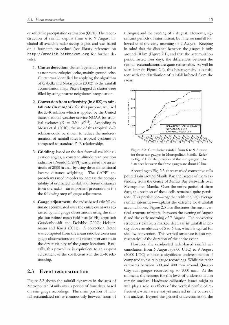
2.3 Event reconstruction
Figure 2.2 shows the rainfall dynamics in the area of
Metropolitan Manila over a period of four days, based
on rain gauge recordings. The main portion of rain-
fall accumulated rather continuously between noon of
6 August and the evening of 7 August. However, sig-
nificant periods of intermittent, but intense rainfall fol-
lowed until the early morning of 9 August. Keeping
in mind that the distance between the gauges is only
around 10 km (Figure 2.1), and that the accumulation
period lasted four days, the differences between the
rainfall accumulations are quite remarkable. As will be
seen later (in Figure 2.4), this heterogeneity is consis-
tent with the distribution of rainfall inferred from the
radar.
Figure 2.2: Cumulative rainfall from 6 to 9 August
for three rain gauges in Metropolitan Manila. Refer
to Fig. 2.1 for the position of the rain gauges. The
distances between the three gauges are about 10 km.
According to Fig. 2.3, threemarked convective cells
poured rain around Manila Bay, the largest of them ex-
tending from the centre of Manila Bay eastwards over
Metropolitan Manila. Over the entire period of three
days, the position of these cells remained quite persis-
tent. This persistence––together with the high average
rainfall intensities––explains the extreme local rainfall
accumulations. Figure 2.3 also illustrates the mean ver-
tical structure of rainfall between the evening of August
6 and the early morning of 7 August. The convective
structures exhibit a marked decrease in rainfall inten-
sity above an altitude of 5 to 6 km, which is typical for
shallow convection. This vertical structure is also rep-
resentative of the duration of the entire event.
However, the unadjusted radar-based rainfall ac-
cumulation from 6 August (08:00 UTC) to 9 August
(20:00 UTC) exhibits a significant underestimation if
compared to the rain gauge recordings. While the radar
estimates between 300 and 400 mm around Quezon
City, rain gauges recorded up to 1000 mm. At the
moment, the reasons for this level of underestimation
remain unclear. Hardware calibration issues might as
well play a role as effects of the vertical profile of re-
flectivity, which were not yet analysed in the course of
this analysis. Beyond this general underestimation, the

14 Chapter 2. Using the new Philippine radar network to reconstruct the Habagat of August 2012 monsoon event
Figure 2.3: Mean rainfall intensity in the night from 6 August (20:00 UTC) until 7 August (08:00 UTC) as seen by
the Subic S-band radar. The central figure shows a CAPPI at 3000 m altitude (for the rainfall estimation, we used the
Pseudo-CAPPI at 2000 m; see Sect. 2.2). The marginal plots show the vertical distribution of intensity maxima along
the x- and y-axis, respectively. In the area around Manila Bay, three marked cells appear. For these cells, the rainfall
intensity exhibits a marked decrease above an altitude of 5 to 6 km, indicating rather shallow convection.
Subic radar shows massive beam shielding in the south-
ern sectors, which is caused by Mount Natib, a volcano
and caldera complex located in the province of Bataan.
Other sectors of the Subic radar are affected by partial
beam shielding due to a set of mountain peaks in the
northern vicinity of the radar.
In order to correct for the substantial underestima-
tion, rain gauge recordings were used to adjust the rain-
fall estimated by the radar at an altitude of 2000m (using
the mean field bias adjustment approach). This proce-
dure reduced the crossvalidation RMSE of the event-
scale rainfall accumulation by more than half. The re-
sulting rainfall distribution is shown in Figure 2.4. This
figure gives an impressive view on the amount of rain
that actually came down around Metropolitan Manila.
Obviously, the actual “epicentre” of the event was situ-
ated rather over the Manila Bay than over Metropolitan
Manila itself.
Due to its size and shape, the Marikina River basin
(see Figure 2.1)—as it did in September 2009—most
strongly contributed to the flooding of Metropolitan
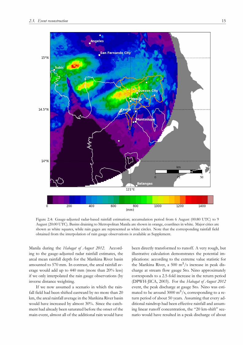
2.3. Event reconstruction 15
Figure 2.4: Gauge-adjusted radar-based rainfall estimation; accumulation period from 6 August (00:80 UTC) to 9
August (20:00 UTC). Basins draining to Metropolitan Manila are shown in orange, coastlines in white. Major cities are
shown as white squares, while rain gages are represented as white circles. Note that the corresponding rainfall field
obtained from the interpolation of rain gauge observations is available as Supplement.
Manila during the Habagat of August 2012. Accord-
ing to the gauge-adjusted radar rainfall estimates, the
areal mean rainfall depth for the Marikina River basin
amounted to 570 mm. In contrast, the areal rainfall av-
erage would add up to 440 mm (more than 20% less)
if we only interpolated the rain gauge observations (by
inverse distance weighting.
If we now assumed a scenario in which the rain-
fall field had been shifted eastward by no more than 20
km, the areal rainfall average in theMarikina River basin
would have increased by almost 30%. Since the catch-
ment had already been saturated before the onset of the
main event, almost all of the additional rain would have
been directly transformed to runoff. A very rough, but
illustrative calculation demonstrates the potential im-
plications: according to the extreme value statistic for
the Marikina River, a 500 m3/s increase in peak dis-charge at stream flow gauge Sto. Nino approximately
corresponds to a 2.5-fold increase in the return period
(DPWH-JICA, 2003). For the Habagat of August 2012
event, the peak discharge at gauge Sto. Nino was esti-
mated to be around 3000 m3/s, corresponding to a re-turn period of about 50 years. Assuming that every ad-
ditional raindrop had been effective rainfall and assum-
ing linear runoff concentration, the “20 km-shift” sce-
nario would have resulted in a peak discharge of about

16 Chapter 2. Using the new Philippine radar network to reconstruct the Habagat of August 2012 monsoon event
3900 m3/s—or a return period of more than 200 years.
The return period of the flood event related to Typhoon
Ketsana in September 2009 was estimated to be 150
years (Tabios III, 2009).
2.4 Conclusions
The local rain gauge recordings in Quezon City already
indicate the magnitude of the Habagat of August 2012
event. However, the rain gauge data alone could not
provide a complete picture of what happened around
Metropolitan Manila from 6 to 9 August.
Only the combination of the Subic S-band radar
and the dense rain gauge network around Metropolitan
Manila reveals that a significant portion of the heavy
rainfall was dropped right over the shorelines of Manila
Bay. Assuming a scenario in which the rainfall field was
shifted eastwards by no more than 20 km, the peak dis-
charge of the Marikina River would have increased by
almost 30%, potentially resulting into a return period
well beyond the 150 yr of Typhoon Ketsana in Septem-
ber 2009. It appears that—despite the terrible harm
and damage that was caused by this flood event—the
Habagat of August 2012 was no more than a glimpse
of the disaster that Metropolitan Manila missed by no
more than 20 km.
Nonetheless, a lot of open questions remain to be
answered, particularly concerning the underestimation
of rainfall by the radar, the potential effects of inhomo-
geneous vertical reflectivity profiles, the potential role
of wind drift (fromManila Bay toMetropolitanManila),
and also the hydrological processes which resulted from
the rainfall event. Beyond, additional data for the region
are available from a C-band weather radar located near
Tagaytay City. However, these data were not consid-
ered in this study since the role of attenuation induced
by heavy rainfall has yet to be determined. All these
questions need to be addressed as soon as possible so
that the equipment installed can allow for the most ac-
curate analysis of extreme rain events that certainly will
occur in the future. However, even with the current
level of data processing, the recently installed Philip-
pine radar network demonstrates a huge potential for
high-resolution rainfall monitoring as well as for risk
mitigation and management in the Philippines.
Acknowledgements
The radar data for this analysis were provided by the
Philippine Atmospheric, Geophysical and Astronom-
ical Services Administration (PAGASA, http://pa-gasa.dost.gov.ph). The rain gauge data were
kindly provided by the Philippine government’s Project
NOAH (National Operational Assessment of Haz-
ards, http://noah.dost.gov.ph). The study was also
funded through Project NOAH, as well as by the Ger-
man Ministry for Education and Research (BMBF)
through the PROGRESS project (http://www.earth-
in-progress), and through the GeoSim graduate re-
search school (http://www.geo-x.net/geosim).

2.4. Conclusions 17
Supplemental material to the manuscript
Figure 2.5: Accumulated rainfall as estimated from the interpolation of rain gauge observations using inverse distance
weighting; accumulation period fromAug 6 (00:80UTC) toAug 9 (20:00UTC). Basins draining toMetropolitanManila
are shown in orange, coastlines in white. Major cities are shown as white squares, while rain gages are represented as
white circles.


19
Chapter 3
Enhancing the Consistency of Spaceborne and Ground-Based
Radar Comparisons by Using Beam Blockage Fraction as a
Quality Filter
This chapter is published as:
Crisologo, Irene, Robert A. Warren, Kai Mühlbauer, and Maik Heistermann. 2018. “Enhancing the Consistency
of Spaceborne and Ground-Based Radar Comparisons by Using Beam Blockage Fraction as a Quality Filter.”
Atmospheric Measurement Techniques 11 (9): 5223–36. https://doi.org/10.5194/amt-11-5223-2018.
Abstract
We explore the potential of spaceborne radar (SR) observations from the Ku-band precipitation radars onboard the
Tropical Rainfall MeasuringMission (TRMM) andGlobal PrecipitationMeasurement (GPM) satellites as a reference
to quantify the ground radar (GR) reflectivity bias. To this end, the 3D volume-matching algorithm proposed by
Schwaller and Morris (2011) is implemented and applied to 5 years (2012–2016) of observations. We further extend
the procedure by a framework to take into account the data quality of each ground radar bin. Through thesemethods,
we are able to assign a quality index to each matching SR–GR volume, and thus compute the GR calibration bias as
a quality-weighted average of reflectivity differences in any sample of matching GR–SR volumes. We exemplify the
idea of quality-weighted averaging by using the beam blockage fraction as the basis of a quality index. As a result,
we can increase the consistency of SR and GR observations, and thus the precision of calibration bias estimates.
The remaining scatter between GR and SR reflectivity, as well as the variability of bias estimates between overpass
events indicate, however, that other error sources are not yet fully addressed. Still, our study provides a framework
to introduce any other quality variables that are considered relevant in a specific context. The code that implements
our analysis is based on the open-source software library wradlib, and is, together with the data, publicly available to
monitor radar calibration, or to scrutinize long series of archived radar data back to December 1997, when TRMM
became operational.
3.1 Introduction
Weather radars are essential tools in providing high-
quality information about precipitation with high spa-
tial and temporal resolution in three dimensions. How-
ever, several uncertainties deteriorate the accuracy of
rainfall products, with calibration contributing the most
amount (Houze et al., 2004), while also varying in
time (Wang and Wolff, 2009). While adjusting ground
radars (GR) by comparison with a network of rain
gauges (also know as gauge adjustment ) is a widely used
method, it suffers from representativeness issues. Fur-
thermore, gauge adjustment accumulates uncertainties
along the entire rainfall estimation chain (e.g. includ-
ing the uncertain transformation from reflectivity to
rainfall rate), and thus does not provide a direct ref-
erence for the measurement of reflectivity. Relative
calibration (defined as the assessment of bias between
the reflectivity of two radars) has been steadily gain-
ing popularity, in particular the comparison with space-
borne precipitation radars (SR) (such as the precip-
itation radar onboard the Tropical Rainfall Measur-
ing Mission (TRMM; 1997–2014; Kummerow et al.
(1998)) and the dual-frequency precipitation radar on

20 Chapter 3. Enhancing the Consistency of Spaceborne and Ground-Based Radar Comparisons
the subsequent Global Precipitation Measurement mis-
sion (GPM; 2014–present; Hou et al. (2013)). Sev-
eral studies have shown that surface precipitation esti-
mates from GRs can be reliably compared to precipita-
tion estimates from SRs for both TRMM (Amitai et al.,
2009; Joss et al., 2006; Kirstetter et al., 2012) and GPM
(Gabella et al., 2017; Petracca et al., 2018; Speirs et al.,
2017). In addition, a major advantage of relative calibra-
tion and gauge adjustment in contrast to the absolute
calibration (i.e. minimizing the bias in measured power
between an external or internal reference noise source
and the radar at hand) is that they can be carried out a
posteriori, and thus be applied to historical data.
Since both ground radars and spaceborne precipi-
tation radars provide a volume-integrated measurement
of reflectivity, a direct comparison of the observations
can be done in three dimensions (Anagnostou et al.,
2001; Gabella et al., 2006, 2011; Keenan et al., 2003;
Warren et al., 2018). Moreover, as the spaceborne
radars are and have been constantly monitored and vali-
dated (with their calibration accuracy proven to be con-
sistently within 1 dB) (TRMM: Kawanishi et al. (2000);
Takahashi et al. (2003); GPM: Furukawa et al. (2015);
Kubota et al. (2014); Toyoshima et al. (2015)), they have
been suggested as a suitable reference relative calibra-
tion of ground radars (Anagnostou et al., 2001; Islam
et al., 2012; Liao et al., 2001; Schumacher and Houze Jr,
2003).
Relative calibration between SRs and GRs was orig-
inally suggested by Schumacher and Houze (2000), but
the first method to match SR and GR reflectivity mea-
surements was developed by Anagnostou et al. (2001).
In their method, SR and GR measurements are resam-
pled to a common 3-D grid. Liao et al. (2001) devel-
oped a similar resampling method. Such 3-D resam-
pling methods have been used in comparing SR and
GR for both SR validation and GR bias determination
(Bringi et al., 2012; Gabella et al., 2006, 2011; Park et al.,
2015; Wang and Wolff, 2009; Zhang et al., 2018; Zhong
et al., 2017) Another method was suggested by Bolen
and Chandrasekar (2003) and later on further devel-
oped by Schwaller and Morris (2011), where the SR–
GR matching is based on the geometric intersection
of SR and GR beams. This geometry matching algo-
rithm confines the comparison to those locations where
both instruments have actual observations, without in-
terpolation or extrapolation. The method has also been
used in a number of studies comparing SR and GR re-
flectivities (Chandrasekar et al., 2003; Chen and Chan-
drasekar, 2016; Islam et al., 2012; Kim et al., 2014; Wen
et al., 2011). A sensitivity study byMorris and Schwaller
(2011) found that method to give more precise esti-
mates of relative calibration bias as compared to grid-
based methods.
Due to different viewing geometries, ground radars
and spaceborne radars are affected by different sources
of uncertainty and error. Observational errors with re-
gard to atmospheric properties such as reflectivity are,
for example, caused by ground clutter or partial beam
blocking. Persistent systematic errors in the observa-
tion of reflectivity by ground radars are particularly
problematic: the intrinsic assumption of the bias es-
timation is that the only systematic source of error is
radar calibration. It is therefore particularly important
to address such systematic observation errors.
In this study, we demonstrate that requirement
with the example of partial beam blocking. The anal-
ysis is entirely based on algorithms implemented in
the open-source software library wradlib (Heistermann
et al., 2013b), including a technique to infer partial beam
blocking by simulating the interference of the radar
beam with terrain surface based on a digital elevation
model. Together, that approach might become a ref-
erence for weather services around the world who are
struggling to create unbiased radar observations from
many years of archived single-polarized radar data, or
to consistently monitor the bias of their radar obser-
vations. We demonstrate the approach in a case study
with 5 years of data from the single-polarized S-band
radar near the city of Subic, Philippines, which had been
shown in previous studies to suffer from substantial
miscalibration (Abon et al., 2016; Heistermann et al.,
2013a).
3.2 Data
3.2.1 Spaceborne precipitation radar
Precipitation radar data were gathered from TRMM
2A23 and 2A25 version 7 products (NASA, 2017) for
overpass events intersecting with the Subic ground
radar coverage from 1 June 2012 to 30 September 2014,
and GPM 2AKu version 5A products (Iguchi et al.,
2010) from 1 June 2014 to 31December 2016. Ka-band
observations have not been considered due to higher
susceptibility to attenuation, and a limited validity of
Rayleigh scattering in a substantial portion of rainfall
cases (Baldini et al., 2012). From the collection of over-
passes within these dates, only 183 TRMM overpasses
and 103 GPM passes were within the radar coverage.
The data were downloaded from NASA’s Precipitation

3.3. Method 21
Processing System (PPS) through the STORM web in-
terface (https://storm.pps.eosdis.nasa.gov/storm/) on
15 February 2018 for TRMM and 14 June 2018 for
GPM. The parameters of TRMM/GPM extracted for
the analysis are the same as Warren et al. (2018; their
Table 3).
It is important to note that, at the time of writ-
ing, changes in calibration parameters applied in the
GPMVersion 5 products resulted in an increase of +1.1
dB from the corresponding TRMM version 7 products
(NASA, 2017).
3.2.2 Ground radar
The Philippine Atmospheric, Geophysical, and Astro-
nomical Services Administration (PAGASA) maintains
a nationwide network of 10 weather radars, 8 of which
are single-polarization S-band radars and 2 are dual-
polarization C-band radars. The Subic radar, which
covers the greater Metropolitan Manila area, has the
most extensive set of archived data. The radar cover-
age includes areas that receive some of the highest mean
annual rainfall in the country.
The Subic radar sits on top of a hill at 532 m.a.s.l.
in the municipality of Bataan, near the border with
Zambales (location: 14.82 ◦N, 120.36 ◦E) (see Figure3.1). To its south stands Mt. Natib (1253 m.a.s.l.) and
to its north run the Zambales Mountains (the highest
peak stands at 2037 m.a.s.l.). To the west is the Re-
dondo Peninsula in the southern part of the Zambales
province, where some mountains are also situated. Al-
most half of the coverage of the Subic radar is water,
with Manila Bay to its south-east and the West Philip-
pine Sea to the west. Technical specifications of the
radar are summarized in Table 3.2.2. Data from April
2012 to December 2016 were obtained from PAGASA.
Throughout the 5 years the scan strategy remained the
same, except for 2015 when it was limited to only three
elevation angles per volume due to hardware issues.
The standard scanning strategy was re-implemented in
2016.
Table 3.1: Characteristics of the Subic radar and
its volume scan strategy. The numbers in paren-
theses correspond to scans in 2015, where the
scanning strategy was different due to hardware
issues.
Subic Radar
Polarization Single-Pol
Position (lat/lon) 14.82◦N 120.36 ◦EAltitude 532 m.a.s.l.
Maximum Range 120 km (150 km)
Azimuth resolution 1 ◦
Beam width 0.95 ◦
Gate length 500 m (250 m)
Number of elevation angles 14 (3)
Elevation angles 0.5, 1.5, 2.4, 3.4, 4.3,
5.3, 6.2, 7.5, 8.7, 10,
12, 14, 16.7, 19.5 (◦)(0.0, 1.0, 2.0)
Volume cycle interval 9 minutes
Data available since April 2012
Peak power 850 kW
Wavelength 10.7 cm
3.3 Method
3.3.1 Partial beam shielding and quality in-
dex based on beam blockage fraction
In an ideal situation, SR and GR should have the same
measurements for the same volume of the atmosphere,
as they are measuring the same target. However, obser-
vational differences may arise due to different view ge-
ometries, different operating frequencies, different en-
vironmental conditions of each instrument, and differ-
ent processes along the propagation path of the beam.
As pointed out before, we focus on beam blockage as
an index of GR data quality.
In regions of complex topography, ground radars
are typically affected by the effects of beam blockage,
induced by the interaction of the beam with the ter-
rain surface resulting in a weakening or even loss of the
signal. To quantify that process within the Subic radar
coverage, a beam blockage map is generated following
the algorithm proposed by Bech et al. (2003). It assesses
the extent of occultation using a digital elevation model
(DEM). While Bech et al. (2003) used the GTOPO30
DEM at a resolution of around 1 km, higher DEM res-
olutions are expected to increase the accuracy of esti-
mates of beam blockage fraction, as shown by Kucera
et al. (2004), in particular the near range of the radar

22 Chapter 3. Enhancing the Consistency of Spaceborne and Ground-Based Radar Comparisons
Figure 3.1: (a) Map of the Philippines showing the region of study and (b) the 120km coverage of the Subic radar
(location marked with red diamond) with the SRTM digital elevation model of the surrounding area.
(Cremonini et al., 2016). The DEM used in this study
is from the Shuttle Radar Topography Mission (SRTM)
data, with 1 arc-second (approximately 30-meter) res-
olution. The DEM was resampled to the coordinates
of the radar bin centroids, using spline interpolation, in
order to match the polar resolution of the radar data
(500 m in range and 1◦ in azimuth, extending to a max-imum range of 120 km from the radar site; see Figure
3.1). A beam blockage map is generated for all available
elevation angles.
The beam blockage fraction was calculated for each
bin and each antenna pointing angle. The cumulative
beam blockage was then calculated along each ray. A
cumulative beam blockage fraction (BBF) of 1.0 corre-
sponds to full occlusion, and a value of 0.0 to perfect
visibility.
The quality index based on beam blockage fraction
is then computed following Zhang et al. (2011) as
QBBF =
1 BBF ≤ 0.11 − BBF −0.1
0.4 0.1 < BBF ≤ 0.50 BBF > 0.5
(3.1)
A slightly different formulation to transform partial
beam blockage to a quality index has been presented in
other studies (Figueras i Ventura and Tabary, 2013; For-
nasiero et al., 2005; Ośródka et al., 2014; Rinollo et al.,
2013) where the quality is zero (0) if BBF is above a
certain threshold, and then linearly increases to one (1)
above that threshold. It should be noted that these ap-
proaches are equally valid and can be used in determin-
ing the quality index based on beam blockage.
Figure 3.2: Quality index map of the beam
blockage fraction for the Subic radar at (a) 0.0◦,(b) 0.5◦, (c) 1.0◦, and (d) 1.5◦ elevation angles.
Figure 3.2 shows the beam blockage map for the
two lowest elevation angles of each scanning strategy.
Figure 3.2a and c are for 0.0◦ and 1.0◦, which are thetwo lowest elevation angles in 2015, while Figure 3.2b
and d are for 0.5◦ and 1.5◦, which are the two lowestelevation angles for the rest of the dataset.
3.3. Method 23
As expected, the degree of beam blockage de-
creases with increasing antenna elevation, yielding the
most pronounced beam blockage at 0.0◦. Each blockedsector can be explained by the topography (see Figure
3.1), with the Zambales Mountains causing blockage in
the northern sector, Mt. Natib in the southern sector,
and the Redondo peninsula mountains in the western
sector. The Sierra Madre also causes some partial beam
blocking in the far east, and a narrow partial blocking
northeast of the station where Mt. Arayat is located.
As the elevation angle increases, the beam blockage be-
comes less pronounced or even disappears. Substantial
blockage persists, however, for the higher elevation an-
gles in the northern and southern sectors.
3.3.2 SR–GR Volume Matching
SR and GR data were matched only for the wet pe-
riod within each year, which is from June to December.
Several meta-data parameters were extracted from the
TRMM 2A23 and GPM 2AKu products for each SR
gate, such as the corresponding ray’s brightband height
and width, gate coordinates in three dimensions (lon-
gitude and latitude of each ray’s Earth intercept and
range gate index), time of overpass, precipitation type
(stratiform, convective, or other ), and rain indicators (rain cer-
tain or no-rain). The parallax-corrected altitude (above
mean sea level) and horizontal location (with respect to
the GR) of each gate were determined as outlined in
the appendix of Warren et al. (2018). From the bright-
band height/width and the altitude of each SR gate,
the brightband membership of each gate was calculated
by grouping all rays in an overpass and computing the
mean brightband height and width. A ratio value of less
than zero indicates that the gate is below the bright-
band, and greater than one indicates that the gate is
above the brightband, and a value between zero and
one means that the gate is within the brightband. Only
gates below and above the brightband were considered
in the comparison. Warren et al. (2018) found a posi-
tive bias in GR–SR reflectivity difference for volume-
matched samples within the melting layer, compared to
those above and below the melting layer. They specu-
lated that this was due to underestimation of the Ku- to
S-band frequency correction for melting snow. In ad-
dition, while usually the samples above the brightband
are used in GPM validation, there are significantly more
samples below the melting layer, especially in a tropical
environment such as the Philippines. To ensure that
there are sufficient bins with actual rain included in the
comparison, overpasses with less than 100 gates flagged
as rain certain were discarded.
For each SR overpass, the GR sweep with the scan
time closest to the overpass time within a 10-min win-
dow (±5-min from overpass time) was selected. Both
the SR and GR data were then geo-referenced into a
common azimuthal equidistant projection centered on
the location of the ground radar.
In order tominimize systematic differences in com-
paring the SR and GR reflectivities caused by the dif-
ferent measuring frequencies, the SR reflectivities were
converted from Ku- to S-band following the formula:
Z(S) = Z(Ku) +4∑
i=0ai[Z(Ku)]i (3.2)
where the ai are the coefficients for dry snow and dry
hail, rain, and in between at varying melting stages (Ta-
ble 1 of Cao et al. (2013)). We used the coefficients
for snow in the reflectivity conversion above the bright-
band, following Warren et al. (2018).
The actual volume matching algorithm closely fol-
lows the work of Schwaller and Morris (2011), where
SR reflectivity is spatially and temporally matched with
GR reflectivity without interpolation. The general con-
cept is highlighted by Figure 3.3: each matching sample
consists of bins from only one SR ray and one GR sweep.
From the SR ray, those bins were selected that intersect
with the vertical extent of a specific GR sweep at the
SR ray location. From each GR sweep, those bins were
selected that intersect with the horizontal footprint of
the SR ray at the corresponding altitude. The SR and
GR reflectivity of each matched volume was computed
as the average reflectivity of the intersecting SR and GR
bins.
The nominal minimum sensitivity of both TRMM
PR and GPM KuPR is 18 dBZ, so only values above
this level were considered in the calculation of average
SR reflectivity in the matched volume. In addition, the
fraction of SR gates within a matched volume above
that threshold was also recorded. On the other hand,
all GR bins are included in the calculation of average
GR reflectivity, after setting the bins with reflectivities
below 0.0 dBZ to 0.0 dBZ, as suggested by Morris and
Schwaller (2011). The filtering criteria applied in the
workflow are summarized in Table 3.2.

24 Chapter 3. Enhancing the Consistency of Spaceborne and Ground-Based Radar Comparisons
Figure 3.3: Diagram illustrating the geometric intersection. Left panel shows a single SR beam intersecting GR sweeps
of two different elevation angles. The two top right panels illustrate the intersection of SR–GR sample volumes in the
near and far ranges and the two bottom right panels show the projection of these intersections along an SR ray. From
Schwaller and Morris (2011) ©American Meteorological Society. Used with permission.
Table 3.2: Filtering criteria for the matching work-
flow.
Criteria Condition
Minimum number of pixels in
overpass tagged as ’rain’
100
Brightband membership below or above
GR range limits (min–max) 15 – 115 km
Minimum fraction of bins
above minimum SR sensitivity
0.7
Minimum fraction of bins
above minimum GR sensitivity
0.7
Maximum time difference
between SR and GR
5 min
Minimum PR reflectivity 18 dBZ
3.3.3 Assessment of the average reflectivity
bias
Beam blockage and the correspondingGR quality maps
were computed for each GR bin (cf. Section 3.3.1). For
eachmatched SR–GR volume, the data quality was then
based on the minimum quality of the GR bins in that
volume.
To analyze the effect of data quality on the esti-
mation of GR calibration bias, we compared two es-
timation approaches: a simple mean bias that does
not take into account beam blockage, and a weighted
mean bias that considers the quality value of each sam-
ple as weights. The corresponding standard deviation
and weighted standard deviation were calculated as well.
The overall process is summarized in Figure 3.4. In this
way, we provide an overview of the variability of our
bias estimates over time.
Figure 3.4: Flowchart describing the processing
steps to calculate the mean bias and the weighted
mean bias between ground radar data and satellite
radar data. The results of each step are shown in
Section 3.4.
3.3.4 Computational details
In order to promote transparency and reproducibility of
this study, we mostly followed the guidelines provided
by Irving (2016) which have also been implemented by
a number of recent studies (Blumberg et al., 2017; Irv-
ing and Simmonds, 2016; Rasp et al., 2018).

3.4. Results and discussion 25
The entire processing workflow is based on wradlib
(Heistermann et al., 2013b), an extensively documented
open-source software library for processing weather
radar data. At the time of writing, we used version
1.0.0 released on 01 April 2018, based on Python
3.6. The main dependencies include Numerical Python
(NumPy; Oliphant (2015)), Matplotlib (Hunter, 2007),
Scientific Python (SciPy; Jones et al. (2014)), h5py
(Collette, 2013), netCDF4 (Rew et al., 1989), and gdal
(GDAL Development Team, 2017).
Reading the TRMM 2A23 and 2A25 version 7
data, GPM 2AKu version 5A data, and Subic ground
radar data in the netCDF format converted through the
EDGE software of EEC radars was done through the
input-output module of wradlib. The beam blockage
modelling is based on the Bech et al. (2003) method im-
plemented as a function in wradlib’s data quality mod-
ule. The volume-matching procedure is built upon the
georeferencing and zonal statistics modules, accompa-
nied by Pandas (McKinney, 2010) for organizing and
analysing the resulting database of matched bins. Vi-
sualization was carried out with the help of matplotlib
(Hunter, 2007) and Py-ART (Helmus and Collis, 2016).
An accompanying GitHub repository that
hosts the Jupyter notebooks of the work-
flow and sample data is made available at
https://github.com/wradlib/radargpm-beamblockage.
3.4 Results and discussion
3.4.1 Single event comparison
From the 183 TRMM and 103 GPM overpasses that
intersected with the 120 km Subic radar range, only 74
TRMM and 40 GPM overpasses were considered valid
after applying the selection criteria listed in Table 3.2.
In order to get a better idea about the overall workflow,
we first exemplify the results for two specific overpass
events—one for TRMM, and one for GPM.
Case 1: 08 November 2013
For the TRMM overpass event on November 8, 2013,
the top row of Figure 3.5 shows SR (a) and GR (b)
reflectivity as well as the resulting differences (c) for
matching samples at an elevation angle of 0.5◦. Eachcircle in the plots represents a matched volume. A cor-
responding map of QBBF is shown in (d) while (e)
shows a scatter plot of GR versus SR reflectivities, with
points coloured according to their QBBF . The reflec-
tivity differencemap and scatter plot indicate significant
variability with absolute differences of up to and ex-
ceeding 10 dB. Large differences can be observed at the
edges of the southern sector affected by beam block-
age (cf. also Figure 3.2). Major parts of that sector did
not receive any signal due to total beam blockage, high-
lighted in Figure 3.5a with black circles showing the bins
where the GR did not obtain valid observations. At the
edges, however, partial beam blockage caused substan-
tially lower GR reflectivity values. As expected, large
negative differences of ZGR–ZSR are characterized by
low quality.
Consequently, the estimate of the calibration bias
substantially depends on the consideration of partial
beam blockage (or quality). Ignoring quality (simple
mean) yields a bias estimate of -1.9 dB while the quality-
weighted average yields a bias estimate of -1.2 dB. Ac-
cordingly, the standard deviation is reduced from 3.4 to
2.6 dB, indicating a more precise bias estimate.
This case demonstrates how partial beam blockage
affects the estimation of GR calibration bias. At a low
elevation angle, substantial parts of the sweep are af-
fected by total beam blockage. The affected bins are ei-
ther below the detection limit, or they do not exceed the
GR threshold specified in Table 3.2. As a consequence,
these bins will not be considered in the matched sam-
ples and will thus not influence the bias estimate, irre-
spective of using partial beam blockage as a quality fil-
ter. At a higher elevation angle, though, the same bins
might not be affected by total beam blockage, but by par-
tial beam blockage, as also becomes obvious from Fig-
ure 3.2. Considering these bins in the matched samples
will cause a systematic error in the estimate of calibra-
tion bias, unless we use the partial beam blockage frac-
tion as a quality filter by computing a quality-weighted
average of reflectivity. As a consequence, the effect of
quality-weighted averaging (with partial beam blockage
fraction as a quality variable) can be most pronounced
at “intermediate” elevation angles, depending on the
specific topography and its location with respect to the
ground.
The effect becomes obvious for the next elevation
angle. Figure 3.6 is equivalent to Figure 3.5, but for
an elevation angle of 1.5◦: as the sector of total beamblockage shrinks at that elevation, the impact of par-
tial beam blockage on the estimation of GR calibration
bias increases. For an antenna elevation of 1.5◦, somebins in areas of partial beam blockage have very large
negative biases (over 20 dB). Ignoring beam blockage
for this elevation angle yields a bias estimate of -2.1 dB
(simplemean), while the quality-weighted average yields
a bias of -1.4 dB. At the same time, considering quality

26 Chapter 3. Enhancing the Consistency of Spaceborne and Ground-Based Radar Comparisons
Figure 3.5: GR-centered maps of volume-matched samples from 8 November 2013 at 0.5◦ elevation angle of (a) SRreflectivity, (b) GR reflectivity, (c) difference between GR and SR reflectivities, and (d)QBBF . (e) Scatter plot ofZGR
versus ZSR where each point is coloured based on the data quality (QBBF ). The solid line in (a)–(d) is the edge of
the SR swath, the other edge lies outside the figure. The dashed line denotes the central axis of the swath. The solid
concentric circles demarcate the 15 km and 115 km ranges from the radar. In (a) observations that are present in the
SR data but not detected by the GR are encircled in black. The mean brightband is at a height of 4685 meters.
substantially reduces the standard deviation from 3.4
dB to 2.1 dB.
Case 2: 01 October 2015
The second case confirms the findings in the previous
section for a GPM overpass on October 1, 2015. That
overpass captured an event in the northern and eastern
part of the radar coverage where partial beam block-
age is dominant, as well as a small part of the south-
ern sector with partial and total beam blockage. Figure
3.7 shows the results of that overpass in analogy to the
previous figures, for an antenna elevation of 0.0◦. Thefigure shows a dramatic impact of partial beam block-
age, with a dominant contribution from the northern
part, but also clear effects from the eastern and south-
ern sectors. The scatter plot of ZGR over ZSR in Fig-
ure 3.7e demonstrates how the consideration of par-
tial beam blockage increases the consistency between
GR and SR observations and allows for a more reliable
estimation of the GR calibration bias: ignoring partial
beam blockage (simple mean) yields a bias of -2.7 dB,
while the quality-weighted average bias is -1.1 dB. Tak-
ing into account quality decreases the standard devia-
tion from 3.8 dB to 2.7 dB.
3.4.2 Overall June–November comparison
during the 5-year observation period
Finally, we applied both the simple and quality-weighted
mean bias estimations to each of the TRMM and GPM

3.4. Results and discussion 27
Figure 3.6: Same as in Figure 3.5 but for 1.5◦ elevation angle.
overpasses from 2012 to 2016 that met the criteria spec-
ified in Section 3.3.2, Table 3.2. As pointed out in Sec-
tion 3.3.2, the matching procedure itself is carried out
per GR sweep, i.e. separately for each antenna elevation
angle.
As a result, we obtain a time series of bias estimates
for GR calibration, as shown in Figure 3.8. In this fig-
ure, the calibration bias for each overpass is computed
from the full GR volume, i.e. including matched sam-
ples from all available antenna elevations. In the upper
panel (a), each marker represents the quality-weighted
mean bias for a specific SR overpass (circles for GPM,
triangles for TRMM). The centre panel (b) highlights
the differences between the quality-weighted and sim-
ple mean approaches, by quantifying the effect of tak-
ing into account GR data quality (in this case, partial
beam blockage). The bottom panel (c) shows the dif-
ferences between the quality-weighted standard devia-
tion and the simple standard deviation of differences,
illustrating how taking into account GR quality affects
the precision of the bias estimates.
The time series provide several important insights.
(1) Effect of quality-weighting on bias estima-
tion. Figure 3.8b and c together illustrate the benefit
of taking into account GR data quality (i.e. beam block-
age) when we estimate GR calibration bias. It does not
come as a surprise that the difference between ∆Z∗
and ∆Z is mostly positive because the areas suffer-
ing from partial beam blockage register weaker signals
(i.e. lower reflectivity) than expected, producing a lower
mean bias. Giving the associated volume-matched sam-
ples low weights in the calculation of the mean bias
brings the quality-weighted bias up. In the same vein,
the beam-blocked bins introduce scatter, and assign-
ing them low weights decreases the standard deviation.
Figure 3.8c shows, as a consequence, that the quality-
weighted bias estimates are consistently more precise:
in the vast majority of overpasses, the quality-weighted
standard deviation is substantially smaller than the sim-
ple standard deviation. That result is also consistent
with the case study result shown above. It should be
noted, though, that for some overpasses, the quality-
weighting procedure (which is in effect a filtering) can

28 Chapter 3. Enhancing the Consistency of Spaceborne and Ground-Based Radar Comparisons
Figure 3.7: As in Figure 3.5 but for the overpass on 01 October 2015. The mean brightband level is found at 4719
meters for this case.
cause an increase in the bias estimate and/or the stan-
dard deviation of that estimate. That effect occurs for
overpasses with particularly low numbers of matched
samples, and, presumably, with rainfall in regions in
which our estimated beam blockage fraction is subject
to higher errors (caused by e.g. the inadequateness of
the assumed Gaussian antenna pattern, variability of at-
mospheric refractivity, or errors related to the DEM, its
resolution and its interpolation to ground radar bins).
In total, however, the effect of decreasing standard de-
viation vastly dominates.
(2) GPM and TRMM radars are consistent. In
2014, both TRMM and GPM overpasses are available.
That period of overlap shows that the GR calibration
bias estimates that are based on both TRMM and GPM
observations can be considered homogeneous. Using
TRMM data, the average calibration bias for all 2014
overpasses amounts to 1.6 ± 1.3 dB, while using the
GPM overpasses yields a bias of 1.8 ± 1.5 dB. The dif-
ference between TRMM version 7 and GPM version
5 reflectivities mentioned in Section 3.2.1 falls within
the uncertainties in the annual estimated mean bias,
which makes us confident that the substantial year-to-
year changes in our bias estimates are based on changes
in GR calibration.
(3) Change in bias over time: Despite the vari-
ability of bias estimates between the individual overpass
events, the time series still provides us with a clear sig-
nal: the bias estimates appear to fluctuate around an av-
erage value that appears to be quite persistent over the
duration of the corresponding wet seasons of the differ-
ent years, i.e. over intervals of several months. Consid-
ering the average calibration bias over the different wet
seasons (horizontal lines in Figure 3.8a), we can clearly
observe changes in calibration bias over time. The bias
was most pronounced in 2012 and 2013, with average
bias estimates around -4.1 dB for 2012 and -2.5 dB for
2013. For 2014, the absolute calibration bias was much
smaller, at a level of 1.4 dB, while for 2015 and 2016, the
situation improved further, with an average bias of 0.0
dB in 2015 and 0.6 dB in 2016. It is important to note
that these values were computed as the average bias and

3.4. Results and discussion 29
Figure 3.8: (a) Time series of the weighted mean bias (∆Z∗) from 2012 to 2016. Analysis covers only the wet season
from June to December. Triangle markers represent TRMM overpasses while circle markers are GPM overpasses.
Symbols are coloured according to the number of volume-matched samples on a logarithmic scale: light grey: 10–99,
medium grey: 100–999, and black: 1000+. Blue and orange solid (dashed) horizontal lines represent the weighted
average (standard deviation) of all individual matched samples within the year for TRMM and GPM, respectively. (b)
The difference between the weighted mean biases (∆Z∗) and the simple mean biases (∆Z). (c) The standard devia-tion of the weighted mean bias minus the standard deviation of the simple mean bias values. The green vertical lines
indicate the dates of the two case studies.
its standard deviation across all matched volumes and
not as the average of bias estimates across overpasses.
Accordingly, the standard deviation (as indicated by the
dashed lines) is quite high since it includes all the scatter
from the individual overpasses. We have to assume that
a fundamental issue with regard to calibration main-
tenance was addressed between 2013 and 2014 in the
context of hardware changes (i.e. replacement of mag-
netron). Unfortunately, we were not able to retrieve
detailed information on maintenance operations that
might explain the changes in bias of the radar through-
out the years.
(4) Short-term variability of bias estimates be-
tween overpasses. There is a strong variability of the
estimated calibration bias between overpasses (Figure
3.8a) and spatially within each overpass (Figures 3.5
to 3.7). That variability is clearly not a desirable prop-
erty, as we would not expect changes in calibration bias
to occur at the observed frequency, amplitude, and ap-
parent randomness. As a consequence, we have to as-
sume that the variability is a cumulative result of vari-
ous and dynamic sources of uncertainty along the entire
process of observation, product generation, matching,
and filtering. That assumption is well in line with many
other studies (such as Anagnostou et al. (2001); Dur-
den et al. (1998); Joss et al. (2006); Kim et al. (2014);
Meneghini et al. (2000); Rose and Chandrasekar (2005);
Schwaller and Morris (2011); Seto and Iguchi (2015);
Wang and Wolff (2009); Warren et al. (2018), to name
only a few) which discuss e.g. fundamental issues with
the backscattering model for different wavelengths and
sampling volumes; the uncertainty of beam propaga-
tion subject to fluctuations in atmospheric refractivity;
residual errors in the geometric intersection of the vol-
ume samples; uncertainties in SR reflectivity subject to
the effects of attenuation correction at Ku-band, non-
uniform beam filling and undesirable synergies between
the two; rapid dynamics in backscattering target during
30 Chapter 3. Enhancing the Consistency of Spaceborne and Ground-Based Radar Comparisons
the time interval between SR overpass and GR sweep;
effects of non-meteorological echoes for both SR and
GR; and, presumably, also short-term hardware insta-
bilities. Considering these uncertainties, together with
the fact that the quality-weighting in our case study ex-
plicitly accounts for beam blockage only, the short-term
variability becomes plausible. However, it is beyond the
scope of this study to disentangle the sources of this
variability.
3.5 Conclusions
In 2011, Schwaller and Morris presented a new tech-
nique to match spaceborne radar (SR) and ground-
based radar (GR) reflectivity observations, with the aim
to determine the GR calibration bias. Our study ex-
tends that technique by an approach that takes into
account the quality of the ground radar observations.
Each GR bin was assigned a quality index between 0
and 1, which was used to assign a quality value to each
matched volume of SR and GR observations. For any
sample of matched volumes (e.g. all matched volumes
of one overpass, or a combination of multiple over-
passes), the calibration bias can then be computed as
a quality-weighted average of the differences between
GR and SR reflectivity in all samples. We exemplified
that approach by applying aGR data quality index based
on the beam blockage fraction, and we demonstrated
the added value for both TRMM and GPM overpasses
over the 115 km range of the Subic S-band radar in the
Philippines for a 5-year period.
Although the variability of the calibration bias esti-
mates between overpasses is high, we showed that tak-
ing into account partial beam blockage leads to more
consistent andmore precise estimates of GR calibration
bias. Analyzing 5 years of archived data from the Subic
S-band radar (2012–2016), we also demonstrated that
the calibration standard of the Subic radar substantially
improved over the years, from bias levels of around -4.1
dB in 2012 to bias levels of around 1.4 dB in 2014 and
settling down to a bias of 0.6 dB in 2016. Of course,
more recent comparisons with GPM are needed to ver-
ify that this level of accuracy has been maintained. Case
studies for specific overpass events also showed that the
necessity to account for partial beam blockage might
even increase for higher antenna elevations. That ap-
plies when sectors with total beam blockage (in which
no valid matched volumes are retrieved at all) turn into
sectors with partial beam blockage at higher elevation
angles.
Considering the scatter between SR and GR reflec-
tivity in the matched volumes of one overpass (see case
studies), as well as the variability of bias estimates be-
tween satellite overpasses (see time series), it is obvi-
ous that we do not yet account for various sources of
uncertainties. Also, the simulation of beam blockage
itself might still be prone to errors. Nevertheless, the
idea of the quality-weighted estimation of calibration
bias presents a consistent framework that allows for the
integration of any quality variables that are considered
important in a specific environment or setting. For ex-
ample, if we consider C-band instead of S-band radars,
path-integrated attenuation needs to be taken into ac-
count for the ground radar, and wet radome attenua-
tion probably as well (Austin, 1987; Merceret andWard,
2000; Villarini and Krajewski, 2010). The framework
could also be extended by explicitly assigning a quality
index to SR observations, too. In the context of this
study, that was implicitly implemented by filtering the
SR data, e.g. based on brightband membership. An al-
ternative approach to filtering could be weighting the
samples based on their proximity to the brightband, the
level of path-integrated attenuation (as e.g. indicated by
the GPM 2AKu variables pathAtten and the associated
reliability flag (reliabFlag)) or the prominence of non-
uniform beam filling (which could e.g. be estimated
based on the variability of GR reflectivity within the SR
footprint; see e.g. Han et al. (2018)).
In addition, with the significant effort devoted to
weather radar data quality characterization in Europe
(Michelson et al., 2005), and the number of approaches
in determining an overall quality index based on differ-
ent quality factors (Einfalt et al., 2010), it is straight-
forward to extend the approach beyond beam blockage
fraction.
Despite the fact that there is still ample room for
improvement, our tool that combines SR–GR volume
matching and quality-weighted bias estimation is read-
ily available for application or further scrutiny. In
fact, our analysis is the first of its kind that is en-
tirely based on open-source software, and is thus fully
transparent, reproducible, and adjustable (see alsoHeis-
termann et al. (2014)). Therefore this study, for the
first time, demonstrates the utilization of wradlib func-
tions that have just recently been implemented to sup-
port the volume matching procedure and the simu-
lation of partial beam blockage. We also make the
complete workflow available together with the under-
lying ground and spaceborne radar data. Both code

3.5. Conclusions 31
and results can be accessed at the following repos-
itory https://github.com/wradlib/radargpm-beamblockage upon the publication of this paper.
Through these open-source resources, ourmethod-
ology provides both research institutions and weather
services with a valuable tool that can be applied
to monitor radar calibration, and—perhaps more
importantly—to quantify the calibration bias for long
time series of archived radar observations, basically be-
ginning with the availability of TRMM radar observa-
tions in December 1997.
Acknowledgements
The radar data for this analysis were provided by
the Philippine Atmospheric, Geophysical and Astro-
nomical Services Administration (PAGASA, http://pa-
gasa.dost.gov.ph). The study was also funded by the
German government through the German Academic
Exchange Service (https://www.daad.de/en/). We
would like to thank Daniel Michelson, Marco Gabella,
and one anonymous referee for their valuable insights
and comments that significantly improved the paper.

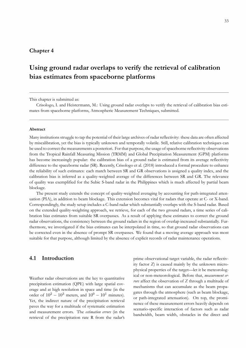
33
Chapter 4
Using ground radar overlaps to verify the retrieval of calibration
bias estimates from spaceborne platforms
This chapter is submitted as:
Crisologo, I. and Heistermann, M.: Using ground radar overlaps to verify the retrieval of calibration bias esti-
mates from spaceborne platforms, Atmospheric Measurement Techniques, submitted.
Abstract
Many institutions struggle to tap the potential of their large archives of radar reflectivity: these data are often affected
by miscalibration, yet the bias is typically unknown and temporally volatile. Still, relative calibration techniques can
be used to correct themeasurements a posteriori. For that purpose, the usage of spaceborne reflectivity observations
from the Tropical Rainfall Measuring Mission (TRMM) and Global Precipitation Measurement (GPM) platforms
has become increasingly popular: the calibration bias of a ground radar is estimated from its average reflectivity
difference to the spaceborne radar (SR). Recently, Crisologo et al. (2018) introduced a formal procedure to enhance
the reliability of such estimates: each match between SR and GR observations is assigned a quality index, and the
calibration bias is inferred as a quality-weighted average of the differences between SR and GR. The relevance
of quality was exemplified for the Subic S-band radar in the Philippines which is much affected by partial beam
blockage.
The present study extends the concept of quality-weighted averaging by accounting for path-integrated atten-
uation (PIA), in addition to beam blockage. This extension becomes vital for radars that operate at C- or X-band.
Correspondingly, the study setup includes a C-band radar which substantially overlaps with the S-band radar. Based
on the extended quality-weighting approach, we retrieve, for each of the two ground radars, a time series of cali-
bration bias estimates from suitable SR overpasses. As a result of applying these estimates to correct the ground
radar observations, the consistency between the ground radars in the region of overlap increased substantially. Fur-
thermore, we investigated if the bias estimates can be interpolated in time, so that ground radar observations can
be corrected even in the absence of prompt SR overpasses. We found that a moving average approach was most
suitable for that purpose, although limited by the absence of explicit records of radar maintenance operations.
4.1 Introduction
Weather radar observations are the key to quantitative
precipitation estimation (QPE) with large spatial cov-
erage and at high resolution in space and time (in the
order of 102 − 103 meters, and 100 − 101 minutes).Yet, the indirect nature of the precipitation retrieval
paves the way for a multitude of systematic estimation
and measurement errors. The estimation errors (in the
retrieval of the precipitation rate R from the radar’s
prime observational target variable, the radar reflectiv-
ity factor Z) is caused mainly by the unknown micro-
physical properties of the target—let it be meteorolog-
ical or non-meteorological. Before that, measurement er-
rors affect the observation of Z through a multitude of
mechanisms that can accumulate as the beam propa-
gates through the atmosphere (such as beam blockage,
or path-integrated attenuation). On top, the promi-
nence of these measurement errors heavily depends on
scenario-specific interaction of factors such as radar
bandwidth, beam width, obstacles in the direct and

34 Chapter 4. Using ground radar overlaps to verify the retrieval of calibration bias estimates from spaceborne platforms
wider vicinity, topography in the radar coverage, atmo-
spheric refractivity, or the microphysical properties of
precipitation along the beam’s propagation path. Much
has been written about these sources of uncertainty, and
much has been done to address them adequately (see
Villarini and Krajewski (2010) for an extensive review).
Yet, the single-most contribution of uncertainty to
radar-based QPE often comes, maybe surprising to
some, from the (mis)calibration or (in)stability of the
radar instrument itself (Houze et al., 2004) which can
also vary in time (Wang and Wolff, 2009). Apart from
the simple fact that miscalibration can easily deterio-
rate the accuracy of precipitation estimates by an or-
der of magnitude, calibration issues become particularly
annoying if weather radars are operated in a network
where the consistency of calibration between radars is a
prerequisite for high-quality radar mosaics (see e.g. Seo
et al. (2014)).
There are various options to carry out and monitor
the calibration of a radar instrument in an operational
context through absolute calibration techniques (based
on a well-defined reference noise source, see Doviak
and Zrnić (2006) for an overview). Yet, to the reflectiv-
ity that is already measured and recorded, any changes
to the instrument’s calibration are irrelevant. In such a
case, relative calibration techniques can be used to cor-
rect the measurements a posteriori. Many institutions
have archivedmassive radar reflectivity records over the
years, but they struggle to tap the potential of these data
due to unknown and temporally volatile calibration bi-
ases. And while radar polarimetry offers new opportu-
nities to address calibration issues, many archived data
still originate from single-polarization radars.
As to relative calibration, the usage of rain gauge
observations is typically not recommended, not only
due to issues of representativeness in space and time,
but also due to the fact that a comparison between R,
as observed by rain gauges, and R, as retrieved from
radar reflectivities, lumps over measurement and esti-
mation uncertainties. As an alternative, the usage of
spaceborne reflectivity observations from the Tropical
Rainfall Measuring Mission (TRMM) and Global Pre-
cipitation Measurement (GPM) platforms has become
increasingly popular over the recent years. Measure-
ment accuracies of both TRMM and GPM are reported
to have excellent calibration (within < 1dB) (Kawanishi
et al., 2000; Hou et al., 2013), and thus can be used as
a reference to calibrate reflectivity. Moreover, a major
benefit of relative calibration is that it allows for a pos-
teriori correction of historical data.
In a recent study for an S-band radar in the Philip-
pines, Crisologo et al. (2018) adopted a technique to
match ground radar (GR) and spaceborne radar (SR)
observations. That technique was originally suggested
by Bolen and Chandrasekar (2003), then further devel-
oped by Schumacher and Houze Jr (2003), and finally
by Warren et al. (2018). The underlying idea of that
technique is to match observations based on the geo-
metric intersection of SR and GR beams. That way, the
algorithm confines the comparison to locations where
both instruments have valid observations, and avoids
artefacts from interpolation or extrapolation. In that
context, Crisologo et al. (2018) demonstrated that ex-
plicitly taking into account the quality of the GR ob-
servations is vital to enhance the consistency between
SR and GR reflectivity measurements, and thus to es-
timate the calibration bias more reliably. The relevance
of quality was exemplified by considering partial beam
blockage: for each GR bin, a quality index between
0 and 1 was inferred from the beam blockage frac-
tion. These quality indices were then used to compute
a quality-weighted average of volume matched GR re-
flectivities.
The present study aims to extend the approach of
Crisologo et al. (2018) in several respects:
1. We extend the framework to account for the
quality of GR observations by introducing path
integrated attenuation (PIA) as a quality variable,
in addition to partial beam blockage. Instead of
attempting to correct GR reflectivities for PIA,
we explicitly acknowledge the uncertainty of any
PIA estimate by assigning a lowweight to anyGR
bins that are substantially affected by PIA. In or-
der to investigate the role of PIA, we include a
C-band weather radar in the present study, in ad-
dition to the S-band radar included by Crisologo
et al. (2018).
2. We verify the ability to estimate the GR calibra-
tion bias from SR overpass data by evaluating the
consistency of GR reflectivity measurements in
a region of overlap, before and after bias correc-
tion.
3. We investigate whether estimates of GR calibra-
tion bias, as obtained from SR overpass data, can
be interpolated in time in order to correct GR
reflectivity observations for miscalibration, even
for those times in which no suitable SR over-
passes were available.

4.2. Data and Study Area 35
The latter item—the interpolation of bias estimates
in time—would be a key requirement towards actually
tapping the potential of the fundamental concept in re-
search and applications: if we aim to use SR overpass
data for monitoring GR calibration bias, and for a ho-
mogeneous correction of archived GR reflectivities, we
have to assume that those bias estimates are, to some
extent, representative in time. Crisologo et al. (2018)
found that the bias estimates for the Subic S-band radar
exhibited a substantial short-term temporal variability,
and stated that they “would not expect changes in calibration
bias to occur at the observed frequency, amplitude, and appar-
ent randomness.” By investigating whether such bias esti-
mates can be interpolated in time, the present paper will
investigate whether the apparently “volatile” behaviour
of calibration bias is not a mere artefact of the estima-
tion procedure, but a real property of the investigated
radar systems.
Section 4.2 of the present paper will describe the
study area and the underlying radar data sets; section
4.3 will outline the methodologies of matching GR and
SR as well as GR and GR observations, the quantifica-
tion of beam blockage and PIA, and the quality-based
framework for bias estimation; in section 4.4, we will
show and discuss the various inter-comparison results;
and section 4.5 will conclude.
4.2 Data and Study Area
The Philippine Atmospheric, Geophysical, and Astro-
nomical Services Administration (PAGASA), the coun-
try’s weather agency, maintains a network of 10 ground
radars all over the country, of which 8 are single-
polarization S-Band radars and 2 are dual-polarization
C-Band radars. Two of the longest running radars are
Subic and Tagaytay. Between the two radars lies Manila
Bay, bordered on the east by Metro Manila, the coun-
try’s most densely populated area at approximately 13
Million inhabitants. This region of overlap regularly ex-
periences torrential rains from monsoon and typhoons
extending for several days (Heistermann et al., 2013a;
Lagmay et al., 2015).
4.2.1 Subic radar (SUB)
The Subic radar is a single-polarization S-band radar sit-
uated on top of a hill at 532 m a.s.l. in the municipal-
ity of Bataan (location: 14.82◦N, 120.36◦E) (see Figure4.1). To its north lies the Zambales Mountains (highest
peak: 2037 m a.s.l.) and to its south stands Mt. Natib
(1253 m a.s.l.). The Sierra Madre Mountains run along
the eastern part of the Luzon Island, at the far-east end
of the radar coverage. Technical specifications are avail-
able in Table 4.1. Please note that Subic sweeps at 1.5
and 2.4 degree elevation were excluded for the years
2013 and 2014, due to apparently erratic and inconsis-
tent behaviour.
4.2.2 Tagaytay radar (TAG)
Located about 100 km across the Manila Bay from the
Subic radar is the Tagaytay radar, a dual-polarized C-
Band radar. It sits along the Taal Volcano caldera ridge
at 752 m a.s.l. in the municipality of Batangas. The
radar coverage also includes the southern part of the
Sierra Madre Mountains. Technical specifications are
available in Table 4.1.
Data during the rainy seasons of 2012–2014 and
2016 are used in this study. The scanning setup for
Tagaytay was experimentally changed during 2015 and
reverted back in 2016. In order to ensure homogeneity
in the GR intercomparison, we excluded the year 2015
from the analysis.
4.2.3 Spaceborne precipitation radar
Spaceborne radar data were collected from TRMM
2A23 and 2A25 version 7 (NASA, 2017) for over-
pass events in 2012–2014, and GPM 2AKu version 5A
products (Iguchi et al., 2010) from 2014–2016, dur-
ing the rainy season of June to December. The data
were downloaded from NASA’s Precipitation Process-
ing System (PPS) through the STORM web interface
(https://storm.pps.eosdis.nasa.gov/storm/). The pa-
rameters of TRMM/GPM extracted for the analysis are
the same as specified in Table 3 of Warren et al. (2018).
4.3 Methods
4.3.1 Overview
We facilitate the comparison of effectively three instru-
ments: the two ground radars and the spaceborne radar
(see 4.2). While throughout the study period, the avail-
able spaceborne radar platform changed from TRMM
(2012–2014) to GPM (2014–2016), the consistency be-
tween the two for the year 2014 for the study area
(Crisologo et al., 2018) allows us to consider the two
rather as a single reference instrument. The compari-
son of the three platforms has two main components:
1. The SR–GR comparison is motivated by the es-
timation of theGR calibration bias. We define
that bias as the mean difference (∆ZSR−SUB or

36 Chapter 4. Using ground radar overlaps to verify the retrieval of calibration bias estimates from spaceborne platforms
Figure 4.1: Locations of the Subic (red diamond) and Tagaytay (blue diamond) radars showing the 120 km range with
the region of overlap. Metropolitan Manila is outlined in black beside Manila Bay. The relative location of the study
area with respect to the Philippines is shown in the inset.
∆ZSR−T AG, in dBZ) between SR and GR, as-
suming SR to be a well-calibrated reference. As
shown by Crisologo et al. (2018), we can improve
the bias estimation if we give a lower weight to
those matched samples which we assume to be
affected by a systematic GR measurement error.
Please note that we use the term calibration bias
throughout the paper, as it is more commonly
used. Strictly speaking, though, it is rather an “in-
strument bias” that lumps over any systematic ef-
fects of calibration and instrument stability along
the radar receiver chain.
2. The GR–GR comparison is motivated by the
evaluation of the consistency between the two
ground radars. For that purpose, we can
consider the mean difference (∆ZT AG−SUB)
between the two ground radars (in dBZ)
and the standard deviation of the differences
(σ(∆ZT AG−SUB), in dBZ). The differences inthe region of overlap of two error-free ground
radars would have a mean and a standard devi-
ation of zero. Different levels of miscalibration
of the two ground radars would increase the ab-
solute value of the mean difference (which, in
turn, implies that the mean difference would be
zero if both GR were affected by the same level
of miscalibration). But what about systematic
measurement errors that are spatially heteroge-
neous in the region of overlap (such as beam
blockage or PIA)? Although they could also af-
fect the mean difference, we expect them to par-
ticularly increase the standard deviation of the
differences. Hence, a removal of spatially hetero-
geneous measurements errors from both GRs

4.3. Methods 37
Table 4.1: Technical specifications of Subic and Tagaytay Radar.
Subic Radar Tagaytay Radar
Bandwidth S-Band C-Band
Polarization Single-pol Dual-pol
Position (lat/lon) 14.822°N 120.363°E 14.123°N 120.974°E
Altitude 532 m a.s.l. 752 m a.s.l.
Maximum Range 120 km
Azimuth Resolution 1 ◦
Gate length 500 m
Number of elevation angles 14
Elevation angles 0.5°, 1.5°, 2.4°, 3.4°, 4.3°, 5.3°, 6.2°, 7.5°, 8.7°, 10°, 12°, 14°, 16.7°, 19.5°
Volume cycle interval 8 minutes 15 minutes
Start of operation 2012 2012
would reduce σ(∆ZT AG−SUB), while a correc-tion of calibration bias of both GRs would re-
duce the absolute value of(∆ZT AG−SUB). And
while we admit that neither (∆ZT AG−SUB) nor
σ(∆ZT AG−SUB) could be considered imperativemeasures of reliability of any of the two ground
radars, we still assume that any decrease in their
absolute values would raise our confidence in any
of the two radars’ reflectivity observations.
Figure 4.2: Schematic diagram of the SR–GR
calibration bias estimation and GR–GR inter-
comparison. The SUB and TAG calibration
biases (∆ZSR−SUB and ∆ZSR−T AG, respec-
tively) are calculated with respect to SR, and used
to correct the ground radar reflectivities. The
mean difference between SUB and TAG radars
are calculated before (∆ZT AG−SUB ) and after
bias correction (∆ZcorrT AG−SUB )
4.3.2 SR–GR matching
To determine the calibration bias of each radar, we
employ the relative calibration approach by using the
spaceborne-radar (SR) as a reference. In order to avoid
introducing errors by interpolation, we use a volume-
matching procedure. The 3D geometric matching
method proposed by Schwaller and Morris (2011), fur-
ther developed by Warren et al. (2018), was used to
match SR bins to GR bins. This method has been im-
plemented with the Subic radar for the same time pe-
riod by Crisologo et al. (2018). In this study, we extend
it to the TAG radar. Since the two radars are operating
under the same scanning strategy and spatial resolution,
the thresholds applied in filtering the data are kept the
same as in the SR–SUB comparison described in Sec-
tion 3.2 Table 3 of Crisologo et al. (2018). Details of
the SR data specifications and the matching procedure
can be found in Crisologo et al. (2018).
4.3.3 GR–GR matching
We compare the reflectivities of both ground radars in
the overlapping region to quantify the mean and the
standard deviation of their differences, and thus the ef-
fectiveness of the quality-weighting and the relative cal-
ibration procedure. In order to compare reflectivities
from different radars, the different viewing geometries
must be carefully considered. The polar coordinates
of each radar are transformed into azimuthal equidis-
tant projection coordinates, centered on each radar.
Each radar cartesian coordinate is then transformed
into the other radar’s spherical coordinate system, such
that each of the radar bins of the TAG radar have co-
ordinates with respect to the SUB radar, and vice versa.

38 Chapter 4. Using ground radar overlaps to verify the retrieval of calibration bias estimates from spaceborne platforms
For this purpose, we use the georeferencing module of
the wradlib library (https://wradlib.org) which allows
for transforming between any spherical and Cartesian
reference systems. Bins of the TAG radar that are less
than 120 km away from the SUB radar are chosen. The
same is done for bins of the SUB radar. In order to
match only bins of similar volume, Seo et al. (2014) sug-
gested a matching zone of 3 km within the equidistant
line between the two radars. We decided tomake this re-
quirement less strict in order to include more matches,
and thus extended this range to 10 km. From the se-
lected bins, each SUB bin is matched with the closest
TAG bin, not exceeding 250 m in distance. The match-
ing SUB and TAG bins are exemplarily shown in black
in Figure 4.3 for the 0.5◦ elevation angle, such that eachblack bin in the SUB row corresponds with a black bin
in the TAG row.
4.3.4 Estimation of path-integrated attenua-
tion
Atmospheric attenuation depends on the radar’s operat-
ing frequency (Holleman et al., 2006). For radar signals
with wavelengths below 10 cm (such as C- and X-band
radars), significant attenuation due to precipitation can
occur (Vulpiani et al., 2006), depending on precipitation
intensity (Holleman et al., 2006). In tropical areas such
as the Philippines, where torrential rains and typhoons
abound, C-band radars suffer from substantial PIA.
In this study, we require PIA estimates as a quality
variable to assign different weights of GR reflectivity
samples when computing quality-weighted averages of
reflectivity (see section 4.3.6). For that purpose, PIA is
estimated by using dual-pol moments observed by the
TAG radar. The corresponding procedure includes the
removal of non-meteorological echoes based on a fuzzy
echo classification, and the reconstruction of the differ-
ential propagation phase from which PIA is finally es-
timated. The method is based on Vulpiani et al. (2012),
and was comprehensively documented and verified for
the TAG radar by Crisologo et al. (2014) which is why
we only briefly outline it in the following.
The fuzzy classification of meteorological vs. non-
meteorological echoes was based on the following deci-
sion variables: the Doppler velocity, the copolar cross-
correlation, the textures (Gourley et al., 2007) of dif-
ferential reflectivity, copolar cross-correlation, and dif-
ferential propagation phase (ΦDP ), and a static clutter
map. The parameters of the trapezoidal membership
functions as well as the weights of the decision variables
are specified in Table 2 of Crisologo et al. (2014). Bins
classified as non-meteorological were removed from
the beam profile and then filled in the subsequent pro-
cessing step. In that step, a clean ΦDP profile is recon-
structed by removing the effects of wrapping, system
offset and residual artifacts. The reconstruction con-
sists of an iterative procedure in which KDP is repeat-
edly estimated from ΦDP using a convolutional filter,
and ΦDP again retrieved from KDP via integration,
after filtering spurious and physically implausibleKDP
values.
According to Bringi et al. (1990), specific attenu-
ation, αhh (dB km−1), is linearly related to KDP by
a coefficient γhh (dB deg−1) which we assume to be
constant in time and space with a value of γhh = 0.08
(Carey et al., 2000). Hence, the two-way path-integrated
attenuation, Ahh (dB), can then be obtained from the
integral of the specific attenuation along each beam—
which is equivalent to our reconstructed ΦDP from
which the system offset (ΦDP (r0)) was removed in theprevious step.
Ahh(s) = 2∫ r
r0αhh(s)ds (4.1)
= 2γhh
∫ r
r0KDP (s)ds (4.2)
= γhh(ΦDP (r) − ΦDP (r0)) (4.3)
4.3.5 Beam Blockage
In regions of complex topography, the ground radar
beam can be totally or partially blocked by topographic
obstacles, resulting in weakening or loss of the sig-
nal. To simulate the extent of beam blockage for each
ground radar, as introduced by topography, we used the
algorithm proposed by Bech et al. (2003), together with
the Shuttle Radar Topography Mission (SRTM) DEM
with a 1 arc-second (approximately 30 m) resolution.
The procedure has been documented in Crisologo et al.
(2018) in more detail. In summary, the values of the
DEM are resampled to the radar bin centroid coordi-
nates to match the polar resolution of the radar data.
Then, the algorithm computes the beam blockage frac-
tion for each radar bin by comparing the elevation of
the radar beam in that bin with the terrain elevation.
Finally, the cumulative beam blockage fraction (BBF) is
calculated for all the bins along each ray, where a value
of 1.0 corresponds to total occlusion and a value of 0.0
to complete visibility.

4.4. Results and Discussion 39
4.3.6 Quality index and quality-weighted av-
eraging
The quality index is a quantity used to describe data
quality, represented by numbers ranging from 0 (poor
quality) to 1 (excellent quality), with the objective of
characterizing data quality independent of the source,
hardware, and signal processing (Einfalt et al., 2010).
To calculate a quality index for the beam block-
age fraction, the transformation function suggested by
Zhang et al. (2011) is used:
QBBF =
1 BBF ≤ 0.1
1 − BBF −0.10.4 0.1 < BBF ≤ 0.5
0 BBF > 0.5
(4.4)
Figure 4.3 shows the beam blockage quality index
(QBBF ) maps of SUB and TAG for the lowest ele-
vation angle. Subic is substantially affected by beam
blockage in the northern and southern sector, due to
the radar sitting between two mountains along a moun-
tain range. The southern beam blockage sector of the
Subic radar clearly affects the region of overlap with the
Tagaytay radar. Meanwhile, TAG has a clearer view to-
wards the north, with only a narrow sector to the east
and partially in the south being affected by very high
beam blockage. It is not shown in the figure, but the
higher elevation angles of the TAG radar are not af-
fected by any beam blockage.
For path-integrated attenuation, the values are
transformed into a quality index as
QP IA=
1 for Kr,s < Kmin
0 for Kr,s > KmaxKmax−Kr,s
Kmax−Kminelse,
(4.5)
following the function proposed by Friedrich et al.
(2006), where Kmin and Kmax are the lower and up-
per attenuation thresholds. The values for Kmin and
Kmax are chosen to be 1 dB and 10 dB.
Multiple quality indices from different quality vari-
ables can be combined in order to obtain a single index
of total quality. Different combination approaches have
been suggested, e.g. by addition or multiplication (Nor-
man et al., 2010), or by weighted averaging (Michelson
et al., 2005). We chose to combine QBBF and QP IA
multiplicatively, in order to make sure that a low value
of either of the two propagates to the total quality in-
dex (QGR = QGR,BBF ∗ QGR,P IA), where QGR can
either be QSUB or QT AG.
It should be noted that QSUB,P IA is always con-
sidered to have a value of 1, as we consider attenuation
negligible for S-band radars, so that effectively QSUB
= QSUB,BBF .
Based on this quality index QGR, we follow the
quality-weighting approach as outlined in Crisologo et
al. (2018). For each match between SR and GR bins,
the qualityQmatch is obtained from theminimumQGR
value of the GR bins in that match. We then compute
the average and the standard deviation of the reflectivity
differences between SR and GR by using the Qmatch
values as linear weights (see Crisologo et al. (2018) for
details). We basically follow the same approach when
we compute the quality-weighted average and standard
deviation of the differences between the two ground
radars, SUB and TAG, in the region of overlap. Here,
the quality Qmatch of each match is computed as the
product QSUB ∗ QT AG of the two matched GR bins.
It should be emphasized at this point that, in the re-
gion of overlap, the TAG radar is not affected by beam
blockage. So while the computation of calibration bias
for the TAG radar, based on SR overpasses, is affected
by QT AG,BBF (as it uses the full TAG domain), the
comparison of SUB and TAG reflectivities is, in fact,
only governed by QSUB,BBF and QT AG,P IA.
4.3.7 Computational details
Following the guidelines for transparency and repro-
ducibility in weather and climate sciences as suggested
by Irving (2016), we have made the entire process-
ing workflow and sample data available online at
https://github.com/IreneCrisologo/inter-radar. The main components of that workflow are
based on the open source software library for pro-
cessing weather radar data called wradlib (Heistermann
et al., 2013b), version 1.2 (released on 31.10.2018) based
on Python 3.6. The main dependencies of wradlib in-
clude Numerical Python (NumPy; Oliphant (2015),
Matplotlib (Hunter, 2007), Scientific Python (SciPy;
Jones et al. (2014)), h5py (Collette, 2013), netCDF4
(Rew et al., 1989), gdal (GDAL Development Team,
2017), and pandas (McKinney, 2010).
4.4 Results and Discussion
The presentation and discussion of results falls into
four parts.
1. In section 4.4.1, we demonstrate the effect of ex-
tending the framework of quality-weighting by
path-integrated attenuation. This is done by
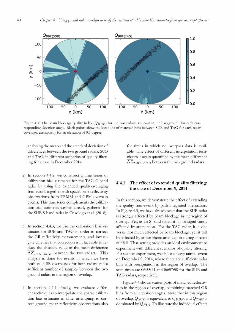
40 Chapter 4. Using ground radar overlaps to verify the retrieval of calibration bias estimates from spaceborne platforms
Figure 4.3: The beam blockage quality index (QBBF ) for the two radars is shown in the background for each cor-
responding elevation angle. Black points show the locations of matched bins between SUB and TAG for each radar
coverage, exemplarily for an elevation of 0.5 degree.
analysing the mean and the standard deviation of
differences between the two ground radars, SUB
and TAG, in different scenarios of quality filter-
ing for a case in December 2014.
2. In section 4.4.2, we construct a time series of
calibration bias estimates for the TAG C-band
radar by using the extended quality-averaging
framework together with spaceborne reflectivity
observations from TRMM and GPM overpass
events. This time series complements the calibra-
tion bias estimates we had already gathered for
the SUB S-band radar in Crisologo et al. (2018).
3. In section 4.4.3, we use the calibration bias es-
timates for SUB and TAG in order to correct
the GR reflectivity measurements, and investi-
gate whether that correction is in fact able to re-
duce the absolute value of the mean difference
∆ZT AG−SUB between the two radars. This
analysis is done for events in which we have
both valid SR overpasses for both radars and a
sufficient number of samples between the two
ground radars in the region of overlap.
4. In section 4.4.4, finally, we evaluate differ-
ent techniques to interpolate the sparse calibra-
tion bias estimates in time, attempting to cor-
rect ground radar reflectivity observations also
for times in which no overpass data is avail-
able. The effect of different interpolation tech-
niques is again quantified by the mean difference
∆ZT AG−SUB between the two ground radars.
4.4.1 The effect of extended quality filtering:
the case of December 9, 2014
In this section, we demonstrate the effect of extending
the quality framework by path-integrated attenuation.
In Figure 4.3, we have already seen that the SUB radar
is strongly affected by beam blockage in the region of
overlap. Yet, as an S-band radar, it is not significantly
affected by attenuation. For the TAG radar, it is vice
versa: not much affected by beam blockage, yet it will
be affected by atmospheric attenuation during intense
rainfall. That setting provides an ideal environment to
experiment with different scenarios of quality filtering.
For such an experiment, we chose a heavy rainfall event
on December 9, 2014, where there are sufficient radar
bins with precipitation in the region of overlap. The
scan times are 06:55:14 and 06:57:58 for the SUB and
TAG radars, respectively.
Figure 4.4 shows scatter plots of matched reflectiv-
ities in the region of overlap, combining matched GR
bins from all elevation angles. Note that in this region
of overlap,QSUB is equivalent toQBBF , andQT AG is
dominated byQP IA. To illustrate the individual effects

4.4. Results and Discussion 41
of the quality indices in the comparison, we simply re-
fer to the dominating quality index instead of the asso-
ciated radar (i.e. QBBF for SUB and QP IA for TAG).
The points in the scatter plot are colored depending on
the quality index of the corresponding matched sam-
ple: in Figure 4.4a, we can see that matches with a very
low QBBF value (i.e. high beam blockage) are concen-
trated above the 1:1 line, since beam blockage causes
the Subic radar to underestimate in comparison to the
Tagaytay radar. If we consider each matched sample ir-
respective of data quality, the mean difference between
the two radars is 1.7 dB, with a standard deviation of 8.1
dB. Taking QBBF into account changes the mean dif-
ference to -1.9 dB—which is higher in absolute terms—
and decreases the standard deviation to 5.5 dB. Fig-
ure 4.4b demonstrates the effect of using only PIA for
quality filtering: Points with low QP IA (i.e. high PIA)
are concentrated below the 1:1 line, corresponding to
an underestimation of the TAG radar as compared to
the SUB radar. Considering only QP IA for quality-
weighting increases the mean difference between TAG
and SUB to a value of 3.5 dB, and decreases the standard
deviation just slightly to a value of 7.5 dB. By combin-
ing the two quality factors, we can reduce the absolute
value of ∆ZT AG−SUB from 1.7 dBZ to -0.7 dB, and,
more notably, the standard deviation from 8.1 dBZ to
4.6 dBZ (Figure 4.4c). That effect also becomes appar-
ent in Figure 4.4d in which we show how the multiplica-
tive combination of quality factors not only pushes the
mean of the differences towards zero, but also narrows
down the distribution of differences dramatically.
Remembering item (2) from section 4.3.1, it is the
reduction of standard deviation that we are most inter-
ested in at this point: it demonstrates that the two GR
become more consistent if we filter systematic errors
that are spatially heterogeneous in the region of over-
lap. The low absolute value of the mean difference is,
for this case study, not a result of correcting for calibra-
tion bias—which is addressed in the following sections.
On the basis of these results, we will, in the follow-
ing sections, only refer to values of mean and standard
deviation of (SR–GR or GR–GR) differences that are
computed by means of quality-weighting, with the qual-
ity of a matched sample quantified as Qmatch.
4.4.2 Estimating the GR calibration bias
from SR overpass events
In Figure 8a of Crisologo et al. (2018), we had already
shown the time series of quality-averaged differences
between the SUB ground radar and the SR platforms
TRMM and GPM, using beam blockage as a quality
variable. Extending the framework for quality-weighted
averaging by PIA, we have now computed the corre-
sponding time series of quality-weighted mean differ-
ences for the TAG radar. Figure 4.5 shows the time
series of calibration biases, as estimated from quality-
weighted mean differences, for both SUB and TAG
radars for years 2012–2014 and 2016. The first panel
corresponds to Figure 8a of Crisologo et al. (2018). For
SUB, there is a total of 96 SR overpass events that fit
the filtering criteria referred to in Section III.2, while
for TAG, we only found 45 matches. Compared to the
spaceborne radars, both SUB and TAG are dramati-
cally underestimating at the beginning of operation in
2012, where the underestimation of the TAG radar is
even more pronounced. From 2014, the calibration im-
proves for both radars.
As pointed out in Crisologo et al. (2018), there is a
strong variability of the estimated calibration biases be-
tween overpasses for SUB. This behaviour can be con-
firmed for the TAG radar, with particularly drastic cases
in 2013. Potential causes for this short-term variabil-
ity have been discussed in Crisologo et al. (2018), and
could include, e.g., residual errors in the volume sam-
ple intersections, short-term hardware instability, rapid
changes in precipitation during the time interval be-
tween GR sweep and SR overpass, and uncertainties in
the estimation of PIA, to name a few.
4.4.3 The effect of bias correction on the GR
consistency: case studies
In this and the following section, we evaluate the effect
of using the calibration bias estimates obtained from
SR overpasses to actually correct the GR reflectivity
measurements. We start, in this section, by analysing
events in which we have both: valid SR overpass events
for SUB and TAG, as well as a sufficient number of
matched GR samples in the region of overlap. That
way, we can directly evaluate how an “instantaneous”
estimate of the GR calibration bias estimates affects the
GR consistency, as explained in item (2) of section 4.3.1.
In contrast to section 4.4.1, in which we focused on
the standard deviation of differences between the two
ground radars, we now focus on the mean differences
in order to capture the effect of bias correction.
The first case is a particularly illustrative example:
an extreme precipitation event that took place right in
the region of overlap at a time in which both radars,
SUB and TAG, apparently were affected by massive
miscalibration, according to Figure 4.6 the so-called

42 Chapter 4. Using ground radar overlaps to verify the retrieval of calibration bias estimates from spaceborne platforms
Figure 4.4: Scatter plot of reflectivity matches between Tagaytay and Subic radars. The marker color scale represents
the data quality based on (a) beam blockage fraction (QBBF ), (b) path-integrated attenuation (QP IA), and (c) the
multiplicative combination of the two (Qmatch), where the darker colors denote high data quality and lighter colors
signify low data quality. The ridgeline plots (d) show the distribution of the reflectivity differences of the remaining
points if we choose points only with high quality index (in this case, we select an arbitrary cutoff value of Qmatch =
0.7). The mean is marked with the corresponding vertical line.
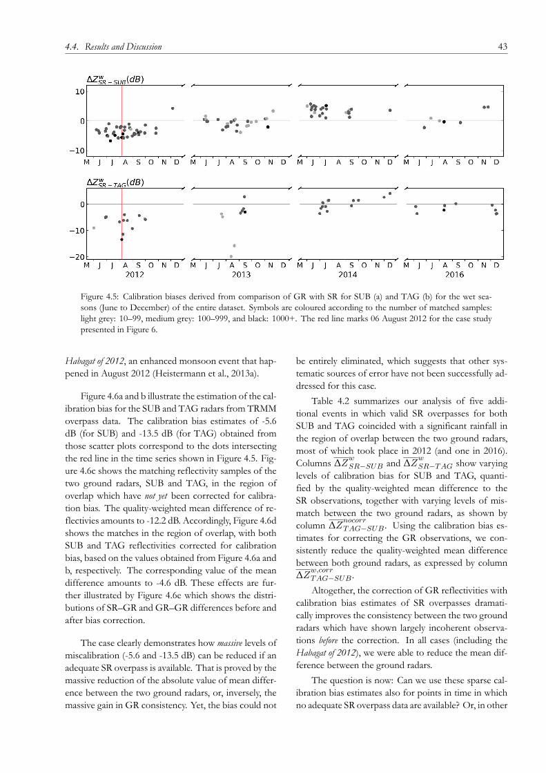
4.4. Results and Discussion 43
Figure 4.5: Calibration biases derived from comparison of GR with SR for SUB (a) and TAG (b) for the wet sea-
sons (June to December) of the entire dataset. Symbols are coloured according to the number of matched samples:
light grey: 10–99, medium grey: 100–999, and black: 1000+. The red line marks 06 August 2012 for the case study
presented in Figure 6.
Habagat of 2012, an enhanced monsoon event that hap-
pened in August 2012 (Heistermann et al., 2013a).
Figure 4.6a and b illustrate the estimation of the cal-
ibration bias for the SUB and TAG radars from TRMM
overpass data. The calibration bias estimates of -5.6
dB (for SUB) and -13.5 dB (for TAG) obtained from
those scatter plots correspond to the dots intersecting
the red line in the time series shown in Figure 4.5. Fig-
ure 4.6c shows the matching reflectivity samples of the
two ground radars, SUB and TAG, in the region of
overlap which have not yet been corrected for calibra-
tion bias. The quality-weighted mean difference of re-
flectivies amounts to -12.2 dB. Accordingly, Figure 4.6d
shows the matches in the region of overlap, with both
SUB and TAG reflectivities corrected for calibration
bias, based on the values obtained from Figure 4.6a and
b, respectively. The corresponding value of the mean
difference amounts to -4.6 dB. These effects are fur-
ther illustrated by Figure 4.6e which shows the distri-
butions of SR–GR and GR–GR differences before and
after bias correction.
The case clearly demonstrates how massive levels of
miscalibration (-5.6 and -13.5 dB) can be reduced if an
adequate SR overpass is available. That is proved by the
massive reduction of the absolute value of mean differ-
ence between the two ground radars, or, inversely, the
massive gain in GR consistency. Yet, the bias could not
be entirely eliminated, which suggests that other sys-
tematic sources of error have not been successfully ad-
dressed for this case.
Table 4.2 summarizes our analysis of five addi-
tional events in which valid SR overpasses for both
SUB and TAG coincided with a significant rainfall in
the region of overlap between the two ground radars,
most of which took place in 2012 (and one in 2016).
Columns ∆ZwSR−SUB and ∆Z
wSR−T AG show varying
levels of calibration bias for SUB and TAG, quanti-
fied by the quality-weighted mean difference to the
SR observations, together with varying levels of mis-
match between the two ground radars, as shown by
column ∆ZnocorrT AG−SUB . Using the calibration bias es-
timates for correcting the GR observations, we con-
sistently reduce the quality-weighted mean difference
between both ground radars, as expressed by column
∆Zw,corrT AG−SUB .
Altogether, the correction of GR reflectivities with
calibration bias estimates of SR overpasses dramati-
cally improves the consistency between the two ground
radars which have shown largely incoherent observa-
tions before the correction. In all cases (including the
Habagat of 2012), we were able to reduce the mean dif-
ference between the ground radars.
The question is now: Can we use these sparse cal-
ibration bias estimates also for points in time in which
no adequate SR overpass data are available? Or, in other
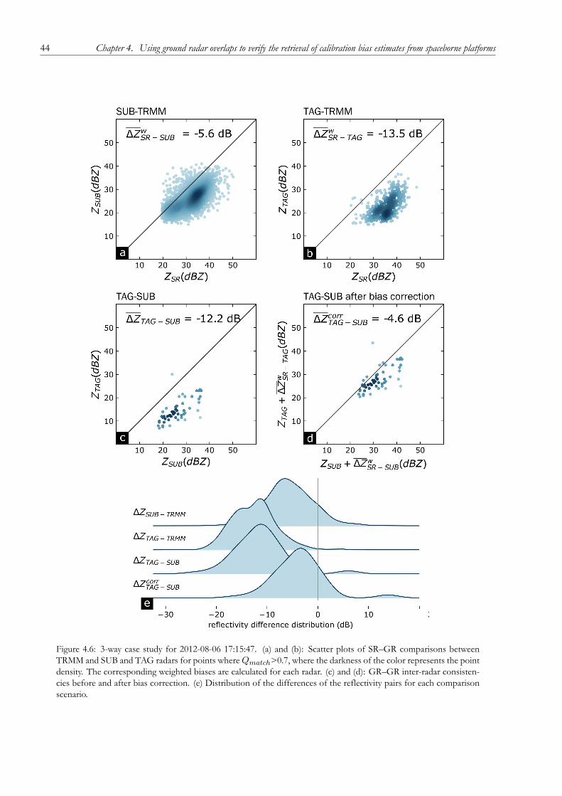
44 Chapter 4. Using ground radar overlaps to verify the retrieval of calibration bias estimates from spaceborne platforms
Figure 4.6: 3-way case study for 2012-08-06 17:15:47. (a) and (b): Scatter plots of SR–GR comparisons between
TRMM and SUB and TAG radars for points whereQmatch>0.7, where the darkness of the color represents the point
density. The corresponding weighted biases are calculated for each radar. (c) and (d): GR–GR inter-radar consisten-
cies before and after bias correction. (e) Distribution of the differences of the reflectivity pairs for each comparison
scenario.

4.4. Results and Discussion 45
Table 4.2: Calibration biases and inter-radar consistencies for different bias calculation scenarios
Npts ∆ZwSR−SUB ∆Z
wSR−T AG ∆Z
nocorrT AG−SUB ∆Z
w,corrT AG−SUB
2012-06-11 21:37:41 528 -3.4 -6.3 -3.5 -0.2
2012-06-28 22:14:46 48 -3.5 -5.1 -1.3 -0.2
2012-07-02 20:09:47 1248 -5 -11.4 -7 -2.1
2012-08-06 17:17:23 1121 -5.6 -13.5 -12.3 -4.6
2012-08-31 13:44:31 34 -5.1 -9.3 -1.9 1.1
2016-08-12 11:40:28 1277 -0.3 -2.3 -5.7 -4.3
words, can we interpolate calibration bias estimates in
time?
4.4.4 Can we interpolate calibration bias es-
timates in time?
The spaceborne radar platform (SR) rarely overpasses
both GR radar domains in a way that significant rainfall
sufficiently extends over both GR domains including
the GR region of overlap. Hence, our previous demon-
stration of the effective correction of GR calibration
bias yielded only few examples. From a more prac-
tical point of view, however, we are more interested
in how we can use SR overpass data for those situa-
tions in which adequate SR coverage is unavailable—
which is, obviously, rather the rule than the exception.
An intuitive approach is to interpolate the calibration
bias estimates from valid SR overpasses in time, and
use the interpolated values to correct GR observations
for any point in time. We can do such an interpola-
tion independently for each ground radar, based on the
set of valid SR overpasses available for each. In order
to examine the effectiveness of such an interpolation,
we again use the absolute value of the mean difference
between the two ground radars as a measure of their
(in-)consistency. Based on the reduction of that abso-
lute value, as compared to uncorrected GR reflectivi-
ties, we benchmark the performance of three interpo-
lation approaches:
1. Linear interpolation in time;
2. Moving average: we compute the calibration bias
at any point in time based on calibration bias es-
timates in a 30-day window around that point,
together with a triangular weighting function;
3. Seasonal average: For any point in time in the ana-
lyzed wet season of a year, we compute the cali-
bration bias as the average of all calibration bias
estimates available in that year.
This benchmark analysis is not considered to be
comprehensive, but rather exemplary in terms of ex-
amined interpolation techniques. The three techniques
illustrate different assumptions on the temporal repre-
sentativeness of calibration bias estimates, as obtained
from SR overpasses: a seasonal average reflects a rather
low level of confidence in the temporal representative-
ness. The underlying assumption would be that we con-
sider any short-term variability as “noise” which should
be averaged out. The linear interpolation puts more
confidence into each individual bias estimate, and as-
sumes that we can actually interpolate between any two
points in time. Obviously, a 30-day moving average is
somewhere in between the two.
Table 4.3 provides an annual summary of the ab-
solute mean differences in reflectivity between the two
ground radars, without bias correction and with correc-
tion of bias obtained from different interpolation tech-
niques. Firstly, the mean absolute difference between
the radars is always lower after correction, irrespective
of the year or the interpolation method. Hence, it is
generally better to use calibration bias estimates to cor-
rect GR reflectivities even for those times in which no
valid SR overpasses are available. The 30-day moving
average appears to outperform the other two interpo-
lation methods—on average, and for each year from
2012 to 2014. In 2016, neither interpolation method
substantially reduces the mean absolute difference ob-
tained for the uncorrected GR data.
The performance of the moving average suggests
that it is possible for the calibration of radars to drift
slowly in time, with variability stemming from sources
which are difficult to disentangle. However, for peri-
ods of time when the radar is relatively well-calibrated
and stable, the bias correction only offers a slight, if any,
improvement in the consistency between two radars.
In order to better understand the variability “be-
hind” the annual averages in Table 4.3, Figure 4.7 shows

46 Chapter 4. Using ground radar overlaps to verify the retrieval of calibration bias estimates from spaceborne platforms
Table 4.3: Mean absolute ∆ZT AG−SUB for different correction scenarios and years
Mean absolute ∆ZT AG−SUB (dB)
No correction Seasonal mean Linear interpolation Moving average
All years 4.9 4.0 3.0 2.7
2012 4.4 3.4 2.6 2.3
2013 8.6 7.1 4.5 4.1
2014 4.4 3.8 3.2 2.9
2016 1.8 1.8 1.7 1.7
Figure 4.7: The differences between the inter-radar consistency before and after correcting for the ground radar cal-
ibration biases following a rolling window averaging for samples with significant number of matches. The hollow
(filled) circles represent the daily mean before (after) correction. The line color represents an improvement (green) or
a decline (pink) in the consistency between the two ground radars.
the effects of bias correction on a daily basis, exempli-
fied for the moving average interpolation. The hollow
circles represent the daily mean differences between the
two ground radars before (∆ZT AG−SUB) correction,
while the filled circles show the daily mean differences
after (∆Zw,corrT AG−SUB) correction. The length of the bar
shows the magnitude of the change, while the color of
the bar signifies a reduction of the absolute value of
the mean difference (green, for improvement) or an
increase in in the absolute value (pink, for a degrada-
tion of consistency between the two ground radars). In
83 out of 121 days, bias correction improves the con-
sistency between the two ground radars by more than
1 dB. Inversely, though, this implies that in 17 out of
121 days, the use of interpolated bias estimates causes a
degradation of consistency between the ground radars,
expressed as an increase of more than 1 dB in the ab-
solute mean differences. Furthermore, we can identify
several days for which the bias correction decreases the
absolute mean differences, but not to a level that could
be considered as acceptable for quantitative precipita-
tion estimation.
4.5 Conclusions
In 2011, Schwaller and Morris had presented a tech-
nique to match reflectivity observations from space-
borne radars (SR) and ground radars (GR). Crisologo
et al. (2018) extended that technique by introducing the
concept of quality-weighted averaging of reflectivity in
order to retrieve the GR calibration bias from match-
ing SR overpass data. They exemplified the concept of
quality weighting by using beam blockage as a quality
variable, and demonstrated the effectiveness of the ap-
proach for the Subic S-band radar in the Philippines.
The present study has extended the concept of
quality-weighted averaging by accounting for path-
integrated attenuation (PIA) as a quality variable, in ad-
dition to beam blockage. Accounting for PIA becomes
vital for ground radars that operate at C- or X-band. In
4.5. Conclusions 47
addition to the Subic S-band radar, this study has in-
cluded the Tagaytay C-band radar which substantially
overlaps with the Subic radar.
In the first part of this study, we have demonstrated
that only accounting for both, beam blockage and path-
integrated attenuation, allows for a consistent compari-
son of observations from the two ground radars, Subic
and Tagaytay: after transforming the quality variables
“beam blockage fraction” and “path-integrated attenu-
ation” into quality indices QBBF and QP IA, with val-
ues between zero and one, we computed the quality-
weighted standard deviation of matching reflectivities
in the region of overlap between the two ground radars
for an event on December 9, 2014. Using a quality in-
dex based on the multiplicative combination of QBBF
and QP IA, we were able to dramatically reduce the
quality-weighted standard deviation from 8.1 dBZ to
4.6 dBZ, while using QBBF and QP IA alone would
have only reduced the standard deviation to 5.5 or 7.5
dBZ, respectively. Based on that result, we have used,
with confidence, the combined quality index through-
out the rest of the study.
The next step involved the retrieval of the GR cali-
bration bias from SR overpass data for the Tagaytay C-
band radar (for the Subic S-band radar, that had already
been done by Crisologo et al. (2018)). For eachmatched
volume in the SR–GR intersection, the combined qual-
ity index was computed for the Tagaytay radar, and used
as weights in calculating the calibration bias as a quality-
weighted average of the differences between SR andGR
reflectivities. We applied this approach throughout a 4-
year period to come up with a time series of the his-
torical calibration bias estimates of the TAG radar, and
found the calibration of the TAG radar to be exception-
ally poor and volatile in the years 2012 and 2013, with
substantial improvements in 2014 and 2016.
In order to demonstrate the effectiveness of esti-
mating and applying the GR calibration bias obtained
from SR overpass data, we have compared, in the region
of overlap, the corrected and uncorrected reflectivities
of the Subic and Tagaytay radars, for six significant rain-
fall events in which all three instruments—TAG, SUB
and the SR—had recorded a sufficient number of ob-
servations. We have shown that the independent bias
correction is able to massively increase the consistency
of the two ground radar observations, as expressed by a
reduction of the absolute mean difference between the
GR observations in the region of overlap, for each of
the six events—in one case even by almost 7.7 dB. The
main lesson from these cases is, that we can legitimately
interpret the quality-weighted mean difference between
SR and GR reflectivities as the instantaneous GR cal-
ibration bias, even if the magnitude of that bias varies
substantially within short periods of time.
Yet, the question remains how to correct for cal-
ibration bias in the absence of useful SR overpasses.
That question is particularly relevant for the reanaly-
sis of archived measurements from single-pol weather
radars. In this study, we have evaluated three differ-
ent approaches to interpolate calibration bias estimates
from SR overpass data in time: linear interpolation, a
30-day moving average, and a seasonal average. Each
of these approaches illustrates different assumptions
on the temporal representativeness of the calibration
bias estimates. On average, any of these approaches
produced calibration bias estimates that were able to
reduce the mean absolute difference between the GR
observations, which increases our confidence in the
corrected GR observations. Of all interpolation ap-
proaches, themoving 30-day window outperformed the
other two approaches. However, we also found that be-
hind the average improvement of GR–GR consistency,
there were also a number of cases in which the con-
sistency between the ground radars was degraded, or
in which high inconsistencies could not be significantly
improved. Altogether, it still appears difficult to inter-
polate such a volatile behaviour, even if we consider the
actual calibration bias estimates from the SR overpasses
as quite reliable.
In that context, maintenance protocols of the af-
fected ground radars would be very helpful in in-
terpreting and interpolating time series of calibra-
tion bias estimates. Such records were unavail-
able for the present study, which made it hard to
understand the observed variability of calibration
bias estimates. Yet, this information will mostly
be internally available at those institutions operat-
ing the weather radars. With the software code
and sample data of our study being openly available
(https://github.com/IreneCrisologo/inter-radar),such institutions are now enabled to carry out analyses
as the present study themselves, while being able to
benefit from cross-referencing the results with internal
maintenance protocols.
The correction of GR calibration appeared partic-
ularly effective in periods with massive levels of mis-
calibration. For such cases, interpolated bias estimates
allowed for an effective improvement of raw GR re-
flectivities. Yet, we need to continue disentangling dif-
ferent sources of uncertainty for both SR and GR ob-
servations in order to separate actual variations in in-
strument calibration and stability from measurement

48 Chapter 4. Using ground radar overlaps to verify the retrieval of calibration bias estimates from spaceborne platforms
errors that accumulate along the propagation path, and
to better understand the requirements to robustly esti-
mating these properties from limited samples. Progress
on these ends should also improve the potential for in-
terpolating calibration bias estimates in time, in order
to tap the potential of historical radar archives for radar
climatology, and to increase the homogeneity of com-
posite products from heterogeneous weather radar net-
works.
Acknowledgements
The radar data for this analysis were provided by
the Philippine Atmospheric, Geophysical and Astro-
nomical Services Administration (PAGASA, http://pa-
gasa.dost.gov.ph). The study was also funded by the
German government through the German Academic
Exchange Service (https://www.daad.de/en/).

49
Chapter 5
Discussion, Limitations, Outlook
Precipitation is the main driver of environmental and
hydrological processes, and has a large impact in terms
of natural hazards (through floods, debris flow, land-
slides, avalanches). Hence, there is an increasing need
for more reliable precipitation estimates and forecasts
at high temporal and spatial resolution. The recently-
acquired Subic radar data allowed a first look at the
capabilities and advantages it offers in weather moni-
toring in the Philippines. Radar data was used to re-
construct the enhanced southwest monsoon event of
2012 over Metro Manila. Torrential rainfall fell contin-
uously over the course of four days, as the tail of Ty-
phoon Haikui passing north of the Philippines pulled
in even more moisture along with the already ongoing
monsoon winds and rains. Radar-derived rainfall esti-
mates underestimated by as much as 60% when com-
pared with gauge measurements. Gauge-adjusted radar
data reconstruction showed that while Metro Manila
received the most rainfall over land, most of the rain
actually fell over Manila Bay. This feature of the rain-
fall distribution would not have been identified from
rain gauge interpolation alone, as demonstrated by the
Supplemental figure of Chapter 2, as well as Figure 2a
and c in a later study by (Abon et al., 2016). Addition-
ally, the radar-based rainfall distribution map showed
other localized areas (about 15–25 km wide) of high
rainfall accumulation which were also missed in the rain
gauge interpolation map (Supplemental figure of Chap-
ter 2). These plume-like features re-appeared in the
radar-based rainfall distribution map of a similar event
(southwest monsoon enhanced by a north-passing ty-
phoon) the following year, which were driven by the
interaction of stratovolcanoes with the monsoon (Lag-
may et al., 2015).
The archipelagic nature of the country’s geogra-
phy prohibits a dense and well-spaced network of
rain gauges that can be used to effectively com-
pare gauge measurements and radar rainfall-estimates.
The highly convective characteristic of local rainfall
produces strong thunderstorms that can be compact
enough to travel in between rain gauges and be left
undetected. With the sparseness of the gauges and
the uncertainty that comes with the rainfall-rainrate
transformation, as well as the lack of auxiliary calibra-
tors such as disdrometers and radar profilers, we in-
stead turned to relative calibration. Reflectivities from
ground-based radars (GR) are compared with reflec-
tivities from spaceborne radars (SR), namely TRMM
(for data from 2012–2014) and GPM (for data from
2014–2016). A more common approach in comparing
SR and GR is by reprojecting and interpolating the sur-
face rainfall estimates onto either a common 2D carte-
sian grid on the Earth’s surface or the volumetric rain-
fall estimates onto a common 3D cartesian grid. The
3D volume matching method of (Schwaller and Morris,
2011) used in this paper avoids uncertainties that could
be introduced by interpolation by considering only the
volumes of the SR beam and GR beam that intersect.
In addition, directly comparing the primary measured
quantity reflectivity circumvents the need to convert to
rain rate, which is another potential source of uncer-
tainties if rain gauges are used as a reference.
By avoiding these known potential additional
sources of errors, this thesis was able to focus on the
sources of systematic errors that could influence the
comparison between SR and GR. The consideration
of data quality started with the beam blockage frac-
tion (BBF) for Chapter 3 and included path-integrated
attenuation (PIA) for Chapter 4. These quality fac-
tors were then used as weights in taking the weighted-
average of the differences between the SR and GR re-
flectivities for a single coincidence of an SR overpass
and a GR sweep. The weighted-averaging approach
allows low quality data resulting from BBF and PIA,
sources of uncertainty that are heterogeneous in space, to
be filtered out for a more consistent estimate of calibra-
tion bias, which is homogeneous in space.
In Chapters 3 and 4, it was shown that introducing a
data quality framework in the comparison increases the
consistency of bias estimates between two datasets. In
a case study discussed in Section 3.4, reflectivity differ-
ence maps between SR overpass andGR sweep indicate
that significant variability (with absolute differences up

50 Chapter 5. Discussion, Limitations, Outlook
to 10 dB) can be found at the edges of the blind sec-
tor, due to partial beam blockage. The locations of the
large absolute differences are consistent with the loca-
tions of the low data quality. Assigning weights to beam
blockage fraction (0 for the poorest data quality due to
total beam blockage up to 1 for the best data quality
without any topographic obstacles) in calculating the
calibration bias reduces the scatter and consequently
decreases the standard deviation of the differences be-
tween SR andGR reflectivity (Figure 3.6), which in turn
increases the confidence in the bias estimation. The
same reduction in standard deviation occurs as well in
the vast majority of overpasses. The GR–GR compar-
ison in Chapter 4 similarly demonstrates the benefits
of considering BBF and PIA. The case study in Fig-
ure 4.4 shows that individually, usingQBBF andQP IA
as weights reduces the standard deviation of the differ-
ences between the reflectivities from the two ground
radars, but considering both quality indices at the same
time decreases the standard deviation by almost half, as
opposed to considering all points equally. The combi-
nation of quality factors also dramatically narrows down
the distribution of the reflectivity differences. These
results demonstrate that BBF and PIA do not only af-
fect Quantitative Precipitation Estimation (QPE), but
also the comparability of two radars. The advantages
of quality-weighting therefore applies to both SR–GR
comparisons and GR–GR comparisons.
Being able to determine the calibration bias of one
radar in Chapter 3 using the SR–GRmatching approach
and applying the method and correction to two over-
lapping radars in Chapter 4 tells us that SR and GR re-
flectivities are consistent enough (after filtering out low
data quality) to allow for calibration bias estimates. This
consistency presents the potential of calibrating multi-
ple radars in a network against a single reference, using
a uniform approach. In this study, this was demon-
strated for at least two radars in the Philippine radar
network. The increased agreement between the two
ground radars after calibration demonstrates the feasi-
bility of SR as a stable travelling reference. The method
also allows for bias estimation at instantaneous points
in time, as opposed to gauge calibration where errors
are lumped over an hourly or daily timeframe. Due to
its unobstructive nature, this relative calibrationmethod
can also be done continuously, so that calibration mon-
itoring can be done even while the radars are opera-
tional.
Chapter 3 also discusses the consistency of TRMM
and GPM with respect to each other. In the analysis of
the bias time series for Subic radar, TRMM and GPM
overpasses were both available for 2014. The period
of overlap showed that GR calibration bias estimates
based on both TRMM and GPM observations can be
considered homogeneous. Based on this assessment,
TRMM and GPM were lumped together as a continu-
ous dataset when comparing SR and GR reflectivities
for bias correction in Chapter 4.
It was discussed in the latter part of Chapter 3 (Sec-
tion 3.4.2) that the bias fluctuates around an average
value that varies year by year and appears to be quite
persistent over the duration of the corresponding wet
seasons from 2012–2016. The drastic change in bias
between 2013 and 2014 for the Subic radar (Figure 3.8)
has to be assumed to be due to calibration maintenance
in terms of hardware changes (i.e. magnetron replace-
ment). Unfortunately, similar information about the
Tagaytay radar’s maintenance history was not available.
Detailed information regarding maintenance protocols
would be useful in explaining the changes in bias of
radars throughout the years as demonstrated in War-
ren et al. (2018). Chapter 4 (Section 4.4.4.) reaffirms
us that there is substantial short-term variability. Even
after identifying and addressing the effects of BBF and
PIA, heavy fluctuations of bias persist. The causes of
these fluctuations could not yet be disentangled. Yet,
we were able to reduce the mean absolute difference
before and after bias correction when using interpolated
bias estimates. So irrespective of the actual causes of
fluctuation, the variability exhibits some level of conti-
nuity, so that an interpolation of bias estimates in time
contributes to an overall improvement.
Aside from internal calibration of the precipita-
tion radars onboard TRMM/GPM, external monitor-
ing is also carried out through comparison with selected
well-calibrated ground radars. Several ground valida-
tion sites can be found in different locations around the
world (Hou et al., 2013). Some of these sites are estab-
lished primarily for this purpose, while some are part of
existing radar networks whose calibration are deemed
accurate enough to use as reference. The geometry
matching method of Schwaller and Morris (2011) that
was used in Chapters 3 and 4 was developed with this
application in mind—to compare reflectivities between
ground radars and spaceborne radars to check if they
are consistent with each other. While ground validation
sites are typically set up to have the least possible errors,
the method can still be applied for a more extensive
global approach in ground validation using radars not
included in the validation radars list. The consistency
of the ground radar observations with the spaceborne

Chapter 5. Discussion, Limitations, Outlook 51
radar observations in Chapter 3 also serves, albeit indi-
rectly, as a validation of the SR estimates in the study
region.
Limitations of the study
Beam blockage and path-integrated attenuation are only
two of the possible sources of uncertainties that could
affect data quality. Furthermore, attenuation was only
considered for the ground radar, while the spaceborne
radars may also experience attenuation. However, this
has already been acknowledged and addressed by the
corresponding SR data teams, by providing attenuation-
corrected datasets. The SR data product used in the
analysis are already attenuation-corrected and the val-
ues were taken as-is. To take this approach further,
the framework of quality-weighted averaging could and
should be extended to the SR data as well, including not
only attenuation, but also the effects of non-uniform
beam filling.
It should be noted that the approaches in calcu-
lating beam blockage and path-integrated attenuation
are not absolute. In this thesis, they were calculated as
part of the processing chain, and not as readily avail-
able quantities. Exploring these variables further are
research topics in themselves, but a sufficient method
had to be selected. For the beam blockage fraction cal-
culation, the method presented by Bech et al. (2003)
was used. The radar’s field of view is simulated in their
model using information on the scan geometry and the
surrounding topography based on a digital elevation
model. The implementation of this model assumes that
there is no vertical gradient of refractivity, so in cases
where super-refraction of the atmosphere may be pos-
sible, this method may not apply. As for the retrieval of
the PIA, the specific differential phase (KDP ), which
was used to calculate PIA following the algorithm pro-
posed by Vulpiani et al. (2012). This method was al-
ready proven to work well with the dataset (Crisologo
et al., 2014). While other KDP retrieval methods ex-
ist (Bringi and Chandrasekar, 2001; Wang and Chan-
drasekar, 2009), it is beyond the scope of this thesis
to explore their differences, but certainly, the philoso-
pher’s stone has not yet been found when it comes
to the reliable reconstruction of ΦDP and KDP , and
hence the retrieval of PIA.
Aside from the methodological, data limitations
also exist. TRMM and its successor GPMwas launched
in 1997 and 2014, respectively, therefore the SR-GR
method of bias estimation can only be done as far back
as the start of the corresponding instrument. Addition-
ally, with the study area close to the equator, the swath
density is not as high as it is nearer the poles. There are
at most two SR overpasses that go over the Philippines
everyday, and they don’t always intersect with the radars
used in this study. Applying the methods to study ar-
eas with high swath overpass frequency could provide
more samples to increase the reliability of the results.
Unfortunately, we were not able to gain access to
the calibration and maintenance history of the Subic
and Tagaytay radars as recorded by PAGASA, and man-
ual cross-checking of the changes in radar calibration
against the maintenance records was not possible. De-
termining the exact dates of maintenance events that
could have changed the radar calibration and comparing
them with the observed changes in the analysis would
allow us to differentiate between the effects of deliber-
ate calibration and those of instrument instability and
system drift. The findings with respect to the annual
calibration changes of the Subic radar were relayed to
radar engineers in PAGASA, and they confirmed that
some hardware changes (i.e. magnetron replacement)
were performed in 2014, but no further details were
given.
The observed variability of the calibration biases
over time could result from cumulative effects of sev-
eral sources of uncertainty along the entire data collec-
tion and generation process. Examples of such sources
could be uncertainty of beam propagation due to fluc-
tuations in atmospheric refractivity; non-uniform beam
filling; residual errors in the geometric intersections of
the volume samples; and rapid changes in precipitation
during the time interval between the radars being com-
pared, to name a few. Additionally, hardware instabili-
ties owing to the effects of temperature, thermal expan-
sion, and gradual degradation of the system, can also
contribute to calibration drifts.
Outlook
There is still much to understand about radar calibra-
tion, and the myriad of factors that contribute to its
stability and reliability. The quality-weighted framework
developed in this thesis can be expanded to the space-
borne radar observations as well, by e.g. considering
the clutter identification of the Dual-frequency Precip-
itation Radar of the GPM (Watters et al., 2018). The
GPM 2a Ku dataset also includes other variables which
could be related to data quality, such as the level of path-
integrated attenuation, the quality of brightband detec-
tion, and estimation of ground clutter elevation (Iguchi

52 Chapter 5. Discussion, Limitations, Outlook
et al., 2010).
Furthermore, the quality-based method for bias es-
timation and correction can also be extended to the
other radars in the Philippine radar network to ensure a
consistent and reliable rainfall measurement through-
out the country. The Philippine government pro-
gram Nationwide Operational Assessment of Hazards
(Project NOAH), which tackles disaster research and
development, makes use of the weather radars together
with the Himawari-8 satellite for monitoring and now-
casting rainfall probability in a web-based platform that
delivers hazard-related information to the public in
near-real-time (Lagmay et al., 2017). The project also
conducts flood simulations for early warning using his-
torical and real-time rainfall data based on rain gauges,
which at the moment are more reliable in terms of ac-
curacy and availability compared to radar data. With
the potential increase in accuracy of radar rainfall esti-
mates through careful bias estimation and calibration,
and with the continuous efforts of PAGASA to im-
prove the coverage and availability of the radar data,
weather radar observations can be integrated to hydro-
logical simulations for early warnings.
The improvement in the consistency between the
Subic and Tagaytay radars after the bias correction of
the individual radars signify a step towards better us-
ability of archived data. Despite the remaining fluctu-
ation, we have shown the possibility of increasing the
homogeneity of reflectivity records by removing tem-
porally variable calibration biases. Historical calibration
of radar data archive could be useful for climatological
studies and re-analysis of past events for better under-
standing of involved processes.

53
Chapter 6
Summary and Conclusion
Calibration and methods to improve calibration bias es-
timates serve as the main thread of the three papers
comprising this thesis. This work tells the story of how
the calibration bias was first noticed for the Subic radar,
to the attempts at using spaceborne radars as reference
for bias estimation for two overlapping radars (Subic
and Tagaytay) experiencing different error sources, to
investigating whether miscalibration of archived radar
data can be corrected to a certain extent.
The first paper established the presence of miscali-
bration for the Subic radar, while also giving a first look
at the unique rainfall distribution following an intense
rainfall caused by typhoon-enhanced monsoon. In this
chapter, we have shown that most of the rainfall during
the Habagat 2012 actually precipitated over Manila Bay,
and not in Quezon City, as the rain gauges recorded.
The gap in the spatial distribution of the rain gauges
was supplemented by the high-spatial resolution data
of the radars.
An approach by Schwaller and Morris (2011) to
compare spaceborne radars (SR) and ground radars
(GR) for calibration bias estimation was extended in the
second paper. A framework for data quality and quality-
weighted averaging was introduced, where a quality in-
dex based on beam blockage fraction (whereQBBF =0 for total beam blockage and QBBF = 1 for ab-sence of any beam blockage along the beam) was used
as weights in calculating the weighted mean difference
between SR and GRmeasurements. The use of quality-
weighted averaging, as opposed to simple averaging,
decreased the standard deviation of the mean differ-
ences between SR and GR reflectivities, thereby in-
creasing the consistency between the two radars. This
decrease in standard deviation means that the estima-
tion of the bias is more reliable. Based on the map of
the matched SR–GR bins and the scatter plot of the
differences between SR and GR reflectivities colored
based onQBBF , the points on the scatter plot lying far
from the perfect match come from the areas affected
by beam blockage.
We took this concept of quality-based calibration
bias estimation further in the third paper and applied it
to the neighboring Tagaytay radar (TAG) which over-
laps with the Subic radar (SUB). For days when data
for all three radars (SR, TAG, SUB) were present, we
showed that the agreement of the reflectivity measure-
ments in the overlapping area between the two ground
radars increased after bias correction.
Furthermore, a moving average interpolation of the
SR-derived biases was able to fill in the gaps in the radar
calibration time series where no SR overpasses were
available. We demonstrate that taking a moving average
(therefore assuming that the bias drifts slowly in time)
of the bias to correct for days without an SR overpass
produces better results than simply taking the seasonal
average and using that to correct all days within that
season.
In support of reproducibility and transparency in
the atmospheric sciences, all software used in this thesis
are reported in the text, and workflow scripts and sam-
ple data are made available in publicly available Github
repositories.


55
Chapter 7
Additional Publications
I also contributed to the following publications during the course of the doctoral research, aside from themanuscripts
listed in Chapter 1.
Bronstert, Axel, Ankit Agarwal, Berry Boessenkool, Irene Crisologo, Madlen Fischer, Maik Heistermann, Lisei
Köhn-Reich, et al. 2018. “Forensic Hydro-Meteorological Analysis of an Extreme Flash Flood: The 2016-05-29
Event in Braunsbach, SW Germany.” Science of The Total Environment 630 (July): 977–91.
https://doi.org/10.1016/j.scitotenv.2018.02.241.
Ozturk, Ugur, Dadiyorto Wendi, Irene Crisologo, Adrian Riemer, Ankit Agarwal, Kristin Vogel, José Andrés
López-Tarazón, and Oliver Korup. 2018. “Rare Flash Floods and Debris Flows in Southern Germany.” Science of
The Total Environment 626 (June): 941–52. https://doi.org/10.1016/j.scitotenv.2018.01.172.


57
Bibliography
Abon, C. C., David, C. P. C., and Pellejera, N. E. B. (2011). Reconstructing the Tropical Storm Ketsanaflood event in Marikina River, Philippines. Hydrology and Earth System Sciences, 15(4):1283–1289.Event.
Abon, C. C., Kneis, D., Crisologo, I., Bronstert, A., David, C. P. C., and Heistermann, M. (2016).Evaluating the potential of radar-based rainfall estimates for streamflow and flood simulations inthe Philippines. Geomatics, Natural Hazards and Risk, 7(4):1390–1405. Hydrology.
Amitai, E., Llort, X., and Sempere-Torres, D. (2009). Comparison of TRMM radar rainfall estimateswith NOAA next-generation QPE. Journal of the Meteorological Society of Japan, 87(Sp. Iss. SI):109–118.interradar.
Anagnostou, E. N., Morales, C. A., and Dinku, T. (2001). The use of TRMM precipitation radar obser-vations in determining ground radar calibration biases. Journal of Atmospheric and Oceanic Technology,18(4):616–628. interradar.
Atlas, D. (2002). Radar calibration. Bulletin of the American Meteorological Society, 83(9):1313–1316. Gen-eral.
Austin, P. M. (1987). Relation between Measured Radar Reflectivity and Surface Rainfall. MonthlyWeather Review, 115(5):1053–1070. Radar Uncertainty.
Baldini, L., Chandrasekar, V., and Moisseev, D. (2012). Microwave radar signatures of precipita-tion from S-band to Ka-band: application to GPM mission. European Journal of Remote Sensing,45(1):75–88. General.
Bech, J., Codina, B., Lorente, J., and Bebbington, D. (2003). The sensitivity of single polarizationweather radar beam blockage correction to variability in the vertical refractivity gradient. Journal ofAtmospheric and Oceanic Technology, 20(6):845–855. Radar Uncertainty.
Blumberg, W. G., Halbert, K. T., Supinie, T. A., Marsh, P. T., Thompson, R. L., and Hart, J. A. (2017).SHARPpy: An Open-Source Sounding Analysis Toolkit for the Atmospheric Sciences. Bulletin ofthe American Meteorological Society, 98(8):1625–1636. Software.
Bolen, S. M. and Chandrasekar, V. (2003). Methodology for aligning and comparing spaceborne radarand ground-based radar observations. Journal of Atmospheric and Oceanic Technology, 20(5):647–659.interradar.
Software& Data
Uncertaintiesin Data
Data quality Events HydrologyGeneral infoon radar & data
processing
Inter-radarcomparison

58 BIBLIOGRAPHY
Bringi, V. N. and Chandrasekar, V. (2001). Polarimetric Doppler Weather Radar: Principles and Applications.Cambridge University Press.
Bringi, V. N., Chandrasekar, V., Balakrishnan, N., and Zrnić, D. S. (1990). An Examination of Propa-gation Effects in Rainfall on Radar Measurements at Microwave Frequencies. Journal of Atmosphericand Oceanic Technology, 7(6):829–840. Radar Uncertainty.
Bringi, V. N., Huang, G.-J., Munchak, S. J., Kummerow, C. D., Marks, D. A., and Wolff, D. B. (2012).Comparison of Drop Size Distribution Parameter (D 0 ) and Rain Rate from S-Band Dual-PolarizedGround Radar, TRMM Precipitation Radar (PR), and Combined PR–TMI: Two Events from Kwa-jalein Atoll. Journal of Atmospheric and Oceanic Technology, 29(11):1603–1616. General.
Cao, Q., Hong, Y., Qi, Y., Wen, Y., Zhang, J., Gourley, J. J., and Liao, L. (2013). Empirical conversion ofthe vertical profile of reflectivity from Ku-band to S-band frequency. Journal of Geophysical Research:Atmospheres, 118(4):1814–1825. General.
Carey, L. D., Rutledge, S. A., Ahijevych, D. A., and Keenan, T. D. (2000). Correcting Propagation Ef-fects in C-Band Polarimetric Radar Observations of Tropical Convection Using Differential Prop-agation Phase. Journal of Applied Meteorology, 39(9):1405–1433. Radar Uncertainty.
Cayanan, E., Chen, T.-C., Argete, J., Yen, M.-C., and Nilo, P. (2011). The Effect of Tropical Cy-clones on Southwest Monsoon Rainfall in the Philippines. Journal of the Meteorological Society of Japan,89A:123–139. Event.
Chandrasekar, V., Bolen, S., and Gorgucci, E. (2003). Microphysical cross validation of space-borne radar and ground polarimetric radar. IEEE Transactions on Geoscience and Remote Sensing,41(10):2153–2165. interradar.
Chen, H. and Chandrasekar, V. (2016). Validation of NASA’s Global Precipitation Measurement mis-sion with a high-resolution ground radar network. InURSI Asia-Pacific Radio Science Conference (URSIAP-RASC), pages 836–839. IEEE. interradar.
Collette, A. (2013). Python and HDF5. O’Reilly. Software.Cremonini, R., Moisseev, D., and Chandrasekar, V. (2016). Airborne laser scan data: a valuable tool withwhich to infer weather radar partial beam blockage in urban environments. Atmospheric MeasurementTechniques, 9(10):5063–5075. Data quality.
Crisologo, I., Vulpiani, G., Abon, C. C., David, C. P. C., Bronstert, A., and Heistermann, M. (2014). Po-larimetric rainfall retrieval from a C-Band weather radar in a tropical environment (The Philippines).Asia-Pacific Journal of Atmospheric Sciences, 50(S1):595–607. General.
Crisologo, I., Warren, R. A., Mühlbauer, K., and Heistermann, M. (2018). Enhancing the consistencyof spaceborne and ground-based radar comparisons by using beam blockage fraction as a qualityfilter. Atmospheric Measurement Techniques, 11(9):5223–5236. interradar.
Doviak, R. J. and Zrnić, D. S. (2006). Doppler radar and weather observations. Academic Press, Mineola,N.Y., 2nd ed., dover ed. edition. General.
DPWH-JICA (2003). Department of Public Works and Highways, DPWH Japan International Coop-eration Agency, JICA: Manual on Flood Control Planning, Project for the Enhancement of Capa-bilities in Flood Control. Event.
Droegemeier, K. K., Smith, J. D., Businger, S., Doswell, C., Doyle, J., Duffy, C., Foufoula-Georgiou,E., Graziano, T., James, L. D., Krajewski, V., LeMone, M., Lettenmaier, D., Mass, C., Pielke, R.,Rutledge, S., Ray, P., Schaake, J., and Zipser, E. (2000). Hydrological Aspects of Weather Predictionand Flood Warnings: Report of the Ninth Prospectus Development Team of the U.S. WeatherResearch Program. Bulletin of the American Meteorological Society, 81(11):2665–2680. Hydrology.
Durden, S. L., Haddad, Z. S., Kitiyakara, A., and Li, F. K. (1998). Effects of Nonuniform Beam Fillingon Rainfall Retrieval for the TRMM Precipitation Radar. Journal of Atmospheric and Oceanic Technology,15(3):635–646. Radar Uncertainty.

BIBLIOGRAPHY 59
Einfalt, T., Szturc, J., and Ośródka, K. (2010). The quality index for radar precipitation data: a towerof Babel? Atmospheric Science Letters, 11(2):139–144. Data quality.
Fabry, F. (2015). Radar Meteorology: Principles and Practice. Cambridge University Press, Cambridge.General.
Figueras i Ventura, J. and Tabary, P. (2013). The New French Operational Polarimetric Radar RainfallRate Product. Journal of Applied Meteorology and Climatology, 52(8):1817–1835. General.
Fornasiero, A., Alberoni, P. P., Amorati, R., Ferraris, L., and Taramasso, A. C. (2005). Effects of prop-agation conditions on radar beam-ground interaction: impact on data quality. Advances in Geosciences,2:201–208. Data quality.
Friedrich, K., Hagen, M., and Einfalt, T. (2006). A quality control concept for radar reflectivity, polari-metric parameters, and Doppler velocity. Journal of Atmospheric and Oceanic Technology, 23(7):865–887.Data quality.
Furukawa, K., Nio, T., Konishi, T., Oki, R., Masaki, T., Kubota, T., Iguchi, T., and Hanado, H. (2015).Current status of the dual-frequency precipitation radar on the global precipitation measurementcore spacecraft. In Sensors, Systems, and Next-Generation Satellites XIX, volume 9639, page 96390G.International Society for Optics and Photonics. General.
Gabella, M., Joss, J., Perona, G., and Michaelides, S. (2006). Range adjustment for ground-based radar,derived with the spaceborne TRMM precipitation radar. IEEE Transactions on Geoscience and RemoteSensing, 44(1):126–133. interradar.
Gabella, M., Morin, E., and Notarpietro, R. (2011). Using TRMM spaceborne radar as a referencefor compensating ground-based radar range degradation: Methodology verification based on raingauges in Israel. Journal of Geophysical Research, 116(D2). interradar.
Gabella, M. and Notarpietro, R. (2002). Ground clutter characterization and elimination in moun-tainous terrain. In Proceedings of ERAD (2002), pages 305–311, Delft. Copernicus GmbH. RadarUncertainty.
Gabella, M., Speirs, P., Hamann, U., Germann, U., and Berne, A. (2017). Measurement of Precipitationin the Alps Using Dual-Polarization C-Band Ground-Based Radars, the GPM Spaceborne Ku-BandRadar, and Rain Gauges. Remote Sensing, 9(11):1147. interradar.
GDAL Development Team (2017). GDAL - Geospatial Data Abstraction Library, Version 2.2.3.Software.
Goudenhoofdt, E. and Delobbe, L. (2009). Evaluation of radar-gauge merging methods for quantita-tive precipitation estimates. Hydrology and Earth System Sciences, 13(2):195–203. General.
Gourley, J. J., Tabary, P., and Parent du Chatelet, J. (2007). A Fuzzy Logic Algorithm for the Separationof Precipitating from Nonprecipitating Echoes Using Polarimetric Radar Observations. Journal ofAtmospheric and Oceanic Technology, 24(8):1439–1451. Radar Uncertainty.
Han, J., Chu, Z., Wang, Z., Xu, D., Li, N., Kou, L., Xu, F., and Zhu, Y. (2018). The establishmentof optimal ground-based radar datasets by comparison and correlation analyses with space-borneradar data. Meteorological Applications, 25(1):161–170. interradar.
Heistermann, M., Collis, S., Dixon, M. J., Giangrande, S., Helmus, J. J., Kelley, B., Koistinen, J., Michel-son, D. B., Peura, M., Pfaff, T., and Wolff, D. B. (2014). The Emergence of Open-Source Softwarefor the Weather Radar Community. Bulletin of the American Meteorological Society, 96(1):117–128. Soft-ware.
Heistermann, M., Crisologo, I., Abon, C. C., Racoma, B. A., Jacobi, S., Servando, N. T., David, C.P. C., and Bronstert, A. (2013a). Brief communication ”Using the new Philippine radar networkto reconstruct the Habagat of August 2012 monsoon event around Metropolitan Manila”. Nat.Hazards Earth Syst. Sci., 13(3):653–657. Event.
Heistermann, M., Jacobi, S., and Pfaff, T. (2013b). Technical Note: An open source library for pro-cessing weather radar data (wradlib). Hydrology and Earth System Sciences, 17(2):863–871. Software.

60 BIBLIOGRAPHY
Heistermann, M. and Kneis, D. (2011). Benchmarking quantitative precipitation estimation by con-ceptual rainfall-runoff modeling. Water Resources Research, 47(6). Hydrology.
Helmus, J. and Collis, S. (2016). The Python ARM Radar Toolkit (Py-ART), a Library for Workingwith Weather Radar Data in the Python Programming Language. Journal of Open Research Software,4(1). Software.
Holleman, I., Michelson, D., Galli, G., Germann, U., and Peura, M. (2006). Quality information forradars and radar data. Data quality.
Hong, Y. and Gourley, J. J. (2015). Radar Hydrology: Principles, models, and applications. CRC Press, Taylor& Francis Group. General.
Hou, A. Y., Kakar, R. K., Neeck, S., Azarbarzin, A. A., Kummerow, C. D., Kojima, M., Oki, R.,Nakamura, K., and Iguchi, T. (2013). The Global Precipitation Measurement Mission. Bulletin of theAmerican Meteorological Society, 95(5):701–722. Software.
Houze, Jr., R. A., Brodzik, S., Schumacher, C., Yuter, S. E., and Williams, C. R. (2004). Uncertaintiesin oceanic radar rain maps at Kwajalein and implications for satellite validation. Journal of AppliedMeteorology, 43(8):1114–1132. Radar Uncertainty.
Hunter, J. D. (2007). Matplotlib: A 2d Graphics Environment. Computing in Science Engineering,9(3):90–95. Software.
Iguchi, T., Seto, S., Meneghini, R., Yoshida, N., Awaka, J., and Kubota, T. (2010). GPM/DPR level-2algorithm theoretical basis document. NASA Goddard Space Flight Center, Greenbelt, MD, USA, Tech.Rep. Software.
Irving, D. (2016). A Minimum Standard for Publishing Computational Results in the Weather andClimate Sciences. Bulletin of the American Meteorological Society, 97(7):1149–1158. Software.
Irving, D. and Simmonds, I. (2016). A New Method for Identifying the Pacific–South American Pat-tern and Its Influence on Regional Climate Variability. Journal of Climate, 29(17):6109–6125. Software.
Islam, T., Rico-Ramirez, M. A., Han, D., Srivastava, P. K., and Ishak, A. M. (2012). Performance eval-uation of the TRMM precipitation estimation using ground-based radars from the GPM validationnetwork. Journal of Atmospheric and Solar-Terrestrial Physics, 77:194–208. interradar.
Jones, E., Oliphant, T. E., and Peterson, P. (2014). SciPy: open source scientific tools for Python.Software.
Joss, J., Gabella, M., Michaelides, S. C. h. r., and Perona, G. (2006). Variation of weather radar sensitivityat ground level and from space: case studies and possible causes. Meteorologische Zeitschrift, pages485–496. interradar.
Joss, J., Thams, J., and Waldvogel, A. (1968). The accuracy of daily rainfall measurements by radar. InProceedings of the 13th Radar Meteorology Conference, pages 448–451, Montreal. American MeteorologicalSociety. Radar Uncertainty.
Kawanishi, T., Kuroiwa, H., Kojima, M., Oikawa, K., Kozu, T., Kumagai, H., Okamoto, K., Okumura,M., Nakatsuka, H., and Nishikawa, K. (2000). TRMM Precipitation Radar. Advances in Space Research,25(5):969–972. Software.
Keenan, T. D., Ebert, E., Chandrasekar, V., Bringi, V. N., and Whimpey, M. (2003). Comparison ofTRMM Satellite-Based Rainfall with Surface Radar and Gauge Information. In 31st Conference onRadar Meteorology, Seattle, Washington. American Meteorological Society. interradar.
Kim, J.-H., Ou, M.-L., Park, J.-D., Morris, K. R., Schwaller, M. R., and Wolff, D. B. (2014). GlobalPrecipitation Measurement (GPM) Ground Validation (GV) Prototype in the Korean Peninsula.Journal of Atmospheric and Oceanic Technology, 31(9):1902–1921. interradar.
Kirstetter, P.-E., Hong, Y., Gourley, J. J., Schwaller, M., Petersen, W., and Zhang, J. (2012). Compari-son of TRMM 2a25 Products, Version 6 and Version 7, with NOAA/NSSL Ground Radar–BasedNational Mosaic QPE. Journal of Hydrometeorology, 14(2):661–669. interradar.
Kubota, T., Yoshida, N., Urita, S., Iguchi, T., Seto, S., Meneghini, R., Awaka, J., Hanado, H., Kida,

BIBLIOGRAPHY 61
S., and Oki, R. (2014). Evaluation of Precipitation Estimates by at-Launch Codes of GPM/DPRAlgorithms Using Synthetic Data from TRMM/PR Observations. IEEE Journal of Selected Topics inApplied Earth Observations and Remote Sensing, 7(9):3931–3944. Radar Uncertainty.
Kucera, P. A., Krajewski, W. F., and Young, C. B. (2004). Radar beam occultation studies using GISand DEM technology: An example study of Guam. Journal of Atmospheric and Oceanic Technology,21(7):995–1006. Radar Uncertainty.
Kummerow, C., Barnes, W., Kozu, T., Shiue, J., and Simpson, J. (1998). The Tropical Rainfall Mea-suring Mission (TRMM) Sensor Package. Journal of Atmospheric and Oceanic Technology, 15(3):809–817.Software.
Lagmay, A. M. F., Bagtasa, G., Crisologo, I. A., Racoma, B. A. B., and David, C. P. C. (2015). Volcanoesmagnify Metro Manila’s southwest monsoon rains and lethal floods. Frontiers in Earth Science, 2:36.Event.
Lagmay, A. M. F., Racoma, B. A., Aracan, K. A., Alconis-Ayco, J., and Saddi, I. L. (2017). Disseminatingnear-real-time hazards information and flood maps in the Philippines through Web-GIS. Journal ofEnvironmental Sciences, 59:13–23. Software.
Lazo, J. K., Morss, R. E., and Demuth, J. L. (2009). 300 Billion Served: Sources, Perceptions, Uses, andValues of Weather Forecasts. Bulletin of the American Meteorological Society, 90(6):785–798. General.
Liao, L., Meneghini, R., and Iguchi, T. (2001). Comparisons of rain rate and reflectivity factor derivedfrom the TRMM precipitation radar and the WSR-88d over the Melbourne, Florida, site. Journal ofAtmospheric and Oceanic Technology, 18(12):1959–1974. interradar.
McKinney, W. (2010). Data structures for statistical computing in python. In Proceedings of the 9th Pythonin Science Conference, volume 445, pages 51–56. Austin, TX. Software.
Meneghini, R., Iguchi, T., Kozu, T., Liao, L., Okamoto, K., Jones, J. A., and Kwiatkowski, J. (2000). Useof the Surface Reference Technique for Path Attenuation Estimates from the TRMM PrecipitationRadar. Journal of Applied Meteorology, 39(12):2053–2070. Radar Uncertainty.
Merceret, F. and Ward, J. G. (2000). Attenuation of Weather Radar Signals Due to Wetting of theRadome by Rainwater or Incomplete Filling of the Beam Volume. Technical report, NASA Centerfor AeroSpace Information. Radar Uncertainty.
Michelson, D., Einfalt, T., Holleman, I., Gjertsen, U., Friedrich, Katja, Haase, G., Lindskog, M., andJurczyk, A. (2005). Weather radar data quality in Europe quality control and characterisation. PublicationsOffice, Luxembourg. Data quality.
Morris, K. R. and Schwaller, M. (2011). Sensitivity of spaceborne and ground radar comparison resultsto data analysis methods and constraints. In 35th Conference on Radar Meteorology, Pittsburgh, PA.American Meteorological Society. interradar.
Moser, H., Howard, K., Zhang, J., and Vasiloff, S. (2010). Improving QPE for Tropical Systems withEnvironmental Moisture Fields and Vertical Profiles of Reflectivity. In Extended Abstract for the 24thConf. on Hydrology. Amer. Meteor. Soc. General.
NASA (2017). Precipitation Processing System Tropical Rainfall Measuring Mission File Specificationfor TRMM Products. Software.
NASA (2017). Release Notes for the PR Level 1 products. Software.NDRRMC (2012). NDRRMC (National Disaster Risk Reduction and Management Council) Update:SitRep No. 20: re Effects of Southwest Monsoon Enhanced by Typhoon Haikui. Event.
Norman, K., Gaussiat, N., Harrison, D., Scovell, R., and Boscacci, M. (2010). A quality index for radardata. OPERA deliverable OPERA_2010_03. Data quality.
Oliphant, T. E. (2015). Guide to NumPy. CreateSpace Independent Publishing Platform, USA, 2ndedition. Software.
Ośródka, K., Szturc, J., and Jurczyk, A. (2014). Chain of data quality algorithms for 3-D single-polarization radar reflectivity (RADVOL-QC system). Meteorological Applications, 21(2):256–270.

62 BIBLIOGRAPHY
Data quality.Park, S., Jung, S.-H., and Lee, G. (2015). Cross Validation of TRMM PR Reflectivity Profiles Using 3dReflectivity Composite from the Ground-Based Radar Network over the Korean Peninsula. Journalof Hydrometeorology, 16(2):668–687. interradar.
Petracca, M., D’Adderio, L. P., Porcù, F., Vulpiani, G., Sebastianelli, S., and Puca, S. (2018). Valida-tion of GPM Dual-Frequency Precipitation Radar (DPR) Rainfall Products over Italy. Journal ofHydrometeorology, 19(5):907–925. interradar.
Peura, M., Koistinen, J., and Hohti, H. (2006). Quality information in processing weather radar datafor varying user needs. In Proceedings of Fourth European Conference on Radar Meterology (ERAD06).Data quality.
Rasp, S., Selz, T., and Craig, G. C. (2018). Variability and Clustering of Midlatitude Summertime Con-vection: Testing the Craig and Cohen Theory in a Convection-Permitting Ensemble with StochasticBoundary Layer Perturbations. Journal of the Atmospheric Sciences, 75(2):691–706. General.
Rew, R., Davis, G., Emmerson, S., Cormack, C., Caron, J., Pincus, R., Hartnett, E., Heimbigner, D.,Lynton Appel, and Fisher, W. (1989). Unidata NetCDF. Software.
Rinehart, R. (1991). Radar for Meteorologists. University of North Dakota, Office of the President.General.
Rinollo, A., Vulpiani, G., Puca, S., Pagliara, P., Kaňák, J., Lábó, E., Okon, L., Roulin, E., Baguis, P.,Cattani, E., Laviola, S., and Levizzani, V. (2013). Definition and impact of a quality index for radar-based reference measurements in the H-SAF precipitation product validation. Natural Hazards andEarth System Science, 13(10):2695–2705. Data quality.
Rose, C. R. and Chandrasekar, V. (2005). A systems approach to GPM dual-frequency retrieval. IEEETransactions on Geoscience and Remote Sensing, 43(8):1816–1826. General.
Schumacher, C. and Houze, Jr., R. A. (2000). Comparison of Radar Data from the TRMM Satelliteand Kwajalein Oceanic Validation Site. Journal of Applied Meteorology, 39:2151–2164. interradar.
Schumacher, C. and Houze Jr, R. A. (2003). Stratiform rain in the tropics as seen by the TRMMprecipitation radar. Journal of Climate, 16(11):1739–1756. General.
Schwaller, M. R. and Morris, K. R. (2011). A Ground Validation Network for the Global PrecipitationMeasurement Mission. Journal of Atmospheric and Oceanic Technology, 28(3):301–319. interradar.
Seo, B.-C., Krajewski, W. F., and Smith, J. A. (2014). Four-dimensional reflectivity data comparisonbetween two ground-based radars: methodology and statistical analysis. Hydrological Sciences Journal,59(7):1320–1334. interradar.
Seto, S. and Iguchi, T. (2015). Intercomparison of Attenuation Correction Methods for the GPMDual-Frequency Precipitation Radar. Journal of Atmospheric and Oceanic Technology, 32(5):915–926.interradar.
Speirs, P., Gabella, M., and Berne, A. (2017). A comparison between the GPM dual-frequency pre-cipitation radar and ground-based radar precipitation rate estimates in the Swiss Alps and Plateau.Journal of Hydrometeorology. interradar.
Tabios III, G. (2009). Marikina River flood hydraulic simulation during typhoon Ondoy of 26 Septem-ber 2009. Event.
Takahashi, N., Kuroiwa, H., and Kawanishi, T. (2003). Four-year result of external calibration forPrecipitation Radar (PR) of the Tropical Rainfall Measuring Mission (TRMM) satellite. IEEE Trans-actions on Geoscience and Remote Sensing, 41(10):2398–2403. General.
Toyoshima, K., Masunaga, H., and Furuzawa, F. A. (2015). Early Evaluation of Ku- and Ka-BandSensitivities for the Global Precipitation Measurement (GPM) Dual-Frequency Precipitation Radar(DPR). SOLA, 11(0):14–17. Radar Uncertainty.
Ulbrich, C. and Lee, L. (1999). Rainfall Measurement Error by WSR-88d Radars due to Variations inZ R Law Parameters and the Radar Constant. Journal of Atmospheric and Oceanic Technology, 16(8):1017.

BIBLIOGRAPHY 63
Radar Uncertainty.Villarini, G. and Krajewski, W. F. (2010). Review of the Different Sources of Uncertainty in SinglePolarization Radar-Based Estimates of Rainfall. Surveys in Geophysics, 31(1):107–129. Radar Uncer-tainty.
Vulpiani, G., Marzano, F. S., Chandrasekar, V., Berne, A., and Uijlenhoet, R. (2006). Rainfall rateretrieval in presence of path attenuation using C-band polarimetric weather radars. Natural Hazardsand Earth System Science, 6(3):439–450. Radar Uncertainty.
Vulpiani, G., Montopoli, M., Passeri, L. D., Gioia, A. G., Giordano, P., and Marzano, F. S. (2012). Onthe Use of Dual-Polarized C-Band Radar for Operational Rainfall Retrieval in Mountainous Areas.Journal of Applied Meteorology and Climatology, 51(2):405–425. Radar Uncertainty.
Wang, J. and Wolff, D. B. (2009). Comparisons of Reflectivities from the TRMM Precipitation Radarand Ground-Based Radars. Journal of Atmospheric and Oceanic Technology, 26(5):857–875. interradar.
Wang, Y. and Chandrasekar, V. (2009). Algorithm for Estimation of the Specific Differential Phase.Journal of Atmospheric and Oceanic Technology, 26(12):2565–2578.
Warren, R. A., Protat, A., Siems, S. T., Ramsay, H. A., Louf, V., Manton, M. J., and Kane, T. A.(2018). Calibrating ground-based radars against TRMM and GPM. Journal of Atmospheric and OceanicTechnology. interradar.
Watters, D., Battaglia, A., Mroz, K., and Tridon, F. (2018). Validation of the GPM Version-5 SurfaceRainfall Products over Great Britain and Ireland. Journal of Hydrometeorology, 19(10):1617–1636.
Wen, Y., Hong, Y., Zhang, G., Schuur, T. J., Gourley, J. J., Flamig, Z., Morris, K. R., and Cao, Q. (2011).Cross Validation of Spaceborne Radar and Ground Polarimetric Radar Aided by Polarimetric EchoClassification of Hydrometeor Types. Journal of Applied Meteorology and Climatology, 50(7):1389–1402.interradar.
Zhang, J., Qi, Y., Howard, K., Langston, C., and Kaney, B. (2011). Radar quality index (RQI)—A com-bined measure of beam blockage and VPR effects in a national network. In Proceedings, InternationalSymposium on Weather Radar and Hydrology. Data quality.
Zhang, S., Zhu, Y., Wang, Z., and Wang, Y. (2018). Consistency analysis and correction of ground-based radar observations using space-borne radar. Journal of Atmospheric and Solar-Terrestrial Physics,169:114–121. interradar.
Zhong, L., Yang, R., Wen, Y., Chen, L., Gou, Y., Li, R., Zhou, Q., andHong, Y. (2017). Cross-evaluationof reflectivity from the space-borne precipitation radar and multi-type ground-based weather radarnetwork in China. Atmospheric Research, 196:200–210. interradar.