Embed Size (px)
Citation preview

MODIFIED OBSERVER SYSTEMS WITH REDUCED SENSITIVITY
USING STATE VARIABLE FEEDBACK
Prepared Under Grant NGL-03-002-O06 National Aeronautics and Space Administration
(Donald G Schultz Project Director)
by
Theodore L Williams
Electrical Engineering Department The University of Arizona
Tucson Arizona July 1969
n0181 oH
C1 j [PAGES) 4(COOcl
Axq (CATEGORY
Engineering Experiment Station The University of Arizona
College of Engineering
Tucson Arizona
Reproduced by the HOU SCLrEARING eh nical
for Federal Scientific amp Technical
Information Springfield Va 22151
httpsntrsnasagovsearchjspR=19700001877 2018-09-01T101001+0000Z
TABLE OF CONTENTS
Page
Introduction i 1
Guilleman-Truxal Design Procedure 2
State Variable Feedback Design Procedure 5
Modified Observer System 9
Modified Observer System Design 13
Program I 16
Program 2 16
Program 3 17
Input Data 17
Output Data 17
Program 4 18
Results 18
Bibliography 20
Appendix I 21
Program MODOBSI 25
Appendix 2 29
Program MODOBS2 31
Appendix 3 o 37
Program MODOBS3 43
Appendix 4 49
Program MODOBS4 51
Appendix 5 55
Program STVFDBK 57
Appendix 6 o Z 64
Program BODE4 67
Appendix 7 70
Appendix 8 80
Appendix 9 85
LIST OF ILLUSTRATIONS
Figure Page
I Guilleman-Truxal Block Diagram 3
2 State Variable Feedback Block Diagram o 7
3 Luenburger Observer Block Diagram 10
4 Modified Observer Block Diagram 11
5 Muterspaughs Modified Observer Block Diagram 12
61 Sensitivity of High-performance Plant 74
62 Open and Closed Loop Transfer Functions 77
63 Sensitivity of Second Order Functions 78
64 Loop Gain Function of Second Order System 79
81 Sensitivity of Third Order System 82
Introduction
This report describes a method to design feedback control systems
with both series and feedback compensators When only the output state
of a linear system is available the use of both series and feedback
compensation provides more flexibility in the design than using a
single compensation network The sensitivity of the closed-loop system
to plant variations can be reduced below the values achieved by using
only series compensation or open loop compensation (no feedback)
Comparisons of just series compensation with the combined series and
feedback compensationare made in appendices 7 and 8
This report begins with a description of the classical Guilleman-
Truxalil] design method and a brief description of the state variable
feedback method of compensation [2] More detail can be found in the
references cited The following section discusses the more general
modified observer system and discusses the design procedure associated
with modified observer systems Several case studies and detailed
descriptions of four numerical techniques are included as appendices
Three digital computer programs (FORTRAN IV) are included to
facilitate the required manipulations These programs are augmented by
two supplementary programs to modify the input data and the output data
If the plant has N poles then both the series compensator and
the feedback compensator will have N-1 poles and N-i zeros Under these
circumstances the plant transfer function and the desired closed loop
transfer function are sufficient to specify all the parameters in both
compensators except the pole positions of the feedback compensator
Thus the user is free to select these pole positions to achieve the
2
lowest sensitivity The first program leaves this choice to the user
The second program selects the pole positions which minimizes the
sensitivity to low frequency variations in the plant parameters This
program is restricted to those plants with no zeros The third program
evaluates the weighted integral sensitivity over all frequencies for a
system with a specified compensation The user is free to weight those
frequencies where the disturbance is greatest The fourth program uses
the pole posieions of the feedback compensator as input The output
specifies the complete compensation and the position of the poles of
both the series and feedback compensators It is useful for determining
the stability of the compensators and checking the accuracy of the
previous results
Guilleman Truxal Design Procedure
Assume that the overall open loop gain function is given by G(s)
as shown in Pig 1 Then with unity feedback the closed loop transfer
function is given by
Y(s) = (s) R(s) 1 + G(s)
If G(s) is written as the ratio of two polynomials
G(s) GD(s)
then
Y(s) = GN(s) R(s) GD(s) + GN(s)
C(s) IGp(s) Y(s)
C(s)
Figure I Cuilleman Truxal Block Diagram
4
Equating the numerator and denominator polynomials
GN(s) = C(s) (1)
GD(s) = R(s) - Y(s)
The design procedure is as follows
1 From the specifications choose the desired closed
loop response Y(s)R(s)
2 From step 1 and eqn 1 determine GN(s) and GD(s)
3 Choose a suitable series compensator which shifts the
poles and zeros of the plant to the positions specified
by step 2
The above steps are simplified if one uses Guillemans suggesshy
tion to select a C(s)R(s) which results in real zeros for GD(s) Then
the zeros of GD(s) can be simply determined from a plot of R(s) - C(s)
for only negative real values of a One pair of complex conjugate
poles and a group of poles on the negative real axis is usually chosen
to meet the above requirements
For example suppose the plant is given by
i
Gp(s) = s s+l) (2)
and that the specifications can be satisfied if
Y(s) -100 R(s) 2 + 20s + 100
5
From (1)
GN (s) - 100
GD(s) = S2 + 20s
The series compensator C(s) and the plant transfer funetion must equal
G(s)
C(s) op(s) 100 a(s+20)
From (2)
C(s) = 100(s+l) (4)(s+20)
Effectively the series compensator moved the time constant of the
motor from 1 to 120
The success of this procedure depends upon the accurate modeling
of the motor over the range of frequencies from zero to well above 20
radianssec Otherwise additional poles in the plant transfer function
will alter the actual closed loop transfer function In particular the
real system may become unstable
State Variable Feedback Design Procedure
This design procedure is similar in many respects to the above
procedure First a desired closed loop response is selebted which
satisfies the bandwidth rise time steady state error and other requireshy
ments The plant is divided into a set of first order transfer functions
which may be interconnected The output of each of these first order
systems is fed back to the input through a fixed gain element By
adjusting these gain any desired closed loop transfer function can be
achieved
The above process is somewhat simplified if we first introduce
a new function Heq(s)0 This function specifies the transfer function
between the output and the input which yields the same result as state
variable feedback From Fig 2 the equivalent feedback from the output
is i s+ k2 + k3 Heq(s) = kl Gi (s GI(S)G2()
In terms of Heq(s) the state variable feedback results in the closed
loop response given by
Y(s)= KGp(s) (5) R(s) 1 + KGp(s) Heq(s)
The procedure is as follows
1 Select the desired Y(s)R(s) from the specifications
2 Equate the desired Y(s)R(s) to theone achieved by the
feedback from each state
3 Solve for the feedback coefficients
Details of the design procedure when zeros are present are given by
Schultz and Melsa [2 ] For example if
0p(s)= 1s (s+l)
Y(s) 100 R(s) s + 20s + 100
Then if G(s) 2(s)
Heq(s) - k1 + k2s
-- G3(s) G2 (s) ---GI(s) Y(s)
F 2
Figure 2 State Variable Feedback Block Diagram
8
From (5)
100 K2 2 s + 20s + 100 s + s + K(k1 + k2s)
Equating the numerator and denominator polynomials
K = 100
KkI1 100
1+Kk2 - 20
Solving for k1 and k
K = 100
k = 1
k2 19
This design yields exactly the same transfer function as the
Guilleman-Truxal (GT) method The two methods are not the same if a
small change is made in the plant transfer function The state variable
feedback (SVF) system changes less than the GT system
If the sensitivity is defined as the percentage change in the
closed loop transfer function for a small percentage change in a plant
parameter say K then
S K _ d dK dT K
T T K dK T
where for simplicity
T(s) - Y(s)R(s)
9
If K is the gain then
T(a) =KG(s)1 + KG(s) Heq(s)
dT(s) G(s) K Gp(s) G(s) fea (s) 2dK I + KG(s) Heq(s) (1+ KG(s) Heq(s))
Using this result in the definition of sensitivity
T = T(s) (6) T KG(s)
For the GT system from (6)
K s(s+20)
2T (s + 20s + 100)
For the SVF system from (6)
K s (s+1)ST 2 a + 20s + 100
For the GT system the sensitivity is greater at all frequencies than
the SV sensitivity especially at low frequencies
Modified Observer Systems
LuenbergerE ] has shown that an eytimate of the states in the
plant can be implemented as shown in Fig 3 When state variableshy
feedback is used from these states a specified closed loop response may
be achieved Muterspaugh [4 has modified this configuration by block
diagram manipulations to a form similar to that shown in Fig 5 The
1 2 2NN-1
kI
Figure 3 Luenburger Observer Block Diagram
r C(s) G(s) Y
Figure 4 Modified Observer Block Diagram
A(s)
I+
gt G(s) Y H(s)
Figure 5 Muterspaughs Modified Observer Block Diagram
13
series compensator shown in Fig 4 C(s) reduces to the Guilleman-TruxalLiJ
compensation in the case where H(s) is one Similarly this control system
reduces to the Heq [2 ] type of control resulting from state variable
feedback considerations when C(s) is one Fig 4 represents a more
general configuration than either Guilleman-Truxal or Heq type compensashy
tion All three configurations shown in the above figures are equivalent
Assuming that only the output is available the Heq configuration
is not realizable since Heq has zeros but no poles Guilleman-Truxal
type compensation is sensitive to plant variations Series and feedback
compensation is used to achieve low sensitivity and realizability If
Heq has zeros in the LP then the modified observer (MO) system is
slightly higher in sensitivity than Heq but if Req has zeros in the RHP
then the MO system is dramatically better These comments are illusshy
trated in the case studies at the end of this report
Modified observer System Design
This section derives the necessary conditions which C(s) and H(s)
must satisfy such that the desired transfer function Y(a)R(s) is
achieved when the plant has a transfer function G(s) The relationship
among these transfer functions is
T(s) 1() C(s) G(s)fR(s) 1 + C(s) G(s) H(s) (7)
If the feedback signals shown in Fig 3 are combined (using
block diagram manipulations) the resulting transfer functions are
A(s)=k2 1P1 (S)+k 2 (fIpI(s)p 2 (s)+12P2 (s))++knceiPl(s)+ -PNI(s))
H(s)k 1+k2p1 +k 3P1p2++kpN-1
14
Since the poles of H(s) and A(s) are arbitrary the control systems shown
in Fig 5 have N-i arbitrary parameters however the poles of A and R
are identical
One more manipulation of the system shown in Fig 3 results in
the system of Fig 4 where
1 C(s) - I + A(s)
The zeros of C(s) are the same as the poles of A(s) therefore the N-1
zeros of C(s) are also the same as the N-i poles of H(s)
From these facts (7) can be used to determine the denominator
of C(s) and the numerator of H(s) Dropping the argument a in (7) and
denoting the transfer functions by
CDC(s)
H(s) -
G(s) ONGD
T(s) - R
Eqn 7 becomes
CN GN 1 CD GD(8) R 1i+ CN GN HN
CD GD HD
If the right hand is simplified then
Y CN GN HD (9)R CD GD HD + CNCN
Since CN and HD are the same denote them both by P(s) Then (9) simplishy
fies to
15
Y GN P (10)R CD GD + NHN
cross multiplying on both sides results in the polynomial
Y(CDGD+GNHN) - R-GNP (11)
Define the number of zeros in G as NG the number of poles as
ND and similarly NY and NR for T(s) If the order of both sides of
(11) is to be the same then
NY + ND - 1 + ND NR+ NG + ND - 1
NY + ND NR + NG (12)
NR - NY -ND - NG
Thus the pole zero excess of the plant determines the pole zero excess
of the desired closed loop transfer function If like powers of (11)
are equated then NY + 2ND equations result Since CD and 1N are undeshy
termined the number of unknowns is 2ND For NY = 0 the number of
unknowns is equal to the number of equations Just as in regular state
variable feedback[2 for zeros in YR additional states must be
created Let the order of P(s) by N-l then (12) becomes
NY + N - I + ND = NR + NG + N - 1
and for the number equations to be equal to the unknowns
NY + ND + N = 2N (13)
N = NY+ ND
16
Thus the order of both controller systems C(s) and H(s) must be one
less than the number of poles of G plus the number of zeros of YR
assuming that (11) represents a set of linearly independent equations
The design procedure is as follows
1 Select the desired closed loop transfer function from the
specifications
2 Select a polynomial P(s)
3 Equate the actual and desired transfer functions (iO) and
solve for the coefficients of CD(s) and HN(s)
Program 1
The first program (MODOBSI) computes the transfer function of
the series compensator and the feedback compensator as a linear function
of the denominator of the feedback compensator The user must specify
the plant transfer function and the desired closed loop transfer
function Thus this program specifies the design of the system except
for the poles of the feedback compensator which the user is free to
choose in any way he wishes
Program 2
The second program (MODOBS2) computes the transfer function of
the series compensator and the feedback compensator which minimize the
low frequency sensitivity of the closed loop system to plant variations
The user must specify the plant transfer function and the desired closed
loop transfer function If the time constants in the plant are much
lower than in the closed loop system the poles of the feedback compenshy
17
sator may be in the right half plane (RHP) If the poles of the compenshy
sator are in the RHP then the system will be vyD sensitive to variations
in the parameters of the compensators In this case it is better to
use one of the other programs This program is limited to systems with
no zeros
Program 3
The third program (MODOBS3) computes the weighted integral
sensitivity of the system for a given polynomial P(s) The user must
specify the plant transfer function closed loop transfer function the
weighting to be given the sensitivity as the frequency varies and the
denominator of the feedback transfer function P(s) The weighting
function must have more poles than zeros
Input Data
In many circumstances the available data for the plant is in
state variable form This data is converted to a transfer function by
the STVFDBK program The details of the program are included in reference
1 The program listing and input data format are also included in the
Appendix
Output Data
The program BODE4 is provided to plot the transfer functions
computed in the above programs on a logarithmic scale For each program
some of the transfer functions of interest are
1 Plant transfer function
2 Closed loop transfer function
3 Sensitivity as a function of frequency
4 Loop gain function
The loop gain function divided by one plus the loop gain is the proportion
of measurement noise at each frequency which will reach the output Thus
if the loop gain is much greater than one then nearly all the noise
reaches the output and if the loop gain is much less than one very little
measurement noise reaches the output If the phase shift of the loop
gain is nearly 180 at a gain of one the measurement noise will he
amplified
Program 4
The fourth program (MODOBS4) is useful to check the results of
the design Given P(s) and the results of the first program (MODOBSI)
this program computes HN(s) CD(s) and the roots of both the series and
feedback compensators This program and the first program give a
complete determination of the design
Results
A discussion of each program and several caee studies are inclushy
ded in the Appendices MDDOBSI is useful to compute HN(s) and CD(s) in
terms of the coefficients of P(s) Quite amazingly the coefficients of
N and CD are linearly dependent upon the coefficients of P HODOBS2
computes the coefficients of both compensators which achieve minimum low
frequency sensitivity Essentially this result is achieved by forcing
CD(s) to be an N-i order integrator which increases the gain at low
frequency and thereby decreases the sensitivity since SK = (s)
Unfortunately if the plant denominator coefficients are smaller than
19
those of the denominator of the closed loop transfer function the feedback
compensators may have poles in the RHP MODOBS3 determines the weighted
integral sensitivity when P(s) is specified MODOBS4 is useful for
checking the roots of the resulting compensators after a design is
complete Test results are given in the appendix for three examples
These examples show that an improvement in the system sensitivity over
that of just a series compensator can be achieved even if only the output
is available When the closed loop response is much faster than the open
loop the sensitivity of the MODOBS system approaches the sensitivity of
the Req system (which is best but not realizable) if the roots of P(s)
are made much larger than the closed loop roots If the closed loop
response is not much faster than the open loop response then the MODOBS
system may have a sensitivity lower than the Heq system This situation
exists whenever Heq(s) has zeros in the RHP These results point out
the important fact that a sacrifice in sensitivity to plant variations
is made by increasing the system performance requirements Because of
this fact careful attention to the plant performance should be made for
lowest sensitivity and unnecessary demands on overall system performance
should be avoided
20
Bibliography
1 J C Truxal Control System Synthesis McGraw-Hill 1955 Chapter 5
2 J L Melsa and D G Schultz Linear Control Systems McGraw-Hill 1969 Chapter 9
3 D G Luenberger Observing the State of a Linear System IEEE Transactions on Mil Elec April 1964
4 M E Muterspaugh State Variable Feedback and Unavailable States HS Thesis 1968
5 F H Effertz Comment on Two Coupled Matrix Algorithms for the Evaluation of the rms Error Criterion of Linear Systems Proceedings of the IEEE November 1966 p 1629
6 J L Melsa A Digital Computer Program for the Analysis and Synthesis of State Variable Feedback Systems NASA Contract Report CR-850 August 1967
7 L E Weaver et al A Control System Study for an In-Core Thermionic Reactor J P L Report 32-1355 January 1969
21
Appendix I - MODOBSI
Dis cussion
The basic algorithm of this program is based upon (5) First the
following polynomials in s are computed
T = (GD)(Y)
Q = (GN)(R)
V = (GN)(Y)
so that (5) becomes
(T)(CD) + (V) (HN) = (Q) (e) (Al)
Each of the terms in (Al) are polynomials in s where P(s) is unspecified
For instance P(s) = P3s2 + P The coefficients of CD(s) and HN(s) are
the unknowns
As an example suppose the plant is second order then P(s) is
first order In this case (Al) becomes
(CD2T3 +H 2 V3 )s 3 + (CD2T2 + CD1T3 + H2 V2 + H1 V3 )s2 + (CD2T1 + CD1T2
2 + H2V I + HIV2)s + (CDIT + HV) = P2Q 3s + (P2Q2 + PIQ3 )s2
+ (P2Q + P1 Q2 )s + PlQl (A2)
Equating coefficients of like powers of s results in the equations
T3CD 2 + V3H2 Q3P2
T2CD2 + T3CD1 + V2H 2 + V3H1 Q2P2 + Q3PI
22
T1 CD2 + T2 CDI + VIH2 + V2H 1 QlP2 + Q2P
TICD1 + V1Hi = Q1F1 (A3)
These equations can be rewritten more compactly in matrix notation as
T3 0 V3 0 CD2 f 0 Q3TN12N-2 T2 T3 V2 V3 CD11 214-22-Q3 Q3 Q22 (A)
2 T V1 V2 H2 Q2 QI P2j _ Ql 0
2N-2- shy - N-i-)
The matrix on the left will be defined as matrix A and the matrix on
the right will be defined as matrix C Then
CD2 CDI _ - 1
CD= A-C (A5)
H I
Therefore A- C relates the unknowns CDi and Hi to the parameters Pi
MODOBS1 forms the matrix A from the two arrays T and V and then inverts
A Next the C matrix is formed from the Q array and then A 1 C is
computed and printed
23
Input Format
Card No Columns Description Format
1 1 NY = order of Y(s) in YIR II
2 NR = order of R(s) in YR Ii
3 NG = order of GN(s) in GNGD i1
4 ND = order of GD(s) in GNGD Ii
I 5-80 Identification of problem 8AI0
20 Cn of 2 11-0 Coefficient of s in Y(s) FI03
11-20 Coefficient of aI in f(s) P1e3
etc
71-80 Coefficient of s7 in Y(s) F103
3 1-10 Coefficient of a in R(s) F103 etc
4 i-i0 Coefficient of s in GN(s) FIO3
etc
5 etc Coefficientof a in GD(s) FI03
Notes
1 If more than eight coefficients are required then two cards may be
used to identify that polynomial
2 A decimal point must be used for each coefficient but not for card
No 1 The decimal point may be placed in any of the ten columns
for each coefficient
24
3 As many problems may be run as desired by repeating the above format
for each problem
Output Format
See example
Subroutines to be Used
PLYMLT Multiplies two polynomials together
MXINV Inverts matrix A
PRNTRAT Prints the ratio of two polynomials
Flow Diagram
Read NYNRNG
ND
FRead Y(s)R(s)GN(s) GD(s)
Compute T = YGDQ = GNRV = GNYj
Form A Matrix
Invert A Matrixi
lForm C Matrixl
A -1
ComputeBA7 C
Print CD and E
Arrays
PROGRAM MODOBSI (INPUTOUTPUTTAPE4INPUT)
ODIMENSION Y IC) R(10) GD(IO) GN(IC) V(201 T(20) G(20)14A(S363)AI(36 3)C( 3611) B(36 1U ID(G)
C Y(S)R(S) IS DESIRED CLOSED LOOP RESPONSE C SP(S)GD(S) IS PLANT TRANSFE FUNCTION C NY IS ORDER OF NUM IN Y(SlR(S) NR IS ORDER OF DEN C NG IS ORDER OF NU OF G(S) NO IS ORDER OF-DEN C NR-NY MUST EQUAL ND-NG 1 READ 1U1NYNRNGNDID
PRINT 200NYNRNGNDIO
IF(EOF4) 99t2 2 NY1=NY4 1
READ 102 (Y(I)I=-INY1) C YI) IS COEFF OF S(I-I) IN Y(S)
NR I=NR C RII) IS COEFF OFS(I-1)IN-P(S) 3 READ I102 (R(I) IINRI)
CALL PRNTRAT(YNY1RNRI IHTIHS) __C_ GN(Il IS COEFF9F_SCI-1LIN_-GNtSL
NGl1NGI NO 1NDI
_4 -READ 102 (GN ) I 1NG1) C GOD(I) IS COEFF OF S(I-1) IN GO(S) 5 READ 102 (CG (I)I--1NDI)
CALL PRNTRAT(GNNGIGDNO HGIHS___ C FORM CHARACTERISTIC POLYNOMIAL
CALL PLYMLT (GDND1YNYITO) CALL PLYMLT GNNG1RNRI00-CALL PLYMLT (GN NGGYNYIVO) NYNGzN Y1 4NGI NR+NG+iN __ 00 6 IrNYNGN
C NA IS ORDER CF A MATRIX WHERE A IS MATRIX RELATING UNKNOWNS -6- V( --- - - TO PARAM P
NA_- 2 (N--1) DO 20 J-1NA IF- (J GT (N- IlJGO__TO2_12 00 10 Iz1NA INDN- L J IF _( IND-SLT_ I)_GOTO8_ IF (IND GTN) GO TO 8 AUIJ)- T(INa) 30 TO 10shy
8 A(IJ) O 10 CONTINUE
Gi__TO_2D
12 DO 20 I=INA IND 1-I+J IF- (INDLT__GO__18__ IF (INDGTN) GO TO 18 A(IJ)-V(IND) GO-T 0 _2D
18 A(IJ)-O 20 CONTINUE
CALL MXINV-(ANAtAll_ C C IS THE COEFF ARRAT
NM IrN-1 _DOZ4__I NA-_ DO 24 J=1YNMI IN= 2N-I- J
IFiINDLT1) GO TO 22 IF (INDGTN) GO TO 22
C(IJ) = O(INO) -
GO TO 24 22 C(IJ)rO 24 CONTINUE C B IS AICTAE ROwS OF 5 ARE EQUAL TO CD AND HN C COLS ARE COEFF OF P PARAMETERS
D0 30 INA 00 30 KzlNM1 B(IK)--O 00 3fJ--JNA
30 B(IK)-AICIJ C(JK+B(IK) PRINT 2O1KK--lNMI) DO 40 I--NMI
NC =N -I 40 PRINT 202 NC (B I-Kt NM1I
DO 50 I=NNA
NBzNA+-I -50 PRINT 204t-NB (8(1I(1 Kzl-NM-1
GO TO I 99 STOP -101-FORM ATf l A 1f)V t 102 FORMAT (BF103) 200 FORMAT (1HI4(2XI1) 2X6A1i0) 201 FORMAT IH X8 ( 314- P( I 11 I-) OX)) 202 FORMAT 14H CO(I2--)10(E1U33X)) 204 FORMAT (4H HN(I12H)=)I(EIO33X))
END SUBROUTINE PRNTRAT (ANNBvNOEPVARINDVAR) DIMENSION A( 20)B( 20H_(20)N(20)AT20BT(20)NEt 1
DO 6 I--NN AT(I)-- -IF-(-AY f-4i 6-3
3 H(NE)zlH+
AT(NE)rA(1) GO TO 5
4 H(NE)--IH-
AT (NE) -A(I) N(NE)I-1 NErNEI
6 CONT INUE NE=NE-1 PR IN-T 10 0 MIN=MINO(NE 10) PRINT 10lCN(I)IzMIN) PRINT 102 (HRU1 ATI) INDVAR Il tMIN) IF (NE-if]) 8987
7 PRINT 101 (N(I IrIINE) PRINT 102 CHI)AT(I)INDVARI--INEI
__ NF= O0 16 I--IND BT (I)--DIF C B(C) 191G13
13 H(NF)rlH4 BT(NF zB(I)
-GO-_ T _15 14 H(NFI -IH-
BT (NF) =-B(I)
r27 15 N(NF)=I-I
NF zN Fi-I 16 CONTINUE
NF =N F- I HH= IH-NH=rAX 013NE 13 NF) NHzMINO(130NH)
20 PRINT 103 DEPVARINOVAR (HH I=INH) MIN MINO(NF 10) PRINT 101 (N(I)IzIMIN) PRINT 102 (Hi(I)BT(I ) 1NDVAR-I---1MIN IF (NF-101) 28P2827
27 PRINT 0l (N(I) IzIINF) PRINT 102 (H(IJBT(I)TNDVARI=N-FI)shy
28 CONTINUE 100 FORMAT C iHO) 101 FORMAT (6XI(11X 12)) 102 FORMAT 6XID(AIGlC4 AI1H H 103 FORMAT tIXtAIIHCAI2H)= 30AI)
RE TURN END SUBROUTINE MXINV (R N RI) SUBROUTINE TO FIND THE INVERSE- ----- GIVEN
C MATRIX R N IS ORDER OF MATRIX RI IS INVERSE C MATRIX SUBROUTINE USES GAUSS-JORDAN REDUCTION C R MATRIX IS PRESERVED DIAGONAL ELEMENTS OF R-US
BE NONZERO C DIMENSIONR(3G36IRA(3G72) RI(36v36)
C STATEMENTS 20-26 ENTER R ARRAY INTO RA ARRAY - C AND SET LAST N COLUMNS OF RA ARRAY TO IDENTITY
C - MATRIX 20 DO 26 I 1 NI-v 21 DO 24 J I N
_22__RA IJ) -R(I- J) 23 NJ = N + J 24 RA(INJ) = 0 2 5 _NI z N + I 26 RA(INI) = 1
C C ST AT EM ENTS _ii-12_REDUCE MATLRIX__RA _SOH_ATZ_JRFSR_LK C COLUMNS ARE SET EQUAL TO THE IDENTITY MATRIX
i NP = 2 N 2_DO 12 I - N
C -
C STATEMENTS 3-5 ARE USED TO SET MAIN DIAGONAL _C ELEMENT TOUNITY
3 ALFA = RA(TI) 4 DO 5 J = I NP S RA(IJ) r RA(I J) _ALFA
C C STATEMENTS 6-11 ARE USED TO SET ELEMENTS OF ITH C COLUMN TO -ZERO
6 00 11 K = 1 N 7 IF (K - I) 8 11t 8 8 BETA = RAiKI) 9 DO 10 J = It NP
10 RA(KJ) = RA(KJ) - BETA RA(IJ) - ICONTINUE_ 12 CONTINUE
C
TO LAST 28 C STATEMENTS 30-33 SET INVERSE MATRIX RI EUAL
C N COLUMNS OF RA ARRAY
30 DO 33 J 1 N 31 JN J + N 32 00 33 I 1 N 33 RI(IJ) rRA(IJN) 34 RETURN
END SUBROUTINE PLYMLT (ALBMCN)
C C MULTIPLY ONE POLYNOMIAL BY ANOTHER
C C DEFINITION OF SYMBOLS IN ARGUMENT LIST C A(I) MULTIPLICAND COEFFICIENTS INTHEORDER AE) S(I-1) C L NUMBER OF COEFFICIENTS OF A C B(I) MULTIPLIER COEFFICIENTS IN THE ORDER 8(I)SI-1)
C M NUMBER OF COEFFICIENTS
C C11) PRODUCT COEFFICIENTS IN THE ORDER C(19S(I-1)
C N NUMBER OF COEFFICIENTc Ac r
C C REMARKS C IF N-- C(I) SET TO ZERO AND PRODUCT FORMED OTHERWISE THE
C I-PRODUCT AND SUM NEWC-OLD C + AB IS FORMED
DIMENSION A(iD) B(IO) t C(20) LPML+M- 1 IF (N) 10102iZ
I DO 1 J- LPM 11 C(J)-Oo 12 DO 13 J--ILPM
MA X-MA XD (J + I-M il)) shy
- MINzMINO(L DO 13 IrMAXMIN
13 CC(J)=A(I)B(J+II) + C(J) RETURN END
3434 IN CORE THERMIONIC REACTO R
116708 481228 384520 200 1 16708 -4870635__4085815__39226_ 100 116708 481228 384520 200- 503585E-610542E- 3 058639 18804 1
END OF INFORMATION
29
Appendix 2 - MODOBS2
Discussion
If CD(s) in (5) is defined by CD(s) = CD N-i (BI)
where N is the order of the plants then the system will have minimum
low frequency sensitivity because the forward loop gain will be increased
at low frequencies If there are no zeros in Y(s)R(s) or in G(s) (5)
reduces to a simple set of linear equations shown below For simplishy
city RN+ I and GDN+t are set equal to one For zero steady state error
Y = R1
PNl PN= I PN-I = N-I
PN-2 + RNPN-1 CN-2
(B2)
P + 2 + ReN- =1 I I
IN I = P RY
HN2 =PI RY + P2
+HN=NPI RNY + P 2 -Y +i - GD1Y
Where the C terms are defined by
C I GD2 - R2
C2 = GD3 - R3
CN- 1 GDN - N
30
The Eqns (B2) are simply solved in the order shown by back
substitution That is PN-1 may be usedto solve for PN-2 which may be
used to solve for PN-3 etc
Input Format
Card No Columns Description Format
1 1 N = Order of the Plant G(s) Ii
2-80 ID Identification of problem 8A1O
2 1-10 Y = Numerator of YR F10o3
0 3 1-10 R(1) = coeff of s in R(s) F103
11-20 R(2) = coeff of s I in R(s) FIO3
etc
7 71-80 R(7) = coeff of s in R(s) FI03
4 1-10 GN = numerator of G(s) F103
5 1-10 GD(l) = coeff of s in GD(s) F1O3
771-80 GD(7) = coeff of s in GD(s) F103
See notes following input format for MODOBSIo
Output Format
See example
Subroutines to be Used
PRNTRAT - Prints the ratio of two polynomials
PROMT - Determines the roots of P(s) to see if any roots are in
RHP
PROGRAM OOS2 (Y4PUT OUTPUTC4=INPUT)IO41 N j (l10 1 ( l ) 1 ([) Cl(In)ID( 3)PHN 1 )CD t13)
C U (IG) V (10) C PqOGRAM TO CALCULATE MINIMUM LOW-FREO SENSITIVITY MODIFIED C OBSERVER SYSTEM C Y(S)R(S) IS DESIRED CLOSED LOOP RESPONSE C GN(S)GD(S) IS PLANT TRANSFER FUNCTION C N IS ORDER OF DEN IN Y(S)R(S) C N IS ORDER OF DEN IN GN(S)GDIS) C R(I) IS COEF OF S(I-1) IN R(S) C C ASSUMPTIONS C C TRANSFER FCN GAINS ARE NORMALIZED SUCH THAT R (N+1)I1
C AND GD(N I )=I C C DESIRED TRANSFER FCN HAS ZERO STEADY STATE C
-C GD(I) IS-COE-F-- O-F S(I-I)1NGO(S) C Y(S)=Y GN(S)-GN (NO ZEROS ALLOWED) C I READ 101 N ID
IF(EOF4)99 2 2 READ I02Y
READ 102 (R(I)IzIN) NP i-N+ I
GD(NPI) =1 5 RNPI_)-1 READ 102 GN
3 READ 102t CGD(I)tlz1N) PRINT 200DNIO10 PRINT 201
CALL PRNTRAT CYIRNPHTIHS) PRINT 202
CALL PRNTRAT(GNGDNP11HG1HSI C-C --SOLVE FOR DEN OF H P(S)
NM I=N-I do 40 II -NM1 IPIlzI+I
-4 -CI) zG0c IP 1I-R IiT P(N) -
005[ I=ItNMj NI N-I P(NI)zC(NI)
IFCILE1) GOTO-50_ DO 49 Jz2I J2=N-J+2
4 P(NI )zP( NI )-R( J2 )P( JI ) 51 CONTINUE
CALL PROOT (NMIPUV) PRINT 205
PRINT 206 (U(I)V(I) I=INM1)
ERROR THUS YR(1)
SOLVE FOR NUM OF HHN(S) DO 60 1N HN (I 0 - 00 60 JzlI IJI j4
C
6C PN Il)r( Ji R (IJ) Y +HN( I) 32 HN (N )HN (N)-GD (1 )Y
PRINT 203 CALL PRNTRATIHNNPNIHH1HS) PO 80 1i NMI
80 CO(I)zO CD(N)zl PRINT 204 CALL PRNTRAT(PNCDN1HC1HS) G z YGN PRINT 210 G GO TO I
99 STOP 101 FORMAT (Il 84101 102 FORMAT (SF1O3)
200 FORM AT(IHII0X II 4X 8AID) 201 FORMAT(1HOTHE DESIRED CLOSED LOOP TRANSFER FUNCTION IS)
202 FORMAT(1HOTHE TRANSFER FUNCTION OF THE PLANT IS)
203 FORMAT(IHOTHE TRANSFER FUNCTION OF THEFEEDBACK COMPNSATOR IS)
204 FPRMAT(lHOTHE TRANSFER FUNCTION OF THE SERIES COMPENSATOR IS)
205 FORMAT (IHO 5X THE ROOTS OF P (SI ARt 13XREAL PART IOXIMAGINARY PART)
-20 FORMAT 32X2E207f 210 FORMAT4IHOTHE ADDITIONAL FORWARD LOOP GAIN REQUIRED IS
1YGNElfl3) END SUBROUTINE PRNTRAT (ANNSNDDEPVARINOVAR) DIMENSION A(20)B(20vH(20) N(20 1 AT(20) PT 20 NE z1 00 6 Iz1NN AT(1)=D IF C(IA ) 463
3 H CNE )= IH + AT (NE) =AtI) GO TO 5
4 H(NE)=IH-AT (NE) =-A( I) N(NE)--I-1 NE-NEI
6 CONTINUE NE=NE-1 PRINT 100 MINMINO(NE v1O
PRINT IOl (N(IhI=IMIN)
PRINT 102 (H(IAT(I)INDVARI-IMIN) IF (WE-10) 8
7 PRINT 101t (N(I)IzlINE) PRINT 102 (H(I)AT(I)INDVARIn1NEl NF o_-8_ N --1 80 16 I1NU
BT(IzO IF ( (I) 1141613
13 H(NF)zlH+ BT(NF)l=B(I)
-GO T0- 15 __ - 14 H(NF) zlH-
BT (NF)z-B(I) - 15 N(NF)=I-1 -
NFZNF41
33 ID CONTINUE
NF NF- I HHL IH-NHMAXO( 13NE 13NF) NHzMINO( 130NH)
20 PRINT 1G3DEPVARINDVAR(HH 1=1NH) MINMINO(NF 10)
PRINT 101 (N(I)IlMIN) PRINT 1G2( H(I)BT(I)INOVART IMIN] IF (NF-in) 2828927
27 PRINT 101iN(I) I11 NF) PRINT 102 (H(I)BT(I)tINDVARI-IINF]
28 CONTINUE 100 FORMAT (1HO) 101 FORMAT (GX1O( IIX12)) 102 FORMAT (GXI0(AIGIO4 A1IH )
103 FORMAT (1XA1IH(Ai2H)-130A1) RETURN END
___SUBR CUT INEPR O0 TN _A U fVtIIRR) DIMENSION A(20)U(20)V(20)H(21)8(21 )C(21) IREV-IR NC -N +IDOll--i Nu
H( I) rA( I) _i CONTINUEL
00
3 IFIH( 1)) 24 2 NCNC-1
V NC )z0 U NC O DO 1002 I= 1NC H(I)--H(I+1 )
1002 CONTINUE GOT03
S_IF (NC- 1) 5 10 05 5 IF (NC-2) 7i 7
6 R=-H( 1H(2) GOT050
7 IF INC- 3) 9-819 8 P-H(2)H(3)
__0 1) H (3_)_ GO TO7g
q IFCABSCH(NC-1)1H(NC)-ABS(H(2)H(1))101919 10- IREV - IREV_
M=NC2 DO11I=-1 M
_-NL-zNC+ 1 -I-FrH( NL) H NL )H( I)
11 H( I) F -IF (O )139 12 913
12 P=D GOTO 15shy
13 PzPQ 0= (
15 IF(R)16191G 16 R=1 R 19 E5E- ]C
B(NC)H(NC) C(NC)H(NC) B(NC+1 )zO C( NC 1)z 0 NP NC- 1
20 0049J= I 100C DO 2111l1 NP ITNC-I I BC I rH(I)+RB(+1)
--21C( I) =B (I)+RC( I+ 1) IFCABS(B(I )H(1))-E)5050 24
24 IF(C(2)232223 2amp R= RlI-
GO TO 30 23 R=R-B(1) CC2)
30 D0Q3711zlNP IzNC-I I BI)i(I)-PB(I+I)-OB(I+2)
37C( I) =B (I)-P C(i1l) OC(12) IF(H (2)) 323132
31 IF(ABS(C2)H(1))-E)333334 32 IF(ABS(B(2)H(2) )-E) 33v3 34 33 IF(ABS(B(1)H(1))-E)707034
34 CBARrC(2)-B(2) DC(3) 2-CB ARC ( 4) IF(D)363536
35 PzP-2 0= (o t GOT049
36 PP(-82)C(3)-BC1)C(4))D - Q+ (-( 2)CBARB(1) C(3 00)
49 CONTINUE
ErE 10 GOT020
50 NC-NC-1 VtNC)D
IF (IPEV) 51 5252 51 U(NC)=1R-
GOT053 52 U(NC)-R 53 00541lNC
H(I) B(1+1) 54 CONTINUE
GOT04 70 NC=NC-2
---- IF(IREV)71727 71 QPr1O
P=P(Q2 0) GOTO73-_
72 OPPP Q-P 2 0
73 F-(PP)2-OP IF(F )74 7575
74 U(NC+I)z-PP U(NC)-PP V(NC 1 )SORT(-F) V( NC 1-V (NC+ 1) GOT076
75 U(NC+11-(PPABS(PP))(ABS(PP)SQRT(F)J V( NC+1 )0 U(NC )OPU (NC1) V( NC )O
76 D0771INC H(I) B(1 2)
77 CONTINUE GOT04
LDO RE TURN END
3 CASE STUDY II THIRD ORDE-SYSTE14shy1000 1000 200 20 D O -
2500 100
36
Flow Diagram
Read N ID
Y R(I)
GN GD(I)
Print N ID
YRy G
Form C(I)
ISolve for P(s)j
Solve for HN(s)I
Print H(s)
Print C(s)
37
Appendix 3 - MODOBS3
Discussion
This program uses the following data
1 Plant transfer function G(s)
2 Desired closed loop transfer function T(s)
3 The denominator (P(s)) of the feedback compensator H(s)
4 A desired weighting function W(s) on the integral over
frequency of the sensitivity of the closed loop response
to forward loop gain changes
The program then calculates the weighted integral sensitivity of
the system The method of calculation is based upon an algorithm by
EffertzL5] The integrand of the integral sensitivity is calculated
from
I S W(S) S (S) ds
2r f G(s)C(s) ds
The algorithm is based upon an iterative manipulation of the coefficients
in the numerator and denominator of the integrand in such a way that the
integral of the squared magnitude results
A closed form solution for the integral
jm n 2rj jo h(P)h(-P) 2 -joo
1 30 dP 1 j F(P)F(-P) dP
(BI)
is presented in the paper by F H Effertz The solution takes the form
38
of Equation 4 in his paper A better algorithm for the computation of
Equation 4 in Effertz is presented in the correspondence by Pazdera
(Equation 7) A modified forn of Pazderas algorithm has been coded in
FORTRAN and is included A test problem is also included
The use of Equation 4 in Effertz can be best illustrated by an
example Suppose we wish to evaluate the following
(B2)Ls2+ Cb) [2bLn = 2I -
It can be shown from residue theory that the correct answer is
I = - residue of F(s) F(-s) at s = a (B3)n
- residue of F(s) F(-s) at s = b
where F(s) F(-s) indicates the function to be integrated over s = jW
Then the answer is
22 2
= - c-a (c2-b2 c2+abn 2a(a+b)(a-b) 2b(a+b)(b-a) = 2ab(a+b) CR4)
To use Equation 4 from Effertz we must make the following associations
using the complex frequency variable s in place of p
22 s= c -g(P) = (s+c)(c-s)
then s (B5)
2
h(P) = s + (a+b) s + ab
then p s N=2
1
a a 2 =ab
39
The integral for n = 2 can be expressed as
bb [bloaaob I- (B6)
a0 t ol [jaza1-2 1ao a 2
Substituting the correct values of a0 a etc and cancelling minus
signs for this problem we obtain
ab +c In = 2ab(a+b) (B7)
What is most interesting is that the result depends only on the coeffishy
cients of the known function being integrated and not on the poles of
the function as one would suspect from residue theory
It has been mentioned that the algorithm from Pazdera (Equation 7)
has been programmed Some charges in the nomenclature of Equation 7 were
necessary to facilitate coding Note that the practice in Effertz and
Pazdera is to make the highest membered coefficient correspond to the
lowest power of the variable p Note also that subscripts such as ao
are in evidence To facilitate coding the lowest numbered coefficient
was subscripted in the form A(l) and this coefficient was associated with
0 ththe lowest power of the variable p in this case p In general the i
coefficient A(I) is associated with the (i-1)s t power of p P -l (In
FORTRAN the expression A(O) is not allowed) Note from equation I above
what must be done to operate on the function F(s) F(-s) If F(s) is of
the form
F(s) = C(S) (B8)A(S)
then the algorithms suggested in both Effertz and Pazdera require the use
40
of
g(s) = C(S) C(-S) (B9)
h(s) = A(S)
It is more desirable to input C(S) and A(S) rather than C(S) C(-S) and
A(S) Consequently one uses the INTSQ subroutine by coding the coeffishy
cients of C(S) and A(S) with ascending subscripts corresponding to
ascending powers of S The subroutine provides the operation C(S) C(-S)
Furthermore the subroutine checks to see if the lowest coefficient of
C(S) or A(S) is zero so that factors of S may be either considered or
cancelled Two basic requirements must be met by A(S) and C(S) First
the roots of A(S) and C(S) must at least have non-negative real parts
(Hurwitz polynomial requirement) Secondly the highest power of C(S)
must be at least one less than the highest power of A(S) for convergence
to be assured If A(S) is Nth order one inputs the N coefficients of
A(S) and the N-i coefficients of C(S)
The use of this subroutine INTSQ may be best illustrated by an
example Suppose we desired to evaluate the integral
I = JD F_ 7 4 - JdS n -joe 3 + 3s2 + 2s + L[43 + - 2s
(BIO)
The polynomials C(S) and A(S) as defined in Equation B8 are input into
the program as
C(1) = 4 A(l) = I
C(2) I A(2) = 2
(Bi) C(3) o A(3)= 3
A(4) = 4
41
The program then utilizes the modified Pazdera algorithm and prints out
the message
THE VALUE OF THE INTEGRAL IS 12250
To check this answer one can use Effertz Equation 4 for a third order
case (n=3)
a oa 101o 2 1 n
= (142a
0 a
aI a a 0
I 2a
boa2a3+b2aoal-aoa3b alaaa a (BI2)
0 1 20 - o2 2 3o 31 o 13a22o0
For our example problem the following associations follow
b =0 a =4 0 0
b 1 -l a = 3 (B13)
b2 =16 =2a 2
a 113
Substituting the values of Equation B13 into Equation B12 verifies the
computers solution I = 1225n
Input Format
Card No Columns Description Format_
See format for MODOBSI
K 1-10 P(1) - coeff of so in P(s) BE103
11-20 P(2) - coeff of s in P(s) 8E103
etc
42
Input Eormat (contd)
Card No Columns Description Format
K+I 1 NW - Number of coeff in denom of W(s) II
K+2 1-10 WN(I) - coeff of s in num of W(s) 8E103
11-20 WN(2) - coeff of s in num of W(s) 8EI03 etc
K+3 1-10 WD(1) - coeff of s deg in den of W(s) 8E103
11-20 WD(2) - coeff of s in den of W(s) 8E103 etc
43
PROGRAM MODORS3(INPUTOUTPUTTAPE4-INPUT ) DIMENSION Y( 10)R(10)c-D(IO) SN(lOhIP(10)CD(0) HN(IO)SN(40)bull
IS0(40) B(36 18)WN(10) WD 10)SNT(40)SDT(40)C
I CALL MODOBSI (YP GN GO5 NY1 NR1 NGI NDI C N-1 IS THE NUMBER OF COEF IN P(S) HN(S) CD(S)
NrNR 1+NGI- 1 N =rN -1 READ 10 lP(I)Iz1NI)
C W(S) = WNWD MUST HAVE MORE POLES THAN ZEROS C NW IS THE NUMBER OF TERMS IN THE DENOMINATOR OF WS)
READ 103NW READ 102 (WN(I)I-INW)_ READ 102 (WD(I)I-INW) PRINT 205 CALL PRNTRAT (WNNWDNW1HW4-lkHS) CALL PLYMLT(GDNDlY NYI SN 0) N2=NDI+NYI-I
_CALL_ PLYMLTT(yN NWSNN 2 SNT D) CALL PLYMLT (GNNG1 R NRI SO 0) CALL PLYMLT(WDNWSDN2SDT C)
__N3=NW+N2-1 -
N4 =N 3+ NI-1 N22N1 11
-a- DO 10 I= 1Nl CD(I)=0 HN(I)O 00 10 J1pN1 CD (I)B(N-I J)P J )+CD( I)
10 HN(I)zB(N2-IJ)P(J) +HN(I)_P -I NJ_Z0 I--_
CALL PRNTRAT(PN1CDN1IHCIHS) PRINT 202
CALLP RNTRATAHN NI P Ni1H Ht l1 CALL PLYMLT( CDN1 SNT N3 SN C) CALL PLYMLTI- PN1SDT N3SD 0) -N5=N4 ---CALL INTSQ(SDSNN4S) PRINT 204 S
- GO T ---O-- -- 102 FORMAT 18 E1O3) 103 FORMAT III)
-201 -FO RM ampTL__TJJLJERANS ER_-F-UN CT-O-N--OF--L sESERIS--COMENSJ-IO-R- i-l 202 FORMAT(O THE TRANSFER FUNCTION OF THE FEEDBACK COMPENSATOR IS) 204 FORMAT(O THE WEIGHTED INTEGRAL SENSITIVITY ISEIO3) 20S -FORM-AT( Oi-tJ-WEIGHTINGFUNCTION-OF-HE- INTEGRALSENS-IIVlTY-YI-_shy
1) END
_SUBROUTINEMOOOBS1 LYR GN GD B N-YI-NRI-NGL-ND44-UDIMENSION Y(IO) RU1G) GD(10) GNIG) t V(20) T(20)9 Q(20) IA(3636)AI(3G36)C(36l8)B(36 1B)ID(6)
C _Y(S)R(S) IS DESIRED-CLOSED LOOP C GP(S)GD(S) IS PLANT TRANSFERFUNCTION C NY IS ORDER OF NUM IN Y(S)R(S) NR IS ORDER OF DEN
_C_ --NGJ S OR DEROFJN UaOF_ GASJ_ID- S--DRDELO DE C NR-NY MUST EQUAL ND-NG C Y(I) IS COEFF OF S(I-1) IN Y(S)
C RP I) IS COEFF OF S( 1-f1 IN Q(S)
C GN(I) IS COEFF OF S(I-11 IN GN(S) C GOCI) IS COEFF OF S(I-1) IN GO(S) 1 READ 1UINYiNRNGNDIO
IF(EOF4) 99t2 2 NY IrNY +1
NR ic NR --READ 102 (YCI)IIlNYI)
3 READ 12z (R(I) I--NRl) PRINT 200NY vNRvNGNO ID CALL PRNTRAT(YNYl R NRI 1HT IS) NuGl=NG I
ND i ND-shy4 READ 102 IGN I I--I NG1) 5 READ 102 (GD(I)IzlND1)
CALL PRNTRATIGNNG1GDNDI 1H3IHS) C FORM CHARACTERISTIC POLYNOMIAL
CALL PLYMLT (GDNDIYNY1TO) CALL PLYMLT GNNGIRNR10) CALL PLYMLT (GN NGIYNY1V0i NYNG=NY1+NGI N rNR+NG+I 00 6 IzNYNGN
C NA IS ORDER OF A MATRIX WHERE A IS MATRIX 6 V(I)zfl
NA= 2 (N-1 DO 20 J-INA IF ( J GT ( N- 1) GO_TO_1 2 DO 10 IrINA IND-N-I+J IF (IND LT 1) GO TO 8 IF (IND GTN) GO TO 8 A(IJ)= TIIND) GO TO 10
8 A(IJ)zO 10 CONTINUE
GO TO 20 12 DO 20 I=lNA
IND --- I+J IF fINDLTI)_ GO TO 18 IF (INDGTN) GO TO 18 A(IJ) zV(IND)
GO TO 20 18 A(IJ)rO 20 CONTINUE
CALL MXINV_ (ANAAI_) C IS THE COEFF ARRAY-C
NMlzN- 1 DO 24 IrItNA DO 24 JrINM1 INDz2N-I-J
IF(INDLT1) GO TO 22 IF (INDOTN) GO TO 22 C(IJ) - O(IND) GO TO 24
22 C(IJ)zO 24 CONTINUE
__C B IS AICTHE RUWs UF B ANt LIUAL IU) (U C COEFF OF P_ PARAMETERS
00 30 IrINA
44
RELATING UNKNOWNS TO PARAM P
AN_)_HN_THECOLSAR
00 30 KzlIMI B (I K) 0 00 30Jr1NA
30 B(IK) AI(IJ)C(JK)+B( T K) PRINT 201IKv(K=1 NM1 DO 40 I=INMI NC =N -I
40 PRINT 202NC(B(IK)Kr1NM1) DO 50 IzNNA NB -N A 1- I
50 PRINT 204v NB(B(IKIK--NMI) RETURN
99 STOP 101 FORMAT (4116A10) 102 FORMAT (SF103) 200 FORMAT I1HIv4(2XI1) 2XGA1O 201 FORMAT (10X3(3H P(I1lH)vgX)H 202 FORMAT (4H CD(I12H)zO(E1O 33X) 204 FORMAT (4H HN(IIZH)=IO(EIO 33X)L
ENO SUBROUTINE PLYMLT (ALBMCN)
C MULTIPLY ONE POLYNOMIAL BY ANOTHER C
C DEFINITION OF SYMBOLS IN ARGUMENT LIST C AI) MULTIPLICAND COEFFICIENTS IN THEOROER A(I) S(I-I)
C L NUMBER OF COEFFICIENTS OF A _C_ _B I) __MULTILPLIER CO EE-CIENiS-LNTlLODE3-IIi-plusmnSflt-WL-
C M NUMBER OF COEFFICIENTS OF B C CII) PROOUCT COEFFICIENTS IN THE ORDER C(I)S(I-1)
_
C C REMARKS
_C _IF -LO_ C (t1---ETJO_=EOANIRRO IUCTER-MF] lkRWLD T TRiLEJP-PO-DIC C AND SUM NEWC= OLD C AB C
DIMENS ION A( 101 D_cL20j LPML M- 1 IF (N) 101012
At1 -DO i - J-=l LPM__ I] C(J)zOO
12 DO 13 J=ILPM __M AXzMA XO (J+1-MJ
MINMINO (L J ) 00 13 I=MAXMI C ( J )=A _I u KB (Jt 1 RETURN
END
IS FORMED
SU BR OUT I NE P RN TRAT (A NNB N D DEPV AR INDVA RJ_ -
DIMENSION A(20)B(2)H(20 )N( 20)AT(20) BT(20) NE l
-DO JI1NN___ AT (I 1 IF ( A() 1 4993 H( NE = IH AT (NE) zA(I) GO TO 5 H(NE)I-H-
AT(NE) -A(I) N(NE)rI-1 5
146NErN E+1
6 CONTINUE NE =NE- I PRINT ion MINz INC(NE 10) PRINT iO1(N(I)T--MIN) PRINT 10Z (H(I)ATCI) INUVARI1MIN) IF (NE-in) 387
7 PRINT 101 (N(I)IrlNE) PRINT 102 (HCI)AT(I)INOVARvl--IrNE)
8 NF I DO 16 I-1ND ST(I)-O IF ( B(I) ) 141G13
13 H(NF)zIH+ ST (NF) -B(I) GO TO 15
14 H(NF) -IH-BT (NF) -- B(I
15 N( NF)zI--I NFrNF+ 1
16 CONTINUE NF =NF- I-HH =1H-
NH=MAXCD13NE 13 NF) -NH=MINO(130NH)Y
20 PRINT 103t DEPVARINDVAR (H H I-INH)MIN=MINO (NF 10) PRINT 101 (N(I-IiMIN) PRINT 102 (HI )BT(I)INDVARIlMIN)
IF (NF-ID) 282827 27 PRINT 101 N(Il) I=I-1NF)
PRINT 102 CH(I)BTII)INDVARI-i1NF) 28 CONTINUE 166- FO PM AT IHO-shy101 FORMAT f6Xv10(IIX12)) 102 FORMAT (GX0(A1G1O4 AIIH 103 FORMAT t IX A1 IHIAL 2H)Z 130AI])
RETURN END SUBROUTINE MXINV (R RI)
C SUBROUTINE TO FIND THE INVERSE OF A GIVEN C MATRIX R N IS ORDER OF MATRIXv RI IS INVERSE C MATRIX SU-BROUTINE USES GAUSS-JORDAN REOUCTION C R MATRIX IS PRESERVED DIAGONAL ELEMENTS OF R MUST BE NONZERO
DIMENSIONR(33G ARA(3 72) RI(363)
C STATEMENTS 20-26 ENTER R ARRAY INTO RA ARRAY C AND SET LAST N COLUMNS OF RA ARRAY TO IDENTITY-C MATRIX
20 00 26 I = I N 210 24 J = l N 22 RA IJ) - R(IJ) 23 NJ = N J 24 RA(INJ) = 0 25 NI = N + I 26 RACItNI) = 1
C C STATEMENTS 1-1-REDUCE MATRIX RA -SOTHAT FIRST N C COLUMNS ARE SET EQUAL TO THE IDENTITY MATRIX
471 NP = 2 N
2O 12 I 1 N
C STATEMENTS 3-5 ARE USED TO SET MAIN DIAGONAL C ELEMENT TO UNITY
3 ALFA = RA(II) 4 DO 5 J I NP 5 RA(IJ) z RA(IJ) ALFA
C C STATEMENTS 6-11 ARE USED TO SE-T ELEMENTS OF ITH C COLUMN TO ZERO
6 00 11 K = 1 N 7 IF (K - I) 89 11 8 8 BETA RA(KI)
9 DO 10 J I NP 10 RA(KJ) RA(KJ) - BET A- RA(IiJ 11 CONTINUE
12 CONTINUE C C STATEMENTS 30-33 SET INVERSE MATRI-X- RI-EQUAL-TO-LAS-T-C N COLUMNS OF RA ARRAY - 30 DO 33 J 1 N
31 JN = J + N 32 00 33 I 1 N
33 RI(IJ) RA(IJN) 34 RETURN
END SUBROUTINE PLYSQ_ (CN8j___ DIMENSION C(40)B(4D)
C RETURNS BCS) = C(S)C(-S) TO MAIN PROGRA-M C B(I) IS COEF OFS -l IN S -------C C(I) IS COEF OF S I-I IN C (S) C N-I IS NUMBER OF COEF IN B(S) AND C(S)
N1I (N- I)-12---shy00 20 I=lNI MO =-I _BCI) zD II z 2I-i
DO 20 K=1 II MO z -1MO
20 B(I)B(I)MOC(K)C( 2I-K) NMIN-i
- N2-N +I 00 30 I=N2vNM1 IIN=2I-NMI
MO(-I) NMI DO 30 K-IINNMI
O -IMO
30 B(I) r3(I)+MOC (K)C( 2I-K) RETURN
-- END - SUBROUTINE INTSO (ACNS)-DIMENSION B(IOhA(II)C(ID)
C___ RETURNS SZINTEGRAL OF C(S)C(-Si A CS )A( -S)-TO MAI-NRPROGRAMo C B(S) HAS N-I TERMS A(S) HAS N TERMS C B(I) IS COEF OF S(2I-2) - ISCOEF OF S(I-I)2C- -C(I) C IF THE LOWER ORDER DEN AND NUM COEFF ARE SMALL (LESS THAN C 0) THEN DIVIDE BOTH NUM AND DEN BY S2
48
0 1 OE -6 1 IF ( ASS( At 1) )-O) 2220 2 IF (A3S(C(1)-O) 4420 4 IF (K-I) 556 5 PRINT 200 6 PRINT 20IA(1) C(1)
N=N- I 00 10 I1N A(I)=A(1+1 IF(I-N) 8 1010
8 C(I)C(I1I) 10 CONTINUE
GO TO 1 20 CALL PLYSO (CNB)
NM2N-2
DO 50 K=INM2 NK =N -K BA=B(NK) A(NKI) AAO IF(KEOI) GO TO 40 AAzA (NK+2) tA(NKt 1)
40 NMK=(N-K)2 DO 50 I1 NMK NKIzNK-2I1+ B(NK-I )rB(NK-I)-BAA (NKI) A(NKI+i)zA(NKI+)- AAA-NKIj
50 CONTINUE SZB(1) (2A(2)A(I)
RETURN 200 FORMAT (0 THE FOLLOWLNG COEFF WERE FOUND TO BE SMALL AND CANCELL
lED IN THE NUMERATOR AND DENOMINATOR) 1FORMAT (THE DENOMINATOR COEFF EID3 THE NUMERATOR COEFF
1= E103) END
0303-CASE STUDY-IIt -THIRDORDER SYSTEM 1000 000 ___ 2020 i_ 1000
2500 100 1
2
49
Appendix 4 - MODOBS4
Discussion
MODOBS4 uses the matrix relating the coefficients of CD(s) and
HN(s) to the coefficients of P(s) and also the coefficients of P(s) to
determine both the series compensators and the feedback compensators
The roots of the compensators are included
Input format
Card No Columns Description Format
1 1 N = order of plant G(s) II
2-80 ID = Identification 8AI0
2 1-10 CD(l1) coeff of array from MODOBSI EIO3
11-20 CD(12) coeff of array from MODOBSI E-1O3
3 1-10 CD(21) coeff of array from MODOBSI EIO3
11-20 CD(22) coeff of array from MODOBSI E103
N+2 1-10 HN(11) coeff of array from MODOBSI E103
11-20 HN(12) coeff of array from MODOBSI E103
2N+2 1-10 P(l) - coeff of st in P(s) E103
11-20 P(2) - coeff of s in P(s) E103
etc
50
Flow Diagram
Read CD(IJ)
HN(IJ)
P(I)
Compute N
C(J) = Z CD(IJ)P(J) J=l N
H(l) = Z HN(IJ)P(J) J=l
Compute roots of
P(s) and C(s)
Print H(s)
P(s) C(s) and
roots of P(s) and C(s)
IOUN I S I LGO
C PROGRAM PROGRAM
MODOOS4( INPUT OUTPUT TAPE4zINPUT TO CALCULATE CO mPENSATORS WITH P(S) AND RESULTS OF MODOBSi
DIMENSION ID(8) CD (1R 18 ) HN (I 8v 18) C( 18 )PH( 1S )v U 23) V120)P[20 C N IS THE ORDER OF THE PLANT G(S) AND NO OF COEF IN P(S) i READ 100v N ID
IF(EOF4 992 2 PRINT 200 N ID
DO 10 I1IN 10 READ 101 (CO(IJ)JIP N
DO 15 lr1N 15 READ 1019 (HNIIJ) JIN)
READ -101 (PCI) I=IN)
DO 20 I=1N CI I) za HI I ) O DO 20 Jrl N C( I) =C (I)+CD (I J)P(J) H( I ) -H (I)+HN (IJjP (J)-PRINT 204 CALL PRNTRAT(PNtCN1HCiHS) -PRINT205 CALL PRNTRAT (HNPNIHHIHS) NM1=N- 1 CALL PROOT _(NMltCUtVI)- PRINT 201 PRINT 202v(UI)vV(III=IvNMl)
CALL PRO OTNM1 P UV PRINT 203 PRINT 202CUCI)vV(I)vII1NMl) CALL PROOT (NM1NUVI) PRINT 220 PRINT 202(U(I)VCI)I=INM1)
-GOTO_1_ STOP
100 FORMAT t II8AO) _101 _FORMAT_ (8E103)- -- - -- 200 FORMAT (IH12XI12XsAlo) 201 FORMAT(IHSXTHE ROOTS OF C(S) ARE13XPEAL PARTI0XIMAG1NARY
PART) 202 FORMAT (32X2E207) 203 FORMAT (IHO5XTHE ROOTS OF P(S) ARE13XREAL PART1OX-ruwiNARY
-1PART )- 220 FORMAT (1HP5XTHE ROOTS OF- HN(S) ARE13XREAL PART10XIMAGINARY
1PART) -204--FRMAT-IH 0 -- HE--R NS EFRFU NCT-L-ON-CO$FTHamp SERILEs OBZ-NS-AORSt-IL
205 FORMAT CIH THE TRANSFER FUNCTION OF THE FEEDBACK COMPENSATOR IS 1) -END SUBROUTINE PRNTRAT (ANN3NDOEPVARINElVAR) DIMENSION A(20)8(20)H(20)N(n ATt fnl RTlrn) -NE - --
DO G I =INN AT (I lD IF (L l I -
52
3
4
5
6
7
8
__13__
14
1s
16
_20
27
28 10(
01 102 103
H( NE )= IH+ AT(NE)=A(I) GO TO 5 H(NE)zIH-AT(NE) -A() N(NE)I-I NE NE+ 1 CONTINUE NE =N E- I PRINT 100 MINzMINO(NE 10) PRINT 101 CN(I)I-IMIN) PRINT 102 (HCI)AT(I) INDVAR I=i MIN) IF (NE-In) 887 PRINT 101 (N(I-1I11 9NE)- -PRINT 102 CH(I)AT(I)INOVARI=11NE) NF =1
DO 16 IiND BT (I )=O IF ( 8(I) 1 141613 H(NF)=IH+ BT(NF)-B-(I) GO TO 15 H(NF) =IH-BT (NF) =-B( I) N(NF )=-I-I NFzNF+I CONTINUE NF NF-1 H-I H-NHzM AXO 13NE 13N F) NH-MINC( 130NH)
-PRINT 103OEPVARINDVARC(HHt I--1NH) MINzMINO(NF 10) PRINT 101 (N(I)I-lMIN) PRINT 1O2_(HII)BT N 1MIN)_I NDVARtI
IF (NF-IP) 28 t28 27 PRINT 101(N(I) IzIINF) PRINT 102H(I)BT(I)9INVARwI11NF) CONTINUE FORMAT (IHO) FORMAT (6XIlX12) FORMAT (6X O(AlG1O4 AlIH ) FORMAT (1XAIH(AIv2H)-130A1) RETURN--END SUBROUTINEPROOT( N A U V IR) DI-MENS ION A( 20) U( 20_3 V( Z0_LAvj21)3821 ) C 21 L IREV-IR NC-N+I DOI--ANC_HI)=AI)
153
CONTINUE PO 0=0 RO0
3 IF(H(l))42i 2 NCNC- I
V(NC)O U(NC )O 00 100211 NC H(I) H(+l)
-1002 CONTINUE GOT03
4 IF (NC-1)5 1005 5 IF (NC-2) 7G7 6 Rr-H(I)H(2)
GOT050 - 7 IF (NC-3) 99 83shy
8 PH(2)H(3) QH(I)H(3)
- - GOTOYG 9 IFCABS(H(NC-1)HNC))-ABS(H2)H(lelo 1919
10 IREV-IREV -MNC2 -
D0111I M NL =N C 1- I
FHC NLI I-HNL)HfI)
11 H(I)F -__IF( 0 ) 13LIL3
12 PO GOT0 15
-13 PPO 0=1 0
15 IF(R)16191616I_R1R 19 E-5E-10
B(NC)-H(NC) C(NC)H(NC
B(NC+I)-O C(NC+I) NPNC- 1
20 D049JI 100D 0021 Ii NP
- INC-I1
B(I)HCI)+RB(I+1) 21 CCI) B(I)RC( 1+1) IF ABS ( 8 j H _i-) - 50vLQ 2L
24 IF(C(2)l232223 22 RzR+I
- GOTO30------- 23 R=R-B( 1) C(2) 30 003711 =1 NP
= -IzNC-I B( I ) HCI -P B I1) -g B( 1+2 )
541
37 C(I)--B(I)-PC(Ii1)-OC(12)
31 IF (H (2 ) 323132 IF(ASS(B(Z)H(I) )-E) 33s3 34
32 IF(ABS(S(2)H(2))-E)333334 33 IF(ABS (1( I)H( 1) )-E) 7070 34
34 CBAR-C(2 )-8(2) UWC(3)2-C8ARC (4) IF (D)36 3536
35 PzP-2 zQ (Q+)
GOT049 36 P-P+(B(2)C(3)-B(I)C(4))D
OQi(-B(2)CBAR+B()rf 4I)n 49 CONTINUE
E=E10 GOT020-50 NC =NC- i1_
VINC Jr 0 IF (IREV) 51 5252
-5-1 U( NC ) 1-LR- GOT053
52 U(NC)-R -53-DO54Iz 1 -NCshy
H(I)=BtI+1) 54 CONTINUE -- GO TO 4 --
70 NCzNC-2 IF(IREV) 71 72 72
_7___L QP-l PP P G 2 ) GOT073
72 UPr= PP P 2 0
73 F= (PP) 2- UP IF (F )775 75_
74 U(NC+I)-PP U(NC)=-PP V(NC 1Ir)SOPT (-I V( NC )-V (NC+ ) GOT076
75 U(NC+1)z-(PPABS (PP) )tABS(PP) +SORTCF)) V(NC+I I=O U( NC )-=P U (NC+ 1) V( NC )-O
76DO77IINC H(Il)B (-2)
77 CONTINUE GOT04
100 RETURN FND
55
Appendix 5 - STVFDBK
Discussion
A discussion of this program is given in reference 6 The input
is formed from the state equations x = Ax + bu y = cx where x is the
state vector u is the input and y is the output The major use of this
program is to convert the state variable form of the plant to the equishy
valent open loop transfer functions
Input Format
Card No Column Description Format
1 1-20 Identification of problem 4A5
21-22 N = right order of A matrix an 12 integer right justified in the field
2 1-10 a11 = first element of A matrix 8E10O
11-20 8E100a12
3 1-10 a2 1 8El00
11-20 a22
n+2 1-10 b 8E100
11-20 b2 8E100
56
Input Format (contd)
Card No Column Description Format
n+3 1-10 c1 8EIO0
11-20 8ElOO 2
etc
n+4 1-80 Blank card
Notes
As many problem may be run as desired by repeating the above set
of cards for each problem
57
PROGRAM STVFDBK (INPUT OUIPUT TAPF4 Ir DUT)
C OPEN LOOP CNLY DIMENSION A(13 lO R( 10 H( 10 C(IO)NAME(4iAA(IO I )[E (O) DIMENSION O( i)PC 110CC(IOHH(10) PIN(l0 IDU( OV(10)
2000 FOPMAT(QSHO t-s 4 ) 2001 FORMAT (2A10I12) 2002 FOPMAT (8E100) 2003 FORMAT IIHISX1ln1HPROBLEM IDENT 5X 2A10) 2004 FORMAT(lHSX 12HTHE A MATRIX) 20$ FORMAT (GE207) 2006 FORMAT(INHO5Xl2HTHE 8 -MATRIX) 2007 FORMAT(1HOsx4HTHE CLOSED-LOOP CHARACTERISTICPOLYNOMIAL) 2008 FORMAT(IHO5X25HTHE FEE09ACK COEFFICIENTS)
2009 FORMATC1IHO5X1IOHTHE GAIN CCIG7) 2010 FORMAT(1HO5X12HTHE C MATRIX5XSH)
2011 FORMAT(1HO 5X 24HDENOMINATOR COEFFICIENTS) 2012 FORMAT( HO5X 22HNUMERATOR COEFFICIENTS) 2013 FORMAT(1HO5X23HTHE NUMERATOR OF H-EQUIVALENTI_ 2014 FORMAT (IHO5X22HOPEN-LOOP CALCULATIONS)
2015 FORMAT(IHO5X 2GHMAXIMUM NORMALIZED ERROR E102) 2016 FORMAT(I1)-20D17 -ORM AT Ia 5X 24HNCLOSEOD--LOOP--CL-CULATIO-N-s)-shy
2018 FORMAT(IHO56XHKEY - I3XSH) 2019 FORMAT(IHO5X 23HPLANT IS UNCONTROLLABLESXt1CHs)shy2020 FORMAT(1HO4X 35HPLANT IS NUMERICALLY UNCONTROLLABLElOX
I 16HMAX DEVIATION z E1O25X 1OHt _ 202 1 FO RM AT1RO 4ITH A LlX_PELPART W14HIMACJNARY05 ROOTS
1ART)
2022 FORMAT(25X 2E2071 - 2023 FORMATIHO-) C READ INPUT DATA 1 READ 2001 (NAME(I)I=2)N
-- __ IF(EOFr4_lO0tO____ __
B0 PRINT 2003CNAME(I) Iz1 2 PRINT 2004 -DO2 IzlN
READ 2002 (A (I J )JzlN) 2 PRINT 2005(A(IJ)JrlN)
PRINT- 200-- -
READ 2002t (B(I )IUN) PRINT 20059(8(I) IlN)
Cz_ CHECK CO NTkO LLAB ILiTYLL-DO 7 I = N AA (Ii )rBC I)
7- QO NTIN UE-__ DO 8 I2N LrI-1 00 8 JrlN AA ( PIr)O DO 8 K1N
___ AA JI)AA(J IJt+AJJA )_AA(KLL_ 8 CONTINUE
CONTR=DET( AA N) IFCCONTR) 3943
4 PRINT 2019 GO TO 9
_C NOTEUSE OF -DUM-YARGUMENT CALLED_ 3 CALL SIMEO(AACNPINCI
00 43 I=IN
00 43 J-1N 58 P( IJ) 0 00 43 KZ1N P( 1J) =P (IJ)+AA (IK )FINE KJ
43 CONTINUE
ERROR 00 44 I--tN DO 44 JzlN IF(I-J) 454645
4G ERR ASS(P(IJ)-1O GO TO 44
45 ERR ABS(P(IJ)) 44 ERROR = AMAXI(ERRERROR
IF(ERROR-IE-s5 94747 47 PRINT 2020ERROR
C-- OPEN-LOOP CALCULATIONS__ 9 PRINT 2000
PRINT 2b14 NN zN+1 PRINT 2011 CALL CHRE(AiND) PRINT 20 05(I ( I-1 _w CALL PROOT (N BU Vv+ ) PRINT 2021 PRINT 2022 U(IJVII-- N 0011 I1N P(IN)8()
-11-CO NTIN UE__-_ DO 12JJ=2 YN 0012 IiN
- J=N-JJ+I K=J+I
P(IJ) D(K)B(I) - DO12_Lzt N_ ____
P( IJ) P(IJ)+A( IL)PLK 1 12 CONTINUE
-72- RE AD 2002 -CC Ii-I=INL 00 70 11 N IF(C(I)) 717071
-70---CONTINUE GO TO i
71 PRINT 2023 PRINT 2010
PRINT 2005t (C(I)I1N) 49 0013 I1N
_ CCIjz-O0
0013 J 1N CC(I)P(JJ I)C (J)+CC (I)
_13__-CONTINUE 00 100 I1N M=NN-I
_IFACCM) )1-J1-10U103 100 CONTINUE
101 PRINT 2012 PRINT -2005 CCAII i bullM)-
HzM- i IF(M) 105105103
-- 103-CALL- PROOT-(MCC UV-+-l PRINT 2021 PRINT 2022(U(I) V(I) I-1 M)
9
105 GO TO 72 10 STOP
END
SUBROUTINEPROOT IN At U V IR DIMENSION A(20)U(20)V(20)H(21 )8(21 C(21) IREV=IR NC =N+1 DOIIl NC H( I) A (II CONTINUE P=O 0=0 R D
3 IF(H(1)4924 2 NC =NC- I
V( NC )-0 U NC)= D010021r1NC H(I) H(I+l)
1002 CONTINUE GOT03
4 IFCNC-1)51005 -S--IF(NC-2)7s57 6 R=-H(1)H(2)
C-TO50 7 IF (NC-3) 9 9
8 PrH(2)H(3) OH(1)H(31 GOTO70 IF(ABSH(NC-I)H(NC))-ABSH(2)H(I) )1 1919
-1 IRE V-IREV M=NC2 001111 M NL =NC I-I FzH NL )
HINL)H(I) 11- H( I) rF
I IF ( ) I3tI2 13 12 PrO
GTO 1 5_ 13 PrPO
OrI o --15 _IFR )1 tIj9j_6__ 16 R-1R 19 E=5E-10
_ B(NC )H(NC) CINC=H(NC) B(NC11=O CCNC+1 )0 NPrNC- I
20 D049J1 1000 [021111 NP
INC-I I B(I)= H(I)+RBCI+1)
21 C(I) B(I) PC(I+ 1) __
IF(ABS(8(1)H(1) )-E) 5050 24 24 IF(C(2)232223 22 R2+ 1
GOTO30 23 R=R-B(I)C(2)
30 D037111 N0 1plusmn2 I-NC-I1 B I) --H(I )-PB(I+I) -Q5( I+2)
37 CCI) r3(I)-PC(1 1) -OC(142) IF(H(2)) 323132
31 IF(ABS( (2H(1) )-E) 3v3 34 32 IF(ABS(BCZ)fiH(2) -EU 3333 34 33 IF(ABS(B(1)H(1))-E)707034
34 C3AR--C ( 2 )- B(2) OC(3) 2-CBARC (4)
IF (D)3635 v36 35 P-P-2
00(0+1 GOT049
36 PzP (B(2)C(3)-B(1)C(4)1D OQ+(-B(2)CBAR4B()C(3))D
49 CONTINUE
EzE 10 2
50 NC-NC-1 V( NC ) 0 IF( IREV) 51 vuavt
SI U(NC)=I-R GOTO53
52 U(NC)zR 53 D054I=NC
H(I)--B(I+I) __5 LLL_CONT INUE
GOT04 70 NCNC-2
__IF (IRE Vi 71 t72v -72 71 OP-IQ
PPrP(Q20)____GO TO 73 __
72 OP0 PP P 20
73 Fr(PP)2-OP IF(F)74 7575
74 U(NC+I)--PP _ _U(NC h-PP
V( NC+1 )=SORT (-Fl V(NC)=-V (NC I)
___ GOTOTE
75 U(NC4I)z-(PPABS(PP))(ABS(PP)+SQRT(F)) V( NC+ I)7O
__U( NC )OPU (NC-l- V(NC)O
76 D0771INC C( I) 8 CI2J
77 CONTINUE GOTO4
_Ia _RETU RN-END FUNCTION OET(AN)
C FUNCTION DET DETERMINES THODEERMINANT__OFITHEMA-TRIX A DIMENSION A(1O10) B(10 10)
C SET B EQUAL TO A BECAUSE WE DESTROY A IN THE PROCESS 0O_1IK1_N______ DO I JKzlN B(IKJK) = A(IKJK)
61I CONTINUE NN N-I D 10
C IF N-- THEN BYPASS PIVOT PROCEDURE r0 DIRECTLY TO CALCULATION IF(NN) 69693 OF OCT
C START PIVOT SEARCH PROCEDURE 3 00 100 Lr NN
LL z L41 AMAX = A(LL)
IML
JM = L DO 15 IzLN 00 15 JLN IF (AMAX-ABS(AIIJi)) 101515
10 IM IJ4i z J
AMAXz ABS(A(IJ)) 15 CONTINUE
C FOUND PIVOT AT ROW IM AND AT COLUMN JM C IF ALL REMAINING TERMS IN THE MATRIX ARE ZERO SET O6T20 AND
IF tAMAX) 7070 14 RETURN C NOW CHANGE ROWS AND rfl IIMN T mVtrCCADY 14- -IF (IM-L)G201G
16 DO 17 J2IN T = A(IMJ) A(IMJI A(LJ)
17 A(LJ) T D -D
20 IF(JM-L) 219252 21 DO22 IzN
T = A(IJM) AIIJM) A(IL)
22 A(IL) T ___=_ o- D ___
C PIVOT NOW AT A(LvLDIVIOE ROW L BY A(LL) 25 DO 30 KILLN
A(LKlI -LAiLK1)A_(LL 3- CONTINUE C NOW PRODUCE ZEROES BELOW MAIN DIAGONALAhJLI--
---- DO 50 JZLLN__ DO 50 KrLLN A(JK) = A(JK)-A(JL)A(LKY
_50 -CONTINUE_ 100 CONTINUE
C MULTIPLY MAIN DIAGONAL ELEMENTS TO GET VALUE OF THE DETERMINANT _ 63DQ 200 I0_N_
D = DA(I) 200 CONTINUE
DET _ C NOW RESTORE THE VALUES OF THE A MATRIX
DO 2 IKrIN _j0 2 JKclN-
A(IKJK) = B(IKJK) 2 CONTINUE
_ _RETURN 70 DET=O
D0 4 JK=IN 4DOIK1N
A(IKJK) = B(IKJK) 4 CONTINUE
162RE TURN
END SUBROUTINE SIMEG (AXOOTKC AINVX) DIMENSION A O10U) IO10)XDOT(1 )X(Ic ) AINVtl10O) DO1 I=1KC D0I J1KC AINV (I J I=O
1 B(IJ)-A(IJ) 002 IIKC AINV(IIl=l
2 X( I) =XDOT(I) D03 I1 KC COMP 7O KI IF(ABS(2(KpI))-ABS(COMP))5t54
4 COMP=3KI
NK 5 K=K+1
IF(K-KC)GGi7 7 IF(B(NrI))851w8 8 IF(N-I)51t 9 9 0010 MI-XC
TEMP=B(I M) BC IM) =B(NM) (NM) =TEMP TEMP =A INV( I M) AINV CIM)=AINV (NM)
0_AINVA(N M )=TE1P- TEMP X (I I X( 1) =X (N)
_X(N) -TE-1 P- 12 X(I) X(I)B(I1)
TEMP = B(II) - -DO13- KC =i --
AINV(IM) = AINVfIMTEMP 13 B(IM) = BCIM)TEMP
-- DO16 JIKC -----shyIF(J-)14 1614
14 IF(B(JI)) 15115 -I5-X (J) zX J- )8 B CJIi X( I-)
-TEMP =B (J I ) DO17 N=1KC
-- A INV(JNAINVJPN ) TEMPtAJN VC(ltN) 17 B(JPN) zB(JN)-TEMPB IN) 16 CONTINUE
___3_C0 NTINUE__ RETURN
51 PRINT52IKC 52-FORMAT E 18HI-ERROR IN-CLUWMN--IC22ZX3HO--ATRIX-5X-3IHKCI 1-
RETURN END
_-SUBROUTINE CHEQ-(AN-CJ-_-----DIMENSION Jtll)C(l)B(1010) A(IO 10)D0300) NN =N +1
__D020 I=1 NNC C(I) O
20 CONTINUE C (NN L z-
0014 M1ltN KD
63
L 1
J( 1) =1 GO TO 2
I J(L)--J(L)+ 2 IF(L-M) 3550 3 MM =M-1
DO 4 T-LMM II=I~l
4 J(IIIJ I|)+l 5 CALE FORM(JMAB)
K-K+ I D(K) mET (BMl DO G Ilim L--M- I+ I IF (J(L]- (N-M L I) 1 5c
6 CONTINUE Hi = N-M+1 D014 I-IK C(MI)=C(M)_O(I)(-)M CONTINUE
RETURN 50 PRINT 2000
RETURN 2000 FORMAT (1HO5X14HERROR IN CHREQI
END SUBROUTINE FORM(JMAB) DIMENSION At 1O0] B (IflI10JC) 001 T110M DO1 K=IM NR =J (I NC =J (K
1 B(IK)ZA(NRNC) RETURN
-ENO
64
Appendix 6 - BODE4
Discussion
This program is used for providing phase and log magnitude versus
frequency plots for the resulting open and closed loop transfer functions
The author is indebted to Dr L P Huelsman for this program
Input Format
Card No Column Description Format
1-80 LTR = Title of problem BOAl
2 3 NC = No of functions to be plotted 13
3 1-3 NP = No of values of frequency in 13 the plot (1-100)
4-6 NPD = No of frequency pointsdecade 13
7-9 NHZ - Log10 of starting frequency in 13 Hz
10-12 NSCAL - Max ordinate of magnitude 13 on frequency plot in dbtimes SCALM (minimum value is 100 SCALM) db lower)
13-15 NPHS = Indicator for phase plot 0 13 if no plot desired I if-plot is desired
16-18 MSCAL = Max ordinate for-phase 13 plot in degrees times SCALP (minimum ordinate (100-SCALP) lower)
21-30 SCALM = Scale factor for magnitude E100 data (10 if no scaling desired)
31-40 SCALP = Scale factor for phase data E1O0 (10 if n6 scaling desired)
65
Input Format (contd)
Card No Column Description Format
4 1-3 ND = Max degree of numerator and 13 denominator polynomials (1-19)
5 1-80 A = Numerator coefficients for 8E100 first function (in ascending order use 10 columns for each coeffishycient)
6 1-80 B = Denominator coefficients for 8E100 first function (in ascending order use 10 columns for each coeffishycient)
Notes
1 The maximum magnitude in db which will be plotted is NSCALSCALM
however the maximum value indicated on the plot will be NSCAL
2 The minimum magnitude in db which will be plotted is (NSCAL-100
SCALM however the minimum value indicated on the plot is
NSCAL-I00
3 The above comments also apply to the phase
4 The actual values of the variables are listed in the printout
for every frequency
10N H Z +from 10N H Z to NPND5 The frequency range in Hz is
6 For each function to be plotted cards 4 through 6 must be
repeated As many cards as necessary may be used to specify
A and B when ND 8
Examples
If the function varies from +10 to -10 db then choose SCALM = 5
and NSCAL = 50 since
66
NSCALSCALM = 10
(NSCAL-100)SCALN = -10
If the minimum frequency is 01 Hz and the maximum frequency of
the plot is 100 Hz with 20 points per decade then the total number of
points is
NP = decades(pointsdecade) = (log 10 (max freq) - NHZ) NPD
= 4 - 20 = 80
071
PROGRAM BODE4 (INPUTOUTPUT TAPE 4zINPUT) DIMENSION LTR(80)
DIMENSION Y(5100)
DIMENSION X110)
PHSD-O READ IOO LTR IF (EOF4) 999t2
2 PRINT 101 LTR READ 1O5NC PRINT 110NC
162 READ 105NPNPDNHZNSCALNPHSMSCAL SCALMSCALP
PRINT 112NPNPDNHZ DO 140 K=INC PRINT 1159K READ 77 (X(I)lS)
77 FORMAT (BF104) PRINT 78(X(I)f=15)shy
78 FORMAT(1 X(I) X IOF1Z 3) NX 1 PRINT 201 DO 140 JJ=1NP FRG XL4( NX INHZ NPD) RAD=G 2831 8FRQ
CALL MAG7 (RADFM X PHSD)
137 FML=20ALOGIO(FM)Y(K -J)FMLS CALM _
140 PRINT 2021 JFRORAOFMFML PHSD
PRINT 145 SCALMLTR CALL PLOT4(YNCNPNSC-AL) GO TO I
999gSTOP OD FORM AT-(80 A 1) 101 FORMAT (IH1 BOAl) 105 FORMAT (G132X2EIOO)
110 FORMAT (IHO IGHNUMBER OF CASES-plusmn
112 FORMAT (1H0137H POINTS I1 7HDECADE SX18 HSTARTING FROM 10
1 13)shyi-115 HO1-2H-CAESE NUMBER 12)FORMAT-- --shy
14H SCALE EIO31XSOA1145 FORMAT (IH114HMAGNITUDE DATA FACTOR=
201 FORMAT ( 1IH 25 X 5HHERT Z 13X_7HRADJSEC 17 X3HMAG 18X 2HDB 17X Y3 HOE( i
202 FORMAT 1X I 5 5XSE208) __ END
SUBROUTINE PLOT4(YMNFNS) ARRAY (FORTRAN 4)C SUBROUTINE FOR PLOTTING 5 X 100 INPUT
DIMENSION Y(5v 100) r LINE(101)L(1_JL(S)
DATA (JL(I) li5) IHA 1HB IHCIHDPHEvJNJPJI JBLANKJZ 11H- IH+ 1HI IH v1H$I
D 99 -I-I-101 LINE (I )-JBLANK
99 CONTINUE N=D
68
C PRINT ORDINATE SCALE 00 101 1111 L (I) zi f I- itO+NS
101 CONTINUE PRINT 105 (L()lIlrj)
105 FORMAT (3Xv1(I14 X) GHY(11)) GO TO 115
110 IF (N10-(N-1)10) 125125115 C -CONSTRUCT ORDINATE GRAPH LINE
115 NDO 00 120 I=1910
ND=N04 1 LINE(ND) =JP DO 120 Jl9
N =NO 1 120 LINE(ND)=JN
LINE (101 )zJP IF (N) 135121i35
121 PRINT 17ONLINE GO TO 185
C___ CONSTRUCT i-LINE OF_ ABSCISA GR__AP LLF-
125 00 130 I110li1 LINE (I) =JI
130 CONTINUE C CHANGE NUMERICAL DATA TO LETTERS
135 DO 160 I=IM _XNSNS _ JA=Y (IN )+O149999-XNS
IF (JA-laI) 140155145
__140 IF (JA) 150150155_ 145 LINE(101)-JZ
GO TO 1GO 150_LINE(1)=JZ
GO TO 160
155 LINE(JA)-JL(I) 160 CONTINUE
C PRINT LINE OF DA-T-A-IF (NI1O-(N-I)10) 175175165
-- 165PRINr 170NLINEYIN 170 FORMAT (IXIL41O1A1IX E125)
GO TO 185 A175PRINT 180LINEYlN)_
180 FORMAT (5X1O1A1XEZS5) C SET LINE VARIABLES TO ZERO -85 Do - L=Li1DL
LINE (I)=JBLANK 190 CONTINUE
195 -N=N+1 IF (N-NF) 110110200
69
200 RETURN END FUNCTION XL4 (NLOLPI AN N AL 0 LO ALPzLP AA rNALP+ ALO IF (AA) 100100 105
100 XL 4 I 10 C-AA I GO TO 1101
105 XLl10AA 110 N-N+1
RETURN END -
SUBROUTINE MAG77 (STAMPXPHASE) DIMENSION X(10) COMPLEX GNGDDN0DPNCNCOT GN =CMPLX(7S8S1720)CMPLX(798S-1720) 3880
I CMPLX(1ThOS+3310)- CMPLX(176OS-331l -2 CMPLX(C08S+575O) CMPLXRO-8S-5-75-O) 3 CMPLX(828S 945UI CMPLX(328S-9450) GD ZCMPLX (4605) SCMPLX(44 5S+2820) CMPLX (445S-2820)
1 CMPLX(844S+4780) CMPLX(844vS-478O) 2 CMPLXE1305S+74OO) CMPLX(1305S-740O) 3 CMPLX(1915S+108ZO) CMPLX(1915S-1020) DN-515E+1CMPLX(10300S -
DDCMPLX(G50OS)CMPLX(12GO0S+5880)CMPLX(1260OS-5880) 1 CMPLX(2E1OS+1470O)CmPLX(2510S-14700) 2 CMPLX (391C0S+18100)CMPLX(39100S-18100 PN- CMPLX(1010OS) 10100 CNz1335CMPLX (142S+248 )CMPLX(142 5-248) CD CMPLX(OS)CMPLX (500S) T=(GNDDCD) f(GDD0CDOGNDNNPN )I TAMP rCABS( TI AZREAL CT) B-AIMAG( T) PHASEzATAN2(B A)573 RETURN CN=X(3)CMPLX(XU)S) CMPLX(X(4hS) CDCMPLX(X(21S)CMPLX( X(5)PS) CMPLX(OtS) T--(GNGD)(DNDD) (CNCD) PN) END
70
Appendix 7 - Case Study I
Second Order Plant
Discussion
A second order plant has been selected so that some insight into
the effect of compensators can be obtained before the computer programs
are used Suppose that the plant transfer function is
G(s) (6-1)G (s+b)
and the desired transfer function is a Butterworth type response for
maximum bandwidth
T(s) = 100 (6-2)s 2lOs+100
The feedback compensator will be of the form
H(s) 12 - (6-3)P1+5
where arbitrarily P2=1 since the numerator and denominator may be multishy
plied by any constant For zero steady state error at low frequencies
H =P
The transfer function of the series compensator is of the form
C(s) D+Cs (6-4)CDI+CD2s
From the relation between the closed loop transfer function and the open
loop transfer function
71
G(s)C(s)(s)=+(s)C(s)H(s)
(6-5)
l00(P 1+s)100
s2+1 0 s(s+b)(CDI+CD2s)+100(HI+H 2 )lOs+100
Cross multiplying and equating coefficients result in the
equations
3 a 1 = CD2
2s 10+PI = CDI+1 CD2
i 00+ 10 P = bCD1 +IOOH2
0 s P =H
Solving for CD2 CD and H2 the above equations become
CD2 = 1
CD1 = J 10+P1 -b
H2 = 1+(PI-b)(4710 - b100)
H = PI
Thus the compensators are specified except for b and P1
Sensitivity
The sensitivity of the closed loop system to variations in plant
gain is
S K T(s) s(s+b) (CDI+S) (6-6)T G(s)C(s) 2+ 10s+100)(Pl+s)
72
The low frequency sensitivity is
T 1bCDl(6K - 100P (6-7)
which is minimum for CDI = 0 which implies
CD = 10+PI-b = 0
(6-8) P = b-F 10
Unless PI is positive the feedback compensator will be unstable and the overall system will be infinitely sensitive to variations in PI If PI
is positfve then (6-8) is a restriction on the plant time constant The
only alternative is to make PI sufficiently large to keep the sensitivity
low cf eqn 6-7 It is interesting to compare the sensitivity of this
system with the Heq compensator and the Guilleman-Truxal compensator
He Compensator
Choose Heq to be Heq(s) = 1+k2s Then
T(s) Gs )+=1(s)Heq(s)
100 100 2+10 s+10O e(s+b)+l00(l+k
2s)
Equating coefficients
104= b+100k2
k =2 100
T = T(s)= s(s+b)K G(s) s2+104s+100
--
73
Guilleman-Truxal
Choose
s+b =C(s) S+c
100 100
s2+o12 s+100 s(s+c)+l00
Cross multiplying and equating coefficients
c - I1
Thus the sensitivity is
s(s+lOF2)TK (s2+P2 10s+100)
The above sensitivities are plotted in Fig 6-1 for the case of
where b = 20 and CD = 0
If b = 10 then for P positive the sensitivity is minimized
if P is made large CDIP is nearly one if P 40 The three sensishy1
tivities are shown below
MODOBS
T s(s+10(s+4414) K (s2+10v+100)(s+40)
Heq
T s(s+10) KK = (s2+10y +lO0)
20
10
0
Gain (db) G(s) = 00C(s) = s+586
-10 s(s+20)s
T(s) = 100 s2+ 2 10s+100 Hs)- 1(s)lo484s+586s58
-20+O s+586
uilleman-Truxal1
-30
1 Frequency (Hz)
01
Figure 6i Sensitivity of High-performance 1lant 4shy
75
Guilleman-Truxal
K 2s(s+l03F)TK (s2+104-s+100)
Notice that for b = 20 the MODOBS system is significantly better
at all frequencies below IHz The Heq compensation is both unrealizable
and largest in sensitivity for this case When the forward gain is small
then no compensation will help the sensitivity Thus all the proposed
systems have a sensitivity near one for frequencies above IHz
For b = 10 the low frequency plant gain must be greater to
achieve the same T(s) The Guilleman-Truxal compensation decreases the
forward gain proportionately so that the sensitivity is unchanged The
Heq compensation does not change the forward gain therefore the sensitivity
is reduced from the case where b = 20 The MODOBS system also improves
in sensitivity but this system will only be as low in sensitivity as the
Heq method when PI is infinitely large Nevertheless the MODOBS
compensation has the advantage of being realizable
Integral Sensitivity
For the plant with a pole at -20 the integral sensitivity
(weighted by 1s) is
I j jO I s(s+20)(s-4-P1-586) 2
Sr 2- s (s2+IOffs+100)(S+P 1
This integral can be evaluated directly from Newton Gould and Kaiser
p 372
The minimum low frequency sensitivity was attained for PI = 586
which from MODOBS3 has an integral sensitivity of 012 The minimum
76
integral sensitivity is 0085 for PI = 8 In this simple case this can be
determined analytically by plotting S as PI is varied
Final Design
From the integral sensitivity data a final design choice is
b = 20
P = +8
The following graphs are shown in Figs 6-2 to 6-4
Fig 6-2 Plant transfer function
Fig 6-3 Sensitivity function
Fig 6-4 Loop gain function
Conclusion
From the above figures the design demonstrates the dependence of
the sensitivity on the plant parameters If the time constants in the
closed loop transfer function are much greater than those in the plant
a sacrifice in the system sensitivity at low frequencies must be made
In addition the compensator will have large gains associated with the
feedback which complicate the design of the compensators and increase
the effect of the measurement noise
20
10 open loop
0 closed loop
-10
Gain (dbo)
-20
-30
-40 1
Figure 62
100C(s) =s(s+20) T(s) s2+ s2+
100
10s+100
Frequency (Hz)
Open and Closed Loop Transfer Functions
0
0
-5
Guilleman-Truxal
-10
Gain
(db)
-15
-20
-25 1
I 110 Frequency (Hz)
Figure 63 Sensitivity of Second Order Systems o
10 MDB
0
Guilleman-Truxal
010
Gain (db)
-20
-30
-40 0
Frequency (Hz)
Figure 64 Loop Gain Function of Second Order System
80
Appendix 8 - Case Study 11
Third Order Plant
Discussion
A third order plant has been selected to compare the computer
results with hand calculations The results agree in all the calculations
discussed below The plant transfer function is chosen to be of the form
1000
S3+GD 3 s2-D2 s+GTD
and the desired closed loop transfer function is again chosen with a
Butterworth type denominator
1000T(s) =
s 3+20s2+200s+lO00
MODOBS2
The equations for the coefficients of P(s)=PI+P2SP3s2 which give
minimum low frequency sensitivity were derived in Appendix 2 For N=3
P3 i
= GD3 - 20P2
P 1 GD2 - 200 - 20(P2 )
These equations are satisfied if
GD3 = 20
GD2 = 200
Low frequency sensitivity will be improved if the plant is Type 1 or
81
equivalently has a pole at the origin thus
GD = 0
The poles of the plant are the roots of
s(s2+20s+200) = 0
s = -10 + jlO
For the plant to have real roots then
GD2 - 4GD 2 ) o 3 2
and in order for PI and P2 to be positive
GD3 gt 20
GD2 gt 200 + 20P2
These requirements can be met if
GD3 gt 6828
20(GD3 - 10) lt GD2 lt GD2 4 20G3 3-2
GD = 0
If GD3 is near 68 then P1 must be near zero Under these circumshy
stances the zero of CD(s) cancels the pole at a low frequency and the
low frequency sensitivity suffers Suppose that
GD = 100
5
0
-5
Sensitivity (db)
-10
Guilleman-Truxal MDBS
-15
-20 i
Figure 81
1
Frequency (Hz)
Sensitivity of Third Order System
1010
0
83
Then
1800lt GD2 2500
2
P3 = I
P2 = GD - 20 - 80
PI = GD - 1800
To keep the low frequency pole of P(s) as large as possible it is best to
make GD2 large thus
GD3 = 100
GD2 = 2500
GDI = 0
P3 = I
P2 = 80
PI = 700
Sensitivity
If the plant can be selected as above the sensitivity becomes
2s) s(s 2+100s+2500)T TIL K G(s)C(s) (s3+20s2+200s+1000)(s2+80s+700)
For this choice of the plant the system will have minimum low
frequency sensitivity and a stable feedback compensator A comparison
of the sensitivity of this system with only a series compensator which
achieves the same closed ioop response is shown in Fig 8-1 Except
for frequencies between 141 Hz and 141 Hz the sensitivity is improved
by using the MODOBS system
84
Discussion
Again the importance of choosing a plant which is consistent
with the requirements of the overall system is evident A slow system
cannot be made to react quickly and also have good sensitivity characshy
teristics using second order compensators
85
Appendix 9
Case III In core Thermionic Reactor
The plant and the desired transfer function for an in core
[73thermionic reactor have been discussed by Weaver et al The characshy
teristics of the system are given in the above report This appendix
addresses itself to the question of realization of the desired transfer
function for the fourth order model when-only the output is available
The plant transfer function is given by
C(s) =(s+ 0326)(s+1)(s+l
79) 200 (s+0119+j0164)(s+0119-J0164)(s+00663)(s+185)
and the desired transfer function is
Y(s) 200(s+0326)(s+l)(s+l79) R(s) 100(s+0326)(s+l)(s+179)s+2)
When these terms are multiplied out the resulting transfer functions are
32+200s
116708+481228s+38452sG(s) =
50358510 6+l054210 3+0568639s2+8804s 3+s4
2s2+200s3 Y(s) 116708+481228s+345
R(s) 116708+4870635s+4085815s2+39226s3+OOs 4
This problem represents a special case in that the numerator of G(s) and
YR(deg ) is the same Equating the real and desired closed loop transfer
functions yields
I(s)= G(S)C(s)T(s) a iI+G(s)C(s)H(s)
and in terms of the nuerator and denominator polynomials
86
TN(s) GN(s)CN(s)HD(s) TD(s) GD(s)CD(s)HD(s)+GN(s)CN(s)HN(s)
Since CN(s) = HD(s) a P(s) and TN(s) = GN(s)
1 P(s) TD(s) GD(s)CD(s)+GN(s)HN(s)
Equating the like terms in the above equation and expressing the result
in vector matrix form one gets
GD(1) 0 0 0 CD(1) ON(l) 0 0 0 HN(1)
GD(2) GD(l) 0 0 CD(2) GN(2) GN(1) 0 0 HN(2)
GD(3) GD(2) GD(1) 0 CD(3) GN(3) GN(2) GN(1) 0 HN(3)
GD(4) GD(3) GD(2) GD(1) CD(4) GN(4) GN(3) GN(2) GN(1) HN(4)
GD(5) GD(4)- GD(3) GD(2) + 0 GN(4) GN(3) GN(2)
0 GD(5) GD(4) GD(3) 0 0 GN(4) GN(3)
0 0GD(5)GD(4) 0 0 0 GN(4)
o o 0 GD(5) 0 0 0 0
TD(l) 0 0 0 P(l)
TD(2) TD(l) 0 0 P(2)
TD(3) TD(2) TD(1) 0 P(3)
TD(4) TD(3) TD(2) TD(1) _P(4)
TD(5) TD(4) TD(3) TD(2)
0 TD(5) TD(4) TD()
0 0 TD(5) TD(4)
0 0 0 TD(5)
87
Plugging in the appropriate coefficients from the above expressions for
TD(s) GN(s) and GD(s) the unknowns GD(s) and HN(s) are equal to
CD(1)
CD(2) 119114E+01 -544224E+00 963714E+00 -172292E+01
141485E+02 -212494E+02 391935E+02 -700789E+02 P(1)
932689E+02 -165161E+03 296273E+03 -528468E+03 - 331178E-14 356005E-14 -l10191E-13 lOOOOOE+01 P2)
HN(l) 999949E-01 234842E-05 -415859E-05 743467E-05 496319E-01 100486E+00 -868215E-03 155222E-02 (3) 509230E-01 761501E-01 535279E-01 830837E-01 466345E+00 825805E+00 -147636E+01 282909E+01
HN(4)
The resulting expression can also be solved for P(s) in terms of C(s) that
is
P(1) CD(1)
P(2) 1F028E-0o 128262E-03 -527575E-04 647151E-04 CD(2) [1-332179E-01 162916E-01 -204714E-02 261570E-02
P(3) I-219815E-01 904156E-02 -109084E-02 192750E-01 CD(3)L 0 0 0 100000E-01
CD(4)P(4)
If one selects CD(1) equal to zero then there will be an integrator in the
forward path which results in a system with zero low frequency sensitivity
The requirements for open loop stability are positive coefficients and
CD(l) CD(4)ltCD(2) CD(3)
P(1) P(4) lt P(2) P(3)
These requirements can easily be met when CD(1) is zero if
CD(3) lt CD(2) + CD(3)
88
The choice frr CD(s) is arbitrarily made
CD(s) = s(s +s+l)
then
2-P(s) = 7227-10 3 + 1686 s + 27226 s + 1 s3
The resulting system has a stable open loop compensator and zero low
frequency sensitivity and zero steady state error These characteristics
are an improvement over the response of the state variable feedback
system while both have the same closed loop response In addition only
the output state needs to be measured however two third order compenshy
sators are required
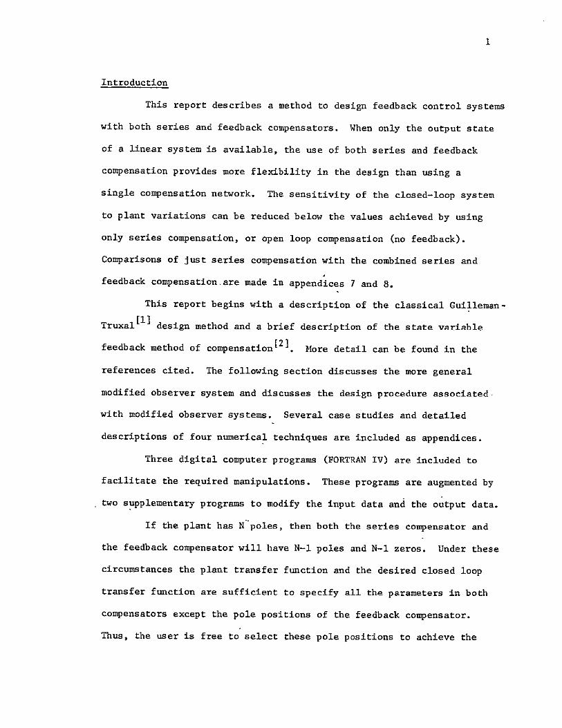
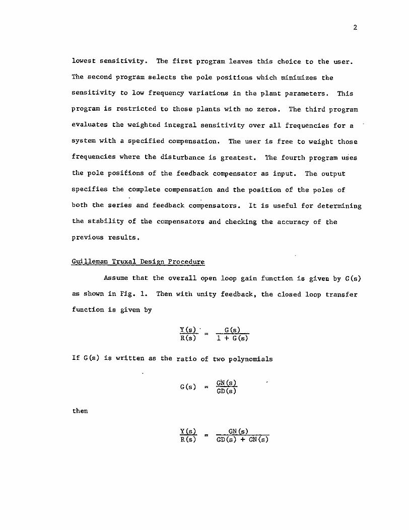
2
lowest sensitivity The first program leaves this choice to the user
The second program selects the pole positions which minimizes the
sensitivity to low frequency variations in the plant parameters This
program is restricted to those plants with no zeros The third program
evaluates the weighted integral sensitivity over all frequencies for a
system with a specified compensation The user is free to weight those
frequencies where the disturbance is greatest The fourth program uses
the pole posieions of the feedback compensator as input The output
specifies the complete compensation and the position of the poles of
both the series and feedback compensators It is useful for determining
the stability of the compensators and checking the accuracy of the
previous results
Guilleman Truxal Design Procedure
Assume that the overall open loop gain function is given by G(s)
as shown in Pig 1 Then with unity feedback the closed loop transfer
function is given by
Y(s) = (s) R(s) 1 + G(s)
If G(s) is written as the ratio of two polynomials
G(s) GD(s)
then
Y(s) = GN(s) R(s) GD(s) + GN(s)
C(s) IGp(s) Y(s)
C(s)
Figure I Cuilleman Truxal Block Diagram
4
Equating the numerator and denominator polynomials
GN(s) = C(s) (1)
GD(s) = R(s) - Y(s)
The design procedure is as follows
1 From the specifications choose the desired closed
loop response Y(s)R(s)
2 From step 1 and eqn 1 determine GN(s) and GD(s)
3 Choose a suitable series compensator which shifts the
poles and zeros of the plant to the positions specified
by step 2
The above steps are simplified if one uses Guillemans suggesshy
tion to select a C(s)R(s) which results in real zeros for GD(s) Then
the zeros of GD(s) can be simply determined from a plot of R(s) - C(s)
for only negative real values of a One pair of complex conjugate
poles and a group of poles on the negative real axis is usually chosen
to meet the above requirements
For example suppose the plant is given by
i
Gp(s) = s s+l) (2)
and that the specifications can be satisfied if
Y(s) -100 R(s) 2 + 20s + 100
5
From (1)
GN (s) - 100
GD(s) = S2 + 20s
The series compensator C(s) and the plant transfer funetion must equal
G(s)
C(s) op(s) 100 a(s+20)
From (2)
C(s) = 100(s+l) (4)(s+20)
Effectively the series compensator moved the time constant of the
motor from 1 to 120
The success of this procedure depends upon the accurate modeling
of the motor over the range of frequencies from zero to well above 20
radianssec Otherwise additional poles in the plant transfer function
will alter the actual closed loop transfer function In particular the
real system may become unstable
State Variable Feedback Design Procedure
This design procedure is similar in many respects to the above
procedure First a desired closed loop response is selebted which
satisfies the bandwidth rise time steady state error and other requireshy
ments The plant is divided into a set of first order transfer functions
which may be interconnected The output of each of these first order
systems is fed back to the input through a fixed gain element By
adjusting these gain any desired closed loop transfer function can be
achieved
The above process is somewhat simplified if we first introduce
a new function Heq(s)0 This function specifies the transfer function
between the output and the input which yields the same result as state
variable feedback From Fig 2 the equivalent feedback from the output
is i s+ k2 + k3 Heq(s) = kl Gi (s GI(S)G2()
In terms of Heq(s) the state variable feedback results in the closed
loop response given by
Y(s)= KGp(s) (5) R(s) 1 + KGp(s) Heq(s)
The procedure is as follows
1 Select the desired Y(s)R(s) from the specifications
2 Equate the desired Y(s)R(s) to theone achieved by the
feedback from each state
3 Solve for the feedback coefficients
Details of the design procedure when zeros are present are given by
Schultz and Melsa [2 ] For example if
0p(s)= 1s (s+l)
Y(s) 100 R(s) s + 20s + 100
Then if G(s) 2(s)
Heq(s) - k1 + k2s
-- G3(s) G2 (s) ---GI(s) Y(s)
F 2
Figure 2 State Variable Feedback Block Diagram
8
From (5)
100 K2 2 s + 20s + 100 s + s + K(k1 + k2s)
Equating the numerator and denominator polynomials
K = 100
KkI1 100
1+Kk2 - 20
Solving for k1 and k
K = 100
k = 1
k2 19
This design yields exactly the same transfer function as the
Guilleman-Truxal (GT) method The two methods are not the same if a
small change is made in the plant transfer function The state variable
feedback (SVF) system changes less than the GT system
If the sensitivity is defined as the percentage change in the
closed loop transfer function for a small percentage change in a plant
parameter say K then
S K _ d dK dT K
T T K dK T
where for simplicity
T(s) - Y(s)R(s)
9
If K is the gain then
T(a) =KG(s)1 + KG(s) Heq(s)
dT(s) G(s) K Gp(s) G(s) fea (s) 2dK I + KG(s) Heq(s) (1+ KG(s) Heq(s))
Using this result in the definition of sensitivity
T = T(s) (6) T KG(s)
For the GT system from (6)
K s(s+20)
2T (s + 20s + 100)
For the SVF system from (6)
K s (s+1)ST 2 a + 20s + 100
For the GT system the sensitivity is greater at all frequencies than
the SV sensitivity especially at low frequencies
Modified Observer Systems
LuenbergerE ] has shown that an eytimate of the states in the
plant can be implemented as shown in Fig 3 When state variableshy
feedback is used from these states a specified closed loop response may
be achieved Muterspaugh [4 has modified this configuration by block
diagram manipulations to a form similar to that shown in Fig 5 The
1 2 2NN-1
kI
Figure 3 Luenburger Observer Block Diagram
r C(s) G(s) Y
Figure 4 Modified Observer Block Diagram
A(s)
I+
gt G(s) Y H(s)
Figure 5 Muterspaughs Modified Observer Block Diagram
13
series compensator shown in Fig 4 C(s) reduces to the Guilleman-TruxalLiJ
compensation in the case where H(s) is one Similarly this control system
reduces to the Heq [2 ] type of control resulting from state variable
feedback considerations when C(s) is one Fig 4 represents a more
general configuration than either Guilleman-Truxal or Heq type compensashy
tion All three configurations shown in the above figures are equivalent
Assuming that only the output is available the Heq configuration
is not realizable since Heq has zeros but no poles Guilleman-Truxal
type compensation is sensitive to plant variations Series and feedback
compensation is used to achieve low sensitivity and realizability If
Heq has zeros in the LP then the modified observer (MO) system is
slightly higher in sensitivity than Heq but if Req has zeros in the RHP
then the MO system is dramatically better These comments are illusshy
trated in the case studies at the end of this report
Modified observer System Design
This section derives the necessary conditions which C(s) and H(s)
must satisfy such that the desired transfer function Y(a)R(s) is
achieved when the plant has a transfer function G(s) The relationship
among these transfer functions is
T(s) 1() C(s) G(s)fR(s) 1 + C(s) G(s) H(s) (7)
If the feedback signals shown in Fig 3 are combined (using
block diagram manipulations) the resulting transfer functions are
A(s)=k2 1P1 (S)+k 2 (fIpI(s)p 2 (s)+12P2 (s))++knceiPl(s)+ -PNI(s))
H(s)k 1+k2p1 +k 3P1p2++kpN-1
14
Since the poles of H(s) and A(s) are arbitrary the control systems shown
in Fig 5 have N-i arbitrary parameters however the poles of A and R
are identical
One more manipulation of the system shown in Fig 3 results in
the system of Fig 4 where
1 C(s) - I + A(s)
The zeros of C(s) are the same as the poles of A(s) therefore the N-1
zeros of C(s) are also the same as the N-i poles of H(s)
From these facts (7) can be used to determine the denominator
of C(s) and the numerator of H(s) Dropping the argument a in (7) and
denoting the transfer functions by
CDC(s)
H(s) -
G(s) ONGD
T(s) - R
Eqn 7 becomes
CN GN 1 CD GD(8) R 1i+ CN GN HN
CD GD HD
If the right hand is simplified then
Y CN GN HD (9)R CD GD HD + CNCN
Since CN and HD are the same denote them both by P(s) Then (9) simplishy
fies to
15
Y GN P (10)R CD GD + NHN
cross multiplying on both sides results in the polynomial
Y(CDGD+GNHN) - R-GNP (11)
Define the number of zeros in G as NG the number of poles as
ND and similarly NY and NR for T(s) If the order of both sides of
(11) is to be the same then
NY + ND - 1 + ND NR+ NG + ND - 1
NY + ND NR + NG (12)
NR - NY -ND - NG
Thus the pole zero excess of the plant determines the pole zero excess
of the desired closed loop transfer function If like powers of (11)
are equated then NY + 2ND equations result Since CD and 1N are undeshy
termined the number of unknowns is 2ND For NY = 0 the number of
unknowns is equal to the number of equations Just as in regular state
variable feedback[2 for zeros in YR additional states must be
created Let the order of P(s) by N-l then (12) becomes
NY + N - I + ND = NR + NG + N - 1
and for the number equations to be equal to the unknowns
NY + ND + N = 2N (13)
N = NY+ ND
16
Thus the order of both controller systems C(s) and H(s) must be one
less than the number of poles of G plus the number of zeros of YR
assuming that (11) represents a set of linearly independent equations
The design procedure is as follows
1 Select the desired closed loop transfer function from the
specifications
2 Select a polynomial P(s)
3 Equate the actual and desired transfer functions (iO) and
solve for the coefficients of CD(s) and HN(s)
Program 1
The first program (MODOBSI) computes the transfer function of
the series compensator and the feedback compensator as a linear function
of the denominator of the feedback compensator The user must specify
the plant transfer function and the desired closed loop transfer
function Thus this program specifies the design of the system except
for the poles of the feedback compensator which the user is free to
choose in any way he wishes
Program 2
The second program (MODOBS2) computes the transfer function of
the series compensator and the feedback compensator which minimize the
low frequency sensitivity of the closed loop system to plant variations
The user must specify the plant transfer function and the desired closed
loop transfer function If the time constants in the plant are much
lower than in the closed loop system the poles of the feedback compenshy
17
sator may be in the right half plane (RHP) If the poles of the compenshy
sator are in the RHP then the system will be vyD sensitive to variations
in the parameters of the compensators In this case it is better to
use one of the other programs This program is limited to systems with
no zeros
Program 3
The third program (MODOBS3) computes the weighted integral
sensitivity of the system for a given polynomial P(s) The user must
specify the plant transfer function closed loop transfer function the
weighting to be given the sensitivity as the frequency varies and the
denominator of the feedback transfer function P(s) The weighting
function must have more poles than zeros
Input Data
In many circumstances the available data for the plant is in
state variable form This data is converted to a transfer function by
the STVFDBK program The details of the program are included in reference
1 The program listing and input data format are also included in the
Appendix
Output Data
The program BODE4 is provided to plot the transfer functions
computed in the above programs on a logarithmic scale For each program
some of the transfer functions of interest are
1 Plant transfer function
2 Closed loop transfer function
3 Sensitivity as a function of frequency
4 Loop gain function
The loop gain function divided by one plus the loop gain is the proportion
of measurement noise at each frequency which will reach the output Thus
if the loop gain is much greater than one then nearly all the noise
reaches the output and if the loop gain is much less than one very little
measurement noise reaches the output If the phase shift of the loop
gain is nearly 180 at a gain of one the measurement noise will he
amplified
Program 4
The fourth program (MODOBS4) is useful to check the results of
the design Given P(s) and the results of the first program (MODOBSI)
this program computes HN(s) CD(s) and the roots of both the series and
feedback compensators This program and the first program give a
complete determination of the design
Results
A discussion of each program and several caee studies are inclushy
ded in the Appendices MDDOBSI is useful to compute HN(s) and CD(s) in
terms of the coefficients of P(s) Quite amazingly the coefficients of
N and CD are linearly dependent upon the coefficients of P HODOBS2
computes the coefficients of both compensators which achieve minimum low
frequency sensitivity Essentially this result is achieved by forcing
CD(s) to be an N-i order integrator which increases the gain at low
frequency and thereby decreases the sensitivity since SK = (s)
Unfortunately if the plant denominator coefficients are smaller than
19
those of the denominator of the closed loop transfer function the feedback
compensators may have poles in the RHP MODOBS3 determines the weighted
integral sensitivity when P(s) is specified MODOBS4 is useful for
checking the roots of the resulting compensators after a design is
complete Test results are given in the appendix for three examples
These examples show that an improvement in the system sensitivity over
that of just a series compensator can be achieved even if only the output
is available When the closed loop response is much faster than the open
loop the sensitivity of the MODOBS system approaches the sensitivity of
the Req system (which is best but not realizable) if the roots of P(s)
are made much larger than the closed loop roots If the closed loop
response is not much faster than the open loop response then the MODOBS
system may have a sensitivity lower than the Heq system This situation
exists whenever Heq(s) has zeros in the RHP These results point out
the important fact that a sacrifice in sensitivity to plant variations
is made by increasing the system performance requirements Because of
this fact careful attention to the plant performance should be made for
lowest sensitivity and unnecessary demands on overall system performance
should be avoided
20
Bibliography
1 J C Truxal Control System Synthesis McGraw-Hill 1955 Chapter 5
2 J L Melsa and D G Schultz Linear Control Systems McGraw-Hill 1969 Chapter 9
3 D G Luenberger Observing the State of a Linear System IEEE Transactions on Mil Elec April 1964
4 M E Muterspaugh State Variable Feedback and Unavailable States HS Thesis 1968
5 F H Effertz Comment on Two Coupled Matrix Algorithms for the Evaluation of the rms Error Criterion of Linear Systems Proceedings of the IEEE November 1966 p 1629
6 J L Melsa A Digital Computer Program for the Analysis and Synthesis of State Variable Feedback Systems NASA Contract Report CR-850 August 1967
7 L E Weaver et al A Control System Study for an In-Core Thermionic Reactor J P L Report 32-1355 January 1969
21
Appendix I - MODOBSI
Dis cussion
The basic algorithm of this program is based upon (5) First the
following polynomials in s are computed
T = (GD)(Y)
Q = (GN)(R)
V = (GN)(Y)
so that (5) becomes
(T)(CD) + (V) (HN) = (Q) (e) (Al)
Each of the terms in (Al) are polynomials in s where P(s) is unspecified
For instance P(s) = P3s2 + P The coefficients of CD(s) and HN(s) are
the unknowns
As an example suppose the plant is second order then P(s) is
first order In this case (Al) becomes
(CD2T3 +H 2 V3 )s 3 + (CD2T2 + CD1T3 + H2 V2 + H1 V3 )s2 + (CD2T1 + CD1T2
2 + H2V I + HIV2)s + (CDIT + HV) = P2Q 3s + (P2Q2 + PIQ3 )s2
+ (P2Q + P1 Q2 )s + PlQl (A2)
Equating coefficients of like powers of s results in the equations
T3CD 2 + V3H2 Q3P2
T2CD2 + T3CD1 + V2H 2 + V3H1 Q2P2 + Q3PI
22
T1 CD2 + T2 CDI + VIH2 + V2H 1 QlP2 + Q2P
TICD1 + V1Hi = Q1F1 (A3)
These equations can be rewritten more compactly in matrix notation as
T3 0 V3 0 CD2 f 0 Q3TN12N-2 T2 T3 V2 V3 CD11 214-22-Q3 Q3 Q22 (A)
2 T V1 V2 H2 Q2 QI P2j _ Ql 0
2N-2- shy - N-i-)
The matrix on the left will be defined as matrix A and the matrix on
the right will be defined as matrix C Then
CD2 CDI _ - 1
CD= A-C (A5)
H I
Therefore A- C relates the unknowns CDi and Hi to the parameters Pi
MODOBS1 forms the matrix A from the two arrays T and V and then inverts
A Next the C matrix is formed from the Q array and then A 1 C is
computed and printed
23
Input Format
Card No Columns Description Format
1 1 NY = order of Y(s) in YIR II
2 NR = order of R(s) in YR Ii
3 NG = order of GN(s) in GNGD i1
4 ND = order of GD(s) in GNGD Ii
I 5-80 Identification of problem 8AI0
20 Cn of 2 11-0 Coefficient of s in Y(s) FI03
11-20 Coefficient of aI in f(s) P1e3
etc
71-80 Coefficient of s7 in Y(s) F103
3 1-10 Coefficient of a in R(s) F103 etc
4 i-i0 Coefficient of s in GN(s) FIO3
etc
5 etc Coefficientof a in GD(s) FI03
Notes
1 If more than eight coefficients are required then two cards may be
used to identify that polynomial
2 A decimal point must be used for each coefficient but not for card
No 1 The decimal point may be placed in any of the ten columns
for each coefficient
24
3 As many problems may be run as desired by repeating the above format
for each problem
Output Format
See example
Subroutines to be Used
PLYMLT Multiplies two polynomials together
MXINV Inverts matrix A
PRNTRAT Prints the ratio of two polynomials
Flow Diagram
Read NYNRNG
ND
FRead Y(s)R(s)GN(s) GD(s)
Compute T = YGDQ = GNRV = GNYj
Form A Matrix
Invert A Matrixi
lForm C Matrixl
A -1
ComputeBA7 C
Print CD and E
Arrays
PROGRAM MODOBSI (INPUTOUTPUTTAPE4INPUT)
ODIMENSION Y IC) R(10) GD(IO) GN(IC) V(201 T(20) G(20)14A(S363)AI(36 3)C( 3611) B(36 1U ID(G)
C Y(S)R(S) IS DESIRED CLOSED LOOP RESPONSE C SP(S)GD(S) IS PLANT TRANSFE FUNCTION C NY IS ORDER OF NUM IN Y(SlR(S) NR IS ORDER OF DEN C NG IS ORDER OF NU OF G(S) NO IS ORDER OF-DEN C NR-NY MUST EQUAL ND-NG 1 READ 1U1NYNRNGNDID
PRINT 200NYNRNGNDIO
IF(EOF4) 99t2 2 NY1=NY4 1
READ 102 (Y(I)I=-INY1) C YI) IS COEFF OF S(I-I) IN Y(S)
NR I=NR C RII) IS COEFF OFS(I-1)IN-P(S) 3 READ I102 (R(I) IINRI)
CALL PRNTRAT(YNY1RNRI IHTIHS) __C_ GN(Il IS COEFF9F_SCI-1LIN_-GNtSL
NGl1NGI NO 1NDI
_4 -READ 102 (GN ) I 1NG1) C GOD(I) IS COEFF OF S(I-1) IN GO(S) 5 READ 102 (CG (I)I--1NDI)
CALL PRNTRAT(GNNGIGDNO HGIHS___ C FORM CHARACTERISTIC POLYNOMIAL
CALL PLYMLT (GDND1YNYITO) CALL PLYMLT GNNG1RNRI00-CALL PLYMLT (GN NGGYNYIVO) NYNGzN Y1 4NGI NR+NG+iN __ 00 6 IrNYNGN
C NA IS ORDER CF A MATRIX WHERE A IS MATRIX RELATING UNKNOWNS -6- V( --- - - TO PARAM P
NA_- 2 (N--1) DO 20 J-1NA IF- (J GT (N- IlJGO__TO2_12 00 10 Iz1NA INDN- L J IF _( IND-SLT_ I)_GOTO8_ IF (IND GTN) GO TO 8 AUIJ)- T(INa) 30 TO 10shy
8 A(IJ) O 10 CONTINUE
Gi__TO_2D
12 DO 20 I=INA IND 1-I+J IF- (INDLT__GO__18__ IF (INDGTN) GO TO 18 A(IJ)-V(IND) GO-T 0 _2D
18 A(IJ)-O 20 CONTINUE
CALL MXINV-(ANAtAll_ C C IS THE COEFF ARRAT
NM IrN-1 _DOZ4__I NA-_ DO 24 J=1YNMI IN= 2N-I- J
IFiINDLT1) GO TO 22 IF (INDGTN) GO TO 22
C(IJ) = O(INO) -
GO TO 24 22 C(IJ)rO 24 CONTINUE C B IS AICTAE ROwS OF 5 ARE EQUAL TO CD AND HN C COLS ARE COEFF OF P PARAMETERS
D0 30 INA 00 30 KzlNM1 B(IK)--O 00 3fJ--JNA
30 B(IK)-AICIJ C(JK+B(IK) PRINT 2O1KK--lNMI) DO 40 I--NMI
NC =N -I 40 PRINT 202 NC (B I-Kt NM1I
DO 50 I=NNA
NBzNA+-I -50 PRINT 204t-NB (8(1I(1 Kzl-NM-1
GO TO I 99 STOP -101-FORM ATf l A 1f)V t 102 FORMAT (BF103) 200 FORMAT (1HI4(2XI1) 2X6A1i0) 201 FORMAT IH X8 ( 314- P( I 11 I-) OX)) 202 FORMAT 14H CO(I2--)10(E1U33X)) 204 FORMAT (4H HN(I12H)=)I(EIO33X))
END SUBROUTINE PRNTRAT (ANNBvNOEPVARINDVAR) DIMENSION A( 20)B( 20H_(20)N(20)AT20BT(20)NEt 1
DO 6 I--NN AT(I)-- -IF-(-AY f-4i 6-3
3 H(NE)zlH+
AT(NE)rA(1) GO TO 5
4 H(NE)--IH-
AT (NE) -A(I) N(NE)I-1 NErNEI
6 CONT INUE NE=NE-1 PR IN-T 10 0 MIN=MINO(NE 10) PRINT 10lCN(I)IzMIN) PRINT 102 (HRU1 ATI) INDVAR Il tMIN) IF (NE-if]) 8987
7 PRINT 101 (N(I IrIINE) PRINT 102 CHI)AT(I)INDVARI--INEI
__ NF= O0 16 I--IND BT (I)--DIF C B(C) 191G13
13 H(NF)rlH4 BT(NF zB(I)
-GO-_ T _15 14 H(NFI -IH-
BT (NF) =-B(I)
r27 15 N(NF)=I-I
NF zN Fi-I 16 CONTINUE
NF =N F- I HH= IH-NH=rAX 013NE 13 NF) NHzMINO(130NH)
20 PRINT 103 DEPVARINOVAR (HH I=INH) MIN MINO(NF 10) PRINT 101 (N(I)IzIMIN) PRINT 102 (Hi(I)BT(I ) 1NDVAR-I---1MIN IF (NF-101) 28P2827
27 PRINT 0l (N(I) IzIINF) PRINT 102 (H(IJBT(I)TNDVARI=N-FI)shy
28 CONTINUE 100 FORMAT C iHO) 101 FORMAT (6XI(11X 12)) 102 FORMAT 6XID(AIGlC4 AI1H H 103 FORMAT tIXtAIIHCAI2H)= 30AI)
RE TURN END SUBROUTINE MXINV (R N RI) SUBROUTINE TO FIND THE INVERSE- ----- GIVEN
C MATRIX R N IS ORDER OF MATRIX RI IS INVERSE C MATRIX SUBROUTINE USES GAUSS-JORDAN REDUCTION C R MATRIX IS PRESERVED DIAGONAL ELEMENTS OF R-US
BE NONZERO C DIMENSIONR(3G36IRA(3G72) RI(36v36)
C STATEMENTS 20-26 ENTER R ARRAY INTO RA ARRAY - C AND SET LAST N COLUMNS OF RA ARRAY TO IDENTITY
C - MATRIX 20 DO 26 I 1 NI-v 21 DO 24 J I N
_22__RA IJ) -R(I- J) 23 NJ = N + J 24 RA(INJ) = 0 2 5 _NI z N + I 26 RA(INI) = 1
C C ST AT EM ENTS _ii-12_REDUCE MATLRIX__RA _SOH_ATZ_JRFSR_LK C COLUMNS ARE SET EQUAL TO THE IDENTITY MATRIX
i NP = 2 N 2_DO 12 I - N
C -
C STATEMENTS 3-5 ARE USED TO SET MAIN DIAGONAL _C ELEMENT TOUNITY
3 ALFA = RA(TI) 4 DO 5 J = I NP S RA(IJ) r RA(I J) _ALFA
C C STATEMENTS 6-11 ARE USED TO SET ELEMENTS OF ITH C COLUMN TO -ZERO
6 00 11 K = 1 N 7 IF (K - I) 8 11t 8 8 BETA = RAiKI) 9 DO 10 J = It NP
10 RA(KJ) = RA(KJ) - BETA RA(IJ) - ICONTINUE_ 12 CONTINUE
C
TO LAST 28 C STATEMENTS 30-33 SET INVERSE MATRIX RI EUAL
C N COLUMNS OF RA ARRAY
30 DO 33 J 1 N 31 JN J + N 32 00 33 I 1 N 33 RI(IJ) rRA(IJN) 34 RETURN
END SUBROUTINE PLYMLT (ALBMCN)
C C MULTIPLY ONE POLYNOMIAL BY ANOTHER
C C DEFINITION OF SYMBOLS IN ARGUMENT LIST C A(I) MULTIPLICAND COEFFICIENTS INTHEORDER AE) S(I-1) C L NUMBER OF COEFFICIENTS OF A C B(I) MULTIPLIER COEFFICIENTS IN THE ORDER 8(I)SI-1)
C M NUMBER OF COEFFICIENTS
C C11) PRODUCT COEFFICIENTS IN THE ORDER C(19S(I-1)
C N NUMBER OF COEFFICIENTc Ac r
C C REMARKS C IF N-- C(I) SET TO ZERO AND PRODUCT FORMED OTHERWISE THE
C I-PRODUCT AND SUM NEWC-OLD C + AB IS FORMED
DIMENSION A(iD) B(IO) t C(20) LPML+M- 1 IF (N) 10102iZ
I DO 1 J- LPM 11 C(J)-Oo 12 DO 13 J--ILPM
MA X-MA XD (J + I-M il)) shy
- MINzMINO(L DO 13 IrMAXMIN
13 CC(J)=A(I)B(J+II) + C(J) RETURN END
3434 IN CORE THERMIONIC REACTO R
116708 481228 384520 200 1 16708 -4870635__4085815__39226_ 100 116708 481228 384520 200- 503585E-610542E- 3 058639 18804 1
END OF INFORMATION
29
Appendix 2 - MODOBS2
Discussion
If CD(s) in (5) is defined by CD(s) = CD N-i (BI)
where N is the order of the plants then the system will have minimum
low frequency sensitivity because the forward loop gain will be increased
at low frequencies If there are no zeros in Y(s)R(s) or in G(s) (5)
reduces to a simple set of linear equations shown below For simplishy
city RN+ I and GDN+t are set equal to one For zero steady state error
Y = R1
PNl PN= I PN-I = N-I
PN-2 + RNPN-1 CN-2
(B2)
P + 2 + ReN- =1 I I
IN I = P RY
HN2 =PI RY + P2
+HN=NPI RNY + P 2 -Y +i - GD1Y
Where the C terms are defined by
C I GD2 - R2
C2 = GD3 - R3
CN- 1 GDN - N
30
The Eqns (B2) are simply solved in the order shown by back
substitution That is PN-1 may be usedto solve for PN-2 which may be
used to solve for PN-3 etc
Input Format
Card No Columns Description Format
1 1 N = Order of the Plant G(s) Ii
2-80 ID Identification of problem 8A1O
2 1-10 Y = Numerator of YR F10o3
0 3 1-10 R(1) = coeff of s in R(s) F103
11-20 R(2) = coeff of s I in R(s) FIO3
etc
7 71-80 R(7) = coeff of s in R(s) FI03
4 1-10 GN = numerator of G(s) F103
5 1-10 GD(l) = coeff of s in GD(s) F1O3
771-80 GD(7) = coeff of s in GD(s) F103
See notes following input format for MODOBSIo
Output Format
See example
Subroutines to be Used
PRNTRAT - Prints the ratio of two polynomials
PROMT - Determines the roots of P(s) to see if any roots are in
RHP
PROGRAM OOS2 (Y4PUT OUTPUTC4=INPUT)IO41 N j (l10 1 ( l ) 1 ([) Cl(In)ID( 3)PHN 1 )CD t13)
C U (IG) V (10) C PqOGRAM TO CALCULATE MINIMUM LOW-FREO SENSITIVITY MODIFIED C OBSERVER SYSTEM C Y(S)R(S) IS DESIRED CLOSED LOOP RESPONSE C GN(S)GD(S) IS PLANT TRANSFER FUNCTION C N IS ORDER OF DEN IN Y(S)R(S) C N IS ORDER OF DEN IN GN(S)GDIS) C R(I) IS COEF OF S(I-1) IN R(S) C C ASSUMPTIONS C C TRANSFER FCN GAINS ARE NORMALIZED SUCH THAT R (N+1)I1
C AND GD(N I )=I C C DESIRED TRANSFER FCN HAS ZERO STEADY STATE C
-C GD(I) IS-COE-F-- O-F S(I-I)1NGO(S) C Y(S)=Y GN(S)-GN (NO ZEROS ALLOWED) C I READ 101 N ID
IF(EOF4)99 2 2 READ I02Y
READ 102 (R(I)IzIN) NP i-N+ I
GD(NPI) =1 5 RNPI_)-1 READ 102 GN
3 READ 102t CGD(I)tlz1N) PRINT 200DNIO10 PRINT 201
CALL PRNTRAT CYIRNPHTIHS) PRINT 202
CALL PRNTRAT(GNGDNP11HG1HSI C-C --SOLVE FOR DEN OF H P(S)
NM I=N-I do 40 II -NM1 IPIlzI+I
-4 -CI) zG0c IP 1I-R IiT P(N) -
005[ I=ItNMj NI N-I P(NI)zC(NI)
IFCILE1) GOTO-50_ DO 49 Jz2I J2=N-J+2
4 P(NI )zP( NI )-R( J2 )P( JI ) 51 CONTINUE
CALL PROOT (NMIPUV) PRINT 205
PRINT 206 (U(I)V(I) I=INM1)
ERROR THUS YR(1)
SOLVE FOR NUM OF HHN(S) DO 60 1N HN (I 0 - 00 60 JzlI IJI j4
C
6C PN Il)r( Ji R (IJ) Y +HN( I) 32 HN (N )HN (N)-GD (1 )Y
PRINT 203 CALL PRNTRATIHNNPNIHH1HS) PO 80 1i NMI
80 CO(I)zO CD(N)zl PRINT 204 CALL PRNTRAT(PNCDN1HC1HS) G z YGN PRINT 210 G GO TO I
99 STOP 101 FORMAT (Il 84101 102 FORMAT (SF1O3)
200 FORM AT(IHII0X II 4X 8AID) 201 FORMAT(1HOTHE DESIRED CLOSED LOOP TRANSFER FUNCTION IS)
202 FORMAT(1HOTHE TRANSFER FUNCTION OF THE PLANT IS)
203 FORMAT(IHOTHE TRANSFER FUNCTION OF THEFEEDBACK COMPNSATOR IS)
204 FPRMAT(lHOTHE TRANSFER FUNCTION OF THE SERIES COMPENSATOR IS)
205 FORMAT (IHO 5X THE ROOTS OF P (SI ARt 13XREAL PART IOXIMAGINARY PART)
-20 FORMAT 32X2E207f 210 FORMAT4IHOTHE ADDITIONAL FORWARD LOOP GAIN REQUIRED IS
1YGNElfl3) END SUBROUTINE PRNTRAT (ANNSNDDEPVARINOVAR) DIMENSION A(20)B(20vH(20) N(20 1 AT(20) PT 20 NE z1 00 6 Iz1NN AT(1)=D IF C(IA ) 463
3 H CNE )= IH + AT (NE) =AtI) GO TO 5
4 H(NE)=IH-AT (NE) =-A( I) N(NE)--I-1 NE-NEI
6 CONTINUE NE=NE-1 PRINT 100 MINMINO(NE v1O
PRINT IOl (N(IhI=IMIN)
PRINT 102 (H(IAT(I)INDVARI-IMIN) IF (WE-10) 8
7 PRINT 101t (N(I)IzlINE) PRINT 102 (H(I)AT(I)INDVARIn1NEl NF o_-8_ N --1 80 16 I1NU
BT(IzO IF ( (I) 1141613
13 H(NF)zlH+ BT(NF)l=B(I)
-GO T0- 15 __ - 14 H(NF) zlH-
BT (NF)z-B(I) - 15 N(NF)=I-1 -
NFZNF41
33 ID CONTINUE
NF NF- I HHL IH-NHMAXO( 13NE 13NF) NHzMINO( 130NH)
20 PRINT 1G3DEPVARINDVAR(HH 1=1NH) MINMINO(NF 10)
PRINT 101 (N(I)IlMIN) PRINT 1G2( H(I)BT(I)INOVART IMIN] IF (NF-in) 2828927
27 PRINT 101iN(I) I11 NF) PRINT 102 (H(I)BT(I)tINDVARI-IINF]
28 CONTINUE 100 FORMAT (1HO) 101 FORMAT (GX1O( IIX12)) 102 FORMAT (GXI0(AIGIO4 A1IH )
103 FORMAT (1XA1IH(Ai2H)-130A1) RETURN END
___SUBR CUT INEPR O0 TN _A U fVtIIRR) DIMENSION A(20)U(20)V(20)H(21)8(21 )C(21) IREV-IR NC -N +IDOll--i Nu
H( I) rA( I) _i CONTINUEL
00
3 IFIH( 1)) 24 2 NCNC-1
V NC )z0 U NC O DO 1002 I= 1NC H(I)--H(I+1 )
1002 CONTINUE GOT03
S_IF (NC- 1) 5 10 05 5 IF (NC-2) 7i 7
6 R=-H( 1H(2) GOT050
7 IF INC- 3) 9-819 8 P-H(2)H(3)
__0 1) H (3_)_ GO TO7g
q IFCABSCH(NC-1)1H(NC)-ABS(H(2)H(1))101919 10- IREV - IREV_
M=NC2 DO11I=-1 M
_-NL-zNC+ 1 -I-FrH( NL) H NL )H( I)
11 H( I) F -IF (O )139 12 913
12 P=D GOTO 15shy
13 PzPQ 0= (
15 IF(R)16191G 16 R=1 R 19 E5E- ]C
B(NC)H(NC) C(NC)H(NC) B(NC+1 )zO C( NC 1)z 0 NP NC- 1
20 0049J= I 100C DO 2111l1 NP ITNC-I I BC I rH(I)+RB(+1)
--21C( I) =B (I)+RC( I+ 1) IFCABS(B(I )H(1))-E)5050 24
24 IF(C(2)232223 2amp R= RlI-
GO TO 30 23 R=R-B(1) CC2)
30 D0Q3711zlNP IzNC-I I BI)i(I)-PB(I+I)-OB(I+2)
37C( I) =B (I)-P C(i1l) OC(12) IF(H (2)) 323132
31 IF(ABS(C2)H(1))-E)333334 32 IF(ABS(B(2)H(2) )-E) 33v3 34 33 IF(ABS(B(1)H(1))-E)707034
34 CBARrC(2)-B(2) DC(3) 2-CB ARC ( 4) IF(D)363536
35 PzP-2 0= (o t GOT049
36 PP(-82)C(3)-BC1)C(4))D - Q+ (-( 2)CBARB(1) C(3 00)
49 CONTINUE
ErE 10 GOT020
50 NC-NC-1 VtNC)D
IF (IPEV) 51 5252 51 U(NC)=1R-
GOT053 52 U(NC)-R 53 00541lNC
H(I) B(1+1) 54 CONTINUE
GOT04 70 NC=NC-2
---- IF(IREV)71727 71 QPr1O
P=P(Q2 0) GOTO73-_
72 OPPP Q-P 2 0
73 F-(PP)2-OP IF(F )74 7575
74 U(NC+I)z-PP U(NC)-PP V(NC 1 )SORT(-F) V( NC 1-V (NC+ 1) GOT076
75 U(NC+11-(PPABS(PP))(ABS(PP)SQRT(F)J V( NC+1 )0 U(NC )OPU (NC1) V( NC )O
76 D0771INC H(I) B(1 2)
77 CONTINUE GOT04
LDO RE TURN END
3 CASE STUDY II THIRD ORDE-SYSTE14shy1000 1000 200 20 D O -
2500 100
36
Flow Diagram
Read N ID
Y R(I)
GN GD(I)
Print N ID
YRy G
Form C(I)
ISolve for P(s)j
Solve for HN(s)I
Print H(s)
Print C(s)
37
Appendix 3 - MODOBS3
Discussion
This program uses the following data
1 Plant transfer function G(s)
2 Desired closed loop transfer function T(s)
3 The denominator (P(s)) of the feedback compensator H(s)
4 A desired weighting function W(s) on the integral over
frequency of the sensitivity of the closed loop response
to forward loop gain changes
The program then calculates the weighted integral sensitivity of
the system The method of calculation is based upon an algorithm by
EffertzL5] The integrand of the integral sensitivity is calculated
from
I S W(S) S (S) ds
2r f G(s)C(s) ds
The algorithm is based upon an iterative manipulation of the coefficients
in the numerator and denominator of the integrand in such a way that the
integral of the squared magnitude results
A closed form solution for the integral
jm n 2rj jo h(P)h(-P) 2 -joo
1 30 dP 1 j F(P)F(-P) dP
(BI)
is presented in the paper by F H Effertz The solution takes the form
38
of Equation 4 in his paper A better algorithm for the computation of
Equation 4 in Effertz is presented in the correspondence by Pazdera
(Equation 7) A modified forn of Pazderas algorithm has been coded in
FORTRAN and is included A test problem is also included
The use of Equation 4 in Effertz can be best illustrated by an
example Suppose we wish to evaluate the following
(B2)Ls2+ Cb) [2bLn = 2I -
It can be shown from residue theory that the correct answer is
I = - residue of F(s) F(-s) at s = a (B3)n
- residue of F(s) F(-s) at s = b
where F(s) F(-s) indicates the function to be integrated over s = jW
Then the answer is
22 2
= - c-a (c2-b2 c2+abn 2a(a+b)(a-b) 2b(a+b)(b-a) = 2ab(a+b) CR4)
To use Equation 4 from Effertz we must make the following associations
using the complex frequency variable s in place of p
22 s= c -g(P) = (s+c)(c-s)
then s (B5)
2
h(P) = s + (a+b) s + ab
then p s N=2
1
a a 2 =ab
39
The integral for n = 2 can be expressed as
bb [bloaaob I- (B6)
a0 t ol [jaza1-2 1ao a 2
Substituting the correct values of a0 a etc and cancelling minus
signs for this problem we obtain
ab +c In = 2ab(a+b) (B7)
What is most interesting is that the result depends only on the coeffishy
cients of the known function being integrated and not on the poles of
the function as one would suspect from residue theory
It has been mentioned that the algorithm from Pazdera (Equation 7)
has been programmed Some charges in the nomenclature of Equation 7 were
necessary to facilitate coding Note that the practice in Effertz and
Pazdera is to make the highest membered coefficient correspond to the
lowest power of the variable p Note also that subscripts such as ao
are in evidence To facilitate coding the lowest numbered coefficient
was subscripted in the form A(l) and this coefficient was associated with
0 ththe lowest power of the variable p in this case p In general the i
coefficient A(I) is associated with the (i-1)s t power of p P -l (In
FORTRAN the expression A(O) is not allowed) Note from equation I above
what must be done to operate on the function F(s) F(-s) If F(s) is of
the form
F(s) = C(S) (B8)A(S)
then the algorithms suggested in both Effertz and Pazdera require the use
40
of
g(s) = C(S) C(-S) (B9)
h(s) = A(S)
It is more desirable to input C(S) and A(S) rather than C(S) C(-S) and
A(S) Consequently one uses the INTSQ subroutine by coding the coeffishy
cients of C(S) and A(S) with ascending subscripts corresponding to
ascending powers of S The subroutine provides the operation C(S) C(-S)
Furthermore the subroutine checks to see if the lowest coefficient of
C(S) or A(S) is zero so that factors of S may be either considered or
cancelled Two basic requirements must be met by A(S) and C(S) First
the roots of A(S) and C(S) must at least have non-negative real parts
(Hurwitz polynomial requirement) Secondly the highest power of C(S)
must be at least one less than the highest power of A(S) for convergence
to be assured If A(S) is Nth order one inputs the N coefficients of
A(S) and the N-i coefficients of C(S)
The use of this subroutine INTSQ may be best illustrated by an
example Suppose we desired to evaluate the integral
I = JD F_ 7 4 - JdS n -joe 3 + 3s2 + 2s + L[43 + - 2s
(BIO)
The polynomials C(S) and A(S) as defined in Equation B8 are input into
the program as
C(1) = 4 A(l) = I
C(2) I A(2) = 2
(Bi) C(3) o A(3)= 3
A(4) = 4
41
The program then utilizes the modified Pazdera algorithm and prints out
the message
THE VALUE OF THE INTEGRAL IS 12250
To check this answer one can use Effertz Equation 4 for a third order
case (n=3)
a oa 101o 2 1 n
= (142a
0 a
aI a a 0
I 2a
boa2a3+b2aoal-aoa3b alaaa a (BI2)
0 1 20 - o2 2 3o 31 o 13a22o0
For our example problem the following associations follow
b =0 a =4 0 0
b 1 -l a = 3 (B13)
b2 =16 =2a 2
a 113
Substituting the values of Equation B13 into Equation B12 verifies the
computers solution I = 1225n
Input Format
Card No Columns Description Format_
See format for MODOBSI
K 1-10 P(1) - coeff of so in P(s) BE103
11-20 P(2) - coeff of s in P(s) 8E103
etc
42
Input Eormat (contd)
Card No Columns Description Format
K+I 1 NW - Number of coeff in denom of W(s) II
K+2 1-10 WN(I) - coeff of s in num of W(s) 8E103
11-20 WN(2) - coeff of s in num of W(s) 8EI03 etc
K+3 1-10 WD(1) - coeff of s deg in den of W(s) 8E103
11-20 WD(2) - coeff of s in den of W(s) 8E103 etc
43
PROGRAM MODORS3(INPUTOUTPUTTAPE4-INPUT ) DIMENSION Y( 10)R(10)c-D(IO) SN(lOhIP(10)CD(0) HN(IO)SN(40)bull
IS0(40) B(36 18)WN(10) WD 10)SNT(40)SDT(40)C
I CALL MODOBSI (YP GN GO5 NY1 NR1 NGI NDI C N-1 IS THE NUMBER OF COEF IN P(S) HN(S) CD(S)
NrNR 1+NGI- 1 N =rN -1 READ 10 lP(I)Iz1NI)
C W(S) = WNWD MUST HAVE MORE POLES THAN ZEROS C NW IS THE NUMBER OF TERMS IN THE DENOMINATOR OF WS)
READ 103NW READ 102 (WN(I)I-INW)_ READ 102 (WD(I)I-INW) PRINT 205 CALL PRNTRAT (WNNWDNW1HW4-lkHS) CALL PLYMLT(GDNDlY NYI SN 0) N2=NDI+NYI-I
_CALL_ PLYMLTT(yN NWSNN 2 SNT D) CALL PLYMLT (GNNG1 R NRI SO 0) CALL PLYMLT(WDNWSDN2SDT C)
__N3=NW+N2-1 -
N4 =N 3+ NI-1 N22N1 11
-a- DO 10 I= 1Nl CD(I)=0 HN(I)O 00 10 J1pN1 CD (I)B(N-I J)P J )+CD( I)
10 HN(I)zB(N2-IJ)P(J) +HN(I)_P -I NJ_Z0 I--_
CALL PRNTRAT(PN1CDN1IHCIHS) PRINT 202
CALLP RNTRATAHN NI P Ni1H Ht l1 CALL PLYMLT( CDN1 SNT N3 SN C) CALL PLYMLTI- PN1SDT N3SD 0) -N5=N4 ---CALL INTSQ(SDSNN4S) PRINT 204 S
- GO T ---O-- -- 102 FORMAT 18 E1O3) 103 FORMAT III)
-201 -FO RM ampTL__TJJLJERANS ER_-F-UN CT-O-N--OF--L sESERIS--COMENSJ-IO-R- i-l 202 FORMAT(O THE TRANSFER FUNCTION OF THE FEEDBACK COMPENSATOR IS) 204 FORMAT(O THE WEIGHTED INTEGRAL SENSITIVITY ISEIO3) 20S -FORM-AT( Oi-tJ-WEIGHTINGFUNCTION-OF-HE- INTEGRALSENS-IIVlTY-YI-_shy
1) END
_SUBROUTINEMOOOBS1 LYR GN GD B N-YI-NRI-NGL-ND44-UDIMENSION Y(IO) RU1G) GD(10) GNIG) t V(20) T(20)9 Q(20) IA(3636)AI(3G36)C(36l8)B(36 1B)ID(6)
C _Y(S)R(S) IS DESIRED-CLOSED LOOP C GP(S)GD(S) IS PLANT TRANSFERFUNCTION C NY IS ORDER OF NUM IN Y(S)R(S) NR IS ORDER OF DEN
_C_ --NGJ S OR DEROFJN UaOF_ GASJ_ID- S--DRDELO DE C NR-NY MUST EQUAL ND-NG C Y(I) IS COEFF OF S(I-1) IN Y(S)
C RP I) IS COEFF OF S( 1-f1 IN Q(S)
C GN(I) IS COEFF OF S(I-11 IN GN(S) C GOCI) IS COEFF OF S(I-1) IN GO(S) 1 READ 1UINYiNRNGNDIO
IF(EOF4) 99t2 2 NY IrNY +1
NR ic NR --READ 102 (YCI)IIlNYI)
3 READ 12z (R(I) I--NRl) PRINT 200NY vNRvNGNO ID CALL PRNTRAT(YNYl R NRI 1HT IS) NuGl=NG I
ND i ND-shy4 READ 102 IGN I I--I NG1) 5 READ 102 (GD(I)IzlND1)
CALL PRNTRATIGNNG1GDNDI 1H3IHS) C FORM CHARACTERISTIC POLYNOMIAL
CALL PLYMLT (GDNDIYNY1TO) CALL PLYMLT GNNGIRNR10) CALL PLYMLT (GN NGIYNY1V0i NYNG=NY1+NGI N rNR+NG+I 00 6 IzNYNGN
C NA IS ORDER OF A MATRIX WHERE A IS MATRIX 6 V(I)zfl
NA= 2 (N-1 DO 20 J-INA IF ( J GT ( N- 1) GO_TO_1 2 DO 10 IrINA IND-N-I+J IF (IND LT 1) GO TO 8 IF (IND GTN) GO TO 8 A(IJ)= TIIND) GO TO 10
8 A(IJ)zO 10 CONTINUE
GO TO 20 12 DO 20 I=lNA
IND --- I+J IF fINDLTI)_ GO TO 18 IF (INDGTN) GO TO 18 A(IJ) zV(IND)
GO TO 20 18 A(IJ)rO 20 CONTINUE
CALL MXINV_ (ANAAI_) C IS THE COEFF ARRAY-C
NMlzN- 1 DO 24 IrItNA DO 24 JrINM1 INDz2N-I-J
IF(INDLT1) GO TO 22 IF (INDOTN) GO TO 22 C(IJ) - O(IND) GO TO 24
22 C(IJ)zO 24 CONTINUE
__C B IS AICTHE RUWs UF B ANt LIUAL IU) (U C COEFF OF P_ PARAMETERS
00 30 IrINA
44
RELATING UNKNOWNS TO PARAM P
AN_)_HN_THECOLSAR
00 30 KzlIMI B (I K) 0 00 30Jr1NA
30 B(IK) AI(IJ)C(JK)+B( T K) PRINT 201IKv(K=1 NM1 DO 40 I=INMI NC =N -I
40 PRINT 202NC(B(IK)Kr1NM1) DO 50 IzNNA NB -N A 1- I
50 PRINT 204v NB(B(IKIK--NMI) RETURN
99 STOP 101 FORMAT (4116A10) 102 FORMAT (SF103) 200 FORMAT I1HIv4(2XI1) 2XGA1O 201 FORMAT (10X3(3H P(I1lH)vgX)H 202 FORMAT (4H CD(I12H)zO(E1O 33X) 204 FORMAT (4H HN(IIZH)=IO(EIO 33X)L
ENO SUBROUTINE PLYMLT (ALBMCN)
C MULTIPLY ONE POLYNOMIAL BY ANOTHER C
C DEFINITION OF SYMBOLS IN ARGUMENT LIST C AI) MULTIPLICAND COEFFICIENTS IN THEOROER A(I) S(I-I)
C L NUMBER OF COEFFICIENTS OF A _C_ _B I) __MULTILPLIER CO EE-CIENiS-LNTlLODE3-IIi-plusmnSflt-WL-
C M NUMBER OF COEFFICIENTS OF B C CII) PROOUCT COEFFICIENTS IN THE ORDER C(I)S(I-1)
_
C C REMARKS
_C _IF -LO_ C (t1---ETJO_=EOANIRRO IUCTER-MF] lkRWLD T TRiLEJP-PO-DIC C AND SUM NEWC= OLD C AB C
DIMENS ION A( 101 D_cL20j LPML M- 1 IF (N) 101012
At1 -DO i - J-=l LPM__ I] C(J)zOO
12 DO 13 J=ILPM __M AXzMA XO (J+1-MJ
MINMINO (L J ) 00 13 I=MAXMI C ( J )=A _I u KB (Jt 1 RETURN
END
IS FORMED
SU BR OUT I NE P RN TRAT (A NNB N D DEPV AR INDVA RJ_ -
DIMENSION A(20)B(2)H(20 )N( 20)AT(20) BT(20) NE l
-DO JI1NN___ AT (I 1 IF ( A() 1 4993 H( NE = IH AT (NE) zA(I) GO TO 5 H(NE)I-H-
AT(NE) -A(I) N(NE)rI-1 5
146NErN E+1
6 CONTINUE NE =NE- I PRINT ion MINz INC(NE 10) PRINT iO1(N(I)T--MIN) PRINT 10Z (H(I)ATCI) INUVARI1MIN) IF (NE-in) 387
7 PRINT 101 (N(I)IrlNE) PRINT 102 (HCI)AT(I)INOVARvl--IrNE)
8 NF I DO 16 I-1ND ST(I)-O IF ( B(I) ) 141G13
13 H(NF)zIH+ ST (NF) -B(I) GO TO 15
14 H(NF) -IH-BT (NF) -- B(I
15 N( NF)zI--I NFrNF+ 1
16 CONTINUE NF =NF- I-HH =1H-
NH=MAXCD13NE 13 NF) -NH=MINO(130NH)Y
20 PRINT 103t DEPVARINDVAR (H H I-INH)MIN=MINO (NF 10) PRINT 101 (N(I-IiMIN) PRINT 102 (HI )BT(I)INDVARIlMIN)
IF (NF-ID) 282827 27 PRINT 101 N(Il) I=I-1NF)
PRINT 102 CH(I)BTII)INDVARI-i1NF) 28 CONTINUE 166- FO PM AT IHO-shy101 FORMAT f6Xv10(IIX12)) 102 FORMAT (GX0(A1G1O4 AIIH 103 FORMAT t IX A1 IHIAL 2H)Z 130AI])
RETURN END SUBROUTINE MXINV (R RI)
C SUBROUTINE TO FIND THE INVERSE OF A GIVEN C MATRIX R N IS ORDER OF MATRIXv RI IS INVERSE C MATRIX SU-BROUTINE USES GAUSS-JORDAN REOUCTION C R MATRIX IS PRESERVED DIAGONAL ELEMENTS OF R MUST BE NONZERO
DIMENSIONR(33G ARA(3 72) RI(363)
C STATEMENTS 20-26 ENTER R ARRAY INTO RA ARRAY C AND SET LAST N COLUMNS OF RA ARRAY TO IDENTITY-C MATRIX
20 00 26 I = I N 210 24 J = l N 22 RA IJ) - R(IJ) 23 NJ = N J 24 RA(INJ) = 0 25 NI = N + I 26 RACItNI) = 1
C C STATEMENTS 1-1-REDUCE MATRIX RA -SOTHAT FIRST N C COLUMNS ARE SET EQUAL TO THE IDENTITY MATRIX
471 NP = 2 N
2O 12 I 1 N
C STATEMENTS 3-5 ARE USED TO SET MAIN DIAGONAL C ELEMENT TO UNITY
3 ALFA = RA(II) 4 DO 5 J I NP 5 RA(IJ) z RA(IJ) ALFA
C C STATEMENTS 6-11 ARE USED TO SE-T ELEMENTS OF ITH C COLUMN TO ZERO
6 00 11 K = 1 N 7 IF (K - I) 89 11 8 8 BETA RA(KI)
9 DO 10 J I NP 10 RA(KJ) RA(KJ) - BET A- RA(IiJ 11 CONTINUE
12 CONTINUE C C STATEMENTS 30-33 SET INVERSE MATRI-X- RI-EQUAL-TO-LAS-T-C N COLUMNS OF RA ARRAY - 30 DO 33 J 1 N
31 JN = J + N 32 00 33 I 1 N
33 RI(IJ) RA(IJN) 34 RETURN
END SUBROUTINE PLYSQ_ (CN8j___ DIMENSION C(40)B(4D)
C RETURNS BCS) = C(S)C(-S) TO MAIN PROGRA-M C B(I) IS COEF OFS -l IN S -------C C(I) IS COEF OF S I-I IN C (S) C N-I IS NUMBER OF COEF IN B(S) AND C(S)
N1I (N- I)-12---shy00 20 I=lNI MO =-I _BCI) zD II z 2I-i
DO 20 K=1 II MO z -1MO
20 B(I)B(I)MOC(K)C( 2I-K) NMIN-i
- N2-N +I 00 30 I=N2vNM1 IIN=2I-NMI
MO(-I) NMI DO 30 K-IINNMI
O -IMO
30 B(I) r3(I)+MOC (K)C( 2I-K) RETURN
-- END - SUBROUTINE INTSO (ACNS)-DIMENSION B(IOhA(II)C(ID)
C___ RETURNS SZINTEGRAL OF C(S)C(-Si A CS )A( -S)-TO MAI-NRPROGRAMo C B(S) HAS N-I TERMS A(S) HAS N TERMS C B(I) IS COEF OF S(2I-2) - ISCOEF OF S(I-I)2C- -C(I) C IF THE LOWER ORDER DEN AND NUM COEFF ARE SMALL (LESS THAN C 0) THEN DIVIDE BOTH NUM AND DEN BY S2
48
0 1 OE -6 1 IF ( ASS( At 1) )-O) 2220 2 IF (A3S(C(1)-O) 4420 4 IF (K-I) 556 5 PRINT 200 6 PRINT 20IA(1) C(1)
N=N- I 00 10 I1N A(I)=A(1+1 IF(I-N) 8 1010
8 C(I)C(I1I) 10 CONTINUE
GO TO 1 20 CALL PLYSO (CNB)
NM2N-2
DO 50 K=INM2 NK =N -K BA=B(NK) A(NKI) AAO IF(KEOI) GO TO 40 AAzA (NK+2) tA(NKt 1)
40 NMK=(N-K)2 DO 50 I1 NMK NKIzNK-2I1+ B(NK-I )rB(NK-I)-BAA (NKI) A(NKI+i)zA(NKI+)- AAA-NKIj
50 CONTINUE SZB(1) (2A(2)A(I)
RETURN 200 FORMAT (0 THE FOLLOWLNG COEFF WERE FOUND TO BE SMALL AND CANCELL
lED IN THE NUMERATOR AND DENOMINATOR) 1FORMAT (THE DENOMINATOR COEFF EID3 THE NUMERATOR COEFF
1= E103) END
0303-CASE STUDY-IIt -THIRDORDER SYSTEM 1000 000 ___ 2020 i_ 1000
2500 100 1
2
49
Appendix 4 - MODOBS4
Discussion
MODOBS4 uses the matrix relating the coefficients of CD(s) and
HN(s) to the coefficients of P(s) and also the coefficients of P(s) to
determine both the series compensators and the feedback compensators
The roots of the compensators are included
Input format
Card No Columns Description Format
1 1 N = order of plant G(s) II
2-80 ID = Identification 8AI0
2 1-10 CD(l1) coeff of array from MODOBSI EIO3
11-20 CD(12) coeff of array from MODOBSI E-1O3
3 1-10 CD(21) coeff of array from MODOBSI EIO3
11-20 CD(22) coeff of array from MODOBSI E103
N+2 1-10 HN(11) coeff of array from MODOBSI E103
11-20 HN(12) coeff of array from MODOBSI E103
2N+2 1-10 P(l) - coeff of st in P(s) E103
11-20 P(2) - coeff of s in P(s) E103
etc
50
Flow Diagram
Read CD(IJ)
HN(IJ)
P(I)
Compute N
C(J) = Z CD(IJ)P(J) J=l N
H(l) = Z HN(IJ)P(J) J=l
Compute roots of
P(s) and C(s)
Print H(s)
P(s) C(s) and
roots of P(s) and C(s)
IOUN I S I LGO
C PROGRAM PROGRAM
MODOOS4( INPUT OUTPUT TAPE4zINPUT TO CALCULATE CO mPENSATORS WITH P(S) AND RESULTS OF MODOBSi
DIMENSION ID(8) CD (1R 18 ) HN (I 8v 18) C( 18 )PH( 1S )v U 23) V120)P[20 C N IS THE ORDER OF THE PLANT G(S) AND NO OF COEF IN P(S) i READ 100v N ID
IF(EOF4 992 2 PRINT 200 N ID
DO 10 I1IN 10 READ 101 (CO(IJ)JIP N
DO 15 lr1N 15 READ 1019 (HNIIJ) JIN)
READ -101 (PCI) I=IN)
DO 20 I=1N CI I) za HI I ) O DO 20 Jrl N C( I) =C (I)+CD (I J)P(J) H( I ) -H (I)+HN (IJjP (J)-PRINT 204 CALL PRNTRAT(PNtCN1HCiHS) -PRINT205 CALL PRNTRAT (HNPNIHHIHS) NM1=N- 1 CALL PROOT _(NMltCUtVI)- PRINT 201 PRINT 202v(UI)vV(III=IvNMl)
CALL PRO OTNM1 P UV PRINT 203 PRINT 202CUCI)vV(I)vII1NMl) CALL PROOT (NM1NUVI) PRINT 220 PRINT 202(U(I)VCI)I=INM1)
-GOTO_1_ STOP
100 FORMAT t II8AO) _101 _FORMAT_ (8E103)- -- - -- 200 FORMAT (IH12XI12XsAlo) 201 FORMAT(IHSXTHE ROOTS OF C(S) ARE13XPEAL PARTI0XIMAG1NARY
PART) 202 FORMAT (32X2E207) 203 FORMAT (IHO5XTHE ROOTS OF P(S) ARE13XREAL PART1OX-ruwiNARY
-1PART )- 220 FORMAT (1HP5XTHE ROOTS OF- HN(S) ARE13XREAL PART10XIMAGINARY
1PART) -204--FRMAT-IH 0 -- HE--R NS EFRFU NCT-L-ON-CO$FTHamp SERILEs OBZ-NS-AORSt-IL
205 FORMAT CIH THE TRANSFER FUNCTION OF THE FEEDBACK COMPENSATOR IS 1) -END SUBROUTINE PRNTRAT (ANN3NDOEPVARINElVAR) DIMENSION A(20)8(20)H(20)N(n ATt fnl RTlrn) -NE - --
DO G I =INN AT (I lD IF (L l I -
52
3
4
5
6
7
8
__13__
14
1s
16
_20
27
28 10(
01 102 103
H( NE )= IH+ AT(NE)=A(I) GO TO 5 H(NE)zIH-AT(NE) -A() N(NE)I-I NE NE+ 1 CONTINUE NE =N E- I PRINT 100 MINzMINO(NE 10) PRINT 101 CN(I)I-IMIN) PRINT 102 (HCI)AT(I) INDVAR I=i MIN) IF (NE-In) 887 PRINT 101 (N(I-1I11 9NE)- -PRINT 102 CH(I)AT(I)INOVARI=11NE) NF =1
DO 16 IiND BT (I )=O IF ( 8(I) 1 141613 H(NF)=IH+ BT(NF)-B-(I) GO TO 15 H(NF) =IH-BT (NF) =-B( I) N(NF )=-I-I NFzNF+I CONTINUE NF NF-1 H-I H-NHzM AXO 13NE 13N F) NH-MINC( 130NH)
-PRINT 103OEPVARINDVARC(HHt I--1NH) MINzMINO(NF 10) PRINT 101 (N(I)I-lMIN) PRINT 1O2_(HII)BT N 1MIN)_I NDVARtI
IF (NF-IP) 28 t28 27 PRINT 101(N(I) IzIINF) PRINT 102H(I)BT(I)9INVARwI11NF) CONTINUE FORMAT (IHO) FORMAT (6XIlX12) FORMAT (6X O(AlG1O4 AlIH ) FORMAT (1XAIH(AIv2H)-130A1) RETURN--END SUBROUTINEPROOT( N A U V IR) DI-MENS ION A( 20) U( 20_3 V( Z0_LAvj21)3821 ) C 21 L IREV-IR NC-N+I DOI--ANC_HI)=AI)
153
CONTINUE PO 0=0 RO0
3 IF(H(l))42i 2 NCNC- I
V(NC)O U(NC )O 00 100211 NC H(I) H(+l)
-1002 CONTINUE GOT03
4 IF (NC-1)5 1005 5 IF (NC-2) 7G7 6 Rr-H(I)H(2)
GOT050 - 7 IF (NC-3) 99 83shy
8 PH(2)H(3) QH(I)H(3)
- - GOTOYG 9 IFCABS(H(NC-1)HNC))-ABS(H2)H(lelo 1919
10 IREV-IREV -MNC2 -
D0111I M NL =N C 1- I
FHC NLI I-HNL)HfI)
11 H(I)F -__IF( 0 ) 13LIL3
12 PO GOT0 15
-13 PPO 0=1 0
15 IF(R)16191616I_R1R 19 E-5E-10
B(NC)-H(NC) C(NC)H(NC
B(NC+I)-O C(NC+I) NPNC- 1
20 D049JI 100D 0021 Ii NP
- INC-I1
B(I)HCI)+RB(I+1) 21 CCI) B(I)RC( 1+1) IF ABS ( 8 j H _i-) - 50vLQ 2L
24 IF(C(2)l232223 22 RzR+I
- GOTO30------- 23 R=R-B( 1) C(2) 30 003711 =1 NP
= -IzNC-I B( I ) HCI -P B I1) -g B( 1+2 )
541
37 C(I)--B(I)-PC(Ii1)-OC(12)
31 IF (H (2 ) 323132 IF(ASS(B(Z)H(I) )-E) 33s3 34
32 IF(ABS(S(2)H(2))-E)333334 33 IF(ABS (1( I)H( 1) )-E) 7070 34
34 CBAR-C(2 )-8(2) UWC(3)2-C8ARC (4) IF (D)36 3536
35 PzP-2 zQ (Q+)
GOT049 36 P-P+(B(2)C(3)-B(I)C(4))D
OQi(-B(2)CBAR+B()rf 4I)n 49 CONTINUE
E=E10 GOT020-50 NC =NC- i1_
VINC Jr 0 IF (IREV) 51 5252
-5-1 U( NC ) 1-LR- GOT053
52 U(NC)-R -53-DO54Iz 1 -NCshy
H(I)=BtI+1) 54 CONTINUE -- GO TO 4 --
70 NCzNC-2 IF(IREV) 71 72 72
_7___L QP-l PP P G 2 ) GOT073
72 UPr= PP P 2 0
73 F= (PP) 2- UP IF (F )775 75_
74 U(NC+I)-PP U(NC)=-PP V(NC 1Ir)SOPT (-I V( NC )-V (NC+ ) GOT076
75 U(NC+1)z-(PPABS (PP) )tABS(PP) +SORTCF)) V(NC+I I=O U( NC )-=P U (NC+ 1) V( NC )-O
76DO77IINC H(Il)B (-2)
77 CONTINUE GOT04
100 RETURN FND
55
Appendix 5 - STVFDBK
Discussion
A discussion of this program is given in reference 6 The input
is formed from the state equations x = Ax + bu y = cx where x is the
state vector u is the input and y is the output The major use of this
program is to convert the state variable form of the plant to the equishy
valent open loop transfer functions
Input Format
Card No Column Description Format
1 1-20 Identification of problem 4A5
21-22 N = right order of A matrix an 12 integer right justified in the field
2 1-10 a11 = first element of A matrix 8E10O
11-20 8E100a12
3 1-10 a2 1 8El00
11-20 a22
n+2 1-10 b 8E100
11-20 b2 8E100
56
Input Format (contd)
Card No Column Description Format
n+3 1-10 c1 8EIO0
11-20 8ElOO 2
etc
n+4 1-80 Blank card
Notes
As many problem may be run as desired by repeating the above set
of cards for each problem
57
PROGRAM STVFDBK (INPUT OUIPUT TAPF4 Ir DUT)
C OPEN LOOP CNLY DIMENSION A(13 lO R( 10 H( 10 C(IO)NAME(4iAA(IO I )[E (O) DIMENSION O( i)PC 110CC(IOHH(10) PIN(l0 IDU( OV(10)
2000 FOPMAT(QSHO t-s 4 ) 2001 FORMAT (2A10I12) 2002 FOPMAT (8E100) 2003 FORMAT IIHISX1ln1HPROBLEM IDENT 5X 2A10) 2004 FORMAT(lHSX 12HTHE A MATRIX) 20$ FORMAT (GE207) 2006 FORMAT(INHO5Xl2HTHE 8 -MATRIX) 2007 FORMAT(1HOsx4HTHE CLOSED-LOOP CHARACTERISTICPOLYNOMIAL) 2008 FORMAT(IHO5X25HTHE FEE09ACK COEFFICIENTS)
2009 FORMATC1IHO5X1IOHTHE GAIN CCIG7) 2010 FORMAT(1HO5X12HTHE C MATRIX5XSH)
2011 FORMAT(1HO 5X 24HDENOMINATOR COEFFICIENTS) 2012 FORMAT( HO5X 22HNUMERATOR COEFFICIENTS) 2013 FORMAT(1HO5X23HTHE NUMERATOR OF H-EQUIVALENTI_ 2014 FORMAT (IHO5X22HOPEN-LOOP CALCULATIONS)
2015 FORMAT(IHO5X 2GHMAXIMUM NORMALIZED ERROR E102) 2016 FORMAT(I1)-20D17 -ORM AT Ia 5X 24HNCLOSEOD--LOOP--CL-CULATIO-N-s)-shy
2018 FORMAT(IHO56XHKEY - I3XSH) 2019 FORMAT(IHO5X 23HPLANT IS UNCONTROLLABLESXt1CHs)shy2020 FORMAT(1HO4X 35HPLANT IS NUMERICALLY UNCONTROLLABLElOX
I 16HMAX DEVIATION z E1O25X 1OHt _ 202 1 FO RM AT1RO 4ITH A LlX_PELPART W14HIMACJNARY05 ROOTS
1ART)
2022 FORMAT(25X 2E2071 - 2023 FORMATIHO-) C READ INPUT DATA 1 READ 2001 (NAME(I)I=2)N
-- __ IF(EOFr4_lO0tO____ __
B0 PRINT 2003CNAME(I) Iz1 2 PRINT 2004 -DO2 IzlN
READ 2002 (A (I J )JzlN) 2 PRINT 2005(A(IJ)JrlN)
PRINT- 200-- -
READ 2002t (B(I )IUN) PRINT 20059(8(I) IlN)
Cz_ CHECK CO NTkO LLAB ILiTYLL-DO 7 I = N AA (Ii )rBC I)
7- QO NTIN UE-__ DO 8 I2N LrI-1 00 8 JrlN AA ( PIr)O DO 8 K1N
___ AA JI)AA(J IJt+AJJA )_AA(KLL_ 8 CONTINUE
CONTR=DET( AA N) IFCCONTR) 3943
4 PRINT 2019 GO TO 9
_C NOTEUSE OF -DUM-YARGUMENT CALLED_ 3 CALL SIMEO(AACNPINCI
00 43 I=IN
00 43 J-1N 58 P( IJ) 0 00 43 KZ1N P( 1J) =P (IJ)+AA (IK )FINE KJ
43 CONTINUE
ERROR 00 44 I--tN DO 44 JzlN IF(I-J) 454645
4G ERR ASS(P(IJ)-1O GO TO 44
45 ERR ABS(P(IJ)) 44 ERROR = AMAXI(ERRERROR
IF(ERROR-IE-s5 94747 47 PRINT 2020ERROR
C-- OPEN-LOOP CALCULATIONS__ 9 PRINT 2000
PRINT 2b14 NN zN+1 PRINT 2011 CALL CHRE(AiND) PRINT 20 05(I ( I-1 _w CALL PROOT (N BU Vv+ ) PRINT 2021 PRINT 2022 U(IJVII-- N 0011 I1N P(IN)8()
-11-CO NTIN UE__-_ DO 12JJ=2 YN 0012 IiN
- J=N-JJ+I K=J+I
P(IJ) D(K)B(I) - DO12_Lzt N_ ____
P( IJ) P(IJ)+A( IL)PLK 1 12 CONTINUE
-72- RE AD 2002 -CC Ii-I=INL 00 70 11 N IF(C(I)) 717071
-70---CONTINUE GO TO i
71 PRINT 2023 PRINT 2010
PRINT 2005t (C(I)I1N) 49 0013 I1N
_ CCIjz-O0
0013 J 1N CC(I)P(JJ I)C (J)+CC (I)
_13__-CONTINUE 00 100 I1N M=NN-I
_IFACCM) )1-J1-10U103 100 CONTINUE
101 PRINT 2012 PRINT -2005 CCAII i bullM)-
HzM- i IF(M) 105105103
-- 103-CALL- PROOT-(MCC UV-+-l PRINT 2021 PRINT 2022(U(I) V(I) I-1 M)
9
105 GO TO 72 10 STOP
END
SUBROUTINEPROOT IN At U V IR DIMENSION A(20)U(20)V(20)H(21 )8(21 C(21) IREV=IR NC =N+1 DOIIl NC H( I) A (II CONTINUE P=O 0=0 R D
3 IF(H(1)4924 2 NC =NC- I
V( NC )-0 U NC)= D010021r1NC H(I) H(I+l)
1002 CONTINUE GOT03
4 IFCNC-1)51005 -S--IF(NC-2)7s57 6 R=-H(1)H(2)
C-TO50 7 IF (NC-3) 9 9
8 PrH(2)H(3) OH(1)H(31 GOTO70 IF(ABSH(NC-I)H(NC))-ABSH(2)H(I) )1 1919
-1 IRE V-IREV M=NC2 001111 M NL =NC I-I FzH NL )
HINL)H(I) 11- H( I) rF
I IF ( ) I3tI2 13 12 PrO
GTO 1 5_ 13 PrPO
OrI o --15 _IFR )1 tIj9j_6__ 16 R-1R 19 E=5E-10
_ B(NC )H(NC) CINC=H(NC) B(NC11=O CCNC+1 )0 NPrNC- I
20 D049J1 1000 [021111 NP
INC-I I B(I)= H(I)+RBCI+1)
21 C(I) B(I) PC(I+ 1) __
IF(ABS(8(1)H(1) )-E) 5050 24 24 IF(C(2)232223 22 R2+ 1
GOTO30 23 R=R-B(I)C(2)
30 D037111 N0 1plusmn2 I-NC-I1 B I) --H(I )-PB(I+I) -Q5( I+2)
37 CCI) r3(I)-PC(1 1) -OC(142) IF(H(2)) 323132
31 IF(ABS( (2H(1) )-E) 3v3 34 32 IF(ABS(BCZ)fiH(2) -EU 3333 34 33 IF(ABS(B(1)H(1))-E)707034
34 C3AR--C ( 2 )- B(2) OC(3) 2-CBARC (4)
IF (D)3635 v36 35 P-P-2
00(0+1 GOT049
36 PzP (B(2)C(3)-B(1)C(4)1D OQ+(-B(2)CBAR4B()C(3))D
49 CONTINUE
EzE 10 2
50 NC-NC-1 V( NC ) 0 IF( IREV) 51 vuavt
SI U(NC)=I-R GOTO53
52 U(NC)zR 53 D054I=NC
H(I)--B(I+I) __5 LLL_CONT INUE
GOT04 70 NCNC-2
__IF (IRE Vi 71 t72v -72 71 OP-IQ
PPrP(Q20)____GO TO 73 __
72 OP0 PP P 20
73 Fr(PP)2-OP IF(F)74 7575
74 U(NC+I)--PP _ _U(NC h-PP
V( NC+1 )=SORT (-Fl V(NC)=-V (NC I)
___ GOTOTE
75 U(NC4I)z-(PPABS(PP))(ABS(PP)+SQRT(F)) V( NC+ I)7O
__U( NC )OPU (NC-l- V(NC)O
76 D0771INC C( I) 8 CI2J
77 CONTINUE GOTO4
_Ia _RETU RN-END FUNCTION OET(AN)
C FUNCTION DET DETERMINES THODEERMINANT__OFITHEMA-TRIX A DIMENSION A(1O10) B(10 10)
C SET B EQUAL TO A BECAUSE WE DESTROY A IN THE PROCESS 0O_1IK1_N______ DO I JKzlN B(IKJK) = A(IKJK)
61I CONTINUE NN N-I D 10
C IF N-- THEN BYPASS PIVOT PROCEDURE r0 DIRECTLY TO CALCULATION IF(NN) 69693 OF OCT
C START PIVOT SEARCH PROCEDURE 3 00 100 Lr NN
LL z L41 AMAX = A(LL)
IML
JM = L DO 15 IzLN 00 15 JLN IF (AMAX-ABS(AIIJi)) 101515
10 IM IJ4i z J
AMAXz ABS(A(IJ)) 15 CONTINUE
C FOUND PIVOT AT ROW IM AND AT COLUMN JM C IF ALL REMAINING TERMS IN THE MATRIX ARE ZERO SET O6T20 AND
IF tAMAX) 7070 14 RETURN C NOW CHANGE ROWS AND rfl IIMN T mVtrCCADY 14- -IF (IM-L)G201G
16 DO 17 J2IN T = A(IMJ) A(IMJI A(LJ)
17 A(LJ) T D -D
20 IF(JM-L) 219252 21 DO22 IzN
T = A(IJM) AIIJM) A(IL)
22 A(IL) T ___=_ o- D ___
C PIVOT NOW AT A(LvLDIVIOE ROW L BY A(LL) 25 DO 30 KILLN
A(LKlI -LAiLK1)A_(LL 3- CONTINUE C NOW PRODUCE ZEROES BELOW MAIN DIAGONALAhJLI--
---- DO 50 JZLLN__ DO 50 KrLLN A(JK) = A(JK)-A(JL)A(LKY
_50 -CONTINUE_ 100 CONTINUE
C MULTIPLY MAIN DIAGONAL ELEMENTS TO GET VALUE OF THE DETERMINANT _ 63DQ 200 I0_N_
D = DA(I) 200 CONTINUE
DET _ C NOW RESTORE THE VALUES OF THE A MATRIX
DO 2 IKrIN _j0 2 JKclN-
A(IKJK) = B(IKJK) 2 CONTINUE
_ _RETURN 70 DET=O
D0 4 JK=IN 4DOIK1N
A(IKJK) = B(IKJK) 4 CONTINUE
162RE TURN
END SUBROUTINE SIMEG (AXOOTKC AINVX) DIMENSION A O10U) IO10)XDOT(1 )X(Ic ) AINVtl10O) DO1 I=1KC D0I J1KC AINV (I J I=O
1 B(IJ)-A(IJ) 002 IIKC AINV(IIl=l
2 X( I) =XDOT(I) D03 I1 KC COMP 7O KI IF(ABS(2(KpI))-ABS(COMP))5t54
4 COMP=3KI
NK 5 K=K+1
IF(K-KC)GGi7 7 IF(B(NrI))851w8 8 IF(N-I)51t 9 9 0010 MI-XC
TEMP=B(I M) BC IM) =B(NM) (NM) =TEMP TEMP =A INV( I M) AINV CIM)=AINV (NM)
0_AINVA(N M )=TE1P- TEMP X (I I X( 1) =X (N)
_X(N) -TE-1 P- 12 X(I) X(I)B(I1)
TEMP = B(II) - -DO13- KC =i --
AINV(IM) = AINVfIMTEMP 13 B(IM) = BCIM)TEMP
-- DO16 JIKC -----shyIF(J-)14 1614
14 IF(B(JI)) 15115 -I5-X (J) zX J- )8 B CJIi X( I-)
-TEMP =B (J I ) DO17 N=1KC
-- A INV(JNAINVJPN ) TEMPtAJN VC(ltN) 17 B(JPN) zB(JN)-TEMPB IN) 16 CONTINUE
___3_C0 NTINUE__ RETURN
51 PRINT52IKC 52-FORMAT E 18HI-ERROR IN-CLUWMN--IC22ZX3HO--ATRIX-5X-3IHKCI 1-
RETURN END
_-SUBROUTINE CHEQ-(AN-CJ-_-----DIMENSION Jtll)C(l)B(1010) A(IO 10)D0300) NN =N +1
__D020 I=1 NNC C(I) O
20 CONTINUE C (NN L z-
0014 M1ltN KD
63
L 1
J( 1) =1 GO TO 2
I J(L)--J(L)+ 2 IF(L-M) 3550 3 MM =M-1
DO 4 T-LMM II=I~l
4 J(IIIJ I|)+l 5 CALE FORM(JMAB)
K-K+ I D(K) mET (BMl DO G Ilim L--M- I+ I IF (J(L]- (N-M L I) 1 5c
6 CONTINUE Hi = N-M+1 D014 I-IK C(MI)=C(M)_O(I)(-)M CONTINUE
RETURN 50 PRINT 2000
RETURN 2000 FORMAT (1HO5X14HERROR IN CHREQI
END SUBROUTINE FORM(JMAB) DIMENSION At 1O0] B (IflI10JC) 001 T110M DO1 K=IM NR =J (I NC =J (K
1 B(IK)ZA(NRNC) RETURN
-ENO
64
Appendix 6 - BODE4
Discussion
This program is used for providing phase and log magnitude versus
frequency plots for the resulting open and closed loop transfer functions
The author is indebted to Dr L P Huelsman for this program
Input Format
Card No Column Description Format
1-80 LTR = Title of problem BOAl
2 3 NC = No of functions to be plotted 13
3 1-3 NP = No of values of frequency in 13 the plot (1-100)
4-6 NPD = No of frequency pointsdecade 13
7-9 NHZ - Log10 of starting frequency in 13 Hz
10-12 NSCAL - Max ordinate of magnitude 13 on frequency plot in dbtimes SCALM (minimum value is 100 SCALM) db lower)
13-15 NPHS = Indicator for phase plot 0 13 if no plot desired I if-plot is desired
16-18 MSCAL = Max ordinate for-phase 13 plot in degrees times SCALP (minimum ordinate (100-SCALP) lower)
21-30 SCALM = Scale factor for magnitude E100 data (10 if no scaling desired)
31-40 SCALP = Scale factor for phase data E1O0 (10 if n6 scaling desired)
65
Input Format (contd)
Card No Column Description Format
4 1-3 ND = Max degree of numerator and 13 denominator polynomials (1-19)
5 1-80 A = Numerator coefficients for 8E100 first function (in ascending order use 10 columns for each coeffishycient)
6 1-80 B = Denominator coefficients for 8E100 first function (in ascending order use 10 columns for each coeffishycient)
Notes
1 The maximum magnitude in db which will be plotted is NSCALSCALM
however the maximum value indicated on the plot will be NSCAL
2 The minimum magnitude in db which will be plotted is (NSCAL-100
SCALM however the minimum value indicated on the plot is
NSCAL-I00
3 The above comments also apply to the phase
4 The actual values of the variables are listed in the printout
for every frequency
10N H Z +from 10N H Z to NPND5 The frequency range in Hz is
6 For each function to be plotted cards 4 through 6 must be
repeated As many cards as necessary may be used to specify
A and B when ND 8
Examples
If the function varies from +10 to -10 db then choose SCALM = 5
and NSCAL = 50 since
66
NSCALSCALM = 10
(NSCAL-100)SCALN = -10
If the minimum frequency is 01 Hz and the maximum frequency of
the plot is 100 Hz with 20 points per decade then the total number of
points is
NP = decades(pointsdecade) = (log 10 (max freq) - NHZ) NPD
= 4 - 20 = 80
071
PROGRAM BODE4 (INPUTOUTPUT TAPE 4zINPUT) DIMENSION LTR(80)
DIMENSION Y(5100)
DIMENSION X110)
PHSD-O READ IOO LTR IF (EOF4) 999t2
2 PRINT 101 LTR READ 1O5NC PRINT 110NC
162 READ 105NPNPDNHZNSCALNPHSMSCAL SCALMSCALP
PRINT 112NPNPDNHZ DO 140 K=INC PRINT 1159K READ 77 (X(I)lS)
77 FORMAT (BF104) PRINT 78(X(I)f=15)shy
78 FORMAT(1 X(I) X IOF1Z 3) NX 1 PRINT 201 DO 140 JJ=1NP FRG XL4( NX INHZ NPD) RAD=G 2831 8FRQ
CALL MAG7 (RADFM X PHSD)
137 FML=20ALOGIO(FM)Y(K -J)FMLS CALM _
140 PRINT 2021 JFRORAOFMFML PHSD
PRINT 145 SCALMLTR CALL PLOT4(YNCNPNSC-AL) GO TO I
999gSTOP OD FORM AT-(80 A 1) 101 FORMAT (IH1 BOAl) 105 FORMAT (G132X2EIOO)
110 FORMAT (IHO IGHNUMBER OF CASES-plusmn
112 FORMAT (1H0137H POINTS I1 7HDECADE SX18 HSTARTING FROM 10
1 13)shyi-115 HO1-2H-CAESE NUMBER 12)FORMAT-- --shy
14H SCALE EIO31XSOA1145 FORMAT (IH114HMAGNITUDE DATA FACTOR=
201 FORMAT ( 1IH 25 X 5HHERT Z 13X_7HRADJSEC 17 X3HMAG 18X 2HDB 17X Y3 HOE( i
202 FORMAT 1X I 5 5XSE208) __ END
SUBROUTINE PLOT4(YMNFNS) ARRAY (FORTRAN 4)C SUBROUTINE FOR PLOTTING 5 X 100 INPUT
DIMENSION Y(5v 100) r LINE(101)L(1_JL(S)
DATA (JL(I) li5) IHA 1HB IHCIHDPHEvJNJPJI JBLANKJZ 11H- IH+ 1HI IH v1H$I
D 99 -I-I-101 LINE (I )-JBLANK
99 CONTINUE N=D
68
C PRINT ORDINATE SCALE 00 101 1111 L (I) zi f I- itO+NS
101 CONTINUE PRINT 105 (L()lIlrj)
105 FORMAT (3Xv1(I14 X) GHY(11)) GO TO 115
110 IF (N10-(N-1)10) 125125115 C -CONSTRUCT ORDINATE GRAPH LINE
115 NDO 00 120 I=1910
ND=N04 1 LINE(ND) =JP DO 120 Jl9
N =NO 1 120 LINE(ND)=JN
LINE (101 )zJP IF (N) 135121i35
121 PRINT 17ONLINE GO TO 185
C___ CONSTRUCT i-LINE OF_ ABSCISA GR__AP LLF-
125 00 130 I110li1 LINE (I) =JI
130 CONTINUE C CHANGE NUMERICAL DATA TO LETTERS
135 DO 160 I=IM _XNSNS _ JA=Y (IN )+O149999-XNS
IF (JA-laI) 140155145
__140 IF (JA) 150150155_ 145 LINE(101)-JZ
GO TO 1GO 150_LINE(1)=JZ
GO TO 160
155 LINE(JA)-JL(I) 160 CONTINUE
C PRINT LINE OF DA-T-A-IF (NI1O-(N-I)10) 175175165
-- 165PRINr 170NLINEYIN 170 FORMAT (IXIL41O1A1IX E125)
GO TO 185 A175PRINT 180LINEYlN)_
180 FORMAT (5X1O1A1XEZS5) C SET LINE VARIABLES TO ZERO -85 Do - L=Li1DL
LINE (I)=JBLANK 190 CONTINUE
195 -N=N+1 IF (N-NF) 110110200
69
200 RETURN END FUNCTION XL4 (NLOLPI AN N AL 0 LO ALPzLP AA rNALP+ ALO IF (AA) 100100 105
100 XL 4 I 10 C-AA I GO TO 1101
105 XLl10AA 110 N-N+1
RETURN END -
SUBROUTINE MAG77 (STAMPXPHASE) DIMENSION X(10) COMPLEX GNGDDN0DPNCNCOT GN =CMPLX(7S8S1720)CMPLX(798S-1720) 3880
I CMPLX(1ThOS+3310)- CMPLX(176OS-331l -2 CMPLX(C08S+575O) CMPLXRO-8S-5-75-O) 3 CMPLX(828S 945UI CMPLX(328S-9450) GD ZCMPLX (4605) SCMPLX(44 5S+2820) CMPLX (445S-2820)
1 CMPLX(844S+4780) CMPLX(844vS-478O) 2 CMPLXE1305S+74OO) CMPLX(1305S-740O) 3 CMPLX(1915S+108ZO) CMPLX(1915S-1020) DN-515E+1CMPLX(10300S -
DDCMPLX(G50OS)CMPLX(12GO0S+5880)CMPLX(1260OS-5880) 1 CMPLX(2E1OS+1470O)CmPLX(2510S-14700) 2 CMPLX (391C0S+18100)CMPLX(39100S-18100 PN- CMPLX(1010OS) 10100 CNz1335CMPLX (142S+248 )CMPLX(142 5-248) CD CMPLX(OS)CMPLX (500S) T=(GNDDCD) f(GDD0CDOGNDNNPN )I TAMP rCABS( TI AZREAL CT) B-AIMAG( T) PHASEzATAN2(B A)573 RETURN CN=X(3)CMPLX(XU)S) CMPLX(X(4hS) CDCMPLX(X(21S)CMPLX( X(5)PS) CMPLX(OtS) T--(GNGD)(DNDD) (CNCD) PN) END
70
Appendix 7 - Case Study I
Second Order Plant
Discussion
A second order plant has been selected so that some insight into
the effect of compensators can be obtained before the computer programs
are used Suppose that the plant transfer function is
G(s) (6-1)G (s+b)
and the desired transfer function is a Butterworth type response for
maximum bandwidth
T(s) = 100 (6-2)s 2lOs+100
The feedback compensator will be of the form
H(s) 12 - (6-3)P1+5
where arbitrarily P2=1 since the numerator and denominator may be multishy
plied by any constant For zero steady state error at low frequencies
H =P
The transfer function of the series compensator is of the form
C(s) D+Cs (6-4)CDI+CD2s
From the relation between the closed loop transfer function and the open
loop transfer function
71
G(s)C(s)(s)=+(s)C(s)H(s)
(6-5)
l00(P 1+s)100
s2+1 0 s(s+b)(CDI+CD2s)+100(HI+H 2 )lOs+100
Cross multiplying and equating coefficients result in the
equations
3 a 1 = CD2
2s 10+PI = CDI+1 CD2
i 00+ 10 P = bCD1 +IOOH2
0 s P =H
Solving for CD2 CD and H2 the above equations become
CD2 = 1
CD1 = J 10+P1 -b
H2 = 1+(PI-b)(4710 - b100)
H = PI
Thus the compensators are specified except for b and P1
Sensitivity
The sensitivity of the closed loop system to variations in plant
gain is
S K T(s) s(s+b) (CDI+S) (6-6)T G(s)C(s) 2+ 10s+100)(Pl+s)
72
The low frequency sensitivity is
T 1bCDl(6K - 100P (6-7)
which is minimum for CDI = 0 which implies
CD = 10+PI-b = 0
(6-8) P = b-F 10
Unless PI is positive the feedback compensator will be unstable and the overall system will be infinitely sensitive to variations in PI If PI
is positfve then (6-8) is a restriction on the plant time constant The
only alternative is to make PI sufficiently large to keep the sensitivity
low cf eqn 6-7 It is interesting to compare the sensitivity of this
system with the Heq compensator and the Guilleman-Truxal compensator
He Compensator
Choose Heq to be Heq(s) = 1+k2s Then
T(s) Gs )+=1(s)Heq(s)
100 100 2+10 s+10O e(s+b)+l00(l+k
2s)
Equating coefficients
104= b+100k2
k =2 100
T = T(s)= s(s+b)K G(s) s2+104s+100
--
73
Guilleman-Truxal
Choose
s+b =C(s) S+c
100 100
s2+o12 s+100 s(s+c)+l00
Cross multiplying and equating coefficients
c - I1
Thus the sensitivity is
s(s+lOF2)TK (s2+P2 10s+100)
The above sensitivities are plotted in Fig 6-1 for the case of
where b = 20 and CD = 0
If b = 10 then for P positive the sensitivity is minimized
if P is made large CDIP is nearly one if P 40 The three sensishy1
tivities are shown below
MODOBS
T s(s+10(s+4414) K (s2+10v+100)(s+40)
Heq
T s(s+10) KK = (s2+10y +lO0)
20
10
0
Gain (db) G(s) = 00C(s) = s+586
-10 s(s+20)s
T(s) = 100 s2+ 2 10s+100 Hs)- 1(s)lo484s+586s58
-20+O s+586
uilleman-Truxal1
-30
1 Frequency (Hz)
01
Figure 6i Sensitivity of High-performance 1lant 4shy
75
Guilleman-Truxal
K 2s(s+l03F)TK (s2+104-s+100)
Notice that for b = 20 the MODOBS system is significantly better
at all frequencies below IHz The Heq compensation is both unrealizable
and largest in sensitivity for this case When the forward gain is small
then no compensation will help the sensitivity Thus all the proposed
systems have a sensitivity near one for frequencies above IHz
For b = 10 the low frequency plant gain must be greater to
achieve the same T(s) The Guilleman-Truxal compensation decreases the
forward gain proportionately so that the sensitivity is unchanged The
Heq compensation does not change the forward gain therefore the sensitivity
is reduced from the case where b = 20 The MODOBS system also improves
in sensitivity but this system will only be as low in sensitivity as the
Heq method when PI is infinitely large Nevertheless the MODOBS
compensation has the advantage of being realizable
Integral Sensitivity
For the plant with a pole at -20 the integral sensitivity
(weighted by 1s) is
I j jO I s(s+20)(s-4-P1-586) 2
Sr 2- s (s2+IOffs+100)(S+P 1
This integral can be evaluated directly from Newton Gould and Kaiser
p 372
The minimum low frequency sensitivity was attained for PI = 586
which from MODOBS3 has an integral sensitivity of 012 The minimum
76
integral sensitivity is 0085 for PI = 8 In this simple case this can be
determined analytically by plotting S as PI is varied
Final Design
From the integral sensitivity data a final design choice is
b = 20
P = +8
The following graphs are shown in Figs 6-2 to 6-4
Fig 6-2 Plant transfer function
Fig 6-3 Sensitivity function
Fig 6-4 Loop gain function
Conclusion
From the above figures the design demonstrates the dependence of
the sensitivity on the plant parameters If the time constants in the
closed loop transfer function are much greater than those in the plant
a sacrifice in the system sensitivity at low frequencies must be made
In addition the compensator will have large gains associated with the
feedback which complicate the design of the compensators and increase
the effect of the measurement noise
20
10 open loop
0 closed loop
-10
Gain (dbo)
-20
-30
-40 1
Figure 62
100C(s) =s(s+20) T(s) s2+ s2+
100
10s+100
Frequency (Hz)
Open and Closed Loop Transfer Functions
0
0
-5
Guilleman-Truxal
-10
Gain
(db)
-15
-20
-25 1
I 110 Frequency (Hz)
Figure 63 Sensitivity of Second Order Systems o
10 MDB
0
Guilleman-Truxal
010
Gain (db)
-20
-30
-40 0
Frequency (Hz)
Figure 64 Loop Gain Function of Second Order System
80
Appendix 8 - Case Study 11
Third Order Plant
Discussion
A third order plant has been selected to compare the computer
results with hand calculations The results agree in all the calculations
discussed below The plant transfer function is chosen to be of the form
1000
S3+GD 3 s2-D2 s+GTD
and the desired closed loop transfer function is again chosen with a
Butterworth type denominator
1000T(s) =
s 3+20s2+200s+lO00
MODOBS2
The equations for the coefficients of P(s)=PI+P2SP3s2 which give
minimum low frequency sensitivity were derived in Appendix 2 For N=3
P3 i
= GD3 - 20P2
P 1 GD2 - 200 - 20(P2 )
These equations are satisfied if
GD3 = 20
GD2 = 200
Low frequency sensitivity will be improved if the plant is Type 1 or
81
equivalently has a pole at the origin thus
GD = 0
The poles of the plant are the roots of
s(s2+20s+200) = 0
s = -10 + jlO
For the plant to have real roots then
GD2 - 4GD 2 ) o 3 2
and in order for PI and P2 to be positive
GD3 gt 20
GD2 gt 200 + 20P2
These requirements can be met if
GD3 gt 6828
20(GD3 - 10) lt GD2 lt GD2 4 20G3 3-2
GD = 0
If GD3 is near 68 then P1 must be near zero Under these circumshy
stances the zero of CD(s) cancels the pole at a low frequency and the
low frequency sensitivity suffers Suppose that
GD = 100
5
0
-5
Sensitivity (db)
-10
Guilleman-Truxal MDBS
-15
-20 i
Figure 81
1
Frequency (Hz)
Sensitivity of Third Order System
1010
0
83
Then
1800lt GD2 2500
2
P3 = I
P2 = GD - 20 - 80
PI = GD - 1800
To keep the low frequency pole of P(s) as large as possible it is best to
make GD2 large thus
GD3 = 100
GD2 = 2500
GDI = 0
P3 = I
P2 = 80
PI = 700
Sensitivity
If the plant can be selected as above the sensitivity becomes
2s) s(s 2+100s+2500)T TIL K G(s)C(s) (s3+20s2+200s+1000)(s2+80s+700)
For this choice of the plant the system will have minimum low
frequency sensitivity and a stable feedback compensator A comparison
of the sensitivity of this system with only a series compensator which
achieves the same closed ioop response is shown in Fig 8-1 Except
for frequencies between 141 Hz and 141 Hz the sensitivity is improved
by using the MODOBS system
84
Discussion
Again the importance of choosing a plant which is consistent
with the requirements of the overall system is evident A slow system
cannot be made to react quickly and also have good sensitivity characshy
teristics using second order compensators
85
Appendix 9
Case III In core Thermionic Reactor
The plant and the desired transfer function for an in core
[73thermionic reactor have been discussed by Weaver et al The characshy
teristics of the system are given in the above report This appendix
addresses itself to the question of realization of the desired transfer
function for the fourth order model when-only the output is available
The plant transfer function is given by
C(s) =(s+ 0326)(s+1)(s+l
79) 200 (s+0119+j0164)(s+0119-J0164)(s+00663)(s+185)
and the desired transfer function is
Y(s) 200(s+0326)(s+l)(s+l79) R(s) 100(s+0326)(s+l)(s+179)s+2)
When these terms are multiplied out the resulting transfer functions are
32+200s
116708+481228s+38452sG(s) =
50358510 6+l054210 3+0568639s2+8804s 3+s4
2s2+200s3 Y(s) 116708+481228s+345
R(s) 116708+4870635s+4085815s2+39226s3+OOs 4
This problem represents a special case in that the numerator of G(s) and
YR(deg ) is the same Equating the real and desired closed loop transfer
functions yields
I(s)= G(S)C(s)T(s) a iI+G(s)C(s)H(s)
and in terms of the nuerator and denominator polynomials
86
TN(s) GN(s)CN(s)HD(s) TD(s) GD(s)CD(s)HD(s)+GN(s)CN(s)HN(s)
Since CN(s) = HD(s) a P(s) and TN(s) = GN(s)
1 P(s) TD(s) GD(s)CD(s)+GN(s)HN(s)
Equating the like terms in the above equation and expressing the result
in vector matrix form one gets
GD(1) 0 0 0 CD(1) ON(l) 0 0 0 HN(1)
GD(2) GD(l) 0 0 CD(2) GN(2) GN(1) 0 0 HN(2)
GD(3) GD(2) GD(1) 0 CD(3) GN(3) GN(2) GN(1) 0 HN(3)
GD(4) GD(3) GD(2) GD(1) CD(4) GN(4) GN(3) GN(2) GN(1) HN(4)
GD(5) GD(4)- GD(3) GD(2) + 0 GN(4) GN(3) GN(2)
0 GD(5) GD(4) GD(3) 0 0 GN(4) GN(3)
0 0GD(5)GD(4) 0 0 0 GN(4)
o o 0 GD(5) 0 0 0 0
TD(l) 0 0 0 P(l)
TD(2) TD(l) 0 0 P(2)
TD(3) TD(2) TD(1) 0 P(3)
TD(4) TD(3) TD(2) TD(1) _P(4)
TD(5) TD(4) TD(3) TD(2)
0 TD(5) TD(4) TD()
0 0 TD(5) TD(4)
0 0 0 TD(5)
87
Plugging in the appropriate coefficients from the above expressions for
TD(s) GN(s) and GD(s) the unknowns GD(s) and HN(s) are equal to
CD(1)
CD(2) 119114E+01 -544224E+00 963714E+00 -172292E+01
141485E+02 -212494E+02 391935E+02 -700789E+02 P(1)
932689E+02 -165161E+03 296273E+03 -528468E+03 - 331178E-14 356005E-14 -l10191E-13 lOOOOOE+01 P2)
HN(l) 999949E-01 234842E-05 -415859E-05 743467E-05 496319E-01 100486E+00 -868215E-03 155222E-02 (3) 509230E-01 761501E-01 535279E-01 830837E-01 466345E+00 825805E+00 -147636E+01 282909E+01
HN(4)
The resulting expression can also be solved for P(s) in terms of C(s) that
is
P(1) CD(1)
P(2) 1F028E-0o 128262E-03 -527575E-04 647151E-04 CD(2) [1-332179E-01 162916E-01 -204714E-02 261570E-02
P(3) I-219815E-01 904156E-02 -109084E-02 192750E-01 CD(3)L 0 0 0 100000E-01
CD(4)P(4)
If one selects CD(1) equal to zero then there will be an integrator in the
forward path which results in a system with zero low frequency sensitivity
The requirements for open loop stability are positive coefficients and
CD(l) CD(4)ltCD(2) CD(3)
P(1) P(4) lt P(2) P(3)
These requirements can easily be met when CD(1) is zero if
CD(3) lt CD(2) + CD(3)
88
The choice frr CD(s) is arbitrarily made
CD(s) = s(s +s+l)
then
2-P(s) = 7227-10 3 + 1686 s + 27226 s + 1 s3
The resulting system has a stable open loop compensator and zero low
frequency sensitivity and zero steady state error These characteristics
are an improvement over the response of the state variable feedback
system while both have the same closed loop response In addition only
the output state needs to be measured however two third order compenshy
sators are required
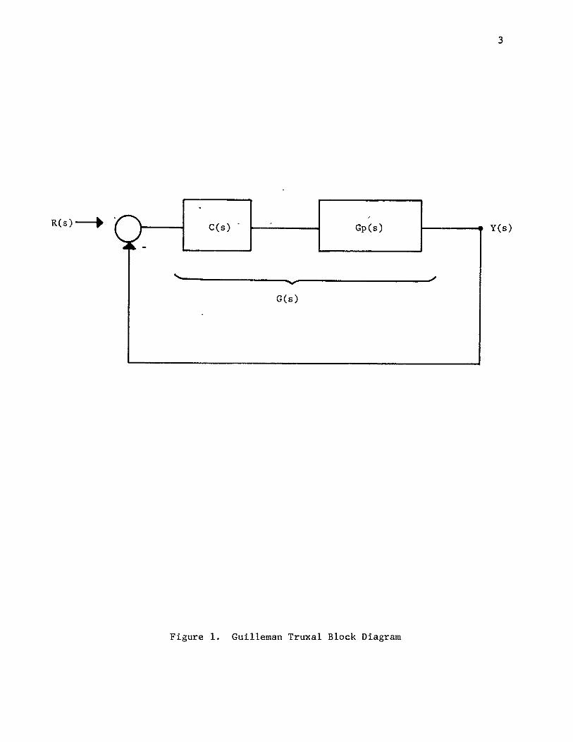

4
Equating the numerator and denominator polynomials
GN(s) = C(s) (1)
GD(s) = R(s) - Y(s)
The design procedure is as follows
1 From the specifications choose the desired closed
loop response Y(s)R(s)
2 From step 1 and eqn 1 determine GN(s) and GD(s)
3 Choose a suitable series compensator which shifts the
poles and zeros of the plant to the positions specified
by step 2
The above steps are simplified if one uses Guillemans suggesshy
tion to select a C(s)R(s) which results in real zeros for GD(s) Then
the zeros of GD(s) can be simply determined from a plot of R(s) - C(s)
for only negative real values of a One pair of complex conjugate
poles and a group of poles on the negative real axis is usually chosen
to meet the above requirements
For example suppose the plant is given by
i
Gp(s) = s s+l) (2)
and that the specifications can be satisfied if
Y(s) -100 R(s) 2 + 20s + 100
5
From (1)
GN (s) - 100
GD(s) = S2 + 20s
The series compensator C(s) and the plant transfer funetion must equal
G(s)
C(s) op(s) 100 a(s+20)
From (2)
C(s) = 100(s+l) (4)(s+20)
Effectively the series compensator moved the time constant of the
motor from 1 to 120
The success of this procedure depends upon the accurate modeling
of the motor over the range of frequencies from zero to well above 20
radianssec Otherwise additional poles in the plant transfer function
will alter the actual closed loop transfer function In particular the
real system may become unstable
State Variable Feedback Design Procedure
This design procedure is similar in many respects to the above
procedure First a desired closed loop response is selebted which
satisfies the bandwidth rise time steady state error and other requireshy
ments The plant is divided into a set of first order transfer functions
which may be interconnected The output of each of these first order
systems is fed back to the input through a fixed gain element By
adjusting these gain any desired closed loop transfer function can be
achieved
The above process is somewhat simplified if we first introduce
a new function Heq(s)0 This function specifies the transfer function
between the output and the input which yields the same result as state
variable feedback From Fig 2 the equivalent feedback from the output
is i s+ k2 + k3 Heq(s) = kl Gi (s GI(S)G2()
In terms of Heq(s) the state variable feedback results in the closed
loop response given by
Y(s)= KGp(s) (5) R(s) 1 + KGp(s) Heq(s)
The procedure is as follows
1 Select the desired Y(s)R(s) from the specifications
2 Equate the desired Y(s)R(s) to theone achieved by the
feedback from each state
3 Solve for the feedback coefficients
Details of the design procedure when zeros are present are given by
Schultz and Melsa [2 ] For example if
0p(s)= 1s (s+l)
Y(s) 100 R(s) s + 20s + 100
Then if G(s) 2(s)
Heq(s) - k1 + k2s
-- G3(s) G2 (s) ---GI(s) Y(s)
F 2
Figure 2 State Variable Feedback Block Diagram
8
From (5)
100 K2 2 s + 20s + 100 s + s + K(k1 + k2s)
Equating the numerator and denominator polynomials
K = 100
KkI1 100
1+Kk2 - 20
Solving for k1 and k
K = 100
k = 1
k2 19
This design yields exactly the same transfer function as the
Guilleman-Truxal (GT) method The two methods are not the same if a
small change is made in the plant transfer function The state variable
feedback (SVF) system changes less than the GT system
If the sensitivity is defined as the percentage change in the
closed loop transfer function for a small percentage change in a plant
parameter say K then
S K _ d dK dT K
T T K dK T
where for simplicity
T(s) - Y(s)R(s)
9
If K is the gain then
T(a) =KG(s)1 + KG(s) Heq(s)
dT(s) G(s) K Gp(s) G(s) fea (s) 2dK I + KG(s) Heq(s) (1+ KG(s) Heq(s))
Using this result in the definition of sensitivity
T = T(s) (6) T KG(s)
For the GT system from (6)
K s(s+20)
2T (s + 20s + 100)
For the SVF system from (6)
K s (s+1)ST 2 a + 20s + 100
For the GT system the sensitivity is greater at all frequencies than
the SV sensitivity especially at low frequencies
Modified Observer Systems
LuenbergerE ] has shown that an eytimate of the states in the
plant can be implemented as shown in Fig 3 When state variableshy
feedback is used from these states a specified closed loop response may
be achieved Muterspaugh [4 has modified this configuration by block
diagram manipulations to a form similar to that shown in Fig 5 The
1 2 2NN-1
kI
Figure 3 Luenburger Observer Block Diagram
r C(s) G(s) Y
Figure 4 Modified Observer Block Diagram
A(s)
I+
gt G(s) Y H(s)
Figure 5 Muterspaughs Modified Observer Block Diagram
13
series compensator shown in Fig 4 C(s) reduces to the Guilleman-TruxalLiJ
compensation in the case where H(s) is one Similarly this control system
reduces to the Heq [2 ] type of control resulting from state variable
feedback considerations when C(s) is one Fig 4 represents a more
general configuration than either Guilleman-Truxal or Heq type compensashy
tion All three configurations shown in the above figures are equivalent
Assuming that only the output is available the Heq configuration
is not realizable since Heq has zeros but no poles Guilleman-Truxal
type compensation is sensitive to plant variations Series and feedback
compensation is used to achieve low sensitivity and realizability If
Heq has zeros in the LP then the modified observer (MO) system is
slightly higher in sensitivity than Heq but if Req has zeros in the RHP
then the MO system is dramatically better These comments are illusshy
trated in the case studies at the end of this report
Modified observer System Design
This section derives the necessary conditions which C(s) and H(s)
must satisfy such that the desired transfer function Y(a)R(s) is
achieved when the plant has a transfer function G(s) The relationship
among these transfer functions is
T(s) 1() C(s) G(s)fR(s) 1 + C(s) G(s) H(s) (7)
If the feedback signals shown in Fig 3 are combined (using
block diagram manipulations) the resulting transfer functions are
A(s)=k2 1P1 (S)+k 2 (fIpI(s)p 2 (s)+12P2 (s))++knceiPl(s)+ -PNI(s))
H(s)k 1+k2p1 +k 3P1p2++kpN-1
14
Since the poles of H(s) and A(s) are arbitrary the control systems shown
in Fig 5 have N-i arbitrary parameters however the poles of A and R
are identical
One more manipulation of the system shown in Fig 3 results in
the system of Fig 4 where
1 C(s) - I + A(s)
The zeros of C(s) are the same as the poles of A(s) therefore the N-1
zeros of C(s) are also the same as the N-i poles of H(s)
From these facts (7) can be used to determine the denominator
of C(s) and the numerator of H(s) Dropping the argument a in (7) and
denoting the transfer functions by
CDC(s)
H(s) -
G(s) ONGD
T(s) - R
Eqn 7 becomes
CN GN 1 CD GD(8) R 1i+ CN GN HN
CD GD HD
If the right hand is simplified then
Y CN GN HD (9)R CD GD HD + CNCN
Since CN and HD are the same denote them both by P(s) Then (9) simplishy
fies to
15
Y GN P (10)R CD GD + NHN
cross multiplying on both sides results in the polynomial
Y(CDGD+GNHN) - R-GNP (11)
Define the number of zeros in G as NG the number of poles as
ND and similarly NY and NR for T(s) If the order of both sides of
(11) is to be the same then
NY + ND - 1 + ND NR+ NG + ND - 1
NY + ND NR + NG (12)
NR - NY -ND - NG
Thus the pole zero excess of the plant determines the pole zero excess
of the desired closed loop transfer function If like powers of (11)
are equated then NY + 2ND equations result Since CD and 1N are undeshy
termined the number of unknowns is 2ND For NY = 0 the number of
unknowns is equal to the number of equations Just as in regular state
variable feedback[2 for zeros in YR additional states must be
created Let the order of P(s) by N-l then (12) becomes
NY + N - I + ND = NR + NG + N - 1
and for the number equations to be equal to the unknowns
NY + ND + N = 2N (13)
N = NY+ ND
16
Thus the order of both controller systems C(s) and H(s) must be one
less than the number of poles of G plus the number of zeros of YR
assuming that (11) represents a set of linearly independent equations
The design procedure is as follows
1 Select the desired closed loop transfer function from the
specifications
2 Select a polynomial P(s)
3 Equate the actual and desired transfer functions (iO) and
solve for the coefficients of CD(s) and HN(s)
Program 1
The first program (MODOBSI) computes the transfer function of
the series compensator and the feedback compensator as a linear function
of the denominator of the feedback compensator The user must specify
the plant transfer function and the desired closed loop transfer
function Thus this program specifies the design of the system except
for the poles of the feedback compensator which the user is free to
choose in any way he wishes
Program 2
The second program (MODOBS2) computes the transfer function of
the series compensator and the feedback compensator which minimize the
low frequency sensitivity of the closed loop system to plant variations
The user must specify the plant transfer function and the desired closed
loop transfer function If the time constants in the plant are much
lower than in the closed loop system the poles of the feedback compenshy
17
sator may be in the right half plane (RHP) If the poles of the compenshy
sator are in the RHP then the system will be vyD sensitive to variations
in the parameters of the compensators In this case it is better to
use one of the other programs This program is limited to systems with
no zeros
Program 3
The third program (MODOBS3) computes the weighted integral
sensitivity of the system for a given polynomial P(s) The user must
specify the plant transfer function closed loop transfer function the
weighting to be given the sensitivity as the frequency varies and the
denominator of the feedback transfer function P(s) The weighting
function must have more poles than zeros
Input Data
In many circumstances the available data for the plant is in
state variable form This data is converted to a transfer function by
the STVFDBK program The details of the program are included in reference
1 The program listing and input data format are also included in the
Appendix
Output Data
The program BODE4 is provided to plot the transfer functions
computed in the above programs on a logarithmic scale For each program
some of the transfer functions of interest are
1 Plant transfer function
2 Closed loop transfer function
3 Sensitivity as a function of frequency
4 Loop gain function
The loop gain function divided by one plus the loop gain is the proportion
of measurement noise at each frequency which will reach the output Thus
if the loop gain is much greater than one then nearly all the noise
reaches the output and if the loop gain is much less than one very little
measurement noise reaches the output If the phase shift of the loop
gain is nearly 180 at a gain of one the measurement noise will he
amplified
Program 4
The fourth program (MODOBS4) is useful to check the results of
the design Given P(s) and the results of the first program (MODOBSI)
this program computes HN(s) CD(s) and the roots of both the series and
feedback compensators This program and the first program give a
complete determination of the design
Results
A discussion of each program and several caee studies are inclushy
ded in the Appendices MDDOBSI is useful to compute HN(s) and CD(s) in
terms of the coefficients of P(s) Quite amazingly the coefficients of
N and CD are linearly dependent upon the coefficients of P HODOBS2
computes the coefficients of both compensators which achieve minimum low
frequency sensitivity Essentially this result is achieved by forcing
CD(s) to be an N-i order integrator which increases the gain at low
frequency and thereby decreases the sensitivity since SK = (s)
Unfortunately if the plant denominator coefficients are smaller than
19
those of the denominator of the closed loop transfer function the feedback
compensators may have poles in the RHP MODOBS3 determines the weighted
integral sensitivity when P(s) is specified MODOBS4 is useful for
checking the roots of the resulting compensators after a design is
complete Test results are given in the appendix for three examples
These examples show that an improvement in the system sensitivity over
that of just a series compensator can be achieved even if only the output
is available When the closed loop response is much faster than the open
loop the sensitivity of the MODOBS system approaches the sensitivity of
the Req system (which is best but not realizable) if the roots of P(s)
are made much larger than the closed loop roots If the closed loop
response is not much faster than the open loop response then the MODOBS
system may have a sensitivity lower than the Heq system This situation
exists whenever Heq(s) has zeros in the RHP These results point out
the important fact that a sacrifice in sensitivity to plant variations
is made by increasing the system performance requirements Because of
this fact careful attention to the plant performance should be made for
lowest sensitivity and unnecessary demands on overall system performance
should be avoided
20
Bibliography
1 J C Truxal Control System Synthesis McGraw-Hill 1955 Chapter 5
2 J L Melsa and D G Schultz Linear Control Systems McGraw-Hill 1969 Chapter 9
3 D G Luenberger Observing the State of a Linear System IEEE Transactions on Mil Elec April 1964
4 M E Muterspaugh State Variable Feedback and Unavailable States HS Thesis 1968
5 F H Effertz Comment on Two Coupled Matrix Algorithms for the Evaluation of the rms Error Criterion of Linear Systems Proceedings of the IEEE November 1966 p 1629
6 J L Melsa A Digital Computer Program for the Analysis and Synthesis of State Variable Feedback Systems NASA Contract Report CR-850 August 1967
7 L E Weaver et al A Control System Study for an In-Core Thermionic Reactor J P L Report 32-1355 January 1969
21
Appendix I - MODOBSI
Dis cussion
The basic algorithm of this program is based upon (5) First the
following polynomials in s are computed
T = (GD)(Y)
Q = (GN)(R)
V = (GN)(Y)
so that (5) becomes
(T)(CD) + (V) (HN) = (Q) (e) (Al)
Each of the terms in (Al) are polynomials in s where P(s) is unspecified
For instance P(s) = P3s2 + P The coefficients of CD(s) and HN(s) are
the unknowns
As an example suppose the plant is second order then P(s) is
first order In this case (Al) becomes
(CD2T3 +H 2 V3 )s 3 + (CD2T2 + CD1T3 + H2 V2 + H1 V3 )s2 + (CD2T1 + CD1T2
2 + H2V I + HIV2)s + (CDIT + HV) = P2Q 3s + (P2Q2 + PIQ3 )s2
+ (P2Q + P1 Q2 )s + PlQl (A2)
Equating coefficients of like powers of s results in the equations
T3CD 2 + V3H2 Q3P2
T2CD2 + T3CD1 + V2H 2 + V3H1 Q2P2 + Q3PI
22
T1 CD2 + T2 CDI + VIH2 + V2H 1 QlP2 + Q2P
TICD1 + V1Hi = Q1F1 (A3)
These equations can be rewritten more compactly in matrix notation as
T3 0 V3 0 CD2 f 0 Q3TN12N-2 T2 T3 V2 V3 CD11 214-22-Q3 Q3 Q22 (A)
2 T V1 V2 H2 Q2 QI P2j _ Ql 0
2N-2- shy - N-i-)
The matrix on the left will be defined as matrix A and the matrix on
the right will be defined as matrix C Then
CD2 CDI _ - 1
CD= A-C (A5)
H I
Therefore A- C relates the unknowns CDi and Hi to the parameters Pi
MODOBS1 forms the matrix A from the two arrays T and V and then inverts
A Next the C matrix is formed from the Q array and then A 1 C is
computed and printed
23
Input Format
Card No Columns Description Format
1 1 NY = order of Y(s) in YIR II
2 NR = order of R(s) in YR Ii
3 NG = order of GN(s) in GNGD i1
4 ND = order of GD(s) in GNGD Ii
I 5-80 Identification of problem 8AI0
20 Cn of 2 11-0 Coefficient of s in Y(s) FI03
11-20 Coefficient of aI in f(s) P1e3
etc
71-80 Coefficient of s7 in Y(s) F103
3 1-10 Coefficient of a in R(s) F103 etc
4 i-i0 Coefficient of s in GN(s) FIO3
etc
5 etc Coefficientof a in GD(s) FI03
Notes
1 If more than eight coefficients are required then two cards may be
used to identify that polynomial
2 A decimal point must be used for each coefficient but not for card
No 1 The decimal point may be placed in any of the ten columns
for each coefficient
24
3 As many problems may be run as desired by repeating the above format
for each problem
Output Format
See example
Subroutines to be Used
PLYMLT Multiplies two polynomials together
MXINV Inverts matrix A
PRNTRAT Prints the ratio of two polynomials
Flow Diagram
Read NYNRNG
ND
FRead Y(s)R(s)GN(s) GD(s)
Compute T = YGDQ = GNRV = GNYj
Form A Matrix
Invert A Matrixi
lForm C Matrixl
A -1
ComputeBA7 C
Print CD and E
Arrays
PROGRAM MODOBSI (INPUTOUTPUTTAPE4INPUT)
ODIMENSION Y IC) R(10) GD(IO) GN(IC) V(201 T(20) G(20)14A(S363)AI(36 3)C( 3611) B(36 1U ID(G)
C Y(S)R(S) IS DESIRED CLOSED LOOP RESPONSE C SP(S)GD(S) IS PLANT TRANSFE FUNCTION C NY IS ORDER OF NUM IN Y(SlR(S) NR IS ORDER OF DEN C NG IS ORDER OF NU OF G(S) NO IS ORDER OF-DEN C NR-NY MUST EQUAL ND-NG 1 READ 1U1NYNRNGNDID
PRINT 200NYNRNGNDIO
IF(EOF4) 99t2 2 NY1=NY4 1
READ 102 (Y(I)I=-INY1) C YI) IS COEFF OF S(I-I) IN Y(S)
NR I=NR C RII) IS COEFF OFS(I-1)IN-P(S) 3 READ I102 (R(I) IINRI)
CALL PRNTRAT(YNY1RNRI IHTIHS) __C_ GN(Il IS COEFF9F_SCI-1LIN_-GNtSL
NGl1NGI NO 1NDI
_4 -READ 102 (GN ) I 1NG1) C GOD(I) IS COEFF OF S(I-1) IN GO(S) 5 READ 102 (CG (I)I--1NDI)
CALL PRNTRAT(GNNGIGDNO HGIHS___ C FORM CHARACTERISTIC POLYNOMIAL
CALL PLYMLT (GDND1YNYITO) CALL PLYMLT GNNG1RNRI00-CALL PLYMLT (GN NGGYNYIVO) NYNGzN Y1 4NGI NR+NG+iN __ 00 6 IrNYNGN
C NA IS ORDER CF A MATRIX WHERE A IS MATRIX RELATING UNKNOWNS -6- V( --- - - TO PARAM P
NA_- 2 (N--1) DO 20 J-1NA IF- (J GT (N- IlJGO__TO2_12 00 10 Iz1NA INDN- L J IF _( IND-SLT_ I)_GOTO8_ IF (IND GTN) GO TO 8 AUIJ)- T(INa) 30 TO 10shy
8 A(IJ) O 10 CONTINUE
Gi__TO_2D
12 DO 20 I=INA IND 1-I+J IF- (INDLT__GO__18__ IF (INDGTN) GO TO 18 A(IJ)-V(IND) GO-T 0 _2D
18 A(IJ)-O 20 CONTINUE
CALL MXINV-(ANAtAll_ C C IS THE COEFF ARRAT
NM IrN-1 _DOZ4__I NA-_ DO 24 J=1YNMI IN= 2N-I- J
IFiINDLT1) GO TO 22 IF (INDGTN) GO TO 22
C(IJ) = O(INO) -
GO TO 24 22 C(IJ)rO 24 CONTINUE C B IS AICTAE ROwS OF 5 ARE EQUAL TO CD AND HN C COLS ARE COEFF OF P PARAMETERS
D0 30 INA 00 30 KzlNM1 B(IK)--O 00 3fJ--JNA
30 B(IK)-AICIJ C(JK+B(IK) PRINT 2O1KK--lNMI) DO 40 I--NMI
NC =N -I 40 PRINT 202 NC (B I-Kt NM1I
DO 50 I=NNA
NBzNA+-I -50 PRINT 204t-NB (8(1I(1 Kzl-NM-1
GO TO I 99 STOP -101-FORM ATf l A 1f)V t 102 FORMAT (BF103) 200 FORMAT (1HI4(2XI1) 2X6A1i0) 201 FORMAT IH X8 ( 314- P( I 11 I-) OX)) 202 FORMAT 14H CO(I2--)10(E1U33X)) 204 FORMAT (4H HN(I12H)=)I(EIO33X))
END SUBROUTINE PRNTRAT (ANNBvNOEPVARINDVAR) DIMENSION A( 20)B( 20H_(20)N(20)AT20BT(20)NEt 1
DO 6 I--NN AT(I)-- -IF-(-AY f-4i 6-3
3 H(NE)zlH+
AT(NE)rA(1) GO TO 5
4 H(NE)--IH-
AT (NE) -A(I) N(NE)I-1 NErNEI
6 CONT INUE NE=NE-1 PR IN-T 10 0 MIN=MINO(NE 10) PRINT 10lCN(I)IzMIN) PRINT 102 (HRU1 ATI) INDVAR Il tMIN) IF (NE-if]) 8987
7 PRINT 101 (N(I IrIINE) PRINT 102 CHI)AT(I)INDVARI--INEI
__ NF= O0 16 I--IND BT (I)--DIF C B(C) 191G13
13 H(NF)rlH4 BT(NF zB(I)
-GO-_ T _15 14 H(NFI -IH-
BT (NF) =-B(I)
r27 15 N(NF)=I-I
NF zN Fi-I 16 CONTINUE
NF =N F- I HH= IH-NH=rAX 013NE 13 NF) NHzMINO(130NH)
20 PRINT 103 DEPVARINOVAR (HH I=INH) MIN MINO(NF 10) PRINT 101 (N(I)IzIMIN) PRINT 102 (Hi(I)BT(I ) 1NDVAR-I---1MIN IF (NF-101) 28P2827
27 PRINT 0l (N(I) IzIINF) PRINT 102 (H(IJBT(I)TNDVARI=N-FI)shy
28 CONTINUE 100 FORMAT C iHO) 101 FORMAT (6XI(11X 12)) 102 FORMAT 6XID(AIGlC4 AI1H H 103 FORMAT tIXtAIIHCAI2H)= 30AI)
RE TURN END SUBROUTINE MXINV (R N RI) SUBROUTINE TO FIND THE INVERSE- ----- GIVEN
C MATRIX R N IS ORDER OF MATRIX RI IS INVERSE C MATRIX SUBROUTINE USES GAUSS-JORDAN REDUCTION C R MATRIX IS PRESERVED DIAGONAL ELEMENTS OF R-US
BE NONZERO C DIMENSIONR(3G36IRA(3G72) RI(36v36)
C STATEMENTS 20-26 ENTER R ARRAY INTO RA ARRAY - C AND SET LAST N COLUMNS OF RA ARRAY TO IDENTITY
C - MATRIX 20 DO 26 I 1 NI-v 21 DO 24 J I N
_22__RA IJ) -R(I- J) 23 NJ = N + J 24 RA(INJ) = 0 2 5 _NI z N + I 26 RA(INI) = 1
C C ST AT EM ENTS _ii-12_REDUCE MATLRIX__RA _SOH_ATZ_JRFSR_LK C COLUMNS ARE SET EQUAL TO THE IDENTITY MATRIX
i NP = 2 N 2_DO 12 I - N
C -
C STATEMENTS 3-5 ARE USED TO SET MAIN DIAGONAL _C ELEMENT TOUNITY
3 ALFA = RA(TI) 4 DO 5 J = I NP S RA(IJ) r RA(I J) _ALFA
C C STATEMENTS 6-11 ARE USED TO SET ELEMENTS OF ITH C COLUMN TO -ZERO
6 00 11 K = 1 N 7 IF (K - I) 8 11t 8 8 BETA = RAiKI) 9 DO 10 J = It NP
10 RA(KJ) = RA(KJ) - BETA RA(IJ) - ICONTINUE_ 12 CONTINUE
C
TO LAST 28 C STATEMENTS 30-33 SET INVERSE MATRIX RI EUAL
C N COLUMNS OF RA ARRAY
30 DO 33 J 1 N 31 JN J + N 32 00 33 I 1 N 33 RI(IJ) rRA(IJN) 34 RETURN
END SUBROUTINE PLYMLT (ALBMCN)
C C MULTIPLY ONE POLYNOMIAL BY ANOTHER
C C DEFINITION OF SYMBOLS IN ARGUMENT LIST C A(I) MULTIPLICAND COEFFICIENTS INTHEORDER AE) S(I-1) C L NUMBER OF COEFFICIENTS OF A C B(I) MULTIPLIER COEFFICIENTS IN THE ORDER 8(I)SI-1)
C M NUMBER OF COEFFICIENTS
C C11) PRODUCT COEFFICIENTS IN THE ORDER C(19S(I-1)
C N NUMBER OF COEFFICIENTc Ac r
C C REMARKS C IF N-- C(I) SET TO ZERO AND PRODUCT FORMED OTHERWISE THE
C I-PRODUCT AND SUM NEWC-OLD C + AB IS FORMED
DIMENSION A(iD) B(IO) t C(20) LPML+M- 1 IF (N) 10102iZ
I DO 1 J- LPM 11 C(J)-Oo 12 DO 13 J--ILPM
MA X-MA XD (J + I-M il)) shy
- MINzMINO(L DO 13 IrMAXMIN
13 CC(J)=A(I)B(J+II) + C(J) RETURN END
3434 IN CORE THERMIONIC REACTO R
116708 481228 384520 200 1 16708 -4870635__4085815__39226_ 100 116708 481228 384520 200- 503585E-610542E- 3 058639 18804 1
END OF INFORMATION
29
Appendix 2 - MODOBS2
Discussion
If CD(s) in (5) is defined by CD(s) = CD N-i (BI)
where N is the order of the plants then the system will have minimum
low frequency sensitivity because the forward loop gain will be increased
at low frequencies If there are no zeros in Y(s)R(s) or in G(s) (5)
reduces to a simple set of linear equations shown below For simplishy
city RN+ I and GDN+t are set equal to one For zero steady state error
Y = R1
PNl PN= I PN-I = N-I
PN-2 + RNPN-1 CN-2
(B2)
P + 2 + ReN- =1 I I
IN I = P RY
HN2 =PI RY + P2
+HN=NPI RNY + P 2 -Y +i - GD1Y
Where the C terms are defined by
C I GD2 - R2
C2 = GD3 - R3
CN- 1 GDN - N
30
The Eqns (B2) are simply solved in the order shown by back
substitution That is PN-1 may be usedto solve for PN-2 which may be
used to solve for PN-3 etc
Input Format
Card No Columns Description Format
1 1 N = Order of the Plant G(s) Ii
2-80 ID Identification of problem 8A1O
2 1-10 Y = Numerator of YR F10o3
0 3 1-10 R(1) = coeff of s in R(s) F103
11-20 R(2) = coeff of s I in R(s) FIO3
etc
7 71-80 R(7) = coeff of s in R(s) FI03
4 1-10 GN = numerator of G(s) F103
5 1-10 GD(l) = coeff of s in GD(s) F1O3
771-80 GD(7) = coeff of s in GD(s) F103
See notes following input format for MODOBSIo
Output Format
See example
Subroutines to be Used
PRNTRAT - Prints the ratio of two polynomials
PROMT - Determines the roots of P(s) to see if any roots are in
RHP
PROGRAM OOS2 (Y4PUT OUTPUTC4=INPUT)IO41 N j (l10 1 ( l ) 1 ([) Cl(In)ID( 3)PHN 1 )CD t13)
C U (IG) V (10) C PqOGRAM TO CALCULATE MINIMUM LOW-FREO SENSITIVITY MODIFIED C OBSERVER SYSTEM C Y(S)R(S) IS DESIRED CLOSED LOOP RESPONSE C GN(S)GD(S) IS PLANT TRANSFER FUNCTION C N IS ORDER OF DEN IN Y(S)R(S) C N IS ORDER OF DEN IN GN(S)GDIS) C R(I) IS COEF OF S(I-1) IN R(S) C C ASSUMPTIONS C C TRANSFER FCN GAINS ARE NORMALIZED SUCH THAT R (N+1)I1
C AND GD(N I )=I C C DESIRED TRANSFER FCN HAS ZERO STEADY STATE C
-C GD(I) IS-COE-F-- O-F S(I-I)1NGO(S) C Y(S)=Y GN(S)-GN (NO ZEROS ALLOWED) C I READ 101 N ID
IF(EOF4)99 2 2 READ I02Y
READ 102 (R(I)IzIN) NP i-N+ I
GD(NPI) =1 5 RNPI_)-1 READ 102 GN
3 READ 102t CGD(I)tlz1N) PRINT 200DNIO10 PRINT 201
CALL PRNTRAT CYIRNPHTIHS) PRINT 202
CALL PRNTRAT(GNGDNP11HG1HSI C-C --SOLVE FOR DEN OF H P(S)
NM I=N-I do 40 II -NM1 IPIlzI+I
-4 -CI) zG0c IP 1I-R IiT P(N) -
005[ I=ItNMj NI N-I P(NI)zC(NI)
IFCILE1) GOTO-50_ DO 49 Jz2I J2=N-J+2
4 P(NI )zP( NI )-R( J2 )P( JI ) 51 CONTINUE
CALL PROOT (NMIPUV) PRINT 205
PRINT 206 (U(I)V(I) I=INM1)
ERROR THUS YR(1)
SOLVE FOR NUM OF HHN(S) DO 60 1N HN (I 0 - 00 60 JzlI IJI j4
C
6C PN Il)r( Ji R (IJ) Y +HN( I) 32 HN (N )HN (N)-GD (1 )Y
PRINT 203 CALL PRNTRATIHNNPNIHH1HS) PO 80 1i NMI
80 CO(I)zO CD(N)zl PRINT 204 CALL PRNTRAT(PNCDN1HC1HS) G z YGN PRINT 210 G GO TO I
99 STOP 101 FORMAT (Il 84101 102 FORMAT (SF1O3)
200 FORM AT(IHII0X II 4X 8AID) 201 FORMAT(1HOTHE DESIRED CLOSED LOOP TRANSFER FUNCTION IS)
202 FORMAT(1HOTHE TRANSFER FUNCTION OF THE PLANT IS)
203 FORMAT(IHOTHE TRANSFER FUNCTION OF THEFEEDBACK COMPNSATOR IS)
204 FPRMAT(lHOTHE TRANSFER FUNCTION OF THE SERIES COMPENSATOR IS)
205 FORMAT (IHO 5X THE ROOTS OF P (SI ARt 13XREAL PART IOXIMAGINARY PART)
-20 FORMAT 32X2E207f 210 FORMAT4IHOTHE ADDITIONAL FORWARD LOOP GAIN REQUIRED IS
1YGNElfl3) END SUBROUTINE PRNTRAT (ANNSNDDEPVARINOVAR) DIMENSION A(20)B(20vH(20) N(20 1 AT(20) PT 20 NE z1 00 6 Iz1NN AT(1)=D IF C(IA ) 463
3 H CNE )= IH + AT (NE) =AtI) GO TO 5
4 H(NE)=IH-AT (NE) =-A( I) N(NE)--I-1 NE-NEI
6 CONTINUE NE=NE-1 PRINT 100 MINMINO(NE v1O
PRINT IOl (N(IhI=IMIN)
PRINT 102 (H(IAT(I)INDVARI-IMIN) IF (WE-10) 8
7 PRINT 101t (N(I)IzlINE) PRINT 102 (H(I)AT(I)INDVARIn1NEl NF o_-8_ N --1 80 16 I1NU
BT(IzO IF ( (I) 1141613
13 H(NF)zlH+ BT(NF)l=B(I)
-GO T0- 15 __ - 14 H(NF) zlH-
BT (NF)z-B(I) - 15 N(NF)=I-1 -
NFZNF41
33 ID CONTINUE
NF NF- I HHL IH-NHMAXO( 13NE 13NF) NHzMINO( 130NH)
20 PRINT 1G3DEPVARINDVAR(HH 1=1NH) MINMINO(NF 10)
PRINT 101 (N(I)IlMIN) PRINT 1G2( H(I)BT(I)INOVART IMIN] IF (NF-in) 2828927
27 PRINT 101iN(I) I11 NF) PRINT 102 (H(I)BT(I)tINDVARI-IINF]
28 CONTINUE 100 FORMAT (1HO) 101 FORMAT (GX1O( IIX12)) 102 FORMAT (GXI0(AIGIO4 A1IH )
103 FORMAT (1XA1IH(Ai2H)-130A1) RETURN END
___SUBR CUT INEPR O0 TN _A U fVtIIRR) DIMENSION A(20)U(20)V(20)H(21)8(21 )C(21) IREV-IR NC -N +IDOll--i Nu
H( I) rA( I) _i CONTINUEL
00
3 IFIH( 1)) 24 2 NCNC-1
V NC )z0 U NC O DO 1002 I= 1NC H(I)--H(I+1 )
1002 CONTINUE GOT03
S_IF (NC- 1) 5 10 05 5 IF (NC-2) 7i 7
6 R=-H( 1H(2) GOT050
7 IF INC- 3) 9-819 8 P-H(2)H(3)
__0 1) H (3_)_ GO TO7g
q IFCABSCH(NC-1)1H(NC)-ABS(H(2)H(1))101919 10- IREV - IREV_
M=NC2 DO11I=-1 M
_-NL-zNC+ 1 -I-FrH( NL) H NL )H( I)
11 H( I) F -IF (O )139 12 913
12 P=D GOTO 15shy
13 PzPQ 0= (
15 IF(R)16191G 16 R=1 R 19 E5E- ]C
B(NC)H(NC) C(NC)H(NC) B(NC+1 )zO C( NC 1)z 0 NP NC- 1
20 0049J= I 100C DO 2111l1 NP ITNC-I I BC I rH(I)+RB(+1)
--21C( I) =B (I)+RC( I+ 1) IFCABS(B(I )H(1))-E)5050 24
24 IF(C(2)232223 2amp R= RlI-
GO TO 30 23 R=R-B(1) CC2)
30 D0Q3711zlNP IzNC-I I BI)i(I)-PB(I+I)-OB(I+2)
37C( I) =B (I)-P C(i1l) OC(12) IF(H (2)) 323132
31 IF(ABS(C2)H(1))-E)333334 32 IF(ABS(B(2)H(2) )-E) 33v3 34 33 IF(ABS(B(1)H(1))-E)707034
34 CBARrC(2)-B(2) DC(3) 2-CB ARC ( 4) IF(D)363536
35 PzP-2 0= (o t GOT049
36 PP(-82)C(3)-BC1)C(4))D - Q+ (-( 2)CBARB(1) C(3 00)
49 CONTINUE
ErE 10 GOT020
50 NC-NC-1 VtNC)D
IF (IPEV) 51 5252 51 U(NC)=1R-
GOT053 52 U(NC)-R 53 00541lNC
H(I) B(1+1) 54 CONTINUE
GOT04 70 NC=NC-2
---- IF(IREV)71727 71 QPr1O
P=P(Q2 0) GOTO73-_
72 OPPP Q-P 2 0
73 F-(PP)2-OP IF(F )74 7575
74 U(NC+I)z-PP U(NC)-PP V(NC 1 )SORT(-F) V( NC 1-V (NC+ 1) GOT076
75 U(NC+11-(PPABS(PP))(ABS(PP)SQRT(F)J V( NC+1 )0 U(NC )OPU (NC1) V( NC )O
76 D0771INC H(I) B(1 2)
77 CONTINUE GOT04
LDO RE TURN END
3 CASE STUDY II THIRD ORDE-SYSTE14shy1000 1000 200 20 D O -
2500 100
36
Flow Diagram
Read N ID
Y R(I)
GN GD(I)
Print N ID
YRy G
Form C(I)
ISolve for P(s)j
Solve for HN(s)I
Print H(s)
Print C(s)
37
Appendix 3 - MODOBS3
Discussion
This program uses the following data
1 Plant transfer function G(s)
2 Desired closed loop transfer function T(s)
3 The denominator (P(s)) of the feedback compensator H(s)
4 A desired weighting function W(s) on the integral over
frequency of the sensitivity of the closed loop response
to forward loop gain changes
The program then calculates the weighted integral sensitivity of
the system The method of calculation is based upon an algorithm by
EffertzL5] The integrand of the integral sensitivity is calculated
from
I S W(S) S (S) ds
2r f G(s)C(s) ds
The algorithm is based upon an iterative manipulation of the coefficients
in the numerator and denominator of the integrand in such a way that the
integral of the squared magnitude results
A closed form solution for the integral
jm n 2rj jo h(P)h(-P) 2 -joo
1 30 dP 1 j F(P)F(-P) dP
(BI)
is presented in the paper by F H Effertz The solution takes the form
38
of Equation 4 in his paper A better algorithm for the computation of
Equation 4 in Effertz is presented in the correspondence by Pazdera
(Equation 7) A modified forn of Pazderas algorithm has been coded in
FORTRAN and is included A test problem is also included
The use of Equation 4 in Effertz can be best illustrated by an
example Suppose we wish to evaluate the following
(B2)Ls2+ Cb) [2bLn = 2I -
It can be shown from residue theory that the correct answer is
I = - residue of F(s) F(-s) at s = a (B3)n
- residue of F(s) F(-s) at s = b
where F(s) F(-s) indicates the function to be integrated over s = jW
Then the answer is
22 2
= - c-a (c2-b2 c2+abn 2a(a+b)(a-b) 2b(a+b)(b-a) = 2ab(a+b) CR4)
To use Equation 4 from Effertz we must make the following associations
using the complex frequency variable s in place of p
22 s= c -g(P) = (s+c)(c-s)
then s (B5)
2
h(P) = s + (a+b) s + ab
then p s N=2
1
a a 2 =ab
39
The integral for n = 2 can be expressed as
bb [bloaaob I- (B6)
a0 t ol [jaza1-2 1ao a 2
Substituting the correct values of a0 a etc and cancelling minus
signs for this problem we obtain
ab +c In = 2ab(a+b) (B7)
What is most interesting is that the result depends only on the coeffishy
cients of the known function being integrated and not on the poles of
the function as one would suspect from residue theory
It has been mentioned that the algorithm from Pazdera (Equation 7)
has been programmed Some charges in the nomenclature of Equation 7 were
necessary to facilitate coding Note that the practice in Effertz and
Pazdera is to make the highest membered coefficient correspond to the
lowest power of the variable p Note also that subscripts such as ao
are in evidence To facilitate coding the lowest numbered coefficient
was subscripted in the form A(l) and this coefficient was associated with
0 ththe lowest power of the variable p in this case p In general the i
coefficient A(I) is associated with the (i-1)s t power of p P -l (In
FORTRAN the expression A(O) is not allowed) Note from equation I above
what must be done to operate on the function F(s) F(-s) If F(s) is of
the form
F(s) = C(S) (B8)A(S)
then the algorithms suggested in both Effertz and Pazdera require the use
40
of
g(s) = C(S) C(-S) (B9)
h(s) = A(S)
It is more desirable to input C(S) and A(S) rather than C(S) C(-S) and
A(S) Consequently one uses the INTSQ subroutine by coding the coeffishy
cients of C(S) and A(S) with ascending subscripts corresponding to
ascending powers of S The subroutine provides the operation C(S) C(-S)
Furthermore the subroutine checks to see if the lowest coefficient of
C(S) or A(S) is zero so that factors of S may be either considered or
cancelled Two basic requirements must be met by A(S) and C(S) First
the roots of A(S) and C(S) must at least have non-negative real parts
(Hurwitz polynomial requirement) Secondly the highest power of C(S)
must be at least one less than the highest power of A(S) for convergence
to be assured If A(S) is Nth order one inputs the N coefficients of
A(S) and the N-i coefficients of C(S)
The use of this subroutine INTSQ may be best illustrated by an
example Suppose we desired to evaluate the integral
I = JD F_ 7 4 - JdS n -joe 3 + 3s2 + 2s + L[43 + - 2s
(BIO)
The polynomials C(S) and A(S) as defined in Equation B8 are input into
the program as
C(1) = 4 A(l) = I
C(2) I A(2) = 2
(Bi) C(3) o A(3)= 3
A(4) = 4
41
The program then utilizes the modified Pazdera algorithm and prints out
the message
THE VALUE OF THE INTEGRAL IS 12250
To check this answer one can use Effertz Equation 4 for a third order
case (n=3)
a oa 101o 2 1 n
= (142a
0 a
aI a a 0
I 2a
boa2a3+b2aoal-aoa3b alaaa a (BI2)
0 1 20 - o2 2 3o 31 o 13a22o0
For our example problem the following associations follow
b =0 a =4 0 0
b 1 -l a = 3 (B13)
b2 =16 =2a 2
a 113
Substituting the values of Equation B13 into Equation B12 verifies the
computers solution I = 1225n
Input Format
Card No Columns Description Format_
See format for MODOBSI
K 1-10 P(1) - coeff of so in P(s) BE103
11-20 P(2) - coeff of s in P(s) 8E103
etc
42
Input Eormat (contd)
Card No Columns Description Format
K+I 1 NW - Number of coeff in denom of W(s) II
K+2 1-10 WN(I) - coeff of s in num of W(s) 8E103
11-20 WN(2) - coeff of s in num of W(s) 8EI03 etc
K+3 1-10 WD(1) - coeff of s deg in den of W(s) 8E103
11-20 WD(2) - coeff of s in den of W(s) 8E103 etc
43
PROGRAM MODORS3(INPUTOUTPUTTAPE4-INPUT ) DIMENSION Y( 10)R(10)c-D(IO) SN(lOhIP(10)CD(0) HN(IO)SN(40)bull
IS0(40) B(36 18)WN(10) WD 10)SNT(40)SDT(40)C
I CALL MODOBSI (YP GN GO5 NY1 NR1 NGI NDI C N-1 IS THE NUMBER OF COEF IN P(S) HN(S) CD(S)
NrNR 1+NGI- 1 N =rN -1 READ 10 lP(I)Iz1NI)
C W(S) = WNWD MUST HAVE MORE POLES THAN ZEROS C NW IS THE NUMBER OF TERMS IN THE DENOMINATOR OF WS)
READ 103NW READ 102 (WN(I)I-INW)_ READ 102 (WD(I)I-INW) PRINT 205 CALL PRNTRAT (WNNWDNW1HW4-lkHS) CALL PLYMLT(GDNDlY NYI SN 0) N2=NDI+NYI-I
_CALL_ PLYMLTT(yN NWSNN 2 SNT D) CALL PLYMLT (GNNG1 R NRI SO 0) CALL PLYMLT(WDNWSDN2SDT C)
__N3=NW+N2-1 -
N4 =N 3+ NI-1 N22N1 11
-a- DO 10 I= 1Nl CD(I)=0 HN(I)O 00 10 J1pN1 CD (I)B(N-I J)P J )+CD( I)
10 HN(I)zB(N2-IJ)P(J) +HN(I)_P -I NJ_Z0 I--_
CALL PRNTRAT(PN1CDN1IHCIHS) PRINT 202
CALLP RNTRATAHN NI P Ni1H Ht l1 CALL PLYMLT( CDN1 SNT N3 SN C) CALL PLYMLTI- PN1SDT N3SD 0) -N5=N4 ---CALL INTSQ(SDSNN4S) PRINT 204 S
- GO T ---O-- -- 102 FORMAT 18 E1O3) 103 FORMAT III)
-201 -FO RM ampTL__TJJLJERANS ER_-F-UN CT-O-N--OF--L sESERIS--COMENSJ-IO-R- i-l 202 FORMAT(O THE TRANSFER FUNCTION OF THE FEEDBACK COMPENSATOR IS) 204 FORMAT(O THE WEIGHTED INTEGRAL SENSITIVITY ISEIO3) 20S -FORM-AT( Oi-tJ-WEIGHTINGFUNCTION-OF-HE- INTEGRALSENS-IIVlTY-YI-_shy
1) END
_SUBROUTINEMOOOBS1 LYR GN GD B N-YI-NRI-NGL-ND44-UDIMENSION Y(IO) RU1G) GD(10) GNIG) t V(20) T(20)9 Q(20) IA(3636)AI(3G36)C(36l8)B(36 1B)ID(6)
C _Y(S)R(S) IS DESIRED-CLOSED LOOP C GP(S)GD(S) IS PLANT TRANSFERFUNCTION C NY IS ORDER OF NUM IN Y(S)R(S) NR IS ORDER OF DEN
_C_ --NGJ S OR DEROFJN UaOF_ GASJ_ID- S--DRDELO DE C NR-NY MUST EQUAL ND-NG C Y(I) IS COEFF OF S(I-1) IN Y(S)
C RP I) IS COEFF OF S( 1-f1 IN Q(S)
C GN(I) IS COEFF OF S(I-11 IN GN(S) C GOCI) IS COEFF OF S(I-1) IN GO(S) 1 READ 1UINYiNRNGNDIO
IF(EOF4) 99t2 2 NY IrNY +1
NR ic NR --READ 102 (YCI)IIlNYI)
3 READ 12z (R(I) I--NRl) PRINT 200NY vNRvNGNO ID CALL PRNTRAT(YNYl R NRI 1HT IS) NuGl=NG I
ND i ND-shy4 READ 102 IGN I I--I NG1) 5 READ 102 (GD(I)IzlND1)
CALL PRNTRATIGNNG1GDNDI 1H3IHS) C FORM CHARACTERISTIC POLYNOMIAL
CALL PLYMLT (GDNDIYNY1TO) CALL PLYMLT GNNGIRNR10) CALL PLYMLT (GN NGIYNY1V0i NYNG=NY1+NGI N rNR+NG+I 00 6 IzNYNGN
C NA IS ORDER OF A MATRIX WHERE A IS MATRIX 6 V(I)zfl
NA= 2 (N-1 DO 20 J-INA IF ( J GT ( N- 1) GO_TO_1 2 DO 10 IrINA IND-N-I+J IF (IND LT 1) GO TO 8 IF (IND GTN) GO TO 8 A(IJ)= TIIND) GO TO 10
8 A(IJ)zO 10 CONTINUE
GO TO 20 12 DO 20 I=lNA
IND --- I+J IF fINDLTI)_ GO TO 18 IF (INDGTN) GO TO 18 A(IJ) zV(IND)
GO TO 20 18 A(IJ)rO 20 CONTINUE
CALL MXINV_ (ANAAI_) C IS THE COEFF ARRAY-C
NMlzN- 1 DO 24 IrItNA DO 24 JrINM1 INDz2N-I-J
IF(INDLT1) GO TO 22 IF (INDOTN) GO TO 22 C(IJ) - O(IND) GO TO 24
22 C(IJ)zO 24 CONTINUE
__C B IS AICTHE RUWs UF B ANt LIUAL IU) (U C COEFF OF P_ PARAMETERS
00 30 IrINA
44
RELATING UNKNOWNS TO PARAM P
AN_)_HN_THECOLSAR
00 30 KzlIMI B (I K) 0 00 30Jr1NA
30 B(IK) AI(IJ)C(JK)+B( T K) PRINT 201IKv(K=1 NM1 DO 40 I=INMI NC =N -I
40 PRINT 202NC(B(IK)Kr1NM1) DO 50 IzNNA NB -N A 1- I
50 PRINT 204v NB(B(IKIK--NMI) RETURN
99 STOP 101 FORMAT (4116A10) 102 FORMAT (SF103) 200 FORMAT I1HIv4(2XI1) 2XGA1O 201 FORMAT (10X3(3H P(I1lH)vgX)H 202 FORMAT (4H CD(I12H)zO(E1O 33X) 204 FORMAT (4H HN(IIZH)=IO(EIO 33X)L
ENO SUBROUTINE PLYMLT (ALBMCN)
C MULTIPLY ONE POLYNOMIAL BY ANOTHER C
C DEFINITION OF SYMBOLS IN ARGUMENT LIST C AI) MULTIPLICAND COEFFICIENTS IN THEOROER A(I) S(I-I)
C L NUMBER OF COEFFICIENTS OF A _C_ _B I) __MULTILPLIER CO EE-CIENiS-LNTlLODE3-IIi-plusmnSflt-WL-
C M NUMBER OF COEFFICIENTS OF B C CII) PROOUCT COEFFICIENTS IN THE ORDER C(I)S(I-1)
_
C C REMARKS
_C _IF -LO_ C (t1---ETJO_=EOANIRRO IUCTER-MF] lkRWLD T TRiLEJP-PO-DIC C AND SUM NEWC= OLD C AB C
DIMENS ION A( 101 D_cL20j LPML M- 1 IF (N) 101012
At1 -DO i - J-=l LPM__ I] C(J)zOO
12 DO 13 J=ILPM __M AXzMA XO (J+1-MJ
MINMINO (L J ) 00 13 I=MAXMI C ( J )=A _I u KB (Jt 1 RETURN
END
IS FORMED
SU BR OUT I NE P RN TRAT (A NNB N D DEPV AR INDVA RJ_ -
DIMENSION A(20)B(2)H(20 )N( 20)AT(20) BT(20) NE l
-DO JI1NN___ AT (I 1 IF ( A() 1 4993 H( NE = IH AT (NE) zA(I) GO TO 5 H(NE)I-H-
AT(NE) -A(I) N(NE)rI-1 5
146NErN E+1
6 CONTINUE NE =NE- I PRINT ion MINz INC(NE 10) PRINT iO1(N(I)T--MIN) PRINT 10Z (H(I)ATCI) INUVARI1MIN) IF (NE-in) 387
7 PRINT 101 (N(I)IrlNE) PRINT 102 (HCI)AT(I)INOVARvl--IrNE)
8 NF I DO 16 I-1ND ST(I)-O IF ( B(I) ) 141G13
13 H(NF)zIH+ ST (NF) -B(I) GO TO 15
14 H(NF) -IH-BT (NF) -- B(I
15 N( NF)zI--I NFrNF+ 1
16 CONTINUE NF =NF- I-HH =1H-
NH=MAXCD13NE 13 NF) -NH=MINO(130NH)Y
20 PRINT 103t DEPVARINDVAR (H H I-INH)MIN=MINO (NF 10) PRINT 101 (N(I-IiMIN) PRINT 102 (HI )BT(I)INDVARIlMIN)
IF (NF-ID) 282827 27 PRINT 101 N(Il) I=I-1NF)
PRINT 102 CH(I)BTII)INDVARI-i1NF) 28 CONTINUE 166- FO PM AT IHO-shy101 FORMAT f6Xv10(IIX12)) 102 FORMAT (GX0(A1G1O4 AIIH 103 FORMAT t IX A1 IHIAL 2H)Z 130AI])
RETURN END SUBROUTINE MXINV (R RI)
C SUBROUTINE TO FIND THE INVERSE OF A GIVEN C MATRIX R N IS ORDER OF MATRIXv RI IS INVERSE C MATRIX SU-BROUTINE USES GAUSS-JORDAN REOUCTION C R MATRIX IS PRESERVED DIAGONAL ELEMENTS OF R MUST BE NONZERO
DIMENSIONR(33G ARA(3 72) RI(363)
C STATEMENTS 20-26 ENTER R ARRAY INTO RA ARRAY C AND SET LAST N COLUMNS OF RA ARRAY TO IDENTITY-C MATRIX
20 00 26 I = I N 210 24 J = l N 22 RA IJ) - R(IJ) 23 NJ = N J 24 RA(INJ) = 0 25 NI = N + I 26 RACItNI) = 1
C C STATEMENTS 1-1-REDUCE MATRIX RA -SOTHAT FIRST N C COLUMNS ARE SET EQUAL TO THE IDENTITY MATRIX
471 NP = 2 N
2O 12 I 1 N
C STATEMENTS 3-5 ARE USED TO SET MAIN DIAGONAL C ELEMENT TO UNITY
3 ALFA = RA(II) 4 DO 5 J I NP 5 RA(IJ) z RA(IJ) ALFA
C C STATEMENTS 6-11 ARE USED TO SE-T ELEMENTS OF ITH C COLUMN TO ZERO
6 00 11 K = 1 N 7 IF (K - I) 89 11 8 8 BETA RA(KI)
9 DO 10 J I NP 10 RA(KJ) RA(KJ) - BET A- RA(IiJ 11 CONTINUE
12 CONTINUE C C STATEMENTS 30-33 SET INVERSE MATRI-X- RI-EQUAL-TO-LAS-T-C N COLUMNS OF RA ARRAY - 30 DO 33 J 1 N
31 JN = J + N 32 00 33 I 1 N
33 RI(IJ) RA(IJN) 34 RETURN
END SUBROUTINE PLYSQ_ (CN8j___ DIMENSION C(40)B(4D)
C RETURNS BCS) = C(S)C(-S) TO MAIN PROGRA-M C B(I) IS COEF OFS -l IN S -------C C(I) IS COEF OF S I-I IN C (S) C N-I IS NUMBER OF COEF IN B(S) AND C(S)
N1I (N- I)-12---shy00 20 I=lNI MO =-I _BCI) zD II z 2I-i
DO 20 K=1 II MO z -1MO
20 B(I)B(I)MOC(K)C( 2I-K) NMIN-i
- N2-N +I 00 30 I=N2vNM1 IIN=2I-NMI
MO(-I) NMI DO 30 K-IINNMI
O -IMO
30 B(I) r3(I)+MOC (K)C( 2I-K) RETURN
-- END - SUBROUTINE INTSO (ACNS)-DIMENSION B(IOhA(II)C(ID)
C___ RETURNS SZINTEGRAL OF C(S)C(-Si A CS )A( -S)-TO MAI-NRPROGRAMo C B(S) HAS N-I TERMS A(S) HAS N TERMS C B(I) IS COEF OF S(2I-2) - ISCOEF OF S(I-I)2C- -C(I) C IF THE LOWER ORDER DEN AND NUM COEFF ARE SMALL (LESS THAN C 0) THEN DIVIDE BOTH NUM AND DEN BY S2
48
0 1 OE -6 1 IF ( ASS( At 1) )-O) 2220 2 IF (A3S(C(1)-O) 4420 4 IF (K-I) 556 5 PRINT 200 6 PRINT 20IA(1) C(1)
N=N- I 00 10 I1N A(I)=A(1+1 IF(I-N) 8 1010
8 C(I)C(I1I) 10 CONTINUE
GO TO 1 20 CALL PLYSO (CNB)
NM2N-2
DO 50 K=INM2 NK =N -K BA=B(NK) A(NKI) AAO IF(KEOI) GO TO 40 AAzA (NK+2) tA(NKt 1)
40 NMK=(N-K)2 DO 50 I1 NMK NKIzNK-2I1+ B(NK-I )rB(NK-I)-BAA (NKI) A(NKI+i)zA(NKI+)- AAA-NKIj
50 CONTINUE SZB(1) (2A(2)A(I)
RETURN 200 FORMAT (0 THE FOLLOWLNG COEFF WERE FOUND TO BE SMALL AND CANCELL
lED IN THE NUMERATOR AND DENOMINATOR) 1FORMAT (THE DENOMINATOR COEFF EID3 THE NUMERATOR COEFF
1= E103) END
0303-CASE STUDY-IIt -THIRDORDER SYSTEM 1000 000 ___ 2020 i_ 1000
2500 100 1
2
49
Appendix 4 - MODOBS4
Discussion
MODOBS4 uses the matrix relating the coefficients of CD(s) and
HN(s) to the coefficients of P(s) and also the coefficients of P(s) to
determine both the series compensators and the feedback compensators
The roots of the compensators are included
Input format
Card No Columns Description Format
1 1 N = order of plant G(s) II
2-80 ID = Identification 8AI0
2 1-10 CD(l1) coeff of array from MODOBSI EIO3
11-20 CD(12) coeff of array from MODOBSI E-1O3
3 1-10 CD(21) coeff of array from MODOBSI EIO3
11-20 CD(22) coeff of array from MODOBSI E103
N+2 1-10 HN(11) coeff of array from MODOBSI E103
11-20 HN(12) coeff of array from MODOBSI E103
2N+2 1-10 P(l) - coeff of st in P(s) E103
11-20 P(2) - coeff of s in P(s) E103
etc
50
Flow Diagram
Read CD(IJ)
HN(IJ)
P(I)
Compute N
C(J) = Z CD(IJ)P(J) J=l N
H(l) = Z HN(IJ)P(J) J=l
Compute roots of
P(s) and C(s)
Print H(s)
P(s) C(s) and
roots of P(s) and C(s)
IOUN I S I LGO
C PROGRAM PROGRAM
MODOOS4( INPUT OUTPUT TAPE4zINPUT TO CALCULATE CO mPENSATORS WITH P(S) AND RESULTS OF MODOBSi
DIMENSION ID(8) CD (1R 18 ) HN (I 8v 18) C( 18 )PH( 1S )v U 23) V120)P[20 C N IS THE ORDER OF THE PLANT G(S) AND NO OF COEF IN P(S) i READ 100v N ID
IF(EOF4 992 2 PRINT 200 N ID
DO 10 I1IN 10 READ 101 (CO(IJ)JIP N
DO 15 lr1N 15 READ 1019 (HNIIJ) JIN)
READ -101 (PCI) I=IN)
DO 20 I=1N CI I) za HI I ) O DO 20 Jrl N C( I) =C (I)+CD (I J)P(J) H( I ) -H (I)+HN (IJjP (J)-PRINT 204 CALL PRNTRAT(PNtCN1HCiHS) -PRINT205 CALL PRNTRAT (HNPNIHHIHS) NM1=N- 1 CALL PROOT _(NMltCUtVI)- PRINT 201 PRINT 202v(UI)vV(III=IvNMl)
CALL PRO OTNM1 P UV PRINT 203 PRINT 202CUCI)vV(I)vII1NMl) CALL PROOT (NM1NUVI) PRINT 220 PRINT 202(U(I)VCI)I=INM1)
-GOTO_1_ STOP
100 FORMAT t II8AO) _101 _FORMAT_ (8E103)- -- - -- 200 FORMAT (IH12XI12XsAlo) 201 FORMAT(IHSXTHE ROOTS OF C(S) ARE13XPEAL PARTI0XIMAG1NARY
PART) 202 FORMAT (32X2E207) 203 FORMAT (IHO5XTHE ROOTS OF P(S) ARE13XREAL PART1OX-ruwiNARY
-1PART )- 220 FORMAT (1HP5XTHE ROOTS OF- HN(S) ARE13XREAL PART10XIMAGINARY
1PART) -204--FRMAT-IH 0 -- HE--R NS EFRFU NCT-L-ON-CO$FTHamp SERILEs OBZ-NS-AORSt-IL
205 FORMAT CIH THE TRANSFER FUNCTION OF THE FEEDBACK COMPENSATOR IS 1) -END SUBROUTINE PRNTRAT (ANN3NDOEPVARINElVAR) DIMENSION A(20)8(20)H(20)N(n ATt fnl RTlrn) -NE - --
DO G I =INN AT (I lD IF (L l I -
52
3
4
5
6
7
8
__13__
14
1s
16
_20
27
28 10(
01 102 103
H( NE )= IH+ AT(NE)=A(I) GO TO 5 H(NE)zIH-AT(NE) -A() N(NE)I-I NE NE+ 1 CONTINUE NE =N E- I PRINT 100 MINzMINO(NE 10) PRINT 101 CN(I)I-IMIN) PRINT 102 (HCI)AT(I) INDVAR I=i MIN) IF (NE-In) 887 PRINT 101 (N(I-1I11 9NE)- -PRINT 102 CH(I)AT(I)INOVARI=11NE) NF =1
DO 16 IiND BT (I )=O IF ( 8(I) 1 141613 H(NF)=IH+ BT(NF)-B-(I) GO TO 15 H(NF) =IH-BT (NF) =-B( I) N(NF )=-I-I NFzNF+I CONTINUE NF NF-1 H-I H-NHzM AXO 13NE 13N F) NH-MINC( 130NH)
-PRINT 103OEPVARINDVARC(HHt I--1NH) MINzMINO(NF 10) PRINT 101 (N(I)I-lMIN) PRINT 1O2_(HII)BT N 1MIN)_I NDVARtI
IF (NF-IP) 28 t28 27 PRINT 101(N(I) IzIINF) PRINT 102H(I)BT(I)9INVARwI11NF) CONTINUE FORMAT (IHO) FORMAT (6XIlX12) FORMAT (6X O(AlG1O4 AlIH ) FORMAT (1XAIH(AIv2H)-130A1) RETURN--END SUBROUTINEPROOT( N A U V IR) DI-MENS ION A( 20) U( 20_3 V( Z0_LAvj21)3821 ) C 21 L IREV-IR NC-N+I DOI--ANC_HI)=AI)
153
CONTINUE PO 0=0 RO0
3 IF(H(l))42i 2 NCNC- I
V(NC)O U(NC )O 00 100211 NC H(I) H(+l)
-1002 CONTINUE GOT03
4 IF (NC-1)5 1005 5 IF (NC-2) 7G7 6 Rr-H(I)H(2)
GOT050 - 7 IF (NC-3) 99 83shy
8 PH(2)H(3) QH(I)H(3)
- - GOTOYG 9 IFCABS(H(NC-1)HNC))-ABS(H2)H(lelo 1919
10 IREV-IREV -MNC2 -
D0111I M NL =N C 1- I
FHC NLI I-HNL)HfI)
11 H(I)F -__IF( 0 ) 13LIL3
12 PO GOT0 15
-13 PPO 0=1 0
15 IF(R)16191616I_R1R 19 E-5E-10
B(NC)-H(NC) C(NC)H(NC
B(NC+I)-O C(NC+I) NPNC- 1
20 D049JI 100D 0021 Ii NP
- INC-I1
B(I)HCI)+RB(I+1) 21 CCI) B(I)RC( 1+1) IF ABS ( 8 j H _i-) - 50vLQ 2L
24 IF(C(2)l232223 22 RzR+I
- GOTO30------- 23 R=R-B( 1) C(2) 30 003711 =1 NP
= -IzNC-I B( I ) HCI -P B I1) -g B( 1+2 )
541
37 C(I)--B(I)-PC(Ii1)-OC(12)
31 IF (H (2 ) 323132 IF(ASS(B(Z)H(I) )-E) 33s3 34
32 IF(ABS(S(2)H(2))-E)333334 33 IF(ABS (1( I)H( 1) )-E) 7070 34
34 CBAR-C(2 )-8(2) UWC(3)2-C8ARC (4) IF (D)36 3536
35 PzP-2 zQ (Q+)
GOT049 36 P-P+(B(2)C(3)-B(I)C(4))D
OQi(-B(2)CBAR+B()rf 4I)n 49 CONTINUE
E=E10 GOT020-50 NC =NC- i1_
VINC Jr 0 IF (IREV) 51 5252
-5-1 U( NC ) 1-LR- GOT053
52 U(NC)-R -53-DO54Iz 1 -NCshy
H(I)=BtI+1) 54 CONTINUE -- GO TO 4 --
70 NCzNC-2 IF(IREV) 71 72 72
_7___L QP-l PP P G 2 ) GOT073
72 UPr= PP P 2 0
73 F= (PP) 2- UP IF (F )775 75_
74 U(NC+I)-PP U(NC)=-PP V(NC 1Ir)SOPT (-I V( NC )-V (NC+ ) GOT076
75 U(NC+1)z-(PPABS (PP) )tABS(PP) +SORTCF)) V(NC+I I=O U( NC )-=P U (NC+ 1) V( NC )-O
76DO77IINC H(Il)B (-2)
77 CONTINUE GOT04
100 RETURN FND
55
Appendix 5 - STVFDBK
Discussion
A discussion of this program is given in reference 6 The input
is formed from the state equations x = Ax + bu y = cx where x is the
state vector u is the input and y is the output The major use of this
program is to convert the state variable form of the plant to the equishy
valent open loop transfer functions
Input Format
Card No Column Description Format
1 1-20 Identification of problem 4A5
21-22 N = right order of A matrix an 12 integer right justified in the field
2 1-10 a11 = first element of A matrix 8E10O
11-20 8E100a12
3 1-10 a2 1 8El00
11-20 a22
n+2 1-10 b 8E100
11-20 b2 8E100
56
Input Format (contd)
Card No Column Description Format
n+3 1-10 c1 8EIO0
11-20 8ElOO 2
etc
n+4 1-80 Blank card
Notes
As many problem may be run as desired by repeating the above set
of cards for each problem
57
PROGRAM STVFDBK (INPUT OUIPUT TAPF4 Ir DUT)
C OPEN LOOP CNLY DIMENSION A(13 lO R( 10 H( 10 C(IO)NAME(4iAA(IO I )[E (O) DIMENSION O( i)PC 110CC(IOHH(10) PIN(l0 IDU( OV(10)
2000 FOPMAT(QSHO t-s 4 ) 2001 FORMAT (2A10I12) 2002 FOPMAT (8E100) 2003 FORMAT IIHISX1ln1HPROBLEM IDENT 5X 2A10) 2004 FORMAT(lHSX 12HTHE A MATRIX) 20$ FORMAT (GE207) 2006 FORMAT(INHO5Xl2HTHE 8 -MATRIX) 2007 FORMAT(1HOsx4HTHE CLOSED-LOOP CHARACTERISTICPOLYNOMIAL) 2008 FORMAT(IHO5X25HTHE FEE09ACK COEFFICIENTS)
2009 FORMATC1IHO5X1IOHTHE GAIN CCIG7) 2010 FORMAT(1HO5X12HTHE C MATRIX5XSH)
2011 FORMAT(1HO 5X 24HDENOMINATOR COEFFICIENTS) 2012 FORMAT( HO5X 22HNUMERATOR COEFFICIENTS) 2013 FORMAT(1HO5X23HTHE NUMERATOR OF H-EQUIVALENTI_ 2014 FORMAT (IHO5X22HOPEN-LOOP CALCULATIONS)
2015 FORMAT(IHO5X 2GHMAXIMUM NORMALIZED ERROR E102) 2016 FORMAT(I1)-20D17 -ORM AT Ia 5X 24HNCLOSEOD--LOOP--CL-CULATIO-N-s)-shy
2018 FORMAT(IHO56XHKEY - I3XSH) 2019 FORMAT(IHO5X 23HPLANT IS UNCONTROLLABLESXt1CHs)shy2020 FORMAT(1HO4X 35HPLANT IS NUMERICALLY UNCONTROLLABLElOX
I 16HMAX DEVIATION z E1O25X 1OHt _ 202 1 FO RM AT1RO 4ITH A LlX_PELPART W14HIMACJNARY05 ROOTS
1ART)
2022 FORMAT(25X 2E2071 - 2023 FORMATIHO-) C READ INPUT DATA 1 READ 2001 (NAME(I)I=2)N
-- __ IF(EOFr4_lO0tO____ __
B0 PRINT 2003CNAME(I) Iz1 2 PRINT 2004 -DO2 IzlN
READ 2002 (A (I J )JzlN) 2 PRINT 2005(A(IJ)JrlN)
PRINT- 200-- -
READ 2002t (B(I )IUN) PRINT 20059(8(I) IlN)
Cz_ CHECK CO NTkO LLAB ILiTYLL-DO 7 I = N AA (Ii )rBC I)
7- QO NTIN UE-__ DO 8 I2N LrI-1 00 8 JrlN AA ( PIr)O DO 8 K1N
___ AA JI)AA(J IJt+AJJA )_AA(KLL_ 8 CONTINUE
CONTR=DET( AA N) IFCCONTR) 3943
4 PRINT 2019 GO TO 9
_C NOTEUSE OF -DUM-YARGUMENT CALLED_ 3 CALL SIMEO(AACNPINCI
00 43 I=IN
00 43 J-1N 58 P( IJ) 0 00 43 KZ1N P( 1J) =P (IJ)+AA (IK )FINE KJ
43 CONTINUE
ERROR 00 44 I--tN DO 44 JzlN IF(I-J) 454645
4G ERR ASS(P(IJ)-1O GO TO 44
45 ERR ABS(P(IJ)) 44 ERROR = AMAXI(ERRERROR
IF(ERROR-IE-s5 94747 47 PRINT 2020ERROR
C-- OPEN-LOOP CALCULATIONS__ 9 PRINT 2000
PRINT 2b14 NN zN+1 PRINT 2011 CALL CHRE(AiND) PRINT 20 05(I ( I-1 _w CALL PROOT (N BU Vv+ ) PRINT 2021 PRINT 2022 U(IJVII-- N 0011 I1N P(IN)8()
-11-CO NTIN UE__-_ DO 12JJ=2 YN 0012 IiN
- J=N-JJ+I K=J+I
P(IJ) D(K)B(I) - DO12_Lzt N_ ____
P( IJ) P(IJ)+A( IL)PLK 1 12 CONTINUE
-72- RE AD 2002 -CC Ii-I=INL 00 70 11 N IF(C(I)) 717071
-70---CONTINUE GO TO i
71 PRINT 2023 PRINT 2010
PRINT 2005t (C(I)I1N) 49 0013 I1N
_ CCIjz-O0
0013 J 1N CC(I)P(JJ I)C (J)+CC (I)
_13__-CONTINUE 00 100 I1N M=NN-I
_IFACCM) )1-J1-10U103 100 CONTINUE
101 PRINT 2012 PRINT -2005 CCAII i bullM)-
HzM- i IF(M) 105105103
-- 103-CALL- PROOT-(MCC UV-+-l PRINT 2021 PRINT 2022(U(I) V(I) I-1 M)
9
105 GO TO 72 10 STOP
END
SUBROUTINEPROOT IN At U V IR DIMENSION A(20)U(20)V(20)H(21 )8(21 C(21) IREV=IR NC =N+1 DOIIl NC H( I) A (II CONTINUE P=O 0=0 R D
3 IF(H(1)4924 2 NC =NC- I
V( NC )-0 U NC)= D010021r1NC H(I) H(I+l)
1002 CONTINUE GOT03
4 IFCNC-1)51005 -S--IF(NC-2)7s57 6 R=-H(1)H(2)
C-TO50 7 IF (NC-3) 9 9
8 PrH(2)H(3) OH(1)H(31 GOTO70 IF(ABSH(NC-I)H(NC))-ABSH(2)H(I) )1 1919
-1 IRE V-IREV M=NC2 001111 M NL =NC I-I FzH NL )
HINL)H(I) 11- H( I) rF
I IF ( ) I3tI2 13 12 PrO
GTO 1 5_ 13 PrPO
OrI o --15 _IFR )1 tIj9j_6__ 16 R-1R 19 E=5E-10
_ B(NC )H(NC) CINC=H(NC) B(NC11=O CCNC+1 )0 NPrNC- I
20 D049J1 1000 [021111 NP
INC-I I B(I)= H(I)+RBCI+1)
21 C(I) B(I) PC(I+ 1) __
IF(ABS(8(1)H(1) )-E) 5050 24 24 IF(C(2)232223 22 R2+ 1
GOTO30 23 R=R-B(I)C(2)
30 D037111 N0 1plusmn2 I-NC-I1 B I) --H(I )-PB(I+I) -Q5( I+2)
37 CCI) r3(I)-PC(1 1) -OC(142) IF(H(2)) 323132
31 IF(ABS( (2H(1) )-E) 3v3 34 32 IF(ABS(BCZ)fiH(2) -EU 3333 34 33 IF(ABS(B(1)H(1))-E)707034
34 C3AR--C ( 2 )- B(2) OC(3) 2-CBARC (4)
IF (D)3635 v36 35 P-P-2
00(0+1 GOT049
36 PzP (B(2)C(3)-B(1)C(4)1D OQ+(-B(2)CBAR4B()C(3))D
49 CONTINUE
EzE 10 2
50 NC-NC-1 V( NC ) 0 IF( IREV) 51 vuavt
SI U(NC)=I-R GOTO53
52 U(NC)zR 53 D054I=NC
H(I)--B(I+I) __5 LLL_CONT INUE
GOT04 70 NCNC-2
__IF (IRE Vi 71 t72v -72 71 OP-IQ
PPrP(Q20)____GO TO 73 __
72 OP0 PP P 20
73 Fr(PP)2-OP IF(F)74 7575
74 U(NC+I)--PP _ _U(NC h-PP
V( NC+1 )=SORT (-Fl V(NC)=-V (NC I)
___ GOTOTE
75 U(NC4I)z-(PPABS(PP))(ABS(PP)+SQRT(F)) V( NC+ I)7O
__U( NC )OPU (NC-l- V(NC)O
76 D0771INC C( I) 8 CI2J
77 CONTINUE GOTO4
_Ia _RETU RN-END FUNCTION OET(AN)
C FUNCTION DET DETERMINES THODEERMINANT__OFITHEMA-TRIX A DIMENSION A(1O10) B(10 10)
C SET B EQUAL TO A BECAUSE WE DESTROY A IN THE PROCESS 0O_1IK1_N______ DO I JKzlN B(IKJK) = A(IKJK)
61I CONTINUE NN N-I D 10
C IF N-- THEN BYPASS PIVOT PROCEDURE r0 DIRECTLY TO CALCULATION IF(NN) 69693 OF OCT
C START PIVOT SEARCH PROCEDURE 3 00 100 Lr NN
LL z L41 AMAX = A(LL)
IML
JM = L DO 15 IzLN 00 15 JLN IF (AMAX-ABS(AIIJi)) 101515
10 IM IJ4i z J
AMAXz ABS(A(IJ)) 15 CONTINUE
C FOUND PIVOT AT ROW IM AND AT COLUMN JM C IF ALL REMAINING TERMS IN THE MATRIX ARE ZERO SET O6T20 AND
IF tAMAX) 7070 14 RETURN C NOW CHANGE ROWS AND rfl IIMN T mVtrCCADY 14- -IF (IM-L)G201G
16 DO 17 J2IN T = A(IMJ) A(IMJI A(LJ)
17 A(LJ) T D -D
20 IF(JM-L) 219252 21 DO22 IzN
T = A(IJM) AIIJM) A(IL)
22 A(IL) T ___=_ o- D ___
C PIVOT NOW AT A(LvLDIVIOE ROW L BY A(LL) 25 DO 30 KILLN
A(LKlI -LAiLK1)A_(LL 3- CONTINUE C NOW PRODUCE ZEROES BELOW MAIN DIAGONALAhJLI--
---- DO 50 JZLLN__ DO 50 KrLLN A(JK) = A(JK)-A(JL)A(LKY
_50 -CONTINUE_ 100 CONTINUE
C MULTIPLY MAIN DIAGONAL ELEMENTS TO GET VALUE OF THE DETERMINANT _ 63DQ 200 I0_N_
D = DA(I) 200 CONTINUE
DET _ C NOW RESTORE THE VALUES OF THE A MATRIX
DO 2 IKrIN _j0 2 JKclN-
A(IKJK) = B(IKJK) 2 CONTINUE
_ _RETURN 70 DET=O
D0 4 JK=IN 4DOIK1N
A(IKJK) = B(IKJK) 4 CONTINUE
162RE TURN
END SUBROUTINE SIMEG (AXOOTKC AINVX) DIMENSION A O10U) IO10)XDOT(1 )X(Ic ) AINVtl10O) DO1 I=1KC D0I J1KC AINV (I J I=O
1 B(IJ)-A(IJ) 002 IIKC AINV(IIl=l
2 X( I) =XDOT(I) D03 I1 KC COMP 7O KI IF(ABS(2(KpI))-ABS(COMP))5t54
4 COMP=3KI
NK 5 K=K+1
IF(K-KC)GGi7 7 IF(B(NrI))851w8 8 IF(N-I)51t 9 9 0010 MI-XC
TEMP=B(I M) BC IM) =B(NM) (NM) =TEMP TEMP =A INV( I M) AINV CIM)=AINV (NM)
0_AINVA(N M )=TE1P- TEMP X (I I X( 1) =X (N)
_X(N) -TE-1 P- 12 X(I) X(I)B(I1)
TEMP = B(II) - -DO13- KC =i --
AINV(IM) = AINVfIMTEMP 13 B(IM) = BCIM)TEMP
-- DO16 JIKC -----shyIF(J-)14 1614
14 IF(B(JI)) 15115 -I5-X (J) zX J- )8 B CJIi X( I-)
-TEMP =B (J I ) DO17 N=1KC
-- A INV(JNAINVJPN ) TEMPtAJN VC(ltN) 17 B(JPN) zB(JN)-TEMPB IN) 16 CONTINUE
___3_C0 NTINUE__ RETURN
51 PRINT52IKC 52-FORMAT E 18HI-ERROR IN-CLUWMN--IC22ZX3HO--ATRIX-5X-3IHKCI 1-
RETURN END
_-SUBROUTINE CHEQ-(AN-CJ-_-----DIMENSION Jtll)C(l)B(1010) A(IO 10)D0300) NN =N +1
__D020 I=1 NNC C(I) O
20 CONTINUE C (NN L z-
0014 M1ltN KD
63
L 1
J( 1) =1 GO TO 2
I J(L)--J(L)+ 2 IF(L-M) 3550 3 MM =M-1
DO 4 T-LMM II=I~l
4 J(IIIJ I|)+l 5 CALE FORM(JMAB)
K-K+ I D(K) mET (BMl DO G Ilim L--M- I+ I IF (J(L]- (N-M L I) 1 5c
6 CONTINUE Hi = N-M+1 D014 I-IK C(MI)=C(M)_O(I)(-)M CONTINUE
RETURN 50 PRINT 2000
RETURN 2000 FORMAT (1HO5X14HERROR IN CHREQI
END SUBROUTINE FORM(JMAB) DIMENSION At 1O0] B (IflI10JC) 001 T110M DO1 K=IM NR =J (I NC =J (K
1 B(IK)ZA(NRNC) RETURN
-ENO
64
Appendix 6 - BODE4
Discussion
This program is used for providing phase and log magnitude versus
frequency plots for the resulting open and closed loop transfer functions
The author is indebted to Dr L P Huelsman for this program
Input Format
Card No Column Description Format
1-80 LTR = Title of problem BOAl
2 3 NC = No of functions to be plotted 13
3 1-3 NP = No of values of frequency in 13 the plot (1-100)
4-6 NPD = No of frequency pointsdecade 13
7-9 NHZ - Log10 of starting frequency in 13 Hz
10-12 NSCAL - Max ordinate of magnitude 13 on frequency plot in dbtimes SCALM (minimum value is 100 SCALM) db lower)
13-15 NPHS = Indicator for phase plot 0 13 if no plot desired I if-plot is desired
16-18 MSCAL = Max ordinate for-phase 13 plot in degrees times SCALP (minimum ordinate (100-SCALP) lower)
21-30 SCALM = Scale factor for magnitude E100 data (10 if no scaling desired)
31-40 SCALP = Scale factor for phase data E1O0 (10 if n6 scaling desired)
65
Input Format (contd)
Card No Column Description Format
4 1-3 ND = Max degree of numerator and 13 denominator polynomials (1-19)
5 1-80 A = Numerator coefficients for 8E100 first function (in ascending order use 10 columns for each coeffishycient)
6 1-80 B = Denominator coefficients for 8E100 first function (in ascending order use 10 columns for each coeffishycient)
Notes
1 The maximum magnitude in db which will be plotted is NSCALSCALM
however the maximum value indicated on the plot will be NSCAL
2 The minimum magnitude in db which will be plotted is (NSCAL-100
SCALM however the minimum value indicated on the plot is
NSCAL-I00
3 The above comments also apply to the phase
4 The actual values of the variables are listed in the printout
for every frequency
10N H Z +from 10N H Z to NPND5 The frequency range in Hz is
6 For each function to be plotted cards 4 through 6 must be
repeated As many cards as necessary may be used to specify
A and B when ND 8
Examples
If the function varies from +10 to -10 db then choose SCALM = 5
and NSCAL = 50 since
66
NSCALSCALM = 10
(NSCAL-100)SCALN = -10
If the minimum frequency is 01 Hz and the maximum frequency of
the plot is 100 Hz with 20 points per decade then the total number of
points is
NP = decades(pointsdecade) = (log 10 (max freq) - NHZ) NPD
= 4 - 20 = 80
071
PROGRAM BODE4 (INPUTOUTPUT TAPE 4zINPUT) DIMENSION LTR(80)
DIMENSION Y(5100)
DIMENSION X110)
PHSD-O READ IOO LTR IF (EOF4) 999t2
2 PRINT 101 LTR READ 1O5NC PRINT 110NC
162 READ 105NPNPDNHZNSCALNPHSMSCAL SCALMSCALP
PRINT 112NPNPDNHZ DO 140 K=INC PRINT 1159K READ 77 (X(I)lS)
77 FORMAT (BF104) PRINT 78(X(I)f=15)shy
78 FORMAT(1 X(I) X IOF1Z 3) NX 1 PRINT 201 DO 140 JJ=1NP FRG XL4( NX INHZ NPD) RAD=G 2831 8FRQ
CALL MAG7 (RADFM X PHSD)
137 FML=20ALOGIO(FM)Y(K -J)FMLS CALM _
140 PRINT 2021 JFRORAOFMFML PHSD
PRINT 145 SCALMLTR CALL PLOT4(YNCNPNSC-AL) GO TO I
999gSTOP OD FORM AT-(80 A 1) 101 FORMAT (IH1 BOAl) 105 FORMAT (G132X2EIOO)
110 FORMAT (IHO IGHNUMBER OF CASES-plusmn
112 FORMAT (1H0137H POINTS I1 7HDECADE SX18 HSTARTING FROM 10
1 13)shyi-115 HO1-2H-CAESE NUMBER 12)FORMAT-- --shy
14H SCALE EIO31XSOA1145 FORMAT (IH114HMAGNITUDE DATA FACTOR=
201 FORMAT ( 1IH 25 X 5HHERT Z 13X_7HRADJSEC 17 X3HMAG 18X 2HDB 17X Y3 HOE( i
202 FORMAT 1X I 5 5XSE208) __ END
SUBROUTINE PLOT4(YMNFNS) ARRAY (FORTRAN 4)C SUBROUTINE FOR PLOTTING 5 X 100 INPUT
DIMENSION Y(5v 100) r LINE(101)L(1_JL(S)
DATA (JL(I) li5) IHA 1HB IHCIHDPHEvJNJPJI JBLANKJZ 11H- IH+ 1HI IH v1H$I
D 99 -I-I-101 LINE (I )-JBLANK
99 CONTINUE N=D
68
C PRINT ORDINATE SCALE 00 101 1111 L (I) zi f I- itO+NS
101 CONTINUE PRINT 105 (L()lIlrj)
105 FORMAT (3Xv1(I14 X) GHY(11)) GO TO 115
110 IF (N10-(N-1)10) 125125115 C -CONSTRUCT ORDINATE GRAPH LINE
115 NDO 00 120 I=1910
ND=N04 1 LINE(ND) =JP DO 120 Jl9
N =NO 1 120 LINE(ND)=JN
LINE (101 )zJP IF (N) 135121i35
121 PRINT 17ONLINE GO TO 185
C___ CONSTRUCT i-LINE OF_ ABSCISA GR__AP LLF-
125 00 130 I110li1 LINE (I) =JI
130 CONTINUE C CHANGE NUMERICAL DATA TO LETTERS
135 DO 160 I=IM _XNSNS _ JA=Y (IN )+O149999-XNS
IF (JA-laI) 140155145
__140 IF (JA) 150150155_ 145 LINE(101)-JZ
GO TO 1GO 150_LINE(1)=JZ
GO TO 160
155 LINE(JA)-JL(I) 160 CONTINUE
C PRINT LINE OF DA-T-A-IF (NI1O-(N-I)10) 175175165
-- 165PRINr 170NLINEYIN 170 FORMAT (IXIL41O1A1IX E125)
GO TO 185 A175PRINT 180LINEYlN)_
180 FORMAT (5X1O1A1XEZS5) C SET LINE VARIABLES TO ZERO -85 Do - L=Li1DL
LINE (I)=JBLANK 190 CONTINUE
195 -N=N+1 IF (N-NF) 110110200
69
200 RETURN END FUNCTION XL4 (NLOLPI AN N AL 0 LO ALPzLP AA rNALP+ ALO IF (AA) 100100 105
100 XL 4 I 10 C-AA I GO TO 1101
105 XLl10AA 110 N-N+1
RETURN END -
SUBROUTINE MAG77 (STAMPXPHASE) DIMENSION X(10) COMPLEX GNGDDN0DPNCNCOT GN =CMPLX(7S8S1720)CMPLX(798S-1720) 3880
I CMPLX(1ThOS+3310)- CMPLX(176OS-331l -2 CMPLX(C08S+575O) CMPLXRO-8S-5-75-O) 3 CMPLX(828S 945UI CMPLX(328S-9450) GD ZCMPLX (4605) SCMPLX(44 5S+2820) CMPLX (445S-2820)
1 CMPLX(844S+4780) CMPLX(844vS-478O) 2 CMPLXE1305S+74OO) CMPLX(1305S-740O) 3 CMPLX(1915S+108ZO) CMPLX(1915S-1020) DN-515E+1CMPLX(10300S -
DDCMPLX(G50OS)CMPLX(12GO0S+5880)CMPLX(1260OS-5880) 1 CMPLX(2E1OS+1470O)CmPLX(2510S-14700) 2 CMPLX (391C0S+18100)CMPLX(39100S-18100 PN- CMPLX(1010OS) 10100 CNz1335CMPLX (142S+248 )CMPLX(142 5-248) CD CMPLX(OS)CMPLX (500S) T=(GNDDCD) f(GDD0CDOGNDNNPN )I TAMP rCABS( TI AZREAL CT) B-AIMAG( T) PHASEzATAN2(B A)573 RETURN CN=X(3)CMPLX(XU)S) CMPLX(X(4hS) CDCMPLX(X(21S)CMPLX( X(5)PS) CMPLX(OtS) T--(GNGD)(DNDD) (CNCD) PN) END
70
Appendix 7 - Case Study I
Second Order Plant
Discussion
A second order plant has been selected so that some insight into
the effect of compensators can be obtained before the computer programs
are used Suppose that the plant transfer function is
G(s) (6-1)G (s+b)
and the desired transfer function is a Butterworth type response for
maximum bandwidth
T(s) = 100 (6-2)s 2lOs+100
The feedback compensator will be of the form
H(s) 12 - (6-3)P1+5
where arbitrarily P2=1 since the numerator and denominator may be multishy
plied by any constant For zero steady state error at low frequencies
H =P
The transfer function of the series compensator is of the form
C(s) D+Cs (6-4)CDI+CD2s
From the relation between the closed loop transfer function and the open
loop transfer function
71
G(s)C(s)(s)=+(s)C(s)H(s)
(6-5)
l00(P 1+s)100
s2+1 0 s(s+b)(CDI+CD2s)+100(HI+H 2 )lOs+100
Cross multiplying and equating coefficients result in the
equations
3 a 1 = CD2
2s 10+PI = CDI+1 CD2
i 00+ 10 P = bCD1 +IOOH2
0 s P =H
Solving for CD2 CD and H2 the above equations become
CD2 = 1
CD1 = J 10+P1 -b
H2 = 1+(PI-b)(4710 - b100)
H = PI
Thus the compensators are specified except for b and P1
Sensitivity
The sensitivity of the closed loop system to variations in plant
gain is
S K T(s) s(s+b) (CDI+S) (6-6)T G(s)C(s) 2+ 10s+100)(Pl+s)
72
The low frequency sensitivity is
T 1bCDl(6K - 100P (6-7)
which is minimum for CDI = 0 which implies
CD = 10+PI-b = 0
(6-8) P = b-F 10
Unless PI is positive the feedback compensator will be unstable and the overall system will be infinitely sensitive to variations in PI If PI
is positfve then (6-8) is a restriction on the plant time constant The
only alternative is to make PI sufficiently large to keep the sensitivity
low cf eqn 6-7 It is interesting to compare the sensitivity of this
system with the Heq compensator and the Guilleman-Truxal compensator
He Compensator
Choose Heq to be Heq(s) = 1+k2s Then
T(s) Gs )+=1(s)Heq(s)
100 100 2+10 s+10O e(s+b)+l00(l+k
2s)
Equating coefficients
104= b+100k2
k =2 100
T = T(s)= s(s+b)K G(s) s2+104s+100
--
73
Guilleman-Truxal
Choose
s+b =C(s) S+c
100 100
s2+o12 s+100 s(s+c)+l00
Cross multiplying and equating coefficients
c - I1
Thus the sensitivity is
s(s+lOF2)TK (s2+P2 10s+100)
The above sensitivities are plotted in Fig 6-1 for the case of
where b = 20 and CD = 0
If b = 10 then for P positive the sensitivity is minimized
if P is made large CDIP is nearly one if P 40 The three sensishy1
tivities are shown below
MODOBS
T s(s+10(s+4414) K (s2+10v+100)(s+40)
Heq
T s(s+10) KK = (s2+10y +lO0)
20
10
0
Gain (db) G(s) = 00C(s) = s+586
-10 s(s+20)s
T(s) = 100 s2+ 2 10s+100 Hs)- 1(s)lo484s+586s58
-20+O s+586
uilleman-Truxal1
-30
1 Frequency (Hz)
01
Figure 6i Sensitivity of High-performance 1lant 4shy
75
Guilleman-Truxal
K 2s(s+l03F)TK (s2+104-s+100)
Notice that for b = 20 the MODOBS system is significantly better
at all frequencies below IHz The Heq compensation is both unrealizable
and largest in sensitivity for this case When the forward gain is small
then no compensation will help the sensitivity Thus all the proposed
systems have a sensitivity near one for frequencies above IHz
For b = 10 the low frequency plant gain must be greater to
achieve the same T(s) The Guilleman-Truxal compensation decreases the
forward gain proportionately so that the sensitivity is unchanged The
Heq compensation does not change the forward gain therefore the sensitivity
is reduced from the case where b = 20 The MODOBS system also improves
in sensitivity but this system will only be as low in sensitivity as the
Heq method when PI is infinitely large Nevertheless the MODOBS
compensation has the advantage of being realizable
Integral Sensitivity
For the plant with a pole at -20 the integral sensitivity
(weighted by 1s) is
I j jO I s(s+20)(s-4-P1-586) 2
Sr 2- s (s2+IOffs+100)(S+P 1
This integral can be evaluated directly from Newton Gould and Kaiser
p 372
The minimum low frequency sensitivity was attained for PI = 586
which from MODOBS3 has an integral sensitivity of 012 The minimum
76
integral sensitivity is 0085 for PI = 8 In this simple case this can be
determined analytically by plotting S as PI is varied
Final Design
From the integral sensitivity data a final design choice is
b = 20
P = +8
The following graphs are shown in Figs 6-2 to 6-4
Fig 6-2 Plant transfer function
Fig 6-3 Sensitivity function
Fig 6-4 Loop gain function
Conclusion
From the above figures the design demonstrates the dependence of
the sensitivity on the plant parameters If the time constants in the
closed loop transfer function are much greater than those in the plant
a sacrifice in the system sensitivity at low frequencies must be made
In addition the compensator will have large gains associated with the
feedback which complicate the design of the compensators and increase
the effect of the measurement noise
20
10 open loop
0 closed loop
-10
Gain (dbo)
-20
-30
-40 1
Figure 62
100C(s) =s(s+20) T(s) s2+ s2+
100
10s+100
Frequency (Hz)
Open and Closed Loop Transfer Functions
0
0
-5
Guilleman-Truxal
-10
Gain
(db)
-15
-20
-25 1
I 110 Frequency (Hz)
Figure 63 Sensitivity of Second Order Systems o
10 MDB
0
Guilleman-Truxal
010
Gain (db)
-20
-30
-40 0
Frequency (Hz)
Figure 64 Loop Gain Function of Second Order System
80
Appendix 8 - Case Study 11
Third Order Plant
Discussion
A third order plant has been selected to compare the computer
results with hand calculations The results agree in all the calculations
discussed below The plant transfer function is chosen to be of the form
1000
S3+GD 3 s2-D2 s+GTD
and the desired closed loop transfer function is again chosen with a
Butterworth type denominator
1000T(s) =
s 3+20s2+200s+lO00
MODOBS2
The equations for the coefficients of P(s)=PI+P2SP3s2 which give
minimum low frequency sensitivity were derived in Appendix 2 For N=3
P3 i
= GD3 - 20P2
P 1 GD2 - 200 - 20(P2 )
These equations are satisfied if
GD3 = 20
GD2 = 200
Low frequency sensitivity will be improved if the plant is Type 1 or
81
equivalently has a pole at the origin thus
GD = 0
The poles of the plant are the roots of
s(s2+20s+200) = 0
s = -10 + jlO
For the plant to have real roots then
GD2 - 4GD 2 ) o 3 2
and in order for PI and P2 to be positive
GD3 gt 20
GD2 gt 200 + 20P2
These requirements can be met if
GD3 gt 6828
20(GD3 - 10) lt GD2 lt GD2 4 20G3 3-2
GD = 0
If GD3 is near 68 then P1 must be near zero Under these circumshy
stances the zero of CD(s) cancels the pole at a low frequency and the
low frequency sensitivity suffers Suppose that
GD = 100
5
0
-5
Sensitivity (db)
-10
Guilleman-Truxal MDBS
-15
-20 i
Figure 81
1
Frequency (Hz)
Sensitivity of Third Order System
1010
0
83
Then
1800lt GD2 2500
2
P3 = I
P2 = GD - 20 - 80
PI = GD - 1800
To keep the low frequency pole of P(s) as large as possible it is best to
make GD2 large thus
GD3 = 100
GD2 = 2500
GDI = 0
P3 = I
P2 = 80
PI = 700
Sensitivity
If the plant can be selected as above the sensitivity becomes
2s) s(s 2+100s+2500)T TIL K G(s)C(s) (s3+20s2+200s+1000)(s2+80s+700)
For this choice of the plant the system will have minimum low
frequency sensitivity and a stable feedback compensator A comparison
of the sensitivity of this system with only a series compensator which
achieves the same closed ioop response is shown in Fig 8-1 Except
for frequencies between 141 Hz and 141 Hz the sensitivity is improved
by using the MODOBS system
84
Discussion
Again the importance of choosing a plant which is consistent
with the requirements of the overall system is evident A slow system
cannot be made to react quickly and also have good sensitivity characshy
teristics using second order compensators
85
Appendix 9
Case III In core Thermionic Reactor
The plant and the desired transfer function for an in core
[73thermionic reactor have been discussed by Weaver et al The characshy
teristics of the system are given in the above report This appendix
addresses itself to the question of realization of the desired transfer
function for the fourth order model when-only the output is available
The plant transfer function is given by
C(s) =(s+ 0326)(s+1)(s+l
79) 200 (s+0119+j0164)(s+0119-J0164)(s+00663)(s+185)
and the desired transfer function is
Y(s) 200(s+0326)(s+l)(s+l79) R(s) 100(s+0326)(s+l)(s+179)s+2)
When these terms are multiplied out the resulting transfer functions are
32+200s
116708+481228s+38452sG(s) =
50358510 6+l054210 3+0568639s2+8804s 3+s4
2s2+200s3 Y(s) 116708+481228s+345
R(s) 116708+4870635s+4085815s2+39226s3+OOs 4
This problem represents a special case in that the numerator of G(s) and
YR(deg ) is the same Equating the real and desired closed loop transfer
functions yields
I(s)= G(S)C(s)T(s) a iI+G(s)C(s)H(s)
and in terms of the nuerator and denominator polynomials
86
TN(s) GN(s)CN(s)HD(s) TD(s) GD(s)CD(s)HD(s)+GN(s)CN(s)HN(s)
Since CN(s) = HD(s) a P(s) and TN(s) = GN(s)
1 P(s) TD(s) GD(s)CD(s)+GN(s)HN(s)
Equating the like terms in the above equation and expressing the result
in vector matrix form one gets
GD(1) 0 0 0 CD(1) ON(l) 0 0 0 HN(1)
GD(2) GD(l) 0 0 CD(2) GN(2) GN(1) 0 0 HN(2)
GD(3) GD(2) GD(1) 0 CD(3) GN(3) GN(2) GN(1) 0 HN(3)
GD(4) GD(3) GD(2) GD(1) CD(4) GN(4) GN(3) GN(2) GN(1) HN(4)
GD(5) GD(4)- GD(3) GD(2) + 0 GN(4) GN(3) GN(2)
0 GD(5) GD(4) GD(3) 0 0 GN(4) GN(3)
0 0GD(5)GD(4) 0 0 0 GN(4)
o o 0 GD(5) 0 0 0 0
TD(l) 0 0 0 P(l)
TD(2) TD(l) 0 0 P(2)
TD(3) TD(2) TD(1) 0 P(3)
TD(4) TD(3) TD(2) TD(1) _P(4)
TD(5) TD(4) TD(3) TD(2)
0 TD(5) TD(4) TD()
0 0 TD(5) TD(4)
0 0 0 TD(5)
87
Plugging in the appropriate coefficients from the above expressions for
TD(s) GN(s) and GD(s) the unknowns GD(s) and HN(s) are equal to
CD(1)
CD(2) 119114E+01 -544224E+00 963714E+00 -172292E+01
141485E+02 -212494E+02 391935E+02 -700789E+02 P(1)
932689E+02 -165161E+03 296273E+03 -528468E+03 - 331178E-14 356005E-14 -l10191E-13 lOOOOOE+01 P2)
HN(l) 999949E-01 234842E-05 -415859E-05 743467E-05 496319E-01 100486E+00 -868215E-03 155222E-02 (3) 509230E-01 761501E-01 535279E-01 830837E-01 466345E+00 825805E+00 -147636E+01 282909E+01
HN(4)
The resulting expression can also be solved for P(s) in terms of C(s) that
is
P(1) CD(1)
P(2) 1F028E-0o 128262E-03 -527575E-04 647151E-04 CD(2) [1-332179E-01 162916E-01 -204714E-02 261570E-02
P(3) I-219815E-01 904156E-02 -109084E-02 192750E-01 CD(3)L 0 0 0 100000E-01
CD(4)P(4)
If one selects CD(1) equal to zero then there will be an integrator in the
forward path which results in a system with zero low frequency sensitivity
The requirements for open loop stability are positive coefficients and
CD(l) CD(4)ltCD(2) CD(3)
P(1) P(4) lt P(2) P(3)
These requirements can easily be met when CD(1) is zero if
CD(3) lt CD(2) + CD(3)
88
The choice frr CD(s) is arbitrarily made
CD(s) = s(s +s+l)
then
2-P(s) = 7227-10 3 + 1686 s + 27226 s + 1 s3
The resulting system has a stable open loop compensator and zero low
frequency sensitivity and zero steady state error These characteristics
are an improvement over the response of the state variable feedback
system while both have the same closed loop response In addition only
the output state needs to be measured however two third order compenshy
sators are required
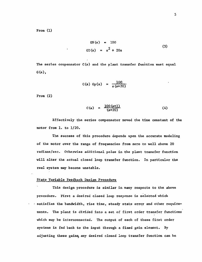
5
From (1)
GN (s) - 100
GD(s) = S2 + 20s
The series compensator C(s) and the plant transfer funetion must equal
G(s)
C(s) op(s) 100 a(s+20)
From (2)
C(s) = 100(s+l) (4)(s+20)
Effectively the series compensator moved the time constant of the
motor from 1 to 120
The success of this procedure depends upon the accurate modeling
of the motor over the range of frequencies from zero to well above 20
radianssec Otherwise additional poles in the plant transfer function
will alter the actual closed loop transfer function In particular the
real system may become unstable
State Variable Feedback Design Procedure
This design procedure is similar in many respects to the above
procedure First a desired closed loop response is selebted which
satisfies the bandwidth rise time steady state error and other requireshy
ments The plant is divided into a set of first order transfer functions
which may be interconnected The output of each of these first order
systems is fed back to the input through a fixed gain element By
adjusting these gain any desired closed loop transfer function can be
achieved
The above process is somewhat simplified if we first introduce
a new function Heq(s)0 This function specifies the transfer function
between the output and the input which yields the same result as state
variable feedback From Fig 2 the equivalent feedback from the output
is i s+ k2 + k3 Heq(s) = kl Gi (s GI(S)G2()
In terms of Heq(s) the state variable feedback results in the closed
loop response given by
Y(s)= KGp(s) (5) R(s) 1 + KGp(s) Heq(s)
The procedure is as follows
1 Select the desired Y(s)R(s) from the specifications
2 Equate the desired Y(s)R(s) to theone achieved by the
feedback from each state
3 Solve for the feedback coefficients
Details of the design procedure when zeros are present are given by
Schultz and Melsa [2 ] For example if
0p(s)= 1s (s+l)
Y(s) 100 R(s) s + 20s + 100
Then if G(s) 2(s)
Heq(s) - k1 + k2s
-- G3(s) G2 (s) ---GI(s) Y(s)
F 2
Figure 2 State Variable Feedback Block Diagram
8
From (5)
100 K2 2 s + 20s + 100 s + s + K(k1 + k2s)
Equating the numerator and denominator polynomials
K = 100
KkI1 100
1+Kk2 - 20
Solving for k1 and k
K = 100
k = 1
k2 19
This design yields exactly the same transfer function as the
Guilleman-Truxal (GT) method The two methods are not the same if a
small change is made in the plant transfer function The state variable
feedback (SVF) system changes less than the GT system
If the sensitivity is defined as the percentage change in the
closed loop transfer function for a small percentage change in a plant
parameter say K then
S K _ d dK dT K
T T K dK T
where for simplicity
T(s) - Y(s)R(s)
9
If K is the gain then
T(a) =KG(s)1 + KG(s) Heq(s)
dT(s) G(s) K Gp(s) G(s) fea (s) 2dK I + KG(s) Heq(s) (1+ KG(s) Heq(s))
Using this result in the definition of sensitivity
T = T(s) (6) T KG(s)
For the GT system from (6)
K s(s+20)
2T (s + 20s + 100)
For the SVF system from (6)
K s (s+1)ST 2 a + 20s + 100
For the GT system the sensitivity is greater at all frequencies than
the SV sensitivity especially at low frequencies
Modified Observer Systems
LuenbergerE ] has shown that an eytimate of the states in the
plant can be implemented as shown in Fig 3 When state variableshy
feedback is used from these states a specified closed loop response may
be achieved Muterspaugh [4 has modified this configuration by block
diagram manipulations to a form similar to that shown in Fig 5 The
1 2 2NN-1
kI
Figure 3 Luenburger Observer Block Diagram
r C(s) G(s) Y
Figure 4 Modified Observer Block Diagram
A(s)
I+
gt G(s) Y H(s)
Figure 5 Muterspaughs Modified Observer Block Diagram
13
series compensator shown in Fig 4 C(s) reduces to the Guilleman-TruxalLiJ
compensation in the case where H(s) is one Similarly this control system
reduces to the Heq [2 ] type of control resulting from state variable
feedback considerations when C(s) is one Fig 4 represents a more
general configuration than either Guilleman-Truxal or Heq type compensashy
tion All three configurations shown in the above figures are equivalent
Assuming that only the output is available the Heq configuration
is not realizable since Heq has zeros but no poles Guilleman-Truxal
type compensation is sensitive to plant variations Series and feedback
compensation is used to achieve low sensitivity and realizability If
Heq has zeros in the LP then the modified observer (MO) system is
slightly higher in sensitivity than Heq but if Req has zeros in the RHP
then the MO system is dramatically better These comments are illusshy
trated in the case studies at the end of this report
Modified observer System Design
This section derives the necessary conditions which C(s) and H(s)
must satisfy such that the desired transfer function Y(a)R(s) is
achieved when the plant has a transfer function G(s) The relationship
among these transfer functions is
T(s) 1() C(s) G(s)fR(s) 1 + C(s) G(s) H(s) (7)
If the feedback signals shown in Fig 3 are combined (using
block diagram manipulations) the resulting transfer functions are
A(s)=k2 1P1 (S)+k 2 (fIpI(s)p 2 (s)+12P2 (s))++knceiPl(s)+ -PNI(s))
H(s)k 1+k2p1 +k 3P1p2++kpN-1
14
Since the poles of H(s) and A(s) are arbitrary the control systems shown
in Fig 5 have N-i arbitrary parameters however the poles of A and R
are identical
One more manipulation of the system shown in Fig 3 results in
the system of Fig 4 where
1 C(s) - I + A(s)
The zeros of C(s) are the same as the poles of A(s) therefore the N-1
zeros of C(s) are also the same as the N-i poles of H(s)
From these facts (7) can be used to determine the denominator
of C(s) and the numerator of H(s) Dropping the argument a in (7) and
denoting the transfer functions by
CDC(s)
H(s) -
G(s) ONGD
T(s) - R
Eqn 7 becomes
CN GN 1 CD GD(8) R 1i+ CN GN HN
CD GD HD
If the right hand is simplified then
Y CN GN HD (9)R CD GD HD + CNCN
Since CN and HD are the same denote them both by P(s) Then (9) simplishy
fies to
15
Y GN P (10)R CD GD + NHN
cross multiplying on both sides results in the polynomial
Y(CDGD+GNHN) - R-GNP (11)
Define the number of zeros in G as NG the number of poles as
ND and similarly NY and NR for T(s) If the order of both sides of
(11) is to be the same then
NY + ND - 1 + ND NR+ NG + ND - 1
NY + ND NR + NG (12)
NR - NY -ND - NG
Thus the pole zero excess of the plant determines the pole zero excess
of the desired closed loop transfer function If like powers of (11)
are equated then NY + 2ND equations result Since CD and 1N are undeshy
termined the number of unknowns is 2ND For NY = 0 the number of
unknowns is equal to the number of equations Just as in regular state
variable feedback[2 for zeros in YR additional states must be
created Let the order of P(s) by N-l then (12) becomes
NY + N - I + ND = NR + NG + N - 1
and for the number equations to be equal to the unknowns
NY + ND + N = 2N (13)
N = NY+ ND
16
Thus the order of both controller systems C(s) and H(s) must be one
less than the number of poles of G plus the number of zeros of YR
assuming that (11) represents a set of linearly independent equations
The design procedure is as follows
1 Select the desired closed loop transfer function from the
specifications
2 Select a polynomial P(s)
3 Equate the actual and desired transfer functions (iO) and
solve for the coefficients of CD(s) and HN(s)
Program 1
The first program (MODOBSI) computes the transfer function of
the series compensator and the feedback compensator as a linear function
of the denominator of the feedback compensator The user must specify
the plant transfer function and the desired closed loop transfer
function Thus this program specifies the design of the system except
for the poles of the feedback compensator which the user is free to
choose in any way he wishes
Program 2
The second program (MODOBS2) computes the transfer function of
the series compensator and the feedback compensator which minimize the
low frequency sensitivity of the closed loop system to plant variations
The user must specify the plant transfer function and the desired closed
loop transfer function If the time constants in the plant are much
lower than in the closed loop system the poles of the feedback compenshy
17
sator may be in the right half plane (RHP) If the poles of the compenshy
sator are in the RHP then the system will be vyD sensitive to variations
in the parameters of the compensators In this case it is better to
use one of the other programs This program is limited to systems with
no zeros
Program 3
The third program (MODOBS3) computes the weighted integral
sensitivity of the system for a given polynomial P(s) The user must
specify the plant transfer function closed loop transfer function the
weighting to be given the sensitivity as the frequency varies and the
denominator of the feedback transfer function P(s) The weighting
function must have more poles than zeros
Input Data
In many circumstances the available data for the plant is in
state variable form This data is converted to a transfer function by
the STVFDBK program The details of the program are included in reference
1 The program listing and input data format are also included in the
Appendix
Output Data
The program BODE4 is provided to plot the transfer functions
computed in the above programs on a logarithmic scale For each program
some of the transfer functions of interest are
1 Plant transfer function
2 Closed loop transfer function
3 Sensitivity as a function of frequency
4 Loop gain function
The loop gain function divided by one plus the loop gain is the proportion
of measurement noise at each frequency which will reach the output Thus
if the loop gain is much greater than one then nearly all the noise
reaches the output and if the loop gain is much less than one very little
measurement noise reaches the output If the phase shift of the loop
gain is nearly 180 at a gain of one the measurement noise will he
amplified
Program 4
The fourth program (MODOBS4) is useful to check the results of
the design Given P(s) and the results of the first program (MODOBSI)
this program computes HN(s) CD(s) and the roots of both the series and
feedback compensators This program and the first program give a
complete determination of the design
Results
A discussion of each program and several caee studies are inclushy
ded in the Appendices MDDOBSI is useful to compute HN(s) and CD(s) in
terms of the coefficients of P(s) Quite amazingly the coefficients of
N and CD are linearly dependent upon the coefficients of P HODOBS2
computes the coefficients of both compensators which achieve minimum low
frequency sensitivity Essentially this result is achieved by forcing
CD(s) to be an N-i order integrator which increases the gain at low
frequency and thereby decreases the sensitivity since SK = (s)
Unfortunately if the plant denominator coefficients are smaller than
19
those of the denominator of the closed loop transfer function the feedback
compensators may have poles in the RHP MODOBS3 determines the weighted
integral sensitivity when P(s) is specified MODOBS4 is useful for
checking the roots of the resulting compensators after a design is
complete Test results are given in the appendix for three examples
These examples show that an improvement in the system sensitivity over
that of just a series compensator can be achieved even if only the output
is available When the closed loop response is much faster than the open
loop the sensitivity of the MODOBS system approaches the sensitivity of
the Req system (which is best but not realizable) if the roots of P(s)
are made much larger than the closed loop roots If the closed loop
response is not much faster than the open loop response then the MODOBS
system may have a sensitivity lower than the Heq system This situation
exists whenever Heq(s) has zeros in the RHP These results point out
the important fact that a sacrifice in sensitivity to plant variations
is made by increasing the system performance requirements Because of
this fact careful attention to the plant performance should be made for
lowest sensitivity and unnecessary demands on overall system performance
should be avoided
20
Bibliography
1 J C Truxal Control System Synthesis McGraw-Hill 1955 Chapter 5
2 J L Melsa and D G Schultz Linear Control Systems McGraw-Hill 1969 Chapter 9
3 D G Luenberger Observing the State of a Linear System IEEE Transactions on Mil Elec April 1964
4 M E Muterspaugh State Variable Feedback and Unavailable States HS Thesis 1968
5 F H Effertz Comment on Two Coupled Matrix Algorithms for the Evaluation of the rms Error Criterion of Linear Systems Proceedings of the IEEE November 1966 p 1629
6 J L Melsa A Digital Computer Program for the Analysis and Synthesis of State Variable Feedback Systems NASA Contract Report CR-850 August 1967
7 L E Weaver et al A Control System Study for an In-Core Thermionic Reactor J P L Report 32-1355 January 1969
21
Appendix I - MODOBSI
Dis cussion
The basic algorithm of this program is based upon (5) First the
following polynomials in s are computed
T = (GD)(Y)
Q = (GN)(R)
V = (GN)(Y)
so that (5) becomes
(T)(CD) + (V) (HN) = (Q) (e) (Al)
Each of the terms in (Al) are polynomials in s where P(s) is unspecified
For instance P(s) = P3s2 + P The coefficients of CD(s) and HN(s) are
the unknowns
As an example suppose the plant is second order then P(s) is
first order In this case (Al) becomes
(CD2T3 +H 2 V3 )s 3 + (CD2T2 + CD1T3 + H2 V2 + H1 V3 )s2 + (CD2T1 + CD1T2
2 + H2V I + HIV2)s + (CDIT + HV) = P2Q 3s + (P2Q2 + PIQ3 )s2
+ (P2Q + P1 Q2 )s + PlQl (A2)
Equating coefficients of like powers of s results in the equations
T3CD 2 + V3H2 Q3P2
T2CD2 + T3CD1 + V2H 2 + V3H1 Q2P2 + Q3PI
22
T1 CD2 + T2 CDI + VIH2 + V2H 1 QlP2 + Q2P
TICD1 + V1Hi = Q1F1 (A3)
These equations can be rewritten more compactly in matrix notation as
T3 0 V3 0 CD2 f 0 Q3TN12N-2 T2 T3 V2 V3 CD11 214-22-Q3 Q3 Q22 (A)
2 T V1 V2 H2 Q2 QI P2j _ Ql 0
2N-2- shy - N-i-)
The matrix on the left will be defined as matrix A and the matrix on
the right will be defined as matrix C Then
CD2 CDI _ - 1
CD= A-C (A5)
H I
Therefore A- C relates the unknowns CDi and Hi to the parameters Pi
MODOBS1 forms the matrix A from the two arrays T and V and then inverts
A Next the C matrix is formed from the Q array and then A 1 C is
computed and printed
23
Input Format
Card No Columns Description Format
1 1 NY = order of Y(s) in YIR II
2 NR = order of R(s) in YR Ii
3 NG = order of GN(s) in GNGD i1
4 ND = order of GD(s) in GNGD Ii
I 5-80 Identification of problem 8AI0
20 Cn of 2 11-0 Coefficient of s in Y(s) FI03
11-20 Coefficient of aI in f(s) P1e3
etc
71-80 Coefficient of s7 in Y(s) F103
3 1-10 Coefficient of a in R(s) F103 etc
4 i-i0 Coefficient of s in GN(s) FIO3
etc
5 etc Coefficientof a in GD(s) FI03
Notes
1 If more than eight coefficients are required then two cards may be
used to identify that polynomial
2 A decimal point must be used for each coefficient but not for card
No 1 The decimal point may be placed in any of the ten columns
for each coefficient
24
3 As many problems may be run as desired by repeating the above format
for each problem
Output Format
See example
Subroutines to be Used
PLYMLT Multiplies two polynomials together
MXINV Inverts matrix A
PRNTRAT Prints the ratio of two polynomials
Flow Diagram
Read NYNRNG
ND
FRead Y(s)R(s)GN(s) GD(s)
Compute T = YGDQ = GNRV = GNYj
Form A Matrix
Invert A Matrixi
lForm C Matrixl
A -1
ComputeBA7 C
Print CD and E
Arrays
PROGRAM MODOBSI (INPUTOUTPUTTAPE4INPUT)
ODIMENSION Y IC) R(10) GD(IO) GN(IC) V(201 T(20) G(20)14A(S363)AI(36 3)C( 3611) B(36 1U ID(G)
C Y(S)R(S) IS DESIRED CLOSED LOOP RESPONSE C SP(S)GD(S) IS PLANT TRANSFE FUNCTION C NY IS ORDER OF NUM IN Y(SlR(S) NR IS ORDER OF DEN C NG IS ORDER OF NU OF G(S) NO IS ORDER OF-DEN C NR-NY MUST EQUAL ND-NG 1 READ 1U1NYNRNGNDID
PRINT 200NYNRNGNDIO
IF(EOF4) 99t2 2 NY1=NY4 1
READ 102 (Y(I)I=-INY1) C YI) IS COEFF OF S(I-I) IN Y(S)
NR I=NR C RII) IS COEFF OFS(I-1)IN-P(S) 3 READ I102 (R(I) IINRI)
CALL PRNTRAT(YNY1RNRI IHTIHS) __C_ GN(Il IS COEFF9F_SCI-1LIN_-GNtSL
NGl1NGI NO 1NDI
_4 -READ 102 (GN ) I 1NG1) C GOD(I) IS COEFF OF S(I-1) IN GO(S) 5 READ 102 (CG (I)I--1NDI)
CALL PRNTRAT(GNNGIGDNO HGIHS___ C FORM CHARACTERISTIC POLYNOMIAL
CALL PLYMLT (GDND1YNYITO) CALL PLYMLT GNNG1RNRI00-CALL PLYMLT (GN NGGYNYIVO) NYNGzN Y1 4NGI NR+NG+iN __ 00 6 IrNYNGN
C NA IS ORDER CF A MATRIX WHERE A IS MATRIX RELATING UNKNOWNS -6- V( --- - - TO PARAM P
NA_- 2 (N--1) DO 20 J-1NA IF- (J GT (N- IlJGO__TO2_12 00 10 Iz1NA INDN- L J IF _( IND-SLT_ I)_GOTO8_ IF (IND GTN) GO TO 8 AUIJ)- T(INa) 30 TO 10shy
8 A(IJ) O 10 CONTINUE
Gi__TO_2D
12 DO 20 I=INA IND 1-I+J IF- (INDLT__GO__18__ IF (INDGTN) GO TO 18 A(IJ)-V(IND) GO-T 0 _2D
18 A(IJ)-O 20 CONTINUE
CALL MXINV-(ANAtAll_ C C IS THE COEFF ARRAT
NM IrN-1 _DOZ4__I NA-_ DO 24 J=1YNMI IN= 2N-I- J
IFiINDLT1) GO TO 22 IF (INDGTN) GO TO 22
C(IJ) = O(INO) -
GO TO 24 22 C(IJ)rO 24 CONTINUE C B IS AICTAE ROwS OF 5 ARE EQUAL TO CD AND HN C COLS ARE COEFF OF P PARAMETERS
D0 30 INA 00 30 KzlNM1 B(IK)--O 00 3fJ--JNA
30 B(IK)-AICIJ C(JK+B(IK) PRINT 2O1KK--lNMI) DO 40 I--NMI
NC =N -I 40 PRINT 202 NC (B I-Kt NM1I
DO 50 I=NNA
NBzNA+-I -50 PRINT 204t-NB (8(1I(1 Kzl-NM-1
GO TO I 99 STOP -101-FORM ATf l A 1f)V t 102 FORMAT (BF103) 200 FORMAT (1HI4(2XI1) 2X6A1i0) 201 FORMAT IH X8 ( 314- P( I 11 I-) OX)) 202 FORMAT 14H CO(I2--)10(E1U33X)) 204 FORMAT (4H HN(I12H)=)I(EIO33X))
END SUBROUTINE PRNTRAT (ANNBvNOEPVARINDVAR) DIMENSION A( 20)B( 20H_(20)N(20)AT20BT(20)NEt 1
DO 6 I--NN AT(I)-- -IF-(-AY f-4i 6-3
3 H(NE)zlH+
AT(NE)rA(1) GO TO 5
4 H(NE)--IH-
AT (NE) -A(I) N(NE)I-1 NErNEI
6 CONT INUE NE=NE-1 PR IN-T 10 0 MIN=MINO(NE 10) PRINT 10lCN(I)IzMIN) PRINT 102 (HRU1 ATI) INDVAR Il tMIN) IF (NE-if]) 8987
7 PRINT 101 (N(I IrIINE) PRINT 102 CHI)AT(I)INDVARI--INEI
__ NF= O0 16 I--IND BT (I)--DIF C B(C) 191G13
13 H(NF)rlH4 BT(NF zB(I)
-GO-_ T _15 14 H(NFI -IH-
BT (NF) =-B(I)
r27 15 N(NF)=I-I
NF zN Fi-I 16 CONTINUE
NF =N F- I HH= IH-NH=rAX 013NE 13 NF) NHzMINO(130NH)
20 PRINT 103 DEPVARINOVAR (HH I=INH) MIN MINO(NF 10) PRINT 101 (N(I)IzIMIN) PRINT 102 (Hi(I)BT(I ) 1NDVAR-I---1MIN IF (NF-101) 28P2827
27 PRINT 0l (N(I) IzIINF) PRINT 102 (H(IJBT(I)TNDVARI=N-FI)shy
28 CONTINUE 100 FORMAT C iHO) 101 FORMAT (6XI(11X 12)) 102 FORMAT 6XID(AIGlC4 AI1H H 103 FORMAT tIXtAIIHCAI2H)= 30AI)
RE TURN END SUBROUTINE MXINV (R N RI) SUBROUTINE TO FIND THE INVERSE- ----- GIVEN
C MATRIX R N IS ORDER OF MATRIX RI IS INVERSE C MATRIX SUBROUTINE USES GAUSS-JORDAN REDUCTION C R MATRIX IS PRESERVED DIAGONAL ELEMENTS OF R-US
BE NONZERO C DIMENSIONR(3G36IRA(3G72) RI(36v36)
C STATEMENTS 20-26 ENTER R ARRAY INTO RA ARRAY - C AND SET LAST N COLUMNS OF RA ARRAY TO IDENTITY
C - MATRIX 20 DO 26 I 1 NI-v 21 DO 24 J I N
_22__RA IJ) -R(I- J) 23 NJ = N + J 24 RA(INJ) = 0 2 5 _NI z N + I 26 RA(INI) = 1
C C ST AT EM ENTS _ii-12_REDUCE MATLRIX__RA _SOH_ATZ_JRFSR_LK C COLUMNS ARE SET EQUAL TO THE IDENTITY MATRIX
i NP = 2 N 2_DO 12 I - N
C -
C STATEMENTS 3-5 ARE USED TO SET MAIN DIAGONAL _C ELEMENT TOUNITY
3 ALFA = RA(TI) 4 DO 5 J = I NP S RA(IJ) r RA(I J) _ALFA
C C STATEMENTS 6-11 ARE USED TO SET ELEMENTS OF ITH C COLUMN TO -ZERO
6 00 11 K = 1 N 7 IF (K - I) 8 11t 8 8 BETA = RAiKI) 9 DO 10 J = It NP
10 RA(KJ) = RA(KJ) - BETA RA(IJ) - ICONTINUE_ 12 CONTINUE
C
TO LAST 28 C STATEMENTS 30-33 SET INVERSE MATRIX RI EUAL
C N COLUMNS OF RA ARRAY
30 DO 33 J 1 N 31 JN J + N 32 00 33 I 1 N 33 RI(IJ) rRA(IJN) 34 RETURN
END SUBROUTINE PLYMLT (ALBMCN)
C C MULTIPLY ONE POLYNOMIAL BY ANOTHER
C C DEFINITION OF SYMBOLS IN ARGUMENT LIST C A(I) MULTIPLICAND COEFFICIENTS INTHEORDER AE) S(I-1) C L NUMBER OF COEFFICIENTS OF A C B(I) MULTIPLIER COEFFICIENTS IN THE ORDER 8(I)SI-1)
C M NUMBER OF COEFFICIENTS
C C11) PRODUCT COEFFICIENTS IN THE ORDER C(19S(I-1)
C N NUMBER OF COEFFICIENTc Ac r
C C REMARKS C IF N-- C(I) SET TO ZERO AND PRODUCT FORMED OTHERWISE THE
C I-PRODUCT AND SUM NEWC-OLD C + AB IS FORMED
DIMENSION A(iD) B(IO) t C(20) LPML+M- 1 IF (N) 10102iZ
I DO 1 J- LPM 11 C(J)-Oo 12 DO 13 J--ILPM
MA X-MA XD (J + I-M il)) shy
- MINzMINO(L DO 13 IrMAXMIN
13 CC(J)=A(I)B(J+II) + C(J) RETURN END
3434 IN CORE THERMIONIC REACTO R
116708 481228 384520 200 1 16708 -4870635__4085815__39226_ 100 116708 481228 384520 200- 503585E-610542E- 3 058639 18804 1
END OF INFORMATION
29
Appendix 2 - MODOBS2
Discussion
If CD(s) in (5) is defined by CD(s) = CD N-i (BI)
where N is the order of the plants then the system will have minimum
low frequency sensitivity because the forward loop gain will be increased
at low frequencies If there are no zeros in Y(s)R(s) or in G(s) (5)
reduces to a simple set of linear equations shown below For simplishy
city RN+ I and GDN+t are set equal to one For zero steady state error
Y = R1
PNl PN= I PN-I = N-I
PN-2 + RNPN-1 CN-2
(B2)
P + 2 + ReN- =1 I I
IN I = P RY
HN2 =PI RY + P2
+HN=NPI RNY + P 2 -Y +i - GD1Y
Where the C terms are defined by
C I GD2 - R2
C2 = GD3 - R3
CN- 1 GDN - N
30
The Eqns (B2) are simply solved in the order shown by back
substitution That is PN-1 may be usedto solve for PN-2 which may be
used to solve for PN-3 etc
Input Format
Card No Columns Description Format
1 1 N = Order of the Plant G(s) Ii
2-80 ID Identification of problem 8A1O
2 1-10 Y = Numerator of YR F10o3
0 3 1-10 R(1) = coeff of s in R(s) F103
11-20 R(2) = coeff of s I in R(s) FIO3
etc
7 71-80 R(7) = coeff of s in R(s) FI03
4 1-10 GN = numerator of G(s) F103
5 1-10 GD(l) = coeff of s in GD(s) F1O3
771-80 GD(7) = coeff of s in GD(s) F103
See notes following input format for MODOBSIo
Output Format
See example
Subroutines to be Used
PRNTRAT - Prints the ratio of two polynomials
PROMT - Determines the roots of P(s) to see if any roots are in
RHP
PROGRAM OOS2 (Y4PUT OUTPUTC4=INPUT)IO41 N j (l10 1 ( l ) 1 ([) Cl(In)ID( 3)PHN 1 )CD t13)
C U (IG) V (10) C PqOGRAM TO CALCULATE MINIMUM LOW-FREO SENSITIVITY MODIFIED C OBSERVER SYSTEM C Y(S)R(S) IS DESIRED CLOSED LOOP RESPONSE C GN(S)GD(S) IS PLANT TRANSFER FUNCTION C N IS ORDER OF DEN IN Y(S)R(S) C N IS ORDER OF DEN IN GN(S)GDIS) C R(I) IS COEF OF S(I-1) IN R(S) C C ASSUMPTIONS C C TRANSFER FCN GAINS ARE NORMALIZED SUCH THAT R (N+1)I1
C AND GD(N I )=I C C DESIRED TRANSFER FCN HAS ZERO STEADY STATE C
-C GD(I) IS-COE-F-- O-F S(I-I)1NGO(S) C Y(S)=Y GN(S)-GN (NO ZEROS ALLOWED) C I READ 101 N ID
IF(EOF4)99 2 2 READ I02Y
READ 102 (R(I)IzIN) NP i-N+ I
GD(NPI) =1 5 RNPI_)-1 READ 102 GN
3 READ 102t CGD(I)tlz1N) PRINT 200DNIO10 PRINT 201
CALL PRNTRAT CYIRNPHTIHS) PRINT 202
CALL PRNTRAT(GNGDNP11HG1HSI C-C --SOLVE FOR DEN OF H P(S)
NM I=N-I do 40 II -NM1 IPIlzI+I
-4 -CI) zG0c IP 1I-R IiT P(N) -
005[ I=ItNMj NI N-I P(NI)zC(NI)
IFCILE1) GOTO-50_ DO 49 Jz2I J2=N-J+2
4 P(NI )zP( NI )-R( J2 )P( JI ) 51 CONTINUE
CALL PROOT (NMIPUV) PRINT 205
PRINT 206 (U(I)V(I) I=INM1)
ERROR THUS YR(1)
SOLVE FOR NUM OF HHN(S) DO 60 1N HN (I 0 - 00 60 JzlI IJI j4
C
6C PN Il)r( Ji R (IJ) Y +HN( I) 32 HN (N )HN (N)-GD (1 )Y
PRINT 203 CALL PRNTRATIHNNPNIHH1HS) PO 80 1i NMI
80 CO(I)zO CD(N)zl PRINT 204 CALL PRNTRAT(PNCDN1HC1HS) G z YGN PRINT 210 G GO TO I
99 STOP 101 FORMAT (Il 84101 102 FORMAT (SF1O3)
200 FORM AT(IHII0X II 4X 8AID) 201 FORMAT(1HOTHE DESIRED CLOSED LOOP TRANSFER FUNCTION IS)
202 FORMAT(1HOTHE TRANSFER FUNCTION OF THE PLANT IS)
203 FORMAT(IHOTHE TRANSFER FUNCTION OF THEFEEDBACK COMPNSATOR IS)
204 FPRMAT(lHOTHE TRANSFER FUNCTION OF THE SERIES COMPENSATOR IS)
205 FORMAT (IHO 5X THE ROOTS OF P (SI ARt 13XREAL PART IOXIMAGINARY PART)
-20 FORMAT 32X2E207f 210 FORMAT4IHOTHE ADDITIONAL FORWARD LOOP GAIN REQUIRED IS
1YGNElfl3) END SUBROUTINE PRNTRAT (ANNSNDDEPVARINOVAR) DIMENSION A(20)B(20vH(20) N(20 1 AT(20) PT 20 NE z1 00 6 Iz1NN AT(1)=D IF C(IA ) 463
3 H CNE )= IH + AT (NE) =AtI) GO TO 5
4 H(NE)=IH-AT (NE) =-A( I) N(NE)--I-1 NE-NEI
6 CONTINUE NE=NE-1 PRINT 100 MINMINO(NE v1O
PRINT IOl (N(IhI=IMIN)
PRINT 102 (H(IAT(I)INDVARI-IMIN) IF (WE-10) 8
7 PRINT 101t (N(I)IzlINE) PRINT 102 (H(I)AT(I)INDVARIn1NEl NF o_-8_ N --1 80 16 I1NU
BT(IzO IF ( (I) 1141613
13 H(NF)zlH+ BT(NF)l=B(I)
-GO T0- 15 __ - 14 H(NF) zlH-
BT (NF)z-B(I) - 15 N(NF)=I-1 -
NFZNF41
33 ID CONTINUE
NF NF- I HHL IH-NHMAXO( 13NE 13NF) NHzMINO( 130NH)
20 PRINT 1G3DEPVARINDVAR(HH 1=1NH) MINMINO(NF 10)
PRINT 101 (N(I)IlMIN) PRINT 1G2( H(I)BT(I)INOVART IMIN] IF (NF-in) 2828927
27 PRINT 101iN(I) I11 NF) PRINT 102 (H(I)BT(I)tINDVARI-IINF]
28 CONTINUE 100 FORMAT (1HO) 101 FORMAT (GX1O( IIX12)) 102 FORMAT (GXI0(AIGIO4 A1IH )
103 FORMAT (1XA1IH(Ai2H)-130A1) RETURN END
___SUBR CUT INEPR O0 TN _A U fVtIIRR) DIMENSION A(20)U(20)V(20)H(21)8(21 )C(21) IREV-IR NC -N +IDOll--i Nu
H( I) rA( I) _i CONTINUEL
00
3 IFIH( 1)) 24 2 NCNC-1
V NC )z0 U NC O DO 1002 I= 1NC H(I)--H(I+1 )
1002 CONTINUE GOT03
S_IF (NC- 1) 5 10 05 5 IF (NC-2) 7i 7
6 R=-H( 1H(2) GOT050
7 IF INC- 3) 9-819 8 P-H(2)H(3)
__0 1) H (3_)_ GO TO7g
q IFCABSCH(NC-1)1H(NC)-ABS(H(2)H(1))101919 10- IREV - IREV_
M=NC2 DO11I=-1 M
_-NL-zNC+ 1 -I-FrH( NL) H NL )H( I)
11 H( I) F -IF (O )139 12 913
12 P=D GOTO 15shy
13 PzPQ 0= (
15 IF(R)16191G 16 R=1 R 19 E5E- ]C
B(NC)H(NC) C(NC)H(NC) B(NC+1 )zO C( NC 1)z 0 NP NC- 1
20 0049J= I 100C DO 2111l1 NP ITNC-I I BC I rH(I)+RB(+1)
--21C( I) =B (I)+RC( I+ 1) IFCABS(B(I )H(1))-E)5050 24
24 IF(C(2)232223 2amp R= RlI-
GO TO 30 23 R=R-B(1) CC2)
30 D0Q3711zlNP IzNC-I I BI)i(I)-PB(I+I)-OB(I+2)
37C( I) =B (I)-P C(i1l) OC(12) IF(H (2)) 323132
31 IF(ABS(C2)H(1))-E)333334 32 IF(ABS(B(2)H(2) )-E) 33v3 34 33 IF(ABS(B(1)H(1))-E)707034
34 CBARrC(2)-B(2) DC(3) 2-CB ARC ( 4) IF(D)363536
35 PzP-2 0= (o t GOT049
36 PP(-82)C(3)-BC1)C(4))D - Q+ (-( 2)CBARB(1) C(3 00)
49 CONTINUE
ErE 10 GOT020
50 NC-NC-1 VtNC)D
IF (IPEV) 51 5252 51 U(NC)=1R-
GOT053 52 U(NC)-R 53 00541lNC
H(I) B(1+1) 54 CONTINUE
GOT04 70 NC=NC-2
---- IF(IREV)71727 71 QPr1O
P=P(Q2 0) GOTO73-_
72 OPPP Q-P 2 0
73 F-(PP)2-OP IF(F )74 7575
74 U(NC+I)z-PP U(NC)-PP V(NC 1 )SORT(-F) V( NC 1-V (NC+ 1) GOT076
75 U(NC+11-(PPABS(PP))(ABS(PP)SQRT(F)J V( NC+1 )0 U(NC )OPU (NC1) V( NC )O
76 D0771INC H(I) B(1 2)
77 CONTINUE GOT04
LDO RE TURN END
3 CASE STUDY II THIRD ORDE-SYSTE14shy1000 1000 200 20 D O -
2500 100
36
Flow Diagram
Read N ID
Y R(I)
GN GD(I)
Print N ID
YRy G
Form C(I)
ISolve for P(s)j
Solve for HN(s)I
Print H(s)
Print C(s)
37
Appendix 3 - MODOBS3
Discussion
This program uses the following data
1 Plant transfer function G(s)
2 Desired closed loop transfer function T(s)
3 The denominator (P(s)) of the feedback compensator H(s)
4 A desired weighting function W(s) on the integral over
frequency of the sensitivity of the closed loop response
to forward loop gain changes
The program then calculates the weighted integral sensitivity of
the system The method of calculation is based upon an algorithm by
EffertzL5] The integrand of the integral sensitivity is calculated
from
I S W(S) S (S) ds
2r f G(s)C(s) ds
The algorithm is based upon an iterative manipulation of the coefficients
in the numerator and denominator of the integrand in such a way that the
integral of the squared magnitude results
A closed form solution for the integral
jm n 2rj jo h(P)h(-P) 2 -joo
1 30 dP 1 j F(P)F(-P) dP
(BI)
is presented in the paper by F H Effertz The solution takes the form
38
of Equation 4 in his paper A better algorithm for the computation of
Equation 4 in Effertz is presented in the correspondence by Pazdera
(Equation 7) A modified forn of Pazderas algorithm has been coded in
FORTRAN and is included A test problem is also included
The use of Equation 4 in Effertz can be best illustrated by an
example Suppose we wish to evaluate the following
(B2)Ls2+ Cb) [2bLn = 2I -
It can be shown from residue theory that the correct answer is
I = - residue of F(s) F(-s) at s = a (B3)n
- residue of F(s) F(-s) at s = b
where F(s) F(-s) indicates the function to be integrated over s = jW
Then the answer is
22 2
= - c-a (c2-b2 c2+abn 2a(a+b)(a-b) 2b(a+b)(b-a) = 2ab(a+b) CR4)
To use Equation 4 from Effertz we must make the following associations
using the complex frequency variable s in place of p
22 s= c -g(P) = (s+c)(c-s)
then s (B5)
2
h(P) = s + (a+b) s + ab
then p s N=2
1
a a 2 =ab
39
The integral for n = 2 can be expressed as
bb [bloaaob I- (B6)
a0 t ol [jaza1-2 1ao a 2
Substituting the correct values of a0 a etc and cancelling minus
signs for this problem we obtain
ab +c In = 2ab(a+b) (B7)
What is most interesting is that the result depends only on the coeffishy
cients of the known function being integrated and not on the poles of
the function as one would suspect from residue theory
It has been mentioned that the algorithm from Pazdera (Equation 7)
has been programmed Some charges in the nomenclature of Equation 7 were
necessary to facilitate coding Note that the practice in Effertz and
Pazdera is to make the highest membered coefficient correspond to the
lowest power of the variable p Note also that subscripts such as ao
are in evidence To facilitate coding the lowest numbered coefficient
was subscripted in the form A(l) and this coefficient was associated with
0 ththe lowest power of the variable p in this case p In general the i
coefficient A(I) is associated with the (i-1)s t power of p P -l (In
FORTRAN the expression A(O) is not allowed) Note from equation I above
what must be done to operate on the function F(s) F(-s) If F(s) is of
the form
F(s) = C(S) (B8)A(S)
then the algorithms suggested in both Effertz and Pazdera require the use
40
of
g(s) = C(S) C(-S) (B9)
h(s) = A(S)
It is more desirable to input C(S) and A(S) rather than C(S) C(-S) and
A(S) Consequently one uses the INTSQ subroutine by coding the coeffishy
cients of C(S) and A(S) with ascending subscripts corresponding to
ascending powers of S The subroutine provides the operation C(S) C(-S)
Furthermore the subroutine checks to see if the lowest coefficient of
C(S) or A(S) is zero so that factors of S may be either considered or
cancelled Two basic requirements must be met by A(S) and C(S) First
the roots of A(S) and C(S) must at least have non-negative real parts
(Hurwitz polynomial requirement) Secondly the highest power of C(S)
must be at least one less than the highest power of A(S) for convergence
to be assured If A(S) is Nth order one inputs the N coefficients of
A(S) and the N-i coefficients of C(S)
The use of this subroutine INTSQ may be best illustrated by an
example Suppose we desired to evaluate the integral
I = JD F_ 7 4 - JdS n -joe 3 + 3s2 + 2s + L[43 + - 2s
(BIO)
The polynomials C(S) and A(S) as defined in Equation B8 are input into
the program as
C(1) = 4 A(l) = I
C(2) I A(2) = 2
(Bi) C(3) o A(3)= 3
A(4) = 4
41
The program then utilizes the modified Pazdera algorithm and prints out
the message
THE VALUE OF THE INTEGRAL IS 12250
To check this answer one can use Effertz Equation 4 for a third order
case (n=3)
a oa 101o 2 1 n
= (142a
0 a
aI a a 0
I 2a
boa2a3+b2aoal-aoa3b alaaa a (BI2)
0 1 20 - o2 2 3o 31 o 13a22o0
For our example problem the following associations follow
b =0 a =4 0 0
b 1 -l a = 3 (B13)
b2 =16 =2a 2
a 113
Substituting the values of Equation B13 into Equation B12 verifies the
computers solution I = 1225n
Input Format
Card No Columns Description Format_
See format for MODOBSI
K 1-10 P(1) - coeff of so in P(s) BE103
11-20 P(2) - coeff of s in P(s) 8E103
etc
42
Input Eormat (contd)
Card No Columns Description Format
K+I 1 NW - Number of coeff in denom of W(s) II
K+2 1-10 WN(I) - coeff of s in num of W(s) 8E103
11-20 WN(2) - coeff of s in num of W(s) 8EI03 etc
K+3 1-10 WD(1) - coeff of s deg in den of W(s) 8E103
11-20 WD(2) - coeff of s in den of W(s) 8E103 etc
43
PROGRAM MODORS3(INPUTOUTPUTTAPE4-INPUT ) DIMENSION Y( 10)R(10)c-D(IO) SN(lOhIP(10)CD(0) HN(IO)SN(40)bull
IS0(40) B(36 18)WN(10) WD 10)SNT(40)SDT(40)C
I CALL MODOBSI (YP GN GO5 NY1 NR1 NGI NDI C N-1 IS THE NUMBER OF COEF IN P(S) HN(S) CD(S)
NrNR 1+NGI- 1 N =rN -1 READ 10 lP(I)Iz1NI)
C W(S) = WNWD MUST HAVE MORE POLES THAN ZEROS C NW IS THE NUMBER OF TERMS IN THE DENOMINATOR OF WS)
READ 103NW READ 102 (WN(I)I-INW)_ READ 102 (WD(I)I-INW) PRINT 205 CALL PRNTRAT (WNNWDNW1HW4-lkHS) CALL PLYMLT(GDNDlY NYI SN 0) N2=NDI+NYI-I
_CALL_ PLYMLTT(yN NWSNN 2 SNT D) CALL PLYMLT (GNNG1 R NRI SO 0) CALL PLYMLT(WDNWSDN2SDT C)
__N3=NW+N2-1 -
N4 =N 3+ NI-1 N22N1 11
-a- DO 10 I= 1Nl CD(I)=0 HN(I)O 00 10 J1pN1 CD (I)B(N-I J)P J )+CD( I)
10 HN(I)zB(N2-IJ)P(J) +HN(I)_P -I NJ_Z0 I--_
CALL PRNTRAT(PN1CDN1IHCIHS) PRINT 202
CALLP RNTRATAHN NI P Ni1H Ht l1 CALL PLYMLT( CDN1 SNT N3 SN C) CALL PLYMLTI- PN1SDT N3SD 0) -N5=N4 ---CALL INTSQ(SDSNN4S) PRINT 204 S
- GO T ---O-- -- 102 FORMAT 18 E1O3) 103 FORMAT III)
-201 -FO RM ampTL__TJJLJERANS ER_-F-UN CT-O-N--OF--L sESERIS--COMENSJ-IO-R- i-l 202 FORMAT(O THE TRANSFER FUNCTION OF THE FEEDBACK COMPENSATOR IS) 204 FORMAT(O THE WEIGHTED INTEGRAL SENSITIVITY ISEIO3) 20S -FORM-AT( Oi-tJ-WEIGHTINGFUNCTION-OF-HE- INTEGRALSENS-IIVlTY-YI-_shy
1) END
_SUBROUTINEMOOOBS1 LYR GN GD B N-YI-NRI-NGL-ND44-UDIMENSION Y(IO) RU1G) GD(10) GNIG) t V(20) T(20)9 Q(20) IA(3636)AI(3G36)C(36l8)B(36 1B)ID(6)
C _Y(S)R(S) IS DESIRED-CLOSED LOOP C GP(S)GD(S) IS PLANT TRANSFERFUNCTION C NY IS ORDER OF NUM IN Y(S)R(S) NR IS ORDER OF DEN
_C_ --NGJ S OR DEROFJN UaOF_ GASJ_ID- S--DRDELO DE C NR-NY MUST EQUAL ND-NG C Y(I) IS COEFF OF S(I-1) IN Y(S)
C RP I) IS COEFF OF S( 1-f1 IN Q(S)
C GN(I) IS COEFF OF S(I-11 IN GN(S) C GOCI) IS COEFF OF S(I-1) IN GO(S) 1 READ 1UINYiNRNGNDIO
IF(EOF4) 99t2 2 NY IrNY +1
NR ic NR --READ 102 (YCI)IIlNYI)
3 READ 12z (R(I) I--NRl) PRINT 200NY vNRvNGNO ID CALL PRNTRAT(YNYl R NRI 1HT IS) NuGl=NG I
ND i ND-shy4 READ 102 IGN I I--I NG1) 5 READ 102 (GD(I)IzlND1)
CALL PRNTRATIGNNG1GDNDI 1H3IHS) C FORM CHARACTERISTIC POLYNOMIAL
CALL PLYMLT (GDNDIYNY1TO) CALL PLYMLT GNNGIRNR10) CALL PLYMLT (GN NGIYNY1V0i NYNG=NY1+NGI N rNR+NG+I 00 6 IzNYNGN
C NA IS ORDER OF A MATRIX WHERE A IS MATRIX 6 V(I)zfl
NA= 2 (N-1 DO 20 J-INA IF ( J GT ( N- 1) GO_TO_1 2 DO 10 IrINA IND-N-I+J IF (IND LT 1) GO TO 8 IF (IND GTN) GO TO 8 A(IJ)= TIIND) GO TO 10
8 A(IJ)zO 10 CONTINUE
GO TO 20 12 DO 20 I=lNA
IND --- I+J IF fINDLTI)_ GO TO 18 IF (INDGTN) GO TO 18 A(IJ) zV(IND)
GO TO 20 18 A(IJ)rO 20 CONTINUE
CALL MXINV_ (ANAAI_) C IS THE COEFF ARRAY-C
NMlzN- 1 DO 24 IrItNA DO 24 JrINM1 INDz2N-I-J
IF(INDLT1) GO TO 22 IF (INDOTN) GO TO 22 C(IJ) - O(IND) GO TO 24
22 C(IJ)zO 24 CONTINUE
__C B IS AICTHE RUWs UF B ANt LIUAL IU) (U C COEFF OF P_ PARAMETERS
00 30 IrINA
44
RELATING UNKNOWNS TO PARAM P
AN_)_HN_THECOLSAR
00 30 KzlIMI B (I K) 0 00 30Jr1NA
30 B(IK) AI(IJ)C(JK)+B( T K) PRINT 201IKv(K=1 NM1 DO 40 I=INMI NC =N -I
40 PRINT 202NC(B(IK)Kr1NM1) DO 50 IzNNA NB -N A 1- I
50 PRINT 204v NB(B(IKIK--NMI) RETURN
99 STOP 101 FORMAT (4116A10) 102 FORMAT (SF103) 200 FORMAT I1HIv4(2XI1) 2XGA1O 201 FORMAT (10X3(3H P(I1lH)vgX)H 202 FORMAT (4H CD(I12H)zO(E1O 33X) 204 FORMAT (4H HN(IIZH)=IO(EIO 33X)L
ENO SUBROUTINE PLYMLT (ALBMCN)
C MULTIPLY ONE POLYNOMIAL BY ANOTHER C
C DEFINITION OF SYMBOLS IN ARGUMENT LIST C AI) MULTIPLICAND COEFFICIENTS IN THEOROER A(I) S(I-I)
C L NUMBER OF COEFFICIENTS OF A _C_ _B I) __MULTILPLIER CO EE-CIENiS-LNTlLODE3-IIi-plusmnSflt-WL-
C M NUMBER OF COEFFICIENTS OF B C CII) PROOUCT COEFFICIENTS IN THE ORDER C(I)S(I-1)
_
C C REMARKS
_C _IF -LO_ C (t1---ETJO_=EOANIRRO IUCTER-MF] lkRWLD T TRiLEJP-PO-DIC C AND SUM NEWC= OLD C AB C
DIMENS ION A( 101 D_cL20j LPML M- 1 IF (N) 101012
At1 -DO i - J-=l LPM__ I] C(J)zOO
12 DO 13 J=ILPM __M AXzMA XO (J+1-MJ
MINMINO (L J ) 00 13 I=MAXMI C ( J )=A _I u KB (Jt 1 RETURN
END
IS FORMED
SU BR OUT I NE P RN TRAT (A NNB N D DEPV AR INDVA RJ_ -
DIMENSION A(20)B(2)H(20 )N( 20)AT(20) BT(20) NE l
-DO JI1NN___ AT (I 1 IF ( A() 1 4993 H( NE = IH AT (NE) zA(I) GO TO 5 H(NE)I-H-
AT(NE) -A(I) N(NE)rI-1 5
146NErN E+1
6 CONTINUE NE =NE- I PRINT ion MINz INC(NE 10) PRINT iO1(N(I)T--MIN) PRINT 10Z (H(I)ATCI) INUVARI1MIN) IF (NE-in) 387
7 PRINT 101 (N(I)IrlNE) PRINT 102 (HCI)AT(I)INOVARvl--IrNE)
8 NF I DO 16 I-1ND ST(I)-O IF ( B(I) ) 141G13
13 H(NF)zIH+ ST (NF) -B(I) GO TO 15
14 H(NF) -IH-BT (NF) -- B(I
15 N( NF)zI--I NFrNF+ 1
16 CONTINUE NF =NF- I-HH =1H-
NH=MAXCD13NE 13 NF) -NH=MINO(130NH)Y
20 PRINT 103t DEPVARINDVAR (H H I-INH)MIN=MINO (NF 10) PRINT 101 (N(I-IiMIN) PRINT 102 (HI )BT(I)INDVARIlMIN)
IF (NF-ID) 282827 27 PRINT 101 N(Il) I=I-1NF)
PRINT 102 CH(I)BTII)INDVARI-i1NF) 28 CONTINUE 166- FO PM AT IHO-shy101 FORMAT f6Xv10(IIX12)) 102 FORMAT (GX0(A1G1O4 AIIH 103 FORMAT t IX A1 IHIAL 2H)Z 130AI])
RETURN END SUBROUTINE MXINV (R RI)
C SUBROUTINE TO FIND THE INVERSE OF A GIVEN C MATRIX R N IS ORDER OF MATRIXv RI IS INVERSE C MATRIX SU-BROUTINE USES GAUSS-JORDAN REOUCTION C R MATRIX IS PRESERVED DIAGONAL ELEMENTS OF R MUST BE NONZERO
DIMENSIONR(33G ARA(3 72) RI(363)
C STATEMENTS 20-26 ENTER R ARRAY INTO RA ARRAY C AND SET LAST N COLUMNS OF RA ARRAY TO IDENTITY-C MATRIX
20 00 26 I = I N 210 24 J = l N 22 RA IJ) - R(IJ) 23 NJ = N J 24 RA(INJ) = 0 25 NI = N + I 26 RACItNI) = 1
C C STATEMENTS 1-1-REDUCE MATRIX RA -SOTHAT FIRST N C COLUMNS ARE SET EQUAL TO THE IDENTITY MATRIX
471 NP = 2 N
2O 12 I 1 N
C STATEMENTS 3-5 ARE USED TO SET MAIN DIAGONAL C ELEMENT TO UNITY
3 ALFA = RA(II) 4 DO 5 J I NP 5 RA(IJ) z RA(IJ) ALFA
C C STATEMENTS 6-11 ARE USED TO SE-T ELEMENTS OF ITH C COLUMN TO ZERO
6 00 11 K = 1 N 7 IF (K - I) 89 11 8 8 BETA RA(KI)
9 DO 10 J I NP 10 RA(KJ) RA(KJ) - BET A- RA(IiJ 11 CONTINUE
12 CONTINUE C C STATEMENTS 30-33 SET INVERSE MATRI-X- RI-EQUAL-TO-LAS-T-C N COLUMNS OF RA ARRAY - 30 DO 33 J 1 N
31 JN = J + N 32 00 33 I 1 N
33 RI(IJ) RA(IJN) 34 RETURN
END SUBROUTINE PLYSQ_ (CN8j___ DIMENSION C(40)B(4D)
C RETURNS BCS) = C(S)C(-S) TO MAIN PROGRA-M C B(I) IS COEF OFS -l IN S -------C C(I) IS COEF OF S I-I IN C (S) C N-I IS NUMBER OF COEF IN B(S) AND C(S)
N1I (N- I)-12---shy00 20 I=lNI MO =-I _BCI) zD II z 2I-i
DO 20 K=1 II MO z -1MO
20 B(I)B(I)MOC(K)C( 2I-K) NMIN-i
- N2-N +I 00 30 I=N2vNM1 IIN=2I-NMI
MO(-I) NMI DO 30 K-IINNMI
O -IMO
30 B(I) r3(I)+MOC (K)C( 2I-K) RETURN
-- END - SUBROUTINE INTSO (ACNS)-DIMENSION B(IOhA(II)C(ID)
C___ RETURNS SZINTEGRAL OF C(S)C(-Si A CS )A( -S)-TO MAI-NRPROGRAMo C B(S) HAS N-I TERMS A(S) HAS N TERMS C B(I) IS COEF OF S(2I-2) - ISCOEF OF S(I-I)2C- -C(I) C IF THE LOWER ORDER DEN AND NUM COEFF ARE SMALL (LESS THAN C 0) THEN DIVIDE BOTH NUM AND DEN BY S2
48
0 1 OE -6 1 IF ( ASS( At 1) )-O) 2220 2 IF (A3S(C(1)-O) 4420 4 IF (K-I) 556 5 PRINT 200 6 PRINT 20IA(1) C(1)
N=N- I 00 10 I1N A(I)=A(1+1 IF(I-N) 8 1010
8 C(I)C(I1I) 10 CONTINUE
GO TO 1 20 CALL PLYSO (CNB)
NM2N-2
DO 50 K=INM2 NK =N -K BA=B(NK) A(NKI) AAO IF(KEOI) GO TO 40 AAzA (NK+2) tA(NKt 1)
40 NMK=(N-K)2 DO 50 I1 NMK NKIzNK-2I1+ B(NK-I )rB(NK-I)-BAA (NKI) A(NKI+i)zA(NKI+)- AAA-NKIj
50 CONTINUE SZB(1) (2A(2)A(I)
RETURN 200 FORMAT (0 THE FOLLOWLNG COEFF WERE FOUND TO BE SMALL AND CANCELL
lED IN THE NUMERATOR AND DENOMINATOR) 1FORMAT (THE DENOMINATOR COEFF EID3 THE NUMERATOR COEFF
1= E103) END
0303-CASE STUDY-IIt -THIRDORDER SYSTEM 1000 000 ___ 2020 i_ 1000
2500 100 1
2
49
Appendix 4 - MODOBS4
Discussion
MODOBS4 uses the matrix relating the coefficients of CD(s) and
HN(s) to the coefficients of P(s) and also the coefficients of P(s) to
determine both the series compensators and the feedback compensators
The roots of the compensators are included
Input format
Card No Columns Description Format
1 1 N = order of plant G(s) II
2-80 ID = Identification 8AI0
2 1-10 CD(l1) coeff of array from MODOBSI EIO3
11-20 CD(12) coeff of array from MODOBSI E-1O3
3 1-10 CD(21) coeff of array from MODOBSI EIO3
11-20 CD(22) coeff of array from MODOBSI E103
N+2 1-10 HN(11) coeff of array from MODOBSI E103
11-20 HN(12) coeff of array from MODOBSI E103
2N+2 1-10 P(l) - coeff of st in P(s) E103
11-20 P(2) - coeff of s in P(s) E103
etc
50
Flow Diagram
Read CD(IJ)
HN(IJ)
P(I)
Compute N
C(J) = Z CD(IJ)P(J) J=l N
H(l) = Z HN(IJ)P(J) J=l
Compute roots of
P(s) and C(s)
Print H(s)
P(s) C(s) and
roots of P(s) and C(s)
IOUN I S I LGO
C PROGRAM PROGRAM
MODOOS4( INPUT OUTPUT TAPE4zINPUT TO CALCULATE CO mPENSATORS WITH P(S) AND RESULTS OF MODOBSi
DIMENSION ID(8) CD (1R 18 ) HN (I 8v 18) C( 18 )PH( 1S )v U 23) V120)P[20 C N IS THE ORDER OF THE PLANT G(S) AND NO OF COEF IN P(S) i READ 100v N ID
IF(EOF4 992 2 PRINT 200 N ID
DO 10 I1IN 10 READ 101 (CO(IJ)JIP N
DO 15 lr1N 15 READ 1019 (HNIIJ) JIN)
READ -101 (PCI) I=IN)
DO 20 I=1N CI I) za HI I ) O DO 20 Jrl N C( I) =C (I)+CD (I J)P(J) H( I ) -H (I)+HN (IJjP (J)-PRINT 204 CALL PRNTRAT(PNtCN1HCiHS) -PRINT205 CALL PRNTRAT (HNPNIHHIHS) NM1=N- 1 CALL PROOT _(NMltCUtVI)- PRINT 201 PRINT 202v(UI)vV(III=IvNMl)
CALL PRO OTNM1 P UV PRINT 203 PRINT 202CUCI)vV(I)vII1NMl) CALL PROOT (NM1NUVI) PRINT 220 PRINT 202(U(I)VCI)I=INM1)
-GOTO_1_ STOP
100 FORMAT t II8AO) _101 _FORMAT_ (8E103)- -- - -- 200 FORMAT (IH12XI12XsAlo) 201 FORMAT(IHSXTHE ROOTS OF C(S) ARE13XPEAL PARTI0XIMAG1NARY
PART) 202 FORMAT (32X2E207) 203 FORMAT (IHO5XTHE ROOTS OF P(S) ARE13XREAL PART1OX-ruwiNARY
-1PART )- 220 FORMAT (1HP5XTHE ROOTS OF- HN(S) ARE13XREAL PART10XIMAGINARY
1PART) -204--FRMAT-IH 0 -- HE--R NS EFRFU NCT-L-ON-CO$FTHamp SERILEs OBZ-NS-AORSt-IL
205 FORMAT CIH THE TRANSFER FUNCTION OF THE FEEDBACK COMPENSATOR IS 1) -END SUBROUTINE PRNTRAT (ANN3NDOEPVARINElVAR) DIMENSION A(20)8(20)H(20)N(n ATt fnl RTlrn) -NE - --
DO G I =INN AT (I lD IF (L l I -
52
3
4
5
6
7
8
__13__
14
1s
16
_20
27
28 10(
01 102 103
H( NE )= IH+ AT(NE)=A(I) GO TO 5 H(NE)zIH-AT(NE) -A() N(NE)I-I NE NE+ 1 CONTINUE NE =N E- I PRINT 100 MINzMINO(NE 10) PRINT 101 CN(I)I-IMIN) PRINT 102 (HCI)AT(I) INDVAR I=i MIN) IF (NE-In) 887 PRINT 101 (N(I-1I11 9NE)- -PRINT 102 CH(I)AT(I)INOVARI=11NE) NF =1
DO 16 IiND BT (I )=O IF ( 8(I) 1 141613 H(NF)=IH+ BT(NF)-B-(I) GO TO 15 H(NF) =IH-BT (NF) =-B( I) N(NF )=-I-I NFzNF+I CONTINUE NF NF-1 H-I H-NHzM AXO 13NE 13N F) NH-MINC( 130NH)
-PRINT 103OEPVARINDVARC(HHt I--1NH) MINzMINO(NF 10) PRINT 101 (N(I)I-lMIN) PRINT 1O2_(HII)BT N 1MIN)_I NDVARtI
IF (NF-IP) 28 t28 27 PRINT 101(N(I) IzIINF) PRINT 102H(I)BT(I)9INVARwI11NF) CONTINUE FORMAT (IHO) FORMAT (6XIlX12) FORMAT (6X O(AlG1O4 AlIH ) FORMAT (1XAIH(AIv2H)-130A1) RETURN--END SUBROUTINEPROOT( N A U V IR) DI-MENS ION A( 20) U( 20_3 V( Z0_LAvj21)3821 ) C 21 L IREV-IR NC-N+I DOI--ANC_HI)=AI)
153
CONTINUE PO 0=0 RO0
3 IF(H(l))42i 2 NCNC- I
V(NC)O U(NC )O 00 100211 NC H(I) H(+l)
-1002 CONTINUE GOT03
4 IF (NC-1)5 1005 5 IF (NC-2) 7G7 6 Rr-H(I)H(2)
GOT050 - 7 IF (NC-3) 99 83shy
8 PH(2)H(3) QH(I)H(3)
- - GOTOYG 9 IFCABS(H(NC-1)HNC))-ABS(H2)H(lelo 1919
10 IREV-IREV -MNC2 -
D0111I M NL =N C 1- I
FHC NLI I-HNL)HfI)
11 H(I)F -__IF( 0 ) 13LIL3
12 PO GOT0 15
-13 PPO 0=1 0
15 IF(R)16191616I_R1R 19 E-5E-10
B(NC)-H(NC) C(NC)H(NC
B(NC+I)-O C(NC+I) NPNC- 1
20 D049JI 100D 0021 Ii NP
- INC-I1
B(I)HCI)+RB(I+1) 21 CCI) B(I)RC( 1+1) IF ABS ( 8 j H _i-) - 50vLQ 2L
24 IF(C(2)l232223 22 RzR+I
- GOTO30------- 23 R=R-B( 1) C(2) 30 003711 =1 NP
= -IzNC-I B( I ) HCI -P B I1) -g B( 1+2 )
541
37 C(I)--B(I)-PC(Ii1)-OC(12)
31 IF (H (2 ) 323132 IF(ASS(B(Z)H(I) )-E) 33s3 34
32 IF(ABS(S(2)H(2))-E)333334 33 IF(ABS (1( I)H( 1) )-E) 7070 34
34 CBAR-C(2 )-8(2) UWC(3)2-C8ARC (4) IF (D)36 3536
35 PzP-2 zQ (Q+)
GOT049 36 P-P+(B(2)C(3)-B(I)C(4))D
OQi(-B(2)CBAR+B()rf 4I)n 49 CONTINUE
E=E10 GOT020-50 NC =NC- i1_
VINC Jr 0 IF (IREV) 51 5252
-5-1 U( NC ) 1-LR- GOT053
52 U(NC)-R -53-DO54Iz 1 -NCshy
H(I)=BtI+1) 54 CONTINUE -- GO TO 4 --
70 NCzNC-2 IF(IREV) 71 72 72
_7___L QP-l PP P G 2 ) GOT073
72 UPr= PP P 2 0
73 F= (PP) 2- UP IF (F )775 75_
74 U(NC+I)-PP U(NC)=-PP V(NC 1Ir)SOPT (-I V( NC )-V (NC+ ) GOT076
75 U(NC+1)z-(PPABS (PP) )tABS(PP) +SORTCF)) V(NC+I I=O U( NC )-=P U (NC+ 1) V( NC )-O
76DO77IINC H(Il)B (-2)
77 CONTINUE GOT04
100 RETURN FND
55
Appendix 5 - STVFDBK
Discussion
A discussion of this program is given in reference 6 The input
is formed from the state equations x = Ax + bu y = cx where x is the
state vector u is the input and y is the output The major use of this
program is to convert the state variable form of the plant to the equishy
valent open loop transfer functions
Input Format
Card No Column Description Format
1 1-20 Identification of problem 4A5
21-22 N = right order of A matrix an 12 integer right justified in the field
2 1-10 a11 = first element of A matrix 8E10O
11-20 8E100a12
3 1-10 a2 1 8El00
11-20 a22
n+2 1-10 b 8E100
11-20 b2 8E100
56
Input Format (contd)
Card No Column Description Format
n+3 1-10 c1 8EIO0
11-20 8ElOO 2
etc
n+4 1-80 Blank card
Notes
As many problem may be run as desired by repeating the above set
of cards for each problem
57
PROGRAM STVFDBK (INPUT OUIPUT TAPF4 Ir DUT)
C OPEN LOOP CNLY DIMENSION A(13 lO R( 10 H( 10 C(IO)NAME(4iAA(IO I )[E (O) DIMENSION O( i)PC 110CC(IOHH(10) PIN(l0 IDU( OV(10)
2000 FOPMAT(QSHO t-s 4 ) 2001 FORMAT (2A10I12) 2002 FOPMAT (8E100) 2003 FORMAT IIHISX1ln1HPROBLEM IDENT 5X 2A10) 2004 FORMAT(lHSX 12HTHE A MATRIX) 20$ FORMAT (GE207) 2006 FORMAT(INHO5Xl2HTHE 8 -MATRIX) 2007 FORMAT(1HOsx4HTHE CLOSED-LOOP CHARACTERISTICPOLYNOMIAL) 2008 FORMAT(IHO5X25HTHE FEE09ACK COEFFICIENTS)
2009 FORMATC1IHO5X1IOHTHE GAIN CCIG7) 2010 FORMAT(1HO5X12HTHE C MATRIX5XSH)
2011 FORMAT(1HO 5X 24HDENOMINATOR COEFFICIENTS) 2012 FORMAT( HO5X 22HNUMERATOR COEFFICIENTS) 2013 FORMAT(1HO5X23HTHE NUMERATOR OF H-EQUIVALENTI_ 2014 FORMAT (IHO5X22HOPEN-LOOP CALCULATIONS)
2015 FORMAT(IHO5X 2GHMAXIMUM NORMALIZED ERROR E102) 2016 FORMAT(I1)-20D17 -ORM AT Ia 5X 24HNCLOSEOD--LOOP--CL-CULATIO-N-s)-shy
2018 FORMAT(IHO56XHKEY - I3XSH) 2019 FORMAT(IHO5X 23HPLANT IS UNCONTROLLABLESXt1CHs)shy2020 FORMAT(1HO4X 35HPLANT IS NUMERICALLY UNCONTROLLABLElOX
I 16HMAX DEVIATION z E1O25X 1OHt _ 202 1 FO RM AT1RO 4ITH A LlX_PELPART W14HIMACJNARY05 ROOTS
1ART)
2022 FORMAT(25X 2E2071 - 2023 FORMATIHO-) C READ INPUT DATA 1 READ 2001 (NAME(I)I=2)N
-- __ IF(EOFr4_lO0tO____ __
B0 PRINT 2003CNAME(I) Iz1 2 PRINT 2004 -DO2 IzlN
READ 2002 (A (I J )JzlN) 2 PRINT 2005(A(IJ)JrlN)
PRINT- 200-- -
READ 2002t (B(I )IUN) PRINT 20059(8(I) IlN)
Cz_ CHECK CO NTkO LLAB ILiTYLL-DO 7 I = N AA (Ii )rBC I)
7- QO NTIN UE-__ DO 8 I2N LrI-1 00 8 JrlN AA ( PIr)O DO 8 K1N
___ AA JI)AA(J IJt+AJJA )_AA(KLL_ 8 CONTINUE
CONTR=DET( AA N) IFCCONTR) 3943
4 PRINT 2019 GO TO 9
_C NOTEUSE OF -DUM-YARGUMENT CALLED_ 3 CALL SIMEO(AACNPINCI
00 43 I=IN
00 43 J-1N 58 P( IJ) 0 00 43 KZ1N P( 1J) =P (IJ)+AA (IK )FINE KJ
43 CONTINUE
ERROR 00 44 I--tN DO 44 JzlN IF(I-J) 454645
4G ERR ASS(P(IJ)-1O GO TO 44
45 ERR ABS(P(IJ)) 44 ERROR = AMAXI(ERRERROR
IF(ERROR-IE-s5 94747 47 PRINT 2020ERROR
C-- OPEN-LOOP CALCULATIONS__ 9 PRINT 2000
PRINT 2b14 NN zN+1 PRINT 2011 CALL CHRE(AiND) PRINT 20 05(I ( I-1 _w CALL PROOT (N BU Vv+ ) PRINT 2021 PRINT 2022 U(IJVII-- N 0011 I1N P(IN)8()
-11-CO NTIN UE__-_ DO 12JJ=2 YN 0012 IiN
- J=N-JJ+I K=J+I
P(IJ) D(K)B(I) - DO12_Lzt N_ ____
P( IJ) P(IJ)+A( IL)PLK 1 12 CONTINUE
-72- RE AD 2002 -CC Ii-I=INL 00 70 11 N IF(C(I)) 717071
-70---CONTINUE GO TO i
71 PRINT 2023 PRINT 2010
PRINT 2005t (C(I)I1N) 49 0013 I1N
_ CCIjz-O0
0013 J 1N CC(I)P(JJ I)C (J)+CC (I)
_13__-CONTINUE 00 100 I1N M=NN-I
_IFACCM) )1-J1-10U103 100 CONTINUE
101 PRINT 2012 PRINT -2005 CCAII i bullM)-
HzM- i IF(M) 105105103
-- 103-CALL- PROOT-(MCC UV-+-l PRINT 2021 PRINT 2022(U(I) V(I) I-1 M)
9
105 GO TO 72 10 STOP
END
SUBROUTINEPROOT IN At U V IR DIMENSION A(20)U(20)V(20)H(21 )8(21 C(21) IREV=IR NC =N+1 DOIIl NC H( I) A (II CONTINUE P=O 0=0 R D
3 IF(H(1)4924 2 NC =NC- I
V( NC )-0 U NC)= D010021r1NC H(I) H(I+l)
1002 CONTINUE GOT03
4 IFCNC-1)51005 -S--IF(NC-2)7s57 6 R=-H(1)H(2)
C-TO50 7 IF (NC-3) 9 9
8 PrH(2)H(3) OH(1)H(31 GOTO70 IF(ABSH(NC-I)H(NC))-ABSH(2)H(I) )1 1919
-1 IRE V-IREV M=NC2 001111 M NL =NC I-I FzH NL )
HINL)H(I) 11- H( I) rF
I IF ( ) I3tI2 13 12 PrO
GTO 1 5_ 13 PrPO
OrI o --15 _IFR )1 tIj9j_6__ 16 R-1R 19 E=5E-10
_ B(NC )H(NC) CINC=H(NC) B(NC11=O CCNC+1 )0 NPrNC- I
20 D049J1 1000 [021111 NP
INC-I I B(I)= H(I)+RBCI+1)
21 C(I) B(I) PC(I+ 1) __
IF(ABS(8(1)H(1) )-E) 5050 24 24 IF(C(2)232223 22 R2+ 1
GOTO30 23 R=R-B(I)C(2)
30 D037111 N0 1plusmn2 I-NC-I1 B I) --H(I )-PB(I+I) -Q5( I+2)
37 CCI) r3(I)-PC(1 1) -OC(142) IF(H(2)) 323132
31 IF(ABS( (2H(1) )-E) 3v3 34 32 IF(ABS(BCZ)fiH(2) -EU 3333 34 33 IF(ABS(B(1)H(1))-E)707034
34 C3AR--C ( 2 )- B(2) OC(3) 2-CBARC (4)
IF (D)3635 v36 35 P-P-2
00(0+1 GOT049
36 PzP (B(2)C(3)-B(1)C(4)1D OQ+(-B(2)CBAR4B()C(3))D
49 CONTINUE
EzE 10 2
50 NC-NC-1 V( NC ) 0 IF( IREV) 51 vuavt
SI U(NC)=I-R GOTO53
52 U(NC)zR 53 D054I=NC
H(I)--B(I+I) __5 LLL_CONT INUE
GOT04 70 NCNC-2
__IF (IRE Vi 71 t72v -72 71 OP-IQ
PPrP(Q20)____GO TO 73 __
72 OP0 PP P 20
73 Fr(PP)2-OP IF(F)74 7575
74 U(NC+I)--PP _ _U(NC h-PP
V( NC+1 )=SORT (-Fl V(NC)=-V (NC I)
___ GOTOTE
75 U(NC4I)z-(PPABS(PP))(ABS(PP)+SQRT(F)) V( NC+ I)7O
__U( NC )OPU (NC-l- V(NC)O
76 D0771INC C( I) 8 CI2J
77 CONTINUE GOTO4
_Ia _RETU RN-END FUNCTION OET(AN)
C FUNCTION DET DETERMINES THODEERMINANT__OFITHEMA-TRIX A DIMENSION A(1O10) B(10 10)
C SET B EQUAL TO A BECAUSE WE DESTROY A IN THE PROCESS 0O_1IK1_N______ DO I JKzlN B(IKJK) = A(IKJK)
61I CONTINUE NN N-I D 10
C IF N-- THEN BYPASS PIVOT PROCEDURE r0 DIRECTLY TO CALCULATION IF(NN) 69693 OF OCT
C START PIVOT SEARCH PROCEDURE 3 00 100 Lr NN
LL z L41 AMAX = A(LL)
IML
JM = L DO 15 IzLN 00 15 JLN IF (AMAX-ABS(AIIJi)) 101515
10 IM IJ4i z J
AMAXz ABS(A(IJ)) 15 CONTINUE
C FOUND PIVOT AT ROW IM AND AT COLUMN JM C IF ALL REMAINING TERMS IN THE MATRIX ARE ZERO SET O6T20 AND
IF tAMAX) 7070 14 RETURN C NOW CHANGE ROWS AND rfl IIMN T mVtrCCADY 14- -IF (IM-L)G201G
16 DO 17 J2IN T = A(IMJ) A(IMJI A(LJ)
17 A(LJ) T D -D
20 IF(JM-L) 219252 21 DO22 IzN
T = A(IJM) AIIJM) A(IL)
22 A(IL) T ___=_ o- D ___
C PIVOT NOW AT A(LvLDIVIOE ROW L BY A(LL) 25 DO 30 KILLN
A(LKlI -LAiLK1)A_(LL 3- CONTINUE C NOW PRODUCE ZEROES BELOW MAIN DIAGONALAhJLI--
---- DO 50 JZLLN__ DO 50 KrLLN A(JK) = A(JK)-A(JL)A(LKY
_50 -CONTINUE_ 100 CONTINUE
C MULTIPLY MAIN DIAGONAL ELEMENTS TO GET VALUE OF THE DETERMINANT _ 63DQ 200 I0_N_
D = DA(I) 200 CONTINUE
DET _ C NOW RESTORE THE VALUES OF THE A MATRIX
DO 2 IKrIN _j0 2 JKclN-
A(IKJK) = B(IKJK) 2 CONTINUE
_ _RETURN 70 DET=O
D0 4 JK=IN 4DOIK1N
A(IKJK) = B(IKJK) 4 CONTINUE
162RE TURN
END SUBROUTINE SIMEG (AXOOTKC AINVX) DIMENSION A O10U) IO10)XDOT(1 )X(Ic ) AINVtl10O) DO1 I=1KC D0I J1KC AINV (I J I=O
1 B(IJ)-A(IJ) 002 IIKC AINV(IIl=l
2 X( I) =XDOT(I) D03 I1 KC COMP 7O KI IF(ABS(2(KpI))-ABS(COMP))5t54
4 COMP=3KI
NK 5 K=K+1
IF(K-KC)GGi7 7 IF(B(NrI))851w8 8 IF(N-I)51t 9 9 0010 MI-XC
TEMP=B(I M) BC IM) =B(NM) (NM) =TEMP TEMP =A INV( I M) AINV CIM)=AINV (NM)
0_AINVA(N M )=TE1P- TEMP X (I I X( 1) =X (N)
_X(N) -TE-1 P- 12 X(I) X(I)B(I1)
TEMP = B(II) - -DO13- KC =i --
AINV(IM) = AINVfIMTEMP 13 B(IM) = BCIM)TEMP
-- DO16 JIKC -----shyIF(J-)14 1614
14 IF(B(JI)) 15115 -I5-X (J) zX J- )8 B CJIi X( I-)
-TEMP =B (J I ) DO17 N=1KC
-- A INV(JNAINVJPN ) TEMPtAJN VC(ltN) 17 B(JPN) zB(JN)-TEMPB IN) 16 CONTINUE
___3_C0 NTINUE__ RETURN
51 PRINT52IKC 52-FORMAT E 18HI-ERROR IN-CLUWMN--IC22ZX3HO--ATRIX-5X-3IHKCI 1-
RETURN END
_-SUBROUTINE CHEQ-(AN-CJ-_-----DIMENSION Jtll)C(l)B(1010) A(IO 10)D0300) NN =N +1
__D020 I=1 NNC C(I) O
20 CONTINUE C (NN L z-
0014 M1ltN KD
63
L 1
J( 1) =1 GO TO 2
I J(L)--J(L)+ 2 IF(L-M) 3550 3 MM =M-1
DO 4 T-LMM II=I~l
4 J(IIIJ I|)+l 5 CALE FORM(JMAB)
K-K+ I D(K) mET (BMl DO G Ilim L--M- I+ I IF (J(L]- (N-M L I) 1 5c
6 CONTINUE Hi = N-M+1 D014 I-IK C(MI)=C(M)_O(I)(-)M CONTINUE
RETURN 50 PRINT 2000
RETURN 2000 FORMAT (1HO5X14HERROR IN CHREQI
END SUBROUTINE FORM(JMAB) DIMENSION At 1O0] B (IflI10JC) 001 T110M DO1 K=IM NR =J (I NC =J (K
1 B(IK)ZA(NRNC) RETURN
-ENO
64
Appendix 6 - BODE4
Discussion
This program is used for providing phase and log magnitude versus
frequency plots for the resulting open and closed loop transfer functions
The author is indebted to Dr L P Huelsman for this program
Input Format
Card No Column Description Format
1-80 LTR = Title of problem BOAl
2 3 NC = No of functions to be plotted 13
3 1-3 NP = No of values of frequency in 13 the plot (1-100)
4-6 NPD = No of frequency pointsdecade 13
7-9 NHZ - Log10 of starting frequency in 13 Hz
10-12 NSCAL - Max ordinate of magnitude 13 on frequency plot in dbtimes SCALM (minimum value is 100 SCALM) db lower)
13-15 NPHS = Indicator for phase plot 0 13 if no plot desired I if-plot is desired
16-18 MSCAL = Max ordinate for-phase 13 plot in degrees times SCALP (minimum ordinate (100-SCALP) lower)
21-30 SCALM = Scale factor for magnitude E100 data (10 if no scaling desired)
31-40 SCALP = Scale factor for phase data E1O0 (10 if n6 scaling desired)
65
Input Format (contd)
Card No Column Description Format
4 1-3 ND = Max degree of numerator and 13 denominator polynomials (1-19)
5 1-80 A = Numerator coefficients for 8E100 first function (in ascending order use 10 columns for each coeffishycient)
6 1-80 B = Denominator coefficients for 8E100 first function (in ascending order use 10 columns for each coeffishycient)
Notes
1 The maximum magnitude in db which will be plotted is NSCALSCALM
however the maximum value indicated on the plot will be NSCAL
2 The minimum magnitude in db which will be plotted is (NSCAL-100
SCALM however the minimum value indicated on the plot is
NSCAL-I00
3 The above comments also apply to the phase
4 The actual values of the variables are listed in the printout
for every frequency
10N H Z +from 10N H Z to NPND5 The frequency range in Hz is
6 For each function to be plotted cards 4 through 6 must be
repeated As many cards as necessary may be used to specify
A and B when ND 8
Examples
If the function varies from +10 to -10 db then choose SCALM = 5
and NSCAL = 50 since
66
NSCALSCALM = 10
(NSCAL-100)SCALN = -10
If the minimum frequency is 01 Hz and the maximum frequency of
the plot is 100 Hz with 20 points per decade then the total number of
points is
NP = decades(pointsdecade) = (log 10 (max freq) - NHZ) NPD
= 4 - 20 = 80
071
PROGRAM BODE4 (INPUTOUTPUT TAPE 4zINPUT) DIMENSION LTR(80)
DIMENSION Y(5100)
DIMENSION X110)
PHSD-O READ IOO LTR IF (EOF4) 999t2
2 PRINT 101 LTR READ 1O5NC PRINT 110NC
162 READ 105NPNPDNHZNSCALNPHSMSCAL SCALMSCALP
PRINT 112NPNPDNHZ DO 140 K=INC PRINT 1159K READ 77 (X(I)lS)
77 FORMAT (BF104) PRINT 78(X(I)f=15)shy
78 FORMAT(1 X(I) X IOF1Z 3) NX 1 PRINT 201 DO 140 JJ=1NP FRG XL4( NX INHZ NPD) RAD=G 2831 8FRQ
CALL MAG7 (RADFM X PHSD)
137 FML=20ALOGIO(FM)Y(K -J)FMLS CALM _
140 PRINT 2021 JFRORAOFMFML PHSD
PRINT 145 SCALMLTR CALL PLOT4(YNCNPNSC-AL) GO TO I
999gSTOP OD FORM AT-(80 A 1) 101 FORMAT (IH1 BOAl) 105 FORMAT (G132X2EIOO)
110 FORMAT (IHO IGHNUMBER OF CASES-plusmn
112 FORMAT (1H0137H POINTS I1 7HDECADE SX18 HSTARTING FROM 10
1 13)shyi-115 HO1-2H-CAESE NUMBER 12)FORMAT-- --shy
14H SCALE EIO31XSOA1145 FORMAT (IH114HMAGNITUDE DATA FACTOR=
201 FORMAT ( 1IH 25 X 5HHERT Z 13X_7HRADJSEC 17 X3HMAG 18X 2HDB 17X Y3 HOE( i
202 FORMAT 1X I 5 5XSE208) __ END
SUBROUTINE PLOT4(YMNFNS) ARRAY (FORTRAN 4)C SUBROUTINE FOR PLOTTING 5 X 100 INPUT
DIMENSION Y(5v 100) r LINE(101)L(1_JL(S)
DATA (JL(I) li5) IHA 1HB IHCIHDPHEvJNJPJI JBLANKJZ 11H- IH+ 1HI IH v1H$I
D 99 -I-I-101 LINE (I )-JBLANK
99 CONTINUE N=D
68
C PRINT ORDINATE SCALE 00 101 1111 L (I) zi f I- itO+NS
101 CONTINUE PRINT 105 (L()lIlrj)
105 FORMAT (3Xv1(I14 X) GHY(11)) GO TO 115
110 IF (N10-(N-1)10) 125125115 C -CONSTRUCT ORDINATE GRAPH LINE
115 NDO 00 120 I=1910
ND=N04 1 LINE(ND) =JP DO 120 Jl9
N =NO 1 120 LINE(ND)=JN
LINE (101 )zJP IF (N) 135121i35
121 PRINT 17ONLINE GO TO 185
C___ CONSTRUCT i-LINE OF_ ABSCISA GR__AP LLF-
125 00 130 I110li1 LINE (I) =JI
130 CONTINUE C CHANGE NUMERICAL DATA TO LETTERS
135 DO 160 I=IM _XNSNS _ JA=Y (IN )+O149999-XNS
IF (JA-laI) 140155145
__140 IF (JA) 150150155_ 145 LINE(101)-JZ
GO TO 1GO 150_LINE(1)=JZ
GO TO 160
155 LINE(JA)-JL(I) 160 CONTINUE
C PRINT LINE OF DA-T-A-IF (NI1O-(N-I)10) 175175165
-- 165PRINr 170NLINEYIN 170 FORMAT (IXIL41O1A1IX E125)
GO TO 185 A175PRINT 180LINEYlN)_
180 FORMAT (5X1O1A1XEZS5) C SET LINE VARIABLES TO ZERO -85 Do - L=Li1DL
LINE (I)=JBLANK 190 CONTINUE
195 -N=N+1 IF (N-NF) 110110200
69
200 RETURN END FUNCTION XL4 (NLOLPI AN N AL 0 LO ALPzLP AA rNALP+ ALO IF (AA) 100100 105
100 XL 4 I 10 C-AA I GO TO 1101
105 XLl10AA 110 N-N+1
RETURN END -
SUBROUTINE MAG77 (STAMPXPHASE) DIMENSION X(10) COMPLEX GNGDDN0DPNCNCOT GN =CMPLX(7S8S1720)CMPLX(798S-1720) 3880
I CMPLX(1ThOS+3310)- CMPLX(176OS-331l -2 CMPLX(C08S+575O) CMPLXRO-8S-5-75-O) 3 CMPLX(828S 945UI CMPLX(328S-9450) GD ZCMPLX (4605) SCMPLX(44 5S+2820) CMPLX (445S-2820)
1 CMPLX(844S+4780) CMPLX(844vS-478O) 2 CMPLXE1305S+74OO) CMPLX(1305S-740O) 3 CMPLX(1915S+108ZO) CMPLX(1915S-1020) DN-515E+1CMPLX(10300S -
DDCMPLX(G50OS)CMPLX(12GO0S+5880)CMPLX(1260OS-5880) 1 CMPLX(2E1OS+1470O)CmPLX(2510S-14700) 2 CMPLX (391C0S+18100)CMPLX(39100S-18100 PN- CMPLX(1010OS) 10100 CNz1335CMPLX (142S+248 )CMPLX(142 5-248) CD CMPLX(OS)CMPLX (500S) T=(GNDDCD) f(GDD0CDOGNDNNPN )I TAMP rCABS( TI AZREAL CT) B-AIMAG( T) PHASEzATAN2(B A)573 RETURN CN=X(3)CMPLX(XU)S) CMPLX(X(4hS) CDCMPLX(X(21S)CMPLX( X(5)PS) CMPLX(OtS) T--(GNGD)(DNDD) (CNCD) PN) END
70
Appendix 7 - Case Study I
Second Order Plant
Discussion
A second order plant has been selected so that some insight into
the effect of compensators can be obtained before the computer programs
are used Suppose that the plant transfer function is
G(s) (6-1)G (s+b)
and the desired transfer function is a Butterworth type response for
maximum bandwidth
T(s) = 100 (6-2)s 2lOs+100
The feedback compensator will be of the form
H(s) 12 - (6-3)P1+5
where arbitrarily P2=1 since the numerator and denominator may be multishy
plied by any constant For zero steady state error at low frequencies
H =P
The transfer function of the series compensator is of the form
C(s) D+Cs (6-4)CDI+CD2s
From the relation between the closed loop transfer function and the open
loop transfer function
71
G(s)C(s)(s)=+(s)C(s)H(s)
(6-5)
l00(P 1+s)100
s2+1 0 s(s+b)(CDI+CD2s)+100(HI+H 2 )lOs+100
Cross multiplying and equating coefficients result in the
equations
3 a 1 = CD2
2s 10+PI = CDI+1 CD2
i 00+ 10 P = bCD1 +IOOH2
0 s P =H
Solving for CD2 CD and H2 the above equations become
CD2 = 1
CD1 = J 10+P1 -b
H2 = 1+(PI-b)(4710 - b100)
H = PI
Thus the compensators are specified except for b and P1
Sensitivity
The sensitivity of the closed loop system to variations in plant
gain is
S K T(s) s(s+b) (CDI+S) (6-6)T G(s)C(s) 2+ 10s+100)(Pl+s)
72
The low frequency sensitivity is
T 1bCDl(6K - 100P (6-7)
which is minimum for CDI = 0 which implies
CD = 10+PI-b = 0
(6-8) P = b-F 10
Unless PI is positive the feedback compensator will be unstable and the overall system will be infinitely sensitive to variations in PI If PI
is positfve then (6-8) is a restriction on the plant time constant The
only alternative is to make PI sufficiently large to keep the sensitivity
low cf eqn 6-7 It is interesting to compare the sensitivity of this
system with the Heq compensator and the Guilleman-Truxal compensator
He Compensator
Choose Heq to be Heq(s) = 1+k2s Then
T(s) Gs )+=1(s)Heq(s)
100 100 2+10 s+10O e(s+b)+l00(l+k
2s)
Equating coefficients
104= b+100k2
k =2 100
T = T(s)= s(s+b)K G(s) s2+104s+100
--
73
Guilleman-Truxal
Choose
s+b =C(s) S+c
100 100
s2+o12 s+100 s(s+c)+l00
Cross multiplying and equating coefficients
c - I1
Thus the sensitivity is
s(s+lOF2)TK (s2+P2 10s+100)
The above sensitivities are plotted in Fig 6-1 for the case of
where b = 20 and CD = 0
If b = 10 then for P positive the sensitivity is minimized
if P is made large CDIP is nearly one if P 40 The three sensishy1
tivities are shown below
MODOBS
T s(s+10(s+4414) K (s2+10v+100)(s+40)
Heq
T s(s+10) KK = (s2+10y +lO0)
20
10
0
Gain (db) G(s) = 00C(s) = s+586
-10 s(s+20)s
T(s) = 100 s2+ 2 10s+100 Hs)- 1(s)lo484s+586s58
-20+O s+586
uilleman-Truxal1
-30
1 Frequency (Hz)
01
Figure 6i Sensitivity of High-performance 1lant 4shy
75
Guilleman-Truxal
K 2s(s+l03F)TK (s2+104-s+100)
Notice that for b = 20 the MODOBS system is significantly better
at all frequencies below IHz The Heq compensation is both unrealizable
and largest in sensitivity for this case When the forward gain is small
then no compensation will help the sensitivity Thus all the proposed
systems have a sensitivity near one for frequencies above IHz
For b = 10 the low frequency plant gain must be greater to
achieve the same T(s) The Guilleman-Truxal compensation decreases the
forward gain proportionately so that the sensitivity is unchanged The
Heq compensation does not change the forward gain therefore the sensitivity
is reduced from the case where b = 20 The MODOBS system also improves
in sensitivity but this system will only be as low in sensitivity as the
Heq method when PI is infinitely large Nevertheless the MODOBS
compensation has the advantage of being realizable
Integral Sensitivity
For the plant with a pole at -20 the integral sensitivity
(weighted by 1s) is
I j jO I s(s+20)(s-4-P1-586) 2
Sr 2- s (s2+IOffs+100)(S+P 1
This integral can be evaluated directly from Newton Gould and Kaiser
p 372
The minimum low frequency sensitivity was attained for PI = 586
which from MODOBS3 has an integral sensitivity of 012 The minimum
76
integral sensitivity is 0085 for PI = 8 In this simple case this can be
determined analytically by plotting S as PI is varied
Final Design
From the integral sensitivity data a final design choice is
b = 20
P = +8
The following graphs are shown in Figs 6-2 to 6-4
Fig 6-2 Plant transfer function
Fig 6-3 Sensitivity function
Fig 6-4 Loop gain function
Conclusion
From the above figures the design demonstrates the dependence of
the sensitivity on the plant parameters If the time constants in the
closed loop transfer function are much greater than those in the plant
a sacrifice in the system sensitivity at low frequencies must be made
In addition the compensator will have large gains associated with the
feedback which complicate the design of the compensators and increase
the effect of the measurement noise
20
10 open loop
0 closed loop
-10
Gain (dbo)
-20
-30
-40 1
Figure 62
100C(s) =s(s+20) T(s) s2+ s2+
100
10s+100
Frequency (Hz)
Open and Closed Loop Transfer Functions
0
0
-5
Guilleman-Truxal
-10
Gain
(db)
-15
-20
-25 1
I 110 Frequency (Hz)
Figure 63 Sensitivity of Second Order Systems o
10 MDB
0
Guilleman-Truxal
010
Gain (db)
-20
-30
-40 0
Frequency (Hz)
Figure 64 Loop Gain Function of Second Order System
80
Appendix 8 - Case Study 11
Third Order Plant
Discussion
A third order plant has been selected to compare the computer
results with hand calculations The results agree in all the calculations
discussed below The plant transfer function is chosen to be of the form
1000
S3+GD 3 s2-D2 s+GTD
and the desired closed loop transfer function is again chosen with a
Butterworth type denominator
1000T(s) =
s 3+20s2+200s+lO00
MODOBS2
The equations for the coefficients of P(s)=PI+P2SP3s2 which give
minimum low frequency sensitivity were derived in Appendix 2 For N=3
P3 i
= GD3 - 20P2
P 1 GD2 - 200 - 20(P2 )
These equations are satisfied if
GD3 = 20
GD2 = 200
Low frequency sensitivity will be improved if the plant is Type 1 or
81
equivalently has a pole at the origin thus
GD = 0
The poles of the plant are the roots of
s(s2+20s+200) = 0
s = -10 + jlO
For the plant to have real roots then
GD2 - 4GD 2 ) o 3 2
and in order for PI and P2 to be positive
GD3 gt 20
GD2 gt 200 + 20P2
These requirements can be met if
GD3 gt 6828
20(GD3 - 10) lt GD2 lt GD2 4 20G3 3-2
GD = 0
If GD3 is near 68 then P1 must be near zero Under these circumshy
stances the zero of CD(s) cancels the pole at a low frequency and the
low frequency sensitivity suffers Suppose that
GD = 100
5
0
-5
Sensitivity (db)
-10
Guilleman-Truxal MDBS
-15
-20 i
Figure 81
1
Frequency (Hz)
Sensitivity of Third Order System
1010
0
83
Then
1800lt GD2 2500
2
P3 = I
P2 = GD - 20 - 80
PI = GD - 1800
To keep the low frequency pole of P(s) as large as possible it is best to
make GD2 large thus
GD3 = 100
GD2 = 2500
GDI = 0
P3 = I
P2 = 80
PI = 700
Sensitivity
If the plant can be selected as above the sensitivity becomes
2s) s(s 2+100s+2500)T TIL K G(s)C(s) (s3+20s2+200s+1000)(s2+80s+700)
For this choice of the plant the system will have minimum low
frequency sensitivity and a stable feedback compensator A comparison
of the sensitivity of this system with only a series compensator which
achieves the same closed ioop response is shown in Fig 8-1 Except
for frequencies between 141 Hz and 141 Hz the sensitivity is improved
by using the MODOBS system
84
Discussion
Again the importance of choosing a plant which is consistent
with the requirements of the overall system is evident A slow system
cannot be made to react quickly and also have good sensitivity characshy
teristics using second order compensators
85
Appendix 9
Case III In core Thermionic Reactor
The plant and the desired transfer function for an in core
[73thermionic reactor have been discussed by Weaver et al The characshy
teristics of the system are given in the above report This appendix
addresses itself to the question of realization of the desired transfer
function for the fourth order model when-only the output is available
The plant transfer function is given by
C(s) =(s+ 0326)(s+1)(s+l
79) 200 (s+0119+j0164)(s+0119-J0164)(s+00663)(s+185)
and the desired transfer function is
Y(s) 200(s+0326)(s+l)(s+l79) R(s) 100(s+0326)(s+l)(s+179)s+2)
When these terms are multiplied out the resulting transfer functions are
32+200s
116708+481228s+38452sG(s) =
50358510 6+l054210 3+0568639s2+8804s 3+s4
2s2+200s3 Y(s) 116708+481228s+345
R(s) 116708+4870635s+4085815s2+39226s3+OOs 4
This problem represents a special case in that the numerator of G(s) and
YR(deg ) is the same Equating the real and desired closed loop transfer
functions yields
I(s)= G(S)C(s)T(s) a iI+G(s)C(s)H(s)
and in terms of the nuerator and denominator polynomials
86
TN(s) GN(s)CN(s)HD(s) TD(s) GD(s)CD(s)HD(s)+GN(s)CN(s)HN(s)
Since CN(s) = HD(s) a P(s) and TN(s) = GN(s)
1 P(s) TD(s) GD(s)CD(s)+GN(s)HN(s)
Equating the like terms in the above equation and expressing the result
in vector matrix form one gets
GD(1) 0 0 0 CD(1) ON(l) 0 0 0 HN(1)
GD(2) GD(l) 0 0 CD(2) GN(2) GN(1) 0 0 HN(2)
GD(3) GD(2) GD(1) 0 CD(3) GN(3) GN(2) GN(1) 0 HN(3)
GD(4) GD(3) GD(2) GD(1) CD(4) GN(4) GN(3) GN(2) GN(1) HN(4)
GD(5) GD(4)- GD(3) GD(2) + 0 GN(4) GN(3) GN(2)
0 GD(5) GD(4) GD(3) 0 0 GN(4) GN(3)
0 0GD(5)GD(4) 0 0 0 GN(4)
o o 0 GD(5) 0 0 0 0
TD(l) 0 0 0 P(l)
TD(2) TD(l) 0 0 P(2)
TD(3) TD(2) TD(1) 0 P(3)
TD(4) TD(3) TD(2) TD(1) _P(4)
TD(5) TD(4) TD(3) TD(2)
0 TD(5) TD(4) TD()
0 0 TD(5) TD(4)
0 0 0 TD(5)
87
Plugging in the appropriate coefficients from the above expressions for
TD(s) GN(s) and GD(s) the unknowns GD(s) and HN(s) are equal to
CD(1)
CD(2) 119114E+01 -544224E+00 963714E+00 -172292E+01
141485E+02 -212494E+02 391935E+02 -700789E+02 P(1)
932689E+02 -165161E+03 296273E+03 -528468E+03 - 331178E-14 356005E-14 -l10191E-13 lOOOOOE+01 P2)
HN(l) 999949E-01 234842E-05 -415859E-05 743467E-05 496319E-01 100486E+00 -868215E-03 155222E-02 (3) 509230E-01 761501E-01 535279E-01 830837E-01 466345E+00 825805E+00 -147636E+01 282909E+01
HN(4)
The resulting expression can also be solved for P(s) in terms of C(s) that
is
P(1) CD(1)
P(2) 1F028E-0o 128262E-03 -527575E-04 647151E-04 CD(2) [1-332179E-01 162916E-01 -204714E-02 261570E-02
P(3) I-219815E-01 904156E-02 -109084E-02 192750E-01 CD(3)L 0 0 0 100000E-01
CD(4)P(4)
If one selects CD(1) equal to zero then there will be an integrator in the
forward path which results in a system with zero low frequency sensitivity
The requirements for open loop stability are positive coefficients and
CD(l) CD(4)ltCD(2) CD(3)
P(1) P(4) lt P(2) P(3)
These requirements can easily be met when CD(1) is zero if
CD(3) lt CD(2) + CD(3)
88
The choice frr CD(s) is arbitrarily made
CD(s) = s(s +s+l)
then
2-P(s) = 7227-10 3 + 1686 s + 27226 s + 1 s3
The resulting system has a stable open loop compensator and zero low
frequency sensitivity and zero steady state error These characteristics
are an improvement over the response of the state variable feedback
system while both have the same closed loop response In addition only
the output state needs to be measured however two third order compenshy
sators are required
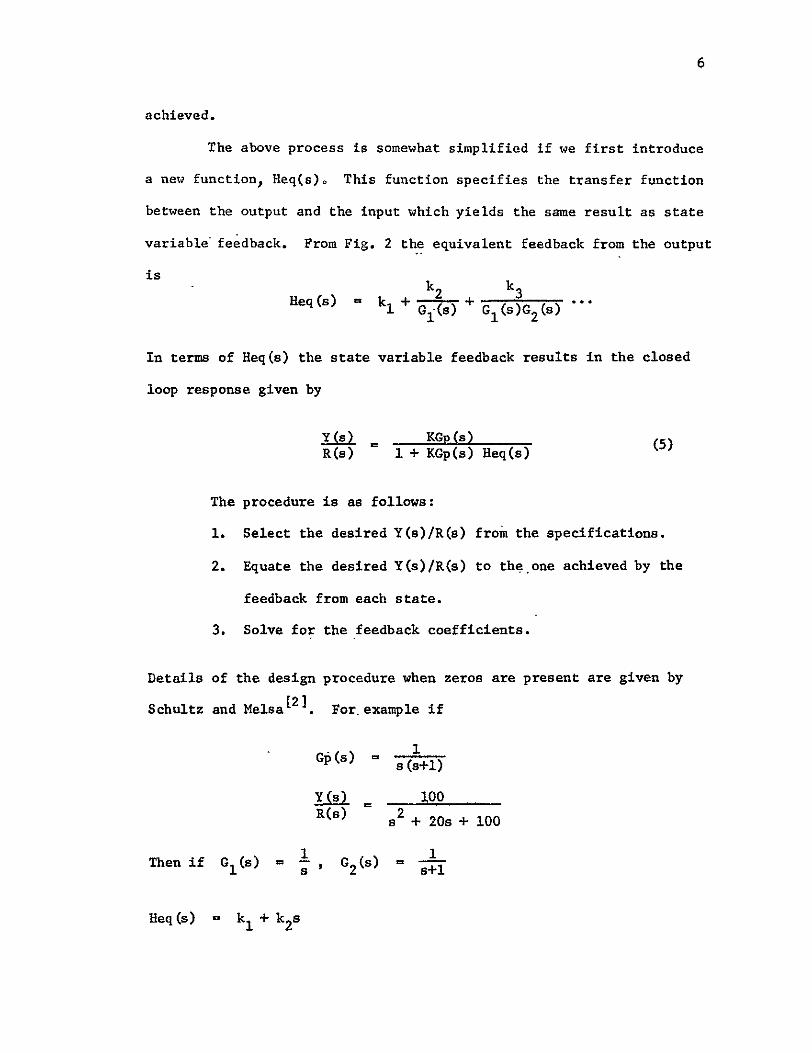

8
From (5)
100 K2 2 s + 20s + 100 s + s + K(k1 + k2s)
Equating the numerator and denominator polynomials
K = 100
KkI1 100
1+Kk2 - 20
Solving for k1 and k
K = 100
k = 1
k2 19
This design yields exactly the same transfer function as the
Guilleman-Truxal (GT) method The two methods are not the same if a
small change is made in the plant transfer function The state variable
feedback (SVF) system changes less than the GT system
If the sensitivity is defined as the percentage change in the
closed loop transfer function for a small percentage change in a plant
parameter say K then
S K _ d dK dT K
T T K dK T
where for simplicity
T(s) - Y(s)R(s)
9
If K is the gain then
T(a) =KG(s)1 + KG(s) Heq(s)
dT(s) G(s) K Gp(s) G(s) fea (s) 2dK I + KG(s) Heq(s) (1+ KG(s) Heq(s))
Using this result in the definition of sensitivity
T = T(s) (6) T KG(s)
For the GT system from (6)
K s(s+20)
2T (s + 20s + 100)
For the SVF system from (6)
K s (s+1)ST 2 a + 20s + 100
For the GT system the sensitivity is greater at all frequencies than
the SV sensitivity especially at low frequencies
Modified Observer Systems
LuenbergerE ] has shown that an eytimate of the states in the
plant can be implemented as shown in Fig 3 When state variableshy
feedback is used from these states a specified closed loop response may
be achieved Muterspaugh [4 has modified this configuration by block
diagram manipulations to a form similar to that shown in Fig 5 The
1 2 2NN-1
kI
Figure 3 Luenburger Observer Block Diagram
r C(s) G(s) Y
Figure 4 Modified Observer Block Diagram
A(s)
I+
gt G(s) Y H(s)
Figure 5 Muterspaughs Modified Observer Block Diagram
13
series compensator shown in Fig 4 C(s) reduces to the Guilleman-TruxalLiJ
compensation in the case where H(s) is one Similarly this control system
reduces to the Heq [2 ] type of control resulting from state variable
feedback considerations when C(s) is one Fig 4 represents a more
general configuration than either Guilleman-Truxal or Heq type compensashy
tion All three configurations shown in the above figures are equivalent
Assuming that only the output is available the Heq configuration
is not realizable since Heq has zeros but no poles Guilleman-Truxal
type compensation is sensitive to plant variations Series and feedback
compensation is used to achieve low sensitivity and realizability If
Heq has zeros in the LP then the modified observer (MO) system is
slightly higher in sensitivity than Heq but if Req has zeros in the RHP
then the MO system is dramatically better These comments are illusshy
trated in the case studies at the end of this report
Modified observer System Design
This section derives the necessary conditions which C(s) and H(s)
must satisfy such that the desired transfer function Y(a)R(s) is
achieved when the plant has a transfer function G(s) The relationship
among these transfer functions is
T(s) 1() C(s) G(s)fR(s) 1 + C(s) G(s) H(s) (7)
If the feedback signals shown in Fig 3 are combined (using
block diagram manipulations) the resulting transfer functions are
A(s)=k2 1P1 (S)+k 2 (fIpI(s)p 2 (s)+12P2 (s))++knceiPl(s)+ -PNI(s))
H(s)k 1+k2p1 +k 3P1p2++kpN-1
14
Since the poles of H(s) and A(s) are arbitrary the control systems shown
in Fig 5 have N-i arbitrary parameters however the poles of A and R
are identical
One more manipulation of the system shown in Fig 3 results in
the system of Fig 4 where
1 C(s) - I + A(s)
The zeros of C(s) are the same as the poles of A(s) therefore the N-1
zeros of C(s) are also the same as the N-i poles of H(s)
From these facts (7) can be used to determine the denominator
of C(s) and the numerator of H(s) Dropping the argument a in (7) and
denoting the transfer functions by
CDC(s)
H(s) -
G(s) ONGD
T(s) - R
Eqn 7 becomes
CN GN 1 CD GD(8) R 1i+ CN GN HN
CD GD HD
If the right hand is simplified then
Y CN GN HD (9)R CD GD HD + CNCN
Since CN and HD are the same denote them both by P(s) Then (9) simplishy
fies to
15
Y GN P (10)R CD GD + NHN
cross multiplying on both sides results in the polynomial
Y(CDGD+GNHN) - R-GNP (11)
Define the number of zeros in G as NG the number of poles as
ND and similarly NY and NR for T(s) If the order of both sides of
(11) is to be the same then
NY + ND - 1 + ND NR+ NG + ND - 1
NY + ND NR + NG (12)
NR - NY -ND - NG
Thus the pole zero excess of the plant determines the pole zero excess
of the desired closed loop transfer function If like powers of (11)
are equated then NY + 2ND equations result Since CD and 1N are undeshy
termined the number of unknowns is 2ND For NY = 0 the number of
unknowns is equal to the number of equations Just as in regular state
variable feedback[2 for zeros in YR additional states must be
created Let the order of P(s) by N-l then (12) becomes
NY + N - I + ND = NR + NG + N - 1
and for the number equations to be equal to the unknowns
NY + ND + N = 2N (13)
N = NY+ ND
16
Thus the order of both controller systems C(s) and H(s) must be one
less than the number of poles of G plus the number of zeros of YR
assuming that (11) represents a set of linearly independent equations
The design procedure is as follows
1 Select the desired closed loop transfer function from the
specifications
2 Select a polynomial P(s)
3 Equate the actual and desired transfer functions (iO) and
solve for the coefficients of CD(s) and HN(s)
Program 1
The first program (MODOBSI) computes the transfer function of
the series compensator and the feedback compensator as a linear function
of the denominator of the feedback compensator The user must specify
the plant transfer function and the desired closed loop transfer
function Thus this program specifies the design of the system except
for the poles of the feedback compensator which the user is free to
choose in any way he wishes
Program 2
The second program (MODOBS2) computes the transfer function of
the series compensator and the feedback compensator which minimize the
low frequency sensitivity of the closed loop system to plant variations
The user must specify the plant transfer function and the desired closed
loop transfer function If the time constants in the plant are much
lower than in the closed loop system the poles of the feedback compenshy
17
sator may be in the right half plane (RHP) If the poles of the compenshy
sator are in the RHP then the system will be vyD sensitive to variations
in the parameters of the compensators In this case it is better to
use one of the other programs This program is limited to systems with
no zeros
Program 3
The third program (MODOBS3) computes the weighted integral
sensitivity of the system for a given polynomial P(s) The user must
specify the plant transfer function closed loop transfer function the
weighting to be given the sensitivity as the frequency varies and the
denominator of the feedback transfer function P(s) The weighting
function must have more poles than zeros
Input Data
In many circumstances the available data for the plant is in
state variable form This data is converted to a transfer function by
the STVFDBK program The details of the program are included in reference
1 The program listing and input data format are also included in the
Appendix
Output Data
The program BODE4 is provided to plot the transfer functions
computed in the above programs on a logarithmic scale For each program
some of the transfer functions of interest are
1 Plant transfer function
2 Closed loop transfer function
3 Sensitivity as a function of frequency
4 Loop gain function
The loop gain function divided by one plus the loop gain is the proportion
of measurement noise at each frequency which will reach the output Thus
if the loop gain is much greater than one then nearly all the noise
reaches the output and if the loop gain is much less than one very little
measurement noise reaches the output If the phase shift of the loop
gain is nearly 180 at a gain of one the measurement noise will he
amplified
Program 4
The fourth program (MODOBS4) is useful to check the results of
the design Given P(s) and the results of the first program (MODOBSI)
this program computes HN(s) CD(s) and the roots of both the series and
feedback compensators This program and the first program give a
complete determination of the design
Results
A discussion of each program and several caee studies are inclushy
ded in the Appendices MDDOBSI is useful to compute HN(s) and CD(s) in
terms of the coefficients of P(s) Quite amazingly the coefficients of
N and CD are linearly dependent upon the coefficients of P HODOBS2
computes the coefficients of both compensators which achieve minimum low
frequency sensitivity Essentially this result is achieved by forcing
CD(s) to be an N-i order integrator which increases the gain at low
frequency and thereby decreases the sensitivity since SK = (s)
Unfortunately if the plant denominator coefficients are smaller than
19
those of the denominator of the closed loop transfer function the feedback
compensators may have poles in the RHP MODOBS3 determines the weighted
integral sensitivity when P(s) is specified MODOBS4 is useful for
checking the roots of the resulting compensators after a design is
complete Test results are given in the appendix for three examples
These examples show that an improvement in the system sensitivity over
that of just a series compensator can be achieved even if only the output
is available When the closed loop response is much faster than the open
loop the sensitivity of the MODOBS system approaches the sensitivity of
the Req system (which is best but not realizable) if the roots of P(s)
are made much larger than the closed loop roots If the closed loop
response is not much faster than the open loop response then the MODOBS
system may have a sensitivity lower than the Heq system This situation
exists whenever Heq(s) has zeros in the RHP These results point out
the important fact that a sacrifice in sensitivity to plant variations
is made by increasing the system performance requirements Because of
this fact careful attention to the plant performance should be made for
lowest sensitivity and unnecessary demands on overall system performance
should be avoided
20
Bibliography
1 J C Truxal Control System Synthesis McGraw-Hill 1955 Chapter 5
2 J L Melsa and D G Schultz Linear Control Systems McGraw-Hill 1969 Chapter 9
3 D G Luenberger Observing the State of a Linear System IEEE Transactions on Mil Elec April 1964
4 M E Muterspaugh State Variable Feedback and Unavailable States HS Thesis 1968
5 F H Effertz Comment on Two Coupled Matrix Algorithms for the Evaluation of the rms Error Criterion of Linear Systems Proceedings of the IEEE November 1966 p 1629
6 J L Melsa A Digital Computer Program for the Analysis and Synthesis of State Variable Feedback Systems NASA Contract Report CR-850 August 1967
7 L E Weaver et al A Control System Study for an In-Core Thermionic Reactor J P L Report 32-1355 January 1969
21
Appendix I - MODOBSI
Dis cussion
The basic algorithm of this program is based upon (5) First the
following polynomials in s are computed
T = (GD)(Y)
Q = (GN)(R)
V = (GN)(Y)
so that (5) becomes
(T)(CD) + (V) (HN) = (Q) (e) (Al)
Each of the terms in (Al) are polynomials in s where P(s) is unspecified
For instance P(s) = P3s2 + P The coefficients of CD(s) and HN(s) are
the unknowns
As an example suppose the plant is second order then P(s) is
first order In this case (Al) becomes
(CD2T3 +H 2 V3 )s 3 + (CD2T2 + CD1T3 + H2 V2 + H1 V3 )s2 + (CD2T1 + CD1T2
2 + H2V I + HIV2)s + (CDIT + HV) = P2Q 3s + (P2Q2 + PIQ3 )s2
+ (P2Q + P1 Q2 )s + PlQl (A2)
Equating coefficients of like powers of s results in the equations
T3CD 2 + V3H2 Q3P2
T2CD2 + T3CD1 + V2H 2 + V3H1 Q2P2 + Q3PI
22
T1 CD2 + T2 CDI + VIH2 + V2H 1 QlP2 + Q2P
TICD1 + V1Hi = Q1F1 (A3)
These equations can be rewritten more compactly in matrix notation as
T3 0 V3 0 CD2 f 0 Q3TN12N-2 T2 T3 V2 V3 CD11 214-22-Q3 Q3 Q22 (A)
2 T V1 V2 H2 Q2 QI P2j _ Ql 0
2N-2- shy - N-i-)
The matrix on the left will be defined as matrix A and the matrix on
the right will be defined as matrix C Then
CD2 CDI _ - 1
CD= A-C (A5)
H I
Therefore A- C relates the unknowns CDi and Hi to the parameters Pi
MODOBS1 forms the matrix A from the two arrays T and V and then inverts
A Next the C matrix is formed from the Q array and then A 1 C is
computed and printed
23
Input Format
Card No Columns Description Format
1 1 NY = order of Y(s) in YIR II
2 NR = order of R(s) in YR Ii
3 NG = order of GN(s) in GNGD i1
4 ND = order of GD(s) in GNGD Ii
I 5-80 Identification of problem 8AI0
20 Cn of 2 11-0 Coefficient of s in Y(s) FI03
11-20 Coefficient of aI in f(s) P1e3
etc
71-80 Coefficient of s7 in Y(s) F103
3 1-10 Coefficient of a in R(s) F103 etc
4 i-i0 Coefficient of s in GN(s) FIO3
etc
5 etc Coefficientof a in GD(s) FI03
Notes
1 If more than eight coefficients are required then two cards may be
used to identify that polynomial
2 A decimal point must be used for each coefficient but not for card
No 1 The decimal point may be placed in any of the ten columns
for each coefficient
24
3 As many problems may be run as desired by repeating the above format
for each problem
Output Format
See example
Subroutines to be Used
PLYMLT Multiplies two polynomials together
MXINV Inverts matrix A
PRNTRAT Prints the ratio of two polynomials
Flow Diagram
Read NYNRNG
ND
FRead Y(s)R(s)GN(s) GD(s)
Compute T = YGDQ = GNRV = GNYj
Form A Matrix
Invert A Matrixi
lForm C Matrixl
A -1
ComputeBA7 C
Print CD and E
Arrays
PROGRAM MODOBSI (INPUTOUTPUTTAPE4INPUT)
ODIMENSION Y IC) R(10) GD(IO) GN(IC) V(201 T(20) G(20)14A(S363)AI(36 3)C( 3611) B(36 1U ID(G)
C Y(S)R(S) IS DESIRED CLOSED LOOP RESPONSE C SP(S)GD(S) IS PLANT TRANSFE FUNCTION C NY IS ORDER OF NUM IN Y(SlR(S) NR IS ORDER OF DEN C NG IS ORDER OF NU OF G(S) NO IS ORDER OF-DEN C NR-NY MUST EQUAL ND-NG 1 READ 1U1NYNRNGNDID
PRINT 200NYNRNGNDIO
IF(EOF4) 99t2 2 NY1=NY4 1
READ 102 (Y(I)I=-INY1) C YI) IS COEFF OF S(I-I) IN Y(S)
NR I=NR C RII) IS COEFF OFS(I-1)IN-P(S) 3 READ I102 (R(I) IINRI)
CALL PRNTRAT(YNY1RNRI IHTIHS) __C_ GN(Il IS COEFF9F_SCI-1LIN_-GNtSL
NGl1NGI NO 1NDI
_4 -READ 102 (GN ) I 1NG1) C GOD(I) IS COEFF OF S(I-1) IN GO(S) 5 READ 102 (CG (I)I--1NDI)
CALL PRNTRAT(GNNGIGDNO HGIHS___ C FORM CHARACTERISTIC POLYNOMIAL
CALL PLYMLT (GDND1YNYITO) CALL PLYMLT GNNG1RNRI00-CALL PLYMLT (GN NGGYNYIVO) NYNGzN Y1 4NGI NR+NG+iN __ 00 6 IrNYNGN
C NA IS ORDER CF A MATRIX WHERE A IS MATRIX RELATING UNKNOWNS -6- V( --- - - TO PARAM P
NA_- 2 (N--1) DO 20 J-1NA IF- (J GT (N- IlJGO__TO2_12 00 10 Iz1NA INDN- L J IF _( IND-SLT_ I)_GOTO8_ IF (IND GTN) GO TO 8 AUIJ)- T(INa) 30 TO 10shy
8 A(IJ) O 10 CONTINUE
Gi__TO_2D
12 DO 20 I=INA IND 1-I+J IF- (INDLT__GO__18__ IF (INDGTN) GO TO 18 A(IJ)-V(IND) GO-T 0 _2D
18 A(IJ)-O 20 CONTINUE
CALL MXINV-(ANAtAll_ C C IS THE COEFF ARRAT
NM IrN-1 _DOZ4__I NA-_ DO 24 J=1YNMI IN= 2N-I- J
IFiINDLT1) GO TO 22 IF (INDGTN) GO TO 22
C(IJ) = O(INO) -
GO TO 24 22 C(IJ)rO 24 CONTINUE C B IS AICTAE ROwS OF 5 ARE EQUAL TO CD AND HN C COLS ARE COEFF OF P PARAMETERS
D0 30 INA 00 30 KzlNM1 B(IK)--O 00 3fJ--JNA
30 B(IK)-AICIJ C(JK+B(IK) PRINT 2O1KK--lNMI) DO 40 I--NMI
NC =N -I 40 PRINT 202 NC (B I-Kt NM1I
DO 50 I=NNA
NBzNA+-I -50 PRINT 204t-NB (8(1I(1 Kzl-NM-1
GO TO I 99 STOP -101-FORM ATf l A 1f)V t 102 FORMAT (BF103) 200 FORMAT (1HI4(2XI1) 2X6A1i0) 201 FORMAT IH X8 ( 314- P( I 11 I-) OX)) 202 FORMAT 14H CO(I2--)10(E1U33X)) 204 FORMAT (4H HN(I12H)=)I(EIO33X))
END SUBROUTINE PRNTRAT (ANNBvNOEPVARINDVAR) DIMENSION A( 20)B( 20H_(20)N(20)AT20BT(20)NEt 1
DO 6 I--NN AT(I)-- -IF-(-AY f-4i 6-3
3 H(NE)zlH+
AT(NE)rA(1) GO TO 5
4 H(NE)--IH-
AT (NE) -A(I) N(NE)I-1 NErNEI
6 CONT INUE NE=NE-1 PR IN-T 10 0 MIN=MINO(NE 10) PRINT 10lCN(I)IzMIN) PRINT 102 (HRU1 ATI) INDVAR Il tMIN) IF (NE-if]) 8987
7 PRINT 101 (N(I IrIINE) PRINT 102 CHI)AT(I)INDVARI--INEI
__ NF= O0 16 I--IND BT (I)--DIF C B(C) 191G13
13 H(NF)rlH4 BT(NF zB(I)
-GO-_ T _15 14 H(NFI -IH-
BT (NF) =-B(I)
r27 15 N(NF)=I-I
NF zN Fi-I 16 CONTINUE
NF =N F- I HH= IH-NH=rAX 013NE 13 NF) NHzMINO(130NH)
20 PRINT 103 DEPVARINOVAR (HH I=INH) MIN MINO(NF 10) PRINT 101 (N(I)IzIMIN) PRINT 102 (Hi(I)BT(I ) 1NDVAR-I---1MIN IF (NF-101) 28P2827
27 PRINT 0l (N(I) IzIINF) PRINT 102 (H(IJBT(I)TNDVARI=N-FI)shy
28 CONTINUE 100 FORMAT C iHO) 101 FORMAT (6XI(11X 12)) 102 FORMAT 6XID(AIGlC4 AI1H H 103 FORMAT tIXtAIIHCAI2H)= 30AI)
RE TURN END SUBROUTINE MXINV (R N RI) SUBROUTINE TO FIND THE INVERSE- ----- GIVEN
C MATRIX R N IS ORDER OF MATRIX RI IS INVERSE C MATRIX SUBROUTINE USES GAUSS-JORDAN REDUCTION C R MATRIX IS PRESERVED DIAGONAL ELEMENTS OF R-US
BE NONZERO C DIMENSIONR(3G36IRA(3G72) RI(36v36)
C STATEMENTS 20-26 ENTER R ARRAY INTO RA ARRAY - C AND SET LAST N COLUMNS OF RA ARRAY TO IDENTITY
C - MATRIX 20 DO 26 I 1 NI-v 21 DO 24 J I N
_22__RA IJ) -R(I- J) 23 NJ = N + J 24 RA(INJ) = 0 2 5 _NI z N + I 26 RA(INI) = 1
C C ST AT EM ENTS _ii-12_REDUCE MATLRIX__RA _SOH_ATZ_JRFSR_LK C COLUMNS ARE SET EQUAL TO THE IDENTITY MATRIX
i NP = 2 N 2_DO 12 I - N
C -
C STATEMENTS 3-5 ARE USED TO SET MAIN DIAGONAL _C ELEMENT TOUNITY
3 ALFA = RA(TI) 4 DO 5 J = I NP S RA(IJ) r RA(I J) _ALFA
C C STATEMENTS 6-11 ARE USED TO SET ELEMENTS OF ITH C COLUMN TO -ZERO
6 00 11 K = 1 N 7 IF (K - I) 8 11t 8 8 BETA = RAiKI) 9 DO 10 J = It NP
10 RA(KJ) = RA(KJ) - BETA RA(IJ) - ICONTINUE_ 12 CONTINUE
C
TO LAST 28 C STATEMENTS 30-33 SET INVERSE MATRIX RI EUAL
C N COLUMNS OF RA ARRAY
30 DO 33 J 1 N 31 JN J + N 32 00 33 I 1 N 33 RI(IJ) rRA(IJN) 34 RETURN
END SUBROUTINE PLYMLT (ALBMCN)
C C MULTIPLY ONE POLYNOMIAL BY ANOTHER
C C DEFINITION OF SYMBOLS IN ARGUMENT LIST C A(I) MULTIPLICAND COEFFICIENTS INTHEORDER AE) S(I-1) C L NUMBER OF COEFFICIENTS OF A C B(I) MULTIPLIER COEFFICIENTS IN THE ORDER 8(I)SI-1)
C M NUMBER OF COEFFICIENTS
C C11) PRODUCT COEFFICIENTS IN THE ORDER C(19S(I-1)
C N NUMBER OF COEFFICIENTc Ac r
C C REMARKS C IF N-- C(I) SET TO ZERO AND PRODUCT FORMED OTHERWISE THE
C I-PRODUCT AND SUM NEWC-OLD C + AB IS FORMED
DIMENSION A(iD) B(IO) t C(20) LPML+M- 1 IF (N) 10102iZ
I DO 1 J- LPM 11 C(J)-Oo 12 DO 13 J--ILPM
MA X-MA XD (J + I-M il)) shy
- MINzMINO(L DO 13 IrMAXMIN
13 CC(J)=A(I)B(J+II) + C(J) RETURN END
3434 IN CORE THERMIONIC REACTO R
116708 481228 384520 200 1 16708 -4870635__4085815__39226_ 100 116708 481228 384520 200- 503585E-610542E- 3 058639 18804 1
END OF INFORMATION
29
Appendix 2 - MODOBS2
Discussion
If CD(s) in (5) is defined by CD(s) = CD N-i (BI)
where N is the order of the plants then the system will have minimum
low frequency sensitivity because the forward loop gain will be increased
at low frequencies If there are no zeros in Y(s)R(s) or in G(s) (5)
reduces to a simple set of linear equations shown below For simplishy
city RN+ I and GDN+t are set equal to one For zero steady state error
Y = R1
PNl PN= I PN-I = N-I
PN-2 + RNPN-1 CN-2
(B2)
P + 2 + ReN- =1 I I
IN I = P RY
HN2 =PI RY + P2
+HN=NPI RNY + P 2 -Y +i - GD1Y
Where the C terms are defined by
C I GD2 - R2
C2 = GD3 - R3
CN- 1 GDN - N
30
The Eqns (B2) are simply solved in the order shown by back
substitution That is PN-1 may be usedto solve for PN-2 which may be
used to solve for PN-3 etc
Input Format
Card No Columns Description Format
1 1 N = Order of the Plant G(s) Ii
2-80 ID Identification of problem 8A1O
2 1-10 Y = Numerator of YR F10o3
0 3 1-10 R(1) = coeff of s in R(s) F103
11-20 R(2) = coeff of s I in R(s) FIO3
etc
7 71-80 R(7) = coeff of s in R(s) FI03
4 1-10 GN = numerator of G(s) F103
5 1-10 GD(l) = coeff of s in GD(s) F1O3
771-80 GD(7) = coeff of s in GD(s) F103
See notes following input format for MODOBSIo
Output Format
See example
Subroutines to be Used
PRNTRAT - Prints the ratio of two polynomials
PROMT - Determines the roots of P(s) to see if any roots are in
RHP
PROGRAM OOS2 (Y4PUT OUTPUTC4=INPUT)IO41 N j (l10 1 ( l ) 1 ([) Cl(In)ID( 3)PHN 1 )CD t13)
C U (IG) V (10) C PqOGRAM TO CALCULATE MINIMUM LOW-FREO SENSITIVITY MODIFIED C OBSERVER SYSTEM C Y(S)R(S) IS DESIRED CLOSED LOOP RESPONSE C GN(S)GD(S) IS PLANT TRANSFER FUNCTION C N IS ORDER OF DEN IN Y(S)R(S) C N IS ORDER OF DEN IN GN(S)GDIS) C R(I) IS COEF OF S(I-1) IN R(S) C C ASSUMPTIONS C C TRANSFER FCN GAINS ARE NORMALIZED SUCH THAT R (N+1)I1
C AND GD(N I )=I C C DESIRED TRANSFER FCN HAS ZERO STEADY STATE C
-C GD(I) IS-COE-F-- O-F S(I-I)1NGO(S) C Y(S)=Y GN(S)-GN (NO ZEROS ALLOWED) C I READ 101 N ID
IF(EOF4)99 2 2 READ I02Y
READ 102 (R(I)IzIN) NP i-N+ I
GD(NPI) =1 5 RNPI_)-1 READ 102 GN
3 READ 102t CGD(I)tlz1N) PRINT 200DNIO10 PRINT 201
CALL PRNTRAT CYIRNPHTIHS) PRINT 202
CALL PRNTRAT(GNGDNP11HG1HSI C-C --SOLVE FOR DEN OF H P(S)
NM I=N-I do 40 II -NM1 IPIlzI+I
-4 -CI) zG0c IP 1I-R IiT P(N) -
005[ I=ItNMj NI N-I P(NI)zC(NI)
IFCILE1) GOTO-50_ DO 49 Jz2I J2=N-J+2
4 P(NI )zP( NI )-R( J2 )P( JI ) 51 CONTINUE
CALL PROOT (NMIPUV) PRINT 205
PRINT 206 (U(I)V(I) I=INM1)
ERROR THUS YR(1)
SOLVE FOR NUM OF HHN(S) DO 60 1N HN (I 0 - 00 60 JzlI IJI j4
C
6C PN Il)r( Ji R (IJ) Y +HN( I) 32 HN (N )HN (N)-GD (1 )Y
PRINT 203 CALL PRNTRATIHNNPNIHH1HS) PO 80 1i NMI
80 CO(I)zO CD(N)zl PRINT 204 CALL PRNTRAT(PNCDN1HC1HS) G z YGN PRINT 210 G GO TO I
99 STOP 101 FORMAT (Il 84101 102 FORMAT (SF1O3)
200 FORM AT(IHII0X II 4X 8AID) 201 FORMAT(1HOTHE DESIRED CLOSED LOOP TRANSFER FUNCTION IS)
202 FORMAT(1HOTHE TRANSFER FUNCTION OF THE PLANT IS)
203 FORMAT(IHOTHE TRANSFER FUNCTION OF THEFEEDBACK COMPNSATOR IS)
204 FPRMAT(lHOTHE TRANSFER FUNCTION OF THE SERIES COMPENSATOR IS)
205 FORMAT (IHO 5X THE ROOTS OF P (SI ARt 13XREAL PART IOXIMAGINARY PART)
-20 FORMAT 32X2E207f 210 FORMAT4IHOTHE ADDITIONAL FORWARD LOOP GAIN REQUIRED IS
1YGNElfl3) END SUBROUTINE PRNTRAT (ANNSNDDEPVARINOVAR) DIMENSION A(20)B(20vH(20) N(20 1 AT(20) PT 20 NE z1 00 6 Iz1NN AT(1)=D IF C(IA ) 463
3 H CNE )= IH + AT (NE) =AtI) GO TO 5
4 H(NE)=IH-AT (NE) =-A( I) N(NE)--I-1 NE-NEI
6 CONTINUE NE=NE-1 PRINT 100 MINMINO(NE v1O
PRINT IOl (N(IhI=IMIN)
PRINT 102 (H(IAT(I)INDVARI-IMIN) IF (WE-10) 8
7 PRINT 101t (N(I)IzlINE) PRINT 102 (H(I)AT(I)INDVARIn1NEl NF o_-8_ N --1 80 16 I1NU
BT(IzO IF ( (I) 1141613
13 H(NF)zlH+ BT(NF)l=B(I)
-GO T0- 15 __ - 14 H(NF) zlH-
BT (NF)z-B(I) - 15 N(NF)=I-1 -
NFZNF41
33 ID CONTINUE
NF NF- I HHL IH-NHMAXO( 13NE 13NF) NHzMINO( 130NH)
20 PRINT 1G3DEPVARINDVAR(HH 1=1NH) MINMINO(NF 10)
PRINT 101 (N(I)IlMIN) PRINT 1G2( H(I)BT(I)INOVART IMIN] IF (NF-in) 2828927
27 PRINT 101iN(I) I11 NF) PRINT 102 (H(I)BT(I)tINDVARI-IINF]
28 CONTINUE 100 FORMAT (1HO) 101 FORMAT (GX1O( IIX12)) 102 FORMAT (GXI0(AIGIO4 A1IH )
103 FORMAT (1XA1IH(Ai2H)-130A1) RETURN END
___SUBR CUT INEPR O0 TN _A U fVtIIRR) DIMENSION A(20)U(20)V(20)H(21)8(21 )C(21) IREV-IR NC -N +IDOll--i Nu
H( I) rA( I) _i CONTINUEL
00
3 IFIH( 1)) 24 2 NCNC-1
V NC )z0 U NC O DO 1002 I= 1NC H(I)--H(I+1 )
1002 CONTINUE GOT03
S_IF (NC- 1) 5 10 05 5 IF (NC-2) 7i 7
6 R=-H( 1H(2) GOT050
7 IF INC- 3) 9-819 8 P-H(2)H(3)
__0 1) H (3_)_ GO TO7g
q IFCABSCH(NC-1)1H(NC)-ABS(H(2)H(1))101919 10- IREV - IREV_
M=NC2 DO11I=-1 M
_-NL-zNC+ 1 -I-FrH( NL) H NL )H( I)
11 H( I) F -IF (O )139 12 913
12 P=D GOTO 15shy
13 PzPQ 0= (
15 IF(R)16191G 16 R=1 R 19 E5E- ]C
B(NC)H(NC) C(NC)H(NC) B(NC+1 )zO C( NC 1)z 0 NP NC- 1
20 0049J= I 100C DO 2111l1 NP ITNC-I I BC I rH(I)+RB(+1)
--21C( I) =B (I)+RC( I+ 1) IFCABS(B(I )H(1))-E)5050 24
24 IF(C(2)232223 2amp R= RlI-
GO TO 30 23 R=R-B(1) CC2)
30 D0Q3711zlNP IzNC-I I BI)i(I)-PB(I+I)-OB(I+2)
37C( I) =B (I)-P C(i1l) OC(12) IF(H (2)) 323132
31 IF(ABS(C2)H(1))-E)333334 32 IF(ABS(B(2)H(2) )-E) 33v3 34 33 IF(ABS(B(1)H(1))-E)707034
34 CBARrC(2)-B(2) DC(3) 2-CB ARC ( 4) IF(D)363536
35 PzP-2 0= (o t GOT049
36 PP(-82)C(3)-BC1)C(4))D - Q+ (-( 2)CBARB(1) C(3 00)
49 CONTINUE
ErE 10 GOT020
50 NC-NC-1 VtNC)D
IF (IPEV) 51 5252 51 U(NC)=1R-
GOT053 52 U(NC)-R 53 00541lNC
H(I) B(1+1) 54 CONTINUE
GOT04 70 NC=NC-2
---- IF(IREV)71727 71 QPr1O
P=P(Q2 0) GOTO73-_
72 OPPP Q-P 2 0
73 F-(PP)2-OP IF(F )74 7575
74 U(NC+I)z-PP U(NC)-PP V(NC 1 )SORT(-F) V( NC 1-V (NC+ 1) GOT076
75 U(NC+11-(PPABS(PP))(ABS(PP)SQRT(F)J V( NC+1 )0 U(NC )OPU (NC1) V( NC )O
76 D0771INC H(I) B(1 2)
77 CONTINUE GOT04
LDO RE TURN END
3 CASE STUDY II THIRD ORDE-SYSTE14shy1000 1000 200 20 D O -
2500 100
36
Flow Diagram
Read N ID
Y R(I)
GN GD(I)
Print N ID
YRy G
Form C(I)
ISolve for P(s)j
Solve for HN(s)I
Print H(s)
Print C(s)
37
Appendix 3 - MODOBS3
Discussion
This program uses the following data
1 Plant transfer function G(s)
2 Desired closed loop transfer function T(s)
3 The denominator (P(s)) of the feedback compensator H(s)
4 A desired weighting function W(s) on the integral over
frequency of the sensitivity of the closed loop response
to forward loop gain changes
The program then calculates the weighted integral sensitivity of
the system The method of calculation is based upon an algorithm by
EffertzL5] The integrand of the integral sensitivity is calculated
from
I S W(S) S (S) ds
2r f G(s)C(s) ds
The algorithm is based upon an iterative manipulation of the coefficients
in the numerator and denominator of the integrand in such a way that the
integral of the squared magnitude results
A closed form solution for the integral
jm n 2rj jo h(P)h(-P) 2 -joo
1 30 dP 1 j F(P)F(-P) dP
(BI)
is presented in the paper by F H Effertz The solution takes the form
38
of Equation 4 in his paper A better algorithm for the computation of
Equation 4 in Effertz is presented in the correspondence by Pazdera
(Equation 7) A modified forn of Pazderas algorithm has been coded in
FORTRAN and is included A test problem is also included
The use of Equation 4 in Effertz can be best illustrated by an
example Suppose we wish to evaluate the following
(B2)Ls2+ Cb) [2bLn = 2I -
It can be shown from residue theory that the correct answer is
I = - residue of F(s) F(-s) at s = a (B3)n
- residue of F(s) F(-s) at s = b
where F(s) F(-s) indicates the function to be integrated over s = jW
Then the answer is
22 2
= - c-a (c2-b2 c2+abn 2a(a+b)(a-b) 2b(a+b)(b-a) = 2ab(a+b) CR4)
To use Equation 4 from Effertz we must make the following associations
using the complex frequency variable s in place of p
22 s= c -g(P) = (s+c)(c-s)
then s (B5)
2
h(P) = s + (a+b) s + ab
then p s N=2
1
a a 2 =ab
39
The integral for n = 2 can be expressed as
bb [bloaaob I- (B6)
a0 t ol [jaza1-2 1ao a 2
Substituting the correct values of a0 a etc and cancelling minus
signs for this problem we obtain
ab +c In = 2ab(a+b) (B7)
What is most interesting is that the result depends only on the coeffishy
cients of the known function being integrated and not on the poles of
the function as one would suspect from residue theory
It has been mentioned that the algorithm from Pazdera (Equation 7)
has been programmed Some charges in the nomenclature of Equation 7 were
necessary to facilitate coding Note that the practice in Effertz and
Pazdera is to make the highest membered coefficient correspond to the
lowest power of the variable p Note also that subscripts such as ao
are in evidence To facilitate coding the lowest numbered coefficient
was subscripted in the form A(l) and this coefficient was associated with
0 ththe lowest power of the variable p in this case p In general the i
coefficient A(I) is associated with the (i-1)s t power of p P -l (In
FORTRAN the expression A(O) is not allowed) Note from equation I above
what must be done to operate on the function F(s) F(-s) If F(s) is of
the form
F(s) = C(S) (B8)A(S)
then the algorithms suggested in both Effertz and Pazdera require the use
40
of
g(s) = C(S) C(-S) (B9)
h(s) = A(S)
It is more desirable to input C(S) and A(S) rather than C(S) C(-S) and
A(S) Consequently one uses the INTSQ subroutine by coding the coeffishy
cients of C(S) and A(S) with ascending subscripts corresponding to
ascending powers of S The subroutine provides the operation C(S) C(-S)
Furthermore the subroutine checks to see if the lowest coefficient of
C(S) or A(S) is zero so that factors of S may be either considered or
cancelled Two basic requirements must be met by A(S) and C(S) First
the roots of A(S) and C(S) must at least have non-negative real parts
(Hurwitz polynomial requirement) Secondly the highest power of C(S)
must be at least one less than the highest power of A(S) for convergence
to be assured If A(S) is Nth order one inputs the N coefficients of
A(S) and the N-i coefficients of C(S)
The use of this subroutine INTSQ may be best illustrated by an
example Suppose we desired to evaluate the integral
I = JD F_ 7 4 - JdS n -joe 3 + 3s2 + 2s + L[43 + - 2s
(BIO)
The polynomials C(S) and A(S) as defined in Equation B8 are input into
the program as
C(1) = 4 A(l) = I
C(2) I A(2) = 2
(Bi) C(3) o A(3)= 3
A(4) = 4
41
The program then utilizes the modified Pazdera algorithm and prints out
the message
THE VALUE OF THE INTEGRAL IS 12250
To check this answer one can use Effertz Equation 4 for a third order
case (n=3)
a oa 101o 2 1 n
= (142a
0 a
aI a a 0
I 2a
boa2a3+b2aoal-aoa3b alaaa a (BI2)
0 1 20 - o2 2 3o 31 o 13a22o0
For our example problem the following associations follow
b =0 a =4 0 0
b 1 -l a = 3 (B13)
b2 =16 =2a 2
a 113
Substituting the values of Equation B13 into Equation B12 verifies the
computers solution I = 1225n
Input Format
Card No Columns Description Format_
See format for MODOBSI
K 1-10 P(1) - coeff of so in P(s) BE103
11-20 P(2) - coeff of s in P(s) 8E103
etc
42
Input Eormat (contd)
Card No Columns Description Format
K+I 1 NW - Number of coeff in denom of W(s) II
K+2 1-10 WN(I) - coeff of s in num of W(s) 8E103
11-20 WN(2) - coeff of s in num of W(s) 8EI03 etc
K+3 1-10 WD(1) - coeff of s deg in den of W(s) 8E103
11-20 WD(2) - coeff of s in den of W(s) 8E103 etc
43
PROGRAM MODORS3(INPUTOUTPUTTAPE4-INPUT ) DIMENSION Y( 10)R(10)c-D(IO) SN(lOhIP(10)CD(0) HN(IO)SN(40)bull
IS0(40) B(36 18)WN(10) WD 10)SNT(40)SDT(40)C
I CALL MODOBSI (YP GN GO5 NY1 NR1 NGI NDI C N-1 IS THE NUMBER OF COEF IN P(S) HN(S) CD(S)
NrNR 1+NGI- 1 N =rN -1 READ 10 lP(I)Iz1NI)
C W(S) = WNWD MUST HAVE MORE POLES THAN ZEROS C NW IS THE NUMBER OF TERMS IN THE DENOMINATOR OF WS)
READ 103NW READ 102 (WN(I)I-INW)_ READ 102 (WD(I)I-INW) PRINT 205 CALL PRNTRAT (WNNWDNW1HW4-lkHS) CALL PLYMLT(GDNDlY NYI SN 0) N2=NDI+NYI-I
_CALL_ PLYMLTT(yN NWSNN 2 SNT D) CALL PLYMLT (GNNG1 R NRI SO 0) CALL PLYMLT(WDNWSDN2SDT C)
__N3=NW+N2-1 -
N4 =N 3+ NI-1 N22N1 11
-a- DO 10 I= 1Nl CD(I)=0 HN(I)O 00 10 J1pN1 CD (I)B(N-I J)P J )+CD( I)
10 HN(I)zB(N2-IJ)P(J) +HN(I)_P -I NJ_Z0 I--_
CALL PRNTRAT(PN1CDN1IHCIHS) PRINT 202
CALLP RNTRATAHN NI P Ni1H Ht l1 CALL PLYMLT( CDN1 SNT N3 SN C) CALL PLYMLTI- PN1SDT N3SD 0) -N5=N4 ---CALL INTSQ(SDSNN4S) PRINT 204 S
- GO T ---O-- -- 102 FORMAT 18 E1O3) 103 FORMAT III)
-201 -FO RM ampTL__TJJLJERANS ER_-F-UN CT-O-N--OF--L sESERIS--COMENSJ-IO-R- i-l 202 FORMAT(O THE TRANSFER FUNCTION OF THE FEEDBACK COMPENSATOR IS) 204 FORMAT(O THE WEIGHTED INTEGRAL SENSITIVITY ISEIO3) 20S -FORM-AT( Oi-tJ-WEIGHTINGFUNCTION-OF-HE- INTEGRALSENS-IIVlTY-YI-_shy
1) END
_SUBROUTINEMOOOBS1 LYR GN GD B N-YI-NRI-NGL-ND44-UDIMENSION Y(IO) RU1G) GD(10) GNIG) t V(20) T(20)9 Q(20) IA(3636)AI(3G36)C(36l8)B(36 1B)ID(6)
C _Y(S)R(S) IS DESIRED-CLOSED LOOP C GP(S)GD(S) IS PLANT TRANSFERFUNCTION C NY IS ORDER OF NUM IN Y(S)R(S) NR IS ORDER OF DEN
_C_ --NGJ S OR DEROFJN UaOF_ GASJ_ID- S--DRDELO DE C NR-NY MUST EQUAL ND-NG C Y(I) IS COEFF OF S(I-1) IN Y(S)
C RP I) IS COEFF OF S( 1-f1 IN Q(S)
C GN(I) IS COEFF OF S(I-11 IN GN(S) C GOCI) IS COEFF OF S(I-1) IN GO(S) 1 READ 1UINYiNRNGNDIO
IF(EOF4) 99t2 2 NY IrNY +1
NR ic NR --READ 102 (YCI)IIlNYI)
3 READ 12z (R(I) I--NRl) PRINT 200NY vNRvNGNO ID CALL PRNTRAT(YNYl R NRI 1HT IS) NuGl=NG I
ND i ND-shy4 READ 102 IGN I I--I NG1) 5 READ 102 (GD(I)IzlND1)
CALL PRNTRATIGNNG1GDNDI 1H3IHS) C FORM CHARACTERISTIC POLYNOMIAL
CALL PLYMLT (GDNDIYNY1TO) CALL PLYMLT GNNGIRNR10) CALL PLYMLT (GN NGIYNY1V0i NYNG=NY1+NGI N rNR+NG+I 00 6 IzNYNGN
C NA IS ORDER OF A MATRIX WHERE A IS MATRIX 6 V(I)zfl
NA= 2 (N-1 DO 20 J-INA IF ( J GT ( N- 1) GO_TO_1 2 DO 10 IrINA IND-N-I+J IF (IND LT 1) GO TO 8 IF (IND GTN) GO TO 8 A(IJ)= TIIND) GO TO 10
8 A(IJ)zO 10 CONTINUE
GO TO 20 12 DO 20 I=lNA
IND --- I+J IF fINDLTI)_ GO TO 18 IF (INDGTN) GO TO 18 A(IJ) zV(IND)
GO TO 20 18 A(IJ)rO 20 CONTINUE
CALL MXINV_ (ANAAI_) C IS THE COEFF ARRAY-C
NMlzN- 1 DO 24 IrItNA DO 24 JrINM1 INDz2N-I-J
IF(INDLT1) GO TO 22 IF (INDOTN) GO TO 22 C(IJ) - O(IND) GO TO 24
22 C(IJ)zO 24 CONTINUE
__C B IS AICTHE RUWs UF B ANt LIUAL IU) (U C COEFF OF P_ PARAMETERS
00 30 IrINA
44
RELATING UNKNOWNS TO PARAM P
AN_)_HN_THECOLSAR
00 30 KzlIMI B (I K) 0 00 30Jr1NA
30 B(IK) AI(IJ)C(JK)+B( T K) PRINT 201IKv(K=1 NM1 DO 40 I=INMI NC =N -I
40 PRINT 202NC(B(IK)Kr1NM1) DO 50 IzNNA NB -N A 1- I
50 PRINT 204v NB(B(IKIK--NMI) RETURN
99 STOP 101 FORMAT (4116A10) 102 FORMAT (SF103) 200 FORMAT I1HIv4(2XI1) 2XGA1O 201 FORMAT (10X3(3H P(I1lH)vgX)H 202 FORMAT (4H CD(I12H)zO(E1O 33X) 204 FORMAT (4H HN(IIZH)=IO(EIO 33X)L
ENO SUBROUTINE PLYMLT (ALBMCN)
C MULTIPLY ONE POLYNOMIAL BY ANOTHER C
C DEFINITION OF SYMBOLS IN ARGUMENT LIST C AI) MULTIPLICAND COEFFICIENTS IN THEOROER A(I) S(I-I)
C L NUMBER OF COEFFICIENTS OF A _C_ _B I) __MULTILPLIER CO EE-CIENiS-LNTlLODE3-IIi-plusmnSflt-WL-
C M NUMBER OF COEFFICIENTS OF B C CII) PROOUCT COEFFICIENTS IN THE ORDER C(I)S(I-1)
_
C C REMARKS
_C _IF -LO_ C (t1---ETJO_=EOANIRRO IUCTER-MF] lkRWLD T TRiLEJP-PO-DIC C AND SUM NEWC= OLD C AB C
DIMENS ION A( 101 D_cL20j LPML M- 1 IF (N) 101012
At1 -DO i - J-=l LPM__ I] C(J)zOO
12 DO 13 J=ILPM __M AXzMA XO (J+1-MJ
MINMINO (L J ) 00 13 I=MAXMI C ( J )=A _I u KB (Jt 1 RETURN
END
IS FORMED
SU BR OUT I NE P RN TRAT (A NNB N D DEPV AR INDVA RJ_ -
DIMENSION A(20)B(2)H(20 )N( 20)AT(20) BT(20) NE l
-DO JI1NN___ AT (I 1 IF ( A() 1 4993 H( NE = IH AT (NE) zA(I) GO TO 5 H(NE)I-H-
AT(NE) -A(I) N(NE)rI-1 5
146NErN E+1
6 CONTINUE NE =NE- I PRINT ion MINz INC(NE 10) PRINT iO1(N(I)T--MIN) PRINT 10Z (H(I)ATCI) INUVARI1MIN) IF (NE-in) 387
7 PRINT 101 (N(I)IrlNE) PRINT 102 (HCI)AT(I)INOVARvl--IrNE)
8 NF I DO 16 I-1ND ST(I)-O IF ( B(I) ) 141G13
13 H(NF)zIH+ ST (NF) -B(I) GO TO 15
14 H(NF) -IH-BT (NF) -- B(I
15 N( NF)zI--I NFrNF+ 1
16 CONTINUE NF =NF- I-HH =1H-
NH=MAXCD13NE 13 NF) -NH=MINO(130NH)Y
20 PRINT 103t DEPVARINDVAR (H H I-INH)MIN=MINO (NF 10) PRINT 101 (N(I-IiMIN) PRINT 102 (HI )BT(I)INDVARIlMIN)
IF (NF-ID) 282827 27 PRINT 101 N(Il) I=I-1NF)
PRINT 102 CH(I)BTII)INDVARI-i1NF) 28 CONTINUE 166- FO PM AT IHO-shy101 FORMAT f6Xv10(IIX12)) 102 FORMAT (GX0(A1G1O4 AIIH 103 FORMAT t IX A1 IHIAL 2H)Z 130AI])
RETURN END SUBROUTINE MXINV (R RI)
C SUBROUTINE TO FIND THE INVERSE OF A GIVEN C MATRIX R N IS ORDER OF MATRIXv RI IS INVERSE C MATRIX SU-BROUTINE USES GAUSS-JORDAN REOUCTION C R MATRIX IS PRESERVED DIAGONAL ELEMENTS OF R MUST BE NONZERO
DIMENSIONR(33G ARA(3 72) RI(363)
C STATEMENTS 20-26 ENTER R ARRAY INTO RA ARRAY C AND SET LAST N COLUMNS OF RA ARRAY TO IDENTITY-C MATRIX
20 00 26 I = I N 210 24 J = l N 22 RA IJ) - R(IJ) 23 NJ = N J 24 RA(INJ) = 0 25 NI = N + I 26 RACItNI) = 1
C C STATEMENTS 1-1-REDUCE MATRIX RA -SOTHAT FIRST N C COLUMNS ARE SET EQUAL TO THE IDENTITY MATRIX
471 NP = 2 N
2O 12 I 1 N
C STATEMENTS 3-5 ARE USED TO SET MAIN DIAGONAL C ELEMENT TO UNITY
3 ALFA = RA(II) 4 DO 5 J I NP 5 RA(IJ) z RA(IJ) ALFA
C C STATEMENTS 6-11 ARE USED TO SE-T ELEMENTS OF ITH C COLUMN TO ZERO
6 00 11 K = 1 N 7 IF (K - I) 89 11 8 8 BETA RA(KI)
9 DO 10 J I NP 10 RA(KJ) RA(KJ) - BET A- RA(IiJ 11 CONTINUE
12 CONTINUE C C STATEMENTS 30-33 SET INVERSE MATRI-X- RI-EQUAL-TO-LAS-T-C N COLUMNS OF RA ARRAY - 30 DO 33 J 1 N
31 JN = J + N 32 00 33 I 1 N
33 RI(IJ) RA(IJN) 34 RETURN
END SUBROUTINE PLYSQ_ (CN8j___ DIMENSION C(40)B(4D)
C RETURNS BCS) = C(S)C(-S) TO MAIN PROGRA-M C B(I) IS COEF OFS -l IN S -------C C(I) IS COEF OF S I-I IN C (S) C N-I IS NUMBER OF COEF IN B(S) AND C(S)
N1I (N- I)-12---shy00 20 I=lNI MO =-I _BCI) zD II z 2I-i
DO 20 K=1 II MO z -1MO
20 B(I)B(I)MOC(K)C( 2I-K) NMIN-i
- N2-N +I 00 30 I=N2vNM1 IIN=2I-NMI
MO(-I) NMI DO 30 K-IINNMI
O -IMO
30 B(I) r3(I)+MOC (K)C( 2I-K) RETURN
-- END - SUBROUTINE INTSO (ACNS)-DIMENSION B(IOhA(II)C(ID)
C___ RETURNS SZINTEGRAL OF C(S)C(-Si A CS )A( -S)-TO MAI-NRPROGRAMo C B(S) HAS N-I TERMS A(S) HAS N TERMS C B(I) IS COEF OF S(2I-2) - ISCOEF OF S(I-I)2C- -C(I) C IF THE LOWER ORDER DEN AND NUM COEFF ARE SMALL (LESS THAN C 0) THEN DIVIDE BOTH NUM AND DEN BY S2
48
0 1 OE -6 1 IF ( ASS( At 1) )-O) 2220 2 IF (A3S(C(1)-O) 4420 4 IF (K-I) 556 5 PRINT 200 6 PRINT 20IA(1) C(1)
N=N- I 00 10 I1N A(I)=A(1+1 IF(I-N) 8 1010
8 C(I)C(I1I) 10 CONTINUE
GO TO 1 20 CALL PLYSO (CNB)
NM2N-2
DO 50 K=INM2 NK =N -K BA=B(NK) A(NKI) AAO IF(KEOI) GO TO 40 AAzA (NK+2) tA(NKt 1)
40 NMK=(N-K)2 DO 50 I1 NMK NKIzNK-2I1+ B(NK-I )rB(NK-I)-BAA (NKI) A(NKI+i)zA(NKI+)- AAA-NKIj
50 CONTINUE SZB(1) (2A(2)A(I)
RETURN 200 FORMAT (0 THE FOLLOWLNG COEFF WERE FOUND TO BE SMALL AND CANCELL
lED IN THE NUMERATOR AND DENOMINATOR) 1FORMAT (THE DENOMINATOR COEFF EID3 THE NUMERATOR COEFF
1= E103) END
0303-CASE STUDY-IIt -THIRDORDER SYSTEM 1000 000 ___ 2020 i_ 1000
2500 100 1
2
49
Appendix 4 - MODOBS4
Discussion
MODOBS4 uses the matrix relating the coefficients of CD(s) and
HN(s) to the coefficients of P(s) and also the coefficients of P(s) to
determine both the series compensators and the feedback compensators
The roots of the compensators are included
Input format
Card No Columns Description Format
1 1 N = order of plant G(s) II
2-80 ID = Identification 8AI0
2 1-10 CD(l1) coeff of array from MODOBSI EIO3
11-20 CD(12) coeff of array from MODOBSI E-1O3
3 1-10 CD(21) coeff of array from MODOBSI EIO3
11-20 CD(22) coeff of array from MODOBSI E103
N+2 1-10 HN(11) coeff of array from MODOBSI E103
11-20 HN(12) coeff of array from MODOBSI E103
2N+2 1-10 P(l) - coeff of st in P(s) E103
11-20 P(2) - coeff of s in P(s) E103
etc
50
Flow Diagram
Read CD(IJ)
HN(IJ)
P(I)
Compute N
C(J) = Z CD(IJ)P(J) J=l N
H(l) = Z HN(IJ)P(J) J=l
Compute roots of
P(s) and C(s)
Print H(s)
P(s) C(s) and
roots of P(s) and C(s)
IOUN I S I LGO
C PROGRAM PROGRAM
MODOOS4( INPUT OUTPUT TAPE4zINPUT TO CALCULATE CO mPENSATORS WITH P(S) AND RESULTS OF MODOBSi
DIMENSION ID(8) CD (1R 18 ) HN (I 8v 18) C( 18 )PH( 1S )v U 23) V120)P[20 C N IS THE ORDER OF THE PLANT G(S) AND NO OF COEF IN P(S) i READ 100v N ID
IF(EOF4 992 2 PRINT 200 N ID
DO 10 I1IN 10 READ 101 (CO(IJ)JIP N
DO 15 lr1N 15 READ 1019 (HNIIJ) JIN)
READ -101 (PCI) I=IN)
DO 20 I=1N CI I) za HI I ) O DO 20 Jrl N C( I) =C (I)+CD (I J)P(J) H( I ) -H (I)+HN (IJjP (J)-PRINT 204 CALL PRNTRAT(PNtCN1HCiHS) -PRINT205 CALL PRNTRAT (HNPNIHHIHS) NM1=N- 1 CALL PROOT _(NMltCUtVI)- PRINT 201 PRINT 202v(UI)vV(III=IvNMl)
CALL PRO OTNM1 P UV PRINT 203 PRINT 202CUCI)vV(I)vII1NMl) CALL PROOT (NM1NUVI) PRINT 220 PRINT 202(U(I)VCI)I=INM1)
-GOTO_1_ STOP
100 FORMAT t II8AO) _101 _FORMAT_ (8E103)- -- - -- 200 FORMAT (IH12XI12XsAlo) 201 FORMAT(IHSXTHE ROOTS OF C(S) ARE13XPEAL PARTI0XIMAG1NARY
PART) 202 FORMAT (32X2E207) 203 FORMAT (IHO5XTHE ROOTS OF P(S) ARE13XREAL PART1OX-ruwiNARY
-1PART )- 220 FORMAT (1HP5XTHE ROOTS OF- HN(S) ARE13XREAL PART10XIMAGINARY
1PART) -204--FRMAT-IH 0 -- HE--R NS EFRFU NCT-L-ON-CO$FTHamp SERILEs OBZ-NS-AORSt-IL
205 FORMAT CIH THE TRANSFER FUNCTION OF THE FEEDBACK COMPENSATOR IS 1) -END SUBROUTINE PRNTRAT (ANN3NDOEPVARINElVAR) DIMENSION A(20)8(20)H(20)N(n ATt fnl RTlrn) -NE - --
DO G I =INN AT (I lD IF (L l I -
52
3
4
5
6
7
8
__13__
14
1s
16
_20
27
28 10(
01 102 103
H( NE )= IH+ AT(NE)=A(I) GO TO 5 H(NE)zIH-AT(NE) -A() N(NE)I-I NE NE+ 1 CONTINUE NE =N E- I PRINT 100 MINzMINO(NE 10) PRINT 101 CN(I)I-IMIN) PRINT 102 (HCI)AT(I) INDVAR I=i MIN) IF (NE-In) 887 PRINT 101 (N(I-1I11 9NE)- -PRINT 102 CH(I)AT(I)INOVARI=11NE) NF =1
DO 16 IiND BT (I )=O IF ( 8(I) 1 141613 H(NF)=IH+ BT(NF)-B-(I) GO TO 15 H(NF) =IH-BT (NF) =-B( I) N(NF )=-I-I NFzNF+I CONTINUE NF NF-1 H-I H-NHzM AXO 13NE 13N F) NH-MINC( 130NH)
-PRINT 103OEPVARINDVARC(HHt I--1NH) MINzMINO(NF 10) PRINT 101 (N(I)I-lMIN) PRINT 1O2_(HII)BT N 1MIN)_I NDVARtI
IF (NF-IP) 28 t28 27 PRINT 101(N(I) IzIINF) PRINT 102H(I)BT(I)9INVARwI11NF) CONTINUE FORMAT (IHO) FORMAT (6XIlX12) FORMAT (6X O(AlG1O4 AlIH ) FORMAT (1XAIH(AIv2H)-130A1) RETURN--END SUBROUTINEPROOT( N A U V IR) DI-MENS ION A( 20) U( 20_3 V( Z0_LAvj21)3821 ) C 21 L IREV-IR NC-N+I DOI--ANC_HI)=AI)
153
CONTINUE PO 0=0 RO0
3 IF(H(l))42i 2 NCNC- I
V(NC)O U(NC )O 00 100211 NC H(I) H(+l)
-1002 CONTINUE GOT03
4 IF (NC-1)5 1005 5 IF (NC-2) 7G7 6 Rr-H(I)H(2)
GOT050 - 7 IF (NC-3) 99 83shy
8 PH(2)H(3) QH(I)H(3)
- - GOTOYG 9 IFCABS(H(NC-1)HNC))-ABS(H2)H(lelo 1919
10 IREV-IREV -MNC2 -
D0111I M NL =N C 1- I
FHC NLI I-HNL)HfI)
11 H(I)F -__IF( 0 ) 13LIL3
12 PO GOT0 15
-13 PPO 0=1 0
15 IF(R)16191616I_R1R 19 E-5E-10
B(NC)-H(NC) C(NC)H(NC
B(NC+I)-O C(NC+I) NPNC- 1
20 D049JI 100D 0021 Ii NP
- INC-I1
B(I)HCI)+RB(I+1) 21 CCI) B(I)RC( 1+1) IF ABS ( 8 j H _i-) - 50vLQ 2L
24 IF(C(2)l232223 22 RzR+I
- GOTO30------- 23 R=R-B( 1) C(2) 30 003711 =1 NP
= -IzNC-I B( I ) HCI -P B I1) -g B( 1+2 )
541
37 C(I)--B(I)-PC(Ii1)-OC(12)
31 IF (H (2 ) 323132 IF(ASS(B(Z)H(I) )-E) 33s3 34
32 IF(ABS(S(2)H(2))-E)333334 33 IF(ABS (1( I)H( 1) )-E) 7070 34
34 CBAR-C(2 )-8(2) UWC(3)2-C8ARC (4) IF (D)36 3536
35 PzP-2 zQ (Q+)
GOT049 36 P-P+(B(2)C(3)-B(I)C(4))D
OQi(-B(2)CBAR+B()rf 4I)n 49 CONTINUE
E=E10 GOT020-50 NC =NC- i1_
VINC Jr 0 IF (IREV) 51 5252
-5-1 U( NC ) 1-LR- GOT053
52 U(NC)-R -53-DO54Iz 1 -NCshy
H(I)=BtI+1) 54 CONTINUE -- GO TO 4 --
70 NCzNC-2 IF(IREV) 71 72 72
_7___L QP-l PP P G 2 ) GOT073
72 UPr= PP P 2 0
73 F= (PP) 2- UP IF (F )775 75_
74 U(NC+I)-PP U(NC)=-PP V(NC 1Ir)SOPT (-I V( NC )-V (NC+ ) GOT076
75 U(NC+1)z-(PPABS (PP) )tABS(PP) +SORTCF)) V(NC+I I=O U( NC )-=P U (NC+ 1) V( NC )-O
76DO77IINC H(Il)B (-2)
77 CONTINUE GOT04
100 RETURN FND
55
Appendix 5 - STVFDBK
Discussion
A discussion of this program is given in reference 6 The input
is formed from the state equations x = Ax + bu y = cx where x is the
state vector u is the input and y is the output The major use of this
program is to convert the state variable form of the plant to the equishy
valent open loop transfer functions
Input Format
Card No Column Description Format
1 1-20 Identification of problem 4A5
21-22 N = right order of A matrix an 12 integer right justified in the field
2 1-10 a11 = first element of A matrix 8E10O
11-20 8E100a12
3 1-10 a2 1 8El00
11-20 a22
n+2 1-10 b 8E100
11-20 b2 8E100
56
Input Format (contd)
Card No Column Description Format
n+3 1-10 c1 8EIO0
11-20 8ElOO 2
etc
n+4 1-80 Blank card
Notes
As many problem may be run as desired by repeating the above set
of cards for each problem
57
PROGRAM STVFDBK (INPUT OUIPUT TAPF4 Ir DUT)
C OPEN LOOP CNLY DIMENSION A(13 lO R( 10 H( 10 C(IO)NAME(4iAA(IO I )[E (O) DIMENSION O( i)PC 110CC(IOHH(10) PIN(l0 IDU( OV(10)
2000 FOPMAT(QSHO t-s 4 ) 2001 FORMAT (2A10I12) 2002 FOPMAT (8E100) 2003 FORMAT IIHISX1ln1HPROBLEM IDENT 5X 2A10) 2004 FORMAT(lHSX 12HTHE A MATRIX) 20$ FORMAT (GE207) 2006 FORMAT(INHO5Xl2HTHE 8 -MATRIX) 2007 FORMAT(1HOsx4HTHE CLOSED-LOOP CHARACTERISTICPOLYNOMIAL) 2008 FORMAT(IHO5X25HTHE FEE09ACK COEFFICIENTS)
2009 FORMATC1IHO5X1IOHTHE GAIN CCIG7) 2010 FORMAT(1HO5X12HTHE C MATRIX5XSH)
2011 FORMAT(1HO 5X 24HDENOMINATOR COEFFICIENTS) 2012 FORMAT( HO5X 22HNUMERATOR COEFFICIENTS) 2013 FORMAT(1HO5X23HTHE NUMERATOR OF H-EQUIVALENTI_ 2014 FORMAT (IHO5X22HOPEN-LOOP CALCULATIONS)
2015 FORMAT(IHO5X 2GHMAXIMUM NORMALIZED ERROR E102) 2016 FORMAT(I1)-20D17 -ORM AT Ia 5X 24HNCLOSEOD--LOOP--CL-CULATIO-N-s)-shy
2018 FORMAT(IHO56XHKEY - I3XSH) 2019 FORMAT(IHO5X 23HPLANT IS UNCONTROLLABLESXt1CHs)shy2020 FORMAT(1HO4X 35HPLANT IS NUMERICALLY UNCONTROLLABLElOX
I 16HMAX DEVIATION z E1O25X 1OHt _ 202 1 FO RM AT1RO 4ITH A LlX_PELPART W14HIMACJNARY05 ROOTS
1ART)
2022 FORMAT(25X 2E2071 - 2023 FORMATIHO-) C READ INPUT DATA 1 READ 2001 (NAME(I)I=2)N
-- __ IF(EOFr4_lO0tO____ __
B0 PRINT 2003CNAME(I) Iz1 2 PRINT 2004 -DO2 IzlN
READ 2002 (A (I J )JzlN) 2 PRINT 2005(A(IJ)JrlN)
PRINT- 200-- -
READ 2002t (B(I )IUN) PRINT 20059(8(I) IlN)
Cz_ CHECK CO NTkO LLAB ILiTYLL-DO 7 I = N AA (Ii )rBC I)
7- QO NTIN UE-__ DO 8 I2N LrI-1 00 8 JrlN AA ( PIr)O DO 8 K1N
___ AA JI)AA(J IJt+AJJA )_AA(KLL_ 8 CONTINUE
CONTR=DET( AA N) IFCCONTR) 3943
4 PRINT 2019 GO TO 9
_C NOTEUSE OF -DUM-YARGUMENT CALLED_ 3 CALL SIMEO(AACNPINCI
00 43 I=IN
00 43 J-1N 58 P( IJ) 0 00 43 KZ1N P( 1J) =P (IJ)+AA (IK )FINE KJ
43 CONTINUE
ERROR 00 44 I--tN DO 44 JzlN IF(I-J) 454645
4G ERR ASS(P(IJ)-1O GO TO 44
45 ERR ABS(P(IJ)) 44 ERROR = AMAXI(ERRERROR
IF(ERROR-IE-s5 94747 47 PRINT 2020ERROR
C-- OPEN-LOOP CALCULATIONS__ 9 PRINT 2000
PRINT 2b14 NN zN+1 PRINT 2011 CALL CHRE(AiND) PRINT 20 05(I ( I-1 _w CALL PROOT (N BU Vv+ ) PRINT 2021 PRINT 2022 U(IJVII-- N 0011 I1N P(IN)8()
-11-CO NTIN UE__-_ DO 12JJ=2 YN 0012 IiN
- J=N-JJ+I K=J+I
P(IJ) D(K)B(I) - DO12_Lzt N_ ____
P( IJ) P(IJ)+A( IL)PLK 1 12 CONTINUE
-72- RE AD 2002 -CC Ii-I=INL 00 70 11 N IF(C(I)) 717071
-70---CONTINUE GO TO i
71 PRINT 2023 PRINT 2010
PRINT 2005t (C(I)I1N) 49 0013 I1N
_ CCIjz-O0
0013 J 1N CC(I)P(JJ I)C (J)+CC (I)
_13__-CONTINUE 00 100 I1N M=NN-I
_IFACCM) )1-J1-10U103 100 CONTINUE
101 PRINT 2012 PRINT -2005 CCAII i bullM)-
HzM- i IF(M) 105105103
-- 103-CALL- PROOT-(MCC UV-+-l PRINT 2021 PRINT 2022(U(I) V(I) I-1 M)
9
105 GO TO 72 10 STOP
END
SUBROUTINEPROOT IN At U V IR DIMENSION A(20)U(20)V(20)H(21 )8(21 C(21) IREV=IR NC =N+1 DOIIl NC H( I) A (II CONTINUE P=O 0=0 R D
3 IF(H(1)4924 2 NC =NC- I
V( NC )-0 U NC)= D010021r1NC H(I) H(I+l)
1002 CONTINUE GOT03
4 IFCNC-1)51005 -S--IF(NC-2)7s57 6 R=-H(1)H(2)
C-TO50 7 IF (NC-3) 9 9
8 PrH(2)H(3) OH(1)H(31 GOTO70 IF(ABSH(NC-I)H(NC))-ABSH(2)H(I) )1 1919
-1 IRE V-IREV M=NC2 001111 M NL =NC I-I FzH NL )
HINL)H(I) 11- H( I) rF
I IF ( ) I3tI2 13 12 PrO
GTO 1 5_ 13 PrPO
OrI o --15 _IFR )1 tIj9j_6__ 16 R-1R 19 E=5E-10
_ B(NC )H(NC) CINC=H(NC) B(NC11=O CCNC+1 )0 NPrNC- I
20 D049J1 1000 [021111 NP
INC-I I B(I)= H(I)+RBCI+1)
21 C(I) B(I) PC(I+ 1) __
IF(ABS(8(1)H(1) )-E) 5050 24 24 IF(C(2)232223 22 R2+ 1
GOTO30 23 R=R-B(I)C(2)
30 D037111 N0 1plusmn2 I-NC-I1 B I) --H(I )-PB(I+I) -Q5( I+2)
37 CCI) r3(I)-PC(1 1) -OC(142) IF(H(2)) 323132
31 IF(ABS( (2H(1) )-E) 3v3 34 32 IF(ABS(BCZ)fiH(2) -EU 3333 34 33 IF(ABS(B(1)H(1))-E)707034
34 C3AR--C ( 2 )- B(2) OC(3) 2-CBARC (4)
IF (D)3635 v36 35 P-P-2
00(0+1 GOT049
36 PzP (B(2)C(3)-B(1)C(4)1D OQ+(-B(2)CBAR4B()C(3))D
49 CONTINUE
EzE 10 2
50 NC-NC-1 V( NC ) 0 IF( IREV) 51 vuavt
SI U(NC)=I-R GOTO53
52 U(NC)zR 53 D054I=NC
H(I)--B(I+I) __5 LLL_CONT INUE
GOT04 70 NCNC-2
__IF (IRE Vi 71 t72v -72 71 OP-IQ
PPrP(Q20)____GO TO 73 __
72 OP0 PP P 20
73 Fr(PP)2-OP IF(F)74 7575
74 U(NC+I)--PP _ _U(NC h-PP
V( NC+1 )=SORT (-Fl V(NC)=-V (NC I)
___ GOTOTE
75 U(NC4I)z-(PPABS(PP))(ABS(PP)+SQRT(F)) V( NC+ I)7O
__U( NC )OPU (NC-l- V(NC)O
76 D0771INC C( I) 8 CI2J
77 CONTINUE GOTO4
_Ia _RETU RN-END FUNCTION OET(AN)
C FUNCTION DET DETERMINES THODEERMINANT__OFITHEMA-TRIX A DIMENSION A(1O10) B(10 10)
C SET B EQUAL TO A BECAUSE WE DESTROY A IN THE PROCESS 0O_1IK1_N______ DO I JKzlN B(IKJK) = A(IKJK)
61I CONTINUE NN N-I D 10
C IF N-- THEN BYPASS PIVOT PROCEDURE r0 DIRECTLY TO CALCULATION IF(NN) 69693 OF OCT
C START PIVOT SEARCH PROCEDURE 3 00 100 Lr NN
LL z L41 AMAX = A(LL)
IML
JM = L DO 15 IzLN 00 15 JLN IF (AMAX-ABS(AIIJi)) 101515
10 IM IJ4i z J
AMAXz ABS(A(IJ)) 15 CONTINUE
C FOUND PIVOT AT ROW IM AND AT COLUMN JM C IF ALL REMAINING TERMS IN THE MATRIX ARE ZERO SET O6T20 AND
IF tAMAX) 7070 14 RETURN C NOW CHANGE ROWS AND rfl IIMN T mVtrCCADY 14- -IF (IM-L)G201G
16 DO 17 J2IN T = A(IMJ) A(IMJI A(LJ)
17 A(LJ) T D -D
20 IF(JM-L) 219252 21 DO22 IzN
T = A(IJM) AIIJM) A(IL)
22 A(IL) T ___=_ o- D ___
C PIVOT NOW AT A(LvLDIVIOE ROW L BY A(LL) 25 DO 30 KILLN
A(LKlI -LAiLK1)A_(LL 3- CONTINUE C NOW PRODUCE ZEROES BELOW MAIN DIAGONALAhJLI--
---- DO 50 JZLLN__ DO 50 KrLLN A(JK) = A(JK)-A(JL)A(LKY
_50 -CONTINUE_ 100 CONTINUE
C MULTIPLY MAIN DIAGONAL ELEMENTS TO GET VALUE OF THE DETERMINANT _ 63DQ 200 I0_N_
D = DA(I) 200 CONTINUE
DET _ C NOW RESTORE THE VALUES OF THE A MATRIX
DO 2 IKrIN _j0 2 JKclN-
A(IKJK) = B(IKJK) 2 CONTINUE
_ _RETURN 70 DET=O
D0 4 JK=IN 4DOIK1N
A(IKJK) = B(IKJK) 4 CONTINUE
162RE TURN
END SUBROUTINE SIMEG (AXOOTKC AINVX) DIMENSION A O10U) IO10)XDOT(1 )X(Ic ) AINVtl10O) DO1 I=1KC D0I J1KC AINV (I J I=O
1 B(IJ)-A(IJ) 002 IIKC AINV(IIl=l
2 X( I) =XDOT(I) D03 I1 KC COMP 7O KI IF(ABS(2(KpI))-ABS(COMP))5t54
4 COMP=3KI
NK 5 K=K+1
IF(K-KC)GGi7 7 IF(B(NrI))851w8 8 IF(N-I)51t 9 9 0010 MI-XC
TEMP=B(I M) BC IM) =B(NM) (NM) =TEMP TEMP =A INV( I M) AINV CIM)=AINV (NM)
0_AINVA(N M )=TE1P- TEMP X (I I X( 1) =X (N)
_X(N) -TE-1 P- 12 X(I) X(I)B(I1)
TEMP = B(II) - -DO13- KC =i --
AINV(IM) = AINVfIMTEMP 13 B(IM) = BCIM)TEMP
-- DO16 JIKC -----shyIF(J-)14 1614
14 IF(B(JI)) 15115 -I5-X (J) zX J- )8 B CJIi X( I-)
-TEMP =B (J I ) DO17 N=1KC
-- A INV(JNAINVJPN ) TEMPtAJN VC(ltN) 17 B(JPN) zB(JN)-TEMPB IN) 16 CONTINUE
___3_C0 NTINUE__ RETURN
51 PRINT52IKC 52-FORMAT E 18HI-ERROR IN-CLUWMN--IC22ZX3HO--ATRIX-5X-3IHKCI 1-
RETURN END
_-SUBROUTINE CHEQ-(AN-CJ-_-----DIMENSION Jtll)C(l)B(1010) A(IO 10)D0300) NN =N +1
__D020 I=1 NNC C(I) O
20 CONTINUE C (NN L z-
0014 M1ltN KD
63
L 1
J( 1) =1 GO TO 2
I J(L)--J(L)+ 2 IF(L-M) 3550 3 MM =M-1
DO 4 T-LMM II=I~l
4 J(IIIJ I|)+l 5 CALE FORM(JMAB)
K-K+ I D(K) mET (BMl DO G Ilim L--M- I+ I IF (J(L]- (N-M L I) 1 5c
6 CONTINUE Hi = N-M+1 D014 I-IK C(MI)=C(M)_O(I)(-)M CONTINUE
RETURN 50 PRINT 2000
RETURN 2000 FORMAT (1HO5X14HERROR IN CHREQI
END SUBROUTINE FORM(JMAB) DIMENSION At 1O0] B (IflI10JC) 001 T110M DO1 K=IM NR =J (I NC =J (K
1 B(IK)ZA(NRNC) RETURN
-ENO
64
Appendix 6 - BODE4
Discussion
This program is used for providing phase and log magnitude versus
frequency plots for the resulting open and closed loop transfer functions
The author is indebted to Dr L P Huelsman for this program
Input Format
Card No Column Description Format
1-80 LTR = Title of problem BOAl
2 3 NC = No of functions to be plotted 13
3 1-3 NP = No of values of frequency in 13 the plot (1-100)
4-6 NPD = No of frequency pointsdecade 13
7-9 NHZ - Log10 of starting frequency in 13 Hz
10-12 NSCAL - Max ordinate of magnitude 13 on frequency plot in dbtimes SCALM (minimum value is 100 SCALM) db lower)
13-15 NPHS = Indicator for phase plot 0 13 if no plot desired I if-plot is desired
16-18 MSCAL = Max ordinate for-phase 13 plot in degrees times SCALP (minimum ordinate (100-SCALP) lower)
21-30 SCALM = Scale factor for magnitude E100 data (10 if no scaling desired)
31-40 SCALP = Scale factor for phase data E1O0 (10 if n6 scaling desired)
65
Input Format (contd)
Card No Column Description Format
4 1-3 ND = Max degree of numerator and 13 denominator polynomials (1-19)
5 1-80 A = Numerator coefficients for 8E100 first function (in ascending order use 10 columns for each coeffishycient)
6 1-80 B = Denominator coefficients for 8E100 first function (in ascending order use 10 columns for each coeffishycient)
Notes
1 The maximum magnitude in db which will be plotted is NSCALSCALM
however the maximum value indicated on the plot will be NSCAL
2 The minimum magnitude in db which will be plotted is (NSCAL-100
SCALM however the minimum value indicated on the plot is
NSCAL-I00
3 The above comments also apply to the phase
4 The actual values of the variables are listed in the printout
for every frequency
10N H Z +from 10N H Z to NPND5 The frequency range in Hz is
6 For each function to be plotted cards 4 through 6 must be
repeated As many cards as necessary may be used to specify
A and B when ND 8
Examples
If the function varies from +10 to -10 db then choose SCALM = 5
and NSCAL = 50 since
66
NSCALSCALM = 10
(NSCAL-100)SCALN = -10
If the minimum frequency is 01 Hz and the maximum frequency of
the plot is 100 Hz with 20 points per decade then the total number of
points is
NP = decades(pointsdecade) = (log 10 (max freq) - NHZ) NPD
= 4 - 20 = 80
071
PROGRAM BODE4 (INPUTOUTPUT TAPE 4zINPUT) DIMENSION LTR(80)
DIMENSION Y(5100)
DIMENSION X110)
PHSD-O READ IOO LTR IF (EOF4) 999t2
2 PRINT 101 LTR READ 1O5NC PRINT 110NC
162 READ 105NPNPDNHZNSCALNPHSMSCAL SCALMSCALP
PRINT 112NPNPDNHZ DO 140 K=INC PRINT 1159K READ 77 (X(I)lS)
77 FORMAT (BF104) PRINT 78(X(I)f=15)shy
78 FORMAT(1 X(I) X IOF1Z 3) NX 1 PRINT 201 DO 140 JJ=1NP FRG XL4( NX INHZ NPD) RAD=G 2831 8FRQ
CALL MAG7 (RADFM X PHSD)
137 FML=20ALOGIO(FM)Y(K -J)FMLS CALM _
140 PRINT 2021 JFRORAOFMFML PHSD
PRINT 145 SCALMLTR CALL PLOT4(YNCNPNSC-AL) GO TO I
999gSTOP OD FORM AT-(80 A 1) 101 FORMAT (IH1 BOAl) 105 FORMAT (G132X2EIOO)
110 FORMAT (IHO IGHNUMBER OF CASES-plusmn
112 FORMAT (1H0137H POINTS I1 7HDECADE SX18 HSTARTING FROM 10
1 13)shyi-115 HO1-2H-CAESE NUMBER 12)FORMAT-- --shy
14H SCALE EIO31XSOA1145 FORMAT (IH114HMAGNITUDE DATA FACTOR=
201 FORMAT ( 1IH 25 X 5HHERT Z 13X_7HRADJSEC 17 X3HMAG 18X 2HDB 17X Y3 HOE( i
202 FORMAT 1X I 5 5XSE208) __ END
SUBROUTINE PLOT4(YMNFNS) ARRAY (FORTRAN 4)C SUBROUTINE FOR PLOTTING 5 X 100 INPUT
DIMENSION Y(5v 100) r LINE(101)L(1_JL(S)
DATA (JL(I) li5) IHA 1HB IHCIHDPHEvJNJPJI JBLANKJZ 11H- IH+ 1HI IH v1H$I
D 99 -I-I-101 LINE (I )-JBLANK
99 CONTINUE N=D
68
C PRINT ORDINATE SCALE 00 101 1111 L (I) zi f I- itO+NS
101 CONTINUE PRINT 105 (L()lIlrj)
105 FORMAT (3Xv1(I14 X) GHY(11)) GO TO 115
110 IF (N10-(N-1)10) 125125115 C -CONSTRUCT ORDINATE GRAPH LINE
115 NDO 00 120 I=1910
ND=N04 1 LINE(ND) =JP DO 120 Jl9
N =NO 1 120 LINE(ND)=JN
LINE (101 )zJP IF (N) 135121i35
121 PRINT 17ONLINE GO TO 185
C___ CONSTRUCT i-LINE OF_ ABSCISA GR__AP LLF-
125 00 130 I110li1 LINE (I) =JI
130 CONTINUE C CHANGE NUMERICAL DATA TO LETTERS
135 DO 160 I=IM _XNSNS _ JA=Y (IN )+O149999-XNS
IF (JA-laI) 140155145
__140 IF (JA) 150150155_ 145 LINE(101)-JZ
GO TO 1GO 150_LINE(1)=JZ
GO TO 160
155 LINE(JA)-JL(I) 160 CONTINUE
C PRINT LINE OF DA-T-A-IF (NI1O-(N-I)10) 175175165
-- 165PRINr 170NLINEYIN 170 FORMAT (IXIL41O1A1IX E125)
GO TO 185 A175PRINT 180LINEYlN)_
180 FORMAT (5X1O1A1XEZS5) C SET LINE VARIABLES TO ZERO -85 Do - L=Li1DL
LINE (I)=JBLANK 190 CONTINUE
195 -N=N+1 IF (N-NF) 110110200
69
200 RETURN END FUNCTION XL4 (NLOLPI AN N AL 0 LO ALPzLP AA rNALP+ ALO IF (AA) 100100 105
100 XL 4 I 10 C-AA I GO TO 1101
105 XLl10AA 110 N-N+1
RETURN END -
SUBROUTINE MAG77 (STAMPXPHASE) DIMENSION X(10) COMPLEX GNGDDN0DPNCNCOT GN =CMPLX(7S8S1720)CMPLX(798S-1720) 3880
I CMPLX(1ThOS+3310)- CMPLX(176OS-331l -2 CMPLX(C08S+575O) CMPLXRO-8S-5-75-O) 3 CMPLX(828S 945UI CMPLX(328S-9450) GD ZCMPLX (4605) SCMPLX(44 5S+2820) CMPLX (445S-2820)
1 CMPLX(844S+4780) CMPLX(844vS-478O) 2 CMPLXE1305S+74OO) CMPLX(1305S-740O) 3 CMPLX(1915S+108ZO) CMPLX(1915S-1020) DN-515E+1CMPLX(10300S -
DDCMPLX(G50OS)CMPLX(12GO0S+5880)CMPLX(1260OS-5880) 1 CMPLX(2E1OS+1470O)CmPLX(2510S-14700) 2 CMPLX (391C0S+18100)CMPLX(39100S-18100 PN- CMPLX(1010OS) 10100 CNz1335CMPLX (142S+248 )CMPLX(142 5-248) CD CMPLX(OS)CMPLX (500S) T=(GNDDCD) f(GDD0CDOGNDNNPN )I TAMP rCABS( TI AZREAL CT) B-AIMAG( T) PHASEzATAN2(B A)573 RETURN CN=X(3)CMPLX(XU)S) CMPLX(X(4hS) CDCMPLX(X(21S)CMPLX( X(5)PS) CMPLX(OtS) T--(GNGD)(DNDD) (CNCD) PN) END
70
Appendix 7 - Case Study I
Second Order Plant
Discussion
A second order plant has been selected so that some insight into
the effect of compensators can be obtained before the computer programs
are used Suppose that the plant transfer function is
G(s) (6-1)G (s+b)
and the desired transfer function is a Butterworth type response for
maximum bandwidth
T(s) = 100 (6-2)s 2lOs+100
The feedback compensator will be of the form
H(s) 12 - (6-3)P1+5
where arbitrarily P2=1 since the numerator and denominator may be multishy
plied by any constant For zero steady state error at low frequencies
H =P
The transfer function of the series compensator is of the form
C(s) D+Cs (6-4)CDI+CD2s
From the relation between the closed loop transfer function and the open
loop transfer function
71
G(s)C(s)(s)=+(s)C(s)H(s)
(6-5)
l00(P 1+s)100
s2+1 0 s(s+b)(CDI+CD2s)+100(HI+H 2 )lOs+100
Cross multiplying and equating coefficients result in the
equations
3 a 1 = CD2
2s 10+PI = CDI+1 CD2
i 00+ 10 P = bCD1 +IOOH2
0 s P =H
Solving for CD2 CD and H2 the above equations become
CD2 = 1
CD1 = J 10+P1 -b
H2 = 1+(PI-b)(4710 - b100)
H = PI
Thus the compensators are specified except for b and P1
Sensitivity
The sensitivity of the closed loop system to variations in plant
gain is
S K T(s) s(s+b) (CDI+S) (6-6)T G(s)C(s) 2+ 10s+100)(Pl+s)
72
The low frequency sensitivity is
T 1bCDl(6K - 100P (6-7)
which is minimum for CDI = 0 which implies
CD = 10+PI-b = 0
(6-8) P = b-F 10
Unless PI is positive the feedback compensator will be unstable and the overall system will be infinitely sensitive to variations in PI If PI
is positfve then (6-8) is a restriction on the plant time constant The
only alternative is to make PI sufficiently large to keep the sensitivity
low cf eqn 6-7 It is interesting to compare the sensitivity of this
system with the Heq compensator and the Guilleman-Truxal compensator
He Compensator
Choose Heq to be Heq(s) = 1+k2s Then
T(s) Gs )+=1(s)Heq(s)
100 100 2+10 s+10O e(s+b)+l00(l+k
2s)
Equating coefficients
104= b+100k2
k =2 100
T = T(s)= s(s+b)K G(s) s2+104s+100
--
73
Guilleman-Truxal
Choose
s+b =C(s) S+c
100 100
s2+o12 s+100 s(s+c)+l00
Cross multiplying and equating coefficients
c - I1
Thus the sensitivity is
s(s+lOF2)TK (s2+P2 10s+100)
The above sensitivities are plotted in Fig 6-1 for the case of
where b = 20 and CD = 0
If b = 10 then for P positive the sensitivity is minimized
if P is made large CDIP is nearly one if P 40 The three sensishy1
tivities are shown below
MODOBS
T s(s+10(s+4414) K (s2+10v+100)(s+40)
Heq
T s(s+10) KK = (s2+10y +lO0)
20
10
0
Gain (db) G(s) = 00C(s) = s+586
-10 s(s+20)s
T(s) = 100 s2+ 2 10s+100 Hs)- 1(s)lo484s+586s58
-20+O s+586
uilleman-Truxal1
-30
1 Frequency (Hz)
01
Figure 6i Sensitivity of High-performance 1lant 4shy
75
Guilleman-Truxal
K 2s(s+l03F)TK (s2+104-s+100)
Notice that for b = 20 the MODOBS system is significantly better
at all frequencies below IHz The Heq compensation is both unrealizable
and largest in sensitivity for this case When the forward gain is small
then no compensation will help the sensitivity Thus all the proposed
systems have a sensitivity near one for frequencies above IHz
For b = 10 the low frequency plant gain must be greater to
achieve the same T(s) The Guilleman-Truxal compensation decreases the
forward gain proportionately so that the sensitivity is unchanged The
Heq compensation does not change the forward gain therefore the sensitivity
is reduced from the case where b = 20 The MODOBS system also improves
in sensitivity but this system will only be as low in sensitivity as the
Heq method when PI is infinitely large Nevertheless the MODOBS
compensation has the advantage of being realizable
Integral Sensitivity
For the plant with a pole at -20 the integral sensitivity
(weighted by 1s) is
I j jO I s(s+20)(s-4-P1-586) 2
Sr 2- s (s2+IOffs+100)(S+P 1
This integral can be evaluated directly from Newton Gould and Kaiser
p 372
The minimum low frequency sensitivity was attained for PI = 586
which from MODOBS3 has an integral sensitivity of 012 The minimum
76
integral sensitivity is 0085 for PI = 8 In this simple case this can be
determined analytically by plotting S as PI is varied
Final Design
From the integral sensitivity data a final design choice is
b = 20
P = +8
The following graphs are shown in Figs 6-2 to 6-4
Fig 6-2 Plant transfer function
Fig 6-3 Sensitivity function
Fig 6-4 Loop gain function
Conclusion
From the above figures the design demonstrates the dependence of
the sensitivity on the plant parameters If the time constants in the
closed loop transfer function are much greater than those in the plant
a sacrifice in the system sensitivity at low frequencies must be made
In addition the compensator will have large gains associated with the
feedback which complicate the design of the compensators and increase
the effect of the measurement noise
20
10 open loop
0 closed loop
-10
Gain (dbo)
-20
-30
-40 1
Figure 62
100C(s) =s(s+20) T(s) s2+ s2+
100
10s+100
Frequency (Hz)
Open and Closed Loop Transfer Functions
0
0
-5
Guilleman-Truxal
-10
Gain
(db)
-15
-20
-25 1
I 110 Frequency (Hz)
Figure 63 Sensitivity of Second Order Systems o
10 MDB
0
Guilleman-Truxal
010
Gain (db)
-20
-30
-40 0
Frequency (Hz)
Figure 64 Loop Gain Function of Second Order System
80
Appendix 8 - Case Study 11
Third Order Plant
Discussion
A third order plant has been selected to compare the computer
results with hand calculations The results agree in all the calculations
discussed below The plant transfer function is chosen to be of the form
1000
S3+GD 3 s2-D2 s+GTD
and the desired closed loop transfer function is again chosen with a
Butterworth type denominator
1000T(s) =
s 3+20s2+200s+lO00
MODOBS2
The equations for the coefficients of P(s)=PI+P2SP3s2 which give
minimum low frequency sensitivity were derived in Appendix 2 For N=3
P3 i
= GD3 - 20P2
P 1 GD2 - 200 - 20(P2 )
These equations are satisfied if
GD3 = 20
GD2 = 200
Low frequency sensitivity will be improved if the plant is Type 1 or
81
equivalently has a pole at the origin thus
GD = 0
The poles of the plant are the roots of
s(s2+20s+200) = 0
s = -10 + jlO
For the plant to have real roots then
GD2 - 4GD 2 ) o 3 2
and in order for PI and P2 to be positive
GD3 gt 20
GD2 gt 200 + 20P2
These requirements can be met if
GD3 gt 6828
20(GD3 - 10) lt GD2 lt GD2 4 20G3 3-2
GD = 0
If GD3 is near 68 then P1 must be near zero Under these circumshy
stances the zero of CD(s) cancels the pole at a low frequency and the
low frequency sensitivity suffers Suppose that
GD = 100
5
0
-5
Sensitivity (db)
-10
Guilleman-Truxal MDBS
-15
-20 i
Figure 81
1
Frequency (Hz)
Sensitivity of Third Order System
1010
0
83
Then
1800lt GD2 2500
2
P3 = I
P2 = GD - 20 - 80
PI = GD - 1800
To keep the low frequency pole of P(s) as large as possible it is best to
make GD2 large thus
GD3 = 100
GD2 = 2500
GDI = 0
P3 = I
P2 = 80
PI = 700
Sensitivity
If the plant can be selected as above the sensitivity becomes
2s) s(s 2+100s+2500)T TIL K G(s)C(s) (s3+20s2+200s+1000)(s2+80s+700)
For this choice of the plant the system will have minimum low
frequency sensitivity and a stable feedback compensator A comparison
of the sensitivity of this system with only a series compensator which
achieves the same closed ioop response is shown in Fig 8-1 Except
for frequencies between 141 Hz and 141 Hz the sensitivity is improved
by using the MODOBS system
84
Discussion
Again the importance of choosing a plant which is consistent
with the requirements of the overall system is evident A slow system
cannot be made to react quickly and also have good sensitivity characshy
teristics using second order compensators
85
Appendix 9
Case III In core Thermionic Reactor
The plant and the desired transfer function for an in core
[73thermionic reactor have been discussed by Weaver et al The characshy
teristics of the system are given in the above report This appendix
addresses itself to the question of realization of the desired transfer
function for the fourth order model when-only the output is available
The plant transfer function is given by
C(s) =(s+ 0326)(s+1)(s+l
79) 200 (s+0119+j0164)(s+0119-J0164)(s+00663)(s+185)
and the desired transfer function is
Y(s) 200(s+0326)(s+l)(s+l79) R(s) 100(s+0326)(s+l)(s+179)s+2)
When these terms are multiplied out the resulting transfer functions are
32+200s
116708+481228s+38452sG(s) =
50358510 6+l054210 3+0568639s2+8804s 3+s4
2s2+200s3 Y(s) 116708+481228s+345
R(s) 116708+4870635s+4085815s2+39226s3+OOs 4
This problem represents a special case in that the numerator of G(s) and
YR(deg ) is the same Equating the real and desired closed loop transfer
functions yields
I(s)= G(S)C(s)T(s) a iI+G(s)C(s)H(s)
and in terms of the nuerator and denominator polynomials
86
TN(s) GN(s)CN(s)HD(s) TD(s) GD(s)CD(s)HD(s)+GN(s)CN(s)HN(s)
Since CN(s) = HD(s) a P(s) and TN(s) = GN(s)
1 P(s) TD(s) GD(s)CD(s)+GN(s)HN(s)
Equating the like terms in the above equation and expressing the result
in vector matrix form one gets
GD(1) 0 0 0 CD(1) ON(l) 0 0 0 HN(1)
GD(2) GD(l) 0 0 CD(2) GN(2) GN(1) 0 0 HN(2)
GD(3) GD(2) GD(1) 0 CD(3) GN(3) GN(2) GN(1) 0 HN(3)
GD(4) GD(3) GD(2) GD(1) CD(4) GN(4) GN(3) GN(2) GN(1) HN(4)
GD(5) GD(4)- GD(3) GD(2) + 0 GN(4) GN(3) GN(2)
0 GD(5) GD(4) GD(3) 0 0 GN(4) GN(3)
0 0GD(5)GD(4) 0 0 0 GN(4)
o o 0 GD(5) 0 0 0 0
TD(l) 0 0 0 P(l)
TD(2) TD(l) 0 0 P(2)
TD(3) TD(2) TD(1) 0 P(3)
TD(4) TD(3) TD(2) TD(1) _P(4)
TD(5) TD(4) TD(3) TD(2)
0 TD(5) TD(4) TD()
0 0 TD(5) TD(4)
0 0 0 TD(5)
87
Plugging in the appropriate coefficients from the above expressions for
TD(s) GN(s) and GD(s) the unknowns GD(s) and HN(s) are equal to
CD(1)
CD(2) 119114E+01 -544224E+00 963714E+00 -172292E+01
141485E+02 -212494E+02 391935E+02 -700789E+02 P(1)
932689E+02 -165161E+03 296273E+03 -528468E+03 - 331178E-14 356005E-14 -l10191E-13 lOOOOOE+01 P2)
HN(l) 999949E-01 234842E-05 -415859E-05 743467E-05 496319E-01 100486E+00 -868215E-03 155222E-02 (3) 509230E-01 761501E-01 535279E-01 830837E-01 466345E+00 825805E+00 -147636E+01 282909E+01
HN(4)
The resulting expression can also be solved for P(s) in terms of C(s) that
is
P(1) CD(1)
P(2) 1F028E-0o 128262E-03 -527575E-04 647151E-04 CD(2) [1-332179E-01 162916E-01 -204714E-02 261570E-02
P(3) I-219815E-01 904156E-02 -109084E-02 192750E-01 CD(3)L 0 0 0 100000E-01
CD(4)P(4)
If one selects CD(1) equal to zero then there will be an integrator in the
forward path which results in a system with zero low frequency sensitivity
The requirements for open loop stability are positive coefficients and
CD(l) CD(4)ltCD(2) CD(3)
P(1) P(4) lt P(2) P(3)
These requirements can easily be met when CD(1) is zero if
CD(3) lt CD(2) + CD(3)
88
The choice frr CD(s) is arbitrarily made
CD(s) = s(s +s+l)
then
2-P(s) = 7227-10 3 + 1686 s + 27226 s + 1 s3
The resulting system has a stable open loop compensator and zero low
frequency sensitivity and zero steady state error These characteristics
are an improvement over the response of the state variable feedback
system while both have the same closed loop response In addition only
the output state needs to be measured however two third order compenshy
sators are required

9
If K is the gain then
T(a) =KG(s)1 + KG(s) Heq(s)
dT(s) G(s) K Gp(s) G(s) fea (s) 2dK I + KG(s) Heq(s) (1+ KG(s) Heq(s))
Using this result in the definition of sensitivity
T = T(s) (6) T KG(s)
For the GT system from (6)
K s(s+20)
2T (s + 20s + 100)
For the SVF system from (6)
K s (s+1)ST 2 a + 20s + 100
For the GT system the sensitivity is greater at all frequencies than
the SV sensitivity especially at low frequencies
Modified Observer Systems
LuenbergerE ] has shown that an eytimate of the states in the
plant can be implemented as shown in Fig 3 When state variableshy
feedback is used from these states a specified closed loop response may
be achieved Muterspaugh [4 has modified this configuration by block
diagram manipulations to a form similar to that shown in Fig 5 The
1 2 2NN-1
kI
Figure 3 Luenburger Observer Block Diagram
r C(s) G(s) Y
Figure 4 Modified Observer Block Diagram
A(s)
I+
gt G(s) Y H(s)
Figure 5 Muterspaughs Modified Observer Block Diagram
13
series compensator shown in Fig 4 C(s) reduces to the Guilleman-TruxalLiJ
compensation in the case where H(s) is one Similarly this control system
reduces to the Heq [2 ] type of control resulting from state variable
feedback considerations when C(s) is one Fig 4 represents a more
general configuration than either Guilleman-Truxal or Heq type compensashy
tion All three configurations shown in the above figures are equivalent
Assuming that only the output is available the Heq configuration
is not realizable since Heq has zeros but no poles Guilleman-Truxal
type compensation is sensitive to plant variations Series and feedback
compensation is used to achieve low sensitivity and realizability If
Heq has zeros in the LP then the modified observer (MO) system is
slightly higher in sensitivity than Heq but if Req has zeros in the RHP
then the MO system is dramatically better These comments are illusshy
trated in the case studies at the end of this report
Modified observer System Design
This section derives the necessary conditions which C(s) and H(s)
must satisfy such that the desired transfer function Y(a)R(s) is
achieved when the plant has a transfer function G(s) The relationship
among these transfer functions is
T(s) 1() C(s) G(s)fR(s) 1 + C(s) G(s) H(s) (7)
If the feedback signals shown in Fig 3 are combined (using
block diagram manipulations) the resulting transfer functions are
A(s)=k2 1P1 (S)+k 2 (fIpI(s)p 2 (s)+12P2 (s))++knceiPl(s)+ -PNI(s))
H(s)k 1+k2p1 +k 3P1p2++kpN-1
14
Since the poles of H(s) and A(s) are arbitrary the control systems shown
in Fig 5 have N-i arbitrary parameters however the poles of A and R
are identical
One more manipulation of the system shown in Fig 3 results in
the system of Fig 4 where
1 C(s) - I + A(s)
The zeros of C(s) are the same as the poles of A(s) therefore the N-1
zeros of C(s) are also the same as the N-i poles of H(s)
From these facts (7) can be used to determine the denominator
of C(s) and the numerator of H(s) Dropping the argument a in (7) and
denoting the transfer functions by
CDC(s)
H(s) -
G(s) ONGD
T(s) - R
Eqn 7 becomes
CN GN 1 CD GD(8) R 1i+ CN GN HN
CD GD HD
If the right hand is simplified then
Y CN GN HD (9)R CD GD HD + CNCN
Since CN and HD are the same denote them both by P(s) Then (9) simplishy
fies to
15
Y GN P (10)R CD GD + NHN
cross multiplying on both sides results in the polynomial
Y(CDGD+GNHN) - R-GNP (11)
Define the number of zeros in G as NG the number of poles as
ND and similarly NY and NR for T(s) If the order of both sides of
(11) is to be the same then
NY + ND - 1 + ND NR+ NG + ND - 1
NY + ND NR + NG (12)
NR - NY -ND - NG
Thus the pole zero excess of the plant determines the pole zero excess
of the desired closed loop transfer function If like powers of (11)
are equated then NY + 2ND equations result Since CD and 1N are undeshy
termined the number of unknowns is 2ND For NY = 0 the number of
unknowns is equal to the number of equations Just as in regular state
variable feedback[2 for zeros in YR additional states must be
created Let the order of P(s) by N-l then (12) becomes
NY + N - I + ND = NR + NG + N - 1
and for the number equations to be equal to the unknowns
NY + ND + N = 2N (13)
N = NY+ ND
16
Thus the order of both controller systems C(s) and H(s) must be one
less than the number of poles of G plus the number of zeros of YR
assuming that (11) represents a set of linearly independent equations
The design procedure is as follows
1 Select the desired closed loop transfer function from the
specifications
2 Select a polynomial P(s)
3 Equate the actual and desired transfer functions (iO) and
solve for the coefficients of CD(s) and HN(s)
Program 1
The first program (MODOBSI) computes the transfer function of
the series compensator and the feedback compensator as a linear function
of the denominator of the feedback compensator The user must specify
the plant transfer function and the desired closed loop transfer
function Thus this program specifies the design of the system except
for the poles of the feedback compensator which the user is free to
choose in any way he wishes
Program 2
The second program (MODOBS2) computes the transfer function of
the series compensator and the feedback compensator which minimize the
low frequency sensitivity of the closed loop system to plant variations
The user must specify the plant transfer function and the desired closed
loop transfer function If the time constants in the plant are much
lower than in the closed loop system the poles of the feedback compenshy
17
sator may be in the right half plane (RHP) If the poles of the compenshy
sator are in the RHP then the system will be vyD sensitive to variations
in the parameters of the compensators In this case it is better to
use one of the other programs This program is limited to systems with
no zeros
Program 3
The third program (MODOBS3) computes the weighted integral
sensitivity of the system for a given polynomial P(s) The user must
specify the plant transfer function closed loop transfer function the
weighting to be given the sensitivity as the frequency varies and the
denominator of the feedback transfer function P(s) The weighting
function must have more poles than zeros
Input Data
In many circumstances the available data for the plant is in
state variable form This data is converted to a transfer function by
the STVFDBK program The details of the program are included in reference
1 The program listing and input data format are also included in the
Appendix
Output Data
The program BODE4 is provided to plot the transfer functions
computed in the above programs on a logarithmic scale For each program
some of the transfer functions of interest are
1 Plant transfer function
2 Closed loop transfer function
3 Sensitivity as a function of frequency
4 Loop gain function
The loop gain function divided by one plus the loop gain is the proportion
of measurement noise at each frequency which will reach the output Thus
if the loop gain is much greater than one then nearly all the noise
reaches the output and if the loop gain is much less than one very little
measurement noise reaches the output If the phase shift of the loop
gain is nearly 180 at a gain of one the measurement noise will he
amplified
Program 4
The fourth program (MODOBS4) is useful to check the results of
the design Given P(s) and the results of the first program (MODOBSI)
this program computes HN(s) CD(s) and the roots of both the series and
feedback compensators This program and the first program give a
complete determination of the design
Results
A discussion of each program and several caee studies are inclushy
ded in the Appendices MDDOBSI is useful to compute HN(s) and CD(s) in
terms of the coefficients of P(s) Quite amazingly the coefficients of
N and CD are linearly dependent upon the coefficients of P HODOBS2
computes the coefficients of both compensators which achieve minimum low
frequency sensitivity Essentially this result is achieved by forcing
CD(s) to be an N-i order integrator which increases the gain at low
frequency and thereby decreases the sensitivity since SK = (s)
Unfortunately if the plant denominator coefficients are smaller than
19
those of the denominator of the closed loop transfer function the feedback
compensators may have poles in the RHP MODOBS3 determines the weighted
integral sensitivity when P(s) is specified MODOBS4 is useful for
checking the roots of the resulting compensators after a design is
complete Test results are given in the appendix for three examples
These examples show that an improvement in the system sensitivity over
that of just a series compensator can be achieved even if only the output
is available When the closed loop response is much faster than the open
loop the sensitivity of the MODOBS system approaches the sensitivity of
the Req system (which is best but not realizable) if the roots of P(s)
are made much larger than the closed loop roots If the closed loop
response is not much faster than the open loop response then the MODOBS
system may have a sensitivity lower than the Heq system This situation
exists whenever Heq(s) has zeros in the RHP These results point out
the important fact that a sacrifice in sensitivity to plant variations
is made by increasing the system performance requirements Because of
this fact careful attention to the plant performance should be made for
lowest sensitivity and unnecessary demands on overall system performance
should be avoided
20
Bibliography
1 J C Truxal Control System Synthesis McGraw-Hill 1955 Chapter 5
2 J L Melsa and D G Schultz Linear Control Systems McGraw-Hill 1969 Chapter 9
3 D G Luenberger Observing the State of a Linear System IEEE Transactions on Mil Elec April 1964
4 M E Muterspaugh State Variable Feedback and Unavailable States HS Thesis 1968
5 F H Effertz Comment on Two Coupled Matrix Algorithms for the Evaluation of the rms Error Criterion of Linear Systems Proceedings of the IEEE November 1966 p 1629
6 J L Melsa A Digital Computer Program for the Analysis and Synthesis of State Variable Feedback Systems NASA Contract Report CR-850 August 1967
7 L E Weaver et al A Control System Study for an In-Core Thermionic Reactor J P L Report 32-1355 January 1969
21
Appendix I - MODOBSI
Dis cussion
The basic algorithm of this program is based upon (5) First the
following polynomials in s are computed
T = (GD)(Y)
Q = (GN)(R)
V = (GN)(Y)
so that (5) becomes
(T)(CD) + (V) (HN) = (Q) (e) (Al)
Each of the terms in (Al) are polynomials in s where P(s) is unspecified
For instance P(s) = P3s2 + P The coefficients of CD(s) and HN(s) are
the unknowns
As an example suppose the plant is second order then P(s) is
first order In this case (Al) becomes
(CD2T3 +H 2 V3 )s 3 + (CD2T2 + CD1T3 + H2 V2 + H1 V3 )s2 + (CD2T1 + CD1T2
2 + H2V I + HIV2)s + (CDIT + HV) = P2Q 3s + (P2Q2 + PIQ3 )s2
+ (P2Q + P1 Q2 )s + PlQl (A2)
Equating coefficients of like powers of s results in the equations
T3CD 2 + V3H2 Q3P2
T2CD2 + T3CD1 + V2H 2 + V3H1 Q2P2 + Q3PI
22
T1 CD2 + T2 CDI + VIH2 + V2H 1 QlP2 + Q2P
TICD1 + V1Hi = Q1F1 (A3)
These equations can be rewritten more compactly in matrix notation as
T3 0 V3 0 CD2 f 0 Q3TN12N-2 T2 T3 V2 V3 CD11 214-22-Q3 Q3 Q22 (A)
2 T V1 V2 H2 Q2 QI P2j _ Ql 0
2N-2- shy - N-i-)
The matrix on the left will be defined as matrix A and the matrix on
the right will be defined as matrix C Then
CD2 CDI _ - 1
CD= A-C (A5)
H I
Therefore A- C relates the unknowns CDi and Hi to the parameters Pi
MODOBS1 forms the matrix A from the two arrays T and V and then inverts
A Next the C matrix is formed from the Q array and then A 1 C is
computed and printed
23
Input Format
Card No Columns Description Format
1 1 NY = order of Y(s) in YIR II
2 NR = order of R(s) in YR Ii
3 NG = order of GN(s) in GNGD i1
4 ND = order of GD(s) in GNGD Ii
I 5-80 Identification of problem 8AI0
20 Cn of 2 11-0 Coefficient of s in Y(s) FI03
11-20 Coefficient of aI in f(s) P1e3
etc
71-80 Coefficient of s7 in Y(s) F103
3 1-10 Coefficient of a in R(s) F103 etc
4 i-i0 Coefficient of s in GN(s) FIO3
etc
5 etc Coefficientof a in GD(s) FI03
Notes
1 If more than eight coefficients are required then two cards may be
used to identify that polynomial
2 A decimal point must be used for each coefficient but not for card
No 1 The decimal point may be placed in any of the ten columns
for each coefficient
24
3 As many problems may be run as desired by repeating the above format
for each problem
Output Format
See example
Subroutines to be Used
PLYMLT Multiplies two polynomials together
MXINV Inverts matrix A
PRNTRAT Prints the ratio of two polynomials
Flow Diagram
Read NYNRNG
ND
FRead Y(s)R(s)GN(s) GD(s)
Compute T = YGDQ = GNRV = GNYj
Form A Matrix
Invert A Matrixi
lForm C Matrixl
A -1
ComputeBA7 C
Print CD and E
Arrays
PROGRAM MODOBSI (INPUTOUTPUTTAPE4INPUT)
ODIMENSION Y IC) R(10) GD(IO) GN(IC) V(201 T(20) G(20)14A(S363)AI(36 3)C( 3611) B(36 1U ID(G)
C Y(S)R(S) IS DESIRED CLOSED LOOP RESPONSE C SP(S)GD(S) IS PLANT TRANSFE FUNCTION C NY IS ORDER OF NUM IN Y(SlR(S) NR IS ORDER OF DEN C NG IS ORDER OF NU OF G(S) NO IS ORDER OF-DEN C NR-NY MUST EQUAL ND-NG 1 READ 1U1NYNRNGNDID
PRINT 200NYNRNGNDIO
IF(EOF4) 99t2 2 NY1=NY4 1
READ 102 (Y(I)I=-INY1) C YI) IS COEFF OF S(I-I) IN Y(S)
NR I=NR C RII) IS COEFF OFS(I-1)IN-P(S) 3 READ I102 (R(I) IINRI)
CALL PRNTRAT(YNY1RNRI IHTIHS) __C_ GN(Il IS COEFF9F_SCI-1LIN_-GNtSL
NGl1NGI NO 1NDI
_4 -READ 102 (GN ) I 1NG1) C GOD(I) IS COEFF OF S(I-1) IN GO(S) 5 READ 102 (CG (I)I--1NDI)
CALL PRNTRAT(GNNGIGDNO HGIHS___ C FORM CHARACTERISTIC POLYNOMIAL
CALL PLYMLT (GDND1YNYITO) CALL PLYMLT GNNG1RNRI00-CALL PLYMLT (GN NGGYNYIVO) NYNGzN Y1 4NGI NR+NG+iN __ 00 6 IrNYNGN
C NA IS ORDER CF A MATRIX WHERE A IS MATRIX RELATING UNKNOWNS -6- V( --- - - TO PARAM P
NA_- 2 (N--1) DO 20 J-1NA IF- (J GT (N- IlJGO__TO2_12 00 10 Iz1NA INDN- L J IF _( IND-SLT_ I)_GOTO8_ IF (IND GTN) GO TO 8 AUIJ)- T(INa) 30 TO 10shy
8 A(IJ) O 10 CONTINUE
Gi__TO_2D
12 DO 20 I=INA IND 1-I+J IF- (INDLT__GO__18__ IF (INDGTN) GO TO 18 A(IJ)-V(IND) GO-T 0 _2D
18 A(IJ)-O 20 CONTINUE
CALL MXINV-(ANAtAll_ C C IS THE COEFF ARRAT
NM IrN-1 _DOZ4__I NA-_ DO 24 J=1YNMI IN= 2N-I- J
IFiINDLT1) GO TO 22 IF (INDGTN) GO TO 22
C(IJ) = O(INO) -
GO TO 24 22 C(IJ)rO 24 CONTINUE C B IS AICTAE ROwS OF 5 ARE EQUAL TO CD AND HN C COLS ARE COEFF OF P PARAMETERS
D0 30 INA 00 30 KzlNM1 B(IK)--O 00 3fJ--JNA
30 B(IK)-AICIJ C(JK+B(IK) PRINT 2O1KK--lNMI) DO 40 I--NMI
NC =N -I 40 PRINT 202 NC (B I-Kt NM1I
DO 50 I=NNA
NBzNA+-I -50 PRINT 204t-NB (8(1I(1 Kzl-NM-1
GO TO I 99 STOP -101-FORM ATf l A 1f)V t 102 FORMAT (BF103) 200 FORMAT (1HI4(2XI1) 2X6A1i0) 201 FORMAT IH X8 ( 314- P( I 11 I-) OX)) 202 FORMAT 14H CO(I2--)10(E1U33X)) 204 FORMAT (4H HN(I12H)=)I(EIO33X))
END SUBROUTINE PRNTRAT (ANNBvNOEPVARINDVAR) DIMENSION A( 20)B( 20H_(20)N(20)AT20BT(20)NEt 1
DO 6 I--NN AT(I)-- -IF-(-AY f-4i 6-3
3 H(NE)zlH+
AT(NE)rA(1) GO TO 5
4 H(NE)--IH-
AT (NE) -A(I) N(NE)I-1 NErNEI
6 CONT INUE NE=NE-1 PR IN-T 10 0 MIN=MINO(NE 10) PRINT 10lCN(I)IzMIN) PRINT 102 (HRU1 ATI) INDVAR Il tMIN) IF (NE-if]) 8987
7 PRINT 101 (N(I IrIINE) PRINT 102 CHI)AT(I)INDVARI--INEI
__ NF= O0 16 I--IND BT (I)--DIF C B(C) 191G13
13 H(NF)rlH4 BT(NF zB(I)
-GO-_ T _15 14 H(NFI -IH-
BT (NF) =-B(I)
r27 15 N(NF)=I-I
NF zN Fi-I 16 CONTINUE
NF =N F- I HH= IH-NH=rAX 013NE 13 NF) NHzMINO(130NH)
20 PRINT 103 DEPVARINOVAR (HH I=INH) MIN MINO(NF 10) PRINT 101 (N(I)IzIMIN) PRINT 102 (Hi(I)BT(I ) 1NDVAR-I---1MIN IF (NF-101) 28P2827
27 PRINT 0l (N(I) IzIINF) PRINT 102 (H(IJBT(I)TNDVARI=N-FI)shy
28 CONTINUE 100 FORMAT C iHO) 101 FORMAT (6XI(11X 12)) 102 FORMAT 6XID(AIGlC4 AI1H H 103 FORMAT tIXtAIIHCAI2H)= 30AI)
RE TURN END SUBROUTINE MXINV (R N RI) SUBROUTINE TO FIND THE INVERSE- ----- GIVEN
C MATRIX R N IS ORDER OF MATRIX RI IS INVERSE C MATRIX SUBROUTINE USES GAUSS-JORDAN REDUCTION C R MATRIX IS PRESERVED DIAGONAL ELEMENTS OF R-US
BE NONZERO C DIMENSIONR(3G36IRA(3G72) RI(36v36)
C STATEMENTS 20-26 ENTER R ARRAY INTO RA ARRAY - C AND SET LAST N COLUMNS OF RA ARRAY TO IDENTITY
C - MATRIX 20 DO 26 I 1 NI-v 21 DO 24 J I N
_22__RA IJ) -R(I- J) 23 NJ = N + J 24 RA(INJ) = 0 2 5 _NI z N + I 26 RA(INI) = 1
C C ST AT EM ENTS _ii-12_REDUCE MATLRIX__RA _SOH_ATZ_JRFSR_LK C COLUMNS ARE SET EQUAL TO THE IDENTITY MATRIX
i NP = 2 N 2_DO 12 I - N
C -
C STATEMENTS 3-5 ARE USED TO SET MAIN DIAGONAL _C ELEMENT TOUNITY
3 ALFA = RA(TI) 4 DO 5 J = I NP S RA(IJ) r RA(I J) _ALFA
C C STATEMENTS 6-11 ARE USED TO SET ELEMENTS OF ITH C COLUMN TO -ZERO
6 00 11 K = 1 N 7 IF (K - I) 8 11t 8 8 BETA = RAiKI) 9 DO 10 J = It NP
10 RA(KJ) = RA(KJ) - BETA RA(IJ) - ICONTINUE_ 12 CONTINUE
C
TO LAST 28 C STATEMENTS 30-33 SET INVERSE MATRIX RI EUAL
C N COLUMNS OF RA ARRAY
30 DO 33 J 1 N 31 JN J + N 32 00 33 I 1 N 33 RI(IJ) rRA(IJN) 34 RETURN
END SUBROUTINE PLYMLT (ALBMCN)
C C MULTIPLY ONE POLYNOMIAL BY ANOTHER
C C DEFINITION OF SYMBOLS IN ARGUMENT LIST C A(I) MULTIPLICAND COEFFICIENTS INTHEORDER AE) S(I-1) C L NUMBER OF COEFFICIENTS OF A C B(I) MULTIPLIER COEFFICIENTS IN THE ORDER 8(I)SI-1)
C M NUMBER OF COEFFICIENTS
C C11) PRODUCT COEFFICIENTS IN THE ORDER C(19S(I-1)
C N NUMBER OF COEFFICIENTc Ac r
C C REMARKS C IF N-- C(I) SET TO ZERO AND PRODUCT FORMED OTHERWISE THE
C I-PRODUCT AND SUM NEWC-OLD C + AB IS FORMED
DIMENSION A(iD) B(IO) t C(20) LPML+M- 1 IF (N) 10102iZ
I DO 1 J- LPM 11 C(J)-Oo 12 DO 13 J--ILPM
MA X-MA XD (J + I-M il)) shy
- MINzMINO(L DO 13 IrMAXMIN
13 CC(J)=A(I)B(J+II) + C(J) RETURN END
3434 IN CORE THERMIONIC REACTO R
116708 481228 384520 200 1 16708 -4870635__4085815__39226_ 100 116708 481228 384520 200- 503585E-610542E- 3 058639 18804 1
END OF INFORMATION
29
Appendix 2 - MODOBS2
Discussion
If CD(s) in (5) is defined by CD(s) = CD N-i (BI)
where N is the order of the plants then the system will have minimum
low frequency sensitivity because the forward loop gain will be increased
at low frequencies If there are no zeros in Y(s)R(s) or in G(s) (5)
reduces to a simple set of linear equations shown below For simplishy
city RN+ I and GDN+t are set equal to one For zero steady state error
Y = R1
PNl PN= I PN-I = N-I
PN-2 + RNPN-1 CN-2
(B2)
P + 2 + ReN- =1 I I
IN I = P RY
HN2 =PI RY + P2
+HN=NPI RNY + P 2 -Y +i - GD1Y
Where the C terms are defined by
C I GD2 - R2
C2 = GD3 - R3
CN- 1 GDN - N
30
The Eqns (B2) are simply solved in the order shown by back
substitution That is PN-1 may be usedto solve for PN-2 which may be
used to solve for PN-3 etc
Input Format
Card No Columns Description Format
1 1 N = Order of the Plant G(s) Ii
2-80 ID Identification of problem 8A1O
2 1-10 Y = Numerator of YR F10o3
0 3 1-10 R(1) = coeff of s in R(s) F103
11-20 R(2) = coeff of s I in R(s) FIO3
etc
7 71-80 R(7) = coeff of s in R(s) FI03
4 1-10 GN = numerator of G(s) F103
5 1-10 GD(l) = coeff of s in GD(s) F1O3
771-80 GD(7) = coeff of s in GD(s) F103
See notes following input format for MODOBSIo
Output Format
See example
Subroutines to be Used
PRNTRAT - Prints the ratio of two polynomials
PROMT - Determines the roots of P(s) to see if any roots are in
RHP
PROGRAM OOS2 (Y4PUT OUTPUTC4=INPUT)IO41 N j (l10 1 ( l ) 1 ([) Cl(In)ID( 3)PHN 1 )CD t13)
C U (IG) V (10) C PqOGRAM TO CALCULATE MINIMUM LOW-FREO SENSITIVITY MODIFIED C OBSERVER SYSTEM C Y(S)R(S) IS DESIRED CLOSED LOOP RESPONSE C GN(S)GD(S) IS PLANT TRANSFER FUNCTION C N IS ORDER OF DEN IN Y(S)R(S) C N IS ORDER OF DEN IN GN(S)GDIS) C R(I) IS COEF OF S(I-1) IN R(S) C C ASSUMPTIONS C C TRANSFER FCN GAINS ARE NORMALIZED SUCH THAT R (N+1)I1
C AND GD(N I )=I C C DESIRED TRANSFER FCN HAS ZERO STEADY STATE C
-C GD(I) IS-COE-F-- O-F S(I-I)1NGO(S) C Y(S)=Y GN(S)-GN (NO ZEROS ALLOWED) C I READ 101 N ID
IF(EOF4)99 2 2 READ I02Y
READ 102 (R(I)IzIN) NP i-N+ I
GD(NPI) =1 5 RNPI_)-1 READ 102 GN
3 READ 102t CGD(I)tlz1N) PRINT 200DNIO10 PRINT 201
CALL PRNTRAT CYIRNPHTIHS) PRINT 202
CALL PRNTRAT(GNGDNP11HG1HSI C-C --SOLVE FOR DEN OF H P(S)
NM I=N-I do 40 II -NM1 IPIlzI+I
-4 -CI) zG0c IP 1I-R IiT P(N) -
005[ I=ItNMj NI N-I P(NI)zC(NI)
IFCILE1) GOTO-50_ DO 49 Jz2I J2=N-J+2
4 P(NI )zP( NI )-R( J2 )P( JI ) 51 CONTINUE
CALL PROOT (NMIPUV) PRINT 205
PRINT 206 (U(I)V(I) I=INM1)
ERROR THUS YR(1)
SOLVE FOR NUM OF HHN(S) DO 60 1N HN (I 0 - 00 60 JzlI IJI j4
C
6C PN Il)r( Ji R (IJ) Y +HN( I) 32 HN (N )HN (N)-GD (1 )Y
PRINT 203 CALL PRNTRATIHNNPNIHH1HS) PO 80 1i NMI
80 CO(I)zO CD(N)zl PRINT 204 CALL PRNTRAT(PNCDN1HC1HS) G z YGN PRINT 210 G GO TO I
99 STOP 101 FORMAT (Il 84101 102 FORMAT (SF1O3)
200 FORM AT(IHII0X II 4X 8AID) 201 FORMAT(1HOTHE DESIRED CLOSED LOOP TRANSFER FUNCTION IS)
202 FORMAT(1HOTHE TRANSFER FUNCTION OF THE PLANT IS)
203 FORMAT(IHOTHE TRANSFER FUNCTION OF THEFEEDBACK COMPNSATOR IS)
204 FPRMAT(lHOTHE TRANSFER FUNCTION OF THE SERIES COMPENSATOR IS)
205 FORMAT (IHO 5X THE ROOTS OF P (SI ARt 13XREAL PART IOXIMAGINARY PART)
-20 FORMAT 32X2E207f 210 FORMAT4IHOTHE ADDITIONAL FORWARD LOOP GAIN REQUIRED IS
1YGNElfl3) END SUBROUTINE PRNTRAT (ANNSNDDEPVARINOVAR) DIMENSION A(20)B(20vH(20) N(20 1 AT(20) PT 20 NE z1 00 6 Iz1NN AT(1)=D IF C(IA ) 463
3 H CNE )= IH + AT (NE) =AtI) GO TO 5
4 H(NE)=IH-AT (NE) =-A( I) N(NE)--I-1 NE-NEI
6 CONTINUE NE=NE-1 PRINT 100 MINMINO(NE v1O
PRINT IOl (N(IhI=IMIN)
PRINT 102 (H(IAT(I)INDVARI-IMIN) IF (WE-10) 8
7 PRINT 101t (N(I)IzlINE) PRINT 102 (H(I)AT(I)INDVARIn1NEl NF o_-8_ N --1 80 16 I1NU
BT(IzO IF ( (I) 1141613
13 H(NF)zlH+ BT(NF)l=B(I)
-GO T0- 15 __ - 14 H(NF) zlH-
BT (NF)z-B(I) - 15 N(NF)=I-1 -
NFZNF41
33 ID CONTINUE
NF NF- I HHL IH-NHMAXO( 13NE 13NF) NHzMINO( 130NH)
20 PRINT 1G3DEPVARINDVAR(HH 1=1NH) MINMINO(NF 10)
PRINT 101 (N(I)IlMIN) PRINT 1G2( H(I)BT(I)INOVART IMIN] IF (NF-in) 2828927
27 PRINT 101iN(I) I11 NF) PRINT 102 (H(I)BT(I)tINDVARI-IINF]
28 CONTINUE 100 FORMAT (1HO) 101 FORMAT (GX1O( IIX12)) 102 FORMAT (GXI0(AIGIO4 A1IH )
103 FORMAT (1XA1IH(Ai2H)-130A1) RETURN END
___SUBR CUT INEPR O0 TN _A U fVtIIRR) DIMENSION A(20)U(20)V(20)H(21)8(21 )C(21) IREV-IR NC -N +IDOll--i Nu
H( I) rA( I) _i CONTINUEL
00
3 IFIH( 1)) 24 2 NCNC-1
V NC )z0 U NC O DO 1002 I= 1NC H(I)--H(I+1 )
1002 CONTINUE GOT03
S_IF (NC- 1) 5 10 05 5 IF (NC-2) 7i 7
6 R=-H( 1H(2) GOT050
7 IF INC- 3) 9-819 8 P-H(2)H(3)
__0 1) H (3_)_ GO TO7g
q IFCABSCH(NC-1)1H(NC)-ABS(H(2)H(1))101919 10- IREV - IREV_
M=NC2 DO11I=-1 M
_-NL-zNC+ 1 -I-FrH( NL) H NL )H( I)
11 H( I) F -IF (O )139 12 913
12 P=D GOTO 15shy
13 PzPQ 0= (
15 IF(R)16191G 16 R=1 R 19 E5E- ]C
B(NC)H(NC) C(NC)H(NC) B(NC+1 )zO C( NC 1)z 0 NP NC- 1
20 0049J= I 100C DO 2111l1 NP ITNC-I I BC I rH(I)+RB(+1)
--21C( I) =B (I)+RC( I+ 1) IFCABS(B(I )H(1))-E)5050 24
24 IF(C(2)232223 2amp R= RlI-
GO TO 30 23 R=R-B(1) CC2)
30 D0Q3711zlNP IzNC-I I BI)i(I)-PB(I+I)-OB(I+2)
37C( I) =B (I)-P C(i1l) OC(12) IF(H (2)) 323132
31 IF(ABS(C2)H(1))-E)333334 32 IF(ABS(B(2)H(2) )-E) 33v3 34 33 IF(ABS(B(1)H(1))-E)707034
34 CBARrC(2)-B(2) DC(3) 2-CB ARC ( 4) IF(D)363536
35 PzP-2 0= (o t GOT049
36 PP(-82)C(3)-BC1)C(4))D - Q+ (-( 2)CBARB(1) C(3 00)
49 CONTINUE
ErE 10 GOT020
50 NC-NC-1 VtNC)D
IF (IPEV) 51 5252 51 U(NC)=1R-
GOT053 52 U(NC)-R 53 00541lNC
H(I) B(1+1) 54 CONTINUE
GOT04 70 NC=NC-2
---- IF(IREV)71727 71 QPr1O
P=P(Q2 0) GOTO73-_
72 OPPP Q-P 2 0
73 F-(PP)2-OP IF(F )74 7575
74 U(NC+I)z-PP U(NC)-PP V(NC 1 )SORT(-F) V( NC 1-V (NC+ 1) GOT076
75 U(NC+11-(PPABS(PP))(ABS(PP)SQRT(F)J V( NC+1 )0 U(NC )OPU (NC1) V( NC )O
76 D0771INC H(I) B(1 2)
77 CONTINUE GOT04
LDO RE TURN END
3 CASE STUDY II THIRD ORDE-SYSTE14shy1000 1000 200 20 D O -
2500 100
36
Flow Diagram
Read N ID
Y R(I)
GN GD(I)
Print N ID
YRy G
Form C(I)
ISolve for P(s)j
Solve for HN(s)I
Print H(s)
Print C(s)
37
Appendix 3 - MODOBS3
Discussion
This program uses the following data
1 Plant transfer function G(s)
2 Desired closed loop transfer function T(s)
3 The denominator (P(s)) of the feedback compensator H(s)
4 A desired weighting function W(s) on the integral over
frequency of the sensitivity of the closed loop response
to forward loop gain changes
The program then calculates the weighted integral sensitivity of
the system The method of calculation is based upon an algorithm by
EffertzL5] The integrand of the integral sensitivity is calculated
from
I S W(S) S (S) ds
2r f G(s)C(s) ds
The algorithm is based upon an iterative manipulation of the coefficients
in the numerator and denominator of the integrand in such a way that the
integral of the squared magnitude results
A closed form solution for the integral
jm n 2rj jo h(P)h(-P) 2 -joo
1 30 dP 1 j F(P)F(-P) dP
(BI)
is presented in the paper by F H Effertz The solution takes the form
38
of Equation 4 in his paper A better algorithm for the computation of
Equation 4 in Effertz is presented in the correspondence by Pazdera
(Equation 7) A modified forn of Pazderas algorithm has been coded in
FORTRAN and is included A test problem is also included
The use of Equation 4 in Effertz can be best illustrated by an
example Suppose we wish to evaluate the following
(B2)Ls2+ Cb) [2bLn = 2I -
It can be shown from residue theory that the correct answer is
I = - residue of F(s) F(-s) at s = a (B3)n
- residue of F(s) F(-s) at s = b
where F(s) F(-s) indicates the function to be integrated over s = jW
Then the answer is
22 2
= - c-a (c2-b2 c2+abn 2a(a+b)(a-b) 2b(a+b)(b-a) = 2ab(a+b) CR4)
To use Equation 4 from Effertz we must make the following associations
using the complex frequency variable s in place of p
22 s= c -g(P) = (s+c)(c-s)
then s (B5)
2
h(P) = s + (a+b) s + ab
then p s N=2
1
a a 2 =ab
39
The integral for n = 2 can be expressed as
bb [bloaaob I- (B6)
a0 t ol [jaza1-2 1ao a 2
Substituting the correct values of a0 a etc and cancelling minus
signs for this problem we obtain
ab +c In = 2ab(a+b) (B7)
What is most interesting is that the result depends only on the coeffishy
cients of the known function being integrated and not on the poles of
the function as one would suspect from residue theory
It has been mentioned that the algorithm from Pazdera (Equation 7)
has been programmed Some charges in the nomenclature of Equation 7 were
necessary to facilitate coding Note that the practice in Effertz and
Pazdera is to make the highest membered coefficient correspond to the
lowest power of the variable p Note also that subscripts such as ao
are in evidence To facilitate coding the lowest numbered coefficient
was subscripted in the form A(l) and this coefficient was associated with
0 ththe lowest power of the variable p in this case p In general the i
coefficient A(I) is associated with the (i-1)s t power of p P -l (In
FORTRAN the expression A(O) is not allowed) Note from equation I above
what must be done to operate on the function F(s) F(-s) If F(s) is of
the form
F(s) = C(S) (B8)A(S)
then the algorithms suggested in both Effertz and Pazdera require the use
40
of
g(s) = C(S) C(-S) (B9)
h(s) = A(S)
It is more desirable to input C(S) and A(S) rather than C(S) C(-S) and
A(S) Consequently one uses the INTSQ subroutine by coding the coeffishy
cients of C(S) and A(S) with ascending subscripts corresponding to
ascending powers of S The subroutine provides the operation C(S) C(-S)
Furthermore the subroutine checks to see if the lowest coefficient of
C(S) or A(S) is zero so that factors of S may be either considered or
cancelled Two basic requirements must be met by A(S) and C(S) First
the roots of A(S) and C(S) must at least have non-negative real parts
(Hurwitz polynomial requirement) Secondly the highest power of C(S)
must be at least one less than the highest power of A(S) for convergence
to be assured If A(S) is Nth order one inputs the N coefficients of
A(S) and the N-i coefficients of C(S)
The use of this subroutine INTSQ may be best illustrated by an
example Suppose we desired to evaluate the integral
I = JD F_ 7 4 - JdS n -joe 3 + 3s2 + 2s + L[43 + - 2s
(BIO)
The polynomials C(S) and A(S) as defined in Equation B8 are input into
the program as
C(1) = 4 A(l) = I
C(2) I A(2) = 2
(Bi) C(3) o A(3)= 3
A(4) = 4
41
The program then utilizes the modified Pazdera algorithm and prints out
the message
THE VALUE OF THE INTEGRAL IS 12250
To check this answer one can use Effertz Equation 4 for a third order
case (n=3)
a oa 101o 2 1 n
= (142a
0 a
aI a a 0
I 2a
boa2a3+b2aoal-aoa3b alaaa a (BI2)
0 1 20 - o2 2 3o 31 o 13a22o0
For our example problem the following associations follow
b =0 a =4 0 0
b 1 -l a = 3 (B13)
b2 =16 =2a 2
a 113
Substituting the values of Equation B13 into Equation B12 verifies the
computers solution I = 1225n
Input Format
Card No Columns Description Format_
See format for MODOBSI
K 1-10 P(1) - coeff of so in P(s) BE103
11-20 P(2) - coeff of s in P(s) 8E103
etc
42
Input Eormat (contd)
Card No Columns Description Format
K+I 1 NW - Number of coeff in denom of W(s) II
K+2 1-10 WN(I) - coeff of s in num of W(s) 8E103
11-20 WN(2) - coeff of s in num of W(s) 8EI03 etc
K+3 1-10 WD(1) - coeff of s deg in den of W(s) 8E103
11-20 WD(2) - coeff of s in den of W(s) 8E103 etc
43
PROGRAM MODORS3(INPUTOUTPUTTAPE4-INPUT ) DIMENSION Y( 10)R(10)c-D(IO) SN(lOhIP(10)CD(0) HN(IO)SN(40)bull
IS0(40) B(36 18)WN(10) WD 10)SNT(40)SDT(40)C
I CALL MODOBSI (YP GN GO5 NY1 NR1 NGI NDI C N-1 IS THE NUMBER OF COEF IN P(S) HN(S) CD(S)
NrNR 1+NGI- 1 N =rN -1 READ 10 lP(I)Iz1NI)
C W(S) = WNWD MUST HAVE MORE POLES THAN ZEROS C NW IS THE NUMBER OF TERMS IN THE DENOMINATOR OF WS)
READ 103NW READ 102 (WN(I)I-INW)_ READ 102 (WD(I)I-INW) PRINT 205 CALL PRNTRAT (WNNWDNW1HW4-lkHS) CALL PLYMLT(GDNDlY NYI SN 0) N2=NDI+NYI-I
_CALL_ PLYMLTT(yN NWSNN 2 SNT D) CALL PLYMLT (GNNG1 R NRI SO 0) CALL PLYMLT(WDNWSDN2SDT C)
__N3=NW+N2-1 -
N4 =N 3+ NI-1 N22N1 11
-a- DO 10 I= 1Nl CD(I)=0 HN(I)O 00 10 J1pN1 CD (I)B(N-I J)P J )+CD( I)
10 HN(I)zB(N2-IJ)P(J) +HN(I)_P -I NJ_Z0 I--_
CALL PRNTRAT(PN1CDN1IHCIHS) PRINT 202
CALLP RNTRATAHN NI P Ni1H Ht l1 CALL PLYMLT( CDN1 SNT N3 SN C) CALL PLYMLTI- PN1SDT N3SD 0) -N5=N4 ---CALL INTSQ(SDSNN4S) PRINT 204 S
- GO T ---O-- -- 102 FORMAT 18 E1O3) 103 FORMAT III)
-201 -FO RM ampTL__TJJLJERANS ER_-F-UN CT-O-N--OF--L sESERIS--COMENSJ-IO-R- i-l 202 FORMAT(O THE TRANSFER FUNCTION OF THE FEEDBACK COMPENSATOR IS) 204 FORMAT(O THE WEIGHTED INTEGRAL SENSITIVITY ISEIO3) 20S -FORM-AT( Oi-tJ-WEIGHTINGFUNCTION-OF-HE- INTEGRALSENS-IIVlTY-YI-_shy
1) END
_SUBROUTINEMOOOBS1 LYR GN GD B N-YI-NRI-NGL-ND44-UDIMENSION Y(IO) RU1G) GD(10) GNIG) t V(20) T(20)9 Q(20) IA(3636)AI(3G36)C(36l8)B(36 1B)ID(6)
C _Y(S)R(S) IS DESIRED-CLOSED LOOP C GP(S)GD(S) IS PLANT TRANSFERFUNCTION C NY IS ORDER OF NUM IN Y(S)R(S) NR IS ORDER OF DEN
_C_ --NGJ S OR DEROFJN UaOF_ GASJ_ID- S--DRDELO DE C NR-NY MUST EQUAL ND-NG C Y(I) IS COEFF OF S(I-1) IN Y(S)
C RP I) IS COEFF OF S( 1-f1 IN Q(S)
C GN(I) IS COEFF OF S(I-11 IN GN(S) C GOCI) IS COEFF OF S(I-1) IN GO(S) 1 READ 1UINYiNRNGNDIO
IF(EOF4) 99t2 2 NY IrNY +1
NR ic NR --READ 102 (YCI)IIlNYI)
3 READ 12z (R(I) I--NRl) PRINT 200NY vNRvNGNO ID CALL PRNTRAT(YNYl R NRI 1HT IS) NuGl=NG I
ND i ND-shy4 READ 102 IGN I I--I NG1) 5 READ 102 (GD(I)IzlND1)
CALL PRNTRATIGNNG1GDNDI 1H3IHS) C FORM CHARACTERISTIC POLYNOMIAL
CALL PLYMLT (GDNDIYNY1TO) CALL PLYMLT GNNGIRNR10) CALL PLYMLT (GN NGIYNY1V0i NYNG=NY1+NGI N rNR+NG+I 00 6 IzNYNGN
C NA IS ORDER OF A MATRIX WHERE A IS MATRIX 6 V(I)zfl
NA= 2 (N-1 DO 20 J-INA IF ( J GT ( N- 1) GO_TO_1 2 DO 10 IrINA IND-N-I+J IF (IND LT 1) GO TO 8 IF (IND GTN) GO TO 8 A(IJ)= TIIND) GO TO 10
8 A(IJ)zO 10 CONTINUE
GO TO 20 12 DO 20 I=lNA
IND --- I+J IF fINDLTI)_ GO TO 18 IF (INDGTN) GO TO 18 A(IJ) zV(IND)
GO TO 20 18 A(IJ)rO 20 CONTINUE
CALL MXINV_ (ANAAI_) C IS THE COEFF ARRAY-C
NMlzN- 1 DO 24 IrItNA DO 24 JrINM1 INDz2N-I-J
IF(INDLT1) GO TO 22 IF (INDOTN) GO TO 22 C(IJ) - O(IND) GO TO 24
22 C(IJ)zO 24 CONTINUE
__C B IS AICTHE RUWs UF B ANt LIUAL IU) (U C COEFF OF P_ PARAMETERS
00 30 IrINA
44
RELATING UNKNOWNS TO PARAM P
AN_)_HN_THECOLSAR
00 30 KzlIMI B (I K) 0 00 30Jr1NA
30 B(IK) AI(IJ)C(JK)+B( T K) PRINT 201IKv(K=1 NM1 DO 40 I=INMI NC =N -I
40 PRINT 202NC(B(IK)Kr1NM1) DO 50 IzNNA NB -N A 1- I
50 PRINT 204v NB(B(IKIK--NMI) RETURN
99 STOP 101 FORMAT (4116A10) 102 FORMAT (SF103) 200 FORMAT I1HIv4(2XI1) 2XGA1O 201 FORMAT (10X3(3H P(I1lH)vgX)H 202 FORMAT (4H CD(I12H)zO(E1O 33X) 204 FORMAT (4H HN(IIZH)=IO(EIO 33X)L
ENO SUBROUTINE PLYMLT (ALBMCN)
C MULTIPLY ONE POLYNOMIAL BY ANOTHER C
C DEFINITION OF SYMBOLS IN ARGUMENT LIST C AI) MULTIPLICAND COEFFICIENTS IN THEOROER A(I) S(I-I)
C L NUMBER OF COEFFICIENTS OF A _C_ _B I) __MULTILPLIER CO EE-CIENiS-LNTlLODE3-IIi-plusmnSflt-WL-
C M NUMBER OF COEFFICIENTS OF B C CII) PROOUCT COEFFICIENTS IN THE ORDER C(I)S(I-1)
_
C C REMARKS
_C _IF -LO_ C (t1---ETJO_=EOANIRRO IUCTER-MF] lkRWLD T TRiLEJP-PO-DIC C AND SUM NEWC= OLD C AB C
DIMENS ION A( 101 D_cL20j LPML M- 1 IF (N) 101012
At1 -DO i - J-=l LPM__ I] C(J)zOO
12 DO 13 J=ILPM __M AXzMA XO (J+1-MJ
MINMINO (L J ) 00 13 I=MAXMI C ( J )=A _I u KB (Jt 1 RETURN
END
IS FORMED
SU BR OUT I NE P RN TRAT (A NNB N D DEPV AR INDVA RJ_ -
DIMENSION A(20)B(2)H(20 )N( 20)AT(20) BT(20) NE l
-DO JI1NN___ AT (I 1 IF ( A() 1 4993 H( NE = IH AT (NE) zA(I) GO TO 5 H(NE)I-H-
AT(NE) -A(I) N(NE)rI-1 5
146NErN E+1
6 CONTINUE NE =NE- I PRINT ion MINz INC(NE 10) PRINT iO1(N(I)T--MIN) PRINT 10Z (H(I)ATCI) INUVARI1MIN) IF (NE-in) 387
7 PRINT 101 (N(I)IrlNE) PRINT 102 (HCI)AT(I)INOVARvl--IrNE)
8 NF I DO 16 I-1ND ST(I)-O IF ( B(I) ) 141G13
13 H(NF)zIH+ ST (NF) -B(I) GO TO 15
14 H(NF) -IH-BT (NF) -- B(I
15 N( NF)zI--I NFrNF+ 1
16 CONTINUE NF =NF- I-HH =1H-
NH=MAXCD13NE 13 NF) -NH=MINO(130NH)Y
20 PRINT 103t DEPVARINDVAR (H H I-INH)MIN=MINO (NF 10) PRINT 101 (N(I-IiMIN) PRINT 102 (HI )BT(I)INDVARIlMIN)
IF (NF-ID) 282827 27 PRINT 101 N(Il) I=I-1NF)
PRINT 102 CH(I)BTII)INDVARI-i1NF) 28 CONTINUE 166- FO PM AT IHO-shy101 FORMAT f6Xv10(IIX12)) 102 FORMAT (GX0(A1G1O4 AIIH 103 FORMAT t IX A1 IHIAL 2H)Z 130AI])
RETURN END SUBROUTINE MXINV (R RI)
C SUBROUTINE TO FIND THE INVERSE OF A GIVEN C MATRIX R N IS ORDER OF MATRIXv RI IS INVERSE C MATRIX SU-BROUTINE USES GAUSS-JORDAN REOUCTION C R MATRIX IS PRESERVED DIAGONAL ELEMENTS OF R MUST BE NONZERO
DIMENSIONR(33G ARA(3 72) RI(363)
C STATEMENTS 20-26 ENTER R ARRAY INTO RA ARRAY C AND SET LAST N COLUMNS OF RA ARRAY TO IDENTITY-C MATRIX
20 00 26 I = I N 210 24 J = l N 22 RA IJ) - R(IJ) 23 NJ = N J 24 RA(INJ) = 0 25 NI = N + I 26 RACItNI) = 1
C C STATEMENTS 1-1-REDUCE MATRIX RA -SOTHAT FIRST N C COLUMNS ARE SET EQUAL TO THE IDENTITY MATRIX
471 NP = 2 N
2O 12 I 1 N
C STATEMENTS 3-5 ARE USED TO SET MAIN DIAGONAL C ELEMENT TO UNITY
3 ALFA = RA(II) 4 DO 5 J I NP 5 RA(IJ) z RA(IJ) ALFA
C C STATEMENTS 6-11 ARE USED TO SE-T ELEMENTS OF ITH C COLUMN TO ZERO
6 00 11 K = 1 N 7 IF (K - I) 89 11 8 8 BETA RA(KI)
9 DO 10 J I NP 10 RA(KJ) RA(KJ) - BET A- RA(IiJ 11 CONTINUE
12 CONTINUE C C STATEMENTS 30-33 SET INVERSE MATRI-X- RI-EQUAL-TO-LAS-T-C N COLUMNS OF RA ARRAY - 30 DO 33 J 1 N
31 JN = J + N 32 00 33 I 1 N
33 RI(IJ) RA(IJN) 34 RETURN
END SUBROUTINE PLYSQ_ (CN8j___ DIMENSION C(40)B(4D)
C RETURNS BCS) = C(S)C(-S) TO MAIN PROGRA-M C B(I) IS COEF OFS -l IN S -------C C(I) IS COEF OF S I-I IN C (S) C N-I IS NUMBER OF COEF IN B(S) AND C(S)
N1I (N- I)-12---shy00 20 I=lNI MO =-I _BCI) zD II z 2I-i
DO 20 K=1 II MO z -1MO
20 B(I)B(I)MOC(K)C( 2I-K) NMIN-i
- N2-N +I 00 30 I=N2vNM1 IIN=2I-NMI
MO(-I) NMI DO 30 K-IINNMI
O -IMO
30 B(I) r3(I)+MOC (K)C( 2I-K) RETURN
-- END - SUBROUTINE INTSO (ACNS)-DIMENSION B(IOhA(II)C(ID)
C___ RETURNS SZINTEGRAL OF C(S)C(-Si A CS )A( -S)-TO MAI-NRPROGRAMo C B(S) HAS N-I TERMS A(S) HAS N TERMS C B(I) IS COEF OF S(2I-2) - ISCOEF OF S(I-I)2C- -C(I) C IF THE LOWER ORDER DEN AND NUM COEFF ARE SMALL (LESS THAN C 0) THEN DIVIDE BOTH NUM AND DEN BY S2
48
0 1 OE -6 1 IF ( ASS( At 1) )-O) 2220 2 IF (A3S(C(1)-O) 4420 4 IF (K-I) 556 5 PRINT 200 6 PRINT 20IA(1) C(1)
N=N- I 00 10 I1N A(I)=A(1+1 IF(I-N) 8 1010
8 C(I)C(I1I) 10 CONTINUE
GO TO 1 20 CALL PLYSO (CNB)
NM2N-2
DO 50 K=INM2 NK =N -K BA=B(NK) A(NKI) AAO IF(KEOI) GO TO 40 AAzA (NK+2) tA(NKt 1)
40 NMK=(N-K)2 DO 50 I1 NMK NKIzNK-2I1+ B(NK-I )rB(NK-I)-BAA (NKI) A(NKI+i)zA(NKI+)- AAA-NKIj
50 CONTINUE SZB(1) (2A(2)A(I)
RETURN 200 FORMAT (0 THE FOLLOWLNG COEFF WERE FOUND TO BE SMALL AND CANCELL
lED IN THE NUMERATOR AND DENOMINATOR) 1FORMAT (THE DENOMINATOR COEFF EID3 THE NUMERATOR COEFF
1= E103) END
0303-CASE STUDY-IIt -THIRDORDER SYSTEM 1000 000 ___ 2020 i_ 1000
2500 100 1
2
49
Appendix 4 - MODOBS4
Discussion
MODOBS4 uses the matrix relating the coefficients of CD(s) and
HN(s) to the coefficients of P(s) and also the coefficients of P(s) to
determine both the series compensators and the feedback compensators
The roots of the compensators are included
Input format
Card No Columns Description Format
1 1 N = order of plant G(s) II
2-80 ID = Identification 8AI0
2 1-10 CD(l1) coeff of array from MODOBSI EIO3
11-20 CD(12) coeff of array from MODOBSI E-1O3
3 1-10 CD(21) coeff of array from MODOBSI EIO3
11-20 CD(22) coeff of array from MODOBSI E103
N+2 1-10 HN(11) coeff of array from MODOBSI E103
11-20 HN(12) coeff of array from MODOBSI E103
2N+2 1-10 P(l) - coeff of st in P(s) E103
11-20 P(2) - coeff of s in P(s) E103
etc
50
Flow Diagram
Read CD(IJ)
HN(IJ)
P(I)
Compute N
C(J) = Z CD(IJ)P(J) J=l N
H(l) = Z HN(IJ)P(J) J=l
Compute roots of
P(s) and C(s)
Print H(s)
P(s) C(s) and
roots of P(s) and C(s)
IOUN I S I LGO
C PROGRAM PROGRAM
MODOOS4( INPUT OUTPUT TAPE4zINPUT TO CALCULATE CO mPENSATORS WITH P(S) AND RESULTS OF MODOBSi
DIMENSION ID(8) CD (1R 18 ) HN (I 8v 18) C( 18 )PH( 1S )v U 23) V120)P[20 C N IS THE ORDER OF THE PLANT G(S) AND NO OF COEF IN P(S) i READ 100v N ID
IF(EOF4 992 2 PRINT 200 N ID
DO 10 I1IN 10 READ 101 (CO(IJ)JIP N
DO 15 lr1N 15 READ 1019 (HNIIJ) JIN)
READ -101 (PCI) I=IN)
DO 20 I=1N CI I) za HI I ) O DO 20 Jrl N C( I) =C (I)+CD (I J)P(J) H( I ) -H (I)+HN (IJjP (J)-PRINT 204 CALL PRNTRAT(PNtCN1HCiHS) -PRINT205 CALL PRNTRAT (HNPNIHHIHS) NM1=N- 1 CALL PROOT _(NMltCUtVI)- PRINT 201 PRINT 202v(UI)vV(III=IvNMl)
CALL PRO OTNM1 P UV PRINT 203 PRINT 202CUCI)vV(I)vII1NMl) CALL PROOT (NM1NUVI) PRINT 220 PRINT 202(U(I)VCI)I=INM1)
-GOTO_1_ STOP
100 FORMAT t II8AO) _101 _FORMAT_ (8E103)- -- - -- 200 FORMAT (IH12XI12XsAlo) 201 FORMAT(IHSXTHE ROOTS OF C(S) ARE13XPEAL PARTI0XIMAG1NARY
PART) 202 FORMAT (32X2E207) 203 FORMAT (IHO5XTHE ROOTS OF P(S) ARE13XREAL PART1OX-ruwiNARY
-1PART )- 220 FORMAT (1HP5XTHE ROOTS OF- HN(S) ARE13XREAL PART10XIMAGINARY
1PART) -204--FRMAT-IH 0 -- HE--R NS EFRFU NCT-L-ON-CO$FTHamp SERILEs OBZ-NS-AORSt-IL
205 FORMAT CIH THE TRANSFER FUNCTION OF THE FEEDBACK COMPENSATOR IS 1) -END SUBROUTINE PRNTRAT (ANN3NDOEPVARINElVAR) DIMENSION A(20)8(20)H(20)N(n ATt fnl RTlrn) -NE - --
DO G I =INN AT (I lD IF (L l I -
52
3
4
5
6
7
8
__13__
14
1s
16
_20
27
28 10(
01 102 103
H( NE )= IH+ AT(NE)=A(I) GO TO 5 H(NE)zIH-AT(NE) -A() N(NE)I-I NE NE+ 1 CONTINUE NE =N E- I PRINT 100 MINzMINO(NE 10) PRINT 101 CN(I)I-IMIN) PRINT 102 (HCI)AT(I) INDVAR I=i MIN) IF (NE-In) 887 PRINT 101 (N(I-1I11 9NE)- -PRINT 102 CH(I)AT(I)INOVARI=11NE) NF =1
DO 16 IiND BT (I )=O IF ( 8(I) 1 141613 H(NF)=IH+ BT(NF)-B-(I) GO TO 15 H(NF) =IH-BT (NF) =-B( I) N(NF )=-I-I NFzNF+I CONTINUE NF NF-1 H-I H-NHzM AXO 13NE 13N F) NH-MINC( 130NH)
-PRINT 103OEPVARINDVARC(HHt I--1NH) MINzMINO(NF 10) PRINT 101 (N(I)I-lMIN) PRINT 1O2_(HII)BT N 1MIN)_I NDVARtI
IF (NF-IP) 28 t28 27 PRINT 101(N(I) IzIINF) PRINT 102H(I)BT(I)9INVARwI11NF) CONTINUE FORMAT (IHO) FORMAT (6XIlX12) FORMAT (6X O(AlG1O4 AlIH ) FORMAT (1XAIH(AIv2H)-130A1) RETURN--END SUBROUTINEPROOT( N A U V IR) DI-MENS ION A( 20) U( 20_3 V( Z0_LAvj21)3821 ) C 21 L IREV-IR NC-N+I DOI--ANC_HI)=AI)
153
CONTINUE PO 0=0 RO0
3 IF(H(l))42i 2 NCNC- I
V(NC)O U(NC )O 00 100211 NC H(I) H(+l)
-1002 CONTINUE GOT03
4 IF (NC-1)5 1005 5 IF (NC-2) 7G7 6 Rr-H(I)H(2)
GOT050 - 7 IF (NC-3) 99 83shy
8 PH(2)H(3) QH(I)H(3)
- - GOTOYG 9 IFCABS(H(NC-1)HNC))-ABS(H2)H(lelo 1919
10 IREV-IREV -MNC2 -
D0111I M NL =N C 1- I
FHC NLI I-HNL)HfI)
11 H(I)F -__IF( 0 ) 13LIL3
12 PO GOT0 15
-13 PPO 0=1 0
15 IF(R)16191616I_R1R 19 E-5E-10
B(NC)-H(NC) C(NC)H(NC
B(NC+I)-O C(NC+I) NPNC- 1
20 D049JI 100D 0021 Ii NP
- INC-I1
B(I)HCI)+RB(I+1) 21 CCI) B(I)RC( 1+1) IF ABS ( 8 j H _i-) - 50vLQ 2L
24 IF(C(2)l232223 22 RzR+I
- GOTO30------- 23 R=R-B( 1) C(2) 30 003711 =1 NP
= -IzNC-I B( I ) HCI -P B I1) -g B( 1+2 )
541
37 C(I)--B(I)-PC(Ii1)-OC(12)
31 IF (H (2 ) 323132 IF(ASS(B(Z)H(I) )-E) 33s3 34
32 IF(ABS(S(2)H(2))-E)333334 33 IF(ABS (1( I)H( 1) )-E) 7070 34
34 CBAR-C(2 )-8(2) UWC(3)2-C8ARC (4) IF (D)36 3536
35 PzP-2 zQ (Q+)
GOT049 36 P-P+(B(2)C(3)-B(I)C(4))D
OQi(-B(2)CBAR+B()rf 4I)n 49 CONTINUE
E=E10 GOT020-50 NC =NC- i1_
VINC Jr 0 IF (IREV) 51 5252
-5-1 U( NC ) 1-LR- GOT053
52 U(NC)-R -53-DO54Iz 1 -NCshy
H(I)=BtI+1) 54 CONTINUE -- GO TO 4 --
70 NCzNC-2 IF(IREV) 71 72 72
_7___L QP-l PP P G 2 ) GOT073
72 UPr= PP P 2 0
73 F= (PP) 2- UP IF (F )775 75_
74 U(NC+I)-PP U(NC)=-PP V(NC 1Ir)SOPT (-I V( NC )-V (NC+ ) GOT076
75 U(NC+1)z-(PPABS (PP) )tABS(PP) +SORTCF)) V(NC+I I=O U( NC )-=P U (NC+ 1) V( NC )-O
76DO77IINC H(Il)B (-2)
77 CONTINUE GOT04
100 RETURN FND
55
Appendix 5 - STVFDBK
Discussion
A discussion of this program is given in reference 6 The input
is formed from the state equations x = Ax + bu y = cx where x is the
state vector u is the input and y is the output The major use of this
program is to convert the state variable form of the plant to the equishy
valent open loop transfer functions
Input Format
Card No Column Description Format
1 1-20 Identification of problem 4A5
21-22 N = right order of A matrix an 12 integer right justified in the field
2 1-10 a11 = first element of A matrix 8E10O
11-20 8E100a12
3 1-10 a2 1 8El00
11-20 a22
n+2 1-10 b 8E100
11-20 b2 8E100
56
Input Format (contd)
Card No Column Description Format
n+3 1-10 c1 8EIO0
11-20 8ElOO 2
etc
n+4 1-80 Blank card
Notes
As many problem may be run as desired by repeating the above set
of cards for each problem
57
PROGRAM STVFDBK (INPUT OUIPUT TAPF4 Ir DUT)
C OPEN LOOP CNLY DIMENSION A(13 lO R( 10 H( 10 C(IO)NAME(4iAA(IO I )[E (O) DIMENSION O( i)PC 110CC(IOHH(10) PIN(l0 IDU( OV(10)
2000 FOPMAT(QSHO t-s 4 ) 2001 FORMAT (2A10I12) 2002 FOPMAT (8E100) 2003 FORMAT IIHISX1ln1HPROBLEM IDENT 5X 2A10) 2004 FORMAT(lHSX 12HTHE A MATRIX) 20$ FORMAT (GE207) 2006 FORMAT(INHO5Xl2HTHE 8 -MATRIX) 2007 FORMAT(1HOsx4HTHE CLOSED-LOOP CHARACTERISTICPOLYNOMIAL) 2008 FORMAT(IHO5X25HTHE FEE09ACK COEFFICIENTS)
2009 FORMATC1IHO5X1IOHTHE GAIN CCIG7) 2010 FORMAT(1HO5X12HTHE C MATRIX5XSH)
2011 FORMAT(1HO 5X 24HDENOMINATOR COEFFICIENTS) 2012 FORMAT( HO5X 22HNUMERATOR COEFFICIENTS) 2013 FORMAT(1HO5X23HTHE NUMERATOR OF H-EQUIVALENTI_ 2014 FORMAT (IHO5X22HOPEN-LOOP CALCULATIONS)
2015 FORMAT(IHO5X 2GHMAXIMUM NORMALIZED ERROR E102) 2016 FORMAT(I1)-20D17 -ORM AT Ia 5X 24HNCLOSEOD--LOOP--CL-CULATIO-N-s)-shy
2018 FORMAT(IHO56XHKEY - I3XSH) 2019 FORMAT(IHO5X 23HPLANT IS UNCONTROLLABLESXt1CHs)shy2020 FORMAT(1HO4X 35HPLANT IS NUMERICALLY UNCONTROLLABLElOX
I 16HMAX DEVIATION z E1O25X 1OHt _ 202 1 FO RM AT1RO 4ITH A LlX_PELPART W14HIMACJNARY05 ROOTS
1ART)
2022 FORMAT(25X 2E2071 - 2023 FORMATIHO-) C READ INPUT DATA 1 READ 2001 (NAME(I)I=2)N
-- __ IF(EOFr4_lO0tO____ __
B0 PRINT 2003CNAME(I) Iz1 2 PRINT 2004 -DO2 IzlN
READ 2002 (A (I J )JzlN) 2 PRINT 2005(A(IJ)JrlN)
PRINT- 200-- -
READ 2002t (B(I )IUN) PRINT 20059(8(I) IlN)
Cz_ CHECK CO NTkO LLAB ILiTYLL-DO 7 I = N AA (Ii )rBC I)
7- QO NTIN UE-__ DO 8 I2N LrI-1 00 8 JrlN AA ( PIr)O DO 8 K1N
___ AA JI)AA(J IJt+AJJA )_AA(KLL_ 8 CONTINUE
CONTR=DET( AA N) IFCCONTR) 3943
4 PRINT 2019 GO TO 9
_C NOTEUSE OF -DUM-YARGUMENT CALLED_ 3 CALL SIMEO(AACNPINCI
00 43 I=IN
00 43 J-1N 58 P( IJ) 0 00 43 KZ1N P( 1J) =P (IJ)+AA (IK )FINE KJ
43 CONTINUE
ERROR 00 44 I--tN DO 44 JzlN IF(I-J) 454645
4G ERR ASS(P(IJ)-1O GO TO 44
45 ERR ABS(P(IJ)) 44 ERROR = AMAXI(ERRERROR
IF(ERROR-IE-s5 94747 47 PRINT 2020ERROR
C-- OPEN-LOOP CALCULATIONS__ 9 PRINT 2000
PRINT 2b14 NN zN+1 PRINT 2011 CALL CHRE(AiND) PRINT 20 05(I ( I-1 _w CALL PROOT (N BU Vv+ ) PRINT 2021 PRINT 2022 U(IJVII-- N 0011 I1N P(IN)8()
-11-CO NTIN UE__-_ DO 12JJ=2 YN 0012 IiN
- J=N-JJ+I K=J+I
P(IJ) D(K)B(I) - DO12_Lzt N_ ____
P( IJ) P(IJ)+A( IL)PLK 1 12 CONTINUE
-72- RE AD 2002 -CC Ii-I=INL 00 70 11 N IF(C(I)) 717071
-70---CONTINUE GO TO i
71 PRINT 2023 PRINT 2010
PRINT 2005t (C(I)I1N) 49 0013 I1N
_ CCIjz-O0
0013 J 1N CC(I)P(JJ I)C (J)+CC (I)
_13__-CONTINUE 00 100 I1N M=NN-I
_IFACCM) )1-J1-10U103 100 CONTINUE
101 PRINT 2012 PRINT -2005 CCAII i bullM)-
HzM- i IF(M) 105105103
-- 103-CALL- PROOT-(MCC UV-+-l PRINT 2021 PRINT 2022(U(I) V(I) I-1 M)
9
105 GO TO 72 10 STOP
END
SUBROUTINEPROOT IN At U V IR DIMENSION A(20)U(20)V(20)H(21 )8(21 C(21) IREV=IR NC =N+1 DOIIl NC H( I) A (II CONTINUE P=O 0=0 R D
3 IF(H(1)4924 2 NC =NC- I
V( NC )-0 U NC)= D010021r1NC H(I) H(I+l)
1002 CONTINUE GOT03
4 IFCNC-1)51005 -S--IF(NC-2)7s57 6 R=-H(1)H(2)
C-TO50 7 IF (NC-3) 9 9
8 PrH(2)H(3) OH(1)H(31 GOTO70 IF(ABSH(NC-I)H(NC))-ABSH(2)H(I) )1 1919
-1 IRE V-IREV M=NC2 001111 M NL =NC I-I FzH NL )
HINL)H(I) 11- H( I) rF
I IF ( ) I3tI2 13 12 PrO
GTO 1 5_ 13 PrPO
OrI o --15 _IFR )1 tIj9j_6__ 16 R-1R 19 E=5E-10
_ B(NC )H(NC) CINC=H(NC) B(NC11=O CCNC+1 )0 NPrNC- I
20 D049J1 1000 [021111 NP
INC-I I B(I)= H(I)+RBCI+1)
21 C(I) B(I) PC(I+ 1) __
IF(ABS(8(1)H(1) )-E) 5050 24 24 IF(C(2)232223 22 R2+ 1
GOTO30 23 R=R-B(I)C(2)
30 D037111 N0 1plusmn2 I-NC-I1 B I) --H(I )-PB(I+I) -Q5( I+2)
37 CCI) r3(I)-PC(1 1) -OC(142) IF(H(2)) 323132
31 IF(ABS( (2H(1) )-E) 3v3 34 32 IF(ABS(BCZ)fiH(2) -EU 3333 34 33 IF(ABS(B(1)H(1))-E)707034
34 C3AR--C ( 2 )- B(2) OC(3) 2-CBARC (4)
IF (D)3635 v36 35 P-P-2
00(0+1 GOT049
36 PzP (B(2)C(3)-B(1)C(4)1D OQ+(-B(2)CBAR4B()C(3))D
49 CONTINUE
EzE 10 2
50 NC-NC-1 V( NC ) 0 IF( IREV) 51 vuavt
SI U(NC)=I-R GOTO53
52 U(NC)zR 53 D054I=NC
H(I)--B(I+I) __5 LLL_CONT INUE
GOT04 70 NCNC-2
__IF (IRE Vi 71 t72v -72 71 OP-IQ
PPrP(Q20)____GO TO 73 __
72 OP0 PP P 20
73 Fr(PP)2-OP IF(F)74 7575
74 U(NC+I)--PP _ _U(NC h-PP
V( NC+1 )=SORT (-Fl V(NC)=-V (NC I)
___ GOTOTE
75 U(NC4I)z-(PPABS(PP))(ABS(PP)+SQRT(F)) V( NC+ I)7O
__U( NC )OPU (NC-l- V(NC)O
76 D0771INC C( I) 8 CI2J
77 CONTINUE GOTO4
_Ia _RETU RN-END FUNCTION OET(AN)
C FUNCTION DET DETERMINES THODEERMINANT__OFITHEMA-TRIX A DIMENSION A(1O10) B(10 10)
C SET B EQUAL TO A BECAUSE WE DESTROY A IN THE PROCESS 0O_1IK1_N______ DO I JKzlN B(IKJK) = A(IKJK)
61I CONTINUE NN N-I D 10
C IF N-- THEN BYPASS PIVOT PROCEDURE r0 DIRECTLY TO CALCULATION IF(NN) 69693 OF OCT
C START PIVOT SEARCH PROCEDURE 3 00 100 Lr NN
LL z L41 AMAX = A(LL)
IML
JM = L DO 15 IzLN 00 15 JLN IF (AMAX-ABS(AIIJi)) 101515
10 IM IJ4i z J
AMAXz ABS(A(IJ)) 15 CONTINUE
C FOUND PIVOT AT ROW IM AND AT COLUMN JM C IF ALL REMAINING TERMS IN THE MATRIX ARE ZERO SET O6T20 AND
IF tAMAX) 7070 14 RETURN C NOW CHANGE ROWS AND rfl IIMN T mVtrCCADY 14- -IF (IM-L)G201G
16 DO 17 J2IN T = A(IMJ) A(IMJI A(LJ)
17 A(LJ) T D -D
20 IF(JM-L) 219252 21 DO22 IzN
T = A(IJM) AIIJM) A(IL)
22 A(IL) T ___=_ o- D ___
C PIVOT NOW AT A(LvLDIVIOE ROW L BY A(LL) 25 DO 30 KILLN
A(LKlI -LAiLK1)A_(LL 3- CONTINUE C NOW PRODUCE ZEROES BELOW MAIN DIAGONALAhJLI--
---- DO 50 JZLLN__ DO 50 KrLLN A(JK) = A(JK)-A(JL)A(LKY
_50 -CONTINUE_ 100 CONTINUE
C MULTIPLY MAIN DIAGONAL ELEMENTS TO GET VALUE OF THE DETERMINANT _ 63DQ 200 I0_N_
D = DA(I) 200 CONTINUE
DET _ C NOW RESTORE THE VALUES OF THE A MATRIX
DO 2 IKrIN _j0 2 JKclN-
A(IKJK) = B(IKJK) 2 CONTINUE
_ _RETURN 70 DET=O
D0 4 JK=IN 4DOIK1N
A(IKJK) = B(IKJK) 4 CONTINUE
162RE TURN
END SUBROUTINE SIMEG (AXOOTKC AINVX) DIMENSION A O10U) IO10)XDOT(1 )X(Ic ) AINVtl10O) DO1 I=1KC D0I J1KC AINV (I J I=O
1 B(IJ)-A(IJ) 002 IIKC AINV(IIl=l
2 X( I) =XDOT(I) D03 I1 KC COMP 7O KI IF(ABS(2(KpI))-ABS(COMP))5t54
4 COMP=3KI
NK 5 K=K+1
IF(K-KC)GGi7 7 IF(B(NrI))851w8 8 IF(N-I)51t 9 9 0010 MI-XC
TEMP=B(I M) BC IM) =B(NM) (NM) =TEMP TEMP =A INV( I M) AINV CIM)=AINV (NM)
0_AINVA(N M )=TE1P- TEMP X (I I X( 1) =X (N)
_X(N) -TE-1 P- 12 X(I) X(I)B(I1)
TEMP = B(II) - -DO13- KC =i --
AINV(IM) = AINVfIMTEMP 13 B(IM) = BCIM)TEMP
-- DO16 JIKC -----shyIF(J-)14 1614
14 IF(B(JI)) 15115 -I5-X (J) zX J- )8 B CJIi X( I-)
-TEMP =B (J I ) DO17 N=1KC
-- A INV(JNAINVJPN ) TEMPtAJN VC(ltN) 17 B(JPN) zB(JN)-TEMPB IN) 16 CONTINUE
___3_C0 NTINUE__ RETURN
51 PRINT52IKC 52-FORMAT E 18HI-ERROR IN-CLUWMN--IC22ZX3HO--ATRIX-5X-3IHKCI 1-
RETURN END
_-SUBROUTINE CHEQ-(AN-CJ-_-----DIMENSION Jtll)C(l)B(1010) A(IO 10)D0300) NN =N +1
__D020 I=1 NNC C(I) O
20 CONTINUE C (NN L z-
0014 M1ltN KD
63
L 1
J( 1) =1 GO TO 2
I J(L)--J(L)+ 2 IF(L-M) 3550 3 MM =M-1
DO 4 T-LMM II=I~l
4 J(IIIJ I|)+l 5 CALE FORM(JMAB)
K-K+ I D(K) mET (BMl DO G Ilim L--M- I+ I IF (J(L]- (N-M L I) 1 5c
6 CONTINUE Hi = N-M+1 D014 I-IK C(MI)=C(M)_O(I)(-)M CONTINUE
RETURN 50 PRINT 2000
RETURN 2000 FORMAT (1HO5X14HERROR IN CHREQI
END SUBROUTINE FORM(JMAB) DIMENSION At 1O0] B (IflI10JC) 001 T110M DO1 K=IM NR =J (I NC =J (K
1 B(IK)ZA(NRNC) RETURN
-ENO
64
Appendix 6 - BODE4
Discussion
This program is used for providing phase and log magnitude versus
frequency plots for the resulting open and closed loop transfer functions
The author is indebted to Dr L P Huelsman for this program
Input Format
Card No Column Description Format
1-80 LTR = Title of problem BOAl
2 3 NC = No of functions to be plotted 13
3 1-3 NP = No of values of frequency in 13 the plot (1-100)
4-6 NPD = No of frequency pointsdecade 13
7-9 NHZ - Log10 of starting frequency in 13 Hz
10-12 NSCAL - Max ordinate of magnitude 13 on frequency plot in dbtimes SCALM (minimum value is 100 SCALM) db lower)
13-15 NPHS = Indicator for phase plot 0 13 if no plot desired I if-plot is desired
16-18 MSCAL = Max ordinate for-phase 13 plot in degrees times SCALP (minimum ordinate (100-SCALP) lower)
21-30 SCALM = Scale factor for magnitude E100 data (10 if no scaling desired)
31-40 SCALP = Scale factor for phase data E1O0 (10 if n6 scaling desired)
65
Input Format (contd)
Card No Column Description Format
4 1-3 ND = Max degree of numerator and 13 denominator polynomials (1-19)
5 1-80 A = Numerator coefficients for 8E100 first function (in ascending order use 10 columns for each coeffishycient)
6 1-80 B = Denominator coefficients for 8E100 first function (in ascending order use 10 columns for each coeffishycient)
Notes
1 The maximum magnitude in db which will be plotted is NSCALSCALM
however the maximum value indicated on the plot will be NSCAL
2 The minimum magnitude in db which will be plotted is (NSCAL-100
SCALM however the minimum value indicated on the plot is
NSCAL-I00
3 The above comments also apply to the phase
4 The actual values of the variables are listed in the printout
for every frequency
10N H Z +from 10N H Z to NPND5 The frequency range in Hz is
6 For each function to be plotted cards 4 through 6 must be
repeated As many cards as necessary may be used to specify
A and B when ND 8
Examples
If the function varies from +10 to -10 db then choose SCALM = 5
and NSCAL = 50 since
66
NSCALSCALM = 10
(NSCAL-100)SCALN = -10
If the minimum frequency is 01 Hz and the maximum frequency of
the plot is 100 Hz with 20 points per decade then the total number of
points is
NP = decades(pointsdecade) = (log 10 (max freq) - NHZ) NPD
= 4 - 20 = 80
071
PROGRAM BODE4 (INPUTOUTPUT TAPE 4zINPUT) DIMENSION LTR(80)
DIMENSION Y(5100)
DIMENSION X110)
PHSD-O READ IOO LTR IF (EOF4) 999t2
2 PRINT 101 LTR READ 1O5NC PRINT 110NC
162 READ 105NPNPDNHZNSCALNPHSMSCAL SCALMSCALP
PRINT 112NPNPDNHZ DO 140 K=INC PRINT 1159K READ 77 (X(I)lS)
77 FORMAT (BF104) PRINT 78(X(I)f=15)shy
78 FORMAT(1 X(I) X IOF1Z 3) NX 1 PRINT 201 DO 140 JJ=1NP FRG XL4( NX INHZ NPD) RAD=G 2831 8FRQ
CALL MAG7 (RADFM X PHSD)
137 FML=20ALOGIO(FM)Y(K -J)FMLS CALM _
140 PRINT 2021 JFRORAOFMFML PHSD
PRINT 145 SCALMLTR CALL PLOT4(YNCNPNSC-AL) GO TO I
999gSTOP OD FORM AT-(80 A 1) 101 FORMAT (IH1 BOAl) 105 FORMAT (G132X2EIOO)
110 FORMAT (IHO IGHNUMBER OF CASES-plusmn
112 FORMAT (1H0137H POINTS I1 7HDECADE SX18 HSTARTING FROM 10
1 13)shyi-115 HO1-2H-CAESE NUMBER 12)FORMAT-- --shy
14H SCALE EIO31XSOA1145 FORMAT (IH114HMAGNITUDE DATA FACTOR=
201 FORMAT ( 1IH 25 X 5HHERT Z 13X_7HRADJSEC 17 X3HMAG 18X 2HDB 17X Y3 HOE( i
202 FORMAT 1X I 5 5XSE208) __ END
SUBROUTINE PLOT4(YMNFNS) ARRAY (FORTRAN 4)C SUBROUTINE FOR PLOTTING 5 X 100 INPUT
DIMENSION Y(5v 100) r LINE(101)L(1_JL(S)
DATA (JL(I) li5) IHA 1HB IHCIHDPHEvJNJPJI JBLANKJZ 11H- IH+ 1HI IH v1H$I
D 99 -I-I-101 LINE (I )-JBLANK
99 CONTINUE N=D
68
C PRINT ORDINATE SCALE 00 101 1111 L (I) zi f I- itO+NS
101 CONTINUE PRINT 105 (L()lIlrj)
105 FORMAT (3Xv1(I14 X) GHY(11)) GO TO 115
110 IF (N10-(N-1)10) 125125115 C -CONSTRUCT ORDINATE GRAPH LINE
115 NDO 00 120 I=1910
ND=N04 1 LINE(ND) =JP DO 120 Jl9
N =NO 1 120 LINE(ND)=JN
LINE (101 )zJP IF (N) 135121i35
121 PRINT 17ONLINE GO TO 185
C___ CONSTRUCT i-LINE OF_ ABSCISA GR__AP LLF-
125 00 130 I110li1 LINE (I) =JI
130 CONTINUE C CHANGE NUMERICAL DATA TO LETTERS
135 DO 160 I=IM _XNSNS _ JA=Y (IN )+O149999-XNS
IF (JA-laI) 140155145
__140 IF (JA) 150150155_ 145 LINE(101)-JZ
GO TO 1GO 150_LINE(1)=JZ
GO TO 160
155 LINE(JA)-JL(I) 160 CONTINUE
C PRINT LINE OF DA-T-A-IF (NI1O-(N-I)10) 175175165
-- 165PRINr 170NLINEYIN 170 FORMAT (IXIL41O1A1IX E125)
GO TO 185 A175PRINT 180LINEYlN)_
180 FORMAT (5X1O1A1XEZS5) C SET LINE VARIABLES TO ZERO -85 Do - L=Li1DL
LINE (I)=JBLANK 190 CONTINUE
195 -N=N+1 IF (N-NF) 110110200
69
200 RETURN END FUNCTION XL4 (NLOLPI AN N AL 0 LO ALPzLP AA rNALP+ ALO IF (AA) 100100 105
100 XL 4 I 10 C-AA I GO TO 1101
105 XLl10AA 110 N-N+1
RETURN END -
SUBROUTINE MAG77 (STAMPXPHASE) DIMENSION X(10) COMPLEX GNGDDN0DPNCNCOT GN =CMPLX(7S8S1720)CMPLX(798S-1720) 3880
I CMPLX(1ThOS+3310)- CMPLX(176OS-331l -2 CMPLX(C08S+575O) CMPLXRO-8S-5-75-O) 3 CMPLX(828S 945UI CMPLX(328S-9450) GD ZCMPLX (4605) SCMPLX(44 5S+2820) CMPLX (445S-2820)
1 CMPLX(844S+4780) CMPLX(844vS-478O) 2 CMPLXE1305S+74OO) CMPLX(1305S-740O) 3 CMPLX(1915S+108ZO) CMPLX(1915S-1020) DN-515E+1CMPLX(10300S -
DDCMPLX(G50OS)CMPLX(12GO0S+5880)CMPLX(1260OS-5880) 1 CMPLX(2E1OS+1470O)CmPLX(2510S-14700) 2 CMPLX (391C0S+18100)CMPLX(39100S-18100 PN- CMPLX(1010OS) 10100 CNz1335CMPLX (142S+248 )CMPLX(142 5-248) CD CMPLX(OS)CMPLX (500S) T=(GNDDCD) f(GDD0CDOGNDNNPN )I TAMP rCABS( TI AZREAL CT) B-AIMAG( T) PHASEzATAN2(B A)573 RETURN CN=X(3)CMPLX(XU)S) CMPLX(X(4hS) CDCMPLX(X(21S)CMPLX( X(5)PS) CMPLX(OtS) T--(GNGD)(DNDD) (CNCD) PN) END
70
Appendix 7 - Case Study I
Second Order Plant
Discussion
A second order plant has been selected so that some insight into
the effect of compensators can be obtained before the computer programs
are used Suppose that the plant transfer function is
G(s) (6-1)G (s+b)
and the desired transfer function is a Butterworth type response for
maximum bandwidth
T(s) = 100 (6-2)s 2lOs+100
The feedback compensator will be of the form
H(s) 12 - (6-3)P1+5
where arbitrarily P2=1 since the numerator and denominator may be multishy
plied by any constant For zero steady state error at low frequencies
H =P
The transfer function of the series compensator is of the form
C(s) D+Cs (6-4)CDI+CD2s
From the relation between the closed loop transfer function and the open
loop transfer function
71
G(s)C(s)(s)=+(s)C(s)H(s)
(6-5)
l00(P 1+s)100
s2+1 0 s(s+b)(CDI+CD2s)+100(HI+H 2 )lOs+100
Cross multiplying and equating coefficients result in the
equations
3 a 1 = CD2
2s 10+PI = CDI+1 CD2
i 00+ 10 P = bCD1 +IOOH2
0 s P =H
Solving for CD2 CD and H2 the above equations become
CD2 = 1
CD1 = J 10+P1 -b
H2 = 1+(PI-b)(4710 - b100)
H = PI
Thus the compensators are specified except for b and P1
Sensitivity
The sensitivity of the closed loop system to variations in plant
gain is
S K T(s) s(s+b) (CDI+S) (6-6)T G(s)C(s) 2+ 10s+100)(Pl+s)
72
The low frequency sensitivity is
T 1bCDl(6K - 100P (6-7)
which is minimum for CDI = 0 which implies
CD = 10+PI-b = 0
(6-8) P = b-F 10
Unless PI is positive the feedback compensator will be unstable and the overall system will be infinitely sensitive to variations in PI If PI
is positfve then (6-8) is a restriction on the plant time constant The
only alternative is to make PI sufficiently large to keep the sensitivity
low cf eqn 6-7 It is interesting to compare the sensitivity of this
system with the Heq compensator and the Guilleman-Truxal compensator
He Compensator
Choose Heq to be Heq(s) = 1+k2s Then
T(s) Gs )+=1(s)Heq(s)
100 100 2+10 s+10O e(s+b)+l00(l+k
2s)
Equating coefficients
104= b+100k2
k =2 100
T = T(s)= s(s+b)K G(s) s2+104s+100
--
73
Guilleman-Truxal
Choose
s+b =C(s) S+c
100 100
s2+o12 s+100 s(s+c)+l00
Cross multiplying and equating coefficients
c - I1
Thus the sensitivity is
s(s+lOF2)TK (s2+P2 10s+100)
The above sensitivities are plotted in Fig 6-1 for the case of
where b = 20 and CD = 0
If b = 10 then for P positive the sensitivity is minimized
if P is made large CDIP is nearly one if P 40 The three sensishy1
tivities are shown below
MODOBS
T s(s+10(s+4414) K (s2+10v+100)(s+40)
Heq
T s(s+10) KK = (s2+10y +lO0)
20
10
0
Gain (db) G(s) = 00C(s) = s+586
-10 s(s+20)s
T(s) = 100 s2+ 2 10s+100 Hs)- 1(s)lo484s+586s58
-20+O s+586
uilleman-Truxal1
-30
1 Frequency (Hz)
01
Figure 6i Sensitivity of High-performance 1lant 4shy
75
Guilleman-Truxal
K 2s(s+l03F)TK (s2+104-s+100)
Notice that for b = 20 the MODOBS system is significantly better
at all frequencies below IHz The Heq compensation is both unrealizable
and largest in sensitivity for this case When the forward gain is small
then no compensation will help the sensitivity Thus all the proposed
systems have a sensitivity near one for frequencies above IHz
For b = 10 the low frequency plant gain must be greater to
achieve the same T(s) The Guilleman-Truxal compensation decreases the
forward gain proportionately so that the sensitivity is unchanged The
Heq compensation does not change the forward gain therefore the sensitivity
is reduced from the case where b = 20 The MODOBS system also improves
in sensitivity but this system will only be as low in sensitivity as the
Heq method when PI is infinitely large Nevertheless the MODOBS
compensation has the advantage of being realizable
Integral Sensitivity
For the plant with a pole at -20 the integral sensitivity
(weighted by 1s) is
I j jO I s(s+20)(s-4-P1-586) 2
Sr 2- s (s2+IOffs+100)(S+P 1
This integral can be evaluated directly from Newton Gould and Kaiser
p 372
The minimum low frequency sensitivity was attained for PI = 586
which from MODOBS3 has an integral sensitivity of 012 The minimum
76
integral sensitivity is 0085 for PI = 8 In this simple case this can be
determined analytically by plotting S as PI is varied
Final Design
From the integral sensitivity data a final design choice is
b = 20
P = +8
The following graphs are shown in Figs 6-2 to 6-4
Fig 6-2 Plant transfer function
Fig 6-3 Sensitivity function
Fig 6-4 Loop gain function
Conclusion
From the above figures the design demonstrates the dependence of
the sensitivity on the plant parameters If the time constants in the
closed loop transfer function are much greater than those in the plant
a sacrifice in the system sensitivity at low frequencies must be made
In addition the compensator will have large gains associated with the
feedback which complicate the design of the compensators and increase
the effect of the measurement noise
20
10 open loop
0 closed loop
-10
Gain (dbo)
-20
-30
-40 1
Figure 62
100C(s) =s(s+20) T(s) s2+ s2+
100
10s+100
Frequency (Hz)
Open and Closed Loop Transfer Functions
0
0
-5
Guilleman-Truxal
-10
Gain
(db)
-15
-20
-25 1
I 110 Frequency (Hz)
Figure 63 Sensitivity of Second Order Systems o
10 MDB
0
Guilleman-Truxal
010
Gain (db)
-20
-30
-40 0
Frequency (Hz)
Figure 64 Loop Gain Function of Second Order System
80
Appendix 8 - Case Study 11
Third Order Plant
Discussion
A third order plant has been selected to compare the computer
results with hand calculations The results agree in all the calculations
discussed below The plant transfer function is chosen to be of the form
1000
S3+GD 3 s2-D2 s+GTD
and the desired closed loop transfer function is again chosen with a
Butterworth type denominator
1000T(s) =
s 3+20s2+200s+lO00
MODOBS2
The equations for the coefficients of P(s)=PI+P2SP3s2 which give
minimum low frequency sensitivity were derived in Appendix 2 For N=3
P3 i
= GD3 - 20P2
P 1 GD2 - 200 - 20(P2 )
These equations are satisfied if
GD3 = 20
GD2 = 200
Low frequency sensitivity will be improved if the plant is Type 1 or
81
equivalently has a pole at the origin thus
GD = 0
The poles of the plant are the roots of
s(s2+20s+200) = 0
s = -10 + jlO
For the plant to have real roots then
GD2 - 4GD 2 ) o 3 2
and in order for PI and P2 to be positive
GD3 gt 20
GD2 gt 200 + 20P2
These requirements can be met if
GD3 gt 6828
20(GD3 - 10) lt GD2 lt GD2 4 20G3 3-2
GD = 0
If GD3 is near 68 then P1 must be near zero Under these circumshy
stances the zero of CD(s) cancels the pole at a low frequency and the
low frequency sensitivity suffers Suppose that
GD = 100
5
0
-5
Sensitivity (db)
-10
Guilleman-Truxal MDBS
-15
-20 i
Figure 81
1
Frequency (Hz)
Sensitivity of Third Order System
1010
0
83
Then
1800lt GD2 2500
2
P3 = I
P2 = GD - 20 - 80
PI = GD - 1800
To keep the low frequency pole of P(s) as large as possible it is best to
make GD2 large thus
GD3 = 100
GD2 = 2500
GDI = 0
P3 = I
P2 = 80
PI = 700
Sensitivity
If the plant can be selected as above the sensitivity becomes
2s) s(s 2+100s+2500)T TIL K G(s)C(s) (s3+20s2+200s+1000)(s2+80s+700)
For this choice of the plant the system will have minimum low
frequency sensitivity and a stable feedback compensator A comparison
of the sensitivity of this system with only a series compensator which
achieves the same closed ioop response is shown in Fig 8-1 Except
for frequencies between 141 Hz and 141 Hz the sensitivity is improved
by using the MODOBS system
84
Discussion
Again the importance of choosing a plant which is consistent
with the requirements of the overall system is evident A slow system
cannot be made to react quickly and also have good sensitivity characshy
teristics using second order compensators
85
Appendix 9
Case III In core Thermionic Reactor
The plant and the desired transfer function for an in core
[73thermionic reactor have been discussed by Weaver et al The characshy
teristics of the system are given in the above report This appendix
addresses itself to the question of realization of the desired transfer
function for the fourth order model when-only the output is available
The plant transfer function is given by
C(s) =(s+ 0326)(s+1)(s+l
79) 200 (s+0119+j0164)(s+0119-J0164)(s+00663)(s+185)
and the desired transfer function is
Y(s) 200(s+0326)(s+l)(s+l79) R(s) 100(s+0326)(s+l)(s+179)s+2)
When these terms are multiplied out the resulting transfer functions are
32+200s
116708+481228s+38452sG(s) =
50358510 6+l054210 3+0568639s2+8804s 3+s4
2s2+200s3 Y(s) 116708+481228s+345
R(s) 116708+4870635s+4085815s2+39226s3+OOs 4
This problem represents a special case in that the numerator of G(s) and
YR(deg ) is the same Equating the real and desired closed loop transfer
functions yields
I(s)= G(S)C(s)T(s) a iI+G(s)C(s)H(s)
and in terms of the nuerator and denominator polynomials
86
TN(s) GN(s)CN(s)HD(s) TD(s) GD(s)CD(s)HD(s)+GN(s)CN(s)HN(s)
Since CN(s) = HD(s) a P(s) and TN(s) = GN(s)
1 P(s) TD(s) GD(s)CD(s)+GN(s)HN(s)
Equating the like terms in the above equation and expressing the result
in vector matrix form one gets
GD(1) 0 0 0 CD(1) ON(l) 0 0 0 HN(1)
GD(2) GD(l) 0 0 CD(2) GN(2) GN(1) 0 0 HN(2)
GD(3) GD(2) GD(1) 0 CD(3) GN(3) GN(2) GN(1) 0 HN(3)
GD(4) GD(3) GD(2) GD(1) CD(4) GN(4) GN(3) GN(2) GN(1) HN(4)
GD(5) GD(4)- GD(3) GD(2) + 0 GN(4) GN(3) GN(2)
0 GD(5) GD(4) GD(3) 0 0 GN(4) GN(3)
0 0GD(5)GD(4) 0 0 0 GN(4)
o o 0 GD(5) 0 0 0 0
TD(l) 0 0 0 P(l)
TD(2) TD(l) 0 0 P(2)
TD(3) TD(2) TD(1) 0 P(3)
TD(4) TD(3) TD(2) TD(1) _P(4)
TD(5) TD(4) TD(3) TD(2)
0 TD(5) TD(4) TD()
0 0 TD(5) TD(4)
0 0 0 TD(5)
87
Plugging in the appropriate coefficients from the above expressions for
TD(s) GN(s) and GD(s) the unknowns GD(s) and HN(s) are equal to
CD(1)
CD(2) 119114E+01 -544224E+00 963714E+00 -172292E+01
141485E+02 -212494E+02 391935E+02 -700789E+02 P(1)
932689E+02 -165161E+03 296273E+03 -528468E+03 - 331178E-14 356005E-14 -l10191E-13 lOOOOOE+01 P2)
HN(l) 999949E-01 234842E-05 -415859E-05 743467E-05 496319E-01 100486E+00 -868215E-03 155222E-02 (3) 509230E-01 761501E-01 535279E-01 830837E-01 466345E+00 825805E+00 -147636E+01 282909E+01
HN(4)
The resulting expression can also be solved for P(s) in terms of C(s) that
is
P(1) CD(1)
P(2) 1F028E-0o 128262E-03 -527575E-04 647151E-04 CD(2) [1-332179E-01 162916E-01 -204714E-02 261570E-02
P(3) I-219815E-01 904156E-02 -109084E-02 192750E-01 CD(3)L 0 0 0 100000E-01
CD(4)P(4)
If one selects CD(1) equal to zero then there will be an integrator in the
forward path which results in a system with zero low frequency sensitivity
The requirements for open loop stability are positive coefficients and
CD(l) CD(4)ltCD(2) CD(3)
P(1) P(4) lt P(2) P(3)
These requirements can easily be met when CD(1) is zero if
CD(3) lt CD(2) + CD(3)
88
The choice frr CD(s) is arbitrarily made
CD(s) = s(s +s+l)
then
2-P(s) = 7227-10 3 + 1686 s + 27226 s + 1 s3
The resulting system has a stable open loop compensator and zero low
frequency sensitivity and zero steady state error These characteristics
are an improvement over the response of the state variable feedback
system while both have the same closed loop response In addition only
the output state needs to be measured however two third order compenshy
sators are required
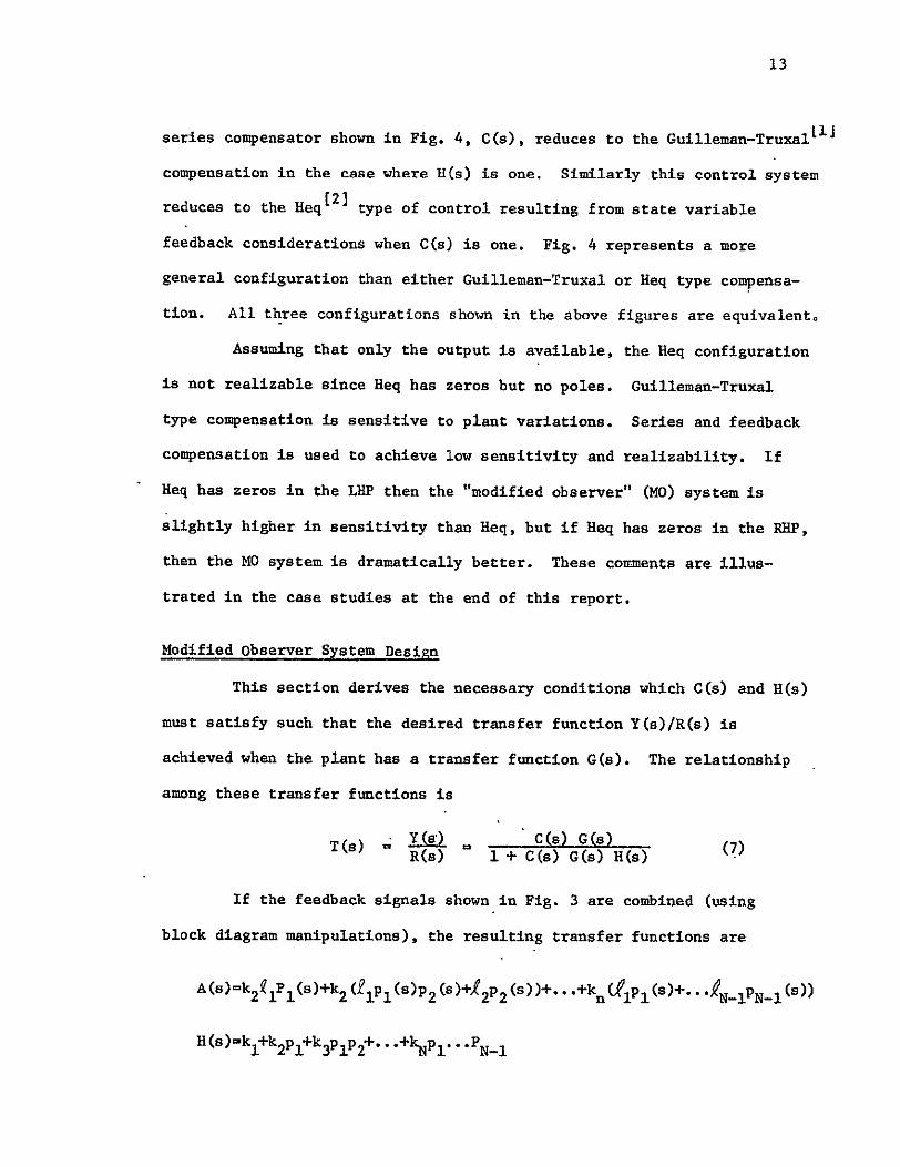
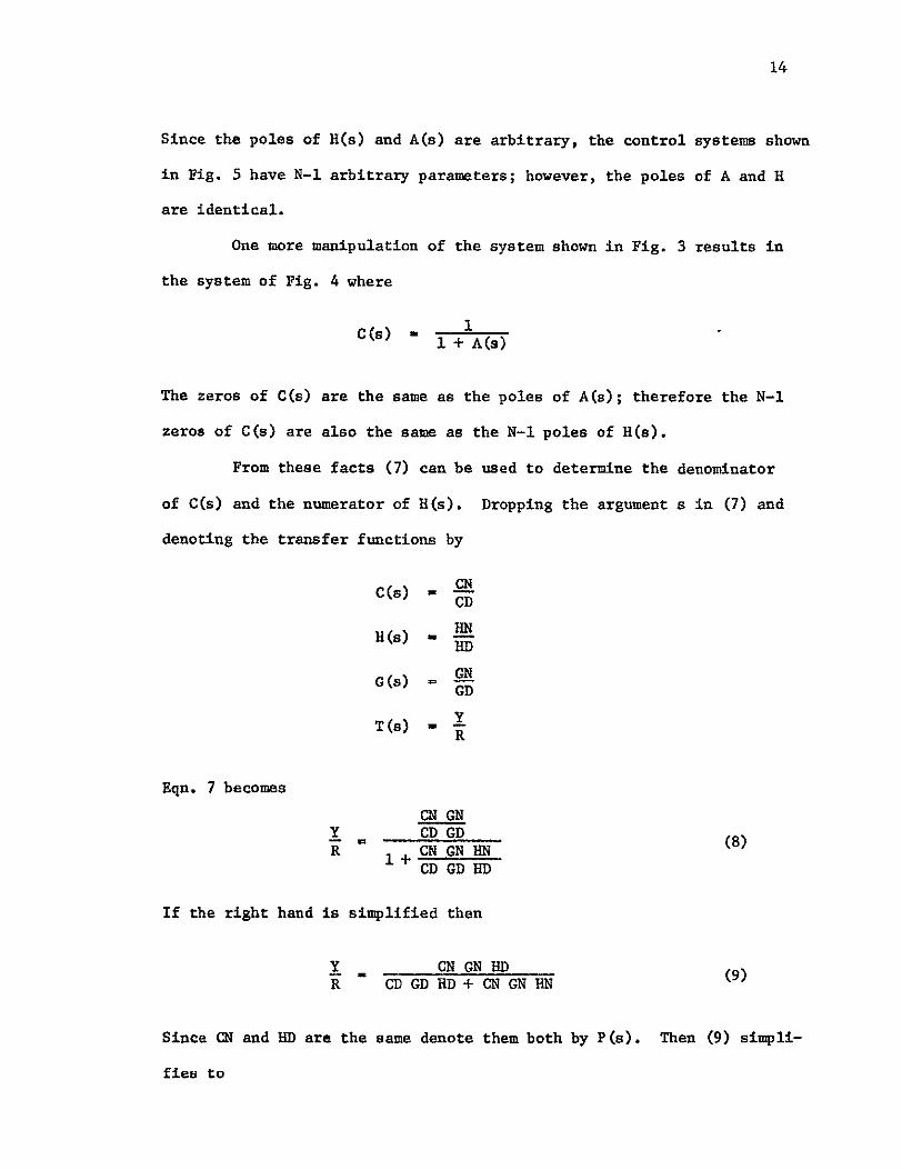
14
Since the poles of H(s) and A(s) are arbitrary the control systems shown
in Fig 5 have N-i arbitrary parameters however the poles of A and R
are identical
One more manipulation of the system shown in Fig 3 results in
the system of Fig 4 where
1 C(s) - I + A(s)
The zeros of C(s) are the same as the poles of A(s) therefore the N-1
zeros of C(s) are also the same as the N-i poles of H(s)
From these facts (7) can be used to determine the denominator
of C(s) and the numerator of H(s) Dropping the argument a in (7) and
denoting the transfer functions by
CDC(s)
H(s) -
G(s) ONGD
T(s) - R
Eqn 7 becomes
CN GN 1 CD GD(8) R 1i+ CN GN HN
CD GD HD
If the right hand is simplified then
Y CN GN HD (9)R CD GD HD + CNCN
Since CN and HD are the same denote them both by P(s) Then (9) simplishy
fies to
15
Y GN P (10)R CD GD + NHN
cross multiplying on both sides results in the polynomial
Y(CDGD+GNHN) - R-GNP (11)
Define the number of zeros in G as NG the number of poles as
ND and similarly NY and NR for T(s) If the order of both sides of
(11) is to be the same then
NY + ND - 1 + ND NR+ NG + ND - 1
NY + ND NR + NG (12)
NR - NY -ND - NG
Thus the pole zero excess of the plant determines the pole zero excess
of the desired closed loop transfer function If like powers of (11)
are equated then NY + 2ND equations result Since CD and 1N are undeshy
termined the number of unknowns is 2ND For NY = 0 the number of
unknowns is equal to the number of equations Just as in regular state
variable feedback[2 for zeros in YR additional states must be
created Let the order of P(s) by N-l then (12) becomes
NY + N - I + ND = NR + NG + N - 1
and for the number equations to be equal to the unknowns
NY + ND + N = 2N (13)
N = NY+ ND
16
Thus the order of both controller systems C(s) and H(s) must be one
less than the number of poles of G plus the number of zeros of YR
assuming that (11) represents a set of linearly independent equations
The design procedure is as follows
1 Select the desired closed loop transfer function from the
specifications
2 Select a polynomial P(s)
3 Equate the actual and desired transfer functions (iO) and
solve for the coefficients of CD(s) and HN(s)
Program 1
The first program (MODOBSI) computes the transfer function of
the series compensator and the feedback compensator as a linear function
of the denominator of the feedback compensator The user must specify
the plant transfer function and the desired closed loop transfer
function Thus this program specifies the design of the system except
for the poles of the feedback compensator which the user is free to
choose in any way he wishes
Program 2
The second program (MODOBS2) computes the transfer function of
the series compensator and the feedback compensator which minimize the
low frequency sensitivity of the closed loop system to plant variations
The user must specify the plant transfer function and the desired closed
loop transfer function If the time constants in the plant are much
lower than in the closed loop system the poles of the feedback compenshy
17
sator may be in the right half plane (RHP) If the poles of the compenshy
sator are in the RHP then the system will be vyD sensitive to variations
in the parameters of the compensators In this case it is better to
use one of the other programs This program is limited to systems with
no zeros
Program 3
The third program (MODOBS3) computes the weighted integral
sensitivity of the system for a given polynomial P(s) The user must
specify the plant transfer function closed loop transfer function the
weighting to be given the sensitivity as the frequency varies and the
denominator of the feedback transfer function P(s) The weighting
function must have more poles than zeros
Input Data
In many circumstances the available data for the plant is in
state variable form This data is converted to a transfer function by
the STVFDBK program The details of the program are included in reference
1 The program listing and input data format are also included in the
Appendix
Output Data
The program BODE4 is provided to plot the transfer functions
computed in the above programs on a logarithmic scale For each program
some of the transfer functions of interest are
1 Plant transfer function
2 Closed loop transfer function
3 Sensitivity as a function of frequency
4 Loop gain function
The loop gain function divided by one plus the loop gain is the proportion
of measurement noise at each frequency which will reach the output Thus
if the loop gain is much greater than one then nearly all the noise
reaches the output and if the loop gain is much less than one very little
measurement noise reaches the output If the phase shift of the loop
gain is nearly 180 at a gain of one the measurement noise will he
amplified
Program 4
The fourth program (MODOBS4) is useful to check the results of
the design Given P(s) and the results of the first program (MODOBSI)
this program computes HN(s) CD(s) and the roots of both the series and
feedback compensators This program and the first program give a
complete determination of the design
Results
A discussion of each program and several caee studies are inclushy
ded in the Appendices MDDOBSI is useful to compute HN(s) and CD(s) in
terms of the coefficients of P(s) Quite amazingly the coefficients of
N and CD are linearly dependent upon the coefficients of P HODOBS2
computes the coefficients of both compensators which achieve minimum low
frequency sensitivity Essentially this result is achieved by forcing
CD(s) to be an N-i order integrator which increases the gain at low
frequency and thereby decreases the sensitivity since SK = (s)
Unfortunately if the plant denominator coefficients are smaller than
19
those of the denominator of the closed loop transfer function the feedback
compensators may have poles in the RHP MODOBS3 determines the weighted
integral sensitivity when P(s) is specified MODOBS4 is useful for
checking the roots of the resulting compensators after a design is
complete Test results are given in the appendix for three examples
These examples show that an improvement in the system sensitivity over
that of just a series compensator can be achieved even if only the output
is available When the closed loop response is much faster than the open
loop the sensitivity of the MODOBS system approaches the sensitivity of
the Req system (which is best but not realizable) if the roots of P(s)
are made much larger than the closed loop roots If the closed loop
response is not much faster than the open loop response then the MODOBS
system may have a sensitivity lower than the Heq system This situation
exists whenever Heq(s) has zeros in the RHP These results point out
the important fact that a sacrifice in sensitivity to plant variations
is made by increasing the system performance requirements Because of
this fact careful attention to the plant performance should be made for
lowest sensitivity and unnecessary demands on overall system performance
should be avoided
20
Bibliography
1 J C Truxal Control System Synthesis McGraw-Hill 1955 Chapter 5
2 J L Melsa and D G Schultz Linear Control Systems McGraw-Hill 1969 Chapter 9
3 D G Luenberger Observing the State of a Linear System IEEE Transactions on Mil Elec April 1964
4 M E Muterspaugh State Variable Feedback and Unavailable States HS Thesis 1968
5 F H Effertz Comment on Two Coupled Matrix Algorithms for the Evaluation of the rms Error Criterion of Linear Systems Proceedings of the IEEE November 1966 p 1629
6 J L Melsa A Digital Computer Program for the Analysis and Synthesis of State Variable Feedback Systems NASA Contract Report CR-850 August 1967
7 L E Weaver et al A Control System Study for an In-Core Thermionic Reactor J P L Report 32-1355 January 1969
21
Appendix I - MODOBSI
Dis cussion
The basic algorithm of this program is based upon (5) First the
following polynomials in s are computed
T = (GD)(Y)
Q = (GN)(R)
V = (GN)(Y)
so that (5) becomes
(T)(CD) + (V) (HN) = (Q) (e) (Al)
Each of the terms in (Al) are polynomials in s where P(s) is unspecified
For instance P(s) = P3s2 + P The coefficients of CD(s) and HN(s) are
the unknowns
As an example suppose the plant is second order then P(s) is
first order In this case (Al) becomes
(CD2T3 +H 2 V3 )s 3 + (CD2T2 + CD1T3 + H2 V2 + H1 V3 )s2 + (CD2T1 + CD1T2
2 + H2V I + HIV2)s + (CDIT + HV) = P2Q 3s + (P2Q2 + PIQ3 )s2
+ (P2Q + P1 Q2 )s + PlQl (A2)
Equating coefficients of like powers of s results in the equations
T3CD 2 + V3H2 Q3P2
T2CD2 + T3CD1 + V2H 2 + V3H1 Q2P2 + Q3PI
22
T1 CD2 + T2 CDI + VIH2 + V2H 1 QlP2 + Q2P
TICD1 + V1Hi = Q1F1 (A3)
These equations can be rewritten more compactly in matrix notation as
T3 0 V3 0 CD2 f 0 Q3TN12N-2 T2 T3 V2 V3 CD11 214-22-Q3 Q3 Q22 (A)
2 T V1 V2 H2 Q2 QI P2j _ Ql 0
2N-2- shy - N-i-)
The matrix on the left will be defined as matrix A and the matrix on
the right will be defined as matrix C Then
CD2 CDI _ - 1
CD= A-C (A5)
H I
Therefore A- C relates the unknowns CDi and Hi to the parameters Pi
MODOBS1 forms the matrix A from the two arrays T and V and then inverts
A Next the C matrix is formed from the Q array and then A 1 C is
computed and printed
23
Input Format
Card No Columns Description Format
1 1 NY = order of Y(s) in YIR II
2 NR = order of R(s) in YR Ii
3 NG = order of GN(s) in GNGD i1
4 ND = order of GD(s) in GNGD Ii
I 5-80 Identification of problem 8AI0
20 Cn of 2 11-0 Coefficient of s in Y(s) FI03
11-20 Coefficient of aI in f(s) P1e3
etc
71-80 Coefficient of s7 in Y(s) F103
3 1-10 Coefficient of a in R(s) F103 etc
4 i-i0 Coefficient of s in GN(s) FIO3
etc
5 etc Coefficientof a in GD(s) FI03
Notes
1 If more than eight coefficients are required then two cards may be
used to identify that polynomial
2 A decimal point must be used for each coefficient but not for card
No 1 The decimal point may be placed in any of the ten columns
for each coefficient
24
3 As many problems may be run as desired by repeating the above format
for each problem
Output Format
See example
Subroutines to be Used
PLYMLT Multiplies two polynomials together
MXINV Inverts matrix A
PRNTRAT Prints the ratio of two polynomials
Flow Diagram
Read NYNRNG
ND
FRead Y(s)R(s)GN(s) GD(s)
Compute T = YGDQ = GNRV = GNYj
Form A Matrix
Invert A Matrixi
lForm C Matrixl
A -1
ComputeBA7 C
Print CD and E
Arrays
PROGRAM MODOBSI (INPUTOUTPUTTAPE4INPUT)
ODIMENSION Y IC) R(10) GD(IO) GN(IC) V(201 T(20) G(20)14A(S363)AI(36 3)C( 3611) B(36 1U ID(G)
C Y(S)R(S) IS DESIRED CLOSED LOOP RESPONSE C SP(S)GD(S) IS PLANT TRANSFE FUNCTION C NY IS ORDER OF NUM IN Y(SlR(S) NR IS ORDER OF DEN C NG IS ORDER OF NU OF G(S) NO IS ORDER OF-DEN C NR-NY MUST EQUAL ND-NG 1 READ 1U1NYNRNGNDID
PRINT 200NYNRNGNDIO
IF(EOF4) 99t2 2 NY1=NY4 1
READ 102 (Y(I)I=-INY1) C YI) IS COEFF OF S(I-I) IN Y(S)
NR I=NR C RII) IS COEFF OFS(I-1)IN-P(S) 3 READ I102 (R(I) IINRI)
CALL PRNTRAT(YNY1RNRI IHTIHS) __C_ GN(Il IS COEFF9F_SCI-1LIN_-GNtSL
NGl1NGI NO 1NDI
_4 -READ 102 (GN ) I 1NG1) C GOD(I) IS COEFF OF S(I-1) IN GO(S) 5 READ 102 (CG (I)I--1NDI)
CALL PRNTRAT(GNNGIGDNO HGIHS___ C FORM CHARACTERISTIC POLYNOMIAL
CALL PLYMLT (GDND1YNYITO) CALL PLYMLT GNNG1RNRI00-CALL PLYMLT (GN NGGYNYIVO) NYNGzN Y1 4NGI NR+NG+iN __ 00 6 IrNYNGN
C NA IS ORDER CF A MATRIX WHERE A IS MATRIX RELATING UNKNOWNS -6- V( --- - - TO PARAM P
NA_- 2 (N--1) DO 20 J-1NA IF- (J GT (N- IlJGO__TO2_12 00 10 Iz1NA INDN- L J IF _( IND-SLT_ I)_GOTO8_ IF (IND GTN) GO TO 8 AUIJ)- T(INa) 30 TO 10shy
8 A(IJ) O 10 CONTINUE
Gi__TO_2D
12 DO 20 I=INA IND 1-I+J IF- (INDLT__GO__18__ IF (INDGTN) GO TO 18 A(IJ)-V(IND) GO-T 0 _2D
18 A(IJ)-O 20 CONTINUE
CALL MXINV-(ANAtAll_ C C IS THE COEFF ARRAT
NM IrN-1 _DOZ4__I NA-_ DO 24 J=1YNMI IN= 2N-I- J
IFiINDLT1) GO TO 22 IF (INDGTN) GO TO 22
C(IJ) = O(INO) -
GO TO 24 22 C(IJ)rO 24 CONTINUE C B IS AICTAE ROwS OF 5 ARE EQUAL TO CD AND HN C COLS ARE COEFF OF P PARAMETERS
D0 30 INA 00 30 KzlNM1 B(IK)--O 00 3fJ--JNA
30 B(IK)-AICIJ C(JK+B(IK) PRINT 2O1KK--lNMI) DO 40 I--NMI
NC =N -I 40 PRINT 202 NC (B I-Kt NM1I
DO 50 I=NNA
NBzNA+-I -50 PRINT 204t-NB (8(1I(1 Kzl-NM-1
GO TO I 99 STOP -101-FORM ATf l A 1f)V t 102 FORMAT (BF103) 200 FORMAT (1HI4(2XI1) 2X6A1i0) 201 FORMAT IH X8 ( 314- P( I 11 I-) OX)) 202 FORMAT 14H CO(I2--)10(E1U33X)) 204 FORMAT (4H HN(I12H)=)I(EIO33X))
END SUBROUTINE PRNTRAT (ANNBvNOEPVARINDVAR) DIMENSION A( 20)B( 20H_(20)N(20)AT20BT(20)NEt 1
DO 6 I--NN AT(I)-- -IF-(-AY f-4i 6-3
3 H(NE)zlH+
AT(NE)rA(1) GO TO 5
4 H(NE)--IH-
AT (NE) -A(I) N(NE)I-1 NErNEI
6 CONT INUE NE=NE-1 PR IN-T 10 0 MIN=MINO(NE 10) PRINT 10lCN(I)IzMIN) PRINT 102 (HRU1 ATI) INDVAR Il tMIN) IF (NE-if]) 8987
7 PRINT 101 (N(I IrIINE) PRINT 102 CHI)AT(I)INDVARI--INEI
__ NF= O0 16 I--IND BT (I)--DIF C B(C) 191G13
13 H(NF)rlH4 BT(NF zB(I)
-GO-_ T _15 14 H(NFI -IH-
BT (NF) =-B(I)
r27 15 N(NF)=I-I
NF zN Fi-I 16 CONTINUE
NF =N F- I HH= IH-NH=rAX 013NE 13 NF) NHzMINO(130NH)
20 PRINT 103 DEPVARINOVAR (HH I=INH) MIN MINO(NF 10) PRINT 101 (N(I)IzIMIN) PRINT 102 (Hi(I)BT(I ) 1NDVAR-I---1MIN IF (NF-101) 28P2827
27 PRINT 0l (N(I) IzIINF) PRINT 102 (H(IJBT(I)TNDVARI=N-FI)shy
28 CONTINUE 100 FORMAT C iHO) 101 FORMAT (6XI(11X 12)) 102 FORMAT 6XID(AIGlC4 AI1H H 103 FORMAT tIXtAIIHCAI2H)= 30AI)
RE TURN END SUBROUTINE MXINV (R N RI) SUBROUTINE TO FIND THE INVERSE- ----- GIVEN
C MATRIX R N IS ORDER OF MATRIX RI IS INVERSE C MATRIX SUBROUTINE USES GAUSS-JORDAN REDUCTION C R MATRIX IS PRESERVED DIAGONAL ELEMENTS OF R-US
BE NONZERO C DIMENSIONR(3G36IRA(3G72) RI(36v36)
C STATEMENTS 20-26 ENTER R ARRAY INTO RA ARRAY - C AND SET LAST N COLUMNS OF RA ARRAY TO IDENTITY
C - MATRIX 20 DO 26 I 1 NI-v 21 DO 24 J I N
_22__RA IJ) -R(I- J) 23 NJ = N + J 24 RA(INJ) = 0 2 5 _NI z N + I 26 RA(INI) = 1
C C ST AT EM ENTS _ii-12_REDUCE MATLRIX__RA _SOH_ATZ_JRFSR_LK C COLUMNS ARE SET EQUAL TO THE IDENTITY MATRIX
i NP = 2 N 2_DO 12 I - N
C -
C STATEMENTS 3-5 ARE USED TO SET MAIN DIAGONAL _C ELEMENT TOUNITY
3 ALFA = RA(TI) 4 DO 5 J = I NP S RA(IJ) r RA(I J) _ALFA
C C STATEMENTS 6-11 ARE USED TO SET ELEMENTS OF ITH C COLUMN TO -ZERO
6 00 11 K = 1 N 7 IF (K - I) 8 11t 8 8 BETA = RAiKI) 9 DO 10 J = It NP
10 RA(KJ) = RA(KJ) - BETA RA(IJ) - ICONTINUE_ 12 CONTINUE
C
TO LAST 28 C STATEMENTS 30-33 SET INVERSE MATRIX RI EUAL
C N COLUMNS OF RA ARRAY
30 DO 33 J 1 N 31 JN J + N 32 00 33 I 1 N 33 RI(IJ) rRA(IJN) 34 RETURN
END SUBROUTINE PLYMLT (ALBMCN)
C C MULTIPLY ONE POLYNOMIAL BY ANOTHER
C C DEFINITION OF SYMBOLS IN ARGUMENT LIST C A(I) MULTIPLICAND COEFFICIENTS INTHEORDER AE) S(I-1) C L NUMBER OF COEFFICIENTS OF A C B(I) MULTIPLIER COEFFICIENTS IN THE ORDER 8(I)SI-1)
C M NUMBER OF COEFFICIENTS
C C11) PRODUCT COEFFICIENTS IN THE ORDER C(19S(I-1)
C N NUMBER OF COEFFICIENTc Ac r
C C REMARKS C IF N-- C(I) SET TO ZERO AND PRODUCT FORMED OTHERWISE THE
C I-PRODUCT AND SUM NEWC-OLD C + AB IS FORMED
DIMENSION A(iD) B(IO) t C(20) LPML+M- 1 IF (N) 10102iZ
I DO 1 J- LPM 11 C(J)-Oo 12 DO 13 J--ILPM
MA X-MA XD (J + I-M il)) shy
- MINzMINO(L DO 13 IrMAXMIN
13 CC(J)=A(I)B(J+II) + C(J) RETURN END
3434 IN CORE THERMIONIC REACTO R
116708 481228 384520 200 1 16708 -4870635__4085815__39226_ 100 116708 481228 384520 200- 503585E-610542E- 3 058639 18804 1
END OF INFORMATION
29
Appendix 2 - MODOBS2
Discussion
If CD(s) in (5) is defined by CD(s) = CD N-i (BI)
where N is the order of the plants then the system will have minimum
low frequency sensitivity because the forward loop gain will be increased
at low frequencies If there are no zeros in Y(s)R(s) or in G(s) (5)
reduces to a simple set of linear equations shown below For simplishy
city RN+ I and GDN+t are set equal to one For zero steady state error
Y = R1
PNl PN= I PN-I = N-I
PN-2 + RNPN-1 CN-2
(B2)
P + 2 + ReN- =1 I I
IN I = P RY
HN2 =PI RY + P2
+HN=NPI RNY + P 2 -Y +i - GD1Y
Where the C terms are defined by
C I GD2 - R2
C2 = GD3 - R3
CN- 1 GDN - N
30
The Eqns (B2) are simply solved in the order shown by back
substitution That is PN-1 may be usedto solve for PN-2 which may be
used to solve for PN-3 etc
Input Format
Card No Columns Description Format
1 1 N = Order of the Plant G(s) Ii
2-80 ID Identification of problem 8A1O
2 1-10 Y = Numerator of YR F10o3
0 3 1-10 R(1) = coeff of s in R(s) F103
11-20 R(2) = coeff of s I in R(s) FIO3
etc
7 71-80 R(7) = coeff of s in R(s) FI03
4 1-10 GN = numerator of G(s) F103
5 1-10 GD(l) = coeff of s in GD(s) F1O3
771-80 GD(7) = coeff of s in GD(s) F103
See notes following input format for MODOBSIo
Output Format
See example
Subroutines to be Used
PRNTRAT - Prints the ratio of two polynomials
PROMT - Determines the roots of P(s) to see if any roots are in
RHP
PROGRAM OOS2 (Y4PUT OUTPUTC4=INPUT)IO41 N j (l10 1 ( l ) 1 ([) Cl(In)ID( 3)PHN 1 )CD t13)
C U (IG) V (10) C PqOGRAM TO CALCULATE MINIMUM LOW-FREO SENSITIVITY MODIFIED C OBSERVER SYSTEM C Y(S)R(S) IS DESIRED CLOSED LOOP RESPONSE C GN(S)GD(S) IS PLANT TRANSFER FUNCTION C N IS ORDER OF DEN IN Y(S)R(S) C N IS ORDER OF DEN IN GN(S)GDIS) C R(I) IS COEF OF S(I-1) IN R(S) C C ASSUMPTIONS C C TRANSFER FCN GAINS ARE NORMALIZED SUCH THAT R (N+1)I1
C AND GD(N I )=I C C DESIRED TRANSFER FCN HAS ZERO STEADY STATE C
-C GD(I) IS-COE-F-- O-F S(I-I)1NGO(S) C Y(S)=Y GN(S)-GN (NO ZEROS ALLOWED) C I READ 101 N ID
IF(EOF4)99 2 2 READ I02Y
READ 102 (R(I)IzIN) NP i-N+ I
GD(NPI) =1 5 RNPI_)-1 READ 102 GN
3 READ 102t CGD(I)tlz1N) PRINT 200DNIO10 PRINT 201
CALL PRNTRAT CYIRNPHTIHS) PRINT 202
CALL PRNTRAT(GNGDNP11HG1HSI C-C --SOLVE FOR DEN OF H P(S)
NM I=N-I do 40 II -NM1 IPIlzI+I
-4 -CI) zG0c IP 1I-R IiT P(N) -
005[ I=ItNMj NI N-I P(NI)zC(NI)
IFCILE1) GOTO-50_ DO 49 Jz2I J2=N-J+2
4 P(NI )zP( NI )-R( J2 )P( JI ) 51 CONTINUE
CALL PROOT (NMIPUV) PRINT 205
PRINT 206 (U(I)V(I) I=INM1)
ERROR THUS YR(1)
SOLVE FOR NUM OF HHN(S) DO 60 1N HN (I 0 - 00 60 JzlI IJI j4
C
6C PN Il)r( Ji R (IJ) Y +HN( I) 32 HN (N )HN (N)-GD (1 )Y
PRINT 203 CALL PRNTRATIHNNPNIHH1HS) PO 80 1i NMI
80 CO(I)zO CD(N)zl PRINT 204 CALL PRNTRAT(PNCDN1HC1HS) G z YGN PRINT 210 G GO TO I
99 STOP 101 FORMAT (Il 84101 102 FORMAT (SF1O3)
200 FORM AT(IHII0X II 4X 8AID) 201 FORMAT(1HOTHE DESIRED CLOSED LOOP TRANSFER FUNCTION IS)
202 FORMAT(1HOTHE TRANSFER FUNCTION OF THE PLANT IS)
203 FORMAT(IHOTHE TRANSFER FUNCTION OF THEFEEDBACK COMPNSATOR IS)
204 FPRMAT(lHOTHE TRANSFER FUNCTION OF THE SERIES COMPENSATOR IS)
205 FORMAT (IHO 5X THE ROOTS OF P (SI ARt 13XREAL PART IOXIMAGINARY PART)
-20 FORMAT 32X2E207f 210 FORMAT4IHOTHE ADDITIONAL FORWARD LOOP GAIN REQUIRED IS
1YGNElfl3) END SUBROUTINE PRNTRAT (ANNSNDDEPVARINOVAR) DIMENSION A(20)B(20vH(20) N(20 1 AT(20) PT 20 NE z1 00 6 Iz1NN AT(1)=D IF C(IA ) 463
3 H CNE )= IH + AT (NE) =AtI) GO TO 5
4 H(NE)=IH-AT (NE) =-A( I) N(NE)--I-1 NE-NEI
6 CONTINUE NE=NE-1 PRINT 100 MINMINO(NE v1O
PRINT IOl (N(IhI=IMIN)
PRINT 102 (H(IAT(I)INDVARI-IMIN) IF (WE-10) 8
7 PRINT 101t (N(I)IzlINE) PRINT 102 (H(I)AT(I)INDVARIn1NEl NF o_-8_ N --1 80 16 I1NU
BT(IzO IF ( (I) 1141613
13 H(NF)zlH+ BT(NF)l=B(I)
-GO T0- 15 __ - 14 H(NF) zlH-
BT (NF)z-B(I) - 15 N(NF)=I-1 -
NFZNF41
33 ID CONTINUE
NF NF- I HHL IH-NHMAXO( 13NE 13NF) NHzMINO( 130NH)
20 PRINT 1G3DEPVARINDVAR(HH 1=1NH) MINMINO(NF 10)
PRINT 101 (N(I)IlMIN) PRINT 1G2( H(I)BT(I)INOVART IMIN] IF (NF-in) 2828927
27 PRINT 101iN(I) I11 NF) PRINT 102 (H(I)BT(I)tINDVARI-IINF]
28 CONTINUE 100 FORMAT (1HO) 101 FORMAT (GX1O( IIX12)) 102 FORMAT (GXI0(AIGIO4 A1IH )
103 FORMAT (1XA1IH(Ai2H)-130A1) RETURN END
___SUBR CUT INEPR O0 TN _A U fVtIIRR) DIMENSION A(20)U(20)V(20)H(21)8(21 )C(21) IREV-IR NC -N +IDOll--i Nu
H( I) rA( I) _i CONTINUEL
00
3 IFIH( 1)) 24 2 NCNC-1
V NC )z0 U NC O DO 1002 I= 1NC H(I)--H(I+1 )
1002 CONTINUE GOT03
S_IF (NC- 1) 5 10 05 5 IF (NC-2) 7i 7
6 R=-H( 1H(2) GOT050
7 IF INC- 3) 9-819 8 P-H(2)H(3)
__0 1) H (3_)_ GO TO7g
q IFCABSCH(NC-1)1H(NC)-ABS(H(2)H(1))101919 10- IREV - IREV_
M=NC2 DO11I=-1 M
_-NL-zNC+ 1 -I-FrH( NL) H NL )H( I)
11 H( I) F -IF (O )139 12 913
12 P=D GOTO 15shy
13 PzPQ 0= (
15 IF(R)16191G 16 R=1 R 19 E5E- ]C
B(NC)H(NC) C(NC)H(NC) B(NC+1 )zO C( NC 1)z 0 NP NC- 1
20 0049J= I 100C DO 2111l1 NP ITNC-I I BC I rH(I)+RB(+1)
--21C( I) =B (I)+RC( I+ 1) IFCABS(B(I )H(1))-E)5050 24
24 IF(C(2)232223 2amp R= RlI-
GO TO 30 23 R=R-B(1) CC2)
30 D0Q3711zlNP IzNC-I I BI)i(I)-PB(I+I)-OB(I+2)
37C( I) =B (I)-P C(i1l) OC(12) IF(H (2)) 323132
31 IF(ABS(C2)H(1))-E)333334 32 IF(ABS(B(2)H(2) )-E) 33v3 34 33 IF(ABS(B(1)H(1))-E)707034
34 CBARrC(2)-B(2) DC(3) 2-CB ARC ( 4) IF(D)363536
35 PzP-2 0= (o t GOT049
36 PP(-82)C(3)-BC1)C(4))D - Q+ (-( 2)CBARB(1) C(3 00)
49 CONTINUE
ErE 10 GOT020
50 NC-NC-1 VtNC)D
IF (IPEV) 51 5252 51 U(NC)=1R-
GOT053 52 U(NC)-R 53 00541lNC
H(I) B(1+1) 54 CONTINUE
GOT04 70 NC=NC-2
---- IF(IREV)71727 71 QPr1O
P=P(Q2 0) GOTO73-_
72 OPPP Q-P 2 0
73 F-(PP)2-OP IF(F )74 7575
74 U(NC+I)z-PP U(NC)-PP V(NC 1 )SORT(-F) V( NC 1-V (NC+ 1) GOT076
75 U(NC+11-(PPABS(PP))(ABS(PP)SQRT(F)J V( NC+1 )0 U(NC )OPU (NC1) V( NC )O
76 D0771INC H(I) B(1 2)
77 CONTINUE GOT04
LDO RE TURN END
3 CASE STUDY II THIRD ORDE-SYSTE14shy1000 1000 200 20 D O -
2500 100
36
Flow Diagram
Read N ID
Y R(I)
GN GD(I)
Print N ID
YRy G
Form C(I)
ISolve for P(s)j
Solve for HN(s)I
Print H(s)
Print C(s)
37
Appendix 3 - MODOBS3
Discussion
This program uses the following data
1 Plant transfer function G(s)
2 Desired closed loop transfer function T(s)
3 The denominator (P(s)) of the feedback compensator H(s)
4 A desired weighting function W(s) on the integral over
frequency of the sensitivity of the closed loop response
to forward loop gain changes
The program then calculates the weighted integral sensitivity of
the system The method of calculation is based upon an algorithm by
EffertzL5] The integrand of the integral sensitivity is calculated
from
I S W(S) S (S) ds
2r f G(s)C(s) ds
The algorithm is based upon an iterative manipulation of the coefficients
in the numerator and denominator of the integrand in such a way that the
integral of the squared magnitude results
A closed form solution for the integral
jm n 2rj jo h(P)h(-P) 2 -joo
1 30 dP 1 j F(P)F(-P) dP
(BI)
is presented in the paper by F H Effertz The solution takes the form
38
of Equation 4 in his paper A better algorithm for the computation of
Equation 4 in Effertz is presented in the correspondence by Pazdera
(Equation 7) A modified forn of Pazderas algorithm has been coded in
FORTRAN and is included A test problem is also included
The use of Equation 4 in Effertz can be best illustrated by an
example Suppose we wish to evaluate the following
(B2)Ls2+ Cb) [2bLn = 2I -
It can be shown from residue theory that the correct answer is
I = - residue of F(s) F(-s) at s = a (B3)n
- residue of F(s) F(-s) at s = b
where F(s) F(-s) indicates the function to be integrated over s = jW
Then the answer is
22 2
= - c-a (c2-b2 c2+abn 2a(a+b)(a-b) 2b(a+b)(b-a) = 2ab(a+b) CR4)
To use Equation 4 from Effertz we must make the following associations
using the complex frequency variable s in place of p
22 s= c -g(P) = (s+c)(c-s)
then s (B5)
2
h(P) = s + (a+b) s + ab
then p s N=2
1
a a 2 =ab
39
The integral for n = 2 can be expressed as
bb [bloaaob I- (B6)
a0 t ol [jaza1-2 1ao a 2
Substituting the correct values of a0 a etc and cancelling minus
signs for this problem we obtain
ab +c In = 2ab(a+b) (B7)
What is most interesting is that the result depends only on the coeffishy
cients of the known function being integrated and not on the poles of
the function as one would suspect from residue theory
It has been mentioned that the algorithm from Pazdera (Equation 7)
has been programmed Some charges in the nomenclature of Equation 7 were
necessary to facilitate coding Note that the practice in Effertz and
Pazdera is to make the highest membered coefficient correspond to the
lowest power of the variable p Note also that subscripts such as ao
are in evidence To facilitate coding the lowest numbered coefficient
was subscripted in the form A(l) and this coefficient was associated with
0 ththe lowest power of the variable p in this case p In general the i
coefficient A(I) is associated with the (i-1)s t power of p P -l (In
FORTRAN the expression A(O) is not allowed) Note from equation I above
what must be done to operate on the function F(s) F(-s) If F(s) is of
the form
F(s) = C(S) (B8)A(S)
then the algorithms suggested in both Effertz and Pazdera require the use
40
of
g(s) = C(S) C(-S) (B9)
h(s) = A(S)
It is more desirable to input C(S) and A(S) rather than C(S) C(-S) and
A(S) Consequently one uses the INTSQ subroutine by coding the coeffishy
cients of C(S) and A(S) with ascending subscripts corresponding to
ascending powers of S The subroutine provides the operation C(S) C(-S)
Furthermore the subroutine checks to see if the lowest coefficient of
C(S) or A(S) is zero so that factors of S may be either considered or
cancelled Two basic requirements must be met by A(S) and C(S) First
the roots of A(S) and C(S) must at least have non-negative real parts
(Hurwitz polynomial requirement) Secondly the highest power of C(S)
must be at least one less than the highest power of A(S) for convergence
to be assured If A(S) is Nth order one inputs the N coefficients of
A(S) and the N-i coefficients of C(S)
The use of this subroutine INTSQ may be best illustrated by an
example Suppose we desired to evaluate the integral
I = JD F_ 7 4 - JdS n -joe 3 + 3s2 + 2s + L[43 + - 2s
(BIO)
The polynomials C(S) and A(S) as defined in Equation B8 are input into
the program as
C(1) = 4 A(l) = I
C(2) I A(2) = 2
(Bi) C(3) o A(3)= 3
A(4) = 4
41
The program then utilizes the modified Pazdera algorithm and prints out
the message
THE VALUE OF THE INTEGRAL IS 12250
To check this answer one can use Effertz Equation 4 for a third order
case (n=3)
a oa 101o 2 1 n
= (142a
0 a
aI a a 0
I 2a
boa2a3+b2aoal-aoa3b alaaa a (BI2)
0 1 20 - o2 2 3o 31 o 13a22o0
For our example problem the following associations follow
b =0 a =4 0 0
b 1 -l a = 3 (B13)
b2 =16 =2a 2
a 113
Substituting the values of Equation B13 into Equation B12 verifies the
computers solution I = 1225n
Input Format
Card No Columns Description Format_
See format for MODOBSI
K 1-10 P(1) - coeff of so in P(s) BE103
11-20 P(2) - coeff of s in P(s) 8E103
etc
42
Input Eormat (contd)
Card No Columns Description Format
K+I 1 NW - Number of coeff in denom of W(s) II
K+2 1-10 WN(I) - coeff of s in num of W(s) 8E103
11-20 WN(2) - coeff of s in num of W(s) 8EI03 etc
K+3 1-10 WD(1) - coeff of s deg in den of W(s) 8E103
11-20 WD(2) - coeff of s in den of W(s) 8E103 etc
43
PROGRAM MODORS3(INPUTOUTPUTTAPE4-INPUT ) DIMENSION Y( 10)R(10)c-D(IO) SN(lOhIP(10)CD(0) HN(IO)SN(40)bull
IS0(40) B(36 18)WN(10) WD 10)SNT(40)SDT(40)C
I CALL MODOBSI (YP GN GO5 NY1 NR1 NGI NDI C N-1 IS THE NUMBER OF COEF IN P(S) HN(S) CD(S)
NrNR 1+NGI- 1 N =rN -1 READ 10 lP(I)Iz1NI)
C W(S) = WNWD MUST HAVE MORE POLES THAN ZEROS C NW IS THE NUMBER OF TERMS IN THE DENOMINATOR OF WS)
READ 103NW READ 102 (WN(I)I-INW)_ READ 102 (WD(I)I-INW) PRINT 205 CALL PRNTRAT (WNNWDNW1HW4-lkHS) CALL PLYMLT(GDNDlY NYI SN 0) N2=NDI+NYI-I
_CALL_ PLYMLTT(yN NWSNN 2 SNT D) CALL PLYMLT (GNNG1 R NRI SO 0) CALL PLYMLT(WDNWSDN2SDT C)
__N3=NW+N2-1 -
N4 =N 3+ NI-1 N22N1 11
-a- DO 10 I= 1Nl CD(I)=0 HN(I)O 00 10 J1pN1 CD (I)B(N-I J)P J )+CD( I)
10 HN(I)zB(N2-IJ)P(J) +HN(I)_P -I NJ_Z0 I--_
CALL PRNTRAT(PN1CDN1IHCIHS) PRINT 202
CALLP RNTRATAHN NI P Ni1H Ht l1 CALL PLYMLT( CDN1 SNT N3 SN C) CALL PLYMLTI- PN1SDT N3SD 0) -N5=N4 ---CALL INTSQ(SDSNN4S) PRINT 204 S
- GO T ---O-- -- 102 FORMAT 18 E1O3) 103 FORMAT III)
-201 -FO RM ampTL__TJJLJERANS ER_-F-UN CT-O-N--OF--L sESERIS--COMENSJ-IO-R- i-l 202 FORMAT(O THE TRANSFER FUNCTION OF THE FEEDBACK COMPENSATOR IS) 204 FORMAT(O THE WEIGHTED INTEGRAL SENSITIVITY ISEIO3) 20S -FORM-AT( Oi-tJ-WEIGHTINGFUNCTION-OF-HE- INTEGRALSENS-IIVlTY-YI-_shy
1) END
_SUBROUTINEMOOOBS1 LYR GN GD B N-YI-NRI-NGL-ND44-UDIMENSION Y(IO) RU1G) GD(10) GNIG) t V(20) T(20)9 Q(20) IA(3636)AI(3G36)C(36l8)B(36 1B)ID(6)
C _Y(S)R(S) IS DESIRED-CLOSED LOOP C GP(S)GD(S) IS PLANT TRANSFERFUNCTION C NY IS ORDER OF NUM IN Y(S)R(S) NR IS ORDER OF DEN
_C_ --NGJ S OR DEROFJN UaOF_ GASJ_ID- S--DRDELO DE C NR-NY MUST EQUAL ND-NG C Y(I) IS COEFF OF S(I-1) IN Y(S)
C RP I) IS COEFF OF S( 1-f1 IN Q(S)
C GN(I) IS COEFF OF S(I-11 IN GN(S) C GOCI) IS COEFF OF S(I-1) IN GO(S) 1 READ 1UINYiNRNGNDIO
IF(EOF4) 99t2 2 NY IrNY +1
NR ic NR --READ 102 (YCI)IIlNYI)
3 READ 12z (R(I) I--NRl) PRINT 200NY vNRvNGNO ID CALL PRNTRAT(YNYl R NRI 1HT IS) NuGl=NG I
ND i ND-shy4 READ 102 IGN I I--I NG1) 5 READ 102 (GD(I)IzlND1)
CALL PRNTRATIGNNG1GDNDI 1H3IHS) C FORM CHARACTERISTIC POLYNOMIAL
CALL PLYMLT (GDNDIYNY1TO) CALL PLYMLT GNNGIRNR10) CALL PLYMLT (GN NGIYNY1V0i NYNG=NY1+NGI N rNR+NG+I 00 6 IzNYNGN
C NA IS ORDER OF A MATRIX WHERE A IS MATRIX 6 V(I)zfl
NA= 2 (N-1 DO 20 J-INA IF ( J GT ( N- 1) GO_TO_1 2 DO 10 IrINA IND-N-I+J IF (IND LT 1) GO TO 8 IF (IND GTN) GO TO 8 A(IJ)= TIIND) GO TO 10
8 A(IJ)zO 10 CONTINUE
GO TO 20 12 DO 20 I=lNA
IND --- I+J IF fINDLTI)_ GO TO 18 IF (INDGTN) GO TO 18 A(IJ) zV(IND)
GO TO 20 18 A(IJ)rO 20 CONTINUE
CALL MXINV_ (ANAAI_) C IS THE COEFF ARRAY-C
NMlzN- 1 DO 24 IrItNA DO 24 JrINM1 INDz2N-I-J
IF(INDLT1) GO TO 22 IF (INDOTN) GO TO 22 C(IJ) - O(IND) GO TO 24
22 C(IJ)zO 24 CONTINUE
__C B IS AICTHE RUWs UF B ANt LIUAL IU) (U C COEFF OF P_ PARAMETERS
00 30 IrINA
44
RELATING UNKNOWNS TO PARAM P
AN_)_HN_THECOLSAR
00 30 KzlIMI B (I K) 0 00 30Jr1NA
30 B(IK) AI(IJ)C(JK)+B( T K) PRINT 201IKv(K=1 NM1 DO 40 I=INMI NC =N -I
40 PRINT 202NC(B(IK)Kr1NM1) DO 50 IzNNA NB -N A 1- I
50 PRINT 204v NB(B(IKIK--NMI) RETURN
99 STOP 101 FORMAT (4116A10) 102 FORMAT (SF103) 200 FORMAT I1HIv4(2XI1) 2XGA1O 201 FORMAT (10X3(3H P(I1lH)vgX)H 202 FORMAT (4H CD(I12H)zO(E1O 33X) 204 FORMAT (4H HN(IIZH)=IO(EIO 33X)L
ENO SUBROUTINE PLYMLT (ALBMCN)
C MULTIPLY ONE POLYNOMIAL BY ANOTHER C
C DEFINITION OF SYMBOLS IN ARGUMENT LIST C AI) MULTIPLICAND COEFFICIENTS IN THEOROER A(I) S(I-I)
C L NUMBER OF COEFFICIENTS OF A _C_ _B I) __MULTILPLIER CO EE-CIENiS-LNTlLODE3-IIi-plusmnSflt-WL-
C M NUMBER OF COEFFICIENTS OF B C CII) PROOUCT COEFFICIENTS IN THE ORDER C(I)S(I-1)
_
C C REMARKS
_C _IF -LO_ C (t1---ETJO_=EOANIRRO IUCTER-MF] lkRWLD T TRiLEJP-PO-DIC C AND SUM NEWC= OLD C AB C
DIMENS ION A( 101 D_cL20j LPML M- 1 IF (N) 101012
At1 -DO i - J-=l LPM__ I] C(J)zOO
12 DO 13 J=ILPM __M AXzMA XO (J+1-MJ
MINMINO (L J ) 00 13 I=MAXMI C ( J )=A _I u KB (Jt 1 RETURN
END
IS FORMED
SU BR OUT I NE P RN TRAT (A NNB N D DEPV AR INDVA RJ_ -
DIMENSION A(20)B(2)H(20 )N( 20)AT(20) BT(20) NE l
-DO JI1NN___ AT (I 1 IF ( A() 1 4993 H( NE = IH AT (NE) zA(I) GO TO 5 H(NE)I-H-
AT(NE) -A(I) N(NE)rI-1 5
146NErN E+1
6 CONTINUE NE =NE- I PRINT ion MINz INC(NE 10) PRINT iO1(N(I)T--MIN) PRINT 10Z (H(I)ATCI) INUVARI1MIN) IF (NE-in) 387
7 PRINT 101 (N(I)IrlNE) PRINT 102 (HCI)AT(I)INOVARvl--IrNE)
8 NF I DO 16 I-1ND ST(I)-O IF ( B(I) ) 141G13
13 H(NF)zIH+ ST (NF) -B(I) GO TO 15
14 H(NF) -IH-BT (NF) -- B(I
15 N( NF)zI--I NFrNF+ 1
16 CONTINUE NF =NF- I-HH =1H-
NH=MAXCD13NE 13 NF) -NH=MINO(130NH)Y
20 PRINT 103t DEPVARINDVAR (H H I-INH)MIN=MINO (NF 10) PRINT 101 (N(I-IiMIN) PRINT 102 (HI )BT(I)INDVARIlMIN)
IF (NF-ID) 282827 27 PRINT 101 N(Il) I=I-1NF)
PRINT 102 CH(I)BTII)INDVARI-i1NF) 28 CONTINUE 166- FO PM AT IHO-shy101 FORMAT f6Xv10(IIX12)) 102 FORMAT (GX0(A1G1O4 AIIH 103 FORMAT t IX A1 IHIAL 2H)Z 130AI])
RETURN END SUBROUTINE MXINV (R RI)
C SUBROUTINE TO FIND THE INVERSE OF A GIVEN C MATRIX R N IS ORDER OF MATRIXv RI IS INVERSE C MATRIX SU-BROUTINE USES GAUSS-JORDAN REOUCTION C R MATRIX IS PRESERVED DIAGONAL ELEMENTS OF R MUST BE NONZERO
DIMENSIONR(33G ARA(3 72) RI(363)
C STATEMENTS 20-26 ENTER R ARRAY INTO RA ARRAY C AND SET LAST N COLUMNS OF RA ARRAY TO IDENTITY-C MATRIX
20 00 26 I = I N 210 24 J = l N 22 RA IJ) - R(IJ) 23 NJ = N J 24 RA(INJ) = 0 25 NI = N + I 26 RACItNI) = 1
C C STATEMENTS 1-1-REDUCE MATRIX RA -SOTHAT FIRST N C COLUMNS ARE SET EQUAL TO THE IDENTITY MATRIX
471 NP = 2 N
2O 12 I 1 N
C STATEMENTS 3-5 ARE USED TO SET MAIN DIAGONAL C ELEMENT TO UNITY
3 ALFA = RA(II) 4 DO 5 J I NP 5 RA(IJ) z RA(IJ) ALFA
C C STATEMENTS 6-11 ARE USED TO SE-T ELEMENTS OF ITH C COLUMN TO ZERO
6 00 11 K = 1 N 7 IF (K - I) 89 11 8 8 BETA RA(KI)
9 DO 10 J I NP 10 RA(KJ) RA(KJ) - BET A- RA(IiJ 11 CONTINUE
12 CONTINUE C C STATEMENTS 30-33 SET INVERSE MATRI-X- RI-EQUAL-TO-LAS-T-C N COLUMNS OF RA ARRAY - 30 DO 33 J 1 N
31 JN = J + N 32 00 33 I 1 N
33 RI(IJ) RA(IJN) 34 RETURN
END SUBROUTINE PLYSQ_ (CN8j___ DIMENSION C(40)B(4D)
C RETURNS BCS) = C(S)C(-S) TO MAIN PROGRA-M C B(I) IS COEF OFS -l IN S -------C C(I) IS COEF OF S I-I IN C (S) C N-I IS NUMBER OF COEF IN B(S) AND C(S)
N1I (N- I)-12---shy00 20 I=lNI MO =-I _BCI) zD II z 2I-i
DO 20 K=1 II MO z -1MO
20 B(I)B(I)MOC(K)C( 2I-K) NMIN-i
- N2-N +I 00 30 I=N2vNM1 IIN=2I-NMI
MO(-I) NMI DO 30 K-IINNMI
O -IMO
30 B(I) r3(I)+MOC (K)C( 2I-K) RETURN
-- END - SUBROUTINE INTSO (ACNS)-DIMENSION B(IOhA(II)C(ID)
C___ RETURNS SZINTEGRAL OF C(S)C(-Si A CS )A( -S)-TO MAI-NRPROGRAMo C B(S) HAS N-I TERMS A(S) HAS N TERMS C B(I) IS COEF OF S(2I-2) - ISCOEF OF S(I-I)2C- -C(I) C IF THE LOWER ORDER DEN AND NUM COEFF ARE SMALL (LESS THAN C 0) THEN DIVIDE BOTH NUM AND DEN BY S2
48
0 1 OE -6 1 IF ( ASS( At 1) )-O) 2220 2 IF (A3S(C(1)-O) 4420 4 IF (K-I) 556 5 PRINT 200 6 PRINT 20IA(1) C(1)
N=N- I 00 10 I1N A(I)=A(1+1 IF(I-N) 8 1010
8 C(I)C(I1I) 10 CONTINUE
GO TO 1 20 CALL PLYSO (CNB)
NM2N-2
DO 50 K=INM2 NK =N -K BA=B(NK) A(NKI) AAO IF(KEOI) GO TO 40 AAzA (NK+2) tA(NKt 1)
40 NMK=(N-K)2 DO 50 I1 NMK NKIzNK-2I1+ B(NK-I )rB(NK-I)-BAA (NKI) A(NKI+i)zA(NKI+)- AAA-NKIj
50 CONTINUE SZB(1) (2A(2)A(I)
RETURN 200 FORMAT (0 THE FOLLOWLNG COEFF WERE FOUND TO BE SMALL AND CANCELL
lED IN THE NUMERATOR AND DENOMINATOR) 1FORMAT (THE DENOMINATOR COEFF EID3 THE NUMERATOR COEFF
1= E103) END
0303-CASE STUDY-IIt -THIRDORDER SYSTEM 1000 000 ___ 2020 i_ 1000
2500 100 1
2
49
Appendix 4 - MODOBS4
Discussion
MODOBS4 uses the matrix relating the coefficients of CD(s) and
HN(s) to the coefficients of P(s) and also the coefficients of P(s) to
determine both the series compensators and the feedback compensators
The roots of the compensators are included
Input format
Card No Columns Description Format
1 1 N = order of plant G(s) II
2-80 ID = Identification 8AI0
2 1-10 CD(l1) coeff of array from MODOBSI EIO3
11-20 CD(12) coeff of array from MODOBSI E-1O3
3 1-10 CD(21) coeff of array from MODOBSI EIO3
11-20 CD(22) coeff of array from MODOBSI E103
N+2 1-10 HN(11) coeff of array from MODOBSI E103
11-20 HN(12) coeff of array from MODOBSI E103
2N+2 1-10 P(l) - coeff of st in P(s) E103
11-20 P(2) - coeff of s in P(s) E103
etc
50
Flow Diagram
Read CD(IJ)
HN(IJ)
P(I)
Compute N
C(J) = Z CD(IJ)P(J) J=l N
H(l) = Z HN(IJ)P(J) J=l
Compute roots of
P(s) and C(s)
Print H(s)
P(s) C(s) and
roots of P(s) and C(s)
IOUN I S I LGO
C PROGRAM PROGRAM
MODOOS4( INPUT OUTPUT TAPE4zINPUT TO CALCULATE CO mPENSATORS WITH P(S) AND RESULTS OF MODOBSi
DIMENSION ID(8) CD (1R 18 ) HN (I 8v 18) C( 18 )PH( 1S )v U 23) V120)P[20 C N IS THE ORDER OF THE PLANT G(S) AND NO OF COEF IN P(S) i READ 100v N ID
IF(EOF4 992 2 PRINT 200 N ID
DO 10 I1IN 10 READ 101 (CO(IJ)JIP N
DO 15 lr1N 15 READ 1019 (HNIIJ) JIN)
READ -101 (PCI) I=IN)
DO 20 I=1N CI I) za HI I ) O DO 20 Jrl N C( I) =C (I)+CD (I J)P(J) H( I ) -H (I)+HN (IJjP (J)-PRINT 204 CALL PRNTRAT(PNtCN1HCiHS) -PRINT205 CALL PRNTRAT (HNPNIHHIHS) NM1=N- 1 CALL PROOT _(NMltCUtVI)- PRINT 201 PRINT 202v(UI)vV(III=IvNMl)
CALL PRO OTNM1 P UV PRINT 203 PRINT 202CUCI)vV(I)vII1NMl) CALL PROOT (NM1NUVI) PRINT 220 PRINT 202(U(I)VCI)I=INM1)
-GOTO_1_ STOP
100 FORMAT t II8AO) _101 _FORMAT_ (8E103)- -- - -- 200 FORMAT (IH12XI12XsAlo) 201 FORMAT(IHSXTHE ROOTS OF C(S) ARE13XPEAL PARTI0XIMAG1NARY
PART) 202 FORMAT (32X2E207) 203 FORMAT (IHO5XTHE ROOTS OF P(S) ARE13XREAL PART1OX-ruwiNARY
-1PART )- 220 FORMAT (1HP5XTHE ROOTS OF- HN(S) ARE13XREAL PART10XIMAGINARY
1PART) -204--FRMAT-IH 0 -- HE--R NS EFRFU NCT-L-ON-CO$FTHamp SERILEs OBZ-NS-AORSt-IL
205 FORMAT CIH THE TRANSFER FUNCTION OF THE FEEDBACK COMPENSATOR IS 1) -END SUBROUTINE PRNTRAT (ANN3NDOEPVARINElVAR) DIMENSION A(20)8(20)H(20)N(n ATt fnl RTlrn) -NE - --
DO G I =INN AT (I lD IF (L l I -
52
3
4
5
6
7
8
__13__
14
1s
16
_20
27
28 10(
01 102 103
H( NE )= IH+ AT(NE)=A(I) GO TO 5 H(NE)zIH-AT(NE) -A() N(NE)I-I NE NE+ 1 CONTINUE NE =N E- I PRINT 100 MINzMINO(NE 10) PRINT 101 CN(I)I-IMIN) PRINT 102 (HCI)AT(I) INDVAR I=i MIN) IF (NE-In) 887 PRINT 101 (N(I-1I11 9NE)- -PRINT 102 CH(I)AT(I)INOVARI=11NE) NF =1
DO 16 IiND BT (I )=O IF ( 8(I) 1 141613 H(NF)=IH+ BT(NF)-B-(I) GO TO 15 H(NF) =IH-BT (NF) =-B( I) N(NF )=-I-I NFzNF+I CONTINUE NF NF-1 H-I H-NHzM AXO 13NE 13N F) NH-MINC( 130NH)
-PRINT 103OEPVARINDVARC(HHt I--1NH) MINzMINO(NF 10) PRINT 101 (N(I)I-lMIN) PRINT 1O2_(HII)BT N 1MIN)_I NDVARtI
IF (NF-IP) 28 t28 27 PRINT 101(N(I) IzIINF) PRINT 102H(I)BT(I)9INVARwI11NF) CONTINUE FORMAT (IHO) FORMAT (6XIlX12) FORMAT (6X O(AlG1O4 AlIH ) FORMAT (1XAIH(AIv2H)-130A1) RETURN--END SUBROUTINEPROOT( N A U V IR) DI-MENS ION A( 20) U( 20_3 V( Z0_LAvj21)3821 ) C 21 L IREV-IR NC-N+I DOI--ANC_HI)=AI)
153
CONTINUE PO 0=0 RO0
3 IF(H(l))42i 2 NCNC- I
V(NC)O U(NC )O 00 100211 NC H(I) H(+l)
-1002 CONTINUE GOT03
4 IF (NC-1)5 1005 5 IF (NC-2) 7G7 6 Rr-H(I)H(2)
GOT050 - 7 IF (NC-3) 99 83shy
8 PH(2)H(3) QH(I)H(3)
- - GOTOYG 9 IFCABS(H(NC-1)HNC))-ABS(H2)H(lelo 1919
10 IREV-IREV -MNC2 -
D0111I M NL =N C 1- I
FHC NLI I-HNL)HfI)
11 H(I)F -__IF( 0 ) 13LIL3
12 PO GOT0 15
-13 PPO 0=1 0
15 IF(R)16191616I_R1R 19 E-5E-10
B(NC)-H(NC) C(NC)H(NC
B(NC+I)-O C(NC+I) NPNC- 1
20 D049JI 100D 0021 Ii NP
- INC-I1
B(I)HCI)+RB(I+1) 21 CCI) B(I)RC( 1+1) IF ABS ( 8 j H _i-) - 50vLQ 2L
24 IF(C(2)l232223 22 RzR+I
- GOTO30------- 23 R=R-B( 1) C(2) 30 003711 =1 NP
= -IzNC-I B( I ) HCI -P B I1) -g B( 1+2 )
541
37 C(I)--B(I)-PC(Ii1)-OC(12)
31 IF (H (2 ) 323132 IF(ASS(B(Z)H(I) )-E) 33s3 34
32 IF(ABS(S(2)H(2))-E)333334 33 IF(ABS (1( I)H( 1) )-E) 7070 34
34 CBAR-C(2 )-8(2) UWC(3)2-C8ARC (4) IF (D)36 3536
35 PzP-2 zQ (Q+)
GOT049 36 P-P+(B(2)C(3)-B(I)C(4))D
OQi(-B(2)CBAR+B()rf 4I)n 49 CONTINUE
E=E10 GOT020-50 NC =NC- i1_
VINC Jr 0 IF (IREV) 51 5252
-5-1 U( NC ) 1-LR- GOT053
52 U(NC)-R -53-DO54Iz 1 -NCshy
H(I)=BtI+1) 54 CONTINUE -- GO TO 4 --
70 NCzNC-2 IF(IREV) 71 72 72
_7___L QP-l PP P G 2 ) GOT073
72 UPr= PP P 2 0
73 F= (PP) 2- UP IF (F )775 75_
74 U(NC+I)-PP U(NC)=-PP V(NC 1Ir)SOPT (-I V( NC )-V (NC+ ) GOT076
75 U(NC+1)z-(PPABS (PP) )tABS(PP) +SORTCF)) V(NC+I I=O U( NC )-=P U (NC+ 1) V( NC )-O
76DO77IINC H(Il)B (-2)
77 CONTINUE GOT04
100 RETURN FND
55
Appendix 5 - STVFDBK
Discussion
A discussion of this program is given in reference 6 The input
is formed from the state equations x = Ax + bu y = cx where x is the
state vector u is the input and y is the output The major use of this
program is to convert the state variable form of the plant to the equishy
valent open loop transfer functions
Input Format
Card No Column Description Format
1 1-20 Identification of problem 4A5
21-22 N = right order of A matrix an 12 integer right justified in the field
2 1-10 a11 = first element of A matrix 8E10O
11-20 8E100a12
3 1-10 a2 1 8El00
11-20 a22
n+2 1-10 b 8E100
11-20 b2 8E100
56
Input Format (contd)
Card No Column Description Format
n+3 1-10 c1 8EIO0
11-20 8ElOO 2
etc
n+4 1-80 Blank card
Notes
As many problem may be run as desired by repeating the above set
of cards for each problem
57
PROGRAM STVFDBK (INPUT OUIPUT TAPF4 Ir DUT)
C OPEN LOOP CNLY DIMENSION A(13 lO R( 10 H( 10 C(IO)NAME(4iAA(IO I )[E (O) DIMENSION O( i)PC 110CC(IOHH(10) PIN(l0 IDU( OV(10)
2000 FOPMAT(QSHO t-s 4 ) 2001 FORMAT (2A10I12) 2002 FOPMAT (8E100) 2003 FORMAT IIHISX1ln1HPROBLEM IDENT 5X 2A10) 2004 FORMAT(lHSX 12HTHE A MATRIX) 20$ FORMAT (GE207) 2006 FORMAT(INHO5Xl2HTHE 8 -MATRIX) 2007 FORMAT(1HOsx4HTHE CLOSED-LOOP CHARACTERISTICPOLYNOMIAL) 2008 FORMAT(IHO5X25HTHE FEE09ACK COEFFICIENTS)
2009 FORMATC1IHO5X1IOHTHE GAIN CCIG7) 2010 FORMAT(1HO5X12HTHE C MATRIX5XSH)
2011 FORMAT(1HO 5X 24HDENOMINATOR COEFFICIENTS) 2012 FORMAT( HO5X 22HNUMERATOR COEFFICIENTS) 2013 FORMAT(1HO5X23HTHE NUMERATOR OF H-EQUIVALENTI_ 2014 FORMAT (IHO5X22HOPEN-LOOP CALCULATIONS)
2015 FORMAT(IHO5X 2GHMAXIMUM NORMALIZED ERROR E102) 2016 FORMAT(I1)-20D17 -ORM AT Ia 5X 24HNCLOSEOD--LOOP--CL-CULATIO-N-s)-shy
2018 FORMAT(IHO56XHKEY - I3XSH) 2019 FORMAT(IHO5X 23HPLANT IS UNCONTROLLABLESXt1CHs)shy2020 FORMAT(1HO4X 35HPLANT IS NUMERICALLY UNCONTROLLABLElOX
I 16HMAX DEVIATION z E1O25X 1OHt _ 202 1 FO RM AT1RO 4ITH A LlX_PELPART W14HIMACJNARY05 ROOTS
1ART)
2022 FORMAT(25X 2E2071 - 2023 FORMATIHO-) C READ INPUT DATA 1 READ 2001 (NAME(I)I=2)N
-- __ IF(EOFr4_lO0tO____ __
B0 PRINT 2003CNAME(I) Iz1 2 PRINT 2004 -DO2 IzlN
READ 2002 (A (I J )JzlN) 2 PRINT 2005(A(IJ)JrlN)
PRINT- 200-- -
READ 2002t (B(I )IUN) PRINT 20059(8(I) IlN)
Cz_ CHECK CO NTkO LLAB ILiTYLL-DO 7 I = N AA (Ii )rBC I)
7- QO NTIN UE-__ DO 8 I2N LrI-1 00 8 JrlN AA ( PIr)O DO 8 K1N
___ AA JI)AA(J IJt+AJJA )_AA(KLL_ 8 CONTINUE
CONTR=DET( AA N) IFCCONTR) 3943
4 PRINT 2019 GO TO 9
_C NOTEUSE OF -DUM-YARGUMENT CALLED_ 3 CALL SIMEO(AACNPINCI
00 43 I=IN
00 43 J-1N 58 P( IJ) 0 00 43 KZ1N P( 1J) =P (IJ)+AA (IK )FINE KJ
43 CONTINUE
ERROR 00 44 I--tN DO 44 JzlN IF(I-J) 454645
4G ERR ASS(P(IJ)-1O GO TO 44
45 ERR ABS(P(IJ)) 44 ERROR = AMAXI(ERRERROR
IF(ERROR-IE-s5 94747 47 PRINT 2020ERROR
C-- OPEN-LOOP CALCULATIONS__ 9 PRINT 2000
PRINT 2b14 NN zN+1 PRINT 2011 CALL CHRE(AiND) PRINT 20 05(I ( I-1 _w CALL PROOT (N BU Vv+ ) PRINT 2021 PRINT 2022 U(IJVII-- N 0011 I1N P(IN)8()
-11-CO NTIN UE__-_ DO 12JJ=2 YN 0012 IiN
- J=N-JJ+I K=J+I
P(IJ) D(K)B(I) - DO12_Lzt N_ ____
P( IJ) P(IJ)+A( IL)PLK 1 12 CONTINUE
-72- RE AD 2002 -CC Ii-I=INL 00 70 11 N IF(C(I)) 717071
-70---CONTINUE GO TO i
71 PRINT 2023 PRINT 2010
PRINT 2005t (C(I)I1N) 49 0013 I1N
_ CCIjz-O0
0013 J 1N CC(I)P(JJ I)C (J)+CC (I)
_13__-CONTINUE 00 100 I1N M=NN-I
_IFACCM) )1-J1-10U103 100 CONTINUE
101 PRINT 2012 PRINT -2005 CCAII i bullM)-
HzM- i IF(M) 105105103
-- 103-CALL- PROOT-(MCC UV-+-l PRINT 2021 PRINT 2022(U(I) V(I) I-1 M)
9
105 GO TO 72 10 STOP
END
SUBROUTINEPROOT IN At U V IR DIMENSION A(20)U(20)V(20)H(21 )8(21 C(21) IREV=IR NC =N+1 DOIIl NC H( I) A (II CONTINUE P=O 0=0 R D
3 IF(H(1)4924 2 NC =NC- I
V( NC )-0 U NC)= D010021r1NC H(I) H(I+l)
1002 CONTINUE GOT03
4 IFCNC-1)51005 -S--IF(NC-2)7s57 6 R=-H(1)H(2)
C-TO50 7 IF (NC-3) 9 9
8 PrH(2)H(3) OH(1)H(31 GOTO70 IF(ABSH(NC-I)H(NC))-ABSH(2)H(I) )1 1919
-1 IRE V-IREV M=NC2 001111 M NL =NC I-I FzH NL )
HINL)H(I) 11- H( I) rF
I IF ( ) I3tI2 13 12 PrO
GTO 1 5_ 13 PrPO
OrI o --15 _IFR )1 tIj9j_6__ 16 R-1R 19 E=5E-10
_ B(NC )H(NC) CINC=H(NC) B(NC11=O CCNC+1 )0 NPrNC- I
20 D049J1 1000 [021111 NP
INC-I I B(I)= H(I)+RBCI+1)
21 C(I) B(I) PC(I+ 1) __
IF(ABS(8(1)H(1) )-E) 5050 24 24 IF(C(2)232223 22 R2+ 1
GOTO30 23 R=R-B(I)C(2)
30 D037111 N0 1plusmn2 I-NC-I1 B I) --H(I )-PB(I+I) -Q5( I+2)
37 CCI) r3(I)-PC(1 1) -OC(142) IF(H(2)) 323132
31 IF(ABS( (2H(1) )-E) 3v3 34 32 IF(ABS(BCZ)fiH(2) -EU 3333 34 33 IF(ABS(B(1)H(1))-E)707034
34 C3AR--C ( 2 )- B(2) OC(3) 2-CBARC (4)
IF (D)3635 v36 35 P-P-2
00(0+1 GOT049
36 PzP (B(2)C(3)-B(1)C(4)1D OQ+(-B(2)CBAR4B()C(3))D
49 CONTINUE
EzE 10 2
50 NC-NC-1 V( NC ) 0 IF( IREV) 51 vuavt
SI U(NC)=I-R GOTO53
52 U(NC)zR 53 D054I=NC
H(I)--B(I+I) __5 LLL_CONT INUE
GOT04 70 NCNC-2
__IF (IRE Vi 71 t72v -72 71 OP-IQ
PPrP(Q20)____GO TO 73 __
72 OP0 PP P 20
73 Fr(PP)2-OP IF(F)74 7575
74 U(NC+I)--PP _ _U(NC h-PP
V( NC+1 )=SORT (-Fl V(NC)=-V (NC I)
___ GOTOTE
75 U(NC4I)z-(PPABS(PP))(ABS(PP)+SQRT(F)) V( NC+ I)7O
__U( NC )OPU (NC-l- V(NC)O
76 D0771INC C( I) 8 CI2J
77 CONTINUE GOTO4
_Ia _RETU RN-END FUNCTION OET(AN)
C FUNCTION DET DETERMINES THODEERMINANT__OFITHEMA-TRIX A DIMENSION A(1O10) B(10 10)
C SET B EQUAL TO A BECAUSE WE DESTROY A IN THE PROCESS 0O_1IK1_N______ DO I JKzlN B(IKJK) = A(IKJK)
61I CONTINUE NN N-I D 10
C IF N-- THEN BYPASS PIVOT PROCEDURE r0 DIRECTLY TO CALCULATION IF(NN) 69693 OF OCT
C START PIVOT SEARCH PROCEDURE 3 00 100 Lr NN
LL z L41 AMAX = A(LL)
IML
JM = L DO 15 IzLN 00 15 JLN IF (AMAX-ABS(AIIJi)) 101515
10 IM IJ4i z J
AMAXz ABS(A(IJ)) 15 CONTINUE
C FOUND PIVOT AT ROW IM AND AT COLUMN JM C IF ALL REMAINING TERMS IN THE MATRIX ARE ZERO SET O6T20 AND
IF tAMAX) 7070 14 RETURN C NOW CHANGE ROWS AND rfl IIMN T mVtrCCADY 14- -IF (IM-L)G201G
16 DO 17 J2IN T = A(IMJ) A(IMJI A(LJ)
17 A(LJ) T D -D
20 IF(JM-L) 219252 21 DO22 IzN
T = A(IJM) AIIJM) A(IL)
22 A(IL) T ___=_ o- D ___
C PIVOT NOW AT A(LvLDIVIOE ROW L BY A(LL) 25 DO 30 KILLN
A(LKlI -LAiLK1)A_(LL 3- CONTINUE C NOW PRODUCE ZEROES BELOW MAIN DIAGONALAhJLI--
---- DO 50 JZLLN__ DO 50 KrLLN A(JK) = A(JK)-A(JL)A(LKY
_50 -CONTINUE_ 100 CONTINUE
C MULTIPLY MAIN DIAGONAL ELEMENTS TO GET VALUE OF THE DETERMINANT _ 63DQ 200 I0_N_
D = DA(I) 200 CONTINUE
DET _ C NOW RESTORE THE VALUES OF THE A MATRIX
DO 2 IKrIN _j0 2 JKclN-
A(IKJK) = B(IKJK) 2 CONTINUE
_ _RETURN 70 DET=O
D0 4 JK=IN 4DOIK1N
A(IKJK) = B(IKJK) 4 CONTINUE
162RE TURN
END SUBROUTINE SIMEG (AXOOTKC AINVX) DIMENSION A O10U) IO10)XDOT(1 )X(Ic ) AINVtl10O) DO1 I=1KC D0I J1KC AINV (I J I=O
1 B(IJ)-A(IJ) 002 IIKC AINV(IIl=l
2 X( I) =XDOT(I) D03 I1 KC COMP 7O KI IF(ABS(2(KpI))-ABS(COMP))5t54
4 COMP=3KI
NK 5 K=K+1
IF(K-KC)GGi7 7 IF(B(NrI))851w8 8 IF(N-I)51t 9 9 0010 MI-XC
TEMP=B(I M) BC IM) =B(NM) (NM) =TEMP TEMP =A INV( I M) AINV CIM)=AINV (NM)
0_AINVA(N M )=TE1P- TEMP X (I I X( 1) =X (N)
_X(N) -TE-1 P- 12 X(I) X(I)B(I1)
TEMP = B(II) - -DO13- KC =i --
AINV(IM) = AINVfIMTEMP 13 B(IM) = BCIM)TEMP
-- DO16 JIKC -----shyIF(J-)14 1614
14 IF(B(JI)) 15115 -I5-X (J) zX J- )8 B CJIi X( I-)
-TEMP =B (J I ) DO17 N=1KC
-- A INV(JNAINVJPN ) TEMPtAJN VC(ltN) 17 B(JPN) zB(JN)-TEMPB IN) 16 CONTINUE
___3_C0 NTINUE__ RETURN
51 PRINT52IKC 52-FORMAT E 18HI-ERROR IN-CLUWMN--IC22ZX3HO--ATRIX-5X-3IHKCI 1-
RETURN END
_-SUBROUTINE CHEQ-(AN-CJ-_-----DIMENSION Jtll)C(l)B(1010) A(IO 10)D0300) NN =N +1
__D020 I=1 NNC C(I) O
20 CONTINUE C (NN L z-
0014 M1ltN KD
63
L 1
J( 1) =1 GO TO 2
I J(L)--J(L)+ 2 IF(L-M) 3550 3 MM =M-1
DO 4 T-LMM II=I~l
4 J(IIIJ I|)+l 5 CALE FORM(JMAB)
K-K+ I D(K) mET (BMl DO G Ilim L--M- I+ I IF (J(L]- (N-M L I) 1 5c
6 CONTINUE Hi = N-M+1 D014 I-IK C(MI)=C(M)_O(I)(-)M CONTINUE
RETURN 50 PRINT 2000
RETURN 2000 FORMAT (1HO5X14HERROR IN CHREQI
END SUBROUTINE FORM(JMAB) DIMENSION At 1O0] B (IflI10JC) 001 T110M DO1 K=IM NR =J (I NC =J (K
1 B(IK)ZA(NRNC) RETURN
-ENO
64
Appendix 6 - BODE4
Discussion
This program is used for providing phase and log magnitude versus
frequency plots for the resulting open and closed loop transfer functions
The author is indebted to Dr L P Huelsman for this program
Input Format
Card No Column Description Format
1-80 LTR = Title of problem BOAl
2 3 NC = No of functions to be plotted 13
3 1-3 NP = No of values of frequency in 13 the plot (1-100)
4-6 NPD = No of frequency pointsdecade 13
7-9 NHZ - Log10 of starting frequency in 13 Hz
10-12 NSCAL - Max ordinate of magnitude 13 on frequency plot in dbtimes SCALM (minimum value is 100 SCALM) db lower)
13-15 NPHS = Indicator for phase plot 0 13 if no plot desired I if-plot is desired
16-18 MSCAL = Max ordinate for-phase 13 plot in degrees times SCALP (minimum ordinate (100-SCALP) lower)
21-30 SCALM = Scale factor for magnitude E100 data (10 if no scaling desired)
31-40 SCALP = Scale factor for phase data E1O0 (10 if n6 scaling desired)
65
Input Format (contd)
Card No Column Description Format
4 1-3 ND = Max degree of numerator and 13 denominator polynomials (1-19)
5 1-80 A = Numerator coefficients for 8E100 first function (in ascending order use 10 columns for each coeffishycient)
6 1-80 B = Denominator coefficients for 8E100 first function (in ascending order use 10 columns for each coeffishycient)
Notes
1 The maximum magnitude in db which will be plotted is NSCALSCALM
however the maximum value indicated on the plot will be NSCAL
2 The minimum magnitude in db which will be plotted is (NSCAL-100
SCALM however the minimum value indicated on the plot is
NSCAL-I00
3 The above comments also apply to the phase
4 The actual values of the variables are listed in the printout
for every frequency
10N H Z +from 10N H Z to NPND5 The frequency range in Hz is
6 For each function to be plotted cards 4 through 6 must be
repeated As many cards as necessary may be used to specify
A and B when ND 8
Examples
If the function varies from +10 to -10 db then choose SCALM = 5
and NSCAL = 50 since
66
NSCALSCALM = 10
(NSCAL-100)SCALN = -10
If the minimum frequency is 01 Hz and the maximum frequency of
the plot is 100 Hz with 20 points per decade then the total number of
points is
NP = decades(pointsdecade) = (log 10 (max freq) - NHZ) NPD
= 4 - 20 = 80
071
PROGRAM BODE4 (INPUTOUTPUT TAPE 4zINPUT) DIMENSION LTR(80)
DIMENSION Y(5100)
DIMENSION X110)
PHSD-O READ IOO LTR IF (EOF4) 999t2
2 PRINT 101 LTR READ 1O5NC PRINT 110NC
162 READ 105NPNPDNHZNSCALNPHSMSCAL SCALMSCALP
PRINT 112NPNPDNHZ DO 140 K=INC PRINT 1159K READ 77 (X(I)lS)
77 FORMAT (BF104) PRINT 78(X(I)f=15)shy
78 FORMAT(1 X(I) X IOF1Z 3) NX 1 PRINT 201 DO 140 JJ=1NP FRG XL4( NX INHZ NPD) RAD=G 2831 8FRQ
CALL MAG7 (RADFM X PHSD)
137 FML=20ALOGIO(FM)Y(K -J)FMLS CALM _
140 PRINT 2021 JFRORAOFMFML PHSD
PRINT 145 SCALMLTR CALL PLOT4(YNCNPNSC-AL) GO TO I
999gSTOP OD FORM AT-(80 A 1) 101 FORMAT (IH1 BOAl) 105 FORMAT (G132X2EIOO)
110 FORMAT (IHO IGHNUMBER OF CASES-plusmn
112 FORMAT (1H0137H POINTS I1 7HDECADE SX18 HSTARTING FROM 10
1 13)shyi-115 HO1-2H-CAESE NUMBER 12)FORMAT-- --shy
14H SCALE EIO31XSOA1145 FORMAT (IH114HMAGNITUDE DATA FACTOR=
201 FORMAT ( 1IH 25 X 5HHERT Z 13X_7HRADJSEC 17 X3HMAG 18X 2HDB 17X Y3 HOE( i
202 FORMAT 1X I 5 5XSE208) __ END
SUBROUTINE PLOT4(YMNFNS) ARRAY (FORTRAN 4)C SUBROUTINE FOR PLOTTING 5 X 100 INPUT
DIMENSION Y(5v 100) r LINE(101)L(1_JL(S)
DATA (JL(I) li5) IHA 1HB IHCIHDPHEvJNJPJI JBLANKJZ 11H- IH+ 1HI IH v1H$I
D 99 -I-I-101 LINE (I )-JBLANK
99 CONTINUE N=D
68
C PRINT ORDINATE SCALE 00 101 1111 L (I) zi f I- itO+NS
101 CONTINUE PRINT 105 (L()lIlrj)
105 FORMAT (3Xv1(I14 X) GHY(11)) GO TO 115
110 IF (N10-(N-1)10) 125125115 C -CONSTRUCT ORDINATE GRAPH LINE
115 NDO 00 120 I=1910
ND=N04 1 LINE(ND) =JP DO 120 Jl9
N =NO 1 120 LINE(ND)=JN
LINE (101 )zJP IF (N) 135121i35
121 PRINT 17ONLINE GO TO 185
C___ CONSTRUCT i-LINE OF_ ABSCISA GR__AP LLF-
125 00 130 I110li1 LINE (I) =JI
130 CONTINUE C CHANGE NUMERICAL DATA TO LETTERS
135 DO 160 I=IM _XNSNS _ JA=Y (IN )+O149999-XNS
IF (JA-laI) 140155145
__140 IF (JA) 150150155_ 145 LINE(101)-JZ
GO TO 1GO 150_LINE(1)=JZ
GO TO 160
155 LINE(JA)-JL(I) 160 CONTINUE
C PRINT LINE OF DA-T-A-IF (NI1O-(N-I)10) 175175165
-- 165PRINr 170NLINEYIN 170 FORMAT (IXIL41O1A1IX E125)
GO TO 185 A175PRINT 180LINEYlN)_
180 FORMAT (5X1O1A1XEZS5) C SET LINE VARIABLES TO ZERO -85 Do - L=Li1DL
LINE (I)=JBLANK 190 CONTINUE
195 -N=N+1 IF (N-NF) 110110200
69
200 RETURN END FUNCTION XL4 (NLOLPI AN N AL 0 LO ALPzLP AA rNALP+ ALO IF (AA) 100100 105
100 XL 4 I 10 C-AA I GO TO 1101
105 XLl10AA 110 N-N+1
RETURN END -
SUBROUTINE MAG77 (STAMPXPHASE) DIMENSION X(10) COMPLEX GNGDDN0DPNCNCOT GN =CMPLX(7S8S1720)CMPLX(798S-1720) 3880
I CMPLX(1ThOS+3310)- CMPLX(176OS-331l -2 CMPLX(C08S+575O) CMPLXRO-8S-5-75-O) 3 CMPLX(828S 945UI CMPLX(328S-9450) GD ZCMPLX (4605) SCMPLX(44 5S+2820) CMPLX (445S-2820)
1 CMPLX(844S+4780) CMPLX(844vS-478O) 2 CMPLXE1305S+74OO) CMPLX(1305S-740O) 3 CMPLX(1915S+108ZO) CMPLX(1915S-1020) DN-515E+1CMPLX(10300S -
DDCMPLX(G50OS)CMPLX(12GO0S+5880)CMPLX(1260OS-5880) 1 CMPLX(2E1OS+1470O)CmPLX(2510S-14700) 2 CMPLX (391C0S+18100)CMPLX(39100S-18100 PN- CMPLX(1010OS) 10100 CNz1335CMPLX (142S+248 )CMPLX(142 5-248) CD CMPLX(OS)CMPLX (500S) T=(GNDDCD) f(GDD0CDOGNDNNPN )I TAMP rCABS( TI AZREAL CT) B-AIMAG( T) PHASEzATAN2(B A)573 RETURN CN=X(3)CMPLX(XU)S) CMPLX(X(4hS) CDCMPLX(X(21S)CMPLX( X(5)PS) CMPLX(OtS) T--(GNGD)(DNDD) (CNCD) PN) END
70
Appendix 7 - Case Study I
Second Order Plant
Discussion
A second order plant has been selected so that some insight into
the effect of compensators can be obtained before the computer programs
are used Suppose that the plant transfer function is
G(s) (6-1)G (s+b)
and the desired transfer function is a Butterworth type response for
maximum bandwidth
T(s) = 100 (6-2)s 2lOs+100
The feedback compensator will be of the form
H(s) 12 - (6-3)P1+5
where arbitrarily P2=1 since the numerator and denominator may be multishy
plied by any constant For zero steady state error at low frequencies
H =P
The transfer function of the series compensator is of the form
C(s) D+Cs (6-4)CDI+CD2s
From the relation between the closed loop transfer function and the open
loop transfer function
71
G(s)C(s)(s)=+(s)C(s)H(s)
(6-5)
l00(P 1+s)100
s2+1 0 s(s+b)(CDI+CD2s)+100(HI+H 2 )lOs+100
Cross multiplying and equating coefficients result in the
equations
3 a 1 = CD2
2s 10+PI = CDI+1 CD2
i 00+ 10 P = bCD1 +IOOH2
0 s P =H
Solving for CD2 CD and H2 the above equations become
CD2 = 1
CD1 = J 10+P1 -b
H2 = 1+(PI-b)(4710 - b100)
H = PI
Thus the compensators are specified except for b and P1
Sensitivity
The sensitivity of the closed loop system to variations in plant
gain is
S K T(s) s(s+b) (CDI+S) (6-6)T G(s)C(s) 2+ 10s+100)(Pl+s)
72
The low frequency sensitivity is
T 1bCDl(6K - 100P (6-7)
which is minimum for CDI = 0 which implies
CD = 10+PI-b = 0
(6-8) P = b-F 10
Unless PI is positive the feedback compensator will be unstable and the overall system will be infinitely sensitive to variations in PI If PI
is positfve then (6-8) is a restriction on the plant time constant The
only alternative is to make PI sufficiently large to keep the sensitivity
low cf eqn 6-7 It is interesting to compare the sensitivity of this
system with the Heq compensator and the Guilleman-Truxal compensator
He Compensator
Choose Heq to be Heq(s) = 1+k2s Then
T(s) Gs )+=1(s)Heq(s)
100 100 2+10 s+10O e(s+b)+l00(l+k
2s)
Equating coefficients
104= b+100k2
k =2 100
T = T(s)= s(s+b)K G(s) s2+104s+100
--
73
Guilleman-Truxal
Choose
s+b =C(s) S+c
100 100
s2+o12 s+100 s(s+c)+l00
Cross multiplying and equating coefficients
c - I1
Thus the sensitivity is
s(s+lOF2)TK (s2+P2 10s+100)
The above sensitivities are plotted in Fig 6-1 for the case of
where b = 20 and CD = 0
If b = 10 then for P positive the sensitivity is minimized
if P is made large CDIP is nearly one if P 40 The three sensishy1
tivities are shown below
MODOBS
T s(s+10(s+4414) K (s2+10v+100)(s+40)
Heq
T s(s+10) KK = (s2+10y +lO0)
20
10
0
Gain (db) G(s) = 00C(s) = s+586
-10 s(s+20)s
T(s) = 100 s2+ 2 10s+100 Hs)- 1(s)lo484s+586s58
-20+O s+586
uilleman-Truxal1
-30
1 Frequency (Hz)
01
Figure 6i Sensitivity of High-performance 1lant 4shy
75
Guilleman-Truxal
K 2s(s+l03F)TK (s2+104-s+100)
Notice that for b = 20 the MODOBS system is significantly better
at all frequencies below IHz The Heq compensation is both unrealizable
and largest in sensitivity for this case When the forward gain is small
then no compensation will help the sensitivity Thus all the proposed
systems have a sensitivity near one for frequencies above IHz
For b = 10 the low frequency plant gain must be greater to
achieve the same T(s) The Guilleman-Truxal compensation decreases the
forward gain proportionately so that the sensitivity is unchanged The
Heq compensation does not change the forward gain therefore the sensitivity
is reduced from the case where b = 20 The MODOBS system also improves
in sensitivity but this system will only be as low in sensitivity as the
Heq method when PI is infinitely large Nevertheless the MODOBS
compensation has the advantage of being realizable
Integral Sensitivity
For the plant with a pole at -20 the integral sensitivity
(weighted by 1s) is
I j jO I s(s+20)(s-4-P1-586) 2
Sr 2- s (s2+IOffs+100)(S+P 1
This integral can be evaluated directly from Newton Gould and Kaiser
p 372
The minimum low frequency sensitivity was attained for PI = 586
which from MODOBS3 has an integral sensitivity of 012 The minimum
76
integral sensitivity is 0085 for PI = 8 In this simple case this can be
determined analytically by plotting S as PI is varied
Final Design
From the integral sensitivity data a final design choice is
b = 20
P = +8
The following graphs are shown in Figs 6-2 to 6-4
Fig 6-2 Plant transfer function
Fig 6-3 Sensitivity function
Fig 6-4 Loop gain function
Conclusion
From the above figures the design demonstrates the dependence of
the sensitivity on the plant parameters If the time constants in the
closed loop transfer function are much greater than those in the plant
a sacrifice in the system sensitivity at low frequencies must be made
In addition the compensator will have large gains associated with the
feedback which complicate the design of the compensators and increase
the effect of the measurement noise
20
10 open loop
0 closed loop
-10
Gain (dbo)
-20
-30
-40 1
Figure 62
100C(s) =s(s+20) T(s) s2+ s2+
100
10s+100
Frequency (Hz)
Open and Closed Loop Transfer Functions
0
0
-5
Guilleman-Truxal
-10
Gain
(db)
-15
-20
-25 1
I 110 Frequency (Hz)
Figure 63 Sensitivity of Second Order Systems o
10 MDB
0
Guilleman-Truxal
010
Gain (db)
-20
-30
-40 0
Frequency (Hz)
Figure 64 Loop Gain Function of Second Order System
80
Appendix 8 - Case Study 11
Third Order Plant
Discussion
A third order plant has been selected to compare the computer
results with hand calculations The results agree in all the calculations
discussed below The plant transfer function is chosen to be of the form
1000
S3+GD 3 s2-D2 s+GTD
and the desired closed loop transfer function is again chosen with a
Butterworth type denominator
1000T(s) =
s 3+20s2+200s+lO00
MODOBS2
The equations for the coefficients of P(s)=PI+P2SP3s2 which give
minimum low frequency sensitivity were derived in Appendix 2 For N=3
P3 i
= GD3 - 20P2
P 1 GD2 - 200 - 20(P2 )
These equations are satisfied if
GD3 = 20
GD2 = 200
Low frequency sensitivity will be improved if the plant is Type 1 or
81
equivalently has a pole at the origin thus
GD = 0
The poles of the plant are the roots of
s(s2+20s+200) = 0
s = -10 + jlO
For the plant to have real roots then
GD2 - 4GD 2 ) o 3 2
and in order for PI and P2 to be positive
GD3 gt 20
GD2 gt 200 + 20P2
These requirements can be met if
GD3 gt 6828
20(GD3 - 10) lt GD2 lt GD2 4 20G3 3-2
GD = 0
If GD3 is near 68 then P1 must be near zero Under these circumshy
stances the zero of CD(s) cancels the pole at a low frequency and the
low frequency sensitivity suffers Suppose that
GD = 100
5
0
-5
Sensitivity (db)
-10
Guilleman-Truxal MDBS
-15
-20 i
Figure 81
1
Frequency (Hz)
Sensitivity of Third Order System
1010
0
83
Then
1800lt GD2 2500
2
P3 = I
P2 = GD - 20 - 80
PI = GD - 1800
To keep the low frequency pole of P(s) as large as possible it is best to
make GD2 large thus
GD3 = 100
GD2 = 2500
GDI = 0
P3 = I
P2 = 80
PI = 700
Sensitivity
If the plant can be selected as above the sensitivity becomes
2s) s(s 2+100s+2500)T TIL K G(s)C(s) (s3+20s2+200s+1000)(s2+80s+700)
For this choice of the plant the system will have minimum low
frequency sensitivity and a stable feedback compensator A comparison
of the sensitivity of this system with only a series compensator which
achieves the same closed ioop response is shown in Fig 8-1 Except
for frequencies between 141 Hz and 141 Hz the sensitivity is improved
by using the MODOBS system
84
Discussion
Again the importance of choosing a plant which is consistent
with the requirements of the overall system is evident A slow system
cannot be made to react quickly and also have good sensitivity characshy
teristics using second order compensators
85
Appendix 9
Case III In core Thermionic Reactor
The plant and the desired transfer function for an in core
[73thermionic reactor have been discussed by Weaver et al The characshy
teristics of the system are given in the above report This appendix
addresses itself to the question of realization of the desired transfer
function for the fourth order model when-only the output is available
The plant transfer function is given by
C(s) =(s+ 0326)(s+1)(s+l
79) 200 (s+0119+j0164)(s+0119-J0164)(s+00663)(s+185)
and the desired transfer function is
Y(s) 200(s+0326)(s+l)(s+l79) R(s) 100(s+0326)(s+l)(s+179)s+2)
When these terms are multiplied out the resulting transfer functions are
32+200s
116708+481228s+38452sG(s) =
50358510 6+l054210 3+0568639s2+8804s 3+s4
2s2+200s3 Y(s) 116708+481228s+345
R(s) 116708+4870635s+4085815s2+39226s3+OOs 4
This problem represents a special case in that the numerator of G(s) and
YR(deg ) is the same Equating the real and desired closed loop transfer
functions yields
I(s)= G(S)C(s)T(s) a iI+G(s)C(s)H(s)
and in terms of the nuerator and denominator polynomials
86
TN(s) GN(s)CN(s)HD(s) TD(s) GD(s)CD(s)HD(s)+GN(s)CN(s)HN(s)
Since CN(s) = HD(s) a P(s) and TN(s) = GN(s)
1 P(s) TD(s) GD(s)CD(s)+GN(s)HN(s)
Equating the like terms in the above equation and expressing the result
in vector matrix form one gets
GD(1) 0 0 0 CD(1) ON(l) 0 0 0 HN(1)
GD(2) GD(l) 0 0 CD(2) GN(2) GN(1) 0 0 HN(2)
GD(3) GD(2) GD(1) 0 CD(3) GN(3) GN(2) GN(1) 0 HN(3)
GD(4) GD(3) GD(2) GD(1) CD(4) GN(4) GN(3) GN(2) GN(1) HN(4)
GD(5) GD(4)- GD(3) GD(2) + 0 GN(4) GN(3) GN(2)
0 GD(5) GD(4) GD(3) 0 0 GN(4) GN(3)
0 0GD(5)GD(4) 0 0 0 GN(4)
o o 0 GD(5) 0 0 0 0
TD(l) 0 0 0 P(l)
TD(2) TD(l) 0 0 P(2)
TD(3) TD(2) TD(1) 0 P(3)
TD(4) TD(3) TD(2) TD(1) _P(4)
TD(5) TD(4) TD(3) TD(2)
0 TD(5) TD(4) TD()
0 0 TD(5) TD(4)
0 0 0 TD(5)
87
Plugging in the appropriate coefficients from the above expressions for
TD(s) GN(s) and GD(s) the unknowns GD(s) and HN(s) are equal to
CD(1)
CD(2) 119114E+01 -544224E+00 963714E+00 -172292E+01
141485E+02 -212494E+02 391935E+02 -700789E+02 P(1)
932689E+02 -165161E+03 296273E+03 -528468E+03 - 331178E-14 356005E-14 -l10191E-13 lOOOOOE+01 P2)
HN(l) 999949E-01 234842E-05 -415859E-05 743467E-05 496319E-01 100486E+00 -868215E-03 155222E-02 (3) 509230E-01 761501E-01 535279E-01 830837E-01 466345E+00 825805E+00 -147636E+01 282909E+01
HN(4)
The resulting expression can also be solved for P(s) in terms of C(s) that
is
P(1) CD(1)
P(2) 1F028E-0o 128262E-03 -527575E-04 647151E-04 CD(2) [1-332179E-01 162916E-01 -204714E-02 261570E-02
P(3) I-219815E-01 904156E-02 -109084E-02 192750E-01 CD(3)L 0 0 0 100000E-01
CD(4)P(4)
If one selects CD(1) equal to zero then there will be an integrator in the
forward path which results in a system with zero low frequency sensitivity
The requirements for open loop stability are positive coefficients and
CD(l) CD(4)ltCD(2) CD(3)
P(1) P(4) lt P(2) P(3)
These requirements can easily be met when CD(1) is zero if
CD(3) lt CD(2) + CD(3)
88
The choice frr CD(s) is arbitrarily made
CD(s) = s(s +s+l)
then
2-P(s) = 7227-10 3 + 1686 s + 27226 s + 1 s3
The resulting system has a stable open loop compensator and zero low
frequency sensitivity and zero steady state error These characteristics
are an improvement over the response of the state variable feedback
system while both have the same closed loop response In addition only
the output state needs to be measured however two third order compenshy
sators are required
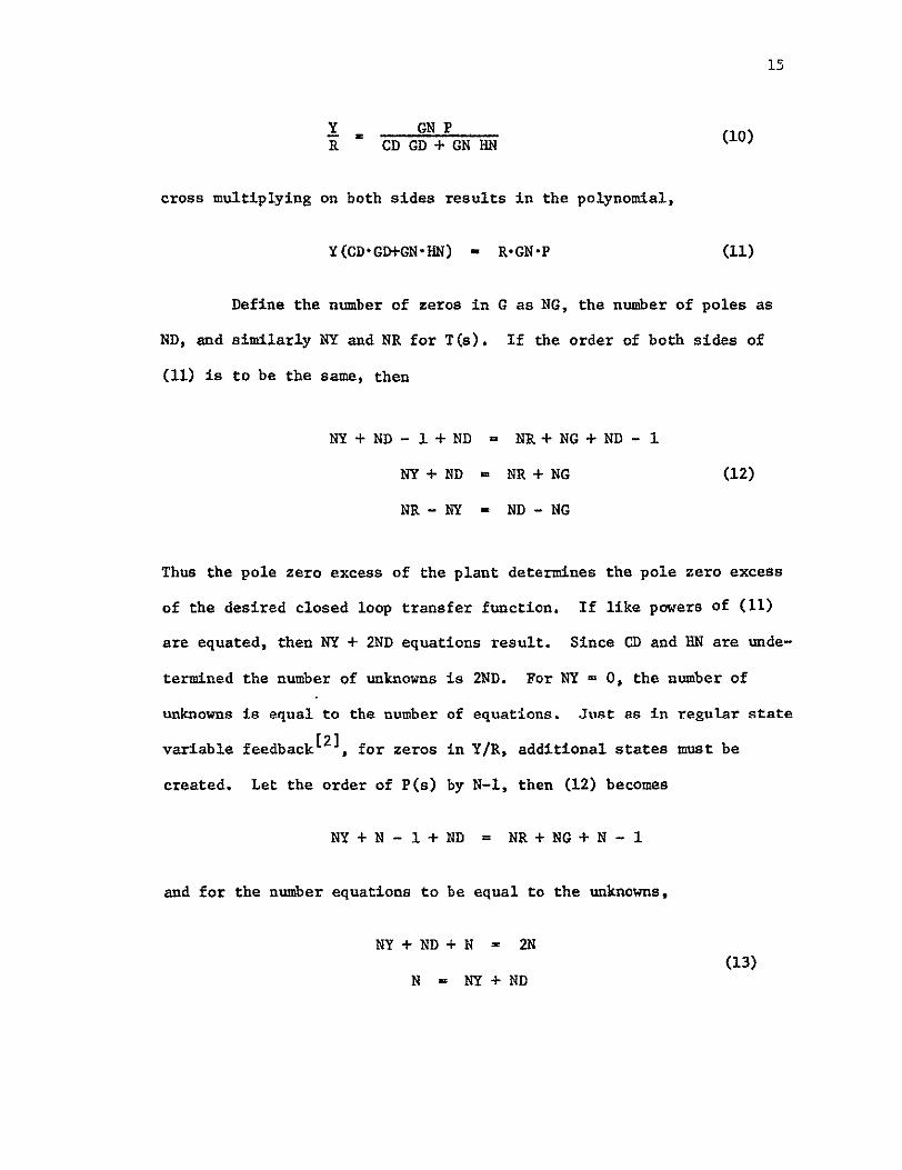
16
Thus the order of both controller systems C(s) and H(s) must be one
less than the number of poles of G plus the number of zeros of YR
assuming that (11) represents a set of linearly independent equations
The design procedure is as follows
1 Select the desired closed loop transfer function from the
specifications
2 Select a polynomial P(s)
3 Equate the actual and desired transfer functions (iO) and
solve for the coefficients of CD(s) and HN(s)
Program 1
The first program (MODOBSI) computes the transfer function of
the series compensator and the feedback compensator as a linear function
of the denominator of the feedback compensator The user must specify
the plant transfer function and the desired closed loop transfer
function Thus this program specifies the design of the system except
for the poles of the feedback compensator which the user is free to
choose in any way he wishes
Program 2
The second program (MODOBS2) computes the transfer function of
the series compensator and the feedback compensator which minimize the
low frequency sensitivity of the closed loop system to plant variations
The user must specify the plant transfer function and the desired closed
loop transfer function If the time constants in the plant are much
lower than in the closed loop system the poles of the feedback compenshy
17
sator may be in the right half plane (RHP) If the poles of the compenshy
sator are in the RHP then the system will be vyD sensitive to variations
in the parameters of the compensators In this case it is better to
use one of the other programs This program is limited to systems with
no zeros
Program 3
The third program (MODOBS3) computes the weighted integral
sensitivity of the system for a given polynomial P(s) The user must
specify the plant transfer function closed loop transfer function the
weighting to be given the sensitivity as the frequency varies and the
denominator of the feedback transfer function P(s) The weighting
function must have more poles than zeros
Input Data
In many circumstances the available data for the plant is in
state variable form This data is converted to a transfer function by
the STVFDBK program The details of the program are included in reference
1 The program listing and input data format are also included in the
Appendix
Output Data
The program BODE4 is provided to plot the transfer functions
computed in the above programs on a logarithmic scale For each program
some of the transfer functions of interest are
1 Plant transfer function
2 Closed loop transfer function
3 Sensitivity as a function of frequency
4 Loop gain function
The loop gain function divided by one plus the loop gain is the proportion
of measurement noise at each frequency which will reach the output Thus
if the loop gain is much greater than one then nearly all the noise
reaches the output and if the loop gain is much less than one very little
measurement noise reaches the output If the phase shift of the loop
gain is nearly 180 at a gain of one the measurement noise will he
amplified
Program 4
The fourth program (MODOBS4) is useful to check the results of
the design Given P(s) and the results of the first program (MODOBSI)
this program computes HN(s) CD(s) and the roots of both the series and
feedback compensators This program and the first program give a
complete determination of the design
Results
A discussion of each program and several caee studies are inclushy
ded in the Appendices MDDOBSI is useful to compute HN(s) and CD(s) in
terms of the coefficients of P(s) Quite amazingly the coefficients of
N and CD are linearly dependent upon the coefficients of P HODOBS2
computes the coefficients of both compensators which achieve minimum low
frequency sensitivity Essentially this result is achieved by forcing
CD(s) to be an N-i order integrator which increases the gain at low
frequency and thereby decreases the sensitivity since SK = (s)
Unfortunately if the plant denominator coefficients are smaller than
19
those of the denominator of the closed loop transfer function the feedback
compensators may have poles in the RHP MODOBS3 determines the weighted
integral sensitivity when P(s) is specified MODOBS4 is useful for
checking the roots of the resulting compensators after a design is
complete Test results are given in the appendix for three examples
These examples show that an improvement in the system sensitivity over
that of just a series compensator can be achieved even if only the output
is available When the closed loop response is much faster than the open
loop the sensitivity of the MODOBS system approaches the sensitivity of
the Req system (which is best but not realizable) if the roots of P(s)
are made much larger than the closed loop roots If the closed loop
response is not much faster than the open loop response then the MODOBS
system may have a sensitivity lower than the Heq system This situation
exists whenever Heq(s) has zeros in the RHP These results point out
the important fact that a sacrifice in sensitivity to plant variations
is made by increasing the system performance requirements Because of
this fact careful attention to the plant performance should be made for
lowest sensitivity and unnecessary demands on overall system performance
should be avoided
20
Bibliography
1 J C Truxal Control System Synthesis McGraw-Hill 1955 Chapter 5
2 J L Melsa and D G Schultz Linear Control Systems McGraw-Hill 1969 Chapter 9
3 D G Luenberger Observing the State of a Linear System IEEE Transactions on Mil Elec April 1964
4 M E Muterspaugh State Variable Feedback and Unavailable States HS Thesis 1968
5 F H Effertz Comment on Two Coupled Matrix Algorithms for the Evaluation of the rms Error Criterion of Linear Systems Proceedings of the IEEE November 1966 p 1629
6 J L Melsa A Digital Computer Program for the Analysis and Synthesis of State Variable Feedback Systems NASA Contract Report CR-850 August 1967
7 L E Weaver et al A Control System Study for an In-Core Thermionic Reactor J P L Report 32-1355 January 1969
21
Appendix I - MODOBSI
Dis cussion
The basic algorithm of this program is based upon (5) First the
following polynomials in s are computed
T = (GD)(Y)
Q = (GN)(R)
V = (GN)(Y)
so that (5) becomes
(T)(CD) + (V) (HN) = (Q) (e) (Al)
Each of the terms in (Al) are polynomials in s where P(s) is unspecified
For instance P(s) = P3s2 + P The coefficients of CD(s) and HN(s) are
the unknowns
As an example suppose the plant is second order then P(s) is
first order In this case (Al) becomes
(CD2T3 +H 2 V3 )s 3 + (CD2T2 + CD1T3 + H2 V2 + H1 V3 )s2 + (CD2T1 + CD1T2
2 + H2V I + HIV2)s + (CDIT + HV) = P2Q 3s + (P2Q2 + PIQ3 )s2
+ (P2Q + P1 Q2 )s + PlQl (A2)
Equating coefficients of like powers of s results in the equations
T3CD 2 + V3H2 Q3P2
T2CD2 + T3CD1 + V2H 2 + V3H1 Q2P2 + Q3PI
22
T1 CD2 + T2 CDI + VIH2 + V2H 1 QlP2 + Q2P
TICD1 + V1Hi = Q1F1 (A3)
These equations can be rewritten more compactly in matrix notation as
T3 0 V3 0 CD2 f 0 Q3TN12N-2 T2 T3 V2 V3 CD11 214-22-Q3 Q3 Q22 (A)
2 T V1 V2 H2 Q2 QI P2j _ Ql 0
2N-2- shy - N-i-)
The matrix on the left will be defined as matrix A and the matrix on
the right will be defined as matrix C Then
CD2 CDI _ - 1
CD= A-C (A5)
H I
Therefore A- C relates the unknowns CDi and Hi to the parameters Pi
MODOBS1 forms the matrix A from the two arrays T and V and then inverts
A Next the C matrix is formed from the Q array and then A 1 C is
computed and printed
23
Input Format
Card No Columns Description Format
1 1 NY = order of Y(s) in YIR II
2 NR = order of R(s) in YR Ii
3 NG = order of GN(s) in GNGD i1
4 ND = order of GD(s) in GNGD Ii
I 5-80 Identification of problem 8AI0
20 Cn of 2 11-0 Coefficient of s in Y(s) FI03
11-20 Coefficient of aI in f(s) P1e3
etc
71-80 Coefficient of s7 in Y(s) F103
3 1-10 Coefficient of a in R(s) F103 etc
4 i-i0 Coefficient of s in GN(s) FIO3
etc
5 etc Coefficientof a in GD(s) FI03
Notes
1 If more than eight coefficients are required then two cards may be
used to identify that polynomial
2 A decimal point must be used for each coefficient but not for card
No 1 The decimal point may be placed in any of the ten columns
for each coefficient
24
3 As many problems may be run as desired by repeating the above format
for each problem
Output Format
See example
Subroutines to be Used
PLYMLT Multiplies two polynomials together
MXINV Inverts matrix A
PRNTRAT Prints the ratio of two polynomials
Flow Diagram
Read NYNRNG
ND
FRead Y(s)R(s)GN(s) GD(s)
Compute T = YGDQ = GNRV = GNYj
Form A Matrix
Invert A Matrixi
lForm C Matrixl
A -1
ComputeBA7 C
Print CD and E
Arrays
PROGRAM MODOBSI (INPUTOUTPUTTAPE4INPUT)
ODIMENSION Y IC) R(10) GD(IO) GN(IC) V(201 T(20) G(20)14A(S363)AI(36 3)C( 3611) B(36 1U ID(G)
C Y(S)R(S) IS DESIRED CLOSED LOOP RESPONSE C SP(S)GD(S) IS PLANT TRANSFE FUNCTION C NY IS ORDER OF NUM IN Y(SlR(S) NR IS ORDER OF DEN C NG IS ORDER OF NU OF G(S) NO IS ORDER OF-DEN C NR-NY MUST EQUAL ND-NG 1 READ 1U1NYNRNGNDID
PRINT 200NYNRNGNDIO
IF(EOF4) 99t2 2 NY1=NY4 1
READ 102 (Y(I)I=-INY1) C YI) IS COEFF OF S(I-I) IN Y(S)
NR I=NR C RII) IS COEFF OFS(I-1)IN-P(S) 3 READ I102 (R(I) IINRI)
CALL PRNTRAT(YNY1RNRI IHTIHS) __C_ GN(Il IS COEFF9F_SCI-1LIN_-GNtSL
NGl1NGI NO 1NDI
_4 -READ 102 (GN ) I 1NG1) C GOD(I) IS COEFF OF S(I-1) IN GO(S) 5 READ 102 (CG (I)I--1NDI)
CALL PRNTRAT(GNNGIGDNO HGIHS___ C FORM CHARACTERISTIC POLYNOMIAL
CALL PLYMLT (GDND1YNYITO) CALL PLYMLT GNNG1RNRI00-CALL PLYMLT (GN NGGYNYIVO) NYNGzN Y1 4NGI NR+NG+iN __ 00 6 IrNYNGN
C NA IS ORDER CF A MATRIX WHERE A IS MATRIX RELATING UNKNOWNS -6- V( --- - - TO PARAM P
NA_- 2 (N--1) DO 20 J-1NA IF- (J GT (N- IlJGO__TO2_12 00 10 Iz1NA INDN- L J IF _( IND-SLT_ I)_GOTO8_ IF (IND GTN) GO TO 8 AUIJ)- T(INa) 30 TO 10shy
8 A(IJ) O 10 CONTINUE
Gi__TO_2D
12 DO 20 I=INA IND 1-I+J IF- (INDLT__GO__18__ IF (INDGTN) GO TO 18 A(IJ)-V(IND) GO-T 0 _2D
18 A(IJ)-O 20 CONTINUE
CALL MXINV-(ANAtAll_ C C IS THE COEFF ARRAT
NM IrN-1 _DOZ4__I NA-_ DO 24 J=1YNMI IN= 2N-I- J
IFiINDLT1) GO TO 22 IF (INDGTN) GO TO 22
C(IJ) = O(INO) -
GO TO 24 22 C(IJ)rO 24 CONTINUE C B IS AICTAE ROwS OF 5 ARE EQUAL TO CD AND HN C COLS ARE COEFF OF P PARAMETERS
D0 30 INA 00 30 KzlNM1 B(IK)--O 00 3fJ--JNA
30 B(IK)-AICIJ C(JK+B(IK) PRINT 2O1KK--lNMI) DO 40 I--NMI
NC =N -I 40 PRINT 202 NC (B I-Kt NM1I
DO 50 I=NNA
NBzNA+-I -50 PRINT 204t-NB (8(1I(1 Kzl-NM-1
GO TO I 99 STOP -101-FORM ATf l A 1f)V t 102 FORMAT (BF103) 200 FORMAT (1HI4(2XI1) 2X6A1i0) 201 FORMAT IH X8 ( 314- P( I 11 I-) OX)) 202 FORMAT 14H CO(I2--)10(E1U33X)) 204 FORMAT (4H HN(I12H)=)I(EIO33X))
END SUBROUTINE PRNTRAT (ANNBvNOEPVARINDVAR) DIMENSION A( 20)B( 20H_(20)N(20)AT20BT(20)NEt 1
DO 6 I--NN AT(I)-- -IF-(-AY f-4i 6-3
3 H(NE)zlH+
AT(NE)rA(1) GO TO 5
4 H(NE)--IH-
AT (NE) -A(I) N(NE)I-1 NErNEI
6 CONT INUE NE=NE-1 PR IN-T 10 0 MIN=MINO(NE 10) PRINT 10lCN(I)IzMIN) PRINT 102 (HRU1 ATI) INDVAR Il tMIN) IF (NE-if]) 8987
7 PRINT 101 (N(I IrIINE) PRINT 102 CHI)AT(I)INDVARI--INEI
__ NF= O0 16 I--IND BT (I)--DIF C B(C) 191G13
13 H(NF)rlH4 BT(NF zB(I)
-GO-_ T _15 14 H(NFI -IH-
BT (NF) =-B(I)
r27 15 N(NF)=I-I
NF zN Fi-I 16 CONTINUE
NF =N F- I HH= IH-NH=rAX 013NE 13 NF) NHzMINO(130NH)
20 PRINT 103 DEPVARINOVAR (HH I=INH) MIN MINO(NF 10) PRINT 101 (N(I)IzIMIN) PRINT 102 (Hi(I)BT(I ) 1NDVAR-I---1MIN IF (NF-101) 28P2827
27 PRINT 0l (N(I) IzIINF) PRINT 102 (H(IJBT(I)TNDVARI=N-FI)shy
28 CONTINUE 100 FORMAT C iHO) 101 FORMAT (6XI(11X 12)) 102 FORMAT 6XID(AIGlC4 AI1H H 103 FORMAT tIXtAIIHCAI2H)= 30AI)
RE TURN END SUBROUTINE MXINV (R N RI) SUBROUTINE TO FIND THE INVERSE- ----- GIVEN
C MATRIX R N IS ORDER OF MATRIX RI IS INVERSE C MATRIX SUBROUTINE USES GAUSS-JORDAN REDUCTION C R MATRIX IS PRESERVED DIAGONAL ELEMENTS OF R-US
BE NONZERO C DIMENSIONR(3G36IRA(3G72) RI(36v36)
C STATEMENTS 20-26 ENTER R ARRAY INTO RA ARRAY - C AND SET LAST N COLUMNS OF RA ARRAY TO IDENTITY
C - MATRIX 20 DO 26 I 1 NI-v 21 DO 24 J I N
_22__RA IJ) -R(I- J) 23 NJ = N + J 24 RA(INJ) = 0 2 5 _NI z N + I 26 RA(INI) = 1
C C ST AT EM ENTS _ii-12_REDUCE MATLRIX__RA _SOH_ATZ_JRFSR_LK C COLUMNS ARE SET EQUAL TO THE IDENTITY MATRIX
i NP = 2 N 2_DO 12 I - N
C -
C STATEMENTS 3-5 ARE USED TO SET MAIN DIAGONAL _C ELEMENT TOUNITY
3 ALFA = RA(TI) 4 DO 5 J = I NP S RA(IJ) r RA(I J) _ALFA
C C STATEMENTS 6-11 ARE USED TO SET ELEMENTS OF ITH C COLUMN TO -ZERO
6 00 11 K = 1 N 7 IF (K - I) 8 11t 8 8 BETA = RAiKI) 9 DO 10 J = It NP
10 RA(KJ) = RA(KJ) - BETA RA(IJ) - ICONTINUE_ 12 CONTINUE
C
TO LAST 28 C STATEMENTS 30-33 SET INVERSE MATRIX RI EUAL
C N COLUMNS OF RA ARRAY
30 DO 33 J 1 N 31 JN J + N 32 00 33 I 1 N 33 RI(IJ) rRA(IJN) 34 RETURN
END SUBROUTINE PLYMLT (ALBMCN)
C C MULTIPLY ONE POLYNOMIAL BY ANOTHER
C C DEFINITION OF SYMBOLS IN ARGUMENT LIST C A(I) MULTIPLICAND COEFFICIENTS INTHEORDER AE) S(I-1) C L NUMBER OF COEFFICIENTS OF A C B(I) MULTIPLIER COEFFICIENTS IN THE ORDER 8(I)SI-1)
C M NUMBER OF COEFFICIENTS
C C11) PRODUCT COEFFICIENTS IN THE ORDER C(19S(I-1)
C N NUMBER OF COEFFICIENTc Ac r
C C REMARKS C IF N-- C(I) SET TO ZERO AND PRODUCT FORMED OTHERWISE THE
C I-PRODUCT AND SUM NEWC-OLD C + AB IS FORMED
DIMENSION A(iD) B(IO) t C(20) LPML+M- 1 IF (N) 10102iZ
I DO 1 J- LPM 11 C(J)-Oo 12 DO 13 J--ILPM
MA X-MA XD (J + I-M il)) shy
- MINzMINO(L DO 13 IrMAXMIN
13 CC(J)=A(I)B(J+II) + C(J) RETURN END
3434 IN CORE THERMIONIC REACTO R
116708 481228 384520 200 1 16708 -4870635__4085815__39226_ 100 116708 481228 384520 200- 503585E-610542E- 3 058639 18804 1
END OF INFORMATION
29
Appendix 2 - MODOBS2
Discussion
If CD(s) in (5) is defined by CD(s) = CD N-i (BI)
where N is the order of the plants then the system will have minimum
low frequency sensitivity because the forward loop gain will be increased
at low frequencies If there are no zeros in Y(s)R(s) or in G(s) (5)
reduces to a simple set of linear equations shown below For simplishy
city RN+ I and GDN+t are set equal to one For zero steady state error
Y = R1
PNl PN= I PN-I = N-I
PN-2 + RNPN-1 CN-2
(B2)
P + 2 + ReN- =1 I I
IN I = P RY
HN2 =PI RY + P2
+HN=NPI RNY + P 2 -Y +i - GD1Y
Where the C terms are defined by
C I GD2 - R2
C2 = GD3 - R3
CN- 1 GDN - N
30
The Eqns (B2) are simply solved in the order shown by back
substitution That is PN-1 may be usedto solve for PN-2 which may be
used to solve for PN-3 etc
Input Format
Card No Columns Description Format
1 1 N = Order of the Plant G(s) Ii
2-80 ID Identification of problem 8A1O
2 1-10 Y = Numerator of YR F10o3
0 3 1-10 R(1) = coeff of s in R(s) F103
11-20 R(2) = coeff of s I in R(s) FIO3
etc
7 71-80 R(7) = coeff of s in R(s) FI03
4 1-10 GN = numerator of G(s) F103
5 1-10 GD(l) = coeff of s in GD(s) F1O3
771-80 GD(7) = coeff of s in GD(s) F103
See notes following input format for MODOBSIo
Output Format
See example
Subroutines to be Used
PRNTRAT - Prints the ratio of two polynomials
PROMT - Determines the roots of P(s) to see if any roots are in
RHP
PROGRAM OOS2 (Y4PUT OUTPUTC4=INPUT)IO41 N j (l10 1 ( l ) 1 ([) Cl(In)ID( 3)PHN 1 )CD t13)
C U (IG) V (10) C PqOGRAM TO CALCULATE MINIMUM LOW-FREO SENSITIVITY MODIFIED C OBSERVER SYSTEM C Y(S)R(S) IS DESIRED CLOSED LOOP RESPONSE C GN(S)GD(S) IS PLANT TRANSFER FUNCTION C N IS ORDER OF DEN IN Y(S)R(S) C N IS ORDER OF DEN IN GN(S)GDIS) C R(I) IS COEF OF S(I-1) IN R(S) C C ASSUMPTIONS C C TRANSFER FCN GAINS ARE NORMALIZED SUCH THAT R (N+1)I1
C AND GD(N I )=I C C DESIRED TRANSFER FCN HAS ZERO STEADY STATE C
-C GD(I) IS-COE-F-- O-F S(I-I)1NGO(S) C Y(S)=Y GN(S)-GN (NO ZEROS ALLOWED) C I READ 101 N ID
IF(EOF4)99 2 2 READ I02Y
READ 102 (R(I)IzIN) NP i-N+ I
GD(NPI) =1 5 RNPI_)-1 READ 102 GN
3 READ 102t CGD(I)tlz1N) PRINT 200DNIO10 PRINT 201
CALL PRNTRAT CYIRNPHTIHS) PRINT 202
CALL PRNTRAT(GNGDNP11HG1HSI C-C --SOLVE FOR DEN OF H P(S)
NM I=N-I do 40 II -NM1 IPIlzI+I
-4 -CI) zG0c IP 1I-R IiT P(N) -
005[ I=ItNMj NI N-I P(NI)zC(NI)
IFCILE1) GOTO-50_ DO 49 Jz2I J2=N-J+2
4 P(NI )zP( NI )-R( J2 )P( JI ) 51 CONTINUE
CALL PROOT (NMIPUV) PRINT 205
PRINT 206 (U(I)V(I) I=INM1)
ERROR THUS YR(1)
SOLVE FOR NUM OF HHN(S) DO 60 1N HN (I 0 - 00 60 JzlI IJI j4
C
6C PN Il)r( Ji R (IJ) Y +HN( I) 32 HN (N )HN (N)-GD (1 )Y
PRINT 203 CALL PRNTRATIHNNPNIHH1HS) PO 80 1i NMI
80 CO(I)zO CD(N)zl PRINT 204 CALL PRNTRAT(PNCDN1HC1HS) G z YGN PRINT 210 G GO TO I
99 STOP 101 FORMAT (Il 84101 102 FORMAT (SF1O3)
200 FORM AT(IHII0X II 4X 8AID) 201 FORMAT(1HOTHE DESIRED CLOSED LOOP TRANSFER FUNCTION IS)
202 FORMAT(1HOTHE TRANSFER FUNCTION OF THE PLANT IS)
203 FORMAT(IHOTHE TRANSFER FUNCTION OF THEFEEDBACK COMPNSATOR IS)
204 FPRMAT(lHOTHE TRANSFER FUNCTION OF THE SERIES COMPENSATOR IS)
205 FORMAT (IHO 5X THE ROOTS OF P (SI ARt 13XREAL PART IOXIMAGINARY PART)
-20 FORMAT 32X2E207f 210 FORMAT4IHOTHE ADDITIONAL FORWARD LOOP GAIN REQUIRED IS
1YGNElfl3) END SUBROUTINE PRNTRAT (ANNSNDDEPVARINOVAR) DIMENSION A(20)B(20vH(20) N(20 1 AT(20) PT 20 NE z1 00 6 Iz1NN AT(1)=D IF C(IA ) 463
3 H CNE )= IH + AT (NE) =AtI) GO TO 5
4 H(NE)=IH-AT (NE) =-A( I) N(NE)--I-1 NE-NEI
6 CONTINUE NE=NE-1 PRINT 100 MINMINO(NE v1O
PRINT IOl (N(IhI=IMIN)
PRINT 102 (H(IAT(I)INDVARI-IMIN) IF (WE-10) 8
7 PRINT 101t (N(I)IzlINE) PRINT 102 (H(I)AT(I)INDVARIn1NEl NF o_-8_ N --1 80 16 I1NU
BT(IzO IF ( (I) 1141613
13 H(NF)zlH+ BT(NF)l=B(I)
-GO T0- 15 __ - 14 H(NF) zlH-
BT (NF)z-B(I) - 15 N(NF)=I-1 -
NFZNF41
33 ID CONTINUE
NF NF- I HHL IH-NHMAXO( 13NE 13NF) NHzMINO( 130NH)
20 PRINT 1G3DEPVARINDVAR(HH 1=1NH) MINMINO(NF 10)
PRINT 101 (N(I)IlMIN) PRINT 1G2( H(I)BT(I)INOVART IMIN] IF (NF-in) 2828927
27 PRINT 101iN(I) I11 NF) PRINT 102 (H(I)BT(I)tINDVARI-IINF]
28 CONTINUE 100 FORMAT (1HO) 101 FORMAT (GX1O( IIX12)) 102 FORMAT (GXI0(AIGIO4 A1IH )
103 FORMAT (1XA1IH(Ai2H)-130A1) RETURN END
___SUBR CUT INEPR O0 TN _A U fVtIIRR) DIMENSION A(20)U(20)V(20)H(21)8(21 )C(21) IREV-IR NC -N +IDOll--i Nu
H( I) rA( I) _i CONTINUEL
00
3 IFIH( 1)) 24 2 NCNC-1
V NC )z0 U NC O DO 1002 I= 1NC H(I)--H(I+1 )
1002 CONTINUE GOT03
S_IF (NC- 1) 5 10 05 5 IF (NC-2) 7i 7
6 R=-H( 1H(2) GOT050
7 IF INC- 3) 9-819 8 P-H(2)H(3)
__0 1) H (3_)_ GO TO7g
q IFCABSCH(NC-1)1H(NC)-ABS(H(2)H(1))101919 10- IREV - IREV_
M=NC2 DO11I=-1 M
_-NL-zNC+ 1 -I-FrH( NL) H NL )H( I)
11 H( I) F -IF (O )139 12 913
12 P=D GOTO 15shy
13 PzPQ 0= (
15 IF(R)16191G 16 R=1 R 19 E5E- ]C
B(NC)H(NC) C(NC)H(NC) B(NC+1 )zO C( NC 1)z 0 NP NC- 1
20 0049J= I 100C DO 2111l1 NP ITNC-I I BC I rH(I)+RB(+1)
--21C( I) =B (I)+RC( I+ 1) IFCABS(B(I )H(1))-E)5050 24
24 IF(C(2)232223 2amp R= RlI-
GO TO 30 23 R=R-B(1) CC2)
30 D0Q3711zlNP IzNC-I I BI)i(I)-PB(I+I)-OB(I+2)
37C( I) =B (I)-P C(i1l) OC(12) IF(H (2)) 323132
31 IF(ABS(C2)H(1))-E)333334 32 IF(ABS(B(2)H(2) )-E) 33v3 34 33 IF(ABS(B(1)H(1))-E)707034
34 CBARrC(2)-B(2) DC(3) 2-CB ARC ( 4) IF(D)363536
35 PzP-2 0= (o t GOT049
36 PP(-82)C(3)-BC1)C(4))D - Q+ (-( 2)CBARB(1) C(3 00)
49 CONTINUE
ErE 10 GOT020
50 NC-NC-1 VtNC)D
IF (IPEV) 51 5252 51 U(NC)=1R-
GOT053 52 U(NC)-R 53 00541lNC
H(I) B(1+1) 54 CONTINUE
GOT04 70 NC=NC-2
---- IF(IREV)71727 71 QPr1O
P=P(Q2 0) GOTO73-_
72 OPPP Q-P 2 0
73 F-(PP)2-OP IF(F )74 7575
74 U(NC+I)z-PP U(NC)-PP V(NC 1 )SORT(-F) V( NC 1-V (NC+ 1) GOT076
75 U(NC+11-(PPABS(PP))(ABS(PP)SQRT(F)J V( NC+1 )0 U(NC )OPU (NC1) V( NC )O
76 D0771INC H(I) B(1 2)
77 CONTINUE GOT04
LDO RE TURN END
3 CASE STUDY II THIRD ORDE-SYSTE14shy1000 1000 200 20 D O -
2500 100
36
Flow Diagram
Read N ID
Y R(I)
GN GD(I)
Print N ID
YRy G
Form C(I)
ISolve for P(s)j
Solve for HN(s)I
Print H(s)
Print C(s)
37
Appendix 3 - MODOBS3
Discussion
This program uses the following data
1 Plant transfer function G(s)
2 Desired closed loop transfer function T(s)
3 The denominator (P(s)) of the feedback compensator H(s)
4 A desired weighting function W(s) on the integral over
frequency of the sensitivity of the closed loop response
to forward loop gain changes
The program then calculates the weighted integral sensitivity of
the system The method of calculation is based upon an algorithm by
EffertzL5] The integrand of the integral sensitivity is calculated
from
I S W(S) S (S) ds
2r f G(s)C(s) ds
The algorithm is based upon an iterative manipulation of the coefficients
in the numerator and denominator of the integrand in such a way that the
integral of the squared magnitude results
A closed form solution for the integral
jm n 2rj jo h(P)h(-P) 2 -joo
1 30 dP 1 j F(P)F(-P) dP
(BI)
is presented in the paper by F H Effertz The solution takes the form
38
of Equation 4 in his paper A better algorithm for the computation of
Equation 4 in Effertz is presented in the correspondence by Pazdera
(Equation 7) A modified forn of Pazderas algorithm has been coded in
FORTRAN and is included A test problem is also included
The use of Equation 4 in Effertz can be best illustrated by an
example Suppose we wish to evaluate the following
(B2)Ls2+ Cb) [2bLn = 2I -
It can be shown from residue theory that the correct answer is
I = - residue of F(s) F(-s) at s = a (B3)n
- residue of F(s) F(-s) at s = b
where F(s) F(-s) indicates the function to be integrated over s = jW
Then the answer is
22 2
= - c-a (c2-b2 c2+abn 2a(a+b)(a-b) 2b(a+b)(b-a) = 2ab(a+b) CR4)
To use Equation 4 from Effertz we must make the following associations
using the complex frequency variable s in place of p
22 s= c -g(P) = (s+c)(c-s)
then s (B5)
2
h(P) = s + (a+b) s + ab
then p s N=2
1
a a 2 =ab
39
The integral for n = 2 can be expressed as
bb [bloaaob I- (B6)
a0 t ol [jaza1-2 1ao a 2
Substituting the correct values of a0 a etc and cancelling minus
signs for this problem we obtain
ab +c In = 2ab(a+b) (B7)
What is most interesting is that the result depends only on the coeffishy
cients of the known function being integrated and not on the poles of
the function as one would suspect from residue theory
It has been mentioned that the algorithm from Pazdera (Equation 7)
has been programmed Some charges in the nomenclature of Equation 7 were
necessary to facilitate coding Note that the practice in Effertz and
Pazdera is to make the highest membered coefficient correspond to the
lowest power of the variable p Note also that subscripts such as ao
are in evidence To facilitate coding the lowest numbered coefficient
was subscripted in the form A(l) and this coefficient was associated with
0 ththe lowest power of the variable p in this case p In general the i
coefficient A(I) is associated with the (i-1)s t power of p P -l (In
FORTRAN the expression A(O) is not allowed) Note from equation I above
what must be done to operate on the function F(s) F(-s) If F(s) is of
the form
F(s) = C(S) (B8)A(S)
then the algorithms suggested in both Effertz and Pazdera require the use
40
of
g(s) = C(S) C(-S) (B9)
h(s) = A(S)
It is more desirable to input C(S) and A(S) rather than C(S) C(-S) and
A(S) Consequently one uses the INTSQ subroutine by coding the coeffishy
cients of C(S) and A(S) with ascending subscripts corresponding to
ascending powers of S The subroutine provides the operation C(S) C(-S)
Furthermore the subroutine checks to see if the lowest coefficient of
C(S) or A(S) is zero so that factors of S may be either considered or
cancelled Two basic requirements must be met by A(S) and C(S) First
the roots of A(S) and C(S) must at least have non-negative real parts
(Hurwitz polynomial requirement) Secondly the highest power of C(S)
must be at least one less than the highest power of A(S) for convergence
to be assured If A(S) is Nth order one inputs the N coefficients of
A(S) and the N-i coefficients of C(S)
The use of this subroutine INTSQ may be best illustrated by an
example Suppose we desired to evaluate the integral
I = JD F_ 7 4 - JdS n -joe 3 + 3s2 + 2s + L[43 + - 2s
(BIO)
The polynomials C(S) and A(S) as defined in Equation B8 are input into
the program as
C(1) = 4 A(l) = I
C(2) I A(2) = 2
(Bi) C(3) o A(3)= 3
A(4) = 4
41
The program then utilizes the modified Pazdera algorithm and prints out
the message
THE VALUE OF THE INTEGRAL IS 12250
To check this answer one can use Effertz Equation 4 for a third order
case (n=3)
a oa 101o 2 1 n
= (142a
0 a
aI a a 0
I 2a
boa2a3+b2aoal-aoa3b alaaa a (BI2)
0 1 20 - o2 2 3o 31 o 13a22o0
For our example problem the following associations follow
b =0 a =4 0 0
b 1 -l a = 3 (B13)
b2 =16 =2a 2
a 113
Substituting the values of Equation B13 into Equation B12 verifies the
computers solution I = 1225n
Input Format
Card No Columns Description Format_
See format for MODOBSI
K 1-10 P(1) - coeff of so in P(s) BE103
11-20 P(2) - coeff of s in P(s) 8E103
etc
42
Input Eormat (contd)
Card No Columns Description Format
K+I 1 NW - Number of coeff in denom of W(s) II
K+2 1-10 WN(I) - coeff of s in num of W(s) 8E103
11-20 WN(2) - coeff of s in num of W(s) 8EI03 etc
K+3 1-10 WD(1) - coeff of s deg in den of W(s) 8E103
11-20 WD(2) - coeff of s in den of W(s) 8E103 etc
43
PROGRAM MODORS3(INPUTOUTPUTTAPE4-INPUT ) DIMENSION Y( 10)R(10)c-D(IO) SN(lOhIP(10)CD(0) HN(IO)SN(40)bull
IS0(40) B(36 18)WN(10) WD 10)SNT(40)SDT(40)C
I CALL MODOBSI (YP GN GO5 NY1 NR1 NGI NDI C N-1 IS THE NUMBER OF COEF IN P(S) HN(S) CD(S)
NrNR 1+NGI- 1 N =rN -1 READ 10 lP(I)Iz1NI)
C W(S) = WNWD MUST HAVE MORE POLES THAN ZEROS C NW IS THE NUMBER OF TERMS IN THE DENOMINATOR OF WS)
READ 103NW READ 102 (WN(I)I-INW)_ READ 102 (WD(I)I-INW) PRINT 205 CALL PRNTRAT (WNNWDNW1HW4-lkHS) CALL PLYMLT(GDNDlY NYI SN 0) N2=NDI+NYI-I
_CALL_ PLYMLTT(yN NWSNN 2 SNT D) CALL PLYMLT (GNNG1 R NRI SO 0) CALL PLYMLT(WDNWSDN2SDT C)
__N3=NW+N2-1 -
N4 =N 3+ NI-1 N22N1 11
-a- DO 10 I= 1Nl CD(I)=0 HN(I)O 00 10 J1pN1 CD (I)B(N-I J)P J )+CD( I)
10 HN(I)zB(N2-IJ)P(J) +HN(I)_P -I NJ_Z0 I--_
CALL PRNTRAT(PN1CDN1IHCIHS) PRINT 202
CALLP RNTRATAHN NI P Ni1H Ht l1 CALL PLYMLT( CDN1 SNT N3 SN C) CALL PLYMLTI- PN1SDT N3SD 0) -N5=N4 ---CALL INTSQ(SDSNN4S) PRINT 204 S
- GO T ---O-- -- 102 FORMAT 18 E1O3) 103 FORMAT III)
-201 -FO RM ampTL__TJJLJERANS ER_-F-UN CT-O-N--OF--L sESERIS--COMENSJ-IO-R- i-l 202 FORMAT(O THE TRANSFER FUNCTION OF THE FEEDBACK COMPENSATOR IS) 204 FORMAT(O THE WEIGHTED INTEGRAL SENSITIVITY ISEIO3) 20S -FORM-AT( Oi-tJ-WEIGHTINGFUNCTION-OF-HE- INTEGRALSENS-IIVlTY-YI-_shy
1) END
_SUBROUTINEMOOOBS1 LYR GN GD B N-YI-NRI-NGL-ND44-UDIMENSION Y(IO) RU1G) GD(10) GNIG) t V(20) T(20)9 Q(20) IA(3636)AI(3G36)C(36l8)B(36 1B)ID(6)
C _Y(S)R(S) IS DESIRED-CLOSED LOOP C GP(S)GD(S) IS PLANT TRANSFERFUNCTION C NY IS ORDER OF NUM IN Y(S)R(S) NR IS ORDER OF DEN
_C_ --NGJ S OR DEROFJN UaOF_ GASJ_ID- S--DRDELO DE C NR-NY MUST EQUAL ND-NG C Y(I) IS COEFF OF S(I-1) IN Y(S)
C RP I) IS COEFF OF S( 1-f1 IN Q(S)
C GN(I) IS COEFF OF S(I-11 IN GN(S) C GOCI) IS COEFF OF S(I-1) IN GO(S) 1 READ 1UINYiNRNGNDIO
IF(EOF4) 99t2 2 NY IrNY +1
NR ic NR --READ 102 (YCI)IIlNYI)
3 READ 12z (R(I) I--NRl) PRINT 200NY vNRvNGNO ID CALL PRNTRAT(YNYl R NRI 1HT IS) NuGl=NG I
ND i ND-shy4 READ 102 IGN I I--I NG1) 5 READ 102 (GD(I)IzlND1)
CALL PRNTRATIGNNG1GDNDI 1H3IHS) C FORM CHARACTERISTIC POLYNOMIAL
CALL PLYMLT (GDNDIYNY1TO) CALL PLYMLT GNNGIRNR10) CALL PLYMLT (GN NGIYNY1V0i NYNG=NY1+NGI N rNR+NG+I 00 6 IzNYNGN
C NA IS ORDER OF A MATRIX WHERE A IS MATRIX 6 V(I)zfl
NA= 2 (N-1 DO 20 J-INA IF ( J GT ( N- 1) GO_TO_1 2 DO 10 IrINA IND-N-I+J IF (IND LT 1) GO TO 8 IF (IND GTN) GO TO 8 A(IJ)= TIIND) GO TO 10
8 A(IJ)zO 10 CONTINUE
GO TO 20 12 DO 20 I=lNA
IND --- I+J IF fINDLTI)_ GO TO 18 IF (INDGTN) GO TO 18 A(IJ) zV(IND)
GO TO 20 18 A(IJ)rO 20 CONTINUE
CALL MXINV_ (ANAAI_) C IS THE COEFF ARRAY-C
NMlzN- 1 DO 24 IrItNA DO 24 JrINM1 INDz2N-I-J
IF(INDLT1) GO TO 22 IF (INDOTN) GO TO 22 C(IJ) - O(IND) GO TO 24
22 C(IJ)zO 24 CONTINUE
__C B IS AICTHE RUWs UF B ANt LIUAL IU) (U C COEFF OF P_ PARAMETERS
00 30 IrINA
44
RELATING UNKNOWNS TO PARAM P
AN_)_HN_THECOLSAR
00 30 KzlIMI B (I K) 0 00 30Jr1NA
30 B(IK) AI(IJ)C(JK)+B( T K) PRINT 201IKv(K=1 NM1 DO 40 I=INMI NC =N -I
40 PRINT 202NC(B(IK)Kr1NM1) DO 50 IzNNA NB -N A 1- I
50 PRINT 204v NB(B(IKIK--NMI) RETURN
99 STOP 101 FORMAT (4116A10) 102 FORMAT (SF103) 200 FORMAT I1HIv4(2XI1) 2XGA1O 201 FORMAT (10X3(3H P(I1lH)vgX)H 202 FORMAT (4H CD(I12H)zO(E1O 33X) 204 FORMAT (4H HN(IIZH)=IO(EIO 33X)L
ENO SUBROUTINE PLYMLT (ALBMCN)
C MULTIPLY ONE POLYNOMIAL BY ANOTHER C
C DEFINITION OF SYMBOLS IN ARGUMENT LIST C AI) MULTIPLICAND COEFFICIENTS IN THEOROER A(I) S(I-I)
C L NUMBER OF COEFFICIENTS OF A _C_ _B I) __MULTILPLIER CO EE-CIENiS-LNTlLODE3-IIi-plusmnSflt-WL-
C M NUMBER OF COEFFICIENTS OF B C CII) PROOUCT COEFFICIENTS IN THE ORDER C(I)S(I-1)
_
C C REMARKS
_C _IF -LO_ C (t1---ETJO_=EOANIRRO IUCTER-MF] lkRWLD T TRiLEJP-PO-DIC C AND SUM NEWC= OLD C AB C
DIMENS ION A( 101 D_cL20j LPML M- 1 IF (N) 101012
At1 -DO i - J-=l LPM__ I] C(J)zOO
12 DO 13 J=ILPM __M AXzMA XO (J+1-MJ
MINMINO (L J ) 00 13 I=MAXMI C ( J )=A _I u KB (Jt 1 RETURN
END
IS FORMED
SU BR OUT I NE P RN TRAT (A NNB N D DEPV AR INDVA RJ_ -
DIMENSION A(20)B(2)H(20 )N( 20)AT(20) BT(20) NE l
-DO JI1NN___ AT (I 1 IF ( A() 1 4993 H( NE = IH AT (NE) zA(I) GO TO 5 H(NE)I-H-
AT(NE) -A(I) N(NE)rI-1 5
146NErN E+1
6 CONTINUE NE =NE- I PRINT ion MINz INC(NE 10) PRINT iO1(N(I)T--MIN) PRINT 10Z (H(I)ATCI) INUVARI1MIN) IF (NE-in) 387
7 PRINT 101 (N(I)IrlNE) PRINT 102 (HCI)AT(I)INOVARvl--IrNE)
8 NF I DO 16 I-1ND ST(I)-O IF ( B(I) ) 141G13
13 H(NF)zIH+ ST (NF) -B(I) GO TO 15
14 H(NF) -IH-BT (NF) -- B(I
15 N( NF)zI--I NFrNF+ 1
16 CONTINUE NF =NF- I-HH =1H-
NH=MAXCD13NE 13 NF) -NH=MINO(130NH)Y
20 PRINT 103t DEPVARINDVAR (H H I-INH)MIN=MINO (NF 10) PRINT 101 (N(I-IiMIN) PRINT 102 (HI )BT(I)INDVARIlMIN)
IF (NF-ID) 282827 27 PRINT 101 N(Il) I=I-1NF)
PRINT 102 CH(I)BTII)INDVARI-i1NF) 28 CONTINUE 166- FO PM AT IHO-shy101 FORMAT f6Xv10(IIX12)) 102 FORMAT (GX0(A1G1O4 AIIH 103 FORMAT t IX A1 IHIAL 2H)Z 130AI])
RETURN END SUBROUTINE MXINV (R RI)
C SUBROUTINE TO FIND THE INVERSE OF A GIVEN C MATRIX R N IS ORDER OF MATRIXv RI IS INVERSE C MATRIX SU-BROUTINE USES GAUSS-JORDAN REOUCTION C R MATRIX IS PRESERVED DIAGONAL ELEMENTS OF R MUST BE NONZERO
DIMENSIONR(33G ARA(3 72) RI(363)
C STATEMENTS 20-26 ENTER R ARRAY INTO RA ARRAY C AND SET LAST N COLUMNS OF RA ARRAY TO IDENTITY-C MATRIX
20 00 26 I = I N 210 24 J = l N 22 RA IJ) - R(IJ) 23 NJ = N J 24 RA(INJ) = 0 25 NI = N + I 26 RACItNI) = 1
C C STATEMENTS 1-1-REDUCE MATRIX RA -SOTHAT FIRST N C COLUMNS ARE SET EQUAL TO THE IDENTITY MATRIX
471 NP = 2 N
2O 12 I 1 N
C STATEMENTS 3-5 ARE USED TO SET MAIN DIAGONAL C ELEMENT TO UNITY
3 ALFA = RA(II) 4 DO 5 J I NP 5 RA(IJ) z RA(IJ) ALFA
C C STATEMENTS 6-11 ARE USED TO SE-T ELEMENTS OF ITH C COLUMN TO ZERO
6 00 11 K = 1 N 7 IF (K - I) 89 11 8 8 BETA RA(KI)
9 DO 10 J I NP 10 RA(KJ) RA(KJ) - BET A- RA(IiJ 11 CONTINUE
12 CONTINUE C C STATEMENTS 30-33 SET INVERSE MATRI-X- RI-EQUAL-TO-LAS-T-C N COLUMNS OF RA ARRAY - 30 DO 33 J 1 N
31 JN = J + N 32 00 33 I 1 N
33 RI(IJ) RA(IJN) 34 RETURN
END SUBROUTINE PLYSQ_ (CN8j___ DIMENSION C(40)B(4D)
C RETURNS BCS) = C(S)C(-S) TO MAIN PROGRA-M C B(I) IS COEF OFS -l IN S -------C C(I) IS COEF OF S I-I IN C (S) C N-I IS NUMBER OF COEF IN B(S) AND C(S)
N1I (N- I)-12---shy00 20 I=lNI MO =-I _BCI) zD II z 2I-i
DO 20 K=1 II MO z -1MO
20 B(I)B(I)MOC(K)C( 2I-K) NMIN-i
- N2-N +I 00 30 I=N2vNM1 IIN=2I-NMI
MO(-I) NMI DO 30 K-IINNMI
O -IMO
30 B(I) r3(I)+MOC (K)C( 2I-K) RETURN
-- END - SUBROUTINE INTSO (ACNS)-DIMENSION B(IOhA(II)C(ID)
C___ RETURNS SZINTEGRAL OF C(S)C(-Si A CS )A( -S)-TO MAI-NRPROGRAMo C B(S) HAS N-I TERMS A(S) HAS N TERMS C B(I) IS COEF OF S(2I-2) - ISCOEF OF S(I-I)2C- -C(I) C IF THE LOWER ORDER DEN AND NUM COEFF ARE SMALL (LESS THAN C 0) THEN DIVIDE BOTH NUM AND DEN BY S2
48
0 1 OE -6 1 IF ( ASS( At 1) )-O) 2220 2 IF (A3S(C(1)-O) 4420 4 IF (K-I) 556 5 PRINT 200 6 PRINT 20IA(1) C(1)
N=N- I 00 10 I1N A(I)=A(1+1 IF(I-N) 8 1010
8 C(I)C(I1I) 10 CONTINUE
GO TO 1 20 CALL PLYSO (CNB)
NM2N-2
DO 50 K=INM2 NK =N -K BA=B(NK) A(NKI) AAO IF(KEOI) GO TO 40 AAzA (NK+2) tA(NKt 1)
40 NMK=(N-K)2 DO 50 I1 NMK NKIzNK-2I1+ B(NK-I )rB(NK-I)-BAA (NKI) A(NKI+i)zA(NKI+)- AAA-NKIj
50 CONTINUE SZB(1) (2A(2)A(I)
RETURN 200 FORMAT (0 THE FOLLOWLNG COEFF WERE FOUND TO BE SMALL AND CANCELL
lED IN THE NUMERATOR AND DENOMINATOR) 1FORMAT (THE DENOMINATOR COEFF EID3 THE NUMERATOR COEFF
1= E103) END
0303-CASE STUDY-IIt -THIRDORDER SYSTEM 1000 000 ___ 2020 i_ 1000
2500 100 1
2
49
Appendix 4 - MODOBS4
Discussion
MODOBS4 uses the matrix relating the coefficients of CD(s) and
HN(s) to the coefficients of P(s) and also the coefficients of P(s) to
determine both the series compensators and the feedback compensators
The roots of the compensators are included
Input format
Card No Columns Description Format
1 1 N = order of plant G(s) II
2-80 ID = Identification 8AI0
2 1-10 CD(l1) coeff of array from MODOBSI EIO3
11-20 CD(12) coeff of array from MODOBSI E-1O3
3 1-10 CD(21) coeff of array from MODOBSI EIO3
11-20 CD(22) coeff of array from MODOBSI E103
N+2 1-10 HN(11) coeff of array from MODOBSI E103
11-20 HN(12) coeff of array from MODOBSI E103
2N+2 1-10 P(l) - coeff of st in P(s) E103
11-20 P(2) - coeff of s in P(s) E103
etc
50
Flow Diagram
Read CD(IJ)
HN(IJ)
P(I)
Compute N
C(J) = Z CD(IJ)P(J) J=l N
H(l) = Z HN(IJ)P(J) J=l
Compute roots of
P(s) and C(s)
Print H(s)
P(s) C(s) and
roots of P(s) and C(s)
IOUN I S I LGO
C PROGRAM PROGRAM
MODOOS4( INPUT OUTPUT TAPE4zINPUT TO CALCULATE CO mPENSATORS WITH P(S) AND RESULTS OF MODOBSi
DIMENSION ID(8) CD (1R 18 ) HN (I 8v 18) C( 18 )PH( 1S )v U 23) V120)P[20 C N IS THE ORDER OF THE PLANT G(S) AND NO OF COEF IN P(S) i READ 100v N ID
IF(EOF4 992 2 PRINT 200 N ID
DO 10 I1IN 10 READ 101 (CO(IJ)JIP N
DO 15 lr1N 15 READ 1019 (HNIIJ) JIN)
READ -101 (PCI) I=IN)
DO 20 I=1N CI I) za HI I ) O DO 20 Jrl N C( I) =C (I)+CD (I J)P(J) H( I ) -H (I)+HN (IJjP (J)-PRINT 204 CALL PRNTRAT(PNtCN1HCiHS) -PRINT205 CALL PRNTRAT (HNPNIHHIHS) NM1=N- 1 CALL PROOT _(NMltCUtVI)- PRINT 201 PRINT 202v(UI)vV(III=IvNMl)
CALL PRO OTNM1 P UV PRINT 203 PRINT 202CUCI)vV(I)vII1NMl) CALL PROOT (NM1NUVI) PRINT 220 PRINT 202(U(I)VCI)I=INM1)
-GOTO_1_ STOP
100 FORMAT t II8AO) _101 _FORMAT_ (8E103)- -- - -- 200 FORMAT (IH12XI12XsAlo) 201 FORMAT(IHSXTHE ROOTS OF C(S) ARE13XPEAL PARTI0XIMAG1NARY
PART) 202 FORMAT (32X2E207) 203 FORMAT (IHO5XTHE ROOTS OF P(S) ARE13XREAL PART1OX-ruwiNARY
-1PART )- 220 FORMAT (1HP5XTHE ROOTS OF- HN(S) ARE13XREAL PART10XIMAGINARY
1PART) -204--FRMAT-IH 0 -- HE--R NS EFRFU NCT-L-ON-CO$FTHamp SERILEs OBZ-NS-AORSt-IL
205 FORMAT CIH THE TRANSFER FUNCTION OF THE FEEDBACK COMPENSATOR IS 1) -END SUBROUTINE PRNTRAT (ANN3NDOEPVARINElVAR) DIMENSION A(20)8(20)H(20)N(n ATt fnl RTlrn) -NE - --
DO G I =INN AT (I lD IF (L l I -
52
3
4
5
6
7
8
__13__
14
1s
16
_20
27
28 10(
01 102 103
H( NE )= IH+ AT(NE)=A(I) GO TO 5 H(NE)zIH-AT(NE) -A() N(NE)I-I NE NE+ 1 CONTINUE NE =N E- I PRINT 100 MINzMINO(NE 10) PRINT 101 CN(I)I-IMIN) PRINT 102 (HCI)AT(I) INDVAR I=i MIN) IF (NE-In) 887 PRINT 101 (N(I-1I11 9NE)- -PRINT 102 CH(I)AT(I)INOVARI=11NE) NF =1
DO 16 IiND BT (I )=O IF ( 8(I) 1 141613 H(NF)=IH+ BT(NF)-B-(I) GO TO 15 H(NF) =IH-BT (NF) =-B( I) N(NF )=-I-I NFzNF+I CONTINUE NF NF-1 H-I H-NHzM AXO 13NE 13N F) NH-MINC( 130NH)
-PRINT 103OEPVARINDVARC(HHt I--1NH) MINzMINO(NF 10) PRINT 101 (N(I)I-lMIN) PRINT 1O2_(HII)BT N 1MIN)_I NDVARtI
IF (NF-IP) 28 t28 27 PRINT 101(N(I) IzIINF) PRINT 102H(I)BT(I)9INVARwI11NF) CONTINUE FORMAT (IHO) FORMAT (6XIlX12) FORMAT (6X O(AlG1O4 AlIH ) FORMAT (1XAIH(AIv2H)-130A1) RETURN--END SUBROUTINEPROOT( N A U V IR) DI-MENS ION A( 20) U( 20_3 V( Z0_LAvj21)3821 ) C 21 L IREV-IR NC-N+I DOI--ANC_HI)=AI)
153
CONTINUE PO 0=0 RO0
3 IF(H(l))42i 2 NCNC- I
V(NC)O U(NC )O 00 100211 NC H(I) H(+l)
-1002 CONTINUE GOT03
4 IF (NC-1)5 1005 5 IF (NC-2) 7G7 6 Rr-H(I)H(2)
GOT050 - 7 IF (NC-3) 99 83shy
8 PH(2)H(3) QH(I)H(3)
- - GOTOYG 9 IFCABS(H(NC-1)HNC))-ABS(H2)H(lelo 1919
10 IREV-IREV -MNC2 -
D0111I M NL =N C 1- I
FHC NLI I-HNL)HfI)
11 H(I)F -__IF( 0 ) 13LIL3
12 PO GOT0 15
-13 PPO 0=1 0
15 IF(R)16191616I_R1R 19 E-5E-10
B(NC)-H(NC) C(NC)H(NC
B(NC+I)-O C(NC+I) NPNC- 1
20 D049JI 100D 0021 Ii NP
- INC-I1
B(I)HCI)+RB(I+1) 21 CCI) B(I)RC( 1+1) IF ABS ( 8 j H _i-) - 50vLQ 2L
24 IF(C(2)l232223 22 RzR+I
- GOTO30------- 23 R=R-B( 1) C(2) 30 003711 =1 NP
= -IzNC-I B( I ) HCI -P B I1) -g B( 1+2 )
541
37 C(I)--B(I)-PC(Ii1)-OC(12)
31 IF (H (2 ) 323132 IF(ASS(B(Z)H(I) )-E) 33s3 34
32 IF(ABS(S(2)H(2))-E)333334 33 IF(ABS (1( I)H( 1) )-E) 7070 34
34 CBAR-C(2 )-8(2) UWC(3)2-C8ARC (4) IF (D)36 3536
35 PzP-2 zQ (Q+)
GOT049 36 P-P+(B(2)C(3)-B(I)C(4))D
OQi(-B(2)CBAR+B()rf 4I)n 49 CONTINUE
E=E10 GOT020-50 NC =NC- i1_
VINC Jr 0 IF (IREV) 51 5252
-5-1 U( NC ) 1-LR- GOT053
52 U(NC)-R -53-DO54Iz 1 -NCshy
H(I)=BtI+1) 54 CONTINUE -- GO TO 4 --
70 NCzNC-2 IF(IREV) 71 72 72
_7___L QP-l PP P G 2 ) GOT073
72 UPr= PP P 2 0
73 F= (PP) 2- UP IF (F )775 75_
74 U(NC+I)-PP U(NC)=-PP V(NC 1Ir)SOPT (-I V( NC )-V (NC+ ) GOT076
75 U(NC+1)z-(PPABS (PP) )tABS(PP) +SORTCF)) V(NC+I I=O U( NC )-=P U (NC+ 1) V( NC )-O
76DO77IINC H(Il)B (-2)
77 CONTINUE GOT04
100 RETURN FND
55
Appendix 5 - STVFDBK
Discussion
A discussion of this program is given in reference 6 The input
is formed from the state equations x = Ax + bu y = cx where x is the
state vector u is the input and y is the output The major use of this
program is to convert the state variable form of the plant to the equishy
valent open loop transfer functions
Input Format
Card No Column Description Format
1 1-20 Identification of problem 4A5
21-22 N = right order of A matrix an 12 integer right justified in the field
2 1-10 a11 = first element of A matrix 8E10O
11-20 8E100a12
3 1-10 a2 1 8El00
11-20 a22
n+2 1-10 b 8E100
11-20 b2 8E100
56
Input Format (contd)
Card No Column Description Format
n+3 1-10 c1 8EIO0
11-20 8ElOO 2
etc
n+4 1-80 Blank card
Notes
As many problem may be run as desired by repeating the above set
of cards for each problem
57
PROGRAM STVFDBK (INPUT OUIPUT TAPF4 Ir DUT)
C OPEN LOOP CNLY DIMENSION A(13 lO R( 10 H( 10 C(IO)NAME(4iAA(IO I )[E (O) DIMENSION O( i)PC 110CC(IOHH(10) PIN(l0 IDU( OV(10)
2000 FOPMAT(QSHO t-s 4 ) 2001 FORMAT (2A10I12) 2002 FOPMAT (8E100) 2003 FORMAT IIHISX1ln1HPROBLEM IDENT 5X 2A10) 2004 FORMAT(lHSX 12HTHE A MATRIX) 20$ FORMAT (GE207) 2006 FORMAT(INHO5Xl2HTHE 8 -MATRIX) 2007 FORMAT(1HOsx4HTHE CLOSED-LOOP CHARACTERISTICPOLYNOMIAL) 2008 FORMAT(IHO5X25HTHE FEE09ACK COEFFICIENTS)
2009 FORMATC1IHO5X1IOHTHE GAIN CCIG7) 2010 FORMAT(1HO5X12HTHE C MATRIX5XSH)
2011 FORMAT(1HO 5X 24HDENOMINATOR COEFFICIENTS) 2012 FORMAT( HO5X 22HNUMERATOR COEFFICIENTS) 2013 FORMAT(1HO5X23HTHE NUMERATOR OF H-EQUIVALENTI_ 2014 FORMAT (IHO5X22HOPEN-LOOP CALCULATIONS)
2015 FORMAT(IHO5X 2GHMAXIMUM NORMALIZED ERROR E102) 2016 FORMAT(I1)-20D17 -ORM AT Ia 5X 24HNCLOSEOD--LOOP--CL-CULATIO-N-s)-shy
2018 FORMAT(IHO56XHKEY - I3XSH) 2019 FORMAT(IHO5X 23HPLANT IS UNCONTROLLABLESXt1CHs)shy2020 FORMAT(1HO4X 35HPLANT IS NUMERICALLY UNCONTROLLABLElOX
I 16HMAX DEVIATION z E1O25X 1OHt _ 202 1 FO RM AT1RO 4ITH A LlX_PELPART W14HIMACJNARY05 ROOTS
1ART)
2022 FORMAT(25X 2E2071 - 2023 FORMATIHO-) C READ INPUT DATA 1 READ 2001 (NAME(I)I=2)N
-- __ IF(EOFr4_lO0tO____ __
B0 PRINT 2003CNAME(I) Iz1 2 PRINT 2004 -DO2 IzlN
READ 2002 (A (I J )JzlN) 2 PRINT 2005(A(IJ)JrlN)
PRINT- 200-- -
READ 2002t (B(I )IUN) PRINT 20059(8(I) IlN)
Cz_ CHECK CO NTkO LLAB ILiTYLL-DO 7 I = N AA (Ii )rBC I)
7- QO NTIN UE-__ DO 8 I2N LrI-1 00 8 JrlN AA ( PIr)O DO 8 K1N
___ AA JI)AA(J IJt+AJJA )_AA(KLL_ 8 CONTINUE
CONTR=DET( AA N) IFCCONTR) 3943
4 PRINT 2019 GO TO 9
_C NOTEUSE OF -DUM-YARGUMENT CALLED_ 3 CALL SIMEO(AACNPINCI
00 43 I=IN
00 43 J-1N 58 P( IJ) 0 00 43 KZ1N P( 1J) =P (IJ)+AA (IK )FINE KJ
43 CONTINUE
ERROR 00 44 I--tN DO 44 JzlN IF(I-J) 454645
4G ERR ASS(P(IJ)-1O GO TO 44
45 ERR ABS(P(IJ)) 44 ERROR = AMAXI(ERRERROR
IF(ERROR-IE-s5 94747 47 PRINT 2020ERROR
C-- OPEN-LOOP CALCULATIONS__ 9 PRINT 2000
PRINT 2b14 NN zN+1 PRINT 2011 CALL CHRE(AiND) PRINT 20 05(I ( I-1 _w CALL PROOT (N BU Vv+ ) PRINT 2021 PRINT 2022 U(IJVII-- N 0011 I1N P(IN)8()
-11-CO NTIN UE__-_ DO 12JJ=2 YN 0012 IiN
- J=N-JJ+I K=J+I
P(IJ) D(K)B(I) - DO12_Lzt N_ ____
P( IJ) P(IJ)+A( IL)PLK 1 12 CONTINUE
-72- RE AD 2002 -CC Ii-I=INL 00 70 11 N IF(C(I)) 717071
-70---CONTINUE GO TO i
71 PRINT 2023 PRINT 2010
PRINT 2005t (C(I)I1N) 49 0013 I1N
_ CCIjz-O0
0013 J 1N CC(I)P(JJ I)C (J)+CC (I)
_13__-CONTINUE 00 100 I1N M=NN-I
_IFACCM) )1-J1-10U103 100 CONTINUE
101 PRINT 2012 PRINT -2005 CCAII i bullM)-
HzM- i IF(M) 105105103
-- 103-CALL- PROOT-(MCC UV-+-l PRINT 2021 PRINT 2022(U(I) V(I) I-1 M)
9
105 GO TO 72 10 STOP
END
SUBROUTINEPROOT IN At U V IR DIMENSION A(20)U(20)V(20)H(21 )8(21 C(21) IREV=IR NC =N+1 DOIIl NC H( I) A (II CONTINUE P=O 0=0 R D
3 IF(H(1)4924 2 NC =NC- I
V( NC )-0 U NC)= D010021r1NC H(I) H(I+l)
1002 CONTINUE GOT03
4 IFCNC-1)51005 -S--IF(NC-2)7s57 6 R=-H(1)H(2)
C-TO50 7 IF (NC-3) 9 9
8 PrH(2)H(3) OH(1)H(31 GOTO70 IF(ABSH(NC-I)H(NC))-ABSH(2)H(I) )1 1919
-1 IRE V-IREV M=NC2 001111 M NL =NC I-I FzH NL )
HINL)H(I) 11- H( I) rF
I IF ( ) I3tI2 13 12 PrO
GTO 1 5_ 13 PrPO
OrI o --15 _IFR )1 tIj9j_6__ 16 R-1R 19 E=5E-10
_ B(NC )H(NC) CINC=H(NC) B(NC11=O CCNC+1 )0 NPrNC- I
20 D049J1 1000 [021111 NP
INC-I I B(I)= H(I)+RBCI+1)
21 C(I) B(I) PC(I+ 1) __
IF(ABS(8(1)H(1) )-E) 5050 24 24 IF(C(2)232223 22 R2+ 1
GOTO30 23 R=R-B(I)C(2)
30 D037111 N0 1plusmn2 I-NC-I1 B I) --H(I )-PB(I+I) -Q5( I+2)
37 CCI) r3(I)-PC(1 1) -OC(142) IF(H(2)) 323132
31 IF(ABS( (2H(1) )-E) 3v3 34 32 IF(ABS(BCZ)fiH(2) -EU 3333 34 33 IF(ABS(B(1)H(1))-E)707034
34 C3AR--C ( 2 )- B(2) OC(3) 2-CBARC (4)
IF (D)3635 v36 35 P-P-2
00(0+1 GOT049
36 PzP (B(2)C(3)-B(1)C(4)1D OQ+(-B(2)CBAR4B()C(3))D
49 CONTINUE
EzE 10 2
50 NC-NC-1 V( NC ) 0 IF( IREV) 51 vuavt
SI U(NC)=I-R GOTO53
52 U(NC)zR 53 D054I=NC
H(I)--B(I+I) __5 LLL_CONT INUE
GOT04 70 NCNC-2
__IF (IRE Vi 71 t72v -72 71 OP-IQ
PPrP(Q20)____GO TO 73 __
72 OP0 PP P 20
73 Fr(PP)2-OP IF(F)74 7575
74 U(NC+I)--PP _ _U(NC h-PP
V( NC+1 )=SORT (-Fl V(NC)=-V (NC I)
___ GOTOTE
75 U(NC4I)z-(PPABS(PP))(ABS(PP)+SQRT(F)) V( NC+ I)7O
__U( NC )OPU (NC-l- V(NC)O
76 D0771INC C( I) 8 CI2J
77 CONTINUE GOTO4
_Ia _RETU RN-END FUNCTION OET(AN)
C FUNCTION DET DETERMINES THODEERMINANT__OFITHEMA-TRIX A DIMENSION A(1O10) B(10 10)
C SET B EQUAL TO A BECAUSE WE DESTROY A IN THE PROCESS 0O_1IK1_N______ DO I JKzlN B(IKJK) = A(IKJK)
61I CONTINUE NN N-I D 10
C IF N-- THEN BYPASS PIVOT PROCEDURE r0 DIRECTLY TO CALCULATION IF(NN) 69693 OF OCT
C START PIVOT SEARCH PROCEDURE 3 00 100 Lr NN
LL z L41 AMAX = A(LL)
IML
JM = L DO 15 IzLN 00 15 JLN IF (AMAX-ABS(AIIJi)) 101515
10 IM IJ4i z J
AMAXz ABS(A(IJ)) 15 CONTINUE
C FOUND PIVOT AT ROW IM AND AT COLUMN JM C IF ALL REMAINING TERMS IN THE MATRIX ARE ZERO SET O6T20 AND
IF tAMAX) 7070 14 RETURN C NOW CHANGE ROWS AND rfl IIMN T mVtrCCADY 14- -IF (IM-L)G201G
16 DO 17 J2IN T = A(IMJ) A(IMJI A(LJ)
17 A(LJ) T D -D
20 IF(JM-L) 219252 21 DO22 IzN
T = A(IJM) AIIJM) A(IL)
22 A(IL) T ___=_ o- D ___
C PIVOT NOW AT A(LvLDIVIOE ROW L BY A(LL) 25 DO 30 KILLN
A(LKlI -LAiLK1)A_(LL 3- CONTINUE C NOW PRODUCE ZEROES BELOW MAIN DIAGONALAhJLI--
---- DO 50 JZLLN__ DO 50 KrLLN A(JK) = A(JK)-A(JL)A(LKY
_50 -CONTINUE_ 100 CONTINUE
C MULTIPLY MAIN DIAGONAL ELEMENTS TO GET VALUE OF THE DETERMINANT _ 63DQ 200 I0_N_
D = DA(I) 200 CONTINUE
DET _ C NOW RESTORE THE VALUES OF THE A MATRIX
DO 2 IKrIN _j0 2 JKclN-
A(IKJK) = B(IKJK) 2 CONTINUE
_ _RETURN 70 DET=O
D0 4 JK=IN 4DOIK1N
A(IKJK) = B(IKJK) 4 CONTINUE
162RE TURN
END SUBROUTINE SIMEG (AXOOTKC AINVX) DIMENSION A O10U) IO10)XDOT(1 )X(Ic ) AINVtl10O) DO1 I=1KC D0I J1KC AINV (I J I=O
1 B(IJ)-A(IJ) 002 IIKC AINV(IIl=l
2 X( I) =XDOT(I) D03 I1 KC COMP 7O KI IF(ABS(2(KpI))-ABS(COMP))5t54
4 COMP=3KI
NK 5 K=K+1
IF(K-KC)GGi7 7 IF(B(NrI))851w8 8 IF(N-I)51t 9 9 0010 MI-XC
TEMP=B(I M) BC IM) =B(NM) (NM) =TEMP TEMP =A INV( I M) AINV CIM)=AINV (NM)
0_AINVA(N M )=TE1P- TEMP X (I I X( 1) =X (N)
_X(N) -TE-1 P- 12 X(I) X(I)B(I1)
TEMP = B(II) - -DO13- KC =i --
AINV(IM) = AINVfIMTEMP 13 B(IM) = BCIM)TEMP
-- DO16 JIKC -----shyIF(J-)14 1614
14 IF(B(JI)) 15115 -I5-X (J) zX J- )8 B CJIi X( I-)
-TEMP =B (J I ) DO17 N=1KC
-- A INV(JNAINVJPN ) TEMPtAJN VC(ltN) 17 B(JPN) zB(JN)-TEMPB IN) 16 CONTINUE
___3_C0 NTINUE__ RETURN
51 PRINT52IKC 52-FORMAT E 18HI-ERROR IN-CLUWMN--IC22ZX3HO--ATRIX-5X-3IHKCI 1-
RETURN END
_-SUBROUTINE CHEQ-(AN-CJ-_-----DIMENSION Jtll)C(l)B(1010) A(IO 10)D0300) NN =N +1
__D020 I=1 NNC C(I) O
20 CONTINUE C (NN L z-
0014 M1ltN KD
63
L 1
J( 1) =1 GO TO 2
I J(L)--J(L)+ 2 IF(L-M) 3550 3 MM =M-1
DO 4 T-LMM II=I~l
4 J(IIIJ I|)+l 5 CALE FORM(JMAB)
K-K+ I D(K) mET (BMl DO G Ilim L--M- I+ I IF (J(L]- (N-M L I) 1 5c
6 CONTINUE Hi = N-M+1 D014 I-IK C(MI)=C(M)_O(I)(-)M CONTINUE
RETURN 50 PRINT 2000
RETURN 2000 FORMAT (1HO5X14HERROR IN CHREQI
END SUBROUTINE FORM(JMAB) DIMENSION At 1O0] B (IflI10JC) 001 T110M DO1 K=IM NR =J (I NC =J (K
1 B(IK)ZA(NRNC) RETURN
-ENO
64
Appendix 6 - BODE4
Discussion
This program is used for providing phase and log magnitude versus
frequency plots for the resulting open and closed loop transfer functions
The author is indebted to Dr L P Huelsman for this program
Input Format
Card No Column Description Format
1-80 LTR = Title of problem BOAl
2 3 NC = No of functions to be plotted 13
3 1-3 NP = No of values of frequency in 13 the plot (1-100)
4-6 NPD = No of frequency pointsdecade 13
7-9 NHZ - Log10 of starting frequency in 13 Hz
10-12 NSCAL - Max ordinate of magnitude 13 on frequency plot in dbtimes SCALM (minimum value is 100 SCALM) db lower)
13-15 NPHS = Indicator for phase plot 0 13 if no plot desired I if-plot is desired
16-18 MSCAL = Max ordinate for-phase 13 plot in degrees times SCALP (minimum ordinate (100-SCALP) lower)
21-30 SCALM = Scale factor for magnitude E100 data (10 if no scaling desired)
31-40 SCALP = Scale factor for phase data E1O0 (10 if n6 scaling desired)
65
Input Format (contd)
Card No Column Description Format
4 1-3 ND = Max degree of numerator and 13 denominator polynomials (1-19)
5 1-80 A = Numerator coefficients for 8E100 first function (in ascending order use 10 columns for each coeffishycient)
6 1-80 B = Denominator coefficients for 8E100 first function (in ascending order use 10 columns for each coeffishycient)
Notes
1 The maximum magnitude in db which will be plotted is NSCALSCALM
however the maximum value indicated on the plot will be NSCAL
2 The minimum magnitude in db which will be plotted is (NSCAL-100
SCALM however the minimum value indicated on the plot is
NSCAL-I00
3 The above comments also apply to the phase
4 The actual values of the variables are listed in the printout
for every frequency
10N H Z +from 10N H Z to NPND5 The frequency range in Hz is
6 For each function to be plotted cards 4 through 6 must be
repeated As many cards as necessary may be used to specify
A and B when ND 8
Examples
If the function varies from +10 to -10 db then choose SCALM = 5
and NSCAL = 50 since
66
NSCALSCALM = 10
(NSCAL-100)SCALN = -10
If the minimum frequency is 01 Hz and the maximum frequency of
the plot is 100 Hz with 20 points per decade then the total number of
points is
NP = decades(pointsdecade) = (log 10 (max freq) - NHZ) NPD
= 4 - 20 = 80
071
PROGRAM BODE4 (INPUTOUTPUT TAPE 4zINPUT) DIMENSION LTR(80)
DIMENSION Y(5100)
DIMENSION X110)
PHSD-O READ IOO LTR IF (EOF4) 999t2
2 PRINT 101 LTR READ 1O5NC PRINT 110NC
162 READ 105NPNPDNHZNSCALNPHSMSCAL SCALMSCALP
PRINT 112NPNPDNHZ DO 140 K=INC PRINT 1159K READ 77 (X(I)lS)
77 FORMAT (BF104) PRINT 78(X(I)f=15)shy
78 FORMAT(1 X(I) X IOF1Z 3) NX 1 PRINT 201 DO 140 JJ=1NP FRG XL4( NX INHZ NPD) RAD=G 2831 8FRQ
CALL MAG7 (RADFM X PHSD)
137 FML=20ALOGIO(FM)Y(K -J)FMLS CALM _
140 PRINT 2021 JFRORAOFMFML PHSD
PRINT 145 SCALMLTR CALL PLOT4(YNCNPNSC-AL) GO TO I
999gSTOP OD FORM AT-(80 A 1) 101 FORMAT (IH1 BOAl) 105 FORMAT (G132X2EIOO)
110 FORMAT (IHO IGHNUMBER OF CASES-plusmn
112 FORMAT (1H0137H POINTS I1 7HDECADE SX18 HSTARTING FROM 10
1 13)shyi-115 HO1-2H-CAESE NUMBER 12)FORMAT-- --shy
14H SCALE EIO31XSOA1145 FORMAT (IH114HMAGNITUDE DATA FACTOR=
201 FORMAT ( 1IH 25 X 5HHERT Z 13X_7HRADJSEC 17 X3HMAG 18X 2HDB 17X Y3 HOE( i
202 FORMAT 1X I 5 5XSE208) __ END
SUBROUTINE PLOT4(YMNFNS) ARRAY (FORTRAN 4)C SUBROUTINE FOR PLOTTING 5 X 100 INPUT
DIMENSION Y(5v 100) r LINE(101)L(1_JL(S)
DATA (JL(I) li5) IHA 1HB IHCIHDPHEvJNJPJI JBLANKJZ 11H- IH+ 1HI IH v1H$I
D 99 -I-I-101 LINE (I )-JBLANK
99 CONTINUE N=D
68
C PRINT ORDINATE SCALE 00 101 1111 L (I) zi f I- itO+NS
101 CONTINUE PRINT 105 (L()lIlrj)
105 FORMAT (3Xv1(I14 X) GHY(11)) GO TO 115
110 IF (N10-(N-1)10) 125125115 C -CONSTRUCT ORDINATE GRAPH LINE
115 NDO 00 120 I=1910
ND=N04 1 LINE(ND) =JP DO 120 Jl9
N =NO 1 120 LINE(ND)=JN
LINE (101 )zJP IF (N) 135121i35
121 PRINT 17ONLINE GO TO 185
C___ CONSTRUCT i-LINE OF_ ABSCISA GR__AP LLF-
125 00 130 I110li1 LINE (I) =JI
130 CONTINUE C CHANGE NUMERICAL DATA TO LETTERS
135 DO 160 I=IM _XNSNS _ JA=Y (IN )+O149999-XNS
IF (JA-laI) 140155145
__140 IF (JA) 150150155_ 145 LINE(101)-JZ
GO TO 1GO 150_LINE(1)=JZ
GO TO 160
155 LINE(JA)-JL(I) 160 CONTINUE
C PRINT LINE OF DA-T-A-IF (NI1O-(N-I)10) 175175165
-- 165PRINr 170NLINEYIN 170 FORMAT (IXIL41O1A1IX E125)
GO TO 185 A175PRINT 180LINEYlN)_
180 FORMAT (5X1O1A1XEZS5) C SET LINE VARIABLES TO ZERO -85 Do - L=Li1DL
LINE (I)=JBLANK 190 CONTINUE
195 -N=N+1 IF (N-NF) 110110200
69
200 RETURN END FUNCTION XL4 (NLOLPI AN N AL 0 LO ALPzLP AA rNALP+ ALO IF (AA) 100100 105
100 XL 4 I 10 C-AA I GO TO 1101
105 XLl10AA 110 N-N+1
RETURN END -
SUBROUTINE MAG77 (STAMPXPHASE) DIMENSION X(10) COMPLEX GNGDDN0DPNCNCOT GN =CMPLX(7S8S1720)CMPLX(798S-1720) 3880
I CMPLX(1ThOS+3310)- CMPLX(176OS-331l -2 CMPLX(C08S+575O) CMPLXRO-8S-5-75-O) 3 CMPLX(828S 945UI CMPLX(328S-9450) GD ZCMPLX (4605) SCMPLX(44 5S+2820) CMPLX (445S-2820)
1 CMPLX(844S+4780) CMPLX(844vS-478O) 2 CMPLXE1305S+74OO) CMPLX(1305S-740O) 3 CMPLX(1915S+108ZO) CMPLX(1915S-1020) DN-515E+1CMPLX(10300S -
DDCMPLX(G50OS)CMPLX(12GO0S+5880)CMPLX(1260OS-5880) 1 CMPLX(2E1OS+1470O)CmPLX(2510S-14700) 2 CMPLX (391C0S+18100)CMPLX(39100S-18100 PN- CMPLX(1010OS) 10100 CNz1335CMPLX (142S+248 )CMPLX(142 5-248) CD CMPLX(OS)CMPLX (500S) T=(GNDDCD) f(GDD0CDOGNDNNPN )I TAMP rCABS( TI AZREAL CT) B-AIMAG( T) PHASEzATAN2(B A)573 RETURN CN=X(3)CMPLX(XU)S) CMPLX(X(4hS) CDCMPLX(X(21S)CMPLX( X(5)PS) CMPLX(OtS) T--(GNGD)(DNDD) (CNCD) PN) END
70
Appendix 7 - Case Study I
Second Order Plant
Discussion
A second order plant has been selected so that some insight into
the effect of compensators can be obtained before the computer programs
are used Suppose that the plant transfer function is
G(s) (6-1)G (s+b)
and the desired transfer function is a Butterworth type response for
maximum bandwidth
T(s) = 100 (6-2)s 2lOs+100
The feedback compensator will be of the form
H(s) 12 - (6-3)P1+5
where arbitrarily P2=1 since the numerator and denominator may be multishy
plied by any constant For zero steady state error at low frequencies
H =P
The transfer function of the series compensator is of the form
C(s) D+Cs (6-4)CDI+CD2s
From the relation between the closed loop transfer function and the open
loop transfer function
71
G(s)C(s)(s)=+(s)C(s)H(s)
(6-5)
l00(P 1+s)100
s2+1 0 s(s+b)(CDI+CD2s)+100(HI+H 2 )lOs+100
Cross multiplying and equating coefficients result in the
equations
3 a 1 = CD2
2s 10+PI = CDI+1 CD2
i 00+ 10 P = bCD1 +IOOH2
0 s P =H
Solving for CD2 CD and H2 the above equations become
CD2 = 1
CD1 = J 10+P1 -b
H2 = 1+(PI-b)(4710 - b100)
H = PI
Thus the compensators are specified except for b and P1
Sensitivity
The sensitivity of the closed loop system to variations in plant
gain is
S K T(s) s(s+b) (CDI+S) (6-6)T G(s)C(s) 2+ 10s+100)(Pl+s)
72
The low frequency sensitivity is
T 1bCDl(6K - 100P (6-7)
which is minimum for CDI = 0 which implies
CD = 10+PI-b = 0
(6-8) P = b-F 10
Unless PI is positive the feedback compensator will be unstable and the overall system will be infinitely sensitive to variations in PI If PI
is positfve then (6-8) is a restriction on the plant time constant The
only alternative is to make PI sufficiently large to keep the sensitivity
low cf eqn 6-7 It is interesting to compare the sensitivity of this
system with the Heq compensator and the Guilleman-Truxal compensator
He Compensator
Choose Heq to be Heq(s) = 1+k2s Then
T(s) Gs )+=1(s)Heq(s)
100 100 2+10 s+10O e(s+b)+l00(l+k
2s)
Equating coefficients
104= b+100k2
k =2 100
T = T(s)= s(s+b)K G(s) s2+104s+100
--
73
Guilleman-Truxal
Choose
s+b =C(s) S+c
100 100
s2+o12 s+100 s(s+c)+l00
Cross multiplying and equating coefficients
c - I1
Thus the sensitivity is
s(s+lOF2)TK (s2+P2 10s+100)
The above sensitivities are plotted in Fig 6-1 for the case of
where b = 20 and CD = 0
If b = 10 then for P positive the sensitivity is minimized
if P is made large CDIP is nearly one if P 40 The three sensishy1
tivities are shown below
MODOBS
T s(s+10(s+4414) K (s2+10v+100)(s+40)
Heq
T s(s+10) KK = (s2+10y +lO0)
20
10
0
Gain (db) G(s) = 00C(s) = s+586
-10 s(s+20)s
T(s) = 100 s2+ 2 10s+100 Hs)- 1(s)lo484s+586s58
-20+O s+586
uilleman-Truxal1
-30
1 Frequency (Hz)
01
Figure 6i Sensitivity of High-performance 1lant 4shy
75
Guilleman-Truxal
K 2s(s+l03F)TK (s2+104-s+100)
Notice that for b = 20 the MODOBS system is significantly better
at all frequencies below IHz The Heq compensation is both unrealizable
and largest in sensitivity for this case When the forward gain is small
then no compensation will help the sensitivity Thus all the proposed
systems have a sensitivity near one for frequencies above IHz
For b = 10 the low frequency plant gain must be greater to
achieve the same T(s) The Guilleman-Truxal compensation decreases the
forward gain proportionately so that the sensitivity is unchanged The
Heq compensation does not change the forward gain therefore the sensitivity
is reduced from the case where b = 20 The MODOBS system also improves
in sensitivity but this system will only be as low in sensitivity as the
Heq method when PI is infinitely large Nevertheless the MODOBS
compensation has the advantage of being realizable
Integral Sensitivity
For the plant with a pole at -20 the integral sensitivity
(weighted by 1s) is
I j jO I s(s+20)(s-4-P1-586) 2
Sr 2- s (s2+IOffs+100)(S+P 1
This integral can be evaluated directly from Newton Gould and Kaiser
p 372
The minimum low frequency sensitivity was attained for PI = 586
which from MODOBS3 has an integral sensitivity of 012 The minimum
76
integral sensitivity is 0085 for PI = 8 In this simple case this can be
determined analytically by plotting S as PI is varied
Final Design
From the integral sensitivity data a final design choice is
b = 20
P = +8
The following graphs are shown in Figs 6-2 to 6-4
Fig 6-2 Plant transfer function
Fig 6-3 Sensitivity function
Fig 6-4 Loop gain function
Conclusion
From the above figures the design demonstrates the dependence of
the sensitivity on the plant parameters If the time constants in the
closed loop transfer function are much greater than those in the plant
a sacrifice in the system sensitivity at low frequencies must be made
In addition the compensator will have large gains associated with the
feedback which complicate the design of the compensators and increase
the effect of the measurement noise
20
10 open loop
0 closed loop
-10
Gain (dbo)
-20
-30
-40 1
Figure 62
100C(s) =s(s+20) T(s) s2+ s2+
100
10s+100
Frequency (Hz)
Open and Closed Loop Transfer Functions
0
0
-5
Guilleman-Truxal
-10
Gain
(db)
-15
-20
-25 1
I 110 Frequency (Hz)
Figure 63 Sensitivity of Second Order Systems o
10 MDB
0
Guilleman-Truxal
010
Gain (db)
-20
-30
-40 0
Frequency (Hz)
Figure 64 Loop Gain Function of Second Order System
80
Appendix 8 - Case Study 11
Third Order Plant
Discussion
A third order plant has been selected to compare the computer
results with hand calculations The results agree in all the calculations
discussed below The plant transfer function is chosen to be of the form
1000
S3+GD 3 s2-D2 s+GTD
and the desired closed loop transfer function is again chosen with a
Butterworth type denominator
1000T(s) =
s 3+20s2+200s+lO00
MODOBS2
The equations for the coefficients of P(s)=PI+P2SP3s2 which give
minimum low frequency sensitivity were derived in Appendix 2 For N=3
P3 i
= GD3 - 20P2
P 1 GD2 - 200 - 20(P2 )
These equations are satisfied if
GD3 = 20
GD2 = 200
Low frequency sensitivity will be improved if the plant is Type 1 or
81
equivalently has a pole at the origin thus
GD = 0
The poles of the plant are the roots of
s(s2+20s+200) = 0
s = -10 + jlO
For the plant to have real roots then
GD2 - 4GD 2 ) o 3 2
and in order for PI and P2 to be positive
GD3 gt 20
GD2 gt 200 + 20P2
These requirements can be met if
GD3 gt 6828
20(GD3 - 10) lt GD2 lt GD2 4 20G3 3-2
GD = 0
If GD3 is near 68 then P1 must be near zero Under these circumshy
stances the zero of CD(s) cancels the pole at a low frequency and the
low frequency sensitivity suffers Suppose that
GD = 100
5
0
-5
Sensitivity (db)
-10
Guilleman-Truxal MDBS
-15
-20 i
Figure 81
1
Frequency (Hz)
Sensitivity of Third Order System
1010
0
83
Then
1800lt GD2 2500
2
P3 = I
P2 = GD - 20 - 80
PI = GD - 1800
To keep the low frequency pole of P(s) as large as possible it is best to
make GD2 large thus
GD3 = 100
GD2 = 2500
GDI = 0
P3 = I
P2 = 80
PI = 700
Sensitivity
If the plant can be selected as above the sensitivity becomes
2s) s(s 2+100s+2500)T TIL K G(s)C(s) (s3+20s2+200s+1000)(s2+80s+700)
For this choice of the plant the system will have minimum low
frequency sensitivity and a stable feedback compensator A comparison
of the sensitivity of this system with only a series compensator which
achieves the same closed ioop response is shown in Fig 8-1 Except
for frequencies between 141 Hz and 141 Hz the sensitivity is improved
by using the MODOBS system
84
Discussion
Again the importance of choosing a plant which is consistent
with the requirements of the overall system is evident A slow system
cannot be made to react quickly and also have good sensitivity characshy
teristics using second order compensators
85
Appendix 9
Case III In core Thermionic Reactor
The plant and the desired transfer function for an in core
[73thermionic reactor have been discussed by Weaver et al The characshy
teristics of the system are given in the above report This appendix
addresses itself to the question of realization of the desired transfer
function for the fourth order model when-only the output is available
The plant transfer function is given by
C(s) =(s+ 0326)(s+1)(s+l
79) 200 (s+0119+j0164)(s+0119-J0164)(s+00663)(s+185)
and the desired transfer function is
Y(s) 200(s+0326)(s+l)(s+l79) R(s) 100(s+0326)(s+l)(s+179)s+2)
When these terms are multiplied out the resulting transfer functions are
32+200s
116708+481228s+38452sG(s) =
50358510 6+l054210 3+0568639s2+8804s 3+s4
2s2+200s3 Y(s) 116708+481228s+345
R(s) 116708+4870635s+4085815s2+39226s3+OOs 4
This problem represents a special case in that the numerator of G(s) and
YR(deg ) is the same Equating the real and desired closed loop transfer
functions yields
I(s)= G(S)C(s)T(s) a iI+G(s)C(s)H(s)
and in terms of the nuerator and denominator polynomials
86
TN(s) GN(s)CN(s)HD(s) TD(s) GD(s)CD(s)HD(s)+GN(s)CN(s)HN(s)
Since CN(s) = HD(s) a P(s) and TN(s) = GN(s)
1 P(s) TD(s) GD(s)CD(s)+GN(s)HN(s)
Equating the like terms in the above equation and expressing the result
in vector matrix form one gets
GD(1) 0 0 0 CD(1) ON(l) 0 0 0 HN(1)
GD(2) GD(l) 0 0 CD(2) GN(2) GN(1) 0 0 HN(2)
GD(3) GD(2) GD(1) 0 CD(3) GN(3) GN(2) GN(1) 0 HN(3)
GD(4) GD(3) GD(2) GD(1) CD(4) GN(4) GN(3) GN(2) GN(1) HN(4)
GD(5) GD(4)- GD(3) GD(2) + 0 GN(4) GN(3) GN(2)
0 GD(5) GD(4) GD(3) 0 0 GN(4) GN(3)
0 0GD(5)GD(4) 0 0 0 GN(4)
o o 0 GD(5) 0 0 0 0
TD(l) 0 0 0 P(l)
TD(2) TD(l) 0 0 P(2)
TD(3) TD(2) TD(1) 0 P(3)
TD(4) TD(3) TD(2) TD(1) _P(4)
TD(5) TD(4) TD(3) TD(2)
0 TD(5) TD(4) TD()
0 0 TD(5) TD(4)
0 0 0 TD(5)
87
Plugging in the appropriate coefficients from the above expressions for
TD(s) GN(s) and GD(s) the unknowns GD(s) and HN(s) are equal to
CD(1)
CD(2) 119114E+01 -544224E+00 963714E+00 -172292E+01
141485E+02 -212494E+02 391935E+02 -700789E+02 P(1)
932689E+02 -165161E+03 296273E+03 -528468E+03 - 331178E-14 356005E-14 -l10191E-13 lOOOOOE+01 P2)
HN(l) 999949E-01 234842E-05 -415859E-05 743467E-05 496319E-01 100486E+00 -868215E-03 155222E-02 (3) 509230E-01 761501E-01 535279E-01 830837E-01 466345E+00 825805E+00 -147636E+01 282909E+01
HN(4)
The resulting expression can also be solved for P(s) in terms of C(s) that
is
P(1) CD(1)
P(2) 1F028E-0o 128262E-03 -527575E-04 647151E-04 CD(2) [1-332179E-01 162916E-01 -204714E-02 261570E-02
P(3) I-219815E-01 904156E-02 -109084E-02 192750E-01 CD(3)L 0 0 0 100000E-01
CD(4)P(4)
If one selects CD(1) equal to zero then there will be an integrator in the
forward path which results in a system with zero low frequency sensitivity
The requirements for open loop stability are positive coefficients and
CD(l) CD(4)ltCD(2) CD(3)
P(1) P(4) lt P(2) P(3)
These requirements can easily be met when CD(1) is zero if
CD(3) lt CD(2) + CD(3)
88
The choice frr CD(s) is arbitrarily made
CD(s) = s(s +s+l)
then
2-P(s) = 7227-10 3 + 1686 s + 27226 s + 1 s3
The resulting system has a stable open loop compensator and zero low
frequency sensitivity and zero steady state error These characteristics
are an improvement over the response of the state variable feedback
system while both have the same closed loop response In addition only
the output state needs to be measured however two third order compenshy
sators are required

20
Bibliography
1 J C Truxal Control System Synthesis McGraw-Hill 1955 Chapter 5
2 J L Melsa and D G Schultz Linear Control Systems McGraw-Hill 1969 Chapter 9
3 D G Luenberger Observing the State of a Linear System IEEE Transactions on Mil Elec April 1964
4 M E Muterspaugh State Variable Feedback and Unavailable States HS Thesis 1968
5 F H Effertz Comment on Two Coupled Matrix Algorithms for the Evaluation of the rms Error Criterion of Linear Systems Proceedings of the IEEE November 1966 p 1629
6 J L Melsa A Digital Computer Program for the Analysis and Synthesis of State Variable Feedback Systems NASA Contract Report CR-850 August 1967
7 L E Weaver et al A Control System Study for an In-Core Thermionic Reactor J P L Report 32-1355 January 1969
21
Appendix I - MODOBSI
Dis cussion
The basic algorithm of this program is based upon (5) First the
following polynomials in s are computed
T = (GD)(Y)
Q = (GN)(R)
V = (GN)(Y)
so that (5) becomes
(T)(CD) + (V) (HN) = (Q) (e) (Al)
Each of the terms in (Al) are polynomials in s where P(s) is unspecified
For instance P(s) = P3s2 + P The coefficients of CD(s) and HN(s) are
the unknowns
As an example suppose the plant is second order then P(s) is
first order In this case (Al) becomes
(CD2T3 +H 2 V3 )s 3 + (CD2T2 + CD1T3 + H2 V2 + H1 V3 )s2 + (CD2T1 + CD1T2
2 + H2V I + HIV2)s + (CDIT + HV) = P2Q 3s + (P2Q2 + PIQ3 )s2
+ (P2Q + P1 Q2 )s + PlQl (A2)
Equating coefficients of like powers of s results in the equations
T3CD 2 + V3H2 Q3P2
T2CD2 + T3CD1 + V2H 2 + V3H1 Q2P2 + Q3PI
22
T1 CD2 + T2 CDI + VIH2 + V2H 1 QlP2 + Q2P
TICD1 + V1Hi = Q1F1 (A3)
These equations can be rewritten more compactly in matrix notation as
T3 0 V3 0 CD2 f 0 Q3TN12N-2 T2 T3 V2 V3 CD11 214-22-Q3 Q3 Q22 (A)
2 T V1 V2 H2 Q2 QI P2j _ Ql 0
2N-2- shy - N-i-)
The matrix on the left will be defined as matrix A and the matrix on
the right will be defined as matrix C Then
CD2 CDI _ - 1
CD= A-C (A5)
H I
Therefore A- C relates the unknowns CDi and Hi to the parameters Pi
MODOBS1 forms the matrix A from the two arrays T and V and then inverts
A Next the C matrix is formed from the Q array and then A 1 C is
computed and printed
23
Input Format
Card No Columns Description Format
1 1 NY = order of Y(s) in YIR II
2 NR = order of R(s) in YR Ii
3 NG = order of GN(s) in GNGD i1
4 ND = order of GD(s) in GNGD Ii
I 5-80 Identification of problem 8AI0
20 Cn of 2 11-0 Coefficient of s in Y(s) FI03
11-20 Coefficient of aI in f(s) P1e3
etc
71-80 Coefficient of s7 in Y(s) F103
3 1-10 Coefficient of a in R(s) F103 etc
4 i-i0 Coefficient of s in GN(s) FIO3
etc
5 etc Coefficientof a in GD(s) FI03
Notes
1 If more than eight coefficients are required then two cards may be
used to identify that polynomial
2 A decimal point must be used for each coefficient but not for card
No 1 The decimal point may be placed in any of the ten columns
for each coefficient
24
3 As many problems may be run as desired by repeating the above format
for each problem
Output Format
See example
Subroutines to be Used
PLYMLT Multiplies two polynomials together
MXINV Inverts matrix A
PRNTRAT Prints the ratio of two polynomials
Flow Diagram
Read NYNRNG
ND
FRead Y(s)R(s)GN(s) GD(s)
Compute T = YGDQ = GNRV = GNYj
Form A Matrix
Invert A Matrixi
lForm C Matrixl
A -1
ComputeBA7 C
Print CD and E
Arrays
PROGRAM MODOBSI (INPUTOUTPUTTAPE4INPUT)
ODIMENSION Y IC) R(10) GD(IO) GN(IC) V(201 T(20) G(20)14A(S363)AI(36 3)C( 3611) B(36 1U ID(G)
C Y(S)R(S) IS DESIRED CLOSED LOOP RESPONSE C SP(S)GD(S) IS PLANT TRANSFE FUNCTION C NY IS ORDER OF NUM IN Y(SlR(S) NR IS ORDER OF DEN C NG IS ORDER OF NU OF G(S) NO IS ORDER OF-DEN C NR-NY MUST EQUAL ND-NG 1 READ 1U1NYNRNGNDID
PRINT 200NYNRNGNDIO
IF(EOF4) 99t2 2 NY1=NY4 1
READ 102 (Y(I)I=-INY1) C YI) IS COEFF OF S(I-I) IN Y(S)
NR I=NR C RII) IS COEFF OFS(I-1)IN-P(S) 3 READ I102 (R(I) IINRI)
CALL PRNTRAT(YNY1RNRI IHTIHS) __C_ GN(Il IS COEFF9F_SCI-1LIN_-GNtSL
NGl1NGI NO 1NDI
_4 -READ 102 (GN ) I 1NG1) C GOD(I) IS COEFF OF S(I-1) IN GO(S) 5 READ 102 (CG (I)I--1NDI)
CALL PRNTRAT(GNNGIGDNO HGIHS___ C FORM CHARACTERISTIC POLYNOMIAL
CALL PLYMLT (GDND1YNYITO) CALL PLYMLT GNNG1RNRI00-CALL PLYMLT (GN NGGYNYIVO) NYNGzN Y1 4NGI NR+NG+iN __ 00 6 IrNYNGN
C NA IS ORDER CF A MATRIX WHERE A IS MATRIX RELATING UNKNOWNS -6- V( --- - - TO PARAM P
NA_- 2 (N--1) DO 20 J-1NA IF- (J GT (N- IlJGO__TO2_12 00 10 Iz1NA INDN- L J IF _( IND-SLT_ I)_GOTO8_ IF (IND GTN) GO TO 8 AUIJ)- T(INa) 30 TO 10shy
8 A(IJ) O 10 CONTINUE
Gi__TO_2D
12 DO 20 I=INA IND 1-I+J IF- (INDLT__GO__18__ IF (INDGTN) GO TO 18 A(IJ)-V(IND) GO-T 0 _2D
18 A(IJ)-O 20 CONTINUE
CALL MXINV-(ANAtAll_ C C IS THE COEFF ARRAT
NM IrN-1 _DOZ4__I NA-_ DO 24 J=1YNMI IN= 2N-I- J
IFiINDLT1) GO TO 22 IF (INDGTN) GO TO 22
C(IJ) = O(INO) -
GO TO 24 22 C(IJ)rO 24 CONTINUE C B IS AICTAE ROwS OF 5 ARE EQUAL TO CD AND HN C COLS ARE COEFF OF P PARAMETERS
D0 30 INA 00 30 KzlNM1 B(IK)--O 00 3fJ--JNA
30 B(IK)-AICIJ C(JK+B(IK) PRINT 2O1KK--lNMI) DO 40 I--NMI
NC =N -I 40 PRINT 202 NC (B I-Kt NM1I
DO 50 I=NNA
NBzNA+-I -50 PRINT 204t-NB (8(1I(1 Kzl-NM-1
GO TO I 99 STOP -101-FORM ATf l A 1f)V t 102 FORMAT (BF103) 200 FORMAT (1HI4(2XI1) 2X6A1i0) 201 FORMAT IH X8 ( 314- P( I 11 I-) OX)) 202 FORMAT 14H CO(I2--)10(E1U33X)) 204 FORMAT (4H HN(I12H)=)I(EIO33X))
END SUBROUTINE PRNTRAT (ANNBvNOEPVARINDVAR) DIMENSION A( 20)B( 20H_(20)N(20)AT20BT(20)NEt 1
DO 6 I--NN AT(I)-- -IF-(-AY f-4i 6-3
3 H(NE)zlH+
AT(NE)rA(1) GO TO 5
4 H(NE)--IH-
AT (NE) -A(I) N(NE)I-1 NErNEI
6 CONT INUE NE=NE-1 PR IN-T 10 0 MIN=MINO(NE 10) PRINT 10lCN(I)IzMIN) PRINT 102 (HRU1 ATI) INDVAR Il tMIN) IF (NE-if]) 8987
7 PRINT 101 (N(I IrIINE) PRINT 102 CHI)AT(I)INDVARI--INEI
__ NF= O0 16 I--IND BT (I)--DIF C B(C) 191G13
13 H(NF)rlH4 BT(NF zB(I)
-GO-_ T _15 14 H(NFI -IH-
BT (NF) =-B(I)
r27 15 N(NF)=I-I
NF zN Fi-I 16 CONTINUE
NF =N F- I HH= IH-NH=rAX 013NE 13 NF) NHzMINO(130NH)
20 PRINT 103 DEPVARINOVAR (HH I=INH) MIN MINO(NF 10) PRINT 101 (N(I)IzIMIN) PRINT 102 (Hi(I)BT(I ) 1NDVAR-I---1MIN IF (NF-101) 28P2827
27 PRINT 0l (N(I) IzIINF) PRINT 102 (H(IJBT(I)TNDVARI=N-FI)shy
28 CONTINUE 100 FORMAT C iHO) 101 FORMAT (6XI(11X 12)) 102 FORMAT 6XID(AIGlC4 AI1H H 103 FORMAT tIXtAIIHCAI2H)= 30AI)
RE TURN END SUBROUTINE MXINV (R N RI) SUBROUTINE TO FIND THE INVERSE- ----- GIVEN
C MATRIX R N IS ORDER OF MATRIX RI IS INVERSE C MATRIX SUBROUTINE USES GAUSS-JORDAN REDUCTION C R MATRIX IS PRESERVED DIAGONAL ELEMENTS OF R-US
BE NONZERO C DIMENSIONR(3G36IRA(3G72) RI(36v36)
C STATEMENTS 20-26 ENTER R ARRAY INTO RA ARRAY - C AND SET LAST N COLUMNS OF RA ARRAY TO IDENTITY
C - MATRIX 20 DO 26 I 1 NI-v 21 DO 24 J I N
_22__RA IJ) -R(I- J) 23 NJ = N + J 24 RA(INJ) = 0 2 5 _NI z N + I 26 RA(INI) = 1
C C ST AT EM ENTS _ii-12_REDUCE MATLRIX__RA _SOH_ATZ_JRFSR_LK C COLUMNS ARE SET EQUAL TO THE IDENTITY MATRIX
i NP = 2 N 2_DO 12 I - N
C -
C STATEMENTS 3-5 ARE USED TO SET MAIN DIAGONAL _C ELEMENT TOUNITY
3 ALFA = RA(TI) 4 DO 5 J = I NP S RA(IJ) r RA(I J) _ALFA
C C STATEMENTS 6-11 ARE USED TO SET ELEMENTS OF ITH C COLUMN TO -ZERO
6 00 11 K = 1 N 7 IF (K - I) 8 11t 8 8 BETA = RAiKI) 9 DO 10 J = It NP
10 RA(KJ) = RA(KJ) - BETA RA(IJ) - ICONTINUE_ 12 CONTINUE
C
TO LAST 28 C STATEMENTS 30-33 SET INVERSE MATRIX RI EUAL
C N COLUMNS OF RA ARRAY
30 DO 33 J 1 N 31 JN J + N 32 00 33 I 1 N 33 RI(IJ) rRA(IJN) 34 RETURN
END SUBROUTINE PLYMLT (ALBMCN)
C C MULTIPLY ONE POLYNOMIAL BY ANOTHER
C C DEFINITION OF SYMBOLS IN ARGUMENT LIST C A(I) MULTIPLICAND COEFFICIENTS INTHEORDER AE) S(I-1) C L NUMBER OF COEFFICIENTS OF A C B(I) MULTIPLIER COEFFICIENTS IN THE ORDER 8(I)SI-1)
C M NUMBER OF COEFFICIENTS
C C11) PRODUCT COEFFICIENTS IN THE ORDER C(19S(I-1)
C N NUMBER OF COEFFICIENTc Ac r
C C REMARKS C IF N-- C(I) SET TO ZERO AND PRODUCT FORMED OTHERWISE THE
C I-PRODUCT AND SUM NEWC-OLD C + AB IS FORMED
DIMENSION A(iD) B(IO) t C(20) LPML+M- 1 IF (N) 10102iZ
I DO 1 J- LPM 11 C(J)-Oo 12 DO 13 J--ILPM
MA X-MA XD (J + I-M il)) shy
- MINzMINO(L DO 13 IrMAXMIN
13 CC(J)=A(I)B(J+II) + C(J) RETURN END
3434 IN CORE THERMIONIC REACTO R
116708 481228 384520 200 1 16708 -4870635__4085815__39226_ 100 116708 481228 384520 200- 503585E-610542E- 3 058639 18804 1
END OF INFORMATION
29
Appendix 2 - MODOBS2
Discussion
If CD(s) in (5) is defined by CD(s) = CD N-i (BI)
where N is the order of the plants then the system will have minimum
low frequency sensitivity because the forward loop gain will be increased
at low frequencies If there are no zeros in Y(s)R(s) or in G(s) (5)
reduces to a simple set of linear equations shown below For simplishy
city RN+ I and GDN+t are set equal to one For zero steady state error
Y = R1
PNl PN= I PN-I = N-I
PN-2 + RNPN-1 CN-2
(B2)
P + 2 + ReN- =1 I I
IN I = P RY
HN2 =PI RY + P2
+HN=NPI RNY + P 2 -Y +i - GD1Y
Where the C terms are defined by
C I GD2 - R2
C2 = GD3 - R3
CN- 1 GDN - N
30
The Eqns (B2) are simply solved in the order shown by back
substitution That is PN-1 may be usedto solve for PN-2 which may be
used to solve for PN-3 etc
Input Format
Card No Columns Description Format
1 1 N = Order of the Plant G(s) Ii
2-80 ID Identification of problem 8A1O
2 1-10 Y = Numerator of YR F10o3
0 3 1-10 R(1) = coeff of s in R(s) F103
11-20 R(2) = coeff of s I in R(s) FIO3
etc
7 71-80 R(7) = coeff of s in R(s) FI03
4 1-10 GN = numerator of G(s) F103
5 1-10 GD(l) = coeff of s in GD(s) F1O3
771-80 GD(7) = coeff of s in GD(s) F103
See notes following input format for MODOBSIo
Output Format
See example
Subroutines to be Used
PRNTRAT - Prints the ratio of two polynomials
PROMT - Determines the roots of P(s) to see if any roots are in
RHP
PROGRAM OOS2 (Y4PUT OUTPUTC4=INPUT)IO41 N j (l10 1 ( l ) 1 ([) Cl(In)ID( 3)PHN 1 )CD t13)
C U (IG) V (10) C PqOGRAM TO CALCULATE MINIMUM LOW-FREO SENSITIVITY MODIFIED C OBSERVER SYSTEM C Y(S)R(S) IS DESIRED CLOSED LOOP RESPONSE C GN(S)GD(S) IS PLANT TRANSFER FUNCTION C N IS ORDER OF DEN IN Y(S)R(S) C N IS ORDER OF DEN IN GN(S)GDIS) C R(I) IS COEF OF S(I-1) IN R(S) C C ASSUMPTIONS C C TRANSFER FCN GAINS ARE NORMALIZED SUCH THAT R (N+1)I1
C AND GD(N I )=I C C DESIRED TRANSFER FCN HAS ZERO STEADY STATE C
-C GD(I) IS-COE-F-- O-F S(I-I)1NGO(S) C Y(S)=Y GN(S)-GN (NO ZEROS ALLOWED) C I READ 101 N ID
IF(EOF4)99 2 2 READ I02Y
READ 102 (R(I)IzIN) NP i-N+ I
GD(NPI) =1 5 RNPI_)-1 READ 102 GN
3 READ 102t CGD(I)tlz1N) PRINT 200DNIO10 PRINT 201
CALL PRNTRAT CYIRNPHTIHS) PRINT 202
CALL PRNTRAT(GNGDNP11HG1HSI C-C --SOLVE FOR DEN OF H P(S)
NM I=N-I do 40 II -NM1 IPIlzI+I
-4 -CI) zG0c IP 1I-R IiT P(N) -
005[ I=ItNMj NI N-I P(NI)zC(NI)
IFCILE1) GOTO-50_ DO 49 Jz2I J2=N-J+2
4 P(NI )zP( NI )-R( J2 )P( JI ) 51 CONTINUE
CALL PROOT (NMIPUV) PRINT 205
PRINT 206 (U(I)V(I) I=INM1)
ERROR THUS YR(1)
SOLVE FOR NUM OF HHN(S) DO 60 1N HN (I 0 - 00 60 JzlI IJI j4
C
6C PN Il)r( Ji R (IJ) Y +HN( I) 32 HN (N )HN (N)-GD (1 )Y
PRINT 203 CALL PRNTRATIHNNPNIHH1HS) PO 80 1i NMI
80 CO(I)zO CD(N)zl PRINT 204 CALL PRNTRAT(PNCDN1HC1HS) G z YGN PRINT 210 G GO TO I
99 STOP 101 FORMAT (Il 84101 102 FORMAT (SF1O3)
200 FORM AT(IHII0X II 4X 8AID) 201 FORMAT(1HOTHE DESIRED CLOSED LOOP TRANSFER FUNCTION IS)
202 FORMAT(1HOTHE TRANSFER FUNCTION OF THE PLANT IS)
203 FORMAT(IHOTHE TRANSFER FUNCTION OF THEFEEDBACK COMPNSATOR IS)
204 FPRMAT(lHOTHE TRANSFER FUNCTION OF THE SERIES COMPENSATOR IS)
205 FORMAT (IHO 5X THE ROOTS OF P (SI ARt 13XREAL PART IOXIMAGINARY PART)
-20 FORMAT 32X2E207f 210 FORMAT4IHOTHE ADDITIONAL FORWARD LOOP GAIN REQUIRED IS
1YGNElfl3) END SUBROUTINE PRNTRAT (ANNSNDDEPVARINOVAR) DIMENSION A(20)B(20vH(20) N(20 1 AT(20) PT 20 NE z1 00 6 Iz1NN AT(1)=D IF C(IA ) 463
3 H CNE )= IH + AT (NE) =AtI) GO TO 5
4 H(NE)=IH-AT (NE) =-A( I) N(NE)--I-1 NE-NEI
6 CONTINUE NE=NE-1 PRINT 100 MINMINO(NE v1O
PRINT IOl (N(IhI=IMIN)
PRINT 102 (H(IAT(I)INDVARI-IMIN) IF (WE-10) 8
7 PRINT 101t (N(I)IzlINE) PRINT 102 (H(I)AT(I)INDVARIn1NEl NF o_-8_ N --1 80 16 I1NU
BT(IzO IF ( (I) 1141613
13 H(NF)zlH+ BT(NF)l=B(I)
-GO T0- 15 __ - 14 H(NF) zlH-
BT (NF)z-B(I) - 15 N(NF)=I-1 -
NFZNF41
33 ID CONTINUE
NF NF- I HHL IH-NHMAXO( 13NE 13NF) NHzMINO( 130NH)
20 PRINT 1G3DEPVARINDVAR(HH 1=1NH) MINMINO(NF 10)
PRINT 101 (N(I)IlMIN) PRINT 1G2( H(I)BT(I)INOVART IMIN] IF (NF-in) 2828927
27 PRINT 101iN(I) I11 NF) PRINT 102 (H(I)BT(I)tINDVARI-IINF]
28 CONTINUE 100 FORMAT (1HO) 101 FORMAT (GX1O( IIX12)) 102 FORMAT (GXI0(AIGIO4 A1IH )
103 FORMAT (1XA1IH(Ai2H)-130A1) RETURN END
___SUBR CUT INEPR O0 TN _A U fVtIIRR) DIMENSION A(20)U(20)V(20)H(21)8(21 )C(21) IREV-IR NC -N +IDOll--i Nu
H( I) rA( I) _i CONTINUEL
00
3 IFIH( 1)) 24 2 NCNC-1
V NC )z0 U NC O DO 1002 I= 1NC H(I)--H(I+1 )
1002 CONTINUE GOT03
S_IF (NC- 1) 5 10 05 5 IF (NC-2) 7i 7
6 R=-H( 1H(2) GOT050
7 IF INC- 3) 9-819 8 P-H(2)H(3)
__0 1) H (3_)_ GO TO7g
q IFCABSCH(NC-1)1H(NC)-ABS(H(2)H(1))101919 10- IREV - IREV_
M=NC2 DO11I=-1 M
_-NL-zNC+ 1 -I-FrH( NL) H NL )H( I)
11 H( I) F -IF (O )139 12 913
12 P=D GOTO 15shy
13 PzPQ 0= (
15 IF(R)16191G 16 R=1 R 19 E5E- ]C
B(NC)H(NC) C(NC)H(NC) B(NC+1 )zO C( NC 1)z 0 NP NC- 1
20 0049J= I 100C DO 2111l1 NP ITNC-I I BC I rH(I)+RB(+1)
--21C( I) =B (I)+RC( I+ 1) IFCABS(B(I )H(1))-E)5050 24
24 IF(C(2)232223 2amp R= RlI-
GO TO 30 23 R=R-B(1) CC2)
30 D0Q3711zlNP IzNC-I I BI)i(I)-PB(I+I)-OB(I+2)
37C( I) =B (I)-P C(i1l) OC(12) IF(H (2)) 323132
31 IF(ABS(C2)H(1))-E)333334 32 IF(ABS(B(2)H(2) )-E) 33v3 34 33 IF(ABS(B(1)H(1))-E)707034
34 CBARrC(2)-B(2) DC(3) 2-CB ARC ( 4) IF(D)363536
35 PzP-2 0= (o t GOT049
36 PP(-82)C(3)-BC1)C(4))D - Q+ (-( 2)CBARB(1) C(3 00)
49 CONTINUE
ErE 10 GOT020
50 NC-NC-1 VtNC)D
IF (IPEV) 51 5252 51 U(NC)=1R-
GOT053 52 U(NC)-R 53 00541lNC
H(I) B(1+1) 54 CONTINUE
GOT04 70 NC=NC-2
---- IF(IREV)71727 71 QPr1O
P=P(Q2 0) GOTO73-_
72 OPPP Q-P 2 0
73 F-(PP)2-OP IF(F )74 7575
74 U(NC+I)z-PP U(NC)-PP V(NC 1 )SORT(-F) V( NC 1-V (NC+ 1) GOT076
75 U(NC+11-(PPABS(PP))(ABS(PP)SQRT(F)J V( NC+1 )0 U(NC )OPU (NC1) V( NC )O
76 D0771INC H(I) B(1 2)
77 CONTINUE GOT04
LDO RE TURN END
3 CASE STUDY II THIRD ORDE-SYSTE14shy1000 1000 200 20 D O -
2500 100
36
Flow Diagram
Read N ID
Y R(I)
GN GD(I)
Print N ID
YRy G
Form C(I)
ISolve for P(s)j
Solve for HN(s)I
Print H(s)
Print C(s)
37
Appendix 3 - MODOBS3
Discussion
This program uses the following data
1 Plant transfer function G(s)
2 Desired closed loop transfer function T(s)
3 The denominator (P(s)) of the feedback compensator H(s)
4 A desired weighting function W(s) on the integral over
frequency of the sensitivity of the closed loop response
to forward loop gain changes
The program then calculates the weighted integral sensitivity of
the system The method of calculation is based upon an algorithm by
EffertzL5] The integrand of the integral sensitivity is calculated
from
I S W(S) S (S) ds
2r f G(s)C(s) ds
The algorithm is based upon an iterative manipulation of the coefficients
in the numerator and denominator of the integrand in such a way that the
integral of the squared magnitude results
A closed form solution for the integral
jm n 2rj jo h(P)h(-P) 2 -joo
1 30 dP 1 j F(P)F(-P) dP
(BI)
is presented in the paper by F H Effertz The solution takes the form
38
of Equation 4 in his paper A better algorithm for the computation of
Equation 4 in Effertz is presented in the correspondence by Pazdera
(Equation 7) A modified forn of Pazderas algorithm has been coded in
FORTRAN and is included A test problem is also included
The use of Equation 4 in Effertz can be best illustrated by an
example Suppose we wish to evaluate the following
(B2)Ls2+ Cb) [2bLn = 2I -
It can be shown from residue theory that the correct answer is
I = - residue of F(s) F(-s) at s = a (B3)n
- residue of F(s) F(-s) at s = b
where F(s) F(-s) indicates the function to be integrated over s = jW
Then the answer is
22 2
= - c-a (c2-b2 c2+abn 2a(a+b)(a-b) 2b(a+b)(b-a) = 2ab(a+b) CR4)
To use Equation 4 from Effertz we must make the following associations
using the complex frequency variable s in place of p
22 s= c -g(P) = (s+c)(c-s)
then s (B5)
2
h(P) = s + (a+b) s + ab
then p s N=2
1
a a 2 =ab
39
The integral for n = 2 can be expressed as
bb [bloaaob I- (B6)
a0 t ol [jaza1-2 1ao a 2
Substituting the correct values of a0 a etc and cancelling minus
signs for this problem we obtain
ab +c In = 2ab(a+b) (B7)
What is most interesting is that the result depends only on the coeffishy
cients of the known function being integrated and not on the poles of
the function as one would suspect from residue theory
It has been mentioned that the algorithm from Pazdera (Equation 7)
has been programmed Some charges in the nomenclature of Equation 7 were
necessary to facilitate coding Note that the practice in Effertz and
Pazdera is to make the highest membered coefficient correspond to the
lowest power of the variable p Note also that subscripts such as ao
are in evidence To facilitate coding the lowest numbered coefficient
was subscripted in the form A(l) and this coefficient was associated with
0 ththe lowest power of the variable p in this case p In general the i
coefficient A(I) is associated with the (i-1)s t power of p P -l (In
FORTRAN the expression A(O) is not allowed) Note from equation I above
what must be done to operate on the function F(s) F(-s) If F(s) is of
the form
F(s) = C(S) (B8)A(S)
then the algorithms suggested in both Effertz and Pazdera require the use
40
of
g(s) = C(S) C(-S) (B9)
h(s) = A(S)
It is more desirable to input C(S) and A(S) rather than C(S) C(-S) and
A(S) Consequently one uses the INTSQ subroutine by coding the coeffishy
cients of C(S) and A(S) with ascending subscripts corresponding to
ascending powers of S The subroutine provides the operation C(S) C(-S)
Furthermore the subroutine checks to see if the lowest coefficient of
C(S) or A(S) is zero so that factors of S may be either considered or
cancelled Two basic requirements must be met by A(S) and C(S) First
the roots of A(S) and C(S) must at least have non-negative real parts
(Hurwitz polynomial requirement) Secondly the highest power of C(S)
must be at least one less than the highest power of A(S) for convergence
to be assured If A(S) is Nth order one inputs the N coefficients of
A(S) and the N-i coefficients of C(S)
The use of this subroutine INTSQ may be best illustrated by an
example Suppose we desired to evaluate the integral
I = JD F_ 7 4 - JdS n -joe 3 + 3s2 + 2s + L[43 + - 2s
(BIO)
The polynomials C(S) and A(S) as defined in Equation B8 are input into
the program as
C(1) = 4 A(l) = I
C(2) I A(2) = 2
(Bi) C(3) o A(3)= 3
A(4) = 4
41
The program then utilizes the modified Pazdera algorithm and prints out
the message
THE VALUE OF THE INTEGRAL IS 12250
To check this answer one can use Effertz Equation 4 for a third order
case (n=3)
a oa 101o 2 1 n
= (142a
0 a
aI a a 0
I 2a
boa2a3+b2aoal-aoa3b alaaa a (BI2)
0 1 20 - o2 2 3o 31 o 13a22o0
For our example problem the following associations follow
b =0 a =4 0 0
b 1 -l a = 3 (B13)
b2 =16 =2a 2
a 113
Substituting the values of Equation B13 into Equation B12 verifies the
computers solution I = 1225n
Input Format
Card No Columns Description Format_
See format for MODOBSI
K 1-10 P(1) - coeff of so in P(s) BE103
11-20 P(2) - coeff of s in P(s) 8E103
etc
42
Input Eormat (contd)
Card No Columns Description Format
K+I 1 NW - Number of coeff in denom of W(s) II
K+2 1-10 WN(I) - coeff of s in num of W(s) 8E103
11-20 WN(2) - coeff of s in num of W(s) 8EI03 etc
K+3 1-10 WD(1) - coeff of s deg in den of W(s) 8E103
11-20 WD(2) - coeff of s in den of W(s) 8E103 etc
43
PROGRAM MODORS3(INPUTOUTPUTTAPE4-INPUT ) DIMENSION Y( 10)R(10)c-D(IO) SN(lOhIP(10)CD(0) HN(IO)SN(40)bull
IS0(40) B(36 18)WN(10) WD 10)SNT(40)SDT(40)C
I CALL MODOBSI (YP GN GO5 NY1 NR1 NGI NDI C N-1 IS THE NUMBER OF COEF IN P(S) HN(S) CD(S)
NrNR 1+NGI- 1 N =rN -1 READ 10 lP(I)Iz1NI)
C W(S) = WNWD MUST HAVE MORE POLES THAN ZEROS C NW IS THE NUMBER OF TERMS IN THE DENOMINATOR OF WS)
READ 103NW READ 102 (WN(I)I-INW)_ READ 102 (WD(I)I-INW) PRINT 205 CALL PRNTRAT (WNNWDNW1HW4-lkHS) CALL PLYMLT(GDNDlY NYI SN 0) N2=NDI+NYI-I
_CALL_ PLYMLTT(yN NWSNN 2 SNT D) CALL PLYMLT (GNNG1 R NRI SO 0) CALL PLYMLT(WDNWSDN2SDT C)
__N3=NW+N2-1 -
N4 =N 3+ NI-1 N22N1 11
-a- DO 10 I= 1Nl CD(I)=0 HN(I)O 00 10 J1pN1 CD (I)B(N-I J)P J )+CD( I)
10 HN(I)zB(N2-IJ)P(J) +HN(I)_P -I NJ_Z0 I--_
CALL PRNTRAT(PN1CDN1IHCIHS) PRINT 202
CALLP RNTRATAHN NI P Ni1H Ht l1 CALL PLYMLT( CDN1 SNT N3 SN C) CALL PLYMLTI- PN1SDT N3SD 0) -N5=N4 ---CALL INTSQ(SDSNN4S) PRINT 204 S
- GO T ---O-- -- 102 FORMAT 18 E1O3) 103 FORMAT III)
-201 -FO RM ampTL__TJJLJERANS ER_-F-UN CT-O-N--OF--L sESERIS--COMENSJ-IO-R- i-l 202 FORMAT(O THE TRANSFER FUNCTION OF THE FEEDBACK COMPENSATOR IS) 204 FORMAT(O THE WEIGHTED INTEGRAL SENSITIVITY ISEIO3) 20S -FORM-AT( Oi-tJ-WEIGHTINGFUNCTION-OF-HE- INTEGRALSENS-IIVlTY-YI-_shy
1) END
_SUBROUTINEMOOOBS1 LYR GN GD B N-YI-NRI-NGL-ND44-UDIMENSION Y(IO) RU1G) GD(10) GNIG) t V(20) T(20)9 Q(20) IA(3636)AI(3G36)C(36l8)B(36 1B)ID(6)
C _Y(S)R(S) IS DESIRED-CLOSED LOOP C GP(S)GD(S) IS PLANT TRANSFERFUNCTION C NY IS ORDER OF NUM IN Y(S)R(S) NR IS ORDER OF DEN
_C_ --NGJ S OR DEROFJN UaOF_ GASJ_ID- S--DRDELO DE C NR-NY MUST EQUAL ND-NG C Y(I) IS COEFF OF S(I-1) IN Y(S)
C RP I) IS COEFF OF S( 1-f1 IN Q(S)
C GN(I) IS COEFF OF S(I-11 IN GN(S) C GOCI) IS COEFF OF S(I-1) IN GO(S) 1 READ 1UINYiNRNGNDIO
IF(EOF4) 99t2 2 NY IrNY +1
NR ic NR --READ 102 (YCI)IIlNYI)
3 READ 12z (R(I) I--NRl) PRINT 200NY vNRvNGNO ID CALL PRNTRAT(YNYl R NRI 1HT IS) NuGl=NG I
ND i ND-shy4 READ 102 IGN I I--I NG1) 5 READ 102 (GD(I)IzlND1)
CALL PRNTRATIGNNG1GDNDI 1H3IHS) C FORM CHARACTERISTIC POLYNOMIAL
CALL PLYMLT (GDNDIYNY1TO) CALL PLYMLT GNNGIRNR10) CALL PLYMLT (GN NGIYNY1V0i NYNG=NY1+NGI N rNR+NG+I 00 6 IzNYNGN
C NA IS ORDER OF A MATRIX WHERE A IS MATRIX 6 V(I)zfl
NA= 2 (N-1 DO 20 J-INA IF ( J GT ( N- 1) GO_TO_1 2 DO 10 IrINA IND-N-I+J IF (IND LT 1) GO TO 8 IF (IND GTN) GO TO 8 A(IJ)= TIIND) GO TO 10
8 A(IJ)zO 10 CONTINUE
GO TO 20 12 DO 20 I=lNA
IND --- I+J IF fINDLTI)_ GO TO 18 IF (INDGTN) GO TO 18 A(IJ) zV(IND)
GO TO 20 18 A(IJ)rO 20 CONTINUE
CALL MXINV_ (ANAAI_) C IS THE COEFF ARRAY-C
NMlzN- 1 DO 24 IrItNA DO 24 JrINM1 INDz2N-I-J
IF(INDLT1) GO TO 22 IF (INDOTN) GO TO 22 C(IJ) - O(IND) GO TO 24
22 C(IJ)zO 24 CONTINUE
__C B IS AICTHE RUWs UF B ANt LIUAL IU) (U C COEFF OF P_ PARAMETERS
00 30 IrINA
44
RELATING UNKNOWNS TO PARAM P
AN_)_HN_THECOLSAR
00 30 KzlIMI B (I K) 0 00 30Jr1NA
30 B(IK) AI(IJ)C(JK)+B( T K) PRINT 201IKv(K=1 NM1 DO 40 I=INMI NC =N -I
40 PRINT 202NC(B(IK)Kr1NM1) DO 50 IzNNA NB -N A 1- I
50 PRINT 204v NB(B(IKIK--NMI) RETURN
99 STOP 101 FORMAT (4116A10) 102 FORMAT (SF103) 200 FORMAT I1HIv4(2XI1) 2XGA1O 201 FORMAT (10X3(3H P(I1lH)vgX)H 202 FORMAT (4H CD(I12H)zO(E1O 33X) 204 FORMAT (4H HN(IIZH)=IO(EIO 33X)L
ENO SUBROUTINE PLYMLT (ALBMCN)
C MULTIPLY ONE POLYNOMIAL BY ANOTHER C
C DEFINITION OF SYMBOLS IN ARGUMENT LIST C AI) MULTIPLICAND COEFFICIENTS IN THEOROER A(I) S(I-I)
C L NUMBER OF COEFFICIENTS OF A _C_ _B I) __MULTILPLIER CO EE-CIENiS-LNTlLODE3-IIi-plusmnSflt-WL-
C M NUMBER OF COEFFICIENTS OF B C CII) PROOUCT COEFFICIENTS IN THE ORDER C(I)S(I-1)
_
C C REMARKS
_C _IF -LO_ C (t1---ETJO_=EOANIRRO IUCTER-MF] lkRWLD T TRiLEJP-PO-DIC C AND SUM NEWC= OLD C AB C
DIMENS ION A( 101 D_cL20j LPML M- 1 IF (N) 101012
At1 -DO i - J-=l LPM__ I] C(J)zOO
12 DO 13 J=ILPM __M AXzMA XO (J+1-MJ
MINMINO (L J ) 00 13 I=MAXMI C ( J )=A _I u KB (Jt 1 RETURN
END
IS FORMED
SU BR OUT I NE P RN TRAT (A NNB N D DEPV AR INDVA RJ_ -
DIMENSION A(20)B(2)H(20 )N( 20)AT(20) BT(20) NE l
-DO JI1NN___ AT (I 1 IF ( A() 1 4993 H( NE = IH AT (NE) zA(I) GO TO 5 H(NE)I-H-
AT(NE) -A(I) N(NE)rI-1 5
146NErN E+1
6 CONTINUE NE =NE- I PRINT ion MINz INC(NE 10) PRINT iO1(N(I)T--MIN) PRINT 10Z (H(I)ATCI) INUVARI1MIN) IF (NE-in) 387
7 PRINT 101 (N(I)IrlNE) PRINT 102 (HCI)AT(I)INOVARvl--IrNE)
8 NF I DO 16 I-1ND ST(I)-O IF ( B(I) ) 141G13
13 H(NF)zIH+ ST (NF) -B(I) GO TO 15
14 H(NF) -IH-BT (NF) -- B(I
15 N( NF)zI--I NFrNF+ 1
16 CONTINUE NF =NF- I-HH =1H-
NH=MAXCD13NE 13 NF) -NH=MINO(130NH)Y
20 PRINT 103t DEPVARINDVAR (H H I-INH)MIN=MINO (NF 10) PRINT 101 (N(I-IiMIN) PRINT 102 (HI )BT(I)INDVARIlMIN)
IF (NF-ID) 282827 27 PRINT 101 N(Il) I=I-1NF)
PRINT 102 CH(I)BTII)INDVARI-i1NF) 28 CONTINUE 166- FO PM AT IHO-shy101 FORMAT f6Xv10(IIX12)) 102 FORMAT (GX0(A1G1O4 AIIH 103 FORMAT t IX A1 IHIAL 2H)Z 130AI])
RETURN END SUBROUTINE MXINV (R RI)
C SUBROUTINE TO FIND THE INVERSE OF A GIVEN C MATRIX R N IS ORDER OF MATRIXv RI IS INVERSE C MATRIX SU-BROUTINE USES GAUSS-JORDAN REOUCTION C R MATRIX IS PRESERVED DIAGONAL ELEMENTS OF R MUST BE NONZERO
DIMENSIONR(33G ARA(3 72) RI(363)
C STATEMENTS 20-26 ENTER R ARRAY INTO RA ARRAY C AND SET LAST N COLUMNS OF RA ARRAY TO IDENTITY-C MATRIX
20 00 26 I = I N 210 24 J = l N 22 RA IJ) - R(IJ) 23 NJ = N J 24 RA(INJ) = 0 25 NI = N + I 26 RACItNI) = 1
C C STATEMENTS 1-1-REDUCE MATRIX RA -SOTHAT FIRST N C COLUMNS ARE SET EQUAL TO THE IDENTITY MATRIX
471 NP = 2 N
2O 12 I 1 N
C STATEMENTS 3-5 ARE USED TO SET MAIN DIAGONAL C ELEMENT TO UNITY
3 ALFA = RA(II) 4 DO 5 J I NP 5 RA(IJ) z RA(IJ) ALFA
C C STATEMENTS 6-11 ARE USED TO SE-T ELEMENTS OF ITH C COLUMN TO ZERO
6 00 11 K = 1 N 7 IF (K - I) 89 11 8 8 BETA RA(KI)
9 DO 10 J I NP 10 RA(KJ) RA(KJ) - BET A- RA(IiJ 11 CONTINUE
12 CONTINUE C C STATEMENTS 30-33 SET INVERSE MATRI-X- RI-EQUAL-TO-LAS-T-C N COLUMNS OF RA ARRAY - 30 DO 33 J 1 N
31 JN = J + N 32 00 33 I 1 N
33 RI(IJ) RA(IJN) 34 RETURN
END SUBROUTINE PLYSQ_ (CN8j___ DIMENSION C(40)B(4D)
C RETURNS BCS) = C(S)C(-S) TO MAIN PROGRA-M C B(I) IS COEF OFS -l IN S -------C C(I) IS COEF OF S I-I IN C (S) C N-I IS NUMBER OF COEF IN B(S) AND C(S)
N1I (N- I)-12---shy00 20 I=lNI MO =-I _BCI) zD II z 2I-i
DO 20 K=1 II MO z -1MO
20 B(I)B(I)MOC(K)C( 2I-K) NMIN-i
- N2-N +I 00 30 I=N2vNM1 IIN=2I-NMI
MO(-I) NMI DO 30 K-IINNMI
O -IMO
30 B(I) r3(I)+MOC (K)C( 2I-K) RETURN
-- END - SUBROUTINE INTSO (ACNS)-DIMENSION B(IOhA(II)C(ID)
C___ RETURNS SZINTEGRAL OF C(S)C(-Si A CS )A( -S)-TO MAI-NRPROGRAMo C B(S) HAS N-I TERMS A(S) HAS N TERMS C B(I) IS COEF OF S(2I-2) - ISCOEF OF S(I-I)2C- -C(I) C IF THE LOWER ORDER DEN AND NUM COEFF ARE SMALL (LESS THAN C 0) THEN DIVIDE BOTH NUM AND DEN BY S2
48
0 1 OE -6 1 IF ( ASS( At 1) )-O) 2220 2 IF (A3S(C(1)-O) 4420 4 IF (K-I) 556 5 PRINT 200 6 PRINT 20IA(1) C(1)
N=N- I 00 10 I1N A(I)=A(1+1 IF(I-N) 8 1010
8 C(I)C(I1I) 10 CONTINUE
GO TO 1 20 CALL PLYSO (CNB)
NM2N-2
DO 50 K=INM2 NK =N -K BA=B(NK) A(NKI) AAO IF(KEOI) GO TO 40 AAzA (NK+2) tA(NKt 1)
40 NMK=(N-K)2 DO 50 I1 NMK NKIzNK-2I1+ B(NK-I )rB(NK-I)-BAA (NKI) A(NKI+i)zA(NKI+)- AAA-NKIj
50 CONTINUE SZB(1) (2A(2)A(I)
RETURN 200 FORMAT (0 THE FOLLOWLNG COEFF WERE FOUND TO BE SMALL AND CANCELL
lED IN THE NUMERATOR AND DENOMINATOR) 1FORMAT (THE DENOMINATOR COEFF EID3 THE NUMERATOR COEFF
1= E103) END
0303-CASE STUDY-IIt -THIRDORDER SYSTEM 1000 000 ___ 2020 i_ 1000
2500 100 1
2
49
Appendix 4 - MODOBS4
Discussion
MODOBS4 uses the matrix relating the coefficients of CD(s) and
HN(s) to the coefficients of P(s) and also the coefficients of P(s) to
determine both the series compensators and the feedback compensators
The roots of the compensators are included
Input format
Card No Columns Description Format
1 1 N = order of plant G(s) II
2-80 ID = Identification 8AI0
2 1-10 CD(l1) coeff of array from MODOBSI EIO3
11-20 CD(12) coeff of array from MODOBSI E-1O3
3 1-10 CD(21) coeff of array from MODOBSI EIO3
11-20 CD(22) coeff of array from MODOBSI E103
N+2 1-10 HN(11) coeff of array from MODOBSI E103
11-20 HN(12) coeff of array from MODOBSI E103
2N+2 1-10 P(l) - coeff of st in P(s) E103
11-20 P(2) - coeff of s in P(s) E103
etc
50
Flow Diagram
Read CD(IJ)
HN(IJ)
P(I)
Compute N
C(J) = Z CD(IJ)P(J) J=l N
H(l) = Z HN(IJ)P(J) J=l
Compute roots of
P(s) and C(s)
Print H(s)
P(s) C(s) and
roots of P(s) and C(s)
IOUN I S I LGO
C PROGRAM PROGRAM
MODOOS4( INPUT OUTPUT TAPE4zINPUT TO CALCULATE CO mPENSATORS WITH P(S) AND RESULTS OF MODOBSi
DIMENSION ID(8) CD (1R 18 ) HN (I 8v 18) C( 18 )PH( 1S )v U 23) V120)P[20 C N IS THE ORDER OF THE PLANT G(S) AND NO OF COEF IN P(S) i READ 100v N ID
IF(EOF4 992 2 PRINT 200 N ID
DO 10 I1IN 10 READ 101 (CO(IJ)JIP N
DO 15 lr1N 15 READ 1019 (HNIIJ) JIN)
READ -101 (PCI) I=IN)
DO 20 I=1N CI I) za HI I ) O DO 20 Jrl N C( I) =C (I)+CD (I J)P(J) H( I ) -H (I)+HN (IJjP (J)-PRINT 204 CALL PRNTRAT(PNtCN1HCiHS) -PRINT205 CALL PRNTRAT (HNPNIHHIHS) NM1=N- 1 CALL PROOT _(NMltCUtVI)- PRINT 201 PRINT 202v(UI)vV(III=IvNMl)
CALL PRO OTNM1 P UV PRINT 203 PRINT 202CUCI)vV(I)vII1NMl) CALL PROOT (NM1NUVI) PRINT 220 PRINT 202(U(I)VCI)I=INM1)
-GOTO_1_ STOP
100 FORMAT t II8AO) _101 _FORMAT_ (8E103)- -- - -- 200 FORMAT (IH12XI12XsAlo) 201 FORMAT(IHSXTHE ROOTS OF C(S) ARE13XPEAL PARTI0XIMAG1NARY
PART) 202 FORMAT (32X2E207) 203 FORMAT (IHO5XTHE ROOTS OF P(S) ARE13XREAL PART1OX-ruwiNARY
-1PART )- 220 FORMAT (1HP5XTHE ROOTS OF- HN(S) ARE13XREAL PART10XIMAGINARY
1PART) -204--FRMAT-IH 0 -- HE--R NS EFRFU NCT-L-ON-CO$FTHamp SERILEs OBZ-NS-AORSt-IL
205 FORMAT CIH THE TRANSFER FUNCTION OF THE FEEDBACK COMPENSATOR IS 1) -END SUBROUTINE PRNTRAT (ANN3NDOEPVARINElVAR) DIMENSION A(20)8(20)H(20)N(n ATt fnl RTlrn) -NE - --
DO G I =INN AT (I lD IF (L l I -
52
3
4
5
6
7
8
__13__
14
1s
16
_20
27
28 10(
01 102 103
H( NE )= IH+ AT(NE)=A(I) GO TO 5 H(NE)zIH-AT(NE) -A() N(NE)I-I NE NE+ 1 CONTINUE NE =N E- I PRINT 100 MINzMINO(NE 10) PRINT 101 CN(I)I-IMIN) PRINT 102 (HCI)AT(I) INDVAR I=i MIN) IF (NE-In) 887 PRINT 101 (N(I-1I11 9NE)- -PRINT 102 CH(I)AT(I)INOVARI=11NE) NF =1
DO 16 IiND BT (I )=O IF ( 8(I) 1 141613 H(NF)=IH+ BT(NF)-B-(I) GO TO 15 H(NF) =IH-BT (NF) =-B( I) N(NF )=-I-I NFzNF+I CONTINUE NF NF-1 H-I H-NHzM AXO 13NE 13N F) NH-MINC( 130NH)
-PRINT 103OEPVARINDVARC(HHt I--1NH) MINzMINO(NF 10) PRINT 101 (N(I)I-lMIN) PRINT 1O2_(HII)BT N 1MIN)_I NDVARtI
IF (NF-IP) 28 t28 27 PRINT 101(N(I) IzIINF) PRINT 102H(I)BT(I)9INVARwI11NF) CONTINUE FORMAT (IHO) FORMAT (6XIlX12) FORMAT (6X O(AlG1O4 AlIH ) FORMAT (1XAIH(AIv2H)-130A1) RETURN--END SUBROUTINEPROOT( N A U V IR) DI-MENS ION A( 20) U( 20_3 V( Z0_LAvj21)3821 ) C 21 L IREV-IR NC-N+I DOI--ANC_HI)=AI)
153
CONTINUE PO 0=0 RO0
3 IF(H(l))42i 2 NCNC- I
V(NC)O U(NC )O 00 100211 NC H(I) H(+l)
-1002 CONTINUE GOT03
4 IF (NC-1)5 1005 5 IF (NC-2) 7G7 6 Rr-H(I)H(2)
GOT050 - 7 IF (NC-3) 99 83shy
8 PH(2)H(3) QH(I)H(3)
- - GOTOYG 9 IFCABS(H(NC-1)HNC))-ABS(H2)H(lelo 1919
10 IREV-IREV -MNC2 -
D0111I M NL =N C 1- I
FHC NLI I-HNL)HfI)
11 H(I)F -__IF( 0 ) 13LIL3
12 PO GOT0 15
-13 PPO 0=1 0
15 IF(R)16191616I_R1R 19 E-5E-10
B(NC)-H(NC) C(NC)H(NC
B(NC+I)-O C(NC+I) NPNC- 1
20 D049JI 100D 0021 Ii NP
- INC-I1
B(I)HCI)+RB(I+1) 21 CCI) B(I)RC( 1+1) IF ABS ( 8 j H _i-) - 50vLQ 2L
24 IF(C(2)l232223 22 RzR+I
- GOTO30------- 23 R=R-B( 1) C(2) 30 003711 =1 NP
= -IzNC-I B( I ) HCI -P B I1) -g B( 1+2 )
541
37 C(I)--B(I)-PC(Ii1)-OC(12)
31 IF (H (2 ) 323132 IF(ASS(B(Z)H(I) )-E) 33s3 34
32 IF(ABS(S(2)H(2))-E)333334 33 IF(ABS (1( I)H( 1) )-E) 7070 34
34 CBAR-C(2 )-8(2) UWC(3)2-C8ARC (4) IF (D)36 3536
35 PzP-2 zQ (Q+)
GOT049 36 P-P+(B(2)C(3)-B(I)C(4))D
OQi(-B(2)CBAR+B()rf 4I)n 49 CONTINUE
E=E10 GOT020-50 NC =NC- i1_
VINC Jr 0 IF (IREV) 51 5252
-5-1 U( NC ) 1-LR- GOT053
52 U(NC)-R -53-DO54Iz 1 -NCshy
H(I)=BtI+1) 54 CONTINUE -- GO TO 4 --
70 NCzNC-2 IF(IREV) 71 72 72
_7___L QP-l PP P G 2 ) GOT073
72 UPr= PP P 2 0
73 F= (PP) 2- UP IF (F )775 75_
74 U(NC+I)-PP U(NC)=-PP V(NC 1Ir)SOPT (-I V( NC )-V (NC+ ) GOT076
75 U(NC+1)z-(PPABS (PP) )tABS(PP) +SORTCF)) V(NC+I I=O U( NC )-=P U (NC+ 1) V( NC )-O
76DO77IINC H(Il)B (-2)
77 CONTINUE GOT04
100 RETURN FND
55
Appendix 5 - STVFDBK
Discussion
A discussion of this program is given in reference 6 The input
is formed from the state equations x = Ax + bu y = cx where x is the
state vector u is the input and y is the output The major use of this
program is to convert the state variable form of the plant to the equishy
valent open loop transfer functions
Input Format
Card No Column Description Format
1 1-20 Identification of problem 4A5
21-22 N = right order of A matrix an 12 integer right justified in the field
2 1-10 a11 = first element of A matrix 8E10O
11-20 8E100a12
3 1-10 a2 1 8El00
11-20 a22
n+2 1-10 b 8E100
11-20 b2 8E100
56
Input Format (contd)
Card No Column Description Format
n+3 1-10 c1 8EIO0
11-20 8ElOO 2
etc
n+4 1-80 Blank card
Notes
As many problem may be run as desired by repeating the above set
of cards for each problem
57
PROGRAM STVFDBK (INPUT OUIPUT TAPF4 Ir DUT)
C OPEN LOOP CNLY DIMENSION A(13 lO R( 10 H( 10 C(IO)NAME(4iAA(IO I )[E (O) DIMENSION O( i)PC 110CC(IOHH(10) PIN(l0 IDU( OV(10)
2000 FOPMAT(QSHO t-s 4 ) 2001 FORMAT (2A10I12) 2002 FOPMAT (8E100) 2003 FORMAT IIHISX1ln1HPROBLEM IDENT 5X 2A10) 2004 FORMAT(lHSX 12HTHE A MATRIX) 20$ FORMAT (GE207) 2006 FORMAT(INHO5Xl2HTHE 8 -MATRIX) 2007 FORMAT(1HOsx4HTHE CLOSED-LOOP CHARACTERISTICPOLYNOMIAL) 2008 FORMAT(IHO5X25HTHE FEE09ACK COEFFICIENTS)
2009 FORMATC1IHO5X1IOHTHE GAIN CCIG7) 2010 FORMAT(1HO5X12HTHE C MATRIX5XSH)
2011 FORMAT(1HO 5X 24HDENOMINATOR COEFFICIENTS) 2012 FORMAT( HO5X 22HNUMERATOR COEFFICIENTS) 2013 FORMAT(1HO5X23HTHE NUMERATOR OF H-EQUIVALENTI_ 2014 FORMAT (IHO5X22HOPEN-LOOP CALCULATIONS)
2015 FORMAT(IHO5X 2GHMAXIMUM NORMALIZED ERROR E102) 2016 FORMAT(I1)-20D17 -ORM AT Ia 5X 24HNCLOSEOD--LOOP--CL-CULATIO-N-s)-shy
2018 FORMAT(IHO56XHKEY - I3XSH) 2019 FORMAT(IHO5X 23HPLANT IS UNCONTROLLABLESXt1CHs)shy2020 FORMAT(1HO4X 35HPLANT IS NUMERICALLY UNCONTROLLABLElOX
I 16HMAX DEVIATION z E1O25X 1OHt _ 202 1 FO RM AT1RO 4ITH A LlX_PELPART W14HIMACJNARY05 ROOTS
1ART)
2022 FORMAT(25X 2E2071 - 2023 FORMATIHO-) C READ INPUT DATA 1 READ 2001 (NAME(I)I=2)N
-- __ IF(EOFr4_lO0tO____ __
B0 PRINT 2003CNAME(I) Iz1 2 PRINT 2004 -DO2 IzlN
READ 2002 (A (I J )JzlN) 2 PRINT 2005(A(IJ)JrlN)
PRINT- 200-- -
READ 2002t (B(I )IUN) PRINT 20059(8(I) IlN)
Cz_ CHECK CO NTkO LLAB ILiTYLL-DO 7 I = N AA (Ii )rBC I)
7- QO NTIN UE-__ DO 8 I2N LrI-1 00 8 JrlN AA ( PIr)O DO 8 K1N
___ AA JI)AA(J IJt+AJJA )_AA(KLL_ 8 CONTINUE
CONTR=DET( AA N) IFCCONTR) 3943
4 PRINT 2019 GO TO 9
_C NOTEUSE OF -DUM-YARGUMENT CALLED_ 3 CALL SIMEO(AACNPINCI
00 43 I=IN
00 43 J-1N 58 P( IJ) 0 00 43 KZ1N P( 1J) =P (IJ)+AA (IK )FINE KJ
43 CONTINUE
ERROR 00 44 I--tN DO 44 JzlN IF(I-J) 454645
4G ERR ASS(P(IJ)-1O GO TO 44
45 ERR ABS(P(IJ)) 44 ERROR = AMAXI(ERRERROR
IF(ERROR-IE-s5 94747 47 PRINT 2020ERROR
C-- OPEN-LOOP CALCULATIONS__ 9 PRINT 2000
PRINT 2b14 NN zN+1 PRINT 2011 CALL CHRE(AiND) PRINT 20 05(I ( I-1 _w CALL PROOT (N BU Vv+ ) PRINT 2021 PRINT 2022 U(IJVII-- N 0011 I1N P(IN)8()
-11-CO NTIN UE__-_ DO 12JJ=2 YN 0012 IiN
- J=N-JJ+I K=J+I
P(IJ) D(K)B(I) - DO12_Lzt N_ ____
P( IJ) P(IJ)+A( IL)PLK 1 12 CONTINUE
-72- RE AD 2002 -CC Ii-I=INL 00 70 11 N IF(C(I)) 717071
-70---CONTINUE GO TO i
71 PRINT 2023 PRINT 2010
PRINT 2005t (C(I)I1N) 49 0013 I1N
_ CCIjz-O0
0013 J 1N CC(I)P(JJ I)C (J)+CC (I)
_13__-CONTINUE 00 100 I1N M=NN-I
_IFACCM) )1-J1-10U103 100 CONTINUE
101 PRINT 2012 PRINT -2005 CCAII i bullM)-
HzM- i IF(M) 105105103
-- 103-CALL- PROOT-(MCC UV-+-l PRINT 2021 PRINT 2022(U(I) V(I) I-1 M)
9
105 GO TO 72 10 STOP
END
SUBROUTINEPROOT IN At U V IR DIMENSION A(20)U(20)V(20)H(21 )8(21 C(21) IREV=IR NC =N+1 DOIIl NC H( I) A (II CONTINUE P=O 0=0 R D
3 IF(H(1)4924 2 NC =NC- I
V( NC )-0 U NC)= D010021r1NC H(I) H(I+l)
1002 CONTINUE GOT03
4 IFCNC-1)51005 -S--IF(NC-2)7s57 6 R=-H(1)H(2)
C-TO50 7 IF (NC-3) 9 9
8 PrH(2)H(3) OH(1)H(31 GOTO70 IF(ABSH(NC-I)H(NC))-ABSH(2)H(I) )1 1919
-1 IRE V-IREV M=NC2 001111 M NL =NC I-I FzH NL )
HINL)H(I) 11- H( I) rF
I IF ( ) I3tI2 13 12 PrO
GTO 1 5_ 13 PrPO
OrI o --15 _IFR )1 tIj9j_6__ 16 R-1R 19 E=5E-10
_ B(NC )H(NC) CINC=H(NC) B(NC11=O CCNC+1 )0 NPrNC- I
20 D049J1 1000 [021111 NP
INC-I I B(I)= H(I)+RBCI+1)
21 C(I) B(I) PC(I+ 1) __
IF(ABS(8(1)H(1) )-E) 5050 24 24 IF(C(2)232223 22 R2+ 1
GOTO30 23 R=R-B(I)C(2)
30 D037111 N0 1plusmn2 I-NC-I1 B I) --H(I )-PB(I+I) -Q5( I+2)
37 CCI) r3(I)-PC(1 1) -OC(142) IF(H(2)) 323132
31 IF(ABS( (2H(1) )-E) 3v3 34 32 IF(ABS(BCZ)fiH(2) -EU 3333 34 33 IF(ABS(B(1)H(1))-E)707034
34 C3AR--C ( 2 )- B(2) OC(3) 2-CBARC (4)
IF (D)3635 v36 35 P-P-2
00(0+1 GOT049
36 PzP (B(2)C(3)-B(1)C(4)1D OQ+(-B(2)CBAR4B()C(3))D
49 CONTINUE
EzE 10 2
50 NC-NC-1 V( NC ) 0 IF( IREV) 51 vuavt
SI U(NC)=I-R GOTO53
52 U(NC)zR 53 D054I=NC
H(I)--B(I+I) __5 LLL_CONT INUE
GOT04 70 NCNC-2
__IF (IRE Vi 71 t72v -72 71 OP-IQ
PPrP(Q20)____GO TO 73 __
72 OP0 PP P 20
73 Fr(PP)2-OP IF(F)74 7575
74 U(NC+I)--PP _ _U(NC h-PP
V( NC+1 )=SORT (-Fl V(NC)=-V (NC I)
___ GOTOTE
75 U(NC4I)z-(PPABS(PP))(ABS(PP)+SQRT(F)) V( NC+ I)7O
__U( NC )OPU (NC-l- V(NC)O
76 D0771INC C( I) 8 CI2J
77 CONTINUE GOTO4
_Ia _RETU RN-END FUNCTION OET(AN)
C FUNCTION DET DETERMINES THODEERMINANT__OFITHEMA-TRIX A DIMENSION A(1O10) B(10 10)
C SET B EQUAL TO A BECAUSE WE DESTROY A IN THE PROCESS 0O_1IK1_N______ DO I JKzlN B(IKJK) = A(IKJK)
61I CONTINUE NN N-I D 10
C IF N-- THEN BYPASS PIVOT PROCEDURE r0 DIRECTLY TO CALCULATION IF(NN) 69693 OF OCT
C START PIVOT SEARCH PROCEDURE 3 00 100 Lr NN
LL z L41 AMAX = A(LL)
IML
JM = L DO 15 IzLN 00 15 JLN IF (AMAX-ABS(AIIJi)) 101515
10 IM IJ4i z J
AMAXz ABS(A(IJ)) 15 CONTINUE
C FOUND PIVOT AT ROW IM AND AT COLUMN JM C IF ALL REMAINING TERMS IN THE MATRIX ARE ZERO SET O6T20 AND
IF tAMAX) 7070 14 RETURN C NOW CHANGE ROWS AND rfl IIMN T mVtrCCADY 14- -IF (IM-L)G201G
16 DO 17 J2IN T = A(IMJ) A(IMJI A(LJ)
17 A(LJ) T D -D
20 IF(JM-L) 219252 21 DO22 IzN
T = A(IJM) AIIJM) A(IL)
22 A(IL) T ___=_ o- D ___
C PIVOT NOW AT A(LvLDIVIOE ROW L BY A(LL) 25 DO 30 KILLN
A(LKlI -LAiLK1)A_(LL 3- CONTINUE C NOW PRODUCE ZEROES BELOW MAIN DIAGONALAhJLI--
---- DO 50 JZLLN__ DO 50 KrLLN A(JK) = A(JK)-A(JL)A(LKY
_50 -CONTINUE_ 100 CONTINUE
C MULTIPLY MAIN DIAGONAL ELEMENTS TO GET VALUE OF THE DETERMINANT _ 63DQ 200 I0_N_
D = DA(I) 200 CONTINUE
DET _ C NOW RESTORE THE VALUES OF THE A MATRIX
DO 2 IKrIN _j0 2 JKclN-
A(IKJK) = B(IKJK) 2 CONTINUE
_ _RETURN 70 DET=O
D0 4 JK=IN 4DOIK1N
A(IKJK) = B(IKJK) 4 CONTINUE
162RE TURN
END SUBROUTINE SIMEG (AXOOTKC AINVX) DIMENSION A O10U) IO10)XDOT(1 )X(Ic ) AINVtl10O) DO1 I=1KC D0I J1KC AINV (I J I=O
1 B(IJ)-A(IJ) 002 IIKC AINV(IIl=l
2 X( I) =XDOT(I) D03 I1 KC COMP 7O KI IF(ABS(2(KpI))-ABS(COMP))5t54
4 COMP=3KI
NK 5 K=K+1
IF(K-KC)GGi7 7 IF(B(NrI))851w8 8 IF(N-I)51t 9 9 0010 MI-XC
TEMP=B(I M) BC IM) =B(NM) (NM) =TEMP TEMP =A INV( I M) AINV CIM)=AINV (NM)
0_AINVA(N M )=TE1P- TEMP X (I I X( 1) =X (N)
_X(N) -TE-1 P- 12 X(I) X(I)B(I1)
TEMP = B(II) - -DO13- KC =i --
AINV(IM) = AINVfIMTEMP 13 B(IM) = BCIM)TEMP
-- DO16 JIKC -----shyIF(J-)14 1614
14 IF(B(JI)) 15115 -I5-X (J) zX J- )8 B CJIi X( I-)
-TEMP =B (J I ) DO17 N=1KC
-- A INV(JNAINVJPN ) TEMPtAJN VC(ltN) 17 B(JPN) zB(JN)-TEMPB IN) 16 CONTINUE
___3_C0 NTINUE__ RETURN
51 PRINT52IKC 52-FORMAT E 18HI-ERROR IN-CLUWMN--IC22ZX3HO--ATRIX-5X-3IHKCI 1-
RETURN END
_-SUBROUTINE CHEQ-(AN-CJ-_-----DIMENSION Jtll)C(l)B(1010) A(IO 10)D0300) NN =N +1
__D020 I=1 NNC C(I) O
20 CONTINUE C (NN L z-
0014 M1ltN KD
63
L 1
J( 1) =1 GO TO 2
I J(L)--J(L)+ 2 IF(L-M) 3550 3 MM =M-1
DO 4 T-LMM II=I~l
4 J(IIIJ I|)+l 5 CALE FORM(JMAB)
K-K+ I D(K) mET (BMl DO G Ilim L--M- I+ I IF (J(L]- (N-M L I) 1 5c
6 CONTINUE Hi = N-M+1 D014 I-IK C(MI)=C(M)_O(I)(-)M CONTINUE
RETURN 50 PRINT 2000
RETURN 2000 FORMAT (1HO5X14HERROR IN CHREQI
END SUBROUTINE FORM(JMAB) DIMENSION At 1O0] B (IflI10JC) 001 T110M DO1 K=IM NR =J (I NC =J (K
1 B(IK)ZA(NRNC) RETURN
-ENO
64
Appendix 6 - BODE4
Discussion
This program is used for providing phase and log magnitude versus
frequency plots for the resulting open and closed loop transfer functions
The author is indebted to Dr L P Huelsman for this program
Input Format
Card No Column Description Format
1-80 LTR = Title of problem BOAl
2 3 NC = No of functions to be plotted 13
3 1-3 NP = No of values of frequency in 13 the plot (1-100)
4-6 NPD = No of frequency pointsdecade 13
7-9 NHZ - Log10 of starting frequency in 13 Hz
10-12 NSCAL - Max ordinate of magnitude 13 on frequency plot in dbtimes SCALM (minimum value is 100 SCALM) db lower)
13-15 NPHS = Indicator for phase plot 0 13 if no plot desired I if-plot is desired
16-18 MSCAL = Max ordinate for-phase 13 plot in degrees times SCALP (minimum ordinate (100-SCALP) lower)
21-30 SCALM = Scale factor for magnitude E100 data (10 if no scaling desired)
31-40 SCALP = Scale factor for phase data E1O0 (10 if n6 scaling desired)
65
Input Format (contd)
Card No Column Description Format
4 1-3 ND = Max degree of numerator and 13 denominator polynomials (1-19)
5 1-80 A = Numerator coefficients for 8E100 first function (in ascending order use 10 columns for each coeffishycient)
6 1-80 B = Denominator coefficients for 8E100 first function (in ascending order use 10 columns for each coeffishycient)
Notes
1 The maximum magnitude in db which will be plotted is NSCALSCALM
however the maximum value indicated on the plot will be NSCAL
2 The minimum magnitude in db which will be plotted is (NSCAL-100
SCALM however the minimum value indicated on the plot is
NSCAL-I00
3 The above comments also apply to the phase
4 The actual values of the variables are listed in the printout
for every frequency
10N H Z +from 10N H Z to NPND5 The frequency range in Hz is
6 For each function to be plotted cards 4 through 6 must be
repeated As many cards as necessary may be used to specify
A and B when ND 8
Examples
If the function varies from +10 to -10 db then choose SCALM = 5
and NSCAL = 50 since
66
NSCALSCALM = 10
(NSCAL-100)SCALN = -10
If the minimum frequency is 01 Hz and the maximum frequency of
the plot is 100 Hz with 20 points per decade then the total number of
points is
NP = decades(pointsdecade) = (log 10 (max freq) - NHZ) NPD
= 4 - 20 = 80
071
PROGRAM BODE4 (INPUTOUTPUT TAPE 4zINPUT) DIMENSION LTR(80)
DIMENSION Y(5100)
DIMENSION X110)
PHSD-O READ IOO LTR IF (EOF4) 999t2
2 PRINT 101 LTR READ 1O5NC PRINT 110NC
162 READ 105NPNPDNHZNSCALNPHSMSCAL SCALMSCALP
PRINT 112NPNPDNHZ DO 140 K=INC PRINT 1159K READ 77 (X(I)lS)
77 FORMAT (BF104) PRINT 78(X(I)f=15)shy
78 FORMAT(1 X(I) X IOF1Z 3) NX 1 PRINT 201 DO 140 JJ=1NP FRG XL4( NX INHZ NPD) RAD=G 2831 8FRQ
CALL MAG7 (RADFM X PHSD)
137 FML=20ALOGIO(FM)Y(K -J)FMLS CALM _
140 PRINT 2021 JFRORAOFMFML PHSD
PRINT 145 SCALMLTR CALL PLOT4(YNCNPNSC-AL) GO TO I
999gSTOP OD FORM AT-(80 A 1) 101 FORMAT (IH1 BOAl) 105 FORMAT (G132X2EIOO)
110 FORMAT (IHO IGHNUMBER OF CASES-plusmn
112 FORMAT (1H0137H POINTS I1 7HDECADE SX18 HSTARTING FROM 10
1 13)shyi-115 HO1-2H-CAESE NUMBER 12)FORMAT-- --shy
14H SCALE EIO31XSOA1145 FORMAT (IH114HMAGNITUDE DATA FACTOR=
201 FORMAT ( 1IH 25 X 5HHERT Z 13X_7HRADJSEC 17 X3HMAG 18X 2HDB 17X Y3 HOE( i
202 FORMAT 1X I 5 5XSE208) __ END
SUBROUTINE PLOT4(YMNFNS) ARRAY (FORTRAN 4)C SUBROUTINE FOR PLOTTING 5 X 100 INPUT
DIMENSION Y(5v 100) r LINE(101)L(1_JL(S)
DATA (JL(I) li5) IHA 1HB IHCIHDPHEvJNJPJI JBLANKJZ 11H- IH+ 1HI IH v1H$I
D 99 -I-I-101 LINE (I )-JBLANK
99 CONTINUE N=D
68
C PRINT ORDINATE SCALE 00 101 1111 L (I) zi f I- itO+NS
101 CONTINUE PRINT 105 (L()lIlrj)
105 FORMAT (3Xv1(I14 X) GHY(11)) GO TO 115
110 IF (N10-(N-1)10) 125125115 C -CONSTRUCT ORDINATE GRAPH LINE
115 NDO 00 120 I=1910
ND=N04 1 LINE(ND) =JP DO 120 Jl9
N =NO 1 120 LINE(ND)=JN
LINE (101 )zJP IF (N) 135121i35
121 PRINT 17ONLINE GO TO 185
C___ CONSTRUCT i-LINE OF_ ABSCISA GR__AP LLF-
125 00 130 I110li1 LINE (I) =JI
130 CONTINUE C CHANGE NUMERICAL DATA TO LETTERS
135 DO 160 I=IM _XNSNS _ JA=Y (IN )+O149999-XNS
IF (JA-laI) 140155145
__140 IF (JA) 150150155_ 145 LINE(101)-JZ
GO TO 1GO 150_LINE(1)=JZ
GO TO 160
155 LINE(JA)-JL(I) 160 CONTINUE
C PRINT LINE OF DA-T-A-IF (NI1O-(N-I)10) 175175165
-- 165PRINr 170NLINEYIN 170 FORMAT (IXIL41O1A1IX E125)
GO TO 185 A175PRINT 180LINEYlN)_
180 FORMAT (5X1O1A1XEZS5) C SET LINE VARIABLES TO ZERO -85 Do - L=Li1DL
LINE (I)=JBLANK 190 CONTINUE
195 -N=N+1 IF (N-NF) 110110200
69
200 RETURN END FUNCTION XL4 (NLOLPI AN N AL 0 LO ALPzLP AA rNALP+ ALO IF (AA) 100100 105
100 XL 4 I 10 C-AA I GO TO 1101
105 XLl10AA 110 N-N+1
RETURN END -
SUBROUTINE MAG77 (STAMPXPHASE) DIMENSION X(10) COMPLEX GNGDDN0DPNCNCOT GN =CMPLX(7S8S1720)CMPLX(798S-1720) 3880
I CMPLX(1ThOS+3310)- CMPLX(176OS-331l -2 CMPLX(C08S+575O) CMPLXRO-8S-5-75-O) 3 CMPLX(828S 945UI CMPLX(328S-9450) GD ZCMPLX (4605) SCMPLX(44 5S+2820) CMPLX (445S-2820)
1 CMPLX(844S+4780) CMPLX(844vS-478O) 2 CMPLXE1305S+74OO) CMPLX(1305S-740O) 3 CMPLX(1915S+108ZO) CMPLX(1915S-1020) DN-515E+1CMPLX(10300S -
DDCMPLX(G50OS)CMPLX(12GO0S+5880)CMPLX(1260OS-5880) 1 CMPLX(2E1OS+1470O)CmPLX(2510S-14700) 2 CMPLX (391C0S+18100)CMPLX(39100S-18100 PN- CMPLX(1010OS) 10100 CNz1335CMPLX (142S+248 )CMPLX(142 5-248) CD CMPLX(OS)CMPLX (500S) T=(GNDDCD) f(GDD0CDOGNDNNPN )I TAMP rCABS( TI AZREAL CT) B-AIMAG( T) PHASEzATAN2(B A)573 RETURN CN=X(3)CMPLX(XU)S) CMPLX(X(4hS) CDCMPLX(X(21S)CMPLX( X(5)PS) CMPLX(OtS) T--(GNGD)(DNDD) (CNCD) PN) END
70
Appendix 7 - Case Study I
Second Order Plant
Discussion
A second order plant has been selected so that some insight into
the effect of compensators can be obtained before the computer programs
are used Suppose that the plant transfer function is
G(s) (6-1)G (s+b)
and the desired transfer function is a Butterworth type response for
maximum bandwidth
T(s) = 100 (6-2)s 2lOs+100
The feedback compensator will be of the form
H(s) 12 - (6-3)P1+5
where arbitrarily P2=1 since the numerator and denominator may be multishy
plied by any constant For zero steady state error at low frequencies
H =P
The transfer function of the series compensator is of the form
C(s) D+Cs (6-4)CDI+CD2s
From the relation between the closed loop transfer function and the open
loop transfer function
71
G(s)C(s)(s)=+(s)C(s)H(s)
(6-5)
l00(P 1+s)100
s2+1 0 s(s+b)(CDI+CD2s)+100(HI+H 2 )lOs+100
Cross multiplying and equating coefficients result in the
equations
3 a 1 = CD2
2s 10+PI = CDI+1 CD2
i 00+ 10 P = bCD1 +IOOH2
0 s P =H
Solving for CD2 CD and H2 the above equations become
CD2 = 1
CD1 = J 10+P1 -b
H2 = 1+(PI-b)(4710 - b100)
H = PI
Thus the compensators are specified except for b and P1
Sensitivity
The sensitivity of the closed loop system to variations in plant
gain is
S K T(s) s(s+b) (CDI+S) (6-6)T G(s)C(s) 2+ 10s+100)(Pl+s)
72
The low frequency sensitivity is
T 1bCDl(6K - 100P (6-7)
which is minimum for CDI = 0 which implies
CD = 10+PI-b = 0
(6-8) P = b-F 10
Unless PI is positive the feedback compensator will be unstable and the overall system will be infinitely sensitive to variations in PI If PI
is positfve then (6-8) is a restriction on the plant time constant The
only alternative is to make PI sufficiently large to keep the sensitivity
low cf eqn 6-7 It is interesting to compare the sensitivity of this
system with the Heq compensator and the Guilleman-Truxal compensator
He Compensator
Choose Heq to be Heq(s) = 1+k2s Then
T(s) Gs )+=1(s)Heq(s)
100 100 2+10 s+10O e(s+b)+l00(l+k
2s)
Equating coefficients
104= b+100k2
k =2 100
T = T(s)= s(s+b)K G(s) s2+104s+100
--
73
Guilleman-Truxal
Choose
s+b =C(s) S+c
100 100
s2+o12 s+100 s(s+c)+l00
Cross multiplying and equating coefficients
c - I1
Thus the sensitivity is
s(s+lOF2)TK (s2+P2 10s+100)
The above sensitivities are plotted in Fig 6-1 for the case of
where b = 20 and CD = 0
If b = 10 then for P positive the sensitivity is minimized
if P is made large CDIP is nearly one if P 40 The three sensishy1
tivities are shown below
MODOBS
T s(s+10(s+4414) K (s2+10v+100)(s+40)
Heq
T s(s+10) KK = (s2+10y +lO0)
20
10
0
Gain (db) G(s) = 00C(s) = s+586
-10 s(s+20)s
T(s) = 100 s2+ 2 10s+100 Hs)- 1(s)lo484s+586s58
-20+O s+586
uilleman-Truxal1
-30
1 Frequency (Hz)
01
Figure 6i Sensitivity of High-performance 1lant 4shy
75
Guilleman-Truxal
K 2s(s+l03F)TK (s2+104-s+100)
Notice that for b = 20 the MODOBS system is significantly better
at all frequencies below IHz The Heq compensation is both unrealizable
and largest in sensitivity for this case When the forward gain is small
then no compensation will help the sensitivity Thus all the proposed
systems have a sensitivity near one for frequencies above IHz
For b = 10 the low frequency plant gain must be greater to
achieve the same T(s) The Guilleman-Truxal compensation decreases the
forward gain proportionately so that the sensitivity is unchanged The
Heq compensation does not change the forward gain therefore the sensitivity
is reduced from the case where b = 20 The MODOBS system also improves
in sensitivity but this system will only be as low in sensitivity as the
Heq method when PI is infinitely large Nevertheless the MODOBS
compensation has the advantage of being realizable
Integral Sensitivity
For the plant with a pole at -20 the integral sensitivity
(weighted by 1s) is
I j jO I s(s+20)(s-4-P1-586) 2
Sr 2- s (s2+IOffs+100)(S+P 1
This integral can be evaluated directly from Newton Gould and Kaiser
p 372
The minimum low frequency sensitivity was attained for PI = 586
which from MODOBS3 has an integral sensitivity of 012 The minimum
76
integral sensitivity is 0085 for PI = 8 In this simple case this can be
determined analytically by plotting S as PI is varied
Final Design
From the integral sensitivity data a final design choice is
b = 20
P = +8
The following graphs are shown in Figs 6-2 to 6-4
Fig 6-2 Plant transfer function
Fig 6-3 Sensitivity function
Fig 6-4 Loop gain function
Conclusion
From the above figures the design demonstrates the dependence of
the sensitivity on the plant parameters If the time constants in the
closed loop transfer function are much greater than those in the plant
a sacrifice in the system sensitivity at low frequencies must be made
In addition the compensator will have large gains associated with the
feedback which complicate the design of the compensators and increase
the effect of the measurement noise
20
10 open loop
0 closed loop
-10
Gain (dbo)
-20
-30
-40 1
Figure 62
100C(s) =s(s+20) T(s) s2+ s2+
100
10s+100
Frequency (Hz)
Open and Closed Loop Transfer Functions
0
0
-5
Guilleman-Truxal
-10
Gain
(db)
-15
-20
-25 1
I 110 Frequency (Hz)
Figure 63 Sensitivity of Second Order Systems o
10 MDB
0
Guilleman-Truxal
010
Gain (db)
-20
-30
-40 0
Frequency (Hz)
Figure 64 Loop Gain Function of Second Order System
80
Appendix 8 - Case Study 11
Third Order Plant
Discussion
A third order plant has been selected to compare the computer
results with hand calculations The results agree in all the calculations
discussed below The plant transfer function is chosen to be of the form
1000
S3+GD 3 s2-D2 s+GTD
and the desired closed loop transfer function is again chosen with a
Butterworth type denominator
1000T(s) =
s 3+20s2+200s+lO00
MODOBS2
The equations for the coefficients of P(s)=PI+P2SP3s2 which give
minimum low frequency sensitivity were derived in Appendix 2 For N=3
P3 i
= GD3 - 20P2
P 1 GD2 - 200 - 20(P2 )
These equations are satisfied if
GD3 = 20
GD2 = 200
Low frequency sensitivity will be improved if the plant is Type 1 or
81
equivalently has a pole at the origin thus
GD = 0
The poles of the plant are the roots of
s(s2+20s+200) = 0
s = -10 + jlO
For the plant to have real roots then
GD2 - 4GD 2 ) o 3 2
and in order for PI and P2 to be positive
GD3 gt 20
GD2 gt 200 + 20P2
These requirements can be met if
GD3 gt 6828
20(GD3 - 10) lt GD2 lt GD2 4 20G3 3-2
GD = 0
If GD3 is near 68 then P1 must be near zero Under these circumshy
stances the zero of CD(s) cancels the pole at a low frequency and the
low frequency sensitivity suffers Suppose that
GD = 100
5
0
-5
Sensitivity (db)
-10
Guilleman-Truxal MDBS
-15
-20 i
Figure 81
1
Frequency (Hz)
Sensitivity of Third Order System
1010
0
83
Then
1800lt GD2 2500
2
P3 = I
P2 = GD - 20 - 80
PI = GD - 1800
To keep the low frequency pole of P(s) as large as possible it is best to
make GD2 large thus
GD3 = 100
GD2 = 2500
GDI = 0
P3 = I
P2 = 80
PI = 700
Sensitivity
If the plant can be selected as above the sensitivity becomes
2s) s(s 2+100s+2500)T TIL K G(s)C(s) (s3+20s2+200s+1000)(s2+80s+700)
For this choice of the plant the system will have minimum low
frequency sensitivity and a stable feedback compensator A comparison
of the sensitivity of this system with only a series compensator which
achieves the same closed ioop response is shown in Fig 8-1 Except
for frequencies between 141 Hz and 141 Hz the sensitivity is improved
by using the MODOBS system
84
Discussion
Again the importance of choosing a plant which is consistent
with the requirements of the overall system is evident A slow system
cannot be made to react quickly and also have good sensitivity characshy
teristics using second order compensators
85
Appendix 9
Case III In core Thermionic Reactor
The plant and the desired transfer function for an in core
[73thermionic reactor have been discussed by Weaver et al The characshy
teristics of the system are given in the above report This appendix
addresses itself to the question of realization of the desired transfer
function for the fourth order model when-only the output is available
The plant transfer function is given by
C(s) =(s+ 0326)(s+1)(s+l
79) 200 (s+0119+j0164)(s+0119-J0164)(s+00663)(s+185)
and the desired transfer function is
Y(s) 200(s+0326)(s+l)(s+l79) R(s) 100(s+0326)(s+l)(s+179)s+2)
When these terms are multiplied out the resulting transfer functions are
32+200s
116708+481228s+38452sG(s) =
50358510 6+l054210 3+0568639s2+8804s 3+s4
2s2+200s3 Y(s) 116708+481228s+345
R(s) 116708+4870635s+4085815s2+39226s3+OOs 4
This problem represents a special case in that the numerator of G(s) and
YR(deg ) is the same Equating the real and desired closed loop transfer
functions yields
I(s)= G(S)C(s)T(s) a iI+G(s)C(s)H(s)
and in terms of the nuerator and denominator polynomials
86
TN(s) GN(s)CN(s)HD(s) TD(s) GD(s)CD(s)HD(s)+GN(s)CN(s)HN(s)
Since CN(s) = HD(s) a P(s) and TN(s) = GN(s)
1 P(s) TD(s) GD(s)CD(s)+GN(s)HN(s)
Equating the like terms in the above equation and expressing the result
in vector matrix form one gets
GD(1) 0 0 0 CD(1) ON(l) 0 0 0 HN(1)
GD(2) GD(l) 0 0 CD(2) GN(2) GN(1) 0 0 HN(2)
GD(3) GD(2) GD(1) 0 CD(3) GN(3) GN(2) GN(1) 0 HN(3)
GD(4) GD(3) GD(2) GD(1) CD(4) GN(4) GN(3) GN(2) GN(1) HN(4)
GD(5) GD(4)- GD(3) GD(2) + 0 GN(4) GN(3) GN(2)
0 GD(5) GD(4) GD(3) 0 0 GN(4) GN(3)
0 0GD(5)GD(4) 0 0 0 GN(4)
o o 0 GD(5) 0 0 0 0
TD(l) 0 0 0 P(l)
TD(2) TD(l) 0 0 P(2)
TD(3) TD(2) TD(1) 0 P(3)
TD(4) TD(3) TD(2) TD(1) _P(4)
TD(5) TD(4) TD(3) TD(2)
0 TD(5) TD(4) TD()
0 0 TD(5) TD(4)
0 0 0 TD(5)
87
Plugging in the appropriate coefficients from the above expressions for
TD(s) GN(s) and GD(s) the unknowns GD(s) and HN(s) are equal to
CD(1)
CD(2) 119114E+01 -544224E+00 963714E+00 -172292E+01
141485E+02 -212494E+02 391935E+02 -700789E+02 P(1)
932689E+02 -165161E+03 296273E+03 -528468E+03 - 331178E-14 356005E-14 -l10191E-13 lOOOOOE+01 P2)
HN(l) 999949E-01 234842E-05 -415859E-05 743467E-05 496319E-01 100486E+00 -868215E-03 155222E-02 (3) 509230E-01 761501E-01 535279E-01 830837E-01 466345E+00 825805E+00 -147636E+01 282909E+01
HN(4)
The resulting expression can also be solved for P(s) in terms of C(s) that
is
P(1) CD(1)
P(2) 1F028E-0o 128262E-03 -527575E-04 647151E-04 CD(2) [1-332179E-01 162916E-01 -204714E-02 261570E-02
P(3) I-219815E-01 904156E-02 -109084E-02 192750E-01 CD(3)L 0 0 0 100000E-01
CD(4)P(4)
If one selects CD(1) equal to zero then there will be an integrator in the
forward path which results in a system with zero low frequency sensitivity
The requirements for open loop stability are positive coefficients and
CD(l) CD(4)ltCD(2) CD(3)
P(1) P(4) lt P(2) P(3)
These requirements can easily be met when CD(1) is zero if
CD(3) lt CD(2) + CD(3)
88
The choice frr CD(s) is arbitrarily made
CD(s) = s(s +s+l)
then
2-P(s) = 7227-10 3 + 1686 s + 27226 s + 1 s3
The resulting system has a stable open loop compensator and zero low
frequency sensitivity and zero steady state error These characteristics
are an improvement over the response of the state variable feedback
system while both have the same closed loop response In addition only
the output state needs to be measured however two third order compenshy
sators are required
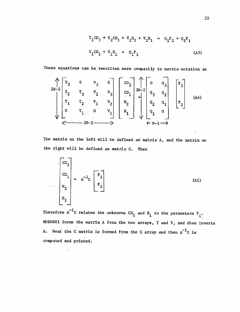
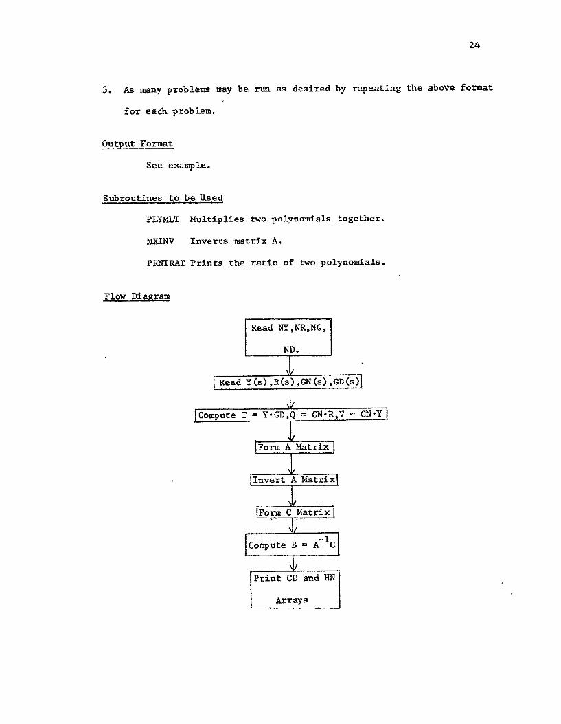
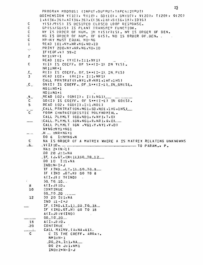
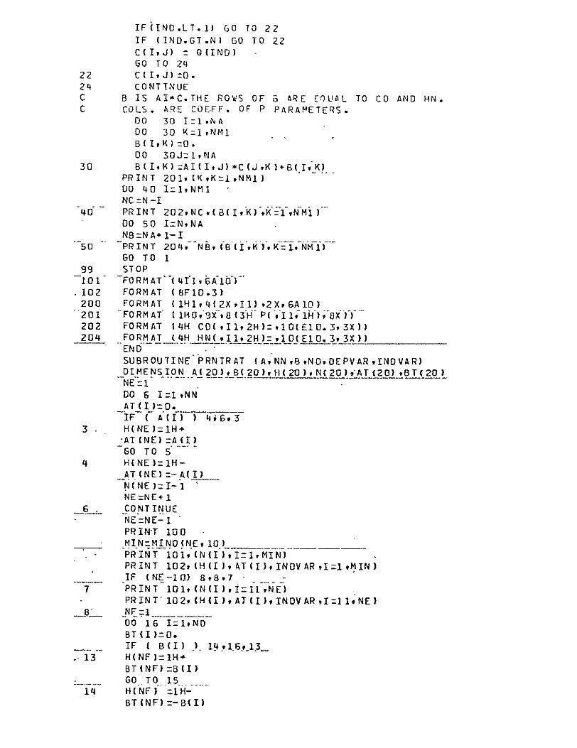
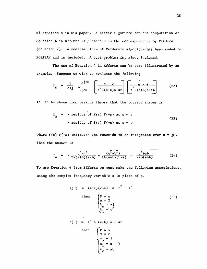
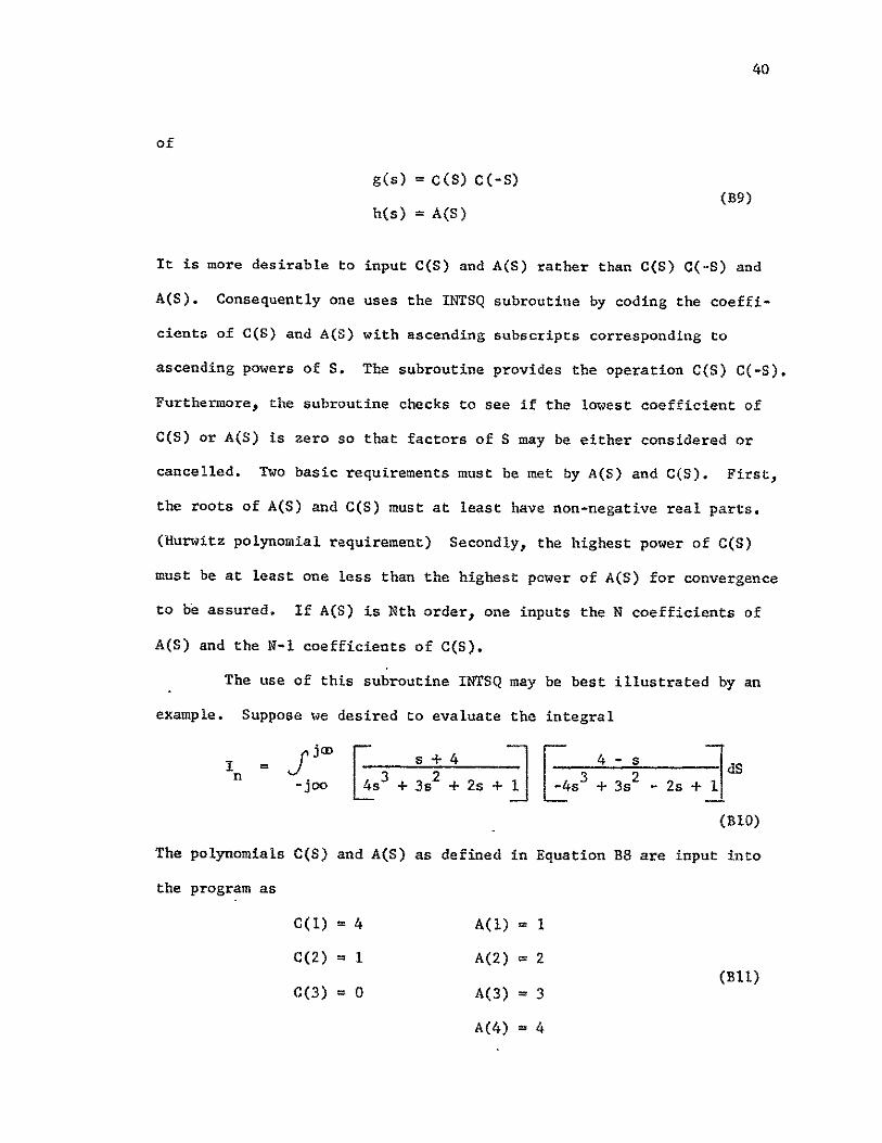
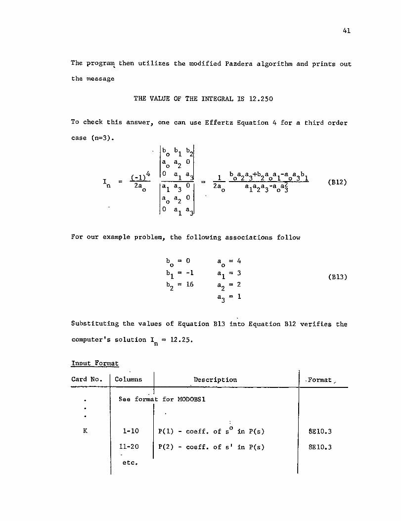
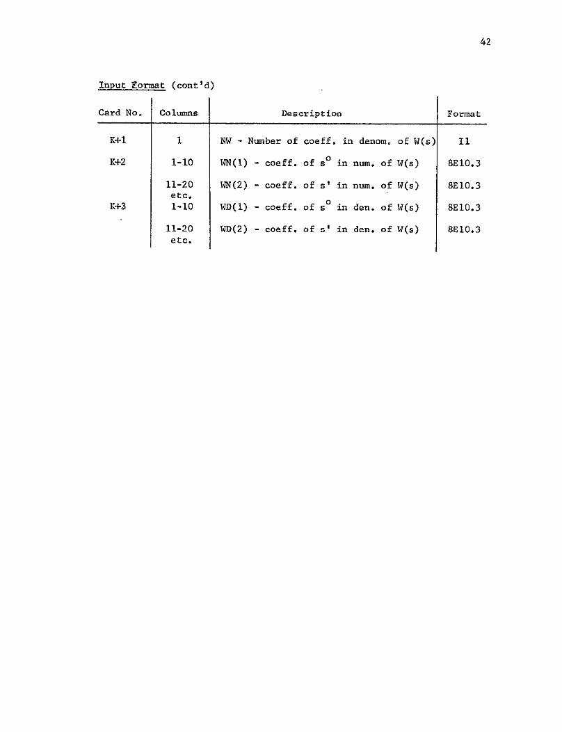
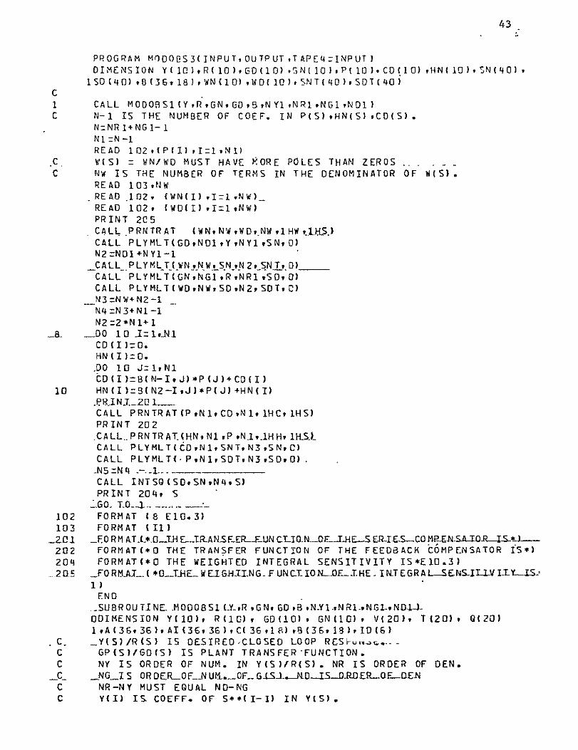
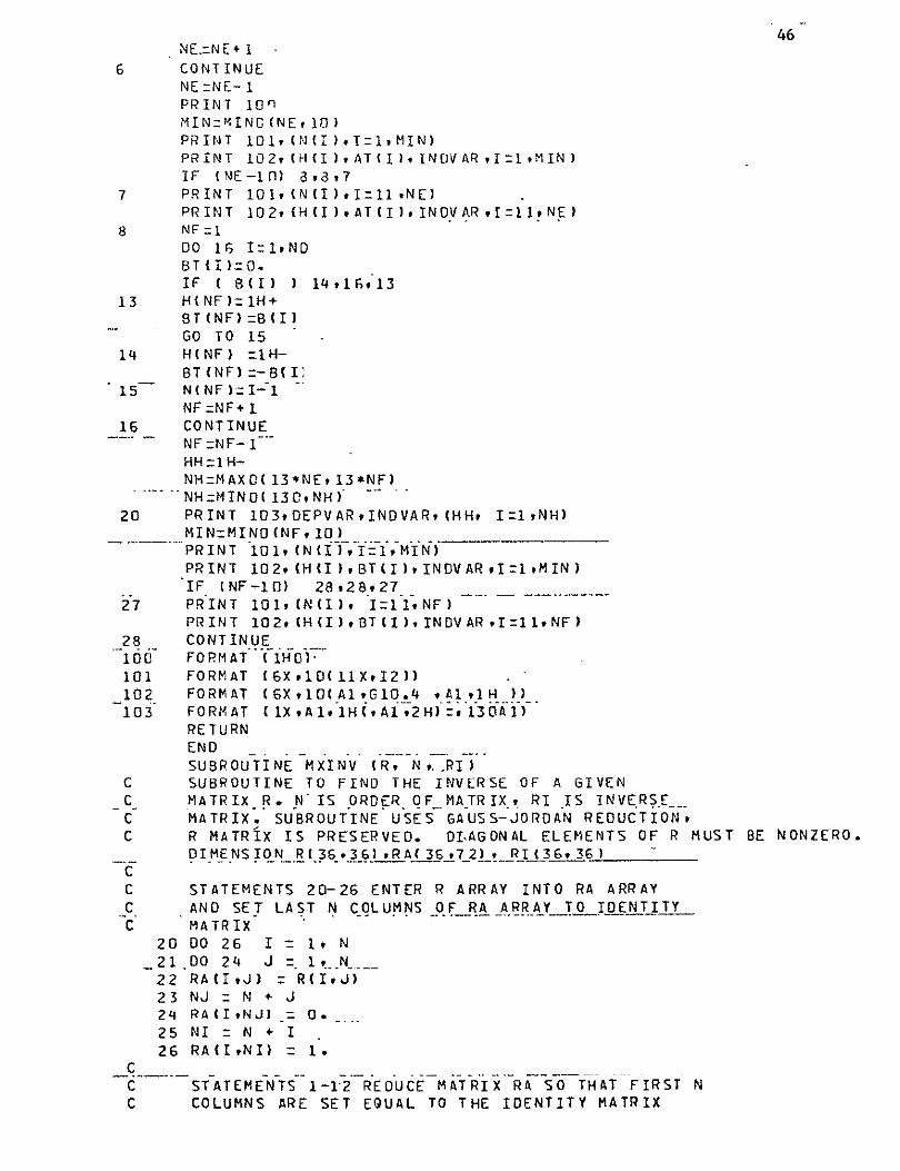
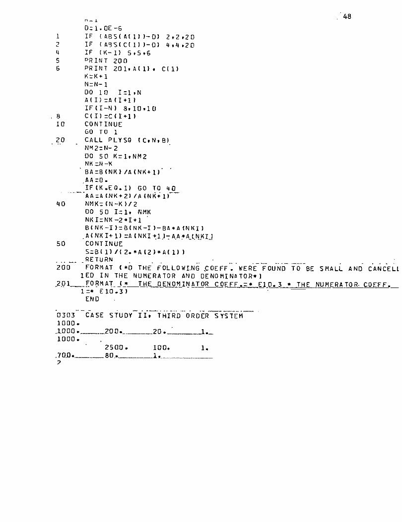
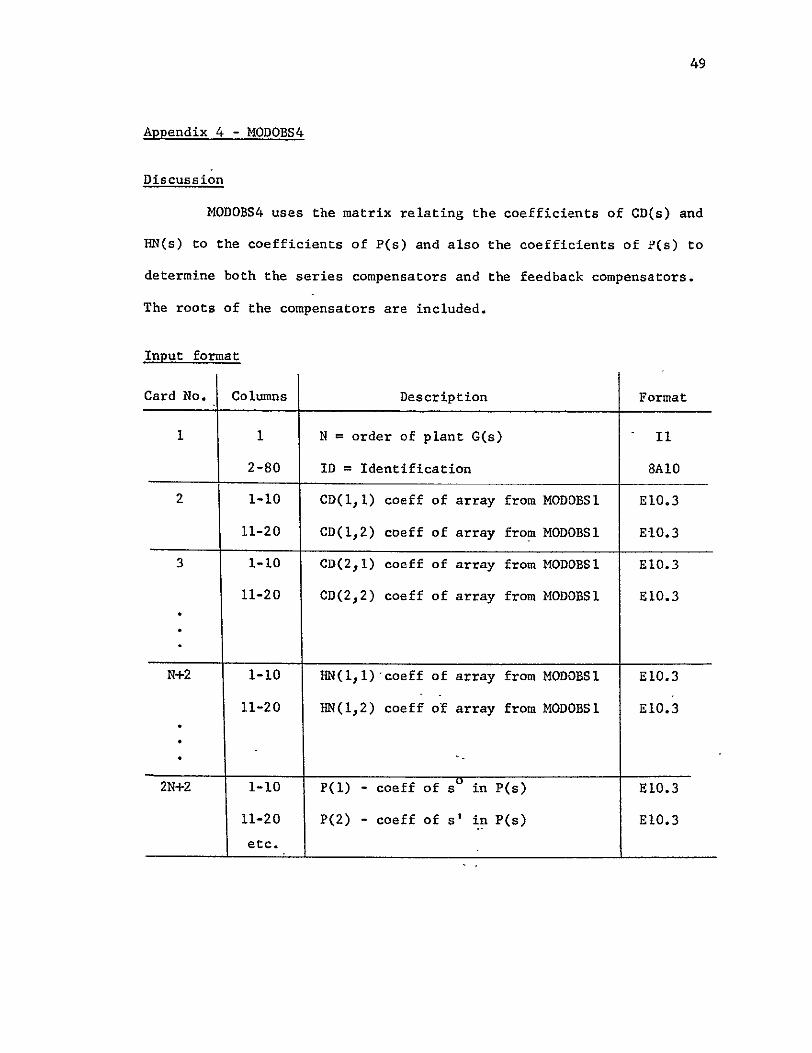
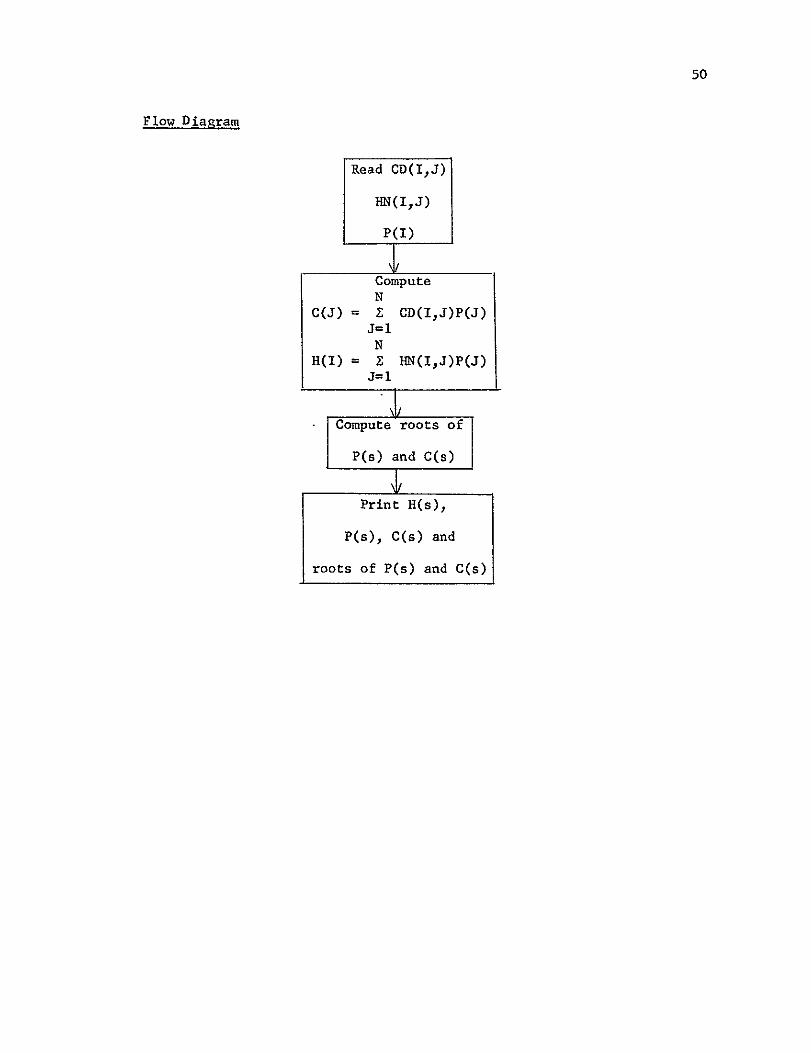
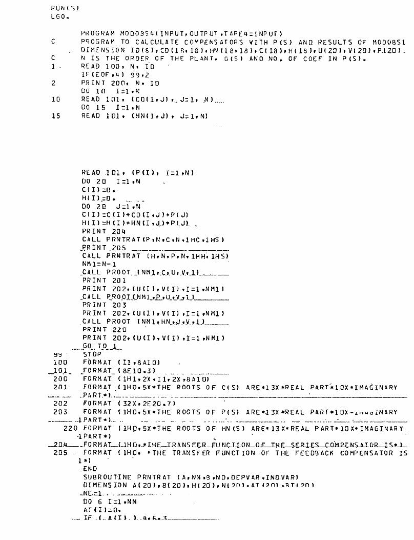
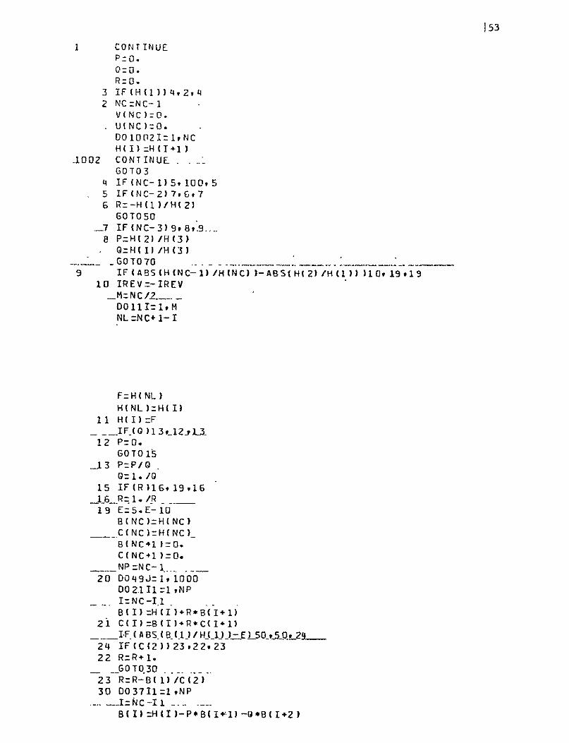
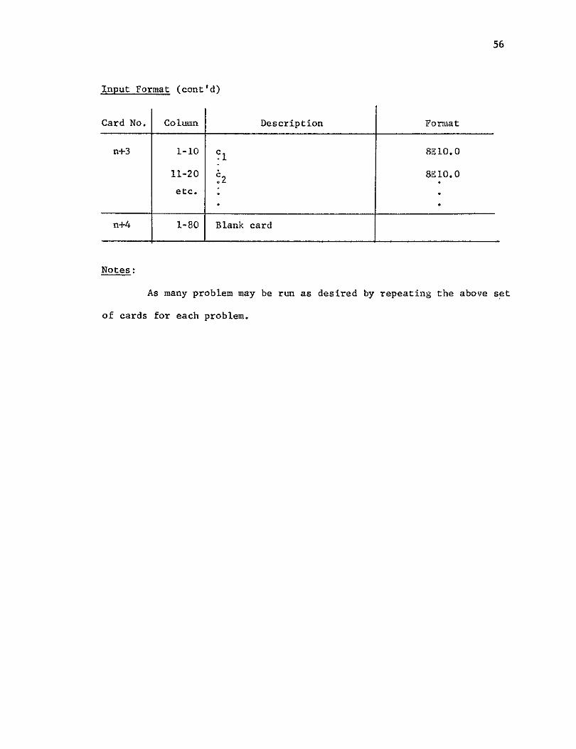
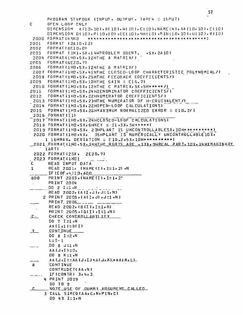
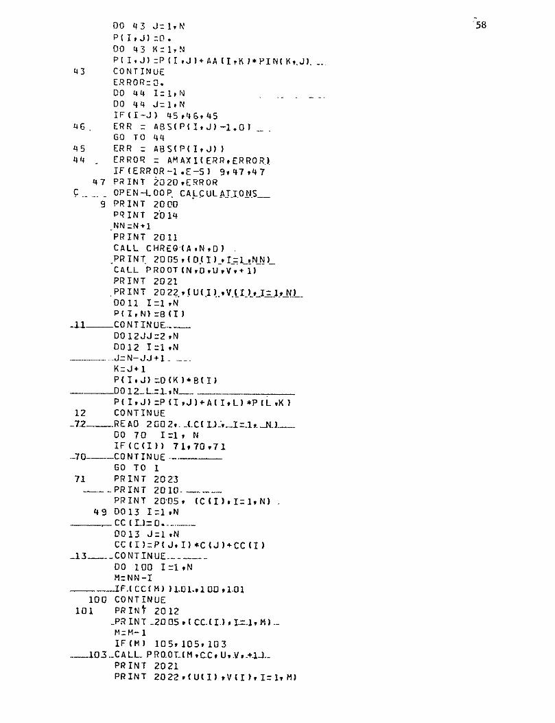
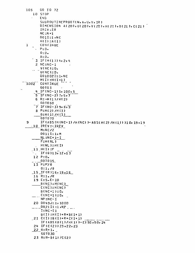
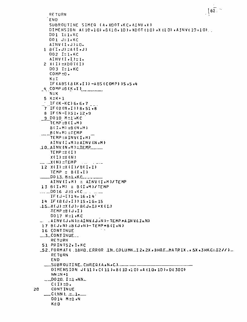
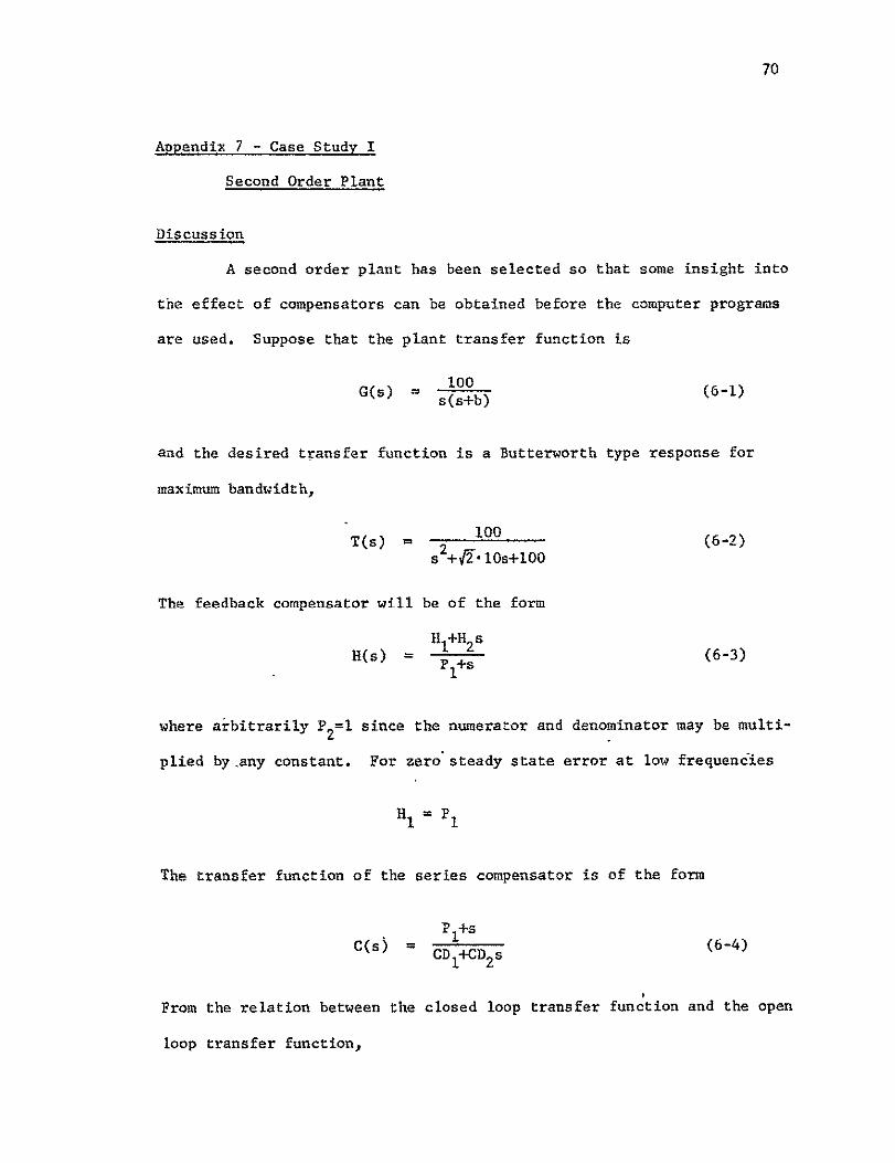
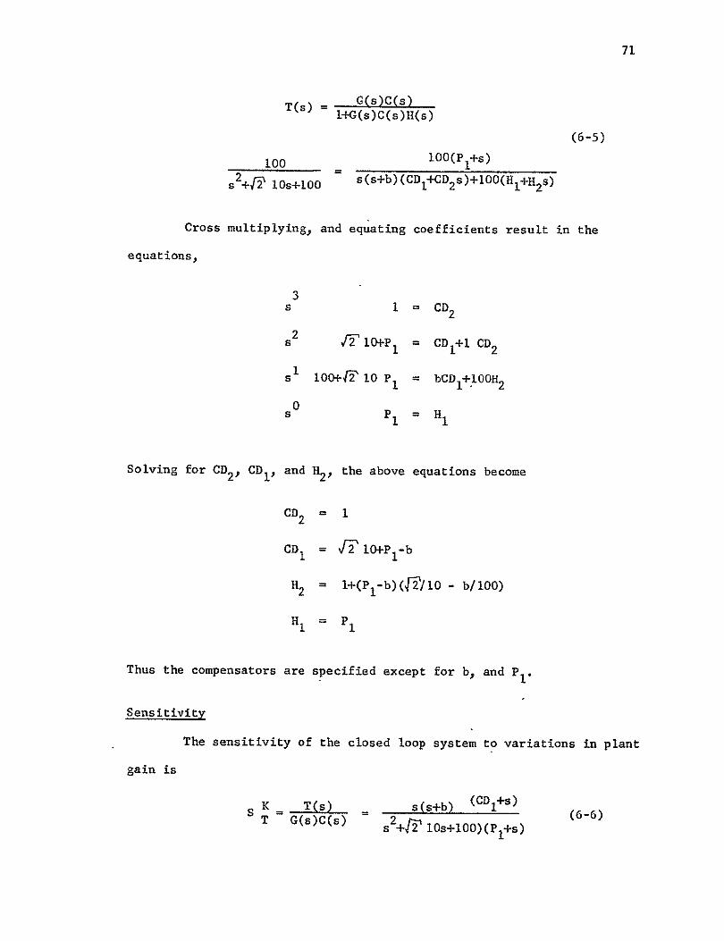

20
10
0
Gain (db) G(s) = 00C(s) = s+586
-10 s(s+20)s
T(s) = 100 s2+ 2 10s+100 Hs)- 1(s)lo484s+586s58
-20+O s+586
uilleman-Truxal1
-30
1 Frequency (Hz)
01
Figure 6i Sensitivity of High-performance 1lant 4shy
75
Guilleman-Truxal
K 2s(s+l03F)TK (s2+104-s+100)
Notice that for b = 20 the MODOBS system is significantly better
at all frequencies below IHz The Heq compensation is both unrealizable
and largest in sensitivity for this case When the forward gain is small
then no compensation will help the sensitivity Thus all the proposed
systems have a sensitivity near one for frequencies above IHz
For b = 10 the low frequency plant gain must be greater to
achieve the same T(s) The Guilleman-Truxal compensation decreases the
forward gain proportionately so that the sensitivity is unchanged The
Heq compensation does not change the forward gain therefore the sensitivity
is reduced from the case where b = 20 The MODOBS system also improves
in sensitivity but this system will only be as low in sensitivity as the
Heq method when PI is infinitely large Nevertheless the MODOBS
compensation has the advantage of being realizable
Integral Sensitivity
For the plant with a pole at -20 the integral sensitivity
(weighted by 1s) is
I j jO I s(s+20)(s-4-P1-586) 2
Sr 2- s (s2+IOffs+100)(S+P 1
This integral can be evaluated directly from Newton Gould and Kaiser
p 372
The minimum low frequency sensitivity was attained for PI = 586
which from MODOBS3 has an integral sensitivity of 012 The minimum
76
integral sensitivity is 0085 for PI = 8 In this simple case this can be
determined analytically by plotting S as PI is varied
Final Design
From the integral sensitivity data a final design choice is
b = 20
P = +8
The following graphs are shown in Figs 6-2 to 6-4
Fig 6-2 Plant transfer function
Fig 6-3 Sensitivity function
Fig 6-4 Loop gain function
Conclusion
From the above figures the design demonstrates the dependence of
the sensitivity on the plant parameters If the time constants in the
closed loop transfer function are much greater than those in the plant
a sacrifice in the system sensitivity at low frequencies must be made
In addition the compensator will have large gains associated with the
feedback which complicate the design of the compensators and increase
the effect of the measurement noise
20
10 open loop
0 closed loop
-10
Gain (dbo)
-20
-30
-40 1
Figure 62
100C(s) =s(s+20) T(s) s2+ s2+
100
10s+100
Frequency (Hz)
Open and Closed Loop Transfer Functions
0
0
-5
Guilleman-Truxal
-10
Gain
(db)
-15
-20
-25 1
I 110 Frequency (Hz)
Figure 63 Sensitivity of Second Order Systems o
10 MDB
0
Guilleman-Truxal
010
Gain (db)
-20
-30
-40 0
Frequency (Hz)
Figure 64 Loop Gain Function of Second Order System
80
Appendix 8 - Case Study 11
Third Order Plant
Discussion
A third order plant has been selected to compare the computer
results with hand calculations The results agree in all the calculations
discussed below The plant transfer function is chosen to be of the form
1000
S3+GD 3 s2-D2 s+GTD
and the desired closed loop transfer function is again chosen with a
Butterworth type denominator
1000T(s) =
s 3+20s2+200s+lO00
MODOBS2
The equations for the coefficients of P(s)=PI+P2SP3s2 which give
minimum low frequency sensitivity were derived in Appendix 2 For N=3
P3 i
= GD3 - 20P2
P 1 GD2 - 200 - 20(P2 )
These equations are satisfied if
GD3 = 20
GD2 = 200
Low frequency sensitivity will be improved if the plant is Type 1 or
81
equivalently has a pole at the origin thus
GD = 0
The poles of the plant are the roots of
s(s2+20s+200) = 0
s = -10 + jlO
For the plant to have real roots then
GD2 - 4GD 2 ) o 3 2
and in order for PI and P2 to be positive
GD3 gt 20
GD2 gt 200 + 20P2
These requirements can be met if
GD3 gt 6828
20(GD3 - 10) lt GD2 lt GD2 4 20G3 3-2
GD = 0
If GD3 is near 68 then P1 must be near zero Under these circumshy
stances the zero of CD(s) cancels the pole at a low frequency and the
low frequency sensitivity suffers Suppose that
GD = 100
5
0
-5
Sensitivity (db)
-10
Guilleman-Truxal MDBS
-15
-20 i
Figure 81
1
Frequency (Hz)
Sensitivity of Third Order System
1010
0
83
Then
1800lt GD2 2500
2
P3 = I
P2 = GD - 20 - 80
PI = GD - 1800
To keep the low frequency pole of P(s) as large as possible it is best to
make GD2 large thus
GD3 = 100
GD2 = 2500
GDI = 0
P3 = I
P2 = 80
PI = 700
Sensitivity
If the plant can be selected as above the sensitivity becomes
2s) s(s 2+100s+2500)T TIL K G(s)C(s) (s3+20s2+200s+1000)(s2+80s+700)
For this choice of the plant the system will have minimum low
frequency sensitivity and a stable feedback compensator A comparison
of the sensitivity of this system with only a series compensator which
achieves the same closed ioop response is shown in Fig 8-1 Except
for frequencies between 141 Hz and 141 Hz the sensitivity is improved
by using the MODOBS system
84
Discussion
Again the importance of choosing a plant which is consistent
with the requirements of the overall system is evident A slow system
cannot be made to react quickly and also have good sensitivity characshy
teristics using second order compensators
85
Appendix 9
Case III In core Thermionic Reactor
The plant and the desired transfer function for an in core
[73thermionic reactor have been discussed by Weaver et al The characshy
teristics of the system are given in the above report This appendix
addresses itself to the question of realization of the desired transfer
function for the fourth order model when-only the output is available
The plant transfer function is given by
C(s) =(s+ 0326)(s+1)(s+l
79) 200 (s+0119+j0164)(s+0119-J0164)(s+00663)(s+185)
and the desired transfer function is
Y(s) 200(s+0326)(s+l)(s+l79) R(s) 100(s+0326)(s+l)(s+179)s+2)
When these terms are multiplied out the resulting transfer functions are
32+200s
116708+481228s+38452sG(s) =
50358510 6+l054210 3+0568639s2+8804s 3+s4
2s2+200s3 Y(s) 116708+481228s+345
R(s) 116708+4870635s+4085815s2+39226s3+OOs 4
This problem represents a special case in that the numerator of G(s) and
YR(deg ) is the same Equating the real and desired closed loop transfer
functions yields
I(s)= G(S)C(s)T(s) a iI+G(s)C(s)H(s)
and in terms of the nuerator and denominator polynomials
86
TN(s) GN(s)CN(s)HD(s) TD(s) GD(s)CD(s)HD(s)+GN(s)CN(s)HN(s)
Since CN(s) = HD(s) a P(s) and TN(s) = GN(s)
1 P(s) TD(s) GD(s)CD(s)+GN(s)HN(s)
Equating the like terms in the above equation and expressing the result
in vector matrix form one gets
GD(1) 0 0 0 CD(1) ON(l) 0 0 0 HN(1)
GD(2) GD(l) 0 0 CD(2) GN(2) GN(1) 0 0 HN(2)
GD(3) GD(2) GD(1) 0 CD(3) GN(3) GN(2) GN(1) 0 HN(3)
GD(4) GD(3) GD(2) GD(1) CD(4) GN(4) GN(3) GN(2) GN(1) HN(4)
GD(5) GD(4)- GD(3) GD(2) + 0 GN(4) GN(3) GN(2)
0 GD(5) GD(4) GD(3) 0 0 GN(4) GN(3)
0 0GD(5)GD(4) 0 0 0 GN(4)
o o 0 GD(5) 0 0 0 0
TD(l) 0 0 0 P(l)
TD(2) TD(l) 0 0 P(2)
TD(3) TD(2) TD(1) 0 P(3)
TD(4) TD(3) TD(2) TD(1) _P(4)
TD(5) TD(4) TD(3) TD(2)
0 TD(5) TD(4) TD()
0 0 TD(5) TD(4)
0 0 0 TD(5)
87
Plugging in the appropriate coefficients from the above expressions for
TD(s) GN(s) and GD(s) the unknowns GD(s) and HN(s) are equal to
CD(1)
CD(2) 119114E+01 -544224E+00 963714E+00 -172292E+01
141485E+02 -212494E+02 391935E+02 -700789E+02 P(1)
932689E+02 -165161E+03 296273E+03 -528468E+03 - 331178E-14 356005E-14 -l10191E-13 lOOOOOE+01 P2)
HN(l) 999949E-01 234842E-05 -415859E-05 743467E-05 496319E-01 100486E+00 -868215E-03 155222E-02 (3) 509230E-01 761501E-01 535279E-01 830837E-01 466345E+00 825805E+00 -147636E+01 282909E+01
HN(4)
The resulting expression can also be solved for P(s) in terms of C(s) that
is
P(1) CD(1)
P(2) 1F028E-0o 128262E-03 -527575E-04 647151E-04 CD(2) [1-332179E-01 162916E-01 -204714E-02 261570E-02
P(3) I-219815E-01 904156E-02 -109084E-02 192750E-01 CD(3)L 0 0 0 100000E-01
CD(4)P(4)
If one selects CD(1) equal to zero then there will be an integrator in the
forward path which results in a system with zero low frequency sensitivity
The requirements for open loop stability are positive coefficients and
CD(l) CD(4)ltCD(2) CD(3)
P(1) P(4) lt P(2) P(3)
These requirements can easily be met when CD(1) is zero if
CD(3) lt CD(2) + CD(3)
88
The choice frr CD(s) is arbitrarily made
CD(s) = s(s +s+l)
then
2-P(s) = 7227-10 3 + 1686 s + 27226 s + 1 s3
The resulting system has a stable open loop compensator and zero low
frequency sensitivity and zero steady state error These characteristics
are an improvement over the response of the state variable feedback
system while both have the same closed loop response In addition only
the output state needs to be measured however two third order compenshy
sators are required

0
-5
Guilleman-Truxal
-10
Gain
(db)
-15
-20
-25 1
I 110 Frequency (Hz)
Figure 63 Sensitivity of Second Order Systems o
10 MDB
0
Guilleman-Truxal
010
Gain (db)
-20
-30
-40 0
Frequency (Hz)
Figure 64 Loop Gain Function of Second Order System
80
Appendix 8 - Case Study 11
Third Order Plant
Discussion
A third order plant has been selected to compare the computer
results with hand calculations The results agree in all the calculations
discussed below The plant transfer function is chosen to be of the form
1000
S3+GD 3 s2-D2 s+GTD
and the desired closed loop transfer function is again chosen with a
Butterworth type denominator
1000T(s) =
s 3+20s2+200s+lO00
MODOBS2
The equations for the coefficients of P(s)=PI+P2SP3s2 which give
minimum low frequency sensitivity were derived in Appendix 2 For N=3
P3 i
= GD3 - 20P2
P 1 GD2 - 200 - 20(P2 )
These equations are satisfied if
GD3 = 20
GD2 = 200
Low frequency sensitivity will be improved if the plant is Type 1 or
81
equivalently has a pole at the origin thus
GD = 0
The poles of the plant are the roots of
s(s2+20s+200) = 0
s = -10 + jlO
For the plant to have real roots then
GD2 - 4GD 2 ) o 3 2
and in order for PI and P2 to be positive
GD3 gt 20
GD2 gt 200 + 20P2
These requirements can be met if
GD3 gt 6828
20(GD3 - 10) lt GD2 lt GD2 4 20G3 3-2
GD = 0
If GD3 is near 68 then P1 must be near zero Under these circumshy
stances the zero of CD(s) cancels the pole at a low frequency and the
low frequency sensitivity suffers Suppose that
GD = 100
5
0
-5
Sensitivity (db)
-10
Guilleman-Truxal MDBS
-15
-20 i
Figure 81
1
Frequency (Hz)
Sensitivity of Third Order System
1010
0
83
Then
1800lt GD2 2500
2
P3 = I
P2 = GD - 20 - 80
PI = GD - 1800
To keep the low frequency pole of P(s) as large as possible it is best to
make GD2 large thus
GD3 = 100
GD2 = 2500
GDI = 0
P3 = I
P2 = 80
PI = 700
Sensitivity
If the plant can be selected as above the sensitivity becomes
2s) s(s 2+100s+2500)T TIL K G(s)C(s) (s3+20s2+200s+1000)(s2+80s+700)
For this choice of the plant the system will have minimum low
frequency sensitivity and a stable feedback compensator A comparison
of the sensitivity of this system with only a series compensator which
achieves the same closed ioop response is shown in Fig 8-1 Except
for frequencies between 141 Hz and 141 Hz the sensitivity is improved
by using the MODOBS system
84
Discussion
Again the importance of choosing a plant which is consistent
with the requirements of the overall system is evident A slow system
cannot be made to react quickly and also have good sensitivity characshy
teristics using second order compensators
85
Appendix 9
Case III In core Thermionic Reactor
The plant and the desired transfer function for an in core
[73thermionic reactor have been discussed by Weaver et al The characshy
teristics of the system are given in the above report This appendix
addresses itself to the question of realization of the desired transfer
function for the fourth order model when-only the output is available
The plant transfer function is given by
C(s) =(s+ 0326)(s+1)(s+l
79) 200 (s+0119+j0164)(s+0119-J0164)(s+00663)(s+185)
and the desired transfer function is
Y(s) 200(s+0326)(s+l)(s+l79) R(s) 100(s+0326)(s+l)(s+179)s+2)
When these terms are multiplied out the resulting transfer functions are
32+200s
116708+481228s+38452sG(s) =
50358510 6+l054210 3+0568639s2+8804s 3+s4
2s2+200s3 Y(s) 116708+481228s+345
R(s) 116708+4870635s+4085815s2+39226s3+OOs 4
This problem represents a special case in that the numerator of G(s) and
YR(deg ) is the same Equating the real and desired closed loop transfer
functions yields
I(s)= G(S)C(s)T(s) a iI+G(s)C(s)H(s)
and in terms of the nuerator and denominator polynomials
86
TN(s) GN(s)CN(s)HD(s) TD(s) GD(s)CD(s)HD(s)+GN(s)CN(s)HN(s)
Since CN(s) = HD(s) a P(s) and TN(s) = GN(s)
1 P(s) TD(s) GD(s)CD(s)+GN(s)HN(s)
Equating the like terms in the above equation and expressing the result
in vector matrix form one gets
GD(1) 0 0 0 CD(1) ON(l) 0 0 0 HN(1)
GD(2) GD(l) 0 0 CD(2) GN(2) GN(1) 0 0 HN(2)
GD(3) GD(2) GD(1) 0 CD(3) GN(3) GN(2) GN(1) 0 HN(3)
GD(4) GD(3) GD(2) GD(1) CD(4) GN(4) GN(3) GN(2) GN(1) HN(4)
GD(5) GD(4)- GD(3) GD(2) + 0 GN(4) GN(3) GN(2)
0 GD(5) GD(4) GD(3) 0 0 GN(4) GN(3)
0 0GD(5)GD(4) 0 0 0 GN(4)
o o 0 GD(5) 0 0 0 0
TD(l) 0 0 0 P(l)
TD(2) TD(l) 0 0 P(2)
TD(3) TD(2) TD(1) 0 P(3)
TD(4) TD(3) TD(2) TD(1) _P(4)
TD(5) TD(4) TD(3) TD(2)
0 TD(5) TD(4) TD()
0 0 TD(5) TD(4)
0 0 0 TD(5)
87
Plugging in the appropriate coefficients from the above expressions for
TD(s) GN(s) and GD(s) the unknowns GD(s) and HN(s) are equal to
CD(1)
CD(2) 119114E+01 -544224E+00 963714E+00 -172292E+01
141485E+02 -212494E+02 391935E+02 -700789E+02 P(1)
932689E+02 -165161E+03 296273E+03 -528468E+03 - 331178E-14 356005E-14 -l10191E-13 lOOOOOE+01 P2)
HN(l) 999949E-01 234842E-05 -415859E-05 743467E-05 496319E-01 100486E+00 -868215E-03 155222E-02 (3) 509230E-01 761501E-01 535279E-01 830837E-01 466345E+00 825805E+00 -147636E+01 282909E+01
HN(4)
The resulting expression can also be solved for P(s) in terms of C(s) that
is
P(1) CD(1)
P(2) 1F028E-0o 128262E-03 -527575E-04 647151E-04 CD(2) [1-332179E-01 162916E-01 -204714E-02 261570E-02
P(3) I-219815E-01 904156E-02 -109084E-02 192750E-01 CD(3)L 0 0 0 100000E-01
CD(4)P(4)
If one selects CD(1) equal to zero then there will be an integrator in the
forward path which results in a system with zero low frequency sensitivity
The requirements for open loop stability are positive coefficients and
CD(l) CD(4)ltCD(2) CD(3)
P(1) P(4) lt P(2) P(3)
These requirements can easily be met when CD(1) is zero if
CD(3) lt CD(2) + CD(3)
88
The choice frr CD(s) is arbitrarily made
CD(s) = s(s +s+l)
then
2-P(s) = 7227-10 3 + 1686 s + 27226 s + 1 s3
The resulting system has a stable open loop compensator and zero low
frequency sensitivity and zero steady state error These characteristics
are an improvement over the response of the state variable feedback
system while both have the same closed loop response In addition only
the output state needs to be measured however two third order compenshy
sators are required
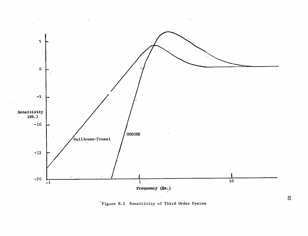
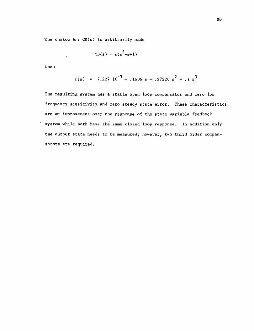


![Variable-Length Limited Feedback Beamforming in Multiple ... › J4.pdflimited feedback beamforming schemes have been introduced and analyzed in [13], [14]. Random vector quantizers](https://img.pdfslide.net/doc/110x75/60b7cd4b1d2b4b790035971a/variable-length-limited-feedback-beamforming-in-multiple-a-j4pdf-limited.jpg)