Embed Size (px)
Citation preview
Using Support Vector Machines,
Convolutional Neural Networks and
Deep Belief Networks for Partially
Occluded Object Recognition
Joseph Lin Chu
A Thesis
in
The Department
of
Computer Science
Presented in Partial Fulfillment of the Requirements
for the Degree of Master of Computer Science (Computer Science) at
Concordia University
Montreal, Quebec, Canada
March 2014
c© Joseph Lin Chu, 2014

CONCORDIA UNIVERSITY
School of Graduate Studies
This is to certify that the thesis prepared
By: Joseph Lin Chu
Entitled: Using Support Vector Machines, Convolutional Neural Networks
and Deep Belief Networks for Partially Occluded Object Recog-
nition
and submitted in partial fulfilment of the requirements for the degree of
Master of Computer Science
complies with the regulations of this University and meets the accepted standards with
respect to originality and quality.
Signed by the final examining committee:
Dr. Rajagopalan Jayakumar, Chair
Dr. Tien Dai Bui, Examiner
Dr. Thomas G. Fevens, Examiner
Dr. Adam Krzyzak, Supervisor
Approved by
Chair of CS Department or Graduate Program Director
2014
Dean of Faculty
Abstract
Using Support Vector Machines, Convolutional Neural Networks and Deep
Belief Networks for Partially Occluded Object Recognition
Joseph Lin Chu
Artificial neural networks have been widely used for machine learning tasks such as ob-
ject recognition. Recent developments have made use of biologically inspired architectures,
such as the Convolutional Neural Network, and the Deep Belief Network. A theoretical
method for estimating the optimal number of feature maps for a Convolutional Neural Net-
work maps using the dimensions of the receptive field or convolutional kernel is proposed.
Empirical experiments are performed that show that the method works to an extent for
extremely small receptive fields, but doesn’t generalize as clearly to all receptive field sizes.
We then test the hypothesis that generative models such as the Deep Belief Network should
perform better on occluded object recognition tasks than purely discriminative models such
as Convolutional Neural Networks. We find that the data does not support this hypothesis
when the generative models are run in a partially discriminative manner. We also find that
the use of Gaussian visible units in a Deep Belief Network trained on occluded image data
allows it to also learn to classify non-occluded images.
iii

Acknowledgement
I would like to heartily thank my supervisor, Professor Adam Krzyzak, for allowing me to
be his graduate student and helping and supporting me greatly in my efforts to conduct
research and become a Master of Computer Science. I want to thank him for his patience,
generosity, and consideration.
I would also like to thank my friends and family for their support and advice. In
particular, I want to thank my mother and father for their dedicated support and their
willingness to allow me to explore the thesis option and pursue my dreams to be a researcher
in this field. I want to thank them for their patience and their ever loyal support. As well,
thank you my friends for listening to me, and supporting me throughout this endeavour.
I would like as well to thank Concordia University, and the good people at the Depart-
ment of Computer Science and Software Engineering, for enabling me to pursue my dreams
and achieve this much. I especially want to thank Halina Monkiewicz for her assistance as
graduate coordinator in getting me into those courses that mattered.
In addition I wish to thank Professor Doina Precup of McGill University for letting
me take her class and learn a great deal from her. I would also like to thank Professor
Ching Y. Suen, Professor Sabine Bergler, Professor Tien Dai Bui, and Professor Thomas
G. Fevens of Concordia University for also letting me take their classes and allowing me to
learn from them, as well as any other professors and fellow students who I was granted the
pleasure of becoming acquainted with in my journey through graduate school.
Thank you dear reader for taking the time to look at the culmination of years of
effort, struggle, and uncertainty. I hope that you enjoy the fruits of my labour.
iv
Table of Contents
List of Figures . . . . . . . . . . . . . . . . . . . . . . . . . . . . . . . . . . . . . ix
List of Tables . . . . . . . . . . . . . . . . . . . . . . . . . . . . . . . . . . . . . . xii
List of Algorithms . . . . . . . . . . . . . . . . . . . . . . . . . . . . . . . . . . . xiii
List of Symbols . . . . . . . . . . . . . . . . . . . . . . . . . . . . . . . . . . . . . xiv
List of Abbreviations . . . . . . . . . . . . . . . . . . . . . . . . . . . . . . . . . . xv
1 Introduction 1
2 Literature Review 7
2.1 Basics of Artificial Neural Networks . . . . . . . . . . . . . . . . . . . . . . 7
2.2 Convolutional Neural Networks . . . . . . . . . . . . . . . . . . . . . . . . . 9
2.3 Support Vector Machines . . . . . . . . . . . . . . . . . . . . . . . . . . . . 11
2.4 Deep Belief Networks . . . . . . . . . . . . . . . . . . . . . . . . . . . . . . . 11
2.5 Further Developments in Artificial Neural Networks . . . . . . . . . . . . . 13
3 Optimizing Convolutional Neural Networks 14
3.1 Overview . . . . . . . . . . . . . . . . . . . . . . . . . . . . . . . . . . . . . 14
3.2 Topology of LeNet-5 . . . . . . . . . . . . . . . . . . . . . . . . . . . . . . . 16
3.3 Theoretical Analysis . . . . . . . . . . . . . . . . . . . . . . . . . . . . . . . 20
v
3.4 Methodology . . . . . . . . . . . . . . . . . . . . . . . . . . . . . . . . . . . 25
3.5 Analysis and Results . . . . . . . . . . . . . . . . . . . . . . . . . . . . . . . 28
3.6 Discussion . . . . . . . . . . . . . . . . . . . . . . . . . . . . . . . . . . . . . 32
3.7 Conclusions . . . . . . . . . . . . . . . . . . . . . . . . . . . . . . . . . . . . 34
4 Deep Belief Networks 35
5 Methodology 43
6 Analysis and Results 59
6.1 Results on NORB . . . . . . . . . . . . . . . . . . . . . . . . . . . . . . . . 59
6.1.1 Support Vector Machines . . . . . . . . . . . . . . . . . . . . . . . . 59
6.1.2 Convolutional Neural Networks . . . . . . . . . . . . . . . . . . . . . 61
6.1.3 Deep Belief Networks . . . . . . . . . . . . . . . . . . . . . . . . . . 62
6.1.4 Comparison . . . . . . . . . . . . . . . . . . . . . . . . . . . . . . . . 65
6.1.5 Visualizations . . . . . . . . . . . . . . . . . . . . . . . . . . . . . . . 68
7 Discussion 73
8 Conclusions 79
Bibliography 81
A Original Data of Individual Runs 88
vi
List of Figures
1.1 The basic architecture of the Convolutional Neural Network (CNN). . . . . 3
1.2 The structure of the general Boltzmann Machine, and the Restricted Boltz-mann Machine (RBM). . . . . . . . . . . . . . . . . . . . . . . . . . . . . . . 5
1.3 The structure of the Deep Belief Network (DBN). . . . . . . . . . . . . . . . 5
2.1 A comparison between the Convolutional layer and the Subsampling layer.Circles represent the receptive fields of the cells of the layer subsequent to theone represented by the square lattice. On the left, an 8 x 8 input layer feedsinto a 6 x 6 convolutional layer using receptive fields of size 3 x 3 with anoffset of 1 cell. On the right, a 6 x 6 input layer feeds into a 2 x 2 subsamplinglayer using receptive fields of size 3 x 3 with an offset of 3 cells. . . . . . . . 10
3.1 The architecture of the LeNet-5 Convolutional Neural Network. . . . . . . . 14
3.2 Details of the convolutional operator used by LeNet-5 CNN. . . . . . . . . . 17
3.3 The 16 possible binary feature maps of a 2x2 receptive field, with their re-spective entropy values. . . . . . . . . . . . . . . . . . . . . . . . . . . . . . 21
3.4 Images from the Caltech-20 data set. . . . . . . . . . . . . . . . . . . . . . . 25
3.5 Graphs of the accuracy given a variable number of feature maps for a 1x1receptive field. . . . . . . . . . . . . . . . . . . . . . . . . . . . . . . . . . . 29
3.6 Graphs of the accuracy given a variable number of feature maps for a 2x2receptive field. . . . . . . . . . . . . . . . . . . . . . . . . . . . . . . . . . . 29
3.7 Graphs of the accuracy given a variable number of feature maps for a 3x3receptive field. . . . . . . . . . . . . . . . . . . . . . . . . . . . . . . . . . . 30
vii
3.8 Graphs of the accuracy given a variable number of feature maps for a 5x5receptive field. . . . . . . . . . . . . . . . . . . . . . . . . . . . . . . . . . . 30
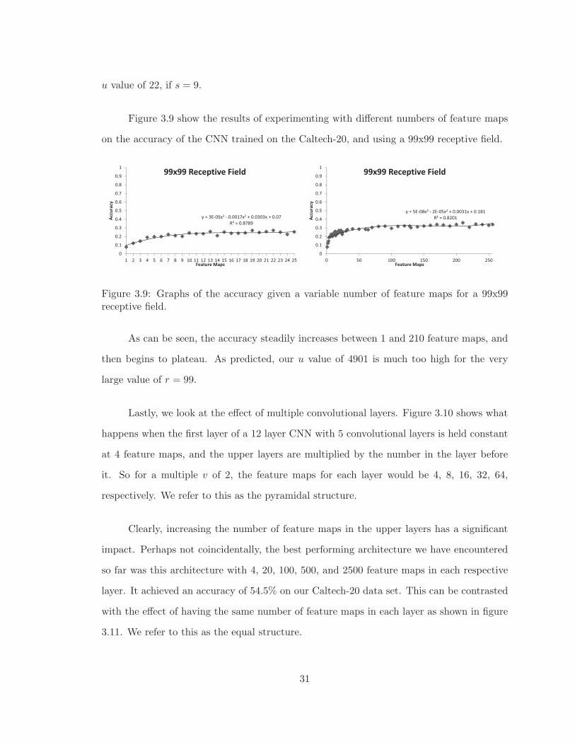
3.9 Graphs of the accuracy given a variable number of feature maps for a 99x99receptive field. . . . . . . . . . . . . . . . . . . . . . . . . . . . . . . . . . . 31
3.10 Graph of the accuracy given a variable number of feature maps for a networkwith 5 convolutional layers of 2x2 receptive field. Here the higher layers area multiple of the lower layers. . . . . . . . . . . . . . . . . . . . . . . . . . . 32
3.11 Graph of the accuracy given a variable number of feature maps for a networkwith 5 convolutional layers of 2x2 receptive field. Here each layer has thesame number of feature maps. . . . . . . . . . . . . . . . . . . . . . . . . . . 32
4.1 The structure of the general Boltzmann Machine. . . . . . . . . . . . . . . . 36
5.1 Images from the Caltech-20 non-occluded test set. . . . . . . . . . . . . . . 44
5.2 Images from the Caltech-20 occluded test set. . . . . . . . . . . . . . . . . . 44
5.3 Images from the small NORB non-occluded test set. . . . . . . . . . . . . . 57
5.4 Images from the small NORB occluded test set. . . . . . . . . . . . . . . . . 58
6.1 A visualization of the first layer weights of a DBN with binary visible unitsand 2000 hidden nodes, trained on non-occluded NORB data. . . . . . . . . 68
6.2 A visualization of the first layer weights of the DBN with binary visible unitsand 4000 hidden nodes, trained on non-occluded NORB data. . . . . . . . . 69
6.3 A visualization of the first layer weights of the DBN with Gaussian visibleunits and 4000 hidden nodes, trained on non-occluded NORB data. . . . . . 69
6.4 A visualization of the first layer weights of a DBN with binary visible unitsand 2000 hidden nodes, trained on occluded NORB data. . . . . . . . . . . 70
6.5 A visualization of the first layer weights of the DBN with binary visible unitsand 4000 hidden nodes, trained on occluded NORB data. . . . . . . . . . . 70
6.6 A visualization of the first layer weights of the DBN with Gaussian visibleunits and 4000 hidden nodes, trained on occluded NORB data. . . . . . . . 71
viii

6.7 A visualization of the first layer weights of a DBN with binary visible unitsand 2000 hidden nodes, trained on mixed NORB data. . . . . . . . . . . . . 71
6.8 A visualization of the first layer weights of the DBN with binary visible unitsand 4000 hidden nodes, trained on mixed NORB data. . . . . . . . . . . . . 72
6.9 A visualization of the first layer weights of the DBN with Gaussian visibleunits and 4000 hidden nodes, trained on mixed NORB data. . . . . . . . . . 72
ix
List of Tables
5.1 Results of experiments with Support Vector Machine (SVM) on the Caltech-20 to determine best parameter configuration. . . . . . . . . . . . . . . . . . 45
5.2 The architecture of the CNN used on the Caltech-20. . . . . . . . . . . . . . 45
5.3 The architecture of the CNN used on the Caltech-101, based on Ranzato etal. [43]. . . . . . . . . . . . . . . . . . . . . . . . . . . . . . . . . . . . . . . 46
5.4 The architecture of the CNN used on the NORB dataset, based on Huang &LeCun [26]. . . . . . . . . . . . . . . . . . . . . . . . . . . . . . . . . . . . . 46
5.5 Experiments conducted using the CNN algorithm and different parameterson the Caltech-20. . . . . . . . . . . . . . . . . . . . . . . . . . . . . . . . . 47
5.6 A comparison of various computers and Matlab versions in terms of the speedof performing a 3 Epoch CNN run on the MNIST. . . . . . . . . . . . . . . 48
5.7 The results of experiments done to test the parameters for various configu-rations of DBNs, on the Caltech-20. . . . . . . . . . . . . . . . . . . . . . . 50
5.8 Further results of experiments done to test the parameters for various con-figurations of DBNs, on the Caltech-20. . . . . . . . . . . . . . . . . . . . . 51
5.9 Early results of experiments done to test the speed of various configurationsof DBNs, on the Caltech-20 using the old or Rouncey laptop computer. . . 52
5.10 Early results of experiments done to test the speed of various configurations ofDBNs, on the Caltech-20 using the Sylfaen lab computer, comparing Matlabversions 2009a and 2011a. . . . . . . . . . . . . . . . . . . . . . . . . . . . . 53
5.11 Comparing the speed of various versions of Matlab using the Destrier laptopcomputer. . . . . . . . . . . . . . . . . . . . . . . . . . . . . . . . . . . . . . 53
x
5.12 The results of an experiment to test the effect of hard-wired sparsity on DBNson the Caltech-20. . . . . . . . . . . . . . . . . . . . . . . . . . . . . . . . . 54
5.13 Speed Tests Using Python/Theano-based DBN on MNIST . . . . . . . . . . 54
5.14 Speed Tests Using Python/Theano-based CNN on MNIST . . . . . . . . . . 54
5.15 Speed Tests Using Python/Theano-based DBN on Caltech-20 . . . . . . . . 55
5.16 Speed Tests Using Python/Theano-based CNN on Caltech-20 . . . . . . . . 55
5.17 Speed Tests Using Python/Theano-based DBN on NORB . . . . . . . . . . 56
5.18 Speed Tests Using Python/Theano-based CNN on NORB . . . . . . . . . . 56
5.19 Results and Times for CNN trained on Non-Occluded dataset of NORB for100 Epochs Using Matlab Library. . . . . . . . . . . . . . . . . . . . . . . . 57
5.20 Results and Times for CNN trained on Non-Occluded dataset of NORB for100 Epochs Using Matlab Library. . . . . . . . . . . . . . . . . . . . . . . . 57
6.1 A comparison of the accuracy results of the non-occluded, occluded, andmixed trained SVMs on the NORB dataset. . . . . . . . . . . . . . . . . . . 61
6.2 A comparison of the accuracy results of the non-occluded, occluded, andmixed trained CNNs on the NORB dataset. . . . . . . . . . . . . . . . . . . 62
6.3 A comparison of the accuracy results of the non-occluded, occluded, andmixed trained DBNs using binary visible units with 2000 hidden nodes. . . 63
6.4 A comparison of the accuracy results of the non-occluded, occluded, andmixed trained DBNs using binary visible units with 4000 hidden nodes. . . 64
6.5 A comparison of the accuracy results of the non-occluded, occluded, andmixed trained DBNs using Gaussian visible units with 4000 hidden nodes. . 65
6.6 Comparison of the accuracy results of the Classifier Algorithms on the Non-Occluded Training Images . . . . . . . . . . . . . . . . . . . . . . . . . . . . 66
6.7 Comparison of the accuracy results of the Classifier Algorithms on the Oc-cluded Training Images . . . . . . . . . . . . . . . . . . . . . . . . . . . . . 67
6.8 Comparison of the accuracy results of the Classifier Algorithms on the MixedTraining Images . . . . . . . . . . . . . . . . . . . . . . . . . . . . . . . . . . 67
xi
7.1 Comparison of the accuracy results of the Classifier Algorithms with thosein the literature on NORB . . . . . . . . . . . . . . . . . . . . . . . . . . . . 75
A.1 The accuracy results of SVMs trained on the non-occluded training set of theNORB dataset. . . . . . . . . . . . . . . . . . . . . . . . . . . . . . . . . . . 88
A.2 The accuracy results of SVMs trained on the occluded training set of theNORB dataset. . . . . . . . . . . . . . . . . . . . . . . . . . . . . . . . . . . 89
A.3 The accuracy results of SVMs trained on the mixed training set of the NORBdataset. . . . . . . . . . . . . . . . . . . . . . . . . . . . . . . . . . . . . . . 89
A.4 The accuracy results of CNNs of various parameters on the NORB dataset. 90
A.5 The accuracy results of CNNs trained exclusively on the occluded trainingset of the NORB dataset. . . . . . . . . . . . . . . . . . . . . . . . . . . . . 90
A.6 The accuracy results of CNNs trained on the mixed training set of the NORBdataset. . . . . . . . . . . . . . . . . . . . . . . . . . . . . . . . . . . . . . . 91
A.7 The results of DBNs of various parameters trained on the non-occluded train-ing set on the NORB dataset. . . . . . . . . . . . . . . . . . . . . . . . . . . 91
A.8 The results of DBNs of various parameters trained on the occluded trainingset on the NORB dataset. . . . . . . . . . . . . . . . . . . . . . . . . . . . . 92
A.9 The results of DBNs of various parameters trained on the mixed training seton the NORB dataset. . . . . . . . . . . . . . . . . . . . . . . . . . . . . . . 92
xii

List of Algorithms
1 The Backpropagation training algorithm. From: [34] . . . . . . . . . . . . . . 9
xiii

List of Symbols
〈〉 angle brackets - enclose the expectations ofthe distribution labeled in the subscript
* convolution - integral of the product of twofunctions after one is reversed and shifted
xiv

List of Abbreviations
AI Artificial IntelligenceANN Artificial Neural Network
CDBN Convolutional Deep Belief NetworkCK Cohn-KanadeCNN Convolutional Neural NetworkCRBM Convolutional Restricted Boltzmann MachineCRUM Computational-Representational Under-
standing of MindCUDA Compute Unified Device Architecture
DBM Deep Boltzmann MachineDBN Deep Belief Network
GPU Graphical Processing Unit
LIRBM Local Impact Restricted Boltzmann Machine
MSE Mean Squared Error
PDP Parallel Distributed Processing
RBM Restricted Boltzmann Machine
SML Stochastic Maximum LikelihoodSVM Support Vector Machine
TCNN Tiled Convolutional Neural NetworkTFD Toronto Face Database
xv
Chapter 1
Introduction
Artificial Intelligence (AI) is a field of computer science that is primarily concerned with
mimicking or duplicating human and animal intelligence in computers. This is often consid-
ered a lofty goal, as the nature of the human mind has historically been seen as something
beyond scientific purview. From Plato to Descartes, philosophers generally believed the
mind to exist in a separate realm of ideas and souls, a world beyond scrutiny by the natural
sciences.
In the 20th century however, psychology gradually began to show that the mind
was within the realm of the natural [41]. Cognitive Science in particular has embraced
functionalism, the view that mental states can exist anywhere that the functionality exists to
represent them, and the Computational-Representational Understanding of Mind (CRUM)
[53], which suggests that the brain can be understood with analogy to computational models.
This includes using what are known as connectionist models, which attempt to duplicate
the biological structure of the brains neuronal networks. And in the past few decades, many
strides have been made in the field of AI, and much of this has come from developments in
machine learning and pattern recognition.
1

Machine Learning is a particular subfield of AI that attempts to get computers to learn
much in the way that the human brain is capable of doing. As such, research into machine
learning generally involves developing learning algorithms that are able to perform such
tasks as object recognition or speech recognition. Object recognition is of particular interest
to the Cognitive Scientist in that it shows potential to allow for a semantic representation
of objects to be realized.
Psychologists have long debated about the nature of mental imagery [2, p. 111].
Though the idea that images are stored in the mind as mental pictures, of the brain being
able to exactly reproduce visual perception in all its original detail is thought of as an incor-
rect understanding of perception, it does appear that brain is able to recollect constructed
representations of objects perceived previously [42]. These representations lack the exact
pixel by pixel accuracy of the originating visual object, but then it is highly unlikely that
our perception of images possesses such accuracy either. The phenomenon of visual illusions
is only possible because perception fundamentally involves a degree of cognitive processing.
What we see in our minds is not merely a reflection of the real world so much as a
combination of real world information with prior knowledge of a given object or objects in
general. The properties of objects we see are thus partly projections of our memory, filling
in the blanks and allowing us to identify objects without having to thoroughly investigate
every angle. For these reasons we have chosen to study occluded images in particular,
as they better represent what humans in the real world see. It is the hope that machine
learning algorithms can be applied to learn to recognize objects even though they may be
obscured by occlusions in the visual field.
Among the most successful of the machine learning algorithms are those used with
Artificial Neural Networks (ANNs), which are biologically inspired connectionist computa-
tional constructs of potentially remarkable sophistication and value. Based loosely upon
the actual biological structure of neuronal networks in the brain, research into ANNs has
2
had a long and varied history. As a machine learning algorithm, ANNs have historically
suffered from significant challenges and setbacks due the limitations of hardware at the time,
as well as mistaken beliefs about the limits of their algorithmic potential. Only recently
have computers reached the level of processing speed for the use of ANN to be realistically
feasible.
ANNs can range in complexity from a single node Perceptron, to a multilayer network
with thousands of nodes and connections. The early Perceptron was famously denigrated by
Marvin Minsky as being unable to process the exclusive-or circuit, and much ANN research
funding was lost after such criticisms [47]. And yet, after many years in the AI Winters of
the 1970s, late 1980s, and early 1990s where funding for AI research dried up temporarily,
ANNs have seen a recent resurgence of popularity.
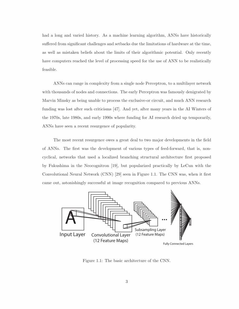
The most recent resurgence owes a great deal to two major developments in the field
of ANNs. The first was the development of various types of feed-forward, that is, non-
cyclical, networks that used a localized branching structural architecture first proposed
by Fukushima in the Neocognitron [19], but popularized practically by LeCun with the
Convolutional Neural Network (CNN) [29] seen in Figure 1.1. The CNN was, when it first
came out, astonishingly successful at image recognition compared to previous ANNs.
A ...
Input Layer Convolutional Layer
(12 Feature Maps)
Subsampling Layer
(12 Feature Maps)
Fully Connected Layers
Figure 1.1: The basic architecture of the CNN.
3
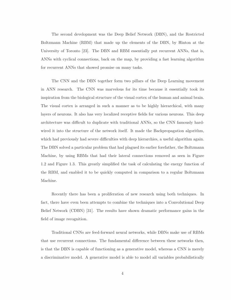
The second development was the Deep Belief Network (DBN), and the Restricted
Boltzmann Machine (RBM) that made up the elements of the DBN, by Hinton at the
University of Toronto [23]. The DBN and RBM essentially put recurrent ANNs, that is,
ANNs with cyclical connections, back on the map, by providing a fast learning algorithm
for recurrent ANNs that showed promise on many tasks.
The CNN and the DBN together form two pillars of the Deep Learning movement
in ANN research. The CNN was marvelous for its time because it essentially took its
inspiration from the biological structure of the visual cortex of the human and animal brain.
The visual cortex is arranged in such a manner as to be highly hierarchical, with many
layers of neurons. It also has very localized receptive fields for various neurons. This deep
architecture was difficult to duplicate with traditional ANNs, so the CNN famously hard-
wired it into the structure of the network itself. It made the Backpropagation algorithm,
which had previously had severe difficulties with deep hierarchies, a useful algorithm again.
The DBN solved a particular problem that had plagued its earlier forefather, the Boltzmann
Machine, by using RBMs that had their lateral connections removed as seen in Figure
1.2 and Figure 1.3. This greatly simplified the task of calculating the energy function of
the RBM, and enabled it to be quickly computed in comparison to a regular Boltzmann
Machine.
Recently there has been a proliferation of new research using both techniques. In
fact, there have even been attempts to combine the techniques into a Convolutional Deep
Belief Network (CDBN) [31]. The results have shown dramatic performance gains in the
field of image recognition.
Traditional CNNs are feed-forward neural networks, while DBNs make use of RBMs
that use recurrent connections. The fundamental difference between these networks then,
is that the DBN is capable of functioning as a generative model, whereas a CNN is merely
a discriminative model. A generative model is able to model all variables probabilistically
4
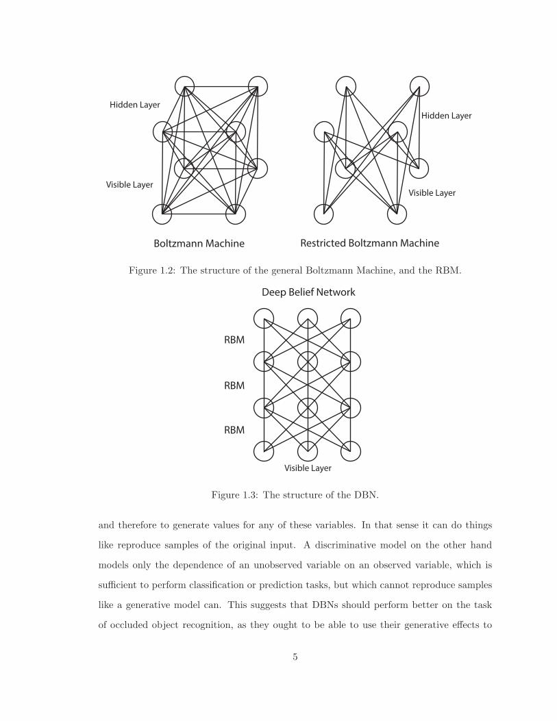
Boltzmann Machine Restricted Boltzmann Machine
Visible Layer
Hidden Layer
Visible Layer
Hidden Layer
Figure 1.2: The structure of the general Boltzmann Machine, and the RBM.
Deep Belief Network
RBM
RBM
RBM
Visible Layer
Figure 1.3: The structure of the DBN.
and therefore to generate values for any of these variables. In that sense it can do things
like reproduce samples of the original input. A discriminative model on the other hand
models only the dependence of an unobserved variable on an observed variable, which is
sufficient to perform classification or prediction tasks, but which cannot reproduce samples
like a generative model can. This suggests that DBNs should perform better on the task
of occluded object recognition, as they ought to be able to use their generative effects to
5
partially reconstruct the image to aid in classification. This is what we wish to show in our
work comparing CNNs, and DBNs [9].
Such research has a myriad of potential applications. In addition to the aforemen-
tioned potential to realize object representations in an artificial mind, a more immediate
and realistic goal is to advance reverse image search to a level of respectable performance
at identifying objects from user provided pictures. For instance, a user could provide an
image with various objects, some of which may well be occluded by other objects, and a
program could potentially identify and classify the various objects in the image. There are a
wide variety of potential uses for a system that is able to effectively identify objects despite
occlusions, as real world images are rarely uncluttered and clean of occlusion.
Object recognition is not the only area of research that stands to benefit from im-
proved machine learning algorithms. Speech recognition has also benefited recently from
the use of these algorithms [36]. As such, it’s apparent that advances in ANNs have a
wide variety of applications in many fields. In terms of the applicability of our research
on occlusions, speech is also known to occasionally have their own equivalent to occlusions
in the form of noise. Being able to learn effectively in spite of noise, whether visual noise
like occlusions, or auditory noise, is an essential part of any real-world pattern recognition
system. Perceptual noise will exist in any of the perceptual modalities, whether visual,
auditory, or somatosensory. Missing data, occlusions, noise, these things are common con-
cerns in any signal processing system. Therefore, the value of this research potentially
extends beyond mere object recognition. Nevertheless, for simplicity’s sake, we shall focus
on the object recognition problem, and the particular problem of occlusions as a region of
particular interest.
6

Chapter 2
Literature Review
2.1 Basics of Artificial Neural Networks
ANNs have their foundation in the works of McCulloch and Pitts [33], who presented the
earliest models of the artificial neuron [34]. Among the earliest learning algorithms for
such artificial neurons was presented by Hebb [20], who devised Hebbian Learning, which
was based on the biological observation that neurons that fired together, tended to wire
together, so to speak. The basic foundation of the artificial neuron is simply described by
Equation (2.1).
output = f(n∑
i=1
wixi) = f(net) (2.1)
Where, wi is the connection weight of node i, xi is the input of node i, and f is
the activation function, which is usually a threshold function or a sigmoid function such as
7
Equation (2.2).
f(net) = z +1
1 + exp(−x ·net+ y)(2.2)
Then the Perceptron model was developed by Rosenblatt [45], which used a gradient
descent based learning algorithm. The Perceptron is centred on a single neuron, and can
be considered the most basic of feed-forward ANNs. They are able to function as linear
classifiers, using a simple step function as seen in Equation (2.3).
f(net) =
⎧⎪⎨⎪⎩
1 if∑n
i=0wixi > 0
0 otherwise(2.3)
There are some well-known limitations regarding the Perceptron that were detailed
by Minsky & Papert [35], namely that they do not work on problems where the sample
data are not linearly separable.
Learning algorithms for ANNs containing many neurons were developed by Dreyfus
[14], Bryson & Ho [6], Werbos [56], and most famously by McClelland & Rumelhart [32], who
revived the concept of ANNs under the banner of Parallel Distributed Processing (PDP).
The modern implementation of the Backpropagation learning algorithm was provided by
Rumelhart, Hinton, & Williams [46]. Backpropagation was a major advance on traditional
gradient descent methods, in that it provided multi-layer feed-forward ANNs with a highly
competitive supervised learning algorithm. The Backpropagation algorithm (as shown in
Algorithm 1) is a supervised learning algorithm that changes network weights to try to
minimize the Mean Squared Error (MSE) (see Equation (2.4)) between the desired and the
8
actual outputs of the network.
MSE =1
P
P∑p=1
K∑j=1
(|op,j − dp,j |)2 (2.4)
Where, dp,j is the desired output, and op,j is the actual output.
Algorithm 1: The Backpropagation training algorithm. From: [34]
1 Start with randomly chosen weights;
2 while MSE is unsatisfactory and computational bounds are not exceeded, do
3 for each input pattern xp, 1 ≥ p ≥ P do
4 Compute hidden node inputs (net(1)p,j );
5 Compute hidden node outputs (x(1)p,j );
6 Compute inputs to the output nodes(net(2)p,k);
7 Compute the network outputs (op,k);
8 Compute the error between op,k and desired output dp,k;
9 Modify the weights between hidden and output nodes:;
10 Δw2,1k,j = η(dp,k − op,k)S
′(net(2)p,k)x(1)p,j ;
11 Modify the weights between input and hidden nodes:;
12 Δw1,0j,i = η
∑k
((dp,k − op,k)S
′(net(2)p,k) w(2,1)k,j
)S′(net(1)p,j )xp,i;
2.2 Convolutional Neural Networks
The earliest of the hierarchical ANNs based on the visual cortexs architecture was the
Neocognitron, first proposed by Fukushima & Miyake [19]. This network was based on
the work of neuroscientists Hubel & Wiesel [27], who showed the existence of Simple and
Complex Cells in the visual cortex. A Simple Cell responds to excitation and inhibition in
a specific region of the visual field. A Complex Cell responds to patterns of excitation and
9
inhibition in anywhere a larger receptive field. Together these cells effectively perform a
delocalization of features in the visual receptive field. Fukushima took the notion of Simple
and Complex Cells to create the Neocognitron, which implemented layers of such neurons
in a hierarchical architecture [18]. However, the Neocognitron, while promising in theory,
had difficulty being put into practice effectively, in part because it was originally proposed
in the 1980s when computers simply weren’t as fast as they are today.
Then LeCun et al. [29] developed the CNN while working at AT&T labs, which made
use of multiple Convolutional and Subsampling layers, while also brilliantly using stochastic
gradient descent and backpropagation to create a feed-forward network that performed
astonishingly well on image recognition tasks such as the MNIST, which consisted of digit
characters. The Convolutional Layer of the CNN is equivalent to the Simple Cell Layer of
the Neocognitron, while the Subsampling Layer of the CNN is equivalent to the Complex
Cell Layer of the Neocognitron. Essentially they delocalize features from the visual receptive
field, allowing such features to be identified with a degree of shift invariance. The differences
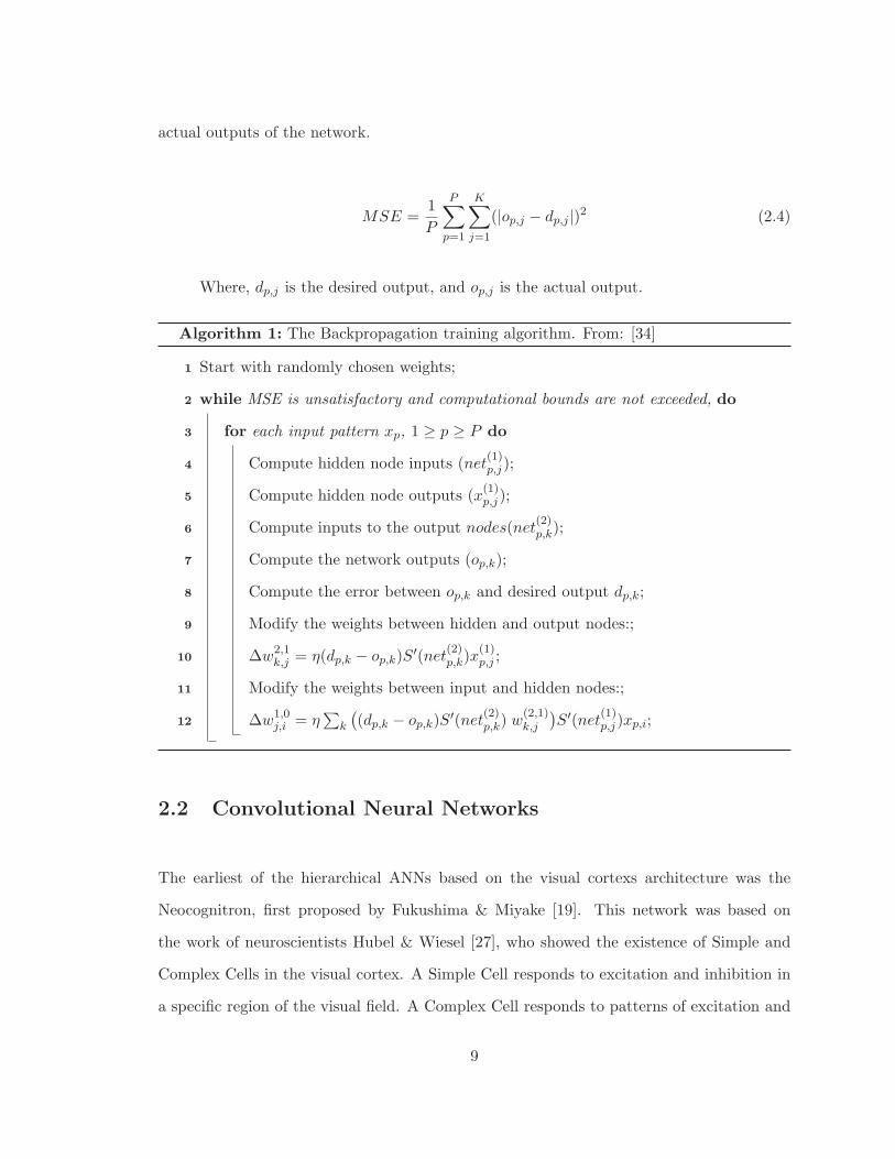
between these layers can be seen in Figure 2.1.
Convolutional Layer
Subsampling Layer
VS.
Figure 2.1: A comparison between the Convolutional layer and the Subsampling layer. Cir-cles represent the receptive fields of the cells of the layer subsequent to the one representedby the square lattice. On the left, an 8 x 8 input layer feeds into a 6 x 6 convolutional layerusing receptive fields of size 3 x 3 with an offset of 1 cell. On the right, a 6 x 6 input layerfeeds into a 2 x 2 subsampling layer using receptive fields of size 3 x 3 with an offset of 3cells.
10
This unique structure allows the CNN to have two important advantages over a fully-
connected ANN. First, is the use of the local receptive field, and second is weight-sharing.
Both of these advantages have the effect of decreasing the number of weight parameters in
the network, thereby making computation of these networks easier.
More details regarding the CNN are described in Chapter 3.
2.3 Support Vector Machines
The Support Vector Machine (SVM) is a powerful discriminant classifier first developed by
Cortes & Vapnik [13]. Although not considered to be an ANN strictly speaking, Collobert
& Bengio [12] showed that they had many similarities to Perceptrons with the obvious
exception of learning algorithm. CNNs were found to be excellent feature extractors for
other classifiers such as SVMs as seen in Huang & LeCun [26], as well as Ranzato et al.
[43]. This generally involves taking the output of the lower layers of the CNN as feature
extractors for the classifier.
2.4 Deep Belief Networks
One of the more recent developments in machine learning research has been the Deep Belief
Network (DBN). The DBN is a recurrent ANN with undirected connections. Structurally,
it is made up of multiple layers of RBMs, such that it can be seen as a “deep architecture”.
“Deep architectures” can have many hidden layers, as compared to “shallow architectures”
which only have usually one hidden layer. To understand how this “deep architecture” is
an effective structure, we must first understand the basic nature of a recurrent ANN.
Recurrent ANNs differ from feed-forward ANNs in that their connections can form
11
cycles. Such networks cannot use simple Backpropagation or other feed-forward based
learning algorithms. The advantage of recurrent ANNs is that they can possess associative
memory-like behaviour. Early Recurrent ANNs, such as the Hopfield network [25], were
limited. The Hopfield network was only a single layer architecture that could only learn
very limited problems due to limited memory capacity. A multi-layer generalization of the
Hopfield Network was developed known as the Boltzmann Machine [1], which while able
to store considerably more memory, suffered from being overly slow to train. A variant of
the Boltzmann Machine, which initially saw little use, was first known as a Harmonium
[52], but later called a RBM, and was developed by removing the lateral connections from
the network. Then Hinton [21] developed a fast algorithm for RBMs called Contrastive
Divergence, which uses Gibbs sampling within a gradient descent process. An RBM can be
defined by the energy function in Equation (2.5) [3].
E(v, h) =∑
i∈visibleaivi −
∑j∈hidden
bjhj −∑i,j
vihjwi,j (2.5)
where vi and hj are the binary states of the visible unit i and hidden unit j, ai and
bj are their biases, and wi,j is the weight connection between them [22].
The weight update in an RBM is given by Equation (2.6) below.
Δwi,j = ε(〈vihj〉data − 〈vihj〉recon) (2.6)
By stacking RBMs together, they formed the DBN, which produced then state of the
art performance on such tasks as the MNIST [23]. Later DBNs were also applied to 3D
object recognition [37]. Ranzato, Susskind, Mnih, & Hinton [44] also showed how effective
DBNs could be on occluded facial images.
12
More details of the DBN are provided in Chapter 4.
2.5 Further Developments in Artificial Neural Networks
There has even been a proliferation of work on combining CNNs and DBNs. The CDBN of
Lee, Grosse, Ranganath, & Ng [31] combined the two algorithms together. This is possible
because strictly speaking the Convolutional nature of the CNN is in the structure of the
network, which the DBN can implement. To do this, one creates Convolutional Restricted
Boltzmann Machines (CRBMs) for the CDBN to use in its layers. Another modification has
also been shown by Schulz, Muller, & Behnke [50], which creates Local Impact Restricted
Boltzmann Machines (LIRBMs), which utilize localized lateral connections, similar to work
by Osindero & Hinton [40]. These networks are primarily RBMs in terms of learning
algorithm, but both utilize CNN style localizing structures.
Deep Boltzmann Machines (DBMs) courtesy of Salakhutdinov & Hinton [48] brought
about a dramatic reemergence of the old Boltzmann Machine architecture. Using a new
learning algorithm, they were able to produce exceptional results on the MNIST and NORB.
Ngiam et al. [38] also developed a superior version of the CNN called the Tiled Convolutional
Neural Network (TCNN). Despite these state-of-the-art advances, we choose to use more
developed and mature algorithms, namely the SVM, CNN, and DBN.
13
Chapter 3
Optimizing Convolutional Neural
Networks
3.1 Overview
A ...
.
.
.
INPUT
(32 x 32)
Convolutional Layer(6 feature maps)
(28 x 28 each) Subsampling Layer(6 feature maps)
(14 x 14 each)
Convolutional Layer(16 feature maps)
(10 x 10 each) Subsampling Layer(16 feature maps)
(5 x 5 each)
Fully Connected
Layers(84 nodes)
(10 nodes)
Convolutional Layer(120 feature maps)
Convolution
(5 x 5 receptive field)
Subsampling
(2 x 2 receptive field)
Convolution
(5 x 5 receptive field)
Subsampling
(2 x 2 receptive field)
Convolution
(5 x 5 receptive field)
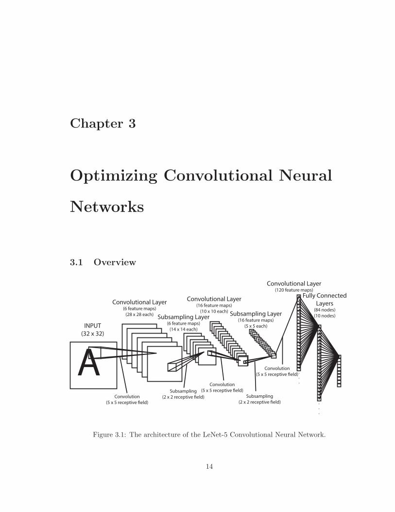
Figure 3.1: The architecture of the LeNet-5 Convolutional Neural Network.
14
Figure 3.1 shows the entire architecture of the LeNet-5 CNN, as the quintessential
example of a CNN [29]. It consists of a series of layers, including an input layer, followed by
a number of feature extracting Convolutional and Subsampling layers, and finally a number
of fully connected layers that perform the classification.
A Convolutional layer can be described according to:
xout = S(∑i
xin ∗ ki + b), (3.1)
where xin is the previous layer, k is a convolution kernel, S is a non-linear function (such
as a hyperbolic tangent sigmoid, described in Equation (3.2)), and b is a scalar bias. See
[26] for details.
S = tanhx =sinhx
coshx=
ex − e−x
ex + e−x=
e2x − 1
e2x + 1=
1− e−2x
1 + e−2x. (3.2)
This output creates a feature map that is made up of nodes that each effectively share
the same weights of a receptive field or convolutional kernel. So, as in the example from
Figure 2.1, a 3x3 receptive field applied to an 8x8 input layer will create a 6x6 feature map
with 9 weights + 1 bias = 10 free parameters and 9 × 36 = 324 weights + 1 bias = 325
connections. The number of free parameters therefore is equal to the number of nodes in
the receptive field multiplied by the number of feature maps in the current layer, multiplied
by the number of feature maps in the previous layer (the input layer counts as one feature
map), plus biases. Meanwhile, the number of total connections is equal to the number of
nodes in the receptive field multiplied by the number of nodes in each feature map multiplied
by the number of feature maps in the current layer, multiplied by the number of feature
maps in the previous layer (the input layer counts as one feature map), plus biases. To
train such weights, we can use gradient descent, with the gradient of a shared weight being
15

the sum of the gradient of the shared parameters.
A Subsampling layer can be described as follows:
xout = S(β∑
xn×nin + b), (3.3)
where xn×nin is either the average or the max of an n × n block in the previous layer, β is
a trainable scalar, b is a scalar bias, and S is a non-linear function (such as a hyperbolic
tangent sigmoid). See [26] for details.
This output results in a number of subsampled feature maps equal to the number
of feature maps of the previous layer. The number of free parameters then is simply the
number of feature maps, plus biases. The total number of connections is equal to the
number of nodes in the subsampled feature maps multiplied by the number of feature maps
multiplied by the number of nodes in the receptive field, plus biases.
Some CNNs also implement non-complete connection schemes between layers, such
that only some of the feature maps of a previous layer are connected to the feature maps of
a subsequent layer. These can range from hand-crafted connection matrices as seen in [29],
to random connection matrices, as well as completely connected implementations.
The final fully connected layers can be a wide variety of ANN classifiers, but are
most commonly are a multi-layer perceptron that takes as input the output of the previous
feature extracting layers, and performs classification. The entire CNN can be trained with
Backpropagation, and that is how we choose to train our networks.
3.2 Topology of LeNet-5
The convolutional operator used in LeNet-5 can be described in more detail as follows:
16
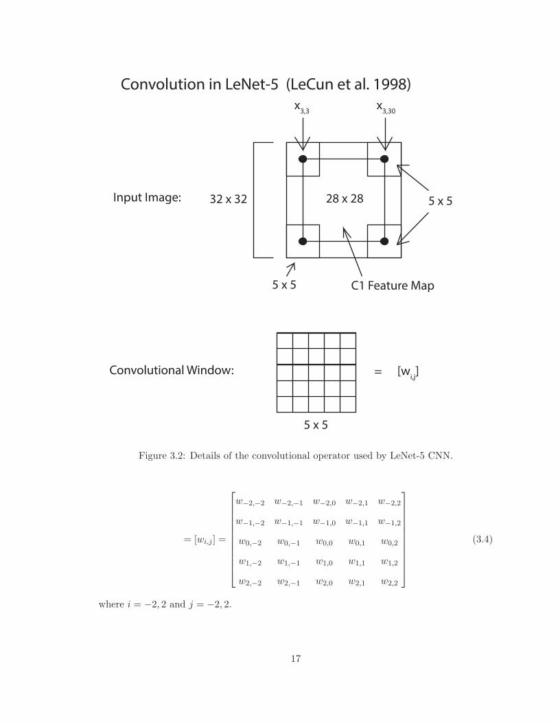
x3,3
x3,30
28 x 2832 x 32
5 x 5 C1 Feature Map
5 x 5
Convolution in LeNet-5 (LeCun et al. 1998)
Input Image:
Convolutional Window:
5 x 5
= [wi,j]
Figure 3.2: Details of the convolutional operator used by LeNet-5 CNN.
= [wi,j ] =
⎡⎢⎢⎢⎢⎢⎢⎢⎢⎢⎢⎣
w−2,−2 w−2,−1 w−2,0 w−2,1 w−2,2
w−1,−2 w−1,−1 w−1,0 w−1,1 w−1,2
w0,−2 w0,−1 w0,0 w0,1 w0,2
w1,−2 w1,−1 w1,0 w1,1 w1,2
w2,−2 w2,−1 w2,0 w2,1 w2,2
⎤⎥⎥⎥⎥⎥⎥⎥⎥⎥⎥⎦
(3.4)
where i = −2, 2 and j = −2, 2.
17
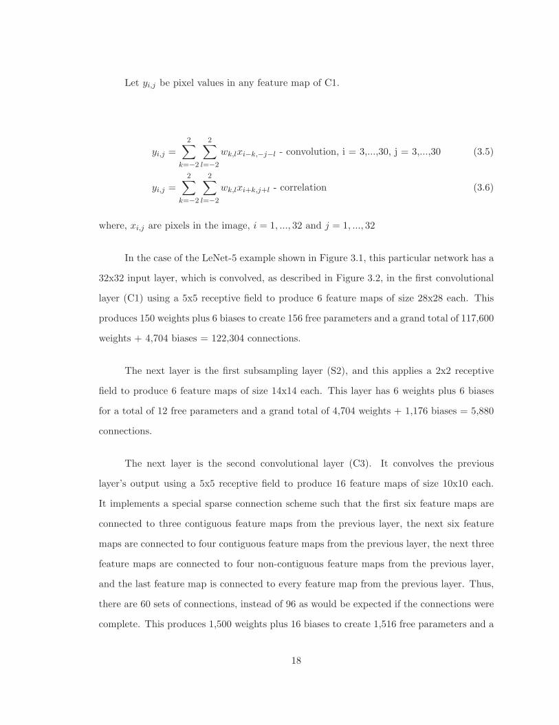
Let yi,j be pixel values in any feature map of C1.
yi,j =
2∑k=−2
2∑l=−2
wk,lxi−k,−j−l - convolution, i = 3,...,30, j = 3,...,30 (3.5)
yi,j =
2∑k=−2
2∑l=−2
wk,lxi+k,j+l - correlation (3.6)
where, xi,j are pixels in the image, i = 1, ..., 32 and j = 1, ..., 32
In the case of the LeNet-5 example shown in Figure 3.1, this particular network has a
32x32 input layer, which is convolved, as described in Figure 3.2, in the first convolutional
layer (C1) using a 5x5 receptive field to produce 6 feature maps of size 28x28 each. This
produces 150 weights plus 6 biases to create 156 free parameters and a grand total of 117,600
weights + 4,704 biases = 122,304 connections.
The next layer is the first subsampling layer (S2), and this applies a 2x2 receptive
field to produce 6 feature maps of size 14x14 each. This layer has 6 weights plus 6 biases
for a total of 12 free parameters and a grand total of 4,704 weights + 1,176 biases = 5,880
connections.
The next layer is the second convolutional layer (C3). It convolves the previous
layer’s output using a 5x5 receptive field to produce 16 feature maps of size 10x10 each.
It implements a special sparse connection scheme such that the first six feature maps are
connected to three contiguous feature maps from the previous layer, the next six feature
maps are connected to four contiguous feature maps from the previous layer, the next three
feature maps are connected to four non-contiguous feature maps from the previous layer,
and the last feature map is connected to every feature map from the previous layer. Thus,
there are 60 sets of connections, instead of 96 as would be expected if the connections were
complete. This produces 1,500 weights plus 16 biases to create 1,516 free parameters and a
18

grand total of 150,000 weights + 1600 biases = 151,600 connections.
The next layer is the second subsampling layer (S4), and this applies a 2x2 receptive
field to produce 16 feature maps of size 5x5 each. This layer has 16 weights plus 16 biases
for a total of 32 free parameters and a grand total of 1,600 weights + 400 biases = 2,000
connections.
Next in line we have the third and final convolutional layer (C5). It convolves the
previous layer’s output using a 5x5 receptive field to produce 120 feature maps of size 1x1
each. This produces 48,000 weights plus 120 biases to create 48,120 free parameters and
connections.
The next layer is a fully connected layer (F6) containing 84 nodes, which brings about
10,080 weights plus 84 biases to create 10,164 connections.
The final output layer of the original LeNet-5 was actually an Radial Basis Function
layer that had each node compute the Euclidian Radial Basis Function for each class. This
layer has 840 connections to the previous layer.
This brings the total number free parameters in the network to 60,840 and the total
number of connections in the network to 340,908.
As can be seen from the LeNet-5 example, the apparent complexity of the CNN comes
mostly from its unique structural properties, which introduce a number of hyper-parameters,
such as feature map numbers, and receptive field sizes.
19
3.3 Theoretical Analysis
CNNs have particularly many hyper-parameters due to the structure of the network. De-
termining the optimal hyper-parameters can appear to be a bit of an art. In particular,
the number of feature maps for a given convolutional layer tends to be chosen based on
empirical performance rather than on any sort of theoretical justification [51]. Numbers in
the first convolutional layer range from very small (3-6) [29], [39], to very large (96-1600)
[10], [11], [16], [28].
One wonders then, if there is some sort of theoretical rationale that can be used to
determine the optimal number of feature maps, given other hyper-parameters. In particular,
one would expect that the dimensions of the receptive field, ought to have some influence
on this optimum [8].
A receptive field of width r consists of r2 elements or nodes. If we have feature maps
m then, the maximum number of possible feature maps before duplication, given an 8-bit
grey scale image is 256r2. Since the difference between a grey level of say, 100 and 101,
is roughly negligible, we simplify and reduce the number of bins in the histogram so to
speak from 256 to 2. Looking at binary features as a way of simplifying the problem is not
unheard of [5]. So, given a binary image the number of possible binary feature maps before
duplication is
Ω = 2r2, (3.7)
which is still a rapidly increasing number.
Let’s look at some very simple receptive fields. Take a receptive field of size 1x1. How
many feature maps would it take before additional maps become completely redundant?
Applying Ω would suggest two.
20
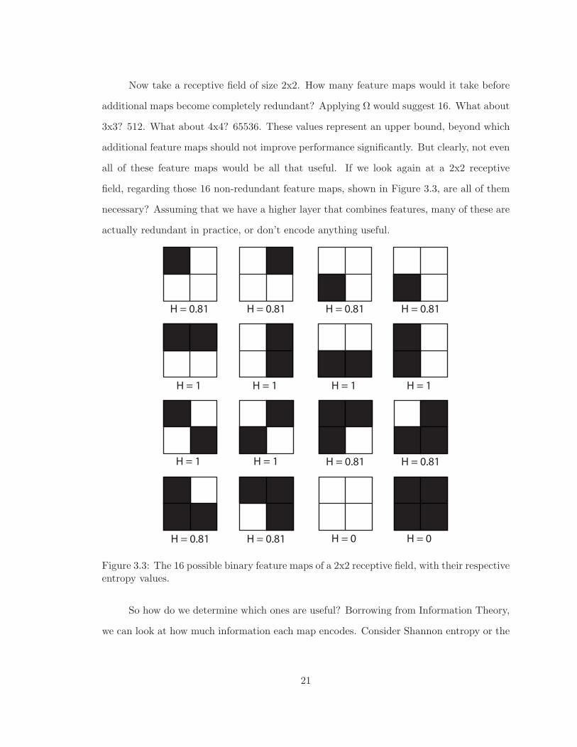
Now take a receptive field of size 2x2. How many feature maps would it take before
additional maps become completely redundant? Applying Ω would suggest 16. What about
3x3? 512. What about 4x4? 65536. These values represent an upper bound, beyond which
additional feature maps should not improve performance significantly. But clearly, not even
all of these feature maps would be all that useful. If we look again at a 2x2 receptive
field, regarding those 16 non-redundant feature maps, shown in Figure 3.3, are all of them
necessary? Assuming that we have a higher layer that combines features, many of these are
actually redundant in practice, or don’t encode anything useful.
H = 0.81
H = 1
H = 0.81 H = 0.81 H = 0.81
H = 0.81 H = 0.81
H = 0.81 H = 0.81
H = 1 H = 1 H = 1
H = 1 H = 1
H = 0 H = 0
Figure 3.3: The 16 possible binary feature maps of a 2x2 receptive field, with their respectiveentropy values.
So how do we determine which ones are useful? Borrowing from Information Theory,
we can look at how much information each map encodes. Consider Shannon entropy or the
21
amount of information given
H(X) = −n∑
i=1
p(xi) log2 p(xi). (3.8)
Thus, we calculate the Shannon entropy of each feature map, again, shown in Figure
3.3. The combined set has an average Shannon entropy of 0.7806. What’s interesting here
is that we can group the Shannon entropy values together. In the 2x2 case, there are six
patterns equal to an entropy of 1, while there are eight patterns with an entropy of around
0.81, and two patterns with an entropy of 0. Thus we have three bins of entropy values so
to speak.
Thus, we hypothesize a very simple theoretical method, one that admittedly simplifies
a very complex problem. Shannon entropy has the obvious disadvantage that it does not
tell us about the spatial relationship between neighbouring pixels. And again, we assume
binary feature maps. Nevertheless, we propose this as an initial attempt to approximate
the underlying reality.
The number of different possible entropy values for the total binary feature map set
of a particular receptive field size is determined by considering the number of elements in
a receptive field r2. The number of unique ways you can fill the binary histogram of the
possible feature maps then is r2 + 1. But roughly half the patterns are inverses of each
other. So the actual number of unique entropy values is (r2+1)/2 if r is odd. Or (r2)/2+1
if r is even.
Given the the number of different entropy values
h(r) =
⎧⎪⎨⎪⎩
r2+12 if r is odd
r2
2 + 1 if r is even(3.9)
22
the number of useful feature maps is
u = h+ s, (3.10)
where s is a term that describes the additional useful feature maps above this minimum of
h. We know from the 1x1 receptive field feature map set that s is at least 1, because when
r = 1, the receptive field is a single pixel filter, and optimally functions as a binary filter.
In such a case, u = Ω = 2. In the minimum case that s = 1, then in the case of 1x1, u = 2.
In the case of 2x2, u = 4. In the case of 3x3, u = 6. This is a lower bound on u that we
shall use until we can determine what s actually is.
To understand this, think of a receptive field that takes up the entire space of the
image. If the image is 100x100, then the receptive field is 100x100. In such an instance, each
feature map is essentially a template, and the network performs what is essentially template
matching. Thus the number of useful feature maps is based strictly on the number of useful
templates. If you have enough templates, you can approximate the data set. Any more
than that would be unnecessary. To determine how many such templates would be useful,
consider again, the number of different Shannon entropies in the feature set. While it is not
guaranteed that two templates with the same entropy would be identical, two templates
with different entropies are certainly different. Also consider the difference between that
100x100 receptive field, and a 99x99 receptive field. The differences between the two in
terms of number of useful feature maps intuitively seems negligible. This suggests that s is
either a constant, or at most a linearly increasing term. One thing else to consider is that
as h increases, the distance between various entropies decreases, to the point where many
of the values start to become nearly the same. Thus, one will expect that for very high
values of r, u will be too high.
Some possibilities for s that we propose to consider are based on the notion of the
way in which square lattices can be divided into different types of squares based on their
23
position. For 1x1, there is only one square with no adjacent squares, but for 2x2 there are
exactly four corner squares. A 3x3 receptive field also has exactly four corner squares, but
also four edge squares and one inner square. A 4x4 receptive field has four corner squares,
eight non-corner edge squares, and four inner squares. From this we see that the number
of each type of square for r > 1 is the constant 4 for corners, 4(r − 2) for non-corner edge
squares, and (r−2)2 for inner squares. A receptive field of size 3x3 or greater has four corner
regions, four edge regions, and one inner area. Thus, if we assume that positional/spatial
information is relevant, then s could be at least the number of types of squares in the
receptive field. This suggests that s = 1 for r = 1 and r = 2, and s = 3 for r > 2.
Alternatively, we can assume that it is the number of distinct regions that determines s, in
which case, s = 1 for r = 1, s = 4 for r = 2, and s = 9 for r > 2.
Any less than u and the theory predicts a drop in performance. Above this number
the theory is agnostic about one of three possible directions. Either the additional feature
maps won’t affect the predictive power of the model, so we should see a plateau, or the
Curse of Dimensionality will cause the predictive power of the model to begin to drop, or
as seen in previous papers such as [11], the predictive power of the model will begin to
increase, albeit at a slower rate.
Thus far we have taken care of the first convolutional layer. For the second convo-
lutional layer and beyond, the question arises of whether or not to stick to this formula
for u, or whether it makes more sense to increase the number of feature maps in some
proportion to the number in the previous convolutional layer. Upper convolutional layers
are not simply taking the pixel intensities, but instead, combining the feature maps of the
lower layer. In which case, it makes sense to change the formula for u for upper layers to:
ul = vul−1, (3.11)
where v is some multiplier value and l is the layer. Candidates for this value range from
24
ul−1 itself, to some constant such as 2 or 4.
There is no substitute for empirical evidence, so we test the theory by running exper-
iments to exhaustively search for the hypothetical, optimal number of feature maps.
3.4 Methodology
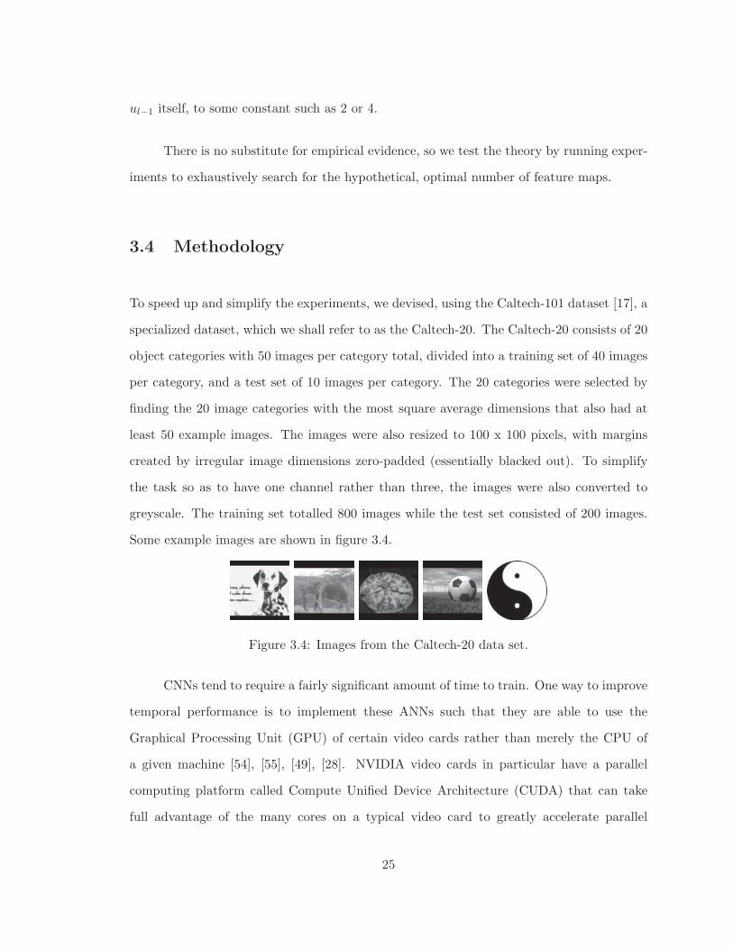
To speed up and simplify the experiments, we devised, using the Caltech-101 dataset [17], a
specialized dataset, which we shall refer to as the Caltech-20. The Caltech-20 consists of 20
object categories with 50 images per category total, divided into a training set of 40 images
per category, and a test set of 10 images per category. The 20 categories were selected by
finding the 20 image categories with the most square average dimensions that also had at
least 50 example images. The images were also resized to 100 x 100 pixels, with margins
created by irregular image dimensions zero-padded (essentially blacked out). To simplify
the task so as to have one channel rather than three, the images were also converted to
greyscale. The training set totalled 800 images while the test set consisted of 200 images.
Some example images are shown in figure 3.4.
Figure 3.4: Images from the Caltech-20 data set.
CNNs tend to require a fairly significant amount of time to train. One way to improve
temporal performance is to implement these ANNs such that they are able to use the
Graphical Processing Unit (GPU) of certain video cards rather than merely the CPU of
a given machine [54], [55], [49], [28]. NVIDIA video cards in particular have a parallel
computing platform called Compute Unified Device Architecture (CUDA) that can take
full advantage of the many cores on a typical video card to greatly accelerate parallel
25
computing tasks. ANNs are quite parallel in nature, and thus quite amenable to this.
Thus, for our implementation of the CNN, we turned to the Python-based Theano library
(http://deeplearning.net/software/theano/) [4]. We were able to find appropriate
Deep Learning Python scripts for the CNN. Our tests suggest that the speed of the CNN
using the GPU improved by a factor of eight, as compared to just using the CPU.
CNNs require special consideration when implementing their architecture. A method
was devised to calculate a usable set of architecture parameters. The relationship between
layers can be described as follows. To calculate the reasonable dimensions of a square layer
from either its previous layer (or next layer) in the hierarchy requires at least some of the
following variables to be assigned. Let x be the width of the previous (or current) square
layer. Let y be the width of the current (or next) square layer. Let r be the width of the
square receptive field of nodes in the previous (or current) layer to each current (or next)
layer node, and f be the offset distance between the receptive fields of adjacent nodes in the
current (or next) layer. The relationship between these variables is best described by the
equation below.
y =x− (r − f)
f, (3.12)
where, x ≥ y, x ≥ r ≥ f , and f > 0.
For convolutional layers this generalizes because f = 1, to:
y = x− r + 1. (3.13)
26
For subsampling layers, this generalizes because r = f, to:
y =x
f. (3.14)
From this we can determine the dimensions of each layer. To describe a CNN, we
adopt a similar convention to [10]. An example architecture for the CNN on the NORB
dataset [30] can be written out as:
96 × 96 → 8C5 → S4 → 24C6 → S3 → 24C6 → 100N → 5N , where the number
before C is the number of feature maps in a convolutional layer, the number after C is the
receptive field width in a convolutional layer, the number after S is the receptive field width
of a subsampling layer, and the number before N is the number of nodes in a fully connected
layer.
For us to effectively test a single convolutional layer, we use a series of architectures,
where v is a variable number of feature maps:
100× 100 → vC1 → S2 → 500N → 20N
100× 100 → vC2 → S3 → 500N → 20N
100× 100 → vC3 → S2 → 500N → 20N
100× 100 → vC5 → S3 → 500N → 20N
100× 100 → vC99 → S1 → 500N → 20N
The reason why we sometimes use 3x3 subsampling receptive fields is that the size of
the convolved feature maps are divisible by 3 but not 2. Otherwise we choose to use 2x2
subsampling receptive fields where possible. We find that, with the exception of the unique
27
99x99 receptive field, not using subsampling produces too many features and parameters
and causes the network to have difficulty learning. The method of subsampling we use is
max-pooling, which involves taking the maximum value seen in the receptive field of the
subsampling layer.
For testing multiple convolutional layers, we use the following architecture, where vi
is a variable number of feature maps for each layer:
100 × 100 → v1C2 → S3 → v2C2 → S2 → v3C2 → S3 → v4C2 → S2 → v5C2 →S1 → 500N → 20N
All our networks use the same basic classifier, which is a multi-layer Perceptron with
500 hidden nodes and 20 output nodes. Various other parameters for the CNN were also
experimented with to determine the optimal parameters to use in our experiments. We
eventually settled on 100 epochs of training. The CNN learning rate and learning rate
decrement parameters were determined by trial and error. The learning rate was initially
set to 0.1, and gradually decremented to approximately 0.001.
3.5 Analysis and Results
The following figures are intentionally fitted with a trend line that attempts to test the
hypothesis that a cubic function approximates the data. It should not be construed to
suggest that this is in fact the underlying function.
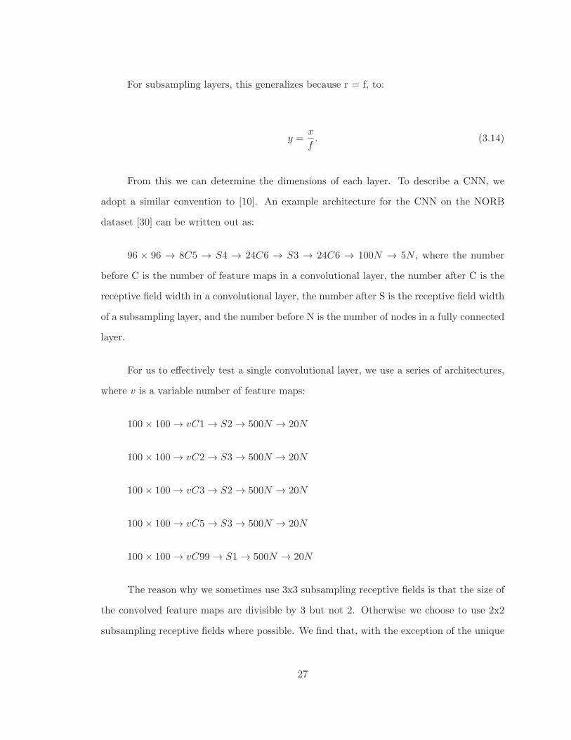
Figure 3.5 shows the results of experimenting with different numbers of feature maps
on the accuracy of the CNN trained on the Caltech-20, and using a 1x1 receptive field.
As can be seen, the accuracy quickly increases between 1 and 2 feature maps, and
then levels off for more than 2 feature maps. This is consistent with the theory, albeit, the
28
y = 6E 05x3 0.0021x2 + 0.0222x + 0.3104R² = 0.3476
0
0.1
0.2
0.3
0.4
0.5
0.6
0.7
0.8
0.9
1
1 2 3 4 5 6 7 8 9 10 11 12 13 14 15 16 17 18 19 20
Accuracy
Feature Maps
1x1 Receptive Field
y = 4E 08x3 1E 05x2 + 0.001x + 0.3623R² = 0.1096
0
0.1
0.2
0.3
0.4
0.5
0.6
0.7
0.8
0.9
1
0 50 100 150 200 250
Accuracy
Feature Maps
1x1 Receptive Field
Figure 3.5: Graphs of the accuracy given a variable number of feature maps for a 1x1receptive field.
plateau beyond seems to be neither increasing nor decreasing, which suggests some kind of
saturation point around 2.
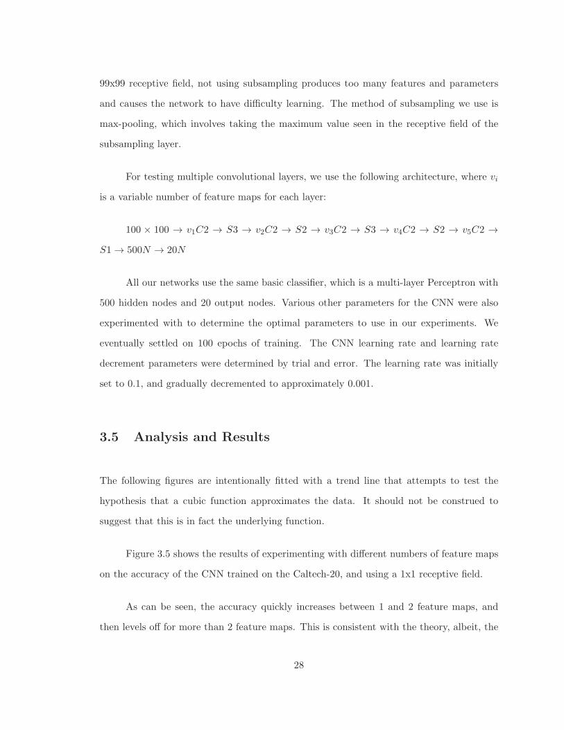
Figure 3.6 shows the results of experimenting with different numbers of feature maps
on the accuracy of the CNN trained on the Caltech-20, and using a 2x2 receptive field.
y = 7E 05x3 0.0025x2 + 0.0277x + 0.3226R² = 0.6069
0
0.1
0.2
0.3
0.4
0.5
0.6
0.7
0.8
0.9
1
1 2 3 4 5 6 7 8 9 10 11 12 13 14 15 16 17 18 19 20
Accuracy
Feature Maps
2x2 Receptive Field
y = 2E 08x3 6E 06x2 + 0.0007x + 0.3988R² = 0.117
0
0.1
0.2
0.3
0.4
0.5
0.6
0.7
0.8
0.9
1
0 50 100 150 200 250
Accuracy
Feature Maps
2x2 Receptive Field
Figure 3.6: Graphs of the accuracy given a variable number of feature maps for a 2x2receptive field.
As can be seen, the accuracy quickly increases between 1 and 4 feature maps, and
then levels off for more than 4 feature maps. This is consistent with the theory where
s = 1. The plateau beyond seems to be neither increasing nor decreasing, which suggests
some kind of saturation point around 4.
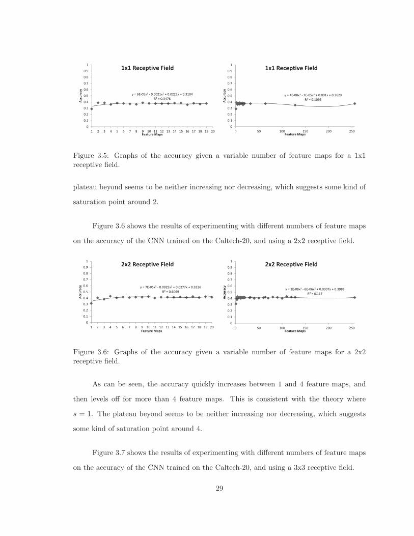
Figure 3.7 shows the results of experimenting with different numbers of feature maps
on the accuracy of the CNN trained on the Caltech-20, and using a 3x3 receptive field.
29
y = 1E 05x3 0.0008x2 + 0.0138x + 0.3492R² = 0.2701
0
0.1
0.2
0.3
0.4
0.5
0.6
0.7
0.8
0.9
1
0 2 4 6 8 10 12 14 16 18 20 22 24 26 28 30 32
Accuracy
Feature Maps
3x3 Receptive Field
y = 3E 08x3 1E 05x2 + 0.0014x + 0.3944R² = 0.2363
0
0.1
0.2
0.3
0.4
0.5
0.6
0.7
0.8
0.9
1
0 50 100 150 200 250
Accuracy
Feature Maps
3x3 Receptive Field
Figure 3.7: Graphs of the accuracy given a variable number of feature maps for a 3x3receptive field.
As can be seen, the accuracy increases between 1 and 6 feature maps, and then
proceeds to plateau somewhat erratically. Unlike the previous receptive field sizes however,
there are accuracies greater than that found at u. The plateau also appears less stable.
Predicted u values of 8 and 14 don’t appear to correlate well.
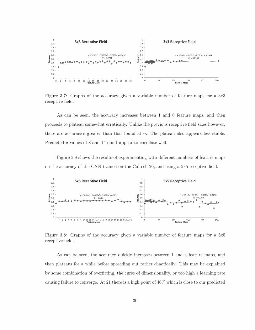
Figure 3.8 shows the results of experimenting with different numbers of feature maps
on the accuracy of the CNN trained on the Caltech-20, and using a 5x5 receptive field.
y = 5E 06x3 0.0005x2 + 0.0091x + 0.3871R² = 0.363
0
0.1
0.2
0.3
0.4
0.5
0.6
0.7
0.8
0.9
1
1 2 3 4 5 6 7 8 9 10 11 12 13 14 15 16 17 18 19 20 21 22 23 24 25
Accuracy
Feature Maps
5x5 Receptive Field
y = 9E 10x3 1E 07x2 0.0003x + 0.4296R² = 0.2769
0
0.1
0.2
0.3
0.4
0.5
0.6
0.7
0.8
0.9
1
0 50 100 150 200 250
Accuracy
Feature Maps
5x5 Receptive Field
Figure 3.8: Graphs of the accuracy given a variable number of feature maps for a 5x5receptive field.
As can be seen, the accuracy quickly increases between 1 and 4 feature maps, and
then plateaus for a while before spreading out rather chaotically. This may be explained
by some combination of overfitting, the curse of dimensionality, or too high a learning rate
causing failure to converge. At 21 there is a high point of 46% which is close to our predicted
30
u value of 22, if s = 9.
Figure 3.9 show the results of experimenting with different numbers of feature maps
on the accuracy of the CNN trained on the Caltech-20, and using a 99x99 receptive field.
y = 3E 05x3 0.0017x2 + 0.0303x + 0.07R² = 0.8789
0
0.1
0.2
0.3
0.4
0.5
0.6
0.7
0.8
0.9
1
1 2 3 4 5 6 7 8 9 10 11 12 13 14 15 16 17 18 19 20 21 22 23 24 25
Accuracy
Feature Maps
99x99 Receptive Field
y = 5E 08x3 2E 05x2 + 0.0031x + 0.181R² = 0.8201
0
0.1
0.2
0.3
0.4
0.5
0.6
0.7
0.8
0.9
1
0 50 100 150 200 250
Accuracy
Feature Maps
99x99 Receptive Field
Figure 3.9: Graphs of the accuracy given a variable number of feature maps for a 99x99receptive field.
As can be seen, the accuracy steadily increases between 1 and 210 feature maps, and
then begins to plateau. As predicted, our u value of 4901 is much too high for the very
large value of r = 99.
Lastly, we look at the effect of multiple convolutional layers. Figure 3.10 shows what
happens when the first layer of a 12 layer CNN with 5 convolutional layers is held constant
at 4 feature maps, and the upper layers are multiplied by the number in the layer before
it. So for a multiple v of 2, the feature maps for each layer would be 4, 8, 16, 32, 64,
respectively. We refer to this as the pyramidal structure.
Clearly, increasing the number of feature maps in the upper layers has a significant
impact. Perhaps not coincidentally, the best performing architecture we have encountered
so far was this architecture with 4, 20, 100, 500, and 2500 feature maps in each respective
layer. It achieved an accuracy of 54.5% on our Caltech-20 data set. This can be contrasted
with the effect of having the same number of feature maps in each layer as shown in figure
3.11. We refer to this as the equal structure.
31

y = 0.0108x3 0.1245x2 + 0.4896x 0.1417R² = 0.9925
0
0.1
0.2
0.3
0.4
0.5
0.6
0.7
0.8
0.9
1
1 2 3 4 5
Accuracy
Feature Maps Multiplier (4 in 1st Layer)
5 Convolutional Layers (2x2)
Figure 3.10: Graph of the accuracy given a variable number of feature maps for a networkwith 5 convolutional layers of 2x2 receptive field. Here the higher layers are a multiple ofthe lower layers.
y = 0.0001x3 0.0057x2 + 0.0733x + 0.0203R² = 0.9366
0
0.1
0.2
0.3
0.4
0.5
0.6
0.7
0.8
0.9
1
1 2 3 4 5 6 7 8 9 10 11 12 13 14 15 16 17 18 19 20
Accuracy
Feature Maps in Each Layer
5 Convolutional Layers (2x2)
y = 2E 07x3 1E 04x2 + 0.0104x + 0.1989R² = 0.7801
0
0.1
0.2
0.3
0.4
0.5
0.6
0.7
0.8
0.9
1
0 50 100 150 200 250
Accuracy
Feature Maps in Each Layer
5 Convolutional Layers (2x2)
Figure 3.11: Graph of the accuracy given a variable number of feature maps for a networkwith 5 convolutional layers of 2x2 receptive field. Here each layer has the same number offeature maps.
While the accuracy rises with the number of feature maps as well, it should be noted
that for the computational cost, the pyramidal structure appears to be a better use of
resources than the equal structure.
3.6 Discussion
It appears that the theoretical method seems to hold well for receptive fields of size 1x1,
and 2x2. For larger sizes, the data is not as clear. The data from the 3x3 and 5x5 receptive
field experiments suggests that there can be complicating factors involved that cause the
32
data to spread. Such factors could include, the curse of dimensionality, and also, technical
issues such as failure to converge due to too high a learning rate, or overfitting. As our
experimental set up is intentionally very simple, we lack many of the normalizing methods
that might otherwise improve performance. The data from the 99x99 receptive field experi-
ment is interesting because it starts to plateau much sooner than predicted by the equation
for u. However, we mentioned before that this would probably happen with the current
version of u. The number of different entropies at r = 99 are probably very close together
and an improved u equation should take this into account.
It should also be emphasized that our results could be particular to our choice of
hyper-parameters such as learning rate and our choice of a very small dataset.
Nevertheless, what we do not find, is the clear and simple monotonically increasing
function seen in [11], and [16]. Rather, the data shows that after an initial rise, the function
seems to plateau and it is uncertain whether it can be construed to be rising or falling or
stable. Even in the case of the 99x99 receptive field, past 210 feature maps, we see what
appears to be the beginnings of such a plateau.
This is not the case with highly layered networks however, which do appear to show
a monotonically increasing function in terms of increasing the number of feature maps.
However, this could well be due to the optimal number of feature maps in the last layer
being exceedingly high due to multiplier effects.
One thing that could considerably improve our work would be finding some kind
of measure of spatial entropy rather than relying on Shannon entropy. The problem with
Shannon entropy is of course, that it does not consider the potential information that comes
from the arrangement of neighbouring pixels. We might very well improve our estimates of
u by taking into consideration the spatial entropy in h, rather than relying on the s term.
Future work should likely include looking at what the optimal receptive field size is.
33
Our experiments hint at this value as being greater than 3x3 and [11] suggests that it is
less than 8x8, but performing the exhaustive search without knowing the optimal number
of feature maps for each receptive field size is a computationally complex task.
As with [28], we find that more convolutional layers seems to improve performance.
The optimal number of such layers is something else that should be looked at in the future.
3.7 Conclusions
Our experiments provided some additional data to consider for anyone interested in opti-
mizing a CNN. Though the theoretical method is not clear beyond certain extremely small
or extremely large receptive fields, it does suggest that there is some relationship between
the receptive field size and the number of useful feature maps in a given convolutional layer
of a CNN. It nevertheless may prove to be a useful approximation.
Our experiments also suggest that when comparing architectures with equal num-
bers of feature maps in each layer with architectures that have pyramidal schemes where
the number of feature maps increase by some multiple, that the pyramidal methods use
computing resources more effectively.
In any case, we were unable to determine clearly the optimal number of feature maps
for receptive fields larger than 2x2. Thus, for subsequent experiments, we rely on the feature
map numbers that are used by papers in the literature to determine our architectures.
34
Chapter 4
Deep Belief Networks
One of the more recent developments in machine learning research has been the Deep Belief
Network (DBN). The DBN is a recurrent ANN with undirected connections. Structurally,
it is made up of multiple layers of RBMs, such that it can be seen as a ‘deep’ architecture.
To understand how this is an effective structure, we must first understand the basic nature
of a recurrent ANN.
Recurrent ANNs differ from feed-forward ANNs in that their connections can form
cycles. Such networks cannot use simple Backpropagation or other feed-forward based
learning algorithms. The advantage of recurrent ANNs is that they can possess associative
memory-like behaviour. Early Recurrent ANNs, such as the Hopfield network [25], showed
promise in this regard, but were limited. The Hopfield network was only a single layer
architecture that could only learn very limited problems due to limited memory capacity.
A multi-layer generalization of the Hopfield Network was developed known as the Boltzmann
Machine [1], which while able to store considerably more memory, suffered from being overly
slow to train.
A Boltzmann Machine is an energy-based model [3] [22]. This represents an analogy
35

Boltzmann Machine
Visible Layer
Hidden Layer
Weight
{
{Node
Figure 4.1: The structure of the general Boltzmann Machine.
from physics, and in particular, statistical mechanics [15]. It thus has a scalar energy that
represents a particular configuration of variables. A physical analogy of this would be to
imagine that the network is representative of a number of physical magnets, each of which
can be either positive or negative (+1 or -1). The weights are functions of the physical
separations between the magnets, and each pair of magnets has an associated interaction
energy that depends on their state, separation, and other physical properties. The energy
of the full system is thus the sum of these interaction energies.
Such an energy-based model learns by changing its energy function such that it has a
shape that possesses desirable properties. Commonly, this corresponds to having a low or
lowest energy, which is the most stable configuration. Thus we try to find a way to minimize
the energy of a Boltzmann Machine. The energy of a Boltzmann Machine can be defined
by:
E(x, h) =∑
i∈visibleaixi −
∑j∈hidden
bjhj −∑i,j
xihjwi,j −∑i,j
xixjui,j −∑i,j
hihjvi,j (4.1)
36
This in turn is applied to a probability distribution:
P (x) =e−E(x)
Z(4.2)
where Z is the partition function:
Z =∑x
e−E(x) (4.3)
We modify these equations to incorporate hidden variables:
P (x, h) =e−E(x,h)
Z(4.4)
P (x) =∑h
P (x, h) =∑h
e−E(x,h)
Z(4.5)
Z =∑x,h
e−E(x,h) (4.6)
The concept of Free Energy is borrowed from physics, where it is the useable subset
of energy, also known as the available energy to do work after subtracting the entropy, and
represents a marginalization of the energy in the log domain:
F (x) = − log∑h
e−E(x,h) (4.7)
37

and
Z =∑x
e−F (x) (4.8)
Next we derive the data log-likelihood gradient.
Let’s rewrite Equation (4.5) using Free Energy as follows:
P (x) =1
Z
∑h
e−E(x,h)
=1
Ze−[− log
∑h e−E(x,h)]
=1
Ze−F (x) (4.9)
Let θ represent the parameters (the weights) of the model. The data log-likelihood
gradient thus becomes:
∂ logP (x)
∂θ=
∂
∂θ
(log
e−F (x)
Z
)
=∂
∂θ
[log e−F (x) − logZ
]=
∂
∂θ[−F (x)− logZ]
= −∂F (x)
∂θ− 1
Z
∂Z
∂θ(4.10)
Using the definition of Z given in Equation (4.8), and shown in Equation (4.9) and
Equation (4.10), we have:
38
∂ logP (x)
∂θ= −∂F (x)
∂θ− 1
Z
∑x
∂
∂θe−F (x)
= −∂F (x)
∂θ+
1
Z
∑x
e−F (x) · ∂F (x)
∂θ
= −∂F (x)
∂θ+
∑x
P (x)∂F (x)
∂θ(4.11)
Having this gradient allows us to perform stochastic gradient descent as a way of find-
ing that desired lowest energy state mentioned earlier. However, in practice, this gradient
is difficult to calculate for a regular Boltzmann Machine, and while not intractable, it is a
very slow computation.
A variant of the Boltzmann Machine was first known as a Harmonium [52], but later
called a RBM, which initially saw little use. Then Hinton [21] developed a fast learning
algorithm for RBMs called Contrastive Divergence, which uses Gibbs sampling within a
gradient descent process. The RBM is primarily different from a regular Boltzmann Machine
by the simple fact that it lacks the lateral or sideways connections within layers. As such,
an RBM can be defined by the simpler energy function as follows:
E(v, h) =∑
i∈visibleaivi −
∑j∈hidden
bjhj −∑i,j
vihjwi,j (4.12)
where vi and hj are the binary states of the visible unit i and hidden unit j, ai and bj are
their biases, and wi,j is the weight connection between them [22].
Applying the data log-likelihood gradient from earlier, we can now find the derivative
39
of the log probability of a training vector with respect to a weight:
∂ log p(v)
∂wij= 〈vihj〉data − 〈vihj〉model (4.13)
where, the angle brackets enclose the expectations of the distribution labeled in the sub-
script. And thus, the change in a weight in an RBM is given by the learning rule:
Δwi,j = ε(〈vihj〉data − 〈vihj〉model) (4.14)
where ε is the learning rate.
〈vihj〉data is fairly easy to calculate. If you take a randomly selected training vector
v, then the binary state hj of each of the hidden units is 1 with probability:
p(hj = 1|v) = σ(bj +∑i
viwij) (4.15)
where σ(x) a logistic sigmoid function such as 1/(1 + exp(−x)).
Similarly, given a hidden vector hj with weights wij , we can get an unbiased sample
of the state of a visible unit:
p(vi = 1|h) = σ(ai +∑j
hjwij) (4.16)
〈vihj〉model is much more difficult to calculate, and so we use an approximation
〈vihj〉recon instead. Basically this reconstruction consists of first setting the visible units
to a training vector, then computing the binary states of the hidden units in parallel with
equation 4.15. Next, set each vi to 1 with a probability according to equation 4.16, and we
40
get a reconstruction.
Δwi,j = ε(〈vihj〉data − 〈vihj〉recon) (4.17)
This learning rule attempts to approximate the gradient of an objective function
called the Contrastive Divergence (which itself is an approximation of the log-likelihood
gradient), though it is not actually following the gradient. Despite this, it works quite well
for many applications, and is much faster than the previously mentioned way of learning
regular Boltzmann Machines.
By stacking RBMs together, Hinton, Osindero, & Teh, [23] created the DBN. The
DBN is trained in a greedy, layer-wise fashion. This generally involves pre-training each
RBM separately starting at the bottom layer and working up to the top layer. All layers
have their weights initialized using unsupervised learning in the pre-training phase, after
which fine-tuning using Backpropagation is performed using the labeled data, training in a
supervised manner.
Mathematically, we can describe a DBN with l layers according to the joint distribu-
tion below, given an observed vector x, and l hidden layers hk [3].
P (x, h1, ..., hl) =
(l−2∏k=0
P (hk|hk+1)
)P (hl−1, hl) (4.18)
In this case, x = h0, while P (hk−1|hk) is a visible-given-hidden conditional distri-
bution in the RBM at level k of the DBN, and P (hl−1, hl) is the top-level RBM’s joint
distribution.
When introduced, the DBN produced then state of the art performance on such tasks
41

as the MNIST. Later DBNs were also applied to 3D object recognition [37]. Ranzato,
Susskind, Mnih, & Hinton [44] also showed how effective DBNs could be on occluded facial
images.
42
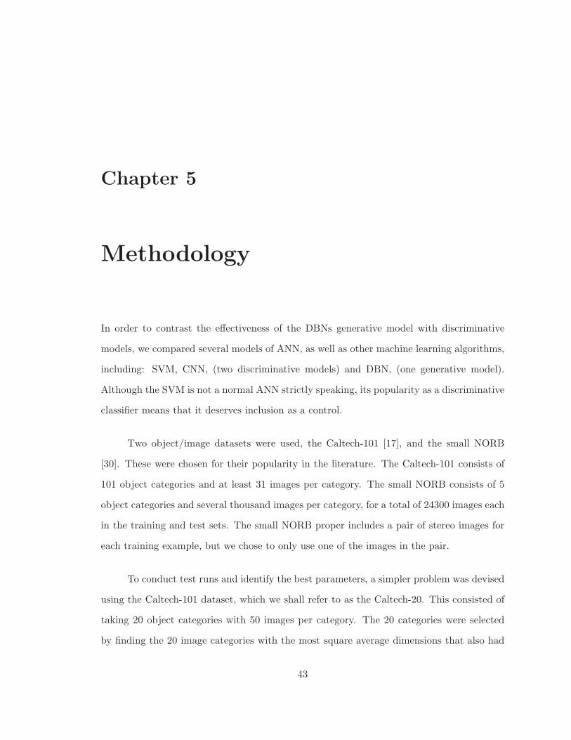
Chapter 5
Methodology
In order to contrast the effectiveness of the DBNs generative model with discriminative
models, we compared several models of ANN, as well as other machine learning algorithms,
including: SVM, CNN, (two discriminative models) and DBN, (one generative model).
Although the SVM is not a normal ANN strictly speaking, its popularity as a discriminative
classifier means that it deserves inclusion as a control.
Two object/image datasets were used, the Caltech-101 [17], and the small NORB
[30]. These were chosen for their popularity in the literature. The Caltech-101 consists of
101 object categories and at least 31 images per category. The small NORB consists of 5
object categories and several thousand images per category, for a total of 24300 images each
in the training and test sets. The small NORB proper includes a pair of stereo images for
each training example, but we chose to only use one of the images in the pair.
To conduct test runs and identify the best parameters, a simpler problem was devised
using the Caltech-101 dataset, which we shall refer to as the Caltech-20. This consisted of
taking 20 object categories with 50 images per category. The 20 categories were selected
by finding the 20 image categories with the most square average dimensions that also had
43
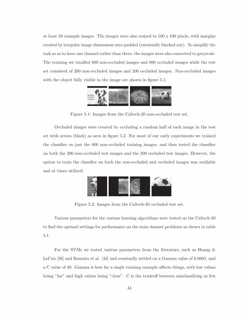
at least 50 example images. The images were also resized to 100 x 100 pixels, with margins
created by irregular image dimensions zero-padded (essentially blacked out). To simplify the
task so as to have one channel rather than three, the images were also converted to greyscale.
The training set totalled 800 non-occluded images and 800 occluded images while the test
set consisted of 200 non-occluded images and 200 occluded images. Non-occluded images
with the object fully visible in the image are shown in figure 5.1.
Figure 5.1: Images from the Caltech-20 non-occluded test set.
Occluded images were created by occluding a random half of each image in the test
set with zeroes (black) as seen in figure 5.2. For most of our early experiments we trained
the classifier on just the 800 non-occluded training images, and then tested the classifier
on both the 200 non-occluded test images and the 200 occluded test images. However, the
option to train the classifier on both the non-occluded and occluded images was available
and at times utilized.
Figure 5.2: Images from the Caltech-20 occluded test set.
Various parameters for the various learning algorithms were tested on the Caltech-20
to find the optimal settings for performance on the main dataset problems as shown in table
5.1.
For the SVMs we tested various parameters from the literature, such as Huang &
LeCun [26] and Ranzato et al. [43] and eventually settled on a Gamma value of 0.0005, and
a C value of 40. Gamma is how far a single training example affects things, with low values
being ”far” and high values being ”close”. C is the tradeoff between misclassifying as few
44

Table 5.1: Results of experiments with SVM on the Caltech-20 to determine best parameterconfiguration.
SVM Selection Parameters Accuracy on RAW TestCalled Source Version Gamma C Training Non-Occluded OccludedSVM1 Default 0.0001 1 0.359 0.315 0.130SVM2 Ranzato et al. 5.6E-07 2100 0.726 0.320 0.130SVM3 Huang & LeCun SVM 0.0001 40 0.966 0.370 0.185SVM4 Huang & LeCun SVM/CNN 0.2 1 1.000 0.080 0.070
Huang & LeCun SVM 0.0005 40 1.000 0.380 0.135Note: Configurations mainly based on papers in the literature.
training samples as possible (high C) and a smooth decision surface (low C). For code for
the SVMs, we used the library “LIBSVM” by Chih-Chung Chang and Chih-Jen Lin from
the National Taiwan University [7].
For the CNN, Sirotenko’s Matlab library “CNN Convolutional neural network class”
(http://www.mathworks.com/matlabcentral/fileexchange/24291-cnn-convolutional-
neural-network-class) was used and modified extensively to serve our purposes. Using
the method and equations from Chapter 3, we can determine the dimensions of each layer for
the Caltech-20 as seen in table 5.2, where S, C and F represent convolutional, subsampling
and fully connected layers, respectively.
Table 5.2: The architecture of the CNN used on the Caltech-20.
Layer Nodes k or r Feature MapsConnections
Actual Theoretical
S1 100x100C2 96x96 5 8 200 1843200S3 24x24 4 8 8 73728C4 20x20 5 32 6400 2560000S5 5x5 4 32 32 12800C6 1x1 5 128 102400 102400F1 512 1 65536 33554432F2 20 1 10240 204800
Total Connections: 184816 38351360
Note: Connections are raw weights excluding biases.
Similarly, the architecture for the CNN on the Caltech-101 dataset can also be engi-
neered as shown in table 5.3.
45
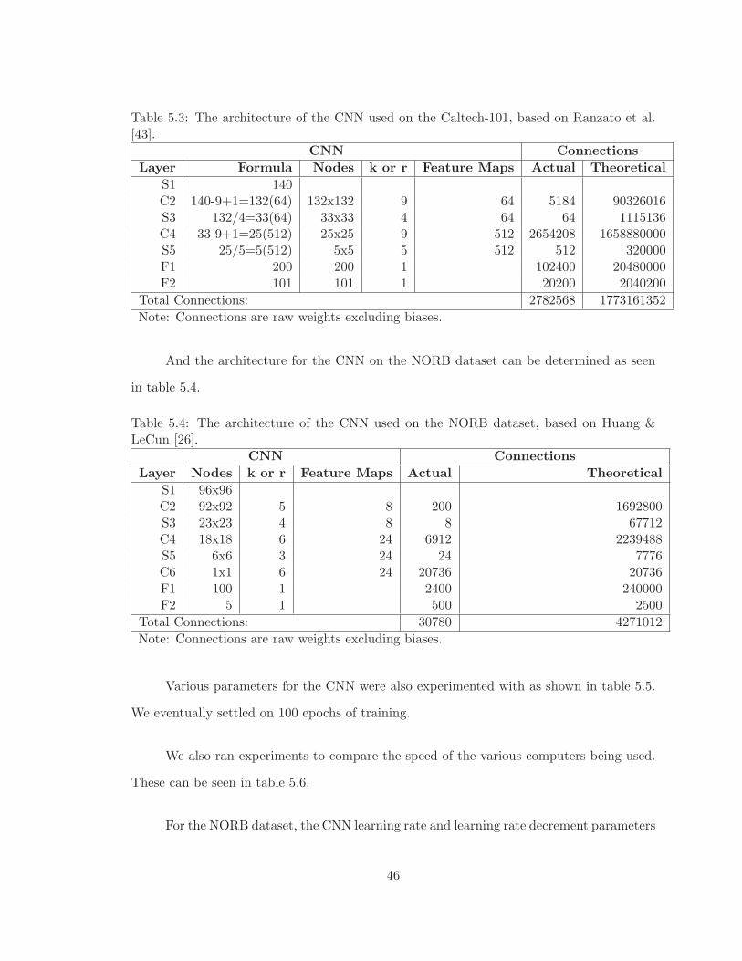
Table 5.3: The architecture of the CNN used on the Caltech-101, based on Ranzato et al.[43].
CNN Connections
Layer Formula Nodes k or r Feature Maps Actual Theoretical
S1 140C2 140-9+1=132(64) 132x132 9 64 5184 90326016S3 132/4=33(64) 33x33 4 64 64 1115136C4 33-9+1=25(512) 25x25 9 512 2654208 1658880000S5 25/5=5(512) 5x5 5 512 512 320000F1 200 200 1 102400 20480000F2 101 101 1 20200 2040200
Total Connections: 2782568 1773161352
Note: Connections are raw weights excluding biases.
And the architecture for the CNN on the NORB dataset can be determined as seen
in table 5.4.
Table 5.4: The architecture of the CNN used on the NORB dataset, based on Huang &LeCun [26].
CNN Connections
Layer Nodes k or r Feature Maps Actual Theoretical
S1 96x96C2 92x92 5 8 200 1692800S3 23x23 4 8 8 67712C4 18x18 6 24 6912 2239488S5 6x6 3 24 24 7776C6 1x1 6 24 20736 20736F1 100 1 2400 240000F2 5 1 500 2500
Total Connections: 30780 4271012
Note: Connections are raw weights excluding biases.
Various parameters for the CNN were also experimented with as shown in table 5.5.
We eventually settled on 100 epochs of training.
We also ran experiments to compare the speed of the various computers being used.
These can be seen in table 5.6.
For the NORB dataset, the CNN learning rate and learning rate decrement parameters
46
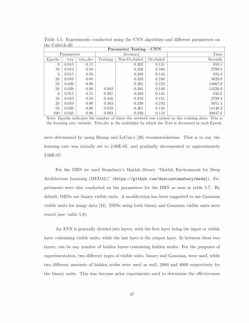
Table 5.5: Experiments conducted using the CNN algorithm and different parameters onthe Caltech-20.
Parameter Testing - CNNParameters Accuracy Time
Epochs teta teta dec Training Non-Occluded Occluded Seconds3 0.015 0.15 0.302 0.131 859.110 0.010 0.50 0.326 0.160 2799.53 0.015 0.50 0.288 0.143 834.420 0.010 0.80 0.328 0.180 5629.850 0.020 0.90 0.361 0.152 14067.950 0.020 0.90 0.943 0.385 0.140 14226.93 0.015 0.15 0.381 0.288 0.145 832.610 0.010 0.50 0.416 0.310 0.151 2799.420 0.010 0.80 0.563 0.338 0.192 5651.450 0.020 0.90 0.919 0.361 0.145 14146.3
100 0.040 0.90 0.983 0.330 0.118 28647.0Note: Epochs indicates the number of times the network was trained on the training data. Teta isthe learning rate variable. Teta dec is the multiplier by which the Teta is decreased in each Epoch.
were determined by using Huang and LeCun’s [26] recommendations. That is to say, the
learning rate was initially set to 2.00E-05, and gradually decremented to approximately
2.00E-07.
For the DBN we used Stansbury’s Matlab library “Matlab Environment for Deep
Architecture Learning (MEDAL)” (https://github.com/dustinstansbury/medal). Ex-
periments were also conducted on the parameters for the DBN as seen in table 5.7. By
default, DBNs use binary visible units. A modification has been suggested to use Gaussian
visible units for image data [24]. DBNs using both binary and Gaussian visible units were
tested (see: table 5.8).
An ANN is generally divided into layers, with the first layer being the input or visible
layer containing visible units, while the last layer is the output layer. In between these two
layers, can be any number of hidden layers containing hidden nodes. For the purposes of
experimentation, two different types of visible units, binary and Gaussian, were used, while
two different amounts of hidden nodes were used as well, 2000 and 4000 respectively for
the binary units. This was because prior experiments used to determine the effectiveness
47
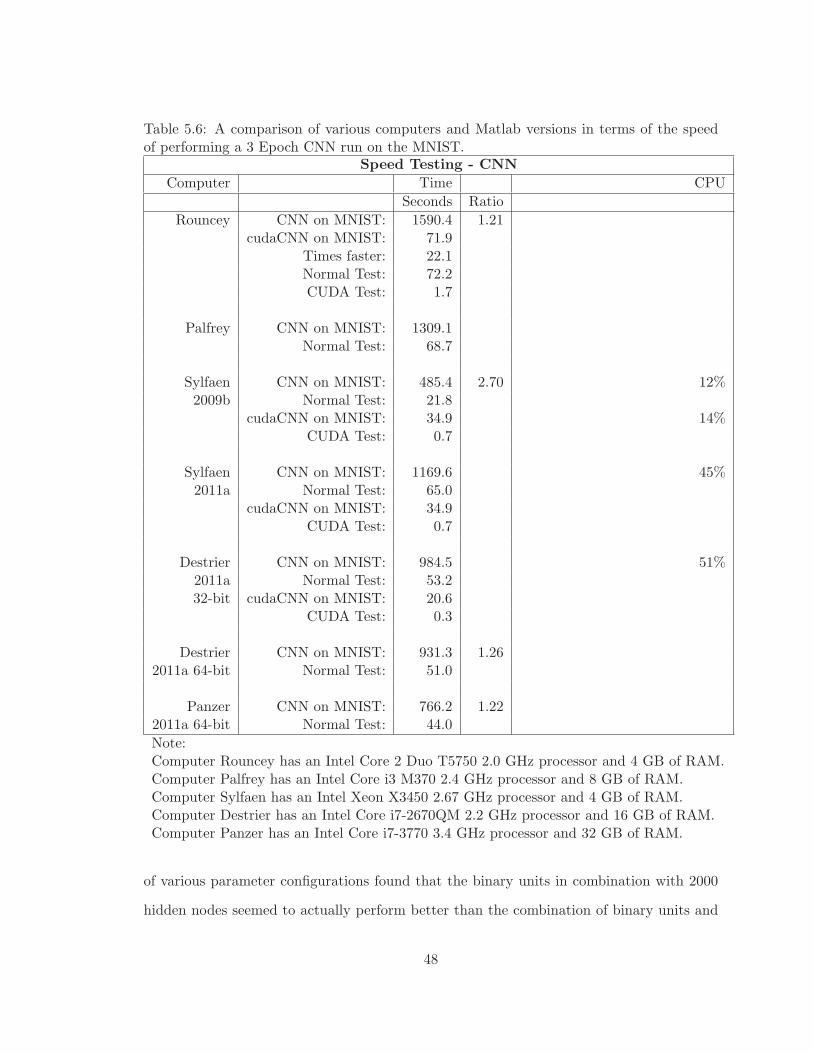
Table 5.6: A comparison of various computers and Matlab versions in terms of the speedof performing a 3 Epoch CNN run on the MNIST.
Speed Testing - CNN
Computer Time CPU
Seconds Ratio
Rouncey CNN on MNIST: 1590.4 1.21cudaCNN on MNIST: 71.9
Times faster: 22.1Normal Test: 72.2CUDA Test: 1.7
Palfrey CNN on MNIST: 1309.1Normal Test: 68.7
Sylfaen CNN on MNIST: 485.4 2.70 12%2009b Normal Test: 21.8
cudaCNN on MNIST: 34.9 14%CUDA Test: 0.7
Sylfaen CNN on MNIST: 1169.6 45%2011a Normal Test: 65.0
cudaCNN on MNIST: 34.9CUDA Test: 0.7
Destrier CNN on MNIST: 984.5 51%2011a Normal Test: 53.232-bit cudaCNN on MNIST: 20.6
CUDA Test: 0.3
Destrier CNN on MNIST: 931.3 1.262011a 64-bit Normal Test: 51.0
Panzer CNN on MNIST: 766.2 1.222011a 64-bit Normal Test: 44.0
Note:Computer Rouncey has an Intel Core 2 Duo T5750 2.0 GHz processor and 4 GB of RAM.Computer Palfrey has an Intel Core i3 M370 2.4 GHz processor and 8 GB of RAM.Computer Sylfaen has an Intel Xeon X3450 2.67 GHz processor and 4 GB of RAM.Computer Destrier has an Intel Core i7-2670QM 2.2 GHz processor and 16 GB of RAM.Computer Panzer has an Intel Core i7-3770 3.4 GHz processor and 32 GB of RAM.
of various parameter configurations found that the binary units in combination with 2000
hidden nodes seemed to actually perform better than the combination of binary units and
48

4000 hidden nodes, which was different than expected. Gaussian units on the other hand,
showed greater effectiveness at 4000 hidden nodes, than at 2000 hidden nodes, which was
expected. For this reason, we tested multiple configurations as shown. The original raw
data can be found in Appendix A.
For simplicity, we can refer to these configurations as B-2000 for binary visible units
and 2000 hidden nodes, B-4000 for binary visible units and 4000 hidden nodes, and G-4000
for Gaussian visible units and 4000 hidden nodes.
The speed of various machines was also tested as shown in table 5.9, table 5.10, and
table 5.11. These also showed that the time taken to run each network is proportional to
the number of hidden units, and to a lesser extent the number of layers of the network. Also
confirmed was that it appeared that two layer DBNs tended to have the best performance.
The newer versions of Matlab also had a slight performance boost over the older versions.
In addition, a version of the DBN library was modified to test the effect of sparsity
on the performance of the network as shown in table 5.12. The method we used to create
sparsity was at the initialization of the network to randomly set some of the hidden node
weight connections to zero using a randomized matrix of ones and zeroes. The results of this
experiment show that added hard-wired randomized sparsity appears to actually decrease
the performance of the network. As such, this version of the network was discarded and
not used in further experiments.
As previously indicated, the amount of time required to run these neural network
simulations is considerable. One way to improve temporal performance is to implement
these neural networks such that they are able to use the GPU of certain video cards rather
than merely the CPU of a given machine. Nvidia video cards in particular have a parallel
computing platform called CUDA that can take full advantage of the many cores on a
typical video card to greatly accelerate parallel computing tasks. ANNs are quite parallel
49

Table
5.7:Theresultsof
experim
ents
doneto
test
theparametersforvariousconfigurationsofDBNs,
ontheCaltech-20.
Para
meterTesting-DBN
Para
meters
Accuracy
Layers
Hidden
Epochs
Anneal
Learning
weigh
tdecay
eta
Momentum
BatchSize
Training
Non-O
ccluded
Occluded
21000
50no
default
0.10
100
0.271
0.154
21000
50no
CD
0.259
0.169
21000
50no
SML
0.094
0.094
21000
50yes
default
0.261
0.167
21000
100
no
default
0.263
0.166
21000
200
no
default
0.254
0.165
21000
50no
default
TRUE
0.266
0.166
21000
50no
default
0.20
0.261
0.181
21000
50no
default
0.50
0.219
0.152
21000
50no
default
0.01
0.180
0.145
21000
100
no
default
0.20
0.258
0.164
21000
100
no
default
0.05
0.268
0.174
21000
50no
default
0.05
0.219
0.177
21000
50no
default
0.10
0.9
0.212
0.167
21000
50no
default
0.10
0.1
0.281
0.243
0.168
21000
50no
default
0.10
0.315
0.259
0.177
21000
50no
default
0.10
20
0.367
0.255
0.173
21000
50no
default
0.10
10
0.355
0.231
0.142
22000
50no
default
0.10
100
0.393
0.305
0.160
22000
100
no
default
0.10
100
0.409
0.310
0.180
Note:Layersindicatesthenumber
ofRBMsin
theDBN.Hidden
indicatesthenumber
ofhidden
nodes
per
layer.
Epochsindicatesthe
number
oftimes
thenetwork
wastrained
onthetrainingdata.Annealindicateswhether
ornotSim
ulatedAnnealingwasused.Learning
indicatesthetypelearningalgorithm
used,either
ContrastiveDivergence
orStochastic
Maxim
um
Likelihood(SML),
withthedefault
being
ContrastiveDivergence.Weightdecay
indicateswhether
ornotweightdecay
wasused.Eta
indicatesthelearningrate
parameter.Momentum
indicatestheparameter
formomentum.BatchSizeindicatesthenumber
ofsamplesin
each
batchfedto
thenetwork
duringlearning.
50
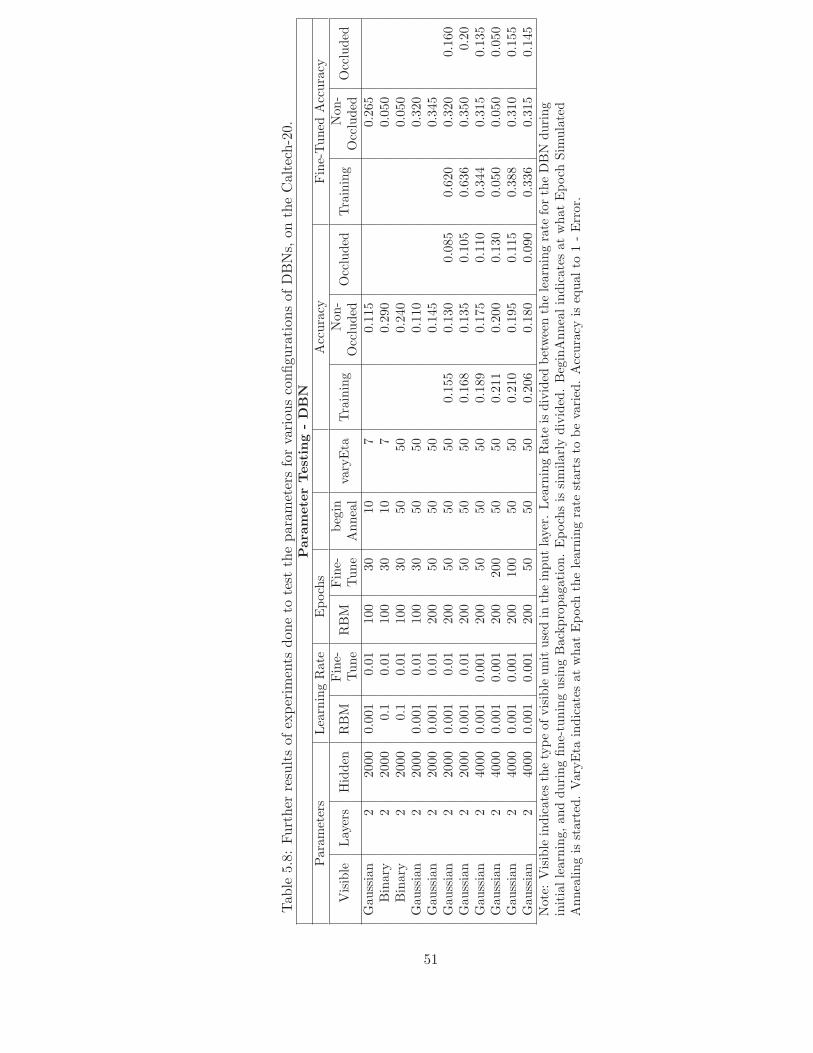
Tab
le5.8:Further
resultsof
experim
ents
doneto
test
theparametersforvariousconfigurationsofDBNs,
ontheCaltech-20.
Para
meterTesting-DBN
Parameters
LearningRate
Epochs
Accuracy
Fine-Tuned
Accuracy
Visible
Layers
Hidden
RBM
Fine-
RBM
Fine-
begin
varyEta
Training
Non-
Occluded
Training
Non-
Occluded
Tune
Tune
Anneal
Occluded
Occluded
Gaussian
22000
0.001
0.01
100
3010
70.115
0.265
Binary
22000
0.1
0.01
100
3010
70.290
0.050
Binary
22000
0.1
0.01
100
3050
500.240
0.050
Gaussian
22000
0.001
0.01
100
3050
500.110
0.320
Gaussian
22000
0.001
0.01
200
5050
500.145
0.345
Gaussian
22000
0.001
0.01
200
5050
500.155
0.130
0.085
0.620
0.320
0.160
Gaussian
22000
0.001
0.01
200
5050
500.168
0.135
0.105
0.636
0.350
0.20
Gaussian
24000
0.001
0.001
200
5050
500.189
0.175
0.110
0.344
0.315
0.135
Gaussian
24000
0.001
0.001
200
200
5050
0.211
0.200
0.130
0.050
0.050
0.050
Gaussian
24000
0.001
0.001
200
100
5050
0.210
0.195
0.115
0.388
0.310
0.155
Gaussian
24000
0.001
0.001
200
5050
500.206
0.180
0.090
0.336
0.315
0.145
Note:Visible
indicatesthetypeofvisible
unitusedin
theinputlayer.LearningRate
isdivided
betweenthelearningrate
fortheDBN
during
initiallearning,andduringfine-tuningusingBackpropagation.Epochsissimilarlydivided.BeginAnnealindicatesat
whatEpoch
Sim
ulated
Annealingis
started.VaryEta
indicatesat
whatEpoch
thelearningrate
startsto
bevaried.Accuracy
isequalto
1-Error.
51

Table 5.9: Early results of experiments done to test the speed of various configurations ofDBNs, on the Caltech-20 using the old or Rouncey laptop computer.
Caltech-20: DBN
Parameters AccuracyTime(s)
Layers Units Non-Occluded Occluded
1 100 0.160 0.135-0.200 91.82 100 0.195 0.130 91.53 100 0.155 0.1104 100 0.175 0.150 94.71 200 0.215 0.125 134.22 200 0.235 0.170 135.83 200 0.165 0.1704 200 0.190 0.165 142.81 500 0.190 0.140 260.22 500 0.245 0.165 282.93 500 0.245 0.1504 500 0.180 0.195 306.51 1000 0.260 0.140 469.52 1000 0.265 0.175 521.33 1000 0.155 0.1554 1000 0.170 0.110 628.91 2000 0.265 0.1502 2000 0.280 0.190 1075.72 500-1000 0.225 0.200 305.12 1000-500 0.245 0.180 499.7
Note: Layers indicates the number of RBMs used in the DBN. Units indicates the numberof hidden units in each RBM.
in nature, and thus quite amenable to this. However, the libraries we used initially were not
written in such a way as to be able to take advantage of CUDA. In order to find an effective
alternative, we turned to the Python-based Theano library (http://deeplearning.net/
software/theano/) [4]. While we were able to find appropriate Deep Learning Python
scripts for the CNN and DBN, their implementation was not as advanced as the Matlab-
based libraries we were already using. In particular, the DBN script did not implement
Gaussian visible units. Alas, while it would have been possible to implement these ourselves,
it would have required additional time and effort, and as it was already relatively late in
the term, it was decided to stick with our working Matlab implementations. Perhaps in
the future, for work beyond this thesis, taking advantage of the GPU by using a Theano-
52
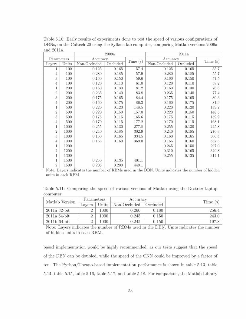
Table 5.10: Early results of experiments done to test the speed of various configurations ofDBNs, on the Caltech-20 using the Sylfaen lab computer, comparing Matlab versions 2009aand 2011a.
2009a 2011aParameters Accuracy
Time (s)Accuracy
Time (s)Layers Units Non-Occluded Occluded Non-Occluded Occluded
1 100 0.125 0.165 57.4 0.125 0.165 55.72 100 0.280 0.185 57.9 0.280 0.185 55.73 100 0.160 0.150 59.6 0.160 0.150 57.54 100 0.120 0.110 61.0 0.120 0.110 58.21 200 0.160 0.130 81.2 0.160 0.130 76.62 200 0.235 0.140 83.8 0.235 0.140 77.43 200 0.175 0.165 84.4 0.175 0.165 80.34 200 0.160 0.175 86.3 0.160 0.175 81.91 500 0.220 0.120 148.5 0.220 0.120 139.72 500 0.220 0.150 157.0 0.220 0.150 148.53 500 0.175 0.115 165.6 0.175 0.115 159.94 500 0.170 0.115 177.2 0.170 0.115 168.11 1000 0.255 0.130 277.8 0.255 0.130 245.82 1000 0.240 0.185 302.9 0.240 0.185 276.33 1000 0.160 0.165 334.5 0.160 0.165 306.44 1000 0.165 0.160 369.0 0.165 0.160 337.51 1200 0.245 0.150 297.02 1200 0.310 0.165 329.81 1300 0.255 0.135 314.11 1500 0.250 0.135 401.12 1500 0.205 0.200 449.1
Note: Layers indicates the number of RBMs used in the DBN. Units indicates the number of hiddenunits in each RBM.
Table 5.11: Comparing the speed of various versions of Matlab using the Destrier laptopcomputer.
Matlab VersionParameters Accuracy
Time (s)Layers Units Non-Occluded Occluded
2011a 32-bit 2 1000 0.260 0.180 256.4
2011a 64-bit 2 1000 0.245 0.150 243.0
2011b 64-bit 2 1000 0.245 0.150 197.8
Note: Layers indicates the number of RBMs used in the DBN. Units indicates the numberof hidden units in each RBM.
based implementation would be highly recommended, as our tests suggest that the speed
of the DBN can be doubled, while the speed of the CNN could be improved by a factor of
ten. The Python/Theano-based implementation performance is shown in table 5.13, table
5.14, table 5.15, table 5.16, table 5.17, and table 5.18. For comparison, the Matlab Library
53
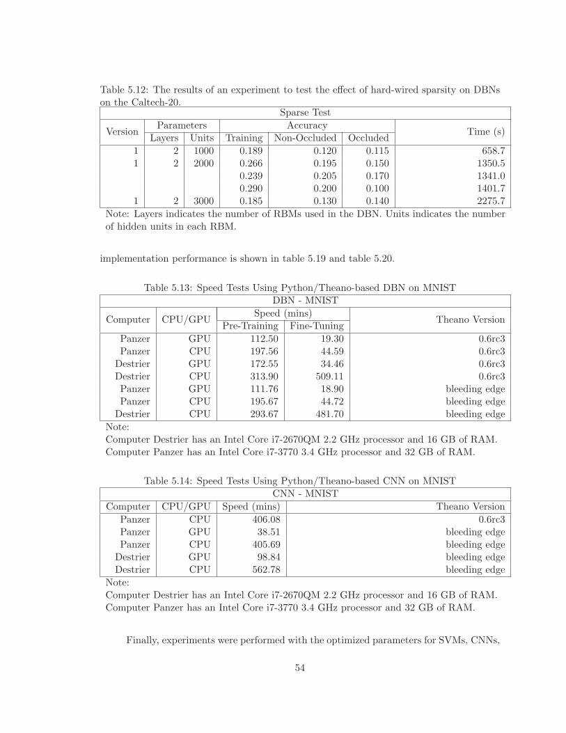
Table 5.12: The results of an experiment to test the effect of hard-wired sparsity on DBNson the Caltech-20.
Sparse Test
VersionParameters Accuracy
Time (s)Layers Units Training Non-Occluded Occluded
1 2 1000 0.189 0.120 0.115 658.71 2 2000 0.266 0.195 0.150 1350.5
0.239 0.205 0.170 1341.00.290 0.200 0.100 1401.7
1 2 3000 0.185 0.130 0.140 2275.7
Note: Layers indicates the number of RBMs used in the DBN. Units indicates the numberof hidden units in each RBM.
implementation performance is shown in table 5.19 and table 5.20.
Table 5.13: Speed Tests Using Python/Theano-based DBN on MNISTDBN - MNIST
Computer CPU/GPUSpeed (mins)
Theano VersionPre-Training Fine-Tuning
Panzer GPU 112.50 19.30 0.6rc3Panzer CPU 197.56 44.59 0.6rc3
Destrier GPU 172.55 34.46 0.6rc3Destrier CPU 313.90 509.11 0.6rc3Panzer GPU 111.76 18.90 bleeding edgePanzer CPU 195.67 44.72 bleeding edge
Destrier CPU 293.67 481.70 bleeding edge
Note:Computer Destrier has an Intel Core i7-2670QM 2.2 GHz processor and 16 GB of RAM.Computer Panzer has an Intel Core i7-3770 3.4 GHz processor and 32 GB of RAM.
Table 5.14: Speed Tests Using Python/Theano-based CNN on MNISTCNN - MNIST
Computer CPU/GPU Speed (mins) Theano Version
Panzer CPU 406.08 0.6rc3Panzer GPU 38.51 bleeding edgePanzer CPU 405.69 bleeding edge
Destrier GPU 98.84 bleeding edgeDestrier CPU 562.78 bleeding edge
Note:Computer Destrier has an Intel Core i7-2670QM 2.2 GHz processor and 16 GB of RAM.Computer Panzer has an Intel Core i7-3770 3.4 GHz processor and 32 GB of RAM.
Finally, experiments were performed with the optimized parameters for SVMs, CNNs,
54
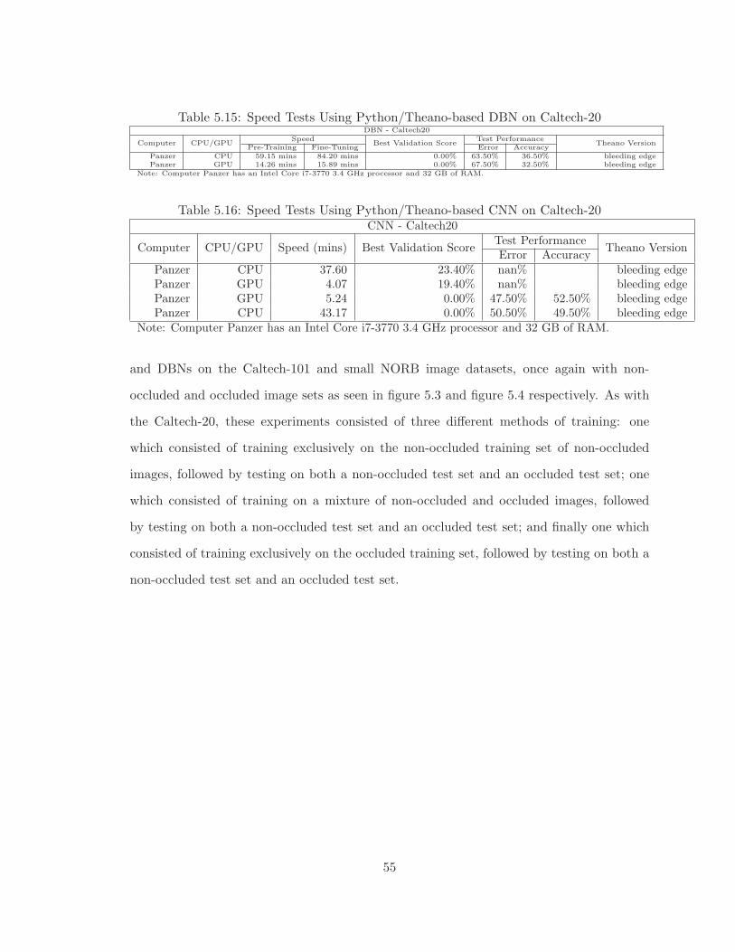
Table 5.15: Speed Tests Using Python/Theano-based DBN on Caltech-20DBN - Caltech20
Computer CPU/GPUSpeed
Best Validation ScoreTest Performance
Theano VersionPre-Training Fine-Tuning Error Accuracy
Panzer CPU 59.15 mins 84.20 mins 0.00% 63.50% 36.50% bleeding edgePanzer GPU 14.26 mins 15.89 mins 0.00% 67.50% 32.50% bleeding edge
Note: Computer Panzer has an Intel Core i7-3770 3.4 GHz processor and 32 GB of RAM.
Table 5.16: Speed Tests Using Python/Theano-based CNN on Caltech-20CNN - Caltech20
Computer CPU/GPU Speed (mins) Best Validation ScoreTest Performance
Theano VersionError Accuracy
Panzer CPU 37.60 23.40% nan% bleeding edgePanzer GPU 4.07 19.40% nan% bleeding edgePanzer GPU 5.24 0.00% 47.50% 52.50% bleeding edgePanzer CPU 43.17 0.00% 50.50% 49.50% bleeding edge
Note: Computer Panzer has an Intel Core i7-3770 3.4 GHz processor and 32 GB of RAM.
and DBNs on the Caltech-101 and small NORB image datasets, once again with non-
occluded and occluded image sets as seen in figure 5.3 and figure 5.4 respectively. As with
the Caltech-20, these experiments consisted of three different methods of training: one
which consisted of training exclusively on the non-occluded training set of non-occluded
images, followed by testing on both a non-occluded test set and an occluded test set; one
which consisted of training on a mixture of non-occluded and occluded images, followed
by testing on both a non-occluded test set and an occluded test set; and finally one which
consisted of training exclusively on the occluded training set, followed by testing on both a
non-occluded test set and an occluded test set.
55
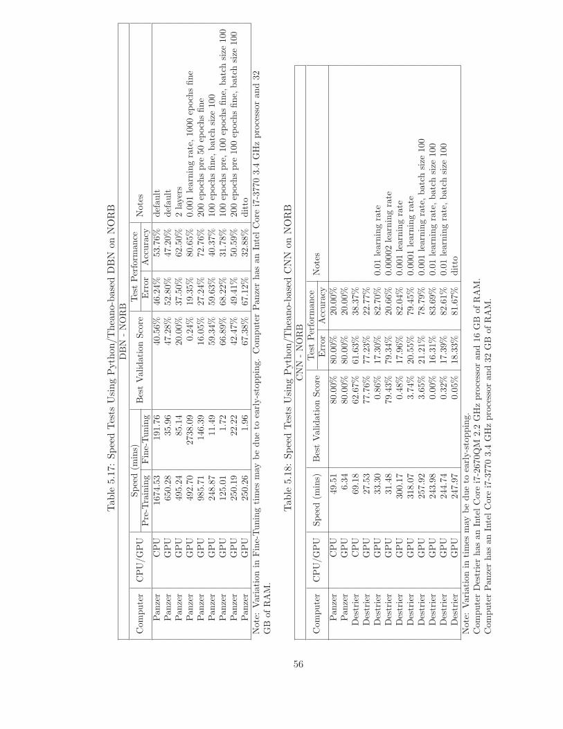
Tab
le5.17:SpeedTests
UsingPython/Theano-basedDBN
onNORB
DBN
-NORB
Computer
CPU/GPU
Speed(m
ins)
BestValidationScore
TestPerform
ance
Notes
Pre-Training
Fine-Tuning
Error
Accuracy
Pan
zer
CPU
1674.53
191.76
40.56%
46.24%
53.76%
default
Pan
zer
GPU
650.28
35.96
47.28%
52.80%
47.20%
default
Pan
zer
GPU
495.24
85.14
20.00%
37.50%
62.50%
2layers
Pan
zer
GPU
492.70
2738.09
0.24%
19.35%
80.65%
0.001learningrate,1000ep
ochsfine
Pan
zer
GPU
985.71
146.39
16.05%
27.24%
72.76%
200ep
ochspre
50ep
ochsfine
Pan
zer
GPU
248.87
11.49
59.34%
59.63%
40.37%
100ep
ochsfine,
batchsize
100
Pan
zer
GPU
125.01
1.72
66.89%
68.22%
31.78%
100ep
ochspre,100ep
ochsfine,
batchsize
100
Pan
zer
GPU
250.19
22.22
42.47%
49.41%
50.59%
200ep
ochspre
100ep
ochsfine,
batchsize
100
Pan
zer
GPU
250.26
1.96
67.38%
67.12%
32.88%
ditto
Note:Variationin
Fine-Tuningtimes
may
bedueto
early-stopping.ComputerPan
zerhasan
IntelCore
i7-37703.4
GHzprocessorand32
GB
ofRAM.
Tab
le5.18:SpeedTests
UsingPython/Theano-basedCNN
onNORB
CNN
-NORB
Computer
CPU/GPU
Speed(m
ins)
BestValidationScore
TestPerform
ance
Notes
Error
Accuracy
Pan
zer
CPU
49.51
80.00%
80.00%
20.00%
Pan
zer
GPU
6.34
80.00%
80.00%
20.00%
Destrier
CPU
69.18
62.67%
61.63%
38.37%
Destrier
GPU
27.53
77.76%
77.23%
22.77%
Destrier
GPU
33.30
0.86%
17.30%
82.70%
0.01learningrate
Destrier
GPU
31.48
79.43%
79.34%
20.66%
0.00002learningrate
Destrier
GPU
300.17
0.48%
17.96%
82.04%
0.001learningrate
Destrier
GPU
318.07
3.74%
20.55%
79.45%
0.0001learningrate
Destrier
GPU
257.92
3.65%
21.21%
78.79%
0.001learningrate,batchsize
100
Destrier
GPU
243.98
0.00%
16.31%
83.69%
0.01learningrate,batchsize
100
Destrier
GPU
244.74
0.32%
17.39%
82.61%
0.01learningrate,batchsize
100
Destrier
GPU
247.97
0.05%
18.33%
81.67%
ditto
Note:Variationin
times
may
bedueto
early-stopping.
ComputerDestrierhasan
IntelCore
i7-2670QM
2.2GHzprocessoran
d16GB
ofRAM.
ComputerPan
zerhasan
IntelCore
i7-37703.4
GHzprocessoran
d32GB
ofRAM.
56
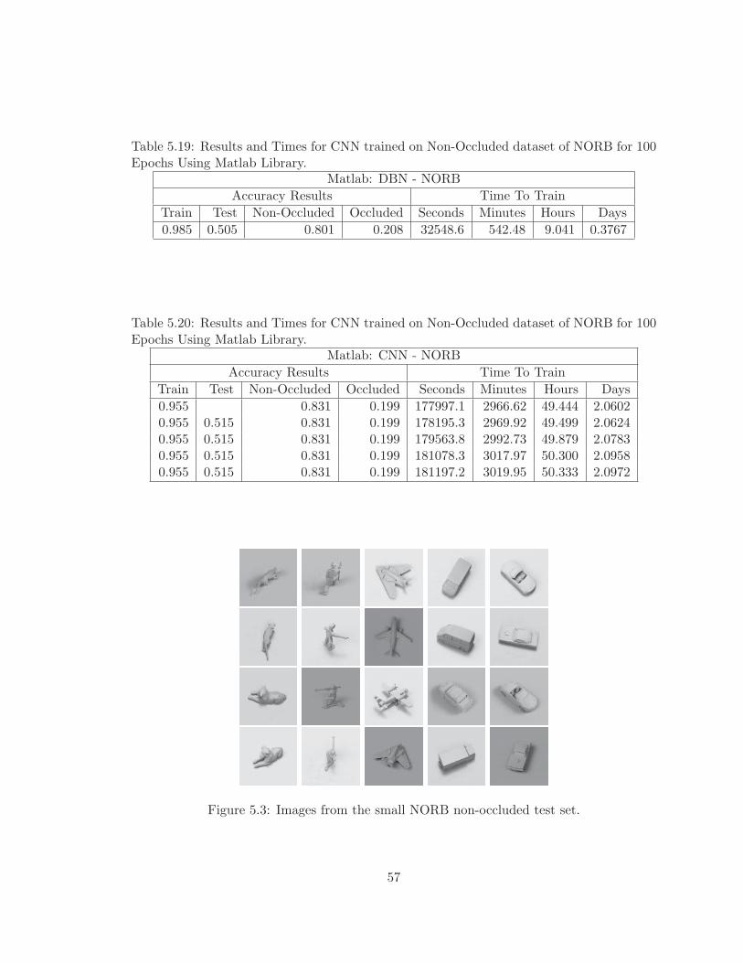
Table 5.19: Results and Times for CNN trained on Non-Occluded dataset of NORB for 100Epochs Using Matlab Library.
Matlab: DBN - NORB
Accuracy Results Time To Train
Train Test Non-Occluded Occluded Seconds Minutes Hours Days
0.985 0.505 0.801 0.208 32548.6 542.48 9.041 0.3767
Table 5.20: Results and Times for CNN trained on Non-Occluded dataset of NORB for 100Epochs Using Matlab Library.
Matlab: CNN - NORB
Accuracy Results Time To Train
Train Test Non-Occluded Occluded Seconds Minutes Hours Days
0.955 0.831 0.199 177997.1 2966.62 49.444 2.06020.955 0.515 0.831 0.199 178195.3 2969.92 49.499 2.06240.955 0.515 0.831 0.199 179563.8 2992.73 49.879 2.07830.955 0.515 0.831 0.199 181078.3 3017.97 50.300 2.09580.955 0.515 0.831 0.199 181197.2 3019.95 50.333 2.0972
Figure 5.3: Images from the small NORB non-occluded test set.
57
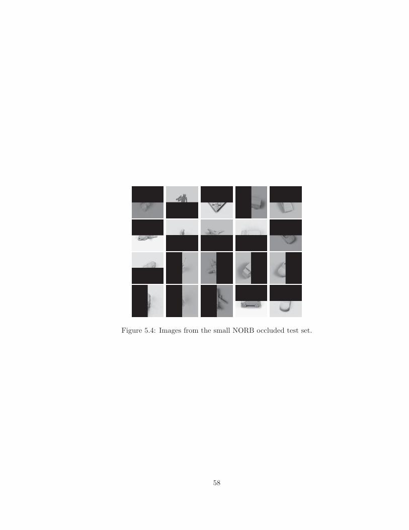
Figure 5.4: Images from the small NORB occluded test set.
58
Chapter 6
Analysis and Results
The performance of machine learning algorithms in recognizing the object in an occluded
image depends on the method of training. The training process can consist of various data
sets, ranging from one made up exclusively of non-occluded images, to one made up exclu-
sively of occluded images, and also various mixtures of the two. The fully trained algorithm
can then be tested in terms of accuracy on both non-occluded images, and occluded images.
A further testing set containing a mixture of non-occluded and occluded images can also
be used.
6.1 Results on NORB
6.1.1 Support Vector Machines
Table 6.1 provides a direct comparison of the non-occluded, occluded, and mixed trained
SVMs. The original raw data can be found in Appendix A. The results show that when the
SVM is trained with only non-occluded training images, its object recognition performance
59
on non-occluded test images is reasonably good (83% accuracy), but the same algorithm
performs poorly on the occluded test images (20% accuracy). On the other hand, when
the SVM is trained with only occluded training images, it performs reasonably well at
object recognition on the occluded test images (69% accuracy), but performs poorly on the
non-occluded test images (20% accuracy).
The results also showed that training the SVM on the mixed data set containing
both non-occluded and occluded images, led it to do well at object recognition on the non-
occluded test images (81% accuracy), on the occluded test images (69% accuracy), and
also on the mixed test images (75% accuracy). These accuracies on the non-occluded test
images are comparable to the SVMs trained on the non-occluded training images (i.e., 81%
vs. 83%). Furthermore, its accuracy on the occluded test images is comparable to the
SVMs trained on the occluded training images (i.e., 69% vs. 69%).
When comparing performance on the mixed test data set, the SVM performed better
if trained with the mixed training data set (75% accuracy), than if it was trained using
the non-occluded training images (51% accuracy), or the occluded training images (45%
accuracy) alone.
When testing the SVM on the same training data set as it was trained on, the accuracy
on the object recognition task was slightly lower when using the mixed training images (97%
accuracy) than if it was trained exclusively on the non-occluded training images (99.9%
accuracy), or exclusively on the occluded training images (99% accuracy). To understand
this, the concept of overfitting must be considered. Overfitting occurs when a learning
algorithm learns to fit itself to the training data, rather than learning the general concept
that it is desired to learn from the training data. In such an instance, the performance on
the test data can actually decrease while accuracy on the original training data continues
to increase. Obviously, performance on the original training data should be better than
performance on previously unseen test data, but it is possible that if the difference between
60
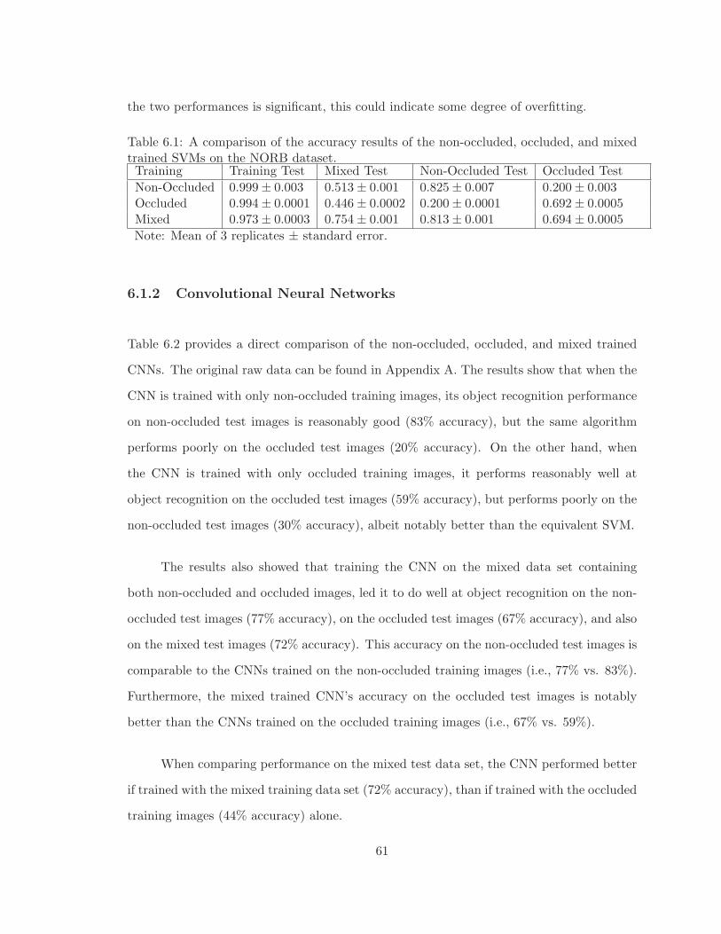
the two performances is significant, this could indicate some degree of overfitting.
Table 6.1: A comparison of the accuracy results of the non-occluded, occluded, and mixedtrained SVMs on the NORB dataset.Training Training Test Mixed Test Non-Occluded Test Occluded Test
Non-Occluded 0.999± 0.003 0.513± 0.001 0.825± 0.007 0.200± 0.003Occluded 0.994± 0.0001 0.446± 0.0002 0.200± 0.0001 0.692± 0.0005Mixed 0.973± 0.0003 0.754± 0.001 0.813± 0.001 0.694± 0.0005
Note: Mean of 3 replicates ± standard error.
6.1.2 Convolutional Neural Networks
Table 6.2 provides a direct comparison of the non-occluded, occluded, and mixed trained
CNNs. The original raw data can be found in Appendix A. The results show that when the
CNN is trained with only non-occluded training images, its object recognition performance
on non-occluded test images is reasonably good (83% accuracy), but the same algorithm
performs poorly on the occluded test images (20% accuracy). On the other hand, when
the CNN is trained with only occluded training images, it performs reasonably well at
object recognition on the occluded test images (59% accuracy), but performs poorly on the
non-occluded test images (30% accuracy), albeit notably better than the equivalent SVM.
The results also showed that training the CNN on the mixed data set containing
both non-occluded and occluded images, led it to do well at object recognition on the non-
occluded test images (77% accuracy), on the occluded test images (67% accuracy), and also
on the mixed test images (72% accuracy). This accuracy on the non-occluded test images is
comparable to the CNNs trained on the non-occluded training images (i.e., 77% vs. 83%).
Furthermore, the mixed trained CNN’s accuracy on the occluded test images is notably
better than the CNNs trained on the occluded training images (i.e., 67% vs. 59%).
When comparing performance on the mixed test data set, the CNN performed better
if trained with the mixed training data set (72% accuracy), than if trained with the occluded
training images (44% accuracy) alone.
61
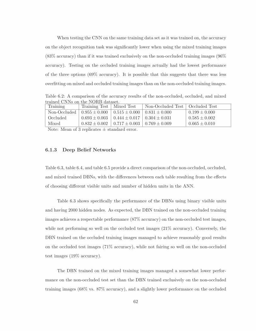
When testing the CNN on the same training data set as it was trained on, the accuracy
on the object recognition task was significantly lower when using the mixed training images
(83% accuracy) than if it was trained exclusively on the non-occluded training images (96%
accuracy). Testing on the occluded training images actually had the lowest performance
of the three options (69% accuracy). It is possible that this suggests that there was less
overfitting on mixed and occluded training images than on the non-occluded training images.
Table 6.2: A comparison of the accuracy results of the non-occluded, occluded, and mixedtrained CNNs on the NORB dataset.Training Training Test Mixed Test Non-Occluded Test Occluded Test
Non-Occluded 0.955± 0.000 0.515± 0.000 0.831± 0.000 0.199± 0.000Occluded 0.693± 0.003 0.444± 0.017 0.304± 0.031 0.585± 0.002Mixed 0.832± 0.002 0.717± 0.003 0.769± 0.009 0.665± 0.010
Note: Mean of 3 replicates ± standard error.
6.1.3 Deep Belief Networks
Table 6.3, table 6.4, and table 6.5 provide a direct comparison of the non-occluded, occluded,
and mixed trained DBNs, with the differences between each table resulting from the effects
of choosing different visible units and number of hidden units in the ANN.
Table 6.3 shows specifically the performance of the DBNs using binary visible units
and having 2000 hidden nodes. As expected, the DBN trained on the non-occluded training
images achieves a respectable performance (87% accuracy) on the non-occluded test images,
while not performing so well on the occluded test images (21% accuracy). Conversely, the
DBN trained on the occluded training images managed to achieve reasonably good results
on the occluded test images (71% accuracy), while not fairing so well on the non-occluded
test images (19% accuracy).
The DBN trained on the mixed training images managed a somewhat lower perfor-
mance on the non-occluded test set than the DBN trained exclusively on the non-occluded
training images (68% vs. 87% accuracy), and a slightly lower performance on the occluded
62
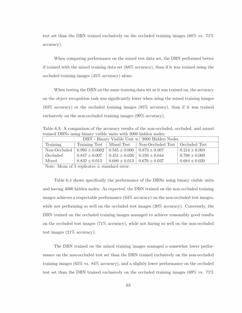
test set than the DBN trained exclusively on the occluded training images (68% vs. 71%
accuracy).
When comparing performance on the mixed test data set, the DBN performed better
if trained with the mixed training data set (68% accuracy), than if it was trained using the
occluded training images (45% accuracy) alone.
When testing the DBN on the same training data set as it was trained on, the accuracy
on the object recognition task was significantly lower when using the mixed training images
(83% accuracy) or the occluded training images (85% accuracy), than if it was trained
exclusively on the non-occluded training images (99% accuracy).
Table 6.3: A comparison of the accuracy results of the non-occluded, occluded, and mixedtrained DBNs using binary visible units with 2000 hidden nodes.
DBN - Binary Visible Unit w/ 2000 Hidden Nodes
Training Training Test Mixed Test Non-Occluded Test Occluded Test
Non-Occluded 0.993± 0.0002 0.545± 0.000 0.873± 0.007 0.214± 0.004Occluded 0.847± 0.007 0.451± 0.026 0.193± 0.044 0.708± 0.009Mixed 0.832± 0.013 0.680± 0.013 0.676± 0.037 0.684± 0.020
Note: Mean of 3 replicates ± standard error.
Table 6.4 shows specifically the performance of the DBNs using binary visible units
and having 4000 hidden nodes. As expected, the DBN trained on the non-occluded training
images achieves a respectable performance (84% accuracy) on the non-occluded test images,
while not performing so well on the occluded test images (20% accuracy). Conversely, the
DBN trained on the occluded training images managed to achieve reasonably good results
on the occluded test images (71% accuracy), while not fairing so well on the non-occluded
test images (21% accuracy).
The DBN trained on the mixed training images managed a somewhat lower perfor-
mance on the non-occluded test set than the DBN trained exclusively on the non-occluded
training images (65% vs. 84% accuracy), and a slightly lower performance on the occluded
test set than the DBN trained exclusively on the occluded training images (69% vs. 71%
63
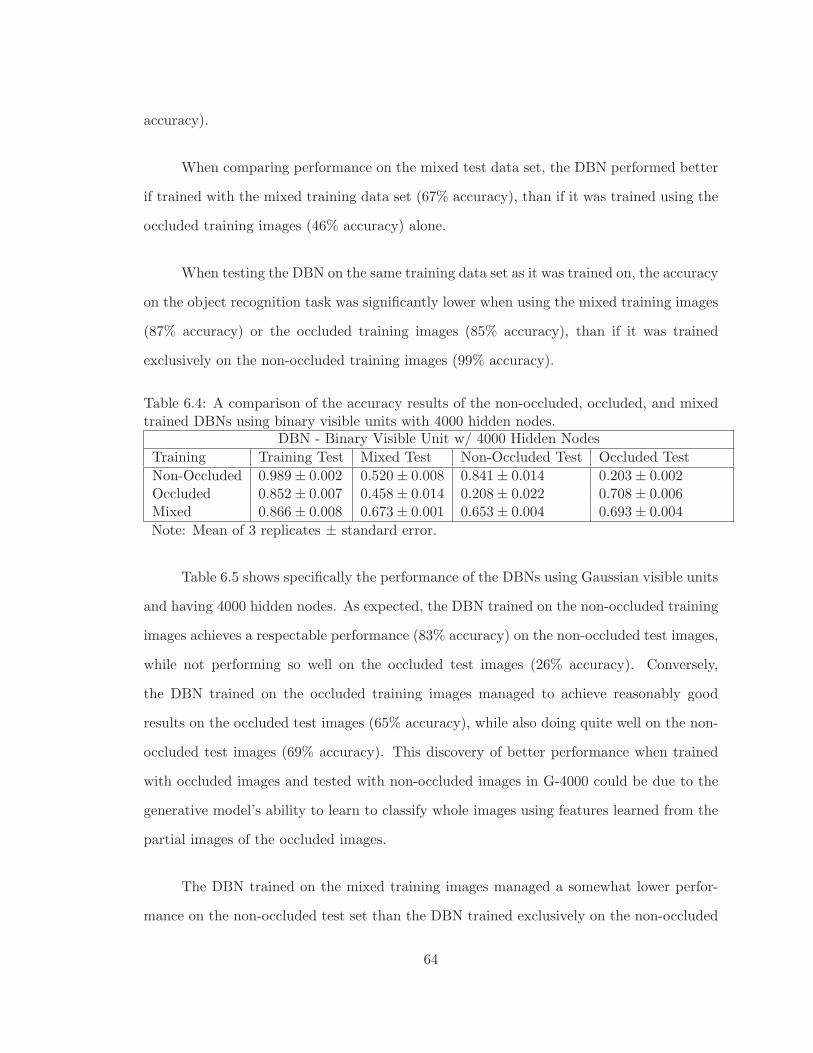
accuracy).
When comparing performance on the mixed test data set, the DBN performed better
if trained with the mixed training data set (67% accuracy), than if it was trained using the
occluded training images (46% accuracy) alone.
When testing the DBN on the same training data set as it was trained on, the accuracy
on the object recognition task was significantly lower when using the mixed training images
(87% accuracy) or the occluded training images (85% accuracy), than if it was trained
exclusively on the non-occluded training images (99% accuracy).
Table 6.4: A comparison of the accuracy results of the non-occluded, occluded, and mixedtrained DBNs using binary visible units with 4000 hidden nodes.
DBN - Binary Visible Unit w/ 4000 Hidden Nodes
Training Training Test Mixed Test Non-Occluded Test Occluded Test
Non-Occluded 0.989± 0.002 0.520± 0.008 0.841± 0.014 0.203± 0.002Occluded 0.852± 0.007 0.458± 0.014 0.208± 0.022 0.708± 0.006Mixed 0.866± 0.008 0.673± 0.001 0.653± 0.004 0.693± 0.004
Note: Mean of 3 replicates ± standard error.
Table 6.5 shows specifically the performance of the DBNs using Gaussian visible units
and having 4000 hidden nodes. As expected, the DBN trained on the non-occluded training
images achieves a respectable performance (83% accuracy) on the non-occluded test images,
while not performing so well on the occluded test images (26% accuracy). Conversely,
the DBN trained on the occluded training images managed to achieve reasonably good
results on the occluded test images (65% accuracy), while also doing quite well on the non-
occluded test images (69% accuracy). This discovery of better performance when trained
with occluded images and tested with non-occluded images in G-4000 could be due to the
generative model’s ability to learn to classify whole images using features learned from the
partial images of the occluded images.
The DBN trained on the mixed training images managed a somewhat lower perfor-
mance on the non-occluded test set than the DBN trained exclusively on the non-occluded
64
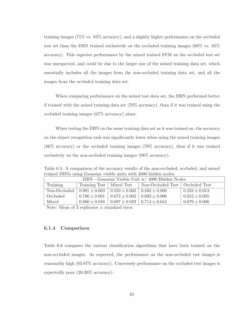
training images (71% vs. 83% accuracy), and a slightly higher performance on the occluded
test set than the DBN trained exclusively on the occluded training images (68% vs. 65%
accuracy). This superior performance by the mixed trained SVM on the occluded test set
was unexpected, and could be due to the larger size of the mixed training data set, which
essentially includes all the images from the non-occluded training data set, and all the
images from the occluded training data set.
When comparing performance on the mixed test data set, the DBN performed better
if trained with the mixed training data set (70% accuracy), than if it was trained using the
occluded training images (67% accuracy) alone.
When testing the DBN on the same training data set as it was trained on, the accuracy
on the object recognition task was significantly lower when using the mixed training images
(86% accuracy) or the occluded training images (79% accuracy), than if it was trained
exclusively on the non-occluded training images (98% accuracy).
Table 6.5: A comparison of the accuracy results of the non-occluded, occluded, and mixedtrained DBNs using Gaussian visible units with 4000 hidden nodes.
DBN - Gaussian Visible Unit w/ 4000 Hidden Nodes
Training Training Test Mixed Test Non-Occluded Test Occluded Test
Non-Occluded 0.981± 0.003 0.550± 0.002 0.832± 0.006 0.258± 0.013Occluded 0.786± 0.001 0.673± 0.002 0.693± 0.006 0.652± 0.005Mixed 0.860± 0.016 0.697± 0.023 0.714± 0.044 0.679± 0.006
Note: Mean of 3 replicates ± standard error.
6.1.4 Comparison
Table 6.6 compares the various classification algorithms that have been trained on the
non-occluded images. As expected, the performance on the non-occluded test images is
reasonably high (83-87% accuracy). Conversely performance on the occluded test images is
expectedly poor (20-26% accuracy).
65
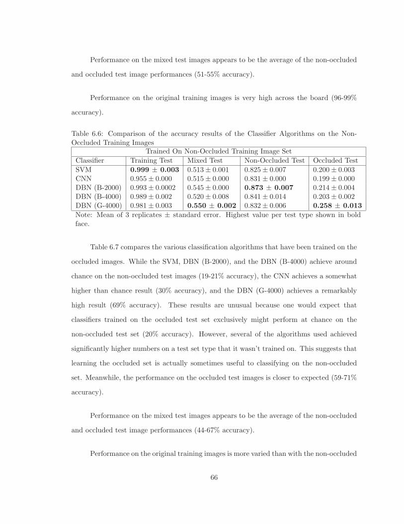
Performance on the mixed test images appears to be the average of the non-occluded
and occluded test image performances (51-55% accuracy).
Performance on the original training images is very high across the board (96-99%
accuracy).
Table 6.6: Comparison of the accuracy results of the Classifier Algorithms on the Non-Occluded Training Images
Trained On Non-Occluded Training Image Set
Classifier Training Test Mixed Test Non-Occluded Test Occluded Test
SVM 0.999 ± 0.003 0.513± 0.001 0.825± 0.007 0.200± 0.003CNN 0.955± 0.000 0.515± 0.000 0.831± 0.000 0.199± 0.000DBN (B-2000) 0.993± 0.0002 0.545± 0.000 0.873 ± 0.007 0.214± 0.004DBN (B-4000) 0.989± 0.002 0.520± 0.008 0.841± 0.014 0.203± 0.002DBN (G-4000) 0.981± 0.003 0.550 ± 0.002 0.832± 0.006 0.258 ± 0.013
Note: Mean of 3 replicates ± standard error. Highest value per test type shown in boldface.
Table 6.7 compares the various classification algorithms that have been trained on the
occluded images. While the SVM, DBN (B-2000), and the DBN (B-4000) achieve around
chance on the non-occluded test images (19-21% accuracy), the CNN achieves a somewhat
higher than chance result (30% accuracy), and the DBN (G-4000) achieves a remarkably
high result (69% accuracy). These results are unusual because one would expect that
classifiers trained on the occluded test set exclusively might perform at chance on the
non-occluded test set (20% accuracy). However, several of the algorithms used achieved
significantly higher numbers on a test set type that it wasn’t trained on. This suggests that
learning the occluded set is actually sometimes useful to classifying on the non-occluded
set. Meanwhile, the performance on the occluded test images is closer to expected (59-71%
accuracy).
Performance on the mixed test images appears to be the average of the non-occluded
and occluded test image performances (44-67% accuracy).
Performance on the original training images is more varied than with the non-occluded
66
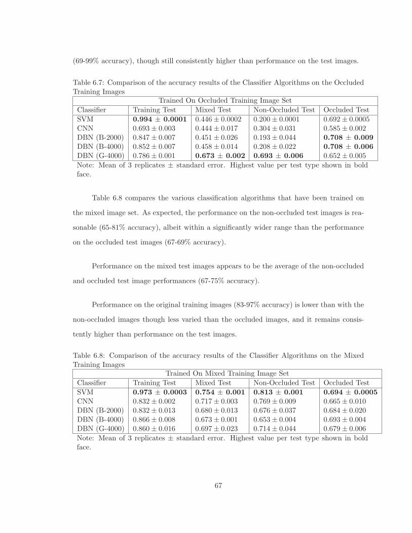
(69-99% accuracy), though still consistently higher than performance on the test images.
Table 6.7: Comparison of the accuracy results of the Classifier Algorithms on the OccludedTraining Images
Trained On Occluded Training Image Set
Classifier Training Test Mixed Test Non-Occluded Test Occluded Test
SVM 0.994 ± 0.0001 0.446± 0.0002 0.200± 0.0001 0.692± 0.0005CNN 0.693± 0.003 0.444± 0.017 0.304± 0.031 0.585± 0.002DBN (B-2000) 0.847± 0.007 0.451± 0.026 0.193± 0.044 0.708 ± 0.009DBN (B-4000) 0.852± 0.007 0.458± 0.014 0.208± 0.022 0.708 ± 0.006DBN (G-4000) 0.786± 0.001 0.673 ± 0.002 0.693 ± 0.006 0.652± 0.005
Note: Mean of 3 replicates ± standard error. Highest value per test type shown in boldface.
Table 6.8 compares the various classification algorithms that have been trained on
the mixed image set. As expected, the performance on the non-occluded test images is rea-
sonable (65-81% accuracy), albeit within a significantly wider range than the performance
on the occluded test images (67-69% accuracy).
Performance on the mixed test images appears to be the average of the non-occluded
and occluded test image performances (67-75% accuracy).
Performance on the original training images (83-97% accuracy) is lower than with the
non-occluded images though less varied than the occluded images, and it remains consis-
tently higher than performance on the test images.
Table 6.8: Comparison of the accuracy results of the Classifier Algorithms on the MixedTraining Images
Trained On Mixed Training Image Set
Classifier Training Test Mixed Test Non-Occluded Test Occluded Test
SVM 0.973 ± 0.0003 0.754 ± 0.001 0.813 ± 0.001 0.694 ± 0.0005CNN 0.832± 0.002 0.717± 0.003 0.769± 0.009 0.665± 0.010DBN (B-2000) 0.832± 0.013 0.680± 0.013 0.676± 0.037 0.684± 0.020DBN (B-4000) 0.866± 0.008 0.673± 0.001 0.653± 0.004 0.693± 0.004DBN (G-4000) 0.860± 0.016 0.697± 0.023 0.714± 0.044 0.679± 0.006
Note: Mean of 3 replicates ± standard error. Highest value per test type shown in boldface.
67
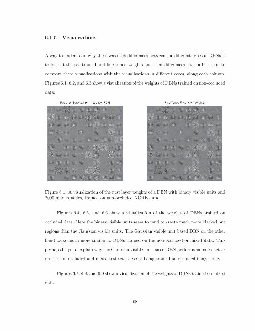
6.1.5 Visualizations
A way to understand why there was such differences between the different types of DBNs is
to look at the pre-trained and fine-tuned weights and their differences. It can be useful to
compare these visualizations with the visualizations in different cases, along each column.
Figures 6.1, 6.2, and 6.3 show a visualization of the weights of DBNs trained on non-occluded
data.
Figure 6.1: A visualization of the first layer weights of a DBN with binary visible units and2000 hidden nodes, trained on non-occluded NORB data.
Figures 6.4, 6.5, and 6.6 show a visualization of the weights of DBNs trained on
occluded data. Here the binary visible units seem to tend to create much more blacked out
regions than the Gaussian visible units. The Gaussian visible unit based DBN on the other
hand looks much more similar to DBNs trained on the non-occluded or mixed data. This
perhaps helps to explain why the Gaussian visible unit based DBN performs so much better
on the non-occluded and mixed test sets, despite being trained on occluded images only.
Figures 6.7, 6.8, and 6.9 show a visualization of the weights of DBNs trained on mixed
data.
68
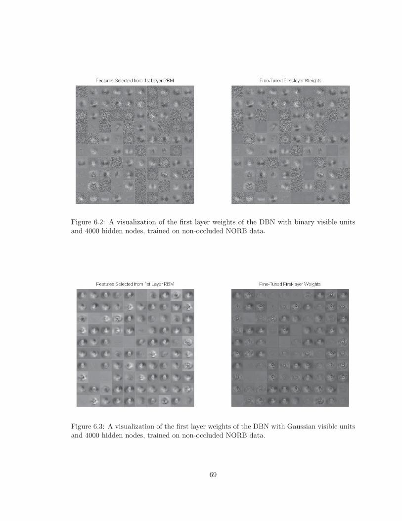
Figure 6.2: A visualization of the first layer weights of the DBN with binary visible unitsand 4000 hidden nodes, trained on non-occluded NORB data.
Figure 6.3: A visualization of the first layer weights of the DBN with Gaussian visible unitsand 4000 hidden nodes, trained on non-occluded NORB data.
69
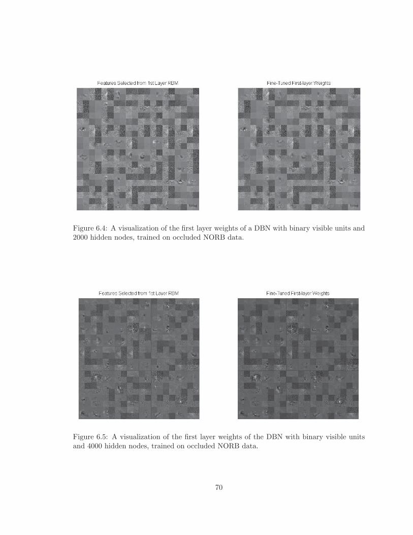
Figure 6.4: A visualization of the first layer weights of a DBN with binary visible units and2000 hidden nodes, trained on occluded NORB data.
Figure 6.5: A visualization of the first layer weights of the DBN with binary visible unitsand 4000 hidden nodes, trained on occluded NORB data.
70
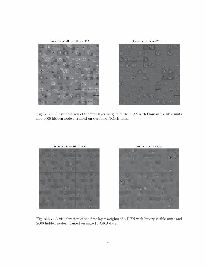
Figure 6.6: A visualization of the first layer weights of the DBN with Gaussian visible unitsand 4000 hidden nodes, trained on occluded NORB data.
Figure 6.7: A visualization of the first layer weights of a DBN with binary visible units and2000 hidden nodes, trained on mixed NORB data.
71
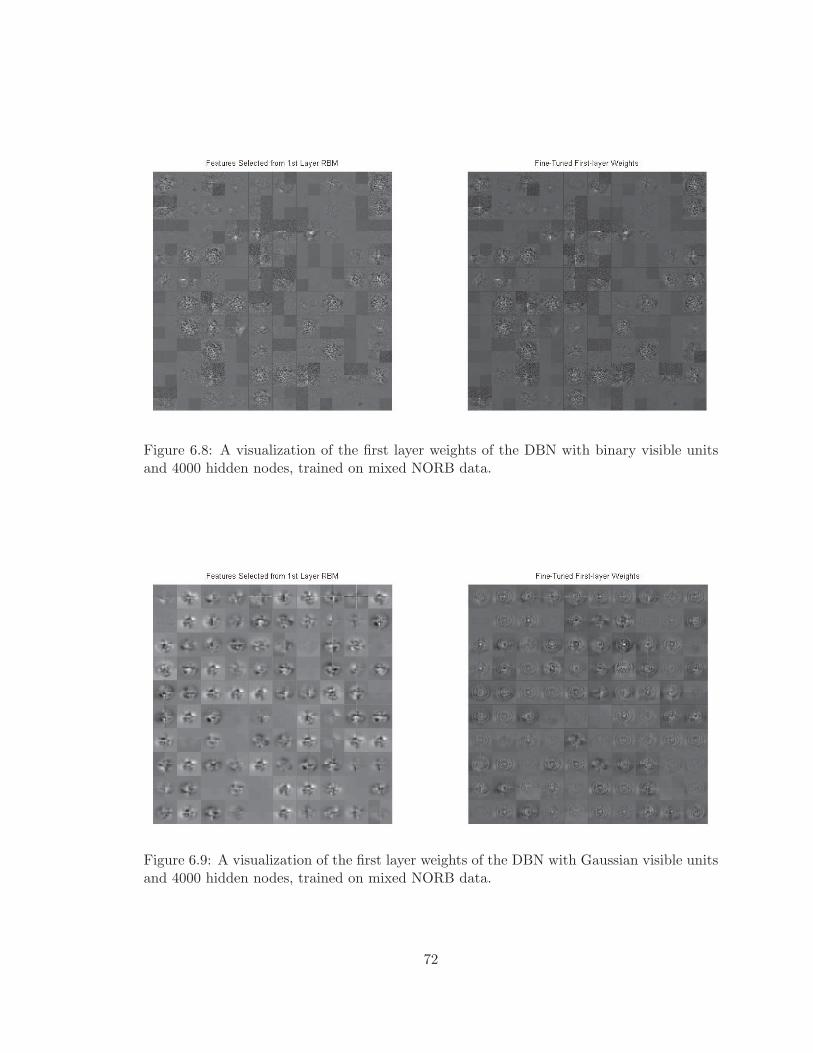
Figure 6.8: A visualization of the first layer weights of the DBN with binary visible unitsand 4000 hidden nodes, trained on mixed NORB data.
Figure 6.9: A visualization of the first layer weights of the DBN with Gaussian visible unitsand 4000 hidden nodes, trained on mixed NORB data.
72
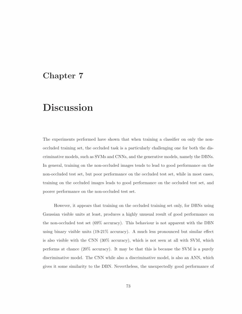
Chapter 7
Discussion
The experiments performed have shown that when training a classifier on only the non-
occluded training set, the occluded task is a particularly challenging one for both the dis-
criminative models, such as SVMs and CNNs, and the generative models, namely the DBNs.
In general, training on the non-occluded images tends to lead to good performance on the
non-occluded test set, but poor performance on the occluded test set, while in most cases,
training on the occluded images leads to good performance on the occluded test set, and
poorer performance on the non-occluded test set.
However, it appears that training on the occluded training set only, for DBNs using
Gaussian visible units at least, produces a highly unusual result of good performance on
the non-occluded test set (69% accuracy). This behaviour is not apparent with the DBN
using binary visible units (19-21% accuracy). A much less pronounced but similar effect
is also visible with the CNN (30% accuracy), which is not seen at all with SVM, which
performs at chance (20% accuracy). It may be that this is because the SVM is a purely
discriminative model. The CNN while also a discriminative model, is also an ANN, which
gives it some similarity to the DBN. Nevertheless, the unexpectedly good performance of
73
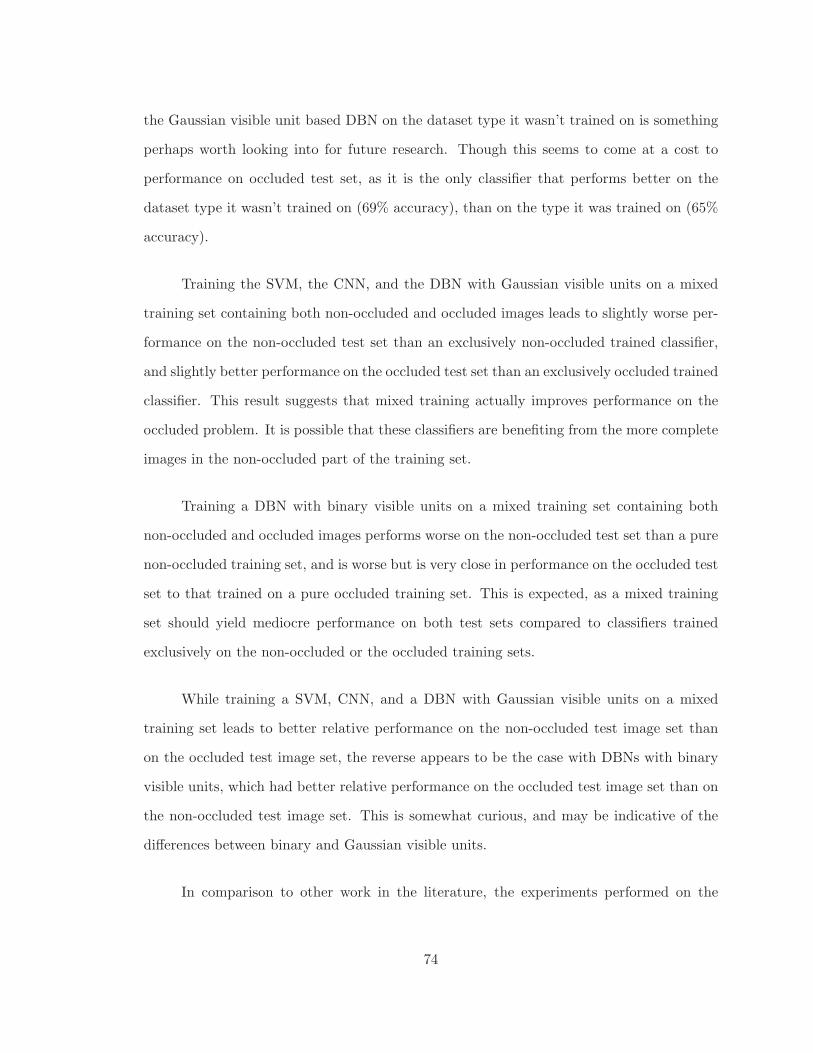
the Gaussian visible unit based DBN on the dataset type it wasn’t trained on is something
perhaps worth looking into for future research. Though this seems to come at a cost to
performance on occluded test set, as it is the only classifier that performs better on the
dataset type it wasn’t trained on (69% accuracy), than on the type it was trained on (65%
accuracy).
Training the SVM, the CNN, and the DBN with Gaussian visible units on a mixed
training set containing both non-occluded and occluded images leads to slightly worse per-
formance on the non-occluded test set than an exclusively non-occluded trained classifier,
and slightly better performance on the occluded test set than an exclusively occluded trained
classifier. This result suggests that mixed training actually improves performance on the
occluded problem. It is possible that these classifiers are benefiting from the more complete
images in the non-occluded part of the training set.
Training a DBN with binary visible units on a mixed training set containing both
non-occluded and occluded images performs worse on the non-occluded test set than a pure
non-occluded training set, and is worse but is very close in performance on the occluded test
set to that trained on a pure occluded training set. This is expected, as a mixed training
set should yield mediocre performance on both test sets compared to classifiers trained
exclusively on the non-occluded or the occluded training sets.
While training a SVM, CNN, and a DBN with Gaussian visible units on a mixed
training set leads to better relative performance on the non-occluded test image set than
on the occluded test image set, the reverse appears to be the case with DBNs with binary
visible units, which had better relative performance on the occluded test image set than on
the non-occluded test image set. This is somewhat curious, and may be indicative of the
differences between binary and Gaussian visible units.
In comparison to other work in the literature, the experiments performed on the
74
SVM and CNN did not exceed the performance of the results from Huang and LeCun [26].
Huang and LeCun were able to achieve 88.4% accuracy with their SVM on the small NORB
dataset, and 93.8% accuracy with their CNN on the small NORB dataset. The SVM in
our experiments, with the same parameters as Huang and LeCun, achieved 82.5% ± 0.7%
accuracy, while our CNN achieved 83.1% accuracy. Our best performing algorithm was
actually a DBN using binary visible units and 2000 hidden nodes, which achieved 87%
accuracy. In comparison, Nair and Hinton [37], achieved 93.5% accuracy with their DBN
on the standard small NORB dataset, and 94.8% accuracy with their DBN using extra
unlabeled data. Thus, on the non-occluded or non-occluded images, we did not achieve
quite as good results as the best in the literature, as shown in table 7.1.
Table 7.1: Comparison of the accuracy results of the Classifier Algorithms with those inthe literature on NORB
Trained On Unoccluded NORB Images and Tested on Unoccluded NORB Images
Classifier Accuracy
Our SVM 0.825± 0.007SVM from Huang and LeCun [26] 0.884Our CNN 0.831± 0.000CNN from Huang and LeCun [26] 0.938Our DBN (B-2000) 0.873± 0.007Our DBN (B-4000) 0.841± 0.014Our DBN (G-4000) 0.832± 0.006DBN from Nair and Hinton [37] 0.935
Note: Mean of 3 replicates ± standard error.
A major reason for our relatively inferior performance was that we chose to only take
one of the two stereo images in the NORB dataset to be used by our algorithms. The top
performing results in the literature on the other hand, generally made use of both of the
stereo images. We chose not to use the stereo pair images primarily because of limitations
on our part, namely that it would double the size of the dataset in memory, and that in
the case of the CNN it would require a considerable modification to the architecture of the
network. Thus, we chose to save both memory and time by using only the single image.
This was an important choice, because we were limited in the amount of RAM available on
our computers, and the amount of time to required to train with even this limited version
75
of the NORB was quite substantial. Also, in reality it often difficult to obtain stereo images
without resorting to some special robotic vision setup. Conversely, single images are readily
available in many datasets, CCTV cameras, and Internet searches.
As far as occluded images are concerned, there is a lack of results in the literature
that are directly comparable to our work. Probably the most similar work done so far
would be Ranzato et al. [44]. Their work on classifying facial expressions includes some
use of occlusion. Rather than using NORB, they used the Cohn-Kanade (CK) dataset, and
the Toronto Face Database (TFD), classifying 7 different facial expressions, rather than 5
objects. Their Type 3 - right half, Type 4 - bottom half, and Type 5 - top half occlusions
are most similar to the occlusions we used in our experiments. Unlike our experiments, their
deep generative model actually attempts to reconstruct the image first before classifying.
This takes full advantage of the unique properties of generative models. As such, they
achieve fairly impressive results, as shown in Figure 7 of Ranzato et al. [44], and Figure 8
of Ranzato et al. [44].
The top graphs of both of these figures show the results when only test images are
occluded. This is would be equivalent to our performance seen in column five of table 6.6,
where the classifiers are trained on the non-occluded, and tested on the occluded images.
Similarly to what we found in our own experiments, Ranzato et al. [44] found this to be
the more difficult task for most models than the alternative of training on occluded images
and testing on occluded images.
The bottom graphs of both of these figures show the results when both training and
test images are occluded. This is would be equivalent to our performance seen in column
five of table 6.7, where the classifiers are trained on the occluded, and tested on the occluded
images. Similarly to what we found in our own experiments, Ranzato et al. [44] found this
to be an easier task for most models than training on the non-occluded images and testing
on the occluded images.
76
Overall these figures in combination with our own results appear to show that the ad-
vantage of using a generative model comes from the reconstruction process that Ranzato et
al. [44] were able to use, and is not simply a result of classification using a generative model
discriminatively as we did. Further research naturally could involve actually implementing
some kind of reconstruction process similar to what Ranzato et al. [44] used, except on the
small NORB dataset, to see whether or not this conjecture actually holds.
A further possible reason why the performance of the generative DBN did not exceed
the discriminative models could be because the DBNs were fine-tuned with Backpropaga-
tion. As this process is inherently discriminative rather than generative, the final resulting
network perhaps behaves more like a discriminative model than a generative model. If this
is the case, we should be able to see some difference in the accuracy of the model when it has
only been pre-trained, and not yet fine-tuned with Backpropagation. Looking at Appendix
table A.7 we see that the pre-fine-tuning performance of a DBN trained on the non-occluded
dataset, and tested on the occluded data is comparable to that after fine-tuning with Back-
propagation. To truly test this possibility, we may need to find a generative model that is
fully generative through and through, such as a DBM.
We did run some experiments with more complicated occlusions than merely the four
half-planes that we used in the main experiment, but it was found that for the most part,
performance was related mainly to what percentage of the actual object was occluded by
the occlusions. Things like moving the occlusion across the image, only led to increasing
this percentage of occlusion and generally reducing performance.
Also, the features that our algorithms used were selected by the algorithm through
learning, and so it is possible that incorporating preprocessing or feature extracting layers
for features that would be useful in spite of the occlusions, such as texture, might in theory
improve performance, though it should be said that the value of most of these algorithms
is in their ability to determine their own features through learning.
77
Our experiments involved a significant amount of searching for ideal hyper-parameters
for various configurations of the various algorithms. Much of the work was done by man-
ually tuning these hyper-parameters and exhaustively searching for the best values. Some
efficiency could possibly be introduced by a method of automatic parameter setting, that
would involve using scripts to exhaustively search possible configurations. However, as most
of the time involved in the exhaustive searches was in the actual running of the various con-
figurations, it would probably have a minimal overall impact.
Future work may include experiments on other data sets, such as the Caltech-101
proper, which would allow us to be more certain that the findings of our previous experi-
ments hold for data sets other than just NORB. We could also look at using more generative
reconstruction techniques with the DBN, to see whether or not the extra stage that Ranzato
et al. [44] used can be performed using the regular DBN architecture, rather than their
Deep Generative Model. Other future research might also include testing different types of
occlusions than the ones we used, to see whether or not that could make a difference, and
to what degree.
As mentioned in Chapter 3, there is also possible as a future research direction,
the possibility of additional efforts to optimize the hyper-parameters of the CNN, such as
additional work to clarify the number of feature maps considerations, as well as perhaps
determining the optimal receptive field size, and also the optimal number of layers. Given it
is uncertain how much these hyper-parameters depend on a particular data set, so running
some of the previous experiments using other data sets than the Caltech-20, such as on
NORB or the Caltech-101 proper, could yield some interesting results. Furthermore, an
effort into seeing whether or not a more useful measure of spatial entropy can be found
could also be considered.
78
Chapter 8
Conclusions
Our experiments with the CNN, in attempting to determine the optimal number of feature
maps, were able to find that the reality is not as clear as what other papers tend to suggest.
This is not to imply that they are incorrect, but only that there is some uncertainty regarding
whether or not a monotonically increasing function best describes the data. As such, it
suggests that more research work could be done to dissolve this uncertainty.
It thus appears that the original hypothesis that the generative models would perform
significantly better on the occluded task than the discriminative models is not well supported
by the results of the experiments performed. Rather, when run in a discriminative manner,
the generative model, in our case, the DBN appears to perform close to equally well to the
discriminative models, the SVM and the CNN. This suggests that, with regards to other
findings in the literature which use generative models and are able to show a difference,
that this difference is primarily due to the additional use of reconstruction processes, and
is not due to merely the architecture and training algorithm itself.
On the other hand, with regards to DBNs using Gaussian visible units, when trained
on the occluded training set and tested on the non-occluded dataset, show remarkable
79

performance that perhaps warrants further research. In fact, this may suggest that inten-
tionally occluding data sets may allow for good performance on both the non-occluded and
occluded tasks, at least when using this particular variant of DBN. Such could prove useful
in tasks in which the original training set is non-occluded, but the real-world test data may
well be occluded, such as in the case of real-world face recognition from CCTV cameras.
80
Bibliography
[1] Ackley, D. H., Hinton, G. E. and Sejnowski, T. J. [1985], ‘A learning algorithm for
boltzmann machines’, Cognitive Science 9, 147–169.
[2] Anderson, J. R. [2000], Cognitive Psychology And Its Implications, 5th ed. edn, Worth
Publishers, New York.
[3] Bengio, Y. [2009], ‘Learning deep architectures for ai’, Foundations and Trends in
Machine Learning 2(1), 1–127.
[4] Bergstra, J., Breuleux, O., Bastien, F., Lamblin, P., Pascanu, R., Desjardins, G.,
Turian, J., Warde-Farley, D. and Bengio, Y. [2010], Theano: a CPU and GPU math
expression compiler, in ‘Proceedings of the Python for Scientific Computing Conference
(SciPy)’.
[5] Boureau, Y.-L., Ponce, J. and LeCun, Y. [2010], A theoretical analysis of feature
pooling in visual recognition, in ‘Proceedings of the 27th International Conference on
Machine Learning (ICML-10)’, pp. 111–118.
[6] Bryson, A. E. and Ho, Y. C. [1969], Applied Optimal Control, Blaisdell, New York.
[7] Chang, C.-C. and Lin, C.-J. [2011], ‘LIBSVM: A library for support vector machines’,
ACM Transactions on Intelligent Systems and Technology 2, 27:1–27:27. Software
available at http://www.csie.ntu.edu.tw/~cjlin/libsvm.
81
[8] Chu, J. L. and Krzyzak, A. [2014a], Analysis of feature maps selection in supervised
learning using convolutional neural networks, in M. Sokolova and P. van Beek, eds,
‘Canadian Conference on Artificial Intelligence 2014, Lecture Notes on Artifical Intel-
ligece (LNAI)’, Vol. 8436, Springer International Publishing Switzerland, pp. 59–70.
[9] Chu, J. L. and Krzyzak, A. [2014b], Application of support vector machines, convo-
lutional neural networks and deep belief networks to recognition of partially occluded
objects, in L. Rutkowski, ed., ‘The 13th International Conference on Artificial In-
telligence and Soft Computing ICAISC 2014, Lecture Notes on Artifical Intelligece
(LNAI)’, Vol. 8467, Springer International Publishing Switzerland, pp. 34–46.
[10] Ciresan, D., Meier, U. and Schmidhuber, J. [2012], Multi-column deep neural networks
for image classification, in ‘Proceedings of 2012 IEEE Conference on Computer Vision
and Pattern Recognition (CVPR)’, IEEE, pp. 3642–3649.
[11] Coates, A., Ng, A. Y. and Lee, H. [2011], An analysis of single-layer networks in
unsupervised feature learning, in ‘International Conference on Artificial Intelligence
and Statistics (AISTATS)’, pp. 215–223.
[12] Collobert, R. and Bengio, S. [2004], ‘Links between perceptrons, mlps and svms’,
Proceedings of the 21st International Conference on Machine Learning p. 23.
[13] Cortes, C. and Vapnik, V. N. [1995], ‘Support-vector networks’, Machine Learning
20, 273–297.
[14] Dreyfus, S. [1962], ‘The numerical solution of variational problems’, Journal of Math-
ematical Analysis and Applications 5(1), 30–45.
[15] Duda, R. O., Hart, P. E. and Stork, D. G. [2001], Pattern Classification, second edition
edn, John Wiley & Sons, Inc.
[16] Eigen, D., Rolfe, J., Fergus, R. and LeCun, Y. [2013], ‘Understanding Deep Architec-
tures using a Recursive Convolutional Network’, ArXiv e-prints .
82

[17] Fei-Fei, L., Fergus, R. and Perona, P. [2004], ‘Learning generative visual models from
few training examples: an incremental bayesian approach tested on 101 object cat-
egories’, Workshop on Generative-Model Based Vision, IEEE Computer Vision and
Pattern Recognition 2004 .
[18] Fukushima, K. [2003], ‘Neocognitron for handwritten digit recognition’, Neurocomput-
ing 51, 161–180.
[19] Fukushima, K. and Miyake, S. [1982], ‘Neocognitron: A new algorithm for pat-
tern recognition tolerant of deformations and shifts in position’, Pattern Recognition
15(6), 455–469.
[20] Hebb, D. [1949], The Organization of Behaviour, John Wiley, New York.
[21] Hinton, G. E. [2002], ‘Training products of experts by minimizing contrastive diver-
gence’, Neural Computation 14(8), 1771–1800.
[22] Hinton, G. E. [2010], ‘A practical guide to training restricted boltzmann machines’,
Momentum 9(1), 599–619.
[23] Hinton, G. E., Osindero, S. and Teh, Y. W. [2006], ‘A fast learning algorithm for deep
belief nets’, Neural Computation 18, 1527–1554.
[24] Hinton, G. E. and Salakhutdinov, R. R. [2006], ‘Reducing the dimensionality of data
with neural networks’, Science 313, 504–507.
[25] Hopfield, J. J. [1982], ‘Neural networks and physical systems with emergent collective
computational abilities’, Proceedings of the National Academy of Sciences of the USA
79(8), 2554–2558.
[26] Huang, F. J. and LeCun, Y. [2006], ‘Large-scale learning with svm and convolutional
nets for generic object categorization’, Proceedings of the 2006 IEEE Conference on
Computer Vision and Pattern Recognition (CVPR) 1, 284–291.
83

[27] Hubel, D. H. and Wiesel, T. N. [1962], ‘Receptive fields, binocular interaction and func-
tional architecture in a cats visual cortex’, Journal of Physiology (London) 160, 106–
154.
[28] Krizhevsky, A., Sutskever, I. and Hinton, G. [2012], Imagenet classification with deep
convolutional neural networks, in ‘Advances in Neural Information Processing Systems
25’, pp. 1106–1114.
[29] LeCun, Y., Bottou, L., Bengio, Y. and P., H. [1998], ‘Gradient-based learning applied
to document recognition’, Proceedings of the IEEE 86(11), 2278–2324.
[30] LeCun, Y., Huang, F. and Bottou, L. [2004], ‘Learning methods for generic object
recognition with invariance to pose and lighting’, Proceedings of IEEE Conference on
Computer Vision and Pattern Recognition (CVPR) 2, 97–104.
[31] Lee, H., Grosse, R., Ranganath, R. and Ng, A. Y. [2009], ‘Convolutional deep belief
networks for scalable unsupervised learning of hierarchical representations’, Proceedings
of the 26th International Conference on Machine Learning pp. 609–616.
[32] McClelland, J. and Rumelhart, D. [1988], Explorations in Parallel Distributed Process-
ing, MIT Press, Cambridge.
[33] McCulloch, W. S. and Pitts, W. [1943], ‘A logical calculus of ideas immanent in nervous
activity’, Bulletin of Mathematical Biophysics 5, 115–133.
[34] Mehrotra, K., Mohan, C. K. and Ranka, S. [1997], Elements Of Artificial Neural Net-
works, The MIT Press, Cambridge, MA.
[35] Minsky, M. L. and Papert, S. A. [1969], Perceptrons, MIT Press, Cambridge.
[36] Mohamed, A. R., Yu, D. and Deng, L. [2010], ‘Investigation of full-sequence training
of deep belief networks for speech recognition’, Conference of the International Speech
Communication Association (INTERSPEECH) pp. 2846–2849.
84
[37] Nair, V. and Hinton, G. E. [2009], ‘3d object recognition with deep belief nets’, Ad-
vances in Neural Information Processing Systems (NIPS) pp. 1339–1347.
[38] Ngiam, J., Chen, Z., Chia, D., Koh, P. W., Le, Q. V. and Ng, A. [2010], ‘Tiled
convolutional neural networks’, Advances in Neural Information Processing Systems
(NIPS) pp. 1279–1287.
[39] Nguyen, G. H., Phung, S. L. and Bouzerdoum, A. [2009], Reduced training of con-
volutional neural networks for pedestrian detection, in ‘International Conference on
Information Technology and Applications’.
[40] Osindero, S. and Hinton, G. [2008], ‘Modeling image patches with a directed hierarchy
of markov random fields’, Advances In Neural Information Processing Systems (NIPS)
20.
[41] Pylyshyn, Z. W. [1998], ‘What is cognitive science?’.
URL: http://ruccs.rutgers.edu/ftp/pub/papers/ruccsbook.PDF
[42] Pylyshyn, Z. W. [2003], ‘Return of the mental image: Are there really pictures in the
brain?’, Trends in Cognitive Science 7(3), 113–118.
[43] Ranzato, M. A., Huang, F. J., Boureau, Y. L. and LeCun, Y. [2007], ‘Unsupervised
learning of invariant feature hierarchies with applications to object recognition’, 2007
IEEE Conference on Computer Vision and Pattern Recognition (CVPR) pp. 1–8.
[44] Ranzato, M., Susskind, J., Mnih, V. and Hinton, G. [2011], ‘On deep generative models
with applications to recognition’, 2011 IEEE Conference on Computer Vision and
Pattern Recognition (CVPR) pp. 2857–2864.
[45] Rosenblatt, F. [1958], ‘The perceptron, a probabilistic model for information storage
and organization in the brain’, Psychological Review 62, 386–408.
[46] Rumelhart, D. E., Hinton, G. E. and Williams, R. J. [1986], ‘Learning internal repre-
sentations by error propagation’, Parallel Distributed Processing 1.
85
[47] Russell, S. and Norvig, P., eds [2003], Artificial Intelligence: A Modern Approach, 2nd
ed. edn, Pearson Education, Upper Saddle River, NJ.
[48] Salakhutdinov, R. and Hinton, G. E. [2009], ‘Deep boltzmann machines’, International
Conference on Artificial Intelligence and Statistics (AISTATS) pp. 448–455.
[49] Scherer, D., Schulz, H. and Behnke, S. [2010], Accelerating large-scale convolutional
neural networks with parallel graphics multiprocessors, in ‘Artificial Neural Networks–
ICANN 2010’, Springer, pp. 82–91.
[50] Schulz, H., Muller, A. and S., B. [2010], ‘Exploiting local structure in stacked boltz-
mann machines’, European Symposium on Artificial Neural Networks, Computational
Intelligence and Machine Learning (ESANN) .
[51] Simard, P., Steinkraus, D. and Platt, J. C. [2003], Best practices for convolutional
neural networks applied to visual document analysis., in ‘International Conference on
Document Analysis and Recognition (ICDAR)’, Vol. 3, pp. 958–962.
[52] Smolensky, P. [1986], Information processing in dynamical systems: Foundations of
harmony theory, in D. E. Rumelhart and J. L. McLelland, eds, ‘Parallel Distributed
Processing: Explorations in the Microstructure of Cognition’, Vol. 1, MIT Press, chap-
ter 6, pp. 194–281.
[53] Thagard, P. [1996], Mind: Introduction To Cognitive Science, The MIT Press, Cam-
bridge, MA.
[54] Uetz, R. and Behnke, S. [2009a], Large-scale object recognition with cuda-accelerated
hierarchical neural networks, in ‘IEEE International Conference on Intelligent Com-
puting and Intelligent Systems, 2009. ICIS 2009.’, Vol. 1, IEEE, pp. 536–541.
[55] Uetz, R. and Behnke, S. [2009b], Locally-connected hierarchical neural networks for
gpu-accelerated object recognition, in ‘NIPS 2009 Workshop on Large-Scale Machine
Learning: Parallelism and Massive Datasets’.
86

[56] Werbos, P. [1974], Beyond regression: New tools for prediction and analysis in the
behavioral sciences, PhD thesis, Harvard University.
87
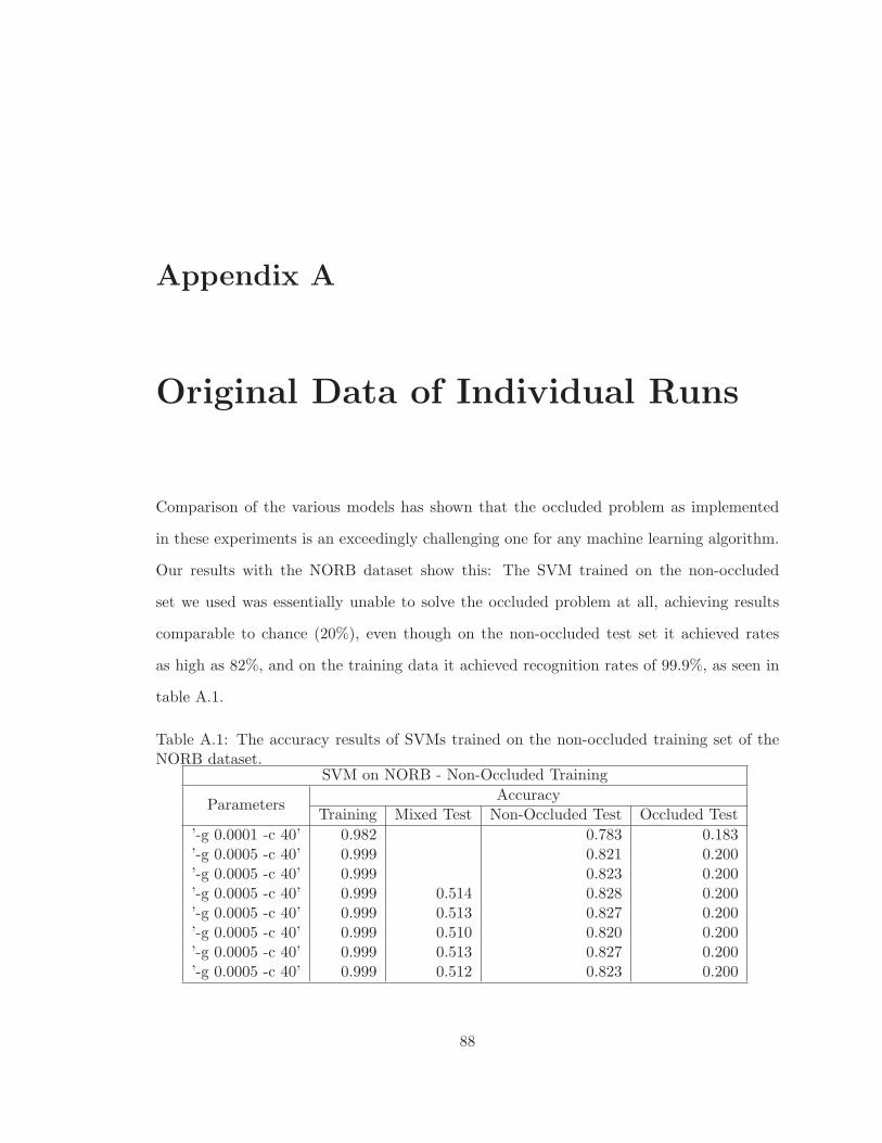
Appendix A
Original Data of Individual Runs
Comparison of the various models has shown that the occluded problem as implemented
in these experiments is an exceedingly challenging one for any machine learning algorithm.
Our results with the NORB dataset show this: The SVM trained on the non-occluded
set we used was essentially unable to solve the occluded problem at all, achieving results
comparable to chance (20%), even though on the non-occluded test set it achieved rates
as high as 82%, and on the training data it achieved recognition rates of 99.9%, as seen in
table A.1.
Table A.1: The accuracy results of SVMs trained on the non-occluded training set of theNORB dataset.
SVM on NORB - Non-Occluded Training
ParametersAccuracy
Training Mixed Test Non-Occluded Test Occluded Test
’-g 0.0001 -c 40’ 0.982 0.783 0.183’-g 0.0005 -c 40’ 0.999 0.821 0.200’-g 0.0005 -c 40’ 0.999 0.823 0.200’-g 0.0005 -c 40’ 0.999 0.514 0.828 0.200’-g 0.0005 -c 40’ 0.999 0.513 0.827 0.200’-g 0.0005 -c 40’ 0.999 0.510 0.820 0.200’-g 0.0005 -c 40’ 0.999 0.513 0.827 0.200’-g 0.0005 -c 40’ 0.999 0.512 0.823 0.200
88
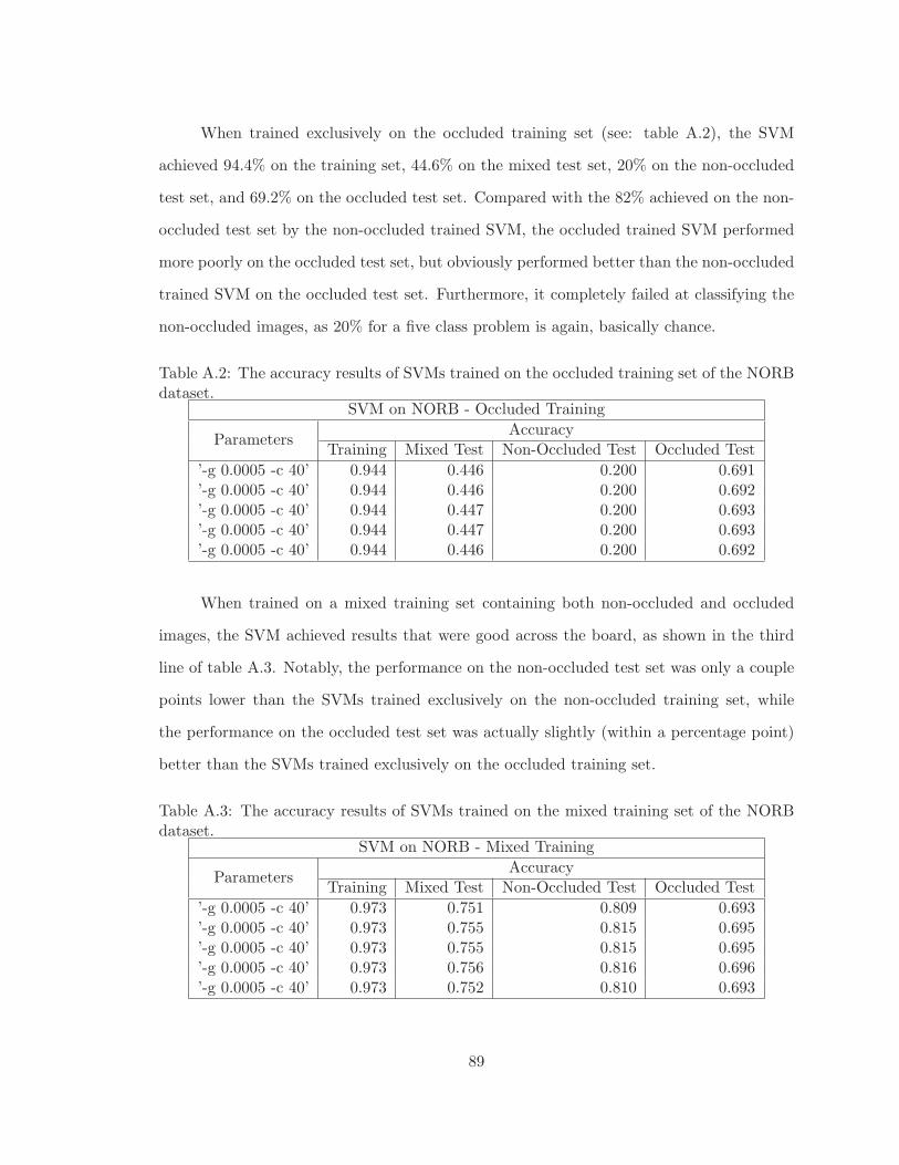
When trained exclusively on the occluded training set (see: table A.2), the SVM
achieved 94.4% on the training set, 44.6% on the mixed test set, 20% on the non-occluded
test set, and 69.2% on the occluded test set. Compared with the 82% achieved on the non-
occluded test set by the non-occluded trained SVM, the occluded trained SVM performed
more poorly on the occluded test set, but obviously performed better than the non-occluded
trained SVM on the occluded test set. Furthermore, it completely failed at classifying the
non-occluded images, as 20% for a five class problem is again, basically chance.
Table A.2: The accuracy results of SVMs trained on the occluded training set of the NORBdataset.
SVM on NORB - Occluded Training
ParametersAccuracy
Training Mixed Test Non-Occluded Test Occluded Test
’-g 0.0005 -c 40’ 0.944 0.446 0.200 0.691’-g 0.0005 -c 40’ 0.944 0.446 0.200 0.692’-g 0.0005 -c 40’ 0.944 0.447 0.200 0.693’-g 0.0005 -c 40’ 0.944 0.447 0.200 0.693’-g 0.0005 -c 40’ 0.944 0.446 0.200 0.692
When trained on a mixed training set containing both non-occluded and occluded
images, the SVM achieved results that were good across the board, as shown in the third
line of table A.3. Notably, the performance on the non-occluded test set was only a couple
points lower than the SVMs trained exclusively on the non-occluded training set, while
the performance on the occluded test set was actually slightly (within a percentage point)
better than the SVMs trained exclusively on the occluded training set.
Table A.3: The accuracy results of SVMs trained on the mixed training set of the NORBdataset.
SVM on NORB - Mixed Training
ParametersAccuracy
Training Mixed Test Non-Occluded Test Occluded Test
’-g 0.0005 -c 40’ 0.973 0.751 0.809 0.693’-g 0.0005 -c 40’ 0.973 0.755 0.815 0.695’-g 0.0005 -c 40’ 0.973 0.755 0.815 0.695’-g 0.0005 -c 40’ 0.973 0.756 0.816 0.696’-g 0.0005 -c 40’ 0.973 0.752 0.810 0.693
89
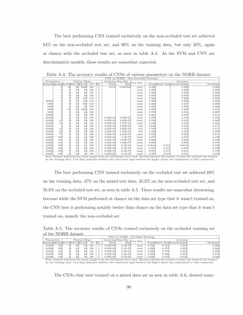
The best performing CNN trained exclusively on the non-occluded test set achieved
84% on the non-occluded test set, and 96% on the training data, but only 20%, again
at chance with the occluded test set, as seen in table A.4. As the SVM and CNN are
discriminative models, these results are somewhat expected.
Table A.4: The accuracy results of CNNs of various parameters on the NORB dataset.CNN on NORB - Non-Occluded Training
Parameters Feature Maps Learning Step SizeCon Map
AccuracyDatasetEpochsS1/C2S3/C4S5/C6 F7 F8 Start End TrainMixed TestNon-Occluded Occluded
3 12 96 2400 100 5 0.015 0.000338 rand 0.200 0.200 0.2003 8 24 24 100 5 rand 0.200 0.200 0.2003 8 24 24 100 5 rand 0.200 0.200 0.2003 8 24 24 100 5 rand 0.200 0.200 0.2003 8 32 128 512 5 rand 0.200 0.200 0.200
24300 3 8 32 128 512 5 rand 0.200 0.200 0.2001000 3 8 32 128 512 5 rand 0.226 0.247 0.2041000 3 8 24 24 100 5 rand 0.695 0.506 0.1961000 3 12 96 2400 100 5 rand 0.200 0.200 0.2211000 3 8 24 24 100 5 rand 0.759 0.551 0.207
24300 3 8 24 24 100 5 rand 0.601 0.557 0.21424300 3 8 24 24 100 5 2.00E-05 2.00E-07 rand 0.595 0.553 0.25224300 10 8 24 24 100 5 2.00E-05 2.02E-07 rand 0.766 0.643 0.24024300 50 8 24 24 100 5 2.00E-05 1.97E-07 rand 0.896 0.763 0.20124300 3 8 24 24 100 5 2.00E-05 2.00E-07 full 0.640 0.544 0.17724300 10 8 24 24 100 5 2.00E-05 2.02E-07 full 0.786 0.703 0.21724300 50 8 24 24 100 5 2.00E-05 1.97E-07 full 0.902 0.763 0.19924300 75 8 24 24 100 5 2.00E-05 2.05E-07 rand 0.932 0.802 0.21324300 100 8 24 24 100 5 2.00E-05 2.1E-07 rand 0.955 0.831 0.19924300 125 8 24 24 100 5 2.00E-05 1.99E-07 rand 0.962 0.842 0.19924300 150 8 24 24 100 5 2.00E-05 1.98E-07 rand 0.959 0.825 0.19724300 100 8 24 24 100 5 2.00E-05 2.1E-07 rand 0.9549 0.515 0.8312 0.19924300 100 8 24 24 100 5 2.00E-05 2.1E-07 rand 0.955 0.515 0.831 0.19924300 100 8 24 24 100 5 2.00E-05 2.1E-07 rand 0.955 0.515 0.831 0.19924300 100 8 24 24 100 5 2.00E-05 2.1E-07 rand 0.955 0.515 0.831 0.199Note: Dataset indicates how many images from the full dataset were used. Epochs indicates the number of times the network was trainedon the training data. Con Map indicates whether the connection map between the higher layers was randomized or fully connected.
The best performing CNN trained exclusively on the occluded test set achieved 69%
on the training data, 47% on the mixed test data, 35.2% on the non-occluded test set, and
58.8% on the occluded test set, as seen in table A.5. These results are somewhat interesting,
because while the SVM performed at chance on the data set type that it wasn’t trained on,
the CNN here is performing notably better than chance on the data set type that it wasn’t
trained on, namely the non-occluded set.
Table A.5: The accuracy results of CNNs trained exclusively on the occluded training setof the NORB dataset.
CNN on NORB - Occluded TrainingParameters Feature Maps Learning Step Size
Con MapAccuracy
DatasetEpochsS1/C2S3/C4S5/C6 F7 F8 Start End TrainMixed TestNon-Occluded Occluded24300 100 8 24 24 100 5 2.00E-05 2.1E-07 rand 0.705 0.424 0.261 0.58624300 100 8 24 24 100 5 2.00E-05 2.1E-07 rand 0.690 0.470 0.352 0.58824300 100 8 24 24 100 5 2.00E-05 2.1E-07 rand 0.690 0.470 0.352 0.58824300 100 8 24 24 100 5 2.00E-05 2.1E-07 rand 0.690 0.388 0.201 0.57624300 100 8 24 24 100 5 2.00E-05 2.1E-07 rand 0.690 0.470 0.352 0.588Note: Dataset indicates how many images from the full dataset were used. Epochs indicates the number of times the network was trainedon the training data. Con Map indicates whether the connection map between the higher layers was randomized or fully connected.
The CNNs that were trained on a mixed data set as seen in table A.6, showed some-
90

what lower accuracy on the non-occluded test set than the CNNs trained exclusively on
the non-occluded training set, but also showed somewhat higher accuracy on the occluded
test set than the CNNs trained exclusively on the occluded training set. It appears that
while performance on the non-occluded test set was hampered by mixing in occluded im-
ages to the training, the reverse effect occurred with the occluded test set, with performance
improved by including non-occluded images.
Table A.6: The accuracy results of CNNs trained on the mixed training set of the NORBdataset.
CNN on NORB - Mixed TrainingParameters Feature Maps Learning Step Size
Con MapAccuracy
DatasetEpochsS1/C2S3/C4S5/C6 F7 F8 Start End TrainMixed TestNon-Occluded Occluded48600 100 8 24 24 100 5 2.00E-05 2.1E-07 rand 0.832 0.719 0.756 0.68248600 100 8 24 24 100 5 2.00E-05 2.1E-07 rand 0.838 0.708 0.772 0.64548600 100 8 24 24 100 5 2.00E-05 2.1E-07 rand 0.827 0.723 0.793 0.65348600 100 8 24 24 100 5 2.00E-05 2.1E-07 rand 0.832 0.719 0.756 0.682Note: Dataset indicates how many images from the full dataset were used. Epochs indicates the number of times the network was trainedon the training data. Con Map indicates whether the connection map between the higher layers was randomized or fully connected.
What was interesting was the performance of our generative models on the occluded
problem. The best DBN, again trained on the non-occluded training set, achieved 86%
accuracy on the non-occluded test set, and 99.4% accuracy on the training data, but only
achieved 22.2% accuracy on the occluded test set, which was only slightly better than
chance (shown in table A.7). Note that a DBN using Gaussian visible units was able to
achieve slightly better results at 25.6% accuracy on the occluded test set, albeit at a cost
to performance on the non-occluded test set, which it achieved only 80% on. While these
results are low, they are at least somewhat better than the discriminative models.
Table A.7: The results of DBNs of various parameters trained on the non-occluded trainingset on the NORB dataset.
DBN on NORB - Non-Occluded Training
VisibleParameters Learning Rate Epochs Accuracy Fine-Tuned Accuracy
Layers Hidden RBM Fine-TuneRBMFine-TuneTrainingNon-OccludedOccludedTrainingNon-Occluded OccludedGaussian 2 2000 0.001 0.001 200 50 0.531 0.465 0.241 0.986 0.802 0.256
Binary 2 2000 0.100 0.010 200 50 0.200 0.200 0.200 0.200 0.200 0.200Binary 2 2000 0.010 0.001 200 50 0.622 0.559 0.226 0.993 0.860 0.222
Gaussian 2 4000 0.001 0.001 200 50 0.522 0.461 0.249 0.977 0.837 0.233Binary 2 4000 0.010 0.001 200 50 0.611 0.535 0.239 0.990 0.859 0.201Note: Visible indicates the type of visible input nodes. Layers indicates the number of RBMs. Hidden indicates the number of hiddennodes in the hidden layer of each RBM.
More interesting perhaps were the results of training the DBN on just the occluded
training dataset. The results (shown in table A.8) are interesting because while the binary
visible unit based DBNs perform as expected, with much higher performance on the oc-
91
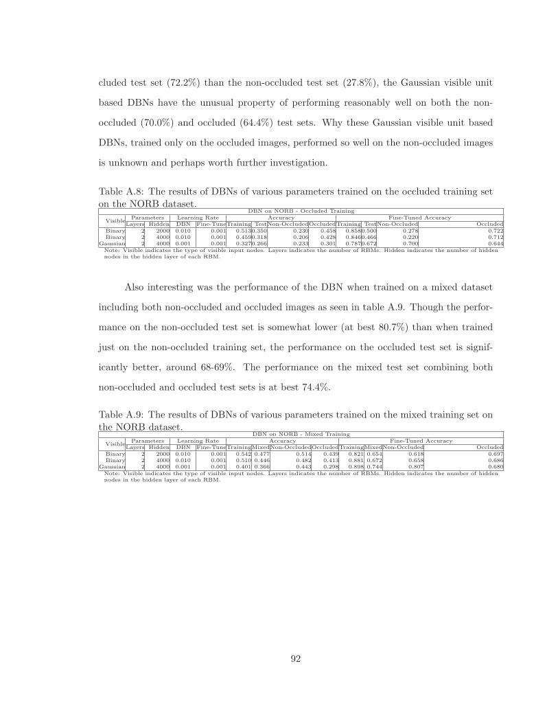
cluded test set (72.2%) than the non-occluded test set (27.8%), the Gaussian visible unit
based DBNs have the unusual property of performing reasonably well on both the non-
occluded (70.0%) and occluded (64.4%) test sets. Why these Gaussian visible unit based
DBNs, trained only on the occluded images, performed so well on the non-occluded images
is unknown and perhaps worth further investigation.
Table A.8: The results of DBNs of various parameters trained on the occluded training seton the NORB dataset.
DBN on NORB - Occluded Training
VisibleParameters Learning Rate Accuracy Fine-Tuned Accuracy
Layers Hidden DBN Fine-TuneTraining TestNon-OccludedOccludedTraining TestNon-Occluded OccludedBinary 2 2000 0.010 0.001 0.5130.350 0.230 0.458 0.8580.500 0.278 0.722Binary 2 4000 0.010 0.001 0.4590.318 0.206 0.428 0.8460.466 0.220 0.712
Gaussian 2 4000 0.001 0.001 0.3270.266 0.233 0.301 0.7870.672 0.700 0.644Note: Visible indicates the type of visible input nodes. Layers indicates the number of RBMs. Hidden indicates the number of hiddennodes in the hidden layer of each RBM.
Also interesting was the performance of the DBN when trained on a mixed dataset
including both non-occluded and occluded images as seen in table A.9. Though the perfor-
mance on the non-occluded test set is somewhat lower (at best 80.7%) than when trained
just on the non-occluded training set, the performance on the occluded test set is signif-
icantly better, around 68-69%. The performance on the mixed test set combining both
non-occluded and occluded test sets is at best 74.4%.
Table A.9: The results of DBNs of various parameters trained on the mixed training set onthe NORB dataset.
DBN on NORB - Mixed Training
VisibleParameters Learning Rate Accuracy Fine-Tuned Accuracy
Layers Hidden DBN Fine-TuneTrainingMixedNon-OccludedOccludedTrainingMixedNon-Occluded OccludedBinary 2 2000 0.010 0.001 0.542 0.477 0.514 0.439 0.821 0.654 0.618 0.697Binary 2 4000 0.010 0.001 0.510 0.446 0.482 0.413 0.881 0.672 0.658 0.686
Gaussian 2 4000 0.001 0.001 0.401 0.366 0.443 0.298 0.898 0.744 0.807 0.680Note: Visible indicates the type of visible input nodes. Layers indicates the number of RBMs. Hidden indicates the number of hiddennodes in the hidden layer of each RBM.
92
![Convolutional Pose Machines - cv-foundation.org · Convolutional Pose Machines Shih-En Wei ... we show a systematic design for how convolutional net- ... The pose machine [29] is](https://img.pdfslide.net/doc/110x75/5b77196a7f8b9a3b7e8cdcf6/convolutional-pose-machines-cv-convolutional-pose-machines-shih-en-wei-.jpg)