ISTITUTO DI STUDI E ANALISI ECONOMICA

Using the results of qualitative surveys in quantitative analysis

by

Enrico D’Elia ISAE, Piazza dell’Indipendenza, 4, 00185 Rome (Italy),

ICStat and Statistical Office of the City of Rome

Working paper n. 56 September 2005

The Series “Documenti di Lavoro” of the Istituto di Studi e Analisi Economica – Institute for Studies and Economic Analyses (ISAE) hosts the preliminary results of the research projects carried out within ISAE. The diffusion of the papers is subject to the favourable opinion of an anonymous referee, whom we would like to thank. The opinions expressed are merely the Authors’ own and in no way involve the ISAE responsability.

The series is meant for experts and policy-makers with the aim of submitting proposals and raising suggestions and criticism.

La serie “Documenti di Lavoro” dell’Istituto di Studi e Analisi Economica

ospita i risultati preliminari di ricerche predisposte all’interno dell’ISAE: La diffusione delle ricerche è autorizzata previo il parere favorevole di un anonimo esperto della materia che qui si ringrazia. Le opinioni espresse nei “Documenti di Lavoro” riflettono esclusivamente il pensiero degli autori e non impegnano la responsabilità dell’Ente.

La serie è destinata agli esperti e agli operatori di politica economica, al fine di formulare proposte e suscitare suggerimenti o critiche.

Stampato presso la sede dell’Istituto

ISAE - Piazza dell’Indipendenza, 4 – 00185 Roma. Tel. +39-06444821; www.isae.it

ABSTRACT

The answers to qualitative questions put to economic operators can be integrated in standard macro-economic analysis by using a “quantification” procedure chosen among the probabilistic approach, the regression methods or the latent factor approach. The first one is the most commonly used. It is based on the assumption that the respondents reply that the value of the reference variable x can be described by a certain statement (e.g.: x stays stable) if it lies between two known thresholds (e.g.: ±5% around its initial value). A number of quantified indicators may be derived by assuming a special functional form for the frequency distribution of opinions and expectations of respondents about x. According to the regression approach, the respondents attach to each qualitative answer a reference value of x, which can be estimated by regressing an available quantitative measure of x against the time series (or longitudinal samples) of percentages of people who gave each qualitative answer. Finally, one can assume that every percentage of answers is driven by a single common “latent factor”, which can be estimated by applying to the percentages of answers the standard tools of multivariate statistics. All of the three approaches include as a special case the “balance statistic”, adopted very often in empirical analyses. Both the theoretical analysis and the empirical evidence on the relative merits of various methods are mixed. In general, no single quantification technique clearly outperforms the others, at least in preliminary analysis. However, when the quantified indicators must be included as explanatory variables in standard econometric models, the regression approach seems the most suitable and natural one. On its turn, the latent factor approach provides a profitable alternative to the regression method in exploratory analyses and when multicollinearity and degrees of freedom of estimates become severe constraints.

Key Words: Expectations, Latent factors, Qualitative surveys, Quantification methods, Short term indicators.

JEL Classification: C16, C35, C82, E32

NON-TECHNICAL SUMMARY

Since the sixties qualitative surveys have been carried out in many Countries, in order to collect opinions and expectations of entrepreneurs and consumers, as the percentages of answers collected within the qualitative surveys provide timely and reliable information about the state of economy and markets.

Usually, questions present only three alternative replies, and are often referenced as “trichotomous” questions, but some generalisations to the “polichotomous” case are possible as well. Typically trichotomous qualitative questions belong to two classes. The first kind of questions sounds like “How is the level of variable x?”, and the interviewed person is asked to choose among few possible replies such as “High”, “Normal”, and “Low”. The second type of questions is “How did (or will) variable x change?”, and the following alternative replies are admitted: “It did (will) increase”, “It did (will) stay stable”, and “It did (will) decrease”. Both the cases may be treated within an unified methodological framework, however, the literature devoted the major attention to the latter class of questions. In fact, the answer “It did (will) stay stable” can be naturally associated to a small change of x close to zero. However the same methodologies can be possibly adapted to the first kind of questions as well, provided that x is measured as deviation from its “normal” level, which is associated to something close to zero.

There are at least three main approaches to convert the results of qualitative surveys to standard quantitative variables. The first, and most widely used, method is some variant of the probabilistic approach. The principle behind this approach is that the respondents reply that the value of the reference variable x can be described by a certain statement (e.g.: x stays stable) if it lies between two known thresholds (e.g.: ±5% around its initial value). Thus, by assuming that the functional form of the underlying probability distribution of opinions and expectations about x is known, the average value of x can be expressed as a function of the aforementioned thresholds. Also a measure of opinions heterogeneity and operators uncertainty can be derived in the same analytical framework.

The second approach is based on regression techniques aimed to estimate the value of x underlying each qualitative answer. This method requires the regression of a standard quantitative measure of x against the time series of percentage of people who gave each qualitative answer.

The third method regards the percentages of each qualitative answer as a function of a common “latent measure” of x observed by people but not by

statisticians. Usual multivariate techniques may help in estimating the dynamics or the sectoral variations (but not the absolute level) of the latent factor affecting the opinions and expectations expressed by the interviewed operators.

As matter of fact, the time series of percentages of answers collected in qualitative surveys are very correlated. First of all, this fact implies that the latent variable approach is possibly sound and reliable. However it also suggests that even very sophisticated methods, based on complicated transformations of original percentages, tend to produce indicators that, in fact, follow the common trend and cycle that can be easily deduced by whatever time series of percentage, or a simple combination thereof. This fact explains and justifies the widespread use of the “balance” between the percentages of “optimistic” and “pessimistic” answers.

The empirical evidence on the performance of various methods is mixed. Generally, no one procedure outperforms the other, even if some authors have pointed out the sharp inefficiency of balance statistic and others have noticed that dynamic regression models are generally superior. In analysing data from surveys on Italian consumers and entrepreneurs, it has been recommended the use of dynamic regression models, even if other methods tend to produce very similar results, as far as the general dynamics of the resulting indicators is concerned, since the time series of the percentage of answers falling in each category are usually highly correlated. First of all, this fact suggests that what quantification technique is adopted is not so crucial, at least in preliminary analysis. Secondly, in case, it is profitable to follow the “latent factor” approach, that exploits exactly the particular covariance structure of the results. However, when the quantified indicators must be included as explanatory variables in standard econometric models, the regression approach seems to be the most suitable and practicable (and natural) one. Also, the latent factor method can be used as a profitable alternative to the complete regression approach, when multicollinearity and degrees of freedom of estimates become severe constraints.

L’USO DEI RISULTATI DELLE INDAGINI QUALITATIVE NELL’ANALISI QUANTITATIVA

SINTESI

Le risposte alle domande qualitative poste agli operatori economici possono essere integrate nei tradizionali schemi di analisi utilizzando una procedura di “quantificazione”, scelta tra quelle basate sull’approccio probabilistico, sui metodi di regressione o sull’approccio delle variabili latenti. Il primo metodo è quello più utilizzato e si basa sull’ipotesi che il valore della variabile di riferimento x sia descritto da una particolare definizione qualitativa (p.es.: x è stabile) se i rispondenti credono che x sia compreso all’interno di un determinato intervallo (p.es: entro il ±5% rispetto al valore iniziale). E’ possibile ricavare diversi indicatori quantificati a seconda delle ipotesi fatte sulla forma funzionale della distribuzione di probabilità delle opinioni e delle aspettative dei rispondenti. Secondo l’approccio della regressione, i rispondenti associano a ciascuna modalità di risposta qualitativa un preciso valore di riferimento per x, che può essere stimato regredendo un indicatore quantitativo su x sulle percentuali di risposte rilevate per ciascuna modalità. Infine, si può ipotizzare che tutte le percentuali di risposte siano determinate da un unico “fattore latente” comune, che può essere stimato tramite le consuete tecniche multivariate applicate alla serie storiche (o alle cross-section) delle percentuali stesse. I tre approcci comprendono, come caso particolare, il “saldo”, che viene utilizzato comunemente nella maggior parte delle analisi empiriche. Nè i meriti teorici, nè le evidenze empiriche sui diversi metodi portano a conclusioni univoche. In generale, non esiste un metodo di quantificazione che risulti sempre migliore di tutti gli altri, almeno nelle analisi preliminari. Quando gli indicatori quantificati sono destinati ad essere inclusi nei modelli econometrici, l’approccio della regressione sembra preferibile. D’altra parte, il metodo del fattore latente può fornire una utile alternativa alla regressione sia nell’analisi esplorativa, sia quando si presentano problemi di collinearità e di scarsi gradi di libertà delle stime.

Parole chiave: Aspettative, Fattori latenti, Indagini qualitative, Metodi di quantificazione, Indicatori congiunturali

Classificazione JEL: C16, C35, C82, E32

CONTENTS

1 INTRODUCTION Pag. 9

2 THE PROBABILISTIC APPROACH “ 11

2.1 The role of the assumptions about the thresholds and the probability distribution “ 15

3 THE REGRESSION METHODS “ 16

4 QUANTIFIED INDICATORS AS LATENT VARIABLES “ 18

5 CONCLUSIVE REMARKS “ 21

REFERENCES “ 23

9

1 INTRODUCTION1

The answers to qualitative questions put to economic operators provide timely and reliable information about the state of economy and markets. Since the sixties qualitative surveys have been carried out in the OECD area and in many other countries (see CIRET, 1998), in order to collect opinions and expectations of entrepreneurs and consumers.

The results of qualitative surveys may be treated both in the framework of individual behaviour disaggregated models (see the recent contributions by Kaiser and Spitz, 2000, and Mitchell, Smith and Weale, 2002, among the others), and in aggregated form. The latter is preferred in macro-economic analysis. In the mainstream literature, surveys with three alternative replies, often referenced as “trichotomous” questions, are usually considered, but some generalisations to the “polichotomous” questions are possible as well.

Typically qualitative questions belong to two classes. The first kind of questions sounds like “How is the level of variable x?”, and the interviewed person is asked to choose among few possible replies such as “High”, “Normal”, and “Low”. The second type of questions is “How did (or will) variable x change?”, and the following alternative replies are admitted: “It did (will) increase”, “It did (will) stay stable”, and “It did (will) decrease”.

Analysis of qualitative surveys has been mainly devoted to the second class of questions, where the answer “It did (will) stay stable” can be naturally associated to a small change of x close to zero. However the same methodologies can be possibly adapted to the first kind of questions as well, provided that x is measured as deviation from its “normal” level, which is associated to something close to zero. For the sake of simplicity, questions of the second type are considered in what follows, but the generalisation is straightforward.

The results of qualitative surveys are usually reported as time series or cross section data of percentage of people giving each answer. For the sake of simplicity, only time series are explicitly referred to in what follows, without any loss of generality, since the latter is certainly the most common case. The percentages of answers are hardly included directly in econometric models and even in formal analyses. At best, the percentage of the “optimistic” operators (i.e. answering “High” or “It did (will) increase”) can be considered, compared to

1 The views reported in this paper are those of the author and do not involve the institutions he is

affiliated to under any respect. The author gratefully acknowledges the suggestions and criticisms come from some researchers who read the very first draft of the paper and from two anonymous referees. Of course, the author is the only responsible for any mistake.

10

the “pessimistic” ones (i.e. answering “Low” or “It did (will) decrease”). However, it may be difficult to interpret the parameters associated to such variables in standard econometric models.

There are at least three main approaches to convert the results of qualitative surveys to standard quantitative variables. The first, and most widely used, method is some variant of the probabilistic approach, sketched by Theil (1952) and popularised by Carlson and Parkin (1975). The principle behind this approach is that the respondents reply that the value of the reference variable x can be described by a certain statement (e.g.: x stays stable) if it lies between two known thresholds (e.g.: ±5% around its initial value). Thus, by assuming that the functional form of the underlying probability distribution of opinions and expectations about x is known, the average value of x can be expressed as a function of the aforementioned thresholds. Also a measure of opinions heterogeneity and operators uncertainty can be derived in the same analytical framework.

The second approach, introduced by Anderson (1952) and developed by Pesaran (1984), is based on regression techniques aimed to estimate the value of x underlying each qualitative answer. This method requires the regression of a standard quantitative measure of x against the time series of percentage of people who gave each qualitative answer. In principle, this is a way to extrapolate standard quantitative indicators by using the survey results.

The third method aimed to integrate qualitative surveys in quantitative analysis, proposed by D’Elia (1991), regards the percentages of each qualitative answer as function of a common “latent measure” of x observed by people but not by statisticians. Usual multivariate techniques may help in estimating the dynamics or the sectoral variations (but not the absolute level) of the latent factor affecting the opinions and expectations expressed by the interviewed operators.

As matter of fact, the time series of percentages of answers collected in qualitative surveys are very correlated. First of all, this fact implies that the latent variable approach is possibly sound and reliable. However it also suggests that even very sophisticated methods, based on complicated transformations of original percentages, tend to produce indicators that, in fact, follow the common trend and cycle that can be easily deduced by whatever time series of percentage, or a simple combination thereof. This fact explains and justifies the widespread use of the “balance” between the percentages of “optimistic” and “pessimistic” answers.

The aim of this paper is to provide the interested reader with a non-technical critical survey of various quantification methods. The remainder of this

11

paper is organised in four sections. The next section describes the popular probabilistic approach, stressing its strength, mainly due to a consistent statistical framework, but also some drawbacks, specially related to some difficulties in generalising the methods to questions with more than three possible answers. The sub-section 2.1 specifically discusses the (minor) role of the assumptions about the thresholds and the probability distribution.

Paragraph 3 is devoted to the regression approach, that seems more flexible, but requires the knowledge of a quantitative measure of the variable to be quantified, at least referred to a small sample of past observations. Section 4 describes the method based on latent variables, that is as flexible as the regression approach, but does not require extraneous information on the variable to be treated. Few conclusive remarks and a synoptic table of quantification methods close the paper.

2 THE PROBABILISTIC APPROACH

Let assume that the operators observe the random variable x, whose cumulative probability distribution is F(x, θ), where θ is a vector of parameters, particularly including the average µ and a dispersion measure (e.g. the standard error) σ. In addition, let the operators answer “It did (will) stay stable” if x lies in the interval [-δ, δ], where δ is an unknown strictly positive constant. Then the following two equivalences hold:

F(-δ, θ) = p1 [1]

and

F(δ, θ) = p1 + p2 [2]

where p1 and p2 are the (observed) percentages of people who answered “It did (will) decrease” and “It did (will) stay stable” respectively.

Given the functional form of F(.), the couple of equations [1] and [2] allow to determine two components of θ as function of p1, p2 and δ. As a consequence, if F(.) is completely characterised by two parameters only, like the normal distribution, it is possible to estimate univocally the average of x, say µ, as a function of of p1, p2 and δ. Thus, the time series of µ can be considered

12

a quantification of the opinions (or expectations) underlying the answers of operators to the survey.

Most of the literature about the previous problem has been developed for the analysis of price expectations. Carlson and Parkin (1975), in their seminal paper, drew out explicit formulas for µ and σ as functions of p1 and p2 and the width of indifference area, that is 2δ, assuming that the probability distribution of x is normal. In the case of inflationary expectations, δ has a straightforward interpretation as the price change that can be neglected according to the operators opinion. More generally, δ comes out to be a simple scalar factor for µ and σ.

Let define Q(p, θ) the inverse function such that Q(p, θ) = x when F(x, θ) = p. It is well known that, in the case of normal distribution, Q(p, µ, σ) = σ )(pQ̂ + µ,

where the values of )(pQ̂ = Q(p, 0, 1) are tabulated. Thus, from [1] and [2] it reads

µ = )−)+ )+ +)

121

211

(pQ̂p(pQ̂p(pQ̂(pQ̂δ [3]

and

σ = )−)+ 121 (pQ̂p(pQ̂

2δ [4]

As far as only the dynamics of the time series of µ is concerned, δ can be considered a pure scale parameters, not affecting the percentage change of µ. In other cases, δ can be estimated imposing some additional constraint on µ. For instance, Carlson and Parkin (1975) assume that, on average, µ is an unbiased estimate of ongoing inflation rate and set δ in [3] in order to fulfil this condition in a given sample of past observations (possibly a sliding sample).

Carlson (1975), Wachtel (1977), Fishe and Lahiri (1981), Batchelor (1981), Batchelor and Orr (1987), Balcombe (1996) and Berk (1999), among the others, assumed non-normal probability distribution for x, but the dynamics (not the absolute level) of resulting quantified indicators do not differ too much from the one obtained following Carlson and Parkin (1975). This result will be discussed specifically in the section 2.1.

If the distribution of x is uniform within the interval [0,1], then F(x) = x, and Q(p) = p. Thus [3] reads

13

µ = δ 2

21

ppp2

+

[5]

On its turn, the dispersion parameter σ is such that

σ = 2p

2δ [6]

thus, combining [5] and [6] it reads

µ = 2

σ (2p1 – p2) [7]

Since, by definition, p1 + p2 + p3 = 1, [7] implies that

µ = 2

σ (1 + p3 – p1) [8]

Thus, if σ is fixed (that is δ is let changing over time conformably) µ turns out to be a linear transformation of the traditional “balance”, that is p3 – p1, commonly used as a quantification of the results of qualitative surveys, and popularised by Theil (1952). Also the dynamics of the simple balance has been found not so different from the more sophisticated indicator proposed by Carlson and Parkin (1975).

A straightforward generalisation of the balance is the weighted balance, in which each time series of percentage is multiplied by a scale parameter, other than 1 and -1, associated respectively to p3 and p1. For instance, larger weight can be given to the more volatile time series of percentages (see also section 4 below). By weighting the percentages of answers, eventually with symmetric weights, the balance approach can be applied also to questions with more than three possible answers. In addition, Lankes and Wolters (1988) demonstrated that the probability method results can be approximated by a weighted balance indicator.

The probabilistic approach was generalised to the polychotomous case, that is when more than three alternative answers are admitted as well. Then the following set of conditions, corresponding to [1] and [2], can be defined:

F(β1, θ) = p1

… [9]

F(βk-1, θ) = p1 + … + pk-1

14

where k is the number of alternative answers, β’ = (β1, … , βk-1) is a vector of thresholds to be defined and θ’ = (µ, σ, θ1, … , θh) is a vector of unknown parameters. As in the previous case, let assume, for the sake of simplicity, that the inverse function Q(p1 + … + ph, θ) = βh is such that Q(p1 + … + ph, µ, σ, θ∗) = σ Q(p1 + … + ph, 0, 1, θ∗) + µ, where θ∗ is the set of parameters excluding µ and σ. Of course, θ∗ may be an empty set, as in the case of normal distribution; in other cases θ∗ may include “degrees of freedom”, “shape” parameters, etc. In addition, µ and σ can be viewed respectively as a “location” and a “scale” parameter of distribution F(x). In fact, many continuous probabilistic distribution functions admit the former decomposition (see Johnson and Kotz, 1970). Under the former assumptions, equations [9] give

µ = β1 – σ Q(p1, 0, 1, θ∗)

… [10]

µ = βk-1 – σ Q(p1 + … + pk-1, 0, 1, θ∗)

that is a system of k-1 (hopefully independent) equations in k+h+1 unknown quantities (i.e.: µ, σ, β and the h elements of θ∗). Of course, an explicit solution for µ and σ can be found only by fixing at least h+2 parameters in [10], that is µ and σ are expressed as a function of h+2 parameters established a priori. In the case analysed by Carlson and Parkin (1975), only three answers are admitted, opinions on x are normally distributed, it holds h = 0 and the two fixed quantities are β2 = −β1 = δ. Sometimes, in system [10] there are more equations than free parameters, specially if Q(.) does not depend on a set of additional parameters, that is h = 0, and some elements of β are fixed. In such cases, some elements of either θ∗ or β turn out to depend on µ and σ.

In general, the special nature of questions suggests proper sets of constraints. For instance, in the survey among consumers carried out by the European Commission (1997) the question on expected inflation admits the following five alternative answers: prices will “fall slightly”, “be stable”, “increase at a slower rate”, “increase at the same rate” or “increase more rapidly”. As in the three alternative case, one may assume that respondents reply that prices will fall slightly if the expected inflation rate is lower than -δ% and that prices will be stable if they are likely to rise less than δ%. It implies that β2 = −β1 = δ. In addition, respondents will answer that prices will ’increase at the same rate’ if the expected inflation lays between (π−γ)% and (π+γ)%, where π is the actual inflation rate and γ is a positive indifference threshold, not necessarily the same as δ. Thus β4 – π = π – β3 = γ. The latter four constraints on β reduce the

15

unknown quantities in [10] to µ, σ, δ, and γ. If θ∗ is an empty set, that is h=0, the set of equations [10] provides a unique solution for µ as a function of actual inflation π and the observed percentage of answers transformed in quantiles by using some arbitrary inverse distribution function Q(.) (see Batchelor and Orr, 1988). If the further (reasonable) constraint δ = γ is imposed, then δ and γ would turn out to depend on µ and σ as well. Quite the reverse, if asymmetrical thresholds are assumed (see Seitz, 1988), µ and σ depend on some additional parameters, playing exactly the same role of δ in the trichotomous case studied by Carlson and Parkin (1975).

2.1 The role of the assumptions about the thresholds and the probability distribution

It is worth noticing that additional assumptions on the thresholds, if any, probably play a little role in determining the general dynamics of quantified indicator µ. The same holds for the shape of distribution function. As matter of fact, in the very short run, the thresholds β and the other parameters of Q(.) are likely to be almost stable, while µ and the scale parameter σ are allowed to change. Thus, taking into account only the changes of µ and σ in the time interval (t-1, t), say ∆µ = µt – µt-1 and ∆σ = σt – σt-1, the system of equations [10] can be approximated and rearranged as follows

∆µ ≅ σ0 q1 ∆p1 − Q1 ∆σ

… [11]

∆µ ≅ σ0 qk-1 ∆(p1 + … + pk-1) − Qk-1 ∆σ

where the parameters σ0, Qj = Q(p1 + … + pj, 0, 1, θ∗) and )...( 1 j

jj pp

Qq

++∂

∂−=

are evaluated for some reference (typical) set of percentages of answers. In the case of unimodal frequency distributions, universally considered in the literature on quantification procedures, it is likely that mainly the size of qj and Qj changes by assuming different distribution functions, but not their ranking, that is if for the typical set of percentages qj ≥ qi ≥ ... ≥ qk holds for a given Q(.) it also generally holds for other distribution functions. The same applies to Qj as well. Thus, the general profile of the time series of µ is not expected to change too much by varying the assumptions on the distribution of opinions and expectations of respondents. Nevertheless, both the level and the variability of µ may be

16

strongly affected. It implies that different quantified indicators generally show almost the same turning points.

The system [11] provides a joint solution for ∆µ and ∆σ in the special case

of trichotomous questions, that is ∆µ = ( )

21

2121221

QQpQqpQqQq

−∆ − ∆ − 1

0σ and

∆σ = ( )

21

22210 QQ

pqpqq−

∆−∆− 1σ . Thus, both ∆µ and ∆σ can be expressed as

linear combinations of the changes ∆p1 and ∆p2. More generally, in the polychotomous case, the system [11] is overidentified, that is k-3 equations must be redundant owing to some deterministic relation assumed between qj and ∆(p1 + … + pj).

The major advantages of probability approach is that it is theoretically appealing. In addition, the results depend only on the observed percentages of answers and, only to a minor extent, to the assumptions on the probability distribution of the variables and on the indifference thresholds of respondents. However, this approach could provide very volatile series, specially when the denominator in [3] is very small, that happens when the percentage of “neutral” answers is not very large and, in addition, it is quite volatile itself. In fact, the balance is not much sensitive to the size of the percentage of “neutral” answers, but it provides an index that is naturally bounded within the interval [-1, 1] and becomes quite inelastic in the neighbourhood of those limits, that is when the large majority of operators chose only one of the possible answers. Finally, it is not easy to generalise the probabilistic approach to the polychotomous case, since then more than one scale parameter, like δ, must be set.

3 THE REGRESSION METHODS

Another way of addressing to the quantification of the results of qualitative surveys is to assume that operators implicitly attach to each qualitative answer also a numeric value of the variable. For instance, they reply “It did (will) decrease” when x decreases by 5%, and “It did (will) increase” when it grows by 10%. In principle, also the balance may be interpreted along those lines, 1 being the “increasing” level of x and -1 being its “decreasing” level. Of course, reference values of x corresponding to each possible qualitative answer are seldom available. However, when a traditional quantitative estimate of x is

17

available, it is possible, in principle, to regress the latter indicator against the time series of the percentages of various types of answers. Then, the parameter of each explanatory variable can be regarded as a statistical estimate of the unknown reference level of x associated to this type of answer. Of course, timely quantitative measures of x are not strictly requested, since only a reliable sample of data is needed in order to run the regression. In addition, the regression model may be augmented by a list of other explanatory variables, such as a time trend, seasonal dummies, etc.

The regression approach has been introduced by Anderson (1952), and popularised by Pesaran (1984). Let assume that Pt = (p1t, …, pkt) is the vector of the percentages of each type of answers given to the qualitative survey carried out at time t, and Yt is a standard quantitative measure of the opinions (or expectations) xt, then the regression model

Yt = a1 p1t + … + ak pkt + ut [12]

where ut is a random disturbance, provides a statistical estimate of the parameters aj. 2 Of course, the estimates of aj are complicated functions of the observations on Pt and Yt. For instance, in the simplest case of ordinary least squares estimator, â = (â 1, …, â k) is given by the well known formula â = Σ-1Φ, where Σ and Φ are the variance matrix of the time series Pt and the covariance between Pt and Yt respectively.

Of course, the percentages Pt may enter the regression model [12] also after some algebraic manipulation, such as logarithmic, logistic or exponential transformation. In this case, the parameters â cannot be interpreted as the average level of x attached by the interviewed persons to each qualitative answer. Also Pesaran (1984, 1987) proposed using non linear regression models and Smith and McAleer (1995) suggested exploiting time-varying parameters models, even if both estimators often suffer convergence problems.

The regression approach is very simple and is based on a smaller amount of assumptions compared to the probabilistic approach. Furthermore, it allows treating the percentage of non-response as any other time series of percentages, in a way which is internally consistent, contrary to the possible “adhockeries” required by the probabilistic methods. However, the regression approach requires the availability of some quantitative measure of the relevant variable, and this requirement could be very restrictive, specially in the case of expectations or “business climate”. In addition, the components of Pt are generally highly correlated to each other, thus multicollinearity is very likely to

2 The constant term is dropped from the regression model, since p1t + …+ pkt =1 by definition.

18

flaw the estimates of parameters. However, sometimes sequential differentiation of time series and some algebraic transformations may reduce this problem.

The regression approach admits a straightforward and very interesting generalisation. Since usually the quantified indicator, say qt, has to be used in the framework of an econometric model instead of the unobserved variable yt, than it is efficient to integrate the quantification procedure in the estimation of the model. For instance, let suppose that the following model has to be estimated

zt = b0 qt + b1 x1t + … + bh xht + et [13]

where zt and xjt are standard quantitative explanatory variables. It is possible to “expand” qt in [13] as a linear function of p1t, …, pkt, obtaining the following generalised model

zt = a*1 p1t + … + a*k pkt + b1 x1t + … + bh xht + vt [14]

where the coefficients a*j can be estimated by using the usual techniques, and the disturbance vt includes both the original disturbance et and the (hopefully random) difference between yt and qt. Of course, this fact may introduce heteroscedasticity and autocorrelation of residual in model [14]. It is worth noticing that the latter quantification procedure possibly provides different quantified indicators for different models. In addition, the expanded model [14] may suffer multicollinearity among the variables. Applications of [14] can be found in D’Elia (1991) and in ISAE (2002).

4 QUANTIFIED INDICATORS AS LATENT VARIABLES

Operators replaying to a qualitative survey choose their answer among few alternatives according to their opinion about the relevant variable x (e.g.: prices, production, etc.). Thus, the probability to choose the j-th answer, say pjt, is “driven” by the level of x, as it is assumed in standard logit and probit models (see Maddala, 1983, for a classic reference). Variable x may be seen as a “latent variable”, in the sense of Goldberger (1974). Assuming, for the sake of simplicity, that the relation between pjt and xt is linear, it reads

19

p1t = α1 xt + e1t

… [15]

pkt = αk xt + ekt

where αj is unknown; ejt is a disturbance, almost surely heteroscedastic (see Maddala, 1983); since p1t + …+ pkt =1 holds by definition one equation in [15], say the last one, is redundant. By taking whatever linear combination of equations [15], one gets

xt = β1 p1t + … + βk pkt + vt [16]

where the parameters βj are still unknown; vt = γ1 e1t + … + γk ekt and γj are the arbitrary coefficients of the linear combination of equations [15].

It is worth noticing that [16] may be derived by rearranging equations [11], which approximate the general outcome of probabilistic methods, by assuming further that the variance of opinions and expectations on x does not change over time. In addition, [16] resembles [12], that is the base of the regression approach. However, here the variable on the left hand side of equation is unknown, while it was observable in [12]. Thus, [16] may be considered a very general framework to transform the results of qualitative surveys to quantitative indicators.

Of course, it is impossible to estimate the parameters βj in [16] without imposing some additional conditions. Otherwise, the scale and variability of xt would be undetermined. A workable set of “normalization” constraints is to impose that E(xt) = 0 and that E(xt

2) is a maximum for whatever set of parameters β’ = (β1, … , βk) satisfying the normalization constraint β’ β = 1. The first condition implies that [16] can be written as

xt = β1 p*1t + … + βk p*kt + vt [17]

where p*jt = pjt – E(pjt). It is well known that maximising

E(xt2) = β’ Φ β + σ2

v

sub β’ β = 1

respect to β, where Φ = E(p*t p*’t) is the covariance matrix of the vector p*’t = (p*1t, … p*kt) and σ2

v is the variance of vt, means to maximise the Lagrange’s equation

[18]

20

L = β’ Φ β + σ2v - λ (β’ β - 1) [19]

respect to both β and the parameter λ. The first order condition for L being a maximum are

∂

∂βL

= 2 Φ β - 2λβ = 0

∂

∂λL

= β’ β - 1= 0

provided that ∂

∂β

σ 2v =

∂ ∂

λσ 2v = 0 since the disturbance term vt in [17] does not

depend on β and λ. The solution of [20] is that β is the eigenvector of Φ associated to its

maximum eigenvalue (see, for instance, Morrison, 1990). This solution is generally referenced as the first “principal component” of the set of time series (p1t, … , pkt).

Usually the time series (p1t, … , pkt) are highly correlated to each other, so that their covariance matrix degenerates to

Φ = ∆σH ∆σ [21]

where ∆σ is a diagonal matrix reporting the standard error of each time series pjt and H is symmetric matrix whose elements on the main diagonal are 1, and the others are close to 1 or -1, depending on the wording of the questions. For instance, in the case of the survey among consumers carried out by the European Commission (1997) it is very likely that the percentage of people who expects that the prices will “fall slightly” is negatively related to the percentage of consumers replying that prices will “increase more rapidly”, while it is positively related to the percentage of the other answers (i.e.: the prices will “be stable”, “increase at a slower rate” or “increase at the same rate”). It is well known (see, for instance, Morrison, 1990) that a matrix such H admits as first eigenvector

z = ∆σz* [22]

where z* is a vector whose elements are 1 or -1. It implies that each coefficient βj in [17] equals σj or σj. Thus the quantification of the results of a qualitative survey derived from the latent variable approach looks like a “generalised” balance of various percentages of answers, where the more volatile is the time

[20]

21

series of percentages, the larger is its weight. This quantification collapses to the traditional balance (apart from the sign, that is undetermined) as σ1 ≈ σ3, that is all but unrealistic. Without any loss of generality, one can fix to 1 the element of z* associated to the most favourable answer (e.g.: “It will increase very much”), so that the percentages of “optimistic” answers have positive weights, while the others enter the quantified index with negative coefficients, fully in accordance with intuition.

The main advantage of the “latent factor” approach is that it does not require any “extraneous” information about x, other that the time series of the percentages of answers. Secondly, it follows directly from the typical covariance structure of those time series. Furthermore, the latter approach can be straightforwardly extended in the case of more than 3 possible answer, contrary to the probabilistic method. As in the regression procedure, the percentage of non-response can be treated as any other time series of percentages. Finally, the “latent factor” approach could be useful both in preliminary analysis of quantified indicators and in econometric models, as a “parsimonious” alternative to the regression method.

5 CONCLUSIVE REMARKS

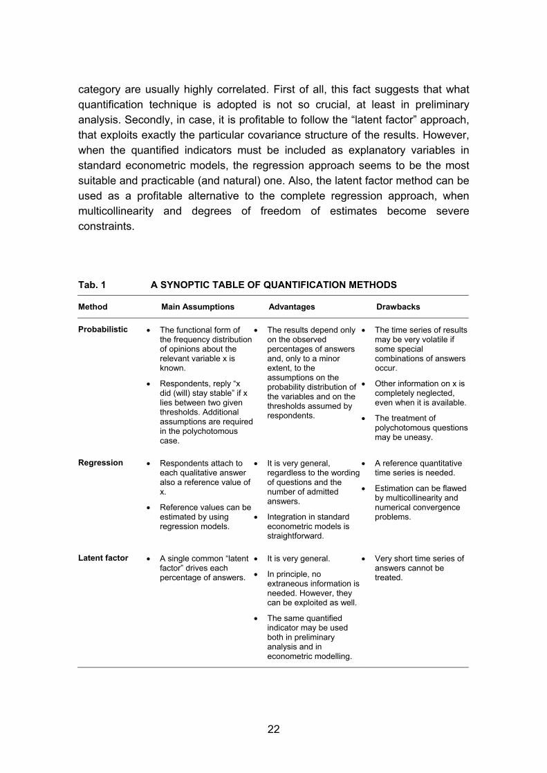
Qualitative surveys provide researchers and analysts with timely and reliable information about many economic phenomena. Various methodologies have been developed in order to transform the results of such surveys in standard quantitative indicators, possibly to be integrated in the usual analytical frameworks. Table 1 below provides a swift comparison of different approaches.

The empirical evidence on the performance of various methods is mixed. For instance, in analysing data on UK manufacturing industry, Driver and Urga (2003) concluded that, generally, no one procedure outperforms the other, partially contradicting the results reported by Cunningham (1997), who pointed out the sharp inefficiency of balance statistic. Smith and McAleer (1995), working out Australian data, noticed that dynamic regression models are generally superior. In analysing data from surveys on Italian consumers and entrepreneurs, also D’Elia (1991, 1993) recommended the use of dynamic regression models, but found also that various methods tend to produce very similar results, as far as the general dynamics of the resulting indicators is concerned, since the time series of the percentage of answers falling in each

22

category are usually highly correlated. First of all, this fact suggests that what quantification technique is adopted is not so crucial, at least in preliminary analysis. Secondly, in case, it is profitable to follow the “latent factor” approach, that exploits exactly the particular covariance structure of the results. However, when the quantified indicators must be included as explanatory variables in standard econometric models, the regression approach seems to be the most suitable and practicable (and natural) one. Also, the latent factor method can be used as a profitable alternative to the complete regression approach, when multicollinearity and degrees of freedom of estimates become severe constraints.

Tab. 1 A SYNOPTIC TABLE OF QUANTIFICATION METHODS

Method Main Assumptions Advantages Drawbacks

Probabilistic • The functional form of the frequency distribution of opinions about the relevant variable x is known.

• Respondents, reply “x did (will) stay stable” if x lies between two given thresholds. Additional assumptions are required in the polychotomous case.

• The results depend only on the observed percentages of answers and, only to a minor extent, to the assumptions on the probability distribution of the variables and on the thresholds assumed by respondents.

• The time series of results may be very volatile if some special combinations of answers occur.

• Other information on x is completely neglected, even when it is available.

• The treatment of polychotomous questions may be uneasy.

Regression • Respondents attach to each qualitative answer also a reference value of x.

• Reference values can be estimated by using regression models.

• It is very general, regardless to the wording of questions and the number of admitted answers.

• Integration in standard econometric models is straightforward.

• A reference quantitative time series is needed.

• Estimation can be flawed by multicollinearity and numerical convergence problems.

Latent factor • A single common “latent factor” drives each percentage of answers.

• It is very general.

• In principle, no extraneous information is needed. However, they can be exploited as well.

• The same quantified indicator may be used both in preliminary analysis and in econometric modelling.

• Very short time series of answers cannot be treated.

23

REFERENCES

Anderson, O. (1952), “The business test of the IFO-Institute for economic research, Munich, and its theoretical model”, Revue de l'Institut International de Statistique, vol. 20.

Balcombe, K. (1996), “The Carlson-Parkin method applied to NZ price expectations using QSBO survey data”, Economics Letters, vol. 51.

Batchelor, R. A. (1981), “Aggregate expectations under the stable laws”, Journal of Econometrics, vol. 16.

Batchelor, R. A. and Orr, A. B. (1988), “Inflation expectations revisited”, Economica, vol. 55.

Berk, J. (1999), “Measuring Inflation Expectations: A Survey Data Approach”, Applied Economics, 31.

Carlson, J. A. (1975), “Are Price Expectations Normally Distributed?”, Journal of the American Statistical Association, vol. 70, n. 352.

Carlson, J.A. and Parkin, M. (1975), “Inflation expectations”, Economica, vol. 42.

CIRET (1998), “International Business, Investment and Consumer Surveys: A Synoptic Table”, CIRET Office, Munich.

Cunningham, A. (1997), “Quantifying survey data”, Bank of England Quarterly Bulletin, August.

D'Elia, E. (1991), “La quantificazione dei risultati dei sondaggi congiunturali: un confronto tra procedure”, Rassegna dei lavori dell'ISCO, n. 13.

D'Elia, E. (1993), “Forecasting Prices by Opinion Survey Data: the Italian Experience”, in Contributed papers submitted for the 20th CIRET Conference 1991, CIRET studien n. 43.

Driver, C. and Urga, G. (2003), “Transforming Qualitative Survey Data: Performance Comparisons for the UK”, mimeo.

EUROPEAN COMMISSION (1997), ‘The joint harmonised EU programme of business and consumer surveys’, European Economy Vol. 6.

Fishe, R. P. H. and Lahiri, K. (1981), “On the estimation of inflationary expetactions from qualitative responses”, Journal of Econometrics, vol. 16.

Goldberger, A.S. (1974), “Unobservable variables in econometrics”, in Frontiers in econometrics, Zarembka, P. (ed.), Academic Press, New York.

ISAE (2002), “Fluttuazioni dei mercati finanziari e consumi delle famiglie italiane”, in Rapporto trimestrale ISAE, Rome.

Johnson, N. L. and Kotz, S. (1970), Continuous univariate distributions, Vol I and II, Wiley, New York.

24

Kaiser, U. and Spitz, A. (2000), “Quantification of qualitative data using ordered probit models with an application to a business survey in the German service sector”, paper presented at the 25th CIRET Conference, Paris.

Lankes, F. and Wolters, J. (1988), Das IFO-Geschäftsklima und seine Komponenten als vorlaufende Indikatoren. Empirische Ergebnisse für die Verbrauchs- und Investitionsg üterindustrie für 1975-1986 , FU Berlin, Fachbereich Wirtschaftswissenschaft, Diskussionsarbeit, No. 5/1988.

Maddala, G. S. (1983) Limited-Dependent and Qualitative Variables, Econometric Society Monographs No. 3, Cambridge University Press.

Mitchell, J., Smith, R. J. and Weale, M. R. (2002), “Aggregate versus Disaggregate Survey-Based Indicators of Economic Activity”, mimeo, presented at the Econometric Society European Meeting held in Lausanne.

Morrison, D. F. (1990), Multivariate statistical methods, (3rd Ed.). New York: McGraw-Hill.

Pesaran, M. H. (1984), “Expectations formation and macroeconomic modelling”, in Contemporary macroeconomic modelling, P. MALGRANGE e P.A. MUET (eds.), Blackwell, Oxford.

Seitz, H. (1988), “The Estimation of Inflation Forecasts from Business Survey Data”, Applied Economics, vol. 20.

Smith, J. and Mcaleer, M.(1995), “Alternative procedures for converting qualitative response data to quantitative expectations: an application to Australian manufacturing”, Journal of Applied Econometrics, Vol.10.

Theil, H. (1952), “On the time shape of economic microvariables and the Munich Business Test”, Revue de l'Istitut International de Statistique, vol.23.

Wachtel, P. (1977), “Survey measures of expected inflation and their potential usefulness”, in Analysis of inflation: 1965-1974, J. POPKIN (ed.), NBER, Ballinger, Cambridge.

Working Papers available:

n. 31/03 S. DE NARDIS C. VICARELLI

The Impact of Euro on Trade: the (Early) Effect Is not So Large

n. 32/03 S. LEPROUX L'inchiesta ISAE-UE presso le imprese del commercio al minuto tradizionale e della grande distribuzione: la revisione dell'impianto metodologico

n. 33/03 G. BRUNO C. LUPI

Forecasting Euro-area Industrial Production Using (Mostly)\ Business Surveys Data

n. 34/03 C. DE LUCIA Wage Setters, Central Bank Conservatism and Economic Performance

n. 35/03 E. D'ELIA B. M. MARTELLI

Estimation of Households Income from Bracketed Income Survey Data

n. 36/03 G. PRINCIPE Soglie dimensionali e regolazione del rapporto di lavoro in Italia

n. 37/03 M. BOVI A Nonparametric Analysis of the International Business Cycles

n. 38/03 S. DE NARDIS M. MANCINI C. PAPPALARDO

Regolazione del mercato del lavoro e crescita dimensionale delle imprese: una verifica sull'effetto soglia dei 15 dipendenti

n. 39/03 C. MILANA ALESSANDRO ZELI

Productivity Slowdown and the Role of the Ict in Italy: a Firm-level Analysis

n. 40/04 R. BASILE S. DE NARDIS

Non linearità e dinamica della dimensione d'impresa in Italia

n. 41/04 G. BRUNO E. OTRANTO

Dating the Italian Business Cycle: a Comparison of Procedures

n. 42/04 C. PAPPALARDO G. PIRAS

Vector-auto-regression Approach to Forecast Italian Imports

n. 43/04 R. DE SANTIS Has Trade Structure Any Importance in the Transmission of Currency Shocks? An Empirical Application for Central and Eastern European Acceding Countries to EU

Working Papers available:

n. 44/04 L. DE BENEDICTIS C. VICARELLI

Trade Potentials in Gravity Panel Data Models

n. 45/04 S. DE NARDIS C. PENSA

How Intense Is Competition in International Markets of Traditional Goods? The Case of Italian Exporters

n. 46/04 M. BOVI The Dark, and Independent, Side of Italy

n. 47/05 M. MALGARINI P. MARGANI B.M. MARTELLI

Re-engineering the ISAE manufacturing survey

n. 48/05 R. BASILE A. GIUNTA

Things change. Foreign market penetration and firms’ behaviour in industrial districts: an empirical analysis

n. 49/05 C. CICCONI Building smooth indicators nearly free of end-of-sample revisions

n. 50/05 T. CESARONI M. MALGARINI G. ROCCHETTI

L’inchiesta ISAE sugli investimenti delle imprese manifatturiere ed estrattive: aspetti metodologici e risultati

n. 51/05 G. ARBIA G. PIRAS

Convergence in per-capita GDP across European regions using panel data models extended to spatial autocorrelation effects

n. 52/05 L. DE BENEDICTIS R. DE SANTIS C. VICARELLI

Hub-and-Spoke or else? Free trade agreements in the “enlarged” European Union

n. 53/05 R. BASILE M. COSTANTINI S. DESTEFANIS

Unit root and cointegration tests for cross-sectionally correlated panels. Estimating regional production functions

n. 54/05 C. DE LUCIA M. MEACCI

Does job security matter for consumption? An analysis on Italian microdata

n. 55/05 G. ARBIA R. BASILE G. PIRAS

Using Spatial Panel Data in Modelling Regional Growth and Convergence